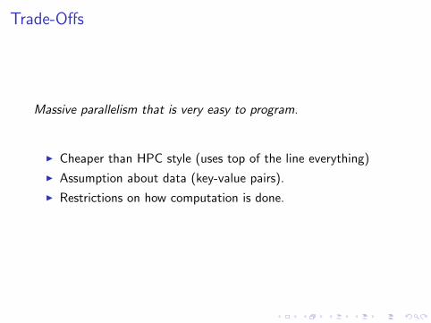
Trade-Offs

Massive parallelism that is very easy to program.

I Cheaper than HPC style (uses top of the line everything)

I Assumption about data (key-value pairs).

I Restrictions on how computation is done.

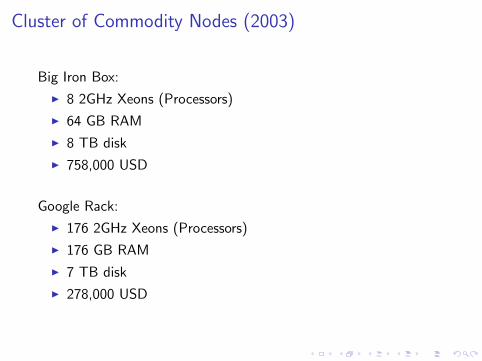
Cluster of Commodity Nodes (2003)

Big Iron Box:

I 8 2GHz Xeons (Processors)

I 64 GB RAM

I 8 TB disk

I 758,000 USD

Google Rack:

I 176 2GHz Xeons (Processors)

I 176 GB RAM

I 7 TB disk

I 278,000 USD

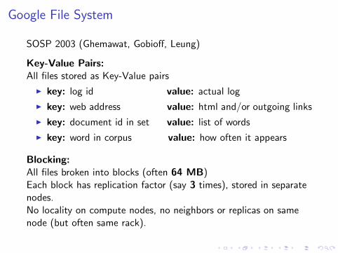
Google File System

SOSP 2003 (Ghemawat, Gobioff, Leung)

Key-Value Pairs:All files stored as Key-Value pairs

I key: log id value: actual log

I key: web address value: html and/or outgoing links

I key: document id in set value: list of words

I key: word in corpus value: how often it appears

Blocking:All files broken into blocks (often 64 MB)Each block has replication factor (say 3 times), stored in separatenodes.No locality on compute nodes, no neighbors or replicas on samenode (but often same rack).

No locality?

Really?

I Resiliency: if one dies, use another(on big clusters happens all the time)

I Redundancy: If one is slow, use another(...curse of last reducer)

I Heterogeneity: Format quite flexible, 64MB often still enough(recall: IO-Efficiency)

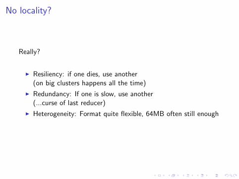
No locality?

Really?

I Resiliency: if one dies, use another(on big clusters happens all the time)

I Redundancy: If one is slow, use another(...curse of last reducer)

I Heterogeneity: Format quite flexible, 64MB often still enough

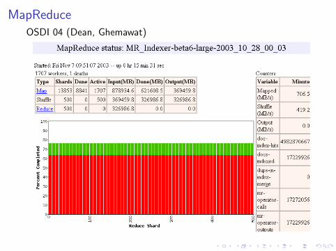
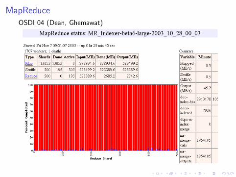
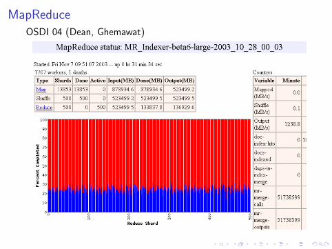
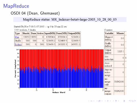
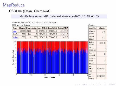
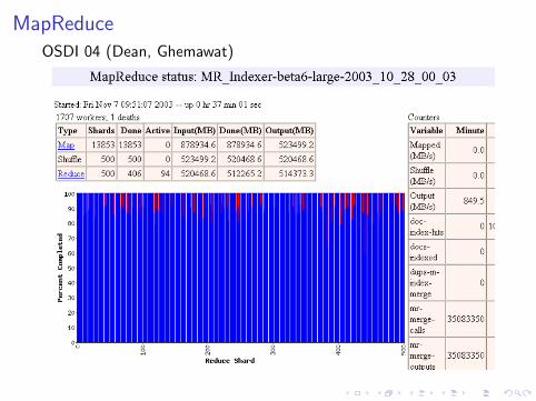
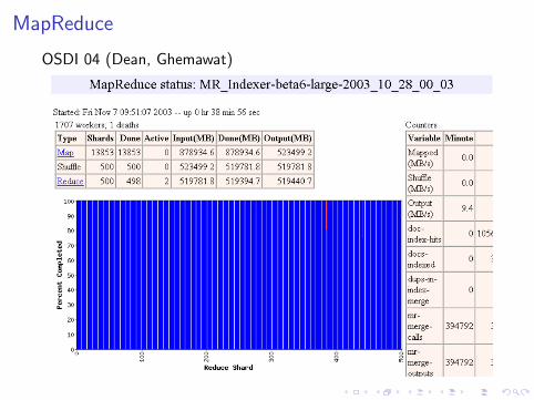
MapReduce

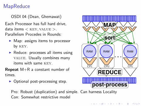
OSDI 04 (Dean, Ghemawat)

Each Processor has full hard drive,data items < key,value >.Parallelism Procedes in Rounds:

I Map: assigns items to processorby key.

I Reduce: processes all items usingvalue. Usually combines manyitems with same key.

Repeat M+R a constant number of times.

I Optional post-processing step.

CPU

RAM

CPU

RAM

CPU

RAM

MAP

REDUCE

sort

post-processPro: Robust (duplication) and simple. Can harness LocalityCon: Somewhat restrictive model

MapReduce

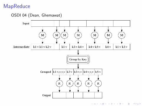
OSDI 04 (Dean, Ghemawat)

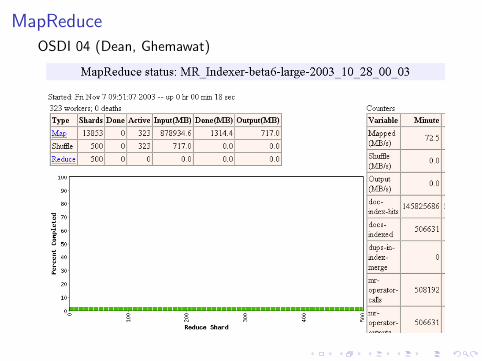
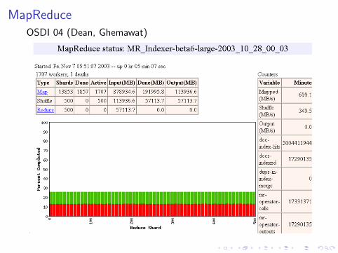
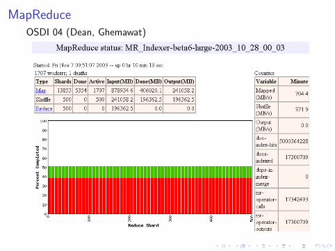
MapReduce

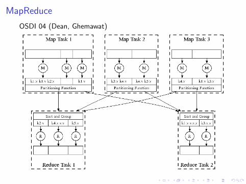
OSDI 04 (Dean, Ghemawat)

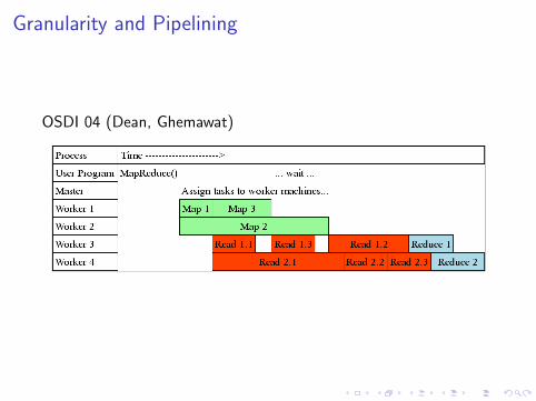
Granularity and Pipelining

OSDI 04 (Dean, Ghemawat)

MapReduceOSDI 04 (Dean, Ghemawat)

MapReduceOSDI 04 (Dean, Ghemawat)

MapReduceOSDI 04 (Dean, Ghemawat)

MapReduceOSDI 04 (Dean, Ghemawat)

MapReduceOSDI 04 (Dean, Ghemawat)

MapReduceOSDI 04 (Dean, Ghemawat)

MapReduceOSDI 04 (Dean, Ghemawat)

MapReduceOSDI 04 (Dean, Ghemawat)

MapReduceOSDI 04 (Dean, Ghemawat)

MapReduce

OSDI 04 (Dean, Ghemawat)

MapReduce

OSDI 04 (Dean, Ghemawat)

Last Reducer

Typically Map phase linear on blocks. Reducers more variable.

No answer until the last one is done!Some machines get slow/crash!

Solution: Automatically run back-up copies. Take first tocomplete.

Scheduled by Master NodeOrganizes computation, but does not process data.If this fails, all goes down.

Last Reducer

Typically Map phase linear on blocks. Reducers more variable.

No answer until the last one is done!Some machines get slow/crash!

Solution: Automatically run back-up copies. Take first tocomplete.

Scheduled by Master NodeOrganizes computation, but does not process data.If this fails, all goes down.

Example 1: Word Count

Given text corpus 〈 doc id, list of words 〉, count how many of eachword exists.

Map:

For each word w → 〈w , 1〉

Reduce:{〈w , c1〉, 〈w , c2〉, 〈w , c3〉, . . .} → 〈w ,

∑i ci 〉

w = “the” is 7% of all words!Combine: (before Map goes to Shuffle phase){〈w , c1〉, 〈w , c2〉, 〈w , c3〉, . . .} → 〈w ,

∑i ci 〉

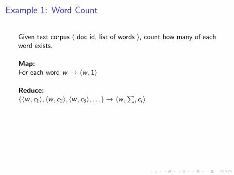
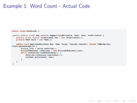
Example 1: Word Count

Given text corpus 〈 doc id, list of words 〉, count how many of eachword exists.

Map:For each word w → 〈w , 1〉

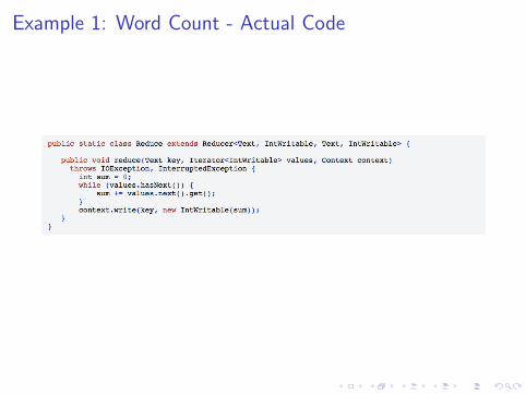
Reduce:

{〈w , c1〉, 〈w , c2〉, 〈w , c3〉, . . .} → 〈w ,∑

i ci 〉

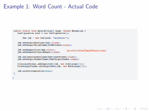
w = “the” is 7% of all words!Combine: (before Map goes to Shuffle phase){〈w , c1〉, 〈w , c2〉, 〈w , c3〉, . . .} → 〈w ,

∑i ci 〉

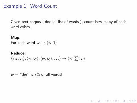
Example 1: Word Count

Given text corpus 〈 doc id, list of words 〉, count how many of eachword exists.

Map:For each word w → 〈w , 1〉

Reduce:{〈w , c1〉, 〈w , c2〉, 〈w , c3〉, . . .} →

〈w ,∑

i ci 〉

w = “the” is 7% of all words!Combine: (before Map goes to Shuffle phase){〈w , c1〉, 〈w , c2〉, 〈w , c3〉, . . .} → 〈w ,

∑i ci 〉

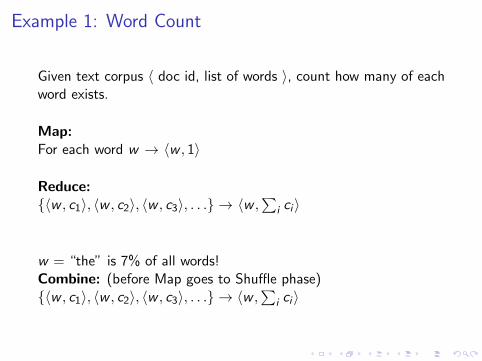
Example 1: Word Count

Given text corpus 〈 doc id, list of words 〉, count how many of eachword exists.

Map:For each word w → 〈w , 1〉

Reduce:{〈w , c1〉, 〈w , c2〉, 〈w , c3〉, . . .} → 〈w ,

∑i ci 〉

w = “the” is 7% of all words!Combine: (before Map goes to Shuffle phase){〈w , c1〉, 〈w , c2〉, 〈w , c3〉, . . .} → 〈w ,

∑i ci 〉

Example 1: Word Count

Given text corpus 〈 doc id, list of words 〉, count how many of eachword exists.

Map:For each word w → 〈w , 1〉

Reduce:{〈w , c1〉, 〈w , c2〉, 〈w , c3〉, . . .} → 〈w ,

∑i ci 〉

w = “the” is 7% of all words!

Combine: (before Map goes to Shuffle phase){〈w , c1〉, 〈w , c2〉, 〈w , c3〉, . . .} → 〈w ,

∑i ci 〉

Example 1: Word Count

Given text corpus 〈 doc id, list of words 〉, count how many of eachword exists.

Map:For each word w → 〈w , 1〉

Reduce:{〈w , c1〉, 〈w , c2〉, 〈w , c3〉, . . .} → 〈w ,

∑i ci 〉

w = “the” is 7% of all words!Combine: (before Map goes to Shuffle phase){〈w , c1〉, 〈w , c2〉, 〈w , c3〉, . . .} → 〈w ,

∑i ci 〉

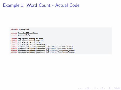
Example 1: Word Count - Actual Code

Example 1: Word Count - Actual Code

Example 1: Word Count - Actual Code

Example 1: Word Count - Actual Code

Example 2: Inverted Index

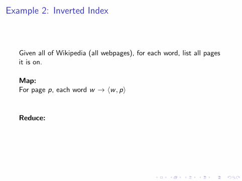
Given all of Wikipedia (all webpages), for each word, list all pagesit is on.

Map:

For page p, each word w → 〈w , p〉

Reduce:{〈w , p1〉, 〈w , p2〉, 〈w , p3〉, . . .} → 〈w ,∪ipi 〉

Example 2: Inverted Index

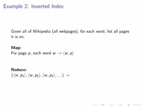
Given all of Wikipedia (all webpages), for each word, list all pagesit is on.

Map:For page p, each word w → 〈w , p〉

Reduce:

{〈w , p1〉, 〈w , p2〉, 〈w , p3〉, . . .} → 〈w ,∪ipi 〉

Example 2: Inverted Index

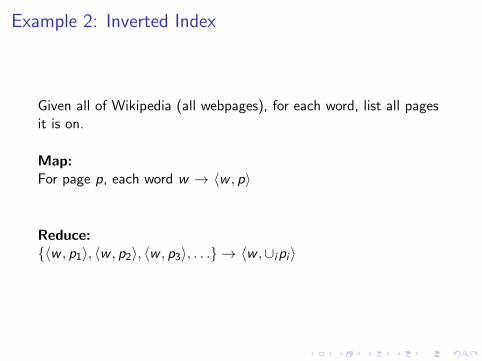
Given all of Wikipedia (all webpages), for each word, list all pagesit is on.

Map:For page p, each word w → 〈w , p〉

Reduce:{〈w , p1〉, 〈w , p2〉, 〈w , p3〉, . . .} →

〈w ,∪ipi 〉

Example 2: Inverted Index

Given all of Wikipedia (all webpages), for each word, list all pagesit is on.

Map:For page p, each word w → 〈w , p〉

Reduce:{〈w , p1〉, 〈w , p2〉, 〈w , p3〉, . . .} → 〈w ,∪ipi 〉

Example 2: Inverted Index

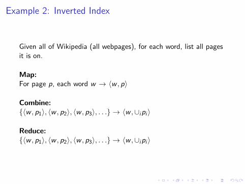
Given all of Wikipedia (all webpages), for each word, list all pagesit is on.

Map:For page p, each word w → 〈w , p〉

Combine:{〈w , p1〉, 〈w , p2〉, 〈w , p3〉, . . .} → 〈w ,∪ipi 〉

Reduce:{〈w , p1〉, 〈w , p2〉, 〈w , p3〉, . . .} → 〈w ,∪ipi 〉

Hadoop

Open source version of MapReduce (and related, e.g. HDFS)

I Began 2005 (Cutting + Cafarella) supported by Yahoo!

I Stable enough for large scale around 2008

I Source code released 2009

Java (MapReduce in C++)

Led to widespread adoption in industry and academia!

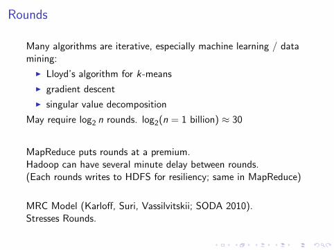
Rounds

Many algorithms are iterative, especially machine learning / datamining:

I Lloyd’s algorithm for k-means

I gradient descent

I singular value decomposition

May require log2 n rounds.

log2(n = 1 billion) ≈ 30

MapReduce puts rounds at a premium.Hadoop can have several minute delay between rounds.(Each rounds writes to HDFS for resiliency; same in MapReduce)

MRC Model (Karloff, Suri, Vassilvitskii; SODA 2010).Stresses Rounds.

Rounds

Many algorithms are iterative, especially machine learning / datamining:

I Lloyd’s algorithm for k-means

I gradient descent

I singular value decomposition

May require log2 n rounds. log2(n = 1 billion) ≈ 30

MapReduce puts rounds at a premium.Hadoop can have several minute delay between rounds.(Each rounds writes to HDFS for resiliency; same in MapReduce)

MRC Model (Karloff, Suri, Vassilvitskii; SODA 2010).Stresses Rounds.

Rounds

Many algorithms are iterative, especially machine learning / datamining:

I Lloyd’s algorithm for k-means

I gradient descent

I singular value decomposition

May require log2 n rounds. log2(n = 1 billion) ≈ 30

MapReduce puts rounds at a premium.Hadoop can have several minute delay between rounds.(Each rounds writes to HDFS for resiliency; same in MapReduce)

MRC Model (Karloff, Suri, Vassilvitskii; SODA 2010).Stresses Rounds.

Rounds

Many algorithms are iterative, especially machine learning / datamining:

I Lloyd’s algorithm for k-means

I gradient descent

I singular value decomposition

May require log2 n rounds. log2(n = 1 billion) ≈ 30

MapReduce puts rounds at a premium.Hadoop can have several minute delay between rounds.(Each rounds writes to HDFS for resiliency; same in MapReduce)

MRC Model (Karloff, Suri, Vassilvitskii; SODA 2010).Stresses Rounds.

Bulk Synchronous Parallel

Les Valiant [1989] BSPCreates “barriers” in parallel algorithm.

1. Each processor computes on data

2. Processors send/receive data

3. Barrier : All processors wait forcommunication to end globally

Allows for easy synchronization. Easierto analyze since handles many messysynchronization details if this isemulated.

CPU

RAM

CPU

RAM

CPU

RAM

CPU

RAM

CPU

RAM

Bulk Synchronous Parallel

Les Valiant [1989] BSPCreates “barriers” in parallel algorithm.

1. Each processor computes on data

2. Processors send/receive data

3. Barrier : All processors wait forcommunication to end globally

Allows for easy synchronization. Easierto analyze since handles many messysynchronization details if this isemulated.

CPU

RAM

CPU

RAM

CPU

RAM

CPU

RAM

CPU

RAM

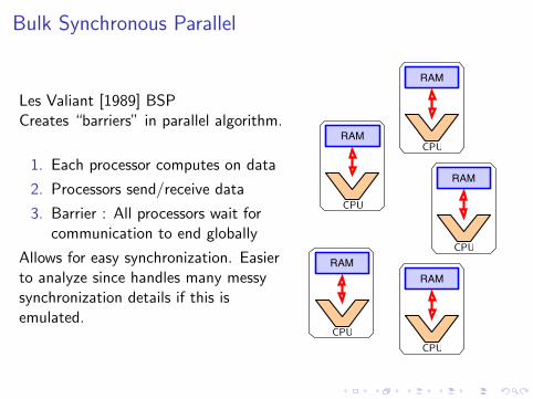
Bulk Synchronous Parallel

Les Valiant [1989] BSPCreates “barriers” in parallel algorithm.

1. Each processor computes on data

2. Processors send/receive data

3. Barrier : All processors wait forcommunication to end globally

Allows for easy synchronization. Easierto analyze since handles many messysynchronization details if this isemulated.

CPU

RAM

CPU

RAM

CPU

RAM

CPU

RAM

CPU

RAM

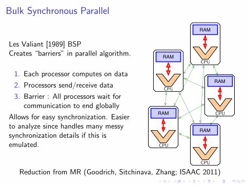
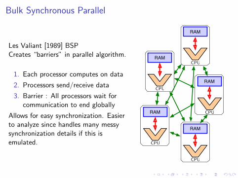
Reduction from MR (Goodrich, Sitchinava, Zhang; ISAAC 2011)

Replication Rate

Consider a join of two sets of size R, S of size n = 10, 000.List pair (r , s) ∈ R × S if f (r , s) = 1, for some function f .

Option 1: Create n2 reducers.Replication rate of g = n.

Option 2: Create 1 reducers.Reducer of size 2n, has n2 = 100million operation.Replication rate g = 1. No parallelism.

Option 3: Create g2 reducers, each with 2 groups of size n/g .Reducer size 2n/g , (n/g)2 operations (g = 10 only 1million).Replication rate of g .

Replication Rate

Consider a join of two sets of size R, S of size n = 10, 000.List pair (r , s) ∈ R × S if f (r , s) = 1, for some function f .

Option 1: Create n2 reducers.Replication rate of g = n.

Option 2: Create 1 reducers.Reducer of size 2n, has n2 = 100million operation.Replication rate g = 1. No parallelism.

Option 3: Create g2 reducers, each with 2 groups of size n/g .Reducer size 2n/g , (n/g)2 operations (g = 10 only 1million).Replication rate of g .

Replication Rate

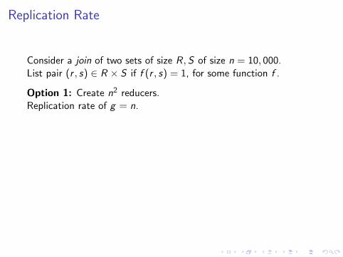
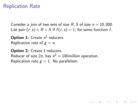
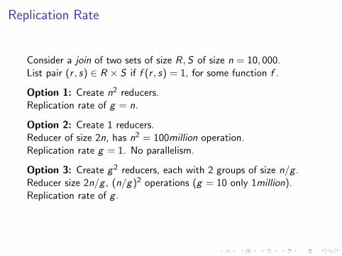
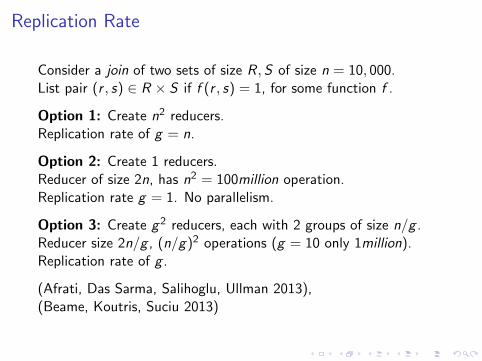
Consider a join of two sets of size R, S of size n = 10, 000.List pair (r , s) ∈ R × S if f (r , s) = 1, for some function f .

Option 1: Create n2 reducers.Replication rate of g = n.

Option 2: Create 1 reducers.Reducer of size 2n, has n2 = 100million operation.Replication rate g = 1. No parallelism.

Option 3: Create g2 reducers, each with 2 groups of size n/g .Reducer size 2n/g , (n/g)2 operations (g = 10 only 1million).Replication rate of g .

Replication Rate

Consider a join of two sets of size R, S of size n = 10, 000.List pair (r , s) ∈ R × S if f (r , s) = 1, for some function f .

Option 1: Create n2 reducers.Replication rate of g = n.

Option 2: Create 1 reducers.Reducer of size 2n, has n2 = 100million operation.Replication rate g = 1. No parallelism.

Option 3: Create g2 reducers, each with 2 groups of size n/g .Reducer size 2n/g , (n/g)2 operations (g = 10 only 1million).Replication rate of g .

(Afrati, Das Sarma, Salihoglu, Ullman 2013),(Beame, Koutris, Suciu 2013)

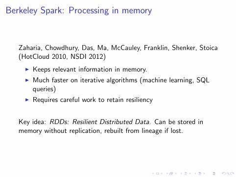
Berkeley Spark: Processing in memory

Zaharia, Chowdhury, Das, Ma, McCauley, Franklin, Shenker, Stoica(HotCloud 2010, NSDI 2012)

I Keeps relevant information in memory.

I Much faster on iterative algorithms (machine learning, SQLqueries)

I Requires careful work to retain resiliency

Key idea: RDDs: Resilient Distributed Data. Can be stored inmemory without replication, rebuilt from lineage if lost.