Introduction to MATLAB for MTH

453 – Numerical Analysis

Greg Reese, Ph.D

Research Computing Support Group

Academic Technology Services

Miami UniversitySeptember 2010

Introduction to MATLAB for MTH 453 – Numerical

Analysis

© 2010 Greg Reese. All rights reserved 2

3

Workshop information

To get a copy of this presentation, go towww.muohio.edu/researchcomputing

then click on Research Software Support & Development

then on Matlab Tutorials

and download the file entitledIntroduction to MATLAB for MTH 453

4

Workshop information

Format• Interactive presentation with hands-on

use of MATLABRequirements• NoneDuration• Two hoursStyle• Informal – ask questions any time you

want!

5

Outline

• Overview of MATLAB• MATLAB environment

– Getting started– Arithmetic– Variables, mathematical functions– Getting help on MATLAB

6

Outline• Vector (a collection of numbers)

– Creating– Plotting– Arithmetic

• Plotting– Make quick plots– Change plot details– Use plots in other programs

• Programming– Write very simple MATLAB programs

7

Outline

Special topics for numerical analysis• Specifying numerical precision of output• Writing MATLAB functions• Plotting functions you wrote

8

MATLAB

• Stands for MATrix LABoratory– Originally designed for efficient

computation with matrices

• Language and environment for technical computing

Overview

9

Overview

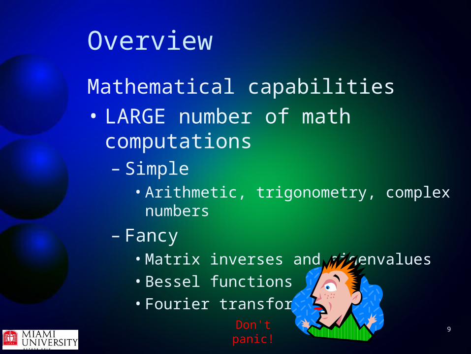
Mathematical capabilities

• LARGE number of math computations– Simple

• Arithmetic, trigonometry, complex numbers

– Fancy• Matrix inverses and eigenvalues• Bessel functions• Fourier transforms

Don't panic!

10

Overview

Graphics

• Easily plot data

• Annotate graphs

• 2D and 3D data visualization

• Image processing

11

Getting Started

Double-click on MATLAB icon on desktop. Close all windows except one with the prompt (>>). That window is called the command window.

Most of your work takes place in the command window. After you press ENTER you get the answer and get another prompt.

12

Getting Started

NOTE

After typing a MATLAB command you always press ENTER to activate it. Won't show that anymore

13

Getting Started

Try It• To learn what version of MATLAB

you have run the ver command

• To find today's date enter date

14

Terminology

MATLAB designed to work on matrices• matrix – a rectangular array of

numbers

• vector – a matrix with only one row or columnrow vector column vector

• scalar – a matrix with only one row and column, i.e., a number

1.3 2

-7 -3.4

9 8

1 7 -4.3

0.05

-33.7

100

99

-23.8 1009.76

15

Variables

variable – a name that represents a MATLAB object such as a scalar, vector or matrix.

You can change (vary) the value of a variable

16

Variables

Variable name

• Must start with a letter

• Have any number of letters, digits, or underscores

• No spaces allowed (use an underscore instead)

• Only first 31 characters of a name are important to MATLAB

17

Variables

MATLAB is case-sensitive, i.e., it distinguishes between upper and lower case letters in a variable name

• BOB, bob, and Bob count as different names

Tip - Don't purposely make names that differ only in capitalization. You, not MATLAB, will get confused!

18

Variables

To make a variable just type its name followed by an equals sign and a value, e.g., x = 5

To see the value of a variable just type its name at the command prompt.

• If there's no variable with that name (for example, “y”), MATLAB will say??? Undefined function or variable 'y'.

Spaces are optional

19

Variables

Tip – variable name should have meaning

Example – “Number of students” might be num_students or numStudents, but not x or n

20

Numbers

Numbers

• Can have decimal point, leading plus or minus sign, e.g., 3 4.7 -5 +5 .01 0.01 0.010

• Scientific notation – use “e” to specify power of ten, e.g., 6.02 × 1023 is 6.02e237.02 × 10-34 is 7.02e-34

21

Numbers

Numbers

• Internally variables have precision of about 16 decimal digits and range from about 10-308 to 10+308

(good enough for government work!)

22

Variables

Try It• Make variables to represent the

following constants and set them to the indicated values

Speed of light 3.00×108

Plank's constant 6.63×10-34

Avogadro's number 6.02×1023

Degrees in a circle 360Bottles of beer 99

23

Arithmetic

MATLAB

• Has normal arithmetic operations

• Has some that are not as familiar

• Use standard evaluation order– 3 × 5 + 7 = 22 (multiply first, then add)

• Can use parentheses in usual way to change evaluation order

– 3 × ( 5 + 7 ) = 36

24

Arithmetic

Symbol Operation

+ Addition

- Subtraction

* Multiplication

/ Division

^ Power

Arithmetic on scalars

25

Arithmetic

You can use MATLAB as a fancy calculator. For example, to evaluate 4x3 – 3x + 7 at x = 3.5 type4*3.5^3 – 3*3.5 + 7

Try It at Home•Try the above. You should get 168

•Try it for x = 0 . Is MATLAB correct?

26

Arithmetic

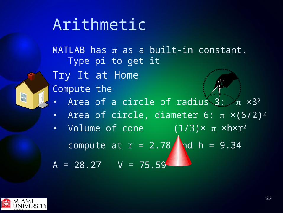
MATLAB has as a built-in constant. Type pi to get it

Try It at HomeCompute the• Area of a circle of radius 3: ×32

• Area of circle, diameter 6: ×(6/2)2

• Volume of cone (1/3)× ×h×r2

compute at r = 2.78 and h = 9.34

A = 28.27 V = 75.59

27

Variables

It's more common to do arithmetic on variables. Do it the same way as with constants. For example:

>> radius = 5

radius = 5

>> area = pi * radius ^ 2

area = 78.5398

28

Variables

Try It at Home• Make variables for the height and

width of a triangle and set them to 5 and 10. Compute the area of the triangle using the variables (25)

29

Variables

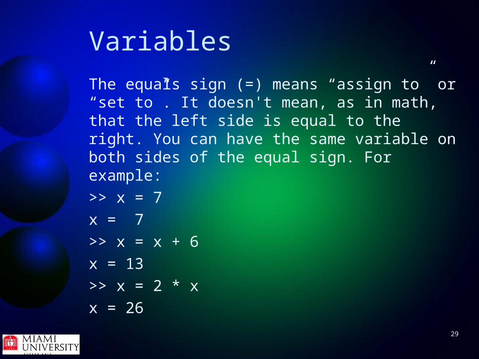
The equals sign (=) means “assign to” or “set to”. It doesn't mean, as in math, that the left side is equal to the right. You can have the same variable on both sides of the equal sign. For example:

>> x = 7

x = 7

>> x = x + 6

x = 13

>> x = 2 * x

x = 26

30

Variables

Tip• Left and right arrow keys move

within current command line

• Up and down arrow keys move among command lines

• Type letters then use up and down arrow keys to move among command lines starting with those letters

31

VariablesTry It• Type r=5 and ENTER• Type pi*r^2 for area

To compute area for new radius

1. Press up arrow twice

2. Use backspace key to delete the 5

3. Type 10 and ENTER

4. Press up arrow key twice

5. Press ENTER for area of new radius

32

Variables

TipIt can get tedious seeing intermediate values such as the radius and the height. To suppress the output of a command, put a semicolon at the end of the line, e.g., r=5;

33

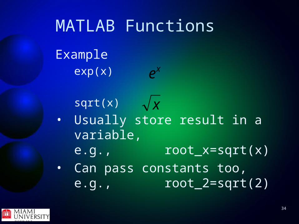
MATLAB Functions

You're likely to want to compute functions of a variable, e.g.,

MATLAB has a large number of standard mathematical functions. To compute the function of a variable write the function name followed by the variable in parentheses.

x kxe )ln(x

34

MATLAB Functions

Exampleexp(x)

sqrt(x)

• Usually store result in a variable, e.g., root_x=sqrt(x)

• Can pass constants too,e.g., root_2=sqrt(2)

xe

x

35

MATLAB Functions

You can make complicated expressions by combining variables, functions, and arithmetic, e.g.,

5*exp(-k*t)+17.4*sin(2*pi*t/T)

Note how similar math and MATLAB are.

Tte kt 2sin4.175 Math

MATLAB

“*” means “×”

36

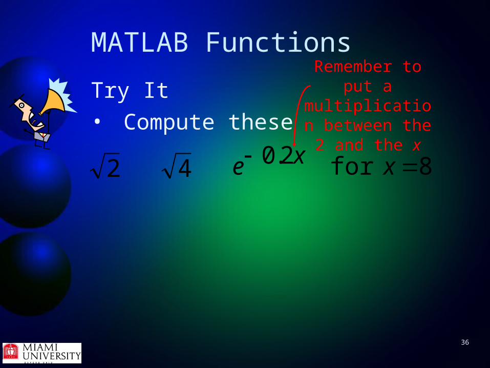
MATLAB Functions

Try It• Compute these

2 4 8for2.0 xxe

Remember to put a multiplication between the 2

and the x

37

Formatted Output

Computed precision (number of significant digits) and displayed precision are independent

•Computations always done with full precision

•Displayed precision can be changed

38

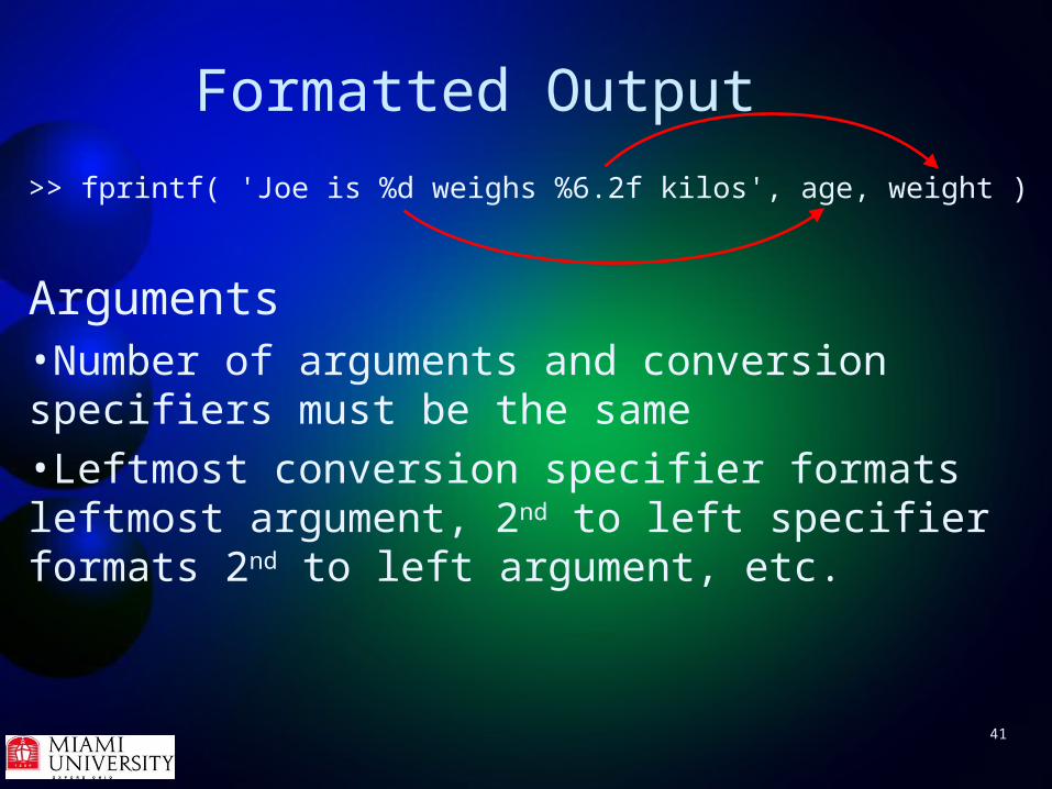
Formatted Output

For full control of displayed number of digits, use fprintf command

fprintf( format, n1, n2, n3 )

>> fprintf( 'Joe weighs %6.2f kilos', n1 )

Format string

Argument

Conversion specifier

39

Formatted OutputExample>> format long

>> pi

3.14159265358979

>> fprintf( 'pi=%4.2f', pi ) pi=3.14

>> fprintf( 'pi=%5.2f', pi ) pi= 3.14

Four characters: 3, ., 1, 4

Five characters: space, 3, ., 1, 4

40

Formatted Output

>> fprintf( 'Joe weighs %6.2f kilos', n1 )

Format string

• May contain text and/or conversion specifiers

• Must be enclosed in SINGLE quotes, not double quotes, aka quotation marks (“ ”)

Format string

41

Formatted Output

>> fprintf( 'Joe is %d weighs %6.2f kilos', age, weight )

Arguments•Number of arguments and conversion specifiers must be the same•Leftmost conversion specifier formats leftmost argument, 2nd to left specifier formats 2nd to left argument, etc.

42

Formatted Output

>> fprintf( 'Joe weighs %6.2f kilos', n1 )

General conversion specifier is %w.pt• % = start of specifier• w = width: a numeral giving the minimum number

of characters to be displayed• p = “precision”: the number of digits to the right of

the decimal point• t = “conversion character” (output format):

– d = decimal (integer), f = fixed point, e = scientific notation

Conversion specifier

43

Formatted OutputExample>> fprintf( 'pi=%4.2e', pi ) pi=3.14e+000

>> fprintf( 'pi=%12.4e', pi ) pi= 3.1416e+000

>> fprintf( 'pi=%.3e', pi ) pi=3.142e+000

Omitted width makes output occupy minimum width

44

Formatted OutputFor integers, use %w.pd• If value has less numerals than w, output

preceded by blanks• Use of p makes output have enough preceding

zeros to make width w• Typical use is %d, which displays exact number

of numerals in value• If value has fractional part, display is scientific.

Use round, ceil, or floor on value to get integer display

45

Formatted OutputExample>> age = 13;

>> fprintf( 'Tim is %d years old', age ) Tim is 13 years old

>> fprintf( 'Tim is %5d years old', age ) Tim is 13 years old

>> fprintf( 'Tim is %.4d years old', age )

Tim is 0013 years old

46

Formatted OutputExample>> weight = 22.7;

>> fprintf( 'Tim weighs %d lbs.', weight ) Tim weighs 2.270000e+001 lbs.

>> fprintf( 'Tim weighs %d lbs.',

round( weight ) ) Tim weighs 23 lbs.

>> fprintf( 'Tim weighs %d lbs.',

floor( weight ) ) Tim weighs 22 lbs.

47

Formatted OutputFormat strings are often long. Can break a string by 1.Put an open square bracket ( [ ) in front of first single quote

2.Put a second single quote where you want to stop the line

3.Follow that quote with an ellipsis (three periods)

4.Press ENTER, which moves cursor to next line

5.Type in remaining text in single quotes

6.Put a close square bracket ( ] )

7.Put the rest of the fprintf command

48

Formatted Output

Example>> weight = 178.3;

>> age = 17;

>> fprintf( ['Tim weighs %.1f lbs'...

' and is %d years old'], weight, age )

Tim weighs 178.3 lbs and is 17 years old

49

Formatted OutputBy default, fprintf does not move to next line after writing output.

Example>>fprintf('Age=%d Weight=%.1f', 13, 102.3)

Age=13 Weight=102.3>>

Output didn't move to next line

50

Formatted OutputTo move output to next line, put \n in text wherever you want to move to next line.

Example>> age=13; weight = 83.4; height = 1.8;

>> fprintf('Tim is %d years old\n'...

'He weighs %.1f kilos\nand is %.1f'...

' meters tall\n', age, weight, height )

Tim is 13 years old

He weighs 83.4 kilos

And is 1.8 meters tall

>>

Backslash (\), not forward slash (/)

51

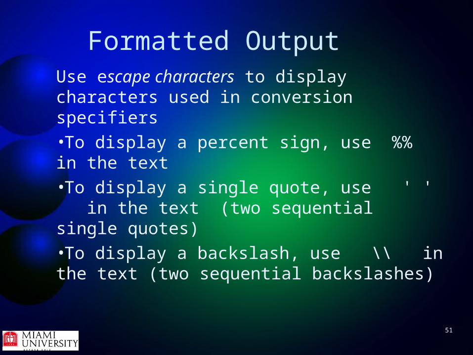
Formatted OutputUse escape characters to display characters used in conversion specifiers

•To display a percent sign, use %% in the text

•To display a single quote, use ' ' in the text (two sequential single quotes)

•To display a backslash, use \\ in the text (two sequential backslashes)

52

Formatted OutputTry It at HomeSet the variables kpm (kilometers per mile) and mm (marathon miles) to 1.6 and 26.2 . Make these outputs:Output 11 mile is 1.6 kilometers

Output 21 km is about 0.6 miles, but really 0.625 miles

Output 3There are 26.2 miles and 41.9 km in a marathon

Output 4One marathon is about 26 miles or 42 km

53

Formatted Outputfprintf has many more capabilities. To find out about them you can ask MATLAB for help on fprintf.

54

Getting Help

To get help on a MATLAB command, type “help” followed by space and the command name, e.g.,

>> help fprintf

Try It at Home

55

Getting Help

MATLAB will display information on what the command does, what its inputs and outputs are, what algorithms it uses, etc. It also displays links to related commands.

56

Getting help

Questions?

• Variables

• Arithmetic

• Formatting

• Help

57

Vectors

A vector is a one-dimensional matrix. It is a single row or a single column.

37 98.72

-0.4

1 5 24 98.6 100.01 -0.3

MATLAB is designed to work with vectors and matrices and manipulates them very efficiently.

column vectorrow vector

58

Vectors

To create a row vector v with specific numbers n1, n2, and n3:

>> v = [n1 n2 n3]

Try ItMake the row vector 1 4 9 16>> v=[1 4 9 16]

v = 1 4 9 16

59

Vectors

Each member of a vector is called an element. The number of elements in a vector is its size or length.

To get the length of a vector v use

>> length(v)

MATLAB provides some easy ways to generate common vectors.

60

VectorsCommand Operation

zeros(1,n) Create a row vector of n zeros

ones(1,n) Create a row vector of n ones

rand(1,n) Create a row vector of n numbers uniformly distributed between 0 and 1

randn(1,n) Create a row vector of n normally distributed numbers with mean 0 and std. dev. 1

61

Vectors

You can easily create a row vector of consecutive numbers by using a colon. m:n or m:k:n

Example3:7

3 4 5 6 7

10:2:20 10 12 14 16 18 20

7:-1:4 7 6 5 4

1:0.1:1.5 1 1.1 1.2 1.3 1.4 1.5

62

Vectors

The colon is particularly useful for making a sequence of values of an independent variable that can be used to evaluate the dependent variable.

Example>> time = 0:0.25:2

time = 0 0.2500 0.5000 0.7500 1.0000 1.2500

1.5000 1.7500 2.0000

63

Vector in functions

Most MATLAB functions work on vectors. They evaluate the function at every element of the vector. The result is a vector of the same dimension, i.e., both input and output vectors have the same number of elements and they are both either row vectors or column vectors

64

Vectors

Try It Evaluate et from 0 to 2.5 in steps of 0.5

>> t=0:0.5:2.5

t = 0 0.5 1.0 1.5 2.0 2.5

>> y=exp(t)

y = 1.00 1.65 2.72 4.48 7.39 12.18

65

Vectors

One of MATLAB's big strengths is its ability to let you easily make plots. To plot a vector y use the command plot(y).

plot(y) plots values of y versus the element number. In this case, since t has 6 elements, the element numbers are 1,2, … 6.

66

VectorsTry ItPlot the y produced previously

67

Plotting

To plot values in the vector x on the horizontal axis and in the vector y on the vertical axis:•>> plot(x,y)•x and y must be same dimension

Try ItMake a plot of t on the horizontal axis and y on the vertical axis

68

Plotting

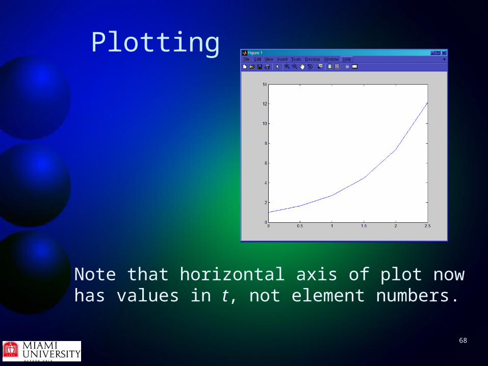
Note that horizontal axis of plot now has values in t, not element numbers.

69

Vectors and Scalars

When performing arithmetic between a scalar and vector MATLAB does the arithmetic between the scalar and each element of the vector. This is called elementwise arithmetic.

70

Vectors and Scalars

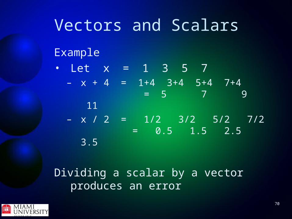
Example• Let x = 1 3 5 7

– x + 4 = 1+4 3+4 5+4 7+4 = 5 7 9 11

– x / 2 = 1/2 3/2 5/2 7/2 = 0.5 1.5 2.5 3.5

Dividing a scalar by a vector produces an error

71

Vectors and Scalars

Try It at HomeLet x = 2 4 6

Compute

• x + 4

• 4 * x

• 4 / x

72

Combining vectors

x and y are vectors of same dimension• x + y is elementwise sum• x – y is elementwise difference• x .* y is elementwise multiplication• x ./ y is elementwise division• x .^ y is elementwise power

Make sure you put the period in front of the arithmetic operation on the last three

73

Combining vectors

Try ItMake the vectors x = 1 2 3

y = 4 5 6 and z = 7 8

Compute x + y, y .* x

Try It at HomeCompute x - z, x ./ y, and x .^ y

74

Plotting

Try ItNow let's make a line with noise added to it>> x = 0:0.1:10;

>> y = 10 + 0.5 * x;

>> y = y + randn( size( y ) );

>> plot( x, y )

75

Plotting

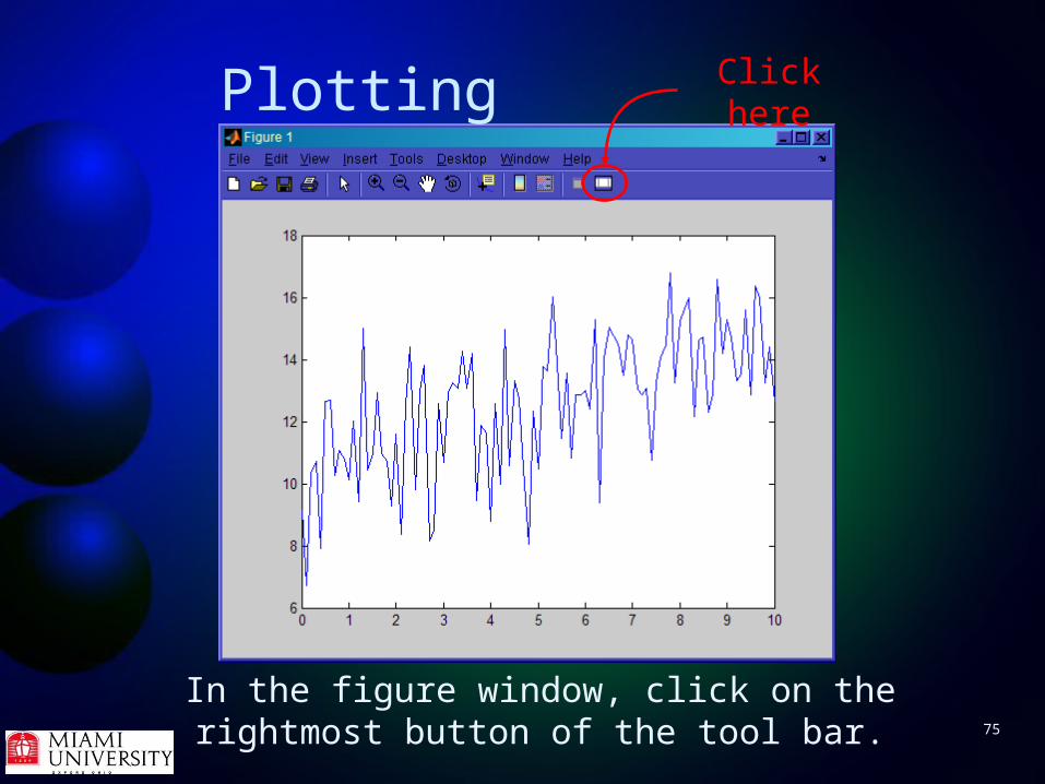
In the figure window, click on the rightmost button of the tool bar.

Click here

76

Plotting

Click on the arrow button in the tool bar. This lets you select what part of the plot to work on

Click here

77

PlottingTo change the vertical axis, left click on either axis. The big box on the bottom will now say “Property Editor – Axes”

1.Click on the y-axis tab

2.Put in 0 and 20 for the y limits

3.Click on the figure and watch the plot change

78

PlottingGet fancier

1. On the y-axis tab, enter the label“Power (watts)”

2. On the x-axis tab, enter the label“Time (sec)”

3. In the title box, add the title“Power measurements in first 10 secs”

4. Click on the title and in the Property Editor change the font to 16 pt bold

79

Plotting

Saving a plot in memory

• Choose Edit, Copy Figure– Go to other program, e.g., Word,

PowerPoint, and paste

• On PC, to copy figure window1. Display window

2. Press Alt+PrintScreen

3. Go to other program and paste

80

Plotting

Saving a plot

• To save in MATLAB format, choose File, Save

– Can work on it later– Can use as model for other plots– Can show your significant other your

that you have an artistic side

81

Plotting

Saving a plot

• To save in format other than MATLAB, choose File, Save As, then select type from “Save as type” dropdown box

– Can load saved figure into other software

82

Plotting

Tip• To include figure in other programs

and not change size, save in raster format (BMP, JPEG, PNG, TIFF)

• To include in other programs and change size, save in vector format (EPS, EMF)

• To distribute across operating systems, save as Adobe Acrobat format (PDF)

83

Plotting

CAREFUL!

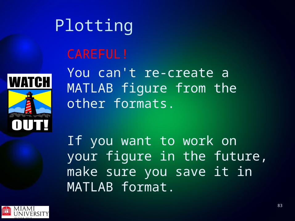
You can't re-create a MATLAB figure from the other formats.

If you want to work on your figure in the future, make sure you save it in MATLAB format.

84

Plotting

Questions?• Vectors

• Plotting

85

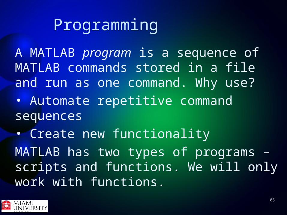
Programming

A MATLAB program is a sequence of MATLAB commands stored in a file and run as one command. Why use?

• Automate repetitive command sequences

• Create new functionality

MATLAB has two types of programs – scripts and functions. We will only work with functions.

86

Functions

A function is a MATLAB program that can accepts inputs and produce outputs. Some functions don't take any inputs and/or produce outputs.

A function is called or executed (run) by another program or function. That program can pass it input and receive the function's output.

87

Functions

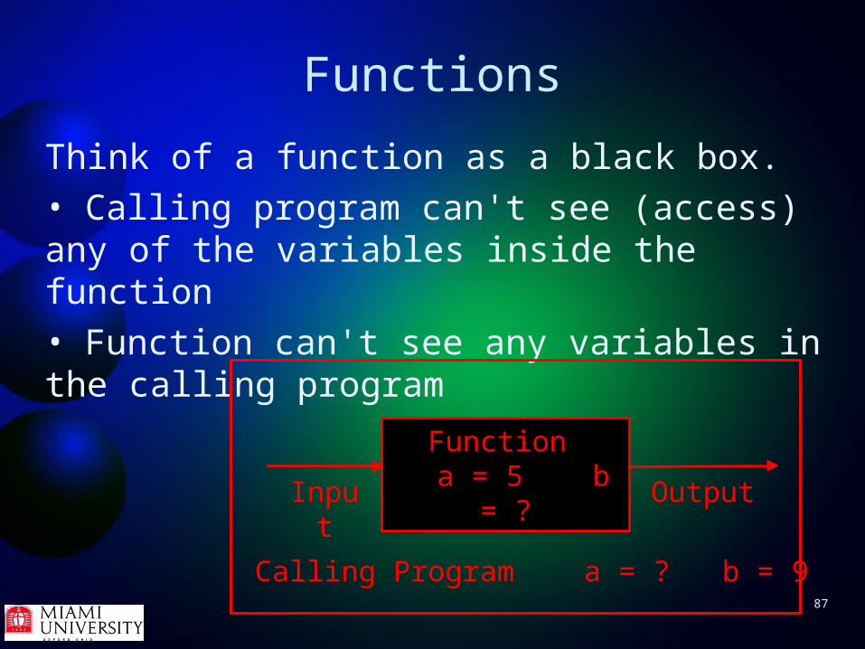
Think of a function as a black box.

• Calling program can't see (access) any of the variables inside the function

• Function can't see any variables in the calling program

Function a = 5 b = ?Input Output

Calling Program a = ? b = 9

88

Functions

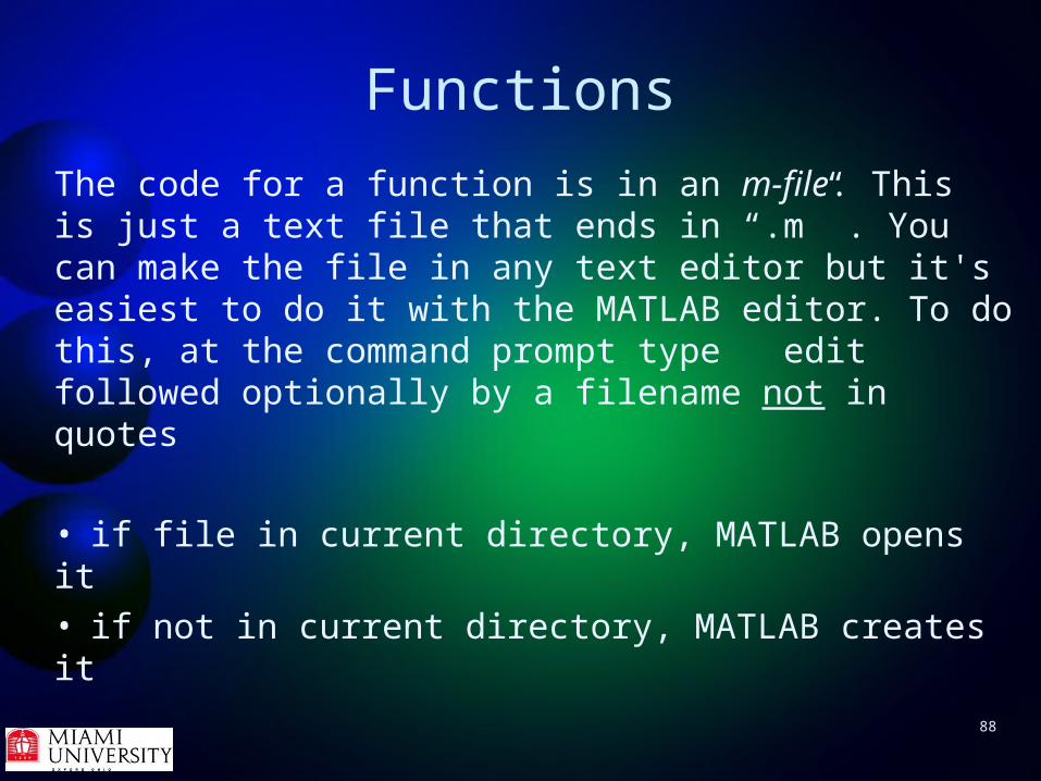
The code for a function is in an m-file. This is just a text file that ends in “.m” . You can make the file in any text editor but it's easiest to do it with the MATLAB editor. To do this, at the command prompt type edit followed optionally by a filename not in quotes

• if file in current directory, MATLAB opens it

• if not in current directory, MATLAB creates it

89

Functions

As soon as you make an m-file, give it a name (if needed) and save it. Do this by choosing “Save” or “Save as” under the file menu.

Try ItMake an m-file and save it as compute_area.m

>> edit compute_area.m

Choose File menu, Save

90

Functions

Function names

•Must begin with a letter

•Can contain any letters, numbers, or an underscore

•Name of file that contains function should be function name with “.m” appended

– Example: the function compute_area should be in the file called compute_area.m

91

Functionsfunction y = fname( v1, v2 )

First line of function is called the function line• “function” – keyword that tells MATLAB function starts with this line. Must be the word “function”• “y” – output variable(s). Can be any variable name• “fname” – any function name• “v1”, “v2” – input variable(s). Can be any variable name

For multiple outputs, use form

[x y] = fname( v1, v2 )

92

Functionsfunction y = fname( v1, v2 )• function ends when another function line appears or there's no more code in file• if function has outputs, must declare variables with output variable names and compute their values before function ends

Try ItMake the first line of your function be

function area = compute_area( a, b, n )

93

Functions

compute_area computes an approximation of the area under the function 1 / x in the interval [a,b]

Algorithm

1.Divide interval into n equal sections

2.Compute area of rectangle at each section by multiplying section width by function height at left side of section

3.Output is sum of rectangle areas

94

FunctionsTry ItIn your file, write

function area = compute_area( a, b, n )

delta = ( b – a ) / n;

x = a:delta:b;

y = ones( size( x ) );

y = y ./ x;

area = sum( delta * y );

Rectangle width Rectangle height

Rectangle area

95

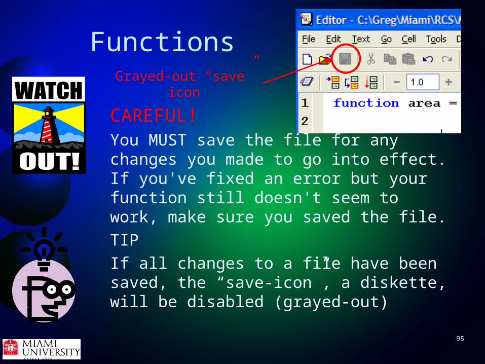
Functions

CAREFUL! You MUST save the file for any changes you made to go into effect. If you've fixed an error but your function still doesn't seem to work, make sure you saved the file.

TIP

If all changes to a file have been saved, the “save-icon”, a diskette, will be disabled (grayed-out)

Grayed-out “save” icon

96

FunctionsTry It

Call your function from the MATLAB command line. Use the interval [1,5] and 100, 1000, and then 10000 sections. What answers do you get? ( 1.6336, 1.6118, 1.6097 )

What should the answer be? ( 1.6094)

How did I get that number?

97

Functions

The usefulness of compute_area is very limited because it only works on one function – f(x) = 1 / x. We can make compute_area work on any function by having it call another function as its integrand. That way we just change that function and not compute_area.

To call one function from another, just make an m-file for each function and put both files in the same folder.

98

FunctionsTry ItIn compute_area, replace the 4th and 5th lines with

y = integrand( x )

function area = compute_area( a, b, n )

delta = ( b – a ) / n;

x = a:delta:b;

y = integrand( x );

area = sum( delta * y );

99

FunctionsTry It

Then make the m-file integrand.m Let's use the exponential function.

function y = integrand( x )

% return y = exp( -x )

% y is a vector of the same size as x

y = exp( -x );

Any line that starts with a percent sign (%) is a comment line. MATLAB ignores it.

100

Functions

Try It

Call compute_area from the MATLAB command line. Use the interval [0,1] and 1000 sections. What answer do you get? ( 0.6328 )

What should the answer be? 0.6321 ( = 1 – e-1 )

101

Loops

MATLAB has two program structures that let you execute a set of program lines repeatedly.

for-loop – executes the set of lines a given number of times

while-loop – executes the set of lines while a given condition is true

102

Loops

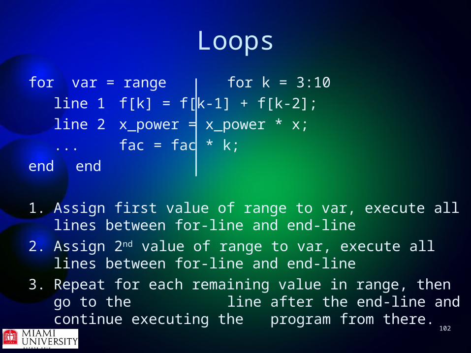
for var = range for k = 3:10

line 1 f[k] = f[k-1] + f[k-2];

line 2 x_power = x_power * x;

... fac = fac * k;

end end

1. Assign first value of range to var, execute all lines between for-line and end-line

2. Assign 2nd value of range to var, execute all lines between for-line and end-line

3. Repeat for each remaining value in range, then go to the line after the end-line and continue executing the

program from there.

103

LoopsTry It

ex = 1 + x + x2/2! + x3/3! + …

Make a function to compute a given number of terms of the Taylor series expansion of ex . The function should accept x and the number of terms n.

Run it for x = 1 and various values of n

104

LoopsTry It

ex = 1 + x + x2/2! + x3/3! + …

function sum = myexp( x, n )

sum = 1;

factorial = 1;

for k = 1:n

factorial = factorial * k;

sum = sum + x^k / factorial;

end

105

Loopswhile( condition ) while( abs(sum-z) > 1e-5 )

line 1 sum = sum + 10;

line 2 count = count + 1;

... fprintf( '%d\n',count );

end end

Evaluate the condition– If it's true, execute all the lines through the end-line and go to the

previous step.– If it's false, go to the line after the end-line and start executing the

program there.

106

LoopsTry It at Home

e-x = 1 – x + x2/2! – x3/3! + …

Make a function to compute the Taylor series expansion of e-x . Stop adding

terms when you get to one that won't change the value of the sum

Run it for x = 1

eps is the smallest number in MATLAB that can be added to another number and change its value

107

LoopsTry It at Home

e-x = 1 – x + x2/2! – x3/3! + …

function sum = while_exp( x )

sum = 1; term = -x; k = 1;

while( abs( term ) > eps )

sum = sum + term;

k = k + 1;

term = -term * x / k;

end

function sum = while_exp( x )

sum = 1;

term = -x;

k = 1;

while( abs( term ) > eps )

sum = sum + term;

k = k + 1;

term = -term * x / k;

end

108

MATLAB forMTH 453

Questions• Functions?

• Loops?

109

Easy Plots

“Easy Plot” family of plotting functions• Plot functions specified by notation e.g.,

sin(x), instead of by data• Plot functions specified in m-files• One- and two-dimensional functions• Make mesh, contour, surface plots• Can rotate, zoom, pan, annotate plots

110

Easy Plots

ezplot – plots 1D functions

>> ezplot( fun )

or

>> ezplot( fun, [ xmin xmax ] )• First form's range is -2π < x < 2π• fun can be in MATLAB notation between

single quote marks, e.g., 'x^4 – 3*x^3 + 2*x – 1'

• fun can be a MATLAB or custom function, e.g., compute_area

111

Easy Plots

To plot a function you wrote, say my_function, pass function name preceded by “@”>> ezplot( @my_function , [ xmin xmax ] )

•my_function must accept exactly one argument that can be a vector and produce one output vector of same size as input. Output element is function evaluated at corresponding input element, e.g., if y = my_function( x ) y(i) = my_function( x(i) )

112

Easy Plots

Since the input can be a vector, to do elementwise multiplication, division, and powers, make sure to use vector, not scalar, operations, i.e., use .*, ./, and .^, not *, /, and ^

y = square( x )

y = x * x;

y = square( x )

y = x .* x;

Wrong

Right!

113

Easy Plots

Try ItMake a function called

hyperbolicSine and plot it over the given limits

55for 2

)sinh(

xee

xxx

114

Easy Plotsfunction y = hyperbolicSine( x )

y = ( exp(x) - exp(-x) ) / 2;

>> ezplot( @hyperbolicSine, [-5 5] )

Title automatically set to function name

115

Easy Plots

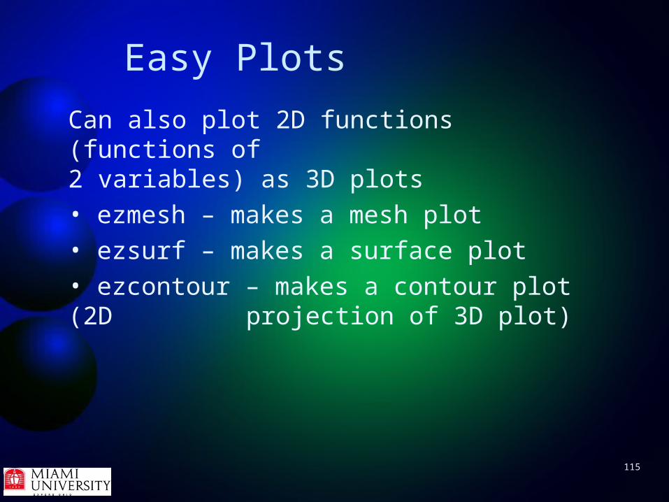
Can also plot 2D functions (functions of 2 variables) as 3D plots• ezmesh – makes a mesh plot• ezsurf – makes a surface plot• ezcontour – makes a contour plot (2D projection of 3D plot)

116

Easy Plots

ezmesh – plots 2D functions>> ezmesh( fun )

or>> ezmesh( fun, [ xmin xmax ymin ymax ] )

• First form's range is -2π < x < 2π, -2π < y < 2π• fun must accept exactly two arguments, which

may be vectors or matrices so as before, use elementwise operators

117

Easy Plots

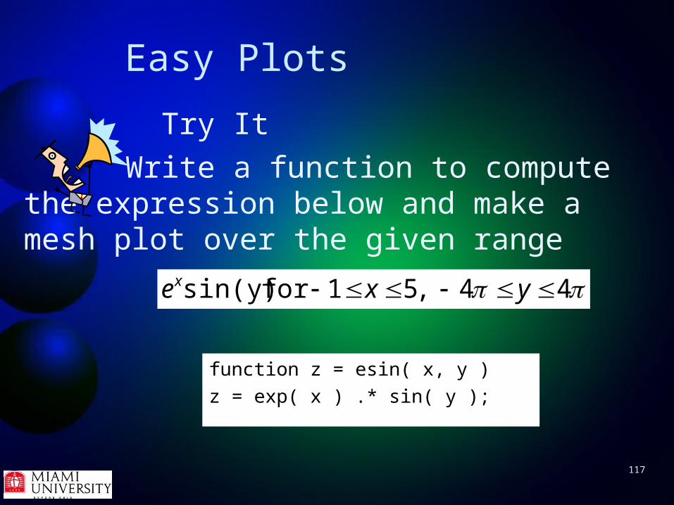
Try ItWrite a function to compute the

expression below and make a mesh plot over the given range

44 ,51for sin(y) yxex

function z = esin( x, y )

z = exp( x ) .* sin( y );

118

Easy Plots

>> ezmesh( @esin, [ -1 5 -4*pi 4*pi ] )

119

Easy Plots

ezsurf – plots 2D functions as solid surfaces>> ezsurf( fun )

or>> ezsurf( fun, [ xmin xmax ymin ymax ] )

• First form's range is -2π < x < 2π, -2π < y < 2π• fun must accept exactly two arguments, which

may be vectors or matrices so as before, use elementwise operators

120

Easy Plots

Try ItUse the previous function you wrote to

compute the expression below and make a surface plot over the given range

44 ,51for sin(y) yxex

121

Easy Plots

>> ezsurf( @esin, [ -1 5 -4*pi 4*pi ] )

122

Easy Plots

To get more information out of 3D plot, can:• Rotate• Magnify• Shrink• Move• Display values at a point• Display colorbar

123

Easy PlotsTo rotate, press the rotate button on the figure window toolbar, put the cursor over the plot and drag.

To return to the original position, in the command window type view(3)

>> view(3)

124

Easy PlotsTo zoom in (magnify), press the button with the magnifying glass and a plus on the figure window toolbar, put the cursor over the plot and click. The plot zooms in at that point. Clicking again zooms again.

To return to the original size, double click on the plot

125

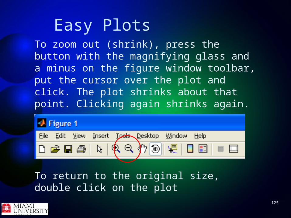
Easy PlotsTo zoom out (shrink), press the button with the magnifying glass and a minus on the figure window toolbar, put the cursor over the plot and click. The plot shrinks about that point. Clicking again shrinks again.

To return to the original size, double click on the plot

126

Easy PlotsTo pan (move), press the button with the hand on the figure window toolbar, put the cursor over the plot and drag. Panning is particularly useful with zoomed images.

To return to the original position, double click on the plot

127

Easy PlotsTry ItTry rotating, zooming, shrinking, panning and returning the plot to its original state.

Rotated Zoomed Zoomed and panned

128

Easy PlotsTo display the (x,y,z) values at a point in a 3D plot, press the button with the cross and yellow box in the figure window toolbar, put the cursor over the plot and click or drag.

129

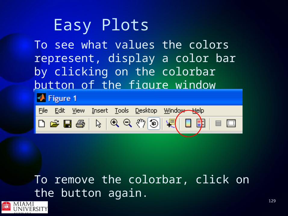
Easy PlotsTo see what values the colors represent, display a color bar by clicking on the colorbar button of the figure window toolbar.

To remove the colorbar, click on the button again.

130

Easy Plots

131

Easy Plots

Questions?

132

The End

133

Extra Material

134

File Output

Convenient to store output in file

• Creates record of work

• Easier than copying output by hand

• Can edit with text or MATLAB editor

• Can turn in homework

135

File Output

Making an output file takes three steps

1. Open the file

2. Write to the file

3. Close the file

136

File Output

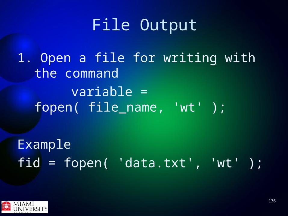
1. Open a file for writing with the command

variable = fopen( file_name, 'wt' );

Examplefid = fopen( 'data.txt', 'wt' );

137

File Output

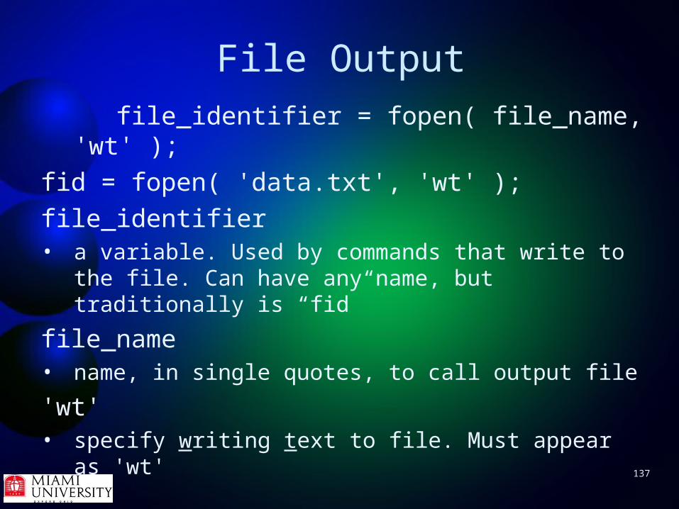
file_identifier = fopen( file_name, 'wt' );

fid = fopen( 'data.txt', 'wt' );

file_identifier• a variable. Used by commands that write to the

file. Can have any name, but traditionally is “fid”

file_name• name, in single quotes, to call output file

'wt'• specify writing text to file. Must appear as 'wt'

138

File Output

file_identifier = fopen( file_name, 'wt' );

fid = fopen( 'data.txt', 'wt' );

• if the file doesn't exist, MATLAB creates it

• if the file exists, MATLAB erases everything in it before writing to it

139

File Output2. Write to the file using fprintf fprintf( file_identifier, format_specifier, n1, n2 );

Examplefprintf( fid, 'Student %d is %d\n',...

studentId, studentAge );

• Use file identifier from you got from fopen• fprintf operates exactly as printing to screen but

first argument is fid

140

File Output3. Close the file with command fclose

fclose( file_identifier );

Examplefclose( fid );

• Use file identifier from you got from fopen• Once closed, can't write to it anymore

141

File Output

ExampleDownload write1.m from Web site type it up

142

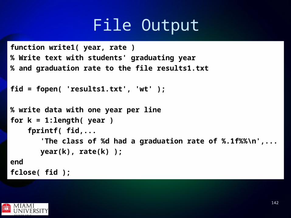
File Outputfunction write1( year, rate )

% Write text with students' graduating year

% and graduation rate to the file results1.txt

fid = fopen( 'results1.txt', 'wt' );

% write data with one year per line

for k = 1:length( year )

fprintf( fid,...

'The class of %d had a graduation rate of %.1f%%\n',...

year(k), rate(k) );

end

fclose( fid );

143

File OutputExample• Create two vectors with the students'

graduation year and graduation rate and call write1.m . Look at the output file with Notepad or Wordpad

• Add lines to write1.m that print the name of a university and college/school within the university

144

File OutputCan make tables in output file but process is clumsy. Must align output by hand

ExampleDownload write2.m from Web or type it in

145

File Outputfunction write2( year, rate )

% Write a table with students' graduating year

% and graduation rate

fid = fopen( 'results2.txt', 'wt' );

%if fid == -1

% error( 'Couldn''t open results2.txt' );

%end

% write top of table

fprintf( fid, '|------|------|--------|\n' );

146

File Output% write the table header

fprintf( fid, '| Item | Year | Rate |\n' );

% write each row of data

for k = 1:length( year )

fprintf( fid, '|------|------|--------|\n' );

fprintf( fid, '| %4d | %4d | %5.1f%% |\n',...

k, year(k), rate(k) );

end

% write bottom of table

fprintf( fid, '|------|------|--------|\n' );

fclose( fid );

147

File OutputExample• Create two vectors with the students'

graduation year and graduation rate and call write2.m . Look at the output file with Notepad or Wordpad

• Change the file so that each column of the table is two spaces wider, one on each side of the column header word