KTH ROYAL INSTITUTE

OF TECHNOLOGY

Introduction to Model Order Reduction Lecture 1: Introduction and overview Henrik Sandberg, Bart Besselink, Madhu N. Belur

Overview of Today’s Lecture

• What is model (order) reduction? Why is it important?

• What is included in the course? What is not included?

• Preliminary program

• What is expected from you? How to pass?

• Sign up for course

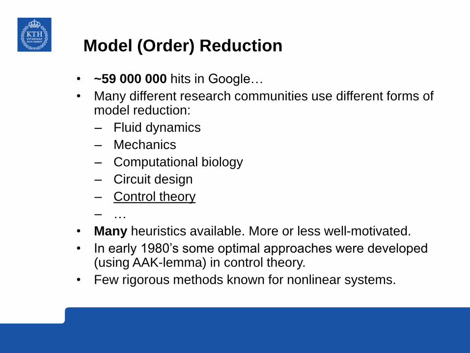
Model (Order) Reduction

• ~59 000 000 hits in Google…

• Many different research communities use different forms of model reduction:

– Fluid dynamics

– Mechanics

– Computational biology

– Circuit design

– Control theory

– …

• Many heuristics available. More or less well-motivated.

• In early 1980’s some optimal approaches were developed (using AAK-lemma) in control theory.

• Few rigorous methods known for nonlinear systems.

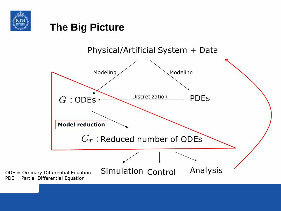
The Big Picture

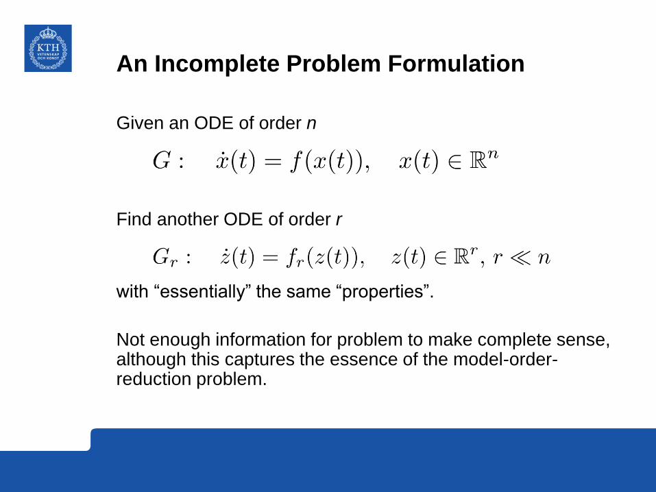
An Incomplete Problem Formulation

Given an ODE of order n

Find another ODE of order r

with “essentially” the same “properties”.

Not enough information for problem to make complete sense, although this captures the essence of the model-order-reduction problem.

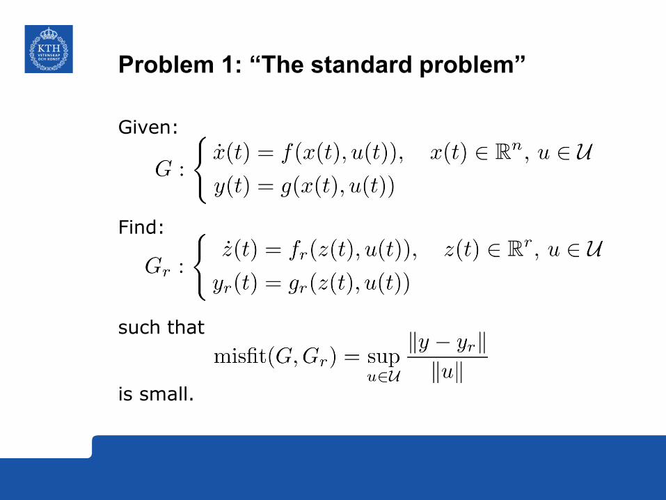
Problem 1: “The standard problem”

Given:

Find:

such that

is small.

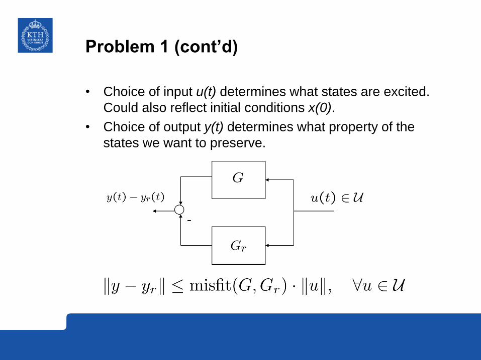
Problem 1 (cont’d)

• Choice of input u(t) determines what states are excited.

Could also reflect initial conditions x(0).

• Choice of output y(t) determines what property of the

states we want to preserve.

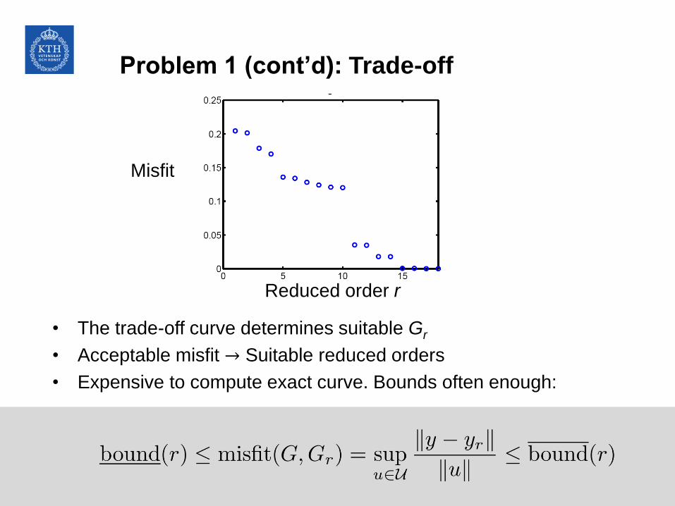
Problem 1 (cont’d): Trade-off

• The trade-off curve determines suitable Gr

• Acceptable misfit → Suitable reduced orders

• Expensive to compute exact curve. Bounds often enough:

Misfit

Reduced order r

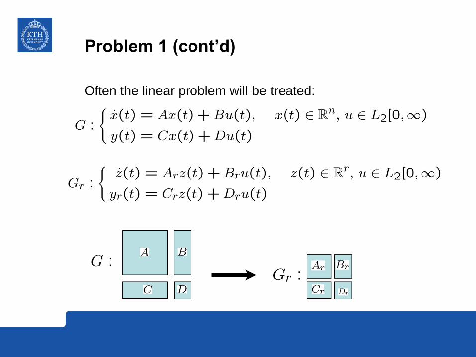
Problem 1 (cont’d)

Often the linear problem will be treated:

Problem 1 (cont’d)

A good model-reduction method gives us:

1. bound(r) – To help us choose a suitable approximation order r before the reduced-order model has to be computed; and

2. a reduced-order model (fr ,gr) alt. (Ar ,Br ,Cr ,Dr).

Such methods exist for some classes of models (typically linear). Many heuristics fail to provide bound(r).

Note: After a reduced-order Gr model is found, usually misfit(G,Gr) can be computed (although it may be expensive)

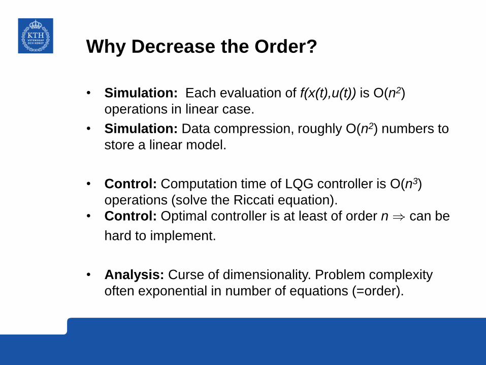
Why Decrease the Order?

• Simulation: Each evaluation of f(x(t),u(t)) is O(n2)

operations in linear case.

• Simulation: Data compression, roughly O(n2) numbers to

store a linear model.

• Control: Computation time of LQG controller is O(n3)

operations (solve the Riccati equation).

• Control: Optimal controller is at least of order n can be

hard to implement.

• Analysis: Curse of dimensionality. Problem complexity

often exponential in number of equations (=order).

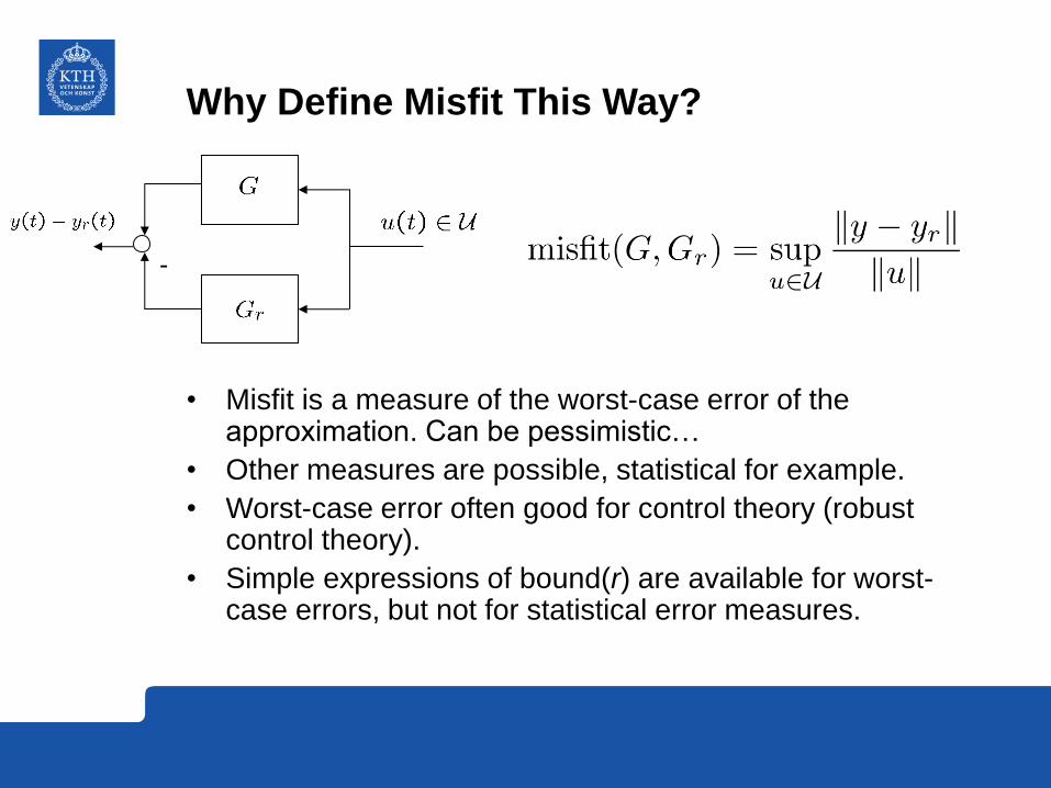
Why Define Misfit This Way?

• Misfit is a measure of the worst-case error of the approximation. Can be pessimistic…

• Other measures are possible, statistical for example.

• Worst-case error often good for control theory (robust control theory).

• Simple expressions of bound(r) are available for worst-case errors, but not for statistical error measures.

-

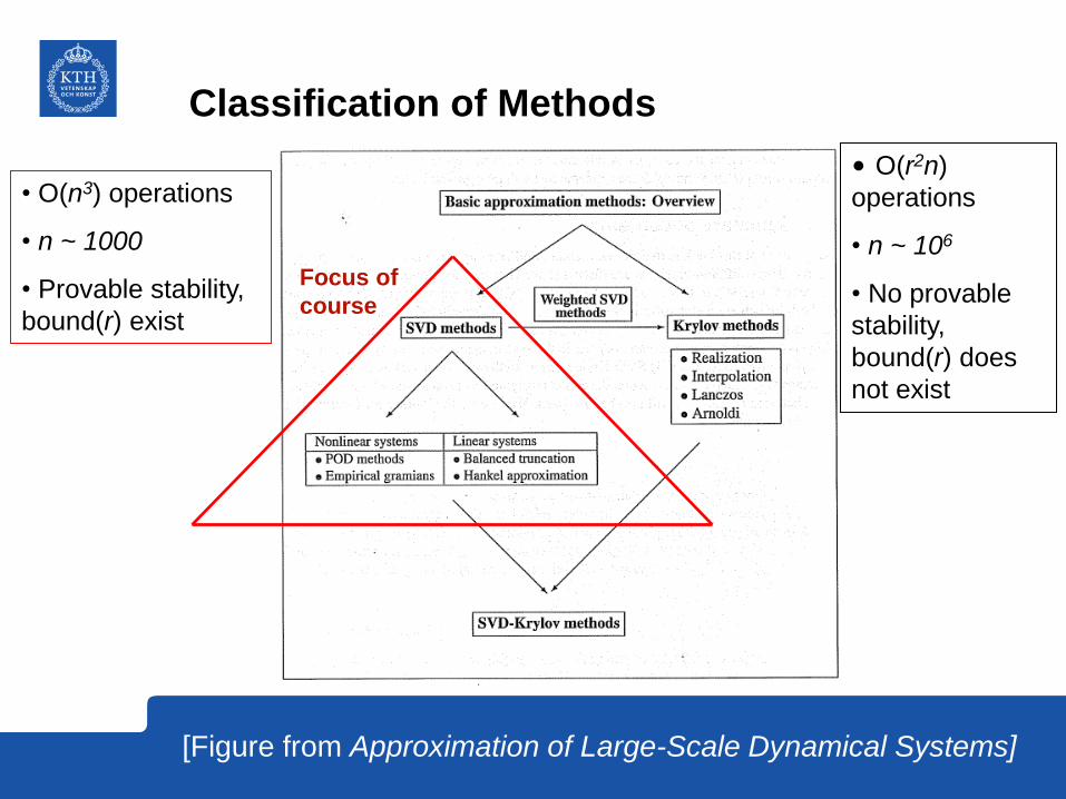
Classification of Methods

Focus of

course

• O(n3) operations

• n ~ 1000

• Provable stability,

bound(r) exist

• O(r2n)

operations

• n ~ 106

• No provable

stability,

bound(r) does

not exist

[Figure from Approximation of Large-Scale Dynamical Systems]

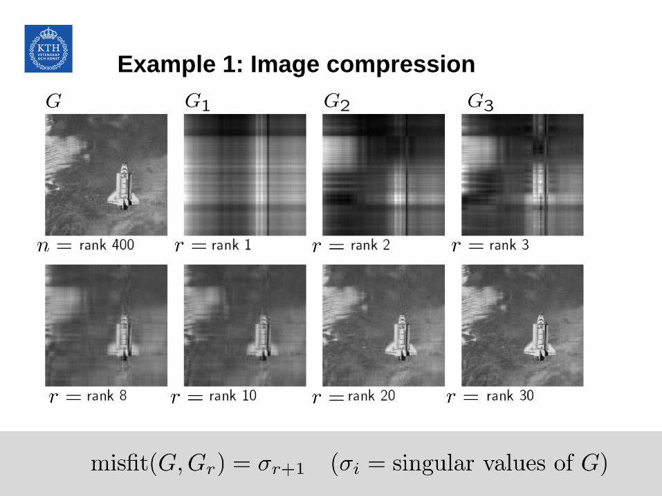
Example 1: Image compression

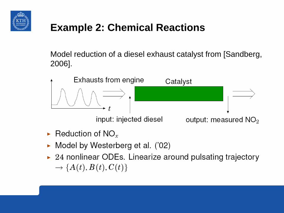
Example 2: Chemical Reactions

Model reduction of a diesel exhaust catalyst from [Sandberg,

2006].

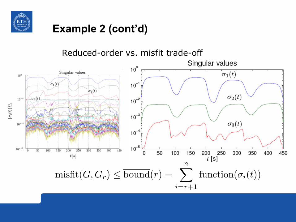
Example 2 (cont’d)

Reduced-order vs. misfit trade-off

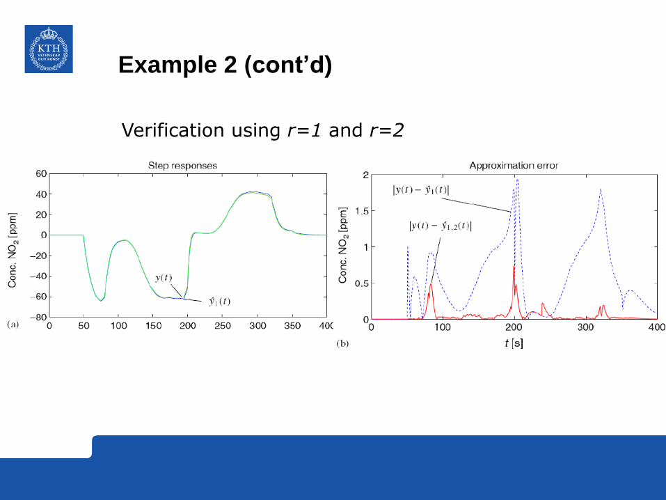
Example 2 (cont’d)

Verification using r=1 and r=2

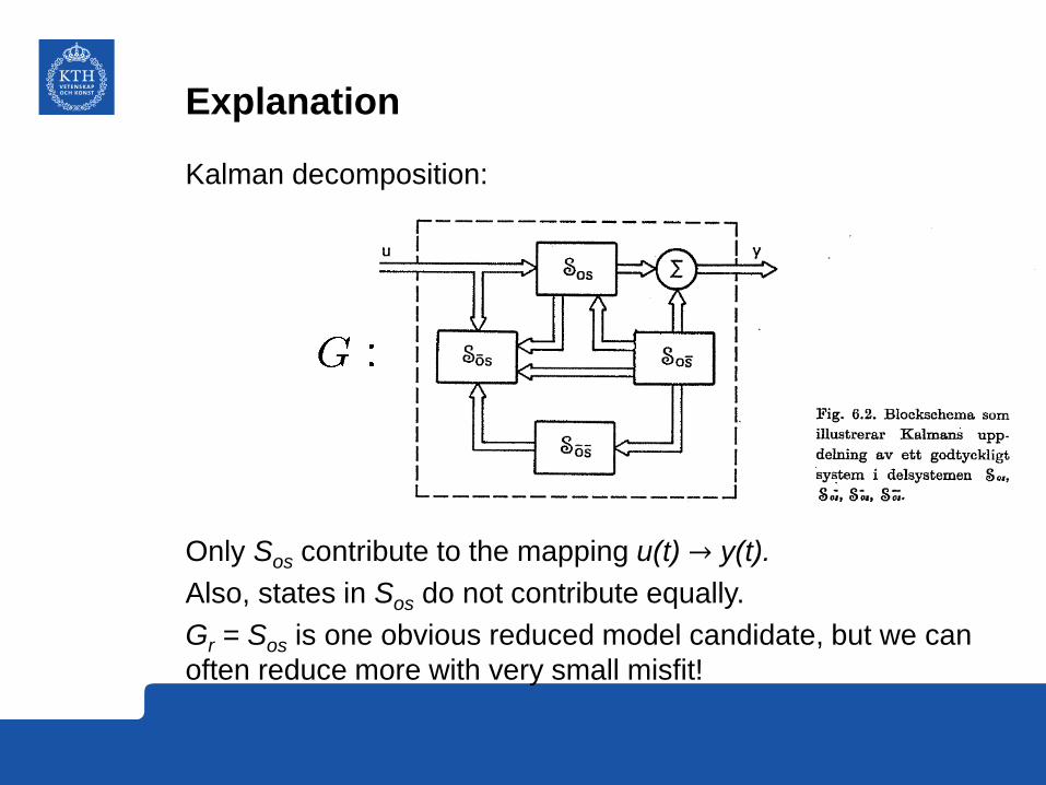
Explanation

Kalman decomposition:

Only Sos contribute to the mapping u(t) → y(t).

Also, states in Sos do not contribute equally.

Gr = Sos is one obvious reduced model candidate, but we can

often reduce more with very small misfit!

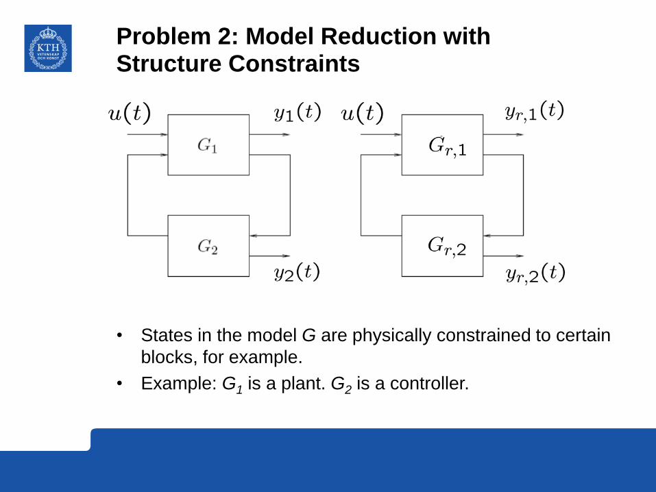
Problem 2: Model Reduction with Structure Constraints

• States in the model G are physically constrained to certain

blocks, for example.

• Example: G1 is a plant. G2 is a controller.

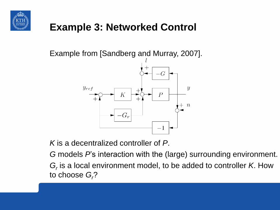
Example 3: Networked Control

Example from [Sandberg and Murray, 2007].

K is a decentralized controller of P.

G models P’s interaction with the (large) surrounding environment.

Gr is a local environment model, to be added to controller K. How

to choose Gr?

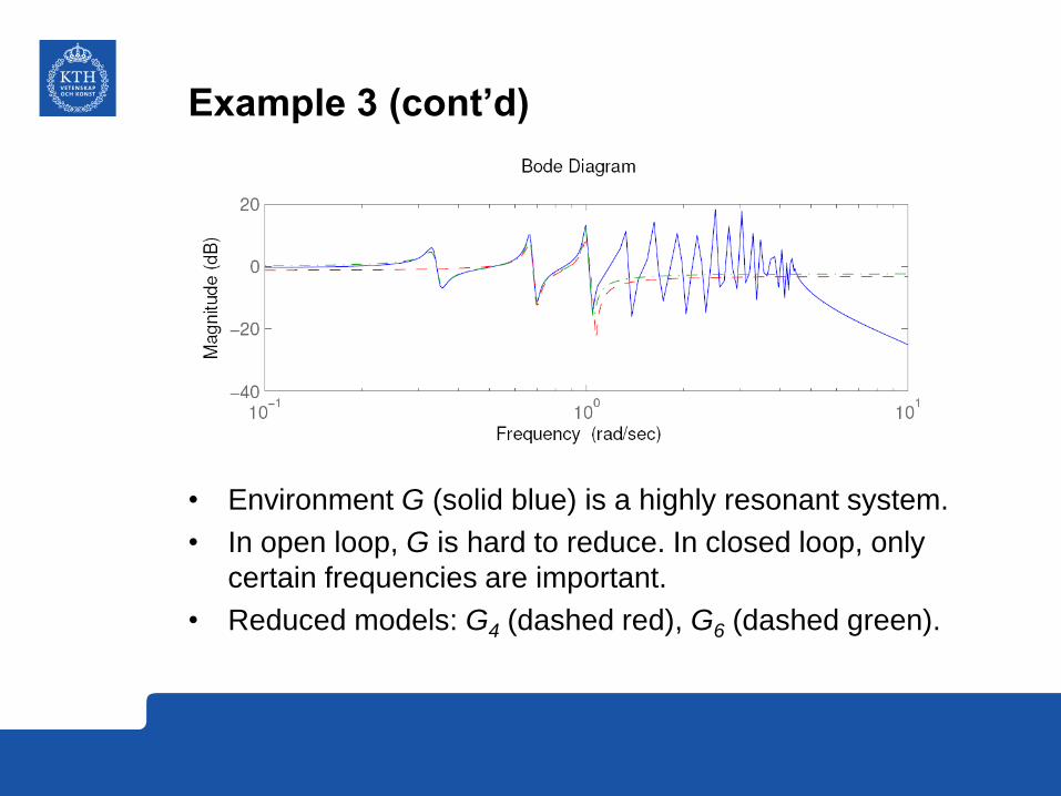
Example 3 (cont’d)

• Environment G (solid blue) is a highly resonant system.

• In open loop, G is hard to reduce. In closed loop, only

certain frequencies are important.

• Reduced models: G4 (dashed red), G6 (dashed green).

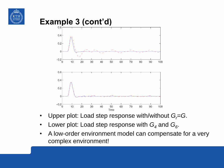
Example 3 (cont’d)

• Upper plot: Load step response with/without Gr=G.

• Lower plot: Load step response with G4 and G6.

• A low-order environment model can compensate for a very

complex environment!

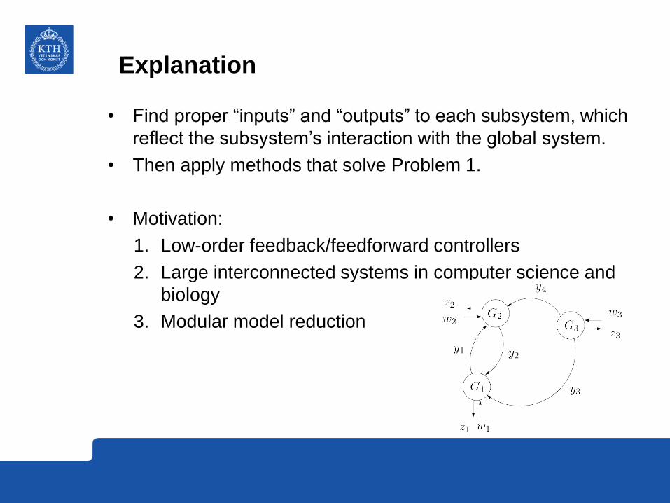
Explanation

• Find proper “inputs” and “outputs” to each subsystem, which

reflect the subsystem’s interaction with the global system.

• Then apply methods that solve Problem 1.

• Motivation:

1. Low-order feedback/feedforward controllers

2. Large interconnected systems in computer science and

biology

3. Modular model reduction

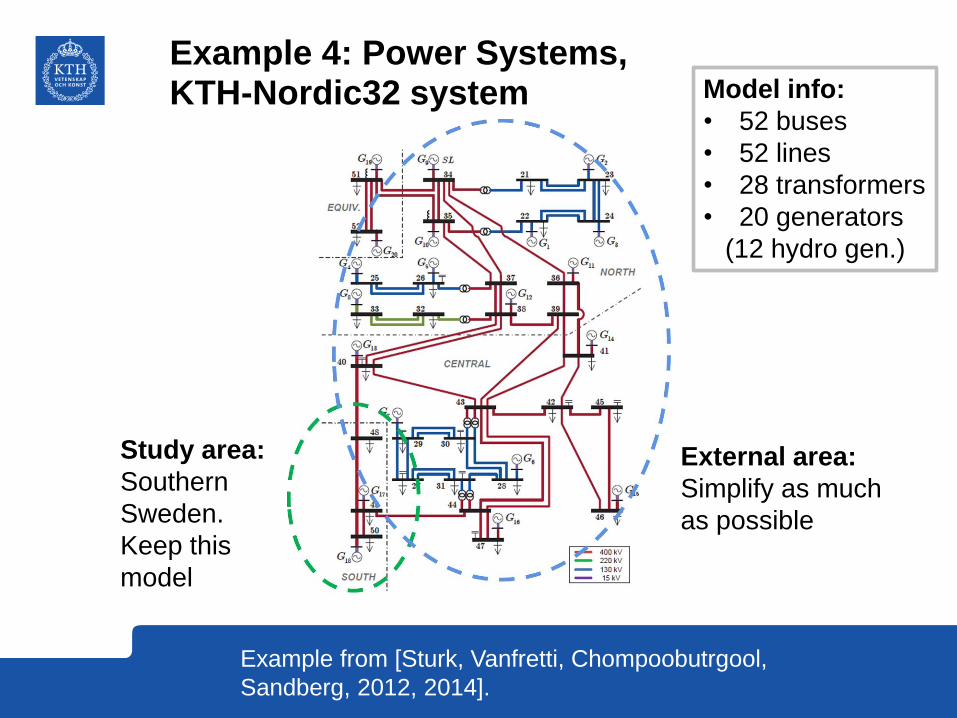
Example 4: Power Systems, KTH-Nordic32 system

Study area:

Southern

Sweden.

Keep this

model

External area:

Simplify as much

as possible

Model info:

• 52 buses

• 52 lines

• 28 transformers

• 20 generators

(12 hydro gen.)

Example from [Sturk, Vanfretti, Chompoobutrgool,

Sandberg, 2012, 2014].

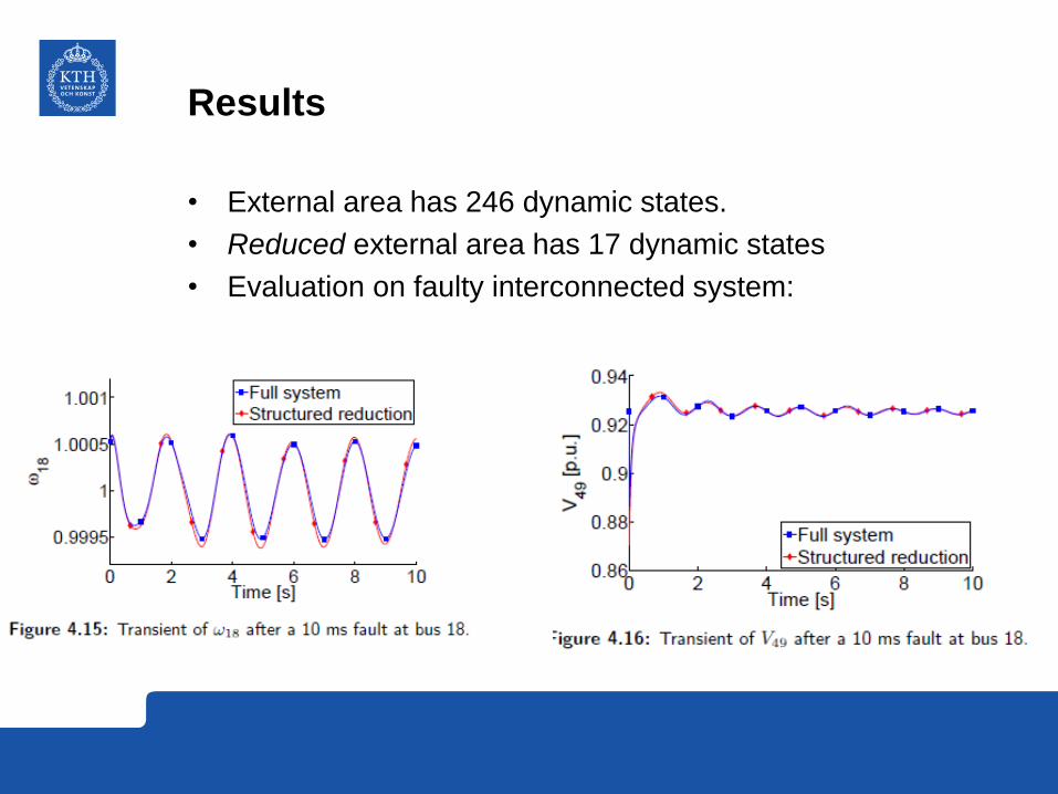
Results

• External area has 246 dynamic states.

• Reduced external area has 17 dynamic states

• Evaluation on faulty interconnected system:

What You Will Learn in the Course

• Norms of signals and systems, some Hilbert space theory.

• Principal Component Analysis (PCA)/Proper Orthogonal Decomposition (POD)/Singular Value Decomposition (SVD).

• Realization theory: Observability and controllability from optimal control/estimation perspective.

• Balanced truncation for linear systems (with extension to nonlinear systems).

• Hankel norm approximation.

• Uncertainty and robustness analysis of models (small-gain theorem), controller reduction.

• Optimization/LMI approaches.

• Behavioral theory (Madhu Belur).

Course Basics

• Graduate level

• Pass/fail

• 7 ECTS

• Course code: FEL3500

• Prerequisites:

1. Linear algebra

2. Basic systems theory (state-space models, controllability, observability etc.)

3. Familiarity with MATLAB

Course Material

Two books entirely devoted to model reduction are available:

1. Obinata and Anderson: Model Reduction for Control Systems Design (online version)

2. Antoulas: Approximation of Large-Scale Dynamical Systems

These books are not required for the course (although they are very good). Complete references on webpage.

Parts of these control/optimization books are used

1. Luenberger: Optimization by Vector Space Methods

2. Green and Limebeer: Linear Robust Control (online version)

3. Doyle, Francis, and Tannenbaum: Feedback Control Theory (online version)

Course Material (cont’d)

• Relevant research articles will be distributed.

• Generally no slides. White/black board will be used.

• Minimalistic lecture notes (PDFs) provided every lecture,

containing:

1. Summary of most important results (generally without

proofs)

2. Exercises

3. Reading advice

To Get Credits, You Need to Complete…

1. Exercises

• Exercises handed out with each lecture

• At the end of the course, at least 75% of the exercises should have been solved and turned in on time

• Exercises for Lectures 1-4 due April 17

• Exercises for Lectures 5-8 due May 12

2. Exam

• A 24h take-home exam

• You decide when to take it, but it should be completed at the latest 3 months after course ends

• No cooperation allowed

• Problems similar to exercises

Next Lecture

• Wednesday April 2 at 13:15-15 in L41.

• We start with the simplest methods:

– Modal truncation

– Singular perturbation/residualization

– Model projection

• First set of exercises handed out.

• Model-reduction method complexity increases with time in the course.

• First exercise session on Friday April 4 is devoted to repetition of basic linear systems concepts, Hilbert spaces, norms, operators,…

• Hope to see you on Wednesday!