Introduction to Nonparametric Estimation A.B.Tsybakovpluto.huji.ac.il/~pchiga/teaching/Nonparametric... · 2016-12-06 · Solutions to the exercises from \Introduction to Nonparametric

$Page 1: Introduction to Nonparametric Estimation A.B.Tsybakovpluto.huji.ac.il/~pchiga/teaching/Nonparametric... · 2016-12-06 · Solutions to the exercises from \Introduction to Nonparametric$
Solutions to the exercises from

“Introduction to Nonparametric Estimation”

A.B.Tsybakov

Pavel Chigansky

Department of Statistics, The Hebrew University, Mount Scopus, Jerusalem91905, Israel

E-mail address: [email protected]

These solutions have been written during the course, based on A. Tsybakov’s “Introductionto Nonparametric Estimation”, I taught at the Department of Statistics of the Hebrew Universityduring the spring semester of 2012. All the errors and mistypes are exclusively mine and I willbe delighted to get any improvement suggestions, remarks or bug reports. I am grateful to Mr.Luong Minh Khoa for proofreading of these notes.

P.Ch, 2012

1. NONPARAMETRIC ESTIMATORS 3

1. Nonparametric Estimators

Exerecise 1.1.

(1) Argue that any symmetric kernel K is a kernel of order 1 whenever the function u 7→uK(u) is integrable.

(2) Find the maximum order of the Silverman kernel:

K(u) =1

2exp

(− |u|/

√2)

sin(|u|/√

2 + π/4).

Hint: Apply the Fourier transform and write the Silverman kernel as

K(u) =

∫ ∞−∞

cos(2πtu)

1 + (2πt)4dt.

Solution

Note that u 7→ |u|jK(u) is integrable for any j ≥ 1 and hence∫umK(u)du = imK(m)(0), m ≥ 1,

where K(t) =∫eituK(u)du is the Fourier transform of K, given by

K(ω) =2π

1 + ω4.

Hence for m = 1,

K ′(0) = − 4ω3

(1 + ω4)2 ∣∣ω:=0

= 0

which is also obvious by symmetry. Further, a calculation reveals that K ′′(0) = K ′′′(0) = 0,

while K(4)(0) = −2π · 24. Hence the Silverman kernel is of order 3.

Exerecise 1.2. Kernel estimator of the s-th derivative p(s) of a density p ∈ P(β, L), s < β,can be defined as follows:

pn,s(x) =1

nhs+1

n∑i=1

K

(Xi − xh

).

Here h > 0 is a bandwidth and K : R 7→ R is a bounded kernel with support [−1, 1] satisfyingfor ` = bβc: ∫

ujK(u)du = 0, j ∈ 0, ..., ` \ s (1.1)∫usK(u)du = s!. (1.2)

(1) Prove that, uniformly over the class P(β, L), the bias of pn,s(x0) is bounded by chβ−s

and the variance of pn,s(x0) is bounded by c′

nh2s+1 , where c and c′ are appropriateconstants and x0 is a point in R.

4

(2) Prove that the maximum of the MSE of pn,s(x0) over P(β, L) is of order O(n− 2(β−s)

2β+1

)as n→∞ if the bandwidth h := hn is chosen optimally.

(3) Let (ϕm) be the orthonormal Legendre basis on [−1, 1]. Show that the kernel

K(u) =∑m=0

ϕ(s)m (0)ϕm(u)1|u|≤1

satisfies the conditions (1.1) and (1.2).

Solution

(1) The variance of the estimate pn,s(x0) is

Ep(pn,s(x0)− Eppn,s(x0)

)2=

1

nh2(s+1)Ep

(K

(X1 − x0

h

)− EpK

(X1 − x0

h

))2

≤

1

nh2(s+1)EpK

2

(X1 − x0

h

)=

1

nh2s+1

∫K2(v)p(x0 + vh)dv ≤ K2

max

1

nh2s+1,

i.e. the claim holds with c′ := K2max = maxx∈[−1,1] |K(x)|.

The bias term satisfies

b(x0) = Eppn,s(x0)− p(s)(x0) =1

hs+1

∫K

(u− x0

h

)p(u)du− p(s)(x0) =

1

hs

∫K(v)p(x0 + vh)dv − p(s)(x0) =

1

hs

∫K(v)

(p(x0) + p(1)(x0)vh+ ...+

1

`!p(`)(x0 + τvh)(vh)`

)dv − p(s)(x0).

By the conditions (1.1) and (1.2),

|b(x0)| ≤ 1

`!

1

hs

∫ ∣∣∣K(v)(p(`)(x0 + τvh)− p(`)(x0)

)(vh)`

∣∣∣dv ≤1

`!

1

hs

∫|K(v)|L|vh|β−`|vh|`dv ≤ L

`!hβ−s

∫|K(v)||v|βdv =: chβ−s.

(2) For any n ≥ 1 and h > 0,

supp∈P(β,L)

Ep(pn,s(x0)− p(x0)

)2= b2(x0) + σ2(x0) ≤ ch2(β−s) +

c′

nh2s+1.

The right hand side is minimized over h by

h∗n :=

(c′(2s+ 1)

2c(β − s)

) 12β+1

n− 1

2β+1

so that

supp∈P(β,L)

Ep(pn,s(x0)− p(x0)

)2 ≤ Cn− 2(β−s)2β+1 .


(3) Since ϕi is a complete orthonormal basis in L([−1, 1]), the functions uj satisfy

uj =

j∑i=1

bjiϕi(u),

with some constants bji. Hence for j ∈ 0, ..., `,

∫ujK(u)du =

∑m=0

ϕ(s)m (0)

j∑i=1

bji

∫ 1

−1ϕi(u)ϕm(u)du =

j∑m=0

ϕ(s)m (0)bjm =

ds

dus

( j∑m=0

ϕm(u)bjm

)u=0

=( dsdus

uj)u=0

.

The latter term vanishes both for j < s and j > s. For j = s,∫ujK(u)du = s! is obtained.

Exerecise 1.3. Consider the estimator of the two dimensional kernel density p(x, y) fromthe i.i.d. sample (X1, Y1), ..., (Xn, Yn)

pn(x, y) =1

nh2

n∑i=1

K

(Xi − xh

)K

(Yi − yh

), (x, y) ∈ R2.

Assume that the density p belongs to the class of all probability densities on R2 satisfying theHolder condition∣∣p(x, y)− p(x′, y′)

∣∣ ≤ L(|x− x′|β + |y − y′|β), (x, y), (x′y′) ∈ R2,

with given constants 0 < β ≤ 1 and L > 0. Let (x0, y0) be a fixed point in R2. Derive the upperbounds for the bias and the variance of pn(x0, y0) and an upper bound for the mean squared riskat (x0, y0). Find the minimizer h = h∗n of the upper bound of the risk and the correspondingrate of convergence.

Solution

The variance is given by

σ2(x0, y0) = Ep(pn(x0, y0)− Epp(x0, y0)

)2=

1

n2h4Ep

(n∑i=1

K

(Xi − xh

)K

(Yi − yh

)− EpK

(Xi − xh

)K

(Yi − yh

))2

=

≤ 1

n

1

h4

∫ ∫K2

(u− x0

h

)K2

(v − y0

h

)p(u, v)dudv =

1

n

1

h2

∫ ∫K2(u)K2(v)p(x0 + uh, y0 + vh)dudv ≤ 1

n

1

h2pmax

(∫K2(u)du

)2

=: c′1

n

1

h2

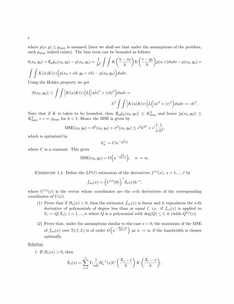
6

where p(x, y) ≤ pmax is assumed (later we shall see that under the assumptions of the problem,such pmax indeed exists). The bias term can be bounded as follows

b(x0, y0) = Eppn(x0, y0)− p(x0, y0) =1

h2

∫ ∫K

(u− x0

h

)K

(v − y0

h

)p(u, v)dudv − p(x0, y0) =∫ ∫

K(u)K(v)(p(x0 + uh, y0 + vh)− p(x0, y0)

)dudv.

Using the Holder property we get

|b(x0, y0)| ≤∫ ∫ ∣∣∣K(u)K(v)

∣∣∣L(|uh|β + |vh|β)dudv =

hβ∫ ∫ ∣∣∣K(u)K(v)

∣∣∣L(|u|β + |v|β)dudv =: chβ.

Note that if K is taken to be bounded, then |Eppn(x0, y0)| ≤ K2max and hence |p(x0, y0)| ≤

K2max + c =: pmax for h < 1. Hence the MSE is given by

MSE(x0, y0) = b2(x0, y0) + σ2(x0, y0) ≤ c2h2β + c′1

n

1

h2,

which is optimized by

h∗n := Cn− 1

2β+2

where C is a constant. This gives

MSE(x0, y0) = O(n− 2β

2β+2

), n→∞.

Exerecise 1.4. Define the LP (`) estimators of the derivatives f (s)(x), s = 1, ..., ` by

fns(x) =(U (s)(0)

)>θn(x)h−s,

where U (s)(x) is the vector whose coordinates are the s-th derivatives of the correspondingcoordinates of U(x).

(1) Prove that if Bn(x) > 0, then the estimator fns(x) is linear and it reproduces the s-th

derivative of polynomials of degree less than or equal `, i.e. if fns(x) is applied to

Yi := Q(Xi), i = 1, ..., n where Q is a polynomial with deg(Q) ≤ `, it yields Q(s)(x).

(2) Prove that, under the assumptions similar to the case s = 0, the maximum of the MSE

of fns(x) over Σ(β, L) is of order O(n− 2(β−s)

2β+1

)as n → ∞ if the bandwidth is chosen

optimally.

Solution

1. If Bn(x) > 0, then

θn(x) =n∑i=1

Yi1

nhB−1n (x)U

(Xi − xh

)K

(Xi − xh

),


and hence

fns(x) =(U (s)(0)

)>θn(x)h−s =

n∑i=1

YiWs∗ni (x),

with

W s∗ni (x) =

1

nh1+s

(U (s)(0)

)>B−1n (x)U

(Xi − xh

)K

(Xi − xh

)i.e. the estimator fns is linear.

If Q is a polynomial of order `, then

Q(Xi) = Q(x) +Q′(x)(Xi − x) + ...+1

`!Q(`)(x)(Xi − x)` = q(x)>U

(Xi − xh

),

where

q(x) =(Q(x), Q′(x)h, ..., Q(`)h`

).

Consequently,

θn(x) =argminθ∈R`+1

n∑i=1

(Q(Xi)− θ>U

(Xi − xh

))2K(Xi − x

h

)=

argminθ∈R`+1

n∑i=1

((q(x)− θ)>U

(Xi − xh

))2K(Xi − x

h

)= q(x).

Note that

U(s)j (x) =

ds

dxs1

j!xj =

0 s > j

1(j−s)!x

j−s s ≤ j, j = 1, ..., `

and hence the s-th entry of the vector U(s)j (0) is 1 and all the rest are zeros.

Hence if fns(x) is applied to Yi = Q(Xi) it yields

fns(x) =(U (s)(0)

)>θn(x)h−s =

(U (s)(0)

)>q(x)h−s = Q(s)(x).

In particular,n∑i=1

(Xi − xh

)kW s∗ni (x) =

0 k ∈ 0, ..., ` \ ss! k = s

(1.3)

2. The weights W s∗ni (x) satisfy the properties

(i) max1≤i≤n∣∣W s∗

ni (x)∣∣ ≤ C∗ 1

nh1+s

(ii)∑n

i=1

∣∣W s∗ni (x)

∣∣ ≤ C∗ 1hs

(iii) W s∗ni (x) = 0 whenever |Xi − x| > h

8

with a constant C∗ and h ≥ 12n . Indeed,

max1≤i≤n

∣∣W s∗ni (x)

∣∣ =

1

nh1+smax

1≤i≤n

∣∣∣∣(U (s)(0))>B−1n (x)U

(Xi − xh

)K

(Xi − xh

)∣∣∣∣ ≤1

nh1+smax

1≤i≤n

∥∥∥∥B−1n (x)U

(Xi − xh

)K

(Xi − xh

)∥∥∥∥1|Xi−x|≤h ≤

1

nh1+s

Kmax

λ0max

1≤i≤n

∥∥∥∥U (Xi − xh

)∥∥∥∥1|Xi−x|≤h ≤

1

nh1+s

Kmax

λ0max

1≤i≤n‖U (1)‖ ≤ 2

nh1+s

Kmax

λ0.

Similarly,n∑i=1

∣∣W s∗ni (x)

∣∣ =

1

nh1+s

n∑i=1

∣∣∣∣(U (s)(0))>B−1n (x)U

(Xi − xh

)K

(Xi − xh

)∣∣∣∣1|Xi−x|≤h ≤1

h1+s

Kmax

λ0‖U (1)‖ 1

n

n∑i=1

1|Xi−x|≤h ≤

1

h1+s

Kmax

λ0‖U (1)‖ a0 max

(2h,

1

n

)≤ 1

hs4Kmaxa0

λ0,

and (i) and (ii) hold with e.g. C∗ := 2Kmaxλ0

(1 + 2a0). The claim (iii) is obvious.Further,

Ef

(fns(x)− f (s)(x)

)2=

Ef

(fns(x)− Ef fns(x)

)2+(Ef fns(x)− f (s)(x)

)2= σ2(x) + b2(x).

For the variance term we have

σ2(x) = Ef

( n∑i=1

ξiWs∗ni (x)

)2≤ σ2

max

n∑i=1

(W s∗ni (x)

)2≤ σ2

maxC2∗

1

nh1+2s:= q1

1

nh1+2s.

The bias term can be bounded as follows:

b(x) = Ef fns(x)− f (s)(x) =

n∑i=1

f(Xi)Ws∗ni (x)− f (s)(x) =

n∑i=1

(f(x) + f ′(x)(Xi − x) + ...+

1

`!f `(x+ τi(Xi − x)

)(Xi − x)`

)W s∗ni (x)− f (s)(x) =

1

`!

n∑i=1

(f `(x+ τi(Xi − x)

)− f `

(x))

(Xi − x)`W s∗ni (x),


where |τi| < 1 and we used (1.3). Hence

|b(x)| ≤ 1

`!

n∑i=1

∣∣∣f `(x+ τi(Xi − x))− f `

(x)∣∣∣|Xi − x|`|W s∗

ni (x)| ≤

L

`!

n∑i=1

|x−Xi|β|W s∗ni (x)|1|x−Xi|≤h ≤

LC∗`!

hβ−s =: q2hβ−s.

Assembling all parts together we obtain

supx∈[0,1]

Ef

(fns(x)− f (s)(x)

)2≤ q1

1

nh1+2s+ q2

2h2(β−s).

The optimal choice of the bandwidth is h∗n := cn− 1

2β+1 for which we get

supf∈Σ(β,L)

supx∈[0,1]

Ef

(fns(x)− f (s)(x)

)2≤ Cn−

2(β−s)2β+1

with a constant C > 0, for all sufficiently large n.

Exerecise 1.5. Show that the rectangular kernel

K(u) =1

2I(|u| ≤ 1)

and the biweight kernel

K(u) =15

16(1− u2)21|u|≤1

are inadmissible.

Solution

The Fourier transform of the rectangular kernel is

K(ω) =1

2

∫ 1

−1eixωdx =

eiω − eiω

2iω=

sin(ω)

ω.

This is a continuous function (when extended to zero by continuity) and K(3π/2) = −2π/3.Hence the kernel is inadmissible by Proposition 1.8.

For the biweight kernel

K(ω) =15

ω5

((3− ω2) sinω − 3ω cosω

).

The kernel is inadmissible by continuity, since K(2π) < 0.

Exerecise 1.6. Let K ∈ L2(R) be symmetric and such that K ∈ L∞(R). Show that

(1) the condition

∃A <∞ : ess supt∈R\0

∣∣1− K(t)∣∣

|t|β≤ A, (1.4)

10

is equivalent to

∃t0, A0 <∞ : ess sup0<|t|<|t0|

|1− K(t)||t|β

≤ A0. (1.5)

(2) for integer β the condition (1.4) is satisfied if K is a kernel of order β − 1 and∫|u|β|K(u)|du <∞

Solution

1. Suppose (1.5) holds, then

ess supt∈R\0

∣∣1− K(t)∣∣

|t|β≤ ess sup

0<|t|<|t0|

|1− K(t)||t|β

+ ess sup|t|≥|t0|

∣∣1− K(t)∣∣

|t|β≤

A0 +1 + ‖K‖∞|t0|β

,

which verifies (1.4). The other direction is obvious.

2. If∫|u|βK(u)du <∞, the Fourier transform is β times differentiable at zero and K(i)(0) =

0 for i = 1, ..., β − 1, since K is of order β − 1. Hence,

K(t) = 1 +1

β!K(β)(τt)tβ,

where τ ∈ [−1, 1]. Hence

sup|t|≤1

|1− K(t)||t|β

≤ 1

β!sup

s∈[−1,1]|K(β)(s)| <∞,

where we used the fact that K(t) is bounded on [−1, 1], being continuous on it. By the Riemann-

Lebesgue lemma, limt→∞ K(t) = 0 and by continuity K is bounded. The claim now follows from1.

Exerecise 1.7. Let P be the class of all probability densities p on R such that∫exp(α|ω|r)|ϕ(ω)|2dω ≤ L2,

where α > 0, r > 0, L > 0 are given constants and ϕ is the Fourier transform of p. Showthat for any n ≥ 1 the kernel density estimator p with the sinc kernel and appropriately chosenbandwidth h = hn satisfies

supp∈P

Ep

∫ (pn(x)− p(x)

)2dx ≤ C (log n)1/r

n,

where C > 0 is a constant dependng only on r, L and α.

Solution


Recall that

2πMISE = 2πEp

∫ (pn(x)− p(x)

)2dx =

∫ ∣∣1− K(hω)∣∣2|ϕ(ω)|2dω+

1

n

∫|K(hω)|2dω − 1

n

∫|K(hω)|2|ϕ(ω)|2dω.

For the sinc kernel K(u) = sinuπu with K(ω) = 1|ω|≤1, the latter gives

2πMISE =

∫1|ω|>1/h|ϕ(ω)|2dω +

1

n

∫1|ω|≤1/hdω −

1

n

∫1|ω|≤1/h|ϕ(ω)|2dω =∫

R\[−1/h,1/h]|ϕ(ω)|2dω +

2

nh− 1

n

∫ 1/h

−1/h|ϕ(ω)|2dω ≤∫

R\[−1/h,1/h]e−α|ω|

reα|ω|

r |ϕ(ω)|2dω +2

nh≤

e−α|1/h|r

∫R\[−1/h,1/h]

eα|ω|r |ϕ(ω)|2dω +

2

nh≤ e−α|1/h|rL2 +

2

nh.

For hn :=α1/r

(log n)1/rwe get the bound

MISE ≤ 1

2π

(1

nL2 +

1

α1/r

2(log n)1/r

n

)≤ C (log n)1/r

n,

with an obvious constant C.

Exerecise 1.8. Let Pa, where a > 0, be the class of all probability densities p on R suchthat the support of the characteristic function ϕ is included in a given interval [−a, a]. Showthat for any n ≥ 1, the kernel density estimator pn with the sinc kernel and appropriately chosenbandwidth h satisfies

supp∈Pa

∫ (pn(x)− p(x)

)2dx ≤ a

πn.

This example, due to Ibragimon and Hasminskii (1983), shows that it is possible to estimatethe density with rate

√n on sufficiently small nonparametric classes of functions.

Solution

As in the previous problem,

2πMISE ≤∫R\[−1/h,1/h]

|ϕ(ω)|2dω +2

nh.

The claim follows with the choice h := 1a , since ϕ(ω) = 0 for |ω| > a.

Exerecise 1.9. Let (X1, ..., Xn) be an i.i.d. sample from a density p ∈ L2[0, 1].

(1) Show that cj are unbiased estimators of the Fourier coefficients cj =∫ 1

0 p(x)ϕj(x)dxand find the variance of cj .

12

(2) Express the MISE of the estimator pn,N as a function of p and the sequence (ϕj).Denote it by MISE(N).

(3) Derive an unbiased risk estimation method. Show that

Ep(J(N)

)= MISE(N)−

∫p2,

where

J(N) =1

n− 1

N∑j=1

(2

n

n∑i=1

ϕ2j (Xi)− (n+ 1)c2

j

).

Propose the data driven selector of N .

(4) Suppose now that (ϕj) is the trigonometric basis. Show that the MISE of pn,N isbounded by

N + 1

n+ ρN ,

where ρN =∑∞

j=N+1 c2j . Use this bound to prove that uniformly over the class of all

the densities p belonging to the Sobolev class of periodic functions W per(β, L), β > 0

and L > 0, the MISE of pn,N is of the order O(n− 2β

2β+1

)for an appropriate choice of

N = Nn.

Solution

1. Clearly, cj are unbiased:

Epcj = Epϕj(X1) = cj

and

varp(cj) = Ep(cj − cj)2 =1

nEp(ϕj(X1)− cj

)2=

1

n

(Epϕ

2j (X1)− c2

j

)=

1

n

(∫ϕ2jp−

(∫ϕjp)2)

2. Note that

Epn,N (x) =N∑j=1

cjϕj(x)

and

varp

(pn,N (x)

)= Ep

( N∑j=1

(cj − cj)ϕj(x))2.

Hence

MISE(N) = Ep

∫ ( N∑j=1

(cj − cj)ϕj)2

+

∫ ( N∑j=1

cjϕj −∞∑j=1

cjϕj

)2=

N∑j=1

Ep(cj − cj)2 +

∞∑j=N+1

c2j =

1

n

N∑j=1

(Epϕ

2j (X1)− c2

j

)+

∞∑j=N+1

c2j


3. Following the suggestion

Ep(J(N)

)=

1

n− 1

N∑j=1

(2

n

n∑i=1

Epϕ2j (Xi)− (n+ 1)Epc

2j

)=

1

n− 1

N∑j=1

(2Epϕ

2j (X1)− (n+ 1)

( 1

n

(Epϕ

2j (X1)− c2

j

)+ c2

j

))=

1

n

N∑j=1

(Epϕ

2j (X1)− (n+ 1)c2

j

)and hence

Ep(J(N)

)−MISE(N) =

1

n

N∑j=1

(Epϕ

2j (X1)− (n+ 1)c2

j

)− 1

n

N∑j=1

(Epϕ

2j (X1)− c2

j

)−

∞∑j=N+1

c2j =

−∞∑j=1

c2j = −

∫p2,

where we used Parseval’s identity.Since the same N maximizes both MISE(N) and Ep

(J(N)

), it makes sense to select

N := argminN≥1J(N)

and to plug it into pn,N .4. Recall that for even j

ϕj(x) =√

2 cos(πjx),

and hence

ϕ2j (x) = 2

1 + cos(2πjx)

2= 1 +

1√2ϕ2j(x).

Similarly, for odd j

ϕj(x) =√

2 sin(π(j − 1)x),

and

ϕ2j (x) = 2

1− cos(2π(j − 1)x)

2= 1− 1√

2ϕ2(j−1)(x).

Hence

Epϕ2j (X1) = 1 +

1√2

c2j j is even

−c2(j−1) j is odd

Consequently, e.g. for even N

MISE(N) =1

n

N∑j=1

(Epϕ

2j (X1)− c2

j

)+ ρN =

N

n+

1√2c2N −

1

n

N∑j=1

c2j + ρN ≤

N + 1

n+ ρN ,

The same bound holds for odd N ’s.

14

If p ∈W per(β, L), then the sequence of Fourier coefficients (cj) belong to the Sobolev ellipsoid

Θ(β,Q) with Q = L2/π2β and hence

ρN =∞∑

j=N+1

c2j ≤

1

a2N+1

∞∑j=N+1

c2ja

2j ≤ QN−2β.

Now the choice Nn := bαn1

2β+1 c with a constant α > 0 yields the claimed upper bound.

Exerecise 1.10. Consider the nonparametric regression model under Assumption (A) andsuppose that f belongs to the Sobolev class of periodic functions W per(β, L) with β ≥ 2. Theaim of this exercise is to study the weighted projection estimator

fn,λ(x) =

n∑j=1

λj θjϕj(x),

where λj ’s are real constants (weights), θj = 1n

∑ni=1 Yiϕj(Xi) are the Fourier coefficients esti-

mates.

(1) Prove that the risk MISE of fn,λ is minimized with respect to λj ’s by 1

λ∗j :=θj(θj + αj)

ε2 + (θj + αj)2, j = 1, ..., n

where ε2 = σ2ξ/n (λ∗j ’s are the weights corresponding to the weighted projection oracle).

(2) Check that the corresponding value of the risk is

MISE(λ∗) =n∑j=1

ε2θ2j

ε2 + (θj + αj)2+ ρn,

where ρn =∑∞

j=n+1 θ2j .

(3) Prove thatn∑j=1

ε2θ2j

ε2 + (θj + αj)2=(

1 + o(1)) n∑j=1

ε2θ2j

ε2 + θ2j

.

(4) Prove that

ρn =(1 + o(1)

) ∞∑j=n+1

ε2θ2j

ε2 + θ2j

.

(5) Deduce from the above results that

MISE(λ∗) = A∗n(1 + o(1)

), n→∞,

1recall that

αj =1

n

n∑i=1

f(i/n)ϕj(i/n)−∫fϕj .


where

A∗n =∞∑j=1

ε2θ2j

ε2 + θ2j

.

(6) Check that2

A∗n < minN≥1

An,N .

Solution

1. Recall that for 1 ≤ j ≤ n− 1 (an in fact for j = n as well, check!)

Eθj = θj + αj , E(θj − θj

)2= σ2

ξ/n+ α2j = ε2 + α2

j .

Hence

MISE =E

∫ ( n∑j=1

λj θjϕj(x)−∞∑j=1

θjϕj(x))2dx =

E

∫ ( n∑j=1

(λj θj − θj

)ϕj(x)−

∞∑j=n+1

θjϕj(x))2dx =

n∑j=1

E(λj θj − θj

)2+

∞∑j=n+1

θ2j .

Since

E(λj θj − θj

)2= E

(λj(θj − θj) + (λj − 1)θj

)2=

λ2jE(θj − θj)2 + 2λjE(θj − θj)(λj − 1)θj + (λj − 1)2θ2

j =

λ2j

(ε2 + α2

j

)+ 2λjαj(λj − 1)θj + (λj − 1)2θ2

j =

λ2jε

2 +(λjαj + (λj − 1)θj

)2,

we obtain

MISE(λ) =

n∑j=1

(λ2jε

2 +(λjαj + (λj − 1)θj

)2)

+ ρn.

The summands in the first term are parabolas, minimized by

λ∗j =θj(αj + θj)

ε2 + (αj + θj)2.

2. Direct calculation shows that the corresponding MISE is given by

MISE(λ∗) =n∑j=1

ε2θ2j

ε2 + (αj + θj)2+ ρn

2An,N =σ2ξN

n+ ρN is the leading term (for β > 1 in the upper bound for the MISE of the simple projection

estimator we studied in class.)

16

3. We have

ε2θ2j

ε2 + (αj + θj)2=

ε2θ2j

ε2 + θ2j

ε2 + θ2j

ε2 + (αj + θj)2=

ε2θ2j

ε2 + θ2j

(1 +

θ2j − (αj + θj)

2

ε2 + (αj + θj)2

)=

ε2θ2j

ε2 + θ2j

(1− αj(αj + 2θj)

ε2 + (αj + θj)2

).

Further, ∣∣∣∣ αj(αj + 2θj)

ε2 + (αj + θj)2

∣∣∣∣ =

∣∣∣∣∣ 2αj(αj + θj)

ε2 + (αj + θj)2−

α2j

ε2 + (αj + θj)2

∣∣∣∣∣ ≤ |αj/ε|+ |αj/ε|2where we used the elementary inequality |x|

ε2+x2≤ 1

21ε , x ∈ R. Recall that for θ ∈ Θ(β,Q) with

β > 1/2

max1≤j≤n−1

|αj | ≤ Cβ,Qn−β+1/2,

and that ε = σ2ξ/n. Hence for β ≥ 2,

|αj/ε|+ |αj/ε|2 ≤ C1n−β+1,

for all n, large enough. Consequently,∣∣∣∣∣∣n∑j=1

ε2θ2j

ε2 + (αj + θj)2−

n∑j=1

ε2θ2j

ε2 + θ2j

∣∣∣∣∣∣ ≤ C1n−β+1

n∑j=1

ε2θ2j

ε2 + θ2j

,

which verifies the claim for β > 1.4. Note that

θ2j =

ε2θ2j

ε2 + θ2j

+ θ2j

θ2j

ε2 + θ2j

.

Since∑∞

j=1 θ2ja

2j ≤ Q <∞, the sequence rj := θ2

ja2j converges to zero as j →∞. Hence

∞∑j=n+1

θ2j

θ2j

ε2 + θ2j

=1

ε2

∞∑j=n+1

rja2j

ε2θ2j

ε2 + θ2j

≤

1

ε2

supj≥n+1 rj

a2n+1

∞∑j=n+1

ε2θ2j

ε2 + θ2j

≤ C 1

n−1

supj≥n+1 rj

(n+ 1)2β

∞∑j=n+1

ε2θ2j

ε2 + θ2j

.

Hence for β ≥ 1,∣∣∣∣∣∣ρn −∞∑

j=n+1

ε2θ2j

ε2 + θ2j

∣∣∣∣∣∣ =

∣∣∣∣∣∣∞∑

j=n+1

θ2j −

∞∑j=n+1

ε2θ2j

ε2 + θ2j

∣∣∣∣∣∣ =

∞∑j=n+1

θ2j

θ2j

ε2 + θ2j

≤ o(1)

∞∑j=n+1

ε2θ2j

ε2 + θ2j

,

as claimed.5. Obviously follows from (3) and (4).


6. Using the identity y2 = y2x2

y2+x2+ y4

y2+x2, we get

minN≥1

An,N = minN≥1

(σ2ξN

n+ ρN

)= min

N≥1

N∑j=1

ε2 +∞∑

j=N+1

θ2j

=

minN≥1

N∑j=1

( ε2θ2j

ε2 + θ2j

+ε4

ε2 + θ2j

)+

∞∑j=N+1

( ε2θ2j

ε2 + θ2j

+θ4j

ε2 + θ2j

) =

∞∑j=1

ε2θ2j

ε2 + θ2j

+ minN≥1

N∑j=1

ε4

ε2 + θ2j

+

∞∑j=N+1

θ4j

ε2 + θ2j

> A∗n.

Exerecise 1.11. Consider the nonparametric regression model under the Assumption (A).

The smoothing spline estimator fspn (x) is defined as a solution of the following minimizationproblem

fspn = argminf∈W

(1

n

n∑i=1

(Yi − f(Xi)

)2+ κ

∫ 1

0

(f ′′(x)

)2dx

),

where κ is the smoothing parameter and W is one of the sets of functions defined below.

(1) First suppose that W is the set of all the functions : [0, 1] 7→ R such that f ′ is absolutely

continuous. Prove that the estimator fspn reproduces polynomials of degree ≤ 1 if n ≥ 2

(2) Suppose next that W is the set of all the functions f : [0, 1] 7→ R such that (i) f ′

is absolutely continuous and (ii) the periodicity condition is satisfied: f(0) = f(1),f ′(0) = f ′(1). Prove that the minimization problem is equivalent to

min(bj)

∞∑j=1

(− 2θjbj + b2j (κπ

4a2j + 1)

(1 +O(n−1)

)),

where bj are the Fourier coefficients of f , the term O(n−1) is uniform in (bj) and aj aredefined as for the Sobolev ellipsoid.

(3) Assume now that the term O(n−1) in the latter minimization problem is negligible.Formally replacing it by zero, find the solution and conclude that the periodic splineestimator is approximately equal to a weighted projection estimator

fspn (x) ≈∞∑j=1

λ∗j θjϕj(x),

with the weights λ∗j written explicitly.

18

(4) Use (3) to show that for sufficiently small κ the spline estimator fspn is approximatedby the kernel estimator

fn(x) =1

nh

n∑i=1

YiK(Xi − x

h

),

where h = κ1/4 and K is the Silverman kernel.

Solution

1. Let Q be the space of linear polynomials, then

minf∈W

(1

n

n∑i=1

(Yi − f(Xi)

)2+ κ

∫ 1

0

(f ′′(x)

)2dx

)≤

minf∈Q

(1

n

n∑i=1

(Yi − f(Xi)

)2+ κ

∫ 1

0

(f ′′(x)

)2dx

)=

mina,b∈R

1

n

n∑i=1

(Yi − b− aXi

)2.

If Yi = b′ + a′Xi and n ≥ 2, the latter expression vanishes and the minimizing constants areexactly a′ and b′, i.e. fspn (x) = b′ + a′x as claimed.

2. In this case, f(x) =∑∞

j=1 bjϕj(x), where (ϕj) is the trigonometric Fourier basis. Notethat for even j

d2

dx2ϕj(x) =

d2

dx2cos(

2πj

2x)

= −π2j2ϕj(x),

and for odd jd2

dx2ϕj(x) =

d2

dx2sin(

2πj − 1

2x)

= −π2(j − 1)2ϕj(x),

i.e. for any j ≥ 0d2

dx2ϕj(x) = −π2ajϕj(x),

where aj ’s are as in the definition of the Sobolev ellipsoid, corresponding to β = 2.Hence, if we assume that f ′′ is square integrable3, by the Parseval identity∫ 1

0(f ′′(x))2dx =

∞∑j=1

(π2ajbj

)2.

Further,

1

n

n∑i=1

(Yi − f(Xi)

)2=

1

n

n∑i=1

Y 2i −

2

n

n∑i=1

Yif(Xi) +1

n

n∑i=1

f2(Xi).

For the design Xi = i/n,

1

n

n∑i=1

Yif(Xi) =1

n

n∑i=1

Yi

∞∑j=1

bjϕj(i/n) =

∞∑j=1

bj θj .

3if f ′′ is not square integrable, then the original minimization problem is ill defined


Also

1

n

n∑i=1

f2(Xi)−∫ 1

0f2 =

∞∑j=1

∞∑k=1

bjbk1

n

n∑i=1

ϕj(i/n)ϕk(i/n)−∞∑j=1

b2j =

∞∑j=n

∞∑k=n

bjbk1

n

n∑i=1

ϕj(i/n)ϕk(i/n)−∞∑j=n

b2j ,

and applying the Cauchy Schwarz inequality, we get

∣∣∣∣∣ 1nn∑i=1

f2(Xi)−∫ 1

0f2

∣∣∣∣∣ ≤ 21

n

n∑i=1

( ∞∑j=n

|bj |)2

+

∞∑j=n

b2j ≤

2

∞∑j=1

b2ja2j

∞∑j=n

1

a2j

+1

a2n

∞∑j=1

b2ja2j =

∞∑j=1

b2ja2j

2

∞∑j=n

1

a2j

+1

a2n

≤ Cn−3∞∑j=1

b2ja2j ,

where C is an absolute constant.Assembling all parts together, we get

1

n

n∑i=1

(Yi − f(Xi)

)2+ κ

∫ 1

0

(f ′′(x)

)2dx =

1

n

n∑i=1

Y 2i − 2

∞∑j=1

bj θj +∞∑j=1

b2j +O(n−3)∞∑j=1

b2ja2j + κπ4

∞∑j=1

b2ja2j ,

which verifies the claim.3. Note that the expression −2θjbj + b2j (κπ

4a2j + 1) is minimized by

b∗j =θj

κπ4a2j + 1

and hence the approximate equality holds with

λ∗j =1

κπ4a2j + 1

.

20

4. Suppose that h := 12κ

1/4 is small enough to justify the approximation:

fn(x) =1

nh

n∑i=1

YiK

(Xi − xh

)=

1

nh

n∑i=1

Yi

∫R

cos(

2πtXi−xh

)1 + (2πt)4

dt ≈

1

nh

n∑i=1

Yi

∞∑j=−∞,j 6=0

cos(

2πhjXi−xh

)1 + (2πhj)4

h =1

n

n∑i=1

Yi

∞∑j=−∞,j 6=0

cos(

2πj(Xi − x))

1 + (2πhj)4=

1

n

n∑i=1

Yi

∞∑j=−∞,j 6=0

cos(2πjXi) cos(2πjx) + sin(2πjXi) sin(2πjx)

1 + (2πhj)4=

1

n

n∑i=1

Yi

∞∑j=1

2 cos(2πjXi) cos(2πjx) + 2 sin(2πjXi) sin(2πjx)

1 + (2πhj)4=

1

n

n∑i=1

Yi

∞∑j=1

ϕ2j(Xi)ϕ2j(x) + ϕ2j+1(Xi)ϕ2j+1(x)

1 + (2πhj)4=

∞∑j=1

θ2jϕ2j(x) + θ2j+1ϕ2j+1(x)

1 + (2πhj)4=

∞∑j=1

θjϕj(x)

1 + π4κa2j

= fspn (x).

2. Lower bounds on the minimax risk

Exerecise 2.1. Give an example of measures P0 and P1 such that pe,1 is arbitrarily closeto 1.

Hint: consider two discrete measures on 0, 1.

Solution

Let X ∼ Ber(p) under P0 and X ∼ Ber(q) under P1. Since X ∈ 0, 1, the only possible(non-randomized) tests are ψ′(X) = X and ψ′′(X) = 1−X. For the test ψ′(X) = X, we have

P0(ψ′(X) = 1) = P0(X = 1) = p, P1(ψ′(X) = 0) = 1− q

and

P0(ψ′′(X) = 1) = P0(X = 0) = 1− p, P1(ψ′′(X) = 0) = P1(X = 1) = q.

Hence

pe,1 = infψ

(P0(ψ = 1) ∨ P1(ψ = 0)

)= min

(p ∨ (1− q), (1− p) ∨ q

),

which approaches 1 as e.g. both p and q approach 1.

Exerecise 2.2. Let P and Q be two probability measures with densities p and q w.r.t. theLebesgue measure on [0, 1] such that

0 < c1 ≤ p(x), q(x) < c2 <∞, ∀x ∈ [0, 1].

2. LOWER BOUNDS ON THE MINIMAX RISK 21

Show that the Kullback divergence K(P,Q) is equivalent to the squared L2 distance betweenthe two densities, i.e.

k1

∫(p− q)2 ≤ K(P,Q) ≤ k2

∫(p− q)2

where k1, k2 are constants (independent of p and q). The same true for the χ2 divergence.

Solution

Since both densities are bounded,

0 < c1/c2 ≤ q(x)/p(x) ≤ c2/c1 <∞.Since 1 ∈ [c1/c2, c2/c1], by the Taylor theorem

log x = x− 1− 1

2

1

ξ2(x− 1)2, x ∈ [c1/c2, c2/c1]

where ξ is a point, possibly dependent on x, such that |ξ − 1| ≤ |x − 1|. Hence for all x ∈[c1/c2, c2/c1]

x− 1− 1

2(c2/c1)2(x− 1)2 ≤ log x ≤ x− 1− 1

2(c1/c2)2(x− 1)2.

Since p(x) ≥ c1 and q(x) ≥ c1, P ∼ Q and

K(P,Q) = −∫p log

q

p≤ −

∫p(qp− 1− 1

2(c2/c1)2(q/p− 1)2

)=

1

2(c2/c1)2

∫p(q/p− 1)2 ≤ 1

2(c2/c1)2 1

c1

∫(q − p)2.

Similarly, the lower bound is obtained.

Exerecise 2.3. Prove that if the probability measures P and Q are mutually absolutelycontinuous (i.e. equivalent), then

K(P,Q) ≤ χ2(Q,P)/2.

Solution

The claim is apparently false, as the following counterexample shows. Let P and Q be Ber(p)and Ber(q) distributions. Then

K(P,Q) = p logp

q+ (1− p) log

1− p1− q

,

and1

2χ2(Q,P) =

1

2p(qp− 1)2

+1

2(1− p)

(1− q1− p

− 1)2.

For p = 0.5 and q = 0.1, the numerical calculation yields

K(P,Q) = 0.5108...

and1

2χ2(Q,P) = 0.3200...

22

Exerecise 2.4. Consider the nonparametric regression model

Yi = f(i/n) + ξi, i = 1, ..., n

where f is a function on [0, 1] with values in R and ξi are arbitrary random variables. Using thetechnique of two hypotheses show that

limn→∞

infTn

supf∈C[0,1]

Ef‖Tn − f‖∞ = +∞,

where C[0, 1] is the space of al continuous functions on [0, 1]. In words, no rate of convergencecan be attained uniformly on such a large functional class as C[0, 1].

Solution

Consider the hypotheses f0n(x) ≡ 0 and

f1n(x) = n(

1−∣∣2nx− 1

∣∣)1x∈[0,1/n], x ∈ [0, 1].

Clearly, fin ∈ C[0, 1], i = 0, 1 and

d(f0n, f1n) = ‖f1n‖∞ = n := 2s,

with s := Aψn, ψn = n and A = 1/2. Further, since P0 = P1, K(P0,P1) = 0 and hencepe,1 ≥ 1/2. Consequently,

infTn

supf∈C[0,1]

Efn−1‖Tn − f‖∞ ≥ c

with a constant c > 0, which verifies the claim.

Exerecise 2.5. Suppose that Assumptions (B) and (LP2) hold and assume that the randomvariables ξi are Gaussian. Prove (2.38) using Theorem 2.1.

Solution

Take the same hypotheses as in the text, i.e. f0n(x) ≡ 0 and f1n(x) = LhβnK(x−x0hn

)where

K is a nonnegative function in C∞(R) ∩ Σ(β, 1/2) satisfying K(u) > 0 if and only if |u| < 1/2.Clearly, P0 ∼ P1 and

dP0

dP1=

n∏i=1

pξ(Yi)

pξ(Yi − f1n(Xi))= exp

(−

n∑i=1

Yif1n(Xi) +1

2

n∑i=1

f21n(Xi)

)=

exp

(−

n∑i=1

ξif1n(Xi)−1

2

n∑i=1

f21n(Xi)

)=: exp

(σnZ −

1

2σ2n

),

where Z ∼ N(0, 1) under P1 and σ2n =

∑ni=1 f

21n(Xi). As in the text (page 94), under the

assumption (LP2), σ2 := supn σ2n <∞ and hence

P1

(dP0

dP1≥ 1)

= P1

(Z ≥ 1

2σn

)≥ P1

(Z ≥ 1

2σ)

= Φ(−σ/2),

and consequently,

pe,1 ≥ supτ>0

τ

1 + τP1

(dP0

dP1≥ τ

)≥ 1

2P1

(dP0

dP1≥ 1)≥ 1

2Φ(−σ/2) > 0,


and the claim follows from the general reduction scheme.

Exerecise 2.6. Improve the bound of Theorem 2.6 by computing the maximum on the righthand side of (2.48). Do we obtain that pe,M is arbitrarily close to 1 for M →∞ and α→ 0, asin the Kullback case (cf. (2.53)) ?

Solution

The function

Φ(τ) =Mτ

1 +Mτ

(1− τ(α∗ + 1)

)is maximized at

τ∗ :=1

M

(√1 +M/(α∗ + 1)− 1

)with

Φ(τ∗) =

(1−

√α∗ + 1

α∗ + 1 +M

)(1− α∗ + 1

M

(√1 +

M

α∗ + 1− 1

)).

For the choice α∗ := αM , we get

Φ(τ∗) =

(1−

√αM + 1

αM + 1 +M

)(1− αM + 1

M

(√1 +

M

αM + 1− 1

))M→∞−−−−→

(1−

√α

α+ 1

)(1− α

(√1 +

1

α− 1

))=(

1−√

α

α+ 1

)(1−√α(√α+ 1−

√α) ) α→0−−−→ 1

Exerecise 2.7. Consider the regression model with random design:

Yi = f(Xi) + ξi, i = 1, ..., n

where Xi are i.i.d. random variables with density µ(·) on [0, 1] such that µ(x) ≤ µ0 < ∞ forall x ∈ [0, 1], the random variables ξi are i.i.d. with density pξ on R, and the random vector(X1, ..., Xn) is independent of (ξ1, ..., ξn). Let f ∈ Σ(β, L), β > 0, L> 0 and let x0 ∈ [0, 1] be afixed point.

(1) Suppose first that pξ satisfies∫ (√pξ(y)−

√pξ(y + t)

)2dy ≤ p∗t2, t ∈ R,

with a positive constant p∗. Prove the bound

limn→∞

inffn

supf∈Σ(β,L)

Efn2β

2β+1

(fn(x0)− f(x0)

)2≥ c,

where c > 0 depends only on β, L, µ0, p∗.

24

(2) Suppose now that the variables ξi are i.i.d. and uniformly distributed on [−1, 1]. Provethe bound

limn→∞

inffn

supf∈Σ(β,L)

Efn2ββ+1

(fn(x0)− f(x0)

)2≥ c′,

where c′ > 0 depends only on β, L, µ0. Note that the rate here is n− ββ+1 , which is faster

than the usual rate n− β

2β+1 . Furthermore, it can be proved that ψn = n− ββ+1 is the

optimal rate of convergence in the model with uniformly distributed errors.

Solution

(1) We shall use the following property of the Hellinger distance. Define the convolution(the subscript ξ in pξ is omitted for brevity)

(p ∗ µ)(x) =

∫ 1

0p(x− f(y)

)µ(y)dy, x ∈ R.

By the Jensen inequality√(p ∗ µ)(x) =

√∫ 1

0p(x− f(y)

)µ(y)dy ≥

∫ 1

0

√p(x− f(y)

)µ(y)dy,

and hence

H2(p, p ∗ µ) =

∫ (√p(x)−

√(p ∗ µ)(x)

)2dx =

2− 2

∫ √p(x)

√(p ∗ µ)(x)dx ≤ 2− 2

∫ √p(x)

∫ 1

0

√p(x− f(y)

)µ(y)dydx =∫ 1

0

(2− 2

∫ √p(x)

√p(x− f(y))dx

)µ(y)dy =∫ 1

0

∫ (√p(x)−

√p(x− f(y))

)2dxµ(y)dy ≤ p∗

∫ 1

0f2(y)µ(y)dy.

To prove the required bound, we shall use the two hypotheses as in the text (see eq. (2.32)-(2.33))

f0n(x) ≡ 0, and f1n(x) = LhβnK

(x− x0

hn

), x ∈ [0, 1].

It is left to show that pe,1 ≥ c > 0 with a constant c independent of n. To this end, we shall usethe bound

H2(P0,P1) ≤ α < 2 =⇒ pe,1 ≥1

2

(1−

√α(1− α/4)

).

By the independence, P0 corresponds to the densityn∏i=1

p(ui), u ∈ Rn

and P1 to the densityn∏i=1

(p ∗ µ)(ui), u ∈ Rn.


Since

H2(P0,P1) = 2

(1−

(1− H2(p, p ∗ µ)

2

)n),

it is left to show that infn(1− 1

2H2(p, p ∗ µ)

)n> 0 or equivalently

supnnH2(p, p ∗ µ) <∞.

For f1n as above, we have (recall that hn = c0n− 1

2β+1 )

nH2(p, p ∗ µ) ≤ np∗∫ 1

0f2

1n(y)µ(y)dy = L2p∗nh2βn

∫ 1

0K2

(y − x0

hn

)µ(y)dy ≤

L2p∗‖K‖2∞nh2βn

∫ 1

01|y−x0|≤hn/2µ(y)dy ≤ L2p∗‖K‖2∞µ0nh

2β+1n =

L2p∗‖K‖2∞µ0c2β+10 ,

(2.1)

as required.(2) For the uniform density p(x) = 1

21|x|≤1, we have∫ (√p(y)−

√p(y + t)

)2dy =

1

2

∫ (1|y|≤1 − 1|y+t|≤1

)2dy = min(2, |t|) ≤ |t|,

and as in (1)

H2(p, p ∗ µ) ≤∫ 1

0|f(y)|µ(y)dy.

Choosing hn = c0n− 1β+1 and proceeding as in (1), we get

nH2(p, p ∗ µ) ≤ np∗∫ 1

0f1n(y)µ(y)dy = Lnhβn

∫ 1

0K

(y − x0

hn

)µ(y)dy ≤

L‖K‖∞µ0nhβ+1n ≤ L‖K‖∞µ0c

β+10 ,

which yields the claimed result.

Exerecise 2.8. Let X1, ..., Xn be i.i.d. random variables on R having density p ∈ P(β, L),β > 0, L > 0. Show that

limn→∞

inffn

supp∈P(β,L)

Epn2β

2β+1

(pn(x0)− p(x0)

)2≥ c,

for any x0 ∈ R, where c > 0 depends only on β and L.

Solution

Consider the hypotheses

p0(x) = ϕσ(x), p1n(x) = ϕσ(x) + gn(x),

where ϕσ is the N(0, σ2) density with some σ > 0 to be chosen later,

gn(x) := LhβnR(x− x0

hn

)

26

and R is a bounded C∞(R)∩ΣR(β, 1/2) function, supported on an interval ∆ ⊂ R,∫R(x)dx = 0

and R(0) > 0. For example, one can take R(x) = K(x)−K(x− 1), where K is defined in (2.34)of [1].

Note that since R is bounded and∫R(x)dx = 0, p1n(x) is a probability density for all n

large enough. Following the reduction scheme presented in text, we shall check the conditions

(i) p1n ∈ Σ(β, L)

(ii) |p0(x0)− p1n(x0)| ≥ 2s = 2Aψn, where ψn = n− β

2β+1 and A > 0

(iii) K(P1,P0) ≤ α <∞

The condition (i) obviously holds for σ large enough, since ϕ and its derivatives are bounded(similarly to eq. (2.35) in [1]). Further,

|p0(x0)− p1n(x0)| = |p1n(x0)| = Lh2βn |R(0)| = 2Aψn,

i.e. (ii) holds with A = L|R(0)|/2 > 0.Finally, since Xi’s are i.i.d. both under P0 and P1, using the elementary inequality log(a+

x) ≤ log a+ x/a, we get

K(P1,P0) = nK(p1n, p0) = n

∫ (ϕσ(x) + gn(x)

)log

ϕσ(x) + gn(x)

ϕσ(x)dx =

≤ n∫ (

ϕσ(x) + gn(x)) gn(x)

ϕσ(x)dx = n

∫ 1

0

g2n(x)

ϕσ(x)dx ≤

1

infx∈∆ ψσ(x)nL2h2β+1

n ‖R‖22 =: α,

which completes the proof.

Exerecise 2.9. Suppose that Assumptions (B) and (LP2) hold and let x0 ∈ [0, 1]. Provethe bound (Stone, 1980)

lima→0

limn→∞

infTn

supf∈Σ(β,L)

Pf

(n

β2β+1

∣∣Tn(x0)− f(x0)∣∣ ≥ a) = 1.

Hint: introduce the hypotheses

f0n(x) ≡ 0, fjn(x) = θjLhβnK

(x− x0

hn

),

with θj = j/M , j = 1, ...,M .

Solution

Recall that

infTn

supf∈Σ(β,L)

Pf

(∣∣Tn(x0)− f(x0)∣∣ ≥ an− β

2β+1

)≥ pe,M ≥

√M

1 +√M

(1− 2α−

√2α

logM

), (2.2)


wheneverd(fjn, fkn) = |fjn(x0)− fkn(x0)| ≥ 2Aψn, j 6= k (2.3)

with A = a/2 and ψn = n− β

2β+1 and

1

M

M∑j=1

K(Pj ,P0) ≤ α logM, (2.4)

for some α > 0.

For the hypotheses appearing in the hint with hn = c0n− 1

2β+1 ,

|fjn(x0)− fkn(x0)| = |j − k|M

LhβnK(0) ≥ 1

MLK(0)cβ0ψn,

and hence (2.3) holds, if we choose

c0 :=

(aM

LK(0)

)1/β

.

Further,

K(Pj ,P0) =n∑i=1

∫pξ(u) log

pξ(u)

pξ(u− fjn(Xi))du ≤ p∗

n∑i=1

f2jn(Xi) ≤

p∗(j/M)2L2h2βn ‖K‖2∞

n∑i=1

1|Xi−x0|≤hn/2 ≤

p∗(j/M)2L2h2βn ‖K‖2∞na0 max(hn, 1/n) ≤ p∗‖K‖2∞a0L

2(j/M)2c2β+10 =

p∗‖K‖2∞a0L2(j/M)2

(aM

LK(0)

)2+1/β

=: Cj2M1/βa2+1/β

and hence

1

M

M∑j=1

K(Pj ,P0) ≤ CM1/β−1a2+1/βM∑j=1

j2 ≤ C ′(aM)2+1/β.

Now choose α := 1log 1

a

and M := 1/a, then for any a ∈ (0, 1),

limn→∞

infTn

supf∈Σ(β,L)

Pf

(∣∣Tn(x0)− f(x0)∣∣ ≥ an− β

2β+1

)≥

1

1 +√a

1− 21

log 1a

−√√√√ 2(

log 1a

)2

a→0−−−→ 1,

as claimed.

Exerecise 2.10. Let X1, ..., Xn be i.i.d. random variables on R with density p ∈ P(β, L)where β > 0 and L > 0. Prove the bound

limn→∞

infTn

supp∈P(β,L)

Epn2β

2β+1 ‖Tn − p‖22 ≥ c

28

where c > 0 depends only on β and L.

Solution

Using the notations of Section 2.6.1 [1], define

gk(x) = LhβnK′(x− xkhn

), k = 1, ...,m, x ∈ R

where K ′ is the derivative of the function, defined in (2.34) of [1]. Let

pjn(x) =1

σϕ(x/σ) +

m∑k=1

ω(j)k gk(x), j = 0, ...,M, x ∈ R

where ϕ is the standard Gaussian density, σ > 0 is a constant to be chosen shortly and ω(j)’sare m-tuples in the Varshamov-Gilbert subset of Ω = 0, 1m (see Lemma 2.9, [1]). Since∫gk(x)dx = 0 and supx∈R |gk(x)| ≤ L‖K ′‖∞hβn, all pjn’s are probability densities for sufficiently

large n. Following the reduction scheme presented in the text, the claimed bound follows fromthe conditions (see Theorem 2.7)

(i) pjn ∈ P(β, L), j = 0, ...,M

(ii) ‖pjn − pin‖2 ≥ 2s = 2Aψn, where ψn = n− β

2β+1 and A > 0

(iii) 1M

∑Mi=1K(Pj ,P0) ≤ α logM for some α ∈ (0, 1/8).

The condition (i) is obvious for sufficiently large σ, since ϕ and all its derivatives are bounded(see eq. (2.35) in [1]). Further,

‖pjn − pin‖2 =

∫ ( m∑k=1

(ω

(j)k − ω

(i)k

)gk(x)

)2

dx =

‖g1‖22m∑k=1

(ω

(j)k − ω

(i)k

)2= L2h2β+1

n ‖K ′‖22ρ(ω(i), ω(j)),

where ρ(·, ·) is the Hamming distance. By the Varshamov-Gilbert lemma ρ(ω(i), ω(j)) ≥ m/8and hence (ii) holds if m := 1/hn, as in the text.


Using the elementary inequality log(a+ x) ≤ log(a) + xa (and setting ϕσ(x) := 1

σϕ(x/σ) forbrevity):

K(pjn, pj0) =

∫pjn(x) log

pjn(x)

p0n(x)dx =∫ (

ϕσ(x) +m∑k=1

ω(j)k gk(x)

)(log

(ϕσ(x) +

m∑k=1

ω(j)k gk(x)

)− logϕσ(x)

)dx ≤

∫ (ϕσ(x) +

m∑k=1

ω(j)k gk(x)

)∑mk=1 ω

(j)k gk(x)

ϕσ(x)dx =

∫ 1

0

(∑mk=1 ω

(j)k gk(x)

)2

ϕσ(x)dx ≤

ϕ−1σ (1)‖g1‖22

m∑k=1

ω(j)k ≤ ϕ

−1σ (1)L2‖K ′‖22h2β+1

n m =: Ch2βn ,

where we used m = 1/hn. Note that n = c2β+10 h−2β−1

n and hence

K(Pj ,P0) ≤ Cnh2βn = C ′h−1

n = C ′m ≤ α logM,

where we used the V-G inequality M ≥ 2m/8. The design constant c0 can be chosen so thatα ∈ (0, 1/8) and hence (iii) holds. This completes the proof.

Exerecise 2.11. Consider the nonparametric regression model

Yi = f(i/n) + ξi, i = 1, ..., n,

where the random variables ξi are i.i.d. with distribution N(0, 1) and where f ∈ W per(β, L),L > 0 and β ∈ 1, 2, .... Prove the bound

limn→∞

infTn

supf∈W per(β,L)

(n

log n

) 2β−12β

Ef‖Tn − f‖2∞ ≥ c,

where c > 0 depends only on β and L.

Solution

Consider the hypotheses

f0n(x) ≡ 0, fjn(x) = Lhβ−1/2n K

(x− xjM

), j = 1, ...,M

where hn = c0

(n

logn

)− 12β

, M = d1/hne and xj = j−1/2M and K is the function defined in eq.

(2.33) [1]. To prove the claimed bound, we shall check

(i) fjn ∈W per(β, L), j = 1, ...,M

(ii) ‖fjn − fin‖∞ ≥ 2s = 2Aψn with ψn =(

nlogn

)−β−1/22β

(iii) 1M

∑Mj=1K(Pj ,P0) ≤ α logM with α ∈ (0, 1/8)

30

Note that by construction, fjn’s and all their derivatives vanish at x = 0 and x = 1 and∫ 1

0

(f

(β)jn (x)

)2dx = L2h

2(β− 12

)n h−2β

n

∫ 1

0

(K(`)

(x− xjhn

))2

dx = L2‖K(`)‖22,

and (i) holds, if we adjust K appropriately (i.e. choose a small enough in eq. (2.34), [1]).Next we have

‖fjn − fin‖∞ = Lhβ−1/2n sup

x∈[0,1]

∣∣∣∣K (x− xiM

)−K

(x− xjM

)∣∣∣∣ = Lhβ−1/2n K(0) = 2Aψn,

with A = 12L ‖K(0)‖∞ c

β−1/20 , and thus (ii) is satisfied.

Finally, since ξi’s are i.i.d N(0, 1),

K(Pj ,P0) =1

2

n∑i=1

f2jn(Xi) =

1

2L2h2β−1

n

n∑i=1

K2

(Xi − xjM

)≤

1

2L2h2β−1

n ‖K‖2∞n∑i=1

1|Xi−xj |≤M/2 =1

2L2h2β−1

n ‖K‖2∞CardXi ∈ supp(fjn)

and hence

1

M

M∑j=1

K(Pj ,P0) =1

2L2h2β−1

n ‖K‖2∞1

M

M∑j=1

CardXi ∈ supp(fjn)

=

1

2L2h2β−1

n ‖K‖2∞n/M =1

2L2‖K‖2∞h2β

n n =1

2L2‖K‖2∞c

2β0 log n.

For sufficiently large n,

logM ≥ log h−1n = log c0 +

1

2β(log n− log log n) ≥ 1

4βlog n

and (iii) follows, if c0 is chosen small enough.

3. Asymptotic efficiency and adaptation

Exerecise 3.1. Consider an exponential ellipsoid

Θ =

θ ∈ R∞ :∞∑j=1

e2αjθ2j ≤ Q

where α > 0 and Q > 0.

(1) Give an asymptotic expression, as ε→ 0, for the minimax linear risk on Θ.

(2) Prove that the simple projection estimator defined by

θk = yk1k≤N∗, k = 1, 2, ...

with an appropriately chosen integer N∗ = N∗(ε), is an asymptotically minimax lin-ear estimator on the ellipsoid Θ. Therefore it shares this property with the Pinskerestimator for the same ellipsoid.

3. ASYMPTOTIC EFFICIENCY AND ADAPTATION 31

Solution

1. We shall first find the asymptotic of κ applying Lemma 3.1 [1] to aj = eαj :

Q =ε2

κ

∞∑j=1

aj(1− κaj)+ =ε2

κ

∞∑j=1

eαj(1− κeαj)+ =ε2

κ

M∑j=1

eαj(1− κeαj),

where M = b 1α log 1

κc. Using the geometric series summation formula

M∑j=1

aj = aaM − 1

a− 1=aM+1

a− 1(1 + o(1)), a > 1, M →∞

we get

ε2

κ

M∑j=1

eαj(1− κeαj) =ε2

κ

eα(M+1)

eα − 1

(1 + o(1)

)− ε2 e

2α(M+1)

e2α − 1

(1 + o(1)

)=

ε2

κ2

eα

eα − 1

(1 + o(1)

)− ε2

κ2

e2α

e2α − 1

(1 + o(1)

)=ε2

κ2

eα

e2α − 1

(1 + o(1)

)and consequently

κ =ε

Q1/2

eα/2

(e2α − 1)1/2

(1 + o(1)

)=: κ∗

(1 + o(1)

)Next we shall apply Lemma 3.2 [1] to calculate the optimal risk:

D∗ =ε2∞∑j=1

(1− κaj

)+

= ε2M∑j=1

(1− κeαj

)=

ε2

(M − κe

α(M+1)

eα − 1

(1 + o(1)

))= ε2

(1

αlog

1

κ− eα

eα − 1

(1 + o(1)

))=

1

αε2 log

1

ε

(1 + o(1)

), ε→ 0

2. The risk of the suggested estimator (i.e. λj = 1j≤N∗) is given by

R(λ, θ) =∞∑j=1

(1− λj)2θ2j + ε2λ2

j = ε2N∗ +∞∑

j=N∗+1

θ2j =

ε2N∗ +

∞∑j=N∗+1

e−2αje2αjθ2j = ε2N∗ + e−2αN∗

∞∑j=N∗+1

e−2α(j−N∗)e2αjθ2j ≤

ε2N∗ + e−2αN∗∞∑j=1

e2αjθ2j ≤ ε2N∗ + e−2αN∗Q.

If we choose N∗ε = 1α log 1

ε , we obtain the upper bound

R(λ, θ) ≤ 1

αε2 log

1

ε+ ε2Q =

1

αε2 log

1

ε

(1 + o(1)

),

32

which coincides with the lower bound obtained in (1) and hence the simple estimate is asymp-totically minimax among the linear estimators.

Exerecise 3.2. Suppose that we observe

yj = θj + ξj , j = 1, ..., d

where the random variables ξj are i.i.d. with distribution N(0, 1). Consider the estimation of

parameter θ = (θ1, ..., θd). Take Θ(Q) =θ ∈ Rd : ‖θ‖2 ≤ Qd

with some Q > 0, where ‖ · ‖

denotes the Euclidian norm on Rd. Define the minimax risk

R∗d(Θ(Q)

)= inf

θsup

θ∈Θ(Q)Eθ

1

d‖θ − θ‖2,

where Eθ is the expectation with respect to the joint distribution of (y1, ..., yd). Prove that

limd→∞

R∗d(Θ(Q)

)=

Q

Q+ 1.

Hint: to obtain the lower bound on the minimax risk, take 0 < δ < 1 and apply the scheme ofSection 3.3.2 with the prior distribution N(0, δQ) on each of the coordinates of θ.

Solution

We shall derive the upper bound in two ways: by means of the James-Stein estimator andby explicit calculation of the risk of the linear minimax estimator.

The upper bound I.

Recall that the James-Stein estimator θJS =(

1− d−2‖y‖2

)y has the risk

1

dEθ‖θJS − θ‖2 = 1− 1

dEθ

(d− 2)2

‖y‖2= 1− (d− 2)2

d2Eθ

11d‖y‖2

.

Denote by P the probability induced by the vector ξ, then

R∗d(Θ(Q)

)≤ sup

θ∈Θ(Q)

1

dEθ‖θJS − θ‖2 = sup

θ∈Θ(Q)

(1− (d− 2)2

d2Eθ

11d‖y‖2

)=

1− (d− 2)2

d2inf

θ∈Θ(Q)E

11d‖θ + ξ‖2

.

Calculations similar to those in Lemma 3.7 [1] and the dominated convergence theorem implycontinuity of the function h(θ) := E 1

1d‖θ+ξ‖2 on Rd for d large enough. Since Θ(Q) is compact,

the infimum in the latter expression is attained at a point θ∗d ∈ Θ(Q). Hence

limd→∞

R∗d(Θ(Q)

)≤ 1− lim

d→∞E

11d‖θ∗d + ξ‖2

†≤

1− E1

limd→∞1d

(‖θ∗d‖2 + 2〈θ∗d, ξ〉+ ‖ξ‖2

) ‡≤ 1− E

1

Q+ 1 + limd→∞2d〈θ∗d, ξ〉


where the inequality † holds by the Fatou lemma and the bound ‡ holds by the law of largenumbers and since θ∗d ∈ Θ(Q). Finally, note that for each d large enough, η := 〈θ∗d, ξ〉/‖θ∗d‖ ∼N(0, 1) and hence

∞∑d=1

E

∣∣∣∣1d〈θ∗d, ξ〉∣∣∣∣4 ≤ ∞∑

d=1

Q2

d2E|η|4 <∞.

The Borel-Cantelli lemma now implies limd→∞2d〈θ∗d, ξ〉 = 0 P-a.s. and the upper bound follows:

limd→∞

R∗d(Θ(Q)

)≤ 1− 1

Q+ 1=

Q

Q+ 1.

The upper bound II.

Consider the linear estimator θ(λ) with the weights λj , j = 1, ..., d and the correspondingrisk

R(λ, θ) =1

dEθ

d∑j=1

(λjyj − θj)2 =1

d

d∑j=1

(λj − 1)2θ2j +

1

d

d∑j=1

λ2j .

To find the maximal risk over Θ(Q), note that for θ ∈ Θ(Q),

1

d

d∑j=1

(λj − 1)2θ2j ≤ max

j≤d(λj − 1)2 1

d

d∑j=1

θ2j ≤ max

j≤d(λj − 1)2Q,

and this bound is attained on θ ∈ Θ(Q) with

θj =

√dQ j = j∗

0 j 6= j∗

where j∗ = argmaxj≤d(λj − 1)2. Hence

supθ∈Θ(Q)

R(λ, θ) = maxj≤d

(λj − 1)2Q+1

d

d∑j=1

λ2j .

The entries of the minimizer of the latter expression over λ ∈ Rd are confined to the interval[0, 1], since otherwise the risk can be reduced. Further, for any λ ∈ [0, 1]d the risk can be reducedby decreasing all the entries to be equal to the minimal one. Hence the minimum is attained byλ ∈ [0, 1]d with constant entries i.e.:

infλ∈Rd

supθ∈Θ(Q)

R(λ, θ) = inft∈[0,1]

((t− 1)2Q+ t2

)=

Q

Q+ 1.

To recap, the linear minimax (Pinsker) estimator has constant weights

`j =Q

Q+ 1, j = 1, ..., d

and the corresponding risk is

infλ∈Rd

supθ∈Θ(Q)

R(λ, θ) = R(`, θ) =Q

Q+ 1.

34

The lower bound.

To derive the lower bound, define the prior density

µ(θ) =d∏i=1

µδQ(θi), θ ∈ Rd,

where µσ(x) is the density of N(0, σ2) distribution. Then

R∗d(Θ(Q)

)= inf

θ∈Rdsup

θ∈Θ(Q)Eθ

1

d‖θ − θ‖2 †=

infθ∈Θ(Q)

supθ∈Θ(Q)

Eθ1

d‖θ − θ‖2 ≥ inf

θ∈Θ(Q)

∫Θ(Q)

Eθ1

d‖θ − θ‖2µ(θ)dθ =

infθ∈Θ(Q)

(∫Rd

Eθ1

d‖θ − θ‖2µ(θ)dθ −

∫Θc(Q)

Eθ1

d‖θ − θ‖2µ(θ)dθ

)≥

infθ∈Rd

∫Rd

Eθ1

d‖θ − θ‖2µ(θ)dθ − sup

θ∈Θ(Q)

∫Θc(Q)

Eθ1

d‖θ − θ‖2µ(θ)dθ := I −R,

where † holds since Θ(Q) is closed and compact and hence projecting θ onto Θ(Q) only re-duces4the risk. The term I contributes the main asymptotic:

I = infθ∈Rd

∫Rd

Eθ1

d‖θ − θ‖2µ(θ)dθ ≥ 1

d

d∑i=1

infθ

∫Rd

Eθ(θi − θi)2µ(θ)dθ =

1

d

d∑i=1

infθi

∫Rd

Eθ(θi − θi)2µ(θ)dθ†≥ 1

d

d∑i=1

1

δQ+ 1=

δQ

δQ+ 1,

where in † we used the explicit formula for the Bayes risk in the problem of estimating θi ∼N(0, δQ) given yj = θj + ξj , j = 1, ..., d with independent θj ’s and ξj ’s and ξj ∼ N(0, 1).

Next we shall bound the residual term:

R = supθ∈Θ(Q)

∫Θc(Q)

Eθ1

d‖θ − θ‖2µ(θ)dθ ≤∫

Θc(Q)

2

d‖θ‖2µ(θ)dθ +

∫Θc(Q)

supθ∈Θ(Q)

2

dEθ‖θ‖2µ(θ)dθ ≤

2

dEµ‖θ‖21θ∈Θc + 2QPµ(Θc) ≤ 2

d

√Eµ‖θ‖4

√Pµ(θ ∈ Θc) + 2QPµ(Θc) ≤

6δQ√

Pµ(θ ∈ Θc) + 2QPµ(Θc),

4see the exact explanation following eq. (3.36) page 149 [1]


where in the last inequality we used the bound

Eµ‖θ‖4 = Eµ

(d∑i=1

θ2i

)2

=∑i 6=j

Eµθ2iEµθ2

j +d∑i=1

Eµθ4i =

∑i 6=j

(δQ)2 +d∑i=1

Eµ3(δQ)2 ≤ 3d2(δQ)2.

For any 0 < δ < 1,

Pµ(Θc) = Pµ

(1

d

d∑i=1

θ2i > Q

)= Pµ

(1

d

d∑i=1

(θ2i − δQ) > (1− δ)Q

)≤

Pµ

(∣∣∣∣∣1dd∑i=1

(θ2i − δQ)

∣∣∣∣∣ > (1− δ)Q

)≤ 1

(1− δ)2Q2

1

d2Eµ

(d∑i=1

(θ2i − δQ)

)2

=

1

(1− δ)2Q2

1

d2Eµ

d∑i=1

(θ2i − δQ)2 =

1

d

2(δQ)2

(1− δ)2Q2

d→∞−−−→ 0,

and hence

limd→∞

R∗d(Θ(Q)

)≥ δQ

δQ+ 1.

The claimed asymptotic follows by taking δ → 1.

Exerecise 3.3. Consider the setting of Exercise 3.2

(1) Prove that the Stein estimator

θS =

(1− d

‖y‖2

)y,

as well as the positive part Stein estimator

θS+ =

(1− d

‖y‖2

)+

y,

are adaptive in the exact minimax sense over the family of classes Θ(Q), Q > 0, thatis, for all Q > 0

limd→∞

supθ∈Θ(Q)

Eθ

(1

d‖θ − θ‖2

)≤ Q

Q+ 1,

with θ = θS or θ = θS+. (Here, we deal with adaptation at an unknown radius Q ofthe ball Θ(Q)).

Hint: apply Lemma 3.10

(2) Prove that the linear minimax estimator on Θ(Q) (the Pinsker estimator) is inadmis-sible on the class Θ(Q′) such that 0 < Q′ < Q for all d > d1, where d1 depends only onQ and Q′.

36

Solution

1. By Lemma 3.10, for all d ≥ 4 and θ ∈ Θ(Q),

1

dEθ‖θS − θ‖2 ≤

1d‖θ‖

2

1d‖θ‖2 + 1

+4

d≤ Q

Q+ 1+

4

d,

which proves the claim (the same bound holds for θS+).2. In Exercise 3.2(2) we saw that the linear minimax (Pinsker) estimator has constant

weights

`j =Q

1 +Q, j = 1, ..., d.

The corresponding risk function is

R(`, θ) =1

dEθ‖θ(`)− θ‖2 =

1

d

d∑j=1

((`j − 1)2θ2

j + `2j

)=

1

(Q+ 1)2

1

d

d∑j=1

θ2j +

(Q

1 +Q

)2

=

1

(Q+ 1)2Q+

(Q

1 +Q

)2

+1

(Q+ 1)2

(1

d

d∑j=1

θ2j −Q

)=:

Q

Q+ 1+ r,

where

r =1

(Q+ 1)2

(1

d

d∑j=1

θ2j −Q

)≤ 1

(Q+ 1)2

(Q′ −Q

)< 0, ∀θ ∈ Θ(Q′).

Hence for any θ ∈ Θ(Q′) and all sufficiently large d’s

R(`, θ) ≥ R(θS , θ)−4

d+ r > R(θS , θ).

Exerecise 3.4. Consider the Model 1 of Section 3.4. Let τ > 0.

(1) Show that the hard thresholding estimator θHT with the components

θj,HT = 1|yj |>τyj , j = 1, ..., d,

is the solution of the minimization problem

minθ∈Rd

d∑j=1

(yj − θj)2 + τ2d∑j=1

1θj 6=0

.

(2) Show that the soft thresholding estimator θST with the components

θj,ST =

(1− τ

|yj |

)+

yj , j = 1, ..., d


is the solution of the minimization problem

minθ∈Rd

d∑j=1

(yj − θj)2 + 2τd∑j=1

|θj |

.

Solution

1. Since

(yj − θj)2 + τ21θj 6=0 =(

(yj − θj)2 + τ2)1θj 6=0 + y2

j1θj=0 ≥

τ21θj 6=0 + y2j1θj=0 ≥ τ2 ∧ y2

j ,

it follows that for any θ ∈ Rd

d∑j=1

(yj − θj)2 + τ2d∑j=1

1θj 6=0 =

d∑j=1

((yj − θj)2 + τ21θj 6=0

)≥

d∑j=1

τ2 ∧ y2j

This lower bound is attained at the suggested estimator, since

(yj − θj,HT )2 + τ21θj,HT 6=0 = 1|yj |>ττ2 + 1|yj |≤τy

2j = τ2 ∧ y2

j .

2. As before, the minimization can be carried out componentwise. The scalar functiont 7→ ψ(t) := (yj − t)2 + 2τ |t| is smooth, except for t = 0. Hence it’s local minima over R \ 0must satisfy

d

dtψ(t) = −2(yj − t) + 2τsign(t) = 0.

The latter has two solutions: t+ := yj − τ , if yj > τ , and t− := yj + τ , if yj < −τ . For yj > τ

ψ(t+) = τ2 + 2τ(yj − τ) = y2j − (yj − τ)2 < y2

j = ψ(0)

and hence t+ is the global minimum in the case yj > τ . Similarly, t− is the minimum if yj < −τ .When |yj | ≤ τ , the function ψ(t) doesn’t have any extrema on R \ 0 and hence the globalminimum is at the origin. To recap, the minimum is given at

θ∗j = (yj − sign(yj)τ)1|yj |>τ =

(1− τ

|yj |

)yj1|yj |>τ =

(1− τ

|yj |

)+

yj ,

as claimed.

Exerecise 3.5. Consider Model 1 of Section 3.4. Using Stein’s lemma, show that thestatistic

J1(τ) =d∑j=1

(2ε2 + τ2 − y2

j

)1|yj |≥τ

is an unbiased estimator of the risk of the soft thresholding estimator θST , up to the additiveterm ‖θ‖2 that does not depend on τ :

EθJ1(τ) = Eθ‖θST − θ‖2 − ‖θ‖2.

Based on this, suggest a data-driven choice of the threshold τ .

38

Solution

On one hand, we have

Eθ‖θST − θ‖2 = Eθ

d∑j=1

((1− τ

|yj |

)+

yj − θj

)2

=

d∑j=1

θ2jPθ(|yj | < τ) + Eθ

d∑j=1

(yj − τsign(yj)− θj

)21|yj |≥τ =

d∑j=1

θ2j + Eθ

d∑j=1

(y2j − 2(yj − θj)τsign(yj) + τ2 − 2θjyj

)1|yj |≥τ =

d∑j=1

θ2j + Eθ

d∑j=1

(τ2 − y2

j

)1|yj |≥τ − 2

d∑j=1

Eθ(θj − yj)f(yj),

where

f(u) =(u− τsign(u)

)1|u|≥τ, u ∈ R.

Note that f(u) =∫ u

0 1|s|≥τds and hence f(u) is absolutely continuous and by the Stein lemma

Eθ(θj − yj)f(yj) = −ε2Eθ1|yj |≥τ,

which verifies the claim.Ideally we would choose τ so that the risk or, equivalently, EθJ1(τ) is minimized. This is

impractical, since such choice depends on the unknown θ and hence it is not unreasonable tochoose τ to minimize J1(τ). A close look reveals that J1 doesn’t have a minimum, but its versionwith the strict inequality in the indicator

J1(τ) :=d∑j=1

(2ε2 + τ2 − y2

j

)1|yj |>τ

does and the optimal value τ∗ belongs to the data set y1, ..., yd, since otherwise the value ofJ1 can be decreased by setting it to the greatest yj less than τ∗. Moreover, τ∗ does not exceed

the greatest yj smaller than√

2ε, which is checked by contradiction. These properties reducefinding τ∗ to a simple computationally efficient search.

Exerecise 3.6. Consider Model 1 of Section 3.4. Let τ > 0.

(1) Show that the global hard thresholding estimator

θGHT = 1‖y‖>τy

is a solution of the minimization problem

minθ∈Rd

d∑j=1

(yj − θj)2 + τ21‖θ‖6=0

.


(2) Show that the global soft thresholding estimator

θGST =

(1− τ

‖y‖

)+

y

is a solution of the minimization problem

minθ∈Rd

d∑j=1

(yj − θj)2 + 2τ‖θ‖

.

Solution

1. We haved∑j=1

(yj − θj)2 + τ21‖θ‖6=0 =

d∑j=1

y2j1‖θ‖=0 +

(τ2 +

d∑j=1

(yj − θj)2)1‖θ‖6=0 ≥ ‖y‖2 ∧ τ2.

The inequality is saturated by the choice θ := 1‖y‖≥τy, and the claim follows.2. The function

g(θ) :=

d∑j=1

(yj − θj)2 + 2τ‖θ‖

is differentiable on Rd \ 0 and hence all of its extrema on this set satisfy ∇g(θ) = 0, i.e.

∇g(θ) = −2(y − θ) + 2τθ

‖θ‖= 0,

which yields

θ

(1 +

τ

‖θ‖

)= y.

This means that the extremum θ∗ has the same direction as y, i.e. it has the form θ∗ = yt,where t > 0 solves the scalar equation

t

(1 +

τ

t‖y‖

)= 1.

This equation doesn’t have a solution when ‖y‖ < τ and has the unique solution t = 1 − τ‖y‖

otherwise. Hence when ‖y‖ < τ the only possible minima is outside Rd \ 0, i.e. at the origin.When ‖y‖ ≥ τ the only extremum of g(θ) over Rd \ 0 is

θ∗ =

(1− τ

‖y‖

)y.

This point is clearly a local minimum, since g(θ)→∞ as θ → 0. To decide when it is a globalminimum, we shall compare the values of g(0) = ‖y‖2 and

g(θ∗) = ‖y‖2 − 2〈θ∗, y〉+ ‖θ∗‖2 + 2τ‖θ∗‖ =

g(0)− 2

(1− τ

‖y‖

)‖y‖2 +

(1− τ

‖y‖

)2

‖y‖2 + 2τ

(1− τ

‖y‖

)‖y‖ =

g(0)− (‖y‖ − τ)2.

40

Hence for ‖y‖ ≥ τ , the θ∗ is the global minimum, which verifies the suggested solution.

Exerecise 3.7. Consider the Model 1 of Section 3.4 Define a global hard thresholdingestimator of the vector θ = (θ1, ..., θd) as follows

θ = 1‖y‖>τy,

where τ = 2ε√d.

(1) Prove that for ‖θ‖2 ≤ ε2d/4 we have

Pθ(θ = y) ≤ exp(−c0d),

where c0 > 0 is an absolute constant.Hint: Use the following inequality

P

d∑j=1

(ξ2j − 1) ≥ td

≤ exp

(− t

2d

8

), t ∈ (0, 1].

(2) Based on (1) prove that

Eθ‖θ − θ‖2 ≤ ‖θ‖2 + c1ε2d exp(−c0d/2),

for ‖θ‖2 ≤ ε2d/4 with an absolute constat c1 > 0.

(3) Show that, for all θ ∈ Rd,

Eθ‖θ − θ‖2 ≤ 9ε2d.

(4) Combine (2) and (3) to prove the oracle inequality

Eθ‖θ − θ‖2 ≤ c2dε2‖θ‖2

dε2 + ‖θ‖2+ c1ε

2d exp(−c0d/2), θ ∈ Rd,

where c2 > 0 is an absolute constant.Hint: min(a, b) ≤ 2ab

a+b for all a ≥ 0, b > 0.

(5) We switch now to the Gaussian sequence model (3.10):

yj = θj + εξj , j ≥ 1.

Introduce the blocks Bj of size card(Bj) = j and define the estimators

θk = 1‖y‖(j)>τjyk for k ∈ Bj , j = 1, 2, ..., J,

where τj = 2ε√j, J ≥ 1/ε2, and θk = 0 for k >

∑Jj=1 card(Bj). Set θ = (θ1, θ2, ...).

Prove the oracle inequality

Eθ‖θ − θ‖2 ≤ c3 minλ∈Λmon

R(λ, θ) + c4ε2, θ ∈ `2(N),

where c3 > 0 and c4 > 0 are absolute constants.


(6) Show that the estimator θ define in (5) is adaptive in the minimax sense on the familyof classes Θ(β,Q), β > 0, Q > 0, i.e. for all sufficiently small ε > 0,

supθ∈Θ(β,Q)

Eθ‖θ − θ‖2 ≤ C(β,Q)ε4β

2β+1 , ∀β > 0, Q > 0,

where C(β,Q) is a constant depending only on β and Q.

Solution

1. For any θ ∈ Rd,

Pθ(θ = y) = Pθ(‖y‖ > τ) = Pθ(‖θ + εξ‖ > τ) ≤ Pθ(‖θ‖+ ε‖ξ‖ > τ) = Pθ

(‖ξ‖ > τ − ‖θ‖

ε

)=

Pθ

(‖ξ‖ >

2ε√d− 1

2ε√d

ε

)= Pθ

(‖ξ‖2 > 9

4d

)= Pθ

d∑j=1

(ξ2j − 1) >

5

4d

≤ exp

(− 25

128d

),

i.e. the claim holds with c0 = 25/128.2. By the Cauchy-Schwarz inequality and the bound from (1)

Eθ‖θ − θ‖2 = ‖θ‖2Pθ(‖y‖ ≤ τ) + ε2Eθ‖ξ‖21‖y‖>τ ≤ ‖θ‖2 + ε2√Eθ‖ξ‖4

√P(‖y‖ > τ)

and the claim follows with c1 :=√

3, since by the Jensen inequality

√Eθ‖ξ‖4 =

√√√√Eθ

( d∑j=1

ξ2j

)2≤

√√√√dEθ

d∑j=1

ξ4j =√

3d2 ≤√

3d.

3. For θ ∈ Rd,

Eθ‖θ − θ‖2 = ‖θ‖2Pθ(‖y‖ < τ) + Eθ‖y − θ‖21‖y‖≥τ ≤ ‖θ‖2Pθ(‖y‖ < τ) + ε2d.

For ‖θ‖ > τ , by the symmetry of the Gaussian distribution 5

Pθ(‖y‖ < τ) = Pθ(‖εξ + θ‖2 < τ2) = Pθ(‖εξ + v‖2 < τ2) =

Pθ

(εξ1 + ‖θ‖)2 + ε2d∑j=2

ξ2j < τ2

≤ Pθ

(∣∣∣ξ1 + ‖θ‖/ε∣∣∣ < τ/ε

)=

∫ τ/ε−‖θ‖/ε

−τ/ε−‖θ‖/εϕ(x)dx ≤

∫ τ/ε−‖θ‖/ε

−∞ϕ(x)dx = Φ

(τ/ε− ‖θ‖/ε

).

Hence

‖θ‖2Pθ(‖y‖ < τ) = ‖θ‖2Pθ(‖y‖ < τ)1‖θ‖≤τ + ‖θ‖2Pθ(‖y‖ < τ)1‖θ‖>τ ≤τ2 + sup

‖θ‖≥τ‖θ‖2Φ

(τ/ε− ‖θ‖/ε

)= τ2 + ε2 sup

x≥τ/εx2Φ

(τ/ε− x

).

5v is the vector with all but one zero entries which equals ‖θ‖ and ϕ and Φ are the N(0, 1) density and thec.d.f. respectively

42

A calculation shows that for d ≥ 2, the supremum is attained at x := τ/ε and hence

‖θ‖2Pθ(‖y‖ < τ) ≤ τ2 +1

2τ2.

For d = 1, the supremum is less than 13τ

2 and hence

Eθ‖θ − θ‖2 ≤3

2τ2 + ε2d ≤ 7ε2d, θ ∈ Rd, d ≥ 1,

as claimed.Remark. Only a slightly worse bound is obtained in a simpler way:

Eθ‖θ − θ‖2 ≤ 2Eθ‖θ − y‖2 + 2Eθ‖y − θ‖2 = 2Eθ‖y‖21‖y‖≤τ + 2ε2Eθ‖ξ‖2 =

2τ2 + 2ε2Eθ‖ξ‖2 = 10ε2d

4. Following the hint, for ‖θ‖2 ≤ ε2d/4

Eθ‖θ − θ‖2 ≤ ‖θ‖2 + c1ε2d exp(−c0d/2) ≤ min

(‖θ‖2, ε2d

)+ c1ε

2d exp(−c0d/2) ≤2‖θ‖2ε2d

‖θ‖2 + ε2d+ c1ε

2d exp(−c0d/2).

On the other hand, for any θ ∈ Rd,

9‖θ‖2ε2d

‖θ‖2 + ε2d+ c1ε

2d exp(−c0d/2) ≥ 9ε2d ≥ Eθ‖θ − θ‖2

and hence the claimed bound in fact holds with c2 := 9 for any θ ∈ Rd.5. Let θ(j) and θ(j) denote the restrictions of the sequences θ and θ to the block Bj and

Nmax :=∑J

j=1 card(Bj) = 12J(J + 1). Recall that

mintj∈R‖tjy(j) − θ(j)‖2 =

card(Bj)ε2‖θ(j)‖2

card(Bj)ε2 + ‖θ(j)‖2

and hence by the oracle inequality from (4),

Eθ‖θ − θ‖2 =J∑j=1

Eθ‖θ(j) − θ(j)‖2 +∑

k>Nmax

θ2k ≤

c2

J∑j=1

mintj∈R‖tjy(j) − θ(j)‖2 +

J∑j=1

c1ε2card(Bj)e

− c02

card(Bj) +∑

k>Nmax

θ2k =

c2 infλ∈Λ∗

R(λ, θ) + c1ε2

J∑j=1

je−c02j†≤

c2

(1 + η

)inf

λ∈ΛmonR(λ, θ) + c2ε

2T1 + c1ε2∞∑j=1

je−c02j = c3 inf

λ∈ΛmonR(λ, θ) + c4ε

2

where c3 := 2c2 and

c4 := c2 + c1

∞∑j=1

je−c02j <∞.


and the bound † holds6 by Lemma 3.11 on page 175 [1], with η := 1 and T1 := 1.6.Pinsker’s weights belong to Λmon. Hence for sufficiently small ε > 0

minλ∈Λmon

R(λ, θ) ≤ R(`, θ) = C∗ε4β

2β+1 (1 + o(1))

and the claim follows from the bound, obtained in (5).

6Note that Lemma 3.11 is valid for any Nmax (Nmax = [1/ε2] is not assumed). In our case, Nmax ∝ J2 = 1/ε4.


Bibliography

[1] A.Tsybakov, Introduction to Nonparametric Estimation, Springer, 2009

45

Documents

Introduction to Nonparametric Estimation A.B.Tsybakovpluto.huji.ac.il/~pchiga/teaching/Nonparametric... · 2016-12-06 · Solutions to the exercises from \Introduction to Nonparametric