Introduction to Operations Research and Mathematical Modeling

1

Introduction to Operations Research and

Mathematical Modeling

A Case Study Approach

(tagg.org, n.d.)

Karin Vorwerk, Ph.D., Department of Mathematics, Westfield State University

2

TABLE OF CONTENTS

ABOUT THIS CLASS ........................................................................................................................................ 5 What is Operations Research .................................................................................................................... 5

What is Mathematical Modeling .............................................................................................................. 6

The Case Study Approach ......................................................................................................................... 6

Topics Covered .......................................................................................................................................... 7

Class Schedule ........................................................................................................................................... 8

Grading ...................................................................................................................................................... 9

Resources .................................................................................................................................................. 9

DEER POPULATIONS – POPULATION MODELS ............................................................................................ 10 Learning Goals ......................................................................................................................................... 10

Case Study Description – Deer Population ............................................................................................. 10

References .......................................................................................................................................... 10

A First Model ........................................................................................................................................... 10

Introducing Carrying Capacity ................................................................................................................. 12

Introducing Hunting ................................................................................................................................ 13

Introducing Predators ............................................................................................................................. 14

Diagrams and Recursive Sequences – Multiple Populations .................................................................. 16

COMPUTATING AREAS – SIMULATION 1 .................................................................................................... 18 Learning Goals ......................................................................................................................................... 18

Case Study Description – Computing Areas ............................................................................................ 18

Solution Approach .................................................................................................................................. 18

MODELING THE SPREAD OF DISEASES – SIMULATION 2 ............................................................................ 22 Learning Goals ......................................................................................................................................... 22

Case Study Description - Diseases .......................................................................................................... 22


DESIGNING A CAMPGROUND – SIMPLEX METHOD .................................................................................... 26 Learning Goals ......................................................................................................................................... 26

Case Study Description - Campground ................................................................................................... 26

References .......................................................................................................................................... 26

Solution Approach – Two Variables ........................................................................................................ 27

Assumptions made about linear programming problem ................................................................... 27

Graphical Simplex solution procedure ................................................................................................ 28

Stating the Solution ............................................................................................................................. 31

Refinements to the graphical solution .................................................................................................... 31

Solution Approach – Algebraic Simplex Method .................................................................................... 32

Corner points, interior corner points, slack variables ......................................................................... 32

Solving the full problem ...................................................................................................................... 34

Stating the solution ............................................................................................................................. 36

Solution Approach – Using Excel............................................................................................................. 36

3

A Remark on BIP and Integer Programming ........................................................................................... 38

A Final Comment ..................................................................................................................................... 39

NATIONAL PARK – NETWORKS AND ASSIGNMENT .................................................................................... 40 Learning Goals ......................................................................................................................................... 40

Case Study Description – National Park .................................................................................................. 40

References .......................................................................................................................................... 41

Part 1: Work Force – Resource Allocation .............................................................................................. 41

Refinements ........................................................................................................................................ 43


Part 2: Shuttle service – Shortest Path and Maximum Flow .................................................................. 46

Shortest Path ....................................................................................................................................... 47


Maximum Flow ................................................................................................................................... 48

Maximum Flow – Minimum Cost ........................................................................................................ 51


Part 3: Plowing – Minimum Spanning Tree ............................................................................................ 52


Part 4: Deliveries – Traveling Salesman Problem ................................................................................... 54

Nearest Neighbor Approach ............................................................................................................... 54

Sub-tour Reversal ................................................................................................................................ 55

TSP using Excel .................................................................................................................................... 57


Part 5: Road Patrols – Traversing ............................................................................................................ 59


GAS EXPLORATION – DECISION ANALYSIS .................................................................................................. 61 Learning Goals ......................................................................................................................................... 61

Case Study Description – Gas Exploration .............................................................................................. 61

References .......................................................................................................................................... 61


Stating the Solution................................................................................................................................. 65

ROCK PAPER SCISSORS – GAME THEORY .................................................................................................... 66 Learning Goals ......................................................................................................................................... 66

Case Study Description – Rock Paper Scissors ........................................................................................ 66

References .......................................................................................................................................... 66


Maximizing expected return ............................................................................................................... 67

Minimizing potential loss .................................................................................................................... 68

Saddle points ....................................................................................................................................... 68

Dominated strategies .......................................................................................................................... 69

Mixed strategy .................................................................................................................................... 70

Stating the Solution................................................................................................................................. 71

4

BRAND LOYALTY – MARKOV CHAINS .......................................................................................................... 72 Learning Goals ......................................................................................................................................... 72

Case Study Description – Brand Loyalty.................................................................................................. 72

References .......................................................................................................................................... 73


Notation .............................................................................................................................................. 73

Part 1: Status Quo ................................................................................................................................... 74


Part 2: Increase Customer Loyalty .......................................................................................................... 77


Part 3: Attracting New Customers .......................................................................................................... 78


A Final Comment ..................................................................................................................................... 79

APPENDICES ................................................................................................................................................ 80 A1: How to Write a Request for Proposals ............................................................................................. 80

A2: Selected Topics for Proposals ........................................................................................................... 83

A3: References ........................................................................................................................................ 86

A4: Acknowledgements .......................................................................................................................... 87

A5: Index ................................................................................................................................................. 88

5

ABOUT THIS CLASS

This course is intended as a first introduction to Operations Research and Mathematical Modeling, and

to give students an early exposure to Applied Mathematics. By the end of this course, students should

have gained an understanding of the wide applicability and interdisciplinary nature of Operations

Research and Mathematical Modeling. Students are invited to continue exploring through Independent

Studies and/or research projects; see me if you are interested.

This course is designed for sophomores or higher, I assume students have completed Calculus 1 and 2,

Linear Algebra, and ideally a Statistics course. However, it should be possible for students to fill in any

gaps they may have.

Much of OR and Mathematical Modeling involves the use of programming and computers. For the

relatively problem we will study Excel is a powerful, readily available, and common tool. Excel skills

learned in this class should be readily transferrable to other applications and future jobs. I do not expect

any of you to have any Excel skills, you will learn what you need in class.

Operations research is frequently viewed as a discipline in itself, not just as a branch of mathematics.

An introductory, one semester course in Operations Research and Mathematical Modeling can only give

an overview. I have attempted to cover many of the central ideas, topics, and solution approaches, but

had to omit others and some of the more technical details.

By necessity, I have simplified and streamlined much of the material. Vocabulary is kept simple. While

it is important for me that you understand why procedures and algorithms work, we will stress the

applied side of Mathematics and keep proofs to a minimum. I am happy to provide additional

theoretical background to those students who are interested.

What is Operations Research

Operations Research can be defined as a he application of scientific and analytic methods to the

management of organizations and businesses, providing a quantitative basis for problem-solving and

making complex decisions.

Operations Research is yet another example of scientific progress being initiated by military applications

and then adapted to civilian use. The beginnings of Operations Research are generally recognized as

having initiated in England during WWII, when British scientists set out to make decisions regarding the

best use and allocations of scarce resources to various military operations. After the war, their ideas

were transferred to the civilian sector and further developed to increase efficiency and productivity.

6

OR is concerned with the practical management of organizations. To be successful, you have to be able

to clearly communicate your solution(s) to the decision makers in that organization.

A OR study of a problem may involve mathematics, statistics, probability theory, computer science,

economics, psychology, maybe politics, and of course an understanding of the area the problem was

derived from. Therefore, OR studies usually involve a team of individuals with a range of diverse

backgrounds and skills.

A OR study of a problem may involve mathematics, statistics, probability theory, computer science,

economics, psychology, maybe politics, and of course an understanding of the area the problem was

derived from. Therefore, OR studies usually involve a team of individuals with a range of diverse

backgrounds and skills.

What is Mathematical Modeling

By now it should be obvious that OR is concerned with solving real life problems using Mathematics.

Thus, it is necessary to translate these problems into mathematical terms, the process we call

mathematical modeling. The majority of applications will involve varying degrees of approximations and

simplifications. Rather than considering all variables and influences, the modeler has to concentrate on

the dominant variables that control the behavior of the real system.

There are three phases to mathematical modeling:

1) Model construction

This entails the translation of your real-world problem into mathematical terms. If you are lucky,

then there exist standard models (for example for population growth).

2) Model solution

This is usually the easy, or at least well-defined step. You will use mathematical methods you

learn in class to solve your problem.

3) Model validation

You have to check whether your model “makes sense”, i.e. does the model adequately predict

the behavior of the system under study. Are the results intuitively acceptable? A common

method for checking the model is to compare model output to historical data, or, if no such data

is available, to use simulation to validate the model output.

The Case Study Approach

In Applied Mathematics, usually the problem comes first, then potential solution approaches are

explored. For this reason, we use a case study approach. Different, somewhat realistic scenarios are

used to motivated different solution methods, rather than introducing a solution process first and then

7

demonstrating it on a problem. In addition, students will work on their own case studies in groups. Each

group will act as client for their own problem and as consultant for another group’s problem. Instead of

exams and a final, students will submit three intermediate reports, a final report, and give a final

presentation.

In this class, we will define two groups:

1. The clients pose the problem to be investigated and solved. The clients will write a request for

proposals (see appendix) soliciting consultants to work for them. It is the clients’ responsibility to

provide all the constraints and a clear definition of the problem, to help the consultant understand

the parameters and boundaries involved, and to ultimately judge the proposed solution and final

product.

2. The consultants will work on the actual problem and suggest a best solution (a characteristic of OR

is that there may not be a perfect solution, but rather one or more solutions tied for best). While the

consultant team must deal with all the technical (i.e. mathematical) aspects of the problem, the final

report and proposed solution need to be phrased in terms appropriate to the original problem and

understandable to lay people.

Topics Covered

In this book, we cover these traditional OR topics:

Linear Programming

Simplex Method

o Graphical solution

o Analytical solution

BIP and integer problems

Network and assignment problems

o Resource allocation

o Assignment problems

o Shortest path problem

o Maximum flow problems

o Traveling salesman problem

o Decision Analysis

Game Theory

o Zero sum two player games

o Mixed and pure strategies

Simulations

Mathematical Modeling topics:

Population models

o Exponential growth

o Logistic growth

o Predator-prey models

Spread of diseases

Translating OR problems into

mathematical form

Additional topics may be included as the class’ interests dictate.

8

Class Schedule

The table below shows the due dates for the reports etc. Note that homework is not included in this list.

It is your responsibility to know what was assigned and when. If you miss class, you need to either get

the notes from a friend or come talk to me.

1 Thursday, September 7, 2017

2 Tuesday, September 12, 2017

3 Thursday, September 14, 2017 Groups Due

4 Tuesday, September 19, 2017 Topic Due

5 Thursday, September 21, 2017

6 Tuesday, September 26, 2017 RFP Due

7 Thursday, September 28, 2017 RFP presentations

8 Tuesday, October 3, 2017 Choose topic

9 Thursday, October 5, 2017

10 Tuesday, October 10, 2017


12 Tuesday, October 17, 2017 Report 1 Due





17 Thursday, November 2, 2017

18 Tuesday, November 7, 2017 Report 2 Due


20 Tuesday, November 14, 2017



Thursday, November 23, 2017 Thanksgiving



25 Tuesday, December 5, 2017 Report 3 Due

26 Thursday, December 7, 2017

27 Tuesday, December 12, 2017

28 Thursday, December 14, 2017 Last day of class

Final exam Period TBD

Final Presentations

9

Grading

There are no exams in this class. Instead, you will be graded on weekly homework relating to the

material covered in class a, your reports, your final presentation, and your final paper. Each group will

rate the participation and contribution of its members and grade their clients work according to rubrics

handed out in class.

Homework: 30

RFP: 10

Three reports 25

Final report 25

Final presentation 10

Resources

Appendix 3 contains a list of books you may find helpful, and are welcome to borrow for a few days (or

get through the inter library loan system ILL). My favorite OR book is (Hillier & Lieberman, 2005). This

classic is also the most comprehensive and detailed text I know of. It covers every topic (except the first

three chapters) in much detail and is an excellent reference. There is a wealth of actual case studies

included.

If you are looking for a more technical reference, you should have a look at (Marlow, 2012). Originally

copyrighted in 1978, the updated 2012 version still retains that traditional math book feel. Another

book I like to refer to is (Taha, 2003).

We will be using Excel a lot, and you will (have to) become very familiar with it. Each chapter will

introduce you to some of the techniques we will be using in this class. Make sure you are able to

reproduce all the spreadsheets we create in class. When in doubt, ask. Because Excel changes/updates

every few years, and most likely people will work with different versions of it, your spread sheets may

look different from mine. You will need to attend class to learn this. An excellent, although somewhat

dated resource is (Neuwirth & Arganbright, 2004).

Finally, I am happy to make this book available to you as a PDF and share my Excel files with you.

10

DEER POPULATIONS – POPULATION MODELS

Learning Goals

In this chapter, we will first develop a simple population model and then refine it to include carrying

capacity, harvest, and predation. In addition, you will learn how to use Excel.

In Excel, you should be able to:

Enter and copy formulas

hold a parameter fixed

create and customize a scatter plot

customize your ribbon

manage add-ins

Insert a scroll bar (form control)

Use Goal Seek

Case Description – Deer Population

In the fictitious county of Taxfield a debate is going on about how best to manage the deer herd.

Currently, the deer population stands at about 60 deer per square mile, as urban development has

created the habitat deer thrive in and people also feed deer in the winter months. The natural (i.e. no

feeding) density is 20 deer per square mile (dpsm), the desired density is around 15 deer per square

mile. You are to develop a model for the deer population that allows to model the effects of various

management options (hunting, introducing predators). Taxfield county has an area of 877 square miles.

References

For further reading on deer and coyote/coywolf, see the following websites:

http://www.georgiawildlife.com/DeerFacts

http://www.theridgefieldpress.com/44515/deer-count-shows-dense-population/

http://www.easterncoyoteresearch.com/easterncoyotelifecycle/

http://www.petersenshunting.com/predators/are-coyotes-killing-your-deer/

A First Model

We will first assume that our deer population has unlimited room and feed and is not affected by

predators, hunting, cars, etc. In this case, the rate at which your herd grows is entirely dependent on

how many deer you have.

We introduce the variables t: time

D(t): number of deer at time t

r: growth rate of deer (a combination of births and deaths)

h: time step

http://www.georgiawildlife.com/DeerFacts

http://www.theridgefieldpress.com/44515/deer-count-shows-dense-population/

http://www.easterncoyoteresearch.com/easterncoyotelifecycle/

http://www.petersenshunting.com/predators/are-coyotes-killing-your-deer/

11

Using notation from calculus, we get:

t in change

D(t) in change=r∙D(t)

You may know that the solution is D(t) = D(0)∙ert. But we are trying to model/solve this with Excel. This

means that we need to take the continuous problem and translate it into a discrete formulation. Recall

the difference quotient definition of the derivative:

D’(t) = 0h

l im h

D(t)h)D(t ,

which means that D’(t) ≈ h

D(t)h)D(t = r∙D(t) if h is very small

Solving for D(t+h) gives D(t+h) ≈ D(t)+h∙D’(t)

or, in this case, D(t+h) ≈ D(t)+h∙r∙D(t).

Note: You may recognize this as the equation of the tangent line, or the linear approximation of D(t), or

the first two terms of the Taylor series.

Another note: Not surprisingly, when replacing the derivative by its approximation, we introduce an

error into our model. In addition, there may be rounding errors, cut-off errors, and others. The field of

Numerical Analysis deals with quantifying and controlling these and other errors.

In this set-up, D(0), h, and r are parameters that we would like to be able to change without having to

change our formula. In class, we created a spreadsheet that allows us to do just that. As a reminder,

here is a copy showing the formulas used. Note that the graph shows exponential growth as expected.

12

Introducing Carrying Capacity

If you think about it, the exponential growth model is not realistic. According to that model, the

population would grow faster and faster without bound. In reality, you will run out of space, food, and

patience long before then. The maximum sustainable number of deer, given the natural environment, is

called the carrying capacity C. We need to change our basic model to reflect that

The population will grow if you have less deer than the carrying capacity, i.e. D’(t) > 0 if

D(t)<C

The population will shrink if you have more deer than the carrying capacity, i.e. D’(t) < 0

if D(t)<C

The population will be stable if you either have no deer (duh) or exactly the right

number – carrying capacity, i.e. D’(t) = 0 if D(t)=0 or D(t)=C.

We will do so by adjusting our original equation by a factor of C-D(t):

D’(t) = r∙D(t)∙(C-D(t))

We again replace D’(t) with the approximation h

D(t)h)D(t and solve for D(t+h).

h

D(t)h)D(t = r∙D(t)∙(C-D(t))

↔ D(t+h) = D(t) + h∙r∙D(t)∙(C-D(t))

13

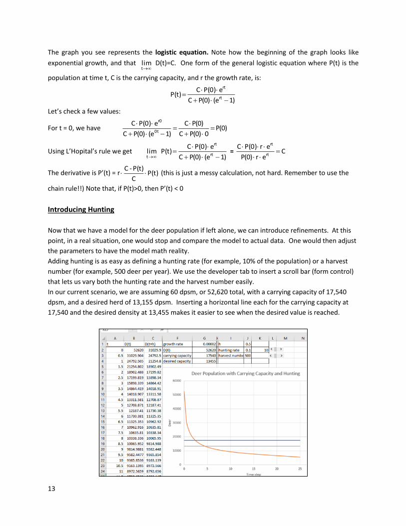
The graph you see represents the logistic equation. Note how the beginning of the graph looks like

exponential growth, and that t

lim D(t)=C. One form of the general logistic equation where P(t) is the

population at time t, C is the carrying capacity, and r the growth rate, is:

)1(e)0(PC

eP(0)CP(t)

rt

rt

Let’s check a few values:

For t = 0, we have )0(P0)0(PC

)0(PC

)1(e)0(PC

eP(0)C0t

r0

Using L’Hopital’s rule we get t

lim )1(e)0(PC

eP(0)CP(t)

rt

rt

= C

er)0(P

erP(0)Crt

rt

The derivative is P’(t) = r P(t)C

P(t)-C (this is just a messy calculation, not hard. Remember to use the

chain rule!!) Note that, if P(t)>0, then P’(t) < 0

Introducing Hunting

Now that we have a model for the deer population if left alone, we can introduce refinements. At this

point, in a real situation, one would stop and compare the model to actual data. One would then adjust

the parameters to have the model math reality.

Adding hunting is as easy as defining a hunting rate (for example, 10% of the population) or a harvest

number (for example, 500 deer per year). We use the developer tab to insert a scroll bar (form control)

that lets us vary both the hunting rate and the harvest number easily.

In our current scenario, we are assuming 60 dpsm, or 52,620 total, with a carrying capacity of 17,540

dpsm, and a desired herd of 13,155 dpsm. Inserting a horizontal line each for the carrying capacity at

17,540 and the desired density at 13,455 makes it easier to see when the desired value is reached.

14

Another option is to use the Goal Seek function. Go to Data, then What-If-Analysis, then Goal Seek. If

possible, Excel will find the solution. Note however that you can only use one variable at a time. A

combination of hunting rate and harvest number is not possible. We will learn a method to deal with

multivariable problems in the chapter on Simplex.

Assuming you want to reach the optimal density after 10 time steps by varying the hunting rate, then

you will enter the information shown in the picture below. You will find that a 9.2% hunting rate is

needed.

Introducing Predators

So far, we have investigated one population. Let’s introduce a second population of predators, say

coyotes. (While coyotes do rarely attack adult deer, they can kill up to 75% of newborn fawns). The

population of deer should go up if there are many deer and few coyotes, and down if there are many

coyotes and few deer. Similarly, the population of coyotes goes down if there are too many coyotes

(starvation) and up if there are many deer. The two populations are mutually dependent. Of course, this

is a bit of a simplification, as coyotes have other prey (rodents, hare, rabbits, carrion…)

Here is a possible model:

change in # of deer = deer growth rate ∙ # of deer – prey rate ∙ # of coyotes ∙ # of deer

change in # of coyotes = - coyote starvation rate ∙# of coyotes + feeding rate ∙ # of coyotes ∙ # of deer

Here the “feeding rate” is really the rate at which deer are turned into baby coyotes….

15

Whenever you create a model, i.e. go from the real world to mathematical equations, you should make

sure you define your variables and write down the definitions. Otherwise it will be almost impossible for

anyone else – or you, later – to make sense of what you did. So, get into the habit.

Let t = time

D(t) = number of deer at time t

C(t) = number of coyotes at time t

r = hamster growth rate

p = prey rate

s = starvation rate

f = feeding rate

The model thus becomes a system of differential equations: D’(t) = r∙D(t) - p∙C(t)∙D(t)

C’(t) = -s∙C(t) + f∙C(t)∙D(t)

I set this spreadsheet up a little different to make the formulas easier to read. Instead of computing

D(t+h) and C(t+h) directly, we first compute the changes in D (t) and C(t), resp., and add them to (D(t)

and C(t). D(t+h) thus becomes D(t)+change in D, and C(t+h) = C(t) + change in C.

Have a look at the graph on the left. You see cyclical behavior in both populations, with the peaks

increasing and slightly off-set. This is due to the time lag as a population increases due to increased food

supply, or decreases due to lack of food and predation. This behavior becomes even more obvious as

you plot deer population vs predators. Instead of reaching a constant state with seasonal fluctuations in

populations, the coyote numbers will drop below 1, i.e. the predators will die out.

16

Note: Any model is only as good as the data you used to construct it. Both the predator-prey model and

the logistic growth model with hunting need to be carefully calibrated to make the model fit reality.

Diagrams and Recursive Sequences – Multiple Populations

Sometimes, it is more convenient or intuitive to express populations as recursive sequences. In that

case, one would use P0 instead of P(0) and Pn instead of P(nh) or P(t+h). For example, the logistic

population model P(t+h) = P(t) + h∙r∙P(t)∙(C-P(t)) would become

Pn+1 = Pn + h∙r ∙ Pn ∙ (C – Pn), P0 = P(0).

In our current model, we really should consider more than two populations, even if we are concerned

only with the deer population. Predators prey mostly on the young, only adults breed, and hunters will

take only adults. When dealing with multiple populations, it often helps to represent to represent them

with a diagram, where arrows represent the interactions between populations.

In this example, we assume that 40% of young grow up to be adults (half male, half female), each female

produces 2 young per year, and the life span for adults is a little over two years. Male and female deer

are hunted at different rates.

We express these relationships with recursive sequences:

Yn+1 = 2Fn

Fn+1 = 0.2 Yn + 0.5 Fn

Mn+1 = 0.2 Yn + + 0.3 Mn

With Pn :=

n

n

n

M

F

Y

and A :=

3.002.0

05.02.0

020

, this becomes Pn+1 = A ∙ Pn .

If you took Linear Algebra with me, you may recognize this equation. However, the recurrence equations

are easier to implement in Excel.

17

Obviously, the harvest rate here is too high; the population crashes. If you would outlaw doe hunting,

the population stabilizes at 1378 total deer.

You may want to introduce additional refinements to your model, for example stocking or migration, a

second food source, changing the constant growth rate to a seasonally varying rate, randomizing the

prey rate, etc. At least at the beginning, while you are still getting used to this, it is important to start

simple and slowly.

Note that this process can be used to model the spread of infections or rumors, a zombie apocalypse,

chemical reactions, and more. This is a central concept of applied mathematics, adapting models and

methods to the situation at hand.

18

COMPUTING AREAS – SIMULATION 1

Learning Goals

In this chapter, we will study how to estimate areas (integrals) using random numbers and repeated

simulations. We will use Excel to

generate random numbers

write simple IF statements

use data tables for repeated simulations

Case Study Description –Computing Areas

Consider dxeσ2π

1b

a

σ2

μ)(x2

2

. If you already took Statistics, you may recognize the Normal

Distribution. More precisely, for a normally distributed random variable x with mean μ and

standard deviation σ:

P(a<x<b) = dxeσ2π

1b

a

σ2

μ)(x2

2

.

Unfortunately, this integral does not have a closed form solution (anti-derivative). Your task is to

produce an EXCEL work sheet that approximates the value of the integral for any a, b, μ, and σ the user

chooses

Solution Approach

There are many other and better solution approaches to this problem. We could use a series expansion

such as Taylor series, or Riemann sums or Simpson’s rule to approximate the value. However, the goal is

to learn how to run simulations with EXCEL, so we will use that approach instead. The basic idea is to

enclose the graph of the function in a rectangle and then generate many random points scattered

uniformly across that rectangle. If you use enough points, and if you repeat the process often enough,

then the ratio of the points under the curve to the total number of points should be equal to the

proportion of the area under the curve. For example, if 90% of all random points end up under the

curve, then it makes sense to assume that the area under the curve represents 90% of the total area.

(Again, I realize this is not the most sensible approach, but we are focused on learning Excel here, not on

finding the most elegant solution to a problem)

19

The function 2

2

σ2

μ)(x

eσ2π

1

takes on its maximum value at σ2π

1 and is always positive. It makes

sense to use the rectangle from a to b on the x-axis and from 0 to σ2π

1on the y-axis.

To generate the random points, we use the rand() function. This function returns a random number

between 0 and 1. The x-coordinate of our point needs to be between a and b, so we need to stretch the

interval [0,1] by a factor of a-b and shift by a factor of a. The y-coordinate of our point needs to be

between 0 and σ2π

1, so we need to stretch the interval [0,1] by a factor of

σ2π

1. Next, we compute

y = f(x) = 2

2

σ2

μ)(x

eσ2π

1

to see if the point is below or above the curve. This is achieved with the IF

statement: if the y-coordinate of the random point is less than y=f(x), then we assign a value of

1, else a value of 0. We then have to add up all the “1”s and divide by the total number of

random points used (I chose 500), to find the proportion of points under the curve. All that is

left to do is to compute the area under the curve.

Here is what those formulas look like in Excel:

And here is a sheet showing some values:

20

For a = -1.96, b = 1.96, μ = 0, and σ = 1 the approximation exact to four decimals is 0.9500, so we are a

bit off. There are two ways to fix that. We could copy the formula to more than the 500 points used, or

we could repeat the experiment many times and average the results. We will do the latter. Basically, we

want to compute the area many, let’s say 25, times. To do that, first highlight where the table goes. It is

important that the original computation is the top left cell, and that you have two columns. Next go to

Data, What-If-Analysis, Data Table. Our table is arranged in a column, but because we do not want to

change anything from run to run, we choose an empty unrelated cell as the Column input cell.

21

Hit “enter, and you will see the results which you can then average with the “= AVERAGE(I11:I13)”

command.

Note that this idea can be used to find the size of any area. You can use it to estimate constants, for

example π. If you use a different distribution, you could model the spread of spills (normal distribution),

population density of bugs (Poisson distribution), and more. Modeling is all about being creative, using

methods and ideas you may be familiar with and then adapting them to new situations.

22

MODELING THE SPREAD OF DISEASES – SIMULATION 2

Learning Goals

After this chapter, you, you should be able to:

Use nested IF, AND statements

Use COUNTIF

Use RANDBETWEEN

Record macros

Use conditional formatting

Case Study Description – Diseases

An outbreak of a new flu strain needs to be contained. For this particular flu, people will get sick only if

they have contact with one or more sick people, and then only with a 50% chance. Once sick, they

either recover and become immune, or they die. The probability of dying increases with the number of

sick people the patient came in contact with while being sick: 0 contacts: full recovery and immunity, 1-4

contacts, 5% chance of death, 5-9 contacts, 20% chance of death. Generate a spreadsheet that simulates

the spread of disease through a population.

Solution Approach

There are many – and better – ways to model the spread of diseases than the following. However, the

point is to learn how to use the nested “if” statement, conditional formatting, and macros, so bear with

me.

A problem like this becomes messy fast, so we will start simple and then refine. A flow chart helps to

organize and then simplify all the rules. To deal with probabilities, imagine flipping a coin or die.

23

Syntax: =IF (Statement to check, what to do/value if true, what to do/value if false)

AND (statement 1, statement 2,…)

=COUNTIF (range, when to count)

=RANDBETWEEN (lower bound, upper bound)

In this case: =IF(cell is dead, dead, IF(AND(cell has 1+ sick neighbors, flip 1),sick, healthy)))

We will use three 25x25 grids: one represents the state today, one the state tomorrow, and one keeps

track of the number of sick neighbors each cell has. We assign an arbitrary value to the four possible

states, dead = 0, sick = 1, healthy = 2, immune = 3.

Below is a screenshot of the formula you need to enter in the “tomorrow” block and copy to all cells in

that block.

24

Pretty up your worksheet by adding titles and conditional formatting to the blocks. Conditional

formatting is under the HOME tab.

Including all the rules give a flow chart like this:

This gives a very convoluted nested statement, give it a shot yourself before you look up the solution.

Add a few formulas that count the number of sick, healthy, immune, and dead cells.

Finally, we include macros. When you record a macro, you really create a short cut to perform a series

of tasks. You use it if you need to repeat those tasks repeatedly. Basically, you replace a series of key

strokes or instructions with a single keystroke. We record two macros, one to copy the values of the

third (tomorrow) block to the first (today) block, and one to re-set the whole worksheet. The record

macro button is in the DEVELOPER tab. Make sure to remember to add a description of your macro.

As you run your worksheet, if you start with a single sick cell in the center, you should see an ever-

expanding blob of dead and immune cells and a few healthy ones. Because of the randomness involved,

and depending on your styling, your sheet will look different than mine.

25

And here is a solution for the formula that goes into the tomorrow block (cell BC4 is the top left cell for

me) and then is copied to all the cells in the block:

=IF(C4=0, 0, IF(C4=3,3, IF(AND(C4=1, AC4>4), IF(RANDBETWEEN(1,5)=1, 0, 3),

IF(C4=1,IF(RANDBETWEEN(1,20)=1,0,3), IF(AND(AC4>0,RANDBETWEEN(0,1)=1), 1, 2)))))

This set up can be used to model anything where the state of one cell depends on some or all of its

neighbors. Applications include: spread of rumors, dissipation of heat, spread of a population, Zombies

invading, built-up in cities, invasive species, …

26

DESIGNING A CAMPGROUND – SIMPLEX METHOD

The Simplex method is probably the classic method of solving constraint optimization problems. We will

use this solution approach, sometimes in modified form, over and over in this class, not just in this

chapter.

Learning Goals

You will learn

How to recognize linear programming (LP) problems

Vocabulary of LP problems

Graphical solution

Algebraic solution

Excel solution with the Excel Solver

Case Study Description - Campground

You are opening a campground in the Florida Keys, and you are trying to make as much money as

possible. You are planning a mix of RV sites, tent sites, and yurts. Let’s assume you already own 10

acres, and that you can make $80/day profit on each RV, $20/day profit on each tent, and $200 profit on

each Yurt. However, there are restrictions:

1) Infrastructure takes up 20% of your site

2) You can have 20 RVs per acre, or

3) You can have 40 tents per acre, or

4) You can have 10 yurts per acre

5) You have a budget of $100,000. It costs you $1000 to develop an RV site, $200 for a tent site,

and $8000 for a yurt.

6) Maintenance for the bath houses etc. is 15 min/week/camper unit. You can afford 70hrs/week

in maintenance help

7) Zoning ordinance requires you to have at least 20 tent sites

What is the best layout for your campground, and how much profit can you make per day?

References

This case study was inspired by the Knights Key RV park in Florida. Read more about it here:

http://www.knightskeyrvresortandmarina.com/news/

http://www.miaminewtimes.com/news/developers-plan-to-replace-rv-park-with-five-

star-resort-stirs-fears-hopes-in-keys-8038648

http://www.knightskeyrvresortandmarina.com/news/

http://www.miaminewtimes.com/news/developers-plan-to-replace-rv-park-with-five-star-resort-stirs-fears-hopes-in-keys-8038648

http://www.miaminewtimes.com/news/developers-plan-to-replace-rv-park-with-five-star-resort-stirs-fears-hopes-in-keys-8038648

27

Solution Approach – Two Variables

We will again first look at a simpler problem by ignoring the yurts and only considering RV spaces and

tents.

Let r be the number of RVs, t the number of tents, and P(r,t) the profit. Your goal is to maximize P(r,t) =

80 r+ 20t. This function is called the objective function. The variables r and t are called decision

variables. You can see that in the current case P(r,t) gets bigger if you increase r and/or t. If you picture

a graph with r on the horizontal and t on the vertical axis, then the direction of increase for the

objective function is to the top right.

Translating the relevant restrictions into equations gives

Simplified

1) r/20+t/40 ≤ 8

2) r ≤ 160

3) t ≤ 320

5) 1,000r+200t ≤ 100,000

6) (r + t)/4 ≤ 70

7) t ≥ 20

8) r, t ≥ 0

↔

↔

↔

↔

↔

↔

↔

1) 2r+t ≤ 320

2) r ≤ 160

3) t ≤ 320

5) 5r+t ≤ 500

6) r+t ≤ 280

7) t ≥ 20

8) r, t ≥ 0

These are called the functional constraints.

In addition, you can’t have negative sites, so we have the non-negativity constraints

5) r ≥ 0

6) t ≥ 0.

A problem like the above with linear constraints and a linear objective function is called a linear

programming problem.

Assumptions made about linear programming problem

Proportionality For both the objective function and the constraints, a change in a decision variable will

result in a proportional change in the objective function or constraint. (Note that this rules out any

exponents on the decision variables other than 1.)

Additivity Both the objective function and the constraints are the sums of the respective changes in the

decision variables (This means no multiplying different decision variables).

Basically, the proportionality and additivity assumptions are just fancy ways of saying that all

functions in a linear programming problem are linear in the decision variables.

Divisibility We are assuming that our decision variables can be non-integer, i.e. may take on fractional

values. Problems with an integer constraint are called integer programming problems, we will only

touch on them briefly later.

28

Certainty We act as if the value assigned to each parameter is known, precise, and constant over time.

This is rarely the case, so we need to compensate for that by performing sensitivity analysis. Basically,

we need to investigate how much it affects our solution if the parameters change.

Graphical Simplex solution procedure

We will start with some vocabulary:

Feasible solution: A solution for which all constraints are satisfied, not necessarily an optimal

Solution.

Infeasible solution: A solution that violates at least one constraint.

Optimal solution: a solution that optimizes (could be a minimum or maximum, depending on

your problem) the objective function. There may or may not be an optimal solution.

Feasible region: The set of all feasible solutions

Corner point: the intersection of two or more constraints

Corner point feasible solution CPF solution: A solution that occurs at a corner of the feasible

region

The first step in the graphical solution procedure is to draw the feasible region (note that this gets really

ugly if you have three or more variables).

The non-negativity constraints mean that we are looking for a solution in the first quadrant only.

The constraints 2) r ≤ 160, 3) t ≤ 320, and 7) t ≥ 20 mean you have to stay left of the line r=160, below

the line t=320 and above the line t=20. You see that the constraint t ≥ 20 dominates the constraint t ≥ 0,

so the latter is redundant.

29

Adding the remaining constraints yields this graph: Go ahead, shade the feasible region and identify all

redundant constraints.

All the points in the feasible region are possible solutions. Your job is to pick (one of) the best solutions.

Note that there may not be a single best solution but rather several optimal solutions.

We have not yet used the objective function P(r,t)=80r+20t. Because we do not have a value for P(r,t),

so we will draw P(r,t) for a few random values of P(r,t) to get an idea of what it looks like. For

P(r,t)=1600, 2400, 3200 we get the lines shown in the next picture. Note that they are all parallel, and

that the lines corresponding to the larger value of P(r,t) move to the top left. The direction of increase is

just as we expected, to the top right.

30

As you move the line for the P(r,t) to the right you increase your profit. But you also have to stay in the

feasible region. Convince yourself that one of two cases will occur: either a unique optimal solution will

be found at a corner point, or infinitely many optimal solutions returning the same maximum value for

P(r,t) will be found along a section of the boundary of the feasible region that includes two corner

points. Therefore, we need to compute the corner points, i.e. the intersections of the constraints, and

move P(r,t) as far to the right as possible without leaving the feasible region.

From the picture above, you can see that the optimal solution will be at the intersection of the lines

corresponding to constraints 1) and 5).

r/20 + t/40 ≤ 8 and 1000t + 200t ≤ 100,000

which is at the point r=60, t=200. (Now would be a good time to review how to solve systems of

equations….). This gives us a profit P(60,200) = 60 ∙ $80 + 200 ∙ $20 =$8800.

31

Stating the Solution

In OR, typically someone hires you to work your problem, and then expects you to give the answer in

the context of the problem. You can’t just say “the solution is at r=60, t= 200, P(r,t)=8800”. Give the

answer like this:

“To maximize potential profit, the campground should have 60 RV sites and 200 tent sites. In that case,

the potential profit per day, assuming full occupancy, is $8800. You are limited by the available land and

budget available, not by available labor or any zoning rules. You will have to hire 65 hours of help per

week (260 camping units at 15 minutes/week/unit).”

Refinements to the graphical solution

One “brute force” approach to the graphical solution method would be to compute all intersections of

all constraints, check if that corner is in the feasible region, and then compute the objective function at

those points. However, the number of intersections increases quadratically with the number of lines (

2

1)n(n for n non-parallel lines), so this approach quickly gets out of hand. Instead, the idea is to start

at an easy to find corner of the feasible region. Often, the origin works. From that point, check the

adjacent feasible corner points and move to the “best”. Continue until there is no more improvement.

Here is what that would look like in our case:

We start at a simple corner. Usually, people use the origin, which is not on the feasible region here, so

we start at (0,20). Adjacent corners are (0,280) and (96, 20) with P(0, 20) = 400, P(0, 280) = 5600, and

P(96, 20) = 8080. (96, 20) is best, so we move there. Next, check the adjacent corner (60, 200). It gives

P(60, 200) = 8800 which is an improvement, so move there. Check the next adjacent corner (40, 240) It

gives P(40, 240) = 8000. This is worse, so (60,200) is the optimal solution.

There is of course a big problem with this approach. It relies on us having a graph of the feasible region

and being able to see the adjacent feasible corner points. If you are dealing with a large number of

constraints and variables, this is not possible. We therefor take the idea of looking at adjacent feasible

corners and moving towards the one that gives the best value for the objective function, and translate it

into an algebraic method.

32

Solution Approach – Algebraic Simplex Method

As these are only three variables, we could still draw the feasible region, now a solid bound by planes.

However, we need an approach that works for any number of variables. The key to this method is the

fact that an optimal solution will occur at a corner point of the feasible region. While the n-dimensional

proof is beyond the scope of this class, this fact should be intuitively clear in the 2-d and 3-d cases.

We will first demonstrate the algebraic method on the two-variable problem (RV and tent only) and

then solve the full problem.

Corner points, interior corner points, slack variables

We introduce slack variables to turn the inequalities into equalities. Basically, a slack variable lets you

know how close you are to maxing out the constraint. In the current case, we have:

Constraints Augmented constraints

1) 4r+t ≤ 320

2) 5r+t ≤ 500

3) r+t ≤ 280

4) t ≥ 20

5) r, t ≥ 0

1) 2r + t + s1 = 320

2) 5r + t + s2 = 500

3) r + t + s3 = 280

4) t - s4 = 20

5) r, t, s1, s2, s3, s4 ≥ 0

A point is a corner point if it sits at the intersection of two or more constraints, i.e. if two or more slack

variables are zero. A point is a feasible solution (i.e. inside the feasible region) if all slack variables are

non-negative. A point is outside the feasible region if any slack variable is negative. We will from now on

express each point as (r, t, s1, s2, s3, s4). Given r and t, one computes the values of the slack variables

from the augmented constraints.

Examples: r=100, t=20 → (100, 20, 100, -20, 140,0) outside the feasible region

r=10, t=30 → (10, 30, 270, 420, 240, 10) inside feasible region

r=150, t=20 → (150, 20, 0, -270, 110,0) corner outside feasible region

Initializing

Because (0,0) is not on the feasible region, we again start at (r, t) = (0, 20), which has the augmented

form (0, 20, 300, 480, 240, 0). We are sitting on the intersection of the lines r=0 and t=20.

The adjusted objective function

Note: If the origin is a feasible corner point and you start at the origin, you can skip this step.

We are sitting on the intersection of the lines r=0 and t=20. To reach the next adjacent corner, we have

to move along one of those lines, but which one? If we move along the line r=0, we move away from the

line t=20, which is the same as saying we are increasing the corresponding slack, s4. If we move along

the line t=20, we increase r. We want to choose the direction of increase that gives us the fastest

33

increase in P. The original objective function is P(r,t) = 80r + 20t, which does not let us see what happens

if we increase s4 We have to rewrite P(r,t) in terms of r and s4.

Using equation 4) we get t=20+s4, and thus P(r, s4) = 80r + 20(20+s4) = 400 + 80r + 20s4

Determining which way to move

We want to choose the direction of increase that gives us the fastest increase in P. The objective

function is P(r, s4) = 400 + 80r + 20s4. Because the variable r has the biggest coefficient, 80, an increase in

r should give the best return.

Determining how far to move – the next corner

We will leave s4 at is current value, 0, and increase r as much as possible without leaving the feasible

region, i.e. without having t, s1, s2, s3, s4 become negative.

1) 2r + t + s1 = 320 s1 = 320-20-2r ≥ 0, so r ≤ 150

2) 5r + t + s2 = 500 s2 = 500- 20-5r ≥ 0, so r ≤ 96

3) r + t + s3 = 280 s3 = 280-20-r ≥ 0, so r ≤ 240

4) t - s4 = 20 t=20

So, r can be increased to 96.

Augmented form of the next corner

Using r=96, s4=0, and substituting into the equations 1-4, we have the augmented point (96, 20, 108, 0,

164, 0). Note that this is the same corner (96, 20) we used above.


We are now sitting on the intersection of the lines 5r + t + s2 = 500 and t=20. To reach the next adjacent

corner, we have to move along one of those lines, which means either increasing s2 or s4. We have to

rewrite P(r,t) in terms of s2 and s4.

Using equations 2 and 4, we find that 5r = 500 – t – s2 and t=20 + s4, which yields 5r = 480 – s4 – s2.

Substituting into P:

P(s2, s4) = 400 + 80r + 20s4 = 400 + 16(480 – s4 – s2) = 20 s4 = 8080 + 4s4 – 16 s2

Now we will repeat the above steps until the solution/objective function can no longer be improved

upon.


Because the s4 has the only positive coefficient, this is the only direction that will yield an increase in P.


We will leave s2 at is current value, 0, and increase s4 as much as possible without leaving the feasible

region.

1) 2r + t + s1 = 320 s1 = 320 – t - 2r

34

2) 5r + t + s2 = 500 s2 = 500 - t - 5r

3) r + t + s3 = 280 s3 = 280 - t - r

4) t - s4 = 20 t = 20 + s4

We use that s2= 0 and t = 20 + s4. This gives the set of equations:

1) s1 = 108 – 0.6s4 ≥ 0, so s4 ≤ 96

2) r = 96 – 0.2s4 ≥ 0, so s4 ≤ 480

3) s3 = 164 – 0.8s4 ≥ 0, so s4 ≤ 205

4) t = 20 + s4 ≥ 0, so s4 ≥ -20 (as 20 is positive, this is true anyway)

So s4 can be increase up to 180.


Using s2= 0, s4=180, and substituting into the equations 1-4, we have the augmented point (60, 200, 0, 0,

20, 180). Note that this is the second corner (60, 200) we used above.


We again re-write the objective function, this time in terms of s1 and s2:

P(s1, s2) = 8080 + 4s4 – 16 s2 = 8080+4(180-1.6 s1) -16 s2 = 8800 – 6.6 s1 – 16 s2. Note that increasing either

s1 or s2 will decrease the value of P, so we have reached the maximum. As s1 and s2 are non-negative, we

can also see that the maximum for P occurs when s1 and s2 are zero, at P=8800. Again, this is the same

answer we arrived at earlier.

A nice side effect is that we can tell which constraints are holding us back, namely those associated with

the zero slack variables s1 and s2. s1 corresponds to the space limitations, and s2 to the budget

restrictions.

Solving the full problem

We are now ready to look at the original problem. We will assume you went to the bank and got a loan

for $246,000 to supplement your original budget. Here are the constraints again:

1) Infrastructure takes up 20% of your site

2) You can have 20 RVs per acre, or

3) You can have 40 tents per acre, or

4) You can have 10 yurts per acre

5) You have a budget of $346,000. It costs you $1000 to develop an RV site, $200 for a tent site,

and $8000 for a yurt.

6) Maintenance for the bath houses etc. is 15 min/week/camper unit, you can afford 70hrs/week

in maintenance help

7) Zoning ordinance requires you to have at least 20 tent sites

35

Functional Constraints Simplified Constraints Augmented Constraints

r/20 + t/40 + y/10 ≤ 8

1000r + 200t + 8000y ≤ 346,000

(r + t + y)/4 ≤ 70

t ≥ 20

2r + t + 4y ≤ 320

5r + t + 40y ≤ 1730

r + t + y ≤ 280

t ≥ 20

2r + t + 4y + s1 = 320

5r + t + 40y + s2 = 1750

r + t + y + s3 = 280

t - s4 = 20

Non-negativity constraints:

r, t, y, s1, s2, s3, s4 ≥ 0

Objective function:

Maximize P(r,t,y) =80r + 20t + 200y

Initializing

Because (0,0,0) is not on the feasible region, we start at (r, t, y) = (0, 20, 0), which has the augmented

form (0, 20, 0, 300, 480, 240, 0). We are sitting on the intersection of the planes r=0, t=20, y=0. The

augmented form of this corner is (0, 20, 0, 300, 1710, 260, 0)


Rewriting P as P(r, y, s4) gives: P(P(r, y, s4) = 400 + 80r + 200y + 20s4.


Looking at the coefficients of r, y, s4 in the objective function, we find that we should increase y and

leave r and s4 = 0.


Using r=0 and s4 = 0, the constraints become

t + 4y + s1 = 320 4y + s1 = 300 s1 = 300-4y ≥0 → y ≤ 75

t + 40y + s2 = 1750 40y + s2 = 1730 s2 = 1730-40y ≥0 → y ≤ 42.75

t + y + s3 = 280 y + s3 = 260 s3 = 260-y ≥0 → y ≤ 260

t = 20

So, y can be increased up to 42.75.


With r=0, s4 = 0, and y=42.75, we find the new augmented corner to be (0, 20, 42.75, 129, 0, 217.25, 0).


We need to rewrite the objective function in terms of r, s2, and s4:

P(r, s2, s4) = 8950 + 55r + 15 s4 – 5s2

The solution is not optimal yet, (there are still positive coefficients in the objective function), so we keep

going.

36


We see that we should increase r and leave s2 and s4 = 0.


With s2 and s4 = 0, we have

2r+t+4y+s1=320 2r+4y+s1=300 s1=129–1.5r≥0 → r ≤ 86

5r+t+40y=1750 5r+40y=1730 40y=1710–5r → r ≤ 342

r+t+y+s3=280 r+y+s3=260 s3=236.25–0.875r≥0 → r ≤ 270

t=20

So, y can be increased up to 86.


With y=86, s2 = 2, and s4 = 0 we find the new augmented corner to be (86, 20, 32, 0, 0, 142, 0)


We need to rewrite the objective function in terms of s1, s2, and s4:

P(s1, s2, s4) = 13680 - 363

2s1 - 1

3

1s2 – 18 s4.

Note that now all variables have negative coefficients, so we cannot increase the value of P past 13680.

The first, second, and fourth constraints are maxed out; we are limited in our ability to increase the

profit by space, money, and zoning restrictions.


To maximize potential profit, the campground should have 86 RV sites, 20 tent sites, and 32 yurts. This

will take an initial investment of $346,000. The potential profit per day, assuming full occupancy, is

$13,680. You are limited by the available land and budget available and the zoning law requiring 20 tent

sites. You will have to hire 34.5 hours of help per week (138 camping units at 15 minutes/week/unit).”

Solution Approach – Using Excel

Now that we know how the solution method works, we can use Excel to do the work for us.

First, we must set up the work sheet. One way that works well is shown on the next page. The

fields highlighted in green are necessary, the others serve to explain and label what we are

doing.

37

Excel has a built-in Solver under the Data tab (if you don’t see it, you have to add it in. Go to

file/options/Add-ins/Manage Excel Add-ins/Solver Add-in). If you choose “show iteration results

in the options tab, the solver will stop at each iteration and show you the corner/solution it has

arrived found at that step. You will see that the solver goes through the same steps and corner

points as we did when we worked the problem “by hand”.

38

A Remark on BIP and Integer Programming

In the previous examples, our solutions came out to be integers, even though we did not put that

restriction in place. In the case that the solution to the LP problem is an integer, it is also so optimal

solution to the Integer IP problem. However, usually the IP problem or BIP problem (binary integer

program) are much harder to solve than the LP problem. Let’s discuss why this is.

At first, it seems that IP and BIP problems should be easier to solve, after all, there is only a finite

number of possible integer valued points in a bounded feasible region. An enumeration algorithm

should work, just try all finite solution and pick the best. Assume we have a problem with n variables. In

the case of the BIP that means there are 2n possible solutions to check. In the case of an IP problem,

even if the variables are bound between say 0 and 10, that is 11n solution. The growth in complexity is

exponential. While that may work for our class problems, actual OR problems typically have hundreds of

thousands of variables.

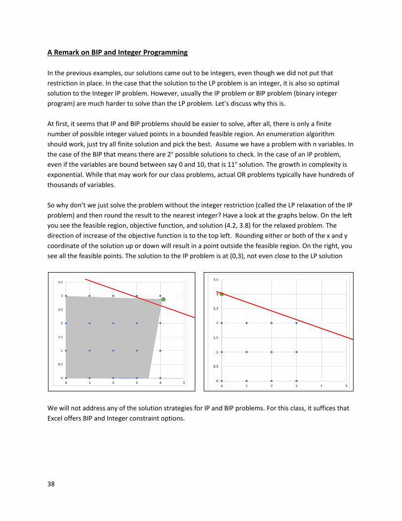
So why don’t we just solve the problem without the integer restriction (called the LP relaxation of the IP

problem) and then round the result to the nearest integer? Have a look at the graphs below. On the left

you see the feasible region, objective function, and solution (4.2, 3.8) for the relaxed problem. The

direction of increase of the objective function is to the top left. Rounding either or both of the x and y

coordinate of the solution up or down will result in a point outside the feasible region. On the right, you

see all the feasible points. The solution to the IP problem is at (0,3), not even close to the LP solution

We will not address any of the solution strategies for IP and BIP problems. For this class, it suffices that

Excel offers BIP and Integer constraint options.

39

A Final Comment

We completely ignore that LP requirement of divisibility, i.e. the fact that the decision variables could

conceivably be fractions. In our current case study, fractional answers make no sense, one cannot build

.38 of a yurt for example. Fortunately, this problem was carefully set up to ensure the solution came out

as an integer. In real life, that won’t be the case. Excel has the option to add an integer constraint to

your decision variables.

There are a lot of methods to work around the strict LP requirements, for example the linearity

requirement. If we have time, we will address some of them at the end of class. Meanwhile, if your

group projects run into some issues with the LP requirements, please see me.

Now a developer comes and offers you $1,1 million/acre. What do you do?

40

NATIONAL PARK – NETWORKS AND ASSIGNMENT

In this chapter, we will examine three types of problems:

1) In allocation problems, a limited resource “supply” is allocated to various entities “demand”.

We will see what happens if demand exceeds supply and vice versa.

2) Assignment problems assign exactly one of n task to each of exactly n workers

3) Network problems look at a variety of issues arising in a network of nodes and arcs, from

spanning trees to traversal problems.

Learning Goals

Allocation problems

Assignment problems

Shortest path problem

Flow problems

o Maximum flow

o Maximum flow – minimum cost

Traveling salesman problem

Using Excel to solve the above

Case Study Description

A very popular National Park is facing a number of challenges and has hired your company to propose

solutions to the following:

1. Due to budget cuts, much of the work in the park such as interpretive services and trail

maintenance is done by volunteers. What is the most efficient way to assign them to the various

tasks and locations? Also, you need to make sure each location has one full-time ranger on site.

2. Traffic has gotten so bad that the park is considering banning personal vehicles on some roads

and using shuttle busses instead. What should the bus routes be? How many busses are

needed? Is a shuttle service even feasible?

3. During winter, some of the park roads will be closed. However, enough roads need to be plowed

to allow access to all ranger stations. Which roads should be plowed?

4. A delivery truck needs to visit each of the parks location. What is the best route to take?

5. All roads need to be patrolled daily. What is the best route for the ranger to take?

Following is a simplified park map showing roads and attractions. As needed, you will also be provided

with information regarding length, driving time, and shuttle capacity for each road segment.

41

References

Budget cuts and overcrowding are very real issues for our National Parks. For more information

on both, see:

https://www.npca.org/articles/1500-budget-proposal-threatens-national-

parks#sm.0000ks3wtu35mdezurz1liyktck1t

http://www.ournationalparks.us/park_issues/busy_parks_seek_approaches_to_manag

e_crowds_cars/

https://www.nps.gov/zion/planyourvisit/traffic.htm

http://www.triplepundit.com/2016/03/national-parks-face-crowding-degradation/

http://www.hcn.org/articles/arches-crowds-tourism-national-parks-utah

https://www.nps.gov/yell/planyourvisit/visitationstats.htm

Part 1: Work Force – Resource Allocation

Let’s assume volunteers are available at the entrances to the park, HQ, NE, and SE. From there, you will

have to transport them to the different locations and tasks. There is trail construction going on at VC

and GF, so a lot of volunteers are needed there. GF is a very popular tourist destination, so lots of help is

needed there as well. The cost/volunteer hour depends on a number of factors, such as distance to park

entrance, nature of work, insurances required, etc. This table shows a summary of cost, supply, and

demand.

We will denote each location by its initials, for example NE for North entrance, CL for Canyon lands etc.

Four corners pass does not need any staffing, so we omit it.

This is an example of an allocation problem. A resource (volunteer hours, water rights, money, fish

catch) is allocated to different areas (park location, cities, departments, canneries). In the ideal case,

supply matches demand exactly. Let’s start by assuming this is happening here:

North

Entrance

Canyon

Lands

White

Falls

Four

Corners

Pass

Tall

Mountain

Geyser

Field

Head

quarters

camp

ground

Visitor

Center

Bear

Meadow

South

Entrance

https://www.npca.org/articles/1500-budget-proposal-threatens-national-parks#sm.0000ks3wtu35mdezurz1liyktck1t

https://www.npca.org/articles/1500-budget-proposal-threatens-national-parks#sm.0000ks3wtu35mdezurz1liyktck1t

http://www.ournationalparks.us/park_issues/busy_parks_seek_approaches_to_manage_crowds_cars/

http://www.ournationalparks.us/park_issues/busy_parks_seek_approaches_to_manage_crowds_cars/

https://www.nps.gov/zion/planyourvisit/traffic.htm

http://www.triplepundit.com/2016/03/national-parks-face-crowding-degradation/

http://www.hcn.org/articles/arches-crowds-tourism-national-parks-utah

https://www.nps.gov/yell/planyourvisit/visitationstats.htm

42

Cost per hour HQ NE SE CG VC WF CL TM BM GF Supply

North volunteer 6 5 10 6 10 8 9 9 15 20 120

South volunteer 6 10 5 7 9 9 10 9 12 18 200

HQ volunteer 5 6 6 5 9 9 10 11 11 18 300

Demand 50 30 30 50 100 100 20 20 20 200

Note how the supply column and demand row add up to the same value, 620. Your objective is to

minimize cost while meeting demand. Note that in this ideal case supply = demand. This problem can be

set up as a linear programming problem and solved with the simplex method. You should check that the

assumptions for a LP problem hold.

To solve this problem with Excel, we set up a second table containing the decision variables, i.e. how

many hours from which source are being allocated to which area. Initially, we set them all to zero. The

highlighted cells contain formulas. We can now use the Excel solver.

43

The solver returns the solution, which the park can then implement, and the total weekly cost of $6710.

Hours assigned HQ NE SE CG VC WF CL TM BM GF Total supplied

North volunteer 0 0 0 0 0 100 20 0 0 0 120

South volunteer 0 0 30 0 0 0 0 20 0 150 200

HQ volunteer 50 30 0 50 100 0 0 0 20 50 300

Total used 50 30 30 50 100 100 20 20 20 200

total cost 6710

We were lucky and got integer value solutions. However, in this case the divisibility requirement of LP

problems is satisfied, we could allow fractional hours worked.

Refinements

Let’s assume you have too many volunteers, i.e. supply > demand. We incorporate them by assigning

those hours we don’t need to the “excess” column and proceeding otherwise just like before:

Cost per hour HQ NE SE CG VC WF CL TM BM GF excess

supply

North volunteer 6 5 10 6 10 8 9 9 15 20 0

200

South volunteer 6 10 5 7 9 9 10 9 12 18 0

250

HQ volunteer 5 6 6 5 9 9 10 11 11 18 0

300

Demand 50 30 30 50 100 100 20 20 20 200 130

Hours assigned HQ NE SE CG VC WF CL TM BM GF excess

Total

supplied

North volunteer 0 0 0 0 0 0 0 0 0 0 0

0

South volunteer 0 0 0 0 0 0 0 0 0 0 0

0

HQ volunteer 0 0 0 0 0 0 0 0 0 0 0

0

Total used 0 0 0 0 0 0 0 0 0 0 0

total cost 0

The table below shows the solution. Not surprisingly, with more volunteers available the overall cost

went down.

Hours assigned HQ NE SE CG VC WF CL TM BM GF not used

North volunteer 0 30 0 0 0 100 20 20 0 0 30

South volunteer 0 0 30 0 100 0 0 0 0 20 100

HQ volunteer 50 0 0 50 0 0 0 0 20 180 0

total cost 6680

44

If we have not enough volunteers, i.e. supply < demand, we adjust the table by introducing a row

“missing volunteers”. Let’s also assume that the visitor center absolutely needs all its requested

volunteers. We achieve that by making the cost for the “missing volunteers” $50000, so high that that

will not be an option.

Cost per hour HQ NE SE CG VC WF CL TM BM GF

Supply

North volunteer 6 5 10 6 10 8 9 9 15 20

120

South volunteer 6 10 5 7 9 9 10 9 12 18

200

HQ volunteer 5 6 6 5 9 9 10 11 11 18

300

Missing 0 0 0 0 50000 0 0 0 0 0

20

Demand 50 30 30 60 100 100 30 20 20 200

Hours assigned HQ NE SE CG VC WF CL TM BM GF

Total supplied

North volunteer 0 0 0 0 0 90 30 0 0 0

120

South volunteer 0 0 30 0 100 10 0 20 0 40

200

HQ volunteer 50 30 0 60 0 0 0 0 20 140

300

Missing 0 0 0 0 0 0 0 0 0 20

20

Total used 50 30 30 60 100 100 30 20 20 200

total cost 6500

Next consider the case where GF, not happy with losing 20 volunteers, specifies both the minimum

supply and ideal supply. We again make it prohibitively expensive to not give them the minimum.

Cost per hour HQ NE SE CG VC WF CL TM BM GF min GF+

Supply

North volunteer 6 5 10 6 10 8 9 9 15 20 20

120

South volunteer 6 10 5 7 9 9 10 9 12 18 18

200

HQ volunteer 5 6 6 5 9 9 10 11 11 18 18

300

Missing 0 0 0 0 50000 0 0 0 0 50000 0

20

Demand 50 30 30 60 100 100 30 20 20 190 10

Hours assigned HQ NE SE CG VC WF CL TM BM GF min GF+

Total supplied

North volunteer 0 30 0 0 0 60 30 0 0 0 0

120

South volunteer 0 0 30 0 100 40 0 20 0 10 0

200

HQ volunteer 50 0 0 60 0 0 0 0 10 180 0

300

Missing 0 0 0 0 0 0 0 0 10 0 10

20

Total used 50 30 30 60 100 100 30 20 20 190 10

total cost 6570

45

Finally, we need to assign exactly one ranger to each location. This is an example for an assignment

problem, rather than having a resource that can be divided up, we have to make 1-1 assignments. We

do this by setting both supply and demand totals to one, and using the solver constraints to set each

decision variable to binary. If a certain ranger can’t or won’t work in a location, we just make the hourly

cost too expensive for that particular assignment.

Cost per hour HQ NE SE CG VC WF CL TM BM GF

Total

R1 0 0 1 0 0 0 0 0 0 0

1

R2 1 0 0 0 0 0 0 0 0 0

1

R3 0 0 0 1 0 0 0 0 0 0

1

R4 0 0 0 0 0 0 1 0 0 0

1

R5 0 0 0 0 0 0 0 0 0 1

1

R6 0 0 0 0 0 1 0 0 0 0

1

R7 0 1 0 0 0 0 0 0 0 0

1

R8 0 0 0 0 0 0 0 0 1 0

1

R9 0 0 0 0 0 0 0 1 0 0

1

R10 0 0 0 0 1 0 0 0 0 0

1

Total 1 1 1 1 1 1 1 1 1 1

Cost 306

46

If we had more rangers than needed, we would again add a placeholder column “not needed” and

assign one of the rangers to it. If we had too few rangers, one of the locations would not get staffed, i.e.

we’d have an option “not staffed” as an additional row.


To minimize cost, rangers and volunteers should be assigned as follows (assuming exactly enough

volunteers:

R1 → SE Assign the 120 NE volunteer hours as follows: 100 hours to WF, 20 hours to CL

R2 → HQ Assign the 200 SE volunteer hours as follows: 30 hours to SE, 150 hours to GF

R3 → CG Assign the 300 NE volunteer hours as follows: 50 hours to HQ, 30 hours to NE,

R4 → CL 50 hours to CG, 100 hours to VC, 20 hours to BM, and 50 hours to GF

R5 → GF

R6 → WF

R7 → NE

R8 → BM

R9 → TM

R10→ VC

The total cost is $6,710/ hour for the volunteers and $306 / hour for the rangers.

Note that a similar set-up could be used to instead focus on worker preferences for assignments, their

suitability for a task by ranking them, the driving distance to locations, or including urgency of

assignments.

Part 2: Shuttle service – Shortest Path and Maximum Flow

We will examine two questions:

1) What is the shortest route in terms of time from HQ to GF and

2) Given the limited capacity of the narrow roads in the park, what is the maximum number of shuttle

busses we can get from HQ to GF per hour? How much is it going to cost us? And how many visitors can

we transport per hour?

We will refer to the table on the next page listing distance, drive time, and capacity for each road

segment in the park. Assume that driving time is the same in either direction, and that capacity is as well

(i.e. we can run the full capacity in each direction). Instead of minimizing time, one could choose to

maximize profit, maximize popularity, or minimize miles driven or incorporate constraints such as

parking available at different locations or one-way roads.

47

Shortest Path

From To Miles Minutes Capacity

HQ NE 15 20 30

WF 20 30 20

CG 5 15 10

SE 13 22 30

NE HQ 15 20 30

WF 12 30 15

CG HQ 5 15 10

SE 7 14 10

VC 5 20 5

WF 9 15 8

SE HQ 13 22 30

CG 7 14 10

VC 22 25 30

VC SE 22 25 30

CG 5 20 5

WF 15 30 9

FCP 8 15 5

GF 32 45 20

BM 16 20 30

WF NE 12 30 15

HQ 20 30 20

CG 9 15 8

VC 15 30 9

FCP 5 15 3

CL 15 20 12

FCP WF 5 15 3

VC 8 15 5

TM 10 15 6

CL 11 15 8

CL WF 15 20 12

FCP 11 15 8

TM 4 20 2

GF 16 28 8

TM FCP 10 15 6

CL 4 20 2

GF 3 15 2

BM VC 16 20 30

GF 20 30 15

GF CL 16 28 8

TM 3 15 2

VC 32 45 20

BM 20 30 15

To find the shortest path from HQ to GF, we can start by

deleting all the roads that are not needed. For example, if

we start at HQ, we will not go back from NE to HQ.

Similarly, once we reach GF, we are done and do not need

to leave again. This step is not strictly necessary to solve

our small problem, but it is good form.

We will adopt terminology you may be familiar with from

Discrete Structure. What we have here is a network

problem. A network consists of nodes or vertices, the

locations, and arcs, the roads. A (directed) path from A to B

is a sequence of connecting arcs where the direction is

from A to B. The out-degree, deg+ of a node is the number

of arcs originating at that node (leaving). The in-degree,

deg-, of a node is the number of arcs terminating at that

node (entering). The net flow is deg+ - deg-. For our first

question, we are looking for a shortest path from HQ to GF.

Because HQ is our start point, we want it to have a net flow

of 1. Our end point, GF, needs to have a net flow of -1,

while all other nodes are either intermediate nodes or not

used at all, so they all have zero net flow. You should

convince yourself that this set-up guarantees a connected

path from HQ to GF.

This problem can again be framed as a Linear Programming

problem. We have a linear objective function to minimize,

namely the sum of the times needed for all chosen paths.

The decision variables, one for each path, have just two

values. We set them =1 if the path is chosen, and =0

otherwise.

To compute net flow, we use the SumIf function. The SumIf

function checks range_1 for any value that meets the

criteria, and if it finds them adds up the corresponding

entries in the sum_range.

Syntax: =SumIf(range_1, criteria, sum_range)

48

For details on how to set up the work sheet, refer to the screenshot below. There are two important

things: First of all, the decision variables need to be constraint to be binary. That way, we avoid partial

roads, which make no sense. Second, it is important to hold the ranges in the “SumIf” statement fixed

(use F4 key or $$ signs)


The solution turns out HQ→WF→FCP→TM→GF for a total of 75 minutes driving time. This is the

shortest path (in terms of time) available. As far as the capacity is concerned, we need to use the

minimum capacity for any of the four legs, which is 2 for TM to GF.

Maximum Flow

Two shuttles are not much, we will probably need more. How many shuttle busses total could we get

from HQ to GF? And how can we do that with minimum total time? This question really asks us to solve

49

a problem with two objective functions: Maximize flow while minimizing total time. To answer that

question, we look at our park map, this time annotated with the capacities.

We already run 2 shuttles on HQ→WF→FCP→TM→GF, so we change the numbers to reflect capacities

still available. In effect, the road from TM to GF is no longer available. We eliminate that option from

our list. (line 33).

Running the shortest path problem again (with one road less) gives us the path HQ→WF→CL→F→GF,

with 78 minutes. This route will accommodate 8 additional shuttles. We again adjust our map and table

to reflect that yet another route is maxed out.

50

We continue alternating the shortest path problem with adjusting route list and map, and arrive at the

solution:

route time capacity

HQ→WF→FCP→TM→GF 75 2

HQ→WF→CL→GF 78 8

HQ→CG→VC→GF 80 5

HQ→SE→VC→GF 92 15

HQ→SE→VC→BM→GF 97 15

Average time ≈ 89 min Total shuttles: 45

This is an example of a greedy algorithm. In each iteration, we pick what is best without considering the

impact on future iterations. A greedy algorithm may, depending on the problem, have the effect that

each iteration gives the optimal result given the previous iterations, but not necessarily the best result

overall.

Following is a different, two-step approach. First, we solve the maximum flow problem without cost

concerns. We use the max capacity as one of our constraints and allow the decision variables to

be integers. The net flow is restricted only for the transitional nodes.

We find that the maximum possible flow is 45, just as before. Next, we can address cost (time).

51

Maximum Flow – Minimum Cost

To solve the maximum flow problem with cost constraints we use the result from the last section and

modify the minimum cost problem. We set the netflow for our start point, HQ, to the maximum capacity

and the netflow of our end point, GF, to the negative maximum capacity. Of course, we also change the

objective function.

The average time needed is the same as before, ≈ 90 minutes per shuttle. Note that you could use this

last set-up to find the lowest average time for any number of shuttles, as long as the total stays at or

below capacity.

While the total number of shuttles and the time needed is the same for both approaches, the routes

taken are different. This is common for maximum flow problems. In fact, if you choose to solve a

maximum flow problem by hand, it does not matter which route you start with.

52


If we use 50 passenger busses, we can transport 2250 passengers per hour using the maximum possible

45 shuttles per hour leaving HQ. Given that the roundtrip takes and average 90 minutes, and allowing 90

minutes at GF for sightseeing, this probably means we should start leaving HQ at 8 am and have the last

shuttle leave no later than 4pm. This means we need 135 busses and can transport 18,000 passengers

per day. This may not be enough (given that, for example, Yellowstone sees 900,000+ visitors in July).

We may have to consider bigger busses, wider roads, or restricting visitor numbers.

Part 3: Plowing – Minimum Spanning Tree

This problem is an example of a minimum spanning tree problem. A minimum spanning tree is a subset

of a connected, weighted, undirected graph that connects all the nodes together in such a way that the

total arc weight (cost) is minimized. There can be no cycles or loops, otherwise the tree would not be

minimal.

Our plowing contractor charges by the mile, so we are trying to minimize distance, not driving time.

Each road needs two passes, one in each direction. Here again a greedy algorithm works. Start with a

graph showing all the locations (nodes), roads (arcs), and distances (weights). Build the tree by including

the shortest roads first, but only if they do not create any loops. Add the next shortest roads, again

watching out for loops. Continue until you have a connected tree.

We will add roads TM→GF (3), CL→TM(4), WF→CL (5), HQ→CG (5), CG→VC (5) successively.

Next are SE→CG (7) and VC→FCP (8), but not CG→WF (9) which would create a loop. We can add

TM→FCP (10), but not FCP→CL (11).

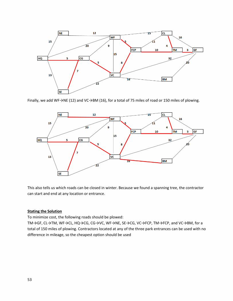
53

Finally, we add WF→NE (12) and VC→BM (16), for a total of 75 miles of road or 150 miles of plowing.

This also tells us which roads can be closed in winter. Because we found a spanning tree, the contractor

can start and end at any location or entrance.


To minimize cost, the following roads should be plowed:

TM→GF, CL→TM, WF→CL, HQ→CG, CG→VC, WF→NE, SE→CG, VC→FCP, TM→FCP, and VC→BM, for a

total of 150 miles of plowing. Contractors located at any of the three park entrances can be used with no

difference in mileage, so the cheapest option should be used

54

Part 4: Deliveries – Traveling Salesman Problem

Assume you need to deliver supplies to each of the 11 locations in the park, starting and ending at HQ.

You want to visit each location exactly once. In graph theory, a path that visits each vertex in a graph

exactly once and ends and starts at the same vertex is called a Hamiltonian circuit. The problem of

finding the minimum cost such path is called the Traveling Salesman Problem (TSP), probably the most

famous problem in OR. This is a notoriously difficult problem to solve efficiently.

There are 11 locations to visit in a circuit. One could attempt to list all possible paths of length 11, pick

out the potential solutions (those through all 11 locations), compute the length and pick the best. The

problem with this brute force approach is that there are so many possibilities. In the worst-case

scenario, i.e. a complete graph with 11 vertices (complete means that each vertex is connected to every

other vertex), there are 400,814,12

!10

2

)!1n(

possible paths to check. While we do have only 21

edges instead of the 55 of a complete graph, it is still not feasible to find and check all potential paths.

We will use an approach called a heuristic, which is short for heuristic technique. A heuristic is an

approach that uses a practical, often intuitive approach to problem solving. It is not guaranteed to yield

the optimal result, but instead one that is “good enough” (hopefully),

Nearest neighbor approach

The nearest neighbor approach is fast, simple, and often yields a good short path. However, there are

instances where it doesn’t work at all or even yields the worst path. The idea is to start at an arbitrary

vertex, chose the edge to the nearest unconnected vertex, and continue until the circuit is complete.

This approach works well if the graph is complete or nearly so. In our case, starting at HQ, we end up

“stuck”, there is no path from BM back to NE:

You may have noticed that we had choices at FCP, however, each of them will lead to the same problem.

There just aren’t enough edges.

55

One way around this is to use a modified nearest neighbor approach. We recognize that there are two

nodes, NE and BM, where we do not have a choice how to reach them. We can therefor treat those

segments (shown below) as a unit and try the nearest neighbor approach again.

Starting at HQ, this time we get a solution. The total length of this circuit is 209.

Sub-tour Reversal

Next, we examine a technique called sub-tour reversal. We start with any possible directed circuit:

56

This circuit is not – and doesn’t have to be – perfect, it just serves as a starting point. The idea is to look

at sub-tours, starting with one-segment ones, then two-segments, etc. We will look at each of those

sub-tours and check if the total cost can be improved if we reverse direction. If we reverse direction, it

will also affect the two path segments directly adjacent. We again start at HQ.

HQ→SE If we reverse HQ→SE, the edges NE→HQ and SE→CG no longer work (left graph). We can

add HQ→CG, but there is no edge from NE to SE. Without it, the circuit is broken.

SE→CG Reversing SE→CG to CG→SE means the adjacent edges, HQ→SE and SE→VC no longer

work. We replace them with HQ→CG and SE→VC, respectively. This results in a reduction

of cost by 12.

CG→VC Not possible, can’t connect CG to BM

VC→BM Not possible, can’t connect CG to BM

BM→GF Not possible, can’t connect TM to BM

GF→TM Not possible, can’t connect TM to BM

TM→CL This reversal is possible; however, it results in an increase in cost by 13.

CL→FCP This reversal is possible, but it results in no change in total cost.

FCP→WF Not possible, can’t connect FCP to NE

WF→NE Not possible, can’t connect FCP to NE

NE→HQ Not possible, can’t connect NE to SE

Of all three possible 1-segment subtour reversals, reversing SE→CG to CG→SE gives the best result, so

we will implement that. Next, we check all two-segment sub-tours, then all three-segment sub-tours

and so on (it turns out none of those are reversible). Our final circuit looks like this:

57

TSP using Excel

To use Excel to solve the TSP problem, we first have to set up the distance matrix. It shows the distance in

minutes between each pair of nodes. As we have done earlier, we set this value to a large number when no

such path exists to make sure that option is never chosen. Note that the matrix is symmetrical, this is

because all our roads can be driven in either direction. If we had one-way roads the matrix would no longer

be symmetrical.

This is no longer a linear programming problem. For example, we assign the different nodes arbitrary

numbers, so the contribution of the decision variables to the value of the objective function is no longer

proportional to their value. Excel offers two other solver options: A generalized reduced gradient algorithm

and an evolutionary algorithm. The details of these algorithms are a bit beyond this class, though I am

happy to talk to you outside the class room if you are interested. Basically, the GRG method finds the

direction of steepest increase or decrease to move towards the maximum/minimum. It works well if the

objective functions and feasible region are smooth-ish (think parabolas, cones, etc.). The evolutionary

algorithm does not have any smoothness requirements. It uses a random start point and then evolves the

next generation of solution points from that start point (a little like the path-reversal, but with a strong

random element). It does not use gradient information, so you cannot be sure you reached the best

solution. The evolutionary solver will keep searching for better solutions until it no longer makes sufficient

progress or runs out of time. We will use the Evolutionary Solver option.

We start with an arbitrary sequence 1-2-3-4-5-6-7-8-9-10-11-1. The INDEX function is used to look the

associated time in the distance matrix.

Syntax: =INDEX(range where to look, what row to use, optional: what column to use)

The objective function is simply the sum of the times. As our only constraint we use the “all different”

option. The constraint “$C$22:$C$32 = AllDifferent” means that the 11 decision variables stored in

$C$22:$C$32 must be integers in the range 1 – 11, with each one different from all the others, i.e. we

require permutations of {1, 2, 3, 4, 5, 6, 7, 8, 9, 10, 11}. Finally, you want to choose the option to set a time

limit for your solver, 60 seconds should be sufficient.

58

The solver returns the solution below. The time requirement is the same as we found in our previous

attempts.

Circuit Time

WF 6 20

CL 8 15

FCP 7 15

TM 9 15

GF 10 30

BM 11 20

VC 5 15

SE 3 14

CG 4 15

HQ 1 20

NE 2 30

WF 6


Starting at HQ, the route traveled will take 209 minutes or 3 hours 29 minutes. An optimal route to take

is HQ→NE→WF→CL→FCP→TM→GF→BM→VC→SE→CG→HQ. An alternate of same length is

HQ→NE→WF→FCP→CL→TM→GF→BM→VC→SE→CG→HQ, and of course both routes can be reversed.

59

Part 5: Road Patrols – Traversing

To ensure the safety of visitors, a ranger has to patrol the entire road system in the park daily, starting

and ending at HQ while minimizing travel time. If possible, they should drive each road only once in

either direction. In graph theory, a path that visits each arc in a graph exactly once and ends and starts

at the same vertex is called a Eulerian circuit. You may recall from Discrete Mathematics that a Euler

circuit exists if and only if the degree of each vertex is even, i.e. an even number of edges connect to

each vertex. Unfortunately, that is not the case here, SE and TM both have degree 3.

We already know that it is not possible to traverse each road exactly once, so the question now

becomes how many times each road needs to be traveled, and in which direction. We re-arrange our

table to list both road directions next to each other. This makes it easier to write the constraints: “each

segment needs to be traveled at least once in either direction”.

60


It will take a single ranger 514 minutes or 8 hours 34 minutes to patrol all the roads in the park. One

possible optimal route is:

HQ→NE→WF→HQ→CG→WF→FCP→VC→WF→CL→FCP→TM→GF→CL→TM→FCP→VC→GF→BM→VC

→CG→SE→VC→SE→HQ. This is just one of many options. The only rule is that either all roads have to

be travelled in the direction and frequencies shown, or all directions have to be reversed.

The patrol as specified is not possible without overtime, especially not if anything needs attention.

Possible alternatives are:

Splitting the area between two or more patrols or two or more days

Eliminating roads from the patrol

Faster car?

Comment: Note that this is a Euler path if you eliminate the second traversals. Basically, we have a Euler

path from SE to TM + the fastest way / shortest path linking the beginning and end of that Euler path. If

you think of each arrow as an undirected arc, then all nodes have even degree and a Euler circuit exists.

Basically, we figured out where edges need to be added to have the cheapest possible Euler

path/circuit.

61

GAS EXPLORATION – DECISION ANALYSIS

Learning Goals

In this chapter, you will learn how to organize a situation with different possible courses of action and

associated outcomes into a flowchart (decision tree). We will examine how to incorporate uncertainty,

expected values, and conditional probabilities to determine optimal strategies. To quote (Hillier &

Lieberman, 2005): “Decision Analysis provides a framework and methodology for rational decision

making when the outcomes are uncertain”.

Case Study Description

Your company is interested in exploring fracking for gas in Pennsylvania. You just signed a six-year lease

on a promising tract of land, and you now have to decide how to proceed. Here are the parameters:

1000-acre tract

Annual lease is $5/acre paid up front + 15% royalty

One time signing bonus of $200/acre

50-50 chance of productive

It’ll cost $6 million to drill a well, potential for three wells

After deducting royalties, each well could bring profit of $15 million over six years of productive

life span

Option to do seismic survey at $4 million, but a survey is not 100% accurate. In fact, we will

assume that a survey will detect gas – if there is any – with 85% probability, but might also

return a positive result with 5% probability if there really is not enough gas to drill (false

positive)

A positive survey would bring the value of your lease to $10 million, you could sell that lease

A negative survey would drop the value of your lease to $0

If you sell without a survey, you are confident you could sell the lease for $300,000.

References

For further reading on the economics of gas exploration, see the following websites:

http://extension.psu.edu/publications/ua448/view

http://marcelluscoalition.org/wp-content/uploads/2016/10/FINAL-Post-Production-

Toolkit_100616.pdf

http://extension.psu.edu/natural-resources/natural-gas/news/2010/11/seismic-surveying

http://geology.com/royalty/production-decline.shtml

http://extension.psu.edu/publications/ua448/view

http://marcelluscoalition.org/wp-content/uploads/2016/10/FINAL-Post-Production-Toolkit_100616.pdf

http://marcelluscoalition.org/wp-content/uploads/2016/10/FINAL-Post-Production-Toolkit_100616.pdf

http://extension.psu.edu/natural-resources/natural-gas/news/2010/11/seismic-surveying

http://geology.com/royalty/production-decline.shtml

62

Solution Approach

As you can tell, there are lots of options to choose from. We will organize them in a decision tree. Note

that there are some nodes that allow you to make a decision, and others where nature/fate/luck comes

in. Read the tree left to right.

Next, we add the cost of each decision in million $ and the total cost for each path taken. Negative

numbers stand for costs/losses.

gas

drill no gas

positive

survery

sell

conduct

survery

gas

lease drill no gas

negative

survey

sell

gas

no

survey

drill no gas

sell

don't

lease

gas

4522.77

drill

-18

no gas

0-22.23

positive

survery

sell

10 5.77

survey

-4

gas

4522.77

lease

-0.23

drill

-18

no gas

0-22.23

negative

survey

sell

±0-4.23

gas

4526.77

no

survey

±0

drill

-18

no gas

0 -18.23

sell

0.30.07

don't

lease

± 0

± 0

63

You immediately see that the best-case scenario would be to not do a survey, drill and find gas but of

course that depends on being lucky. This is where we use statistics to compute the probabilities of each

scenario, and the expected values of each action. We are given the following:

P(gas) = 0.5 P(no gas) = 0.5

P(positive survey|gas) = 0.85 P(positive survey|no gas) = 0.05

These imply:

P(negative survey|gas) = 0.15 P(negative survey|no gas) = 0.95

What we really need to know is the probability that a positive survey means that there really is gas, i.e.

P(gas|positive survey). This a case for Bayes Law. Bayes Law states:

For a given partition B1, B2, B3, … and an event A:

)...P(B)B|P(A)P(B)B|P(A)P(B)B|P(A

)P(B)B|P(AA)|P(B

332211

111

In our case:

18

17

0.50.050.50.85

0.50.85

P(gas)gas) no|survey P(positive P(gas)gas)|survey P(positive

P(gas) gas)|survey P(positivesurvey) positive|P(gas

and therefore P(no gas| positive survey) = 181 .

Similarly P(gas|negative survey) = 223 and P(no gas|negative survey) =

2219 .

So, if you have a positive survey and drill, you have a 17/18 chance of finding a lot of gas and making

$22.77 million, and a 1/18 chance of finding nothing and losing $22.23 million. In other words, the

conditional expectations are

E[drill|positive survery] = 27.2023.2218

177.22

18

17

and

E[drill|negative survery] = 094.1623.2222

1977.22

22

3 .

Of course, E[sell|positive survey] = 5.77 and E[sell|negative survey] = -4.23.

In summary, if you drill after a positive survey, your expected return of $20.27 million is better than

what you would earn under the alternative (don’t drill, sell), so you discard the selling option. We call

this “pruning the tree”. Similarly, if you have a negative survey, you should sell to minimize your

expected loss.

If you don’t pay for a survey and just drill, you have a 50-50 chance of finding gas and your expected

return is E[drill, no survey] = 0.5 ∙ 23.77 - 0.5 ∙ 18.23 = 1.108, still better than what you can expect if you

don’t do a survey and just re-sell your lease.

64

Here is the “pruned” decision tree with just the optimal decisions and expected values in [] identified so

far:

So, should you pay for a survey in the first place? To answer that, we need to find a few more

probabilities and expected values. We will have to use the Law of Total Probability and the definition of

conditional probability. For a given partition B1, B2, B3, … and an event A:

P(A) = P(A∩B1) + P(A∩B2) + P(A∩B3)… = P(A|B1) ∙ P(B1) + P(A|B2) ∙ P(B2) + P(A|B3) ∙ P(B3)…

Therefore,

P(positive survey) =P(positive survey|gas) ∙P(gas) + P(positive survey|no gas) ∙P(no gas)

= 0.5 ∙0.85 + 0.5 ∙0.05 = 0.45

P(negative survey) =P(negative survey|gas) ∙P(gas) + P(negative survey|no gas) ∙P(no gas)

= 0.5 ∙0.15 + 0.5 ∙0.95 = 0.55

Assuming you follow the optimal strategies, your expected return if you choose to conduct a survey is

E[survey] = 0.45 ∙ 20.27 - 0.55 ∙ 4.23 = 6.795. This is much better than the best outcome for not

conducting a survey, which was 1.108.

gas

4522.77

drill

-18

[20.27]

no gas

0 -22.23

positive

survery

survey

-4

lease

-0.23

negative

survey

sell

±0

[-4.23]

-4.23

gas

4526.77

no survey

±0

[1.108]

drill

-18

[1.108]

no gas

0 -18.23

don't

lease

± 0

± 0

65


Under the given parameters, the optimal strategy is to buy the lease and conduct a survey. In the case of

a positive survey, one should drill and can expect a profit of $20.27 million. If the survey is negative, one

should sell the lease to minimize the loss, $4,23 million.

Worst case scenario under optimal strategy: Company drills and finds no gas, looses $22.23 million

Best case scenario under optimal strategy: Company drills and finds gas, profit of $22.77 million

gas

4522.77

drill

-18

[20.27]

no gas

0 -22.23

positive

survery

survey

-4

lease

-0.23

negative

survey

sell

±0

[-4.23]

-4.23

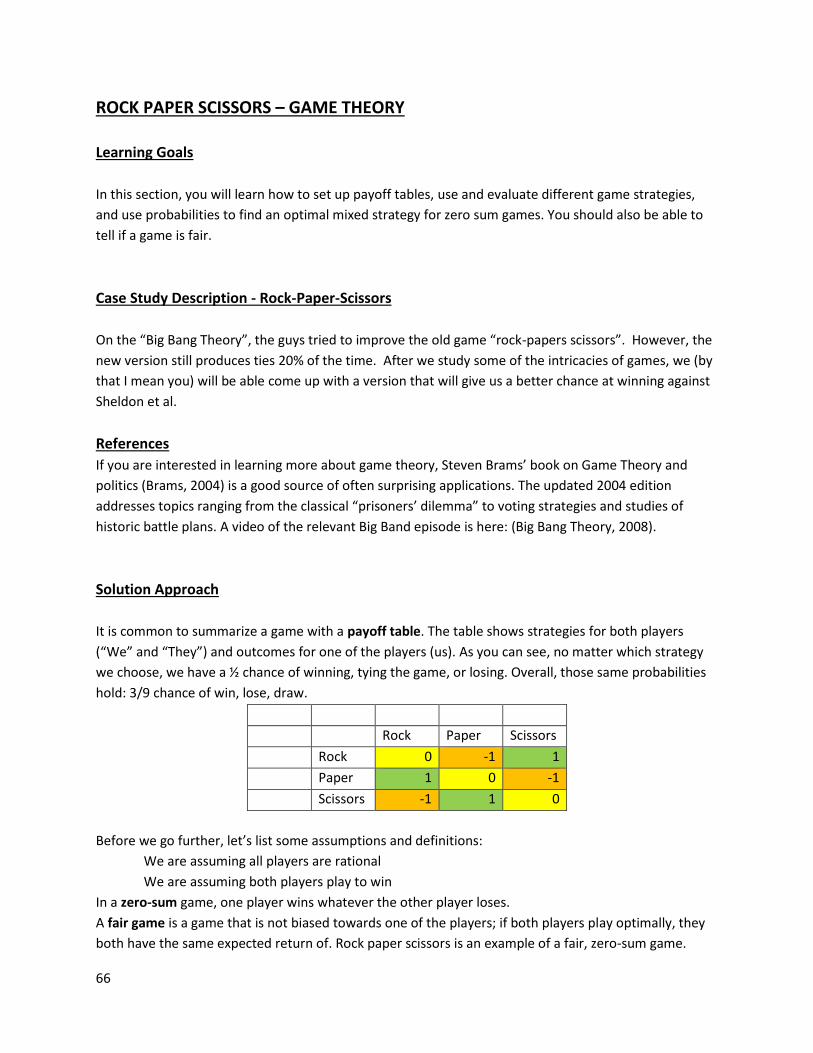
66

ROCK PAPER SCISSORS – GAME THEORY

Learning Goals

In this section, you will learn how to set up payoff tables, use and evaluate different game strategies,

and use probabilities to find an optimal mixed strategy for zero sum games. You should also be able to

tell if a game is fair.

Case Study Description - Rock-Paper-Scissors

On the “Big Bang Theory”, the guys tried to improve the old game “rock-papers scissors”. However, the

new version still produces ties 20% of the time. After we study some of the intricacies of games, we (by

that I mean you) will be able come up with a version that will give us a better chance at winning against

Sheldon et al.

References

If you are interested in learning more about game theory, Steven Brams’ book on Game Theory and

politics (Brams, 2004) is a good source of often surprising applications. The updated 2004 edition

addresses topics ranging from the classical “prisoners’ dilemma” to voting strategies and studies of

historic battle plans. A video of the relevant Big Band episode is here: (Big Bang Theory, 2008).

Solution Approach

It is common to summarize a game with a payoff table. The table shows strategies for both players

(“We” and “They”) and outcomes for one of the players (us). As you can see, no matter which strategy

we choose, we have a ½ chance of winning, tying the game, or losing. Overall, those same probabilities

hold: 3/9 chance of win, lose, draw.

Rock Paper Scissors

Rock 0 -1 1

Paper 1 0 -1

Scissors -1 1 0

Before we go further, let’s list some assumptions and definitions:

We are assuming all players are rational

We are assuming both players play to win

In a zero-sum game, one player wins whatever the other player loses.

A fair game is a game that is not biased towards one of the players; if both players play optimally, they

both have the same expected return of. Rock paper scissors is an example of a fair, zero-sum game.

67

Adding the additional strategies “lizard” and “Spock” increases the size of the table and reduces the

odds of a tie to 1/5, but still doesn’t substantially change the game.

Rock Paper Scissors Lizard Spock

Rock 0 -1 1 1 -1

Paper 1 0 -1 -1 1

Scissors -1 1 0 1 -1

Lizard -1 1 -1 0 1

Spock 1 -1 1 -1 0

Approach 1: Maximizing expected return

One possible game plan is to choose the strategy that yields the greatest average return. In the table

above, that doesn’t help because, if both players randomly chose what to throw, i.e. if each strategy has

the same 1/5 probability of being chosen, then each strategy has an expected value of 0. But in the

video we watched in class, they complain that everyone always chooses “Spock”. Adding probabilities

changes the game:

probability 0.05 0.05 0.1 0.1 0.7


Average return for Us – Expected value

Rock 0 -1 1 1 -1

=SUMPRODUCT(B12:F12,$B$10:$F$10) =-0.55

Paper 1 0 -1 -1 1

=SUMPRODUCT(B13:F13,$B$10:$F$10) =0.55


=SUMPRODUCT(B14:F14,$B$10:$F$10) =-0.6

Lizard -1 1 -1 0 1

=SUMPRODUCT(B15:F15,$B$10:$F$10) =0.6

Spock 1 -1 1 -1 0

=SUMPRODUCT(B16:F16,$B$10:$F$10) =0

We find that under these circumstances, we should play Lizard, because that has the highest expected

return.

A possible refinement would be to assign value to each item. For example, rocks are cheap, so losing a

rock could be equated with losing 1 point, paper 2 points, scissors 3 points, Lizard 4, and Spock 5.

Assuming equal probabilities, this results in the following pay-off table and expected returns:

value 1 2 3 4 5


Average Return for Us

Rock 0 -1 3 4 -1

1.0

Paper 1 0 -2 -2 5

0.4


0

Lizard -4 2 -4 0 5

-0.2

Spock 1 -5 3 -5 0

-1.2

Average Return

for Them 1 0.4 0 -0.2 -1.2

68

We see that now “Rock” is the best strategy for both parties with an expected return of 0 for everyone.

Of course, if They think we will play “Rock”, They may change their strategy to “Paper” or “Spock”, so we

should change to “Lizard”, which will cause Them to change to “Rock” or “Scissors”, which makes us go

to “Spock”, etc. etc.…

Approach 2: Minimizing potential loss

Another strategy, especially for risk adverse people, is to minimize potential loss. We again use the

payoff table, but this time we find the maximum potential loss for each strategy, we perform a worst-

case analysis:


max loss for Us

Rock 0 -1 3 4 -1

-1

Paper 1 0 -2 -2 5

-2


-3

Lizard -4 2 -4 0 5

-4

Spock 1 -5 3 -5 0

-5

max loss for Them

-1 -2 -3 -4 -5

Both players should use “rock” as their strategy, as it minimizes potential losses for both parties. Again,

once the other team notices our strategy, they will change theirs, which will make us change ours, and

so forth.

Approach 3: Looking for a saddle point

Let’s assume we just assign letters to each strategy, and values to the outcomes as shown in the table

below. The strategies that minimize potential loss are “C” for Us and “B” for Them. The outcome is the

same for both players, 0, so this is a fair game. Note that, unlike any of the two previous scenarios, no

party benefits from unilaterally changing their strategy. If either party changes their strategy without

the other changing as well, their outcome will get worse. On the other hand, having a game like this

were the outcome can be reasoned out beforehand and both players are risk adverse is also somewhat

boring.

A B C D E

max loss for Us

A 1 -1 0 -1 4

-1

B -3 -1 1 0 -8

-8

C 2 0 0 8 4

0

D -2 -3 -3 -4 2

-4

E 1 0 2 -1 2

-1

max loss for Them

-2 0 -2 -8 -4

69

Approach 4: Looking for dominated strategies

Sometimes one finds looking at the payoff table that one strategy is always better than another. For

example, in the table below, strategy “C” is better for Them than either strategy A or E. We say “C

dominates D and E”.

A B C D E

A -1 1 -1 1 -1

B 2 -2 -2 0 2

C -1 -4 -3 2 -2

D 2 1 1 2 1

E 2 3 -3 2 -2

If C is always better, then there is no reason for Them to use strategies A or E, we can eliminate them.

A B C D E

A -1 1 -1 1 -1

B 2 -2 -2 0 2

C -1 -4 -3 2 -2

D 2 1 1 2 1

E 2 3 -3 2 -2

Now we see that for Us, D dominates A, B, and C, so we can eliminate them as well.

A B C D E

A -1 1 -1 1 -1

B 2 -2 -2 0 2

C -1 -4 -3 2 -2

D 2 1 1 2 1

E 2 3 -3 2 -2

Now, for Them, strategy C dominates D and B.

A B C D E

A -1 1 -1 1 -1

B 2 -2 -2 0 2

C -1 -4 -3 2 -2

D 2 1 1 2 1

E 2 3 -3 2 -2

For Us, the choice become D. The value of the game is 1 for Us, and therefore -1 for Them. If everyone

logically reasons out the dominated and dominant strategies, We will follow D and They will follow C.

We say we solved the game, there is no more uncertainty or chance (and it got boring…)

70

Note that this is the same result we would have gotten if we had followed the risk adverse strategy. We

again have a saddle point, but this time They can change strategy without getting a worse result (from C

to B or E), while We can’t. However, no-one can improve by changing without the other one changing as

well.

A B C D E

A -1 1 -1 1 -1 -1

B 2 -2 -2 0 2 -2

C -1 -4 -3 2 -2 -4

D 2 1 1 2 1 1

E 2 3 -3 2 -2 -3

2 3 1 2 2

Approach 5: Mixed Strategy

A B C D E

A -1 0 1 -1 2

B 2 0 -5 2 -4

C 1 2 3 1 3

D -1 -1 -1 0 -1

E -1 -1 -1 2 -1

Looking at this pay-off table, you see that We should play “C”, because we always win with that strategy.

But if we always play “C”, They will catch on and play “A”, which will hold our wins down. So, how often

should we use “C”? We start again by eliminating dominated strategies:

For Us, “C” beats “D”. After eliminating “D”, ”A” beats “D” and “C” beats “E” for Them. Finally, “C” beats

“A” and “E” for us, and we are left with a greatly reduced table:

A B C

B 2 0 -5

C 1 2 3

We have two options, play B or C. Let’s assign probability p that we play “B” and probability 1-p that we

use “C”. Our expected returns are:

If They use “A”: 2∙p+1∙(1-p) = 1+p

If They use “B”: 0∙p+2∙ (1-p) = 2-2∙p

If They use “C”: -5∙p+3∙ (1-p) = 3-8∙p

The three lines are shown below. Let’s examine the meaning: Assume We choose p=0 (i.e. we always

play “C”). Then the worst case is that our return is 1. If p=1, then the worst case is that we lose -5. So if

71

we wanted a pure strategy, i.e. a strategy with no probabilities, we should play “C” all the time (p=0). If

we choose a mixed strategy, then the best of the worst cases happens when p=1/3. Our best mixed

strategy is to play “C” 2/3 of the time, and “B” 1/3 of the time. In that case, our expected return, the

value of the game, is 4/3. Note that in this example, it does not matter what They do.

Formal derivation of optimal strategy for player 2, Them:

Let’s a be the probability that player 2 uses “A”, b that they choose “B”, and c that they choose “C”.

Then our expected return becomes:

a (1+p) + b (2-2p) + c (3-8p)

Assuming we play our optimal strategy, we get 34 a +

34 b +

34 c =

34 or a +b + c = 1. Because a, b, c are

probabilities, this equality holds for all choices of a, b, c, so any strategy for player 2 yields the same

results. There is nothing They can do. We win.


We notice that adding more options to our pay-off table while keeping the pay-off for win at 1, loss at -1

decreases the probability of a tie, but does not improve our odds of winning. At best, as the number of

options approaches ∞, our chance of winning/losing approaches 50-50. To really rig the game in our

favor, we cannot allow a symmetrical pay-off table but have to skew the pay-off in our favor. We

probably will not get this by Sheldon long enough to work.

-2

-1.5

-1

-0.5

0

0.5

1

1.5

2

2.5

3

0 0.2 0.4 0.6 0.8 1

retu

rn

p

1+p

2-2p

3-5p

optimal p

72

BRAND LOYALTY – MARKOV CHAINS

Learning Goals

Markov chains

Steady state probabilities

Goal Seek

Data tables

Case Study Description – Brand Loyalty

Profit margins at car dealerships and auto makers are notoriously low (excepting maybe luxury brands).

You are working for a manufacturer and have been asked to examine the following questions:

1) Under the status quo, will we increase/decrease/hold constant our customer base?

2) Our company wants to reach a 30% market share in 10 tears. One option would be to improve

our cars’ quality to increase retention. By how much would we have to increase our customer

loyalty in order to reach a 30% market share in 10 years?

3) Alternatively, we could employ targeted advertising. How many of our nearest competitor’s

customers would have to switch to us to give us a 30% market share in 10 years? What do we

have to do to become the company with the biggest market share?

You have already conducted surveys and collected data from a variety of sources. The matrix below

shows the probabilities that a current customer will either be loyal to his/her brand or switch to the

competitor indicated. You also gathered information on current market share.

Transition probabilities and brand loyalty Matrix T

Next car

1 2 3 4 5 6 7 8

Current car Ours Comp. A Comp. B Comp. C Comp. D Comp. E Comp. F Other

1 Ours 0.41 0.4 0.15 0.02 0.01 0.005 0 0.005

2 Comp. A 0.3 0.49 0.1 0 0 0.1 0.01 0

3 Comp. B 0.1 0.11 0.48 0.2 0 0 0.02 0.09

4 Comp. C 0.05 0.05 0.2 0.61 0.05 0.01 0 0.03

5 Comp. D 0.15 0.05 0.03 0 0.56 0.07 0.06 0.08

6 Comp. E 0.16 0.1 0.2 0.1 0.01 0.4 0.002 0.028

7 Comp. F 0.2 0.01 0.17 0.01 0.02 0.03 0.32 0.24

8 Other 0.3 0 0.1 0.1 0.04 0.05 0.05 0.36

73

Note that the rows of T add up to 1

Market share/current state vector M(0)

1 2 3 4 5 6 7 8

Ours Comp. A Comp. B Comp. C Comp. D Comp. E Comp. F Other

0.08 0.3 0.09 0.1 0.2 0.11 0.07 0.05

References

https://www.quora.com/What-is-the-profit-margin-of-a-new-car-dealer

https://www.experianplc.com/media/news/2016/vehicle-loyalty-rates/

http://www.consumerreports.org/car-reliability-owner-satisfaction/car-brands-ranked-by-

satisfaction/

Solution Approach

We will use a Markov process to model this situation. Let’s start with some definitions and notation.

Notation

X(t) (or XtError! Bookmark not defined. for short) is an indexed random variable where t = 0, 1, 2, 3, …

Xt represents a measurable characteristic of interest at time t, in our case the brand that a

customer chooses. We are assuming there are N distinct, non-overlapping states 1, 2, 3, …, N

that the system can fall in. For us the states are “buys our brand, buys competitor A, buys

competitor B, etc.” We therefore have 8 states.

A stochastic process is defined as the indexed collection of all those Xt. We write

{Xt} = {X0, X1, X2, …}

We say a stochastic process is a Markov Process if it has the memory-less property (formally the

Markovian property)

P(Xt+1 = j | Xo= i0, X1=i1, X2=i2,…,Xt=i)=P(Xt+1 = j | Xt = i)

Basically, this means that only the immediate past (where the process just was) matters, not

what happened before that. In our context: A customer chooses the next brand only based on

his/her experience with their current car, not with any cars they owned in the past.

P(Xt+1 = j | Xt = i) is the conditional transition probability from state i to state j at time t, i.e. the

probability to move from I to j in 1 step.

If P(Xt+1 = j | Xt = i) is the same for all the different t’s, i.e. if

P(Xt+1 = j | Xt = i) = P(X1 = j | X0 = i) = P(X2 = j | X1= i) = P(X3 = j | X2= i)…

then we say we have stationary transition probabilities and write P(Xt+1 = j | Xt = i) = pij.

https://www.quora.com/What-is-the-profit-margin-of-a-new-car-dealer

https://www.experianplc.com/media/news/2016/vehicle-loyalty-rates/

http://www.consumerreports.org/car-reliability-owner-satisfaction/car-brands-ranked-by-satisfaction/

http://www.consumerreports.org/car-reliability-owner-satisfaction/car-brands-ranked-by-satisfaction/

74

This means that, at least for the time frame we are interested in, the odds of switching from one

brand to another do not change. We will only deal with stationary transition probabilities in this

class.

We write pij(n) for the probability to go from i to j in n steps. p1,4

(3) is the probability that a

customer starts with our brand (state 1) and after three steps switches to competitor C (state 4)

State j is accessible from state i if pij(n) >0 for some n. For example, states 6 is accessible from

state 1, while state 7 is not.

States i and j communicate if it is accessible from j and j is accessible from i.

A state is transient if, after entering it once, the processes may or may not come back to it.

A state is recurrent if, after entering it once, the processes will guaranteed come back to it.

A state is absorbing if, after entering it, the process will never leave again.

A state is periodic with period m if the process can only return every m>1 steps. This means that

pii(n) = 0 for all integers n other than m, 2m, 3m,…

Finally, let Mi(n) stand for the market share of brand i at time n. With that notation, M1

(0) = 0.08 =

our current market share, M2(0) = 0.3 = competitor A’s current market share.

Part 1: Status Quo

Let’s start with question 1: What will happen if nothing changes the current transition probabilities and

we start with today’s market shares?

Our market share next year is determined by the market share this year and the percent of drivers

switching to/from us. In particular:

M1(1)

= M1(0) p1,1 + M2

(0) p2,1 + M3(0) p3,1 + … + M8

(0) p8,1

M2(1)

= M1(0) p1,2 + M2

(0) p2,2 + M3(0) p3,2 + … + M8

(0) p8,2

⁞ ⁞ ⁞

M8(1)

= M1(0) p1,8 + M2

(0) p2,8 + M3(0) p3,8 + … + M8

(0) p8,8

You may recognize this a simply being M(0)∙T. In general, we have M(n) = M(n-1)∙T = M(0) ∙Tn.

We will use the MMULT function in Excel to perform the repeated matrix multiplications:

Syntax: Highlight the destination array first, then type MMULT(first matrix, second matrix), finally press

CTRL+ALT+ENTER (not just ENTER!!). We are interested in how the market share changes over time. To

compute it, I am using M(n) = M(n-1) ∙T. Notice how the array M in the formula changes, while the matrix T

is held fixed (F4).

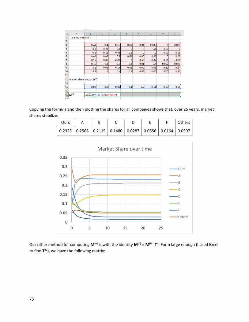
75

Copying the formula and then plotting the shares for all companies shows that, over 25 years, market

shares stabilize.

Ours A B C D E F Others

0.2325 0.2566 0.2115 0.1480 0.0287 0.0556 0.0164 0.0507

Our other method for computing M(n) is with the identity M(n) = M(0) ∙Tn. For n large enough (I used Excel

to find T42), we have the following matrix:

0

0.05

0.1

0.15

0.2

0.25

0.3

0.35

0 5 10 15 20 25

Market Share over time

Ours

A

B

C

D

E

F

Others

76

Note the entries in each column are constant and match the market shares we computed earlier.

Basically, in the long run the probability to buy brand X is the same no matter what brand a customer

bought before. We call these probabilities the steady state probabilities πi. The formal definition of a

steady state probability is: πk = n

lim pi,k(n).

It is of course possible to find the steady state probabilities algebraically. To do that, one has to solve the

steady state equations:

πk =

N

1i

ki,i pπ

for k=1, 2, 3, …, N

N

0i

iπ = 1

π1 = π1 ∙ p1,1 + π2 ∙ p2,1 +…+ π8 ∙ p8,1 π2 = π1 ∙ p1,2 + π2 ∙ p2,2 +…+ π8 ∙ p8,2 ⁞ π8 = π1 ∙ p1,8 + π2 ∙ p2,8 +…+ π8 ∙ p8,8

π1 + π2 + π3 +…+ π8 = 1

0 = π1 ∙ (p1,1 -1)+ π2 ∙ p2,1 +…+ π8 ∙ p8,1 0 = π1 ∙ p1,2 + π2 ∙ (p2,2 -1) +…+ π8 ∙ p8,2 ⁞ 0 = π1 ∙ p1,8 + π2 ∙ p2,8 +…+ π8 ∙ (p8,8-1)

π1 + π2 + π3 +…+ π8 = 1

In matrix form, this becomes:

0.41-1 0.3 0.1 0.05 0.15 0.16 0.2 0.3

π1

0

0.4 0.49-1 0.11 0.05 0.05 0.1 0.01 0

π2

0

0.15 0.1 0.48-1 0.2 0.03 0.2 0.17 0.1

π3

0

0.02 0 0.2 0.61-1 0 0.1 0.01 0.1 ∙ π4 = 0

0.01 0 0 0.05 0.56-1 0.01 0.02 0.04

π5

0

0.005 0.1 0 0.01 0.07 0.4-1 0.03 0.05

π6

0

0 0.01 0.02 0 0.06 0.002 0.32-1 0.05

π7

0

0.005 0 0.09 0.03 0.08 0.028 0.24 0.36-1

π8

1

1 1 1 1 1 1 1 1

We can solve this system of 8 variables in 9 equations with any of the methods learned in Linear Algebra

and arrive at the solution (rounded to 4 decimals):

π1

0.2325

π2

0.2565

π3

0.2115

π4 = 0.1480

π5

0.0287

π6

0.0556

π7

0.0164

π8

0.0507

77


Under the status quo, our long-term market share will be 23.25 %, which will put us in second place

after having been in 1st place with 23.32% in year 2. Our main competitor is brand A.

Part 2: Increase Customer Loyalty

We already have computed what our market share in 10 years will be, namely 23.31%. Let’s assume we

increase our customer loyalty at the expense of the other customers proportionally. We will use two

strategies to answer the question.

Goal Seek

To use Goal Seek, we simply have to go to DATA, What-If Analysis, Goal Seek and fill in the dialog box as

shown. You may not get the desired accuracy. If not, go to FILE, options, formulas, and adjust the “max

change” box downwards. Our answer is that we need to increase our customer loyalty by 17.204% to

58,2.4% in order to reach 29.99978% market share.

One disadvantage of Goal Seek is the “black box” feel of it. I prefer Data Table, which also give me the

advantage of returning numerous values.

The initial set-up is the same as before. We add as column of all increase percentages we are potentially

interested in. Highlight the two columns as shown first, then go to DATA, What-If Analysis, Data Table.

Because our table is arranged in columns, you want to choose the cell that is changing as the column

input variable. Excel will now repeat the calculation of M(10) with each of the values highlighted.

78


We need to increase our customer loyalty by 17.21% to 58.21% in order to reach 30% market share. The

table above shows the effect of increases between 0% and 29% in customer loyalty.

Part 3: Attracting New Customers

Brand A is the brand we lose most of our customers to, and also the source of most of our new

customers, so we will concentrate on them. Our advertising will focus on the demographic that would

otherwise return to brand A, i.e. any loss to their brand loyalty is an equal gain to us. We again use the

Data Table function, but this time we add a column for the difference in our market share

and company A’s. When using the Data Table function, we need to highlight all three columns as shown.

79

And here are the solutions:

Customers switching from A to us 0% 1% 2% 3% 4% 5%

Our market share 0.23313 0.23597 0.23875 0.24148 0.24414 0.24676

Difference to brand A -0.02401 -0.01838 -0.01287 -0.00747 -0.00219 0.00298

Customers switching from A to us 29% 30% 31% 32% 33% 34%

Our market share 0.2964 0.2980 0.2997 0.3012 0.3028 0.3043

Difference to brand A 0.1013 0.1045 0.1077 0.1109 0.1140 0.1170


We need to attract about 65.3% (32% out of 49%) of Brand A’s loyal customers to our brand to reach the

30% market share goal. On the other hand, we need only conquer 10% (5% out of 49%) of their loyal

customers to become the biggest brand with 24.68% market share.

A Final Comment

Brand loyalty is a classic application of Markov chains. There are many interesting and varying

applications of Markov Chains, ranging from internet searches (Googles page rank) to gambling to

poetry (The Russian mathematician Andrey Markov (1856 – 1922) first studied patterns of vowels and

consonants in Alexander Pushkin’s novel in verse Eugene Onegin).

In our example, we have used a finite state irreducible ergodic Markov chain. (Irreducible means that all

states communicate, ergodic simply means that all states are aperiodic and recurrent). Other Markov

chains may not have steady state probabilities. For example, if we have periodic states, the steady state

probabilities may not exist.

Finally, there are many more interesting questions we have omitted. For example, how long does it take

until a customer returns to a brand (recurrence time)? How long does it take for a customer from brand

A to buy our car (first passage time)? How often does a customer return?

80

APPENDICES

A1: How to Write a Request for Proposals

The following is adapted from (Technology Evaluation Centers, 2017).

Preparation

1. Start by answering each of the following questions Why? Who? What? How? and When? as

shown below:

a. WHY?

Why does your organization need a new solution?

Answering this question allows you to create the section called Statement of

Purpose.

b. WHO?

Provide a brief description of your organization.

This information will become the Background information.

c. WHAT?

What is the nature of your project?

What are the needs?

What are the expected outcomes?

Answering these questions allows you to complete the following sections:

Scope of Work

Outcome and Performance Standards

Deliverables

d. HOW?

What is the contract?

What kind of information and documents do you expect to receive from your

consultants?

How will proposals be evaluated and the best matching solution selected?

This information will be used for the sections:

Term of Contract

Payments, Incentives, and Penalties

Contractual Terms and Conditions

Requirements for Proposal Preparation

Evaluation and Award Process

e. WHEN?

When to submit questions, proposal?

When the decision will be taken?

81

What is the whole selection process timeframe?

Who are the people responsible for evaluating proposals? For taking the final

decision?

Answering these questions allows you to populate both sections Process Schedule,

and Points of contact for future correspondence.

Writing the RFP

It seems obvious, but use a formal letterhead and do not handwrite your RFP. It needs to look

professional.

Common Sections of an RFP

By answering the questions above, you were able to gather relevant information that will help

you detail the common sections of an RFP. Here is a brief description for each and any of the

common sections of your RFP:

1. Statement of Purpose

Describe the extent of products and services your organization is looking for, as well as, the

overall objectives of the contract.

2. Background Information

Present a brief overview of your organization and its operations, using statistics, customer

demographics, and psychographics. State your strengths and weaknesses honestly. Don't

forget to include comprehensive information on the people who will handle future

correspondence.

3. Scope of Work

Enumerate the specific duties to be performed by the provider and the expected outcomes.

Include a detailed listing of responsibilities, particularly when sub-contractors are involved.

4. Outcome and Performance Standards

Specify the outcome targets, minimal performance standards expected from the contractor,

and methods for monitoring performance and process for implementing corrective actions.

5. Deliverables

Provide a list of all products, reports, and plans that will be delivered to your organization

and propose a delivery schedule.

6. Term of Contract

Specify length, start date and end date of the contract, and the options for renewal.

7. Payments, Incentives, and Penalties

List all the terms of payment for adequate performance. Highlight the basis for incentives

for superior performance and penalties for inadequate performance or lack of compliance.

82

8. Contractual Terms and Conditions

Attach standard contracting forms, certifications, and assurances. You may include

requirements specific to this particular contract.

9. Requirements for Proposal Preparation

A consistent structure in terms of content, information, and documents types simplifies

things for the people evaluating the proposals. Therefore, you should request a particular

structure for the proposal and provide an exhaustive list of documents you want to receive.

10. Evaluation and Award Process

Lay down the procedures and criteria used for evaluating proposals and for making the final

contract award.

11. Process Schedule

Clearly and concisely present the timeline for the steps leading to the final decision, such as

the dates for submitting the letter of intent, sending questions, attending the pre-proposal

conference, submitting the proposal, etc.

12. Contacts

Include a complete list of people to contact for information on the RFP, or with any other

questions. Incorporate their name, title, responsibilities, and the various ways of contacting

them into this list.

13. Do not forget to send your RFP via certified mail.

14. Since things sometimes get a little more complicated than usual, remember to consult a

lawyer for further information before doing anything.

83

A2: Selected Topics for Projects

Following are some sample projects of the type students can solve in class. Of course, you are welcome

to propose your own. A good project (for this class) has the following characteristics:

Information and data are readily available on the web

Well defined question

Manageable scope

If you have an idea, run it by me and we’ll see if it can work in the context of this class. If you can’t find

data, you may have to “make it up”. In that case, make sure you list all assumptions you make.

1. School bus routes in Huntington

Each year, the Gateway Regional School district publishes that years updated bus routes. Some of

these routes are almost one hour long, meaning that children will spend almost two hours per day

on the bus. Is there a better way? How much would that cost?

http://www.grsd.org/userfiles/4/my%20files/website/2017/all%20routes%20for%20internet-

2016-2017-9-12.pdf?id=4130

2. Retirement Decisions

Massachusetts retirees have a variety of options for their retirement. Which one is the best option

depends on a variety of factors, such as years of service, level of spousal and survivor benefits,

market performance, and others. How should one decide which plan to choose?

http://www.mass.gov/treasury/retirement/for-current-emps/estimate-retirement.html

3. Brown snake infestation in Guam

Brown tree snakes present an ecological danger in Guam. A variety of controls have been employed

(see sources). What happens if the effort is relaxed? If nothing is done? Is it even possible to

eradicate the snakes?

http://www.slate.com/blogs/trending/2012/09/17/guam_s_spider_infestation_due_to_invasiv

e_brown_snakes_.html

http://world.time.com/2013/12/03/rodent-commandos-parachute-into-guam-to-battle-snake-

infestation/

http://voices.yahoo.com/brown-tree-snake-infestation-guam-134308.html

4. Trout species competition in Lake Pend Oreille

Lake Pend Oreille is a 134 square mile lake in Idaho where non-native fish species compete with

native species. The world’s-record bull trout, a 32-pounder, was caught there in 1949. Since the

early 2000, an aggressive management program has been implemented to protect kokanee salmon.

The source below details these efforts, what is needed is a look in the future to model how

populations may develop and what measures might be necessary.

https://idfg.idaho.gov/Kokanee-rebound-in-Lake-Pend-Oreille

http://www.grsd.org/userfiles/4/my%20files/website/2017/all%20routes%20for%20internet-2016-2017-9-12.pdf?id=4130

http://www.grsd.org/userfiles/4/my%20files/website/2017/all%20routes%20for%20internet-2016-2017-9-12.pdf?id=4130

http://www.mass.gov/treasury/retirement/for-current-emps/estimate-retirement.html

http://www.slate.com/blogs/trending/2012/09/17/guam_s_spider_infestation_due_to_invasive_brown_snakes_.html

http://www.slate.com/blogs/trending/2012/09/17/guam_s_spider_infestation_due_to_invasive_brown_snakes_.html

http://world.time.com/2013/12/03/rodent-commandos-parachute-into-guam-to-battle-snake-infestation/

http://world.time.com/2013/12/03/rodent-commandos-parachute-into-guam-to-battle-snake-infestation/

http://voices.yahoo.com/brown-tree-snake-infestation-guam-134308.html

https://idfg.idaho.gov/Kokanee-rebound-in-Lake-Pend-Oreille

84

5. Other invasive species

There are a number of interesting invasive species in the US, for example jumping carp in the Mississippi

watershed carp (you got to watch the video, even if this is not your project)

http://www.asiancarp.org/

https://www.youtube.com/watch?v=rPeg1tbBt0A

Burmese Python I South Florida:

https://www.youtube.com/watch?v=p3PfoESyphQ

http://www.nps.gov/ever/naturescience/npspythonmanagement.htm

6. Hardy Kiwi

There is currently a discussion going on in Massachusetts on whether to list hardy Kiwi as an invasive

species. The problem is that Kiwi is also a potentially lucrative cash crop for farmers. What should be

done?

https://www.bostonglobe.com/metro/2017/01/09/the-hardy-kiwi-scourge-savior-for-new-

england-farmers/tNFY9Fem1qyamVHPoU2alK/story.html

7. PC life-cycle management

At Westfield State, computers in labs and offices are replaced on a rotating basis. What is the

optimal frequency (from a budgetary standpoint) for doing so?

https://www.intel.com/content/dam/www/public/us/en/documents/best-practices/pc-

lifecycle-management.pdf

8. Zombies

In 2014, the Pentagon / US strategic command devised an elaborate plan should a zombie

apocalypse befall the country. CONOP 8888, outlines a detailed plan. Using your own version of

zombies, create first a population model and then a management strategy.

http://www.cnn.com/2014/05/16/politics/pentagon-zombie-apocalypse/index.html

9. Departmental work load

Our department has to deal with many tasks other than teaching, ranging from recruiting new

students to budgets to course development, maintaining the website, and much more. How should

those tasks be prioritized and assigned?

10. Retail space

Where and how a product is displayed in a store has a large effect on sales. Your company makes

premium jellies and you are responsible for arranging the shelf space to maximize profits. Should

you pay for more space?

http://www.bain.com/publications/articles/the-new-mission-for-brands.aspx

https://www.forbes.com/forbes/2002/0415/130.html#

11. Water allocation in California

http://www.asiancarp.org/

https://www.youtube.com/watch?v=rPeg1tbBt0A

https://www.youtube.com/watch?v=p3PfoESyphQ

http://www.nps.gov/ever/naturescience/npspythonmanagement.htm

https://www.bostonglobe.com/metro/2017/01/09/the-hardy-kiwi-scourge-savior-for-new-england-farmers/tNFY9Fem1qyamVHPoU2alK/story.html

https://www.bostonglobe.com/metro/2017/01/09/the-hardy-kiwi-scourge-savior-for-new-england-farmers/tNFY9Fem1qyamVHPoU2alK/story.html

https://www.intel.com/content/dam/www/public/us/en/documents/best-practices/pc-lifecycle-management.pdf

https://www.intel.com/content/dam/www/public/us/en/documents/best-practices/pc-lifecycle-management.pdf

http://www.cnn.com/2014/05/16/politics/pentagon-zombie-apocalypse/index.html

http://www.bain.com/publications/articles/the-new-mission-for-brands.aspx

https://www.forbes.com/forbes/2002/0415/130.html

85

Water in California is over allocated (i.e. there is more demand than supply). Farmers,

ranchers, cities, and fish are competing for the resources. Create an allocation model for the

central valley that could be used to solve this problem.

https://en.wikipedia.org/wiki/Water_in_California

http://www.mercurynews.com/2016/04/01/california-water-allocation-has-winners-

losers/

https://www.usbr.gov/mp/cvp-water/

12. The Salton Sea

The Salton Sea in California lies at the lowest elevations of the Salton Sink in the Colorado Desert of

Southern California, about 235 feet below sea level. It’s water level is completely dependent on scares

rain and run-off. Create a model for water level and/or surface area and/or evaporation and/or water

temperature that could be used to help future decision about mitigating environmental hazards.

http://www.desertsun.com/story/news/environment/2017/03/16/california-has-new-383-

million-plan-shrinking-salton-sea/99124850/

https://waterdata.usgs.gov/ca/nwis/uv?site_no=10254005

https://www.newsdeeply.com/water/articles/2016/08/31/california-is-running-out-of-time-to-

save-the-salton-sea

13. Random walk for mice

Maze experiments are a popular way to test the learning ability of mice, hamsters, rates and the

like. Design a random walk model for such a maze to answer questions such as: what are the odds

the mouse just randomly solved the maze? What is the average time to solve the maze?

http://www.slate.com/articles/health_and_science/the_mouse_trap/2011/11/rat_mazes_and_

mouse_mazes_a_history_.html

http://www.all-science-fair-projects.com/print_project_1101_78

If you are more interested in the theory behind OR, you are also welcome to study some of the

more advanced topics such as

Sensitivity analysis

Branch and bound technique for solving BIP problems

Franke-Wolfe algorithm for non-linear objective functions

Queuing models

Critical path method

https://en.wikipedia.org/wiki/Water_in_California

http://www.mercurynews.com/2016/04/01/california-water-allocation-has-winners-losers/

http://www.mercurynews.com/2016/04/01/california-water-allocation-has-winners-losers/

https://www.usbr.gov/mp/cvp-water/

http://www.desertsun.com/story/news/environment/2017/03/16/california-has-new-383-million-plan-shrinking-salton-sea/99124850/

http://www.desertsun.com/story/news/environment/2017/03/16/california-has-new-383-million-plan-shrinking-salton-sea/99124850/

https://waterdata.usgs.gov/ca/nwis/uv?site_no=10254005

https://www.newsdeeply.com/water/articles/2016/08/31/california-is-running-out-of-time-to-save-the-salton-sea

https://www.newsdeeply.com/water/articles/2016/08/31/california-is-running-out-of-time-to-save-the-salton-sea

http://www.slate.com/articles/health_and_science/the_mouse_trap/2011/11/rat_mazes_and_mouse_mazes_a_history_.html

http://www.slate.com/articles/health_and_science/the_mouse_trap/2011/11/rat_mazes_and_mouse_mazes_a_history_.html

http://www.all-science-fair-projects.com/print_project_1101_78

86

A3: References

Big Bang Theory. (2008, November). Retrieved from season 2 episode 8 The Lizard Spock Expansion:

https://www.youtube.com/watch?v=cSLeBKT7-sM

Brams, S. J. (2004). Game Theory and Politics. Dover.

Hillier, F., & Lieberman, G. (2005). Introduction to Operations Research. McGraw Hill.

Marlow, W. (2012). Mathematics for Operations Research. Dover.

Neuwirth, E., & Arganbright, D. (2004). The Active Modeler: Mathematical Modeling with Microsoft

Excel. Thomson Brooks/Cole.

NOVA on PBS. (2013, 10 16). Retrieved from youtube.com:

https://www.youtube.com/watch?v=XeypDbd3lzo&feature=youtu.be&list=PL9OMJke2jE_CuZgi

OUJ0frfw3TRLKQByw&t=1411

tagg.org. (n.d.). Retrieved from http://tagg.org/pix/EDT2013/wPureMaths.jpg

Taha. (2003). Operations Research - an Introduction . Pearson.

Technology Evaluation Centers. (2017). Retrieved from rfp-templates.com: https://www.rfp-

templates.com/how-to/write-an-rfp

87

A4: Acknowledgements

This project was made possible by a sabbatical release granted at Westfield State University for the

spring 2017 semester. I appreciate the support shown by Dr. Elizabeth Preston, Interim President of

Westfield State University, Dr. Marsha Marotta, Interim Vice President of Academic Affairs at Westfield

State University in approving this sabbatical project. I am indebted to the taxpayers of Massachusetts

for funding me during the sabbatical and allowing me the time to work on and develop this book.

My heart-felt thanks go out to my husband Michael for his patience listening to me talk through

problems and for his help formulating, my son Erik for lending me his fast computing center and

technical support and to my daughter Kristine for debugging code and acting as a sounding board for

many examples. I especially want to thank all my previous students who served as Guinea pigs and

helped me refine the teaching techniques used in this book. You taught me more than I taught you.

Thanks,

Karin Vorwerk

88

A5: Index Allocation problem ..................................................................................................................................... 41 Bayes Law .................................................................................................................................................... 63 Carrying capacity C ...................................................................................................................................... 12 Constraints

augmented .............................................................................................................................................. 32 functional ................................................................................................................................................ 27 non-negativity ......................................................................................................................................... 27 redundant ............................................................................................................................................... 28

Corner point ................................................................................................................................................ 28 Data table

changing input ........................................................................................................................................ 77 Decision variables ....................................................................................................................................... 27 Direction of increase ................................................................................................................................... 27 Eulerian circuit ............................................................................................................................................ 59 Excel functions

AND ......................................................................................................................................................... 23 AVERAGE ................................................................................................................................................. 21 COUNTIF .................................................................................................................................................. 23 DATA TABLE, constant ............................................................................................................................ 20 GOAL SEEK ............................................................................................................................................... 14 IF ............................................................................................................................................................ 23 INDEX ...................................................................................................................................................... 57 Macros .................................................................................................................................................... 24 MMULT ................................................................................................................................................... 74 RAND ....................................................................................................................................................... 19 RANDBETWEEN ....................................................................................................................................... 23 SUMIF ...................................................................................................................................................... 47

Fair game..................................................................................................................................................... 66 Feasible region ............................................................................................................................................ 28 Greedy algorithm ........................................................................................................................................ 50 Hamiltonian circuit ...................................................................................................................................... 54 In-degree ..................................................................................................................................................... 47 Law of Total Probability .............................................................................................................................. 64 Markov Process ........................................................................................................................................... 73 Maximum flow problem

with cost constraints ............................................................................................................................... 51 without cost concerns ............................................................................................................................. 50

Mixed strategy ............................................................................................................................................ 71 Nearest neighbor approach ........................................................................................................................ 54 Net flow ....................................................................................................................................................... 47 Objective function ....................................................................................................................................... 27 Out-degree .................................................................................................................................................. 47 Payoff table ................................................................................................................................................. 66 Pure strategy ............................................................................................................................................... 71 Slack variables ............................................................................................................................................. 32 Solution

89

CPF .......................................................................................................................................................... 28 feasible .................................................................................................................................................... 28 infeasible ................................................................................................................................................. 28 optimal .................................................................................................................................................... 28

State absorbing ................................................................................................................................................ 74 accessible ................................................................................................................................................ 74 communicating ....................................................................................................................................... 74 periodic ................................................................................................................................................... 74 recurrent ................................................................................................................................................. 74 transient .................................................................................................................................................. 74

Stationary transition probabilities .............................................................................................................. 73 Steady state equations ............................................................................................................................... 76 Steady state probabilities πi ........................................................................................................................ 76 Stochastic process ....................................................................................................................................... 73 Sub-tour reversal ........................................................................................................................................ 55 Transition probability .................................................................................................................................. 73 Traveling salesman problem ....................................................................................................................... 54 Zero-sum game ........................................................................................................................................... 66

Documents

Introduction to Operations Research and Mathematical Modeling