Introduction to Parallel Programming - ННГУ · Nizhni Novgorod, 2005 Introduction to Parallel Programming: Parallel Methods for Partial Differential Equations ©GergelV.P. 15

University of Nizhni NovgorodFaculty of Computational Mathematics & Cybernetics

Section 12.

Parallel Methods for Partial Differential Equations

Introduction to Parallel Introduction to Parallel ProgrammingProgramming

Gergel V.P., Professor, D.Sc.,Software Department

Nizhni Novgorod, 2005 Introduction to Parallel Programming: Parallel Methods for Partial Differential Equations© Gergel V.P. 2 70

Contents…

Problem StatementMethods for Solving the Partial Differential EquationsParallel Computations for Shared Memory Systems:– Problem of Blocking in Mutual Exclusion– Problem of Indeterminacy in Parallel Calculations – Race Condition of Threads– Deadlock Problem– Elimination of Calculation Indeterminacy– Parallel Wave Computation Scheme– Block-structured (Checkerboard) Decomposition – Load Balancing


Contents

Parallel Computations for Distributed Memory Systems:– Data Decomposition Schemes– Striped Decomposition– Parallelization of Data Communications– Collective Communications– Block-structured (Checkerboard) Decomposition– Computational Pipelining (Multiple Wave Computation

Scheme)– Overview of Data Communications in Solving Partial

Differential EquationsSummary


Introduction

Partial Differential Equations (PDE) are widely used for developing models in various scientific and technical fieldsAnalysis of mathematical models based on differential equations is provided by the numerical methodsThe performed computation is greatly time-consuming

Numerical solving of partial differential equations is a subject of intensive research


Problem Statement

Lets consider the numerical solving of the Dirichlet problem for the Poisson equation as the case study for PDE Calculations. This problem can be formulated as follows:

⎪⎩

⎪⎨⎧

∈=

∈=+

,),(),,(),(

,),(),,(0

2

2

2

2

Dyxyxgyxu

Dyxyxfyu

xu

δδ

δδ

}1,0:),{( ≤≤∈= yxDyxD


Methods for Solving the Partial Differential Equations…

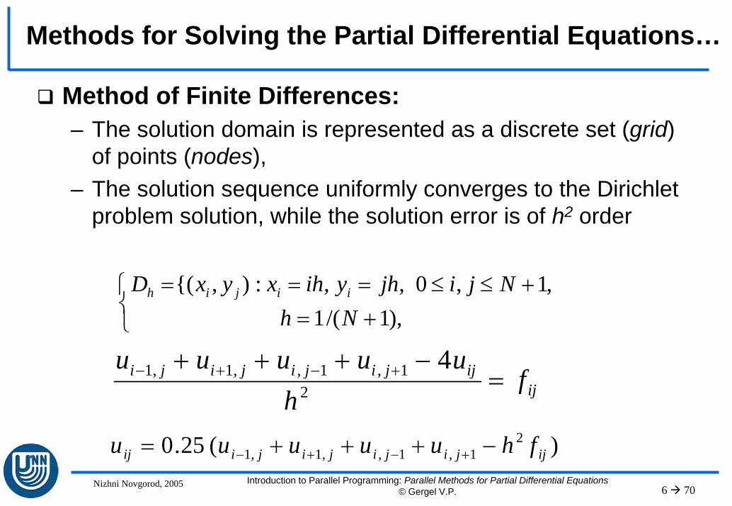
Method of Finite Differences:– The solution domain is represented as a discrete set (grid)

of points (nodes),– The solution sequence uniformly converges to the Dirichlet

problem solution, while the solution error is of h2 order

⎩⎨⎧

+=+≤≤===

),1/(1,1,0,,:),{(

NhNjijhyihxyxD iijih

ijijjijijiji f

huuuuu

=−+++ +−+−

21,1,,1,1 4

)(25.0 21,1,,1,1 ijjijijijiij fhuuuuu −+++= +−+−


Methods for Solving the Partial Differential Equations…

The Gauss-Seidel method…

)(25.0 2111,1,,1,1 ij

kkkkkij fhuuuuu

jijijiji−+++= −−

+−+−

(i,j)(i+1,j)(i-1,j)

(i,j+1)

(i,j-1)• • • • • • •

• • • • • • •

• • • • • • •

• • • • • • •

• • • • • • •

• • • • • • •

• • • • • • •

Calculation complexityT = kmN2

where- N - number of nodes for each dimension,- m - number of operations for one node,- k - number of iterations


Algorithm 1: The Sequential Gauss-Seidel Algorithm

// Algorithm 12.1do {dmax = 0; // maximum deviation of values ufor ( i=1; i<N+1; i++ )for ( j=1; j<N+1; j++ ) {temp = u[i][j];u[i][j] = 0.25*(u[i-1][j]+u[i+1][j]+

u[i][j-1]+u[i][j+1]–h*h*f[i][j]);dm = fabs(temp-u[i][j]);if ( dmax < dm ) dmax = dm;

}} while ( dmax > eps );

Code


A Computational Example

⎪⎪⎪

⎩

⎪⎪⎪

⎨

⎧

=+−=+−=−=−

∈=

,1,200100,1,200100,0,200100,0,200100

,),(,0),(

xyyxxyyx

Dyxyxf

N = 100ε = 0.1k = 210


Parallel Computations for Shared Memory Systems…

The possible way for obtaining software for parallel computations – rewriting the existing sequential programsRewriting can be implemented either automatically by a complier or directly by a programmerThe second approach prevails as the possibilities of automatic program analysis for generating parallel versions of programs are rather restrictedThe application of new algorithmic languages oriented at parallel programming leads to the necessity for a considerable reprogramming of the existing software


Parallel Computations for Shared Memory Systems…

The possible problem solution is the application of some means "outside of programming language". For instance, they may be directives or comments which are processed by a special preprocessor before the program is compiledDirectives can be used to point out different ways to parallelize a program, while the original program text remains the sameThe preprocessor replaces the parallelism directives by some additional program code (as a rule in the form of addressing the procedures of a parallel library)If there’s no preprocessor, the compiler would ignore directives and construct the original sequential program code


Parallel Computations for Shared Memory Systems

The unity of the program code for sequential and parallel calculations reduces the difficulties in parallel programs’

development and maintenance

Conversion of sequential programs to parallel ones by means of directives’ application allows to implement the stage-by-stage

technology of parallel software development that is greatly valued in programming


OpenMP Technology

To specify program fragments that can be executed in parallel, the programmer adds directives (C/C++) or comments (Fortran) into the programThese directives (or comments) allow to determine the parallel regions of the program

As a result of this approach the program can be represented as a sequence of interleaved serial (one-thread) and parallel

(multi-thread) parts of the codeSuch type of computing is usually referred as the fork-join (or pulsatile) parallelism


Algorithm 1.2: The first variant of the Gauss-Seidel parallelalgorithm

// Algorithm 12.2omp_lock_t dmax_lock;omp_init_lock (dmax_lock);do {dmax = 0; // maximum deviation of values u

#pragma omp parallel for shared(u,n,dmax) private(i,temp,d)for ( i=1; i<N+1; i++ ) {

#pragma omp parallel for shared(u,n,dmax) private(j,temp,d)for ( j=1; j<N+1; j++ ) {

temp = u[i][j];u[i][j] = 0.25*(u[i-1][j]+u[i+1][j]+

u[i][j-1]+u[i][j+1]–h*h*f[i][j]);d = fabs(temp-u[i][j])omp_set_lock(dmax_lock);if ( dmax < d ) dmax = d;

omp_unset_lock(dmax_lock);} // the end of inner parallel region

} // the end of outer parallel region} while ( dmax > eps );

Code


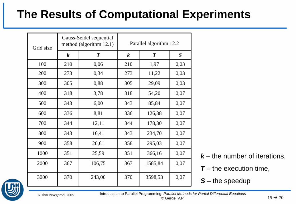
The Results of Computational Experiments

Gauss-Seidel sequential method (algorithm 12.1) Parallel algorithm 12.2

k T k T S

100 210 0,06 210 1,97 0,03

200 273 0,34 273 11,22 0,03

300 305 0,88 305 29,09 0,03

400 318 3,78 318 54,20 0,07

500 343 6,00 343 85,84 0,07

600 336 8,81 336 126,38 0,07

700 344 12,11 344 178,30 0,07

800 343 16,41 343 234,70 0,07

900 358 20,61 358 295,03 0,07

1000 351 25,59 351 366,16 0,07

2000 367 106,75 367 1585,84 0,07

3000 370 243,00 370 3598,53 0,07

Grid size

k – the number of iterations,

T – the execution time,

S – the speedup


Estimation of the Approach

The developed parallel algorithm provides the solution to the given problem It can be used up to N2 processors for program execution There are the excessively high synchronization of the parallel regions of the programLow level of processors’ load

Low efficiency


Problem: Blocking in Mutual Exclusion…

Each parallel thread after processing values must check (and probably change) the value dmax

The permission for using the variable has to be obtained by one thread only. The other threads must be blocked. After the shared variable is released the next thread may get control, etc.


Problem: Blocking in Mutual Exclusion

Exec

utio

n tim

e

Parallel execution

Blocking

Sequential execution

Processors (threads) 1 2 3 4 5 6 7 8

As a result a multithread parallel program turns practically into a sequentially executable code


Algorithm 1.3: The Second Variant of the Gauss-Seidel Parallel Algorithm

// Algorithm 12.3omp_lock_t dmax_lock;omp_init_lock(dmax_lock);do {dmax = 0; // maximum deviation of values u

#pragma omp parallel for shared(u,n,dmax)private(i,temp,d,dm)for ( i=1; i<N+1; i++ ) {

dm = 0;for ( j=1; j<N+1; j++ ) {

temp = u[i][j];u[i][j] = 0.25*(u[i-1][j]+u[i+1][j]+

u[i][j-1]+u[i][j+1]–h*h*f[i][j]);d = fabs(temp-u[i][j]);if ( dm < d ) dm = d;

}

omp_set_lock(dmax_lock);if ( dmax < dm ) dmax = dm;

omp_unset_lock(dmax_lock);}

} // the end of parallel region} while ( dmax > eps ); Code



Gauss-Seidel sequential method (algorithm 12.1) Parallel algorithm 12.2 Parallel algorithm 12.3

k T k T S k T S

100 210 0,06 210 1,97 0,03 210 0,03 2,03

200 273 0,34 273 11,22 0,03 273 0,14 2,43

300 305 0,88 305 29,09 0,03 305 0,36 2,43

400 318 3,78 318 54,20 0,07 318 0,64 5,90

500 343 6,00 343 85,84 0,07 343 1,06 5,64

600 336 8,81 336 126,38 0,07 336 1,50 5,88

700 344 12,11 344 178,30 0,07 344 2,42 5,00

800 343 16,41 343 234,70 0,07 343 8,08 2,03

900 358 20,61 358 295,03 0,07 358 11,03 1,87

1000 351 25,59 351 366,16 0,07 351 13,69 1,87

2000 367 106,75 367 1585,84 0,07 367 56,63 1,89

3000 370 243,00 370 3598,53 0,07 370 128,66 1,89

Grid size



Considerable decrease in the number of shared variable accessThe maximum possible parallelism decreases to the level of NAs a result – a considerable decrease in costs of thread synchronization and a decrease of computation serialization effect

The best speedup parameters


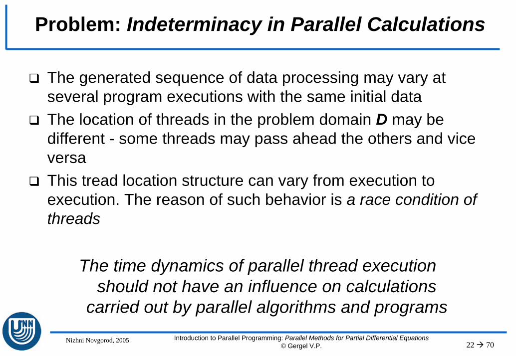
Problem: Indeterminacy in Parallel Calculations

The generated sequence of data processing may vary at several program executions with the same initial dataThe location of threads in the problem domain D may be different - some threads may pass ahead the others and vice versaThis tread location structure can vary from execution to execution. The reason of such behavior is a race condition of threads

The time dynamics of parallel thread execution should not have an influence on calculations

carried out by parallel algorithms and programs


Race Condition of Threads

A possible solution: capture and blocking of the used rows

Processors(threads)

previous iteration values

Processor 2 passes ahead (the “old” values are used)

current iteration l

1 2 3

1 2 3

1 2 3

Processor 2 lacks behind (“new” values are used)

Processor 2 intermediate (“old” and “new” values are used)

grid nodes, for which the “new”values are executed


Problem: Deadlocks

For the mutual exclusion of access to the grid nodes a set of semaphores row_lock[N] may be introduced. It will allow the threads to block the access to their grid rows

// the thread is processing the row iomp_set_lock(row_lock[i]);omp_set_lock(row_lock[i+1]);omp_set_lock(row_lock[i-1]);// processing the grid row i omp_unset_lock(row_lock[i]);omp_unset_lock(row_lock[i+1]);omp_unset_lock(row_lock[i-1]);

Thread 1 Thread 2

Row 1

Row 2

The threads block first rows 1 and 2 and only then pass over to blocking the rest of the rows – deadlock


Deadlock Avoidance

Approach: the appropriate order in rows’ blocking

// the thread is processing the row iomp_set_lock(row_lock[i+1]);omp_set_lock(row_lock[i]);omp_set_lock(row_lock[i-1]);// < processing the grid row i >omp_unset_lock(row_lock[i+1]);omp_unset_lock(row_lock[i]);omp_unset_lock(row_lock[i-1]);

Indeterminacy of calculations is not provided yet


Elimination of Calculation Indeterminacy

To eliminate calculation indeterminacy the Gauss-Jacobi method can be used, which use separate places to store the results of the previous and the current iterations


Algorithm 1.4: The Parallel Gauss-Jacobi method…

// Algorithm 12.4omp_lock_t dmax_lock;omp_init_lock(dmax_lock);do {

dmax = 0; // maximum deviation of values u #pragma omp parallel for shared(u,n,dmax)\

private(i,temp,d,dm)for ( i=1; i<N+1; i++ ) {

dm = 0;for ( j=1; j<N+1; j++ ) {

temp = u[i][j];un[i][j] = 0.25*(u[i-1][j]+u[i+1][j]+

u[i][j-1]+u[i][j+1]–h*h*f[i][j]);d = fabs(temp-un[i][j])if ( dm < d ) dm = d;

}

to be continued


Algorithm 1.4: The Parallel Gauss-Jacobi method

omp_set_lock(dmax_lock);if ( dmax < dm ) dmax = dm;

omp_unset_lock(dmax_lock);}

} // the end of parallel region

for ( i=1; i<N+1; i++ ) // data updatefor ( j=1; j<N+1; j++ )

u[i][j] = un[i][j];} while ( dmax > eps );

Code


The results of Computational Experiments

Sequential Gauss-Jacobi method (algorithm 12.4)

Parallel Gauss-Jacobi method developed on the analogy of the algorithm 12.3

k T k T S

100 5257 1,39 5257 0,73 1,90

200 23067 23,84 23067 11,00 2,17

300 26961 226,23 26961 29,00 7,80

400 34377 562,94 34377 66,25 8,50

500 56941 1330,39 56941 191,95 6,93

600 114342 3815,36 114342 2247,95 1,70

700 64433 2927,88 64433 1699,19 1,72

800 87099 5467,64 87099 2751,73 1,99

900 286188 22759,36 286188 11776,09 1,93

1000 152657 14258,38 152657 7397,60 1,93

2000 337809 134140,64 337809 70312,45 1,91

3000 655210 247726,69 655210 129752,13 1,91

Grid size



Uniqueness of the calculationsUse of the additional memorySmaller convergence rate

Another possible approach to eliminate the mutual dependences of parallel threads is to apply the red/black row alteration scheme. In this scheme the execution of each iteration is subdivided into two sequential stages:

– At the first stage only the rows with even numbers are processed,

– At the second stage - the rows with odd numbers are used


Red/Black Row Alteration Scheme

border values previous iteration values

Stage 1

Stage 2

values after stage 1 of the current iteration

values after stage 2 of the current iteration


Estimation of the Approach…

No additional memory is requiredThe algorithm guarantees uniqueness of calculations, which do not coincide with the results obtained by means of sequential algorithmSmaller convergence rate

Potentiality for the increase in the efficiency of calculations



The Gauss-Jacobi method Red/black row alteration scheme

Additional memory is not required

Use of the additional memory

The algorithm guarantees uniqueness of calculations, though the obtained results may not coincide with the results of the sequential calculations

Calculation schemes demonstrate the convergence rate, which is worse than the original convergence rate of the Gauss-Seidel method


Parallel Wave Computation Scheme…

Let us now consider the parallel algorithms with the following characteristics - the performed calculations and the obtained results have to be completely identical to the ones of the original sequential methodAmong such techniques - the wavefront or hyperplane methodThe wavefront method can be explained as follows – it is evident that to provide calculations identical as at the original sequential method the following should be taken into account:– At the first step the node u11 may be processed only,– Then – at the second step - the node u21 and u12 may be recalculated, etc.

As a result at each step the nodes that may be processed form a bottom-up grid diagonal with the numbers determined by the step number


Parallel Wave Computation Scheme…

border values values of the previous iteration

Growing wave

values of the current iteration nodes, at which values can be recalculated

Wave peak Decaying wave


Algorithm 1.5: Parallel Algorithm Based on WaveCalculation Scheme…

// Algorithm 12.5omp_lock_t dmax_lock;omp_init_lock(dmax_lock);

do {dmax = 0; // maximum variation of values u

// growing wave (nx – wave size)for ( nx=1; nx<N+1; nx++ ) {

dm[nx] = 0;#pragma omp parallel for shared(u,nx,dm) private(i,j,temp,d)

for ( i=1; i<nx+1; i++ ) {j = nx + 1 – i;temp = u[i][j];

u[i][j] = 0.25*(u[i-1][j]+u[i+1][j]+u[i][j-1]+u[i][j+1]*h*f[i][j]);d = fabs(temp-u[i][j])if ( dm[i] < d ) dm[i] = d;

} // the end of parallel region}


Algorithm 1.5: Parallel Algorithm Based on WaveCalculation Scheme

// decaying wavefor ( nx=N-1; nx>0; nx-- ) {#pragma omp parallel for shared(u,nx,dm) private(i,j,temp,d)

for ( i=N-nx+1; i<N+1; i++ ) {j = 2*N - nx – I + 1;temp = u[i][j];u[i][j] = 0.25*(u[i-1][j]+u[i+1][j]+u[i][j-1]+u[i][j+1]–h*h*f[i][j]);d = fabs(temp-u[i][j])if ( dm[i] < d ) dm[i] = d;

} // the end of parallel region}

#pragma omp parallel for shared(n,dm,dmax) private(i)for ( i=1; i<nx+1; i++ ) {

omp_set_lock(dmax_lock);if ( dmax < dm[i] ) dmax = dm[i];

omp_unset_lock(dmax_lock);} // the end of parallel region

} while ( dmax > eps );

Code


Parallel Wave Computation Scheme

The final part of calculations for computing the maximum deviation of values u is the least efficient due to high additional synchronization cost Chucking (fragmentation) – the technique of increasing sequential computation blocks to reduce the synchronization cost The possible variant to implement this approach may be the following:

chunk = 200; // sequential part size#pragma omp parallel for shared(n,dm,dmax)private(i,d)for ( i=1; i<nx+1; i+=chunk ) {d = 0;for ( j=i; j<i+chunk; j++ )if ( d < dm[j] ) d = dm[j];

omp_set_lock(dmax_lock);if ( dmax < d ) dmax = d;

omp_unset_lock(dmax_lock); } the end of parallel region



Sequential Gauss-Seidel method (algorithm 12.1) Parallel algorithm 12.5

k t k t S

100 210 0,06 210 0,30 0,21

200 273 0,34 273 0,86 0,40

300 305 0,88 305 1,63 0,54

400 318 3,78 318 2,50 1,51

500 343 6,00 343 3,53 1,70

600 336 8,81 336 5,20 1,69

700 344 12,11 344 8,13 1,49

800 343 16,41 343 12,08 1,36

900 358 20,61 358 14,98 1,38

1000 351 25,59 351 18,27 1,40

2000 367 106,75 367 69,08 1,55

3000 370 243,00 370 149,36 1,63

Grid size



Low efficiency of cache useIn order to increase the computation performance by efficient cache utilization the following conditions need to be provided:

– The performed calculations use the same data repeatedly (data processing locality),

– The performed calculations provide access to memory elements with sequentially increasing addresses (sequential access)

To meet such requirements the procedure of processing some rectangular blocks of the grid should be considered


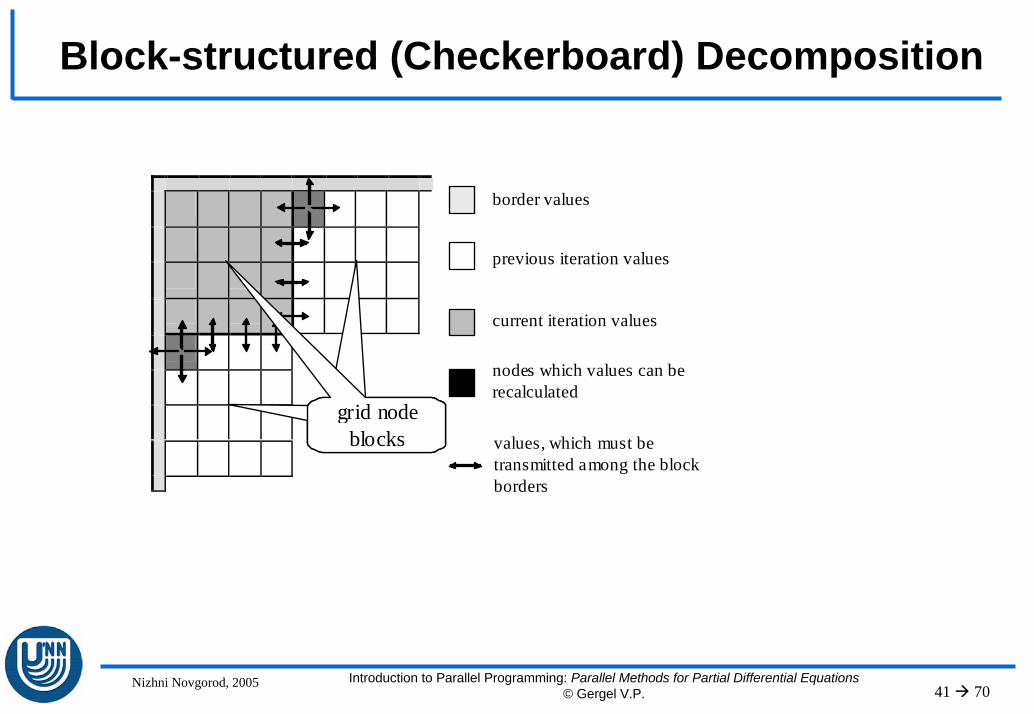
Block-structured (Checkerboard) Decomposition

border values

previous iteration values

current iteration values

nodes which values can be recalculated

values, which must be transmitted among the block borders

grid node blocks


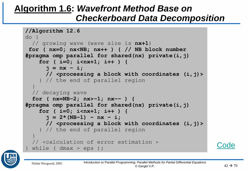
Algorithm 1.6: Wavefront Method Base onCheckerboard Data Decomposition

//Algorithm 12.6do {// growing wave (wave size is nx+1)

for ( nx=0; nx<NB; nx++ ) { // NB block number#pragma omp parallel for shared(nx) private(i,j)

for ( i=0; i<nx+1; i++ ) {j = nx – i;// <processing a block with coordinates (i,j)>

} // the end of parallel region}// decaying wavefor ( nx=NB-2; nx>-1; nx-- ) {

#pragma omp parallel for shared(nx) private(i,j)for ( i=0; i<nx+1; i++ ) {j = 2*(NB-1) - nx – i;// <processing a block with coordinates (i,j)>

} // the end of parallel region}// <calculation of error estimation >

} while ( dmax > eps ); Code


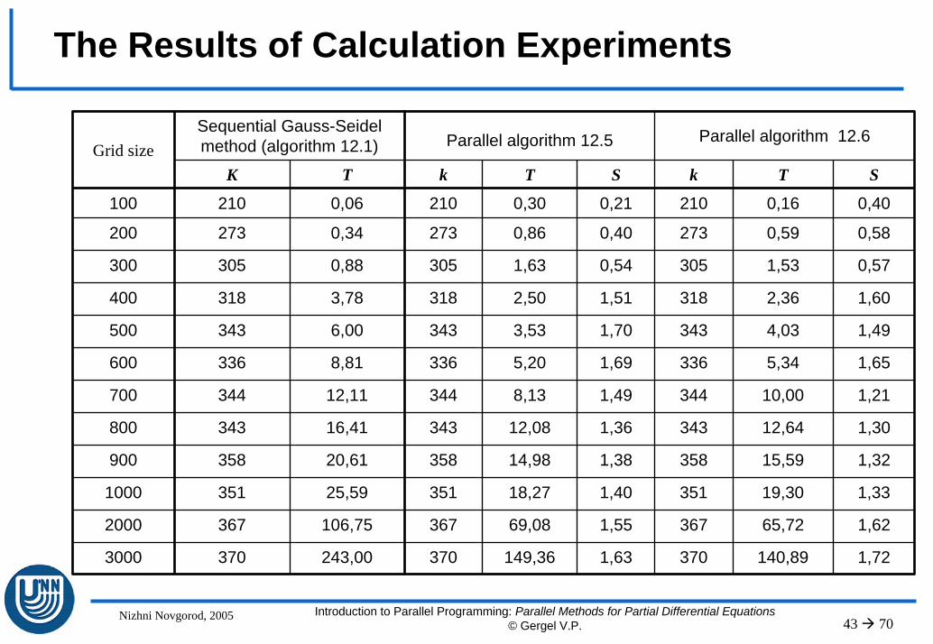
The Results of Calculation Experiments

Sequential Gauss-Seidel method (algorithm 12.1) Parallel algorithm 12.5 Parallel algorithm 12.6

K T k T S k T S

100 210 0,06 210 0,30 0,21 210 0,16 0,40

200 273 0,34 273 0,86 0,40 273 0,59 0,58

300 305 0,88 305 1,63 0,54 305 1,53 0,57

400 318 3,78 318 2,50 1,51 318 2,36 1,60

500 343 6,00 343 3,53 1,70 343 4,03 1,49

600 336 8,81 336 5,20 1,69 336 5,34 1,65

700 344 12,11 344 8,13 1,49 344 10,00 1,21

800 343 16,41 343 12,08 1,36 343 12,64 1,30

900 358 20,61 358 14,98 1,38 358 15,59 1,32

1000 351 25,59 351 18,27 1,40 351 19,30 1,33

2000 367 106,75 367 69,08 1,55 367 65,72 1,62

3000 370 243,00 370 149,36 1,63 370 140,89 1,72

Grid size



Block processing is performed on different processors and the blocks are mutually disjoint - as a results there are no additional costs to support for cache coherency of different processors The situations when processors stay idle are possible

It is possible to increase the efficiency of calculations


Processor Load Balancing

The block size determines the granularity of parallel computationsChoosing the level of granularity it is possible to provide the required efficiency of parallel methodsTo provide the uniform processor loads (load balancing) all the computational works can be arranged as a job queueIn the course of computations the processor, which is already unloaded, may ask for a job from the queue

A job queue is the general management scheme of load balancing for a shared memory system


Algorithm 1.7: Load Balancing Based on Job Queue Management Scheme

//Algorithm 12.7// <data initialization> // <loading the initial block pointer into the job queue>// pick up the block from the job queue (if the job queue is not empty)while ( (pBlock=GetBlock()) != NULL ) { // <block processing> // marking the neighboring block readiness for processingomp_set_lock(pBlock->pNext.Lock); // right-hand neighbor

pBlock->pNext.Count++;if ( pBlock->pNext.Count == 2 )

PutBlock(pBlock->pNext);omp_unset_lock(pBlock->pNext.Lock);omp_set_lock(pBlock->pDown.Lock); // lower neighbor

pBlock->pDown.Count++;if ( pBlock->pDown.Count == 2 )

PutBlock(pBlock->pDown);omp_unset_lock(pBlock->pDown.Lock);

} // the end of computations, as the queue is empty


Parallel Computations for Distributed Memory Systems

Many parallel computation problems such as the race condition, deadlocks, serialization are common for the systems with shared and distributed memory

The communication of parallel program parts on different processors can only be provided through message passing


Data Decomposition Schemes

In the considered the Dirichlet problem there are two different data decomposition schemes: – The one-dimensional or striped decomposition of

the domain grid,– The two-dimensional or block-structured

(checkerboard) decomposition of the domain gridIn case of striped decomposition the domain grid is divided into horizontal or vertical strips The number of strips is defined by the number of processors. The size of strips is usually equal The strips are distributed among the processors for processing


Striped Decomposition

Remarks:– The border rows of the previous and the next strips should

be copied on the processor, which performs processing a strip,

– Border row copying should be performed prior to the beginning of the execution of each method iteration

1

• • • • • • •

• • • • • • • • • • • • • •

• • • • • • • • • • • • • •

• • • • • • • • • • • • • •

0

Processors

2

• • • • • • •

• • • • • • • • • • • • • •

• • • • • • • • • • • • • •

• • • • • • • • • • • • • •

(i,j)(i+1,j)(i-1,j)

(i,j+1)

(i,j-1)


Algorithm 1.8: The Gauss-Seidel Method, the StripedData Decomposition

// Algorithm 12.8// The Gauss-Seidel method, the striped decomposition// operations performed on each processordo {

// <border row exchange between the neighbors>// <strip processing>// <calculating the computational error dmax>

while ( dmax > eps ); // eps – the required accuracy

Code


Data Distribution between Processors…

At the first stage each processor transmits its lowest border row to the following processor and receives the analogous row from the previous processor At the second stage processors transmit their upper border rows to the previous neighbors and receive the analogous rows from the following neighbor


Data Distribution between Processors…

Carrying out such data transmission operations may be implemented as follows:// transmission of the lowest border row to the following// processor and receiving the transmitted border row // from the previous processor

if ( ProcNum != NP-1 )Send(u[M][*],N+2,NextProc);if ( ProcNum != 0 )Receive(u[0][*],N+2,PrevProc);

Such implemented scheme produces the strictly sequential execution of data transmission operationsApplying nonblocking communications may not provide an efficient parallel scheme of processor interactions


Parallelization of Data Communications

At the first step all odd processors transmit data, and the evenprocessors receive the data At the second step the processors change their roles: the even processors perform the operation Send, the odd processors perform the operation Receive

// transmission of the lowest border row to the following processor// and receiving the transmitted row from the previous processorif ( ProcNum % 2 == 1 ) { // odd processorif ( ProcNum != NP-1 )Send(u[M][*],N+2,NextProc);if ( ProcNum != 0 )Receive(u[0][*],N+2,PrevProc);

}else { // even processorif ( ProcNum != 0 )Receive(u[0][*],N+2,PrevProc);if ( ProcNum != NP-1 )Send(u[M][*],N+2,NextProc);

}


Collective Communications

Operation of accumulating and broadcasting the data may be implemented by the use of the cascade schemeObtaining of the maximum value of local errors calculated by theprocessors may be provided by means of the following technique:– At the first step finding of the maximum values for pairwise grouped

processor - such calculations may be performed at different processor pairs in parallel,

– At the second step analogous pairwise calculations may be applied for finding the maximum values among the obtained results, etc.

According with the cascade scheme it is necessary to perform log2p of parallel iterations to calculate the total maximum value (p is the number of processors)


Algorithm 1.8: The Gauss-Seidel Method, Implementationwith Collective Communication Operations

// Algorithm 12.8 – Implementation with Collective Operations

// The Gauss-Seidel method, the striped decomposition// operations performed on each processordo {

// border strip row exchange with the neighbors Sendrecv(u[M][*],N+2,NextProc,u[0][*],N+2,PrevProc);Sendrecv(u[1][*],N+2,PrevProc,u[M+1][*],N+2,NextProc);

// <strip processing with the error estimation dm >// <calculating the computational error dmax> Reduce(dm,dmax,MAX,0);

Broadcast(dmax,0);

} while ( dmax > eps ); // eps – the required accuracy


The Results of Calculations Experiments

Gauss-Seidel sequential method Parallel algorithm 1.8

k T k T S

100 210 0,06 210 0,54 0,11

200 273 0,35 273 0,86 0,41

300 305 0,92 305 0,92 1,00

400 318 1,69 318 1,27 1,33

500 343 2,88 343 1,72 1,68

600 336 4,04 336 2,16 1,87

700 344 5,68 344 2,52 2,25

800 343 7,37 343 3,32 2,22

900 358 9,94 358 4,12 2,41

1000 351 11,87 351 4,43 2,68

2000 367 50,19 367 15,13 3,32

3000 364 113,17 364 37,96 2,98

Grid size


Striped Wavefront Computations

To form a wavefront calculations each strip can be represented logically as a set of blocksAs a result of such logical structure the wavefrontcomputation scheme may be executed. At the first step the block marked by the number 1 may be processed. Then – at the second step – the blocks marked by the number 2 may be recalculated, etc.

Proc

esso

rs 1

0

2

1 2 3 4 5 6 7 8

2 3 4 5 6 7 8 9

3 4 5 6 7 8 9 10

4 5 6 7 8 9 10 11

3


Block-structured (Checkerboard) Decomposition…

In case of the block-structured (checkerboard) data decomposition the number of the border rows on each processor is increased, which leads correspondingly to a greater number of data communications in the border row transmission (but the number of transmitted elements is reduced) The use of the checkerboard scheme of data decomposition is appropriate if the number of grid nodes is essentially large


Block-structured (Checkerboard) Decomposition…

// Algorithm 12.9// The Gauss-Seidel method, the striped decomposition// operations executed on each processordo {// obtaining border nodesif ( ProcNum / NB != 0 ) { // nonzero row of processors// obtaining data from upper processorReceive(u[0][*],M+2,TopProc); // upper rowReceive(dmax,1,TopProc); // computational error

}if ( ProcNum % NB != 0 ) { // nonzero column of processors// obtaining data from left processorReceive(u[*][0],M+2,LeftProc); // left columnReceive(dm,1,LeftProc); // computational errorIf ( dm > dmax ) dmax = dm;

}


Block-structured (Checkerboard) Decomposition

// <processing a block with computational error dmax >// transmission of border nodesif ( ProcNum / NB != NB-1 ) { // processor row is not last//data transmission to the lower processorSend(u[M+1][*],M+2,DownProc); // bottom rowSend(dmax,1,DownProc); // computational error

}if ( ProcNum % NB != NB-1 ) { // processor column is not last

// data transmission to the right processorSend(u[*][M+1],M+2,RightProc); // right columnSend(dmax,1, RightProc); // computational error

}// synchronization and distribution of the value dmaxBarrier();Broadcast(dmax,NP-1);

} while ( dmax > eps ); // eps – the required accuracy

Code


Computational Pipelining (Multiple WavefrontComputation Scheme)…

The wavefront computation efficiency decreases considerably because the processors perform calculations only at the moment when their blocks belongs to the wave computation front

To improve the load balancing among the processors a multiple wavefront computation scheme can be applied

The multiple wavefront method can be explained as follows: the processors may start processing the blocks of the following wave after executing the current calculation iteration


Computational Pipelining (Multiple WavefrontComputation Scheme)

0 1 2 3

4 5 6 7

8 9 10 11

12 13 14 15

blocks of the previous iteration

Growing wave

blocks of the current iteration

blocks which nodes can be recalculated

Wave peak Decaying wave

0 1 2 3

4 5 6 7

8 9 10 11

12 13 14 15

0 1 2 3

4 5 6 7

8 9 10 11

12 13 14 15


Overview of Data Communications in Solving Partial Differential Equations

0 1 2

Processors

One-to-all d istribution of the grid node number

MPI_Bcast

Corresponding MPI function

Communicat ion operation

Scattering strips (blocks) of the grid nodes

MPI_Scatter

Exchanging borders of neighbor strips or blocks

MPI_Sendrecv

All-to-all calculating and distributing the computatinal error

MPI_Allreduce

Gathering strips ( blocks) of the grid nodes

MPI_Gather


Summary

The ways of parallel algorithm development for the systems with shared and distributed memory are discussed on the example of solving the partial differential equationsIn case of parallel computations on the systems with shared memory the main attention is given to the OpenMPtechnology; various aspects concerning with parallel programming are considered In case of parallel computations on the systems with distributed memory the problems of the data decomposition and the information communications between the processors are discussed; striped and checkerboard decomposition schemes are presented


Discussions

What are the ways to increase the efficiency of wavefront methods?How can the job queue balance the computational load?What problems have to be solved in the process of parallel computation on distributed memory systems? What basic operations of data communications are used in the parallel methods of the Dirichletproblem?


Exercises

Develop the parallel algorithm implementation of the wavefront computation scheme including the block-structured data decomposition scheme Develop theoretical estimation of the algorithm execution timeCarry out the computational experiments. Compare the results of computational experiments and the obtained theoretical estimations


References

Gergel, V.P., Strongin, R.G. (2001, 2003 - 2 edn.). Introduction to Parallel Computations. - N.Novgorod: University of NizhniNovgorod (In Russian)Buyya, R. (1999). High Performance Cluster Computing. Volume 1: Architectures and Systems. Volume 2:Programming and Applications. - Prentice Hall PTR, Prentice-Hall Inc.Chandra, R. et al. (2000). Programming in OpenMP. - Morgan Kaufmann.Group W,Lusk E, Skjellum A. (1994). Using MPI. Portable Parallel Programming with the Message-Passing Interface. – MIT Press.Pacheco, P. (1996). Parallel Programming with MPI. - Morgan Kaufmann.Pfister, G.P. (1995). In Search of Clusters. - Prentice Hall PTR, Upper Saddle River, NJ.Quinn, M. J. (2004). Parallel Programming in C with MPI and OpenMP. – New York, NY: McGraw-Hill.


Next Section

Parallel Methods for Global Optimization


Author’s Team

Gergel V.P., Professor, Doctor of Science in Engineering, Course Author

Grishagin V.A., Associate Professor, Candidate of Science inMathematics

Abrosimova O.N., Assistant Professor (chapter 10)Kurylev A.L., Assistant Professor (learning labs 4,5)Labutin D.Y., Assistant Professor (ParaLab system)Sysoev A.V., Assistant Professor (chapter 1)Gergel A.V., Post-Graduate Student (chapter 12, learning lab 6)Labutina A.A., Post-Graduate Student (chapters 7,8,9,

learning labs 1,2,3, ParaLab system)Senin A.V., Post-Graduate Student (chapter 11, learning labs on

Microsoft Compute Cluster)Liverko S.V., Student (ParaLab system)


About the project

The purpose of the project is to develop the set of educational materials for the teaching course “Multiprocessor computational systems and parallel programming”. This course is designed for the consideration of the parallel computation problems, which are stipulated in the recommendations of IEEE-CS and ACM Computing Curricula 2001. The educational materials can be used for teaching/training specialists in the fields of informatics, computer engineering and information technologies. The curriculum consists of the training course “Introduction to the methods of parallel programming” and the computer laboratory training “The methods and technologies of parallel program development”. Such educational materials makes possible to seamlessly combine both the fundamental education in computer science and the practical training in the methods of developing the software for solving complicated time-consuming computational problems using the high performance computational systems.

The project was carried out in Nizhny Novgorod State University, the Software Department of the Computing Mathematics and Cybernetics Faculty (http://www.software.unn.ac.ru). The project was implemented with the support of Microsoft Corporation.

http://www.software.unn.ac.ru/

Documents

Introduction to Parallel Programming - ННГУ · Nizhni Novgorod, 2005 Introduction to Parallel Programming: Parallel Methods for Partial Differential Equations ©GergelV.P. 15