Embed Size (px)
Citation preview
INTRODUCTION TO
PLASMA PHYSICS
AND CONTROLLED
FUSION
SECOND EDITION
Volume 1: Plasma Physics
Francis E Chen Electrical Engineering Department
School of Engineering and Applied Science University of California, Los Angeles
Los Angeles, California
PLENUM PRESS NEW YORK AND LONDON

Library of Congress Cataloging in Publication Data
Chen, Francis F., 1929-lntroduction to plasma physics and controlled fusion.
Rev. ed. of: Introduction to plasma physics. 1974. Bibliography: p.
Includes indexes. Contents: v. I. Plasma physics. I. Plasm-. (Ionized gases) I. Chen, Francis F., 1929-
lntroduction to plasma physics. II. Title. QC718.C39 !983 530.4'4 83-17666 ISBN 0-306-41332-9
10 98 7
This volume is based on Chapters 1-8 of the first edition of lntroducu·on ID PlasTTIIJ Physics, published in 1974.
© 1984 Plenum Press, New York A Division of Plenum Publishing Corporation 233 Spring Street, New York, N.Y. 10013
All rights reserved
No part of this book may be reproduced, stored in a retrieval system, or transmitted in any form or by any means, electronic, mechanical, photocopying, microfilming, recording, or otherwise, without written permission from the Publisher
Printed in the United States of America

To the poet and the eternal scholar ...
M. Conrad Chen Evelyn C. Chen


PREFACE
TOT
DITIO
In the nine years since this book was first written, rapid progress has been made scientifically in nuclear fusion, space physics, and nonlinear plasma theory. At the same time, the energy shortage on the one hand and the exploration of Jupiter and Saturn on the other have increased the national awareness of the important applications of plasma physics to energy production and to the understanding of our space environment.
I n magnetic confinement fusion, this period has seen the attainment of a Lawson number n-rE of 2 x 1013 cm-3 sec in the Alcator tokamaks at MIT; neutral-beam heating of the PL T tokamak at Princeton to KTi =
6.5 keV; increase of average {3 to 3%-5% in tokamaks at Oak Ridge and General Atomic; and the stabilization of mirror-confined plasmas at Livermore, together with injection of ion current to near field-reversal conditions in the 2XIIB device. Invention of the tandem mirror has given magnetic confinement a new and exciting dimension. New ideas have emerged, such as the compact torus, surface-field devices, and the EBT mirror-torus hybrid, and some old ideas, such as the stellarator and the reversed-field pinch, have been revived. Radiofrequency heating has become a new star with its promise of de current drive. Perhaps most importantly, great progress has been made in the understanding of the M HD behavior of toroidal plasmas: tearing modes, magnetic Vll

Vlll Preface to the Second Edition
islands, and disruptions. Concurrently, the problems of reactor design, fusion technology, and fission-fusion hybrids have received serious attention for the first time.
Inertial confinement fusion has grown from infancy to a research effort one-fourth as large as magnetic fusion. With the 25-TW Shiva laser at Livermore, 3 X l 010 thermonuclear neutrons have been produced in a single pellet implosion, and fuel compressions to one hundred times liquid hydrogen density have been achieved. The nonlinear plasma processes involved in the coupling of laser radiation to matter have received meticulous attention, and the important phenomena of resonance absorption, stimulated Brillouin and Raman scattering, and spontaneous magnetic field generation are well on the way to being understood. Particle drivers-electron beams, light-ion beams, and heavy-ion beams-have emerged as potential alternates to lasers, and these have brought their own set of plasma problems.
In space plasma physics, the concept of a magnetosphere has become well developed, as evidenced by the prediction and observation of whistler waves in the Jovian magnetosphere. The structure of the solar corona and its relation to sunspot magnetic fields and solar wind generation have become well understood, and the theoretical description of how the aurora borealis arises appears to be in good shape.
Because of the broadening interest in fusion, Chapter 9 of the first edition has been expanded into a comprehensive text on the physics of fusion and will be published as Volume 2. The material originated from my lecture notes for a graduate course on magnetic fusion but has been simplified by replacing long mathematical calculations with short ones based on a physical picture of what the plasma is doing. It is this task which delayed the completion of the second edition by about three years.
Volume 1, which incorporates the first eight chapters of the first edition, retains its original simplicity but has been corrected and expanded. A number of subtle errors pointed out by students and professors have been rectified. In response to their requests, the system of units has been changed, reluctantly, to mks (SI). To physicists of my own generation, my apologies; but take comfort in the thought that the first edition has become a collector's item.
The dielectric tensor for cold plasmas has now been included; it was placed in Appendix B to avoid complicating an already long and difficult chapter for the beginner, but it is there for ready reference. The chapter on kinetic theory has been expanded to include ion Landau damping of acoustic waves, the plasma dispersion function, and Bernstein waves. The chapter on nonlinear effects now incorporates a treat-

ment of solitons via the Korteweg-deVries and nonlinear Schrodinger equations. This section contains more detail than the rest of Volume 1, but purposely so, to whet the appetite of the advanced student. Helpful hints from G. Morales and K. Nishikawa are hereby acknowledged.
For the benefit of teachers, new problems from a decade of exams have been added, and the solutions to the old problems are given. A sample three-hour final exam for undergraduates will be found in Appendix C. The problem answers have been checked by David Brower; any errors are his, not mine.
Finally, in regard to my cryptic dedication, I have good news and bad news. The bad news is that the poet (my father) has moved on to the land of eternal song. The good news is that the eternal scholar (my mother) has finally achieved her goal, a Ph. D. at 72. The educational process is unending.
Francis F. Chen Los Angeles, 1983
IX Preface to the
Second Edition


PREFACE
TO THE FIRST
EDITION
This book grew out of lecture notes for an undergraduate course in plasma physics that has been offered for a number of years at UCLA. With the current increase in interest in controlled fusion and the widespread use of plasma physics in space research and relativistic astrophysics, it makes sense for the study of plasmas to become a part of an undergraduate student's basic experience, along with subjects like thermodynamics or quantum mechanics. Although the primary purpose of this book was to fulfill a need for a text that seniors or juniors can really understand, I hope it can also serve as a painless way for scientists in other fields-solid state or laser physics, for instance-to become acquainted with plasmas.
Two guiding principles were followed: Do not leave algebraic steps as an exercise for the reader, and do not let the algebra obscure the physics. The extent to which these opposing aims could be met is largely due to the treatment of plasma as two interpenetrating fluids. The two-fluid picture is both easier to understand and more accurate than the single-fluid approach, at least for low-density plasma phenomena.
The initial chapters assume very little preparation on the part of the student, but the later chapters are meant to keep pace with his increasing degree of sophistication. In a nine- or ten-week quarter, it is possible to cover the first six and one-half chapters. The material for XI

Xll Preface to the First Edition
these chapters was carefully selected to contain only what is essential. The last two and one-half chapters may be used in a semester course or as additional reading. Considerable effort was made to give a clear explanation of Landau damping-one that does not depend on a knowledge of contour integration. I am indebted to Tom O'Neil and George Schmidt for help in simplifying the physical picture originally given by john Dawson.
Some readers will be distressed by the use of cgs electrostatic units. It is, of course, senseless to argue about units; any experienced physicist can defend his favorite system eloquently and with faultless logic. The system here is explained in Appendix I and was chosen to avoid unnecessary writing of c, f-Lo, and Eo, as well as to be consistent with the majority of research papers in plasma physics.
I would like to thank Miss Lisa Tatar and Mrs. Betty Rae Brown for a highly intuitive job of deciphering my handwriting, Mr. Tim Lambert for a similar degree of understanding in the preparation of the drawings, and most of all Ande Chen for putting up with a large number of deserted evenings.
Francis F. Chen Los Angeles, 1974

CONTENTS
Preface to the Second Edition vii
Preface to the First Edition xi
1. INTRODUCTION 1 Occurrence of Plasmas in Nature • Definition of Plasma 3 • Concept of Tempemture 4 • Debye Shielding 8 • The Plasma Pammeter 1 } • C?·iteria for Plasmas 1 1 • Applications of Plasma Physics 13
2. SINGLE-PARTICLE MOTIONS Introduction 19 • Uniform E and B Fields B Field 26 • Nonuniform E Field 36 Field 39 • Time-Varying B Field 41 •
Center Drifts 43 • Adiabatic Invariants 43
19 19 • Nonuniform
• Time-Varying E Summary of Guiding
3. PLASMAS AS FLUIDS 53 Introduction 53 • Relation of Plasma Physics to Ordinary" Electromag-netics 54 o The Fluid Equation of Motion 58 • Fluid Drifts Perpendicular to B 68 • Fluid Drifts Parallel to B 75 • The Plasma Approximation 77 Xlll

XIV Contents
4. WAVES IN PLASMAS 79 Representation of Waves 79 • Group Velocity 81 • Plasma Oscillations 82 • Electron Plasma Waves 87 • Sound Waves 94 • Ion Waves 95 • Validity of the Plasma Approxima-tion 98 • Comparison of Ion and Electron Waves 99 • Electro-static Electron Oscillations Perpendicular to B I 00 • Electrostatic I on Waves Perpendicular to B 1 09 • The Lower Hybrid Frequency 112 •
ElectTomagnetic Waves with B0 = 0 114 • Experimental Applications I l 7 • Electromagnetic Waves Perpendicular to B0 122 •
Cutoffs a.nd Resonances 126 • Electromagnetic Waves Parallel to Bo 12 8 Experimental Consequences 131 Hydromagnetic Waves 136 • Magnetosonic Waves 142 • Summary of Elementary Plasma Waves 144 • The CMA Diagram 146
5. DIFFUSION AND RESISTIVITY 155 Diffusion and Mobility in Weakly Ionized Gases 155 • Decay of a Plasma by Diffusion 159 • Steady State Solutions 165 • Recombina-tion 167 • Diffusion across a Magnetic Field 169 • Collisions in Fully Ionized Plasmas 176 • The Single-Fluid MHD Equations 184 • Diffusion in Fully Ionized Plasmas 186 • Solutions of the Diffusion Equation 188 Bohm Diffusion and Neoclassical Diffusion 190
6. EQUILIBRIUM AND STABILITY Introduction 199 • Hydromagnetic Equilibrium 201 •
cept of (3 203 Diffusion of Magnetic Field into a Plasma Classification of Instabilities 208 • Two-Stream Instability The "Gravitational" Instability 215 • Resistive Drift Waves The Weibel Instabilit)• 223
7. KINETIC THEORY
199 The Con-205 •
211 •
218 •
225 The Meaning of f(v) 225 • Equations of Kinetic Theory 230 •
Derivation of the Fluid Equations 236 • Plasma Oscillations and Landau Damping 240 • The Meaning of Landau Damping 245 • A Physical Derivation of Landau Damping 256 • BGK and Van Kampen Modtts 261 • Experimental Verification 262 • Ion Landau Damp-ing 267 • Kinetic Effects in a Magnetic Field 274
8. NONLINEAR EFFECTS 287 Introduction 287 • Sheaths 290 • Ion Acoustic Shock Waves 297 • The Pondemmotive Force 305 • Parametric Instabilities 309 • Plasma Echoes 324 • Nonlinear Landau Damping 328 • Equations of Nonlinear Plasma Physics 330

APPENDICES
Appendix A. Units, Constants and Formulas, Vector Relations 349
Appendix B. Theory of Waves in a Cold Uniform Plasma 355
Appendix C. Sample Three-Hour Final Exam 36 1
Appendix D. Answers to Some Problems 369
Index
Index to Problems
417
421
XV Contents

INTRODUCTION TO
PLASMA PHYSICS AND CONTROLLED
FUSION SECOND EDITION
Volume t: Plasma Physics


Chapter One
INTRODUCTION
OCCURRENCE OF PLASMAS IN NATURE 1.1
It has often been said that 99% of the matter in the universe is in the plasma state; that is, in the form of an electrified gas with the atoms dissociated into positive ions and negative electrons. This estimate may not be very accurate, but it is certainly a reasonable one in view of the fact that stellar interiors and atmospheres, gaseous nebulae, and much of the interstellar hydrogen are plasmas. In our own neighborhood, as soon as one leaves the earth's atmosphere, one encounters the plasma comprising the Van Allen radiation belts and the solar wind. On the other hand, in our everyday lives encounters with plasmas are limited to a few examples: the flash of a lightning bolt, the soft glow of the Aurora Borealis, the conducting gas inside a fluorescent tube or neon sign, and the slight amount of ionization in a rocket exhaust. It would seem that we live in the I% of the universe in which plasmas do not occur naturally.
The reason for this can be seen from the Saha equation, which tells us the amount of ionization to be expected in a gas in thermal equilibrium:
3/2 n· Jr � = 2.4 X 10²¹ __ e-U;fKT [1-1]
Here n; and nn are, respectively, the density (number per m3) of ionized
atoms and of neutral atoms, Jr is the gas temperature in °K, K is Boltzmann's constant, and U; is the ionization energy of the gas-that

2 Chapter One
--
is, the number of ergs required to remove the outermost electron from an atom. (The mks or International System of units will be used in this book.) For ordinary air at room temperature, we may take nn = 3 x 1025 m-3 (see Problem 1- 1), T = 300°K, and U; = 14.5 eV (for nitrogen), where 1 eV = 1.6 X 10⁻¹⁹]. The fractional ionization n;/(n,. + n;) = n;/n,. predicted by Eq. [ 1- 1] is ridiculously low:
As the temperature is raised, the degree of ionization remains low until U; is only a few times KT. Then n;/n,. rises abruptly, and the gas is in a plasma state. Further increase in temperature makes n,. less than n;, and the plasma eventually becomes fully ionized. This is the reason plasmas exist in astronomical bodies with temperatures of millions of degrees, but not on the earth. Life could not easily co�xist with a plasma-at least, plasma of the type we are talking about. The natural occurrence of plasmas at high temperatures is the reason for the designation "the fourth state of matter."
Although we do not intend to emphasize the Saha equation, we should point out its physical meaning. Atoms in a gas have a spread of thermal energies, and an atom is ionized when, by chance, it suffers a
--
--
--
--
--
FIGURE 1-1 Illustrating the long range of electrostatic forces in a plasma.

collision of high enough energy to knock out an electron. In a cold gas, such energetic collisions occur infrequently, since an atom must be accelerated to much higher than the average energy by a series of "favorable" collisions. The exponential factor in Eq. [ 1- 1] expresses the fact that the number of fast atoms falls exponentially with U;/ KT. Once an atom is ionized, it remains charged until it meets an electron; it then very likely recombines with the electron to become neutral again. The recombination rate clearly depends on the density of electrons, which we can take as equal ton;. The equilibrium ion density, therefore, should decrease with n;; and this is the reason for the factor n � 1 on the right-hand side of Eq. [ 1- 1]. The plasma in the interstellar medium owes its existence to the low value of n; (about 1 per em\ and hence the low recombination rate.
DEFINITION OF PLASMA 1.2
Any ionized gas cannot be called a plasma, of course; there is always some small degree of ionization in any gas. A useful definition is as follows:
A plasma is a quasineutral gas of charged and neutral particles which
exhibits collective behavior.
We must now define "quasineutral" and "collective behavior." The meaning of quasineutrality will be made clear in Section 1.4. What is meant by "collective behavior" is as follows.
Consider the forces acting on a molecule of, say, ordinary air. Since the molecule is neutral, there is no net electromagnetic force on it, and the force of gravity is negligible. The molecule moves undisturbed until it makes a collision with another molecule, and these collisions control the particle's motion. A macroscopic force applied to a neutral gas, such as from a loudspeaker generatin� sound waves, is transmitted to the individual atoms by collisions. The si.tuation is totally different in a plasma, which has charged particles. As these charges move around, they can generate local concentrations of positive or negative charge, which give rise to electric fields. Motion of charges also generates currents, and hence magnetic fields. These fields affect the motion of other charged particles far away.
Let us consider the effect on each other of two slightly charged regions of plasma separated by a distance r (Fig. 1-1). The Coulomb force between A and B diminishes as l/r2• However, for a given solid angle (that is, t1r/r = constant), the volume of plasma in B that can affect
3 Int-roduction

4 Chapter One
A increases as r3. Therefore, elements of plasma exert a force on one another even at large distances. It is this long-ranged Coulomb force that gives the plasma a large repertoire of possible motions and enriches the field of study known as plasma physics. In fact, the most interesting results concern so-called "collisionless" plasmas, in which the long-range electromagnetic forces are so much larger than the forces due to ordinary local collisions that the latter can be neglected altogether. By "collective behavior" we mean motions that depend not only on local conditions but on the state of the plasma in remote regions as well.
The word "plasma" seems to be a misnomer. It comes from the Greek 1rAacrp,a, -a'To�, 'TO, which means something molded or fabricated. Because of collective behavior, a plasma does not tend to conform to external influences; rather, it often behaves as if it had a mind of its own.
1.3 CONCEPT OF TEMPERATURE
Before proceeding further, it is well to review and extend our physical notions of "temperature." A gas in thermal equilibrium has particles of all velocities, and the most probable distribution of these velocities is known as the Maxwellian distribution. For simplicity, consider a gas in which the particles can move only in one dimension. (This is not entirely frivolous; a strong magnetic field, for instance, can constrain electrons to move only along the field lines.) The one-dimensional Maxwellian distribution is given by
f(u) = A exp (-4rnu2/ KT) [l-2]
where f du is the number of particles per m3 with velocity between u and u + du, 4rnu2 is the kinetic energy, and K is Boltzmann's constant,
K = 1.38 X 10⁻²³ JtK
The density n, or number of particles per m3, is given by (see Fig. 1-2)
n = t: f(u) du [1-3]
The constant A is related to the density n by (see Problem 1-2) 1/2
A = n(21T�T) [l-4]
The width of the distribution is characterized by the constant T, which we call the temperature. To see the exact meaning of T, we can

f(u)
0 u A Maxwellian velocity distribution. FIGURE 1-2
1. J
compute the average kinetic energy of particles in this distribution:
L: �mu2f(u) du Eav = ----::-:co :-----L./(u.) du
Defining
v,h = (2KT/m)112
we can write Eq. [ 1-2] as
and
and Eq. [ 1-5] as co
I 3
f " " 2mAv,h -
co [exp (-y-)]y· dy Eav = co
A v,h Leo exp ( -/) dy
The integral in the numerator is integrable by parts :
fco 2 1 2 co fco
I 2
-coy· [exp (-y )]ydy = [-2[exp (-y )]y]-oo- -
co -2exp (-y ) dy
= � L: exp (-/) dy
Cancelling the integrals, we have
Thus the average kinetic energy is �KT.
[1-5]
[1-6]
[1-7]
5 Introduction

6 Cha·pter One
It is easy to extend this result to three dimensions. Maxwell's distribution is then
[1-8]
where 3/2
A3 = n(21T�T) [1-9]
The average kinetic energy is
We note that this expression is symmetric in u, v, and w, since a Maxwellian distribution is isotropic. Consequently, each of the three terms in the numerator is the same as the others. We need only to evaluate the first term and multiply by three:
3A3 J �mu2 exp (-�mu.2/ KT) du JJ exp [ -�m(v2 + w2)/ KT] dv dw Eav =
J 1 9/ JJ 1 2 9 / d d A3 exp (-2mu· KT)du exp[-2m (v +w·) KT] v w
Using our previous result, we have
Eav = �KT [1-10]
The general result is that Ea,· equals �KT per degree of freedom. Since T and Ea.- are so closely related, it is customary in plasma
physics to give temperatures in units of energy. To avoid confusion on the number of dimensions involved, it is not Eav but the energy corresponding to KT that is used to denote the temperature. For KT = 1 e V =
1.6 x 10⁻¹⁹ J, we have
l.6x 10-19 T = 1.38 X 10-23 = 11,600
Thus the conversion factor is
[1-11]
By a 2-eV plasma we mean that KT = 2 eV, or Eav = 3 eV in three dimensions.
It is interesting that a plasma can have several temperatures at the same time. It often happens that the ions and the electrons have separate

7 Maxwellian distributions with different temperatures T; and T,. This can come about because the collision rate among ions or among electrons thPmselves is larger than the rate of collisions between an ion and an electron. Then each species can be in its own thermal equilibrium, but the plasma may not last long enough for the two temperatures to equalize. When there is a magnetic field B, even a single species, say ions, can have two temperatures. This is because the forces acting on an ion along Bare different from those acting perpendicular to B (due to the Lorentz force). The componetttS of velocity perpendicular to B and parallel to B may then belong to different Maxwellian distributions with temperatures T .1 and Tn.
Introduction
Before leaving our review of the notion of temperature, we should dispel the popular misconception that high temperature necessarily means a lot of heat. People are usually amazed to learn that the electron temperature inside a fluorescent light bulb is about 20,000°K. "My, it doesn't feel that hot!" Of cour!>e, the heat capacity must also be taken into account. The density of electrons inside a fluorescent tube is much less than that of a gas at atmospheric pressure, and the total amount of heat transferred to the wall by electrons striking it at their thermal velocities is not that great. Everyone has had the experience of a cigarette ash dropped innocuously on his hand. Although the temperature is high enough to cause a burn, the total amount of heat involved is not. Many laboratory plasmas have temperatures of the order of 1,000,000°K (100 eV), but at densities of 1018-1019 per m3, the heating of the walls is not a serious consideration.
1-1. Compute the density (in units of m-3) of an ideal gas under the following PROBLEMS conditions:
{a) At ooc and 760 Torr pressure (I Torr= 1 mm Hg). This is called the Loschmidt number.
{b) In a vacuum of I o-3 Torr at room temperature (20°C). This number is a useful one for the experimentalist to know by heart ( 1 0-3 Torr= 1 micron).
1-2. Derive the constant A for a normalized one-dimensional Maxwellian distribution
/(u) = A exp (-mu2/2KT)
such that

8 Chapter One
_____ ....,.,,,..._ __ ..,_,.
PLASMA
FIGURE 1-3 Debye shielding.
1.4 DEBYE SHIELDING
+ ++ +++ + + + +
+ + + + + + + +
+ ++ ++ + + + +
A fundamental characteristic of the behavior of a plasma is its ability to shield out electric potentials that are applied to it. Suppose we tried to put an electric field inside a plasma by inserting two charged balls connected to a battery (Fig. 1-3). The balls would attract particles of the opposite charge, and almost immediately a cloud of ions would surround the negative ball and a cloud of electrons would surround the positive ball. (We assume that a layer of dielectric keeps the plasma from actually recombining on the surface, or that the battery is large enough to maintain the potential in spite of this.) If the plasma were cold and there were no thermal motions, there would be just as many charges in the cloud as in the ball; the shielding would be perfect, and no electric field would be present in the body of the plasma outside of the clouds. On the other hand, if the temperature is finite, those particles that are at the edge of the cloud, where the electric field is weak, have enough thermal energy to escape from the electrostatic potential well. The "edge" of the cloud then occurs at the radius where the potential energy is approximately equal to the thermal energy KT of the particles, and the shielding is not complete. Potentials of the order of KT/e can leak into the plasma and cause finite electric fields to exist there.
Let us compute the approximate thickness of such a charge cloud. Imagine that the potential ¢> on the plane x = 0 is held at a value ¢>0 by a perfectly transparent grid (Fig. 1-4). We wish to compute ¢> (x). For simplicity, we assume that the ion-electron mass ratio M/m is infinite, so that the ions do not move but form a uniform background of positive charge. To be more precise, we can say that M/m is large enough that

0 X Potential distribution near a grid in a plasma. FIGURE 1·4
the inertia of the ions prevents them from moving significantly on the time scale of the experiment. Poisson's equation in one dimension is
(Z = 1) [1-12]
If the density far away is nco, we have
ni = nco
In the presence of a potential energy qcf>, the electron distribution function is
f(u) =A exp [ -(�mu 2 + qcf> )/ KT,]
It would not be worthwhile to prove this here. What this equation says is intuitively obvious: There are fewer particles at places where the potential energy is large, since not all particles have enough energy to get there. Integrating f(u) over u, setting q = -e, and noting that n, (cf> �
0) = nco, we find n, =nco exp (ecf>/ KT,)
This equation will be derived with more physical insight in Section 3.5. Substituting for ni and n, in Eq. [ 1- 12], we have
In the region where iecf>/KT,I « 1, we can expand the exponential in a Taylor series:
[1-13]
9 Introduction

10 Chapter One
No simplification is possible for the region near the grid, where I e¢/ KT,I may be large. Fortunately, this region does not contribute much to the thickness of the cloud (called a sheath), because the potential falls very rapidly there. Keeping only the linear terms in Eq. [l-13], we have
Defining
d2¢ nooe2 t:o dx2 = KT, 4>
= (t:oKT,) 1/2 Ao- ? ne-
where n stands for noo, we can write the solution of Eq. [l-14] as
4> = 4>o exp (-!xi /Ao)
[1-14]
[1-15)
[ 1-16]
The quantity A0, called the Debye length, is a measure of the shielding distance or thickness of the sheath.
Note that as the density is increased, A 0 decreases, as one would expect, since each layer of plasma contains more electrons. Furthermore, A0 increases with increasing KT,. Without thermal agitation, the charge cloud would collapse to an infinitely thin layer. Finally, it is the electron temperature which is used in the definition of A 0 because the electrons, being more mobile than the ions, generally do the shielding by moving so as to create a surplus or deficit of negative charge. Only in special situations is this not true (see Problem 1-5).
The following are useful forms of Eq. [ 1- 15]:
A0 = 69(T/n) 112 m,
A0 = 7430(KT/n)112 m, [1-17]
KTin eV
We are now in a position to define "quasineutrality." If the dimensions L of a system are much larger than A0, then whenever local concentrations of charge arise or external potentials are introduced into the system, these are shielded out in a distance short compared with L, leaving the bulk of the plasma free of large electric potentials or fields. Outside of the sheath on the wall or on an obstacle, V2¢ is very small, and n; is equal to n., typically, to better than one part in 106. It takes only a small charge imbalance to give rise to potentials of the order of KT/e. The plasma is "quasineutral"; that is, neutral enough so that one can take n; = n, = n, where n is a common density called the plasma

density, but not so neutral that all the interesting electromagnetic forces vanish.
A criterion for an ionized gas to be a plasma is that it be dense enough that A 0 is much smaller than L.
The phenomenon of Debye shielding also occurs-in modified form-in single-species systems, such as the electron streams in klystrons and magnetrons or the proton beam in a cyclotron. In such cases, any local bunching of particles causes a large unshielded electric field unless the density is extremely low (which it often is). An externally imposed potential-from a wire probe, for instance-would be shielded out by an adjustment of the density near the electrode. Single-species systems, or unneutralized plasmas, are not strictly plasmas; but the mathematical tools of plasma physics can be used to study such systems.
THE PLASMA PARAMETER 1.5
The picture of Debye shielding that we have given above is valid only if there are enough particles in the charge cloud. Clearly, if there are only one or two particles in the sheath region, Debye shielding would not be a statistically valid concept. Using Eq. [ 1- 17], we can compute the number N0 of particles in a "Debye sphere":
(Tin °K) [1-18]
In addition to A0 « L, "collective behavior" requires
No»> 1 [1-19]
CRITERIA FOR PLASMAS 1.6
We have given two conditions that an ionized gas must satisfy to be called a plasma. A third condition has to do with collisions. The weakly ionized gas in a jet exhaust, for example, does not qualify as a plasma because the charged particles collide so frequently with neutral atoms that their motion is controlled by ordinary hydrodynamic forces rather than by electromagnetic forces. If w is the frequency of typical plasma oscillations
and T is the mean time between collisions with neutral atoms, we require
wT > 1 for the gas to behave like a plasma rather than a neutral gas.
11 In.troduction

12 Chapter One
The three conditions a plasma must satisfy are therefore:
l. Ao « L. 2. No>» 1. 3. WT > 1.
PROBLEMS 1-3. On a log-log plot of n, vs. KT, with n, from 106 to 1025 m-3, and KT, from 0.0 1 to 105 eV, draw l ines of constant t\0 and N0. On this graph, place the following points (n in m-3, KT in eV):
l. Typical fusion reactor: n = I 021, KT = I 0,000. 2. Typical fusion experiments: n = 1019, KT = 1 00 (torus); n = 1023, KT =
1 000 (pinch). 3. Typical ionosphere: n = 1011, KT = 0.0 5 . 4. Typical glow discharge: n = 1 015, KT = 2. 5. Typical Aarne: n = 1 014, KT = 0.1. 6. Typical Cs plasma; n = 1 017, KT = 0 .2. 7. Interplanetary space: n = l 06, KT = 0 . 0 I.
Convince yourself that these are plasmas.
1-4. Compute the pressure, in atmospheres a nd in tons/ft2, exerted by a thermonuclear plasma on its container. Assume KT, = KT1 = 20 keV, n = 1 021 m-3, and P = nKT, where T = T1 + T,.
1-5. In a strictly steady state situation, both the ions and the electrons will follow the Boltzmann relation
n; = n0 exp (-q;</J/ KT;)
For the case of an in finite, transparen t grid charged to a potential ¢, show that the shielding distance is then given approximately by
Show that t\ 0 is determined by the temperature of the colder species.
1-6. An alternative derivation of t\0 will give further insight to its meaning. Consider two infinite , parallel plates at x = ±d, set at potential <P = 0. The space between them is uniformly filled by a gas of density n of particles of c harge q. (a) Using Poisson's equation, show that the potential distribution between the plates is
<P = !!!L (d2 - x2) 2Eo
(b) Show that for d >A 0, the energy needed to transport a particle from a plate to the midplane is greater than the average kinetic energy of the particles.

1-7. Compute A0 and N0 for the following cases:
(a) A glow discharge, with n = 1016 m-3, KT, = 2 eV.
(b) The earth's ionosphere, with n = 1012 m-3, KT, = 0.1 eV.
(c) A 17-pinch, with n = 1023 rn-3, KT, = 800 eV.
APPLICATIONS OF PLASMA PHYSICS 1.7
Plasmas can be characterized by the two parameters n and KT,. Plasma applications cover an extremely wide range of n and KT,: n varies over 28 orders of magnitude from 106 to 1034 m -3, and KT can vary over seven orders from 0. 1 to 106 e V. Some of these applications are discussed very briefly below. The tremendous range of density can be appreciated when one realizes that air and water differ in density by only 103, while water and white dwarf stars are separated by only a factor of 105. Even neutron stars are only 1015 times denser than water. Yet gaseous plasmas in the entire density range of 1028 can be described by the same set of equations, since only the classical (non-quantum mechanical) laws of physics are needed.
Gas Discharges (Gaseous Electronics) 1. 7.1
The earliest work with plasmas was that of Langmuir, Tonks, and their collaborators in the 1920's. This research was inspired by the need to develop vacuum tubes that could carry large currents, and therefore had to be filled with ionized gases. The research was done with weakly ionized glow discharges and positive columns typically with KT, = 2 eV and 1014 < n < 1018 m-3• It was here that the shielding phenomenon was discovered; the sheath surrounding an electrode could be seen visually as a dark layer. Gas discharges are encountered nowadays in mercury rectifiers, hydrogen thyratrons, ignitrons, spark gaps, welding arcs, neon and fluorescent lights, and lightning discharges.
Controlled Thermonuclear Fusion 1. 7.2
Modern plasma physics had it beginnings around 1952, when it was proposed that the hydrogen bomb fusion reaction be controlled to make a reactor. The principal reactions, which involve deuterium (D) and
1 3 Introduction

14 Chapter One
tritium (T) atoms, are as follows:
D + D � 3He + n + 3.2 MeV
D + D � T + p + 4.0 MeV
D + T � 4He + n + 17.6 MeV
The cross sections for these fusion reactions are appreciable only for incident energies above 5 ke V. Accelerated beams of deuterons bombarding a target will not work, because most of the deuterons will lose their energy by scattering before undergoing a fusion reaction. It is necessary to create a plasma in which the thermal energies are in the 10-keV range. The problem of heating and containing such a plasma is responsible for the rapid growth of the science of plasma physics since 1952. The problem is still unsolved, and most of the active research in plasma physics is directed toward the solution of this problem.
1. 7 .3 Space Physics
Another important application of plasma physics is in the study of the earth's environment in space. A continuous stream of charged particles, called the solar wind, impinges on the earth's magnetosphere, which shields us from this radiation and is distorted by it in the process. Typical parameters in the solar wind are n = 5 X 10⁶m-3, KT; = 10 e V, KT. = 50 eV, B = 5 x 10⁻⁹ T, and drift velocity 300 km/sec. The ionosphere, extending from an altitude of 50 km to 10 earth radii, is populated by a weakly ionized plasma with density varying with altitude up to n =
1012 m-3. The temperature is only 10-1 eV. The Van Allen belts are composed of charged particles trapped by the earth's magnetic field. Here we have n ::s 109m-3, KT. ::s 1 keY, KT; = 1 eV, and B =
500 x 10-9 T. In addition, there is a hot component with n = 103m-3 and KT. = 40 keY.
1. 7.4 Modern Astrophysics
Stellar interiors and atmospheres are hot enough to be in the plasma state. The temperature at the core of the sun, for instance, is estimated to be 2 keY; thermonuclear reactions occurring at this temperature are responsible for the sun's radiation. The solar corona is a tenuous plasma with temperatures up to 200 eV. The interstellar medium contains ionized hydrogen with n = 106 m-3. Various plasma theories have been used to explain the acceleration of cosmic rays. Although the stars in a galaxy

are not charged, they behave like particles in a plasma; and plasma kinetic theory has been used to predict the development of galaxies. Radio astronomy has uncovered numerous sources of radiation that most likely originate from plasmas. The Crab nebula is a rich source of plasma phenomena because it is known to contain a magnetic field. It also contains a visual pulsar. Current theories of pulsars picture them as rapidly rotating neutron stars with plasmas emitting synchrotron radiation from the surface.
MHD Energy Conversion and Ion Propulsion 1. 7.5
Getting back down to earth, we come to two practical applications of plasma physics. Magnetohydrodynamic ( MHD) energy conversion utilizes a dense plasma jet propelled across a magnetic field to generate electricity (Fig. 1-5). The Lorentz force qv x B, where vis the jet velocity, causes the ions to drift upward and the electrons downward, charging the two electrodes to different potentials. Electrical current can then be drawn from the electrodes without the inefficiency of a heat cycle.
The same principle in reverse has been used to develop engines for interplanetary missions. In Fig. 1-6, a current is driven through a plasma by applying a voltage to the two electrodes. The j x B force shoots the plasma out of the rocket, and the ensuing reaction force accelerates the rocket. The plasma ejected must always be neutral; otherwise, the space ship will charge to a high potential.
Solid State Plasmas I. 7.6
The free electrons and holes in semiconductors constitute a plasma exhibiting the same sort of oscillations and instabilities as a gaseous plasma. Plasmas injected into InSb have been particularly useful in
@B
8
... v t + evxB
� - evxB
Principle of the MHD generator. FIGURE 1-5
15 Introduction

16 Chapter One
+l @ B
...
- 1 FIGURE 1-6 Principle of plasma-jet engine for spacecraft propulsion.
v
studies of these phenomena. Because of the lattice effects, the effective collision frequency is much less than one would expect in a solid with n = l 029 m -s. Furthermore, the holes in a semiconductor can have a very low effective mass-as little as 0.0 l m,- and therefore have high cyclotron frequencies even in moderate magnetic fields. If one were to calculate N0 for a solid state plasma, it would be less than unity because of the low temperature and high density. Quantum mechanical effects (uncertainty principle) , however, give the plasma an effective temperature high enough to make N0 respectably large. Certain liquids, such as solutions of sodium in ammonia, have been found to behave like plasmas also.
1.7.7 Gas Lasers
The most common method to "pump" a gas laser-that is, to invert the population in the states that give rise to light amplification-is to use a gas discharge. This can be a low-pressure glow discharge for a de laser or a high-pressure avalanche discharge in a pulsed laser. The He-Ne lasers commonly used for alignment and surveying and the Ar and Kr
lasers used in light shows are examples of de gas lasers. The powerful C02 laser is finding commercial application as a cutting tool. Molecular lasers make possible studies of the hitherto inaccessible far infrared region of the electromagnetic spectrum. These can be directly excited by an electrical discharge, as in the hydrogen cyanide ( HCN) laser, or can be optically pumped by a C02 laser, as with the methyl fluoride (C H3F) or methyl alcohol (C H30H) lasers. Even solid state lasers, such as Nd-glass, depend on a plasma for their operation, since the flash tubes used for pumping contain gas discharges.

G
-
G
1-8. I n l aser fusion, the core of a small pellet of DT is compressed to a densi ty of 1 033 m-3 at a temperature of 5 0,000,000°K. Estimate the number of particles in a Debye sphere in this plasma.
1-9. A distant galaxy contains a cloud of protons and antiprotons, each with density n = 1 06 m-3 and tem perature 1 00°K . What is the Debye length)
1- 10. A spherical condu ctor of radius a is immersed i n a plasma and charged to a potential c/>0. The electrons remain Maxwellian and move to form a Debye shield , but the ions are stationary during the time frame of the experiment. Assum i n g ¢>0 « KT./ e, derive an expression for the poten tial as a function of r
in terms of a, ¢>0, and A 0. ( H i n t : Assume a solu tion of the form e-h/r. )
1 - 1 1 . A field-effect transistor (FET) is basically an electron valve that operates on a fi n i te-Debye-length effect. Conduction electrons fl ow from the source S to the d ra i n D through a semiconducting material when a potential is applied between them. When a negative potential is applied to the insulated gate G, n o curren t c a n flow through G, but t h e applied potential leaks into t h e semiconductor and repels electrons. The chan nel width is narrowed and the electron fl ow i m peded in proportion to the gate potential . If the thickness of the device is too large , Debye shielding prevents the gate voltage from penetrating far enough. Estimate the maximum thickness of the conduction layer of an n-channel FET if i t has doping level ( plasma density) of 1 022 m-3, is at room temperature, and is to be n o more than 10 Debye lengths thick. (See Fig. P l - 1 1 . )
1 7 Introduction
FIGURE P1-11
PROBLEMS

Chapter T'Wo
SINGLE-PARTIC E
INTRODUCTION 2.1
What makes plasmas particularly difficult to a nalyze is the fact that the densities fall in an intermediate range. Fluids l ike water are so dense tha t the motions of individual molecules do not have to be considered. Collisions dominate, and the simple equations of ordinary fluid dynamics suffice. At the other extreme in very l ow-density devices like the alternating-gradient synchrotron, only single-particle trajectories need be considered; collective effects are often u ni mportant. Plasmas behave sometimes like fluids, a nd sometimes l ike a collection of individual particles. The first step in learning how to deal with this schizophrenic personality is to understand h ow single particles behave in electric a nd
magnetic fields. This chapter differs from succeeding ones in that the E
and B fields are assumed to be prescribed and not affected by the charged particles.
UNIFORM E AND B FIELDS 2.2
E = 0 2.2.1
In this case, a charged particle has a simple cyclotron gyration. The equation of motion is
dv m- =qvxB
dt [2-1]
19

20 Chapter Two
Taking z to be the direction of B (B = Bz), we have
[2-2)
This describes a sim ple harmonic oscilla tor at the cyclotron frequency, which we define to be
[2-3)
By the convention we have chosen, We is a lways nonnega tive. B is measured in tesla , or webers/ m2, a uni t equal to 104 gauss . The solution of Eq . [2-2] is then
the ± denoting the sign of q. We may choose the phase 8 so that
[2-4a]
where V.t is a positive constant denoting the speed in the plane perpendicular to B. Then
m . 1 . . iwt . vy =-v,=±-v, = ±zv.Le ' =y qB We
Integrating once aga in , we have
.V.L iwt x-x0 =-z-e ' We
We define the Larmor radius to be
V .L iw t Y- Yo = ±-e ' We
v.L mv.L rL= - = --We lqiB
Taking the real part of Eq. [2-5], we have
[2-4b]
[2-5]
[2-6]
[2-7)

ION
GUIDING CENTER
ELECTRON
21 Single-Particle
Motions
Larmor orbits in a magnetic field. FIGURE 2-1
This describes a circular orbit a guiding cen ter (x0, y0) which is fixed (Fig. 2-1) . The direction of the gyration is always such that the magnetic field generated by the
' charged part icle is opposite to the externally imposed
field . Plasma particles, therefore, tend to reduce the magnetic field, and plasmas are diamagnetic. In addition to this motion, there is an arbitrary velocity v, along B which is not a ffected by B. The trajectory of a charged particle in space is, in general, a helix.
Finite E 2.2.2
I f now we allow an electric field to be present, the motion will be found to be the sum of two motions: the usual circular Larmor gyration plus a drift of the guiding center. We may choose E to l ie in the x-z plane so that Ey = 0. As before, the z component of velocity is unrelated to the transverse components and can be treated separately . The equation of motion is now
whose z component is
or
dv m-=q (E +vxB)
d t
dv, q -=- E d t m '
q E, v, = - t + v,o
m
[2-8)
[2-9)

22 Chapter Two
This is a straightforward acceleration along B. The transverse components of Eq. [2-8] are
Differentiating, we have (for constant E)
•• 2 Vx = -wcVx
We can write this as
d2 ( E,) 2 ( E,) - v +- = -w v + -dt2 Y B c y B
[2-10]
[2-ll]
so that Eq. [2-11] is reduced to the previous case i f we replace Vy by vy + (E,/ B). Equation [2-4] is therefore replaced by
iwt v, = V.t e '
. iwl Ex v =±tv e ' - -y .t B [2-12]
The Larmor motion is the same as before, but there is superimposed a dri ft Vgc of the guiding center i n the -y direction (for Ex > 0) (Fig. 2-2).
y E
X
z
ION
FIGURE 2-2 Particle drifts in crossed electric and magnetic fields.
ELECTRON

To obtain a general formula for Vgc, we can solve Eq. [2-8] in vector form . We may omit them dv/dt term in Eq. [2-8] , since this term gives only the circular motion at w" which we already know about. Then Eq. [2- 8] becomes
E+vXB=O [2-13]
Taking the cross product w ith B, we have
E X B = B X (v x B) = vB 2 - B(v · B) (2-14)
The transverse components of this equation are
v .LK< = E X BIB 2 = v E (2-15]
We define this to be V£, the electric field d ri ft of the guiding center. I n ma gnitude, this drift is
E(V/ m) m VE = -
B (tesla) sec (2-16]
It is important to note that vE is independent of q, m, and v.L. T he reason is obvious from the following physical picture. In the first halfcycle of the ion's orbit in Fig. 2-2, it gains energy from the electric field a nd increases in v .L and, hence, in rL. In the second half-cycle, it loses energy and decreases in rL. This difference in rL on the left and right s ides of the orbit causes the drift vE. A negative electron gyrates in the opposite direction but also gains energy in the opposite direction; it ends
� \'.' up drifting in the same direction as a n ion :rr or particles of the same velocity but different mass, the lighter one will have smaller rL and hence d ift less per cycle. H owever, its gyration frequency is also larger, and the two effects exactly cancel. Two particles of the same mass but different energy would have the same w,. The s lower one wil l have smaller r L and hence gain less energy from E in a half-cycle . However, for less energetic particles the. fractional cha nge in rL for a given change in energy is larger , and these two effects cancel (Problem 2-4) .
The three-dimensional orbit in s pa ce is therefore a slanted helix with changing pitch (Fig . 2-3).
Gravitational Field 2.2.3
The foregoing result ca n be applied to other forces by replaci n g qE i n the equation of motion [2-8] b y a general force F. The guidin g center
23 Single-Particle
Motions

24 Chapter Two
FIGURE 2-3 The actual orbit of a gyrating particle in space.
drift caused by F is theq
lFxB Vf = q ]32
ExB
_............E
In particular, ifF is the force of gravity mg, there is a drift
m gxB v ---
g- q B 2
[2-17)
[2-18)
This is similar to the drift V£ in that it is perpendicular to both the force
and B, but it differs in one important respect. The drift Vg changes sign
with the particle's charge. Under a gravitational force, ions and electrons
drift in opposite directions, so there is a net current density in the plasma given by
gXB j = n(M + m ) --2-B [2-19]
The physical reason for this drift (Fig. 2-4) is again the change in Larmor
radius as the particle gains and loses energy in the gravitational field.
Now the electrons gyrate in the opposite sense to the ions, but the force
on them is in the same direction, so the drift is in the opposite direction.
The magnitude of Vg is usually negligible (Problem 2-6) , but when the
lines of force are curved, there is an effective gravitational force due to

g
ION @B
�QQOQOOOOOOOOOOOOOO� ELECTRON
25 Single-Particle
Motions
The drift of a gyrating particle in a gravitational field. FIGURE 2-4
centrifu ga l f orce. This f orce , which is not negligi ble, is i ndependent of mass; this is why we did not stress the m dependence of Eq. [2-18] . Centrifu gal f orce is the basis of a plasma instabili ty called the "gravitational" i nstabili ty, which has n othing to do with real gravity.
2-1. Compute rL for the following cases if v0 is negligible:
(a) A 10-keV electron in the earth's magnetic field of 5 x 10⁻⁵ T.
(b)· A solar wind proton with streaming velocity 300 km/sec, B = 5 x 10⁻⁹ T.
(c) A 1-keV He+ ion in the solar atmosphere near a sunspot, where B =
5 X 10⁻² T.
(d) A 3 . 5-MeV He++ ash particle in an 8-T DT fusion reactor.
2-2. In the TFTR (Tokamak Fusion Test Reactor) at Princeton, the plasma will be heated by injection of 200-ke V neutral deuterium atoms, which, after entering the magnetic field, are converted to 200-keV D ions (A = 2) by charge exchange. These ions are confined only if rL « a, where a = 0.6 m is the minor radius of the toroidal plasma. Compute the maximum Larmor radius in a 5-T field to see if this is satisfied.
2-3. An ion engine (see Fig. 1-6) has a 1-T magnetic field, and a hydrogen plasma is to be shot out at an Ex B velocity of 1000 km/sec. How much internal electric field must be present in the plasma?
2-4. Show that v£ is the same for two ions of equal mass and charge but different energies, by using the following physical picture (see Fig. 2-2). Approximate the right half of the orbit by a semicircle corresponding to the ion energy after acceleration by the E field, and the left half by a semicircle corresponding to the energy after deceleration. You may assume that E is weak, so that the fractional change in v .1 is small.
PROBLEMS

26 Chapter Two
FIGURE P2-7
2-5. Suppose electrons obey the Boltzmann relation of Problem 1-5 in a cylindrically symmetric plasma column in which n (1·) varies with a scale length A; that is, anjar = -n/A.
(a) Using E = -'V¢, find the radial electric field for given A.
(b) For electrons, show that finite Larmor radius effects are large if v£ is as large as v,h. Specifically, show that rL = 2A if v£ = v,h.
(c) Is (b) also true for ions?
Hint: Do not use Poisson's equation.
2-6. Suppose that a so-called Q-machine has a uniform field of 0.2 T and a cylindrical plasma with KT, = KT; = 0. 2 eV. The density profile is found experimentally to be of the form
n =n0exp[exp (-r2/a2)-l]
Assume the density obeys the electron Boltzmann relation n = no exp (e¢/ KT,).
(a) Calculate the maximum v£ if a = I em.
(b) Compare this with v. due to the earth's gravitational field.
(c) To what value can B be lowered before the ions of potassium (A = 39, Z = I) have a Larmor radius equal to a?
2-7. An unneutralized electron beam has density n, = 1014 m-3 and radius a= I em and flows along a 2-T magnetic field. I f B is in the +z direction and E is the electrostatic field due to the beam's charge, calculate the magnitude and direction of the Ex B drift at r = a. (See Fig. P2-7 .)
2.3 NONUNIFORM B FIELD
Now that the concept of a guiding center drift is firmly established, we
can discuss the motion of particles in inhomogeneous fields-E and B
fields which vary in space or time. For uniform fields we were able to
obtain exact expressions for the guiding center drifts. As soon as we
introduce inhomogeneity, the problem becomes too complicated to solve

y 27
00000 t uuv Single-Particle
B 0
0 0 0 0 0 0 0 \7181 X 8
0 0 0 z \QQQQQQQQQQQQJ The drift of a gyrating particle in a nonuniform magnetic field. FIGURE 2-5
exactly . To get an a p proximate answer, it is customary to expa n d in the small ratio rL/ L, where L is the scale length of the inhomogeneity. This type of theory, called orbit theory, can become extremely involved. We shall examine only the simplest cases, where only one inhomogeneity occurs at a time.
VB 1 B: Grad-E Drift 2.3.1
Here the l ines of force* are straight, but t heir density increases, say, in they direction (Fig. 2-5) . We can anticipate the result by using our s imple physical picture. The gradient in I B I causes t he Larmor radius to be lar ger at the bottom of the orbit than a t the top, and this should lead to a drif t , in opposite directions for ions and electrons, perpendicular to both B and VB. The drift velocity should obviously be propor tional to rL/L and to v.L.
Consider the L orentz force F = qv X B, averaged over a gyration . Clearly, Fx = 0, since the part icle spends as much time moving u p as down. We wish to calculate Fy, i n a n approximate fas hion, by using the undisturbed orbit of the particl e to find the average. The u n disturbed orbit i s given by Eqs. [2-4] and [2-7] f or a uniform B field . Taking the real part of
Eq. [ 2-4], we have
Fy = -qvxB, (y) = -qv .L(cos w,t) [Eo± rL(cos w,t) �:J [2-20]
where we have made a Taylor expa nsion of B field about the point xo = 0, Yo= 0 and have used Eq. [2-7]:
B = B0 + (r · V)B + · · · [2-21] B, = Bo + y(BB,/oy) + · · ·
*The magnetic field lines are often called "lines of force." They are not lines of force.
The misnomer is perpetuated here to prepare the student for the treacheries of his
profession.
Motions

28 Chapter Two
This expansion of course requires rL/ L « 1, where L is the scale length of aE)ay. The first term of Eq. [2-20] averages to zero i n a gyration, and the average of cos
2 wet is � . so that
The guiding center drift velocity is then
1 FXB 1 Fy A v.LrL 1 aEA Vgc =- --., - = - -x = + -- - -x q E - q I E I E 2 ay
[2-22)
[2-23]
where we have used Eq. [2-17]. Since the c hoice of they axis was arbitrary , this can be generalized to
[2-24]
This has all the dependences we expected from the physical picture; only the factor � (arisi ng from the averagi ng) was not predicted . N ote that the ± stands for the sign of the charge, and lightface E stands for I E 1 . The quanti ty vv8 i s called the grad-E drift; it is in opposite directions for ions and electrons and causes a current transverse to B. An exact calculation of vv8 would require usi ng the exact orbit, includi ng the drift, in the averagi n g process.
2.3.2 Curved B: Curvature Drift
Here we assume the lines of force to be curved with a constant radius
of curvature Rc, and we take I E I to be constant (Fig. 2-6) . Such a field does not obey Maxwell's equations in a vacuum, so in practice the grad-E drift will always be added to the effect derived here. A guiding center drift arises from the centrifugal force fel t by the particles as they move along the field lines in their thermal motion. If v� denotes the average square of the component of random velocity along B, the average centrifugal force i s
[2-25)

29 Single-Particle
Motions
A curved magnetic field. FIGURE 2-6
Accordi n g to Eq. [2- 17), this gives rise to a drift
[2-26]
The drift VR is called the curvature drift. We must now compute the grad-E drift which accompanies this
when the decrease of I B I with radius is taken into account. I n a vaqmm, we have V x B = 0. I n the cylindrical coordinates of Fig . 2-6, V x B has only a z component, since B has only a e component and VB only an r component. We then have
Thus
1 a (V x B), = - -(rB8) = 0
r ar
1 IBI ce -Re
VIE I lEI
Using Eq. [2-24), we have
1 Bo ex:
r
VvB = + .!_ v.LrLB X IBI Re = ± .!_ v� ReX B =
.!_ �v2 ReX B 2 B2 R� 2 We R;B 2 q .l R;B2
[2-27)
[2-28)
[2-29]

30 ChapleT Two
Adding this to VR, we have the total drift i n a curved vacuum field:
m R, x B ( 9 1 9) VR + Vva =- 9 9 VIJ + -vj_
q R;B- 2 [2-30]
I t is unfortunate that t hese drifts add. This means that if one bends a magnetic field into a t orus for the purpose of confining a t hermonuclear plasma , the particles will drift out of the torus no mat ter how one juggles the temperatures and magnetic fields.
For a Ma xwell ian distribution , Eqs. [1-7] and [ 1-1 0] indicat e t hat vW and �v� are each equal to KT/m, since v.L involves two degrees of freedom. Equations [2-3] and [ 1-6] t he n a l low us to write t he a verage curved-field drift as
[2-30a)
where y here is the direction of R, X B. This shows that vR+VB d epends on the charge of the species but not on i ts mass.
2.3.3 VBIIB: Magnetic Mirrors
Now we consider a magnetic field whic h is pointed primarily i n the z
direction and whose magnitude varies in the z direction. Let the field be ax.isy�metric , wit h B9 = 0 and a;ae = 0. Since the lines of force converge and diverge, there is necessarily a component B, ( Fig. 2-7). We wish to show t ha t t his gives rise to a force which can t ra p a part icle in a magnetic field .
t1, � �-=---- ----\
\_.. I �
FIGURE 2-7 Drift of a particle in a magnetic mirror field.
� 1\
� E 1\ z

We can obtain Br from V · B = 0:
1 a aB, --(rBr)+-=0 T ar az
[2-31]
If aB,/ az is g1ven at r = 0 and does not vary much with r, we have a pproxi mately
fr aB, 1 2 [aB,] rBr = - r- dr = - -r -
0 az 2 az r �o
B = - -r-1 [aB,]
r
2 az r�o
[2-32]
The variation of IE I with r causes a grad-E drift of guiding centers about the axis of symmetry , but there is no radial grad-E drift , beca use aBjae = 0. The components of the Lorentz force are
Fr = q(veB,- v$e) Q)
Fe= q(-vrE, + v,Er ) (2) ®
F, = q(vrlfe-VeEr) @)
[2-33]
Two terms vanish if B8 = 0, and terms 1 and 2 give rise to the usual Larmor gyration. Term 3 vanishes on the axis; when it does not vanish, this azimuthal force causes a dri ft in the radial direction. T his drift merely makes the guiding centers follow the lines of force. Term 4 i s the one we are i nterested in . Using Eq . [2-32] , we obtain
[2-34]
We m ust now average over one gyration . For simplicity , consider a parti cle whose guiding center lies on the a xis . Then v8 is a constant d urin g a gyration; dependin g on the sign of q, v8 is =Fv1_. Since r = rL, the average force i s
F- l aB, l v� aB, l mv� aE,
, = =F -qvl.rL- = =F -q-- = -- ---- [2-35] 2 az 2 w, az 2 E az
We define the magnetic moment of the gyratin g particle to be
[2-36]
31 Single-Particle
1Vfotions

32 Chapter Two
so that
F, = -f.L(oBJaz) [2-37]
This is a speci fic example of t h e force on a diamagnetic particle, which in general can be written
[2-38]
where ds is a line element along B. Note that the defini tion [2-36] is the same as t he usual definition f or the magnetic moment of a c urrent l oop with area A and current I: f.L = !A. In the case of a s ingly c harged i on,
I is generated by a charge e coming around wc/27T ti mes a second: I= ew,/27T. T he area A is 1rrt = 7Tvi/w;. Thus
7TV� ew, l v�e 1 mv� f.L = -')- -- = - -= - --
(.()� 27T 2 w, 2 B
As the particle moves into regions of stronger or weaker B, its Larmor radius c hanges, but f.L remains invariant. To prove this, consider the com ponent of the equ ation of motion along B:
dv11 aB m- = -f.L-
dt as [2-39)
Multiplying by vu on t he lef t a n d its equivalent ds/ dt on the right, we have
[2-40]
Here dB/ dt is the variation of B as seen by the particle; B itself is constant. The particle's e nergy must be conserved , so we have
d ( l 2 1 2) d ( l 2 ) - -mvu + -mv.t. = - -mvu + f.LB = 0 dt 2 2 dt 2
With E q. [2-40] t his becomes
so that
dB d -f.L-+ -(f.LB) = 0
dt dt
[2-41]
[2-42]
The invariance of f.L is the basis for one of the pri mary schemes for plasma confinement: the magnetic mirror. As a particle moves from a weak- field region to a strong-field region in the course of its thermal

33 Single-Particle
Motions
A plasma trapped between magnetic mirrors. FIGURE 2-8
motion, it sees an increasing B, and therefore its v-'- must increase i n order to keep f.L constant. Si nce its total energy must remai n c onstant, vn must necessarily decrease . If B is high enough in the "throat" of the mirror, vn eventually becomes zero; and the particle is "reflected" back to the weak-field region. It is, of course, the force Fu whic h causes the reflection. The nonuniform field of a sim ple pair of coils f orms two magnetic mirrors between which a plasma can be trapped ( Fi g. 2-8) . This effect works on both ions and electrons.
The trapping is not perfect, however. For instance, a partic le with v-'- = 0 wil l have no magnetic moment and wil l not feel any force along B. A particle with small v_�_/v11 at the mid plane (B = 80) wil l also escape if the maximum field Bm is not large enough. For given B0 and Bm. which particles wil l escape? A particle with v-'- = v _�_0 and vn = v110 at the midplane wil l have v-'- = v � and vn = 0 at its turning point. Let the field be B' there. Then the i nvariance of f.L yields
Conservation of energy requires
12 2 2 2 V-'- = V _LO +VItO =: Vo
Combining Eqs . [2-43] and [2-44], we find
Bo vio vio . 2 --; = ---;2 = -2 ==Sin (} B v_�_ Vo
[2-43]
[2-44]
[2-45]
where (} is the pitch angle of the orbit i n the weak-field region. Particles with smaller e will mirror in regions of higher B. If e is too smal l, B' exceeds B,.; and the particle does not mirror at all. Replacing B' by Bm i n Eq. [2-45] , we see that the smallest(} of a confined particle is given by
[2-46]

34 Chapter Two
FIGURE 2-9 The loss cone.
I I
I \ I \ I----- \
( -; ...... ____ ......
where Rm is the mirror ratio. Equation [2-46] defines the boundary of a region in velocity s pace in the shape of a cone, called a loss cone (Fig. 2- 9). Particles lying within the loss cone are not confined. Consequently, a mirror-confined plasma is never isot ropic . N ote that the loss cone is independent of q or m. Without collisions, both ions and electrons are e·qually well confined. When collisions occur, part icles are lost when they change their pitch angle in a collision and are scattered into t he loss cone. Generally, elect rons are lost more easily because they have a h igher collision frequency .
The magnetic mirror was first proposed by Enrico Fermi a s a mechanism for the acceleration of cosmic rays . Prot ons bouncing between magnet ic mirrors approaching each other at high velocity coul d gain energy at each bounce. How such mirrors could arise is anot her story.
A f urther example of the mirror effect is the confinement of particles in the Van Allen b elts. The magnetic field of the earth , being strong at the poles and weak at t he equator, forms a n at u ral mirror with rat her large Rm.
PROBLEMS 2-8. Suppose the earth's magnetic field is 3 x 10⁻⁵ T at the equator and falls off as l/r3, as for a perfect dipole. Let there be an isotropic population of l-eV protons and 30-ke V electrons, each with density n = 107m-3 at r = 5 earth radii in the equatorial plane.
(a) Compute the ion and electron VB drift velocities.
(b) Does an electron drift eastward or westward?
(c) How long does it take an electron to encircle the earth?
(d) Compute the ring current density in A/m2.
Note: The curvature drift is not negligible and will affect the numerical answer, but neglect it anyway.
2-9. An electron lies at rest in the magnetic field of an infinite straight wire carrying a current I. At t = 0, the wire is suddenly charged to a positive potential cf> without affecting I. The electron gains energy from the electric field and begins to drift.
(a) Draw a diagram showing the orbit of the electron and the relative directions of I, B, v£, vv8, and vR.
(b) Calculate the magnitudes of these drifts at a radius of I em if I = 500 A, cf> = 460 V, and the radius of the wire is I mm. Assume that¢ is held at 0 Von the vacuum chamber walls IO em away.
Hint: A good intuitive picture of the motion is needed in addition to the formulas given in the text.
2-10. A 20-keV deuteron in a large mirror fusion device has a pitch angle 8 of 45° at the midplane, where B = 0.7 T. Compute its Larmor radius.
2-11. A plasma with an isotropic velocity distribution is placed in a magnetic mirror trap with mirror ratio Rm = 4. There are no collisions, so the particles in the loss cone simply escape, and the rest remain trapped. What fraction is trapped?
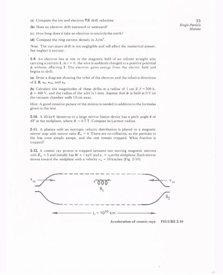
2-12. A cosmic ray proton is trapped between two moving magnetic mirrors with Rm = 5 and initially has W = I ke V and v 1. = v11 at the midplane. Each mirror moves toward the midplane with a velocity Vm = IO km/sec (Fig. 2- 10) .
.....,.1-------- L == 1010 km
35 Single-Particle
Motions
Acceleration of cosmic rays. FIGURE 2-10

36 Chapter Two
(a) Using the loss cone formula and the invariance of 11-. find the energy to which the proton will be accelerated before it escapes.
(b) How long will it take to reach that energy?
I. Treat the mirrors as A at pistons and show that the velocity gained at each bounce is 2vm.
2. Compute the number of bounces necessary. 3. Compute the timeT it takes to traverse L that many times. Factor-of-two
accuracy will suffice.
2.4 NONUNIFORM E FIELD
y
Now we let the magnetic field be uniform and the electric field be nonuniform. For simpl icity, we assume E to be in the x direction and to vary sinusoidal ly in the x direction (Fig. 2- 1 1 ):
E = Eo(cos kx)x [2-47)
This field d istribution has a wavelengt h A = 271'/k and is the result of a sinusoidal d istribution of charges , which we need not specify . I n practice, such a charge d istribution can arise in a plasma during a wave motion. The equatio n of motion is
m(dv/dt) = q[E(x) + v X B] [2-48)
X
@B
FIGURE 2-11 Drift of a gyrating particle in a nonuniform electric field.

whose transverse components are
. qB q v, = -vy + -E,(x)
m m
. qB v� = - -v,
m
•• 2 2Ex(x) vy = -w,vy- w, s-
[2-49]
[2-50]
[2-51]
Here E, (x) is the electric field at the position of the particle. To evaluate this, we need to k now the particle's orbit, which we are trying to solve for in the first place. If the electric field is weak, we may , as an approximation , use the undisturbed orbit to evaluate E,(x). The orbit in the absence of theE field was given in Eq. [2-7]:
[2-52)
From Eqs . [2-51] and [2-47], we now have
[2-53]
Anticipating the result , we look for a solution which is the sum of a gyration at w, and a s teady drift vE· Since we are interested in finding an expression for V£, we take out the gyratory motion by averaging over a cycle. Equation [2-50] then gives v, = 0. I n Eq. [2-53], the oscillating term Vy clearly averages to zero, and we h ave
[2-54]
Expanding the cosine, we h ave
cos k (x0 + rL sin w,t) = cos (kx0) cos (krL s in w,t)
- sin (kx0) sin (krL s in w,t) [2-55]
I t will suffice to treat the smal l Larmor radius case, krL « l. The Taylor expansiOns
COS E = 1 - �E 2 + · · · [2-56]
s inE = E + · · ·
37 Single-Particle
Motions

38 Chapter Two
allow us to write
- (sin kx0)krL sin wet
The last term vanishes upon averaging over time, and Eq. [2-54] gives
[2-57]
Thus the usual Ex B drif t is modified by the inhom ogeneity to read
[2-58]
The physical reason for this is easy to see. A n ion with its guiding center at a maximum of E actually spends a good deal of i ts time in regions of weaker E. Its average drift, therefore, is less thanE/ B evaluated at the guiding center. I n a l inearly varying E field, the ion would be in a stronger field on one side of the orbit and in a field weaker by the same amount on the other side; the correction to V£ then cancels out. From this it is clear that the correction term depends on the second derivative of E. For the sinusoidal distribution we assumed, the second derivative is always negative with respect to E. For an arbitrary variation of E, we need only replace ik by V and write Eq. [2-58] as
( 1 9 9)ExB vE = 1 + -ri:_V- --9-
4 B-[2-59]
The second term is called the finite-Larmor-radius effect. What is the significance of this correction? Since rL is much larger for ions than for
electrons , V£ is no longer independen t of species . I f a density dum p occurs in a plasma, an electric field can cause the ions and electrons to separate, generating another electr ic fidd. If there is a feedback mechanism that causes the second electric field to enhance the first one, E grows indefinitely, and the plasma is u ns table. Such an instability, called a drift instability, will be discussed in a l ater chapter . The grad-E drift, of course, is also a finite-Larmor-radius effect and also causes charges to separate. Accordin g to Eq. [2-24], however , vv8 is proportion al to krL, w hereas the correction term in Eq. [2-58] is proportional to k2r�. The nonuniform-E-field effect, therefore, is important at relatively large k, or small

scale lengths of the inhomogeneity. For this reason, dr ift i nstabilities belong to a more general class called microinstabilities.
TIME-VARYING E FIELD
Let us now ta ke E and B to be uniform i n space but varying in time. First, consider the case in which E alone varies sinusoidally in time, and let it lie along the x axis:
E =Eo eiw< x
Since Ex =fi!x. •}e can write Eq. [2-50] as
Let us define
? ( iw Ex) Vx = -w; Vx =F
We B
_ iw Ex Vp := ±-
w, B
- Ex V£ := --
B
[2-60]
[2-61]
[2-62]
where the tilde has been added merely to emphasize that the drift is oscillating . The u pper (lower) s ign , as usual, denotes positive ( negative) q. Now Eqs. [2-50] a nd [2-5 1 ] become
•• ? ( -Vx = -w; Vx- Vp) [2-63]
By analogy with Eq. [2-1 2], we try a solution which is the sum of a drift and a gyratory motion:
iw l """ vx=v_�_e ' +vp
· iw t -v1 = ±tv-'- e ' + v E
I f we now differentiate twice with res pect to time, we find
. . 2 ( 2 2) -Vx = -w c Vx + W c - W Vp
Vy = -wzvy + (w;- w2)vE
[2-64)
[2-65]
This is not the same as Eq. [2-63] unless w2 « w � . If we now make the assumption that E varies slowly, so that w2 « w�, then Eq. [ 2-64]
. is the
approximate solution to Eq. [2-63] .
2.5
39 Single-Particle
I'vfotions

40 Chapter Two
Equation [2-64] tells us that the guidin g center motion has two components. They component, perpendicular to B and E, is the usual
Ex B drift, except that VE now oscillates slowly at the frequency w. The x component, a new drift along the direction of E, is called the polarization drift. By replacin g iw by aj at, we can generalize Eq. [2-62] and define the polarization drift as
1 dE Vp = ± ---
w,B dt [2-66]
Since vp is in opposite directions for 1ons and electrons, there ts a polarization wrrent; for Z = 1, this is
. ne dE p dE ]p = ne (v;p - v.p) =
eB2(M + m)dt =
B2 dt
where p is the mass density.
[2-67]
The physical reason for the polarization c urrent is simple (Fig. 2- 12) . Consider an ion at rest i n a magnetic field. If a field E is suddenly applied, the first thing the ion does is t o move in the direction of E.
Only after picking u p a velocity v does the ion f eel a Lorentz force ev x B
and begin to move downward in Fig. (2- 1 2) . If E is now kept consta nt , there is no further vp drift but only a V£ drift . H owever , if E is reversed, there is again a momentary drift, this time to the left. Thus vp is a s tartup drift due to inertia and occurs only in the first half-cycle of each gyration
during which E c ha n ges. Consequently, vp goes to zero with w/w,. The polarization effect i n a plasma is similar to that i n a solid
dielectric, where D = EoE + P. The dipoles in a plasma are ions and
E ...
..
8B
FIGURE 2-12 The polarization drift.

electrons separated by a distance rL. But since ions and electrons can move around to preserve quasineutrality , the applica tion of a steady E
field does not result in a polarization field P. H owever, if E oscillates, an oscil lating current jp results from the lag due to the ion inertia.
TIME-VARYING B FIELD
Finally, we al low the magnetic field to vary in time. S ince the Lorentz force is a lways perpendicular to v, a magnetic field itself ca nnot impart energy to a charged pa rticle. H owever, associated with B is an electric field given by
V X E = -B [2-68]
and this ca n accelerate the particles . We can no lon ger assume the fields
to be completely uniform. Let v J. = di/ dt be the transverse velocity I being the element of path alon g a particle trajectory (with vn neglected). Ta king the scalar product of the equation of motion [2-8] with v J. , we have
!!.._(.!.nlv2) = qE · v = qE · dl
dt 2 .L .L dt [2-69]
The cha n ge in one gyration is obta ined by integrating over one period :
If the field changes slowly, we can replace the time integral by a line integral over the unperturbed orbit:
o(�mv�) = f qE · dl = q t (V x E)· dS
= -q L :8. dS [2-70]
Here S is the surface enclosed by the Larmor orbit and has a direction
given by the right-hand rule when the fingers point in the direction of v. Since the plasma is diamagnetic, w e have B · dS < 0 for ions and >0 for electrons . Then Eq. [2-70] becomes
2 I 2 · ( 1 2) • 2 · V.t m 2mv.L 27TB 8 -mv.t = ±qB7rrL = ±q7TB- -- = --· --
2 We ±qB B We [2-71]
2.6
41 Single-Particle
Motions
42 Chapter Two
A B
0 0
FIGURE 2-13 Two-stage adiabatic compression of a plasma.
The quantity 2TrB/w, = B/f, is just the change 8B during one period of gyration. Thus
[2-72]
Since the left-hand side is 8 (JLB ), we have the desired result
[2-73]
The magnetic moment is invariant in slowly varying magnetic fields. As the B field varies in strengt h , the Larmor orbits expand and
contract, and the particles lose and gain transverse energy. This exchange of energy between the part icles and the field is described very s im ply by Eq. [2-73]. The invariance of I.L allows us to prove easily the following well-known theorem:
Th.e magnetic flux through a Larmor orbit is con sta.n t.
The flux <t> is given by BS, wit h S = Trr�. Thus
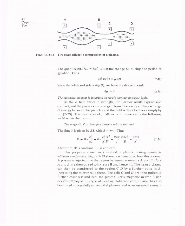
Therefore , <t> is constant if I.L is constant. This property is used in a m ethod of plasma heating known as
adiabatic compression. Figure 2-13 s hows a schematic of how th is is done. A plasma is injected into the region between the m irrors A and B. Coils A and B are t hen pulsed to increase B and hence v �- The heated plasma can t hen be transferred to the region C-D by a further pulse in A, increasing the m irror ratio t here . The coils C and D are t hen pulsed to further compress and heat the plasma. Early magnetic mirror fusion devices employed t his type of heating. Adiabatic com pression has also been used successfully on toroidal plasmas and is an essential element

o f laser-driven fusion schemes usmg eith er magnetic or i nertial 43 confinement . Single-Particle
SUMMARY OF GUIDING CENTER DRIFTS 2. 7
General force F:
Electr-ic field:
Gravitational field:
Nonuniform E:
Nonuniform B field
Grad-B drift:
Cw·vature dTift:
Cw-ved vacuum field:
Polarization dTift:
lFxB Vf = q Ji2
ExB V£ = --2 -B
mgXB v =---
g q B2 ( l 9 9)EXB
V£ = 1 + 4ri:_V- Ji2
m ( 9 1 9) R, X B VR +vvB = - Vif + -v:t. �
q 2 R,B 1 dE
Vp = ± -- -
w,B dt
[2-17]
[2-15]
[2-18]
[2-59]
[2-24]
[2-26]
[2-30]
[2-66]
ADIABATIC INVARIANTS 2.8
It i s well know n i n classical mechanics t hat w henever a system has a periodic motion, t he action i ntegral t p dq taken over a period is a constant of the motion. Here p and q are the generalized momentum and coordinate which repeat t hemselves in the motion . If a slow change is made i n t h e system, s o t hat the motion i s not quite periodic, the constant of t he motion does not change and is then called an adiabatic invariant. By slow
here we mean slow compared wit h t he period of motion, so t hat the integral t P dq i s wel l defined even though it i s strictly no longer an
ivfotions

44 Chapter Two
integral over a closed path. Adiabatic invariants play an important role in plasma physics; they allow us to obta in simple answers in many instances involving complicated motions. There are three adiabatic invarian ts, each corresponding to a different type of periodic motion .
2.8.1 The First Adiabatic Invariant, f.L
We have already met the quantity
f.L = mv�/2B
and have proved its invariance in spatial ly and temporally varying B
fields . The periodic motion involved, of cour se , is the Larmor gyration. If we ta ke p to be angular momentum mv.Lr and dq to be the coordinate d(}, the action integ ral becomes
[2-75]
Thus J.L is a constan t of the motion as long as q/m is not changed . We have proved the invariance of f.L only with the implicit assumption w/ w, « 1, where w is a frequency characterizing the rate of change of B
as seen by the particle . A proof exists, however, that f.L is invariant even when w :S w,. In theorists' language, f.L is invariant " to all orders in an expansion in w/w,." What this means in practice is that f.L remains much more nearly constant than B does during one period of gyration .
I t is just as important to know when an adiabatic invariant does not exist as to know when it does. Adiabatic invariance of f.L is violated w hen w is not small compared with w,. We give three examples of this.
(A) Magnetic Pumping. If the strength of B in a mirror con fin ement system is varied sin usoidally, the particles' v .1 would oscillate; but there would be no gain of energy in the long run. However, if the particles
mak e collisions, the invariance of f.L is violated, and the plasma can be hea ted . In particular, a particle making a collision during the compression phase can transfer part of its gyration energy into v11 energy, and this is n ot taken out again in the expansion phase.
(B) Cyclotron Heating. Now imagine that the B field is oscillated at the frequency w,. The induced electric field will then rotate in phase with some of the particles and accelerate their Larmor motion contin uously. The condition w « w, is violated, f.L is not conserved, and the plasma can be heated .

O R D I N A R Y 0 M I R R O R \
r CUSP
I M I R R O R
45 Single-Particle
Motions
Plasma confinement in a cusped magnetic field. FIGURE 2-14
(C) Magnetic Cusps. If the current in one of the co ils in a s im ple magnetic mirror system is reversed, a magnetic cusp is formed (Fig . 2- 1 4) . This configuration has , in addition to the usual m irrors , a spindle-cus p m irror extending over 360° in azimuth. A plasma con fined in a cusp device is supposed to have better stability properties than that in an ordinary mirror . Unfortunately, the loss-cone losses are larger because of the additional loss region ; and the particle m otion is nonadiaba tic . Since the B field vanishes at the center of symmetry, We is zero there; and IL is not preserved . The local Larmor radius near the center is larger than the device . B ecause of this , the adiabatic invariant IL does n ot guarantee that particles outside a loss cone will s tay outside after passing through the nonadiabatic region. Fortunately, there is in this case another invariant: the canonical angular m omentum P6 = mTv8 - eTA8. This ensures that there will be a population of particles trapped indefinitely until they make a collision .
The Second Adiabatic Invariant, ] 2.8 .. 2
Consider a particle tra pped between two magnetic m irrors : I t bounces between them and therefore has a periodic motion at the "bounce frequency." A constant of this motion is given by f mvu ds, where ds is an element of path length (of the guiding center) along a field l ine . H owever, since the guiding center drifts across field lines, the motion is not exactly per iodic, and the constant of the m otion becomes an adiabatic invariant. This is called the longitudinal invaTiant ] and is defined for a hal f-cycle
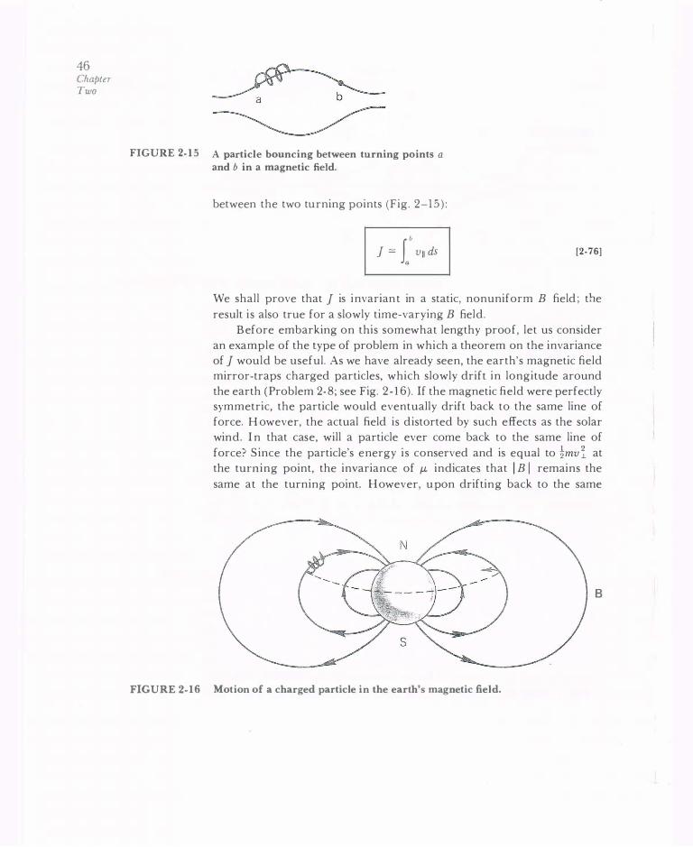
46 Chapter Two
FIGURE 2-15 A particle bouncing between turning points a and b in a magnetic field.
between the two turning points (Fig. 2-15 ) :
b
1 = 1 vu ds [2-76]
We shall prove that 1 is invarian t in a static, nonuniform B field ; the result is also true for a slowly time-varying B field.
B efore embarking on this somewhat lengthy proof, let us consider an example of the type of problem in which a theorem on the in variance of 1 would be useful. As we have already seen, the earth's magnetic field mirror-traps charged particles, which slowly drift in longitude around the earth (Problem 2- 8; see Fig. 2 - 1 6) . If the magnetic field were perfectly symmetric, the particle would eventually drift back to the same line of force. H owever, the actual field is d istorted by such effects as the solar wind. I n that case, will a particle ever come back to the same line of force? S ince the particle's energy is conserved and is equal to !mv i at the turning point, the in variance of f.L indicates that I B I remains the same at the turning point. However, u pon drifting back to the same
FIGURE 2-16 Motion of a charged particle in the earth's magnetic field.
B

longitude, a particle may find itself on another l ine of force at a different altitude. This cannot happen if I is conserved . I determines the length of the line of force between turning points, and no two l ines have the same length between points with the same I B 1 . Consequently, the particle returns to the same line of force even in a slightly asymmetric field.
To prove the invariance of I. we first consider the invariance of v u 8s, w here 8s is a segment of the path along B (Fig. 2 - 17) . Because of guiding center drifts, a particle on s wil l find itself on another l ine of force & ' after a time D.t. The length of & ' is defined by passing planes perpendicular to B through the end points of 8s. The length of 8s IS
obviously proportional to the radius of curvature :
so that
8s &'
R, R �
8s ' - 8s R � - Rc
!:l.t 8s f:.tR, [2-77]
The "radial" component of Vgc is just
[2-78)
From Eqs. [2-24] and [2-26], we have
1 B X VB mv lf R, X B Vgc = VVB + V R = ± -vJ.TL 2 + -- __ ?_2_ (2-79)
2 B q R ; B
The last term has n o component along R,. Using Eqs. [2-78] and [2-79] , we can write Eq. [2-77] as
I d R, 1 m vl R,
Os dt Os = Vgc • R; = 2 q
B3 (B X VB ) · R ; [2-80)
This is the rate of change of 8s as seen by the particle. We must 'now get the rate of change of vn as seen by the particle. The parallel and
os'
B
4 7 Single-Particle
Motions
Proof of the invariance of ]. FIGURE 2-17

48 Chapter Two
perpendicular energies are defined by
W I 2 I 2 I 2 = 2mvu + 2mv .L = 2mv u + �B = Wu + w.L
Thus vu can be written 1 / 2 vu = [ (2/m ) (W - �B )]
Here W and � are constant, and only B varies. Therefore,
�B 2 w - �B
1 �!3 �!3 - - - = - --2 2 w11 mv 11
[2-81]
[2-82]
[2-83]
Since B was assumed static, B is not zero only because of the guiding center motion :
N ow we have
� (Rc x B) · VB
: q R�B 2 1 m v � (B X VB ) · Rc - - - -2 q B R �B 2
The fractional change in v11 8s is
l d 1 d8s 1 dvu -- - (vu & ) = - - + - -vu 8s dt 8s dt vu dt
[2-84]
[2-85]
[2-86]
From Eqs . [2-80) and [2-85} , we see that these two terms cancel, so that
vu 8s = constant [2-87]
This is not exactly the same as saying that f is constant, however. I n takin g the integral o f v11 8s between the turning points, i t may be that the turning points on & ' do not coincide with the intersections of the perpendicular planes (Fig. 2 - 1 7) . However, any error in J arising from such a discrepancy is negligible because near the turning points, vu is
nearly zero. Consequently, we have proved b
J = 1 vu ds = constan t [2-88]
An example of the violation of J invariance is given by a plasma heating scheme called transit-time magnetic pumping. Suppose an oscillati n g current is applied to the coils of a mirror system so that the· mirrors alternately approach and withdraw from each other near the boun ce frequency. Those particles that have the right bounce frequency will always see an approaching m irror and will therefore gain v11• f is not conserved in this case because the change of B occurs on a time scale not long compared with the bounce time.

The Third Adiabatic Invariant, <I> 2.8.3
Referring again to Fig. 2-16, we see that the slow drift of a guiding center around the earth constitutes a third type of periodic motion. The adiabatic invariant connected with this turns out to be the total magnetic flux <I> enclosed by the drift surface. It is almost obvious that, as B varies, the particle wil l stay on a surface such that the total number of l ines of force enclosed remains constant. This i nvariant, <I>, has few applications because most fluctuations of B occur on a time scale short compared with the drift period . As an example of the violation of <I> invariance, we can cite some recent work on the excitation of hydromagnetic waves in the ionosphere. These waves have a long period comparable to the drift time of a particle around the earth. The particles can therefore encounter the wave in the same phase each time around. I f the phase is right, the wave can be excited by the conversion of particle d ri ft energy to wave energy.
49 Single-Particle
ll.fotions
2-13. Derive the result of Problem 2- 12(b) directly by using the invariance of ]. PROBLEMS
(a) Let J uu ds = vaL and differentiate with respect to time.
(b) From this, get an expression for T in terms of dL/dt. Set dL/dt = -2um to obtain the answer.
2-14. In plasma heating by adiabatic compression, the invariance of f:.L re'quires that KT.L increase as B increases. The magnetic field, however, cannot accelerate particles because the Lorentz force qv x 8 is always perpendicular to the velocity. How do the particles gain energy?
2-15. The polarization drift up can also be derived from energy conservation. If E is oscillating, the E x B drift also oscillates; and there is an energy �u� associated with the guiding center motion. Since energy can be gained from an E field only by motion along E, there must be a drift up in the E direction. By equating the rate of change of �mu� with the rate of energy gain from vp · E,
find the required value of up. ·
2-16. A hydrogen plasma is heated by applying a radiofrequency wave with E
perpendicular to B and with an angular frequency w = 109 rad/sec. The confining magnetic field is 1 T. Is the motion of (a) the electrons and (b) the ions in response to this wave adiabatic?
2-17. A 1-keV proton with uu = 0 in a uniform magnetic field B = 0. 1 T is accelerated as B is slowly increased to 1 T. It then makes an elastic collision with a heavy particle and changes direction so that u .L = uu. The 8-field is then slowly decreased back to 0. 1 T. What is the proton's energy now?

50 Chapter Two
FIGURE P2-1 8
FIGURE P2- 1 9
z
8
2-18. A collisionless hydrogen plasma is con fined in a torus in which external
windings provide a magnetic field B ly ing al most entirely in the c/J direction.
The plasma is i nitially Maxwellian at KT = I keV. At l = 0, B i s gradually increased from I T to 3 T in 1 00 11-sec, and the plasma is compressed .
(a) Show that the magnetic moment 11- remains invariant for both ions and electrons.
(b) Calculate the temperatures T1. and T11 after compression.
2-19 . A uniform plasma is created i n a toroidal chamber with square cross
section, as show n . The magnetic field is provided by a current I along the axis
of symmetry. The d imensions are a = I em, R = I 0 em. The plasma is Maxwellian
at KT = I 00 e V and has density n = I 019 m -3. There is n o electric field.
I a
l I
�"�f..t----R ----t� - a -

(a) Draw typical orbits for ions and electrons wjth v0 = 0 drifting in the nonuniform B field.
(b) Calculate the rate of charge accumulation (in coulombs per second) on the entire top plate of the chamber due to the combined vv8 and vR drifts. The magnetic field at the center of the chamber is 1 T, and you may make a large aspect ratio (R » a ) approximation where necessary.
2-20. Suppose the magnetic field along the axis of a magnetic mirror is given by B, = B0( 1 + a2z 2) .
(a) If an electron at z = 0 has a velocity given by v 2 = 3vW = 1 . 5v� , at what value of z is the electron reflected ?
(b) Write the equation of motion of the guiding center for the direction parallel to the field.
(c) Show that the motion is sinusoidal, and calculate its frequency.
(d) Calculate the longitudinal invariant ] corresponding to this motion.
2-2 1 . An infinite straight wire carries a constant current I in the +z direction. At t = 0, an electron of small gyro radius is at z = 0 and r = r0 with v .LO = v110. (.l and I I refer to the direction relative to the magnetic field.)
(a) Calculate the magnitude and direction of the resulting guiding center drift velocity.
(b) Suppose that the current increases slowly in time in such a way that a constant electric field in the ±z direction is induced. Indicate on a diagram the relative directions of I, B, E. and v£.
(c) Do v .L and v11 increase, decrease, or remain the same as the current increases? Why?
5 1 Single-Particle
Motions


Chapter Three
PLAS
D
INTRODUCTION 3.1
In a plasma the situation is much more complicated than that in the last
chapter; the E and B fields are not prescribed but are determined by
the positions and motions of the charges themselves. One must solve a
self-consistent problem; that is, find a set of particle trajectories and field patterns such that the particles will generate the fields as they move along their orbits and the fields will cause the particles to move in those exact orbits. And this must be done in a time-varying situation!
We have seen that a typical plasma density might be 1012 ion-electron pairs per cm3. If each of these particles follows a complicated trajectory
and it is necessary to follow each of these, predicting the plasma's behavior
would be a hopeless task. Fortunately, this is not usually necessary
because, surprisingly, the majority-perhaps as much as 80%-of plasma
phenomena observed in real experiments can be explained by a rather crude model. This model is that used in fluid mechanics, in which the
identity of the individual particle is neglected, and only the motion of fluid elements is taken into account. Of course, in the case of plasmas,
the fluid contains electrical charges. In an ordinary fluid, frequent
collisions between particles keep the particles in a fluid element moving
together. It is surprising that such a model works for plasmas, which generally have infrequent collisions. But we shall see that there is a reason for th is.
In the greater part of this book, we shall be concerned with what can be learned from the fluid theory of plasmas. A more refined 53

54 Chapter
Three treatment-the kinetic theory of plasmas-requires more mathematical calculation than is appropriate for an introductory course. An introduc
tion to kinetic theory is given in Chapter 7. In some plasma problems, neither fluid theory nor kinetic theory
is sufficient to describe the plasma's behavior. Then one has to fall back
on the tedious process of following the individual trajectories. Modern computers can do this, although they have only enough memory to store the position and velocity components for about 104 particles and, except in a few cases, can solve problems only in one or two dimensions. Nonetheless, computer simulation has recently begun to play an impor
tant role in filling the gap between theory and experiment in those
instances where even kinetic theory cannot come close to explaining what is observed.
3.2 RELATION OF PLASMA PHYSICS TO ORDINARY ELECTRO MAGNETICS
3.2.1 Maxwell's Equations
In vacuum:
In a medium:
E0V · E = cr
v X E = -B
V · B = 0
V X B = ,u0(j + EoE)
V· D=cr
V X E = -B
V · B = 0
V x H =j+D
D=EE
B=,uH
[3-1]
[3-2]
[3-3]
[3-4]
[3-5]
[3-6]
[3-7]
[3·8]
[3-9]
[3-10]
In Eqs. [3-5] and [3-8], cr and j stand for the "free" charge and current
densities. The "bound" charge and current densities arising from polarization and magnetization of the mef:lium are included in the definition

of the quantities D and H in terms of E and JL. In a plasma, the ions
and electrons comprising the plasma are the equivalent of the "bound"
charges and currents. Since these charges move in a complicated way,
it 'is impractical to try to lump their effects into two constants � and JL. Consequently, in plasma physics, one generally works with the vacuum
equations [3-1]-[3-4], in which <r and j include all the charges and currents, both external and internal.
Note that we have used E and B in the vacuum equations rather than their counterparts D and H, which are related by the constants Eo
and JLo. This is because the forces qE and j x B depend on E and B rather than D and H, and it is not necessary to introduce the latter
quantities as long as one is dealing with the vacuum equations.
Classical Treatment of Magnetic Materials 3.2.2
Since each gyrating particle has a magnetic moment, it would seem that
the logical thing to d� would be to consider a plasma as a magnetic material with a permeability Ji-m· (We have put a subscript m on the permeability to distinguish it from the adiabatic invariant JL.) To see why this is not clone in practice, let us review the way magnetic materials are
usually treated_.
The ferromagnetic domains, say, of a piece of iron have magnetic
moments JL;, giving rise to a bulk magnetization
[3-ll]
per unit volume. This has the same effect as a bound current density
equal to
h =VxM [3-12]
In the vacuum equation [3-4], we must include in j both this current and the "free," or externally applied, current j1:
We wish to write Eq. [3-13] in the simple form
V x H = ir + EoE by including h in the definition of H. This can be done if we let
[3-13)
[3-14)
[3-15)
55 Plasmas
As Fluids

56 Chapter Three
To get a simple relation between Band H, we assume M to be proportional to B or H:
M=xmH [3-16]
The constant Xm is the magnetic susceptibility. We now have
[3-17]
This simple relation between B and H is possible because of the linear form of Eq. [3-16].
In a plasma with a magnetic field, each particle has a magnetic moment J10, and the quantity M is the sum of all these Jl.a's in I m3. But we now have
1 MocB
The relation between M and H (or B) is no longer linear, and we cannot write B = f.Lm H with f.J-m constant. It is therefore not useful to consider a plasma as a magnetic medium.
3.2.3 Class.ical Treatment of Dielectrics
The polarization P per unit volume is the sum over all the individual moments p; of the electric dipoles. This gives rise to a bound charge
density
crb = -v · P [3-18]
In the vacuum equation [3-1], we must include both the bound charge
and the free charge:
[3-19]
We wish to write this in the simple form
V · D = a:1 [3-20]
by including CTb in the definition of D. This can be done by letting
D=t:0E+P=«:E [3-21]
If P is linearly proportional to E,
P = «:ox.E [3-22]
then E is a constant given by
E = (1 + x.)Eo [3-23]

There is no a priori reason why a relation like [3-22] cannot be valid in a plasma, so we may proceed to try to get an expression forE in a plasma.
The Dielectric Constant of a Plasma
We have seen in Section 2.5 that a fluctuating E field gives rise to a
polarization current jp. This leads, in turn, to a polarization charge given
by the equation of continuity:
aiJp '"' • o at+ v . ]p = [3·24]
This is the equivalent of Eq. [3-18], except that, as we noted before, a
polarization effect does not arise in a plasma unless the electric field is
time varying. Since we have an explicit expression for jp but not for IJp, it is easier to work with the fourth Maxwell equation, Eq. [3-4]:
We wish to write this in the form
This can be done if we let
V x B =P-oOr+ EE)
]p E = Eo+-....
E
From Eq. [2-67] for jp, we have
2 or
E P.oPC ER :=-= 1 + --2-
Eo B
[3·25]
[3-26]
[3-27]
[3-28]
This is the low-frequency plasma dielectric constant for transverse motions. The
qualifications are necessary because our expression for jp is valid only
for w2 « w� and for E perpendicular to B. The general expression for E, of course, is very complicated and hardly fits on one page.
Note that as p --+ 0, ER approaches its vacuum value, unity, as it should. As B --+ oo, ER also approaches unity. This is because the polarization drift vp then vanishes, and the particles do not move in response
to the transverse electric field. In a usual laboratory plasma, the second
term in E'q. [3-28] is large compared with unity. For instance, if n = 1016 m -3 and B = 0.1 T we have (for hydrogen)
P,opc2 (47T X 10-7)(1016)(1.67 X 10⁻²⁷)(9 X 10¹⁶) --2-= 2 = 189 B (0.1)
3.2.4
57 Plasmas
As Fluids

58 Chapter Three
PROBLEMS
This means that the electric fields due to the particles in the plasma
greatly alter the fields applied externally. A plasma with large E shields
ou t alternating fields, just as a plasma with small A 0 shields out de fields.
3-1. Derive the uniform-plasma low-frequency dielectric constant, Eq. [3-28], by reconciling the time derivative of the equation V · D = V ·(�:E)= 0 with that of the vacuum Poisson equation [3-1], with the help of equations [3-24] and [2-67].
3-2. If the ion cyclotron frequency is denoted by !1, and the ion plasma frequency
is defined by
!lp = (ne2/�:0M)112
where M is the ion mass, under what circumstances is the dielectric constant E approximately equal to n;;n;?
3.3 THE FLUID EQUATION OF MOTION
Maxwell's equations tell us what E and B are for a given state of the plasma. To solve the self-consistent problem, we must also have an equation giving the plasma's response to given E and B. In the fluid
approximation, we consider the plasma to be composed of two or more
interpenetrating fiuids, one for each species. In the simplest case, when
there is only one species of ion, we shall need two equations of motion, one for the positively charged ion fluid and one for the negatively charged electron fluid. In a partially ionized gas, we shall also need an equation for the fluid of neutral atoms. The neutral fluid will interact with the ions and electrons only through collisions. The ion and electron fluids will interact with each other even in the absence of collisions, because of the E and B fields they generate.
3.3.1 The Convective Derivative
The equation of motion for a single particle is
dv m- = q(E + v X B) dt
[3-29]
Assume first that there are no collisions and no thermal motions. Then all the particles in a fluid element move together, and the average velocity u of the particles in the element is the same as the individual particle

velocity v. The fluid equation is obtained simply by multiplying Eq. [3-29] by the density n:
du mn - = qn (E + u x B) dt
[3-30]
This is, however, not a convenient form to use. In Eq. [3-29], the time
derivative is to be taken at the position of the particles. On the other hand,
we wish to have an equation for fluid elements fixed in space, because it
would be impractical to do otherwise. Consider a drop of cream in a cup of coffee as a fluid element. As the coffee is stirred, the drop distorts
into a filament and finally disperses all over the cup, losing its identity.
A fluid element at a fixed spot in the cup, however, retains its identity although particles continually go in and out of it.
To make the transformation to variables in a fixed frame, consider G(x, t) to be any property of a fluid in one-dimensional x space. The
change of G with time in a frame moving with the fluid is the sum of two terms:
dG(x, t) aG aG dx aG aG _...:....:......:.. = - + - - = - + u -
dt at ax dt at X ax [3-31)
The first term on the right represents the change of G at a fixed point
in space, and the second term represents the change of Gas the observer moves with the fluid into a region in which G is different. In three dimensions, Eq. [3-31] generalizes to
dG aG -=- + (u·V)G dt at
[3-32]
This is called the convective derivative and is sometimes written DG / Dt. Note that (u · V) is a scalar differential operator. Since the sign of this
term is sometimes a source of confusion, we give two simple examples.
Figure 3-1 shows an electric water heater in which the hot water
has risen to the top and the cold water has sunk to the bottom. Let G (x, t) be the temperature T; VG is then upward. Consider a fluid element
near the edge of the tank. If the heater element is turned on, the fluid element is heated as it moves, and we have dT/dt > 0. If, in addition, a
paddle wheel sets up a flow pattern as shown, the temperature in a fixed fluid element is lowered by the convection of cold water from the bottom.
In this case, we have aT/ax > 0 and u, > 0, so that u · VT > 0. The temperature change in the fixed element, ar;at, is given by a balance
59 Plasmas
As Fluids

60 Chapter
Three
FIGURE 3-1 Motion of fluid elements in a hot water heater.
of these effects,
aT dT -= - -u ·VT at dt
[3-33]
It is quite clear that aT/at can be made zero, at least for a short time.
As a second example we may take G to be the salinity S of the water
near the mouth of a river (Fig. 3-2). If x is the upstream direction, there
OCEAN - vs
FIGURE 3-2 Direction of the salinity gradient at the mouth of a river.
x-

is normally a gradient of S such that aSjax < 0. When the tide comes
in, the entire interface between salt and fresh water moves upstream,
and Ux > 0. Thus
as as - = -ux - > 0 at ax [3-34]
meaning that the salinity increases at any given point. Of course, if it
rains, the salinity decreases everywhere, and a negative term dS/ dt is to be added to the middle part of Eq. [3-34].
As a final example. take G to be the density of cars near a freeway entrance at rush hour. A driver will see the density around him increasing
as he approaches the crowded freeway. This is the convective term
(u · V)G. At the same time, the local streets may be filiing with cars that enter from driveways, so that the density will increase even if the observer
does not move. This is the aGjat term. The total increase seen by the
observer is the sum of these effects.
In the case of a plasma, we take G to be the fluid velocity u and write Eq. [3-30] as
mn[ �; + (u · V)u J = qn (E + u X B) [3-35]
where aujat is the time derivative in a fixed frame.
The Stress Tensor 3.3.2
When thermal motions are taken into account, a pressure force has to
be added to the right-hand side of Eq. [3-35]. This force arises from the
y
z
X
Origin of the elements of the stress tensor. FIGURE 3-3
61 Plasmas
As Fluids
62 Chapter Three
random motion of particles in and out of a fluid element and does not appear in the equation for a single particle. Let a fluid element Lh !::.y l::.z be centered at (x0, �t::.y, �l::.z) (Fig. 3-3). For simplicity, we shall consider
only the x component of motion through the faces A and B. The number of particles per second passing through the face A with velocity vx is
!::.nv x � -where !::.nv is the number of particles per m3 with velocity Vx:
Each particle carries a momentum mvx. The density n and temperature
KT in each cube is assumed to have the value associated with the cube's
center. The momentum PA+ carried into the element at xo through A is then
[3-36]
The sum over !::.nv results in the average v; over the distribution. The
factor � comes from the fact that only half the particles in the cube at
x0- !::.x are going toward face A. Similarly, the momentum carried out
through face B is
Thus the net gain in x momentum from right-moving particles is
' a ......, = !::.y !::.z 2m ( -t::.x) -
a (rzv.�)
X
[3-37]
This result will be just doubled by the contribution of left-moving
particles, since they carry negative x momentum and also move in the opposite direction relative to the gradient of nv �. The total change of momentum of the fluid element at x0 is therefore
a a ......, - (nmux ) !::.x !::.y !::.z = -m- (nv;) .!::.x !::.y !::.z at ax
[3-38]
Let the velocity Vx of a particle be decomposed into two parts,
Ux = Vx
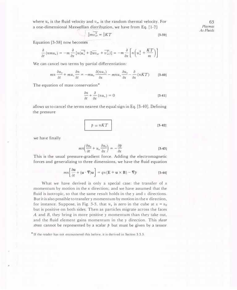
where Ux is the fluid velocity and Vxr is the random thermal velocity. For
a one-dimensional MaxwJ!Ilian distribution, we have from Eq. [l-7]
j �mv;r = �KT [3-39]
Equation [3-38] now becomes
a a 2 - 2" a [ ( 2 KT )] - (nmux) = -m- [n(Ux + 2UVxr + Vxr)] = -m- n Ux +-at ax ax m
We can cancel two terms by partial differentiation:
aux an a(nux) aux a mn- + mu.- = -mu ---- mnu ---(nKT) [3-40)
at X at X ax X ax ax
The equation of mass conservation*
an a -+-(nu) = 0 at ax
X [3-41]
allows us to cancel the terms nearest the equal sign in Eq. [3-40]. Defining
the pressure
we have finally
p ;= nKT
mn(aux
+ Ux aux )
= - ap
at ax ax
[3-42)
[3-43]
This is the usual pressure-gradient force. Adding the electromagnetic forces and generalizing to three dimensions, we have the fluid equation
mn[ �� + (u · V)u J = qn (E + u x B) - Vp [3-44)
What we have derived is only a special case: the transfer of x momentum by motion in the x direction; and we have assumed that the
fluid is isotropic, so that the same result holds in the y and z directions. But it is also possible to transfer y momentum by motion in the x direction, for instance. Suppose, in Fig. 3-3, that Uy is zero in the cube at x = x0
but is positive on both sides. Then as particles migrate across the faces
A and B, they bring in more positive y momentum than they take out,
and the fluid element gains momentum in the y direction. This shear stress cannot be represented by a scalar p but must be given by a tensor
*If the reader has not encountered this before, it is derived in Section 3.3.5.
63 Plasmas
As Fluids

64 Chapter Three
P, the stress tensor, whose components Pii = mn uiui specify both the
direction of motion and the component of momentum involved. In the
general case the term -'ilp is replaced by -V · P. We shall not give the stress tensor here except for the two simplest
cases. When the distribution function is an isotropic Maxwellian, P is
written
0 p 0
[3-45]
V · P is just 'ilp. In Section 1.3, we noted that a plasma could have two
temperatures T .L and Tu in the presence of a magnetic field. In that case,
there would be two pressures p .L = nKT .L and Pu = nKTu. The stress
tensor is then
(p.l P= � [3-46]
where the coordinate of the third row or column is the direction of B. This is still diagonal and shows isotropy in a plane perpendicular to B.
In an ordinary fluid, the off-diagonal elements of P are usually
associated with viscosity. When particles make collisions, they come off
with an average velocity in the direction of the fluid velocity u at the
point where they made their last collision. This momentum is transferred
to another fluid element upon the next collision. This tends to equalize u at different points, and the resulting resistance to shear flow is what we intuitively think of as viscosity. The longer the mean free path, the farther momentum is carried, and the larger is the viscosity. In a plasma there is a similar effect which occurs even in the absence of collisions. The Larmor gyration of particles (particularly ions) brings them into
different parts of the plasma and tends to equalize the fluid velocities there. The Larmor radius rather than the mean free path sets the scale
of this kind of collisionless viscosity. It is a finite-Larmor-radius effect
which occurs in addition to collisional viscosity and is closely related to
the vE drift in a nonuniform E field (Eq. [2-58]).
3.3.3 Collisions
If there is a neutral gas, the charged fluid will exchange momentum with it through collisions. The momentum lost per collision will be
proportional to the relative velocity u - u0, where u0 is the velocity of

the neutral fluid. If r, the mean free time between collisions, is approxi
mately constant, the resulting force term can be roughly written as
-mn (u- u0)/r. The equation of motion [3-44] can be generalized to include anisotropic pressure and neutral collisions as follows:
[au ] mn(u- uo) mn -+ (u · V)u = qn (E + u X B) - V · P - _ ___:__ _ __.::.:...
� 1' [3-47]
Collisions between charged particles have not been included; these will
be treated in Chapter 5.
Comparison with Ordinary Hydrodynamics 3.3.4
Ordinary fluids obey the Navier-Stokes e·quation
[3-48]
This is the same as the plasma equation [3-47] except for the absence of electromagnetic forces and collisions between species (there being
only one species). The viscosity term pv V2 u, where v is the kinematic
viscosity coefficient, is just the collisional part of V · P - Vp in the absence
of magnetic fields. Equation [3-48] describes a fluid in which there are
frequent collisions between particles. Equation [3-47], on the other hand,
was derived without any explicit statement of the collision rate. Since
the two equations are identical except for the E and B terms, can Eq.
[3-4 7] really describe a plasma species? The answer is a guarded yes, and the reasons for this will tell us the limitations of the fluid theory.
In the derivation of Eq. [3-47], we did actually assume implicitly that there were collisions. This assumption came in Eq. [3-39] when we
took the velocity distribution to be Maxwellian. Such a distribution generally comes about as the result of frequent collisions. However, this
assumption was used only to take the average of v ;"' Any other distribu
tion with the same average would give us the same answer. The fluid
theory, therefore, is not very sensitive to deviations from the Maxwellian
distribution, although there are instances in which these deviations are important. Kinetic theory must then be used.
There is also an empirical observation by Irving Langmuir which helps the fluid theory. In working with the electrostatic probes which bear h is name, Langmuir discovered that the electron distribution func
tion was far more nearly Maxwellian than could be accounted for by the collision rate. This phenomenon, called Langmuir's paradox, has been
65 Plasmas
As Fluids

66 Chapter Three
3.3.5
attributed at times to high-frequency oscillations. There has been no satisfactory resolution of the paradox, but this seems to be one of the
few instances in plasma physics where nature works in our favor.
Another reason the fluid model works for plasmas is that the mag
netic field, when there is one, can play ,the role of collisions in a certain sense. When a particle is accelerated, say by an E field, it would con
tinuously increase in velocity if it were allowed to free-stream. When
there are frequent collisions, the particle comes to a limiting velocity proportional to E. The electrons in a copper wire, for instance, drift together with a velocity v = ,u.E, where ,u is the mobility. A magnetic
field also limits free-streaming by forcing particles to gyrate in Larmor orbits. The electrons in a plasma also drift together with a velocity proportional toE, namely, v£ =E x B/B2. In this sense, a collisionless
plasma behaves like a collisional fluid. Of course, particles do free-stream
along the magnetic field, and the fluid picture is not particularly suitable
for motions in that direction. For motions perpendicular to B, the fluid theory is a good approximation.
Equation of Continuity
The conservation of matter requires that the total number of particles Nin a volume V can change only if there is a net flux of particles across the surface S bounding that volume. Since the particle flux density is nu, we have, by the divergence theorem,
aN J an f J - = - dV = - nu · dS = - 'iJ · (nu) dV at vat v
[3-49]
Since this must hold for any volume V, the integrands must be equal:
an -+ 'iJ • (nu) = 0 at
[3-50]
There is one such equation of continuity for each species. Any sources or sinks of particles are to be added to the right-hand side.
3.3.6 Equation of State
One more relation is needed to close the system of equations. For this, we can use the thermodynamic equation of state relating p ton:
[3-51)

where C is a constant and y is the ratio of specific heats Cp/ Cv. The
term Vp is therefore given by
Vp Vn - = y -p n
For isothermal compression, we have
Vp = V(nKT) = KTVn
[3-52]
so that, clearly, y = 1. For adiabatic compression, KT will also change, giving y a value larger than one. If N is the number of degrees of
freedom, y is given by
y = (2 + N)/N [3-53]
The validity of the equation of state requires that heat flow be negligible;
that is, that thermal conductivity be low. Again, this is more likely to be
true in directions perpendicular to B than parallel to it. Fortunately,
most basic phenomena can be described adequately by the crude assumption of Eq. [3-51].
The Complete Set of Fluid Equations 3.3.7
For simplicity, let the plasma have only two species: ions and electrons; extension to more species is trivial. The charge and current densities are
then given by 1 � I �"-'"t
[3-54]
Since single-particle motions will no longer be considered, we may now
use v instead of u for the fluid velocity. We shall neglect collisions and viscosity. Equations [3-1 ]-[3-4], [3-44], [3-50], and [3-51] form the follow
ing set:
V X E = -B V ·B=O
-1 . f..Lo V X B = n;q;v; + n.q,v, + EoE
[3-55]
[3-56]
[3-57]
[3-58]
1 = t, e [3-59]
67 Plasmas
As Fluids

68 Chapter Three
an-_J + V · (n·v·) = 0 at 1 1
1 = �. e
j = i, e [3-60]
[3-61]
There are 16 scalar unknowns: n;, n., p,, p., v;, v., E, and B. There are apparently 18 scalar equations if we count each vector equation as three scalar equations. However, two of Maxwell's equations are superfluous, since Eqs. [3-55] and [3-57] can be recovered from the divergences of Eqs. [3-58] and [3-56] (Problem 3-3). The simultaneous solution of this set of 16 equations in 16 unknowns gives a self-consistent set of fields
and motions in the fluid approximation.
3.4 FLUID DRIITS PERPENDICULAR TO B
Since a fluid element is composed of many individual particles, one would expect the fluid to have drifts perpendicular to B if the individual guiding centers have such drifts. However, since the Vp term appears
only in the fluid equations, there is a drift associated with it which the fluid elements have but the particles do not have. For each species, we
have an equation of motion
mn[av +(v·V)v] =qn(E+vxB)-Vp
at ® ® Q) Consider the ratio of term CD to term ®:
CD� lmniwv.L I = !!!..._ ® qnv.LB w,
[3-62]
Here we have taken ajat = iw and are concerned only with V.t. For drifts
slow compared with the time scale of w" we may neglect term CD. We shall also neglect the (v · V)v term and show a posteriori that this is all right. Let E and B be uniform, but let n and p have a gradient. This is the usual situation in a magnetically confined plasma column (Fig. 3-4).
Taking the cross product of Eq. [3-62] with B, we have (neglecting the
left-hand side)
0 = qn[E X B + (v.t x B) X B)- Vp X B
= qn[E x B + B(v.L/ B)- v.tB2)-Vp X B
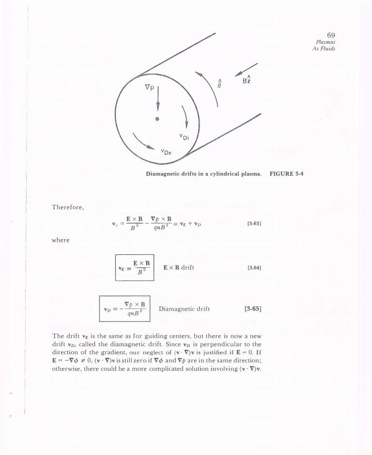
Therefore,
where
/. Bz
Diamagnetic drifts in a cylindrical plasma. FIGURE 3-4
Ex B Vp X B V J.. = --2- - 2 """ V£ + VD
B qnB
I v, � E ;, 8 I E x B dcift
Vp xB vv """ - 2 Diamagnetic drift
qnB
[3-63]
[3.64]
[3-65]
The drift V£ is the same as for guiding centers, but there is now a new drift vv, called the diamagnetic drift. Since vv is perpendicular to the direction of the gradient, our neglect of (v · V)v is justified if E = 0. If
E = -V¢ � 0, (v · V)v is still zero if V¢ and Vp are in the same direction;
otherwise, there could be a more complicated solution involving (v · V)v.
69 Plasmas
As Fluids

70 Chapter Three
Os
- 'iln
FiGURE 3-5 Origin of the diamagnetic drift.
With the help of Eq. [3-52], we can write the diamagnetic drift as
'YKTz x Vn Vv =±-- --eB n
[3-661
In particular, for an isothermal plasma in the geometry of Fig. 3-4, in which Vn = n'r, we have the following formulas familiar to experimen
talists who have worked with Q-machines*:
KT;n' A vv; = -- - (} eB n
KT. n' A Vve = --- - (}
eB n
The magnitude of vv is easily computed from the formula
KT (eV) 1 m
v D = B ( T) A sec
where A is the density scale length ln/n'l in m.
[3-67]
[3-68]
The physical reason for this drift can be seen from Fig. 3-5. Here we have drawn the orbits of ions gyrating in a magnetic field. There is a density gradient toward the left, as indicated by the density of orbits.
*A Q-machine produces a quiescent plasma by thermal ionization of Cs or K atoms impinging
on hot tungsten plates. Diamagnetic drifts were first measured in Q-machines.

Through any fixed volume element there are more ions moving down
ward than upward, since the downward-moving ions come from a region
of higher density. There is, therefore, a fluid drift perpendicular to Vn and B, even though the guiding centers are stationary. The diamagnetic drift reverses sign with q because the direction of gyration reverses. The magnitude of v0 does not depend on mass because them -l/2 dependence
of the velocity is cancelled by the m 112 dependence of the Larmor radius-less of the density gradient is sampled during a gyration if the
mass is small. Since ions and electrons drift in opposite directions, there is a
diamagnetic current . For 1' = Z = I, this is given by
B xVn j0 = ne(vn;- vn,) = (KTi + KT,) B 2 [3-69]
In the particle picture, one would not expect to measure a current if the guiding centers do not drift. In the fluid picture, the current jv flows
wherever there is a pressure gradient. These two viewpoints can be reconciled if one considers that all experiments must be carried out in a finite-sized plasma. Suppose the plasma were in a rigid box (Fig. 3-6).
If one were to calculate the current from the single-particle picture, one
would have to take into account the particles at the edges which have
cycloidal paths. Since there are more particles on the left than on the
right, there is a net current downward, in agreement with the fluid
picture. The reader may not be satisfied with this explanation because it was
necessary to specify reflecting walls. If the walls were absorbing or if they were removed, one would find that electric fields would develop
A
Particle drifts in a bounded plasma, illustrating the relation to fluid drifts. FIGURE 3-6
71 Plasmas
As Fluids

72 Chapter Three
because more of one species-the one with larger Larmor radius-would be collected than the other. Then the guiding centers would drift, and the simplicity of the model would be lost. Alternatively, one could imagine
trying to measure the diamagnetic current with a current probe (Fig. 3-7). This is just a transformer with a core of magnetic material. The
primary winding is the plasma current threading the core, and the
secondary is a multiturn winding all around the core. Let the whole thing be infinitesimally thin, so it does not intercept any particles. It is clear from Fig. 3-7 that a net upward current would be measured, there
being higher density on the left than on the right, so that the diamagnetic
current is a real current. From this example, one can see that it can be quite tricky to work with the single-particle picture. The fluid theory usually gives the right results when applied straightforwardly, even
though it contains "fictitious" drifts like the diamagnetic drift.
What about the grad-E and curvature drifts which appeared in the single-particle picture? The curvature drift also exists in the fluid picture,
since the centrifugal force is felt by all the particles in a fluid element as they move around a bend in the magnetic field. A term Fer =
Vn _/
FIGURE 3-7 Measuring the diamagnetic current in an inhomogeneous plasma.
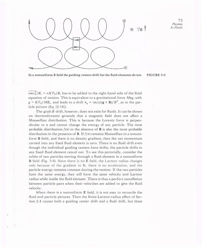
In a nonuniform B field the guiding centers drift but the fluid elements do not. FIGURE 3-8
nmvlfj Rc = nKTn/ Rc has to be added to the right-hand side of the fluid
equation of motion. This is equivalent to a gravitational force Mng, with
g = KT11/ MRc, and leads to a drift vg = (m/q)(g x B)/ B2, as in the par
ticle picture (Eq. [2-18]).
The grad-E drift, however, does not exist for fluids. It can be shown on thermodynamic grounds that a magnetic field does not affect a Maxwellian distribution. This is because the Lorentz force is perpen
dicular to v and cannot change the energy of any particle. The most probable distribution f(v) in the absence of B is also the most probable
distribution in the presence of B. If f(v) remains Maxwellian in a nonuni
form B field, and there is no density gradient, then the·net momentum
carried into any fixed fluid element is zero. There is no fluid drift even
though the individual guiding centers have drifts; the particle drifts in
any fixed fluid element cancel out. To see this pictorially, consider the orbits of two particles moving through a fluid element in a nonuniform B field (Fig. 3-8). Since there is no E field, the Larmor radius changes only because of the gradient in B; there is no acceleration, and the particle energy remains constant during the motion. If the two particles
have the same energy, they will have the same velocity and Larmor
radius while inside the fluid element. There is thus a perfect cancellation
between particle pairs when their velocities are added to give the fluid
velocity. When there is a nonuniform E field, it is not easy to reconcile the
fluid and particle pictures. Then the finite-Larmor-radius effect of Section 2.4 causes both a guiding center drift and a fluid drift, but these
73 Plasmas
As Fluids

74 Chapter Three
are not the same; in fact, they have opposite signs! The particle drift was calculated in Chapter 2, and the fluid drift can be calculated from
the off-diagonal elements of P. It is extremely difficult to explain how the finite-Larmor-radius effects differ. A simple picture like Fig. 3-6 will
not work because one has to take into account subtle points like the following: In the presence of a density gradient, the density of guiding centers is not the same as the density of particles!
PROBLEMS �-3. Show that Eqs. [3-55] and [3-57) are redundant in the set of Maxwell's equations.
3-4. Show that the expression for j0 on the right-hand side of Eq. [3-69] has the dimensions of a current density.
3-5. Show that if the current calculated from the particle picture (Fig. 3-6) agrees with that calculated from the diamagnetic drift for one width of the box, then it will agree for all widths.
3-6. An isothermal plasma is confined between the planes x = ±a in a magnetic field B = BJ,. The density distribution is
n = n0(1 - x 2/ a 2) (a) Derive an expression for the electron diamagnetic drift velocity v0, as a function of x.
(b) Draw a diagram showing the density profile and the direction of v0, on both sides of the midplane if B is out of the paper.
(c) Evaluate v0, at x = a/2 if B = 0.2 T, KT, = 2 eV, and a = 4 em.
3-7. A cylindrically symmetric plasma column in a uniform B field has
n (r) = n0 exp (-r2/r�) and n, = n, = n0 exp (e</J/ KT,) (a) Show that vE and v0, are equal and opposite.
(b) Show that the plasma rotates as a solid body.
(c) In the frame which rotates with velocity v£, some plasma waves (drift waves) propagate with a phase velocity v., = 0.5v0,. What is v., in the lab frame? On a diagram of the r - (J plane, draw arrows indicating the relative magnitudes and directions of v£, v0., and v., in the lab frame.
3-8. (a} For the plasma of Problem 3-7, find the diamagnetic current density io as a function of radius.
(b) Evaluate j0 in A/m2 for B = 0.4 T, n0 = 10'6 m-3, KT, = KT, = 0.25 eV, r = r0 = I em.

(c) In the lab frame, is this current carried by ions or by electrons or by both?
3-9. In the preceding problem, by how much does the diamagnetic current reduce B on the axis? Hint: You may use Ampere's circuital law over an appropriate path.
FLUID DRIFTS PARALLEL TO B
The z component of the fluid equation of motion is
[av, J ap mn at + (v · V)v. = qnE, -
az [3-70]
The convective term can often be neglected because it is much smaller
th!ln the avJat term. We shall avoid complicated arguments here and simply consider cases in which v, is spatially uniform. Using Eq. [3-52],
we have
•
av, q -yKT an -=- E,---at m mn az [3-71}
This shows that the fluid is accelerated along B under the combined electrostatic and pressure gradient forces. A particularly important result
is obtained by applying Eq. [3-71] to massless electrons. Taking the limit m � 0 and specifying q = -e and E = -V4> , we have*
qE. = e a4> = -yKT, an - az n az [3-72]
Electrons are so mobile that their heat conductivity is almost infinite.
We may then assume isothermal electrons and take 'Y = 1. Integrating,
we have
e</J = KT. In n + C
or
I n = n0 exp (e4>/ KT.) [3-73]
This is just the Boltzmann relation for electrons. What this means physically is that electrons, being light, are very
mobile and would be accelerated to high energies very quickly if there
Why can't v, -> oo, keeping mv, constant? Consider the energy!
3.5
75 Plasmas
As Fluids

76 Chapter Three
FIGURE 3-9
• 00 • o• • Oe o• o •o
V'p
FP ...
FE
E "1!1!!(
¢ Physical reason for potential.
o�B�•
J•o
· � o .o •
... --
.....
- ....
.....
+
o• • ... o.
0 0 B
the Boltzmann relation between density and
were a net force on them. Since electrons cannot leave a region en masse without leaving behind a large ion charge, the electrostatic and pressure
gradient forces on the electrons must be closely in balance. This condition leads to the Boltzmann relation. Note that Eq. [3-73] applies to each line of force separately. Different lines of force may be charged to different
potentials arbitrarily unless a mechanism is provided for the electrons
to move across B. The conductors on which lines of force terminate can
provide such a mechanism, and the experimentalist has to take these end effects into account carefully.
Figure 3-9 shows graphically what occurs when there is a local density clump in the plasma. Let the density gradient be toward the center of
the diagram, and suppose KT is constant. There is then a pressure
gradient toward the center. Since the plasma is quasineutral, the gradient exists for both the electron and ion fluids. Consider the pressure gradient
force Fp on the electron fluid. It drives the mobile electrons away from the center, leaving the ions behind. The resulting positive charge gener
ates a field E whose force FE on the electrons opposes F P· Only when FE is equal and opposite to Fp is a steady state achieved. If B is constant, E is an electrostatic field E = -V¢, and 4> must be large at the center, where n is large. This is just what Eq. [3-73] tells us. The deviation from strict neutrality adjusts itself so that there is just enough charge to set up the
E field required to balance the forces on the electrons.

THE PLASMA APPROXIMATION 3.6
The previous example reveals an important characteristic of plasmas
that has wide application. We are used to solving for E from Poisson's equation when we are given the charge density a. In a plasma, the opposite procedure is generally used. E is found from the equations of
motion, and Poisson's equation is used only to find a. The reason is that a plasma has an overriding tendency to remain neutral. If the ions move, the electrons will follow. E must adjust itself so that the orbits of the elect rons and ions preserve neutrality. The charge density is of secondary importance; it will adjust itself so that Poisson's equation is satisfied. This
is true, of course, only for low-frequency motions in which the electron
inertia is not a factor.
In a plasma, it is usually possible to assume n; = n, and V · E ¥- 0 at
the same time. We shall call this the plasma approximation. It is a fundamental trait of plasmas, one which is difficult for the novice to understand.
Do not use Poisson 's equation to obtain E unless it is unavoidable ! In the set of fluid equations [3-55]-[3-61] , we may now eliminate Poisson's equation and also eliminate one of the unknowns by setting n; = n, = n.
The plasma approximation is almost the same as the condition of
quasineutrality discussed earlier but has a more exact meaning. Whereas
quasineutrality refers to a general tendency for a plasma to be neutral
in its state of rest, the plasma approximation is a mathematical shortcut
that one can use even for wave motions. As long as these motions are
slow enough that both ions and electrons have time to move, it is a good approximation to replace Poisson's equation by the equation n; = n,. Of course, if only one species can move and the other cannot follow, such as in high-frequency electron waves, then the plasma approximation is not valid, and E must be found from Maxwell's equations rather th_an from the ion and electron equations of motion. We shall return to the question of the validity of the plasma approximation when we come to
the theory of ion waves. At that time, it will become clear why we had to use Poisson's equation in the derivation of Debye shielding.
77 Plasmas
As Fluids


Chapter Four
s
p s
REPRESENTATION OF WAVES 4.1
Any periodic motion of a fluid can be decomposed by Fourier analysis into a superposition of sinusoidal oscillations with different frequencies
w and wavelengths A. A simple wave is any one of these components. When the oscillation amplitude is small, the waveform is generally sinusoidal; and there is only 'one component. This is the situation we shall consider.
Any sinusoidally oscillating quantity-say, the density n-can be represented as follows:
n =nexp [i(k·r -wt)] [4-l]
where, in Cartesian coordinates,
[4-2)
Here n is a constant defining the amplitude of the wave, and k is called the propagation constant. If the wave propagates in the x direction, k has only an x component, and E'q. [4-1] becomes
n = n ei(kx-wt)
By convention, the exponential notation means that the real part of the expression is to be taken as the measurable quantity. Let us choose ii to be real; we shall soon see that this corresponds to a choice of the origins 79

80 Chapter Four
of x and t. The real part of n is then
Re (n) = ii cos (kx- wt) [4-31
A point of constant phase on the wave moves so that (d/ dt)(kx -wt) = 0, or
[4-4]
This is called the phase velocity. If w/ k is positive, the wave moves to the
right; that is, x increases as t increases, so as to keep kx - wt constant. If w/ k is negative, the wave moves to the left. We could equally well
have taken
n = ii e i(kx+wl)
in which case positive w/k would have meant negative phase velocity. This is a convention that is sometimes used, but we shall not adopt it. From Eq. [4-3], it is clear that reversing the sign of both w and k makes no difference.
Consider now another oscillating quantity in the wave, say the electric field E. Since we have already chosen the phase of n to be zero, we must
allow E to have a different phase 8:
E = E cos (kx - wt + 8) or E = E ei(kx-wl+ll) [4-5]
where E is a real, constant vector. It is customary to incorporate the phase information into E by
allowing E to be complex. We can write
where Ec is a complex amplitude. The phase 8 can be recovered from Ec, since Re (Ec) = E cos 8 and Im (Ec) = E sin 8, so that
lm (Ec) tan 8 =
Re (Ec) [4-6]
From now on, we shall assume that all amplitudes are complex and drop the subscript c. Any oscillating quantity g1 will be written
g1 =g1exp[i(k·r-wt)] [4-7]

.,
so that g1 can stand for either the complex amplitude or the entire expression [4-7]. There can be no confusion, because in linear wave theory the same exponential factor will occur on both sides of any equation
and can be cancelled out.
4-1. The oscillating density n 1 and potential <P, in a "drift wave" are related by PROBLEM � = e¢ 1 w * + ia
n0 KT, w + ia
where it is only necessary to know that all the other symbols (except i) stand for
positive constants.
(a) Find an expression for the phase 8 of <P 1 relative ton 1• (For simplicity, assume
that n1 is real.)
(b) If w < w*, does <P 1 lead or lag n 1?
GROUP VELOCITY 4.2
The phase velocity of a wave in a plasma often exceeds the velocity of light c. This does not violate the theory of relativity, because an infinitely
long wave train of constant amplitude cannot carry information. The carrier of a radio wave, for instance, carries no information until it is modulated. The modulation information does not travel at the phase velocity but at the group velocity, which is always less than c. To illustrate this, we may consider a modulated wave formed by adding ("beating") two waves of nearly equal frequencies. Let these waves be
E1 = Eo cos [(k + ilk)x- (w + Llw)t]
E2 =Eo cos [(k- ilk)x- (w - Llw )t] [4-8]
E 1 and E2 differ in frequency by 2ilw. Since each wave must have the phase velocity w/ k appropriate to the medium in which they propagate, one must allow for a difference 2ilk in propagation constant. Using the abbreviations
a = kx- wt
b = (Llk )x - (Llw )t
81 Waves in
Plasmas

82 Chapter Four
FIGURE 4-1 Spatial variation of the electric field of two waves with a frequency difference.
we have
E 1 + E2 =Eo cos (a + b) + Eo cos (a -b)
= E 0( cos a cos b - sin a sin b + cos a cos b + sin a sin b)
= 2E 0 cos a cos b
E1 + E2 = 2E0 cos [ (M)x- (llw)t] cos (kx- wt) (4-9]
This is a sinusoidally modulated wave (Fig. 4-1). The envelope of the wave, given by cos [ (Ilk )x - (llw )t], is what carries information; it travels
at velocity llw/ Ilk. Taking the limit llw -7 0, we define the group velocit)• to be
I Vg =dw/dk I [4-10]
It is this quantity that cannot exceed c.
4.3 PLASMA OSCILLATIONS
If the electrons in a plasma are displaced from a uniform background
of ions, electric fields will be built up in such a direction as to restore the neutrality of the plasma by pulling the electrons back to their original positions. Because of their inertia, the electrons will overshoot and oscillate around their equilibrium positions with a characteristic frequency known as the plasma frequency. This oscillation is so fast that the massive ions do not have time to respond to the oscillating field and may be considered as fixed. In Fig. 4-2, the open rectangles represent typical e1ements of the ion fluid, and the darkened rectangles the alter
nately displaced elements of the electron fluid. The resulting charge bunching causes a spatially periodic E field, which tends to restore the electrons to their neutral positions.
c.

+ + + +
�D D��D D� �D D��D D� �D D��D D� �D D��D D�
E � ]l:l!o .. ..
Mechanism of plasma oscillations.
We shall derive an expression for the plasma frequency wp in the
simplest case, making the following assumptions: ( 1) There is no magnetic field; (2) there are no thermal motions (KT = 0); (3) the ions are fixed in space in a uniform distribution; (4) the plasma is infinite in extent; and (5) the electron motions occur only in the x direction. As a consequence of the last assumption, we have
V =X. ajax E=Ex VxE=O E= -V¢ [4-11]
There is, therefore, no fluctuating magnetic field; this is an electrostatic oscillation.
The electron equations of motion and continuity are [av, J mn, at+ (v, · V)v, = -en, E
an. - + V · (n v) = 0 at
e e
[4-12]
[4-13]
The only Maxwell equation we shall need is the one that does not involve B: Poisson's equation. This case is an exception to the general rule of Section 3.6 that Poisson's equation cannot be used to find E. This is a
high-frequency oscillation; electron inertia is important, and the deviation from neutrality is the main effect in this particular case. Consequently, we write
[4-14]
83 Waves in
Plasmas
FIGURE 4-2

84 Chapter Four
Equations [4-2]-[4-14] can easily be solved by the procedure of
linearization. By this we mean that the amplitude of oscillation is small, and terms containing higher powers of amplitude factors can be neglected. We first separate the dependent variables into two parts: an "equili
brium" part indicated by a subscript 0, and a "perturbation" part indicated by a subscript I:
n, =no+n1 [4-15]
The equilibrium quantities express the state of the plasma in the absence of the oscillation. Since we have assumed a uniform neutral plasma at
rest before the electrons are displaced, we have
Vno = Vo = Eo = 0
ano =
avo =
aEo = O
at at at
Equation [ 4- 12] now becomes
[4-16]
[4-17]
The term {v1 • V)v1 is seen to be quadratic in an amplitude quantity, and we shall linearize by neglecting it. The linear theory is valid as long as I v d is small enough that such quadratic terms are indeed negligible. Similar I y, Eq. [ 4-13] becomes
[4-18]
In Poisson's equation [ 4-1 4], we note that n;0 = n,0 in equilibrium and
that n;1 = 0 by the assumption of fixed ions, so we have
The oscillating quantities are assumed to behave sinusoidally:
i(kx-wt),.. v1=v1e x
[4-19)
[4-20)
- "\

The time derivative ajat can therefore be replaced by gradient V by ikx. Equations [ 4-17]-[ 4-19] now become
-imwv 1 = -eE 1
-iwn 1 = -noikv 1
Eliminating n1 and £1, we have for Eq. [4-21]
. -e -noikvi .n0e2 -1mwv1 = -e-- = -t-- vl
ikEo -tw Eow
If v 1 does not vanish, we must have
w2 = noe2/mEo
The plasma frequency is therefore
( 2) 1/2 noe Wp = -
Eom rad/sec
Numerically, one can use the approximate formula
-tw, and the
[4-21]
[4-22]
[4-23]
[4-24]
[4-25]
[4-26]
This frequency, depending only on the plasma density, is one of the fundamental parameters of a plasma. Because of the smallness of m, the plasma frequency is usually very high. For instance, in a plasma of density n = 10
18 m-3, we have
1s 112 9 -1 G [p = 9(10 ) = 9 X 10 sec = 9 Hz
Radiation at [p normally lies in the microwave range. We can compare this with another electron frequency: we. A useful numerical formula is
fee = 28 GHz/Tesla [4-27]
Thus if B = 0.32 T and n = 1018 m -3, the cyclotron frequency is approximately equal to the plasma frequency for electrons.
Equation [4-25] tells us that if a plasma oscillation is to occur at all, it must have a frequency depending only on n. In particular, w does not depend on k, so the group velocity dw/dk is zero. The disturbance does not propagate. How this can happen can be made clear with a mechanical analogy (Fig. 4-3). Imagine a number of heavy balls suspended by springs
85 Waves in
Plasmas
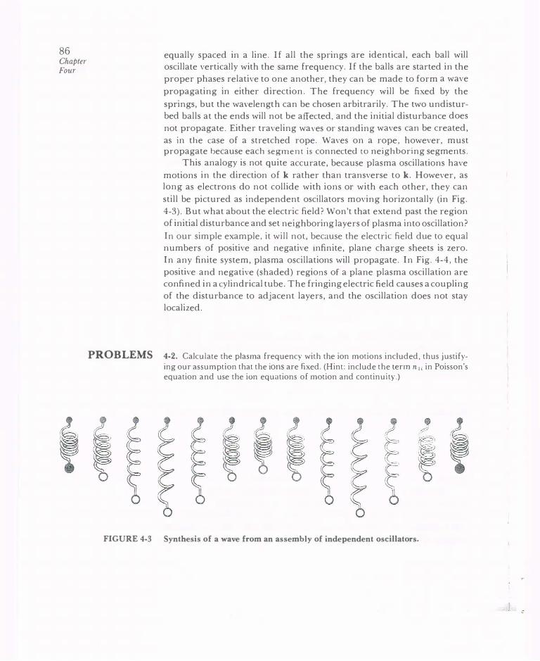
86 Chapter Four
equally spaced in a line. If all the springs are identical, each ball will oscillate vertically with the same frequency. If the balls are started in the proper phases relative to one another, they can be made to form a wave
propagating in either direction. The frequency will be fixed by the
springs, but the wavelength can be chosen arbitrarily. The two undisturbed balls at the ends will not be affected, and the initial disturbance does
not propagate. Either traveling waves or standing waves can be created,
as in the case of a stretched rope. Waves on a rope, however, must propagate because each segment is connected to neighboring segments.
This analogy is not quite accurate, because plasma oscillations have motions in the direction of k rather than transverse to k. However, as long as electrons do not collide with ions or with each other, they can
still be pictured as independent oscillators moving horizontally (in Fig. 4-3). But what about the electric field? Won't that extend past the region of initial disturbance and set neighboring layers of plasma into oscillation?
In our simple example, it will not, because the electric field due to equal numbers of positive and negative infinite, plane charge sheets is zero. In any finite system, plasma oscillations will propagate. In Fig. 4-4, the positive and negative (shaded) regions of a plane plasma oscillation are confined in a cylindrical tube. The fringing electric field causes a coupling of the disturbance to adjacent layers, and the oscillation does not stay localized.
PROBLEMS 4-2. Calculate the plasma frequency with the ion motions included, thus justify
ing our assumption that the ions are fixed. (Hint: include the term n 1, in Poisson's equation and use the ion equations of motion and continuity.)
J
FIGURE 4-3 Synthesis of a wave from an assembly of independent oscillators.

E
Plasma oscillations propagate in a finite medium because of FIGURE 4-4 fringing fields.
4-3. For a simple plasma oscillation with fixed ions and a space-time behavior exp[i(kx- wt)]. calculate the phase 8 for </>1, £1, and v1 if the phase of n1 is zero. Illustrate the relative phases by drawing sine waves representing n 1, </> 1, E 1, and v1: (a) as a function of x at t = 0, (b) as a function oft at x = 0 for w/k > 0,
and (c) as a function of I at x = 0 for w/k < 0. Note that the time patterns can be obtained by translating the x patterns in the proper direction, as if the wave
were passing by a fixed observer.
4-4. By writing the linearized Poisson's equation used in the derivation of simple plasma oscillations in the form
V · (EE) = 0
derive an expression for the dielectric constant E applicable to high-frequency longitudinal motions.
ELECTRON PLASMA WAVES 4.4
There is another effect that can cause plasma oscillations to propagate,
and that is thermal motion. Electrons streaming into adjacent layers of
plasma with their thermal velocities will carry information about what
is happening in the oscillating region. The plasma oscillation can then
properly be called a plasma wave. We can easily treat this effect by adding
a term -Vp, to the equation of motion [ 4-12]. In the one-dimensional
problem, y will be three, according to Eq. [3-53]. Hence,
ft v v an1 A v p, = 3KT, n, = 3KT, (no+ n1) = 3KT,-x ax
and the linearized equation of motion is
avl anl mno- = -enoEl- 3KT-at e ax [4-28]
87 Waves in
Plasmas

88 Chapter Four
Note that in linearizing we have neglected the terms n1 av1/at and n1E1 as well as the (v1 · V)v1 term. With Eq. [4-20], Eq. [4-28] becomes
-imwnov 1 = -enoE 1 - 3KT.ikn 1
E 1 and n 1 are still given by Eqs. [ 4-23] and [ 4-22], and we have
. [ ( -e ) . J noik zmwn0v 1 = en0 -.- + 3KT.zk -.-v 1
zkE 0 zw 2 2 (noe 3KTek2)
W V1 = -- + -- V1 Eom m
2 2 3k2 2 w = (J) p + 2 v th
[4-29]
[4-30]
where v;h = 2KT./m. The frequency now depends on k, and the group
velocity is finite:
2w dw = �v�h 2k dk
dw 3 k 2 3 v �h Vg =
dk = 2 W V,h = 2 V<J>
[4-31) .
That vg is always less than c can easily be seen from a graph of Eq. [ 4-30]. Figure 4-5 is a plot of the dispersion relation w(k) as given by Eq. [4-30]. At any point P on this curve, the slope of a line drawn from the origin gives the phase velocity w/ k. The slope of the curve at P gives the group
w
FIGURE 4-5 Dispersion relation for electron plasma waves (Bohm-Gross waves).
k

velocity. This is clearly always less than (3/2)112v,h, which, in our nonrela
tivistic theory, is much less than c. Note that at large k (small A), information travels essentially at the thermal velocity. At small k (large A),
information travels more slowly than v,h even though vq, is greater than
v,h· This is because the density gradient is small at large A, and thermal
motions carry very little net momentum into adjacent layers. The existence of plasma oscillations has been known since the days
of Langmuir in the 1920s. It was not until 1949 that Bohm and Gross
worked out a detailed theory telling how the waves would propagate and how they could be excited. A simple way to excite plasma waves would be to apply an oscillating potential to a grid or a series of grids in a plasma; however, oscillators in the GHz range were not generally available in those days. Instead, one had to use an electron beam to excite plasma waves. If the electrons in the beam were bunched so that they passed by any fixed point at a frequency fp, they would generate
an electric field at that frequency and excite plasma oscillations. It is not
necessary to form the electron bunches beforehand; once the plasma oscillations arise, they will bunch the electrons, and the oscillations will grow by a positive feedback mechanism. An experiment to test this theory was first performed by Looney and Brown in 1 954. Their apparatus was· entirely contained in a glass bulb about 10 em in diameter (Fig. 4-6). A plasma filling the bulb was formed by an electrical discharge between the cathodes K and an anode ring A under a low pressure (3 X 10⁻³ Torr)
-200 v
Schematic of the Looney-Brown experiment on plasma oscillations. FIGURE 4-6
89 Waves in
Plasmas

90 Chapter Fo·ur
1.0
.8 N
N I .6 l'J
N ...... .4
.2
0 0
DISCHARGE CURRENT (MA)
2
100 200 300
4 6 8 10 12
FIGURE 4-7 Square of the observed frequency vs. plasma density, which is generally proportional to the discharge current. The inset shows the observed spatial distribution of oscillation intensity, indicating the existence of a different standing wave pattern for each of the groups of experimental points. [From D. H. Looney and S. C. Brown, Ph)'s. Rev. 93, 965 (1954).]
of mercury vapor. An electron beam was created in a side arm containing a negatively biased filament. The emitted electrons were accelerated to 200 V and shot into the plasma through a small hole. A thin, movable
probe wire connected to a radio receiver was used to pick up the
oscillations. Figure 4-7 shows their experimental results for l vs. discharge current, which is generally proportional to density. The points
show a linear dependence, in rough agreement with Eq. [4-26]. Deviations from the straight line could be attributed to the k2v�h term in E·q. [ 4-30]. However, not all frequencies were observed ; k had to be such that an integral number of half wavelengths fit along the plasma column. The standing wave patterns are shown at the left of Fig. 4-7. The predicted traveling plasma waves could not be seen in this experiment, probably because the beam was so thin that thermal motions carried electrons out of the beam, thus dissipating the oscillation energy. The

electron bunching was accomplished not in the plasma but in the oscillating sheaths at the ends of the plasma column. In this early experiment, one learned that reproducing the conditions assumed in the uniformplasma theory requires considerable skill.
A number of recent experiments have verified the Bohm-Gross dispersion relation, Eq. [4-30], with precision. As an example of modern
experimental technique, we show the results of Barrett, Jones, and Franklin. Figure 4-8 is a schematic of their apparatus. The cylindrical column of quiescent plasma is produced in a Q-machine by thermal
ionization of Cs atoms on hot tungsterr plates (not shown). A strong magnetic field restricts electrons to motions along the column. The waves
EXCITER PROBE
RECEIVER PROBE
,
��EAK rn ..
V/177//IIZIZI/7711///1171/IIIII/ZIIIIJ
- ...
1-----il_--fl A TTE N- 1.._ _ _.-----..---.,_ __ -.J I UATOR I t
SIGNAL
GENERATOR 10-1200 MHz
PHASE
LOCK MODULATOR 1-----l 500 kHz
CRYSTAL
MIXER
t 500kHz TUNED AMPLIFIER
t CHART
RECORDER
DC
BREAK
Schematic of an experiment to measure plasma waves. [From P. J. Barrett, FIGURE 4-8 H. G. Jones, and R. N. Franklin, Plasma Physics 10, 911 (1968).]
91 Waves in Plasmas

92 Chapter Four
' '\
i� n = 0 2x1010 em·3
f 950 MHz A 3.5 em
n = 4x108em·3 0
f 170MHz A = 1.3 em
f 20 MHz A 5.1 em
FIGURE 4-9 Spatial variation of the perturbed density in a plasma wave, as indicated by an interferometer, which multiplies the instantaneous density signals from two probes and takes the time average. The interferometer is tuned to the wave frequency, which varies with the density. The apparent damping at low densities is caused by noise in the plasma. [From Barrett, Jones, and Franklin, loc. cit.]
are excited by a wire probe driven by an oscillator and are detected by a second, movable probe. A metal shield surrounding the plasma prevents communication between the probes by ordinary microwave (electromagnetic wave) propagation, since the shield constitutes a waveguide beyond cutoff for the frequency used. The traveling waveforms are traced by interferometry: the transmitted and received signals are detected by a crystal which gives a large de output when the signals are in phase and zero output when they are 90° out of phase. The resulting
signal is shown in Fig. 4-9 as a function of position along the column.
Synchronous detection is used to suppress the noise level. The excitation signal is chopped at 500 kHz, and the received signal should also be modulated at 500 kHz. By detecting only the 500-kHz component of the received signal, noise at other frequencies is eliminated. The traces of

Fig. 4-9 give a measurement of k. When the oscillator frequency w is varied, a plot of the dispersion curve (w/wp)2 vs. ka is obtained, where
a is the radius of the column (Fig. 4-1 0). The various curves are labeled according to the value of wpa/v,h. For v,h = 0, we have the curve labeled ro, which corresponds to the dispersion relation w = Wp. For finite v,h, the curves correspond to that of Fig. 4-5. There is good agreement between the experimental points and the theoretical curves. The decrease of w at small ka is the finite-geometry effect shown in Fig. 4-4. In this particular experiment, that effect can be explained another way. To satisfy the boundary condition imposed by the conducting shield, namely that E = 0 on the conductor, the plasma waves must travel at an angle
to the magnetic field. Destructive interference between waves traveling with an outward radial component of k and those traveling inward enables the boundary condition to be satisfied. However, waves traveling
1.4
1.2
1.0
N .8 a. 3 -
N 3 .6
.4
.2
I 0
0 2 4 6 8 10 12 14 16 ka
l-8 20 22
Comparison of the measured and calculated dispersion curves for electron FIGURE 4-10 plasma waves in a cylinder of radius a. [From Barrett, Jones, and Franklin, lac. cit.]
93 Waves in
Plasmas
24
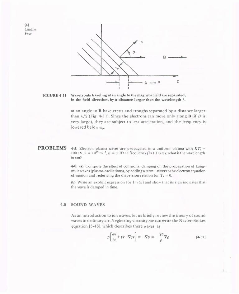
94 Chapter Four
I .. ,
k
A. sec e
B _.
z
FIGURE 4-11 Wavefronts traveling at an angle to the magnetic field are separated, in the field direction, by a distance larger than the wavelength A.
at an angle to B have crests and troughs separated by a distance larger than A/2 (Fig. 4-ll ) . Since the electrons can move only along B (if B is
very large), they are subject to less acceleration, and the frequency is lowered below wp.
PROBLEMS 4-5. Electron plasma waves are propagated in a uniform plasma with KT, = lOOeV,n = 1016m-3,B = 0. If the frequencyfis 1.1 GHz,whatis the wavelength
in em?
4-6. (a) Compute the effect of collisional damping on the propagation of Lang
muir waves (plasma oscillations), by adding a term -mnvv to the electron e·quation
of motion and rederiving the dispersion relation for T, = 0.
(b) Write an explicit expression for Im (w) and show that its sign indicates that
the wave is damped in time.
4.5 SOUND WAVES
As an introduction to ion waves, let us briefly review the theory of sound waves in ordinary air. Neglecting viscosity, we can write theN a vier-Stokes
equation [3-48], which describes these waves, as
[av J 'YP p - + (v·V)v =-Vp=--Vp
at p [4-32]

The equation of continuity is
ap -+ V · (pv) = 0 at [4-33]
Linearizing about a stationary equilibrium with uniform Po and p0, we have
. 'YPo .k -twpovi = - -t PI Po
-iwpl + poik · v1 = 0
[4-34)
[4-35]
where we have again taken a wave dependence of the form
exp [i(k · r- wt)]
For a plane wave with k = kx and v = vx, we find, upon eliminating p1,
or
. 'YPo .kpoikv 1 -zwpovl =- - z -.--Po tw
2 2 'YPo w v1 = k -vi Po
� = (":00) 1/2
= ("�) 1/2 =
Cs
[4-36]
This is the expression for the velocity Cs of sound waves in a neutral gas. The waves are pressure waves propagating from one layer to the next
by collisions among the air molecules. In a plasma with no neutrals and few collisions, an analogous phenomenon occurs. This is called an ion acoustic wave, or, simply, an ion wave.
ION WAVES 4.6
In the absence of collisions, ordinary sound waves would not occur. Ions can still transmit vibrations to each other because of their charge, however; and acoustic waves can occur through the intermediary of an electric field. Since the motion of massive ions will be involved, these
95 Waves in
Plasmas

96 Chapter Four
will be low- frequency oscillations, and we can use the plasma approxima
tion of Section 3.6. We therefore assume n; = n, = n and do not use Poisson's equation. The ion fluid equation in the absence of a magnetic field is [av· J Mn af + (v; · V)v; = enE- Vp = -en V<f> - y;KT, Vn [4-37]
We have assumed E = -V<f> and used the equation of state. Linearizing
and assuming plane waves, we have
-iwMn0v; 1 = -en0ik<P 1 - y;KT;ikn 1 [4-38]
As for the electrons, we may assume m = 0 and apply the argument of Section 3.5, regarding motions along B, to the present case of B = 0. The balance of forces on electrons, therefore, requires
( e<f> 1 ) ( e</> 1 ) n, = n = no exp -- = n0 l + -- + · · ·
KT, KT,
The perturbation in density of electrons, and, therefore, of ions, is then
e<f> 1 n1 = n0--
KT, [4-39]
Here the n0 of Boltzmann's relation also stands for the density in the e·quilibrium plasma, in which we can choose <Po = 0 because we have
assumed Eo== 0. In linearizing Eq. [4-39], we have dropped the higherorder terms in the Taylor expansion of the exponential.
The only other equation needed is the linearized ion equation of continuity. From Eq. [ 4-22], we have
[4-40]
In Eq. [4-38], we may substitute for </J1 and n1 in terms of v;1 from Eqs. [ 4-39] and [ 4-40] and obtain
. ( . KT, . ) n0ikv;J twMnov; 1 == en0tk-- + y;KT1tk -.--
enn tw
2 _
k2 (KT. y;KT,) w - -- +--
M M
1/2 � = (KT. + y;KT,)
""' k M
Vs [4-41]

) t '
I
w
k
Dispersion relation for ion FIGURE 4-12
acoustic waves in the limit of small Debye length.
This is the dispersion relation for ion acoustic waves; vs is the sound speed
in a plasma. Since the ions suffer one-dimensional compressions in the
plane waves we have assumed, we may set -y; = 3 here. The electrons
move so fast relative to these waves that they have time to equalize their
temperature everywhere; therefore, the electrons are isothermal, and
-y, = 1. Otherwise, a factor-y, would appear in front of KT, in Eq. (4-41 ). The dispersion curve for ion waves (Fig. 4-12) has a fundamentally
different character from that for electron waves (Fig. 4-5). Plasma oscillations are basically constant-frequency waves, with a correction due to thermal motions. Ion waves are basically constant-velocity waves and exist only when there are thermal motions. For ion waves, the group velocity is equal to
the phase velocity. The reasons for this difference can be seen from the
following description of the physical mechanisms involved. In electron
plasma oscillations, the other species (namely, ions) remains essentially
fixed. In ion acoustic waves, the other species (namely, electrons) is far
from fixed; in fact, electrons are pulled along with the ions and tend to shield out electric fields arising from the bunching of ions. However, this
shielding is not perfect because, as we saw in Section 1.4, potentials of the order of KT,/ e can leak out because of electron thermal motions. What happens is as follows. The ions form regions of compression and
rarefaction, just as in an ordinary sound wave. The compressed regions
tend to expand into the rarefactions, for two reasons. First, the ion
thermal motions spread out the ions; this effect gives rise to the second
term in the square root of Eq. [4-41]. Second, the ion bunches are
positively charged and tend to disperse because of the resulting electric
field. This field is largely shielded out by electrons, and only a fraction, proportional to KT., is available to act on the ion bunches. This effect
gives rise to the first term in the square root of Eq. [ 4-41 ]. The ions overshoot because of their inertia, and the compressions and rarefactions are regenerated to form a wave.
97 Waves in Plasmas

98 Chapter Four
The second effect mentioned above leads to a curious phenomenon.
When KTi goes to zero, ion waves still exist. This does not happen in a
neutral gas (Eq. [4-36]). The acoustic velocity is then given by
v, = (KT./ M) 112 [4-42]
This is often observed in laboratory plasmas, in which the condition Ti « T, is a common occurrence. The sound speed v, depends on electron
temperature (because the electric field is proportional to it) and on ion mass (because the fluid's inertia is proportional to it).
4. 7 VALIDITY OF THE PLASMA APPROXIMATION
In deriving the velocity of ion waves, we used the neutrality condition
ni = n, while allowing E to be finite. To see what error was engendered
in the process, we now allow ni to differ from n, and use the linearized
Poisson equation:
[4-43] The electron density is given by the linearized Boltzmann relation [ 4-39]:
ecjJ 1 nei =--no
KT, [4-44]
Inserting this into Eq. [4-43], we have
EocPI(k2A� + 1) = eni1A� [4-45]
The ion density is given by the linearized ion continuity equation [ 4-40]:
k nil= -noV;I
w [4-46]
Inserting Eqs. [ 4-45] and [ 4-46] into the ion equation of motion [ 4-38], we find
[4-47]
[4-48]

This is the same as we obtained previously (Eq. [4-41]) except for the
factor 1 + k 2 A�- Our assumption n; = n. has given rise to an error of order k 2 A� = (27TA 0/ A )2. Since A 0 is very small in most experiments, the plasma approximation is valid for all except the shortest wavelength waves.
COMPARISON OF ION AND ELECTRON WAVES 4.8
If we consider these short-wavelength waves by taking e A� » 1, Eq. [ 4-4 7] becomes
[4-491
We have, for simplicity, also taken the limit T, � 0. Here Op is the ion
plasma fre·quency. For high frequencies (short wavelengths) the ion acoustic wave turns into a constant-frequency wave. There is thus a
complementary behavior between electron plasma waves and ion acoustic
waves: the former are basically constant frequency, but become constant
velocity at large k; the latter are basically constant velocity, but become
constant frequency at large k. This comparison is shown graphically in Fig. 4-13.
Experimental verification of the existence of ion waves was first
accomplished by Wong, Motley, and D'Angelo. Figure 4-14 shows their
apparatus, which was again a Q-machine. (It is no accident that we have referred to Q-machines so often; careful experimental checks of plasma
w ELECTRON
/ /
k
ION w
k Comparison of the dispersion curves for electron plasma waves and ion FIGURE 4-13
acoustic waves.
99 Waves in
Plasmas

100 Chapter Four
theory were possible only after schemes to make quiescent plasmas were
discovered.) Waves were launched and detected by grids inserted into
the plasma. Figure 4-15 shows oscilloscope traces of the transmitted and
received signals. From the phase shift, one can find the phase velocity (same as group velocity in this case). These phase shifts are plotted as
functions of distance in Fig. 4-16 for a plasma density of 3 x 10¹⁷ m -3.
The slopes of such lines give the phase velocities plotted in Fig. 4-17 for the two masses and various plasma densities n0. The constancy of Vs with wand no is demonstrated experimentally, and the two sets of points for
K and Cs plasmas show the proper dependence on M.
4..9 ELECTROSTATIC ELECTRON OSCILLATIONS PERPENDICULAR TO B
Up to now, we have assumed B = 0. When a magnetic field exists, many more types of waves are possible. We shall examine only the simplest cases, starting with high-frequency, electrostatic, electron oscillations
r LANGMUIR
I PROBE
MAGNET
SINE BURST GENERATOR
HOT TUNGSTEN
) PLATE - �ms:JptLmiHHliF,iL_ne_x_r_:c _(_:I_: � _n:._,'"_:_ __ -�� DC BIAS
NEUTRAL BEAM OVEN
I OS: I LLOSCOPE
FIGURE 4-14 Q-machine experiment to detect ion waves. [From N. Rynn and N. D'Angelo, Rev. Sci. lnstrum. 31, 1326 (1960).]

d=3cm
- .... v 'V "' 1\ I� "
\ \ I \ll lL \J } \ �v
d=5.5cm
- .... � ' � ....
' I " ,, 1\ " IV �
0 40 80 1 20 160 200 t (J1 sec )
D-RIVER
RECEIVER
(X 50)
DRIVER
RECEIVER
(X50)
Oscillograms of signals from the driver and FIGURE 4-15
receiver grids, separated by a distance d, show-ing the delay indicative of a traveling wave. [From A. Y. Wong, R. W. Motley, and N. D'Angelo, Phys. Rev. 133, A436 (1964).]
propagating at right angles to the magnetic field. First, we should define the terms perpendicular, p�rallel, longitudinal, transverse, electrostatic, and electromagnetic. Parallel and perpendicular will be used to denote the direction of k relative to the undisturbed magnetic field B0. Longi
tudinal and transverse refer to the direction of k relative to the oscillating
electric field E 1• If the oscillating magnetic field B 1 is zero, the wave is
electrostatic; otherwise, it is electromagnetic. The last two sets of terms are
related by Maxwell's equation
[4-50]
or
[4-51]
If a wave is longitudinal, k x E 1 vanishes, and the wave is also electrostatic. If the wave is transverse, B1 is finite, and the wave is electromagnetic.
101 Waves in Plasmas
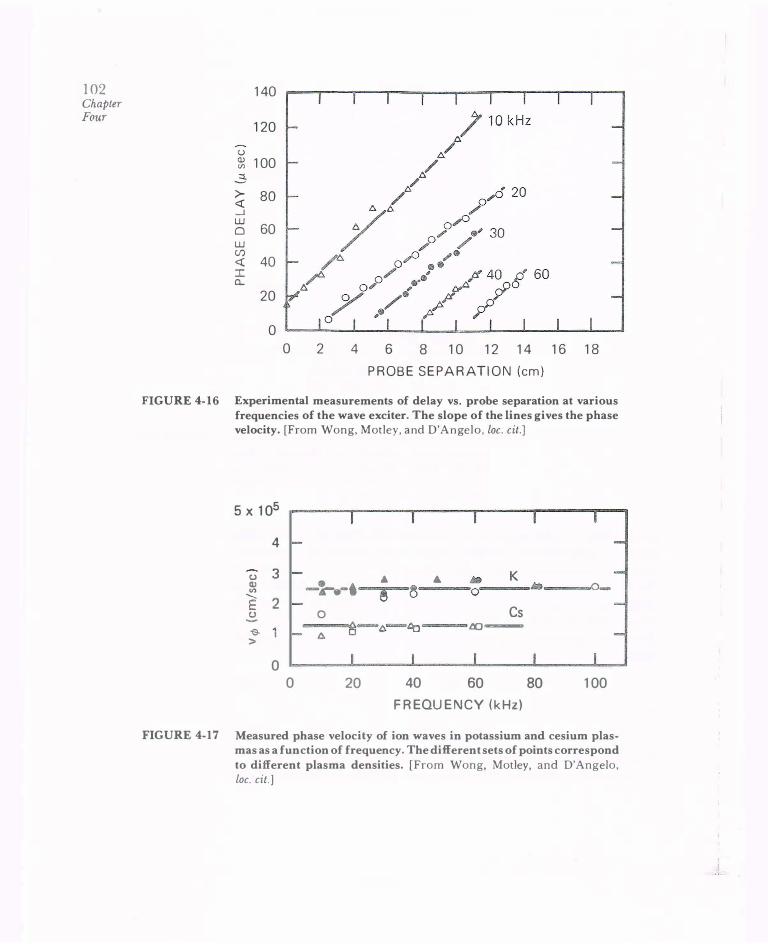
102 Chapter Four
140
120 (.) � 100
2 >- 80 <( _j u.J 0 60 u.J (/) <( 40 I a...
20
0 0 2 4 6 8 10 12 14 16 18
PROBE SE PARATION (em)
FIGURE 4-16 Experimental measurements of delay vs. probe separation at various frequencies of the wave exciter. The slope of the lines gives the phase velocity. [From Wong, Motley, and D'Angelo, loc. cit.]
5 X 10⁵
4
(.) 3 ... A K CIJ -::-...-• � Ia 0-VI 0 ....... e E 2 Cs (.) 0 -
""B-�-"tl � .00=-> �
0 0 20 40 60 80 100
FREQUENCY (kHz)
FIGURE 4-17 Measured phase velocity of ion waves in potassium and cesium plasmas as a function of frequency. The different sets of points correspond to different plasma densities. [From Wong, Motley, and D'Angelo, loc. cit.]

z 1 B0 /WAVE FRONTS
I+H--- k, E1
b-----------------�- X
Geometry of a longitudinal plane FIGURE 4-18
wave propagating at right angles to B0•
It is of course possible for k to be at an arbitrary angle to B0 or E1; then
one would have a mixture of the principal modes presented here.
Coming back to the electron oscillations perpendicular to B0, we
shall assume that the ions are too massive to move at the frequencies involved and form a fixed, uniform background of positive charge. We
shall also neglect thermal motions and set KT. = 0. The equilibrium plasma, as usual, has constant and uniform n0 and B0 and zero Eo and v0. The motion of electrons is then governed by the following linearized equations:
av.l m -- = -e(E1 +Vet x B0)
at
an. I -- + n0V · v 1 = 0
at e
[4-52]
[4-53]
[4-54]
We shall consider only longitudinal waves with k i iE1. Without loss of generality, we can choose the x axis to lie along k and E1, and the z axis to lie alongB0 (Fig. 4-18). Thus ky = k, = Ey = E, = 0, k = kx, and E = Ex.
Dropping the subscripts 1 and e and separating Eq. [ 4-52] into com
ponents, we have
-iwmvx = -eE - ev.)J o
-iwmv, = 0
[4-55]
[4-56]
103 Waves in
Plasmas

104 Chapter Four
Solving for Vy in Eq. [4-56] and substituting into Eq. [4-55]. we have
. ieBo twmvx = eE + eBo--vx
mw
[4-57]
Note that Vx becomes infinite at cyclotron resonance, w =we. This is to be expected, since the electric field changes sign with Vx and continuously accelerates the electrons. [The fluid and single-particle equations are
identical when the (v · V)v and Vp terms are both neglected; all the
particles move together.] From the linearized form of Eq. [ 4-53], we have
k ni = -noVx
w
Linearizing Eq. [4-54] and using the last two results, we have
. k eE ( w �) -I
tkEoE = -e-no-.- 1-2 w zmw w
The dispersion relation is therefore
[4-58]
[4-59]
[4-60]
The frequency wh is called the upper hybrid frequency. Electrostatic electron
waves across B have this frequency, while those along B are the usual
plasma oscillations with w = wp. The group velocity is again zero as long
as thermal motions are neglected.
A physical picture of this oscillation is given in Fig. 4- 19. Electrons
in the plane wave form regions of compression and rarefaction, as in a
plasma oscillation. However, there is now a B field perpendicular to the
motion, and the Lorentz force turns the trajectories into ellipses. There are two restoring forces acting on the electrons: the electrostatic field
and the Lorentz force. The increased restoring force makes the frequency larger than that of a plasma oscillation. As the magnetic field goes to zero, we goes to zero in Eq. [4-60], and one recovers a plasma
oscillation. As the plasma density goes to zero, wp goes to zero, and one
has a simple Larmor gyration, since the electrostatic forces vanish with
density.

\ ELECTRON \ ORBIT
<'IT\ PLANES OF CONSTANT DENSITY
Motion of electrons in an upper hybrid oscillation. FIGURE 4-19
The existence of the upper hybrid frequency has been verified
experimentally by microwave transmission across a magnetic field. As
the plasma density is varied, the transmission through the plasma takes
a dip at the density that makes wh equal to the applied frequency. This is because the upper hybrid oscillations are excited, and energy is absorbed from the beam. From Eq. [ 4-60], we find a linear relationship
between w ;/w2 and the density:
This linear relation is followed by the experimental points on Fig. 4-20,
where w �/w2 is plotted against the discharge current, which is propor
tional ton.
If we now consider propagation at an angle () to B, we will get two possible waves. One is like the plasma oscillation, and the other is like the upper hybrid oscillation, but both will be modified by the angle of
propagation. The details of this are left as an exercise (Problem. 4-8). Figure 4-21 shows schematically the w - k, diagram for these two waves for fixed kx, where kJ k, = tan 8. Because of the symmetry of Eq. [ 4-60],
the case w, > w p is the same as the case w p > w, with the subscripts interchanged. For large k,, the wave travels parallel to B0• One wave is
the plasma oscillation at w = wp; the other wave, at w = w" is a spurious
root at k, --+ oo. For small k, we have the situation of k _.1_ B0 discussed in
105 Waves in
Plasmas

106 Chapter Four
1.0
.9 POINTS OF MINIMUM
TRANSMISSION
.8
.7
.6
w2 c
.5 w2 •
.4
.3
.2
.1 ., •
0 0 20 40 60 80 100 120 140
DISCHARGE CURRENT (mA)
FIGURE 4-20 Results of an experiment to detect the existence of the upper hybrid frequency by mapping the conditions for maximum absorption (minimum transmission) of microwave energy sent across a magnetic field. The field at which this occurs (expressed as w�/ w 2) is plotted against discharge current (proportional to plasma density). [From R. S. Harp, Proceedings of the Seventh Intemational ConfeTence on Phenomena
in Ionized Gases, Belgrade, 1965, II, 294 (1966).]
this section. The lower branch vanishes, while the upper branch approaches the hybrid oscillation at w = wh. These curves were first calculated by Trivelpiece and Gould, who also verified them experimentally (Fig. 4-22). The Trivelpiece-Gould experiment was done in a cylindrical plasma column; it can be shown that varying k, in this case is equivalent to propagating plane waves at various angles to B0.

w 1 O'i Waves in
Plasmas
0
w
0
The Trivelpiece-Gould dispersion curves FIGURE 4-21
for electrostatic electron waves in a con-ducting cylinder filled with a uniform plasma and a coaxial magnetic field. [From A. W. Trivelpiece and R. W. Gould,]. Appl. Phys. 30, 1784 (1959).]
4-7. For the upper hybrid oscillation, show that the elliptical orbits (Fig. 4-19) PROBLEMS are always elongated in the direction of k. (Hint: From the equation of motion, derive an expression for v./v, in terms of w/w,.)

108 Chapter Four
3 I I I I
THEORY
EXPERIMENT
-
0 I I _I I 0 2 4 6 8 10
FIGURE 4-22 Experimental verification of the Trivelpiece-Gould curves, showing the existence of backward waves; that is, waves whose group velocity, as indicated by the slope of the dispersion curve, is opposite in direction to the phase velocity. [From Trivelpiece and Gould, lac. cit.]
4-8. Find the dispersion relation for electrostatic electron waves propagating at an arbitrary angle (} relative to B0. Hint: Choose the x axis so that k and E lie in the x - z plane (Fig. P4-8). Then
Ex =E1sinO, E<=E1cos8, E, = 0 and similarly for k. Solve the equations of motion and continuity and Poisson's equation in the usual way with no uniform and Vo = E0 = 0.

z
k,E
X
(a) Show that the answer is
w2(w2- w�) + w �w � cos2 () = 0 (b) Write out the two solutions of this quadratic for w2, and show that in the limits() 4 0 and() 4 Tr/2, our previous results are recovered. Show that in these limits, one of the two solutions is a spurious root with no physical meaning.
(c) By completing the square, show that the above equation is the equation of an ellipse:
(d) Plot the ellipse for wp/ w, = l, 2, and ro.
(e) Show that if w, > wp, the lower root for w is always less than wp for•any () > 0 and the upper root always lies between w, and wh; and that if Wp > w" the lower root lies below w, while the upper root is between Wp and wh.
FIGURE P4-8
ELECTROSTATIC ION WAVES PERPENDICULAR TO B 4.10
We next consider what happens to the ion acoustic wave when k is perpendicular to B0. It is tempting to set k · B0 exactly equal to zero, but
this would lead to a result (Section 4.11) which , although mathematically correct, does not describe what usually happens in real plasmas. Instead,
we shall let k be almost perpendicular to B0; what we mean by "almost"
will be made clear later. We shall assume the usual infinite plasma in
e·quilibrium, with n0 and B0 constant and uniform and v0 =Eo= 0. For
simplicity, we shall take T; = 0; we shall not miss any important effects because we know that acoustic waves still exist if T; = 0. We also assume electrostatic waves with k x E = 0, so that E = -V¢. The geometry is shown in Fig. 4-23. The angle �1T- B is taken to be so small that we may
109 Waves in
Plasmas

1 10 Chapter Four z I
WAVE FRONTS
Bo �
e I
' I Jo k,E I
-- I 1T - e - -I 2
l
X
FIGURE 4-23 Geometry of an electrostatic ion cyclotron wave propagating nearly at right angles to B0•
take E = E1x and V = ikx as far as the ion motion is concerned. For the
electrons, however, it makes a great deal of difference whether �1T - 0 is
zero, or small but finite. The electrons have such small Larmor radii
that they cannot move in the x direction to preserve charge neutrality;
all that the E field does is make them drift back and forth in the y direction. If 0 is not exactly 1T/2, however, the electrons can move along the dashed line (along B0) in Fig. 4-23 to carry charge from negative to positive regions in the wave and carry out Debye shielding. The ions cannot do this effectively because their inertia prevents them from moving such long distances in a wave period; this is why we can neglect
k, for ions. The critical angle x = �1T - 0 is proportional to the ratio of
ion to electron parallel velocities: x = (m/ M)112 (in radians). For angles x larger than this, the following treatment is valid. For angles x smaller
than this, the treatment of Section 4.11 is valid.
After this lengthy introduction, we proceed to the brief derivation of the result. For the ion equation of motion, we have
av,l M-- = -eVc/>1 +evil X B0
at [4-61]
Assuming plane waves propagating in the x direction and separating into components, we have
-iwMv;x = -eikcf> 1 + ev;.,B o [4-62]
-iwMv;y =

Solving as before, we find
[4-63]
where fl, = eB 0/ M is the ion cyclotron frequency. The ion equation of
continuity yields, as usual,
k n;1 = no-vix
w [4-64]
Assuming the electrons can move along B0 because of the finiteness of the angle x, we can use the Boltzmann relation for electrons. In linearized
form, this is
n,1 e¢1 no KT. [4-65)
The plasma approximation n; = n. now closes the system of equations.
With the help of Eqs. [4-64] and [4-65], we can write Eq. [4-63] as
( 1 - fl�) Vix = .!!!____ KT, nok V
;x
w Mw en0 w
[4-66]
Since we have taken KT; = 0, we can write this as
[4-67]
This is the dispersion relation for electrostatic ion cyclotron waves. The physical explanation of these waves is very similar to that in
Fig. 4-19 for upper hybrid waves. The ions undergo an acoustic-type oscillation, but the Lorentz force constitutes a new restoring force giving
rise to then; term in Eq. [4-67]. The acoustic dispersion relation w2 =
k2v; is valid if the electrons provide Debye shielding. In this case, they do so by flowing long distances along B0.
Electrostatic ion cyclotron waves were first observed by Motley and
D'Angelo, again in a Q-machine (Fig. 4-24). The waves propagated radially outward across the magnetic field and were excited by a current drawn along the axis to a small auxiliary electrode. The reason for excitation is rather complicated and will not be given here. Figure 4-25
gives their results for the wave frequency vs. magnetic field. In this
Ill Waves in Plasmas
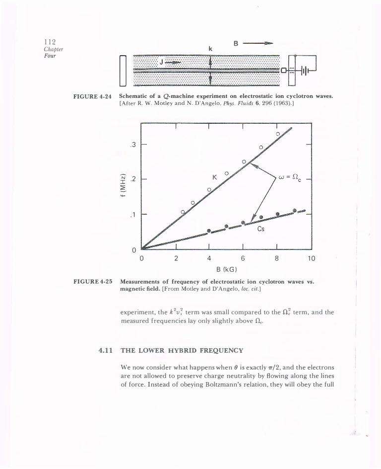
1 12 Chapter Four
FIGURE 4-24
B k
:-:·:·:·:·:·:·:· :·: ·:·:·:· J ·:.·.······: · : · : ·:-:-: ·:·:·:·:·: ·: -:-:·:· : -:·:·:·:·:·:-:-:-:-:-:·:·:·:·: · :·:·: -:·:-:-:-:-:·:·:·:·:-:-: ·:·:·:·:-: · .................. ......... .. .....................
·.·.-.·.·.· .-.·
... · ... . .........
·.·.·.-.· .·.·.-.·.·.·.·.-.·....................................
I � ··r-:··· · ·(··· :� ··r··············· ····j· · · ······r·· ···:·;····r·············op :H:·::: :\::(:::t::i:::::::::::;:�:�:
·: ::::·:;:::::·:::I:::�:: ::IIt:·?:::· ::�:\�:::;r;r: ::·:·::::::·;:: :)::?: ·I:�:): :': ::: I
Schematic of a Q-macbine experiment on electrostatic ion cyclotron waves. [After R. W. Motley and N. D'Angelo, Phys. Fluids 6, 296 (1963).]
.3
:I: .2 �
.1
0 0 2 4 6 8 10
B (kG)
FIGURE 4-25 Measurements of frequency of electrostatic ion cyclotron waves vs. magnetic field. [From Motley and D'Angelo, loc. cit.]
experiment, the k2v; term was small compared to then� term, and the
measured frequencies lay only slightly above fie.
4.11 THE LOWER HYBRID FREQUENCY
We now consider what happens when () is exactly 7T/2, and the electrons are not allowed to preserve charge neutrality by flowing along the lines
of force. Instead of obeying Boltzmann's relation, they will obey the full

equation of motion, Eq. [3-62]. If we keep the electron mass finite, this equation is nontrivial even if we assume T. = 0 and drop the Vp, term:.
hence, we shall do so in the interest of simplicity. The ion equation of motion is unchanged from Eq. [4-63]:
ek D.�) -1
v· = - 4>1 ( 1 - --, tx Mw · w-
[4-68]
By changing e to-e, M tom, and D., to-w, in Eq. [4-68], we can write
down the result of solving Eq. [3-62] for electrons, with T, = 0:
k 2 -1 e ( w,) Vex =--c/>1 1-2
mw w
The equations of continuity give
k n;1 =no-v; I
w
[4-69]
[4-70]
The plasma approximation n; = n. then requires v; 1 = v, 1• Setting Eqs.
[4-68] and [4-69] equal to each other, we have
( D.�) ( w�) M 1 - w 2 = -m 1 -w
2
[4-71]
This is called the lower hybrid frequency. If we had used Poisson's equation
instead of the plasma approximation, we would have obtained
[4-7la]
In low-density plasmas the latter term actually domin ates. The plasma approximation is not valid at such high frequencies. Lower hybrid oscillations can be observed only if (J is very close to 1T/2.
1 13 Waves in
Plasmas

1 14 Chapter Four
4.12 ELECTROMAGNETIC WAVES WITH B0 = 0
Next in the order of complexity come waves with B1 ,C. 0. These are transverse electromagnetic waves-light waves or radio waves traveling
through a plasma. We begin with a brief review of light waves in a
vacuum. The relevant Maxwell equations are
[4-72]
[4-73]
since in a vacuum j = 0 and Eo/1-o = c -2_ Taking the curl of Eq. [ 4-73]
and substituting into the time derivative of Eq. [4-72], we have
c 2V x (V x B 1) = v x :E 1 = -8 1
Again assuming planes waves varying as exp [i(kx- wt)], we have
w2B1 = -c2k x (k X B1) = -c2[k(k · B1)- k2B1]
[4-74]
[4-75]
Since k · B 1 = -iV · B 1 = 0 by another of Maxwell's equations, the result
IS
[4-76]
and c is the phase velocity w/ k of light waves. In a plasma with B0 = 0, Eq. [4-72] is unchanged, but we must add
a term i1/t<o to Eq. [4-73] to account for currents due to first-order charged particle motions:
The time derivative of this is
2 • 1 aj 1 •• cVxBI =--+EI
€o at
while the curl of Eq. [ 4-72] is
v x (V x E1) = V(V- E1)- V2E1 = -v x :81
[4-77]
[4-78]
[4-79]
Eliminating V x B1 and assuming an exp [i(k · r- wt)] dependence, we
have
By transverse waves we mean k · E1 = 0, so· this becomes
( 2 2k2)E . . I w - c 1 =-zwJ1 t<o
[4-80]
[4-81]
L

If we consider light waves or microwaves, these will be of such high
frequency that the ions can be considered as fixed. The current j 1 then
comes entirely from electron motion:
[4-82)
From the linearized electron equation of motion, we have (for KT, = 0):
ave! m -- = -eE
at
eE1 V , t = -.
tmUJ
Equation [ 4-81] now can be written
[4-83)
[4-84]
The expression for w � is recognizable on the right-hand side, and the result is
2 2 2 2 UJ = Wp + C k [4-85]
This is the dispersion relation for electromagnetic waves propagating
in a plasma with no de magnetic field. We see that the vacuum relation
[ 4-76] is modified by a term w ! reminiscent of plasma oscillations. The
phase velocity of a light wave in a plasma is greater than the velocity of
light:
2 2 2 w 2 UJp 2 v<t> =---., = c +-9>c
k- k-[4-86]
However, the group velocity cannot exceed the velocity of light. From Eq. (4-85), we find
[4-87]
so that vg is less than c whenever vq, is greater than c. The dispersion
relation [4-85] is shown in Fig. 4-26. This diagram resembles that of Fig.
4-5 for plasma waves, but the dispersion relation is really quite different because the asymptotic velocity c in Fig. 4-26 is so much larger than the thermal velocity v,h in Fig. 4-5. More importantly, there is a difference
in damping of the waves. Plasma waves with large kv,h are highly damped, a result we shall obtain from kinetic theory in Chapter 7. Electromagnetic
1 15 Waves in
Plasmas
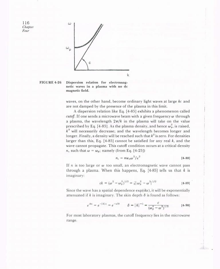
116 Chapter Four
k
FIGURE 4-26 Dispersion relation for electromagnetic waves in a plasma with no qc magnetic field.
waves, on the other hand, become ordinary light waves at large kc and
are not damped by the presence of the plasma in this limit.
A dispersion relation like Eq. [ 4-85] exhibits a phenomenon called
cutoff. If one sends a microwave beam with a given frequency w through
a plasma, the wavelength 2-rr/ k in the plasma will take on the value
prescribed by Eq. [ 4-85]. As the plasma density, and hence w! , is raised,
k2 will necessarily decrease; and the wavelength becomes longer and longer. Finally, a density will be reached such that k2 is zero. For densities
larger than this, Eq. [ 4-85] cannot be satisfied for any real k, and the wave cannot propagate. This cutoff condition occurs at a critical density nc such that w = wp; namely (from Eq. [4-25])
nc = me:0w2/e
2 [4-88]
If n is too large or w too small, an electromagnetic wave cannot pass
through a plasma. When this happens, Eq. [4-85] tells us that k is
imaginary:
k ( 2 2
) I /2 'I 2 2 1 1 /2
C = W - Wp = Z Wp - W [4-89]
Since the wave has a spatial dependence exp(ikx), it will be exponentially attenuated if k is imaginary. The skin depth 8 is found as follows:
eikx
= e-ikix = e-x/8 [4-90]
For most laboratory plasmas, the cutoff frequency lies in the microwave
range.
_L

EXPERIMENTAL APPLICATIONS 4.13
The phenomenon of cutoff suggests an easy way to measure plasma density. A beam of microwaves generated by a klystron is launched
toward the plasma by a horn antenna (Fig. 4-27). The transmitted beam is collected by another horn and is detected by a crystal. As the frequency
or the plasma density is varied, the detected signal will disappear
whenever the condition [ 4-88] is satisfied somewhere in the plasma. This
procedure gives the maximum density. It is not a convenient or versatile scheme because the range of frequencies generated by a single microwave generator is limited.
A widely used method of density measurement relies on the disper
sion, or variation of index of refraction, predicted by Eq. [4-85]. The
index of refraction n is defined as
n = c/vcb = ck/w [4-91)
This clearly varies with w, and a plasma is a dispersive medium. A
microwave interferometer employing the same physical principles as the
Michelson interferometer is used to measure density (Fig. 4-28). The
signal from a klystron is split into two paths. Part of the signal goes to
the detector through the "reference leg." The other part is sent through
the plasma with horn antennas. The detector responds to the mean square of the sum of the amplitudes of the two received signals. These signals are adjusted to be equal in amplitude and 180° out of phase in
the absence of plasma by the attenuator and phase shifter, so that the detector output is zero. When the plasma is turned on, the phase of the signal in the plasma leg is changed as the wavelength increases (Fig. 4-29). The detector then gives a finite output signal. As the density
increases, the detector output goes through a maximum and a minimum
every time the phase shift changes by 360°. The average density in the
PLASMA
�K:L v::::s�T�R�O�N�===�E::--__,_,_ •••••••••• ��---t...:::D.::_ET.:_:E:,:C:_:T_::O:,:_R:.J
Microwave measurement of plasma density by the cutoff of the transmitted FIGURE 4-27
signal.
1 17 Waves in
Plasmas

1 18 Chapter Four
MAGIC
TEE
plasma is found from the number of such fringe shifts. Actually, one
usually uses a high enough frequency that the fringe shift is kept small.
Then the density is linearly proportional to the fringe shift (Problem 4-13). The sensitivity of this technique at low densities is limited to the
stability of the reference leg against vibrations and thermal expansion. Corrections must also be made for attenuation due to collisions and for diffraction and refraction by the finite-sized plasma.
The fact that the index of refraction is less than unity for a plasma has some interesting consequences. A convex plasma lens (Fig. 4-30) is divergent rather than convergent. This effect is important in the laser
solenoid proposal for a linear fusion reactor. A plasma hundreds of
meters long is confined by a strong magnetic field and heated by absorp
tion of C02 laser radiation (Fig. 4-31). If the plasma has a normal density
profile (maximum on the axis), it behaves like a negative lens and causes
the laser beam to diverge into the walls. If an inverted density profile
(minimum on the axis) can be created, however, the lens effect becomes converging; and the radiation is focused and trapped by the plasma. The inverted profile can be produced by squeezing the plasma with a
pulsed coil surrounding it, or it can be produced by the laser beam itself. As the beam heats the plasma, the latter expands, decreasing the density at the center of the beam. The C02 laser operates at A = 10.6 f.Lm,
WAVE GUIDE
�REFERENCE LEG----I ATTENUATOR
r-PLASMA LEG�
<rr:H�:uu� PHASE SHIFTER
:::::::::::::::::::::::::::
DETECTOR OSCILLOSCOPE
PLASMA
FIGURE 4-28 A microwave interferometer for plasma density measurement.

n
I
WAVE PATTERN IN PLASMA
DETECTOR OUTPUT
DENSITY
CUTOFF
The observed signal from an interferometer (right) as plasma density is FIGURE 4-29
increased, and the corresponding wave patterns in the plasma (left).
LASER
A plasma lens has unusual optical proper- FIGURE 4-30 ties, since the index of refraction is less than unity.
A plasma confined in a long, linear solenoid will trap the C02 laser light used FIGURE 4-31
to heat it only if the plasma has a density minimum on axis. The vacuum chamber has been omitted for clarity.
1 19 Waves in
Plasmas

120 Chapter Four
corresponding to a frequency
The critical density is, from Eq. [4-88],
However, because of the long path lengths involved, the refraction effects
are important even at densities of 1022 m -
3 . The focusing effect of a
hollow plasma has been shown experimentally. Perhaps the best known effect of the plasma cutoff is the application
to shortwave radio communication. When a radio wave reaches an altitude in the ionosphere where the plasma density is sufficiently high,
the wave is reflected (Fig. 4-32), making it possible to send signals around
the earth. If we take the maximum density to be 1012 m -3 the critical
frequency is of the order of 10 MHz (cf. Eq. [4-26]). To communicate
with space vehicles, it is necessary to use frequencies above this in order to penetrate the ionosphere. However, during reentry of a space vehicle,
a plasma is generated by the intense heat of friction. This causes a plasma cutoff, resulting in a communications blackout during reentry (Fig. 4-32).
PROBLEMS 4-9. A space capsule making a reentry into the earth's atmosphere suffers a communications blackout because a plasma is generated by the shock wave in front of the capsule. If the radio operates at a frequency of 300 MHz, what is the minimum plasma density during the blackout?
4-10. Hannes Alfven, the first plasma physicist to be awarded the Nobel prize, has suggested that perhaps the primordial universe was symmetric between matter and antimatter. Suppose the universe was at one time a uniform mixture of protons, antiprotons, electrons, and positrons, each species having a density n0•
(a) Work out the dispersion relation for high-frequency electromagnetic waves in this plasma. You may neglect collisions, annihilations, and thermal effects.
(b) Work out the dispersion relation for ion waves, using Poisson's equation. You may neglect T, (but not T,) and assume that all leptons follow the Boltzmann relation.
4-11. For electromagnetic waves, show that the index of refraction is equal to the square root of the appropriate plasma dielectric constant (cf. Problem 4-4).
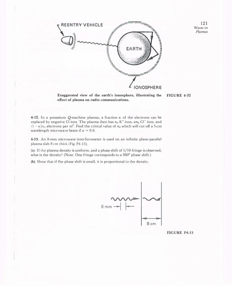
\EENTRY VEHICLE
'l. � � X
?
;;ONOSPHERE Exaggerated view of the earth's ionosphere, illustrating the FIGURE 4-32
effect of plasma on radio communications.
4-12. In a potassium Q-machine plasma, a fraction K of the electrons can be replaced by negative Cl ions. The plasma then has n0 K+ ions, Kn0 Cl- ions, and (1 - K )no electrons per m3. Find the critical value of n0 which will cut off a 3-cm wavelength microwave beam if K = 0.6.
4-13. An 8-mm microwave interferometer is used on an infinite plane-parallel plasma slab 8 em thick (Fig. P4-13).
(a) If the plasma density is uniform, and a phase shift of 1/10 fringe is observed, what is the density? (Note: One fringe corresponds to a 360° phase shift.)
(b) Show that if rhe phase shift is small, it is proportional to the density.
Scm
FIGURE P4-13
12 1 Waves in
Plasmas

122 Chapter Four
4.14 ELECTROMAGNETIC WAVES PERPENDICULAR TO B0
We now consider the propagation of electromagnetic waves when a magnetic field is present. We treat first the case of perpendicular propa
gation, k .l Bo. If we take transverse waves, with k .l E 1, there are still
two choices: E1 can be parallel to B0 or perpendicular to B0 (Fig. 4-33).
4.14.1 Ordinary Wave, E1 II B0
If E1 is parallel to Bo, we may take Bo = B0z, E1 = E1z, and k = kx. In
a real experiment, this geometry is approximated by a beam of micro
waves incident on a plasma column with the narrow dimension of the waveguide in line with B0 (Fig. 4-34).
The wave equation for this case is still given by Eq. [4-81]:
[4-921
Since E1 = E 1z, we need only the component v.,. This is given by the equation of motion
[4-931
Since this is the same as the equation for B0 = 0, the result is the same
as we had previously for B0 = 0:
I 2 2 2k2 W = Wp + C
z t Bo E11IB0
E,lBO * y
k
X
FIGURE 4-33 Geometry for electromagnetic waves propagating at right angles to B0.
[4-94]

An ordinary wave launched from a waveguide antenna toward FIGURE 4-34 a magnetized plasma column.
This wave, with E1 II B0, is called the ordinary wave. The terminology "ordinary" and "extraordinary" is taken from crystal optics; however,
the terms have been interchanged. In plasma physics, it makes more sense to let the "ordinary" wave be the one that is not affected by the
magnetic field. Strict analogy with crystal optics would have required
calling this the "extraordinary" wave.
Extraordinary Wave, E1 _l_ B0 4.14.2
If Et is perpendicular to B0, the electron motion will be affected by B0,
and the dispersion relation will be changed. To treat this case, one would
be tempted to take E1 = EtY and k = kx (Fig. 4-33). However, it turns out that waves with E1 _1_ B0 tend to be elliptically polarized instead of plane polarized. That is, as such a wave propagates into a plasma, it develops a component Ex along k, thus becoming partly longitudinal and
partly transverse. To treat this mode properly, we must allow E1 to have
123 Waves in
Plasmas

124 Chapter Four
z
y
X
FIGURE 4-35 The E-vector of an extraordinary wave is elliptically polarized. The components Ex and E, oscillate 90° out of phase, so that the total electric field vector E1 has a tip that moves in an ellipse once in each wave period.
both x andy components (Fig. 4-35):
E1 = Exx + E,y [4-95]
The lineari:zed electron equation of motion (with KT, = 0) is now
-imwv,1 = -e(E + v,1 X B0)
Only the x andy components are nontrivial; they are
-ze v, = - (E1- VxBo)
mw
[4-96]
[4-97]
The subscripts 1 and e have been suppressed. Solving for Vx and v, as
usual, we find
e ( . w, ) ( w �) -I
Vx = mw -zEx - -;;; E, 1 - w 2
e ( . w, ) ( w �)-I v1 =
mw -zE1 + w Ex 1 - w 2
[4-98]
The wave equation is given by Eq. [4-80], where we must now keep the
longitudinal term k · E1 = kEx:
(w2- c2k2)E1 + c2kExk = -iwjr/Eo = inoweve�/Eo [4-99]

Separating this into x and y components and using Eq. [ 4-98], we have . 2 -1 w2Ex = _ twnoe _e_ (iEx + w, Ey)(l _ w;)
€0 mw w w
Introducing the definition of wp, we may write this set as
[4-100)
[4-101]
These are two simultaneous equations for Ex and Ey which are compatible only if the determinant of the coefficients vanishes:
II� �ll=o [4-102)
Since the coefficient A is w 2- w t where wh is the upper hybrid frequency defined by Eq. [4-60], the condition AD = BC can be written
[4-103]
This can be simplified by a few algebraic manipulations. Replacing the first w� on the right-hand side by w; + w� and multiplying through by w2 - wt we have
2k 2 2 2 2 4 2/ 2 _c _ _ 1_wp(w -wh)+(wpw, w) 2 - 2 2 2 2 w (w -w,)(w -wh)
[4-104)
1 25 Waves in Plasmas
126 Chapter Four
4.15
This is the dispersion relation for the extraordinary wave. It is an electromagnetic wave, partly transverse and partly longitudinal, which propagates perpendicular to Bo with E1 perpendicular to B0.
CUTOFFS AND RESONANCES
The dispersion relation for the extraordinary wave is considerably
more complicated than any we have met up to now. To analyze what it means, it is useful to define the terms cutoff and resonance. A cutoff occurs in a plasma when the index of refraction goes to zero; that is, when the wavelength becomes infinite, since ii = ck/ w. A resonance occurs when the index of refraction becomes infinite; that is, when the wavelength becomes zero. As a wave propagates through a region in which Wp and we are changing, it may encounter cutoffs and resonances. A wave is generally reflected at a cutoff and absorbed at a resonance.
The resonance of the extraordinary wave is found by setting k equal to infinity in Eq. [ 4- 1 04]. For any finite w, k � ro implies w � wh, so that a resonance occurs at a point in the plasma where
2 2 2 2 Wh = Wp +We = W [4-105]
This is easily recognized as the dispersion relation for electrostatic waves propagating across B0 (Eq. [4-60]). As a wave of given w approaches the resonance point, both its phase velocity and its group velocity approach zero, and the wave energy is converted into upper hybrid oscillations. The extraordinary wave is partly electromagnetic and partly electrostatic; it can easily be shown (Problem 4-14) that at resonance this wave loses its electromagnetic character and becomes an electrostatic oscillation.
The cutoffs of the extraordinary wave are found by setting k equal to zero in Eq. [4- 104]. Dividing by w2-w�, we can write the resulting equation for w as follows:
A few tricky algebraic steps will yield a simple expression for w: 2 2 We Wp
1- 2 2-� w -wp w
1_ w; _ w�/w2
w2- 1- (w�/w2)
[4-106]
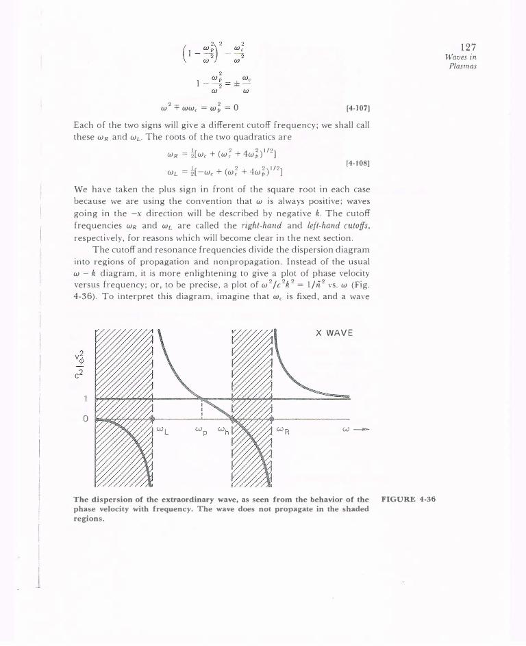
2 2 0 W =F WWe = Wp = [4-107]
Each of the two signs will give a different cutoff frequency; we shall call
these wR and wL. The roots of the two quadratics are
WR =�[we+ (w; + 4w�)112] I [ 2 2 I /2] WL = 2 -we+ (we + 4wp)
[4-108]
We have taken the plus sign in front of the square root in each case
because we are using the convention that w is always positive; waves
going in the -x direction will be described by negative k. The cutoff
frequencies wR and wL are called the right-hand and left-hand cutoffs,
respectively, for reasons which will become clear in the next section.
The cutoff and resonance frequencies divide the dispersion diagram
into regions of propagation and nonpropagation. Instead of the usual
w - k diagram, it is more enlightening to give a plot of phase velocity
versus frequency; or, to be precise, a plot of w2/c2k2 = I/1i2 vs. w (Fig.
4-36). To interpret this diagram, imagine that We is fixed, and a wave
X WAVE
0 w--
The dispersion of the extraordinary wave, as seen from the behavior of the FIGURE 4-36
phase velocity with frequency. The wave does not propagate in the shaded regions.
127 Waves in
Plasmas

1 28 Chapter Four
0 WAVE
0 w---
FIGURE 4-37 A similar dispersion diagram for the ordinary wave.
with a fixed freque:1cy w is sent into a plasrn,a from the outside. As the
wave encounters regions of increasing density, the frequencies wL, Wp, wh, and WR all increase, moving to the right in the diagram. This is the
same as if the density were fixed and the frequency w were gradually being decreased. Taking the latter point of view, we see that at large w (or low density), the phase velocity approaches the velocity of liE,ht. As the wave travels further, v"' increases until the right-hand cutoff w = wR is encountered. There, v<�> becomes infinite. Between the w = WR and w = wh layers, w2/k2 is negative, and there is no propagation possible. At w = wh, there is a resonance, and v"' goes to zero. Between w = wh and w = WL, propagation is again possible. In this region, the wave travels either faster or slower than c depending on whether w is smaller or
larger than w'p. From Eq. [4-104], it is clear that at w = wp, the wave
travels at the velocity c. For w < wL, there is another region of non propagation. The extraordinary wave, therefore, has two regions of propagation separated by a stop band.
By way of comparison, we show in Fig. 4-37 the same sort of diagram for the ordinary wave. This dispersion relation has only one cutoff and no resonances.
4.16 ELECTROMAGNETIC WAVES PARALLEL TO B0
Now we let k lie along the z axis and allow E1 to have both transverse components Ex and E�:
k = ki [4-109]
I i
I
I I I I I I I I I
J I I I I
.L

The wave equation [ 4-99] for the extraordinary wave can still be used if we simply change k from kx to kz. From Eq. [4-100], the components are now
2 . 2 2 2 Wp ( ZWe ) (w - C k )Ex = 2/ 2 Ex - -Ey 1-We W W
2 . 2 2 2 Wp ( ZWe ) (w - c k )Ey = 2/ 2 Ey + -Ex
1-W e W W
Using the abbreviation
we can write the coupled equations for Ex and E1 as
2 2 2 . We (w - c k -a)Ex + za- Ey = 0
w
2 2k2 . We (w - c -a)Ey- za-Ex = 0
w
Setting the determinant of the coefficients to zero, we have
(w2-c2k2- a)2 = (awe/w)2
Thus
w2- c2k2-a = ±awc/w
w2-c2k2=a(1±We) = w�
/ 2 (1±We) W 1 -(w e W ) W
2 1 ± (we/w) w; = Wp = [1 + (we/w)][I-(wc/w)] 1 =t= (wc/w)
[4-110]
[4-111]
[4-112]
[4-ll3]
[4-ll4]
[4-ll5]
The =F sign indicates that there are two possible solutions to Eq. [ 4-112] corresponding to two different waves that can propagate along B0. The dispersion relations are
2k2 2/ 2 ii2 = c __ = 1- wp w w2 1-(we/w)
2k 2 2/ 2 -2 C Wp W n = -9- = 1 ----'----
w- I+ (wc/w)
(R wave) [4-116]
(L wave) [4-ll7]
129 Waves in Plasmas

130 Chapter Four
z
X
±k ±k
y
FIGURE 4-38 Geometry of right- and left-handed circularly polarized waves propagating along B0.
The R and L waves turn out to be circularly polarized, the designations R and L meaning, respectively, right-hand circular polarization and left
hand circular polarization (Problem 4- 17). The geometry is shown in Fig. 4-38. The electric field vector for the R wave rotates clockwise in time as viewed along the direction of B0, and vice versa for the L wave. Since Eqs. [ 4-116] and [ 4- 117] depend only on k 2, the direction of rotation of the E vector is independent of the sign of k ; the polarization is the same for waves propagating in the opposite direction. To summarize: The principal electromagnetic waves propagating along B0 are a right-hand (R) and a left-hand (L) circularly polarized wave; the principal waves propagating across B0 are a plane-polarized wave (0-wave) and an elliptically polarized wave (X-wave).
We next consider the cutoffs and resonances of the R and L waves. For the R wave, k becomes infinite at w = We; the wave is then in resonance with the cyclotron motion of the electrons. The direction of rotation of the plane of polarization is the same as the direction of gyration of electrons; the wave loses its energy in continuously accelerating the electrons, and it cannot propagate. The L wave, on the other hand, does not have a cyclotron resonance with the electrons because it rotates in the opposite sense. As is easily seen from Eq. [ 4- 1 17], the L wave does not have a resonance for positive w. If we had included ion motions in our treatment, the L wave would have been found to have a resonance at w = flc, since it would then rotate with the ion gyration.
I I I I I
I I I I I I

0
'\ L WAVE '
:\/ I � I '- , I -... ..... I ..... .....
',w/2 '
\\ I \I l I
I
----- ... --.
WR w ---
The u';/c2 vs. w diagrams for the Land R waves. The regions of non propagation FIGURE 4-39 (u';/c2 < 0) have not been shaded, since they are different for the two waves.
The cutoffs are obtained by setting k = 0 in Eqs. [4- 1 16] and [4- 1 17]. We then obtain the same equations as we had for the cutoffs of the X wave (Eq. [4- 107]). Thus the cutoff frequencies are the same as before. The R wave, with the minus sign in Eqs. [ 4- 1 16] and [ 4- 1 07], has the higher cutoff frequency WR given by Eq. [4- 108]; the L wave, with the plus sign, has the lower cutoff frequency wL. This is the reason for the notation wR, wL chosen previously. The dispersion diagram for the R and L waves is shown in Fig. 4-39. The L wave has a stop band at low frequencies; it behaves like the 0 wave except that the cutoff occurs at wL instead of Wp. The R wave has a stop band between WR and we, but there is a second band of propagation, with vq, < c, below we. The wave in this low-frequency region is called the whistler mode and is of extreme importance in the study of ionospheric phenomena.
EXPERIMENTAL CONSEQUENCES 4.17
The Whistler Mode 4.17 .1
Early investigators of radio emissions from the ionosphere were
rewarded by various whistling sounds in the audiofrequency range. Figure 4-40 shows a spectrogram of the frequency received as a function
13 1 Waves in
Plasmas

132 Chapter Four
20-
N I � '+-
0 -
-=-- -. .. -'-�
I
, __
I I 0 2 3
t (sec) FIGURE 4-40 Actual spectrograms of whistler signals, showing the cur
vature caused by the low-frequency branch of the R-wave dispersion relation (Fig. 4-39). At each time t, the receiver rapidly scans the frequency range between 0 and 20kHz, tracing a vertical line. The recorder makes a spot whose darkness is proportional to the intensity of the signal at each frequency. The downward motion of the dark spot with time then indicates a descending glide tone. [Courtesy of D. L. Carpen ter,]. Ceophys. Res. 71, 693 (1966).]
of time. There is typically a series of descending glide tones, which can be heard over a loudspeaker. This phenomenon is easily explained in terms of the dispersion characteristics of the R wave. When a lightning flash occurs in the Southern Hemisphere, radio noise of all frequencies is generated. Among the waves generated in the plasma of the ionosphere and magnetosphere are R waves traveling along the earth's magnetic field. These waves are guided by the field lines and are detected by observers in Canada. However, different frequencies arrive at different times. From Fig. 4-39, it can be seen that for w < wc/2, the phase velocity increases with frequency (Problem 4- 19). It can also be shown (Problem 4-20) that the group velocity increases with frequency. Thus the low frequencies arrive later, giving rise to the descending tone. Several whistles can be produced by a single lightning flash because of propagation along different tubes of force A, B, C (Fig. 4-4 1). Since the waves have w < we, they must have frequencies lower than the lowest gyrofrequency along the tube of force, about 100 kHz.' Either the whistles lie directly in the audio range or they can easily be converted into audio signals by heterodyning.
I I l· i ' I I I I I I
I
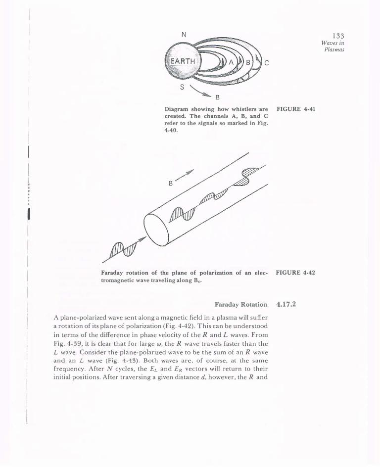
I I I: r ,.
J I I I I I I
c
Diagram showing how whistlers are FIGURE 4-41 created. The channels A, B, and C refer to the signals so marked in Fig. 4-40.
Faraday rotation of the plane of polarization of an elec- FIGURE 4-42
tromagnetic wave traveling along B0•
Faraday Rotation 4.17 .2
A plane-polarized wave sent along a magnetic field in a plasma will suffer a rotation of its plane of polarization (Fig. 4-42). This can be understood in terms of the difference in phase velocity of the R and L waves. From Fig. 4-39, it is clear that for large w, the R wave travels faster than the L wave. Consider the plane-polarized wave to be the sum of an R wave and an L wave (Fig. 4-43). Both waves are, of course, at the same
frequency. After N cycles, the EL and ER vectors will return to their initial positions. After traversing a given distanced, however, the R and
133 Waves in Plasmas

1 34 Chapter Four
+
FIGURE 4-43 A plane-polarized wave as the sum of left- and right
handed circularly polarized waves.
+
FIGURE 4-44 After traversing the plasma, the L wave is advanced in phase relative to the R wave, and the plane of polarization is rotated.
L waves will have undergone a different number of cycles, since they require a different amount of time to cover the distance. Since the L wave travels more slowly, it will have undergone N + E cycles at the position where the R wave has undergone N cycles. The vectors then have the positions shown in Fig. 4-44. The plane of polarization is seen to have rotated. A measurement of this rotation by means of a microwave horn can be used to give a value of w! and, hence, of the density (Problem 4-22). The effect of Faraday rotation has been verified experimentally, but it is not as useful a method of density measurement as microwave interferometry, because access at the ends of a plasma column is usually difficult, and because the effect is small unless the density is so high that refraction becomes a problem.
When powerful pulsed lasers are used to produce a dense plasma by vaporizing a solid target, magnetic fields of megagauss intensities are sometimes spontaneously generated. These have been detected by Faraday rotation using laser light of higher frequency than the main beam. In interstellar space, the path lengths are so long that Faraday rotation
I I
I I I I I I I I I I

135 is important even at very low densities. This effect has been used to explain the polarization of microwave radiation generated by maser action in clouds of OH or H20 molecules during t h e formation of new stars.
Waves in Plasmas
4-14. Prove t h at the extraordinary wave is purely electrostatic at resonance. PROBLEMS Hint: Express t h e ratio E,/ E. as a function of w and set w equal t o wh.
4-15. Prove t h at t he critical points on Fig . 4-36 are correctly ordered; namely, that WL < Wp < Wh < WR.
4-16. Show t h at t he X-wave group velocity v anishes at cutoffs and resonances. You may neglect ion motions.
4-1 7. Prove that t he R and L waves are right- and left-circularly polarized as follows:
(a) Show that t he simultaneous equations for E. and E, can be writte n i n t he for m
F(w )(E. - iE,) = 0 , G(w)(E. + iE,) = 0
where F(w ) = 0 for the R wave and G (w) = 0 for the L wave.
(b) For t he R wave, G (w) 'i 0; and therefore Ex = -iE,. Recalling the exponential time dependence of E, show that E t hen rotates i n the electron gyration direction. Confir m that E rot ates in the opposite direction for t he L wave.
(c) For the R wave, draw the helices traced by the tip of the E v ector i n space at a given time for (i) k, > 0 and (ii) k, < 0 . N ote that t he rotation of E is in t he same direction i n both instances i f one stays at a fixed position and watches t he helix pass by.
4-18. Left- hand circularly polarized w av es are propagated along a u ni form magnetic field B = Boi into a plasma with density increasi ng wit h z. At what density is cutoff reac hed iff= 2.8 GHz and B0 = 0 .3 T?
4-19. Show t hat t he w histler mode has maxi mu m phase velocity at w = w,/2 and that t his maximum is l ess than the velocity of light.
4-20. Show that t he grou p velocity of the w hi stler mode is proportional t o w 112
i f w « w, and E » l.
4-2 1. Show t hat t here is no Faraday rotation i n a positronium plasma (equal numbers of positrons and electrons).
4-22. Faraday r otation of an 8-m m-wavelength microwave beam in a unifor m plasma i n a 0. 1-T magnetic field is measured . T h e plane o f polarization i s found t o be rotated 90° after traversing l m of plasma. What is the density?
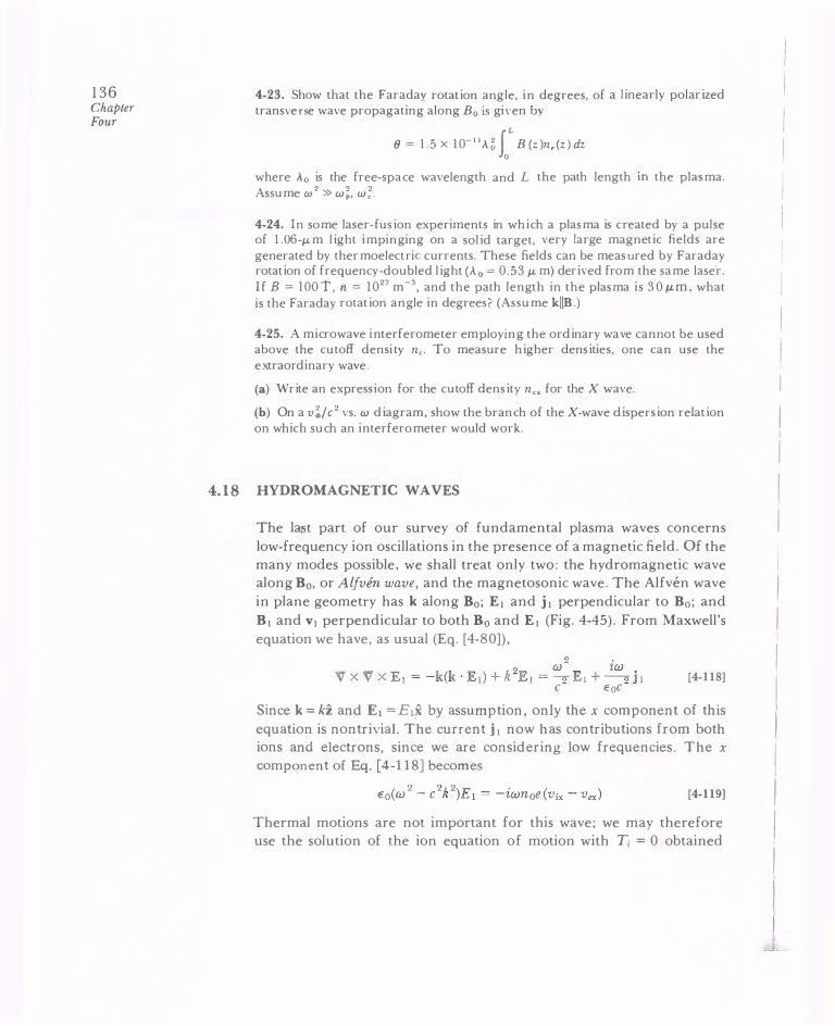
136 Chapter Four
4.18
4-23. Show that the F araday rotation angle, i n degrees, of a linearly polarized transverse wave propagating along Bois gi ven by
(} = 1.5 x 10-"A� 1L B(z)n,(z)dz
where A0 is the free-space wavelength and L the path length m the plasma. Assume w2 » w �, w ; .
4-24. I n some laser- fusion ex periments in which a plasma is c reated by a pulse of 1.06-� m light impi n ging on a solid target, very large magnetic fields are generated by thermoelectric currents. These fields can be measured by F araday rotation of frequency-doubled light (A0 = 0.53 �m) derived from the same lase·r . I f B = 100 1, n = 1027 m -3, and the path length in the plasma i s 30 � m, what is the Faraday rotation angle in degrees? (Assume kiiB.)
4-25. A microwave i nterferometer em ployin g the ordinary wave cannot be used above the cutoff densi ty n,. To measure higher densities, one can use the extraordinary wave.
(a) Write an ex pression for the cutoff density ncx for the X wave.
(b) On a v!/c2 vs. w diagram , show the branch of the X-wave dispersion relation on whic h such an i nterferometer would work.
HYDROMAGNETIC WAVES
The la1>t part of our survey of fundamental plasma waves concerns low-frequency ion oscillations in the presence of a magnetic field. Of the many modes possible, we shall treat only two: the hydromagnetic wave along B0, or Alfvin wave, and the magnetosonic wave. The Alfven wave in plane geometry has k along 80; E1 and j 1 perpendicular to Bo; and B1 and v1 perpendicular to both 80 and E1 (Fig. 4-45). From Maxwell's equation we have, as usual (Eq. [4-80]),
[4-118]
Since k = kZ and E1 = E1x by assumption, only the x component of this
equation is nontrivial. The current j1 now has contributions from both
ions and electrons, since we are considering low frequencies. The x
compon ent of Eq. [ 4-118] becomes [4-119]
Thermal motions are not important for this wave; we may therefore use the solution of the ion equation of motion with T; = 0 obtained
I
I I I I I I I I
I I I I I I I I ' I

z
y
v 1' s,
X Geometry of an Alfven wave propagating FIGURE 4-45 along Bo.
previously in Eq. [4-63]. For completeness, we include here the component v;y, which was not written explicitly before:
ie D� -I
V;x = Mw ( 1- w2) £1
e De ( D�)-1 v· = --- 1-- E1 'Y Mw w w2
[4-120]
The corresponding solution to the electron equation of motion is found by letting M � m, e � -e, De � -we, and then taking the limit w� » w2:
. 2 ze w v,x = -- �E��o mw We
[4-121]
In this limit, the Larmor gyrations of the electrons are neglected, and the electrons have simply an E x B drift in the y direction. Inserting these solutions into Eq. [ 4-119], we obtain
2 2 2 . ie ( n;) -I Eo(w - c k )EI = -zwn0e-- 1-� £1 Mw w [4-122]
They components of v1 are needed only for the physical picture to be given later. Using the definition of the ion plasma frequency Dp (Eq.
137 Waves in Plasmas

138 Chapter Four
[4-49]), we have
[4-123)
We must now make the further assumption w 2 « !1�; hydromagnetic waves have frequencies well below ion cyclotron resonance. In this limit, Eq. [4-123] becomes
2 2k 2 2 D! 2 n0e 2 M2 2 p w -c = -w � = -w -- � = -w --? n, EoM e Bo EoBo
2 2 2 w c c
fl = 1 + (p/E0B�) = _1_+_(_P_I-L_o_/ B----,6 )-c"2 [4-124]
where p is the mass density n0M. This answer is no surprise, since the denominator can be recognized as the relative dielectric constant for low-frequency perpendicular motions (Eq. [3-28]). Equation [4-124]
simply gives the phase velocity for an electromagnetic wave in a dielectric medium:
w c c -k = ( )1/2 = "172 ER/.LR E R
for 1-LR = 1
As we have seen previously, E is much larger than unity for most laboratory plasmas, and Eq. [ 4-124] can be written approximately as
w Bo - = vcb = 1/? k (!-LoP) -[4-125]
These hydromagnetic waves travel along B0 at a constant velocity VA,
called the A lfvin velocity :
_ I 112 VA= B (P-oP) [4-126]
This is a characteristic velocity at which perturbations of the lines of force travel. The dielectric constant of Eq. [3-28] can now be written
[4-127]
Note that v A is small for well-developed plasmas with appreciable density, and therefore ER is large.
To understand what happens physically in an Alfven wave, recall that this is an electromagnetic wave with a fluctuating magnetic field B1

I I I
I i I I I ' I i
I I I I I I I i j
given by
Ex = (w/k)B1 [4-128)
The small component B1, when added to B0, gives the lines of force a sinusoidal ripple, shown ex�ggerated in Fig. 4-46. At the point shown, B1 is in the positive y direction, so, according to Eq. [ 4- 128], E, is in the positive x direction if w/ k is in the z direction. The electric field Ex gives the plasma an E1 x B0 drift in the negative y direction. Since we have taken the limit (J) 2 « n;, both ions and electrons will have the same drift v,, according to Eqs. [4- 120] and [4- 12 1]. Thus, the fluid moves up and down in they direction, as previously indicated in Fig. 4-45. The magnitude of this velocity is jE,/ B0j. Since the ripple in the field is moving by at the phase velocity w/ k, the line of force is also moving downward at the point indicated in Fig. 4-46. The downward velocity of the line of force is (w/k)jBy/B0j, which, according to Eq. [4-128], is just equal to the fluid velocity jEx/B0j. Thus, the fluid and the field lines oscillate together as if the particles were stuck to the lines. The lines of force act as if they were mass-loaded strings under tension, and an Alfven wave can be regarded as the propagating disturbance occurring when the strings are plucked. This concept of plasma frozen to lines of force and moving with them is a useful one for understanding many low-frequency plasma phenomena. It can be shown that this notion is an accurate one as long as there is no electric field along B.
It remains for us to see what sustains the electric field Ex which we presupposed was there. As E1 fluctuates, the ions' inertia causes them
X
Relation among the oscillating quantities in an Alfven wave and the (exagger- FIGURE 4-46 ated) distortion of the lines of force.
139 Waves in Plasmas
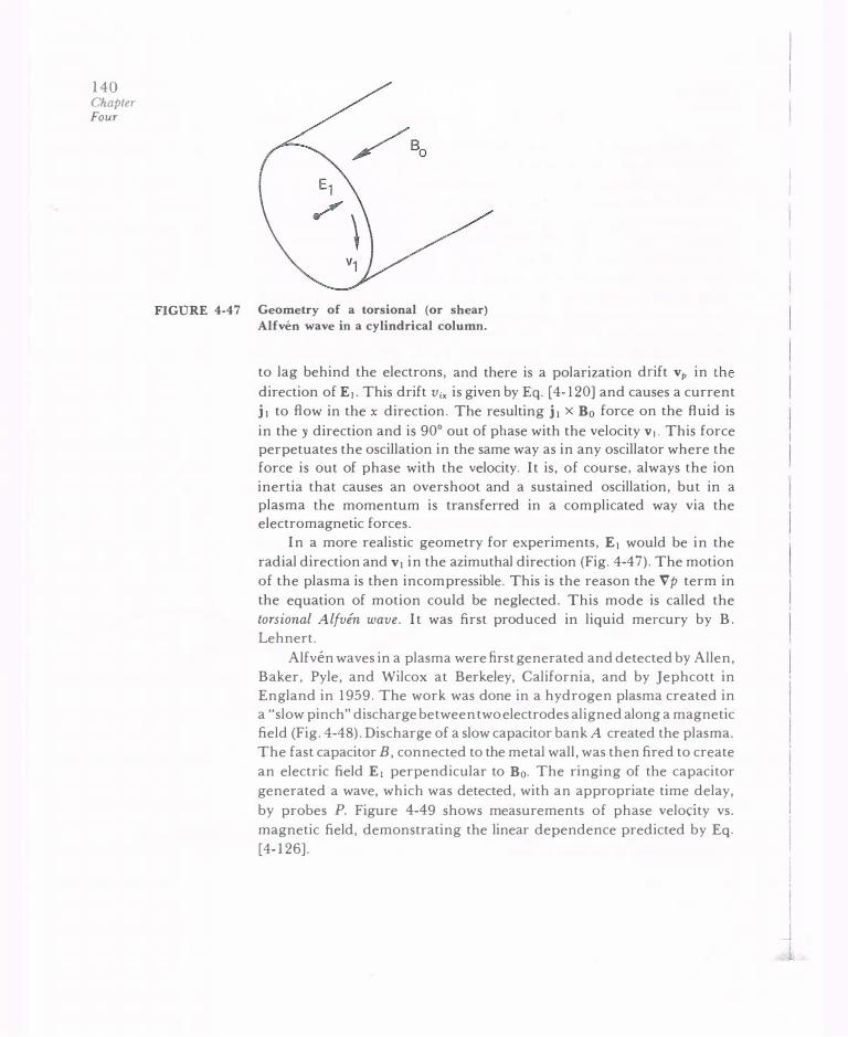
140 Chapter Fou.r
FIGURE 4-47 Geometry of a torsional (or shear) Alfvim wave in a cylindrical column.
to lag behind the electrons, and there is a polarization drift vp in the direction of E1. This drift Vix is given by Eq. [ 4-120] and causes a current j 1 to flow in the x direction. The resulting j 1 x B0 force on the fluid is in they direction and is 90° out of phase with the velocity VJ. This force perpetuates the oscillation in the same way as in any oscillator where the force is out of phase with the velocity. It is, of course, always the ion inertia that causes an overshoot and a sustained oscillation, but in a plasma the momentum is transferred in a complicated way via the electromagnetic forces.
In a more realistic geometry for experiments, E1 would be in the radial direction and v1 in the azimuthal direction (Fig. 4-47). The motion of the plasma is then incompressible. This is the reason the Vp term in the equation of motion could be neglected. This mode is called the torsional Alfven wave. It was first produced in liquid mercury by B. Lehnert.
Alfven waves in a plasma were first generated and detected by Allen, Baker, Pyle, and Wilcox at Berkeley, California, and by Jephcott in England in 1959. The work was done in a hydrogen plasma created in a "slow pinch" discharge between two electrodes aligned along a magnetic field (Fig. 4-48). Discharge of a slow capacitor bank A created the plasma. The fast capacitor B, connected to the metal wall, was then fired to create an electric field E1 perpendicular to B0. The ringing of the capacitor generated a wave, which was detected, with an appropriate time delay, by probes P. Figure 4-49 shows measurements of phase velodty vs. magnetic field, demonstrating the linear dependence predicted by Eq. [4-126].

B
A s o
Schematic of an experiment to detect Alfven waves. [From J. M. Wi lcox, FIGURE 4-48 F. I. Boley, and A . W. DeSilva, Phys. Fluids 3, 15 (I 960).)
6 X 10⁷ I I I I I
5 - 0 -
o.,'
4 - 0� -
(.) ,_§...e Cli 3 - .a-8� -t/) ...._ E a.f'! (.) 2 .,& -0- 1- -> .,-""
t- ,, -
�., 0 I I I I
0 4 8 12 16 20 80 (kG)
Measured phase velocity of Alfven waves vs. magnetic field. [From Wilcox, FIGURE 4-49 Boley, and DeSilva, loc. cit.]
This experiment was a difficult one, because a large magnetic field of 1 T was needed to overcome damping. With large B0, VA, and hence the wavelength, become uncomfortably large unless the density is high. In the experiment of Wilcox et al., a density of 6 X 10²¹ m-3 was used to achieve a low Alfven speed of 2.8 x 10⁵m/sec. Note that it is not possible
141 Waves in Plasmas

142 Chapter Four
4.19
to increase p by using a heavier atom. The frequency w = kv A is proportional to M-1 12, while the cyclotron frequency flc is proportional to M-1. Therefore, the ratio w/ilc is proportional to M112• With heavier atoms it is not possible to satisfy the condition w2 « n�.
MAGNETOSONIC WAVES
Finally, we consider low-frequency electromagnetic waves propagating across B0. Again we may take B0 = Bii and E1 = E 1x, but we now let k = ky (Fig. 4-50). Now we see that the E1 X B0 drifts lie along k, so that the plasma will be compressed and released in the course of the oscillation. It is necessary, therefore, to keep the Vp term in the equation of motion. For the ions, we have
OV;J Mno- = eno(E1 + v; 1 X B0) - y;KT; Vn 1
at
With our choice of E1 and k, this becomes
z
X
ie k y,KT; n 1 v;, = -- (-v;xBo) +- -- -J\tf w w M no
y
k
[4-129]
[4-130]
[4-131]
FIGURE 4-50 Geometry of a magnetosonic wave propagating at right angles to B0.
I I I I I
I I I I I I
I j I I I I J

The equation of continuity yields
so that Eq. [4-13 1] becomes
With the abbreviation
this becomes
Combining this with Eq. [4- 130], we have
ie ifl, ( ifl,) _ 1 v· =-E + - - - (1 - A ) v· 1x Mw x w w 1x
_ ( 1 _ n; 1 w 2) = � V,x 1- A Mw
Ex
[4-132]
[4-133]
[4-134]
[4-135]
This is the only component of v; 1 we shall need, since the only nontrivial component of the wave equation [4-81] is
[4-136]
To obtain v,x, we need only to make the appropriate changes in Eq. [4- 135] and take the limit of small electron mass, so that w2 « w� and w2 « k2v�he:
ie w2 ( k2 -y.KT.) ik2 -y.KT. Vex =- -2 1 - 2 -- Ex � - --2 -- Ex mw w, w m wB0 · e
Putting the last three equations together we have
2 2 2 . [ ie ( 1 - A ) Eo(w - c k )Ex = -zwnoe --Ex r. 2/ 2 Mw 1 - A - (u, w )
ik2M y,KT. J + --2 -- Ex wBo eM
[4-137]
[4-138]
143 Waves in
Plasmas

144 Chapter Four
We shall again assume w 2 « !1�. so that l -A can be neglected relative to n;;w2. With the help of the definitions of !1p and V_.\, we have
Since
2 2k 2( l y.KT.) !1� ( 2 k 2 y,KT,) _ O w -c + --9- +-9 w - -- -
MvA. D� M
Eq. [4- 139] becomes
where v, is the acoustic speed. Finally, we have
[4-139]
[4-140)
[4-142]
This is the dispersion relation for the magnetosonic wave propagating perpendicular to B0. It is an acoustic wave in which the compressions and rarefactions are produced not by motions along E, but by Ex B drifts across E. In the limit B0 � 0, v.-.. � 0, the magnetosonic wave turns into an ordinary ion acoustic wave. In the limit KT � 0, v, � 0, the pressure gradient forces vanish, and the wave becomes a modified Alfven wave. The phase velocity of the magnetosonic mode is almost always larger than v .-.. ; for this reason, it is often called simply the "fast" hydromagnetic wave.
4.20 SUMMARY OF ELEMENTARY PLASMA WAVES
Electron waves (electrostatic)
Bo = 0 or k II Bo:
k _!_ B0:
2 2 3 2 2 w = Wp + 2k v,h
2 2 2 2 w =wp +w, =wh (Plasma oscillations)
(Upper hybrid oscillations)
[4-143]
[4-144]
J

I j l I . I I l I I l
Ion waves (electrostatic)
Bo=Oork jj B0: w2= k2v;
= k 2 y.KT. + 'YiKTi M
(Acoustic waves) [4-145]
k l_ B0:
or
Electron waves (electromagnetic)
Bo = 0: 2 2 k2 2 W = Wp + C
2k2 2 II C Wp
k l_ Bo, E 1 Bo: -2 = 1 - 2
k i! Bo:
w w
9 9 2 9 c -k - _ 1 _ wp/w-
2 -w 1-(wjw)
2k2 2 / 2 C Wp W -9-= 1 - ----"-'---w- 1+(wjw)
Ion waves (electromagnetic)
Bo = 0:
k i! B0:
k l_ B0:
None
(Electrostatic ion
cyclotron waves)
(Lower hybrid
oscillations)
(Light waves)
(0 wave)
(X wave)
(R wave)
(whistler mode)
(L wave)
[4-146]
[4-147]
[4-148)
[4-149]
[4-150]
[4-151]
[4-152]
(Alfven wave) [4-153]
(Magnetosonic wave) [4-154]
This set of dispersion relations is a greatly simplified one covering only the principal directions of propagation. Nonetheless, it is a very useful set of equations to have in mind as a frame of reference for discussing more complicated wave motions. -It is often possible to
145 Waves in Plasmas

146 Chapter Four
4.21
understand a complex situation as a modification or superposition of these basic modes of oscillation.
THE CMA DIAGRAM
When propagation occurs at an angle to the magnetic field, the phase velocities change with angle. Some of the modes listed above with k II B0 and k ..L B0 change continuously into each other; other modes simply disappear at a critical angle. This complicated state of affairs is greatly clarified by the Clemmow-Mullaly-Allis (CMA) diagram, so named for its co-inventors by T. H. Stix. Such a diagram is shown in Fig. 4-51. The CMA diagram is valid, however, only for cold plasmas, with Ti = T. = 0. Extension to finite temperatures introduces so much complexity that the
diagram is no longer useful.
Figure 4-51 is a plot of w,/w vs. w!/w2 or, equivalently, a plot of
magnetic field vs. density. For a given frequency w, any experimental situation characterized by wp and w, is denoted by a point on the graph. The total space is divided into sections by the various cutoffs and resonances we have encountered. For instance, the extraordinary wave cutoff
2 ') 9 • d
. I . b I d 2/ ? h at w = w; + w; IS a qua ratiC re atwn etween w, w an wp w-; t e
resulting parabola can be recognized on Fig. 4-51 as the curve labeled "upper hybrid resonance." These cutoff and resonance curves separate
regions of propagation and nonpropagation for the various waves. The sets of waves that can exist in the different regions will therefore be
different.
The small diagram in each region indicates not only which waves are present but also how the phase velocity varies qualitatively with angle. The magnetic field is imagined to be vertical on the diagram. The distance
from the center to any point on an ellipse or figure-eight at an angle (} to the vertical is proportional to the phase velocity at that angle with respect to the magnetic field. For instance, in the triangular region marked with an* on Fig. 4-51, we see that the L wave becomes the X wave as 8 varies from zero to 'TT'/2. The R wave has a velocity smaller than the L wave, and it disappears as 8 varies from zero to 'TT'/2. It does not turn into the 0 wave, because w2 < w! in that region, and the 0 wave does not exist.
The upper regions of the CMA diagram correspond tow « w,. The
low-frequency ion waves are found here. Since thermal velocities have been neglected on this diagram, the electrostatic ion waves do not appear;
they propagate only in warm plasmas. One can regard the CMA diagram
I
I j i
I I I I
l I I I '

@o n< RESONANCE (�} M/m �--------�----�--��-- ------�--------�
R Qx
0 R ...J
8 UJ u.. u 1- L UJ @a z <.::> * <( :2 0:: L 0
x@ 3 ---u 3
L
Qx -s>c v�
R 0� @x�
0 0 2
d /<.oi p OR DENSITY
A Clemmow-Mullaly-Allis diagram for classification of waves in a cold FIGURE 4-51
plasma.
147 Waves in
Plasmas
148 Chapter Four
PROBLEMS
as a "plasma pond": A pebble dropped m each regiOn will send out ripples with shapes like the ones shown.
4-26. A hydrogen discharge in a 1-T field produces a density of 1 0'6 m-3 .
(a) What is the A lfven speed v .. ,?
(h) Suppose v" had come out greater than c. Does this mean that Alf ve n waves travel faster than the speed of light?
4-27. Calculate the Alfven speed i n a region of the magnetosphere where B = 10-8 T , n = 108m-3, and M = MH = 1 .67 x 10-27 kg.
4-28. Suppose you have created a laboratory plasma with n = 1015 m-3 and B = 10-2 T. You co nnect a 1 60-MHz signal generato r to a probe i nserted into t he plasma.
(a) Draw a CMA diagram and indicate the regio n in which the experiment is located.
(b) What electromagnetic waves m ight be excited and pro pagated in the plasma?
4-29. Suppose you wish to design an experiment in which standing torsio nal Alfve n waves are generated in a cyl indrical plasma colum n , so that the standing wave has m aximum amplitude at the m idplane and nodes at the ends. To satisfy the condition w « n" you make w = 0 . 1f1, .
(a) If you could create a hydrogen plasma with n = 10'9 m-3 and B = 1 T, how long does the colum n have to be?
(h) If you tried to do this with a 0 .3 T Q-machine, in which the singly charged Cs io ns have an atomic weight 133 and a density n = 1018 m-3, how long wo uld the plasma have to be? Hint: Figure out the scaling factors and use the result of part (a) .
4-30. A pulsar emits a broad spectrum of electromagnetic radiation, which is detected with a receiver tuned to the neighborhood off = 80 MHz. Because of the dispersio n in group velocity caused by the interstellar plasma, the observed frequency during each pulse drifts at a rate given by df/dt = -5 M H z/sec.
(a) If the interstellar magnetic field is negligible and w 2 » w !. show that
where fp is the plasma frequency and x is the distance of the pulsar .
(h) I f the average electron density i n space i s 2 x 1 05m-3, how far away i s the pulsar? ( 1 parsec= 3 x 10¹⁶ m. )

4-31. .A three-component plasma has a density n0 of electrons, (1 - € )no of ions of mass M,. and En11 of ions of mass M2. Let T;, = T;2 = 0 , T, ¥- 0 .
(a) Derive a dispersion relation for elect rostatic i on cyclotron waves.
(b) Find a simple ex pression for w2 when € is s mall .
(c) Evaluate t h e wave f requencies for a case w he n € i s not small: a 50-50% D-T mixture at KT, = 10 keY, Bo = 5 T, and k = I e m-' .
4-32. For a Langmuir plasma osci llation, s how t hat the time-averaged electron ki netic energy per m3 is equal to t he elect ric field energy density �€0(£2) .
4-33. For an Alfve n wave, show that t h e time-averaged ion ki netic energy per m3 is equal to t he magnetic wave energy (Bn/2JLo.
4-34. Figure P4-34 s h ows a far-infrared laser operating at A = 337 �J. m. When Bo = 0, t his radiation easily penetrates the plas ma w henever w9 is less t han w, or n < n, = 1022 m-3 . H owever, because of t he long pat h lengt h , the defoc using effect of t he plas ma (cf . Fig. 4-30) spoils t h e optical cavity, and t he density is limited by the conditions w! < Ew
2, where E « !. In the interest of increasing
t he limiti ng density, and hence t he laser output power, a magnetic field B0 is added.
(a) If € is unchanged, s h ow that t he limiting density can be increased if left-hand circularly polarized waves are propagated.
(b) If n is to be doubled , how large does B0 have to be?
"-----=1 1----""---------' + -DISCHARGE PULSER
CONCAVE MIRROR FLAT MIRROR WITH
OUTPUT COUPLING HOLE
PLASTIC WINDOW
Schematic of a pulsed HCN laser. FIGURE P4-34
149 Waves in Plasmas

1 50 Chapter Four
(c) Show that the plasma is a focusing lens for the whistler mode.
(d) Can one use the whistler mode and therefore go to much higher densities)
4-35. Use Ma,.."Wel l's equations and the electron equation of motion to derive the dispersion relation for light waves propagating through a uniform, unmagnetized, collisionless, isothermal plasma with density n and finite electron temperature T,. (Ignore ion motions.)
4-36. Prove that transverse waves · are unaffected by the Vp term whenever k X Bo = 0, even if ion motion is included.
4-37. Consider the damping of an ordinary wave caused by a constant collision frequency v between electrons and ions.
(a) Show that the d ispersion relation is
c2e w ! - = I - ----''---
w2 w (w + iv) (b) For waves damped i n t ime (k real) when v/w « 1 , show that the damping rate y = - Im (w) is approximately
(c) For waves damped in space (w real) when v/ w « I , show that the attenuation distance 8 = (Im k )- 1 is approximately
4-38. It has been proposed to build a solar power station in space with huge panels of solar cells collecting sunl ight 24 hours a day. The power is transmitted to earth in a 30-cm-wavelength microwave beam . We wish to estimate how much of the power is lost i n heating u p the ionosphere. Treating the latter as a weakly ionized gas with constant electron-neutral col lision frequency, what fraction of the beam power is lost in traversing 1 00 km of plasma with n, = 1 0 1 1 m-3, n. = 1 0 1 6 m-3, and uv = I 0- 1 4 m3/sec?
4-39. The Appleton-Hartree dispersion relation for high-frequency electromagnetic waves propagating at an angle (J to the magnetic field is
c �k2 2w � ( l - w !/w 2) -2- = 1 - 9 9/ 2 9 . 2 2 . 4 9 I •; 9 o 9 l ' '9 w 2w· ( l - w f, w ) - w ; sm (J ±w, [w, sm (J +4w·( - w -p w ·)" cos· 8 -
Discuss the cutoffs and resonances of this equation. Which are independent of (} ?
4-40. Microwaves with free-space wavelength A0 equal t o 1 e m are sent through a plasma slab 10 em thick in which the density and magnetic field are uniform and given by n 0 = 2 . 8 x l 0 1 8 m-3 and B 0 = 1 .07 T. Calculate the number of wavelengths inside the slab if (see Fig. P4-40)
I I I j I

y
__ ( a )-.d!o"O .!*
-?J t ( b ) E
z
(a) the waveguide is oriented so that E 1 is in the £ direction;
(b) the waveguide is oriented so that E1 is in the y direction.
X
4-4 1 . A cold plasma is composed of positi\·e ions of charge Ze and mass M + and negative ions of charge -e and mass M_. In the equilibrium state, there is no magnetic or electric field and no velocity; and the respective densities are no+ and n0_ = Zno+· Derive the dispersion relation for plane electromagnetic waves.
4-42. Ion waves are generated in a gas-discharge plasma in a mixture of argon
and helium gases. The plasma has the following constituents:
(a) Electrons of density n0 and temperature KT, ;
(b) Argon ions of density nA, mass MA. charge +Ze, and temperature 0 ; and
(c) He ions of density nH. mass MH. charge +e, and temperature 0.
Derive an expression for the phase velocity of the waves using a linearized, one-dimensional theory with the plasma approximation and the Boltzmann
relation for electrons.
4-43. In a remote part of the universe, there exists a plasma cons1stmg of
positrons and fully stripped antifermium nuclei of charge -Ze, where Z = 1 00. From the equations of motion, continuity, and Poisson, derive a dispersion relation for plasma oscillations in this plasma, including ion motions. Define the plasma frequencies. You may assume KT = 0, B0 = 0, and all other simplifying initial conditions .
FIGURE P4-40
15 1 Waves in Plasmas

1 52 Chapter Four
FIGURE P4-46
4-44. Intelligent l ife on a planet in the Crab nebula tries to communicate with us primitive creatures on the earth . We receive radio signals in the 1 08- 1 09 Hz range, but the spectrum stops abruptly at 1 20 M Hz. From optical measurements, i t is possible to place an upper l imit of 36 G on the magnetic field in the vicinity of the parent star. If the star is located in an HII region (one which contains ionized hydrogen), and if the radio signals are affected by some sort of cutoff in the plasma there, what is a reasonable lower limit to the plasma density) (I gauss = 1 0-4 T .)
4-45. A space ship is moving through the ionosphere of Jupiter at a speed of 100 km/sec, parallel to the 1 0-5-T magnetic field . If the motion is supersonic (v > v, ) , ion acoustic shock waves would be generated. If, in addition, the motion is super-Alfvenic (v > vA). magnetic shock waves would also be excited. I nstruments on board indicate the former but not the latter. Find l imits to the plasma density and electron temperature and indicate whether these are upper or lower limits. Assume that the atmosphere of Jupiter contains cold , singly charged molecular ions of H2 , He, CH4, C02, and N H4 with an average atomic weight of 1 0 .
4-46. A n extraordinary wave with frequency w i s incident o n a plasma from the outside. The variation of the right-hand cutoff frequency WR and the upper hybrid resonance frequency wh with radius are as shown. There is an evanescent layer in w h ich the wave cannot propagate. I f the density gradient at the point where w = wh is given by lan/arl = n/r0, show that the distance d between the w = wR and wh points is approximately d = (wjw )ro.
w
r
I I j I I )
I I I

I I I
l I I
I ! I I I I I I \ I I
I I I I I I
J
4-47. By introducing a gradient in B0, it is possible to make the u pper hybrid resonance accessible to an X wave sent in from the outside of the plasma (cf. preceding problem).
(a) Draw on an wJw vs. w!/w2 diagram the path taken by the wave, showing how the wR cutoff is avoided.
(b) Show that the required change in B0 between the plasma surface and the upper hybrid layer is
4-48. A certain plasma wave has the dispersion relation
where w2 =w ! + D!. Write explicit expressions for the resonance and cutoff frequencies (or for the squares thereof), when t: = m/ M « 1 .
4-49. The extraordinary wave with 10n motions included has the following dispersion relation :
(a) Show that this is identical to the equation in the previous problem. (Warning: this problem may be hazardous to your mental health. )
(b) If w1 and wL are the lower hybrid and left-hand cutoff frequencies of this wave, show that the ordering n, :5 wt :5 wL is always obeyed.
(c) Using these results and the known phase velocity in the w � 0 limit, draw a ·qualitative v�/c2 vs. w plot showing the regions of propagation and evanescence.
4-50. We wish to do lower-hybrid heating of a hydrogen plasma column with w� = 0 at r = a and wp = �w, at the center, in a uniform magnetic field. The ante n na launches an X wave with ku = 0 .
153 Waves in Plasmas

1 54 Chapter Four
(a) Draw a qualitative plot of w" n" W L , and W I vs. radius. This graph should not be to scale, but it should show correctly the relative magnitudes of these frequencies at the edge and center of the plasma.
(h) Estimate the thickness of the evanescent layer between w1 and wL (cf. previous problem) if the rf frequency w is set equal to w1 at the center.
(c) Repeat (a) and (b) for wp(max) = 2w" and draw a conclusion about this antenna design.
4-5 1. The electromagnetic ion cyclotron wave (Stix wave) is sometimes used for radiofrequency heating of fusion plasmas. Derive the dispersion relation as follows :
(a) Derive a wave equation in the form of Eq . [ 4- 1 1 8] but with displacement current neglected.
(b) Write the x and )' components of this equation assuming kx = 0, k2 = k; + k; , a n d k, k ,E, = 0 .
(c) To evaluate j 1 = n 0 e (v, - v, ) , derive the ion equivalent of E q . [ 4-98] t o obtain v,, to make a low-frequency approximation so that v, is simply the E x B drift.
(d) I nsert the result of (c) into (b) to obtain two simultaneous homogeneous equations for Ex and £,, using the definition for ilp in Eq. [ 4-49].
(e) Set the determinant to zero and solve to lowest order in n� to obtain

Separating this into x andy components and using Eq. [4-98], we have 2 -1
w2Ex =- iwnoe _e_ (iEx + w, Ey)( l- w�) Eo mw w w
Introducing the definition of wp, we may write this set as
2 We 2 .WpWc 2
J 2 [ w ( 1 -
w 2) - w p Ex + z -----;;;- Ei = 0
® ®
[ 2 2 2 ( w�) 2] .w;w, (w - c k ) l-w2 - Wp Ey- z-----;;;- Ex= 0
@ ©
[4-100]
[4-101]
These are two simultaneous equations for Ex and Ey which are compatible only if the determinant of the coefficients vanishes:
II� �ll=o [4-102]
Since the coefficient A is w 2-w t where wh is the upper hybrid frequency defined by Eq. [4-60], the condition AD= BC can be written
[4-103]
This can be simplified by a few algebraic manipulations. Replacing the first w� on the right-hand side by w; + w; and multiplying through by w2-wt we have
2 2 2 2 2 2 _ 1 _ W p W ( W - W h) + W pW c - 2 2 2 2 2
w (w - w ,)(w - w h) 2 2 2 2 2 2 2 _1_wpw (w -w,)-wp(w -w,)
- w2 (w2- w�)(w2- w�)
[4-104]
125 Waves in Plasmas
126 Chapter Four
4.15
This is the dispersion relation for the extraordinary wave. It is an electromagnetic wave, partly transverse and partly longitudinal, which propagates perpendicular to B0 with E1 perpendicular to B0.
CUTOFFS AND RESONANCES
The dispersion relation for the extraordinary wave is considerably
more complicated than any we have met up to now. To analyze what it means, it is useful to define the terms cutoff and resonance. A c-utoff occurs in a plasma when the index of refraction goes to zero; that is, when the wavelength becomes infinite, since ii = ck/ w. A resonance occurs when the index of refraction becomes infinite; that is, when the wavelength becomes zero. As a wave propagates through a region in which wp and we are changing, it may encounter cutoffs and resonances. A wave is
generally reflected at a cutoff and absorbed at a resonance. The resonance of the extraordinary wave is found by setting k equal
to infinity in Eq. [ 4- I 04]. For any finite w, k �co implies w � wh, so that a resonance occurs at a point in the plasma where
[4-105]
This is easily recognized as the dispersion relation for electrostatic waves propagating across B0 (Eq. [ 4-60]). As a wave of given w approaches the resonance point, both its phase velocity and its group velocity approach zero, and the wave energy is converted into upper hybrid oscillations. The extraordinary wave is partly electromagnetic and partly electrostatic; it can easily be shown (Problem 4-14) that at resonance this wave loses its electromagnetic character and becomes an electrostatic oscillation.
The cutoffs of the extraordinary wave are found by setting k equal to zero in Eq. [4- 104]. Dividing by w2 -w!, we can write the resulting equation for w as follows:
A few tricky algebraic steps will yield a simple expression for w:
2 2 We Wp 1- 2 2-2 w -wp w
w� w�/w2 1 -2 = ----'-,;,--...,-w 1- (w;/w2)
[4-106)

2 2 0 W =!= WWe = Wp = [4-107)
Each of the two signs will give a different cutoff frequency; we shall call
these wR and wL. The roots of the two quadratics are
WR =�[we+ (w; + 4w;)112]
WL =�[-we+ (w; + 4w;)112] [4-108]
We have taken the plus sign in front of the square root m each case
because we are using the convention that w is always positive; waves
going in the -x direction will be described by negative k. The cutoff
frequencies WR and wL are called the right-hand and left-hand cutoffs, respectively, for reasons which will become clear in the next section.
The cutoff and resonance frequencies divide the dispersion diagram
into regions of propagation and nonpropagation. Instead of the usual
w - k diagram, it is more enlightening to give a plot of phase velocity
versus frequency; or, to be precise, a plot of w2 /c2k 2 = l/ii2 vs. w (Fig.
4-36). To interpret this diagram, imagine that We is fixed, and a wave
X WAVE
0 w--
The dispersion of the extraordinary wave, as seen from the behavior of the FIGURE 4-36 phase velocity with frequency. The wave does not propagate in the shaded regions.
127 Waves in Plasmas

128 Chapter Four
0 WAVE
0 w---
FIGURE 4-37 A similar dispersion diagram for the ordinary wave.
with a fixed freque!lcy w is sent into a plasrn,a from the outside. As the
wave encounters regions of increasing density, the frequencies wL, Wp, wh, and wR all increase, moving to the right in the diagram. This is the same as if the density were fixed and the frequency w were gradually being decreased. Taking the latter point of view, we see that at large w
(or low density), the phase velocity approaches the velocity of lie,ht. As the wave travels further, vd> increases until the right-hand cutoff w = wR
is encountered. There, vd> becomes infinite. Between the w = wR and w = wh layers, w 2-/ k 2 is negative, and there is no propagation possible. At w = wh, there is a resonance, and vd> goes to zero. Between w = wh
and w = wL, propagation is again possible. In this region, the wave travels either faster or slower than c depending on whether w is smaller or larger than w'p· From Eq. [ 4-l 04], it is clear that at w = wp, the wave travels at the velocity c. For w < wL, there is another region of non propagation. The extraordinary wave, therefore, has two regions of propagation separated by a stop band.
By way of comparison, we show in Fig. 4-37 the same sort of diagram for the ordinary wave. This dispersion relation has only one cutoff and no resonances.
4.16 ELECTROMAGNETIC WAVES PARALLEL TO B0
Now we let k lie along the z axis and allow E1 to have both transverse components Ex and Ey:
k = ki [4-109] I I
I I I
I
I I
/ ! / I I
J
The wave equation [ 4-99] for the extraordinary wave can still be used if we simply change k from kx to kz. From Eq. [4-IO O], the components are now
2 . 2 2 2 Wp ( ZW, ) (w - c k )Ey = 2 / 2 Ey + -Ex I- w, w w
Using the abbreviation
2 Wp a == 2 2 I- (w, /w )
we can write the coupled equations for Ex and Ey as
Setting the determinant of the coefficients to zero, we have
(w2 - c2 k2 -a)2 = (aw,/w)2
Thus
w2 -c2 k2 -a = ±aw,/w
w2 -c2 k2 =a( l± w') = w�/ 2 ( l±w') w 1 - (w, w ) w
2 I± (w,/w) w� = Wp = [1 + (w,/w)][1-(wc/w)] 1 + (w,/w)
[4-110]
[4-111]
[4-112]
[4-113]
[4-114]
[4-115]
The + sign indicates that there are two possible solutions to Eq. [ 4-112] corresponding to two different waves that can propagate along B0. The dispersion relations are
2 k2 2 / 2 �2 C Wp W
n =--r= l ----'--'---w I- (w,/w)
2 k 2 2 / 2 •2 C Wp W n = -2- = 1 - _ __..!:.:_----,-w l+(wc/w)
(R wave) [4-116]
(L wave) [4-117]
129 Waves in Plasmas

130 Chapter Four
z
X
±k ±k
y
FIGURE 4-38 Geometry of right- and left-handed circularly polarized waves propagating along 80.
The R and L waves turn out to be circularly polarized, the designations R and L meaning, respectively, right-hand circular polarization and lefthand circular polarization ( Problem 4-17). The geometry is shown in Fig. 4-38. The electric field vector for the R wave rotates clockwise in time as viewed along the direction of B0, and vice versa for the L wave. Since Eqs. [ 4-116] and [ 4- 1 17] depend only on k 2, the direction of rotation of the E vector is independent of the sign of k ; the polarization is the same for waves propagating in the opposite direction. To summarize: The principal electromagnetic waves propagating along B0 are a right-hand (R) and a left-hand (L) circularly polarized wave; the principal waves propagating across B0 are a plane-polarized wave (0-wave) and an elliptically polarized wave (X-wave).
We next consider the cutoffs and resonances of the R and L waves. For the R wave, k becomes infinite at w =we; the wave is then in resonance with the cyclotron motion of the electrons. The direction of rotation of the plane of polarization is the same as the direction of gyration of electrons; the wave loses its energy in continuously accelerating the electrons, and it cannot propagate. The L wave, on the other hand, does not have a cyclotron resonance with the electrons because it rotates in the opposite sense. As is easily seen from Eq. [4- 1 17], the L wave does not have a resonance for positive w. If we had included ion motions in
our treatment, the L wave would have been found to have a resonance at w = De, since it would then rotate with the ion gyration.
I I
I I I
I
I
I I
I I

0 ' w /2 � c
'
'\ L WAVE '
:\; I " I '- , I .... .... I -- -
\\ I , , l I
I
-- -- .., -- .
WR w -
The v �/ c 2 vs. w diagrams for the L and R waves. The regions of non propagation FIGURE 4-39 (v';/c2 < 0) have not been shaded, since they are different for the two waves.
The cutoffs are obtained by setting k = 0 in Eqs. [ 4-116] and [ 4-117]. We then obtain the same equations as we had for the cutoffs of the X wave (Eq. [ 4-1 07]). Thus the cutoff frequencies are the same as before. The R wave, with the minus sign in Eqs. [ 4-116] and [ 4-1 07], has the higher cutoff frequency WR given by Eq. [4-108]; the L wave, with the plus sign, has the lower cutoff frequency wL. This is the reason for the notation wR, uh chosen previously. The dispersion diagram for the R and L waves is shown in Fig. 4-39. The L wave has a stop band at low frequencies; it behaves like the 0 wave except that the cutoff occurs at wL instead of wp. The R wave has a stop band between WR and w,, but there is a second band of propagation, with V<t> < c, below w,. The wave in this low-frequency region is called the whistler mode and is of extreme importance in the study of ionospheric phenomena.
EXPERIMENTAL C ONSEQUENCES 4.17
The Whistler Mode 4.17.1 Early investigators of radio emissiOns from the ionosphere were
rewarded by various whistling sounds in the audiofrequency range. Figure 4-40 shows a spectrogram of the frequency received as a function
131 Waves in Plasmas

132 Chapter Four
20 -· -· -·-�
N I .::,::. .....
�--�· 0 -
I I I 0 2 3
t (sec) FIGURE 4-40 Actual spectrograms of whistler signals, showing the cur
vature caused by the low-frequency branch of the R-wave dispersion relation (Fig. 4-39). At each time t, the receiver rapidly scans the frequency range between 0 and 20kHz, tracing a vertical line. The recorder makes a spot whose darkness is proportional to the intensity of the signal at each frequency. The downward motion of the dark spot with time then indicates a descending glide tone. [Courtesy of D. L. Carpenter,]. Geophys. Res. 71,693 (1966).]
of time. There is typically a series of descending glide tones, which can be heard over a loudspeaker. This phenomenon is easily explained in terms of the dispersion characteristics of the R wave. When a lightning flash occurs in the Southern Hemisphere, radio noise of all frequencies is generated. Among the waves generated in the plasma of the ionosphere and magnetosphere are R waves traveling along the earth's magnetic field. These waves are guided by the field lines and are detected by observers in Canada. However, different frequencies arrive at different times. From Fig. 4-39, it can be seen that for w < w,/2, the phase velocity increases with frequency (Problem 4-19). It can also be shown (Problem 4-20) that the group velocity increases with frequency. Thus the low frequencies arrive later, giving rise to the descending tone. Several whistles can be produced by a single lightning flash because of propagation along different tubes of force A, B, C (Fig. 4-41). Since the waves have w < w" they must have frequencies lower than the lowest gyrofrequency along the tube of force, about 100 kHz.' Either the whistles lie directly in the audio range or they can easily be converted into audio signals by heterodyning.
I I i f

I I �; f �
I
I I
I I
I
c
Diagram showing how whistlers are FIGURE 4-41 created. The channels A, B, and C refer to the signals so marked in Fig. 4-40.
Faraday rotation of the plane of polarization of an elec- FIGURE 4-42 tromagnetic wave traveling along B0•
Faraday Rotation 4.17 .2 A plane-polarized wave sent along a magnetic field in a plasma will suffer a rotation of its plane of polarization (Fig. 4-42). This can be understood in terms of the difference in phase velocity of the R and L waves. From Fig. 4-39, it is clear that for large w, the R wave travels faster than the L wave. Consider the plane-polarized wave to be the sum of an R wave and an L wave (Fig. 4-43). Both waves are, of course, at the same
frequency. After N cycles, the EL and ER vectors will return to their initial positions. After traversing a given distanced, however, the R and
133 Waves in Plasmas

134 Chapter Four
+
FIGURE 4-43 A plane-polarized wave as the sum of left- and righthanded circularly polarized waves.
@B 0
+
FIGURE 4-44 After traversing the plasma, the L wave is advanced in phase relative to the R wave, and the plane of polarization is rotated.
L waves will have undergone a different number of cycles, since they require a different amount of time to cover the distance. Since the L wave travels more slowly, it will have undergone N + E cycles at the position where the R wave has undergone N cycles. The vectors then have the positions shown in Fig. 4-44. The plane of polarization is seen to have rotated. A measurement of this rotation by means of a microwave horn can be used to give a value of w! and, hence, of the density (Problem 4-22). The effect of Faraday rotation has been verified experimentally, but it is not as useful a method of density measurement as microwave interferometry, because access at the ends of a plasma column is usually difficult, and because the effect is small unless the density is so high that refraction becomes a problem.
When powerful pulsed lasers are used to produce a dense plasma by vaporizing a solid target, magnetic fields of megagauss intensities are sometimes spontaneously generated. These have been detected by Faraday rotation using laser light of higher frequency than the main beam. In interstellar space, the path lengths are so long that Faraday rotation

135 is important even at very low densities. This effect has been used to explain the polarization of microwave radiation generated by maser action in clouds of OH or H20 molecules during the formation of new stars.
Waves in Plasmas
4-14. Prove that the extraordinary wave is purely electrostatic at resonance . PROBLEMS Hint: Express the ratio E,/ Ex as a function of w and set w equal to wh.
4-15. Prove that the critical points on Fig. 4-36 are correctly ordered; namely, that WL < Wp < Wh < WR.
4-16. Show that the X-wave group velocity vanishes at cutoffs and resonances . You may neglect ion motions.
4-17. Prove that the R and L waves are right- and left-circularly polarized as follows:
(a) Show that the simultaneous equations for Ex and E, can be written in the form
F( w )(Ex - iE,) = 0, G(w)(Ex + iE,) = 0
where F(w) = 0 for the R wave and C (w) = 0 for the L wave.
(b) For the R wave, C (w) ,t 0; and therefore E, = -iE,. Recalling the exponential time dependence o f E, show that E then rotates in the electron gyration direction. Confirm that E rotates in the opposite direction for the L wave.
(c) For the R wave, draw the helices traced by the tip of the E vector in space at a given time for ( i) k, > 0 and (ii) k, < 0. Note that the rotation o f E is in the same direction in both instances if one stays at a fixed position and watches the helix pass by.
4-18. Left-hand circularly polarized waves are propagated along a uniform magnetic field B = B0z into a plasma with density increasing with z. At what density is cutoff reached iff= 2.8 GHz and B0 = 0.3 T?
4-19. Show that the whistler mode has maximum phase velocity at w = wJ2 and that this maximum is less than the velocity of light.
4-20. Show that the group velocity of the whistler mode is proportional to w 112
i f w « w, and € » 1 .
4-21. Show that there is no Faraday rotation in a positronium plasma (equal numbers o f positrons and electrons) .
4-22. Faraday rotation of an 8-mm-wavelength microwave beam in a uniform plasma in a 0. 1-T magnetic field is measured. The plane of polarization is found to be rotated goo a fter traversing 1 m o f plasma . What is the density?

136 Chapter Four
4.18
4-23. Show that the Faraday rotation angle, in degrees, of a linearly polarized transverse wave propagating along B0 is given by
() = 1.5 x I0-11A� 1L B(z)n,(z)dz
where A0 is the free-space wavelength and L the path length m the plasma. Assume w2 » w;, w;.
4-24. In some laser-fusion experiments in which a plasma is created by a pulse of 1.06-J,.t.m light impinging on a solid target , very large magnetic fields are generated by thermoelectric currents . These fields can be measured by Faraday rotation of frequency-doubled light (A0 = 0.53 J.t.m) derived from the same laser. If B = I 00 i, n = I 027 m -3, and the path length in the plasma is 30 J.t. m, what is the Faraday rotation angle in degrees? ( Assume kiiB.) 4-25. A microwave interferometer employing the ordinary wave cannot be used above the cutoff density n,. To measure higher densities, one can use the extraordinary wave.
(a) Write an expression for the cutoff density n,, for the X wave.
(b) On a v!/c2 vs. w d iagram, show the branch of the X-wave dispersion relation on which such an interferometer would work.
HYDROMAGNETIC WAVES
The la,st part of our survey of fundamental plasma waves concerns low-frequency ion oscillations in the presence of a magnetic field. Of the many modes possible, we shall treat only two: the hydromagnetic wave along B0, or Alfven wave, and the magnetosonic wave. The Alfven wave in plane geometry has k along B0; E1 and j 1 perpendicular to B0; and B1 and v1 perpendicular to both B0 and E1 (Fig. 4-45). From Maxwell's equation we have, as usual (Eq. [4-80]),
[4-118]
Since k = kz and E1 = £1x by assumption, only the x component of this
equation is nontrivial. The current j1 now has contributions from both
ions and electrons, since we are considering low frequencies. The x component of Eq. [4-118] becomes
[4-119]
Thermal motions are not important for this wave; we may therefore use the solution of the ion equation of motion with T; = 0 obtained
I I I I
I
I I I I
I I I
I I
I I I I I I J

z
y
v 1, B1
X
Geometry of an Alfven wave propagating FIGURE 4-45 along Bo.
previously in Eq. [ 4-63]. For completeness, we include here the component v;y, which was not written explicitly before:
ie n� -1
V;_, = Mw ( l- w2) £1
e De ( D�) -1 V;y =--- I -2 £1 Mw w w
[4·120]
The corresponding solution to the electron equation of motion is found by letting M __,.. m, e __,.. -e, De__,.. -we, and then taking the limit w� » w2:
[4-121]
In this limit, the Larmor gyrations of the electrons are neglected, and the electrons have simply an E x B drift in the y direction. Inserting these solutions into Eq. [ 4-119], we obtain
2 2 2 . ie ( n;) -I e0(w - c k )£1 = -twn0e-- 1- � £1 Mw w [4-122)
They components of v1 are needed only for the physical picture to be given later. Using the definition of the ion plasma frequency Up (Eq.
137 Waves in Plasmas
138 Chapter Four
[ 4-49]), we have
n? -1 2 2k 2 r. 2( 1 �) w - c = u p - � w
[4-123]
We must now make the further assumption w 2 « fl�; hydromagnetic waves have frequencies well below ion cyclotron resonance. In this limit, Eq. [ 4-123] becomes
r. 2 ? M? 2 2k 2 2 H p 2 noe - - 2 P w - c = -w - = -w -- 2""9 = - w --? n� EoM e Eo EoEo
2 2 2 w c c
k 2 =
1 + (p / E oE �) = _1_+_( _P_f.L_o_/ E__,.6 )-c""' 2 [4-124]
where p is the mass density n0M. This answer is no surprise, since the denominator can be recognized as the relative dielectric constant for low-frequency perpendicular motions (Eq. [3-28]). Equation [4-124]
simply gives the phase velocity for an electromagnetic wave in a dielectric medium:
w c c -k = ( ) I / 2 = 172 ER f.LR € R
for f.LR = 1
As we have seen previously, E is much larger than unity for most laboratory plasmas, and Eq. [ 4-124] can be written approximately as
w Eo - = V<J> = 1/ 2 k (f.LoP) [4-125]
These hydromagnetic waves travel along B0 at a constant velocity VA,
called the Alfven velocity:
[4-126]
This is a characteristic velocity at which perturbations of the lines of force travel. The dielectric constant of Eq. [3-28] can now be written
ER = €/Eo = l + (c2 /v�) [4-127]
Note that VA is small for well-developed plasmas with appreciable density, and therefore ER is large.
To understand what happens physically in an Alfven wave, recall that this is an electromagnetic wave with a fluctuating magnetic field B 1
__..... -

I
I
I I I
I I I
I I
I ' I I
j
given by
[4-128)
The small component By, when added to B0, gives the lines of force a sinusoidal ripple, shown ex;;tggerated in Fig. 4-46. At the point shown, BY is in the positive y direction, so, according to Eq. [4-128], Ex is in the positive x direction if w/k is in the z direction. The electric field Ex gives the plasma an E1 x B0 drift in the negative y direction. Since we have taken the limit w 2 « n;' both ions and electrons will have the same drift Vy, according to Eqs. [4-120] and [4-121]. Thus, the fluid moves up and down in they direction, as previously indicated in Fig. 4-45. The magnitude of this velocity is lEx/ B0j. Since the ripple in the field is moving by at the phase velocity w/ k, the line of force is also moving downward at the point indicated in Fig. 4-46. The downward velocity of the line of force is (w/k)IBy/Bol. which, according to Eq. [4-128], is just equal to the fluid velocity lEx/ B01. Thus, the fluid and the field lines oscillate together
as if the particles were stuck to the lines. The lines of force act as if they were mass-loaded strings under tension, and an Alfven wave can be regarded as the propagating disturbance occurring when the strings are plucked. This concept of plasma frozen to lines of force and moving with them is a useful one for understanding many low-frequency plasma phenomena. It can be shown that this notion is an accurate one as long as there is no electric field along B.
It remains for us to see what sustains the electric field Ex which we presupposed was there. As E1 fluctuates, the ions' inertia causes them
X
Relation among the oscillating quantities in an Alfven wave and the (exagger- FIGURE 4-46
ated) distortion of the lines of force.
139 Waves in Plasmas

140 Chapter Fou.r
FIGURE 4-47 Geometry of a torsional (or shear) Alfven wave in a cylindrical column.
to lag behind the electrons, and there is a polarization drift Vp in the direction of E1• This drift v,x is given by Eq. [ 4-120] and causes a current j 1 to flow in the x direction. The resulting j 1 X Bo force on the fluid is in the y direction and is 90° out of phase with the velocity v1• This force perpetuates the oscillation in the same way as in any oscillator where the force is out of phase with the velocity. It is, of course, always the ion inertia that causes an overshoot and a sustained oscillation, but in a plasma the momentum is transferred in a complicated way via the electromagnetic forces.
In a more realistic geometry for experiments, E1 would be in the radial direction and v1 in the azimuthal direction (Fig. 4-47). The motion of the plasma is then incompressible. This is the reason the Vp term in the equation of motion could be neglected. This mode is called the torsional Alfven wave. It was first produced in liquid mercury by B. Lehnert.
Alfven waves in a plasma were first generated and detected by Allen, Baker, Pyle, and Wilcox at Berkeley, California, and by Jephcott in England in 1959. The work was done in a hydrogen plasma created in a "slow pinch" discharge between two electrodes aligned along a magnetic field (Fig. 4-48). Discharge of a slow capacitor bank A created the plasma. The fast capacitor B, connected to the metal wall, was then fired to create an electric field E1 perpendicular to B0. The ringing of the capacitor generated a wave, which was detected, with an appropriate time delay, by probes P. Figure 4-49 shows measurements of phase velo.;:ity vs.
magnetic field, demonstrating the linear dependence predicted by Eq. [4-126].
I I I l I ...::...L

8
A s � 0
Schematic of an experiment to detect Alfven waves. [From J. M. Wilcox, FIGURE 4-48 F. I. Boley, and A. W. DeSilva, Phys. Fluids 3, 15 (1960).]
6 X 10⁷ I I ' I I
5 � 0 -O�'
4 � 0� -u �..0 Q) 3 ,_ .a-8-'8 -(f) ----E i!!.{J' u 2 ,.& -s. - -> .,.,
- , .,., -
, .
0 I I I I 0 4 8 12 16 20
80 (kG)
Measured phase velocity of Alfvim waves vs. magnetic field. [From Wilcox, FIGURE 4-49 Boley, and DeSilva, loc. cit.]
This experiment was a difficult one, because a large magnetic field of 1 T was needed to overcome damping. With large B0, VA, and hence the wavelength, become uncomfortably large unless the density is high. In the experiment of Wilcox et al., a density of 6 x 10²¹ m-3 was used to achieve a low Alfven speed of 2.8 x 10⁵m/sec. Note that it is not possible
141 Waves in Plasmas

142 Chapter Four
4.19
to increase p by using a heavier atom. The frequency w = kv A is proportional to M-
112, while the cyclotron frequency De is proportional to M-1. Therefore, the ratio w /!lc is proportional to M112. With heavier atoms it is not possible to satisfy the condition w 2 « n�.
MAGNETOSONIC WAVES
Finally, we consider low-frequency electromagnetic waves propagating across B0• Again we may take B0 = B0z and E1 = E 1x, but we now let k = ky (Fig. 4-50). Now we see that the E1 x B0 drifts lie along k, so that the plasma will be compressed and released in the course of the oscillation. It is necessary, therefore, to keep the Vp term in the equation of motion. For the ions, we have
With our choice of E1 and k, this becomes
z
X
ie k y;KT; n 1 V;y = " " (-v;xBo) +- -M -
J VIW w n0
y k
[4-129]
[4-130]
[4-131]
FIGURE 4-50 Geometry of a magnetosonic wave propagating at right angles to B0.
I I I I
I I I I I I I
I I I I I I I
I j I '

The equation of continuity yields
so that Eq. [4-131] becomes
With the abbreviation
this becomes
k2 y;KT; A=2 -w M
Combining this with Eq. [4-130], we have
ie iflc ( iflc) -I v· = -E +- -- (1-A) v· •x Mw x w w 1x
. ( 1 - n� I w 2) = J!_ E V,x 1-A Mw x
[4-132]
[4-133]
[4-134]
[4-135]
This is the only component of v;1 we shall need, since the only nontrivial component of the wave equation [4-81] is
[4-136]
To obtain Vex. we need only to make the appropriate changes in Eq. [ 4-135] and take the limit of small electron mass, so that w 2 « w � and w2 « k2vZhe:
ie w 2 ( k 2 y,KT,) ik 2 y,KT, Vex = --2 1- 2 -- Ex� ---2 --Ex
mw w, w m wB 0 · e
Putting the last three equations together we have
2 2 2 . [ ie ( 1 - A ) Eo(w -C k )Ex= -zwnoe --Ex A 2/ 2 Mw 1 - A - (uc w ) ik2M y,KT, J + -B2 -M Ex w o e
[4-137]
[4-138]
143 Waves in Plasmas
144 Chapter Four
We shall again assume u/ « n�, so that 1 -A can be neglected relative
to n�/w2. With the help of the definitions of Op and VA, we have
Since
2 2k 2( 1 y.KT.) n! ( 2 k 2 y;KT;) _ O w -c + --- + - w - -- -Mv� 0� M
Eq. [4-139] becomes
where Vs is the acoustic speed. Finally, we have
[4-139]
[4-140]
[4-142)
This is the dispersion relation for the magnetosonic wave propagating
perpendicular to B0. It is an acoustic wave in which the compressions
and rarefactions are produced not by motions along E, but by E x B
drifts across E. In the limit B0 � 0, v ... � 0, the magnetosonic wave turns
into an ordinary ion acoustic wave. In the limit KT � 0, Vs � 0, the
pressure gradient forces vanish, and the wave becomes a modified Alfven
wave. The phase velocity of the magnetosonic mode is almost always
larger than v A; for this reason, it is often called simply the "fast" hydro
magnetic wave.
4.20 SUMMARY OF ELEMENTARY PLASMA WAVES
Electron waves (electrostatic)
Bo = 0 or k II Bo:
k l. B0: 2 2 2 2 W = Wp + We = Wh
(Plasma oscillations)
(Upper hybrid oscillations)
[4-143]
[4-144)

I on waves (electrostatic)
Bo = 0 or k II B0: w 2 = k 2v;
= k 2 "f,KT, + 'Y;KT; M
(Acoustic waves) [4-145]
k ..l Bo:
or
Electron waves (electromagnetic)
Bo = 0:
k iiBo: 2k2 2/ 2 c __ = 1_ wp w w2 1-(wc/w)
2k2 2/ 2 C W p W -<)-= 1 -----'-----w- l +(wc/w)
Ion waves (electromagnetic)
Bo = 0: None
k iiBo:
k ..l Bo:
(Electrostatic ion
cyclotron waves)
(Lower hybrid
oscillations)
(Light waves)
(0 wave)
(X wave)
(R wave)
(whistler mode)
(L wave)
[4-146]
[4-147]
[4-148]
[4-149)
[4-150]
[4-151]
[4-152]
(Aifven wave) [4-153)
(Magnetosonic wave) [4-154]
This set of dispersion relations is a greatly simplified one covering
only the principal directions of propagation. Nonetheless, it is a very
useful set of equations to have in mind as a frame of reference
for discussing more complicated wave motions. -It is often possible to
145 Waves in Plasmas

146 Chapter Four
4.21
understand a complex situation as a modification or superposition of these basic modes of oscillation.
THE CMA DIAGRAM
When propagation occurs at an angle to the magnetic field, the phase velocities change with angle. Some of the modes listed above with k II B0 and k _L B0 change continuously into each other; other modes simply disappear at a critical angle. This complicated state of affairs is greatly clarified by the Clemmow-Mullaly-AIIis (CMA) diagram, so named for its co-inventors by T. H. Stix. Such a diagram is shown in Fig. 4-5 1. The CMA diagram is valid, however, only for cold plasmas, with T; = T. = 0.
Extension to finite temperatures introduces so much complexity that the
diagram is no longer useful. Figure 4-51 is a plot of we/ w vs. w ;; w 2 or, equivalently, a plot of
magnetic field vs. density. For a given frequency w, any experimental situation characterized by wp and We is denoted by a point on the graph. The total space is divided into sections by the various cutoffs and resonances we have encountered. For instance, the extraordinary wave cutoff
9 9 9 • d
. I
. b I d 9/ 9 h at w- = w; + w;, IS a qua ratlC re atwn etween we w an w;, w-; t e
resulting parabola can be recognized on Fig. 4-51 as the curve labeled "upper hybrid resonance." These cutoff and resonance curves separate regions of propagation and nonpropagation for the various waves. The sets of waves that can exist in the different regions will therefore be different.
The small diagram in each region indicates not only which waves are present but also how the phase velocity varies qualitatively with angle. The magnetic field is imagined to be vertical on the diagram. The distance from the center to any point on an ellipse or figure-eight at an angle () to the vertical is proportional to the phase velocity at that angle with respect to the magnetic field. For instance, in the triangular region marked with an * on Fig. 4-51, we see that the L wave becomes the X wave as () varies from zero to Tr/2. The R wave has a velocity smaller than the L wave, and it disappears as (} varies from zero to Tr/2. It does not turn into the 0 wave, because w 2 < w! in that region, and the 0 wave does not exist.
The upper regions of the CMA diagram correspond tow « we. The
low-frequency ion waves are found here. Since thermal velocities have been neglected on this diagram, the electrostatic ion waves do not appear; they propagate only in warm plasmas. One can regard the CMA diagram
I J
_j
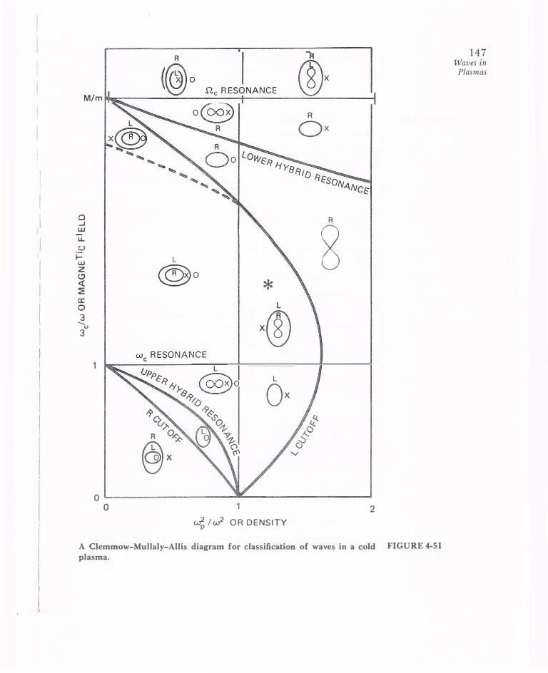
I
I I I
I
I I i
I I I I I
I I i
I I
I I I
l
@o U0 RESONANCE (�)x M/m �------��----�--�--------��-------; R Qx
0 R _J
3 UJ � u I- L UJ @o z (.!:)
* <( � a: L 0
·® 3 --(.) 3
L Qx -90 v�
R 0� @·�
0 0 2
d!w2 p OR DENSITY
A Clemmow-Mullaly-AIIis diagram for classification of waves in a cold FIGURE 4-51 plasma.
147 Waves in Plasmas

148 Chapter Four
PROBLEMS
as a "plasma pond": A pebble dropped m each region will send out
ripples with shapes like the ones shown.
4-26. A hydrogen discharge in a 1-T field produces a density of 1016 m-3
(a) What is the Alfven speed vA?
(h) Suppose vA had come out greater than c. Does this mean that Alfven waves travel faster than the speed of light?
4-27. Calculate the Alfven speed in a region of the magnetosphere where B = 10-8 T, n = 108m-3, and M = MH = 1.67 x 10⁻²⁷ kg.
4-28. Suppose you have created a laboratory plasma with n = 1015 m-3 and B = 10-2T. You connect a 160-MHz signal generator to a probe inserted into the plasma.
(a) Draw a CMA diagram and indicate the region in which the experiment is located.
(b) What electromagnetic waves might be excited and propagated in the plasma?
4-29. Suppose you wish to design an experiment in which standing torsional Alfven waves are generated in a cylindrical plasma column, so that the standing wave has maximum amplitude at the midplane and nodes at the ends. To satisfy the condition w « n" you make w = 0.10,.
(a) If you could create a hydrogen plasma with n = 1019 m -3 and B = 1 T, how long does the column have to be?
(h) If you tried to do this with a 0.3 T Q-machine, in which the singly charged Cs ions have an atomic weight 133 and a density n = 1018 m-3, how long would the plasma have to be? Hint: Figure out the scaling factors and use the result of part (a).
4-30. A pulsar emits a broad spectrum of electromagnetic radiation, which is detected with a receiver tuned to the neighborhood off= 80 MHz. Because of the dispersion in group velocity caused by the interstellar plasma, the observed frequency during each pulse drifts at a rate given by df/dt = -5 MHz/sec.
(a) If the interstellar magnetic field is negligible and w 2 » w !. show that
df c F dt = - ; fp
where [p is the plasma frequency and x is the distance of the pulsar.
(b) If the average electron density in space is 2 x 10⁵m-3, how far away is the pulsar? (1 parsec= 3 x 10¹⁶ m.)

4-31. .A three-component plasma has a density n0 of electrons, ( 1- E)n0 of ions of mass A1,, and Eno of ions of mass M2. Let T;, = T;2 = 0, T, ,e, 0.
(a) Derive a dispersion relation for electrostatic ion cyclotron waves.
(b) Find a simple expression for w2 when € is small.
(c) Evaluate the wave frequencies for a case when € is not small: a 50-50% D-T mixture at KT, = 10 keY, 80 = 5 T, and k = 1 cm-1•
4-32. For a Langmuir plasma oscillation, show that the time-averaged electron kinetic energy per m3 is equal to the electric field energy density k€0(£2). 4-33. For an Alfven wave, show that the time-averaged ion kinetic energy per m3 is equal to the magnetic wave energy (BD/2f.Lo·
4-34. Figure P4-34 shows a far-infrared laser operating at A = 337 f.Lm. When B0 = 0, this radiation easily penetrates the plasma whenever Wp is less than w, or n < n, = 1022 m-3. However, because of the long path length, the defocusing effect of the plasma (cf. Fig. 4-30) spoils the optical cavity, and the density is limited by the conditions w ; < Ew2, where E « 1. In the interest of increasing the limiting density, and hence the laser output power, a magnetic field B0 is added.
(a) If € is unchanged, show that the limiting density can be increased if left-hand circularly polarized waves are propagated.
(b) If n is to be doubled, how large does B0 have to be?
'-----« 11------"'--------' + -DISC HARGE PULSER
CONCAVE MIRROR FLAT MIRROR WITH
OUTPUT COUPLING HOLE
PLASTIC WINDOW
Schematic of a pulsed HCN laser. FIGURE P4-34
149 Waves in
Plasmas

150 Chapter Four
(c) Show that the plasma is a focusing lens for the whistler mode.
(d) Can one use the whistler mode and therefore go to much higher densities?
4-35. Use Maxwell's equations and the electron equation of motion to derive the dispersion relation for light waves propagating through a uniform, unmagnetized, collisionless, isothermal plasma with density n and finite electron temperature T,. (Ignore ion motions.)
4-36. Prove that transverse waves · are unaffected by the Vp term whenever k x B0 = 0, even if ion motion is included.
4-37. Consider the damping of an ordinary wave caused by a constant collision frequency v between electrons and ions.
(a) Show that the dispersion relation is
c 2k 2 w ; - = 1 - ----''---w2 w (w + iv)
(h) For waves damped in time (k real) when v/w « 1, show that the damping rate y = -lm (w ) is approximately
(c) For waves damped in space (w real) when v/w « l , show that the attenuation distance 8 = (Im k )- 1 is approximately
4-38. It has been proposed to build a solar power station in space with huge panels of solar cells collecting sunlight 24 hours a day. The power is transmitted to earth in a 30-crn-wavelength microwave beam. We wish to estimate how much of the power is lost in heating up the ionosphere. Treating the latter as a weakly ionized gas with constant electron-neutral collision frequency, what fraction of the beam power is lost in traversing 1 00 km of plasma with n, = 1 0 1 1 m-3, n. = 1 0 16 m-3, and CTV = 1 0- 1 4 m3/sec?
4-39. The Appleton-Hartree dispersion relation for high-frequency electromagnetic waves propagating at an angle () to the magnetic field is
c 2e 2w ; ( l - w !/w 2) -2- = 1 2 9 9/ 2 9 . 2 9 . 4 9 9/ 2 2 2 i /9 w w· ( J - w ;; w )-w; sm ()±w, [w� sm ()+4w· ( l -w;; w ) cos ()] -
Discuss the cutoffs and resonances of this equation. Which are independent of () ?
4-40. Microwaves with free-space wavelength .A 0 equal to 1 em are sent through a plasma slab 10 em thick in which the density and magnetic field are uniform and given by n 0 = 2.8 x l 0 1 8 m-3 and B0 = 1 .07 T. Calculate the number of wavelengths inside the slab if (see Fig. P4-40)
l I
i I l I I I j
i_

y
-�( a�) .........,.D � --?' : ( b )
E z
(a) the waveguide is oriented so that E 1 is in the z direction;
(h) the waveguide is oriented so that E1 is in the y direction.
X
4-4 1 . A cold plasma is composed of positive ions of cha rge Ze and mass M + and negative ions of charge -e and mass i'vL. In the equilibrium sta te, there is no magnetic or electric field and no velocity; and the respective densities are n o+ and n 0_ = Zno+· Derive the dispersion relation for pla ne electromagnetic waves.
4-42. Ion waves a re generated in a gas-discharge plasma in a mixture of argon and helium gases. The plasma has the following constituents:
(a) Electrons of density n0 and temperature KT, ; (h) Argon ions of density n_..., mass M_..., charge +Ze, and temperature 0 ; and
(c) He ions of density nH, mass MH, charge +e, and temperature 0.
Derive an expression for the phase velocity of the waves using a linearized , one-dimensional theory with the plasma approximation and the Boltzmann relation for electrons.
4-43. I n a remote part of the universe, there exists a plasma cons1stmg of positrons a nd fully stripped antifermium nuclei of charge -Ze, where Z = 1 00. From the equations of motion, continu ity, and Poisson, derive a dispersion relation for plasma oscillations in this plasma, including ion motions. Define the plasma frequencies. You may assume KT = 0, B0 = 0, and all other simplifying initial conditions.
FIGURE P4-40
1 5 1 Waves in
Plasmas
1 52 Chapter Four
FIGURE P4-46
4-44. Intelligent life on a planet in the Crab nebula tries to communicate with us primitive creatures on the earth. We receive radio signals in the 1 08- 109 Hz range, but the spectrum stops abruptly at 1 20 MHz. From optical measurements, it is possible to place an upper limit of 36 G on the magnetic field in the vicinity of the parent star. If the star is located in an HII region (one which contains ionized hydrogen), and if the radio signals are affected by some sort of cutoff in the plasma there, what is a reasonable lower limit to the plasma density? ( I gauss = 1 0-4 T.)
4-45. A space ship is moving through the ionosphere of Jupiter at a speed of 1 00 km/sec, parallel to the 10-"-T magnetic field. I f the motion is supersonic (u > u, ) , ion acoustic shock waves would be generated . If, in addition, the motion is super-Alfvenic (v > vA) . magnetic shock waves would also be excited . Instruments on board indicate the former but not the latter. Find limits to the plasma density and electron temperature and indicate whether these are upper or lower limits. Assume that the atmosphere of Jupiter contains cold, singly charged molecular ions of H2, He, CH4, C02, and NH4 with an average atomic weight of 1 0.
4-46. An extraordinary wave with frequency w is incident on a plasma from the outside. The variation of the right-hand cutoff frequency wR and the upper hybrid resonance frequency wh with radius are as shown. There is an evanescent layer in which the wave cannot propagate. I f the density gradient at the point where w = wh is given by Janjar J = n/r0, show that the distance d between the w = wR and wh points is approximately d = (wJ w )ro.
w
r
J

I I I
I I I
I ( I I I
I I \ I I I I I
\
4-47. By introducing a gradient in B0, it is possible to make the upper hybrid resonance accessible to an X wave sent in from the outside of the plasma (cf. preceding problem) .
(a) Draw on an wc/w vs . w!/w2 diagram the path taken by the wave, showing how the wR cutoff is avoided .
(b) Show that the required change in Bo between the plasma surface and the upper hybrid layer is
4-48. A certain plasma wave has the dispersion relation
where w 2 = w ; + n;. Write explicit expressions for the resonance and cutoff frequencies (or for the squares thereof), when e = m/ M « 1 .
4-49. The extraordinary wave with ion motions included has the following dispersion relation :
(w, w ; n, n ; ) 2 ---------(1) w 2 - w; w w 2 - n;
w ! n: l ---- --w 2 - w; w 2 -n;
(a) Show that this is identical to the equation in the previous problem. (Warning : this problem may be hazardous to your mental health.)
(b) If Wt and wL are the lower hybrid and left-hand cutoff frequencies of this wave, show that the ordering fl, S w1 s wL is always obeyed.
(c) Using these results and the known phase velocity in the w � 0 limit , draw a ·qualitative v!/c2 vs. w plot showing the regions of propagation and evanescence.
4-50. We wish to do lower-hybrid heating of a hydrogen plasma column with wp = 0 at r = a and wp = �w, at the center, in a uniform magnetic field. The ante nna launches an X wave with ku = 0 .
1 5 3 Waves in Plasmas

1 54 Chapter Four
(a) D raw a qualitative plot of w" n" WL, and w, vs. radius. This graph should not be to scale, but it should show correctly the relative magnitudes of these frequencies at the edge and center of the plasma.
(h) E stimate the thickness of the evanescent layer between w, and wL ( cf . previous problem) if the rf frequency w is set equal to w1 at the center.
(c) Repeat ( a) and (b ) for wp (max) = 2w" and draw a conclusion about this antenna design .
4-5 1 . The electromagnetic ion cyclotron wave (Stix wave) is sometimes used for radio frequency heating of fusion plasmas. Derive the dispersion relation as fol lows :
(a) Derive a wave equation in the form of Eq. [ 4- 1 1 8) but with displacement current neglected.
(b) Write the x and y components of this equation assuming k. = 0, k 2 = k ; + k ;, and k,k,E, = 0.
( c) To evaluate j 1 = n 0 e ( v, - v, ) , derive the ion equ ivalent of Eq. [4-98] to obtain v,, to make a low-frequency approximation so that v, is simply the E x B drift.
(d) Insert the result of (c) into ( b ) to obtain· two simultaneous homogeneous equations for E. and £,, using the definition for !lp in Eq. [ 4-49).
(e) Set the determinant to zero and solve to lowest order in n; to obtain

Chapter Five
I s NAN
VI
DIFFUSION AND MOBILITY IN WEAKLY IONIZED GASES 5.1
The infinite, homogeneous plasmas assumed in the previous chapter for
the equilibrium conditions are, of course, highly idealized. Any realistic plasma will have a density gradient, and the plasma will tend to diffuse toward regions of low density. The central problem in controlled thermonuclear reactions is to impede the rate of diffusion by using a magnetic field. Before tackling the magnetic field problem, however, we shall consider the case of diffusion in the absence of magnetic fields. A further simplification results if we assume that the plasma is weakly ionized, so that charge particles collide primarily with neutral atoms rather than with one another. The case of a fully ionized plasma is deferred to a later section, since it results in a nonlinear equation for which there are few simple illustrative solutions. In any case, partially ionized gases are not rare: High-pressure arcs and ionospheric plasmas fall into this category, and most of the early work on gas discharges involved fractional ionizations between 10-3 and 10-6, when collisions with neutral atoms are dominant.
The picture, then, is of a nonuniform distribution of ions and electrons in a dense background of neutrals (Fig. 5-l). As the plasma spreads out as a result of pressure-gradient and electric field forces, the individual particles undergo a random walk, colliding fre·quently with
the neutral atoms. We begin with a brief review of definitions from atomic theory. 155

156 Chapter Five
0
0 0
0 0 0
0 0
0
0
0
FIGURE 5-l Diffusion of gas atoms by random
collisions.
5.1.1 Collision Parameters
•
When an electron, say, collides with a neutral atom, it may lose any fraction of its initial momentum, depending on the angle at which it rebounds. In a head-on collision with a heavy atom, the electron can lose twice its initial momentum, since its velocity reverses sign after the collision. The probability of momentum loss can be expressed in terms of the equivalent cross section a- that the atoms would have if they were perfect absorbers of momentum.
In Fig. 5-2, electrons are incident upon a slab of area A and thickness dx containing nn neutral atoms per m3. The atoms are imagined to be opaque spheres of cross-sectional area a-; that is, every time an electron
. ...
.. A
�dxr FIGURE 5-2 Illustration of the definition of cross section.

comes within the area blocked by the atom, the electron loses all of its momentum. The number of atoms in the slab is
The fraction of the slab blocked by atoms is
nnACT dx/ A = nnCT dx
If a flux r of electrons is incident on the slab, the flux emerging on the other side is
r· = f(l- nncrdx )
Thus the change off with distance is
or
d r I dx = -nnCT r
r =foe -n,ax ==foe -x!>. .. [5-1) In a distance Am, the flux would be decreased to 1/e of its initial value. The quantity Am is the mean free path for collisions:
[5-2]
After traveling a distance Am, a particle will have had a good probability of making a collision. The mean time between collisions, for particles of velocity v, is given by
and the mean frequency of collisions is
T-l = v/Am = nnCTV [5-3]
If we now average over particles of all velocities v in a Maxwellian distribution, we have what is generally called the collision frequency 11:
II = nnCTV [5-4]
Diffusion Parameters 5.1.2
The fluid equation of motion including collisions is, for any species,
dv [av J mn - =mn -+(v·V)v =±enE -Vp-mnllv dt at [5-5)
157 Diffusion and
Resistivity

158 Chapter Five
where again the ± indicates the sign of the charge. The averaging process used to compute v is such as to make Eq. [5-5] correct; we need not be concerned with the details of this computation. The quantity v
must, however, be assumed to be a constant in order for Eq. [5-5] to be useful. We shall consider a steady state in which av/at = 0. If v is sufficiently small (or v sufficiently large), a fluid element will not move into regions of different E and Vp in a collision time, and the convective derivative dv/dt will also vanish. Setting the left-hand side of Eq. [5-5] to zero, we have, for an isothermal plasma,
1 v = -- (±enE- KTVn)
mnv
e KTVn =± - E- - -
mv mv n
[5-6]
The coefficients above are called the mobi!ity and the diffusion coefficient:
l /.L = I q I / mv I Mobility
I D = KT/mv Diffusion coefficient
[5-7]
[5-8]
These will be different for each species. Note that D is measured in m2 /sec. The transport coefficients /.L and D are connected by the Einstein relation:
[5-9]
With the help of these definitions, the flux ri of the jth species can be
written
(5-10]
Fick 's law of diffusion is a special case of this, occurring when either E = 0 or the particles are uncharged, so that /.L = 0:
Fick's Jaw [5-11]

This equation merely expresses the fact that diffusion is a random-walk process, in which a net flux from dense regions to less dense regions occurs simply because more particles start in the dense region. This flux is obviously proportional to the gradient of the density. In plasmas, Fick's law is not necessarily obeyed. Because of the possibility of organized motions (plasma waves), a plasma may spread out in a manner which is
not truly random.
DECAY OF A PLASMA BY DIFFUSION 5.2
Ambipolar Diffusion 5.2.1
We now consider how a plasma created in a container decays by diffusion to the walls. Once ions and electrons reach the wall, they recombine
there. The density near the wall, therefore, is essentially zero. The Auid equations of motion and continuity govern the plasma behavior; but if the decay is slow, we need only keep the time derivative in the continuity equation. The time derivative in the equation of motion, Eq. (5-5], will be negligible if the collision frequency v is large. We thus have
an -+V·r- =o at 1 [5-12]
with ri given by Eq. [5-10]. It is clear that if r; and r. were not equal, a serious charge imbalance would soon arise. If the plasma is much larger than a Debye length, it must be quasineutral; and one would expect that the rates of diffusion of ions and electrons would somehow adjust themselves so that the two species leave at the same rate. How this happens is easy to see. The electrons, being lighter, have higher thermal velocities and tend to leave the plasma first. A positive charge is left behind, and an electric field is set up of such a polarity as to retard the loss of electrons and accelerate the loss of ions. The required E field is found by setting r; = r. = r. From Eq. [5-10], we can write
D· - D Vn E= • · -
t.L; + �-'-• n
[5-13]
[5-14]
159 Diffusion and
Resistivity

160 Chapter Five
The common flux r is then given by
Di-D. r = JL; Vn - D, Vn /Li +li-e
= - JL;D, + ILeDi Vn Ii-i +li-e
This is Fick's law with a new diffusion coefficient
[5-15]
[5-16]
called the ambipolar diffusion coefficient. If this IS constant, Eq. [5-12] becomes simply
[5-17)
The magnitude of Da can be estimated if we take li-e » JL;. That this is true can be seen from Eq. [5-7]. Since v is proportional to the thermal velocity, which is proportional to m-112, 11- is proportional to rn-112. Equations [5-16] and [5-9] then give
For T, = T;, we have
JL; · T. Da = D, +- D, = D; +
T D,
li-e i
Da = 2D;
[5-18)
(5-19]
The effect of the ambipolar electric field is to enhance the diffusion of ions by a factor of two, but the diffusion rate of the two species together is primarily controlled by the slower species.
Diffusion in a Slab
The diffusion equation [5-17] can easily be solved by the method of separation of variables. We let
n(r,t) = T(t)S(r) [5-20)

whereupon Eq. [5-17], with the subscript on Da understood, becomes
SdT = DTV2S
dt _!_ dT = !!_ v2 5 T dt S
[5-21)
[5-22)
Since the left side is a function of time alone and the right side a function of space alone, they must both be equal to the same constant, which we shall call -1 /T. The function T then obeys the equation
with the solution
dT T dt
T = T0 e-I/T
The spatial partS obeys the equation
l V2S = - -s DT
In slab geometry, this becomes
d2S dx2
= 1 --s
DT
with the solution X . X s = A cos I/? + B Sin I/? (DT) - (DT) -
[5-23)
[5-24)
[5-25)
[5-26]
[5-27)
We would expect the density to be nearly zero at the walls (Fig. 5-3) and to have one or more peaks in between. The simplest solution is that with a single maximum. By symmetry, we can reject the odd (sine) term in Eq. [5-27]. The boundary conditions S = 0 at x = ±L then requires
or
Combining Eqs. [5-20], [5-24], [5-27], and [5-28], we have
-1/T 1TX n = no e cos-
2L
[5-28]
[5-29]
16 1 Diffusion and
Resistivity

162 Chapter Five
X -L 0 +L
FIGURE 5-3 Density of a plasma at various
times as it decays by diffusion
to the walls.
This is called the lowest diffusion mode. The density distribution is a cosine, and the peak density decays exponentially with time. The time constant 'T increases with L and varies inversely with D, as one would expect.
There are, of course, higher diffusion modes with more than one peak. Suppose the initial density distribution is as shown by the top curve in Fig. 5-4. Such an arbitrary distribution can be expanded in a Fourier senes:
( (l + �)7TX . m7TX) n = no L at cos
- + L bm sm --t L m L
[5-30]
We have chosen the indices so that the boundary condition at x = ±L is
automatically satisfied. To treat the time dependence, we can try a solution of the form
("\' -t/-r (l + �)7TX "\' -t/T . m7TX) n = no ,:_ate 1 cos + ,:_ bm e � sm --
t L m L [5-31]
Substituting this into the diffusion equation [5-17], we see that each cosine term yields a relation of the form
[5-32]

·I
-L 0 +L X
163 Diffusion and
Resistivity
Decay of an initially nonuniform FIGURE 5-4
plasma, showing the rapid disappear-
ance of the higher-order diffusion
modes.
and similarly for the sine terms. Thus the decay time constant for the lth mode is given by [ L ]2 1
71 == (l + hrr D [5-33)
The fine-grained structure of the density distribution, corresponding to large l numbers, decays faster, with a smaller time constant 7'1• The plasma decay will proceed as indicated in Fig. 5-4. First, the fine structure will be washed out by diffusion. Then the lowest diffusion mode, the simple cosine distribution of Fig. 5-3, will be reached. Finally, the peak density continues to decay while the plasma density profile retains the same shape.
Diffusion in a Cylinder 5.2.3
The spatial part of the diffusion equation, Eq. [5-25], reads, in cylindrical geometry,
d2S 1 dS 1 -2 + --+-5=0 dr 1· dr DT [5-34]
This differs from Eq. [5-26] by the addition of the middle term, which merely accounts for the change in coordinates. The need for the extra term is illustrated simply i'n Fig. 5-5. If a slice of plasma in (A) is moved toward larger x without being allowed to expand, the density would

164 Chapter Five
X
A 8
FIGURE 5-5 Motion of a plasma slab in rectilinear and cylindrical geometry, illustrating the difference between a cosine and a Bessel function.
remain constant. On the other hand, if a shell of plasma in (B) is moved toward larger r with the shell thickness kept constant, the density would necessarily decrease as 1 /r. Consequently, one would expect the solution to Eq. [5-34] to be like a damped cosine (Fig. 5-6). This function is called a Bessel function of order zero, and Eq. [5-34] is called Bessel's equation (of
order zero). Instead of the symbol cos, it is given the symbol ] 0. The function ]0(r/[Dr]112) is a solution to Eq. [5-34], just as cos [x/(Dr)112] is
a solution to Eq. [5-26]. Both cos kx and ]0(kr) are expressible in terms
1
J0 (kr)
0
FIGURE 5.6 The Bessel function of order zero.
8 14 kr

of infinite series and may be found in mathematical tables. Unfortunately, Bessel functions are not yet found in hand calculators.
To satisfy the boundary condition n = 0 at T = a, we must set a/(DT)112 equal to the first zero of ]0; namely, 2.4. This yields the decay time constant T. The plasma again decays exponentially, since the temporal part o f the diffusion equation, Eq. [5-23], is unchanged. We have described the lowest diffusion mode in a cylinder. Higher diffusion modes, with more than one maximum in the cylinder, will be given in terms of Bessel functions of higher order, in direct analogy to the case of slab geometry.
STEADY STATE SOLUTIONS 5.3
In many experiments, a plasma is maintained in a steady state by con
tinuous ionization or injection of plasma to offset the losses. To calculate
the density profile in this case, we must add a source term to the equation of continuity:
an ....,.., -- D v - n = Q(r) at
[5-35]
The sign is chosen so that when Q is positive, it represents a source and contributes to positive an/ at. In steady state, we set an/ at = 0 and are left with a Poisson-type equation for n (r).
Constant Ionization Function 5.3.1
In many weakly ionized gases, ionization is produced by energetic electrons in the tail of the Maxwellian distribution. In this case, the source term Q is proportional to the electron density n. Setting Q = Zn, where Z is the "ionization function," we have
[5-36]
This is the same equation as that for S, Eq. [5-25]. Consequently, the density profile is a cosine or Bessel function, as in the case of a decaying plasma, only in this case the density remains constant. The plasma is maintained against diffusion losses by whatever heat source keeps the electron temperature at its constant value and by a small influx of neutral atoms to replenish those that are ionized.
165 Diffusion and
Resistivit)'

166 Chapter Five
5.3.2 Plane Source
We next consider what profile would be obtained in slab geometry if
there is a localized source on the plane x = 0. Such a source might be,
for instance, a slit-collimated beam of ultraviolet light strong enough to ionize the neutral gas. The steady state diffusion equation is then
d2n Q dx2 =
- D 8(0) [5-37]
Except at x = 0, the density must satisfy a2n/ax2 = 0. This obviously has the solution (Fig. 5-7)
[5-38]
The plasma has a linear profile. The discontinuity in slope at the source is characteristic of 8 -function sources.
5.3.3 Line Source
Finally, we consider a cylindrical plasma with a source located on the axis. Such a source might, for instance, be a beam of energetic electrons producing ionization along the axis. Except at r = 0, the density must satisfy
I a ( an) -- r- - 0 r ar ar
The solution that vanishes at r =
a is
n = n0 In (a/r)
X -L 0 +L
FIGURE 5-7 The triangular density profile
resulting from a plane source under diffusion.
[5-39]
[5-40]
J.

I I l
I I I
I I l
I I I
1
a 0 a
r
167 Diffusion and
Resistivity
The logarithmic density profile FIGURE 5-8
resulting from a line source under diffusion.
The density becomes infinite at r = 0 (Fig. 5-8); it is not possible to determine the density near the axis accurately without considering the
finite width of the source.
RECOMBINATION 5.4
When an ion and an electron collide, particularly at low relative velocity, they have a finite probability of recombining into a neutral atom. To conserve momentum, a third body must be present. If this third body is an emitted photon, the process is called radiative recombination. If it is a particle, the process is called three-body recombination. The loss of plasma by recombination can be represented by a negative source term in the
equation of continuity. It is clear that this term will be proportional to n,n; = n 2. In the absence of the diffusion terms, the equation of continuity then becomes
on/ot = -an 2 [5-41]
The constant of proportionality a is called the recombination coefficient and has units of m3 /sec. Equation [5-41] is a nonlinear equation for n. This means that the straightforward method for satisfying initial and boundary conditions by linear superposition of solutions is not available. Fortunately, Eq. [5.41] is such a simple nonlinear equation that the

168 Chapter Five
0
solution can be found by inspection. It is
l l -- = --+at n (r,t) n0(r)
[5-42]
where no(r) is the initial density distribution. It is easily verified that this satisfies Eq. [5-41]. After the density has fallen far below its initial value,
it decays reciprocally with time:
n ex: 1/at [5-43] This is a fundamentally different behavior from the case of diffusion, in which the time variation is exponential.
Figure 5-9 shows the results of measurements of the density decay in the afterglow of a weakly ionized H plasma. When the density is high,
2 3 4 5 t (msec)
FIGURE 5-9 Density decay curves of a weakly ionized plasma under recombination and
diffusion. [From S. C. Brown, Basic Data of Plasma Physics, John Wiley and Sons, New York, 1959.]

J
0 0 0 0 � 169
0 � 0 0 B Diffusion and a- Resistivity 0 0
0 0 0 0 0 JI'Bb
0 0 0 0 0 0
... 0 0 0 0 0 0
A charged particle in a magnetic field will gyrate about FIGURE 5-10
the same line of force until it makes a collision.
recombination, which is proportional ton 2, is dominant, and the density decays reciprocally. After the density has reached a low value, diffusion
becomes dominant, and the decay is thenceforth exponential.
DIFFUSION ACROSS A MAGNETIC FIELD 5.5
The rate of plasma loss by diffusion can be decreased by a magnetic field; this is the problem of confinement in controlled fusion research. Consider a weakly ionized plasma in a magnetic field (Fig. 5-10). Charged particles will move along B by diffusion and mobility according to Eq. [5-10], since B does not affect motion in the parallel direction. Thus we
have, for each species,
an f = ± 11nE - D-" ,.... " az [5-44]
If there were no collisions, particles would not diffuse at all in the perpendicular direction-they would continue to gyrate about the sameline of force. There are, of course, particle drifts across B because of electric fields or gradients in B, but these can be arranged to be parallel to the walls. For instance, in a perfectly symmetric cylinder (Fig. 5-11), the gradients are all in the radial direction, so that the guiding center drifts are in the azimuthal direction. The drifts would then be harmless.
When there are collisions, particles migrate across B to the walls along the gradients. They do this by a random-walk process (Fig. 5-12). When an ion, say, collides with a neutral atom, the ion leaves the collision traveling in a different direction. It continues to gyrate about the mag
netic field in the same direction, but its phase of gyration is changed discontinuously. (The Larmor radius may also change, but let us suppose that the ion does not gain or lose energy on the average.)

170 Chapter Five
FIGURE 5-ll Particle drifts in a cylindrically symmetric plasma column do not lead to
losses.
FIGURE 5-12 Diffusion of gyrating particles by collisions with neutral atoms.
The guiding center, therefore, shifts position in a collision and undergoes a random walk. The particles will 0:.ffuse in the direction opposite Vn.
The step length in the random walk is no longer Am, as in magnetic-fieldfree diffusion, but has instead the magnitude of the Larmor radius rL. Diffusion across B can therefore be slowed down by decreasing rL; that is, by increasing B.
To see how this comes about, we write the perpendicular component of the fluid equation of motion for either species as follows:
dv1_ mn- = ±en(E + V1_ x B)- KTVn- mnvv = 0 [5-45]
dt
-,

We have again assumed that the plasma is isothermal and that v is large enough for the dvj_/dt term to be negligible. The x andy components are
an mnvvx = ±enEx - KT- ± env/3
ax
an mnvvy = ±enE, - KT- �envxB
ay
Using the definitions of p. and D, we have
D an w, Vx = ±p.Ex -- -±-vy
n ax 1/
D an w, Vy = ±p.E, - - - �- Vx
n ay 1/
Substituting for Vx, we may solve for vy:
[5-46]
[5-47]
2 2 D an 2 2 Ex 2 2 KT 1 an v.(1 + w T ) = ±JJ-£ -- -- w T - ± W T - - - [5-48] ' '
y n ay ' B ' eB n ax
where T = v-1. Similarly, Vx is given by
? ? D an 2 ? E, 2 ? KT I an v (I + w -T-) = ±p.E -- - + w T-- � w T-- - - [5-49] X c X n ax c B c eB n ay
The last two terms of these equations contain the E X B and diamagnetic drifts:
Ey Ex VEx =
B V£y =
B [5-50]
KT 1 an KT 1 an VOx=�--- vv, = ±- --
eB n ay eB n ax
The first two terms can be simplified by defining the perpendicular mobility and diffusion coefficients:
J.l.j_ =
1 + 2 2 W,T
D Dj_ =I+ 2 2
W,T [5-51]
With the help of Eqs. [5-50] and [5-5I], we can write Eqs. [5-48] and [5-49] as
[5·52]
17 1 Diffusion and
Resistivity

172 Chapter Five
From this, it is evident that the perpendicular velocity of either species is composed of two parts. First, there are usual vE and vv drifts perpendicular to the gradients in potential and density. These drifts are slowed down by collisions with neutrals; the drag factor 1 + (v2 / w ;) becomes unity when v � 0. Second, there are the mobility and diffusion drifts parallel to the gradients in potential and density. These drifts have the same form as in the B = 0 case, but the coefficients f.t and D are reduced by the factor I + w;-r2.
The product w,-r is an important quantity in magnetic confinement. When w ;-r2 « 1, the magnetic field has little effect on diffusion. When w;-r2 » I, the magnetic field significantly retards the rate of diffusion across B. The following alternative forms for w,-r can easily be verified:
w,-r = wc/v = {-tB = A,./rL
In the limit w �-r2 » I, we have
KT 1 KTv D 1. = - --.;--<) = --9
mv w;-r- mw;
[5-53]
[5-54]
Comparing with Eq. [5-8), we see that the role of the collision frequency v has been reversed. In diffusion parallel to B, D is proportional to v-I, since collisions retard the motion. In diffusion perpendicular to B, D 1.
is proportional to v, since collisions are needed for cross-field migration. The dependence on m has also been reversed. Keeping in mind that v . . I -112 I D -112 h"l D 1 19 I IS proportion a to m , we see t 1at ex:: m , w 1 e 1. ex:: m - . n parallel diffusion, electrons move faster than ions because of their higher thermal velocity; in perpendicular diffusion, electrons escape more slowly because of their smaller Larmor radius.
Disregarding numerical factors of order unity, we may write Eq. [5-8] as
[5-55]
This form, the square of a length over a time, shows that diffusion is a random-walk process with a step length Am. Equation [5-54] can be written
KTv 2 r� rr D 1. = --2 - v th -2- v - -mw, v,h -r
[5-56]
This shows that perpendicular diffusion is a random-walk process with a step length rL, rather than Am.
5.5.1 Ambipolar Diffusion across B
Because the diffusion and mobility coefficients are anisotropic 111 the presence of a magnetic field, the problem of ambipolar diffusion is not
J

['ill
['ell ..,. t B
173 Diffusion and
Resistivity
Parallel and perpendicular particle fluxes in a magnetic field. FIGURE 5-13
as straightforward as in the B = 0 case. Consider the particle fluxes perpendicular to B (Fig. 5-13). Ordinarily, since r . .�. is smaller than f;.�., a transverse electric field would be set up so as to aid electron diffusion and retard ion diffusion. However, this electric field can be short-circuited by an imbalance of the fluxes along B. That is, the negative charge resulting from reJ. < ft.1. can be dissipated by electrons escaping along
the field lines. Although the total diffusion must be ambipolar, the
perpendicular part of the losses need not be ambipolar. The ions can diffuse out primarily radially, while the electrons diffuse out primarily along B. Whether or not this in fact happens depends on the particular experiment. In short plasma columns with the field lines terminating on conducting plates, one would expect the ambipolar electric field to be short-circuited out. Each species then diffuses radially at a different rate. In long, thin plasma columns terminated by insulating plates, one would expect the radial diffusion to be ambipolar because escape along B is arduous.
Mathematically, the problem is to solve simultaneously the equations of continuity [5-12] for ions and electrons. It is not the fluxes rj but the divergences V · ri which must be set equal to each other. Separating v. rj into perpendicular and parallel components, we have
[5-57]
The equation resulting from setting V · r, = V · r. cannot easily be separated into one-dimensional equations. Furthermore, the answer depends sensitively on the boundary conditions at the ends of the field lines.
Unless the plasma is so long that parallel diffusion can be neglected altogether, there is no simple answer to the problem of ambipolar diffusion across a magnetic field.

174 Chapter Five
5.5.2 Experimental Checks
ANODE
Whether or not a magnetic field reduces transverse diffusion in accord
ance with Eq. [5-51] became the subject of numerous investigations. The
first experiment performed in a tube long enough that diffusion to the
ends could be neglected was that of Lehnert and Hoh in Sweden. They
used a helium positive column about 1 em in diameter and 3.5 m long
(Fig. 5-14). In such a plasma, the electrons are continuously lost by radial
diffusion to the walls and are replenished by ionization of the neutral
gas by the electrons in the tail of the velocity distribution. These fast
electrons, in turn, are replenished by acceleration in the longitudinal
electric field. Consequently, one would expect E, to be roughly propor
tional to the rate of transverse diffusion. Two probes set in the wall of
the discharge tube were used to measure Ez as B was varied. The ratio
of E, (B) toE, (0) is shown as a function of B in Fig. 5-15. At low B fields,
the experimental points follow closely the predicted curve, calculated on
the basis of Eq. [5-52]. At a critical field B, of about 0.2 T, however, the
experimental points departed from theory and, in fact, showed an increase of diffusion with B. The critical field B, increased with pressure, suggest
ing that a critical value of Wc'r was involved and that something went
wrong with the "classical" theory of diffusion when Wc'r was too large.
The trouble was soon found by Kadomtsev and Nedospasov in the
U.S.S.R. These theorists discovered that an instability should develop at
high magnetic fields; that is, a plasma wave would be excited by theE=
field, and that this wave would cause enhanced radial losses. The theory
correctly predicted the value of B,. The wave, in the form of a helical
distortion of the plasma column, was later seen directly in an experiment
b y Allen, Paulikas, and Pyle at Berkeley. This helical instability of the
positive column was the first instance in which "anomalous diffusion"
across magnetic fields was definitively explained, but the explanation was
PROBES CATHODE
B -...., ... ..-
FIGURE 5-14 The Lehnert-Hoh experiment to check the effect of a magnetic field on
diffusion in a weakly ionized gas.
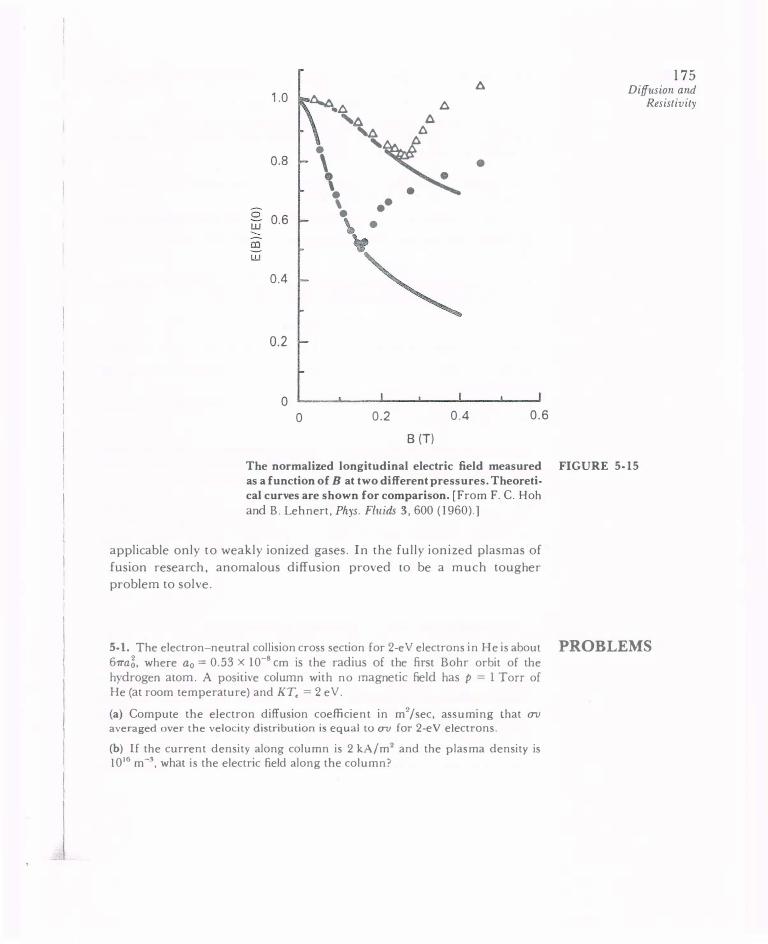
1 75 A Diffusion and 1.0 � .. A A
'.6. A
•
�� 0.8 \ e
• \ ••
0 0.6 • LLJ \ • CD LLJ
� 0.4
0.2
0 0 0.2 0.4 0.6
B(T)
The normalized longitudinal electric field measured FIGURE 5-15
as a function of B at two different pressures. Theoreti-
cal curves are shown for comparison. [From F. C. Hoh and B. Lehnert, Phys. Fluids 3, 600 (I 960).]
applicable only to weakly ionized gases. In the fully ionized plasmas of fusion research, anomalous diffusion proved to be a much tougher problem to solve.
Resistivity
5-l. The electron-neutral collision cross section for 2-eV electrons in He is about PROBLEMS 61ra�, where a0 = 0.53 x 10⁻⁸ em is the radius of the first Bohr orbit of the hydrogen atom. A positive column with no magnetic field has p = l Torr of He (at room temperature) and KT, = 2 eV.
(a) Compute the electron diffusion coefficient in m2 /sec, assuming that av averaged over the velocity distribution is equal to av for 2-eV electrons.
{b) If the current density along column is 2 kA/m2 and the plasma density is 1016 m-3, what is the electric field along the column?

176 Chapter Five
5-2. A weakly ionized plasma slab in plane geometry has a density distribution
n(x) = n0cos (7Tx/2L) -L:5x:5L
The plasma decays by both diffusion and recombination. If L = 0.03 m, D =
0.4 m2/sec, and a = 10-15 m3 /sec, at what density will the rate of loss by diffusion be equal to the rate of loss by recombination?
5-3. A weakly ionized plasma is created in a cubical aluminum box of length L on each side. It decays by ambipolar diffusion.
(a) Write an expression for the density distribution in the lowest diffusion mode.
(b) Define what you mean by the decay time constant and compute it if D. =
10-3m2/sec.
5-4. A long, cylindrical positive column has B = 0.2 T, KT; = 0.1 eV, and other parameters the same as in Problem 5-1. The density profile is
with the boundary condition n = 0 at 1· = a = l em. Note: ]0(z) = 0 at z = 2.4.
(a) Show that the am bipolar diffusion coefficient to be used above can be approximated by DJ.•·
(b) Neglecting recombination and losses from the ends of the column, compute the confinement time T.
5-5. For the density profile of Fig. 5-7, derive an expression for the peak density n0 in terms of the source strength Q and the other parameters of the problem. (Hint: E"quate the source per m2 to the particle flux to the walls per m2.)
5-6. You do a recombination experiment in a weakly ionized gas in which the main loss mechanism is recombination. You create a plasma of density 1020 m-3 by a sudden burst of ultraviolet radiation and observe that the density decays to half its initial value in 10 msec. What is the value of the recombination coefficient a? Give units.
5.6 COLLISIONS IN FULLY IONIZED PLASMAS
When the plasma is composed of ions and electrons alone, all collisions are Coulomb collisions between charged particles. However, there is a distinct difference between (a) collisions between like particles (ion-ion or electron-electron collisions) and (b) collisions between unlike particles (ion-electron or electron-ion collisions). Consider two identical particles colliding (Fig. 5-16). If it is a head-on collision, the particles e merge with
their velocities reversed ; they simply interchange their orbits, and the
I l 1

I I I l I I
J
---, ' / '
I \
\ \ / ' ,
,....__...,.,
os
177 Diffusion and
Resistivity
Shift of guiding centers of two like particles FIGURE 5-16
making a 90° collision.
two guiding centers remain in the same places. The result is the same
as in a glancing collision, in which the trajectories are hardly disturbed. The worst that can happen is a goo collision, in which the velocities are changed goo in direction. The orbits after collision will then be the dashed circles, and the guiding centers will have shifted. However, it is clear that the "center of mass" of the two guiding centers remains stationary. For this reason, collisions between like particles give rise to very little diffusion.
This situation is to be contrasted with the case of ions colliding with neutral atoms. In that case, the final velocity of the neutral is of no concern, and the ion random-walks away from its initial position. In the case of ion-ion collisions, however, there is a detailed balance in each collision; for each ion that moves outward, there is another that moves inward as a result of the collision.
When two particles of opposite charge collide, however, the situation is entirely different (Fig. 5-17). The worst case is now the 180° collision, in which the particles emerge with their velocities reversed. Since they must continue to gyrate about the lines of force in the proper sense, both guiding centers will move in the same direction. Unlik e-particle
collisions give rise to diffusion. The physical picture is somewhat different for ions and electrons because of the disparity in mass. The electrons bounce off the nearly stationary ions and random-walk in the usual fashion. The ions are slightly jostled in each collision and move about as a result of frequent bombardment by electrons. Nonetheless, because of the conservation of momentum in each collision, the rates of diffusion are the same for ions and electrons, as we shall show.

178 Chapter Five
/.?' ,..... / i' ,, tf \ \
I \ I \ I \ I I \ ' / I \ ,._ __ ..... I \ I
" / ' / ......... ..__.,
OB
FIGURE 5-17 Shift of guiding centers of two
oppositely charged particles making a 180° collision.
5.6.1 Plasma Resistivity
The fluid equations of motion including the effects of charged-particle collisions may be written as follows (cf. Eq. [3-47]):
dv Mn Tt =en (E + v; X B)- Vp; - V · 'TT; + P;,
dv, mn- = -en (E + v X B) - Vp - V · n + P
dl ' e e eo
[5-58]
The terms P;, and P,; represent, respectively, the momentum gain of the ion fluid caused by collisions with electrons, and vice versa. The stress tensor P; has been split into the isotropic part Pi and the anisotropic viscosity tensor Tr;. Like-particle collisions, which give rise to stresses within each fluid individually, are contained inn;. Since these collisions do not give rise to much diffusion, we shall ignore the terms V · n;. As for the terms P,; and P;., which represent the friction between the two fluids, the conservation of momentum requires
P;, = -P,1 [5-59)
l

I I
I J
We can write P,; m terms of the collision frequency m the usual manner:
[5-60]
and similarly for P;,. Since the collisions are Coulomb collisions, one would expect P,; to be proportional to the Coulomb force, which is proportional to e2 (for singly charged ions). Furthermore, P,; must be proportional to the density of electrons n, and to the density of scattering centers n;, which, of course, is equal ton,. Finally, P,; should be proportional to the relative velocity of the two fluids. On physical grounds, then, we can write P,; as
2 2 P,; = Tfe n (v; - v,) [5-61]
where Tf is a constant of proportionality. Comparing this with Eq. [5-60], we see that
2 ne 11,; = - Tf 7n
[5-62]
The constant Tf is the specific resistivity of the plasma; that this jibes with the usual meaning of resistivity will become clear shortly.
Mechanics of Coulomb Collisions 5.6.2
When an electron collides with a neutral atom, no force is felt until the electron is close to the atom on the scale of atomic dimensions; the collisions are like billiard-ball collisions. When an electron collides with an ion, the electron is gradually deflected by the long-range Coulomb field of the ion. Nonetheless, one can derive an effective cross section for this kind of collision. It will suffice for our purposes to give an order-of-magnitude estimate of the cross section. In Fig. 5-18, an electron of velocity v approaches a fixed ion of charge e.ln the absence of Coulomb forces, the eleqron would have a distance of closest approach r0, called the impact parameter. In the presence of a Coulomb attraction, the electron will be deflected by an angle x, which is related to r0. The Coulomb force IS
2 e F= - ---2 47TEor
[5-63]
179 Diffusion and
Resistivity

180 Chapter Five
mv
FIGURE 5-18 Orbit of an electron making a Coulomb collision with an ion.
This force is felt during the time the electron is in the vicinity of the ion; this time is roughly
T = To/v [5-64]
The change in the electron's momentum is therefore approximately
2 e �(mv) =I FTI = ---
41TEoToV [5-65]
We wish to estimate the cross section for large-angle collisions, in which x � 90Q For a 90° collision, the change in mv is of the order of mv i tself. Thus
.:l(mv) = mv = e2/41TE0r0v,
The cross section is then
u = 1rr6 = e4/l61TE6m2v4
The collision frequency is, therefore,
v,; = nuv = ne4/l61TE6m2v3
and the resistivity is
m e 2
[5-66]
[5-67]
[5-68]
7J = -2 v,; = 2 3 [5-69] ne 161TE0mv
For a Maxwellian distribution of electrons, we may replace v2 by KT,/m for our order-of-magnitude estimate:
1re2m 112 [5-70]
I
I ! l I I I
I I t
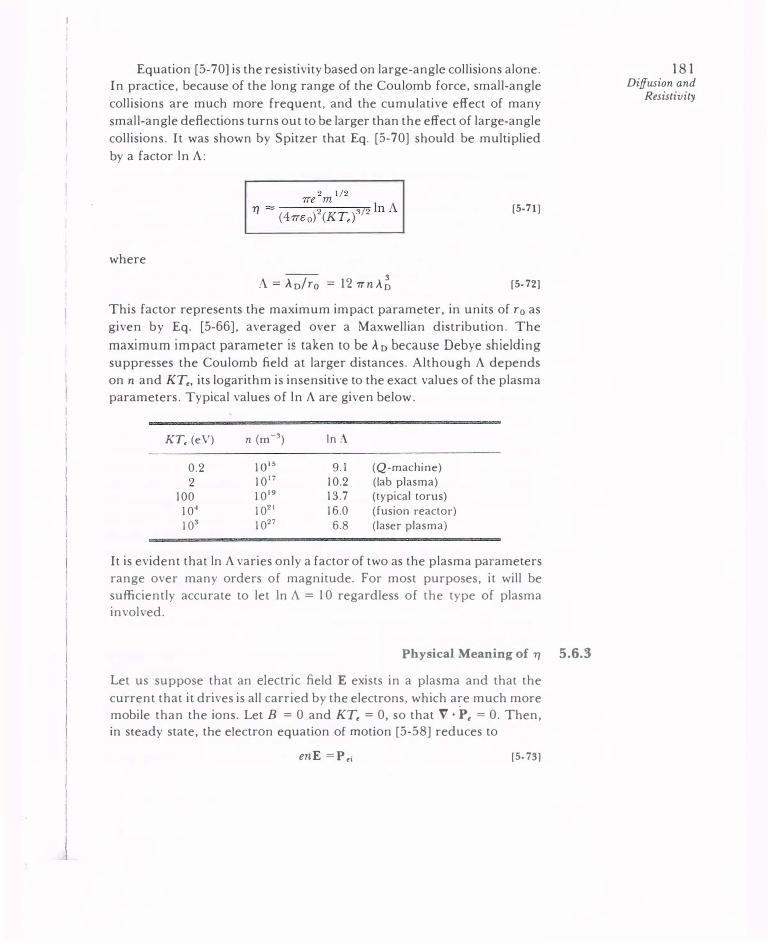
Equation [5-70] is the resistivity based on large-angle collisions alone. In practice, because of the long range of the Coulomb force, small-angle collisions are much more frequent, and the cumulative effect of many small-angle deflections turns out to be larger than the effect of large-angle collisions. It was shown by Spitzer that Eq. [5-70] should be multiplied by a factor In A:
where --
3 A= Ao/ro = 12 7TnA0
[5-71]
[5-72]
This factor represents the maximum impact parameter, in units of r0 as given by Eq. [5-66], averaged over a Maxwellian distribution. The maximum impact parameter is taken to be An because Debye shielding suppresses the Coulomb field at larger distances. Although A depends on n and KT., its logarithm is insensitive to the exact values of the plasma parameters. Typical values of In A are given below.
KT, (eV) n (m -3) InA
0.2 1 o" 9.1 (Q-rnachine) 2 1017 10.2 (lab plasma)
100 1019 13.7 (typical torus) 104 1021 16.0 (fusion reactor) 103 1027 6.8 (laser plasma)
It is evident that In A varies only a factor of two as the plasma parameters range over many orders of magnitude. For most purposes, it will be sufficiently accurate to let In A = 10 regardless of the type of plasma involved.
Physical Meaning of 71 5.6.3
Let us suppose that an electric field E exists in a plasma and that the current that it drives is all carried by the electrons, which are much more mobile than the ions. Let B = 0 and KT. = 0, so that V · P, = 0. Then, in steady state, the electron equation of motion [5-58] reduces to
enE =P ei [5-73]
18 1 Diffusion and
Resistivity

182 Chapter Five
Since j = en(v;-v,), Eq. [5-61] can be written
P,; = 71enj [5-74]
so that Eq. [5-73] becomes
[5-75]
This is simply Ohm's law, and the constant 77 is just the specific resistivity. The expression for 7J in a plasma, as given by Eq. [5-71] or Eq. [5-69], has several features which should be pointed out.
(A) In Eq. [5-71], we see that 77 is independent of density (except for the weak dependence in In A). This is a rather surprising result, since it means that if a field E is applied to a plasma, the current j, as given by Eq. [5-75], is independent of the number of charge carriers. The reason is that although j increases with n., the frictional drag against the ions increases with n;. Since n. = n;, these two effects cancel. This cancellation can be seen in Eqs. [5-68] and [5-69]. The collision frequency v,; is indeed proportional ton, but the factor n cancels out in 71· A fully ionized plasma behaves quite differently from a weakly ionized one in this respect. In a weakly ionized plasma, we have j = -nev., v, = -,u, E, so that j ==
ne,u, E. Since 1-L· depends only on the density of neutrals, the current is proportional to the plasma density n.
(B) Equation [5-71] shows that 7J is proportional to (KT,)-312. As a plasma is heated, the Coulomb cross section decreases, and the resistivity drops rather rapidly with increasing temperature. Plasmas at thermonuclear temperatures (tens of ke V) are essentially collisionless; this is the reason so much theoretical research is done on collisionless plasmas. Of course, there must always be some collisions; otherwise, there would not be any fusion reactions either. An easy way to heat a plasma is simply to pass a current through it. The I2R (or j277) losses then turn up as an increase in electron temperature. This is called ohmic heating. The (KT,f312 dependence of 7J, however, does not allow this method to be used up to thermonuclear temperatures. The plasma becomes such a good conductor at temperatures above 1 keV that ohmic heating is a very slow process in that range.
(C) Equation [5-68] shows that v,; varies as v -3. The fast electrons in the tail of the velocity distribution make very few collisions. The current is therefore carried mainly by these electrons rather than by the bulk of the electrons in the main body of the distribution. The strong dependence on v has another interesting consequence. If an electric field is suddenly applied to a plasma, a phenomenon known as electron runaway can occur. A few electrons which happen to be moving fast in

I
!
the direction of -E when the field is applied will have gained so much energy before encountering an ion that they can make only a glancing collision. This allows them to pick up more energy from the electric field and decrease their collision cross section even further. If E is large enough, the cross section falls so fast that these runaway electrons never make a collision. They form an accelerated electron beam detached from the main body of the distribution.
Numerical Values of 11
Exact computations of 71 which take into account the ion recoil in each collision and are properly averaged over the electron distribution were first given by Spitzer. The following result for hydrogen is sometimes called the Spitzer resistivity:
� _5 Z In A 1111 = �.2 X 10 T312(e V) ohm-m [5-76]
Here Z is the ion charge number, which we have taken to be 1 elsewhere in this book. Since the dependence on M is weak, these values can also be used for other gases. The subscript II means that this value of 71 is to be used for motions parallel to B. For motions perpendicular to B, one should use 11.1 given by
[5-77]
This does not mean that conductivity along B is only two times better than conductivity across B. A factor like w ;r2 still has to be taken into account. The factor 2.0 comes from a difference in weighting of the various velocities in the electron distribution. In perpendicular motions, the slow electrons, which have small Larmor radii, contribute more to the resistivity than in parallel motions.
For KT, = 100 eV, Eq. [5-76] yields
11 = 5 x 10⁻⁷ ohm-m
This is to be compared with various metallic conductors:
copper . . . .. . .. .. . .. . . 11 = 2 X 10⁻⁸ ohm-m
stainless steel ... . . .. . . . 71 = 7 x 10⁻⁷ ohm-m
mercury . . . .. . .. . . . . . . 11 = 1 o-6 ohm-m
A l 00-e V plasma, therefore, has a conductivity like that of stainless steel.
5.6.4
183 Diffmion and
Resistivity

184 Chapter Five
5.7 THE SINGLE-FLUID MHD EQUATIONS
We now come to the problem of diffusion in a fully ionized plasma. Since the dissipative term P,; contains the difference in velocities v; - v.,
it is simpler to work with a linear combination of the ion and electron equations such that v; - v, is the unknown rather than v; or v, separately. Up to now, we have regarded a plasma as composed of two interpenetrating Auids. The linear combination we are going to choose will describe the plasma as a single fluid, like liquid mercury, with a mass density p and an electrical conductivity 1/ T). These are the equations of magneto hydrodynamics (MHD).
For a quasineutral plasma with singly charged ions, we can define the mass density p, mass velocity v, and current density j as follows:
I 1\fv; + mv, v = - (n·Jlfv· + n mv) = --'----p ' ' • e M+m
[5-78]
[5-79]
[5-80]
In the equation of motion, we shall add a term Mng for a gravitational force. This term can be used to represent any nonelectromagnetic force applied to the plasma. The ion and electron equations can be written
av· Mn a(-= en(E + v; x B)- Vp; + Mng + P;, [5-81]
av. mn- = -en(E + v, X B)- Vp, + mng + P, ; [5-82]
at
For simplicity, we have neglected the viscosity tensor 1T, as we did earlier. This neglect does not incur much error if the Larmor radius is much smaller than the scale length over which the various quantities change. We have also neglected the (v · V)v terms because the derivation would be unnecessarily complicated otherwise. This simplification is more difficult to justify. To avoid a lengthy discussion, we shall simply say that v is assumed to be so small that this quadratic term is negligible.
We now add Eqs. [5-81] and [5-82], obtaining
a n- ( Mv; + mv,) = en(v; -v,) X B- 'Vp + n ( M + m)g [5-83]
at
The electric field has cancelled out, as have the collision terms P,; = -P;,.
We have introduced the notation
P = p; + p, [5-84]
j I

for the total pressure. With the help of Eqs. [5-78]-[5-80], Eq. [5-83] can
be written simply
av . B
� p-=JX - vp+pg
at [5-85]
This is the single-fluid equation of motion describing the mass flow. The
electric field does not appear explicitly because the fluid is neutral. The
three body forces on the right-hand side are exactly what one would have expected.
A less obvious equation is obtained by taking a different linear
combination of the two-fluid equations. Let us multiply Eq. [5-81] by m
and Eq. [5-82] by M and subtract the latter from the former. The result
IS
a Mmn-(v;-v,) = en(M + m)E + en(mv; + Mv,) X B-m Vp;
at
+ MVp,-(M + m)P,1
With the help of Eqs. (5-78], [5-80], and [5-6 1 ], this becomes
Mmn a (j) . -- - - = epE- (M + m)ne1)J-m Vp, + M Vp, e at n
+ en(mv; + Mv,) X B
The last term can be simplified as follows:
mv; + Mv, = Mv; + mv, + M(v,-vi)+ m(v1-v,)
p j =-v-(M- m)-
n ne
Dividing Eq. [5-87] by ep, we now have
[5-86]
[5-87]
[5-88]
. 1 [Mmn a ( j ) . J E+v x B-771=- --- - +(M-m)JXB+mVp,-MVp, ep e at n
[5-89]
The ajat term can be neglected in slow motions, where inertial (i.e.,
cyclotron frequency) effects are unimportant. In the limit m/ M � 0, Eq. [5-89] then becomes
1 E + v x B = 71j +-(j X B-Vp,)
en [5-90]
185 Diffusion and
Resistivity

186 Chapter Five
This is our second equation, called the generalized Ohm's law. It describes the electrical properties of the conducting fluid. The j x B term is called the Hall current term. It often happens that this and the last term are small enough to be neglected; Ohm's law is then simply
E+vXB=r]j [5-91]
Equations of continuity for mass p and charge a are easily obtained from the sum and difference of the ion and electron equations of
continuity. The set of MHD equations is then as follows:
av p-=j x B-Vp+pg
at
E+v x B=r)j
ap -+ V · (pv) = 0 at
a a -+V·j=O at
[5-85]
[5-91]
[5-92]
[5-93]
Together with Maxwell's equations, this set is often used to describe the
e·quilibrium state of the plasma. It can also be used to derive plasma
waves, but it is considerably less accurate than the two-fluid equations we have been using. For problems involving resistivity, the simplicity of
the MHD equations outweighs their disadvantages. The MHD equations
have been used extensively by astrophysicists working in cosmic electrodynamics, by hydrodynamicists working on MHD energy conversion, and
by fusion theorists working with complicated magnetic geometries.
5.8 DIFFUSION IN FULLY IONIZE D PLASMAS
In the absence of gravity, Eqs. [5-85] and [5-9 1] for a steady state plasma
become
j x B = Vp
E+vXB=77j
The parallel component of the latter equation is simply
En= 1Jt!iu
[5-94]
[5-95]
_f I

which is the ordinary Ohm's law. The perpendicular component is found by taking the cross-product with B:
E x B + (vJ. x B) X B = 77J.j X B = 77J. Vp
EXB-vJ.B2=77J. Vp
EX B 71J. v J. = --2- - -2 Vp
B B [5-96]
The first term is just theE x B drift of both species together. The second term is the diffusion velocity in the direction of -Vp. For instance, in an axisymmetric cylindrical plasma in which E and Vp are in the radial direction, we would have
11 J. ap v -- --
r- B2 ar
The flux associated with diffusion is
11J.n(KT; + KT.) V rJ.=nvJ.=- 2 n
B
[5-97)
[5-98]
This has the form of Fick's law, Eq. [5-11], with the diffusion coefficient
[5-99]
This is the so-called "classical" diffusion coefficient for a fully ionized gas. Note that DJ. is proportional to 1/B2, just as in the case of weakly
ionized gases. This dependence is characteristic of classical diffusion and can ultimately be traced back to the random-walk process with a step length rL. Equation [5-99], however, differs from Eq. [5-54] for a partially ionized gas in three essential ways. First, D J. is not a constant in a fully ionized gas; it is proportional ton. This is because the density of scattering centers is not fixed by the neutral atom density but is the plasma density itself. Second, since 17 is proportional to (KT) -312, D J. decreases with increasing temperature in a fully ionized gas. The opposite is true in a partially ionized gas. The reason for the difference is the velocity dependence of the Coulomb cross section. Third, diffusion is automatically ambipolar in a fully ionized gas (as long as like-particle collisions are neglected). DJ. in Eq. [5-99] is the coefficient for the entire fluid; no ambipolar electric field arises, because both species diffuse at the same rate. This is a consequence of the conservation of momentum in ion-
187 Di!f11.sion and
Resistivity

188 Chapter Five
5.9
electron collisions. This point is somewhat clearer if ones uses the twoAuid equations (see Problem 5-15).
Finally, we wish to point out that there is no transverse mobility in a fully ionized gas. Equation [5-96] for v.L contains no component along
E which depends on E. If a transverse E field is applied to a uniform
plasma, both species drift together with the E x B velocity. Since there
is no relative drift between the two species, they do not collide, and there
is no drift in the direction of E. Of course, there are collisions due to
thermal motions, and this simple result is only an approximate one. It
comes from our neglect of (a) like-particle collisions, (b) the electron
mass, and (c) the last two terms in Ohm's law, Eq. [5-90].
SOLUTIONS OF THE DIFFUSION EQUATION
Since D .L is not a constant in a fully ionized gas, let us define a quantity
A which is constant:
A= ryKT/B2 [5-100]
We have assumed that KT and B are uniform, and that the dependence
of 17 on n through the In 1\ factor can be ignored. For the case T; = T., we then have
D.L = 2nA
The equation of continuity [5-92] can now be written
anjat = V · (D.L Vn) = A V · (2n Vn)
an/at = A V2n 2
[5-101]
[5-102]
This is a nonlinear equation for n, for which there are very few simple
solutions.
5.9.1 Time Dependence
If we separate the variables by letting
n = T(t)S(r)
we can write Eq. [5-1 02] as
[5-103]

where -1/r is the separation constant. The spatial part of this equation
is difficult to solve, but the temporal part is the same equation that we
encountered in recombination, Eq. [5-41]. The solution, therefore, is
1 1 t - = - + T To T
[5-104]
At large times t, the density decays as 1/ t, as in the case of recombination.
This reciprocal decay is what would be expected of a fully ionized plasma
diffusing classically. The exponential decay of a weakly ionized gas is a
distinctly different behavior.
Time-Independent Solutions 5.9.2
There is one case in which the diffusion equation can be solved simply.
Imagine a long plasma column (Fig. 5-19) with a source on the axis which
maintains a steady state as plasma is lost by radial diffusion and recombi
nation. The density profile outside the source region will be determined
by the competition between diffusion and recombination. The density
falloff distance will be short if diffusion is small and recombination is
large, and will be long in the opposite case. In the region outside the
source, the equation of continuity is
[5-105]
This equation is linear in n 2 and can easily be solved. In cylindrical geometry, the solution is a Bessel function. In plane geometry, Eq. [5-1 05]
reads
t ----_:/_'
----- --
�
in2 a 2 ---- n ax2 -
A
B __.,_
[5-106]
. .
. . . .
.· : . . ·.
. . . . . .
. . .
. . . .
. . . .
. ..
. . .
.
. . . ..
· .. .. . . . ·. . . . . . . . . . . � .
• a • • • • • • • • • • ·• •• • • • • •• •
• •
·:· :·:·��:.:?:t��·�:t�.�:.�:���.���:���.)�:·:��·�:·�"·�:t·:�·:�·�:�·:·:·:· : ·.·.·.·�-�--�·�···�t.·�·v�--���--�-��-�"ii�-:��-��;;·�-·�-�-�--�--���r;;�,�-.·��····
··
·
.. ·
. ·.· . ..
� .. ·· .
.. . ·.
• .
...
• .
. : ... . . . . . -� ·.. . .
. ·
.· . . ..
. · : � ·. ·
. . . . .
. . . . . . . . . . . . . . . .. .. . . ..
189 Diffusion and
Resistivity
Diffusion of a fully ionized cylindrical plasma a cross a magnetic field. FIGURE 5-19

190 Chapter Five
with the solution
The scale distance is
2 9 J/9 n = n0exp [-(a/A) -x]
l = (A/a)112
[5-107]
[5-108]
Since A changes with magnetic field while a remains constant, the change
of l with B constitutes a check of classical diffusion. This experiment was actually tried on a Q-machine, which provides a fully ionized plasma.
Unfortunately, the presence of asymmetric E x B drifts leading to
another type of loss-by convection-made the experiment inconclusive.
Finally, we wish to point out a scaling law which is applicable to any
fully ionized steady state plasma maintained by a constant source Q in
a uniform B field. The equation of continuity then reads
[5-109]
Since n and B occur only in the combination n/ B, the density profile will remain unchanged as B is changed, and the density itself will increase
linearly with B:
nocB [5-llO]
One might have expected the e·quilibrium density n to scale as B2, since
D .1 oc B -2; but one must remember that D .1 is itself proportional to n.
5.10 BOHM DIFFUSION AND NEOCLASSICAL DIFFUSION
Although the theory of diffusion via Coulomb collisions had been known for a long time, laboratory verification of the 1 / B 2 dependence of D J..
in a fully ionized plasma eluded all experimenters until the 1960s. In almost all previous experiments, DJ.. scaled as B-1, rather than B-2, and
the decay of plasmas was found to be exponential, rather than reciprocal,
with time. Furthermore, the absolute value of D .1 was far larger than
that given by Eq. [5-99]. This anomalously poor magnetic confinement
was first noted in 1946 by Bohm, Burhop, and Massey, who were
developing a magnetic arc for use in uranium isotope separation. Bohm
gave the semiempirical formula
1 KT, D1. =- -- ==Ds
16 eB [5-111)
I

This formula was obeyed in a surprising number of different experi
ments. Diffusion following this law is called Bohm diffusion. Since D6 is
independent of density, the decay is exponential with time. The time
constant in a cylindrical column of radius Rand length L can be estimated
as follows:
N n7TR2L nR r=--- = =-dN/dt L27TRL 2L
where N is the total number of ion-electron pairs in the plasma. With
the flux L given by Fick's law and Bohm's formula, we have
nR nR R2 T = = = -- =Ts
2D6 an/aT 2D6n/ R 2D6
The quantity r8 is often called the Bohm time.
[5-112]
Perhaps the most extensive series of experiments verifying the Bohm
formula was done on a half-dozen devices called stellarators at Princeton.
A stellarator is a toroidal magnetic container with the lines of force
twisted so as to average out the grad-B and curvature drifts described
in Section 2.3. Figure 5-20 shows a compilation of data taken m·er a
decade on many different types of discharges in the Model C Stellarator. The measured values of r lie near a line representing the Bohm time
r6. Close adherence to Bohm diffusion would have serious consequences
for the controlled fusion program. Equation [5- 1 1 1 ] shows that D6 increases, rather than decreases, with temperature, and though it
decreases with B, it decreases more slowly than expected. In absolute
magnitude, D6 is also much larger than D J.· For instance, for a I 00-eV
plasma in 1 -T field, we have
_ __!__ ( 1 02) ( 1 .6 X 1 0-19) _ ')� 2
Ds- 1 6 ( 1 .6 X 1 0-19) ( 1 ) - 6._::> m /sec
If the density is 1019 m-3, the classical diffusion coefficient is
(2) ( 1 019) ( 102) ( 1 .6 X 1 0-19)
( 1 ) 2
(2.0)(5.2 X 10⁻⁵) ( 1 0) X ( 1 00) 3/2
= (320 ) ( 1 .04 x 1 0-6) = 3.33x 1 0-4m2/sec
The disagreement is four orders of magnitude. Several explanations have been proposed for Bohm diffusion. First,
there is the possibility of magnetic field errors. In the complicated
191 Diffusion and
Resistivity

192 Chapter Five
(.) Cl) rJl
.s �
w
� i= f-� � w z u:::: z 0 u
100
10
1.0
'o ALKALI PLASMA (DATA NORMALIZED TO 12.3 KG, 5.0 em RADIUS)
G .�RESISTIVE MICROWAVE c;' HEATING
' 00
0 '• ELECTRON CYCLOTRON 0 V RESONANCE HEATING
�' OHMIC HEATING: ' AFTERGLOW /'
BOHM DIFFUSION .../" 0'-. c:r oc 8/KTe "'
OHMIC /O' HEATING o, 6
ION CYCLOTRON � RESONANCE HEATING .../" �
0.1�--._�����--�����._--����� 0.1 1.0 10 100
KTel 8 (arb. units) FIGURE 5-20 Summary of confinement time measurements taken on various types of dis
charges in the Model C Stellarator, showing adherence to the Bohm diffusion
law. [Courtesy of D. J. Grove, Princeton University Plasma Physics Laboratory,
sponsored by the U.S. Atomic Energy Commission.]
geometries used in fusion research, it is not always clear that the lines
of force either close upon themselves or even stay within the chamber. Since the mean free paths are so long, only a slight asymmetry in the magnetic coil structure will enable electrons to wander out to the walls
without making collisions. The ambipolar electric field will then pull the
ions out. Second, there is the possibility of asymmetric electric fields.
These can arise from obstacles inserted into the plasma, from asym
metries in the vacuum chamber, or from asymmetries in the way the plasma is created or heated. The deE x B drifts then need not be parallel
to the walls, and ions and electrons can be carried together to the walls
byE X B convection. The drift patterns, called convective cells, have been
observed. Finally, there is the possibility of oscillating electric fields arising

from unstable plasma waves. If these fluctuating fields are random, the E x B drifts constitute a collisionless random-walk process. Even if the oscillating field is a pure sine wave, it can lead to enhanced losses because the phase of the E x B drift can be such that the drift is always outward whenever the fluctuation in density is positive. One may regard this situation as a moving convective cell pattern. Fluctuating electric fields are often observed when there is anomalous diffusion, but in many cases, it can be shown that the fields are not responsible for all of the losses. All three anomalous loss mechanisms may be present at the same time in experiments on fully ionized plasmas.
The scaling of D8 with KT. and B can easily be shown to be the natural one whenever the losses are caused byE x B drifts, either stationary or oscillating. Let the escape flux be proportional to the Ex B drift velocity:
f1. = nv1. a: nE/ B [5-113]
Because of Debye shielding, the max1mum potential m the plasma is given by
e<f>max = KT. [5-114]
If R is a characteristic scale length of the plasma (of the order of its radius), the maximum electric field is then
E =</>max
= KT
max R eR
This leads to a flux f1. given by
n KT. KT. f1. = y- -- = -y--Vn = -D8 Vn
R eB eB
[5-115]
[5-116]
where y is some fraction less than unity. Thus the fact that D8 is proportional to KT./ eB is no surprise. The value y = rl; has no theoretical justification but is an empirical number agreeing with most experiments to within a factor of two or three.
Recent experiments on toroidal devices have achieved confinement times of order 100-r8. This was accomplished by carefully eliminating oscillations and asymmetries. However, in toroidal devices, other effects occur which enhance collisional diffusion. Figure 5-21 shows a torus with helical lines of force. The twist is needed to eliminate the unidirectional grad-E and curvature drifts. As a particle follows a line of force, it sees a larger I Bl near the inside wall of the torus and a smaller I Bl near the outside wall. Some particles are trapped by the magnetic mirror effect
193 Diffusion and
Resistivity

194 Chapter Five
FIGURE 5-21 A banana orbit of a particle confined in the twisted magnetic field of
a toroidal confinement device. The "orbit" is really the locus of points
at which the particle crosses the plane of the paper.
Dl
BANANA Dl FFUSION
MODIFIED PLATEAU CLASSICAL i REGION DIFFUSION
I I I I
v FIGURE 5-22 Behavior of the neoclassical diffusion coefficient with
collision frequency v.
and do not circulate all the way around the torus. The guiding centers of these trapped particles trace out banana-shaped orbits as they make successive passes through a given cross section (Fig. 5-21 ). As a particle makes collisions, it becomes trapped and untrapped successively and goes from one banana orbit to another. The random-walk step length is therefore the width of the banana orbit rather than rL, and the "classical" diffusion coefficient is increased. This is called neoclassical diffusion. The dependence of D1. on v is shown in Fig. 5-22. In the region of small v, banana diffusion is larger than classical diffusion. In the region of large v, there is classical diffusion, but it is modified by

currents along B. The theoretical curve for neoclassical diffusion has
been observed experimentally by Ohkawa at La Jolla, California.
5-7. Show that the mean free path A,; for electron-ion collisions is proportional tor;.
5-8. A Tokamak is a toroidal plasma container in which a current is driven in the fully ionized plasma by an electric field applied along B (Fig. P5-8). How many V /m must be applied to drive a total current of 200 kA in a plasma with KT, = 500 eV and a cross-sectional area of 75 cm2'
5-9. Suppose the plasma in a fusion reactor is in the shape of a cylinder 1.2 m in diameter and 100m long . The 5-T magnetic field is uniform except for short mirror regions at the ends, which we may neglect. Other parameters are KT; =
20 keY, KT, = 10 keY, and n = 1021 m-3 (at r = 0). The density profile is found experimentally to be approximately as sketched in Fig. P5-9.
(a) Assuming classical diffusion, calculateD l. at r = 0.5 m.
(b) Calculate dN I dt, the total number of ion-electron pairs leaving the central region radially per second.
n
50 50
195 Diffusion and
Resistivity
PROBLEMS
FIGURE P5-8
0 r (em) FIGURE P5-9

196 Chapter Five
(c) Estimate the confinement timeT by -r = -N/(dN/dt). Note: a rough estimate is all that can be expected in this type of problem. The profile has obviously been affected by processes other than classical diffusion.
5-10. Estimate the classical diffusion time of a plasma cylinder 10 em in radius, with n = 102' m-3, KT, = KT; = 10 keV, B = 5 T.
5-11. A cylindrical plasma column has a density distribution
n =n0(1-r2/a2) where a= 10 em and n o= 1019 m-3. If KT, = 100 eV, KT; = 0, and the axial magnetic field Bo is 1 T, what is the ratio between the Bohm and the classical diffusion coefficients perpendicular to 80?
5-12. A weakly ionized plasma can still be governed by Spitzer resistivity if v,; » v,.,, where v,0 is the electron-neutral collision frequency. Here are some data for the electron-neutral momentum transfer cross section cr,0 in square angstroms (A 2):
Helium Argon
E = 2eV
6.3 2.5
E = I O eV
4.1 13.8
For singly ionized He and A plasmas with KT, = 2 and 10 eV (4 cases), estimate the fractional ionization f = n;/(n0 + n;) at which v,; = v,0, assuming that the value
of (J11(T,) can be crudely approximated by cr(E)f;i(E), where E = KT,. (Hint: For v,0, use Eq. [7-11); for v,;, use Eqs. [5-62] and [5-76].
5-13. The plasma in a toroidal stellarator is ohmically heated by a current along B of 105 A/m2. The density is uniform at n = 1019 m-3 and does not change. The Joule heat 11/ goes to the electrons. Calculate the rate of increase of KT, in eV/11-sec at the time when KT, = 10 eV.
5:14. In a 0-pinch, a large current is discharged through a one-turn coil. The rising magnetic field inside the coil induces a surface current in the highly conducting plasma. The surface current is opposite in direction to the coil current and hence keeps the magnetic field out of the plasma. The magnetic field pressure between the coil and the plasma then compresses the plasma. This can work only if the magnetic field does not penetrate into the plasma during the pulse. Using the Spitzer resistivity, estimate the maximum pulse length for a hydrogen 0-pinch whose initial conditions are KT, = 10 eV, n = 1022 m-3, r = 2 em, if the field is to penetrate only 1/10 of the way to the axis.
5-15. Consider an axisymmetric cylindrical plasma with E = E,i, B = Bz, and Vp; = Vp, = iapjar. If we neglect the (v · V)v term, which is tantamount to neglecting the centrifugal force, the steady state two-fluid j'!quations can be written in the form
en(E + v, X B)- Vp;- e2n 2ry(v,- v,) = 0
-en(E + v, x B)- Vp, + e2n 2ry(v,- v,) = 0

(a) From the 8 components of these equations, show that V;, = v.,..
(b) From the r components, show that v;8 = v£ + v0; (j = i, e). (c) Find an expression for v;, showing that it does not depend onE,.
5-16. Use the single-fluid MHD equation of motion and the mass continuity equation to calculate the phase velocity of an ion acoustic wave in an unmagnetized, uniform plasma with T, » T;.
5-17 Calculate the resistive damping of Alfven waves by deriving the dispersion relation from the single-fluid equations [5-85] and [5-91] and Maxwell's equations [ 4-72] and [4 -77]. Linearize and neglect gravity, displacement current, and Vp.
(a) Show that
�: = c2Eo(!,�- iw11) (b) Find an explicit expression for Im (k) when w is real and 17 is small.
5-18. If a cylindrical plasma diffuses at the Bohm rate, calculate the steady state radial density profile n (r), ignoring the fact that it may be unstable. Assume that the density is zero at r = oo and has a value n0 at r = r0.
5-19. A cylindrical column of plasma in a uniform magnetic field B = B}. carries a uniform current density j = j,z, where z is a unit vector parallel to the axis of the cylinder.
(a) Calculate the magnetic field B(t·) produced by this plasma current.
(b) Write an expression for the grad -E drift of a charged particle with v11 = 0 in terms of B,, j, r, V.t, q, and m. You may assume that the field calculated in (a) is small compared to B, (but not zero).
(c) If the plasma has electrical resistivity, there is also an electric field E = E,z. Calculate the azimuthal electron drift due to this field, taking into account the helicity of the B field.
(d) Draw a diagram showing the direction of the drifts in (b) and (c) for both ions and electrons in the (r, 8) plane.
197 Diffusion and
Resistivity
FIGURE P5-14


Chapter Six
A y
INTRODUCTION 6.1
I f we look only at the motions of individual particles. it would be easy to design a magnetic field which will confine a collisionless plasma. We
need only make sure that the lines of force do not hit the vacuum wall and arrange the symmetry of the system in such a way that all the particle drifts V£, vv8, and so forth are parallel to the walls. From a macroscopic
fluid viewpoint, however, it is not easy to see whether a plasma will be
confined in a magnetic field designed to contain individual particles. No
matter how the external fields are arranged , the plasma can generate
internal fields which affect its motion. For instance, charge bunching can
create E fields which can cause Ex B drifts to the wall. Currents in the
plasma can generate B fields which cause grad-E drifts outward.
We can arbitrarily divide the problem of confinement into two parts:
the problem of equilibrium and the problem of stability. The difference
between equilibrium and stability is best illustrated by a mechanical
analogy. Figure 6-1 shows various cases of a marble resting on a hard surface. An equilibrum is a state in which all the forces are balanced, so
that a time-independent solution is possible. The equilibrium is stable
or unstable according to whether small perturbations are damped or
amplified. I n case (F), the marble is in a stable equilibrium as long as it is not pushed too far. Once it is moved beyond a threshold, it is in an unstable state. This is called an "explosive instability." In case (G), the marble is in an unstable state, but it cannot make very large excursions. 199

200 Chapter Six
A B c
NO EQUILIBRIUM NEUTRALLY STABLE (METASTABLE)
EQUILIBRIUM
D
STABLE EQUI Ll BR IUM
F
EOUI LIBRIUM WITH LINEAR
STABILITY AND NONLINEAR
I NST ABILITY
E
UNSTABLE EQUILIBRIUM
G
EQUILIBRIUM WITH
LINEAR INSTABILITY
AND NONLINEAR
STABILITY
FIGURE 6-1 Mechanical analogy of various types of equlibrium.
I ! J t

Such an instability is not very dangerous if the nonlinear limit to the
amplitude of the motion is small . The situation with a plasma is, of course, much more complicated than what is seen in Fig. 6-1; to achieve equilibrium requires balancing the forces on each fluid element. Of the two problems, equilibrium and stability, the latter is easier to treat. One
can linearize the equations of motion for small deviations from an
equilibrium state. We then have linear equations, just as in the case of
plasma waves. The equilibrium problem, on the other hand, is a nonlinear
problem like that of diffusion . In complex magnetic geometries, the
calculation of equilibria is a tedious process.
HYDROMAGNETIC EQUILIBRIUM 6.2
Although the general problem of equilibrium is complicated, severa
physical concepts are easily gleaned from the MHD equations. For a
steady state witha/at = Oand g = 0, the plasma must satisfy(cf .. Eq. [5-85])
and
Vp = j x B
V X B = fLoj
[6-1]
[6-2)
From the simple equation [6-1 ] , we can already make several observa
tions . (A) Equation [6-1] states that there is a balance of forces between
the pressure-gradient force and the Lorentz force. How does this come about? Consider a cylindrical plasma with Vp directed toward the axis
(Fig. 6-2). To counteract the outward force of expansion, there must be an azimuthal current in the direction shown. The magnitude of the
required current can be found by taking the cross product of Eq. [6-1]
with B:
. B x Vp B x Vn Jl. = --2 - = (KTi + KT.) <> B B- [6-3]
This is just the diamagnetic current found previously in Eq. [3-69]! From
a single-particle viewpoint, the diamagnetic current arises from the
Larmor gyration velocities of the particles, which do n ot average to zero when there is a density gradient. From an MHD fluid viewpoint, the diamagnetic current is generated by the Vp force across B; the resulting current is just sufficient to balance the forces on each element of fluid and stop the m otion.
201 Equilibrium and Stability

202 Chapter Six
FIGURE 6-2 The j x B force of the diamagnetic current balances the pressure-gradient force in steady state.
(B) Equation [6-1] obviously tells us that j and Bare each perpen
dicular to Vp. This is not a trivial statement when one considers that the
geometry may be very complicated. Imagine a toroidal plasma in which
there is a smooth radial density gradient so that the surfaces of constant density (actually, constant p) are nested tori (Fig. 6-3). Since j and Bare perpendicular to Vp, they must lie on the surfaces of constant p. In
general, the lines of force and of current may be twisted this way and that, but they must not cross the constant-p surfaces.
FIGURE 6-3 Both the j and B vectors lie on constant-pressure surfaces.
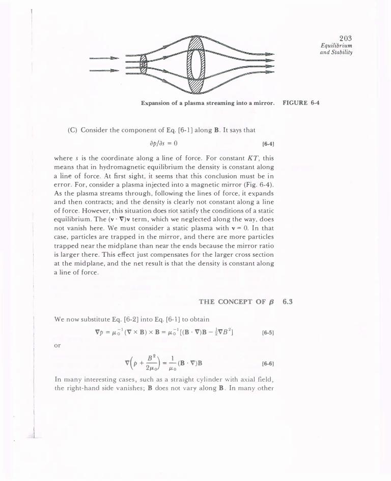
j
Expansion of a plasma streaming into a mirror. FIGURE 6-4
(C) Consider the component of Eq. [6-l] along B. It says that
ap;as = o [6-4]
where s is the coordinate along a line of force. For constant KT, this means that in hydromagnetic equilibrium the density is constant along a line of force. At first sight, it seems that this conclusion must be in error. For, consider a plasma injected into a magnetic mirror (Fig. 6-4). As the plasma streams through, following the lines of force, it expands and then contracts; and the density is clearly not constant along a line of force. However, this situation does riot satisfy the conditions of a static equilibrium. The (v · V)v term, which we neglected along the way, does not vanish here. We must consider a static plasma with v = 0. In that case, particles are trapped in the mirror, and there are more particles trapped near the midplane than near the ends because the mirror ratio is larger there. This effect just compensates for the larger cross section at the midplane, and the net result is that the density is constant along a line of force.
THE CONCEPT OF (J 6.3
We now substitute Eq. [6-2] into Eq. [6-1] to obtain
or
vp = �-to1 (V x B) x B = �-to1 [(B. V)B- �VB2J
( B2) I V p + - = - (B · V)B
2�-to I-to
[6-5]
[6-6)
In many interesting cases, such as a straight cylinder with axial field,
the right-hand side vanishes; B does not vary along B. In many other
203 Equilibrium and Stability

204 Chapter Six
FIGURE 6-5 In a finite-13 plasma, the diamagnetic current significantly decreases the magnetic field, keeping the sum of the magnetic and particle pressures a constant.
cases, the right-hand side is small. Equation (6-6] then says that
B2 p + -- = constant
21-Lo [6-7]
Since B2/2i-Lo is the magnetic field pressure, the sum of the particle
pressure and the magnetic field pressure is a constant. In a plasma with
a density gradient (Fig. 6-5), the magnetic field must be low where the
density is high, and vice versa. The decrease of the magnetic field inside
the plasma is caused, of course, by the diamagnetic current. The size of
the diamagnetic effect is indicated by the ratio of the two terms in Eq.
[6-7]. This ratio is usually denoted by�:
Particle pressure [6-8)
Magnetic field pressure
Up to now we have implicitly considered low-13 plasmas, in which 11 is
between 10-3 and 10-6. The diamagnetic effect, therefore, is very small.
This is the reason we could assume a uniform field B0 in the treatment
of plasma waves. If t1 is low, it does not matter whether the denominator
of Eq. [6-8] is evaluated with the vacuum field or the field in the presence
of plasma. If t1 is high, the local value of B can be greatly reduced by
the plasma. In that case, it is customary to use the vacuum value of B
J

I j
in the definition of {3. High-{3 plasmas are common in space and MHD energy conversion research. Fusion reactors will have to have {3 well in excess of 1% in order to be economical, since the energy produced is
proportional to n 2, while the cost of the magnetic container increases
with some pmver of B. In principle, one can have a {3 = 1 plasma in which the diamagnetic
current generates a field exactly equal and opposite to an externally
generated uniform field. There are then two regions: a region of plasma
without field , and a region of field without plasma. I f the external field
lines are straight, this equilibrium would likely be unstable, since it is like a blob of jel ly held together with stretched rubber bands . It remains
to be seen whether a {3 = 1 plasma of this type can ever be achieved. I n
some magnetic configurations, the vacuum field has a null inside the
plasma; the local value of {3 would then be infinite there . This happens,
for instance, when fields are applied only near the surface of a large
plasma. It is then customary to define {3 as the ratio of maximum particle pressure to maximum magnetic pressure; in this sense, it is not possible
for a magnetically confined plasma to have {3 > 1 .
DIFFUSION OF MAGNETIC FIELD INTO A PLASMA 6.4
A problem which often arises in astrophysics is the diffusion of a magnetic
field into a plasma. I f there is a boundary between a region with plasma but no field and a region with field but no plasma (Fig. 6-6), the regions
will stay separated if the plasma has no resistivity, for the same reason
that flux cannot penetrate a superconductor. Any emf that the moving
lines of force generate will create an infinite current, and this is not
possible. As the plasma moves around, therefore, it pushes the lines of
PLASMA ONLY
In a perfectly conducting plasma, regions of plasma and magnetic field can FIGURE 6-6 be separated by a sharp boundary. Currents on the surface exclude the field from the plasma.
205 Equilibrium and Stability

206 Chapter Six
force and can bend and twist them. This may be the reason for the filamentary structure of the gas in the Crab nebula. If the resistivity is finite, however, the plasma can move through the field and vice versa. This diffusion takes a certain amount of time, and if the motions are slow enough, the lines of force need not be distorted by the gas motions. The diffusion time is easily calculated from the equations (cf. Eq. [5-91])
V X E = -B
E+vxB=17j
[6-9]
[6-10]
For simplicity, let us assume that the plasma is at rest and the field lines are moving into it. Then v = 0, and we ha\'e
[6-11]
Since j is given by Eq. [6-2], this becomes
aB 11 17 9 - = -- V x (V x B) = -- [V(V · B)- v-B] [6-12] at f.J..o f.J..o
Since V · B = 0, we obtain a diffusion equation of the type encountered in Chapter 5:
[6-13]
This can be solved by the separation of variables, as usual. To get a rough estimate, let us take L to be the scale length of the spatial variation of B. Then we have
where
aB '17 -= --9B at f.J..oL-
B = Bo e=t/T
'T = f.J..oL 2/11
[6-14]
[6-15]
[6-16]
This is the characteristic time for magnetic field penetration into a plasma.
The time T can also be interpreted as the time for annihilation of the magnetic field. As the field lines move through the plasma, the induced currenb cause ohmic heating of the plasma. This energy comes from the energy of the field. The energy lost per m3 in a time 'T is 11/'T. Since
. V B f.J..oJ = X B =-L [6-17]

t I I I I
l I I
J
from Maxwell's equation with displacement current neglected, the energy
dissipation is
[6-18]
Thus T is essential ly the time it takes for the field energy to be dissipated
into Joule heat.
207 Equilibrium and Stability
6-1. Suppose that an electromagnetic instability limits {3 to (m/ M)112 in a D-D PROBLEMS reactor. Let the magnetic field be limited to 20 T by the strength of materials. If KT, = KT, = 20 ke V, find the maximum plasma density that can be contained.
6-2. In laser-fusion experiments, absorption of laser light on the surface of a pellet creates a plasma of density n = I 027 m-3 and temperature T, = T, = I 04 eV. Thermoelectric currents can cause spontaneous magnetic fields as high as I 03 T. (a) Show that W(T,; » I in this plasma, and hence electron motion is severely affected by the magnetic field.
(b) Show that {3 » I , so that magnetic fields cannot effectively confine the plasma.
(c) How do the plasma and field move so that the seemingly contradictory conditions (a) and (b) can both be satisfied)
6-3. A cylindrical plasma column of radius a contains a coaxial magnetic field B = B0z and has a pressure profile
P = Po cos2 (m/2a)
(a) Calculate the maximum value of p0.
(b) Using this value of p0, calculate the diamagnetic current j(r) and the total field B(r). (c) Show j(r), B(r), and p(r) on a graph.
(d) If the cylinder is bent into a torus with the lines of force closing upon themselves after a single turn, this equilibrium, in which the macroscopic forces are everywhere balanced, is obviously disturbed. Is it possible to redistribute the pressure p(r, 0) in such a way that the equilibrium is restored?
6-4. Consider an infinite, straight cylinder of plasma with a square density profile created in a uniform field B0 (Fig. P6-4). Show that B vanishes on the axis if /3 = l, by proceeding as follows.
(a) Using the MHO equations, find j.L in steady state for KT =constant.

208 Chapter Six
n(r)
0
FIGURE P6-4
FJ
B=B 0
r a
(b) Using V x B = �0j and Stokes' theorem, integrate over the area of the loop
shown to obtain f"' an/ar Bax- Bo = �ol.KT -- dr
o B (1·)
(c) Do the integral by noting that an/ ar is a o-f unction, so that B (r) at r = a is
the average between B= and B0.
6-5. A diamagnetic loop is a device used to measure plasma presslll·e by detecting
the diamagnetic effect (Fig. P6-5). As the plasma is created, the diamagnetic
current increases, B decreases inside the plasma, and the Aux <I> enclosed by the
loop decreases, inducing a voltage, which is then time-integrated by an RC circuit
(Fig. P6-5).
(a) Show that
I \1 dt = -N �<I>= -N I Bd. dS loop
(b) Use the technique of the previous problem to find Bd(r), but now assume
n (r) = n0 exp [ -(r/r0)2]. To do the integral, assume {3 « 1, so that B can be
approximated by B0 in the integral.
(c) Show that J \1 dt = �N7TT�{3B0, with {3 defined as in Eq. [6-8].
6.5 CLASSIFICATION OF INSTABILITIES
In the treatment of plasma waves, we assumed an unperturbed state
which was one of perfect thermodynamic equilibrium: The particles had

N TURNS
n v
t--
v VOLTAGE
INDUCED
8 = 80 OUTSIDE PLASMA
t--
Maxwellian velocity distributions, and the density and magnetic field were uniform. In such a state of highest entropy, there is no free energy
available to excite waves, and we had to consider waves that were excited
by external means. We now consider states that are not in perfect
thermodynamic equilibrium, although they are in equilibrium in the
sense that all forces are in balance and a time-independent solution is
possible. The free energy which is available can cause waves to be
self-excited; the equilibrium is then an unstable one. An instability is always a motion which decreases the free energy and brings the plasma closer to true thermodynamic equilibrium.
Instabilities may be classified according to the type of free energy
available to drive them. There are four main categories.
1. Streaming instabilities. In this case, either a beam of energetic
particles travels through the plasma, or a current is driven through the
plasma so that the different species have drifts relative to one another.
The drift energy is used to excite waves, and oscillation energy is gained
at the expense of the drift energy in the unperturbed state.
2. Rayleigh-Taylor instabilities. In this case, the plasma has a density gradient or a sharp boundary, so that it is not uniform. In addition, an external, nonelectromagnetic force is applied to the plasma. It is this force which drives the instability. An analogy is available in the example of an inverted glass of water (Fig. 6-7). Although the plane interface
209 Equilibrium and Stability
FIGURE P6-5

210 Chapter Six
FIGURE 6-7
� t t t
g g
Hydrodynamic Rayleigh-Taylor instability of a heavy fluid supported by a light one.
between the water and air is in a state of equilibrium in that the weight of the water is supported by the air pressure, it is an unstable equilibrium. Any ripple in the surface will tend to grow at the expense of potential energy in the gravitational field. This happens whenever a heavy fluid is supported by a light fluid, as is well known in hydrodynamics.
3. Universal instabilities. Even when there are no obvious driving forces such as an electric or a gravitational field, a plasma is not in perfect thermodynamic equilibrium as long as it is confined. The plasma pressure tends to make the plasma expand, and the expansion energy can drive an instability. This type of free energy is always present in any finite plasma, and the resulting waves are called universal instabilities.
4. Kinetic instabilities. In fluid theory the velocity distributions are assumed to be Maxwellian. If the distributions are in fact not Maxwellian, there is a deviation from thermodynamic equilibrium; and instabilities can be drived by the anisotropy of the velocity distribution. For instance, if T11 and T 1. are different, an instability called the modified Harris instability can arise. In mirror devices, there is a deficit of particles with large vn/v 1. because of the loss cone; this anisotropy gives rise to a "loss cone instability."
In the succeeding sections, we shall give a simple example of each of these types of instabilities. The instabilities driven by anisotropy cannot be described by fluid theory and a detailed treatment of them is beyond the scope uf this book.
Not all instabilities are equally dangerous for plasma confinement. A high-frequency instability near wp, for instance, cannot affect the motion of heavy ions. Low-frequency instabilities with w « flc. however, can cause anomalous ambipolar losses via E x B drifts. Instabilities with w = flc do not efficiently transport particles across B but are dangerous

I j
in mirror machines, where particles are lost by diffusion in velocity space 21 1 into the loss cone. Equilibrium
TWO-STREAM INSTABILITY 6.6
As a simple example of a streaming instability, consider a uniform plasma
in which the ions are stationary and the electrons have a velocity v0 relative to the ions . That is, the observer is in a frame moving with the "stream" of ions. Let the plasma be cold (KT, = KT; = 0), and let there be no magnetic field (Bo = 0). The linearized equations of motion are
then
[av, 1 J mno at+ (vo · V)v, 1 = -en0E1
[6-19]
[6-20]
The term (v, 1 • V)v0 in Eq. [6-20] has been dropped because we assume
v0 to be uniform. The (v0 · V)v1 term does not appear in Eq. [6-19] because we have taken v;0 = 0. We look for electrostatic waves of the form
E1 = E e i(kx-wt)x [6-21]
where x is the direction of v0 and k. Equations [6-19] and [6-20] become
mno(-iw + ikv0)v,1 = -en0E,
u A v·1 =--Ex ' Mw
ie Ex Vel=--m w- kv0
[6-22]
[6-23]
The velocities vi, are in the x direction, and we may omit the subscript x. The ion equation of continuity yields
an;, -- + noV · v 1 = 0 at ' k ien0k n;' = -nov;' = • -r 2 E
W lVlW [6-24]
Note that the other terms in V · (nv;) vanish because Vn0 = v0; = 0. The
electron equation of continuity is
an,, -- + noV· Vet + (vo · V)nel = 0 [6-25] at
( -iw + ikvo)n, 1 + iknov, 1 = 0 [6-26]
kno iekn0 n,1 = v,, =- 2 E [6-27] w- kvo m(w- kvo)
and Stability

212 Chapter Six
Since the unstable waves are high-frequency plasma oscillations, we may
not use the plasma approximation but must use Poisson's equation:
. . [ 1 l J tkE0E = e(zenokE) � + k 2 A1w m(w- v0)
The dispersion relation is found upon dividing by ikEoE:
2[m/M l J ] = Wp --? - + ? w- (w - kvor
[6-28]
[6-29]
[6-30]
Let us see if oscillations with real k are stable or unstable. Upon
multiplying through by the common denominator, one would obtain a
fourth-order equation for w. If all the roots wi are real , each root would
indicate a possible oscillation
I f some of the roots are complex, they will occur in complex conjugate
pairs. Let these complex roots be written
[6-31]
where a andy are Re(w) and Im(w ), respectively. The time dependence
is now given by
[6-32]
Positive Im(w) indicates an exponentially growing wave; negative lm(w)
indicates a damped wave. Since the roots wi occur in conjugate pairs,
one of these will always be unstable unless all the roots are real. The
damped roots are not self-excited and are not of interest. The dispersion relation [6-30] can be analyzed without actually
solving the fourth-order equation. Let us define
x = w/wp
Then Eq. [6-30] becomes
y = kvo/ Wp
rn/M l l = -? - + 2 = F(x, y)
x- (x - y)
[6-33]
[6-34]
For any given value of y, we can plot F(x, y) as a function of x. This function will h ave singularities at x = 0 and x = y (Fig. 6-8). The intersec
tions of this curve with the line F(x, y) = 1 give the values of x satisfying the dispersion relation. In the example of Fig. 6-8, there are four
intersections, so there are four real roots wi. However, if we choose a

0 0 y
F(x,y)
X ---1---
213 Equilibrium and Stability
The function F(x, y) in the two-stream instability, when the plasma is FIGURE 6-8 stable.
F(x,y)
0 0 y X _ __, .. ._
The function F(x, y) in the two-stream instability, when the plasma FIGURE 6-9 is unstable.
smaller value of y, the graph would look as shown i n Fig. 6-9. Now there
are only two intersections and, therefore, only two real roots . The other
two roots must be complex, and one of them must correspond to an
unstable wave. Thus, for sufficiently small kv0, the plasma i s unstable.
For any given v0, the plasma is always unstable to long-wavelength
oscillations. The maximum growth rate predicted by Eq. [6-30] is , for
m/M « 1,
[6-35]
Since a small value of kv0 is required for instability, one can say that for a given k, v0 has to be sufficiently small for instability. This does not make much physical sense, since v0 is the source of energy drivin g the

214 Chapter Six
instability. The difficulty comes from our use of the fluid equations. Any real plasma has a finite temperature, and thermal effects should be taken
into account by a kinetic-theory treatment. A phenomenon known as Landau damping (Chapter 7) will then occur for v0 � v,h, and no instabil
ity is predicted if v0 is too small.
This "Buneman" instability, as it is sometimes called, has the following physical explanation. The natural frequency of oscillations in the
electron fluid is Wp, and the natural frequency of oscillations in the ion fluid is flp = (m/ M)112wp. Because of the Doppler shift of the wp oscillations in the moving electron fluid, these two frequencies can coincide in the laboratory frame if kv0 has the proper value. The density fluctuations of ions and electrons can then satisfy Poisson's equation. Moreover. the
electron oscillations can be shown to have negative energy. That is to say, the total kinetic energy of the electrons is less when the oscillation is
present than when it is absent. In the undisturbed beam, the kinetic energy per m3 is �mn0v�. When there is an oscillation, the kinetic energy
is �m (no+ n J)(v0 + v 1t When this is averaged over space, it turns out
to be less than �mn0v� because of the phase relation between n1 and v1 required by the equation of continuity. Consequently, the electron oscilla
tions have negative energy, and the ion oscillations have positive energy.
Both waves can grow together while keeping the total energy of the system constant. An instability of this type i.s used in klystrons to generate
microwaves. Velocity modulation due to E1 causes the electrons to form bunches. As these bunches pass through a microwave resonator, they
can be made to excite the natural modes of the resonator and produce microwave power.
PROBLEMS 6-6.(a) Derive the dispersion relation for a two-stream instability occurring when
there are two cold electron streams with equal and opposite v0 in a background
of fixed ions. Each stream has a density �o·
(b) Calculate the maximum growth rate.
6-7. A plasma consists of two uniform streams of protons with velocities +vox and -v0x, and respective densities �u and �0. There is a neutralizing electron
fluid with density n0 and with v0, = 0. All species are cold, and there is no magnetic field. Derive a dispersion relation for streaming instabilities in this
system.
6-8. A cold electron beam of density 8nu and velocity u is shot into a cold plasma
of density n0 at rest.

(a) Derive a dispersion relation for the high-frequency beam-plasma instability that ensues. (b) The maximum growth rate I'm is difficult to calculate, but one can make a reasonable guess if 8 « 1 by analogy with the electron-ion Buneman instability. Using the result gi,·en without proof in Eq. [6-35], give an expression for I'm in terms of 8.
6-9. Let two cold, counterstreaming ion fluids have densities 4no and velocities ±v0y in a magnetic field B0z and a cold neutralizing electron fluid. The field B0 is strong enough to confine electrons but not strong enough to affect ion orbits.
(a) Obtain the following dispersion relation for electrostatic waves propagating in the ±y direction in the frequency range n� « w2 « w;:
.{12 .{12 2 ---'-"---;;: + , =
w"+l
2(w- kv0)2 2(w + kv0)2 w�
(b) Calculate the dispersion w(k), growth rate y(k), and the range of wave numbers of the unstable waves.
THE "GRAVITATIONAL" INSTABILITY 6. 7
In a plasma, a Rayleigh-Taylor instability can occur because the magnetic
field acts as a light fluid supporting a heavy fluid (the plasma). In curved
magnetic fields, the centrifugal force on the plasma due to particle motion
along the curved l ines of force acts as an equivalent "gravitational" force.
To treat the simplest case, consider a plasma boundary lying in the y-z plane (Fig. 6-1 0). Let there be a density gradient Vn0 in the -x direction and a gravitational field gin the x direction. We may let KT; = KT, = 0
for simplicity and treat the low-13 case, in which B0 is uniform . In the
equilibrium state, the ions obey the equation
Mno(vo · V)vo = en Vo X Bo + Mn0g [6-36]
PLASMA 0B
VACUUM
215 Equilibrium and Stability
A plasma surface subject to a gravitational instability. FIGURE 6-10

21 6 Chapter Six
If g is a constant, v0 will be also; and (v0 · V)v0 vanishes. Taking the cross
product of Eq. [6-36] with B0, we find, as in Section 2.2,
M gx Bo g �
Vo = - --2- = -- Y e Bo flc
[6-37]
The electrons have an opposite drift which can be neglected in the limit m/ M � 0. There is no diamagnetic drift because KT = 0, and no E0 x B0 drift because Eo= 0.
If a ripple should develop in the interface as the result of random thermal fluctuations, the drift v0 will cause the ripple to grow (Fig. 6-ll ) . The drift of ions causes a charge to build up on the sides of the ripple,
and an electric field develops which changes sign as one goes from crest
to trough in the perturbation . As can be seen from Fig. 6- 1 1, the E1 x B0 drift is always upward in those regions where the surface has moved
upward, and downward where it has moved d ownward. The ripple grows
as a result of these properly phased E1 x B0 d rifts.
To find the growth rate, we can perform the usual linearized wave analysis for waves propagating in they direction: k = ky. The perturbed
ion equation of motion is
M(no + n ,)[� (vo + v1) + (v0 + v,) · V(vo + v,) J = e(n0 + n 1)[E1 + (v0 + v1) X B0] + M(n0 + n,)g [6-38]
We now multiply Eq. [6-36] by 1 + (n1/n0) to obtain
M(n0 + n,)(v0 • V)v0 = e(n0 + n1)vo X Bo + M(no + n,)g [6-39]
Subtracting this from Eq. [6-38] and neglecting second-order terms, we have
[6-40]
v;������ ' : ����� ����·I!�: 1
FIGURE 6-11 Physical mechanism of the gravitational instability.
J

1
Note that g has cancelled out. I n formation regarding g, however, is still
contained in v0. For perturbations of the form exp [i (ky - wt)], we have
M(w- kv0)v1 = ie(E1 + v1 X Bo) [6-41]
This is the same as Eq. [ 4-96] except that w is re placed by w - kv0, and
electro n quantities are re pl aced b y ion qu antities. The solution, therefore,
is give n b y Eq. [ 4-98] with the appro priate changes. For Ex = 0 and
the solutio n is
Ey v· =
•x Bo
[6-42]
[6-43)
The latter quantity is the polarizat ion drift in the ion frame. The corres
po nding qu antity for electrons vanishes i n the limit m/ M � 0. For the
electro ns, we therefore have
[6-44]
The perturbed equation o f continuity for ions is
The zeroth-order term vanishes si nce v0 is per pendicul ar to Vn0, and the n 1 V · v0 term vanishes if v0 is constant. The first-order equation is, there fore,
[6-46]
where n� = an0/ ax. The electrons fol low a s impler equ ation, since v,0 = 0
and Vey = 0:
[6-47]
Note that we have used the pl asma approximation and have assumed n;1 = ne1. This is poss ible because the u nstab le waves are o f low frequencies (this can be justified a posteriori). Equations [6-43] and [6-46] yield
k . Ey , '
k w - kv0 Ey
(w- Vo)nl + t - n0 + t no - = 0 Bo flc Bo
Equations [6-44] and [6-47] yield
·b I 0 wn1 + t Bo n0 = b_ iwn1 Bo- �
[6-48)
[6-49)
217 Equilibrium and Stability

218 Chapter Six
Substituting this into Eq. [6-48], we have
k ( 1 w - kvo ) wn 1 (w- vo)nl- no+ kn 0 -�- = 0
fl, no
k ( kn0 w - kv0) w - Vo - I + - 1 w = 0
fl, no [6-50]
[6-51]
Substituting for v0 from Eq. [6-37]. we obtain a quadratic equation for w:
The solutions are 2 k II w - v0w- g(no no)= 0
w = �kvo ± [�k2v� + g(n�/n0)]112
There is instability if w is complex; that is, if
I I I k2 2 -gnuno>4 Vo
[6-52]
[6-53]
[6-54]
From this, we see that instability requires g and n�/n0 to have opposite sign. This is just the statement that the light fluid is supporting the heavy fluid; otherwise, w is real and the plasma is stable. Since g can be used
to model the effects of magnetic field curvature, we see from this that stability depends on the sign of the curvature. Configurations with field
lines bending in toward the plasma tend to be stabilizing, and vice versa. For sufficiently small k (long wavelength), the growth rate is given by
I Y = lm (w) = [-g(n�/n0)]112 I [6-55]
Note that the real part of w idkv0. Since v0 is an ion velocity, this is a
low-frequency oscillation, as previously assumed. The factor of � is merely a consequence of neglecting v0,. The wave is stationary in the frame in which the density-weighted average of all the v0's is zero, which
in this case is the frame moving at � v0. The laboratory frame has no
particular significance in this case.
This instability, which has k 1_ B0, is sometimes called a "flute" instability for the following reason. In a cylinder, the waves travel in the 8 direction if the forces are in the r direction. The surfaces of constant
density then resemble fluted Greek columns (Fig. 6-12).
6.8 RESISTIVE DRIFT WAVES
A simple example of a universal instability is the resistive drift wave. In contrast to gravitational flute modes, drift waves have a small but finite

j
A "flute" instability.
com ponent of k along B0. The constant de nsity surfaces, therefore, resemble flutes with a slight helical twist (Fig. 6-13). If we enlarge the
cross section enclosed by the box in Fig. 6-13 and straighten it out i nto
Cartesian geometry, it would appear as in Fig. 6-14. The o nly driving
force for the i nstability is the pressure gr adie nt KT Vn0 (we assume
KT = constant, for sim plicity). In this case, the zeroth-order drifts (for Eo= 0) are
KT; n� �
V;o = Vo; = --- Y eBo no
KT, nb �
v,o = vo. = - --- y eBo no
[6-56]
[6-57]
From our experie nce with the flute i nstability, we might ex pect drift
waves to have a phase velocity of the order of v0; or v0,. We shall show
that w/ky is approximately equal to v0,.
Since drift w aves h ave finite k., electrons can flow along B0 to establish
a thermodynamic equilibrium among themselves (cf. discussion of Section 4.10). They wi ll then obey the Boltzmann relation (Section 3.5):
[6-58]
At point A i n Fig. 6-14 the de nsity is l arger than in equilibrium, n 1 is positive, and therefore ¢1 is positive. Similarly, at point B, n1 and ¢1 are negative. The difference i n potential means there is· an electric field E1
219 Equilibrium and Stability
FIGURE 6-12

220 Chapter Six
FIGURE 6-13 Geometry of a drift instability in a cylinder. The region in the rectangle is shown in detail in Fig. 6-14.
between A and B. Just as in the case of the fl ute instability, E1 causes a drift v1 = E1 x B0/ B � in the x direction. As the wave passes by, traveling
in the y direction, an observer at point A will see n 1 and ¢1 oscillating
in time. The drift v1 will also oscillate in time, and in fact it is v1 which causes the density to oscillate. Since there is a gradient Vn0 in the -x
direction, the drift v1 will bring plasma of different density to a fixed
observer A. A drift wave, therefore, has a motion such that the fluid
moves back and forth in the x direction although the wave travels in the
y direction.
To be more quantitative, the magnitude of v lx is given by
[6-59]
We shall assume v lx does not vary with x and that k, is much less than
k1; that is, the fluid oscillates incompressibly in the x direction. Consider now the number of guiding centers brought into 1 m3 at a fixed point
A; it is obviously
[6-60]
This is just the equation of continuity for guiding centers, which, of
course, do not have a fluid drift v0. The term n0 V · v1 vanishes because

J
y t 221
Equilibrium
_.__ Vn0 and Stability
0B 0
+
t v,
=<Ill(
t E,
k
DENSE LESS DENSE
X
Physical mechanism of a drift wave. FIGURE 6-14
of our previous assum ption. The d ifference betwee n the density of
guiding centers and the density of particles n 1 gives a correction to Eq. [6-60] which is h igher order and may be neglected here. Using Eqs. [6-59] and [6-58], we can write Eq. [6-60) as
Thus we h ave
w KT. n� -=- -- -=vv k, eBo no
•
[6-61]
[6-62]
These waves, therefore, travel w ith the electron diamag netic drift velocity
and are c al led drift waves. This is the velocity in the y, or azimuthal, direction. I n addition, there is a component of ki n the z directio n. For reasons not given here, this component must satisfy the conditio ns
k, « k, [6-63]

222 Chapter Six
To see why drift waves are unstable, one must realize that v lx is not
quite £)./ B0 for the ions. There are corrections due to the polarization
drift, Eq. [2-66], and the nonuniform E drift, Eq. [2-59]. The result of these drifts is always to make the potential distribution ¢1 lag behind
the density distribution n 1 (Problem 4-1 ). This phase shift causes v1 to be outward where the plasma has already been shifted outward, and vice versa; hence the perturbation grows. In the absence of the phase shift, n 1 and ¢1 would be 90° out of phase, as shown in Fig. 6-14, and drift waves would be purely oscillatory.
The role of resistivity comes in because the field E1 must not be short-circuited by electron A ow along B0. Electron-ion collisions, together
with a long distance �A, between crest and trough of the wave, make it
possible to have a resistive potential drop and a finite value of E1. The
dispersion relation for resistive drift waves is approximately
[6-64]
where
[6-65]
and
k� 0'11 =
k 2 flc (Wc'Te;) y
[6-66]
If 0'11 is large compared with w, Eq. [6-64] can be satisfied only if w = w*.
In that case, we may replace w by w* in the first term. Solving for w, we then obtain
[6-67)
This shows that Im(w) is always positive and IS proportional to the resistivity 71· Drift waves are, therefore, unstable and will eventually occur
in any plasma with a density gradient. Fortunately, the growth rate is rather small, and there are ways to stop it altogether by making Bo nonuniform.
Note that Eq. [6-52] for the Aute instability and Eq. [6-64] for the
drift instability have different structures. In the former, the coefficients

are real, and w is complex when the discriminant of the quadratic is
negative ; this is typical of a reactive instability. I n the latter, the coefficients are complex, so w is always complex; this is typical of a dissipative instability.
6-10. A toroidal hydrogen plasma with circular cross section has major radius R = 50 em, minor radius a = 2 em, 8 = I T, KT, = 10 eV, KT, = I eV, and n o =
1 0 19 m-� . Taking n0/n ;, = a/2 and g = (KT, + KT, ) / MR, estimate the growth rates of the m = I resistive drift wave and the m = I gravitational fl ute mode. (One can usually apply the slab-geometry formulas to cylindrical geometry by replacin g k, by m/r, where m is the azimuthal mode n u mber.)
THE WEIBEL INSTABILITY*
As an example of an instability driven by anisotropy of the distribution
function, we give a physical picture (due to B. D. Fried) of the Weibel instability, in which a magnetic perturbation is made to grow. This will also
serve as an example of an electromagnetic instability. Let the ions be fixed ,
and let the electrons be hotter in the y direction than in the x or z directions.
There is then a preponderance of fast electrons in the ±y directions (Fig.
6-15) , but equal numbers flow up and down, so that there is no net current . Suppose a field B = B,z cos kx spontaneously arises from noise. The Lorentz force -ev x B then bends the electron trajectories as shown by
the dashed curves, with the result that downward-moving electrons
y
z
._. A \
I \
I J
t I
f B � I I
X
223 Equilibrium and Stability
PROBLEM
6.9
Physical mechanism of the Weibel instability. FIGURE 6-15
* A salute t o a good friend, Erich Weibel ( 1 925- 1 9il:l) .

224 Chapter Six
congregate at A and u pward-moving ones at B. The resulting current sheets j = -en ov. are phased ex actly right to gene rate a B field o f the shape
assume d , and the pe rturbat ion g rows. Though the general case requi res a ki netic t reatment, the l im iti ng case Vy = v,h, vx = v, = 0 can be calculated
ve ry s imply from this phy sical pictu re , y ielding a g rowth rate y = wpv,h! c.

I J
I< Chapter Seven
EORY
THE MEANING OF f(v) 7.1
The fluid theory we have been using so far is the simplest description of a plasma; it is indeed fortunate that this approximation is sufficiently accurate to describe the majority of observed phenomena. There are some phenomena, however, for which a fluid treatment is inadequate. For these, we need to consider the velocity distribution function f(v) for each species; this treatment is called kinetic theory. In fluid theory, the dependent variables are functions of only four independent variables: x, y, z, and t. This is possible because the velocity distribution of each species is assumed to be Maxwellian everywhere and can therefore be uniquely specified by only one number, the temperature T. Since collisions can be rare in high-temperature plasmas, deviations from thermal equilibrium can be maintained for relatively long times. As an example, consider two velocity distributions [1(vx) and /2(v,) in a one-dimensional system (Fig. 7-1). These two distributions will have entirely different behaviors, but as long as the areas under the curves are the same, fluid theory does not distinguish between them.
The density is a function of four scalar variables: n = n(r, t). When we consider velocity distributions, we have seven independent variables: f = f(r, v, t). By f(r, v, t), we mean that the number of particles per m3
at position rand timet with velocity components between Vx and Vx + dv" Vy and vy + dvy, and v, and v, + dv, is
225

226 Chapter Seven
FIGURE 7-1 E-xamples of non-Maxwellian distribution functions.
The integral of this is written in several equivalent ways:
n(r, t) = t: dvx t: dvy t: dvJ(r, v, t) = t: f(r, v, t) d3v
= t: f(r, v, t) dv [7-1]
Note that dv is not a vector; it stands for a three-dimensional volume
element in velocity space. Iff is normalized so that
L:J(r, v, t) dv = 1 [7-2]
it is a probability, which we denote by f Thus
f(r, v, t) = n(r, t)/(r, v, t) [7-3]
Note that f is still a function of seven variables, since the shape of the
distribution, as well as the density, can change with space and time. From
Eq. [7-2], it is clear thatfhas the dimensions (m/secf3; and consequently,
from Eq. [7-3], f has the dimensions sec3-m-6.
A particularly important distribution function is the Maxwellian:
� /2 3/2 2/ 2 [m = (m 'TTKT) exp (-v v,h) [7-4]
where
- 2 2 2 1/2 v =(vx +v y +v,) and [7-5)

Vz 227 Kinetic Theory
Vy
Three-dimensional velocity space. FIGURE 7-2
By using the definite integral
[7-6]
one easily verifies that the integral of fm over dvx dvy dv, is unity. There are several average velocities of a Maxwellian distribution
that are commonly used. In Section 1.3, we saw that the root-mean-square velocity is given by
(v2)I/2 =
(3KT/m)I/2 [7-7]
The average magnitude of the velocity I vI, or simply ii, is found as follows:
JC() A 3 ii = -co vf(v) d v [7-8]
Since fm is isotropic, the integral is most easily done in spherical coordinates in v space (Fig. 7-2). Since the volume element of each spherical

228 Chapter Seven
shell is 47Tv2 dv, we have
co _ I 3/9 f 9l 2 9 v = (m 27TKT) - 0 v[exp (-v- v,h)]47Tv- dv
co
( 9 )-3/94 4 f 9 3 d = 7TV:h - 7TV,11 0 [exp (-y-)]y Y
[7-9]
[7-IO]
The definite integral has a value t found by integration by parts. Thus
[7-ll]
The velocity component in a single direction, say Vx, has a different average.
Of course, iJx vanishes for an isotropic distribution; but I vxl does not:
[7-12]
[7-13]
From Eq. [7-6], each of the first two integrals has the value 7T112v,h. The
last integral is simple and has the value v �h· Thus we have
-1 -1 2 -3/2 4 -112 I 112 Vx = (7TV,h ) 7TV,h = 7T v,h = (2KT 7Tm) [7-14]
The random flux crossing an imaginary plane from one side to the other
is given by
r random = �nr;:T = �nii [7-15]
Here we have used Eq. [7 -11] and the fact that only half the particles
cross the plane in either direction. To summarize: For a Maxwellian,
I 1/2 Vrms = (3KT m)
r;f = 2(2KTITrm)112
f;'J = (2KT17Tm)112
[7-7]
[7-11]
[7-14]
[7-16]
For an isotropic distribution like a Maxwellian, we can define another function g(v) which is a function of the scalar magnitude of v such that
[7-17]
; --t

_ __l
For a Maxwellian, we see from Eq. [7-9] that 229
g(v) = 4-rrn(m/2TrKT)312v2 exp (-v2/v�) Kinetic Theory
[7-18]
Figure 7-3 shows the difference between g(v) and a one-dimensional Maxwellian distributionl(vx). Althoughl(vx) is maximum for Vx = 0, g(v) is zero for v = 0. This is just a consequence of the vanishing of the volume in phase space (Fig. 7-2) for v = 0. Sometimes g(v) is carelessly denoted by l(v), as distinct from l(v); but g(v) is a different function of its argument than l(v) is of its argument. From Eq. [7-18], it is clear that
g(v) has dimensions sec/m4. It is impossible to draw a picture of l(r, v) at a given time t unless
we reduce the number of dimensions. In a one-dimensional system,
l(x, vx) can be depicted as a surface (Fig. 7-4). Intersections of that surface with planes x = constant are the velocity distributions l(vx). Intersections. with planes Vx = constant give density profiles for particles with a given vx. If all the curves l(vx) happen to have the same shape, a curve through the peaks would represent the density profile. The dashed curves in Fig. 7-4 are intersections with planes I= constant; these are level curves, or curves of constant f. A projection of these curves onto the x-vx plane will give a topographical map of f. Such maps are very useful for getting a preliminary idea of how the plasma behaves; an example will be given in the next section.
Another type of contour map can be made for I if we consider l(v) at a given point in space. For instance, if the motion is two dimensional, the contours of l(vx, vy) will be circles if I is isotropic in vx, Vy. An
g(v)
0 0
One- and three-dimensional Maxwellian velocity distributions. FIGURE 7-3
v

230 Chapter Seven
f
FIGURE 7-4 A spatially varying one-dimensional distribution f(x, vx)·
anisotropic distribution would have elliptical contours (Fig. 7 -5). A drift
ing Maxwellian would have circular contours displaced from the origin,
and a beam of particles traveling in the x direction would show up as a
separate spike (Fig. 7-6).
A loss cone distribution of a mirror-confined plasma can be represen
ted by contours off in v.L, vu space. Figure 7-7 shows how these would
look.
7.2 EQUATIONS OF KINETIC THEORY
The fundamental equation which f(r, v, t) has to satisfy is the Boltzmann equation:
[7-19]
Here F is the force acting on the particles, and (aflat), is the time rate of change off due to collisions. The symbol V stands, as usual, for the
gradient in (x, y, z) space. The symbol aj av or V v stands for the gradient

231 Kinetic Theory
Contours of constant f for a two-dimensional, anisotropic FIGURE 7-5 distribution.
DRIFTING MAXWELLIAN
/ BEAM
Contours of constant f for a drifting Maxwellian distribution and a "beam" FIGURE 7-6 in two dimensions.

232 Chapter Seven
FIGURE 7-7 Contours of constant/ for a loss-cone distribution. Here v! and v _,_stand for the components of v along and perpendicular to the magnetic field, respectively.
in velocity space:
a A a A a A a - =x - +y - +z
av av, av, av, [7-20]
The meanmg of the Boltzmann equation becomes clear if one remembers that f is a function of seven independent variables. The total derivative of f with time is, therefore
df a[ a[ dx a[ dy a[ dz a[ dv, a[ dvy a[ dv, -= - + - - + - - + - -+ - - + - - + - - [7-21] dt at ax dt ay dt az dt av, dt avy dt av, dt
Here, a[/ at is the explicit dependence on time. The next three terms are
just v · Vf. With the help of Newton's third law,
dv m-=F
dt [7-22]
the last three terms are recognized as (F/m) · (a[/av). As discussed pre
viously in Section 3.3, the total derivative df/ dt can be interpreted as the rate of change as seen in a frame moving with the particles. The difference is that now we must consider the particles to be moving in six-dimensional
(r, v) space; df/dt is the convective derivative in phase space. The
i

233 Kinetic Theory
El/� A
X
A group of points in phase FIGURE 7-8
space, representing the posi-
tion and velocity coordinates of a group of particles, retains
the same phase-space density
as it moves with time.
Boltzmann equation [7 -19] simply says that df / dt is zero unless there are collisions. That this should be true can be seen from the one-dimensional example shown in Fig. 7-8.
The group of particles in an infinitesimal element dx dvx at A all have velocity vx and position x. The density of particles in this phase space is justf(x, vx). As time passes, these particles will move to a different x as a result of their velocity Vx and will change their velocity as a result of the forces acting on them. Since the forces depend on x and vx only, all the particles at A will be accelerated the same amount. After a time t, all the particles will arrive at B in phase space. Since all the particles moved together, the density at B will be the same as at A. If there are collisions, however, the particles can be scattered; and f can be changed by the term (of/ot)c.
In a sufficiently hot plasma, collisions can be neglected. If, furthermore, the force F is entirely electromagnetic, Eq. [7-19] takes the special form
of q of - + v . vI+ -(E + v X B) . - = 0 at m av [7-23]
This is called the Vlasov equation. Because of its comparative simplicity, this is the equation most commonly studied in kinetic theory. When

234 Chapter Seven
there are collisions with neutral atoms, the collision term in Eq. [7 -19] can be approximated by
T [7-24]
where f, is the distribution function of the neutral atoms, and T is a constant collision time. This is called a Krook collision term. It is the kinetic
generalization of the collision term in Eq. [5-5]. When there are Coulomb
colllisions, Eq. [7-1 9] can be approximated by
df a 1 i dt =
- av. (f(flv))2 av av: (f(flv !lv)) [7-25]
This is called the Fokker-Planck equation; it takes into account binary
Coulomb collisions only. Here, llv is the change of velocity in a collision,
and Eq. [7-25] is a shorthand way of writing a rather complicated
expressiOn. The fact that df/ dt is constant in the absence of collisions means
that particles follow the contours of constant f as they move around in
phase space. As an example of how these contours can be used, consider
the beam-plasma instability of Section 6.6. In the unperturbed plasma,
the electrons all have velocity v0, and the contour of constant/ is a straight
line (Fig. 7-9). The function f(x, v.) is a wall rising out of the plane of
the paper at v. = v0. The electrons move along the trajectory shown. When a wave develops, the electric field E1 causes electrons to suffer
changes in v. as they stream along. The trajectory then develops a sinusoidal ripple (Fig. 7-10). This ripple travels at the phase velocity,
0 X
FIGURE 7-9 Representation in one-dimensional phase space of a beam of electrons all with the same velocity u0. The distribution function f(x, v.) is infinite along the line and zero elsewhere. The line is also the trajectory of individual electrons, which move in the direction of the arrow.

I � -
235 Kinetic Theory
0 X
Appearance of the graph of Fig. 7-9 when a plasma wave exists in the FIGURE 7-10 electron beam. The entire pattern moves to the right with the phase
velocity of the wave. If the observer goes to the frame of the wave, the
pattern would stand still, and electrons would be seen to trace the curve
with the velocity v0- v<b.
TRAPPED ELECTRON
FREE ELECTRON . ....
X
The potential of a plasma wave, as seen by an electron. The pattern moves FIGURE 7-11 with the velocity v<b. An electron with small velocity relative to the wave would be trapped in a potential trough and be carried along with the wave.
not the particle velocity. Particles stay on the curve as they move relative to the wave. If E 1 becomes very large as the wave grows, and if there are a few collisions, some electrons will be trapped in the electrostatic potential of the wave. In coordinate space, the wave potential appears as in Fig. 7-11. In phase space, f(x, vx ) will have peaks wherever there is a potential trough (Fig. 7-12). Since the contours off are also electron trajectories, one sees that some electrons move in closed orbits in phase space; these are just the trapped electrons.
Electron trapping is a nonlinear phenomenon which cannot be treated by straightforward solution of the Vlasov equation. However, electron trajectories can be followed on a computer, and the results are

236 Chapter Seven
v
X
FIGURE 7-12 Electron trajectories, or contours of constant f, as seen in the wave frame, in which the pattern is stationary. This type of diagram, appropriate for finite distributions f(v), is easier to understand than the a-function distribution of Fig. 7-10.
often presented in the form of a plot like Fig. 7-12. An example of a
numerical result is shown in Fig. 7-13. This is for a two-stream instability
in which initially the contours off have a gap near vx = 0 which separates electrons moving in opposite directions. The development of this unin
habited gap with time is shown by the shaded regions in Fig. 7-13. This
figure shows that the instability progressively distorts f(v) in a way which
would be hard to describe analytically.
7.3 DERIVATION OF THE FLUID EQUATIONS
The fluid equations we have been using are simply moments of the Boltzmann equation. The lowest moment is obtained by integrating Eq. [7-19] with F specialized to the Lorentz force:
J a[ dv + J v · Vf dv + !]_ J (E + v X B)· a[ dv = J (af\ dv [7-26] � m � � .
The first term gives
f a[ dv = j_ f f dv = an at at at [7-27]
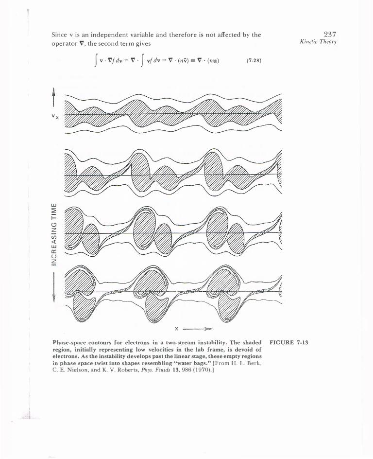
237 Since v is an independent variable and therefore is not affected by the
operator V , the second term gives Kinetic Theory
UJ � 1-<..:J z (/) <( UJ a: u z
J v · Vf dv = V · J vf dv = V · (nv) = V · (nu) [7-28]
X
Phase-space contours for electrons in a two-stream instability. The shaded FIGURE 7-13 region, initially representing low velocities in the lab frame, is devoid of electrons. As the instability develops past the linear stage, these empty regions in phase space twist into shapes resembling "water bags." [From H. L. Berk, C. E. Nielson, and K. V. Roberts, Phys. Fluids 13, 986 (1970).]
238 Chapter Seven
where the average velocity u is the fluid velocity by definition. The E
term vanishes for the following reason:
f a[ J a J .
E · - dv = -·([E) dv = [E · dS = 0 av av Sro [7-29]
The perfect divergence is integrated to give the value of [E on the surface at v = oo. This vanishes if f� 0 faster than v -2 as v � <Xl, as is necessary
for any distribution with finite energy. The v x B term can be written
as follows:
I at J a J a (v X B) ·- d v = - · (fv X B) d v- [- X (v X B) dv = 0 av av av [7-30]
The first integral can again be converted to a surface integral. For a
Maxwellian, f falls faster than any power of v as v � oo, and the integral
therefore vanishes. The second integral vanishes because v x B is perpen
dicular to ajav. Finally, the fourth term in Eq. [7-26] vanishes because
collisions cannot change the total number of particles (recombination is
not considered here). Equations [7-27]-[7-30] then yield the equation of continuity:
an - + V · (nu) = 0 at [7-31]
The next moment of the Boltzmann equation is obtained by multiplying
Eq. [7-19] by mv and integrating over dv. We have
m J v a[ dv + m J v(v · V)f dv + q J v(E + v x B) · a[ dv = J mv (a[) dv
at av at c
[7-32]
·The right-hand side is the change of momentum due to collisions and will give the term P;i in Eq. [5-58]. The first term in Eq. [7-32] gives
J a[ a J a m v- dv = m- vf dv = m-(nu) at at at
The third integral in Eq. [7-32] can be written
f a[ J a v(E + v X B) ·- dv = - · [ fv(E + v x B)] dv av av
[7-33]
- J fv.i_ · (E+v X B) d v- J f(E + v X B) · .i_v dv [7-34] av av
The first two integrals on the right-hand side vanish for the same reasons as before, and av/av is just the identity tensor I. We therefore have
q f v(E+v X B) · :� dv = -q f (E + v x B)f dv = -qn(E + u x B)
[7-35)
Finally, to evaluate the second integral in Eq. [7-32], we first make use of the fact that v is an independent variable not related to V and write
J v(v · V)f dv = J V · (fvv) dv = V · J fvv dv [7-36]
Since the average of a quantity is 1/n times its weighted integral over v, we have
V · J fvv dv = V · nvv [7-37]
Now we may separate v into the average (fluid) velocity u and a thermal velocity w:
v=u+ w [7-38)
Since u is already an average, we have
V · (nvv) = V · (nuu) + V · (nww) + 2V · (nuw) [7-39)
The average w is obviously zero. The quantity mnww is precisely what is meant by the stress tensor P:
P=mnww [7-40)
The remaining term in Eq. [7-39] can be written
V · (nuu) = uV · (nu) + n(u · V)u [7-41)
Collecting our results from Eq. [7-33], [7-35], [7-40], and [7-41], we can write Eq. [7-32] as
a m-(nu) + mu V · (nu) + mn(u · V)u + V · P - qn(E + u x B) = P;i
at [7-42)
Combining the first two terms with the help of Eq. [7-31], we finally obtain the fluid equation of motion:
mn [ �: + (u · V)u J = qn (E + u x B) - V · P + P;i [7-43)
This equation describes the flow of momentum. To treat the flow of energy, we may take the next moment of Boltzmann equation by
239 Kinetic Theory

240 Chapter Seven
7.4
multiplying by �mvv and integrating. We would then obtain the heat flow equation, in which the coefficient of thermal conductivity K would arise
in the same manner as did the stress tensor P. The equation of state
p oc p y is a simple form of the heat flow equation forK = 0.
PLASMA OSCILLATIONS AND LANDAU DAMPING
As an elementary illustration of the use of the Vlasov equation, we shall
derive the dispersion relation for electron plasma oscillations, which we
treated from the fluid point of view in Section 4.3. This derivation will
require a knowledge of contour integration. Those not familiar with this
may skip to Section 7.5. A simpler but longer derivation not using the
theory of complex variables appears in Section 7 .6. In zeroth order, we assume a uniform plasma with a distribution
f0(v), and we let B0 =Eo= 0. In first order, we denote the perturbation
in f(r, v, t) by /J(r, v, t):
f(r, v, t) = [o(v) + [J(r, v, t) [7-44]
Since v is now an independent variable and is not to be linearized, the
first-order Vlasov equation for electrons is
a[l e a[o - + v · V[I -- E I ·-= 0 a t m. av [7-45]
As before, we assume the ions are massive and fixed and that the waves
are plane waves in the x direction
[7-46]
Then Eq. [7-45] becomes
[7-47]
[7-48]
Poisson's equation gives
[7-49]

Substituting for [1 and dividing by ikEoEx, we have
1 =- L fff ato!avx d3v kmEo w- kvx [7-50)
A factor n0 can be factored out if we replace fo by a normalized function
/o: __ w! Joo Jco Joo a/o(Vx, V,, V,)javx d l - dv, dv, k Vx k -co - co - co W - Vx [7-51]
If fo is a Maxwellian or some other factorable distribution, the integrations over v, and v, can be carried out easily. What remains is the onedimensional distribution j0(vx). For instance, a one-dimensional Maxwellian distribution is
A 1/2 9 fm(Vx) == (m/27rKT) exp (-mv;/2KT)
The dispersion relation is, therefore,
[7-52)
[7-53)
Since we are dealing with a one-dimensional problem we may drop the subscript x, being careful not to confuse v (which is really vx) with the total velocity v used earlier:
2 C0 A
l =
w: f a[o/av dv k -co v- (w/k) [7-54]
Here, /0 is understood to be a one-dimensional distribution function, the integrations over v, and v, having been made. Equation [7-54] holds for any equilibrium distribution [0(v ) ; in particular, if /o is Maxwellian, Eq. [7-52] is to be used for it.
The integral in Eq. [7-54] is not straightforward to evaluate because of the singularity at v == w/ k. One might think that the singularity would be of no concern, because in practice w is almost never real; waves are usually slightly damped by collisions or are amplified by some instability mechanism. Since the velocity v is a real quantity, the denominator in Eq. [7-54] never vanishes. Landau was the first to treat this equation properly. He found that even though the singularity lies off the path of integration, its presence introduces an important modification to the plasma wave dispersion relation-an effect not predicted by the fluid theory.
Consider an initial value problem in which the plasma is given a sinusoidal perturbation, and therefore k is real. If the perturbation grows
241 Kinetic Theory

242 Chapter Seven
(a)
or decays, w will be complex. The integral in Eq. [7-54] must be treated
as a contour integral in the complex v plane. Possible contours are shown
in Fig. 7-14 for (a) an unstable wave, with lm(w) > 0, and (b) a damped
wave, with lm(w) < 0. Normally, one would evaluate the line integral
along the real v axis by the residue theorem:
f Gdv+ f Gdv=27riR(w/k) c1 c2
[7-551
where G is the integrand, C1 is the path along the real axis, C2 is the semicircle at infinity, and R(w/k) is the residue at w/k. This works if the integral over C2 vanishes. Unfortunately, this does not happen for a Maxwellian distribution, which contains the factor
2/ 2 exp (-v v,h)
This factor becomes large for v � ±ico, and the contribution from C2
cannot be neglected. Landau showed that when the problem is properly treated as an initial value problem the correct contour to use is the curve
C1 passing below the singularity. This integral must in general be evalu
ated numerically, and Fried and Conte have provided tables for the case when /0 is a Maxwellian.
Although an exact analysis of this problem is complicated, we can obtain an approximate dispersion relation for the case of large phase velocity and weak damping. In this case, the pole at w/k lies near the
real v axis (Fig. 7-15). The contour prescribed by Landau is then a
lm(v) lm(v)
Re(v)
(b)
FIGURE 7-14 Integration contours for the Landau problem for (a) Im (w) > 0 and (b) Im (w) < 0.
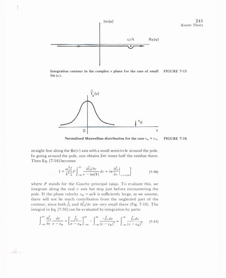
lm(v)
w/k Re(v) •
243 Kinetic Theory
Integration contour in the complex v plane for the case of small FIGURE 7-15 Im (w).
0 v
Normalized Maxwellian distribution for the case v., » v,h· FIGURE 7-16
straight line along the Re(v) axis with a small semicircle around the pole. In going around the pole, one obtains 27Ti times half the residue there. Then Eq. [7-54] becomes
2 C0 -' A
l = w: [pf a[o/av dv+i'TTafo l J k -ro v - (w/k ) av v�w/k
[7-56]
where P stands for the Cauchy principal value. To evaluate this, we integrate along the real v axis but stop just before encountering the pole. If the phase velocity vel> = w/ k is sufficiently large, as we assume, there will not be much contribution from the neglected part of the contour, since both /0 and a/0/av are very small there (Fig. 7-16). The integral in Eq. [7-56] can be evaluated by integration by parts:
fro afo dv [ /0 Jro fro -/0 dv fro /0 dv -ro a;; V- V<f>
= V- Vcf> -ro
--oo (v- V¢)2 = -co (v- V<f>)2
[7-57]

244 Chapter Seven
Since this is just an average of (v - vcl>)-2 over the distribution, the real
part of the dispersion relation can be written
2 w p ------,2 1 = k2 (v-Vet>)
The odd terms vanish upon taking the average, and we have
2 -2 ( 3v2) (v-vet>) =vet> 1 +
v!
[7-58]
[7-59]
[7-60]
We now let fo be Maxwellian and evaluate v2. Remembering that v here
is an abbreviation for Vx, we can write
[7-61]
there being only one degree of freedom. The dispersion relation [7-58]
then becomes
9
2 _ 2 wj; 3KT.k2 W -Wp + 2 -W m
[7-62]
[7-63]
If the thermal correction is small, we may replace w2 by w! in the second
term. We then have
2 2 3KT.k2 w =wp + -m
[7-64]
which is the same as Eq. [4-30], obtained from the fluid equations with
y = 3.
We now return to the imaginary term in Eq. [7-56]. In evaluating
this small term, it will be sufficiently accurate to neglect the thermal
correction to the real part of w and let w2 = w!. From Eqs. [7-57] and
[7-60], we see that the principal value of the integral in Eq. [7-56] is
approximately k2/w2. Equation [7-56] now becomes
9 2 A
I wf, . wpa[o l = -2+t7T�-w k av u=u.,
2( 1 . w� [afo] ) 2 w -z7T� - = wp k av u=u.,
[7-65]
[7-66]
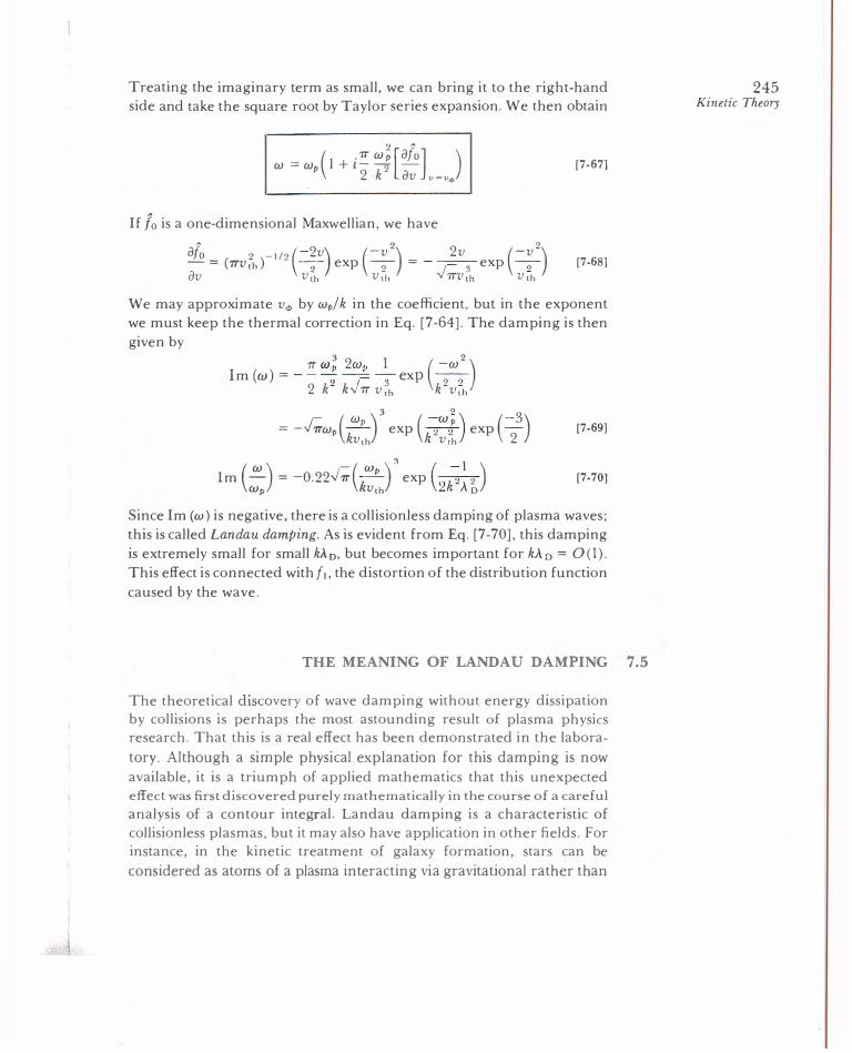
Treating the imaginary term as small, we can bring it to the right-hand side and take the square root by Taylor series expansion. We then obtain
( 7T w; [afo] ) w=wp l+i-2-2 k av v�v"'
If /0 is a one-dimensional Maxwellian, we have
afo 2 -l/2(-2v) (-v2)- 2v (-v2) - = ( 7TV th) ---;- exp ---;- - - 1- 3 exp -2-av Vth Vth Y7TVth Vth
[7-67]
[7-68]
We may approximate v<t> by wp/ k in the coefficient, but in the exponent we must keep the thermal correction in Eq. [7-64]. The damping is then given by
3 2 1 2 Im (w) = - � w: w� -3- exp ( �w
2 ) 2 k kJ7T v,h k v,h
= -J;.wp ( Wp ) 3 exp ( :W}) exp (- 3) [7-69) kv,h k v,h 2
Im (:J = -0.22J;(k:�J 3 exp (2k�� �) [7-70]
Since Im (w) is negative, there is a collisionless damping of plasma waves; this is called Landau damping. As is evident from Eq. [7-70], this damping is extremely small for small kA0, but becomes important for kA0 = 0(1). This effect is connected withf1, the distortion of the distribution function caused by the wave.
THE MEANING OF LANDAU DAMPING 7.5
The theoretical discovery of wave damping without energy dissipation by collisions is perhaps the most astounding result of plasma physics research. That this is a real effect has been demonstrated in the labora
tory. Although a simple physical explanation for this damping is now
available, it is a triumph of applied mathematics that this unexpected effect was first discovered purely mathematically in the course of a careful
analysis of a contour integral. Landau damping is a characteristic of collisionless plasmas, but it may also have application in other fields. For instance, in the kinetic treatment of galaxy formation, stars can be considered as atoms of a plasma interacting via gravitational rather than
245 Kinetic Theory
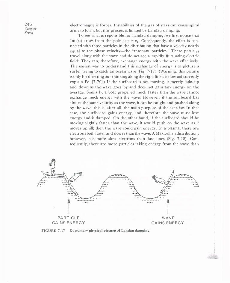
246 Chapter Seven
electromagnetic forces. Instabilities of the gas of stars can cause spiral
arms to form, but this process is limited by Landau damping. To see what is reponsible for Landau damping, we first notice that
Im (w) arises from the pole at v = v<P. Consequently, the effect is connected with those particles in the distribution that have a velocity nearly
equal to the phase velocity-the "resonant particles." These particles travel along with the wave and do not see a rapidly fluctuating electric
field: They can, therefore, exchange energy with the wave effectively. The easiest way to understand this exchange of energy is to picture a surfer trying to catch an ocean wave (Fig. 7-17). (Warning: this picture
is only for directing our thinking along the right lines; it does not correctly
explain Eq. [7-70].) If the surfboard is not moving, it merely bobs up
and down as the wave goes by and does not gain any energy on the
average. Similarly, a boat propelled much faster than the wave cannot exchange much energy with the wave. However, if the surfboard has
almost the same velocity as the wave, it can be caught and pushed along
by the wave; this is, after all, the main purpose of the exercise. In that case, the surfboard gains energy, and therefore the wave must lose energy and is damped. On the other hand, if the surfboard should be moving slightly faster than the wave, it would push on the wave as it
moves uphill; then the wave could gain energy. In a plasma, there are
electrons both faster and slower than the wave. A Maxwellian distribution,
however, has more slow electrons than fast ones (Fig. 7-18). Con
sequently, there are more particles taking energy from the wave than
PARTICLE GAINS ENERGY
FIGURE 7-17 Customary physical picture of Landau damping.
WAVE GAINS ENERGY

J
247 Kinetic TheoTy
0 v
Distortion of a Maxwellian distribution in the region FIGURE 7-18 v "" Vq, caused by Landau damping.
0 v
A double-humped distribution and the region where FIGURE 7-19 instabilities will develop.
vice versa, and the wave is damped. As particles with v = v<P are trapped in the wave, f(v) is flattened near the phase velocity. This distortion is /1 (v) which we calculated. As seen in Fig. 7-18, the perturbed distribution function contains the same number of particles but has gained total energy (at the expense of the wave).
From this discussion, one can surmise that if f0(v) contained more fast particles than slow particles, a wave can be excited. Indeed, from Eq. [7-67], it is apparent that Im (w) is positive if afo/av is positive at v = v"'. Such a distribution is shown in Fig. 7-19. Waves with v"' in the region of positive slope will be unstable, gaining energy at the expense
of the particles. This is just the finite-temperature analogy of the twostream instability. When there are two cold (KT = 0) electron streams

248 Chapter Seven
in motion, f0 ( v) consists of two 8-functions. This is clearly unstable because a[o/a v is infinite; and, indeed, we found the instability from fluid theory. When the streams have finite temperature, kinetic theory
tells us that the relative densities and temperatures of the two streams
must be such as to have a region of positive iJf0/ a v between them; more
precisely, the total distribution function must have a minimum for
instability. The physical picture of a surfer catching waves is very appealing,
but it is not precise enough to give us a real understanding of Landau damping. There are actually two kinds of Landau damping: linear Landau damping, and nonlinear Landau damping. Both kinds are
independent of dissipative collisional mechanisms. If a particle is caught
in the potential well of a wave, the phenomenon is called "trapping." As in the case of the surfer, particles can indeed gain or lose energy in trapping. However, trapping does not lie within the purview of the linear
theory. That this is true can be seen from the equation of motion
[7-71]
If one evaluates E (x) by inserting the exact value of x, the equation would be nonlinear, since E (x) is something like sin kx. What is done in linear theory is to use for x the unperturbed orbit; i.e., x = x 0 + v0t . Then Eq. [7-71] is linear. This approximation, however, is no longer valid when a particle is trapped. When it encounters a potential hill large enough
to reflect it, its velocity and position are, of course, greatly affected by
the wave and are not close to their unperturbed values. In fluid theory,
the equation of motion is
m[�: + (v · V)v] = qE(x) [7-72)
Here, E(x) is to be evaluated in the laboratory frame, which is easy; but to rnake up for it, there is the (v · V)v term. The neglect of (v1 • V)v1 in linear theory amounts to the same thing as using unperturbed orbits. In kinetic theory, the nonlinear term that is neglected is, from Eq. [7-45],
[7-73)
When particles are trapped, they reverse their direction of travel relative
to the wave, so the distribution function f(v) is greatly distu rbed near v = w/k . This means that a[Ija v is comparable to a[0/a v, and the term [7-73] is not negligible. Hence, trapping is not in the linear theory.

i
249 Kinetic Theory
0 u v
Dissection of a distribution f0(v) into a large number of FIGURE 7-20 monoenergetic beams with velocity u and density nu.
When a wave grows to a large amplitude, collisionless damping with trapping does occur. One then finds that the wave does not decay monotonically; rather, the amplitude fluctuates during the decay as the trapped particles bounce back and forth in the potential wells. This is nonlinear Landau damping. Since the result of Eq. [7-67] was derived from a linear theory, it must arise from a different physical effect. The question is: Can untrapped electrons moving close to the phase velocity of the wave exchange energy with the wave? Before giving the answer, let us examine the energy of such electrons.
The Kinetic Energy of a Beam of Electrons 7 .5.1 We may divide the electron distribution f0(v) into a large number of monoenergetic beams ( Fig. 7-20). Consider one of these beams: It has unperturbed velocity u and density nu. The velocity u may lie near Vq,, so that this beam may consist of resonant electrons. We now turn on a
plasma oscillation E (x, t) and consider the kinetic energy of the beam as it moves through the crests and troughs of the wave. The wave is caused by a self-consistent motion of all the beams together. If nu is small enough
( the number of beams large enough), the beam being examined has a negligible effect on the wave and may be considered as moving in a given

250 Chapter Seven
field E(x, t). Let
E =Eo sin (kx-wt) = -d¢/ dx
¢ = (£0/k) cos (kx-wt)
The linearized Auid equation for the beam is
(avl avl) . m - + u- = -e£0 sm (kx-wt)
at ax
A possible solution is
e£0 cos (kx -wt) vi=--
m w -ku
[7-74]
[7-75]
[7-76]
[7-77]
This is the velocity modulation caused by the wave as the beam electrons
move past. To conserve particle Aux, there is a corresponding oscillation
in density, given by the linearized continuity equation:
[7-78)
Since v1 is proportional to cos (kx- wt), we can try n1 = 1"i1 cos (kx-wt).
Substitution of this into Eq. [7-78] yields
eE0k cos (kx -wt) n1 = -nu-- 2
m (w-ku) [7-79]
Figure 7- 21 shows what Eqs. [ 7-77] and [ 7-79] mean. The first two curves show one wavelength of E and of the potential -e¢ seen by the beam electrons. The third curve is a plot of Eq. [ 7 -77] for the case w -ku < 0, or u > vq,. This is easily understood: When the electron a
has climbed the potential hill, its velocity is small, and vice versa. The
fourth curve is v 1 for the case u < vq,, and it is seen that the sign is
reversed. This is because 1he electron b, moving to the left in the frame
of the wave, is decelerated gcing up to the top of the potential barrier;
but since it is moving the opposite way, its velocity v 1 in the positi ve x
direction is maximum there. The moving potential hill accelerates electron b to the right, so by the time it reaches the top, it has the maximum v1. The final curve on Fig. 7-21 shows the density n1, as given by Eq. [7 -79]. This does not change sign with u - Vq,, because in the frame of the wave, both electron a and electron b are slowest at the top of the potential hill, and therefore the density is highest there. The point is that the relative phase between n 1 and v 1 changes sign with u - Vq,.

E
a� -e¢
u<vrp
0 7T
v -¢
�b
u>vrp
kx - wt 27T
251 Kinetic Theory
Phase relations of velocity and density for electrons moving in an FIGURE 7-21 electrostatic wave.
We may now compute the kinetic energy Wk of the beam:
[7-80]
The last three terms contain odd powers of oscillating quantities, so they will vanish when we average over a wavelength. The change in Wk due to the wave is found by subtracting the first term, which is the original

252 Chapter Seven
energy. The average energy change is then
(� Wk) = �m(nuu� + 2un1u1) [7-81]
From Eq. [7-77], we have
[7-82]
the factor � representing (cos2 (kx- wt)). Similarly, from Eq. [7-79], we
have
[7-83]
Consequently,
n, e2E6 w + ku ---4 m (w-ku)3 [7-84]
This result shows that (� Wk) depends on the frame of the observer
and that it does not change secularly with time. Consider the picture of
a frictionless block sliding over a washboard-like surface (Fig. 7- 2 2). In the frame of the washboard, � Wk is proportional to - (ku )-
2 , as seen by taking w = 0 in Eq. [7-84]. It is intuitively clear that (1) (� Wi.) is negative, since the block spends more time at the peaks than at the valleys, and ( 2) the block does not gain or lose energy on the average, once the oscillation is started. Now if one goes into a frame in which the washboard
is moving with a steady velocity w/k (a velocity unaffected by the motion
of the block, since we have assumed that nu is negligibly small compared
with the density of the whole plasma), it is still true that the block does
not gain or lose energy on the average, once the oscillation is started.
But Eq. [7-84] tells us that (� Wk) depends on the velocity w/k, and hence
on the frame of the observer. In particular, it shows that a beam has
FIGURE 7-22 Mechanical analogy for an electron moving in a moving potential.
---w k

253 Kinetic Theory
u-lv11 u u+lv11 v The quadratic relation between FIGURE 7-23
kinetic energy and velocity causes a
symmetric velocity perturbation to
give rise to an increased average
energy.
less energy in the presence of the wave than in its absence if w - ku < 0 or u > v<f>, and it has more energy if w - ku > 0 or u < v<P. The reason for this can be traced back to the phase relation between n 1 and v l· As Fig. 7-23 shows, Wk is a parabolic function of v. As v oscillates between u -I v 11 and u + I v 11, Wk will attain an average value larger than the equilibrium value Wko, provided that the particle spends an ·equal amount of time in each half of the oscillation. This effect is the meaning of the first term in Eq. [7-81], which is positive definite. The second term in that equation is a correction due to the fact that the particle does not distribute its time equally. In Fig. 7-21, one sees that both electron a and electron b spend more time at the top of the potential hill than at the bottom, but electron a reaches that point after a period of deceleration, so that v 1 is negative there, while electron b reaches that point after a period of acceleration (to the right), so that v 1 is positive there. This effect causes(� Wk) to change sign at u = V<f>·
The Effect of Initial Conditions 7 .5.2
The result we have just derived, however, still has nothing to do with linear Landau damping. Damping requires a continuous increase of Wk
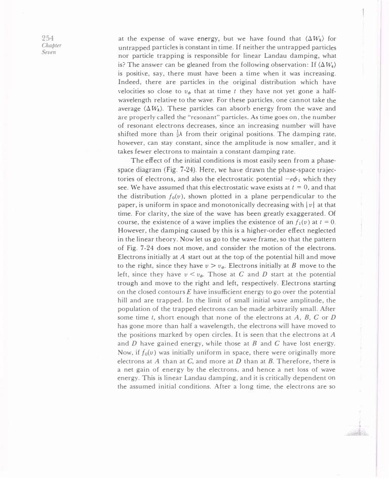
254 Chapter Seven
at the expense of wave energy, but we have found that (d w.) for
untrapped particles is constant in time. If neither the untrapped particles nor particle trapping is responsible for linear Landau damping, what
is? The answer can be gleaned from the following observation: If (d w.)
is positive, say, there must have been a time when it was increasing. Indeed, there are particles in the original distribution which have
velocities so close to vq, that at time t they have not yet gone a half
wavelength relative to the wave. For these particles, one cannot take the average (d w.). These particles can absorb energy from the wave and
are properly called the "resonimt" particles. As time goes on, the number
of resonant electrons decreases, since an increasing number will have shifted more than �A from their original positions. The damping rate,
however, can stay constant, since the amplitude is now smaller, and it
takes fewer electrons to maintain a constant damping rate.
The effect of the initial conditions is most easily seen from a phase
space diagram (Fig. 7-24). Here, we have drawn the phase-space trajec
tories of electrons, and also the electrostatic potential -ecf> 1 which they see. We have assumed that this electrostatic wave exists at t = 0, and that
the distribution f0(v), shown plotted in a plane perpendicular to the paper, is uniform in space and monotonically decreasing with I v I at that
time. For clarity, the size of the wave has been greatly exaggerated. Of course, the existence of a wave implies the existence of an /1 ( v) at t = 0. However, the damping caused by this is a higher-order effect neglected
in the linear theory. Now let us go to the wave frame, so that the pattern
of Fig. 7-24 does not move, and consider the motion of the electrons.
Electrons initially at A start out at the top of the potential hill and move
to the right, since they have v > vq,. Electrons initially at B move to the
left, since they have v < vq,. Those at C and D start at the potential
trough and move to the right and left, respectively. Electrons starting on the closed contours E have insufficient energy to go over the potential hill and are trapped. In the limit of small initial wave amplitude, the population of the trapped electrons can be made arbitrarily small. After some time t , short enough that none of the electrons at A, B, C or D has gone more than half a wavelength, the electrons will have moved to
the positions marked by open circles. It is seen that the electrons at A and D have gained energy, while those at B and C have lost energy.
Now, if fo(v) was initially uniform in space, there were originally more
electrons at A than at C, and more at D than at B. Therefore, there is a net gain of energy by the electrons, and hence a net loss of wave energy. This is linear Landau damping, and it is critically dependent on
the assumed initial conditions. After a long time, the electrons are so

255 smeared out in phase that the initial distribution is forgotten, and there is no further average energy gain, as we found in the previous section. In this picture, both the electrons with v > Vq, and those with v < vq,, when averaged over a wavelength, gain energy at the expense of the wave. This apparent contradiction with the idea developed in the picture of the surfer will be resolved shortly.
Kinetic Theory
0 0
Phase-space trajectories (top) for electrons moving in a potential wave (bottom). FIGURE 7-24 The entire pattern moves to the right. The arrows refer to the direction of electron motion relative to the wave pattern. The equilibrium distribution f0( v) is plotted in a plane perpendicular to the paper.
v
X
X

256 Chapter Seven
7.6 A PHYSICAL DERIVATION OF LANDAU DAMPING
We are now in a position to derive the Landau damping rate without recourse to contour integration. As before, we divide the plasma up into beams of velocity u and density n,, and examine their motion in a wave
E = E 1 sin (kx - wt)
From Eq. [7-77], te velocity of each beam is
eE 1 cos (kx- wt) v 1 = - --:;;;- w -ku
[7-85]
[7-86]
This solution satisfies the equation of motion [7-76], but it does not
satisfy the initial condition v 1 = 0 at t = 0. It is clear that this initial
condition must be imposed; otherwise, v1 would be very large in the
vicinity of u = w/k, and the plasma would be in a specially prepared state initially. We can fix up Eq. [7-86] to satisfy the initial condition by
adding an arbitrary function of kx - kut. The composite solution would still satisfy Eq. [7 -76] because the operator on the left-hand side of Eq. [7-76], when applied to f(kx -kut), gives zero. Obviously, to get v 1 = 0
at t = 0, the function f(kx - kut) must be taken to be -cos (kx- kut). Thus we have, instead of Eq. [7-86],
-e£1 cos(kx -wt)-cos(kx -kut) v�= --
m w -ku [7-87]
Next, we must solve the equation of continuity [7-78] for n 1, again subject to the initial condition n 1 = 0 at t = 0. Since we are now much cleverer
than before, we may try a solution of the form
nl = nl[cos (kx-wt)-cos (kx-kut)] [7-88]
Inserting this into Eq. [7 -78] and using Eq. [7 -87] for v 1, we find
_ . eE 1k sin (kx-wt)- sin (kx-kut) n1 sm (kx-wt) = -n"--
k 2 [7-89] m (w- u)
Apparently, we were not clever enough, since the sin (kx-wt) factor does not cancel. To get a term of the form sin (kx -kut), which came
from the added term in v 1, we can add a term of the form At sin (kx -kut) to n I· This term obviously vanishes at t = 0, and it will give the sin (kx -kut) term when the operator on the left-hand side of Eq. [7 -78] operates on the t factor. When the operator operates on the sin (kx -kut) factor, it yields zero. The coefficient A must be proportional to (w - ku)-1 in

I - J
order to match the same factor in avi/ax. Thus we take
eEik ni = -n
,.-
m- -
(w-
--
ku�
)2
X [cos (kx- wt)-cos (kx- kut)- (w- ku)t sin (kx-kut)] [7-90]
This clearly vanishes at t = 0, and one can easily verify that it satisfies Eq. [7-78].
These expressions for vI and n I allow us now to calculate the work done by the wave on each beam. The force acting on a unit volume of each beam is
and therefore its energy changes at the rate
dW . k - = F,(u + v1) = -eEt srn ( x- wt)(nuu + n,v1 + n1u + n1v1) dt CD ® ® @
[7-91]
[7-92]
We now take the spatial average over a wavelength. The first term vanishes because n,;u is constant. The fourth term can be neglected because it is second order, but in any case it can be shown to have zero average. The terms ® and ® can be evaluated using Eqs. [7 -87] and [7-90] and the identities
(sin (kx- wt) cos (kx-kut)) = -� sin (wt-kut)
(sin (kx - wt) sin (kx- kut)) = � cos (wt- kut)
The result is easily seen to be
e2E� [ sin(wt-kut) =--n 2m " w- ku
k sin (wt-kut)- (w- ku)t cos (wt- kut)] + u 2 (w -ku)
[7-93]
[7-94]
Note that the only terms that survive the averaging process come from the initial conditions.
The total work done on the particles is found by summing over all the beams:
I ( dW) =J fo(u)( dW) du=no f/o(u)(dW) du [7-95]
u dt u nu dt u nu dt u
257 Kinetic Theory

258 Chapter Seven
Inserting Eq. [7-94] and using the definition of wp, we then find for the rate of change of kinetic energy
(d Wk) _ EoEi 2 [f f,� sin (wt -kut) d -- - wp o(u) u dt 2 w - ku f � sin (wt -kut)- (w - ku)t cos (wt- kut) J + fo(u)
k 2 kudu (w- u)
[7-96]
_I 2 2 f00!� d {sin(wt- kut) d [sin(wt-kut)]}
--2EoEtWp o(u) u
k +ud- k -co W - U U W - U
[7-97]
I 2 2 fro � d [ sin (wt - kut)] =2coEiwp
-cofo(u)dudu u
w-ku [7-98]
This is to be set equal to the rate of loss of wave energy density Ww. The wave energy consists of two part�. The first part is the energy density
of the electrostatic field:
[7-99]
The second part is the kinetic energy of oscillation of the particles. If we again divide the plasma up into beams, Eq. [7-84] gives the energy
per beam:
<A ) I nu e2Ei [ 2ku J L.lwk =-- 2 I +---u
4 m (w- ku) (w- ku) [7-100]
In deriving this result, we did not use the correct initial conditions, which are important for the resonant particles; however, the latter contribute
very little to the total energy of the wave. Summing over the beams, we
have
< ) 1 e2Ei fco fo(u) [1 2ku ]d D. wk =
- -- 2 + --- u 4 m -co ( w -ku) w -ku
[7-101]
The second term in the brackets can be neglected in the limit w/k » v,h,
which we shall take in order to compare with our previous results. The dispersion relation is found by Poisson's equation:
kcoE 1 cos (kx-wt) = -e L n1
Using Eq. [ 7- 79] for n 1, we have
2 2 co f, d I = -e- I
nu 2 = _e_ f o(u) u2 Eom u (w -ku) Eom -co (w-ku)
[7-102]
[7 -103]
T 1
Comparing this with Eq. [7- 1 01], we find
Thus
The rate of change of this is given by the negative of Eq. [7-98]:
dWw _ _ 2 fro fA !!_[ sin (w- ku)t] d d - WwWp o(u)d U k
U t -ro U W - U
Integration by parts gives
dWw 2{ [ !A sin (w - ku)t] ro -- = -Wwwp u o (u) _ __:_ __ .:_
dt w- ku -ro
ro A
I
dfo sin (w - ku)t } - u- du -ro du w- ku
[7-104]
[7-105]
[7-106]
The integrated part vanishes for well-behaved functions /0(u), and we have
dWw _ � 2 fro fA' [sin (w- ku)t] - Wwk Wp o (u)
k du dt -ro W - U
[7-107]
where u has been set equal tow/ k (a constant), since only velocities very close to this will contribute to the integral. In fact, for sufficiently large t, the square bracket can be approximated by a delta function:
( w) k . [ sin (w - ku)t] 8 u -- =-lim k 7T t->ro w - ku
[7-108]
Thus
[7- 1 09]
Since Im (w) is the growth rate of £1, and Ww is proportional to Ei, we must have
dWw/dt = 2[Im (w)]Ww [7-110] Hence
[7-111]
in agreement with the previous result, Eq. [7-67], for w = w p.
259 Kinetic Theory

260 Chapter Seven
0
sin(w-ku)t (w-ku)
w-ku
FIGURE 7-25 A function which describes the relative contribution of various velocity groups to Landau damping.
The Resonant Particles
We are now in a position to see precisely which are the resonant particles that contribute to linear Landau damping. Figure 7-25 gives a plot of the factor multiplying fo(u) in the integrand of Eq. [7- 107]. We see that the largest contribution comes from particles with lw - kul < -rr/t, or
lv- v0lt < -rr/k = A/ 2; i.e., those particles in the initial distribution that
have not yet traveled a half-wavelength relative to the wave. The width
of the central peak narrows with time, as expected. The subsidiary peaks
in the "diffraction pattern" of Fig. 7-25 come from particles that have
traveled into neighboring half-wavelengths of the wave potential. These
particles rapidly become spread out in phase, so that they contribute little on the average; the initial distribution is forgotten. Note that the width of the central peak is independent of the initial amplitude of the wave; hence, the resonant particles may include both trapped and untrapped particles. This phenomenon is unrelated to particle trapping.
7 .6.2 Two Paradoxes Resolved
Figure 7-25 shows that the integrand in Eq. [7- 107] is an even function of w - ku, so that particles going both faster than the wave and slower
than the wave add to Landau damping. This is the physical picture we
found in Fig. 7-24. On the other hand, the slope of the curve of Fig. 7-25, which represents the factor in the integrand of Eq. [7-106], is an

_j
261 Kinetic Theory
A Maxwellian distribution seen from a moving frame appears to FIGURE 7-26 have a region of unstable slope.
odd function of w - ku; and one would infer from this that particles traveling faster than the wave give energy to it, while those traveling slower than the wave take energy from it. The two descriptions differ by an integration by parts. Both descriptions are correct; which one is to be chosen depends on whether one wishes to have /0(u) or f�(u) in the integrand.
A second paradox concerns the question of Galilean invariance. If we take the view that damping requires there be fewer particles traveling faster than the wave than slower, there is no problem as long as one is in the frame in which the plasma is at rest. However, if one goes into another frame moving with a velocity V (Fig. 7-26), there would appear to be more particles faster than the wave than slower, and one would expect the wave to grow instead of decay. This paradox is removed by reinserting the second term in Eq. [7-100], which we neglected. As shown in Section 7 .5.1, this term can make (Ll Wk) negative. Indeed, in the frame shown in Fig. 7-26, the second term in Eq. [7- 1 00] is not negligible, (Ll Wk) is negative, and the wave appears to have negative energy (that is, there is more energy in the quiescent, drifting Maxwellian distribution than in the presence of an oscillation). The wave "grows," but adding energy to a negative energy wave makes its amplitude decrease.
BGK AND VAN KAMPEN MODES 7.7
We have seen that Landau damping is directly connected to the re·quirement that f0(v) be initially uniform in space. On the other hand, one can

262 Chapter Seven
generate undamped electron waves if f(v, t = 0) is made to be constant
along the particle trajectories initially. It is easy to see from Fig. 7-24
that the particles will neither gain nor lose energy, on the average, if
the plasma is initially prepared so that the density is constant along each trajectory. Such a wave is called a BGK mode, since it was I. B. Bernstein, ]. M. Greene, and M.D. Kruskal who first showed that undamped waves of arbitrary w, k, amplitude, and waveform were possible. The crucial parameter to adjust in tailoring f(v, t = 0) to form a BGK mode is the
relative number of trapped and untrapped particles. If we take the
small-amplitude limit of a BGK mode, we obtain what is called a Van
Kampen mode. In this limit, only the particles with v = V4> are trapped.
We can change the number of trapped particles by adding to f(v, t = 0)
a term proportional to o(v- v4>). Examination of Fig. 7-24 will show that adding particles along the line v = v4> will not cause damping-at a later
time, there are just as many particles gaining energy as losing energy.
In fact, by choosing distributions with 8-functions at other values of v4>, one can generate undamped Van Kampen modes of arbitrary V4>. Such
singular initial conditions are, however, not physical. To get a smoothly
varying f(v, t = 0), one must sum over Van Kampen modes with a
distribution of V<f>S. Although each mode is undamped, the total per
turbation will show Landau damping because the various modes get out
of phase with one another.
7.8 EXPERIMENTAL VERIFICATION
Although Landau's derivation of collisionless damping was short and neat, it was not clear that it concerned a physically observable phenomenon until ]. M. Dawson gave the longer, intuitive derivation which was paraphrased in Section 7.6. Even then, there were doubts
that the proper conditions could be established in the laboratory. These doubts were removed in 1965 by an experiment by Malmberg and
Wharton. They used probes to excite and detect plasma waves along a
collisionless plasma column. The phase and amplitude of the waves as
a function of distance were obtained by interferometry. A tracing of the
spatial variation of the damped wave is shown in Fig. 7-27. Since in the experiment w was real but k was complex, the result we obtained in Eq. [7-70] cannot be compared with the data. Instead, a calculation of Im (k)/Re (k) for real w has to be made. This ratio also contains the factor exp (-v!/v�h), which is proportional to the number of resonant

263 Kinetic Theory
a: w 1-w :2: 0 a: w u... a: w 1-z
1-:J 0.... 1-:J 0
10 20 30 40 PROBE SEPARATION
Interferometer trace showing the perturbed density pattern in a damped FIGURE 7-27 plasma wave. [From]. H. Malmberg and C. B. Wharton, Phys. Rev. Lett. 17, 175 (1966).)
electrons in a Maxwellian distribution. Consequently, the logarithm of lm (k )/Re (k ) should be proportional to (vq,/v,h)2. Figure 7-28 shows the agreement obtained between the measurements and the theoretical curve.
A similar experiment by Derfler and Simonen was done in plane geometry, so that the results for Re (w) can be compared with Eq. [7-64]. Figure 7-29 shows their measurements of Re (k ) and Im (k ) at different frequencies. The dashed curve represents Eq. [7-64] and is the same as the one drawn in Fig. 4-5. The experimental points deviate from the dashed curve because of the higher-order terms in the expansion of Eq. [7-59]. The theoretical curve calculated from Eq. [7-54], however, fits the data well.
7-1. Plasma waves are generated in a plasma with n = 1017 m-3 and KT, = 10 eV. PROBLEMS If k = 104 m-1, calculate the approximate Landau damping rate lim (w/wp) i . 7-2. An electron plasma wave with 1-cm wavelength is excited in a 10-eV plasma with n = 1015 m-3• The excitation is then removed, and the wave Landau damps away. How long does it take for the amplitude to fall by a factor of e?

264 Chapter Seven
.10
.05
lm(k) Re(k) .02
.01
.005 0
• KT 0 KT
5
6.5 eV 9.6 eV
10 15 20 25
FIGURE 7-28 Verification of Landau damping in the Malmberg-Wharton experiment (loc. cit.)
7-3. An infinite, uniform plasma with fixed ions has an electron distribution function composed of (1) a Maxwellian distribution of "plasma" electrons with
density np and temperature Tp at rest in the laboratory, and (2) a Maxwellian
distribution of "beam" electrons with density nb and temperature Tb centered at
v = Vx (Fig. P7-3). If nb is infinitesimally small, plasma oscillations traveling in the x direction are Landau-damped. If nb is large, there will be a two-stream instability. The critical nb at which instability sets in can be found by setting the
slope of the total distribution function equal to zero. To keep the algebra simple,
we can find an approximate answer as follows.
(a) Write expressions for fp (u) and fb(u), using the abbreviations v = v., a2 =
2KTp/m, b2 = 2KTb/m.
(b) Assume that the phase velocity v<�> will be .the value of v at which [.(v) has the largest positive slope. Find u<t> and f� (v<�>).
(c) Find f� (v<�>) and set f� (v<t>) + f� (v<t>) = 0.

200 265 Kinetic Theory
N I � >u z 100 LlJ ::J a UJ a: LL
0 0 0.8 1.6 2.4
k (mm·1) Experimental measurement of the dispersion relation for plasma FIGURE 7-29 waves in plane geometry. [From H. Derfler and T. Simonen,]. Appl. Phys. 38,5018 (1967).]
(d) For V » b, show that the critical beam density is given approximately by
nb 112 Tb V 2 2 - = (2e) - - exp (- V /a ) np Tp a

266 Chapter Seven
FIGURE P7-3 Unperturbed distribution functions fp(vx) and [b(vx) for the plasma and beam electrons, respectively, in a beam-plasma interaction.
7-4. To model a warm plasma, assume that the ion and electron distribution functions are given by
A a, 1 f,u(v) =- �+ 2
7T v a,
A a; 1 [;u(v) =- �+ 2
TT v ai
(a) Derive the exact dispersion relation in the Vlasov formalism assuming an
electrostatic perturbation.
(b) Obtain an approximate expression for the dispersion relation if w ::::: Dp. Under what conditions are the waves weakly damped? Explain physically why w = n. for very large k.
7-5. Consider an unmagnetized plasma with a fixed, neutralizing ion background. The one-dimensional electron velocity distribution is given by
fu,(v) = gu(v) + ho(v)
where
and
(a) Derive the dispersion relation for high-frequency electrostatic perturbations.
(b) In the limit w/k «a, show that a solution exists in which Im (w) > 0 (i.e., growing oscillations).

7-6. Consider the one-dimensional distribution function 267 f(v) =A f(v) = 0
Kinetic Theory
(a) Calculate the value of the constant A in terms of the plasma density n0. (b) Use the Vlasov and Poisson equations to derive an integral expression for
electrostatic electron plasma waves.
(c) Evaluate the integral and obtain a dispersion relation w(k), keeping terms
to third order in the small quantity kvm/ w.
ION LANDAU DAMPING 7.9
Electrons are not the only possible resonant particles. If a wave has a slow enough phase velocity to match the thermal velocity of ions, ion
Landau damping can occur. The ion acoustic wave, for instance, is greatly affected by Landau damping. Recall from Eq. [ 4-41] that the dispersion relation for ion waves is
1/2 � =
v = (KT. + YiKTi)
k ' M
[7-112]
If T.,;; T;, the phase velocity lies in the region wherefoi (v) has a negative slope, as shown in Fig. 7-30( A). Consequently, ion waves are heavily Landau-damped if T. :5 Ti. Ion waves are observable only if T. » T; [Fig. 7-30(B)], so that the phase velocity lies far in the tail of the ion velocity distribution. A clever way to introduce Landau damping in a
(A) 0 T ::::::T e 1
v --
� v¢
0 (B) Te >> Ti
v
Explanation of Landau damping of ion acoustic waves. ForT,= T,, the phase FIGURE 7-30 velocity lies well within the ion distribution; for T, » T,, there are very few
ions at the phase velocity. Addition of a light ion species (dashed curve) increases Landau damping.

268 Chapter Seven
controlled manner was employed by Alexeff, jones, and Montgomery. A weakly damped ion wave was created in a heavy-ion plasma (such as xenon) with T. » T;. A small amount of a light atom (helium) was then
added. Since the helium had about the same temperature as the xenon but had much smaller mass, its distribution function was much broader,
as shown by the dashed curve in Fig. 7-30(B). The resonant helium ions then caused the wave to damp.
7 .9.1 The Plasma Dispersion Function
To introduce some of the standard terminology of kinetic theory, we
now calculate the ion Landau damping of ion acoustic waves in the
absence of magnetic fields. Ions and electrons follow the Vlasov equation
[7-23] and have perturbations of the form of Eq. [7-46] indicating plane waves propagating in the x direction. The solution for !1 is given by Eq. [7-48] with appropriate modifications:
[Ii = _ iqiE a[o/avi mi w- kvi
[7·113)
where E and vi stand for E., Vxi; and the jth species has charge qi, mass
mi, and particle velocity vi. The density perturbation of the jth species
is given by
[7-114]
Let the equilibrium distributions foi be one-dimensional Maxwellians:
[7-115)
Introducing the dummy integration variables = vJv,hi• we can write n 1i as
where
_ iqiEnoi _1_ f co (d/ ds )(e -s2) ds n1i - 2 112
kmiv thj 1T -co s - (i
We now define the plasma dispersion function Z(():
I fco e-s2 Z(() = 172 -- ds 1T -coS- (
[7·116]
[7-117]
[7-118]
j

This is a contour integral, as explained in Section 7 .4, and analytic continuation to the lower half plane must be used if Im (() < 0. Z(() is a complex function of a complex argument ( since w or k usually has an imaginary part). In cases where Z(() cannot be approximated by an asymptotic formula, one can use the tables of Fried and Conte or a standard computer subroutine.
To express n11 in terms of Z( (), we take the derivative with respect
to (:
I 1 f CO e -s2 Z (() = rr 1/2 -co -(s---(...,)2 ds
Integration by parts yields
1 _ 1 [-e-
'2
J
ro
1 f
ro
(d/ds)(e-'2) Z ( 0 - ----r/2 -- + -r72 ds rr S - ( -co rr -ro S - (
The first term vanishes, as it must for any well-behaved distribution
function. Equation [7-116) can now be written
[7-119]
Poisson's equation is
[7-120]
Combining the last two equations, separating out the electron term explicitly, and defining
flp1 = (no1ZJe2/eoMj)112
we obtain the dispersion relation
2 n2 k2 = �p Z1( (,) + I7 Z1((j)
Vthe J Vthj
[7-121]
[7-122]
Electron plasma waves can be obtained by setting flpi = 0 ( infinitely massive ions). Defining
k 2 2/ 2 -2 D == 2wp Vthe =AD [7-123]
we then obtain
[7-124]
which is the same as Eq. [7-54] when [0, is Maxwellian.
269 Kinetic Theory

270 Chapter Seven
7.9.2 Ion Waves and Their Damping
To obtain ion waves, go back to Eq. [7-122] and use the fact that their phase velocity w/k is much smaller than v,h,; hence(. is small, and
we can expand Z((,) in a power series:
[7-125]
The imaginary term comes from the residue at a pole lying near the
real s axis (of Eq. [ 7-56]) and represents electron Landau damping. For (, « 1, the derivative of Eq. [7- 125] gives
Z'((,) = -2i.J";.(,e ·�- � + · · · = -2 [7-126]
Electron Landau damping can usually be neglected in ion waves because the slope of f,(v) is small near its peak. Replacing Z'((,) by -2 in Eq.
[7-I22] gives the ion wave dispersion relation
n2 A� I----f-Z'((j) = I +k 2A� = 1 [7-127]
i v,"i The term k 2A � represents the deviation from quasineutrality.
We now specialize to the case of a single ion species. Since no, = Z,n0;, the coefficient in Eq. [7-I27] is
2 2 2 2 Op EoKT, no;Z e M
A o -2- = ---2 --v,hi no,e EoM 2kT;
For k 2A� « I, the dispersion relation becomes
'( w ) 2T,
z kv,"' =
ZT,
l ZT, 2 T,
[7-128]
Solving this equation is a nontrivial problem. Suppose we take real
k and complex w to study damping in time. Then the real and imaginary
parts of w must be adjusted so that Im (Z') = 0 and Re (Z') = 2TJZT,. There are in general many possible roots w that satisfy this, all of them having Im w < 0. The least damped, dominant root is the one having the smallest lim w 1. Damping in space is usually treated by taking w real and k complex. Again we get a series of roots k with Im k > 0, represent
ing spatial damping. However, the dominant root does not correspond to the same value of (; as in the complex w case. It turns out that the
spatial problem has to be treated with special attention to the excitation mechanism at the boundaries and with more careful treatment of the
electron term Z'((.).

To obtain an analytic result, we consider the limit(; » 1, corresponding to large temperature ratio e = ZT./T,. The asymptotic expression for Z'((;) is
1 • ,- -{� -2 3 -4 Z ((; ) =-2zv7r(; e • +(; +2( ; + ... [7-129]
If the damping is small, we can neglect the Landau term in the first approximation. Equation [7 -128] becomes
__!__ ( 1 + � __!__
) = � d 2 d e
Since e is assumed large,(; is large; and we can approximate(; by 0/2 in the second term. Thus
or
__!__(1+�)=� (f e e
w: = 2KT; (� +
ZT.) = ZKT. + 3KT; k· M 2 2T, M
[7-130]
[7-131]
This is the ion wave dispersion relation [ 4-41] with -y, = 3, generalized to arbitrary Z.
We now substitute Eqs. [7-129] and [7-130] into Eq. [7-128] retaining the Landau term:
1 (
3) 0 ,- -{2 2 - 1 +- - 2zv7T'r· e ' = -(f e !> •
8
(\ ( 1 + �) = � (1 + ii;. 8(, e-n)
2 (3 +8 )1/2
1 . ,- -{2 - J
(; = -2- ( + ZV7T' 8(; e ')
Expanding the square root, we have
[7-132]
The approximate damping rate is found by using Eq. [7-130] in the imaginary term:
I r I 1/2 _ � = _ m w = (�) 8(3 + 8)112 e-<3+0l/2
Re (; Rew 8
where e = ZT./T; andRew is given by Eq. [7-131].
[7-133]
271 Kinetic Theory

272 Chapter Seven
-lm w
Re w
This asymptotic expression, accurate for large(), shows an exponen
tial decrease in damping with increasing (). When () falls below 10, Eq.
[7-133] becomes inaccurate, and the damping must be computed from
Eq. [7- 128], which employs the Z-function. For the experimentally
interesting region 1 < () < 10, the following simple formula is an analytic fit to the exact solution:
[7-134]
These approximations are compared with the exact result in Fig. 7-31.
DAMPING
A EXACT SOLUTION
B ASYMPTOTIC EXPRESSION
C EMPIRICAL FORMULA
10-3L---�������---L--��_LLU ____ �--��LLLLW .01 0.1 1 10
FIGURE 7-31 Ion Landau damping of acoustic waves. (A) is the exact solution of Eq. [7-128); (B) is the asymptotic formula, Eq. [7-133); and (C) is the empirical fit, Eq. [7-134], good for 1 < (J < 10.

I
What happens when collisions are added to ion Landau damping? 273 Surprisingly little. Ion-electron collisions are weak because the ion and electron fluids move almost in unison, creating little friction between them. Ion-ion collisions ( ion viscosity) can damp ion acoustic waves, but we know that sound waves in air can propagate well in spite of the dominance of collisions. Actually, collisions spoil the particle resonances that cause Landau damping, and one finds that the total damping is less than the Landau damping unless the collision rate is extremely large. In summary, ion Landau damping is almost always the dominant process with ion waves, and this varies exponentially with the ratio ZT,/Ti·
Kinetic Theory
7-7. Ion acoustic waves of 1-cm wavelength are excited in a single ionized xenon PROBLEMS (A= 131) plasma with T, =I eV and T; = 0.1 eV. If the exciter is turned off, how long does it take for the waves to Landau damp to I/ e of their initial amplitude?
7-8. Ion waves with A = 5 em are excited in a singly ionized argon plasma with n, = 1016 m-3, T, = 2 eV, T; = 0.2 eV; and the Landau damping rate is measured. A hydrogen impurity of density nH =an, is then introduced. Calculate the value of a that will double the damping rate.
7-9. In laser fusion experiments one often encounters a hot electron distribution with density nh and temperature Th in addition to the usual population with n., T,. The hot electrons can change the damping of ion waves and hence affect such processes as stimulated Brillouin scattering. Assume Z = I ions with n; and T;, and define (), = T./T;, ()h = Th/T;, a = nh/n;, I- a = n,/n;, t: = m/M and k�; = n;e2/E0KT;.
(a) Write the ion wave dispersion relation for this three-component plasma, expanding the electron Z-functions .
(b) Show that electron Landau damping is not appreciably increased by nh if Th » T,.
(c) Show that ion Landau damping is decreased by nh, and that the effect can be expressed as an increase in the effective temperature ratio T./T;.
7-10. The dispersion relation for electron plasma waves propagating along B0z can be obtained from the dielectric tensor e (Appendix B) and Poisson's equation, V · (e ·E)= 0, where E = -V¢. We then have, for a uniform plasma,

274 Chapter Seven
orE" = 0. For a cold plasma, Problem 4-4 and Eq. [B-18) give
or
For a hot plasma, Eq. [7-124] gives
2 2 W = Wp
w ; '( w ) Eu = 1- k2 2 Z k- = 0
Vth Vth
By expanding the Z-function in the proper limits, show that this equation yields
the Bohm-Gross wave frequency (Eq. [4-30)) and the Landau damping rate (Eq.
[7-70]). .
7.10 KINETIC EFFECTS IN A MAGNETIC FIELD
When either the de magnetic field B0 or the oscillating magnetic field
B1 is finite, the v x B term in the Vlasov equation [7-23] for a collisionless
plasma must be included. The linearized equation [7-45] is then replaced
by
a[1 q ar1 q a[o - + v · V[I + - (v X Bo) ·- =-- (EI + v X B1) ·
at m av m av [7-135]
Resonant particles moving along B0 still cause Landau damping if w/ k =
v,h. but two new kinetic effects now appear which are connected with
the velocity component v .1 perpendicular to B0. One of these is cyclotron
damping, which will be discussed later; the other is the generation of
cyclotron harmonics, leading to the possibility of the oscillations commonly called Bernstein waves.
Harmonics of the cyclotron frequency are generated when the particles' circular Larmor orbits are distorted by the wave fields E1 and B1. These finite-rL effects are neglected in ordinary fluid theory but can be taken into account to order k 2ri. by including the viscosity 1T. A kinetic
treatment can be accurate even for k2rr = 0(1). To understand how
harmonics arise, consider the motion of a particle in an electric field:
E = Ex e i<kx-wo:X
The equation of motion (cf. Eq. [2-10]) is
" + 2 _ _!_ £ i(kx-wt) x w,x - , e m
[7-136]
[7-137]
If krL is not small, the exponent varies from one side of the orbit to the
other. We can approximate kx by substituting the undisturbed orbit

x = rL sin w,t from Eq. [2-7]:
·· + 2 q £ i(krLsin w 1-wt) x w ,x = - ,e '
m The generating function for the Bessel functions ]n(z) is
co e'<I-I/IJ/2 = L t"],(z)
n=-CC
Letting z = krL and t = exp (iw,t), we obtain
eikrl.sinwct = I ]n(krL) einwct -co
·· + 2 = .!!_ £ � J (k )
-i(w-nw,)l X w,x X L n rL e m -co The following solurion can be verified by direct substitution:
_ !!_E � J,(krL)e-i(w-nw,)l X- x L 2 2 m -cow, - (w -nwc)
[7-138]
[7-139]
[7-140]
[7-141]
[7-142]
This shows that the motion has frequency components differing from the driving frequency by multiples of w" and that the amplitudes of these components are proportional to ],(krL)/[w� - (w -nw,)2]. When the denominator vanishes, the amplitude becomes large. This happens when w- nw, = ±w" or w = (n ± l)w,, n = 0, ±1, ±2, . . . ; that is, when the field E(x, t) resonates with any harmonic of w,. In the fluid limit krL � 0, ]n (krL) can be approximated by (krd2)" /n !, which approaches
0 for all n except n = 0. For n = 0, the coefficient in Eq. [7-142] becomes (w;- w2)-1, which is the fluid result ( cf. Eq. [4-57]) containing only the fundamental cyclotron frequency.
The Hot Plasma Dielectric Tensor 7.10.1 After Fourier analysis of /1(r, v, t) in space and time, Eq. [7-135] can be solved for a Maxwellian distribution f0(v), and the resulting expressions f, ( k, v, w) can be used to calculate the density and current of each species. The result is usually expressed in the form of an equivalent dielectric tensor E, such that the displacement vector D = E · E can be used in the Maxwell's equations V · D = 0 and V x B = p,0D to calculate dispersion relations for various waves (see Appendix B). The algebra is horrendous and therefore omitted. We quote only a restricted result valid for non relativistic plasmas with isotropic pressure (T .1 = Tn) and no zero-order drifts
275 Kinetic Theory

276 Chapter Seven
v0i; these restrictions are easily removed, but the general formulas are too cluttered for our purposes. We further assume k = k3c. + k/i, with z being the direction of Bo; no generality is lost by setting k, equal to zero,
since the plasma is isotropic in the plane perpendicular to B0. The elements of €R =, E/ f.o are then
Exx =
2 co
f.xy = -f.yx = i L ± w� e-b(o L n [/,(b)- J;,( b)]Z((,) s W -co
2 I /2 co
[7-1431
. '\' W p (b) -b '\ b I I f.,, = -f.,, = -t f... ± 2 -2 e (u L... [/,( ) - l,(b)]Z ((,)
s W -co
where Z(() is the plasma dispersion function of Eq. [7-118], /,(b) is the n th order Bessel function of imaginary argument, and the other symbols
are defined by
2 2 2 Wps = no,Z, e /Eom,
Wcs = IZ,eB o/ m, I
v;h, = 2KT,/m,
b, = �kirLs = k';KT,/m,w;,
[7-144]
The first sum is over species s, with the understanding that wp, b, (0, and (, all depend on s, and that the ± stands for the sign of the charge. The second sum is over the harmonic number n. The primes indicate differentiation with respect to the argument.
As foreseen, there appear Bessel functions of the finite-rL parameter b. [The change fromj,(b) to/, (b) occurs in the integration over velocities.] The elements of E involving motion along z contain Z'((,), which gives
rise to Landau damping when n = 0 and w/k, = v,h. The n r! 0 terms now make possible another collisonless damping mechanism, cyclotron damping, which occurs when (w ± nw,)/k, = v,h·
I

1 �L
k k 277 Kinetic Theory
(a)
z z
(b) The mechanism of cyclotron damping. FIGURE 7-32
7-11. In the limit of zero temperature, show that the elements of E in Eq. [7-143] PROBLEM reduce to the cold-plasma dielectric tensor given in Appendix B.
Cyclotron Damping 7.10.2 When a particle moving along B0 in a wave with finite k, has the right velocity, it sees a Doppler-shifted frequency w - k,v, equal to ±nwc and is therefore subject to continuous acceleration by the electric field E.L of the wave. Those particles with the "right" phase relative to E.L will gain energy; those with the "wrong" phase will lose energy. Since the energy change
· is the force times the distance, the faster accelerated
particles gain more energy per unit time than what the slower decelerated particles lose. There is, therefore, a net gain of energy by the particles, on the average, at the expense of the wave energy; and the wave is damped. This mechanism differs from Landau damping because the energy gained is in the direction perpendicular to B0, and hence perpendicular to the velocity component that brings the particle into resonance. The resonance is not easily destroyed by phenomena such as trapping. Furthermore, the mere existence of resonant particles suffices to cause damping; one does not need a negative slope fb(v,), as in Landau damping.
To clarify the physical mechanism of cyclotron damping, consider a wave with k = k3. + k,z with k, positive. The wave electric field EJ_ can be decomposed into left- and right-hand circularly polarized components, as shown in Fig. 7-32. For the left-hand component, the vector
EJ_ at positions A, B, and C along the z axis appears as shown in Fig. 7 -32a. Since the wave propagates in the +z direction, a stationary electron would sample the vectors at C, B, and A in succession and therefore

278 Chapter Seven
would see a left-rotating E-field. It would not be accelerated because its
Larmor gyration is in the right-hand (clockwise) direction. However, if
the electron were moving faster than the wave in the z direction, it would
see the vectors at A, B, and C in that order and hence would be resonantly
accelerated if its velocity satisfied the condition w - k,v, = -w,. The
right-hand component of E would appear as shown in fig. 7-�12b. \low
an electron would see a clockwise rotating E-field if it moved more slowly
than the wave, so that the vectors at C, B, and A were sampled in
succession. This electr·on would be accelerated if it met the condition
w - k,v, = +we. A plane or elliptically polarized wave would, therefore, be cyclotron damped by electrons moving in either direction in the wave
frame.
7.10.3 Bernstein Waves Electrostatic wa\·es propagating at right angles to Bo at harmonics
of the cyclotron frequency are called Bernstein waves. The dispersion
relation can be found by using the dielectric elements givenin Eq. [7-143]
in Poisson's equation V · E · E = 0. If we assume electrostatic perturba
tions such that E1 = - V<P 1, and consider waves of the form <b 1 =
<b1 exp i(k · r- wl), Poisson's equation can be written
[7-145] Note that we ha\·e chosen a coordinate system that has k lying in the x-z
plane. so that k, � 0. 'vVe next substitute for En. E," and E, from Eq.
[7-143] and express .2:''((,.) in terms of Z((,.) with the identity
Z'((,.) = -2[1 +(Z(()] [7-146]
PROBLEMS 7-12. PrO\'e Eq. [7-1-t6] directly fr-om the integr;d expressions for/.(() and/.'(().
7-13. The principal part ofZ(() for small and large(, as used in Eqs. [7-125] and [7-129], is gi ven by
Z(() = - 2( (I- k" + · · · ) Z(()= -(I(I+�C"+ ·)
I (j « I I? I » I
Prove these by expanding the denominator in the definition [7-118) of Z( () .
Equation [7 -145] becomes .,
., ., "\' w; --h k : + k � + L -----;, e (o , w !,.(b) II--=. ·-.X
[7-147]
1 -

- i
The expression in the square brackets can be simplified in a few algebraic
steps to 2k;[?-n + ?6Z((n)] by using the definitions b = k';v;h/2w; and
?n = (w + nw,)/k,v,h. Further noting that 2k;w�?o/w2 = 2w�/v;h = k1 for
each species, we can write Eq. [7-147] as
ro k; +k;+Ik1e-b L In(b)[(-n/?o+?oZ(?n)]=O [7-148]
n=-00
The term ?-,/(0 is 1-nwc/w. Since In(b) = Ln(b), the term In(b)nw,/w sums to zero when n goes from -co to co; hence,(-,/ (o can be replaced by 1. Defining k 2 = k! + k ;, we obtain the general dispersion relation
for Bernstein waves:
[7-149]
(A) Electron Bernstein Waves. Let us first consider high-frequency waves
in which the ions do not move. These waves are not sensitive to small deviations from perpendicul-ar propagation, and we may set k, = 0, so that (n �co. There is, therefore, no cyclotron damping; the gaps in the spectrum that we shall find are not caused by such damping. For large
(n. we may replace Z((,.) by -1/(,, according to Eq. [7-129]. Then= 0 term in the second sum of Eq. [7-149] then cancels out, and we can
divide the sum into two sums, as follows:
or
k� + � k � e -ti ln(b)(l-(o/(n) + Jl L,(b)(1-(o/(-,J J = 0
'> 2 -b 00 [ W W J
kj_ +'Lkve L l,(b) 2- ----- = 0 s n=l w+nwc w-nw,
[7 -150]
[7-151]
The bracket collapses to a single term upon combining over a common
denominator:
[7-152]
Using the definitions of kv and b, one obtains the well-known k, = 0 dispersion relation
[7-153]
279 Kinetic Theory

280 Chapter Seven
2
a(w, b) 0
-1
-2
� \
\ \
\ \
wlwC 2
b=1
\ \__ ·�
\
3 FIGURE 7-33 The function a(w, b) for electron Bernstein waves. [From I. B. Bernstein,
Phys. Rev. 109, 10 (1958).]
We now specialize to the case of electron oscillations. Dropping the sum over species, we obtain from Eq. [7 - 152]
k� 2 co e -bl,(b) 2 k2 = 2wc L 2 2 n =a(w, b)
D n=l W -nwc [7-154]
The function a (w, b) for one value of b is shown in Fig. 7-33. The possible values of ware found by drawing a horizontal line ata(w, b)= k�/k� > 0.
It is then clear that possible values of w lie just above each cyclotron harmonic, and that there is a forbidden gap just below each harmonic.
To obtain the fluid limit, we replace In (b) by its small- b value (b/2)" /n! in Eq. [7-153]. Only then = 1 term remains in the limit b � 0, and we obtain
2 2 b 2 )-1 1 = wg -- (w 2 - 1 We b 2 We 2 Wp
2 2 w -we [7-155]
or w2 = w! + w; = w�, which is the upper hybrid oscillation. As k1. � 0, this frequency must be one of the roots. If wh falls between two high harmonics of W0 the shape of the w -k curves changes near w = wh to allow this to occur. Thew -k curves are computed by multiplying Eq. [7-154] by 2w!/w� to obtain k�ri = 4w!a (w, b). The resulting curves
for w/we vs. k1.rL are shown in Fig. 7-34 for various values of w�/w�.

6 r-------------------------------�
w
1 2 3 4 5 kj_rL
281 Kinetic Theory
Electron Bernstein wave dispersion relation. [Adapted from FIGURE 7-34. F. W. Crawford,]. Appl. Phys. 36, 2930 (1965).]
Note that for each such value, the curves change in character above the corresponding hybrid frequency for that case. At the extreme left of the diagram, where the phase velocity approaches the speed of light waves in the plasma, these curves must be modified by including electro!llagnetic corrections.
Electron Bernstein modes have been detected in the laboratory, but inexplicably large spontaneous oscillations at high harmonics of We have also been seen in gas discharges. The story is too long to tell here.
(B) Ion Bernstein Waves. rn the case of waves at ion cyclotron harmonics, one has to distinguish between pure ion Bernstein waves, for which k, = 0, and neutralized ion Bernstein waves, for which k,_ has a small but finite value. The difference, as we have seen earlier for lower hybrid oscillations, is that finite k% allows electrons to flow along B0 to cancel charge

282 Chapter Seven
separations. Though the k,_ = 0 case has already been treated in Eq. [7-153], the distinction between the two cases will be clearer if we go back a step to Eqs. [7 -148] and [7 -149]. Separating out the n = 0 term
and using Eq. [7-146], we have
k� +k; +l:k1e-6Io(b)[-�Z'((o)]+l:k1e-b L ln(b)[1 +(oZ((n)] = 0 niJ!-0 [7-156]
The dividing line between pure and neutralized ion Bernstein waves lies in the electron n = 0 term. If (0, » 1 for the electrons, we can use Eq . [7-129] to write Z'((0,) = 1/(� •. Since w/k, » v,h, in this case, electrons cannot flow rapidly enough along B0 to cancel charge. If (0, « 1, we can use Eq. [7-126] to write Z'((0,) = -2. In this case we have w/k, « v,h.,
and the electrons have time to follow the Boltzmann relation [3-73]. Taking first the (0, » 1 case, we note that (oi » 1 is necessarily true
also, so that then = 0 term in Eq. [7-156] becomes
Here we have taken b, -? 0 and omitted the subscript from bi. Then ¥ 0 terms in Eq. [7-156] are treated as before, so that the electron part is given by Eq. [7-155], and the ion part by the ion term in Eq. [7-153]. The pure ion Bernstein wave dispersion relation then becomes
� I,.(b) J X L 2 = 0 n�I (w/nfle- l) [7-157]
Since (0, » 1 implies small k;, the first term is usually negligible. To examine the fluid limit, we can set the second bracket to zero, separate
out then = 1 term, and use the small-b expansion of In (b), obtaining
w! n! 00 n 2fl!(b/2)n-l 1- 2 2 - 2 n2- I 2 2 2 = o
(J) -we (r) - e n�2n!(w -n flc) [7-158)
The sum vanishes for b = 0, and the remaining terms are equal to the
quantity S of Appendix B. The condition S = 0 yields the upper and lower hyrbid frequencies (see the equation following Eq. [4-70]). Thus, for k1. -? 0, the low-frequency root approaches w1• For finite b, one of the terms in the sum can balance the electron term if w =nne, so there are roots near the ion cyclotron harmonics. The dispersion curves w/fle

600
400
0
-------- --------------------------- 650
--------------- --------------------- 325
2 4 6
283 Kinetic Theory
Pure ion Bernstein waves: agreement between theory and experi- FIGURE 7-35 ment in a Q-machine plasma. [From]. P. M. Schmitt, Phys. Rev. Lett. 31, 982 (1973).]
vs. k1.ru resemble the electron curves in Fig. 7-34. The lowest two roots for the ion case are shown in Fig. 7-35, together with experimental measurements verifying the dispersion relation.
The lower branches of the Bernstein wave dispersion relation exhibit the backward-wave phenomenon, in which thew - k curve has a negative slope, indicating that the group velocity is opposite in direction to the phase velocity. That backward waves actually exist in the laboratory has been verified not only by w vs. k measurements of the type shown in Fig. 7-35, but also by wave interferometer traces which show the motion of phase fronts in the backward direction from receiver to transmitter.
Finally, we consider neutralized Bernstein waves, for which (0, is
small and Z'((0,) = -2. The electron n = 0 term in Eq. [7-156] becomes simply k� •. Assuming that (0; » 1 still holds, the analysis leading to Eq.

284 Chapter Seven
1
0 1 2 3 4
k.Lru FIGURE 7-36 Neutralized ion Bernstein modes: agreement between theory
and experiment in a He microwave discharge. [From E. Ault
and H. Ikezi, Phys. Fluids 13,2874 (1970).]
[7- 157] is unchanged, and Eq. [7- 156] becomes
[7-159]
fork � « k�, an approximate relation for neutralized ion Bernstein waves can be written
Note that electron temperature is now contained in A0, whereas pure ion Bernstein waves, Eq. [7-157], are independent of KT,. If eA� is small, the bracket in Eq. [7-160] must be large; and this can happen only near a resonance w =nile. Thus the neutralized modes are not sensitive

to the lower hybrid resonance w = w1. Indeed, as k1.rLi � 0 the envelope of the dispersion curves approaches the electrostatic ion cyclotron wave relation [ 4-67], which is the Auid limit for neutralized waves.
Neutralized Bernstein modes are not as well documented in experiment as pure Bernstein modes, but we show in Fig. 7-36 one case in which the former have been seen.
285 Kinetic Theory

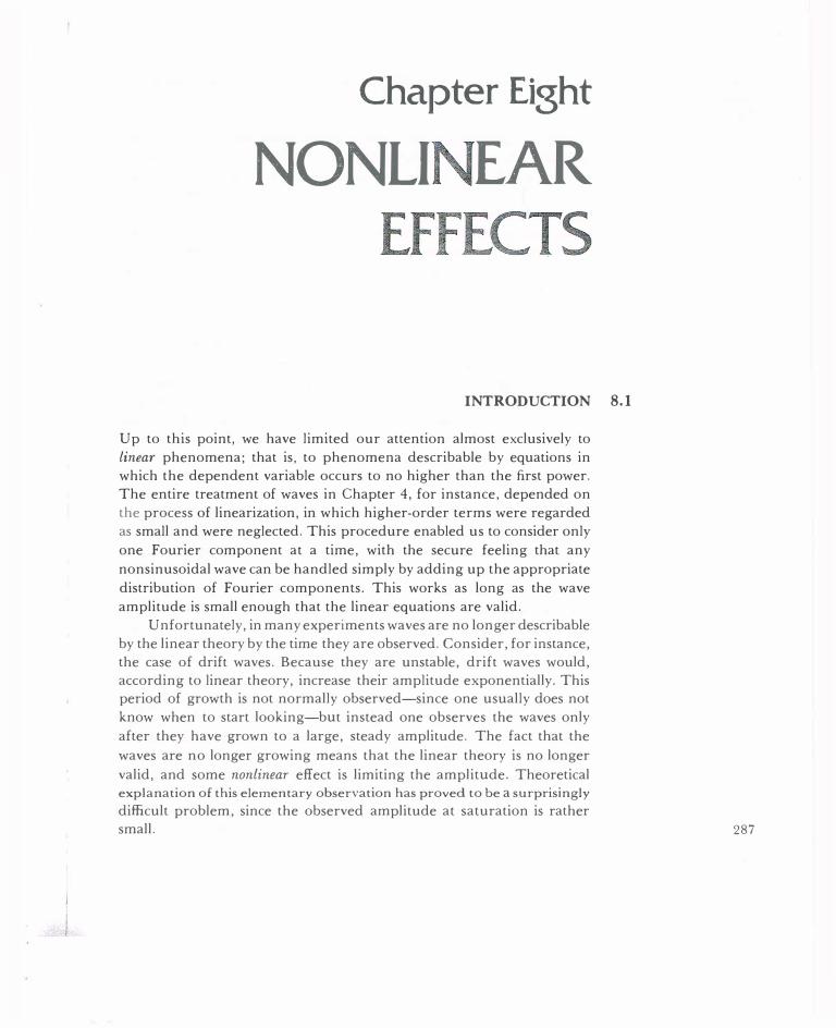
Chapter Eight
NONLI EAR
INTRODUCTION 8.1
Up to this point, we have limited our attention almost exclusively to
linear phenomena; that is, to phenomena describable by equations in which the dependent variable occurs to no higher than the first power. The entire treatment of waves in Chapter 4, for instance, depended on
the process of linearization, in which higher-order terms were regarded as small and were neglected. This procedure enabled us to consider only
one Fourier component at a time, with the secure feeling that any
nonsinusoidal wave can be handled simply by adding up the appropriate
distribution of Fourier components. This works as long as the wave
amplitude is small enough that the linear equations are valid. Unfortunately, in many experiments waves are no longer describable
by the linear theory by the time they are observed. Consider, for instance, the case of drift waves. Because they are unstable, drift waves would, according to linear theory, increase their amplitude exponentially. This period of growth is not normally observed-since one usually does not
know when to start looking-but instead one observes the waves only
after they have grown to a large, steady amplitude. The fact that the
waves are no longer growing means that the linear theory is no longer
valid, and some nonlinear effect is limiting the amplitude. Theoretical explanation of this elementary observation has proved to be a surprisingly
difficult problem, since the observed amplitude at saturation is rather small. 287

288 Chapter Eight
A wave can undergo a number of changes when its amplitude gets large. It can change its shape-say, from a sine wave to a lopsided triangular waveform. This is the same as saying that Fourier components at other frequencies (or wave numbers) are generated. Ultimately, the wave can "break," like ocean waves on a beach, converting the wave energy into thermal energy of the particles. A large wave can trap particles in its potential troughs, thus changing the properties of the medium in which it propagates. We have already encountered this effect in discussing nonlinear Landau damping. If a plasma is so strongly excited that a continuous spectrum of frequencies is present, it is in a state of turbulence. This state must be described statistically, as in the case of ordinary fluid hydrodynamics. An important consequence of plasma turbulence is anomalous resistivity, in which electrons are slowed down by collisions with random electric field fluctuations, rather than with ions. This effect is used for ohmic heating of a plasma (Section 5.6.3) to temperatures so high that ordinary resistivity is insufficient.
Nonlinear phenomena can be grouped into three broad categories: 1. Basically nonlinearizable problems. Diffusion in a fully ionized gas,
for instance, is intrinsically a nonlinear problem (Section 5.8) because the diffusion coefficient varies with density. In Section 6.1, we have seen that problems of hydromagnetic equilibrium are nonlinear. In Section 8.2, we shall give a further example-the important subject of plasma sheaths.
2. Wave-particle interactions. Particle trapping (Section 7.5) Is an example of this and can lead to nonlinear damping. A classic example is the quasilinear effect, in which the equilibrium of the plasma is changed by the waves. Consider the case of a plasma with an electron beam (Fig. 8-1 ). Since the distribution function has a region where df0/ dv is positive, the system has inverse Landau damping, and plasma oscillations with v<P in the positive-slope region are unstable (Eq. [7-67]). The resonant electrons are the first to be affected by wave-particle interactions, and their distribution function will be changed by the wave electric field. The waves are stabilized when f.(v) is flattened by the waves, as shown by the dashed line in Fig. 8-1, so that the new equilibrium distribution no longer has a positive slope. This is a typical quasilinear effect. Another example of wave-particle interactions, that of plasma wave echoes, will be given in Section 8.6.
3. Wave-wave interactions. Waves can interact with each other even in the fluid description, in which individual particle effects are neglected. A single wave can decay by first generating harmonics of its fundamental frequency. These harmonics can then interact with each other and with
..

A double-humped, unstable electron distribution. FIGURE 8-1
the primary wave to form other waves at the beat frequencies. The beat
waves in turn can grow so large that they can interact and form many
more beat frequencies, until the spectrum becomes continuous. It is
interesting to discuss the direction of energy flow in a turbulent spectrum.
In fluid dynamics, long-wavelength modes decay into short-wavelength
modes, because the large eddies contain more energy and can decay
only by splitting into small eddies, which are each less energetic. The smallest eddies then convert their kinetic motion into heat by viscous damping. In a plasma, usually the opposite occurs. Short-wavelength modes tend to coalesce into long-wavelength modes, which are less
energetic. This is because the electric field energy £2/8-rr is of order
k2cf>2/8-rr, so that if ecf> is fixed (usually by KT,), the small-k, long-A modes
have less energy. As a consequence, energy will be transferred to small
k by instabilities at large k, and some mechanism must be found to
dissipate the energy. No such problem exists at large k, where Landau
damping can occur. For motions along B0, nonlinear "modulational"
instabilities could cause the energy at small k to be coupled to ions and
to heat them. For motions perpendicular to B0, the largest eddies will have wavelengths of the order of the plasma radius and could cause plasma loss to the walls by convection.
Although problems still remain to be solved in the linear theory of
waves and instabilities, the mainstream of plas!lla research has turned
to the much less well understood area of nonlinear phenomena. The examples in the following sections will give an idea of some of the effects
that have been studied in theory and in experiment.
289 Nonlinear
Effects

290 Chapter Eight
8.2 SHEATHS
8.2.1 The Necessity for Sheaths
In all practical plasma devices, the plasma is contained in a vacuum chamber of finite size. What happens to the plasma at the wall? For simplicity, let us confine our attention to a one-dimensional model with no magnetic field (Fig. 8-2). Suppose there is no appreciable electric field inside the plasma; we can then let the potential <P be zero there. When ions and electrons hit the wall, they recombine and are lost. Since electrons have much higher thermal velocities than ions, they are lost faster and leave the plasma with a net positive charge. The plasma must then have a potential positive with respect to the wall; i.e., the wall potential <Pw is negative. This potential cannot be distributed over the entire plasma, since Debye shielding (Section 1.4) will confine the potential variation to a layer of the order of several Debye lengths in thickness.
This layer, which must exist on all cold walls with which the plasma is in contact, is called a sheath. The function of a sheath is to form a potential barrier so that the more mobile species, usually electrons, is confined electrostatically. The height of the barrier adjusts itself so that the flux of electrons that have enough energy to go over the barrier to the wall is just equal to the flux of ions reaching the wall.
-d 0 d
FIGURE 8-2 The plasma potential ¢ forms sheaths near the walls so that electrons are reflected. The Coulomb barrier e¢w adjusts itself so that equal numbers of ions and electrons reach the walls per second.
=1. .
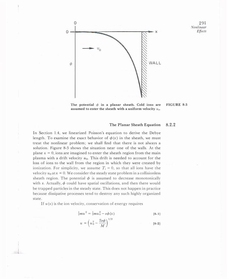
0
---- uo
WALL
The potential ¢ in a planar sheath. Cold ions are FIGURE 8-3 assumed to enter the sheath with a uniform velocity u0.
The Planar Sheath Equation 8.2.2 In Section 1.4, we linearized Poisson's equation to derive the Debye
length. To examine the exact behavior of cf>(x) in the sheath, we must
treat the nonlinear problem; we shall find that there is not always a solution. Figure 8-3 shows the situation near one of the walls. At the
plane x = 0, ions are imagined to enter the sheath region from the main
plasma with a drift velocity u0• This drift is needed to account for the loss of ions to the wall from the region in which they were created by
ionization. For simplicity, we assume T; = 0, so that all ions have the
velocity u0 at x = 0. We consider the steady state problem in a collisionless
sheath region. The potential ¢> is assumed to decrease monotonically with x. Actually, ¢> could have spatial oscillations, and then there would
be trapped particles in the steady state. This does not happen in practice
because dissipative processes tend to destroy any such highly organized state.
If u(x) is the ion velocity, conservation of energy requires
�mu2 = �mu6-ecf>(x)
u = (u�-2:)1/2 [8-1]
[8-2]
291 Nonlinear
Effects

292 Chapter Eight
The ion equation of continuity then gives the ion density n; in terms of the density n0 in the main plasma:
nouo = ni(x)u(x) 2ur) 112
n;(x) = no( 1-Mu�
[8-3]
[8-4]
In steady state, the electrons will follow the Boltzmann relation closely:
n.(x) = n0 exp (ecf>/ KT.)
Poisson's e'quation is then
d2cf>
[ cjJ)
2 c/J)-1/2] Eo dx2 = e(n.- n;) = en0 exp (:T.
- ( 1 - :.u6
[8-5]
[8-6]
The structure of this equation can be seen more clearly if we simplify it with the following changes in notation:
2 1/2 ec/J x=-
KT.
x (
noe ) g=-- x --
Ao EoKT.
Then Eq. [8-6] becomes
.;t{ = uo
-(KT./ M) 172 [8-7]
[8-8]
where the prime denotes d/df This is the nonlinear equation of a plane sheath, and it has an acceptable solution only if .;t{ is large enough. The reason for the symbol .;t{ will become apparent in the following section on shock waves.
8.2.3 The Bohm Sheath Criterion
Equation [8-8] can be integrated once by multiplying both sides by x':
f.< f.� 2 -1/2 I.E.
0 x'x" dg1 =
0 ( 1 + .;t{�) x' dgl-
0 e-xx' dgl [8-9]
where g1 is a dummy variable. Since x = 0 at g = 0, the integrations easily yield
[8-10]
If E = 0 in the plasma, we must set x� = 0 at g = 0. A second integration to find X would have to be done numerically ; but whatever the answer is, the right-hand side of Eq. [8-10] must be positive for all X· In particular,

for X « 1, we can expand the right-hand terms in Taylor series:
2[ x 1 x2 J 1 2 .itt 1 +---- + . . . -1 + 1- x + -x + ... -1 > o ,;(£2 2 ,;(£4 2
or Uo > (KTe/ M)112 [8-11]
This inequality is known as the Bohm sheath criterion. It says that ions must enter the sheath region with a velocity greater than the acoustic velocity V5• To give the ions this directed velocity u0, there must be a
finite electric field in the plasma. Our assumption that x' = 0 at� = 0 is therefore only an approximate one, made possible by the fact that the
scale of the sheath region is usually much smaller than the scale of the
main plasma region in which the ions are accelerated. The value of u0 is somewhat arbitrary, depending on where w.,e choose to put the boundary x = 0 between the plasma and the sheath. Of course, the ion flux
n0u0 is fixed by the ion production rate, so if u0 is varied, the value of n0 at x = 0 will vary inversely with u0• If the ions have finite temperature,
the critical drift velocity u0 will be somewhat lower. The physical reason for the Bohm criterion is easily seen from a
plot of the ion and electron densities vs. x (Fig. 8-4). The electron density
ne falls exponentially with x. according to the Boltzmann relation. The
Qn n
0 X= -e¢/KT e
[u <(KT /M) l/2] o e
___..TO WALL
Variation of ion and electron density (logarithmic scale) with nor- FIGURE 8-4 malized potential X in a sheath. The ion density is drawn for two cases: u0 greater than and u0 less than the critical velocity.
293 Nonlinear
Effects

294 Chapter Eight
8.2.4
ion density also falls, since the ions are accelerated by the sheath potential. If the ions start with a large energy, n;(x) falls slowly, since the sheath field causes a relatively minor change in the ions' velocity. If the ions start with a small energy, n; (x) falls fast, and can go below the n, curve. In that case, n,- n; is positive near x = 0; and Eq. [8-6] tells us that¢ (x) must curve upward, in contradiction to the requirement that the sheath must repel electrons. In order for this not to happen, the slope of n; (x) at x = 0 must be smaller (in absolute value) than that of n,(x); this condition is identical with the condition Ai2 > 1.
The Child-Langmuir Law
Since n, (x) falls exponentially with x. the electron density can be neglected in the region of large x next to the wall (or any negative electrode). Poisson's equation is then approximately
2x -1/2 Ai x"=( 1 + Ai2) =(2x)l/2 [8-12)
Multiplying by x' and integrating from g1 = gs to g1 = g, we have !Cx'2 '2)_ , -2 ""Cx l /2 1/2) 2 - x s - -v Jvt -xs [8-13]
where ts is the place where we started neglecting n,. We can redefine the zero of x so that Xs = 0 at g = gs· We shall also neglect x;, since the slope of the potential curve can be expected to be much steeper in the n, = 0 region than in the finite-n, region. Then Eq. [8-13] becomes
or
x'2 = 23t2Aix 112 I 23/4 ,1,11/2 1/4
X = Jvt X
dx/x1/4 = 23/4Ail/2 dg
Integrating from g = gs tog= gs + d/Ao = �wall• we have
�x�4 = 23/4Ai1/2 d/Ao or
4J2 3/2 Ai=--Xw A2 9 d2 D
[8-14]
[8-15]
[8-16]
[8-17]
Changing back to the variables u0 and¢, and noting that the ion current into the wall is] = en0u0, we then find
= i (
2e)
112sol ¢wl312 ] 9 M d2 [8-18]

l
This is just the well-known Child-Langmuir law of space-charge-limited current in a plane diode.
The potential variation in a plasma-wall system can be divided into three parts. Nearest the wall is an electron-free region whose thickness d is given by Eq. [8-18]. Here] is determined by the ion production rate, and cPw is determined by the equality of electron and ion fluxes. Next comes a region in which n, is appreciable; as shown in Section 1.4,
this region has the scale of the Debye length. Finally, there is a region with much larger scale length, the "presheath," in which the ions are accelerated to the required velocity u0 by a potential drop I¢ I ?: �KT./ e. Depending on the experiment, the scale of the presheath may be set by the plasma radius, the collision mean free path, or the ionization mechanism. The potential distribution, of course, varies smoothly; the division into three regions is made only for convenience and is made possible by the disparity in scale lengths. In the early days of gas discharges, sheaths could be observed as dark layers where no electrons were present to excite atoms to emission. Subsequently, the potential variation has been measured by the electrostatic deflection of a thin electron beam shot parallel to a wall.
Electrostatic Probes 8.2.5 The sheath criterion, Eq. [8- 11], can be used to estimate the flux of ions to a negatively biased probe in a plasma. If the probe has a surface area A, and if the ions entering the sheath have a drift velocity u0?: (KT./ M) 112, then the ion current collected is
I = nseA (KT./ M) 112 [8-19]
The electron current can be neglected if the probe is sufficiently negative (several times KT,) relative to the plasma to repel all but the tail of the Maxwellian electron distribution. The density ns is the plasma density at the edge of the sheath. Let us define the sheath edge to be the place where uo is exactly (KT,/ M)112. To accelerate ions to this velocity requires a pre sheath potential 1¢ I ?: �KT./ e, so that the sheath edge has a potential
cPs= -�KT,/e [8-20]
relative to the body of the plasma. If the electrons are Maxwellian, this determines ns:
[8-21]
295 Nonlinear
Effects

296 Chapter Eight
For our purposes it is accurate enough to replace 0.61 with a round number like 1 /2; thus, the "saturation ion current" to a negative probe is approximately
I 8 = !n0eA (KT./ M) 112 [8-22]
I 8, sometimes called the "Bohm current," gives the plasma density easily, once the temperature is known.
If the Debye length A0, and hence the sheath thickness, is very small compared to the probe dimensions, the area of the sheath edge is effectively the same as the area A of the probe surface, regardless of its shape. At low densities, however, A0 can become large, so that some ions entering the sheath can orbit the probe and miss it. Calculations of orbits for various probe shapes were first made by I. Langmuir and L. Tankshence the name "Langmuir probe" ascribed to this method of measurement. Though tedious, these calculations can give accurate determina
tions of plasma density because an arbitrary definition of sheath edge does not have to be made. By varying the probe voltage, the Maxwellian electron distribution is sampled, and the current-voltage curve of a Langmuir probe can also yield the electron temperature. The electrostatic probe was the first plasma diagnostic and is still the simplest and the most localized measurement device. Unfortunately, material electrodes can be inserted only in low-density, cool plasmas.
PROBLEMS 8-1. A probe whose collecting surface is a square tantalum foil 2 x 2 mm in area is found to give a saturation ion current of 100 J.LA in a singly ionized argon plasma (atomic weight= 40). If KT, = 2 eV, what is the approximate plasma density? (Hint: Both sides of the probe collect ions!)
.
8-2. A solar satellite consisting of 10 km2 of photovoltaic panels is placed in synchronous orbit around the earth. It is immersed in a l-eV atomic hydrogen plasma at density 106m-3. During solar storms the satellite is bombarded by energetic electrons, which charge it to a potential of -2 k V. Calculate the flux of energetic ions bombarding each m2 of the panels.
8-3. The sheath criterion of Eq. [8-11] was derived for a cold-ion plasma. Suppose the ion distribution had a thermal spread in velocity around an average drift speed Uo. Without mathematics, indicate whether you would expect the value of u0 to be above or below the Bohm value, and explain why.
8-4. An ion velocity analyzer consists of a stainless steel cylinder 5 mm in diameter with one end covered with a fine tungsten mesh grid (grid 1). Behind this,

1
inside the cylinder, are a series of insulated, parallel grids. Grid 1 is at "floating" potential-it is not electrically connected. Grid 2 is biased negative to repel all electrons coming through grid I, but it transmits ions. Grid 3 is the analyzer grid, biased so as to decelerate ions accelerated by grid 2. Those ions able to pass through grid 3 are all collected by a collector plate. Grid 4 is a suppressor grid that turns back secondary electrons emitted by the collector. If the plasma density is too high, a space charge problem occurs near grid 3 because the ion density is so large that a potential hill forms in front of grid 3 and repels ions which would otherwise reach grid 3. Using the Child-Langmuir law, estimate the maximum meaningful He+ current that can be measured on a 4-mm-diam collector if grids 2 and 3 are separated by I mm and I 00 V.
ION ACOU STIC SHOCK WAV E S
When a jet travels faster than sound, it creates a shock wave. This is a basically nonlinear phenomenon, since there is no period when the wave is small and growing. The jet is faster than the speed of waves in air, so the undisturbed medium cannot be "warned" by precursor signals before the large shock wave hits it. In hydrodynamic shock waves, collisions are dominant. Shock waves also exist in plasmas, even when there are no collisions. A magnetic shock, the "bow shock," is generated by the earth as it plows through the interplanetary plasma while dragging along a dipole magnetic field. We shall discuss a simpler example: a collisionless, one-dimensional shock wave which develops from a large-amplitude ion wave.
8.3
The Sagdeev Potential 8.3.1 Figure 8-5 shows the idealized potential profile of an ion acoustic shock wave. The reason for this shape will be given presently. The wave is traveling to the left with a velocity u0. If we go to the frame moving with the wave, the function <f>(x ) will be constant in time, and we will see a stream of plasma impinging on the wave from the left with a velocity u0. For simplicity, let T; be zero, so that all the ions are incident with the same velocity u0, and let the electrons be Maxwellian. Since the shock moves much more slowly than the electron thermal speed, the shift in the center velocity of the Maxwellian can be neglected. The velocity of the ions in the shock wave is, from energy conservation,
[8-23]
297 Nonlinear
Effects

298 Chapter Eight
_,.___ UPSTREAM DOWNSTREAM --.-
�
uo
0 0 X
FIGURE 8-5 Typical potential distribution in an ion acoustic shock wave. The wave moves to the left, so that in the wave frame ions stream into the wave from the left with velocity u0.
If n0 is the density of the undisturbed plasma, the ion density in the shock is
n; = nouo = no( I - 2e¢2) u Muo
-1/2 [8-24]
The electron density is given by the Boltzmann relation. Poisson's equation then gives
d2¢
[ ¢ ) 2 ¢ )-1/2]
Eo dx2 = e(n,- n;) = en0 exp (;T, - ( 1- :
u6 [8-25]
This is, of course, the same equation (Eq. [8-6]) as we had for a sheath. A shock wave is no more than a sheath moving through a plasma. We now introduce the dimensionless variables
e¢ x =+-KT,
.11. = uo -(KT,/ M)112 [8-26]
Note that we have changed the sign in the definition of x so as to keep x positive in this problem as well as in the sheath problem. The quantity .11. is called the Mach number of the shock. Equation [8-25] can now be written
[8-27]
which differs from the sheath equation [8-8] only because of the change in sign of X·
I l -'
The behavior of the solution of Eq. [8-27] was made clear by R. Z. Sagdeev, who used an analogy to an oscillator in a potential well. The displacement x of an oscillator subjected to a force- m dV(x )/dx is given by
[8-28]
If the right-hand side of Eq. [8-27] is defined as -dV/dx, the equation is the same as that of an oscillator, with the potential x playing the role of x, and d/d� replacingd/dt. The quasipotential V(x) is sometimes called the Sagdeev potential. The function V(x) can be found from Eq. [8-27] by integration with the boundary condition V(x) = 0 at x = 0:
[8-29]
For .Att lying in a certain range, this function has the shape shown in Fig. 8-6. If this were a real well, a particle entering from the left will go to the right-hand side of the well (x > 0), reflect, and return to x = 0, making a single transit. Similarly, a quasiparticle in our analogy will make a single excursion to positive x and return to x = 0, as shown in Fig. 8-7. Such a pulse is called a soliton; it is a potential and density disturbance propagating to the left in Fig. 8-7 with velocity u0.
Now, if a particle suffers a loss of energy while in the well, it will never return to x = 0 but will oscillate (in time) about some positive value of x. Similarly, a little dissipation will make the potential of a shock wave oscillate (in space) about some positive value of ¢. This is exactly the behavior depicted in Fig. 8-5. Actually, dissipation is not needed for this; reflection of ions from the shock front has the same effect. To understand this, imagine that the ions have a small thermal spread in energy and that the height e¢ of the wave front is just large enough to reflect some of the ions back to the left, while the rest go over the potential hill to the right. The reflected ions cause an increase in ion density in the upstream region to the left of the shock front (Fig. 8-5). This means that the quantity
1 Je x'=- (n,-n; ) dg 1 no o
[8-30]
is decreased. Since x' is the analog of dx/ dt in the oscillator problem, our virtual oscillator has lost velocity and is trapped in the potential well of Fig. 8.6.
299 Nonlinear
Effects

300 Chapter Eight
0 X
v
FIGURE 8-6 The Sagdeev potential V(x). The upper arrow is the trajectory of a quasiparticle describing a soliton: it is reflected at the right and returns. The lower arrows show the motion of a quasiparticle that has lost energy and is trapped in the potential well. The bouncing back and forth describes the oscillations behind a shock front.
<P (or xl
x (or �)
FIGURE 8-7 The potential in a soliton moving to the left.
8.3.2 The Critical Mach Numbers
Solutions of either the soliton type or the wave-train type exist only for a range of .Ji. A !ower limit for .Ji is given by the condition that V(x) be a potential well, rather than a hill. Expanding Eq. [8-29] for x « 1 yields
[8-31]
This is exactly the same, both physically and mathematically, as the Bohm criterion for the existence of a sheath (Eq. [8-11]).
An upper limit to .Ji is imposed by the condition that the function V(x) of Fig. 8-6 must cross the x axis for x > 0; otherwise, the virtual

particle will not be reflected, and the potential will rise indefinitely. From Eq. [8-29], we require [ 2 ) 1/2]
ex - 1 < .;({2 1 - ( 1 - .;(,(� [8-32]
for some x > 0. If the lower critical Mach number is surpassed (.;{{ > 1), the left-hand side, representing the integral of the electron density from zero to x. is initially larger than the right-hand side, representing the integral of the ion density. As x increases, the right-hand side can catch up with with the left-hand side if .;({2 is not too large. However, because of the square root, the largest value x can have is .;({2 /2. This is because e4J cannot exceed �Mu�; otherwise, ions would be excluded from the plasma in the downstream region. Inserting the largest value of x into Eq. [8-32], we have
exp (.;{{2 /2) - 1 < .;({2 or .;({ < 1.6 [8-33]
This is the upper critical Mach number. Shock waves in a cold-ion plasma therefore exist only for 1 < .;({ < 1.6.
As in the case of sheaths, the physical situation is best explained by a diagram of n; .and n, vs. x (Fig. 8-8). This diagram differs from Fig. 8-4 because of the change of sign of 4J. Since the ions are now decelerated rather than accelerated, n; will approach infinity at x = .;({2 /2. The lower critical Mach number ensures that the n; curve lies below the n, curve
Qn n
0 X = e¢/KTe ffi?2/2 Variation of ion and electron density (logarithmic FIGURE 8-8 scale) with normalized potential x in a soliton. The
ion density is drawn for two cases: Mach number
greater than and less than 1.6.
301 Nonlinear
Effects

302 Chapter Eight
at small x, so that the potential cP (x) starts off with the right sign for its curvature. When the curve n;1 crosses the n, curve, the soliton c/J(x) (Fig. 8-7) has an inflection point. Finally, when x is large enough that the areas under the n; and n, curves are equal, the soliton reaches a peak, and then; 1 and n, curves are retraced as x goes back to zero. The e·quality of the areas ensures that the net charge in the soliton is zero; therefore, there is no electric field outside. If .;({ is larger than 1.6, we have the curve n;2, in which the area under the curve is too small even when X has reached its maximum value of .;({2/2.
8.3.3 Wave Steepening
n or
If one propagates an ion wave in a cold-ion plasma, it will have the phase velocity given by Eq. [4-42], corresponding to .;({ = 1. How, then, can one create shocks with.;({ > 1? One must remember that Eq. [ 4-42] was
a linear result valid only at small amplitudes. As the amplitude is increased, an ion wave speeds up and also changes from a sine wave to a sawtooth shape with a steep leading edge (Fig. 8-9). The reason is that the wave electric field has accelerated the ions. In Fig. 8-9, ions at the peak of the potential distribution have a larger velocity in the direction of v<t> than those at the trough, since they have just experienced a period of acceleration as the wave passed by. In linear theory, this difference in velocity is taken into account, but not the displacement resulting from
LINEAR
.__ v
NONLINEAR
FIGURE 8-9 A large-amplitude ion wave steepens so that the leading edge has a larger slope than the trailing edge.

it. In nonlinear theory, it is easy to see that the ions at the peak are shifted to the right, while those at the trough are shifted to the left, thus steepening the wave shape. Since the density perturbation is in phase with the potential, more ions are accelerated to the right than to the left, and the wave causes a net mass flow in the direction of propagation. This causes the wave velocity to exceed the acoustic speed in the undisturbed plasma, so that A1. is larger than unity.
Experimental Observations 8.3.4 Ion acoustic shock waves of the form shown in Fig. 8-5 have been generated by R. J. Taylor, D. R. Baker, and H. Ikezi. To do this, a new plasma source, the DP (or double-plasma) device, was invented. Figure 8-10 shows schematically how it works. Identical plasmas are created in two electrically isolated chambers by discharges between filaments F and the walls W. The plasmas are separated by the negatively biased grid G, which repels electrons and forms an ion sheath on both sides. A voltage pulse, usually in the form of a ramp, is applied between the two chambers. Thi causes the ions in one chamber to stream into the other, exciting
w
+ + -
Schematic of a DP machine in which ion acoustic shock waves were produced FIGURE 8-10 and detected. [Cf. R. J. Taylor, D. R. Baker, and H. Ikezi, Phys. Rev. Lett. 24, 206 (1970).]
303 Nonlinear
Effects
w
p

304 Chapter Eight TIME
(j..LS)
72
I 60
>- 48 1-CJ) 36 z L.U 0
24
12
18 16 14 12 10 8 6 4 2 0 .-..----DISTANCE (em)
FIGURE 8-11 Measurements of the density distribution in a shock wave at various times, showing how the characteristic shape of Fig. 8-5 develops. [From Taylor et al., loc cit.]
a large-amplitude plane wave. The wave is detected by a movable probe or particle velocity analyzer P. Figure 8-11 shows measurements of the density fluctuation in the shock wave as a function of time and probe position. It is seen that the wavefront steepens and then turns into a shock wave of the classic shape. The damping of the oscillations is due to collisions.
PROBLEM 8-5. Calculate the maximum possible velocity of an ion acoustic shock wave in an experiment such as that shown in Fig. 8-10, where T, = 1.5 eV, T, = 0.2 eV, and the gas is argon. What is the maximum possible shock wave amplitude in volts?

Double Layers 8.3.5 A phenomenon related to sheaths and ion acoustic shocks is that of the double layer. This is a localized potential jump, believed to occur naturally in the ionosphere, which neither propagates nor is attached to a boundary. The name comes from the successive layers of net positive and net negative charge that are necessary to create a step in </J(x). Such a step can remain stationary in space only if there is a plasma flow that Doppler shifts a shock front down to zero velocity in the Jab frame, or if the distribution functions of the transmitted and reflected electrons and ions on each side of the discontinuity are specially tailored so as to make this possible. Double layers have been created in the laboratory in "triple-plasma" devices, which are similar to the DP machine shown in Fig. 8-10, but with a third experimental chamber (without filaments) inserted between the two source chambers. By adjusting the relative potentials of the three chambers, which are isolated by grids, streams of ions or electrons can be spilled into the center chamber to form a double layer there. In natural situations double layers are likely to arise where there are gradients in the magnetic field B, not where B is zero or uniform, as in laboratory simulations. In that case, the 11-VB force (Eq. [2-38]) can play a large role in localizing a double layer away from all boundaries. Indeed, the thermal barrier in tandem mirror reactors IS
an example of a double layer with strong magnetic trapping.
TH E POND EROMOTIVE FORCE 8.4
Light waves exert a radiation pressure which is usually very weak and hard to detect. Even the esoteric example of comet tails, formed by the pressure of sunlight, is tainted by the added effect of particles streaming from the sun. When high-powered microwaves or laser beams are used to heat or confine plasmas, however, the radiation pressure can reach several hundred thousand atmospheres! When applied to a plasma, this force is coupled to the particles in a somewhat subtle way and is called the ponderomotive force. Many nonlinear phenomena have a simple explanation in terms of the pondermotive force.
The easiest way to derive this nonlinear force is to consider the motion of an electron in the oscillating E and B fields of a wave. We neglect de Eo and B0 fields. The electron equation of motion is
dv m dt = -e [E(r) + v X B(r)] [8-34]
305 Nonlinear
Effects

306 Chapter Eight
This equation is exact if E and B are evaluated at the instantaneous position of the electron. The nonlinearity comes partly from the v x B term, which is second order because both v and B vanish in the equilibrium, so that the term is no larger than Vz X B 1 , where v 1 and B1 are the linear-theory values. The other part of the nonlinearity, as we shall see, comes from evaluating Eat the actual position of the particle rather than its initial position. Assume a wave electric field of the form
E = E,(r) cos wt [8-35]
where E,(r) contains the spatial dependence. In first order, we may neglect the v X B term in Eq. [8-34] and evaluate Eat the initial position ro. We have
m dvz/dt = -e E(r0)
v1 = -(e/mw )E, sin wt = drz/ dt
or1 = (e/mw2)E, cos wt
[8-36]
[8-37]
[8-38]
It is important to note that in a nonlinear calculation, we cannot write e iw< and take its real part later. Instead, we write its real part explicitly as cos wt. This is because products of oscillating factors appear in nonlinear theory, and the operations of multiplying and taking the real part do not commute.
Going to second order, we expand E(r) about r0:
E(r) = E(ro) + (8rz · V)EI r=ro + · · · [8-39]
We must now add the term v1 x B1 , where Bz is given by Maxwell's equation:
v x E = -aB/at
Bz = -(1/w) V X E,l r=ro sin wt [8-40]
The second-order part of Eq. [8-34] is then
[8-41]
Inserting Eqs. [8-37], [8-38], and [8-40] into [8-41] and averaging over time, we have
[8-42]
Here we used (sin2 wt) = (cos2 wt) = �. The double cross product can be
written as the sum of two terms, one of which cancels the (E, · V)E, term.

L
What remains is
1 e2 .,
fNL = --4
--2 VE; mw [8-43]
This is the effective nonlinear force on a single electron. The force per
m3 is fNL times the electron density n0, which can be written in terms of
w ;. Since E� = 2(£2), we finally have for the ponderomotive force the
formula
[8-44]
If the wave is electromagnetic, the second term in Eq. [8-42] is dominant, and the physical mechanism for FNL is as follows. Electrons oscillate in the direction of E, but the wave magnetic field distorts their
orbits. That is, the Lorentz force -ev x B pushes the electrons in the
direction of k (since vis in the direction of E, and E x B is in the direction
of k). The phases of v and Bare such that the motion does not average
to zero over an oscillation, but there is a secular drift along k. If the
wdve has uniform amplitude, no force is needed to maintain this drift;
but if the wave amplitude varies, the electrons will pile up in regions of
small amplitude, and a force is needed to overcome the space charge. This is why the effective force FNL is proportional to the gradient of (£2). Since the drift for each electron is the same, F NL is proportional to the density-hence the factor w �/ w 2 in E'q. [8-44].
If the wave is electrostatic, the first term in Eq. [8-42] is dominant. Then the physical mechanism is simply that an electron oscillating along
k I I E moves farther in the half-cycle when it is moving from a strong-field
region to a weak-field region than vice versa, so there is a net drift.
Although F NL acts mainly on the electrons, the force is ultimately
transmitted to the ions, since it is a low-frequency or de effect. When
electrons are bunched by FNL, a charge-separation field Ecs is created.
The total force felt by the electrons is
[8-45]
Since the ponderomotive force on the ions is smaller by ll�/ w � = m/ M, the force on the ion fluid is approximately
F, = eEcs [8-46]
Summing the last two equations, we find that the force on the plasma
is FNL·
307 Nonlinear
Effects

308 Chapter Eight
PROBLEMS
A direct effect of FNL is the self-focusing of laser light in a plasma. In Fig. 8-12 we see that a laser beam of finite diameter causes a radially directed ponderomotive force in a plasma. This force moves plasma out of the beam, so that wp is lower and the dielectric constant E is higher inside the beam than outside. The plasma then acts as a convex lens, focusing the beam to a smaller diameter.
8-6. A one-terawatt laser beam is focused to a spot 50 J.Lm in diameter on a solid target. A plasma is created and heated by the beam, and it tries to expand. The ponderomotive force of the beam, which acts mainly on the region of critical density (n = n" or w = wp), pushes the plasma back and causes "profile modification," which is an abrupt change in density at the critical layer.
(a) How much pressure (in N/m2 and in lbf/in.2) is exerted by the ponderomotive force? (Hint: Note that FNL is in units of N/m3 and that the gradient length cancels out. To calculate (£2), assume conservatively that it has the same value as in vacuum, and set the l-TW Poynting Aux equal to the beam's energy density times its group velocity in vacuum. )
· · · · · · · · · · · · · · · · · · · · · · · · · · · · · · · · · · · · · · · · · · · · · · · · · · · · · · · · · · · · · · · · · · · · .. . ..... . .. .. . .... . .. .... . . ... . . . . .... . . . . . ..... . ... .. . ... .... . . . ..
FIGURE 8-12 Self-focusing of a laser beam is caused by the ponderomotive force.
p
FIGURE 8-13 A mechanical analog of a parametric instability.

(b) What is the total force, in tonnes, exerted by the beam on the plasma?
(c) If T, = T, = 1 keY, how large a density jump can the light pressure support?
8-7. Self-focusing occurs when a cylindrically symmetric laser beam of frequency
w is propagated through an underdense plasma; that is, one which has
In steady state, the beam's intensity profile and the density depression caused
by the beam (Fig. 8-12) are related by force balance. Neglecting plasma heating (KT = KT, + KT, = constant), prove the relation
-t!u(£'2}/2r�,KT _ -a(r) n = n0 e =no e
The quantity a(O) is a measure of the relative importance of ponderomotive
pressure to plasma pressure.
PARAMETRIC INSTABILITIE S 8.5
The most thoroughly investigated of the nonlinear wave-wave interac
tions are the "parametric instabilities," so called because of an analogy
with parametric amplifiers, well-known devices in electrical engineering.
A reason for the relatively advanced state of understanding of this subject
is that the theory is basically a linear one, but linear about an oscillating
equilibrium.
Coupled Oscillators 8.5.1
Consider the mechanical model of Fig. 8-13, in which two oscillators M1
and M2 are coupled to a bar resting on a pivot. The pivot Pis made to slide back and forth at a frequency w0, while the natural frequencies of the oscillators are w 1 and w2. It is clear that, in the absence of friction,
the pivot encounters no resistance as long as M1 and M2 are not moving.
Furthermore, if P is not moving and M2 is put into motion, M1 will
move; but as long as w2 is not the natural frequency of M1, the amplitude
will be small. Suppose now that both P and M2 are set into motion. The
displacement of M1 is proportional to the product of the displacement
of M2 and the length of the lever arm and, hence, will vary in time as
cos w2t cos wot = � cos ((w2 + wo)t] + � cos [(w2- w0)t] [8-47]
If W1 is equal to either w2 + wo or w2- w0, M1 will be resonantly excited
and will grow to large amplitude. Once M1 starts oscillating, M2 will also gain energy, because one of the beat frequencies of w 1 with w0 is just
309 Nonlinear
Effects

310 Chapter Eight
8.5.2
w2. Thus, once either oscillator is started, each will be excited by the other, and the system is unstable. The energy, of course, comes from the "pump" P, which encounters resistance once the rod is slanted. If the pump is strong enough, its oscillation amplitude is unaffected by M1 and M2; the instability can then be treated by a linear theory. In a plasma, the oscillators P, M1, and M2 may be different types of waves.
Frequency Matching
The equation of motion for a simple harmonic oscillator x 1 is
[8-48]
where w 1 is its resonant frequency. If it is driven by a time-dependent force which is proportional to the product of the amplitude Eo of the driver, or pump, and the amplitude x2 of a second oscillator, the equation
of motion becomes
[8-49]
where c 1 is a constant indicating the strength of the coupling. A similar equation holds for x2:
[8-50]
Let x1 = i1 coswt, x2 = i2cosw't, and Eo = E0cosw0t. Equation [8-50] becomes
= c2Eoi, �{cos [(wo + w )t] +cos [(w0- w )t]} [8-51]
The driving terms on the right can excite oscillators x2 with frequencies
w' = wo±w [8-52]
In the absence of non:linear interactions, x2 can only have the frequency w2, so we must have w' = w2. However, the driving terms can cause a frequency shift so that w' is only approximately equal to w2. Furthermore, w' can be complex, since there is damping (which has been neglected so far for simplicity), or there can be growth (if there is an instability). In either case, x2 is an oscillator with finite Q and can respond to a range
J
of frequencies about w2. If w is small, one can see from Eq. [8-52] that both choices for w' may lie within the bandwidth of x2, and one must allow for the existence of two oscillators, x2(w0 + w) and x2(w0-w ).
Now let x1 = .i1 cos w"t and x2 = .i2 cos [(w0 ± w)t] and insert into Eq. [8-49]:
= c 1Eu.i2 �(cos {[w0 + (wo ± w )]t} + cos {[wu- (wo ± w )]t})
[8-53]
The driving terms can excite not only the original oscillation x1(w), but
also new frequencies w" = 2w0 ± w. We shall consider the case I w0/ »
/ w d, so that 2w0 ± w lies outside the range of frequencies to which x 1 can respond, and x 1 (2w0 ± w) can be neglected. We therefore have three
oscillators, x1(w), x2(w0- w), and x2(w0 + w), which are coupled by Eqs.
[8-49] and [8-50]:
2 2 (w 1-w )xi(w)- ciEo(wo)[x2(wo- w) + x2(w0 + w)] = 0
[w�- (wu-w)2]x2(wo- w)- c2Eo(wo)xi(w) = 0
[w�- (wu + w/]x2(wo + w)- c2Eo(wo)x1(w) = 0
[8-54]
The dispersion relation is given by setting the determinant of the
coefficients equal to zero:
2 2 w -wl c2Eo c2Eo
c1Eo (w0-w)
2- w�
0
c1Eo 0
2 2 (wo + w) - Wz
A solution with Im(w) > 0 would indicate an instability.
=0 [8-55]
For small frequency shifts and small damping or growth rates, we
can set w and w' approximately equal to the undisturbed frequencies w 1
and w2. Equation [8-52] then gives a frequency matching condition:
[8-56)
When the oscillators are waves in a plasma, wt must be replaced by wt - k · r. There is then also a wavelength matching condition
[8-57]
describing spatial beats; that is, the periodicity of points of constructive and destructive interference in space. The two conditions [8-56] and [8-57] are easily understood by analogy with quantum mechanics.
311 Nonlinear
Effects

312 Chapter Eight
Wp
Wp
w
(A)
w
(C)
Multiplying the former by Planck's constant n, we have
nwo = nw2± l'lwl [8-58]
Eo and x2 may, for instance, be electromagnetic waves, so that nwo and nw2 are the photon energies. The oscillator x1 may be a Langmuir wave, or plasmon, with energy nw1. Equation [8-54] simply states the conservation of energy. Similarly, Eq. [8-53] states the conservation of momentum nk.
\ '\ \
\ I I I I
w, \
k
k
w
Wp ---==,_��fF---
I I I
I I
I I I
I
1 I I
(B)
w
'
(D)
wo ' ' ' ' '
k
k
FIGURE 8-14 Parallelogram constructions showing the w- and k-matching conditions for three parametric instabilities: (A) electron decay instability, (B) parametric decay instability, (C) stimulated Brillouin backscattering instability, and (D) two-plasmon decay instability. In each case, w0 is the incident wave, and w1 and w2 the decay waves. The straight lines are the dispersion relation for ion waves; the narrow parabolas, that for light waves; and the wide parabolas, that for electron waves.

l _i
For plasma waves, the simultaneous satisfaction of Eqs. [8-52] and [8-53] in one-dimensional problems is possible only for certain combinations of waves. The required relationships are best seen on an w-k diagram (Fig. 8-14). Figure 8-14(A) shows the dispersion curves of an electron plasma wave (Bohm-Gross wave) and an ion acoustic wave (cf. Fig. 4-13). A large-amplitude electron wave (w0, k0) can decay into a backward moving electron wave (w2, k2) and an ion wave (w 1, k1). The parallelogram construction ensures that w0 == w 1 + w2 and k0 == k1 + k2. The positions of (w0, k0) and (w2, k2) on the electron curve must be adjusted so that the difference vector lies on the ion curve. Note that an electron wave cannot decay into two other electron waves, because there is no way to make the difference vector lie on the electron curve.
Figure 8-14(B) shows the parallelogram construction for the "parametric decay" instability. Here, (w0, k0) is an incident electromagnetic wave of large phase velocity (w0/k0 = c). It excites an electron wave and an ion wave moving in opposite directions. Since J k0j is small, we have
I kd = -1 k2l and w0 == w1 + w2 for this instability. Figure 8-14(C) shows the w-k diagram for the "parametric backscat
tering" instability, in which a light wave excites an ion wave and another light wave moving in the opposite direction. This can also happen when the ion wave is replaced by a plasma wave. By analogy with similar phenomena in solid state physics, these processes are called, respectively, "stimulated Brillouin scattering" and "stimulated Raman scattering."
Figure 8-14(D) represents the two-plasmon decay instability of an electromagnetic wave. Note that the two decay waves are both electron plasma waves, so that frequency matching can occur only if w0 = 2wp. Expressed in terms of density, this condition is equivalent ton = nc/4, when nc is the critical density (Eq. [ 4-88]) associated with Wo. This instability can therefore be expected to occur only near the "quartercritical" layer of an inhomogeneous plasma.
Instability Threshold 8.5.3
Parametric instabilities will occur at any amplitude if there is no damping, but in practice even a small amount of either collisional or Landau damping will prevent the instability unless the pump wave is rather strong. To calculate the threshold, one must introduce the damping rates r I and r 2 of the oscillators X I and X2. Equation [8-48] then becomes
[8-59]
3 1 3 Nonlinear
Effects

314 Chapter Eight
For instance, if x1 is the displacement of a spring damped by friction, the last term represents a force proportional to the velocity. If x1 is the electron density in a plasma wave damped by electron-neutral collisions, f1 is vc/2 (cf. Problem 4-5). Examination of Eqs. [8-49], [8-50], and [8-54] will show that it is all right to use exponential notation and let d/ dt � -iw for x1 and x2, as long as we keep Eo real and allow x, and i2 to be complex. Equations [8-49) and [8-50] become
(w�- w2- 2iwft)x,(w) = c1x2Eo
[8-60]
We further restrict ourselves to the simple case of two waves-that is, when w = w, and w0- w = w2 but w0 + w is far enough from w2 to be nonresonant-in which case the third row and column of Eq. [8-55] can be ignored. If we now express x1, x2 , and Eo in terms of their peak values, as in Eq. [8-53], a factor of l/2 appears on the right-hand sides of Eq. [8-60]. Discarding the nonresonant terms and eliminating x, and i2 from Eq. [8-60], we obtain
(w2- w7 + 2iwft)[(w0 -w)2- w�- 2i(wo- w)f2J = �c1c2E� [8-61]
At threshold, we may set Im(w) = 0. The lowest threshold will occur at exact frequency matching; i.e., w = w 1, w0- w = w2. Then Eq: [8-61] g1ves
[8-62]
The threshold goes to zero with the damping of either wave.
PROBLEMS 8-8. Prove that stimulated Raman scattering cannot occur at densities above nc/4.
8-9. Stimulated Brillouin scattering is observed when a Nd-glass laser beam (.A = 1.06 11-m) irradiates a solid D2 target (Z = I, M = 2M H) . The backscattered light is red-shifted by 21.9 A. From x-ray spectra, it is determined that KT, =
I keV. Assuming that the scattering occurs in the region where w� « w2, and using Eq. [4-4I] with-y, = 3, make an estimate of the ion temperature.
8-10. For stimulated Brillouin scattering (SBS), we may let x 1 in Eq. [8-60] stand for the ion wave density fluctuation n1, and x2 for the reflected wave electric field £2. The coupling coefficients are then given by
c, = eok;w!/w0w2M c2 = w!w2/nowo

and threshold pump intensity in a homogeneous plasma is given by Eq. [8-62]. This is commonly expressed in terms of (v�,c), the rms electron oscillation velocity caused by the pump wave (cf. Eq. [8-37]):
The damping rate r2 can be found from Problem [4-37b] for v/w «I.
(a) Show that, for T, « T, and v; = KT,/m, the SBS threshold is given by
(v�,J 4f1v
where WJ = kJv, and rl is the ion Landau damping rate given by Eq. [7-133]. (b) Calculate the threshold laser intensity I 0 in W /cm2 for SBS of C02 (I 0.6 1-L m) light in a uniform hydrogen plasma with T, = IOOeV, T, = IOeV, and n0 = 102:' m-3 (Hint: Use the Spitzer resistivity to evaluate v,,.)
8-11. The growth rate of stimulated Brillouin scattering in a homogeneous plasma far above threshold can be computed from Eq. [8-61] by neglecting the damping terms. Let w = w, + i-y and assume -y2 « w : and n « n,. Show that
- ) J/0 Y
= V0,, (Wo -D.p 2c w,
where V0,, is the peak oscillating velocity of the electrons.
Physical Mechanism 8.5.4 The parametric excitation of waves can be understood very simply in
terms of the ponderomotive force (Section 8.4). As an illustration, consider the case of an electromagnetic wave (w0, k0) driving an electron plasma
wave (w2, k2) and a low-frequency ion wave (w1, k1) [Fig. 8-14(8)]. Since
w 1 is small, w0 must be close to wp. However, the behavior is quite different
for w0 < wp and for w0 > wp. The former case gives rise to the "oscillating
two-stream" instability (which will be treated in detail), and the latter to the "parametric decay" instability.
Suppose there is a density perturbation in the plasma of the form n 1 cos k 1x; this perturbation can occur spontaneously as one component of the thermal noise. Let the pump wave have an electric field £0 cos w0t in the x direction, as shown in Fig. 8-15. In the absence of a de field B0, the pump wave follows the relation w� = w� + c2k�, so that k0"" 0 for
w0"" Wp. We may therefore regard £0 as spatially uniform. If w0 is less than wp, which is the resonant frequency of the cold electron fluid, the electrons will move in the direction opposite to £0, while the ions do not move on the time scale of wo. The density ripple then causes a charge separation, as shown in Fig. 8-15. The electrostatic charges create a field
315 Nonlinear
Effects

316 Chapter Eight t ko
E,� n1
--
B . E,x
Eo-a....,...""'><" ........
-v e
FNL ._,_.., I I I I I I I I V'E 1 -----+-I
FIGURE 8-15 Physical mechanism of the oscillating two-stream instability.
E 1, which oscillates at the frequency w0. The pondermotive force due
to the total field is given by Eq. [8-44]:
FNL = -w�V ((Eo+ E1 ) 2) w0 2 Eo [8-63]
Since E0 is uniform and much larger than E1, only the cross term is
important:
2
FNL = - !!:!..2. a (2EoE,) 2 -Wo ax 2 Eo [8-64]
This force does not average to zero, since E 1 changes sign with E0. As
seen in Fig. 8-15, F NL is zero at the peaks and troughs of n 1 but is large where Vn 1 is large. This spatial distribution causes F NL to push electrons from regions of low density to regions of high density. The resulting de electric field drags the ions along also, and the density perturbation grows. The threshold value ofF NL is the value just sufficient to overcome the pressure Vni 1 (KT, + KT.), which tends to smooth the density. The density ripple does not propagate, so that Re(w 1) = 0. This is called the
oscillating two-stream instability because the sloshing electrons have a
time-averaged distribution function which is double-peaked, as in the
two-stream instability (Section 6.6).
If wo is larger than wp, this physical mechanism does not work, because an oscillator driven faster than its resonant frequency moves opposite to the direction of the applied force (this will be explained more clearly in the next section). The directions of v., E1, and FNL are then reversed on Fig. 8-15, and the ponderomotive force moves ions from
dense regions to less dense regions. If the density perturbation did not
move, it would decay. However, if it were a traveling ion acoustic wave, the inertial delay between the application of the force F NL and the change
of ion positions causes the density maxima to move into the regions into
which FNL is pushing the ions. This can happen, of course, only if the phase velocity of the ion wave has just the right value. That this value
is v, can be seen from the fact that the phase of the force F NL in Fig. 8-15 (with the arrows reversed now) is exactly the same as the phase of the electrostatic restoring force in an ion wave, where the potential is maximum at the density maximum and vice versa. Consequently, FNL adds to the restoring force and augments the ion wave. The electrons, meanwhile, oscillate with large amplitude if the pump field is near the natural frequency of the electron fluid; namely, w � = w ! + �k2v�h· The
pump cannot have exactly the frequency w2 because the beat between
w0 and w2 must be at the ion wave frequency w1 = kv,, so that the
expression for F NL in Eq. [8-64] can have the right frequency to excite ion waves. If this frequency matching is satisfied, viz., w 1 = w0 - w2, both an ion wave and an electron wave are excited at the expense of the pump wave. This is the mechanism of the parametric decay instability.
The Oscillating Two-Stream Instability 8.5.5
We shall now actually derive this simplest example of a parametric
instability with the help of the physical picture given in the last section. For simplicity, let the temperatures Ti and T. and the collision rates vi
317 Nonlinear
Effects

318 Chapter Eight
and v, all vanish. The ion fluid then obeys the low-frequency equations
avil Mn0 -- = enoE = FNL
at
ani! avi 1 0 --+no--=
at ax
[8-65]
[8-66]
Since the equilibrium is assumed to be spatially homogeneous, we may Fourier-analyze in space and replace ajax by ik. The last two equations then give
,2 . u nil tk
-9- +- F 0 at- M NL= [8-67]
with FNL given by Eq. [8-64]. To find E1, we must consider the motion of the electrons, given by (av, a )
m - + v,-v, = -e(Eo + E1) at ax
where E 1 is related to the density ne� by Poisson's equation
ikt:0E 1 = -en, 1
[8-68]
[8-69]
We must realize at this point that the quantities E 1, v., and ne1 each have two parts: a high-frequency part, in which the electrons move independently of the ions, and a low-frequency part, in which they move along with the ions in a quasineutral manner. To lowest order, the motion is a high-frequency one in response to the spatially uniform field Eo:
a e e A t
v,o = __
Eo = - -Eo cos Wo at m m
Linearizing about this oscillating equilibrium, we have
av. l . e e -- + zkv,ove1 =-- E1 = - -(E i h + Eu) � m m
[8-70]
[8-71]
where the subscripts h and l denote the high- and low-frequency parts. The first term consists mostly of the high-frequency velocity v,h, given by
2 av.h e n,he -- = --Eih = -.--
at m tkt:om [8-72]
where we have used Eq. [8-69]. The low-frequency part of Eq. [8-71] is
.k
e Z V,oVeh = - -Eit
m
J

The right-hand side is just the ponderomotive term used in Eq. [8-65] to drive the ion waves. It results from the low-frequency beat between
v.o and Veh· The left-hand side can be recognized as related to the electrostatic part of the ponderomotive force expression in Eq. [8-42].
The electron continuity equation is ·
an.1 ·k ·k o -- + z v,on, 1 + noz v, 1 = at
[8-73]
We are interested in the high-frequency part of this equation. In the middle term, only the low-frequency density n,t can beat with Veo to give
a high-frequency term, if we reject phenomena near 2w0 and higher
harmonics. But net = nil by quasineutrality so we have
an.h "k "k - + z noveh + z v,on;t = 0 at
[8-74]
Taking the time derivative, neglecting an;dat, and using Eqs. [8-7 0] and
[8-72], we obtain
[8-75]
Let n,h vary as exp (-i wt):
[8-76]
Equations [8-69] and [8-76] then give the high-frequency field:
[8-77]
In setting w = w 0 we have assumed that the growth rate of n; 1 is very small compared with the frequency of £0• The ponderomotive force
follows from Eq. [8-64]: 2 2 "k Wp e z n;r ( 2) FNL=-2- 2 2£0 w0 m Wp- Wo
[8-78]
Note that both Elh and FNL change sign with w�- w6. This is the reason
the oscillating two-stream instability mechanism does not work for w � > w�. The maximum response will occur for w� = w!. and we may neglect the factor ( w�/ w6). Equation [8-67] can then be written
[8-79]
319 Nonlinear
Effects

320 Chapter Eight
Since the low-frequency perturbation does not propagate in this instability, we can let nil= iii1 exp yt, where y is the growth rate. Thus
2k2 EA2 2 e o y ;::, ---2- 2 2Mm Wp - Wo
[8-80]
and y is real if w � < w !. The actual value of y will depend on how small the denominator in Eq. [8-77] can be made without the approximation w2
= w6. If damping is finite, w�- w2 will have an imaginary part proportional to 2f2wp, where r2 is the damping rate of the electron oscillations. Then we have
Y oc Eo/f�12 [8-81]
Far above threshold, the imaginary part of w will be dominated by the
growth rate y rather than by f2. One then has
A2 .,.,2 Eo � oc -
Y y oc (Eo)2/3 [8-82-]
This behavior of y with Eo is typical of all parametric instabilities. An exact calculation of y and of the threshold value of Eo requires a more careful treatment of the frequency shiftwp- w0 than we can present here.
To solve the problem exactly, one solves for ni1 in Eq. [8-76] and substitutes into Eq. [8-79]:
inil ike at2 = - M n.hEo [8-83]
Equations [8-75] and [8-83] then constitute a pair of equations of the
form of Eqs. [8-49] and [8-50], and the solution of Eq. [8-55] can be used. The frequency w 1 vanishes in that case because the ion wave has w 1 = 0 in the zero-temperature limit.
8.5.6 The Parametric Decay Instability
The derivation for w0 > wp follows the same lines as above and leads to the excitation of a plasma wave and an ion wave. We shall omit the algebra, which is somewhat lengthier than for the oscillating two-stream
instability, but shall instead describe some experimental observations. The parametric decay instability is well documented, having been observed both in the ionosphere and in the laboratory. The oscillating two-stream instability is not often seen, partly because Re (w) = 0 and partly because w0 < wp means that the incident wave is evanscent. Figure

HOT Fl LAMENTS
(CATHODE)
METALLIC CHAMBER (ANODE)
RF SIGNAL GENERATOR 350 MHz
RF POWER AMPLIFIER
P�20W
ISOLATION CAPACITOR
PROBES
Schematic of an experiment in which the parametric decay instability was FIGURE 8-16
verified. [From A. Y. Wong et al., Plasma Physics and Controlled Nuclear Fusion
Research, 1971, I, 335 (International Atomic Energy Agency, Vienna, 1971).]
8-16 shows the apparatus of Stenzel and Wong, consisting of a plasma
source similar to that of Fig. 8-10, a pair of grids between which the
field £0 is generated by an oscillator, and a probe connected to two frequency spectrum analyzers. Figure 8-17 shows spectra of the signals
detected in the plasma. Below threshold, the high-frequency spectrum shows only the pump wave at 400 MHz, while the low-frequency spectrum shows only a small amount of noise. When the pump wave amplitude is increased slightly, an ion wave at 300 kHz appears in the lowfrequency spectrum; and at the same time, a sideband at 399.7 MHz appears in the high-frequency spectrum. The latter is an electron plasma
wave at the difference frequency. The ion wave then can be observed
to beat with the pump wave to give a small signal at the sum frequency, 400. 3 MHz.
This instability has also been observed in ionospheric experiments. Figure 8-18 shows the geometry of an ionospheric modification experiment performed with the large radio telescope at Platteville, Colorado.
321 Nonlinear
Effects

322 Chapter Eight
w _J <t: u (f)
I
'
d a: <t: w z _J
\.. .,. ...
w 0 ::J f_J c.. � <t:
I 0
\iii � �� I
100
A 2-MW radiofrequency beam at 7 MHz is launched from the antenna into the ionosphere. At the layer where w0 2:: Wp, electron and ion waves are generated, and the ionospheric electrons are heated. In another experiment with the large dish antenna at Arecibo, Puerto Rico, the w
and k of the electron waves were measured by probing with a 430-MHz radar beam and observing the scattering from the grating formed by the electron density perturbations.
ION WAVE PLASMA WAVE PUMP WAVE
t
.,.. •
iA l \.. ..... I I I I I
200 300 400 500 -.6 f (kHz)
�
�
I -.4
t
J � \.
I .I \.. I I
-.2 400 f (MHz)
+.2 +.4
BELOW THRESHOLD
ABOVE THRESHOLD
LOW-FREQUENCY HIGH-FREQUENCY SPECTRUM SPECTRUM
FIGURE 8-17 Oscillograms showing the frequency spectra of oscillations observed in the
device of Fig. 8-16. When the driving power is just below threshold, only noise is seen in the low-frequency spectrum and only the driver (pump) signal
in the high-frequency spectrum. A slight increase in power brings the system
above threshold, and the frequencies of a plasma wave and an ion wave
simultaneously appear. [Courtesy of R. Stenzel, UCLA.)

.. 323 B Nonlinear
Effects
Geometry of an ionospheric modification experiment in which radiofrequency FIGURE 8-18
waves were absorbed by parametric decay. [From W. F. Utlaut and R. Cohen, Science 174,245 (1971).]
8-12. In laser fusion, a pellet containing thermonuclear fuel is heated by intense PROBLEMS laser beams. The parametric decay instability can enhance the heating efficiency by converting laser energy into plasma wave energy, which is then transferrred to electrons by Landau damping. If an iodine laser with 1.3-JLm wavelength is used, at what plasma density does parametric decay take place?
8-13. (a) Derive the following dispersion relation for an ion acoustic wave in the presence of an externally applied ponderomotive force F NL:
(w2 + 2ifw- k2v;)n1 = ikFNL/M
where r is the damping rate of the undriven wave (when FNL = 0). (Hint: introduce a "collision frequency" 11 in the ion equation of motion, evaluate r in terms of 11, and eventually replace 11 by its r-equivalent.)
(b) Evaluate F NL for the case of stimulated Brillouin scattering in terms of the amplitudes Eo and £2 of the pump and the backscattered wave, respectively, thus recovering the constant c1 of Problem [8-10]. (Hint: cf. Eq. [8-64].)

324 Chapter Eight
8.6
8-14. In Fig. [8-17] it is seen that the upper sideband at w0 + w 1 is m1ssmg. Indeed, in most parametric processes the upper sideband is observed to be smaller than the lower sideband. Using simple energy arguments, perhaps with a quantum mechanical analogy, explain why this should be so.
PLASMA ECHOES
Since Landau damping does not involve collisions or dissipation, it is a reversible process. That this is true is vividly demonstrated by the remark
able phenomenon of plasma echoes. Figure 8-19 shows a schematic of the experimental arrangement. A plasma wave with frequency w 1 and
wavelength A 1 is generated at the first grid and propagated to the right. The wave is Landau-damped to below the threshold of detectability. A second wave of w2 and A2 is generated by a second grid a distance l from the first one. The second wave also damps away. If a third grid connected to a receiver tuned to w = w2 - w 1 is moved along the plasma column, it will find an echo at a distance l' = lw2/ (w2- w 1). What happens is that
the resonant particles causing the first wave to damp out retains information about the wave in their distribution function. If the second grid is made to reverse the change in the resonant particle distribution, a wave can be made to reappear. Clearly, this process can occur only in a very nearly collisionless plasma. In fact, the echo amplitude has been used as a sensitive measure of the collision rate. Figure 8-20 gives a physical
x=O
EXCITER GRIDS
x=Q X =Q'
-:lilililiilllililll RECEIVER
w2- w1
FIGURE 8-19 Schematic of a plasma echo experiment. [From A. Y. Wong and D. R. Baker, Phys. Rev. 188, 326 (1969).]

w u z <( 1-(j) 0
X= Q'
X=Q
X = 0 ![...._.....,j�-...&.---'---"'--_,J,:_.._.....&.--1 0 T 2r 3T
TIME
4T 5r 6T
Space-time trajectories of gated particles showing the bunching that causes FIGURE 8-20 echoes. The density at various distances is shown at the right. [From D. R. Baker, N. R. Ahern, and A. Y. Wong, Phys. Rev. Lett. 20, 318 (1968).]

326 Chapter Eight
picture of why echoes occur. The same basic mechanism lies behind observations of echoes with electron plasma waves or cyclotron waves.
Figure 8-20 is a plot of distance vs. time, so that the trajectory of a particle with a given velocity is a straight line. At x = 0, a grid periodically allows bunches of particles with a spread in velocity to pass through. Because of the velocity spread, the bunches mix together, and after a distance l, the density, shown at the right of the diagram, becomes constant in time. A second grid at x = l alternately blocks and passes particles at a higher frequency. This selection of particle trajectories in space-time then causes a bunching of particles to reoccur at x = l'.
The relation between l' and l can be obtained from this simplified picture, which neglects the influence of the wave electric field on the particle trajectories. If /1 (v) is the distribution function at the first grid and it is modulated by cos w 1t, the distribution at x > 0 will be given by
f(x,v,t) = f1(v)cos (w1t- :1x) [8-84]
The second grid at x = l will further modulate this distribution by a factor containing w2 and the distance x - l:
[(x, v, t) = [dv) cos ( w1t- :1x) cos [ w2t- :2(x -l) J [8-85]
= [J2(v)�{ cos [ (w2 + w l)t-w2(x-2 + w lx]
+cos [ (w2- wl)t-w2(x-2- wlx]} [8-86]
The echo comes from the second term, which oscillates at w = w2 - w 1 and has an argument independent of v if
w2(x - l) = WtX
or
x = w2l/(w2- w1) = l' [8-87]
The spread in velocities, therefore, does not affect the second term at x = l', and the phase mixing has been undone. When integrated over
velocity, this term gives a density fluctuation at w = w2 - w 1. The first term is undetectable because phase mixing has smoothed the density perturbations. It is clear that l' is positive only if w2 > w 1• The physical reason is that the second grid has less distance in which to unravel the

l I l
J
120 100
80 60 40
llJ 20 0 � 1- 0 _J a_ 80 � <( llJ 60 > 40 1-<( 20 _J llJ 0:::: 0
40 20
0 20
0 0
en &o co
0 cP 0
0 0 0 0
0�
.........
tODllJ 0 0 0 0
w1 w2 o - = 40 KHz <- = 95 KHz 2� 2� w, w2 . - = 95 KHz > - = 40 KHz 2� 2�
Q = 2.0 em
0 0 0 Q = 5.5em 0 oo
·�. �
• Q = 15.0em
4 8 12 16 20 24 28 32 36 40 DISTANCE FROM FIRST GRID (em)
Measurements of echo amplitude profiles for various separa- FIGURE 8-21
tions l between the driver grids. The :>olid circles correspond to the case w2 < w1, for which no echo is expected. [From Baker, Ahern, and Wong, lac. cit.]
perturbations imparted by the first grid, and hence must operate at a
higher frequency.
Figure 8-21 shows the measurements of Baker, Ahern, and Wong
on ion wave echoes. The distance l' varies with l in accord with Eq. [8-87]. The solid dots, corresponding to the case w2 < w1, show the absence of an echo, as expected. The echo amplitude decreases with distance because collisions destroy the coherence of the velocity
modulations.
327 Nonlinear
Effects

328 Chapter Eight
0
co "'0 :; -10 < z � (f)
-20
0 25 50 DISTANCE x FROM EXCITER (em)
FIGURE 8-22 Measurement of the amplitude profile of a nonlinear electron
wave showing nonmonotonic decay. [From R. N. Franklin, S. M. Hamberger, H. Ikezi, G. Lampis, and G. J. Smith, Phys. Rev. Lett. 28, 1114 (1972).]
8.7 NONLINEAR LANDAU DAMPING
When the amplitude of an electron or ion wave excited, say, by a grid is followed in space, it is often found that the decay is not exponential, as predicted by linear theory, if the amplitude is large. Instead, one typically finds that the amplitude decays, grows again, and then oscillates before settling down to a steady value. Such behavior for an electron
wave at 38 MHz is shown in Fig. 8-22. Although other effects may also be operative, these oscillations in arnplitude are exactly what would be
expected from the nonlinear effect of particle trapping discussed in
Section 7.5. Trapping of a particle of velocity v occurs when its energy in the wave frame is smaller than the wave potential; that is, when
le<t>l > �rn(v- V<f>)2
Small waves will trap only these particles moving at high speeds near v<l>. To trap a large number of particles in the main part of the distribution (near v = 0) would require
I I I 2 I I 2 q<f> = 2rnv<1> = 2m(w k) [8-88)

0 X A trapped particle bouncing in the potential well of a wave. FIGURE 8-23
When the wave is this large, its linear behavior can be expected to be greatly modified. Since I c/J I = IE/ k I , the condition [8-88] is equivalent to
w =w8, where w� = lqkE/ml [8-89]
The quantity w8 is called the bounce frequency because it is the frequency
of oscillation of a particle trapped at the bottom of a sinusoidal potential well (Fig. 8-27) . The potential is given by
k lk2 2 c/J = c/Jo( l -cos x)=c/Jo(2 x + ···)
The equation of motion is
[8-90]
d2x 2 dc/J . m
dt2 = -mw x = qE = -q dx
= -qkcjJ0 sm kx [8-91]
The frequency w is not constant unless x is small, sin kx = kx, and c/J is approximately parabolic. Then w takes the value w8 defined in Eq. [8-89]. When the resonant particles are reflected by the potential, they give kinetic energy back to the wave, and the amplitude increases. When the
particles bounce again from the other side, the energy goes back into
the particles, and the wave is damped. Thus, one would expect oscillations
in amplitude at the frequency w8 in the wave frame. In the laboratory
frame, the frequency would be w' = wB + kvcf>; and the amplitude oscillations would have wave number k' = w'/vcf> = k [ l + (wB/w)].
The condition w8 2!: w turns out to define the breakdown of linear theory even when other processes besides particle trapping are respon
sible. Another type of nonlinear Landau damping involves the beating of two waves. Suppose there are two high-frequency electron waves (w1, k1) and (w2, k2). These would beat to form an amplitude envelope traveling at a velocity (w2- w J)/ (k2- k 1) = dw/ dk = Vg. This velocity may be low enough to lie within the ion distribution function. There can then
be an energy exchange with the resonant ions. The potential the ions
329 Nonlinear
Effects

3 30 Chapter Eight
PROBLEMS
see is the effective potential due to the ponderomotive force (Fig. 8-24),
and Landau damping or growth can occur. Damping provides an
effective way to heat ions with high-frequency waves, which do not
ordinarily interact with ions. If the ion distribution is double-humped, it can excite the electron waves. Such an instability is called a modulational
instability.
8-15. Make a graph to show clearly the degree of agreement between the echo data of Fig. 8-21 and Eq. [8-87].
8-16. Calculate the bounce frequency of a deeply trapped electron in a plasma wave with 10-V rms amplitude and 1-cm wavelength.
8.8 EQUATIONS OF NONLINEAR PLASMA PHYSICS
There are two nonlinear equations that have been treated extensively
in connection with nonlinear plasma waves: The Korteweg-de Vries
equation and the nonlinear Schrodinger equation. Each concerns a
different type of nonlinearity. When an ion acoustic wave gains large
amplitude, the main nonlinear effect is wave steepening, whose physical explanation was given in Section 8.3.3. This effect arises from the v · Vv term in the ion equation of motion and is handled mathematically by the Korteweg-de Vries equation. The wave-train and soliton solutions
of Figs. 8-5 and 8-7 are also predicted by this equation. When an electron plasma wave goes nonlinear, the dominant new
effect is that the ponderomotive force of the plasma waves causes the
'----FNL _,.__ ........ ,..,"'
.......... ...__, .......
FIGURE 8-24 The ponderomotive force caused by the envelop of a modulated wave can trap
particles and cause wave-particle resonances at-the group velocity.

background plasma to move away, causing a local depression in density called a caviton. Plasma waves trapped in this cavity then form an isolated
structure called an envelope soliton or envelope solitary wave. Such solutions are described by the nonlinear Schrodinger equation. Considering the
difference in both the physical model and the mathematical form of the governing equations, it is surprising that solitons and envelope solitons
have almost the same shape.
The Korteweg-de Vries Equation 8.8.1
This equation occurs m many physical situations including that of a
weakly nonlinear ion wave:
au au 1 a3U - + U- + --= 0 ar a� 2 ae
[8-92]
where U is amplitude, and r and t are timelike and spacelike variables,
respectively. Although several transformations of variables will be necessary before this form is obtained, two physical features can already be seen. The second term in Eq. [8-92] is easily recognized as the
convective term v · Vv leading to wave steepening. The third term arises from wave dispersion; that is, the k dependence of the phase velocity.
ForT;= 0, ion waves obey the relation (Eq. [4-48])
[8-93]
The dispersive term k 2 A� arises from the deviation from exact neutrality. By Taylor-series expansion, one finds
[8-94]
showing that the dispersive term is proportional to k 3. This is the reason for the third derivative term in Eq. [8-92]. Dispersion must be kept in the theory to prevent very steep wavefronts (corresponding to very large
k) from spuriously dominating the nonlinear behavior.
The Korteweg-de Vries equation admits of a solution in the form of a soliton; that is, a single pulse which retains its shape as it propagates with some velocity c (not the velocity of light!). This means that U depends only on the variable�- cr rather than� or T separately. Defining ( = �- cr, so that ajar = -cd/d( and a; a�= d/d(, we can write Eq. [8-92] as
dU dU 1 d3U -c- + U-+ - -- = 0
d( d( 2 d(3 [8-95]
331 Nonlinear
Effects

332 Chapter Eight
This can be integrated: fro dU 1 fro dU2 1 fro d d2U) -c , d(' dt + 2 , d(' dt + 2 , d('C('2 dt = o [8-96]
(' being a dummy variable. If U(() and its derivatives vanish at large
distances from the soliton (! (! � co) the result is
1 ? 1 d2 u cu--u-----=0 2 2 d(2 [8-97]
Multiplying each term by dU/d(, we can integrate once more, obtaining
or
�cU2-�U3-�(��f = 0
(dU) 2 = � U2(3c - U) d( 3 This equation is satisfied by the soliton solution
U(() = 3c sech2 [(c/2)112(]
[8-98]
[8-99]
[8-100]
as one can verify by direct substitution, making use of the identities
d dx (sech x ) = -sech x tanh x [8-101]
and
sech2 x + tanh2 x = 1 [8-102)
Equation [8-1 00] describes a structure that looks like Fig. 8-7, reach
ing a peak at ( = 0 and vanishing at ( � ±co. The soliton has speed c,
amplitude 3c, and half-width (2/c)112. All are related, so that c specifies
the energy of the soliton. The larger the energy, the larger the speed
and amplitude, and the narrower the width. The occurrence of solitons depends on the initial conditions. If the initial disturbance has enough
energy and the phases are right, a soliton can be generated; otherwise,
a large-amplitude wave will appear. If the initial disturbance has the energy of several solitons and the phases are right, an N-soliton solution
can be generated. Since the speed of the solitons increases with their
size, after a time the solitons will disperse themselves into an ordered
array, as shown in Fig. 8-25.

_._. dx dt
A train of solitons, generated at the left, arrayed according to the relation FIGURE 8-25 among speed, height, and width.
We next wish to show that the Korteweg-de Vries equation describes large-amplitude ion waves. Consider the simple case of one-dimensional waves with cold ions. The fluid equations of motion and continuity are
iJv; iJv; e iJcf> -+v;-= --at ax m ax
on; a at+ ax
(n;v;) = 0
[8-103]
[8·104]
Assume Boltzmann electrons (Eq. [3-73]) ; Poisson's equation is then
2 iJ </> e<b/ KT Eo-2 = e(no e '- n;) ax [8-105]
The following dimensionless variables will make all the coefficients unity:
x' = x/Ao = x(n0e2/E0KT,)112
t' = !1pt = t(noe2/E0M)112
X= ecf>/ KT. n' = n;/no
v' = v/v, = v(M/ KT,)112
[8-106]
333 Nonlinear
Effects

3 34 Chapter Eight
Our set of equations becomes
av' ,av' ax -+v -=-at' ax' ax'
an' a I I 0 -+-(n v) = at' ax'
ix =ex- n' -?.
ax'-
[8-107]
[8-108]
[8-109]
If we were to transform to a frame moving with velocity v' = .;{{, we would recover Eq. [8-27]. As shown following Eq. [8-27], this set of equations admits of soliton solutions for a range of Mach numbers .;(,{_
PROBLEM 8-17. Reduce Eqs. [8-107]-[8-109] to Eq. [8-27] by assuming that x, n', and v'
depend only on the variable f = x'- ./it'. Integrate twice as in Eqs. [8-96]-[8-98] to obtain
�(dx/ df,')2 = ex - 1 + .Jt{ [(Jte- 2x) 112- Jf,f]
Show that soliton solutions can exist only for 1 < .Jtl < 1.6 and 0 <X max < 1.3.
To recover the K - dV equation, we must expand in the wave amplitude and keep one order higher than in the linear theory. Since
for solitons the amplitude and speed are related, we can choose the expansion parameter to be the Mach number excess 8, defined to be
We thus write 8 =.;(,{- 1
n' = 1 +8n1 +82n2 + · · ·
X = 8x1 + 82X2 + · · ·
v' = 8v1 + 82v2 + · · ·
We must also transform to the scaled variables*
{ = 8112(x'- t') T = 83/2t'
* It is not necessary to explain why; the end will justify the means.
[8-110]
[8-111]
[8-112)

so that
_i_ = 81/2.i_ ax' a�
[8-113]
Substituting [8-111] and [8-113] into [8-1 09], we find that the lowest
order terms are proportional to 8, and these give
[8-114]
Doing the same in Eqs. [8-1 07] and [8-1 08], we find that the lowest-order terms are proportional to 8312, and these give
[8-115]
Since all vanish as�-> oo, integration gives
[8-116]
Thus our normalization is such that all the linear perturbations are equal
and can be called U. We next collect the terms proportional to 82 in Eq.
[8-1 09] and to 8512 in Eqs. [8-1 07] and [8-1 08]. This yields the set
[8-117]
[8-118]
[8-119]
Solving for n2 in [8-117] and for av2/a� in [8-113], we substitute into
[8-119]:
[8-120]
Fortunately, x2 cancels out, and replacing all first-order quantities by U results in
au au 1 iu -+ U-+- -= 0 aT a� 2 ae
[8-121]
335 Nonlinear
Effects

336 Chapter Eight
PROBLEM
8.8.2
which is the same as Eq. [8-92]. Thus, ion waves of amplitude one order
higher than linear are described by the Korteweg-de Vries equation.
8-18. A soliton with peak amplitude 12 V is excited in a hydrogen plasma with KT, = 10 eV and n0 = 1016 m-3. Assuming that the Korteweg-de Vries equation describes the soliton, calculate its velocity (in m/sec) and its full width at half maximum (in mm). (Hint: First show that the soliton velocity c is equal to unity in the normalized units used to derive the K-dV equation.)
The Nonlinear Schrodinger Equation
This equation has the standard dimensionless form
iaift +pa2� +qll/!121/t = o at ax-
[8-122]
where 1/t is the wave amplitude, i = (-1)112, and p and q are coefficients whose physical significance will be explained shortly. Equation [8-122] differs from the usual Schrodinger equation
. aift r? a2ift tl1- +- -2- V(x, 1)1/t = 0 at 2m ax
in that the potential V(x, t) depends on 1/t itself, making the last term
nonlinear. Note, however, that V depends only on the magnitude 11/112 and not on the phase of if!. This is to be expected, as far as electron
plasma waves are concerned, because the nonlinearity comes fro.m the ponderomotive force, which depends on the gradient of the wave intensity.
Plane wave solutions of Eq. [8-122] are modulationally unstable if pq > 0; that is, a ripple on the envelope of the wave will tend to grow.
The picture is the same as that of Fig. 8-24 even though we are consider
ing here fluid, rather than discrete particle, effects. For plasma waves,
it is easy to see how the ponderomotive force can cause a modulational
instability. Figure 8-26 shows a plasma wave with a rippled envelope.
The gradient in wave intensity causes a ponderomotive force which moves both electrons and ions toward the intensity minima, forming a
ripple in the plasma density. Plasma waves are trapped in regions of low density because their dispersion relation
2 2 3k2 2 (J) = (J) p + 2 v th [4-30]

n
The ponderomotive force of a plasma wave with nonuniform FIGURE 8-26
intensity causes ions to flow toward the intensity minima. The result-
ing density ripple traps waves in its troughs, thus enhancing the
modulation of the envelope.
permits waves of large k to exist only in regions of small wp. The trapping of part of the k spectrum further enhances the wave intensity in the
regions where it was already high, thus causing the envelop to develop a growing ripple.
The reason the sign of pq matters is that p and q for plasma waves
turn out to be proportional, respectively, to the group dispersion dvg/ dk and the nonlinear frequency shift ow cc aw/al !/11 2. We shall show later that
aw q = - -- cc -ow
al!/11 2 [8-123]
Modulational instability occurs when pq > 0; that is, when 8w and dvg/dk have opposite sign. Figure 8-27 illustrates why this is so. In Fig. 8-27 A,
a ripple in the wave envelope has developed as a result of random
fluctuations. Suppose ow is negative. Then the phase velocity w/ k, whch
is proportional to w, becomes somewhat smaller in the region of high
intensity. This causes the wave crests to pile up on the left of Fig. 8-27B and to spread out on the right. The local value of k is therefore large
on the left and small on the right. If dvg/dk is positive, the group velocity will be larger on the left than the right, so the wave energy will pile up into a smaller space. Thus, the ripple in the envelope will become narrower and larger, as in Fig. 8-27C. If 8w and dvg/dk were of the same sign, this modulational instability would not happen.
337 Nonlinear
Effects

338 Chapter Eight
-- --
(A)
... ........._ - Vrp
--
(B)
--!10- vg
(C)
............
FIGURE 8-27 Modulational instability occurs when the nonlinear
frequency shift and the group velocity dispersion have opposite signs.
Although plane wave solutions to Eq. [8-123] are modulationally unstable when pq > 0, there can be solitary structures called envelope solitons which are stable. These are generated from the basic solution
2A) 112 [ A) 112 J . w(x, t) = ( q sech (p x e'A1 [8-124]
where A is an arbitrary constant which ties together the amplitude, width, and frequency of the packet. At any given time, the disturbance resembles a simple soliton (Eq. [8-100]) (though the hyperbolic secant is not squared here), but the exponential factor makes w(x, t) oscillate between positive and negative values. An envelope soliton moving with

1
/: - .......
/ '
/ /
An envelope soliton. FIGURE 8-28
a velocity V has the more general form (Fig. 8-28)
2A) 112 [(A) 112
]
ljt(x,t)=(-q sech p (x-x0-Vt)
v V2 )] x exp i(At + -x--t + 8o
2p 4p [8-125]
where x0 and (}0 are the initial positiOn and phase. It is seen that the magnitude of V also controls the number of wavelengths inside the
envelope at any given time.
339 Nonlinear
Effects
8-19. Show by direct substitution that Eq. [8-124] is a solution of Eq. [8-122]. PROBLEMS
8-20. Verify Eq. [8-125] by showing that if w(x, t) is a solution of Eq. [8-122], then
I/J=w(x-x0- Vt,t)exp[i(2�x-::t+Oo)]
is also a solution.
We next wish to show that the nonlinear Schrodinger equation
describes large-amplitude electron plasma waves. The procedure is to solve self-consistently for the density cavity that the waves dig by means
of their ponderomotive force and for the behavior of the waves in such a cavity. The high-frequency motion of the electrons is governed by

340 Chapter Eight
equations [4-18], [4-19], and [4-28], which we rewrite as
au e 3KT, an -= --E - -- -at m mno ax
an au - + no-=0 at ax
aE
ax = -Eo1en
[8-126]
[8-127]
[8-128]
where n0 is the uniform unperturbed density; and E, n, and u are,
respectively, the perturbations in electric field, electron density, and Auid velocity. These equations are linearized, so that nonlinearities due to the u · 'Vu and V · (n u) terms are not considered. Taking the time derivative of Eq. [8-127] and the x derivative of Eq. [8-126], we can eliminate u
and E with the he! p of [8-12 8] to obtain
2 2 ., a � _ 3KT, a �
+ n0e· n = 0
at· m ax· mEo [8-129]
We now replace n0 by n0 + 8n to describe the density cavity; this is the
only nonlinear effect considered. Equation [8-129] is of course followed
by any of the linear variables. It will be convenient to write it in terms
of u and use the definition of wp; thus
2 2 a � _ 3KT, a � + w! ( 1 +
8n) u = 0 at· m ax· no
[8-130]
The velocity u consists of a high-frequency part oscillating at w0 (essen
tially the plasma frequency) and a low-frequency part u1 describing the
quasineutral motion of electrons following the ions as they move to form
the density cavity. Both fast and slow spatial variations are included in u1•
Let u(x, t) = Ut(X, t) e
-iwo<
Differentiating twice in time, we obtain
., a·u
(.. 2. . 2 -iw ' -2 = Ut- tWoUl- Wotlt) e 0
at
[8-131]
where the dot stands for a time derivative on the slow time scale. We may therefore neglect u1, which is much smaller than w �u1:
2 a u 2 2. . -iw' -2 = -(woUt + twou1) e 0 at
[8-132)

Substituting into Eq. [8-13 0] gives
[ . . 3KT, a2u1 ( 2 2 2on) ] -iw , 2zwoul+-- -2+ wo -wp-wp- u1 e 0 = 0 m ax no
We now transform to the natural units
obtaining
t' = Wpt w' = w/wp
u' = u(KT,/m)-112
x'=x/An
on'= on/no
[• I au; 3 a2ul 1 12 1 1 '] -iw't' zwo- +- --9 + -(wo - -on )ul e () = 0 at' 2 ax'· 2
Defining the frequency shift 6.
6.=(wo -wp)/wp =w� -1
[8-133]
[8-134]
[8-135] and assuming!:::.« 1, we have w �2 -1 = 21:::.. We may now drop the primes
(these being understood), convert back to u (x, t) via Eq. [8-131 ], and approximate w� by 1 in the first term to obtain
. au 3 a2u ( 1 )
z-+--+ 1:::.--on u = 0 at 2 ax2 2
[8-136]
Here it is understood that aj at is the time derivative on the slow time scale, although u contains both the exp (-iw0t) factor and the slowly varying coefficient u1• We have essentially derived the nonlinear Schrodinger equation [8-122], but it remains to evaluate on in terms of lud2.
The low-frequency equation of motion for the electrons is obtained
by neglecting the inertia term in Eq. [ 4-28] and adding a ponderomotive
force term from Eq. [8-44] an w! a (EoE2)
0 = -enE-KT,---2- ---
ax Wo ax 2 [8-137]
Here we have set y, = 1 since the low-frequency motion should be isothermal rather than adiabatic. We may set
[8-138]
by solving the high-frequency equation [8-126] without the thermal correction. WithE = -V¢ and x = e¢/ KT., Eq. [8-137] becomes
a 1 m a 2 -(x -Inn)- - - -(u ) = 0 ax 2 KT, ax
[8-139]
341 Nonlinear
Effects

342 Chapter Eight
Integrating, setting n = n0 +on, and using the natural units [8-I34], we
have
�(u 2) = :i-1 u 12 = X -In (I + on) =X -on [8-140]
We must now eliminate x by solving the cold-ion equations [H-103] and [8-1 04). Since we are now using the electron variables [8-134], and
since Dp = EWp, v, = E(KT,/m)112, where E = (m/ M)112, the dimensionless form of the ion equations is
1 au, aui ax --+ui-+-= 0 E at ax ax
� aon, + i.[(1 + on;)u;] = 0 E at ax
[8-141]
[8-142]
Here we have set n: =(no+ on;)/n0 =I+ on; and have dropped the
prime. If the soliton is stationary in a frame moving with velocity V, the perturbations depend on x and t only through the combination � = x - x0-Vt. Thus
a a -=-ax a�
and we obtain after linearization
_ v aui +ax= 0 E a� a�
-v aon; + au, = 0 E a� a�
a a -=-Vat a�
E U; = VX
€ on;= VUi
[8-143]
[8-144]
From this and the condition of quasineutrality for the slow motions, we obtain
2 E on,= on;= V2X
Substituting for x in Eq. [8-140], where on is really on., we find
1 2 v2
)-1 on, = 41 u I ( 7 - 1
Upon inserting this into Eq. [8-136], we finally have
3 2 [ 1 v2 -1 J . au a u 2 t -+ - - + 6. --(-? -1) I u I u = o at 2 ax2 8 €-
[8-145]
[8-146]
[8-147]
Comparing with Eq. [8-122], we see that this IS the nonlinear Schrodinger equation if Ll can be neglected and
3 p=-2
1 ( m/M )
q = -S V2 -m/M [8-148]
Finally, it remains to show that p and q are related to the group dispersion and nonlinear frequency shift as stated in Eq. [8-123]. This
is true for V2 « m/ M. In dimensionless units, the Bohm-Gross dispersion relation [ 4-30] reads
w '2 = 1 + on' + 3k '2 [8-149]
where k' = kA0, and we have normalized w to Wpo, the value outside the
density cavity. The group velocity is
so that
dv� 3 dk'
= w' = 3
and
For V2 « E2, Eq. [8-146] gives
on'= -tl u'l2
so that Eq. [8-144] can be written
Then
w'2 = l- tlu'l2 + 3k'2
2w' dw' = - id lur
, dw' 1 ow oc -- =--diu'l2 8
From Eq. [8-148], we have, for V2 « E2,
as previously stated.
1 dw' q=s=- dlu'l2
[8-150]
[8-151]
[8-152]
[8-153]
343 Nonlinear
Effects

344 Chapter Eight
If the condition V2 « �:2 is not satisfied, the ion dynamics must be treated more carefully; one has coupled electron and ion solitons which evolve together in time. This is the situation normally encountered in
experiment and has been treated theoretically.
In summary, a Langmuir-wave soliton is described by Eq. [8-125], with p = � and q = � and with 1/J(x, t) signifying the low-frequency part
of u(x, t), where u, x, and t are all in dimensionless units. Inserting the exp (-iw0t) factor and lettingx0 and 80 be zero, we can write Eq. [8-125] as follows:
[ 2A) 112 J u(x, t) = 4A 112 sech ( 3 (x-Vt)
Xexp{-i[(wo+ �2 -A)t -fx]} (8-154]
The envelope of the soliton propagates with a velocity V, which is so far
unspecified. To find it accurately involves simultaneously solving a Korteweg-de Vries equation describing the motion of the density cavity,
but the underlying physics can be explained much more simply. The
electron plasma waves have a group velocity, and V must be near this
velocity if the wave energy is to move along with the envelope. In dimensionless units, this velocity is, from Eq. [8-150],
3k' V = v� = -, = 3k' w [8-155]
The term i(V/3)x in the exponent of Eq. [8-154] is therefore just the
ikx factor indicating propagation of the waves inside the envelope.
Similarly, the factor -i(V2/6)t is just -i(�)k'2 t', which can be recognized from Eq. [8-149] as the Bohm-Gross frequency for on I = 0, the factor
� coming from expansion of the square root. Since w0 = Wp, the terms Wo + ( V2 /6) represent the Bohm-Gross frequency. and A is therefore
the frequency shift (in units of wp) due to the cavity in on'. The soliton
amplitude and width are given in Eq. [8-154] in terms of the shift A, and the high-frequency electric field can be found from Eq. [8-138].
Cavitons have been observed in devices similar to that of Fig. 8-16. Figures 8-29 and 8-30 show two experiments in which structures like
the envelope solitons discussed above have been generated by injecting
high-power rf into a quiescent plasma. These experiments initiated the
interpretation of laser-fusion data in terms of "profile modification," or
the change in density profile caused by the ponderomotive force of laser

t0 (,usee)
3 z (em)
A density cavity, or "caviton," dug by the FIGURE 8-29
ponderomotive force of an rf field near the
critical layer. The high-frequency oscillations
(not shown) were probed with an electron beam. [From H. C. Kim, R. L. Stenzel, and A. Y. Wong, Phys. Rev. Lett. 33, 886 (1974).]
345 Nonlinear
Effects

346 Chapter Eight
wo = Wpe TIME Cu.s)
o/f :;;k __ >- 0 l-
/ C'\j LU eiS ... 2 > I-LU 0 2 0 ex: 1-u LU ..J LU
0 5 10 15 0 5 10 15
Ci5 2 LU 1-2 a ..J LU Ll..
(A) RADIAL POSITION (em) (B) FIGURE 8-30 Coupled electron and ion wave solitons. In (A) the low-frequency density
cavities are seen to propagate to the left. In (B) the high-frequency electric
field, as measured by wire probes, is found to be large at the local density minima. [From H. Ikezi, K. Nishikawa, H. Hojo, and K. Mima, Plasma Physics and
Controlled Nuclear Fusion Research, 1974, II, 609, International Atomic Energy Agency, Vienna, 1975.]
radiation near the critical layer, where wp = w0, w0 being the laser
frequency.
PROBLEMS 8-21. Check that the relation between the frequency shift A and the soliton amplitude in Eq. [8-154] is reasonable by calculating the average density depression in the soliton and the corresponding average change in Wp. (Hint: Use Eq. [8-146] and assume that the sech2 factor has an average value of ""� over the soliton width.)
8-22. A Langmuir-wave soliton with an envelope amplitude of 3.2 V peak-topeak is excited in a 2-eV plasma with n0 = 1015 m-3• If the electron waves have kA0 = 0.3, find (a) the full width at half maximum of the envelope (in mm), (b) the number of wavelengths within this width, and (c) the frequency shift (in MHz) away from the linear-theory Bohm-Gross frequency.
8-23. A density cavity in the shape of a square well is created in a one-dimensional plasma with KT, = 3 eV. The density outside the cavity is n0 = 1016 m-3, and that inside is n, = 0.4 x 10¹⁶ m _,_If the cavity is long enough that boundary resonances can be ignored, what is the wavelength of the shortest electron plasma wave that can be trapped in the cavity?


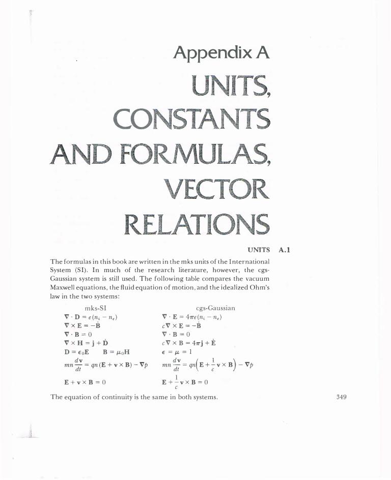
J
Appendix A
co
R
s UNITS A.l
The formulas in this book are written in the mks units of the International System (SI). In much of the research literature, however, the cgs
Gaussian system is still used. The following table compares the vacuum
Maxwell equations, the fluid equation of motion, and the idealized Ohm's
law in the two systems:
mks-SI
V·D=e(ni-n,) V X E = -B V·B = 0 VXH=j+D D = EoE B = J.toH
dv mn dt = qn(E + v x B)-Vp
E+vXB=O
cgs-Gaussian
V · E = 47Te(ni-n,) cVxE=-B V· B = 0 cV x B = 47Tj + E E=J.t=l mn dv = qn(E + .!.v X B) - Vp dt c
1 E+-vXB=O c The equation of continuity is the same in both systems. 349

350 Appendix A
A.2
In the Gaussian system, all electrical quantities are in electrostatic units (esu) except B, which is in gauss (emu); the factors of care written explicitly to accommodate this exception. In the mks system, B is measured in tesla (Wb/m2), each of which is worth 10
4 gauss. Electric fields E are in esu/cm in cgs and V /m in mks. Since one esu of potential is 300 V, one esu/cm is the same as 3 x 10⁴ V /m. The ratio of E to B is dimensionless in the Gaussian system, so that vE = cE/ B. In the mks system, E/ B has the dimensions of a velocity, so that V£ = E/ B. This fact is useful to keep in mind when checking the dimensions of various terms in an equation in looking for algebraic errors.
The current density j = ne v has the same form in both systems. In cgs, n and v are in em -3 and em/ sec, and e has the value e =
4.8 x 10⁻¹⁰ esu; then j comes out in esu/cm2, where 1 esu of current equals c-1 emu or 10/c = 1/(3 x 109) A. In mks, n and v are in m-3 and m/sec, and e has the value e = 1.6 x 10⁻¹⁹ C; then j comes out in A/m2.
Most cgs formulas can be converted to mks by replacing B/c by B and 47T by E 01, where 1/ 47TE 0 = 9 x 10⁹. For instance, electric field energy density is E 2/87T in cgs and Eo£2 /2 in mks, and magnetic field energy density is B 2 /87T in cgs and B 2 /2tJ.o in mks. Here we have used the fact that (Eof.!.o)-112
= c = 3 x ·108 m/sec. The energy KT is usually given in electron volts. In cgs, one must
convert Tev to ergs by multiplying by 1.6 x 10⁻¹² erg/eV. In mks, one converts Tev to joules by multiplying by 1.6 x 10-
19 J/eV. This last number is, of course, just the charge e in mks, since that is how the electron volt is defined.
USEFUL CONSTANTS AND FORMULAS
Constants
mks
c velocity of light 3 x 10⁸m/sec
e electron charge 1.6 X 10⁻¹⁹ C
m electron mass 0.91 X 10⁻³⁰ kg
M proton mass 1.67 X 10⁻²⁷ kg
M/m 1837
cgs --
3 x 10¹⁰ em/sec
4.8 x 10⁻¹⁰ esu
0.91 X 10⁻²⁷ g
1.67 X 10⁻²⁴ g
1837

J
mks
(M/m)I/2 43 43
Constants cgs
K Boltzmann's constant 1.38 X 10⁻²³ ];oK 1.38 X 10-i6 erg;oK
eV electron volt 1.6 x 10⁻¹⁹ J 1.6 x 10⁻¹² erg
1 eV of temperature KT
�:0 permittivity of free space
f.Lo permeability of free space
8.854 X 10⁻¹² F/m
47T X 1 o-7 Him
1Ta6 cross section of H atom 0.88 x 10⁻²⁰ m2
density of neutral atoms at
room temperature and
1 mTorr pressure
Wp plasma frequency
We electron cyclotron
frequency
A o De bye length
rL Larmor radius
v A Alfven speed
mks
( ne2 ) 112
Eom
eB m
(l::�;e) 1/2
mv1_ eB
B
(f.LoP) 1/2
cgs-
Gaussian
(4:e2) 112
eB me
( KTe2) 1/2
41Tne
mv1_c eB
B ( 41Tp) l/2
0.88 x 10⁻¹⁶ cm2
Formulas
Handy formula
(n in cm-3)
fp = 9000 .J-:;, sec -I
fc = 2 .8 GHz/kG
740(Tev/n) 112 em
1.4 T!�2 mm(H)
Eke
2.2 x 10¹¹ :-em
(H) n sec
351 Units, Constants
and Formulas,
Vector Relations

352 Formulas Appendix A
mks
v, acoustic speed
( K:·)
112
(T; = 0)
E X B drift speed E
V£ -
B
diamagnetic KT n'
Vo --
drift speed eB n
magnetic/ plasma nKT
{3 B2 /2/J-o
pressure
v,he electron thermal c:T·) 1/2
speed
llei electron-ion
collision frequency
llee electron-electron
collision frequency
ll;; ion-ion collision frequency
A,; collision mean
free path
eEo peak electron Vosc --
quiver velocity mwo
cgs--Gaussian
( K:·)
112
cE -
B
cKTn' ---
eB n
nKT B2/81r
c:T·) l/2
Wp =-
No
Handy formula (n in em -3)
106 yl/2 em (H)
ev sec
108 E(V /em) em
B(G) sec
1 Os Tev _!_ em
B R sec
5.9 x 10⁷ T!�2 em
sec
_6Zn, In A _1 =2 x 10 T372 sec eV
_6nlnA _1 = 5 x 10 � sec eV
4( m) 112 ( T,f/2 Z M T; llee
=A .. = A;;
eEo --
mwo
2 13 Tev =3 .4 x 10 n ln A
cm(H)
2 Vosc 7 31 2 -2 == · 19AJL c
2 I 2 Vo;c=3.7 13A JL v, Tev

J
A.3 USEFUL VECTOR RELATIONS
A . (B X C) = B . (C X A) = c . (A X B) = (ABC)
A X (B X C) = B(A . C) - C(A . B)
(A X B) . (C X D) = (A . C)(B . D) - (A . D)(B . C)
(A X B) X (C X D) = (ABD)C- (ABC)D = (ACD)B- (BCD)A
V · (</JA) = A· V<{J + <{JV ·A
Vx(<{JA) = V¢ xA+<{JVxA
A X (V X B) = V(A. B) - (A. V)B-(B . V)A- B X (V X A)
V · (Ax B) = B · (V x A)- A · (V x B)
V x (Ax B) = A(V · B) - BV · A + (B · V)A-(A · V)B
V x [(A· V)A) = (A· V)(V x A)+ (V · A)(V x A) - [(V x A) · V]A
V x V x A = V(V ·A)-(V · V)A
v XV¢ = 0
v. (V X A)= 0
Cylindrical Coordinates (r, 8, z)
1 a 1 a a V · A = - -(rAr)+--Ao +-A. r ar r ae az
( laA. aAo) A (aAr aAz) A [1 a laAr] A V x A = ---- r + --- 6 + --(rA8)--- z r ae az az ar r ar r ae
353 Units, Constants
and Formulas, Vector Relations

354 Appendix A
9 [ 9 1 ( aAo)]A v-A = (V . V)A = v-Ar - r2 AT + 2 ()(} r
[ 2 1 ( (JAr)] A 2 A + V Ao - r2 Ao - 2 a;} 9 + V A,z
A( aBr 1 aBT aBT 1 ) (A · V)B = r Ar-+ Ao- -+A,-- -AoBo ar r ()(} az r
+6 A -+A --+A - +-A B A( aBo 1 aBo aBo 1 ) T ar O r ao < az r O T
A(A aB, A 1 aB, A aB,)
+z -+ --+ -T ar O r ao z az
"

Appendix B
COL u ORM
PASMA
As long as T. = T; = 0, the waves described in Chapter 4 can easily be
generalized to an arbitrary number of charged particle species and an
arbitrary angle of propagation 8 relative to the magnetic field. Waves
that depend on finite T, such as ion acoustic waves, are not included in
this treatment.
First, we define the dielectric tensor of a plasma as follows. The
fourth Maxwell equation is
V X B = P,o(j + EoE) [B-1]
where j is the plasma current due to the motion of the various charged
particle species s, with density n, charge q, and velocity Vs:
[B-2]
Considering the plasma to be a dielectric with internal currents j, we may write Eq. [B- 1] as
V x B = p,0D [B-3] 355

356 Appendix B
where
z • D = EoE +- J w
[B-4]
Here we have assumed an exp (-iwt) dependence for all plasma motions. Let the current j be proportional to E but not necessarily in the same direction (because of the magnetic field Boz); we may then define a conductivity tensor a by the relation
Eq. [B-4] becomes
j=a·E
D = Eo(l + _i_a) · E = E · E
Eow
Thus the effective dielectric constant of the plasma is the tensor
E = Eo(l + iaiEoW)
where I is the unit tensor.
[B-5]
[B-6]
[B-7]
To evaluate a, we use the linearized fluid equation of motion for species s, neglecting the collision and pressure terms:
av, m,- = q,(E + v, X B0) at
Defining the cyclotron and plasma frequencies for each species as
Wcs ""' I q,B
o l m,
� noq , Wps == Eoms
[B-8]
[B-9]
we can separate Eq. [B-8] into x, y, and z components and solve for v, obtaining
iq, [Ex ± i (w,,/ w )Ey] Vxs = -- I 2 m,w 1 - (w,, w)
iq, [£1 =F i(w,,/w)Ex] Vys = -- I 2 m,w 1 - (w,, w)
zq, Vu = - £. m,w •
where ± stands for the sign of q,. The plasma current is
j = L no,q,v,
[B-lOa]
[B-lOb]
[B-lOc]
[B-11]

so that
_z_·
jx =I inos iq; Ex± i(wcs/w;Ey
EoW ; EoW m,w I-(wcs/w)
_I _ w!, Ex± i(Wcs/w)Ey
- s W 2 I -(wcsl W )2
Using the identities
I I [ w w J I -(wcs/ W / = 2 W =F Wcs +
W ± Wcs
we can write Eq. [B-12] as follows:
I . l"w;, [( w w ) -; = - - L. - + E EoW X 2 s w2 w =t=wcs w ±wcs X
((JJ (JJ)] + - iE W =t= Wcs W ± Wcs Y
Similarly, they and z components are
Z . "Wp5 W W . . 1 2 [ E0w 2 s w·
(w ± w w =t= w) -;y = -- 1.... -9 ---- -- zEx
( w w ) ] + + Ey
(J) =F Wcs W ± Wcs . 2 Z . "Wps
-- J, = - i.... -2 E, E oW s W
Use of Eq. [B-I4] in Eq. [B-4] gives
I l" [w!, ( w w ) -D =E - - L. - + E Eo X X 2, (JJ2 w=t=wcs w±wcs "
2 +
w_ps ( W _ w ) iE ] W 2 W =F Wcs W ± Wcs y
[B-12]
[B-13]
[B-14]
[B-15]
[B-16]
[B-17]
357 Theory of Waves
in a Cold Uniform Plasma
358 Appendix B
We define the convenient abbreviations
R=I-l:w�, ( w ) s W W ± Wcs
') L = I- L W�s ( W )
s w w + w,,
S = �(R + L) D=�(R-L)* 2
P=l-Iwt;' s W
[B-18]
Using these in Eq. [B-17] and proceeding similarly with the y and z
components, we obtain
E;1Dx =SEx- iDEy Eo1Dy = iDEx + SEy E;1D,_ = PE,_
Comparing with Eq. [B-6], we see that
.�,+� -iD
s 0 �) � ,,.,
[B-19]
[B-20]
We next derive the wave equation by taking the curl of the equation V x E = -B and substituting V x B = /-toE • E, obtaining
.. I .. V XV X E = -1-toEo(ER ·E) = - 2ER · E
c [B-21]
Assuming an exp (ik · r) spatial dependence of E and defining a vector index of refraction
c f.L=-k
w
we can write Eq. [B-21] as
fl. X (fl. X E) + ER • E = 0
[B-22)
[B-23]
The uniform plasma is isotropic in the x-y plane, so we may choose the y axis so that ky = 0, without loss of generality. If() is the angle between k and B0, we then have
1-tx = 1-t sin (} /-t,_ = 1-t cos (} /-ty = 0 [B-24]
*Note that D here stands for "difference." It is not the displacement vector D.
f

The next step is to separate Eq. [B-23] into components, using the elements of ER given in Eq. [B-20]. This procedure readily yields ( S - J.L 2 cos2 ()
R · E = iD J.L 2 sin (} cos ()
-iD 2
J.L 2 sin () cos (}) (Ex) S - J.L 0 Ey = 0
0 P - J.L 2 sin 2 (} E,
[B-25]
From this it is clear that the E., EY components are coupled to E, only if one deviates from the principal angles (} = 0, 90°.
Eq. [B-25] is a set of three simultaneous, homogeneous equations; the condition for the existence of a solution is that the determinant of R vanish: IIRII = 0. Expanding in minors of the second column, we then obtain
(iD)2(P - J.L 2 sin2 ()) + (S - J.L 2)
x [(S - p., 2 cos2 ())(P - p., 2 sin2 (})- p., 4 sin2 (} cos2 fJ] = 0
By replacing cos2 ()by 1- sin2 (),we can solve for sin2 (},obtaining
. 2 -P(p.,4- 2Sp., 2 + RL) sin (} = 4 2 p., (S- P) + p., (PS - RL)
We have used the identity 52- D2 = RL. Similarly,
2 SJ.L 4- (PS + RL)p., 2 + PRL cos (} = 4 2 J.L (S- P) + p., (PS - RL)
Dividing the last two equations, we obtain
2 P(p., 4- 2Sp., 2 + RL) tan (} = ---,---_::_ __ _:__n-___:__ __
SJ.L 4 - (PS + RL ) J.L 2 + PRL
[B-26]
[B-27]
[B-28]
Since 25 = R + L, the numerator and denominator can be factored to give the cold-plasma dispersion relation
[8-29]
The principal modes of Chapter 4 can be recovered by setting() = 0°
and 90°. When (} = 0°, there are three roots: P = 0 (Langmuir wave), f.L 2 = R (R wave), and f.L 2 = L (L wave). When (} = 90°, there are two mots: f.L 2 = RL/ S (extraordinary wave) and JL 2 = P (ordinary wave). By inserting the definitions of Eq. [B- 1 8], one can verify that these are
359 Theory of Waves
in a Cold Uniform Plasma

360 Appendix B
identical to the dispersion relations given in Chapter 4, with the addition of corrections due to ion motions.
The resonances can be found by letting p. go to oo. We then have
tan2 Ores= -P/S [B-30] This shows that the resonance frequencies depend on angle e. If () == Q0, the possible solutions are P = 0 and S == oo. The former is the plasma resonance w = wp, while the latter occurs when either R = co (electron cyclotron resonance) or L = oo (ion cyclotron resonance) . If(} = 90°, the possible solutions are P = oo or S == 0. The former cannot occur for finite wp and w, and the latter yields the upper and lower hybrid frequencies, as well as the two-ion hybrid frequency when there is more than one . . wn species.
The cutoffs can be found by setting p. = 0 in Eq. [B-26]. Again using 52 - D2 = RL, we find that the condition for cutoff is independent of():
PRL == 0 [B-31] The conditions R == 0 and L = 0 yield the WR and wL cutoff frequencies of Chapter 4, with the addition of ion corrections. The condition P = 0 is seen to correspond to cutoff as well as to resonance. This degeneracy is due to our neglect of thermal motions. Actually, P = 0 (or w == wp ) is a resonance for longitudinal waves and a cutoff for transverse waves.
The information contained in Eq. [B-29] is summarized. in the Clemmow-Mullaly-Allis diagram. One further result, not in the diagram, can be obtained easily from this formulation. The middle line of Eq. [B-25] reads
iDEx + (S - 11- 2) Ey = 0
Thus the polarization in the plane perpendicular to B0 is given by
iEx Jl. 2- S -=--
Ey D
[B-32]
[B-33]
From this it is easily seen that waves are linearly polarized at resonance (p. 2 = oo) and circularly polarized at cutoff (1-L 2 = 0, R = 0 or L = 0; thus S =±D).

Appendix C
E
T
SAM
REE-HO R
INA EXAM
PART A (ONE HOUR, CLOSED BOOK)
1. The number of electrons in a De bye sphere for n = 1 017 m -3, KT. = 10 eV is approximately
(A) 135
(B) 0.14
(C) 7.4 X 10³
(D) 1.7 X 10⁵
(E) 3. 5 X 10¹⁰
2. The electron plasma frequency in a plasma of density n = 1020 m -3
IS
(A) 90 MHz
(B) 900 MHz
(C) 9 GHz
(D) 90 GHz
(E) None of the above to within 10% 361

362 Appendix C
3. A doubly charged helium nucleus of energy 3.5 MeV in a magnetic field of 8 T has a maximum Larmor radius of approximately
(A) 2 mm
(B) 2 em
(C) 20 em
(D) 2m (E) 2 ft
4. A laboratory plasma with n = 1016 m-3, KT, = 2 eV, KT; = 0.1 eV, and B = 0.3 T has a beta (plasma pressure/magnetic field pressure) of approximately
(A) 10-7
(B) 10-6
(C) 10-4
(D) 1 o-2 (E) 10-1
5. The grad-E drift vv8 is
(A) always in the same direction as vE
(B) always opposite to V£
(C) sometimes parallel to B
(D) always opposite to the curvature drift VR
(E) sometimes parallel to the diamagnetic drift vv
6. In the toroidal plasma shown, the diamagnetic current flows mainly in the direction
(A) +<f.
(B) -«f,
(C) +0 (D) -9 (E) +z
'e
..

7. In the torus shown on p. 362, torsional Alfven waves can propagate in the directions
(A) ±r
(B) ±9
(C) ±tf, (D) +0 only
(E) -9 only
8. Plasma A is ten times denser than plasma B but has the same temperature and composition. The resistivity of A relative to that of B is
(A) I 00 times smaller
(B) 10 times smaller
(C) approximately the same
(D) I 0 times larger
(E) I 00 times larger
9. The average electron velocity I vi in a I 0-ke V Maxwellian plasma is
(A) 7 x I02 m/sec
(B) 7 x 1 04m/sec
(C) 7 x 10⁵m/sec
(D) 7 x I06 m/sec
(E) 7 x I07 m/sec
IO. Which of the following waves cannot propagate when B0 = 0?
(A) electron plasma wave
(B) the ordinary wave
(C) Alfven wave
(D) ion acoustic wave
(E) Bohm-Gross wave
363 Sample Three-Hour
Final Exam

364 Appendix C
11. A "backward wave" is one which has
(A) k opposite to Bo
(B) w/k < 0
(C) dw/dk < 0
(D) v; = -v,
(E) vq, opposite to vg
12. "Cutoff" and "resonance," respectively, refer to conditions when the dielectric constant is
(A) 0 and co (B) oo and 0
(C) 0 and 1 (D) 1 and 0
(E) not calculable from the plasma approximation
13. The lower and upper hybrid frequencies are, respectively, ..... ..... 1/2 1/2 (A) (upue) and (wpwe)
(B) (fl; + fl�)112 and (w; + w�)112
1/9 9 9 1/2 (C) (wefle) -and (wj; + w;)
(D) ( 2- 2)1/2 d ( 2 + 2)1/2 Wp We an Wp We 1/2 d 1/2 (E) (wRwd an (wpwe)
14. In a fully ionized plasma, diffusion across B is mainly due to
(A) ion-ion collisions
(B) electron-electron collisions
(C) electron-ion collisions
(D) three-body collisions
(E) plasma diamagnetism
15. An exponential density decay with time is characteristic of
(A) fully ionized plasmas under classical diffusion
(B) fully ionized plasmas under recombination

(C) weakly ionized plasmas under recombination
(D) weakly ionized plasmas under classical diffusion
(E) fully ionized plasmas with both diffusion and recombination
16. The whistler mode has a circular polarization which is
(A) clockwise looking in the +Eo direction
(B) clockwise looking in the -E0 direction
(C) counterclockwise looking in the +k direction
(D) counterclockwise looking in the -k direction
(E) both, since the wave is plane polarized
17. The phase velocity of electromagnetic waves in a plasma
(A) is always >c
(B) is never >c
(C) is sometimes >c
(D) is always <c
(E) is never <c
18. The following is not a possible way to heat a plasma:
(A) Cyclotron resonance heating
(B) Adiabatic compression
(C) Ohmic heating
(D) Transit time magnetic pumping
(E) Neoclassical transport
19. The following is not a plasma confinement device:
(A) Baseball coil
(B) Diamagnetic loop
(C) Figure-S stellarator (D) Levitated octopole
(E) Theta pinch
365 Sample Three-Hour
Final Exam

366 Appendix C
20. Landau damping
(A) is caused by "resonant" particles
(B) always occurs in a collisionless plasma
(C) never occurs in a collisionless plasma
(D) is a mathematical result which does not occur in experiment
(E) is the residue of imaginary singularities lying on a semicircle
PART B (TWO HOURS, OPEN BOOK; DO 4 OUT OF 5)
I. Consider a cold plasma composed of n0 hydrogen ions, �no doubly ionized He ions, and 2n0 electrons. Show that there are two lowerhybrid frequencies and give an approximate expression for each. [Hint: You may use the plasma approximation, the assumption m/ M « 1, and the formulas for v1 given in the text. (You need not solve the equations of motion again; just use the known solution.)]
2. Intelligent beings on a distant planet try to communicate with the earth by sending powerful radio waves swept in frequency from 10 to 50 MHz every minute. The linearly polarized emissions must pass through a radiation belt plasma in such a way that E and k are perpendicular to B0. It is found that during solar flares (on their sun), frequencies between 24.25 and 28 MHz do not get through their radiation belt. From this deduce the plasma density and magnetic field there. (Hint: Do not round off numbers too early.)
3. When {3 is larger than m/ M, there is a possibility of coupling between a drift wave and an Alfven wave to produce an instability. A necessary condition for this to happen is that there be synchronism between the parallel wave velocities of the two waves (along B0).
(a) Show that the condition {3 > m/ M is equivalent to VA < v,h·
(b) If KT. = IO eV, B = 0.2 T, k1 = 1 em - I , and n = I021 m-3 find the required value of k, for this interaction in a hydrogen plasma. You may assume n�/n0 =I cm-1, where n� = dn0/dr.
4. When anomalous diffusion is caused by unstable oscillations, Fick's law of diffusion does not necessarily hold. For instance, the growth

rate of drift waves depends on Vn/n, so that the diffusion coefficient D _�_ can itself depend on Vn. Taking a general form for D .L in cylindrical geometry, namely,
(an) q D.t = Ar'nP
ar
show that the time behavior of a plasma decaying under diffusion follows the equation
an = f(r)n p+q+ l at
Show also that the behavior of weakly and fully ionized plasmas IS recovered in the proper limits.
5. In some semiconductors such as gallium arsenide, the current-voltage relation looks like this:
v
There is a region of negative resistance or mobility. Suppose you had a substance with negative mobility for all values of current. Using the equation of motion for weakly ionized plasmas with KT = B = 0,
plus the electron continuity equation and Poisson's equation, perform the usual linearized wave analysis to show that there is instability for
ILe < 0.
367 Sample Three-Hour
Final Exam


Appendix D
A
SOM
1-1. (a) At standard temperature and pressure, a mole of an ideal gas contains 6.022 x 10²³ molecules (Avogadro's number) and occupies 22.4 liters. Hence, the number per m3 is 6.022 x 10²³/2.24 x 1 0-2 = 2.66 x 1025 m-3_
(b) Since PV = NRT, n = N/V = P/RT. Hence n1/n0 = P1T0/P0TI· Taking n0 to be the density in part (a) and n 1 to be that in part (b), we have
Note that a diatomic gas such as H2 will have twice as many atoms per torr as, say, He.
1-2. Consider the integral
in a two-dimensional space. Transforming to cylindrical coordinates, we have
Hence.
I- Joo -x2 dx ,-- e = v 7r -00 369

370 Appendix D
and
1-4.
1-5.
1-6. (a)
d
f"' (2KT
) 112 f"'
[ ( ) 112
] I= -<O
j(u) d u =A ---.;;;- -<0 e-mu'I2KT d u 2;T
= AIC�T
) 1/2
.. A = (m/27rKT)112
p = n (KT,+KT;)= 1021(4X l04)(1.6x 10⁻¹⁹) =6.4x 10⁶N/m2
1 atm= I05N/m2 p = 64 atm
I atm = 1 4.7 lb/in2. = (1 4.7)(1 44)/(2000) = 1 .06 tons/ft2
P -= 68 tons/ ft2
d2<jJ e(n,-n,) __ _!_ ( -«1>/KT, _ e"I>/KT,) -- =- - nroe e dx 2 Eo Eo
= nroe (
e</J + �) Eo KT, KT,
I nroe2 (
1 I ) "- - "- -lxi/An where-= -- -T + KT '+' - '+'O e ' A 1 Eo K ' '
If T, « T,
If T, « T,
-d
A0 = (KT,E0/nroe2)112
Ao = (KT,Eo/nroe2) 112
d2</J nq dx2 =-Eo
Let¢= Ax 2 + Bx + C; ¢' = 2Ax +B; </J" = 2A. At x = 0, ¢' = 0 by symmetry :. B = 0. At x = ±d, <P = 0; therefore, 0 = Ad2 + C and C =
-Ad2. Since
and
<P" = 2A =-nq
Eo 1 A= --nq 2Eo
2 Ad2 I d• •) <P=Ax - =-nq( ·-x -2Eo

(b) Energy to move a charge q from x1 to x2 is change in potential energy
6.(q<f>) = q(</>2- </>1). Let </>1 = 0 at x = ±d and </>2 = (l/2E0)nqd2 at x = 0. Then
I 2 2 'l{ = -nq d
2E0
Let d = Ao; then
I 9 KTE0 I '"C =-nq- --
2-=-KT=E"v
2Eu nq 2
for a one-dimensional Maxwellian distribution. Hence, if d > A0, '"C > EAv· If the velocities are distributed in three dimensions, we have E"v = �KT and '"C > !E . .w. The factor 3 is not important here. The point is that a thermal particle would not have enough energy to go very far in a plasma ( d » ,.\0) if the charge of one species is not neutralized by another species.
1-7. (a) ,.\0=7400(2/ 1016)112= I0-4m, N0=4.8x 10⁴.
(b) ,.\0= 7400(0. 1/1012)112= 2.3X I0-3m, N0=5.4X 10⁴.
(c) A0=7400(800/ 1023)112=6.6x I0-7m, N0= 1.2X 10'.
(a)
(b)
(c)
(d)
[ (2)(104)(1.6 X J0-19)] 112 • 7 v�=
9 _31 =::>.93X10 m/sec
.II X 10
(9. 1 1 X 10-31)(5.93 X 10⁷) r = =6.75m L ( 1.6 X 10 19)(0.5 X 10 4 )
v � = (300)(1 000) = 3 x I O' m/ sec
( 1.67 X 10⁻²⁷)(3 X I O') s TL
= (l.6 X I0-19)(5 X 10_9)
= 6.26 X 10 m = 626 km
-· [(2)(10')(1.6 X 10⁻¹⁹)] 1/2- X s
v.t-(4)(1.67 x IO 27)
- 2.19 10 m/sec
(4)(1.67 X 10⁻²⁷)(2.19 X 10⁵) rL =
( 1.6 X 10⁻¹⁹)(5.00 X 10⁻²) = 0.183 m
2M£ [(2)(4)(1.67 X 10⁻²⁷)(3.5 X 10⁶)(1.6 X 10⁻¹⁹)]112 TL = ---;;i3 =
(2)( 1.6 X 10⁻¹⁹)(8)
= 3.38 x 10⁻²m
371 Answers to
Some Problems

372 Appendix D
CD (2)
Bo E---7
r2 r,
Thus
2-4. Let initial energy be goo, and Larmor radii r1 and r2. as shown. Energy at CD is go, = goo+ eEr,; energy at® is g2 = go- eEr2. {It would be acceptable to say: go,.2 =goo± eEFL here.) Also u�1.2 = 2go,.2/ M. We are asked to make the approximation
1. 9 = Mu1.1.2 = !'vf (2gt.2) 112
t.. eB eB M
= __!___ (2go) 1/2( 1 + eE 1 . . ,) l/2
11, M g" '·-
For small E, expand the square root in a Taylor series:
I (2go) '12( I eE ) r --- 1±--r 1.2 - n M 2 go 1.2
' 0
_ I (2go0) '12[ I eE I (2go) '12] _, r o--- 1±----1·- 11, M 2 goD, M
= __!___ (2go0) 112[ 1 ± � eE __!___ (2g0) 112] D, M 2 goD, M
r _ r = eE __!___ (2go) = 2eE
' 2 goD� M MD�
independent ofgo0. The guiding center moves a distance 2(r1-r2) in a time 2Tr/D" so
4eE 1 2 E _ !;__ u., = 2(r1 -r2)(D,/2Tr) =MD, 2Tr
=; B- B
Thus the guiding center drift is independent of the ion energy goo· The factor 2/Tr would be 1 if we did not make the crude approximation.
2-5. (a)
(b)
Consider electrons:
n = n0e'<f>/KT, :. cf> = (KT,/e) In (n/no)
acf> A KT, 1 an A KT, A E= --r= ---- r = - r ar e n ar eA
E, A KT, A VE = --6= - - 6 8 eBA
_ (2KT,) 112 u,"- ---
m . . lvEI =
KT, � _!_ = � v;" � m eB A 2 w, A

Now, rL = mvj_/eB, so for a distribution of velocities we must find an average rL. Since iJ j_ contains two degrees of freedom, we have
�mv� = 2 x �KT,
The most convenient average is
Using this for vj_ in rL, we have
so that lv£ 1 = v,h implies rL = 2A.
(c) If we take ions instead of electrons, we ha,·e v,"' = (2KTji\11)11" = l'j_;, r�_, = vj_;/w,;, and
If lv£1 = v,h;, it is still true that ru = 2A provided that T, = T,.
2-6. (a)
a¢. E = -V¢ = -r ar
a¢ KT, 2r _,,1., E,(r) = - - = - --;e ar e a-
_KT,_g_ _112_ (0.2)( 1.6 x l0-19) [ _112_ !!_ E max - - e - 2 e - I 7 ea .J2 (l.6X 10-19)(.0 1) C
= 1700 V/m
Emax 17 VE = -- = - = 8500 m/sec max B 0.2
(b) Compare the force Mg with the force e£ for an ion. (mg for an electron would be 1836 times smaller.) g = 9.80 m/sec2. 1\1/g = (39)( 1.67 X 10⁻²⁷)(9. 80) = 6.38 X 10⁻²'' N. e£ max = ( 1.6 X 10⁻¹⁹)( 17) = 2. 75 X 10-1" N = 4 x I 0" Mg. Hence gravitational drift 4 million times smaller.
373 Answers to
Some Problems

374 Appendix D
(c)
2-8.
,...,- c±:> 8 x\78 <.. ...,...I {West)
----
8
MvJ. =10-2m rL = eB
VJ. = (2KT/M) I/2 = [(2)(0.2)(1 6 X 10-19)] 1/2 (39)( !.67 X IQ-27)
= 9.9 x 10²m/sec
B = (39)(!.67 x ro-27)(9.9 x I02) (!0 2)(1.6x !0-19) =4.00x I0-2T
(a)
c 0.3 X !0-4 B =-= T
r3 (r/ R)3
VvB = �VJ.TLIB �;BI = �VTLl:Sl
aB A c A 3 A VB =-r= -3-r=-B(-r) ar T4 T I:SI =; l l v� l 2KT/m KT -vJ.rL =--=----=-2 2 w, 2 eB/m eB
(1.6 X l0-19)(KT)ev l (KT)ev 1.6 X !0-19 B =
-B--
0.3 X 10⁻⁴ B(r=5R)= • =2.4xl0-7T 5
5R = (5)(4000 mile)(l.6 km/mile)(l03 m/km) = 3.2 x 10⁷m
8 (KT)ev = 0.39(KT)ev m/sec Vv B = I 0 2.4 x 1 0 7 Ions: KT = 1 eV vn = 0.39 m/sec
Electrons: KT = 3 x 10⁴ eV VvB = 1.17 X 10⁴m/sec (b) Ions: westward; electrons: eastward.
(c) 2m= (6.28)(3.2 x 10⁷) = 2.0 x 10⁸m
(d)
21TT (2.0 X 1 08) t =-= 4 = 1.7x 10⁴sec=4.8hr Vv8 (1.17 X 10 )
J = nevv8 neglect ions = (107)(1.6 X 10⁻¹⁹)(1.17 x 10⁴) = 1.87 X 10⁻⁸ A/m2
l"

ExB t
2-9. (a) vR = 0, since the electron gains no energy in the parallel (tJ} direction. Since the electron starts at rest with no thermal energy, it will come back to rest after one cycle. Hence, the orbit has sharp cusps instead of loops. It is clear that the vE drift must dominate, since the electron starts to the left, and the Lorentz force makes it move upwards. BxVBt (b) In cylindrical geometry, <P = A In r +B. Since
cP ( 1 o-3) = 460 v and
460 = A In (10-3) + B 0 = A In (O.I) + B
</J(O.I m) = O,
B = - A In (O.I)
460 = A In (!0-3)- A In (O.I)
= A ln (O.O l ) A = 460/ln (O.OI)
460 In (O.I r) rb(r) = [lnr-ln(O.I)]=460 V
In (O.OI) In IOO
E =-a¢
= -460 (.!.....)(=:QJ.)
= 460/r v
ar In I 00 O.I r2 In 100 m
460 4 v -9 =--- = 10 - at r = IO ·m (4.6)(!) m
/( A)10-4 500 X !0-4 B =
5r = (5)(1) = 0.01 T
-VB
To estimate the VB drift, we must find v 1. in the frame moving with the guiding center. Remember that in deriving vvB, vl. was taken as the velocity in the undisturbed circular orbit. Here, the latter is moving with velocity v£, so that it does not look circular in the lab frame. Nonetheless, it can still be decomposed into a circular motion with velocity v 1. plus an E x B drift of the guiding center. Consider the z component of velocity (along the wire). At point CD on the orbit, v, = vE + v cos w,t = 0, where cos w,t = -1, its maximum negative value; hence, V£ = v 1.· The same result can be obtained by considering that at point ® v, = vE + V1. (cos w,t = 1 ). The energy there, �(mv ; ), must equal the energy gained in falling a distance 2rL in an electric field. Thus
e
375 Answers to
Some Problems

376 Appendix D
Now we can calculate Vva:
Vva = � vr IVB
I eB (l.6x 10-19)(10-2)
2 w, B w =-= ' m (9.1 1 x I 0 31)
d B= /(-1) 10-4 dr r2
B T
= 1.76x 10⁹sec-1
���=102m-'
Vva=�v�=� 10 '6 - 4 2 w, 2 1.8 x 10⁹- 2.8 x 10 m/sec
This amounts to a slowing down of the vE drift due to a distortion of the orbit into a hairpin shape � because of the change in Larmor radius. The undisturbed orbit is the path taken by the valve on a bicycle wheel as it rolls along:
0--o-�B----Finally, we note that the finite Larmor radius correction to vE is negligible:
�r2V2�=� rr� 4 L B 4 r2 B
(9.Ilxl0-31)(l06) 7 -• T = = 5. X JQ m L (1.6 X J0-19)(Q.QJ)
9 1 r� r = 10--m :. - -;; = 0.08% 4 r-
2-12. Let all velocities refer to the midplane, and let subscripts i and f refer to initial and final states (before and after acceleration). (a) Given: Rm = 5, V.Li = vu; since 1J- is conserved, v.Lf = v.L,, and only vu will increase. It will increase until the pitch angle () reaches the loss cone:
2 . 2 v .Lf Sin ()m = -2 -- 2 2 2 v.L1+ vu1 1 +vu1/v.L, Hence vff1tvr, = 4, v111 = 2v .Li· Energy is
1 -=-Rm 5
Er = �M(v1� + vrr) = �M(4 + l)vi, = �mvi, E, = !M(vff, + vr,) ='!M(l + 1)vr, = Mvi,
:. E1 = 2.5£, = (2.5)(1) = 2.5 keY

(b) ( 1 ) Let particle have v0 > 0 and hit piston moving at velocity vm < 0. In the frame of the piston, the particle bounces elastically and comes off with its initial velocity, but in the opposite direction. Let ' refer to the frame of the piston. Initial and final velocities in this frame are
Vo Vm --
V� = Vo- Vm
(Note: vm is negative.) Transforming back to lab frame,
Since Vm is negative, the change in velocity is 2lvml· QED (2) At each bounce, the change in momentum is I::.Pn = 2mlvml· If N is the
number of bounces, Pn1 = Pn• + Nt:.p. Thus
N = P111- Pn• = vnf- vn, = 2v_L,- v_L, = � v_L, !::.p 2vm 2vm 2 vm
E, = Mv�, = 1 keV = ( 1 03) ( 1 .6 X 1 0-19) = 1 .6 X 1 0-16 J ( 1 .6 X 1 0-16 ) 1/2 _
. . v_L; =
1 .67 x 1 0_27 = 3.1 x 1 0"m/sec
(3) Average vn is
Vm = 1 04m/sec
1 (3X1 05) N = 2 1 04
= 15 bounces
v = �(vu; + Vtif) = �(v .Li + 2v .Li)
= �VJ.i = 4.6 X 1 05
L = 1 013 m
NL ( 1 5) ( 1013) 8 .. t = - = - = 3.2 x 1 0 sec v 4.6 X 1 0"
( = 10 y)
However, L changes during this time by a distance
so that actual time is more like 2.5 x 1 08 sec. Since only factor-of-two accuracy is required, it is not necessary to sum the series-the above answer of 3.2 x 1 08 sec will do.
377 Answers to
Some Problems

378 Appendix D
2-13. (a) J v11 ds = v1� = constant :. vuL + v11L = 0
(b)
�=-� vu L
. C.vu=!:!!(-L) vu= T L C.vu L 2vl.;- V1.; L T=--.= -ilu -L k(2vJ.; + V1.;) 2vm
= 3.3 x 10⁸ sec
2 1013 - --3 2 X 10⁴
2-14. As B increases, Maxwell's equation V X E = -B predicts an £-field. This induced £-field has a component along v and accelerates the panicle. If B increases slowly and adiabatically, E will be small; but the integrated effect over many Larmor periods will be finite. The invariance of JJ. allows us to calculate the energy increases without doing this integration.
3-1. aujat + V · j = 0, where j = jp = (p/B2)"E. Hence, c:T = -V · [(p/B2):E]. The time derivative of Poisson's equation is v. E = cr/Eo
:. v · t = -(�)v · (;2)t V·(1+E;2)E=O
Assuming the dielectric constant E to be constant in time, we have V · D = V · (EE) = 0. By comparison, E = 1 + p/E0B2.
3-2.
True if E » 1.
nM n; ne2 M2 nM E = 1 +--o=--;;=--�=--2 EoB- n; EoM e-s- EoB
3-3. Take divergence of Eqs. [3-56] and [3-58]:
. a V · (V x E)= -V · B = 0 :. - (V ·B)= 0 at . . V · B = 0 if it is initially zero. This is Eq. [3-57],
V·E V · (V X B) = 0 = JJ.0[q;V · (n;v;) + q,V · (n,v.)] + -2-c
from Eq. [3-60], V · (n;v;) = -n;, V · (n,v,) = -n,
V·E :. JJ.o(-q;n;- q,n,) + -o-= o
c-
i [v · E - _!_ (n·q· + n q J = 0 at Eo ' ' ' '
If [ ] = 0 initially, V · E = (l/E0)(n;q; + n,q,). This is Eq. [3-55].

3-4. B xVn KT ne jD = (KT, + KT,)--2-oc--B e BL
Since KT oc ec/J and E oc -¢/ L, KT/ eL oc E :. }D oc neE/ B oc neu, since E/ B = uE. 3-5. Letj0 be constant in the box of width L. 6n = n'L, lfvl = l6neu,l = ln'Leu,l: from the difference between the currents on the two walls. This current ] D is
over a box of width L, .so the equivalent current density is
IJDI = IJoi/L = ln'eu,l Equation [3-69] gives liDI = IKTVn/BI = IKTn'/BI; hence, once u, is chosen so the two formulas agree for one value of L, they agree for all L, since L cancels out.
3-6. (a)
Isothermal means y = 1.
(b)
VD, = y KT, 2�0 _:_ ( 1 _ X:) -1 = y KT, 2� ( l _ x 2) -1 eB a n., a eB a a 2
n
0 -a 0
- x a
(c) Vv, = (2)/ (0.2)A
A_1 = ��� = (2nu/a2)(a/2) = l/0.04
= 33.3 m_1 n n0(1- a2/4a2) 3/4
:. uv, = (10)(33.3) = 333m/sec
379 Answers to Some Problems
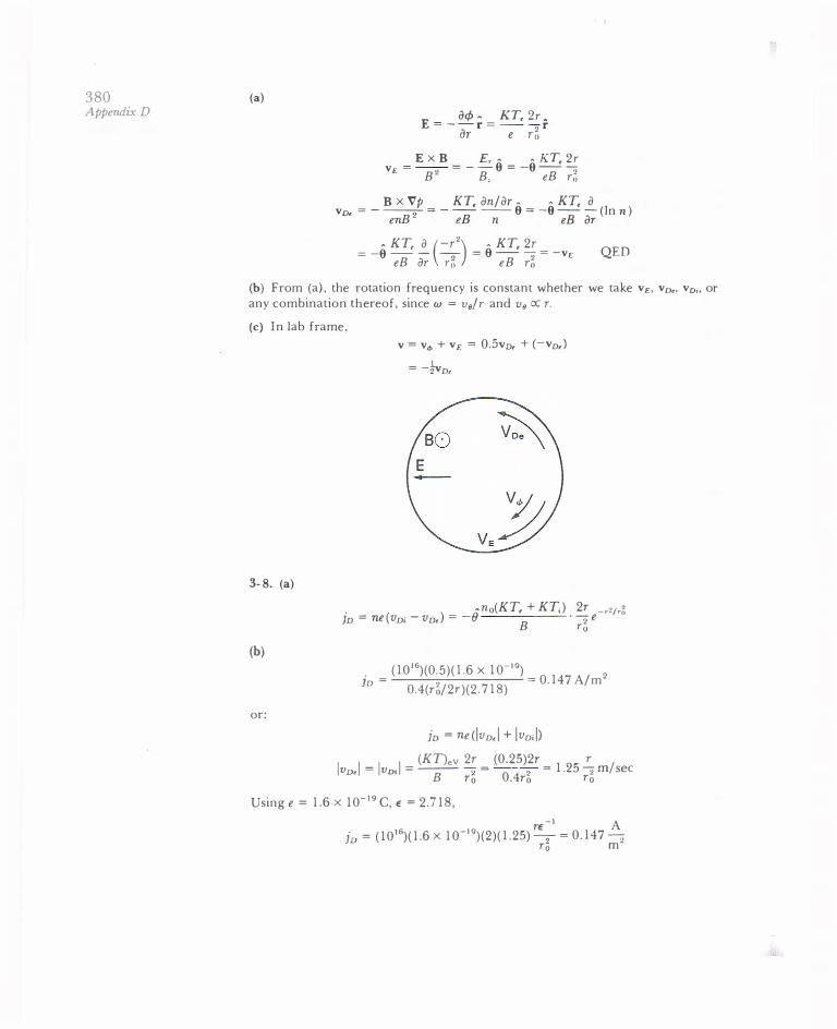
380 Appendix D
(a) E = _
a¢ r = KT, 2T r ar e r�
E x B E, • • KT, 2T VE = --2- = --6 = -6 - -;; B B, eB Tii
I
B x Vp KT, an/aT. • KT, a vv. =- --- =- -- -- 6 = -6 - -(Inn) enB2 � n � �
• KT, a (-r2) • KT, 2r = -6 - - -9 = 6 --;;= -v£ QED eB i3T 1·;; eB Tii
(b) From (a), the rotation frequency is constant whether we take v£, v0., v0;, or any combination thereof, since w = v8/T and v8 ex: r. (c) In lab frame,
3-8. (a)
(b)
or:
v = V<f> + vE = 0.5v0, + (-v0, ) = -�D�
io = ne(vo;- vo,) = _0no(KT, + KT;) 2r 2 • . -e-r frO
B T6
(1016)(0.5)(1.6 X 10⁻¹⁹) = 0.147 A/m2 io = 0.4(r�/2T)(2.718)
io = ne<lvo,l + lvo;l)
I I _ I I _ (KT).v 2r _ (0.25)2r _ T / vo, - vDi - -- 2- 2 - 1.25-,m sec B ro 0.4ro ro
Using e = 1.6 X 10⁻¹⁹ C, E = 2.718, TE-l A
fo = (1016)(1.6 X 10⁻¹⁹)(2)(1.25) -2 = 0.147 2 To m

(c) Since v, = vE + vv, = vE - vE = 0 in the Jab frame, the current is carried entirely by ions.
3-9.
v X B = �OjD J (V X B)· dS =�of jv · dS
f B · dL = �o J jv · dS Choose a loop with one leg along the axis (B = Bo) and one leg far away, where B = Bco. Since jv is in the -9 direction, we can choose the direction of integration dL as shown, so that jv · dS is positive. There is no B, :.
f B · dL = (Bco-Bo)L
. • n ( KT , + KT,) 2r JD = -9 B 2 ro
f no(KT+ KT) J L fco • • dS ' ' -r2fro 2 d d Jv · = 2 e r r z Bcoro o o
= Ln0 (KT, + KT,) [-e_,21,0]"' =
2LnoKT Bco o Bco
0d�
where T, = T,. In this integral, we have approximated B (r) by Bco, since B zs not greatly changed by such a small fv. Thus,
4-1. (a) Solve for ¢1:
2n0KT 6B = Boo-Bo = �o --Bco
2( 41T X 10-7)( 10 16)(0.25 )( 1.6 X 10⁻¹⁹) 0.4
KT, n 1 w + ia w * - ia 4> I = -- - --- X ----:;;-----:e n0 w * + ia w * - ia
KT, ww* + a2 + ia(w*- w) n1 e
B�
381 Answers to
Some Problems
382 Appendix D
If n 1 is real,
Hence,
bn(c/J1) a(w*- w) --- = =tan /5 Re(c/JI) ww* + a2
8 _1 [a(w*- w)J = tan ww* + a2 (b) n1 = n1 e '<>x-wn, while ¢1 = A n1 e'<kx-w•H>, where A is a positive constant. For w < w*, we have 8 > 0. Let the phase of n1 be 0 at (xo, to): kxo- wt0 = 0. If w and k are positive and x0 is fixed, then the phase of c/J 1 is 0 at kx0- wt + 8 = 0 or t > 10• Hence c/J1 lags n1 in time. If lois fixed, kx- wto + 8 = 0 at x < x0, so c/J1 lags n 1 in space also (since w/ k > 0 and the wave moves to the right, the leading wave is at larger x). If k < 0 and w > 0, the phase of c/J 1 would be 0 at x > x0; but since the wave now moves to the left, cf> 1 still lags n 1.
4-2.
I ik£1 = -e(n;l- n<I)
€u -iwmv,� = -eE l (electrons)
-iwMv,1 = eE1 (ions)
-iwn<� = -ikn0v,l (electrons)
-iwn; 1 = -ikn0v; 1 (ions)
k ( -ie) n<I = -n0 -- £1 w mw k ( ie ) n;1 =-no -- E1 w Mw
. I k ie ( I I ) ikE 1 2 2 tkE1=--n0- -+- E1=�(f1p+wp) €0 w w M m w ·
w2 = (w! +f1!)
4-3. Find c/J1, E1, and v1 in terms of n1:
But £1 = -ikc/JJ,
Eq. [4-22]: w n1
v1 = k no
te Eq. [4-23]: E1 = -n�
Eok
e cP1 = ---2 n1 Eo k
Hence, £1 is 90° out of phase with n1; c/>1 is I80° out of phase; and v1 is either in phase or I80° out of phase, depending on the sign of w/k. In (a), E1 is found

from the slope of the </J1 curve, since £1 = -a</>1/ax. In (b), E1/n1 oc i x sgn (k) :. 8 = ±n-/2. If w/k > 0,
£1 oc exp i(kx ± lwlt ± 71'/2)
the ± standing for the sign of k. Hence, E 1 leads n 1 by 90°. Opposite if w/ k < 0.
(a)
4-4.
4-6. (a)
x-
w ->0 k
w -<0 k
(b) (c)
t-
. I I k I k ( -ie) tk£1 =- - en1 = - -en0-v1 = - -en0- - £1 fu fu w fu w mw ( n e2 ) ik I - -0
- 2 E 1 = 0 t:0mw
or
mn0(-iw)v 1 = -enoE1-mn0vv1
. I tk£1 =- -en1 fu
(1 iv) ie£1 v, + - =--
w mw k
n1 = -n0v1 w
(continuity)
. 1 k ie£1 ( iv) _, zk£, =- -e-n0-- I + -t:o w mw w
t-
383 Answers to
Some Problems

384 Appendix D
(b) Let w = x + iy. Then the dispersion relation is x2 -l + 2ixy + ivx- vy = w;. We need the imaginary part: 2xy + vx = 0, y = (- l /2)v :. Im (w) = - v/2.
Since x = Re (w), v > 0, and
E, ex: e-iwc = e-iwt e)·t = e-ixt e-<ll2>vt
the oscillation is damped in time.
4-7. mn0(-iw)v1 = en0E1- en0(v1 X B0). Take B0 in the z direction and E1 and k in the x direction. Then they-component is
-iwmv, = ev.Bo v. . w -= -t-v"j w,
Since w = wh > w" lv./v,l > I ; and the orbit is elongated in the i direction, which is the direction of k.
4-8. (a)
We need n1:
We need v., v,:
l V·E1=- -eni Eo
k=k.i+k,z E, = k, = 0
l i(k.E. + k,E,) =--en I
Eo
ani -+n0V · v1 = 0 at
-iwn 1 + n0i (k.v. + k,v,) = 0
Mn0(-iw)vi = -enoE1- eno(vi X Bo) . . z
e tw,
x-component: Vx = - -- E. --v, mw w
y- component: iw,
v, = 0+- v. w . 2 . 2 -1 te w, -te
( w,
) v. = - -E. + 2 v. = --E. l - 2 mw w mw w
ze z-component: v =-- E z mw z.
Continuity: n0 -u w, ')[
2)
-1 ] n1 =-; (mw kxEx( I-
w2 + k,E,
. en0 -ze w, ')[
2) -1 ] k.Ex + k,E, = t eow
(mw
k.E.( I -w 2 + k,E,
k. = k sin (J k, = k cos (J
• 2 2 Wp · 2 W� 2 2
[ 9)
-1
] . . E I sm (J + kE I cos (J = w 2 kE I sm o( I -
w 2 + kE I cos (J
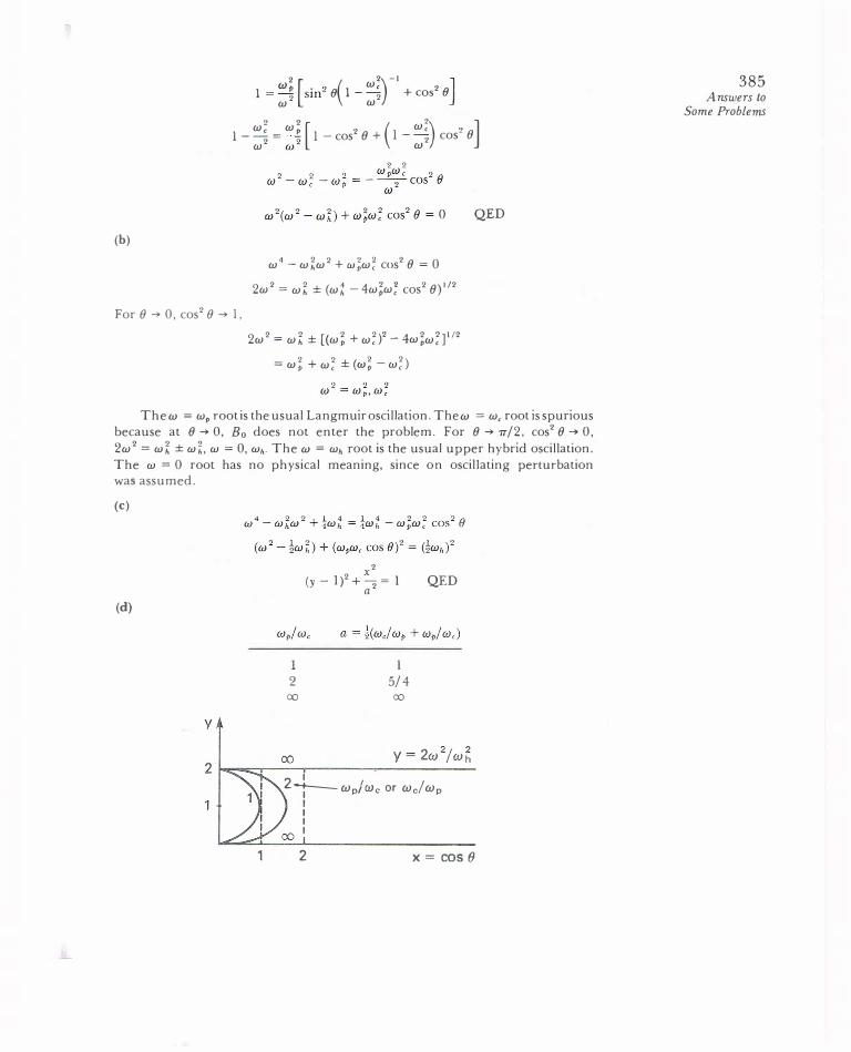
W p . C) w, 2 2 [ 2) -1 ] 1 =
w2 sm- e( 1-w2 + cos e
w; w 2 w, <) 0 2 [ ( 2) ] l-w2 =
w: 1- cos 8 + 1-
w2 cos- 8
(b)
For 8 � 0, cos2 8 � l,
w4- w�w2 + w!w� cos2 8 = 0
2 w2 = w� ± (wZ- 4w;w; cos2 8)112
2 w2 = w� ± [(w! + w�)2- 4w;w�]112
=w!+w�±(w;- w�)
QED
Thew = wp root is the usual Langmuir oscillation. Thew =we root is spurious because at 8 � 0, B0 does not enter the problem. For 8 � 7T/2, cos2 8 � 0, 2w2 = w� ± w%_ w = 0, wh· The w = wh root is the usual upper hybrid oscillation. The w = 0 root has no physical meaning, since on oscillating perturbation was assumed.
(c)
(d)
y
1
2 00
2 o X
(y- It+-= I a2
1 5/4
00
QED
2 I I j-WpfWc or Wc/Wp I I I I
2 X= COS()
385 Answers to
Some Problems

386 Appendix D
(e)
w2 = �(w� + w;) ± [(w� + w;)2- 4w�w; cos2 0]112
Lower root: Take(-) sign; w is maximum when cos2 0 is maximum(= 1). Thus
2 1 [< 2 2 I 2 2IJ w_ <2 Wp +w,)- Wp -w,
=w; ifwp >w,
= w! if w, > wp
Upper root: Take (+) sign; w is maximum when cos2 0 = 0, w� < w�. This root is minimum when cos2 0 = I; thus
2 1 [< 2 2 > I
2 2IJ w+ > 2 wp +w, + Wp -w,
= w; if wp > w,
= w; if w, > Wp
4-10. Use V+, N+ for proton velocity and density V _, N _ for antiprotons v_, n_ for electrons v+, n+ for positrons
(a)
2 2 w = wh.
v X E = -B E V X B = J.Loj +2 c
V X V X E = -(J.LoJ + �) -(k X k X E)= -[J.Lon0e(v+- v_) - :2
2 E J
= eE- k<k/El 1
(w2- c2e)E = -n0e(v+- v_) Eo
mn0v± = ±en0E . e V± = ±-E
m
2 9 2 1 e 9 w - c-k = - n0e- (1 + 1) = 2w;
Eo m
2 nue2 Wp = --
Eom w2 = 2w; + c2k2
(Or the 2 can be incorporated into the definition of wp.)
Thus

(b) V · E, = (1/Eu)(N+-N_ + n+-n_)1, where n+ = n0 e-•<�>IKT+, n_ = n0 e•<t>/KT_ Let T+ = T_ = T , n1± = =F n0e</J/ KT ,. Note: No± = no±= n0 .
4-11.
M(-iw}V± = ±eE1 = ±ike</J
w2 2v;
k2 2+k2Ai,
_ ck n =
w
(M+ = M_ = M)
2 _ kT, v ='
M
4-12. In V X B = ILuj ,, j, is the current carried by electrons only, since Cl- ions are too heavy to move appreciably in response to a signal at microwave frequencies. Hence,
If wp is defined with n0 (i.e., w! = n0e2/E0m), the dispersion relation becomes
Cutoff occurs for f = (l- K)112fp = (0.4)112(9)(n0)112, where
Thus [ !0 '0 ]2 n = = 3 1 x 10¹⁸ m-3 u (0.63)(9) .
387 Answers to
Some Problems

388 Appendix D
4-13. (a) Method 1: Let N = No. of wavelengths in length L = 0.08 m, N0 = No. of wavelengths in absence of plasma.
N=� A L No= Ao
A = 27T k
ck _ ( w!) 112 -- 1--w w2
D.N = No-N = �- Lk = �- !::..._ <:'!_ ( 1 - w!) 1/2 Ao 27T A0 27T c w-
w 27TC Ao
!J.N = :o [ 1- ( 1- ::) 112] = 0.1
L 0.08 -=--= 10 A0 0.008
1 - p ( w2) 112
w2 = 1- 10-2 1 _fl. = 1 _ (2 x 1 o-2) f
f! = [2 X 2 X 10-2 = (;�22 X lQ-2 = 2.8 X 10¹⁹
2 .8 X 1019 1- 3 n = =3.5x 10 ' m-(9)2
Method 2: Let k0 = free-space k. The phase shift is
D.¢ = r D.k dx = (ko- k)L = (0.1)27T
This leads to the same answer. (b) From above, D.N is small if w !I w 2 is small; hence expand square root:
L [ ( 1 w!)J L I w! D.N
= A0 1- 1-2 w2 =
A0 2 w2 oc n
4-14. From Eq. [4-101a], we have for the X-wave
2 2 2 .WpWc (w - W h )Ex + t -- E, = 0
w
QED
At resonance, w = wh : . E, = 0, E = Exx. Since k = kxx, E II k, and the wave is longitudinal and electrostatic.
4-15. Since w� = w; + w;, clearly wp < wh· Further, wL = H-w, + (w� + 4w!)112J
< �[-w, + (w; + 4WcWp + 4w!)112]
= M-w, + (w, + 2a.�p)] = wp :. wL < Wp Also,
WR = Mw, + (w� + 4w!)112] > w,

and
4-17. (a) Multiply Eq. [4-112b] by i and add to Eq. [4-112a]:
Now subtract from Eq. [4-112a]:
Thus,
Since
2 2 <> • We . (w - c k-- a)(Ex- tE,)-a- (Ex-tE,) = 0 w
F(w) = w2 - c2e- a (I + wc/w)
G(w) = w2- c2k2- a(l- wc/w)
2( w!/w2 c2k2) F(w) = w 1 - - -2 1- wc/w w
o( w�/w2 c•e) G(w)=w- 1- --2 1 + wc/w w
From Eqs. [4-116] and [4-117],
F(w) = 0 for the R wave and
G(w) = 0 for the L wave
(b) Ex= -iE, :. E, = iEx. Let Ex= [(z) e-;w•. Then
y
\ I \ I
\. I ,....._ __ _.../
X 0 je =-eve
389 Answers to
Some Problems

390 Appendix D
E, lags E. by goo. Hence E rotates counterclockwise on this diagram. This is the same way electrons gyrate in order to create a clockwise current and generate a B-field opposite to B0. For the L wave, E, == -iE. so that E, = f(z) e -;<w<h/2> and E, leads E, by goo. (c) For an R-wave, E, = iE •. The space dependence is£. = f(t) e ;h. E, = f(t)i e ;k, ==
f(t) eqhh/2>. For k> 0, E, leads E. (has the same phase at smaller z). For k < O, E, lags E. (has the same phase at larger z ) .
L v, X/
Bo
k>O
4-19.
At w = �w"
----
c2e w2
Bo k<O
w!/w2 1- -"-'-----
1 -w,/w
I I
w;/w2 c 2v ;2 = 1 - 1 - wei w
2 -3 dv"' - 2 -1 -c (-2)v<t> -d
--wp 2 2 (2w -w,)- 0 w (w -ww,)
:. 2w-w, = 0
c2 w! 2 = 1--,-2--1 2 V4; 4Wc - 2Wc
V<f> <C.
w = �w,
4 2 1 + u�/>1 w;
4-20.
But
., w!/w2 1- -=---
1-wJw c2k2 = w2-
ww;; w -w,
2 (w-w,)-w 9 c 2 kd k = 2wdw- 2 w;;dw
(w- we)
dw kc2 kc2
dk w + w,w!/2(w-w,)2 w + w!/2w,
( 2 W : ) I /2 ( 2 WW :) I /2 ck = w - = w +--
1- wJw w, if w « w,
To prove the required result, one must also assume v� « c2, as IS true for whistlers, so that w!/ww, « 1 (from line 1). Hence
4-21.
1/9 dw 2 (ww,) - 112 -= c- CX:w
dk w!
2 2 2 I · . (w -c k )E1 =-zwJ1 E'o
(Eq. [4-81])
jl = n0e(vp- v,) (vp is the positron velocity)
From the equation of motion,
±ie ( iw, )( w�)-I v. = mw E. ± --;;; E, 1 - w 2
±ie ( iw, )( w�)-1 v,
=
mw E, +-;;;Ex 1 - w2
theE, term canceling out. Similarly,
2 9 2 2w! (w - c-k )E, =
I 2/ 2 E, -w,w
391 Answers to
Some Problems

392 Appendix D
the Ex term cancelling out. Both equations give
c2k2 2w: -2- = 1 --2-- 2 w w -w,
The R and L waves are degenerate and have the same phase velocities-hence, no Faraday rotation.
4-22. Since the phase difference between the R and L waves is twice the angle of rotation,
LL (kL-kR) dz = 1r
_ ( w!/w2 ) 112 kR.L -ku 1 -
j 1 ±w, w To get a simple expression for kL-kR, we wish to expand the square root. Let us assume we can, and then check later for consistency:
1 w!/w2 ) kR.L = ko( 1 -2 1 ± wJw
kL - kR = �ko W: ( 1 - --1-- )
2 w- 1-wJw 1+wJw _ !k
w; 2wJw -2 °w2 1-w;/w2
2 WpWc 7r = L(kL-kR)=koL-- 2 2 w w -w, 2 'TT"C 9 9 f9 C l - f;
Wp = Lw, (w--w�) ; = 2L -y:-
f, = 2.8 X 1 010(0. 1 ) Hz C 3 X 1 08 f =- = = 3.75 x 10¹⁰Hz
Ao 8 X I0-3
9 (3 X 1 08) ( 1 .4 1 X 10²¹ -7.8 X 1 018) f; = (2)(1) 2.8 X 109
= 7.5 x 1 019 = 92n
n = 9.3 x 1 017 m-3
To justify expansion, note that f, « f, so that
w!/w2 f! 7.5 X 10⁹ 1 ± wJw = [2 =
(3.75 X 10¹⁰)2 = 0·05 « I
4-24. 12.7°.
ko = � c

4-25. (a) The X-wave cutoff frequencies are given by Eq. (4-1 0 7) . Thus,
o 41Tne 2 w;; =w(w±wJ=-
m
We choose the (+) sign, corresponding to the L cutoff, because that gives the higher density .
.
(h)
2 V.p ?
1
0 ����--------�����._ __ ____ __
The left branch is the one that has a cutoff at w = wL· One might worry that this branch is inaccessible if the wave is sent in from outside the plasma. However, if w is kept less than w" the stopband between w, and wR is avoided completely .
4-28. (a)
fc = 28 GHz/T = (2.8 X 10 10) X (10-2) = 2. 8 X 10 8Hz
f = 1. 6 x 10 8 Hz :. wp/w > 1 wJw > 1
= 0 . 62wc
{L = (0. 62) (2.8 X 10 8) = 1.73 X 10 8 > f
393 Answers to
Some Problems

394 Appendix D
We w
Also, f> all ion frequencies.
@�
2 Wp .. -2 w
·d of L uency SI e here, on low-f�f�ron resonance cutoff and cy
(b) The R-wave (whistler mode) is the only wave that propagates here.
4-29. (a)
If A = 2L,
(b)
B 1 v - --- -
A - (JJ.0nM)- [( 1.26 X 10 -6)(1019)(1.67 X 10⁻²⁷))112
= 6.9 x 10⁶m/sec
eB ( 1.6 X 10 -19)(1) 7
fl, = M = (1.67 x 10_27) = 9 .58 X 10 rad/sec
w = 0.1fl, = 9.58 x 10⁶rad/sec
W = kvA = 2-rrvA/A
L = 7TVA = -rr(6.9 X 10⁶)
w 9.58 x 106 = 2.26 m
L cc vA/w cc vA/fl, cc B(nM)-112B -1M cc (M/n )112
( 133) 112( 1 01� 112 :. L = (2.26) -1- 1018) = 82 m
This is why Alfven waves cannot be studied in Q-machines, regardless of B .

4-30.
(a)
(b)
x = cP(- df)-1 f: dt
4-31. (a) Let n �" = (l- E)n0, n�21 = E1!0, n, = n0e¢/kT,
Poisson: ik£1 = k2¢ = _.!._ e (n \ " + n F'- n, ) Eo
(Assume z 1.2 = I, since the ion charge is not explicitly specified.)
Continuity: n \'1 =(I - E)n0�v\'>, w
Equation of motion: (j)- e k ( n�j)-l VI ---¢ 1-2
Miw w (Eq. [4-68])
k2 e ( n;o) -1 e J + En0---,;- 1 - -f- - n0-k - ¢ ""'0 (plasma approximation) w M2 w T,
(b) There are two roots, one near w = 0,1 and one near w = 0,2., I f E � 0, the root near 0,2 approaches 0,2 to keep the last term finite. The usual root, near flc�, is shifted by the presence of the M2 species:
2 2 - 2 2 [ 2 2 2 2 W2- n;IJ W - fl"- k v,, - E k V,, - k V,2 2 2 w - n,2
395 Answers to
Some Problems

396 Appendix D
In the last term, we may approximate w2 by 0�, + k2v;,. Thus,
(c)
4-32.
2 o o 2 [ ev ?2 J 2 o W = !}�, + k-v,, + E
f12 _ !}2 - 1 k v;, c I c2
1 k2v;o 1 ev,r 1 =-
2 2 +- -2--2 2 w - w ,o 2 w -n,r
v;0 = KTJMo = (104)(1.6 X 10⁻¹⁹)/(2)(1.67 X 10-27) = 4.79 X 10¹¹
v?r = �v?o = 3.1 9 X 10¹¹
O,o = e8/M0 = (1.6 X 10⁻¹⁹)(5)/(2)(1.67 X 10-27) = 2.40 X 10⁸
2 n<T = 3D,o = 1.60 X 10⁸ k= lOO m- '
(w2- n�oHw2- n�r> = Wlv;o(w2- n�r> + v;r(w2- n;on
w4-w2[D;0+ D�r+ �k2(v;o + v;r)J
+ n;Dn;r+ M2(v;on�T + v;rn;o) = 0
w 4 - w 2 [ 8. 3 2 X 1 0 16 + 3. 9 9 X 1 0 15) + 1 . 4 7 X 1 033 + 1. 53 X 1 032 = 0
w4- 8.72 X 10¹⁶w2 + 1 .63 x 1033 = 0
w2=�[8.72x l016±(7.60X 1033-6.52X 1033)112]
= 6.0 X 10¹⁶, 2.72 X 10¹⁶
w = 2.45, 1.65 x 10⁸ sec-' f = 3 9 and 26.3 MHz
e � = n0(i mv;) v =--E
' imw
2 2
e 2) :. (v,) = -9 -2(£ m-w
""' 1 e2 2 (
9
e = n0-m--(£2) _ EoWp £·)
2 2 2 -----
m w w2 2
But w2 = w! :. � = �€0(£2).
4-33.
� = n0(�Mvf) V; = E,/8o
.. � = �Mno(ED/80• But V X E, = -B, :. (EI) = (w2/k2)(8D
Mn0 w2 2 � =
28� /;2<8 ,).

For Alfven wave,
4-34. (a) With the L-wave, the cutoff occurs at w = wL, so that one requires w l < EW 2• Since wL < wp if n0 is fixed (Problem 4- 15), one can go to higher values of n0 (for constant Ew2) with the L-wave than with the 0-wave .
(h) For the L-cutoff,
Thus, to double the usual cutoff density of Eomw2 / e2, one must have f, = f
C 3 X 10⁸ 11 f =A=337xl06=8.9xlO Hz
f, = 28 x 109 Hz/T 8.9 X 10¹¹
.. Bo= 28x 109 = 3 1.8T
This would be unreasonably expensive.
(c) The plasma has a density maximum at the center, so it behaves like a convex lens. Such a lens focuses if n > l and defocuses if n < l. The whistler wave always travels with v� < c (Problem 4-l 9), son = c/v� > 1, and the plasma focuses this wave.
(d) The question is one of accessibility. If w < w, everywhere, the whistler wave will propagate regardless of n0. However, if w > w" the wave will be cut off in regions of low density. From (b) above, we see that a field of 3 1.8 T is required; this seems too large for the scheme to be practical.
4-35. The answer should come out the same as for cold plasma.
4-36. The linearized equation of motion for either species is
-iwmn0v1 = qn0(E + v1 X B0)- ykT;kn1
Thus
-iwmnok · V1 = qno(k · E + k · v1 X B0)- ykT;k2n1•
But k · E = 0 for transverse wave, and k · (v1 x B0) = -v1 • (k x B0) = 0 by assumption. The linearized equation of continuity is
-iwn1 + n0ik · v1 = 0
Substituting for k· v,, we have
Thus n1 is arbitrary, and we may take it to be 0. Then the Vp term vanishes for both ions and electrons.
397 Answers to
Some Problems

398 Appendix D
4-44. For a given density, the highest cutoff frequency is wR. Thus the lowest bound for n is given by w = wR.
w; f! w, (1.6 X 10⁻¹⁹)(36 X 10-4) -=-=1--=1- =016 w2 F w (0.91 X 10⁻³⁰)(2'1T)(l.2 X 108) .
n =f!/q2=(0.16)(1.2x l08)2q -2=2.8x 10¹³m-3
4-46. Let w = wR at r1, where n = n1, Wp = wpi; and w = wh at r2. where n = n2, w. = wp2 . Then
Thus
But
So
2 2 2 Wp2 = w -w, 2 - 2 Wp1 - w -ww,
w!2- w!1 = w,(w-w,) = (n2- n1)e2/ E0m
n2- n1 = d/iin/arl = n1d/r0 = (E0m/e2)(w)(w-w,)(d/r0)
d = (wjw)ro
[4-105]
[4-107]
4-47. (a) The accessible resonance is on the far side, past the density maximum.
We
w
0 r 1 w�lw2
(b) Let w,0 be w, at the left boundary, and w, be the value at the resonance layer, where w = wp. Then we require
Thus Wco>w, where w2 = w� + w;
2 2 2 w,0 >w, +wp 2 2 2 w,0 -w, > wp (w,o + wJ(w,0-w,) = 2w,�w, > w!
�w, �B0 w! --=-->--w, Bo 2w�

4-48. These are the upper and lower hybrid frequencies and right- and left-hand cutoff frequencies with ion motions included. Note that w;/w, = n;;n,. Resonance:
or
Cutoff:
(upper hybrid)
1 1 1 - = -- + -w� w,D, D!
(lower hybrid)
This is more easily obtained, without approximation, from the form given in Problem 4-50.
5-l. (a) D, = KT,/mv
v = (2£) '12 = [(2)(2)(1.6 x 10-'9)] m (9.11 x 10-�1)
= 8.39 X 10⁵ m/sec
From Problem 1-lb,
no= (3.3 X I019){103) = 3.3 X 10²² m-3
1/ = no01J = nocro = (3.3 X 10²²)(5.29 X I o-20)(8.39 X I 05)
= 1.46 x I09 sec-•
(b) j = p.,neE
(2)(1.6 X 10⁻¹⁹) 2 2 D,
= (9.I1 x 10-3')(1.46 x 10⁹)
= 2.4 x 10 m /sec
(1.6 X 10⁻¹⁹)(2.4 X 10²) " =eD/KT = �------�--�� ,-, ' ' (2)( 1.6 X 10⁻¹⁹)
= 1.2 x I02 m2/V sec
j 2 X IQ3 E = - = = 1 o4 x 1 o• v 1 p.,ne (1.2 X I02)(1016)(1.6 x 10⁻¹⁹)
• m
399 Answers to
Some Problems

400 Appendix D
5-2.
an= DV2n- an2
at
? a2n ( 7T ) 2 7TX
( 7T ) 2 2 DV·n = D ax2 = -Dn0 2L cos 2L = -D 2L n = -an
D ( 7T ) 2 0.4 ( 7T ) 2 18 3 n =; 2L = 10-15 0.06
= 1.1 x 10 m-
5-4. (a) From Problem 5-1a, v'" = 1.46 x 1 09 sec-1 . We need to find whether
J.L"-1 f.Ld. is large or small:
f.L, Mv;n
J..Li 1nVen V;n = nnUV; CX:: Vthi CX:: mj112
since a- is approximately the same for ion-neutral and electron-neutral collisions. Thus
But
1/0 J.L, = (M) - = (4 x 1,836)112 = 85.7 J.L; m
eB (1.6 X 10⁻¹⁹)(0.2) = 3.52 X 10¹⁰ We =-;;; =
9.11 X 10 31
3.52 X !010 X 24 Wc'Tm = 1.46 X 10⁹
1 + W�T;n = 580
(m)(M) 1/2
acTin = WcTm M m = (24)(85.7)-1 = 0.28
1 1"1 2 2 f.L<J.. = J.L, + HcTin _ 85 7 1.08 _
2 2 - ( • ) - 0.16 « f.Li.l. f.Li 1 + WcT,n 580
J.L. D +J.L D J.L D = 1.1. d e.L 1.1. = D + �D-• • a.l t.l 1.l f.Li.l.+f.Le.l. mi.L
KT D=-J.L e
= De.1. + 0.16Di.i
D,.l. J.L•.1. T, 1 0.1 -=--=- -=0 3 D"- f.Le.1. T, 0.16 2 .
:. Da.l. = De.L[ 1 + (0.16)(0.3)] = 1.05D"- = Dd

(b)
5-5.
5-7.
a ( a ) 2 1 (DT)1/2 = 2.4 .". T =
2.4 DaJ. 1 1
r= -(2.4 X 1 0-2)2 D,J.
2.4 X 10² D,1.=
58
0 =0.4 140( from Problem5-1)
:. T = 42 J.LSec
f=-Ddn/dx n=n0(1-x/L)
r = Dn0/ L (x > 0)
Q = 2r = 2Dno/L :. no= QL/2D
But v,h, oc T;12 and v,, oc T-;312
5-8.
5-9. (a)
:. A,, oc T;12/T;312 oc T;
(assume Z = 1)
= (5.2 X 10-s)( 1 0)
= 4.65 X 10-R f1-m (500)312
j =!/A = (2 X 10⁵)/(7.5 X 10-3) = 2.67 X 10⁷ A/m2
£ = 771U = (4.65 X l0-s)(2.67 X 10⁷) = 1.2 V /m
KT, = 20 keV KT, = 10 keV n = 1012 m-3
B = 5T 71n(KT, + KT,) DJ. =
B2
_5 In A. (l o-3)(1 0) 7JJ.=(2.0)(5.2x 10 )T;/,2= (l04)3/2
= 1.0 X 10⁻⁹ fl-m
(1.0 X J0-9)(1021)(3 X 10⁴)(1.6 X lb- 1 � D J. = -----'--'-----'--'--::---'--'-----� 52
401 Answers to
Some Problems

402 Appendix D
(b)
dN = 21rrLL dt
an n
ar 0.1
dN
an L = -D'-ar
r = 0.50 m L =100 m
- dt = (27T)(0.50)(102) (2.0 x 10⁻⁴)(1021/0.10) = 6 x 10²⁰ sec-'
(c)
5-13.
N n7TT2L r=---=--
-dN/dt -dN/dt r dfe(.tive = 0.55 m
r = (I02') (7T)(0.55)2(102)
= !50 sec 6 X 10²⁰
-In A _ 10 7JII = 5.2 X 10 -'�f1-m = (5.2 X 10-')� T,v JO
= 1.6 X w-s D-m
7JJ"= (1.6X 10-')(105)2= 1.6X I05W/m3
= 1.6 x I 0' J/(m3-sec)
= (1.6 x 10⁵)/(1.6 x 10-19) = 1024 eV/m3-sec
dE;, dt
3 E =
2nKT,
d£,v 3 dTev :. - =-n-
dt 2 dt
dT," = � _1_1024 = 0.67 x 10'eV/sec = 0.067 eV/J-Lsec dt 3 10'9
5-15. (a)
add:
en <4"- v,TB) - y.;, - e2n 21) (v;8 - v,8) = 0 0
f." 2 2 --en(4 - v"B)- eP, + e n 1)(V;8- v,8) - 0
-v,TB + V"B = 0 V;T = V"
(This shows ambipolar diffusion.) /

(b)
ap, 2 2 - o -en (E, + v,0B ) - - + e n 1)(V;,- v.,)ar E, 1 ap;
V;e = - - + -- - = VE + Vo; B en B ar
E, 1 ap, V,0 = --- -- - = V£ + V0, B en B ar
(c) From the first equatior, in (a), 2 2 e n 1)
V;, = - -B (v;0- v,8 ) en
= en17 _I_(ap; + ap,) = _ _!!.._ ap
= v., B en B ar ar B 2 ar
(This shows the absence of cross-field mobility.)
5-17. (a)
Solve for v, in (2):
av, . Pu- = ]1 X Bo at
k · E = 0 (transverse wave)
Substitute in ( 1) , which has no parallel component anyway:
. (E' XBo 77j, X Bo) _ . -twp0 --2- - 2 - ]1 X Bo Bu B o
(1)
(2)
(3 )
Since, by Eq. (3), E and j, are in the same direction, take them both to be in the x-direction. Then they-component is
403 Answers to
Some Problems
404 Appendix D
Equation (3) becomes
(h)
k 2E . E I (
iB 0 77 )
-I 1 =1-Lo�w- - +-
Bo wpo Bo
(B2 ) _,
2 0 . = /.LoW - - t7]W E 1
Po w2 B2 J;2 = /.Lo( �- iw71)
Po
B2 )
-1/2 2 I ? 0 · k =(/.LoW)'-(--zw7J Po
_ (1-LoPo
) 112
( iW7]Po
)-112
-w -- !- --B6 B6
Im (k) = w W1JPo(
/.LoPo)
112 _ w27J 1 2B� B� -2 v�
But for smal177, w = kvA, where k = Re (k)
6-4. (a)
Im (k) = ('17)(k2)
2vA
j x B = Vp = KTVn (KT = KT, + KT, here)
(j x B) x B = KTVn X B = B(j · B)- jB2
The parallel component is 0 = inB2-i1�2 :. iu is arbitrary. The perpendicular component is
(h)
KT KTan � j =-B x Vn =--() .c B2 B ar
I V X B · dS = 1-Lo I j · dS
f B · dL = /.Lo I j · dS = 1-LoL f"' j8 dr
since j and dS are both in the e direction, and L is the width of the loop in the z direction. By symmetry, there can be no Bn so only the two z-legs of the loop contribute to the line integral. Substituting for j8, we have fro an/ar
(B= -Bo)L = 1-LoLKT -- dr o B(r)
(c) an/ ar = -n0 8 (r -a), since an jar is a function that is zero everywhere except
at r = a, is -co there, and has an integral equal to -n0. Thus fro o(r-a) B= - B0 = /.LoKT - n0 dr o B(r)

Since all the diamagnetic current is concentrated at r = a, B takes a jump from a constant value Box inside the plasma to another constant value Bo outside. (Remember that the field inside an infinite solenoid is uniform.) Upon integrating across the jump, one obtains the average value of B on the two sides, Le., B (a) = �(Box + B 0). Thus
- 1 Box- Bo = J.LoKTno �(Box+ Bo) B;x- B� = -2J.LonoKT
B� 2J.LonoKT I- B� = B2 ""'{3 = l
6-5. (a) By Faraday's law, V = -d¢/dt
Box= 0
.. f Vdt = -N f dd� dt = -Nti¢
Since fi¢ is the flux change due to the diamagnetic decrease in B,
-Nt:.<t> = -N f (B- B0) • dS
The sign depends on which side of V is considered positive. In practice, this is of no consequence because the oscilloscope trace can easily be inverted by using the polarity switch.
(b) In Problem 6-4b, we can draw the loop so that its inner leg lies at an arbitrary radius r rather than on the axis. We then have
f""anjar I J""an/arl I B (r )-B 0 = J.LoKT --� dr = J.LoKT -- d r r B(r ) r Bo where again KT is short for L: KT
an ( -2r ) -r•tr2 -=no -, e 0
a r r(i
B( ) B J.LoKTnof r -r"'/r�2 ld I r - o= -- -;;- e r r B 0 r(i oo
= J.LonoKT[e-r'2tr�]� = -J.LonoKT e-r2tr�
Bo Bo This is the diamagnetic change in B at any r. To get the loop signal, we must integrate over the plasma cross section.
f V dt = -N f (B-B0) • dS = -N f f [B (r )- B 0]r dr dO
where both B and dS are in the z direction. Substituting for B(r )-Bo and assuming the coil lies well outside the plasma, we have
405 Answers to
Some Problems

406 Appendix D
(c) The quantity in parentheses is {3 by definition; hence,
f I 2 V dt = 2 N-rrru/3Bo
Both sides of this equation have units of Aux.
6-6. (a) For each stream, we have
(av, v ) . 'k m ii/ + Vo · v1 = -eE1 = (-tw + t v0)v1
-ieE, VJ = ----,-
m(w-kv0) an, -+ no(V · v1) + (v0 · V)n, = 0 at
(-iw + ikv0)n1 + ikn0v1 = 0 kv, n, =now- kvu -ikE1e n,; = nu;m(w-kvo;)2
Poisson: ikE, = (e/t:0)(n 1• +nIb), where stream a has vo. = vox. no. = !no; stream b has Vub = -v0x, nub =!no. Thus
(b)
Let
Then
ikE = _ (� \ (-- ik_eE ') [ !no + --=----..:..!no--=-] I EJ m �-h� �+h�
n0e2 I [ I I ] I = t:0m . 2 (w - kv0)2 + (w + kv�) I 2[ I I J I = 2Wp (w -kv0)2 + (w + kvo)2
2 k2 2 I= w2 w + Vo "(w2-k2v�)2
w4-(w: + 2k2v�)w2 + k2vW:2v�-w:) = 0
w2 = �(w: + 2k2v�) ± �<w! + sw:ev�)112
2ev� X= --2-�
Wp
2 2w2 y=w2 p
/ = 1 + x ±(I + 4x)''2

y can be complex only if the (-) sign is taken. Then y is pure imaginary, and we can let y = iy:
3
y2 = (1 + 4 x)112- (l + x)
.!!_(·l) = 2(1 + 4 x)-112 - l = 0 dx
x=-
Thus
6-8. (a)
'Y2 = (l + 3)1/2- � =!
1 ·.f2Im (w) wp y = -2 = Im (w)= 2m wt>
2 [ l 8 ] l = Wp 2+ 2 w (w -ku)
4
(b) This equation is the same as Eq. [6-30] except that m/ M is replaced by 8, which is also small, and that the rest frame has changed to one moving with velocity u. The maximum growth rate does not depend on frame, as can be seen from Fig. 6-ll by imagining y to be plotted in the z direction vs. x andy; a shift in the origin of x will not affect the {eak. Analogy with Eq. [6-35] then gives
(The exact constant that should appear here is 3'122-413 = 0.69. The derivation of 'Ymax. which is difficult because the dispersion relation is cubic, and the proof that it is independent of frame for real k are left as exercises for the advanced student.)
6-9. (a) Since only they component of v; and E are involved, the given relation is easily found from Eqs. [4-98(b)] and [6-23], plus continuity and Poisson's equation. Note that 09 is defined with no, not ( l/2) no.
(b) Let a= �n;(l + w;/w�)-1, {3 = ev�. Then the dispersion relation reduces to
The dispersion w (k) is given by
w2 =a+ {3 ± (a2 + 4a{3)112
Instability occurs if (a2 + 4a{3)112 >a+ {3, or {3 < 2a, i.e.,
Wher :his is satisfied, the growth rate is given by
407 Answers to
Some Problems

408 Appendix D
7-3. (a)
(h)
(c)
(d)
f.(v) = ....!2__ e-u2/a2 a7r 112
r n J b (v) = --• -e-cu-v>•t••
b'Tr 1/2
f�(v) = � -2(v- V) b,_. l /2 9 e-(v-V)'2jb'l
.. b-
, _ -2nb [ _
2(v - V)2] e-cu-V)2fb2 = 0 r. (v)- b37r 1/2 1 b2
v- v = ±b/J2 v.p=V-bjJ2
f�(v.p) = -nb -112 ( 2) 1/2
7r b2e
f�(v.p) = �(-2)( V _ _ b_) e-CV-blh>'ta•
a7r 2 a 2 2''2
2np V -V'2fa2 = - ---,,2 e a 37r
v » b
, ,. (�) ·nb _112 _ 2npV -v•ta•
7r 6.e - a37rl/2e
n. b2
-= (2e)112- V -v•ta•
np a3 e
� = (2e''2) Tb �e-v2ta•
n Tp a
b2 Tb
a2- T.
7-8. From Eq. [7-127]. we obtain L:a;Z'(l";) = 2T;/ T. , where a;= n0;/n0., {; =
w/kv,hi· Assume at first that aH is small, so that aA = 1, aH =a; furthermore, small a means that V.p will be nearly unchanged from v, of argon. Then doubling the ldlndal! damping rate means Im Z'((H) = Im Z'({A). where Im Z'({;) =
-2iJ7r{;e-
0. Thus
(Ae-
d = a(He-<� a=
(A e-C<!-<�>
(H
M 112 (.4 = (�) a= (40)112 e-d(l-1/40>
(H MH
9 KT, + 3KT, MA 13 (:4 =
MA . 2KT, =
2
a= J4oe-65co.9751 = 1.12 x 10-2 = 1%

Thus a is so small that our initial assumptions are justified.
7-9. (a)
(b)
2k2 I - a a
k2 = Z'((,) + -B -Z'((,) + -B Z'((h) Dt t h
Since (h « (, « I,
I Im Z'((h)l « I Im Z'((,)j (c) Since Z'((h) = Z'((,) = -2), the (h term in (a) is negligible compared with the (,term if (Jh » B, and a< 1 /2. Now the dispersion relation is
, 2k2 2(1- a) 2T, ( T,k2 ) Z ((;) = -2-+ = - I 7 a + --2-ko; B, T, T,k0;
The last term is =eil. 1 and is negligible when quasineutraility holds. Thus the ion wave dispersion relation is the same as usual, except that T;/T, has been replaced by (I- a)T;/T,. Since small T,/T, means less Landau damping, the hot electrons have decreased ion Landau damping.
8-3. Refer to Fig. 8-4. Take a number of ions with u = u0 and split them into two groups, one with u = u0 + t:. and one with u = u0- t:.. After acceleration in a potential ¢, the faster half will have less fractional energy gain (because it started with more energy) and, hence, will have less fractional density decrease. The opposite is true for the slower half, and to first order the total density decrease is the same as if all ions had u = Uo. However, there is a second-order effect which makes the slower group dominate. This can be seen by making t:. so large that u = 0 for the slower half, which clearly must then suffer a huge density decrease. To compensate for this, u0 must be increase d to higher than the Bohm value.
8-4. The maximum current occurs when the space charge of decelerated ions near grid 3 decreases the electric field to zero. Thus we can apply the ChildLangmuir law to the region between grids 2 and 3 .
= �[ (2)(1.6 X 10⁻¹⁹) ] 1/2(8.85 X 1 0-12)(100)3/2 = 27 2�
f 9 (4)(1.67 x 10⁻²⁷) (10-3)2 • m2
I =]A = 0 .34 rnA
8-6. (a) At w0 = w,
409 Answers to
Some Problems

410 Appendix D
:. Poff = �Eo(£2). But Io = CE0(£2) = P/A, where P = 1012 and A = (7T/4)(50 X l0-6)2 = 1 .96 X l0-9 m2
(b)
(c)
8-7.
At T = 0,
8-9.
P 1012 N Peff = 2cA =
(2)(3 X 10⁸)(1.96 X 10⁻⁹) = 8.50 X 10" m2
(8.50 X 10¹¹)(0.2248) 8 Jb = 9 = 1.23 X 10 -9 (39.37t in.-
F =pA
F=Mg
P/2c = 1012/(2)(3 X 108) = 1667 N
M = F/g = 1667/9.8 = 170 kg= 0.17 tonnes
2nKT = Peff :. n = 8.5X10"
(2)(103)(1.6 X 10⁻¹⁹) = 2 .66 X 1027 m-3
FNL = Vp :. }_(nKT) = _!!:_ }__(E0(£2)) ar n, ar 2
..!_on _ _ E_ o _ }__(£2)
n ar 2n,KT ar Inn = _
Eo(£2) 2n,KT +In n0
n = no e -Eu(E2)/2ncKT
nmin = no e -�u(£2)ffi0j,./2n,KT = no e -a
Eo(£2)max :. a= 2n,KT
ko = 27T/Ao = 27T/l.06 X 10-6 = 5.93 X 10⁶ m-1
k, = 2k0 = l.I9 x I07 m-1
v = (KT, + 3KT,) 1/2 = [(103)(1.6 X 10⁻¹�)] 1/2 (I +
�) 1/2 ' M (2)( 1.67 X 10⁻²') ()
( 3) 1/2 w, = �w = k,v, = (l.I9 X 107)(2.I9 X 105) I+ 0
3 1/9 =2.6Ix i012 (I+0
) -
�w �A w0 27Tc -=-- �w =--�A=- -�A wo Ao Au A�

8-10. (a)
(b)
= 3 .67 X 1012
1 + � = (3.67 X 1 012) 2 =
2
8 2.61 x 10¹² 8 = T'=3 ..
T, 1 T = -keV
' 3
2 2M 2 2M kY=� = �=� v; KTr m
.. (v�) 4f1v -
2-= --
Ve W1W2
since w2 = w0 when n « n,.
27rc (27r )(3 X 1 08) 14 -I wo=-= 6 = 1 .78X 10 sec A0 10.6 X 10
2- KT,-(102)(1.6 X w-19)- 13m2 v, - --;--- (0.9 1 x 1 0 3o) - 1.76 x 1 0
sec2
r 112 __!. = (:!) 8(3 + 8)112 e- (3+0112 WI 8
T, e =-= 1 0 T; = 3.40 x w-2
-Sin A (5.2 X 10⁻⁵)( 1 0) -7 17 = 5.2 X 1 0 --sf2 = 312 = 5.2 X 1 0 fl-m T,v ( 1 00)
_ ne217 _ ( 1 023)( 1 .6 X 1 0-19)2(5.2 X 1 0-7) _ 9 _1 v,, - ----;:;;----(0_91 x 10_30)
- 1 .46x 10 sec
( 2) _ (4)(3.4 X 1 0-2)(1.46 X 1 09) 13 _ 7 m2 Vo
- 7 14 ( 1 .76 X 1 0 ) - 1 .96 X 1 0 -0 1 . 8 x 10 sec
41 1 Answers to
Some Problems

412 Appendix D
From Problem 8-6(a):
8-11.
2 2 • m Wo 2 fo = CE0(£·) = CEo --o -(vo)
e·
fo = (3 X 10⁸)(8 .854 X 10-12) (0.91 X J0-30)2(1.78 X 10'4)2(1.96 X 10⁷)
(1.6x w-19)"
= 5.34 x 10¹⁰ w
2 = 5.34 x 10⁶ w2 m em
(w? + 2iyw,-wf)[(w, + iy- w0)2- w�] = !c�c�E�. If w; = w�, (w,-w0f = w�, and y/w, « 1, then
(2iyw,)[2iy(w,- w0)] = ic1c2E� = 4y2w,w2 From Problem 8-10,
8-13. (a)
y2
E0k fw: k iw �e 2 CtC2 = --- = ---now�M w�mM
kiw�e2E� kiw;v�m (2k0)2fl;v� l6w,w2w�mM = l 6w,w2M = 16w0w,
= Wo
2HpVo
y = Vo Wo fl,
2n2 - 2 - ( ) 1/2
4c w0w, 2 w,
au Mno- = eno E -y,KT,Vn- Mno vv + FNL at
Mn0( -iw + 11 )v = en0( -ike/>) - y,KT,ikn 1 + F NL with e-4>/ KT, = n,/ n0, this becomes
(w + iv)v = kv;"!!:.2. + iFNL no Mn0
Continuity: · 'k · 'k ( . )-I [k ,n1 iFNL] Q -zwn1+tn0v = -zwn1+t.n0w+zv v;-+-- = no Mno
(w2 + ivw- ev;)nl = ikFNLI M
When FNL = 0,
w 1 + z- = k v · w = kv 1 --; - = kv --v 2 ( · IJ) 2 2 ( 1 II) i w ' .. ' 2 · w ' 2
Hence -lm w = f = v/2. So (w2 + 2ifw- ev;)n1 = ikFNL/ M (b)
2 2 Wp Wp . FNL = - --VEo(Eo £2) = - -- zkEo(Eo£2) WoW2 W0W2
Thus,
8-14. The upper sideband has liw2 = nw0 + nw1, so that the outgoing photon has more energy than the original photon fuJ0. The lower sideband would be expected to be more favorable energetically, since it is an exothermic reaction, with nw2 = liwo- nwl.
8-18. U(g- cr) = 3c sech2 [(c/2)112(g-cT)], where g = 8112(x'- t'), r = 8312t', x' = x/A0, t' = !1pt, 8 = .;{{- 1
since A 0!1p = v,
112( x- v,t u, ) (=g-ct=8 ---8c-t Ao Ao 81/2
( = -[x- (1 + 8c)v,t] Ao
The soliton has a peak at ( = 0. The velocity of the peak is dx/ dt = (1 + 8c)v,. By definition,
From Eq. [8-111],
dx - = Af.v, = (1 + 8)v, dt
.. c = 1 :. Umax=3c=3
e4>max X max="' KT, ""'8x I max = 8U max
e cPmax 12 1 :. 8 = - --= - - = 0.4 KT, Umax 10 3
v., = (1 + 8)v, = 1.4v,
v = (KT,) 1/2 = [(10)(1.6 X 10⁻¹⁹)] = X 4 ,
M 1.67 x w-27 3.1o 10 v., = 4.33 x 10⁴m/sec
At half maximum, sech2 a=� :. a= 0.8814 = .Jk : . ( = 1.25 = 8112x/A0 at
t = 0, say.
8112 = -Jo.4 = o.632 (E KT) It2 Ao = � = 2.35 X 10⁻⁴m = 0.235 mm
no e 1.25Ao x = ---= 0 46 mm 0.632 . FWHM = 2x = 0.93 mm
41 3 Answers to
Some Problems

414 Appendix D
8-21.
lui= 4A 112lsechxl :. lul2 = 16Aisechxl2
on = �I u 12 ( �22
- I) -I = - �I u 12 = -4A I sech x 12
on= -4Aisechxl2 = -2A
OWp I on I - =-- =- -(2A) =-A wp 2 n 2
:. A is frequency shifted due to on.
8-22. In real units,
(a)
(b)
v 112 [(2A) 112( x \/ )] { ·[(w0 I \/2 ) u = - = 4A sech - - --wpt exp -z - + - -- A wpt v, 3 AD v, Wp 6 v,
\/ X} 3v, Ao T) 112
_
I v, = ( Km' = 5.93 x 10" m sec ( n e 2 )
112 rad Wp = - -1.78 X 10⁹-E'om sec v, Ao =- = 3.33 X 10⁻⁴m Wp k =
(kAo) =
0.3 = 9.02 X 10² m-1 A0 Ao
Up.-p = 4A 1/2 mwv -iwmv = -eE = -e(-ikt/1) :. ¢ =- -;k
"" - mw 1/2 '+'P-P - ek 4A v, w = (w! + 3k2 v;)112 = 2.01 x 10⁹
11o k etf>P-P k et/>p-p KT, I kv, etf>p-p A-=--=------=---4mwv, 4w KT, m v, 4w KT,
= kv, 3.2 = 0.106 4w 2 A= 1.13 X 10-"
I sech X=-2 X= 1.315 = (2A)I'2...:._ 3 Ao
X _ (�)112(1.315)(3.33 X 10⁻⁴) _ X _3 - 2 0.106 -5.04 10
FWHM = 2x = 1.01 x 10-2 = 10.1 mm
N = 1.01 X 10⁻² 2n'/ k = 1.45

(c)
8-23.
8w = Awp = (1.13 X !0-2)(1.78 X 10⁹) = 2 X !07 rad/sec
8f = 8w/27T = 3.2 x 106 = 3.2 MHz
2 = (3)(3)(1.6 x 10⁻¹⁹) = 1.58 x 10¹² m2/sec2 gv, 0.91 X !0-30
(1016)(1 6 X !0-19)2 rad2 2 - · =3I8x1019--2 w p(out)- (8.824 x 10⁻¹²)(0.91 x 10 3o)
. sec
w!(in) = 0.4w;(out)
2 =w;(out)-w!(in)=
3.18xl019(1-0.4) kmax 3v; 1.58 X 1012
= 1.21 X I 07 m -2
27T -3 181 A . = - = 1 81 x 10 m = . mm min kmax .
41 5 Answers to
Some Problems


Accessibility, IS3, 398
Acoustic speed, 352 Adiabatic compression, 42,19
Adiabatic invariants, 43
Alfven velocity, 138,351
Alfven wave, 136
energy density of, 149
damping of, 197,404
shear, 140
torsional, 140
Ambipolar diffusion, 159, 172
Annihilation of magnetic field, 206
Anomalous resistivity, 288
Antimatter, 120
Appleton-Hanree dispersion relation, 150
Arecibo, 322
Aurora borealis, I
Avogadro's number, 369
Banana diffusion, 194
Banana orbit, 194
Beam-plasma instability, 264, 266, 407
Bernstein waves, 278 electron, 280
ion, 282 neutralized, 284
Bessel function, 164, 27S
Beta, 203, 3S2
INDEX
BCK mode, 261
Bohm criterion for sheaths, 292
Bohm current, 296
Bohm diffusion, 190
Bohm-Cross waves, 88, 244
Bohm time, 191
Boltzmann constant, 4, 351
Boltzmann equation, 230
Boltzmann relation, 75
Bounce frequency, 329
Bow shock, earth's, 297
Buneman instability, 214
Caviton, 331,344
Child-Langmuir law, 294
Clemmow-Mullaly-Allis diagram, 146,360
CMA diagram, 360
C02 laser, 118
Cold-plasma dispersion relation, 359
Collective behavior, II Collision frequency
electron-electron, 3.�2
electron-ion, 179,352
ion-ion, 3.'i2
Collisions Coulomb, 179
like-particle, 176
unlike-particle. 177 417
418 Index
Communications blackout, 120 Constant-p surfaces, 202 Continuity, equation of. 66 Convective cells, 192 Convective derivative, 58
Cosmic ray acceleration .. �5 Coulomb barrier, 20 Coulomb collisions, 179 Coupled oscillawrs, 309 Crab nebula, 14, IS2, 206 Critical density, 120 Cross-sen ion
definition, 156
of H atom, 3.?1 momentum transfer, 196
Curvature drift, 29 Cusps, 45 Cutoff, 116, 126,360,399
left-hand, 127 right-hand. 127
Cutoff frequency, 127 Cyclotron harmonics, 274 Cyclotron heating, 144 Cyclotron damping, 277 Cyclotron frequency, 20, 3S6
of electrons. 85, 3S I Cylindrical coordinates, 353
Debye length, 10,351
Debye shielding, 8 Diamagnetic current, 71, 201 Diamagnetic drift, 69, 352 Diamagnetic loop. 208 Diamagnetisn1, 21 Dielectric constant, 87, 138
low-frequency, 57 Dielenric tensor, 3S5
kinetic. 276
Diffusion, 186 across B, I 69 ambipolar, 187 anomalous, 174
Rohm, 190 of magnetic field. 205 neoclassica I, 194
Diffusion coefficient, 158 ambipolar. 160 Bohm. 190 classica I, 187 fully ionized, 171 partially ionized. ISS
Diffusion equation, 188
Diffusion modes, 162
Distribution function, 221 Double layer, 305 DP machine, 303 Drift instability, 218 Drift wave, 81,218 D-T reaction, 14
Earth's magnetic field, 46 EX B drift, 23, 69, 352 Echoes, plasma, 324 Eddies, 289 Effective mass, 16
Einstein relation, 158
Electromagnetic waves, 114
Electron decay insta�ility, 313 Electron-neutral collision cross-senion, 196 Electron thermal velocity, 352 Electron-plasma waves, 87, 244
kinetic dispersion relation, 274 nonlinear, 336
Electron volt, 6, 351 Electrostatic ion cyclotron waves, I l l Electrostatic probes, 295 Envelope soli LOn, 33 I, 338 Equilibrium, 200 Extraordinary wave, 123-:28, 153
Faraday rotation, 133, 13.?-136 Far-infrared laser, 149 Fick's lilw, 1.?8 Field-effect transistor, 17 Finite-Larmor-radius effect, 38 Fluid equations, 67
derivation of, 236 Flute instability. 218 Fokker-Pianck equation, 234 Fried-Come function, 268
Gamma, 67 Gas discharges. 13 Gaussian units, 349 Gennalized Ohm's law, 186
Grad-B drift, 27, 28, 73 Gravitational drift, 24 Gravitational instability, 214
growth rate, 218 Group dispersion, 337 Group velocity, 81, 135 Guiding center, 21 Guiding center drifts, �3
Hall current, 186 Handy formulas. 351

Harmonics, 288
Harris instability, 210
HCN laser, 149
Heat flow equation, 240
High-/3 plasma, 205
Hydromagnetic waves, 136
ICRF heating, 153
Impact parameter, 179
Instabilities classification of, 208
kinetic, 210
streaming, 209
universal, 210
velocity space, 210
Instability
beam-plasma, 214
Buneman, 214
drift, 218
explosive, 199
gravitational, 214
Harris, 210
loss cone, 210
Rayleigh-Taylor, 209
two-stream, 211
Interchange instability, 215
Interferometer, microwave, 117, 121, 136
I nvariance of ] , 45
Invariant
adiabatic, 49
], 45
Jl, 32,42, 44 <P, 49
Iodine laser, 323
Jon acoustic shock, 297
Jon acoustic velocity, 96, 98
Ion acoustic waves, 95, 267, 323
Ion cyclotron waves
electromagnetic, 153
electrostatic, I l l , 149
Ionization function, 165
Ionosphere, 14
Ionospheric modification, 321
Ion propulsion, 15
Ion waves, 95
kinetic dispersion relation, 270
nonlinear, 331
Kadomtsev-Nedospasov instability, I 74
k-Matching, 311
Korteweg-deVries equation, 331
Krook collision term, 234
Landau damping
electron, 240, 245
ion, 267, 271-272
nonlinear, 249, 328
Langmuir probes, 295
Langmuir soliwn, 346
Langmuir wave, 94
energy density of, 149
Langmuir's paradox, 65
Larmor radius, 20, 351
Laser
C02, I 18
far-infrared, 16 gas, 16
HCN, 149
Laser fusion, 323
Lehnen-Hoh experiment, 174
Linear solenoid, 119 Lines of force, 27
freezing of plasma, 139
In A factor, 181 Longitudinal waves, definition of, I 01
Looney-Brown experiment, 89
Loschmidt number, 7, 351, 369
Loss cone, 34
Loss cone distribution, 232
Loss cone instability, 210
Lower hybrid frequency, 113
Lower hybrid heating, 153
L wave, 129
Mach number, 298
Magnetic field
di££usion into plasma, 205
exclusion of, 205
spontaneous, 134, 207
Magnetic mirror, 30, 203
Magnetic moment, 31, 32, 56
Magnetic pressure, 204
Magnetic pumping, 44, 48
Magnewsonic velocity, 144
Magnetosonic waves, 142
Magnetosphere, 14
Malmberg-Wharton experiment, 262
Maxwellian distribution, 4, 226, 229
Maxwell's equations, 54
Mean free path, 157
electron-ion, 195, 352
MHD energy conversion, 15 MHD equations, 184
Microwaves, 117
Mirror ratio, 34
41 9 Index

420 Index
Mobility, 158
transverse, 188
Modulational instability, 289,330,337,338
Navier-Stokes equation, 94
Negative energy waves, 261
Negative ions, 121, 151
Neoclassical diffusion, 194
Neutron stars, 13
Nonlinear frequency shift, 337
Nonlinear Schrodinger equation, 336
Non-Maxwellian distribution, 226
Ohmic heating, 182, 195, 196
Ohm's law, generalized, 186
Omega (w)-matching, 310
Ordinary wave, 122
damping of, !50
Oscillating velocity, 352
Parallel, definition of, 101
Parametric backscattering, 313
Parametric decay instability, 313,317,320
Parametric instabilities, 309
threshold, 314
Partially ionized plasmas, 155
Particle trajectories, 235, 236, 237
Permeability of free space, 351 Permittivity of free space, 351 Perpendicular, definition of, 101
Phase velocity, 80
Physical constants, 350
Plasma approximation, 77,98
Plasma, definition of, 3
Plasma dispersion function, 268
Plasma echoes, 324
Plasma frequency, 82, 85, 351, 356
Plasma lens, 119
Plasma oscillations, 240 damping of, 94
Plasma parameter, II Plasma pond, 148
Plasma temperature, 6
Plasma waves, summary, 144-145
Poisson equation, 9
Polarization, 130, 134,360
Polarization current, 40
Polarization drift, 40, 49
Ponderomotive force, 305, 307
Pres heath, 295
Pressure, 63
Pressure tensor, 61, 64
Probes, electrostatic, 295
Profile modification, 308, 344
Pulsar, 15, 148
Pump wave, 310
Q-machine, 70, 100, 112, 190
Quarter-critical layer, 313
Quasi linear effect, 288
Quasineutrality, 10
Quiver velocity, 352
Radio communication, 120
Radio telescope, 321
Rand L waves, polarization, 135
Random walk, 172
Rayleigh-Taylor instability, 209, 215
Recombination
radiative, 167
three-body, 167
Recombination coefficient, 167
Resistive drift wave, 218, 222
Resistivity, 178, 181
parallel, 183
perpendicular, 183
Resonance, 126
Resonance angle, 360
Resonant panicles, 260
Runaway electrons, 182
R wave, 129
Sagdeev potential, 297, 299, 300
Saha equation, I Self-focusing, 308, 309, 410
Sheath, 10,290
Sheath criterion, 292
Shock waves, 297
Single-fluid equation, 184
Skin depth, 116
Solar corona, 14
Solar wind, I, 14
Soliton, 299, 300, 333, 336
coupled, 344
Sound waves, 94
Spacecraft reentry, 121
Space physics, 14
Spitzer resistivity, 181, 183
State, equation of, 66
Stellarator, 192
Stimulated Brillouin scattering, 313, 314,
315,323,411
Stimulated Raman scattering, 313, 314
Stix waves, 153
Stress tensor, 61, 239
Super-Aifvenic, 152
Supersonic, 152
Susceptibility
electric, 56
magnetic, 56
-

Temperature, 4 Thermal velocity, 228 Thermonuclear fusion, 13
Theta pinch, 196 Transverse, definition of, 101
Trapped electrons, 235
Trapping, 288
Trivelpiece-Gould waves, 106-109 picture of, 86
Turning point, 46
Turbulence, 288, 289 Two-plasmon decay instability, 313 Two-stream instability, 211
Universal instability, 210 Upper hybrid frequency, 104
Van Allen belts, I, 14, 34
Van Kampen mode, 261
1-1 to l-2: 7 1-3 to 1-7: 13
1-8 to 1-11: 17
2-1 to 2-7: 25-26
2-8 to 2-12: 34-35
2-13 to 2-21: 49-51
3- l to 3-2: 58
3-3 to 3-9: 74-75
4-l: 81
4-2 to 4-4: 87 4-5 to 4-6: 94
Vector relations, 352 Velocity analyzer, 296
Velocity average, Maxwellian, 228 Velocity space diagram, 236,237,255 Viscosity, 64,65
collisionless, 64
magnetic, 64, 55
Viscosity tensor, I 78
Vlasov equation, 233
Wavebreaking, 288
Wave-particle interactions, 288 Waves in a cold plasma, 355 Wave steepening, 302
Wave-wave interactions, 288 Weakly ionized gases, I 55 Weibel instability, 223
Whistler waves, 131, I 35
Z-function, 268
I DEX TO PROBLEMS
4-7 to 4-8: 107-109
4-9 to4-13: 120-121
4-14 to 4-25: 135-136 4-26 tO 4-51: 148-154
5-1 to 5-6: 175-176
5-7 to 5-18: 195-197
6-1 to 6-5: 207-208
6-6 to 6-9: 214-215
6-10: 223
7-l to 7-6: 263-267
7-7 to 7-10: 273-274
421 Index
7 - I I: 277
7-12 to 7-13: 278
8-1 to 8-4: 296-297 8-5: 304
8-6 to 8-7: 308-309
8-8 to 8-11: 314-315
8-12 to 8-14: 323-324
8-15 lO 8-16: 330
8- I 7: 334
8-18: 336
8-19 to 8-20: 339
8-21 to 8-23: 346