Embed Size (px)
Citation preview
Introduction to Portfolio and Stochastic Discount FactorMean Variance Frontiers
Enrique SentanaCEMFI
Center for Applied Economics and Policy ResearchIndiana UniversityOctober 3th, 2011
Enrique Sentana () Portfolio and SDF Frontiers 1 / 28

Outline of the presentation
1 Elements of financial decision theory under uncertainty
2 Digression on Hilbert spaces, projections and functionals
3 Portfolio selection
4 Mean-variance frontiers
5 The effects of considering additional assets
Enrique Sentana () Portfolio and SDF Frontiers 2 / 28
Outline of the presentation
1 Elements of financial decision theory under uncertainty
2 Digression on Hilbert spaces, projections and functionals
3 Portfolio selection
4 Mean-variance frontiers
5 The effects of considering additional assets
Enrique Sentana () Portfolio and SDF Frontiers 3 / 28
Elements of financial decision theory under uncertainty
Single consumption good
Discrete-state setting
States of nature (outcomes or elementary events): ωs, s = 1, . . . , SSample space: ΩEvent space: F (σ-algebra)
Probability measure: Π : πs ≥ 0,∑S
s=1 πs = 1Risky asset payoffs: xis (i = 1, . . . , N)Safe asset: x0s = 1 ∀s
Enrique Sentana () Portfolio and SDF Frontiers 4 / 28
Elements of financial decision theory under uncertainty
Financial engineering: Combine existing assets to create new ones
Fixed weight portfolios ps = wixis + wjxjs, wi, wj ∈ RContingent claims (Arrow-Debreu securities): adrs = I(r = s),(r = 1, . . . , S)Market completeness
Felicity function u(xis; s, θ)If state independent, then we can regard asset payoffs as randomvariables xj defined on the underlying probability space (Ω,F ,Π)Preference ordering: xi xj , xi ≺ xj or xi ∼ xj
Expected utility rule: xi xj ⇔ E [u(xi; θ)]− E [u(xj ; θ)] > 0
Enrique Sentana () Portfolio and SDF Frontiers 5 / 28
Elements of financial decision theory under uncertainty
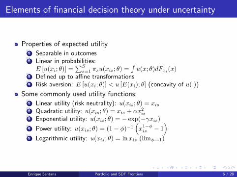
Properties of expected utility1 Separable in outcomes2 Linear in probabilities:E [u(xi; θ)] =
∑Ss=1 πsu(xis; θ) =
∫u(x; θ)dFxi
(x)3 Defined up to affine transformations4 Risk aversion: E [u(xi; θ)] < u [E(xi); θ] (concavity of u(.))
Some commonly used utility functions:1 Linear utility (risk neutrality): u(xis; θ) = xis2 Quadratic utility: u(xis; θ) = xis + αx2
is3 Exponential utility: u(xis; θ) = − exp(−γxis)4 Power utility: u(xis; θ) = (1− φ)−1
(x1−φis − 1
)5 Logarithmic utility: u(xis; θ) = lnxis (limφ→1)
Enrique Sentana () Portfolio and SDF Frontiers 6 / 28
Elements of financial decision theory under uncertainty
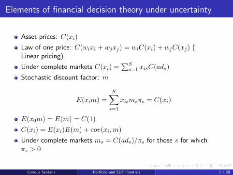
Asset prices: C(xi)Law of one price: C(wixi + wjxj) = wiC(xi) + wjC(xj) (Linear pricing)
Under complete markets C(xi) =∑S
s=1 xisC(ads)Stochastic discount factor: m
E(xim) =S∑
s=1
xismsπs = C(xi)
E(x0m) = E(m) = C(1)C(xi) = E(xi)E(m) + cov(xi,m)Under complete markets ms = C(ads)/πs for those s for whichπs > 0
Enrique Sentana () Portfolio and SDF Frontiers 7 / 28
Elements of financial decision theory under uncertainty
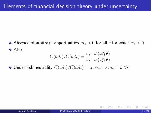
Absence of arbitrage opportunities ms > 0 for all s for which πs > 0Also
C(ads)/C(adr) =πs · u′(xo
s; θ)πr · u′(xo
r; θ)
Under risk neutrality C(ads)/C(adr) = πs/πr ⇒ ms = k ∀s
Enrique Sentana () Portfolio and SDF Frontiers 8 / 28
Outline of the presentation
1 Elements of financial decision theory under uncertainty
2 Digression on Hilbert spaces, projections and functionals
3 Portfolio selection
4 Mean-variance frontiers
5 The effects of considering additional assets
Enrique Sentana () Portfolio and SDF Frontiers 9 / 28

Digression on Hilbert spaces, projections and functionals
A Banach space is a complete normed linear space
A Hilbert space is a Banach space whose norm arises from an innerproduct
Example: L2 : x : E(x2) <∞Mean square inner product: E(yx), x, y ∈ L2
Mean square norm:√E(x2), x ∈ L2
x = y ⇔ E(x− y)2 = 0Any closed linear subspace of L2, H say, is also a Hilbert space
If V (h) > 0 ∀h ∈ H, then H is also a Hilbert space with respect tothe covariance inner product, cov(h1, h2) and the associated standarddeviation norm V 1/2(h).
Enrique Sentana () Portfolio and SDF Frontiers 10 / 28
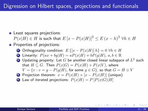
Digression on Hilbert spaces, projections and functionals
Least squares projections:P (x|H) ∈ H is such that E [x− P (x|H)]2 ≤ E (x− h)2 ∀h ∈ HProperties of projections:
1 Orthogonality condition: E [x− P (x|H)]h = 0 ∀h ∈ H2 Linearity: P (ax+ by|H) = aP (x|H) + bP (y|H), a, b ∈ R3 Updating property: Let G be another closed linear subspace of L2 such
that H ⊆ G. Then P (x|G) = P (x|H) + P (x|V ), whereV = v : v = g − P (g|H), for some g ∈ G, so that G = H ⊕ V
4 Projection theorem: x = P (x|H) + [x− P (x|H)] (unique)5 Law of iterated projections: P (x|H) = P [P (x|G)|H]
Enrique Sentana () Portfolio and SDF Frontiers 11 / 28
Digression on Hilbert spaces, projections and functionals
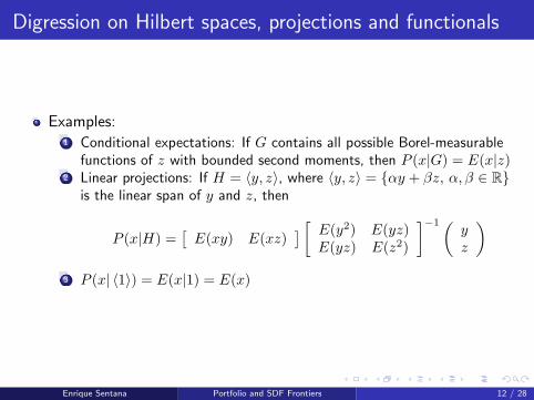
Examples:1 Conditional expectations: If G contains all possible Borel-measurable
functions of z with bounded second moments, then P (x|G) = E(x|z)2 Linear projections: If H = 〈y, z〉, where 〈y, z〉 = αy + βz, α, β ∈ R
is the linear span of y and z, then
P (x|H) =[E(xy) E(xz)
] [ E(y2) E(yz)E(yz) E(z2)
]−1(yz
)3 P (x| 〈1〉) = E(x|1) = E(x)
Enrique Sentana () Portfolio and SDF Frontiers 12 / 28

Digression on Hilbert spaces, projections and functionals
Linear functionalπ() : L2 → R is linear on H ⊆ L2 iffπ(a1h1 + a2h2) = a1π(h1) + a2π(h2) ∀a1, a2 ∈ R and ∀h1, h2 ∈ H.
Continuous functional:π() : L2 → R is continuous on H ⊆ L2 ifflimn→∞E(hn − h)2 = 0⇒ limn→∞ π(hn) = π(h) for hn, h ∈ H.
Riesz representation theorem:If π() is a continuous linear functional mapping H on R, then∃!h# ∈ H such that π(h) = E(hh#) ∀h ∈ H.
Enrique Sentana () Portfolio and SDF Frontiers 13 / 28

Outline of the presentation
1 Elements of financial decision theory under uncertainty
2 Digression on Hilbert spaces, projections and functionals
3 Portfolio selection
4 Mean-variance frontiers
5 The effects of considering additional assets
Enrique Sentana () Portfolio and SDF Frontiers 14 / 28
Portfolio selection
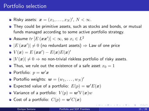
Risky assets: x = (x1, . . . , xN )′, N <∞.
They could be primitive assets, such as stocks and bonds, or mutualfunds managed according to some active portfolio strategy.
Assume tr [E (xx′)] <∞, so xi ∈ L2
|E (xx′)| 6= 0 (no redundant assets) ⇒ Law of one price
V (x) = E (xx′)− E(x)E(x)′
|V (x)| 6= 0 ⇒ no non-trivial riskless portfolio of risky assets.
Thus, we rule out the existence of a safe asset x0 = 1Portfolio: p = w′x
Portoflio weights: w = (w1, . . . , wN )′
Expected value of a portfolio: E(p) = w′E(x)Variance of a portfolio: V (p) = w′V (x)wCost of a portfolio: C(p) = w′C(x)
Enrique Sentana () Portfolio and SDF Frontiers 15 / 28
Portfolio selection
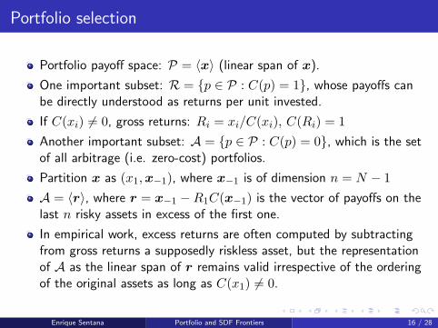
Portfolio payoff space: P = 〈x〉 (linear span of x).
One important subset: R = p ∈ P : C(p) = 1, whose payoffs canbe directly understood as returns per unit invested.
If C(xi) 6= 0, gross returns: Ri = xi/C(xi), C(Ri) = 1Another important subset: A = p ∈ P : C(p) = 0, which is the setof all arbitrage (i.e. zero-cost) portfolios.
Partition x as (x1,x−1), where x−1 is of dimension n = N − 1A = 〈r〉, where r = x−1 −R1C(x−1) is the vector of payoffs on thelast n risky assets in excess of the first one.
In empirical work, excess returns are often computed by subtractingfrom gross returns a supposedly riskless asset, but the representationof A as the linear span of r remains valid irrespective of the orderingof the original assets as long as C(x1) 6= 0.
Enrique Sentana () Portfolio and SDF Frontiers 16 / 28
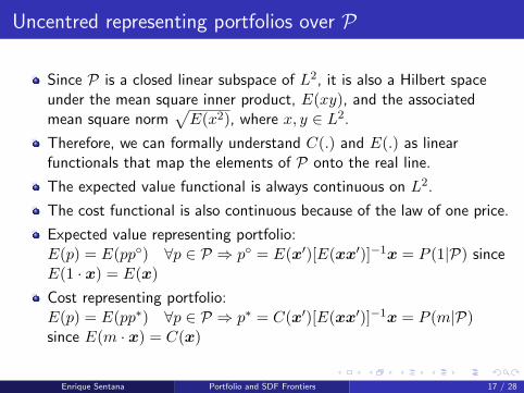
Uncentred representing portfolios over P
Since P is a closed linear subspace of L2, it is also a Hilbert spaceunder the mean square inner product, E(xy), and the associatedmean square norm
√E(x2), where x, y ∈ L2.
Therefore, we can formally understand C(.) and E(.) as linearfunctionals that map the elements of P onto the real line.
The expected value functional is always continuous on L2.
The cost functional is also continuous because of the law of one price.
Expected value representing portfolio:E(p) = E(pp) ∀p ∈ P ⇒ p = E(x′)[E(xx′)]−1x = P (1|P) sinceE(1 · x) = E(x)Cost representing portfolio:E(p) = E(pp∗) ∀p ∈ P ⇒ p∗ = C(x′)[E(xx′)]−1x = P (m|P)since E(m · x) = C(x)
Enrique Sentana () Portfolio and SDF Frontiers 17 / 28

Centred representing portfolios over P
Since we are assuming that no riskless asset exists, we can define analternative expected value representing portfolio such thatE(p) = Cov(p,þ) ∀p ∈ P.
Similarly, we can define an alternative cost representing portfolio suchthat C(p) = Cov(p,þ∗) ∀p ∈ P.
Not surprisingly,
þ∗ = C(x′)[V (x)]−1x = p∗ + [1− E(p)]−1C(p)p,þ = E(x′)[V (x)]−1x = [1− E(p)]−1p.
Enrique Sentana () Portfolio and SDF Frontiers 18 / 28
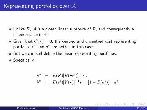
Representing portfolios over A
Unlike R, A is a closed linear subspace of P, and consequently aHilbert space itself.
Given that C(r) = 0, the centred and uncentred cost representingportfolios k∗ and a∗ are both 0 in this case.
But we can still define the mean representing portfolios.
Specifically,
a = E(r′)[E(rr′)]−1r,
k = E(r′)[V (r)]−1r = [1− E(a)]−1a.
Enrique Sentana () Portfolio and SDF Frontiers 19 / 28

Outline of the presentation
1 Elements of financial decision theory under uncertainty
2 Digression on Hilbert spaces, projections and functionals
3 Portfolio selection
4 Mean-variance frontiers
5 The effects of considering additional assets
Enrique Sentana () Portfolio and SDF Frontiers 20 / 28
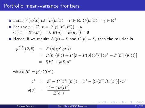
Portfolio mean-variance frontiers
minw V (w′x) s.t. E(w′x) = ν ∈ R, C(w′x) = γ ∈ R+
For any p ∈ P, p = P (p| 〈p∗, p〉) + uC(u) = E(up∗) = 0, E(u) = E(up) = 0Hence, if we require E(p) = ν and C(p) = γ, then the solution is
pMV (ν, c) = P (p| 〈p∗, p〉)= P (p| 〈p∗〉) + P [p− P (p| 〈p∗〉)| 〈p − P (p| 〈p∗〉)〉]= γR∗ + ρ(ν)a
where R∗ = p∗/C(p∗),
a = p − P (p| 〈p∗〉) = p − [C(p)/C(p∗)] · p∗
ρ(v) =ν − γE(R∗)E(a)
Enrique Sentana () Portfolio and SDF Frontiers 21 / 28
Portfolio mean-variance frontiers
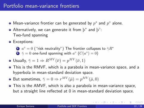
Mean-variance frontier can be generated by p∗ and p alone.
Alternatively, we can generate it from þ∗ and þ:Two-fund spanning
Exceptions:
1 a = 0 (“risk neutrality”) The frontier collapses to γR∗
2 γ = 0 one-fund spanning with a (C(a) = 0)
Usually, γ = 1⇒ RMV (ν) = pMV (ν, 1)This is the RMVF, which is a parabola in mean-variance space, and ahyperbola in mean-standard deviation space.
But sometimes, γ = 0⇒ rMV (µ) = pMV (µ, 0)This is the AMVF, which is also a parabola in mean-variance space,but a straight line reflected at 0 in mean-standard deviation space.
Enrique Sentana () Portfolio and SDF Frontiers 22 / 28

Stochastic discount factor mean-variance frontiers (SMVF)Hansen-Jagannathan volatility bounds
minm∈L2 V (m) s.t. E(m) = c ∈ R+, E(mx) = C(x).
If there were a riskless asset with gross return 1/c:mMV (c) = P (m|P+) = p∗ + α(c)(1− p) = α(c) + þ∗ − cþwhere P+ = 〈1,x〉 and
α(c) =c− E (p∗)1− E(p)
= c [1 + E(þ)]− E(þ∗),
If no riskless asset exists, then we simply repeat this calculation for allpotential values of c, which implies that mMV (c) will be spanned by aconstant, p∗ = P (m|P) and (1− p) = 1− P (1|P) (or þ∗ and þ).
This frontier is also a parabola in mean - variance space for SDF’s,and a hyperbola in mean - standard deviation space.
Enrique Sentana () Portfolio and SDF Frontiers 23 / 28
Duality
Relationship with mean-variance analysis:mMV (c)− α(c) = p∗ − α(c)p so mMV (c) can generally written asan affine transformation of RMV (ν) for some ν
There are two exceptions, which correspond to the asymptotes of theRMVF and SMVF.
If we call RMVc the gross return associated to mMV (c),
|E (R)− 1/c|σ (R)
≤∣∣E (RMV
c
)− 1/c
∣∣σ (RMV
c )=σ[mMV (c)
]E [mMV (c)]
≤ σ (m)E (m)
Absence of arbitrage opportunities: mMV A(c) = maxmMV (c), 0
Enrique Sentana () Portfolio and SDF Frontiers 24 / 28
SMVF from arbitrage portfolios
In the case in which we only have access to arbitrage portfolios, then
mMV (c) =c
1− E(a)(1− a) = c1− [ð − E(k)],
so in this case the frontier SDF’s are spanned by a single “fund”.
Still, this frontier will continue to be a parabola in mean - varianceSDF space, but a straight line that starts from the origin in mean -standard deviation space.
The slope of this line is precisely the maximum (square) Sharpe ratioportfolio attainable over A.
Enrique Sentana () Portfolio and SDF Frontiers 25 / 28

Outline of the presentation
1 Elements of financial decision theory under uncertainty
2 Digression on Hilbert spaces, projections and functionals
3 Portfolio selection
4 Mean-variance frontiers
5 The effects of considering additional assets
Enrique Sentana () Portfolio and SDF Frontiers 26 / 28
The effects on the SMVF and RMVF of includingadditional assets
x1 : original assets (N1 × 1)
x2 : new assets (N2 × 1)
x =(
x′1 x′2)′ : expanded set of assets (N × 1, N = N1 +N2)
RMVF will shift to the left because our investment opportunitiesimprove.
SMVF will rise because there is more information in the data aboutm.
However, this is not always the case:x1 spans the RMVF and/or SMVF generated from x when the oldand new frontiers are the same.
A third and last possibility, which we call tangency, is that thefrontiers share a single point.
In the case of arbitrage portfolios, tangency is equivalent to spanning.
Enrique Sentana () Portfolio and SDF Frontiers 27 / 28
Frontiers with a countably infinite number of primitiveassets
P: closure of the set of payoffs from all possible portfolios of theprimitive assets
⋃∞N=1 PN
Problems: Even if E(xx′) has full rank for all N , there may exists
1 Limiting riskless unit-cost portfolios of risky assets2 Limiting arbitrage opportunities
Once we rule out those possibilities, our previous analysis in terms ofrepresenting portfolios applies.
Enrique Sentana () Portfolio and SDF Frontiers 28 / 28