Introduction to QGIS for Lidar Analysis Table of Contents · 1. The basic functionality of QGIS can be increase via the use of plugins. We will add a raster analysis plug in to create

LITA Summer School, Poznan 24th-28th June 2013

Introduction to QGIS for Lidar Analysis

Table of ContentsAims.................................................................................................................................................................. 2Outcomes......................................................................................................................................................... 2How to use this booklet.................................................................................................................................... 2Task 1 - Setting Up Your QGIS Project............................................................................................................... 3Task 2 – Opening raster files in QGIS and editing their properties................................................................... 6Task 3 – Create a Hillshade (Shaded Relief Model)......................................................................................... 10Task 4 - Preparing a map layout for printing...................................................................................................14

Course Materials designed by Rebecca Bennett, June2013Please use freely for your own information and the instruction of others but recognise the rights of the

author to be acknowledged if the material contained is disseminated.

LITA Lab 1 – Intro to QGIS 1


P re-requisites To follow this workshop you will need QGIS 1.8. Detailed instructions for downloading and installing this software can be found in the pre-course information and are not repeated here.

Aims

The aim of this lab is familiarise yourself with QGIS. In this session you will undertake the following tasks:

• Set up a GIS project• navigate in the GIS• import and view a digital terrain model• edit the properties of a raster• create a hillshaded model• print your map to professional standard

Each of these tasks stand alone as useful GIS tools but together they provide a workflow for visualising lidar and other airborne data.

Outcomes

At the end of the lab you will submit a printed map of your data in pdf form to demonstrate your completion of the technical exercises.

How to use this booklet

Illustrations in this booklet show the icons on screen for each task. The full menu options are notated as follows: File > Open.



Task 1 - Setting Up Your QGIS Project1. Start QGIS. Familiarise yourself with the layout of the screen. The QGIS interface is split into three areas:

Tool Bar at the top, Layer Menu to the left and Map Window to the right.

2. Some of the toolbars at the top of the screen may be compressed. To expand them click on the double arrow

To move the toolbars so that all the icons are visible use the vertical dotted line to the left of each toolbar. Hover your mouse over this line to get cross-hairs then click and drag to move the menu to another part of the screen. To find out the purpose of any icon hover your mouse over it.Below are the key toolbars for this session – you should check that all these are visible.

Navigation toolbar (pan, zoom)

Add data toolbar



3. When you are happy that you can see all the icons in the toolbars your first task will be to set the project properties and save the project. From the File menu select Project Properties

4. We'll be working with data from the UK so set the units in the General tab of the Project Properties box select metres and click apply



5. To set the coordinate reference system (CRS) click on the CRS tab. The data for this tutorial is from the UK so we will search through the list for OSGB 1936. A quick way to do this is to type in the EPSG ID code 27700 and click find. Click apply to set the CRS.

6. Click OK to close Project Properties and return to the main screen.

7. Use File>save to save the project to your working area.



Task 2 – Opening raster files in QGIS and editing their properties1. First we will open four aerial photographs (AP) of the study area using the tool bar icon (layer > add

raster layer). You can hold down the shift or ctrl keys to select multiple filesPGA_SU1752_2008-04-26.jpeg, PGA_SU1753_2008-04-26.jpg, PGA_SU1852_2008-04-26.jpg, PGA_SU1853_2008-04-26.jpg

2. The importer will ask you to define the CRS for each file, check that it is ESPG 27700 (OSGB 1936 / British National Grid) and click OK.



3. The AP files will appear in the layer manager on the left of the QGIS window. You can switch the layers on and off by using the check box beside the layer name.

4. Hovering you mouse over the layer will display the file path of the layer.

5. Practice using the pan and zoom tools to navigate round your raster

6. Next we will open a digital terrain model also using the add raster menu. Pick the Digital Surface Model lidar.asc

7. The order of layers can be changed by dragging the layer up or down the layer menu. Practice moving the AP layers to the top above the lidar layers.

8. To improve the lidar raster display we will now edit the raster properties. In the menu bar, right click on the raster's name and select properties.


Click layer and drag up or down the list


9. Edit the symbology so that the image is stretched to min and max values. This preference can be saved as the default for the file.

10. The lidar raster display should now resemble the image below.



11. Return to the properties menu. In this menu can be found a variety of options for colouring the map, editing transparency and viewing metadata.

Take some time to familiarise yourself with these options:

• Change the raster from greyscale to Pseudocolour• Make the raster 25% transparent• Note below the directory location of the raster file and its CRS

• Note below the “NoData” value of the raster



Task 3 – Create a Hillshade (Shaded Relief Model)1. The basic functionality of QGIS can be increase via the use of plugins. We will add a raster analysis plug in to create a hillshaded model from our lidar terrain model

2. Go to Plugins > Manage Plugins

3. From the menu either filter by the term “raster” or scroll down to find the Raster Terrain Analysis Plugin. Check the box beside it and click open to load the plugin into your QGIS.



4. Navigate to Raster Terrain Analysis. Pick hillshade to open the hillshade menu.

5. In the hillshade menu enter the parameters for your model. It is good practice to include the selected Azimuth (0-359° east of North) angle of illumination to the file name to keep track of the parameters used

{datasource}_{model}_ {z factor}_{azimuth}_{illumination angle} e.g lidar_HS_1_245_15.

We are going to create a number of files so it is important that you label them clearly.



6. Leave the z Factor at 1 for now, check Add Result to Project and click OK



7. We are now going to create a number of models to experiment with the different hillshade settings. As you test the impact of each parameter, keep the other parameters the same. Make a note of the best parameter for your data.

• Z Factor – enhancement of z data, experiment with increasing the factor to improve the visibility of micro-topography. Write the factor selected below.

• Angle of illumination – experiment with sun angles in the range 5° -45°. Select an angle at which you think the microtopography can best be seen. Write the angle selected below.

• Direction of illumination (azimuth) – once you are happy with the first two parameters, create 8 images at 45° intervals.

Save these files you will need them for tomorrow's practical!



Task 4 - Preparing a map layout for printingThe most important thing to remember when printing maps from a GIS is that a map need the following items:

a) title b) a scale barc) a north arrowd) a legend (if more than one layer is shown)e) its real world location

Without these it isn't a map! We are going to produce a map that shows a lidar hillshade for our study area

1. Open the layers you require in the map window. Edit their properties to match how you'd like them to appear in the printed map.

2. Go to File > New Print Composer. You will see the map layout on the left and the composition properties on the right. Edit the window so that it is A4 and portrait in orientation

3. Use the Add New Map icon to draw an area for your map in the map layout

4. On the right hand menu, click Item Properties. Here you can edit the size of the map layout, and the scale of the window. Edit the window to be 200 x 220 with a scale of 5,000. You can also lock the layers that are visible in this tab.



5. Click on the Extents Tab & set the map to the canvas extent (ie the display in the GIS window). The display updates automatically so if the image doesn't look right click back into QGIS and move the map. Return to the Print Layout Window and click “Set map to canvas extent” to refresh. Placing the map in this way can be a little tricky so you can also edit the Y amd X min / max of the bounding box.

6. In the general options we can elect to show a frame and alter its properties. Change the outline width to be 1 px



7. Next we'll add the items that make this a map! First the title. Click on the add label icon and draw a box below the map in the remaining space on the paper.

Add the title of the map by typing in the text box in the Item properties section. Add the parameters of the shaded relief model you selected. It is also good practise to include your name and the date so your final text should look like this:

A Shaded Relief Map of Lidar Data

Z Factor: 1Azimuth: 245°Illumination Angle: 35°Rebecca Bennett25th June 2013

8. In the general properties tab for this item, edit the frame to match the map frame.

9. Save the template to your work area using File > Save as Template



10. Next we'll add a scale bar to the map. Click on the Add Scale Bar Icon and click on your map to place it in the layout.

11. You can edit the size and number of segments in the item properties. Male each segment represent 100m and the total scale cover 500m. You can also change the shape of the scale bar - narrow it to 2mm. Don't forget to add the units of the scale (these are the same as your map units).Experiment with the different types of scale bar until you find one that works well. Remove the frame from this item under it's general properties tab

12. Save your changes to the template.



13. Now we will add the north arrow. Click on the Add Image icon and click in the map.

14. Scroll through the Item options to find a north arrow. Edit the heigh and positioning so it is above the scale bar. Remove the outer frame.

15. You can move any item in the layout by clicking and dragging it. Switch the locations of the legend and north arrow / scale bar.

16. You can also align items in the layout window using the Align Icon. Check that your map and info space are aligned



17. Finally we must make sure that viewers know where the map is in the real world. There are two ways to do this: you can add the coordinates of the centre of the map to the Info Space or your can add a grid to the map.

To add coordinates go back to your QGIS map window and go to Plugins > Add Plugins. Check co-ordinate capture. This will open the co-ordinate capture in the side bar.

18. Click on Start Capture and click in the centre of the study area. You will see that the coordinates of that point are shown in WGS 84 and OSGB. Select copy to clipboard.

19. Return to your print layout and highlight your text box, paste the clipboard contents into the text box.We are using OSGB so you can remove the WGS 84 leaving the 6 figure OS grid coordinates. The level of precision of these figures is inappropriate so round them to the nearest 100 m

417917.984,152878.424 becomes 417900 ,152900

20. Save your work.



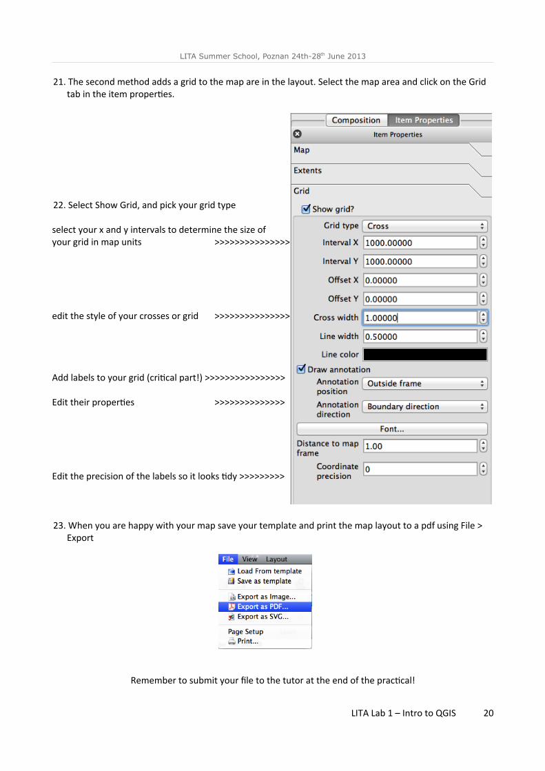
21. The second method adds a grid to the map are in the layout. Select the map area and click on the Grid tab in the item properties.

22. Select Show Grid, and pick your grid type

select your x and y intervals to determine the size of your grid in map units >>>>>>>>>>>>>>>>

edit the style of your crosses or grid >>>>>>>>>>>>>>>

Add labels to your grid (critical part!) >>>>>>>>>>>>>>>>

Edit their properties >>>>>>>>>>>>>>

Edit the precision of the labels so it looks tidy >>>>>>>>>

23. When you are happy with your map save your template and print the map layout to a pdf using File > Export

Remember to submit your file to the tutor at the end of the practical!


Documents

Introduction to QGIS for Lidar Analysis Table of Contents · 1. The basic functionality of QGIS can be increase via the use of plugins. We will add a raster analysis plug in to create