Embed Size (px)
Citation preview

188 Los Alamos Science Number 27 2002
Introduction to Quantum Error Correction
Emanuel Knill, Raymond Laflamme, Alexei Ashikhmin, Howard N. Barnum,Lorenza Viola, and Wojciech H. Zurek
When physically realized, quantum information processing (QIP) can be usedto solve problems in physics simulation, cryptanalysis, and secure communi-cation for which there are no known efficient solutions based on classical
information processing. Numerous proposals exist for building the devices required forQIP by using systems that exhibit quantum properties. Examples include nuclear spinsin molecules, electron spins or charge in quantum dots, collective states of superconduc-tors, and photons (Braunstein and Lo 2000). In all these cases, there are well-establishedphysical models that, under ideal conditions, allow for exact realizations of quantuminformation and its manipulation. However, real physical systems never behave exactlylike the ideal models. The main problems are environmental noise, which is due toincomplete isolation of the system from the rest of the world, and control errors, whichare caused by calibration errors and random fluctuations in control parameters. Attemptsto reduce the effects of these errors are confronted by the conflicting needs of being able to control and reliably measure the quantum systems. These needs require stronginteractions with control devices and systems that are sufficiently well isolated to main-tain coherence, the subtle relationship between the phases in a quantum superposition.The fact that quantum effects rarely persist on macroscopic scales suggests that meetingthese needs requires considerable outside intervention.
Soon after Peter Shor published the efficient quantum factoring algorithm with itsapplications to breaking commonly used public-key cryptosystems, Andrew Steane(1996) and Shor (1995) gave the first constructions of quantum error-correcting codes.These codes make it possible to store quantum information so that one can reverse theeffects of the most likely errors. By demonstrating that quantum information can exist inprotected parts of the state space, they showed that, in principle, it is possible to protectagainst environmental noise when storing or transmitting information. Stimulated bythese results and in order to solve errors happening during computation with quantuminformation, researchers initiated a series of investigations to determine whether it was possible to quantum-compute in a fault-tolerant manner. The outcome of theseinvestigations was positive and culminated in what are now known as accuracy thresholdtheorems (Gottesman 1996, Calderbank et al. 1997, Calderbank et al. 1998, Shor 1996,Kitaev 1997, Knill and Laflamme 1996, Aharonov and Ben-Or 1996, Aharonov andBen-Or 1999, Knill et al. 1998a, Knill et al. 1998b, Gottesman 1998, Preskill 1998).According to these theorems, if the effects of all errors are sufficiently small per quantum bit (qubit) and computation step, then it is possible to process quantum infor-mation arbitrarily accurately with reasonable resource overheads. The requirement onerrors is quantified by a maximum tolerable error rate called the threshold. The thresh-old value depends strongly on the details of the assumed error model. All threshold theorems require that errors at different times and locations be independent and that the basic computational operations can be applied in parallel. Although the proventhresholds are well out of the range of today’s devices, there are signs that, in practice,fault-tolerant quantum computation may be realizable.
In retrospect, advances in quantum error correction and fault-tolerant computationwere made possible by the realization that accurate computation does not require thestate of the physical devices supporting the computation to be perfect. In classical information processing, this observation is so obvious that it is often forgotten: No twoletters “e” on a written page are physically identical, and the number of electrons usedto store a bit in the computer’s memory varies substantially. Nevertheless, we have nodifficulty in accurately identifying the desired letter or state. A crucial conceptual difficulty with quantum information is that, by its very nature, it cannot be identified by being “looked” at. As a result, the sense in which quantum information can be
Number 27 2002 Los Alamos Science 189
Introduction to Quantum Error Correction
190 Los Alamos Science Number 27 2002
� � � �� � � �� � � �� � � �� �
� � � �� � � �� � � �� � � �� �
Encode
Transmit
Decode
accurately stored in a noisy system needs to be defined without reference to an observer.There are two ways to accomplish this task. The first is to define stored information tobe the information that can, in principle, be extracted by a quantum decoding procedure. The second is to explicitly define “subsystems” (particle-like aspects of the quantumdevice) that contain the desired information. The first approach is a natural generaliza-tion of the usual interpretations of classical error-correction methods, whereas the sec-ond is motivated by a way of characterizing quantum particles.
In this article, we motivate and explain the decoding and subsystems view of quantum error correction. We explain how quantum noise in QIP can be described andclassified and summarize the requirements that need to be satisfied for fault tolerance.Considering the capabilities of currently available quantum technology, the require-ments appear daunting. But the idea of subsystems shows that these requirements canbe met in many different, and often unexpected, ways.
Our article is structured as follows: The basic concepts are introduced by example,first for classical and then for quantum codes. We then show how the concepts aredefined in general. Following a discussion of error models and analysis, we state andexplain the necessary and sufficient conditions for detectability of errors and cor-rectability of error sets. That section is followed by a brief introduction to two of themost important methods for constructing error-correcting codes and subsystems. For abasic overview, it suffices to read the beginnings of these more-technical sections. The principles of fault-tolerant quantum computation are outlined in the last section.
Concepts and Examples
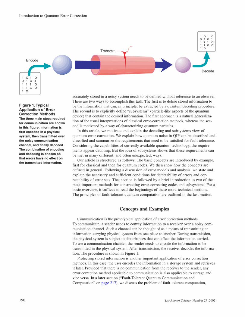
Communication is the prototypical application of error correction methods. To communicate, a sender needs to convey information to a receiver over a noisy com-munication channel. Such a channel can be thought of as a means of transmitting an information-carrying physical system from one place to another. During transmission,the physical system is subject to disturbances that can affect the information carried. To use a communication channel, the sender needs to encode the information to betransmitted in the physical system. After transmission, the receiver decodes the informa-tion. The procedure is shown in Figure 1.
Protecting stored information is another important application of error correctionmethods. In this case, the user encodes the information in a storage system and retrievesit later. Provided that there is no communication from the receiver to the sender, anyerror correction method applicable to communication is also applicable to storage andvice versa. In a later section (“Fault-Tolerant Quantum Communication andComputation” on page 217), we discuss the problem of fault-tolerant computation,
Figure 1. TypicalApplication of ErrorCorrection Methods The three main steps requiredfor communication are shownin this figure: Information isfirst encoded in a physicalsystem, then transmitted overthe noisy communicationchannel, and finally decoded.The combination of encodingand decoding is chosen sothat errors have no effect onthe transmitted information.

which requires enhancing error correction methods in order to enable applying opera-tions to encoded information without losing protection against errors.
To illustrate the different features of error correction methods, we consider threeexamples. We begin by describing them for classical information, but in each case,there is a quantum analogue that will be introduced later.
Trivial Two-Bit Example. Consider a physical system con-sisting of two bits with state space {��, ��, ��, ��}. We use theconvention that state symbols for physical systems subject toerrors are in gray. States changed by errors are shown in red.1 Inthis example, the system is subject to errors that flip (apply thenot operator to) the first bit with probability .5. We wish to safe-ly store one bit of information. To this end, we store the infor-mation in the second physical bit because this bit is unaffectedby the errors (see Figure 2).
As suggested by the usage examples in Figure 1, one canencode one bit of information in the physical system by the mapthat takes o → �� and � → ��. This means that the states o and� of an ideal bit are represented by the states �� and �� of thenoisy physical system, respectively.
To decode the information, one can extract the second bit bythe following map:
(1)
This procedure ensures that the encoded bit is recovered by thedecoding regardless of the error. There are other combinations ofencoding and decoding that work. For example, in the encoding,we could swap the meaning of � and � by using the map � → ��and � → ��. The new decoding procedure adds a bit flip to theone shown above. The only difference between this combinationof encoding/decoding and the previous one lies in the way inwhich the information is represented in the range of the encod-ing. This range consists of the two states �� and �� and is calledthe code. The states in the code are called code words.
Although trivial, the example just given is typical of ways for dealing with errors. That is, there is always a way of viewing the physical system as a pair of abstract sys-tems: The first member of the pair experiences the errors, and the second carries theinformation to be protected. The two abstract systems are called subsystems of the physi-cal system and are usually not identifiable with any of the system’s physical components.The first is the syndrome subsystem, and the second is the information-carrying subsys-tem. Encoding consists of initializing the first system and storing the information in thesecond. Decoding is accomplished by extraction of the second system. In the example,the two subsystems are readily identified as the two physical bits that make up the physi-cal system. The first is the syndrome subsystem and is initialized to � by the encoding.The second carries the encoded information.
�� → ��� → ��� → ��� → �
Number 27 2002 Los Alamos Science 191
Introduction to Quantum Error Correction
� �
� �
� �
� �
� �
� �
not (a) b
a b
a b
Probability = .5
Physical System and Error Model
Usage Examples
Store � in the second bit
Store � in the second bit
Probability = .5
Figure 2. A Simple Error ModelErrors affect only the first bit of a physical two-bit system. All joint states of the two bits are affected byerrors. For example, the joint state ���� is changed by theerror to ����. Nevertheless, the value of the informationrepresented in the second physical bit is unchanged.
1 These graphical conventions are not crucial for understanding what the symbols mean and areintended for emphasis only.

The Repetition Code. The next example is a special case of the main problem ofclassical error correction and occurs in typical communication settings and in computermemories. Let the physical system consist of three bits. The effect of the errors is toindependently flip each bit with probability p, which we take to be p = .25. The repeti-tion code results from triplicating the information to be protected. An encoding is givenby the map o → ���, � → ���. The repetition code is the set {ooo, ���}, which is therange of the encoding. The information can be decoded with majority logic: If two outof three bits are �, the output is �; otherwise, the output is �.
How well does this encoding/decoding combination work for protecting one bit of information against the errors? The decoding fails to extract the bit of information correctly if two or three of the bits were flipped by the error. We can calculate the probability of incorrect decoding as follows: The probability of a given pair of bits having flipped is .252 ∗ .75. There are three different pairs. The probability of three bits having flipped is .253. Thus, the probability of error in the encoded bit is 3 ⋅ .252 ∗ .75 +.253 = 0.15625. This is an improvement over .25, which is the probabilitythat the information represented in one of the three physical bits is corrupted by error.
To see that one can interpret this example by viewing the physical system as a pair of subsystems, it suffices to identify the physical system’s states with the states of a suitable pair. The following shows such a subsystem identification:
(2)
The left side consists of the 8 states of the physical system, which are the possiblestates for the three physical bits making up the system. The right side shows the corre-sponding states for the subsystem pair. The syndrome subsystem is a two-bit subsystem,whose states are shown first. The syndrome subsystem’s states are called syndromes.After the “·” symbol are the states of the information-carrying one-bit subsystem.
In the subsystem identification above, the repetition code consists of the two statesfor which the syndrome is ��. That is, the code states ��� and ��� correspond to thestates �� � � and �� � � of the subsystem pair. For a state in this code, single-bit flips donot change the information-carrying bit, only the syndrome. For example, a bit flip ofthe second bit changes ��� to ���, which is identified with �� ⋅ �. The syndrome haschanged from �� to ��. Similarly, this error changes ��� to ��� ↔ �� ⋅ �. The followingdiagram shows these effects :
(3)��� ↔ �� ⋅ � ��� ↔ �� ⋅ �
��� ↔ �� ⋅ � ��� ↔ �� ⋅ �↓ ↓
��� ↔ �� ⋅ ���� ↔ �� ⋅ ���� ↔ �� ⋅ ���� ↔ �� ⋅ ���� ↔ �� ⋅ ���� ↔ �� ⋅ ���� ↔ �� ⋅ ���� ↔ �� ⋅ �
192 Los Alamos Science Number 27 2002
Introduction to Quantum Error Correction
Note that the syndrome change is the same. In general, with this subsystem identifica-tion, we can infer from the syndrome which single bit was flipped on an encoded state.
Errors usually act cumulatively over time. For the repetition code, this is a problemin the sense that it takes only a few actions of the above error model forthe two- and three-bit errors to overwhelm the encoded information.One way to delay the loss of information is to decode and reencode sufficiently often. Instead of explicitly decoding and reencoding,the subsystem identification can be used directly for the same effect,namely, that of resetting the syndrome subsystem’s state to ��. Forexample, if the state is �� ⋅ �, it needs to be reset to �� ⋅ �. Therefore,using the subsystem identification, resetting requires changing the state��� to ���. It can be checked that, in every case, what is required is toset all bits of the physical system to the majority of the bits. After thesyndrome subsystem has been reset, the information is again protectedagainst the next one-bit error.
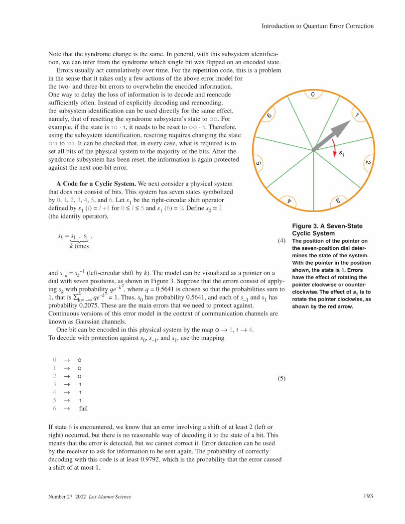
A Code for a Cyclic System. We next consider a physical system that does not consist of bits. This system has seven states symbolized by 0, 1, 2, 3, 4, 5, and 6. Let s1 be the right-circular shift operatordefined by s1 (l) = l +1 for 0 ≤ l ≤ 5 and s1 (6) = 0. Define s0 = 11(the identity operator),
(4)
and s–k = sk–1 (left-circular shift by k). The model can be visualized as a pointer on a
dial with seven positions, as shown in Figure 3. Suppose that the errors consist of apply-ing sk with probability qe–k2
, where q = 0.5641 is chosen so that the probabilities sum to1, that is ∑k
∞= –∞ qe–k2
= 1. Thus, s0 has probability 0.5641, and each of s–1 and s1 hasprobability 0.2075. These are the main errors that we need to protect against.Continuous versions of this error model in the context of communication channels areknown as Gaussian channels.
One bit can be encoded in this physical system by the map � → 1, � → 4. To decode with protection against s0, s–1, and s1, use the mapping
(5)
If state 6 is encountered, we know that an error involving a shift of at least 2 (left orright) occurred, but there is no reasonable way of decoding it to the state of a bit. Thismeans that the error is detected, but we cannot correct it. Error detection can be used by the receiver to ask for information to be sent again. The probability of correctlydecoding with this code is at least 0.9792, which is the probability that the error causeda shift of at most 1.
0 → �1 → �2 → �3 → �4 → �5 → �6 → fail
s s sk = 1 1
,...{k times
Number 27 2002 Los Alamos Science 193
Introduction to Quantum Error Correction
0
65
4 3
2
1
s1
Figure 3. A Seven-StateCyclic SystemThe position of the pointer onthe seven-position dial deter-mines the state of the system.With the pointer in the positionshown, the state is 1. Errorshave the effect of rotating thepointer clockwise or counter-clockwise. The effect of s1 is torotate the pointer clockwise, asshown by the red arrow.

As before, a pair of syndrome and information-carrying subsystems can be identifiedas being used by the encoding and decoding procedures. It suffices to correctly identifythe syndrome states, which we name –�, �, and �, because they indicate which of thelikeliest shifts happened. The resulting subsystem identification is
(6)
A new feature of this subsystem identification is that it is incomplete: Only a subset ofthe state space is identified. In this case, the complement can be used for error detection.
Like the repetition code, this code can be used in a setting where the errors happenrepeatedly. Again, it suffices to reset the syndrome subsystem, in this case to �, to keep theencoded information protected. After the syndrome subsystem has been reset, a subse-quent s1 or s–1 error affects only the syndrome.
Principles of Error Correction
When considering the problem of limiting the effects of errors in information pro-cessing, the first task is to establish the properties of the physical systems that are avail-able for representing and computing with information. Thus, it is necessary to learn thefollowing: the physical system to be used, in particular the structure of its state space;the available means for controlling this system; the type of information to be processed;and the nature of the errors, that is, the error model. With this information, theapproaches used to correct errors in the three examples provided in the previous sectioninvolve the following:
1. Determine a code, which is a subspace of the physical system, that can representthe information to be processed. 2. (a) Identify a decoding procedure that can restore the information represented inthe code after any one of the most likely errors occurred or (b) determine a pair ofsyndrome and information-carrying subsystems such that the code corresponds to a “base” state of the syndrome subsystem and the primary errors act only on the syndrome. 3. Analyze the error behavior of the code and subsystem.
The tasks of determining a code and identifying decoding procedures or subsystemsare closely related. As a result, the following questions are at the foundation of the theory of error correction: What properties must a code satisfy so that it can be used to protect well against a given error model? How does one obtain the decoding or subsystem identification that achieves this protection? In many cases, the answers can be based on choosing a fixed set of error operators that represents well the mostlikely errors and then determining whether these errors can be protected against without any loss of information. Once an error set is fixed, determining whether it iscorrectable can be cast in terms of the idea of detectable errors. This idea works equallywell for both classical and quantum information. We introduce it using classical information concepts.
0 ↔ –� ⋅ �1 ↔ � ⋅ �2 ↔ � ⋅ �3 ↔ –� ⋅ �4 ↔ � ⋅ �5 ↔ � ⋅ �
194 Los Alamos Science Number 27 2002
Introduction to Quantum Error Correction

Error Detection. Error detection was used in the cyclic-system example to reject astate that could not be properly decoded. In the communication setting, error controlmethods based on error detection alone work as follows: The encoded information istransmitted. The receiver checks whether the state is still in the code, that is, whether itcould have been obtained by encoding. If not, the result is rejected. The sender can beinformed of the failure so that the information can be retransmitted. Given a set of erroroperators that need to be protected against, the scheme is successful if, for each erroroperator, either the information is unchanged or the error is detected. Thus, we can saythat an operator E is detectable by a code if, for each state x in the code, either Ex = x orEx is not in the code (see Figure 4).
What errors are detectable by the codes in the examples? The code in the first exam-ple consists of �� and ��. Every operator that affects only the first bit is thereforedetectable. In particular, all the operators in the error model are detectable. In the secondexample, the code consists of the states ��� and ���. The identity operator has no effectand is therefore detectable. Any flips of exactly one or two bits are detectable becausethe states in the code are changed to states outside the code. The error that flips all bits isnot detectable because it preserves the code but changes the states in the code. With thecode for the cyclic system, shifts by –2, –1, 0, 1, and 2 are detectable but not shifts by 3.
To conclude the section, we state a characterization of detectability, which has a natu-ral generalization to the case of quantum information.
Theorem 1. E is detectable by a code if and only if for all x ≠ y in the code, Ex ≠ y.
From Error Detection to Error Correction. Given a code C and a set of error oper-ators E = {11 = E0, El, E2…}, is it possible to determine whether a decoding procedureor subsystem exists such that E is correctable (by C), that is, such that the errors in Edo not affect the encoded information? As explained below, the answer is yes, and thesolution is to check the condition in the following theorem:
Theorem 2. E is correctable by C if and only if, for all x ≠ y in the code and all i andj, it is true that Eix ≠ Ejy.
Observe that the notion of correctability depends on all the errors in the set under con-sideration and, unlike detectability, cannot be applied to individual errors.
To see that the condition for correctability in Theorem 2 is necessary, suppose thatfor some x ≠ y in the code and some i and j, we have z = Eix = Ejy. If the state z isobtained after an unknown error in E, then it is not possible to determine whether theoriginal code word was x or y because we cannot tell whether Ei or Ej occurred.
To see that the condition for correctability in Theorem 2 is sufficient, we assume itand construct a decoding method z → dec(z). Suppose that after an unknown error
Number 27 2002 Los Alamos Science 195
Introduction to Quantum Error Correction
Figure 4. TypicalDetectable andUndetectable Code ErrorsThree examples are shown.In each, the code is representedby a brown oval containingthree code words (greenpoints). The effect of the erroroperator is shown as arrows.(a) The error does not changethe code words and is thereforeconsidered detectable.(b) The error maps the codewords outside the code so thatit is detected. (c) One code wordis mapped to another, as shownby the red arrow. Finding that a received word is still in thecode does not guarantee that itwas the originally encodedword. The error is therefore not detectable.
(a) (b) (c)

occurred, the state z is obtained. There can be one and only one x in the code for whichsome Ei(z) ∈ E satisfies the condition that Ei(z)x = z. Thus, x must be the original codeword, and we can decode z by defining x = dec(z). Note that it is possible for two errorsto have the same effect on some code words. A subsystem identification for this decod-ing is given by z ↔ i(z) ⋅ dec(z), where the syndrome subsystem’s state space consists oferror operator indices i(z) and the information-carrying system’s consists of the codewords dec(z) returned by the decoding. The subsystem identification thus constructed isnot necessarily onto the state space of the subsystem pair. That is, for different codewords x, the set of i(z) such that dec(z) = x can vary and need not be all the errorindices. As we will show, the subsystem identification is onto the state space of the sub-system pair in the case of quantum information. It is instructive to check that, whenapplied to the examples, this subsystem construction does give a version of the subsys-tem identifications provided earlier.
It is possible to relate the condition for correctability of an error set to detectability.For simplicity, assume that each Ei is invertible. (This assumption is satisfied by ourexamples but not by error operators such as “reset bit one to �.”) In this case, the cor-rectability condition is equivalent to the statement that all products Ej
–1 Ei aredetectable. To see the equivalence, first suppose that some Ej
–1 Ei is not detectable.Then, there are x ≠ y in the code such that Ej
–1 Ei x = y. Consequently, Eix = Ejy, andthe error set is not correctable. This argument can be reversed to complete the proof ofequivalence.
If the assumption that the errors are invertible does not hold, the relationship betweendetectability and correctability becomes more complicated, requiring a generalization of the inverse operation. This generalization is simpler in the quantum setting.
Quantum Error Correction
The principles of error correction outlined before apply to the quantum setting asreadily as to the classical setting. The main difference is that the physical system to beused for representing and processing information behaves quantum mechanically andthe type of information is quantum. The question of how classical information can beprotected in quantum systems is also interesting but will not be discussed here. We illus-trate the principles of quantum error correction by considering quantum versions of the three examples given in “Concepts and Examples” and then add a uniquely quantumexample with potentially practical applications in, for example, quantum dot technolo-gies. For an explanation of the basic quantum-information concepts and conventions,see the article “Quantum Information Processing” on page 2.
Trivial Two-Qubit Example. A quantum version of the two-bit example from the previous section consists of two physical qubits, where the errors randomly apply theidentity or one of the Pauli operators to the first qubit. The Pauli operators are defined by
(7) ,
=
0 1
1 0σ y , .
−
=
−
0
0
1 0
0 1σ z
i
iand ,=
=1 0
0 1σ x
196 Los Alamos Science Number 27 2002
Introduction to Quantum Error Correction

Explicitly, the errors have the effect
(8)
where the superscripts in parentheses specify the qubit that an operator acts on. This error model iscalled completely depolarizing on qubit 1. Obviously, a one-qubit state can be stored in the secondphysical qubit without being affected by the errors. An encoding operation that implements thisobservation is
(9)
which realizes an ideal qubit as a two-dimensional subspace of the physical qubits. This subspace isthe quantum code for this encoding. To decode, one can discard physical qubit 1 and return qubit 2,which is considered a natural subsystem of the physical system. In this case, the identification ofsyndrome and information-carrying subsystems is the obvious one associated with the two physicalqubits.
Quantum Repetition Code. The repetition code can be used to protect quantum information in the presence of a restricted error model. Let the physical system consist of three qubits. Errors actby independently applying, to each qubit, the flip operator σx with probability .25. The classicalcode can be made into a quantum code by the superposition principle. Encoding one qubit is accomplished by
(10)
The associated quantum code is the range of the encoding, that is, the two-dimensional subspacespanned by the encoded states |���⟩ and |���⟩.
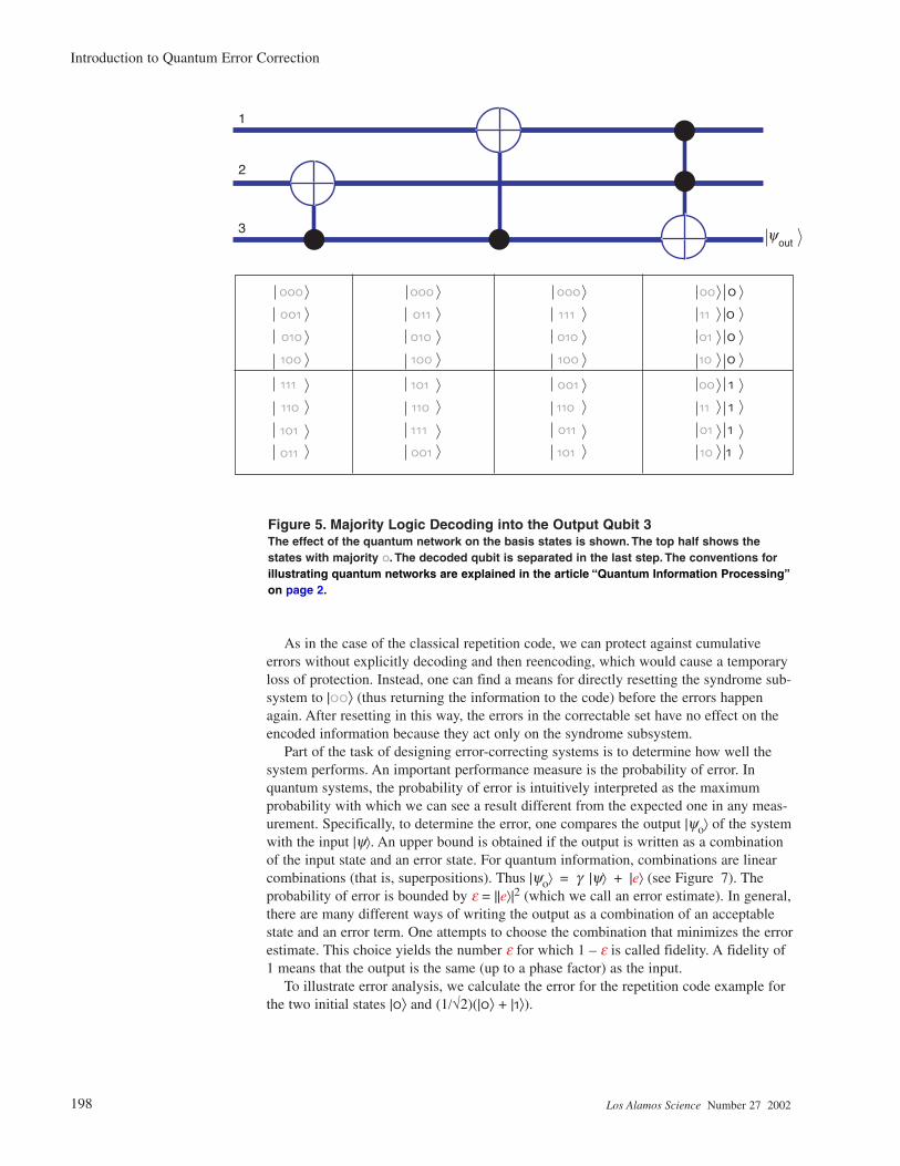
As in the classical case, decoding is accomplished by majority logic. However, it must be imple-mented carefully to avoid destroying quantum coherence in the stored information. One way to dothat is to use only unitary operations to transfer the stored information to the output qubit. Figure 5shows a quantum network that accomplishes this task.
As shown, the decoding network establishes an identification between the three physical qubitsand a pair of subsystems consisting of two qubits representing the syndrome subsystem and one qubit for the information-carrying subsystem. On the left side of the correspondence, the information-carrying subsystem is not identifiable with any one (or two) of the physical qubits.Nevertheless, it exists there through the identification.
To obtain a network for encoding, we reverse the decoding network and initialize qubits 2 and 3in the state |��⟩. The initialization renders the Toffoli gate unnecessary. The complete system with atypical error is shown in Figure 6.
α β� �
|ψ ψ⟩ → |�⟩1 | ⟩2 ,
Probability
Probability
Probability
Probability
,
Number 27 2002 Los Alamos Science 197
Introduction to Quantum Error Correction
As in the case of the classical repetition code, we can protect against cumulativeerrors without explicitly decoding and then reencoding, which would cause a temporaryloss of protection. Instead, one can find a means for directly resetting the syndrome sub-system to |��⟩ (thus returning the information to the code) before the errors happenagain. After resetting in this way, the errors in the correctable set have no effect on theencoded information because they act only on the syndrome subsystem.
Part of the task of designing error-correcting systems is to determine how well thesystem performs. An important performance measure is the probability of error. In quantum systems, the probability of error is intuitively interpreted as the maximumprobability with which we can see a result different from the expected one in any meas-urement. Specifically, to determine the error, one compares the output |ψo⟩ of the systemwith the input |ψ⟩. An upper bound is obtained if the output is written as a combinationof the input state and an error state. For quantum information, combinations are linearcombinations (that is, superpositions). Thus |ψo⟩ = γ |ψ⟩ + |e⟩ (see Figure 7). Theprobability of error is bounded by ε = ||e⟩|2 (which we call an error estimate). In general,there are many different ways of writing the output as a combination of an acceptablestate and an error term. One attempts to choose the combination that minimizes the errorestimate. This choice yields the number ε for which 1 – ε is called fidelity. A fidelity of1 means that the output is the same (up to a phase factor) as the input.
To illustrate error analysis, we calculate the error for the repetition code example forthe two initial states |�⟩ and (1/√2)(|�⟩ + |�⟩).
198 Los Alamos Science Number 27 2002
Introduction to Quantum Error Correction
Figure 5. Majority Logic Decoding into the Output Qubit 3The effect of the quantum network on the basis states is shown. The top half shows thestates with majority ��. The decoded qubit is separated in the last step. The conventions forillustrating quantum networks are explained in the article “Quantum Information Processing”on page 2.
���
���
���
���
���
���
���
���
���
���
���
���
�� �
�� �
�� �
�� �
���
���
���
���
���
���
���
���
���
���
���
���
�� �
�� �
�� �
�� �
1
2
3 ψout

Number 27 2002 Los Alamos Science 199
Introduction to Quantum Error Correction
DecodeEncode
0
0
Z
Z
Figure 6. Networks for the Quantum Repetition Code with a Typical Error The error that occurred can be determined from the state of the syndrome subsystem,which consists of the top two qubits. The encoding is shown as the reverse of the decoding,starting with an initialized syndrome subsystem. When the decoding is reversed to yield the encoding, there is an initial Toffoli gate (shown in gray). Because of the initialization,this gate has no effect and is therefore omitted in an implementation.
ψo
γ ψ
e
Figure 7. Error Estimate Any decomposition of the output state |ψo⟩ into a “good” state γ |ψ⟩ and an (unnormalized)error term |e⟩ gives an estimate ε = ||e⟩|2. For pure states, the optimum estimate is obtainedwhen the error term is orthogonal to the input state. To obtain an error estimate for mixtures,one can use any representation of the state as a probabilistic combination of pure states andcalculate the probabilistic sum of the pure-state errors.
ψ
α βα α α α
β β β β� �
��� ���
��� ���+ → + + + +
�� �
���
���
�� �α β� ��� ( )= �

(11)
(12)
(13)
The final state is a mixture consisting of four correctly decoded components and fourincorrectly decoded ones. The probability of each state in the mixture is shown beforethe colon. The incorrectly decoded information is orthogonal to the encoded informa-tion, and its probability is 0.1563, an improvement over the one-qubit error probabilityof 0.25. The second state behaves quite differently:
(14)
(15)
(16)
Not all error events have been shown, but in each case it can be seen that the state isdecoded correctly, so the error is 0. This shows that the error probability can depend
+ ��� ���∗
. . :25 75
1
22
� � ��� ���
. : .04691
2�� � �⋅ +( )
→encode
→decode
→
⋅⋅⋅⋅⋅⋅⋅⋅
. : ,
. : ,
. : ,
. : ,
. : ,
. : ,
. : ,
. : .
4219
1406
1406
1406
04690469
04690156
�� ��� ��� �� � ��� ��� ��� ��� �
→decode
∗
∗∗
∗∗∗
. :
. . :
. . :
. . :
. . :
. . :
. . :
. :
75
25 75
25 75
25 75
25 75
25 75
25 75
25
3
2
2
2
2
2
2
3
������
������
���������� � �
,
,
,
,
,
,
,
.
→
� ��� encode
200 Los Alamos Science Number 27 2002
Introduction to Quantum Error Correction

significantly on the initial state. To remove this dependence and give a state independenterror quantity, one can use the worst-case, the average, or the entanglement error. Seethe section “Quantum Error Analysis” on page 209.
Quantum Code for a Cyclic System. The shift operators introduced earlier act aspermutations of the seven states of the cyclic system. They can therefore be extended tounitary operators on a seven-state cyclic quantum system with logical basis |0⟩, |1⟩, |2⟩,|3⟩, |4⟩, |5⟩, and |6⟩. The error model introduced earlier makes sense here without modifi-cation, as does the encoding. The subsystem identification now takes the six-dimension-al subspace spanned by |0⟩,.... |5⟩ to a pair consisting of a three-state system with basis|–1⟩, |0⟩, |1⟩ and a qubit. The identification of Equation (6) extends linearly to a unitarysubsystem identification. The procedure for decoding is modified as follows: First, ameasurement determines whether the state is in the six-dimensional subspace or not. Ifit is, the identification is used to extract the qubit. Here is an outline of what happenswhen the state (1/√2)(|�⟩ + |�⟩) is encoded:
(17)
(18)
(19)
(20)
(21)
A “good” state was separated from the output in the case that is shown. The leftovererror term has probability amplitude .0005 ∗ ((1/2)2 + (1/2)2) = .00025, which contributes to the total error (not shown).
Three Quantum Spin-1/2 Particles. Quantum physics provides a rich source of systems with many opportunities for representing and protecting quantum information.Sometimes, it is possible to encode information in such a way that it is protected fromthe errors indefinitely, without intervention. An example is the trivial two-qubit systemdiscussed before. Whenever error protection without intervention is possible, there is aninformation-carrying subsystem such that errors act only on the associated syndromesubsystem regardless of the current state. An information-carrying subsystem with thisproperty is called “noiseless.” A physically motivated example of a one-qubit noiseless
� � 1 4
.05641 4e−
: 3 6
fail
. :
. :
. : 001
5
5 3
fail
. :
. :0005
0005
……
�1
= + +( )
. :00051
2
fail
.0005 :
……
��� �1 .
→encode
→
→detect
→decode
Number 27 2002 Los Alamos Science 201
Introduction to Quantum Error Correction

subsystem can be found in three spin-1/2 particles with errors due to random fluctuations in an external field.
A spin-1/2 particle’s state space is spanned by two states, |↑⟩ and |↓⟩. Intuitively,these states correspond to the spin pointing “up” (|↑⟩) or “down” (|↓⟩) in some chosenreference frame. The state space is therefore the same as that of a qubit, and we canmake the identifications |↑⟩ ↔ |�⟩ and |↓⟩ ↔ |�⟩. An external field causes the spin torotate according to an evolution of the form
(22)
The vector u = (ux, uy, uz) characterizes the direction of the field and the strength of thespin’s interaction with the field. This situation arises, for example, in nuclear magneticresonance with spin-1/2 nuclei, where the fields are magnetic fields (see the article“NMR and Quantum Information Processing” on page 226).
Now consider the physical system composed of three spin-1/2 particles with errorsacting as identical rotations of the three particles. Such errors occur if they are due to auniform external field that fluctuates randomly in direction and strength. The evolutioncaused by a uniform field is given by
(23)
with Ju = (σu(1) + σu
(2) + σu(3))/2 for u = x, y, and z. We can exhibit the error operators
arising from a uniform field in a compact form by defining J = (Jx, Jy, Jz) and v = (ux, uy, uz)t. Then the error operators are given by E(v) = e–iv⋅J, where the dot product in the exponent is calculated like the standard vector dot product.
For a one-qubit noiseless subsystem, the key property of the error model is that theerrors are symmetric under any permutation of the three particles. A permutation of theparticles acts on the particles’ state space by permuting the labels in the logical states.For example, the permutation π that swaps the first two particles acts on logical states as
(24)
To say that the errors are symmetric under particle permutations means that each error E satisfies π–1Eπ = E, or equivalently, Eπ = πE (E commutes with π). To see thatthis condition is satisfied, write
π a b c a b c b a c1 2 3 2 1 3 1 2 3
= = .
ψ ψσ σ σ
ti u u u t
e x x y y z z=− + +( ) 2
.
202 Los Alamos Science Number 27 2002
Introduction to Quantum Error Correction
ψ ψσ σ σ σ σ σ σ σ σ
σ σ
t
i u u u t i u u u t i u u u t
i u
e e e
e
x x y y z z x x y y z z x x y y z z
x x
123
2 2 2
123
1 1 1 2 2 2 3 3 3
1
=
=
− + +
− + +
− + +
− +
( ) ( ) ( ) ( ) ( ) ( ) ( ) ( ) ( )
( )
x x y y y y z z z z
x x y y z z
u u t
i u J u J u J te
( ) ( ) ( ) ( ) ( ) ( ) ( ) ( )
,
2 3 1 2 3 1 2 32
123
123
+
+ + +
+ + +
− + +( )=
σ σ σ σ σ σ σψ
ψ

(25)
If π permutes particle a to particle b, then π–1σu(a)π = σu
(b). It follows that π–1Jπ = J.This expression shows that the errors commute with the particle permutations and there-fore cannot distinguish between the particles. An error model satisfying this property iscalled a collective error model.
If a noiseless subsystem exists, then learning the symmetries of the error model sufficesfor constructing the subsystem. This procedure is explained later, in “ConservedQuantities, Symmetries, and Noiseless Subsystems.” For the three spin-1/2 system, theprocedure results in a one-qubit noiseless subsystem protected from all collective errors.We first exhibit the subsystem identification and then discuss its properties to explain whyit is noiseless. As in the case of the seven-state cyclic system, the identification involves aproper subspace of the physical system’s state space. The subsystem identificationinvolves a four-dimensional subspace and is defined by the following correspondence:
(26)
The state labels for the syndrome subsystem (before the dot in the expressions on theright side) identify it as a spin-1/2 subsystem. In particular, it responds to the errorscaused by uniform fields in the same way as the physical spin-1/2 particles. This behav-ior is caused by 2Ju acting as the u-Pauli operator on the syndrome subsystem. To confirm this property, we apply 2Ju to the logical states of Equation (26) for u = z, x.The property for u = y then follows because iσy = σzσx. Consider 2Jz. Each of the fourstates shown in Equation (26) is an eigenstate of 2Jz. For example, the physical state for |↑⟩ ⋅ |o⟩ is a superposition of states with two spins up (↑) and one spin down (↓). The eigenvalue of such a state with respect to 2Jz is the difference ∆ between the num-ber of spins that are up and down. Thus, 2Jz|↑⟩ ⋅ |�⟩ = |↑⟩ ⋅ |�⟩. The difference is also∆ = 1 for |↑⟩ ⋅ |�⟩ and ∆ = –1 for |↓⟩ ⋅ |�⟩ and |↓⟩ ⋅ |�⟩. Therefore, 2Jz acts as the z-Pauli operator on the syndrome subsystem. To confirm this behavior for 2Jx, we compute2Jx|↑⟩ ⋅ |�⟩.
1
3
1
3
1
3
1 2 32 3
1 2 32 3
1 2 3
1 2 3 1 2 3 1 2 3
1 2 3 1 2 3
↓ ↑ ↑ ↓ ↑ ↑ ↓
↔ ↑ ⋅
↓ ↑ ↑ ↓ ↑ ↑ ↓
↔ ↑ ⋅
↑ ↓ ↓ ↓ ↑ ↓ +
−e ei π π/ /�
�
↓ ↓ ↑
↔ ↓ ⋅
↓ ↓ ↑ ↓ ↓ ↓ ↑
↔ ↓ ⋅e e
1 2 3
1 2 32 3
1 2 3 1 2 3
1
3 .
�
�
↑ +
+
↑ +
+↑ ↑
↑–
–
↓
+
+
+
– //
e e– //
i
e e/ /i π π3 32 2– i
Number 27 2002 Los Alamos Science 203
Introduction to Quantum Error Correction

(27)
Similarly, one can check that, for the other logical states, the effect of 2Jx is to flip theorientation of the syndrome spin. That the subsystem identified in Equation (26) isnoiseless now follows from the fact that the errors E(v) are exponentials of sums ofthe syndrome spin operators Ju. The errors therefore act as the identity on the infor-mation-carrying subsystem.
The noiseless qubit supported by three spin-1/2 particles with collective errors isanother example in which the subsystem identification does not involve the wholestate space of the system. In this case, the errors of the error model cannot removeamplitude from the subspace. As a result, if we detect an error, that is, if we find thatthe system’s state is in the orthogonal complement of the subspace of the subsystemidentification, we can deduce that either the error model is inadequate or we intro-duced errors in the manipulations required for transferring information to the noiseless qubit.
The noiseless subsystem of three spin-1/2 particles can be physically motivated byan analysis of quantum spin numbers. This analysis is outlined in the box on theopposite page.
204 Los Alamos Science Number 27 2002
Introduction to Quantum Error Correction
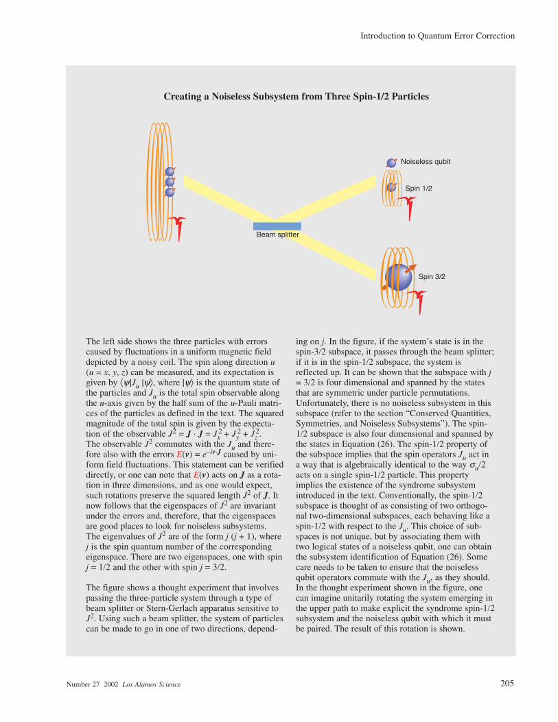
Number 27 2002 Los Alamos Science 205
Introduction to Quantum Error Correction
Noiseless qubit
Spin 1/2
Spin 3/2
Beam splitter
The left side shows the three particles with errorscaused by fluctuations in a uniform magnetic fielddepicted by a noisy coil. The spin along direction u(u = x, y, z) can be measured, and its expectation isgiven by ⟨ψ|Ju |ψ⟩, where |ψ⟩ is the quantum state ofthe particles and Ju is the total spin observable alongthe u-axis given by the half sum of the u-Pauli matri-ces of the particles as defined in the text. The squaredmagnitude of the total spin is given by the expecta-tion of the observable J2 = J ⋅ J = Jx
2 + Jy2 + Jz
2.The observable J2 commutes with the Ju and there-fore also with the errors E(v) = e–iv⋅J caused by uni-form field fluctuations. This statement can be verifieddirectly, or one can note that E(v) acts on J as a rota-tion in three dimensions, and as one would expect,such rotations preserve the squared length J2 of J. Itnow follows that the eigenspaces of J2 are invariantunder the errors and, therefore, that the eigenspacesare good places to look for noiseless subsystems. The eigenvalues of J2 are of the form j (j + 1), wherej is the spin quantum number of the correspondingeigenspace. There are two eigenspaces, one with spinj = 1/2 and the other with spin j = 3/2.
The figure shows a thought experiment that involvespassing the three-particle system through a type ofbeam splitter or Stern-Gerlach apparatus sensitive toJ2. Using such a beam splitter, the system of particlescan be made to go in one of two directions, depend-
ing on j. In the figure, if the system’s state is in thespin-3/2 subspace, it passes through the beam splitter;if it is in the spin-1/2 subspace, the system isreflected up. It can be shown that the subspace with j= 3/2 is four dimensional and spanned by the statesthat are symmetric under particle permutations.Unfortunately, there is no noiseless subsystem in thissubspace (refer to the section “Conserved Quantities,Symmetries, and Noiseless Subsystems”). The spin-1/2 subspace is also four dimensional and spanned bythe states in Equation (26). The spin-1/2 property ofthe subspace implies that the spin operators Ju act ina way that is algebraically identical to the way σu/2acts on a single spin-1/2 particle. This propertyimplies the existence of the syndrome subsystemintroduced in the text. Conventionally, the spin-1/2subspace is thought of as consisting of two orthogo-nal two-dimensional subspaces, each behaving like aspin-1/2 with respect to the Ju. This choice of sub-spaces is not unique, but by associating them withtwo logical states of a noiseless qubit, one can obtainthe subsystem identification of Equation (26). Somecare needs to be taken to ensure that the noiselessqubit operators commute with the Ju, as they should.In the thought experiment shown in the figure, onecan imagine unitarily rotating the system emerging inthe upper path to make explicit the syndrome spin-1/2subsystem and the noiseless qubit with which it mustbe paired. The result of this rotation is shown.
Creating a Noiseless Subsystem from Three Spin-1/2 Particles
Error Models
We have seen several models of physical systems and errors in the examples of the previous sections. Most physical systems under consideration for QIP consist of parti-cles or degrees of freedom that are spatially localized, a feature reflected in the errormodels that are usually investigated. Because we also expect the physically realizedqubits to be localized, the standard error models deal with quantum errors that act inde-pendently on different qubits. Logically realized qubits, such as those implemented bysubsystems different from the physically obvious ones, may have more complicatedresidual-error behaviors.
The Standard Error Models for Qubits. The most investigated error model for qubits consists of independent, depolarizing errors. This model has the effect of com-pletely depolarizing each qubit independently with probability p—see Equation (8). Forone qubit, the model is the least biased in the sense that it is symmetric under rotations.As a result, every state of the qubit is equally affected. Independent depolarizing errorsare considered to be the quantum analogue of the classical independent bit-flip errormodel.
Depolarizing errors are not typical for physically realized qubits. However, given theability to control individual qubits, it is possible to enforce the depolarizing model (seebelow). Consequently, error correction methods designed to control depolarizing errorsapply to all independent error models. Nevertheless, it is worth keeping in mind thatgiven detailed knowledge of the physical errors, a special purpose method is usually better than one designed for depolarizing errors. We therefore begin by showing howone can think about arbitrary error models.
There are several different ways of describing errors affecting a physical system (or “sys” for short) of interest. For most situations, in particular if the initial state of the system is pure, errors can be thought of as being the result of coupling to an initiallyindependent environment for some time. Because of this coupling, the effect of error can always be represented by the process of adjoining an environment (or “env” forshort) in some initial state |0⟩env to the arbitrary state |ψ⟩sys, followed by a unitary coupling evolution U(env, sys) acting jointly on the environment and the system.Symbolically, the process can be written as the map
|ψ⟩sys → U (env, sys)|0⟩env|ψ⟩sys . (28)
Choosing an arbitrary orthonormal basis consisting of the states |e⟩env for the state spaceof the environment, the process can be rewritten in the form
(29)
( )
ψ
ψ
ψ
ψ
ψ
sysenv env,sys
env sys
envenv env,sys
sys
envenv,sys
env
env
sys
env sys
→
=
=
=
∑
∑
∑
,
( ) ( )
( )
( )
U
e e U
e e U
e A
e
env
e
ee
0
0
0
sys
1
206 Los Alamos Science Number 27 2002
Introduction to Quantum Error Correction

where the last step defines operators Ae(sys) acting on the physical system by
Ae(sys) = env⟨e|U(env, sys)|0⟩env. The expression ∑e|e⟩envAe
(sys) is called an environment-labeled operator. The unitarity condition implies that ∑eAe
†Ae = 11 (with system labelsomitted). The environment basis |e⟩env need not represent any physically meaningfulchoice of basis of a real environment. For error analysis, the states |e⟩env are formalstates that label the error operators Ae. One can use an expression of the form shown inEquation (29) even when the |e⟩ are not normalized or orthogonal, keeping in mind that,as a result, the identity implied by the unitarity condition changes.
Note that the state on the right side of Equation (29), representing the effect of theerrors, is correlated with the environment. This means that after removing (or “tracingover”) the environment, the state of the physical system is usually mixed. Instead of introducing an artificial environment, we can also describe the errors by using the density operator formalism for mixed states. Define ρ = |ψ⟩sys
sys⟨ψ|. The effect of the errors on the density matrix ρ is given by the transformation
(30)
This is the “operator sum” formalism (Kraus 1983). The two ways of writing the effects of errors can be applied to the depolarizing-error
model for one qubit. As an environment-labeled operator, depolarization with probabilityp can be written as
(31)
where we introduced five abstract, orthonormal environment states to label the differentevents. In this case, one can think of the model as applying no error with probability 1 – p or completely depolarizing the qubit with probability p. The latter event is repre-sented by applying one of 11, σx, σy, or σz with equal probability p/4. To be able to thinkof the model as randomly applied Pauli matrices, it is crucial that the environment stateslabeling the different Pauli matrices be orthogonal. The square roots of the probabilitiesappear in the operator because, in an environment-labeled operator, it is necessary togive quantum amplitudes. Environment-labeled operators are useful primarily because of their great flexibility and redundancy.
In the operator sum formalism, depolarization with probability p transforms the inputdensity matrix ρ as
(32)
Because the operator sum formalism has less redundancy, it is easier to tell when twoerror effects are equivalent.
In the remainder of this section, we discuss how one can use active intervention tosimplify the error model. To realize this simplification, we intentionally randomize the
ρ ρ ρ σ ρσ σ ρσ σ ρσ→ −( ) + + + +(14
pp
x x y y z z 1 1
= −( ) + + +1 3 44
pp
x x y y z z/ ρ σ ρσ σ ρσ σ ρσ .
1 02
− + + + +pp
x y zx y zenv env env env envσ σ σ ,
ρ ρ→ ∑ A Ae ee
† .
Number 27 2002 Los Alamos Science 207
Introduction to Quantum Error Correction

qubit so that the environment cannot distinguish between the different axes defined by the Pauli spin matrices. Here is a simple randomization that actively converts an arbi-trary error model for a qubit into one that consists of randomly applying Pauli operatorsaccording to some distribution. The distribution is not necessarily uniform, so the newerror model is not yet depolarizing. Before the errors act, apply a random Pauli operatorσu (u = 0, x, y, z, σ0 = 11). After the errors act, apply the inverse of that operator,σu
–1 = σu; then “forget” which operator was applied. This randomization method iscalled twirling (Bennett et al. 1996). To understand twirling, we use environment-labeled operators to demonstrate some of the techniques useful in this context. The sequence of actions implementing twirling can be written as follows (omittinglabels for the physical system):
Apply a random σu remembering u with thehelp of the system C.
Errors act.
Apply σu = σu–1.
Forget which u was used by absorbing its memory in the environment.
The system C that was artificially introduced to carry the memory of u may be a classical memory because there is no need for coherence between different |u⟩C.
To determine the equivalent random Pauli operator error model, it is necessary torewrite the total effect of the procedure using an environment-labeled sum involvingorthogonal environment states and Pauli operators. To do so, express Ae as a sum of thePauli operators, Ae = ∑vαevσv, using the fact that the σv are a linear basis for the spaceof one-qubit operators. Recall that σu anticommutes with σv if 0 ≠ u ≠ v ≠ 0. Thus,σu σv σu = (–1)⟨v,u⟩σv, where ⟨v, u⟩ = 1 if 0 ≠ u ≠ v ≠ 0 and ⟨v, u⟩ = 0 otherwise. We cannow rewrite the last expression of Equation (33) as follows:
(34)
It can be checked that the states (1/2)∑u(–1)⟨v,u⟩|eu⟩env,C are orthonormal for different eand v. As a result, the states ∑eu(1/2)αev(–1)⟨v,u⟩|eu⟩env,C are orthogonal for different vand have probability (square norm) given by pv = ∑e |αev|
2. Introducing √pv|v∼⟩env,C =
∑eu(1/2)αev(–1)⟨v,u⟩|eu⟩env,C, we can write the sum of Equation (34) as
(35)ψ σv v1
21α σ ψev
v u
euvv
v
eu p v−( )
=∑ ,
˜ ,env,C env,C
eu A eu
eu
euu e u
euu ev v u
v
evv u
euvv
env,C env,C
env,C
∑ ∑ ∑
∑∑
=
= −( )
1
2
1
2
1
21
σ σ ψ σ α σ σ ψ
α σ ψ,
.
208 Los Alamos Science Number 27 2002
Introduction to Quantum Error Correction
ψ σ ψ
σ ψ
σ σ ψ
σ σ ψ
→
→
→
→
∑
∑ ∑
∑ ∑
∑
1
21
21
21
2
u
e u A
e u A
eu A
Cu u
e e uu
e u e uu
eu u e u
env C
env C
env,C . (33)

showing that the twirled error model behaves like randomly applied Pauli matriceswith σv applied with probability pv. It is a recommended exercise to reproduce theabove argument using the operator sum formalism.
To obtain the standard depolarizing error model with equal probabilities for thePauli matrices, it is necessary to strengthen the randomization procedure by applyinga random member U of the group generated by the 90° rotations around the x-, y-, andz-axis before the error and then undoing U by applying U–1.
Randomization can be used to transform any one-qubit error model into the depolarizing error model. This explains why the depolarizing model is so useful foranalyzing error correction techniques in situations in which errors act independentlyon different qubits. However, in many physical situations, the independence assump-tions are not satisfied. For example, errors from common internal couplings betweenqubits are generally pairwise correlated to first order. In addition, the operationsrequired to manipulate the qubits and to control the encoded information act on pairsat a time, which tends to spread even single-qubit errors. Still, in all these cases, theprimary error processes are local. This means that there usually exists an environment-labeled sum expression for the total error process in which the amplitudes associatedwith errors acting simultaneously at k locations in time and space decrease exponen-tially with k. In such cases, error correction methods that handle all or most errorsinvolving sufficiently few qubits are still applicable.
Quantum Error Analysis. One of the most important consequences of the subsys-tems interpretation of encoding quantum information in a physical system is that theencoded quantum information can be error-free even though errors have severelychanged the state of the physical system. Almost trivially, any error operator actingonly on the syndrome subsystem has no effect on the quantum information. The goalof error correction is to actively intervene and maintain the syndrome subsystem instates where the dominant error operators continue to have little effect on the informa-tion of interest. An important issue in analyzing error correction methods is to esti-mate the residual error in the encoded information. A simple example of how that canbe done was discussed for the quantum repetition code. The same ideas can be appliedin general. Let sys be the physical system in which the information is encoded, and|ψ⟩sys an initial state containing such information with the syndrome subsystem appro-priately prepared. Errors and error-correcting operations modify the state. The newstate can be expressed with environment labeling as ∑e|e⟩envAe
(sys)|ψ⟩sys. In view ofthe partitioning into information-carrying and syndrome subsystems, good states |e⟩envare those states for which Ae
(sys) acts only on the syndrome subsystem, given that thesyndrome has been prepared. The remaining states |e⟩ form the set of bad states, B.The error probability pe can be bounded from above by
(36)
where |A|1 = maxφ ⟨φ|A|φ⟩, the maximum being taken over normalized states. The secondinequality usually leads to a gross overestimate but is independent of the encoded infor-mation and often suffices for obtaining good results. Because the environment-labeled
≤
( )
∈∑ e Aee B
envsys
1
2
,
p e Ae ee B
≤ ( )∈∑ env
syssysψ
2
Number 27 2002 Los Alamos Science 209
Introduction to Quantum Error Correction

sum is not unique, a goal of the representation of the errors acting on the system is touse “good” operators to the largest extent possible. The flexibility of these error expan-sions makes them very useful for analyzing error models in conjunction with error cor-rection methods.
In principle, we can obtain better expressions for pe by calculating the density matrix ρof the state of the subsystem containing the desired quantum information. This calculationinvolves tracing over the syndrome subsystem. The matrix ρ can then be compared to theintended state. If the intended state is pure, given by |φ⟩, the probability of error is given by1 – ⟨φ|ρ|φ⟩, which is the probability that a measurement that distinguishes between |φ⟩ andits orthogonal complement fails to detect |φ⟩. The quantity ⟨φ|ρ|φ⟩ is called the fidelity of thestate ρ.
For applications to communication, the goal is to be able to reliably transmit arbitrarystates through a communication channel, which may be physical or realized via anencoding/decoding scheme. It is therefore important to characterize the reliability of thechannel independent of the information transmitted. Equation (36) can be used to obtainstate-independent bounds on the error probability but does not readily provide a singlemeasure of reliability. One way to quantify the reliability is to identify the error of thechannel with the average error εa over all possible input states. The reliability is thengiven by the average fidelity 1 – εa. Another elegant way appropriate for QIP is to usethe entanglement fidelity (Schumacher 1996). Entanglement fidelity measures the errorwhen the input is maximally entangled with an identical reference system. In thisprocess, the reference system is imagined to be untouched, so that the state of the refer-ence system, together with the output state, can be compared with the original entangledstate. For a one-qubit channel labeled sys, the reference system is a qubit, which welabel “ref.” An initial, maximally entangled state is
(37)
The reference qubit is assumed to be perfectly isolated and not affected by any errors.The final state ρ(ref,sys) is compared with |B⟩, which gives the entanglement fidelityaccording to the formula fe = ⟨B|ρ (ref,sys)|B⟩. The entanglement error is εe = 1 – fe. Itturns out that this definition does not depend on the choice of maximally entangledstate. Fortunately, the entanglement error and the average error εa are related by a linearexpression:
(38)
For k-qubit channels, the constant 2/3 is replaced by 2k/(2k + 1). Experimental measure-ments of these fidelities do not require the reference system. There are simple averagingformulas to express them in terms of the fidelities for transmitting each of a sufficientlylarge set of pure states. An example of the experimental determination of the entanglementfidelity when the channel is realized by error correction is provided in Knill et al. (2001).
ε εa e= 2
3 .
B = +( )1
2� � � �
ref sys ref sys .
210 Los Alamos Science Number 27 2002
Introduction to Quantum Error Correction

From Quantum Error Detection to Error Correction
In the independent depolarizing error model with small probability p of depolariza-tion, the most likely errors are those that affect a small number of qubits. That is, if wedefine the weight of a product of Pauli operators to be the number of qubits affected, thedominant errors are those of small weight. Because the probability of a nonidentity Paulioperator is 3p/4—see Equation (31)—one expects about (3p/4)n of n qubits to bechanged. As a result, good error-correcting codes are considered to be those for whichall errors of weight ≤ e ≅ (3p/4)n can be corrected. It is desirable that e have a highrate, which means that it is a large fraction of the total number of qubits n (the length ofthe code). Combinatorially, good codes are characterized by a high minimum distance, aconcept that arises naturally in the context of error detection.
Quantum Error Detection. Let C be a quantum code, that is, a subspace of the statespace of a quantum system. Let P be the operator that projects onto C, and P⊥ = 11 – Pthe one that projects onto the orthogonal complement. Then the pair P, P⊥ is associatedwith a measurement that can be used to determine whether a state is in the code or not.If the given state is |ψ⟩, the result of the measurement is P|ψ⟩ with probability |P|ψ⟩|2and P⊥|ψ⟩ otherwise. As in the classical case, an error-detection scheme consists ofpreparing the desired state |ψi⟩ ∈ C, transmitting it through, say, a quantum channel,then measuring whether the state is still in the code, accepting the state if it is, andrejecting it otherwise. We say that C detects error operator E if states accepted after Ehad acted are unchanged except for an overall scale. Using the projection operators, thisis the statement that for every state |ψi⟩ ∈ C, PE|ψi⟩ = λE |ψi⟩. Because P|ψ⟩ is in thecode for every |ψ⟩, it follows that PEP|ψ⟩ = λEP|ψ⟩. It follows that a characterization ofdetectability is given by Theorem 3.
Theorem 3. E is detectable by C if and only if PEP = λEP for some λE.
A second characterization is given by Theorem 4.
Theorem 4. E is detectable by C if and only if for all |ψ⟩, |φ⟩ ∈ C, ⟨ψ|E|φ⟩ = λΕ ⟨ψ|φ⟩ forsome λE.
A third characterization is obtained by taking the condition for classical detectability inTheorem 1 and replacing ≠ by orthogonal to:
Theorem 5. E is detectable by C if and only if for all |φ⟩, |ψ⟩ in the code with |φ⟩ orthogonal to |ψ⟩, E|φ⟩ is orthogonal to |ψ⟩.
For a given code C, the set of detectable errors is closed under linear combinations.That is, if E1 and E2 are both detectable, then so is αE1 + αE2. This useful propertyimplies that, to check detectability, one has to consider only the elements of a linearbasis for the space of errors of interest.
Consider n-qubits with independent depolarizing errors. A robust error-detecting codeshould detect as many of the small-weight errors as possible. This requirement motivatesthe definition of minimum distance: The code C has minimum distance d if the smallest-weight product of Pauli operators E for which C does not detect E is d. The notion comesfrom classical codes for bits, where a set of code words C′ has minimum distance d if the
Number 27 2002 Los Alamos Science 211
Introduction to Quantum Error Correction

smallest number of flips required to change one code word in C′ into another one in C′ is d.For example, the repetition code for three bits has minimum distance 3. Note that theminimum distance for the quantum repetition code is 1: Applying σz
(1) preserves the codeand changes the sign of |���⟩ but not of |���⟩. As a result, σz
(1) is not detectable. Thenotion of minimum distance can be generalized for error models with specified first-ordererror operators (Knill et al. 2000). In the case of depolarizing errors, the first-order erroroperators are single-qubit Pauli matrices, which are the errors of weight 1.
Quantum Error Correction. Let E = {E0 = 11, El ,…} be the set of errors that wewish to be able to correct. When a decoding procedure for the code C exists such that allerrors in E are corrected, we say that E is correctable (by C). A situation in which cor-rectability of E is apparent occurs when the errors Ei are unitary operators satisfying thecondition that EiC are mutually orthogonal subspaces. The repetition code has this prop-erty for the set of errors consisting of the identity and Pauli operators acting on a singlequbit. In this situation, the procedure for decoding is to first make a projective measure-ment and determine which of the subspaces EiC the state is in and then to apply theinverse of the error operator, that is, E†
i. This situation is not far from the generic one.One characterization of correctability is described in Theorem 6.
Theorem 6. E is correctable if and only if there is a linear transformation of the setE such that the operators E′i in the new set satisfy the following properties: (1) The E′iCare mutually orthogonal, and (2) E′i restricted to C is proportional to a restriction to C of a unitary operator.
To relate this characterization to detectability, note that the two properties imply that(E′i ) E′j C is orthogonal to C if i ≠ j and (E′i )
†E′i restricted to C is proportional to the iden-tity on C. In other words, the (E′i )
†E′j are detectable. This detectability condition appliedto the original error set constitutes a second characterization of correctability, as given in Theorem 7.
Theorem 7. E is correctable if and only if the operators in the set E†E = {E†
1 E2 : Ei ∈ E} are detectable.
Before explaining the characterizations of correctability, we consider the situation of n qubits, where the characterization by detectability (Theorem 7) leads to a useful relationship between minimum distance and correctability of low-weight errors.
Theorem 8. If a code on n qubits has a minimum distance of at least 2e + 1, then theset of errors of weight at most e is correctable.
This theorem follows by observing that the weight of E†1 E2 is at most the sum of the
weights of the Ei. As a result of this observation, the problem of finding good ways tocorrect all errors up to a maximum weight reduces to that of constructing codes withsufficiently high minimum distance. Thus, questions such as “what is the maximumdimension of a code of minimum distance d on n qubits?” are of great interest. As inthe case of classical coding theory, this problem appears to be very difficult in gener-al. Answers are known for small n (Calderbank et al. 1998), and there are asymptoticbounds (Ashikhmin and Litsyn 1999). Of course, for achieving low error probabilities,it is not necessary to correct all errors of weight ≤ e, just almost all such errors. Forexample, the concatenated codes used for fault-tolerant quantum computation achievethis goal (see “Fault-Tolerant Quantum Communication and Computation” later in this article).
212 Los Alamos Science Number 27 2002
Introduction to Quantum Error Correction

For the remainder of this section, we explain the characterizations of correctability.Using the conditions for detectability from the previous section, the condition for cor-rectability in Theorem 7 is equivalent to
(39)
This condition is preserved under a linear change of basis for E. That is, if A is anyinvertible matrix with coefficients aij, we can define new error operators Dk = ∑iEiaik.For the Dk, the left side of Equation (39) is
(40)
where Λ is the matrix formed from the λij. Using the fact that Λ is a positive semidefi-nite matrix (that is, for all x, x†Λx ≥ 0, and Λ† = Λ), we can choose A such that A†ΛA is
of the form . In this matrix, the upper left block is the identity operator for
some dimension. An important consequence of invariance under a change of basis of error operators is
that the set of errors correctable by a particular code and decoding procedure is linearlyclosed. Thus, if E and D are corrected by the decoding procedure, then so is αE + βD.This observation also follows from the linearity of quantum mechanically imple-mentable operations.
We explain the condition for correctability by using the subsystems interpretation ofdecoding procedures. For simplicity, assume that 11 ∈ E. To show that correctability ofE implies detectability of all E ∈ E†E, suppose that we have a decoding procedure thatrecovers the information encoded in C after any of the errors in the set E have occurred.Every physically realizable decoding procedure can be implemented by first addingancilla quantum systems in a prepared pure state to form a total system labeled T, thenapplying a unitary map U to the state of T, and finally separating T into a pair of sys-tems (syn, Q), where “syn” corresponds to the syndrome subsystem and Q is a quantumsystem with the same dimension as the code that carries the quantum information afterdecoding. Denote the state space of the physical system containing C as H and the statespace of system X by HX, where X is any one of the other systems. Let V be the unitaryoperator that encodes information by mapping HQ onto C ⊆ H. We have the followingrelationships:
HQ ↔V C ⊆ H ⊆ HT ↔U
Hsyn ⊗ HQ . (41)
Here, we used bidirectional arrows to emphasize that the operators V and U can beinverted on their range and therefore identify the states in their domains with the statesin their ranges. The inclusion H ⊆ HT implicitly identifies H with the subspace deter-mined by the prepared pure state on the ancillas. The last state space of Equation (41) isexpressed as a tensor product, which is the state space of the combined system (syn, Q).
PD D P P a E E a P
a a P
A A P
k l ik i j jlij
ik jlij
ij
kl
† †=
=
= ( )
∑
∑ λ
† ,Λ
PE E P Pi j ij† = λ .
Number 27 2002 Los Alamos Science 213
Introduction to Quantum Error Correction

For states of HQ, we will write |ψ⟩ = |ψ⟩Q ↔V |ψ⟩L ∈ C. Because 11 is a correctable error,it must be the case that |ψ⟩L ↔
U |0⟩syn|ψ⟩ ∈ Hsyn ⊗ HQ for some state |0⟩syn. To estab-lish this fact, use the linearity of the maps. In general,
(42)
The |i⟩syn need not be normalized or orthogonal. Let F be the subspace spanned by the|i⟩syn. Then U induces an identification of F ⊗ HQ with a subspace C ⊆ H. This is the desired subsystem identification. We can then see how the errors act in thisidentification.
(43)
This means that for all |ψ⟩ and |φ⟩,
(44)
that is, all errors in E†E are detectable. Now, suppose that all errors in E†E are detectable. To see that correctability of E fol-
lows, choose a basis for the errors so that λij = δijλi with λi = 1 for i < s and λi = 0 oth-erwise. Define a subsystem identification by
(45)
for 0 ≤ i < s. By assumption and construction, L⟨ψ|Ej†Ei|ψ⟩L = δij, which implies that W
is unitary (after linear extension), and so this is a proper identification. For i ≥ s,Ei |ψ⟩L = 0, which implies that for states in the code, these errors have probability 0.Therefore, the identification can be used to successfully correct E.
Constructing Codes
Stabilizer Codes. Most useful quantum codes are based on stabilizer constructions(Gottesman 1996, Calderbank et al. 1997). Stabilizer codes are useful because theymake it easy to determine which Pauli-product errors are detectable and because theycan be interpreted as special types of classical, linear codes. The latter feature makes itpossible to use well-established techniques from the theory of classical error-correctingcodes to construct good quantum codes.
A stabilizer code of length n for k-qubits (abbreviated as an [[n, k]] code), is a 2k-dimensional subspace of the state space of n-qubits that is characterized by the set of
i W Eisys Lψ ψ ,
LL
synsynψ φ ψ φE E j ij i
† ,=
ψ ψ
ψ ψ
L syn
L syn
↔
↓
↔
0
E ii .
ψ ψ
ψL L
syn
→ E
i
i
.↔U
214 Los Alamos Science Number 27 2002
Introduction to Quantum Error Correction

products of Pauli operators that leave each state in the code invariant. Such Pauli opera-tors are said to stabilize the code. A simple example of a stabilizer code is the quantumrepetition code introduced earlier. The code’s states α|���⟩ + β|���⟩ are exactly thestates that are unchanged after applying σz
(1) σz(2) or σz
(1) σz(3). To simplify the nota-
tion, we write I = 11, X = σx, Y = σy , and Z = σz. A product of Pauli operators can thenbe written as ZIXI = σz
(1) σx(3) (as an example of length 4) with the ordering determin-
ing which qubit is being acted upon by the operators in the product. We can understand the properties of stabilizer codes by working out the example of
the quantum repetition code with the stabilizer formalism. A stabilizer of the code isS = {ZZI, ZIZ}. Let S be the set of Pauli products that are expressible up to a phase asproducts of elements of S. For the repetition code, S = {III, ZZI, ZIZ, IZZ}. S consists ofall Pauli products that stabilize the code. The crucial property of S is that its operatorscommute, that is, for A, B ∈ S, AB = BA. According to results from linear algebra, it follows that the state space H can be decomposed into orthogonal subspaces Hλ suchthat for A ∈ S and |ψ⟩ ∈ Hλ, A|ψ⟩ = λ(A)|ψ⟩. The Hλ are the common eigenspaces of S.The stabilizer code C defined by S is the subspace stabilized by the operators in S,which means that it is given by Hλ with λ(A) = 1. The subspaces for other λ(A) haveequivalent properties and are often included in the set of stabilizer codes. For the repeti-tion code, the stabilized subspace is spanned by the logical basis |���⟩ and |���⟩. Fromthe point of view of stabilizers, there are two ways in which a Pauli product B can bedetectable: (1) if B ∈ S because, in this case, B acts as the identity on the code and (2) if B anticommutes with at least one member (say A) of S. To see that this statement iscorrect, let |ψ⟩ be in the code. Then A(B|ψ⟩) = (AB)|ψ⟩ = –(BA)|ψ⟩= –B(A|ψ⟩) = –B|ψ⟩.Thus, B|ψ⟩ belongs to Hλ with λ(A) = –1. Because this subspace is orthogonal to C =H1, B is detectable. We define the set of Pauli products that commute with all membersof S as S⊥. Thus, B is detectable if either B ∉ S⊥ or B ∈ S. Note that because S consistsof commuting operators, S ⊆ S⊥.
To construct a stabilizer code that can correct all errors of weight at most one (aquantum one-error-correcting code), it suffices to find S with the minimum weight ofnonidentity members of S⊥ being at least three (3 = 2 ⋅ 1 + 1)—also refer to Theorem 8.In this case, we say that S⊥ has minimum distance 3. As an example, we can exhibit astabilizer for the famous length-five one-error-correcting code for one qubit (Bennett etal. 1996, Laflamme et al. 1996):
(46)
As a general rule, it is desirable to exhibit the stabilizer minimally, which means that nomember is the product up to a phase of some of the other members. In this case, thenumber of qubits encoded is n – |S|, where n is the length of the code and |S| is the number of elements of S.
To obtain the correspondence between stabilizer codes and classical binary codes,we replace the symbols I, X, Y, and Z in a Pauli product by 00, 01, 10, and 11, respec-tively. Thus, the members of the stabilizer can be thought of as binary vectors oflength 2n. We use arithmetic modulo 2 for sums, inner products, and application of abinary matrix. Because the numbers modulo 2 (ZZ2) form a mathematical field, thebasic properties of vector spaces and linear algebra apply to binary vectors and matri-ces. Thus, the stabilizer is minimal in the sense introduced above if the correspondingbinary vectors are independent over ZZ2. Given two binary (column) vectors x and y oflength 2 associated with Pauli products, the property of anticommuting is equivalenttoxTBy = 1, where B is the block diagonal 2n × 2n matrix with 2 × 2 blocks given by
S = {X Z Z X I, I X Z Z X, X I X Z Z, Z X I X Z} .
Introduction to Quantum Error Correction
Number 27 2002 Los Alamos Science 215
0 1
1 0
�
This means that S⊥ can be identified with the set of vectors x such that xTBy = 0 for allbinary vectors y associated with the members of S. It turns out that the inner product ⟨x, y⟩ = xTBy arises in the study of classical codes over the four-element mathematicalfield GF(4), which can be represented by the vectors 00, 01, 10, and 11 withaddition modulo 2 and a new multiplication operation. This relationship leads to theconstruction of many good stabilizer codes (Calderbank et al. 1998).
Conserved Quantities, Symmetries, and Noiseless Subsystems. Even though aphysical system may be exposed to error, some of its properties are often not affected bythe errors. If these conserved quantities can be identified with the defining quantities ofqubits or other information units, error-free storage of information can be ensured with-out active intervention. This is the idea behind noiseless subsystems.
When do noiseless subsystems exist and how can they be constructed? The examplesdiscussed in the previous sections show that a noiseless subsystem may be a subset ofphysical qubits, as in the trivial two-qubit example, or it may require a more abstractsubsystem identification, as in the example of the three spin-1/2 particles. As will beexplained, in both cases, there are quantities conserved by the errors that can be used toidentify the noiseless subsystem.
A simple classical example for the use of conserved quantities consists of two physi-cal bits subject to errors that either flip both bits or leave them alone. A quantity invari-ant under this noise model is the parity P(s) of a state s of the two bits. The parity P(s)is defined as the number of �s in the bit string s reduced modulo 2: P(oo) = P(��) = 0,and P(��) = P(��) = 1. Flipping both bits does not change the value of P. Consequently,the two values of P can be used to identify the two states of a noiseless bit. The syndrome subsystem can be associated with the value (nonconserved) of the first physical bit using the function defined by F(�b) = 0, F(�b) = 1. The corresponding subsystem identification is obtained by using the values of P and F as the states of thesyndrome (left) and the noiseless information-carrying subsystem (right) according to ab ↔ F(ab) ⋅ P(ab).
In quantum systems, conserved quantities are associated with the presence of symmetries, that is, with operators that commute with all possible errors. In the trivialtwo-qubit example, operators acting only on qubit 2 commute with the error operators.In particular, if E is any one of the errors, Eσu
(2) = σu(2)E for u = x, y, z. It follows
that the expectations of σu(2) are conserved. That is, if ρ is the initial state (density
matrix) of the two physical qubits and ρ′ is the state after the errors acted, then tr σu
(2)ρ′ = tr σu(2)ρ. Because the state of qubit 2 is completely characterized by
these expectations, it follows immediately that it is unaffected by the noise. The trivial two-qubit example suggests a general strategy for finding a noiseless
qubit: First, determine the commutant of the errors, which is the set of operators thatcommute with all errors. Then, find a subset of the commutant that is algebraicallyequivalent to the operators characterizing a qubit. The equivalence can be formulated as a one-to-one map f from qubit operators to operators in the commutant. For the range of f to be algebraically equivalent, f must be linear and satisfy f(A†) = f(A)† andf(AB) = f(A)f(B). Once such an equivalence is found, a fundamental theorem from therepresentation theory of finite dimensional operator algebras implies that a subsystemidentification for a noiseless qubit exists (Knill et al. 2000, Viola et al. 2001).
The strategy can be applied to the example of three spin-1/2 particles subject to collective errors. One can determine the commutant by using the physical properties ofspin to find the conserved quantities associated with operators in the commutant, as suggested in the box “Creating a Noiseless Subsystem from Three Spin-1/2 Particles” onpage 205. Alternatively, observe that, by definition, this error model is symmetric underpermutations of the particles. Therefore, the actions of these permutations on the state
216 Los Alamos Science Number 27 2002
Introduction to Quantum Error Correction

space form a group ∏ of unitary operators commuting with the errors. It is a fact that thecommutant of the set of collective errors consists of the linear combinations of operatorsin ∏. With respect to the group ∏, one can immediately determine the space V3/2 of sym-metric states, that is, those that are invariant under the permutations. It is spanned by
(47)
A basic result from the representation theory of groups implies that the projection ontoV3/2 is given by P3/2 = (1/6)∑g∈∏g. The orthogonal complement V1/2 of V3/2 is invari-ant under ∏ and can be analyzed separately. With the subsystem identification ofEquation (26) already in hand, one can see that the permutation π1, which permutes the spins according to 1 → 2 → 3 → 1, acts on the noiseless qubit, by applying Z240° = e–iσz2π/3, a 240° rotation around the z-axis. Similarly, the permutation π2, whichexchanges the last two spins, acts as σx on the qubit. To make them algebraically equiv-alent to the corresponding qubit operators, it is necessary to eliminate their action onV3/2 by projecting onto V1/2: π′1 = (1 – P3/2)π1 and π′2 = (1 – P3/2)π2. Sums of productsof π′1 and π′2 are equivalent to the corresponding sums of products of Z240° and σx,which generate all qubit operators. To get the subsystem identification of Equation (26),one can start with a common eigenstate |ψ⟩ of π′1 (a z-rotation on the noiseless qubit)and 2Jz (the syndrome subsystem’s σz) with eigenvalues e–i2π/3 and 1, respectively. Thechoice of eigenvalues implies that |ψ⟩ ↔ |↑⟩ ⋅ |�⟩ in the desired identification. We canobtain the other logical states of the syndrome spin 1/2 and the noiseless qubit by applying π′2, 2Jx, and π′22Jx to |ψ⟩, which act by flipping the states of the qubit or thesyndrome spin. This method for obtaining the subsystem identification generalizes toother operator equivalences and error operators.
Fault-Tolerant Quantum Communication and Computation
The utility of information and information processing depends on the ability toimplement large numbers of information units and information-processing operations.We say that an implementation of information processing is scalable if the implementa-tion can realize arbitrarily many information units and operations without loss of accuracy and with physical resource overheads that are polynomial (or efficient) in the number of information units and operations. Scalable information processing isachieved by implementing information fault-tolerantly.
One of the most important results of the work in quantum error-correction and fault-tolerant computation is the accuracy threshold theorem, according to which scalability is possible, in principle, for quantum information.
Theorem 9. Assume the requirements for scalable QIP (see below). If the error per gate is less than a threshold, then it is possible to efficiently quantum-compute toarbitrary accuracy.
Requirements for Scalable QIP. The value of the threshold accuracy (or error)depends strongly on which set of requirements is used—in particular, the error modelthat is assumed. The requirements are closely related to the basic requirements for constructing a quantum information processor (DiVincenzo 2000) but have to include
↑↑↑ ↑↑↓ + ↑↓↑ + ↓↑↑( ) ↑↓↓ + ↓↑↓ + ↓↓↑( ) ↓↓↓, , , .1
3
1
3
Number 27 2002 Los Alamos Science 217
Introduction to Quantum Error Correction

explicit assumptions on the error model and on the temporal and spatial aspects of theavailable quantum control:Scalable physical systems. It is necessary to access physical systems that are able tosupport qubits or other basic units of quantum information. The systems must be scalable; that is, they must be able to support any number of independent qubits. State preparation. One must be able to prepare any qubit in the standard initial state|�⟩. Any preexisting content is assumed to be lost, as would happen if, for example,the qubit is first discarded and then replaced by a prepared one. The condition can beweakened; that is, it is sufficient that a large fraction of the qubits can be prepared in this way. Measurement. Being able to measure any qubit in the logical basis is a requirement.Again, it is sufficient that a large enough fraction of the qubits are measurable. For solv-ing computational problems with deterministic answers, the standard projective meas-urement can be replaced by weak measurements that return a noisy number whoseexpectation is the probability that a qubit is in the state |�⟩ (Laflamme et al. 2001).Quantum control. One must be able to implement a universal set of unitary quantumgates acting on a small number (usually, at most, two at a time) of qubits. For mostaccuracy thresholds, it is necessary to be able to apply the quantum control in parallel toany number of disjoint pairs of qubits. This parallelism requirement can be weakened ifa nearly noiseless quantum memory is available. The requirement that it be possible toapply two-qubit gates to any pair of qubits is unrealistic given the constraints of three-dimensional space. Work on how to deal with this problem is ongoing (Aharonov andBen-Or 1999). The universality assumption can be substantially weakened by replace-ment of some or all unitary quantum gates with operations to prepare special states orby additional measurement capabilities. See, for example, Michael Nielsen (2001) andthe references therein. Errors. The error probability per gate must be below a threshold and satisfy independ-ence and locality properties (refer to the section “Error Models”). The definition of gateincludes the “no-op,” which is the identity operation implemented over the time requiredfor a computational step. For the most pessimistic, independent, local error models, theerror threshold is above ~10–6; for the independent depolarizing errors, it is believed tobe better than 10–4 (Gottesman and Preskill 1999). For some special error models, thethreshold is substantially higher. For example, for the independent “erasure” errormodel, where error events are always detected, the threshold is above .01, and for anerror model whose errors are specific, unintentional measurements in the standard basisof a qubit, the threshold is 1 (Knill et al. 2000). The threshold is also well above .01when the goal is only to transmit quantum information through noisy quantum channels(Briegel et al. 1998).
Realizing Fault Tolerance. The existing proofs of the accuracy threshold theoremsconsist of explicit instructions for building a scalable quantum information processorand analyses of its robustness against the assumed error model. The instructions for realizing scalable computation are based on the following simple idea. Suppose that theerror rate per operation for some way of realizing qubits is p. We can use these qubitsand a quantum error-correcting code to encode logical qubits for which the storage errorrate is reduced. For example, if a one-error correcting code is used, the error rate perstorage interval for the logical qubits is expected to be ≤ cp2 for some constant c.Suppose that we can show how to implement encoded operations, preparations, meas-urement, and the subroutines required for error correction such that this inequality isnow valid for each basic encoded step, perhaps for a larger constant C. Suppose further-more that the errors for the encoded information still satisfy the assumed error model.The newly defined logical qubits then have an error rate of ≤ Cp2, which is less than p
218 Los Alamos Science Number 27 2002
Introduction to Quantum Error Correction

for p < 1/C. We can use the newly realized qubits as a foundation for making higher-level logical qubits. The result is multiple levels of encodings. In the next level (level 2),the error rate is ≤ C3p4, and after k iterations, it is ≤ C2k–1p2k
, a doubly exponentiallydecreasing function of k. This procedure is called concatenation (refer to Figure 8).Because the complexity, particularly the number of physical qubits needed for each finallogical qubit, grows only singly exponentially in k, the procedure is efficient.Specifically, to achieve a logical error of ε per operation requires of the order of |log(ε)|rresources per logical qubit for some finite r. In practice, this simple idea is still daunt-ingly complex, but there is hope that, for realistic errors in physical systems and bycleverly trading off different variations of these techniques, much of the theoretical com-plexity can be avoided (Steane 1999).
Many important developments and ideas of quantum information were ultimatelyneeded to realize encoded operations, preparations, measurements, and error correctionsubroutines that behave well with respect to concatenation. Stabilizer codes provide aparticularly nice setting for implementing many of these techniques. One reason is thatgood stabilizer codes are readily constructed. Another is that they enable encoding oper-ations in a way that avoids spreading errors between the qubits of a single code word(Gottesman 1998). In addition, there are many tricks based on teleportation that can beused to maintain the syndrome subsystems in acceptably low error states and to imple-ment general operations systematically (Gottesman and Chuang 1999). To learn moreabout all these techniques, see the textbook by Nielsen and Isaac Chuang (2001) and the works of Daniel Gottesman (1998) and John Preskill (1998).
Number 27 2002 Los Alamos Science 219
Introduction to Quantum Error Correction
Figure 8. SchematicRepresentation ofConcatenationThe bottom level representsqubits realized more or lessdirectly in a physical system.Each next level represents logical qubits defined bymeans of subsystems in termsof the previous level’s qubits.More efficient subsystemsmight represent multiplequbits in one code block ratherthan the one qubit per codeblock shown here.
Level Error Rate
k ≤ −C p2 1 2k k
4p C C p
C p
3 2
2 2
2
3 3
4
2
1=
≤
−
3p C Cp
C p
2
2 22 2
32
1=
≤ ( )
−
2 p Cp22≤
1 p...

Concluding Remarks
The advancements in quantum error-correction and fault-tolerant QIP have shownthat, in principle, scalable quantum computation is achievable. This is a crucial resultbecause it suggests that experimental efforts in QIP will eventually lead to more than afew small-scale applications of quantum information to communication and problemswith few qubits. However, the general techniques for achieving scalability that areknown are difficult to realize. Existing technologies are far from achieving sufficientaccuracy even for just two qubits—at least in terms of the demands of the usual accura-cy-threshold theorems. There is hope that more optimistic thresholds can be shown toapply if one takes into consideration the specific constraints of a physical device, betterunderstands the dominant sources of errors, and exploits tailor-made ways of embeddingquantum information into subsystems. Current work in this area is focused on findingsuch methods of quantum error control. These methods include approaches to error con-trol not covered in this article—for example, techniques for actively turning off theerror-inducing environmental interactions (Viola and Lloyd 1998, Viola et al. 1999) and modifications to controlling quantum systems that eliminate systematic and calibrationerrors (Levitt 1982, Cummins and Jones 1999). Further work is also needed to improvethe thresholds for the more pessimistic error models and for developing more-efficientscalability schemes. �
Further Reading
Aharonov, D., and M. Ben-Or. 1996. Fault-Tolerant Quantum Computation with Constant Error Rate. In
Proceedings of the 29th Annual ACM Symposium on the Theory of Computation (STOC). New York:
ACM Press.
———. 1999. Fault-Tolerant Quantum Computation with Constant Error. [Online]: http://eprints.lanl.gov.
(quant-ph/9906129).
Ashikhmin, A., and S. Litsyn. 1999. Upper Bounds on the Size of Quantum Codes. IEEE Trans. Inf. Theory
45: 1206.
Bennett, C. H., D. P. DiVincenzo, J. A. Smolin, and W. K. Wootters. 1996. Mixed State Entanglement and
Quantum Error-Correcting Codes. Phys. Rev. A 54: 3824.
Braunstein, S. L., and H.-K. Lo, eds. 2000. Special Focus Issue on Experimental Proposals for Quantum
Computation: Forward. Fortschr. Phys. 48 (9–11): 76
Briegel, H.-J., W. Dür, J. I. Cirac, and P. Zoller. 1998. Quantum Repeaters for Communication.
[Online]: http://eprints.lanl.gov. (quant-ph/9803056).
Calderbank, A. R., E. M. Rains, P. W. Shor, and N. J. A. Sloane. 1997. Quantum Error Correction and
Orthogonal Geometry. Phys. Rev. A 78: 405.
———. 1998. Quantum Error Correction via Codes over gf(4). IEEE Trans. Inf. Theory 44: 1369.
Cummins, H. K., and J. A. Jones. 2000. Use of Composite Rotations to Correct Systematic Errors in NMR
Quantum Computation. New J. Phys. 2: 6.
DiVincenzo, D. P. 2000. The Physical Implementation of Quantum Computation. Fortschr. Phys. 48: 771.
Gottesman, D. 1996. A Class of Quantum Error-Correcting Codes Saturating the Quantum Hamming
Bound. Phys. Rev. A 54: 1862.
———. 1998. A Theory of Fault-Tolerant Quantum Computation. Phys. Rev. A 57: 127.
Gottesman, D., and I. L. Chuang. 1999. Demonstrating the Viability of Universal Quantum Computation
Using Teleportation and Single-Qubit Operations. Nature 402: 390.
Kitaev, A. Yu. 1997. Quantum Error Correction with Imperfect Gates. In Quantum Communication and
Computing and Measurement. Edited by 0. Hirota et al. New York: Plenum.
Knill, E., and R. Laflamme. 1996. “Concatenated Quantum Codes.” [Online]: http://eprints.lanl.gov.
(quant-ph/9608012).
220 Los Alamos Science Number 27 2002
Introduction to Quantum Error Correction
Contact Information
E. Knill: [email protected]
R. Laflamme: laflamme@iqc. ca
A. Ashikhmin:[email protected]
H. Barnum: [email protected]
L. Viola: [email protected]
W. H. Zurek: [email protected]
Knill, E., R. Laflamme, and G. Milburn. 2000. “Thresholds for Linear Optics Quantum Computation.”
[Online]: http://eprints.lanl.gov. (quant-ph/0006120).
Knill, E., R. Laflamme, and W. H. Zurek. 1998a. Resilient Quantum Computation. Science 279: 342.
———. 1998b. Resilient Quantum Computation: Error Models and Thresholds. Proc. R. Soc. London, Ser. A
454: 365.
Knill, E., R. Laflamme, and L. Viola. 2000. Theory of Quantum Error Correction for General Noise.
Phys. Rev. Lett. 84: 2525.
Kraus, K. 1983. States, Effects and Operations: Fundamental Notions of Quantum Theory. Lecture Notes in
Physics. Vol. 190. Berlin: Springer-Verlag.
Laflamme, R., C. Miquel, J-P. Paz, and W. H. Zurek. 1996. Perfect Quantum Error-Correcting Code. Phys.
Rev. Lett. 77: 198.
Levitt, M. H. 1982. Symmetrical Composite Pulse Sequences for NMR Population-Inversion. I. Compensation
for Radiofrequency Field Inhomogeneity. J Mag. Res. 48:234.
Nielsen, M. A. 2001. Universal Quantum Computation Using Only Projective Measurement, Quantum
Memory, and Preparation of the |0 ⟩ State. [Online]: http://eprints.lanl.gov. (quant-ph/0108020).
Nielsen, M. A., and I. L. Chuang. 2001. Quantum Computation and Quantum Information. Cambridge, U.K.:
Cambridge University Press.
Preskill, J. 1998. Reliable Quantum Computers. Proc. R. Soc. London, Ser. A 454: 385.
Schumacher, B. 1996. Sending Entanglement through Noisy Quantum Channels. Phys. Rev. A 54: 2614.
Shor, P. W. 1995. Scheme for Reducing Decoherence in Quantum Computer Memory. Phys. Rev. A 2: 2493.
———. 1996. Fault-Tolerant Quantum Computation. In Proceedings of the 37th Symposium on the
Foundations of Computer Science (FOCS). p. 56. Los Alamitos, CA: IEEE Press.
Steane, A., 1996. Multiple Particle Interference and Quantum Error Correction. Proc. R. Soc. London, Ser. A
452: 2551.
———. 1999. Efficient Fault-Tolerant Quantum Computing. Nature 399: 124.
Viola, L., and S. Lloyd. Dynamical Suppression of Decoherence in Two-State Quantum Systems. Phys. Rev. A
58: 2733.
Viola, L., E. Knill, R. Laflamme. 2001. Constructing Qubits in Physical Systems. J. Phys. A 34 (35):
7067.
Viola, L., E. Knill, and S. Lloyd. 1999. Dynamical Decoupling of Open Quantum Systems. Phys.
Rev. Lett. 82: 2417.
Number 27 2002 Los Alamos Science 221
Introduction to Quantum Error Correction

Glossary
Bit. The basic unit of deterministic information. It is a system that can be in one of two possible states, � and �.
Bit string. A sequence of �s and �s that represents a state of a sequence of bits. The bit strings are words in the binary alphabet.
Classical information. The type of information based on bits and bit strings and, more generally, on words formed from finite alphabets. This is the information used for communication between people. Classical information can refer to deterministic or probabilistic information, depending on the context.
Code. A set of states that can be used to represent information. The set of states needs to have the properties of the type of information to be represented. The code is usually a subset of the states of a given system Q. It is then a Q-code or a code on Q.If information is represented by a state in the code, Q is said to carry the information.
Code word. A state in a code. The term is primarily used for classical codes defined on bits or systems with nonbinary alphabets.
Concatenation. An iterative procedure in which higher-level logical information units are implemented in terms of lower-level units.
Control error. An error due to nonideal control in applying operations or gates. Communication channel. A means for transmitting information from one place to
another. It can be associated with a physical system in which the information to be transmitted is stored by the sender. The system is subsequently conveyed to the receiver, who can then make use of the information.
Correctable error set. For a given code, a set of errors such that there is an implementable procedure R that, after any one of the errors E acts on a state x in the code, returns the system to the state x = REx. What procedures are implementabledepends on the type of information represented by the system and, if it is a physical system, its physics.
Decoding. The process of transferring information from an encoded form to its “natural” form. In the context of error correction, decoding is often thought of as consisting of two steps: one which removes the errors’ effects (sometimes called the recovery procedure) and one that extracts the information (often also called decoding in a narrower sense).
Depolarizing errors. An error model for qubits in which random Pauli operators are applied independently to each qubit.
Detectable error. For a given code, an error that has no effect if the state is observed to have remained in the code. If the state is no longer in the code, the error is said to have been detected, and the state no longer represents valid information.
Deterministic information. The type of information based on bits and bit strings. This is the same as classical information but explicitly excludes probabilistic information.
Encoding. The process of transferring information from its natural form to an encoded form. It requires an identification of the valid states associated with the information and the states of a code. The process acts on an information unit and replaces it with the system whose state space contains the code.
Environment. In the context of information encoded in a physical system, it refers to other physical systems that may interact with the information-carrying system.
Environmental noise. Noise due to unwanted interactions with the environment. Error. Any unintended effect on the state of a system, particularly in storing or
otherwise processing information.
222 Los Alamos Science Number 27 2002
Introduction to Quantum Error Correction
Error basis. A set of state transformations that can be used to represent any error. For quantum systems, errors can be represented as operators acting on the system’s state space, and an error basis is a maximal, linearly independent set of such operators.
Error control. The term for general procedures that limit the effects of errors on information represented in noisy, physical systems.
Error correction. The process of removing the effects of errors on encoded information. Error-correcting code. A code with additional properties that enable a decoding
procedure to remove the effects of the dominant sources of errors on encoded information. Any code is error correcting for some error model in this sense. To call a code error correcting emphasizes the fact that it was designed for this purpose.
Error model. An explicit description of how and when errors happen in a given system.Typically, a model is specified as a probability distribution over error operators. Moregeneral models may need to be considered, particularly in the context of fault-tolerant computation, for which correlations in time are important.
Fault tolerance. A property of encoded information that is being processed with gates. It means that errors occurring during processing, including control errors and environmental noise, do not seriously affect the information of interest.
Gate. An operation applied to information for the purpose of information processing. Hamming distance. The Hamming distance between two binary words (sequences
of � and �) is the number of positions in which the two words disagree. Hilbert space. An n-dimensional Hilbert space consists of all complex n-dimensional
vectors. A defining operation in a Hilbert space is the inner product. If the vectors arethought of as column vectors, then the inner product ⟨x, y⟩ of x and y is obtained by forming the conjugate transpose x† of x and calculating ⟨x, y⟩ = x†y. The inner product induces the usual norm |x|2 = ⟨x, x⟩.
Information. Something that can be recorded, communicated, and computed with. Information is fungible, which implies that its meaning can be identified regardless of the particulars of the physical realization. Thus, information in one realization (such as ink on a sheet of paper) can be easily transferred to another (for example,spoken words). Types of information include deterministic, probabilistic, and quantum information. Each type is characterized by information units, which are abstract systems whose states represent the simplest information of this type. These define the natural representation of the information. For deterministic information,the unit is the bit, whose states are symbolized by � and �. Information units can be put together to form larger systems and can be processed with basic operations actingon a small number of units at a time.
Length. For codes on n basic information units, the length of the code is n. Minimum distance. The smallest number of errors that is not detectable by a code. In
this context, the error model consists of a set of error operators without specified probabilities. Typically, the concept is used for codes on n information units, and the error model consists of operators acting on any one of the units. For a classical binary code, the minimum distance is the smallest Hamming distance between two code words.
Noise. Any unintended effect on the state of a system, particularly an effect with a stochastic component due to incomplete isolation of the system from its environment.
Operator. A function transforming the states of a system. Operators may be restricted,depending on the system’s properties. For example, operators acting on quantum systems are always assumed to be linear.
Pauli operators. The Hermitian matrices σx, σy, and σz—refer to Equation (7)—acting on qubits. It is often convenient to consider the identity operator to be included in the set of Pauli operators.
Number 27 2002 Los Alamos Science 223
Introduction to Quantum Error Correction

Physical system. A system explicitly associated with a physical device or particle. The term is used to distinguish between abstract systems used to define a type ofinformation and specific realizations, which are subject to environmental noise and
errors due to other imperfections. Probabilistic bit. The basic unit of probabilistic information. It is a system whose state
space consists of all probability distributions over the two states of a bit. The states can be thought of as describing the outcome of a biased coin flip before the coin is flipped.
Probabilistic information. The type of information obtained when the state spaces of deterministic information are extended with arbitrary probability distributions over the deterministic states. This is the main type of classical information with which quantum information is compared.
Quantum information. The type of information obtained when the state space of deterministic information is extended with arbitrary superpositions of deterministic states. Formally, each deterministic state is identified with one of an orthonormal basis vector in a Hilbert space, and superpositions are unit-length vectors that are expressible as complex linear sums of the chosen basis vectors. Ultimately, it is convenient to extend this state space again by permitting probability distributions over the quantum states. This is still called quantum information.
Qubit. The basic unit of quantum information. It is the quantum extension of the deterministic bit; that is, its state space consists of the unit-length vectors in a two-dimensional Hilbert space.
Repetition code. The classical, binary repetition code of length n consists of the two words �� ... � and �� ... �. For quantum variants of this code, one applies the superposition principle to obtain the states consisting of all unit-length complex linear combinations of the two classical code words.
Scalability. A property of physical implementations of information processing that implies that there are no bounds on accurate information processing. That is,arbitrarily many information units can be realized, and they can be manipulated for an arbitrarily long amount of time without loss of accuracy. Furthermore, the realization is polynomially efficient in terms of the number of information units and gates used.
States. The set of states for a system characterizes the system’s behavior and possible configurations.
Subspace. For a Hilbert space, a subspace is a linearly closed subset of the vector space.The term can be used more generally for a system Q of any information type:A subspace of Q or, more specifically, of the state space of Q is a subset of the state space that preserves the properties of the information type represented by Q.
Subsystem. A typical example of a subsystem is the first (qu)bit in a system consisting of two (qu)bits. In general, to obtain a subsystem of system Q, one first selects a subset C of Q’s state space and then identifies C as the state space of a pair of systems. Each member of the pair is then a subsystem of Q. Restrictions apply,depending on the types of information carried by the system and subsystems. For example, if Q is quantum and so are the subsystems, then C has to be a linear subspace and the identification of the subsystems’ state space with C has to be unitary.
224 Los Alamos Science Number 27 2002
Introduction to Quantum Error Correction

Subsystem identification. The mapping or transformation that identifies the state space of two systems with a subset C of states of a system Q. In saying that L is a subsystem of Q, we also introduce a second subsystem and identify the state space of the combined system with the subset of states C.
Syndrome. One of the states of a syndrome subsystem. It is often used more narrowly for one of a distinguished set of basis states of a syndrome subsystem.
Syndrome subsystem. In identifying an information-carrying subsystem in the context of error correction, the other member of the pair of subsystems required for the subsystem identification is called the syndrome subsystem. The terminology comes from classical error correction, in which the syndrome is used to determine the most likely error that has occurred.
System. An entity that can be in any of a specified number of states. An example is a desktop computer whose states are determined by the contents of its variousmemories and disks. Another example is a qubit, which can be thought of as a
particle whose state space is identified with complex, two-dimensional length-one vectors. Here, a system is always associated with a type of information, which in turndetermines the properties of the state space. For example, for quantum information,the state space is a Hilbert space. For deterministic information, it is a finite set called an alphabet.
Twirling. A randomization method for ensuring that errors act like a depolarizing error model. For one qubit, it involves applying a random Pauli operator before the errors occur and then undoing the operator by applying its inverse.
Unitary operator. A linear operator U on a Hilbert space that preserves the inner product. That is, for all x and y, ⟨Ux, Uy⟩ = ⟨x, y⟩. If U is given in matrix form, then this condition is equivalent to U†U = 11.
Weight. For a binary word, the weight is the number of �s in the word. For an error operator acting on n systems by applying an operator to each one of them, the weightis the number of nonidentity operators applied.
Number 27 2002 Los Alamos Science 225
Introduction to Quantum Error Correction