Embed Size (px)
Citation preview
Introduction to R and package sp
Edzer J. PebesmaInstitute for Geoinformatics, University of Munster
GIS Aufbaukurs, Feb 20, 2008

What is R?
I www.r-project.org: “R is a free software environment forstatistical computing and graphics. It compiles and runs on awide variety of UNIX platforms, Windows and MacOS. Todownload R, please choose your preferred CRAN mirror.”
I R implements the language S, an object-oriented languagedesigned for data analysis.
I R is used mostly in academia, S-Plus more in corporatebusinesses
I everything in R is an object
I R uses a data base where it stores its objects; this is empty orloaded on start-up, and (possibly) saved on exit
I during run-time, R does everything in memory, unless you loador save data from/to disk or connection.
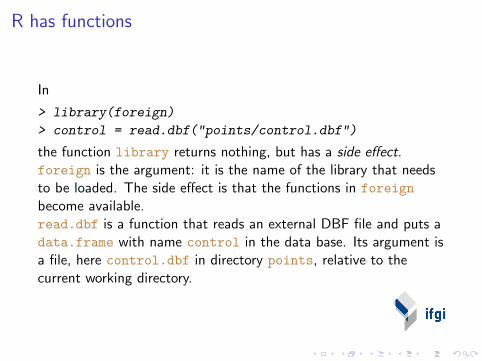
R has functions
In
> library(foreign)
> control = read.dbf("points/control.dbf")
the function library returns nothing, but has a side effect.foreign is the argument: it is the name of the library that needsto be loaded. The side effect is that the functions in foreignbecome available.read.dbf is a function that reads an external DBF file and puts adata.frame with name control in the data base. Its argument isa file, here control.dbf in directory points, relative to thecurrent working directory.
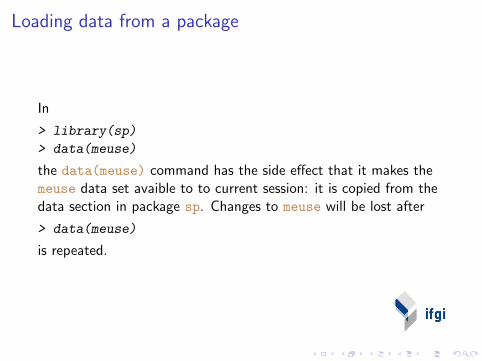
Loading data from a package
In
> library(sp)
> data(meuse)
the data(meuse) command has the side effect that it makes themeuse data set avaible to to current session: it is copied from thedata section in package sp. Changes to meuse will be lost after
> data(meuse)
is repeated.

Assignment
Symbols = and <- assign, as in
> a = 3
> a <- 3
> a
[1] 3
when no assignment takes place, the result is shown (printed orplotted)

Classes – every object has a class> a = 3
> class(a)
[1] "numeric"
> b = list(first = 3, second = "some text", 3:7)
> b
$first[1] 3
$second[1] "some text"
[[3]][1] 3 4 5 6 7
> class(b)
[1] "list"
> class(mean)
[1] "function"
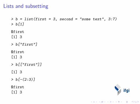
Lists and subsetting
> b = list(first = 3, second = "some text", 3:7)
> b[1]
$first[1] 3
> b["first"]
$first[1] 3
> b[["first"]]
[1] 3
> b[-(2:3)]
$first[1] 3
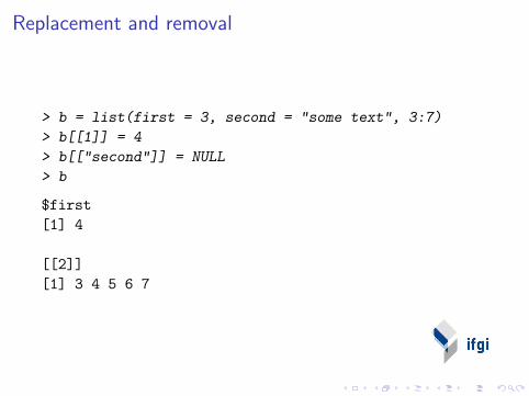
Replacement and removal
> b = list(first = 3, second = "some text", 3:7)
> b[[1]] = 4
> b[["second"]] = NULL
> b
$first[1] 4
[[2]][1] 3 4 5 6 7
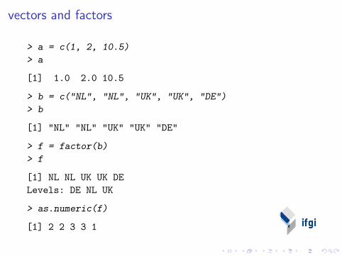
vectors and factors
> a = c(1, 2, 10.5)
> a
[1] 1.0 2.0 10.5
> b = c("NL", "NL", "UK", "UK", "DE")
> b
[1] "NL" "NL" "UK" "UK" "DE"
> f = factor(b)
> f
[1] NL NL UK UK DELevels: DE NL UK
> as.numeric(f)
[1] 2 2 3 3 1
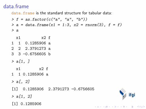
data.framedata.frame is the standard structure for tabular data:
> f = as.factor(c("a", "a", "b"))
> a = data.frame(x1 = 1:3, x2 = rnorm(3), f = f)
> a
x1 x2 f1 1 0.1285906 a2 2 2.3791273 a3 3 -0.6756605 b
> a[1, ]
x1 x2 f1 1 0.1285906 a
> a[, 2]
[1] 0.1285906 2.3791273 -0.6756605
> a[1, 2]
[1] 0.1285906
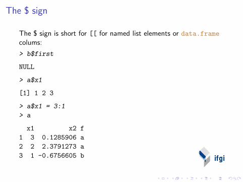
The $ sign
The $ sign is short for [[ for named list elements or data.framecolums:
> b$first
NULL
> a$x1
[1] 1 2 3
> a$x1 = 3:1
> a
x1 x2 f1 3 0.1285906 a2 2 2.3791273 a3 1 -0.6756605 b
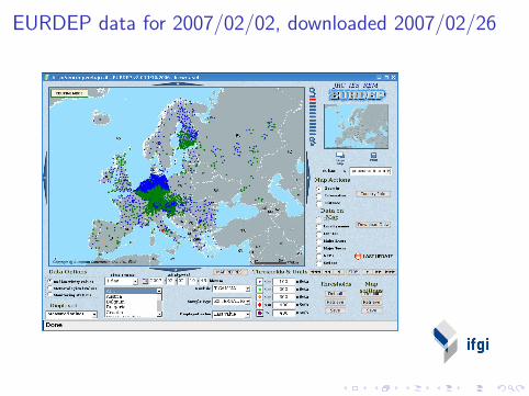
EURDEP data for 2007/02/02, downloaded 2007/02/26
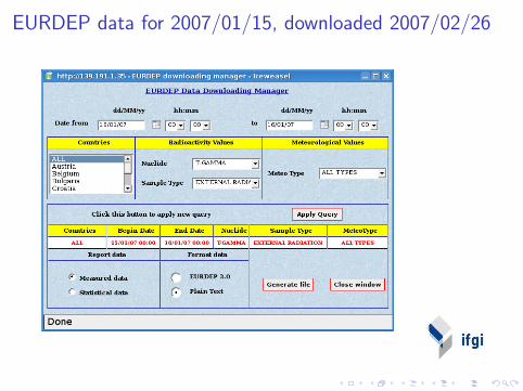
EURDEP data for 2007/01/15, downloaded 2007/02/26
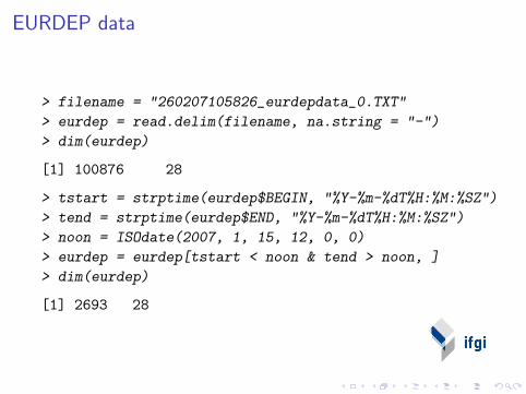
EURDEP data
> filename = "260207105826_eurdepdata_0.TXT"
> eurdep = read.delim(filename, na.string = "-")
> dim(eurdep)
[1] 100876 28
> tstart = strptime(eurdep$BEGIN, "%Y-%m-%dT%H:%M:%SZ")
> tend = strptime(eurdep$END, "%Y-%m-%dT%H:%M:%SZ")
> noon = ISOdate(2007, 1, 15, 12, 0, 0)
> eurdep = eurdep[tstart < noon & tend > noon, ]
> dim(eurdep)
[1] 2693 28
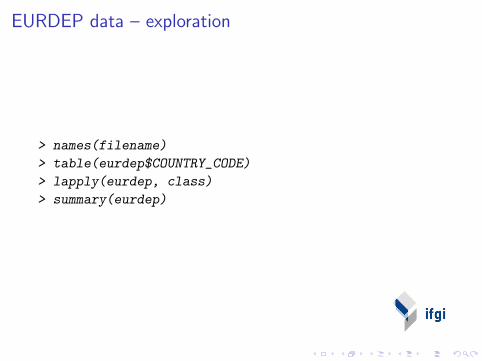
EURDEP data – exploration
> names(filename)
> table(eurdep$COUNTRY_CODE)
> lapply(eurdep, class)
> summary(eurdep)
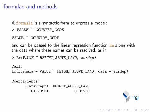
formulae and methods
A formula is a syntactic form to express a model:
> VALUE ~ COUNTRY_CODE
VALUE ~ COUNTRY_CODE
and can be passed to the linear regression function lm along withthe data where these names can be resolved, as in
> lm(VALUE ~ HEIGHT_ABOVE_LAND, eurdep)
Call:lm(formula = VALUE ~ HEIGHT_ABOVE_LAND, data = eurdep)
Coefficients:(Intercept) HEIGHT_ABOVE_LAND
81.73501 -0.01255
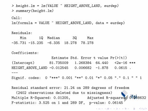
> height.lm = lm(VALUE ~ HEIGHT_ABOVE_LAND, eurdep)
> summary(height.lm)
Call:lm(formula = VALUE ~ HEIGHT_ABOVE_LAND, data = eurdep)
Residuals:Min 1Q Median 3Q Max
-35.731 -15.235 -6.335 18.278 78.278
Coefficients:Estimate Std. Error t value Pr(>|t|)
(Intercept) 81.735009 1.268384 64.440 <2e-16 ***HEIGHT_ABOVE_LAND -0.012545 0.006682 -1.878 0.0615 .---Signif. codes: 0 "***" 0.001 "**" 0.01 "*" 0.05 "." 0.1 " " 1
Residual standard error: 21.24 on 289 degrees of freedom(2402 observations deleted due to missingness)
Multiple R-Squared: 0.01205, Adjusted R-squared: 0.008632F-statistic: 3.525 on 1 and 289 DF, p-value: 0.06145
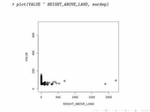
> plot(VALUE ~ HEIGHT_ABOVE_LAND, eurdep)
●●●●●●●●●●●●●
●
●●
●
●●●
●●●●●●●●●●●●●●●●
●
●●●●●
●
●●●●●
●
●●
●●●●●
●●●
●
●●●●●
●●●●●●●●●●
●
●●
●●●●
●●●
●
●●●●●●●●
●●●●●●●●●●●●●●●●●●
●●●●●●●●●●●●●●●●●●●●●●●●●●●●●●●●●●●●●●●●●●●●●●●●●●●●●●●●●●●●●●●●●●●●●●●●●●●●●●●●●●●●●●●●●●●●●●●●●●●●●●●●●●●●●●●●●●●●●●●●●●●●●●
●●●●●●●●●●●●●●●●
●● ●
●
●●
●
●●●●●
● ●●
●●● ●
●●● ●
●● ●● ●●
●●●
●●●
●
●
0 500 1000 1500 2000
020
040
060
0
HEIGHT_ABOVE_LAND
VA
LUE

> plot(VALUE ~ COUNTRY_CODE, eurdep)
●●
●
●
●
●
●
●
●
●
●●
●
● ●
●
●●●●
●
●
●
●
●
●
●
●
●●
●
●●
●
●
●
●
AT CH DK FI GR IE LT LV PL RU SK
5010
015
020
0
COUNTRY_CODE
VA
LUE
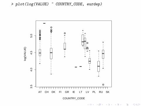
> plot(log(VALUE) ~ COUNTRY_CODE, eurdep)
●
●
●
●●
●●
●
●
●●●
●
●
●
●
AT CH DK FI GR IE LT LV PL RU SK
3.5
4.0
4.5
5.0
COUNTRY_CODE
log(
VA
LUE
)
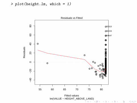
> plot(height.lm, which = 1)
55 60 65 70 75 80
−40
−20
020
4060
80
Fitted values
Res
idua
ls
●
●●●
●
●●●
●●
●●●
●
●
●
●
●
●
●
●
●●
●
●
●
●
●
●●
●●●●
●●
●
●
●
●●
●
●
●
●
●
●
●
●
●
●
●
●●
●
●
●
●
●
●
●●
●
●
●
●
●
●
●
●
●●
●
●
●
●
●
●
●
●
●
●
●●
●
●
●
●●
●●
●●
●
●
●
●
●
●
●
●
●
●
●●●
●
●
●
●●
●
●
●
●●
●
●●
●●
●
●
●
●●
●●
●●
●●
●
●●
●
●
●
●
●
●
●
●
●●
●●●
●●●
●●
●
●●
●
●
●
●
●
●
●●●
●
●
●
●
●
●
●
●
●
●
●
●●
●●
●
●
●
●
●●
●
●
●●●●
●
●●●
●
●
●●
●
●
●●
●●
●
●●
●
●
●●
●●
●
●●
●●
●●●
●
●
●
●●●
●
●
●
●●
●●●
●
●●
●
●
●●
●●●
●
●
●
●●
●
●
●
●
●
●
●
●
●
●●●
●●
●
●
●
●●
●●
●
●
●●
● ●
●
●● ●
●
●
●
●●
●
●
●
lm(VALUE ~ HEIGHT_ABOVE_LAND)
Residuals vs Fitted
55310
56153
54647
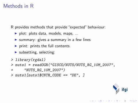
Methods in R
R provides methods that provide “expected” behaviour:
I plot: plots data, models, maps, ...
I summary: gives a summary in a few lines
I print: prints the full contents
I subsetting, selecting:
> library(rgdal)
> nuts1 = readOGR("GISCO/NUTS/NUTS_RG_10M_2007",
+ "NUTS_RG_10M_2007")
> nuts1[nuts1$CNTR_CODE == "DE", ]
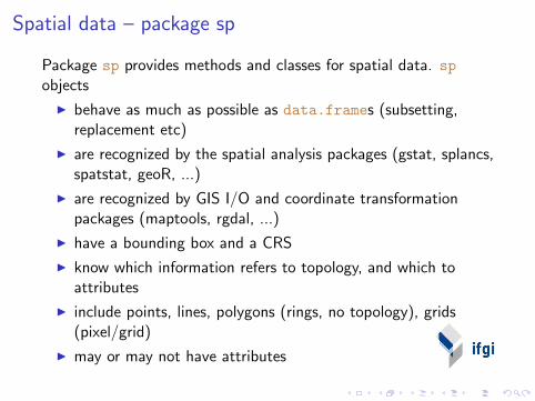
Spatial data – package sp
Package sp provides methods and classes for spatial data. spobjects
I behave as much as possible as data.frames (subsetting,replacement etc)
I are recognized by the spatial analysis packages (gstat, splancs,spatstat, geoR, ...)
I are recognized by GIS I/O and coordinate transformationpackages (maptools, rgdal, ...)
I have a bounding box and a CRS
I know which information refers to topology, and which toattributes
I include points, lines, polygons (rings, no topology), grids(pixel/grid)
I may or may not have attributes
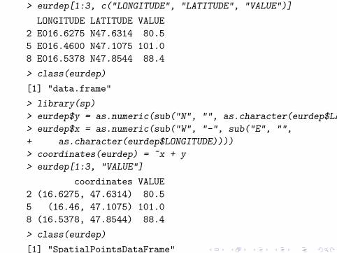
> eurdep[1:3, c("LONGITUDE", "LATITUDE", "VALUE")]
LONGITUDE LATITUDE VALUE2 E016.6275 N47.6314 80.55 E016.4600 N47.1075 101.08 E016.5378 N47.8544 88.4
> class(eurdep)
[1] "data.frame"
> library(sp)
> eurdep$y = as.numeric(sub("N", "", as.character(eurdep$LATITUDE)))
> eurdep$x = as.numeric(sub("W", "-", sub("E", "",
+ as.character(eurdep$LONGITUDE))))
> coordinates(eurdep) = ~x + y
> eurdep[1:3, "VALUE"]
coordinates VALUE2 (16.6275, 47.6314) 80.55 (16.46, 47.1075) 101.08 (16.5378, 47.8544) 88.4
> class(eurdep)
[1] "SpatialPointsDataFrame"attr(,"package")[1] "sp"
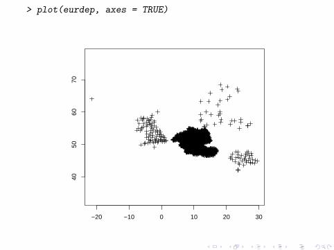
> plot(eurdep, axes = TRUE)
−20 −10 0 10 20 30
4050
6070
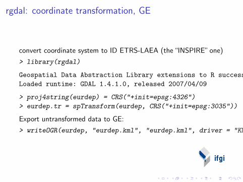
rgdal: coordinate transformation, GE
convert coordinate system to ID ETRS-LAEA (the “INSPIRE” one)
> library(rgdal)
Geospatial Data Abstraction Library extensions to R successfully loadedLoaded runtime: GDAL 1.4.1.0, released 2007/04/09
> proj4string(eurdep) = CRS("+init=epsg:4326")
> eurdep.tr = spTransform(eurdep, CRS("+init=epsg:3035"))
Export untransformed data to GE:
> writeOGR(eurdep, "eurdep.kml", "eurdep.kml", driver = "KML")
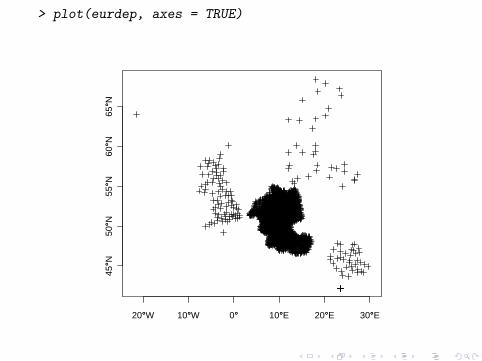
> plot(eurdep, axes = TRUE)
20°°W 10°°W 0°° 10°°E 20°°E 30°°E
45°°N
50°°N
55°°N
60°°N
65°°N
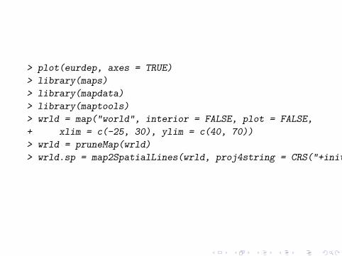
> plot(eurdep, axes = TRUE)
> library(maps)
> library(mapdata)
> library(maptools)
> wrld = map("world", interior = FALSE, plot = FALSE,
+ xlim = c(-25, 30), ylim = c(40, 70))
> wrld = pruneMap(wrld)
> wrld.sp = map2SpatialLines(wrld, proj4string = CRS("+init=epsg:4326"))
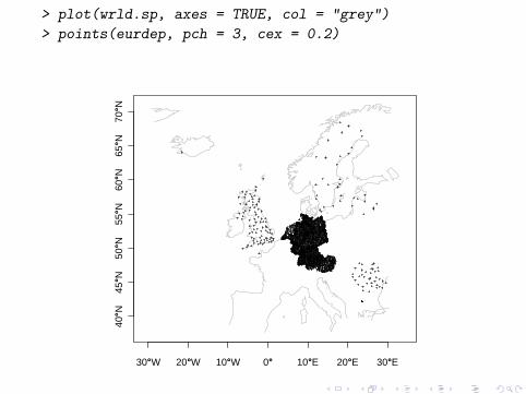
> plot(wrld.sp, axes = TRUE, col = "grey")
> points(eurdep, pch = 3, cex = 0.2)
30°°W 20°°W 10°°W 0°° 10°°E 20°°E 30°°E
40°°N
45°°N
50°°N
55°°N
60°°N
65°°N
70°°N
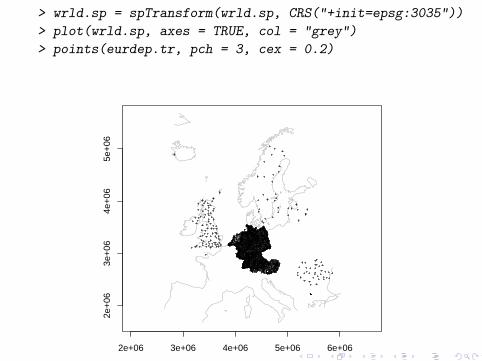
> wrld.sp = spTransform(wrld.sp, CRS("+init=epsg:3035"))
> plot(wrld.sp, axes = TRUE, col = "grey")
> points(eurdep.tr, pch = 3, cex = 0.2)
2e+06 3e+06 4e+06 5e+06 6e+06
2e+
063e
+06
4e+
065e
+06
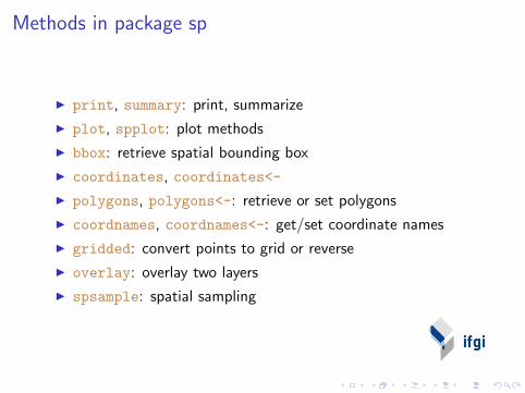
Methods in package sp
I print, summary: print, summarize
I plot, spplot: plot methods
I bbox: retrieve spatial bounding box
I coordinates, coordinates<-
I polygons, polygons<-: retrieve or set polygons
I coordnames, coordnames<-: get/set coordinate names
I gridded: convert points to grid or reverse
I overlay: overlay two layers
I spsample: spatial sampling
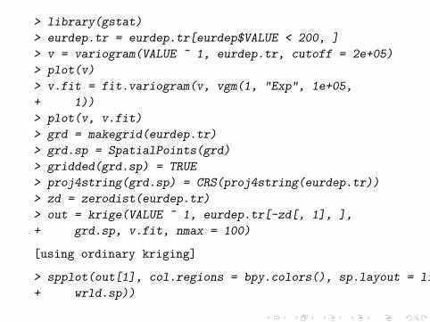
> library(gstat)
> eurdep.tr = eurdep.tr[eurdep$VALUE < 200, ]
> v = variogram(VALUE ~ 1, eurdep.tr, cutoff = 2e+05)
> plot(v)
> v.fit = fit.variogram(v, vgm(1, "Exp", 1e+05,
+ 1))
> plot(v, v.fit)
> grd = makegrid(eurdep.tr)
> grd.sp = SpatialPoints(grd)
> gridded(grd.sp) = TRUE
> proj4string(grd.sp) = CRS(proj4string(eurdep.tr))
> zd = zerodist(eurdep.tr)
> out = krige(VALUE ~ 1, eurdep.tr[-zd[, 1], ],
+ grd.sp, v.fit, nmax = 100)
[using ordinary kriging]
> spplot(out[1], col.regions = bpy.colors(), sp.layout = list("sp.lines",
+ wrld.sp))
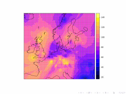
20
40
60
80
100
120
140
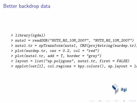
Better backdrop data
> library(rgdal)
> nuts1 = readOGR("NUTS_RG_10M_2007", "NUTS_RG_10M_2007")
> nuts1.tr = spTransform(nuts1, CRS(proj4string(eurdep.tr)))
> plot(eurdep.tr, cex = 0.2, col = "red")
> plot(nuts1.tr, add = T, border = "grey")
> layout = list("sp.polygons", nuts1.tr, first = FALSE)
> spplot(out[1], col.regions = bpy.colors(), sp.layout = layout)


![þ Q Éi o Q Éj - エクステリア通販【キロ本店】 · { ]*Ia â { ]*Ia G Da â G Da { ]*Ia ð r r r r r r r r r r r r r r r r r r r r r r r r r r r r r r r r rrr rr rr](https://img.pdfslide.net/doc/110x75/5f33ece46c9e825a026a2837/-q-i-o-q-j-ffeefoe-ia-ia-g.jpg)

![ESC SSH2 D40 Smart Energy Plan GMCA v2€¦ · r r r r r r r r r r r r r r r r r r r r r r r r r r r r r r r r r r r r r r r r r r r r r r r r r r r r r r r r d Z ] } µ u v ] u l](https://img.pdfslide.net/doc/110x75/5fefd4335a91d366af5b2c64/esc-ssh2-d40-smart-energy-plan-gmca-v2-r-r-r-r-r-r-r-r-r-r-r-r-r-r-r-r-r-r-r-r-r.jpg)