Embed Size (px)
Citation preview

INTRODUCTION
TO REAL ANALYSIS
William F. Trench

INTRODUCTIONTO REAL ANALYSIS
William F. TrenchProfessor Emeritus
Department of Mathematics
Trinity University
San Antonio, Texas, USA

©2003 William F. Trench, all rights reserved
Library of Congress Cataloging-in-Publication Data
Trench, William F.
Introduction to real analysis / William F. Trench
p. cm.
ISBN 0-13-045786-8
1. Mathematical Analysis. I. Title.
QA300.T667 2003
515-dc21 2002032369
Free Hyperlinked Edition 2.01, May 2012
This book was published previously by Pearson Education.
This free edition is made available in the hope that it will be useful as a textbook or refer-
ence. Reproduction is permitted for any valid noncommercial educational, mathematical,
or scientific purpose. However, charges for profit beyond reasonable printing costs are
prohibited.
A complete instructor’s solution manual is available by email to [email protected], sub-
ject to verification of the requestor’s faculty status.

TO BEVERLY

Contents
Preface vi
Chapter 1 The Real Numbers 1
1.1 The Real Number System 11.2 Mathematical Induction 101.3 The Real Line 19
Chapter 2 Differential Calculus of Functions of One Variable 30
2.1 Functions and Limits 302.2 Continuity 532.3 Differentiable Functions of One Variable 732.4 L’Hospital’s Rule 882.5 Taylor’s Theorem 98
Chapter 3 Integral Calculus of Functions of One Variable 113
3.1 Definition of the Integral 1133.2 Existence of the Integral 1283.3 Properties of the Integral 1353.4 Improper Integrals 1513.5 A More Advanced Look at the Existence
of the Proper Riemann Integral 171
Chapter 4 Infinite Sequences and Series 178
4.1 Sequences of Real Numbers 1794.2 Earlier Topics Revisited With Sequences 1954.3 Infinite Series of Constants 200
iv

Contents v
4.4 Sequences and Series of Functions 2344.5 Power Series 257
Chapter 5 Real-Valued Functions of Several Variables 281
5.1 Structure of RRRn 281
5.2 Continuous Real-Valued Function of n Variables 3025.3 Partial Derivatives and the Differential 3165.4 The Chain Rule and Taylor’s Theorem 339
Chapter 6 Vector-Valued Functions of Several Variables 361
6.1 Linear Transformations and Matrices 3616.2 Continuity and Differentiability of Transformations 3786.3 The Inverse Function Theorem 3946.4. The Implicit Function Theorem 417
Chapter 7 Integrals of Functions of Several Variables 435
7.1 Definition and Existence of the Multiple Integral 4357.2 Iterated Integrals and Multiple Integrals 4627.3 Change of Variables in Multiple Integrals 484
Chapter 8 Metric Spaces 518
8.1 Introduction to Metric Spaces 5188.2 Compact Sets in a Metric Space 5358.3 Continuous Functions on Metric Spaces 543
Answers to Selected Exercises 549
Index 563
SUPPLEMENT: Functions Defined by Improper Integrals1 Foreword2 Introduction3 Preparation4 Uniform convergence of improper integrals5 Absolutely Uniformly Convergent Improper Integrals6 Dirich let's Tests7 Consequences of uniform convergence8 Applications to Laplace transforms9 Exercises10 Answers to selected exercises

PrefaceThis is a text for a two-term course in introductory real analysis for junior or senior math-
ematics majors and science students with a serious interest in mathematics. Prospective
educators or mathematically gifted high school students can also benefit from the mathe-
matical maturity that can be gained from an introductory real analysis course.
The book is designed to fill the gaps left in the development of calculus as it is usually
presented in an elementary course, and to provide the background required for insight into
more advanced courses in pure and applied mathematics. The standard elementary calcu-
lus sequence is the only specific prerequisite for Chapters 1–5, which deal with real-valued
functions. (However, other analysis oriented courses, such as elementary differential equa-
tion, also provide useful preparatory experience.) Chapters 6 and 7 require a working
knowledge of determinants, matrices and linear transformations, typically available from a
first course in linear algebra. Chapter 8 is accessible after completion of Chapters 1–5.
Without taking a position for or against the current reforms in mathematics teaching, I
think it is fair to say that the transition from elementary courses such as calculus, linear
algebra, and differential equations to a rigorous real analysis course is a bigger step to-
day than it was just a few years ago. To make this step today’s students need more help
than their predecessors did, and must be coached and encouraged more. Therefore, while
striving throughout to maintain a high level of rigor, I have tried to write as clearly and in-
formally as possible. In this connection I find it useful to address the student in the second
person. I have included 295 completely worked out examples to illustrate and clarify all
major theorems and definitions.
I have emphasized careful statements of definitions and theorems and have tried to be
complete and detailed in proofs, except for omissions left to exercises. I give a thorough
treatment of real-valued functions before considering vector-valued functions. In making
the transition from one to several variables and from real-valued to vector-valued functions,
I have left to the student some proofs that are essentially repetitions of earlier theorems. I
believe that working through the details of straightforward generalizations of more elemen-
tary results is good practice for the student.
Great care has gone into the preparation of the 760 numbered exercises, many with
multiple parts. They range from routine to very difficult. Hints are provided for the more
difficult parts of the exercises.
vi
Preface vii
Organization
Chapter 1 is concerned with the real number system. Section 1.1 begins with a brief dis-
cussion of the axioms for a complete ordered field, but no attempt is made to develop the
reals from them; rather, it is assumed that the student is familiar with the consequences of
these axioms, except for one: completeness. Since the difference between a rigorous and
nonrigorous treatment of calculus can be described largely in terms of the attitude taken
toward completeness, I have devoted considerable effort to developing its consequences.
Section 1.2 is about induction. Although this may seem out of place in a real analysis
course, I have found that the typical beginning real analysis student simply cannot do an
induction proof without reviewing the method. Section 1.3 is devoted to elementary set the-
ory and the topology of the real line, ending with the Heine-Borel and Bolzano-Weierstrass
theorems.
Chapter 2 covers the differential calculus of functions of one variable: limits, continu-
ity, differentiablility, L’Hospital’s rule, and Taylor’s theorem. The emphasis is on rigorous
presentation of principles; no attempt is made to develop the properties of specific ele-
mentary functions. Even though this may not be done rigorously in most contemporary
calculus courses, I believe that the student’s time is better spent on principles rather than
on reestablishing familiar formulas and relationships.
Chapter 3 is to devoted to the Riemann integral of functions of one variable. In Sec-
tion 3.1 the integral is defined in the standard way in terms of Riemann sums. Upper and
lower integrals are also defined there and used in Section 3.2 to study the existence of the
integral. Section 3.3 is devoted to properties of the integral. Improper integrals are studied
in Section 3.4. I believe that my treatment of improper integrals is more detailed than in
most comparable textbooks. A more advanced look at the existence of the proper Riemann
integral is given in Section 3.5, which concludes with Lebesgue’s existence criterion. This
section can be omitted without compromising the student’s preparedness for subsequent
sections.
Chapter 4 treats sequences and series. Sequences of constant are discussed in Sec-
tion 4.1. I have chosen to make the concepts of limit inferior and limit superior parts
of this development, mainly because this permits greater flexibility and generality, with
little extra effort, in the study of infinite series. Section 4.2 provides a brief introduction
to the way in which continuity and differentiability can be studied by means of sequences.
Sections 4.3–4.5 treat infinite series of constant, sequences and infinite series of functions,
and power series, again in greater detail than in most comparable textbooks. The instruc-
tor who chooses not to cover these sections completely can omit the less standard topics
without loss in subsequent sections.
Chapter 5 is devoted to real-valued functions of several variables. It begins with a dis-
cussion of the toplogy of Rn in Section 5.1. Continuity and differentiability are discussed
in Sections 5.2 and 5.3. The chain rule and Taylor’s theorem are discussed in Section 5.4.
viii Preface
Chapter 6 covers the differential calculus of vector-valued functions of several variables.
Section 6.1 reviews matrices, determinants, and linear transformations, which are integral
parts of the differential calculus as presented here. In Section 6.2 the differential of a
vector-valued function is defined as a linear transformation, and the chain rule is discussed
in terms of composition of such functions. The inverse function theorem is the subject of
Section 6.3, where the notion of branches of an inverse is introduced. In Section 6.4. the
implicit function theorem is motivated by first considering linear transformations and then
stated and proved in general.
Chapter 7 covers the integral calculus of real-valued functions of several variables. Mul-
tiple integrals are defined in Section 7.1, first over rectangular parallelepipeds and then
over more general sets. The discussion deals with the multiple integral of a function whose
discontinuities form a set of Jordan content zero. Section 7.2 deals with the evaluation by
iterated integrals. Section 7.3 begins with the definition of Jordan measurability, followed
by a derivation of the rule for change of content under a linear transformation, an intuitive
formulation of the rule for change of variables in multiple integrals, and finally a careful
statement and proof of the rule. The proof is complicated, but this is unavoidable.
Chapter 8 deals with metric spaces. The concept and properties of a metric space are
introduced in Section 8.1. Section 8.2 discusses compactness in a metric space, and Sec-
tion 8.3 discusses continuous functions on metric spaces.
Corrections–mathematical and typographical–are welcome and will be incorporated when
received.
William F. Trench
Home: 659 Hopkinton Road
Hopkinton, NH 03229
CHAPTER 1
The Real Numbers
IN THIS CHAPTER we begin the study of the real number system. The concepts discussed
here will be used throughout the book.
SECTION 1.1 deals with the axioms that define the real numbers, definitions based on
them, and some basic properties that follow from them.
SECTION 1.2 emphasizes the principle of mathematical induction.
SECTION 1.3 introduces basic ideas of set theory in the context of sets of real num-
bers. In this section we prove two fundamental theorems: the Heine–Borel and Bolzano–
Weierstrass theorems.
1.1 THE REAL NUMBER SYSTEM
Having taken calculus, you know a lot about the real number system; however, you prob-
ably do not know that all its properties follow from a few basic ones. Although we will
not carry out the development of the real number system from these basic properties, it is
useful to state them as a starting point for the study of real analysis and also to focus on
one property, completeness, that is probably new to you.
Field Properties
The real number system (which we will often call simply the reals) is first of all a set
fa; b; c; : : : g on which the operations of addition and multiplication are defined so that
every pair of real numbers has a unique sum and product, both real numbers, with the
following properties.
(A) aC b D b C a and ab D ba (commutative laws).
(B) .a C b/C c D aC .b C c/ and .ab/c D a.bc/ (associative laws).
(C) a.b C c/ D ab C ac (distributive law).
(D) There are distinct real numbers 0 and 1 such that aC 0 D a and a1 D a for all a.
(E) For each a there is a real number a such that aC .a/ D 0, and if a ¤ 0, there is
a real number 1=a such that a.1=a/ D 1.
1
2 Chapter 1 The Real Numbers
The manipulative properties of the real numbers, such as the relations
.a C b/2 D a2 C 2abC b2;
.3a C 2b/.4c C 2d/D 12acC 6ad C 8bc C 4bd;.a/ D .1/a; a.b/ D .a/b D ab;
anda
bC c
dD ad C bc
bd.b; d ¤ 0/;
all follow from (A)–(E). We assume that you are familiar with these properties.
A set on which two operations are defined so as to have properties (A)–(E) is called a
field. The real number system is by no means the only field. The rational numbers (which
are the real numbers that can be written as r D p=q, where p and q are integers and q ¤ 0)
also form a field under addition and multiplication. The simplest possible field consists of
two elements, which we denote by 0 and 1, with addition defined by
0C 0 D 1C 1 D 0; 1C 0 D 0C 1 D 1; (1.1.1)
and multiplication defined by
0 0 D 0 1 D 1 0 D 0; 1 1 D 1 (1.1.2)
(Exercise 1.1.2).
The Order Relation
The real number system is ordered by the relation<, which has the following properties.
(F) For each pair of real numbers a and b, exactly one of the following is true:
a D b; a < b; or b < a:
(G) If a < b and b < c, then a < c. (The relation< is transitive.)
(H) If a < b, then aC c < b C c for any c, and if 0 < c, then ac < bc.
A field with an order relation satisfying (F)–(H) is an ordered field. Thus, the real
numbers form an ordered field. The rational numbers also form an ordered field, but it is
impossible to define an order on the field with two elements defined by (1.1.1) and (1.1.2)
so as to make it into an ordered field (Exercise 1.1.2).
We assume that you are familiar with other standard notation connected with the order
relation: thus, a > b means that b < a; a b means that either a D b or a > b; a bmeans that either a D b or a < b; the absolute value of a, denoted by jaj, equals a if
a 0 or a if a 0. (Sometimes we call jaj the magnitude of a.)
You probably know the following theorem from calculus, but we include the proof for
your convenience.
Section 1.1 The Real Number System 3
Theorem 1.1.1 (The Triangle Inequality) If a and b are any two real numbers;
then
jaC bj jaj C jbj: (1.1.3)
Proof There are four possibilities:
(a) If a 0 and b 0, then aC b 0, so jaC bj D aC b D jaj C jbj.(b) If a 0 and b 0, then aC b 0, so jaC bj D a C .b/ D jaj C jbj.(c) If a 0 and b 0, then aC b D jaj jbj.(d) If a 0 and b 0, then aC b D jaj C jbj. Eq. 1.1.3 holds in either case, since
jaC bj D(jaj jbj if jaj jbj;jbj jaj if jbj jaj;
The triangle inequality appears in various forms in many contexts. It is the most impor-
tant inequality in mathematics. We will use it often.
Corollary 1.1.2 If a and b are any two real numbers; then
ja bj ˇjaj jbj
ˇ(1.1.4)
and
ja C bj ˇjaj jbj
ˇ: (1.1.5)
Proof Replacing a by a b in (1.1.3) yields
jaj ja bj C jbj;
so
ja bj jaj jbj: (1.1.6)
Interchanging a and b here yields
jb aj jbj jaj;
which is equivalent to
ja bj jbj jaj; (1.1.7)
since jb aj D ja bj. Since
ˇjaj jbj
ˇD(jaj jbj if jaj > jbj;
jbj jaj if jbj > jaj;
(1.1.6) and (1.1.7) imply (1.1.4). Replacing b byb in (1.1.4) yields (1.1.5), since jbj Djbj.
Supremum of a Set
A set S of real numbers is bounded above if there is a real number b such that x b
whenever x 2 S . In this case, b is an upper bound of S . If b is an upper bound of S ,
then so is any larger number, because of property (G). If ˇ is an upper bound of S , but no
number less than ˇ is, then ˇ is a supremum of S , and we write
ˇ D supS:

4 Chapter 1 The Real Numbers
With the real numbers associated in the usual way with the points on a line, these defini-
tions can be interpreted geometrically as follows: b is an upper bound of S if no point of S
is to the right of b; ˇ D supS if no point of S is to the right of ˇ, but there is at least one
point of S to the right of any number less than ˇ (Figure 1.1.1).
(S = dark line segments)β b
Figure 1.1.1
Example 1.1.1 If S is the set of negative numbers, then any nonnegative number is an
upper bound of S , and supS D 0. If S1 is the set of negative integers, then any number a
such that a 1 is an upper bound of S1, and supS1 D 1.
This example shows that a supremum of a set may or may not be in the set, since S1
contains its supremum, but S does not.
A nonempty set is a set that has at least one member. The empty set, denoted by ;, is the
set that has no members. Although it may seem foolish to speak of such a set, we will see
that it is a useful idea.
The Completeness Axiom
It is one thing to define an object and another to show that there really is an object that
satisfies the definition. (For example, does it make sense to define the smallest positive
real number?) This observation is particularly appropriate in connection with the definition
of the supremum of a set. For example, the empty set is bounded above by every real
number, so it has no supremum. (Think about this.) More importantly, we will see in
Example 1.1.2 that properties (A)–(H) do not guarantee that every nonempty set that
is bounded above has a supremum. Since this property is indispensable to the rigorous
development of calculus, we take it as an axiom for the real numbers.
(I) If a nonempty set of real numbers is bounded above, then it has a supremum.
Property (I) is called completeness, and we say that the real number system is a complete
ordered field. It can be shown that the real number system is essentially the only complete
ordered field; that is, if an alien from another planet were to construct a mathematical
system with properties (A)–(I), the alien’s system would differ from the real number
system only in that the alien might use different symbols for the real numbers and C, ,and <.
Theorem 1.1.3 If a nonempty set S of real numbers is bounded above; then supS is
the unique real number ˇ such that
(a) x ˇ for all x in S I(b) if > 0 .no matter how small/; there is an x0 in S such that x0 > ˇ :
Section 1.1 The Real Number System 5
Proof We first show that ˇ D supS has properties (a) and (b). Since ˇ is an upper
bound of S , it must satisfy (a). Since any real number a less than ˇ can be written as ˇwith D ˇ a > 0, (b) is just another way of saying that no number less than ˇ is an
upper bound of S . Hence, ˇ D supS satisfies (a) and (b).
Now we show that there cannot be more than one real number with properties (a) and
(b). Suppose that ˇ1 < ˇ2 and ˇ2 has property (b); thus, if > 0, there is an x0 in S
such that x0 > ˇ2 . Then, by taking D ˇ2 ˇ1, we see that there is an x0 in S such
that
x0 > ˇ2 .ˇ2 ˇ1/ D ˇ1;
so ˇ1 cannot have property (a). Therefore, there cannot be more than one real number
that satisfies both (a) and (b).
Some Notation
We will often define a set S by writing S D˚xˇ , which means that S consists of all
x that satisfy the conditions to the right of the vertical bar; thus, in Example 1.1.1,
S D˚xˇx < 0
(1.1.8)
and
S1 D˚xˇx is a negative integer
:
We will sometimes abbreviate “x is a member of S” by x 2 S , and “x is not a member of
S” by x … S . For example, if S is defined by (1.1.8), then
1 2 S but 0 … S:
The Archimedean Property
The property of the real numbers described in the next theorem is called the Archimedean
property. Intuitively, it states that it is possible to exceed any positive number, no matter
how large, by adding an arbitrary positive number, no matter how small, to itself sufficiently
many times.
Theorem 1.1.4 (The Archimedean Property) If and are positive; then
n > for some integer n:
Proof The proof is by contradiction. If the statement is false, is an upper bound of
the set
S D˚xˇx D n; n is an integer
:
Therefore, S has a supremum ˇ, by property (I). Therefore,
n ˇ for all integers n: (1.1.9)
6 Chapter 1 The Real Numbers
Since nC 1 is an integer whenever n is, (1.1.9) implies that
.nC 1/ ˇ
and therefore
n ˇ for all integers n. Hence, ˇ is an upper bound of S . Since ˇ < ˇ, this contradicts
the definition of ˇ.
Density of the Rationals and Irrationals
Definition 1.1.5 A set D is dense in the reals if every open interval .a; b/ contains a
member of D.
Theorem 1.1.6 The rational numbers are dense in the reals I that is, if a and b are
real numbers with a < b; there is a rational number p=q such that a < p=q < b.
Proof From Theorem 1.1.4 with D 1 and D ba, there is a positive integer q such
that q.b a/ > 1. There is also an integer j such that j > qa. This is obvious if a 0,
and it follows from Theorem 1.1.4 with D 1 and D qa if a > 0. Let p be the smallest
integer such that p > qa. Then p 1 qa, so
qa < p qaC 1:
Since 1 < q.b a/, this implies that
qa < p < qa C q.b a/ D qb;
so qa < p < qb. Therefore, a < p=q < b.
Example 1.1.2 The rational number system is not complete; that is, a set of rational
numbers may be bounded above (by rationals), but not have a rational upper bound less
than any other rational upper bound. To see this, let
S D˚rˇr is rational and r2 < 2
:
If r 2 S , then r <p2. Theorem 1.1.6 implies that if > 0 there is a rational number r0
such thatp2 < r0 <
p2, so Theorem 1.1.3 implies that
p2 D supS . However,
p2 is
irrational; that is, it cannot be written as the ratio of integers (Exercise 1.1.3). Therefore,
if r1 is any rational upper bound of S , thenp2 < r1. By Theorem 1.1.6, there is a rational
number r2 such thatp2 < r2 < r1. Since r2 is also a rational upper bound of S , this shows
that S has no rational supremum.
Since the rational numbers have properties (A)–(H), but not (I), this example shows
that (I) does not follow from (A)–(H).
Theorem 1.1.7 The set of irrational numbers is dense in the reals I that is, if a and b
are real numbers with a < b; there is an irrational number t such that a < t < b:

Section 1.1 The Real Number System 7
Proof From Theorem 1.1.6, there are rational numbers r1 and r2 such that
a < r1 < r2 < b: (1.1.10)
Let
t D r1 C1p2.r2 r1/:
Then t is irrational (why?) and r1 < t < r2, so a < t < b, from (1.1.10).
Infimum of a Set
A set S of real numbers is bounded below if there is a real number a such that x a
whenever x 2 S . In this case, a is a lower bound of S . If a is a lower bound of S , so is
any smaller number, because of property (G). If ˛ is a lower bound of S , but no number
greater than ˛ is, then ˛ is an infimum of S , and we write
˛ D infS:
Geometrically, this means that there are no points of S to the left of ˛, but there is at least
one point of S to the left of any number greater than ˛.
Theorem 1.1.8 If a nonempty set S of real numbers is bounded below; then infS is
the unique real number ˛ such that
(a) x ˛ for all x in S I(b) if > 0 .no matter how small /, there is an x0 in S such that x0 < ˛ C :
Proof (Exercise 1.1.6)
A set S is bounded if there are numbers a and b such that a x b for all x in S . A
bounded nonempty set has a unique supremum and a unique infimum, and
infS supS (1.1.11)
(Exercise 1.1.7).
The Extended Real Number System
A nonempty set S of real numbers is unbounded above if it has no upper bound, or un-
bounded below if it has no lower bound. It is convenient to adjoin to the real number
system two fictitious points, C1 (which we usually write more simply as 1) and 1,
and to define the order relationships between them and any real number x by
1 < x <1: (1.1.12)
We call1 and 1 points at infinity. If S is a nonempty set of reals, we write
supS D1 (1.1.13)
to indicate that S is unbounded above, and
infS D 1 (1.1.14)
to indicate that S is unbounded below.
8 Chapter 1 The Real Numbers
Example 1.1.3 If
S D˚xˇx < 2
;
then supS D 2 and infS D 1. If
S D˚xˇx 2
;
then supS D 1 and infS D 2. If S is the set of all integers, then supS D 1 and
infS D 1.
The real number system with1 and 1 adjoined is called the extended real number
system, or simply the extended reals. A member of the extended reals differing from 1and 1 is finite; that is, an ordinary real number is finite. However, the word “finite” in
“finite real number” is redundant and used only for emphasis, since we would never refer
to1 or 1 as real numbers.
The arithmetic relationships among1, 1, and the real numbers are defined as follows.
(a) If a is any real number, then
aC1D 1C a D 1;a 1D 1C a D 1;
a
1 Da
1 D 0:
(b) If a > 0, then
a1 D 1a D 1;a .1/ D .1/ a D 1:
(c) If a < 0, then
a1 D 1a D 1;a .1/ D .1/ a D 1:
We also define
1C1 D11 D .1/.1/ D1
and
11 D1.1/ D .1/1 D 1:Finally, we define
j1j D j 1j D 1:
The introduction of1 and1, along with the arithmetic and order relationships defined
above, leads to simplifications in the statements of theorems. For example, the inequality
(1.1.11), first stated only for bounded sets, holds for any nonempty set S if it is interpreted
properly in accordance with (1.1.12) and the definitions of (1.1.13) and (1.1.14). Exer-
cises 1.1.10(b) and 1.1.11(b) illustrate the convenience afforded by some of the arith-
metic relationships with extended reals, and other examples will illustrate this further in
subsequent sections.

Section 1.1 The Real Number System 9
It is not useful to define11, 0 1,1=1, and 0=0. They are called indeterminate
forms, and left undefined. You probably studied indeterminate forms in calculus; we will
look at them more carefully in Section 2.4.
1.1 Exercises
1. Write the following expressions in equivalent forms not involving absolute values.
(a) aC b C ja bj (b) a C b ja bj
(c) aC b C 2cC ja bj CˇaC b 2c C ja bj
ˇ
(d) a C b C 2c ja bj ˇa C b 2c ja bj
ˇ
2. Verify that the set consisting of two members, 0 and 1, with operations defined by
Eqns. (1.1.1) and (1.1.2), is a field. Then show that it is impossible to define an order
< on this field that has properties (F), (G), and (H).
3. Show thatp2 is irrational. HINT: Show that if
p2 D m=n; where m and n are
integers; then both m and n must be even: Obtain a contradiction from this:
4. Show thatpp is irrational if p is prime.
5. Find the supremum and infimum of each S . State whether they are in S .
(a) S D˚xˇx D .1=n/ C Œ1C .1/n n2; n 1
(b) S D˚xˇx2 < 9
(c) S D˚xˇx2 7
(d) S D˚xˇj2x C 1j < 5
(e) S D˚xˇ.x2 C 1/1 > 1
2
(f) S D˚xˇx D rational and x2 7
6. Prove Theorem 1.1.8. HINT: The set T D˚xˇ x 2 S
is bounded above if S is
bounded below: Apply property (I) and Theorem 1.1.3 to T:
7. (a) Show that
inf S sup S .A/
for any nonempty set S of real numbers, and give necessary and sufficient
conditions for equality.
(b) Show that if S is unbounded then (A) holds if it is interpreted according to
Eqn. (1.1.12) and the definitions of Eqns. (1.1.13) and (1.1.14).
8. Let S and T be nonempty sets of real numbers such that every real number is in S
or T and if s 2 S and t 2 T , then s < t . Prove that there is a unique real number ˇ
such that every real number less than ˇ is in S and every real number greater than
ˇ is in T . (A decomposition of the reals into two sets with these properties is a
Dedekind cut. This is known as Dedekind’s theorem.)
10 Chapter 1 The Real Numbers
9. Using properties (A)–(H) of the real numbers and taking Dedekind’s theorem
(Exercise 1.1.8) as given, show that every nonempty set U of real numbers that is
bounded above has a supremum. HINT: Let T be the set of upper bounds of U and
S be the set of real numbers that are not upper bounds of U:
10. Let S and T be nonempty sets of real numbers and define
S C T D˚s C t
ˇs 2 S; t 2 T
:
(a) Show that
sup.S C T / D supS C sup T .A/
if S and T are bounded above and
inf.S C T / D infS C infT .B/
if S and T are bounded below.
(b) Show that if they are properly interpreted in the extended reals, then (A) and
(B) hold if S and T are arbitrary nonempty sets of real numbers.
11. Let S and T be nonempty sets of real numbers and define
S T D˚s t
ˇs 2 S; t 2 T
:
(a) Show that if S and T are bounded, then
sup.S T / D supS infT .A/
and
inf.S T / D infS sup T: .B/
(b) Show that if they are properly interpreted in the extended reals, then (A) and
(B) hold if S and T are arbitrary nonempty sets of real numbers.
12. Let S be a bounded nonempty set of real numbers, and let a and b be fixed real
numbers. Define T D˚as C b
ˇs 2 S
. Find formulas for sup T and infT in terms
of supS and infS . Prove your formulas.
1.2 MATHEMATICAL INDUCTION
If a flight of stairs is designed so that falling off any step inevitably leads to falling off the
next, then falling off the first step is a sure way to end up at the bottom. Crudely expressed,
this is the essence of the principle of mathematical induction: If the truth of a statement
depending on a given integer n implies the truth of the corresponding statement with n
replaced by nC 1, then the statement is true for all positive integers n if it is true for n D 1.
Although you have probably studied this principle before, it is so important that it merits
careful review here.
Peano’s Postulates and Induction
The rigorous construction of the real number system starts with a set N of undefined ele-
ments called natural numbers, with the following properties.
Section 1.2 Mathematical Induction 11
(A) N is nonempty.
(B) Associated with each natural number n there is a unique natural number n0 called
the successor of n.
(C) There is a natural number n that is not the successor of any natural number.
(D) Distinct natural numbers have distinct successors; that is, if n ¤ m, then n0 ¤ m0.
(E) The only subset of N that contains n and the successors of all its elements is N
itself.
These axioms are known as Peano’s postulates. The real numbers can be constructed
from the natural numbers by definitions and arguments based on them. This is a formidable
task that we will not undertake. We mention it to show how little you need to start with to
construct the reals and, more important, to draw attention to postulate (E), which is the
basis for the principle of mathematical induction.
It can be shown that the positive integers form a subset of the reals that satisfies Peano’s
postulates (with n D 1 and n0 D nC 1), and it is customary to regard the positive integers
and the natural numbers as identical. From this point of view, the principle of mathematical
induction is basically a restatement of postulate (E).
Theorem 1.2.1 (Principle of Mathematical Induction) Let P1; P2;. . . ;
Pn; . . . be propositions; one for each positive integer; such that
(a) P1 is trueI(b) for each positive integer n; Pn implies PnC1:
Then Pn is true for each positive integer n:
Proof Let
M D˚nˇn 2 N and Pn is true
:
From (a), 1 2 M, and from (b), n C 1 2 M whenever n 2 M. Therefore, M D N, by
postulate (E).
Example 1.2.1 Let Pn be the proposition that
1C 2C C n D n.nC 1/2
: (1.2.1)
Then P1 is the proposition that 1 D 1, which is certainly true. If Pn is true, then adding
nC 1 to both sides of (1.2.1) yields
.1C 2C C n/C .nC 1/D n.nC 1/2
C .nC 1/
D .nC 1/n2C 1
D .nC 1/.nC 2/2
;
or
1C 2C C .nC 1/D .nC 1/.nC 2/2
;

12 Chapter 1 The Real Numbers
which is PnC1, since it has the form of (1.2.1), with n replaced by nC1. Hence, Pn implies
PnC1, so (1.2.1) is true for all n, by Theorem 1.2.1.
A proof based on Theorem 1.2.1 is an induction proof , or proof by induction. The
assumption that Pn is true is the induction assumption. (Theorem 1.2.3 permits a kind of
induction proof in which the induction assumption takes a different form.)
Induction, by definition, can be used only to verify results conjectured by other means.
Thus, in Example 1.2.1 we did not use induction to find the sum
sn D 1C 2C C nI (1.2.2)
rather, we verified that
sn Dn.nC 1/
2: (1.2.3)
How you guess what to prove by induction depends on the problem and your approach to
it. For example, (1.2.3) might be conjectured after observing that
s1 D 1 D1 22; s2 D 3 D
2 32; s3 D 6 D
4 32:
However, this requires sufficient insight to recognize that these results are of the form
(1.2.3) for n D 1, 2, and 3. Although it is easy to prove (1.2.3) by induction once it has
been conjectured, induction is not the most efficient way to find sn, which can be obtained
quickly by rewriting (1.2.2) as
sn D nC .n 1/C C 1
and adding this to (1.2.2) to obtain
2sn D ŒnC 1C Œ.n 1/C 2C C Œ1C n:
There are n bracketed expressions on the right, and the terms in each add up to n C 1;
hence,
2sn D n.nC 1/;which yields (1.2.3).
The next two examples deal with problems for which induction is a natural and efficient
method of solution.
Example 1.2.2 Let a1 D 1 and
anC1 D1
nC 1an; n 1 (1.2.4)
(we say that an is defined inductively), and suppose that we wish to find an explicit formula
for an. By considering n D 1, 2, and 3, we find that
a1 D1
1; a2 D
1
1 2 ; and a3 D1
1 2 3 ;

Section 1.2 Mathematical Induction 13
and therefore we conjecture that
an D1
nŠ: (1.2.5)
This is given for n D 1. If we assume it is true for some n, substituting it into (1.2.4) yields
anC1 D1
nC 11
nŠD 1
.nC 1/Š;
which is (1.2.5) with n replaced by n C 1. Therefore, (1.2.5) is true for every positive
integer n, by Theorem 1.2.1.
Example 1.2.3 For each nonnegative integer n, let xn be a real number and suppose
that
jxnC1 xnj r jxn xn1j; n 1; (1.2.6)
where r is a fixed positive number. By considering (1.2.6) for n D 1, 2, and 3, we find that
jx2 x1j r jx1 x0j;jx3 x2j r jx2 x1j r2jx1 x0j;jx4 x3j r jx3 x2j r3jx1 x0j:
Therefore, we conjecture that
jxn xn1j rn1jx1 x0j if n 1: (1.2.7)
This is trivial for n D 1. If it is true for some n, then (1.2.6) and (1.2.7) imply that
jxnC1 xnj r.rn1jx1 x0j/; so jxnC1 xnj rnjx1 x0j;
which is proposition (1.2.7) with n replaced by n C 1. Hence, (1.2.7) is true for every
positive integer n, by Theorem 1.2.1.
The major effort in an induction proof (after P1, P2, . . . , Pn, . . . have been formulated)
is usually directed toward showing thatPn impliesPnC1. However, it is important to verify
P1, since Pn may imply PnC1 even if some or all of the propositions P1, P2, . . . , Pn, . . .
are false.
Example 1.2.4 Let Pn be the proposition that 2n 1 is divisible by 2. If Pn is true
then PnC1 is also, since
2nC 1 D .2n 1/C 2:
However, we cannot conclude that Pn is true for n 1. In fact, Pn is false for every n.
The following formulation of the principle of mathematical induction permits us to start
induction proofs with an arbitrary integer, rather than 1, as required in Theorem 1.2.1.

14 Chapter 1 The Real Numbers
Theorem 1.2.2 Let n0 be any integer .positive; negative; or zero/: Let Pn0; Pn0C1;
. . . ; Pn; . . . be propositions; one for each integer n n0; such that
(a) Pn0is true I
(b) for each integer n n0; Pn implies PnC1:
Then Pn is true for every integer n n0:
Proof For m 1, let Qm be the proposition defined by Qm D PmCn01. Then Q1 DPn0
is true by (a). If m 1 and Qm D PmCn01 is true, then QmC1 D PmCn0is true by
(b) with n replaced bymC n0 1. Therefore, Qm is true for allm 1 by Theorem 1.2.1
with P replaced by Q and n replaced by m. This is equivalent to the statement that Pn is
true for all n n0.
Example 1.2.5 Consider the propositionPn that
3nC 16 > 0:
If Pn is true, then so is PnC1, since
3.nC 1/C 16D 3nC 3C 16D .3nC 16/C 3 > 0C 3 (by the induction assumption)
> 0:
The smallest n0 for which Pn0is true is n0 D 5. Hence, Pn is true for n 5, by
Theorem 1.2.2.
Example 1.2.6 Let Pn be the proposition that
nŠ 3n > 0:
If Pn is true, then
.nC 1/Š 3nC1 D nŠ.nC 1/ 3nC1
> 3n.nC 1/ 3nC1 (by the induction assumption)
D 3n.n 2/:
Therefore, Pn implies PnC1 if n > 2. By trial and error, n0 D 7 is the smallest integer
such that Pn0is true; hence, Pn is true for n 7, by Theorem 1.2.2.
The next theorem is a useful consequence of the principle of mathematical induction.
Theorem 1.2.3 Let n0 be any integer .positive; negative; or zero/: LetPn0; Pn0C1;. . . ;
Pn; . . . be propositions; one for each integer n n0; such that
(a) Pn0is true I
(b) for n n0; PnC1 is true if Pn0; Pn0C1;. . . ; Pn are all true.
Then Pn is true for n n0:
Section 1.2 Mathematical Induction 15
Proof For n n0, letQn be the proposition that Pn0, Pn0C1, . . . , Pn are all true. Then
Qn0is true by (a). SinceQn implies PnC1 by (b), and QnC1 is true ifQn and PnC1 are
both true, Theorem 1.2.2 implies that Qn is true for all n n0. Therefore, Pn is true for
all n n0.
Example 1.2.7 An integer p > 1 is a prime if it cannot be factored as p D rs where
r and s are integers and 1 < r , s < p. Thus, 2, 3, 5, 7, and 11 are primes, and, although 4,
6, 8, 9, and 10 are not, they are products of primes:
4 D 2 2; 6 D 2 3; 8 D 2 2 2; 9 D 3 3; 10 D 2 5:
These observations suggest that each integer n 2 is a prime or a product of primes. Let
this proposition be Pn. Then P2 is true, but neither Theorem 1.2.1 nor Theorem 1.2.2
apply, since Pn does not imply PnC1 in any obvious way. (For example, it is not evident
from 24 D 2 2 2 3 that 25 is a product of primes.) However, Theorem 1.2.3 yields the
stated result, as follows. Suppose that n 2 and P2, . . . , Pn are true. Either n C 1 is a
prime or
nC 1 D rs; (1.2.8)
where r and s are integers and 1 < r , s < n, so Pr and Ps are true by assumption. Hence, r
and s are primes or products of primes and (1.2.8) implies that nC1 is a product of primes.
We have now proved PnC1 (that nC 1 is a prime or a product of primes). Therefore, Pn is
true for all n 2, by Theorem 1.2.3.
1.2 Exercises
Prove the assertions in Exercises 1.2.1–1.2.6 by induction.
1. The sum of the first n odd integers is n2.
2. 12 C 22 C C n2 D n.nC 1/.2nC 1/6
:
3. 12 C 32 C C .2n 1/2 D n.4n2 1/3
:
4. If a1, a2, . . . , an are arbitrary real numbers, then
ja1 C a2 C C anj ja1j C ja2j C C janj:
5. If ai 0, i 1, then
.1C a1/.1C a2/ .1C an/ 1C a1 C a2 C C an:
6. If 0 ai 1, i 1, then
.1 a1/.1 a2/ .1 an/ 1 a1 a2 an:
16 Chapter 1 The Real Numbers
7. Suppose that s0 > 0 and sn D 1 esn1, n 1. Show that 0 < sn < 1, n 1.
8. Suppose that R > 0, x0 > 0, and
xnC1 D1
2
R
xn
C xn
; n 0:
Prove: For n 1, xn > xnC1 >pR and
xn pR 1
2n
.x0 pR/2
x0
:
9. Find and prove by induction an explicit formula for an if a1 D 1 and, for n 1,
(a) anC1 Dan
.nC 1/.2nC 1/(b) anC1 D
3an
.2nC 2/.2nC 3/
(c) anC1 D2nC 1nC 1 an (d) anC1 D
1C
1
n
n
an
10. Let a1 D 0 and anC1 D .n C 1/an for n 1, and let Pn be the proposition that
an D nŠ(a) Show that Pn implies PnC1.
(b) Is there an integer n for which Pn is true?
11. Let Pn be the proposition that
1C 2C C n D .nC 2/.n 1/2
:
(a) Show that Pn implies PnC1.
(b) Is there an integer n for which Pn is true?
12. For what integers n is1
nŠ>
8n
.2n/Š‹
Prove your answer by induction.
13. Let a be an integer 2.
(a) Show by induction that if n is a nonnegative integer, then n D aq C r , where
q (quotient) and r (remainder) are integers and 0 r < a.
(b) Show that the result of (a) is true if n is an arbitrary integer (not necessarily
nonnegative).
(c) Show that there is only one way to write a given integer n in the form n Daq C r , where q and r are integers and 0 r < a.
14. Take the following statement as given: If p is a prime and a and b are integers such
that p divides the product ab, then p divides a or b.
Section 1.2 Mathematical Induction 17
(a) Prove: Ifp,p1, . . . , pk are positive primes and p divides the productp1 pk ,
then p D pi for some i in f1; : : : ; kg.(b) Let n be an integer > 1. Show that the prime factorization of n found in
Example 1.2.7 is unique in the following sense: If
n D p1 pr and n D q1q2 qs ;
where p1, . . . , pr , q1, . . . , qs are positive primes, then r D s and fq1; : : : ; qrgis a permutation of fp1; : : : ; prg.
15. Let a1 D a2 D 5 and
anC1 D an C 6an1; n 2:Show by induction that an D 3n .2/n if n 1.
16. Let a1 D 2, a2 D 0, a3 D 14, and
anC1 D 9an 23an1 C 15an2; n 3:Show by induction that an D 3n1 5n1 C 2, n 1.
17. The Fibonacci numbers fFng1nD1 are defined by F1 D F2 D 1 and
FnC1 D Fn C Fn1; n 2:Prove by induction that
Fn D.1C
p5/n .1
p5/n
2np5
; n 1:
18. Prove by induction thatZ 1
0
yn.1 y/r dy DnŠ
.r C 1/.r C 2/ .r C nC 1/if n is a nonnegative integer and r > 1.
19. Suppose that m and n are integers, with 0 m n. The binomial coefficient
n
m
!
is the coefficient of tm in the expansion of .1C t/n; that is,
.1C t/n DnX
mD0
n
m
!tm:
From this definition it follows immediately that n
0
!D n
n
!D 1; n 0:
For convenience we define n
1
!D
n
nC 1
!D 0; n 0:
18 Chapter 1 The Real Numbers
(a) Show that nC 1m
!D n
m
!C
n
m 1
!; 0 m n;
and use this to show by induction on n that
n
m
!D nŠ
mŠ.n m/Š; 0 m n:
(b) Show that
nX
mD0
.1/m n
m
!D 0 and
nX
mD0
n
m
!D 2n:
(c) Show that
.x C y/n DnX
mD0
n
m
!xmynm:
(This is the binomial theorem.)
20. Use induction to find an nth antiderivative of logx, the natural logarithm of x.
21. Let f1.x1/ D g1.x1/ D x1. For n 2, let
fn.x1; x2; : : : ; xn/ D fn1.x1; x2; : : : ; xn1/C 2n2xn Cjfn1.x1; x2; : : : ; xn1/ 2n2xnj
and
gn.x1; x2; : : : ; xn/ D gn1.x1; x2; : : : ; xn1/C 2n2xn jgn1.x1; x2; : : : ; xn1/ 2n2xnj:
Find explicit formulas for fn.x1; x2; : : : ; xn/ and gn.x1; x2; : : : ; xn/.
22. Prove by induction that
sinx C sin 3x C C sin.2n 1/x D 1 cos 2nx
2 sinx; n 1:
HINT: You will need trigonometric identities that you can derive from the identities
cos.A B/ D cosA cosB C sinA sinB;
cos.ACB/ D cosA cosB sinA sinB:
Take these two identities as given:

Section 1.3 The Real Line 19
23. Suppose that a1 a2 an and b1 b2 bn. Let f`1; `2; : : : `ng be a
permutation of f1; 2; : : : ; ng, and define
Q.`1 ; `2; : : : ; `n/ DnX
iD1
.ai b`i/2:
Show that
Q.`1 ; `2; : : : ; `n/ Q.1; 2; : : : ; n/:
1.3 THE REAL LINE
One of our objectives is to develop rigorously the concepts of limit, continuity, differen-
tiability, and integrability, which you have seen in calculus. To do this requires a better
understanding of the real numbers than is provided in calculus. The purpose of this section
is to develop this understanding. Since the utility of the concepts introduced here will not
become apparent until we are well into the study of limits and continuity, you should re-
serve judgment on their value until they are applied. As this occurs, you should reread the
applicable parts of this section. This applies especially to the concept of an open covering
and to the Heine–Borel and Bolzano–Weierstrass theorems, which will seem mysterious at
first.
We assume that you are familiar with the geometric interpretation of the real numbers as
points on a line. We will not prove that this interpretation is legitimate, for two reasons: (1)
the proof requires an excursion into the foundations of Euclidean geometry, which is not
the purpose of this book; (2) although we will use geometric terminology and intuition in
discussing the reals, we will base all proofs on properties (A)–(I) (Section 1.1) and their
consequences, not on geometric arguments.
Henceforth, we will use the terms real number system and real line synonymously and
denote both by the symbol R; also, we will often refer to a real number as a point (on the
real line).
Some Set Theory
In this section we are interested in sets of points on the real line; however, we will consider
other kinds of sets in subsequent sections. The following definition applies to arbitrary
sets, with the understanding that the members of all sets under consideration in any given
context come from a specific collection of elements, called the universal set. In this section
the universal set is the real numbers.
Definition 1.3.1 Let S and T be sets.
(a) S contains T , and we write S T or T S , if every member of T is also in S . In
this case, T is a subset of S .
(b) S T is the set of elements that are in S but not in T .
(c) S equals T , and we write S D T , if S contains T and T contains S ; thus, S D T if
and only if S and T have the same members.
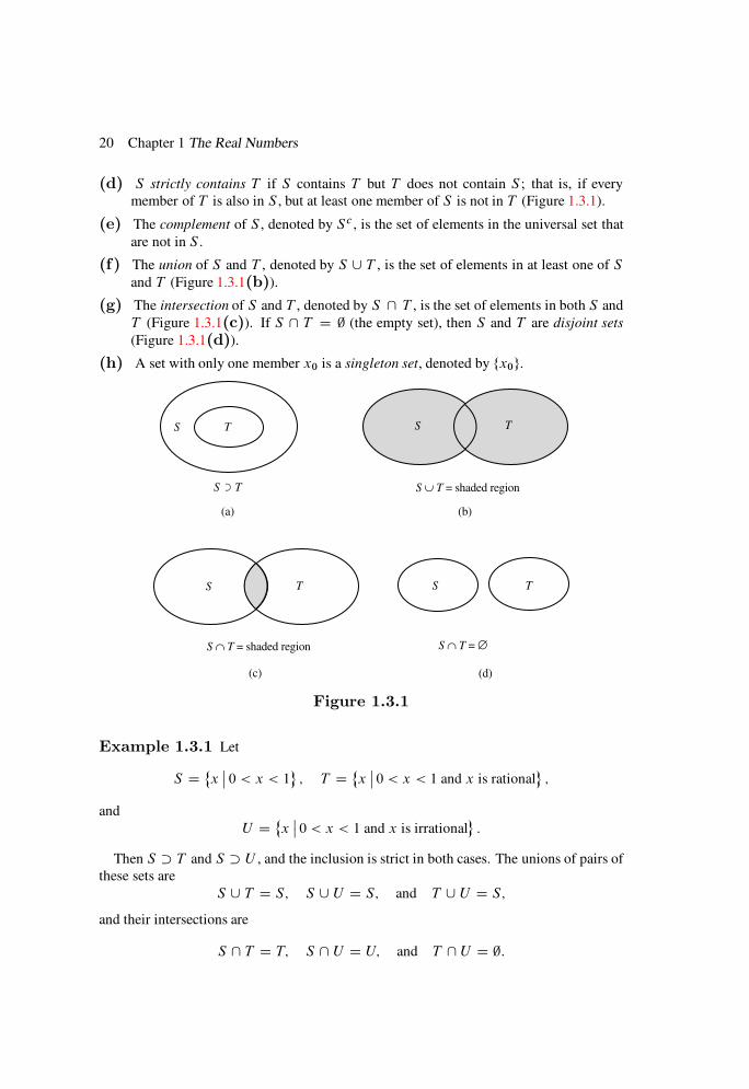
20 Chapter 1 The Real Numbers
(d) S strictly contains T if S contains T but T does not contain S ; that is, if every
member of T is also in S , but at least one member of S is not in T (Figure 1.3.1).
(e) The complement of S , denoted by Sc , is the set of elements in the universal set that
are not in S .
(f) The union of S and T , denoted by S [ T , is the set of elements in at least one of S
and T (Figure 1.3.1(b)).
(g) The intersection of S and T , denoted by S \ T , is the set of elements in both S and
T (Figure 1.3.1(c)). If S \ T D ; (the empty set), then S and T are disjoint sets
(Figure 1.3.1(d)).
(h) A set with only one member x0 is a singleton set, denoted by fx0g.
TS
S T
(a)
S ∪ T = shaded region
(b)
(c) (d)
S ∩ T = shaded region S ∩ T = ∅
TS
TS
TS
Figure 1.3.1
Example 1.3.1 Let
S D˚xˇ0 < x < 1
; T D
˚xˇ0 < x < 1 and x is rational
;
and
U D˚xˇ0 < x < 1 and x is irrational
:
Then S T and S U , and the inclusion is strict in both cases. The unions of pairs of
these sets are
S [ T D S; S [ U D S; and T [ U D S;
and their intersections are
S \ T D T; S \ U D U; and T \ U D ;:
Section 1.3 The Real Line 21
Also,
S U D T and S T D U:
Every set S contains the empty set ;, for to say that ; is not contained in S is to say that
some member of ; is not in S , which is absurd since ; has no members. If S is any set,
then
.Sc/c D S and S \ Sc D ;:If S is a set of real numbers, then S [ Sc D R.
The definitions of union and intersection have generalizations: If F is an arbitrary col-
lection of sets, then [˚SˇS 2 F
is the set of all elements that are members of at least
one of the sets in F , and \˚SˇS 2 F
is the set of all elements that are members of every
set in F . The union and intersection of finitely many sets S1, . . . , Sn are also written asSnkD1 Sk and
TnkD1 Sk . The union and intersection of an infinite sequence fSkg1kD1
of sets
are written asS1
kD1 Sk andT1
kD1 Sk .
Example 1.3.2 If F is the collection of sets
S D˚xˇ < x 1C
; 0 < 1=2;
then
[˚S
ˇS 2 F
D˚xˇ0 < x 3=2
and
\˚S
ˇS 2 F
D˚xˇ1=2 < x 1
:
Example 1.3.3 If, for each positive integer k, the set Sk is the set of real numbers
that can be written as x D m=k for some integer m, thenS1
kD1 Sk is the set of rational
numbers andT1
kD1 Sk is the set of integers.
Open and Closed Sets
If a and b are in the extended reals and a < b, then the open interval .a; b/ is defined by
.a; b/ D˚xˇa < x < b
:
The open intervals .a;1/ and .1; b/ are semi-infinite if a and b are finite, and .1;1/is the entire real line.
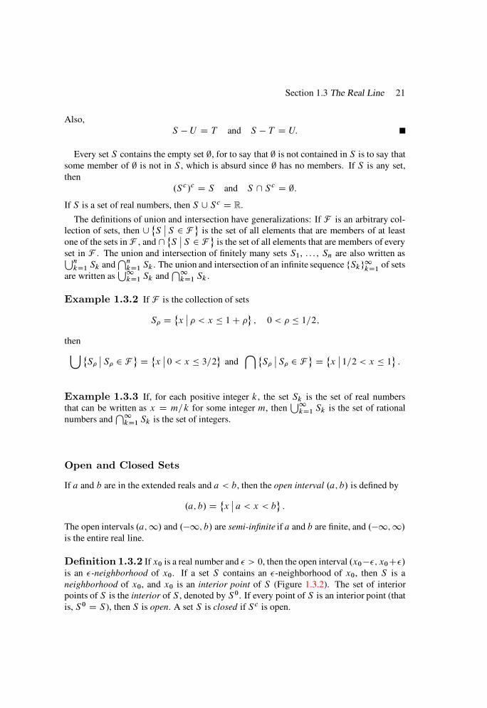
Definition 1.3.2 If x0 is a real number and > 0, then the open interval .x0; x0C/is an -neighborhood of x0. If a set S contains an -neighborhood of x0, then S is a
neighborhood of x0, and x0 is an interior point of S (Figure 1.3.2). The set of interior
points of S is the interior of S , denoted by S0. If every point of S is an interior point (that
is, S0 D S ), then S is open. A set S is closed if Sc is open.

22 Chapter 1 The Real Numbers
( )
x0 + x
0 − x
0
x0 = interior point of S
S = four line segments
Figure 1.3.2
The idea of neighborhood is fundamental and occurs in many other contexts, some of
which we will see later in this book. Whatever the context, the idea is the same: some defi-
nition of “closeness” is given (for example, two real numbers are “close” if their difference
is “small”), and a neighborhood of a point x0 is a set that contains all points sufficiently
close to x0.
Example 1.3.4 An open interval .a; b/ is an open set, because if x0 2 .a; b/ and
minfx0 a; b x0g, then
.x0 ; x0C / .a; b/:
The entire line R D .1;1/ is open, and therefore ; .D Rc/ is closed. However, ; is
also open, for to deny this is to say that ; contains a point that is not an interior point,
which is absurd because ; contains no points. Since ; is open, R .D ;c/ is closed. Thus,
R and ; are both open and closed. They are the only subsets of R with this property
(Exercise 1.3.18).
A deleted neighborhood of a point x0 is a set that contains every point of some neigh-
borhood of x0 except for x0 itself. For example,
S D˚xˇ0 < jx x0j <
is a deleted neighborhood of x0. We also say that it is a deleted -neighborhood of x0.
Theorem 1.3.3
(a) The union of open sets is open:
(b) The intersection of closed sets is closed:
These statements apply to arbitrary collections, finite or infinite, of open and closed sets:
Proof (a) Let G be a collection of open sets and
S D [˚GˇG 2 G
:
If x0 2 S , then x0 2 G0 for some G0 in G , and since G0 is open, it contains some -
neighborhood of x0. Since G0 S , this -neighborhood is in S , which is consequently a
neighborhood of x0. Thus, S is a neighborhood of each of its points, and therefore open,
by definition.
(b) Let F be a collection of closed sets and T D \˚FˇF 2 F
. Then T c D
[˚F c
ˇF 2 F
(Exercise 1.3.7) and, since each F c is open, T c is open, from (a). There-
fore, T is closed, by definition.
Section 1.3 The Real Line 23
Example 1.3.5 If 1 < a < b <1, the set
Œa; b D˚xˇa x b
is closed, since its complement is the union of the open sets .1; a/ and .b;1/. We say
that Œa; b is a closed interval. The set
Œa; b/ D˚xˇa x < b
is a half-closed or half-open interval if 1 < a < b <1, as is
.a; b D˚xˇa < x b
I
however, neither of these sets is open or closed. (Why not?) Semi-infinite closed intervals
are sets of the form
Œa;1/ D˚xˇa x
and .1; a D
˚xˇx a
;
where a is finite. They are closed sets, since their complements are the open intervals
.1; a/ and .a;1/, respectively.
Example 1.3.4 shows that a set may be both open and closed, and Example 1.3.5 shows
that a set may be neither. Thus, open and closed are not opposites in this context, as they
are in everyday speech.
Example 1.3.6 From Theorem 1.3.3 and Example 1.3.4, the union of any collection of
open intervals is an open set. (In fact, it can be shown that every nonempty open subset of
R is the union of open intervals.) From Theorem 1.3.3 and Example 1.3.5, the intersection
of any collection of closed intervals is closed.
It can be shown that the intersection of finitely many open sets is open, and that the
union of finitely many closed sets is closed. However, the intersection of infinitely many
open sets need not be open, and the union of infinitely many closed sets need not be closed
(Exercises 1.3.8 and 1.3.9).
Definition 1.3.4 Let S be a subset of R. Then
(a) x0 is a limit point of S if every deleted neighborhood of x0 contains a point of S .
(b) x0 is a boundary point of S if every neighborhood of x0 contains at least one point
in S and one not in S . The set of boundary points of S is the boundary of S , denoted
by @S . The closure of S , denoted by S , is S D S [ @S .
(c) x0 is an isolated point of S if x0 2 S and there is a neighborhood of x0 that contains
no other point of S .
(d) x0 is exterior to S if x0 is in the interior of Sc . The collection of such points is the
exterior of S .
Example 1.3.7 Let S D .1;1 [ .1; 2/ [ f3g. Then

24 Chapter 1 The Real Numbers
(a) The set of limit points of S is .1;1 [ Œ1; 2.(b) @S D f1; 1; 2; 3g and S D .1;1 [ Œ1; 2[ f3g.(c) 3 is the only isolated point of S .
(d) The exterior of S is .1; 1/ [ .2; 3/[ .3;1/.
Example 1.3.8 For n 1, let
In D
1
2nC 1;1
2n
and S D
1[
nD1
In:
Then
(a) The set of limit points of S is S [ f0g.(b) @S D
˚xˇx D 0 or x D 1=n .n 2/
and S D S [ f0g.
(c) S has no isolated points.
(d) The exterior of S is
.1; 0/ [" 1[
nD1
1
2nC 2;
1
2nC 1
#[1
2;1
:
Example 1.3.9 Let S be the set of rational numbers. Since every interval contains a
rational number (Theorem 1.1.6), every real number is a limit point of S ; thus, S D R.
Since every interval also contains an irrational number (Theorem 1.1.7), every real number
is a boundary point of S ; thus @S D R. The interior and exterior of S are both empty, and
S has no isolated points. S is neither open nor closed.
The next theorem says that S is closed if and only if S D S (Exercise 1.3.14).
Theorem 1.3.5 A set S is closed if and only if no point of Sc is a limit point of S:
Proof Suppose that S is closed and x0 2 Sc . Since Sc is open, there is a neighborhood
of x0 that is contained in Sc and therefore contains no points of S . Hence, x0 cannot be a
limit point of S . For the converse, if no point of Sc is a limit point of S then every point in
Sc must have a neighborhood contained in Sc . Therefore, Sc is open and S is closed.
Theorem 1.3.5 is usually stated as follows.
Corollary 1.3.6 A set is closed if and only if it contains all its limit points:
Theorem 1.3.5 and Corollary 1.3.6 are equivalent. However, we stated the theorem as
we did because students sometimes incorrectly conclude from the corollary that a closed
set must have limit points. The corollary does not say this. If S has no limit points, then the
set of limit points is empty and therefore contained in S . Hence, a set with no limit points
is closed according to the corollary, in agreement with Theorem 1.3.5. For example, any
finite set is closed and so is an infinite set comprised entirely of isolated points, such as the
set of integers.

Section 1.3 The Real Line 25
Open Coverings
A collection H of open sets is an open covering of a set S if every point in S is contained
in a set H belonging to H ; that is, if S [˚HˇH 2 H
.
Example 1.3.10 The sets
S1 D Œ0; 1; S2 D f1; 2; : : : ; n; : : : g;
S3 D1;1
2; : : : ;
1
n; : : :
; and S4 D .0; 1/
are covered by the families of open intervals
H1 Dx 1
N; xC 1
N
ˇˇ 0 < x < 1
; (N D positive integer),
H2 Dn 1
4; nC 1
4
ˇˇ n D 1; 2; : : :
;
H3 D(
1
nC 12
;1
n 12
! ˇˇ n D 1; 2; : : :
);
and
H4 D f.0; /j 0 < < 1g;
respectively.
Theorem 1.3.7 (Heine–Borel Theorem) If H is an open covering of a closed
and bounded subset S of the real line; then S has an open covering eH consisting of finitely
many open sets belonging to H :
Proof Since S is bounded, it has an infimum ˛ and a supremum ˇ, and, since S is
closed, ˛ and ˇ belong to S (Exercise 1.3.17). Define
St D S \ Œ˛; t for t ˛;
and let
F D˚tˇ˛ t ˇ and finitely many sets from H cover St
:
Since Sˇ D S , the theorem will be proved if we can show that ˇ 2 F . To do this, we use
the completeness of the reals.
Since ˛ 2 S , S˛ is the singleton set f˛g, which is contained in some open set H˛ from
H because H covers S ; therefore, ˛ 2 F . Since F is nonempty and bounded above by ˇ,
it has a supremum . First, we wish to show that D ˇ. Since ˇ by definition of F ,
it suffices to rule out the possibility that < ˇ. We consider two cases.
26 Chapter 1 The Real Numbers
CASE 1. Suppose that < ˇ and 62 S . Then, since S is closed, is not a limit point
of S (Theorem 1.3.5). Consequently, there is an > 0 such that
Π; C \ S D ;;
so S D S C. However, the definition of implies that S has a finite subcovering
from H , while S C does not. This is a contradiction.
CASE 2. Suppose that < ˇ and 2 S . Then there is an open set H in H that
contains and, along with , an interval Π; C for some positive . Since S has
a finite covering fH1; : : : ; Hng of sets from H , it follows that S C has the finite covering
fH1; : : : ; Hn; H g. This contradicts the definition of .
Now we know that D ˇ, which is in S . Therefore, there is an open set Hˇ in H that
contains ˇ and along with ˇ, an interval of the form Œˇ ; ˇ C , for some positive .
Since Sˇ is covered by a finite collection of sets fH1; : : : ; Hkg, Sˇ is covered by the
finite collection fH1; : : : ; Hk; Hˇg. Since Sˇ D S , we are finished.
Henceforth, we will say that a closed and bounded set is compact. The Heine–Borel
theorem says that any open covering of a compact set S contains a finite collection that
also covers S . This theorem and its converse (Exercise 1.3.21) show that we could just
as well define a set S of reals to be compact if it has the Heine–Borel property; that is, if
every open covering of S contains a finite subcovering. The same is true of Rn, which we
study in Section 5.1. This definition generalizes to more abstract spaces (called topological
spaces) for which the concept of boundedness need not be defined.
Example 1.3.11 Since S1 in Example 1.3.10 is compact, the Heine–Borel theorem
implies that S1 can be covered by a finite number of intervals from H1. This is easily veri-
fied, since, for example, the 2N intervals from H1 centered at the points xk D k=2N .0 k 2N 1/ cover S1.
The Heine–Borel theorem does not apply to the other sets in Example 1.3.10 since they
are not compact: S2 is unbounded and S3 and S4 are not closed, since they do not contain
all their limit points (Corollary 1.3.6). The conclusion of the Heine–Borel theorem does
not hold for these sets and the open coverings that we have given for them. Each point in
S2 is contained in exactly one set from H2, so removing even one of these sets leaves a
point of S2 uncovered. If eH3 is any finite collection of sets from H3, then
1
n62 [
˚HˇH 2 eH3
for n sufficiently large. Any finite collection f.0; 1/; : : : ; .0; n/g from H4 covers only the
interval .0; max/, where
max D maxf1; : : : ; ng < 1:
The Bolzano–Weierstrass Theorem
As an application of the Heine–Borel theorem, we prove the following theorem of Bolzano
and Weierstrass.
Section 1.3 The Real Line 27
Theorem 1.3.8 (Bolzano–Weierstrass Theorem) Every bounded infinite set
of real numbers has at least one limit point:
Proof We will show that a bounded nonempty set without a limit point can contain only
a finite number of points. If S has no limit points, then S is closed (Theorem 1.3.5) and
every point x of S has an open neighborhoodNx that contains no point of S other than x.
The collection
H D˚Nx
ˇx 2 S
is an open covering for S . Since S is also bounded, Theorem 1.3.7 implies that S can be
covered by a finite collection of sets from H , say Nx1, . . . , Nxn . Since these sets contain
only x1, . . . , xn from S , it follows that S D fx1; : : : ; xng.
1.3 Exercises
1. Find S \ T , .S \ T /c , Sc \ T c , S [ T , .S [ T /c , and Sc [ T c .
(a) S D .0; 1/, T D
12; 3
2
(b) S D
˚xˇx2 > 4
, T D
˚xˇx2 < 9
(c) S D .1;1/, T D ; (d) S D .1;1/, T D .1;1/2. Let Sk D .1 1=k; 2C 1=k, k 1. Find
(a)1[
kD1
Sk (b)1\
kD1
Sk (c)1[
kD1
Sck
(d)1\
kD1
Sck
3. Prove: If A and B are sets and there is a set X such that A [ X D B [ X and
A\ X D B \X , then A D B .
4. Find the largest such that S contains an -neighborhood of x0.
(a) x0 D 34
, S D
12; 1
(b) x0 D 23
, S D
12; 3
2
(c) x0 D 5, S D .1;1/ (d) x0 D 1, S D .0; 2/5. Describe the following sets as open, closed, or neither, and find S0, .Sc/0, and
.S0/c .
(a) S D .1; 2/ [ Œ3;1/ (b) S D .1; 1/ [ .2;1/
(c) S D Œ3;2[ Œ7; 8 (d) S D˚xˇx D integer
6. Prove that .S \ T /c D Sc [ T c and .S [ T /c D Sc \ T c .
7. Let F be a collection of sets and define
I D \˚FˇF 2 F
and U D [
˚FˇF 2 F
:
Prove that (a) I c D [˚F c
ˇF 2 F
and (b) U c D
˚\F c
ˇF 2 F
.
8. (a) Show that the intersection of finitely many open sets is open.

28 Chapter 1 The Real Numbers
(b) Give an example showing that the intersection of infinitely many open sets
may fail to be open.
9. (a) Show that the union of finitely many closed sets is closed.
(b) Give an example showing that the union of infinitely many closed sets may
fail to be closed.
10. Prove:
(a) If U is a neighborhood of x0 and U V , then V is a neighborhood of x0.
(b) If U1, . . . , Un are neighborhoods of x0, so isTn
iD1 Ui .
11. Find the set of limit points of S , @S , S , the set of isolated points of S , and the
exterior of S .
(a) S D .1;2/[ .2; 3/[ f4g [.7;1/(b) S D fall integersg(c) S D [
˚.n; nC 1/
ˇn D integer
(d) S D˚xˇx D 1=n; n D 1; 2; 3; : : :
12. Prove: A limit point of a set S is either an interior point or a boundary point of S .
13. Prove: An isolated point of S is a boundary point of Sc .
14. Prove:
(a) A boundary point of a set S is either a limit point or an isolated point of S .
(b) A set S is closed if and only if S D S .
15. Prove or disprove: A set has no limit points if and only if each of its points is
isolated.
16. (a) Prove: If S is bounded above and ˇ D supS , then ˇ 2 @S .
(b) State the analogous result for a set bounded below.
17. Prove: If S is closed and bounded, then infS and supS are both in S .
18. If a nonempty subset S of R is both open and closed, then S D R.
19. Let S be an arbitrary set. Prove: (a) @S is closed. (b) S0 is open. (c) The exterior
of S is open. (d) The limit points of S form a closed set. (e)SD S .
20. Give counterexamples to the following false statements.
(a) The isolated points of a set form a closed set.
(b) Every open set contains at least two points.
(c) If S1 and S2 are arbitrary sets, then @.S1 [ S2/ D @S1 [ @S2.
(d) If S1 and S2 are arbitrary sets, then @.S1 \ S2/ D @S1 \ @S2.
(e) The supremum of a bounded nonempty set is the greatest of its limit points.
(f) If S is any set, then @.@S/ D @S .
(g) If S is any set, then @S D @S .
(h) If S1 and S2 are arbitrary sets, then .S1 [ S2/0 D S0
1 [ S02 .

Section 1.3 The Real Line 29
21. Let S be a nonempty subset of R such that if H is any open covering of S , then S
has an open covering eH comprised of finitely many open sets from H . Show that
S is compact.
22. A set S is. in a set T if S T S .
(a) Prove: If S and T are sets of real numbers and S T , then S is dense in T
if and only if every neighborhood of each point in T contains a point from S .
(b) State how (a) shows that the definition given here is consistent with the re-
stricted definition of a dense subset of the reals given in Section 1.1.
23. Prove:
(a) .S1 \ S2/0 D S0
1 \ S02 (b) S0
1 [ S02 .S1 [ S2/
0
24. Prove:
(a) @.S1 [ S2/ @S1 [ @S2 (b) @.S1 \ S2/ @S1 [ @S2
(c) @S @S (d) @S D @Sc
(e) @.S T / @S [ @T
CHAPTER 2
Differential Calculus of
Functions of One Variable
IN THIS CHAPTER we study the differential calculus of functions of one variable.
SECTION 2.1 introduces the concept of function and discusses arithmetic operations on
functions, limits, one-sided limits, limits at ˙1, and monotonic functions.
SECTION 2.2 defines continuity and discusses removable discontinuities, composite func-
tions, bounded functions, the intermediate value theorem, uniform continuity, and addi-
tional properties of monotonic functions.
SECTION 2.3 introduces the derivative and its geometric interpretation. Topics covered in-
clude the interchange of differentiation and arithmetic operations, the chain rule, one-sided
derivatives, extreme values of a differentiable function, Rolle’s theorem, the intermediate
value theorem for derivatives, and the mean value theorem and its consequences.
SECTION 2.4 presents a comprehensive discussion of L’Hospital’s rule.
SECTION 2.5 discusses the approximation of a function f by the Taylor polynomials of
f and applies this result to locating local extrema of f . The section concludes with the
extended mean value theorem, which implies Taylor’s theorem.
2.1 FUNCTIONS AND LIMITS
In this section we study limits of real-valued functions of a real variable. You studied
limits in calculus. However, we will look more carefully at the definition of limit and prove
theorems usually not proved in calculus.
A rule f that assigns to each member of a nonempty set D a unique member of a set Y
is a function from D to Y . We write the relationship between a member x of D and the
member y of Y that f assigns to x as
y D f .x/:
The set D is the domain of f , denoted by Df . The members of Y are the possible values
of f . If y0 2 Y and there is an x0 inD such that f .x0/ D y0 then we say that f attains
30

Section 2.1 Functions and Limits 31
or assumes the value y0. The set of values attained by f is the range of f . A real-valued
function of a real variable is a function whose domain and range are both subsets of the
reals. Although we are concerned only with real-valued functions of a real variable in this
section, our definitions are not restricted to this situation. In later sections we will consider
situations where the range or domain, or both, are subsets of vector spaces.
Example 2.1.1 The functions f , g, and h defined on .1;1/ by
f .x/ D x2; g.x/ D sin x; and h.x/ D ex
have ranges Œ0;1/, Œ1; 1, and .0;1/, respectively.
Example 2.1.2 The equation
Œf .x/2 D x (2.1.1)
does not define a function except on the singleton set f0g. If x < 0, no real number satisfies
(2.1.1), while if x > 0, two real numbers satisfy (2.1.1). However, the conditions
Œf .x/2 D x and f .x/ 0
define a function f on Df D Œ0;1/ with values f .x/ Dpx. Similarly, the conditions
Œg.x/2 D x and g.x/ 0
define a function g onDg D Œ0;1/ with values g.x/ D px. The ranges of f and g are
Œ0;1/ and .1; 0, respectively.
It is important to understand that the definition of a function includes the specification
of its domain and that there is a difference between f , the name of the function, and f .x/,
the value of f at x. However, strict observance of these points leads to annoying verbosity,
such as “the function f with domain .1;1/ and values f .x/ D x.” We will avoid this
in two ways: (1) by agreeing that if a function f is introduced without explicitly defining
Df , then Df will be understood to consist of all points x for which the rule defining
f .x/makes sense, and (2) by bearing in mind the distinction between f and f .x/, but not
emphasizing it when it would be a nuisance to do so. For example, we will write “consider
the function f .x/ Dp1 x2,” rather than “consider the function f defined on Œ1; 1
by f .x/ Dp1 x2,” or “consider the function g.x/ D 1= sinx,” rather than “consider
the function g defined for x ¤ k (k D integer) by g.x/ D 1= sinx.” We will also write
f D c (constant) to denote the function f defined by f .x/ D c for all x.
Our definition of function is somewhat intuitive, but adequate for our purposes. More-
over, it is the working form of the definition, even if the idea is introduced more rigorously
to begin with. For a more precise definition, we first define the Cartesian product X Yof two nonempty sets X and Y to be the set of all ordered pairs .x; y/ such that x 2 X and
y 2 Y ; thus,
X Y D˚.x; y/
ˇx 2 X; y 2 Y
:

32 Chapter 2 Differential Calculus of Functions of One Variable
A nonempty subset f of X Y is a function if no x in X occurs more than once as a first
member among the elements of f . Put another way, if .x; y/ and .x; y1/ are in f , then
y D y1. The set of x’s that occur as first members of f is the of f . If x is in the domain
of f , then the unique y in Y such that .x; y/ 2 f is the value of f at x, and we write
y D f .x/. The set of all such values, a subset of Y , is the range of f .
Arithmetic Operations on Functions
Definition 2.1.1 IfDf \Dg ¤ ;; then f Cg; f g; and fg are defined onDf \Dg
by
.f C g/.x/ D f .x/C g.x/;.f g/.x/ D f .x/ g.x/;
and
.fg/.x/ D f .x/g.x/:
The quotient f=g is defined by
f
g
.x/ D f .x/
g.x/
for x in Df \Dg such that g.x/ ¤ 0:
Example 2.1.3 If f .x/ Dp4 x2 and g.x/ D
px 1; then Df D Œ2; 2 and
Dg D Œ1;1/; so f C g; f g; and fg are defined on Df \Dg D Œ1; 2 by
.f C g/.x/ Dp4 x2 C
px 1;
.f g/.x/ Dp4 x2
px 1;
and
.fg/.x/ D .p4 x2/.
px 1/ D
p.4 x2/.x 1/: (2.1.2)
The quotient f=g is defined on .1; 2 by
f
g
.x/ D
r4 x2
x 1:
Although the last expression in (2.1.2) is also defined for 1 < x < 2; it does not
represent fg for such x; since f and g are not defined on .1;2.
Example 2.1.4 If c is a real number, the function cf defined by .cf /.x/ D cf .x/ can
be regarded as the product of f and a constant function. Its domain is Df . The sum and
product of n . 2/ functions f1, . . . , fn are defined by
.f1 C f2 C C fn/.x/ D f1.x/C f2.x/C C fn.x/

Section 2.1 Functions and Limits 33
and
.f1f2 fn/.x/ D f1.x/f2.x/ fn.x/ (2.1.3)
on D DTn
iD1Dfi, provided that D is nonempty. If f1 D f2 D D fn, then (2.1.3)
defines the nth power of f :
.f n/.x/ D .f .x//n :
From these definitions, we can build the set of all polynomials
p.x/ D a0 C a1x C C anxn;
starting from the constant functions and f .x/ D x. The quotient of two polynomials is a
rational function
r.x/ D a0 C a1x C C anxn
b0 C b1x C C bmxm.bm ¤ 0/:
The domain of r is the set of points where the denominator is nonzero.
Limits
The essence of the concept of limit for real-valued functions of a real variable is this: If L
is a real number, then limx!x0f .x/ D L means that the value f .x/ can be made as close
to L as we wish by taking x sufficiently close to x0. This is made precise in the following
definition.
y
x
L +
L −
L
y = f (x)
x0 − δ x
0 + δ x
0
Figure 2.1.1
34 Chapter 2 Differential Calculus of Functions of One Variable
Definition 2.1.2 We say that f .x/ approaches the limit L as x approaches x0, and
write
limx!x0
f .x/ D L;
if f is defined on some deleted neighborhood of x0 and, for every > 0, there is a ı > 0
such that
jf .x/ Lj < (2.1.4)
if
0 < jx x0j < ı: (2.1.5)
Figure 2.1.1 depicts the graph of a function for which limx!x0f .x/ exists.
Example 2.1.5 If c and x are arbitrary real numbers and f .x/ D cx, then
limx!x0
f .x/ D cx0:
To prove this, we write
jf .x/ cx0j D jcx cx0j D jcjjx x0j:
If c ¤ 0, this yields
jf .x/ cx0j < (2.1.6)
if
jx x0j < ı;where ı is any number such that 0 < ı =jcj. If c D 0, then f .x/ cx0 D 0 for all x,
so (2.1.6) holds for all x.
We emphasize that Definition 2.1.2 does not involve f .x0/, or even require that it be
defined, since (2.1.5) excludes the case where x D x0.
Example 2.1.6 If
f .x/ D x sin1
x; x ¤ 0;
then
limx!0
f .x/ D 0
even though f is not defined at x0 D 0, because if
0 < jxj < ı D ;
then
jf .x/ 0j Dˇˇx sin
1
x
ˇˇ jxj < :
On the other hand, the function
g.x/ D sin1
x; x ¤ 0;
has no limit as x approaches 0, since it assumes all values between 1 and 1 in every
neighborhood of the origin (Exercise 2.1.26).
Section 2.1 Functions and Limits 35
The next theorem says that a function cannot have more than one limit at a point.
Theorem 2.1.3 If limx!x0f .x/ exists; then it is unique I that is; if
limx!x0
f .x/ D L1 and limx!x0
f .x/ D L2; (2.1.7)
then L1 D L2:
Proof Suppose that (2.1.7) holds and let > 0. From Definition 2.1.2, there are positive
numbers ı1 and ı2 such that
jf .x/ Li j < if 0 < jx x0j < ıi ; i D 1; 2:
If ı D min.ı1; ı2/, then
jL1 L2j D jL1 f .x/C f .x/ L2j jL1 f .x/j C jf .x/ L2j < 2 if 0 < jx x0j < ı:
We have now established an inequality that does not depend on x; that is,
jL1 L2j < 2:
Since this holds for any positive , L1 D L2.
Definition 2.1.2 is not changed by replacing (2.1.4) with
jf .x/ Lj < K; (2.1.8)
where K is a positive constant, because if either of (2.1.4) or (2.1.8) can be made to hold
for any > 0 by making jx x0j sufficiently small and positive, then so can the other
(Exercise 2.1.5). This may seem to be a minor point, but it is often convenient to work with
(2.1.8) rather than (2.1.4), as we will see in the proof of the following theorem.
A Useful Theorem about Limits
Theorem 2.1.4 If
limx!x0
f .x/ D L1 and limx!x0
g.x/ D L2; (2.1.9)
then
limx!x0
.f C g/.x/ D L1 C L2; (2.1.10)
limx!x0
.f g/.x/ D L1 L2; (2.1.11)
limx!x0
.fg/.x/ D L1L2; (2.1.12)
and, if L2 ¤ 0, (2.1.13)
limx!x0
f
g
.x/ D L1
L2
: (2.1.14)

36 Chapter 2 Differential Calculus of Functions of One Variable
Proof From (2.1.9) and Definition 2.1.2, if > 0, there is a ı1 > 0 such that
jf .x/ L1j < (2.1.15)
if 0 < jx x0j < ı1, and a ı2 > 0 such that
jg.x/ L2j < (2.1.16)
if 0 < jx x0j < ı2. Suppose that
0 < jx x0j < ı D min.ı1; ı2/; (2.1.17)
so that (2.1.15) and (2.1.16) both hold. Then
j.f ˙ g/.x/ .L1 ˙ L2/j D j.f .x/ L1/˙ .g.x/ L2/j jf .x/ L1j C jg.x/ L2j < 2;
which proves (2.1.10) and (2.1.11).
To prove (2.1.12), we assume (2.1.17) and write
j.fg/.x/ L1L2j D jf .x/g.x/ L1L2jD jf .x/.g.x/ L2/C L2.f .x/ L1/j jf .x/jjg.x/ L2j C jL2jjf .x/L1j .jf .x/j C jL2j/ (from (2.1.15) and (2.1.16))
.jf .x/ L1j C jL1j C jL2j/ . C jL1j C jL2j/ from (2.1.15)
.1C jL1j C jL2j/
if < 1 and x satisfies (2.1.17). This proves (2.1.12).
To prove (2.1.14), we first observe that if L2 ¤ 0, there is a ı3 > 0 such that
jg.x/ L2j <jL2j2;
so
jg.x/j > jL2j2
(2.1.18)
if
0 < jx x0j < ı3:
To see this, let L D L2 and D jL2j=2 in (2.1.4). Now suppose that
0 < jx x0j < min.ı1; ı2; ı3/;
so that (2.1.15), (2.1.16), and (2.1.18) all hold. Then
Section 2.1 Functions and Limits 37
ˇˇf
g
.x/ L1
L2
ˇˇ D
ˇˇf .x/g.x/
L1
L2
ˇˇ
D jL2f .x/ L1g.x/jjg.x/L2j
2
jL2j2jL2f .x/ L1g.x/j
D 2
jL2j2jL2Œf .x/ L1C L1ŒL2 g.x/j (from (2.1.18))
2
jL2j2ŒjL2jjf .x/ L1j C jL1jjL2 g.x/j
2
jL2j2.jL2j C jL1j/ (from (2.1.15) and (2.1.16)):
This proves (2.1.14).
Successive applications of the various parts of Theorem 2.1.4 permit us to find limits
without the –ı arguments required by Definition 2.1.2.
Example 2.1.7 Use Theorem 2.1.4 to find
limx!2
9 x2
x C 1and lim
x!2.9 x2/.x C 1/:
Solution If c is a constant, then limx!x0c D c, and, from Example 2.1.5, limx!x0
x Dx0. Therefore, from Theorem 2.1.4,
limx!2
.9 x2/ D limx!2
9 limx!2
x2
D limx!2
9 . limx!2
x/2
D 9 22 D 5;and
limx!2
.x C 1/ D limx!2
x C limx!2
1 D 2C 1 D 3:
Therefore,
limx!2
9 x2
x C 1 Dlimx!2
.9 x2/
limx!2
.x C 1/ D5
3
and
limx!2
.9 x2/.x C 1/ D limx!2
.9 x2/ limx!2
.x C 1/ D 5 3 D 15:
One-Sided Limits
The function
f .x/ D 2x sinpx
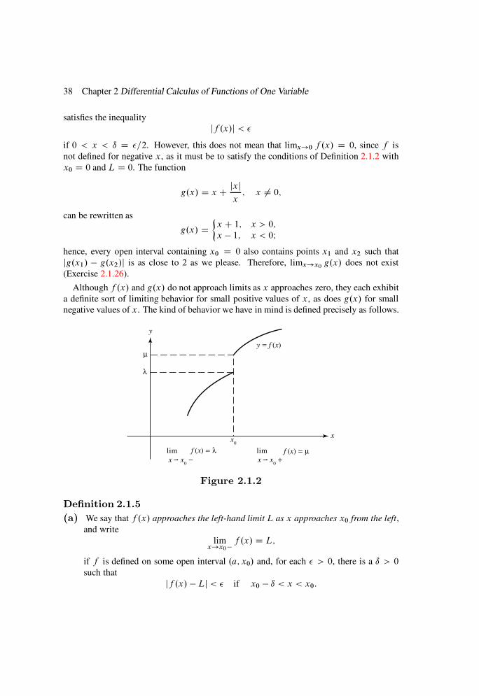
38 Chapter 2 Differential Calculus of Functions of One Variable
satisfies the inequality
jf .x/j <
if 0 < x < ı D =2. However, this does not mean that limx!0 f .x/ D 0, since f is
not defined for negative x, as it must be to satisfy the conditions of Definition 2.1.2 with
x0 D 0 and L D 0. The function
g.x/ D x C jxjx; x ¤ 0;
can be rewritten as
g.x/ Dx C 1; x > 0;
x 1; x < 0Ihence, every open interval containing x0 D 0 also contains points x1 and x2 such that
jg.x1/ g.x2/j is as close to 2 as we please. Therefore, limx!x0g.x/ does not exist
(Exercise 2.1.26).
Although f .x/ and g.x/ do not approach limits as x approaches zero, they each exhibit
a definite sort of limiting behavior for small positive values of x, as does g.x/ for small
negative values of x. The kind of behavior we have in mind is defined precisely as follows.
y
xx
0
x x0 − x x
0 +
f (x) = λ
y = f (x)
f (x) = µlim lim
µ
λ
Figure 2.1.2
Definition 2.1.5
(a) We say that f .x/ approaches the left-hand limit L as x approaches x0 from the left,
and write
limx!x0
f .x/ D L;
if f is defined on some open interval .a; x0/ and, for each > 0, there is a ı > 0
such that
jf .x/ Lj < if x0 ı < x < x0:
Section 2.1 Functions and Limits 39
(b) We say that f .x/ approaches the right-hand limit L as x approaches x0 from the
right, and write
limx!x0C
f .x/ D L;
if f is defined on some open interval .x0; b/ and, for each > 0, there is a ı > 0
such that
jf .x/ Lj < if x0 < x < x0 C ı:
Figure 2.1.2 shows the graph of a function that has distinct left- and right-hand limits at
a point x0.
Example 2.1.8 Let
f .x/ D x
jxj ; x ¤ 0:
If x < 0, then f .x/ D x=x D 1, so
limx!0
f .x/ D 1:
If x > 0, then f .x/ D x=x D 1, so
limx!0C
f .x/ D 1:
Example 2.1.9 Let
g.x/ D x C jxj.1C x/x
sin1
x; x ¤ 0:
If x < 0, then
g.x/ D x sin1
x;
so
limx!0
g.x/ D 0;
since
jg.x/ 0j Dˇˇx sin
1
x
ˇˇ jxj <
if < x < 0; that is, Definition 2.1.5(a) is satisfied with ı D . If x > 0, then
g.x/ D .2C x/ sin1
x;
which takes on every value between 2 and 2 in every interval .0; ı/. Hence, g.x/ does not
approach a right-hand limit at x approaches 0 from the right. This shows that a function
may have a limit from one side at a point but fail to have a limit from the other side.
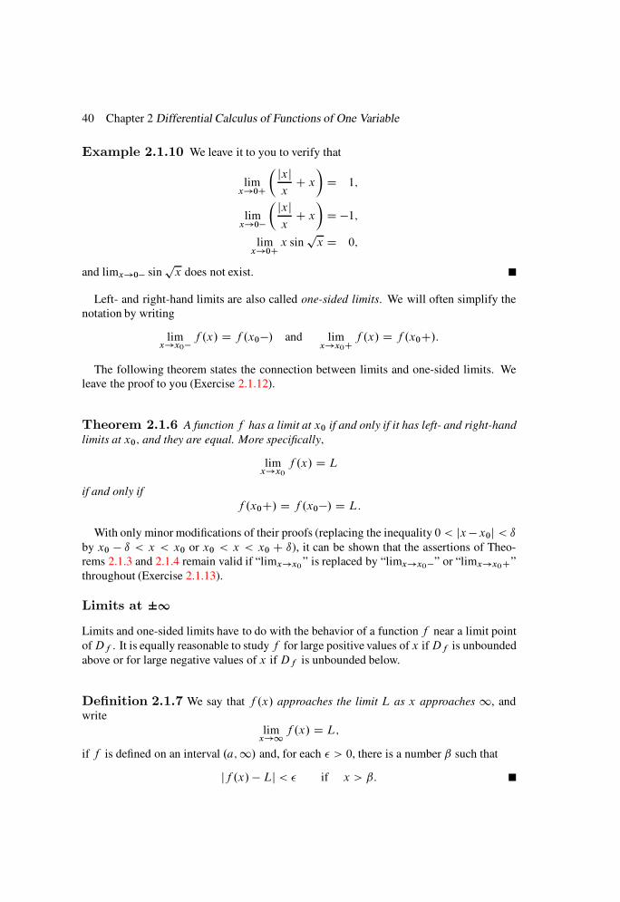
40 Chapter 2 Differential Calculus of Functions of One Variable
Example 2.1.10 We leave it to you to verify that
limx!0C
jxjxC x
D 1;
limx!0
jxjxC x
D 1;
limx!0C
x sinpx D 0;
and limx!0 sinpx does not exist.
Left- and right-hand limits are also called one-sided limits. We will often simplify the
notation by writing
limx!x0
f .x/ D f .x0/ and limx!x0C
f .x/ D f .x0C/:
The following theorem states the connection between limits and one-sided limits. We
leave the proof to you (Exercise 2.1.12).
Theorem 2.1.6 A function f has a limit at x0 if and only if it has left- and right-hand
limits at x0; and they are equal. More specifically;
limx!x0
f .x/ D L
if and only if
f .x0C/ D f .x0/ D L:
With only minor modifications of their proofs (replacing the inequality 0 < jxx0j < ıby x0 ı < x < x0 or x0 < x < x0 C ı), it can be shown that the assertions of Theo-
rems 2.1.3 and 2.1.4 remain valid if “limx!x0” is replaced by “limx!x0” or “limx!x0C”
throughout (Exercise 2.1.13).
Limits at ˙1
Limits and one-sided limits have to do with the behavior of a function f near a limit point
ofDf . It is equally reasonable to study f for large positive values of x ifDf is unbounded
above or for large negative values of x ifDf is unbounded below.
Definition 2.1.7 We say that f .x/ approaches the limit L as x approaches 1, and
write
limx!1
f .x/ D L;
if f is defined on an interval .a;1/ and, for each > 0, there is a number ˇ such that
jf .x/ Lj < if x > ˇ:
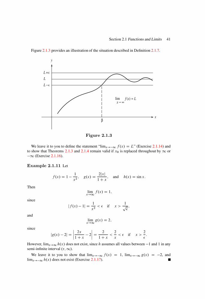
Section 2.1 Functions and Limits 41
Figure 2.1.3 provides an illustration of the situation described in Definition 2.1.7.
x ∞ lim f (x) = L
β
y
L +
L −
L
x
Figure 2.1.3
We leave it to you to define the statement “limx!1 f .x/ D L” (Exercise 2.1.14) and
to show that Theorems 2.1.3 and 2.1.4 remain valid if x0 is replaced throughout by1 or
1 (Exercise 2.1.16).
Example 2.1.11 Let
f .x/ D 1 1
x2; g.x/ D 2jxj
1C x ; and h.x/ D sin x:
Then
limx!1
f .x/ D 1;
since
jf .x/ 1j D 1
x2< if x >
1p;
and
limx!1
g.x/ D 2;
since
jg.x/ 2j Dˇˇ 2x
1C x 2ˇˇ D 2
1C x <2
x< if x >
2
:
However, limx!1 h.x/ does not exist, since h assumes all values between 1 and 1 in any
semi-infinite interval .;1/.We leave it to you to show that limx!1 f .x/ D 1, limx!1 g.x/ D 2, and
limx!1 h.x/ does not exist (Exercise 2.1.17).

42 Chapter 2 Differential Calculus of Functions of One Variable
We will sometimes denote limx!1 f .x/ and limx!1 f .x/ by f .1/ and f .1/,respectively.
Infinite Limits
The functions
f .x/ D 1
x; g.x/ D 1
x2; p.x/ D sin
1
x;
and
q.x/ D 1
x2sin
1
x
do not have limits, or even one-sided limits, at x0 D 0. They fail to have limits in different
ways:
f .x/ increases beyond bound as x approaches 0 from the right and decreases beyond
bound as x approaches 0 from the left;
g.x/ increases beyond bound as x approaches zero;
p.x/ oscillates with ever-increasing frequency as x approaches zero;
q.x/ oscillates with ever-increasing amplitude and frequency as x approaches 0.
The kind of behavior exhibited by f and g near x0 D 0 is sufficiently common and
simple to lead us to define infinite limits.
Definition 2.1.8 We say that f .x/ approaches 1 as x approaches x0 from the left,
and write
limx!x0
f .x/ D1 or f .x0/ D1;
if f is defined on an interval .a; x0/ and, for each real number M , there is a ı > 0 such
that
f .x/ > M if x0 ı < x < x0:
Example 2.1.12 We leave it to you to define the other kinds of infinite limits (Exer-
cises 2.1.19 and 2.1.21) and show that
limx!0
1
xD 1; lim
x!0C
1
xD 1I
limx!0
1
x2D lim
x!0C
1
x2D lim
x!0
1
x2D 1I
limx!1
x2 D limx!1
x2 D 1I
and
limx!1
x3 D1; limx!1
x3 D 1:
Section 2.1 Functions and Limits 43
Throughout this book, “limx!x0f .x/ exists” will mean that
limx!x0
f .x/ D L; where L is finite.
To leave open the possibility that L D ˙1, we will say that
limx!x0
f .x/ exists in the extended reals.
This convention also applies to one-sided limits and limits as x approaches ˙1.
We mentioned earlier that Theorems 2.1.3 and 2.1.4 remain valid if “limx!x0” is re-
placed by “limx!x0” or “limx!x0C.” They are also valid with x0 replaced by ˙1.
Moreover, the counterparts of (2.1.10), (2.1.11), and (2.1.12) in all these versions of The-
orem 2.1.4 remain valid if either or both of L1 and L2 are infinite, provided that their
right sides are not indeterminate (Exercises 2.1.28 and 2.1.29). Equation (2.1.14) and its
counterparts remain valid if L1=L2 is not indeterminate and L2 ¤ 0 (Exercise 2.1.30).
Example 2.1.13 Results like Theorem 2.1.4 yield
limx!1
sinhx D limx!1
ex ex
2D 1
2
lim
x!1ex lim
x!1ex
D 1
2.1 0/ D1;
limx!1
sinhx D limx!1
ex ex
2D 1
2
lim
x!1ex lim
x!1ex
D 1
2.0 1/ D 1;
and
limx!1
ex
xD
limx!1
ex
limx!1
xD 0
1D 0:
Example 2.1.14 If
f .x/ D e2x ex;
we cannot obtain limx!1 f .x/ by writing
limx!1
f .x/ D limx!1
e2x limx!1
ex;
because this produces the indeterminate form11. However, by writing
f .x/ D e2x.1 ex/;
we find that
limx!1
f .x/ D
limx!1
e2x
limx!1
1 limx!1
exD1.1 0/ D1:

44 Chapter 2 Differential Calculus of Functions of One Variable
Example 2.1.15 Let
g.x/ D 2x2 x C 13x2 C 2x 1
:
Trying to find limx!1 g.x/ by applying a version of Theorem 2.1.4 to this fraction as it is
written leads to an indeterminate form (try it!). However, by rewriting it as
g.x/ D 2 1=xC 1=x2
3C 2=x 1=x2; x ¤ 0;
we find that
limx!1
g.x/ Dlim
x!12 lim
x!11=xC lim
x!11=x2
limx!1
3C limx!1
2=x limx!1
1=x2D 2 0C 03C 0 0
D 2
3:
Monotonic Function
A function f is nondecreasing on an interval I if
f .x1/ f .x2/ whenever x1 and x2 are in I and x1 < x2; (2.1.19)
or nonincreasing on I if
f .x1/ f .x2/ whenever x1 and x2 are in I and x1 < x2: (2.1.20)
In either case, f is on I . If can be replaced by < in (2.1.19), f is increasing on I . If can be replaced by > in (2.1.20), f is decreasing on I . In either of these two cases, f is
strictly monotonic on I .
Example 2.1.16 The function
f .x/ D(x; 0 x < 1;
2; 1 x 2;
is nondecreasing on I D Œ0; 2 (Figure 2.1.4), and f is nonincreasing on I D Œ0; 2.
2
21
1
y
x

Section 2.1 Functions and Limits 45
Figure 2.1.4
The function g.x/ D x2 is increasing on Œ0;1/ (Figure 2.1.5),
y
x
y = x2
Figure 2.1.5
and h.x/ D x3 is decreasing on .1;1/ (Figure 2.1.6).
y = − x 3
y
x
Figure 2.1.6

46 Chapter 2 Differential Calculus of Functions of One Variable
In the proof of the following theorem, we assume that you have formulated the definitions
called for in Exercise 2.1.19.
Theorem 2.1.9 Suppose that f is monotonic on .a; b/ and define
˛ D infa<x<b
f .x/ and ˇ D supa<x<b
f .x/:
(a) If f is nondecreasing; then f .aC/ D ˛ and f .b/ D ˇ:(b) If f is nonincreasing; then f .aC/ D ˇ and f .b/ D ˛:
.Here aC D 1 if a D 1 and b D 1 if b D1:/(c) If a < x0 < b, then f .x0C/ and f .x0/ exist and are finite I moreover;
f .x0/ f .x0/ f .x0C/
if f is nondecreasing; and
f .x0/ f .x0/ f .x0C/
if f is nonincreasing:
Proof (a) We first show that f .aC/ D ˛. If
M > ˛, there is an x0 in .a; b/ such that f .x0/ < M . Since f is nondecreasing,
f .x/ < M if a < x < x0. Therefore, if ˛ D 1, then f .aC/ D 1. If ˛ > 1, let
M D ˛C , where > 0. Then ˛ f .x/ < ˛ C , so
jf .x/ ˛j < if a < x < x0: (2.1.21)
If a D 1, this implies that f .1/ D ˛. If a > 1, let ı D x0 a. Then (2.1.21) is
equivalent to
jf .x/ ˛j < if a < x < aC ı;which implies that f .aC/ D ˛.
We now show that f .b/ D ˇ. IfM < ˇ, there is an x0 in .a; b/ such that f .x0/ > M .
Since f is nondecreasing, f .x/ > M if x0 < x < b. Therefore, if ˇ D 1, then
f .b/ D1. If ˇ <1, let M D ˇ , where > 0. Then ˇ < f .x/ ˇ, so
jf .x/ ˇj < if x0 < x < b: (2.1.22)
If b D 1, this implies that f .1/ D ˇ. If b < 1, let ı D b x0. Then (2.1.22) is
equivalent to
jf .x/ ˇj < if b ı < x < b;which implies that f .b/ D ˇ.
(b) The proof is similar to the proof of (a) (Exercise 2.1.34).
(c) Suppose that f is nondecreasing. Applying (a) to f on .a; x0/ and .x0; b/ sepa-
rately shows that
f .x0/ D supa<x<x0
f .x/ and f .x0C/ D infx0<x<b
f .x/:
Section 2.1 Functions and Limits 47
However, if x1 < x0 < x2, then
f .x1/ f .x0/ f .x2/I
hence,
f .x0/ f .x0/ f .x0C/:
We leave the case where f is nonincreasing to you (Exercise 2.1.34).
Limits Inferior and Superior
We now introduce some concepts related to limits. We leave the study of these concepts
mainly to the exercises.
We say that f is bounded on a set S if there is a constantM <1 such that jf .x/j Mfor all x in S .
Definition 2.1.10 Suppose that f is bounded on Œa; x0/, where x0 may be finite or1.
For a x < x0, define
Sf .xI x0/ D supxt<x0
f .t/
and
If .xI x0/ D infxt<x0
f .t/:
Then the left limit superior of f at x0 is defined to be
limx!x0
f .x/ D limx!x0
Sf .xI x0/;
and the left limit inferior of f at x0 is defined to be
limx!x0
f .x/ D limx!x0
If .xI x0/:
(If x0 D1, we define x0 D 1.)
Theorem 2.1.11 If f is bounded on Œa; x0/; then ˇ D limx!x0 f .x/ exists and is
the unique real number with the following properties W(a) If > 0, there is an a1 in Œa; x0/ such that
f .x/ < ˇC if a1 x < x0: (2.1.23)
(b) If > 0 and a1 is in Œa; x0/; then
f .x/ > ˇ for some x 2 Œa1; x0/:
Proof Since f is bounded on Œa; x0/, Sf .xI x0/ is nonincreasing and bounded on
Œa; x0/. By applying Theorem 2.1.9(b) to Sf .xI x0/, we conclude that ˇ exists (finite).
Therefore, if > 0, there is an a in Œa; x0/ such that
ˇ =2 < Sf .xI x0/ < ˇ C =2 if a x < x0: (2.1.24)
48 Chapter 2 Differential Calculus of Functions of One Variable
Since Sf .xI x0/ is an upper bound of˚f .t/
ˇx t < x0
, f .x/ Sf .xI x0/. Therefore,
the second inequality in (2.1.24) implies (2.1.23) with a1 D a. This proves (a). To prove
(b), let a1 be given and define x1 D max.a1; a/. Then the first inequality in (2.1.24)
implies that
Sf .x1I x0/ > ˇ =2: (2.1.25)
Since Sf .x1I x0/ is the supremum of˚f .t/
ˇx1 < t < x0
, there is an x in Œx1; x0/ such
that
f .x/ > Sf .x1I x0/ =2:This and (2.1.25) imply that f .x/ > ˇ . Since x is in Œa1; x0/, this proves (b).
Now we show that there cannot be more than one real number with properties (a) and
(b). Suppose that ˇ1 < ˇ2 and ˇ2 has property (b); thus, if > 0 and a1 is in Œa; x0/,
there is an x in Œa1; x0/ such that f .x/ > ˇ2 . Letting D ˇ2 ˇ1, we see that there
is an x in Œa1; b/ such that
f .x/ > ˇ2 .ˇ2 ˇ1/ D ˇ1;
so ˇ1 cannot have property (a). Therefore, there cannot be more than one real number
that satisfies both (a) and (b).
The proof of the following theorem is similar to this (Exercise 2.1.35).
Theorem 2.1.12 If f is bounded on Œa; x0/; then ˛ D limx!x0 f .x/ exists and is
the unique real number with the following properties:
(a) If > 0; there is an a1 in Œa; x0/ such that
f .x/ > ˛ if a1 x < x0:
(b) If > 0 and a1 is in Œa; x0/; then
f .x/ < ˛ C for some x 2 Œa1; x0/:
2.1 Exercises
1. Each of the following conditions fails to define a function on any domain. State
why.
(a) sinf .x/ D x (b) ef .x/ D jxj
(c) 1C x2 C Œf .x/2 D 0 (d) f .x/Œf .x/ 1 D x2
2. If
f .x/ Dr.x 3/.x C 2/
x 1 and g.x/ Dx2 16x 7
px2 9;
find Df , Df ˙g , Dfg , and Df =g .

Section 2.1 Functions and Limits 49
3. Find Df .
(a) f .x/ D tan x (b) f .x/ D 1p1 j sinxj
(c) f .x/ D 1
x.x 1/(d) f .x/ D sin x
x
(e) eŒf .x/2 D x; f .x/ 0
4. Find limx!x0f .x/, and justify your answers with an –ı proof.
(a) x2 C 2x C 1; x0 D 1 (b)x3 8x 2 ; x0 D 2
(c)1
x2 1 ; x0 D 0 (d)px; x0 D 4
(e)x3 1
.x 1/.x 2/ C x; x0 D 1
5. Prove that Definition 2.1.2 is unchanged if Eqn. (2.1.4) is replaced by
jf .x/ Lj < K;
where K is any positive constant. (That is, limx!x0f .x/ D L according to Defini-
tion 2.1.2 if and only if limx!x0f .x/ D L according to the modified definition.)
6. Use Theorem 2.1.4 and the known limits limx!x0x D x0, limx!x0
c D c to find
the indicated limits.
(a) limx!2
x2 C 2xC 32x3 C 1 (b) lim
x!2
1
x C 1 1
x 1
(c) limx!1
x 1x3 C x2 2x
(d) limx!1
x8 1x4 1
7. Find limx!x0 f .x/ and limx!x0C f .x/, if they exist. Use –ı proofs, where ap-
plicable, to justify your answers.
(a)x C jxjx
; x0 D 0 (b) x cos1
xC sin
1
xC sin
1
jxj ; x0 D 0
(c)jx 1j
x2 C x 2; x0 D 1 (d)
x2 C x 2px C 2
; x0 D 2
8. Prove: If h.x/ 0 for a < x < x0 and limx!x0 h.x/ exists, then limx!x0 h.x/ 0. Conclude from this that if f2.x/ f1.x/ for a < x < x0, then
limx!x0
f2.x/ limx!x0
f1.x/
if both limits exist.
50 Chapter 2 Differential Calculus of Functions of One Variable
9. (a) Prove: If limx!x0f .x/ exists, there is a constant M and a > 0 such that
jf .x/j M if 0 < jx x0j < . (We say then that f is bounded on˚xˇ0 < jx x0j <
.)
(b) State similar results with “limx!x0” replaced by “limx!x0.”
(c) State similar results with “limx!x0” replaced by “limx!x0C.”
10. Suppose that limx!x0f .x/ D L and n is a positive integer. Prove that limx!x0
Œf .x/n DLn (a) by using Theorem 2.1.4 and induction; (b) directly from Definition 2.1.2.
HINT: You will find Exercise 2.1.9 useful for .b/:
11. Prove: If limx!x0f .x/ D L > 0, then limx!x0
pf .x/ D
pL.
12. Prove Theorem 2.1.6.
13. (a) Using the hint stated after Theorem 2.1.6, prove that Theorem 2.1.3 remains
valid with “limx!x0” replaced by “limx!x0.”
(b) Repeat (a) for Theorem 2.1.4.
14. Define the statement “limx!1 f .x/ D L.”
15. Find limx!1 f .x/ if it exists, and justify your answer directly from Definition 2.1.7.
(a)1
x2 C 1(b)
sinx
jxj˛.˛ > 0/ (c)
sinx
jxj˛.˛ 0/
(d) ex sinx (e) tan x (f) ex2
e2x
16. Theorems 2.1.3 and 2.1.4 remain valid with “limx!x0” replaced throughout by
“limx!1” (“limx!1”). How would their proofs have to be changed?
17. Using the definition you gave in Exercise 2.1.14, show that
(a) limx!1
1
1
x2
D 1 (b) lim
x!12jxj1C x D 2
(c) limx!1
sin x does not exist
18. Find limx!1 f .x/, if it exists, for each function in Exercise 2.1.15. Justify your
answers directly from the definition you gave in Exercise 2.1.14.
19. Define
(a) limx!x0
f .x/ D 1 (b) limx!x0C
f .x/ D1 (c) limx!x0C
f .x/ D 1
20. Find
(a) limx!0C
1
x3(b) lim
x!0
1
x3
(c) limx!0C
1
x6(d) lim
x!0
1
x6
(e) limx!x0C
1
.x x0/2k(f) lim
x!x01
.x x0/2kC1
(k D positive integer)
Section 2.1 Functions and Limits 51
21. Define
(a) limx!x0
f .x/ D1 (b) limx!x0
f .x/ D 1
22. Find
(a) limx!0
1
x3(b) lim
x!0
1
x6
(c) limx!x0
1
.x x0/2k(d) lim
x!x0
1
.x x0/2kC1
(k D positive integer)
23. Define
(a) limx!1
f .x/ D 1 (b) limx!1
f .x/ D 1
24. Find
(a) limx!1
x2k (b) limx!1
x2k
(c) limx!1
x2kC1 (d) limx!1
x2kC1
(k=positive integer)
(e) limx!1
px sinx (f) lim
x!1ex
25. Suppose that f and g are defined on .a;1/ and .c;1/ respectively, and that
g.x/ > a if x > c. Suppose also that limx!1 f .x/ D L, where 1 L 1,
and limx!1 g.x/ D 1. Show that limx!1 f .g.x// D L.
26. (a) Prove: limx!x0f .x/ does not exist (finite) if for some 0 > 0, every deleted
neighborhood of x0 contains points x1 and x2 such that
jf .x1/ f .x2/j 0:
(b) Give analogous conditions for the nonexistence of
limx!x0C
f .x/; limx!x0
f .x/; limx!1
f .x/; and limx!1
f .x/:
27. Prove: If 1 < x0 < 1, then limx!x0f .x/ exists in the extended reals if and
only if limx!x0 f .x/ and limx!x0C f .x/ both exist in the extended reals and are
equal, in which case all three are equal.
In Exercises 2.1.28–2.1.30 consider only the case where at least one of L1 and L2 is˙1.
28. Prove: If limx!x0f .x/ D L1, limx!x0
g.x/ D L2, and L1CL2 is not indetermi-
nate, then
limx!x0
.f C g/.x/ D L1 C L2:
52 Chapter 2 Differential Calculus of Functions of One Variable
29. Prove: If limx!1 f .x/ D L1, limx!1 g.x/ D L2, andL1L2 is not indeterminate,
then
limx!1
.fg/.x/ D L1L2:
30. (a) Prove: If limx!x0f .x/ D L1, limx!x0
g.x/ D L2 ¤ 0, and L1=L2 is not
indeterminate, then
limx!x0
f
g
.x/ D L1
L2
:
(b) Show that it is necessary to assume thatL2 ¤ 0 in(a) by considering f .x/ Dsinx, g.x/ D cos x, and x0 D =2.
31. Find
(a) limx!0C
x3 C 2x C 32x4 C 3x2 C 2 (b) lim
x!0
x3 C 2x C 32x4 C 3x2C 2
(c) limx!1
2x4 C 3x2 C 2x3 C 2x C 3 (d) lim
x!12x4 C 3x2 C 2x3 C 2x C 3
(e) limx!1.ex2 ex/ (f) limx!1
x Cpx sinx
2xC ex
32. Find limx!1 r.x/ and limx!1 r.x/ for the rational function
r.x/ D a0 C a1x C C anxn
b0 C b1x C C bmxm;
where an ¤ 0 and bm ¤ 0.
33. Suppose that limx!x0f .x/ exists for every x0 in .a; b/ and g.x/ D f .x/ except
on a set S with no limit points in .a; b/. What can be said about limx!x0g.x/ for
x0 in .a; b/? Justify your answer.
34. Prove Theorem 2.1.9(b), and complete the proof of Theorem 2.1.9(b) in the case
where f is nonincreasing.
35. Prove Theorem 2.1.12.
36. Show that if f is bounded on Œa; x0/, then
(a) limx!x0
f .x/ limx!x0
f .x/.
(b) limx!x0
.f /.x/ D limx!x0
f .x/ and limx!x0
.f /.x/ D limx!x0
f .x/.
(c) limx!x0
f .x/ D limx!x0
f .x/ if and only if limx!x0 f .x/ exists, in which
case
limx!x0
f .x/ D limx!x0
f .x/ D limx!x0
f .x/:
37. Suppose that f and g are bounded on Œa; x0/.

Section 2.2 Continuity 53
(a) Show that
limx!x0
.f C g/.x/ limx!x0
f .x/C limx!x0
g.x/:
(b) Show that
limx!x0
.f C g/.x/ limx!x0
f .x/C limx!x0
g.x/:
(c) State inequalities analogous to those in (a) and (b) for
limx!x0
.f g/.x/ and limx!x0
.f g/.x/:
38. Prove: limx!x0 f .x/ exists (finite) if and only if for each > 0 there is a ı > 0
such that jf .x1/ f .x2/j < if x0 ı < x1, x2 < x0. HINT: For sufficiency;
show that f is bounded on some interval .a; x0/ and
limx!0
f .x/ D limx!x0
f .x/:
Then use Exercise 2.1.36.c/:
39. Suppose that f is bounded on an interval .x0; b. Using Definition 2.1.10 as a guide,
define limx!x0C f .x/ (the right limit superior of f at x0) and limx!x0C f .x/ (the
right limit inferior of f at x0). Then prove that they exist. HINT: Use Theorem 2.1.9:
40. Suppose that f is bounded on an interval .x0; b. Show that limx!x0C f .x/ Dlimx!x0C f .x/ if and only if limx!x0C f .x/ exists, in which case
limx!x0C
f .x/ D limx!x0C
f .x/ D limx!x0C
f .x/:
41. Suppose that f is bounded on an open interval containingx0. Show that limx!x0f .x/
exists if and only if
limx!x0
f .x/ D limx!x0C
f .x/ D limx!x0
f .x/ D limx!x0C
f .x/;
in which case limx!x0f .x/ is the common value of these four expressions.
2.2 CONTINUITY
In this section we study continuous functions of a real variable. We will prove some impor-
tant theorems about continuous functions that, although intuitively plausible, are beyond
the scope of the elementary calculus course. They are accessible now because of our better
understanding of the real number system, especially of those properties that stem from the
completeness axiom.

54 Chapter 2 Differential Calculus of Functions of One Variable
The definitions of
f .x0/ D limx!x0
f .x/; f .x0C/ D limx!x0C
f .x/; and limx!x0
f .x/
do not involve f .x0/ or even require that it be defined. However, the case where f .x0/ is
defined and equal to one or more of these quantities is important.
Definition 2.2.1
(a) We say that f is continuous at x0 if f is defined on an open interval .a; b/ containing
x0 and limx!x0f .x/ D f .x0/.
(b) We say that f is continuous from the left at x0 if f is defined on an open interval
.a; x0/ and f .x0/ D f .x0/.
(c) We say that f is continuous from the right at x0 if f is defined on an open interval
.x0; b/ and f .x0C/ D f .x0/.
The following theorem provides a method for determining whether these definitions are
satisfied. The proof, which we leave to you (Exercise 2.2.1), rests on Definitions 2.1.2,
2.1.5, and 2.2.1.
Theorem 2.2.2
(a) A function f is continuous at x0 if and only if f is defined on an open interval .a; b/
containing x0 and for each > 0 there is a ı > 0 such that
jf .x/ f .x0/j < (2.2.1)
whenever jx x0j < ı:(b) A function f is continuous from the right at x0 if and only if f is defined on an
interval Œx0; b/ and for each > 0 there is a ı > 0 such that (2.2.1) holds whenever
x0 x < x0 C ı:(c) A function f is continuous from the left at x0 if and only if f is defined on an interval
.a; x0 and for each > 0
there is a ı > 0 such that (2.2.1) holds whenever x0 ı < x x0:
From Definition 2.2.1 and Theorem 2.2.2, f is
continuous at x0 if and only if
f .x0/ D f .x0C/ D f .x0/
or, equivalently, if and only if it is continuous from the right and left at x0 (Exercise 2.2.2).
Example 2.2.1 Let f be defined on Œ0; 2 by
f .x/ Dx2; 0 x < 1;x C 1; 1 x 2
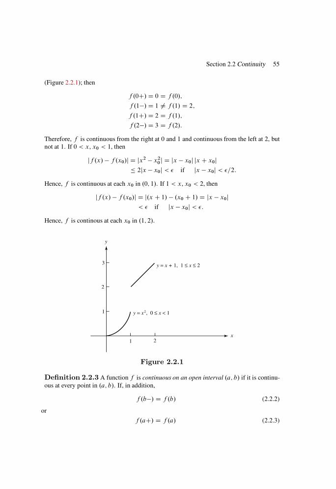
Section 2.2 Continuity 55
(Figure 2.2.1); then
f .0C/D 0 D f .0/;f .1/D 1 ¤ f .1/ D 2;f .1C/D 2 D f .1/;f .2/D 3 D f .2/:
Therefore, f is continuous from the right at 0 and 1 and continuous from the left at 2, but
not at 1. If 0 < x, x0 < 1, then
jf .x/ f .x0/j D jx2 x20 j D jx x0j jx C x0j
2jx x0j < if jx x0j < =2:
Hence, f is continuous at each x0 in .0; 1/. If 1 < x, x0 < 2, then
jf .x/ f .x0/j D j.x C 1/ .x0 C 1/ D jx x0j< if jx x0j < :
Hence, f is continous at each x0 in .1; 2/.
2
3
21
1
y
x
y = x + 1, 1 ≤ x ≤ 2
y = x2, 0 ≤ x < 1
Figure 2.2.1
Definition 2.2.3 A function f is continuous on an open interval .a; b/ if it is continu-
ous at every point in .a; b/. If, in addition,
f .b/ D f .b/ (2.2.2)
or
f .aC/ D f .a/ (2.2.3)
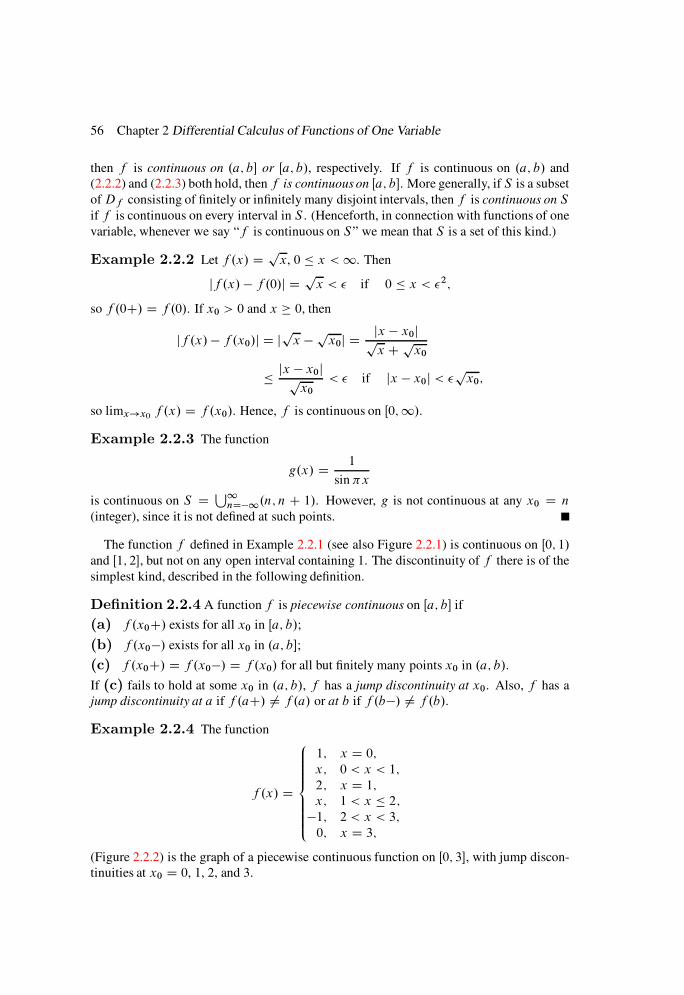
56 Chapter 2 Differential Calculus of Functions of One Variable
then f is continuous on .a; b or Œa; b/, respectively. If f is continuous on .a; b/ and
(2.2.2) and (2.2.3) both hold, then f is continuous on Œa; b. More generally, if S is a subset
ofDf consisting of finitely or infinitely many disjoint intervals, then f is continuous on S
if f is continuous on every interval in S . (Henceforth, in connection with functions of one
variable, whenever we say “f is continuous on S” we mean that S is a set of this kind.)
Example 2.2.2 Let f .x/ Dpx, 0 x <1. Then
jf .x/ f .0/j Dpx < if 0 x < 2;
so f .0C/ D f .0/. If x0 > 0 and x 0, then
jf .x/ f .x0/j D jpx px0j D
jx x0jpx Cpx0
jx x0jpx0
< if jx x0j < px0;
so limx!x0f .x/ D f .x0/. Hence, f is continuous on Œ0;1/.
Example 2.2.3 The function
g.x/ D 1
sinx
is continuous on S DS1
nD1.n; n C 1/. However, g is not continuous at any x0 D n
(integer), since it is not defined at such points.
The function f defined in Example 2.2.1 (see also Figure 2.2.1) is continuous on Œ0; 1/
and Œ1; 2, but not on any open interval containing 1. The discontinuity of f there is of the
simplest kind, described in the following definition.
Definition 2.2.4 A function f is piecewise continuous on Œa; b if
(a) f .x0C/ exists for all x0 in Œa; b/;
(b) f .x0/ exists for all x0 in .a; b;
(c) f .x0C/ D f .x0/ D f .x0/ for all but finitely many points x0 in .a; b/.
If (c) fails to hold at some x0 in .a; b/, f has a jump discontinuity at x0. Also, f has a
jump discontinuity at a if f .aC/ ¤ f .a/ or at b if f .b/ ¤ f .b/.
Example 2.2.4 The function
f .x/ D
8ˆˆ<ˆˆ:
1; x D 0;x; 0 < x < 1;
2; x D 1;x; 1 < x 2;1; 2 < x < 3;
0; x D 3;
(Figure 2.2.2) is the graph of a piecewise continuous function on Œ0; 3, with jump discon-
tinuities at x0 D 0, 1, 2, and 3.
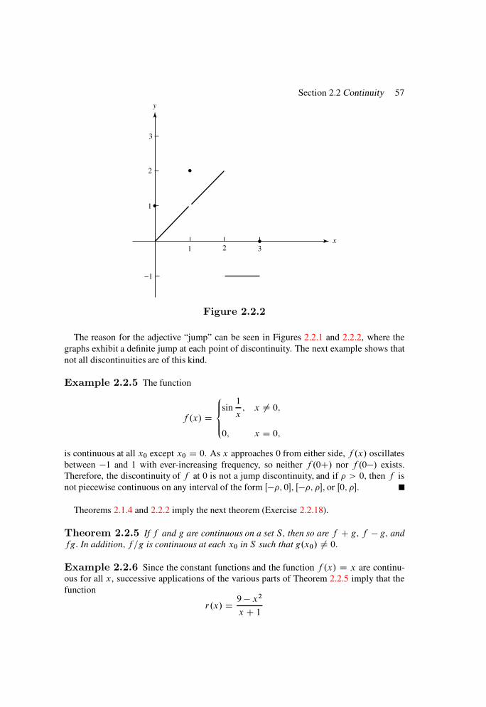
Section 2.2 Continuity 57
2
3
2 31
1
−1
y
x
Figure 2.2.2
The reason for the adjective “jump” can be seen in Figures 2.2.1 and 2.2.2, where the
graphs exhibit a definite jump at each point of discontinuity. The next example shows that
not all discontinuities are of this kind.
Example 2.2.5 The function
f .x/ D
8<
:
sin1
x; x ¤ 0;
0; x D 0;
is continuous at all x0 except x0 D 0. As x approaches 0 from either side, f .x/ oscillates
between 1 and 1 with ever-increasing frequency, so neither f .0C/ nor f .0/ exists.
Therefore, the discontinuity of f at 0 is not a jump discontinuity, and if > 0, then f is
not piecewise continuous on any interval of the form Œ; 0, Œ; , or Œ0; .
Theorems 2.1.4 and 2.2.2 imply the next theorem (Exercise 2.2.18).
Theorem 2.2.5 If f and g are continuous on a set S; then so are f C g; f g; and
fg: In addition; f =g is continuous at each x0 in S such that g.x0/ ¤ 0:
Example 2.2.6 Since the constant functions and the function f .x/ D x are continu-
ous for all x, successive applications of the various parts of Theorem 2.2.5 imply that the
function
r.x/ D9 x2
x C 1
58 Chapter 2 Differential Calculus of Functions of One Variable
is continuous for all x except x D 1 (see Example 2.1.7). More generally, by starting
from Theorem 2.2.5 and using
induction, it can be shown that if f1, f2, . . . , fn are continuous on a set S , then so are
f1 C f2 C C fn and f1f2 fn. Therefore, any rational function
r.x/ D a0 C a1x C C anxn
b0 C b1x C C bmxm.bm ¤ 0/
is continuous for all values of x except those for which its denominator vanishes.
Removable Discontinuities
Let f be defined on a deleted neighborhood of x0 and discontinuous (perhaps even unde-
fined) at x0. We say that f has a at x0 if limx!x0f .x/ exists. In this case, the function
g.x/ D
8<:f .x/ if x 2 Df and x ¤ x0;
limx!x0
f .x/ if x D x0;
is continuous at x0.
Example 2.2.7 The function
f .x/ D x sin1
x
is not defined at x0 D 0, and therefore certainly not continuous there, but limx!0 f .x/ D 0(Example 2.1.6). Therefore, f has a removable discontinuity at 0.
The function
f1.x/ D sin1
x
is undefined at 0 and its discontinuity there is not removable, since limx!0 f1.x/ does not
exist (Example 2.2.5).
Composite Functions
We have seen that the investigation of limits and continuity can be simplified by regarding a
given function as the result of addition, subtraction, multiplication, and division of simpler
functions. Another operation useful in this connection is composition of functions; that is,
substitution of one function into another.
Definition 2.2.6 Suppose that f and g are functions with domains Df and Dg . If
Dg has a nonempty subset T such that g.x/ 2 Df whenever x 2 T , then the composite
function f ı g is defined on T by
.f ı g/.x/ D f .g.x//:

Section 2.2 Continuity 59
Example 2.2.8 If
f .x/ D logx and g.x/ D 1
1 x2;
then
Df D .0;1/ and Dg D˚xˇx ¤ ˙1
:
Since g.x/ > 0 if x 2 T D .1; 1/, the composite function f ı g is defined on .1; 1/ by
.f ı g/.x/ D log1
1 x2:
We leave it to you to verify that g ı f is defined on .0; 1=e/[ .1=e; e/[ .e;1/ by
.g ı f /.x/ D 1
1 .log x/2:
The next theorem says that the composition of continuous functions is continuous.
Theorem 2.2.7 Suppose that g is continuous at x0; g.x0/ is an interior point of Df ;
and f is continuous at g.x0/: Then f ı g is continuous at x0:
Proof Suppose that > 0. Since g.x0/ is an interior point of Df and f is continuous
at g.x0/, there is a ı1 > 0 such that f .t/ is defined and
jf .t/ f .g.x0//j < if jt g.x0/j < ı1: (2.2.4)
Since g is continuous at x0, there is a ı > 0 such that g.x/ is defined and
jg.x/ g.x0/j < ı1 if jx x0j < ı: (2.2.5)
Now (2.2.4) and (2.2.5) imply that
jf .g.x// f .g.x0//j < if jx x0j < ı:
Therefore, f ı g is continuous at x0.
See Exercise 2.2.22 for a related result concerning limits.
Example 2.2.9 In Examples 2.2.2 and 2.2.6 we saw that the function
f .x/ Dpx
is continuous for x > 0, and the function
g.x/ D 9 x2
x C 1is continuous for x ¤ 1. Since g.x/ > 0 if x < 3 or 1 < x < 3, Theorem 2.2.7
implies that the function
.f ı g/.x/ D
s9 x2
x C 1is continuous on .1;3/ [ .1; 3/. It is also continuous from the left at 3 and 3.
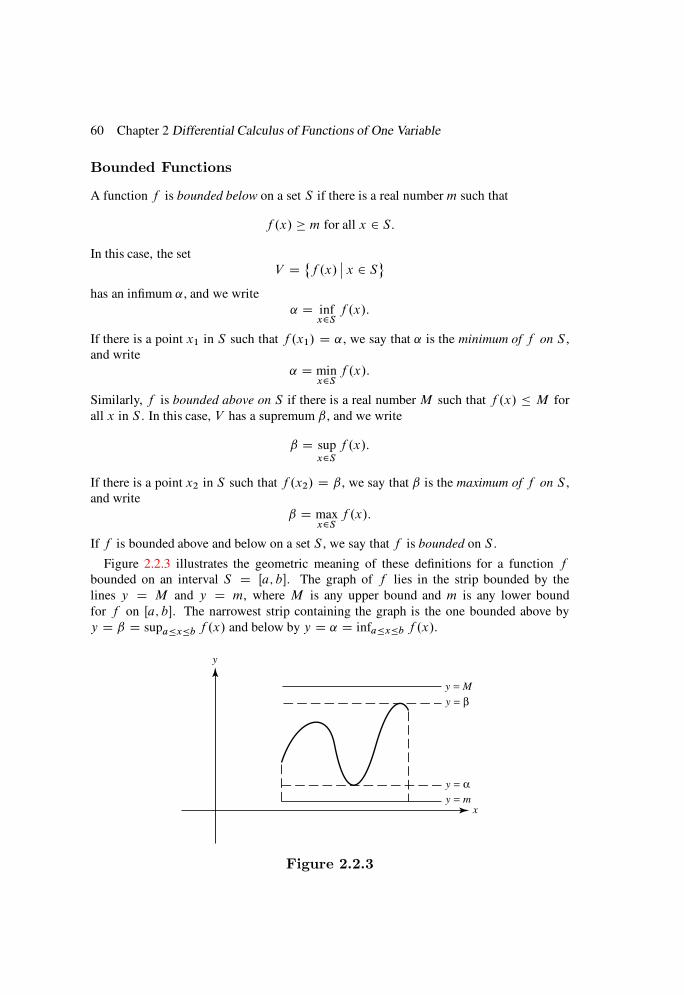
60 Chapter 2 Differential Calculus of Functions of One Variable
Bounded Functions
A function f is bounded below on a set S if there is a real number m such that
f .x/ m for all x 2 S:
In this case, the set
V D˚f .x/
ˇx 2 S
has an infimum ˛, and we write
˛ D infx2S
f .x/:
If there is a point x1 in S such that f .x1/ D ˛, we say that ˛ is the minimum of f on S ,
and write
˛ D minx2S
f .x/:
Similarly, f is bounded above on S if there is a real number M such that f .x/ M for
all x in S . In this case, V has a supremum ˇ, and we write
ˇ D supx2S
f .x/:
If there is a point x2 in S such that f .x2/ D ˇ, we say that ˇ is the maximum of f on S ,
and write
ˇ D maxx2S
f .x/:
If f is bounded above and below on a set S , we say that f is bounded on S .
Figure 2.2.3 illustrates the geometric meaning of these definitions for a function f
bounded on an interval S D Œa; b. The graph of f lies in the strip bounded by the
lines y D M and y D m, where M is any upper bound and m is any lower bound
for f on Œa; b. The narrowest strip containing the graph is the one bounded above by
y D ˇ D supaxb f .x/ and below by y D ˛ D infaxb f .x/.
y
x
y = α
y = β
y = m
y = M
Figure 2.2.3
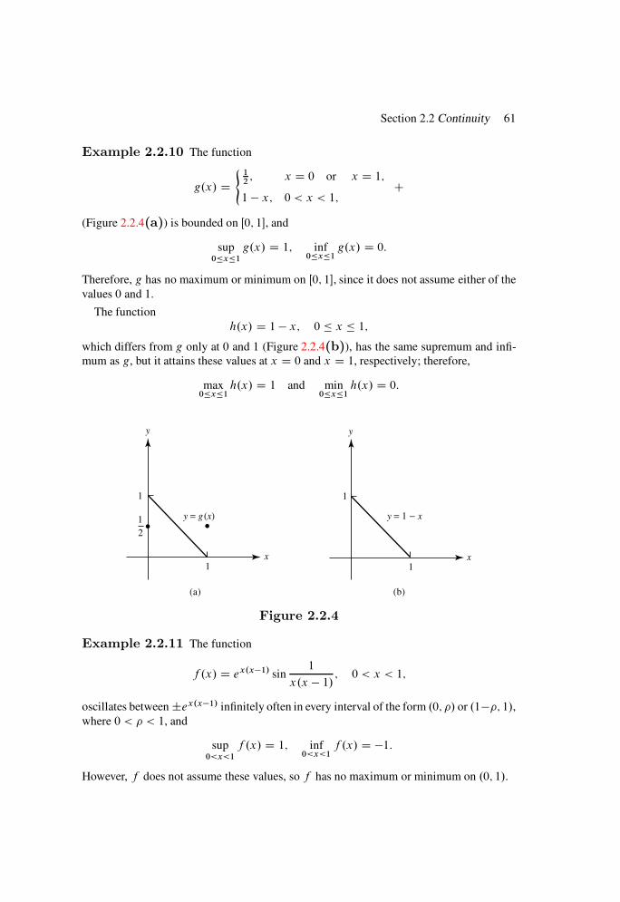
Section 2.2 Continuity 61
Example 2.2.10 The function
g.x/ D(
12; x D 0 or x D 1;1 x; 0 < x < 1;
C
(Figure 2.2.4(a)) is bounded on Œ0; 1, and
sup0x1
g.x/ D 1; inf0x1
g.x/ D 0:
Therefore, g has no maximum or minimum on Œ0; 1, since it does not assume either of the
values 0 and 1.
The function
h.x/ D 1 x; 0 x 1;which differs from g only at 0 and 1 (Figure 2.2.4(b)), has the same supremum and infi-
mum as g, but it attains these values at x D 0 and x D 1, respectively; therefore,
max0x1
h.x/ D 1 and min0x1
h.x/ D 0:
2
1
1
1
y
x1
1
y
x
(a) (b)
y = g (x) y = 1 − x
Figure 2.2.4
Example 2.2.11 The function
f .x/ D ex.x1/ sin1
x.x 1/ ; 0 < x < 1;
oscillates between˙ex.x1/ infinitely often in every interval of the form .0; / or .1; 1/,where 0 < < 1, and
sup0<x<1
f .x/ D 1; inf0<x<1
f .x/ D 1:
However, f does not assume these values, so f has no maximum or minimum on .0; 1/.

62 Chapter 2 Differential Calculus of Functions of One Variable
Theorem 2.2.8 If f is continuous on a finite closed interval Œa; b; then f is bounded
on Œa; b:
Proof Suppose that t 2 Œa; b. Since f is continuous at t , there is an open interval It
containing t such that
jf .x/ f .t/j < 1 if x 2 It \ Œa; b: (2.2.6)
(To see this, set D 1 in (2.2.1), Theorem 2.2.2.) The collection H D˚It
ˇa t b
is
an open covering of Œa; b. Since Œa; b is compact, the Heine–Borel theorem implies that
there are finitely many points t1, t2, . . . , tn such that the intervals It1 , It2 , . . . , Itn cover
Œa; b. According to (2.2.6) with t D ti ,
jf .x/ f .ti /j < 1 if x 2 Iti \ Œa; b:
Therefore,
jf .x/j D j.f .x/ f .ti //C f .ti /j jf .x/ f .ti /j C jf .ti /j
1C jf .ti /j if x 2 Iti \ Œa; b:(2.2.7)
Let
M D 1C max1in
jf .ti/j:
Since Œa; b Sn
iD1
Iti \ Œa; b
, (2.2.7) implies that jf .x/j M if x 2 Œa; b.
This proof illustrates the utility of the Heine–Borel theorem, which allows us to choose
M as the largest of a finite set of numbers.
Theorem 2.2.8 and the completeness of the reals imply that
if f is continuous on a finite closed interval Œa; b, then f has an infimum and a supre-
mum on Œa; b. The next theorem shows that f actually assumes these values at some
points in Œa; b.
Theorem 2.2.9 Suppose that f is continuous on a finite closed interval Œa; b: Let
˛ D infaxb
f .x/ and ˇ D supaxb
f .x/:
Then ˛ and ˇ are respectively the minimum and maximum of f on Œa; bI that is; there are
points x1 and x2 in Œa; b such that
f .x1/ D ˛ and f .x2/ D ˇ:
Proof We show that x1 exists and leave it to you to show that x2 exists (Exercise 2.2.24).
Suppose that there is no x1 in Œa; b such that f .x1/ D ˛. Then f .x/ > ˛ for all
x 2 Œa; b. We will show that this leads to a contradiction.
Suppose that t 2 Œa; b. Then f .t/ > ˛, so
f .t/ >f .t/C ˛
2> ˛:
Section 2.2 Continuity 63
Since f is continuous at t , there is an open interval It about t such that
f .x/ >f .t/C ˛
2if x 2 It \ Œa; b (2.2.8)
(Exercise 2.2.15). The collection H D˚It
ˇa t b
is an open covering of Œa; b. Since
Œa; b is compact, the Heine–Borel theorem implies that there are finitely many points t1,
t2, . . . , tn such that the intervals It1 , It2 , . . . , Itn cover Œa; b. Define
˛1 D min1in
f .ti /C ˛2
:
Then, since Œa; b Sn
iD1.Iti \ Œa; b/, (2.2.8) implies that
f .t/ > ˛1; a t b:
But ˛1 > ˛, so this contradicts the definition of ˛. Therefore, f .x1/ D ˛ for some x1 in
Œa; b.
Example 2.2.12 We used the compactness of Œa; b in the proof of Theorem 2.2.9
when we invoked the Heine–Borel theorem. To see that compactness is essential to the
proof, consider the function
g.x/ D 1 .1 x/ sin1
x;
which is continuous and has supremum 2 on the noncompact interval .0; 1, but does not
assume its supremum on .0; 1, since
g.x/ 1C .1 x/ˇˇsin
1
x
ˇˇ
1C .1 x/ < 2 if 0 < x 1:
As another example, consider the function
f .x/ D ex;
which is continuous and has infimum 0, which it does not attain, on the noncompact interval
.0;1/.
The next theorem shows that if f is continuous on a finite closed interval Œa; b, then f
assumes every value between f .a/ and f .b/ as x varies from a to b (Figure 2.2.5, page 64).
Theorem 2.2.10 (Intermediate Value Theorem) Suppose that f is con-
tinuous on Œa; b; f .a/ ¤ f .b/; and is between f .a/ and f .b/: Then f .c/ D for
some c in .a; b/:

64 Chapter 2 Differential Calculus of Functions of One Variable
a bxx
y
y = f (x)
y = µ
Figure 2.2.5
Proof Suppose that f .a/ < < f .b/. The set
S D˚xˇa x b and f .x/
is bounded and nonempty. Let c D supS . We will show that f .c/ D . If f .c/ > ,
then c > a and, since f is continuous at c, there is an > 0 such that f .x/ > if
c < x c (Exercise 2.2.15). Therefore, c is an upper bound for S , which
contradicts the definition of c as the supremum of S . If f .c/ < , then c < b and there is
an > 0 such that f .x/ < for c x < c C , so c is not an upper bound for S . This is
also a contradiction. Therefore, f .c/ D .
The proof for the case where f .b/ < < f .a/ can be obtained by applying this result
to f .
Uniform Continuity
Theorem 2.2.2 and Definition 2.2.3 imply that a
function f is continuous on a subset S of its domain if for each > 0 and each x0 in S ,
there is a ı > 0, which may depend upon x0 as well as , such that
jf .x/ f .x0/j < if jx x0j < ı and x 2 Df :
The next definition introduces another kind of continuity on a set S .
Definition 2.2.11 A function f is uniformly continuous on a subset S of its domain
if, for every > 0, there is a ı > 0 such that
jf .x/ f .x0/j < whenever jx x0j < ı and x; x0 2 S:
We emphasize that in this definition ı depends only on and S and not on the particular
choice of x and x0, provided that they are both in S .
Example 2.2.13 The function
f .x/ D 2x
Section 2.2 Continuity 65
is uniformly continuous on .1;1/, since
jf .x/ f .x0/j D 2jx x0j < if jx x0j < =2:
Example 2.2.14 If 0 < r <1, then the function
g.x/ D x2
is uniformly continuous on Œr; r . To see this, note that
jg.x/ g.x0/ D jx2 .x0/2j D jx x0j jxC x0j 2r jx x0j;
so
jg.x/ g.x0/j < if jx x0j < ı D
2rand r x; x0 r:
Often a concept is clarified by considering its negation: a function f is not uniformly
continuous on S if there is an 0 > 0 such that if ı is any positive number, there are points
x and x0 in S such that
jx x0j < ı but jf .x/ f .x0/j 0:
Example 2.2.15 The function g.x/ D x2 is uniformly continuous on Œr; r for any
finite r (Example 2.2.14), but not on .1;1/. To see this, we will show that if ı > 0
there are real numbers x and x0 such that
jx x0j D ı=2 and jg.x/ g.x0/j 1:
To this end, we write
jg.x/ g.x0/j D jx2 .x0/2j D jx x0j jx C x0j:
If jx x0j D ı=2 and x; x0 > 1=ı, then
jx x0j jx C x0j >ı
2
1
ıC1
ı
D 1:
Example 2.2.16 The function
f .x/ D cos1
x
is continuous on .0; 1 (Exercise 2.2.23(i)). However, f is not uniformly continuous on
.0; 1, since ˇˇf1
n
f
1
.nC 1/
ˇˇ D 2; n D 1; 2; : : : :
Examples 2.2.15 and 2.2.16 show that a function may be continuous but not uniformly
continuous on an interval. The next theorem shows that this cannot happen if the interval
is closed and bounded, and therefore compact.
66 Chapter 2 Differential Calculus of Functions of One Variable
Theorem 2.2.12 If f is continuous on a closed and bounded interval Œa; b; then f
is uniformly continuous on Œa; b:
Proof Suppose that > 0. Since f is continuous on Œa; b, for each t in Œa; b there is
a positive number ıt such that
jf .x/ f .t/j <
2if jx t j < 2ıt and x 2 Œa; b: (2.2.9)
If It D .t ıt ; t C ıt /, the collection
H D˚It
ˇt 2 Œa; b
is an open covering of Œa; b. Since Œa; b is compact, the Heine–Borel theorem implies that
there are finitely many points t1, t2, . . . , tn in Œa; b such that It1 , It2 , . . . , Itn cover Œa; b.
Now define
ı D minfıt1 ; ıt2; : : : ; ıtng: (2.2.10)
We will show that if
jx x0j < ı and x; x0 2 Œa; b; (2.2.11)
then jf .x/ f .x0/j < .From the triangle inequality,
jf .x/ f .x0/j D j .f .x/ f .tr //C .f .tr / f .x0// j jf .x/ f .tr/j C jf .tr/ f .x0/j: (2.2.12)
Since It1 , It2 , . . . , Itn cover Œa; b, xmust be in one of these intervals. Suppose that x 2 Itr ;
that is,
jx tr j < ıtr : (2.2.13)
From (2.2.9) with t D tr ,
jf .x/ f .tr /j <
2: (2.2.14)
From (2.2.11), (2.2.13), and the triangle inquality,
jx0 tr j D j.x0 x/C .x tr/j jx0 xj C jx tr j < ı C ıtr 2ıtr :
Therefore, (2.2.9) with t D tr and x replaced by x0 implies that
jf .x0/ f .tr/j <
2:
This, (2.2.12), and (2.2.14) imply that jf .x/ f .x0/j < .This proof again shows the utility of the Heine–Borel theorem, which allowed us to
define ı in (2.2.10) as the smallest of a finite set of positive numbers, so that ı is sure to be
positive. (An infinite set of positive numbers may fail to have a smallest positive member;
for example, consider the open interval .0; 1/.)
Corollary 2.2.13 If f is continuous on a set T; then f is uniformly continuous on
any finite closed interval contained in T:

Section 2.2 Continuity 67
Applied to Example 2.2.16, Corollary 2.2.13 implies that the function g.x/ D cos 1=x
is uniformly continuous on Œ; 1 if 0 < < 1.
More About Monotonic Functions
Theorem 2.1.9 implies that if f is monotonic on an interval I , then f is either continuous
or has a jump discontinuity at each x0 in I . This and Theorem 2.2.10 provide the key to
the proof of the following theorem.
Theorem 2.2.14 If f is monotonic and nonconstant on Œa; b; then f is continuous on
Œa; b if and only if its rangeRf D˚f .x/
ˇx 2 Œa; b
is the closed interval with endpoints
f .a/ and f .b/:
Proof We assume that f is nondecreasing, and leave the case where f is nonincreasing
to you (Exercise 2.2.34). Theorem 2.1.9(a) implies that the set eRf D˚f .x/
ˇx 2 .a; b/
is a subset of the open interval .f .aC/; f .b//. Therefore,
Rf D ff .a/g [ eRf [ ff .b/g ff .a/g [ .f .aC/; f .b// [ ff .b/g: (2.2.15)
Now suppose that f is continuous on Œa; b. Then f .a/ D f .aC/, f .b/ D f .b/, so
(2.2.15) implies that Rf Œf .a/; f .b/. If f .a/ < < f .b/, then Theorem 2.2.10
implies that D f .x/ for some x in .a; b/. Hence, Rf D Œf .a/; f .b/.For the converse, suppose that Rf D Œf .a/; f .b/. Since f .a/ f .aC/ and f .b/
f .b/, (2.2.15) implies that f .a/ D f .aC/ and f .b/ D f .b/. We know from Theo-
rem 2.1.9(c) that if f is nondecreasing and a < x0 < b, then
f .x0/ f .x0/ f .x0C/:
If either of these inequalities is strict, Rf cannot be an interval. Since this contradicts
our assumption, f .x0/ D f .x0/ D f .x0C/. Therefore, f is continuous at x0 (Exer-
cise 2.2.2). We can now conclude that f is continuous on Œa; b.
Theorem 2.2.14 implies the following theorem.
Theorem 2.2.15 Suppose that f is increasing and continuous on Œa; b; and let f .a/ Dc and f .b/ D d: Then there is a unique function g defined on Œc; d such that
g.f .x// D x; a x b; (2.2.16)
and
f .g.y// D y; c y d: (2.2.17)
Moreover; g is continuous and increasing on Œc; d :
Proof We first show that there is a function g satisfying (2.2.16) and (2.2.17). Since f
is continuous, Theorem 2.2.14 implies that for each y0 in Œc; d there is an x0 in Œa; b such
that
f .x0/ D y0; (2.2.18)
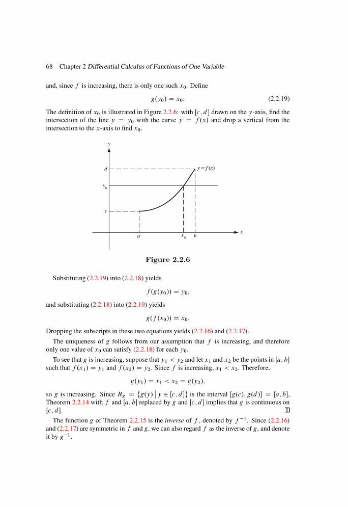
68 Chapter 2 Differential Calculus of Functions of One Variable
and, since f is increasing, there is only one such x0. Define
g.y0/ D x0: (2.2.19)
The definition of x0 is illustrated in Figure 2.2.6: with Œc; d drawn on the y-axis, find the
intersection of the line y D y0 with the curve y D f .x/ and drop a vertical from the
intersection to the x-axis to find x0.
y
d
c
a bx
y = f (x)
x0
y0
Figure 2.2.6
Substituting (2.2.19) into (2.2.18) yields
f .g.y0// D y0;
and substituting (2.2.18) into (2.2.19) yields
g.f .x0// D x0:
Dropping the subscripts in these two equations yields (2.2.16) and (2.2.17).
The uniqueness of g follows from our assumption that f is increasing, and therefore
only one value of x0 can satisfy (2.2.18) for each y0.
To see that g is increasing, suppose that y1 < y2 and let x1 and x2 be the points in Œa; b
such that f .x1/ D y1 and f .x2/ D y2. Since f is increasing, x1 < x2. Therefore,
g.y1/ D x1 < x2 D g.y2/;
so g is increasing. Since Rg D˚g.y/
ˇy 2 Œc; d
is the interval Œg.c/; g.d/ D Œa; b,
Theorem 2.2.14 with f and Œa; b replaced by g and Œc; d implies that g is continuous on
Œc; d .
The function g of Theorem 2.2.15 is the inverse of f , denoted by f 1. Since (2.2.16)
and (2.2.17) are symmetric in f and g, we can also regard f as the inverse of g, and denote
it by g1.

Section 2.2 Continuity 69
Example 2.2.17 If
f .x/ D x2; 0 x R;then
f 1.y/ D g.y/ D py; 0 y R2:
Example 2.2.18 If
f .x/ D 2x C 4; 0 x 2;then
f 1.y/ D g.y/ D y 42
; 4 y 8:
2.2 Exercises
1. Prove Theorem 2.2.2.
2. Prove that a function f is continuous at x0 if and only if
limx!x0
f .x/ D limx!x0C
f .x/ D f .x0/:
3. Determine whether f is continuous or discontinuous from the right or left at x0.
(a) f .x/ Dpx .x0 D 0/ (b) f .x/ D
px .x0 > 0/
(c) f .x/ D 1
x.x0 D 0/ (d) f .x/ D x2 .x0 arbitrary/
(e) f .x/ Dx sin 1=x; x ¤ 0;1; x D 0 .x0 D 0/
(f) f .x/ Dx sin 1=x; x ¤ 00; x D 0 .x0 D 0/
(g) f .x/ D
8<:x C jxj.1C x/
xsin
1
x; x ¤ 0
1; x D 0.x0 D 0/
4. Let f be defined on Œ0; 2 by
f .x/ D(x2; 0 x < 1;
x C 1; 1 x 2:
On which of the following intervals is f continuous according to Definition 2.2.3:
Œ0; 1/, .0; 1/, .0; 1, Œ0; 1, Œ1; 2/, .1; 2/, .1; 2, Œ1; 2?
5. Let
g.x/ Dpx
x 1:
On which of the following intervals is g continuous according to Definition 2.2.3:
Œ0; 1/, .0; 1/, .0; 1, Œ1;1/, .1;1/?
70 Chapter 2 Differential Calculus of Functions of One Variable
6. Let
f .x/ D(
-1 if x is irrational;
1 if x is rational:
Show that f is not continuous anywhere.
7. Let f .x/ D 0 if x is irrational and f .p=q/ D 1=q if p and q are positive inte-
gers with no common factors. Show that f is discontinuous at every rational and
continuous at every irrational on .0;1/.8. Prove: If f assumes only finitely many values, then f is continuous at a point x0 in
D0f
if and only if f is constant on some interval .x0 ı; x0C ı/.9. The characteristic function T of a set T is defined by
T .x/ D(1; x 2 T;
0; x 62 T:
Show that T is continuous at a point x0 if and only if x0 2 T 0 [ .T c/0.
10. Prove: If f and g are continuous on .a; b/ and f .x/ D g.x/ for every x in a dense
subset (Definition 1.1.5) of .a; b/, then f .x/ D g.x/ for all x in .a; b/.
11. Prove that the function g.x/ D logx is continuous on .0;1/. Take the following
properties as given.
(a) limx!1 g.x/ D 0.
(b) g.x1/C g.x2/ D g.x1x2/ if x1; x2 > 0.
12. Prove that the function f .x/ D eax is continuous on .1;1/. Take the following
properties as given.
(a) limx!0 f .x/ D 1.
(b) f .x1 C x2/ D f .x1/f .x2/; 1 < x1; x2 <1.
13. (a) Prove that the functions sinhx and cosh x are continuous for all x.
(b) For what values of x are tanhx and coth x continuous?
14. Prove that the functions s.x/ D sinx and c.x/ D cos x are continuous on .1;1/.Take the following properties as given.
(a) limx!0 c.x/ D 1.
(b) c.x1 x2/ D c.x1/c.x2/C s.x1/s.x2/; 1 < x1; x2 <1.
(c) s2.x/C c2.x/ D 1; 1 < x <1.
15. (a) Prove: If f is continuous at x0 and f .x0/ > , then f .x/ > for all x in
some neighborhood of x0.
(b) State a result analogous to (a) for the case where f .x0/ < .
(c) Prove: If f .x/ for all x in S and x0 is a limit point of S at which f is
continuous, then f .x0/ .
(d) State results analogous to (a), (b), and (c) for the case where f is contin-
uous from the right or left at x0.

Section 2.2 Continuity 71
16. Let jf j be the function whose value at each x in Df is jf .x/j. Prove: If f is
continuous at x0, then so is jf j. Is the converse true?
17. Prove: If f is monotonic on Œa; b, then f is piecewise continuous on Œa; b if and
only if f has only finitely many discontinuities in Œa; b.
18. Prove Theorem 2.2.5.
19. (a) Show that if f1, f2, . . . , fn are continuous on a set S then so are f1 C f2 C C fn and f1f2 fn.
(b) Use (a) to show that a rational function is continuous for all values of x
except the zeros of its denominator.
20. (a) Let f1 and f2 be continuous at x0 and define
F.x/ D max .f1.x/; f2.x// :
Show that F is continuous at x0.
(b) Let f1, f2, . . . , fn be continuous at x0 and define
F.x/ D max .f1.x/; f2.x/; : : : ; fn.x// :
Show that F is continuous at x0.
21. Find the domains of f ı g and g ı f .
(a) f .x/ Dpx; g.x/ D 1 x2 (b) f .x/ D logx; g.x/ D sin x
(c) f .x/ D 1
1 x2; g.x/ D cos x (d) f .x/ D
px; g.x/ D sin 2x
22. (a) Suppose that y0 D limx!x0g.x/ exists and is an interior point of Df , and
that f is continuous at y0. Show that
limx!x0
.f ı g/.x/ D f .y0/:
(b) State an analogous result for limits from the right.
(c) State an analogous result for limits from the left.
23. Use Theorem 2.2.7 to find all points x0 at which the following functions are contin-
uous.
(a)p1 x2 (b) sin ex2
(c) log.1C sinx/
(d) e1=.12x/ (e) sin1
.x 1/2 (f) sin
1
cos x
(g) .1 sin2 x/1=2 (h) cot.1 ex2
/ (i) cos1
x
24. Complete the proof of Theorem 2.2.9 by showing that there is an x2 such that
f .x2/ D ˇ.
72 Chapter 2 Differential Calculus of Functions of One Variable
25. Prove: If f is nonconstant and continuous on an interval I , then the set S D˚yˇy D f .x/; x 2 I
is an interval. Moreover, if I is a finite closed interval, then
so is S .
26. Suppose that f and g are defined on .1;1/, f is increasing, and f ı g is con-
tinuous on .1;1/. Show that g is continuous on .1;1/.27. Let f be continuous on Œa; b/, and define
F.x/ D maxatx
f .t/; a x < b:
(How do we know that F is well defined?) Show that F is continuous on Œa; b/.
28. Let f and g be uniformly continuous on an interval S .
(a) Show that f C g and f g are uniformly continuous on S .
(b) Show that fg is uniformly continuous on S if S is compact.
(c) Show that f=g is uniformly continuous on S if S is compact and g has no
zeros in S .
(d) Give examples showing that the conclusion of (b) and (c) may fail to hold
if S is not compact.
(e) State additional conditions on f and g which guarantee that fg is uniformly
continuous on S even if S is not compact. Do the same for f=g.
29. Suppose that f is uniformly continuous on a set S , g is uniformly continuous on a
set T , and g.x/ 2 S for every x in T . Show that f ı g is uniformly continuous on
T .
30. (a) Prove: If f is uniformly continuous on disjoint closed intervals I1, I2, . . . ,
In, then f is uniformly continuous onSn
j D1 Ij .
(b) Is (a) valid without the word “closed”?
31. (a) Prove: If f is uniformly continuous on a bounded open interval .a; b/, then
f .aC/ and f .b/ exist and are finite. HINT: See Exercise 2.1.38:
(b) Show that the conclusion in (a) does not follow if .a; b/ is unbounded.
32. Prove: If f is continuous on Œa;1/ and f .1/ exists (finite), then f is uniformly
continuous on Œa;1/.33. Suppose that f is defined on .1;1/ and has the following properties.
(i) limx!0
f .x/ D 1 and (ii) f .x1Cx2/ D f .x1/f .x2/; 1 < x1; x2 <1:
Prove:
(a) f .x/ > 0 for all x.
(b) f .rx/ D Œf .x/r if r is rational.
(c) If f .1/ D 1 then f is constant.
Section 2.3 Differentiable Functions of One Variable 73
(d) If f .1/ D > 1, then f is increasing,
limx!1
f .x/ D 1; and limx!1
f .x/ D 0:
(Thus, f .x/ D eax has these properties if a > 0.)
HINT: See Exercises 2.2.10 and 2.2.12:
34. Prove Theorem 2.2.14 in the case where f is nonincreasing.
2.3 DIFFERENTIABLE FUNCTIONS OF ONE VARIABLE
In calculus you studied differentiation, emphasizing rules for calculating derivatives. Here
we consider the theoretical properties of differentiable functions. In doing this, we assume
that you know how to differentiate elementary functions such as xn, ex, and sin x, and we
will use such functions in examples.
Definition of the Derivative
Definition 2.3.1 A function f is differentiable at an interior point x0 of its domain if
the difference quotientf .x/ f .x0/
x x0
; x ¤ x0;
approaches a limit as x approaches x0, in which case the limit is called the derivative of f
at x0, and is denoted by f 0.x0/; thus,
f 0.x0/ D limx!x0
f .x/ f .x0/
x x0
: (2.3.1)
It is sometimes convenient to let x D x0 C h and write (2.3.1) as
f 0.x0/ D limh!0
f .x0 C h/ f .x0/
h:
If f is defined on an open set S , we say that f is differentiable on S if f is differentiable
at every point of S . If f is differentiable on S , then f 0 is a function on S . We say that
f is continuously differentiable on S if f 0 is continuous on S . If f is differentiable on a
neighborhood of x0, it is reasonable to ask if f 0 is differentiable at x0. If so, we denote the
derivative of f 0 at x0 by f 00.x0/. This is the second derivative of f at x0, and it is also
denoted by f .2/.x0/. Continuing inductively, if f .n1/ is defined on a neighborhood of
x0, then the nth derivative of f at x0, denoted by f .n/.x0/, is the derivative of f .n1/ at
x0. For convenience we define the zeroth derivative of f to be f itself; thus
f .0/ D f:
We assume that you are familiar with the other standard notations for derivatives; for
example,
f .2/ D f 00; f .3/ D f 000;
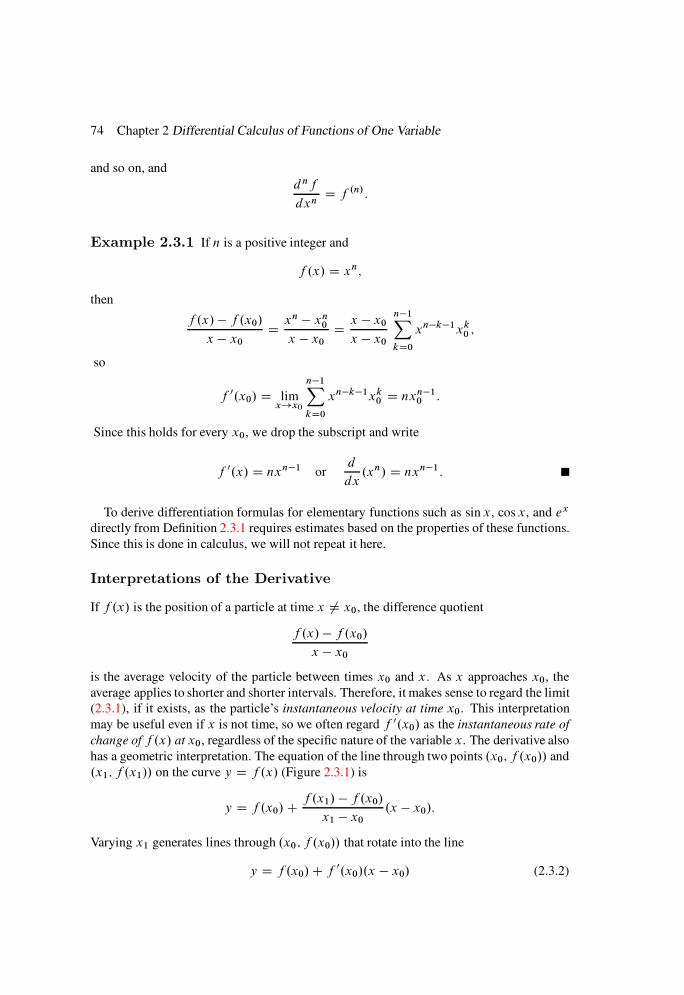
74 Chapter 2 Differential Calculus of Functions of One Variable
and so on, and
dnf
dxnD f .n/:
Example 2.3.1 If n is a positive integer and
f .x/ D xn;
then
f .x/ f .x0/
x x0
Dxn xn
0
x x0
Dx x0
x x0
n1X
kD0
xnk1xk0 ;
so
f 0.x0/ D limx!x0
n1X
kD0
xnk1xk0 D nxn1
0 :
Since this holds for every x0, we drop the subscript and write
f 0.x/ D nxn1 ord
dx.xn/ D nxn1:
To derive differentiation formulas for elementary functions such as sin x, cos x, and ex
directly from Definition 2.3.1 requires estimates based on the properties of these functions.
Since this is done in calculus, we will not repeat it here.
Interpretations of the Derivative
If f .x/ is the position of a particle at time x ¤ x0, the difference quotient
f .x/ f .x0/
x x0
is the average velocity of the particle between times x0 and x. As x approaches x0, the
average applies to shorter and shorter intervals. Therefore, it makes sense to regard the limit
(2.3.1), if it exists, as the particle’s instantaneous velocity at time x0. This interpretation
may be useful even if x is not time, so we often regard f 0.x0/ as the instantaneous rate of
change of f .x/ at x0, regardless of the specific nature of the variable x. The derivative also
has a geometric interpretation. The equation of the line through two points .x0; f .x0// and
.x1; f .x1// on the curve y D f .x/ (Figure 2.3.1) is
y D f .x0/Cf .x1/ f .x0/
x1 x0
.x x0/:
Varying x1 generates lines through .x0; f .x0// that rotate into the line
y D f .x0/C f 0.x0/.x x0/ (2.3.2)
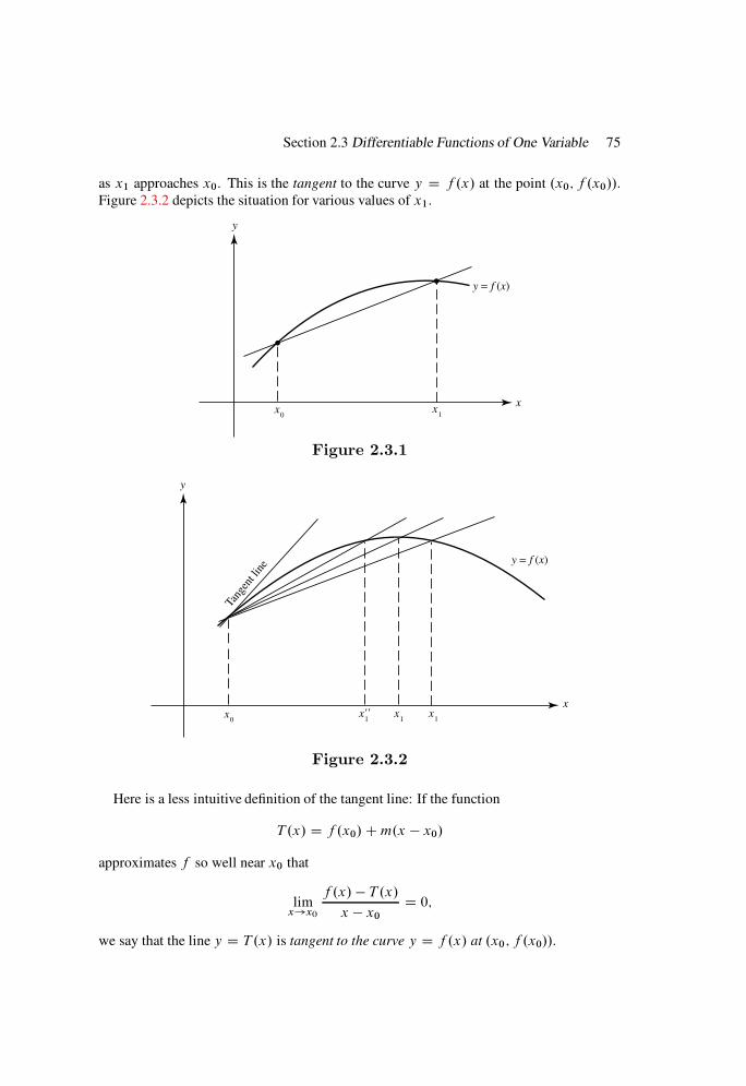
Section 2.3 Differentiable Functions of One Variable 75
as x1 approaches x0. This is the tangent to the curve y D f .x/ at the point .x0; f .x0//.
Figure 2.3.2 depicts the situation for various values of x1.
y
x
y = f (x)
x0 x
1
Figure 2.3.1
y
x
y = f (x)
x0 x
1x
1x
1''
Tang
ent l
ine
Figure 2.3.2
Here is a less intuitive definition of the tangent line: If the function
T .x/ D f .x0/Cm.x x0/
approximates f so well near x0 that
limx!x0
f .x/ T .x/x x0
D 0;
we say that the line y D T .x/ is tangent to the curve y D f .x/ at .x0; f .x0//.

76 Chapter 2 Differential Calculus of Functions of One Variable
This tangent line exists if and only if f 0.x0/ exists, in which casem is uniquely determined
by m D f 0.x0/ (Exercise 2.3.1). Thus, (2.3.2) is the equation of the tangent line.
We will use the following lemma to study differentiable functions.
Lemma 2.3.2 If f is differentiable at x0; then
f .x/ D f .x0/C Œf 0.x0/C E.x/.x x0/; (2.3.3)
where E is defined on a neighborhood of x0 and
limx!x0
E.x/ D E.x0/ D 0:
Proof Define
E.x/ D
8<:
f .x/ f .x0/
x x0
f 0.x0/; x 2 Df and x ¤ x0;
0; x D x0:(2.3.4)
Solving (2.3.4) for f .x/ yields (2.3.3) if x ¤ x0, and (2.3.3) is obvious if x D x0. Defini-
tion 2.3.1 implies that limx!x0E.x/ D 0. We defined E.x0/ D 0 to make E continuous
at x0.
Since the right side of (2.3.3) is continuous at x0, so is the left. This yields the following
theorem.
Theorem 2.3.3 If f is differentiable at x0; then f is continuous at x0:
The converse of this theorem is false, since a function may be continuous at a point
without being differentiable at the point.
Example 2.3.2 The function
f .x/ D jxjcan be written as
f .x/ D x; x > 0; (2.3.5)
or as
f .x/ D x; x < 0: (2.3.6)
From (2.3.5),
f 0.x/ D 1; x > 0;
and from (2.3.6),
f 0.x/ D 1; x < 0:
Neither (2.3.5) nor (2.3.6) holds throughout any neighborhood of 0, so neither can be used
alone to calculate f 0.0/. In fact, since the one-sided limits
limx!0C
f .x/ f .0/x 0 D lim
x!0C
x
x(2.3.7)
and
limx!0
f .x/ f .0/x 0
D limx!0
xxD 1 (2.3.8)

Section 2.3 Differentiable Functions of One Variable 77
are different,
limx!0
f .x/ f .0/x 0
does not exist (Theorem 2.1.6); thus, f is not differentiable at 0, even though it is continu-
ous at 0.
Interchanging Differentiation and Arithmetic Operations
The following theorem should be familiar from calculus.
Theorem 2.3.4 If f and g are differentiable at x0; then so are f Cg; f g; and fg;
with
(a) .f C g/0.x0/ D f 0.x0/C g0.x0/I(b) .f g/0.x0/ D f 0.x0/ g.x0/I(c) .fg/0.x0/ D f 0.x0/g.x0/C f .x0/g
0.x0/:
The quotient f=g is differentiable at x0 if g.x0/ ¤ 0; with
(d)
f
g
0.x0/ D
f 0.x0/g.x0/ f .x0/g0.x0/
Œg.x0/2
:
Proof The proof is accomplished by forming the appropriate difference quotients and
applying Definition 2.3.1 and Theorem 2.1.4. We will prove (c) and leave the rest to you
(Exercises 2.3.9, 2.3.10, and 2.3.11).
The trick is to add and subtract the right quantity in the numerator of the difference
quotient for .fg/0.x0/; thus,
f .x/g.x/ f .x0/g.x0/
x x0
D f .x/g.x/ f .x0/g.x/ C f .x0/g.x/ f .x0/g.x0/
x x0
D f .x/ f .x0/
x x0
g.x/ C f .x0/g.x/ g.x0/
x x0
:
The difference quotients on the right approach f 0.x0/ and g0.x0/ as x approaches x0, and
limx!x0g.x/ D g.x0/ (Theorem 2.3.3). This proves (c).
The Chain Rule
Here is the rule for differentiating a composite function.
Theorem 2.3.5 (The Chain Rule) Suppose that g is differentiable at x0 and f
is differentiable at g.x0/: Then the composite function h D f ı g; defined by
h.x/ D f .g.x//;
is differentiable at x0; with
h0.x0/ D f 0.g.x0//g0.x0/:
78 Chapter 2 Differential Calculus of Functions of One Variable
Proof Since f is differentiable at g.x0/, Lemma 2.3.2 implies that
f .t/ f .g.x0// D Œf 0.g.x0// C E.t/Œt g.x0/;
where
limt!g.x0/
E.t/ D E.g.x0// D 0: (2.3.9)
Letting t D g.x/ yields
f .g.x// f .g.x0// D Œf 0.g.x0//C E.g.x//Œg.x/ g.x0/:
Since h.x/ D f .g.x//, this implies that
h.x/ h.x0/
x x0
D Œf 0.g.x0//C E.g.x//g.x/ g.x0/
x x0
: (2.3.10)
Since g is continuous at x0 (Theorem 2.3.3), (2.3.9) and Theorem 2.2.7 imply that
limx!x0
E.g.x// D E.g.x0// D 0:
Therefore, (2.3.10) implies that
h0.x0/ D limx!x0
h.x/ h.x0/
x x0
D f 0.g.x0//g0.x0/;
as stated.
Example 2.3.3 If
f .x/ D sinx and g.x/ D 1
x; x ¤ 0;
then
h.x/ D f .g.x// D sin1
x; x ¤ 0;
and
h0.x/ D f 0.g.x//g.x/ D
cos1
x
1x2
; x ¤ 0:
It may seem reasonable to justify the chain rule by writing
h.x/ h.x0/
x x0
D f .g.x// f .g.x0//
x x0
Df .g.x// f .g.x0//
g.x/ g.x0/
g.x/ g.x0/
x x0
and arguing that
limx!x0
f .g.x// f .g.x0//
g.x/ g.x0/D f 0.g.x0//

Section 2.3 Differentiable Functions of One Variable 79
(because limx!x0g.x/ D g.x0// and
limx!x0
g.x/ g.x0/
x x0
D g0.x0/:
However, this is not a valid proof (Exercise 2.3.13).
One-Sided Derivatives
One-sided limits of difference quotients such as (2.3.7) and (2.3.8) in Example 2.3.2 are
called one-sided or right- and left-hand derivatives. That is, if f is defined on Œx0; b/, the
right-hand derivative of f at x0 is defined to be
f 0C.x0/ D lim
x!x0C
f .x/ f .x0/
x x0
if the limit exists, while if f is defined on .a; x0, the left-hand derivative of f at x0 is
defined to be
f 0.x0/ D lim
x!x0f .x/ f .x0/
x x0
if the limit exists. Theorem 2.1.6 implies that f is differentiable at x0 if and only if f 0C.x0/
and f 0.x0/ exist and are equal, in which case
f 0.x0/ D f 0C.x0/ D f 0
.x0/:
In Example 2.3.2, f 0C.0/ D 1 and f 0
.0/ D 1.
Example 2.3.4 If
f .x/ D
8<:
x3; x 0;
x2 sin1
x; x > 0;
(2.3.11)
then
f 0.x/ D
8<:
3x2; x < 0;
2x sin1
x cos
1
x; x > 0:
(2.3.12)
Since neither formula in (2.3.11) holds for all x in any neighborhood of 0, we cannot simply
differentiate either to obtain f 0.0/; instead, we calculate
f 0C.0/ D lim
x!0C
x2 sin1
x 0
x 0 D limx!0C
x sin1
xD 0;
f 0.0/ D lim
x!0
x3 0x 0 D lim
x!0x2 D 0I
hence, f 0.0/ D f 0C.0/ D f 0
.0/ D 0.
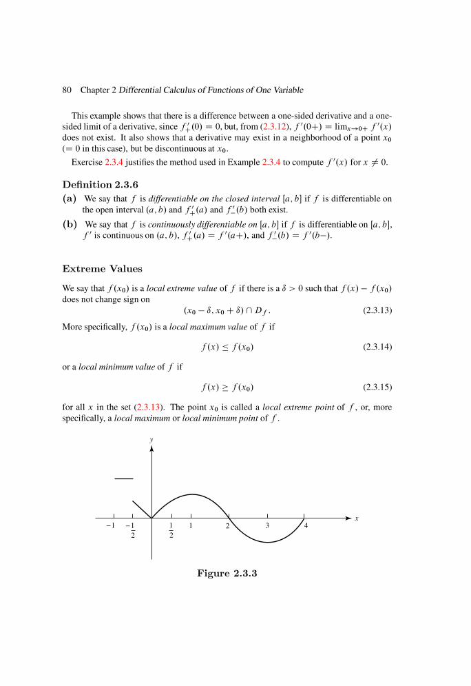
80 Chapter 2 Differential Calculus of Functions of One Variable
This example shows that there is a difference between a one-sided derivative and a one-
sided limit of a derivative, since f 0C.0/ D 0, but, from (2.3.12), f 0.0C/ D limx!0C f 0.x/
does not exist. It also shows that a derivative may exist in a neighborhood of a point x0
(D 0 in this case), but be discontinuous at x0.
Exercise 2.3.4 justifies the method used in Example 2.3.4 to compute f 0.x/ for x ¤ 0.
Definition 2.3.6
(a) We say that f is differentiable on the closed interval Œa; b if f is differentiable on
the open interval .a; b/ and f 0C.a/ and f 0
.b/ both exist.
(b) We say that f is continuously differentiable on Œa; b if f is differentiable on Œa; b,
f 0 is continuous on .a; b/, f 0C.a/ D f 0.aC/, and f 0
.b/ D f 0.b/.
Extreme Values
We say that f .x0/ is a local extreme value of f if there is a ı > 0 such that f .x/ f .x0/
does not change sign on
.x0 ı; x0C ı/\Df : (2.3.13)
More specifically, f .x0/ is a local maximum value of f if
f .x/ f .x0/ (2.3.14)
or a local minimum value of f if
f .x/ f .x0/ (2.3.15)
for all x in the set (2.3.13). The point x0 is called a local extreme point of f , or, more
specifically, a local maximum or local minimum point of f .
y
x1 2
2
3 4−1 −1
2
1
Figure 2.3.3
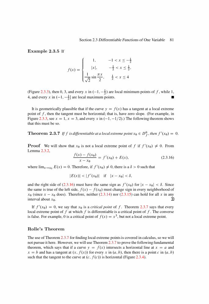
Section 2.3 Differentiable Functions of One Variable 81
Example 2.3.5 If
f .x/ D
8ˆ<ˆ:
1; 1 < x 12
jxj; 12< x 1
2;
1p2
sinx
2; 1
2< x 4
(Figure 2.3.3), then 0, 3, and every x in .1;12/ are local minimum points of f , while 1,
4, and every x in .1;12 are local maximum points.
It is geometrically plausible that if the curve y D f .x/ has a tangent at a local extreme
point of f , then the tangent must be horizontal; that is, have zero slope. (For example, in
Figure 2.3.3, see x D 1, x D 3, and every x in .1;1=2/.) The following theorem shows
that this must be so.
Theorem 2.3.7 If f is differentiable at a local extreme point x0 2 D0f; then f 0.x0/ D 0:
Proof We will show that x0 is not a local extreme point of f if f 0.x0/ ¤ 0. From
Lemma 2.3.2,f .x/ f .x0/
x x0
D f 0.x0/C E.x/; (2.3.16)
where limx!x0E.x/ D 0. Therefore, if f 0.x0/ ¤ 0, there is a ı > 0 such that
jE.x/j < jf 0.x0/j if jx x0j < ı;
and the right side of (2.3.16) must have the same sign as f 0.x0/ for jx x0j < ı. Since
the same is true of the left side, f .x/ f .x0/ must change sign in every neighborhood of
x0 (since x x0 does). Therefore, neither (2.3.14) nor (2.3.15) can hold for all x in any
interval about x0.
If f 0.x0/ D 0, we say that x0 is a critical point of f . Theorem 2.3.7 says that every
local extreme point of f at which f is differentiable is a critical point of f . The converse
is false. For example, 0 is a critical point of f .x/ D x3, but not a local extreme point.
Rolle’s Theorem
The use of Theorem 2.3.7 for finding local extreme points is covered in calculus, so we will
not pursue it here. However, we will use Theorem 2.3.7 to prove the following fundamental
theorem, which says that if a curve y D f .x/ intersects a horizontal line at x D a and
x D b and has a tangent at .x; f .x// for every x in .a; b/, then there is a point c in .a; b/
such that the tangent to the curve at .c; f .c// is horizontal (Figure 2.3.4).
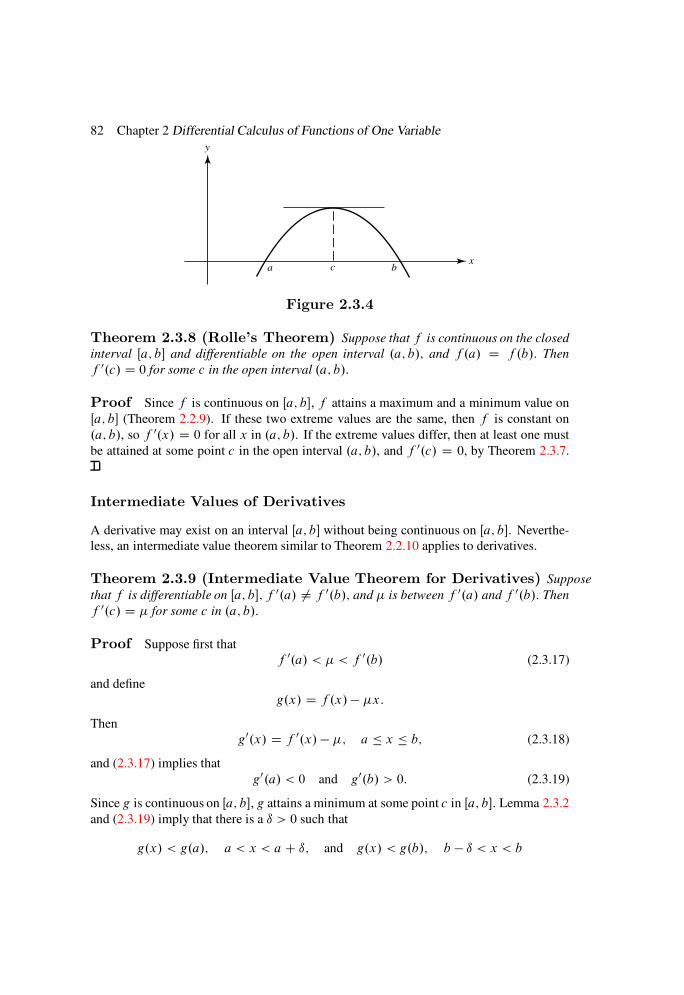
82 Chapter 2 Differential Calculus of Functions of One Variable
y
xbca
Figure 2.3.4
Theorem 2.3.8 (Rolle’s Theorem) Suppose that f is continuous on the closed
interval Œa; b and differentiable on the open interval .a; b/; and f .a/ D f .b/: Then
f 0.c/ D 0 for some c in the open interval .a; b/:
Proof Since f is continuous on Œa; b, f attains a maximum and a minimum value on
Œa; b (Theorem 2.2.9). If these two extreme values are the same, then f is constant on
.a; b/, so f 0.x/ D 0 for all x in .a; b/. If the extreme values differ, then at least one must
be attained at some point c in the open interval .a; b/, and f 0.c/ D 0, by Theorem 2.3.7.
Intermediate Values of Derivatives
A derivative may exist on an interval Œa; b without being continuous on Œa; b. Neverthe-
less, an intermediate value theorem similar to Theorem 2.2.10 applies to derivatives.
Theorem 2.3.9 (Intermediate Value Theorem for Derivatives) Suppose
that f is differentiable on Œa; b; f 0.a/ ¤ f 0.b/; and is between f 0.a/ and f 0.b/: Then
f 0.c/ D for some c in .a; b/:
Proof Suppose first that
f 0.a/ < < f 0.b/ (2.3.17)
and define
g.x/ D f .x/ x:
Then
g0.x/ D f 0.x/ ; a x b; (2.3.18)
and (2.3.17) implies that
g0.a/ < 0 and g0.b/ > 0: (2.3.19)
Since g is continuous on Œa; b, g attains a minimum at some point c in Œa; b. Lemma 2.3.2
and (2.3.19) imply that there is a ı > 0 such that
g.x/ < g.a/; a < x < a C ı; and g.x/ < g.b/; b ı < x < b
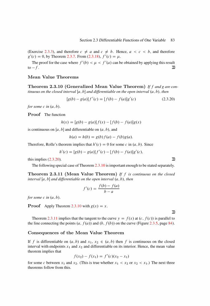
Section 2.3 Differentiable Functions of One Variable 83
(Exercise 2.3.3), and therefore c ¤ a and c ¤ b. Hence, a < c < b, and therefore
g0.c/ D 0, by Theorem 2.3.7. From (2.3.18), f 0.c/ D .
The proof for the case where f 0.b/ < < f 0.a/ can be obtained by applying this result
to f .
Mean Value Theorems
Theorem 2.3.10 (Generalized Mean Value Theorem) If f and g are con-
tinuous on the closed interval Œa; b and differentiable on the open interval .a; b/; then
Œg.b/ g.a/f 0.c/ D Œf .b/ f .a/g0.c/ (2.3.20)
for some c in .a; b/:
Proof The function
h.x/ D Œg.b/ g.a/f .x/ Œf .b/ f .a/g.x/
is continuous on Œa; b and differentiable on .a; b/, and
h.a/ D h.b/ D g.b/f .a/ f .b/g.a/:
Therefore, Rolle’s theorem implies that h0.c/ D 0 for some c in .a; b/. Since
h0.c/ D Œg.b/ g.a/f 0.c/ Œf .b/ f .a/g0.c/;
this implies (2.3.20).
The following special case of Theorem 2.3.10 is important enough to be stated separately.
Theorem 2.3.11 (Mean Value Theorem) If f is continuous on the closed
interval Œa; b and differentiable on the open interval .a; b/; then
f 0.c/ D f .b/ f .a/b a
for some c in .a; b/:
Proof Apply Theorem 2.3.10 with g.x/ D x.
Theorem 2.3.11 implies that the tangent to the curve y D f .x/ at .c; f .c// is parallel to
the line connecting the points .a; f .a// and .b; f .b// on the curve (Figure 2.3.5, page 84).
Consequences of the Mean Value Theorem
If f is differentiable on .a; b/ and x1, x2 2 .a; b/ then f is continuous on the closed
interval with endpoints x1 and x2 and differentiable on its interior. Hence, the mean value
theorem implies that
f .x2/ f .x1/ D f 0.c/.x2 x1/
for some c between x1 and x2. (This is true whether x1 < x2 or x2 < x1.) The next three
theorems follow from this.
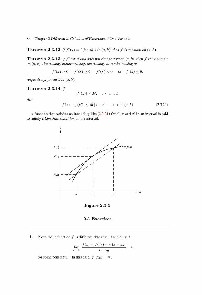
84 Chapter 2 Differential Calculus of Functions of One Variable
Theorem 2.3.12 If f 0.x/ D 0 for all x in .a; b/; then f is constant on .a; b/:
Theorem 2.3.13 If f 0 exists and does not change sign on .a; b/; then f is monotonic
on .a; b/ W increasing; nondecreasing; decreasing; or nonincreasing as
f 0.x/ > 0; f 0.x/ 0; f 0.x/ < 0; or f 0.x/ 0;
respectively; for all x in .a; b/:
Theorem 2.3.14 If
jf 0.x/j M; a < x < b;
then
jf .x/ f .x0/j M jx x0j; x; x0 2 .a; b/: (2.3.21)
A function that satisfies an inequality like (2.3.21) for all x and x0 in an interval is said
to satisfy a Lipschitz condition on the interval.
y
xbca
y = f (x)f (b)
f (c)
f (a)
Figure 2.3.5
2.3 Exercises
1. Prove that a function f is differentiable at x0 if and only if
limx!x0
f .x/ f .x0/ m.x x0/
x x0
D 0
for some constant m. In this case, f 0.x0/ D m.
Section 2.3 Differentiable Functions of One Variable 85
2. Prove: If f is defined on a neighborhood of x0, then f is differentiable at x0 if and
only if the discontinuity of
h.x/ D f .x/ f .x0/
x x0
at x0 is removable.
3. Use Lemma 2.3.2 to prove that if f 0.x0/ > 0, there is a ı > 0 such that
f .x/ < f .x0/ if x0 ı < x < x0 and f .x/ > f .x0/ if x0 < x < x0 C ı:
4. Suppose that p is continuous on .a; c and differentiable on .a; c/, while q is con-
tinuous on Œc; b/ and differentiable on .c; b/. Let
f .x/ D(p.x/; a < x c;
q.x/; c < x < b:
(a) Show that
f 0.x/ D(p0.x/; a < x < c;
q0.x/; c < x < b:
(b) Under what additional conditions on p and q does f 0.c/ exist? Prove that
your stated conditions are necessary and sufficient.
5. Find all derivatives of f .x/ D xn1jxj, where n is a positive integer.
6. Suppose that f 0.0/ exists and f .xC y/ D f .x/f .y/ for all x and y. Prove that f 0
exists for all x.
7. Suppose that c0.0/ D a and s0.0/ D b where a2 C b2 ¤ 0, and
c.x C y/ D c.x/c.y/ s.x/s.y/s.x C y/ D s.x/c.y/ C c.x/s.y/
for all x and y.
(a) Show that c and s are differentiable on .1;1/, and find c0 and s0 in terms
of c, s, a, and b.
(b) (For those who have studied differential equations.) Find c and s explicitly.
8. (a) Suppose that f and g are differentiable at x0, f .x0/ D g.x0/ D 0, and
g0.x0/ ¤ 0. Without using L’Hospital’s rule, show that
limx!x0
f .x/
g.x/D f 0.x0/
g0.x0/:
(b) State the corresponding results for one-sided limits.
9. Prove Theorem 2.3.4(a).

86 Chapter 2 Differential Calculus of Functions of One Variable
10. Prove Theorem 2.3.4(b).
11. Prove Theorem 2.3.4(d).
12. Prove by induction: If n 1 and f .n/.x0/ and g.n/.x0/ exist, then so does .fg/.n/.x0/,
and
.fg/.n/.x0/ DnX
mD0
n
m
!f .m/.x0/g
.nm/.x0/:
HINT: See Exercise 1.2.19: This is Leibniz’s rule for differentiating a product.
13. What is wrong with the “proof” of the chain rule suggested after Example 2.3.3?
Correct it.
14. Suppose that f is continuous and increasing on Œa; b. Let f be differentiable at a
point x0 in .a; b/, with f 0.x0/ ¤ 0. If g is the inverse of f Theorem 2.2.15), show
that g0.f .x0// D 1=f 0.x0/.
15. (a) Show that f 0C.a/ D f 0.aC/ if both quantities exist.
(b) Example 2.3.4 shows that f 0C.a/ may exist even if f 0.aC/ does not. Give an
example where f 0.aC/ exists but f 0C.a/ does not.
(c) Complete the following statement so it becomes a theorem, and prove the
theorem: “If f 0.aC/ exists and f is at a, then f 0C.a/ D f 0.aC/.”
16. Show that f .aC/ and f .b/ exist (finite) if f 0 is bounded on .a; b/. HINT: See
Exercise 2.1.38:
17. Suppose that f is continuous on Œa; b, f 0C.a/ exists, and is between f 0
C.a/ and
.f .b/ f .a//=.b a/. Show that f .c/ f .a/ D .c a/ for some c in .a; b/.
18. Suppose that f is continuous on Œa; b, f 0C.a/ < < f
0.b/, and
.f .b/ f .a//=.b a/ ¤ :
Show that either f .c/ f .a/ D .c a/ or f .c/ f .b/ D .c b/ for some c
in .a; b/.
19. Let
f .x/ D sin x
x; x ¤ 0:
(a) Define f .0/ so that f is continuous at x D 0. HINT: Use Exercise 2.3.8:
(b) Show that if x is a local extreme point of f , then
jf .x/j D .1C x2/1=2:
HINT: Express sinx and cos x in terms of f .x/ and f 0.x/; and add their
squares to obtain a useful identity:
(c) Show that jf .x/j 1 for all x. For what value of x is equality attained?

Section 2.3 Differentiable Functions of One Variable 87
20. Let n be a positive integer and
f .x/ Dsinnx
n sinx; x ¤ k (k D integer):
(a) Define f .k/ so that f is continuous at k . HINT: Use Exercise 2.3.8:
(b) Show that if x is a local extreme point of f , then
jf .x/j D1C .n2 1/ sin2 x
1=2:
HINT: Express sinnx and cos nx in terms of f .x/ and f 0.x/; and add their
squares to obtain a useful identity:
(c) Show that jf .x/j 1 for all x. For what values of x is equality attained?
21. We say that f has at least n zeros, counting multiplicities, on an interval I if there
are distinct points x1, x2, . . . , xp in I such that
f .j /.xi / D 0; 0 j ni 1; 1 i p;
and n1 C C np D n. Prove: If f is differentiable and has at least n zeros,
counting multiplicities, on an interval I , then f 0 has at least n 1 zeros, counting
multiplicities, on I .
22. Give an example of a function f such that f 0 exists on an interval .a; b/ and has a
jump discontinuity at a point x0 in .a; b/, or show that there is no such function.
23. Let x1, x2, . . . , xn and y1, y2, . . . , yn be in .a; b/ and yi < xi , 1 i n. Show
that if f is differentiable on .a; b/, then
nX
iD1
Œf .xi / f .yi / D f 0.c/nX
iD1
.xi yi /
for some c in .a; b/.
24. Prove or give a counterexample: If f is differentiable on a neighborhood of x0, then
f satisfies a Lipschitz condition on some neighborhood of x0.
25. Let
f 00.x/C p.x/f .x/ D 0 and g00.x/C p.x/g.x/ D 0; a < x < b:
(a) Show thatW D f 0g fg0 is constant on .a; b/.
(b) Prove: If W ¤ 0 and f .x1/ D f .x2/ D 0 where a < x1 < x2 < b, then
g.c/ D 0 for some c in .x1; x2/. HINT: Consider f=g:
88 Chapter 2 Differential Calculus of Functions of One Variable
26. Suppose that we extend the definition of differentiability by saying that f is differ-
entiable at x0 if
f 0.x0/ D limx!x0
f .x/ f .x0/
x x0
exists in the extended reals. Show that if
f .x/ D(p
x; x 0;px; x < 0;
then f 0.0/ D1.
27. Prove or give a counterexample: If f is differentiable at x0 in the extended sense of
Exercise 2.3.26, then f is continuous at x0.
28. Assume that f is differentiable on .1;1/ and x0 is a critical point of f .
(a) Let h.x/ D f .x/g.x/, where g is differentiable on .1;1/ and
f .x0/g0.x0/ ¤ 0:
Show that the tangent line to the curve y D h.x/ at .x0; h.x0// and the tangent
line to the curve y D g.x/ at .x0; g.x0/ intersect on the x-axis.
(b) Suppose that f .x0/ ¤ 0. Let h.x/ D f .x/.x x1/, where x1 is arbitrary.
Show that the tangent line to the curve y D h.x/ at .x0; h.x0// intersects the
x-axis at x D x1.
(c) Suppose that f .x0/ ¤ 0. Let h.x/ D f .x/.x x1/2, where x1 ¤ x0. Show
that the tangent line to the curve y D h.x/ at .x0; h.x0// intersects the x-axis
at the midpoint of the interval with endpoints x0 and x1.
(d) Let h.x/ D .ax2 C bx C c/.x x1/, where a ¤ 0 and b2 4ac ¤ 0. Let
x0 D b
2a. Show that the tangent line to the curve y D h.x/ at .x0; h.x0//
intersects the x-axis at x D x1.
(e) Let h be a cubic polynomial with zeros ˛, ˇ, and , where ˛ and ˇ are distinct
and is real. Let x0 D˛C ˇ2
. Show that the tangent line to the curve
y D h.x/ at .x0; h.x0// intersects the axis at x D .
2.4 L’HOSPITAL’S RULE
The method of Theorem 2.1.4 for finding limits of the sum, difference, product, and quo-
tient of functions breaks down in connection with indeterminate forms. The generalized
mean value theorem (Theorem 2.3.10) leads to a method for evaluating limits of indetermi-
nate forms.
Theorem 2.4.1 (L’Hospital’s Rule) Suppose that f and g are differentiable
and g0 has no zeros on .a; b/: Let
limx!b
f .x/ D limx!b
g.x/ D 0 (2.4.1)
Section 2.4 L’Hospital’s Rule 89
or
limx!b
f .x/ D ˙1 and limx!b
g.x/ D ˙1; (2.4.2)
and suppose that
limx!b
f 0.x/
g0.x/D L .finite or˙1/: (2.4.3)
Then
limx!b
f .x/
g.x/D L: (2.4.4)
Proof We prove the theorem for finite L and leave the case where L D ˙1 to you
(Exercise 2.4.1).
Suppose that > 0. From (2.4.3), there is an x0 in .a; b/ such that
ˇˇf
0.c/
g0.c/L
ˇˇ < if x0 < c < b: (2.4.5)
Theorem 2.3.10 implies that if x and t are in Œx0; b/, then there is a c between them, and
therefore in .x0; b/, such that
Œg.x/ g.t/f 0.c/ D Œf .x/ f .t/g0.c/: (2.4.6)
Since g0 has no zeros in .a; b/, Theorem 2.3.11 implies that
g.x/ g.t/ ¤ 0 if x; t 2 .a; b/:
This means that g cannot have more than one zero in .a; b/. Therefore, we can choose x0
so that, in addition to (2.4.5), g has no zeros in Œx0; b/. Then (2.4.6) can be rewritten as
f .x/ f .t/g.x/ g.t/
D f 0.c/
g0.c/;
so (2.4.5) implies that
ˇˇf .x/ f .t/g.x/ g.t/
Lˇˇ < if x; t 2 Œx0; b/: (2.4.7)
If (2.4.1) holds, let x be fixed in Œx0; b/, and consider the function
G.t/ D f .x/ f .t/g.x/ g.t/
L:
From (2.4.1),
limt!b
f .t/ D limt!b
g.t/ D 0;
so
limt!b
G.t/ D f .x/
g.x/L: (2.4.8)
90 Chapter 2 Differential Calculus of Functions of One Variable
Since
jG.t/j < if x0 < t < b;
because of (2.4.7), (2.4.8) implies thatˇˇf .x/g.x/
Lˇˇ :
This holds for all x in .x0; b/, which implies (2.4.4).
The proof under assumption (2.4.2) is more complicated. Again choose x0 so that (2.4.5)
holds and g has no zeros in Œx0; b/. Letting t D x0 in (2.4.7), we see thatˇˇf .x/ f .x0/
g.x/ g.x0/L
ˇˇ < if x0 x < b: (2.4.9)
Since limx!b f .x/ D ˙1, we can choose x1 > x0 so that f .x/ ¤ 0 and f .x/ ¤ f .x0/
if x1 < x < b. Then the function
u.x/ D 1 g.x0/=g.x/
1 f .x0/=f .x/
is defined and nonzero if x1 < x < b, and
limx!b
u.x/ D 1; (2.4.10)
because of (2.4.2).
Sincef .x/ f .x0/
g.x/ g.x0/D f .x/
g.x/
1 f .x0/=f .x/
1 g.x0/=g.x/D f .x/
g.x/u.x/;
(2.4.9) implies that ˇˇ f .x/
g.x/u.x/ L
ˇˇ < if x1 < x < b;
which can be rewritten asˇˇf .x/g.x/
Lu.x/ˇˇ < ju.x/j if x1 < x < b: (2.4.11)
From this and the triangle inequality,ˇˇf .x/g.x/
Lˇˇ
ˇˇf .x/g.x/
Lu.x/ˇˇ C jLu.x/ Lj ju.x/j C jLj ju.x/ 1j: (2.4.12)
Because of (2.4.10), there is a point x2 in .x1; b/ such that
ju.x/ 1j < and therefore ju.x/j < 1C if x2 < x < b:
This, (2.4.11), and (2.4.12) imply thatˇˇf .x/g.x/
Lˇˇ < .1C /C jLj if x2 < x < b;
Section 2.4 L’Hospital’s Rule 91
which proves (2.4.4) under assumption (2.4.2).
Theorem 2.4.1 and the proof given here remain valid if b D 1 and “x ! b” is
replaced by “x ! 1” throughout. Only minor changes in the proof are required to show
that similar theorems are valid for limits from the right, limits at 1, and ordinary (two-
sided) limits. We will take these as given.
The Indeterminate Forms 0=0 and 1=1
We say that f=g is of the form 0=0 as x ! b if
limx!b
f .x/ D limx!b
g.x/ D 0;
or of the form1=1 as x ! b if
limx!b
f .x/ D ˙1
and
limx!b
g.x/ D ˙1:
The corresponding definitions for x ! bC and x ! ˙1 are similar. If f=g is of one of
these forms as x ! b and as x ! bC, then we say that it is of that form as x ! b.
Example 2.4.1 The ratio sinx=x is of the form 0=0 as x ! 0, and L’Hospital’s rule
yields
limx!0
sinx
xD lim
x!0
cos x
1D 1:
Example 2.4.2 The ratio ex=x is of the form1=1 as x ! 1, and L’Hospital’s
rule yields
limx!1
ex
xD lim
x!1ex
1D 1:
Example 2.4.3 Using L’Hospital’s rule may lead to another indeterminate form; thus,
limx!1
ex
x2D lim
x!1ex
2x
if the limit on the right exists in the extended reals. Applying L’Hospital’s rule again yields
limx!1
ex
2xD lim
x!1ex
2D1:
Therefore,
limx!1
ex
x2D1:
More generally,
limx!1
ex
x˛D1
for any real number ˛ (Exercise 2.4.33).
92 Chapter 2 Differential Calculus of Functions of One Variable
Example 2.4.4 Sometimes it pays to combine L’Hospital’s rule with other manipula-
tions. For example,
limx!0
4 4 cos x 2 sin2 x
x4D lim
x!0
4 sinx 4 sinx cos x
4x3
D
limx!0
sinx
x
limx!0
1 cos x
x2
D
limx!0
sinx
x
limx!0
sin x
2x
D 1
2
limx!0
sin x
x
2
D 1
2.1/2 D 1
2(Example 2.4.1):
As another example, L’Hospital’s rule yields
limx!0
ex2
log.1C x/x
D limx!0
2xex2
log.1C x/C ex2
.1C x/1
1D 1:
However, it is better to remove the “determinate” part of the ratio before using L’Hospital’s
rule:
limx!0
ex2
log.1C x/x
D
limx!0
ex2
limx!0
log.1C x/x
D .1/ limx!0
log.1C x/x
D limx!0
1=.1C x/1
D 1:
In using L’Hospital’s rule we usually write, for example,
limx!b
f .x/
g.x/D lim
x!b
f 0.x/
g0.x/(2.4.13)
and then try to find the limit on the right. This is convenient, but technically incorrect, since
(2.4.13) is true only if the limit on the right exists in the extended reals. It may happen that
the limit on the left exists but the one on the right does not. In this case, (2.4.13) is incorrect.
Example 2.4.5 If
f .x/ D x x2 sin1
xand g.x/ D sin x;
then
f 0.x/ D 1 2x sin1
xC cos
1
xand g0.x/ D cos x:

Section 2.4 L’Hospital’s Rule 93
Therefore, limx!0 f0.x/=g0.x/ does not exist. However,
limx!0
f .x/
g.x/D lim
x!0
1 x sin.1=x/
.sin x/=xD 1
1D 1:
The Indeterminate Form 0 1
We say that a product fg is of the form 0 1 as x ! b if one of the factors approaches
0 and the other approaches ˙1 as x ! b. In this case, it may be useful to apply
L’Hospital’s rule after writing
f .x/g.x/ D f .x/
1=g.x/or f .x/g.x/ D g.x/
1=f .x/;
since one of these ratios is of the form 0=0 and the other is of the form1=1 as x ! b.
Similar statements apply to limits as x ! bC, x ! b, and x !˙1.
Example 2.4.6 The product x logx is of the form 0 1 as x ! 0C. Converting it to
an1=1 form yields
limx!0C
x logx D limx!0C
logx
1=x
D limx!0C
1=x
1=x2
D limx!0C
x D 0:
Converting to a 0=0 form leads to a more complicated problem:
limx!0C
x logx D limx!0C
x
1= logx
D limx!0C
1
1=x.logx/2
D limx!0C
x.logx/2 D ‹
Example 2.4.7 The product x log.1C1=x/ is of the form 01 as x !1. Converting
it to a 0=0 form yields
limx!1
x log.1C 1=x/D limx!1
log.1C 1=x/1=x
D limx!1
Œ1=.1C 1=x/ .1=x2/
1=x2
D limx!1
1
1C 1=x D 1:

94 Chapter 2 Differential Calculus of Functions of One Variable
In this case, converting to an1=1 form complicates the problem:
limx!1
x log.1C 1=x/D limx!1
x
1= log.1C 1=x/
D limx!1
1 1Œlog.1C 1=x/2
1=x2
1C 1=x
D limx!1
x.x C 1/Œlog.1C 1=x/2 D ‹
The Indeterminate Form 11
A difference f g is of the form11 as x ! b if
limx!b
f .x/ D limx!b
g.x/ D ˙1:
In this case, it may be possible to manipulate f g into an expression that is no longer
indeterminate, or is of the form 0=0 or1=1 as x ! b. Similar remarks apply to limits
as x ! bC, x ! b, or x ! ˙1.
Example 2.4.8 The difference
sin x
x2 1x
is of the form11 as x ! 0, but it can be rewritten as the 0=0 form
sinx xx2
:
Hence,
limx!0
sinx
x2 1x
D lim
x!0
sinx xx2
D limx!0
cos x 12x
D limx!0
sinx
2D 0:
Example 2.4.9 The difference
x2 xis of the form11 as x !1. Rewriting it as
x2
1 1
x
;
which is no longer indeterminate as x !1, we find that
limx!1
.x2 x/ D limx!1
x2
1 1
x
D
limx!1
x2
limx!1
1 1
x
D .1/.1/ D 1
Section 2.4 L’Hospital’s Rule 95
The Indeterminate Forms 00, 11, and 10
The function f g is defined by
f .x/g.x/ D eg.x/ log f .x/ D exp.g.x/ log f .x//
for all x such that f .x/ > 0. Therefore, if f and g are defined and f .x/ > 0 on an interval
.a; b/, Exercise 2.2.22 implies that
limx!b
Œf .x/g.x/ D exp
lim
x!bg.x/ log f .x/
(2.4.14)
if limx!b g.x/ log f .x/ exists in the extended reals. (If this limit is˙1 then (2.4.14) is
valid if we define e1 D 0 and e1 D 1.) The product g logf can be of the form 0 1in three ways as x ! b:
(a) If limx!b g.x/ D 0 and limx!b f .x/ D 0.
(b) If limx!b g.x/ D ˙1 and limx!b f .x/ D 1.
(c) If limx!b g.x/ D 0 and limx!b f .x/ D 1.
In these three cases, we say that f g is of the form 00, 11, and10, respectively, as x !b. Similar definitions apply to limits as x ! bC, x ! b, and x ! ˙1.
Example 2.4.10 The function xx is of the form 00 as x ! 0C. Since
xx D ex log x
and limx!0C x logx D 0 (Example 2.4.6),
limx!0C
xx D e0 D 1:
Example 2.4.11 The function x1=.x1/ is of the form 11 as x ! 1. Since
x1=.x1/ D exp
logx
x 1
and
limx!1
logx
x 1D lim
x!1
1=x
1D 1;
it follows that
limx!1
x1=.x1/ D e1 D e:
Example 2.4.12 The function x1=x is of the form10 as x !1. Since
x1=x D exp
logx
x
and
limx!1
logx
xD lim
x!11=x
1D 0;
96 Chapter 2 Differential Calculus of Functions of One Variable
it follows that
limx!1
x1=x D e0 D 1:
2.4 Exercises
1. Prove Theorem 2.4.1 for the case where limx!b f0.x/=g0.x/ D ˙1.
In Exercises 2.4.2–2.4.40, find the indicated limits.
2. limx!0
tan1 x
sin1 x
3. limx!0
1 cos x
log.1C x2/4. lim
x!0C
1C cos x
ex 1
5. limx!
sin nx
sinx6. lim
x!0
log.1C x/x
7. limx!1
ex sin ex2
8. limx!1
x sin.1=x/ 9. limx!1
px.e1=x 1/ 10. lim
x!0Ctan x logx
11. limx!
sinx log.j tan xj/ 12. limx!0C
1
xC log.tan x/
13. limx!1
.px C 1
px/ 14. lim
x!0
1
ex 1 1x
15. limx!0
.cot x csc x/ 16. limx!0
1
sinx 1x
17. limx!j sinxjtan x 18. lim
x!=2j tan xjcosx
19. limx!0j sinxjx 20. lim
x!0.1C x/1=x
21. limx!1
xsin.1=x/ 22. limx!0
x
1 cos x 2x
23. limx!0C
x˛ logx 24. limx!e
log.log x/
sin.x e/
25. limx!1
x C 1x 1
px21
26. limx!1C
x C 1x 1
px21
27. limx!1
.log x/ˇ
x28. lim
x!1.cosh x sinh x/
29. limx!1
.x˛ logx/30. lim
x!1ex2
sin.ex/

Section 2.4 L’Hospital’s Rule 97
31. limx!1
x.x C 1/ Œlog.1C 1=x/2 32. limx!0
sinx x C x3=6
x5
33. limx!1
ex
x˛
34. limx!3=2
etanx cos x
35. limx!1C
.logx/˛ log.log x/ 36. limx!1
xx
x logx
37. limx!=2
.sin x/tan x
38. limx!0
ex nX
rD0
xrrŠ
xn.n D integer 1/
39. limx!0
sinx nX
rD0
.1/r x2rC1
.2r C 1/Šx2nC1
.n D integer 0/
40. limx!0
e1=x2
xnD 0 (n D integer)
41. (a) Prove: If f is continuous at x0 and limx!x0f 0.x/ exists, then f 0.x0/ exists
and f 0 is continuous at x0.
(b) Give an example to show that it is necessary to assume in (a) that f is con-
tinuous at x0.
42. The iterated logarithms are defined by L0.x/ D x and
Ln.x/ D log.Ln1.x//; x > an; n 1;
where a1 D 0 and an D ean1; n 1. Show that
(a) Ln.x/ D Ln1.logx/; x > an; n 1.
(b) Ln1.anC/ D 0 and Ln.anC/ D 1.
(c) limx!anC
.Ln1.x//˛Ln.x/ D 0 if ˛ > 0 and n 1.
(d) limx!1
.Ln.x//˛=Ln1.x/ D 0 if ˛ is arbitrary and n 1.
43. Let f be positive and differentiable on .0;1/, and suppose that
limx!1
f 0.x/
f .x/D L; where 0 < L 1:
Define f0.x/ D x and
fn.x/ D f .fn1.x// ; n 1:
Use L’Hospital’s rule to show that
limx!1
.fn.x//˛
fn1.x/D1 if ˛ > 0 and n 1:

98 Chapter 2 Differential Calculus of Functions of One Variable
44. Let f be differentiable on some deleted neighborhoodN of x0, and suppose that f
and f 0 have no zeros in N . Find
(a) limx!x0
jf .x/jf .x/ if limx!x0
f .x/ D 0;
(b) limx!x0
jf .x/j1=.f .x/1/ if limx!x0
f .x/ D 1;
(c) limx!x0
jf .x/j1=f .x/ if limx!x0f .x/ D1.
45. Suppose that f and g are differentiable and g0 has no zeros on .a; b/. Suppose also
that limx!b f 0.x/=g0.x/ D L and either
limx!b
f .x/ D limx!b
g.x/ D 0
or
limx!b
f .x/ D1 and limx!b
g.x/ D ˙1:
Find limx!b.1C f .x//1=g.x/ .
46. We distinguish between11 .D 1/ and .1/1 .D 1/ and between1C1.D 1/ and 1 1 .D 1/. Why don’t we distinguish between 0 1 and
0 .1/,11 and 1C1,1=1 and 1=1, and 11 and 11?
2.5 TAYLOR’S THEOREM
A polynomial is a function of the form
p.x/ D a0 C a1.x x0/C C an.x x0/n; (2.5.1)
where a0, . . . , an and x0 are constants. Since it is easy to calculate the values of a polyno-
mial, considerable effort has been devoted to using them to approximate more complicated
functions. Taylor’s theorem is one of the oldest and most important results on this question.
The polynomial (2.5.1) is said to be written in powers of x x0, and is of degree n if
an ¤ 0. If we wish to leave open the possibility that an D 0, we say that p is of degree
n. In particular, a constant polynomial p.x/ D a0 is of degree zero if a0 ¤ 0. If
a0 D 0, so that p vanishes identically, then p has no degree according to our definition,
which requires at least one coefficient to be nonzero. For convenience we say that the
identically zero polynomial p has degree 1. (Any negative number would do as well as
1. The point is that with this convention, the statement that p is a polynomial of degree
n includes the possibility that p is identically zero.)
Taylor Polynomials
We saw in Lemma 2.3.2 that if f is differentiable at x0, then
f .x/ D f .x0/C f 0.x0/.x x0/C E.x/.x x0/;

Section 2.5 Taylor’s Theorem 99
where
limx!x0
E.x/ D 0:
To generalize this result, we first restate it: the polynomial
T1.x/ D f .x0/C f 0.x0/.x x0/;
which is of degree 1 and satisfies
T1.x0/ D f .x0/; T 01.x0/ D f 0.x0/;
approximates f so well near x0 that
limx!x0
f .x/ T1.x/
x x0
D 0: (2.5.2)
Now suppose that f has n derivatives at x0 and Tn is the polynomial of degree n
such that
T .r/n .x0/ D f .r/.x0/; 0 r n: (2.5.3)
How well does Tn approximate f near x0?
To answer this question, we must first find Tn. Since Tn is a polynomial of degree n,
it can be written as
Tn.x/ D a0 C a1.x x0/C C an.x x0/n; (2.5.4)
where a0, . . . , an are constants. Differentiating (2.5.4) yields
T .r/n .x0/ D rŠar ; 0 r n;
so (2.5.3) determines ar uniquely as
ar Df .r/.x0/
rŠ; 0 r n:
Therefore,
Tn.x/ D f .x0/Cf 0.x0/
1Š.x x0/C C
f .n/.x0/
nŠ.x x0/
n
DnX
rD0
f .r/.x0/
rŠ.x x0/
r :
We call Tn the nth Taylor polynomial of f about x0.
The following theorem describes how Tn approximates f near x0.
Theorem 2.5.1 If f .n/.x0/ exists for some integer n 1 and Tn is the nth Taylor
polynomial of f about x0; then
limx!x0
f .x/ Tn.x/
.x x0/nD 0: (2.5.5)
100 Chapter 2 Differential Calculus of Functions of One Variable
Proof The proof is by induction. Let Pn be the assertion of the theorem. From (2.5.2)
we know that (2.5.5) is true if n D 1; that is, P1 is true. Now suppose that Pn is true for
some integer n 1, and f .nC1/ exists. Since the ratio
f .x/ TnC1.x/
.x x0/nC1
is indeterminate of the form 0=0 as x ! x0, L’Hospital’s rule implies that
limx!x0
f .x/ TnC1.x/
.x x0/nC1D 1
nC 1lim
x!x0
f 0.x/ T 0nC1.x/
.x x0/n(2.5.6)
if the limit on the right exists. But f 0 has an nth derivative at x0, and
T 0nC1.x/ D
nX
rD0
f .rC1/.x0/
rŠ.x x0/
r
is the nth Taylor polynomial of f 0 about x0. Therefore, the induction assumption, applied
to f 0, implies that
limx!x0
f 0.x/ T 0nC1.x/
.x x0/nD 0:
This and (2.5.6) imply that
limx!x0
f .x/ TnC1.x/
.x x0/nC1D 0;
which completes the induction.
It can be shown (Exercise 2.5.8) that if
pn D a0 C a1.x x0/C C an.x x0/n
is a polynomial of degree n such that
limx!x0
f .x/ pn.x/
.x x0/nD 0;
then
ar Df .r/.x0/
rŠI
that is, pn D Tn. Thus, Tn is the only polynomial of degree n that approximates f near
x0 in the manner indicated in (2.5.5).
Theorem 2.5.1 can be restated as a generalization of Lemma 2.3.2.
Lemma 2.5.2 If f .n/.x0/ exists; then
f .x/ DnX
rD0
f .r/.x0/
rŠ.x x0/
r C En.x/.x x0/n; (2.5.7)
where
limx!x0
En.x/ D En.x0/ D 0:

Section 2.5 Taylor’s Theorem 101
Proof Define
En.x/ D
8<:
f .x/ Tn.x/
.x x0/n; x 2 Df fx0g;
0; x D x0:
Then (2.5.5) implies that limx!x0En.x/ D En.x0/ D 0, and it is straightforward to verify
(2.5.7).
Example 2.5.1 If f .x/ D ex, then f .n/.x/ D ex. Therefore, f .n/.0/ D 1 for n 0,
so the nth Taylor polynomial of f about x0 D 0 is
Tn.x/ DnX
rD0
xr
rŠD 1C x
1ŠC x2
2ŠC C xn
nŠ: (2.5.8)
Theorem 2.5.1 implies that
limx!0
ex nX
rD0
xr
rŠ
xnD 0:
(See also Exercise 2.4.38.)
Example 2.5.2 If f .x/ D logx, then f .1/ D 0 and
f .r/.x/ D .1/.r1/ .r 1/Šxr
; r 1;
so the nth Taylor polynomial of f about x0 D 1 is
Tn.x/ DnX
rD1
.1/r1
r.x 1/r
if n 1. (T0 D 0.) Theorem 2.5.1 implies that
limx!1
logx nX
rD1
.1/r1r.x 1/r
.x 1/n D 0; n 1:
Example 2.5.3 If f .x/ D .1C x/q , then
f 0.x/ D q.1C x/q1
f 00.x/ D q.q 1/.1C x/q2
:::
f .n/.x/ D q.q 1/ .q nC 1/.1C x/qn:

102 Chapter 2 Differential Calculus of Functions of One Variable
If we define q
0
!D 1 and
q
n
!D q.q 1/ .q nC 1/
nŠ; n 1;
then
f .n/.0/
nŠD q
n
!;
and the nth Taylor polynomial of f about 0 can be written as
Tn.x/ DnX
rD0
q
r
!xr : (2.5.9)
Theorem 2.5.1 implies that
limx!0
.1C x/q nX
rD0
q
r
!xr
xnD 0; n 0:
If q is a nonnegative integer, then
q
n
!is the binomial coefficient defined in Exer-
cise 1.2.19. In this case, we see from (2.5.9) that
Tn.x/ D .1C x/q D f .x/; n q:
Applications to Finding Local Extrema
Lemma 2.5.2 yields the following theorem.
Theorem 2.5.3 Suppose that f has n derivatives at x0 and n is the smallest positive
integer such that f .n/.x0/ ¤ 0:(a) If n is odd; x0 is not a local extreme point of f:
(b) If n is even; x0 is a local maximum of f if f .n/.x0/ < 0; or a local mininum of f if
f .n/.x0/ > 0:
Proof Since f .r/.x0/ D 0 for 1 r n 1, (2.5.7) implies that
f .x/ f .x0/ D"f .n/.x0/
nŠCEn.x/
#.x x0/
n (2.5.10)
in some interval containing x0. Since limx!x0En.x/ D 0 and f .n/.x0/ ¤ 0, there is a
ı > 0 such that
jEn.x/j <ˇˇˇf .n/.x0/
nŠ
ˇˇˇ if jx x0j < ı:

Section 2.5 Taylor’s Theorem 103
This and (2.5.10) imply thatf .x/ f .x0/
.x x0/n(2.5.11)
has the same sign as f .n/.x0/ if 0 < jx x0j < ı. If n is odd the denominator of (2.5.11)
changes sign in every neighborhood of x0, and therefore so must the numerator (since the
ratio has constant sign for 0 < jx x0j < ı). Consequently, f .x0/ cannot be a local
extreme value of f . This proves (a). If n is even, the denominator of (2.5.11) is positive
for x ¤ x0, so f .x/ f .x0/ must have the same sign as f .n/.x0/ for 0 < jx x0j < ı.
This proves (b).
For n D 2,(b) is called the second derivative test for local extreme points.
Example 2.5.4 If f .x/ D ex3
, then f 0.x/ D 3x2ex3
, and 0 is the only critical point
of f . Since
f 00.x/ D .6x C 9x4/ex3
and
f 000.x/ D .6C 54x3 C 27x6/ex3
;
f 00.0/ D 0 and f 000.0/ ¤ 0. Therefore, Theorem 2.5.3 implies that 0 is not a local extreme
point of f . Since f is differentiable everywhere, it has no local maxima or minima.
Example 2.5.5 If f .x/ D sinx2, then f 0.x/ D 2x cos x2, so the critical points of f
are 0 and ˙p.k C 1=2/, k D 0; 1; 2; : : : . Since
f 00.x/ D 2 cos x2 4x2 sinx2;
f 00.0/ D 2 and f 00˙p.k C 1=2//
D .1/kC1.4k C 2/:
Therefore, Theorem 2.5.3 implies that f attains local minima at 0 and˙p.k C 1=2/ for
odd integers k, and local maxima at ˙p.k C 1=2/ for even integers k.
Taylor’s theorem
Theorem 2.5.1 implies that the error in approximating f .x/ by Tn.x/ approaches zero
faster than .x x0/n as x approaches x0; however, it gives no estimate of the error in
approximating f .x/ by Tn.x/ for a fixed x. For instance, it provides no estimate of the
error in the approximation
e0:1 T2.0:1/ D 1C0:1
1ŠC .0:1/2
2ŠD 1:105 (2.5.12)
obtained by setting n D 2 and x D 0:1 in (2.5.8). The following theorem provides a way
of estimating errors of this kind under the additional assumption that f .nC1/ exists in a
neighborhood of x0.
104 Chapter 2 Differential Calculus of Functions of One Variable
Theorem 2.5.4 (Taylor’s Theorem) Suppose that f .nC1/ exists on an open in-
terval I about x0; and let x be in I: Then the remainder
Rn.x/ D f .x/ Tn.x/
can be written as
Rn.x/ Df .nC1/.c/
.nC 1/Š .x x0/nC1;
where c depends upon x and is between x and x0:
This theorem follows from an extension of the mean value theorem that we will prove
below. For now, let us assume that Theorem 2.5.4 is correct, and apply it.
Example 2.5.6 If f .x/ D ex, then f 000.x/ D ex, and Theorem 2.5.4 with n D 2
implies that
ex D 1C x C x2
2ŠC ecx3
3Š;
where c is between 0 and x. Hence, from (2.5.12),
e0:1 D 1:105C ec.0:1/3
6;
where 0 < c < 0:1. Since 0 < ec < e0:1, we know from this that
1:105 < e0:1 < 1:105C e0:1.0:1/3
6:
The second inequality implies that
e0:1
1 .0:1/
3
6
< 1:105;
so
e0:1 < 1:1052:
Therefore,
1:105 < e0:1 < 1:1052;
and the error in (2.5.12) is less than 0:0002.
Example 2.5.7 In numerical analysis, forward differences are used to approximate
derivatives. If h > 0, the first and second forward differences with spacing h are defined
by
f .x/ D f .x C h/ f .x/and
2f .x/ D Œf .x/D f .x C h/ f .x/D f .x C 2h/ 2f .x C h/C f .x/: (2.5.13)
Higher forward differences are defined inductively (Exercise 2.5.18).
Section 2.5 Taylor’s Theorem 105
We will find upper bounds for the magnitudes of the errors in the approximations
f 0.x0/ f .x0/
h(2.5.14)
and
f 00.x0/ 2f .x0/
h2: (2.5.15)
If f 00 exists on an open interval containing x0 and x0 C h, we can use Theorem 2.5.4 to
estimate the error in (2.5.14) by writing
f .x0 C h/ D f .x0/C f 0.x0/hCf 00.c/h2
2; (2.5.16)
where x0 < c < x0 C h. We can rewrite (2.5.16) as
f .x0 C h/ f .x0/
h f 0.x0/ D
f 0.c/h
2;
which is equivalent tof .x0/
h f 0.x0/ D
f 00.c/h
2:
Therefore, ˇˇf .x0/
h f 0.x0/
ˇˇ M2h
2;
where M2 is an upper bound for jf 00j on .x0; x0C h/.If f 000 exists on an open interval containing x0 and x0 C 2h, we can use Theorem 2.5.4
to estimate the error in (2.5.15) by writing
f .x0 C h/ D f .x0/C hf 0.x0/Ch2
2f 00.x0/C
h3
6f 000.c0/
and
f .x0 C 2h/D f .x0/C 2hf 0.x0/C 2h2f 00.x0/C4h3
3f 000.c1/;
where x0 < c0 < x0 C h and x0 < c1 < x0 C 2h. These two equations imply that
f .x0 C 2h/ 2f .x0 C h/C f .x0/ D h2f 00.x0/C4
3f 000.c1/
1
3f 000.c0/
h3;
which can be rewritten as
2f .x0/
h2 f 00.x0/ D
4
3f 000.c1/
1
3f 000.c0/
h;
because of (2.5.13). Therefore,ˇˇ
2f .x0/
h2 f 00.x0/
ˇˇ 5M3h
3;
where M3 is an upper bound for jf 000j on .x0; x0 C 2h/.
106 Chapter 2 Differential Calculus of Functions of One Variable
The Extended Mean Value Theorem
We now consider the extended mean value theorem, which implies Theorem 2.5.4 (Exer-
cise 2.5.24). In the following theorem, a and b are the endpoints of an interval, but we do
not assume that a < b.
Theorem 2.5.5 (Extended Mean Value Theorem) Suppose thatf is con-
tinuous on a finite closed interval I with endpoints a and b .that is, either I D .a; b/ or
I D .b; a//; f .nC1/ exists on the open interval I 0; and; if n > 0; that f 0, . . . , f .n/ exist
and are continuous at a: Then
f .b/nX
rD0
f .r/.a/
rŠ.b a/r D f .nC1/.c/
.nC 1/Š .b a/nC1 (2.5.17)
for some c in I 0:
Proof The proof is by induction. The mean value theorem (Theorem 2.3.11) implies
the conclusion for n D 0. Now suppose that n 1, and assume that the assertion of the
theorem is true with n replaced by n 1. The left side of (2.5.17) can be written as
f .b/nX
rD0
f .r/.a/
rŠ.b a/r D K .b a/
nC1
.nC 1/Š(2.5.18)
for some number K. We must prove that K D f .nC1/.c/ for some c in I 0. To this end,
consider the auxiliary function
h.x/ D f .x/ nX
rD0
f .r/.a/
rŠ.x a/r K .x a/
nC1
.nC 1/Š ;
which satisfies
h.a/ D 0; h.b/ D 0;(the latter because of (2.5.18)) and is continuous on the closed interval I and differentiable
on I 0, with
h0.x/ D f 0.x/ n1X
rD0
f .rC1/.a/
rŠ.x a/r K .x a/
n
nŠ: (2.5.19)
Therefore, Rolle’s theorem (Theorem 2.3.8) implies that h0.b1/ D 0 for some b1 in I 0;
thus, from (2.5.19),
f 0.b1/ n1X
rD0
f .rC1/.a/
rŠ.b1 a/r K
.b1 a/nnŠ
D 0:
If we temporarily write f 0 D g, this becomes
g.b1/ n1X
rD0
g.r/.a/
r.b1 a/r K
.b1 a/nnŠ
D 0: (2.5.20)
Section 2.5 Taylor’s Theorem 107
Since b1 2 I 0, the hypotheses on f imply that g is continuous on the closed interval J
with endpoints a and b1, g.n/ exists on J 0, and, if n 1, g0, . . . , g.n1/ exist and are
continuous at a (also at b1, but this is not important). The induction hypothesis, applied to
g on the interval J , implies that
g.b1/ n1X
rD0
g.r/.a/
rŠ.b1 a/r D
g.n/.c/
nŠ.b1 a/n
for some c in J 0. Comparing this with (2.5.20) and recalling that g D f 0 yields
K D g.n/.c/ D f .nC1/.c/:
Since c is in I 0, this completes the induction.
2.5 Exercises
1. Let
f .x/ De1=x2
; x ¤ 0;0; x D 0:
Show that f has derivatives of all orders on .1;1/ and every Taylor polynomial
of f about 0 is identically zero. HINT: See Exercise 2.4.40:
2. Suppose that f .nC1/.x0/ exists, and let Tn be the nth Taylor polynomial of f about
x0. Show that the function
En.x/ D
8<:
f .x/ Tn.x/
.x x0/n; x 2 Df fx0g;
0; x D x0;
is differentiable at x0, and find E 0n.x0/.
3. (a) Prove: If f is continuous at x0 and there are constants a0 and a1 such that
limx!x0
f .x/ a0 a1.x x0/
x x0
D 0;
then a0 D f .x0/, f0 is differentiable at x0, and f 0.x0/ D a1.
(b) Give a counterexample to the following statement: If f and f 0 are continuous
at x0 and there are constants a0, a1, and a2 such that
limx!x0
f .x/ a0 a1.x x0/ a2.x x0/2
.x x0/2D 0;
then f 00.x0/ exists.
4. (a) Prove: if f 00.x0/ exists, then
limh!0
f .x0 C h/ 2f .x0/C f .x0 h/h2
D f 00.x0/:

108 Chapter 2 Differential Calculus of Functions of One Variable
(b) Prove or give a counterexample: If the limit in (a) exists, then so does
f 00.x0/, and they are equal.
5. A function f has a simple zero (or a zero of multiplicity1) at x0 if f is differentiable
at x0 and f .x0/ D 0, while f 0.x0/ ¤ 0.
(a) Prove that f has a simple zero at x0 if and only if
f .x/ D g.x/.x x0/;
where g is continuous at x0 and differentiable on a deleted neighborhood of
x0, and g.x0/ ¤ 0.
(b) Give an example showing that g in(a) need not be differentiable at x0.
6. A function f has a double zero (or a zero of multiplicity 2) at x0 if f is twice
differentiable at x0 and f .x0/ D f 0.x0/ D 0, while f 00.x0/ ¤ 0.
(a) Prove that f has a double zero at x0 if and only if
f .x/ D g.x/.x x0/2;
where g is continuous at x0 and twice differentiable on a deleted neighborhood
of x0, g.x0/ ¤ 0, and
limx!x0
.x x0/g0.x/ D 0:
(b) Give an example showing that g in(a) need not be differentiable at x0.
7. Let n be a positive integer. A function f has a zero of multiplicity n at x0 if f
is n times differentiable at x0, f .x0/ D f 0.x0/ D D f .n1/.x0/ D 0 and
f .n/.x0/ ¤ 0. Prove that f has a zero of multiplicity n at x0 if and only if
f .x/ D g.x/.x x0/n;
where g is continuous at x0 and n times differentiable on a deleted neighborhood of
x0, g.x0/ ¤ 0, and
limx!x0
.x x0/j g.j /.x/ D 0; 1 j n 1:
HINT: Use Exercise 2.5.6 and induction:
8. (a) Let
Q.x/ D ˛0 C ˛1.x x0/C C ˛n.x x0/n
be a polynomial of degree n such that
limx!x0
Q.x/
.x x0/nD 0:
Show that ˛0 D ˛1 D D ˛n D 0.
Section 2.5 Taylor’s Theorem 109
(b) Suppose that f is n times differentiable at x0 and p is a polynomial
p.x/ D a0 C a1.x x0/C C an.x x0/n
of degree n such that
limx!x0
f .x/ p.x/.x x0/n
D 0:
Show that
ar Df .r/.x0/
rŠif 0 r nI
that is, p D Tn, the nth Taylor polynomial of f about x0.
9. Show that if f .n/.x0/ and g.n/.x0/ exist and
limx!x0
f .x/ g.x/.x x0/n
D 0;
then f .r/.x0/ D g.r/.x0/, 0 r n.
10. (a) Let Fn, Gn, and Hn be the nth Taylor polynomials about x0 of f , g, and
their product h D fg. Show that Hn can be obtained by multiplying Fn
by Gn and retaining only the powers of x x0 through the nth. HINT: Use
Exercise 2.5.8.b/:
(b) Use the method suggested by (a) to compute h.r/.x0/, r D 1; 2; 3; 4.
(i) h.x/ D ex sinx; x0 D 0(ii) h.x/ D .cos x=2/.logx/; x0 D 1(iii) h.x/ D x2 cos x; x0 D =2(iv) h.x/ D .1C x/1ex; x0 D 0
11. (a) It can be shown that if g is n times differentiable at x and f is n times dif-
ferentiable at g.x/, then the composite function h.x/ D f .g.x// is n times
differentiable at x and
h.n/.x/ DnX
rD1
f .r/.g.x//X
r
rŠ
r1Š rnŠ
g0.x/
1Š
r1g00.x/
2Š
r2
g.n/.x/
nŠ
!rn
whereP
r is over all n-tuples .r1; r2; : : : ; rn/ of nonnegative integers such that
r1 C r2 C C rn D rand
r1 C 2r2 C C nrn D n:
(This is Faa di Bruno’s formula.) However, this formula is quite complicated.
Justify the following alternative method for computing the derivatives of a
composite function at a point x0:

110 Chapter 2 Differential Calculus of Functions of One Variable
Let Fn be the nth Taylor polynomial of f about y0 D g.x0/, and let Gn and
Hn be the nth Taylor polynomials of g and h about x0. Show that Hn can
be obtained by substituting Gn into Fn and retaining only powers of x x0
through the nth. HINT: See Exercise 2.5.8.b/:
(b) Compute the first four derivatives of h.x/ D cos.sin x/ at x0 D 0, using the
method suggested by (a).
12. (a) If g.x0/ ¤ 0 and g.n/.x0/ exists, then the reciprocal h D 1=g is also n times
differentiable at x0, by Exercise 2.5.11(a), with f .x/ D 1=x. Let Gn andHn
be the nth Taylor polynomials of g and h about x0. Use Exercise 2.5.11(a) to
prove that if g.x0/ D 1, thenHn can be obtained by expanding the polynomial
nX
rD1
Œ1 Gn.x/r
in powers of x x0 and retaining only powers through the nth.
(b) Use the method of (a) to compute the first four derivatives of the following
functions at x0.
(i) h.x/ D csc x; x0 D =2(ii) h.x/ D .1C x C x2/1; x0 D 0(iii) h.x/ D sec x; x0 D =4(iv) h.x/ D Œ1C log.1C x/1 ; x0 D 0
(c) Use Exercise 2.5.10 to justify the following alternative procedure for obtaining
Hn, again assuming that g.x0/ D 1: If
Gn.x/ D 1C a1.x x0/C C an.x x0/n
(where, of course, ar D g.r/.x0/=rŠ/ and
Hn.x/ D b0 C b1.x x0/C C bn.x x0/n;
then
b0 D 1; bk D kX
rD1
arbkr ; 1 k n:
13. Determine whether x0 D 0 is a local maximum, local minimum, or neither.
(a) f .x/ D x2ex3(b) f .x/ D x3ex2
(c) f .x/ D 1C x2
1C x3(d) f .x/ D 1C x3
1C x2
(e) f .x/ D x2 sin3 x C x2 cos x (f) f .x/ D ex2sinx
(g) f .x/ D ex sinx2 (h) f .x/ D ex2cos x
14. Give an example of a function that has zero derivatives of all orders at a local mini-
mum point.
Section 2.5 Taylor’s Theorem 111
15. Find the critical points of
f .x/ D x3
3C bx2
2C cx C d
and identify them as local maxima, local minima, or neither.
16. Find an upper bound for the magnitude of the error in the approximation.
(a) sinx x; jxj <
20
(b)p1C x 1C x
2; jxj < 1
8
(c) cos x 1p21
x
4
;
4< x < 5
16
(d) logx .x 1/ .x 1/2
2C .x 1/3
3; jx 1j < 1
64
17. Prove: If
Tn.x/ DnX
rD0
xr
rŠ;
then
Tn.x/ < TnC1.x/ < ex <
1 xnC1
.nC 1/Š
1
Tn.x/
if 0 < x < Œ.nC 1/Š1=.nC1/.
18. The forward difference operators with spacing h > 0 are defined by
0f .x/ D f .x/; f .x/ D f .x C h/ f .x/;
nC1f .x/ D Œnf .x/ ; n 1:
(a) Prove by induction on n: If k 2, c1, . . . , ck are constants, and n 1, then
nŒc1f1.x/C C ckfk.x/ D c1nf1.x/C C ck
nfk.x/:
(b) Prove by induction: If n 1, then
nf .x/ DnX
mD0
.1/nm
n
m
!f .x Cmh/:
HINT: See Exercise 1.2.19:
In Exercises 2.5.19–2.5.22, is the forward difference operator with spacing h > 0.
112 Chapter 2 Differential Calculus of Functions of One Variable
19. Let m and n be nonnegative integers, and let x0 be any real number. Prove by
induction on n that
n.x x0/m D
0 if 0 m n;nŠhn if m D n:
Does this suggest an analogy between “differencing" and differentiation?
20. Find an upper bound for the magnitude of the error in the approximation
f 00.x0/ 2f .x0 h/
h2;
(a) assuming that f 000 is bounded on .x0 h; x0 C h/;(b) assuming that f .4/ is bounded on .x0 h; x0C h/.
21. Let f 000 be bounded on an open interval containing x0 and x0C 2h. Find a constant
k such that the magnitude of the error in the approximation
f 0.x0/ f .x0/
hC k
2f .x0/
h2
is not greater than Mh2, where M D sup˚jf 000.c/j
ˇjx0 < c < x0
.
22. Prove: If f .nC1/ is bounded on an open interval containing x0 and x0 C nh, then
ˇˇ
nf .x0/
hn f .n/.x0/
ˇˇ AnMnC1h;
where An is a constant independent of f and
MnC1 D supx0<c<x0Cnh
jf .nC1/.c/j:
HINT: See Exercises 2.5.18 and 2.5.19:
23. Suppose that f .nC1/ exists on .a; b/, x0, . . . , xn are in .a; b/, and p is the polyno-
mial of degree n such that p.xi / D f .xi /, 0 i n. Prove: If x 2 .a; b/,then
f .x/ D p.x/C f .nC1/.c/
.nC 1/Š .x x0/.x x1/ .x xn/;
where c, which depends on x, is in .a; b/. HINT: Let x be fixed; distinct from x0;
x1; . . . , xn; and consider the function
g.y/ D f .y/ p.y/ K
.nC 1/Š.y x0/.y x1/ .y xn/;
where K is chosen so that g.x/ D 0: Use Rolle’s theorem to show that K Df .nC1/.c/ for some c in .a; b/:
24. Deduce Theorem 2.5.4 from Theorem 2.5.5.

CHAPTER 3
Integral Calculus of
Functions of One Variable
IN THIS CHAPTER we discuss the Riemann integral of a bounded function on a finite
interval Œa; b, and improper integrals in which either the function or the interval of inte-
gration is unbounded.
SECTION 3.1 begins with the definition of the Riemann integral and presents the geo-
metrical interpretation of the Riemann integral as the area under a curve. We show that
an unbounded function cannot be Riemann integrable. Then we define upper and lower
sums and upper and lower integrals of a bounded function. The section concludes with the
definition of the Riemann–Stieltjes integral.
SECTION 3.2 presents necessary and sufficient conditions for the existence of the Riemann
integral in terms of upper and lower sums and upper and lower integrals. We show that
continuous functions and bounded monotonic functions are Riemann integrable.
SECTION 3.3 begins with proofs that the sum and product of Riemann integrable functions
are integrable, and that jf j is Riemann integrable if f is Riemann integrable. Other topics
covered include the first mean value theorem for integrals, antiderivatives, the fundamental
theorem of calculus, change of variables, integration by parts, and the second mean value
theorem for integrals.
SECTION 3.4 presents a comprehensive discussion of improper integrals. Concepts de-
fined and considered include absolute and conditional convergence of an improper integral,
Dirichlet’s test, and change of variable in an improper integral.
SECTION 3.5 defines the notion of a set with Lebesgue measure zero, and presents a
necessary and sufficient condition for a bounded function f to be Riemann integrable on
an interval Œa; b; namely, that the discontinuities of f form a set with Lebesgue masure
zero.
3.1 DEFINITION OF THE INTEGRAL
The integral that you studied in calculus is the Riemann integral, named after the German
mathematician Bernhard Riemann, who provided a rigorous formulation of the integral to113
114 Chapter 3 Integral Calculus of Functions of One Variable
replace the intuitive notion due to Newton and Leibniz. Since Riemann’s time, other kinds
of integrals have been defined and studied; however, they are all generalizations of the
Riemann integral, and it is hardly possible to understand them or appreciate the reasons for
developing them without a thorough understanding of the Riemann integral. In this section
we deal with functions defined on a finite interval Œa; b. A partition of Œa; b is a set of
subintervals
Œx0; x1; Œx1; x2; : : : ; Œxn1; xn; (3.1.1)
where
a D x0 < x1 < xn D b: (3.1.2)
Thus, any set of n C 1 points satisfying (3.1.2) defines a partition P of Œa; b, which we
denote by
P D fx0; x1; : : : ; xng:
The points x0, x1, . . . , xn are the partition points of P . The largest of the lengths of the
subintervals (3.1.1) is the norm of P , written as kP k; thus,
kP k D max1in
.xi xi1/:
If P and P 0 are partitions of Œa; b, then P 0 is a refinement of P if every partition point
of P is also a partition point of P 0; that is, if P 0 is obtained by inserting additional points
between those of P . If f is defined on Œa; b, then a sum
DnX
j D1
f .cj /.xj xj 1/;
where
xj 1 cj xj ; 1 j n;
is a Riemann sum of f over the partitionP D fx0; x1; : : : ; xng. (Occasionally we will say
more simply that is a Riemann sum of f over Œa; b.) Since cj can be chosen arbitrarily
in Œxj ; xj 1, there are infinitely many Riemann sums for a given function f over a given
partitionP .
Definition 3.1.1 Let f be defined on Œa; b. We say that f is Riemann integrable on
Œa; b if there is a number L with the following property: For every > 0, there is a ı > 0
such that
j Lj <
if is any Riemann sum of f over a partitionP of Œa; b such that kP k < ı. In this case,
we say that L is the Riemann integral of f over Œa; b, and write
Z b
a
f .x/ dx D L:
Section 3.1 Definition of the Integral 115
We leave it to you (Exercise 3.1.1) to show thatR b
a f .x/ dx is unique, if it exists; that is,
there cannot be more than one number L that satisfies Definition 3.1.1.
For brevity we will say “integrable” and “integral” when we mean “Riemann integrable”
and “Riemann integral.” Saying thatR b
af .x/ dx exists is equivalent to saying that f is
integrable on Œa; b.
Example 3.1.1 If
f .x/ D 1; a x b;then
nX
j D1
f .cj /.xj xj 1/ DnX
j D1
.xj xj 1/:
Most of the terms in the sum on the right cancel in pairs; that is,
nX
j D1
.xj xj 1/ D .x1 x0/C .x2 x1/C C .xn xn1/
D x0 C .x1 x1/C .x2 x2/C C .xn1 xn1/C xn
D xn x0
D b a:Thus, every Riemann sum of f over any partition of Œa; b equals b a, so
Z b
a
dx D b a:
Example 3.1.2 Riemann sums for the function
f .x/ D x; a x b;are of the form
DnX
j D1
cj .xj xj 1/: (3.1.3)
Since xj 1 cj xj and .xj C xj 1/=2 is the midpoint of Œxj 1; xj , we can write
cj Dxj C xj 1
2C dj ; (3.1.4)
where
jdj j xj xj 1
2 kP k
2: (3.1.5)
Substituting (3.1.4) into (3.1.3) yields
DnX
j D1
xj C xj 1
2.xj xj 1/C
nX
j D1
dj .xj xj 1/
D 1
2
nX
j D1
.x2j x2
j 1/CnX
j D1
dj .xj xj 1/:
(3.1.6)

116 Chapter 3 Integral Calculus of Functions of One Variable
Because of cancellations like those in Example 3.1.1,
nX
j D1
.x2j x2
j 1/ D b2 a2;
so (3.1.6) can be rewritten as
Db2 a2
2C
nX
j D1
dj .xj xj 1/:
Hence,
ˇˇ b
2 a2
2
ˇˇ
nX
j D1
jdj j.xj xj 1/ kP k2
nX
j D1
.xj xj 1/ (see (3.1.5))
D kP k2.b a/:
Therefore, every Riemann sum of f over a partitionP of Œa; b satisfies
ˇˇ b
2 a2
2
ˇˇ < if kP k < ı D 2
b a:
Hence, Z b
a
x dx D b2 a2
2:
The Integral as the Area Under a Curve
An important application of the integral, indeed, the one invariably used to motivate its
definition, is the computation of the area bounded by a curve y D f .x/, the x-axis, and
the lines x D a and x D b (“the area under the curve”), as in Figure 3.1.1.y
xba
y = f (x)
Figure 3.1.1
Section 3.1 Definition of the Integral 117
For simplicity, suppose that f .x/ > 0. Then f .cj /.xj xj 1/ is the area of a rectangle
with base xj xj 1 and height f .cj /, so the Riemann sum
nX
j D1
f .cj /.xj xj 1/
can be interpreted as the sum of the areas of rectangles related to the curve y D f .x/, as
shown in Figure 3.1.2.
y
xa c
1x
1x
2c
2x
3c
3c
4b
y = f (x)
Figure 3.1.2
An apparently plausible argument, that the Riemann sums approximate the area under
the curve more and more closely as the number of rectangles increases and the largest of
their widths is made smaller, seems to support the assertion thatR b
af .x/ dx equals the
area under the curve. This argument is useful as a motivation for Definition 3.1.1, which
without it would seem mysterious. Nevertheless, the logic is incorrect, since it is based
on the assumption that the area under the curve has been previously defined in some other
way. Although this is true for certain curves such as, for example, those consisting of line
segments or circular arcs, it is not true in general. In fact, the area under a more complicated
curve is defined to be equal to the integral, if the integral exists. That this new definition is
consistent with the old one, where the latter applies, is evidence that the integral provides
a useful generalization of the definition of area.
Example 3.1.3 Let f .x/ D x, 1 x 2 (Figure 3.1.3, page 118). The region under
the curve consists of a square of unit area, surmounted by a triangle of area 1=2; thus, the
area of the region is 3=2. From Example 3.1.2,
Z 2
1
x dx D 1
2.22 12/ D 3
2;
so the integral equals the area under the curve.

118 Chapter 3 Integral Calculus of Functions of One Variable
y
x21
y = x
Figure 3.1.3
y
x
y = x2
21
Figure 3.1.4
Example 3.1.4 If
f .x/ D x2; 1 x 2(Figure 3.1.4), then Z 2
1
f .x/ dx D 1
3.23 13/ D 7
3
(Exercise 3.1.4), so we say that the area under the curve is 7=3. However, this is the defini-
tion of the area rather than a confirmation of a previously known fact, as in Example 3.1.3.

Section 3.1 Definition of the Integral 119
Theorem 3.1.2 If f is unbounded on Œa; b; then f is not integrable on Œa; b:
Proof We will show that if f is unbounded on Œa; b, P is any partition of Œa; b, and
M > 0, then there are Riemann sums and 0 of f over P such that
j 0j M: (3.1.7)
We leave it to you (Exercise 3.1.2) to complete the proof by showing from this that f
cannot satisfy Definition 3.1.1.
Let
DnX
j D1
f .cj /.xj xj 1/
be a Riemann sum of f over a partition P of Œa; b. There must be an integer i in
f1; 2; : : : ; ng such that
jf .c/ f .ci /j M
xi xi1
(3.1.8)
for some c in Œxi1xi , because if there were not so, we would have
jf .x/ f .cj /j <M
xj xj 1
; xj 1 x xj ; 1 j n:
Then
jf .x/j D jf .cj /C f .x/ f .cj /j jf .cj /j C jf .x/ f .cj /j
jf .cj /j CM
xj xj 1
; xj 1 x xj ; 1 j n:
which implies that
jf .x/j max1j n
jf .cj /j CM
xj xj 1
; a x b;
contradicting the assumption that f is unbounded on Œa; b.
Now suppose that c satisfies (3.1.8), and consider the Riemann sum
0 DnX
j D1
f .c0j /.xj xj 1/
over the same partitionP , where
c0j D
cj ; j ¤ i;c; j D i:
120 Chapter 3 Integral Calculus of Functions of One Variable
Since
j 0j D jf .c/ f .ci/j.xi xi1/;
(3.1.8) implies (3.1.7).
Upper and Lower Integrals
Because of Theorem 3.1.2, we consider only bounded functions throughout the rest of this
section.
To prove directly from Definition 3.1.1 thatR b
af .x/ dx exists, it is necessary to discover
its value L in one way or another and to show that L has the properties required by the
definition. For a specific function it may happen that this can be done by straightforward
calculation, as in Examples 3.1.1 and 3.1.2. However, this is not so if the objective is to find
general conditions which imply thatR b
af .x/ dx exists. The following approach avoids the
difficulty of having to discover L in advance, without knowing whether it exists in the first
place, and requires only that we compare two numbers that must exist if f is bounded on
Œa; b. We will see thatR b
af .x/ dx exists if and only if these two numbers are equal.
Definition 3.1.3 If f is bounded on Œa; b and P D fx0; x1; : : : ; xng is a partition of
Œa; b, let
Mj D supxj 1xxj
f .x/
and
mj D infxj 1xxj
f .x/:
The upper sum of f over P is
S.P / DnX
j D1
Mj .xj xj 1/;
and the upper integral of f over, Œa; b, denoted by
Z b
a
f .x/ dx;
is the infimum of all upper sums. The lower sum of f over P is
s.P / DnX
j D1
mj .xj xj 1/;
and the lower integral of f over Œa; b, denoted by
Z b
a
f .x/ dx;
is the supremum of all lower sums.
Section 3.1 Definition of the Integral 121
If m f .x/ M for all x in Œa; b, then
m.b a/ s.P / S.P / M.b a/
for every partition P ; thus, the set of upper sums of f over all partitions P of Œa; b is
bounded, as is the set of lower sums. Therefore, Theorems 1.1.3 and 1.1.8 imply thatR b
af .x/ dx and
R b
af .x/ dx exist, are unique, and satisfy the inequalities
m.b a/ Z b
a
f .x/ dx M.b a/
and
m.b a/ Z b
a
f .x/ dx M.b a/:
Theorem 3.1.4 Let f be bounded on Œa; b, and let P be a partition of Œa; b: Then
(a) The upper sum S.P / of f over P is the supremum of the set of all Riemann sums of
f over P:
(b) The lower sum s.P / of f over P is the infimum of the set of all Riemann sums of f
over P:
Proof (a) If P D fx0; x1; : : : ; xng, then
S.P / DnX
j D1
Mj .xj xj 1/;
where
Mj D supxj 1xxj
f .x/:
An arbitrary Riemann sum of f over P is of the form
DnX
j D1
f .cj /.xj xj 1/;
where xj 1 cj xj . Since f .cj / Mj , it follows that S.P /.Now let > 0 and choose cj in Œxj 1; xj so that
f .cj / > Mj
n.xj xj 1/; 1 j n:
The Riemann sum produced in this way is
DnX
j D1
f .cj /.xj xj 1/ >
nX
j D1
Mj
n.xj xj 1//
.xj xj 1/ D S.P / :
Now Theorem 1.1.3 implies that S.P / is the supremum of the set of Riemann sums of f
over P .
(b) Exercise 3.1.7.

122 Chapter 3 Integral Calculus of Functions of One Variable
Example 3.1.5 Let
f .x/ D0 if x is irrational;
1 if x is rational;
and P D fx0; x1; : : : ; xng be a partition of Œa; b. Since every interval contains both ratio-
nal and irrational numbers (Theorems 1.1.6 and 1.1.7),
mj D 0 and Mj D 1; 1 j n:Hence,
S.P / DnX
j D1
1 .xj xj 1/ D b a
and
s.P /DnX
j D1
0 .xj xj 1/ D 0:
Since all upper sums equal b a and all lower sums equal 0, Definition 3.1.3 implies that
Z b
a
f .x/ dx D b a and
Z b
a
f .x/ dx D 0:
Example 3.1.6 Let f be defined on Œ1; 2 by f .x/ D 0 if x is irrational and f .p=q/ D1=q if p and q are positive integers with no common factors (Exercise 2.2.7). If P Dfx0; x1; : : : ; xng is any partition of Œ1; 2, then mj D 0, 1 j n, so s.P / D 0; hence,
Z 2
1
f .x/ dx D 0:
We now show that Z 2
1
f .x/ dx D 0 (3.1.9)
also. Since S.P / > 0 for every P , Definition 3.1.3 implies that
Z 2
1
f .x/ dx 0;
so we need only show that Z 2
1
f .x/ dx 0;
which will follow if we show that no positive number is less than every upper sum. To this
end, we observe that if 0 < < 2, then f .x/ =2 for only finitely many values of x in
Œ1; 2.
Let k be the number of such points and let P0 be a partition of Œ1; 2 such that
kP0k <
2k: (3.1.10)
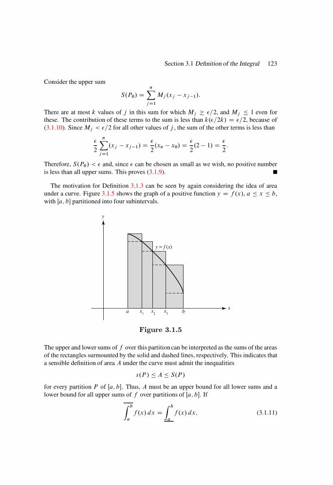
Section 3.1 Definition of the Integral 123
Consider the upper sum
S.P0/ DnX
j D1
Mj .xj xj 1/:
There are at most k values of j in this sum for which Mj =2, and Mj 1 even for
these. The contribution of these terms to the sum is less than k.=2k/ D =2, because of
(3.1.10). SinceMj < =2 for all other values of j , the sum of the other terms is less than
2
nX
j D1
.xj xj 1/ D
2.xn x0/ D
2.2 1/ D
2:
Therefore, S.P0/ < and, since can be chosen as small as we wish, no positive number
is less than all upper sums. This proves (3.1.9).
The motivation for Definition 3.1.3 can be seen by again considering the idea of area
under a curve. Figure 3.1.5 shows the graph of a positive function y D f .x/, a x b,
with Œa; b partitioned into four subintervals.
a x1
x2
x3
b
y = f (x)
y
x
Figure 3.1.5
The upper and lower sums of f over this partition can be interpreted as the sums of the areas
of the rectangles surmounted by the solid and dashed lines, respectively. This indicates that
a sensible definition of area A under the curve must admit the inequalities
s.P / A S.P /
for every partition P of Œa; b. Thus, A must be an upper bound for all lower sums and a
lower bound for all upper sums of f over partitions of Œa; b. If
Z b
a
f .x/ dx DZ b
a
f .x/ dx; (3.1.11)

124 Chapter 3 Integral Calculus of Functions of One Variable
there is only one number, the common value of the upper and lower integrals, with this
property, and we defineA to be that number; if (3.1.11) does not hold, thenA is not defined.
We will see below that this definition of area is consistent with the definition stated earlier
in terms of Riemann sums.
Example 3.1.7 Returning to Example 3.1.3, consider the function
f .x/ D x; 1 x 2:
If P D fx0; x1; : : : ; xng is a partition of Œ1; 2, then, since f is increasing,
Mj D f .xj / D xj and mj D f .xj 1/ D xj 1:
Hence,
S.P / DnX
j D1
xj .xj xj 1/ (3.1.12)
and
s.P /DnX
j D1
xj 1.xj xj 1/: (3.1.13)
By writing
xj Dxj C xj 1
2C xj xj 1
2;
we see from (3.1.12) that
S.P / D 1
2
nX
j D1
.x2j x2
j 1/C1
2
nX
j D1
.xj xj 1/2
D1
2.22 12/C
1
2
nX
j D1
.xj xj 1/2:
(3.1.14)
Since
0 <
nX
j D1
.xj xj 1/2 kP k
nX
j D1
.xj xj 1/ D kP k.2 1/;
(3.1.14) implies that3
2< S.P / 3
2C kP k
2:
Since kP k can be made as small as we please, Definition 3.1.3 implies that
Z b
a
f .x/ dx D 3
2:
A similar argument starting from (3.1.13) shows that
3
2 kP k
2 s.P / < 3
2;
Section 3.1 Definition of the Integral 125
so Z b
a
f .x/ dx D 3
2:
Since the upper and lower integrals both equal 3=2, the area under the curve is 3=2 accord-
ing to our new definition. This is consistent with the result in Example 3.1.3.
The Riemann–Stieltjes Integral
The Riemann–Stieltjes integral is an important generalization of the Riemann integral. We
define it here, but confine our study of it to the exercises in this and other sections of this
chapter.
Definition 3.1.5 Let f and g be defined on Œa; b. We say that f is Riemann–Stieltjes
integrable with respect to g on Œa; b if there is a number L with the following property:
For every > 0, there is a ı > 0 such that
ˇˇˇ
nX
j D1
f .cj /g.xj / g.xj 1/
L
ˇˇˇ < ; (3.1.15)
provided only that P D fx0; x1; : : : ; xng is a partition of Œa; b such that kP k < ı and
xj 1 cj xj ; j D 1; 2; : : : ; n:
In this case, we say that L is the Riemann–Stieltjes integral of f with respect to g over
Œa; b, and write Z b
a
f .x/ dg.x/ D L:
The sumnX
j D1
f .cj /g.xj / g.xj 1/
in (3.1.15) is a Riemann–Stieltjes sum of f with respect to g over the partitionP .
3.1 Exercises
1. Show that there cannot be more than one number L that satisfies Definition 3.1.1.
2. (a) Prove: IfR b
af .x/ dx exists, then for every > 0, there is a ı > 0 such that
j1 2j < if 1 and 2 are Riemann sums of f over partitions P1 and P2
of Œa; b with norms less than ı.
126 Chapter 3 Integral Calculus of Functions of One Variable
(b) Suppose that there is an M > 0 such that, for every ı > 0, there are Riemann
sums 1 and 2 over a partitionP of Œa; bwith kP k < ı such that j12j M . Use (a) to prove that f is not integrable over Œa; b.
3. Suppose thatR b
af .x/ dx exists and there is a number A such that, for every > 0
and ı > 0, there is a partitionP of Œa; b with kP k < ı and a Riemann sum of f
over P that satisfies the inequality j Aj < . Show thatR b
af .x/ dx D A.
4. Prove directly from Definition 3.1.1 that
Z b
a
x2 dx D b3 a3
3:
Do not assume in advance that the integral exists. The proof of this is part of the
problem. HINT: Let P D fx0; x2; : : : ; xng be an arbitrary partition of Œa; b: Use
the mean value theorem to show that
b3 a3
3D
nX
j D1
d 2j .xj xj 1/
for some points d1; . . . , dn; where xj 1 < dj < xj . Then relate this sum to
arbitrary Riemann sums for f .x/ D x2 over P:
5. Generalize the proof of Exercise 3.1.4 to show directly from Definition 3.1.1 that
Z b
a
xm dx D bmC1 amC1
mC 1
if m is an integer 0.
6. Prove directly from Definition 3.1.1 that f .x/ is integrable on Œa; b if and only if
f .x/ is integrable on Œb;a, and, in this case,
Z b
a
f .x/ dx DZ a
b
f .x/ dx:
7. Let f be bounded on Œa; b and let P be a partition of Œa; b. Prove: The lower sum
s.P / of f over P is the infimum of the set of all Riemann sums of f over P .
8. Let f be defined on Œa; b and let P D fx0; x1; : : : ; xng be a partition of Œa; b.
(a) Prove: If f is continuous on Œa; b, then s.P / and S.P / are Riemann sums of
f over P .
(b) Name another class of functions for which the conclusion of (a) is valid.
(c) Give an example where s.P / and S.P / are not Riemann sums of f over P .
Section 3.1 Definition of the Integral 127
9. FindR 1
0f .x/ dx and
R 1
0f .x/ dx if
(a) f .x/ Dx if x is rational;
x if x is irrational:(b) f .x/ D
1 if x is rational;
x if x is irrational:
10. Given thatR b
aex dx exists, evaluate it by using the formula
1C r C r2 C C rn D 1 rnC1
1 r .r ¤ 1/
to calculate certain Riemann sums. HINT: See Exercise 3.1.3:
11. Given thatR b
0sinx dx exists, evaluate it by using the identity
cos.j 1/ cos.j C 1/ D 2 sin sin j
to calculate certain Riemann sums. HINT: See Exercise 3.1.3:
12. Given thatR b
0cos x dx exists, evaluate it by using the identity
sin.j C 1/ sin.j 1/ D 2 sin cos j
to calculate certain Riemann sums. HINT: See Exercise 3.1.3:
13. Show that if g.x/ D x C c (c=constant), thenR b
a f .x/ dg.x/ exists if and only ifR b
af .x/ dx exists, in which case
Z b
a
f .x/ dg.x/ DZ b
a
f .x/ dx:
14. Suppose that 1 < a < d < c <1 and
g.x/ Dg1; a < x < d;
g2; d < x < b;(g1; g2 D constants),
and let g.a/, g.b/, and g.d/ be arbitrary. Suppose that f is defined on Œa; b,
continuous from the right at a and from the left at b, and continuous at d . Show thatR b
af .x/ dg.x/ exists, and find its value.
15. Suppose that 1 < a D a0 < a1 < < ap D b < 1, let g.x/ D gm
(constant) on .am1; am/, 1 m p, and let g.a0/, g.a1/, . . . , g.ap/ be arbitrary.
Suppose that f is defined on Œa; b, continuous from the right at a and from the
left at b, and continuous at a1, a2, . . . , ap1. EvaluateR b
af .x/ dg.x/. HINT: See
Exercise 3.1.14:
16. (a) Give an example whereR b
af .x/ dg.x/ exists even though f is unbounded
on Œa; b. (Thus, the analog of Theorem 3.1.2 does not hold for the Riemann–
Stieltjes integral.)
(b) State and prove an analog of Theorem 3.1.2 for the case where g is increasing.
128 Chapter 3 Integral Calculus of Functions of One Variable
17. For the case where g is nondecreasing and f is bounded on Œa; b, define upper and
lower Riemann–Stieltjes integrals in a way analogous to Definition 3.1.3.
3.2 EXISTENCE OF THE INTEGRAL
The following lemma is the starting point for our study of the integrability of a bounded
function f on a closed interval Œa; b.
Lemma 3.2.1 Suppose that
jf .x/j M; a x b; (3.2.1)
and letP 0 be a partition of Œa; b obtained by adding r points to a partitionP D fx0; x1; : : : ; xngof Œa; b: Then
S.P / S.P 0/ S.P / 2MrkP k (3.2.2)
and
s.P / s.P 0/ s.P /C 2MrkP k: (3.2.3)
Proof We will prove (3.2.2) and leave the proof of (3.2.3) to you (Exercise 3.2.1).
First suppose that r D 1, so P 0 is obtained by adding one point c to the partition P Dfx0; x1; : : : ; xng; then xi1 < c < xi for some i in f1; 2; : : : ; ng. If j ¤ i , the prod-
uct Mj .xj xj 1/ appears in both S.P / and S.P 0/ and cancels out of the difference
S.P / S.P 0/. Therefore, if
Mi1 D supxi1xc
f .x/ and Mi2 D supcxxi
f .x/;
then
S.P / S.P 0/ DMi .xi xi1/ Mi1.c xi1/ Mi2.xi c/
D .Mi Mi1/.c xi1/C .Mi Mi2/.xi c/:(3.2.4)
Since (3.2.1) implies that
0 Mi Mir 2M; r D 1; 2;
(3.2.4) implies that
0 S.P / S.P 0/ 2M.xi xi1/ 2MkP k:
This proves (3.2.2) for r D 1.
Now suppose that r > 1 and P 0 is obtained by adding points c1, c2, . . . , cr to P . Let
P .0/ D P and, for j 1, let P .j / be the partition of Œa; b obtained by adding cj to
P .j 1/. Then the result just proved implies that
0 S.P .j 1// S.P .j // 2MkP .j 1/k; 1 j r:
Section 3.2 Existence of the Integral 129
Adding these inequalities and taking account of cancellations yields
0 S.P .0// S.P .r// 2M.kP .0/k C kP .1/k C C kP .r1/k/: (3.2.5)
Since P .0/ D P , P .r/ D P 0, and kP .k/k kP .k1/k for 1 k r 1, (3.2.5) implies
that
0 S.P / S.P 0/ 2MrkP k;which is equivalent to (3.2.2).
Theorem 3.2.2 If f is bounded on Œa; b; then
Z b
a
f .x/ dx Z b
a
f .x/ dx: (3.2.6)
Proof Suppose that P1 and P2 are partitions of Œa; b and P 0 is a refinement of both.
Letting P D P1 in (3.2.3) and P D P2 in (3.2.2) shows that
s.P1/ s.P 0/ and S.P 0/ S.P2/:
Since s.P 0/ S.P 0/, this implies that s.P1/ S.P2/. Thus, every lower sum is a lower
bound for the set of all upper sums. SinceR b
af .x/ dx is the infimum of this set, it follows
that
s.P1/ Z b
a
f .x/ dx
for every partition P1 of Œa; b. This means thatR b
af .x/ dx is an upper bound for the set
of all lower sums. SinceR b
af .x/ dx is the supremum of this set, this implies (3.2.6).
Theorem 3.2.3 If f is integrable on Œa; b; then
Z b
a
f .x/ dx DZ b
a
f .x/ dx DZ b
a
f .x/ dx:
Proof We prove thatR b
af .x/ dx D
R b
af .x/ dx and leave it to you to show that
R b
af .x/ dx D
R b
af .x/ dx (Exercise 3.2.2).
Suppose that P is a partition of Œa; b and is a Riemann sum of f over P . Since
Z b
a
f .x/ dx Z b
a
f .x/ dx D Z b
a
f .x/ dx S.P /!C .S.P / /
C
Z b
a
f .x/ dx
!;

130 Chapter 3 Integral Calculus of Functions of One Variable
the triangle inequality implies that
ˇˇˇ
Z b
a
f .x/ dx Z b
a
f .x/ dx
ˇˇˇ
ˇˇˇ
Z b
a
f .x/ dx S.P /ˇˇˇ C jS.P / j
Cˇˇˇ
Z b
a
f .x/ dx
ˇˇˇ:
(3.2.7)
Now suppose that > 0. From Definition 3.1.3, there is a partitionP0 of Œa; b such that
Z b
a
f .x/ dx S.P0/ <
Z b
a
f .x/ dx C
3: (3.2.8)
From Definition 3.1.1, there is a ı > 0 such that
ˇˇˇ
Z b
a
f .x/ dx
ˇˇˇ <
3(3.2.9)
if kP k < ı. Now suppose that kP k < ı and P is a refinement of P0. Since S.P / S.P0/
by Lemma 3.2.1, (3.2.8) implies that
Z b
a
f .x/ dx S.P / <Z b
a
f .x/ dx C
3;
so ˇˇˇS.P /
Z b
a
f .x/ dx
ˇˇˇ <
3(3.2.10)
in addition to (3.2.9). Now (3.2.7), (3.2.9), and (3.2.10) imply that
ˇˇˇ
Z b
a
f .x/ dx Z b
a
f .x/ dx
ˇˇˇ <
2
3C jS.P / j (3.2.11)
for every Riemann sum of f over P . Since S.P / is the supremum of these Riemann
sums (Theorem 3.1.4), we may choose so that
jS.P / j <
3:
Now (3.2.11) implies that
ˇˇˇ
Z b
a
f .x/ dx Z b
a
f .x/ dx
ˇˇˇ < :
Since is an arbitrary positive number, it follows that
Z b
a
f .x/ dx DZ b
a
f .x/ dx:
Section 3.2 Existence of the Integral 131
Lemma 3.2.4 If f is bounded on Œa; b and > 0; there is a ı > 0 such that
Z b
a
f .x/ dx S.P / <Z b
a
f .x/ dx C (3.2.12)
and Z b
a
f .x/ dx s.P / >Z b
a
f .x/ dx
if kP k < ı.
Proof We show that (3.2.12) holds if kP k is sufficiently small, and leave the rest of the
proof to you (Exercise 3.2.3).
The first inequality in (3.2.12) follows immediately from Definition 3.1.3. To establish
the second inequality, suppose that jf .x/j K if a x b. From Definition 3.1.3, there
is a partitionP0 D fx0; x1; : : : ; xrC1g of Œa; b such that
S.P0/ <
Z b
a
f .x/ dx C
2: (3.2.13)
If P is any partition of Œa; b, let P 0 be constructed from the partition points of P0 and P .
Then
S.P 0/ S.P0/; (3.2.14)
by Lemma 3.2.1. Since P 0 is obtained by adding at most r points to P , Lemma 3.2.1
implies that
S.P 0/ S.P / 2KrkP k: (3.2.15)
Now (3.2.13), (3.2.14), and (3.2.15) imply that
S.P / S.P 0/C 2KrkP k S.P0/C 2KrkP k
<
Z b
a
f .x/ dx C
2C 2KrkP k:
Therefore, (3.2.12) holds if
kP k < ı D
4Kr:
Theorem 3.2.5 If f is bounded on Œa; b and
Z b
a
f .x/ dx DZ b
a
f .x/ dx D L; (3.2.16)
then f is integrable on Œa; b and
Z b
a
f .x/ dx D L: (3.2.17)

132 Chapter 3 Integral Calculus of Functions of One Variable
Proof If > 0, there is a ı > 0 such that
Z b
a
f .x/ dx < s.P / S.P / <Z b
a
f .x/ dx C (3.2.18)
if kP k < ı (Lemma 3.2.4). If is a Riemann sum of f over P , then
s.P / S.P /;
so (3.2.16) and (3.2.18) imply that
L < < LC
if kP k < ı. Now Definition 3.1.1 implies (3.2.17).
Theorems 3.2.3 and 3.2.5 imply the following theorem.
Theorem 3.2.6 A bounded function f is integrable on Œa; b if and only if
Z b
a
f .x/ dx DZ b
a
f .x/ dx:
The next theorem translates this into a test that can be conveniently applied.
Theorem 3.2.7 If f is bounded on Œa; b; then f is integrable on Œa; b if and only if
for each > 0 there is a partitionP of Œa; b for which
S.P / s.P / < : (3.2.19)
Proof We leave it to you (Exercise 3.2.4) to show that ifR b
af .x/ dx exists, then (3.2.19)
holds for kP k sufficiently small. This implies that the stated condition is necessary for in-
tegrability. To show that it is sufficient, we observe that since
s.P / Z b
a
f .x/ dx Z b
a
f .x/ dx S.P /
for all P , (3.2.19) implies that
0 Z b
a
f .x/ dx Z b
a
f .x/ dx < :
Since can be any positive number, this implies that
Z b
a
f .x/ dx DZ b
a
f .x/ dx:
Therefore,R b
af .x/ dx exists, by Theorem 3.2.5.
The next two theorems are important applications of Theorem 3.2.7.

Section 3.2 Existence of the Integral 133
Theorem 3.2.8 If f is continuous on Œa; b; then f is integrable on Œa; b.
Proof Let P D fx0; x1; : : : ; xng be a partition of Œa; b. Since f is continuous on Œa; b,
there are points cj and c0j in Œxj 1; xj such that
f .cj / D Mj D supxj 1xxj
f .x/
and
f .c0j / D mj D inf
xj 1xxj
f .x/
(Theorem 2.2.9). Therefore,
S.P / s.P / DnX
j D1
f .cj / f .c0
j /.xj xj 1/: (3.2.20)
Since f is uniformly continuous on Œa; b (Theorem 2.2.12), there is for each > 0 a ı > 0
such that
jf .x0/ f .x/j <
b aif x and x0 are in Œa; b and jxx0j < ı. If kP k < ı, then jcj c0
j j < ı and, from (3.2.20),
S.P / s.P / <
b a
nX
j D1
.xj xj 1/ D :
Hence, f is integrable on Œa; b, by Theorem 3.2.7.
Theorem 3.2.9 If f is monotonic on Œa; b; then f is integrable on Œa; b.
Proof Let P D fx0; x1; : : : ; xng be a partition of Œa; b. Since f is nondecreasing,
f .xj / DMj D supxj 1xxj
f .x/
and
f .xj 1/ D mj D infxj 1xxj
f .x/:
Hence,
S.P / s.P / DnX
j D1
.f .xj / f .xj 1//.xj xj 1/:
Since 0 < xj xj 1 kP k and f .xj / f .xj 1/ 0,
S.P / s.P / kP knX
j D1
.f .xj / f .xj 1//
D kP k.f .b/ f .a//:
134 Chapter 3 Integral Calculus of Functions of One Variable
Therefore,
S.P / s.P / < if kP k.f .b/ f .a// < ;so f is integrable on Œa; b, by Theorem 3.2.7.
The proof for nonincreasing f is similar.
We will also use Theorem 3.2.7 in the next section to establish properties of the integral.
In Section 3.5 we will study more general conditions for integrability.
3.2 Exercises
1. Complete the proof of Lemma 3.2.1 by verifying Eqn. (3.2.3).
2. Show that if f is integrable on Œa; b, thenZ b
a
f .x/ dx DZ b
a
f .x/ dx:
3. Prove: If f is bounded on Œa; b, there is for each > 0 a ı > 0 such thatZ b
a
f .x/ dx Z b
a
f .x/ dx < s.P /
if kP k < ı.4. Prove: If f is integrable on Œa; b and > 0, then S.P / s.P / < if kP k is
sufficiently small. HINT: Use Theorem 3.1.4:
5. Suppose that f is integrable and g is bounded on Œa; b, and g differs from f only
at points in a set H with the following property: For each > 0, H can be covered
by a finite number of closed subintervals of Œa; b, the sum of whose lengths is less
than . Show that g is integrable on Œa; b and thatZ b
a
g.x/ dx DZ b
a
f .x/ dx:
HINT: Use Exercise 3.1.3:
6. Suppose that g is bounded on Œ˛; ˇ, and let Q W ˛ D v0 < v1 < < vL D ˇ be
a fixed partition of Œ˛; ˇ. Prove:
(a)Z ˇ
˛
g.u/ du DLX
`D1
Z v`
v`1
g.u/ duI (b)Z ˇ
˛
g.u/ du DLX
`D1
Z v`
v`1
g.u/ du:
7. A function f is of bounded variation on Œa; b if there is a number K such that
nX
j D1
ˇf .aj / f .aj 1/
ˇ K
whenever a D a0 < a1 < < an D b. (The smallest number with this property
is the total variation of f on Œa; b.)

Section 3.3 Properties of the Integral 135
(a) Prove: If f is of bounded variation on Œa; b, then f is bounded on Œa; b.
(b) Prove: If f is of bounded variation on Œa; b, then f is integrable on Œa; b.
HINT: Use Theorems 3.1.4 and 3.2.7:
8. Let P D fx0; x1; : : : ; xng be a partition of Œa; b, c0 D x0 D a, cnC1 D xn D b,
and xj 1 cj xj , j D 1, 2, . . . , n. Verify that
nX
j D1
g.cj /Œf .xj /f .xj 1/ D g.b/f .b/g.a/f .a/nX
j D0
f .xj /Œg.cj C1/g.cj /:
Use this to prove that ifR b
af .x/ dg.x/ exists, then so does
R b
ag.x/ df .x/, and
Z b
a
g.x/ df .x/ D f .b/g.b/ f .a/g.a/ Z b
a
f .x/ dg.x/:
(This is the integration by parts formula for Riemann–Stieltjes integrals.)
9. Let f be continuous and g be of bounded variation (Exercise 3.2.7) on Œa; b.
(a) Show that if > 0, there is a ı > 0 such that j 0j < =2 if and 0
are Riemann–Stieltjes sums of f with respect to g over partitions P and P 0
of Œa; b, where P 0 is a refinement of P and kP k < ı. HINT: Use Theo-
rem 2.2.12:
(b) Let ı be as chosen in (a). Suppose that 1 and 2 are Riemann–Stieltjes
sums of f with respect to g over any partitionsP1 and P2 of Œa; b with norm
less than ı. Show that j1 2j < .(c) If ı > 0, let L.ı/ be the supremum of all Riemann–Stieltjes sums of f with
respect to g over partitions of Œa; b with norms less than ı. Show that L.ı/ is
finite. Then show that L D limı!0C L.ı/ exists. HINT: Use Theorem 2.1.9:
(d) Show thatR b
af .x/ dg.x/ D L.
10. Show thatR b
a f .x/ dg.x/ exists if f is of bounded variation and g is continuous on
Œa; b. HINT: See Exercises 3.2.8 and 3.2.9:
3.3 PROPERTIES OF THE INTEGRAL
We now use the results of Sections 3.1 and 3.2 to establish the properties of the integral.
You are probably familiar with most of these properties, but not with their proofs.
Theorem 3.3.1 If f and g are integrable on Œa; b; then so is f C g; and
Z b
a
.f C g/.x/ dx DZ b
a
f .x/ dx CZ b
a
g.x/ dx:
136 Chapter 3 Integral Calculus of Functions of One Variable
Proof Any Riemann sum of f C g over a partitionP D fx0; x1; : : : ; xng of Œa; b can
be written as
f Cg DnX
j D1
Œf .cj /C g.cj /.xj xj 1/
DnX
j D1
f .cj /.xj xj 1/CnX
j D1
g.cj /.xj xj 1/
D f C g ;
where f and g are Riemann sums for f and g. Definition 3.1.1 implies that if > 0
there are positive numbers ı1 and ı2 such thatˇˇˇf
Z b
a
f .x/ dx
ˇˇˇ <
2if kP k < ı1
and ˇˇˇg
Z b
a
g.x/ dx
ˇˇˇ <
2if kP k < ı2:
If kP k < ı D min.ı1; ı2/, thenˇˇˇf Cg
Z b
a
f .x/ dx Z b
a
g.x/ dx
ˇˇˇ D
ˇˇˇ
f
Z b
a
f .x/ dx
!C g
Z b
a
g.x/ dx
!ˇˇˇ
ˇˇˇf
Z b
a
f .x/ dx
ˇˇˇC
ˇˇˇg
Z b
a
g.x/ dx
ˇˇˇ
<
2C
2D ;
so the conclusion follows from Definition 3.1.1.
The next theorem also follows from Definition 3.1.1 (Exercise 3.3.1).
Theorem 3.3.2 If f is integrable on Œa; b and c is a constant; then cf is integrable
on Œa; b and Z b
a
cf .x/ dx D cZ b
a
f .x/ dx:
Theorems 3.3.1 and 3.3.2 and induction yield the following result (Exercise 3.3.2).
Theorem 3.3.3 If f1; f2; . . . ; fn are integrable on Œa; b and c1; c2; . . . ; cn are
constants; then c1f1 C c2f2 C C cnfn is integrable on Œa; b and
Z b
a
.c1f1 C c2f2 C C cnfn/.x/ dx D c1
Z b
a
f1.x/ dx C c2
Z b
a
f2.x/ dx
C C cn
Z b
a
fn.x/ dx:
Section 3.3 Properties of the Integral 137
Theorem 3.3.4 If f and g are integrable on Œa; b and f .x/ g.x/ for a x b;then Z b
a
f .x/ dx Z b
a
g.x/ dx: (3.3.1)
Proof Since g.x/ f .x/ 0, every lower sum of g f over any partition of Œa; b is
nonnegative. Therefore, Z b
a
.g.x/ f .x// dx 0:
Hence, Z b
a
g.x/ dx Z b
a
f .x/ dx DZ b
a
.g.x/ f .x// dx
DZ b
a
.g.x/ f .x// dx 0;(3.3.2)
which yields (3.3.1). (The first equality in (3.3.2) follows from Theorems 3.3.1 and 3.3.2;
the second, from Theorem 3.2.3.)
Theorem 3.3.5 If f is integrable on Œa; b; then so is jf j, and
ˇˇˇ
Z b
a
f .x/ dx
ˇˇˇ
Z b
a
jf .x/j dx: (3.3.3)
Proof Let P be a partition of Œa; b and define
Mj D sup˚f .x/
ˇxj 1 x xj
;
mj D inf˚f .x/
ˇxj 1 x xj
;
M j D sup˚jf .x/j
ˇxj 1 x xj
;
mj D inf˚jf .x/j
ˇxj 1 x xj
:
ThenM j mj D sup
˚jf .x/j jf .x0/j
ˇxj 1 x; x0 xj
sup˚jf .x/ f .x0/j
ˇxj 1 x; x0 xj
DMj mj :
(3.3.4)
Therefore,
S.P / s.P / S.P / s.P /;where the upper and lower sums on the left are associated with jf j and those on the right are
associated with f . Now suppose that > 0. Since f is integrable on Œa; b, Theorem 3.2.7
implies that there is a partition P of Œa; b such that S.P / s.P / < . This inequality
and (3.3.4) imply that S.P / s.P / < . Therefore, jf j is integrable on Œa; b, again by
Theorem 3.2.7.
Since
f .x/ jf .x/j and f .x/ jf .x/j; a x b;
138 Chapter 3 Integral Calculus of Functions of One Variable
Theorems 3.3.2 and 3.3.4 imply that
Z b
a
f .x/ dx Z b
a
jf .x/j dx and Z b
a
f .x/ dx Z b
a
jf .x/j dx;
which implies (3.3.3).
Theorem 3.3.6 If f and g are integrable on Œa; b; then so is the product fg:
Proof We consider the case where f and g are nonnegative, and leave the rest of the
proof to you (Exercise 3.3.4). The subscripts f , g, and fg in the following argument
identify the functions with which the various quantities are associated. We assume that
neither f nor g is identically zero on Œa; b, since the conclusion is obvious if one of them
is.
If P D fx0; x1; : : : ; xng is a partition of Œa; b, then
Sfg.P / sfg.p/ DnX
j D1
.Mfg;j mfg;j /.xj xj 1/: (3.3.5)
Since f and g are nonnegative, Mfg;j Mf;jMg;j and mfg;j mf;jmg;j . Hence,
Mfg;j mfg;j Mf;jMg;j mf;jmg;j
D .Mf;j mf;j /Mg;j Cmf;j .Mg;j mg;j /
Mg.Mf;j mf;j /CMf .Mg;j mg;j /;
where Mf and Mg are upper bounds for f and g on Œa; b. From (3.3.5) and the last
inequality,
Sfg.P / sfg.P / Mg ŒSf .P / sf .P /CMf ŒSg.P / sg.P /: (3.3.6)
Now suppose that > 0. Theorem 3.2.7 implies that there are partitions P1 and P2 of
Œa; b such that
Sf .P1/ sf .P1/ <
2Mg
and Sg.P2/ sg.P2/ <
2Mf
: (3.3.7)
If P is a refinement of both P1 and P2, then (3.3.7) and Lemma 3.2.1 imply that
Sf .P / sf .P / <
2Mg
and Sg.P / sg.P / <
2Mf
:
This and (3.3.6) yield
Sfg.P / sfg.P / <
2C
2D :
Therefore, fg is integrable on Œa; b, by Theorem 3.2.7.
Section 3.3 Properties of the Integral 139
Theorem 3.3.7 (First Mean Value Theorem for Integrals) Suppose that
u is continuous and v is integrable and nonnegative on Œa; b: Then
Z b
a
u.x/v.x/ dx D u.c/Z b
a
v.x/ dx (3.3.8)
for some c in Œa; b.
Proof From Theorem 3.2.8, u is integrable on Œa; b. Therefore, Theorem 3.3.6 implies
that the integral on the left exists. Ifm D min˚u.x/
ˇa x b
andM D max
˚u.x/
ˇa x b
(recall Theorem 2.2.9), then
m u.x/ Mand, since v.x/ 0,
mv.x/ u.x/v.x/ Mv.x/:
Therefore, Theorems 3.3.2 and 3.3.4 imply that
m
Z b
a
v.x/ dx Z b
a
u.x/v.x/ dx MZ b
a
v.x/ dx: (3.3.9)
This implies that (3.3.8) holds for any c in Œa; b ifR b
av.x/ dx D 0. If
R b
av.x/ dx ¤ 0,
let
u D
Z b
a
u.x/v.x/ dx
Z b
a
v.x/ dx
(3.3.10)
SinceR b
a v.x/ dx > 0 in this case (why?), (3.3.9) implies that m u M , and the
intermediate value theorem (Theorem 2.2.10) implies that u D u.c/ for some c in Œa; b.
This implies (3.3.8).
If v.x/ 1, then (3.3.10) reduces to
u D 1
b a
Z b
a
u.x/ dx;
so u is the average of u.x/ over Œa; b. More generally, if v is any nonnegative integrable
function such thatR b
av.x/ dx ¤ 0, then u in (3.3.10) is the weighted average of u.x/ over
Œa; b with respect to v. Theorem 3.3.7 says that a continuous function assumes any such
weighted average at some point in Œa; b.
Theorem 3.3.8 If f is integrable on Œa; b and a a1 < b1 b; then f is integrable
on Œa1; b1:
140 Chapter 3 Integral Calculus of Functions of One Variable
Proof Suppose that > 0. From Theorem 3.2.7, there is a partitionP D fx0; x1; : : : ; xngof Œa; b such that
S.P / s.P / DnX
j D1
.Mj mj /.xj xj 1/ < : (3.3.11)
We may assume that a1 and b1 are partition points of P , because if not they can be inserted
to obtain a refinement P 0 such that S.P 0/ s.P 0/ S.P / s.P / (Lemma 3.2.1). Let
a1 D xr and b1 D xs. Since every term in (3.3.11) is nonnegative,
sX
j DrC1
.Mj mj /.xj xj 1/ < :
Thus, P D fxr ; xrC1; : : : ; xsg is a partition of Œa1; b1 over which the upper and lower
sums of f satisfy
S.P / s.P / < :Therefore, f is integrable on Œa1; b1, by Theorem 3.2.7.
We leave the proof of the next theorem to you (Exercise 3.3.8).
Theorem 3.3.9 If f is integrable on Œa; b and Œb; c; then f is integrable on Œa; c;
and Z c
a
f .x/ dx DZ b
a
f .x/ dx CZ c
b
f .x/ dx: (3.3.12)
So far we have definedR ˇ
˛f .x/ dx only for the case where ˛ < ˇ. Now we define
Z ˛
ˇ
f .x/ dx D Z ˇ
˛
f .x/ dx
if ˛ < ˇ, and Z ˛
˛
f .x/ dx D 0:
With these conventions, (3.3.12) holds no matter what the relative order of a, b, and c,
provided that f is integrable on some closed interval containing them (Exercise 3.3.9).
Theorem 3.3.8 and these definitions enable us to define a function F.x/ DR x
c f .t/ dt ,
where c is an arbitrary, but fixed, point in Œa; b.
Theorem 3.3.10 If f is integrable on Œa; b and a c b; then the function F
defined by
F.x/ DZ x
c
f .t/ dt
satisfies a Lipschitz condition on Œa; b; and is therefore continuous on Œa; b:
Section 3.3 Properties of the Integral 141
Proof If x and x0 are in Œa; b, then
F.x/ F.x0/ DZ x
c
f .t/ dt Z x0
c
f .t/ dt DZ x
x0
f .t/ dt;
by Theorem 3.3.9 and the conventions just adopted. Since jf .t/j K .a t b/ for
some constant K, ˇˇZ x
x0
f .t/ dt
ˇˇ Kjx x0j; a x; x0 b
(Theorem 3.3.5), so
jF.x/ F.x0/j Kjx x0j; a x; x0 b:
Theorem 3.3.11 If f is integrable on Œa; b and a c b; then F.x/ DR x
cf .t/ dt
is differentiable at any point x0 in .a; b/ where f is continuous; with F 0.x0/ D f .x0/: If
f is continuous from the right at a; then F 0C.a/ D f .a/. If f is continuous from the left
at b; then F 0.b/ D f .b/:
Proof We consider the case where a < x0 < b and leave the rest to you (Exer-
cise 3.3.14). Since1
x x0
Z x
x0
f .x0/ dt D f .x0/;
we can write
F.x/ F.x0/
x x0
f .x0/ D1
x x0
Z x
x0
Œf .t/ f .x0/ dt:
From this and Theorem 3.3.5,
ˇˇF.x/ F.x0/
x x0
f .x0/
ˇˇ 1
jx x0j
ˇˇZ x
x0
jf .t/ f .x0/j dtˇˇ : (3.3.13)
(Why do we need the absolute value bars outside the integral?) Since f is continuous at
x0, there is for each > 0 a ı > 0 such that
jf .t/ f .x0/j < if jx x0j < ı
and t is between x and x0. Therefore, from (3.3.13),
ˇˇF.x/ F.x0/
x x0
f .x0/
ˇˇ < jx x0j
jx x0jD if 0 < jx x0j < ı:
Hence, F 0.x0/ D f .x0/.
142 Chapter 3 Integral Calculus of Functions of One Variable
Example 3.3.1 If
f .x/ D(x; 0 x 1;x C 1; 1 < x 2;
then the function
F.x/ DZ x
0
f .t/ dt D
8ˆ<ˆ:
x2
2; 0 < x 1;
x2
2C x 1; 1 < x 2;
is continuous on Œ0; 2. As implied by Theorem 3.3.11,
F 0.x/ D
8<:x D f .x/; 0 < x < 1;
x C 1 D f .x/; 1 < x < 2;
F 0C.0/ D lim
x!0C
F.x/ F.0/x
D limx!0C
.x2=2/ 0x
D 0 D f .0/;
F 0.2/ D lim
x!2
F.x/ F.2/x 2 D lim
x!2
.x2=2/C x 1 3x 2
D limx!2
x C 42D 3 D f .2/:
F does not have a derivative at x D 1, where f is discontinuous, since
F 0.1/ D 1 and F 0
C.1/ D 2:
The next theorem relates integration and differentiation in another way.
Theorem 3.3.12 Suppose that F is continuous on the closed interval Œa; b and dif-
ferentiable on the open interval .a; b/; and f is integrable on Œa; b: Suppose also that
F 0.x/ D f .x/; a < x < b:
Then Z b
a
f .x/ dx D F.b/ F.a/: (3.3.14)
Proof If P D fx0; x1; : : : ; xng is a partition of Œa; b, then
F.b/ F.a/ DnX
j D1
.F.xj / F.xj 1//: (3.3.15)
From Theorem 2.3.11, there is in each open interval .xj 1; xj / a point cj such that
F.xj / F.xj 1/ D f .cj /.xj xj 1/:
Section 3.3 Properties of the Integral 143
Hence, (3.3.15) can be written as
F.b/ F.a/ DnX
j D1
f .cj /.xj xj 1/ D ;
where is a Riemann sum for f over P . Since f is integrable on Œa; b, there is for each
> 0 a ı > 0 such thatˇˇˇ
Z b
a
f .x/ dx
ˇˇˇ < if kP k < ı:
Therefore, ˇˇˇF.b/ F.a/
Z b
a
f .x/ dx
ˇˇˇ <
for every > 0, which implies (3.3.14).
Corollary 3.3.13 If f 0 is integrable on Œa; b; then
Z b
a
f 0.x/ dx D f .b/ f .a/:
Proof Apply Theorem 3.3.12 with F and f replaced by f and f 0, respectively.
A function F is an antiderivative of f on Œa; b if F is continuous on Œa; b and differ-
entiable on .a; b/, with
F 0.x/ D f .x/; a < x < b:
If F is an antiderivative of f on Œa; b, then so is F C c for any constant c. Conversely,
if F1 and F2 are antiderivatives of f on Œa; b, then F1 F2 is constant on Œa; b (Theo-
rem 2.3.12). Theorem 3.3.12 shows that antiderivatives can be used to evaluate integrals.
Theorem 3.3.14 (Fundamental Theorem of Calculus) If f is continu-
ous on Œa; b; then f has an antiderivative on Œa; b: Moreover; if F is any antiderivative
of f on Œa; b; then Z b
a
f .x/ dx D F.b/ F.a/:
Proof The function F0.x/ DR x
af .t/ dt is continuous on Œa; b by Theorem 3.3.10,
and F 00.x/ D f .x/ on .a; b/ by Theorem 3.3.11. Therefore, F0 is an antiderivative of f
on Œa; b. Now let F D F0C c (c D constant) be an arbitrary antiderivative of f on Œa; b.
Then
F.b/ F.a/ DZ b
a
f .x/ dx C c Z a
a
f .x/ dx c DZ b
a
f .x/ dx:
144 Chapter 3 Integral Calculus of Functions of One Variable
When applying this theorem, we will use the familiar notation
F.b/ F.a/ D F.x/ˇˇb
a
:
Theorem 3.3.15 (Integration by Parts) If u0 and v0 are integrable on Œa; b;
then Z b
a
u.x/v0.x/ dx D u.x/v.x/ˇˇb
a
Z b
a
v.x/u0.x/ dx: (3.3.16)
Proof Since u and v are continuous on Œa; b (Theorem 2.3.3), they are integrable on
Œa; b. Therefore, Theorems 3.3.1 and 3.3.6 imply that the function
.uv/0 D u0v C uv0
is integrable on Œa; b, and Theorem 3.3.12 implies that
Z b
a
Œu.x/v0.x/C u0.x/v.x/ dx D u.x/v.x/ˇˇb
a
;
which implies (3.3.16).
We will use Theorem 3.3.15 here and in the next section to obtain other results.
Theorem 3.3.16 (Second Mean Value Theorem for Integrals) Suppose
that f 0 is nonnegative and integrable and g is continuous on Œa; b: Then
Z b
a
f .x/g.x/ dx D f .a/Z c
a
g.x/ dx C f .b/Z b
c
g.x/ dx (3.3.17)
for some c in Œa; b:
Proof Since f is differentiable on Œa; b, it is continuous on Œa; b (Theorem 2.3.3).
Since g is continuous on Œa; b, so is fg (Theorem 2.2.5). Therefore, Theorem 3.2.8 implies
that the integrals in (3.3.17) exist. If
G.x/ DZ x
a
g.t/ dt; (3.3.18)
thenG0.x/ D g.x/; a < x < b (Theorem 3.3.11). Therefore, Theorem 3.3.15 with u D fand v D G yields
Z b
a
f .x/g.x/ dx D f .x/G.x/ˇˇb
a
Z b
a
f 0.x/G.x/ dx: (3.3.19)
Since f 0 is nonnegative and G is continuous, Theorem 3.3.7 implies that
Z b
a
f 0.x/G.x/ dx D G.c/Z b
a
f 0.x/ dx (3.3.20)

Section 3.3 Properties of the Integral 145
for some c in Œa; b. From Corollary 3.3.12,
Z b
a
f 0.x/ dx D f .b/ f .a/:
From this and (3.3.18), (3.3.20) can be rewritten as
Z b
a
f 0.x/G.x/ dx D .f .b/ f .a//Z c
a
g.x/ dx:
Substituting this into (3.3.19) and noting that G.a/ D 0 yields
Z b
a
f .x/g.x/ dx D f .b/Z b
a
g.x/ dx .f .b/ f .a//Z c
a
g.x/ dx;
D f .a/Z c
a
g.x/ dx C f .b/ Z b
a
g.x/ dx Z a
c
g.x/ dx
!
D f .a/Z c
a
g.x/ dx C f .b/Z b
c
g.x/ dx:
Change of Variable
The following theorem on change of variable is useful for evaluating integrals.
Theorem 3.3.17 Suppose that the transformation x D .t/ maps the interval c t d into the interval a x b; with .c/ D ˛ and .d/ D ˇ; and let f be continuous
on Œa; b: Let 0 be integrable on Œc; d : Then
Z ˇ
˛
f .x/ dx DZ d
c
f ..t//0.t/ dt: (3.3.21)
Proof Both integrals in (3.3.21) exist: the one on the left by Theorem 3.2.8, the one on
the right by Theorems 3.2.8 and 3.3.6 and the continuity of f ..t//. By Theorem 3.3.11,
the function
F.x/ DZ x
a
f .y/ dy
is an antiderivative of f on Œa; b and, therefore, also on the closed interval with endpoints
˛ and ˇ. Hence, by Theorem 3.3.14,
Z ˇ
˛
f .x/ dx D F.ˇ/ F.˛/: (3.3.22)
By the chain rule, the function
G.t/ D F..t//

146 Chapter 3 Integral Calculus of Functions of One Variable
is an antiderivative of f ..t//0 .t/ on Œc; d , and Theorem 3.3.12 implies that
Z d
c
f ..t//0.t/ dt D G.d/ G.c/ D F..d// F..c//
D F.ˇ/ F.˛/:
Comparing this with (3.3.22) yields (3.3.21).
Example 3.3.2 To evaluate the integral
I DZ 1=
p2
1=p
2
.1 2x2/.1 x2/1=2dx
we let
f .x/ D .1 2x2/.1 x2/1=2; 1=p2 x 1=
p2;
and
x D .t/ D sin t; =4 t =4:Then 0.t/ D cos t and
I DZ 1=
p2
1=p
2
f .x/ dx DZ =4
=4
f .sin t/ cos t dt
DZ =4
=4
.1 2 sin2 t/.1 sin2 t/1=2 cos t dt:
(3.3.23)
.1 sin2 t/1=2 D cos t;=4 t =4
and
1 2 sin2 t D cos 2t;
(3.3.23) yields
I DZ =4
=4
cos 2t dt D sin 2t
2
ˇˇ=4
=4
D 1:
Example 3.3.3 To evaluate the integral
I DZ 5
0
sin t
2C cos tdt;
we take .t/ D cos t . Then 0.t/ D sin t and
I D Z 5
0
0.t/
2C .t/ dt D Z 5
0
f ..t//0.t/ dt;
where
f .x/ D 1
2C x:
Section 3.3 Properties of the Integral 147
Therefore, since .0/ D 1 and .5/ D 1,
I D Z 1
1
dx
2C x D log.2C x/ˇˇ1
1
D log 3:
These examples illustrate two ways to use Theorem 3.3.17. In Example 3.3.2 we evalu-
ated the left side of (3.3.21) by transforming it to the right side with a suitable substitution
x D .t/, while in Example 3.3.3 we evaluated the right side of (3.3.21) by recognizing
that it could be obtained from the left side by a suitable substitution.
The following theorem shows that the rule for change of variable remains valid under
weaker assumptions on f if is monotonic.
Theorem 3.3.18 Suppose that 0 is integrable and is monotonic on Œc; d ; and the
transformation x D .t/ maps Œc; d onto Œa; b: Let f be bounded on Œa; b: Then
g.t/ D f ..t//0.t/
is integrable on Œc; d if and only if f is integrable over Œa; b; and in this case
Z b
a
f .x/ dx DZ d
c
f ..t//j0 .t/j dt:
Proof We consider the case where f is nonnegative and is nondecreasing, and leave
the the rest of the proof to you (Exercises 3.3.20 and 3.3.21).
First assume that is increasing. We show first that
Z b
a
f .x/ dx DZ d
c
f ..t//0 .t/ dt: (3.3.24)
Let P D ft0; t1; : : : ; tng be a partition of Œc; d and P D fx0; x1; : : : ; xng with xj D .tj /be the corresponding partition of Œa; b. Define
Uj D sup˚0.t/
ˇtj 1 t tj
;
uj D inf˚0.t/
ˇtj 1 t tj
;
Mj D sup˚f .x/
ˇxj 1 x xj
;
and
M j D sup˚f ..t//0.t/
ˇtj 1 t tj
:
Since is increasing, uj 0. Therefore,
0 uj 0.t/ Uj ; tj 1 t tj :
Since f is nonnegative, this implies that
0 f ..t//uj f ..t//0.t/ f ..t//Uj ; tj 1 t tj :
Therefore,
Mjuj M j MjUj ;

148 Chapter 3 Integral Calculus of Functions of One Variable
which implies that
M j D Mjj ; (3.3.25)
where
uj j Uj : (3.3.26)
Now consider the upper sums
S.P / DnX
j D1
M j .tj tj 1/ and S.P / DnX
j D1
Mj .xj xj 1/: (3.3.27)
From the mean value theorem,
xj xj 1 D .tj / .tj 1/ D 0.j /.tj tj 1/; (3.3.28)
where tj 1 < j < tj , so
uj 0.j / Uj : (3.3.29)
From (3.3.25), (3.3.27), and (3.3.28),
S.P / S.P / DnX
j D1
Mj .j 0.j //.tj tj 1/: (3.3.30)
Now suppose that jf .x/j M , a x b. Then (3.3.26), (3.3.29), and (3.3.30) imply
thatˇS.P / S.P /
ˇM
nX
j D1
.Uj uj /.tj tj 1/:
The sum on the right is the difference between the upper and lower sums of 0 over P .
Since 0 is integrable on Œc; d , this can be made as small as we please by choosing kPksufficiently small (Exercise 3.2.4).
From (3.3.28), kP k KkP k if j0.t/j K, c t d . Hence, Lemma 3.2.4 implies
thatˇˇˇS.P /
Z b
a
f .x/ dx
ˇˇˇ <
3and
ˇˇˇS.P /
Z d
c
f ..t//0.t/ dt
ˇˇˇ <
3(3.3.31)
if kPk is sufficiently small. Nowˇˇˇ
Z b
a
f .x/ dx Z d
c
f ..t// 0.t/ dt
ˇˇˇ
ˇˇˇ
Z b
a
f .x/ dx S.P /ˇˇˇ C jS.P / S.P /j
CˇˇˇS.P /
Z d
c
f ..t//0.t/ dt
ˇˇˇ :
Choosing P so that jS.P / S.P j < =3 in addition to (3.3.31) yieldsˇˇˇ
Z b
a
f .x/ dx Z d
c
f ..t//0.t/ dt
ˇˇˇ < :
Since is an arbitrary positive number, this implies (3.3.24).

Section 3.3 Properties of the Integral 149
If is nondecreasing (rather than increasing), it may happen that xj 1 D xj for some
values of j ; however, this is no real complication, since it simply means that some terms in
S.P / vanish.
By applying (3.3.24) to f , we infer thatZ b
a
f .x/ dx DZ d
c
f ..t//0 .t/ dt; (3.3.32)
sinceZ b
a
.f /.x/ dx D Z b
a
f .x/ dx
andZ d
c
.f ..t/0.t// dt D Z d
c
f ..t//0 .t/ dt:
Now suppose that f is integrable on Œa; b. Then
Z b
a
f .x/ dx DZ b
a
f .x/ dx DZ b
a
f .x/ dx;
by Theorem 3.2.3. From this, (3.3.24), and (3.3.32),
Z d
c
f ..t//0.t/ dt DZ d
c
f ..t//0.t/ dt DZ b
a
f .x/ dx:
This and Theorem 3.2.5 (applied to f ..t//0 .t/) imply that f ..t//0 .t/ is integrable on
Œc; d and Z b
a
f .x/ dx DZ d
c
f ..t//0.t/ dt: (3.3.33)
A similar argument shows that if f ..t//0 .t/ is integrable on Œc; d , then f is integrable
on Œa; b, and (3.3.33) holds.
3.3 Exercises
1. Prove Theorem 3.3.2.
2. Prove Theorem 3.3.3.
3. Can jf j be integrable on Œa; b if f is not?
4. Complete the proof of Theorem 3.3.6. HINT: The partial proof given above implies
that if m1 and m2 are lower bounds for f and g respectively on Œa; b; then
.f m1/.g m2/ is integrable on Œa; b:
5. Prove: If f is integrable on Œa; b and jf .x/j > 0 for a x b, then 1=f is
integrable on Œa; b
150 Chapter 3 Integral Calculus of Functions of One Variable
6. Suppose that f is integrable on Œa; b and define
f C.x/ D(f .x/ if f .x/ 0;0 if f .x/ < 0,
and f .x/ D(0 if f .x/ 0;f .x/ if f .x/ < 0.
Show that f C and f are integrable on Œa; b, and
Z b
a
f .x/ dx DZ b
a
f C.x/ dx CZ b
a
f .x/ dx:
7. Find the weighted average u of u.x/ over Œa; b with respect to v, and find a point c
in Œa; b such that u.c/ D u.
(a) u.x/ D x, v.x/ D x, Œa; bD Œ0; 1(b) u.x/ D sin x, v.x/ D x2, Œa; bD Œ1; 1
(c) u.x/ D x2, v.x/ D ex, Œa; bD Œ0; 18. Prove Theorem 3.3.9.
9. Show that Z c
a
f .x/ dx DZ b
a
f .x/ dx CZ c
b
f .x/ dx
for all possible relative orderings of a, b, and c, provided that f is integrable on a
closed interval containing them.
10. Prove: If f is integrable on Œa; b and a D a0 < a1 < < an D b, then
Z b
a
f .x/ dx DZ a1
a0
f .x/ dx CZ a2
a1
f .x/ dx C CZ an
an1
f .x/ dx:
11. Suppose that f is continuous on Œa; b and P D fx0; x1; : : : ; xng is a partition of
Œa; b. Show that there is a Riemann sum of f over P that equalsR b
af .x/ dx.
12. Suppose that f 0 exists and jf 0.x/j M on Œa; b. Show that any Riemann sum
of f over any partitionP of Œa; b satisfiesˇˇˇ
Z b
a
f .x/ dx
ˇˇˇ M.b a/kP k:
HINT: See Exercise 3.3.11:
13. Prove: If f is integrable and f .x/ 0 on Œa; b, thenR b
af .x/ dx 0, with strict
inequality if f is continuous and positive at some point in Œa; b.
14. Complete the proof of Theorem 3.3.11.
15. State theorems analogous to Theorems 3.3.10 and 3.3.11 for the function
G.x/ DZ c
x
f .t/ dt;
and show how your theorems can be obtained from them.
Section 3.4 Improper Integrals 151
16. The symbolRf .x/ dx denotes an antiderivative of f . A plausible analog of The-
orem 3.3.1 would state that if f and g have antiderivatives on Œa; b, then so does
f C g, which is true, and
Z.f C g/.x/ dx D
Zf .x/ dx C
Zg.x/ dx: .A/
However, this is not true in the usual sense.
(a) Why not?
(b) State a correct interpretation of (A).
17. (See Exercise 3.3.16.) Formulate a valid interpretation of the relation
Z.cf /.x/ dx D c
Zf .x/ dx .c ¤ 0/:
Is your interpretation valid if c D 0?
18. (a) Let f .nC1/ be integrable on Œa; b. Show that
f .b/ DnX
rD0
f .r/.a/
rŠ.b a/r C 1
nŠ
Z b
a
f .nC1/.t/.b t/n dt:
HINT: Integrate by parts and use induction:
(b) What is the connection between (a) and Theorem 2.5.5?
19. In addition to the assumptions of Theorem 3.3.16, suppose that f .a/ D 0, f 6 0,
and g.x/ > 0 .a < x < b/. Show that there is only one point c in Œa; b with the
property stated in Theorem 3.3.16. HINT: Use Exercise 3.3.13:
20. Assuming that Theorem 3.3.18 is true under the additional assumption that f is
nonnegative on Œa; b, show that it is true without this assumption.
21. Assuming that the conclusion of Theorem 3.3.18 is true if is nondecreasing, show
that it is true if is nonincreasing. HINT: Use Exercise 3.1.6:
22. Suppose g0 is integrable and f is continuous on Œa; b. Show thatR b
af .x/ dg.x/
exists and equalsR b
af .x/g0.x/ dx.
23. Supposef and g00 are bounded and fg0 is integrable on Œa; b. Show thatR b
af .x/ dg.x/
exists and equalsR b
af .x/g0.x/ dx. HINT: Use Theorem 2.5.4:
3.4 IMPROPER INTEGRALS
So far we have confined our study of the integral to bounded functions on finite closed
intervals. This was for good reasons:
From Theorem 3.1.2, an unbounded function cannot be integrable on a finite closed
interval.

152 Chapter 3 Integral Calculus of Functions of One Variable
Attempting to formulate Definition 3.1.1 for a function defined on an infinite or semi-
infinite interval would introduce questions concerning convergence of the resulting
Riemann sums, which would be infinite series.
In this section we extend the definition of integral to include cases where f is unbounded
or the interval is unbounded, or both.
We say f is locally integrable on an interval I if f is integrable on every finite closed
subinterval of I . For example,
f .x/ D sinx
is locally integrable on .1;1/;
g.x/ D 1
x.x 1/
is locally integrable on .1; 0/, .0; 1/, and .1;1/; and
h.x/ Dpx
is locally integrable on Œ0;1/.
Definition 3.4.1 If f is locally integrable on Œa; b/, we define
Z b
a
f .x/ dx D limc!b
Z c
a
f .x/ dx (3.4.1)
if the limit exists (finite). To include the case where b D 1, we adopt the convention that
1 D1.
The limit in (3.4.1) always exists if Œa; b/ is finite and f is locally integrable and bounded
on Œa; b/. In this case, Definitions 3.1.1 and 3.4.1 assign the same value toR b
af .x/ dx no
matter how f .b/ is defined (Exercise 3.4.1). However, the limit may also exist in cases
where b D 1 or b < 1 and f is unbounded as x approaches b from the left. In these
cases, Definition 3.4.1 assigns a value to an integral that does not exist in the sense of Def-
inition 3.1.1, andR b
af .x/ dx is said to be an improper integral that converges to the limit
in (3.4.1). We also say in this case that f is integrable on Œa; b/ and thatR b
af .x/ dx exists.
If the limit in (3.4.1) does not exist (finite), we say that the improper integralR b
af .x/ dx
diverges, and f is nonintegrable on Œa; b/. In particular, if limc!bR c
af .x/ dx D ˙1,
we say thatR b
af .x/ dx diverges to˙1, and we write
Z b
a
f .x/ dx D 1 or
Z b
a
f .x/ dx D 1;
whichever the case may be.
Similar comments apply to the next two definitions.
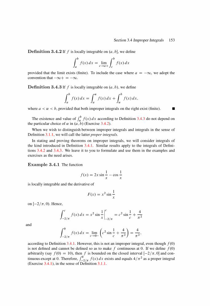
Section 3.4 Improper Integrals 153
Definition 3.4.2 If f is locally integrable on .a; b, we define
Z b
a
f .x/ dx D limc!aC
Z b
c
f .x/ dx
provided that the limit exists (finite). To include the case where a D 1, we adopt the
convention that 1C D 1.
Definition 3.4.3 If f is locally integrable on .a; b/; we define
Z b
a
f .x/ dx DZ ˛
a
f .x/ dx CZ b
˛
f .x/ dx;
where a < ˛ < b, provided that both improper integrals on the right exist (finite).
The existence and value ofR b
af .x/ dx according to Definition 3.4.3 do not depend on
the particular choice of ˛ in .a; b/ (Exercise 3.4.2).
When we wish to distinguish between improper integrals and integrals in the sense of
Definition 3.1.1, we will call the latter proper integrals.
In stating and proving theorems on improper integrals, we will consider integrals of
the kind introduced in Definition 3.4.1. Similar results apply to the integrals of Defini-
tions 3.4.2 and 3.4.3. We leave it to you to formulate and use them in the examples and
exercises as the need arises.
Example 3.4.1 The function
f .x/ D 2x sin1
x cos
1
x
is locally integrable and the derivative of
F.x/ D x2 sin1
x
on Œ2=; 0/. Hence,
Z c
2=
f .x/ dx D x2 sin1
x
ˇˇc
2=
D c2 sin1
cC 4
2
and Z 0
2=
f .x/ dx D limc!0
c2 sin
1
cC 4
2
D 4
2;
according to Definition 3.4.1. However, this is not an improper integral, even though f .0/
is not defined and cannot be defined so as to make f continuous at 0. If we define f .0/
arbitrarily (say f .0/ D 10), then f is bounded on the closed interval Œ2=; 0 and con-
tinuous except at 0. Therefore,R 0
2=f .x/ dx exists and equals 4=2 as a proper integral
(Exercise 3.4.1), in the sense of Definition 3.1.1.
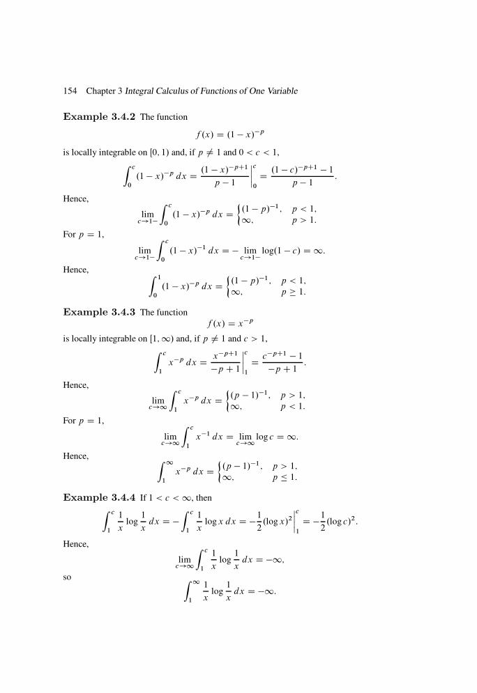
154 Chapter 3 Integral Calculus of Functions of One Variable
Example 3.4.2 The function
f .x/ D .1 x/p
is locally integrable on Œ0; 1/ and, if p ¤ 1 and 0 < c < 1,
Z c
0
.1 x/p dx D .1 x/pC1
p 1
ˇˇc
0
D .1 c/pC1 1p 1 :
Hence,
limc!1
Z c
0
.1 x/p dx D.1 p/1; p < 1;
1; p > 1:
For p D 1,
limc!1
Z c
0
.1 x/1 dx D limc!1
log.1 c/ D1:
Hence, Z 1
0
.1 x/p dx D.1 p/1; p < 1;
1; p 1:
Example 3.4.3 The function
f .x/ D xp
is locally integrable on Œ1;1/ and, if p ¤ 1 and c > 1,
Z c
1
xp dx D xpC1
p C 1
ˇˇc
1
D cpC1 1p C 1 :
Hence,
limc!1
Z c
1
xp dx D.p 1/1; p > 1;
1; p < 1:
For p D 1,
limc!1
Z c
1
x1 dx D limc!1
log c D1:
Hence, Z 1
1
xp dx D.p 1/1; p > 1;
1; p 1:
Example 3.4.4 If 1 < c <1, then
Z c
1
1
xlog
1
xdx D
Z c
1
1
xlogx dx D 1
2.logx/2
ˇˇc
1
D 12.log c/2:
Hence,
limc!1
Z c
1
1
xlog
1
xdx D 1;
so Z 1
1
1
xlog
1
xdx D 1:

Section 3.4 Improper Integrals 155
Example 3.4.5 The function f .x/ D cos x is locally integrable on Œ0;1/ and
limc!1
Z c
0
cos x dx D limc!1
sin c
does not exist; thus,R1
0 cos x dx diverges, but not to˙1.
Example 3.4.6 The function f .x/ D logx is locally integrable on .0; 1, but un-
bounded as x ! 0C. Since
limc!0C
Z 1
c
logx dx D limc!0C
.x logx x/ˇˇ1
c
D 1 limc!0C
.c log c c/ D 1;
Definition 3.4.2 yields Z 1
0
logx dx D 1:
Example 3.4.7 In connection with Definition 3.4.3, it is important to recognize that
the improper integralsR ˛
af .x/ dx and
R b
˛f .x/ dx must converge separately for
R b
af .x/ dx
to converge. For example, the existence of the symmetric limit
limR!1
Z R
R
f .x/ dx;
which is called the principal value ofR1
1 f .x/ dx, does not imply thatR1
1 f .x/ dx
converges; thus,
limR!1
Z R
R
x dx D limR!1
0 D 0;
butR1
0x dx and
R 0
1 x dx diverge and therefore so doesR1
1 x dx.
Theorem 3.4.4 Suppose that f1; f2; . . . ; fn are locally integrable on Œa; b/ and thatR b
af1.x/ dx;
R b
af2.x/ dx; . . . ;
R b
afn.x/ dx converge: Let c1; c2; . . . ; cn be constants:
ThenR b
a.c1f C c2f1 C C cnfn/.x/ dx converges and
Z b
a
.c1f1 C c2f2 C C cnfn/.x/ dx D c1
Z b
a
f1.x/ dx C c2
Z b
a
f2.x/ dx
C C cn
Z b
a
fn.x/ dx:
Proof If a < c < b, then
Z c
a
.c1f1 C c2f2 C C cnfn/.x/ dx D c1
Z c
a
f1.x/ dx C c2
Z c
a
f2.x/ dx
C C cn
Z c
a
fn.x/ dx;
by Theorem 3.3.3. Letting c ! b yields the stated result.
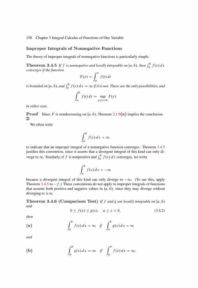
156 Chapter 3 Integral Calculus of Functions of One Variable
Improper Integrals of Nonnegative Functions
The theory of improper integrals of nonnegative functions is particularly simple.
Theorem 3.4.5 If f is nonnegative and locally integrable on Œa; b/; thenR b
af .x/ dx
converges if the function
F.x/ DZ x
a
f .t/ dt
is bounded on Œa; b/, andR b
af .x/ dx D1 if it is not. These are the only possibilities, and
Z b
a
f .t/ dt D supax<b
F.x/
in either case:
Proof Since F is nondecreasing on Œa; b/, Theorem 2.1.9(a) implies the conclusion.
We often write
Z b
a
f .x/ dx <1
to indicate that an improper integral of a nonnegative function converges. Theorem 3.4.5
justifies this convention, since it asserts that a divergent integral of this kind can only di-
verge to1. Similarly, if f is nonpositive andR b
af .x/ dx converges, we write
Z b
a
f .x/ dx > 1
because a divergent integral of this kind can only diverge to 1. (To see this, apply
Theorem 3.4.5 to f .) These conventions do not apply to improper integrals of functions
that assume both positive and negative values in .a; b/, since they may diverge without
diverging to˙1.
Theorem 3.4.6 (Comparison Test) If f and g are locally integrable on Œa; b/
and
0 f .x/ g.x/; a x < b; (3.4.2)
then
(a)Z b
a
f .x/ dx <1 if
Z b
a
g.x/ dx <1
and
(b)Z b
a
g.x/ dx D 1 if
Z b
a
f .x/ dx D1.

Section 3.4 Improper Integrals 157
Proof (a) Assumption (3.4.2) implies thatZ x
a
f .t/ dt Z x
a
g.t/ dt; a x < b
(Theorem 3.3.4), so
supax<b
Z x
a
f .t/ dt supaxb
Z x
a
g.t/ dt:
IfR b
a g.x/ dx < 1, the right side of this inequality is finite by Theorem 3.4.5, so the left
side is also. This implies thatR b
af .x/ dx <1, again by Theorem 3.4.5.
(b) The proof is by contradiction. IfR b
ag.x/ dx <1, then (a) implies that
R b
af .x/ dx <
1, contradicting the assumption thatR b
af .x/ dx D 1.
The comparison test is particularly useful if the integrand of the improper integral is
complicated but can be compared with a function that is easy to integrate.
Example 3.4.8 The improper integral
I DZ 1
0
2C sinx
.1 x/p dx
converges if p < 1, since
0 <2C sinx
.1 x/p 3
.1 x/p; 0 x < 1;
and, from Example 3.4.2,Z 1
0
3 dx
.1 x/p <1; p < 1:
However, I diverges if p 1, since
0 <1
.1 x/p 2C sinx
.1 x/p; 0 x < 1;
and Z 1
0
dx
.1 x/p D1; p 1:
If f is any function (not necessarily nonnegative) locally integrable on Œa; b/, thenZ c
a
f .x/ dx DZ a1
a
f .x/ dx CZ c
a1
f .x/ dx
if a1 and c are in Œa; b/. SinceR a1
af .x/ dx is a proper integral, on letting c ! b we
conclude that if either of the improper integralsR b
af .x/ dx and
R b
a1f .x/ dx converges
then so does the other, and in this caseZ b
a
f .x/ dx DZ a1
a
f .x/ dx CZ b
a1
f .x/ dx:
158 Chapter 3 Integral Calculus of Functions of One Variable
This means that any theorem implying convergence or divergence of an improper integralR b
af .x/ dx in the sense of Definition 3.4.1 remains valid if its hypotheses are satisfied
on a subinterval Œa1; b/ of Œa; b/ rather than on all of Œa; b/. For example, Theorem 3.4.6
remains valid if (3.4.2) is replaced by
0 f .x/ g.x/; a1 x < b;
where a1 is any point in Œa; b/.
From this, you can see that if f .x/ 0 on some subinterval Œa1; b/ of Œa; b/, but not
necessarily for all x in Œa; b/, we can still use the convention introduced earlier for positive
functions; that is, we can writeR b
af .x/ dx < 1 if the improper integral converges orR b
af .x/ dx D1 if it diverges.
Example 3.4.9 If p 0, then
xp
2 .x 1/
p.2C sin x/
.x 1=3/2p 4xp
for x sufficiently large. Therefore, Theorem 3.4.6 and Example 3.4.3 imply thatZ 1
1
.x 1/p.2C sin x/
.x 1=3/2pdx
converges if p > 1 or diverges if p 1.
Theorem 3.4.7 Suppose that f and g are locally integrable on Œa; b/; g.x/ > 0 and
f .x/ 0 on some subinterval Œa1; b/ of Œa; b/; and
limx!b
f .x/
g.x/D M: (3.4.3)
(a) If 0 < M <1; thenR b
af .x/ dx and
R b
ag.x/ dx converge or diverge together.
(b) If M D1 andR b
ag.x/ dx D1; then
R b
af .x/ dx D1.
(c) If M D 0 andR b
ag.x/ dx <1; then
R b
af .x/ dx <1.
Proof (a) From (3.4.3), there is a point a2 in Œa1; b/ such that
0 <M
2<f .x/
g.x/<3M
2; a2 x < b;
and thereforeM
2g.x/ < f .x/ <
3M
2g.x/; a2 x < b: (3.4.4)
Theorem 3.4.6 and the first inequality in (3.4.4) imply that
Z b
a2
g.x/ dx <1 if
Z b
a2
f .x/ dx <1:
Section 3.4 Improper Integrals 159
Theorem 3.4.6 and the second inequality in (3.4.4) imply that
Z b
a2
f .x/ dx <1 if
Z b
a2
g.x/ dx <1:
Therefore,R b
a2f .x/ dx and
R b
a2g.x/ dx converge or diverge together, and in the latter case
they must diverge to1, since their integrands are nonnegative (Theorem 3.4.5).
(b) If M D1, there is a point a2 in Œa1; b/ such that
f .x/ g.x/; a2 x b;
so Theorem 3.4.6(b) implies thatR b
af .x/ dx D1.
(c) If M D 0, there is a point a2 in Œa1; b/ such that
f .x/ g.x/; a2 x b;
so Theorem 3.4.6(a) implies thatR b
af .x/ dx <1.
The hypotheses of Theorem 3.4.7(b) and (c) do not imply thatR b
af .x/ dx and
R b
ag.x/ dx
necessarily converge or diverge together. For example, if b D 1, then f .x/ D 1=x
and g.x/ D 1=x2 satisfy the hypotheses of Theorem 3.4.7(b), while f .x/ D 1=x2 and
g.x/ D 1=x satisfy the hypotheses of Theorem 3.4.7(c). However,R1
11=x dx D 1,
whileR1
11=x2 dx <1.
Example 3.4.10 Let f .x/ D .1C x/p and g.x/ D xp . Since
limx!1
f .x/
g.x/D 1
andR1
1xp dx converges if p > 1 or diverges if p 1 (Example 3.4.3), Theorem 3.4.7
implies that the same is true of
Z 1
1
.1C x/p dx:
Example 3.4.11 The function
f .x/ D xp.1C x/q
is locally integrable on .0;1/. To see whether
I DZ 1
0
xp.1C x/q dx
converges according to Definition 3.4.3, we consider the improper integrals
I1 DZ 1
0
xp.1C x/q dx and I2 DZ 1
1
xp.1C x/q dx
160 Chapter 3 Integral Calculus of Functions of One Variable
separately. (The choice of 1 as the upper limit of I1 and the lower limit of I2 is completely
arbitrary; any other positive number would do just as well.) Since
limx!0C
f .x/
xpD lim
x!0C.1C x/q D 1
and Z 1
0
xp dx D.1 p/1; p < 1;
1; p 1;Theorem 3.4.7 implies that I1 converges if and only if p < 1. Since
limx!1
f .x/
xpqD lim
x!1.1C x/qxq D 1
and Z 1
1
xpq dx D.p C q 1/1; pC q > 1;1; pC q 1;
Theorem 3.4.7 implies that I2 converges if and only if p C q > 1. Combining these
results, we conclude that I converges according to Definition 3.4.3 if and only if p < 1
and p C q > 1.
Absolute Integrability
Definition 3.4.8 We say that f is absolutely integrable on Œa; b/ if f is locally inte-
grable on Œa; b/ andR b
ajf .x/j dx <1. In this case we also say that
R b
af .x/ dx converges
absolutely or is absolutely convergent.
Example 3.4.12 If f is nonnegative and integrable on Œa; b/, then f is absolutely
integrable on Œa; b/, since jf j D f .
Example 3.4.13 Since ˇˇ sinx
xp
ˇˇ 1
xp
andR1
1 xp dx <1 if p > 1 (Example 3.4.3), Theorem 3.4.6 implies that
Z 1
1
j sinxjxp
dx <1; p > 1I
that is, the function
f .x/ Dsinx
xp
is absolutely integrable on Œ1;1/ if p > 1. It is not absolutely integrable on Œ1;1/ if
p 1. To see this, we first consider the case where p D 1. Let k be an integer greater
than 3. Then
Section 3.4 Improper Integrals 161
Z k
1
j sinxjx
dx >
Z k
j sinxjx
dx
Dk1X
j D1
Z .j C1/
j
j sinxjx
dx
>
k1X
j D1
1
.j C 1/
Z .j C1/
j
j sin xj dx:
(3.4.5)
But Z .j C1/
j
j sinxj dx DZ
0
sinx dx D 2;
so (3.4.5) implies thatZ k
1
j sinxjx
dx >2
k1X
j D1
1
j C 1: (3.4.6)
However,1
j C 1Z j C2
j C1
dx
x; j D 1; 2; : : : ;
so (3.4.6) implies that
Z k
1
j sinxjx
>2
k1X
j D1
Z j C2
j C1
dx
x
D 2
Z kC1
2
dx
xD 2
log
k C 12
:
Since limk!1 logŒ.k C 1/=2D 1, Theorem 3.4.5 implies that
Z 1
1
j sinxjx
dx D1:
Now Theorem 3.4.6(b) implies that
Z 1
1
j sinxjxp
dx D1; p 1: (3.4.7)
Theorem 3.4.9 If f is locally integrable on Œa; b/ andR b
ajf .x/j dx < 1; thenR b
af .x/ dx convergesI that is; an absolutely convergent integral is convergent:
Proof If
g.x/ D jf .x/j f .x/;
162 Chapter 3 Integral Calculus of Functions of One Variable
then
0 g.x/ 2jf .x/j
andR b
ag.x/ dx <1, because of Theorem 3.4.6 and the absolute integrability of f . Since
f D jf j g;
Theorem 3.4.4 implies thatR b
a f .x/ dx converges.
Conditional Convergence
We say that f is nonoscillatory at b .D 1 if b D 1/ if f is defined on Œa; b/ and
does not change sign on some subinterval Œa1; b/ of Œa; b/. If f changes sign on every
such subinterval, f is oscillatory at b. For a function that is locally integrable on Œa; b/
and nonoscillatory at b, convergence and absolute convergence ofR b
af .x/ dx amount
to the same thing (Exercise 3.4.16), so absolute convergence is not an interesting concept
in connection with such functions. However, an oscillatory function may be integrable,
but not absolutely integrable, on Œa; b/, as the next example shows. We then say that f is
conditionally integrable on Œa; b/, and thatR b
a f .x/ dx converges conditionally.
Example 3.4.14 We saw in Example 3.4.13 that the integral
I.p/ DZ 1
1
sinx
xpdx
is not absolutely convergent if 0 < p 1. We will show that it converges conditionally for
these values of p.
Integration by parts yields
Z c
1
sinx
xpdx D cos c
cpC cos 1 p
Z c
1
cos x
xpC1dx: (3.4.8)
Since ˇˇ
cos x
xpC1
ˇˇ
1
xpC1
andR1
1xp1 dx < 1 if p > 0, Theorem 3.4.6 implies that xp1 cos x is absolutely
integrable Œ1;1/ if p > 0. Therefore, Theorem 3.4.9 implies that xp1 cos x is integrable
Œ1;1/ if p > 0. Letting c !1 in (3.4.8), we find that I.p/ converges, and
I.p/ D cos 1 pZ 1
1
cos x
xpC1dx if p > 0:
This and (3.4.7) imply that I.p/ converges conditionally if 0 < p 1.
The method used in Example 3.4.14 is a special case of the following test for convergence
of improper integrals.

Section 3.4 Improper Integrals 163
Theorem 3.4.10 (Dirichlet’s Test) Suppose that f is continuous and its an-
tiderivative F.x/ DR x
af .t/ dt is bounded on Œa; b/: Let g0 be absolutely integrable on
Œa; b/; and suppose that
limx!b
g.x/ D 0: (3.4.9)
ThenR b
a f .x/g.x/ dx converges:
Proof The continuous function fg is locally integrable on Œa; b/. Integration by parts
yields
Z c
a
f .x/g.x/ dx D F.c/g.c/ Z c
a
F.x/g0.x/ dx; a c < b: (3.4.10)
Theorem 3.4.6 implies that the integral on the right converges absolutely as c ! b, sinceR b
ajg0.x/j dx <1 by assumption, and
jF.x/g0.x/j M jg0.x/j;
whereM is an upper bound for jF j on Œa; b/. Moreover, (3.4.9) and the boundedness of F
imply that limc!b F.c/g.c/ D 0. Letting c ! b in (3.4.10) yields
Z b
a
f .x/g.x/ dx D Z b
a
F.x/g0.x/ dx;
where the integral on the right converges absolutely.
Dirichlet’s test is useful only if f is oscillatory at b, since it can be shown that if f is
nonoscillatory at b and F is bounded on Œa; b/, thenR b
ajf .x/g.x/j dx <1 if only g is
locally integrable and bounded on Œa; b/ (Exercise 3.4.14).
Example 3.4.15 Dirichlet’s test can also be used to show that certain integrals di-
verge. For example, Z 1
1
xq sinx dx
diverges if q > 0, but none of the other tests that we have studied so far implies this. It
is not enough to argue that the integrand does not approach zero as x ! 1 (a common
mistake), since this does not imply divergence (Exercise 4.4.31). To see that the integral
diverges, we observe that if it converged for some q > 0, then F.x/ DR x
1xq sin x dx
would be bounded on Œ1;1/, and we could let
f .x/ D xq sinx and g.x/ D xq
in Theorem 3.4.10 and conclude thatZ 1
1
sinx dx
also converges. This is false.
164 Chapter 3 Integral Calculus of Functions of One Variable
The method used in Example 3.4.15 is a special case of the following test for divergence
of improper integrals.
Theorem 3.4.11 Suppose that u is continuous on Œa; b/ andR b
au.x/ dx diverges: Let
v be positive and differentiable on Œa; b/; and suppose that limx!b v.x/ D 1 and v0=v2
is absolutely integrable on Œa; b/: ThenR b
au.x/v.x/ dx diverges:
Proof The proof is by contradiction. Let f D uv and g D 1=v, and suppose thatR b
au.x/v.x/ dx converges. Then f has the bounded antiderivativeF.x/ D
R x
au.t/v.t/ dt
on Œa; b/, limx!1 g.x/ D 0 and g0 D v0=v2 is absolutely integrable on Œa; b/. Therefore,
Theorem 3.4.10 implies thatR b
au.x/ dx converges, a contradiction.
If Dirichlet’s test shows thatR b
af .x/g.x/ dx converges, there remains the question of
whether it converges absolutely or conditionally. The next theorem sometimes answers this
question. Its proof can be modeled after the method of Example 3.4.13 (Exercise 3.4.17).
The idea of an infinite sequence, which we will discuss in Section 4.1, enters into the
statement of this theorem. We assume that you recall the concept sufficiently well from
calculus to understand the meaning of the theorem.
Theorem 3.4.12 Suppose that g is monotonic on Œa; b/ andR b
ag.x/ dx D 1: Let f
be locally integrable on Œa; b/ and
Z xj C1
xj
jf .x/j dx ; j 0;
for some positive ; where fxj g is an increasing infinite sequence of points in Œa; b/ such
that limj !1 xj D b and xj C1 xj M; j 0; for someM: Then
Z b
a
jf .x/g.x/j dx D1:
Change of Variable in an Improper Integral
The next theorem enables us to investigate an improper integral by transforming it into
another whose convergence or divergence is known. It follows from Theorem 3.3.18 and
Definitions 3.4.1, 3.4.2, and 3.4.3. We omit the proof.
Theorem 3.4.13 Suppose that is monotonic and 0 is locally integrable on either
of the half-open intervals I D Œc; d / or .c; d ; and let x D .t/ map I onto either of the
half-open intervals J D Œa; b/ or J D .a; b: Let f be locally integrable on J: Then the
improper integrals
Z b
a
f .x/ dx and
Z d
c
f ..t// j0.t/j dt
Section 3.4 Improper Integrals 165
diverge or converge together; in the latter case to the same value. The same conclusion
holds if and 0 have the stated properties only on the open interval .a; b/; the transfor-
mation x D .t/ maps .c; d / onto .a; b/; and f is locally integrable on .a; b/:
Example 3.4.16 To apply Theorem 3.4.13 to
Z 1
0
sinx2 dx;
we use the change of variable x D .t/ Dpt , which takes Œc; d / D Œ0;1/ into Œa; b/ D
Œ0;1/, with 0.t/ D 1=.2pt/. Theorem 3.4.13 implies that
Z 1
0
sin x2 dx D 1
2
Z 1
0
sin tptdt:
Since the integral on the right converges (Example 3.4.14), so does the one on the left.
Example 3.4.17 The integral
Z 1
1
xp dx
converges if and only if p > 1 (Example 3.4.3). Defining .t/ D 1=t and applying
Theorem 3.4.13 yields
Z 1
1
xp dx DZ 1
0
tpj t2j dt DZ 1
0
tp2 dt;
which implies thatR 1
0tq dt converges if and only if q > 1.
3.4 Exercises
1. (a) Let f be locally integrable and bounded on Œa; b/, and let f .b/ be defined
arbitrarily. Show that f is properly integrable on Œa; b, thatR b
af .x/ dx does
not depend on f .b/, and that
Z b
a
f .x/ dx D limc!b
Z c
a
f .x/ dx:
(b) State a result analogous to (a) which ends with the conclusion that
Z b
a
f .x/ dx D limc!aC
Z b
c
f .x/ dx:
2. Show that neither the existence nor the value of the improper integral of Defini-
tion 3.4.3 depends on the choice of the intermediate point ˛.
166 Chapter 3 Integral Calculus of Functions of One Variable
3. Prove: IfR b
a f .x/ dx exists according to Definition 3.4.1 or 3.4.2, thenR b
a f .x/ dx
also exists according to Definition 3.4.3.
4. Find all values of p for which the following integrals exist (i) as proper integrals
(perhaps after defining f at the endpoints of the interval) or (ii) as improper inte-
grals. (iii) Evaluate the integrals for the values of p for which they converge.
(a)Z 1=
0
pxp1 sin
1
x xp2 cos
1
x
dx
(b)Z 2=
0
pxp1 cos
1x C xp2 sin
1
x
dx
(c)Z 1
0
epx dx (d)Z 1
0
xp dx (e)Z 1
0
xp dx.
5. Evaluate
(a)Z 1
0
exxn dx .n D 0; 1; : : : / (b)Z 1
0
ex sinx dx
(c)Z 1
1
x dx
x2 C 1(d)
Z 1
0
x dxp1 x2
(e)Z
0
cos x
x sin x
x2
dx (f)
Z 1
=2
sin x
xC cos x
x2
dx
6. Prove: IfR b
af .x/ dx exists as a proper or improper integral, then
limx!b
Z b
x
f .t/ dt D 0:
7. Prove: If f is locally integrable on Œa; b/, thenR b
af .x/ dx exists if and only if for
each > 0 there is a number r in .a; b/ such thatˇˇZ x2
x1
f .t/ dt
ˇˇ <
whenever r x1, x2 < b. HINT: See Exercise 2.1.38.
8. Determine whether the integral converges or diverges.
(a)Z 1
1
logx C sin xpx
dx (b)Z 1
1
.x2 C 3/3=2
.x4 C 1/3=2sin2 x dx
(c)Z 1
0
1C cos2 xp1C x2
dx (d)Z 1
0
4C cos x
.1C x/pxdx
(e)Z 1
0
.x27 C sinx/ex dx (f)Z 1
0
xp.2C sin x/ dx

Section 3.4 Improper Integrals 167
9. Find all values of p for which the integral converges.
(a)Z =2
0
sin x
xpdx (b)
Z =2
0
cos x
xpdx (c)
Z 1
0
xpex dx
(d)Z =2
0
sin x
.tan x/pdx (e)
Z 1
1
dx
x.logx/p(f)
Z 1
0
dx
x.j logxj/p
(g)Z
0
x dx
.sin x/p
10. Let Ln.x/ be the iterated logarithm defined in Exercise 2.4.42. Show that
Z 1
a
dx
L0.x/L1.x/ Lk.x/ŒLkC1.x/p
converges if and only if p > 1. Here a is any number such that LkC1.x/ > 0 for
x a.
11. Find conditions on p and q such that the integral converges.
(a)Z 1
1
.cos x=2/q
.1 x2/pdx (b)
Z 1
1
.1 x/p.1C x/q dx
(c)Z 1
0
xp dx
.1C x2/q(d)
Z 1
1
Œlog.1C x/p .log x/q
xpCqdx
(e)Z 1
1
.log.1C x/ logx/q
xpdx (f)
Z 1
0
.x sinx/q
xpdx
12. Let f and g be polynomials and suppose that g has no real zeros. Find necessary
and sufficient conditions for convergence of
Z 1
1
f .x/
g.x/dx:
13. Prove: If f and g are locally integrable on Œa; b/ and the improper integralsR b
af 2.x/ dx
andR b
ag2.x/ dx converge, then
R b
af .x/g.x/ dx converges absolutely. HINT: .f ˙
g/2 0:14. Suppose that f is locally integrable and F.x/ D
R x
af .t/ dt is bounded on Œa; b/,
and let f be nonoscillatory at b. Let g be locally integrable and bounded on Œa; b/.
Show that Z b
a
jf .x/g.x/j dx <1:
15. Suppose that g is positive and nonincreasing on Œa; b/ andR b
af .x/ dx exists as
a proper or absolutely convergent improper integral. Show thatR b
a f .x/g.x/ dx
exists and
168 Chapter 3 Integral Calculus of Functions of One Variable
limx!b
1
g.x/
Z b
x
f .t/g.t/ dt D 0:
HINT: Use Exercise 3.4.6:
16. Show that if f is locally integrable on Œa; b/ and nonoscillatory at b, thenR b
af .x/ dx
exists if and only ifR b
ajf .x/j dx <1.
17. (a) Prove Theorem 3.4.12. HINT: See Example 3.4.13:
(b) Show that g satisfies the assumptions of Theorem 3.4.10 if g0 is locally inte-
grable, g is monotonic on Œa; b/, and limx!b g.x/ D 0.
18. Find all values of p for which the integral converges (i) absolutely; (ii) condition-
ally.
(a)Z 1
1
cos x
xpdx (b)
Z 1
2
sin x
x.logx/pdx (c)
Z 1
2
sin x
xp logxdx
(d)Z 1
1
sin 1=x
xpdx (e)
Z 1
0
sin2 x sin 2x
xpdx (f)
Z 1
1
sinx
.1C x2/pdx
19. Suppose that g00 is absolutely integrable on Œ0;1/, limx!1 g0.x/ D 0, and limx!1 g.x/ DL (finite or infinite). Show that
R10g.x/ sin x dx converges if and only if L D 0.
HINT: Integrate by parts:
20. Let h be continuous on Œ0;1/. Prove:
(a) IfR1
0es0xh.x/ dx converges absolutely, then
R10esxh.x/ dx converges
absolutely if s > s0.
(b) IfR1
0es0xh.x/ dx converges, then
R10esxh.x/ dx converges if s > s0.
21. Suppose that f is locally integrable on Œ0;1/, limx!1 f .x/ D A, and ˛ > 1.
Find limx!1 x˛1R x
0f .t/t˛ dt , and prove your answer.
22. Suppose that f is continuous and F.x/ DR x
af .t/ dt is bounded on Œa; b/. Suppose
also that g > 0, g0 is nonnegative and locally integrable on Œa; b/, and limx!b g.x/ D1. Show that
limx!b
1
Œg.x/
Z x
a
f .t/g.t/ dt D 0; > 1:
HINT: Integrate by parts:
23. In addition to the assumptions of Exercise 3.4.22, assume thatR b
af .t/ dt converges.
Show that
limx!b
1
g.x/
Z x
a
f .t/g.t/ dt D 0:
HINT: Let F.x/ DR b
xf .t/ dt; integrate by parts; and use Exercise 3.4.6:
Section 3.4 Improper Integrals 169
24. Suppose that f is continuous, g0.x/ 0, and g.x/ > 0 on Œa; b/. Show that if g0 is
integrable on Œa; b/ andR b
af .x/ dx exists, then
R b
af .x/g.x/ dx exists and
limx!b
1
g.x/
Z b
x
f .t/g.t/ dt D 0:
HINT: Let F.x/ DR b
xf .t/ dt; integrate by parts; and use Exercise 3.4.6:
25. Find all values of p for which the integral converges (i) absolutely; (ii) condition-
ally.
(a)Z 1
0
xp sin 1=x dx (b)Z 1
0
j logxjp dx (c)Z 1
1
xp cos.logx/ dx
(d)Z 1
1
.log x/p dx (e)Z 1
0
sinxp dx
26. Let u1 be positive and satisfy the differential equation
u00 C p.x/u D 0; 0 x <1: .A/
(a) Prove: If Z 1
0
dx
u21.x/
<1;
then the function
u2.x/ D u1.x/
Z 1
x
dt
u21.t/
also satisfies (A), while if
Z 1
0
dx
u21.x/
D1;
then the function
u2.x/ D u1.x/
Z x
0
dt
u21.t/
also satisfies (A).
(b) Prove: If (A) has a solution that is positive on Œ0;1/, then (A) has solutions
y1 and y2 that are positive on .0;1/ and have the following properties:
y1.x/y02.x/ y0
1.x/y2.x/ D 1; x > 0;y1.x/
y2.x/
0< 0; x > 0;
and
limx!1
y1.x/
y2.x/D 0:
170 Chapter 3 Integral Calculus of Functions of One Variable
27. (a) Prove: If h is continuous on Œ0;1/, then the function
u.x/ D c1ex C c2e
x CZ x
0
h.t/ sinh.x t/ dt
satisfies the differential equation
u00 u D h.x/; x > 0:
(b) Rewrite u in the form
u.x/ D a.x/ex C b.x/ex
and show that
u0.x/ D a.x/ex C b.x/ex:
(c) Show that if limx!1 a.x/ D A (finite), then
limx!1
e2x Œb.x/ B D 0
for some constant B . HINT: Use Exercise 3.4.24: Show also that
limx!1
ex Œu.x/ Aex Bex D 0:
(d) Prove: If limx!1 b.x/ D B (finite), then
limx!1
u.x/ex D limx!1
u0.x/ex D B:
HINT: Use Exercise 3.4.23:
28. Suppose that the differential equation
u00C p.x/u D 0 .A/
has a positive solution on Œ0;1/, and therefore has two solutionsy1 and y2 with the
properties given in Exercise 3.4.26(b).
(a) Prove: If h is continuous on Œ0;1/ and c1 and c2 are constants, then
u.x/ D c1y1.x/C c2y2.x/CZ x
0
h.t/ Œy1.t/y2.x/ y1.x/y2.t/ dt .B/
satisfies the differential equation
u00 C p.x/u D h.x/:
For convenience in (b) and (c), rewrite (B) as
u.x/ D a.x/y1.x/C b.x/y2.x/:
Section 3.5 Advanced Look at the Existence of the Proper Riemann Integral 171
(b) Prove: IfR1
0h.t/y2.t/ dt converges, then
R10h.t/y1.t/ dt converges, and
limx!1
u.x/ Ay1.x/ By2.x/
y1.x/D 0
for some constants A and B . HINT: Use Exercise 3.4.24 with f D hy2 and
g D y1=y2:
(c) Prove: IfR1
0h.t/y1.t/ dt converges, then
limx!1
u.x/
y2.x/D B
for some constant B . HINT: Use Exercise 3.4.23 with f D hy1 and g Dy2=y1:
29. Suppose that f , f1, and g are continuous, f > 0, and .f1=f /0 is absolutely inte-
grable on Œa; b/. Show thatR b
af1.x/g.x/ dx converges if
R b
af .x/g.x/ dx does.
30. Let g be locally integrable and f continuous, with f .x/ > 0 on Œa; b/. Sup-
pose that for some positive M and for every r in Œa; b/ there are points x1 and x2
such that (a) r < x1 < x2 < b; (b) g does not change sign in Œx1; x2; and
(c)R x2
x1jg.x/j dx M . Show that
R b
af .x/g.x/ dx diverges. HINT: Use Exer-
cise 3.4.7 and Theorem 3.3.7:
3.5 A MORE ADVANCED LOOK AT THE EXISTENCE OFTHE PROPER RIEMANN INTEGRAL
In Section 3.2 we found necessary and sufficient conditions for existence of the proper
Riemann integral, and in Section 3.3 we used them to study the properties of the integral.
However, it is awkward to apply these conditions to a specific function and determine
whether it is integrable, since they require computations of upper and lower sums and
upper and lower integrals, which may be difficult. The main result of this section is an
integrability criterion due to Lebesgue that does not require computation, but has to do
with how badly discontinuous a function may be and still be integrable.
We emphasize that we are again considering proper integrals of bounded functions on
finite intervals.
Definition 3.5.1 If f is bounded on Œa; b, the oscillation of f on Œa; b is defined by
Wf Œa; bD supax;x0b
jf .x/ f .x0/j;
which can also be written as
Wf Œa; b D supaxb
f .x/ infaxb
f .x/
172 Chapter 3 Integral Calculus of Functions of One Variable
( Exercise 3.5.1). If a < x < b, the oscillation of f at x is defined by
wf .x/ D limh!0C
Wf .x h; xC h/:
The corresponding definitions for x D a and x D b are
wf .a/ D limh!0C
Wf .a; aC h/ and wf .b/ D limh!0C
Wf .b h; b/:
For a fixed x in .a; b/, Wf .x h; x C h/ is a nonnegative and nondecreasing function
of h for 0 < h < min.x a; b x/; therefore, wf .x/ exists and is nonnegative, by
Theorem 2.1.9. Similar arguments apply to wf .a/ and wf .b/.
Theorem 3.5.2 Let f be defined on Œa; b: Then f is continuous at x0 in Œa; b if
and only if wf .x0/ D 0: .Continuity at a or b means continuity from the right or left,
respectively./
Proof Suppose that a < x0 < b. First, suppose that wf .x0/ D 0 and > 0. Then
Wf Œx0 h; x0 C h <
for some h > 0, so
jf .x/ f .x0/j < if x0 h x; x0 x0 C h:
Letting x0 D x0, we conclude that
jf .x/ f .x0/j < if jx x0j < h:
Therefore, f is continuous at x0.
Conversely, if f is continuous at x0 and > 0, there is a ı > 0 such that
jf .x/ f .x0/j <
2and jf .x0/ f .x0/j <
2
if x0 ı x, x0 x0 C ı. From the triangle inequality,
jf .x/ f .x0/j jf .x/ f .x0/j C jf .x0/ f .x0/j < ;
so
Wf Œx0 h; x0 C h if h < ıItherefore, wf .x0/ D 0. Similar arguments apply if x0 D a or x0 D b.
Lemma 3.5.3 If wf .x/ < for a x b; then there is a ı > 0 such that
Wf Œa1; b1 ; provided that Œa1; b1 Œa; b and b1 a1 < ı:
Proof We use the Heine–Borel theorem (Theorem 1.3.7). If wf .x/ < , there is an
hx > 0 such that
jf .x0/ f .x00/j < (3.5.1)

Section 3.5 Advanced Look at the Existence of the Proper Riemann Integral 173
if
x 2hx < x0; x00 < x C 2hx and x0; x00 2 Œa; b: (3.5.2)
If Ix D .x hx; x C hx/, then the collection
H D˚Ix
ˇa x b
is an open covering of Œa; b, so the Heine–Borel theorem implies that there are finitely
many points x1, x2, . . . , xn in Œa; b such that Ix1, Ix2
, . . . , Ixn cover Œa; b. Let
h D min1in
hxi
and suppose that Œa1; b1 Œa; b and b1 a1 < h. If x0 and x00 are in Œa1; b1, then
x0 2 Ixr for some r .1 r n/, so
jx0 xr j < hxr :
Therefore,
jx00 xr j jx00 x0j C jx0 xr j < b1 a1 C hxr
< hC hxr 2hxr :
Thus, any two points x0 and x00 in Œa1; b1 satisfy (3.5.2) with x D xr , so they also satisfy
(3.5.1). Therefore, is an upper bound for the set˚jf .x0/ f .x00/j
ˇx0; x00 2 Œa1; b1
;
which has the supremumWf Œa1; b1. Hence, Wf Œa1; b1 .In the following,L.I / is the length of the interval I .
Lemma 3.5.4 Let f be bounded on Œa; b and define
E D˚x 2 Œa; b
ˇwf .x/
:
Then E is closed; and f is integrable on Œa; b if and only if for every pair of positive
numbers and ı; E can be covered by finitely many open intervals I1; I2;. . . ; Ip such
thatpX
j D1
L.Ij / < ı: (3.5.3)
Proof We first show that E is closed. Suppose that x0 is a limit point of E . If h > 0,
there is an x from E in .x0 h; x0 C h/. Since Œx h1; x C h1 Œx0 h; x0 C h for
sufficiently small h1 and Wf Œx h1; xC h1 , it follows thatWf Œx0 h; x0C h for all h > 0. This implies that x0 2 E, so E is closed (Corollary 1.3.6).
Now we will show that the stated condition in necessary for integrability. Suppose that
the condition is not satisfied; that is, there is a > 0 and a ı > 0 such that
pX
j D1
L.Ij / ı
174 Chapter 3 Integral Calculus of Functions of One Variable
for every finite set fI1; I2; : : : ; Ipg of open intervals covering E. If P D fx0; x1; : : : ; xngis a partition of Œa; b, then
S.P / s.P / DX
j 2A
.Mj mj /.xj xj 1/CX
j 2B
.Mj mj /.xj xj 1/; (3.5.4)
where
A D˚jˇŒxj 1; xj \E ¤ ;
and B D
˚jˇŒxj 1; xj \ E D ;
:
SinceS
j 2A.xj 1; xj / contains all points of E except any of x0, x1, . . . , xn that may
be in E, and each of these finitely many possible exceptions can be covered by an open
interval of length as small as we please, our assumption on E implies that
X
j 2A
.xj xj 1/ ı:
Moreover, if j 2 A, then
Mj mj ;so (3.5.4) implies that
S.P / s.P / X
j 2A
.xj xj 1/ ı:
Since this holds for every partition of Œa; b, f is not integrable on Œa; b, by Theorem 3.2.7.
This proves that the stated condition is necessary for integrability.
For sufficiency, let and ı be positive numbers and let I1, I2, . . . , Ip be open intervals
that cover E and satisfy (3.5.3). Let
eI j D Œa; b\ I j :
(I j D closure of I .) After combining any ofeI 1,eI 2, . . . , eIp that overlap, we obtain a set
of pairwise disjoint closed subintervals
Cj D Œ˛j ; ˇj ; 1 j q . p/;
of Œa; b such that
a ˛1 < ˇ1 < ˛2 < ˇ2 < ˛q1 < ˇq1 < ˛q < ˇq b; (3.5.5)
qX
iD1
.ˇi ˛i / < ı (3.5.6)
and
wf .x/ < ; ˇj x ˛j C1; 1 j q 1:
Also, wf .x/ < for a x ˛1 if a < ˛1 and for ˇq x b if ˇq < b.

Section 3.5 Advanced Look at the Existence of the Proper Riemann Integral 175
Let P0 be the partition of Œa; b with the partition points indicated in (3.5.5), and refine
P0 by partitioning each subinterval Œˇj ; ˛j C1 (as well as Œa; ˛1 if a < ˛1 and Œˇq; b
if ˇq < b) into subintervals on which the oscillation of f is not greater than . This is
possible by Lemma 3.5.3. In this way, after renaming the entire collection of partition
points, we obtain a partitionP D fx0; x1; : : : ; xng of Œa; b for which S.P / s.P / can be
written as in (3.5.4), with
X
j 2A
.xj xj 1/ DqX
iD1
.ˇi ˛i/ < ı
(see (3.5.6)) and
Mj mj ; j 2 B:
For this partition,
X
j 2A
.Mj mj /.xj xj 1/ 2KX
j 2A
.xj xj 1/ < 2Kı;
where K is an upper bound for jf j on Œa; b and
X
j 2B
.Mj mj /.xj xj 1/ .b a/:
We have now shown that if and ı are arbitrary positive numbers, there is a partitionP of
Œa; b such that
S.P / s.P / < 2Kı C .b a/: (3.5.7)
If > 0, let
ı D
4Kand D
2.b a/:
Then (3.5.7) yields
S.P / s.P / < ;and Theorem 3.2.7 implies that f is integrable on Œa; b.
We need the next definition to state Lebesgue’s integrability condition.
Definition 3.5.5 A subset S of the real line is of Lebesgue measure zero if for every
> 0 there is a finite or infinite sequence of open intervals I1, I2, . . . such that
S [
j
Ij (3.5.8)
andnX
j D1
L.Ij / < ; n 1: (3.5.9)

176 Chapter 3 Integral Calculus of Functions of One Variable
Note that any subset of a set of Lebesgue measure zero is also of Lebesgue measure zero.
(Why?)
Example 3.5.1 The empty set is of Lebesgue measure zero, since it is contained in
any open interval.
Example 3.5.2 Any finite set S D fx1; x2; : : : ; xng is of Lebesgue measure zero,
since we can choose open intervals I1, I2, . . . , In such that xj 2 Ij and L.Ij / < =n,
1 j n.
Example 3.5.3 An infinite set is denumerable if its members can be listed in a se-
quence (that is, in a one-to-one correspondence with the positive integers); thus,
S D fx1; x2; : : : ; xn; : : : g: (3.5.10)
An infinite set that does not have this property is nondenumerable. Any denumerable set
(3.5.10) is of Lebesgue measure zero, since if > 0, it is possible to choose open intervals
I1, I2, . . . , so that xj 2 Ij and L.Ij / < 2j , j 1. Then (3.5.9) holds because
1
2C 1
22C 1
23C C 1
2nD 1 1
2n< 1: (3.5.11)
There are also nondenumerable sets of Lebesgue measure zero, but it is beyond the scope
of this book to discuss examples.
The next theorem is the main result of this section.
Theorem 3.5.6 A bounded function f is integrable on a finite interval Œa; b if and
only if the set S of discontinuities of f in Œa; b is of Lebesgue measure zero:
Proof From Theorem 3.5.2,
S D˚x 2 Œa; b
ˇwf .x/ > 0
:
Since wf .x/ > 0 if and only if wf .x/ 1=i for some positive integer i , we can write
S D1[
iD1
Si ; (3.5.12)
where
Si D˚x 2 Œa; b
ˇwf .x/ 1=i
:
Now suppose that f is integrable on Œa; b and > 0. From Lemma 3.5.4, each Si can
be covered by a finite number of open intervals Ii1, Ii2, . . . , Iin of total length less than
=2i . We simply renumber these intervals consecutively; thus,
I1; I2; D I11; : : : ; I1n1; I21; : : : ; I2n2
; : : : ; Ii1; : : : ; Iini; : : : :
Now (3.5.8) and (3.5.9) hold because of (3.5.11) and (3.5.12), and we have shown that the
stated condition is necessary for integrability.
Section 3.5 Advanced Look at the Existence of the Proper Riemann Integral 177
For sufficiency, suppose that the stated condition holds and > 0. Then S can be
covered by open intervals I1; I2; : : : that satisfy (3.5.9). If > 0, then the set
E D˚x 2 Œa; b
ˇwf .x/
of Lemma 3.5.4 is contained inS (Theorem 3.5.2), and thereforeE is covered by I1; I2; : : : .
Since E is closed (Lemma 3.5.4) and bounded, the Heine–Borel theorem implies that E
is covered by a finite number of intervals from I1; I2; : : : . The sum of the lengths of the
latter is less than , so Lemma 3.5.4 implies that f is integrable on Œa; b.
3.5 Exercises
1. In connection with Definition 3.5.1, show that
supx;x0 2Œa;b
jf .x/ f .x0/j D supaxb
f .x/ infaxb
f .x/:
2. Use Theorem 3.5.6 to show that if f is integrable on Œa; b, then so is jf j and, if
f .x/ > 0 .a x b/, so is 1=f .
3. Prove: The union of two sets of Lebesgue measure zero is of Lebesgue measure
zero.
4. Use Theorem 3.5.6 and Exercise 3.5.3 to show that if f and g are integrable on
Œa; b, then so are f C g and fg.
5. Suppose f is integrable on Œa; b, ˛ D infaxb f .x/, and ˇ D supaxb f .x/.
Let g be continuous on Œ˛; ˇ. Show that the composition h D g ı f is integrable
on Œa; b.
6. Let f be integrable on Œa; b, let ˛ D infaxb f .x/ and ˇ D supaxb f .x/, and
suppose that G is continuous on Œ˛; ˇ. For each n 1, let
aC .j 1/.b a/n
uj n; vj n aCj.b a/
n; 1 j n:
Show that
limn!1
1
n
nX
j D1
jG.f .uj n// G.f .vj n//j D 0:
7. Let h.x/ D 0 for all x in Œa; b except for x in a set of Lebesgue measure zero.
Show that ifR b
ah.x/ dx exists, it equals zero. HINT: Any subset of a set of measure
zero is also of measure zero:
8. Suppose that f and g are integrable on Œa; b and f .x/ D g.x/ except for x in a set
of Lebesgue measure zero. Show that
Z b
a
f .x/ dx DZ b
a
g.x/ dx:
CHAPTER 4
Infinite Sequences and Series
IN THIS CHAPTER we consider infinite sequences and series of constants and functions
of a real variable.
SECTION 4.1 introduces infinite sequences of real numbers. The concept of a limit of a
sequence is defined, as is the concept of divergence of a sequence to ˙1. We discuss
bounded sequences and monotonic sequences. The limit inferior and limit superior of a
sequence are defined. We prove the Cauchy convergence criterion for sequences of real
numbers.
SECTION 4.2 defines a subsequence of an infinite sequence. We show that if a sequence
converges to a limit or diverges to˙1, then so do all subsequences of the sequence. Limit
points and boundedness of a set of real numbers are discussed in terms of sequences of
members of the set. Continuity and boundedness of a function are discussed in terms of the
values of the function at sequences of points in its domain.
SECTION 4.3 introduces concepts of convergence and divergence to˙1 for infinite series
of constants. We prove Cauchy’s convergence criterion for a series of constants. In con-
nection with series of positive terms, we consider the comparison test, the integral test, the
ratio test, and Raabe’s test. For general series, we consider absolute and conditional con-
vergence, Dirichlet’s test, rearrangement of terms, and multiplication of one infinite series
by another.
SECTION 4.4 deals with pointwise and uniform convergence of sequences and series of
functions. Cauchy’s uniform convergence criteria for sequences and series are proved, as
is Dirichlet’s test for uniform convergence of a series. We give sufficient conditions for
the limit of a sequence of functions or the sum of an infinite series of functions to be
continuous, integrable, or differentiable.
SECTION 4.5 considers power series. It is shown that a power series that converges on
an open interval defines an infinitely differentiable function on that interval. We define
the Taylor series of an infinitely differentiable function, and give sufficient conditions for
the Taylor series to converge to the function on some interval. Arithmetic operations with
power series are discussed.
178
Section 4.1 Sequences of Real Numbers 179
4.1 SEQUENCES OF REAL NUMBERS
An infinite sequence (more briefly, a sequence) of real numbers is a real-valued function
defined on a set of integers˚nˇn k
. We call the values of the function the terms of the
sequence. We denote a sequence by listing its terms in order; thus,
fsng1k D fsk; skC1; : : : g: (4.1.1)
For example,
1
n2 C 1
1
0
D1;1
2;1
5; : : : ;
1
n2 C 1; : : :
;
f.1/ng10 D f1;1; 1; : : : ; .1/n; : : : g ;
and 1
n 2
1
3
D1;1
2;1
3; : : : ;
1
n 2; : : ::
The real number sn is the nth term of the sequence. Usually we are interested only in the
terms of a sequence and the order in which they appear, but not in the particular value of k
in (4.1.1). Therefore, we regard the sequences
1
n 2
1
3
and
1
n
1
1
as identical.
We will usually write fsng rather than fsng1k . In the absence of any indication to the
contrary, we take k D 0 unless sn is given by a rule that is invalid for some nonnegative
integer, in which case k is understood to be the smallest positive integer such that sn is
defined for all n k. For example, if
sn D1
.n 1/.n 5/ ;
then k D 6.
The interesting questions about a sequence fsng concern the behavior of sn for large n.
Limit of a Sequence
Definition 4.1.1 A sequence fsng converges to a limit s if for every > 0 there is an
integer N such that
jsn sj < if n N: (4.1.2)
In this case we say that fsng is convergent and write
limn!1
sn D s:
A sequence that does not converge diverges, or is divergent
180 Chapter 4 Infinite Sequences and Series
As we saw in Section 2.1 when discussing limits of functions, Definition 4.1.1 is not
changed by replacing (4.1.2) with
jsn sj < K if n N;
where K is a positive constant.
Example 4.1.1 If sn D c for n k, then jsncj D 0 for n k, and limn!1 sn D c.
Example 4.1.2 If
sn D2nC 1nC 1
;
then limn!1 sn D 2, since
jsn 2j Dˇˇ2nC 1nC 1
2nC 2nC 1
ˇˇ D 1
nC 1 I
hence, if > 0, then (4.1.2) holds with s D 2 if N 1=.
Definition 4.1.1 does not require that there be an integer N such that (4.1.2) holds for
all ; rather, it requires that for each positive there be an integer N that satisfies (4.1.2)
for that particular . Usually, N depends on and must be increased if is decreased. The
constant sequences (Example 4.1.1) are essentially the only ones for which N does not
depend on (Exercise 4.1.5).
We say that the terms of a sequence fsng1k satisfy a given condition for all n if sn satisfies
the condition for all n k, or for large n if there is an integer N > k such that sn satisfies
the condition whenever n N . For example, the terms of f1=ng11 are positive for all n,
while those of f1 7=ng11 are positive for large n (take N D 8).
Uniqueness of the Limit
Theorem 4.1.2 The limit of a convergent sequence is unique:
Proof Suppose that
limn!1
sn D s and limn!1
sn D s0:
We must show that s D s0. Let > 0. From Definition 4.1.1, there are integers N1 and N2
such that
jsn sj < if n N1
(because limn!1 sn D s), and
jsn s0j < if n N2
Section 4.1 Sequences of Real Numbers 181
(because limn!1 sn D s0). These inequalities both hold if n N D max.N1; N2/, which
implies that
js s0j D j.s sN /C .sN s0/j js sN j C jsN s0j < C D 2:
Since this inequality holds for every > 0 and js s0j is independent of , we conclude
that js s0j D 0; that is, s D s0.
Sequences Diverging to ˙1
We say that
limn!1
sn D1
if for any real number a, sn > a for large n. Similarly,
limn!1
sn D 1
if for any real number a, sn < a for large n. However, we do not regard fsng as convergent
unless limn!1 sn is finite, as required by Definition 4.1.1. To emphasize this distinction,
we say that fsng diverges to1 .1/ if limn!1 sn D1 .1/.
Example 4.1.3 The sequence fn=2C 1=ng diverges to1, since, if a is any real num-
ber, thenn
2C 1
n> a if n 2a:
The sequence fn n2g diverges to 1, since, if a is any real number, then
n2 C n D n.n 1/ < a if n > 1Cpjaj:
Therefore, we write
limn!1
n
2C 1
n
D1
and
limn!1
.n2 C n/ D 1:
The sequence f.1/nn3g diverges, but not to 1 or1.
Bounded Sequences
Definition 4.1.3 A sequence fsng is bounded above if there is a real number b such
that
sn b for all n;
bounded below if there is a real number a such that
sn a for all n;
or bounded if there is a real number r such that
jsnj r for all n:
182 Chapter 4 Infinite Sequences and Series
Example 4.1.4 If sn D Œ1 C .1/nn, then fsng is bounded below .sn 0/ but
unbounded above, and fsng is bounded above .sn 0/ but unbounded below. If sn D.1/n, then fsng is bounded. If sn D .1/nn, then fsng is not bounded above or below.
Theorem 4.1.4 A convergent sequence is bounded:
Proof By taking D 1 in (4.1.2), we see that if limn!1 sn D s, then there is an integer
N such that
jsn sj < 1 if n N:Therefore,
jsnj D j.sn s/C sj jsn sj C jsj < 1C jsj if n N;
and
jsnj maxfjs0j; js1j; : : : ; jsN1j; 1C jsjgfor all n, so fsng is bounded.
Monotonic Sequences
Definition 4.1.5 A sequence fsng is nondecreasing if sn sn1 for all n, or nonin-
creasing if sn sn1 for all n: A monotonic sequence is a sequence that is either nonin-
creasing or nondecreasing. If sn > sn1 for all n, then fsng is increasing, while if sn < sn1
for all n, fsng is decreasing.
Theorem 4.1.6
(a) If fsng is nondecreasing; then limn!1 sn D supfsng:(b) If fsng is nonincreasing; then limn!1 sn D inffsng:
Proof (a). Let ˇ D supfsng. If ˇ <1, Theorem 1.1.3 implies that if > 0 then
ˇ < sN ˇ
for some integer N . Since sN sn ˇ if n N , it follows that
ˇ < sn ˇ if n N:
This implies that jsnˇj < if n N , so limn!1 sn D ˇ, by Definition 4.1.1. If ˇ D 1and b is any real number, then sN > b for some integer N . Then sn > b for n N , so
limn!1 sn D 1.
We leave the proof of (b) to you (Exercise 4.1.8)
Example 4.1.5 If s0 D 1 and sn D 1esn1 , then 0 < sn 1 for all n, by induction.
Since
snC1 sn D .esn esn1/ if n 1;

Section 4.1 Sequences of Real Numbers 183
the mean value theorem (Theorem 2.3.11) implies that
snC1 sn D etn.sn sn1/ if n 1; (4.1.3)
where tn is between sn1 and sn. Since s1 s0 D 1=e < 0, it follows by induction from
(4.1.3) that snC1 sn < 0 for all n. Hence, fsng is bounded and decreasing, and therefore
convergent.
Sequences of Functional Values
The next theorem enables us to apply the theory of limits developed in Section 2.1 to some
sequences. We leave the proof to you (Exercise 4.1.13).
Theorem 4.1.7 Let limx!1 f .x/ D L; whereL is in the extended reals; and suppose
that sn D f .n/ for large n: Then
limn!1
sn D L:
Example 4.1.6 Let
sn Dlogn
nand f .x/ D logx
x:
By L’Hospital’s rule,
limx!1
logx
xD lim
x!11=x
1D 0:
Hence, limn!1 logn=n D 0.
Example 4.1.7 Let sn D .1C 1=n/n and
f .x/ D1C 1
x
x
D ex log.1C1=x/:
By L’Hospital’s rule,
limx!1
x log
1C 1
x
D lim
x!1log.1C 1=x/
1=x
D limx!1
1x2
1
1C 1=x1=x2
D 1I
hence,
limx!1
1C 1
x
x
D e1 D e and limn!1
1C 1
n
n
D e:
The last equation is sometimes used to define e.
184 Chapter 4 Infinite Sequences and Series
Example 4.1.8 Suppose that sn D n with > 0, and let f .x/ D x D ex log . Since
limx!1
ex log D
8<
:
0; if log < 0 .0 < < 1/;
1; if log D 0 . D 1/;1; if log > 0 . > 1/;
it follows that
limn!1
n D
8<:0; 0 < < 1;
1; D 1;1; > 1:
Therefore,
limn!1
rn D
8<:0; 1 < r < 1;1; r D 1;1; r > 1;
a result that we will use often.
A Useful Limit Theorem
The next theorem enables us to investigate convergence of sequences by examining simpler
sequences. It is analogous to Theorem 2.1.4.
Theorem 4.1.8 Let
limn!1
sn D s and limn!1
tn D t; (4.1.4)
where s and t are finite: Then
limn!1
.csn/ D cs (4.1.5)
if c is a constantI
limn!1
.sn C tn/ D sC t; (4.1.6)
limn!1
.sn tn/ D s t; (4.1.7)
limn!1
.sntn/ D st; (4.1.8)
and
limn!1
sn
tnD s
t(4.1.9)
if tn is nonzero for all n and t ¤ 0.
Proof We prove (4.1.8) and (4.1.9) and leave the rest to you (Exercises 4.1.15 and
4.1.17). For (4.1.8), we write
sntn st D sntn stn C stn st D .sn s/tn C s.tn t/I
Section 4.1 Sequences of Real Numbers 185
hence,
jsntn st j jsn sj jtnj C jsj jtn t j: (4.1.10)
Since ftng converges, it is bounded (Theorem 4.1.4). Therefore, there is a number R such
that jtnj R for all n, and (4.1.10) implies that
jsntn st j Rjsn sj C jsj jtn t j: (4.1.11)
From (4.1.4), if > 0 there are integers N1 and N2 such that
jsn sj< if n N1 (4.1.12)
and
jtn t j < if n N2: (4.1.13)
If N D max.N1; N2/, then (4.1.12) and (4.1.13) both hold when n N , and (4.1.11)
implies that
jsntn st j .R C jsj/ if n N:This proves (4.1.8).
Now consider (4.1.9) in the special case where sn D 1 for all n and t ¤ 0; thus, we want
to show that
limn!1
1
tnD 1
t:
First, observe that since limn!1 tn D t ¤ 0, there is an integerM such that jtnj jt j=2if n M . To see this, we apply Definition 4.1.1 with D jt j=2; thus, there is an integer
M such that jtn t j < jt=2j if n M . Therefore,
jtnj D jt C .tn t/j jjt j jtn t jj jt j2
if n M:
If > 0, choose N0 so that jtn t j < if n N0, and let N D max.N0;M/. Thenˇˇ 1tn1
t
ˇˇ D jt tnjjtnj jt j
2
jt j2 if n N I
hence, limn!1 1=tn D 1=t . Now we obtain (4.1.9) in the general case from (4.1.8) with
ftng replaced by f1=tng.
Example 4.1.9 To determine the limit of the sequence defined by
sn D1
nsin
n
4C 2.1C 3=n/
1C 1=n;
we apply the applicable parts of Theorem 4.1.8 as follows:
limn!1
sn D limn!1
1
nsin
n
4C2h
limn!1
1C 3 limn!1
.1=n/i
limn!1
1C limn!1
.1=n/
D 0C 2.1C 3 0/1C 0
D 2:
186 Chapter 4 Infinite Sequences and Series
Example 4.1.10 Sometimes preliminary manipulations are necessary before applying
Theorem 4.1.8. For example,
limn!1
.n=2/C logn
3nC 4pnD lim
n!11=2C .log n/=n
3C 4n1=2
Dlim
n!11=2C lim
n!1.logn/=n
limn!1
3C 4 limn!1
n1=2
D 1=2C 03C 0 (see Example 4.1.6)
D 1
6:
Example 4.1.11 Suppose that 1 < r < 1 and
s0 D 1; s1 D 1C r; s2 D 1C r C r2; : : : ; sn D 1C r C C rn:
Since
sn rsn D .1C r C C rn/ .r C r2 C C rnC1/ D 1 rnC1;
it follows that
sn D1 rnC1
1 r : (4.1.14)
From Example 4.1.8, limn!1 rnC1 D 0, so (4.1.14) and Theorem 4.1.8 yield
limn!1
.1C r C C rn/ D 1
1 r if 1 < r < 1:
Equations (4.1.5)–(4.1.8) are valid even if s and t are arbitrary extended reals, provided
that their right sides are defined in the extended reals (Exercises 4.1.16, 4.1.18, and 4.1.21);
(4.1.9) is valid if s=t is defined in the extended reals and t ¤ 0 (Exercise 4.1.22).
Example 4.1.12 If 1 < r < 1, then
limn!1
rn
nŠD
limn!1
rn
limn!1
nŠD 0
1D 0;
from (4.1.9) and Example 4.1.8. However, if r > 1, (4.1.9) and Example 4.1.8 yield
limn!1
rn
nŠD
limn!1
rn
limn!1
nŠD 11 ;
an indeterminate form. If r 1, then limn!1 rn does not exist in the extended reals, so
(4.1.9) is not applicable. Theorem 4.1.7 does not help either, since there is no elementary
function f such that f .n/ D rn=nŠ. However, the following argument shows that

Section 4.1 Sequences of Real Numbers 187
limn!1
rn
nŠD 0; 1 < r <1: (4.1.15)
There is an integer M such that
jr jn<1
2if n M:
Let K D rm=MŠ. Then
jr jnnŠ K jr j
M C 1jr j
M C 2 jr j
n< K
1
2
nM
; n > M:
Given > 0, choose N M so that K=2NM < . Then jr jn=nŠ < if n N , which
verifies (4.1.15).
Limits Superior and Inferior
Requiring a sequence to converge may be unnecessarily restrictive in some situations. Of-
ten, useful results can be obtained from assumptions on the limit superior and limit inferior
of a sequence, which we consider next.
Theorem 4.1.9
(a) If fsng is bounded above and does not diverge to 1; then there is a unique real
number s such that; if > 0;
sn < s C for large n (4.1.16)
and
sn > s for infinitely many n: (4.1.17)
(b) If fsng is bounded below and does not diverge to 1; then there is a unique real
number s such that; if > 0;
sn > s for large n (4.1.18)
and
sn < s C for infinitely many n: (4.1.19)
Proof We will prove (a) and leave the proof of (b) to you (Exercise 4.1.23). Since
fsng is bounded above, there is a number ˇ such that sn < ˇ for all n. Since fsng does not
diverge to 1, there is a number ˛ such that sn > ˛ for infinitely many n. If we define
Mk D supfsk; skC1; : : : ; skCr ; : : : g;

188 Chapter 4 Infinite Sequences and Series
then ˛ Mk ˇ, so fMkg is bounded. Since fMkg is nonincreasing (why?), it converges,
by Theorem 4.1.6. Let
s D limk!1
Mk : (4.1.20)
If > 0, then Mk < s C for large k, and since sn Mk for n k, s satisfies (4.1.16).
If (4.1.17) were false for some positive , there would be an integer K such that
sn s if n K:
However, this implies that
Mk s if k K;
which contradicts (4.1.20). Therefore, s has the stated properties.
Now we must show that s is the only real number with the stated properties. If t < s, the
inequality
sn < t Cs t2D s s t
2
cannot hold for all large n, because this would contradict (4.1.17) with D .s t/=2. If
s < t , the inequality
sn > t t s2D s C t s
2
cannot hold for infinitely many n, because this would contradict (4.1.16) with D .ts/=2.
Therefore, s is the only real number with the stated properties.
Definition 4.1.10 The numbers s and s defined in Theorem 4.1.9 are called the limit
superior and limit inferior, respectively, of fsng, and denoted by
s D limn!1
sn and s D limn!1
sn:
We also define
limn!1
sn D 1 if fsng is not bounded above;
limn!1
sn D 1 if limn!1
sn D 1;
limn!1
sn D 1 if fsng is not bounded below;
andlim
n!1sn D 1 if lim
n!1sn D1:
Theorem 4.1.11 Every sequence fsng of real numbers has a unique limit superior; s;
and a unique limit inferior; s, in the extended reals; and
s s: (4.1.21)
Section 4.1 Sequences of Real Numbers 189
Proof The existence and uniqueness of s and s follow from Theorem 4.1.9 and Defini-
tion 4.1.10. If s and s are both finite, then (4.1.16) and (4.1.18) imply that
s < s C
for every > 0, which implies (4.1.21). If s D 1 or s D1, then (4.1.21) is obvious. If
s D1 or s D 1, then (4.1.21) follows immediately from Definition 4.1.10.
Example 4.1.13
limn!1
rn D
8<:1; jr j > 1;1; jr j D 1;0; jr j < 1I
and
limn!1
rn D
8ˆ<ˆ:
1; r > 1;
1; r D 1;0; jr j < 1;1; r D 1;1; r < 1:
Also,
limn!1
n2 D limn!1
n2 D1;
limn!1
.1/n1
1
n
D 1; lim
n!1.1/n
n
1
n
D 1;
and
limn!1
Œ1C .1/n n2 D1; limn!1
Œ1C .1/n n2 D 0:
Theorem 4.1.12 If fsng is a sequence of real numbers, then
limn!1
sn D s (4.1.22)
if and only if
limn!1
sn D limn!1
sn D s: (4.1.23)
Proof If s D ˙1, the equivalence of (4.1.22) and (4.1.23) follows immediately from
their definitions. If limn!1 sn D s (finite), then Definition 4.1.1 implies that (4.1.16)–
(4.1.19) hold with s and s replaced by s. Hence, (4.1.23) follows from the uniqueness of
s and s. For the converse, suppose that s D s and let s denote their common value. Then
(4.1.16) and (4.1.18) imply that
s < sn < sC
for large n, and (4.1.22) follows from Definition 4.1.1 and the uniqueness of limn!1 sn(Theorem 4.1.2).
190 Chapter 4 Infinite Sequences and Series
Cauchy’s Convergence Criterion
To determine from Definition 4.1.1 whether a sequence has a limit, it is necessary to guess
what the limit is. (This is particularly difficult if the sequence diverges!) To use Theo-
rem 4.1.12 for this purpose requires finding s and s. The following convergence criterion
has neither of these defects.
Theorem 4.1.13 (Cauchy’s Convergence Criterion) A sequence fsng of
real numbers converges if and only if; for every > 0; there is an integer N such that
jsn smj < if m; n N: (4.1.24)
Proof Suppose that limn!1 sn D s and > 0. By Definition 4.1.1, there is an integer
N such that
jsr sj <
2if r N:
Therefore,
jsn smj D j.sn s/C .s sm/j jsn sj C js smj < if n;m N:
Therefore, the stated condition is necessary for convergence of fsng. To see that it is suffi-
cient, we first observe that it implies that fsng is bounded (Exercise 4.1.27), so s and s are
finite (Theorem 4.1.9). Now suppose that > 0 and N satisfies (4.1.24). From (4.1.16)
and (4.1.17),
jsn sj < ; (4.1.25)
for some integer n > N and, from (4.1.18) and (4.1.19),
jsm sj < (4.1.26)
for some integer m > N . Since
js sj D j.s sn/C .sn sm/C .sm s/j js snj C jsn smj C jsm sj;
(4.1.24)–(4.1.26) imply that
js sj < 3:Since is an arbitrary positive number, this implies that s D s, so fsng converges, by
Theorem 4.1.12.
Example 4.1.14 Suppose that
jf 0.x/j r < 1; 1 < x <1: (4.1.27)
Show that the equation
x D f .x/ (4.1.28)
has a unique solution.

Section 4.1 Sequences of Real Numbers 191
Solution To see that (4.1.28) cannot have more than one solution, suppose that x Df .x/ and x0 D f .x0/. From (4.1.27) and the mean value theorem (Theorem 2.3.11),
x x0 D f 0.c/.x x0/
for some c between x and x0. This and (4.1.27) imply that
jx x0j r jx x0j:
Since r < 1, x D x0.
We will now show that (4.1.28) has a solution. With x0 arbitrary, define
xn D f .xn1/; n 1: (4.1.29)
We will show that fxng converges. From (4.1.29) and the mean value theorem,
xnC1 xn D f .xn/ f .xn1/ D f 0.cn/.xn xn1/;
where cn is between xn1 and xn. This and (4.1.27) imply that
jxnC1 xnj r jxn xn1j if n 1: (4.1.30)
The inequality
jxnC1 xnj rnjx1 x0j if n 0; (4.1.31)
follows by induction from (4.1.30). Now, if n > m,
jxn xmj D j.xn xn1/C .xn1 xn2/C C .xmC1 xm/j jxn xn1j C jxn1 xn2j C C jxmC1 xmj;
and (4.1.31) yields
jxn xmj jx1 x0j rm.1C r C C rnm1/: (4.1.32)
In Example 4.1.11 we saw that the sequence fskg defined by
sk D 1C r C C rk
converges to 1=.1 r/ if jr j < 1; moreover, since we have assumed here that 0 < r < 1,
fskg is nondecreasing, and therefore sk < 1=.1 r/ for all k. Therefore, (4.1.32) yields
jxn xmj <jx1 x0j1 r rm if n > m:
Now it follows that
jxn xmj <jx1 x0j1 r rN if n;m > N;
and, since limN!1 rN D 0, fxng converges, by Theorem 4.1.13. Ifbx D limn!1 xn, then
(4.1.29) and the continuity of f imply thatbx D f .bx/.
192 Chapter 4 Infinite Sequences and Series
4.1 Exercises
1. Prove: If sn 0 for n k and limn!1 sn D s, then s 0.
2. (a) Show that limn!1 sn D s (finite) if and only if limn!1 jsn sj D 0.
(b) Suppose that jsn sj tn for large n and limn!1 tn D 0. Show that
limn!1 sn D s.3. Find limn!1 sn. Justify your answers from Definition 4.1.1.
(a) sn D 2C1
nC 1(b) sn D
˛ C nˇ C n
(c) sn D1
nsin
n
4
4. Find limn!1 sn. Justify your answers from Definition 4.1.1.
(a) sn Dn
2nCpnC 1
(b) sn Dn2 C 2nC 2n2 C n
(c) sn Dsinnpn
(d) sn Dpn2 C n n
5. State necessary and sufficient conditions on a convergent sequence fsng such that
the integer N in Definition 4.1.1 does not depend upon .
6. Prove: If limn!1 sn D s then limn!1 jsnj D jsj.7. Suppose that limn!1 sn D s (finite) and, for each > 0, jsn tnj < for large n.
Show that limn!1 tn D s.8. Complete the proof of Theorem 4.1.6.
9. Use Theorem 4.1.6 to show that fsng converges.
(a) sn D˛C nˇ C n .ˇ > 0/ (b) sn D
nŠ
nn
(c) sn Drn
1C rn.r > 0/ (d) sn D
.2n/Š
22n.nŠ/2
10. Let y D Tan1x be the solution of x D tan y such that =2 < y < =2. Prove:
If x0 > 0 and xnC1 D Tan1xn .n 0/, then fxng converges.
11. Suppose that s0 and A are positive numbers. Let
snC1 D1
2
sn C
A
sn
; n 0:
(a) Show that snC1 pA if n 0.
(b) Show that snC1 sn if n 1.
(c) Show that s D limn!1 sn exists.
(d) Find s.
12. Prove: If fsng is unbounded and monotonic, then either limn!1 sn D1 or limn!1 sn D1.
13. Prove Theorem 4.1.7.

Section 4.1 Sequences of Real Numbers 193
14. Use Theorem 4.1.7 to find limn!1 sn.
(a) sn D˛C nˇ C n .ˇ > 0/ (b) sn D cos
1
n
(c) sn D n sin1
n(d) sn D logn n
(e) sn D log.nC 1/ log.n 1/15. Suppose that limn!1 sn D s (finite). Show that if c is a constant, then limn!1.csn/ D
cs.
16. Suppose that limn!1 sn D s where s D ˙1. Show that if c is a nonzero constant,
then limn!1.csn/ D cs.17. Prove: If limn!1 sn D s and limn!1 tn D t , where s and t are finite, then
limn!1
.sn C tn/ D sC t and limn!1
.sn tn/ D s t:
18. Prove: If limn!1 sn D s and limn!1 tn D t , where s and t are in the extended
reals, then
limn!1
.sn C tn/ D s C t
if s C t is defined.
19. Suppose that limn!1 tn D t , where 0 < jt j < 1, and let 0 < < 1. Show that
there is an integer N such that tn > t for n N if t > 0, or tn < t for n N if
t < 0. In either case, jtnj > jt j if n N .
20. Prove: If
limn!1
sn ssn C s
D 0; then limn!1
sn D s:
HINT: Define tn D .sn s/=.sn C s/ and solve for sn:
21. Prove: if limn!1 sn D s and limn!1 tn D t , where s and t are in the extended
reals, then
limn!1
sntn D st
provided that st is defined in the extended reals.
22. Prove: If limn!1 sn D s and limn!1 tn D t , then
limn!1
sn
tnD s
t.A/
if s=t is defined in the extended reals and t ¤ 0. Give an example where s=t is
defined in the extended plane, but (A) does not hold.
23. Prove Theorem 4.1.9(b).
24. Find s and s.
(a) sn D Œ.1/n C 1 n2 (b) sn D .1 rn/ sinn
2
194 Chapter 4 Infinite Sequences and Series
(c) sn Dr2n
1C rn.r ¤ 1/ (d) sn D n2 n
(e) sn D .1/ntn where limn!1 tn D t25. Find s and s.
(a) sn D .1/n (b) sn D .1/n2C 3
n
(c) sn DnC .1/n.2nC 1/
n(d) sn D sin
n
3
26. Suppose that limn!1 jsnj D (finite). Show that fsng diverges unless D 0 or the
terms in fsng have the same sign for large n. HINT: Use Exercise 4.1.19:
27. Prove: The sequence fsng is bounded if, for some positive , there is an integer N
such that jsn smj < whenever n, m N .
In Exercises 4.1.28–4.1.31, assume that s, s .or s/, t , and t are in the extended reals, and
show that the given inequalities or equations hold whenever their right sides are defined
.not indeterminate/.
28. (a) limn!1
.sn/ D s (b) limn!1
.sn/ D s
29. (a) limn!1
.sn C tn/ s C t (b) limn!1
.sn C tn/ s C t
30. (a) If sn 0, tn 0, then (i) limn!1
sntn st and (ii) limn!1
sntn st .
(b) If sn 0, tn 0, then (i) limn!1
sntn st and (ii) limn!1
sntn st .
31. (a) If limn!1
sn D s > 0 and tn 0, then (i) limn!1
sntn D st and (ii) limn!1
sntn D st .
(b) If limn!1
sn D s < 0 and tn 0, then (i) limn!1
sntn D st and (ii) limn!1
sntn D st .
32. Suppose that fsng converges and has only finitely many distinct terms. Show that snis constant for large n.
33. Let s0 and s1 be arbitrary, and
snC1 Dsn C sn1
2; n 1:
Use Cauchy’s convergence criterion to show that fsng converges.
34. Let tn Ds1 C s2 C C sn
n, n 1.
(a) Prove: If limn!1 sn D s then limn!1 tn D s.(b) Give an example to show that ftng may converge even though fsng does not.

Section 4.2 Earlier Topics Revisited with Sequences 195
35. (a) Show that
limn!1
1 ˛
1
1 ˛
2
1 ˛
n
D 0; if ˛ > 0:
HINT: Look at the logarithm of the absolute value of the product:
(b) Conclude from (a) that
limn!1
q
n
!D 0 if q > 1;
where
q
n
!is the generalized binomial coefficient of Example 2.5.3.
4.2 EARLIER TOPICS REVISITED WITH SEQUENCES
In Chapter 2.3 we used –ı definitions and arguments to develop the theory of limits,
continuity, and differentiability; for example, f is continuous at x0 if for each > 0 there
is a ı > 0 such that jf .x/ f .x0/j < when jx x0j < ı. The same theory can be
developed by methods based on sequences. Although we will not carry this out in detail,
we will develop it enough to give some examples. First, we need another definition about
sequences.
Definition 4.2.1 A sequence ftkg is a subsequence of a sequence fsng if
tk D snk; k 0;
where fnkg is an increasing infinite sequence of integers in the domain of fsng. We denote
the subsequence ftkg by fsnkg.
Note that fsng is a subsequence of itself, as can be seen by taking nk D k. All other
subsequences of fsng are obtained by deleting terms from fsng and leaving those remaining
in their original relative order.
Example 4.2.1 If
fsng D1
n
D1;1
2;1
3; : : : ;
1
n; : : :
;
then letting nk D 2k yields the subsequence
fs2kg D1
2k
D1
2;1
4; : : : ;
1
2k; : : :
;
and letting nk D 2k C 1 yields the subsequence
fs2kC1g D
1
2k C 1
D1;1
3; : : : ;
1
2k C 1; : : ::

196 Chapter 4 Infinite Sequences and Series
Since a subsequence fsnkg is again a sequence (with respect to k), we may ask whether
fsnkg converges.
Example 4.2.2 The sequence fsng defined by
sn D .1/n1C 1
n
does not converge, but fsng has subsequences that do. For example,
fs2kg D1C 1
2k
and lim
k!1s2k D 1;
while
fs2kC1g D1 1
2k C 1
and lim
k!1s2kC1 D 1:
It can be shown (Exercise 4.2.1) that a subsequence fsnkg of fsng converges to 1 if and
only if nk is even for k sufficiently large, or to 1 if and only if nk is odd for k sufficiently
large. Otherwise, fsnkg diverges.
The sequence in this example has subsequences that converge to different limits. The
next theorem shows that if a sequence converges to a finite limit or diverges to ˙1, then
all its subsequences do also.
Theorem 4.2.2 If
limn!1
sn D s .1 s 1/; (4.2.1)
then
limk!1
snkD s (4.2.2)
for every subsequence fsnkg of fsng:
Proof We consider the case where s is finite and leave the rest to you (Exercise 4.2.4).
If (4.2.1) holds and > 0, there is an integer N such that
jsn sj < if n N:
Since fnkg is an increasing sequence, there is an integer K such that nk N if k K.
Therefore,
jsnkLj < if k K;
which implies (4.2.2).
Theorem 4.2.3 If fsng is monotonic and has a subsequence fsnkg such that
limk!1
snkD s .1 s 1/;
then
limn!1
sn D s:

Section 4.2 Earlier Topics Revisited with Sequences 197
Proof We consider the case where fsng is nondecreasing and leave the rest to you (Ex-
ercise 4.2.6). Since fsnkg is also nondecreasing in this case, it suffices to show that
supfsnkg D supfsng (4.2.3)
and then apply Theorem 4.1.6(a). Since the set of terms of fsnkg is contained in the set of
terms of fsng,supfsng supfsnk
g: (4.2.4)
Since fsng is nondecreasing, there is for every n an integer nk such that sn snk. This
implies that
supfsng supfsnkg:
This and (4.2.4) imply (4.2.3).
Limit Points in Terms of Sequences
In Section 1.3 we defined limit point in terms of neighborhoods: x is a limit point of a set
S if every neighborhood of x contains points of S distinct from x. The next theorem shows
that an equivalent definition can be stated in terms of sequences.
Theorem 4.2.4 A point x is a limit point of a set S if and only if there is a sequence
fxng of points in S such that xn ¤ x for n 1; and
limn!1
xn D x:
Proof For sufficiency, suppose that the stated condition holds. Then, for each > 0,
there is an integerN such that 0 < jxnxj < if n N . Therefore, every -neighborhood
of x contains infinitely many points of S . This means that x is a limit point of S .
For necessity, let x be a limit point of S . Then, for every integer n 1, the interval
.x 1=n; x C 1=n/ contains a point xn .¤ x/ in S . Since jxm xj 1=n if m n,
limn!1 xn D x.
We will use the next theorem to show that continuity can be defined in terms of se-
quences.
Theorem 4.2.5
(a) If fxng is bounded; then fxng has a convergent subsequence:
(b) If fxng is unbounded above; then fxng has a subsequence fxnkg such that
limk!1
xnkD1:
(c) If fxng is unbounded below; then fxng has a subsequence fxnkg such that
limk!1
xnkD 1:
198 Chapter 4 Infinite Sequences and Series
Proof We prove (a) and leave (b) and (c) to you (Exercise 4.2.7). Let S be the
set of distinct numbers that occur as terms of fxng. (For example, if fxng D f.1/ng,S D f1;1g; if fxng D f1; 1
2; 1; 1
3; : : : ; 1; 1=n; : : :g, S D f1; 1
2; : : : ; 1=n; : : : g.) If S
contains only finitely many points, then some x in S occurs infinitely often in fxng; that is,
fxng has a subsequence fxnkg such that xnk
D x for all k. Then limk!1 xnkD x, and we
are finished in this case.
If S is infinite, then, since S is bounded (by assumption), the Bolzano–Weierstrass the-
orem (Theorem 1.3.8) implies that S has a limit point x. From Theorem 4.2.4, there is a
sequence of points fyj g in S , distinct from x, such that
limj !1
yj D x: (4.2.5)
Although each yj occurs as a term of fxng, fyj g is not necessarily a subsequence of fxng,because if we write
yj D xnj;
there is no reason to expect that fnj g is an increasing sequence as required in Defini-
tion 4.2.1. However, it is always possible to pick a subsequence fnjkg of fnj g that is
increasing, and then the sequence fyjkg D fsnjk
g is a subsequence of both fyj g and fxng.Because of (4.2.5) and Theorem 4.2.2 this subsequence converges to x.
Continuity in Terms of Sequences
We now show that continuity can be defined and studied in terms of sequences.
Theorem 4.2.6 Let f be defined on a closed interval Œa; b containing x: Then f is
continuous at x .from the right if x D a; from the left if x D b/ if and only if
limn!1
f .xn/ D f .x/ (4.2.6)
whenever fxng is a sequence of points in Œa; b such that
limn!1
xn D x: (4.2.7)
Proof Assume that a < x < b; only minor changes in the proof are needed if x D a or
x D b. First, suppose that f is continuous at x and fxng is a sequence of points in Œa; b
satisfying (4.2.7). If > 0, there is a ı > 0 such that
jf .x/ f .x/j < if jx xj < ı: (4.2.8)
From (4.2.7), there is an integer N such that jxn xj < ı if n N . This and (4.2.8)
imply that jf .xn/ f .x/j < if n N . This implies (4.2.6), which shows that the stated
condition is necessary.
For sufficiency, suppose that f is discontinuous at x. Then there is an 0 > 0 such that,
for each positive integer n, there is a point xn that satisfies the inequality
jxn xj <1
n

Section 4.2 Earlier Topics Revisited with Sequences 199
while
jf .xn/ f .x/j 0:
The sequence fxng therefore satisfies (4.2.7), but not (4.2.6). Hence, the stated condition
cannot hold if f is discontinuous at x. This proves sufficiency.
Armed with the theorems we have proved so far in this section, we could develop the
theory of continuous functions by means of definitions and proofs based on sequences and
subsequences. We give one example, a new proof of Theorem 2.2.8, and leave others for
exercises.
Theorem 4.2.7 If f is continuous on a closed interval Œa; b; then f is bounded on
Œa; b:
Proof The proof is by contradiction. If f is not bounded on Œa; b, there is for each
positive integer n a point xn in Œa; b such that jf .xn/j > n. This implies that
limn!1
jf .xn/j D 1: (4.2.9)
Since fxng is bounded, fxng has a convergent subsequence fxnkg (Theorem 4.2.5(a)). If
x D limk!1
xnk;
then x is a limit point of Œa; b, so x 2 Œa; b. If f is continuous on Œa; b, then
limk!1
f .xnk/ D f .x/
by Theorem 4.2.6, so
limk!1
jf .xnk/j D jf .x/j
(Exercise 4.1.6), which contradicts (4.2.9). Therefore, f cannot be both continuous and
unbounded on Œa; b
4.2 Exercises
1. Let sn D .1/n.1C 1=n/. Show that limk!1 snkD 1 if and only if nk is even for
large k, limk!1 snkD 1 if and only if nk is odd for large k, and fsnk
g diverges
otherwise.
2. Find all numbersL in the extended reals that are limits of some subsequence of fsngand, for each such L, choose a subsequence fsnk
g such that limk!1 snkD L.
(a) sn D .1/nn (b) sn D1C 1
n
cos
n
2
(c) sn D1 1
n2
sin
n
2(d) sn D
1
n
(e) sn D Œ.1/n C 1 n2 (f) sn DnC 1nC 2
sin
n
4C cos
n
4
200 Chapter 4 Infinite Sequences and Series
3. Construct a sequence fsng with the following property, or show that none exists: for
each positive integer m, fsng has a subsequence converging tom.
4. Complete the proof of Theorem 4.2.2.
5. Prove: If limn!1 sn D s and fsng has a subsequence fsnkg such that .1/ksnk
0,
then s D 0.
6. Complete the proof of Theorem 4.2.3.
7. Prove Theorem 4.2.5(b) and (c).
8. Suppose that fsng is bounded and all convergent subsequences of fsng converge to
the same limit. Show that fsng is convergent. Give an example showing that the
conclusion need not hold if fsng is unbounded.
9. (a) Let f be defined on a deleted neighborhoodN of x. Show that
limx!x
f .x/ D L
if and only if limn!1 f .xn/ D L whenever fxng is a sequence of points inN
such that limn!1 xn D x. HINT: See the proof of Theorem 4.2.6:
(b) State a result like (a) for one-sided limits.
10. Give a proof based on sequences for Theorem 2.2.9. HINT: Use Theorems 4.1.6;
4.2.2; 4.2.5; and 4.2.6:
11. Give a proof based on sequences for Theorem 2.2.12.
12. Suppose that f is defined on a deleted neighborhood N of x and ff .xn/g ap-
proaches a limit whenever fxng is a sequence of points in N and limn!1 xn Dx. Show that if fxng and fyng are two such sequences, then limn!1 f .xn/ Dlimn!1 f .yn/. Infer from this and Exercise 4.2.9 that limx!x f .x/ exists.
13. Prove: If f is defined on a neighborhoodN of x, then f is differentiable at x if and
only if
limn!1
f .xn/ f .x/xn x
exists whenever fxng is a sequence of points inN such that xn ¤ x and limn!1 xn Dx. HINT: Use Exercise 4.2.12:
4.3 INFINITE SERIES OF CONSTANTS
The theory of sequences developed in the last two sections can be combined with the fa-
miliar notion of a finite sum to produce the theory of infinite series. We begin the study of
infinite series in this section.
Definition 4.3.1 If fang1k is an infinite sequence of real numbers, the symbol
1X
nDk
an
Section 4.3 Infinite Series of Constants 201
is an infinite series, and an is the nth term of the series. We say thatP1
nDk an converges to
the sum A, and write1X
nDk
an D A;
if the sequence fAng1k defined by
An D ak C akC1 C C an; n k;
converges to A. The finite sum An is the nth partial sum ofP1
nDk an. If fAng1k diverges,
we say thatP1
nDk an diverges; in particular, if limn!1 An D 1 or 1, we say thatP1nDk an diverges to1 or 1, and write
1X
nDk
an D 1 or
1X
nDk
an D 1:
A divergent infinite series that does not diverge to˙1 is said to oscillate, or be oscillatory.
We will usually refer to infinite series more briefly as series.
Example 4.3.1 Consider the series
1X
nD0
rn; 1 < r < 1:
Here an D rn .n 0/ and
An D 1C r C r2 C C rn D 1 rnC1
1 r; (4.3.1)
which converges to 1=.1 r/ as n!1 (Example 4.1.11); thus, we write
1X
nD0
rn D 1
1 r ; 1 < r < 1:
If jr j > 1, then (4.3.1) is still valid, butP1
nD0 rn diverges; if r > 1, then
1X
nD0
rn D1; (4.3.2)
while if r < 1,P1
nD0 rn oscillates, since its partial sums alternate in sign and their
magnitudes become arbitrarily large for large n. If r D 1, then A2mC1 D 0 and A2m D 1for m 0, while if r D 1, An D nC 1; in both cases the series diverges, and (4.3.2) holds
if r D 1.

202 Chapter 4 Infinite Sequences and Series
The seriesP1
nD0 rn is called the geometric series with ratio r . It occurs in many appli-
cations.
An infinite series can be viewed as a generalization of a finite sum
A DNX
nDk
an D ak C akC1 C C aN
by thinking of the finite sequence fak; akC1; : : : ; aN g as being extended to an infinite se-
quence fang1k with an D 0 for n > N . Then the partial sums ofP1
nDk an are
An D ak C akC1 C C an; k n < N;and
An D A; n N Ithat is, the terms of fAng1k equal the finite sum A for n k. Therefore, limn!1 An
D A.
The next two theorems can be proved by applying Theorems 4.1.2 and 4.1.8 to the partial
sums of the series in question (Exercises 4.3.1 and 4.3.2).
Theorem 4.3.2 The sum of a convergent series is unique:
Theorem 4.3.3 Let1X
nDk
an D A and
1X
nDk
bn D B;
where A and B are finite: Then1X
nDk
.can/ D cA
if c is a constant;1X
nDk
.an C bn/ D AC B;
and1X
nDk
.an bn/ D A B:
These relations also hold if one or both of A and B is infinite, provided that the right sides
are not indeterminate:
Dropping finitely many terms from a series does not alter convergence or divergence,
although it does change the sum of a convergent series if the terms dropped have a nonzero
sum. For example, suppose that we drop the first k terms of a seriesP1
nD0 an, and consider
the new seriesP1
nDk an. Denote the partial sums of the two series by
An D a0 C a1 C C an; n 0;
and
A0n D ak C akC1 C C an; n k:

Section 4.3 Infinite Series of Constants 203
Since
An D .a0 C a1 C C ak1/C A0n; n k;
it follows thatA D limn!1 An exists (in the extended reals) if and only ifA0 D limn!1 A0n
does, and in this case
A D .a0 C a1 C C ak1/C A0:
An important principle follows from this.
Lemma 4.3.4 Suppose that for n sufficiently large .that is; for n some integer N/
the terms ofP1
nDk an satisfy some condition that implies convergence of an infinite series:
ThenP1
nDk an converges: Similarly, suppose that for n sufficiently large the termsP1
nDk an
satisfy some condition that implies divergence of an infinite series: ThenP1
nDk an diverges:
Example 4.3.2 Consider the alternating series test, which we will establish later as a
special case of a more general test:
The seriesP1
k an converges if .1/nan > 0; janC1j < janj; and limn!1 an D 0:
The terms of1X
nD1
16C .2/nn2n
do not satisfy these conditions for all n 1, but they do satisfy them for sufficiently large
n. Hence, the series converges, by Lemma 4.3.4.
We will soon give several conditions concerning convergence of a seriesP1
nDk an with
nonnegative terms. According to Lemma 4.3.4, these results apply to series that have at
most finitely many negative terms, as long as an is nonnegative and satisfies the conditions
for n sufficiently large.
When we are interested only in whetherP1
nDk an converges or diverges and not in its
sum, we will simply say “Pan converges” or “
Pan diverges.” Lemma 4.3.4 justifies
this convention, subject to the understanding thatPan stands for
P1nDk an, where k is an
integer such that an is defined for n k. (For example,
X 1
.n 6/2 stands for
1X
nDk
1
.n 6/2 ;
where k 7.) We writePan D 1 .1/ if
Pan diverges to1 .1/. Finally, let us
agree that1X
nDk
an and
1X
nDkj
anCj
(where we obtain the second expression by shifting the index in the first) both represent the
same series.
204 Chapter 4 Infinite Sequences and Series
Cauchy’s Convergence Criterion for Series
The Cauchy convergence criterion for sequences (Theorem 4.1.13) yields a useful criterion
for convergence of series.
Theorem 4.3.5 (Cauchy’s Convergence Criterion for Series) A seriesPan converges if and only if for every > 0 there is an integer N such that
jan C anC1 C C amj < if m n N: (4.3.3)
Proof In terms of the partial sums fAng ofPan,
an C anC1 C C am D Am An1:
Therefore, (4.3.3) can be written as
jAm An1j < if m n N:
SincePan converges if and only if fAng converges, Theorem 4.1.13 implies the conclu-
sion.
Intuitively, Theorem 4.3.5 means thatPan converges if and only if arbitrarily long sums
an C anC1 C C am; m n;
can be made as small as we please by picking n large enough.
Example 4.3.3 Consider the geometric seriesPrn of Example 4.3.1. If jr j 1, then
frng does not converge to zero. ThereforePrn diverges, as we saw in Example 4.3.1. If
jr j < 1 and m n, then
jAm Anj D jrnC1 C rnC2 C C rmj jr jnC1.1C jr j C C jr jmn1/
D jr jnC11 jr jmn
1 jr j <jr jnC1
1 jr j :
(4.3.4)
If > 0, choose N so thatjr jNC1
1 jr j< :
Then (4.3.4) implies that
jAm Anj < if m n N:
Now Theorem 4.3.5 implies thatPrn converges if jr j < 1, as in Example 4.3.1.
Lettingm D n in (4.3.3) yields the following important corollary of Theorem 4.3.5.
Corollary 4.3.6 IfPan converges; then limn!1 an D 0:

Section 4.3 Infinite Series of Constants 205
It must be emphasized that Corollary 4.3.6 gives a necessary condition for convergence;
that is,Pan cannot converge unless limn!1 an D 0. The condition is not sufficient;
Pan
may diverge even if limn!1 an D 0. We will see examples below.
We leave the proof of the following corollary of Theorem 4.3.5 to you (Exercise 4.3.5).
Corollary 4.3.7 IfPan converges; then for each > 0 there is an integer K such
that ˇˇˇ
1X
nDk
an
ˇˇˇ < if k KI
that is;
limk!1
1X
nDk
an D 0:
Example 4.3.4 If jr j < 1, thenˇˇˇ
1X
nDk
rn
ˇˇˇ D
ˇˇˇr
k
1X
nDk
rnk
ˇˇˇ D
ˇˇˇr
k
1X
nD0
rn
ˇˇˇ D
jr jk1 r :
Therefore, ifjr jK1 r
< ;
then ˇˇˇ
1X
nDk
rn
ˇˇˇ < if k K;
which implies that limk!1P1
nDk rn D 0.
Series of Nonnegative Terms
The theory of seriesPan with terms that are nonnegative for sufficiently large n is simpler
than the general theory, since such a series either converges to a finite limit or diverges to
1, as the next theorem shows.
Theorem 4.3.8 If an 0 for n k; thenPan converges if its partial sums are
bounded; or diverges to1 if they are not: These are the only possibilities and; in either
case;1X
nDk
an D sup˚An
ˇn k
;
where
An D ak C akC1 C C an; n k:

206 Chapter 4 Infinite Sequences and Series
Proof SinceAn D An1Can and an 0 .n k/, the sequence fAng is nondecreasing,
so the conclusion follows from Theorem 4.1.6(a) and Definition 4.3.1.
If an 0 for sufficiently large n, we will writePan <1 if
Pan converges. This con-
vention is based on Theorem 4.3.8, which says that such a series diverges only ifPan D
1. The convention does not apply to series with infinitely many negative terms, because
such series may diverge without diverging to1; for example, the seriesP1
nD0.1/n os-
cillates, since its partial sums are alternately 1 and 0.
Theorem 4.3.9 (The Comparison Test) Suppose that
0 an bn; n k: (4.3.5)
Then
(a)Pan <1 if
Pbn <1:
(b)Pbn D 1 if
Pan D 1:
Proof (a) If
An D ak C akC1 C C an and Bn D bk C bkC1 C C bn; n k;
then, from (4.3.5),
An Bn: (4.3.6)
Now we use Theorem 4.3.8. IfPbn <1, then fBng is bounded above and (4.3.6) implies
that fAng is also; therefore,Pan < 1. On the other hand, if
Pan D 1, then fAng is
unbounded above and (4.3.6) implies that fBng is also; therefore,Pbn D 1.
We leave it to you to show that (a) implies (b).
Example 4.3.5 Sincern
n< rn; n 1;
andPrn <1 if 0 < r < 1, the series
Prn=n converges if 0 < r < 1, by the comparison
test. Comparing these two series is inconclusive if r > 1, since it does not help to know
that the terms ofPrn=n are smaller than those of the divergent series
Prn. If r < 0, the
comparison test does not apply, since the series then have infinitely many negative terms.
Example 4.3.6 Since
rn < nrn
andPrn D 1 if r 1, the comparison test implies that
Pnrn D 1 if r 1. Compar-
ing these two series is inconclusive if 0 < r < 1, since it does not help to know that the
terms ofPnrn are larger than those of the convergent series
Prn.
Section 4.3 Infinite Series of Constants 207
The comparison test is useful if we have a collection of series with nonnegative terms
and known convergence properties. We will now use the comparison test to build such a
collection.
Theorem 4.3.10 (The Integral Test) Let
cn D f .n/; n k; (4.3.7)
where f is positive; nonincreasing; and locally integrable on Œk;1/: Then
Xcn <1 (4.3.8)
if and only if Z 1
k
f .x/ dx <1: (4.3.9)
Proof We first observe that (4.3.9) holds if and only if
1X
nDk
Z nC1
n
f .x/ dx <1 (4.3.10)
(Exercise 4.3.9), so it is enough to show that (4.3.8) holds if and only if (4.3.10) does. From
(4.3.7) and the assumption that f is nonincreasing,
cnC1 D f .nC 1/ f .x/ f .n/ D cn; n x nC 1; n k:
Therefore,
cnC1 DZ nC1
n
cnC1 dx Z nC1
n
f .x/ dx Z nC1
n
cn dx D cn; n k
(Theorem 3.3.4). From the first inequality and Theorem 4.3.9(a) with an D cnC1 and
bn DR nC1
nf .x/ dx, (4.3.10) implies that
PcnC1 < 1, which is equivalent to (4.3.8).
From the second inequality and Theorem 4.3.9(a) with an DR nC1
nf .x/ dx and bn D cn,
(4.3.8) implies (4.3.10).
Example 4.3.7 The integral test implies that the series
X 1
np;
X 1
n.log n/p; and
X 1
n logn Œlog.log n/p
converge if p > 1 and diverge if 0 < p 1, because the same is true of the integralsZ 1
a
dx
xp;
Z 1
a
dx
x.logx/p; and
Z 1
a
dx
x logx Œlog.logx/p
if a is sufficiently large. (See Example 3.4.3 and Exercise 3.4.10.) The three series di-
verge if p 0: the first by Corollary 4.3.6, the second by comparison with the divergent
seriesP1=n, and the third by comparison with the divergent series
P1=.n logn/. (The

208 Chapter 4 Infinite Sequences and Series
divergence of the last two series for p 0 also follows from the integral test, but the
divergence of the first does not. Why not?) These results can be generalized: If
L0.x/ D x and Lk.x/ D logŒLk1.x/; k 1;
then X 1
L0.n/L1.n/ Lk.n/ŒLkC1.n/p
converges if and only if p > 1 (Exercise 4.3.11).
This example provides an infinite family of series with known convergence properties
that can be used as standards for the comparison test.
Except for the series of Example 4.3.7, the integral test is of limited practical value,
since convergence or divergence of most of the series to which it can be applied can be
determined by simpler tests that do not require integration. However, the method used to
prove the integral test is often useful for estimating the rate of convergence or divergence
of a series. This idea is developed in Exercises 4.3.13 and 4.3.14.
Example 4.3.8 The series1X 1
.n2 C n/q (4.3.11)
converges if q > 1=2, by comparison with the convergent seriesP1=n2q , since
1
.n2 C n/q<
1
n2q; n 1:
This comparison is inconclusive if q 1=2, since then
X 1
n2qD1;
and it does not help to know that the terms of (4.3.11) are smaller than those of a divergent
series. However, we can use the comparison test here, after a little trickery. We observe
that1X
nDk1
1
.nC 1/2qD
1X
nDk
1
n2qD 1; q 1=2;
and1
.nC 1/2q<
1
.n2 C n/q :
Therefore, the comparison test implies that
X 1
.n2 C n/qD1; q 1=2:
Section 4.3 Infinite Series of Constants 209
The next theorem is often applicable where the integral test is not. It does not require the
kind of trickery that we used in Example 4.3.8.
Theorem 4.3.11 Suppose that an 0 and bn > 0 for n k: Then
(a)X
an <1 ifX
bn <1 and limn!1
an=bn <1:
(b)X
an D1 ifX
bn D 1 and limn!1
an=bn > 0:
Proof (a) If limn!1 an=bn <1, then fan=bng is bounded, so there is a constant M
and an integer k such that
an Mbn; n k:
SincePbn < 1, Theorem 4.3.3 implies that
P.Mbn/ < 1. Now
Pan < 1, by the
comparison test.
(b) If limn!1 an=bn > 0, there is a constantm and an integer k such that
an mbn; n k:
SincePbn D 1, Theorem 4.3.3 implies that
P.mbn/ D 1. Now
Pan D 1, by the
comparison test.
Example 4.3.9 Let
Xbn D
X 1
npCqand
Xan D
X 2C sin n=6
.nC 1/p.n 1/q :
Thenan
bn
D 2C sinn=6
.1C 1=n/p.1 1=n/q;
so
limn!1
an
bn
D 3 and limn!1
an
bn
D 1:
SincePbn <1 if and only if p C q > 1, the same is true of
Pan, by Theorem 4.3.11.
The following corollary of Theorem 4.3.11 is often useful, although it does not apply to
the series of Example 4.3.9.
Corollary 4.3.12 Suppose that an 0 and bn > 0 for n k; and
limn!1
an
bn
D L;
where 0 < L <1: ThenPan and
Pbn converge or diverge together:

210 Chapter 4 Infinite Sequences and Series
Example 4.3.10 With this corollary we can avoid the kind of trickery used in the
second part of Example 4.3.8, since
limn!1
1
.n2 C n/q
1
n2qD lim
n!11
.1C 1=n/qD 1;
so X 1
.n2 C n/q andX 1
n2q
converge or diverge together.
The Ratio Test
It is sometimes possible to determine whether a series with positive terms converges by
comparing the ratios of successive terms with the corresponding ratios of a series known to
converge or diverge.
Theorem 4.3.13 Suppose that an > 0; bn > 0; and
anC1
an
bnC1
bn
: (4.3.12)
Then
(a)Pan <1 if
Pbn <1:
(b)Pbn D 1 if
Pan D 1:
Proof Rewriting (4.3.12) asanC1
bnC1
an
bn
;
we see that fan=bng is nonincreasing. Therefore, limn!1 an=bn <1, and Theorem 4.3.11(a)implies (a).
To prove (b), suppose thatPan D 1. Since fan=bng is nonincreasing, there is a
number such that bn an for large n. SinceP.an/ D 1 if
Pan D 1, Theo-
rem 4.3.9(b) (with an replaced by an) implies thatPbn D1.
We will use this theorem to obtain two other widely applicable tests: the ratio test and
Raabe’s test.
Theorem 4.3.14 (The Ratio Test) Suppose that an > 0 for n k: Then
(a)Pan <1 if limn!1 anC1=an < 1:
(b)Pan D1 if limn!1 anC1=an > 1:
If
limn!1
anC1
an
1 limn!1
anC1
an
; (4.3.13)
then the test is inconclusiveI that is;Pan may converge or diverge:
Section 4.3 Infinite Series of Constants 211
Proof (a) If
limn!1
anC1
an
< 1;
there is a number r such that 0 < r < 1 and
anC1
an
< r
for n sufficiently large. This can be rewritten as
anC1
an
<rnC1
rn:
SincePrn <1, Theorem 4.3.13(a) with bn D rn implies that
Pan <1.
(b) If
limn!1
anC1
an
> 1;
there is a number r such that r > 1 and
anC1
an
> r
for n sufficiently large. This can be rewritten as
anC1
an
>rnC1
rn:
SincePrn D 1, Theorem 4.3.13(b) with an D rn implies that
Pbn D1.
To see that no conclusion can be drawn if (4.3.13) holds, consider
Xan D
X 1
np:
This series converges if p > 1 or diverges if p 1; however,
limn!1
anC1
an
D limn!1
anC1
an
D 1
for every p.
Example 4.3.11 If
Xan D
X2C sin
n
2
rn;
then
anC1
an
D r2C sin
.nC 1/2
2C sinn
2
which assumes the values 3r=2, 2r=3, r=2, and 2r , each infinitely many times; hence,
limn!1
anC1
an
D 2r and limn!1
anC1
an
Dr
2:
Therefore,Pan converges if 0 < r < 1=2 and diverges if r > 2. The ratio test is
inconclusive if 1=2 r 2.
212 Chapter 4 Infinite Sequences and Series
The following corollary of the ratio test is the familiar ratio rest from calculus.
Corollary 4.3.15 Suppose that an > 0 .n k/ and
limn!1
anC1
an
D L:Then
(a)Pan <1 if L < 1:
(b)Pan D1 if L > 1:
The test is inconclusive if L D 1:
Example 4.3.12 The seriesPan D
Pnrn1 converges if 0 < r < 1 or diverges if
r > 1, sinceanC1
an
D .nC 1/rn
nrn1D1C 1
n
r;
so
limn!1
anC1
an
D r:
Corollary 4.3.15 is inconclusive if r D 1, but then Corollary 4.3.6 implies that the series
diverges.
The ratio test does not imply thatPan <1 if merely
anC1
an
< 1 (4.3.14)
for large n, since this could occur with limn!1 anC1=an D 1, in which case the test is
inconclusive. However, the next theorem shows thatPan <1 if (4.3.14) is replaced by
the stronger condition thatanC1
an
1 pn
for some p > 1 and large n. It also shows thatPan D1 if
anC1
an
1 qn
for some q < 1 and large n.
Theorem 4.3.16 (Raabe’s Test) Suppose that an > 0 for large n: Let
M D limn!1
n
anC1
an
1
and m D limn!1
n
anC1
an
1:
Then
(a)Pan <1 ifM < 1:
(b)Pan D1 ifm > 1:
The test is inconclusive ifm 1 M:
Section 4.3 Infinite Series of Constants 213
Proof (a) We need the inequality
1
.1C x/p > 1 px; x > 0; p > 0: (4.3.15)
This follows from Taylor’s theorem (Theorem 2.5.4), which implies that
1
.1C x/p D 1 px C1
2
p.pC 1/.1C c/pC2
x2;
where 0 < c < x. (Verify.) Since the last term is positive if p > 0, this implies (4.3.15).
Now suppose thatM < p < 1. Then there is an integer k such that
n
anC1
an
1< p; n k;
soanC1
an
< 1 pn; n k:
Hence,anC1
an
<1
.1C 1=n/p; n k;
as can be seen by letting x D 1=n in (4.3.15). From this,
anC1
an
<1
.nC 1/p
1
np; n k:
SinceP1=np <1 if p > 1, Theorem 4.3.13(a) implies that
Pan <1.
(b) Here we need the inequality
.1 x/q < 1 qx; 0 < x < 1; 0 < q < 1: (4.3.16)
This also follows from Taylor’s theorem, which implies that
.1 x/q D 1 qx C q.q 1/.1 c/q2 x2
2;
where 0 < c < x.
Now suppose that 1 < q < m. Then there is an integer k such that
n
anC1
an
1> q; n k;
soanC1
an
1 qn; n k:
If q 0, thenPan D 1, by Corollary 4.3.6. Hence, we may assume that 0 < q < 1, so
the last inequality implies that
anC1
an
>
1 1
n
q
; n k;

214 Chapter 4 Infinite Sequences and Series
as can be seen by setting x D 1=n in (4.3.16). Hence,
anC1
an
>1
nq
1
.n 1/q ; n k:
SinceP1=nq D1 if q < 1, Theorem 4.3.13(b) implies that
Pan D1.
Example 4.3.13 If
Xan D
X nŠ
˛.˛ C 1/.˛ C 2/ .˛ C n 1/ ; ˛ > 0;
then
limn!1
anC1
an
D limn!1
nC 1˛ C n D 1;
so the ratio test is inconclusive. However,
limn!1
n
anC1
an
1D lim
n!1n
nC 1˛ C n
1
D limn!1
n.1 ˛/˛ C n D 1 ˛;
so Raabe’s test implies thatPan < 1 if ˛ > 2 and
Pan D 1 if 0 < ˛ < 2. Raabe’s
test is inconclusive if ˛ D 2, but then the series becomes
X nŠ
.nC 1/ŠDX 1
nC 1;
which we know is divergent.
Example 4.3.14 Consider the seriesPan, where
a2m D.mŠ/2
˛.˛ C 1/ .˛ Cm/ˇ.ˇ C 1/ .ˇ Cm/and
a2mC1 D.mŠ/2.mC 1/
˛.˛ C 1/ .˛ Cm/ˇ.ˇ C 1/ .ˇ CmC 1/ ;
with 0 < ˛ < ˇ. Since
2m
a2mC1
a2m
1D 2m
mC 1
ˇ CmC 1 1D 2mˇ
ˇ CmC 1and
.2mC 1/a2mC2
a2mC1
1D .2mC 1/
mC 1
˛CmC 1 1
D .2mC 1/˛
˛CmC 1;
we have
limn!1
n
anC1
an
1D 2˛ and lim
n!1n
anC1
an
1D 2ˇ:
Raabe’s test implies thatPan < 1 if ˛ > 1=2 and
Pan D 1 if ˇ < 1=2. The test is
inconclusive if 0 < ˛ 1=2 ˇ.
Section 4.3 Infinite Series of Constants 215
The next theorem, which will be useful when we study power series (Section 4.5), con-
cludes our discussion of series with nonnegative terms.
Theorem 4.3.17 (Cauchy’s Root Test) If an 0 for n k; then
(a)Pan <1 if limn!1 a
1=nn < 1:
(b)Pan D1 if limn!1 a
1=nn > 1:
The test is inconclusive if limn!1 a1=nn D 1:
Proof (a) If limn!1 a1=nn < 1, there is an r such that 0 < r < 1 and a
1=nn < r for
large n. Therefore, an < rn for large n. Since
Prn <1, the comparison test implies thatP
an <1.
(b) If limn!1 a1=nn > 1, then a
1=nn > 1 for infinitely many values of n, so
Pan D1,
by Corollary 4.3.6.
Example 4.3.15 Cauchy’s root test is inconclusive if
Xan D
X 1
np;
because then
limn!1
a1=nn D lim
n!1
1
np
1=n
D limn!1
exppn
lognD 1
for all p. However, we know from the integral test thatP1=np < 1 if p > 1 andP
1=np D1 if p 1.
Example 4.3.16 If
Xan D
X2C sin
n
4
n
rn;
then
limn!1
a1=nn D lim
n!1
2C sin
n
4
r D 3r;
and soPan < 1 if r < 1=3 and
Pan D 1 if r > 1=3. The test is inconclusive if
r D 1=3, but then ja8mC2j D 1 for m 0, soPan D1, by Corollary 4.3.6.
Absolute and Conditional Convergence
We now drop the assumption that the terms ofPan are nonnegative for large n. In this
case,Pan may converge in two quite different ways. The first is defined as follows.
Definition 4.3.18 A seriesPan converges absolutely, or is absolutely convergent; ifP
janj <1:

216 Chapter 4 Infinite Sequences and Series
Example 4.3.17 A convergent seriesPan of nonnegative terms is absolutely conver-
gent, sincePan and
Pjanj are the same. More generally, any convergent series whose
terms are of the same sign for sufficiently large n converges absolutely (Exercise 4.3.22).
Example 4.3.18 Consider the series
X sinn
np; (4.3.17)
where is arbitrary and p > 1. Since
ˇˇsinn
np
ˇˇ 1
np
andP1=np <1 if p > 1, the comparison test implies that
Xˇˇsinn
np
ˇˇ <1; p > 1:
Therefore, (4.3.17) converges absolutely if p > 1.
Example 4.3.19 If 0 < p < 1, then the series
X .1/nnp
does not converge absolutely, since
Xˇˇ .1/
n
np
ˇˇ D
X 1
npD 1:
However, the series converges, by the alternating series test, which we prove below.
Any test for convergence of a series with nonnegative terms can be used to test an arbi-
trary seriesPan for absolute convergence by applying it to
Pjanj. We used the compar-
ison test this way in Examples 4.3.18 and 4.3.19.
Example 4.3.20 To test the series
Xan D
X.1/n nŠ
˛.˛ C 1/ .˛ C n 1/; ˛ > 0;
for absolute convergence, we apply Raabe’s test to
Xan D
X nŠ
˛.˛C 1/ .˛ C n 1/:
From Example 4.3.13,Pjanj <1 if ˛ > 2 and
Pjanj D 1 if ˛ < 2. Therefore,
Pan
converges absolutely if ˛ > 2, but not if ˛ < 2. Notice that this does not imply thatPan
diverges if ˛ < 2.

Section 4.3 Infinite Series of Constants 217
The proof of the next theorem is analogous to the proof of Theorem 3.4.9. We leave it to
you (Exercise 4.3.24).
Theorem 4.3.19 IfPan converges absolutely; then
Pan converges:
For example, Theorem 4.3.19 implies that
X sin n
np
converges if p > 1, since it then converges absolutely (Example 4.3.18).
The converse of Theorem 4.3.19 is false; a series may converge without converging abso-
lutely. We say then that the series converges conditionally, or is conditionally convergent;
thus,P.1/n=np converges conditionally if 0 < p 1.
Dirichlet’s Test for Series
Except for Theorem 4.3.5 and Corollary 4.3.6, the convergence tests we have studied so
far apply only to series whose terms have the same sign for large n. The following theo-
rem does not require this. It is analogous to Dirichlet’s test for improper integrals (Theo-
rem 3.4.10).
Theorem 4.3.20 (Dirichlet’s Test for Series) The seriesP1
nDk anbn con-
verges if limn!1 an D 0; XjanC1 anj <1; (4.3.18)
and
jbk C bkC1 C C bnj M; n k; (4.3.19)
for some constantM:
Proof The proof is similar to the proof of Dirichlet’s test for integrals. Define
Bn D bk C bkC1 C C bn; n k
and consider the partial sums ofP1
nDk anbn:
Sn D akbk C akC1bkC1 C C anbn; n k: (4.3.20)
By substituting
bk D Bk and bn D Bn Bn1; n k C 1;
into (4.3.20), we obtain
Sn D akBk C akC1.BkC1 Bk/C C an.Bn Bn1/;
which we rewrite as
Sn D .ak akC1/Bk C .akC1 akC2/BkC1 C C .an1 an/Bn1 C anBn:
(4.3.21)
218 Chapter 4 Infinite Sequences and Series
(The procedure that led from (4.3.20) to (4.3.21) is called summation by parts. It is analo-
gous to integration by parts.) Now (4.3.21) can be viewed as
Sn D Tn1 C anBn; (4.3.22)
where
Tn1 D .ak akC1/Bk C .akC1 akC2/BkC1 C C .an1 an/Bn1I
that is, fTng is the sequence of partial sums of the series
1X
j Dk
.aj aj C1/Bj : (4.3.23)
Since
j.aj aj C1/Bj j M jaj aj C1jfrom (4.3.19), the comparison test and (4.3.18) imply that the series (4.3.23) converges
absolutely. Theorem 4.3.19 now implies that fTng converges. Let T D limn!1 Tn. Since
fBng is bounded and limn!1 an D 0, we infer from (4.3.22) that
limn!1
Sn D limn!1
Tn1 C limn!1
anBn D T C 0 D T:
Therefore,Panbn converges.
Example 4.3.21 To apply Dirichlet’s test to
1X
nD2
sin n
nC .1/n; ¤ k (k D integer);
we take
an D1
nC .1/n and bn D sin n:
Then limn!1 an D 0, and
janC1 anj <3
n.n 1/(verify), so X
janC1 anj <1:Now
Bn D sin 2 C sin 3 C C sin n:
To show that fBng is bounded, we use the trigonometric identity
sin r Dcos
r 1
2
cos
r C 1
2
2 sin.=2/; ¤ 2k;
Section 4.3 Infinite Series of Constants 219
to write
Bn D.cos 3
2 cos 5
2/C .cos 5
2 cos 7
2/C C
cos
n 1
2
cos.nC 1
2/
2 sin.=2/
Dcos 3
2 cos.nC 1
2/
2 sin.=2/;
which implies that
jBnj ˇˇ 1
sin.=2/
ˇˇ ; n 2:
Since fang and fbng satisfy the hypotheses of Dirichlet’s theorem,Panbn converges.
Dirichlet’s test takes a simpler form if fang is nonincreasing, as follows.
Corollary 4.3.21 (Abel’s Test) The seriesPanbn converges if anC1 an for
n k; limn!1 an D 0; and
jbk C bkC1 C C bnj M; n k;
for some constantM:
Proof If anC1 an, then
mX
nDk
janC1 anj DmX
nDk
.an anC1/ D ak amC1:
Since limm!1 amC1 D 0, it follows that
1X
nDk
janC1 anj D ak <1:
Therefore, the hypotheses of Dirichlet’s test are satisfied, soPanbn converges.
Example 4.3.22 The seriesX sinn
np;
which we know is convergent if p > 1 (Example 4.3.18), also converges if 0 < p 1.
This follows from Abel’s test, with an D 1=np and bn D sinn (see Example 4.3.21).
The alternating series test from calculus follows easily from Abel’s test.
Corollary 4.3.22 (Alternating Series Test) The seriesP.1/nan converges
if 0 anC1 an and limn!1 an D 0:
220 Chapter 4 Infinite Sequences and Series
Proof Let bn D .1/n; then fjBnjg is a sequence of zeros and ones and therefore
bounded. The conclusion now follows from Abel’s test.
Grouping Terms in a Series
The terms of a finite sum can be grouped by inserting parentheses arbitrarily. For example,
.1C 7/C .6C 5/C 4 D .1C 7C 6/C .5C 4/ D .1C 7/C .6C 5C 4/:
According to the next theorem, the same is true of an infinite series that converges or
diverges to˙1.
Theorem 4.3.23 Suppose thatP1
nDk an D A; where 1 A 1: Let fnj g11 be
an increasing sequence of integers, with n1 k. Define
b1 D ak C C an1;
b2 D an1C1 C C an2;
:::
br D anr1C1 C C anr :
Then1X
j D1
bnjD A:
Proof If Tr is the r th partial sum ofP1
j D1 bnjand fAng is the nth partial sum ofP1
sDk as , then
Tr D b1 C b2 C C br
D .a1 C C an1/C .an1C1 C C an2
/C C .anr1C1 C C anr /
D Anr :
Thus, fTrg is a subsequence of fAng, so limr!1 Tr D limn!1 An D A by Theorem 4.2.2.
Example 4.3.23 IfP1
nD0.1/nan satisfies the hypotheses of the alternating series
test and converges to the sum S , Theorem 4.3.23 enables us to write
S DkX
nD0
.1/nan C .1/kC1
1X
j D1
.akC2j 1 akC2j /
andS D
kX
nD0
.1/nan C .1/kC1
24akC1
1X
j D1
.akC2j akC2j 1/
35:
Since 0 anC1 an, these two equations imply thatSSk is between 0 and .1/k1akC1.

Section 4.3 Infinite Series of Constants 221
Example 4.3.24 Introducing parentheses in some divergent series can yield seem-
ingly contradictory results. For example, it is tempting to write
1X
nD1
.1/nC1 D .1 1/C .1 1/C D 0C 0C
and conclude thatP1
nD1.1/n D 0, but equally tempting to write
1X
nD1
.1/nC1 D 1 .1 1/ .1 1/
D 1 0 0
and conclude thatP1
nD1.1/nC1 D 1. Of course, there is no contradiction here, since
Theorem 4.3.23 does not apply to this series, and neither of these operations is legitimate.
Rearrangement of Series
A finite sum is not changed by rearranging its terms; thus,
1C 3C 7 D 1C 7C 3 D 3C 1C 7 D 3C 7C 1 D 7C 1C 3 D 7C 3C 1:
This is not true of all infinite series. Let us say thatPbn is a rearrangement of
Pan if
the two series have the same terms, written in possibly different orders. Since the partial
sums of the two series may form entirely different sequences, there is no apparent reason
to expect them to exhibit the same convergence properties, and in general they do not.
We are interested in what happens if we rearrange the terms of a convergent series. We
will see that every rearrangement of an absolutely convergent series has the same sum, but
that conditionally convergent series fail, spectacularly, to have this property.
Theorem 4.3.24 IfP1
nD1 bn is a rearrangement of an absolutely convergent seriesP1nD1 an; then
P1nD1 bn also converges absolutely; and to the same sum:
Proof Let
An D ja1j C ja2j C C janj and Bn D jb1j C jb2j C C jbnj:
For each n 1, there is an integer kn such that b1, b2, . . . , bn are included among a1, a2,
. . . , akn, so Bn Akn
. Since fAng is bounded, so is fBng, and thereforePjbnj < 1
(Theorem 4.3.8).
Now let
An D a1 C a2 C C an; Bn D b1 C b2 C C bn;
A D1X
nD1
an; and B D1X
nD1
bn:
222 Chapter 4 Infinite Sequences and Series
We must show that A D B . Suppose that > 0. From Cauchy’s convergence criterion for
series and the absolute convergence ofPan, there is an integer N such that
jaNC1j C jaNC2j C C jaNCk j < ; k 1:
Choose N1 so that a1, a2, . . . , aN are included among b1, b2, . . . , bN1. If n N1,
then An and Bn both include the terms a1, a2, . . . , aN , which cancel on subtraction; thus,
jAnBnj is dominated by the sum of the absolute values of finitely many terms fromPan
with subscripts greater than N . Since every such sum is less than ,
jAn Bnj < if n N1:
Therefore, limn!1.An Bn/ D 0 and A D B .
To investigate the consequences of rearranging a conditionally convergent series, we
need the next theorem, which is itself important.
Theorem 4.3.25 IfP D fanig11 andQ D famj
g11 are respectively the subsequences
of all positive and negative terms in a conditionally convergent seriesPan; then
1X
iD1
aniD1 and
1X
j D1
amjD 1: (4.3.24)
Proof If both series in (4.3.24) converge, thenPan converges absolutely, while if one
converges and the other diverges, thenPan diverges to 1 or 1. Hence, both must
diverge.
The next theorem implies that a conditionally convergent series can be rearranged to
produce a series that converges to any given number, diverges to˙1, or oscillates.
Theorem 4.3.26 Suppose thatP1
nD1 an is conditionally convergent and and are
arbitrarily given in the extended reals; with : Then the terms ofP1
nD1 an can be
rearranged to form a seriesP1
nD1 bn with partial sums
Bn D b1 C b2 C C bn; n 1;
such that
limn!1
Bn D and limn!1
Bn D : (4.3.25)
Proof We consider the case where and are finite and leave the other cases to you
(Exercise 4.3.36). We may ignore any zero terms that occur inP1
nD1 an. For convenience,
we denote the positive terms by P D f˛i g11 and and the negative terms by Q D fˇj g11 .
We construct the sequence
fbng11 D f˛1; : : : ; ˛m1;ˇ1; : : : ;ˇn1
; ˛m1C1; : : : ; ˛m2;ˇn1C1; : : : ;ˇn2
; : : : g;(4.3.26)
Section 4.3 Infinite Series of Constants 223
with segments chosen alternately from P and Q. Let m0 D n0 D 0. If k 1, let mk and
nk be the smallest integers such thatmk > mk1, nk > nk1,
mkX
iD1
˛i nk1X
j D1
ˇj ; and
mkX
iD1
˛i nkX
j D1
ˇj :
Theorem 4.3.25 implies that this construction is possible: sinceP˛i D
Pˇj D 1, we
can choose mk and nk so that
mkX
iDmk1
˛i and
nkX
j Dnk1
ˇj
are as large as we please, no matter how large mk1 and nk1 are (Exercise 4.3.23). Since
mk and nk are the smallest integers with the specified properties,
BmkCnk1< C ˛mk
; k 2; (4.3.27)
and
ˇnk< BmkCnk
; k 2: (4.3.28)
From (4.3.26), bn < 0 if mk C nk1 < n mk C nk , so
BmkCnk Bn BmkCnk1
; mk C nk1 n mk C nk; (4.3.29)
while bn > 0 if mk C nk < n mkC1 C nk , so
BmkCnk Bn BmkC1Cnk
; mk C nk n mkC1 C nk: (4.3.30)
Because of (4.3.27) and (4.3.28), (4.3.29) and (4.3.30) imply that
ˇnk< Bn < C ˛mk
; mk C nk1 n mk C nk; (4.3.31)
and
ˇnk< Bn < C ˛mkC1
; mk C nk n mkC1 C nk: (4.3.32)
From the first inequality of (4.3.27), Bn for infinitely many values of n. However,
since limi!1 ˛i D 0, the second inequalities in (4.3.31) and (4.3.32) imply that if > 0
then Bn > C for only finitely many values of n. Therefore, limn!1 Bn D . From
the second inequality in (4.3.28), Bn for infinitely many values of n. However, since
limj !1 ˇj D 0, the first inequalities in (4.3.31) and (4.3.32) imply that if > 0 then
Bn < for only finitely many values of n. Therefore, limn!1 Bn D .
Multiplication of Series
The product of two finite sums can be written as another finite sum: for example,
.a0 C a1 C a2/.b0 C b1 C b2/ D a0b0 C a0b1 C a0b2
Ca1b0 C a1b1 C a1b2
Ca2b0 C a2b1 C a2b2;

224 Chapter 4 Infinite Sequences and Series
where the sum on the right contains each product aibj .i; j D 0; 1; 2/ exactly once. These
products can be rearranged arbitrarily without changing their sum. The corresponding
situation for series is more complicated.
Given two series
1X
nD0
an and
1X
nD0
bn
(because of applications in Section 4.5, it is convenient here to start the summation index
at zero), we can arrange all possible products aibj .i; j 0/ in a two-dimensional array:
a0b0 a0b1 a0b2 a0b3 a1b0 a1b1 a1b2 a1b3 a2b0 a2b1 a2b2 a2b3 a3b0 a3b1 a3b2 a3b3 :::
::::::
:::
(4.3.33)
where the subscript on a is constant in each row and the subscript on b is constant in each
column. Any sensible definition of the product
1X
nD0
an
! 1X
nD0
bn
!
clearly must involve every product in this array exactly once; thus, we might define the
product of the two series to be the seriesP1
nD0 pn, where fpng is a sequence obtained
by ordering the products in (4.3.33) according to some method that chooses every product
exactly once. One way to do this is indicated by
a0b0 ! a0b1 a0b2 ! a0b3 # " #
a1b0 a1b1 a1b2 a1b3 # " #a2b0 ! a2b1 ! a2b2 a2b3
#a3b0 a3b1 a3b2 a3b3 #:::
::::::
:::
(4.3.34)

Section 4.3 Infinite Series of Constants 225
and another by
a0b0 ! a0b1 a0b2 ! a0b3 a0b4 . % . %
a1b0 a1b1 a1b2 a1b3 # % . %a2b0 a2b1 a2b2 a2b3
. %a3b0 a3b1 a3b2 a3b3 # %
a4b0
::::::
:::
(4.3.35)
There are infinitely many others, and to each corresponds a series that we might consider
to be the product of the given series. This raises a question: If
1X
nD0
an D A and
1X
nD0
bn D B
where A and B are finite, does every product seriesP1
nD0 pn constructed by ordering the
products in (4.3.33) converge to AB?
The next theorem tells us when the answer is yes.
Theorem 4.3.27 Let
1X
nD0
an D A and
1X
nD0
bn D B;
where A andB are finite, and at least one term of each series is nonzero. ThenP1
nD0 pn DAB for every sequence fpng obtained by ordering the products in (4.3.33) if and only ifPan and
Pbn converge absolutely:Moreover; in this case,
Ppn converges absolutely:
Proof First, let fpng be the sequence obtained by arranging the products faibj g accord-
ing to the scheme indicated in (4.3.34), and define
An D a0 C a1 C C an; An D ja0j C ja1j C C janj;
Bn D b0 C b1 C C bn; Bn D jb0j C jb1j C C jbnj;
Pn D p0 C p1 C C pn; P n D jp0j C jp1j C C jpnj:
From (4.3.34), we see that
P0 D A0B0; P3 D A1B1; P8 D A2B2;
and, in general,
P.mC1/21 D AmBm: (4.3.36)
226 Chapter 4 Infinite Sequences and Series
Similarly,
P .mC1/21 D AmBm: (4.3.37)
IfPjanj <1 and
Pjbnj <1, then fAmBmg is bounded and, since Pm P .mC1/21,
(4.3.37) implies that fPmg is bounded. Therefore,Pjpnj <1, so
Ppn converges. Now
1X
nD0
pn D limn!1
Pn (by definition)
D limm!1
P.mC1/21 (by Theorem 4.2.2)
D limm!1
AmBm (from (4.3.36))
D
limm!1
Am
lim
m!1Bm
(by Theorem 4.1.8)
D AB:
Since any other ordering of the products in (4.3.33) produces a a rearrangement of the
absolutely convergent seriesP1
nD0 pn, Theorem 4.3.24 implies thatPjqnj <1 for every
such ordering and thatP1
nD0 qn D AB . This shows that the stated condition is sufficient.
For necessity, again letP1
nD0 pn be obtained from the ordering indicated in (4.3.34),
and suppose thatP1
nD0 pn and all its rearrangements converge to AB . ThenPpn must
converge absolutely, by Theorem 4.3.26. Therefore, fPm21g is bounded, and (4.3.37)
implies that fAmg and fBmg are bounded. (Here we need the assumption that neitherPan
norPbn consists entirely of zeros. Why?) Therefore,
Pjanj <1 and
Pjbnj <1.
The following definition of the product of two series is due to Cauchy. We will see the
importance of this definition in Section 4.5.
Definition 4.3.28 The Cauchy product ofP1
nD0 an andP1
nD0 bn isP1
nD0 cn, where
cn D a0bn C a1bn1 C C an1b1 C anb0: (4.3.38)
Thus, cn is the sum of all products aibj , where i 0, j 0, and i C j D n; thus,
cn DnX
rD0
arbnr DnX
rD0
branr : (4.3.39)
Henceforth,P1
nD0 an
P1nD0 bn
should be interpreted as the Cauchy product. Notice
that 1X
nD0
an
! 1X
nD0
bn
!D 1X
nD0
bn
! 1X
nD0
an
!;
and that the Cauchy product of two series is defined even if one or both diverge. In the case
where both converge, it is natural to inquire about the relationship between the product of
their sums and the sum of the Cauchy product. Theorem 4.3.27 yields a partial answer to
this question, as follows.
Section 4.3 Infinite Series of Constants 227
Theorem 4.3.29 IfP1
nD0 an andP1
nD0 bn converge absolutely to sums A and B;
then the Cauchy product ofP1
nD0 an andP1
nD0 bn converges absolutely to AB:
Proof Let Cn be the nth partial sum of the Cauchy product; that is,
Cn D c0 C c1 C C cn
(see (4.3.38)). LetP1
nD0 pn be the series obtained by ordering the products fai ; bj g ac-
cording to the scheme indicated in (4.3.35), and define Pn to be its nth partial sum; thus,
Pn D p0 C p1 C C pn:
Inspection of (4.3.35) shows that cn is the sum of the nC1 terms connected by the diagonal
arrows. Therefore, Cn D Pmn , where
mn D 1C 2C C .nC 1/ 1 Dn.nC 3/
2:
From Theorem 4.3.27, limn!1 Pmn D AB , so limn!1 Cn D AB . To see thatPjcnj <
1, we observe thatnX
rD0
jcrj mnX
sD0
jps j
and recall thatPjpsj <1, from Theorem 4.3.27.
Example 4.3.25 Consider the Cauchy product ofP1
nD0 rn with itself. Here an D
bn D rn and (4.3.39) yields
cn D r0rn C r1rn1 C C rn1r1 C rnr0 D .nC 1/rn;
so 1X
nD0
rn
!2
D1X
nD0
.nC 1/rn:
Since1X
nD0
rn D 1
1 r ; jr j < 1;
and the convergence is absolute, Theorem 4.3.29 implies that
1X
nD0
.nC 1/rn D 1
.1 r/2 ; jr j < 1:
Example 4.3.26 If
1X
nD0
an D1X
nD0
˛n
nŠand
1X
nD0
bn D1X
nD0
ˇn
nŠ;
228 Chapter 4 Infinite Sequences and Series
then (4.3.39) yields
cn DnX
mD0
˛nmˇm
.n m/ŠmŠ D1
nŠ
nX
mD0
n
m
!˛nmˇm D
.˛ C ˇ/nnŠ
I
thus, 1X
nD0
˛n
nŠ
! 1X
nD0
ˇn
nŠ
!D
1X
nD0
.˛ C ˇ/nnŠ
: (4.3.40)
You probably know from calculus thatP1
nD0 xn=nŠ converges absolutely for all x to ex.
Thus, (4.3.40) implies that
e˛eˇ D e˛Cˇ ;
a familiar result.
The Cauchy product of two series may converge under conditions weaker than those
of Theorem 4.3.29. If one series converges absolutely and the other converges condi-
tionally, the Cauchy product of the two series converges to the product of the two sums
(Exercise 4.3.40). If two series and their Cauchy product all converge, then the sum of
the Cauchy product equals the product of the sums of the two series (Exercise 4.5.32).
However, the next example shows that the Cauchy product of two conditionally convergent
series may diverge.
Example 4.3.27 If
an D bn D.1/nC1
pnC 1
;
thenP1
nD0 an andP1
nD0 bn converge conditionally. From (4.3.39), the general term of
their Cauchy product is
cn DnX
rD0
.1/rC1.1/nrC1
pr C 1
pn r C 1
D .1/nnX
rD0
1pr C 1
1pn r C 1
;
so
jcnj nX
rD0
1pnC 1
1pnC 1
DnC 1nC 1 D 1:
Therefore, the Cauchy product diverges, by Corollary 4.3.6.
4.3 Exercises
1. Prove Theorem 4.3.2.
2. Prove Theorem 4.3.3.
3. (a) Prove: If an D bn except for finitely many values of n, thenPan and
Pbn
converge or diverge together.
Section 4.3 Infinite Series of Constants 229
(b) Let bnkD ak for some increasing sequence fnkg11 of positive integers, and
bn D 0 if n is any other positive integer. Show that
1X
nD1
bn and
1X
nD1
an
diverge or converge together, and that in the latter case they have the same sum.
(Thus, the convergence properties of a series are not changed by inserting zeros
between its terms.)
4. (a) Prove: IfPan converges, then
limn!1
.an C anC1 C C anCr / D 0; r 0:
(b) Does (a) imply thatPan converges? Give a reason for your answer.
5. Prove Corollary 4.3.7.
6. (a) Verify Corollary 4.3.7 for the convergent seriesP1=np .p > 1/. HINT: See
the proof of Theorem 4.3.10:
(b) Verify Corollary 4.3.7 for the convergent seriesP.1/n=n.
7. Prove: If 0 bn an bnC1, thenPan and
Pbn converge or diverge together.
8. Determine convergence or divergence.
(a)X p
n2 1pn5 C 1
(b)X 1
n21C 1
2sin.n=4/
(c)X 1 en logn
n(d)
Xcos
n2
(e)X
sin
n2(f)
X 1
ntan
n
(g)X 1
ncot
n(h)
X logn
n2
9. Suppose that f .x/ 0 for x k. Prove thatR1
kf .x/ dx <1 if and only if
1X
nDk
Z nC1
n
f .x/ dx <1:
HINT: Use Theorems 3.4.5 and 4.3.8.
10. Use the integral test to find all values of p for which the series converges.
(a)X n
.n2 1/p(b)
X n2
.n3 C 4/p(c)
X sinhn
.cosh n/p
230 Chapter 4 Infinite Sequences and Series
11. Let Ln be the nth iterated logarithm. Show that
X 1
L0.n/L1.n/ Lk.n/ ŒLkC1.n/p
converges if and only if p > 1. HINT: See Exercise 3.4.10.
12. Suppose that g, g0, and .g0/2 gg00 are all positive on ŒR;1/. Show that
X g0.n/
g.n/<1
if and only if limx!1 g.x/ <1.
13. Let
S.p/ D1X
nD1
1
np; p > 1:
Show that
1
.p 1/.N C 1/p1< S.p/
NX
nD1
1
np<
1
.p 1/N p1:
HINT: See the proof of Theorem 4.3.10.
14. Suppose that f is positive, decreasing, and locally integrable on Œ1;1, and let
an DnX
kD1
f .k/ Z n
1
f .x/ dx:
(a) Show that fang is nonincreasing and nonnegative, and
0 < limn!1
an < f .1/:
(b) Deduce from(a) that
D limn!1
1C 1
2C 1
3C C 1
n logn
exists, and 0 < < 1. ( is Euler’s constant; 0:577.)
15. Determine convergence or divergence.
(a)X 2C sin n
n2 C sinn(b)
X nC 1n
rn .r > 0/
(c)X
en cosh n . > 0/ (d)X nC logn
n2.logn/2
(e)X nC logn
n2 logn(f)
X .1C 1=n/n2n
Section 4.3 Infinite Series of Constants 231
16. Let Ln be the nth iterated logarithm. Prove that
X 1
ŒL0.n/q0C1 ŒL1.n/
q1C1 ŒLm.n/qmC1
converges if and only if there is at least one nonzero number in fq0; q1; : : : ; qmg and
the first such is positive. HINT: See Exercises 4.3.11 and 2.4.42.b/:
17. Determine convergence or divergence.
(a)X 2C sin2.n=4/
3n(b)
X n.nC 1/4n
(c)X 3 sin.n=2/
n.n C 1/(d)
X nC .1/nn.nC 1/
18. Determine convergence or divergence, with r > 0.
(a)X nŠ
rn(b)
Xnprn (c)
X rn
nŠ
(d)X r2nC1
.2nC 1/Š (e)X r2n
.2n/Š
19. Determine convergence or divergence.
(a)X .2n/Š
22n.nŠ/2(b)
X .3n/Š
33nnŠ.nC 1/Š.nC 3/Š
(c)X 2nnŠ
5 7 .2nC 3/ (d)X ˛.˛C 1/ .˛ C n 1/
ˇ.ˇ C 1/ .ˇ C n 1/ .˛; ˇ > 0/
20. Determine convergence or divergence.
(a)X nn .2C .1/n/
2n(b)
X1C sin 3n
3
n
(c)X
.nC 1/1C sin.n=6/
3
n
(d)X
1 1n
n2
21. Give counterexamples showing that the following statements are false unless it is
assumed that the terms of the series have the same sign for n sufficiently large.
(a)Pan converges if its partial sums are bounded.
(b) If bn ¤ 0 for n k and limn!1 an=bn D L, where 0 < L <1, thenPan
andPbn converge or diverge together.
(c) If an ¤ 0 and limn!1 anC1=an < 1, thenPan converges.
(d) If an ¤ 0 and limn!1 n Œ.anC1=an/ 1 < 1, thenPan converges.
22. Prove: If the terms of a convergent seriesPan have the same sign for n k, thenP
an converges absolutely.
23. Suppose that an 0 for n m andPan D 1. Prove: If N is an arbitrary integer
m and J is an arbitrary positive number, thenPNCk
nDN an > J for some positive
integer k.
24. Prove Theorem 4.3.19.

232 Chapter 4 Infinite Sequences and Series
25. Show that the series converges absolutely.
(a)X
.1/n 1
n.log n/2(b)
X sinn
2n
(c)X
.1/n 1pn
sin
n(d)
X cosnpn3 1
26. Show that the series converges.
(a)X n sin n
n2 C .1/n .1 < <1/ (b)X cosn
n. ¤ 2k; k D integer/
27. Determine whether the series is absolutely convergent, conditionally convergent, or
divergent.
(a)X bnp
n.b4m D b4mC1 D 1; b4mC2 D b4mC3 D 1/
(b)X 1
nsin
n
6(c)
X 1
n2cos
n
7
(d)X 1 3 5 .2nC 1/
4 6 8 .2nC 4/sin n
28. Let g be a rational function (ratio of two polynomials). Show thatPg.n/rn con-
verges absolutely if jr j < 1 or diverges if jr j > 1. Discuss the possibilities for
jr j D 1.
29. Prove: IfPa2
n <1 andPb2
n <1, thenPanbn converges absolutely.
30. (a) Prove: IfPan converges and
Pa2
n D 1, thenPan converges condition-
ally.
(b) Give an example of a series with the properties described in (a).
31. Suppose that 0 anC1 < an and
limn!1
b1 C b2 C C bn
wn
> 0;
where fwng is a sequence of positive numbers such that
Xwn.an anC1/ D 1:
Show thatPanbn D1. HINT: Use summation by parts.
32. (a) Prove: If 0 < 2 < < 2, then
limn!1
j sin j C j sin 2 j C C j sinn jn
sin
2:
HINT: Show that j sinn j > sin at least “half the time”; more precisely,
show that if j sinm j sin for some integerm then j sin.mC 1/ j > sin .
Section 4.3 Infinite Series of Constants 233
(b) Show thatX sin n
np
converges conditionally if 0 < p 1 and ¤ k (k D integer). HINT: Use
Exercise 4.3.31 and see Example 4.3.22.
33. Show that1X
nD1
.1/nC1
nD 1
2
1X
nD1
1
n.2n 1/ :
34. Let b3mC1, b3mC2 D 2, and b3mC3 D 1 for m 0. Show that
1X
nD1
bn
nD 2
3
1X
mD0
1
.mC 1/.3mC 1/.3mC 2/:
35. LetPbn be obtained by rearranging finitely many terms of a convergent seriesP
an. Show that the two series have the same sum.
36. Prove Theorem 4.3.26 for the case where (a) is finite and D1; (b) D 1and D1; (c) D D1.
37. Give necessary and sufficient conditions for a divergent series to have a convergent
rearrangement.
38. A series diverges unconditionally to1 if every rearrangement of the series diverges
to1. State necessary and sufficient conditions for a series to have this property.
39. Suppose that f and g have derivatives of all orders at 0, and let h D fg. Show
formally that
1X
nD0
f .n/.0/
nŠxn
! 1X
nD0
g.n/.0/
nŠxn
!D
1X
nD0
h.n/.0/
nŠxn
in the sense of the Cauchy product. HINT: See Exercise 2.3.12.
40. Prove: IfPjanj <1 and
Pbn converges (perhaps conditionally), with
P1nD0 an D
A andP1
nD0 bn D B , then the Cauchy product
1X
nD0
cn D 1X
nD0
an
! 1X
nD0
bn
!
converges to AB . HINT: Let fAng, fBng, and fCng be the partial sums of the series.
Show that
Cn AnB DnX
rD0
ar .Bnr B/
and apply Theorem 4.3.5 toPjanj.
234 Chapter 4 Infinite Sequences and Series
41. Suppose that ar 0 for all r 0 and andP1
0 ar D A <1. Show that
limn!1
1
n
n1X
r;sD0
arCs D 0 and limn!1
1
n
n1X
r;sD0
ars D 2A a0:
42. Prove: If limi!1 a.i/j D aj (j 1) and ja.i/
j j j (i; j 1), whereP1
j D1 j <
1, then limi!1P1
j D1 a.i/j D
P1j D1 aj .
4.4 SEQUENCES AND SERIES OF FUNCTIONS
Until now we have considered sequences and series of constants. Now we turn our attention
to sequences and series of real-valued functions defined on subsets of the reals. Throughout
this section, “subset” means “nonempty subset.”
If Fk , FkC1, . . . , Fn; : : : are real-valued functions defined on a subset D of the reals,
we say that fFng is an infinite sequence or (simply a sequence) of functions on D. If the
sequence of values fFn.x/g converges for each x in some subset S ofD, then fFng defines
a limit function on S . The formal definition is as follows.
Definition 4.4.1 Suppose that fFng is a sequence of functions on D and the sequence
of values fFn.x/g converges for each x in some subset S of D. Then we say that fFngconverges pointwise on S to the limit function F , defined by
F.x/ D limn!1
Fn.x/; x 2 S:
Example 4.4.1 The functions
Fn.x/ D1 nx
nC 1
n=2
; n 1;
define a sequence on D D .1; 1, and
limn!1
Fn.x/ D
8<:1; x < 0;
1; x D 0;0; 0 < x 1:
Therefore, fFng converges pointwise on S D Œ0; 1 to the limit function F defined by
F.x/ D1; x D 0;0; 0 < x 1:
Example 4.4.2 Consider the functions
Fn.x/ D xnenx ; x 0; n 1;
(Figure 4.4.1).
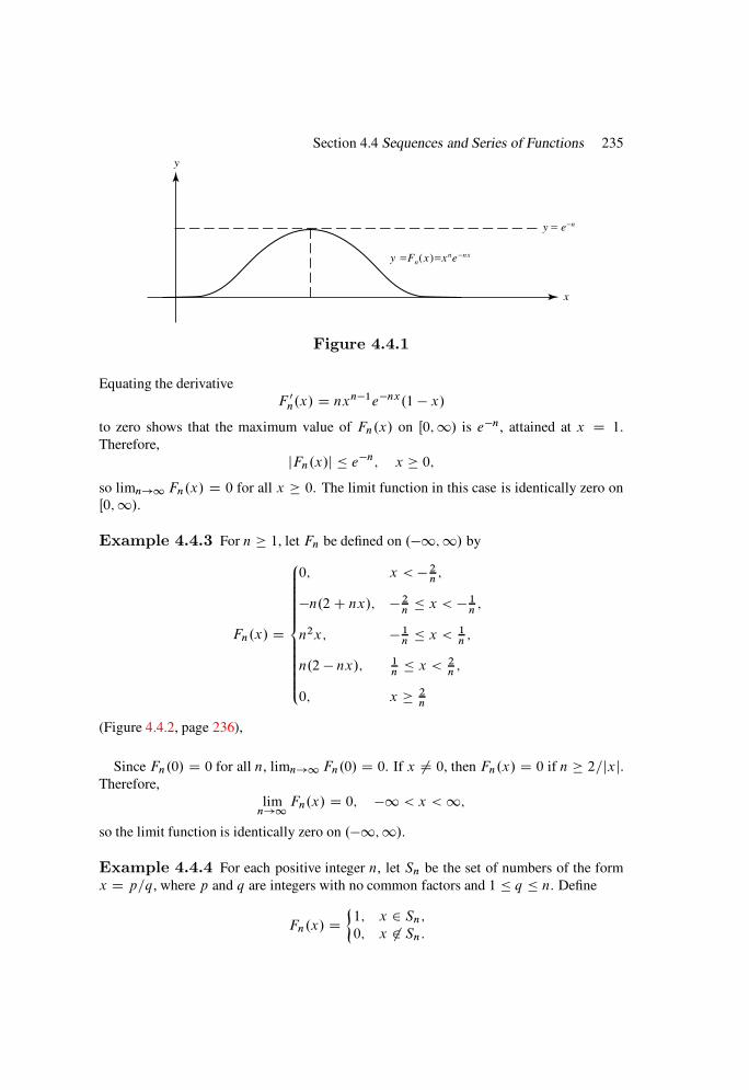
Section 4.4 Sequences and Series of Functions 235
y
x
y =Fn(x)=xne−nx
y = e−n
Figure 4.4.1
Equating the derivative
F 0n.x/ D nxn1enx.1 x/
to zero shows that the maximum value of Fn.x/ on Œ0;1/ is en, attained at x D 1.
Therefore,
jFn.x/j en; x 0;so limn!1 Fn.x/ D 0 for all x 0. The limit function in this case is identically zero on
Œ0;1/.
Example 4.4.3 For n 1, let Fn be defined on .1;1/ by
Fn.x/ D
8ˆˆˆ<ˆˆˆ:
0; x < 2n;
n.2C nx/; 2n x < 1
n;
n2x; 1n x < 1
n;
n.2 nx/; 1n x < 2
n;
0; x 2n
(Figure 4.4.2, page 236),
Since Fn.0/ D 0 for all n, limn!1 Fn.0/ D 0. If x ¤ 0, then Fn.x/ D 0 if n 2=jxj.Therefore,
limn!1
Fn.x/ D 0; 1 < x <1;
so the limit function is identically zero on .1;1/.
Example 4.4.4 For each positive integer n, let Sn be the set of numbers of the form
x D p=q, where p and q are integers with no common factors and 1 q n. Define
Fn.x/ D1; x 2 Sn;
0; x 62 Sn:
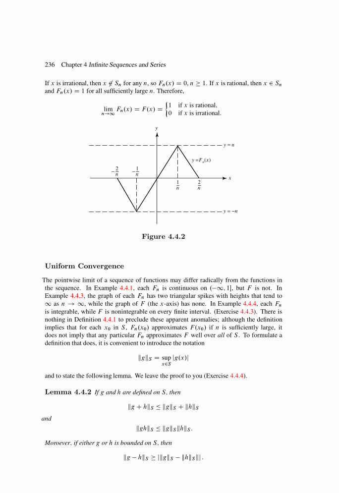
236 Chapter 4 Infinite Sequences and Series
If x is irrational, then x 62 Sn for any n, so Fn.x/ D 0, n 1. If x is rational, then x 2 Sn
and Fn.x/ D 1 for all sufficiently large n. Therefore,
limn!1
Fn.x/ D F.x/ D1 if x is rational;
0 if x is irrational:
y
x
y = −n
y = n
n1
n1
n2
n2
y =Fn(x)
−−
Figure 4.4.2
Uniform Convergence
The pointwise limit of a sequence of functions may differ radically from the functions in
the sequence. In Example 4.4.1, each Fn is continuous on .1; 1, but F is not. In
Example 4.4.3, the graph of each Fn has two triangular spikes with heights that tend to
1 as n ! 1, while the graph of F (the x-axis) has none. In Example 4.4.4, each Fn
is integrable, while F is nonintegrable on every finite interval. (Exercise 4.4.3). There is
nothing in Definition 4.4.1 to preclude these apparent anomalies; although the definition
implies that for each x0 in S , Fn.x0/ approximates F.x0/ if n is sufficiently large, it
does not imply that any particular Fn approximates F well over all of S . To formulate a
definition that does, it is convenient to introduce the notation
kgkS D supx2S
jg.x/j
and to state the following lemma. We leave the proof to you (Exercise 4.4.4).
Lemma 4.4.2 If g and h are defined on S; then
kg C hkS kgkS C khkS
and
kghkS kgkSkhkS :
Moroever; if either g or h is bounded on S; then
kg hkS jkgkS khkSkj :
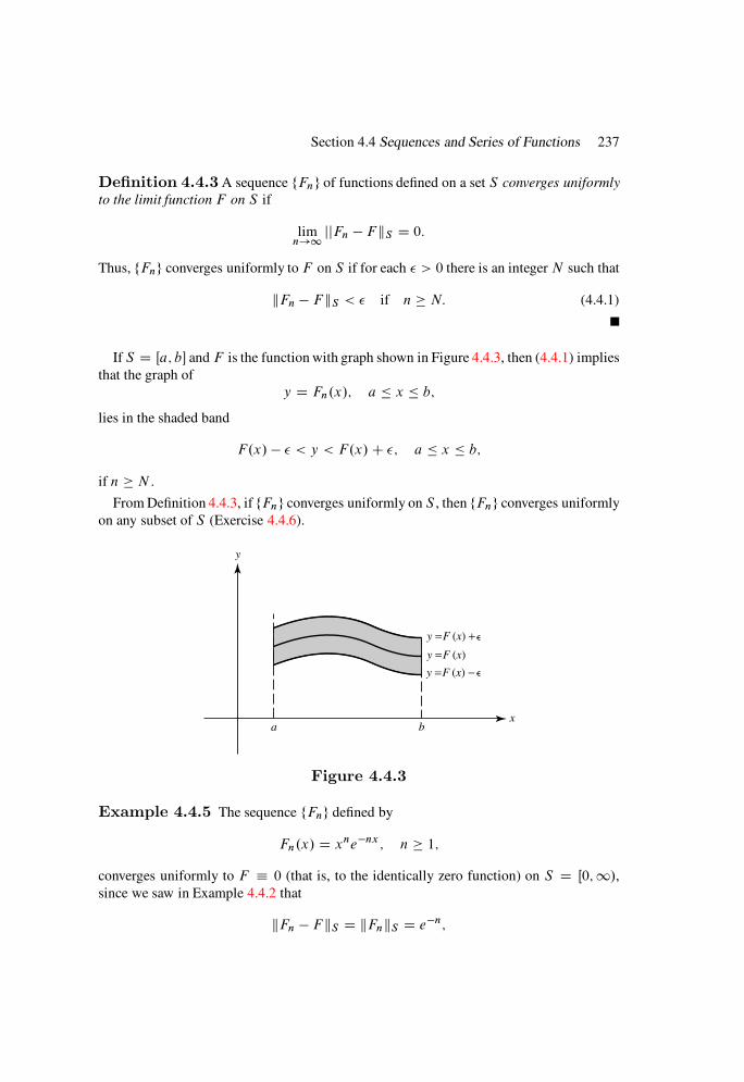
Section 4.4 Sequences and Series of Functions 237
Definition 4.4.3 A sequence fFng of functions defined on a set S converges uniformly
to the limit function F on S if
limn!1
jjFn F kS D 0:
Thus, fFng converges uniformly to F on S if for each > 0 there is an integer N such that
kFn F kS < if n N: (4.4.1)
If S D Œa; b and F is the function with graph shown in Figure 4.4.3, then (4.4.1) implies
that the graph of
y D Fn.x/; a x b;
lies in the shaded band
F.x/ < y < F.x/C ; a x b;
if n N .
From Definition 4.4.3, if fFng converges uniformly on S , then fFng converges uniformly
on any subset of S (Exercise 4.4.6).
y
xa b
y =F (x) −
y =F (x) +
y =F (x)
Figure 4.4.3
Example 4.4.5 The sequence fFng defined by
Fn.x/ D xnenx ; n 1;
converges uniformly to F 0 (that is, to the identically zero function) on S D Œ0;1/,since we saw in Example 4.4.2 that
kFn F kS D kFnkS D en;

238 Chapter 4 Infinite Sequences and Series
so
kFn F kS <
if n > log . For these values of n, the graph of
y D Fn.x/; 0 x <1;
lies in the strip
y ; x 0(Figure 4.4.4).
The next theorem provides alternative definitions of pointwise and uniform convergence.
It follows immediately from Definitions 4.4.1 and 4.4.3.
Theorem 4.4.4 Let fFng be defined on S: Then
(a) fFng converges pointwise to F on S if and only if there is, for each > 0 and x 2 S ,
an integer N .which may depend on x as well as / such that
jFn.x/ F.x/j < if n N:
(b) fFng converges uniformly to F on S if and only if there is for each > 0 an integer
N .which depends only on and not on any particular x in S/ such that
jFn.x/ F.x/j < for all x in S if n N:
y
x
y = e−n
y = e
y = −e
y =xne−nx
Figure 4.4.4
The next theorem follows immediately from Theorem 4.4.4 and Example 4.4.6.
Section 4.4 Sequences and Series of Functions 239
Theorem 4.4.5 If fFng converges uniformly to F on S; then fFng converges pointwise
to F on S: The converse is falseI that is; pointwise convergence does not imply uniform
convergence.
Example 4.4.6 The sequence fFng of Example 4.4.3 converges pointwise to F 0
on .1;1/, but not uniformly, since
kFn F k.1;1/ D Fn
1
n
DˇˇFn
1n
ˇˇ D n;
so
limn!1
kFn F k.1;1/ D1:
However, the convergence is uniform on
S D .1; [ Œ;1/
for any > 0, since
kFn F kS D 0 if n >2
:
Example 4.4.7 If Fn.x/ D xn, n 1, then fFng converges pointwise on S D Œ0; 1
to
F.x/ D1; x D 1;0; 0 x < 1:
The convergence is not uniform on S . To see this, suppose that 0 < < 1. Then
jFn.x/ F.x/j > 1 if .1 /1=n < x < 1:
Therefore,
1 kFn F kS 1for all n 1. Since can be arbitrarily small, it follows that
kFn F kS D 1
for all n 1.
However, the convergence is uniform on Œ0; if 0 < < 1, since then
kFn F kŒ0; D n
and limn!1 n D 0. Another way to say the same thing: fFng converges uniformly on
every closed subset of Œ0; 1/.
The next theorem enables us to test a sequence for uniform convergence without guessing
what the limit function might be. It is analogous to Cauchy’s convergence criterion for
sequences of constants (Theorem 4.1.13).
240 Chapter 4 Infinite Sequences and Series
Theorem 4.4.6 (Cauchy’s Uniform Convergence Criterion) A sequence
of functions fFng converges uniformly on a set S if and only if for each > 0 there is an
integer N such that
kFn FmkS < if n;m N: (4.4.2)
Proof For necessity, suppose that fFng converges uniformly to F on S . Then, if > 0,
there is an integer N such that
kFk F kS <
2if k N:
Therefore,
kFn FmkS D k.Fn F /C .F Fm/kS
kFn F kS C kF FmkS (Lemma 4.4.2)
<
2C
2D if m; n N:
For sufficiency, we first observe that (4.4.2) implies that
jFn.x/ Fm.x/j < if n;m N;
for any fixed x in S . Therefore, Cauchy’s convergence criterion for sequences of constants
(Theorem 4.1.13) implies that fFn.x/g converges for each x in S ; that is, fFng converges
pointwise to a limit function F on S . To see that the convergence is uniform, we write
jFm.x/ F.x/j D jŒFm.x/ Fn.x/C ŒFn.x/ F.x/j jFm.x/ Fn.x/j C jFn.x/ F.x/j kFm FnkS C jFn.x/ F.x/j:
This and (4.4.2) imply that
jFm.x/ F.x/j < C jFn.x/ F.x/j if n;m N: (4.4.3)
Since limn!1 Fn.x/ D F.x/,
jFn.x/ F.x/j <
for some n N , so (4.4.3) implies that
jFm.x/ F.x/j < 2 if m N:
But this inequality holds for all x in S , so
kFm F kS 2 if m N:
Since is an arbitrary positive number, this implies that fFng converges uniformly to F
on S .
The next example is similar to Example 4.1.14.

Section 4.4 Sequences and Series of Functions 241
Example 4.4.8 Suppose that g is differentiable on S D .1;1/ and
jg0.x/j r < 1; 1 < x <1: (4.4.4)
Let F0 be bounded on S and define
Fn.x/ D g.Fn1.x//; n 1: (4.4.5)
We will show that fFng converges uniformly on S . We first note that if u and v are any two
real numbers, then (4.4.4) and the mean value theorem imply that
jg.u/ g.v/j r ju vj: (4.4.6)
Recalling (4.4.5) and applying this inequality with u D Fn1.x/ and v D 0 shows that
jFn.x/j D jg.0/ C .g.Fn1.x// g.0//j jg.0/j C jg.Fn1.x// g.0/j jg.0/j C r jFn1.x/jI
therefore, since F0 is bounded on S , it follows by induction that Fn is bounded on S for
n 1. Moreover, if n 1, then (4.4.5) and (4.4.6) with u D Fn.x/ and v D Fn1.x/
imply that
jFnC1.x/Fn.x/j D jg.Fn.x//g.Fn1 .x//j r jFn.x/Fn1.x/j; 1 < x <1;
so
kFnC1 FnkS rkFn Fn1kS :
By induction, this implies that
kFnC1 FnkS rnkF1 F0kS : (4.4.7)
If n > m, then
kFn FmkS D k.Fn Fn1/C .Fn1 Fn2/C C .FmC1 Fm/kS
kFn Fn1kS C kFn1 Fn2kS C C kFmC1 FmkS ;
from Lemma 4.4.2. Now (4.4.7) implies that
kFn FmkS kF1 F0kS .1C r C r2 C C rnm1/rm
< kF1 F0kS
rm
1 r:
Therefore, if
kF1 F0kS
rN
1 r< ;
then kFn FmkS < if n, m N . Therefore, fFng converges uniformly on S , by
Theorem 4.4.6.
242 Chapter 4 Infinite Sequences and Series
Properties Preserved by Uniform Convergence
We now study properties of the functions of a uniformly convergent sequence that are
inherited by the limit function. We first consider continuity.
Theorem 4.4.7 If fFng converges uniformly to F on S and each Fn is continuous at
a point x0 in S; then so is F . Similar statements hold for continuity from the right and left:
Proof Suppose that each Fn is continuous at x0. If x 2 S and n 1, then
jF.x/ F.x0/j jF.x/ Fn.x/j C jFn.x/ Fn.x0/j C jFn.x0/ F.x0/j jFn.x/ Fn.x0/j C 2kFn F kS :
(4.4.8)
Suppose that > 0. Since fFng converges uniformly to F on S , we can choose n so that
kFn F kS < . For this fixed n, (4.4.8) implies that
jF.x/ F.x0/j < jFn.x/ Fn.x0/j C 2; x 2 S: (4.4.9)
Since Fn is continuous at x0, there is a ı > 0 such that
jFn.x/ Fn.x0/j < if jx x0j < ı;
so, from (4.4.9),
jF.x/ F.x0/j < 3; if jx x0j < ı:
Therefore, F is continuous at x0. Similar arguments apply to the assertions on continuity
from the right and left.
Corollary 4.4.8 If fFng converges uniformly to F on S and each Fn is continuous on
S; then so is F I that is; a uniform limit of continuous functions is continuous.
Now we consider the question of integrability of the uniform limit of integrable func-
tions.
Theorem 4.4.9 Suppose that fFng converges uniformly to F on S D Œa; b. Assume
that F and all Fn are integrable on Œa; b: Then
Z b
a
F.x/ dx D limn!1
Z b
a
Fn.x/ dx: (4.4.10)
Proof Sinceˇˇˇ
Z b
a
Fn.x/ dx Z b
a
F.x/ dx
ˇˇˇ
Z b
a
jFn.x/ F.x/j dx
.b a/kFn F kS
and limn!1 kFn F kS D 0, the conclusion follows.

Section 4.4 Sequences and Series of Functions 243
In particular, this theorem implies that (4.4.10) holds if each Fn is continuous on Œa; b,
because then F is continuous (Corollary 4.4.8) and therefore integrable on Œa; b.
The hypotheses of Theorem 4.4.9 are stronger than necessary. We state the next theorem
so that you will be better informed on this subject. We omit the proof, which is inaccessible
if you skipped Section 3.5, and quite involved in any case.
Theorem 4.4.10 Suppose that fFng converges pointwise to F and each Fn is inte-
grable on Œa; b:
(a) If the convergence is uniform; then F is integrable on Œa; b and (4.4.10) holds.
(b) If the sequence fkFnkŒa;bg is bounded and F is integrable on Œa; b; then (4.4.10)
holds.
Part (a) of this theorem shows that it is not necessary to assume in Theorem 4.4.9 that F
is integrable on Œa; b, since this follows from the uniform convergence. Part (b) is known
as the bounded convergence theorem. Neither of the assumptions of (b) can be omitted.
Thus, in Example 4.4.3, where fkFnkŒ0;1g is unbounded while F is integrable on Œ0; 1,
Z 1
0
Fn.x/ dx D 1; n 1; but
Z 1
0
F.x/ dx D 0:
In Example 4.4.4, where kFnkŒa;b D 1 for every finite interval Œa; b, Fn is integrable for
all n 1, and F is nonintegrable on every interval (Exercise 4.4.3).
After Theorems 4.4.7 and 4.4.9, it may seem reasonable to expect that if a sequence fFngof differentiable functions converges uniformly to F on S , then F 0 D limn!1 F 0
n on S .
The next example shows that this is not true in general.
Example 4.4.9 The sequence fFng defined by
Fn.x/ D xn sin1
xn1
converges uniformly to F 0 on Œr1; r2 if 0 < r1 < r2 < 1 (or, equivalently, on every
compact subset of .0; 1/). However,
F 0n.x/ D nxn1 sin
1
xn1 .n 1/ cos
1
xn1;
so fF 0n.x/g does not converge for any x in .0; 1/.
Theorem 4.4.11 Suppose that F 0n is continuous on Œa; b for all n 1 and fF 0
ngconverges uniformly on Œa; b: Suppose also that fFn.x0/g converges for some x0 in Œa; b:
Then fFng converges uniformly on Œa; b to a differentiable limit function F; and
F 0.x/ D limn!1
F 0n.x/; a < x < b; (4.4.11)
while
F 0C.a/ D lim
n!1F 0
n.aC/ and F 0.b/ D lim
n!1F 0
n.b/: (4.4.12)

244 Chapter 4 Infinite Sequences and Series
Proof Since F 0n is continuous on Œa; b, we can write
Fn.x/ D Fn.x0/CZ x
x0
F 0n.t/ dt; a x b (4.4.13)
(Theorem 3.3.12). Now let
L D limn!1
Fn.x0/
and
G.x/ D limn!1
F 0n.x/: (4.4.14)
Since F 0n is continuous and fF 0
ng converges uniformly to G on Œa; b, G is continuous on
Œa; b (Corollary 4.4.8); therefore, (4.4.13) and Theorem 4.4.9 (with F and Fn replaced by
G and F 0n) imply that fFng converges pointwise on Œa; b to the limit function
F.x/ D LCZ x
x0
G.t/ dt: (4.4.15)
The convergence is actually uniform on Œa; b, since subtracting (4.4.13) from (4.4.15)
yields
jF.x/ Fn.x/j jL Fn.x0/j CˇˇZ x
x0
jG.t/ F 0n.t/j dt
ˇˇ
jL Fn.x0/j C jx x0j kG F 0nkŒa;b;
so
kF FnkŒa;b jL Fn.x0/j C .b a/kG F 0nkŒa;b;
where the right side approaches zero as n!1.
Since G is continuous on Œa; b, (4.4.14), (4.4.15), Definition 2.3.6, and Theorem 3.3.11
imply (4.4.11) and (4.4.12).
Infinite Series of Functions
In Section 4.3 we defined the sum of an infinite series of constants as the limit of the
sequence of partial sums. The same definition can be applied to series of functions, as
follows.
Definition 4.4.12 If ffj g1k is a sequence of real-valued functions defined on a set D
of reals, thenP1
j Dk fj is an infinite series (or simply a series) of functions on D. The
partial sums of ,P1
j Dk fj are defined by
Fn DnX
j Dk
fj ; n k:
If fFng1k converges pointwise to a function F on a subset S of D, we say thatP1
j Dk fj
converges pointwise to the sum F on S , and write
F D1X
j Dk
fj ; x 2 S:

Section 4.4 Sequences and Series of Functions 245
If fFng converges uniformly to F on S , we say thatP1
j Dk fj converges uniformly to F
on S .
Example 4.4.10 The functions
fj .x/ D xj ; j 0;
define the infinite series1X
j D0
xj
on D D .1;1/. The nth partial sum of the series is
Fn.x/ D 1C x C x2 C C xn;
or, in closed form,
Fn.x/ D
8<:
1 xnC1
1 x; x ¤ 1;
nC 1; x D 1(Example 4.1.11). We have seen earlier that fFng converges pointwise to
F.x/ D 1
1 xif jxj < 1 and diverges if jxj 1; hence, we write
1X
j D0
xj D 1
1 x; 1 < x < 1:
Since the difference
F.x/ Fn.x/ DxnC1
1 xcan be made arbitrarily large by taking x close to 1,
kF Fnk.1;1/ D1;
so the convergence is not uniform on .1; 1/. Neither is it uniform on any interval .1; rwith 1 < r < 1, since
kF Fnk.1;r/ 1
2
for every n on every such interval. (Why?) The series does converge uniformly on any
interval Œr; r with 0 < r < 1, since
kF FnkŒr;r DrnC1
1 rand limn!1 rn D 0. Put another way, the series converges uniformly on closed subsets of
.1; 1/.

246 Chapter 4 Infinite Sequences and Series
As for series of constants, the convergence, pointwise or uniform, of a series of functions
is not changed by altering or omitting finitely many terms. This justifies adopting the
convention that we used for series of constants: when we are interested only in whether a
series of functions converges, and not in its sum, we will omit the limits on the summation
sign and write simplyPfn.
Tests for Uniform Convergence of Series
Theorem 4.4.6 is easily converted to a theorem on uniform convergence of series, as fol-
lows.
Theorem 4.4.13 (Cauchy’s Uniform Convergence Criterion) A seriesPfn converges uniformly on a set S if and only if for each > 0 there is an integer N
such that
kfn C fnC1 C C fmkS < if m n N: (4.4.16)
Proof Apply Theorem 4.4.6 to the partial sums ofPfn, observing that
fn C fnC1 C C fm D Fm Fn1:
Setting m D n in (4.4.16) yields the following necessary, but not sufficient, condition
for uniform convergence of series. It is analogous to Corollary 4.3.6.
Corollary 4.4.14 IfPfn converges uniformly on S; then limn!1 kfnkS D 0:
Theorem 4.4.13 leads immediately to the following important test for uniform conver-
gence of series.
Theorem 4.4.15 (Weierstrass’s Test) The seriesPfn converges uniformly
on S if
kfnkS Mn; n k; (4.4.17)
wherePMn <1:
Proof From Cauchy’s convergence criterion for series of constants, there is for each
> 0 an integer N such that
Mn CMnC1 C CMm < if m n N;
which, because of (4.4.17), implies that
kfnkS C kfnC1kS C C kfmkS < if m; n N:
Lemma 4.4.2 and Theorem 4.4.13 imply thatPfn converges uniformly on S .
Section 4.4 Sequences and Series of Functions 247
Example 4.4.11 TakingMn D 1=n2 and recalling that
X 1
n2<1;
we see that X 1
x2 C n2and
X sinnx
n2
converge uniformly on .1;1/.
Example 4.4.12 The series
Xfn.x/ D
Xx
1C x
n
converges uniformly on any set S such that
ˇˇ x
1C x
ˇˇ r < 1; x 2 S; (4.4.18)
because if S is such a set, then
kfnkS rn
and Weierstrass’s test applies, with
XMn D
Xrn <1:
Since (4.4.18) is equivalent to
r1C r x
r
1 r ; x 2 S;
this means that the series converges uniformly on any compact subset of .1=2;1/.(Why?) From Corollary 4.4.14, the series does not converge uniformly on S D .1=2; b/with b < 1 or on S D Œa;1/ with a > 1=2, because in these cases kfnkS D 1 for all
n.
Weierstrass’s test is very important, but applicable only to series that actually exhibit a
stronger kind of convergence than we have considered so far. We say thatPfn converges
absolutely on S ifPjfnj converges pointwise on S , and absolutely uniformly on S ifP
jfnj converges uniformly on S . We leave it to you (Exercise 4.4.21) to verify that our
proof of Weierstrass’s test actually shows thatPfn converges absolutely uniformly on S .
We also leave it to you to show that if a series converges absolutely uniformly on S , then it
converges uniformly on S (Exercise 4.4.20).
The next theorem applies to series that converge uniformly, but perhaps not absolutely
uniformly, on a set S .

248 Chapter 4 Infinite Sequences and Series
Theorem 4.4.16 (Dirichlet’s Test for Uniform Convergence) The se-
ries1X
nDk
fngn
converges uniformly on S if ffng converges uniformly to zero on S;P.fnC1 fn/ con-
verges absolutely uniformly on S; and
kgk C gkC1 C C gnkS M; n k; (4.4.19)
for some constantM:
Proof The proof is similar to the proof of Theorem 4.3.20. Let
Gn D gk C gkC1 C C gn;
and consider the partial sums ofP1
nDk fngn:
Hn D fkgk C fkC1gkC1 C C fngn: (4.4.20)
By substituting
gk D Gk and gn D Gn Gn1; n k C 1;
into (4.4.20), we obtain
Hn D fkGk C fkC1.GkC1 Gk/C C fn.Gn Gn1/;
which we rewrite as
Hn D .fk fkC1/Gk C .fkC1 fkC2/GkC1 C C .fn1 fn/Gn1 C fnGn;
or
Hn D Jn1 C fnGn; (4.4.21)
where
Jn1 D .fk fkC1/Gk C .fkC1 fkC2/GkC1 C C .fn1 fn/Gn1: (4.4.22)
That is, fJng is the sequence of partial sums of the series
1X
j Dk
.fj fj C1/Gj : (4.4.23)
From (4.4.19) and the definition of Gj ,
ˇˇˇ
mX
j Dn
Œfj .x/ fj C1.x/Gj .x/
ˇˇˇ M
mX
j Dn
jfj .x/ fj C1.x/j; x 2 S;

Section 4.4 Sequences and Series of Functions 249
so
mX
j Dn
.fj fj C1/Gj
S
M
mX
j Dn
jfj fj C1j
S
:
Now suppose that > 0. SinceP.fj fj C1/ converges absolutely uniformly on S , The-
orem 4.4.13 implies that there is an integer N such that the right side of the last inequality
is less than if m n N . The same is then true of the left side, so Theorem 4.4.13
implies that (4.4.23) converges uniformly on S .
We have now shown that fJng as defined in (4.4.22) converges uniformly to a limit
function J on S . Returning to (4.4.21), we see that
Hn J D Jn1 J C fnGn:
Hence, from Lemma 4.4.2 and (4.4.19),
kHn JkS kJn1 JkS C kfnkSkGnkS
kJn1 JkS CMkfnkS :
Since fJn1J g and ffng converge uniformly to zero on S , it now follows that limn!1 kHnJkS D 0. Therefore, fHng converges uniformly on S .
Corollary 4.4.17 The seriesP1
nDk fngn converges uniformly on S if
fnC1.x/ fn.x/; x 2 S; n k;
ffng converges uniformly to zero on S; and
kgk C gkC1 C C gnkS M; n k;
for some constantM:
The proof is similar to that of Corollary 4.3.21. We leave it to you (Exercise 4.4.22).
Example 4.4.13 Consider the series
1X
nD1
sinnx
n
with fn D 1=n (constant), gn.x/ D sinnx, and
Gn.x/ D sinx C sin 2x C C sin nx:
We saw in Example 4.3.21 that
jGn.x/j 1
j sin.x=2/j ; n 1; n ¤ 2k (k D integer):
250 Chapter 4 Infinite Sequences and Series
Therefore, fkGnkS g is bounded, and the series converges uniformly on any set S on which
sinx=2 is bounded away from zero. For example, if 0 < ı < , then
ˇˇsin
x
2
ˇˇ sin
ı
2
if x is at least ı away from any multiple of 2 ; hence, the series converges uniformly on
S D1[
kD1Œ2k C ı; 2.k C 1/ ı:
Since Xˇˇsinnx
n
ˇˇ D 1; x ¤ k
(Exercise 4.3.32(b)), this result cannot be obtained from Weierstrass’s test.
Example 4.4.14 The series1X
nD1
.1/nnC x2
satisfies the hypotheses of Corollary 4.4.17 on .1;1/, with
fn.x/ D1
nC x2; gn D .1/n; G2m D 0; and G2mC1 D 1:
Therefore, the series converges uniformly on .1;1/. This result cannot be obtained by
Weierstrass’s test, since X 1
nC x2D 1
for all x.
Continuity, Differentiability, and Integrability of Series
We can obtain results on the continuity, differentiability, and integrability of infinite series
by applying Theorems 4.4.7, 4.4.9, and 4.4.11 to their partial sums. We will state the
theorems and give some examples, leaving the proofs to you.
Theorem 4.4.7 implies the following theorem (Exercise 4.4.23).
Theorem 4.4.18 IfP1
nDk fn converges uniformly to F on S and each fn is contin-
uous at a point x0 in S; then so is F: Similar statements hold for continuity from the right
and left:
Example 4.4.15 In Example 4.4.12 we saw that the series
F.x/ D1X
nD0
x
1C x
n
Section 4.4 Sequences and Series of Functions 251
converges uniformly on every compact subset of .1=2;1/. Since the terms of the series
are continuous on every such subset, Theorem 4.4.4 implies that F is also. In fact, we can
state a stronger result: F is continuous on .1=2;1/, since every point in .1=2;1/ lies
in a compact subinterval of .1=2;1/.The same argument and the results of Example 4.4.13 show that the function
G.x/ D1X
nD1
sinnx
n
is continuous except perhaps at xk D 2k (k D integer).
From Example 4.4.14, the function
H.x/ D1X
nD1
.1/n 1
nC x2
is continuous for all x.
The next theorem gives conditions that permit the interchange of summation and inte-
gration of infinite series. It follows from Theorem 4.4.9 (Exercise 4.4.25). We leave it to
you to formulate an analog of Theorem 4.4.10 for series (Exercise 4.4.26).
Theorem 4.4.19 Suppose thatP1
nDk fn converges uniformly to F on S D Œa; b:
Assume that F and fn; n k; are integrable on Œa; b: Then
Z b
a
F.x/ dx D1X
nDk
Z b
a
fn.x/ dx:
We say in this case thatP1
nDk fn can be integrated term by term over Œa; b.
Example 4.4.16 From Example 4.4.10,
1
1 xD
1X
nD0
xn; 1 < x < 1:
The series converges uniformly, and the limit function is integrable on any closed subinter-
val Œa; b of .1; 1/; hence,
Z b
a
dx
1 xD
1X
nD0
Z b
a
xn dx;
so
log.1 a/ log.1 b/ D1X
nD0
bnC1 anC1
nC 1:
Letting a D 0 and b D x yields
log.1 x/ D 1X
nD0
xnC1
nC 1 ; 1 < x < 1:
252 Chapter 4 Infinite Sequences and Series
The next theorem gives conditions that permit the interchange of summation and differ-
entiation of infinite series. It follows from Theorem 4.4.11 (Exercise 4.4.28).
Theorem 4.4.20 Suppose that fn is continuously differentiable on Œa; b for each n k;P1
nDk fn.x0/ converges for some x0 in Œa; b; andP1
nDk f0
n converges uniformly on
Œa; b: ThenP1
nDk fn converges uniformly on Œa; b to a differentiable function F; and
F 0.x/ D1X
nDk
f 0n.x/; a < x < b;
while
F 0.aC/ D1X
nDk
f 0n.aC/ and F 0.b/ D
1X
nDk
f 0n.b/:
We say in this case thatP1
nDk fn can be differentiated term by term on Œa; b. To apply
Theorem 4.4.20, we first verify thatP1
nDk fn.x0/ converges for some x0 in Œa; b and then
differentiateP1
nDk fn term by term. If the resulting series converges uniformly, then term
by term differentiation was legitimate.
Example 4.4.17 The series
1X
nD1
.1/n 1n
cosx
n(4.4.24)
converges at x0 D 0. Differentiating term by term yields the series
1X
nD1
.1/nC1 1
n2sin
x
n(4.4.25)
of continuous functions. This series converges uniformly on .1;1/, by Weierstrass’s
test. By Theorem 4.4.20, the series (4.4.24) converges uniformly on every finite interval to
the differentiable function
F.x/ D1X
nD1
.1/n 1n
cosx
n; 1 < x <1;
and
F 0.x/ D1X
nD1
.1/nC1 1
n2sin
x
n; 1 < x <1:
Example 4.4.18 The series
E.x/ D1X
nD0
xn
nŠD 1C x C x2
2ŠC x3
3ŠC (4.4.26)
Section 4.4 Sequences and Series of Functions 253
converges uniformly on every interval Œr; r by Weierstrass’s test, because
jxjnnŠ r
n
nŠ; jxj r;
andX rn
nŠ<1
for all r , by the ratio test. Differentiating the right side of (4.4.26) term by term yields the
series1X
nD1
xn1
.n 1/Š D1X
nD0
xn
nŠ;
which is the same as (4.4.26). Therefore, the differentiated series is also uniformly conver-
gent on Œr; r for every r , so the term by term differentiation is legitimate and
E 0.x/ D E.x/; 1 < x <1:
This is not surprising if you recognize that E.x/ D ex.
Example 4.4.19 Failure to verify that the given series converges at some point can
lead to erroneous conclusions. For example, differentiating
1X
nD1
cosx
n(4.4.27)
term by term yields
1X
nD1
1
nsin
x
n;
which converges uniformly on Œr; r for every r , since
ˇˇ1n
sinx
n
ˇˇ jxj
n2(Exercise 2.3.19)
r
n2if jxj r;
andP1=n2 < 1. We cannot conclude from this that (4.4.27) converges uniformly on
Œr; r . In fact, it diverges for every x. (Why?)
4.4 Exercises
1. Find the set S on which fFng converges pointwise, and find the limit function.
(a) Fn.x/ D xn.1 x2/ (b) Fn.x/ D nxn.1 x2/
254 Chapter 4 Infinite Sequences and Series
(c) Fn.x/ D xn.1 xn/ (d) Fn.x/ D sin
1C 1
n
x
(e) Fn.x/ D1C xn
1C x2n(f) Fn.x/ D x sin
x
n
(g) Fn.x/ D n21 cos
x
n
(h) Fn.x/ D nxenx2
(i) Fn.x/ D.x C n/2x2 C n2
2. Prove: If fFng converges to F on Œa; b and Fn is nondecreasing for each n, then F
is nondecreasing.
3. Show that the functions fFng of Example 4.4.4 are integrable and F D limn!1 Fn.x/
is nonintegrable on every finite interval.
4. Prove Lemma 4.4.2.
5. Find F.x/ D limn!1 Fn.x/ on S . Show that fFng converges uniformly to F on
closed subsets of S , but not on S .
(a) Fn.x/ D xn sinnx, S D .1; 1/
(b) Fn.x/ D1
1C x2n, S D fx j x ¤ ˙1g
(c) Fn.x/ Dn2 sinx
1C n2x, S D .0;1/ HINT: See Exercise 2.3.19:
6. (a) Show that if fFng converges uniformly on S , then fFng converges uniformly
on every subset of S .
(b) Show that if fFng converges uniformly on S1, S2, . . . , Sm, then fFng con-
verges uniformly onSm
kD1 Sk .
(c) Give an example where fFng converges uniformly on each of an infinite se-
quence of sets S1, S2, . . . , but not onS1
kD1 Sk .
7. Describe the sets on which the sequences of Exercise 4.4.1 converge uniformly. Re-
strict your attention to sets that are the union of finitely many intervals and singleton
sets.
8. Suppose that fFng converges pointwise on Œa; b and, for each x in Œa; b, there is
an open interval Ix containing x such that fFng converges uniformly on Ix \ Œa; b.Show that fFng converges uniformly on Œa; b.
9. Prove: If fFng converges uniformly to F on S , then limn!1 kFnkS D kFkS .
10. Prove: If fFng converges uniformly to F on S , then F is bounded on S if and only
if limn!1fkFnkSg <1.
11. Prove: If fFng and fGng converge uniformly to F and G on S , then fFn C Gngconverges uniformly to F CG on S .
12. (a) Prove: If fFng and fGng converge uniformly to bounded functions F and G
on S , then fFnGng converges uniformly to FG on S .

Section 4.4 Sequences and Series of Functions 255
(b) Give an example showing that the conclusion of (a) may fail to hold if F or
G is unbounded on S .
13. (a) Suppose that fFng converges uniformly to F on .a; b/. Prove: If x0 < a < b
and Ln D limx!x0Fn.x/ exists (finite) for every n, then L D limn!1 Ln
exists (finite) and
limx!x0
F.x/ D L:
(b) State similar results for limits from the right and left.
14. Find the limits.
(a) limn!1
Z 4
1
n
xsin
x
ndx (b) lim
n!1
Z 2
0
dx
1C x2n
(c) limn!1
Z 1
0
nxenx2
dx (d) limn!1
Z 1
0
1C x
n
n
dx
15. Prove (without using Theorem 4.4.10): If each Fn is integrable and fFng converges
uniformly on Œa; b, then limn!1R b
aFn.x/ dx exists.
16. Prove (without using Theorem 4.4.10): If each Fn is nondecreasing and fFng con-
verges uniformly to F on Œa; b, then
limn!1
Z b
a
Fn.x/ dx DZ b
a
F.x/ dx:
17. Use Weierstrass’s test to determine sets on which the series converges absolutely
uniformly.
(a)X 1
n1=2
x
1C x
n
(b)X 1
n3=2
x
1C x
n
(c)X
nxn.1 x/n (d)X 1
n.x2 C n/
(e)X 1
nx(f)
X .1 x2/n
.1C x2/nsinnx
18. Show that ifPjanj < 1, then
Pan cosnx and
Pan sinnx define continuous
functions on .1;1/.19. (a) Give an example showing that the following “comparison test” is invalid: IfP
fn converges uniformly on S and kgnkS kfnkS , thenPgn converges
uniformly on S .
(b) This “comparison test” can be corrected by adding one word to its hypothesis
and conclusion. What is the word?
20. (a) Explain the difference between the following statements: (i)Pfn converges
absolutely and uniformly on S ; (ii)Pfn converges absolutely uniformly
on S .

256 Chapter 4 Infinite Sequences and Series
(b) Show that ifPfn converges absolutely uniformly on S , then
Pfn converges
uniformly on S .
21. Show that the hypotheses of Weierstrass’s test imply thatPfn converges absolutely
uniformly on S .
22. Prove Corollary 4.4.17.
23. Prove Theorem 4.4.18.
24. Suppose that fang11 is monotonic and limn!1 an D 0. Show that
1X
nD1
an sin nx and
1X
nD1
an cosnx
define functions continuous for all x ¤ 2k (k D integer).
25. Prove Theorem 4.4.19.
26. Formulate an analog of Theorem 4.4.10 for series.
27. In Section 4.5 we will see that
ex2 D1X
nD0
.1/n x2n
nŠand sin x D
1X
nD0
.1/n x2nC1
.2nC 1/Š
for all x, and in both cases the convergence is uniform on every finite interval. Find
series that converge to
(a) F.x/ DZ x
0
et2
dt and (b) G.x/ DZ x
0
sin t
tdt
for all x.
28. Prove Theorem 4.4.20.
29. Show from Example 4.4.17 thatP1
nD1.1/n sin.x=n/ converges uniformly on any
finite interval.
30. Prove: If 0 < anC1 < an andPak
n < 1 for some positive integer k, thenP.1/n sinanx converges uniformly on any finite interval.
31. For n 2, define
fn.x/ D
8ˆ<ˆ:
n4.x nC 1=n3/; n 1=n3 x n;
n4.x n 1=n3/; n x nC 1=n3;
0; jx nj > 1=n3;
and let F.x/ DP1
nD2 fn.x/. Show thatR1
0 F.x/ dx <1, and conclude that ab-
solute convergence of an improper integralR1
0F.x/ dx does not imply that limn!1 F.x/ D
0, even if F is continuous on Œ0;1/.
Section 4.5 Power Series 257
4.5 POWER SERIES
We now consider a class of series sufficiently general to be interesting, but sufficiently
specialized to be easily understood.
Definition 4.5.1 An infinite series of the form
1X
nD0
an.x x0/n; (4.5.1)
where x0 and a0, a1, . . . , are constants, is called a power series in x x0.
The following theorem summarizes the convergence properties of power series.
Theorem 4.5.2 In connection with the power series (4.5.1); define R in the extended
reals by1
RD lim
n!1janj1=n: (4.5.2)
In particular; R D 0 if limn!1 janj1=n D 1, and R D 1 if limn!1 janj1=n D 0: Then
the power series converges
(a) only for x D x0 if R D 0I(b) for all x if R D1; and absolutely uniformly in every bounded setI(c) for x in .x0 R; x0 C R/ if 0 < R <1; and absolutely uniformly in every closed
subset of this interval.
The series diverges if jxx0j > R: No general statement can be made concerning conver-
gence at the endpoints x D x0 CR and x D x0 R W the series may converge absolutely
or conditionally at both; converge conditionally at one and diverge at the other; or diverge
at both:
Proof In any case, the series (4.5.1) converges to a0 if x D x0. If
Xjanjrn <1 (4.5.3)
for some r > 0, thenPan.x x0/
n converges absolutely uniformly in Œx0 r; x0 Cr, by Weierstrass’s test (Theorem 4.4.15) and Exercise 4.4.21. From Cauchy’s root test
(Theorem 4.3.17), (4.5.3) holds if
limn!1
.janjrn/1=n < 1;
which is equivalent to
r limn!1
janj1=n < 1
(Exercise 4.1.30(a)). From (4.5.2), this can be rewritten as r < R, which proves the
assertions concerning convergence in (b) and (c).
If 0 R <1 and jx x0j > R, then

258 Chapter 4 Infinite Sequences and Series
1
R>
1
jx x0j;
so (4.5.2) implies that
janj1=n 1
jx x0jand therefore jan.x x0/
nj 1
for infinitely many values of n. Therefore,Pan.x x0/
n diverges (Corollary 4.3.6) if
jx x0j > R. In particular, the series diverges for all x ¤ x0 if R D 0.
To prove the assertions concerning the possibilities at x D x0 C R and x D x0 Rrequires examples, which follow. (Also, see Exercise 4.5.1.)
The number R defined by (4.5.2) is the radius of convergence ofPan.x x0/
n. If
R > 0, the open interval .x0 R; x0 C R/, or .1;1/ if R D 1, is the interval of
convergence of the series. Theorem 4.5.2 says that a power series with a nonzero radius
of convergence converges absolutely uniformly in every compact subset of its interval of
convergence and diverges at every point in the exterior of this interval. On this last we can
make a stronger statement: Not only doesPan.x x0/
n diverge if jx x0j > R, but the
sequence fan.x x0/ng is unbounded in this case (Exercise 4.5.3(b)).
Example 4.5.1 For the series
X sinn=6
2n.x 1/n;
we have
limn!1
janj1=n D limn!1
j sinn=6
2n
1=n
D 1
2lim
n!1.j sin n=6j/1=n (Exercise 4.1.30(a))
D 1
2.1/ D 1
2:
Therefore, R D 2 and Theorem 4.5.2 implies that the series converges absolutely uniformly
in closed subintervals of .1; 3/ and diverges if x < 1 or x > 3. Theorem 4.5.2 does not
tell us what happens when x D 1 or x D 3, but we can see that the series diverges in both
these cases since its general term does not approach zero.
Example 4.5.2 For the seriesX xn
n;
limn!1
janj1=n D limn!1
1
n
1=n
D limn!1
exp
1
nlog
1
n
D e0 D 1:
Therefore, R D 1 and the series converges absolutely uniformly in closed subintervals
of .1; 1/ and diverges if jxj > 1. For x D 1 the series becomesP.1/n=n, which
converges conditionally, and at x D 1 the series becomesP1=n, which diverges.

Section 4.5 Power Series 259
The next theorem provides an expression forR that, if applicable, is usually easier to use
than (4.5.2).
Theorem 4.5.3 The radius of convergence ofPan.x x0/
n is given by
1
RD lim
n!1
ˇˇanC1
an
ˇˇ
if the limit exists in the extended reals:
Proof From Theorem 4.5.2, it suffices to show that if
L D limn!1
ˇˇanC1
an
ˇˇ (4.5.4)
exists in the extended reals, then
L D limn!1
janj1=n: (4.5.5)
We will show that this is so if 0 < L <1 and leave the cases where L D 0 or L D 1 to
you (Exercise 4.5.7).
If (4.5.4) holds with 0 < L <1 and 0 < < L, there is an integer N such that
L <ˇˇamC1
am
ˇˇ < LC if m N;
so
jamj.L / < jamC1j < jamj.LC / if m N:By induction,
jaN j.L /nN < janj < jaN j.LC /nN if n > N:
Therefore, if
K1 D jaN j.L /N and K2 D jaN j.LC /N ;
then
K1=n1 .L / < janj1=n < K
1=n2 .LC /: (4.5.6)
Since limn!1 K1=n D 1 if K is any positive number, (4.5.6) implies that
L limn!1
janj1=n limn!1
janj1=n LC :
Since is an arbitrary positive number, it follows that
limn!1
janj1=n D L;
which implies (4.5.5).
260 Chapter 4 Infinite Sequences and Series
Example 4.5.3 For the power series
X xn
nŠ;
limn!1
ˇˇanC1
an
ˇˇ D lim
n!1nŠ
.nC 1/Š D limn!1
1
nC 1 D 0:
Therefore, R D1; that is, the series converges for all x, and absolutely uniformly in every
bounded set.
Example 4.5.4 For the power series
XnŠxn;
limn!1
ˇˇanC1
an
ˇˇ D lim
n!1.nC 1/ŠnŠ
D limn!1
.nC 1/ D1:
Therefore, R D 0, and the series converges only if x D 0.
Example 4.5.5 Theorem 4.5.3 does not apply directly to
X .1/n4nnp
x2n (p D constant); (4.5.7)
which has infinitely many zero coefficients (of odd powers of x). However, by setting
y D x2, we obtain the seriesX .1/n
4nnpyn; (4.5.8)
which has nonzero coefficients for which
limn!1
ˇˇanC1
an
ˇˇ D lim
n!14nnp
4nC1.nC 1/p D1
4lim
n!1
1C 1
n
p
D 1
4:
Therefore, (4.5.8) converges if jyj < 4 and diverges if jyj > 4. Setting y D x2, we
conclude that (4.5.7) converges if jxj < 2 and diverges if jxj > 2. At x D ˙2, (4.5.7)
becomesP.1/n=np , which diverges if p 0, converges conditionally if 0 < p 1, and
converges absolutely if p > 1.
Properties of Functions Defined by Power Series
We now study the properties of functions defined by power series. Henceforth, we consider
only power series with nonzero radii of convergence.
Theorem 4.5.4 A power series
f .x/ D1X
nD0
an.x x0/n

Section 4.5 Power Series 261
with positive radius of convergence R is continuous and differentiable in its interval of
convergence; and its derivative can be obtained by differentiating term by termI that is;
f 0.x/ D1X
nD1
nan.x x0/n1; (4.5.9)
which can also be written as
f 0.x/ D1X
nD0
.nC 1/anC1.x x0/n: (4.5.10)
This series also has radius of convergence R:
Proof First, the series in (4.5.9) and (4.5.10) are the same, since the latter is obtained
by shifting the index of summation in the former. Since
limn!1
..nC 1/janj/1=n D limn!1
.nC 1/1=njanj1=n
D
limn!1
.nC 1/1=n
limn!1
janj1=n
(Exercise 4.1.30(a)/
D
limn!1
exp
log.nC 1/
n
lim
n!1janj1=n
D e0
RD 1
R;
the radius of convergence of the power series in (4.5.10) is R (Theorem 4.5.2). Therefore,
the power series in (4.5.10) converges uniformly in every interval Œx0 r; x0C r such that
0 < r < R, and Theorem 4.4.20 now implies (4.5.10) for all x in .x0 R; x0 CR/.Theorem 4.5.4 can be strengthened as follows.
Theorem 4.5.5 A power series
f .x/ D1X
nD0
an.x x0/n
with positive radius of convergence R has derivatives of all orders in its interval of convergence;
which can be obtained by repeated term by term differentiationI thus;
f .k/.x/ D1X
nDk
n.n 1/ .n k C 1/an.x x0/nk : (4.5.11)
The radius of convergence of each of these series is R:
Proof The proof is by induction. The assertion is true for k D 1, by Theorem 4.5.4.
Suppose that it is true for some k 1. By shifting the index of summation, we can rewrite
(4.5.11) as
f .k/.x/ D1X
nD0
.nC k/.n C k 1/ .nC 1/anCk .x x0/n; jx x0j < R:
262 Chapter 4 Infinite Sequences and Series
Defining
bn D .nC k/.nC k 1/ .nC 1/anCk ; (4.5.12)
we rewrite this as
f .k/.x/ D1X
nD0
bn.x x0/n; jx x0j < R:
By Theorem 4.5.4, we can differentiate this series term by term to obtain
f .kC1/.x/ D1X
nD1
nbn.x x0/n1; jx x0j < R:
Substituting from (4.5.12) for bn yields
f .kC1/.x/ D1X
nD1
.nC k/.n C k 1/ .nC 1/nanCk .x x0/n1; jx x0j < R:
Shifting the summation index yields
f .kC1/.x/ D1X
nDkC1
n.n 1/ .n k/an.x x0/nk1 ; jx x0j < R;
which is (4.5.11) with k replaced by k C 1. This completes the induction.
Example 4.5.6 In Example 4.4.10 we saw that
1
1 x D1X
nD0
xn; jxj < 1:
Repeated differentiation yields
kŠ
.1 x/kC1D
1X
nDk
n.n 1/ .n k C 1/xnk
D1X
nD0
.nC k/.nC k 1/ .nC 1/xn; jxj < 1;
so
1
.1 x/kC1D
1X
nD0
nC kk
!xn; jxj < 1:
Example 4.5.7 By the method of Example 4.5.5, it can be shown that the series
S.x/ D1X
nD0
.1/n x2nC1
.2nC 1/Š and C.x/ D1X
nD0
.1/n x2n
.2n/Š
Section 4.5 Power Series 263
converge for all x. Differentiating yields
S 0.x/ D1X
nD0
.1/n xn
.2n/ŠD C.x/
and
C 0.x/ D1X
nD1
.1/n x2n1
.2n 1/ŠD
1X
nD0
.1/n x2nC1
.2nC 1/ŠD S.x/:
These results should not surprise you if you recall that
S.x/ D sin x and C.x/ D cos x:
(We will soon prove this.)
Theorem 4.5.5 has two important corollaries.
Corollary 4.5.6 If
f .x/ D1X
nD0
an.x x0/n; jx x0j < R;
then
an Df .n/.x0/
nŠ:
Proof Setting x D x0 in (4.5.11) yields
f .k/.x0/ D kŠak:
Corollary 4.5.7 (Uniqueness of Power Series) If
1X
nD0
an.x x0/n D
1X
nD0
bn.x x0/n (4.5.13)
for all x in some interval .x0 r; x0C r/; then
an D bn; n 0: (4.5.14)
Proof Let
f .x/ D1X
nD0
an.x x0/n and g.x/ D
1X
nD0
bn.x x0/n:
From Corollary 4.5.6,
an Df .n/.x0/
nŠand bn D
g.n/.x0/
nŠ: (4.5.15)

264 Chapter 4 Infinite Sequences and Series
From (4.5.13), f D g in .x0 r; x0C r/. Therefore,
f .n/.x0/ D g.n/.x0/; n 0:
This and (4.5.15) imply (4.5.14).
Theorems 4.4.19 and 4.5.2 imply the following theorem. We leave the proof to you
(Exercise 4.5.15).
Theorem 4.5.8 If x1 and x2 are in the interval of convergence of
f .x/ D1X
nD0
an.x x0/n;
then Z x2
x1
f .x/ dx D1X
nD0
an
nC 1.x2 x0/
nC1 .x1 x0/nC1
I
that is; a power series may be integrated term by term between any two points in its interval
of convergence:
Example 4.5.16 presents an application of this theorem.
Taylor’s Series
So far we have asked for what values of x a given power series converges, and what are
the properties of its sum. Now we ask a related question: What properties guarantee that a
given function f can be represented as the sum of a convergent power series in x x0? A
partial answer to this question is provided by what we already know: Theorem 4.5.5 tells us
that f must have derivatives of all orders in some neighborhood of x0, and Corollary 4.5.6
tells us that the only power series in x x0 that can possibly converge to f in such a
neighborhood is1X
nD0
f .n/.x0/
nŠ.x x0/
n: (4.5.16)
This is called the Taylor series of f about x0 (also, the Maclaurin series of f , if x0 D 0).
The mth partial sum of (4.5.16) is the Taylor polynomial
Tm.x/ DmX
nD0
f .n/.x0/
nŠ.x x0/
n;
defined in Section 2.5.
The Taylor series of an infinitely differentiable function f may converge to a sum dif-
ferent from f . For example, the function
f .x/ De1=x2
; x ¤ 0;0; x D 0;
Section 4.5 Power Series 265
is infinitely differentiable on .1;1/ and f .n/.0/ D 0 for n 0 (Exercise 2.5.1), so its
Maclaurin series is identically zero.
The answer to our question is provided by Taylor’s theorem (Theorem 2.5.4), which
says that if f is infinitely differentiable on .a; b/ and x and x0 are in .a; b/ then, for every
integer n 0,
f .x/ Tn.x/ Df .nC1/.cn/
.nC 1/Š .x x0/n1; (4.5.17)
where cn is between x and x0. Therefore,
f .x/ D1X
nD0
f .n/.x0/
nŠ.x x0/
n
for an x in .a; b/ if and only if
limn!1
f .nC1/.cn/
.nC 1/Š.x x0/
nC1 D 0:
It is not always easy to check this condition, because the sequence fcng is usually not pre-
cisely known, or even uniquely defined; however, the next theorem is sufficiently general
to be useful.
Theorem 4.5.9 Suppose that f is infinitely differentiable on an interval I and
limn!1
rn
nŠkf .n/kI D 0: (4.5.18)
Then; if x0 2 I 0; the Taylor series
1X
nD0
f .n/.x0/
nŠ.x x0/
n
converges uniformly to f on
Ir D I \ Œx0 r; x0 C r:
Proof From (4.5.17),
kf TnkIr rnC1
.nC 1/Škf .nC1/kIr
rnC1
.nC 1/Škf .nC1/kI ;
so (4.5.18) implies the conclusion.
Example 4.5.8 If f .x/ D sinx, then kf .k/k.1;1/ D 1; k 0. Since
limn!1
rn
nŠD 0; 0 < r <1

266 Chapter 4 Infinite Sequences and Series
(Example 4.1.12), (4.5.18) holds for all r . Since
f .2m/.0/ D 0 and f .2mC1/.0/ D .1/m; m 0;
we see from Theorem 4.5.9, with I D .1;1/, x0 D 0, and r arbitrary, that
sin x D1X
nD0
.1/n x2nC1
.2nC 1/Š ; 1 < x <1;
and the convergence is uniform on bounded sets.
A similar argument shows that
cos x D1X
nD0
.1/n x2n
.2n/Š; 1 < x <1;
with uniform convergence on bounded sets.
Example 4.5.9 If f .x/ D ex, then f .k/.x/ D ex and kf .k/kI D er , k 0, if
I D Œr; r . Since
limn!1
rn
nŠer D 0;
we conclude as in Example 4.5.8 that
ex D1X
nD0
xn
nŠ; 1 < x <1;
with uniform convergence on bounded sets.
Example 4.5.10 If f .x/ D .1C x/q , then
f .n/.x/
nŠD q
n
!.1C x/qn; so
f .n/.0/
nŠD q
n
!(4.5.19)
(Example 2.5.3). The Maclaurin series
1X
nD0
q
n
!xn
is called the binomial series. We saw in Example 2.5.3 that this series equals .1C x/q for
all x if q is a nonnegative integer. We will now show that if q is an arbitrary real number,
then1X
nD0
q
n
!xn D f .x/ D .1C x/q; 0 x < 1: (4.5.20)
Since

Section 4.5 Power Series 267
limn!1
ˇˇˇ
q
nC 1
! q
n
!ˇˇˇ D lim
n!1
ˇˇ q nnC 1
ˇˇ D 1;
the radius of convergence of the series in (4.5.20) is 1. From (4.5.19),
kf .n/kŒ0;1
nŠ Œmax.1; 2q/
ˇˇˇ
q
n
!ˇˇˇ ; n 0:
Therefore, if 0 < r < 1,
limn!1
rn
nŠkf .n/kŒ0;1 Œmax.1; 2q/ lim
n!1
ˇˇˇ
q
n
!ˇˇˇ r
n D 0;
where the last equality follows from the absolute convergence of the series in (4.5.20) on
.1; 1/. Now Theorem 4.5.9 implies (4.5.20).
We cannot prove in this way that the binomial series converges to .1 C x/q on .1; 0/.This requires a form of the remainder in Taylor’s theorem that we have not considered, or
a different kind of proof altogether (Exercise 4.5.20). The complete result is that
.1C x/q D1X
nD0
q
n
!xn; 1 < x < 1; (4.5.21)
for all q, and, as we said earlier, the identity holds for all x if q is a nonnegative integer.
Arithmetic Operations with Power Series
We now consider addition and multiplication of power series, and division of one by an-
other.
We leave the proof of the next theorem to you (Exercise 4.5.21).
Theorem 4.5.10 If
f .x/ D1X
nD0
an.x x0/n; jx x0j < R1; (4.5.22)
g.x/ D1X
nD0
bn.x x0/n; jx x0j < R2; (4.5.23)
and ˛ and ˇ are constants; then
f .x/C ˇg.x/ D1X
nD0
.˛an C ˇbn/.x x0/n; jx x0j < R;
where R minfR1; R2g:
268 Chapter 4 Infinite Sequences and Series
Theorem 4.5.11 If f and g are given by (4.5.22) and (4.5.23); then
f .x/g.x/ D1X
nD0
cn.x x0/n; jx x0j < R; (4.5.24)
wherecn D
nX
rD0
arbnr DnX
rD0
anrbr
and R minfR1; R2g:
Proof Suppose that R1 R2. Since the series (4.5.22) and (4.5.23) converge abso-
lutely to f .x/ and g.x/ if jx x0j < R1, their Cauchy product converges to f .x/g.x/ if
jx x0j < R1, by Theorem 4.3.29. The nth term of this product is
nX
rD0
ar.x x0/rbnr .x x0/
nr D
nX
rD0
arbnr
!.x x0/
n D cn.x x0/n:
Example 4.5.11 If
f .x/ D 1
1 x D1X
nD0
xn; jxj < 1;
and
g.x/ D1X
nD0
bnxn; jxj < R;
then
g.x/
1 x D1X
nD0
snxn; jxj < minf1; Rg;
where
sn D .1/b0 C .1/b1 C C .1/bn
D b0 C b1 C C bn:
Example 4.5.12 From the paragraph following Example 4.5.10,
.1C x/p D1X
nD0
p
n
!xn; jxj < 1;
and
.1C x/q D1X
nD0
q
n
!xn; jxj < 1:

Section 4.5 Power Series 269
Since
.1C x/p.1C x/q D .1C x/pCq D1X
nD0
p C qn
!xn;
while the Cauchy product isP1
nD0 cnxn, with
cn DnX
rD0
p
r
! q
n r
!;
Corollary 4.5.7 implies that
cn D p C qn
!:
This yields the identity p C qn
!D
nX
rD0
p
r
! q
n r
!;
valid for all p and q.
The quotient
f .x/ D h.x/
g.x/(4.5.25)
of two power series
h.x/ D1X
nD0
cn.x x0/n; jx x0j < R1;
and
g.x/ D1X
nD0
bn.x x0/n; jx x0j < R2;
can be represented as a power series
f .x/ D1X
nD0
an.x x0/n (4.5.26)
with a positive radius of convergence, provided that
b0 D g.x0/ ¤ 0:
This is surely plausible. Since g.x0/ ¤ 0 and g is continuous near x0, the denominator
of (4.5.25) differs from zero on an interval about x0. Therefore, f has derivatives of all
orders on this interval, because g and h do. However, the proof that the Taylor series of f
about x0 converges to f near x0 requires the use of the theory of functions of a complex
variable. Therefore, we omit it. However, it is straightforward to compute the coefficients
in (4.5.26) if we accept the validity of the expansion. Since
f .x/g.x/ D h.x/;

270 Chapter 4 Infinite Sequences and Series
Theorem 4.5.11 implies that
nX
rD0
arbnr D cn; n 0:
Solving these equations successively yields
a0 Dc0
b0
;
an D1
b0
cn
n1X
rD0
bnrar
!; n 1:
It is not worthwhile to memorize these formulas. Rather, it is usually better to view the
procedure as follows: Multiply the series f (with unknown coefficients) and g according
to the procedure of Theorem 4.5.11, equate the resulting coefficients with those of h, and
solve the resulting equations successively for a0, a1, . . . .
Example 4.5.13 Suppose that we wish to find the coefficients in the Maclaurin series
tanx D a0 C a1x C a2x2 C :
We first observe that since tan x is an odd function, its derivatives of even order vanish at
x0 D 0, so a2m D 0,m 0. Therefore,
tanx D a1x C a3x3 C a5x
5 C :
Since
tanx Dsin x
cos x;
it follows from Example 4.5.8 that
a1x C a3x3 C a5x
5 C Dx x
3
6C x5
120C
1 x2
2C x4
24C
so
.a1x C a3x3 C a5x
5 C /1 x
2
2C x4
24C
D x x
3
6C x5
120C ;
or, according to Theorem 4.5.11,
a1x Ca3
a1
2
x3 C
a5
a3
2C a1
24
x5 C D x x
3
6C x5
120C :
From Corollary 4.5.7, coefficients of like powers of x on the two sides of this equation
must be equal; hence,
a1 D 1; a3 a1
2D 1
6; a5
a3
2C a1
24D 1
120;
so
a1 D 1; a3 D 1
6C 1
2.1/ D 1
3; a5 D
1
120C 1
2
1
3
1
24.1/ D 2
15:

Section 4.5 Power Series 271
Therefore,
tan x D x Cx3
3C
2
15x5 C :
Example 4.5.14 To find the reciprocal of the power series
g.x/ D 1C ex D 2C1X
nD1
xn
nŠ;
we let h D 1 in (4.5.25). If
1
g.x/D
1X
nD0
anxn;
then
1D .a0 C a1x C a2x2 C a3x
3 C /2C x C x2
2C x3
6C
D 2a0 C .a0 C 2a1/x Ca0
2C a1 C 2a2
x2
Ca0
6C a1
2C a2 C 2a3
x3 C :
From Corollary 4.5.7,
2a0 D 1;a0 C 2a1 D 0;
a0
2C a1 C 2a2 D 0;
a0
6C a1
2C a2 C 2a3 D 0:
Solving these equations successively yields
a0 D1
2;
a1 D a0
2D 1
4;
a2 D 1
2
a0
2C a1
D 1
2
1
4 14
D 0;
a3 D 1
2
a0
6Ca1
2C a2
D
1
2
1
121
8C 0
D
1
48;
so1
1C exD1
2x
4Cx3
48C :

272 Chapter 4 Infinite Sequences and Series
Example 4.5.15 To find the reciprocal of
g.x/ D ex D1X
nD0
xn
nŠ; (4.5.27)
we again let h D 1 in (4.5.25). If
.ex/1 D1X
nD0
anxn;
then
1 D 1X
nD0
anxn
! 1X
nD0
xn
nŠ
!D
1X
nD0
cnxn;
where
cn DnX
rD0
ar
.n r/Š :
From Corollary 4.5.7, c0 D a0 D 1 and cn D 0 if n 1; hence,
an D n1X
rD0
ar
.n r/Š ; n 1: (4.5.28)
Solving these equations successively for a0, a1, . . . yields
a1 D 1
1Š(4.5.1) D 1;
a2 D 1
2Š.1/C 1
1Š.1/
D 1
2;
a3 D 1
3Š.1/C 1
2Š.1/C 1
1Š
1
2
D 1
6
a4 D 1
4Š.1/C
1
3Š.1/C
1
2Š
1
2
C1
1Š
1
6
D
1
24:
From this, we see that
ak D.1/kkŠ
for 0 k 4 and are led to conjecture that this holds for all k. To prove this by induction,
we assume that it is so for 0 k n 1 and compute from (4.5.28):
an D n1X
rD0
1
.n r/Š.1/rrŠ
D 1nŠ
n1X
rD0
.1/r n
r
!(Exercise 1.2.19(a))
D .1/nnŠ
(Exercise 1.2.19(b)):

Section 4.5 Power Series 273
Thus, we have shown that
.ex/1 D1X
nD0
.1/n xn
nŠ:
Since this is precisely the series that results if x is replaced by x in (4.5.27), we have
verified a fundamental property of the exponential function: that
.ex/1 D ex:
This also follows from Example 4.3.26.
Abel’s Theorem
From Theorem 4.5.4, we know that a function f defined by a convergent power series
f .x/ D1X
nD0
an.x x0/n; jx x0j < R; (4.5.29)
is continuous in the open interval .x0R; x0CR/. The next theorem concerns the behavior
of f as x approaches an endpoint of the interval of convergence.
Theorem 4.5.12 (Abel’s Theorem) Let f be defined by a power series (4.5.29)
with finite radius of convergence R:
(a) IfP1
nD0 anRn converges; then
limx!.x0CR/
f .x/ D1X
nD0
anRn:
(b) IfP1
nD0.1/nanRn converges; then
limx!.x0R/C
f .x/ D1X
nD0
.1/nanRn:
Proof We consider a simpler problem first. Let
g.y/ D1X
nD0
bnyn
and1X
nD0
bn D s (finite):
We will show that
limy!1
g.y/ D s: (4.5.30)

274 Chapter 4 Infinite Sequences and Series
From Example 4.5.11,
g.y/ D .1 y/1X
nD0
snyn; (4.5.31)
where
sn D b0 C b1 C C bn:
Since
1
1 yD
1X
nD0
yn and therefore 1 D .1 y/1X
nD0
yn; jyj < 1; (4.5.32)
we can multiply through by s and write
s D .1 y/1X
nD0
syn; jyj < 1:
Subtracting this from (4.5.31) yields
g.y/ s D .1 y/1X
nD0
.sn s/yn; jyj < 1:
If > 0, choose N so that
jsn sj < if n N C 1:
Then, if 0 < y < 1,
jg.y/ sj .1 y/NX
nD0
jsn sjyn C .1 y/1X
nDNC1
jsn sjyn
< .1 y/NX
nD0
jsn sjyn C .1 y/yNC1
1X
nD0
yn
< .1 y/NX
nD0
jsn sj C ;
because of the second equality in (4.5.32). Therefore,
jg.y/ sj < 2
if
.1 y/NX
nD0
jsn sj < :
This proves (4.5.30).
To obtain (a) from this, let bn D anRn and g.y/ D f .x0 C Ry/; to obtain (b), let
bn D .1/nanRn and g.y/ D f .x0 Ry/.

Section 4.5 Power Series 275
Example 4.5.16 The series
f .x/ D 1
1C x D1X
nD0
.1/nxn
diverges at x D 1, while limx!1 f .x/ D 1=2. This shows that the converse of Abel’s
theorem is false. Integrating the series term by term yields
log.1C x/ D1X
nD0
.1/n xnC1
nC 1 ; jxj < 1;
where the power series converges at x D 1, and Abel’s theorem implies that
log 2 D1X
nD0
.1/nC1
nC 1 :
Example 4.5.17 If q 0, the binomial series
1X
nD0
q
n
!xn
converges absolutely for x D ˙1. This is obvious if q is a nonnegative integer, and it
follows from Raabe’s test for other positive values of q, since
ˇˇanC1
an
ˇˇ D
ˇˇˇ
q
nC 1
! q
n
!ˇˇˇ D
n qnC 1
; n > q;
and
limn!1
n
ˇˇanC1
an
ˇˇ 1
D lim
n!1n
n qnC 1 1
D limn!1
n
nC 1.q 1/ D q 1:
Therefore, Abel’s theorem and (4.5.21) imply that
1X
nD0
q
n
!D 2q and
1X
nD0
.1/n q
n
!D 0; q 0:
4.5 Exercises
1. The possibilities listed in Theorem 4.5.2(c) for behavior of a power series at the
endpoints of its interval of convergence do not include absolute convergence at one
endpoint and conditional convergence or divergence at the other. Why can’t these
occur?
276 Chapter 4 Infinite Sequences and Series
2. Find the radius of convergence.
(a)X
nC 1n
n2
Œ2C .1/nn xn (b)P2
pn.x 1/n
(c)X
2C sinn
6
n
.x C 2/n (d)Pn
pnxn
(e)Xx
n
n
3. (a) Prove: If fanrng is bounded and jx1 x0j < r , then
Pan.x1 x0/
n con-
verges.
(b) Prove: IfPan.x x0/
n has radius of convergence R and jx1 x0j > R,
then fan.x1 x0/ng is unbounded.
4. Prove: If g is a rational function defined for all nonnegative integers, thenPanx
n
andPang.n/x
n have the same radius of convergence. HINT: Use Exercise 4.1.30.a/:
5. Suppose that f .x/ DPan.x x0/
n has radius of convergence R and 0 < r <
R1 < R. Show that there is an integer k such thatˇˇˇf .x/
kX
nD0
an.x x0/n
ˇˇˇ
r
R1
kC1 R1
R1 r
if jx x0j r and k k.
6. Suppose that k is a positive integer and
f .x/ D1X
nD0
anxn
has radius of convergence R. Show that the series
g.x/ D f .xk/ D1X
nD0
anxkn
has radius of convergence R1=k.
7. Complete the proof of Theorem 4.5.3 by showing that
(a) R D 0 if limn!1 janC1jıjanj D 1;
(b) R D1 if limn!1 janC1jıjanj D 0.
8. Find the radius of convergence.
(a)P.log n/xn (b)
P2nnp.x C 1/n
(c)X
.1/n 2n
n
!xn (d)
X.1/n n
2 C 1n4n
.x 1/n
(e)X nn
nŠ.x C 2/n (f)
X ˛.˛ C 1/ .˛ C n 1/ˇ.ˇ C 1/ .ˇ C n 1/
xn
(˛, ˇ ¤ negative integer)

Section 4.5 Power Series 277
9. Suppose that an ¤ 0 for n sufficiently large. Show that
(a) limn!1
ˇˇanC1
an
ˇˇ lim
n!1janj1=n and (b) lim
n!1janj1=n lim
n!1
ˇˇanC1
an
ˇˇ :
Show that this implies Theorem 4.5.3.
10. Given that1
1 xD
1X
nD0
xn; jxj < 1;
use Theorem 4.5.4 to expressP1
nD0 n2xn in closed form.
11. The function
Jp.x/ D1X
nD0
.1/nnŠ.nC p/Š
x2
2nCp
.p D integer 0/
is the Bessel function of order p. Show that
(a) J 00 D J1.
(b) J 0p D 1
2.Jp1 JpC1/; p 1.
(c) x2J 00p C xJ 0
p C .x2 p2/Jp D 0.
12. Given that the power series f .x/ DP1
nD0 anxn satisfies
f 0.x/ D 2xf .x/; f .0/ D 1;
find fang. Do you recognize f ?
13. Let
f .x/ D1X
nD0
anxn; jxj < R;
and g.x/ D f .xk/, where k is a positive integer. Show that
g.r/.0/ D 0 if r ¤ kn and g.kn/.0/ D .kn/Š
nŠf .n/.0/; n 0:
14. Let
f .x/ D1X
nD0
an.x x0/n; jx x0j < R;
and f .tn/ D 0, where tn ¤ x0 and limn!1 tn D x0. Show that f .x/ 0
.jx x0j < R/. HINT: Rolle’s theorem helps here:
15. Prove Theorem 4.5.8.
16. Express Z x
1
log t
t 1dt
as a power series in x 1 and find the radius of convergence of the series.

278 Chapter 4 Infinite Sequences and Series
17. By substitutingx2 for x in the geometric series, we obtain
1
1C x2D
1X
nD0
.1/nx2n; jxj < 1:
Use this to express f .x/ D Tan1x .f .0/ D 0/ as a power series in x. Then
evaluate all derivatives of f at x0 D 0, and find a series of constants that converges
to =6.
18. Prove: If
f .x/ D1X
nD0
an.x x0/n; jx x0j < R;
and F is an antiderivative of f on .x0 R; x0CR/, then
F.x/ D C C1X
nD0
an
nC 1.x x0/nC1 ; jx x0j < R;
where C is a constant.
19. Suppose that some derivative of f can be represented by a power series in x x0
in an interval about x0. Show that f and all its derivatives can also.
20. Verify Eqn. (4.5.21) by showing that
.1C x/q
1X
nD0
q
n
!xn D 1; jxj < 1;
HINT: Differentiate:
21. Prove Theorem 4.5.10.
22. Find the Maclaurin series of cosh x and sinhx from the definition in Eqn. (4.5.16),
and also by applying Theorem 4.5.10 to the Maclaurin series for ex and ex.
23. Give an example where the radius of convergence of the product of two power series
is greater than the smaller of the radii of convergence of the factors.
24. Use Theorem 4.5.11 to find the first four nonzero terms in the Maclaurin.
(a) ex sinx (b)ex
1C x2(c)
cos x
1C x6(d) .sin x/ log.1C x/
25. Derive the identity
2 sinx cos x D sin 2x
from the Maclaurin series for sinx, cos x, and sin 2x.
26. (a) Given that
.1 2xt C x2/1=2 D1X
nD0
Pn.t/xn; jxj < 1; .A/
Section 4.5 Power Series 279
if 1 < t < 1, show that P0.t/ D 1, P1.t/ D t , and
PnC1.t/ D2nC 1nC 1
tPn.t/ n
nC 1Pn1.t/; n 1:
HINT: First differentiate (A) with respect to x:
(b) Show from (a) that Pn is a polynomial of degree n. It is the nth Legendre
polynomial, and .12xtCx2/1=2 is the generating function of the sequence
fPng.
27. Define (if necessary) the given function so as to be continuous at x0 D 0, and find
the first four nonzero terms of its Maclaurin series.
(a)xex
sinx(b)
cos x
1C x C x2(c) sec x
(d) x csc x (e)sin 2x
sinx
28. Let a0 D a1 D 5 and anC1 D an 6an1; n 1.
(a) Express F.x/ DP1
nD0 anxn in closed form.
(b) Write F as the difference of two geometric series, and find an explicit formula
for an.
29. Starting from the Maclaurin series
log.1 x/ D 1X
nD0
xnC1
nC 1; jxj < 1;
use Abel’s theorem to evaluate1X
nD0
1
.nC 1/.nC 2/:
30. In Example 4.5.17 we saw that
1X
nD0
q
n
!D 2q; q 0:
Show that this also holds for 1 < q < 0, but not for q 1. HINT: See Exer-
cise 4.1.35:
31. (a) Prove: IfP1
nD0 bn converges, then the series g.x/ DP1
nD0 bnxn converges
uniformly on Œ0; 1. HINT: If > 0, there is an integer N such that
jbn C bnC1 C C bmj < if n;m N:Use summation by parts to show that then
jbnxn C bn1x
n1 C C bmxmj < 2 if 0 x < 1; n;m N:
This is also known as Abel’s theorem:

280 Chapter 4 Infinite Sequences and Series
(b) Show that (a) implies the restricted form of Theorem 4.5.12 (concerning g)
proved in the text.
32. Use Exercise 4.5.31 to show that ifP1
nD0 an,P1
nD0 bn, and their Cauchy productP1nD0 cn all converge, then
1X
nD0
an
! 1X
nD0
bn
!D
1X
nD0
cn:
33. Prove: If
g.x/ D1X
nD0
bnxn; jxj < 1;
and bn 0, then
1X
nD0
bn D limx!1
g.x/ (finite or infinite):
34. Use the binomial series and the relation
d
dx.sin1 x/ D .1 x2/1=2
to obtain the Maclaurin series for sin1 x .sin1 0 D 0/. Deduce from this series
and Exercise 4.5.33 that
1X
nD0
2n
n
!1
22n.2nC 1/D
2:

CHAPTER 5
Real-Valued Functions
of Several Variables
IN THIS CHAPTER we consider real-valued function of n variables, where n > 1.
SECTION 5.1 deals with the structure of Rn, the space of ordered n-tuples of real numbers,
which we call vectors. We define the sum of two vectors, the product of a vector and a
real number, the length of a vector, and the inner product of two vectors. We study the
arithmetic properties of Rn, including Schwarz’s inequality and the triangle inequality. We
define neighborhoods and open sets in Rn, define convergence of a sequence of points in
Rn, and extend the Heine–Borel theorem to R
n. The section concludes with a discussion
of connected subsets of Rn.
SECTION 5.2 deals with boundedness, limits, continuity, and uniform continuity of a func-
tion of n variables; that is, a function defined on a subset of Rn.
SECTION 5.3 defines directional and partial derivatives of a real-valued function of n
variables. This is followed by the definition of differentiablity of such functions. We define
the differential of such a function and give a geometric interpretation of differentiablity.
SECTION 5.4 deals with the chain rule and Taylor’s theorem for a real-valued function of
n variables.
5.1 STRUCTURE OF RRRn
In this chapter we study functions defined on subsets of the real n-dimensional space Rn,
which consists of all ordered n-tuples X D .x1; x2; : : : ; xn/ of real numbers, called the
coordinates or components of X. This space is sometimes called Euclidean n-space.
In this section we introduce an algebraic structure for Rn. We also consider its topologi-
cal properties; that is, properties that can be described in terms of a special class of subsets,
the neighborhoods in Rn. In Section 1.3 we studied the topological properties of R
1, which
we will continue to denote simply as R. Most of the definitions and proofs in Section 1.3
were stated in terms of neighborhoods in R. We will see that they carry over to Rn if the
concept of neighborhood in Rn is suitably defined.
281
282 Chapter 5 Real-Valued Functions of n Variables
Members of R have dual interpretations: geometric, as points on the real line, and alge-
braic, as real numbers. We assume that you are familiar with the geometric interpretation
of members of R2 and R
3 as the rectangular coordinates of points in a plane and three-
dimensional space, respectively. Although Rn cannot be visualized geometrically if n 4,
geometric ideas from R, R2, and R
3 often help us to interpret the properties of Rn for
arbitrary n.
As we said in Section 1.3, the idea of neighborhood is always associated with some
definition of “closeness” of points. The following definition imposes an algebraic structure
on Rn, in terms of which the distance between two points can be defined in a natural way.
In addition, this algebraic structure will be useful later for other purposes.
Definition 5.1.1 The vector sum of
X D .x1; x2; : : : ; xn/ and Y D .y1; y2; : : : ; yn/
is
XC Y D .x1 C y1; x2C y2; : : : ; xnC yn/: (5.1.1)
If a is a real number, the scalar multiple of X by a is
aX D .ax1; ax2; : : : ; axn/: (5.1.2)
Note that “C” has two distinct meanings in (5.1.1): on the left, “C” stands for the newly
defined addition of members of Rn and, on the right, for addition of real numbers. However,
this can never lead to confusion, since the meaning of “C” can always be deduced from
the symbols on either side of it. A similar comment applies to the use of juxtaposition to
indicate scalar multiplication on the left of (5.1.2) and multiplication of real numbers on
the right.
Example 5.1.1 In R4, let
X D .1;2; 6; 5/ and Y D3;5; 4; 1
2
:
Then
XC Y D4;7; 10; 11
2
and
6X D .6;12; 36; 30/:
We leave the proof of the following theorem to you (Exercise 5.1.2).
Section 5.1 Structure of Rn 283
Theorem 5.1.2 If X; Y; and Z are in Rn and a and b are real numbers; then
(a) XC Y D YC X .vector addition is commutative/:
(b) .XC Y/CZ D XC .YC Z/ .vector addition is associative/:
(c) There is a unique vector 0; called the zero vector; such that XC 0 D X for all X in
Rn:
(d) For each X in Rn there is a unique vector X such that XC .X/ D 0:
(e) a.bX/ D .ab/X:(f) .a C b/X D aXC bX:
(g) a.XC Y/ D aXC aY:
(h) 1X D X:
Clearly, 0 D .0; 0; : : : ; 0/ and, if X D .x1; x2; : : : ; xn/, then
X D .x1;x2; : : : ;xn/:
We write XC .Y/ as X Y. The point 0 is called the origin.
A nonempty set V D fX;Y;Z; : : : g, together with rules such as (5.1.1), associating a
unique member of V with every ordered pair of its members, and (5.1.2), associating a
unique member of V with every real number and member of V , is said to be a vector space
if it has the properties listed in Theorem 5.1.2. The members of a vector space are called
vectors. When we wish to emphasize that we are regarding a member of Rn as part of this
algebraic structure, we will speak of it as a vector; otherwise, we will speak of it as a point.
Length, Distance, and Inner Product
Definition 5.1.3 The length of the vector X D .x1; x2; : : : ; xn/ is
jXj D .x21 C x2
2 C C x2n/
1=2:
The distance between points X and Y is jX Yj; in particular, jXj is the distance between
X and the origin. If jXj D 1, then X is a unit vector.
If n D 1, this definition of length reduces to the familiar absolute value, and the distance
between two points is the length of the interval having them as endpoints; for n D 2 and
n D 3, the length and distance of Definition 5.1.3 reduce to the familiar definitions for the
plane and three-dimensional space.
Example 5.1.2 The lengths of the vectors
X D .1;2; 6; 5/ and Y D3;5; 4; 1
2
are
jXj D .12 C .2/2 C 62 C 52/1=2 Dp66
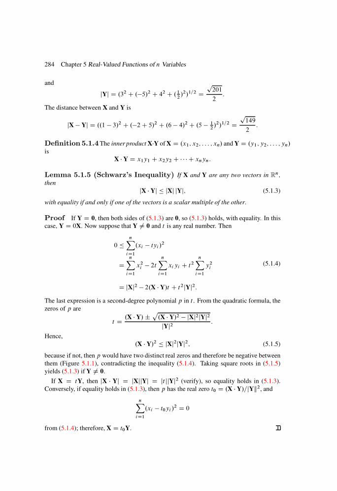
284 Chapter 5 Real-Valued Functions of n Variables
and
jYj D .32 C .5/2 C 42 C .12/2/1=2 D
p201
2:
The distance between X and Y is
jX Yj D ..1 3/2 C .2C 5/2 C .6 4/2 C .5 12/2/1=2 D
p149
2:
Definition 5.1.4The inner product XY of X D .x1; x2; : : : ; xn/ and Y D .y1; y2; : : : ; yn/
is
X Y D x1y1 C x2y2 C C xnyn:
Lemma 5.1.5 (Schwarz’s Inequality) If X and Y are any two vectors in Rn;
then
jX Yj jXj jYj; (5.1.3)
with equality if and only if one of the vectors is a scalar multiple of the other:
Proof If Y D 0, then both sides of (5.1.3) are 0, so (5.1.3) holds, with equality. In this
case, Y D 0X. Now suppose that Y ¤ 0 and t is any real number. Then
0 nX
iD1
.xi tyi /2
DnX
iD1
x2i 2t
nX
iD1
xiyi C t2nX
iD1
y2i
D jXj2 2.X Y/t C t2jYj2:
(5.1.4)
The last expression is a second-degree polynomial p in t . From the quadratic formula, the
zeros of p are
t D .X Y/˙p.X Y/2 jXj2jYj2jYj2 :
Hence,
.X Y/2 jXj2jYj2; (5.1.5)
because if not, then p would have two distinct real zeros and therefore be negative between
them (Figure 5.1.1), contradicting the inequality (5.1.4). Taking square roots in (5.1.5)
yields (5.1.3) if Y ¤ 0.
If X D tY, then jX Yj D jXjjYj D jt jjYj2 (verify), so equality holds in (5.1.3).
Conversely, if equality holds in (5.1.3), then p has the real zero t0 D .X Y/=jYk2, and
nX
iD1
.xi t0yi /2 D 0
from (5.1.4); therefore, X D t0Y.
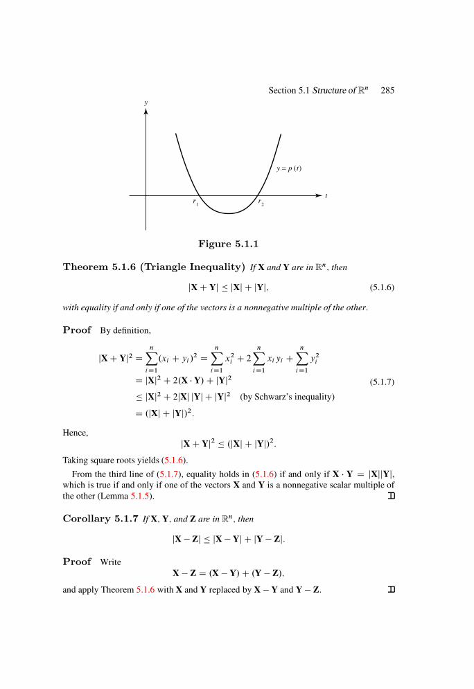
Section 5.1 Structure of Rn 285
y
t
y = p (t)
r1 r
2
Figure 5.1.1
Theorem 5.1.6 (Triangle Inequality) If X and Y are in Rn; then
jXC Yj jXj C jYj; (5.1.6)
with equality if and only if one of the vectors is a nonnegative multiple of the other:
Proof By definition,
jXC Yj2 DnX
iD1
.xi C yi /2 D
nX
iD1
x2i C 2
nX
iD1
xiyi CnX
iD1
y2i
D jXj2 C 2.X Y/C jYj2
jXj2 C 2jXj jYj C jYj2 (by Schwarz’s inequality)
D .jXj C jYj/2:
(5.1.7)
Hence,
jXC Yj2 .jXj C jYj/2:Taking square roots yields (5.1.6).
From the third line of (5.1.7), equality holds in (5.1.6) if and only if X Y D jXjjYj,which is true if and only if one of the vectors X and Y is a nonnegative scalar multiple of
the other (Lemma 5.1.5).
Corollary 5.1.7 If X; Y; and Z are in Rn; then
jX Zj jX Yj C jY Zj:
Proof Write
X Z D .X Y/C .Y Z/;
and apply Theorem 5.1.6 with X and Y replaced by X Y and Y Z.

286 Chapter 5 Real-Valued Functions of n Variables
Corollary 5.1.8 If X and Y are in Rn; then
jX Yj jjXj jYjj :
Proof Since
X D YC .X Y/;
Theorem 5.1.6 implies that
jXj jYj C jX Yj;which is equivalent to
jXj jYj jX Yj:Interchanging X and Y yields
jYj jXj jY Xj:
Since jX Yj D jY Xj, the last two inequalities imply the stated conclusion.
Example 5.1.3 The angle between two nonzero vectors X D .x1; x2; x3/ and Y D.y1; y2; y3/ in R
3 is the angle between the directed line segments from the origin to the
points X and Y (Figure 5.1.2).X
0
Y
Y
X
X−Y
θ
Figure 5.1.2
Applying the law of cosines to the triangle in Figure 5.1.2 yields
jX Yj2 D jXj2 C jYj2 2jXjjYj cos: (5.1.8)
However,
jX Yj2 D .x1 y1/2 C .x2 y2/
2 C .x3 y3/2
D .x21 C x2
2 C x23/C .y2
1 C y22 C y2
3 / 2.x1y1 C x2y2 C x3y3/
D jXj2 C jYj2 2X Y:
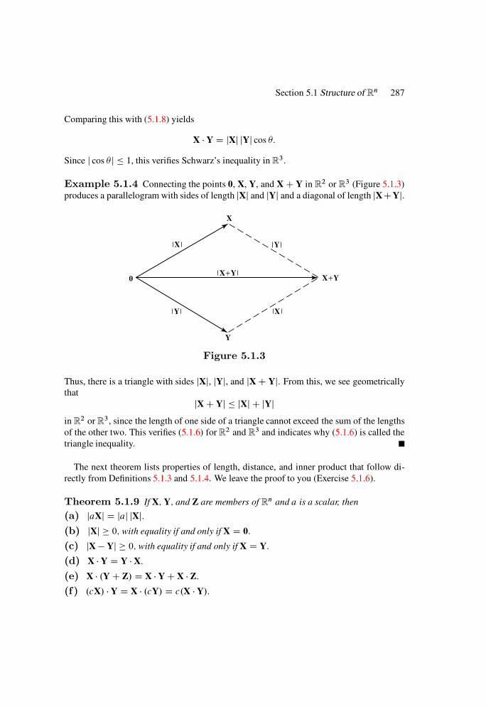
Section 5.1 Structure of Rn 287
Comparing this with (5.1.8) yields
X Y D jXj jYj cos :
Since j cos j 1, this verifies Schwarz’s inequality in R3.
Example 5.1.4 Connecting the points 0, X, Y, and XC Y in R2 or R
3 (Figure 5.1.3)
produces a parallelogram with sides of length jXj and jYj and a diagonal of length jXCYj.
0
X
Y
Y
YX
X
X+YX+Y
Figure 5.1.3
Thus, there is a triangle with sides jXj, jYj, and jXC Yj. From this, we see geometrically
that
jXC Yj jXj C jYj
in R2 or R
3, since the length of one side of a triangle cannot exceed the sum of the lengths
of the other two. This verifies (5.1.6) for R2 and R
3 and indicates why (5.1.6) is called the
triangle inequality.
The next theorem lists properties of length, distance, and inner product that follow di-
rectly from Definitions 5.1.3 and 5.1.4. We leave the proof to you (Exercise 5.1.6).
Theorem 5.1.9 If X; Y; and Z are members of Rn and a is a scalar, then
(a) jaXj D jaj jXj:(b) jXj 0; with equality if and only if X D 0:
(c) jX Yj 0; with equality if and only if X D Y:
(d) X Y D Y X:(e) X .YC Z/ D X YC X Z:(f) .cX/ Y D X .cY/ D c.X Y/:

288 Chapter 5 Real-Valued Functions of n Variables
Line Segments in RRRn
The equation of a line through a point X0 D .x0; y0; ´0/ in R3 can be written parametri-
cally as
x D x0 C u1t; y D y0 C u2t; ´ D ´0 C u3t; 1 < t <1;
where u1, u2, and u3 are not all zero. We write this in vector form as
X D X0 C tU; 1 < t <1; (5.1.9)
with U D .u1; u2; u3/, and we say that the line is through X0 in the direction of U.
There are many ways to represent a given line parametrically. For example,
X D X0 C sV; 1 < s <1; (5.1.10)
represents the same line as (5.1.9) if and only if V D aU for some nonzero real number a.
Then the line is traversed in the same direction as s and t vary from 1 to1 if a > 0, or
in opposite directions if a < 0.
To write the parametric equation of a line through two points X0 and X1 in R3, we take
U D X1 0 in (5.1.9), which yields
X D X0 C t.X1 X0/ D tX1 C .1 t/X0; 1 < t <1:
The line segment from X0 to X1 consists of those points for which 0 t 1.
Example 5.1.5 The line L defined by
x D 1C 2t; y D 3 4t; ´ D 1; 1 < t <1;
which can be rewritten as
X D .1; 3;1/C t.2;4; 0/; 1 < t <1; (5.1.11)
is through X0 D .1; 3;1/ in the direction of U D .2;4; 0/. The same line can be
represented by
X D .1; 3;1/C s.1;2; 0/; 1 < s <1; (5.1.12)
or by
X D .1; 3;1/C .4; 8; 0/; 1 < <1: (5.1.13)
Since
.1;2; 0/ D 1
2.2;4; 0/;
L is traversed in the same direction as t and s vary from 1 to1 in (5.1.11) and (5.1.12).
However, since
.4; 8; 0/D 2.2;4; 0/;

Section 5.1 Structure of Rn 289
L is traversed in opposite directions as t and vary from1 to1 in (5.1.11) and (5.1.13).
Setting t D 1 in (5.1.11), we see that X1 D .1;1;1/ is also on L. The line segment
from X0 to X1 consists of all points of the form
X D t.1;1;1/C .1 t/.1; 3;1/; 0 t 1:
These familiar notions can be generalized to Rn, as follows:
Definition 5.1.10 Suppose that X0 and U are in Rn and U ¤ 0. Then the line through
X0 in the direction of U is the set of all points in Rn of the form
X D X0 C tU; 1 < t <1:
A set of points of the form
X D X0 C tU; t1 t t2;
is called a line segment. In particular, the line segment from X0 to X1 is the set of points of
the form
X D X0 C t.X1 X0/ D tX1 C .1 t/X0; 0 t 1:
Neighborhoods and Open Sets in RRRn
Having defined distance in Rn, we are now able to say what we mean by a neighborhood
of a point in Rn.
Definition 5.1.11 If > 0, the -neighborhood of a point X0 in Rn is the set
N.X0/j D˚XˇjX X0j <
:
An -neighborhood of a point X0 in R2 is the inside, but not the circumference, of the
circle of radius about X0. In R3 it is the inside, but not the surface, of the sphere of radius
about X0.
In Section 1.3 we stated several other definitions in terms of -neighborhoods: neigh-
borhood, interior point, interior of a set, open set, closed set,limit point, boundary point,
boundary of a set, closure of a set, isolated point, exterior point, and exterior of a set. Since
these definitions are the same for Rn as for R, we will not repeat them. We advise you to
read them again in Section 1.3, substituting Rn for R and X0 for x0.
Example 5.1.6 Let S be the set of points in R2 in the square bounded by the lines
x D ˙1, y D ˙1, except for the origin and the points on the vertical lines x D ˙1(Figure 5.1.4, page 290); thus,
S D˚.x; y/
ˇ.x; y/ ¤ .0; 0/; 1 < x < 1; 1 y 1
:
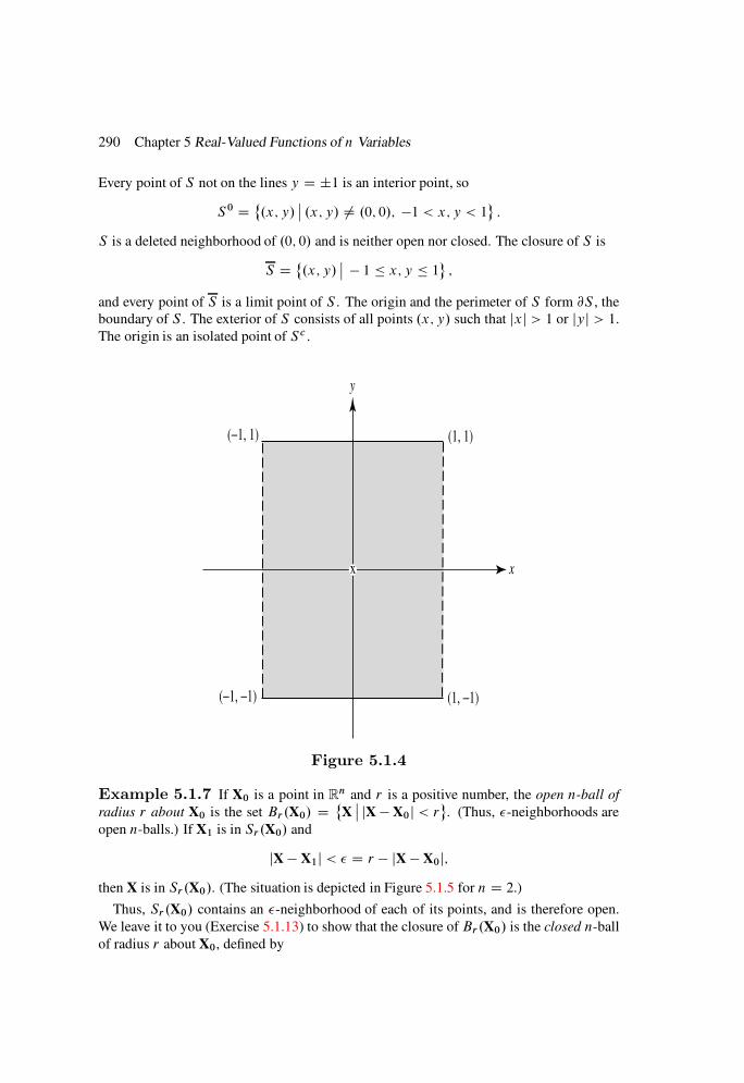
290 Chapter 5 Real-Valued Functions of n Variables
Every point of S not on the lines y D ˙1 is an interior point, so
S0 D˚.x; y/
ˇ.x; y/ ¤ .0; 0/; 1 < x; y < 1
:
S is a deleted neighborhood of .0; 0/ and is neither open nor closed. The closure of S is
S D˚.x; y/
ˇ 1 x; y 1
;
and every point of S is a limit point of S . The origin and the perimeter of S form @S , the
boundary of S . The exterior of S consists of all points .x; y/ such that jxj > 1 or jyj > 1.
The origin is an isolated point of Sc .
y
x
(1, 1)(−1, 1)
(1, −1)(−1, −1)
x
Figure 5.1.4
Example 5.1.7 If X0 is a point in Rn and r is a positive number, the open n-ball of
radius r about X0 is the set Br.X0/ D˚XˇjX X0j < r
. (Thus, -neighborhoods are
open n-balls.) If X1 is in Sr.X0/ and
jX X1j < D r jX X0j;
then X is in Sr.X0/. (The situation is depicted in Figure 5.1.5 for n D 2.)
Thus, Sr.X0/ contains an -neighborhood of each of its points, and is therefore open.
We leave it to you (Exercise 5.1.13) to show that the closure of Br.X0/ is the closed n-ball
of radius r about X0, defined by
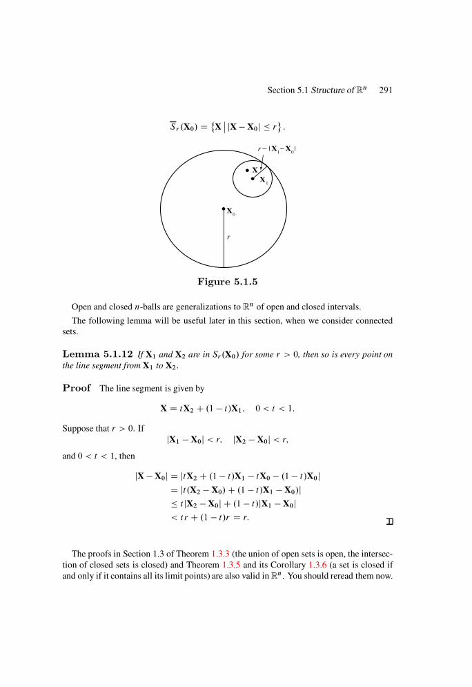
Section 5.1 Structure of Rn 291
Sr .X0/ D˚XˇjX X0j r
:
X0
X1
X
r
r − X1− X
0
Figure 5.1.5
Open and closed n-balls are generalizations to Rn of open and closed intervals.
The following lemma will be useful later in this section, when we consider connected
sets.
Lemma 5.1.12 If X1 and X2 are in Sr.X0/ for some r > 0, then so is every point on
the line segment from X1 to X2:
Proof The line segment is given by
X D tX2 C .1 t/X1; 0 < t < 1:
Suppose that r > 0. If
jX1 X0j < r; jX2 X0j < r;
and 0 < t < 1, then
jX X0j D jtX2 C .1 t/X1 tX0 .1 t/X0jD jt.X2 X0/C .1 t/X1 X0/j t jX2 X0j C .1 t/jX1 X0j< tr C .1 t/r D r:
The proofs in Section 1.3 of Theorem 1.3.3 (the union of open sets is open, the intersec-
tion of closed sets is closed) and Theorem 1.3.5 and its Corollary 1.3.6 (a set is closed if
and only if it contains all its limit points) are also valid in Rn. You should reread them now.

292 Chapter 5 Real-Valued Functions of n Variables
The Heine–Borel theorem (Theorem 1.3.7) also holds in Rn, but the proof in Section 1.3
is valid only for n D 1. To prove the Heine–Borel theorem for general n, we need some
preliminary definitions and results that are of interest in their own right.
Definition 5.1.13 A sequence of points fXrg in Rn converges to the limit X if
limr!1
jXr Xj D 0:
In this case we write
limr!1
Xr D X:
The next two theorems follow from this, the definition of distance in Rn, and what we
already know about convergence in R. We leave the proofs to you (Exercises 5.1.16 and
5.1.17).
Theorem 5.1.14 Let
X D .x1; x2; : : : ; xn/ and Xr D .x1r ; x2r ; : : : ; xnr/; r 1:
Then limr!1 Xr D X if and only if
limr!1
xir D xi ; 1 i nI
that is; a sequence fXrg of points in Rn converges to a limit X if and only if the sequences
of components of fXrg converge to the respective components of X:
Theorem 5.1.15 (Cauchy’s Convergence Criterion) A sequence fXrg in
Rn converges if and only if for each > 0 there is an integerK such that
jXr Xs j < if r; s K:
The next definition generalizes the definition of the diameter of a circle or sphere.
Definition 5.1.16 If S is a nonempty subset of Rn, then
d.S/ D sup˚jX Yj
ˇX;Y 2 S
is the diameter of S . If d.S/ <1; S is boundedI if d.S/ D1, S is unbounded.
Theorem 5.1.17 (Principle of Nested Sets) If S1; S2; . . . are closed nonempty
subsets of Rn such that
S1 S2 Sr (5.1.14)
and
limr!1
d.Sr / D 0; (5.1.15)
then the intersection
I D1\
rD1
Sr
contains exactly one point:

Section 5.1 Structure of Rn 293
Proof Let fXrg be a sequence such that Xr 2 Sr .r 1/. Because of (5.1.14), Xr 2 Sk
if r k, so
jXr Xs j < d.Sk/ if r; s k:
From (5.1.15) and Theorem 5.1.15, Xr converges to a limit X. Since X is a limit point of
every Sk and every Sk is closed, X is in every Sk (Corollary 1.3.6). Therefore, X 2 I , so
I ¤ ;. Moreover, X is the only point in I , since if Y 2 I , then
jX Yj d.Sk/; k 1;
and (5.1.15) implies that Y D X.
We can now prove the Heine–Borel theorem for Rn. This theorem concerns compact
sets. As in R, a compact set in Rn is a closed and bounded set.
Recall that a collection H of open sets is an open covering of a set S if
S [˚HˇH 2 H
:
Theorem 5.1.18 (Heine–Borel Theorem) If H is an open covering of a com-
pact subset S; then S can be covered by finitely many sets from H :
Proof The proof is by contradiction. We first consider the case where n D 2, so that
you can visualize the method. Suppose that there is a covering H for S from which it is
impossible to select a finite subcovering. Since S is bounded, S is contained in a closed
square
T D f.x; y/ja1 x a1 C L; a2 x a2 C Lgwith sides of length L (Figure 5.1.6).
T (1)
S (1) S (2)
S (3)S (4)
T (2)
T (3)T (4)
Figure 5.1.6
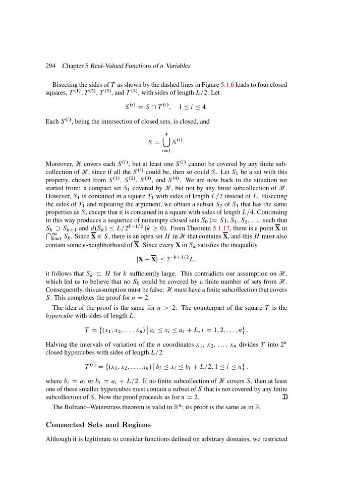
294 Chapter 5 Real-Valued Functions of n Variables
Bisecting the sides of T as shown by the dashed lines in Figure 5.1.6 leads to four closed
squares, T .1/; T .2/, T .3/, and T .4/, with sides of length L=2. Let
S .i/ D S \ T .i/; 1 i 4:
Each S .i/, being the intersection of closed sets, is closed, and
S D4[
iD1
S .i/:
Moreover, H covers each S .i/, but at least one S .i/ cannot be covered by any finite sub-
collection of H , since if all the S .i/ could be, then so could S . Let S1 be a set with this
property, chosen from S .1/, S .2/, S .3/, and S .4/. We are now back to the situation we
started from: a compact set S1 covered by H , but not by any finite subcollection of H .
However, S1 is contained in a square T1 with sides of length L=2 instead of L. Bisecting
the sides of T1 and repeating the argument, we obtain a subset S2 of S1 that has the same
properties as S , except that it is contained in a square with sides of lengthL=4. Continuing
in this way produces a sequence of nonempty closed sets S0 .D S/, S1, S2, . . . , such that
Sk SkC1 and d.Sk/ L=2k1=2 .k 0/. From Theorem 5.1.17, there is a point X inT1kD1 Sk. Since X 2 S , there is an open set H in H that contains X, and thisH must also
contain some -neighborhood of X. Since every X in Sk satisfies the inequality
jX Xj 2kC1=2L;
it follows that Sk H for k sufficiently large. This contradicts our assumption on H ,
which led us to believe that no Sk could be covered by a finite number of sets from H .
Consequently, this assumption must be false: H must have a finite subcollection that covers
S . This completes the proof for n D 2.
The idea of the proof is the same for n > 2. The counterpart of the square T is the
hypercube with sides of length L:
T D˚.x1; x2; : : : ; xn/
ˇai xi ai CL; i D 1; 2; : : : ; n
:
Halving the intervals of variation of the n coordinates x1, x2, . . . , xn divides T into 2n
closed hypercubes with sides of length L=2:
T .i/ D˚.x1; x2; : : : ; xn/
ˇbi xi bi CL=2; 1 i n
;
where bi D ai or bi D ai C L=2. If no finite subcollection of H covers S , then at least
one of these smaller hypercubes must contain a subset of S that is not covered by any finite
subcollection of S . Now the proof proceeds as for n D 2.
The Bolzano–Weierstrass theorem is valid in Rn; its proof is the same as in R.
Connected Sets and Regions
Although it is legitimate to consider functions defined on arbitrary domains, we restricted

Section 5.1 Structure of Rn 295
our study of functions of one variable mainly to functions defined on intervals. There are
good reasons for this. If we wish to raise questions of continuity and differentiability at
every point of the domain D of a function f , then every point of D must be a limit point
of D0. Intervals have this property. Moreover, the definition ofR b
af .x/ dx is obviously
applicable only if f is defined on Œa; b.
It is not productive to consider questions of continuity and differentiability of functions
defined on the union of disjoint intervals, since many important results simply do not hold
for such domains. For example, the intermediate value theorem (Theorem 2.2.10; see also
Exercise 2.2.25) says that if f is continuous on an interval I and f .x1/ < < f .x2/
for some x1 and x2 in I , then f .x/ D for some x in I . Theorem 2.3.12 says that f is
constant on an interval I if f 0 0 on I . Neither of these results holds if I is the union of
disjoint intervals rather than a single interval; thus, if f is defined on I D .0; 1/ [ .2; 3/by
f .x/ D1; 0 < x < 1;
0; 2 < x < 3;
then f is continuous on I , but does not assume any value between 0 and 1, and f 0 0 on
I , but f is not constant.
It is not difficult to see why these results fail to hold for this function: the domain of f
consists of two disconnected pieces. It would be more sensible to regard f as two entirely
different functions, one defined on .0; 1/ and the other on .2; 3/. The two results mentioned
are valid for each of these functions.
As we will see when we study functions defined on subsets of Rn, considerations like
those just cited as making it natural to consider functions defined on intervals in R lead
us to single out a preferred class of subsets as domains of functions of n variables. These
subsets are called regions. To define this term, we first need the following definition.
Definition 5.1.19 A subset S of Rn is connected if it is impossible to represent S as
the union of two disjoint nonempty sets such that neither contains a limit point of the other;
that is, if S cannot be expressed as S D A[ B , where
A ¤ ;; B ¤ ;; A\ B D ;; and A\ B D ;: (5.1.16)
If S can be expressed in this way, then S is disconnected.
Example 5.1.8 The empty set and singleton sets are connected, because they cannot
be represented as the union of two disjoint nonempty sets.
Example 5.1.9 The space Rn is connected, because if R
n D A[ B with A\ B D ;and A \ B D ;, then A A and B B; that is, A and B are both closed and therefore
are both open. Since the only nonempty subset of Rn that is both open and closed is R
n
itself (Exercise 5.1.21), one of A and B is Rn and the other is empty.

296 Chapter 5 Real-Valued Functions of n Variables
y
x
(3, 3)
(3, 2)
(1, 1)
(1, 2)
Figure 5.1.7
If X1;X2; : : : ;Xk are points in Rn and Li is the line segment from Xi to XiC1, 1 i
k 1, we say that L1, L2, . . . , Lk1 form a polygonal path from X1 to Xk , and that X1
and Xk are connected by the polygonal path. For example, Figure 5.1.7 shows a polygonal
path in R2 connecting .0; 0/ to .3; 3/. A set S is polygonally connected if every pair of
points in S can be connected by a polygonal path lying entirely in S .
Theorem 5.1.20 An open set S in Rn is connected if and only if it is polygonally
connected:
Proof For sufficiency, we will show that if S is disconnected, then S is not polygonally
connected. Let S D A [ B , where A and B satisfy (5.1.16). Suppose that X1 2 A and
X2 2 B , and assume that there is a polygonal path in S connecting X1 to X2. Then some
line segment L in this path must contain a point Y1 in A and a point Y2 in B . The line
segment
X D tY2 C .1 t/Y1; 0 t 1;is part of L and therefore in S . Now define
D sup˚ˇtY2 C .1 t/Y1 2 A; 0 t 1
;
and let
X D Y2 C .1 /Y1:
Then X 2 A\B . However, since X 2 A[B andA\B D A\B D ;, this is impossible.
Therefore, the assumption that there is a polygonal path in S from X1 to X2 must be false.

Section 5.1 Structure of Rn 297
For necessity, suppose that S is a connected open set and X0 2 S . Let A be the set
consisting of X0 and the points in S can be connected to X0 by polygonal paths in S . Let
B be set of points in S that cannot be connected to X0 by polygonal paths. If Y0 2 S , then
S contains an -neighborhoodN.Y0/ of Y0, since S is open. Any point Y1 in N.Y0 can
be connected to Y0 by the line segment
X D tY1 C .1 t/Y0; 0 t 1;
which lies in N.Y0/ (Lemma 5.1.12) and therefore in S . This implies that Y0 can be
connected to X0 by a polygonal path in S if and only if every member of N.Y0/ can also.
Thus, N.Y0/ A if Y0 2 A, and N.Y0/ 2 B if Y0 2 B . Therefore, A and B are open.
Since A \ B D ;, this implies that A \ B D A \ B D ; (Exercise 5.1.14). Since A is
nonempty .X0 2 A/, it now follows that B D ;, since if B ¤ ;, S would be disconnected
(Definition 5.1.19). Therefore, A D S , which completes the proof of necessity.
We did not use the assumption that S is open in the proof of sufficiency. In fact, we actu-
ally proved that any polygonally connected set, open or not, is connected. The converse is
false. A set (not open) may be connected but not polygonally connected (Exercise 5.1.29).
Our study of functions on Rn will deal mostly with functions whose domains are regions,
defined next.
Definition 5.1.21 A region S in Rn is the union of an open connected set with some,
all, or none of its boundary; thus, S0 is connected, and every point of S is a limit point of
S0.
Example 5.1.10 Intervals are the only regions in R (Exercise 5.1.31). The n-ball
Br.X0/ (Example 5.1.7) is a region in Rn, as is its closure S r.X0/. The set
S D˚.x; y/
ˇx2 C y2 1 or x2 C y2 4
(Figure 5.1.8(a), page 298) is not a region in R2, since it is not connected. The set S1
obtained by adding the line segment
L1W X D t.0; 2/C .1 t/.0; 1/; 0 < t < 1;
to S (Figure 5.1.8(b)) is connected but is not a region, since points on the line segment are
not limit points of S01 . The set S2 obtained by adding to S1 the points in the first quadrant
bounded by the circles x2 C y2 D 1 and x2 C y2 D 4 and the line segments L1 and
L2W X D t.2; 0/C .1 t/.1; 0/; 0 < t < 1
(Figure 5.1.8(c)), is a region.
More about Sequences in RRRn
From Definition 5.1.13, a sequence fXrg of points in Rn converges to a limit X if and only
if for every > 0 there is an integer K such that
jXr Xj < if r K:
298 Chapter 5 Real-Valued Functions of n Variables
The Rn definitions of divergence, boundedness, subsequence, and sums, differences, and
constant multiples of sequences are analogous to those given in Sections 4.1 and 4.2 for
the case where n D 1. Since Rn is not ordered for n > 1, monotonicity, limits inferior and
superior of sequences in Rn, and divergence to˙1 are undefined for n > 1. Products and
quotients of members of Rn are also undefined if n > 1.
L2
L1
(c)
(a)
L1
(b)
y
x
y
x
y
x
Figure 5.1.8
Several theorems from Sections 4.1 and 4.2 remain valid for sequences in Rn, with proofs
unchanged, provided that “j j" is interpreted as distance in Rn. (A trivial change is re-
quired: the subscript n, used in Sections 4.1 and 4.2 to identify the terms of the sequence,
must be replaced, since n here stands for the dimension of the space.) These include The-
orems 4.1.2 (uniqueness of the limit), 4.1.4 (boundedness of a convergent sequence), parts
of 4.1.8 (concerning limits of sums, differences, and constant multiples of convergent se-
quences), and 4.2.2 (every subsequence of a convergent sequence converges to the limit of
the sequence).
Section 5.1 Structure of Rn 299
5.1 Exercises
With R replaced by Rn, the following exercises from Section 1:3 are also suitable for this
section: 1.3.7-1.3.10; 1.3.12-1.3.15; 1.3.19; 1.3.20 .except (e)/; and 1.3.21:
1. Find aXC bY.
(a) X D .1; 2;3; 1/, Y D .0;1; 2; 0/, a D 3, b D 6(b) X D .1;1; 2/, Y D .0;1; 3/, a D 1, b D 2(c) X D .1
2; 3
2; 1
4; 1
6/, Y D .1
2; 1; 5; 1
3/, a D 1
2, b D 1
6
2. Prove Theorem 5.1.2.
3. Find jXj.(a) .1; 2;3; 1/ (b)
12; 1
3; 1
4; 1
6
(c) .1; 2;1; 3; 4/ (d) .0; 1; 0;1; 0;1/4. Find jX Yj.
(a) X D .3; 4; 5;4/, Y D .2; 0;1; 2/(b) X D .1
2; 1
2; 1
4;1
4/, Y D .1
3;1
6; 1
6;1
3/
(c) X D .0; 0; 0/, Y D .2;1; 2/(d) X D .3;1; 4; 0;1/, Y D .2; 0; 1;4; 1/
5. Find X Y.
(a) X D .3; 4; 5;4/, Y D .3; 0; 3; 3/(b) X D .1
6; 11
12; 9
8; 5
2/, Y D .1
2; 1
2; 1
4;1
4/
(c) X D .1; 2;3; 1; 4/, Y D .1; 2;1; 3; 4/6. Prove Theorem 5.1.9.
7. Find a parametric equation of the line through X0 in the direction of U.
(a) X0 D .1; 2;3; 1/, U D .3; 4; 5;4/(b) X0 D .2; 0;1; 2; 4/, U D .1; 0; 1; 3; 2/(c) X0 D .1
2; 1
2; 1
4;1
4/, U D .1
3;1
6; 1
6;1
3/
8. Suppose that U ¤ 0 and V ¤ 0. Complete the sentence: The equations
X D X0 C tU; 1 < t <1;
and
X D X1 C sV; 1 < s <1;represent the same line in R
n if and only if ...
9. Find the equation of the line segment from X0 to X1.
(a) X0 D .1;3; 4; 2/, X1 D .2; 0;1; 5/(b) X0 D .3; 1 2; 1; 4/, X1 D .2; 0;1; 4;3/(c) X0 D .1; 2;1/, X1 D .0;1;1/
300 Chapter 5 Real-Valued Functions of n Variables
10. Find sup˚ˇN.X0/ S
.
(a) X0 D .1; 2;1; 3/; S D the open 4-ball of radius 7 about .0; 3;2; 2/(b) X0 D .1; 2;1; 3/; S D
˚.x1; x2; x3; x4/
ˇjxi j 5; 1 i 4
(c) X0 D .3; 52/; S D the closed triangle with vertices .2; 0/, .2; 2/, and .4; 4/
11. Find (i) @S ; (ii) S ; (iii) S0; (iv) exterior of S .
(a) S D˚.x1; x2; x3; x4/
ˇjxi j < 3; i D 1; 2; 3
(b) S D˚.x; y; 1/
ˇx2 C y2 1
12. Describe the following sets as open, closed, or neither.
(a) S D˚.x1; x2; x3; x4/
ˇjx1j > 0; x2 < 1; x3 ¤ 2
(b) S D˚.x1; x2; x3; x4/
ˇx1 D 1; x3 ¤ 4
(c) S D˚.x1; x2; x3; x4/
ˇx1 D 1;3 x2 1; x4 D 5
13. Show that the closure of the open n-ball
Br.X0/ D˚XˇjX X0j < r
is the closed n-ball
Br.X0/ D˚XˇjX X0j r
:
14. Prove: If A and B are open and A \ B D ;, then A\ B D A \ B D ;.
15. Show that if limr!1 Xr exists, then it is unique.
16. Prove Theorem 5.1.14.
17. Prove Theorem 5.1.15.
18. Find limr!1 Xr .
(a) Xr Dr sin
r; cos
r; er
(b) Xr D1 1
r2; log
r C 1r C 2
;
1C 1
r
r
19. Find d.S/.
(a) S D˚.x; y; x/
ˇjxj 2; jyj 1; j´ 2j 2
(b) S D.x; y/
ˇ .x 1/29
C .y 2/24
D 1
(c) S D the triangle in R2 with vertices .2; 0/, .2; 2/, and .4; 4/
(d) S D˚.x1; x2; : : : ; xn/
ˇjxi j L; i D 1; 2; : : : ; n
(e) S D˚.x; y; ´/
ˇx ¤ 0; jyj 1; ´ > 2
20. Prove that d.S/ D d.S/ for any set S in Rn.
21. Prove: If a nonempty subset S of Rn is both open and closed, then S D R
n.
Section 5.1 Structure of Rn 301
22. Use the Bolzano–Weierstrass theorem to show that if S1, S2, . . . , Sm, . . . is an
infinite sequence of nonempty compact sets and S1 S2 Sm , thenT1mD1 Sm is nonempty. Show that the conclusion does not follow if the sets are
assumed to be closed rather than compact.
23. Suppose that a sequence U1, U2, . . . of open sets covers a compact set S . Without
using the Heine–Borel theorem, show that S SN
mD1 Um for some N . HINT:
Apply Exercise 5.1.22 to the sets Sn D S \Sn
mD1 Um
c:
(This is a seemingly restricted version of the Heine–Borel theorem, valid for the
case where the covering collection H is denumerable. However, it can be shown
that there is no loss of generality in assuming this.)
24. The distance from a point X0 to a nonempty set S is defined by
dist.X0; S/ D inf˚jX X0j
ˇX 2 S
:
(a) Prove: If S is closed and X0 2 Rn, there is a point X in S such that
jX X0j D dist.X0; S/:
HINT: Apply Exercise 5.1.22 to the sets
Cm D˚XˇX 2 S and jX X0j dist.X0; S/C 1=m
; m 1:
(b) Show that if S is closed and X0 62 S , then dist.X0; S/ > 0.
(c) Show that the conclusions of (a) and (b) may fail to hold if S is not closed.
25. The distance between two nonempty sets S and T is defined by
dist.S; T / D inf˚jX Yj
ˇX 2 S;Y 2 T
:
(a) Prove: If S is closed and T is compact, there are points X in S and Y in T
such that
jX Yj D dist.S; T /:
HINT: Use Exercises 5.1.22 and 5.1.24:
(b) Under the assumptions of (a), show that dist.S; T / > 0 if S \ T D ;.
(c) Show that the conclusions of (a) and (b) may fail to hold if S or T is not
closed or T is unbounded.
26. (a) Prove: If a compact set S is contained in an open set U , there is a positive
number r such that the set
Sr D˚Xˇ
dist.X; S/ r
is contained in U . (You will need Exercise 5.1.24 here.)
(b) Show that Sr is compact.
302 Chapter 5 Real-Valued Functions of Several Variables
27. Let D1 and D2 be compact subsets of Rn. Show that
D D˚.X;Y/
ˇX 2 D1;Y 2 D2
is a compact subset of R2n.
28. Prove: If S is open and S D A[ B where A\ B D A\ B D ;, then A and B are
open.
29. Give an example of a connected set in Rn that is not polygonally connected.
30. Prove that a region is connected.
31. Show that the intervals are the only regions in R.
32. Prove: A bounded sequence in Rn has a convergent subsequence. HINT: Use Theo-
rems 5.1.14; 4.2.2; and 4.2.5.a/:
33. Define “limr!1 Xr D1” if fXrg is a sequence in Rn, n 2.
5.2 CONTINUOUS REAL-VALUED FUNCTIONS OF n VARI-ABLES
We now study real-valued functions of n variables. We denote the domain of a function f
by Df and the value of f at a point X D .x1; x2; : : : ; xn/ by f .X/ or f .x1; x2; : : : ; xn/.
We continue the convention adopted in Section 2.1 for functions of one variable: If a func-
tion is defined by a formula such as
f .X/ D1 x2
1 x22 x2
n
1=2(5.2.1)
or
g.X/ D1 x2
1 x22 x2
n
1(5.2.2)
without specification of its domain, it is to be understood that its domain is the largest
subset of Rn for which the formula defines a unique real number. Thus, in the absence of
any other stipulation, the domain of f in (5.2.1) is the closed n-ball˚XˇjXj 1
, while
the domain of g in (5.2.2) is the set˚XˇjXj ¤ 1
.
The main objective of this section is to study limits and continuity of functions of n
variables. The proofs of many of the theorems here are similar to the proofs of their coun-
terparts in Sections 2.1 and . We leave most of them to you.
Definition 5.2.1 We say that f .X/ approaches the limit L as X approaches X0 and
write
limX!X0
f .X/ D L
if X0 is a limit point of Df and, for every > 0, there is a ı > 0 such that
jf .X/ Lj <
for all X in Df such that
0 < jX X0j < ı:
Section 5.2 Continuous Real-Valued Functions of n Variables 303
Example 5.2.1 If
g.x; y/ D 1 x2 2y2;
then
lim.x;y/!.x0 ;y0/
g.x; y/ D 1 x20 2y2
0 (5.2.3)
for every .x0; y0/. To see this, we write
jg.x; y/ .1 x20 2y2
0/j D j.1 x2 2y2/ .1 x20 2y2
0/j
jx2 x20 j C 2jy2 y2
0 jD j.x C x0/.x x0/j C 2j.y C y0/.y y0/j
jX X0j.jx C x0j C 2jy C y0/j/;
(5.2.4)
since
jx x0j jX X0j and jy y0j jX X0j:If jX X0j < 1, then jxj < jx0j C 1 and jyj < jy0j C 1. This and (5.2.4) imply that
jg.x; y/ .1 x20 2y2
0/j < KjX X0j if jX X0j < 1;
where
K D .2jx0j C 1/C 2.2jy0j C 1/:Therefore, if > 0 and
jX X0j < ı D minf1; =Kg;then ˇ
g.x; y/ .1 x20 2y2
0/ˇ< :
This proves (5.2.3).
Definition 5.2.1 does not require that f be defined at X0, or even on a deleted neighbor-
hood of X0.
Example 5.2.2 The function
h.x; y/ Dsinp1 x2 2y2
p1 x2 2y2
is defined only on the interior of the region bounded by the ellipse
x2 C 2y2 D 1
(Figure 5.2.1(a), page 304). It is not defined at any point of the ellipse itself or on any
deleted neighborhood of such a point. Nevertheless,
lim.x;y/!.x0 ;y0/
h.x; y/ D 1 (5.2.5)
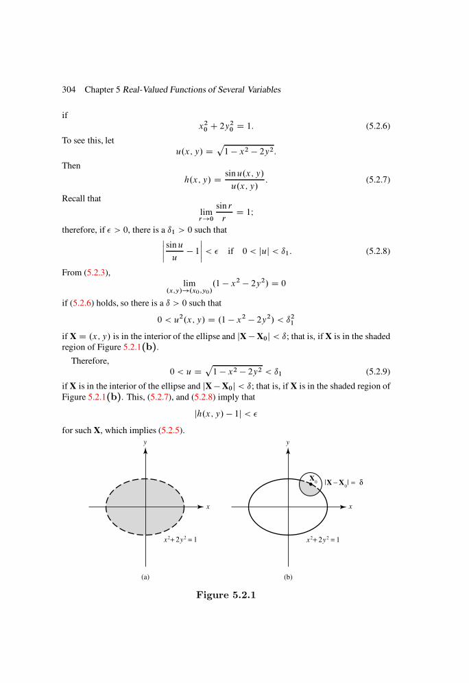
304 Chapter 5 Real-Valued Functions of Several Variables
if
x20 C 2y2
0 D 1: (5.2.6)
To see this, let
u.x; y/ Dp1 x2 2y2:
Then
h.x; y/ D sinu.x; y/
u.x; y/: (5.2.7)
Recall that
limr!0
sin r
rD 1I
therefore, if > 0, there is a ı1 > 0 such thatˇˇ sinu
u 1
ˇˇ < if 0 < juj < ı1: (5.2.8)
From (5.2.3),
lim.x;y/!.x0 ;y0/
.1 x2 2y2/ D 0
if (5.2.6) holds, so there is a ı > 0 such that
0 < u2.x; y/ D .1 x2 2y2/ < ı21
if X D .x; y/ is in the interior of the ellipse and jX X0j < ı; that is, if X is in the shaded
region of Figure 5.2.1(b).
Therefore,
0 < u Dp1 x2 2y2 < ı1 (5.2.9)
if X is in the interior of the ellipse and jXX0j < ı; that is, if X is in the shaded region of
Figure 5.2.1(b). This, (5.2.7), and (5.2.8) imply that
jh.x; y/ 1j <
for such X, which implies (5.2.5).
(a)
y
x
x2+ 2y2 = 1
(b)
y
x
x2+ 2y2 = 1
X − X0 = δ
X0
Figure 5.2.1
Section 5.2 Continuous Real-Valued Functions of n Variables 305
The following theorem is analogous to Theorem 2.1.3. We leave its proof to you (Exer-
cise 5.2.2).
Theorem 5.2.2 If limX!X0f .X/ exists; then it is unique.
When investigating whether a function has a limit at a point X0, no restriction can be
made on the way in which X approaches X0, except that X must be in Df . The next
example shows that incorrect restrictions can lead to incorrect conclusions.
Example 5.2.3 The function
f .x; y/ D xy
x2 C y2
is defined everywhere in R2 except at .0; 0/. Does lim.x;y/!.0;0/ f .x; y/ exist? If we try
to answer this question by letting .x; y/ approach .0; 0/ along the line y D x, we see the
functional values
f .x; x/ D x2
2x2D 1
2
and conclude that the limit is 1=2. However, if we let .x; y/ approach .0; 0/ along the line
y D x, we see the functional values
f .x;x/ D x2
2x2D 1
2
and conclude that the limit equals 1=2. From Theorem 5.2.2, these two conclusions
cannot both be correct. In fact, they are both incorrect. What we have shown is that
limx!0
f .x; x/ D 1
2and lim
x!0f .x;x/ D 1
2:
Since limx!0 f .x; x/ and limx!0 f .x;x/ must both equal lim.x;y/!.0;0/ f .x; y/ if the
latter exists (Exercise 5.2.3(a)), we conclude that the latter does not exist.
The sum, difference, and product of functions of n variables are defined in the same
way as they are for functions of one variable (Definition 2.1.1), and the proof of the next
theorem is the same as the proof of Theorem 2.1.4.
Theorem 5.2.3 Suppose that f and g are defined on a set D; X0 is a limit point of
D; and
limX!X0
f .X/ D L1; limX!X0
g.X/ D L2:
Then
limX!X0
.f C g/.X/ D L1 C L2; (5.2.10)
limX!X0
.f g/.X/ D L1 L2; (5.2.11)
limX!X0
.fg/.X/ D L1L2; (5.2.12)
and; if L2 ¤ 0;
limX!X0
f
g
.X/ D L1
L2
: (5.2.13)
306 Chapter 5 Real-Valued Functions of Several Variables
Infinite Limits and Limits as jXj!1
Definition 5.2.4 We say that f .X/ approaches1 as X approaches X0 and write
limX!X0
f .X/ D 1
if X0 is a limit point of Df and, for every real number M , there is a ı > 0 such that
f .X/ > M whenever 0 < jX X0j < ı and X 2 Df :
We say that
limX!X0
f .X/ D 1
if
limX!X0
.f /.X/ D1:
Example 5.2.4 If
f .X/ D .1 x21 x2
2 x2n/
1=2;
then
limX!X0
f .X/ D 1
if jX0j D 1, because
f .X/ D 1
jX X0j;
so
f .X/ > M if 0 < jX X0j < ı D1
M:
Example 5.2.5 If
f .x; y/ D 1
x C 2y C 1 ;
then lim.x;y/!.1;1/ f .x; y/ does not exist (why not?), but
lim.x;y/!.1;1/
jf .x; y/j D 1:
To see this, we observe that
jx C 2y C 1j D j.x 1/C 2.y C 1/j
p5jX X0j (by Schwarz’s inequality),
where X0 D .1;1/, so
jf .x; y/j D 1
jx C 2y C 1j 1p
5jX X0j:

Section 5.2 Continuous Real-Valued Functions of n Variables 307
Therefore,
jf .x; y/j > M if 0 < jX X0j <1
Mp5:
Example 5.2.6 The function
f .x; y; ´/ D
ˇˇsin
1
x2 C y2 C ´2
ˇˇ
x2 C y2 C ´2
assumes arbitrarily large values in every neighborhood of .0; 0; 0/. For example, if Xk D.xk; yk; ´k/, where
xk D yk D ´k D1q
3k C 1
2
;
then
f .Xk/ Dk C 1
2
:
However, this does not imply that limX!0 f .X/ D1, since, for example, every neighbor-
hood of .0; 0; 0/ also contains points
Xk D
1p3k
;1p3k
;1p3k
for which f .Xk/ D 0.
Definition 5.2.5 If Df is unbounded;we say that
limjXj!1
f .X/ D L (finite)
if for every > 0, there is a number R such that
jf .X/ Lj < whenever jXj R and X 2 Df :
Example 5.2.7 If
f .x; y; ´/ D cos
1
x2 C 2y2 C ´2
;
then
limjXj!1
f .X/ D 1: (5.2.14)
To see this, we recall that the continuity of cos u at u D 0 implies that for each > 0 there
is a ı > 0 such that
j cosu 1j < if juj < ı:

308 Chapter 5 Real-Valued Functions of Several Variables
Since1
x2 C 2y2 C ´2 1
jXj2;
it follows that if jXj > 1=pı, then
1
x2 C 2y2 C ´2< ı:
Therefore,
jf .X/ 1j < :This proves (5.2.14).
Example 5.2.8 Consider the function defined only on the domain
D D˚.x; y/
ˇ0 < y ax
; 0 < a < 1
(Figure 5.2.2), by
f .x; y/ D 1
x y:
We will show that
limjXj!1
f .x; y/ D 0: (5.2.15)
It is important to keep in mind that we need only consider .x; y/ in D, since f is not
defined elsewhere.
InD,
x y x.1 a/ (5.2.16)
and
jXj2 D x2 C y2 x2.1C a2/;
so
x jXjp1C a2
:
This and (5.2.16) imply that
x y 1 ap1C a2
jXj; X 2 D;
so
jf .x; y/j p1C a2
1 a1
jXj ; X 2 D:
Therefore,
jf .x; y/j < if X 2 D and
jXj >p1C a2
1 a1
:
This implies (5.2.15).
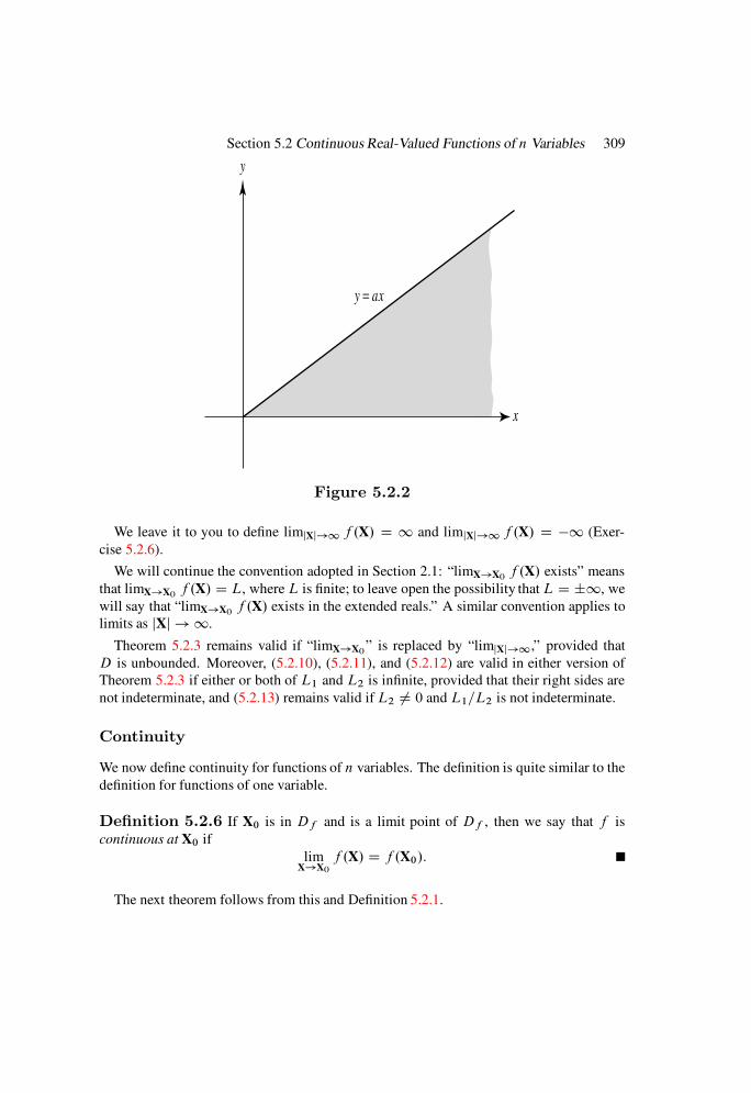
Section 5.2 Continuous Real-Valued Functions of n Variables 309
y
x
y = ax
Figure 5.2.2
We leave it to you to define limjXj!1 f .X/ D 1 and limjXj!1 f .X/ D 1 (Exer-
cise 5.2.6).
We will continue the convention adopted in Section 2.1: “limX!X0f .X/ exists” means
that limX!X0f .X/ D L, where L is finite; to leave open the possibility that L D ˙1, we
will say that “limX!X0f .X/ exists in the extended reals.” A similar convention applies to
limits as jXj ! 1.
Theorem 5.2.3 remains valid if “limX!X0” is replaced by “limjXj!1,” provided that
D is unbounded. Moreover, (5.2.10), (5.2.11), and (5.2.12) are valid in either version of
Theorem 5.2.3 if either or both of L1 and L2 is infinite, provided that their right sides are
not indeterminate, and (5.2.13) remains valid if L2 ¤ 0 and L1=L2 is not indeterminate.
Continuity
We now define continuity for functions of n variables. The definition is quite similar to the
definition for functions of one variable.
Definition 5.2.6 If X0 is in Df and is a limit point of Df , then we say that f is
continuous at X0 if
limX!X0
f .X/ D f .X0/:
The next theorem follows from this and Definition 5.2.1.

310 Chapter 5 Real-Valued Functions of Several Variables
Theorem 5.2.7 Suppose that X0 is in Df and is a limit point of Df : Then f is con-
tinuous at X0 if and only if for each > 0 there is a ı > 0 such that
jf .X/ f .X0/j <
whenever
jX X0j < ı and X 2 Df :
In applying this theorem when X0 2 D0f
, we will usually omit “and X 2 Df ,” it being
understood that Sı .X0/ Df .
We will say that f is continuous on S if f is continuous at every point of S .
Example 5.2.9 From Example 5.2.1, we now see that the function
f .x; y/ D 1 x2 2y2
is continuous on R2.
Example 5.2.10 If we extend the definition of h in Example 5.2.2 so that
h.x; y/ D
8<
:
sinp1 x2 2y2
p1 x2 2y2
; x2 C 2y2 < 1;
1; x2 C 2y2 D 1;
then it follows from Example 5.2.2 that h is continuous on the ellipse
x2 C 2y2 D 1:
We will see in Example 5.2.13 that h is also continuous on the interior of the ellipse.
Example 5.2.11 It is impossible to define the function
f .x; y/ D xy
x2 C y2
at the origin to make it continuous there, since we saw in Example 5.2.3 that
lim.x;y/!.0;0/
f .x; y/
does not exist.
Theorem 5.2.3 implies the next theorem, which is analogous to Theorem 2.2.5 and, like
the latter, permits us to investigate continuity of a given function by regarding the function
as the result of addition, subtraction, multiplication, and division of simpler functions.

Section 5.2 Continuous Real-Valued Functions of n Variables 311
Theorem 5.2.8 If f and g are continuous on a set S in Rn; then so are f Cg; f g;
and fg: Also; f =g is continuous at each X0 in S such that g.X0/ ¤ 0:
Vector-Valued Functions and Composite Functions
Suppose that g1, g2, . . . , gn are real-valued functions defined on a subset T of Rm, and
define the vector-valued function G on T by
G.U/ D .g1.U/; g2.U/; : : : ; gn.U// ; U 2 T:
Then g1, g2, . . . , gn are the component functions of G D .g1; g2; : : : ; gn/. We say that
limU!U0
G.U/ D L D .L1; L2; : : : ; Ln/
if
limU!U0
gi .U/ D Li ; 1 i n;
and that G is continuous at U0 if g1, g2, . . . , gn are each continuous at U0.
The next theorem follows from Theorem 5.1.14 and Definitions 5.2.1 and 5.2.6. We omit
the proof.
Theorem 5.2.9 For a vector-valued function G;
limU!U0
G.U/ D L
if and only if for each > 0 there is a ı > 0 such that
jG.U/ Lj < whenever 0 < jU U0j < ı and U 2 DG:
Similarly, G is continuous at U0 if and only if for each > 0 there is a ı > 0 such that
jG.U/ G.U0/j < whenever jU U0j < ı and U 2 DG:
The following theorem on the continuity of a composite function is analogous to Theo-
rem 2.2.7.
Theorem 5.2.10 Let f be a real-valued function defined on a subset of Rn; and let
the vector-valued function G D .g1; g2; : : : ; gn/ be defined on a domain DG in Rm: Let
the set
T D˚UˇU 2 DG and G.U/ 2 Df
.Figure 5.2.3/, be nonempty; and define the real-valued composite function
h D f ıG
on T by
h.U/ D f .G.U//; U 2 T:Now suppose that U0 is in T and is a limit point of T; G is continuous at U0; and f is
continuous at X0 D G.U0/: Then h is continuous at U0:
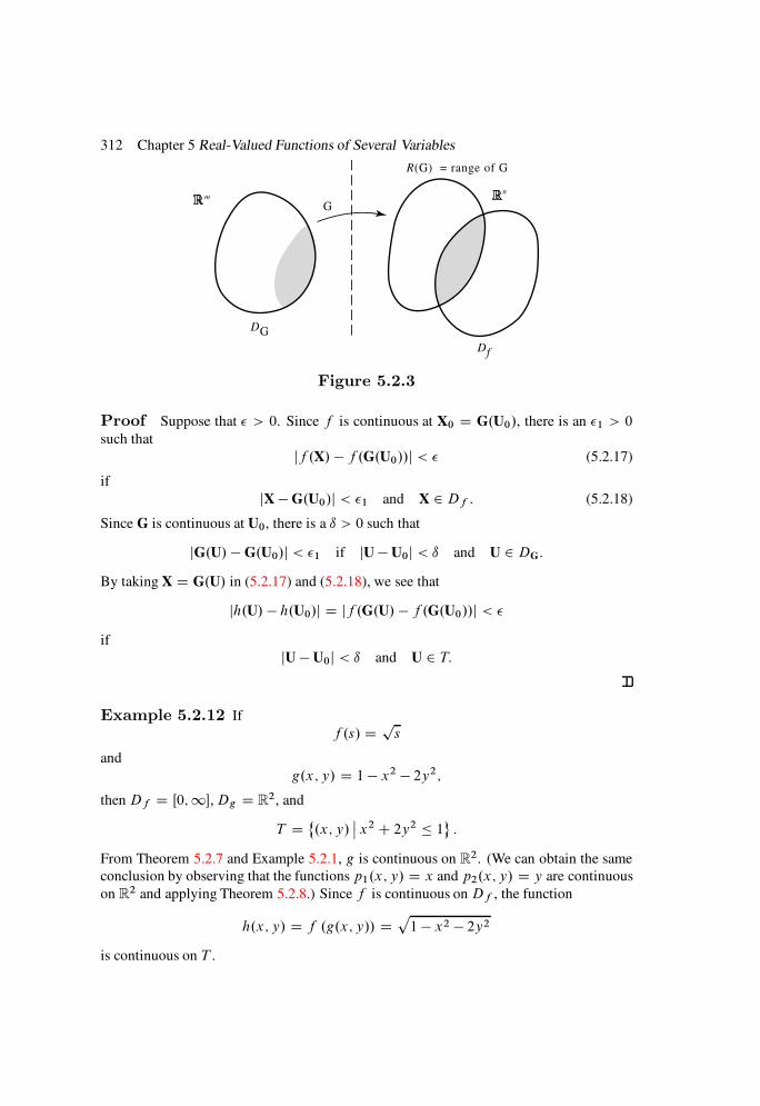
312 Chapter 5 Real-Valued Functions of Several Variables
mn
R(G) = range of G
G
DG
Df
Figure 5.2.3
Proof Suppose that > 0. Since f is continuous at X0 D G.U0/, there is an 1 > 0
such that
jf .X/ f .G.U0//j < (5.2.17)
if
jX G.U0/j < 1 and X 2 Df : (5.2.18)
Since G is continuous at U0, there is a ı > 0 such that
jG.U/ G.U0/j < 1 if jU U0j < ı and U 2 DG:
By taking X D G.U/ in (5.2.17) and (5.2.18), we see that
jh.U/ h.U0/j D jf .G.U/ f .G.U0//j <
if
jU U0j < ı and U 2 T:
Example 5.2.12 If
f .s/ Dps
and
g.x; y/ D 1 x2 2y2;
then Df D Œ0;1,Dg D R2, and
T D˚.x; y/
ˇx2 C 2y2 1
:
From Theorem 5.2.7 and Example 5.2.1, g is continuous on R2. (We can obtain the same
conclusion by observing that the functions p1.x; y/ D x and p2.x; y/ D y are continuous
on R2 and applying Theorem 5.2.8.) Since f is continuous on Df , the function
h.x; y/ D f .g.x; y// Dp1 x2 2y2
is continuous on T .
Section 5.2 Continuous Real-Valued Functions of n Variables 313
Example 5.2.13 If
g.x; y/ Dp1 x2 2y2
and
f .s/ D
8<:
sin s
s; s ¤ 0;
1; s D 0;then Df D .1;1/ and
Dg D T D˚.x; y/
ˇx2 C 2y2 1
:
In Example 5.2.12 we saw that g (we called it h there) is continuous on T . Since f is
continuous onDf , the composite function h D f ı g defined by
h.x; y/ D
8<
:
sinp1 x2 2y2
p1 x2 2y2
; x2 C 2y2 < 1;
1; x2 C 2y2 D 1;
is continuous on T . This implies the result of Example 5.2.2.
Bounded Functions
The definitions of bounded above, bounded below, and bounded on a set S are the same for
functions of n variables as for functions of one variable, as are the definitions of supremum
and infimum of a function on a set S (Section 2.2). The proofs of the next two theorems are
similar to those of Theorems 2.2.8 and 2.2.9 (Exercises 5.2.12 and 5.2.13).
Theorem 5.2.11 If f is continuous on a compact set S in Rn; then f is bounded
on S:
Theorem 5.2.12 Let f be continuous on a compact set S in Rn and
˛ D infX2S
f .X/; ˇ D supX2S
f .X/:
Then
f .X1/ D ˛ and f .X2/ D ˇfor some X1 and X2 in S:
The next theorem is analogous to Theorem 2.2.10.
Theorem 5.2.13 (Intermediate Value Theorem) Let f be continuous on
a region S in Rn: Suppose that A and B are in S and
f .A/ < u < f .B/:
Then f .C/ D u for some C in S:

314 Chapter 5 Real-Valued Functions of Several Variables
Proof If there is no such C, then S D R [ T , where
R D˚XˇX 2 S and f .X/ < u
and
T D˚XˇX 2 S and f .X/ > u
:
If X0 2 R, the continuity of f implies that there is a ı > 0 such that f .X/ < u if jXX0j <ı and X 2 S . This means that X0 62 T . Therefore, R \ T D ;. Similarly, R \ T D ;.
Therefore, S is disconnected (Definition 5.1.19), which contradicts the assumption that S
is a region (Exercise 5.1.30). Hence, we conclude that f .C/ D u for some C in S .
Uniform Continuity
The definition of uniform continuity for functions of n variables is the same as for functions
of one variable; f is uniformly continuous on a subset S of its domain in Rn if for every
> 0 there is a ı > 0 such that
jf .X/ f .X0/j <
whenever jX X0j < ı and X;X0 2 S . We emphasize again that ı must depend only on
and S , and not on the particular points X and X0.
The proof of the next theorem is analogous to that of Theorem 2.2.12. We leave it to you
(Exercise 5.2.14).
Theorem 5.2.14 If f is continuous on a compact set S in Rn; then f is uniformly
continuous on S:
5.2 Exercises
With R replaced by Rn; the following exercises from Sections 2:1 and 2:2 have analogs for
this section: 2.1.5, 2.1.8–2.1.11, 2.1.26, 2.1.28, 2.1.29, 2.1.33, 2.2.8; 2.2.9; 2.2.10, 2.2.15,
2.2.16, 2.2.20, 2.2.29, 2.2.30.
1. Find limX!X0f .X/ and justify your answer with an –ı argument, as required by
Definition 5.2.1. HINT: See Examples 5.2.1 and 5.2.2:
(a) f .X/ D 3x C 4y C ´ 2, X0 D .1; 2; 1/
(b) f .X/ D x3 y3
x y, X0 D .1; 1/
(c) f .X/ Dsin.x C 4y C 2´/x C 4y C 2´ , X0 D .2; 1;1/
Section 5.2 Continuous Real-Valued Functions of n Variables 315
(d) f .X/ D .x2 C y2/ log.x2 C y2/1=2, X0 D .0; 0/
(e) f .X/ Dsin.x y/px y , X0 D .2; 2/
(f) f .X/ D 1
jXje1=jXj, X0 D 0
2. Prove Theorem 5.2.2.
3. If limx!x0y.x/ D y0 and limx!x0
f .x; y.x// D L, we say that f .x; y/ ap-
proaches L as .x; y/ approaches .x0; y0/ along the curve y D y.x/.(a) Prove: If lim.x;y/!.x0 ;y0/ f .x; y/ D L, then f .x; y/ approaches L as .x; y/
approaches .x0; y0/ along any curve y D y.x/ through .x0; y0/.
(b) We saw in Example 5.2.3 that if
f .x; y/ D xy
x2 C y2;
then lim.x;y/!.0;0/ f .x; y/ does not exist. Show, however, that f .x; y/ ap-
proaches a value La as .x; y/ approaches .0; 0/ along any curve y D y.x/
that passes through .0; 0/ with slope a. Find La.
(c) Show that the function
g.x; y/ D x3y4
.x2 C y6/3
approaches 0 as .x; y/ approaches .0; 0/ along a curve as described in (b),
but that lim.x;y/!.0;0/ f .x; y/ does not exist.
4. Determine whether limX!X0f .X/ D ˙1.
(a) f .X/ D j sin.x C 2y C 4´/j.x C 2y C 4´/2
, X0 D .2;1; 0/
(b) f .X/ D 1px y
, X0 D .0; 0/
(c) f .X/ D sin 1=xpx y
, X0 D .0; 0/
(d) f .X/ D 4y2 x2
.x 2y/3, X0 D .2; 1/
(e) f .X/ D sin.x C 2y C 4´/.x C 2y C 4´/2 , X0 D .2;1; 0/
5. Find limjXj!1 f .X/, if it exists.
(a) f .X/ D log.x2 C 2y2 C 4´2/
x2 C y2 C ´2(b) f .X/ D sin.x2 C y2/p
x2 C y2
(c) f .X/ D e.xCy/2
(d) f .X/ D ex2y2

316 Chapter 5 Real-Valued Functions of Several Variables
(e) f .X/ D
8<:
sin.x2 y2/
x2 y2; x ¤ ˙y;
1; x D ˙y6. Define (a) limjXj!1 f .X/ D1 and (b) limjXj!1 f .X/ D 1.
7. Let
f .X/ D jx1ja1jx2ja2 jxnjan
Xjb:
For what nonnegative values of a1, a2, . . . , an, b does limX!0 f .X/ exist in the
extended reals?
8. Let
g.X/ D .x2 C y4/3
1C x6y4:
Show that limjxj!1 g.x; ax/ D 1 for any real number a. Does
limjXj!1
g.X/ D 1‹
9. For each f in Exercise 5.2.1, find the largest set S on which f is continuous or can
be defined so as to be continuous.
10. Repeat Exercise 5.2.9 for the functions in Exercise 5.2.5.
11. Give an example of a function f on R2 such that f is not continuous at .0; 0/,
but f .0; y/ is a continuous function of y on .1;1/ and f .x; 0/ is a continuous
function of x on .1;1/.12. Prove Theorem 5.2.11. HINT: See the proof of Theorem 2.2.8:
13. Prove Theorem 5.2.12. HINT: See the proof of Theorem 2.2.9:
14. Prove Theorem 5.2.14. HINT: See the proof of Theorem 2.2.12:
15. Suppose that X 2 Df Rn and X is a limit point ofDf . Show that f is continuous
at X if and only if limk!1 f .Xk/ D f .X/ whenever fXkg is a sequence of points
in Df such that limk!1 Xk D X. HINT: See the proof of Theorem 4.2.6:
5.3 PARTIAL DERIVATIVES AND THE DIFFERENTIAL
To say that a function of one variable has a derivative at x0 is the same as to say that it
is differentiable at x0. The situation is not so simple for a function f of more than one
variable. First, there is no specific number that can be called the derivative of f at a point
X0 in Rn. In fact, there are infinitely many numbers, called the directional derivatives of
f at X0 (defined below), that are analogous to the derivative of a function of one variable.
Second, we will see that the existence of directional derivatives at X0 does not imply that f
is differentiable at X0, if differentiability at X0 is to imply (as it does for functions of one
variable) that f .X/f .X0/ can be approximated well near X0 by a simple linear function,
or even that f is continuous at X0.

Section 5.3 Partial Derivatives and the Differential 317
We will now define directional derivatives and partial derivatives of functions of several
variables. However, we will still have occasion to refer to derivatives of functions of one
variable. We will call them ordinary derivatives when we wish to distinguish between them
and the partial derivatives that we are about to define.
Definition 5.3.1 Let ˆ be a unit vector and X a point in Rn. The directional derivative
of f at X in the direction of ˆ is defined by
@f .X/
@ˆD lim
t!0
f .XC tˆ/ f .X/t
if the limit exists. That is, @f .X/=@ˆ is the ordinary derivative of the function
h.t/ D f .XC tˆ/
at t D 0, if h0.0/ exists.
Example 5.3.1 Let ˆ D .1; 2; 3/ and
f .x; y; ´/ D 3xy´C 2x2 C ´2:
Then
h.t/ D f .x C t1; y C t2; ´C t3/;
D 3.x C t1/.y C t2/.´ C t3/C 2.x C t1/2 C .´C t3/
2
and
h0.t/ D 31.y C t2/.´C t3/C 32.x C t1/.´C t3/
C 33.x C t1/.y C t2/C 41.x C t1/C 23.´C t3/:
Therefore,
@f .X/
@ˆD h0.0/ D .3y´C 4x/1 C 3x´2 C .3xy C 2´/3: (5.3.1)
The directional derivatives that we are most interested in are those in the directions of
the unit vectors
E1 D .1; 0; : : : ; 0/; E2 D .0; 1; 0; : : : ; 0/; : : : ; En D .0; : : : ; 0; 1/:
(All components of Ei are zero except for the i th, which is 1.) Since X and XC tEi differ
only in the i th coordinate, @f .X/=@Ei is called the partial derivative of f with respect to
xi at X. It is also denoted by @f .X/=@xi or fxi.X/; thus,
@f .X/
@x1
D fx1.X/ D lim
t!0
f .x1 C t; x2; : : : ; xn/ f .x1; x2; : : : ; xn/
t;
318 Chapter 5 Real-Valued Functions of Several Variables
@f .X/
@xi
D fxi.X/ D lim
t!0
f .x1; : : : ; xi1; xi C t; xiC1; : : : ; xn/ f .x1; x2; : : : ; xn/
t
if 2 i n, and
@f .X/
@xn
D fxn.X/ D limt!0
f .x1; : : : ; xn1; xn C t/ f .x1; : : : ; xn1; xn/
t;
if the limits exist.
If we write X D .x; y/, then we denote the partial derivatives accordingly; thus,
@f .x; y/
@xD fx.x; y/ D lim
h!0
f .x C h; y/ f .x; y/h
and@f .x; y/
@yD fy.x; y/ D lim
h!0
f .x; y C h/ f .x; y/h
:
It can be seen from these definitions that to compute fxi.X/ we simply differentiate f
with respect to xi according to the rules for ordinary differentiation, while treating the other
variables as constants.
Example 5.3.2 Let
f .x; y; ´/ D 3xy´C 2x2C ´2 (5.3.2)
as in Example 5.3.1. Taking ˆ D E1 (that is, setting 1 D 1 and 2 D 3 D 0) in (5.3.1),
we find that@f .X/
@xD @f .X/
@E1
D 3y´C 4x;
which is the result obtained by regarding y and ´ as constants in (5.3.2) and taking the
ordinary derivative with respect to x. Similarly,
@f .X/
@yD @f .X/
@E2
D 3x´
and@f .X/
@´D @f .X/
@E3
D 3xy C 2´:
The next theorem follows from the rule just given for calculating partial derivatives.
Theorem 5.3.2 If fxi.X/ and gxi
.X/ exist; then
@.f C g/.X/@xi
D fxi.X/C gxi
.X/;
@.fg/.X/
@xi
D fxi.X/g.X/ C f .X/gxi
.X/;

Section 5.3 Partial Derivatives and the Differential 319
and; if g.X/ ¤ 0;@.f=g/.X/
@xi
Dg.X/fxi
.X/ f .X/gxi.X/
Œg.X/2:
If fxi.X/ exists at every point of a set D, then it defines a function fxi
on D. If this
function has a partial derivative with respect to xj on a subset of D, we denote the partial
derivative by
@
@xj
@f
@xi
D @2f
@xj @xi
D fxi xj:
Similarly,
@
@xk
@2f
@xj@xi
D @3f
@xk@xj@xi
D fxi xj xk:
The function obtained by differentiating f successively with respect to xi1; xi2; : : : ; xir is
denoted by@rf
@xir@xir1 @xi1
D fxi1 xir1
xir I
it is an r th-order partial derivative of f .
Example 5.3.3 The function
f .x; y/ D 3x2y3 C xy
has partial derivatives everywhere. Its first-order partial derivatives are
fx.x; y/ D 6xy3 C y; fy.x; y/ D 9x2y2 C x:
Its second-order partial derivatives are
fxx.x; y/ D 6y3; fyy.x; y/ D 18x2y;
fxy .x; y/ D 18xy2 C 1; fyx.x; y/ D 18xy2 C 1:There are eight third-order partial derivatives. Some examples are
fxxy .x; y/ D 18y2; fxyx.x; y/ D 18y2; fyxx.x; y/ D 18y2:
Example 5.3.4 Compute fxx.0; 0/, fyy.0; 0/, fxy.0; 0/, and fyx.0; 0/ if
f .x; y/ D
8<:.x2y C xy2/ sin.x y/
x2 C y2; .x; y/ ¤ .0; 0/;
0; .x; y/ D .0; 0/:
Solution If .x; y/ ¤ .0; 0/, the ordinary rules for differentiation, applied separately to
x and y, yield
fx.x; y/ D.2xy C y2/ sin.x y/C .x2y C xy2/ cos.x y/
x2 C y2
2x.x2y C xy2/ sin.x y/.x2 C y2/2
; .x; y/ ¤ .0; 0/;(5.3.3)
320 Chapter 5 Real-Valued Functions of Several Variables
and
fy.x; y/ D.x2 C 2xy/ sin.x y/ .x2y C xy2/ cos.x y/
x2 C y2
2y.x2y C xy2/ sin.x y/.x2 C y2/2
; .x; y/ ¤ .0; 0/:(5.3.4)
These formulas do not apply if .x; y/ D .0; 0/, so we find fx.0; 0/ and fy.0; 0/ from their
definitions as difference quotients:
fx.0; 0/ D limx!0
f .x; 0/ f .0; 0/x
D limx!0
0 0xD 0;
fy.0; 0/ D limy!0
f .0; y/ f .0; 0/y
D limy!0
0 0yD 0:
Setting y D 0 in (5.3.3) and (5.3.4) yields
fx.x; 0/ D 0; fy.x; 0/ D sinx; x ¤ 0;
so
fxx.0; 0/ D limx!0
fx.x; 0/ fx.0; 0/
xD lim
x!0
0 0xD 0;
fyx.0; 0/ D limx!0
fy.x; 0/ fy .0; 0/
xD lim
x!0
sinx 0x
D 1:
Setting x D 0 in (5.3.3) and (5.3.4) yields
fx.0; y/ D siny; fy.0; y/ D 0; y ¤ 0;
so
fxy.0; 0/ D limy!0
fx.0; y/ fx.0; 0/
yD lim
y!0
sin y 0y
D 1;
fyy.0; 0/ D limy!0
fy.0; y/ fy .0; 0/
yD lim
y!0
0 0yD 0:
This example shows that fxy.X0/ and fyx.X0/ may differ. However, the next theorem
shows that they are equal if f satisfies a fairly mild condition.
Theorem 5.3.3 Suppose thatf; fx; fy ; and fxy exist on a neighborhoodN of .x0; y0/;
and fxy is continuous at .x0; y0/: Then fyx.x0; y0/ exists, and
fyx.x0; y0/ D fxy.x0; y0/: (5.3.5)
Proof Suppose that > 0. Choose ı > 0 so that the open square
Section 5.3 Partial Derivatives and the Differential 321
Sı D˚.x; y/
ˇjx x0j < ı; jy y0j < ı
is in N and
jfxy.bx;by/ fxy.x0; y0/j < if .bx;by/ 2 Sı : (5.3.6)
This is possible because of the continuity of fxy at .x0; y0/. The function
A.h; k/ D f .x0 C h; y0 C k/ f .x0 C h; y0/ f .x0; y0 C k/C f .x0; y0/ (5.3.7)
is defined if ı < h, k < ı; moreover,
A.h; k/ D .x0 C h/ .x0/; (5.3.8)
where
.x/ D f .x; y0 C k/ f .x; y0/:
Since
0.x/ D fx.x; y0 C k/ fx.x; y0/; jx x0j < ı;(5.3.8) and the mean value theorem imply that
A.h; k/ D Œfx.bx; y0 C k/ fx.bx; y0/ h; (5.3.9)
wherebx is between x0 and x0C h. The mean value theorem, applied to fx.bx; y/ (wherebxis regarded as constant), also implies that
fx.bx; y0 C k/ fx.bx; y0/ D fxy.bx;by/k;
whereby is between y0 and y0 C k. From this and (5.3.9),
A.h; k/ D fxy.bx;by/hk:
Now (5.3.6) implies thatˇˇA.h; k/hk
fxy.x0; y0/
ˇˇ D
ˇfxy .bx;by/ fxy .x0; y0/
ˇ< if 0 < jhj; jkj < ı:
(5.3.10)
Since (5.3.7) implies that
limk!0
A.h; k/
hkD lim
k!0
f .x0 C h; y0 C k/ f .x0 C h; y0/
hk
limk!0
f .x0; y0 C k/ f .x0; y0/
hk
D fy.x0 C h; y0/ fy.x0; y0/
h;
it follows from (5.3.10) thatˇˇfy .x0 C h; y0/ fy.x0; y0/
h fxy.x0; y0/
ˇˇ if 0 < jhj < ı:
322 Chapter 5 Real-Valued Functions of Several Variables
Taking the limit as h! 0 yields
jfyx.x0; y0/ fxy .x0; y0/j :
Since is an arbitrary positive number, this proves (5.3.5).
Theorem 5.3.3 implies the following theorem. We leave the proof to you (Exercises 5.3.10
and 5.3.11).
Theorem 5.3.4 Suppose that f and all its partial derivatives of order r are contin-
uous on an open subset S of Rn: Then
fxi1xi2
;:::;xir.X/ D fxj1
xj2;:::;xjr
.X/; X 2 S; (5.3.11)
if each of the variables x1; x2; . . . ; xn appears the same number of times in
fxi1; xi2 ; : : : ; xirg and fxj1; xj2
; : : : ; xjr g:
If this number is rk; we denote the common value of the two sides of (5.3.11) by
@rf .X/
@xr1
1 @xr2
2 @xrnn
; (5.3.12)
it being understood that
0 rk r; 1 k n; (5.3.13)
r1 C r2 C C rn D r; (5.3.14)
and; if rk D 0; we omit the symbol @x0k
from the “denominator” of (5.3.12):
For example, if f satisfies the hypotheses of Theorem 5.3.4 with k D 4 at a point X0 in
Rn (n 2), then
fxxyy.X0/ D fxyxy .X0/ D fxyyx.X0/ D fyyxx.X0/ D fyxyx.X0/ D fyxxy .X0/;
and their common value is denoted by
@4f .X0/
@x2@y2:
It can be shown (Exercise 5.3.12) that if f is a function of .x1; x2; : : : ; xn/ and .r1; r2; : : : ; rn/
is a fixed ordered n-tuple that satisfies (5.3.13) and (5.3.14), then the number of partial
derivatives fxi1xi2
xirthat involve differentiation ri times with respect to xi , 1 i n,
equals the multinomial coefficient
rŠ
r1Šr2Š rnŠ:
Section 5.3 Partial Derivatives and the Differential 323
Differentiable Functions of Several Variables
A function of several variables may have first-order partial derivatives at a point X0 but fail
to be continuous at X0. For example, if
f .x; y/ D( xy
x2 C y2; .x; y/ ¤ .0; 0/;
0; .x; y/ D .0; 0/;(5.3.15)
then
fx.0; 0/ D limh!0
f .h; 0/ f .0; 0/h
D limh!0
0 0hD 0
and
fy.0; 0/ D limk!0
f .0; k/ f .0; 0/k
D limk!0
0 0kD 0;
but f is not continous at .0; 0/. (See Examples 5.2.3 and 5.2.11.) Therefore, if differentia-
bility of a function of several variables is to be a stronger property than continuity, as it is
for functions of one variable, the definition of differentiability must require more than the
existence of first partial derivatives. Exercise 2.3.1 characterizes differentiability of a func-
tion f of one variable in a way that suggests the proper generalization: f is differentiable
at x0 if and only if
limx!x0
f .x/ f .x0/ m.x x0/
x x0
D 0
for some constant m, in which case m D f 0.x0/.
The generalization to functions of n variables is as follows.
Definition 5.3.5 A function f is differentiable at
X0 D .x10; x20; : : : ; xn0//
if X0 2 D0f
and there are constantsm1, m2, . . . ; mn such that
limX!X0
f .X/ f .X0/ nX
iD1
mi .xi xi0/
jX X0jD 0: (5.3.16)
Example 5.3.5 Let
f .x; y/ D x2 C 2xy:We will show that f is differentiable at any point .x0; y0/, as follows:

324 Chapter 5 Real-Valued Functions of Several Variables
f .x; y/ f .x0; y0/ D x2 C 2xy x20 2x0y0
D x2 x20 C 2.xy x0y0/
D .x x0/.x C x0/C 2.xy x0y/C 2.x0y x0y0/
D .x C x0 C 2y/.x x0/C 2x0.y y0/
D 2.x0 C y0/.x x0/C 2x0.y y0/
C .x x0/.x x0 C 2y 2y0/
D m1.x x0/Cm2.y y0/C .x x0/.x x0 C 2y 2y0/;
where
m1 D 2.x0 C y0/ D fx.x0; y0/ and m2 D 2x0 D fy.x0; y0/: (5.3.17)
Therefore,
jf .x; y/ f .x0; y0/m1.x x0/m2.y y0/jjX X0j
D jx x0jj.x x0/C 2.y y0/jjX X0j
p5jX X0j;
by Schwarz’s inequality. This implies that
limX!X0
f .x; y/ f .x0; y0/ m1.x x0/ m2.y y0/
jX X0jD 0;
so f is differentiable at .x0; y0/.
From (5.3.17), m1 D fx.x0; y0/ and m2 D fy.x0; y0/ in Example 5.3.5. The next
theorem shows that this is not a coincidence.
Theorem 5.3.6 If f is differentiable at X0 D .x10; x20; : : : ; xn0/; then fx1.X0/;
fx2.X0/; . . . ; fxn.X0/ exist and the constantsm1; m2; . . . ; mn in (5.3.16) are given by
mi D fxi.X0/; 1 i nI (5.3.18)
that is;
limX!X0
f .X/ f .X0/ nX
iD1
fxi.X0/.xi xi0/
jX X0jD 0:
Proof Let i be a given integer in f1; 2; : : : ; ng. Let X D X0C tEi , so that xi D xi0C t ,xj D xj 0 if j ¤ i , and jX X0j D jt j. Then (5.3.16) and the differentiability of f at X0
imply that
limt!0
f .X0 C tEi / f .X0/ mi t
tD 0:
Section 5.3 Partial Derivatives and the Differential 325
Hence,
limt!0
f .X0 C tEi / f .X0/
tD mi :
This proves (5.3.18), since the limit on the left is fxi.X0/, by definition.
A linear function is a function of the form
L.X/ D m1x1 Cm2x2 C Cmnxn; (5.3.19)
where m1, m2, . . . ; mn are constants. From Definition 5.3.5, f is differentiable at X0 if
and only if there is a linear function L such that f .X/ f .X0/ can be approximated so
well near X0 by
L.X/ L.X0/ D L.X X0/
that
f .X/ f .X0/ D L.X X0/C E.X/.jX X0j/; (5.3.20)
where
limX!X0
E.X/ D 0: (5.3.21)
Theorem 5.3.7 If f is differentiable at X0; then f is continuous at X0.
Proof From (5.3.19) and Schwarz’s inequality,
jL.X X0/j M jX X0j;
where
M D .m21 Cm2
2 C Cm2n/
1=2:
This and (5.3.20) imply that
jf .X/ f .X0/j .M C jE.X/j/jX X0j;
which, with (5.3.21), implies that f is continuous at X0.
Theorem 5.3.7 implies that the function f defined by (5.3.15) is not differentiable at
.0; 0/, since it is not continuous at .0; 0/. However, fx.0; 0/ and fy.0; 0/ exist, so the
converse of Theorem 5.3.7 is false; that is, a function may have partial derivatives at a
point without being differentiable at the point.
The Differential
Theorem 5.3.7 implies that if f is differentiable at X0, then there is exactly one linear
function L that satisfies (5.3.20) and (5.3.21):
L.X/ D fx1.X0/x1 C fx2
.X0/x2 C C fxn.X0/xn:
326 Chapter 5 Real-Valued Functions of Several Variables
This function is called the differential of f at X0. We will denote it by dX0f and its
value by .dX0f /.X/; thus,
.dX0f /.X/ D fx1
.X0/x1 C fx2.X0/x2 C C fxn.X0/xn: (5.3.22)
In terms of the differential, (5.3.16) can be rewritten as
limX!X0
f .X/ f .X0/ .dX0f /.X X0/
jX X0jD 0:
For convenience in writing dX0f , and to conform with standard notation, we introduce
the function dxi , defined by
dxi.X/ D xi Ithat is, dxi is the function whose value at a point in R
n is the i th coordinate of the point. It
is the differential of the function gi .X/ D xi . From (5.3.22),
dX0f D fx1
.X0/ dx1 C fx2.X0 dx2 C C fxn .X0/ dxn: (5.3.23)
If we write X D .x; y; : : : ; /, then we write
dX0f D fx.X0/ dx C fy.X0/ dy C ;
where dx, dy, . . . are the functions defined by
dx.X/ D x; dy.X/ D y; : : :
When it is not necessary to emphasize the specific point X0, (5.3.23) can be written more
simply as
df D fx1dx1 C fx2
dx2 C C fxn dxn:
When dealing with a specific function at an arbitrary point of its domain, we may use the
hybrid notation
df D fx1.X/ dx1 C fx2
.X/ dx2 C C fxn.X/ dxn:
Example 5.3.6 We saw in Example 5.3.5 that the function
f .x; y/ D x2 C 2xy
is differentiable at every X in Rn, with differential
df D .2x C 2y/ dx C 2x dy:
To find dX0f with X0 D .1; 2/, we set x0 D 1 and y0 D 2; thus,
dX0f D 6 dxC 2 dy
and
.dX0f /.X X0/ D 6.x 1/C 2.y 2/:
Section 5.3 Partial Derivatives and the Differential 327
Since f .1; 2/ D 5, the differentiability of f at .1; 2/ implies that
lim.x;y/!.1;2/
f .x; y/ 5 6.x 1/ 2.y 2/p.x 1/2 C .y 2/2
D 0:
Example 5.3.7 The differential of a function f D f .x/ of one variable is given by
dx0f D f 0.x0/ dx;
where dx is the identity function; that is,
dx.t/ D t:
For example, if
f .x/ D 3x2C 5x3;
then
df D .6x C 15x2/ dx:
If x0 D 1, then
dx0f D 9 dx; .dx0
f /.x x0/ D 9.x C 1/;
and, since f .1/ D 2,
limx!1
f .x/C 2 9.x C 1/x C 1 D 0:
Unfortunately, the notation for the differential is so complicated that it obscures the
simplicity of the concept. The peculiar symbols df , dx, dy, etc., were introduced in
the early stages of the development of calculus to represent very small (“infinitesimal”)
increments in the variables. However, in modern usage they are not quantities at all, but
linear functions. This meaning of the symbol dx differs from its meaning inR b
af .x/ dx,
where it serves merely to identify the variable of integration; indeed, some authors omit it
in the latter context and write simplyR b
a f .
Theorem 5.3.7 implies the following lemma, which is analogous to Lemma 2.3.2. We
leave the proof to you (Exercise 5.3.13).
Lemma 5.3.8 If f is differentiable at X0; then
f .X/ f .X0/ D .dX0f /.X X0/C E.X/jX X0j;
where E is defined in a neighborhood of X0 and
limX!X0
E.X/ D E.X0/ D 0:
Theorems 5.3.2 and 5.3.7 and the definition of the differential imply the following
theorem.
328 Chapter 5 Real-Valued Functions of Several Variables
Theorem 5.3.9 If f and g are differentiable at X0; then so are f C g and fg. The
same is true of f=g if g.X0/ ¤ 0. The differentials are given by
dX0.f C g/ D dX0
f C dX0g;
dX0.fg/ D f .X0/dX0
g C g.X0/dX0f;
and
dX0
f
g
D g.X0/dX0
f f .X0/dX0g
Œg.X0/2:
The next theorem provides a widely applicable sufficient condition for differentiability.
Theorem 5.3.10 If fx1; fx2
; . . . ; fxn exist on a neighborhood of X0 and are contin-
uous at X0; then f is differentiable at X0:
Proof Let X0 D .x10; x20; : : : ; xn0/ and suppose that > 0. Our assumptions imply
that there is a ı > 0 such that fx1; fx2
; : : : ; fxn are defined in the n-ball
Sı.X0/ D˚XˇjX X0j < ı
and
jfxj.X/ fxj
.X0/j < if jX X0j < ı; 1 j n: (5.3.24)
Let X D .x1; x; : : : ; xn/ be in Sı.X0/. Define
Xj D .x1; : : : ; xj ; xj C1;0; : : : ; xn0/; 1 j n 1;
and Xn D X. Thus, for 1 j n, Xj differs from Xj 1 in the j th component only, and
the line segment from Xj 1 to Xj is in Sı .X0/. Now write
f .X/ f .X0/ D f .Xn/ f .X0/ DnX
j D1
Œf .Xj / f .Xj 1/; (5.3.25)
and consider the auxiliary functions
g1.t/ D f .t; x20; : : : ; xn0/;
gj .t/ D f .x1; : : : ; xj 1; t; xj C1;0; : : : ; xn0/; 2 j n 1;gn.t/ D f .x1; : : : ; xn1; t/;
(5.3.26)
where, in each case, all variables except t are temporarily regarded as constants. Since
f .Xj / f .Xj 1/ D gj .xj / gj .xj 0/;
the mean value theorem implies that
f .Xj / f .Xj 1/ D g0j .j /.xj xj 0/;

Section 5.3 Partial Derivatives and the Differential 329
where j is between xj and xj 0. From (5.3.26),
g0j .j / D fxj
.bXj /;
where bXj is on the line segment from Xj 1 to Xj . Therefore,
f .Xj / f .Xj 1/ D fxj.bXj /.xj xj 0/;
and (5.3.25) implies that
f .X/ f .X0/DnX
j D1
fxj.bXj /.xj xj 0/
DnX
j D1
fxj.X0/.xj xj 0/C
nX
j D1
Œfxj.bXj / fxj
.X0/.xj xj 0/:
From this and (5.3.24),ˇˇˇf .X/ f .X0/
nX
j D1
fxj.X0/.xj xj 0/
ˇˇˇ
nX
j D1
jxj xj 0j njX X0j;
which implies that f is differentiable at X0.
We say that f is continuously differentiable on a subset S of Rn if S is contained in an
open set on which fx1, fx2
, . . . ; fxn are continuous. Theorem 5.3.10 implies that such a
function is differentiable at each X0 in S .
Example 5.3.8 If
f .x; y/ D x2 C y2
x y ;
then
fx.x; y/ D2x
x y x2 C y2
.x y/2 and fy.x; y/ D2y
x y Cx2 C y2
.x y/2 :
Since fx and fy are continuous on
S D˚.x; y/
ˇx ¤ y
;
f is continuously differentiable on S .
Example 5.3.9 The conditions of Theorem 5.3.10 are not necessary for differentiabil-
ity; that is, a function may be differentiable at a point X0 even if its first partial derivatives
are not continuous at X0. For example, let
f .x; y/ D
8<:.x y/2 sin
1
x y; x ¤ y;
0; x D y:
330 Chapter 5 Real-Valued Functions of Several Variables
Then
fx.x; y/ D 2.x y/ sin1
x y cos
1
x y; x ¤ y;
and
fx.x; x/ D limh!0
f .x C h; x/ f .x; x/h
D limh!0
h2 sin.1=h/ 0h
D 0;
so fx exists for all .x; y/, but is not continuous on the line y D x. The same is true of fy ,
since
fy.x; y/ D 2.x y/ sin1
x y C cos1
x y ; x ¤ y;
and
fy.x; x/ D limk!0
f .x; x C k/ f .x; x/k
D limk!0
k2 sin.1=k/ 0k
D 0:
Now,
f .x; y/ f .0; 0/ fx.0; 0/x fy.0; 0/ypx2 C y2
D
8<:
.x y/2px2 C y2
sin1
x y ; x ¤ y;
0; x D y;
and Schwarz’s inequality implies that
ˇˇˇ.x y/2px2 C y2
sin1
x y
ˇˇˇ
2.x2 C y2/px2 C y2
D 2px2 C y2; x ¤ y:
Therefore,
lim.x;y/!.0;0/
f .x; y/ f .0; 0/ fx.0; 0/x fy.0; 0/ypx2 C y2
D 0;
so f is differentiable at .0; 0/, but fx and fy are not continuous at .0; 0/.
Geometric Interpretation of Differentiability
In Section 2.3 we saw that if a function f of one variable is differentiable at x0, then the
curve y D f .x/ has a tangent line
y D T .x/ D f .x0/C f 0.x0/.x x0/
that approximates it so well near x0 that
limx!x0
f .x/ T .x/x x0
D 0:
Moreover, the tangent line is the “limit” of the secant line through the points .x1; f .x0//
and .x0; f .x0// as x1 approaches x0.

Section 5.3 Partial Derivatives and the Differential 331
Dy
z
x
z = f (x, y)
Figure 5.3.1
Differentiability of a function of n variables has an analogous geometric interpretation.
We will illustrate it for n D 2. If f is defined in a region D in R2, then the set of points
.x; y; ´/ such that
´ D f .x; y/; .x; y/ 2 D; (5.3.27)
is a surface in R3 (Figure 5.3.1).
y
z
x
z = f (x,y )
(x0, y
0)
Tangent plane
Figure 5.3.2
If f is differentiable at X0 D .x0; y0/, then the plane
´ D T .x; y/ D f .X0/C fx.X0/.x x0/C fy.X0/.y y0/ (5.3.28)
intersects the surface (5.3.27) at .x0; y0; f .x0; y0// and approximates the surface so well
near .x0; y0/ that
332 Chapter 5 Real-Valued Functions of Several Variables
lim.x;y/!.x0 ;y0/
f .x; y/ T .x; y/p.x x0/2 C .y y0/2
D 0
(Figure 5.3.2). Moreover, (5.3.28) is the only plane in R3 with these properties (Exer-
cise 5.3.25). We say that this plane is tangent to the surface ´ D f .x; y/ at the point
.x0; y0; f .x0; y0//. We will now show that it is the “limit” of “secant planes” associated
with the surface ´ D f .x; y/, just as a tangent line to a curve y D f .x/ in R3 is the limit
of secant lines to the curve (Section 2.3).
Let Xi D .xi ; yi / .i D 1; 2; 3/. The equation of the “secant plane” through the points
.xi ; yi ; f .xi ; yi// .i D 1; 2; 3/ on the surface ´ D f .x; y/ (Figure 5.3.3) is of the form
´ D f .X0/C A.x x0/C B.y y0/; (5.3.29)
where A and B satisfy the system
f .X1/ D f .X0/C A.x1 x0/C B.y1 y0/;
f .X2/ D f .X0/C A.x2 x0/C B.y2 y0/:
Solving for A and B yields
AD .f .X1/ f .X0//.y2 y0/ .f .X2/ f .X0//.y1 y0/
.x1 x0/.y2 y0/ .x2 x0/.y1 y0/(5.3.30)
and
B D .f .X2/ f .X0//.x1 x0/ .f .X1/ f .X0//.x2 x0/
.x1 x0/.y2 y0/ .x2 x0/.y1 y0/(5.3.31)
if
.x1 x0/.y2 y0/ .x2 x0/.y1 y0/ ¤ 0; (5.3.32)
which is equivalent to the requirement that X0, X1, and X2 do not lie on a line (Exer-
cise 5.3.23). If we write
X1 D X0 C tU and X2 D X0 C tV;
where U D .u1; u2/ and V D .v1; v2/ are fixed nonzero vectors (Figure 5.3.3), then
(5.3.30), (5.3.31), and (5.3.32) take the more convenient forms
A D
f .X0 C tU/ f .X0/
tv2
f .X0 C tV/ f .X0/
tu2
u1v2 u2v1
; (5.3.33)
B D
f .X0 C tV/ f .X0/
tu1
f .X0 C tU/ f .X0/
tv1
u1v2 u2v1
; (5.3.34)
and
u1v2 u2v1 ¤ 0:

Section 5.3 Partial Derivatives and the Differential 333
y
z
x
X0 X
2
X1
V
U
Figure 5.3.3
If f is differentiable at X0, then
f .X/ f .X0/ D fx.X0/.x x0/C fy.X0/.y y0/C .X/jX X0j; (5.3.35)
where
limX!X0
.X/ D 0: (5.3.36)
Substituting first X D X0C tU and then X D X0C tV in (5.3.35) and dividing by t yields
f .X0 C tU/ f .X0/
tD fx.X0/u1 C fy.X0/u2 C E1.t/jUj (5.3.37)
andf .X0 C tV/ f .X0/
tD fx.X0/v1 C fy.X0/v2 C E2.t/jVj; (5.3.38)
where
E1.t/ D .X0 C tU/jt j=t and E2.t/ D .X0 C tV/jt j=t;
so
limt!0
Ei.t/ D 0; i D 1; 2; (5.3.39)
because of (5.3.36). Substituting (5.3.37) and (5.3.38) into (5.3.33) and (5.3.34) yields
A D fx.X0/C1.t/; B D fy.X0/C2.t/; (5.3.40)
where

334 Chapter 5 Real-Valued Functions of Several Variables
1.t/ Dv2jUjE1.t/ u2jVjE2.t/
u1v2 u2v1
and
2.t/ Du1jVjE2.t/ v1jUjE1.t/
u1v2 u2v1
;
so
limt!0
i .t/ D 0; i D 1; 2; (5.3.41)
because of (5.3.39).
From (5.3.29) and (5.3.40), the equation of the secant plane is
´ D f .X0/C Œfx.X0/C1.t/.x x0/C Œfy.X0/C2.t/.y y0/:
Therefore, because of (5.3.41), the secant plane “approaches” the tangent plane (5.3.28) as
t approaches zero.
Maxima and Minima
We say that X0 is a local extreme point of f if there is a ı > 0 such that
f .X/ f .X0/
does not change sign in Sı .X0/ \Df . More specifically, X0 is a local maximum point if
f .X/ f .X0/
or a local minimum point if
f .X/ f .X0/
for all X in Sı.X0/\Df .
The next theorem is analogous to Theorem 2.3.7.
Theorem 5.3.11 Suppose that f is defined in a neighborhood of X0 in Rn and fx1
.X0/;
fx2.X0/; . . . ; fxn.X0/ exist: Let X0 be a local extreme point of f: Then
fxi.X0/ D 0; 1 i n: (5.3.42)
Proof Let
E1 D .1; 0; : : : ; 0/; E2 D .0; 1; 0; : : : ; 0/; : : : ; En D .0; 0; : : : ; 1/;
and
gi .t/ D f .X0 C tEi /; 1 i n:Then gi is differentiable at t D 0, with
g0i .0/ D fxi
.X0/
Section 5.3 Partial Derivatives and the Differential 335
(Definition 5.3.1). Since X0 is a local extreme point of f , t0 D 0 is a local extreme point
of gi . Now Theorem 2.3.7 implies that g0i .0/ D 0, and this implies (5.3.42).
The converse of Theorem 5.3.11 is false, since (5.3.42) may hold at a point X0 that is
not a local extreme point of f . For example, let X0 D .0; 0/ and
f .x; y/ D x3 C y3:
We say that a point X0 where (5.3.42) holds is a critical point of f . Thus, if f is defined
in a neighborhood of a local extreme point X0, then X0 is a critical point of f ; however, a
critical point need not be a local extreme point of f .
The use of Theorem 5.3.11 for finding local extreme points is covered in calculus, so we
will not pursue it here.
5.3 Exercises
1. Calculate @f .X/=@ˆ.
(a) f .x; y/ D x2 C 2xy cos x, ˆ D 1p3;r2
3
!
(b) f .x; y; ´/ D exCy2C2´ , ˆ D1p3; 1p
3;1p3
(c) f .X/ D jXj2, ˆ D1pn;
1pn; ; 1p
n
(d) f .x; y; ´/ D log.1C x C y C ´/, ˆ D .0; 1; 0/2. Let
f .x; y/ D
8<:
xy sinx
x2 C y2; .x; y/ ¤ .0; 0/;
0; .x; y/ D .0; 0/;and let ˆ D .1; 2/ be a unit vector. Find @f .0; 0/=@ˆ.
3. Find @f .X0/=@ˆ, where ˆ is the unit vector in the direction of X1 X/.
(a) f .x; y; ´/ D sinxy´; X0 D .1; 1;2/, X1 D .3; 2;1/(b) f .x; y; ´/ D e.x2Cy2C2´/; X0 D .1; 0;1/, X1 D .2; 0;1/(c) f .x; y; ´/ D log.1C x C y C ´/; X0 D .1; 0; 1/, X1 D .3; 0;1/(d) f .X/ D jXj4; X0 D 0, X1 D .1; 1; : : : ; 1/
4. Give a geometrical interpretation of the directional derivative @f .x0; y0/=@ˆ of a
function of two variables.
5. Find all first-order partial derivatives.
(a) f .x; y; ´/ D log.x C y C 2´/ (b) f .x; y; ´/ D x2 C 3xy´C 2xy
(c) f .x; y; ´/ D xey´ (d) f .x; y; ´/ D ´C sinx2y
6. Find all second-order partial derivatives of the functions in Exercise 5.3.5.

336 Chapter 5 Real-Valued Functions of Several Variables
7. Find all second-order partial derivatives of the following functions at .0; 0/.
(a) f .x; y/ D
8<:xy.x2 y2
x2 C y2; .x; y/ ¤ .0; 0/;
0; .x; y/ D .0; 0/
(b) f .x; y/ D(x2 tan1 y
x y2 tan1 x
y; x ¤ 0; y ¤ 0;
0; x D 0 or y D 0(Here j tan1 uj < =2.)
8. Find a function f D f .x; y/ such that fxy exists for all .x; y/, but fy exists
nowhere.
9. Let u and v be functions of two variables with continuous second-order partial
derivatives in a region S . Suppose that ux D vy and uy D vx in S . Show
that
uxx C uyy D vxx C vyy D 0in S .
10. Let f be a function of .x1; x2; : : : ; xn/ .n 2/ such that fxi, fxj
, and fxi xj.i ¤
j / exist on a neighborhood of X0 and fxi xjis continuous at X0. Use Theorem 5.3.3
to prove that fxj xi.X0/ exists and equals fxi xj
.X0/.
11. Use Exercise 5.3.10 and induction on r to prove Theorem 5.3.4.
12. Let r1; r2; : : : ; rn be nonnegative integers such that
r1 C r2 C C rn D r 0:
(a) Show that
.´1 C ´2 C C ´n/r D
X
r
rŠ
r1Šr2Š rnŠ´
r1
1 ´r2
2 ´rnn ;
whereP
r denotes summation over all n-tuples .r1; r2; : : : ; rn/ that satisfy
the stated conditions. HINT: This is obvious if n D 1; and it follows from
Exercise 1.2.19 if n D 2: Use induction on n:
(b) Show that there arerŠ
r1Šr2Š rnŠordered n-tuples of integers .i1; i2; : : : ; in/ that contain r1 ones, r2 twos, . . . ,
and rn n’s.
(c) Let f be a function of .x1; x2; : : : ; xn/. Show that there are
rŠ
r1Šr2Š rnŠpartial derivatives fxi1
xi2xir
that involve differentiation ri times with respect
to xi , for i D 1; 2; : : : ; n.
13. Prove Lemma 5.3.8.
Section 5.3 Partial Derivatives and the Differential 337
14. Show that the function
f .x; y/ D
8<:
x2y
x6 C 2y2; .x; y/ ¤ .0; 0/;
0; .x; y/ D .0; 0/;
has a directional derivative in the direction of an arbitrary unit vectorˆ at .0; 0/, but
f is not continuous at .0; 0/.
15. Prove: If fx and fy are bounded in a neighborhood of .x0; y0/, then f is continuous
at .x0; y0/.
16. Show directly from Definition 5.3.5 that f is differentiable at X0.
(a) f .x; y/ D 2x2 C 3xy C y2, X0 D .1; 2/(b) f .x; y; ´/ D 2x2 C 3x C 4y´, X0 D .1; 1; 1/(c) f .X/ D jXj2, X0 arbitrary
17. Suppose that fx exists on a neighborhood of .x0; y0/ and is continuous at .x0; y0/,
while fy merely exists at .x0; y0/. Show that f is differentiable at .x0; y0/.
18. Find df and dX0f , and write .dX0
f /.X X0/.
(a) f .x; y/ D x3 C 4xy2 C 2xy sin x, X0 D .0;2/(b) f .x; y; ´/ D e.xCyC´/, X0 D .0; 0; 0/(c) f .X/ D log.1C x1 C 2x2 C 3x3 C C nxn/, X0 D 0
(d) f .X/ D jXj2r , X0 D .1; 1; 1; : : : ; 1/19. (a) Suppose that f is differentiable at X0 and ˆ D .1; 2; : : : ; n/ is a unit
vector. Show that
@f .X0/
@ˆD fx1
.X0/1 C fx2.X0/2 C C fxn.X0/n:
(b) For what unit vector ˆ does @f .X0/=@ˆ attain its maximum value?
20. Let f be defined on Rn by
f .X/ D g.x1/C g.x2/C C g.xn/;
where
g.u/ D(u2 sin
1
u; u ¤ 0;
0; u D 0:Show that f is differentiable at .0; 0; : : : ; 0/, but fx1
, fx2, . . . , fxn are all discon-
tinuous at .0; 0; : : : ; 0/.
21. The purpose of this exercise is to show that if f , fx and fy exist on a neighborhood
N of .x0; y0/ and fx and fy are differentiable at .x0; y0/, then fxy .x0; y0/ Dfyx.x0; y0/. Suppose that the open square
˚.x; y/
ˇjx x0j < jhj; jy y0j < jhj

338 Chapter 5 Real-Valued Functions of Several Variables
is in N . Consider
B.h/ D f .x0 C h; y0 C h/ f .x0 C h; y0/ f .x0; y0 C h/C f .x0; y0/:
(a) Use the mean value theorem as we did in the proof of Theorem 5.3.3 to write
B.h/ D Œfx.bx; y0 C k/ fx.bx; y0/ h;
where bx is between x0 and x0 C h. Then use the differentiability of fx at
.x0; y0/ to infer that
B.h/ D h2fxy.x0; y0/C hE1.h/; where limh!0
E1.h/
hD 0:
(b) Use the mean value theorem to write
B.h/ Dfy.x0 C h;by/ fy.x0;by/
h;
where by is between y0 and y0 C h. Then use the differentiability of fy at
.x0; y0/ to infer that
B.h/ D h2fyx.x0; y0/C hE2.h/; where limh!0
E2.h/
hD 0:
(c) Infer from (a) and (b) that fxy.x0; y0/ D fyx.x0; y0/.
22. (a) Let fxiand fxj
be differentiable at a point X0 in Rn. Show from Exer-
cise 5.3.21 that
fxi xj.X0/ D fxj xi
.X0/:
(b) Use (a) and induction on r to show that all .r 1/-st order partial derivatives
of f are differentiable on an open subset S of Rn, then fxi1
xi2xir
.X/ (X 2 S )
depends only on the number of differentiations with respect to each variable,
and not on the order in which they are performed.
23. Prove that .x0; y0/, .x1; y1/, and .x2; y2/ lie on a line if and only if
.x1 x0/.y2 y0/ .x2 x0/.y1 y0/ D 0:
24. Find the equation of the tangent plane to the surface
´ D f .x; y/ at .x0; y0; ´0/ D .x0; y0; f .x0; y0//:
(a) f .x; y/ D x2 C y2 1; .x0; y0/ D .1; 2/(b) f .x; y/ D 2x C 3y C 1; .x0; y0/ D .1;1/(c) f .x; y/ D xy sinxy; .x0; y0/ D .1; =2/(d) f .x; y/ D x2 2y2 C 3xy; .x0; y0/ D .2;1/

Section 5.4 The Chain Rule and Taylor’s Theorem 339
25. Prove: If f is differentiable at .x0; y0/ and
lim.x;y/!.x0 ;y0/
f .x; y/ a b.x x0/ c.y y0/p.x x0/2 C .y y0/2
D 0;
then a D f .x0; y0/, b D fx.x0; y0/, and c D fy.x0; y0/.
5.4 THE CHAIN RULE AND TAYLOR’S THEOREM
We now consider the problem of differentiating a composite function
h.U/ D f .G.U//;
where G D .g1; g2; : : : ; gn/ is a vector-valued function, as defined in Section 5.2. We
begin with the following definition.
Definition 5.4.1 A vector-valued function G D .g1; g2; : : : ; gn/ is differentiable at
U0 D .u10; u20; : : : ; um0/
if its component functions g1, g2, . . . , gn are differentiable at U0.
We need the following lemma to prove the main result of the section.
Lemma 5.4.2 Suppose that G D .g1; g2; : : : ; gn/ is differentiable at
U0 D .u10; u20; : : : ; um0/;
and define
M D
0@
nX
iD1
mX
j D1
@gi.U0
@uj
21A
1=2
:
Then; if > 0; there is a ı > 0 such that
jG.U/ G.U0/jjU U0j
< M C if 0 < jU U0j < ı:
Proof Since g1, g2, . . . , gn are differentiable at U0, applying Lemma 5.3.8 to gi shows
that
gi .U/ gi .U0/ D .dU0gi /.U U0/C Ei .U/j.U U0j
DmX
j D1
@gi.U0/
@uj
.uj uj 0/C Ei.U/j.U U0j;(5.4.1)
340 Chapter 5 Real-Valued Functions of Several Variables
where
limU!U0
Ei.U/ D 0; 1 i n: (5.4.2)
From Schwarz’s inequality,
jgi .U/ gi .U0/j .Mi C jEi.U/j/jU U0j;
where
Mi D
0@
mX
j D1
@gi.U0/
@uj
2
1A
1=2
:
Therefore,
jG.U/ G.U0/jjU U0j
nX
iD1
.Mi C jEi .U/j/2!1=2
:
From (5.4.2),
limU!U0
nX
iD1
.Mi C jEi.U/j/2!1=2
D
nX
iD1
M 2i
!1=2
D M;
which implies the conclusion.
The following theorem is analogous to Theorem 2.3.5.
Theorem 5.4.3 (The Chain Rule) Suppose that the real-valued function f is
differentiable at X0 in Rn; the vector-valued function G D .g1; g2; : : : ; gn/ is differentiable
at U0 in Rm; and X0 D G.U0/: Then the real-valued composite function h D f ıG defined
by
h.U/ D f .G.U// (5.4.3)
is differentiable at U0; and
dU0h D fx1
.X0/dU0g1 C fx2
.X0/dU0g2 C C fxn.X0/dU0
gn: (5.4.4)
Proof We leave it to you to show that U0 is an interior point of the domain of h (Exer-
cise 5.4.1), so it is legitimate to ask if h is differentiable at U0.
Let X0 D .x10; x20; : : : ; xn0/. Note that
xi0 D gi .U0/; 1 i n;
by assumption. Since f is differentiable at X0, Lemma 5.3.8 implies that
f .X/ f .X0/ DnX
iD1
fxi.X0/.xi xi0/C E.X/jX X0j; (5.4.5)
where
limX!X0
E.X/ D 0:

Section 5.4 The Chain Rule and Taylor’s Theorem 341
Substituting X D G.U/ and X0 D G.U0/ in (5.4.5) and recalling (5.4.3) yields
h.U/ h.U0/ DnX
iD1
fxi.X0/.gi .U/ gi .U0//C E.G.U//jG.U/ G.U0/j: (5.4.6)
Substituting (5.4.1) into (5.4.6) yields
h.U/ h.U0/ DnX
iD1
fxi.X0/.dU0
gi /.U U0/C
nX
iD1
fxi.X0/Ei .U/
!jU U0j
CE.G.U//jG.U/ G.U0j:
Since
limU!U0
E.G.U// D limX!X0
E.X/ D 0;
(5.4.2) and Lemma 5.4.2 imply that
h.U/ h.U0/ nX
iD1
fxi.X0dU0
gi .U U0/
jU U0jD 0:
Therefore, h is differentiable at U0, and dU0h is given by (5.4.4).
Example 5.4.1 Let
f .x; y; ´/ D 2x2 C 4xy C 3y´;
g1.u; v/ D u2 C v2; g2.u; v/ D u2 2v2; g3.u; v/ D uv;and
h.u; v/ D f .g1.u; v/; g2.u; v/; g3.u; v//:
Let U0 D .1;1/ and
X0 D .g1.U0/; g2.U0/; g3.U0// D .2;1;1/:
Then
fx.X0/ D 4; fy.X0/ D 5; f´.X0/ D 3;
@g1.U0/
@uD 2;
@g1.U0/
@vD 2;
@g2.U0/
@uD 2;
@g2.U0/
@vD 4;
@g3.U0/
@uD 1; @g3.U0/
@vD 1:
Therefore,
dU0g1 D 2 du 2 dv; dU0
g2 D 2 duC 4 dv; dU0g3 D duC dv;
342 Chapter 5 Real-Valued Functions of Several Variables
and, from (5.4.4),
dU0h D fx.X0/ dU0
g1 C fy.X0/ dU0g2 C f´.X0/ dU0
g3
D 4.2 du 2 dv/C 5.2 duC 4 dv/ 3.duC dv/
D 21 duC 9 dv:
Since
dU0h D hu.U0/ duC hv.U0/ dv
we conclude that
hu.U0/ D 21 and hv.U0/ D 9: (5.4.7)
This can also be obtained by writing h explicitly in terms of .u; v/ and differentiating; thus,
h.u; v/ D 2Œg1.u; v/2 C 4g1.u; v/g2.u; v/C 3g2.u; v/g3.u; v/
D 2.u2 C v2/2 C 4.u2 C v2/.u2 2v2/C 3.u2 2v2/uv
D 6u4 C 3u3v 6uv3 6v4:
Hence,
hu.u; v/ D 24u3 C 9u2v 6v3 and hv.u; v/ D 3u3 18uv2 24v3;
so hu.1;1/ D 21 and hv.1;1/ D 9, consistent with (5.4.7).
Corollary 5.4.4 Under the assumptions of Theorem 5.4.3;
@h.U0/
@ui
DnX
j D1
@f .X0/
@xj
@gj .U0/
@ui
; 1 i m: (5.4.8)
Proof Substituting
dU0gi D
@gi.U0/
@u1
du1 C@gi .U0/
@u2
du2 C [email protected]/
@um
dum; 1 i n;
into (5.4.4) and collecting multipliers of du1, du2, . . . , dum yields
dU0h D
mX
iD1
0@
nX
j D1
@f .X0/
@xj
@gj .U0/
@ui
1A dui :
However, from Theorem 5.3.6,
dU0h D
mX
iD1
@h.U0/
@ui
dui :
Comparing the last two equations yields (5.4.8).
Section 5.4 The Chain Rule and Taylor’s Theorem 343
When it is not important to emphasize the particular point X0, we write (5.4.8) less
formally as
@h
@ui
DnX
j D1
@f
@xj
@gj
@ui
; 1 i m; (5.4.9)
with the understanding that in calculating @h.U0/=@ui , @gj=@ui is evaluated at U0 and
@f=@xj at X0 D G.U0/.
The formulas (5.4.8) and (5.4.9) can also be simplified by replacing the symbol G with
X D X.U/; then we write
h.U/ D f .X.U//
@ui
DnX
j D1
@f .X0/
@xj
@xj .U0/
@ui
;
or simply
@h
@ui
DnX
j D1
@f
@xj
@xj
@ui
: (5.4.10)
Example 5.4.2 Let .r; / be polar coordinates in the xy-plane; that is,
x D r cos ; y D r sin :
Suppose that f D f .x; y/ is differentiable on a set S , and let
h.r; / D f .r cos ; r sin /:
If .r cos ; r sin / 2 S , (5.4.10) implies that
@h
@rD @f
@x
@x
@rC @f
@y
@y
@rD cos
@f
@xC sin
@f
@y(5.4.11)
and@h
@D@f
@x
@x
@C@f
@y
@y
@D r sin
@f
@xC r cos
@f
@y;
where fx and fy are evaluated at .x; y/ D .r cos ; r sin /.
The proof of Corollary 5.4.4 suggests a straightforward way to calculate the partial
derivatives of a composite function without using (5.4.10) explicitly. If h.U/ D f .X.U//,then Theorem 5.4.3 , in the more casual notation introduced before Example 5.4.2, implies
that
dh D fx1dx1 C fx2
dx2 C C fxndxn; (5.4.12)
where dx1, dx2, . . . , dxn must be written in terms of the differentials du1, du2, . . . , dum
of the independent variables; thus,

344 Chapter 5 Real-Valued Functions of Several Variables
dxi D@xi
@u1
du1 C@xi
@u2
du2 C C@xi
@um
dum:
Substituting this into (5.4.12) and collecting the multipliers of du1, du2, . . . , dum yields (5.4.10).
Example 5.4.3 If
h.r; ; ´/ D f .x.r; /; y.r; /; ´/;then
dh D fx dx C fy dy C f´ d´:
But
dx D @x
@rdr C @x
@d and dy D @y
@rdr C @y
@d I
hence,
dh D fx
@x
@rdr C @x
@d
C fy
@y
@rdr C @y
@d
C f´ d´
Dfx
@x
@rC fy
@y
@r
dr C
fx
@x
@C fy
@y
@
d C f´ d´;
so
hr D fx
@x
@rC fy
@y
@r; h D fx
@x
@C fy
@y
@; h´ D f´:
Example 5.4.4 Let
h.x/ D f .x; y .x; ´.x// ; ´.x//:
Then
dhD fx dx C fy dy C f´ d´; (5.4.13)
dy D yx dx C y´ d´; (5.4.14)
and
d´ D ´0 dx; (5.4.15)
where the prime indicates differentiation with respect to x. Substituting (5.4.15) into
(5.4.14) yields
dy D .yx C y´´0/ dx
and substituting this and (5.4.15) into (5.4.13) yields
dh D Œfx C fy.yx C y´´0/C f´´
0 dxI
hence,
h0 D fx C fy .yx C y´´0/C f´´
0:
Here fx , fy , and f´ are evaluated at .x; y.x; ´.x//; ´.x//, yx and y´ are evaluated at
.x; ´.x//, and ´0 is evaluated at x.

Section 5.4 The Chain Rule and Taylor’s Theorem 345
Higher Derivatives of Composite Functions
Higher derivatives of composite functions can be computed by repeatedly applying the
chain rule. For example, differentiating (5.4.10) with respect to uk yields
@2h
@uk@ui
DnX
j D1
@
@uk
@f
@xj
@xj
@ui
DnX
j D1
@f
@xj
@2xj
@uk @ui
CnX
j D1
@xj
@ui
@
@uk
@f
@xj
:
(5.4.16)
We must be careful finding@
@uk
@f
@xj
;
which really stands here for@
@uk
@f .X.U//
@xj
: (5.4.17)
The safest procedure is to write temporarily
g.X/ D @f .X/
@xj
I
then (5.4.17) becomes
@g.X.U//
@uk
DnX
sD1
@g.X.U//
@xs
@xs.U/
@uk
:
Since@g
@xs
D@2f
@xs @xj
;
this yields
@
@uk
@f
@xk
D
nX
sD1
@2f
@xs @xj
@xs
@uk
:
Substituting this into (5.4.16) yields
@2h
@uk @ui
DnX
j D1
@f
@xj
@2xj
@uk @ui
CnX
j D1
@xj
@ui
nX
sD1
@2f
@xs @xj
@xs@uk: (5.4.18)
To compute hui uk.U0/ from this formula, we evaluate the partial derivatives of x1, x2,
. . . , xn at U0 and those of f at X0 D X.U0/. The formula is valid if x1, x2, . . . , xn and
their first partial derivatives are differentiable at U0 and f , fxi, fx2
, . . . , fxn and their first
partial derivatives are differentiable at X0.
Instead of memorizing (5.4.18), you should understand how it is derived and use the
method, rather than the formula, when calculating second partial derivatives of composite
functions. The same method applies to the calculation of higher derivatives.

346 Chapter 5 Real-Valued Functions of Several Variables
Example 5.4.5 Suppose that fx and fy in Example 5.4.2 are differentiable on an open
set S in R2. Differentiating (5.4.11) with respect to r yields
@2h
@r2D cos
@
@r
@f
@x
C sin
@
@r
@f
@y
D cos
@2f
@x2
@x
@rC @2f
@y @x
@y
@r
C sin
@2f
@x @y
@x
@rC @2f
@y2
@y
@r
(5.4.19)
if .x; y/ 2 S . Since
@x
@rD cos ;
@y
@rD sin ; and
@2f
@x @yD @2f
@y @x
if .x; y/ 2 S (Exercise 5.3.21), (5.4.19) yields
@2h
@r2D cos2
@2f
@x2C 2 sin cos
@2f
@x @yC sin2
@2f
@y2:
Differentiating (5.4.11) with respect to yields
@2h
@ @rD sin
@f
@xC cos
@f
@yC cos
@
@
@f
@x
C sin
@
@
@f
@y
D sin @f
@xC cos
@f
@yC cos
@2f
@x2
@x
@C @2f
@y @x
@y
@
C sin
@2f
@x @y
@x
@C @2f
@y2
@y
@
:
Since@x
@D r sin and
@y
@D r cos ;
it follows that
@2h
@ @rD sin
@f
@xC cos
@f
@y r sin cos
@2f
@x2 @
2f
@y2
Cr.cos2 sin2 /@2f
@x@y:
The Mean Value Theorem
For a composite function of the form
h.t/ D f .x1.t/; x2.t/; : : : ; xn.t//
where t is a real variable, x1, x2, . . . , xn are differentiable at t0, and f is differentiable at
X0 D X.t0/, (5.4.8) takes the form
h0.t0/ DnX
j D1
fxj.X.t0//x
0j .t0/: (5.4.20)
This will be useful in the proof of the following theorem.

Section 5.4 The Chain Rule and Taylor’s Theorem 347
Theorem 5.4.5 (Mean Value Theorem for Functions of n Variables)Let f be continuous at X1 D .x11; x21; : : : ; xn1/ and X2 D .x12; x22; : : : ; xn2/ and dif-
ferentiable on the line segment L from X1 to X2: Then
f .X2/ f .X1/ DnX
iD1
fxi.X0/.xi2 xi1/ D .dX0
f /.X2 X1/ (5.4.21)
for some X0 on L distinct from X1 and X2.
Proof An equation of L is
X D X.t/ D tX2 C .1 t/X1; 0 t 1:
Our hypotheses imply that the function
h.t/ D f .X.t//
is continuous on Œ0; 1 and differentiable on .0; 1/. Since
xi .t/ D txi2 C .1 t/xi1;
(5.4.20) implies that
h0.t/ DnX
iD1
fxi.X.t//.xi2 xi1/; 0 < t < 1:
From the mean value theorem for functions of one variable (Theorem 2.3.11),
h.1/ h.0/ D h0.t0/
for some t0 2 .0; 1/. Since h.1/ D f .X2/ and h.0/ D f .X1/, this implies (5.4.21) with
X0 D X.t0/.
Corollary 5.4.6 If fx1; fx2
; . . . ; fxn are identically zero in an open region S of Rn;
then f is constant in S:
Proof We will show that if X0 and X are in S , then f .X/ D f .X0/. Since S is an open
region, S is polygonally connected (Theorem 5.1.20). Therefore, there are points
X0;X1; : : : ;Xn D X
such that the line segment Li from Xi1 to Xi is in S , 1 i n. From Theorem 5.4.5,
f .Xi / f .Xi1/ DnX
iD1
.deXif /.Xi Xi1/;
where eX is on Li and therefore in S . Therefore,
fxi.eXi / D fx2
.eXi/ D D fxn.eXi / D 0;
348 Chapter 5 Real-Valued Functions of Several Variables
which means that deXif 0. Hence,
f .X0/ D f .X1/ D D f .Xn/I
that is, f .X/ D f .X0/ for every X in S .
Higher Differentials and Taylor’s Theorem
Suppose that f is defined in an n-ball B.X0/, with > 0. If X 2 B.X0/, then
X.t/ D X0 C t.X X0/ 2 B.X/; 0 t 1;
so the function
h.t/ D f .X.t//is defined for 0 t 1. From Theorem 5.4.3 (see also (5.4.20)),
h0.t/ DnX
iD1
fxi.X.t/.xi xi0/
if f is differentiable in B.X0/, and
h00.t/ DnX
j D1
@
@xj
nX
iD1
@f .X.t//
@xi
.xi xi0/
!.xj xj 0/
DnX
i;j D1
@2f .X.t//
@xj @xi
.xi xi0/.xj xj 0/
if fx1, fx2
, . . . , fxn are differentiable in B.X0/. Continuing in this way, we see that
h.r/.t/ DnX
i1;i2;:::;ir D1
@rf .X.t//
@xir @xir1 @xi1
.xi1xi1;0/.xi2xi2;0/ .xir xir ;0/ (5.4.22)
if all partial derivatives of f of order r 1 are differentiable in B.X0/.
This motivates the following definition.
Definition 5.4.7 Suppose that r 1 and all partial derivatives of f of order r 1are differentiable in a neighborhood of X0. Then the r th differential of f at X0, denoted
by d.r/X0f , is defined by
d.r/X0f D
nX
i1;i2;:::;ir D1
@rf .X0/
@xir@xir1 @xi1
dxi1dxi2 dxir ; (5.4.23)
where dx1, dx2, . . . , dxn are the differentials introduced in Section 5.3; that is, dxi is the
function whose value at a point in Rn is the i th coordinate of the point. For convenience,
we define
.d.0/X0f / D f .X0/:
Notice that d.1/X0f D dX0
f .

Section 5.4 The Chain Rule and Taylor’s Theorem 349
Under the assumptions of Definition 5.4.7, the value of
@rf .X0/
@xir@xir1 @xi1
depends only on the number of times f is differentiated with respect to each variable,
and not on the order in which the differentiations are performed (Exercise 5.3.22). Hence,
Exercise 5.3.12 implies that (5.4.23) can be rewritten as
d.r/X0f D
X
r
rŠ
r1Šr2Š rnŠ@rf .X0/
@xr1
1 @xr2
2 @xrnn
.dx1/r1.dx2/
r2 .dxn/rn ; (5.4.24)
whereP
r indicates summation over all ordered n-tuples .r1; r2; : : : ; rn/ of nonnegative
integers such that
r1 C r2 C C rn D rand @x
ri
i is omitted from the “denominators” of all terms in (5.4.24) for which ri D 0. In
particular, if n D 2,
d.r/X0f D
rX
j D0
r
j
!@rf .x0; y0/
@xj @yrj.dx/j .dy/rj :
Example 5.4.6 Let
f .x; y/ D 1
1C ax C by ;
where a and b are constants. Then
@rf .x; y/
@xj @yrjD .1/r rŠ aj brj
.1C ax C by/rC1;
so
d.r/X0f D .1/r rŠ
.1C ax0 C by0/rC1
rX
j D0
r
j
!aj brj .dx/j .dy/rj
D .1/r rŠ.1C ax0 C by0/rC1
.a dx C b dy/r
if 1C ax0 C by0 ¤ 0.
Example 5.4.7 Let
f .X/ D exp
0@
nX
j D1
ajxj
1A ;
where a1, a2, . . . , an are constants. Then
@rf .X/
@xr1
1 @xr2
2 @xrnn
D .1/rar1
1 ar2
2 arnn exp
0@
nX
j D1
ajxj
1A :
350 Chapter 5 Real-Valued Functions of Several Variables
Therefore,
.d.r/X0f /.ˆ/ D .1/r
X
r
rŠ
r1Šr2Š rnŠa
r1
1 ar2
2 arnn .dx1/
r1.dx2/r2 .dxn/rn
!
exp
0@
nX
j D1
ajxj 0
1A
D .1/r .a1 dx1 C a2 dx2 C C an dxn/r exp
0@
nX
j D1
ajxj 0
1A
(Exercise 5.3.12).
The next theorem is analogous to Taylor’s theorem for functions of one variable (Theo-
rem 2.5.4).
Theorem 5.4.8 (Taylor’s Theorem for Functions of n Variables) Suppose
that f and its partial derivatives of order k are differentiable at X0 and X in Rn and on
the line segment L connecting them: Then
f .X/ DkX
rD0
1
rŠ.d
.r/X0f /.X X/C 1
.k C 1/Š.d
.kC1/
eX f /.X X0/ (5.4.25)
for some eX on L distinct from X0 and X.
Proof Define
h.t/ D f .X0 C t.X X0//: (5.4.26)
With ˆ D X X0, our assumptions and the discussion preceding Definition 5.4.7 imply
that h, h0, . . . , h.kC1/ exist on Œ0; 1. From Taylor’s theorem for functions of one variable,
h.1/ DkX
rD0
h.r/.0/
rŠC h.kC1/./
.k C 1/Š; (5.4.27)
for some 2 .0; 1/. From (5.4.26),
h.0/ D f .X0/ and h.1/ D f .X/: (5.4.28)
From (5.4.22) and (5.4.23) with ˆ D X X0,
h.r/.0/ D .d .r/X0f /.X X0/; 1 r k; (5.4.29)
and
h.kC1/./ DdkC1
eX f.X X0/ (5.4.30)

Section 5.4 The Chain Rule and Taylor’s Theorem 351
whereeX D X0 C .X X0/
is on L and distinct from X0 and X. Substituting (5.4.28), (5.4.29), and (5.4.30) into
(5.4.27) yields (5.4.25).
Example 5.4.8 Theorem 5.4.8 and the results of Example 5.4.6 with X0 D .0; 0/ and
ˆ D .x; y/ imply that if 1C ax C by > 0, then
1
1C ax C byD
kX
rD0
.1/r .ax C by/r C .1/kC1 .ax C by/kC1
.1C ax C by/kC2
for some 2 .0; 1/. (Note that depends on k as well as .x; y/.)
Example 5.4.9 Theorem 5.4.8 and the results of Example 5.4.7 with X0 D 0 and
ˆ D X imply that
exp
0@
nX
j D1
aj xj
1A D
kX
rD0
.1/rrŠ
.a1x1 C a2x2 C C anxn/r
C .1/kC1
.k C 1/Š.a1x1 C a2x2 C C anxn/
kC1
exp
24
0@
nX
j D1
ajxj
1A35 ;
for some 2 .0; 1/.
By analogy with the situation for functions of one variable, we define the kth Taylor
polynomial of f about X0 by
Tk.X/ DkX
rD0
1
rŠ.d
.r/X0f /.X X0/
if the differentials exist; then (5.4.25) can be rewritten as
f .X/ D Tk.X/C1
.k C 1/Š.d
.kC1/
eX f /.X X0/:
A Sufficient Condition for Relative Extreme Values
The next theorem leads to a useful sufficient condition for local maxima and minima. It
is related to Theorem 2.5.1. Strictly speaking, however, it is not a generalization of Theo-
rem 2.5.1 (Exercise 5.4.18).
352 Chapter 5 Real-Valued Functions of Several Variables
Theorem 5.4.9 Suppose that f and its partial derivatives of order k1 are differ-
entiable in a neighborhoodN of a point X0 in Rn and all kth-order partial derivatives of
f are continuous at X0: Then
limX!X0
f .X/ Tk.X/
jX X0jkD 0: (5.4.31)
Proof If > 0, there is a ı > 0 such that Bı .X0/ N and all kth-order partial
derivatives of f satisfy the inequality
ˇˇˇ
@kf .eX/@xik@xik1
@xi1
@kf .X0/
@xik@xik1 @xi1
ˇˇˇ < ;
eX 2 Bı.X0/: (5.4.32)
Now suppose that X 2 Bı.X0/. From Theorem 5.4.8 with k replaced by k 1,
f .X/ D Tk1.X/C1
kŠ.d
.k/
eX f /.X X0/; (5.4.33)
where eX is some point on the line segment from X0 to X and is therefore in Bı .X0/. We
can rewrite (5.4.33) as
f .X/ D Tk.X/C1
kŠ
h.d
.k/
eX f /.X X0/ .d .k/X0f /.X X0/
i: (5.4.34)
But (5.4.23) and (5.4.32) imply that
ˇˇ.d .k/
eX f /.X X0/ .d .k/X0f /.X X0/
ˇˇ < nkjX X0jk (5.4.35)
(Exercise 5.4.17), which implies that
jf .X/ Tk.X/jjX X0jk
<nk
kŠ; X 2 Bı .X0/;
from (5.4.34). This implies (5.4.31).
Let r be a positive integer and X0 D .x10; x20; : : : ; xn0/. A function of the form
p.X/ DX
r
ar1r2:::rn.x1 x10/r1 .x2 x20/
r2 .xn xn0/rn ; (5.4.36)
where the coefficients far1r2:::rng are constants and the summation is over all n-tuples of
nonnegative integers .r1; r2; : : : ; rn/ such that
r1 C r2 C C rn D r;
is a homogeneous polynomial of degree r in X X0, provided that at least one of the
coefficients is nonzero. For example, if f satisfies the conditions of Definition 5.4.7, then
the function
p.X/ D .d .r/X0f /.X X0/
Section 5.4 The Chain Rule and Taylor’s Theorem 353
is such a polynomial if at least one of the r th-order mixed partial derivatives of f at X0 is
nonzero.
Clearly, p.X0/ D 0 if p is a homogeneous polynomial of degree r 1 in X X0.
If p.X/ 0 for all X, we say that p is positive semidefinite; if p.X/ > 0 except when
X D X0, p is positive definite.
Similarly, p is negative semidefinite if p.X/ 0 or negative definite if p.X/ < 0 for all
X ¤ X0. In all these cases, p is semidefinite.
With p as in (5.4.36),
p.XC 2X0/ D .1/rp.X/;so p cannot be semidefinite if r is odd.
Example 5.4.10 The polynomial
p.x; y; ´/ D x2 C y2 C ´2 C xy C x´C y´
is homogeneous of degree 2 in X D .x; y; ´/. We can rewrite p as
p.x; y; ´/ D 1
2
.x C y/2 C .y C ´/2 C .´C x/2
;
so p is nonnegative, and p.x; y; ´/ D 0 if and only if
x C y D y C ´ D ´C x D 0;
which is equivalent to .x; y; ´/ D .0; 0; 0/. Therefore, p is positive definite and p is
negative definite.
The polynomial
p1.x; y; ´/ D x2 C y2 C ´2 C 2xy
can be rewritten as
p1.x; y; ´/ D .x C y/2 C ´2;
so p1 is nonnegative. Since p1.1;1; 0/ D 0, p1 is positive semidefinite and p1 is
negative semidefinite.
The polynomial
p2.x; y; ´/ D x2 y2 C ´2
is not semidefinite, since, for example,
p2.1; 0; 0/ D 1 and p2.0; 1; 0/ D 1:
From Theorem 5.3.11, if f is differentiable and attains a local extreme value at X0, then
dX0f D 0; (5.4.37)
since fx1.X0/ D fx2
.X0/ D D fxn.X0/ D 0. However, the converse is false. The next
theorem provides a method for deciding whether a point satisfying (5.4.37) is an extreme
point. It is related to Theorem 2.5.3.

354 Chapter 5 Real-Valued Functions of Several Variables
Theorem 5.4.10 Suppose that f satisfies the hypotheses of Theorem 5.4.9 with k 2; and
d.r/X0f 0 .1 r k 1/; d
.k/X0f 6 0: (5.4.38)
Then
(a) X0 is not a local extreme point of f unless d.k/X0f is semidefinite as a polynomial in
X X0: In particular; X0 is not a local extreme point of f if k is odd:
(b) X0 is a local minimum point of f if d.k/X0f is positive definite; or a local maximum
point if d.k/X0f is negative definite:
(c) If d.k/X0f is semidefinite; then X0 may be a local extreme point of f; but it need not
be:
Proof From (5.4.38) and Theorem 5.4.9,
limX!X0
f .X/ f .X0/ 1
kŠ.d
.k/X0/.X X0/
jX X0jkD 0: (5.4.39)
If X D X0 C tU, where U is a constant vector, then
.d.k/X0f /.X X0/ D tk.d .k/
X0f /.U/;
so (5.4.39) implies that
limt!0
f .X0 C tU/ f .X0/ tk
kŠ.d
.k/X0f /.U/
tkD 0;
or, equivalently,
limt!0
f .X0 C tU/ f .X0/
tkD 1
kŠ.d
.k/X0f /.U/ (5.4.40)
for any constant vector U.
To prove (a), suppose that d.k/X0f is not semidefinite. Then there are vectors U1 and U2
such that
.d.k/X0f /.U1/ > 0 and .d
.k/X0f /.U2/ < 0:
This and (5.4.40) imply that
f .X0 C tU1/ > f .X0/ and f .X0 C tU2/ < f .X0/
for t sufficiently small. Hence, X0 is not a local extreme point of f .
To prove (b), first assume that d.k/X0f is positive definite. Then it can be shown that
there is a > 0 such that
.d.k/X0f /.X X0/
kŠ jX X0jk (5.4.41)
Section 5.4 The Chain Rule and Taylor’s Theorem 355
for all X (Exercise 5.4.19). From (5.4.39), there is a ı > 0 such that
f .X/ f .X0/ 1
kŠ.d
.k/X0f /.X X0/
jX X0jk>
2if jX X0j < ı:
Therefore,
f .X/ f .X0/ >1
kŠ.d
.k/X0/.X X0/
2jX X0jk if jX X0j < ı:
This and (5.4.41) imply that
f .X/ f .X0/ >
2jX X0jk if jX X0j < ı;
which implies that X0 is a local minimum point of f . This proves half of (b). We leave
the other half to you (Exercise 5.4.20).
To prove (c) merely requires examples; see Exercise 5.4.21.
Corollary 5.4.11 Suppose that f; fx ; and fy are differentiable in a neigborhood of a
critical point X0 D .x0; y0/ of f and fxx ; fyy ; and fxy are continuous at .x0; y0/: Let
D D fxx.x0; y0/fxy .x0; y0/ f 2xy.x0; y0/:
Then
(a) .x0; y0/ is a local extreme point of f if D > 0I .x0; y0/ is a local minimum point if
fxx.x0; y0/ > 0, or a local maximum point if fxx.x0; y0/ < 0:
(b) .x0; y0/ is not a local extreme point of f if D < 0:
Proof Write .x x0; y y0/ D .u; v/ and
p.u; v/ D .d .2/X0f /.u; v/ D Au2 C 2Buv C Cv2;
where A D fxx.x0; y0/, B D fxy.x0; y0/, and C D fyy.x0; y0/, so
D D AC B2:
If D > 0, then A ¤ 0, and we can write
p.u; v/ D Au2 C 2B
Auv C B2
A2v2
CC B
2
A
v2
D AuC B
Av
2
C D
Av2:
This cannot vanish unless u D v D 0. Hence, d.2/X0f is positive definite if A > 0 or
negative definite if A < 0, and Theorem 5.4.10(b) implies (a).
If D < 0, there are three possibilities:

356 Chapter 5 Real-Valued Functions of Several Variables
1. A ¤ 0; then p.1; 0/ D A and p
BA; 1
D D
A.
2. C ¤ 0; then p.0; 1/ D C and p
1;B
C
D D
C.
3. A D C D 0; then B ¤ 0 and p.1; 1/ D 2B and p.1;1/ D 2B .
In each case the two given values of p differ in sign, so X0 is not a local extreme point
of f , from Theorem 5.4.10(a).
Example 5.4.11 If
f .x; y/ D eax2Cby2
;
then
fx.x; y/ D 2axf .x; y/; fy.x; y/ D 2byf .x; y/;
so
fx.0; 0/ D fy.0; 0/ D 0;
and .0; 0/ is a critical point of f . To apply Corollary 5.4.11, we calculate
fxx.x; y/ D .2aC 4a2x2/f .x; y/;
fyy.x; y/ D .2bC 4b2y2/f .x; y/;
fxy.x; y/ D 4abxyf .x; y/:
Therefore,
D D fxx.0; 0/fyy.0; 0/ f 2xy .0; 0/ D .2a/.2b/ .0/.0/ D 4ab:
Corollary 5.4.11 implies that .0; 0/ is a local minimum point if a and b are positive, a local
maximum if a and b are negative, and neither if one is positive and the other is negative.
Corollary 5.4.11 does not apply if a or b is zero.
5.4 Exercises
In the exercises on the use of the chain rule, assume that the functions satisfy appropriate
differentiability conditions.
1. Under the assumptions of Theorem 5.4.3, show that U0 is an interior point of the
domain of h.
Section 5.4 The Chain Rule and Taylor’s Theorem 357
2. Let h.U/ D f .G.U// and find dU0h by Theorem 5.4.3, and then by writing h
explicitly as a function of U.
(a) f .x; y/ D 3x2 C 4xy2 C 3x,
g1.u; v/ D veuCv1,
g2.u; v/ D euCv1,
.u0; v0/ D .0; 1/
(b) f .x; y; ´/ D e.xCyC´/,
g1.u; v; w/ D logu logv C logw,
g2.u; v; w/ D 2 logu 3 logw,
g3.u; v; w/ D loguC logv C 2 logw,
.u0; v0; w0/ D .1; 1; 1/
(c) f .x; y/ D .x C y/2,
g1.u; v/ D u cos v,
g2.u; v/ D u sinv,
.u0; v0/ D .3; =2/
(d) f .x; y; ´/ D x2 C y2 C ´2,
g1.u; v; w/ D u cos v sinw,
g2.u; v; w/ D u cos v cosw,
g3.u; v; w/ D u sin v;
.u0; v0; w0/ D .4; =3; =6/
3. Let h.r; ; ´/ D f .x; y; ´/, where x D r cos and y D r sin . Find hr , h , and
h´ in terms of fx, fy , and f´.
4. Let h.r; ; / D f .x; y; ´/, where x D r sin cos , y D r sin sin , and ´ Dr cos. Find hr , h , and h in terms of fx , fy , and f´.
5. Prove:
(a) If h.u; v/ D f .u2 C v2/, then vhu uhv D 0.
(b) If h.u; v/ D f .sinuC cos v/, then hu sinv C hv cosu D 0.
(c) If h.u; v/ D f .u=v/, then uhu C vhv D 0.
(d) If h.u; v/ D f .g.u; v/;g.u; v//, then dh D .fx fy/ dg.
6. Find hy and h´ if
h.y; ´/ D g.x.y; ´/; y; ´; w.y; ´//:
7. Suppose that u, v, and f are defined on .1;1/. Let u and v be differentiable
and f be continuous for all x. Show that
d
dx
Z v.x/
u.x/
f .t/ dt D f .v.x//v0.x/ f .u.x//u0.x/:
8. We say that f D f .x1; x2; : : : ; xn/ is homogeneous of degree r if Df is open and
there is a constant r such that
f .tx1; tx2; : : : ; txn/ D trf .x1; x2; : : : ; xn/

358 Chapter 5 Real-Valued Functions of Several Variables
whenever t > 0 and .x1; x2; : : : ; xn/ and .tx1; tx2; : : : ; txn/ are in Df . Prove: If
f is differentiable and homogeneous of degree r , then
nX
iD1
xifxi.x1; x2; : : : ; xn/ D rf .x1; x2; : : : ; xn/:
(This is Euler’s theorem for homogeneous functions.)
9. If h.r; / D f .r cos ; r sin /, show that
fxx C fyy D hrr C1
rhr C
1
r2h :
HINT: Rewrite the defining equation as f .x; y/ D h.r.x; y/; .x; y//; with r.x; y/ Dpx2 C y2 and .x; y/ D tan1.y=x/; and differentiate with respect to x and y:
10. Let h.u; v/ D f .a.u; v/; b.u; v//, where au D bv and av D bu. Show that
huu C hvv D .fxx C fyy/.a2u C a2
v/:
11. Prove: If
u.x; t/ D f .x ct/C g.x C ct/;then ut t D c2uxx .
12. Let h.u; v/ D f .uC v; u v/. Show that
(a) fxx fyy D huv (b) fxx C fyy D1
2.huu C hvv/
13. Returning to Exercise 5.4.4, find hrr and hr in terms of the partial derivatives of
f .
14. Let huv D 0 for all .u; v/. Show that h is of the form
h.u; v/ D U.u/ C V.v/:
Use this and Exercise 5.4.12(a) to show that if fxx fyy D 0 for all .x; y/, then
f .x; y/ D U.x C y/ C V.x y/:
15. Prove or give a counterexample: If f is differentiable and fx D 0 in a region D,
then f .x1; y/ D f .x2; y/ whenever .x1; y/ and .x2; y/ are in D; that is f .x; y/
depends only on y.
16. Find T3.X/.
(a) f .x; y/ D ex cosy, X0 D .0; 0/(b) f .x; y/ D exy , X0 D .0; 0/(c) f .x; y; ´/ D .x C y C ´ 3/5, X0 D .1; 1; 1/(d) f .x; y; ´/ D sinx siny sin´, X0 D .0; 0; 0/
17. Use Eqns. (5.4.23) and (5.4.32) to prove Eqn. (5.4.35).
Section 5.4 The Chain Rule and Taylor’s Theorem 359
18. Carefully explain why Theorem 5.4.9 is not a generalization of Theorem 2.5.1.
19. Suppose that p is a homogeneous polynomial of degree r in Y and p.Y/ > 0 for all
nonzero Y in Rn. Show that there is a > 0 such that p.Y/ jYjr for all Y in
Rn. HINT: p assumes a minimum on the set
˚YˇjYj D 1
: Use this to establish the
inequality in Eqn. (5.4.41):
20. Complete the proof of Theorem 5.4.10(b).
21. (a) Show that .0; 0/ is a critical point of each of the following functions, and that
they have positive semidefinite second differentials at .0; 0/.
p.x; y/ D x2 2xy C y2 C x4 C y4Iq.x; y/ D x2 2xy C y2 x4 y4:
(b) Show that D as defined in Corollary 5.4.11 is zero for both p and q.
(c) Show that .0; 0/ is a local minimum point of p but not a local extreme point
of q.
22. Suppose that p D p.x1; x2; : : : ; xn/ is a homogeneous polynomial of degree r
(Exercise 5.4.8). Let i1, i2, . . . , in be nonnegative integers such that
i1 C i2 C C in D k;
and let
q.x1; x2; : : : ; xn/ [email protected]; x2; : : : ; xn/
@xi11 @x
i22 @x
inn
:
Show that q is homogeneous of degree r k, subject to the convention that a
homogeneous polynomial of negative degree is identically zero.
23. Suppose that f D f .x1; x2; : : : ; xn/ is a homogeous function of degree r (Exer-
cise 8), with mixed partial derivative of all orders. Show that
nX
i;j D1
xixj
@2f .x1; x2; : : : ; xn/
@xi@xj
D r.r 1/f .x1; x2; : : : ; xn/
and
nX
i;j;kD1
xixjxk
@3.x1; x2; : : : ; xn/
@xi@xj @xk
D r.r 1/.r 2/f .x1; x2; : : : ; xn/:
Can you generalize these results?
24. Obtain the result in Example 5.4.7 by writing
F.X/ D ea1x1ea2x2 eanxn ;
formally multiplying the series
eaixi D1X
ri D0
.1/ri.aixi/
ri
ri Š; 1 i n
together, and collecting the resulting products appropriately.

360 Chapter 5 Real-Valued Functions of Several Variables
25. Let
f .x; y/ D exCy :
By writing
f .x; y/ D1X
rD0
.x C y/rrŠ
;
and expanding .x C y/r by means of the binomial theorem, verify that
d.r/
(0;0/f D
rX
j D0
r
j
!@rf .0; 0/
@xj @yrj.dx/j .dy/rj :

CHAPTER 6
Vector-Valued Functions
of Several Variables
IN THIS CHAPTER we study the differential calculus of vector-valued functions of several
variables.
SECTION 6.1 reviews matrices, determinants, and linear transformations, which are inte-
gral parts of the differential calculus as presented here.
SECTION 6.2 defines continuity and differentiability of vector-valued functions of several
variables. The differential of a vector-valued function F is defined as a certain linear trans-
formation. The matrix of this linear transformation is called the differential matrix of F,
denoted by F0. The chain rule is extended to compositions of differentiable vector-valued
functions.
SECTION 6.3 presents a complete proof of the inverse function theorem.
SECTION 6.4. uses the inverse function theorem to prove the implicit function theorem.
6.1 LINEAR TRANSFORMATIONS AND MATRICES
In this and subsequent sections it will often be convenient to write vectors vertically; thus,
instead of X D .x1; x2; : : : ; xn/ we will write
X D
26664
x1
x2
:::
xn
37775
when dealing with matrix operations. Although we assume that you have completed a
course in linear algebra, we will review the pertinent matrix operations.
We have defined vector-valued functions as ordered n-tuples of real-valued functions, in
connection with composite functions h D f ıG, where f is real-valued and G is vector-
valued. We now consider vector-valued functions as objects of interest on their own.
361

362 Chapter 6 Vector-Valued Functions of Several Variables
If f1, f2, . . . , fm are real-valued functions defined on a set D in Rn, then
F D
26664
f1
f2
:::
fm
37775
assigns to every X in D an m-vector
F.X/ D
26664
f1.X/
f2.X/:::
fm.X/
37775 :
Recall that f1, f2, . . . , fm are the component functions, or simply components, of F. We
write
F W Rn ! Rm
to indicate that the domain of F is in Rn and the range of F is in R
m. We also say that F is a
transformation from Rn to R
m. Ifm D 1, we identify F with its single component function
f1 and regard it as a real-valued function.
Example 6.1.1 The transformation F W R2 ! R3 defined by
F.x; y/ D
242x C 3yx C 4yx y
35
has component functions
f1.x; y/ D 2xC 3y; f2.x; y/ D x C 4y; f3.x; y/ D x y:
Linear Transformations
The simplest interesting transformations from Rn to R
m are the linear transformations,
defined as follows
Definition 6.1.1 A transformation L W Rn ! Rm defined on all of R
n is linear if
L.XC Y/ D L.X/C L.Y/
for all X and Y in Rn and
L.aX/ D aL.X/
for all X in Rn and real numbers a.

Section 6.1 Linear Transformations and Matrices 363
Theorem 6.1.2 A transformation L W Rn ! Rm defined on all of R
n is linear if and
only if
L.X/ D
26664
a11x1 C a12x2 C C a1nxn
a21x1 C a22x2 C C a2nxn
:::
am1x1 C am2x2 C C amnxn
37775 ; (6.1.1)
where the aij ’s are constants:
Proof If can be seen by induction (Exercise 6.1.1) that if L is linear, then
L.a1X1 C a2X2 C C akXk/ D a1L.X1/C a2L.X2/C C akL.Xk/ (6.1.2)
for any vectors X1, X2, . . . , Xk and real numbers a1, a2, . . . , ak . Any X in Rn can be
written as
XD
26664
x1
x2
:::
xn
37775 D x1
26664
1
0:::
0
37775C x2
26664
0
1:::
0
37775C C xn
26664
0
0:::
1
37775
D x1E1 C x2E2 C C xnEn:
Applying (6.1.2) with k D n, Xi D Ei , and ai D xi yields
L.X/ D x1L.E1/C x2L.E2/C C xnL.En/: (6.1.3)
Now denote
L.Ej / D
26664
a1j
a2j
:::
amj
37775 ;
so (6.1.3) becomes
L.X/ D x1
26664
a11
a21
:::
am1
37775C x2
26664
a12
a22
:::
am2
37775C C xn
26664
a1n
a2n
:::
amn
37775 ;
which is equivalent to (6.1.1). This proves that if L is linear, then L has the form (6.1.1).
We leave the proof of the converse to you (Exercise 6.1.2).
We call the rectangular array
A D
26664
a11 a12 a1n
a21 a21 a2n
::::::
: : ::::
am1 am2 amn
37775 (6.1.4)
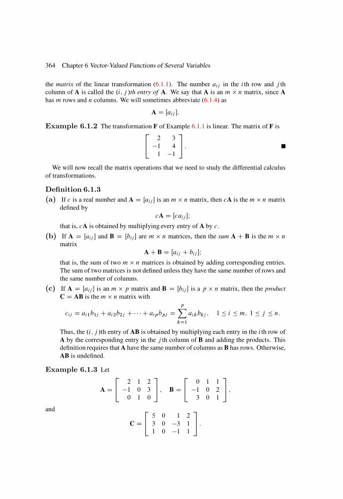
364 Chapter 6 Vector-Valued Functions of Several Variables
the matrix of the linear transformation (6.1.1). The number aij in the i th row and j th
column of A is called the .i; j /th entry of A. We say that A is an m n matrix, since A
has m rows and n columns. We will sometimes abbreviate (6.1.4) as
A D Œaij :
Example 6.1.2 The transformation F of Example 6.1.1 is linear. The matrix of F is24
2 3
1 4
1 1
35 :
We will now recall the matrix operations that we need to study the differential calculus
of transformations.
Definition 6.1.3
(a) If c is a real number and A D Œaij is an m n matrix, then cA is the m n matrix
defined by
cA D Œcaij Ithat is, cA is obtained by multiplying every entry of A by c.
(b) If A D Œaij and B D Œbij are m n matrices, then the sum A C B is the m nmatrix
AC B D Œaij C bij Ithat is, the sum of two m n matrices is obtained by adding corresponding entries.
The sum of two matrices is not defined unless they have the same number of rows and
the same number of columns.
(c) If A D Œaij is an m p matrix and B D Œbij is a p n matrix, then the product
C D AB is them n matrix with
cij D ai1b1j C ai2b2j C C aipbpj DpX
kD1
aikbkj ; 1 i m; 1 j n:
Thus, the .i; j /th entry of AB is obtained by multiplying each entry in the i th row of
A by the corresponding entry in the j th column of B and adding the products. This
definition requires that A have the same number of columns as B has rows. Otherwise,
AB is undefined.
Example 6.1.3 Let
A D
24
2 1 2
1 0 3
0 1 0
35 ; B D
24
0 1 1
1 0 2
3 0 1
35 ;
and
C D
245 0 1 2
3 0 3 1
1 0 1 1
35 :
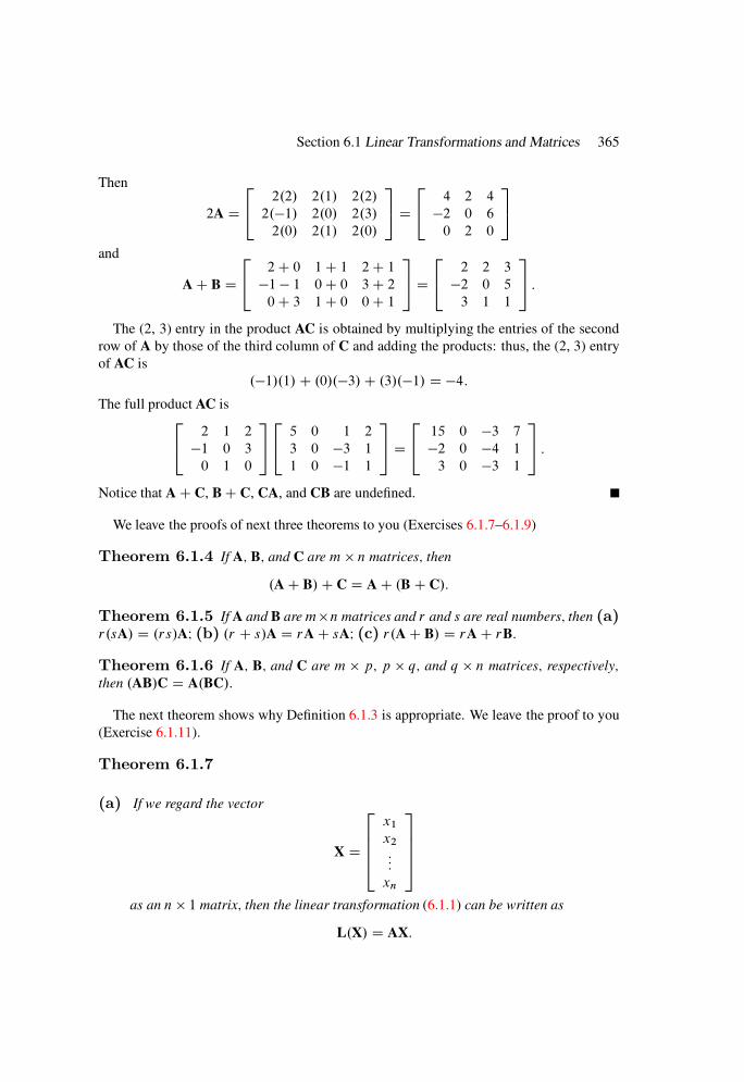
Section 6.1 Linear Transformations and Matrices 365
Then
2A D
24
2.2/ 2.1/ 2.2/
2.1/ 2.0/ 2.3/
2.0/ 2.1/ 2.0/
35 D
24
4 2 4
2 0 6
0 2 0
35
and
AC B D
24
2C 0 1C 1 2C 11 1 0C 0 3C 20C 3 1C 0 0C 1
35 D
24
2 2 3
2 0 5
3 1 1
35 :
The (2, 3) entry in the product AC is obtained by multiplying the entries of the second
row of A by those of the third column of C and adding the products: thus, the (2, 3) entry
of AC is
.1/.1/ C .0/.3/C .3/.1/ D 4:The full product AC is
24
2 1 2
1 0 3
0 1 0
35245 0 1 2
3 0 3 1
1 0 1 1
35 D
24
15 0 3 7
2 0 4 1
3 0 3 1
35 :
Notice that AC C, BC C, CA, and CB are undefined.
We leave the proofs of next three theorems to you (Exercises 6.1.7–6.1.9)
Theorem 6.1.4 If A; B; and C are m n matrices; then
.AC B/C C D AC .BC C/:
Theorem 6.1.5 If A and B aremnmatrices and r and s are real numbers; then (a)r.sA/ D .rs/AI (b) .r C s/A D rAC sAI (c) r.AC B/ D rAC rB:
Theorem 6.1.6 If A; B; and C are m p; p q; and q n matrices; respectively;
then .AB/C D A.BC/:
The next theorem shows why Definition 6.1.3 is appropriate. We leave the proof to you
(Exercise 6.1.11).
Theorem 6.1.7
(a) If we regard the vector
X D
26664
x1
x2
:::
xn
37775
as an n 1 matrix; then the linear transformation (6.1.1) can be written as
L.X/ D AX:
366 Chapter 6 Vector-Valued Functions of Several Variables
(b) If L1 and L2 are linear transformations from Rn to R
m with matrices A1 and A2
respectively; then c1L1 C c2L2 is the linear transformation from Rn to R
m with
matrix c1A1 C c2A2:
(c) If L1 W Rn ! Rp and L2 W Rp ! R
m are linear transformations with matrices A1
and A2; respectively; then the composite function L3 D L2 ı L1; defined by
L3.X/ D L2.L1.X//;
is the linear transformation from Rn to R
m with matrix A2A1:
Example 6.1.4 If
L1.X/ D
24
2x C 3y3x C 2yx C y
35 and L2.X/ D
24x y4xC yx
35 ;
then
A1 D
24
2 3
3 2
1 1
35 and A2 D
241 14 1
1 0
35 :
The linear transformation
L D 2L1 C L2
is defined by
L.X/ D 2L1.X/C L2.X/
D 2
242x C 3y3x C 2yx C y
35C
24x y4xC yx
35
D
24
3x C 5y10x C 5yx C 2y
35 :
The matrix of L is
A D
24
3 5
10 5
1 2
35 D 2A1 C A2:
Example 6.1.5 Let
L1.X/ D
x C 2y3x C 4y
W R2 ! R
2;
and
L2.U/ D
24
uC v
u 2v3uC v
35 W R2 ! R
3:
Section 6.1 Linear Transformations and Matrices 367
Then L3 D L2 ı L1 W R2 ! R3 is given by
L3.X/ D L2..L1.X// D
24
.x C 2y/C .3x C 4y/.x C 2y/ 2.3x C 4y/3.x C 2y/C .3x C 4y/
35 D
24
4xC 6y
7x 10y6x C 10y
35 :
The matrices of L1 and L2 are
A1 D1 2
3 4
and A2 D
24
1 1
1 23 1
35 ;
respectively. The matrix of L3 is
C D
24
4 6
7 106 10
35 D A2A1:
Example 6.1.6 The linear transformations of Example 6.1.5 can be written as
L1.X/ D1 2
3 4
x
y
; L2.U/ D
24
1 1
1 23 1
35u
v
;
and
L3.X/ D
24
4 6
7 106 10
35x
y
:
A New Notation for the Differential
If a real-valued function f W Rn ! R is differentiable at X0, then
dX0f D fx1
.X0/ dx1 C fx2.X0/ dx2 C C fxn.X0/ dxn:
This can be written as a matrix product
dX0f D Œfx1
.X0/ fx2.X0/ fxn.X0/
26664
dx1
dx2
:::
dxn
37775 : (6.1.5)
We define the differential matrix of f at X0 by
f 0.X0/ D Œfx1.X0/ fx2
.X0/ fxn.X0/ (6.1.6)
and the differential linear transformation by
dX D
26664
dx1
dx2
:::
dxn
37775 :
368 Chapter 6 Vector-Valued Functions of Several Variables
Then (6.1.5) can be rewritten as
dX0f D f 0.X0/ dX: (6.1.7)
This is analogous to the corresponding formula for functions of one variable (Exam-
ple 5.3.7), and shows that the differential matrix f 0.X0/ is a natural generalization of the
derivative. With this new notation we can express the defining property of the differential
in a way similar to the form that applies for n D 1:
limX!X0
f .X/ f .X0/ f 0.X0/.X X0/
jX X0jD 0;
where X0 D .x10; x20; : : : ; xn0/ and f 0.X0/.X X0/ is the matrix product
Œfx1.X0/ fx2
.X0/ fxn.X0/
26664
x1 x10
x2 x20
:::
xn xn0
37775 :
As before, we omit the X0 in (6.1.6) and (6.1.7) when it is not necessary to emphasize
the specific point; thus, we write
f 0 Dfx1
fx2 fxn
and df D f 0dX:
Example 6.1.7 If
f .x; y; ´/ D 4x2y´3;
then
f 0.x; y; ´/ D Œ8xy´3 4x2´3 12x2y´2:
In particular, if X0 D .1;1; 2/, then
f 0.X0/ D Œ64 32 48;
so
dX0f D f 0.X0/ dXD Œ64 32 48
24dx
dy
d´
35
D 64 dx C 32 dy 48 d´:
The Norm of a Matrix
We will need the following definition in the next section.
Definition 6.1.8 The norm; kAk; of an m n matrix A D Œaij is the smallest number
such that
jAXj kAk jXjfor all X in R
n:

Section 6.1 Linear Transformations and Matrices 369
To justify this definition, we must show that kAk exists. The components of Y D AX
are
yi D ai1x1 C ai2x2 C C ainxn; 1 i m:By Schwarz’s inequality,
y2i .a2
i1 C a2i2 C C a2
in/jXj2:
Summing this over 1 i m yields
jYj2
0@
mX
iD1
nX
j D1
a2ij
1A jXj2:
Therefore, the set
B D˚KˇjAXj KjXj for all X in R
n
is nonempty. Since B is bounded below by zero, B has an infimum ˛. If > 0, then ˛C is in B because if not, then no number less than ˛C could be in B . Then ˛C would be
a lower bound for B , contradicting the definition of ˛. Hence,
jAXj .˛ C /jXj; X 2 Rn:
Since is an arbitrary positive number, this implies that
jAXj ˛jXj; X 2 Rn;
so ˛ 2 B . Since no smaller number is in B , we conclude that kAk D ˛.
In our applications we will not have to actually compute the norm of a matrix A; rather,
it will be sufficient to know that the norm exists (finite).
Square Matrices
Linear transformations from Rn to R
n will be important when we discuss the inverse func-
tion theorem in Section 6.3 and change of variables in multiple integrals in Section 7.3.
The matrix of such a transformation is square; that is, it has the same number of rows and
columns.
We assume that you know the definition of the determinant
det.A/ D
ˇˇˇˇˇ
a11 a12 a1n
a21 a22 a2n
::::::
: : ::::
an1 an2 ann
ˇˇˇˇˇ
of an n n matrix
A D
26664
a11 a12 a1n
a21 a22 a2n
::::::
: : ::::
an1 an2 ann
37775 :
370 Chapter 6 Vector-Valued Functions of Several Variables
The transpose, At , of a matrix A (square or not) is the matrix obtained by interchanging
the rows and columns of A; thus, if
A D
241 2 3
3 1 4
0 1 2
35 ; then At D
241 3 0
2 1 1
3 4 2
35 :
A square matrix and its transpose have the same determinant; thus,
det.At / D det.A/:
We take the next theorem from linear algebra as given.
Theorem 6.1.9 If A and B are n n matrices; then
det.AB/ D det.A/ det.B/:
The entries ai i , 1 i n, of an nnmatrix A are on the main diagonal of A. The nnmatrix with ones on the main diagonal and zeros elsewhere is called the identity matrix and
is denoted by I; thus, if n D 3,
I D
241 0 0
0 1 0
0 0 1
35 :
We call I the identity matrix because AI D A and IA D A if A is any n n matrix. We
say that an n n matrix A is nonsingular if there is an n n matrix A1, the inverse of A,
such that AA1 D A1A D I. Otherwise, we say that A is singular
Our main objective is to show that an n n matrix A is nonsingular if and only if
det.A/ ¤ 0. We will also find a formula for the inverse.
Definition 6.1.10 Let A D Œaij be an n n matrix; with n 2: The cofactor of an
entry aij is
cij D .1/iCj det.Aij /;
where Aij is the .n 1/ .n 1/matrix obtained by deleting the i th row and j th column
of A: The adjoint of A; denoted by adj.A/; is the n n matrix whose .i; j /th entry is cj i :
Example 6.1.8 The cofactors of
A D
244 2 1
3 1 2
0 1 2
35
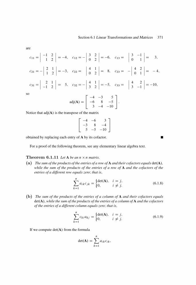
Section 6.1 Linear Transformations and Matrices 371
are
c11 Dˇˇ 1 2
1 2
ˇˇ D 4; c12 D
ˇˇ 3 2
0 2
ˇˇ D 6; c13 D
ˇˇ 3 10 1
ˇˇ D 3;
c21 D ˇˇ 2 1
1 2
ˇˇD 3; c22 D
ˇˇ 4 1
0 2
ˇˇ D 8; c23 D
ˇˇ 4 2
0 1
ˇˇ D 4;
c31 Dˇˇ 2 1
1 2
ˇˇ D 5; c32 D
ˇˇ 4 1
3 2
ˇˇ D 5; c33 D
ˇˇ 4 2
3 1
ˇˇ D 10;
so
adj.A/ D
244 3 5
6 8 53 4 10
35 :
Notice that adj.A/ is the transpose of the matrix
244 6 3
3 8 45 5 10
35
obtained by replacing each entry of A by its cofactor.
For a proof of the following theorem, see any elementary linear algebra text.
Theorem 6.1.11 Let A be an n n matrix:
(a) The sum of the products of the entries of a row of A and their cofactors equals det.A/;
while the sum of the products of the entries of a row of A and the cofactors of the
entries of a different row equals zeroI that is;
nX
kD1
aikcjk D
det.A/; i D j;0; i ¤ j: (6.1.8)
(b) The sum of the products of the entries of a column of A and their cofactors equals
det.A/; while the sum of the products of the entries of a column of A and the cofactors
of the entries of a different column equals zeroI that is;
nX
kD1
ckiakj D
det.A/; i D j;0; i ¤ j: (6.1.9)
If we compute det.A/ from the formula
det.A/ DnX
kD1
aikcik;

372 Chapter 6 Vector-Valued Functions of Several Variables
we say that we are expanding the determinant in cofactors of its i th row. Since we can
choose i arbitrarily from f1; : : : ; ng, there are n ways to do this. If we compute det.A/
from the formula
det.A/ DnX
kD1
akjckj ;
we say that we are expanding the determinant in cofactors of its j th column. There are also
n ways to do this.
In particular, we note that det.I/ D 1 for all n 1.
Theorem 6.1.12 Let A be an n n matrix: If det.A/ D 0; then A is singular: If
det.A/ ¤ 0; then A is nonsingular; and A has the unique inverse
A1 D 1
det.A/adj.A/: (6.1.10)
Proof If det.A/ D 0, then det.AB/ D 0 for any n n matrix, by Theorem 6.1.9.
Therefore, since det.I/ D 1, there is no matrix n n matrix B such that AB D I; that is, A
is singular if det.A/ D 0. Now suppose that det.A/ ¤ 0. Since (6.1.8) implies that
A adj.A/ D det.A/I
and (6.1.9) implies that
adj.A/A D det.A/I;
dividing both sides of these two equations by det.A/ shows that if A1 is as defined in
(6.1.10), then AA1 D A1A D I. Therefore, A1 is an inverse of A. To see that it is the
only inverse, suppose that B is an n n matrix such that AB D I. Then A1.AB/ D A1,
so .A1A/B D A1. Since AA1 D I and IB D B, it follows that B D A1.
Example 6.1.9 In Example 6.1.8 we found that the adjoint of
AD
244 2 1
3 1 2
0 1 2
35
is
adj.A/ D
244 3 5
6 8 53 4 10
35 :
We can compute det.A/ by finding any diagonal entry of A adj.A/. (Why?) This yields
det.A/ D 25. (Verify.) Therefore,
A1 D 125
244 3 5
6 8 53 4 10
35 :
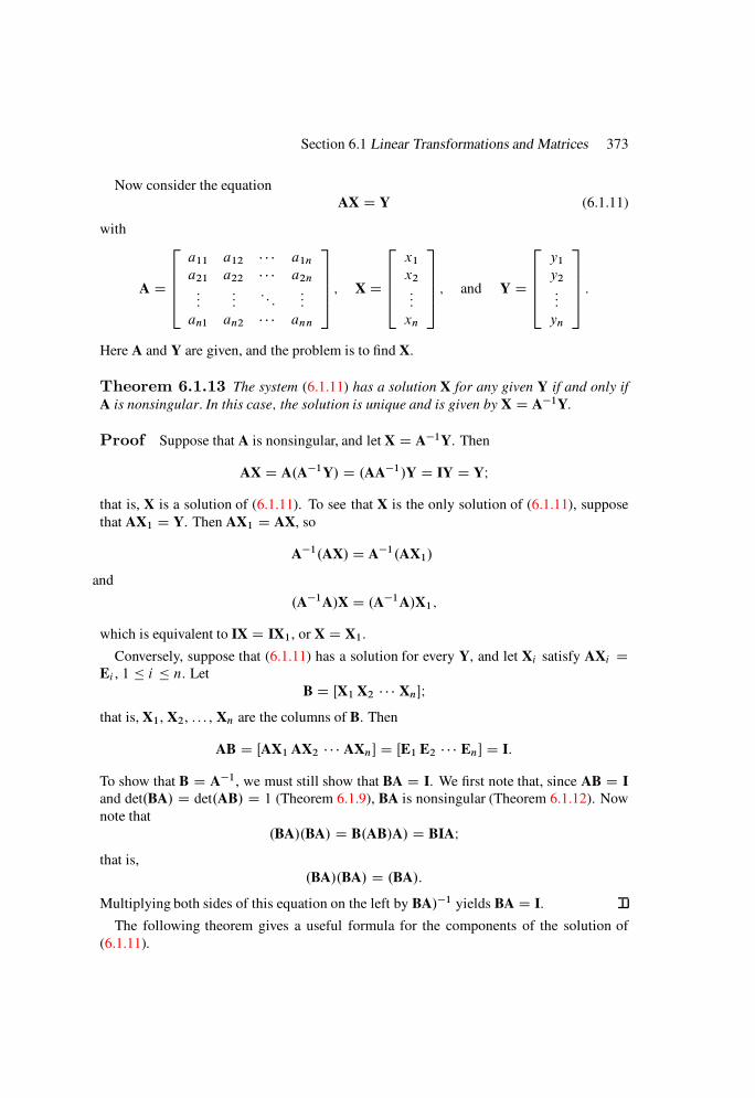
Section 6.1 Linear Transformations and Matrices 373
Now consider the equation
AX D Y (6.1.11)
with
A D
26664
a11 a12 a1n
a21 a22 a2n
::::::
: : ::::
an1 an2 ann
37775 ; X D
26664
x1
x2
:::
xn
37775 ; and Y D
26664
y1
y2
:::
yn
37775 :
Here A and Y are given, and the problem is to find X.
Theorem 6.1.13 The system (6.1.11) has a solution X for any given Y if and only if
A is nonsingular: In this case; the solution is unique and is given by X D A1Y.
Proof Suppose that A is nonsingular, and let X D A1Y. Then
AX D A.A1Y/ D .AA1/Y D IY D YI
that is, X is a solution of (6.1.11). To see that X is the only solution of (6.1.11), suppose
that AX1 D Y. Then AX1 D AX, so
A1.AX/ D A1.AX1/
and
.A1A/X D .A1A/X1;
which is equivalent to IX D IX1, or X D X1.
Conversely, suppose that (6.1.11) has a solution for every Y, and let Xi satisfy AXi DEi , 1 i n. Let
B D ŒX1 X2 XnIthat is, X1, X2, . . . , Xn are the columns of B. Then
AB D ŒAX1 AX2 AXn D ŒE1 E2 En D I:
To show that B D A1, we must still show that BA D I. We first note that, since AB D I
and det.BA/ D det.AB/ D 1 (Theorem 6.1.9), BA is nonsingular (Theorem 6.1.12). Now
note that
.BA/.BA/ D B.AB/A/ D BIAIthat is,
.BA/.BA/ D .BA/:
Multiplying both sides of this equation on the left by BA/1 yields BA D I.
The following theorem gives a useful formula for the components of the solution of
(6.1.11).
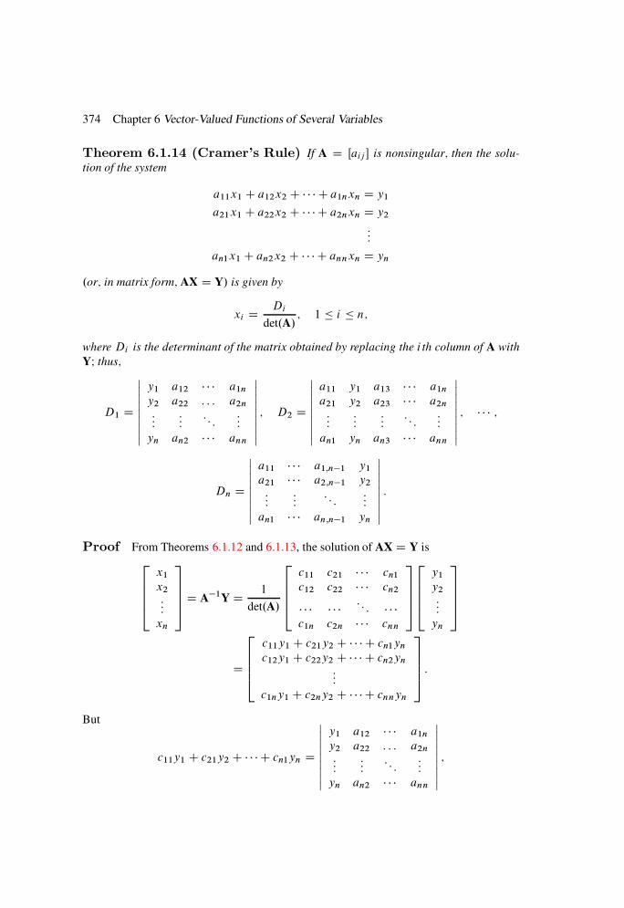
374 Chapter 6 Vector-Valued Functions of Several Variables
Theorem 6.1.14 (Cramer’s Rule) If A D Œaij is nonsingular; then the solu-
tion of the system
a11x1 C a12x2 C C a1nxn D y1
a21x1 C a22x2 C C a2nxn D y2
:::
an1x1 C an2x2 C C annxn D yn
.or; in matrix form; AX D Y/ is given by
xi DDi
det.A/; 1 i n;
where Di is the determinant of the matrix obtained by replacing the i th column of A with
YI thus;
D1 D
ˇˇˇˇˇ
y1 a12 a1n
y2 a22 : : : a2n
::::::
: : ::::
yn an2 ann
ˇˇˇˇˇ; D2 D
ˇˇˇˇˇ
a11 y1 a13 a1n
a21 y2 a23 a2n
::::::
:::: : :
:::
an1 yn an3 ann
ˇˇˇˇˇ; ;
Dn D
ˇˇˇˇˇ
a11 a1;n1 y1
a21 a2;n1 y2
::::::
: : ::::
an1 an;n1 yn
ˇˇˇˇˇ:
Proof From Theorems 6.1.12 and 6.1.13, the solution of AX D Y is
26664
x1
x2
:::
xn
37775 D A1Y D
1
det.A/
26664
c11 c21 cn1
c12 c22 cn2
: : : c1n c2n cnn
37775
26664
y1
y2
:::
yn
37775
D
26664
c11y1 C c21y2 C C cn1yn
c12y1 C c22y2 C C cn2yn
:::
c1ny1 C c2ny2 C C cnnyn
37775 :
But
c11y1 C c21y2 C C cn1yn D
ˇˇˇˇˇ
y1 a12 a1n
y2 a22 : : : a2n
::::::
: : ::::
yn an2 ann
ˇˇˇˇˇ;

Section 6.1 Linear Transformations and Matrices 375
as can be seen by expanding the determinant on the right in cofactors of its first column.
Similarly,
c12y1 C c22y2 C C cn2yn D
ˇˇˇˇˇ
a11 y1 a13 a1n
a21 y2 a23 a2n
::::::
:::: : :
:::
an1 yn an3 ann
ˇˇˇˇˇ;
as can be seen by expanding the determinant on the right in cofactors of its second column.
Continuing in this way completes the proof.
Example 6.1.10 The matrix of the system
4x C 2y C ´ D 13x y C 2´ D 2
y C 2´ D 0
is
A D
244 2 1
3 1 2
0 1 2
35 :
Expanding det.A/ in cofactors of its first row yields
det.A/ D 4ˇˇ 1 2
1 2
ˇˇ 2
ˇˇ 3 2
0 2
ˇˇC 1
ˇˇ 3 10 1
ˇˇ
D 4.4/ 2.6/C 1.3/ D 25:
Using Cramer’s rule to solve the system yields
x D 1
25
ˇˇˇ1 2 1
2 1 2
0 1 2
ˇˇˇ D
2
5; y D
1
25
ˇˇˇ4 1 1
3 2 2
0 0 2
ˇˇˇ D
2
5;
´ D 125
ˇˇˇ4 2 1
3 1 2
0 1 0
ˇˇˇ D
1
5:
A system of n equations in n unknowns
a11x1 C a12x2 C C a1nxn D 0a21x1 C a22x2 C C a2nxn D 0
:::
an1x1 C an2x2 C C annxn D 0
(6.1.12)
(or, in matrix form, AX D 0) is homogeneous. It is obvious that X0 D 0 satisfies this
system. We call this the trivial solution of (6.1.12). Any other solutions of (6.1.12), if they
exist, are nontrivial.
376 Chapter 6 Vector-Valued Functions of Several Variables
We will need the following theorems. The proofs may be found in any linear algebra
text.
Theorem 6.1.15 The homogeneous system (6.1.12) of n equations in n unknowns has
a nontrivial solution if and only if det.A/ D 0:
Theorem 6.1.16 IfA1; A2; . . . ; Ak are nonsingularnnmatrices; then so isA1A2 Ak ;
and
.A1A2 Ak/1 D A1
k A1k1 A
11 :
6.1 Exercises
1. Prove: If L W Rn ! Rm is a linear transformation, then
L.a1X1 C a2X2 C C akXk/ D a1L.X1/C a2L.X2/C C akL.Xk/
if X1;X2; : : : ;Xk are in Rn and a1, a2, . . . , ak are real numbers.
2. Prove that the transformation L defined by Eqn. (6.1.1) is linear.
3. Find the matrix of L.
(a) L.X/ D
243x C 4y C 6´2x 47C 2´7x C 2y C 3´
35 (b) L.X/ D
2664
2x1 C 4x2
3x1 2x2
7x1 4x2
6x1 C x2
3775
4. Find cA.
(a) c D 4; A D
242 2 4 6
0 0 1 3
3 4 7 11
35 (b) c D 2; A D
241 3 0
0 1 2
1 1 3
35
5. Find AC B.
(a) A D
241 2 3
1 1 4
0 1 4
35 ; B D
241 0 3
5 6 70 1 2
35
(b) A D
240 5
3 2
1 7
35 ; B D
241 2
0 3
4 7
35
6. Find AB.
(a) A D
241 2 3
0 1 4
0 1 4
35 ; B D
241 2
0 3
4 7
35
(b) A D5 3 2 1
6 7 4 1
; B D
2664
1
3
4
7
3775

Section 6.1 Linear Transformations and Matrices 377
7. Prove Theorem 6.1.4.
8. Prove Theorem 6.1.5.
9. Prove Theorem 6.1.6.
10. Suppose that AC B and AB are both defined. What can be said about A and B?
11. Prove Theorem 6.1.7.
12. Find the matrix of aL1 C bL2.
(a) L1.x; y; ´/ D
243x C 2y C ´
x C 4y C 2´3x 4y C ´
35,
L2.x; y; ´/ D
24x C y ´
2x C y C 3´y C ´
35; a D 2; b D 1
(b) L1.x; y/ D
242x C 3yx y
4x C y
35 ; L2.x; y/ D
243x yx C yx y
35 ; a D 4; b D
2
13. Find the matrices of L1ıL2 and L2ıL1, where L1 and L2 are as in Exercise 6.1.12(a).
14. Write the transformations of Exercise 6.1.12 in the form L.X/ D AX.
15. Find f 0 and f 0.X0/.
(a) f .x; y; ´/ D 3x2y´, X0 D .1;1; 1/(b) f .x; y/ D sin.x C y/, X0 D .=4; =4/(c) f .x; y; ´/ D xyex´ , X0 D .1; 2; 0/(d) f .x; y; ´/ D tan.x C 2y C ´/, X0 D .=4;=8; =4/(e) f .X/ D jXj W Rn ! R, X0 D .1=
pn; 1=pn; : : : ; 1=
pn/
16. Let A D Œaij be an m n matrix and
D max˚jaij j
ˇ1 i m; 1 i n
:
Show that kAk pmn.
17. Prove: If A has at least one nonzero entry, then kAk ¤ 0.
18. Prove: kAC Bk kAk C kBk.19. Prove: kABk kAk kBk.20. Solve by Cramer’s rule.
(a)x C y C 2´D 1
2x y C ´D 1x 2y 3´D 2
(b)x C y ´ D 5
3x 2y C 2´ D 0
4xC 2y 3´ D 14
378 Chapter 6 Vector-Valued Functions of Several Variables
(c)x C 2y C 3´ D 5x ´ D 1x C y C 2´ D 4
(d)
x y C ´ 2w D 1
2x C y 3´C 3w D 4
3x C 2y C w D 132x C y ´ D 4
21. Find A1 by the method of Theorem 6.1.12.
(a)
1 23 4
(b)
241 2 3
1 0 11 1 2
35
(c)
244 2 1
3 1 2
0 1 2
35 (d)
241 0 1
0 1 1
1 1 0
35
(e)
2664
1 2 0 0
2 3 0 0
0 0 2 3
0 0 1 2
3775 (f)
2664
1 1 2 12 2 1 3
1 4 1 2
3 1 0 1
3775
22. For 1 i; j m, let aij D aij .X/ be a real-valued function continuous on a
compact set K in Rn. Suppose that them m matrix
A.X/ D Œaij .X/
is nonsingular for each X in K, and define them m matrix
B.X;Y/ D Œbij .X;Y/
by
B.X;Y/ D A1.X/A.Y/ I:
Show that for each > 0 there is a ı > 0 such that
jbij .X;Y/j < ; 1 i; j m;
if X;Y 2 K and jX Yj < ı. HINT: Show that bij is continuous on the set
˚.X;Y/
ˇX 2 K; Y 2 K
:
Then assume that the conclusion is false and use Exercise 5.1.32 to obtain a contradiction:
6.2 CONTINUITY AND DIFFERENTIABILITY OF TRANS-FORMATIONS
Throughout the rest of this chapter, transformations F and points X should be considered as
written in vertical form when they occur in connection with matrix operations. However,
we will write X D .x1; x2; : : : ; xn/ when X is the argument of a function.

Section 6.2 Continuity and Differentiability of Transformations 379
Continuous Transformations
In Section 5.2 we defined a vector-valued function (transformation) to be continuous at X0
if each of its component functions is continuous at X0. We leave it to you to show that this
implies the following theorem (Exercise 1).
Theorem 6.2.1 Suppose that X0 is in; and a limit point of; the domain of F W Rn !R
m: Then F is continuous at X0 if and only if for each > 0 there is a ı > 0 such that
jF.X/ F.X0/j < if jX X0j < ı and X 2 DF: (6.2.1)
This theorem is the same as Theorem 5.2.7 except that the “absolute value” in (6.2.1)
now stands for distance in Rm rather than R.
If C is a constant vector, then “limX!X0F.X/ D C” means that
limX!X0
jF.X/ Cj D 0:
Theorem 6.2.1 implies that F is continuous at X0 if and only if
limX!X0
F.X/ D F.X0/:
Example 6.2.1 The linear transformation
L.X/ D
24
x C y C ´2x 3y C ´2xC y ´
35
is continuous at every X0 in R3, since
L.X/ L.X0/ D L.X X0/ D
24
.x x0/C .y y0/C .´ ´0/
2.x x0/ 3.y y0/C .´ ´0/
2.x x0/C .y y0/ .´ ´0/
35 ;
and applying Schwarz’s inequality to each component yields
jL.X/ L.X0/j2 .3C 14C 6/jX X0j2 D 23jX X0j2:
Therefore,
jL.X/ L.X0/j < if jX X0j <p23:
Differentiable Transformations
In Section 5.4 we defined a vector-valued function (transformation) to be differentiable at
X0 if each of its components is differentiable at X0 (Definition 5.4.1). The next theorem
characterizes this property in a useful way.

380 Chapter 6 Vector-Valued Functions of Several Variables
Theorem 6.2.2 A transformation F D .f1; f2; : : : ; fm/ defined in a neighborhood of
X0 2 Rn is differentiable at X0 if and only if there is a constantm n matrix A such that
limX!X0
F.X/ F.X0/ A.X X0/
jX X0jD 0: (6.2.2)
If (6.2.2) holds; then A is given uniquely by
@xj
D
26666666664
@f1.X0/
@x1
@f1.X0/
@x2
@f1.X0/
@xn
@f2.X0/
@x1
@f2.X0/
@x2
@f2.X0/
@xn:::
:::: : :
:::@fm.X0/
@x1
@fm.X0/
@x2
@fm.X0/
@xn
37777777775
: (6.2.3)
Proof Let X0 D .x10; x20; : : : ; xn0/. If F is differentiable at X0, then so are f1, f2,
. . . , fm (Definition 5.4.1). Hence,
limX!X0
fi .X/ fi .X0/ nX
j D1
@fi .X0/
@xj
.xj xj 0/
jX X0jD 0; 1 i m;
which implies (6.2.2) with A as in (6.2.3).
Now suppose that (6.2.2) holds with A D Œaij . Since each component of the vector in
(6.2.2) approaches zero as X approaches X0, it follows that
limX!X0
fi .X/ fi .X0/ nX
j D1
aij .xj xj 0/
jX X0jD 0; 1 i m;
so each fi is differentiable at X0, and therefore so is F (Definition 5.4.1). By Theo-
rem 5.3.6,
aij D@fi .X0/
@xj
; 1 i m; 1 j n;
which implies (6.2.3).
A transformation T W Rn ! Rm of the form
T.X/ D UC A.X X0/;
where U is a constant vector in Rm, X0 is a constant vector in R
n, and A is a constantmnmatrix, is said to be affine. Theorem 6.2.2 says that if F is differentiable at X0, then F can
be well approximated by an affine transformation.

Section 6.2 Continuity and Differentiability of Transformations 381
Example 6.2.2 The components of the transformation
F.X/ D
24x2 C 2xy C ´x C 2x´C yx2 C y2 C ´2
35
are differentiable at X0 D .1; 0; 2/. Evaluating the partial derivatives of the components
there yields
A D
242 2 1
5 1 2
2 0 4
35 :
(Verify). Therefore, Theorem 6.2.2 implies that the affine transformation
T.X/ D F.X0/CA.X X0/
D
243
5
5
35C
242 2 1
5 1 2
2 0 4
3524x 1y
´ 2
35
satisfies
limX!X0
F.X/ T.X/
jX X0jD 0:
Differential of a Transformation
If F D .f1; f2; : : : ; fm/ is differentiable at X0, we define the differential of F at X0 to be
the linear transformation
dX0F D
26664
dX0f1
dX0f2
:::
dX0fm
37775 : (6.2.4)
We call the matrix A in (6.2.3) the differential matrix of F at X0 and denote it by F0.X0/;
thus,
F0.X0/ D
2666666666664
@f1.X0/
@x1
@f1.X0/
@x2
@f1.X0/
@xn
@f2.X0/
@x1
@f2.X0/
@x2
@f2.X0/
@xn
::::::
: : ::::
@fm.X0/
@x1
@fm.X0/
@x2
@fm.X0/
@xn
3777777777775
: (6.2.5)

382 Chapter 6 Vector-Valued Functions of Several Variables
(It is important to bear in mind that while F is a function from Rn to R
m, F0 is not such
a function; F0 is an m n matrix.) From Theorem 6.2.2, the differential can be written in
terms of the differential matrix as
dX0F D F0.X0/
26664
dx1
dx2
:::
dxn
37775 (6.2.6)
or, more succinctly, as
dX0F D F0.X0/ dX;
where
dX D
26664
dx1
dx2
:::
dxn
37775 ;
as defined earlier.
When it is not necessary to emphasize the particular point X0, we write (6.2.4) as
dF D
26664
df1
df2
:::
dfm
37775 ;
(6.2.5) as
F0 D
2666666666664
@f1
@x1
@f1
@x2
@f1
@xn
@f2
@x1
@f2
@x2
@f2
@xn
::::::
: : ::::
@fm
@x1
@fm
@x2
@fm
@xn
3777777777775
;
and (6.2.6) as
dF D F0 dX:
With the differential notation we can rewrite (6.2.2) as
limX!X0
F.X/ F.X0/ F0.X0/.X X0/
jX X0jD 0:

Section 6.2 Continuity and Differentiability of Transformations 383
Example 6.2.3 The linear transformation
F.X/ D
26664
a11x1 C a12x2 C C a1nxn
a21x1 C a22x2 C C a2nxn
:::
am1x1 C am2x2 C C amnxn
37775
can be written as F.X/ D AX, where A D Œaij . Then
F0 D AI
that is, the differential matrix of a linear transformation is independent of X and is the
matrix of the transformation. For example, the differential matrix of
F.x1; x2; x3/ D1 2 3
2 1 0
24x1
x2
x3
35
is
F0 D1 2 3
2 1 0
:
If F.X/ D X (the identity transformation), then F0 D I (the identity matrix).
Example 6.2.4 The transformation
F.x; y/ D
266664
x
x2 C y2
y
x2 C y2
2xy
377775
is differentiable at every point of R2 except .0; 0/, and
F0.x; y/ D
2666664
y2 x2
.x2 C y2/2 2xy
.x2 C y2/2
2xy
.x2 C y2/2x2 y2
.x2 C y2/2
2y 2x
3777775:
In particular,
F0.1; 1/ D
26664
0 12
12
0
2 2
37775 ;

384 Chapter 6 Vector-Valued Functions of Several Variables
so
lim.x;y/!.1;1/
1p.x 1/2 C .y 1/2
26664
12
12
2
37775
26664
0 12
12
0
2 2
37775
x 1y 1
1CCCA
D
240
0
0
35 :
If m D n, the differential matrix is square and its determinant is called the Jacobian of
F. The standard notation for this determinant is
@.f1; f2; : : : ; fn/
@.x1; x2; : : : ; xn/D
ˇˇˇˇˇˇˇˇˇ
@f1
@x1
@f1
@x2
@f1
@xn
@f2
@x1
@f2
@x2
@f2
@xn
::::::
: : ::::
@fn
@x1
@fn
@x2
@fn
@xn
ˇˇˇˇˇˇˇˇˇ
:
We will often write the Jacobian of F more simply as J.F/, and its value at X0 as JF.X0/.
Since an n n matrix is nonsingular if and only if its determinant is nonzero, it follows
that if F W Rn ! R
n is differentiable at X0, then F0.X0/ is nonsingular if and only if
JF.X0/ ¤ 0. We will soon use this important fact.
Example 6.2.5 If
F.x; y; ´/ D
26664
x2 2x C ´
x C 2xy C ´2
x C y C ´
37775 ;
then
@.f1; f2; f3/
@.x1; x2; x3/D JF.X/ D
ˇˇˇ2x 2 0 1
1C 2y 2x 2´
1 1 1
ˇˇˇ
D .2x 2/ˇˇ 2x 2´
1 1
ˇˇC
ˇˇ 1C 2y 2x
1 1
ˇˇ
D .2x 2/.2x 2´/C .1C 2y 2x/:
Section 6.2 Continuity and Differentiability of Transformations 385
In particular, JF.1;1; 1/ D 3, so the differential matrix
F0.1;1; 1/ D
24
0 0 1
1 2 2
1 1 1
35
is nonsingular.
Properties of Differentiable Transformations
We leave the proof of the following theorem to you (Exercise 6.2.16).
Theorem 6.2.3 If F W Rn ! Rm is differentiable at X0; then F is continuous at X0:
Theorem 5.3.10 and Definition 5.4.1 imply the following theorem.
Theorem 6.2.4 Let F D .f1; f2; : : : ; fm/ W Rn ! Rm; and suppose that the partial
derivatives@fi
@xj
; 1 i m; 1 j n; (6.2.7)
exist on a neighborhood of X0 and are continuous at X0: Then F is differentiable at X0:
We say that F is continuously differentiable on a set S if S is contained in an open set
on which the partial derivatives in (6.2.7) are continuous. The next three lemmas give
properties of continuously differentiable transformations that we will need later.
Lemma 6.2.5 Suppose that F W Rn ! R
m is continuously differentiable on a neigh-
borhoodN of X0: Then; for every > 0; there is a ı > 0 such that
jF.X/ F.Y/j < .kF0.X0/k C /jX Yj if A;Y 2 Bı.X0/: (6.2.8)
Proof Consider the auxiliary function
G.X/ D F.X/ F0.X0/X: (6.2.9)
The components of G are
gi .X/ D fi .X/ nX
j D1
@fi.X0/@xj
x j;
so@gi .X/
@xj
D @fi .X/
@xj
@fi.X0/
@xj
:

386 Chapter 6 Vector-Valued Functions of Several Variables
Thus, @gi=@xj is continuous on N and zero at X0. Therefore, there is a ı > 0 such thatˇˇ@gi.X/
@xj
ˇˇ < p
mnfor 1 i m; 1 j n; if jX X0j < ı: (6.2.10)
Now suppose that X, Y 2 Bı.X0/. By Theorem 5.4.5,
gi .X/ gi .Y/ DnX
j D1
@gi .Xi /
@xj
.xj yj /; (6.2.11)
where Xi is on the line segment from X to Y, so Xi 2 Bı.X0/. From (6.2.10), (6.2.11),
and Schwarz’s inequality,
.gi .X/ gi .Y//2
0@
nX
j D1
@gi.Xi /
@xj
2
1A jX Yj2 < 2
mjX Yj2:
Summing this from i D 1 to i D m and taking square roots yields
jG.X/ G.Y/j < jX Yj if X;Y 2 Bı.X0/: (6.2.12)
To complete the proof, we note that
F.X/ F.Y/ D G.X/ G.Y/C F0.X0/.X Y/; (6.2.13)
so (6.2.12) and the triangle inequality imply (6.2.8).
Lemma 6.2.6 Suppose that F W Rn ! R
n is continuously differentiable on a neigh-
borhood of X0 and F0.X0/ is nonsingular: Let
r D 1
k.F0.X0//1k: (6.2.14)
Then; for every > 0; there is a ı > 0 such that
jF.X/ F.Y/j .r /jX Yj if X;Y 2 Bı.X0/: (6.2.15)
Proof Let X and Y be arbitrary points inDF and let G be as in (6.2.9). From (6.2.13),
jF.X/ F.Y/j ˇjF0.X0/.X Y/j jG.X/ G.Y/j
ˇ; (6.2.16)
Since
X Y D ŒF0.X0/1F0.X0/.X Y/;
(6.2.14) implies that
jX Yj 1
rjF0.X0/.X Yj;
so
jF0.X0/.X Y/j r jX Yj: (6.2.17)
Now choose ı > 0 so that (6.2.12) holds. Then (6.2.16) and (6.2.17) imply (6.2.15).
See Exercise 6.2.19 for a stronger conclusion in the case where F is linear.

Section 6.2 Continuity and Differentiability of Transformations 387
Lemma 6.2.7 If F W Rn ! Rm is continuously differentiable on an open set containing
a compact set D; then there is a constantM such that
jF.Y/ F.X/j M jY Xj if X;Y 2 D: (6.2.18)
Proof On
S D˚.X;Y/
ˇX;Y 2 D
R
2n
define
g.X;Y/ D
8<:
jF.Y/ F.X/ F0.X/.Y X/jjY Xj ; Y ¤ X;
0; Y D X:
Then g is continuous for all .X;Y/ in S such that X ¤ Y. We now show that if X0 2 D,
then
lim.X;Y/!.X0;X0/
g.X;Y/ D 0 D g.X0;X0/I (6.2.19)
that is, g is also continuous at points .X0;X0/ in S .
Suppose that > 0 and X0 2 D. Since the partial derivatives of f1, f2, . . . , fm are
continuous on an open set containingD, there is a ı > 0 such thatˇˇ@fi .Y/
@xj
@fi .X/
@xj
ˇˇ < p
mnif X;Y 2 Bı.X0/; 1 i m; 1 j n: (6.2.20)
(Note that @fi=@xj is uniformly continuous on Bı.X0/ for ı sufficiently small, from The-
orem 5.2.14.) Applying Theorem 5.4.5 to f1, f2, . . . , fm, we find that if X, Y 2 Bı .X0/,
then
fi .Y/ fi .X/ DnX
j D1
@fi .Xi /
@xj
.yj xj /;
where Xi is on the line segment from X to Y. From this,
24fi .Y/ fi .X/
nX
j D1
@fi.X/
@xj
.yj xj /
35
2
D
24
nX
j D1
@fi.Xi /
@xj
@fi.X/
@xj
.yj xj /
35
2
jY Xj2nX
j D1
@fi.Xi /
@xj
@fi.X/
@xj
2
(by Schwarz’s inequality)
<2
mjY Xj2 (by (6.2.20)) :
Summing from i D 1 to i D m and taking square roots yields
jF.Y/ F.X/ F0.X/.Y X/j < jY Xj if X;Y 2 Bı .X0/:
This implies (6.2.19) and completes the proof that g is continuous on S .

388 Chapter 6 Vector-Valued Functions of Several Variables
Since D is compact, so is S (Exercise 5.1.27). Therefore, g is bounded on S (Theo-
rem 5.2.12); thus, for some M1,
jF.Y/ F.X/ F0.X/.Y X/j M1jX Yj if X;Y 2 D:
But
jF.Y/ F.X/j jF.Y/ F.X/ F0.X/.Y X/j C jF0.X/.Y X/j .M1 C kF0.X/k/j.Y Xj: (6.2.21)
Since
kF0.X/k
0@
mX
iD1
nX
j D1
@fi.X/
@xj
2
1A
1=2
and the partial derivatives f@fi=@xj g are bounded onD, it follows that kF0.X/k is bounded
on D; that is, there is a constant M2 such that
kF0.X/k M2; X 2 D:
Now (6.2.21) implies (6.2.18) withM DM1 CM2.
The Chain Rule for Transformations
By using differential matrices, we can write the chain rule for transformations in a form
analogous to the form of the chain rule for real-valued functions of one variable (Theo-
rem 2.3.5).
Theorem 6.2.8 Suppose that F W Rn ! Rm is differentiable at X0; G W Rk ! R
n is
differentiable at U0; and X0 D G.U0/: Then the composite function H D F ı G W Rk !R
m; defined by
H.U/ D F.G.U//;
is differentiable at U0:Moreover;
H0.U0/ D F0.G.U0//G0.U0/ (6.2.22)
and
dU0H D dX0
F ı dU0G; (6.2.23)
where ı denotes composition:
Proof The components of H are h1, h2, . . . , hm, where
hi .U/ D fi.G.U//:
Applying Theorem 5.4.3 to hi yields
dU0hi D
nX
j D1
@fi .X0/
@xj
dU0gj ; 1 i m: (6.2.24)
Section 6.2 Continuity and Differentiability of Transformations 389
Since
dU0H D
26664
dU0h1
dU0h2
:::
dU0hm
37775 and dU0
G D
26664
dU0g1
dU0g2
:::
dU0gn
37775 ;
them equations in (6.2.24) can be written in matrix form as
dU0H D F0.X0/dU0
G D F0.G.U0//dU0G: (6.2.25)
But
dU0G D G0.U0/ dU;
where
dU D
26664
du1
du2
:::
duk
37775 ;
so (6.2.25) can be rewritten as
dU0H D F0.G.U0//G
0.U0/ dU:
On the other hand,
dU0H D H0.U0/ dU:
Comparing the last two equations yields (6.2.22). Since G0.U0/ is the matrix of dU0G and
F0.G.U0// D F0.X0/ is the matrix of dX0F, Theorem 6.1.7(c) and (6.2.22) imply (6.2.23).
Example 6.2.6 Let U0 D .1;1/,
G.U/ D G.u; v/ D
26664
pu
pu2 C 3v2
pv C 2
37775 ; F.X/ D F.x; y; ´/ D
"x2 C y2 C 2´2
x2 y2
#;
and
H.U/ D F.G.U//:
Since G is differentiable at U0 D .1;1/ and F is differentiable at
X0 D G.U0/ D .1; 2; 1/;
Theorem 6.2.8 implies that H is differentiable at .1;1/. To find H0.1;1/ from (6.2.22),
we first find that

390 Chapter 6 Vector-Valued Functions of Several Variables
G0.U/ D
26666664
1
2pu
0
upu2 C 3v2
3vpu2 C 3v2
01
2pv C 2
37777775
and
F0.X/ D2x 2y 4´
2x 2y 0
:
Then, from (6.2.22),
H0.1;1/D F0.1; 2; 1/G0.1;1/
D2 4 4
2 4 0
26664
12
0
123
2
0 12
37775 D
3 41 6
:
We can check this by expressing H directly in terms of .u; v/ as
H.u; v/ D
264pu2 C
pu2 C 3v2
2
C 2pv C 2
2pu2
pu2 C 3v2
2
375
DuC u2 C 3v2C 2v C 4
u u2 3v2
and differentiating to obtain
H0.u; v/ D1C 2u 6v C 21 2u 6v
;
which yields
H0.1;1/ D
3 41 6
;
as we saw before.
6.2 Exercises
1. Show that the following definitions are equivalent.
(a) F D .f1; f2; : : : ; fm/ is continuous at X0 if f1, f2, . . . , fm are continuous
at X0.

Section 6.2 Continuity and Differentiability of Transformations 391
(b) F is continuous at X0 if for every > 0 there is a ı > 0 such that jF.X/ F.X0/j < if jX X0j < ı and X 2 DF.
2. Verify that
limX!X0
F.X/ F.X0/ F0.X0/.X X0/
jX X0jD 0:
(a) F.X/ D
243xC 4y2x y
x C y
35 ; X0 D .x0; y0; ´0/
(b) F.X/ D
242x2C xy C 1
xy
x2 C y2
35 ; X0 D .1;1/
(c) F.X/ D
24
sin.x C y/sin.y C ´/sin.x C ´/
35 ; X0 D .=4; 0; =4/
3. Suppose that F W Rn ! R
m and h W Rn ! R have the same domain and are
continuous at X0. Show that the product hF D .hf1; hf2; : : : ; hfm/ is continuous at
X0.
4. Suppose that F and G are transformations from Rn to R
m with common domain D.
Show that if F and G are continuous at X0 2 D, then so are FCG and F G.
5. Suppose that F W Rn ! Rm is defined in a neighborhood of X0 and continuous at
X0, G W Rk ! R
n is defined in a neighborhood of U0 and continuous at U0, and
X0 D G.U0/. Prove that the composite function H D F ıG is continuous at U0.
6. Prove: If F W Rn ! Rm is continuous on a set S , then jFj is continuous on S .
7. Prove: If F W Rn ! Rm is continuous on a compact set S , then jFj is bounded on
S , and there are points X0 and X1 in S such that
jF.X0/j jF.X/j jF.X1/j; X 2 S I
that is, jFj attains its infimum and supremum on S . HINT: Use Exercise 6.2.6:
8. Prove that a linear transformation L W Rn ! Rm is continuous on R
n. Do not use
Theorem 6.2.8.
9. Let A be an m n matrix.
(a) Use Exercises 6.2.7 and 6.2.8 to show that the quantitites
M.A/ D max
jAXjjXj
ˇX ¤ 0
and m.A/ D min
jAXjjXj
ˇX ¤ 0
exist. HINT: Consider the function L.Y/ D AY on S D˚YˇjYj D 1
:

392 Chapter 6 Vector-Valued Functions of Several Variables
(b) Show that M.A/ D kAk.(c) Prove: If n > m or n D m and A is singular, then m.A/ D 0. (This requires a
result from linear algebra on the existence of nontrivial solutions of AX D 0.)
(d) Prove: If n D m and A is nonsingular, then
m.A/M.A1 / D m.A1/M.A/ D 1:
10. We say that F W Rn ! Rm is uniformly continuous on S if each of its components
is uniformly continuous on S . Prove: If F is uniformly continuous on S , then for
each > 0 there is a ı > 0 such that
jF.X/ F.Y/j < if jX Yj < ı and X;Y 2 S:
11. Show that if F is continuous on Rn and F .XCY/ D F.X/ C F.Y/ for all X and Y
in Rn, then A is linear. HINT: The rational numbers are dense in the reals:
12. Find F0 and JF. Then find an affine transformation G such that
limX!X0
F.X/ G.Y/
X X0
D 0:
(a) F.x; y; ´/ D
24
x2 C y C 2´cos.x C y C ´/
exy´
35 ; X0 D .1;1; 0/
(b) F.x; y/ Dex cosy
ex sin y
; X0 D .0; =2/
(c) F.x; y; ´/ D
24x2 y2
y2 ´2
´2 x2
35 ; X0 D .1; 1; 1/
13. Find F0.
(a) F.x; y; ´/ D.x C y C ´/ex
.x2 C y2/ex
(b) F.x/ D
26664
g1.x/
g2.x/:::
gn.x/
37775
(c) F.x; y; ´/ D
24ex siny´
ey sin x´
e´ sinxy
35
14. Find F0 and JF.
(a) F.r; / Dr cos
r sin
(b) F.r; ; / D
24r cos cos
r sin cos
r sin
35
(c) F.r; ; ´/ D
24r cos
r sin
´
35

Section 6.2 Continuity and Differentiability of Transformations 393
15. Prove: If G1 and G2 are affine transformations and
limX!X0
G1.X/ G2.Y/
jX X0jD 0;
then G1 D G2.
16. Prove Theorem 6.2.3.
17. Show that if F W Rn ! Rm is differentiable at X0 and > 0, there is a ı > 0 such
that
jF.X/ F.X0/j .kF0.X0/k C /jX X0j if jX X0j < ı:
Compare this with Lemma 6.2.5.
18. Suppose that F W Rn ! Rn is differentiable at X0 and F0.X0/ is nonsingular. Let
r D 1
kŒF0.X0/1k
and suppose that > 0. Show that there is a ı > 0 such that
jF.X/ F.X0/j .r /jX X0j if jX X0j < ı:
Compare this with Lemma 6.2.6.
19. Prove: If L W Rn ! Rm is defined by L.X/ D A.X/, where A is nonsingular, then
jL.X/ L.Y/j 1
kA1k jX Yj
for all X and Y in Rn.
20. Use Theorem 6.2.8 to find H0.U0/, where H.U/ D F.G.U/. Check your results by
expressing H directly in terms of U and differentiating.
(a) F.x; y; ´/ D
24x2 C y2
´
x2 C y2
35 ; G.u; v; w/ D
2664
w cos u sinv
w sinu sin v
w cos v
3775, U0 D
.=2; =2; 2/
(b) F.x; y/ D
24x2 y2
y
x
35 ; G.u; v/ D
"v cos u
v sinu
#; U0 D .=4; 3/
(c) F.x; y; ´/ D
243x C 4y C 2´C 64x 2y C ´ 1x C y C ´ 2
35 ; G.u; v/ D
24u v
uC v
u 2v
35,
U0 arbitrary
394 Chapter 6 Vector-Valued Functions of Several Variables
(d) F.x; y/ Dx C yx y
; G.u; v; w/ D
2u v C weu2v2
; U0 D .1; 1;2/
(e) F.x; y/ Dx2 C y2
x2 y2
; G.u; v/ D
eu cos v
eu sinv
; U0 D .0; 0/
(f) F.x; y/ D
24x C 2yx y2
x2 C y
35 ; G.u; v/ D
uC 2v2u v2
; U0 D .1;2/
21. Suppose that F and G are continuously differentiable on Rn, with values in R
n, and
let H D F ıG. Show that
@.h1; h2; : : : ; hn/
@.u1; u2; : : : ; un/[email protected]; f2; : : : ; fn/
@.x1; x2; : : : ; xn/
@.g1; g2; : : : ; gn/
@.u1; u2; : : : ; un/:
Where should these Jacobians be evaluated?
22. Suppose that F W Rn ! R
m and X is a limit point of DF contained in DF. Show
that F is continuous at X if and only if limk!1 F.Xk/ D F.X/ whenever fXkg is a
sequence of points inDF such that limk!1 Xk D X. HINT: See Exercise 5.2.15:
23. Suppose that F W Rn ! Rm is continuous on a compact subset S of R
n. Show that
F.S/ is a compact subset of Rm.
6.3 THE INVERSE FUNCTION THEOREM
So far our discussion of transformations has dealt mainly with properties that could just as
well be defined and studied by considering the component functions individually. Now we
turn to questions involving a transformation as a whole, that cannot be studied by regarding
it as a collection of independent component functions.
In this section we restrict our attention to transformations from Rn to itself. It is useful
to interpret such transformations geometrically. If F D .f1; f2; : : : ; fn/, we can think of
the components of
F.X/ D .f1.X/; f2.X/; : : : ; fn.X//
as the coordinates of a point U D F.X/ in another “copy” of Rn. Thus, U D .u1; u2; : : : ; un/,
with
u1 D f1.X/; u2 D f2.X/; : : : ; un D fn.X/:
We say that F maps X to U, and that U is the image of X under F. Occasionally we will
also write @ui=@xj to mean @fi=@xj . If S DF, then the set
F.S/ D˚UˇU D F.X/; X 2 S
is the image of S under F.
We will often denote the components of X by x, y, . . . , and the components of U by u,
v, . . . .
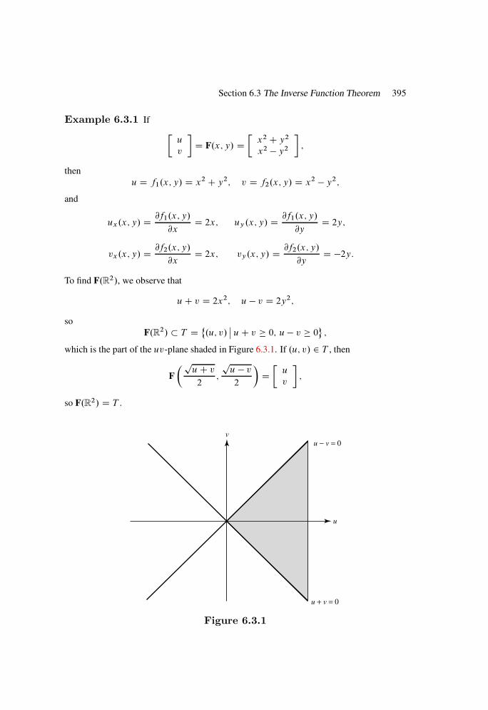
Section 6.3 The Inverse Function Theorem 395
Example 6.3.1 If
u
v
D F.x; y/ D
x2 C y2
x2 y2
;
then
u D f1.x; y/ D x2 C y2; v D f2.x; y/ D x2 y2;
and
ux.x; y/ [email protected]; y/
@xD 2x; uy .x; y/ D
@f1.x; y/
@yD 2y;
vx.x; y/ [email protected]; y/
@xD 2x; vy.x; y/ D
@f2.x; y/
@yD 2y:
To find F.R2/, we observe that
uC v D 2x2; u v D 2y2;
so
F.R2/ T D˚.u; v/
ˇuC v 0; u v 0
;
which is the part of the uv-plane shaded in Figure 6.3.1. If .u; v/ 2 T , then
F
puC v2
;
pu v2
Du
v
;
so F.R2/ D T .
v
u
u + v = 0
u − v = 0
Figure 6.3.1
396 Chapter 6 Vector-Valued Functions of Several Variables
Invertible Transformations
A transformation F is one-to-one, or invertible, if F.X1/ and F.X2/ are distinct whenever
X1 and X2 are distinct points of DF. In this case, we can define a function G on the range
R.F/ D˚UˇU D F.X/ for some X 2 DF
of F by defining G.U/ to be the unique point in DF such that F.U/ D U. Then
DG D R.F/ and R.G/ D DF:
Moreover, G is one-to-one,
G.F.X// D X; X 2 DF;
and
F.G.U// D U; U 2 DG:
We say that G is the inverse of F, and write G D F1. The relation between F and G is
symmetric; that is, F is also the inverse of G, and we write F D G1.
Example 6.3.2 The linear transformation
u
v
D L.x; y/ D
x yx C y
(6.3.1)
maps .x; y/ to .u; v/, where
u D x y;v D x C y: (6.3.2)
L is one-to-one and R.L/ D R2, since for each .u; v/ in R
2 there is exactly one .x; y/
such that L.x; y/ D .u; v/. This is so because the system (6.3.2) can be solved uniquely
for .x; y/ in terms of .u; v/:
x D 12.uC v/;
y D 12.uC v/:
(6.3.3)
Thus,
L1.u; v/ D 1
2
uC vuC v
:
Example 6.3.3 The linear transformation
u
v
D L1.x; y/ D
x C y
2x C 2y
maps .x; y/ onto .u; v/, where
u D x C y;
v D 2x C 2y: (6.3.4)
Section 6.3 The Inverse Function Theorem 397
L1 is not one-to-one, since every point on the line
x C y D c (constant)
is mapped onto the single point .c; 2c/. Hence, L1 does not have an inverse.
The crucial difference between the transformations of Examples 6.3.2 and 6.3.3 is that
the matrix of L is nonsingular while the matrix of L1 is singular. Thus, L (see (6.3.1)) can
be written as u
v
D1 11 1
x
y
; (6.3.5)
where the matrix has the inverse 24
12
12
12
12
35 :
(Verify.) Multiplying both sides of (6.3.5) by this matrix yields
24
12
12
12
12
35u
v
Dx
y
;
which is equivalent to (6.3.3).
Since the matrix 1 1
2 2
of L1 is singular, (6.3.4) cannot be solved uniquely for .x; y/ in terms of .u; v/. In fact, it
cannot be solved at all unless v D 2u.
The following theorem settles the question of invertibility of linear transformations from
Rn to R
n. We leave the proof to you (Exercise 6.3.2).
Theorem 6.3.1 The linear transformation
U D L.X/ D AX .Rn ! Rn/
is invertible if and only if A is nonsingular; in which case R.L/ D Rn and
L1.U/ D A1U:
Polar Coordinates
We will now briefly review polar coordinates, which we will use in some of the following
examples.
The coordinates of any point .x; y/ can be written in infinitely many ways as
x D r cos ; y D r sin ; (6.3.6)

398 Chapter 6 Vector-Valued Functions of Several Variables
where
r2 D x2 C y2
and, if r > 0, is the angle from the x-axis to the line segment from .0; 0/ to .x; y/,
measured counterclockwise (Figure 6.3.2).
y
x
x2 + y
2
(x, y)
θ
Figure 6.3.2
For each .x; y/ ¤ .0; 0/ there are infinitely many values of , differing by integral
multiples of 2 , that satisfy (6.3.6). If is any of these values, we say that is an argument
of .x; y/, and write
D arg.x; y/:
By itself, this does not define a function. However, if is an arbitrary fixed number, then
D arg.x; y/; < C 2;
does define a function, since every half-open interval Œ; C 2/ contains exactly one
argument of .x; y/.
We do not define arg.0; 0/, since (6.3.6) places no restriction on if .x; y/ D .0; 0/ and
therefore r D 0.
The transformation
r
D G.x; y/ D
24px2 C y2
arg.x; y/
35 ; arg.x; y/ < C 2;
is defined and one-to-one on
DG D˚.x; y/
ˇ.x; y/ ¤ .0; 0/
;
and its range is
R.G/ D˚.r; /
ˇr > 0; < C 2
:
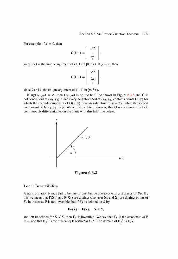
Section 6.3 The Inverse Function Theorem 399
For example, if D 0, then
G.1; 1/ D
264
p2
4
375 ;
since =4 is the unique argument of .1; 1/ in Œ0; 2/. If D , then
G.1; 1/ D
264
p2
9
4
375 ;
since 9=4 is the unique argument of .1; 1/ in Œ; 3/.
If arg.x0; y0/ D , then .x0; y0/ is on the half-line shown in Figure 6.3.3 and G is
not continuous at .x0; y0/, since every neighborhood of .x0; y0/ contains points .x; y/ for
which the second component of G.x; y/ is arbitrarily close to C 2 , while the second
component of G.x0; y0/ is . We will show later, however, that G is continuous, in fact,
continuously differentiable, on the plane with this half-line deleted.
y
x
(x0,
y
0)
φ
Figure 6.3.3
Local Invertibility
A transformation F may fail to be one-to-one, but be one-to-one on a subset S of DF. By
this we mean that F.X1/ and F.X2/ are distinct whenever X1 and X2 are distinct points of
S . In this case, F is not invertible, but if FS is defined on S by
FS .X/ D F.X/; X 2 S;
and left undefined for X 62 S , then FS is invertible. We say that FS is the restriction of F
to S , and that F1S
is the inverse of F restricted to S . The domain of F1S
is F.S/.

400 Chapter 6 Vector-Valued Functions of Several Variables
If F is one-to-one on a neighborhood of X0, we say that F is locally invertible at X0. If
this is true for every X0 in a set S , then F is locally invertible on S .
Example 6.3.4 The transformation
u
v
D F.x; y/ D
x2 y2
2xy
(6.3.7)
is not one-to-one, since
F.x;y/ D F.x; y/: (6.3.8)
It is one-to-one on S if and only if S does not contain any pair of distinct points of the form
.x0; y0/ and .x0;y0/; (6.3.8) implies the necessity of this condition, and its sufficiency
follows from the fact that if
F.x1; y1/ D F.x0; y0/; (6.3.9)
then
.x1; y1/ D .x0; y0/ or .x1; y1/ D .x0;y0/: (6.3.10)
To see this, suppose that (6.3.9) holds; then
x21 y2
1 D x20 y2
0 (6.3.11)
and
x1y1 D x0y0: (6.3.12)
Squaring both sides of (6.3.11) yields
x41 2x2
1y21 C y4
1 D x40 2x2
0y20 C y4
0 :
This and (6.3.12) imply that
x41 x4
0 D y40 y4
1 : (6.3.13)
From (6.3.11),
x21 x2
0 D y21 y2
0 : (6.3.14)
Factoring (6.3.13) yields
.x21 x2
0/.x21 C x2
0/ D .y20 y2
1 /.y20 C y2
1 /:
If either side of (6.3.14) is nonzero, we can cancel to obtain
x21 C x2
0 D y20 y2
1 ;
which implies that x0 D x1 D y0 D y1 D 0, so (6.3.10) holds in this case. On the other
hand, if both sides of (6.3.14) are zero, then
x1 D ˙x0; y1 D ˙y0:
From (6.3.12), the same sign must be chosen in these equalities, which proves that (6.3.8)
implies (6.3.10) in this case also.

Section 6.3 The Inverse Function Theorem 401
We now see, for example, that F is one-to-one on every set S of the form
S D˚.x; y/
ˇax C by > 0
;
where a and b are constants, not both zero. Geometrically, S is an open half-plane; that is,
the set of points on one side of, but not on, the line
ax C by D 0
(Figure 6.3.4). Therefore, F is locally invertible at every X0 ¤ .0; 0/, since every such
point lies in a half-plane of this form. However, F is not locally invertible at .0; 0/. (Why
not?) Thus, F is locally invertible on the entire plane with .0; 0/ removed.
y
x
ax + b
y = 0
(a, b )
ax + by > 0
Figure 6.3.4
It is instructive to find F1S
for a specific choice of S . Suppose that S is the open right
half-plane:
S D˚.x; y/
ˇx > 0
: (6.3.15)
Then F.S/ is the entire uv-plane except for the nonpositive u axis. To see this, note that
every point in S can be written in polar coordinates as
x D r cos ; y D r sin ; r > 0; 2< <
2:
Therefore, from (6.3.7), F.x; y/ has coordinates .u; v/, where
u D x2 y2 D r2.cos2 sin2 / D r2 cos 2;
v D 2xy D 2r2 cos sin D r2 sin 2:
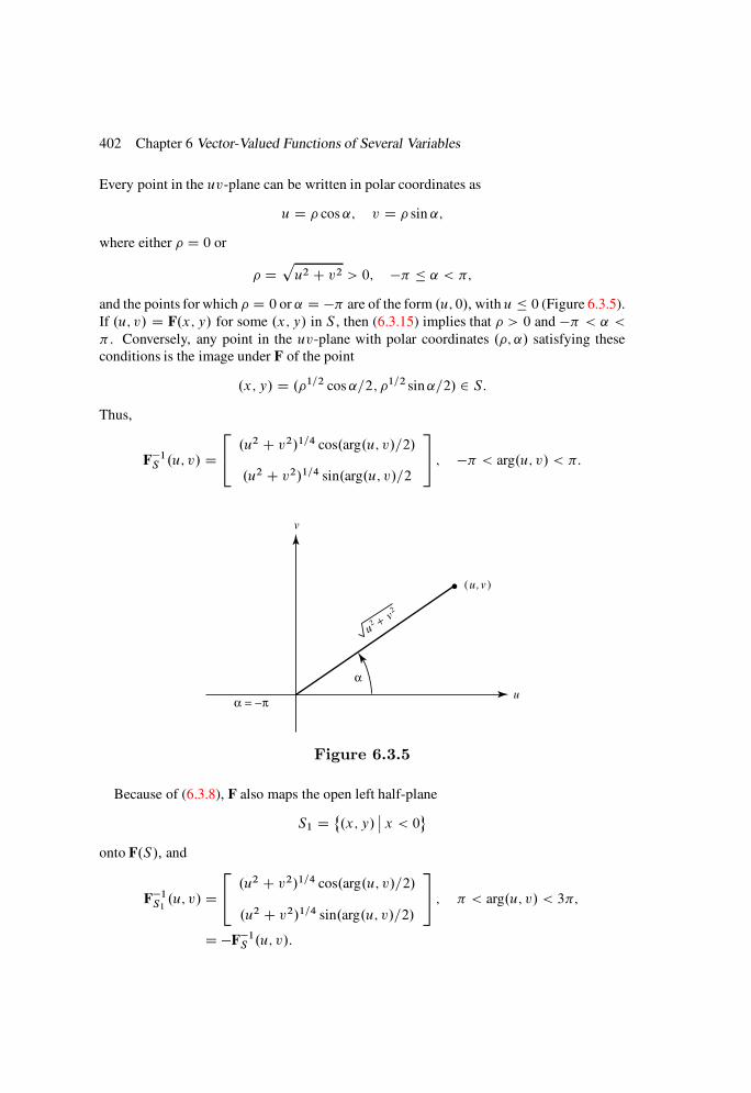
402 Chapter 6 Vector-Valued Functions of Several Variables
Every point in the uv-plane can be written in polar coordinates as
u D cos˛; v D sin ˛;
where either D 0 or
Dpu2 C v2 > 0; ˛ < ;
and the points for which D 0 or ˛ D are of the form .u; 0/, withu 0 (Figure 6.3.5).
If .u; v/ D F.x; y/ for some .x; y/ in S , then (6.3.15) implies that > 0 and < ˛ <
. Conversely, any point in the uv-plane with polar coordinates .; ˛/ satisfying these
conditions is the image under F of the point
.x; y/ D .1=2 cos˛=2; 1=2 sin˛=2/ 2 S:
Thus,
F1S .u; v/ D
24.u2 C v2/1=4 cos.arg.u; v/=2/
.u2 C v2/1=4 sin.arg.u; v/=2
35 ; < arg.u; v/ < :
v
u
(u,v )
α
α = −π
u2 + v
2
Figure 6.3.5
Because of (6.3.8), F also maps the open left half-plane
S1 D˚.x; y/
ˇx < 0
onto F.S/, and
F1S1.u; v/ D
24.u2 C v2/1=4 cos.arg.u; v/=2/
.u2 C v2/1=4 sin.arg.u; v/=2/
35 ; < arg.u; v/ < 3;
D F1S .u; v/:
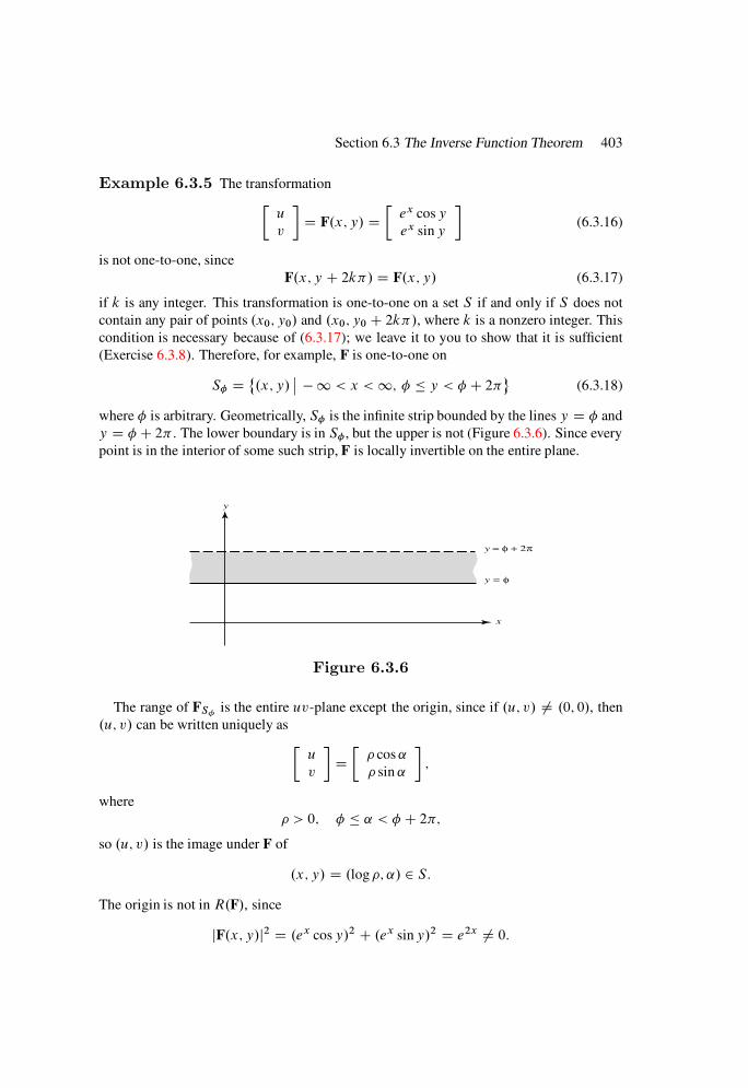
Section 6.3 The Inverse Function Theorem 403
Example 6.3.5 The transformation
u
v
D F.x; y/ D
ex cosy
ex sin y
(6.3.16)
is not one-to-one, since
F.x; y C 2k/ D F.x; y/ (6.3.17)
if k is any integer. This transformation is one-to-one on a set S if and only if S does not
contain any pair of points .x0; y0/ and .x0; y0 C 2k/, where k is a nonzero integer. This
condition is necessary because of (6.3.17); we leave it to you to show that it is sufficient
(Exercise 6.3.8). Therefore, for example, F is one-to-one on
S D˚.x; y/
ˇ1 < x <1; y < C 2
(6.3.18)
where is arbitrary. Geometrically, S is the infinite strip bounded by the lines y D and
y D C 2 . The lower boundary is in S , but the upper is not (Figure 6.3.6). Since every
point is in the interior of some such strip, F is locally invertible on the entire plane.
y
x
y = φ
y = φ + 2π
Figure 6.3.6
The range of FSis the entire uv-plane except the origin, since if .u; v/ ¤ .0; 0/, then
.u; v/ can be written uniquely as
u
v
D cos˛
sin ˛
;
where
> 0; ˛ < C 2;so .u; v/ is the image under F of
.x; y/ D .log; ˛/ 2 S:
The origin is not in R.F/, since
jF.x; y/j2 D .ex cosy/2 C .ex siny/2 D e2x ¤ 0:

404 Chapter 6 Vector-Valued Functions of Several Variables
Finally,
F1S.u; v/ D
24
log.u2 C v2/1=2
arg.u; v/
35 ; arg.u; v/ < C 2:
The domain of F1S
is the entire uv-plane except for .0; 0/.
Regular Transformations
The question of invertibility of an arbitrary transformation F W Rn ! Rn is too general to
have a useful answer. However, there is a useful and easily applicable sufficient condition
which implies that one-to-one restrictions of continuously differentiable transformations
have continuously differentiable inverses.
To motivate our study of this question, let us first consider the linear transformation
F.X/ D AX D
26664
a11 a12 a1n
a21 a22 a2n
::::::
: : ::::
an1 an2 ann
37775
26664
x1
x2
:::
xn
37775 :
From Theorem 6.3.1, F is invertible if and only if A is nonsingular, in which case R.F/ DR
n and
F1.U/ D A1U:
Since A and A1 are the differential matrices of F and F1, respectively, we can say that a
linear transformation is invertible if and only if its differential matrix F0 is nonsingular, in
which case the differential matrix of F1 is given by
.F1/0 D .F0/1:
Because of this, it is tempting to conjecture that if F W Rn ! Rn is continuously differen-
tiable and A0.X/ is nonsingular, or, equivalently, JF.X/ ¤ 0, for X in a set S , then F is
one-to-one on S . However, this is false. For example, if
F.x; y/ Dex cosy
ex sin y
;
then
JF.x; y/ Dˇˇ ex cosy ex siny
ex siny ex cosy
ˇˇ D e2x ¤ 0; (6.3.19)
but F is not one-to-one on R2 (Example 6.3.5). The best that can be said in general is
that if F is continuously differentiable and JF.X/ ¤ 0 in an open set S , then F is locally
invertible on S , and the local inverses are continuously differentiable. This is part of the
inverse function theorem, which we will prove presently. First, we need the following
definition.
Section 6.3 The Inverse Function Theorem 405
Definition 6.3.2 A transformation F W Rn ! R
n is regular on an open set S if F is
one-to-one and continuously differentiable on S , and JF.X/ ¤ 0 if X 2 S . We will also
say that F is regular on an arbitrary set S if F is regular on an open set containing S .
Example 6.3.6 If
F.x; y/ Dx yx C y
(Example 6.3.2), then
JF.x; y/ Dˇˇ 1 11 1
ˇˇ D 2;
so F is one-to-one on R2. Hence, F is regular on R
2.
If
F.x; y/ D
x C y
2x C 2y
(Example 6.3.3), then
JF.x; y/ Dˇˇ 1 1
2 2
ˇˇ D 0;
so F is not regular on any subset of R2.
If
F.x; y/ Dx2 y2
2xy
(Example 6.3.4), then
JF.x; y/ Dˇˇ 2x 2y2y 2x
ˇˇ D 2.x2 C y2/;
so F is regular on any open set S on which F is one-to-one, provided that .0; 0/ 62 S . For ex-
ample, F is regular on the open half-plane˚.x; y/
ˇx > 0
, since we saw in Example 6.3.4
that F is one-to-one on this half-plane.
If
F.x; y/ Dex cosy
ex cosy
(Example 6.3.5), then JF.x; y/ D e2x (see (6.3.19)), so F is regular on any open set on
which it is one-to-one. The interior of S in (6.3.18) is an example of such a set.
Theorem 6.3.3 Suppose that F W Rn ! R
n is regular on an open set S; and let
G D F1S : Then F.S/ is open; G is continuously differentiable on F.S/; and
G0.U/ D .F0.X//1 ; where U D F.X/:
Moreover; since G is one-to-one on F.S/; G is regular on F.S/:
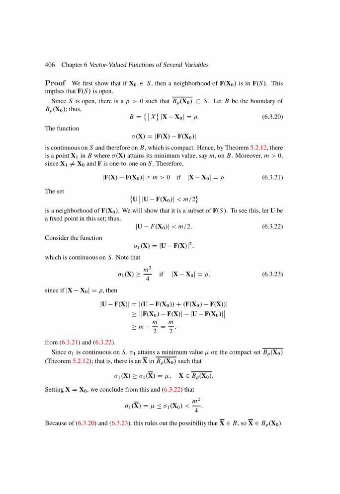
406 Chapter 6 Vector-Valued Functions of Several Variables
Proof We first show that if X0 2 S , then a neighborhood of F.X0/ is in F.S/. This
implies that F.S/ is open.
Since S is open, there is a > 0 such that B.X0/ S . Let B be the boundary of
B.X0/; thus,
B D˚ ˇXjX X0j D : (6.3.20)
The function
.X/ D jF.X/ F.X0/jis continuous on S and therefore on B , which is compact. Hence, by Theorem 5.2.12, there
is a point X1 in B where .X/ attains its minimum value, say m, on B . Moreover, m > 0,
since X1 ¤ X0 and F is one-to-one on S . Therefore,
jF.X/ F.X0/j m > 0 if jX X0j D : (6.3.21)
The set ˚UˇjU F.X0/j < m=2
is a neighborhood of F.X0/. We will show that it is a subset of F.S/. To see this, let U be
a fixed point in this set; thus,
jU F.X0/j < m=2: (6.3.22)
Consider the function
1.X/ D jU F.X/j2;which is continuous on S . Note that
1.X/ m2
4if jX X0j D ; (6.3.23)
since if jX X0j D , then
jU F.X/j D j.U F.X0//C .F.X0/ F.X//jˇjF.X0/ F.X/j jU F.X0/j
ˇ
mm
2Dm
2;
from (6.3.21) and (6.3.22).
Since 1 is continuous on S , 1 attains a minimum value on the compact set B.X0/
(Theorem 5.2.12); that is, there is an X in B.X0/ such that
1.X/ 1.X/ D ; X 2 B.X0/:
Setting X D X0, we conclude from this and (6.3.22) that
1.X/ D 1.X0/ <m2
4:
Because of (6.3.20) and (6.3.23), this rules out the possibility that X 2 B , so X 2 B.X0/.
Section 6.3 The Inverse Function Theorem 407
Now we want to show that D 0; that is, U D F.X/. To this end, we note that 1.X/
can be written as
1.X/ DnX
j D1
.uj fj .X//2 ;
so 1 is differentiable on Bp.X0/. Therefore, the first partial derivatives of 1 are all zero
at the local minimum point X (Theorem 5.3.11), so
nX
j D1
@fj .X/
@xi
.uj fj .X// D 0; 1 i n;
or, in matrix form,
F0.X/.U F.X// D 0:
Since F0.X/ is nonsingular this implies that U D F.X/ (Theorem 6.1.13). Thus, we have
shown that every U that satisfies (6.3.22) is in F.S/. Therefore, since X0 is an arbitrary
point of S , F.S/ is open.
Next, we show that G is continuous on F.S/. Suppose that U0 2 F.S/ and X0 is the
unique point in S such that F.X0/ D U0. Since F0.X0/ is invertible, Lemma 6.2.6 implies
that there is a > 0 and an open neighborhoodN of X0 such that N S and
jF.X/ F.X0/j jX X0j if X 2 N: (6.3.24)
(Exercise 6.2.18 also implies this.) Since F satisfies the hypotheses of the present theorem
on N , the first part of this proof shows that F.N / is an open set containing U0 D F.X0/.
Therefore, there is a ı > 0 such that X D G.U/ is inN if U 2 Bı.U0/. Setting X D G.U/
and X0 D G.U0/ in (6.3.24) yields
jF.G.U// F.G.U0//j jG.U/ G.U0/j if U 2 Bı.U0/:
Since F.G.U// D U, this can be rewritten as
jG.U/ G.U0/j 1
jU U0j if U 2 Bı.U0/; (6.3.25)
which means that G is continuous at U0. Since U0 is an arbitrary point in F.S/, it follows
that G is continous on F.S/.
We will now show that G is differentiable at U0. Since
G.F.X// D X; X 2 S;
the chain rule (Theorem 6.2.8) implies that if G is differentiable at U0, then
G0.U0/F0.X0/ D I

408 Chapter 6 Vector-Valued Functions of Several Variables
(Example 6.2.3). Therefore, if G is differentiable at U0, the differential matrix of G must
be
G0.U0/ D ŒF0.X0/1;
so to show that G is differentiable at U0, we must show that if
H.U/ D G.U/ G.U0/ ŒF0.X0/1.U U0/
jU U0j.U ¤ U0/; (6.3.26)
then
limU!U0
H.U/ D 0: (6.3.27)
Since F is one-to-one on S and F.G.U// D U, it follows that if U ¤ U0, then G.U/ ¤G.U0/. Therefore, we can multiply the numerator and denominator of (6.3.26) by jG.U/G.U0/j to obtain
H.U/ D jG.U/ G.U0jjU U0j
G.U/ G.U0/ ŒF0.X0/
1.U U0/
jG.U/ G.U0/j
!
D jG.U/ G.U0/jjU U0j
F0.X0/
1
U U0 F0.X0/.G.U/ G.U0//
jG.U/ G.U0/j
if 0 < jU U0j < ı. Because of (6.3.25), this implies that
jH.U/j 1
kŒF0.X0/
1kˇˇU U0 F0.X0/.G.U/ G.U0//
jG.U/ G.U0/j
ˇˇ
if 0 < jU U0j < ı. Now let
H1.U/ DU U0 F0.X0/.G.U/ G.U0//
jG.U/ G.U0/j
To complete the proof of (6.3.27), we must show that
limU!U0
H1.U/ D 0: (6.3.28)
Since F is differentiable at X0, we know that if
H2.X/ D limX!X0
F.X/ F.X0/ F0.X0/.X X0/
jX X0j;
then
limX!X0
H2.X/ D 0: (6.3.29)
Since F.G.U// D U and X0 D G.U0/,
H1.U/ D H2.G.U//:
Section 6.3 The Inverse Function Theorem 409
Now suppose that > 0. From (6.3.29), there is a ı1 > 0 such that
jH2.X/j < if 0 < jX X0j D jX G.U0/j < ı1: (6.3.30)
Since G is continuous at U0, there is a ı2 2 .0; ı/ such that
jG.U/ G.U0/j < ı1 if 0 < jU U0j < ı2:
This and (6.3.30) imply that
jH1.U/j D jH2.G.U//j < if 0 < jU U0j < ı2:
Since this implies (6.3.28), G is differentiable at X0.
Since U0 is an arbitrary member of F.N /, we can now drop the zero subscript and
conclude that G is continuous and differentiable on F.N /, and
G0.U/ D ŒF0.X/1; U 2 F.N /:
To see that G is continuously differentiable on F.N /, we observe that by Theorem 6.1.14,
each entry of G0.U/ (that is, each partial derivative @gi.U/=@uj , 1 i; j n) can be
written as the ratio, with nonzero denominator, of determinants with entries of the form
@fr.G.U//
@xs
: (6.3.31)
Since @fr=@xs is continuous on N and G is continuous on F.N /, Theorem 5.2.10 implies
that (6.3.31) is continuous on F.N /. Since a determinant is a continuous function of its
entries, it now follows that the entries of G0.U/ are continuous on F.N /.
Branches of the Inverse
If F is regular on an open set S , we say that F1S is a branch of F1. (This is a convenient
terminology but is not meant to imply that F actually has an inverse.) From this definition,
it is possible to define a branch of F1 on a set T R.F/ if and only if T D F.S/, where
F is regular on S . There may be open subsets of R.F/ that do not have this property, and
therefore no branch of F1 can be defined on them. It is also possible that T D F.S1/ DF.S2/, where S1 and S2 are distinct subsets of DF. In this case, more than one branch of
F1 is defined on T . Thus, we saw in Example 6.3.4 that two branches of F1 may be
defined on a set T . In Example 6.3.5 infinitely many branches of F1 are defined on the
same set.
It is useful to define branches of the argument To do this, we think of the relationship
between polar and rectangular coordinates in terms of the transformation
x
y
D F.r; / D
r cos
r sin
; (6.3.32)
where for the moment we regard r and as rectangular coordinates of a point in an r-
plane. Let S be an open subset of the right half of this plane (that is, S ˚.r; /
ˇr > 0
)

410 Chapter 6 Vector-Valued Functions of Several Variables
that does not contain any pair of points .r; / and .r; C2k/, where k is a nonzero integer.
Then F is one-to-one and continuously differentiable on S , with
F0.r; / D
cos r sin
sin r cos
(6.3.33)
and
JF.r; / D r > 0; .r; / 2 S: (6.3.34)
Hence, F is regular on S . Now let T D F.S/, the set of points in the xy-plane with
polar coordinates in S . Theorem 6.3.3 states that T is open and FS has a continuously
differentiable inverse (which we denote by G, rather than F1S
, for typographical reasons)
r
D G.x; y/ D
24px2 C y2
argS .x; y/
35 ; .x; y/ 2 T;
where argS .x; y/ is the unique value of arg.x; y/ such that
.r; / Dp
x2 C y2; argS .x; y/2 S:
We say that argS.x; y/ is a branch of the argument defined on T . Theorem 6.3.3 also
implies that
G0.x; y/ DF0.r; /
1 D"
cos sin
sin
r
cos
r
#(see (6.3.33))
D
264
xpx2 C y2
ypx2 C y2
y
x2 C y2
x
x2 C y2
375 (see (6.3.32)):
Therefore,
@ argS .x; y/
@xD y
x2 C y2;
@ argS .x; y/
@yD x
x2 C y2: (6.3.35)
A branch of arg.x; y/ can be defined on an open set T of the xy-plane if and only if
the polar coordinates of the points in T form an open subset of the r-plane that does not
intersect the -axis or contain any two points of the form .r; / and .r; C 2k/, where
k is a nonzero integer. No subset containing the origin .x; y/ D .0; 0/ has this property,
nor does any deleted neighborhood of the origin (Exercise 6.3.14), so there are open sets
on which no branch of the argument can be defined. However, if one branch can be defined
on T , then so can infinitely many others. (Why?) All branches of arg.x; y/ have the same
partial derivatives, given in (6.3.35).

Section 6.3 The Inverse Function Theorem 411
Example 6.3.7 The set
T D˚.x; y/
ˇ.x; y/ ¤ .x; 0/ with x 0
;
which is the entire xy-plane with the nonnegative x-axis deleted, can be written as T DF.Sk/, where F is as in (6.3.32), k is an integer, and
Sk D˚.r; /
ˇr > 0; 2k < < 2.k C 1/
:
For each integer k, we can define a branch argSk.x; y/ of the argument in Sk by taking
argSk.x; y/ to be the value of arg.x; y/ that satisfies
2k < argSk.x; y/ < 2.k C 1/:
Each of these branches is continuously differentiable in T , with derivatives as given in
(6.3.35), and
argSk.x; y/ argSj
.x; y/ D 2.k j /; .x; y/ 2 T:
Example 6.3.8 Returning to the transformationu
v
D F.x; y/ D
x2 y2
2xy
;
we now see from Example 6.3.4 that a branch G of F1 can be defined on any subset T of
the uv-plane on which a branch of arg.u; v/ can be defined, and G has the form
x
y
D G.u; v/ D
24.u2 C v2/1=4 cos.arg.u; v/=2/
.u2 C v2/1=4 sin.arg.u; v/=2/
35 ; .u; v/ 2 T; (6.3.36)
where arg.u; v/ is a branch of the argument defined on T . If G1 and G2 are different
branches of F1 defined on the same set T , then G1 D ˙G2. (Why?)
From Theorem 6.3.3,
G0.u; v/ DF0.x; y/
1 D2x 2y2y 2x
1
D 1
2.x2 C y2/
x y
y x
:
Substituting for x and y in terms of u and v from (6.3.36), we find that
@x
@uD @y
@vD x
2.x2 C y2/D 1
2.u2 C v2/1=4cos.arg.u; v/=2/ (6.3.37)
and@x
@vD @y
@uD y
2.x2 C y2/D 1
2.u2 C v2/1=4sin.arg.u; v/=2/: (6.3.38)
It is essential that the same branch of the argument be used here and in (6.3.36).
412 Chapter 6 Vector-Valued Functions of Several Variables
We leave it to you (Exercise 6.3.16) to verify that (6.3.37) and (6.3.38) can also be
obtained by differentiating (6.3.36) directly.
Example 6.3.9 If u
v
D F.x; y/ D
ex cos y
ex siny
(Example 6.3.5), we can also define a branch G of F1 on any subset T of the uv-plane on
which a branch of arg.u; v/ can be defined, and G has the form
x
y
D G.u; v/ D
log.u2 C v2/1=2
arg.u; v/
: (6.3.39)
Since the branches of the argument differ by integral multiples of 2 , (6.3.39) implies that
if G1 and G2 are branches of F1, both defined on T , then
G1.u; v/ G2.u; v/ D
0
2k
(k D integer):
From Theorem 6.3.3,
G0.u; v/ DF0.x; y/
1 Dex cos y ex siny
ex sin y ex cosy
1
D
ex cosy ex siny
ex siny ex cosy
:
Substituting for x and y in terms of u and v from (6.3.39), we find that
@x
@uD @y
@vD ex cosy D e2xu D u
u2 C v2
and@x
@vD @y
@uD ex siny D e2xv D v
u2 C v2:
The Inverse Function Theorem
Examples 6.3.4 and 6.3.5 show that a continuously differentiable function F may fail to
have an inverse on a set S even if JF.X/ ¤ 0 on S . However, the next theorem shows that
in this case F is locally invertible on S .
Theorem 6.3.4 (The Inverse Function Theorem) Let F W Rn ! R
n be
continuously differentiable on an open set S; and suppose that JF.X/ ¤ 0 on S: Then; if
X0 2 S; there is an open neighborhoodN of X0 on which F is regular: Moreover; F.N /
is open and G D F1N
is continuously differentiable on F.N /; with
G0.U/ DF0.X/
1.where U D F.X//; U 2 F.N /:

Section 6.3 The Inverse Function Theorem 413
Proof Lemma 6.2.6 implies that there is an open neighborhoodN of X0 on which F is
one-to-one. The rest of the conclusions then follow from applying Theorem 6.3.3 to F on
N .
Corollary 6.3.5 If F is continuously differentiable on a neighborhood of X0 and JF.X0/ ¤0; then there is an open neighborhoodN of X0 on which the conclusions of Theorem 6.3.4
hold:
Proof By continuity, since JF0.X0/ ¤ 0, JF0.X/ is nonzero for all X in some open
neighborhood S of X0. Now apply Theorem 6.3.4.
Example 6.3.10 Let X0 D .1; 2; 1/ and
24u
v
w
35 D F.x; y; ´/ D
24x C y C .´ 1/2 C 1y C ´C .x 1/2 1´C x C .y 2/2 C 3
35 :
Then
F0.x; y; ´/ D
24
1 1 2´ 22x 2 1 1
1 2y 4 1
35 ;
so
JF.X0/ D
ˇˇˇ1 1 0
0 1 1
1 0 1
ˇˇˇ D 2:
In this case, it is difficult to describeN or find G D F1N explicitly; however, we know that
F.N / is a neighborhood of U0 D F.X0/ D .4; 2; 5/, that G.U0/ D X0 D .1; 2; 1/, and
that
G0.U0/ DF0.X0/
1 D
241 1 0
0 1 1
1 0 1
35
1
D 1
2
24
1 1 1
1 1 11 1 1
35 :
Therefore,
G.U/ D
241
2
1
35C 1
2
24
1 1 1
1 1 11 1 1
3524u 4v 2w 5
35C E.U/;
where
limU!.4;2;5/
E.U/p.u 4/2 C .v 2/2 C .w 5/2
D 0I
thus we have approximated G near U0 D .4; 2; 5/ by an affine transformation.
Theorem 6.3.4 and (6.3.34) imply that the transformation (6.3.32) is locally invertible
on S D˚.r; /
ˇr > 0
, which means that it is possible to define a branch of arg.x; y/ in a
neighborhood of any point .x0; y0/ ¤ .0; 0/. It also implies, as we have already seen, that
414 Chapter 6 Vector-Valued Functions of Several Variables
the transformation (6.3.7) of Example 6.3.4 is locally invertible everywhere except at .0; 0/,
where its Jacobian equals zero, and the transformation (6.3.16) of Example 6.3.5 is locally
invertible everywhere.
6.3 Exercises
1. Prove: If F is invertible, then F1 is unique.
2. Prove Theorem 6.3.1.
3. Prove: The linear transformation L.X/ D AX cannot be one-to-one on any open set
if A is singular. HINT: Use Theorem 6.1.15:
4. Let
G.x; y/ D" p
x2 C y2
arg.x; y/
#; =2 arg.x; y/ < 5=2:
Find
(a) G.0; 1/ (b) G.1; 0/ (c) G.1; 0/
(d) G.2; 2/ (e) G.1; 1/5. Same as Exercise 6.3.4, except that 2 arg.x; y/ < 0.
6. (a) Prove: If f W R ! R is continuous and locally invertible on .a; b/, then f is
invertible on .a; b/.
(b) Give an example showing that the continuity assumption is needed in (a).
7. Let
F.x; y/ Dx2 y2
2xy
(Example 6.3.4) and
S D˚.x; y/
ˇax C by > 0
.a2 C b2 ¤ 0/:
Find F.S/ and F1S
. If
S1 D˚.x; y/
ˇax C by < 0
;
show that F.S1/ D F.S/ and F1S1D F1
S .
8. Show that the transformation
u
v
D F.x; y/ D
ex cosy
ex siny
(Example 6.3.5) is one-to-one on any set S that does not contain any pair of points
.x0; y0/ and .x0; y0 C 2k/, where k is a nonzero integer.

Section 6.3 The Inverse Function Theorem 415
9. Suppose that F W Rn ! Rn is continuous and invertible on a compact set S . Show
that F1S
is continuous. HINT: If F1S
is not continuous at U in F.S/; then there is
an 0 > 0 and a sequence fUkg in F.S/ such that limk!1 Uk D U while
jF1S .Uk/ F1
S .U/j 0; k 1:
Use Exercise 5.1.32 to obtain a contradiction:
10. Find F1 and .F1/0:
(a)
u
v
D F.x; y/ D
4x C 2y3x C y
(b)
24u
v
w
35 D F.x; y; ´/ D
24x C y C 2´3xC y 4´x y C 2´
35
11. In addition to the assumptions of Theorem 6.3.3, suppose that all qth-order .q > 1/
partial derivatives of the components of F are continuous on S . Show that all qth-
order partial derivatives of F1S
are continuous on F.S/.
12. If u
v
D F.x; y/ D
x2 C y2
x2 y2
(Example 6.3.1), find four branches G1, G2, G3, and G4 of F1 defined on
T1 D˚.u; v/
ˇuC v > 0; u v > 0
;
and verify that G0i .u; v/ D .F0.x.u; v/; y.u; v///1 , 1 i 4.
13. Suppose that A is a nonsingular n n matrix and
U D F.X/ D A
26664
x21
x22:::
x2n
37775 :
(a) Show that F is regular on the set
S D˚Xˇeixi > 0; 1 i n
;
where ei D ˙1, 1 i n.
(b) Find F1S.U/. (c) Find .F1
S/0.U/.
14. Let .x; y/ be a branch of arg.x; y/ defined on an open set S .
(a) Show that .x; y/ cannot assume a local extreme value at any point of S .
(b) Prove: If a ¤ 0 and the line segment from .x0; y0/ to .ax0; ay0/ is in S , then
.ax0; ay0/ D .x0; y0/.
(c) Show that S cannot contain a subset of the form
A Dn.x; y/
ˇ0 < r1
px2 C y2 r2
o:
416 Chapter 6 Vector-Valued Functions of Several Variables
(d) Show that no branch of arg.x; y/ can be defined on a deleted neighborhood
of the origin.
15. Obtain Eqn. (6.3.35) formally by differentiating:
(a) arg.x; y/ D cos1 xpx2 C y2
(b) arg.x; y/ D sin1 ypx2 C y2
(c) arg.x; y/ D tan1 y
x
Where do these formulas come from? What is the disadvantage of using any one of
them to define arg.x; y/?
16. For the transformation
u
v
D F.x; y/ D
x2 y2
2xy
(Example 6.3.4), find a branch G of F1 defined on T D˚.u; v/
ˇauC bv > 0
.
Find G0 by means of the formula G0.U/ D ŒF0.X/1 of Theorem 6.3.3, and also by
direct differentiation with respect to u and v.
17. A transformation
F.x; y/ Du.x; y/
v.x; y/
is analytic on a set S if it is continuously differentiable and
ux D vy ; uy D vx
on S . Prove: If F is analytic and regular on S , then F1S
is analytic on F.S/; that is,
xu D uv and xv D uu.
18. Prove: If U D F.X/ and X D G.U/ are inverse functions, then
@.u1; u2; : : : ; un/
@.x1; x2; : : : ; xn
@.x1; x2; : : : ; xn/
@.u1; u2; : : : ; un/D 1:
Where should the Jacobians be evaluated?
19. Give an example of a transformation F W Rn ! Rn that is invertible but not regular
on Rn.
20. Find an affine transformation A that so well approximates the branch G of F1
defined near U0 D F.X0/ that
limU!U0
G.U/ A.U/
jU U0jD 0:
(a)
u
v
D F.x; y/ D
x4y5 4xx3y2 3y
; X0 D .1;1/

Section 6.4 The Implicit Function Theorem 417
(b)
u
v
D F.x; y/ D
x2y C xy2xy C xy2
; X0 D .1; 1/
(c)
24u
v
w
35 D F.x; y; ´/ D
242x2y C x3 C ´
x3 C y´x C y C ´
35 ; X D .0; 1; 1/
(d)
24u
v
w
35 D F.x; y; ´/ D
24x cos y cos ´
x siny cos ´
x sin´
35 ; X0 D .1; =2; /
21. If F is defined by24x
y
´
35 D F.r; ; / D
24r cos cos
r sin cos
r sin
35
and G is a branch of F1, find G0 in terms of r , , and . HINT: See Exer-
cise 6.2.14.b/:
22. If F is defined by 24x
y
´
35 D F.r; ; ´/ D
24r cos
r sin
´
35
and G is a branch of F1, find G0 in terms of r , , and ´. HINT: See Exer-
cise 6.2.14.c/:
23. Suppose that F W Rn ! R
n is regular on a compact set T . Show that F.@T / [email protected] /; that is, boundary points map to boundary points. HINT: Use Exercise 6.2.23
and Theorem 6.3.3 to show that @F.T / F.@T /: Then apply this result with F and
T replaced by F1 and F.T / to show that F.@T / @F.T /:
6.4 THE IMPLICIT FUNCTION THEOREM
In this section we consider transformations from RnCm to R
m. It will be convenient to
denote points in RnCm by
.X;U/ D .x1; x2; : : : ; xn; u1; u2; : : : ; um/:
We will often denote the components of X by x, y, . . . , and the components of U by u, v,
. . . .
To motivate the problem we are interested in, we first ask whether the linear system of
m equations in mC n variables
a11x1 C a12x2 C C a1nxn C b11u1 C b12u2 C C b1mum D 0a21x1 C a22x2 C C a2nxn C b21u1 C b22ux C C b2mum D 0
:::
am1x1 C am2x2 C C amnxn C bm1u1 C bm2u2 C C bmmum D 0
(6.4.1)

418 Chapter 6 Vector-Valued Functions of Several Variables
determines u1, u2, . . . , um uniquely in terms of x1, x2, . . . , xn. By rewriting the system in
matrix form as
AXC BU D 0;
where
A D
26664
a11 a12 a1n
a21 a22 a2n
::::::
: : ::::
am1 am2 amn
37775 ; B D
26664
b11 b12 b1m
b21 b22 b2m
::::::
: : ::::
bm1 bm2 bmm
37775 ;
X D
26664
x1
x2
:::
xn
37775 ; and U D
26664
u1
u2
:::
um
37775 ;
we see that (6.4.1) can be solved uniquely for U in terms of X if the square matrix B is
nonsingular. In this case the solution is
U D B1AX:
For our purposes it is convenient to restate this: If
F.X;U/ D AXC BU; (6.4.2)
where B is nonsingular, then the system
F.X;U/ D 0
determines U as a function of X, for all X in Rn.
Notice that F in (6.4.2) is a linear transformation. If F is a more general transformation
from RnCm to R
m, we can still ask whether the system
F.X;U/ D 0;
or, in terms of components,
f1.x1; x2; : : : ; xn; u1; u2; : : : ; um/ D 0f2.x1; x2; : : : ; xn; u1; u2; : : : ; um/ D 0
:::
fm.x1; x2; : : : ; xn; u1; u2; : : : ; um/ D 0;
can be solved for U in terms of X. However, the situation is now more complicated, even
if m D 1. For example, suppose that m D 1 and
f .x; y; u/ D 1 x2 y2 u2:

Section 6.4 The Implicit Function Theorem 419
If x2 C y2 > 1, then no value of u satisfies
f .x; y; u/ D 0: (6.4.3)
However, infinitely many functions u D u.x; y/ satisfy (6.4.3) on the set
S D˚.x; y/
ˇx2 C y2 1
:
They are of the form
u.x; y/ D .x; y/p1 x2 y2;
where .x; y/ can be chosen arbitrarily, for each .x; y/ in S , to be 1 or 1. We can narrow
the choice of functions to two by requiring that u be continuous on S ; then
u.x; y/ Dp1 x2 y2 (6.4.4)
or
u.x; y/ D p1 x2 y2:
We can define a unique continuous solution u of (6.4.3) by specifying its value at a single
interior point of S . For example, if we require that
u
1p3;1p3
D 1p
3;
then u must be as defined by (6.4.4).
The question of whether an arbitrary system
F.X;U/ D 0
determines U as a function of X is too general to have a useful answer. However, there
is a theorem, the implicit function theorem, that answers this question affirmatively in
an important special case. To facilitate the statement of this theorem, we partition the
differential matrix of F W RnCm ! Rm:
F0 D
26666666664
@f1
@x1
@f1
@x2
@f1
@xn
j @f1
@u1
@f1
@u2
@f1
@um
@f2
@x1
@f2
@x2
@f2
@xn
j @f2
@u1
@f2
@u2
@f2
@um
::::::
: : :::: j
::::::
: : ::::
@fm
@x1
@fm
@x2
@fm
@xn
j @fm
@u1
@fm
@u2
@fm
@um
37777777775
(6.4.5)
or
F0 D ŒFX;FU;
where FX is the submatrix to the left of the dashed line in (6.4.5) and FU is to the right.
For the linear transformation (6.4.2), FX D A and FU D B, and we have seen that the
system F.X;U/ D 0 defines U as a function of X for all X in Rn if FU is nonsingular. The
next theorem shows that a related result holds for more general transformations.
420 Chapter 6 Vector-Valued Functions of Several Variables
Theorem 6.4.1 (The Implicit Function Theorem) Suppose that F W RnCm !R
m is continuously differentiable on an open set S of RnCm containing .X0;U0/: Let
F.X0;U0/ D 0; and suppose that FU.X0;U0/ is nonsingular:Then there is a neighborhood
M of .X0;U0/; contained in S; on which FU.X;U/ is nonsingular and a neighborhoodN
of X0 in Rn on which a unique continuously differentiable transformation G W Rn ! R
m
is defined; such that G.X0/ D U0 and
.X;G.X// 2 M and F.X;G.X// D 0 if X 2 N: (6.4.6)
Moreover;
G0.X/ D ŒFU.X;G.X//1FX.X;G.X//; X 2 N: (6.4.7)
Proof Define ˆ W RnCm ! RnCm by
ˆ.X;U/ D
266666666666664
x1
x2
:::
xn
f1.X;U/
f2.X;U/:::
fm.X;U/
377777777777775
(6.4.8)
or, in “horizontal”notation by
ˆ.X;U/ D .X;F.X;U//: (6.4.9)
Then ˆ is continuously differentiable on S and, since F.X0;U0/ D 0,
ˆ.X0;U0/ D .X0; 0/: (6.4.10)
The differential matrix of ˆ is
ˆ0 D
2666666666666666666666664
1 0 0 0 0 0
0 1 0 0 0 0:::
:::: : :
::::::
:::: : :
:::
0 0 1 0 0 0
@f1
@x1
@f1
@x2
@f1
@xn
@f1
@u1
@f1
@u2
@f1
@um
@f2
@x1
@f2
@x2
@f2
@xn
@f2
@u1
@f2
@u2
@f2
@um
::::::
: : ::::
::::::
: : ::::
@fm
@x1
@fm
@x2
@fm
@xn
@fm
@u1
@fm
@u2
@fm
@um
3777777777777777777777775
D
I 0
FX FU
;
Section 6.4 The Implicit Function Theorem 421
where I is the n n identity matrix, 0 is the n m matrix with all zero entries, and FX
and FU are as in (6.4.5). By expanding det.ˆ0/ and the determinants that evolve from it in
terms of the cofactors of their first rows, it can be shown in n steps that
Jˆ D det.ˆ0/ D
ˇˇˇˇˇˇˇˇ
@f1
@u1
@f1
@u2
@f1
@um
@f2
@u1
@f2
@u2
@f2
@um
::::::
: : ::::
@fm
@u1
@fm
@u2
@fm
@um
ˇˇˇˇˇˇˇˇ
D det.FU/:
In particular,
Jˆ.X0;U0/ D det.FU.X0;U0/ ¤ 0:Since ˆ is continuously differentiable on S , Corollary 6.3.5 implies that ˆ is regular on
some open neighborhoodM of .X0;U0/ and that cM D ˆ.M/ is open.
Because of the form of ˆ (see (6.4.8) or (6.4.9)), we can write points of cM as .X;V/,
where V 2 Rm. Corollary 6.3.5 also implies that ˆ has a a continuously differentiable
inverse .X;V/ defined on cM with values in M . Since ˆ leaves the “X part" of .X;U/
fixed, a local inverse of ˆ must also have this property. Therefore, must have the form
.X;V/ D
266666666666666664
x1
x2
:::
xn
h1.X;V/
h2.X;V/:::
hm.X;V/
377777777777777775
or, in “horizontal” notation,
.X;V/ D .X;H.X;V//;where H W RnCm ! R
m is continuously differentiable on cM . We will show that G.X/ DH.X; 0/ has the stated properties.
From (6.4.10), .X0; 0/ 2 cM and, since cM is open, there is a neighborhoodN of X0 in
Rn such that .X; 0/ 2cM if X 2 N (Exercise 6.4.2). Therefore, .X;G.X// D .X; 0/ 2 M
if X 2 N . Since D ˆ1, .X; 0/ D ˆ.X;G.X//. Setting X D X0 and recalling (6.4.10)
shows that G.X0/ D U0, since ˆ is one-to-one onM .
422 Chapter 6 Vector-Valued Functions of Several Variables
Henceforth we assume that X 2 N . Now,
.X; 0/ D ˆ. .X; 0// (since ˆ D 1/
D ˆ.X;G.X// (since .X; 0/ D .X;G.X//)D .X;F.X;G.X/// (since ˆ.X;U/ D .X;F.X;U//):
Therefore, F.X;G.X// D 0; that is, G satisfies (6.4.6). To see that G is unique, suppose
that G1 W Rn ! Rm also satisfies (6.4.6). Then
ˆ.X;G.X// D .X;F.X;G.X/// D .X; 0/
and
ˆ.X;G1.X// D .X;F.X;G1.X/// D .X; 0/for all X in N . Since ˆ is one-to-one on M , this implies that G.X/ D G1.X/.
Since the partial derivatives
@hi
@xj
; 1 i m; 1 j n;
are continuous functions of .X;V/ on cM , they are continuous with respect to X on the
subset˚.X; 0/
ˇX 2 N
ofcM . Therefore, G is continuously differentiable onN . To verify
(6.4.7), we write F.X;G.X// D 0 in terms of components; thus,
fi .x1; x2; : : : ; xn; g1.X/; g2.X/; : : : ; gm.X// D 0; 1 i m; X 2 N:
Since fi and g1, g2, . . . , gm are continuously differentiable on their respective domains,
the chain rule (Theorem 5.4.3) implies that
@fi .X;G.X//
@xj
CmX
rD1
@fi .X;G.X//
@ur
@gr.X/
@xj
D 0; 1 i m; 1 j n; (6.4.11)
or, in matrix form,
FX.X;G.X// C FU.X;G.X//G0.X/ D 0: (6.4.12)
Since .X;G.X// 2 M for all X in N and FU.X;U/ is nonsingular when .X;U/ 2 M , we
can multiply (6.4.12) on the left by F1U.X;G.X// to obtain (6.4.7). This completes the
proof.
In Theorem 6.4.1 we denoted the implicitly defined transformation by G for reasons
of clarity in the proof. However, in applying the theorem it is convenient to denote the
transformation more informally by U D U.X/; thus, U.X0/ D U0, and we replace (6.4.6)
and (6.4.7) by
.X;U.X// 2M and X.X;U.X// D 0 if X 2 N;
and
U0.X/ D ŒFU.X;U.X//1FX.X;U.X//; X 2 N;

Section 6.4 The Implicit Function Theorem 423
while (6.4.11) becomes
@fi
@xj
CmX
rD1
@fi
@ur
@ur
@xj
D 0; 1 i m; 1 j n; (6.4.13)
it being understood that the partial derivatives of ur and fi are evaluated at X and .X;U.X//,
respectively.
The following corollary is the implicit function theorem for m D 1.
Corollary 6.4.2 Suppose that f W RnC1 ! R is continuously differentiable on an
open set containing .X0; u0/; with f .X0; u0/ D 0 and fu.X0; u0/ ¤ 0. Then there is a
neighborhoodM of .X0; u0/; contained in S; and a neighborhoodN of X0 in Rn on which
is defined a unique continuously differentiable function u D u.X/ W Rn ! R such that
.X; u.X// 2M and fu.X; u.X// ¤ 0; X 2 N;
u.X0/ D u0; and f .X; u.X// D 0; X 2 N:The partial derivatives of u are given by
uxi.X/ D fxi
.X; u.X//
fu.X; u.X//; 1 i n:
Example 6.4.1 Let
f .x; y; u/ D 1 x2 y2 u2
and .x0; y0; u0/ D .12;1
2; 1p
2/. Then f .x0; y0; ´0/ D 0 and
fx.x; y; u/ D 2x; fy.x; y; u/ D 2y; fu.x; y; u/ D 2u:
Since f is continuously differentiable everywhere and fu.x0; y0; u0/ D p2 ¤ 0, Corol-
lary 6.4.2 implies that the conditions
1 x2 y2 u2 D 0; u.1=2;1=2/D 1p2;
determine u D u.x; y/ near .x0; y0/ D .12;1
2/ so that
ux.x; y/ D fx.x; y; u.x; y//
fu.x; y; u.x; y//D xu.x; y/
; (6.4.14)
and
uy.x; y/ D fy .x; y; u.x; y//
fu.x; y; u.x; y//D yu.x; y/
: (6.4.15)
It is not necessary to memorize formulas like (6.4.14) and (6.4.15). Since we know that
f and u are differentiable, we can obtain (6.4.14) and (6.4.15) by applying the chain rule
to the identity
f .x; y; u.x; y// D 0:

424 Chapter 6 Vector-Valued Functions of Several Variables
Example 6.4.2 Let
f .x; y; u/ D x3y2u2 C 3xy4u4 3x6y6u7 C 12x 13 (6.4.16)
and .x0; y0; u0/ D .1;1; 1/, so f .x0; y0; u0/ D 0. Then
fx.x; y; u/ D 3x2y2u2 C 3y4u4 18x5y6u7 C 12;fy.x; y; u/ D 2x3yu2 C 12xy3u4 18x6y5u7;
fu.x; y; u/ D 2x3y2uC 12xy4u3 21x6y6u6:
Since fu.1;1; 1/ D 7 ¤ 0, Corollary 6.4.2 implies that the conditions
f .x; y; u/ D 0; u.1;1/ D 1 (6.4.17)
determine u as a continuously differentiable function of .x; y/ near .1;1/.
If we try to solve (6.4.16) for u, we see very clearly that Theorem 6.4.1 and Corol-
lary 6.4.2 are existence theorems; that is, they tell us that there is a function u D u.x; y/
that satisfies (6.4.17), but not how to find it. In this case there is no convenient formula for
the function, although its partial derivatives can be expressed conveniently in terms of x,
y, and u.x; y/:
ux.x; y/ D fx.x; y; u.x; y//
fu.x; y; u.x; y//; uy.x; y/ D
fy.x; y; u.x; y//
fu.x; y; u.x; y//:
In particular, since u.1;1/ D 1,
ux.1;1/ D 0
7D 0; uy.1;1/ D
4
7D 4
7:
Example 6.4.3 Let
X D
24x
y
´
35 and U D
u
v
;
and
F.X;U/ D2x2 C y2 C ´2 C u2 v2
x2 C ´2 C 2u v
:
If X0 D .1;1; 1/ and U0 D .0; 2/, then F.X0;U0/ D 0. Moreover,
FU.X;U/ D2u 2v2 1
and FX D
4x 2y 2´
2x 0 2´
;
so
det.FU.X0;U0// Dˇˇ 0 42 1
ˇˇ D 8 ¤ 0:

Section 6.4 The Implicit Function Theorem 425
Hence, the conditions
F.X;U/ D 0; U.1;1; 1/ D .0; 2/
determine U D U.X/ near X0. Although it is difficult to find U.X/ explicitly, we can
approximate U.X/ near X0 by an affine transformation. Thus, from (6.4.7),
U0.X0/ D ŒFU.X0;U.X0//1FX.X0;U.X0// (6.4.18)
D 0 42 1
1 4 2 2
2 0 2
D 18
1 4
2 0
4 2 2
2 0 2
D 18
4 2 6
8 4 4
:
Therefore,
limX!.1;1;1/
u.x; y/
v.x; y/
0
2
C 1
8
4 2 6
8 4 4
24x 1y C 1´ 1
35
Œ.x 1/2 C .y C 1/2 C .´ 1/21=2D0
0
:
Again, it is not necessary to memorize (6.4.18), since the partial derivatives of an implic-
itly defined function can be obtained from the chain rule and Cramer’s rule, as in the next
example.
Example 6.4.4 Let u D u.x; y/ and v D v.x; y/ be differentiable and satisfy
x2 C 2y2 C 3´2 C u2 C v D 6
2x3 C 4y2 C 2´2 C uC v2 D 9(6.4.19)
and
u.1;1; 0/ D 1; v.1;1; 0/ D 2: (6.4.20)
To find ux and vx, we differentiate (6.4.19) with respect to x to obtain
2x C 2uux C vx D 06x2 C ux C 2vvx D 0:
Therefore, 2u 1
1 2v
ux
vx
D
2x
6x2
;
426 Chapter 6 Vector-Valued Functions of Several Variables
and Cramer’s rule yields
ux D
ˇˇ 2x 1
6x2 2v
ˇˇ
ˇˇ 2u 1
1 2v
ˇˇD 6x2 4xv
4uv 1
and
vx D
ˇˇ 2u 2x
1 6x2
ˇˇ
ˇˇ 2u 1
1 2v
ˇˇD 2x 12x2u
4uv 1
if 4uv ¤ 1. In particular, from (6.4.20),
ux.1;1; 0/ D29D 2
9; vx.1;1; 0/ D
14
9D 14
9:
Jacobians
It is convenient to extend the notation introduced in Section 6.2 for the Jacobian of a trans-
formation F W Rm ! R
m. If f1, f2, . . . , fm are real-valued functions of k variables,
k m, and 1, 2, . . . , m are any m of the variables, then we call the determinant
ˇˇˇˇˇˇˇˇˇ
@f1
@1
@f1
@2
@f1
@m
@f2
@1
@f2
@2
@f2
@m
::::::
: : ::::
@fm
@1
@fm
@2
@fm
@m
ˇˇˇˇˇˇˇˇˇ
;
the Jacobian of f1, f2, . . . , fm with respect to 1, 2, . . . , m. We denote this Jacobian by
@.f1; f2; : : : ; fm/
@.1; 2; : : : ; m/;
and we denote the value of the Jacobian at a point P by
@.f1; f2; : : : ; fm/
@.1; 2; : : : ; m/
ˇˇˇP
:
Example 6.4.5 If
F.x; y; ´/ D3x2 C 2xy C ´2
4x2 C 2xy2 C ´3
;

Section 6.4 The Implicit Function Theorem 427
[email protected]; f2/
@.x; y/Dˇˇ 6xC 2y 2x
8x C 2y2 4xy
ˇˇ ; @.f1; f2/
@.y; ´/Dˇˇ 2x 2´
4xy 3´2
ˇˇ ;
[email protected]; f2/
@.´; x/Dˇˇ 2´ 6x C 2y3´2 8x C 2y2
ˇˇ :
The values of these Jacobians at X0 D .1; 1; 0/ are
@.f1; f2/
@.x; y/
ˇˇˇX0
Dˇˇ 4 26 4
ˇˇ D 4; @.f1; f2/
@.y; ´/
ˇˇˇX0
Dˇˇ 2 0
4 0
ˇˇ D 0;
and
@.f1; f2/
@.´; x/
ˇˇˇX0
Dˇˇ 0 40 6
ˇˇ D 0:
The requirement in Theorem 6.4.1 that FU.X0;U0/ be nonsingular is equivalent to
@.f1; f2; : : : ; fm/
@.u1; u2; : : : ; um/
ˇˇˇ.X0;U0/
¤ 0:
If this is so then, for a fixed j , Cramer’s rule allows us to write the solution of (6.4.13) as
@ui
@xj
D
@.f1; f2; : : : ; fi ; : : : ; fm/
@.u1; u2; : : : ; xj ; : : : ; um/
@.f1; f2; : : : ; fi ; : : : ; fm/
@.u1; u2; : : : ; ui ; : : : ; um/
; 1 i m;
Notice that the determinant in the numerator on the right is obtained by replacing the i th
column of the determinant in the denominator, which is26666666664
@f1
@ui
@f2
@ui:::@fm
@ui
37777777775
; by
26666666664
@f1
@xj
@f2
@xj:::@fm
@xj
37777777775
:
So far we have considered only the problem of solving a continuously differentiable
system
F.X;U/ D 0 .F W RnCm ! Rm/ (6.4.21)
for the last m variables, u1, u2, . . . , um, in terms of the first n, x1, x2, . . . , xn. This was
merely for convenience; (6.4.21) can be solved near .X0;U0/ for any m of the variables in
terms of the other n, provided only that the Jacobian of f1, f2, . . . , fm with respect to the
chosen m variables is nonzero at .X0;U0/. This can be seen by renaming the variables and
applying Theorem 6.4.1.
428 Chapter 6 Vector-Valued Functions of Several Variables
Example 6.4.6 Let
F.x; y; ´/ Df .x; y; ´/
g.x; y; ´/
be continuously differentiable in a neighborhood of .x0; y0; ´0/. Suppose that
F.x0; y0; ´0/ D 0
and
@.f; g/
@.x; ´/
ˇˇˇ.x0;y0;´0/
¤ 0: (6.4.22)
Then Theorem 6.4.1 with X D .y/ and U D .x; ´/ implies that the conditions
f .x; y; ´/ D 0; g.x; y; ´/ D 0; x.y0/ D x0; ´.y0/ D ´0; (6.4.23)
determine x and ´ as continuously differentiable functions of y near y0. Differentiating
(6.4.23) with respect to y and regarding x and ´ as functions of y yields
fxx0 C fy C f´´
0 D 0gxx
0 C gy C g´´0 D 0:
Rewriting this as
fxx0 C f´´
0 D fy
gxx0C g´´
0 D gy ;
and solving for x0 and ´0 by Cramer’s rule yields
x0 D
ˇˇ fy f´
gy g´
ˇˇ
ˇˇ fx f´
gx g´
ˇˇD
@.f; g/
@.y; ´/
@.f; g/
@.x; ´/
(6.4.24)
and
´0 D
ˇˇ fx fy
gx gy
ˇˇ
ˇˇ fx f´
gx g´
ˇˇD
@.f; g/
@.x; y/
@.f; g/
@.x; ´/
: (6.4.25)
Equation (6.4.22) implies that @.f; g/[email protected]; ´/ is nonzero if y is sufficiently close to y0.
Example 6.4.7 Let X0 D .1; 1; 2/ and
F.x; y; ´/ Df .x; y; ´/
g.x; y; ´/
D6x C 6y C 4´3 44x2 y2 C 8´ 14
:

Section 6.4 The Implicit Function Theorem 429
Then F.X0/ D 0,@.f; g/
@.x; ´/Dˇˇ 6 12´2
2x 8
ˇˇ ;
and
@.f; g/
@.x; ´/
ˇˇˇ.1;1;2/
Dˇˇ 6 48
2 8
ˇˇ D 144 ¤ 0:
Therefore, Theorem 6.4.1 with X D .y/ and U D .x; ´/ implies that the conditions
f .x; y; ´/ D 0; g.x; y; ´/ D 0;
and
x.1/ D 1; ´.1/ D 2; (6.4.26)
determine x and ´ as continuously differentiable functions of y near y0 D 1. From (6.4.24)
and (6.4.25),
x0 D
@.f; g/
@.y; ´/
@.f; g/
@.x; ´/
D
ˇˇ 6 12´2
2y 8
ˇˇ
ˇˇ 6 12´2
2x 8
ˇˇD 2C y´
2
2C x´2
and
´0 D
@.f; g/
@.x; y/
@.f; g/
@.x; ´/
D
ˇˇ 6 6
2x 2y
ˇˇ
ˇˇ 6 12´2
2x 8
ˇˇD y x4C 2x´2
:
These equations hold near y D 1. Together with (6.4.26) they imply that
x0.1/ D 1; ´0.1/ D 0:
Example 6.4.8 Continuing with Example 6.4.7, Theorem 6.4.1 implies that the con-
ditions
f .x; y; ´/ D 0; g.x; y; ´/ D 0; y.1/ D 1; ´.1/ D 2determine y and ´ as functions of x near x0 D 1, since
@.f; g/
@.y; ´/Dˇˇ 6 12´2
2y 8
ˇˇ
and
@.f; g/
@.y; ´/
ˇˇˇ.1;1;2/
Dˇˇ 6 48
2 8
ˇˇ D 144 ¤ 0:
However, Theorem 6.4.1 does not imply that the conditions
f .x; y; ´/ D 0; g.x; y; ´/ D 0; x.2/ D 1; y.2/ D 1

430 Chapter 6 Vector-Valued Functions of Several Variables
define x and y as functions of ´ near ´0 D 2, since
@.f; g/
@.x; y/Dˇˇ 6 6
2x 2y
ˇˇ
and
@.f; g/
@.x; y/
ˇˇˇ.1;1;2/
Dˇˇ 6 6
2 2
ˇˇ D 0:
We close this section by observing that the functions u1, u2, . . . , um defined in Theo-
rem 6.4.1 have higher derivatives if f1; f2; : : : ; fm do, and they may be obtained by differ-
entiating (6.4.13), using the chain rule. (Exercise 6.4.17).
Example 6.4.9 Suppose that u and v are functions of .x; y/ that satisfy
f .x; y; u; v/D x u2 v2 C 9D 0
g.x; y; u; v/ D y u2 C v2 10D 0:
@.u; v/Dˇˇ 2u 2v2u 2v
ˇˇ D 8uv:
From Theorem 6.4.1, if uv ¤ 0, then
ux D1
8uv
@.f; g/
@.x; v/D 1
8uv
ˇˇ 1 2v0 2v
ˇˇ D 1
4u;
uy D1
8uv
@.f; g/
@.y; v/D 1
8uv
ˇˇ 0 2v1 2v
ˇˇ D 1
4u;
vx D1
8uv
@.f; g/
@.u; x/D 1
8uv
ˇˇ 2u 1
2u 0
ˇˇ D 1
4v;
vy D1
8uv
@.f; g/
@.u; y/D 1
8uv
ˇˇ 2u 0
2u 1
ˇˇ D 1
4v:
These can be differentiated as many times as we wish. For example,
uxx D ux
4u2D 1
16u3;
uxy D uy
4u2D 1
16u3;
and
vyx Dvx
4v2D 1
16v2:
Section 6.4 The Implicit Function Theorem 431
6.4 Exercises
1. Solve for U D .u; : : : / as a function of X D .x; : : : /.
(a)
1 1
1 1
u
v
C1 12 3
x
y
D0
0
(b)u v C w C 3x C 2y D 0uC v C w x C y D 0uC v w C y D 0
(c)3uC v C y D sinx
uC 2vC x D siny
(d)2uC 2v C w C 2x C 2y C ´ D 0u vC 2w C x y C 2´ D 03uC 2v w C 3x C 2y ´ D 0
2. Suppose that X0 2 Rn and U0 2 R
m. Prove: If N1 is a neighborhood of .X0;U0/
in RnCm, there is a neighborhoodN of X0 in R
n such that .X;U0/ 2 N1 if X 2 N .
3. Let .X0;U0/ be an arbitrary point in RnCm. Give an example of a function F W
RnCm ! R
m such that F is continuously differentiable on RnCm, F.X0;U0/ D 0,
FU.X0;U0/ is singular, and the conditions F.X;U/ D 0 and U.X0/ D Y0
(a) determine U as a continuously differentiable function of X for all X;
(b) determine U as a continuous function of X for all X, but U is not differentiable
at X0;
(c) do not determine U as a function of X.
4. Let u D u.x; y/ be determined near .1; 1/ by
x2yuC 2xy2u3 3x3y3u5 D 0; u.1; 1/ D 1:
Find ux.1; 1/ and uy .1; 1/.
5. Let u D u.x; y; ´/ be determined near .1; 1; 1/ by
x2y5´2u5 C 2xy2u3 3x3´2u D 0; u.1; 1; 1/ D 1:
Find ux.1; 1; 1/, uy.1; 1; 1/, and u´.1; 1; 1/.
6. Find u.x0; y0/, ux.x0; y0/, and uy.x0; y0/.
(a) 2x2 C y2 C ueu D 6; .x0; y0/ D .1; 2/(b) u.x C 1/C x.y C 2/C y.u 2/ D 0; .x0; y0/ D .1;2/(c) 1 eu sin.x C y/ D 0; .x0; y0/ D .=4; =4/(d) x loguC y logx C u logy D 0; .x0; y0/ D .1; 1/

432 Chapter 6 Vector-Valued Functions of Several Variables
7. Find u.x0; y0/, ux.x0; y0/, and uy.x0; y0/ for all continuously differentiable func-
tions u that satisfy the given equation near .x0; y0/.
(a) 2x2y4 3uxy3 C u2x4y3 D 0; .x0; y0/ D .1; 1/(b) cos u cos x C sinu sin y D 0; .x0; y0/ D .0; /
8. Suppose that U D .u; v/ is continuously differentiable with respect to .x; y; ´/ and
satisfiesx2 C 4y2 C ´2 2u2 C v2 D 4
.x C ´/2 C u v D 3and
u.1; 12;1/ D 2; v.1; 1
2;1/ D 1:
Find U0.1; 12;1/.
9. Let u and v be continuously differentiable with respect to x and satisfy
uC 2u2 C v2 C x2 C 2v x D 0
xuv C eu sin.v C x/D 0
and u.0/ D v.0/ D 0. Find u0.0/ and v0.0/.
10. Let U D .u; v; w/ be continuously differentiable with respect to .x; y/ and satisfy
x2y C xy2 C u2 .v C w/2 D 3exCy u v w D 2
.x C y/2 C uC v C w2 D 3
and U.1;1/ D .1; 2; 0/. Find U0.1;1/.11. Two continuously differentiable transformations U D .u; v/ of .x; y/ satisfy the
system
xyu 4yuC 9xv D 0
2xy 3y2 C v2 D 0
near .x0; y0/ D .1; 1/. Find the value of each transformation and its differential
matrix at .1; 1/.
12. Suppose that u, v, and w are continuously differentiable functions of .x; y; ´/ that
satisfy the system
ex cosy C e´ cosuC ev cosw C x D 3
ex sin y C e´ sinuC ev cosw D 1
ex tany C e´ tanuC ev tanw C ´ D 0
near .x0; y0; ´0/ D .0; 0; 0/, and u.0; 0; 0/ D v.0; 0; 0/ D w.0; 0; 0/ D 0. Find
ux.0; 0; 0/, vx.0; 0; 0/, and wx.0; 0; 0/.
Section 6.4 The Implicit Function Theorem 433
13. Let F D .f; g; h/ be continuously differentiable in a neighborhood of P0 D .x0; y0; ´0; u0; v0/,
F.P0/ D 0, [email protected]; g; h/
@.y; ´; u/
ˇˇP0
¤ 0:
Then Theorem 6.4.1 implies that the conditions
F.x; y; ´; u; v/ D 0; y.x0; v0/ D u0; ´.x0; v0/ D ´0; u.x0; v0/ D u0
determine y, ´, and u as continuously differentiable functions of .x; v/ near .x0; v0/.
Use Cramer’s rule to express their first partial derivatives as ratios of Jacobians.
14. Decide which pairs of the variables x, y, ´, u, and v are determined as functions of
the others by the system
x C 2y C 3´C uC 6v D 02x C 4y C ´C 2uC 2v D 0;
and solve for them.
15. Let y and v be continuously differentiable functions of .x; ´; u/ that satisfy
x2 C 4y2 C ´2 2u2 C v2 D 4
.x C ´/2 C u v D 3
near .x0; ´0; u0/ D .1;1;2/, and suppose that
y.1;1;2/ D 1
2; v.1;1;2/ D 1:
Find yx.1;1;2/ and vu.1;1;2/.16. Let u, v, and x be continuously differentiable functions of .w; y/ that satisfy
x2y C xy2 C u2 .v C w/2 D 3exCy u v w D 2
.x C y/2 C uC v C w2 D 3
near .w0; y0/ D .0;1/, and suppose that
u.0;1/ D 1; v.0;1/ D 2; x.0;1/ D 1:
Find the first partial derivatives of u, v, and x with respect to y and w at .0;1/.17. In addition to the assumptions of Theorem 6.4.1, suppose that F has all partial
derivatives of order q in S . Show that U D U.X/ has all partial derivatives
of order q in N .

434 Chapter 6 Vector-Valued Functions of Several Variables
18. Calculate all first and second partial derivatives at .x0; y0/ D .1; 1/ of the functions
u and v that satisfy
x2 C y2 C u2 C v2 D 3x C y C u C v D 3; u.1; 1/ D 0; v.1; 1/ D 1:
19. Calculate all first and second partial derivatives at .x0; y0/ D .1;1/ of the func-
tions u and v that satisfy
u2 v2 D x y 22uv D x C y 2; u.1;1/ D 1; v.1;1/ D 1:
20. Suppose that f1, f2, . . . , fn are continuously differentiable functions of X in a
region S in Rn, is continuously differentiable function of U in a region T of R
n,
.f1.X/; f2.X/; : : : ; fn.X// 2 T; X 2 S;
.f1.X/; f2.X/; : : : ; fn.X// D 0; X 2 S;
andnX
j D1
2uj.U/ > 0; U 2 T:
Show [email protected]; f2; : : : ; fn/
@.x1; x2; : : : ; xn/D 0; X 2 S:

CHAPTER 7
Integrals of Functions
of Several Variables
IN THIS CHAPTER we study the integral calculus of real-valued functions of several
variables.
SECTION 7.1 defines multiple integrals, first over rectangular parallelepipeds in Rn and
then over more general sets. The discussion deals with the multiple integral of a function
whose discontinuities form a set of Jordan content zero, over a set whose boundary has
Jordan content zero.
SECTION 7.2 deals with evaluation of multiple integrals by means of iterated integrals.
SECTION 7.3 begins with the definition of Jordan measurability, followed by a derivation
of the rule for change of content under a linear transformation, an intuitive formulation of
the rule for change of variables in multiple integrals, and finally a careful statement and
proof of the rule. This is a complicated proof.
7.1 DEFINITION AND EXISTENCE OF THE MULTIPLE IN-TEGRAL
We now consider the Riemann integral of a real-valued function f defined on a subset of
Rn, where n 2. Much of this development will be analogous to the development in
Sections 3.1–3 for n D 1, but there is an important difference: for n D 1, we considered
integrals over closed intervals only, but for n > 1 we must consider more complicated
regions of integration. To defer complications due to geometry, we first consider integrals
over rectangles in Rn, which we now define.
Integrals over Rectangles
The
S1 S2 Sn
of subsets S1, S2, . . . , Sn of R is the set of points .x1; x2; : : : ; xn/ in Rn such that x1 2
S1; x2 2 S2; : : : ; xn 2 Sn. For example, the Cartesian product of the two closed intervals
435
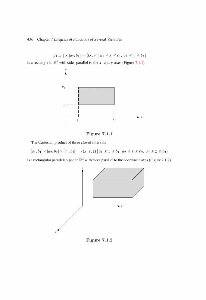
436 Chapter 7 Integrals of Functions of Several Variables
Œa1; b1 Œa2; b2 D˚.x; y/
ˇa1 x b1; a2 y b2
is a rectangle in R2 with sides parallel to the x- and y-axes (Figure 7.1.1).
y
xa
1 b1
a2
b2
Figure 7.1.1
The Cartesian product of three closed intervals
Œa1; b1 Œa2; b2 Œa3; b3 D˚.x; y; ´/
ˇa1 x b1; a2 y b2; a3 ´ b3
is a rectangular parallelepiped in R3 with faces parallel to the coordinate axes (Figure 7.1.2).
z
y
x
Figure 7.1.2
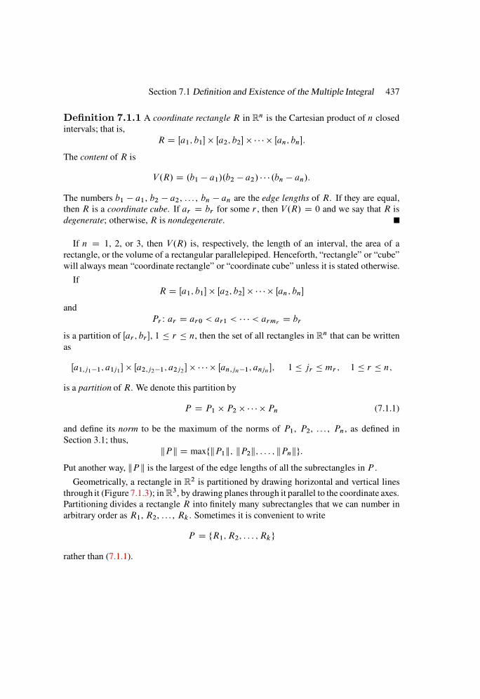
Section 7.1 Definition and Existence of the Multiple Integral 437
Definition 7.1.1 A coordinate rectangle R in Rn is the Cartesian product of n closed
intervals; that is,
R D Œa1; b1 Œa2; b2 Œan; bn:
The content of R is
V.R/ D .b1 a1/.b2 a2/ .bn an/:
The numbers b1 a1, b2 a2, . . . , bn an are the edge lengths of R. If they are equal,
then R is a coordinate cube. If ar D br for some r , then V.R/ D 0 and we say that R is
degenerate; otherwise, R is nondegenerate.
If n D 1, 2, or 3, then V.R/ is, respectively, the length of an interval, the area of a
rectangle, or the volume of a rectangular parallelepiped. Henceforth, “rectangle” or “cube”
will always mean “coordinate rectangle” or “coordinate cube” unless it is stated otherwise.
If
R D Œa1; b1 Œa2; b2 Œan; bn
and
Pr W ar D ar0 < ar1 < < armr D br
is a partition of Œar ; br , 1 r n, then the set of all rectangles in Rn that can be written
as
Œa1;j11; a1j1 Œa2;j21; a2j2
Œan;jn1; anjn; 1 jr mr ; 1 r n;
is a partition of R. We denote this partition by
P D P1 P2 Pn (7.1.1)
and define its norm to be the maximum of the norms of P1, P2, . . . , Pn, as defined in
Section 3.1; thus,
kP k D maxfkP1k; kP2k; : : : ; kPnkg:Put another way, kP k is the largest of the edge lengths of all the subrectangles in P .
Geometrically, a rectangle in R2 is partitioned by drawing horizontal and vertical lines
through it (Figure 7.1.3); in R3, by drawing planes through it parallel to the coordinate axes.
Partitioning divides a rectangle R into finitely many subrectangles that we can number in
arbitrary order as R1, R2, . . . , Rk . Sometimes it is convenient to write
P D fR1; R2; : : : ; Rkg
rather than (7.1.1).
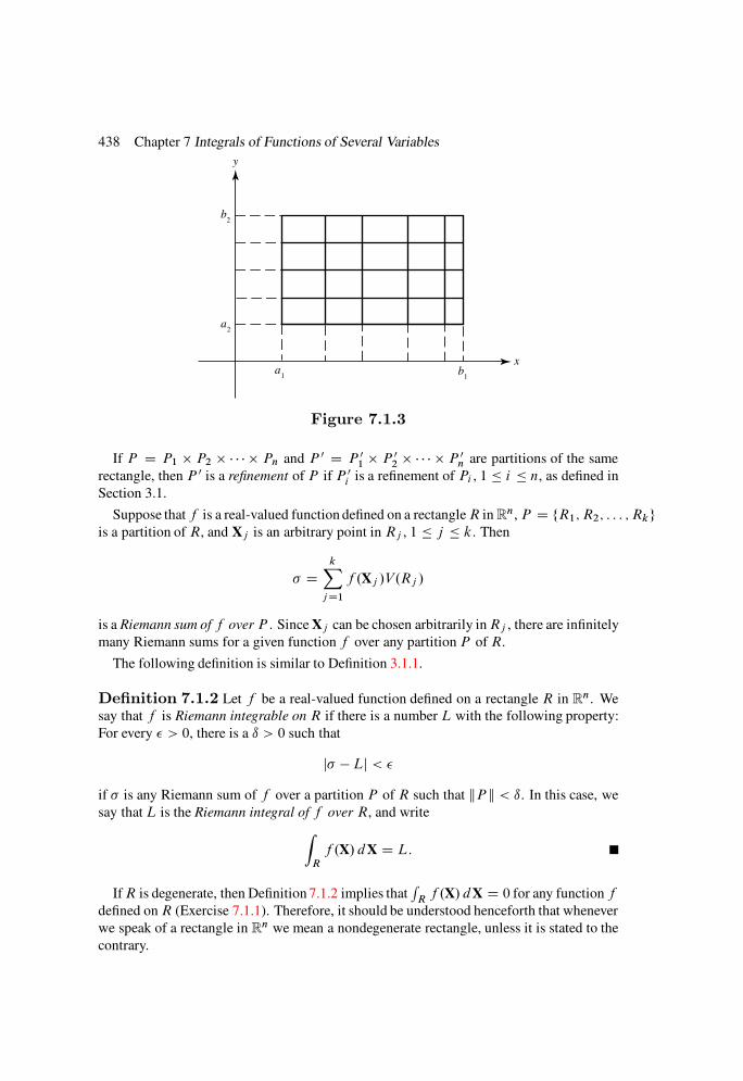
438 Chapter 7 Integrals of Functions of Several Variables
y
xa
1b
1
a2
b2
Figure 7.1.3
If P D P1 P2 Pn and P 0 D P 01 P 0
2 P 0n are partitions of the same
rectangle, then P 0 is a refinement of P if P 0i is a refinement of Pi , 1 i n, as defined in
Section 3.1.
Suppose that f is a real-valued function defined on a rectangleR in Rn, P D fR1; R2; : : : ; Rkg
is a partition of R, and Xj is an arbitrary point in Rj , 1 j k. Then
DkX
j D1
f .Xj /V .Rj /
is a Riemann sum of f over P . Since Xj can be chosen arbitrarily inRj , there are infinitely
many Riemann sums for a given function f over any partitionP ofR.
The following definition is similar to Definition 3.1.1.
Definition 7.1.2 Let f be a real-valued function defined on a rectangle R in Rn. We
say that f is Riemann integrable on R if there is a number L with the following property:
For every > 0, there is a ı > 0 such that
j Lj <
if is any Riemann sum of f over a partition P of R such that kP k < ı. In this case, we
say that L is the Riemann integral of f over R, and write
Z
R
f .X/ dX D L:
IfR is degenerate, then Definition 7.1.2 implies thatR
Rf .X/ dX D 0 for any function f
defined onR (Exercise 7.1.1). Therefore, it should be understood henceforth that whenever
we speak of a rectangle in Rn we mean a nondegenerate rectangle, unless it is stated to the
contrary.

Section 7.1 Definition and Existence of the Multiple Integral 439
The integralR
Rf .X/dX is also written as
Z
R
f .x; y/ d.x; y/ .n D 2/;Z
R
f .x; y; ´/ d.x; y; ´/ .n D 3/;
or Z
R
f .x1; x2; : : : ; xn/ d.x1; x2; : : : ; xn/ (n arbitrary):
Here dX does not stand for the differential of X, as defined in Section 6.2. It merely
identifies x1, x2, . . . , xn, the components of X, as the variables of integration. To avoid this
minor inconsistency, some authors write simplyR
Rf rather than
RRf .X/ dX.
As in the case where n D 1, we will say simply “integrable” or “integral” when we
mean “Riemann integrable” or “Riemann integral.” If n 2, we call the integral of Defi-
nition 7.1.2 a multiple integral; for n D 2 and n D 3 we also call them double and triple
integrals, respectively. When we wish to distinguish between multiple integrals and the
integral we studied in Chapter .n D 1/, we will call the latter an ordinary integral.
Example 7.1.1 FindR
Rf .x; y/ d.x; y/, where
R D Œa; b Œc; d
and
f .x; y/ D x C y:
Solution Let P1 and P2 be partitions of Œa; b and Œc; d ; thus,
P1 W a D x0 < x1 < < xr D b and P2 W c D y0 < y1 < < ys D d:
A typical Riemann sum of f over P D P1 P2 is given by
DrX
iD1
sX
j D1
.ij C ij /.xi xi1/.yj yj 1/; (7.1.2)
where
xi1 ij xi and yj 1 ij yj : (7.1.3)
The midpoints of Œxi1; xi and Œyj 1; yj are
xi Dxi C xi1
2and yj D
yj C yj 1
2; (7.1.4)
and (7.1.3) implies that
jij xi j xi xi1
2 kP1k
2 kP k
2(7.1.5)
and
jij yj j yj yj 1
2 kP2k
2 kP k
2: (7.1.6)
440 Chapter 7 Integrals of Functions of Several Variables
Now we rewrite (7.1.2) as
DrX
iD1
sX
j D1
.xi C yj /.xi xi1/.yj yj 1/
CrX
iD1
sX
j D1
.ij xi/C .ij yj /
.xi xi1/.yj yj 1/:
(7.1.7)
To findR
Rf .x; y/ d.x; y/ from (7.1.7), we recall that
rX
iD1
.xi xi1/ D b a;sX
j D1
.yj yj 1/ D d c (7.1.8)
(Example 3.1.1), and
rX
iD1
.x2i x2
i1/ D b2 a2;
sX
j D1
.y2j y2
j 1/ D d 2 c2 (7.1.9)
(Example 3.1.2).
Because of (7.1.5) and (7.1.6) the absolute value of the second sum in (7.1.7) does not
exceed
kP krX
j D1
sX
j D1
.xi xi1/.yj yj 1/ D kP k"
rX
iD1
.xi xi1/
#24
sX
j D1
.yj yj 1/
35
D kP k.b a/.d c/(see (7.1.8)), so (7.1.7) implies that
ˇˇˇ
rX
iD1
sX
j D1
.xi C yj /.xi xi1/.yj yj 1/
ˇˇˇ kP k.b a/.d c/: (7.1.10)
It now follows that
rX
iD1
sX
j D1
xi .xi xi1/.yj yj 1/ D"
rX
iD1
xi .xi xi1/
#24
sX
j D1
.yj yj 1/
35
D .d c/rX
iD1
xi .xi xi1/ (from (7.1.8))
D d c2
rX
iD1
.x2i x2
i1/ (from (7.1.4))
D d c2
.b2 a2/ (from (7.1.9)):
Similarly,rX
iD1
sX
j D1
yj .xi xi1/.yj yj 1/ Db a2
.d 2 c2/:

Section 7.1 Definition and Existence of the Multiple Integral 441
Therefore, (7.1.10) can be written asˇˇ d c
2.b2 a2/ b a
2.d 2 c2/
ˇˇ kP k.b a/.d c/:
Since the right side can be made as small as we wish by choosing kP k sufficiently small,
Z
R
.x C y/ d.x; y/ D 1
2
.d c/.b2 a2/C .b a/.d 2 c2/
:
Upper and Lower Integrals
The following theorem is analogous to Theorem 3.1.2.
Theorem 7.1.3 If f is unbounded on the nondegenerate rectangle R in Rn; then f is
not integrable on R:
Proof We will show that if f is unbounded on R, P D fR1; R2; : : : ; Rkg is any parti-
tion of R, and M > 0, then there are Riemann sums and 0 of f over P such that
j 0j M: (7.1.11)
This implies that f cannot satisfy Definition 7.1.2. (Why?)
Let
DkX
j D1
f .Xj /V .Rj /
be a Riemann sum of f over P . There must be an integer i in f1; 2; : : : ; kg such that
jf .X/ f .Xi /j M
V.Ri /(7.1.12)
for some X in Ri , because if this were not so, we would have
jf .X/ f .Xj /j <M
V.Rj /; X 2 Rj ; 1 j k:
If this is so, then
jf .X/j D jf .Xj /C f .X/ f .Xj /j jf .Xj /j C jf .X/ f .Xj /j
jf .Xj /j CM
V.Rj /; X 2 Rj ; 1 j k:
However, this implies that
jf .X/j max
jf .Xj /j C
M
V.Rj /
ˇ1 j k
; X 2 R;
which contradicts the assumption that f is unbounded on R.
442 Chapter 7 Integrals of Functions of Several Variables
Now suppose that X satisfies (7.1.12), and consider the Riemann sum
0 DnX
j D1
f .X0j /V .Rj /
over the same partitionP , where
X0j D
Xj ; j ¤ i;X; j D i:
Since
j 0j D jf .X/ f .Xi /jV.Ri /;
(7.1.12) implies (7.1.11).
Because of Theorem 7.1.3, we need consider only bounded functions in connection with
Definition 7.1.2. As in the case where n D 1, it is now convenient to define the upper
and lower integrals of a bounded function over a rectangle. The following definition is
analogous to Definition 3.1.3.
Definition 7.1.4 If f is bounded on a rectangle R in Rn and P D fR1; R2; : : : ; Rkg
is a partition of R, let
Mj D supX2Rj
f .X/; mj D infX2Rj
f .X/:
The upper sum of f over P is
S.P / DkX
j D1
MjV.Rj /;
and the upper integral of f over R, denoted by
Z
R
f .X/ dX;
is the infimum of all upper sums. The lower sum of f over P is
s.P / DkX
j D1
mj V.Rj /;
and the lower integral of f over R, denoted byZ
R
f .X/ dX;
is the supremum of all lower sums.
The following theorem is analogous to Theorem 3.1.4.
Section 7.1 Definition and Existence of the Multiple Integral 443
Theorem 7.1.5 Let f be bounded on a rectangle R and let P be a partition of R:
Then
(a) The upper sum S.P/ of f over P is the supremum of the set of all Riemann sums of
f over P:
(b) The lower sum s.P/ of f over P is the infimum of the set of all Riemann sums of f
over P:
Proof Exercise 7.1.5.
If
m f .X/ M for X in R;
then
mV.R/ s.P / S.P / MV.R/Itherefore,
RRf .X/ dX and
RRf .X/ dX exist, are unique, and satisfy the inequalities
mV.R/ Z
R
f .X/ dX MV.R/
and
mV.R/ Z
R
f .X/ dX MV.R/:
The upper and lower integrals are also written as
Z
R
f .x; y/ d.x; y/ and
Z
R
f .x; y/ d.x; y/ .n D 2/;
Z
R
f .x; y; ´/ d.x; y; ´/ and
Z
R
f .x; y; ´/ d.x; y; ´/ .n D 3/;
or Z
R
f .x1; x2; : : : ; xn/ d.x1; x2; : : : ; xn/
and Z
R
f .x1; x2; : : : ; xn/ d.x1; x2; : : : ; xn/ (n arbitrary):
Example 7.1.2 FindR
Rf .x; y/ d.x; y/ and
RRf .x; y/ d.x; y/, with R D Œa; b
Œc; d and
f .x; y/ D x C y;as in Example 7.1.1.
Solution Let P1 and P2 be partitions of Œa; b and Œc; d ; thus,
P1 W a D x0 < x1 < < xr D b and P2 W c D y0 < y1 < < ys D d:
444 Chapter 7 Integrals of Functions of Several Variables
The maximum and minimum values of f on the rectangle Œxi1; xi Œyj 1; yj are xiCyj
and xi1 C yj 1, respectively. Therefore,
S.P / DrX
iD1
sX
j D1
.xi C yj /.xi xi1/.yj yj 1/ (7.1.13)
and
s.P / DrX
iD1
sX
j D1
.xi1 C yj 1/.xi xi1/.yj yj 1/: (7.1.14)
By substituting
xi C yj D1
2Œ.xi C xi1/C .yj C yj 1/C .xi xi1/C .yj yj 1/
into (7.1.13), we find that
S.P / D 1
2.†1 C†2 C†3 C†4/; (7.1.15)
where
†1 DrX
iD1
.x2i x2
i1/
sX
j D1
.yj yj 1/ D .b2 a2/.d c/;
†2 DrX
iD1
.xi xi1/
sX
j D1
.y2j y2
j 1/ D .b a/.d 2 c2/;
†3 DrX
iD1
.xi xi1/2
sX
j D1
.yj yj 1/ kPk.b a/.d c/;
†4 DrX
iD1
.xi xi1/
sX
j D1
.yj yj 1/2 kPk.b a/.d c/:
Substituting these four results into (7.1.15) shows that
I < S.P / < I C kP k.b a/.d c/;
where
I D .d c/.b2 a2/C .b a/.d 2 c2/
2:
From this, we see that Z
R
.x C y/ d.x; y/ D I:
After substituting
xi1 C yj 1 D1
2Œ.xi C xi1/C .yj C yj 1/ .xi xi1/ .yj yj 1/
into (7.1.14), a similar argument shows that
I kP k.b a/.d c/ < s.P / < I;

Section 7.1 Definition and Existence of the Multiple Integral 445
so Z
R
.x C y/ d.x; y/ D I:
We now prove an analog of Lemma 3.2.1.
Lemma 7.1.6 Suppose that jf .X/j M if X is in the rectangle
R D Œa1; b1 Œa2; b2 Œan; bn:
Let P D P1 P2 Pn and P 0 D P 01 P 0
2 P 0n be partitions of R; where P 0
j
is obtained by adding rj partition points to Pj ; 1 j n: Then
S.P / S.P 0/ S.P / 2MV.R/
0@
nX
j D1
rj
bj aj
1A kP k (7.1.16)
and
s.P / s.P 0/ s.P /C 2MV.R/
0@
nX
j D1
rj
bj aj
1A kP k: (7.1.17)
Proof We will prove (7.1.16) and leave the proof of (7.1.17) to you (Exercise 7.1.7).
First suppose that P 01 is obtained by adding one point to P1, and P 0
j D Pj for 2 j n.
If Pr is defined by
Pr W ar D ar0 < ar1 < < armr D br ; 1 r n;
then a typical subrectangle of P is of the form
Rj1j2jn D Œa1;j11; a1j1 Œa2;j21; a2j2
Œan;jn1; anjn:
Let c be the additional point introduced into P1 to obtain P 01, and suppose that
a1;k1 < c < a1k:
If j1 ¤ k, then Rj1j2jn is common to P and P 0, so the terms associated with it in S.P 0/and S.P / cancel in the difference S.P / S.P 0/. To analyze the terms that do not cancel,
define
R.1/
kj2jnD Œa1;k1; c Œa2;j21; a2j2
Œan;jn1; anjn;
R.2/
kj2jnD Œc; a1k Œa2;j21; a2j2
Œan;jn1; anjn ;
Mkj2jnD sup
˚f .X/
ˇX 2 Rkj2jn
(7.1.18)
and
M.i/
kj2jnD sup
nf .X/
ˇX 2 R.i/
kj2jn
o; i D 1; 2: (7.1.19)
446 Chapter 7 Integrals of Functions of Several Variables
Then S.P / S.P 0/ is the sum of terms of the formhMkj2jn
.a1k a1;k1/ M .1/
kj2jn.c a1;k1/M .2/
kj2jn.a1k c/
i
.a2j2 a2;j21/ .anjn an;jn1/:
(7.1.20)
The terms within the brackets can be rewritten as
.Mkj2jnM .1/
kj2jn/.c a1;k1/C .Mkj2jn
M .2/
kj2jn/.a1k c/; (7.1.21)
which is nonnegative, because of (7.1.18) and (7.1.19). Therefore,
S.P 0/ S.P /: (7.1.22)
Moreover, the quantity in (7.1.21) is not greater than 2M.a1ka1;k1/, so (7.1.20) implies
that the general surviving term in S.P / S.P 0/ is not greater than
2MkP k.a2j2 a2;j21/ .anjn an;jn1/:
The sum of these terms as j2, . . . , jn assume all possible values 1 ji mi , 2 i n,
is
2MkP k.b2 a2/ .bn an/ D2MkP kV.R/b1 a1
:
This implies that
S.P / S.P 0/C 2MkP kV.R/b1 a1
:
This and (7.1.22) imply (7.1.16) for r1 D 1 and r2 D D rn D 0.
Similarly, if ri D 1 for some i in f1; : : : ; ng and rj D 0 if j ¤ i , then
S.P / S.P 0/C2MkP kV.R/bi ai
:
To obtain (7.1.16) in the general case, repeat this argument r1 C r2 C C rn times, as in
the proof of Lemma 3.2.1.
Lemma 7.1.6 implies the following theorems and lemma, with proofs analogous to the
proofs of their counterparts in Section 3.2.
Theorem 7.1.7 If f is bounded on a rectangle R; then
Z
R
f .X/ dX Z
R
f .X/ dX:
Proof Exercise 7.1.8.
The next theorem is analogous to Theorem 3.2.3.
Theorem 7.1.8 If f is integrable on a rectangle R; then
Z
R
f .X/ dX DZ
R
f .X/ dX DZ
R
f .X/ dX:
Proof Exercise 7.1.9.
Section 7.1 Definition and Existence of the Multiple Integral 447
Lemma 7.1.9 If f is bounded on a rectangle R and > 0; there is a ı > 0 such that
Z
R
f .X/ dX S.P / <Z
R
f .X/ dXC
andZ
R
f .X/ dX s.P / >Z
R
f .X/ dX
if kP k < ı:
Proof Exercise 7.1.10.
The next theorem is analogous to Theorem 3.2.5.
Theorem 7.1.10 If f is bounded on a rectangle R and
Z
R
f .X/ dX DZ
R
f .X/ dX D L;
then f is integrable on R; and
Z
R
f .X/ dX D L:
Proof Exercise 7.1.11.
Theorems 7.1.8 and 7.1.10 imply the following theorem, which is analogous to Theo-
rem 3.2.6.
Theorem 7.1.11 A bounded function f is integrable on a rectangle R if and only if
Z
R
f .X/ dX DZ
R
f .X/ dX:
The next theorem translates this into a test that can be conveniently applied. It is analo-
gous to Theorem 3.2.7.
Theorem 7.1.12 If f is bounded on a rectangle R; then f is integrable on R if and
only if for every > 0 there is a partitionP of R such that
S.P / s.P / < :
Proof Exercise 7.1.12.
Theorem 7.1.12 provides a useful criterion for integrability. The next theorem is an
important application. It is analogous to Theorem 3.2.8.
Theorem 7.1.13 If f is continuous on a rectangleR in Rn; then f is integrable onR:
448 Chapter 7 Integrals of Functions of Several Variables
Proof Let > 0. Since f is uniformly continuous on R (Theorem 5.2.14), there is a
ı > 0 such that
jf .X/ f .X0/j <
V.R/(7.1.23)
if X and X0 are inR and jXX0j < ı. Let P D fR1; R2; : : : ; Rkg be a partition ofR with
kP k < ı=pn. Since f is continuous on R, there are points Xj and X0
j in Rj such that
f .Xj / DMj D supX2Rj
f .X/ and f .X0j / D mj D inf
X2Rj
f .X/
(Theorem 5.2.12). Therefore,
S.P/ s.P/ DnX
j D1
.f .Xj / f .X0j //V .Rj /:
Since kP k < ı=pn, jXj X0
j j < ı, and, from (7.1.23) with X D Xj and X0 D X0j ,
S.P/ s.P/ <
V.R/
kX
j D1
V.Rj / D :
Hence, f is integrable on R, by Theorem 7.1.12.
Sets with Zero Content
The next definition will enable us to establish the existence ofR
Rf .X/ dX in cases where
f is bounded on the rectangle R, but is not necessarily continuous for all X in R.
Definition 7.1.14 A subset E of Rn has zero content if for each > 0 there is a finite
set of rectangles T1, T2, . . . , Tm such that
E m[
j D1
Tj (7.1.24)
andmX
j D1
V.Tj / < : (7.1.25)
Example 7.1.3 Since the empty set is contained in every rectangle, the empty set has
zero content. IfE consists of finitely many points X1, X2, . . . , Xm, then Xj can be enclosed
in a rectangle Tj such that
V.Tj / <
m; 1 j m:
Then (7.1.24) and (7.1.25) hold, so E has zero content.

Section 7.1 Definition and Existence of the Multiple Integral 449
Example 7.1.4 Any bounded set E with only finitely many limit points has zero con-
tent. To see this, we first observe that ifE has no limit points, then it must be finite, by the
Bolzano–Weierstrass theorem (Theorem 1.3.8), and therefore must have zero content, by
Example 7.1.3. Now suppose that the limit points of E are X1, X2, . . . , Xm. Let R1, R2,
. . . , Rm be rectangles such that Xi 2 R0i and
V.Ri / <
2m; 1 i m: (7.1.26)
The set of points of E that are not in [mj D1Rj has no limit points (why?) and, being
bounded, must be finite (again by the Bolzano–Weierstrass theorem). If this set contains p
points, then it can be covered by rectangles R01, R0
2, . . . , R0p with
V.R0j / <
2p; 1 j p: (7.1.27)
Now,
E
m[
iD1
Ri
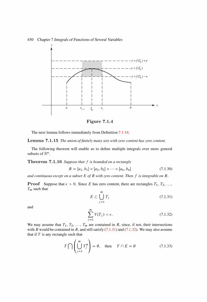
450 Chapter 7 Integrals of Functions of Several Variables
y
x
y = f (ξi) +
y = f (ξi)
y = f (ξi) −
a bxi−1
xiξ
i
Figure 7.1.4
The next lemma follows immediately from Definition 7.1.14.
Lemma 7.1.15 The union of finitely many sets with zero content has zero content:
The following theorem will enable us to define multiple integrals over more general
subsets of Rn.
Theorem 7.1.16 Suppose that f is bounded on a rectangle
R D Œa1; b1 Œa2; b2 Œan; bn (7.1.30)
and continuous except on a subset E of R with zero content: Then f is integrable on R:
Proof Suppose that > 0. Since E has zero content, there are rectangles T1, T2, . . . ,
Tm such that
E m[
j D1
Tj (7.1.31)
andmX
j D1
V.Tj / < : (7.1.32)
We may assume that T1, T2, . . . , Tm are contained in R, since, if not, their intersections
withRwould be contained inR, and still satisfy (7.1.31) and (7.1.32). We may also assume
that if T is any rectangle such that
T\
0@
m[
j D1
T 0j
1A D ;; then T \E D ; (7.1.33)

Section 7.1 Definition and Existence of the Multiple Integral 451
since if this were not so, we could make it so by enlarging T1, T2, . . . , Tm slightly while
maintaining (7.1.32). Now suppose that
Tj D Œa1j ; b1j Œa2j ; b2j Œanj ; bnj ; 1 j m;
let Pi0 be the partition of Œai ; bi (see (7.1.30)) with partition points
ai ; bi ; ai1; bi1; ai2; bi2; : : : ; aim; bim
(these are not in increasing order), 1 i n, and let
P0 D P10 P20 Pn0:
Then P0 consists of rectangles whose union equals [mj D1Tj and other rectangles T 0
1, T 02,
. . . , T 0k
that do not intersect E . (We need (7.1.33) to be sure that T 0i \E D ;; 1 i k:/
If we let
B Dm[
j D1
Tj and C Dk[
iD1
T 0i ;
then R D B [ C and f is continuous on the compact set C . If P D fR1; R2; : : : ; Rkg is
a refinement of P0, then every subrectangle Rj of P is contained entirely in B or entirely
in C . Therefore, we can write
S.P / s.P / D †1.Mj mj /V .Rj /C†2.Mj mj /V .Rj /; (7.1.34)
where †1 and †2 are summations over values of j for which Rj B and Rj C ,
respectively. Now suppose that
jf .X/j M for X in R:
Then
†1.Mj mj /V .Rj / 2M †1V.Rj / D 2MmX
j D1
V.Tj / < 2M; (7.1.35)
from (7.1.32). Since f is uniformly continuous on the compact set C (Theorem 5.2.14),
there is a ı > 0 such thatMj mj < if kP k < ı and Rj C ; hence,
†2.Mj mj /V .Rj / < †2 V.Rj / V .R/:
This, (7.1.34), and (7.1.35) imply that
S.P / s.P / < Œ2M C V.R/
if kP k < ı and P is a refinement of P0. Therefore, Theorem 7.1.12 implies that f is
integrable on R.
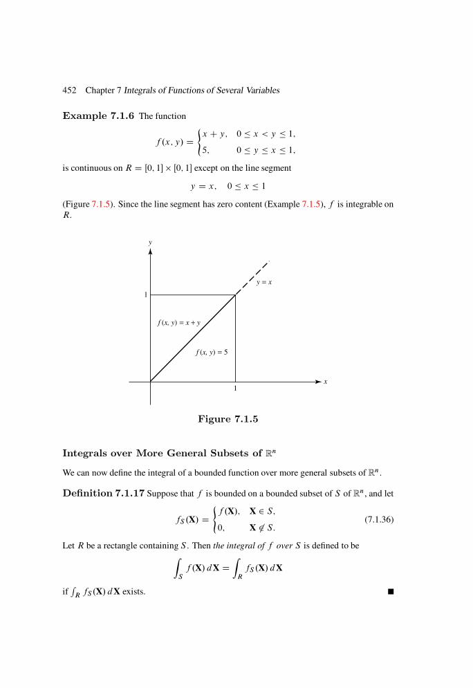
452 Chapter 7 Integrals of Functions of Several Variables
Example 7.1.6 The function
f .x; y/ D(x C y; 0 x < y 1;5; 0 y x 1;
is continuous on R D Œ0; 1 Œ0; 1 except on the line segment
y D x; 0 x 1
(Figure 7.1.5). Since the line segment has zero content (Example 7.1.5), f is integrable on
R.
y
x
f (x, y) = x + y
f (x, y) = 5
y = x
1
1
Figure 7.1.5
Integrals over More General Subsets of Rn
We can now define the integral of a bounded function over more general subsets of Rn.
Definition 7.1.17 Suppose that f is bounded on a bounded subset of S of Rn, and let
fS .X/ D(f .X/; X 2 S;
0; X 62 S:(7.1.36)
Let R be a rectangle containing S . Then the integral of f over S is defined to beZ
S
f .X/ dX DZ
R
fS .X/ dX
ifR
RfS.X/ dX exists.
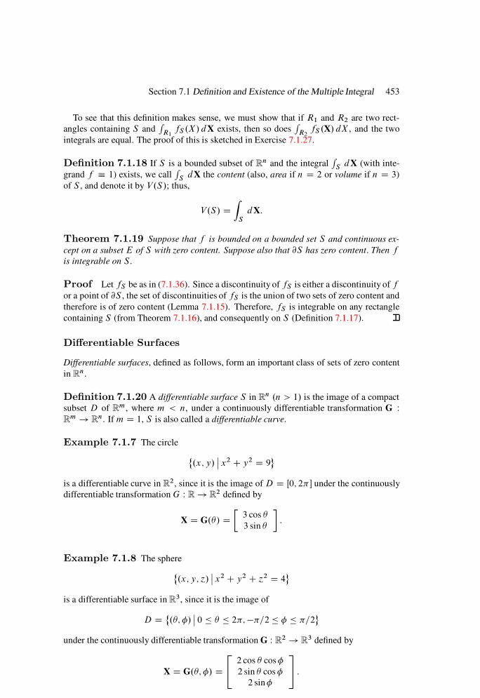
Section 7.1 Definition and Existence of the Multiple Integral 453
To see that this definition makes sense, we must show that if R1 and R2 are two rect-
angles containing S andR
R1fS .X/ dX exists, then so does
RR2fS .X/ dX , and the two
integrals are equal. The proof of this is sketched in Exercise 7.1.27.
Definition 7.1.18 If S is a bounded subset of Rn and the integral
RSdX (with inte-
grand f 1) exists, we callR
SdX the content (also, area if n D 2 or volume if n D 3)
of S , and denote it by V.S/; thus,
V.S/ DZ
S
dX:
Theorem 7.1.19 Suppose that f is bounded on a bounded set S and continuous ex-
cept on a subset E of S with zero content. Suppose also that @S has zero content: Then f
is integrable on S:
Proof Let fS be as in (7.1.36). Since a discontinuity of fS is either a discontinuity of f
or a point of @S , the set of discontinuities of fS is the union of two sets of zero content and
therefore is of zero content (Lemma 7.1.15). Therefore, fS is integrable on any rectangle
containing S (from Theorem 7.1.16), and consequently on S (Definition 7.1.17).
Differentiable Surfaces
Differentiable surfaces, defined as follows, form an important class of sets of zero content
in Rn.
Definition 7.1.20 A differentiable surface S in Rn .n > 1/ is the image of a compact
subset D of Rm, where m < n, under a continuously differentiable transformation G W
Rm ! R
n. If m D 1, S is also called a differentiable curve.
Example 7.1.7 The circle
˚.x; y/
ˇx2 C y2 D 9
is a differentiable curve in R2, since it is the image of D D Œ0; 2 under the continuously
differentiable transformationG W R! R2 defined by
X D G./ D3 cos
3 sin
:
Example 7.1.8 The sphere
˚.x; y; ´/
ˇx2 C y2 C ´2 D 4
is a differentiable surface in R3, since it is the image of
D D˚.; /
ˇ0 2;=2 =2
under the continuously differentiable transformation G W R2 ! R3 defined by
X D G.; / D
242 cos cos
2 sin cos
2 sin
35 :

454 Chapter 7 Integrals of Functions of Several Variables
Example 7.1.9 The set˚.x1; x2; x3; x4/
ˇxi 0 .i D 1; 2; 3; 4/; x1 C x2 D 1; x3 C x4 D 1
is a differentiable surface in R4, since it is the image of D D Œ0; 1 Œ0; 1 under the
continuously differentiable transformation G W R2 ! R4 defined by
X D G.u; v/ D
2664
u
1 uv
1 v
3775 :
Theorem 7.1.21 A differentiable surface in Rn has zero content:
Proof Let S , D, and G be as in Definition 7.1.20. From Lemma 6.2.7, there is a
constant M such that
jG.X/ G.Y/j M jX Yj if X;Y 2 D: (7.1.37)
Since D is bounded,D is contained in a cube
C D Œa1; b1 Œa2; b2 Œam; bm;
where
bi ai D L; 1 i m:Suppose that we partition C into Nm smaller cubes by partitioning each of the intervals
Œai ; bi intoN equal subintervals. Let R1,R2, . . . , Rk be the smaller cubes so produced that
contain points of D, and select points X1, X2, . . . , Xk such that Xi 2 D \Ri , 1 i k.
If Y 2 D \ Ri , then (7.1.37) implies that
jG.Xi / G.Y/j M jXi Yj: (7.1.38)
Since Xi and Y are both in the cube Ri with edge length L=N ,
jXi Yj Lpm
N:
This and (7.1.38) imply that
jG.Xi / G.Y/j MLpm
N;
which in turn implies that G.Y/ lies in a cube eRi in Rn centered at G.Xi /, with sides of
length 2MLpm=N . Now
kX
iD1
V.eRi / D k2ML
pm
N
n
Nm
2ML
pm
N
n
D .2MLpm/nNmn:
Since n > m, we can make the sum on the left arbitrarily small by taking N sufficiently
large. Therefore, S has zero content.
Theorems 7.1.19 and 7.1.21 imply the following theorem.
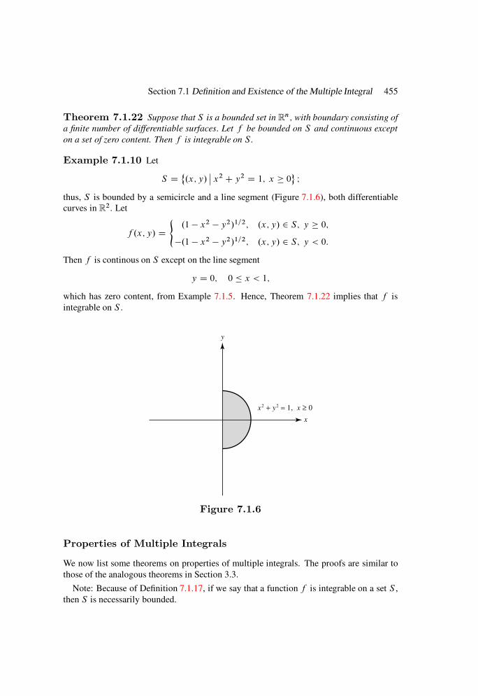
Section 7.1 Definition and Existence of the Multiple Integral 455
Theorem 7.1.22 Suppose that S is a bounded set in Rn; with boundary consisting of
a finite number of differentiable surfaces: Let f be bounded on S and continuous except
on a set of zero content. Then f is integrable on S:
Example 7.1.10 Let
S D˚.x; y/
ˇx2 C y2 D 1; x 0
I
thus, S is bounded by a semicircle and a line segment (Figure 7.1.6), both differentiable
curves in R2. Let
f .x; y/ D(.1 x2 y2/1=2; .x; y/ 2 S; y 0;
.1 x2 y2/1=2; .x; y/ 2 S; y < 0:
Then f is continous on S except on the line segment
y D 0; 0 x < 1;
which has zero content, from Example 7.1.5. Hence, Theorem 7.1.22 implies that f is
integrable on S .
y
x
x2 + y2 = 1, x ≥ 0
Figure 7.1.6
Properties of Multiple Integrals
We now list some theorems on properties of multiple integrals. The proofs are similar to
those of the analogous theorems in Section 3.3.
Note: Because of Definition 7.1.17, if we say that a function f is integrable on a set S ,
then S is necessarily bounded.
456 Chapter 7 Integrals of Functions of Several Variables
Theorem 7.1.23 If f and g are integrable on S; then so is f C g; and
Z
S
.f C g/.X/ dX DZ
S
f .X/ dXCZ
S
g.X/ dX:
Proof Exercise 7.1.20.
Theorem 7.1.24 If f is integrable on S and c is a constant; then cf is integrable on
S; and Z
S
.cf /.X/ dX D cZ
S
f .X/ dX:
Proof Exercise 7.1.21.
Theorem 7.1.25 If f and g are integrable on S and f .X/ g.X/ for X in S; then
Z
S
f .X/ dX Z
S
g.X/ dX:
Proof Exercise 7.1.22.
Theorem 7.1.26 If f is integrable on S; then so is jf j; and
ˇˇZ
S
f .X/ dX
ˇˇ
Z
S
jf .X/j dX:
Proof Exercise 7.1.23.
Theorem 7.1.27 If f and g are integrable on S; then so is the product fg:
Proof Exercise 7.1.24.
Theorem 7.1.28 Suppose that u is continuous and v is integrable and nonnegative on
a rectangle R: Then Z
R
u.X/v.X/ dX D u.X0/
Z
R
v.X/ dX
for some X0 in R:
Proof Exercise 7.1.25.
Lemma 7.1.29 Suppose that S is contained in a bounded set T and f is integrable
on S: Then fS .see (7.1.36)/ is integrable on T; and
Z
T
fS .X/ dX DZ
S
f .X/ dX:
Proof From Definition 7.1.17 with f and S replaced by fS and T ,

Section 7.1 Definition and Existence of the Multiple Integral 457
.fS /T .X/ DfS .X/; X 2 T;0; X 62 T:
Since S T , .fS /T D fS . (Verify.) Now suppose that R is a rectangle containing T .
Then R also contains S (Figure 7.1.7),
RT
Figure 7.1.7
soZ
S
f .X/ dX DZ
R
fS .X/ dX (Definition 7.1.17, applied to f and S/
DZ
R
.fS /T .X/ dX (since .fS /T D fS )
DZ
T
fS .X/ dX (Definition 7.1.17, applied to fS and T /;
which completes the proof.
Theorem 7.1.30 If f is integrable on disjoint sets S1 and S2; then f is integrable on
S1 [ S2; and Z
S1[S2
f .X/ dX DZ
S1
f .X/ dXCZ
S2
f .X/ dX: (7.1.39)
Proof For i D 1, 2, let
fSi.X/ D
(f .X/; X 2 Si ;
0; X 62 Si :
From Lemma 7.1.29 with S D Si and T D S1 [ S2, fSiis integrable on S1 [ S2, and
Z
S1[S2
fSi.X/ dX D
Z
Si
f .X/ dX; i D 1; 2:
Theorem 7.1.23 now implies that fS1C fS2
is integrable on S1 [ S2 andZ
S1[S2
.fS1C fS2
/.X/ dX DZ
S1
f .X/ dXCZ
S2
f .X/ dX: (7.1.40)

458 Chapter 7 Integrals of Functions of Several Variables
Since S1 \ S2 D ;,
fS1C fS2
.X/ D fS1
.X/C fS2.X/ D f .X/; X 2 S1 [ S2:
Therefore, (7.1.40) implies (7.1.39).
We leave it to you to prove the following extension of Theorem 7.1.30. (Exercise 7.1.31(b)).
Corollary 7.1.31 Suppose that f is integrable on sets S1 and S2 such that S1 \ S2
has zero content: Then f is integrable on S1 [ S2; and
Z
S1[S2
f .X/ dX DZ
S1
f .X/ dXCZ
S2
f .X/ dX:
Example 7.1.11 Let
S1 D˚.x; y/
ˇ0 x 1; 0 y 1C x
and
S2 D˚.x; y/
ˇ 1 x 0; 0 y 1 x
(Figure 7.1.8).
S
y
x
y = 1 − x y = 1 + x
1−1
Figure 7.1.8
Then
S1 \ S2 D˚.0; y/
ˇ0 y 1
has zero content. Hence, Corollary 7.1.31 implies that if f is integrable on S1 and S2, then
f is also integrable over
S D S1 [ S2 D˚.x; y/
ˇ 1 x 1; 0 y 1C jxj
(Figure 7.1.9), and
Z
S1[S2
f .X/ dX DZ
S1
f .X/ dXCZ
S2
f .X/ dX:
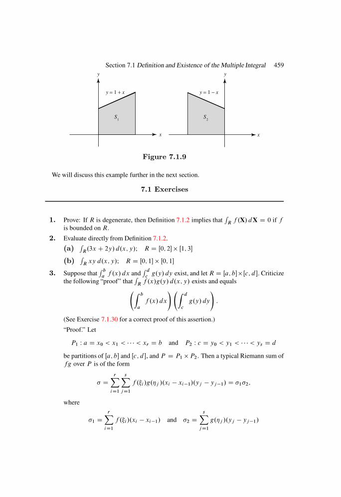
Section 7.1 Definition and Existence of the Multiple Integral 459
y y
x x
y = 1 − xy = 1 + x
S1
S2
Figure 7.1.9
We will discuss this example further in the next section.
7.1 Exercises
1. Prove: If R is degenerate, then Definition 7.1.2 implies thatR
Rf .X/ dX D 0 if f
is bounded on R.
2. Evaluate directly from Definition 7.1.2.
(a)R
R.3x C 2y/ d.x; y/; R D Œ0; 2 Œ1; 3
(b)R
Rxy d.x; y/; R D Œ0; 1 Œ0; 1
3. Suppose thatR b
af .x/ dx and
R d
cg.y/ dy exist, and let R D Œa; b Œc; d . Criticize
the following “proof” thatR
Rf .x/g.y/ d.x; y/ exists and equals
Z b
a
f .x/ dx
! Z d
c
g.y/ dy
!:
(See Exercise 7.1.30 for a correct proof of this assertion.)
“Proof.” Let
P1 W a D x0 < x1 < < xr D b and P2 W c D y0 < y1 < < ys D d
be partitions of Œa; b and Œc; d , and P D P1 P2. Then a typical Riemann sum of
fg over P is of the form
DrX
iD1
sX
j D1
f .i/g.j /.xi xi1/.yj yj 1/ D 12;
where
1 DrX
iD1
f .i/.xi xi1/ and 2 DsX
j D1
g.j /.yj yj 1/
460 Chapter 7 Integrals of Functions of Several Variables
are typical Riemann sums of f over Œa; b and g over Œc; d . Since f and g are
integrable on these intervals,
ˇˇˇ1
Z b
a
f .x/ dx
ˇˇˇ and
ˇˇˇ2
Z d
c
g.y/ dy
ˇˇˇ
can be made arbitrarily small by taking kP1k and kP2k sufficiently small. From
this, it is straightforward to show that
ˇˇˇ
Z b
a
f .x/ dx
! Z d
c
g.y/ dy
!ˇˇˇ
can be made arbitrarily small by taking kP k sufficiently small. This implies the
stated result.
4. Suppose that f .x; y/ 0 on R D Œa; b Œc; d . Justify the interpretation ofRRf .x; y/ d.x; y/, if it exists, as the volume of the region in R
3 bounded by the
surfaces ´ D f .x; y/ and the planes ´ D 0, x D a, x D b, y D c, and y D d .
5. Prove Theorem 7.1.5. HINT: See the proof of Theorem 3.1.4:
6. Suppose that
f .x; y/ D
8ˆ<ˆ:
0 if x and y are rational,
1 if x is rational and y is irrational,
2 if x is irrational and y is rational,
3 if x and y are irrational.
Find
Z
R
f .x; y/ d.x; y/ and
Z
R
f .x; y/ d.x; y/ if R D Œa; b Œc; d :
7. Prove Eqn. (7.1.17) of Lemma 7.1.6.
8. Prove Theorem 7.1.7 HINT: See the proof of Theorem 3.2.2:
9. Prove Theorem 7.1.8 HINT: See the proof of Theorem 3.2.3:
10. Prove Lemma 7.1.9 HINT: See the proof of Lemma 3.2.4:
11. Prove Theorem 7.1.10 HINT: See the proof of Theorem 3.2.5:
12. Prove Theorem 7.1.12 HINT: See the proof of Theorem 3.2.7:
13. Give an example of a denumerable set in R2 that does not have zero content.
14. Prove:
(a) If S1 and S2 have zero content, then S1 [ S2 has zero content.
(b) If S1 has zero content and S2 S1, then S2 has zero content.
(c) If S has zero content, then S has zero content.
15. Show that a degenerate rectangle has zero content.
Section 7.1 Definition and Existence of the Multiple Integral 461
16. Suppose that f is continuous on a compact set S in Rn. Show that the surface
´ D f .X/, X 2 S , has zero content in RnC1. HINT: See Example 7.1.5:
17. Let S be a bounded set such that S \ @S does not have zero content.
(a) Suppose that f is defined on S and f .X/ > 0 on a subset T of S \ @Sthat does not have zero content. Show that f is not integrable on S .
(b) Conclude that V.S/ is undefined.
18. (a) Suppose that h is bounded and h.X/ D 0 except on a set of zero content.
Show thatR
Sh.X/ dX D 0 for any bounded set S .
(b) Suppose thatR
S f .X/ dX exists, g is bounded onS , and f .X/ D g.X/ except
for X in a set of zero content. Show that g is integrable on S and
Z
S
g.X/ dX DZ
S
f .X/ dX:
19. Suppose that f is integrable on a set S and S0 is a subset of S such that @S0 has
zero content. Show that f is integrable on S0.
20. Prove Theorem 7.1.23 HINT: See the proof of Theorem 3.3.1:
21. Prove Theorem 7.1.24.
22. Prove Theorem 7.1.25 HINT: See the proof of Theorem 3.3.4:
23. Prove Theorem 7.1.26 HINT: See the proof of Theorem 3.3.5:
24. Prove Theorem 7.1.27 HINT: See the proof of Theorem 3.3.6:
25. Prove Theorem 7.1.28 HINT: See the proof of Theorem 3.3.7:
26. Prove: If f is integrable on a rectangle R, then f is integrable on any subrectangle
of R. HINT: Use Theorem 7.1.12I see the proof of Theorem 3.3.8:
27. Suppose that R and eR are rectangles, R eR, g is bounded on eR, and g.X/ D 0 if
X 62 R.
(a) Show thatReR g.X/ dX exists if and only if
RRg.X/ dX exists and, in this
case, Z
eRg.X/ dX D
Z
R
g.X/ dX:
HINT: Use Exercise 7.1.26:
(b) Use (a) to show that Definition 7.1.17 is legitimate; that is, the existence and
value ofR
Sf .X/ dX does not depend on the particular rectangle chosen to
contain S .
28. (a) Suppose that f is integrable on a rectangle R and P D fR1; R2; : : : ; Rkg is
a partition of R. Show that
Z
R
f .X/ dX DkX
j D1
Z
Rj
f .X/ dX:
HINT: Use Exercise 7.1.26:
462 Chapter 7 Integrals of Functions of Several Variables
(b) Use (a) to show that if f is continuous on R and P is a partition of R, then
there is a Riemann sum of f over P that equalsR
Rf .X/ dX.
29. Suppose that f is continuously differentiable on a rectangle R. Show that there is a
constant M such that ˇˇ
Z
R
f .X/ dX
ˇˇ MkP k
if is any Riemann sum of f over a partitionP ofR. HINT: Use Exercise 7.1.28.b/
and Theorem 5.4.5:
30. Suppose thatR b
af .x/ dx and
R d
cg.y/ dy exist, and let R D Œa; b Œc; d .
(a) Use Theorems 3.2.7 and 7.1.12 to show that
Z
R
f .x/ d.x; y/ and
Z
R
g.y/ d.x; y/
both exist.
(b) Use Theorem 7.1.27 to prove thatR
Rf .x/g.y/ d.x; y/ exists.
(c) Justify using the argument given in Exercise 7.1.3 to show that
Z
R
f .x/g.y/ d.x; y/ D Z b
a
f .x/ dx
! Z d
c
g.y/ dy
!:
31. (a) Suppose that f is integrable on S and S0 is obtained by removing a set of
zero content from S . Show that f is integrable on S0 andR
S0f .X/ dX DR
Sf .X/ dX.
(b) Prove Corollary 7.1.31.
7.2 ITERATED INTEGRALS AND MULTIPLE INTEGRALS
Except for very simple examples, it is impractical to evaluate multiple integrals directly
from Definitions 7.1.2 and 7.1.17. Fortunately, this can usually be accomplished by evalu-
ating n successive ordinary integrals. To motivate the method, let us first assume that f is
continuous on R D Œa; b Œc; d . Then, for each y in Œc; d , f .x; y/ is continuous with
respect to x on Œa; b, so the integral
F.y/ DZ b
a
f .x; y/ dx
exists. Moreover, the uniform continuity of f on R implies that F is continuous (Exer-
cise 7.2.3) and therefore integrable on Œc; d . We say that
I1 DZ d
c
F.y/ dy DZ d
c
Z b
a
f .x; y/ dx
!dy

Section 7.2 Iterated Integrals and Multiple Integrals 463
is an iterated integral of f over R. We will usually write it as
I1 DZ d
c
dy
Z b
a
f .x; y/ dx:
Another iterated integral can be defined by writing
G.x/ DZ d
c
f .x; y/ dy; a x b;
and defining
I2 DZ b
a
G.x/ dx DZ b
a
Z d
c
f .x; y/ dy
!dx;
which we usually write as
I2 DZ b
a
dx
Z d
c
f .x; y/ dy:
Example 7.2.1 Let
f .x; y/ D x C y
and R D Œ0; 1 Œ1; 2. Then
F.y/ DZ 1
0
f .x; y/ dx DZ 1
0
.x C y/ dx Dx2
2C xy
ˇˇ1
xD0
D 1
2C y
and
I1 DZ 2
1
F.y/ dy DZ 2
1
1
2C y
dy D
y
2C y2
2
ˇˇ2
1
D 2:
Also,
G.x/DZ 2
1
.x C y/ dy Dxy C y2
2
ˇˇ2
yD1
D .2x C 2/ x C 1
2
D x C 3
2;
and
I2 DZ 1
0
G.x/ dx DZ 1
0
x C 3
2
dx D
x2
2C 3x
2
ˇˇ1
0
D 2:
In this example, I1 D I2; moreover, on setting a D 0, b D 1, c D 1, and d D 2 in
Example 7.1.1, we see that Z
R
.x C y/ d.x; y/ D 2;
so the common value of the iterated integrals equals the multiple integral. The following
theorem shows that this is not an accident.

464 Chapter 7 Integrals of Functions of Several Variables
Theorem 7.2.1 Suppose that f is integrable onR D Œa; b Œc; d and
F.y/ DZ b
a
f .x; y/ dx
exists for each y in Œc; d : Then F is integrable on Œc; d ; and
Z d
c
F.y/ dy DZ
R
f .x; y/ d.x; y/I (7.2.1)
that is; Z d
c
dy
Z b
a
f .x; y/ dx DZ
R
f .x; y/ d.x; y/: (7.2.2)
Proof Let
P1 W a D x0 < x1 < < xr D b and P2 W c D y0 < y1 < < ys D d
be partitions of Œa; b and Œc; d , and P D P1 P2. Suppose that
yj 1 j yj ; 1 j s; (7.2.3)
so
DsX
j D1
F.j /.yj yj 1/ (7.2.4)
is a typical Riemann sum of F over P2. Since
F.j / DZ b
a
f .x; j / dx DrX
iD1
Z x
xi1
f .x; j / dx;
(7.2.3) implies that if
mij D inf˚f .x; y/
ˇxi1 x xi ; yj 1 y yj
and
Mij D sup˚f .x; y/
ˇxi1 x xi ; yj 1 y yj
;
thenrX
iD1
mij .xi xi1/ F.j / rX
iD1
Mij .xi xi1/:
Multiplying this by yj yj 1 and summing from j D 1 to j D s yields
sX
j D1
rX
iD1
mij .xi xi1/.yj yj 1/ sX
j D1
F.j /.yj yj 1/
sX
j D1
rX
iD1
Mij .xi xi1/.yj yj 1/;

Section 7.2 Iterated Integrals and Multiple Integrals 465
which, from (7.2.4), can be rewritten as
sf .P/ Sf .P/; (7.2.5)
where sf .P/ and Sf .P/ are the lower and upper sums of f over P. Now let sF .P2/ and
SF .P2/ be the lower and upper sums of F over P2; since they are respectively the infimum
and supremum of the Riemann sums of F over P2 (Theorem 3.1.4), (7.2.5) implies that
sf .P/ sF .P2/ SF .P2/ Sf .P/: (7.2.6)
Since f is integrable on R, there is for each > 0 a partition P of R such that Sf .P/ sf .P/ < , from Theorem 7.1.12. Consequently, from (7.2.6), there is a partition P2 of
Œc; d such that SF .P2/ sF .P2/ < , so F is integrable on Œc; d , from Theorem 3.2.7.
It remains to verify (7.2.1). From (7.2.4) and the definition ofR d
cF.y/ dy, there is for
each > 0 a ı > 0 such thatˇˇˇ
Z d
c
F.y/ dy ˇˇˇ < if kP2k < ıI
that is,
<Z d
c
F.y/ dy < C if kP2k < ı:
This and (7.2.5) imply that
sf .P/ <Z d
c
F.y/ dy < Sf .P/C if kPk < ı;
and this implies that
Z
R
f .x; y/ d.x; y/ Z d
c
F.y/ dy Z
R
f .x; y/ d.x; y/ C (7.2.7)
(Definition 7.1.4). Since
Z
R
f .x; y/ d.x; y/ DZ
R
f .x; y/ d.x; y/
(Theorem 7.1.8) and can be made arbitrarily small, (7.2.7) implies (7.2.1).
If f is continuous onR, then f satisfies the hypotheses of Theorem 7.2.1 (Exercise 7.2.3),
so (7.2.2) is valid in this case.
IfR
Rf .x; y/ d.x; y/ and
Z d
c
f .x; y/ dy; a x b;
466 Chapter 7 Integrals of Functions of Several Variables
exist, then by interchanging x and y in Theorem 7.2.1, we see that
Z b
a
dx
Z d
c
f .x; y/ dy DZ
R
f .x; y/ d.x; y/:
This and (7.2.2) yield the following corollary of Theorem 7.2.1.
Corollary 7.2.2 If f is integrable on Œa; b Œc; d ; then
Z b
a
dx
Z d
c
f .x; y/ dy DZ d
c
dy
Z b
a
f .x; y/ dx;
provided thatR d
cf .x; y/ dy exists for a x b and
R b
af .x; y/ dx exists for c y d:
In particular; these hypotheses hold if f is continuous on Œa; b Œc; d :
Example 7.2.2 The function
f .x; y/ D x C y
is continuous everywhere, so (7.2.2) holds for every rectangle R. For example, let R DŒ0; 1 Œ1; 2. Then (7.2.2) yields
Z
R
.x C y/ d.x; y/ DZ 2
1
dy
Z 1
0
.x C y/ dx DZ 2
1
"x2
2C xy
ˇˇ1
xD0
#dy
DZ 2
1
1
2C y
dy D
y
2C y2
2
ˇˇ2
1
D 2:
Since f also satisfies the hypotheses of Theorem 7.2.1 with x and y interchanged, we
can calculate the double integral from the iterated integral in which the integrations are
performed in the opposite order; thus,
Z
R
.x C y/ d.x; y/ DZ 1
0
dx
Z 2
1
.x C y/ dy DZ 1
0
"xy C y2
2
ˇˇ2
yD1
#dx
DZ 1
0
x C 3
2
dx D
x2
2C 3x
2
ˇˇ1
0
D 2:
A plausible partial converse of Theorem 7.2.1 would be that ifR d
cdyR b
af .x; y/ dx
exists then so doesR
Rf .x; y/ d.x; y/; however, the next example shows that this need not
be so.
Example 7.2.3 If f is defined on R D Œ0; 1 Œ0; 1 by
f .x; y/ D2xy if y is rational;
y if y is irrational;
Section 7.2 Iterated Integrals and Multiple Integrals 467
then Z 1
0
f .x; y/ dx D y; 0 y 1;
and Z 1
0
dy
Z 1
0
f .x; y/ dx DZ 1
0
y dy D1
2:
However, f is not integrable on R (Exercise 7.2.7).
The next theorem generalizes Theorem 7.2.1 to Rn.
Theorem 7.2.3 Let I1; I2; . . . ; In be closed intervals and suppose that f is integrable
onR D I1 I2 In: Suppose that there is an integer p in f1; 2; : : : ; n 1g such that
Fp.xpC1 ; xpC2; : : : ; xn/ DZ
I1I2Ip
f .x1; x2; : : : ; xn/ d.x1; x2; : : : ; xp/
exists for each .xpC1; xpC2; : : : ; xn/ in IpC1 IpC2 In: ThenZ
IpC1IpC2In
Fp.xpC1; xpC2; : : : ; xn/ d.xpC1 ; xpC2; : : : ; xn/
exists and equalsR
R f .X/ dX.
Proof For convenience, denote .xpC1 ; xpC2; : : : ; xn/ by Y. DenotebR D I1I2 Ip and T D IpC1 IpC2 In. LetbP D fbR1;bR2; : : : ;bRkg and Q D fT1; T2; : : : ; Tsgbe partitions ofbR and T , respectively. Then the collection of rectangles of the formbRiTj
(1 i k, 1 j s) is a partition P of R; moreover, every partition P of R is of this
form.
Suppose that
Yj 2 Tj ; 1 j s; (7.2.8)
so
DsX
j D1
Fp.Yj /V .Tj / (7.2.9)
is a typical Riemann sum of Fp over Q. Since
Fp.Yj/ DZ
bRf .x1; x2; : : : ; xp;Yj / d.x1; x2; : : : ; xp/
DkX
j D1
Z
bRj
f .x1; x2; : : : ; xp;Yj / d.x1; x2; : : : ; xp/;
(7.2.8) implies that if
mij D infnf .x1; x2; : : : ; xp;Y/
ˇ.x1; x2; : : : ; xp/ 2 bRi ; Y 2 Tj
o
and
Mij D supnf .x1; x2; : : : ; xp;Y/
ˇ.x1; x2; : : : ; xp/ 2 bRi ; Y 2 Tj
o;
468 Chapter 7 Integrals of Functions of Several Variables
thenkX
iD1
mijV.bRi / Fp.Yj/ kX
iD1
MijV.bRi /:
Multiplying this by V.Tj / and summing from j D 1 to j D s yields
sX
j D1
kX
iD1
mijV.bRi/V .Tj / sX
j D1
Fp.Yj /V .Tj / sX
j D1
kX
iD1
MijV.bRi /V .Tj /;
which, from (7.2.9), can be rewritten as
sf .P/ Sf .P/; (7.2.10)
where sf .P/ and Sf .P/ are the lower and upper sums of f over P. Now let sFp .Q/ and
SFp.Q/ be the lower and upper sums ofFp over Q; since they are respectively the infimum
and supremum of the Riemann sums of Fp over Q (Theorem 7.1.5), (7.2.10) implies that
sf .P/ sFp .Q/ SFp .Q/ Sf .P/: (7.2.11)
Since f is integrable on R, there is for each > 0 a partition P of R such that Sf .P/ sf .P/ < , from Theorem 7.1.12. Consequently, from (7.2.11), there is a partition Q of T
such that SFp .Q/ sFp .Q/ < , so Fp is integrable on T , from Theorem 7.1.12.
It remains to verify thatZ
R
f .X/ dX DZ
T
Fp.Y/ dY: (7.2.12)
From (7.2.9) and the definition ofR
TFp.Y/ dY, there is for each > 0 a ı > 0 such that
ˇˇZ
T
Fp.Y/ dY ˇˇ < if kQk < ıI
that is,
<Z
T
Fp.Y/ dY < C if kQk < ı:
This and (7.2.10) imply that
sf .P/ <Z
T
Fp.Y/ dY < Sf .P/ C if kPk < ı;
and this implies that
Z
R
f .X/ dX Z
T
Fp.Y/ dY Z
R
f .X/ dXC : (7.2.13)
Since
Z
R
f .X/ dX DZ
R
f .X/ dX (Theorem 7.1.8) and can be made arbitrarily small,
(7.2.13) implies (7.2.12).

Section 7.2 Iterated Integrals and Multiple Integrals 469
Theorem 7.2.4 Let Ij D Œaj ; bj ; 1 j n, and suppose that f is integrable on
R D I1 I2 In: Suppose also that the integrals
Fp.xpC1 ; : : : ; xn/ DZ
I1I2Ip
f .X/ d.x1; x2; : : : ; xp/; 1 p n 1;
exist for all
.xpC1; : : : ; xn/ in IpC1 In:
Then the iterated integral
Z bn
an
dxn
Z bn1
an1
dxn1 Z b2
a2
dx2
Z b1
a1
f .X/ dx1
exists and equalsR
Rf .X/ dX:
Proof The proof is by induction. From Theorem 7.2.1, the proposition is true for n D 2.
Now assume n > 2 and the proposition is true with n replaced by n 1. Holding xn fixed
and applying this assumption yields
Fn.xn/ DZ bn1
an1
dxn1
Z bn2
an2
dxn2 Z b2
a2
dx2
Z b1
a1
f .X/ dx1:
Now Theorem 7.2.3 with p D n 1 completes the induction.
Example 7.2.4 Let R D Œ0; 1 Œ1; 2 Œ0; 1 and
f .x; y; ´/ D x C y C ´:
Then
F1.y; ´/ DZ 1
0
.x C y C ´/ dx Dx2
2C xy C x´
ˇˇ1
xD0
D 1
2C y C ´;
F2.´/ DZ 2
1
F1.y; ´/ dy DZ 2
1
1
2C y C ´
dy
Dy
2C y2
2C y´
ˇˇ2
yD1
D 2C ´;
and
Z
R
f .x; y; ´/ d.x; y; ´/ DZ 1
0
F2.´/ d´ DZ 1
0
.2C ´/ d´ D2´C ´2
2
ˇˇ1
0
D 5
2:
The hypotheses of Theorems 7.2.3 and 7.2.4 are stated so as to justify successive in-
tegrations with respect to x1, then x2, then x3, and so forth. It is legitimate to use other
orders of integration if the hypotheses are adjusted accordingly. For example, suppose that

470 Chapter 7 Integrals of Functions of Several Variables
fi1; i2; : : : ; ing is a permutation of f1; 2; : : : ; ng andR
Rf .X/ dX exists, along with
Z
Ii1Ii2
Iij
f .X/ d.xi1 ; xi2; : : : ; xij /; 1 j n 1; (7.2.14)
for each
.xij C1; xij C2
; : : : ; xin/ in Iij C1 Iij C2
Iin : (7.2.15)
Then, by renaming the variables, we infer from Theorem 7.2.4 that
Z
R
f .X/ dX DZ bin
ain
dxin
Z bin1
ain1
dxin1 Z bi2
ai2
dxi2
Z bi1
ai1
f .X/ dxi1 : (7.2.16)
Since there are nŠ permutations of f1; 2; : : : ; ng, there are nŠ ways of evaluating a mul-
tiple integral over a rectangle in Rn, provided that the integrand satisfies appropriate hy-
potheses. In particular, if f is continuous on R and fi1; i2; : : : ; ing is any permutation of
f1; 2; : : : ; ng, then f is continuous with respect to .xi1 ; xi2; : : : ; xij / on Ii1 Ii2 Iij
for each fixed .xij C1; xij C2
; : : : ; xin/ satisfying (7.2.15). Therefore, the integrals (7.2.14)
exist for every permutation of f1; 2; : : : ; ng (Theorem 7.1.13). We summarize this in the
next theorem, which now follows from Theorem 7.2.4.
Theorem 7.2.5 If f is continuous on
R D Œa1; b1 Œa2; b2 Œan; bn;
thenR
Rf .X/ dX can be evaluated by iterated integrals in any of the nŠ ways indicated in
(7.2.16):
Example 7.2.5 If f is continuous onR D Œa1; b1 Œa2; b2 Œa3; b3, then
Z
R
f .x; y; ´/ d.x; y; ´/ DZ b3
a3
d´
Z b2
a2
dy
Z b1
a1
f .x; y; ´/ dx
DZ b2
a2
dy
Z b3
a3
d´
Z b1
a1
f .x; y; ´/ dx
DZ b3
a3
d´
Z b1
a1
dx
Z b2
a2
f .x; y; ´/ dy
DZ b1
a1
dx
Z b3
a3
d´
Z b2
a2
f .x; y; ´/ dy
DZ b2
a2
dy
Z b1
a1
dx
Z b3
a3
f .x; y; ´/ d´
DZ b1
a1
dx
Z b2
a2
dy
Z b3
a3
f .x; y; ´/ d´:

Section 7.2 Iterated Integrals and Multiple Integrals 471
Integrals over More General Sets
We now consider the problem of evaluating multiple integrals over more general sets. First,
suppose that f is integrable on a set of the form
S D˚.x; y/
ˇu.y/ x v.y/; c y d
(7.2.17)
(Figure 7.2.1).
If u.y/ a and v.y/ b for c y d , and
fS .x; y/ D(f .x; y/; .x; y/ 2 S;
0; .x; y/ 62 S;(7.2.18)
then Z
S
f .x; y/ d.x; y/ DZ
R
fS.x; y/ d.x; y/;
where R D Œa; b Œc; d .. From Theorem 7.2.1,
Z
R
fS .x; y/ d.x; y/ DZ d
c
dy
Z b
a
fS .x; y/ dx
provided thatR b
afS.x; y/ dx exists for each y in Œc; d . From (7.2.17) and (7.2.18), this
integral can be written as Z v.y/
u.y/
f .x; y/ dx: (7.2.19)
Thus, we have proved the following theorem.
y
xba
x = v (y )
y = c
y = d
x = u (y)
Figure 7.2.1
Theorem 7.2.6 If f is integrable on the set S in (7.2.17) and the integral (7.2.19)
exists for c y d; then
Z
S
f .x; y/ d.x; y/ DZ d
c
dy
Z v.y/
u.y/
f .x; y/ dx: (7.2.20)
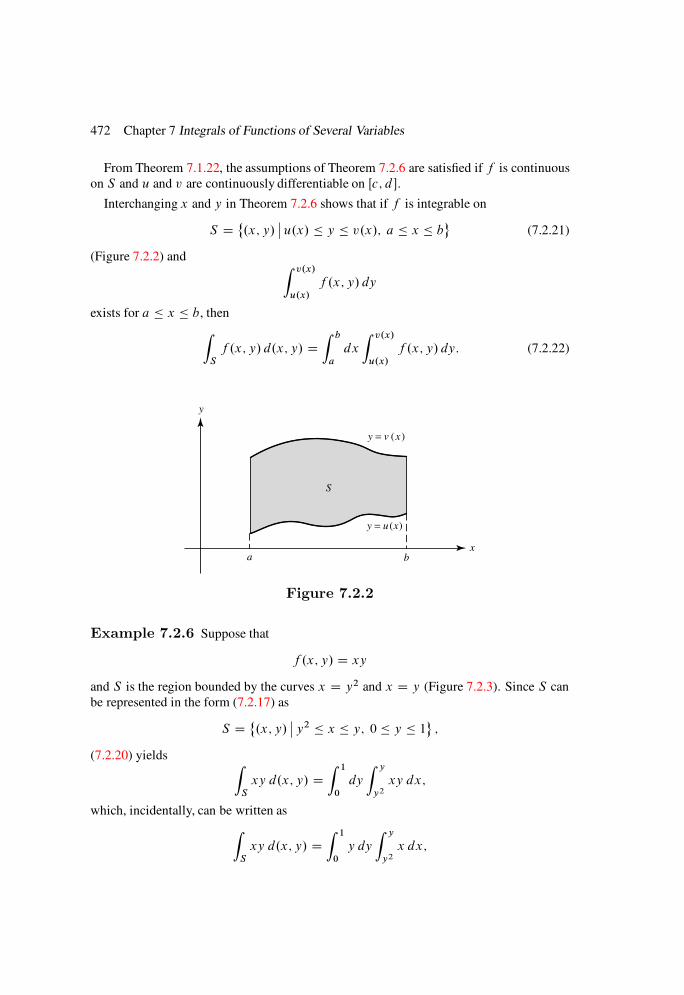
472 Chapter 7 Integrals of Functions of Several Variables
From Theorem 7.1.22, the assumptions of Theorem 7.2.6 are satisfied if f is continuous
on S and u and v are continuously differentiable on Œc; d .
Interchanging x and y in Theorem 7.2.6 shows that if f is integrable on
S D˚.x; y/
ˇu.x/ y v.x/; a x b
(7.2.21)
(Figure 7.2.2) and Z v.x/
u.x/
f .x; y/ dy
exists for a x b, then
Z
S
f .x; y/ d.x; y/ DZ b
a
dx
Z v.x/
u.x/
f .x; y/ dy: (7.2.22)
y
xa b
y = v (x )
y = u (x)
S
Figure 7.2.2
Example 7.2.6 Suppose that
f .x; y/ D xy
and S is the region bounded by the curves x D y2 and x D y (Figure 7.2.3). Since S can
be represented in the form (7.2.17) as
S D˚.x; y/
ˇy2 x y; 0 y 1
;
(7.2.20) yields Z
S
xy d.x; y/ DZ 1
0
dy
Z y
y2
xy dx;
which, incidentally, can be written as
Z
S
xy d.x; y/ DZ 1
0
y dy
Z y
y2
x dx;

Section 7.2 Iterated Integrals and Multiple Integrals 473
since y is independent of x. Evaluating the iterated integral yields
Z
S
xy d.x; y/ DZ 1
0
x2
2
ˇˇy
y2
!y dy D 1
2
Z 1
0
.y3 y5/ dy
D 1
2
y4
4 y
6
6
ˇˇ1
0
D 1
24:
y
x
x = y2
x = y
(1, 1)
S
Figure 7.2.3
In this case we can also represent S in the form (7.2.21) as
S D˚.x; y/
ˇx y
px; 0 x 1
I
hence, from (7.2.22),
Z
S
xy d.x; y/ DZ 1
0
x dx
Z px
x
y dy DZ 1
0
y2
2
ˇˇp
x
yDx
!x dx
D 1
2
Z 1
0
.x2 x3/ dx D 1
2
x3
3 x
4
4
ˇˇ1
0
D 1
24:
Example 7.2.7 To evaluate
Z
S
.x C y/ d.x; y/;
where
S D˚.x; y/
ˇ 1 x 1; 0 y 1C jxj
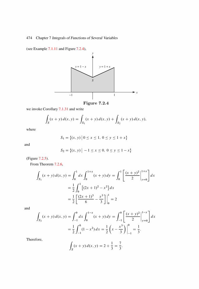
474 Chapter 7 Integrals of Functions of Several Variables
(see Example 7.1.11 and Figure 7.2.4),
S
y
x
y = 1 − x y = 1 + x
1−1
Figure 7.2.4
we invoke Corollary 7.1.31 and write
Z
S
.x C y/ d.x; y/ DZ
S1
.x C y/ d.x; y/ CZ
S2
.x C y/ d.x; y/;
where
S1 D˚.x; y/
ˇ0 x 1; 0 y 1C x
and
S2 D˚.x; y/
ˇ 1 x 0; 0 y 1 x
(Figure 7.2.5).
From Theorem 7.2.6,
Z
S1
.x C y/ d.x; y/ DZ 1
0
dx
Z 1Cx
0
.x C y/ dy DZ 1
0
".x C y/2
2
ˇˇ1Cx
yD0
#dx
D 1
2
Z 1
0
.2x C 1/2 x2
dx
D 1
2
.2x C 1/3
6 x
3
3
ˇˇ1
0
D 2
andZ
S2
.x C y/ d.x; y/ DZ 0
1
dx
Z 1x
0
.x C y/ dy DZ 0
1
".x C y/2
2
ˇˇ1x
yD0
#dx
D 1
2
Z 0
1
.1 x2/ dx D 1
2
x x
3
3
ˇˇ0
1
D 1
3:
Therefore, Z
S
.x C y/ d.x; y/ D 2C 1
3D 7
3:

Section 7.2 Iterated Integrals and Multiple Integrals 475
y y
x x
y = 1 − xy = 1 + x
S1
S2
Figure 7.2.5
Example 7.2.8 To find the area A of the region bounded by the curves
y D x2 C 1 and y D 9 x2
(Figure 7.2.6), we evaluate
A DZ
S
d.x; y/;
where
S D˚.x; y/
ˇx2 C 1 y 9 x2;2 x 2
:
According to Theorem 7.2.6,
A DZ 2
2
dx
Z 9x2
x2C1
dy DZ 2
2
.9 x2/ .x2 C 1/
dx
DZ 2
2
.8 2x2/ dx D8x 2x
3
3
ˇˇ2
2
D 64
3:
y
x
y = x2 + 1
y = 9 − x2
(2, 5)(−2, 5) S
Figure 7.2.6
476 Chapter 7 Integrals of Functions of Several Variables
Theorem 7.2.6 has an analog for n > 2. Suppose that f is integrable on a set S of points
X D .x1; x2; : : : ; xn/ satisfying the inequalities
uj .xj C1; : : : ; xn/ xj vj .xj C1; : : : ; xn/; 1 j n 1;
and
an xn bn:
Then, under appropriate additional assumptions, it can be shown by an argument analogous
to the one that led to Theorem 7.2.6 that
Z
S
f .X/ dX DZ bn
an
dxn
Z vn.xn/
un.xn/
dxn1 Z v2.x3;:::;xn/
u2.x3;:::;xn/
dx2
Z v1.x2;:::;xn/
u1.x2;:::;xn/
f .X/ dx1:
These additional assumptions are tedious to state for general n. The following theorem
contains a complete statement for n D 3.
Theorem 7.2.7 Suppose that f is integrable on
S D˚.x; y; ´/
ˇu1.y; ´/ x v1.y; ´/; u2.´/ y v2.´/; c ´ d
;
and let
S.´/ D˚.x; y/
ˇu1.y; ´/ x v1.y; ´/; u2.´/ y v2.´/
for each ´ in Œc; d : Then
Z
S
f .x; y; ´/ d.x; y; ´/ DZ d
c
d´
Z v2.´/
u2.´/
dy
Z v1.y;´/
u1.y;´/
f .x; y; ´/ dx;
provided that Z v1.y;´/
u1.y;´/
f .x; y; ´/ dx
exists for all .y; ´/ such that
c ´ d and u2.´/ y v2.´/;
and Z
S.´/
f .x; y; ´/ d.x; y/
exists for all ´ in Œc; d :
Example 7.2.9 Suppose that f is continuous on the region S in R3 bounded by the
coordinate planes and the plane
x C y C 2´ D 2
(Figure 7.2.7); thus,

Section 7.2 Iterated Integrals and Multiple Integrals 477
y
x
z
x + y + 2z = 1
Figure 7.2.7
S D˚.x; y; ´/
ˇ0 x 2 y 2´; 0 y 2 2´; 0 ´ 1
:
From Theorem 7.2.7,
Z
S
f .x; y; ´/ d.x; y; ´/ DZ 1
0
d´
Z 22´
0
dy
Z 2y2´
0
f .x; y; ´/ dx:
There are five other iterated integrals that equal the multiple integral. We leave it to you
to verify that
Z
S
f .x; y; ´/ d.x; y; ´/DZ 2
0
dy
Z 1y=2
0
d´
Z 2y2´
0
f .x; y; ´/ dx
DZ 1
0
d´
Z 22´
0
dx
Z 2x2´
0
f .x; y; ´/ dy
DZ 2
0
dx
Z 1x=2
0
d´
Z 2x2´
0
f .x; y; ´/ dy
DZ 2
0
dx
Z 2x
0
dy
Z 1x=2y=2
0
f .x; y; ´/ d´
DZ 2
0
dy
Z 2y
0
dx
Z 1x=2y=2
0
f .x; y; ´/ d´
(Exercise 7.2.15).
Thus far we have viewed the iterated integral as a tool for evaluating multiple integrals.
In some problems the iterated integral is itself the object of interest. In this case a result
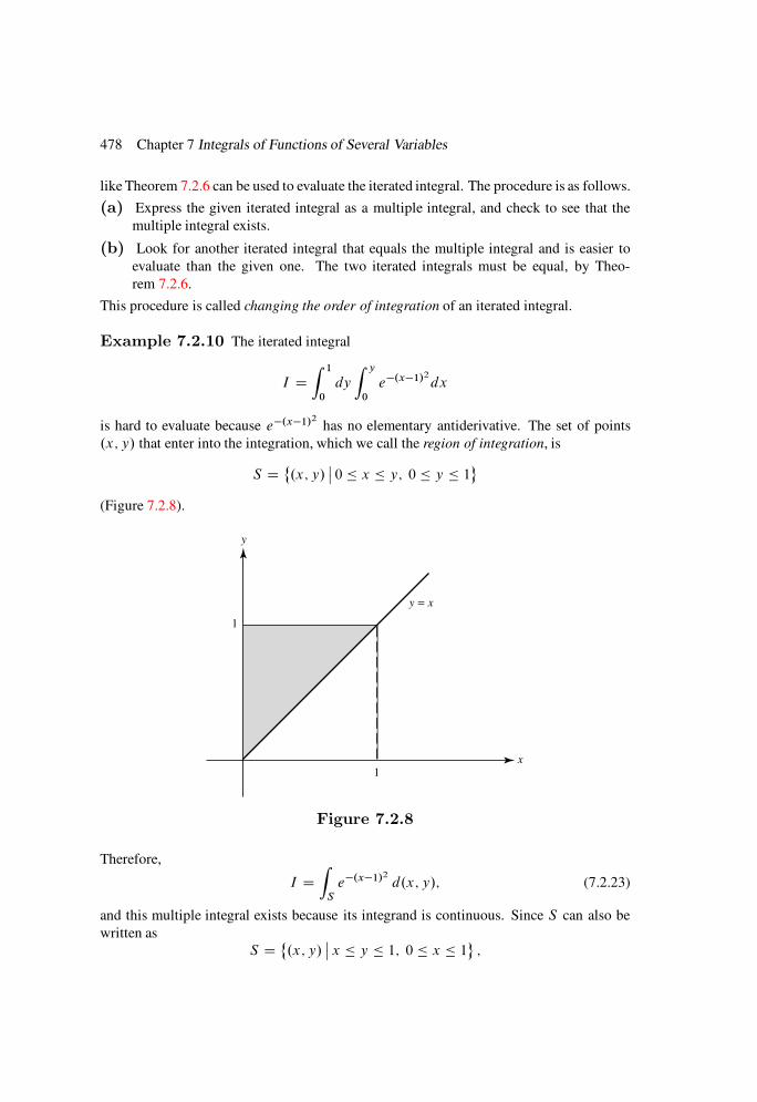
478 Chapter 7 Integrals of Functions of Several Variables
like Theorem 7.2.6 can be used to evaluate the iterated integral. The procedure is as follows.
(a) Express the given iterated integral as a multiple integral, and check to see that the
multiple integral exists.
(b) Look for another iterated integral that equals the multiple integral and is easier to
evaluate than the given one. The two iterated integrals must be equal, by Theo-
rem 7.2.6.
This procedure is called changing the order of integration of an iterated integral.
Example 7.2.10 The iterated integral
I DZ 1
0
dy
Z y
0
e.x1/2
dx
is hard to evaluate because e.x1/2
has no elementary antiderivative. The set of points
.x; y/ that enter into the integration, which we call the region of integration, is
S D˚.x; y/
ˇ0 x y; 0 y 1
(Figure 7.2.8).
y
x
y = x
1
1
Figure 7.2.8
Therefore,
I DZ
S
e.x1/2
d.x; y/; (7.2.23)
and this multiple integral exists because its integrand is continuous. Since S can also be
written as
S D˚.x; y/
ˇx y 1; 0 x 1
;
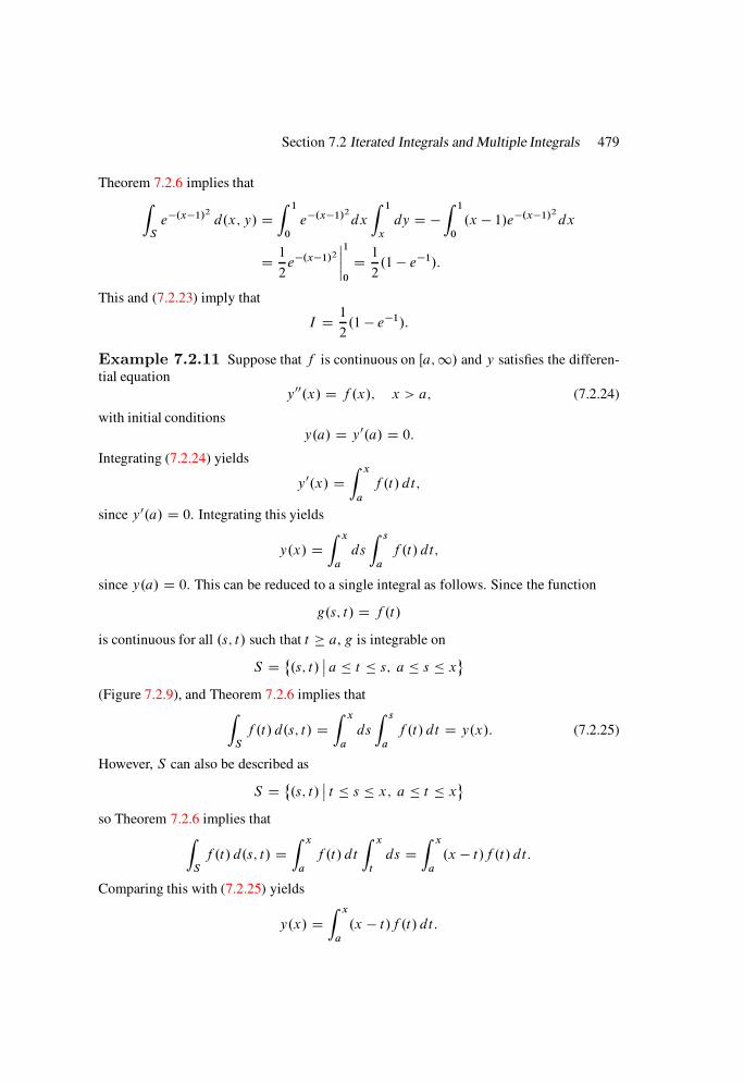
Section 7.2 Iterated Integrals and Multiple Integrals 479
Theorem 7.2.6 implies that
Z
S
e.x1/2
d.x; y/ DZ 1
0
e.x1/2
dx
Z 1
x
dy D Z 1
0
.x 1/e.x1/2
dx
D 1
2e.x1/2
ˇˇ1
0
D 1
2.1 e1/:
This and (7.2.23) imply that
I D 1
2.1 e1/:
Example 7.2.11 Suppose that f is continuous on Œa;1/ and y satisfies the differen-
tial equation
y00.x/ D f .x/; x > a; (7.2.24)
with initial conditions
y.a/ D y0.a/ D 0:Integrating (7.2.24) yields
y0.x/ DZ x
a
f .t/ dt;
since y0.a/ D 0. Integrating this yields
y.x/ DZ x
a
ds
Z s
a
f .t/ dt;
since y.a/ D 0. This can be reduced to a single integral as follows. Since the function
g.s; t/ D f .t/
is continuous for all .s; t/ such that t a, g is integrable on
S D˚.s; t/
ˇa t s; a s x
(Figure 7.2.9), and Theorem 7.2.6 implies thatZ
S
f .t/ d.s; t/ DZ x
a
ds
Z s
a
f .t/ dt D y.x/: (7.2.25)
However, S can also be described as
S D˚.s; t/
ˇt s x; a t x
so Theorem 7.2.6 implies thatZ
S
f .t/ d.s; t/ DZ x
a
f .t/ dt
Z x
t
ds DZ x
a
.x t/f .t/ dt:
Comparing this with (7.2.25) yields
y.x/ DZ x
a
.x t/f .t/ dt:
480 Chapter 7 Integrals of Functions of Several Variables
t
xs
a
a
s = t
S
Figure 7.2.9
7.2 Exercises
1. Evaluate
(a)Z 2
0
dy
Z 1
1
.x C 3y/ dx (b)Z 2
1
dx
Z 1
0
.x3 C y4/ dy
(c)Z 2
=2
x dx
Z 2
1
sinxy dy (d)Z log 2
0
y dy
Z 1
0
xex2ydx
2. Let Ij D Œaj ; bj , 1 j 3, and suppose that f is integrable onR D I1I2I3.
Prove:
(a) If the integral
G.y; ´/ DZ b1
a1
f .x; y; ´/ dx
exists for .y; ´/ 2 I2 I3, thenG is integrable on I2 I3 and
Z
R
f .x; y; ´/ d.x; y; ´/ DZ
I2I3
G.y; ´/ d.y; ´/:
(b) If the integral
H.´/ DZ
I1I2
f .x; y; ´/ d.x; y/

Section 7.2 Iterated Integrals and Multiple Integrals 481
exists for ´ 2 I3, thenH is integrable on I3 and
Z
R
f .x; y; ´/ d.x; y; ´/ DZ b3
a3
H.´/ d´:
HINT: For both parts; see the proof of Theorem 7.2.1:
3. Prove: If f is continuous on Œa; b Œc; d , then the function
F.y/ DZ b
a
f .x; y/ dx
is continuous on Œc; d . HINT: Use Theorem 5.2.14:
4. Suppose that
f .x0; y0/ f .x; y/ if a x x0 b; c y y0 d:
Show that f satisfies the hypotheses of Theorem 7.2.1 onR D Œa; bŒc; d . HINT:
See the proof of Theorem 3.2.9:
5. Evaluate by means of iterated integrals:
(a)Z
R
.xy C 1/ d.x; y/; R D Œ0; 1 Œ1; 2
(b)Z
R
.2x C 3y/ d.x; y/; R D Œ1; 3 Œ1; 2
(c)Z
R
xypx2 C y2
d.x; y/; R D Œ0; 1 Œ0; 1
(d)R
R x cos xy cos 2x d.x; y/; R D Œ0; 14 Œ0; 2
6. Let A be the set of points of the form .2mp; 2mq/, where p and q are odd integers
and m is a nonnegative integer. Let
f .x; y/ D(1; .x; y/ 62 A;0; .x; y/ 2 A:
Show that f is not integrable on any rectangle R D Œa; b Œc; d , but
Z b
a
dx
Z d
c
f .x; y/ dy DZ d
c
dy
Z b
a
f .x; y/ dx D .b a/.d c/: .A/
HINT: For (A); use Theorem 3.5.6 and Exercise 3.5.6:
7. Let
f .x; y/ D2xy if y is rational;
y if y is irrational;
and R D Œ0; 1 Œ0; 1 (Example 7.2.3).

482 Chapter 7 Integrals of Functions of Several Variables
(a) CalculateR
Rf .x; y/ d.x; y/ and
RRf .x; y/ d.x; y/, and show that f is not
integrable on R.
(b) CalculateR 1
0
R 1
0f .x; y/ dy
dx and
R 1
0
R 1
0f .x; y/ dy
dx.
8. Let R D Œ0; 1 Œ0; 1 Œ0; 1, eR D Œ0; 1 Œ0; 1, and
f .x; y; ´/ D
8ˆ<ˆ:
2xy C 2x´ if y and ´ are rational;
y C 2x´ if y is irrational and ´ is rational;
2xy C ´ if y is rational and ´ is irrational;
y C ´ if y and ´ are irrational:
Calculate
(a)Z
R
f .x; y; ´/ d.x; y; ´/ and
Z
R
f .x; y; ´/ d.x; y; ´/
(b)Z
eRf .x; y; ´/ d.x; y/ and
Z
eRf .x; y; ´/ d.x; y/
(c)Z 1
0
dy
Z 1
0
f .x; y; ´/ dx and
Z 1
0
d´
Z 1
0
dy
Z 1
0
f .x; y; ´/ dx.
9. Suppose that f is bounded on R D Œa; b Œc; d . Prove:
(a)Z
R
f .x; y/ d.x; y/ Z b
a
Z d
c
f .x; y/ dy
!dx. HINT: Use Exercise 3.2.6(a):
(b)Z
R
f .x; y/ d.x; y/ Z b
a
Z d
c
f .x; y/ dy
!dx. HINT: Use Exercise 3.2.6(b):
10. Use Exercise 7.2.9 to prove the following generalization of Theorem 7.2.1: If f is
integrable on R D Œa; b Œc; d , then
Z b
a
f .x; y/ dy and
Z d
c
f .x; y/ dy
are integrable on Œa; b, and
Z b
a
Z d
c
f .x; y/ dy
!dx D
Z b
a
Z d
c
f .x; y/ dy
!dx D
Z
R
f .x; y/ d.x; y/:
11. Evaluate
(a)Z
R
.x 2y C 3´/ d.x; y; ´/; R D Œ2; 0 Œ2; 5 Œ3; 2
(b)Z
R
ex2y2
sin x sin´d.x; y; ´/; R D Œ1; 1 Œ0; 2 Œ0; =2
(c)Z
R
.xy C 2x´C y´/ d.x; y; ´/; R D Œ1; 1 Œ0; 1 Œ1; 1
Section 7.2 Iterated Integrals and Multiple Integrals 483
(d)Z
R
x2y3´exy2´2
d.x; y; ´/; R D Œ0; 1 Œ0; 1 Œ0; 1
12. Evaluate
(a)Z
S
.2x C y2/ d.x; y/; S D˚.x; y/
ˇ0 x 9 y2;3 y 3
(b)Z
S
2xy d.x; y/; S is bounded by y D x2 and x D y2
(c)Z
S
ex siny
yd.x; y/; S D
˚.x; y/
ˇlogy x log 2y; =2 y
13. EvaluateR
S.x C y/ d.x; y/, where S is bounded by y D x2 and y D 2x, using
iterated integrals of both possible types.
14. Find the area of the set bounded by the given curves.
(a) y D x2 C 9, y D x2 9, x D 1, x D 1(b) y D x C 2, y D 4 x, x D 0(c) x D y2 4, x D 4 y2
(d) y D e2x, y D 2x, x D 315. In Example 7.2.9, verify the last five representations of
RSf .x; y; ´/ d.x; y; ´/ as
iterated integrals.
16. Let S be the region in R3 bounded by the coordinate planes and the plane x C
2y C 3´ D 1. Let f be continuous on S . Set up six iterated integrals that equalRSf .x; y; ´/ d.x; y; ´/.
17. Evaluate
(a)Z
S
x d.x; y; ´/; S is bounded by the coordinate planes and the plane
3xC y C ´ D 2.
(b)Z
S
ye´ d.x; y; ´/; S D˚.x; y; ´/
ˇ0 x 1; 0 y
px; 0 ´ y2
(c)Z
S
xy´d.x; y; ´/;
S Dn.x; y; ´/
ˇ0 y 1; 0 x
p1 y2; 0 ´
px2 C y2
o
(d)Z
S
y´d.x; y; ´/; S D˚.x; y; ´/
ˇ´2 x p´; 0 y ´; 0 ´ 1
18. Find the volume of S .
(a) S is bounded by the surfaces ´ D x2 C y2 and ´ D 8 x2 y2.
(b) S D f.x; y; ´/ j 0 ´ x2 C y2; .x; y; 0/ is in the triangle with vertices
.0; 1; 0/, .0; 0; 0/, and .1; 0; 0/
(c) S D˚.x; y; ´/
ˇ0 y x2; 0 x 2; 0 ´ y2
(d) S D˚.x; y; ´/
ˇx 0; y 0; 0 ´ 4 4x2 4y2
484 Chapter 7 Integrals of Functions of Several Variables
19. Let R D Œa1; b2 Œa2; b2 Œan; bn. Evaluate
(a)R
R.x1 C x2 C C xn/ dX (b)
RR.x2
1 C x22 C C x2
n/ dX
(c)R
Rx1x2; xn dX
20. Assuming that f is continuous, express
Z 1
1=2
dy
Z p1y2
p
1y2
f .x; y/ dx
as an iterated integral with the order of integration reversed.
21. EvaluateR
S.xCy/ d.x; y/ of Example 7.2.7 by means of iterated integrals in which
the first integration is with respect to x.
22. Evaluate
Z 1
0
x dx
Z p1x2
0
dypx2 C y2
:
23. Suppose that f is continuous on Œa;1/,
y.n/.x/ D f .x/; t a;
and y.a/ D y0.a/ D D y.n1/.a/ D 0.
(a) Integrate repeatedly to show that
y.x/ DZ x
a
dtn
Z tn
a
dtn1 Z t3
a
dt2
Z t2
a
f .t1/ dt1: .A/
(b) By successive reversals of orders of integration as in Example 7.2.11, deduce
from (A) that
y.x/ D 1
.n 1/Š
Z x
a
.x t/n1f .t/ dt:
24. Let T D Œ0; Œ0; ; > 0. By calculating
I.a/ D lim!1
Z
T
exy sinax d.x; y/
in two different ways, show that
Z 1
0
sin ax
xdx D
2if a > 0:
7.3 CHANGE OF VARIABLES IN MULTIPLE INTEGRALS
In Section 3.3 we saw that a change of variables may simplify the evaluation of an ordinary
integral. We now consider change of variables in multiple integrals.

Section 7.3 Change of Variables in Multiple Integrals 485
Prior to formulating the rule for change of variables, we must deal with some rather
involved preliminary considerations.
Jordan Measurable Sets
In Section we defined the content of a set S to be
V.S/ DZ
S
dX (7.3.1)
if the integral exists. If R is a rectangle containing S , then (7.3.1) can be rewritten as
V.S/ DZ
R
S .X/ dX;
where S is the characteristic function of S , defined by
S .X/ D1; X 2 S;0; X 62 S:
From Exercise 7.1.27, the existence and value of V.S/ do not depend on the particular
choice of the enclosing rectangle R. We say that S is Jordan measurable if V.S/ exists.
Then V.S/ is the Jordan content of S .
We leave it to you (Exercise 7.3.2) to show that S has zero content according to Defini-
tion 7.1.14 if and only if S has Jordan content zero.
Theorem 7.3.1 A bounded set S is Jordan measurable if and only if the boundary of
S has zero content:
Proof Let R be a rectangle containing S . Suppose that V.@S/ D 0. Since S is
bounded onR and discontinuous only on @S (Exercise 2.2.9), Theorem 7.1.19 implies thatRR S .X/ dX exists. For the converse, suppose that @S does not have zero content and
let P D fR1; R2; : : : ; Rkg be a partition of R. For each j in f1; 2; : : : ; kg there are three
possibilities:
1. Rj S ; then
min˚ S .X/
ˇX 2 Rj
D max
˚ S .X/
ˇX 2 Rj
D 1:
2. Rj \ S ¤ ; and Rj \ Sc ¤ ;; then
min˚ S .X/
ˇX 2 Rj
D 0 and max
˚ S .X/
ˇX 2 Rj
D 1:
3. Rj Sc ; then
min˚ S .X/
ˇX 2 Rj
D max
˚ S .X/
ˇX 2 Rj
D 0:

486 Chapter 7 Integrals of Functions of Several Variables
Let
U1 D˚jˇRj S
and U2 D
˚jˇRj \ S ¤ ; and Rj \ Sc ¤ ;
: (7.3.2)
Then the upper and lower sums of S over P are
S.P / DX
j 2U1
V.Rj /CX
j 2U2
V.Rj /
D total content of the subrectangles in P that intersect S
(7.3.3)
and
s.P / DX
j 2U1
V.Rj /
D total content of the subrectangles in P contained in S:
(7.3.4)
Therefore,
S.P / s.P / DX
j 2U2
V.Rj /;
which is the total content of the subrectangles in P that intersect both S and Sc . Since
these subrectangles contain @S , which does not have zero content, there is an 0 > 0 such
that
S.P / s.P / 0
for every partitionP of R. By Theorem 7.1.12, this implies that S is not integrable onR,
so S is not Jordan measurable.
Theorems 7.1.19 and 7.3.1 imply the following corollary.
Corollary 7.3.2 If f is bounded and continuous on a bounded Jordan measurable set
S; then f is integrable on S:
Lemma 7.3.3 Suppose that K is a bounded set with zero content and ; > 0: Then
there are cubes C1; C2; . . . ; Cr with edge lengths< such that Cj \K ¤ ;; 1 j r;
K r[
j D1
Cj ; (7.3.5)
andrX
j D1
V.Cj / < :
Proof Since V.K/ D 0, Z
C
K.X/ dX D 0
if C is any cube containingK. From this and the definition of the integral, there is a ı > 0
such that if P is any partition of C with kP k ı and is any Riemann sum of K over
P , then
0 : (7.3.6)

Section 7.3 Change of Variables in Multiple Integrals 487
Now suppose that P D fC1; C2; : : : ; Ckg is a partition of C into cubes with
kP k < min.; ı/; (7.3.7)
and let C1, C2, . . . , Ck be numbered so that Cj \K ¤ ; if 1 j r and Cj \K D ;if r C 1 j k. Then (7.3.5) holds, and a typical Riemann sum of K over P is of the
form
DrX
j D1
K.Xj /V .Cj /
with Xj 2 Cj , 1 j r . In particular, we can choose Xj fromK, so that K .Xj / D 1,
and
DrX
j D1
V.Cj /:
Now (7.3.6) and (7.3.7) imply that C1, C2, . . . , Cr have the required properties.
Transformations of Jordan-Measurable Sets
To formulate the theorem on change of variables in multiple integrals, we must first con-
sider the question of preservation of Jordan measurability under a regular transformation.
Lemma 7.3.4 Suppose that G W Rn ! Rn is continuously differentiable on a bounded
open set S; and let K be a closed subset of S with zero content: Then G.K/ has zero
content.
Proof Since K is a compact subset of the open set S , there is a 1 > 0 such that the
compact set
K1D˚Xˇ
dist.X; K/ 1
is contained in S (Exercise 5.1.26). From Lemma 6.2.7, there is a constantM such that
jG.Y/ G.X/j M jY Xj if X;Y 2 K1: (7.3.8)
Now suppose that > 0. Since V.K/ D 0, there are cubes C1, C2, . . . , Cr with edge
lengths s1, s2, . . . , sr < 1=pn such that Cj \K ¤ ;, 1 j r ,
K r[
j D1
Cj ;
andrX
j D1
V.Cj / < (7.3.9)
(Lemma 7.3.3). For 1 j r , let Xj 2 Cj \K. If X 2 Cj , then
jX Xj j sjpn < 1;

488 Chapter 7 Integrals of Functions of Several Variables
so X 2 K and jG.X/G.Xj /j M jXXj j Mpn sj , from (7.3.8). Therefore, G.Cj /
is contained in a cube eC j with edge length 2Mpn sj , centered at G.Xj /. Since
V.eC j / D .2Mpn/nsn
j D .2Mpn/nV.Cj /;
we now see that
G.K/ r[
j D1
eC j
andrX
j D1
V.eC j / .2Mpn/n
rX
j D1
V.Cj / < .2Mpn/n;
where the last inequality follows from (7.3.9). Since .2Mpn/n does not depend on , it
follows that V.G.K// D 0.
Theorem 7.3.5 Suppose that G W Rn ! Rn is regular on a compact Jordan measur-
able set S: Then G.S/ is compact and Jordan measurable:
Proof We leave it to you to prove that G.S/ is compact (Exercise 6.2.23). Since S
is Jordan measurable, V.@S/ D 0, by Theorem 7.3.1. Therefore, V.G.@S// D 0, by
Lemma 7.3.4. But G.@S/ D @.G.S// (Exercise 6.3.23), so [email protected]/// D 0, which
implies that G.S/ is Jordan measurable, again by Theorem 7.3.1.
Change of Content Under a Linear Transformation
To motivate and prove the rule for change of variables in multiple integrals, we must know
how V.L.S// is related to V.S/ if S is a compact Jordan measurable set and L is a nonsin-
gular linear transformation. (From Theorem 7.3.5, L.S/ is compact and Jordan measurable
in this case.) The next lemma from linear algebra will help to establish this relationship.
We omit the proof.
Lemma 7.3.6 A nonsingular n n matrix A can be written as
A D EkEk1 E1; (7.3.10)
where each Ei is a matrix that can be obtained from the n n identity matrix I by one of
the following operationsW(a) interchanging two rows of II(b) multiplying a row of I by a nonzero constantI(c) adding a multiple of one row of I to another:
Matrices of the kind described in this lemma are called elementary matrices. The key to
the proof of the lemma is that if E is an elementary n n matrix and A is any n nmatrix,
then EA is the matrix obtained by applying to A the same operation that must be applied
to I to produce E (Exercise 7.3.6). Also, the inverse of an elementary matrix of type (a),
(b), or (c) is an elementary matrix of the same type (Exercise 7.3.7).
The next example illustrates the procedure for finding the factorization (7.3.10).
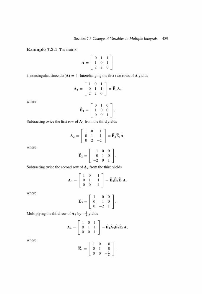
Section 7.3 Change of Variables in Multiple Integrals 489
Example 7.3.1 The matrix
A D
240 1 1
1 0 1
2 2 0
35
is nonsingular, since det.A/ D 4. Interchanging the first two rows of A yields
A1 D
241 0 1
0 1 1
2 2 0
35 D bE1A;
where
bE1 D
240 1 0
1 0 0
0 0 1
35 :
Subtracting twice the first row of A1 from the third yields
A2 D
241 0 1
0 1 1
0 2 2
35 D bE2
bE1A;
where
bE2 D
24
1 0 0
0 1 0
2 0 1
35 :
Subtracting twice the second row of A2 from the third yields
A3 D
241 0 1
0 1 1
0 0 4
35 D bE3
bE2bE1A;
where
bE3 D
241 0 0
0 1 0
0 2 1
35 :
Multiplying the third row of A3 by 14
yields
A4 D
241 0 1
0 1 1
0 0 1
35 D bE4
bA3bE2bE1A;
where
bE4 D
241 0 0
0 1 0
0 0 14
35 :
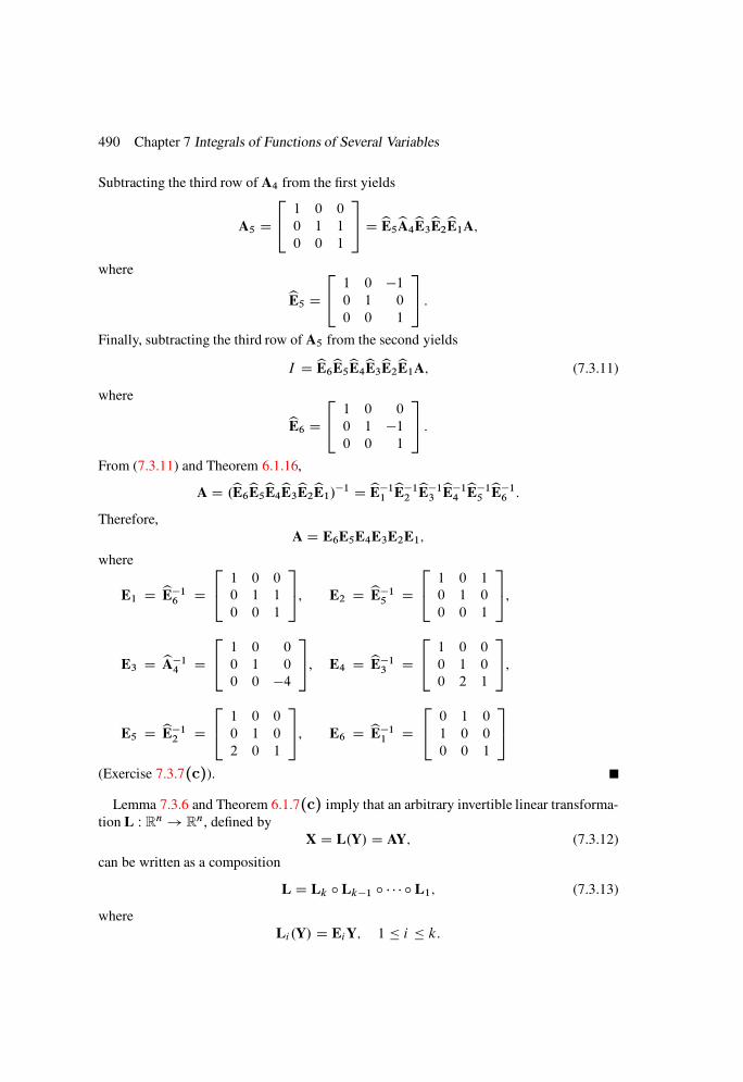
490 Chapter 7 Integrals of Functions of Several Variables
Subtracting the third row of A4 from the first yields
A5 D
241 0 0
0 1 1
0 0 1
35 D bE5
bA4bE3bE2bE1A;
where
bE5 D
241 0 10 1 0
0 0 1
35 :
Finally, subtracting the third row of A5 from the second yields
I D bE6bE5bE4bE3bE2bE1A; (7.3.11)
where
bE6 D
241 0 0
0 1 10 0 1
35 :
From (7.3.11) and Theorem 6.1.16,
A D .bE6bE5bE4bE3bE2bE1/
1 D bE11bE1
2bE1
3bE1
4bE1
5bE1
6 :
Therefore,
A D E6E5E4E3E2E1;
where
E1 D bE16 D
241 0 0
0 1 1
0 0 1
35, E2 D bE1
5 D
241 0 1
0 1 0
0 0 1
35,
E3 D bA14 D
241 0 0
0 1 0
0 0 4
35, E4 D bE1
3 D
241 0 0
0 1 0
0 2 1
35,
E5 D bE12 D
241 0 0
0 1 0
2 0 1
35, E6 D bE1
1 D
240 1 0
1 0 0
0 0 1
35
(Exercise 7.3.7(c)).
Lemma 7.3.6 and Theorem 6.1.7(c) imply that an arbitrary invertible linear transforma-
tion L W Rn ! Rn, defined by
X D L.Y/ D AY; (7.3.12)
can be written as a composition
L D Lk ı Lk1 ı ı L1; (7.3.13)
where
Li.Y/ D EiY; 1 i k:

Section 7.3 Change of Variables in Multiple Integrals 491
Theorem 7.3.7 If S is a compact Jordan measurable subset of Rn and L W Rn ! R
n
is the invertible linear transformation X D L.Y/ D AY; then
V.L.S// D j det.A/jV.S/: (7.3.14)
Proof Theorem 7.3.5 implies that L.S/ is Jordan measurable. If
V.L.R// D j det.A/jV.R/ (7.3.15)
whenever R is a rectangle, then (7.3.14) holds if S is any compact Jordan measurable
set. To see this, suppose that > 0, let R be a rectangle containing S , and let P DfR1; R2; : : : ; Rkg be a partition of R such that the upper and lower sums of S over P
satisfy the inequality
S.P / s.P / < : (7.3.16)
Let U1 and U2 be as in (7.3.2). From (7.3.3) and (7.3.4),
s.P / DX
j 2U1
V.Rj / V.S/ X
j 2U1
V.Rj /CX
j 2U2
V.Rj / D S.P /: (7.3.17)
Theorem 7.3.7 implies that L.R1/, L.R2/, . . . , L.Rk/ and L.S/ are all Jordan measurable.
Since [
j 2U1
Rj S [
j 2S1[S2
Rj ;
it follows that
L
0@ [
j 2U1
Rj
1A L.S/ L
0@ [
j 2S1[S2
Rj
1A :
Since L is one-to-one on Rn, this implies that
X
j 2U1
V.L.Rj // V.L.S// X
j 2U1
V.L.Rj //CX
j 2U2
V.L.Rj //: (7.3.18)
If we assume that (7.3.15) holds whenever R is a rectangle, then
V.L.Rj // D j det.A/jV.Rj /; 1 j k;
so (7.3.18) implies that
s.P / V.L.S//
j det.A/j S.P /:
This, (7.3.16) and (7.3.17) imply that
ˇˇV.S/ V.L.S//j det.A/j
ˇˇ < I
hence, since can be made arbitrarily small, (7.3.14) follows for any Jordan measurable
set.

492 Chapter 7 Integrals of Functions of Several Variables
To complete the proof, we must verify (7.3.15) for every rectangle
R D Œa1; b1 Œa2; b2 Œan; bn D I1 I2 In:
Suppose that A in (7.3.12) is an elementary matrix; that is, let
X D L.Y/ D EY:
CASE 1. If E is obtained by interchanging the i th and j th rows of I, then
xr D
8<:yr if r ¤ i and r ¤ j Iyj if r D i Iyi if r D j :
Then L.R/ is the Cartesian product of I1, I2, . . . , In with Ii and Ij interchanged, so
V.L.R// D V.R/ D j det.E/jV.R/
since det.E/ D 1 in this case (Exercise 7.3.7(a)).
CASE 2. If E is obtained by multiplying the r th row of I by a, then
xr Dyr if r ¤ i ;ayi if r D i :
Then
L.R/ D I1 Ii1 I 0i IiC1 In;
where I 0i is an interval with length equal to jaj times the length of Ii , so
V.L.R// D jajV.R/ D j det.E/jV.R/
since det.E/ D a in this case (Exercise 7.3.7(a)).
CASE 3. If E is obtained by adding a times the j th row of I to its i th row (j ¤ i ), then
xr Dyr if r ¤ i Iyi C ayj if r D i :
Then
L.R/ D˚.x1; x2; : : : ; xn/
ˇai C axj xi bi C axj and ar xr br if r ¤ i
;
which is a parallelogram if n D 2 and a parallelepiped if n D 3 (Figure 7.3.1). Now
V.L.R// DZ
L.R/
dX;
which we can evaluate as an iterated integral in which the first integration is with respect
to xi . For example, if i D 1, then
V.L.R// DZ bn
an
dxn
Z bn1
an1
dxn1 Z b2
a2
dx2
Z b1Caxj
a1Caxj
dx1: (7.3.19)
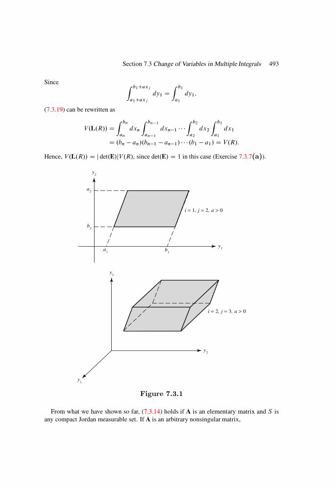
Section 7.3 Change of Variables in Multiple Integrals 493
Since Z b1Caxj
a1Caxj
dy1 DZ b1
a1
dy1;
(7.3.19) can be rewritten as
V.L.R// DZ bn
an
dxn
Z bn1
an1
dxn1 Z b2
a2
dx2
Z b1
a1
dx1
D .bn an/.bn1 an1/ .b1 a1/ D V.R/:
Hence, V.L.R// D j det.E/jV.R/, since det.E/ D 1 in this case (Exercise 7.3.7(a)).
a1
b1
y1
y1
y2
y3
b2
a2
y2
i = 1, j = 2, a > 0
i = 2, j = 3, a > 0
Figure 7.3.1
From what we have shown so far, (7.3.14) holds if A is an elementary matrix and S is
any compact Jordan measurable set. If A is an arbitrary nonsingular matrix,
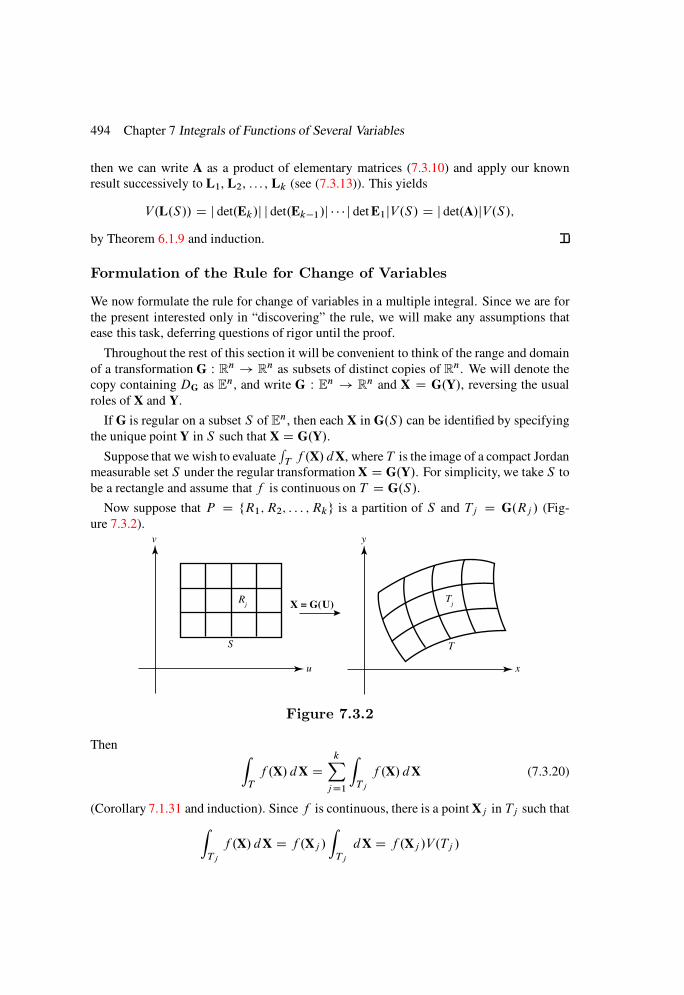
494 Chapter 7 Integrals of Functions of Several Variables
then we can write A as a product of elementary matrices (7.3.10) and apply our known
result successively to L1, L2, . . . , Lk (see (7.3.13)). This yields
V.L.S// D j det.Ek/j j det.Ek1/j j det E1jV.S/ D j det.A/jV.S/;
by Theorem 6.1.9 and induction.
Formulation of the Rule for Change of Variables
We now formulate the rule for change of variables in a multiple integral. Since we are for
the present interested only in “discovering” the rule, we will make any assumptions that
ease this task, deferring questions of rigor until the proof.
Throughout the rest of this section it will be convenient to think of the range and domain
of a transformation G W Rn ! Rn as subsets of distinct copies of R
n. We will denote the
copy containing DG as En, and write G W En ! R
n and X D G.Y/, reversing the usual
roles of X and Y.
If G is regular on a subset S of En, then each X in G.S/ can be identified by specifying
the unique point Y in S such that X D G.Y/.
Suppose that we wish to evaluateR
T f .X/ dX, where T is the image of a compact Jordan
measurable set S under the regular transformation X D G.Y/. For simplicity, we take S to
be a rectangle and assume that f is continuous on T D G.S/.
Now suppose that P D fR1; R2; : : : ; Rkg is a partition of S and Tj D G.Rj / (Fig-
ure 7.3.2).
Tj
T
Rj
S
y
xu
v
X = G(U)
Figure 7.3.2
Then Z
T
f .X/ dX DkX
j D1
Z
Tj
f .X/ dX (7.3.20)
(Corollary 7.1.31 and induction). Since f is continuous, there is a point Xj in Tj such that
Z
Tj
f .X/ dX D f .Xj /
Z
Tj
dX D f .Xj /V .Tj /
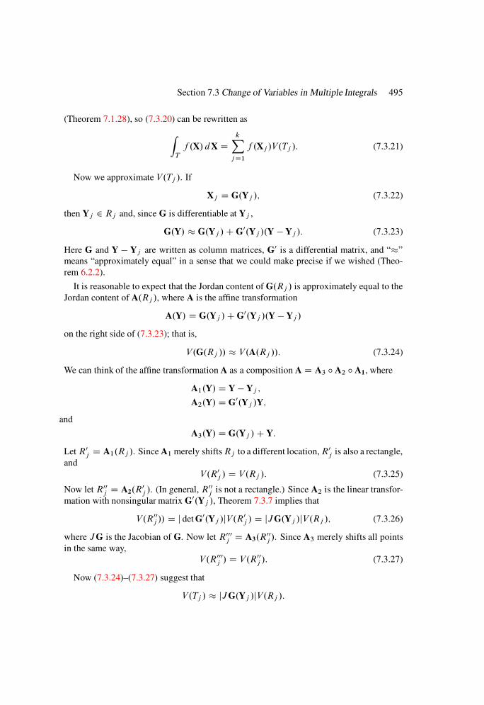
Section 7.3 Change of Variables in Multiple Integrals 495
(Theorem 7.1.28), so (7.3.20) can be rewritten as
Z
T
f .X/ dX DkX
j D1
f .Xj /V .Tj /: (7.3.21)
Now we approximate V.Tj /. If
Xj D G.Yj /; (7.3.22)
then Yj 2 Rj and, since G is differentiable at Yj ,
G.Y/ G.Yj /CG0.Yj /.Y Yj /: (7.3.23)
Here G and Y Yj are written as column matrices, G0 is a differential matrix, and “”
means “approximately equal” in a sense that we could make precise if we wished (Theo-
rem 6.2.2).
It is reasonable to expect that the Jordan content of G.Rj / is approximately equal to the
Jordan content of A.Rj /, where A is the affine transformation
A.Y/ D G.Yj /CG0.Yj /.Y Yj /
on the right side of (7.3.23); that is,
V.G.Rj // V.A.Rj //: (7.3.24)
We can think of the affine transformation A as a composition A D A3 ı A2 ı A1, where
A1.Y/ D Y Yj ;
A2.Y/ D G0.Yj /Y;
and
A3.Y/ D G.Yj /C Y:
Let R0j D A1.Rj /. Since A1 merely shiftsRj to a different location,R0
j is also a rectangle,
and
V.R0j / D V.Rj /: (7.3.25)
Now let R00j D A2.R
0j /. (In general, R00
j is not a rectangle.) Since A2 is the linear transfor-
mation with nonsingular matrix G0.Yj /, Theorem 7.3.7 implies that
V.R00j // D j det G0.Yj /jV.R0
j / D jJG.Yj /jV.Rj /; (7.3.26)
where JG is the Jacobian of G. Now let R000j D A3.R
00j /. Since A3 merely shifts all points
in the same way,
V.R000j / D V.R00
j /: (7.3.27)
Now (7.3.24)–(7.3.27) suggest that
V.Tj / jJG.Yj /jV.Rj /:

496 Chapter 7 Integrals of Functions of Several Variables
(Recall that Tj D G.Rj /.) Substituting this and (7.3.22) into (7.3.21) yields
Z
T
f .X/ dX kX
j D1
f .G.Yj //jJG.Yj /jV.Rj /:
But the sum on the right is a Riemann sum for the integral
Z
S
f .G.Y//jJG.Y/j dY;
which suggests that
Z
T
f .X/ dX DZ
S
f .G.Y//jJG.Y/j dY:
We will prove this by an argument that was published in the American Mathematical
Monthly [Vol. 61 (1954), pp. 81-85] by J. Schwartz.
The Main Theorem
We now prove the following form of the rule for change of variable in a multiple integral.
Theorem 7.3.8 Suppose that G W En ! Rn is regular on a compact Jordan measur-
able set S and f is continuous on G.S/: Then
Z
G.S/
f .X/ dX DZ
S
f .G.Y//jJG.Y/j dY: (7.3.28)
Since the proof is complicated, we break it down to a series of lemmas. We first observe
that both integrals in (7.3.28) exist, by Corollary 7.3.2, since their integrands are continu-
ous. (Note that S is compact and Jordan measurable by assumption, and G.S/ is compact
and Jordan measurable by Theorem 7.3.5.) Also, the result is trivial if V.S/ D 0, since then
V.G.S// D 0 by Lemma 7.3.4, and both integrals in (7.3.28) vanish. Hence, we assume
that V.S/ > 0. We need the following definition.
Definition 7.3.9 If A D Œaij is an n n matrix; then
max
8<:
nX
j D1
jaij jˇ1 i n
9=;
is the infinity norm of A; denoted by kAk1.
Lemma 7.3.10 Suppose that G W En ! Rn is regular on a cube C in E
n; and let A be
a nonsingular n n matrix: Then
V.G.C // j det.A/jmax
˚kA1G0.Y/k1
ˇY 2 C
nV.C/: (7.3.29)

Section 7.3 Change of Variables in Multiple Integrals 497
Proof Let s be the edge length of C . Let Y0 D .c1; c2; : : : ; cn/ be the center of C , and
suppose that H D .y1; y2; : : : ; yn/ 2 C . If H D .h1; h2; : : : ; hn/ is continuously differen-
tiable on C , then applying the mean value theorem (Theorem 5.4.5) to the components of
H yields
hi .Y/ hi .Y0/ DnX
j D1
@hi .Yi /
@yj
.yj cj /; 1 i n;
where Yi 2 C . Hence, recalling that
H0.Y/ D@hi
@yj
n
i;j D1
;
applying Definition 7.3.9, and noting that jyj cj j s=2, 1 j n, we infer that
jhi.Y/ hi.Y0/j s
2max
˚kH0.Y/k1
ˇY 2 C
; 1 i n:
This means that H.C / is contained in a cube with center X0 D H.Y0/ and edge length
smax˚kH0.Y/k1
ˇY 2 C
:
Therefore,V.H.C //
max fkH0.Y/k1
nˇY 2 C
sn
Dmax fkH0.Y/k1
nˇY 2 C
V.C/:
(7.3.30)
Now let
L.X/ D A1X
and set H D L ıG; then
H.C / D L.G.C // and H0 D A1G0;
so (7.3.30) implies that
V.L.G.C /// max
˚kA1G0.Y/k1
ˇY 2 C
nV.C/: (7.3.31)
Since L is linear, Theorem 7.3.7 with A replaced by A1 implies that
V.L.G.C /// D j det.A/1jV.G.C //:
This and (7.3.31) imply that
j det.A1/jV.G.C // max
˚kA1G0.Y/k1
ˇY 2 C
nV.C/:
Since det.A1/ D 1= det.A/, this implies (7.3.29).
Lemma 7.3.11 If G W En ! Rn is regular on a cube C in R
n; then
V.G.C // Z
C
jJG.Y/j dY: (7.3.32)
498 Chapter 7 Integrals of Functions of Several Variables
Proof Let P be a partition of C into subcubes C1, C2, . . . , Ck with centers Y1, Y2, . . . ,
Yk . Then
V.G.C // DkX
j D1
V.G.Cj //: (7.3.33)
Applying Lemma 7.3.10 to Cj with A D G0.Aj / yields
V.G.Cj // jJG.Yj /jmax
˚k.G0.Yj //
1G0.Y/k1ˇ
Y 2 Cj
nV.Cj /: (7.3.34)
Exercise 6.1.22 implies that if > 0, there is a ı > 0 such that
max˚k.G0.Yj //
1G0.Y/k1ˇY 2 Cj
< 1C ; 1 j k; if kP k < ı:
Therefore, from (7.3.34),
V.G.Cj // .1C /njJG.Yj /jV.Cj /;
so (7.3.33) implies that
V.G.C // .1C /nkX
j D1
jJG.Yj /jV.Cj / if kP k < ı:
Since the sum on the right is a Riemann sum forR
CjJG.Y/j dY and can be taken arbi-
trarily small, this implies (7.3.32).
Lemma 7.3.12 Suppose that S is Jordan measurable and ; > 0: Then there are
cubes C1; C2; . . . ; Cr in S with edge lengths < ; such that Cj S; 1 j r;
C 0i \ C 0
j D ; if i ¤ j; and
V.S/ rX
j D1
V.Cj /C : (7.3.35)
Proof Since S is Jordan measurable,Z
C
S .X/ dX D V.S/
if C is any cube containing S . From this and the definition of the integral, there is a ı > 0
such that if P is any partition of C with kP k < ı and is any Riemann sum of S over
P , then > V.S/ =2. Therefore, if s.P / is the lower sum of S over P, then
s.P/ > V.S/ if kPk < ı: (7.3.36)
Now suppose that P D fC1; C2; : : : ; Ckg is a partition of C into cubes with kP k <min.; ı/, and let C1, C2, . . . , Ck be numbered so that Cj S if 1 j r and
Cj \ Sc ¤ ; if j > r . From (7.3.4), s.P/ DPr
j D1 V.Ck/. This and (7.3.36) imply
(7.3.35). Clearly, C 0i \ C 0
j D ; if i ¤ j .
Section 7.3 Change of Variables in Multiple Integrals 499
Lemma 7.3.13 Suppose that G W En ! Rn is regular on a compact Jordan measur-
able set S and f is continuous and nonnegative on G.S/: Let
Q.S/ DZ
G.S/
f .X/ dX Z
S
f .G.Y//jJG.Y/j dY: (7.3.37)
Then Q.S/ 0:
Proof From the continuity of JG and f on the compact sets S and G.S/, there are
constantsM1 and M2 such that
jJG.Y/j M1 if Y 2 S (7.3.38)
and
jf .X/j M2 if X 2 G.S/ (7.3.39)
(Theorem 5.2.11). Now suppose that > 0. Since f ı G is uniformly continuous on S
(Theorem 5.2.14), there is a ı > 0 such that
jf .G.Y// f .G.Y0//j < if jY Y0j < ı and Y;Y0 2 S: (7.3.40)
Now let C1, C2, . . . , Cr be chosen as described in Lemma 7.3.12, with D ı=pn. Let
S1 D
8<:Y 2 S
ˇY …
r[
j D1
Cj
9=; :
Then V.S1/ < and
S D
0@
r[
j D1
Cj
1A [ S1: (7.3.41)
Suppose that Y1, Y2, . . . , Yr are points in C1, C2, . . . , Cr and Xj D G.Yj /, 1 j r .
From (7.3.41) and Theorem 7.1.30,
Q.S/ DZ
G.S1/
f .X/ dX Z
S1
f .G.Y//jJG.Y/j dY
CrX
j D1
Z
G.Cj /
f .X/ dX rX
j D1
Z
Cj
f .G.Y//jJG.Y/j dY
DZ
G.S1/
f .X/ dX Z
S1
f .G.Y//jJG.Y/j dY
CrX
j D1
Z
G.Cj /
.f .X/ f .Aj // dX
CrX
j D1
Z
Cj
..f .G.Yj // f .G.Y///jJ.G.Y/j dY
CrX
j D1
f .Xj /
V.G.Cj //
Z
Cj
jJG.Y/j dY
!:
500 Chapter 7 Integrals of Functions of Several Variables
Since f .X/ 0, Z
S1
f .G.Y//jJG.Y/j dY 0;
and Lemma 7.3.11 implies that the last sum is nonpositive. Therefore,
Q.S/ I1 C I2 C I3; (7.3.42)
where
I1 DZ
G.S1/
f .X/ dX; I2 DrX
j D1
Z
G.Cj /
jf .X/ f .Xj /j dX;
and
I3 DrX
j D1
Z
Cj
jf .G/.Yj // f .G.Y//jjJG.Y/j dY:
We will now estimate these three terms. Suppose that > 0.
To estimate I1, we first remind you that since G is regular on the compact set S , G is
also regular on some open set O containing S (Definition 6.3.2). Therefore, since S1 Sand V.S1/ < , S1 can be covered by cubes T1, T2, . . . , Tm such that
rX
j D1
V.Tj / < (7.3.43)
and G is regular onSm
j D1 Tj . Now,
I1 M2V.G.S1// (from (7.3.39))
M2
mX
j D1
V.G.Tj // .since S1 [mj D1Tj /
M2
mX
j D1
Z
Tj
jJG.Y/j dY (from Lemma 7.3.11)
M2M1 (from (7.3.38) and (7.3.43)):
To estimate I2, we note that if X and Xj are in G.Cj / then X D G.Y/ and Xj D G.Yj /
for some Y and Yj in Cj . Since the edge length of Cj is less than ı=pn, it follows that
jY Yj j < ı, so jf .X/ f .Xj /j < , by (7.3.40). Therefore,
I2 <
rX
j D1
V.G.Cj //
rX
j D1
Z
Cj
jJG.Y/jdY (from Lemma 7.3.11)
M1
rX
j D1
V.Cj / (from (7.3.38)/
M1V.S/ .since [rj D1 Cj S/:
Section 7.3 Change of Variables in Multiple Integrals 501
To estimate I3, we note again from (7.3.40) that jf .G.Yj // f .G.Y//j < if Y and
Yj are in Cj . Hence,
I3 <
rX
j D1
Z
Cj
jJG.Y/jdY
M1
rX
j D1
V.Cj / (from (7.3.38)
M1V.S/
becauseSr
j D1 Cj S and C 0i \ C 0
j D ; if i ¤ j .
From these inequalities on I1, I2, and I3, (7.3.42) now implies that
Q.S/ < M1.M2 C 2V.S//:
Since is an arbitrary positive number, it now follows that Q.S/ 0.
Lemma 7.3.14 Under the assumptions of Lemma 7.3.13; Q.S/ 0:
Proof Let
G1 D G1; S1 D G.S/; f1 D .jJGj/f ıG; (7.3.44)
and
Q1.S1/ DZ
G1.S1/
f1.Y/ dY Z
S1
f1.G1.X//jJG1 .X/j dX: (7.3.45)
Since G1 is regular on S1 (Theorem 6.3.3) and f1 is continuous and nonnegative on
G1.S1/ D S , Lemma 7.3.13 implies thatQ1.S1/ 0. However, substituting from (7.3.44)
into (7.3.45) and again noting that G1.S1/ D S yields
Q1.S1/DZ
S
f .G.Y//jJG.Y/j dY
Z
G.S/
f .G.G1.X///jJG.G1 .X//jjJG1.X/j dX:(7.3.46)
Since G.G1.X// D X, f .G.G1.X/// D f .X/. However, it is important to interpret the
symbol JG.G1.X// properly. We are not substituting G1.X/ into G here; rather, we are
evaluating the determinant of the differential matrix of G at the point Y D G1.X/. From
Theorems 6.1.9 and 6.3.3,
jJG.G1.X//jjJG1 .X/j D 1;
so (7.3.46) can be rewritten as
Q1.S1/ DZ
S
f .G.Y//jJG.Y/j dY Z
G.S/
f .X/ dX D Q.S/:
Since Q1.S1/ 0, it now follows that Q.S/ 0.
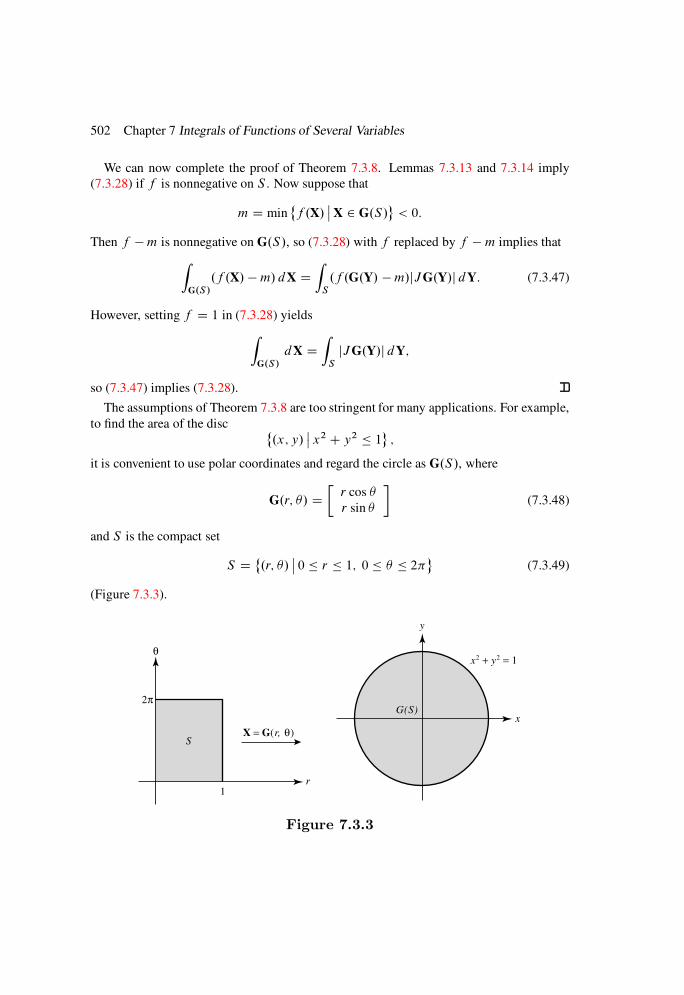
502 Chapter 7 Integrals of Functions of Several Variables
We can now complete the proof of Theorem 7.3.8. Lemmas 7.3.13 and 7.3.14 imply
(7.3.28) if f is nonnegative on S . Now suppose that
m D min˚f .X/
ˇX 2 G.S/
< 0:
Then f m is nonnegative on G.S/, so (7.3.28) with f replaced by f m implies that
Z
G.S/
.f .X/ m/dX DZ
S
.f .G.Y/ m/jJG.Y/j dY: (7.3.47)
However, setting f D 1 in (7.3.28) yields
Z
G.S/
dX DZ
S
jJG.Y/j dY;
so (7.3.47) implies (7.3.28).
The assumptions of Theorem 7.3.8 are too stringent for many applications. For example,
to find the area of the disc ˚.x; y/
ˇx2 C y2 1
;
it is convenient to use polar coordinates and regard the circle as G.S/, where
G.r; / Dr cos
r sin
(7.3.48)
and S is the compact set
S D˚.r; /
ˇ0 r 1; 0 2
(7.3.49)
(Figure 7.3.3).
SX = G(r, θ)
2π
1
θ
y
r
x
x2 + y2 = 1
G(S)
Figure 7.3.3

Section 7.3 Change of Variables in Multiple Integrals 503
Since
G0.r; / D
cos r sin
sin r cos
;
it follows that JG.r; / D r . Therefore, formally applying Theorem 7.3.8 with f 1
yields
A DZ
G.S/
dX DZ
S
r d.r; / DZ 1
0
r dr
Z 2
0
d D :
Although this is a familiar result, Theorem 7.3.8 does not really apply here, since G.r; 0/ DG.r; 2/, 0 r 1, so G is not one-to-one on S , and therefore not regular on S .
The next theorem shows that the assumptions of Theorem 7.3.8 can be relaxed so as to
include this example.
Theorem 7.3.15 Suppose that G W En ! R
n is continuously differentiable on a
bounded open set N containing the compact Jordan measurable set S; and regular on
S0: Suppose also that G.S/ is Jordan measurable; f is continuous on G.S/; andG.C/ is
Jordan measurable for every cube C N . Then
Z
G.S/
f .X/ dX DZ
S
f .G.Y//jJG.Y/j dY: (7.3.50)
Proof Since f is continuous on G.S/ and .jJGj/f ıG is continuous on S , the integrals
in (7.3.50) both exist, by Corollary 7.3.2. Now let
D dist .@S; N c/
(Exercise 5.1.25), and
P D˚Yˇ
dist.Y; @S/ 2:
Then P is a compact subset of N (Exercise 5.1.26) and @S P 0 (Figure 7.3.4).
Since S is Jordan measurable, V.@S/ D 0, by Theorem 7.3.1. Therefore, if > 0, we
can choose cubes C1, C2, . . . , Ck in P 0 such that
@S k[
j D1
C 0j (7.3.51)
andkX
j D1
V.Cj / < (7.3.52)
Now let S1 be the closure of the set of points in S that are not in any of the cubes C1,
C2, . . . , Ck; thus,
S1 D S \[k
j D1Cj
c
:

504 Chapter 7 Integrals of Functions of Several Variables
Because of (7.3.51), S1 \ @S D ;, so S1 is a compact Jordan measurable subset of S0.
Therefore, G is regular on S1, and f is continuous on G.S1/. Consequently, if Q is as
defined in (7.3.37), then Q.S1/ D 0 by Theorem 7.3.8.
N = open set bounded by outer curve
S = closed set bounded by inner curve
∂S
D
ρ
Figure 7.3.4
Now
Q.S/ D Q.S1/CQ.S \ Sc1 / D Q.S \ Sc
1 / (7.3.53)
(Exercise 7.3.11) and
jQ.S \ Sc1 /j
ˇˇˇ
Z
G.S\Sc1
/
f .X/ dX
ˇˇˇC
ˇˇˇ
Z
S\Sc1
f .G.Y//jJG.Y/j dY
ˇˇˇ :
But ˇˇˇ
Z
S\Sc1
f .G.Y//jJG.Y/j dY
ˇˇˇ M1M2V.S \ Sc
1 /; (7.3.54)
where M1 and M2 are as defined in (7.3.38) and (7.3.39). Since S \ Sc1 [k
j D1Cj ,
(7.3.52) implies that V.S \ Sk1 / < ; therefore,
ˇˇˇ
Z
S\Sc1
f .G.Y//jJG.Y/j dY
ˇˇˇ M1M2; (7.3.55)
from (7.3.54). Alsoˇˇˇ
Z
G.S\Sc1
/
f .X/ dX
ˇˇˇ M2V.G.S \ Sc
1 // M2
kX
j D1
V.G.Cj //: (7.3.56)

Section 7.3 Change of Variables in Multiple Integrals 505
By the argument that led to (7.3.30) withH D G and C D Cj ,
V.G.Cj // max
˚kG0.Y/k1
ˇY 2 Cj
nV.Cj /;
so (7.3.56) can be rewritten as
ˇˇˇ
Z
G.S\Sc1
/
f .X/ dX
ˇˇˇ M2
max
˚kG0.Y/k1
ˇY 2 P
n;
because of (7.3.52). Since can be made arbitrarily small, this and (7.3.55) imply that
Q.S \ Sc1 / D 0. Now Q.S/ D 0, from (7.3.53).
The transformation to polar coordinates to compute the area of the disc is now justi-
fied, since G and S as defined by (7.3.48) and (7.3.49) satisfy the assumptions of Theo-
rem 7.3.15.
Polar Coordinates
If G is the transformation from polar to rectangle coordinates
x
y
D G.r; / D
r cos
r sin
; (7.3.57)
then JG.r; / D r and (7.3.50) becomes
Z
G.S/
f .x; y/ d.x; y/ DZ
S
f .r cos ; r sin /r d.r; /
if we assume, as is conventional, that S is in the closed right half of the r-plane. This
transformation is especially useful when the boundaries of S can be expressed conveniently
in terms of polar coordinates, as in the example preceding Theorem 7.3.15. Two more
examples follow.
Example 7.3.2 Evaluate
I DZ
T
.x2 C y/ d.x; y/;
where T is the annulus
T D˚.x; y/
ˇ1 x2 C y2 4
(Figure 7.3.5(b)).
Solution We write T D G.S/, with G as in (7.3.57) and
S D˚.r; /
ˇ1 r 2; 0 2

506 Chapter 7 Integrals of Functions of Several Variables
(Figure 7.3.5(a)). Theorem 7.3.15 implies that
I DZ
S
.r2 cos2 C r sin /r d.r; /;
which we evaluate as an iterated integral:
I DZ 2
1
r2 dr
Z 2
0
.r cos2 C sin / d
DZ 2
1
r2 dr
Z 2
0
r2Cr
2cos 2 C sin
d
since cos2 D
1
2.1C cos 2/
DZ 2
1
r2
r
2C r
4sin 2 cos
ˇˇ2
D0
dr D Z 2
1
r3 dr D r4
4
ˇˇ2
1
D 15
4:
T
S
y
r
x
2π
(a) (b)
θ
21
Figure 7.3.5
Example 7.3.3 Evaluate
I DZ
T
y d.x; y/;
where T is the region in the xy-plane bounded by the curve whose points have polar coor-
dinates satisfying
r D 1 cos ; 0
(Figure 7.3.6(b)).
Solution We write T D G.S/, with G as in (7.3.57) and S the shaded region in
Figure 7.3.6(a). From (7.3.50),
I DZ
S
.r sin /r d.r; /;

Section 7.3 Change of Variables in Multiple Integrals 507
which we evaluate as an iterated integral:
I DZ
0
sin d
Z 1cos
0
r2 dr D 1
3
Z
0
.1 cos /3 sin d
D 1
12.1 cos /4
ˇˇ
0
D 4
3:
TS
r y
xθπ
(b)(a)
Figure 7.3.6
Spherical Coordinates
If G is the transformation from spherical to rectangular coordinates,
24x
y
´
35 D G.r; ; / D
24r cos cos
r sin cos
r sin
35 ; (7.3.58)
then
G0.r; ; / D
24
cos cos r sin cos r cos sin
sin cos r cos cos r sin sin
sin 0 r cos
35
and JG.r; ; / D r2 cos , so (7.3.50) becomes
Z
G.S/
f .x; y; ´/ d.x; y; ´/
DZ
S
f .r cos cos ; r sin cos ; r sin/r2 cos d.r; ; /
(7.3.59)
if we make the conventional assumption that jj =2 and r 0.
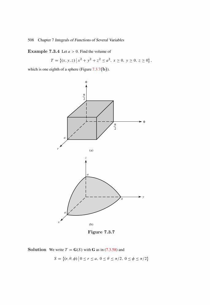
508 Chapter 7 Integrals of Functions of Several Variables
Example 7.3.4 Let a > 0. Find the volume of
T D˚.x; y; ´/
ˇx2 C y2 C ´2 a2; x 0; y 0; ´ 0
;
which is one eighth of a sphere (Figure 7.3.7(b)).
(a)
(b)
y
z
φ
θ
r
x
2
π
2
π
a
a
a
a
Figure 7.3.7
Solution We write T D G.S/ with G as in (7.3.58) and
S D˚.r; ; /
ˇ0 r a; 0 =2; 0 =2

Section 7.3 Change of Variables in Multiple Integrals 509
(Figure 7.3.7(a)), and let f 1 in (7.3.59). Theorem 7.3.15 implies that
V.T /DZ
G.S/
dX DZ
S
r2 cos d.r; ; /
DZ a
0
r2 dr
Z =2
0
d
Z =2
0
cos d Da3
3
2
(7.3.1) D a3
6:
Example 7.3.5 Evaluate the iterated integral
I DZ a
0
x dx
Z pa2x2
0
dy
Z pa2x2y2
0
´d´ .a > 0/:
Solution We first rewrite I as a multiple integral
I DZ
G.S/
x´ d.x; y; ´/
where G and S are as in Example 7.3.4. From Theorem 7.3.15,
I DZ
S
.r cos cos /.r sin/.r2 cos/ d.r; ; /
DZ a
0
r4 dr
Z =2
0
cos d
Z =2
0
cos2 sin d Da5
5
(7.3.1)
1
3
D a5
15:
Other Examples
We now consider other applications of Theorem 7.3.15.
Example 7.3.6 Evaluate
I DZ
T
.x C 4y/ d.x; y/;
where T is the parallelogram bounded by the lines
x C y D 1; x C y D 2; x 2y D 0; and x 2y D 3
(Figure 7.3.8(b)).
Solution We define new variables u and v by
u
v
D F.x; y/ D
x C yx 2y
:

510 Chapter 7 Integrals of Functions of Several Variables
S
v
u2
3
1
(a)
x
y= F−1(u,v)
T
y
x
(b)
x − 2y = 0
x − 2y = 3
x + y = 2
x + y = 1
Figure 7.3.8
Thenx
y
D F1.u; v/ D
2642uC v3
u v3
375 ;
JF1.u; v/ Dˇˇˇ
23
13
131
3
ˇˇˇ D
1
3;
and T D F1.S/, where
S D˚.u; v/
ˇ1 u 2; 0 v 3
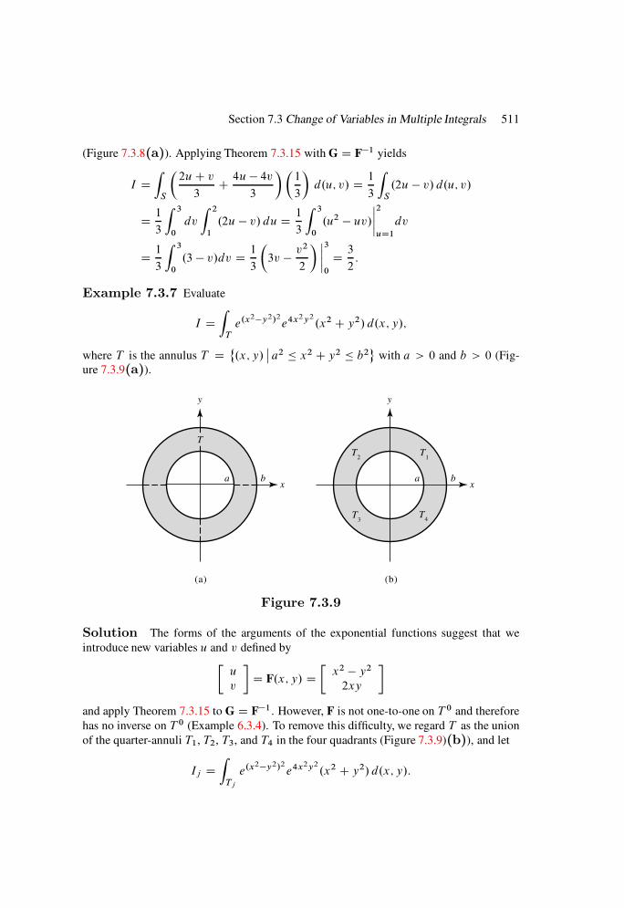
Section 7.3 Change of Variables in Multiple Integrals 511
(Figure 7.3.8(a)). Applying Theorem 7.3.15 with G D F1 yields
I DZ
S
2uC v3C 4u 4v
3
1
3
d.u; v/ D 1
3
Z
S
.2u v/ d.u; v/
D 1
3
Z 3
0
dv
Z 2
1
.2u v/ du D 1
3
Z 3
0
.u2 uv/ˇˇ2
uD1
dv
D 1
3
Z 3
0
.3 v/dv D 1
3
3v v
2
2
ˇˇ3
0
D 3
2:
Example 7.3.7 Evaluate
I DZ
T
e.x2y2/2
e4x2y2
.x2 C y2/ d.x; y/;
where T is the annulus T D˚.x; y/
ˇa2 x2 C y2 b2
with a > 0 and b > 0 (Fig-
ure 7.3.9(a)).
y
x
y
xa b
T
a b
T1
T2
T3
T4
(a) (b)
Figure 7.3.9
Solution The forms of the arguments of the exponential functions suggest that we
introduce new variables u and v defined by
u
v
D F.x; y/ D
x2 y2
2xy
and apply Theorem 7.3.15 to G D F1. However, F is not one-to-one on T 0 and therefore
has no inverse on T 0 (Example 6.3.4). To remove this difficulty, we regard T as the union
of the quarter-annuli T1, T2, T3, and T4 in the four quadrants (Figure 7.3.9)(b)), and let
Ij DZ
Tj
e.x2y2/2
e4x2y2
.x2 C y2/ d.x; y/:

512 Chapter 7 Integrals of Functions of Several Variables
Since the pairwise intersections of T1, T2, T3, and T4 all have zero content, I D I1 CI2 C I3 C I4 (Corollary 7.1.31). Theorem 7.3.8 implies that I1 D I2 D I3 D I4 (Exer-
cise 7.3.12), so I D 4I1. Since I1 does not contain any pairs of distinct points of the form
.x0; y0/ and .x0;y0/, F is one-to-one on T1 (Example 6.3.4),
F.T1/ D S1 D˚.u; v/
ˇa4 u2 C v2 b4; v 0
(Figure 7.3.10(b)),
S1
s1
v
uρ
α
π
a2 b2 a2 b2
(a) (b)
Figure 7.3.10
and a branch G of F1 can be defined on S1 (Example 6.3.8). Now Theorem 7.3.15 implies
that
I1 DZ
S1
e.x2y2/2
e4x2y2
.x2 C y2/jJG.u; v/j d.u; v/;
where x and y must still be written in terms of u and v. Since it is easy to verify that
JF.x; y/ D 4.x2 C y2/
and therefore
JG.u; v/ D 1
4.x2 C y2/;
doing this yields
I1 D1
4
Z
S1
eu2Cv2
d.u; v/: (7.3.60)
To evaluate this integral, we let and ˛ be polar coordinates in the uv-plane (Figure 7.3.11)
and define H by u
v
D H.; ˛/ D
cos˛
sin ˛
I
then S1 D H.eS1/, where
eS1 D˚.; ˛/
ˇa2 b2; 0 ˛

Section 7.3 Change of Variables in Multiple Integrals 513
(Figure 7.3.10(a)); hence, applying Theorem 7.3.15 to (7.3.60) yields
I1 D1
4
Z
eS1
e2jJH.; ˛/j d.; ˛/ D 1
4
Z
eS1
e2
d.; ˛/
D 1
4
Z
0
d˛
Z b2
a2
e2
d D .eb4 ea4/
8I
hence,
I D 4I1 D
2.eb4 ea4
/:
v
u
ρ
α
(u, v)
Figure 7.3.11
Example 7.3.8 Evaluate
I DZ
T
ex1Cx2CCxnd.x1; x2; : : : ; xn/;
where T is the region defined by
ai x1 C x2 C C xi bi ; 1 i n:
Solution We define the new variables y1, y2, . . . , yn by Y D F.X/, where
fi .X/ D x1 C x2 C C xi ; 1 i n:
If G D F1 then T D G.S/, where
S D Œa1; b1 Œa2; b2 Œan; bn;
and JG.Y/ D 1, since JF.X/ D 1 (verify); hence, Theorem 7.3.8 implies that
514 Chapter 7 Integrals of Functions of Several Variables
I DZ
S
eynd.y1; y2; : : : ; yn/
DZ b1
a1
dy1
Z b2
a2
dy2 Z bn1
an1
dyn1
Z bn
an
eyndyn
D .b1 a1/.b2 a2/ .bn1 an1/.ebn ean/:
7.3 Exercises
1. Give a counterexample to the following statement: If S1 and S2 are disjoint subsets
of a rectangle R, then either
Z
R
S1.X/ dXC
Z
R
S2.X/ dX D
Z
R
S1[S2.X/ dX
or Z
R
S1.X/ dXC
Z
R
S2.X/ dX D
Z
R
S1[S2.X/ dX:
2. Show that a set E has content zero according to Definition 7.1.14 if and only if E
has Jordan content zero.
3. Show that if S1 and S2 are Jordan measurable, then so are S1 [ S2 and S1 \ S2.
4. Prove:
(a) If S is Jordan measurable then so is S , and V.S/ D V.S/. Must S be Jordan
measurable if S is?
(b) If T is a Jordan measurable subset of a Jordan measurable set S , then S Tis Jordan measurable.
5. Suppose thatH is a subset of a compact Jordan measurable set S such that the inter-
section ofH with any compact subset of S0 has zero content. Show that V.H/ D 0.
6. Suppose that E is an n n elementary matrix and A is an arbitrary n p matrix.
Show that EA is the matrix obtained by applying to A the operation by which E is
obtained from the n n identity matrix.
7. (a) Calculate the determinants of elementary matrices of types (a), (b), and (c)of Lemma 7.3.6.
(b) Show that the inverse of an elementary matrix of type (a), (b), or (c) is an
elementary matrix of the same type.
(c) Verify the inverses given forbE1; : : : ;bE6 in Example 7.3.1.

Section 7.3 Change of Variables in Multiple Integrals 515
8. Write as a product of elementary matrices.
(a)
241 0 1
1 1 0
0 1 1
35 (b)
242 3 20 1 5
0 2 4
35
9. Suppose that adbc ¤ 0, u1 < u2, and v1 < v2. Find the area of the parallelogram
bounded by the lines
ax C by D u1; ax C by D u2;
cxC dy D v1; cx C dy D v2:
10. Find the volume of the parallelepiped defined by
1 2x C 3y 2´ 2; 5 x C 5y 7; 1 2x C 4y 6:
11. In writing Eqn. (7.3.53) we assumed that
Z
G.S/
f .X/ dX DZ
G.S1/
f .X/ dXCZ
G.S\Sc1
/
f .X/ dX:
Justify this. HINT: Show that G.S1/ \G.S \ Sc1 / has zero content:
12. Use Theorem 7.3.8 to show that I1 D I2 D I3 D I4 in Example 7.3.7.
13. Let ei D ˙1, 0 i n. Let T be a bounded subset of Rn and
bT D˚.e1x1; e2x2; : : : ; enxn/
ˇ.x1; x2; : : : ; xn/ 2 T
:
Suppose that f is defined on T and define g on bT by
g.e1x1; e2x2; : : : ; enxn/ D e0f .x1; x2; : : : ; xn/:
(a) Prove directly from Definitions 7.1.2 and 7.1.17 that f is integrable on T if
and only if g is integrable on bT , and in this case
Z
bTg.Y/ dY D e0
Z
T
f .X/ dX:
(b) Suppose that bT D T ,
f .e1x1; e2x2; : : : ; enxn/ D f .x1; x2; : : : ; xn/;
and f is integrable on T . Show that
Z
T
f .X/ dX D 0:
14. Find the area of
(a)˚.x; y/
ˇy x 4y; 1 x C 2y 3
;
516 Chapter 7 Integrals of Functions of Several Variables
(b)˚.x; y/
ˇ2 xy 4; 2x y 5x
.
15. Evaluate Z
T
.3x2 C 2y C ´/ d.x; y; ´/;
where
T D˚.x; y; ´/
ˇjx yj 1; jy ´j 1; j´C xj 1
:
16. Evaluate Z
T
.y2 C x2y 2x4/ d.x; y/;
where T is the region bounded by the curves
xy D 1; xy D 2; y D x2; y D x2 C 1:
17. Evaluate Z
T
.x4 y4/exy d.x; y/;
where T is the region in the first quadrant bounded by the hyperbolas
xy D 1; xy D 2; x2 y2 D 2; x2 y2 D 3:
18. Find the volume of the ellipsoid
x2
a2Cy2
b2C´2
c2D 1 .a; b; c > 0/:
19. Evaluate Z
T
ex2Cy2C´2
px2 C y2 C ´2
d.x; y; ´/;
where
T D˚.x; y; ´/
ˇ9 x2 C y2 C ´2 25
:
20. Find the volume of the set T bounded by the surfaces ´ D 0, ´ Dpx2 C y2, and
x2 C y2 D 4.
21. Evaluate Z
T
xy´.x4 y4/ d.x; y; ´/;
where
T D˚.x; y; ´/
ˇ1 x2 y2 2; 3 x2 C y2 4; 0 ´ 1
:
22. Evaluate
(a)Z p
2
0
dy
Z p4y2
y
dx
1C x2 C y2(b)
Z 2
0
dx
Z p4x2
0
ex2Cy2
dy
(c)Z 1
1
dx
Z p1x2
p
1x2
dy
Z p1x2y2
0
´2 d´

Section 7.3 Change of Variables in Multiple Integrals 517
23. Use the change of variables
2664
x1
x2
x3
x4
3775 D G.r; 1; 2; 3/ D
2664
r cos 1 cos 2 cos 3
r sin 1 cos 2 cos 3
r sin 2 cos 3
r sin 3
3775
to compute the content of the 4-ball
T D˚.x1; x2; x3; x4/
ˇx2
1 C x22 C x2
3 C x24 a2
:
24. Suppose that A D Œaij is a nonsingular n n matrix and T is the region in Rn
defined by
˛1 ai1x1 C ai2x2 C C ainxn ˇi ; 1 i n:
(a) Find V.T /.
(b) Show that if c1, c2, . . . , cn are constants, then
Z
T
0@
nX
j D1
cjxj
1A dX D V.T /
2
nX
iD1
di.˛i C ˇi/;
where 26664
d1
d2
:::
dn
37775 D .A
t /1
26664
c1
c2
:::
cn
37775 :
25. If Vn is the content of the n-ball T D˚XˇjXj 1
, find the content of the n-
dimensional ellipsoid defined by
nX
j D1
x2j
a2j
1:
Leave the answer in terms of Vn.

CHAPTER 8
Metric Spaces
IN THIS CHAPTER we study metric spaces.
SECTION 8.1 defines the concept and basic properties of a metric space. Several examples
of metric spaces are considered.
SECTION 8.2 defines and discusses compactness in a metric space.
SECTION 8.3 deals with continuous functions on metric spaces.
8.1 INTRODUCTION TO METRIC SPACES
Definition 8.1.1 A metric space is a nonempty set A together with a real-valued func-
tion defined on A A such that if u, v, and w are arbitrary members of A, then
(a) .u; v/ 0, with equality if and only if u D v;
(b) .u; v/ D .v; u/;(c) .u; v/ .u; w/C .w; v/.We say that is a metric on A.
If n 2 and u1, u2, . . . , un are arbitrary members of A, then (c) and induction yield
the inequality
.u1; un/ n1X
iD1
.ui ; uiC1/:
Example 8.1.1 The set R of real numbers with .u; v/ D ju vj is a metric space.
Definition 8.1.1(c) is the familiar triangle inequality:
ju vj ju wj C jw uj:
Motivated by this example, in an arbitrary metric space we call .u; v/ the distance from
u to v, and we call Definition 8.1.1(c) the triangle inequality.
518
Section 8.1 Introduction to Metric Spaces 519
Example 8.1.2 If A is an arbitrary nonempty set, then
.u; v/ D0 if u D v;1 if u ¤ v
is a metric on A (Exercise 8.1.5). We call it the discrete metric.
Example 8.1.2 shows that it is possible to define a metric on any nonempty set A. In
fact, it is possible to define infinitely many metrics on any set with more than one member
(Exercise 8.1.3). Therefore, to specify a metric space completely, we must specify the
couple .A; /, where A is the set and is the metric. (In some cases we will not be so
precise; for example, we will always refer to the real numbers with the metric .u; v/ Dju vj simply as R.)
There is an important kind of metric space that arises when a definition of length is
imposed on a vector space. Although we assume that you are familiar with the definition
of a vector space, we restate it here for convenience. We confine the definition to vector
spaces over the real numbers.
Definition 8.1.2 A vector space A is a nonempty set of elements called vectors on
which two operations, vector addition and scalar multiplication (multiplication by real
numbers) are defined, such that the following assertions are true for all U, V, and W in
A and all real numbers r and s:
1. UC V 2 A;
2. UC V D VC U;
3. UC .VCW/ D .UC V/CW;
4. There is a vector 0 in A such that UC 0 D U;
5. There is a vector U in A such that UC .U/ D 0;
6. rU 2 A;
7. r.UC V/ D rUC rV;
8. .r C s/U D rUC sU;
9. r.sU/ D .rs/U;
10. 1U D U.
We say that A is closed under vector addition if (1) is true, and that A is closed under
scalar multiplication if (6) is true. It can be shown that if B is any nonempty subset of A
that is closed under vector addition and scalar multiplication, then B together with these
operations is itself a vector space. (See any linear algebra text for the proof.) We say that
B is a subspace of A.
Definition 8.1.3 A normed vector space is a vector space A together with a real-valued
function N defined on A, such that if u and v are arbitrary vectors in A and a is a real
number, then
(a) N.u/ 0 with equality if and only if u D 0;
(b) N.au/ D jajN.u/;(c) N.uC v/ N.u/ CN.v/.We say that N is a norm on A, and .A; N / is a normed vector space.
520 Chapter 8 Metric Spaces
Theorem 8.1.4 If .A; N / is a normed vector space; then
.x; y/ D N.x y/ (8.1.1)
is a metric on A:
Proof From (a) with u D x y, .x; y/ D N.x y/ 0, with equality if and only
if x D y. From (b) with u D x y and a D 1,
.y; x/ D N.y x/ D N..x y// D N.x y/ D .x; y/:
From (c) with u D x ´ and v D ´ y,
.x; y/ D N.x y/ N.x ´/CN.´ y/ D .x; ´/C .´; y/:
We will say that the metric in (8.1.1) is induced by the norm N . Whenever we speak of
a normed vector space .A; N /, it is to be understood that we are regarding it as a metric
space .A; /, where is the metric induced by N .
We will often writeN.u/ as kuk. In this case we will denote the normed vector space as
.A; k k/.
Theorem 8.1.5 If x and y are vectors in a normed vector space .A; N /; then
jN.x/ N.y/j N.x y/: (8.1.2)
Proof Since
x D y C .x y/;Definition 8.1.3(c) with u D y and v D x y implies that
N.x/ N.y/ CN.x y/;
or
N.x/ N.y/ N.x y/:Interchanging x and y yields
N.y/ N.x/ N.y x/:
Since N.x y/ D N.y x/ (Definition 8.1.3(b) with u D x y and a D 1), the last
two inequalities imply (8.1.2).
Metrics for RRRn
In Section 5.1 we defined the norm of a vector X D .x1; x2; : : : ; xn/ in Rn as
kXk D
nX
iD1
x2i
!1=2
:

Section 8.1 Introduction to Metric Spaces 521
The metric induced by this norm is
.X;Y/ D
nX
iD1
.xi yi /2
!1=2
:
Whenever we write Rn without identifying the norm or metric specifically, we are referring
to Rn with this norm and this induced metric.
The following definition provides infinitely many norms and metrics on Rn.
Definition 8.1.6 If p 1 and X D .x1; x2; : : : ; xn/, let
kXkp D
nX
iD1
jxi jp!1=p
: (8.1.3)
The metric induced on Rn by this norm is
p.X;Y/ D
nX
iD1
jxi yi jp!1=p
:
To justify this definition, we must verify that (8.1.3) actually defines a norm. Since it is
clear that kXkp 0 with equality if and only if X D 0, and kaXkp D jajkXkp if a is any
real number and X 2 Rn, this reduces to showing that
kXC Ykp kXkp C kYkp (8.1.4)
for every X and Y in Rn. Since
jxi C yi j jxi j C jyi j;
summing both sides of this equation from i D 1 to n yields (8.1.4) with p D 1. To handle
the case where p > 1, we need the following lemmas. The inequality established in the
first lemma is known as Hölder’s inequality.
Lemma 8.1.7 Suppose that1; 2; . . . ; n and 1; 2; . . . ; n are nonnegative numbers:
Let p > 1 and q D p=.p 1/I thus;
1
pC 1
qD 1: (8.1.5)
ThennX
iD1
ii
nX
iD1
pi
!1=p nX
iD1
qi
!1=q
: (8.1.6)
Proof Let ˛ and ˇ be any two positive numbers, and consider the function
f .ˇ/ D ˛p
pC ˇq
q ˛ˇ;
522 Chapter 8 Metric Spaces
where we regard ˛ as a constant. Since f 0.ˇ/ D ˇq1˛ and f 00.ˇ/ D .q 1/ˇq2 > 0
for ˇ > 0, f assumes its minimum value on Œ0;1/ at ˇ D ˛1=.q1/ D ˛p1. But
f .˛p1/ D ˛p
pC ˛.p1/q
q ˛p D ˛p
1
pC 1
q 1
D 0:
Therefore,
˛ˇ ˛p
pC ˇq
qif ˛; ˇ 0: (8.1.7)
Now let
˛i D i
0@
nX
j D1
pj
1A
1=p
and ˇi D i
0@
nX
j D1
qj
1A
1=q
:
From (8.1.7),
˛iˇi
pi
p
0@
nX
j D1
pj
1A
1
C
qi
q
0@
nX
j D1
qj
1A
1
:
From (8.1.5), summing this from i D 1 to n yieldsPn
iD1 ˛iˇi 1, which implies (8.1.6).
Lemma 8.1.8 (Minkowski’s Inequality) Suppose that u1; u2; . . . ; un and v1;
v2; . . . ; vn are nonnegative numbers and p > 1: Then
nX
iD1
.ui C vi/p
!1=p
nX
iD1
upi
!1=p
C
nX
iD1
vpi
!1=p
: (8.1.8)
Proof Again, let q D p=.p 1/. We write
nX
iD1
.ui C vi /p D
nX
iD1
ui .ui C vi /p1 C
nX
iD1
vi .ui C vi /p1: (8.1.9)
From Hölder’s inequality with i D ui and i D .ui C vi /p1,
nX
iD1
ui .ui C vi/p1
nX
iD1
upi
!1=p nX
iD1
.ui C vi /p
!1=q
; (8.1.10)
since q.p 1/ D p. Similarly,
nX
iD1
vi .ui C vi /p1
nX
iD1
vpi
!1=p nX
iD1
.ui C vi /p
!1=q
:
This, (8.1.9), and (8.1.10) imply that
nX
iD1
.ui C vi/p
24
nX
iD1
upi
!1=p
C
nX
iD1
vpi
!1=p35
nX
iD1
.ui C vi /p
!1=q
:
Section 8.1 Introduction to Metric Spaces 523
Since 1 1=q D 1=p, this implies (8.1.8), which is known as Minkowski’s inequality.
We leave it to you to verify that Minkowski’s inequality implies (8.1.4) if p > 1.
We now define the1-norm on Rn by
kXk1 D max˚jxi j
ˇ1 i n
: (8.1.11)
We leave it to you to verify (Exercise 8.1.15) that k k1 is a norm on Rn. The associated
metric is
1.X;Y/ D max˚jxi yi j
ˇ1 i n
:
The following theorem justifies the notation in (8.1.11).
Theorem 8.1.9 If X 2 Rn and p2 > p1 1; then
kXkp2 kXkp1
I (8.1.12)
moreover,
limp!1
kXkp D max˚jxi j
ˇ1 i n
: (8.1.13)
Proof Let u1, u2, . . . , un be nonnegative and M D max˚ui
ˇ1 i n
. Define
.p/ D
nX
iD1
upi
!1=p
:
Since ui=.p/ 1 and p2 > p1,
ui
.p2/
p1
ui
.p2/
p2
I
therefore,
.p1/
.p2/D
nX
iD1
ui
.p2/
p1
!1=p1
nX
iD1
ui
.p2/
p2
!1=p1
D 1;
so .p1/ .p2/. Since M .p/ Mn1=p , limp!1 .p/ D M . Letting ui D jxi jyields (8.1.12) and (8.1.13).
Since Minkowski’s inequality is false if p < 1 (Exercise 8.1.19), (8.1.3) is not a norm in
this case. However, if 0 < p < 1, then
kXkp DnX
iD1
jxi jp
is a norm on Rn (Exercise 8.1.20).
Vector Spaces of Sequences of Real Numbers
In this section and in the exercises we will consider subsets of the vector space R1 con-
sisting of sequences X D fxig1iD1, with vector addition and scalar multiplication defined
by
XC Y D fxi C yi g1iD1 and rX D frxig1iD1:

524 Chapter 8 Metric Spaces
Example 8.1.3 Suppose that 1 < p <1 and let
`p D(
X 2 R1 ˇ 1X
iD1
jxi jp <1):
Let
kXkp D 1X
iD1
jxi jp!1=p
:
Show that .`p ; k kp/ is a normed vector space.
Solution Suppose that X, Y 2 `p . From Minkowski’s inequality,
nX
iD1
jxi C yi jp!1=p
nX
iD1
jxi jp!1=p
C
nX
iD1
jyi jp!1=p
for each n. Since the right side remains bounded as n!1, so does the left, and
1X
iD1
jxi C yi jp!1=p
1X
iD1
jxi jp!1=p
C 1X
iD1
jyi jp!1=p
; (8.1.14)
so XCY 2 `p . Therefore, `p is closed under vector addition. Since `p is obviously closed
under scalar multiplication, `p is a vector space, and (8.1.14) implies that k kp is a norm
on `p .
The metric induced by k kp is
p.X;Y/ D 1X
iD1
jxi yi jp!1=p
:
Henceforth, we will denote .`p ; k kp/ simply by `p .
Example 8.1.4 Let
`1 D˚X 2 R
1 ˇfxig1iD1 is bounded
:
Let
kXk1 D sup˚jxi j
ˇi 1
:
We leave it to you (Exercise 8.1.26) to show that .`1; k k1/ is a normed vector space.
The metric induced by k k1 is
1.X;Y/ D sup˚jxi yi j
ˇi 1
:
Henceforth, we will denote .`1; k k1/ simply by `1.
Section 8.1 Introduction to Metric Spaces 525
Familiar Definitions and Theorems
At this point you may want to review Definition 1.3.1 and Exercises 1.3.6 and 1.3.7, which
apply equally well to subsets of a metric space .A; /.
We will now state some definitions and theorems for a general metric space .A; / that
are analogous to definitions and theorems presented in Section 1.3 for the real numbers. To
avoid repetition, it is to be understood in all these definitions that we are discussing a given
metric space .A; /.
Definition 8.1.10 If u0 2 A and > 0, the set
N.u0/ D˚u 2 A
ˇ.u0; u/ <
is called an -neighborhood of u0. (Sometimes we call S the open ball of radius centered
at u0.) If a subset S of A contains an -neighborhood of u0, then S is a neighborhood of
u0, and u0 is an interior point of S . The set of interior points of S is the interior of S ,
denoted by S0. If every point of S is an interior point (that is, S0 D S ), then S is open. A
set S is closed if Sc is open.
Example 8.1.5 Show that if r > 0, then the open ball
Sr.u0/ D˚u 2 A
ˇ.u0; u/ < r
is an open set.
Solution We must show that if u1 2 Sr.u0/, then there is an > 0 such that
S.u1/ Sr.u0/: (8.1.15)
If u1 2 Sr.u0/, then .u1; u0/ < r . Since
.u; u0/ .u; u1/C .u1; u0/
for any u in A, .u; u0/ < r if .u; u1/ < r .u1; u0/. Therefore, (8.1.15) holds if
< r .u1; u0/.
The entire space A is open and therefore ; .D Ac/ is closed. However, ; is also open,
for to deny this is to say that it contains a point that is not an interior point, which is absurd
because ; contains no points. Since ; is open, A .D ;c/ is closed. If A D R, these are the
only sets that are both open and closed, but this is not so in all metric spaces. For example,
if is the discrete metric, then every subset of A is both open and closed. (Verify!)
A deleted neighborhood of a point u0 is a set that contains every point of some neigh-
borhood of u0 except u0 itself. (If is the discrete metric then the empty set is a deleted
neighborhood of every member of A!)
The proof of the following theorem is identical to the proof Theorem 1.3.3.
526 Chapter 8 Metric Spaces
Theorem 8.1.11
(a) The union of open sets is open.
(b) The intersection of closed sets is closed.
Definition 8.1.12 Let S be a subset of A. Then
(a) u0 is a limit point of S if every deleted neighborhood of u0 contains a point of S .
(b) u0 is a boundary point of S if every neighborhood of u0 contains at least one point
in S and one not in S . The set of boundary points of S is the boundary of S , denoted
by @S . The closure of S , denoted by S , is defined by S D S [ @S .
(c) u0 is an isolated point of S if u0 2 S and there is a neighborhood of u0 that contains
no other point of S .
(d) u0 is exterior to S if u0 is in the interior of Sc . The collection of such points is the
exterior of S .
Although this definition is identical to Definition 1.3.4, you should not assume that con-
clusions valid for the real numbers are necessarily valid in all metric spaces. For example,
if A D R and .u; v/ D ju vj, then
S r.u0/ D˚uˇ.u; u0/ r
:
This is not true in every metric space (Exercise 8.1.6).
For the proof of the following theorem, see the proofs of Theorem 1.3.5 and Corol-
lary 1.3.6.
Theorem 8.1.13 A set is closed if and only if it contains all its limit points:
Completeness
Since metric spaces are not ordered, concepts and results concerning the real numbers that
depend on order for their definitions must be redefined and reexamined in the context of
metric spaces. The first example of this kind is completeness. To discuss this concept, we
begin by defining an infinite sequence (more briefly, a sequence) in a metric space .A; / as
a function defined on the integers n k with values in A. As we did for real sequences, we
denote a sequence in A by, for example, fung D fung1nDk. A subsequence of a sequence
in A is defined in exactly the same way as a subsequence of a sequence of real numbers
(Definition 4.2.1).
Definition 8.1.14 A sequence fung in a metric space .A; / converges to u 2 A if
limn!1
.un; u/ D 0: (8.1.16)
In this case we say that limn!1 un D u.
We leave the proof of the following theorem to you. (See the proofs of Theorems 4.1.2
and 4.2.2.)
Section 8.1 Introduction to Metric Spaces 527
Theorem 8.1.15
(a) The limit of a convergent sequence is unique:
(b) If limn!1 un D u; then every subsequence of fung converges to u:
Definition 8.1.16 A sequence fung in a metric space .A; / is a Cauchy sequence if
for every > 0 there is an integer N such that
.un; um/ < and m; n > N: (8.1.17)
We note that if is the metric induced by a norm k k on A, then (8.1.16) and (8.1.17)
can be replaced by
limn!1
kun uk D 0
and
kun umk < and m; n > N;
respectively.
Theorem 8.1.17 If a sequence fung in a metric space .A; / is convergent; then it is
a Cauchy sequence.
Proof Suppose that limn!1 un D u. If > 0, there is an integer N such that
.un; u/ < =2 if n > N . Therefore, if m, n > N , then
.un; um/ .un; u/C .u; um/ < :
Definition 8.1.18 A metric space .A; / is complete if every Cauchy sequence in A
has a limit.
Example 8.1.6 Theorem 4.1.13 implies that the set R of real numbers with .u; v/
D ju vj is a complete metric space.
This example raises a question that we should resolve before going further. In Section 1.1
we defined completeness to mean that the real numbers have the following property:
Axiom (I). Every nonempty set of real numbers that is bounded above has a supremum.
Here we are saying that the real numbers are complete because every Cauchy sequence
of real numbers has a limit. We will now show that these two usages of “complete” are
consistent.
The proof of Theorem 4.1.13 requires the existence of the (finite) limits inferior and
superior of a bounded sequence of real numbers, a consequence of Axiom (I). However,
the assertion in Axiom (I) can be deduced as a theorem if Axiom (I) is replaced by the
assumption that every Cauchy sequence of real numbers has a limit. To see this, let T be a
nonempty set of real numbers that is bounded above. We first show that there are sequences
fui g1iD1 and fvi g1iD1 with the following properties for all i 1:

528 Chapter 8 Metric Spaces
(a) ui t for some t 2 T and vi t for all t 2 T ;
(b) .vi ui / 2i1.v1 u1/.
(c) ui uiC1 viC1 vi
Since T is nonempty and bounded above, u1 and v1 can be chosen to satisfy (a) with
i D 1. Clearly, (b) holds with i D 1. Let w1 D .u1 C v1/=2, and let
.u2; v2/ D.w1; v1/ if w1 t for some t 2 T ;.u1; w1/ if w1 t for all t 2 T :
In either case, (a) and (b) hold with i D 2 and (c) holds with i D 1. Now suppose that
n > 1 and fu1; : : : ; ung and fv1; : : : ; vng have been chosen so that (a) and (b) hold for
1 i n and (c) holds for 1 i n 1. Let wn D .un C vn/=2 and let
.unC1; vnC1/ D.wn; vn/ if wn t for some t 2 T ;.un ; wn/ if wn t for all t 2 T :
Then (a) and (b) hold for 1 i nC 1 and (c) holds for 1 i n. This completes
the induction.
Now (b) and (c) imply that
0 uiC1 ui 2i1.v1 u1/ and 0 vi viC1 2i1.v1 u1/; i 1:
By an argument similar to the one used in Example 4.1.14, this implies that fuig1iD1 and
fvi g1iD1 are Cauchy sequences. Therefore the sequences both converge (because of our
assumption), and (b) implies that they have the same limit. Let
limi!1
ui D limi!1
vi D ˇ:
If t 2 T , then vi t for all i , so ˇ D limi!1 vi t ; therefore, ˇ is an upper bound of
T . Now suppose that > 0. Then there is an integer N such that uN > ˇ . From the
definition of uN , there is a tN in T such that tN uN > ˇ . Therefore, ˇ D sup T .
Example 8.1.7 (The Metric Space CŒa; b) Let CŒa; b denote the set of all
real-valued functionsf continuous on the finite closed interval Œa; b. From Theorem 2.2.9,
the quantity
kf k D max˚jf .x/j
ˇa x b
is well defined. We leave it to you to verify that it is a norm on CŒa; b. The metric induced
by this norm is
.f; g/ D kf gk D max˚jf .x/ g.x/j
ˇa x b
:
Whenever we refer to CŒa; b, we mean this metric space or, equivalently, this normed
linear space.
From Theorem 4.4.6, a Cauchy sequence ffng in CŒa; b converges uniformly to a func-
tion f on Œa; b, and Corollary 4.4.8 implies that f is inCŒa; b; hence, CŒa; b is complete.

Section 8.1 Introduction to Metric Spaces 529
The Principle of Nested Sets
We say that a sequence fTng of sets is nested if TnC1 Tn for all n.
Theorem 8.1.19 (The Principle of Nested Sets) A metric space .A; / is
complete if and only if every nested sequence fTng of nonempty closed subsets of A such
that limn!1 d.Tn/ D 0 has a nonempty intersection:
Proof Suppose that .A; / is complete and fTng is a nested sequence of nonempty
closed subsets of A such that limn!1 d.Tn/ D 0. For each n, choose tn 2 Tn. If m n,
then tm, tn 2 Tn, so .tn; tm/ < d.Tn/. Since limn!1 d.Tn/ D 0, ftng is a Cauchy se-
quence. Therefore, limn!1 tn D t exists. Since t is a limit point of Tn and Tn is closed
for all n, t 2 Tn for all n. Therefore, t 2 \1nD1Tn; in fact, \1
nD1Tn D ftg. (Why?)
Now suppose that .A; / is not complete, and let ftng be a Cauchy sequence in A that
does not have a limit. Choose n1 so that .tn; tn1/ < 1=2 if n n1, and let T1 D˚
tˇ.t; tn1
/ 1. Now suppose that j > 1 and we have specified n1, n2, . . . , nj 1
and T1, T2, . . . , Tj 1. Choose nj > nj 1 so that .tn; tnj/ < 2j if n nj , and let
Tj D˚tˇ.t; tnj
/ 2j C1. Then Tj is closed and nonempty, Tj C1 Tj for all j ,
and limj !1 d.Tj / D 0. Moreover, tn 2 Tj if n nj . Therefore, if t 2 \1j D1Tj ,
then .tn; t/ < 2j , n nj , so limn!1 tn D t , contrary to our assumption. Hence,
\1j D1Tj D ;.
Equivalent Metrics
When considering more than one metric on a given set A we must be careful, for example,
in saying that a set is open, or that a sequence converges, etc., since the truth or falsity of
the statement will in general depend on the metric as well as the set on which it is imposed.
In this situation we will alway refer to the metric space by its “full name;" that is, .A; /
rather than just A.
Definition 8.1.20 If and are both metrics on a set A, then and are equivalent
if there are positive constants ˛ and ˇ such that
˛ .x; y/
.x; y/ ˇ for all x; y 2 A such that x ¤ y: (8.1.18)
Theorem 8.1.21 If and are equivalent metrics on a set A; then .A; / and .A; /
have the same open sets.
Proof Suppose that (8.1.18) holds. Let S be an open set in .A; / and let x0 2 S . Then
there is an > 0 such that x 2 S if .x; x0/ < , so the second inequality in (8.1.18)
implies that x0 2 S if .x; x0/ =ˇ. Therefore, S is open in .A; /.
Conversely, suppose that S is open in .A; / and let x0 2 S . Then there is an > 0
such that x 2 S if .x; x0/ < , so the first inequality in (8.1.18) implies that x0 2 S if
.x; x0/ ˛. Therefore, S is open in .A; /.
530 Chapter 8 Metric Spaces
Theorem 8.1.22 Any two norms N1 andN2 on Rn induce equivalent metrics on R
n:
Proof It suffices to show that there are positive constants ˛ and ˇ such
˛ N1.X/
N2.X/ ˇ if X ¤ 0: (8.1.19)
We will show that if N is any norm on Rn, there are positive constants aN and bN such
that
aNkXk2 N.X/ bN kXk2 if X ¤ 0 (8.1.20)
and leave it to you to verify that this implies (8.1.19) with ˛ D aN1=bN2
and ˇ D bN1=aN2
.
We write X Y D .x1; x2; : : : ; xn/ as
X Y DnX
iD1
.xi yi /Ei ;
where Ei is the vector with i th component equal to 1 and all other components equal to 0.
From Definition 8.1.3(b), (c), and induction,
N.X Y/ nX
iD1
jxi yi jN.Ei/I
therefore, by Schwarz’s inequality,
N.X Y/ KkX Yk2; (8.1.21)
where
K D
nX
iD1
N 2.Ei/
!1=2
:
From (8.1.21) and Theorem 8.1.5,
jN.X/ N.Y/j KkX Yk2;
so N is continuous on Rn2 D R
n. By Theorem 5.2.12, there are vectors U1 and U2 such
that kU1k2 D kU2k2 D 1,
N.U1/ D min˚N.U/
ˇkUk2 D 1
; and N.U2/ D max
˚N.U/
ˇkUk2 D 1
:
If aN D N.U1/ and bN D N.U2/, then aN and bN are positive (Definition 8.1.3(a)), and
aN N
X
kXk2
bN if X ¤ 0:
This and Definition 8.1.3(b) imply (8.1.20).
We leave the proof of the following theorem to you.
Section 8.1 Introduction to Metric Spaces 531
Theorem 8.1.23 Suppose that and are equivalent metrics on A: Then
(a) A sequence fung converges to u in .A; / if and only if it converges to u in .A; /:
(b) A sequence fung is a Cauchy sequence in .A; / if and only if it is a Cauchy sequence
in .A; /:
(c) .A; / is complete if and only if .A; / is complete:
8.1 Exercises
1. Show that (a), (b), and (c) of Definition 8.1.1 are equivalent to
(i) .u; v/ D 0 if and only if u D v;
(ii) .u; v/ .w; u/C .w; v/.
2. Prove: If x, y, u, and v are arbitrary members of a metric space .A; /, then
j.x; y/ .u; v/j .x; u/C .v; y/:
3. (a) Suppose that .A; / is a metric space, and define
1.u; v/ D.u; v/
1C .u; v/:
Show that .A; 1/ is a metric space.
(b) Show that infinitely many metrics can be defined on any set Awith more than
one member.
4. Let .A; / be a metric space, and let
.u; v/ D .u; v/
1C .u; v/:
Show that a subset of A is open in .A; / if and only if it is open in .A; /.
5. Show that if A is an arbitrary nonempty set, then
.u; v/ D0 if v D u;1 if v ¤ u;
is a metric on A.
6. Suppose that .A; / is a metric space, u0 2 A, and r > 0.
(a) Show that S r .u0/ ˚uˇ.u; u0/ r
if A contains more than one point.
(b) Verify that if is the discrete metric, then S1.u0/ ¤˚uˇ.u; u0/ 1
.
532 Chapter 8 Metric Spaces
7. Prove:
(a) The intersection of finitely many open sets is open.
(b) The union of finitely many closed sets is closed.
8. Prove:
(a) If U is a neighborhood of u0 and U V , then V is a neighborhood of u0.
(b) If U1, U2, . . . , Un are neighborhoods of u0, so is \niD1Ui .
9. Prove: A limit point of a set S is either an interior point or a boundary point of S .
10. Prove: An isolated point of S is a boundary point of Sc .
11. Prove:
(a) A boundary point of a set S is either a limit point or an isolated point of S .
(b) A set S is closed if and only if S D S .
12. Let S be an arbitrary set. Prove: (a) @S is closed. (b) S0 is open. (c) The exterior
of S is open. (d) The limit points of S form a closed set. (e)SD S .
13. Prove:
(a) .S1 \ S2/0 D S0
1 \ S02 (b) S0
1 [ S02 .S1 [ S2/
0
14. Prove:
(a) @.S1 [ S2/ @S1 [ @S2 (b) @.S1 \ S2/ @S1 [ @S2
(c) @S @S (d) @S D @Sc
(e) @.S T / @S [ @T15. Show that
kXk D maxfjx1j; jx2j; : : : ; jxnjg
is a norm on Rn.
16. Suppose that .Ai ; i/, 1 i k, are metric spaces. Let
A D A1 A2 Ak D˚X D .x1; x2; : : : ; xk/
ˇxi 2 Ai ; 1 i k
:
If X and Y are in A, let
.X;Y/ DkX
iD1
.xi ; yi/:
(a) Show that is a metric on A.

Section 8.1 Introduction to Metric Spaces 533
(b) Let fXrg1rD1 D f.x1r ; x2r; : : : ; xkr/g1rD1 be a sequence in A. Show that
limr!1
Xr D bX D .bx1;bx2; : : : ;bxk/
if and only if
limr!1
xir D bxi ; 1 i k:
(c) Show that fXrg1rD1 is a Cauchy sequence in .A; / if and only if fxirg1rD1 is a
Cauchy sequence in .Ai ; i/, 1 i k.
(d) Show that .A; / is complete if and only if .Ai ; i/ is complete, 1 i k.
17. For each positive integer i , let .Ai ; i/ be a metric space. Let A be the set of all
objects of the form X D .x1; x2; : : : ; xn; : : : /, where xi 2 Ai , i 1. (For example,
if Ai D R, i 1, then A D R1.) Let f˛ig1iD1 be any sequence of positive numbers
such thatP1
iD1 ˛i <1.
(a) Show that
.X;Y/ D1X
iD1
˛i
i.xi ; yi /
1C i.xi ; yi /
is a metric on A.
(b) Let fXrg1rD1 D f.x1r ; x2r; : : : ; xnr ; : : : /g1rD1 be a sequence in A. Show that
limr!1
Xr D bX D .bx1;bx2; : : : ;bxn; : : : /
if and only if
limr!1
xir D bxi ; i 1:
(c) Show that fXrg1rD1 is a Cauchy sequence in .A; / if and only if fxirg1rD1 is a
Cauchy sequence in .Ai ; i/ for all i 1.
(d) Show that .A; / is complete if and only if .Ai ; i/ is complete for all i 1.
18. Let CŒ0;1/ be the set of all real-valued functions continuous on Œ0;1/. For each
nonnegative integer n, let
kf kn D max˚jf .x/j
ˇ0 x n
and
n.f; g/ Dkf gkn
1C kf gkn
:
Define
.f; g/ D1X
nD1
1
2n1n.f; g/:
(a) Show that is a metric on CŒ0;1/.
534 Chapter 8 Metric Spaces
(b) Let ffkg1kD1be a sequence of functions in CŒ0;1/. Show that
limk!1
fk D f
in the sense of Definition 8.1.14 if and only if
limk!1
fk.x/ D f .x/
uniformly on every finite subinterval of Œ0;1/.(c) Show that .C Œ0;1/; / is complete.
19. Show that Minkowski’s inequality is false if 0 < p < 1.
20. Suppose that 0 < p < 1. Show that if u and v are nonnegative, then
.uC v/p up C vp :
Use this to show that if X, Y 2 Rn,
.X/ DnX
iD1
jxi jp; and .Y/ DnX
iD1
jyi jp;
then
.XC Y/ .X/C .Y/:Is a norm on R
n?
21. Suppose that X D fxi g1iD1 is in `p , where p > 1. Show that
(a) X 2 `r for all r > p;
(b) If r > p, then kXkr kXkp;
(c) limr!1 kXkr D kXk1.
22. Let .A; / be a metric space.
(a) Suppose that fung and fvng are sequences inA, limn!1 un D u, and limn!1 vn Dv. Show that limn!1 .un; vn/ D .u; v/.
(b) Conclude from (b) that if limn!1 un D u and v is arbitrary in A, then
limn!1 .un; v/ D .u; v/.23. Prove: If fur g1rD1 is a Cauchy sequence in a normed vector space .A; k k/, then
fkurkg1rD1 is bounded.
24. Let
A D(
X 2 R1 ˇ
the partial sums
1X
iD1
xi ; n 1; are bounded
):
(a) Show that
kXk D supn1
ˇˇˇ
nX
iD1
xi
ˇˇˇ
is a norm on A.
(b) Let .X;Y/ D kX Yk. Show that .A; / is complete.

Section 8.2 Compact Sets in a Metric Space 535
25. (a) Show that
kf k DZ b
a
jf .x/j dx
is a norm on CŒa; b,
(b) Show that the sequence ffng defined by
fn.x/ Dx ab a
n
is a Cauchy sequence in .C Œa; b; k k/.(c) Show that .C Œa; b; k k/ is not complete.
26. (a) Verify that `1 is a normed vector space.
(b) Show that `1 is complete.
27. Let A be the subset of R1 consisting of convergent sequences X D fxi g1iD1. Define
kXk D supi1 jxi j. Show that .A; k k/ is a complete normed vector space.
28. LetA be the subset of R1 consisting of sequences X D fxig1iD1 such that limi!1 xi D
0. Define kXk D max˚jxi j
ˇi 1
. Show that .A; kk/ is a complete normed vector
space.
29. (a) Show that Rnp is complete if p 1.
(b) Show that `p is complete if p 1.
30. Show that if X D fxi g1iD1 2 `p and Y D fyi g1iD1 2 `q , where 1=p C 1=q D 1,
then Z D fxiyi g 2 `1.
8.2 COMPACT SETS IN A METRIC SPACE
Throughout this section it is to be understood that .A; / is a metric space and that the sets
under consideration are subsets of A.
We say that a collection H of open subsets of A is an open covering of T if T [˚HˇH 2 H
. We say that T has the Heine–Borel property if every open covering H
of T contains a finite collection bH such that
T [nHˇH 2 bH
o:
From Theorem 1.3.7, every nonempty closed and bounded subset of the real numbers
has the Heine–Borel property. Moreover, from Exercise 1.3.21, any nonempty set of reals
that has the Heine–Borel property is closed and bounded. Given these results, we defined
a compact set of reals to be a closed and bounded set, and we now draw the following
conclusion:
A nonempty set of real numbers has the Heine–Borel property if and only if it is compact.
536 Chapter 8 Metric Spaces
The definition of boundedness of a set of real numbers is based on the ordering of the
real numbers: if a and b are distinct real numbers then either a < b or b < a. Since there
is no such ordering in a general metric space, we introduce the following definition.
Definition 8.2.1 The diameter of a nonempty subset S of A is
d.S/ D sup˚.u; v/
ˇu; v 2 T
:
If d.S/ <1 then S is bounded.
As we will see below, a closed and bounded subset of a general metric space may fail
to have the Heine–Borel property. Since we want “compact" and “has the Heine–Borel
property" to be synonymous in connection with a general metric space, we simply make
the following definition.
Definition 8.2.2 A set T is compact if it has the Heine–Borel property.
Theorem 8.2.3 An infinite subset T of A is compact if and only if every infinite subset
of T has a limit point in T:
Proof Suppose that T has an infinite subset E with no limit point in T . Then, if t 2 T ,
there is an open set Ht such that t 2 Ht and Ht contains at most one member of E . Then
H D [˚Ht
ˇt 2 T
is an open covering of T , but no finite collection fHt1 ; Ht2 ; : : : ; Htkg
of sets from H can cover E , since E is infinite. Therefore, no such collection can cover T ;
that is, T is not compact.
Now suppose that every infinite subset of T has a limit point in T , and let H be an open
covering of T . We first show that there is a sequence fHi g1iD1 of sets from H that covers
T .
If > 0, then T can be covered by -neighborhoods of finitely many points of T . We
prove this by contradiction. Let t1 2 T . If N.t1/ does not cover T , there is a t2 2 T such
that .t1; t2/ . Now suppose that n 2 and we have chosen t1, t2, . . . , tn such that
.ti ; tj / , 1 i < j n. If [niD1N.ti / does not cover T , there is a tnC1 2 T such
that .ti ; tnC1/ , 1 i n. Therefore, .ti ; tj / , 1 i < j n C 1. Hence,
by induction, if no finite collection of -neighborhoods of points in T covers T , there is an
infinite sequence ftng1nD1 in T such that .ti ; tj / , i ¤ j . Such a sequence could not
have a limit point, contrary to our assumption.
By taking successively equal to 1, 1=2, . . . , 1=n, . . . , we can now conclude that, for
each n, there are points t1n, t2n, . . . , tkn;n such that
T kn[
iD1
N1=n.tin/:
Denote Bin D N1=n.tin/, 1 i n, n 1, and define
fG1; G2; G3; :::g D fB11; : : : ; Bk1;1; B12; : : : ; Bk2;2; B13; : : : ; Bk3;3; : : : g:

Section 8.2 Compact Sets in a Metric Space 537
If t 2 T , there is an H in H such that t 2 H . Since H is open, there is an > 0 such
that N.t/ H . Since t 2 Gj for infinitely many values of j and limj !1 d.Gj / D 0,
Gj N.t/ H
for some j . Therefore, if fGjig1iD1 is the subsequence of fGj g such that Gji
is a subset of
some Hi in H (the fHi g are not necessarily distinct), then
T 1[
iD1
Hi : (8.2.1)
We will now show that
T N[
iD1
Hi : (8.2.2)
for some integer N . If this is not so, there is an infinite sequence ftng1nD1 in T such that
tn …n[
iD1
Hi ; n 1: (8.2.3)
From our assumption, ftng1nD1 has a limit t in T . From (8.2.1), t 2 Hk for some k, so
N.t / Hk for some > 0. Since limn!1 tn D t , there is an integer N such that
tn 2 N.t / Hk n[
iD1
Hi ; n > k;
which contradicts (8.2.3). This verifies (8.2.2), so T is compact.
Any finite subset of a metric space obviously has the Heine–Borel property and is there-
fore compact. Since Theorem 8.2.3 does not deal with finite sets, it is often more convenient
to work with the following criterion for compactness, which is also applicable to finite sets.
Theorem 8.2.4 A subset T of a metric A is compact if and only if every infinite se-
quence ftng of members of T has a subsequence that converges to a member of T:
Proof Suppose that T is compact and ftng T . If ftng has only finitely many distinct
terms, there is a t in T such that tn D t for infinitely many values of n; if this is so for
n1 < n2 < , then limj !1 tnjD t . If ftng has infinitely many distinct terms, then ftng
has a limit point t in T , so there are integers n1 < n2 < such that .tnj; t/ < 1=j ;
therefore, limj !1 tnjD t .
Conversely, suppose that every sequence in T has a subsequence that converges to a limit
in T . If S is an infinite subset of T , we can choose a sequence ftng of distinct points in
S . By assumption, ftng has a subsequence that converges to a member t of T . Since t is a
limit point of ftng, and therefore of T , T is compact.
Theorem 8.2.5 If T is compact; then every Cauchy sequence ftng1nD1 in T converges
to a limit in T:
538 Chapter 8 Metric Spaces
Proof By Theorem 8.2.4, ftng has a subsequence ftnjg such that
limj !1
tnjD t 2 T: (8.2.4)
We will show that limn!1 tn D t .Suppose that > 0. Since ftng is a Cauchy sequence, there is an integer N such that
.tn; tm/ < , n > m N . From (8.2.4), there is an m D nj N such that .tm; t/ < .
Therefore,
.tn; t/ .tn; tm/C .tm; t/ < 2; n m:
Theorem 8.2.6 If T is compact; then T is closed and bounded.
Proof Suppose that t is a limit point of T . For each n, choose tn ¤ t 2 B1=n.t/ \ T .
Then limn!1 tn D t . Since every subsequence of ftng also converges to t , t 2 T , by
Theorem 8.2.3. Therefore, T is closed.
The family of unit open balls H D˚B1.t/
ˇt 2 T
is an open covering of T . Since T is
compact, there are finitely many members t1, t2, . . . , tn of T such that S [nj D1B1.tj /.
If u and v are arbitrary members of T , then u 2 B1.tr / and v 2 B1.ts/ for some r and s in
f1; 2; : : : ; ng, so
.u; v/ .u; tr/C .tr ; ts/C .ts ; v/ 2C .tr ; ts/ 2Cmax
˚.ti ; tj /
ˇ1 i < j n
:
Therefore, T is bounded.
The converse of Theorem 8.2.6 is false; for example, if A is any infinite set equipped
with the discrete metric (Example 8.1.2.), then every subset of A is bounded and closed.
However, if T is an infinite subset of A, then H D˚ftgˇt 2 T
is an open covering of T ,
but no finite subfamily of H covers T .
Definition 8.2.7 A set T is totally bounded if for every > 0 there is a finite set T
with the following property: if t 2 T , there is an s 2 T such that .s; t/ < . We say that
T is a finite -net for T .
We leave it to you (Exercise 8.2.4) to show that every totally bounded set is bounded and
that the converse is false.
Theorem 8.2.8 If T is compact; then T is totally bounded.
Proof We will prove that if T is not totally bounded, then T is not compact. If T is not
totally bounded, there is an > 0 such that there is no finite -net for T . Let t1 2 T . Then
there must be a t2 in T such that .t1; t2/ > . (If not, the singleton set ft1g would be a
finite -net for T .) Now suppose that n 2 and we have chosen t1, t2, . . . , tn such that
.ti ; tj / , 1 i < j n. Then there must be a tnC1 2 T such that .ti ; tnC1/ ,1 i n. (If not, ft1; t2; : : : ; tng would be a finite -net for T .) Therefore, .ti ; tj / ,1 i < j nC 1. Hence, by induction, there is an infinite sequence ftng1nD1 in T such
that .ti ; tj / , i ¤ j . Since such a sequence has no limit point, T is not compact, by
Theorem 8.2.4.
Section 8.2 Compact Sets in a Metric Space 539
Theorem 8.2.9 If .A; / is complete and T is closed and totally bounded; then T is
compact.
Proof Let S be an infinite subset ofT , and let fsig1iD1 be a sequence of distinct members
of S . We will show that fsi g1iD1 has a convergent subsequence. Since T is closed, the limit
of this subsequence is in T , which implies that T is compact, by Theorem 8.2.4.
For n 1, let T1=n be a finite 1=n-net for T . Let fsi0g1iD1 D fsig1iD1. Since T1 is
finite and fsi0g1iD1 is infinite, there must be a member t1 of T1 such that .si0; t1/ 1
for infinitely many values of i . Let fsi1g1iD1 be the subsequence of fsi0g1iD1 such that
.si1; t1/ 1.
We continue by induction. Suppose that n > 1 and we have chosen an infinite subse-
quence fsi;n1g1iD1 of fsi;n2g1iD1. Since T1=n is finite and fsi;n1g1iD1 is infinite, there
must be member tn of T1=n such that .si;n1; tn/ 1=n for infinitely many values of
i . Let fsing1iD1 be the subsequence of fsi;n1g1iD1 such that .sin; tn/ 1=n. From the
triangle inequality,
.sin; sj n/ 2=n; i; j 1; n 1: (8.2.5)
Now letbsi D si i , i 1. Then fbsi g1iD1 is an infinite sequence of members of T . Mo-
roever, if i; j n, thenbsi andbsj are both included in fsing1iD1, so (8.2.5) implies that
.bsi ;bsj / 2=n; that is, fbsi g1iD1 is a Cauchy sequence and therefore has a limit, since
.A; / is complete.
Example 8.2.1 Let T be the subset of `1 such that jxi j i , i 1, where limi!1 i D0. Show that T is compact.
Solution We will show that T is totally bounded in `1. Since `1 is complete (Exer-
cise 8.1.26), Theorem 8.2.9 will then imply that T is compact.
Let > 0. Choose N so that i if i > N . Let D max˚i
ˇ1 i n
and let p
be an integer such that p > . Let Q D˚ri
ˇri D integer inŒp; p
. Then the subset
of `1 such that xi 2 Q , 1 i N , and xi D 0, i > N , is a finite -net for T .
Compact Subsets of CŒa; b
In Example 8.1.7 we showed that CŒa; b is a complete metric space under the metric
.f; g/ D kf gk D max˚jf .x/ g.x/j
ˇa x b
:
We will now give necessary and sufficient conditions for a subset of CŒa; b to be compact.
Definition 8.2.10 A subset T of CŒa; b is uniformly bounded if there is a constantM
such that
jf .x/j M if a x b and f 2 T: (8.2.6)
A subset T of CŒa; b is equicontinuous if for each > 0 there is a ı > 0 such that
jf .x1/ f .x2/j if x1; x2 2 Œa; b; jx1 x2j < ı; and f 2 T: (8.2.7)
540 Chapter 8 Metric Spaces
Theorem 2.2.8 implies that for each f in CŒa; b there is a constant Mf which depends
on f , such that
jf .x/j Mf if a x b;
and Theorem 2.2.12 implies that there is a constant ıf which depends on f and such that
jf .x1/ f .x2/j if x1; x2 2 Œa; b and jx1 x2j < ıf :
The difference in Definition 8.2.11 is that the same M and ı apply to all f in T .
Theorem 8.2.11 A nonempty subset T ofCŒa; b is compact if and only if it is closed;
uniformly bounded; and equicontinuous.
Proof For necessity, suppose that T is compact. Then T is closed (Theorem 8.2.6)
and totally bounded (Theorem 8.2.8). Therefore, if > 0, there is a finite subset T Dfg1; g2; : : : ; gkg ofCŒa; b such that if f 2 T , then kf gik for some i in f1; 2; : : : ; kg.If we temporarily let D 1, this implies that
kf k D k.f gi /C gik kf gik C kgik 1C kgik;
which implies (8.2.6) with
M D 1Cmax˚kgik
ˇ1 i k
:
For (8.2.7), we again let be arbitary, and write
jf .x1/ f .x2/j jf .x1/ gi .x1/j C jgi .x1/ gi .x2/j C jgi .x2/ f .x2/j jgi .x1/ gi .x2/j C 2kf gik< jgi .x1/ gi .x2/j C 2:
(8.2.8)
Since each of the finitely many functions g1, g2, . . . , gk is uniformly continuous on Œa; b
(Theorem 2.2.12), there is a ı > 0 such that
jgi .x1/ gi .x2/j < if jx1 x2j < ı; 1 i k:
This and (8.2.8) imply (8.2.7) with replaced by 3. Since this replacement is of no
consequence, this proves necessity.
For sufficiency, we will show that T is totally bounded. Since T is closed by assumption
and CŒa; b is complete, Theorem 8.2.9 will then imply that T is compact.
Let m and n be positive integers and let
r D a Cr
m.b a/; 0 r m; and s D
sM
n; n s nI
that is, a D 0 < 1 < < m D b is a partition of Œa; b into subintervals of length
.b a/=m, and M D n < nC1 < < n1 < n D M is a partition of the
Section 8.2 Compact Sets in a Metric Space 541
segment of the y-axis between y D M and y D M into subsegments of length M=n.
Let Smn be the subset of CŒa; b consisting of functions g such that
fg.0/; g.1/; : : : ; g.m/g fn; nC1 : : : ; n1; ng
and g is linear on Œi1; i , 1 i m. Since there are only .mC 1/.2nC 1/ points of the
form .r ; s/, Smn is a finite subset of CŒa; b.
Now suppose that > 0, and choose ı > 0 to satisfy (8.2.7). Choose m and n so that
.b a/=m < ı and 2M=n < . If f is an arbitrary member of T , there is a g in Smn such
that
jg.i / f .i/j < ; 0 i m: (8.2.9)
If 0 i m 1,
jg.i /g.iC1/j D jg.i /f .i /jC jf .i /f .iC1/jC jf .iC1/g.iC1/j: (8.2.10)
Since iC1 i < ı, (8.2.7), (8.2.9), and (8.2.10) imply that
jg.i / g.iC1/j < 3:
Therefore,
jg.i / g.x/j < 3; i x iC1; (8.2.11)
since g is linear on Œi ; iC1.
Now let x be an arbitrary point in Œa; b, and choose i so that x 2 Œi ; iC1. Then
jf .x/ g.x/j jf .x/ f .i/j C jf .i/ g.i /j C jg.i / g.x/j;
so (8.2.7), (8.2.9), and (8.2.11) imply that jf .x/g.x/j < 5, a x b. Therefore, Smn
is a finite 5-net for T , so T is totally bounded.
Theorem 8.2.12 (Ascoli-Arzela Theorem) Suppose that F is an infinite uni-
formly bounded and equicontinuous family of functions on Œa; b: Then there is a sequence
ffng in F that converges uniformly to a continuous function on Œa; b:
Proof Let T be the closure of F ; that is, f 2 T if and only if either f 2 T or f
is the uniform limit of a sequence of members of F . Then T is also uniformly bounded
and equicontinuous (verify), and T is closed. Hence, T is compact, by Theorem 8.2.12.
Therefore, F has a limit point in T . (In this context, the limit point is a function f in
T .) Since f is a limit point of F , there is for each integer n a function fn in F such that
kfn f k < 1=n; that is ffng converges uniformly to f on Œa; b.
8.2 Exercises
1. Suppose that T1, T2, . . . , Tk are compact sets in a metric space .A; /. Show that
[kj D1Tj is compact.
542 Chapter 8 Metric Spaces
2. (a) Show that a closed subset of a compact set is compact.
(b) Suppose that T is any collection of closed subsets of a metric space .A; /,
and some bT in T is compact. Show that \˚TˇT 2 T
is compact.
(c) Show that if T is a collection of compact subsets of a metric space .A; /,
then \˚TˇT 2 T
is compact.
3. If S and T are nonempty subsets of a metric space .A; /, we define the distance
from S to T by
dist.S; T / D inf˚.s; t/
ˇs 2 S; t 2 T
:
Show that if S and T are compact, then dist.S; T / D .s; t/ for some s in S and
some t in T .
4. (a) Show that every totally bounded set is bounded.
(b) Let
ıir D1 if i D r;0 if i ¤ r;
and let T be the subset of `1 consisting of the sequences Xr D fıirg1iD1,
r 1. Show that T is bounded, but not totally bounded.
5. Let T be a compact subset of a metric space .A; /. Show that there are members s
and t of T such that d.s; t/ D d.T /.6. Let T be the subset of `1 such that jxi j i , i 1, where
P1iD1 i < 1. Show
that T is compact.
7. Let T be the subset of `2 such that jxi j i , i 1, whereP1
i 2i < 1. Show
that T is compact.
8. Let S be a nonempty subset of a metric space .A; / and let u0 be an arbitrary
member of A. Show that S is bounded if and only if D D˚.u; u0/
ˇu 2 S
is
bounded.
9. Let .A; / be a metric space.
(a) Prove: If S is a bounded subset of A, then S (closure of S ) is bounded. Find
d.S/.
(b) Prove: If every bounded closed subset of A is compact, then .A; / is com-
plete.
10. Let .A; / be the metric space defined in Exercise 8.1.16 Let
T D T1 T2 Tk;
where Ti Ai and Ti ¤ ;, 1 i k. Show that T is compact if and only Ti is
compact for 1 i k.
11. Let .A; / be the metric space defined in Exercise 8.1.17. Let
T D T1 T2 Tn ;

Section 8.3 Continuous Functions on Metric Spaces 543
where Ti Ai and Ti ¤ ;, i 1. Show that if T is compact, then Ti is compact
for all i 1.
12. Let fTng1nD1 be a sequence of nonempty closed sets of a metric space such that (a)T1 is compact; (b) TnC1 Tn, n 1; and (c) limn!1 d.Tn/ D 0. Show that
\1nD1Tn contains exactly one member.
8.3 CONTINUOUS FUNCTIONS ON METRIC SPACES
In Chapter we studied real-valued functions defined on subsets of Rn, and in Chapter 6.4.
we studied functions defined on subsets of Rn with values in R
m. These are examples of
functions defined on one metric space with values in another metric space.(Of course, the
two spaces are the same if n D m.)
In this section we briefly consider functions defined on subsets of a metric space .A; /
with values in a metric space .B; /. We indicate that f is such a function by writing
f W .A; /! .B; /:
The domain and range of f are the sets
Df D˚u 2 A
ˇf .u/ is defined
and
Rf D˚v 2 B
ˇv D f .u/ for some u in Df
:
Definition 8.3.1 We say that
limu!bu
f .u/ Dbv
ifbu 2 Df and for each > 0 there is a ı > 0 such that
.f .u/;bv/ < if u 2 Df and 0 < .u;bu/ < ı: (8.3.1)
Definition 8.3.2 We say that f is continuous atbu ifbu 2 Df and for each > 0 there
is a ı > 0 such that
.f .u/; f .bu// < if u 2 Df \Nı .bu/: (8.3.2)
If f is continuous at every point of a set S , then f is continuous on S.
Note that (8.3.2) can be written as
f .Df \Nı.bu// N.f .bu//:
Also, f is automatically continuous at every isolated point of Df . (Why?)

544 Chapter 8 Metric Spaces
Example 8.3.1 If .A; k k/ is a normed vector space, then Theorem 8.3.5 implies that
f .u/ D kuk is a continuous function from .A; / to R, since
jkuk kbukj kubuk:
Here we are applying Definition 8.3.2 with .u;bu/ D kubuk and .v;bv/ D jv bvj.
Theorem 8.3.3 Suppose thatbu 2 Df : Then
limu!bu
f .u/ Dbv (8.3.3)
if and only if
limn!1
f .un/ Dbv (8.3.4)
for every sequence fung inDf such that
limn!1
un Dbu: (8.3.5)
Proof Suppose that (8.3.3) is true, and let fung be a sequence in Df that satisfies
(8.3.5). Let > 0 and choose ı > 0 to satisfy (8.3.1). From (8.3.5), there is an inte-
ger N such that .un;bu/ < ı if n N . Therefore, .f .un/;bv/ < if n N , which
implies (8.3.4).
For the converse, suppose that (8.3.3) is false. Then there is an 0 > 0 and a sequence
fung inDf such that .un;bu/ < 1=n and .f .un/;bv/ 0, so (8.3.4) is false.
We leave the proof of the next two theorems to you.
Theorem 8.3.4 A function f is continuous atbu if and only if
limu!bu
f .u/ D f .bu/:
Theorem 8.3.5 A function f is continuous atbu if and only if
limn!1
f .un/ D f .bu/
whenever fung is a sequence in Df that converges tobu.
Theorem 8.3.6 If f is continuous on a compact set T; then f .T / is compact.
Proof Let fvng be an infinite sequence in f .T /. For each n, vn D f .un/ for some un 2T . Since T is compact, fung has a subsequence funj
g such that limj !1 unjD bu 2 T
(Theorem 8.2.4). From Theorem 8.3.5, limj !1 f .unj/ D f .bu/; that is, limj !1 vnj
Df .bu/. Therefore, f .T / is compact, again by Theorem 8.2.4.
Definition 8.3.7 A function f is uniformly continuous on a subset S ofDf if for each
> 0 there is a ı > 0 such that
.f .u/; f .v// < whenever .u; v/ < ı and u; v 2 S:

Section 8.3 Continuous Functions on Metric Spaces 545
Theorem 8.3.8 If f is continuous on a compact set T; then f is uniformly continuous
on T .
Proof If f is not uniformly continuous on T , then for some 0 > 0 there are sequences
fung and fvng in T such that .un; vn/ < 1=n and
.f .un/; f .vn// 0: (8.3.6)
Since T is compact, fung has a subsequence funkg that converges to a limitbu in T (Theo-
rem 8.2.4). Since .unk; vnk
/ < 1=nk , limk!1 vnkDbu also. Then
limk!1
f .unk/ D lim
k!1f .vnk
/ D f .bu/
(Theorem 8.3.5), which contradicts (8.3.6).
Definition 8.3.9 If f W .A; /! .A; / is defined on all of A and there is a constant ˛
in .0; 1/ such that
.f .u/; f .v// ˛.u; v/ for all .u; v/ 2 A A; (8.3.7)
then f is a contraction of .A; /.
We note that a contraction of .A; / is uniformly continuous on A.
Theorem 8.3.10 (Contraction Mapping Theorem) If f is a contraction
of a complete metric space .A; /; then the equation
f .u/ D u (8.3.8)
has a unique solution:
Proof To see that (8.3.8) cannot have more than one solution, suppose that u D f .u/
and v D f .v/. Then
.u; v/ D .f .u/; f .v//: (8.3.9)
However, (8.3.7) implies that
.f .u/; f .v// ˛.u; v/: (8.3.10)
Since (8.3.9) and (8.3.10) imply that
.u; v/ ˛.u; v/
and ˛ < 1, it follows that .u; v/ D 0. Hence u D v.
We will now show that (8.3.8) has a solution. With u0 arbitrary, define
un D f .un1/; n 1: (8.3.11)
We will show that fung converges. From (8.3.7) and (8.3.11),
.unC1; un/ D .f .un/; f .un1// ˛.un; un1/: (8.3.12)

546 Chapter 8 Metric Spaces
The inequality
.unC1; un/ ˛n.u1; u0/; n 0; (8.3.13)
follows by induction from (8.3.12). If n > m, repeated application of the triangle inequality
yields
.un; um/ .un; un1/C .un1; un2/C C .umC1; um/;
and (8.3.13) yields
.un; um/ .u1; u0/˛m.1C ˛C C ˛nm1/ <
˛m
1 ˛ :
Now it follows that
.un; um/ <.u1; u0/
1 ˛ ˛N if n;m > N;
and, since limN!1 ˛N D 0, fung is a Cauchy sequence. Since A is complete, fung has a
limitbu. Since f is continuous atbu,
f .bu/ D limn!1
f .un1/ D limn!1
un Dbu;
where Theorem 8.3.5 implies the first equality and (8.3.11) implies the second.
Example 8.3.2 Suppose that h D h.x/ is continuous on Œa; b, K D K.x; y/ is con-
tinuous on Œa; b Œa; b, and jK.x; y/j M if a x; y b. Show that if jj <1=M.b a/ there is a unique u in CŒa; b such that
u.x/ D h.x/C Z b
a
K.x; y/u.y/ dy; a x b: (8.3.14)
(This is Fredholm’s integral equation .)
Solution Let A be CŒa; b, which is complete. If u 2 CŒa; b, let f .u/ D v, where
v.x/ D h.x/C Z b
a
K.x; y/u.y/ dy; a x b:
Since v 2 CŒa; b, f W CŒa; b! CŒa; b. If u1, u2 2 CŒa; b, then
jv1.x/ v2.x/j jjZ b
a
jK.x; y/jju1.y/ v1.y/j dy;
so
kv1 v2k jjM.b a/ku1 u2k:
Since jjM.b a/ < 1, f is a contraction. Hence, there is a unique u in CŒa; b such that
f .u/ D u. This u satisfies (8.3.14).

Section 8.3 Continuous Functions on Metric Spaces 547
8.3 Exercises
1. Suppose that f W .A; / ! .B; / and Df D A. Show that the following state-
ments are equivalent.
(a) f is continuous on A.
(b) If V is any open set in .B; /, then f 1.V / is open in .A; /.
(c) If V is any closed set in .B; /, then f 1.V / is closed in .A; /.
2. A metric space .A; / is connected if A cannot be written as A D A1 [ A2, where
A1 and A2 are nonempty disjoint open sets. Suppose that .A; / is connected and
f W .A; /! .B; /, where Df D A, Rf D B , and f is continuous on A. Show
that .B; / is connected.
3. Let f be a continuous real-valued function on a compact subset S of a metric space
.A; /. Let be the usual metric on R; that is, .x; y/ D jx yj.(a) Show that f is bounded on S .
(b) Let ˛ D infu2S f .u/ and ˇ D supu2S f .u/. Show that there are points u1
and u2 in Œa; b such that f .u1/ D ˛ and f .u2/ D ˇ.
4. Let f W .A; / ! .B; / be continuous on a subset U of A. Let u be in U and
define the real-valued function g W .A; /! R by
g.u/ D .f .u/; f .u//; u 2 U:
(a) Show that g is continuous on U .
(b) Show that if U is compact, then g is uniformly continuous on U .
(c) Show that if U is compact, then there is a bu 2 U such that g.u/ g.bu/,u 2 U .
5. Suppose that .A; /, .B; /, and .C; / are metric spaces, and let
f W .A; /! .B; / and g W .B; /! .C; /;
whereDf D A, Rf D Dg D B , and f and g are continuous. Define h W .A; /!.C; / by h.u/ D g.f .u//. Show that h is continuous on A.
6. Let .A; / be the set of all bounded real-valued functions on a nonempty set S ,
with .u; v/ D sups2S ju.s/ v.s/j. Let s1, s2, . . . , sk be members of S , and
f .u/ D g.u.s1/; u.s2/; : : : ; u.sk//, where g is real-valued and continuous on Rk .
Show that f is a continuous function from .A; / to R.
7. Let .A; / be the set of all bounded real-valued functions on a nonempty set S ,
with .u; v/ D sups2S ju.s/ v.s/j. Show that f .u/ D infs2S u.s/ and g.u/ Dsups2S u.s/ are uniformly continuous functions from .A; / to R.
8. Let I Œa; b be the set of all real-valued functions that are Riemann integrable on
Œa; b, with .u; v/ D supaxb ju.x/ v.x/j. Show that f .u/ DZ b
a
u.x/ dx is a
uniformly continuous function from I Œa; b to R.
548 Answers to Selected Exercises
Answers to SelectedExercises
Section 1.1 pp. 9–10
1:1:1 (p. 9) (a) 2max.a; b/ (b) 2min.a; b/ (c) 4max.a; b; c/ (d) 4min.a; b; c/
1:1:5 (p. 9) (a)1 (no); 1 (yes) (b) 3 (no); 3 (no) (c)p7 (yes);
p7 (yes)
(d) 2 (no); 3 (no) (e) 1 (no); 1 (no) (f)p7 (no);
p7 (no)
Section 1.2 pp. 15–19
1:2:9 (p. 16) (a) 2n=.2n/Š (b) 2 3n=.2nC 1/Š (c) 2n.2n/Š=.nŠ/2 (d) nn=nŠ
1:2:10 (p. 16) (b) no 1:2:11 (p. 16) (b) no
1:2:20 (p. 18) An Dxn
nŠ
0@ln x
nX
j D1
1
j
1A
1:2:21 (p. 18) fn.x1; x2; : : : ; xn/ D 2n1 max.x1; x2; : : : ; xn/, gn.x1; x2; : : : ; xn/ D2n1 min.x1; x2; : : : ; xn/
Section 1.3 pp. 27–29
1:3:1 (p. 27) (a) Π12; 1/; .1; 1
2/[Œ1;1/; .1; 0[.3
2;1/; .0; 3
2; .1; 0[.3
2;1/;
.1; 12[ Œ1;1/ (b) .3;2/[ .2; 3/; .1;3[ Œ2; 2[ Œ3;1/; ;; .1;1/; ;;
.1;3 [ Œ2; 2[ Œ3;1/ (c) ;; .1;1/; ;; .1;1/; ;; .1;1/(d) ;; .1;1/; Œ1; 1; .1;1/ [ .1;1/; Œ1; 1; .1;1/1:3:2 (p. 27) (a) .0; 3 (b) Œ0; 2 (c) .1; 1/ [ .2;1/ (d) .1; 0 [ .3;1/1:3:4 (p. 27) (a) 1
4(b) 1
6(c) 6 (d) 1

Answers to Selected Exercises 549
1:3:5 (p. 27) (a) neither; .1; 2/ [ .3;1/; .1;1/ [ .2; 3/; .1;1 [ .2; 3/;.1;1 [ Œ2; 3 (b) open; S ; .1; 2/; Œ1; 2 (c) closed; .3;2/ [ .7; 8/; .1;3/ [.2; 7/[.8;1/; .13 [Œ2; 7[Œ8;1/ (d) closed; ;;
S˚.n; nC 1/
ˇn D integer
;
.1;1/1:3:20 (p. 28) (a)
˚xˇx D 1=n; n D 1; 2; : : :
; (b) ; (c), (d) S1 D rationals,
S2 D irrationals (e) any set whose supremum is an isolated point of the set (f), (g) the
rationals (h) S1 D rationals, S2 D irrationals
Section 2.1 pp. 48–53
2:1:2 (p. 48) Df D Œ2; 1/ [ Œ3;1/, Dg D .1;3 [ Œ3; 7/ [ .7;1/, Df ˙g DDfg D Œ3; 7/[ .7;1/, Df =g D .3; 4/[ .4; 7/[ .7;1/2:1:3 (p. 48) (a), (b)
˚xˇx ¤ .2k C 1/=2 where k D integer
(c)
˚xˇx ¤ 0; 1
(d)˚xˇx ¤ 0
(e) Œ1;1/
2:1:4 (p. 49) (a) 4 (b) 12 (c) 1 (d) 2 (e) 22:1:6 (p. 49) (a) 11
17(b) 2
3(c) 1
3(d) 2
2:1:7 (p. 49) (a) 0; 2 (b) 0, none (c) 13; 1
3(d) none, 0
2:1:15 (p. 50) (a) 0 (b) 0 (c) none (d) 0 (e) none (f) 0
2:1:18 (p. 50) (a) 0 (b) 0 (c) none (d) none (e) none (f) 0
2:1:20 (p. 50) (a)1 (b) 1 (c)1 (d)1 (e)1 (f) 12:1:22 (p. 51) (a) none (b)1 (c)1 (d) none
2:1:24 (p. 51) (a)1 (b)1 (c)1 (d) 1 (e) none (f)12:1:31 (p. 52) (a) 3
2(b) 3
2(c)1 (d) 1 (e)1 (f) 1
2
2:1:32 (p. 52) limx!1 r.x/ D 1 if n > m and an=bm > 0; D 1 if n > m and
an=bm < 0; D an=bm if n D m; D 0 if n < m. limx!1 r.x/ D .1/nm limx!1 r.x/
2:1:33 (p. 52) limx!x0f .x/ D limx!x0
g.x/
2:1:37 (p. 52) (c) limx!x0.f g/.x/ limx!x0 f .x/limx!x0 g.x/; limx!x0.f g/.x/ limx!x0 f .x/ limx!x0 g.x/
Section 2.2 pp. 69–73
2:2:3 (p. 69) (a) from the right (b) continuous (c) none (d) continuous (e)none (f) continuous (g) from the left
2:2:4 (p. 69) Œ0; 1/, .0; 1/, Œ1; 2/, .1; 2/, .1; 2, Œ1; 2 2:2:5 (p. 69) Œ0; 1/, .0; 1/,.1;1/ 2:2:13 (p. 70) (b) tanh x is continuous for all x, cothx for all x ¤ 0

550 Answers to Selected Exercises
2:2:16 (p. 70) No 2:2:21 (p. 71) (a) Œ1; 1, Œ0;1/ (b)S1
nD1.2n; .2nC1//,.0;1/ (c)
S1nD1.n; .nC 1//, .1;1/[ .1; 1/[ .1;1/ (d)
S1nD1Œn; .nC
12/, Œ0;1/
2:2:23 (p. 71) (a) .1; 1/ (b) .1;1/ (c) x0 ¤ .2kC 32/; k D integer (d)
x ¤ 12
(e) x ¤ 1 (f) x ¤ .k C 12/; k D integer (g) x ¤ .k C 1
2/; k D
integer (h) x ¤ 0 (i) x ¤ 0
Section 2.3 pp. 84–88
2:3:4 (p. 85) (b) p.c/ D q.c/ and p0.c/ D q0
C.c/
2:3:5 (p. 85) f .k/.x/ D n.n1/ .nk1/xnk1 jxj if 1 k n1; f .n/.x/ D nŠif x > 0; f .n/.x/ D nŠ if x < 0; f .k/.x/ D 0 if k > n and x ¤ 0; f .k/.0/ does not
exist if k n.
2:3:7 (p. 85) (a) c0 D ac bs, s0 D bc C as (b) c.x/ D eax cos bx, s.x/ Deax sin bx
2:3:15 (p. 86) (b) f .x/ D 1 if x 0, f .x/ D 1 if x > 0; then f 0.0C/ D 0, but
f 0C.0/ does not exist. (c) continuous from the right
2:3:22 (p. 87) There is no such function (Theorem 2.3.9).
2:3:24 (p. 87) Counterexample: Let x0 D 0, f .x/ D jxj3=2 sin.1=x/ if x ¤ 0, and
f .0/ D 0 .
2:3:27 (p. 88) Counterexample: Let x0 D 0, f .x/ D x=jxj if x ¤ 0, f .0/ D 0.
Section 2.4 pp. 96–98
2:4:2 (p. 96) 1 2:4:3 (p. 96) 12
2:4:4 (p. 96)1 2:4:5 (p. 96) .1/n1n
2:4:6 (p. 96) 1 2:4:7 (p. 96) 0 2:4:8 (p. 96) 1 2:4:9 (p. 96) 0
2:4:10 (p. 96) 0 2:4:11 (p. 96) 0 2:4:12 (p. 96) 1 2:4:13 (p. 96) 02:4:14 (p. 96) 1
22:4:15 (p. 96) 0 2:4:16 (p. 96) 0 2:4:17 (p. 96) 1
2:4:18 (p. 96) 1 2:4:19 (p. 96) 1 2:4:20 (p. 96) e 2:4:21 (p. 96) 12:4:24 (p. 96) 1=e 2:4:22 (p. 96) 0
2:4:23 (p. 96) 1 if ˛ 0, 0 if ˛ > 0
2:4:25 (p. 96) e2 2:4:26 (p. 96) 1 2:4:27 (p. 96) 0 2:4:28 (p. 96) 0
2:4:29 (p. 96)1 if ˛ > 0, 1 if ˛ 02:4:30 (p. 96)1 2:4:31 (p. 97) 1 2:4:32 (p. 97) 1=120 2:4:33 (p. 97)12:4:34 (p. 97) 1 2:4:35 (p. 97) 1 if ˛ 0, 0 if ˛ > 0
2:4:36 (p. 97)1 2:4:37 (p. 97) 1 2:4:38 (p. 97) 0 2:4:39 (p. 97) 0
2:4:40 (p. 97) 0 2:4:41 (p. 97) (b) Suppose that g0 is continuous at x0 and f .x/ Dg.x/ if x x0, f .x/ D 1C g.x/ if x > x0.
2:4:44 (p. 97) (a) 1 (b) e (c) 1 2:4:45 (p. 98) eL

Answers to Selected Exercises 551
Section 2.5 pp. 107–112
2:5:2 (p. 107) f .nC1/.x0/=.nC1/Š. 2:5:4 (p. 107) (b) Counterexample: Let x0 D 0and f .x/ D xjxj.2:5:5 (p. 108) (b) Let g.x/ D 1C jx x0j, so f .x/ D .x x0/.1C jx x0j/.2:5:6 (p. 108) (b) Let g.x/ D 1C jx x0j, so f .x/ D .x x0/
2.1C jx x0j/.2:5:10 (p. 109) (b) (i) 1, 2, 2, 0 (ii) 0, , 3=2, 4 C 3=2
(iii) 2=4, 2 , 6C 2=4, 4 (iv) 2, 5, 16, 65
2:5:11 (p. 109) (b) 0, 1, 0, 5
2:5:12 (p. 110) (b) (i) 0, 1, 0, 5 (ii) 1, 0, 6, 24 (iii)p2, 3p2, 11
p2,
57p2 (iv) 1, 3, 14, 88 (a) min (b) neither (c) min (d) max (e)
min (f) neither (g) min (h) min
2:5:14 (p. 110) f .x/ D e1=x2
if x ¤ 0, f .0/ D 0 (Exercise 2:5:1 (p. 107))
2:5:15 (p. 111) None if b2 4c < 0; local min at x1 D .b Cpb2 4c/=2 and local
max at x1 D .b pb2 4c/=2 if b2 4c > 0; if b2 D 4c then x D b=2 is a critical
point, but not a local extreme point.
2:5:16 (p. 111) (a)1
6
20
3
(b)1
83(c)
2
512p2
(d)1
4.63/4
2:5:20 (p. 112) (a)M3h=3, whereM3 D supjxcjh jf .3/.c/j(b)M4h
2=12 whereM4 D supjxcjh jf .4/.c/j2:5:21 (p. 112) k D h=2
Section 3.1 pp. 125–128
3:1:8 (p. 126) (b) monotonic functions (c) Let Œa; b D Œ0; 1 and P D f0; 1g. Let
f .0/ D f .1/ D 12
and f .x/ D x if 0 < x < 1. Then s.P / D 0 and S.P / D 1, but neither
is a Riemann sum of f over P .
3:1:9 (p. 127) (a) 12
, 12(b) 1
2, 1 3:1:10 (p. 127) eb ea 3:1:11 (p. 127)
1 cos b 3:1:12 (p. 127) sin b
3:1:14 (p. 127) f .a/Œg1 g.a/C f .d/.g2 g1/C f .b/Œg.b/ g2
3:1:15 (p. 127) f .a/Œg1 g.a/C f .b/Œg.b/ gp CPp1
mD1 f .am/.gmC1 gm/
3:1:16 (p. 127) (a) If g 1 and f is arbitrary, thenR b
af .x/ dg.x/ D 0.
Section 3.3 pp. 149–151
3:3:7 (p. 150) (a) u D c D 23
(b) u D c D 0 (c) u D .e 2/=.e 1/; c Dpu
552 Answers to Selected Exercises
Section 3.4 pp. 165–171
3:4:4 (p. 166)
(a) (i) p 2 (ii) p > 0 (iii) 0(b) (i) p 2 (ii) p > 0 (iii) 0(c) (i) none (ii) p > 0 (iii) 1=p(d) (i) p 0 (ii) 0 < p < 1 (iii) 1=.1 p/(e) (i) none (ii) none
3:4:5 (p. 166) (a) nŠ (b) 12
(c) divergent (d) 1 (e) 1 (f) 0
3:4:8 (p. 166) (a) divergent (b) convergent (c) divergent (d) convergent (e)convergent (f) divergent
3:4:9 (p. 166) (a) p < 2 (b) p < 1 (c) p > 1 (d) 1 < p < 2 (e) none
(f) none (g) p < 1
3:4:11 (p. 167) (a) p q < 1 (b) p; q < 1 (c) 1 < p < 2q 1 (d) q > 1,
p C q > 1 (e) p C q > 1 (f) q C 1 < p < 3q C 13:4:12 (p. 167) deg g deg f 23:4:18 (p. 168)
(a) (i) p > 1 (ii) 0 < p 1(b) (i) p > 1 (ii) p 1(c) (i) p > 1 (ii) 0 p 1(d) (i) p > 0 (ii) none
(e) (i) 1 < p < 4 (ii) 0 < p 1(f) (i) p > 1
2(ii) 0 < p 1
2
3:4:25 (p. 169)
(a) (i) p > 1 (ii) 2 < p 1(b) (i) p > 1 (ii) none
(c) (i) p < 1 (ii) none
(d) (i) none (ii) none
(e) (i) p < 1 (ii) p > 1
Section 4.1 pp. 192–195
4:1:3 (p. 192) (a) 2 (b) 1 (c) 0 4:1:4 (p. 192) (a) 1=2 (b) 1=2 (c)1=2 (d) 1=2
4:1:11 (p. 192) (d)pA 4:1:14 (p. 193) (a) 1 (b) 1 (c) 1 (d) 1
(e) 0
4:1:22 (p. 193) If sn D 1 and tn D 1=n, then .limn!1 sn/=.limn!1 tn/ D 1=0 D1,
but limn!1 sn=tn D 1.
4:1:24 (p. 193) (a)1, 0 (b)1, 1 if jr j > 1; 2, 2 if r D 1; 0, 0 if r D 1; 1,
1 if jr j < 1 (c)1, 1 if r < 1; 0, 0 if jr j < 1; 12
, 12
if r D 1;1, 1 if r > 1
(d)1,1 (e) jt j, jt j

Answers to Selected Exercises 553
4:1:25 (p. 194) (a) 1, 1 (b) 2, 2 (c) 3, 1 (c)p3=2,
p3=2
4:1:34 (p. 194) (b) If fsng D f1; 0; 1; 0; : : :g, then limn!1 tn D 12
Section 4.2 pp. 199–200
4:2:2 (p. 199) (a) limm!1 s2m D1, limm!1 s2mC1 D 1(b) limm!1 s4m D 1, limm!1 s4mC2 D 1, limm!1 s2mC1 D 0(c) limm!1 s2m D 0, limm!1 s4mC1 D 1, limm!1 s4mC3 D 1(d) limn!1 sn D 0 (e) limm!1 s2m D 1, limm!1 s2mC1 D 0(f) limm!1 s8m D limm!1 s8mC2 D 1, limm!1 s8mC1 D
p2,
limm!1 s8mC3 D limm!1 s8mC7 D 0, limm!1 s8mC5 D p2,
limm!1 s8mC4 D limm!1 s8mC6 D 14:2:3 (p. 199) f1; 2; 1; 2; 3; 1; 2; 3; 4; 1; 2; 3; 4; 5; : : :g4:2:8 (p. 200) Let ftng be any convergent sequence and fsng D ft1; 1; t2; 2; : : : ; tn; n; : : : g.
Section 4.3 pp. 228–234
4:3:4 (p. 229) (b) No; considerP1=n
4:3:8 (p. 229) (a) convergent (b) convergent (c) divergent (d) divergent
(e) convergent (f) convergent (g) divergent (h) convergent
4:3:10 (p. 229) (a) p > 1 (b) p > 1 (c) p > 1
4:3:15 (p. 230) (a) convergent (b) convergent if 0 < r < 1, divergent if r 1(c) divergent (d) convergent (e) divergent (f) convergent
4:3:17 (p. 231) (a) convergent (b) convergent (c) convergent (d) convergent
4:3:18 (p. 231) (a) divergent (b) convergent if and only if 0 < r < 1 or r D 1 and
p < 1 (c) convergent (d) convergent (e) convergent
4:3:19 (p. 231) (a) divergent (b) convergent (c) convergent (d) convergent if
˛ < ˇ 1, divergent if ˛ ˇ 14:3:20 (p. 231) (a) divergent (b) convergent (c) convergent (d) convergent
4:3:21 (p. 231) (a)P.1/n (b)
P.1/n=n,
P.1/nnC 1
n logn
(c)P.1/n2n (d)
P.1/n
4:3:27 (p. 232) (a) conditionally convergent (b) conditionally convergent (c) abso-
lutely convergent (d) absolutely convergent
4:3:28 (p. 232) Let k and s be the degrees of the numerator and denominator, respec-
tively. If jr j D 1, the series converges absolutely if and only if s k C 2. The series
converges conditionally if s D k C 1 and r D 1, and diverges in all other cases, where
s k C 1 and jr j D 1.
4:3:30 (p. 232) (b)P.1/n=
pn 41 (p. ??) (a) 0 (b) 2A a0
554 Answers to Selected Exercises
Section 4.4 pp. 253–256
4:4:1 (p. 253) (a) F.x/ D 0; jxj 1 (b) F.x/ D 0; jxj 1(c) F.x/ D 0; 1 < x 1 (d) F.x/ D sinx; 1 < x <1(e) F.x/ D 1; 1 < x 1; F.x/ D 0; jxj > 1 (f) F.x/ D x; 1 < x <1(g) F.x/ D x2=2; 1 < x <1 (h) F.x/ D 0; 1 < x <1(i) F.x/ D 1; 1 < x <14:4:5 (p. 254) (a) F.x/ D 0 (b) F.x/ D 1; jxj < 1; F.x/ D 0; jxj > 1(c) F.x/ D sinx=x
4:4:6 (p. 254) (c) Fn.x/ D xn; Sk D Œk=.k C 1/; k=.k C 1/4:4:7 (p. 254) (a) Œ1; 1 (b) Œr; r [ f1g [ f1g; 0 < r < 1 (c) Œr; r [ f1g; 0 <r < 1
(d) Œr; r ; r > 0 (e) .1;1=r [ Œr; r [ Œ1=r;1/[ f1g; 0 < r < 1(f) Œr; r ; r > 0 (g) Œr; r ; r > 0 (h) .1;r [ Œr;1/[ f0g; r > 0(i) Œr; r ; r > 04:4:12 (p. 254) (b) Let S D .0; 1, Fn.x/ D sin.x=n/, Gn.x/ D 1=x2; then F D 0,
G D 1=x2, and the convergence is uniform, but kFnGnkS D1.
4:4:14 (p. 255) (a) 3 (b) 1 (c) 12
(d) e 14:4:17 (p. 255) (a) compact subsets of .1
2;1/ (b) Œ1
2;1/ (c) closed sub-
sets of
1 p5
2;1Cp5
2
!(d) .1;1/ (e) Œr;1/; r > 1 (f) compact subsets
of .1; 0/ [ .0;1/4:4:19 (p. 255) (a) Let S D .1;1/, fn D an (constant), where
Pan converges
conditionally, and gn D janj. (b) “absolutely"
4:4:20 (p. 255) (a) (i) means thatPjfn.x/j converges pointwise and
Pfn.x/ con-
verges uniformly on S , while (ii) means thatPjfn.x/j converges uniformly on S .
4:4:27 (p. 256) (a)1X
nD0
.1/n x2nC1
nŠ.2nC 1/(b)
1X
nD0
.1/n x2nC1
.2nC 1/.2nC 1/Š
Section 4.5 pp. 275–280
4:5:2 (p. 276) (a) 1=3e (b) 1 (c) 13
(d) 1 (e)14:5:8 (p. 276) (a) 1 (b) 1
2(c) 1
4(d) 4 (e) 1=e (f) 1
4:5:10 (p. 277) x.1C x/=.1 x/3 4:5:12 (p. 277) ex2
4:5:16 (p. 277)1X
nD1
.1/n1
n2.x 1/nI R D 1
4:5:17 (p. 277) Tan1x D1X
nD0
.1/n x2nC1
.2nC 1/I f .2n/.0/ D 0I f .2nC1/.0/ D .1/2.2n/Š;
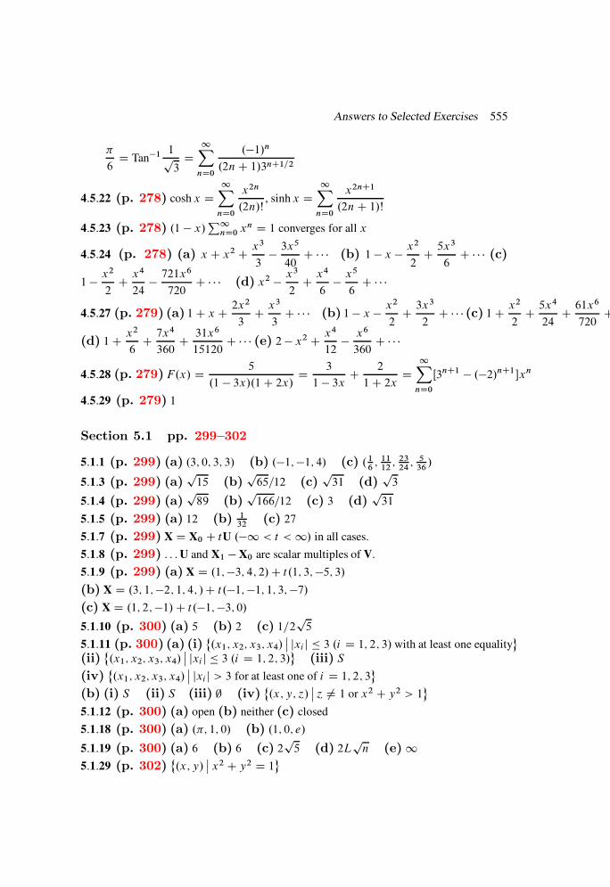
Answers to Selected Exercises 555
6D Tan1 1p
3D
1X
nD0
.1/n.2nC 1/3nC1=2
4:5:22 (p. 278) cosh x D1X
nD0
x2n
.2n/Š, sinh x D
1X
nD0
x2nC1
.2nC 1/Š
4:5:23 (p. 278) .1 x/P1
nD0 xn D 1 converges for all x
4:5:24 (p. 278) (a) x C x2 C x3
3 3x
5
40C (b) 1 x x
2
2C 5x3
6C (c)
1 x2
2C x4
24 721x
6
720C (d) x2 x
3
2C x4
6 x
5
6C
4:5:27 (p. 279) (a) 1C x C 2x2
3C x3
3C (b) 1 x x
2
2C 3x3
2C (c) 1C x2
2C 5x4
24C 61x6
720C
(d) 1C x2
6C 7x4
360C 31x6
15120C (e) 2 x2 C x4
12 x6
360C
4:5:28 (p. 279)F.x/ D 5
.1 3x/.1C 2x/ D3
1 3x C2
1C 2x D1X
nD0
Œ3nC1 .2/nC1 xn
4:5:29 (p. 279) 1
Section 5.1 pp. 299–302
5:1:1 (p. 299) (a) .3; 0; 3; 3/ (b) .1;1; 4/ (c) .16; 11
12; 23
24; 5
36/
5:1:3 (p. 299) (a)p15 (b)
p65=12 (c)
p31 (d)
p3
5:1:4 (p. 299) (a)p89 (b)
p166=12 (c) 3 (d)
p31
5:1:5 (p. 299) (a) 12 (b) 132
(c) 27
5:1:7 (p. 299) X D X0 C tU .1 < t <1/ in all cases.
5:1:8 (p. 299) : : :U and X1 X0 are scalar multiples of V.
5:1:9 (p. 299) (a) X D .1;3; 4; 2/C t.1; 3;5; 3/(b) X D .3; 1;2; 1; 4; /C t.1;1; 1; 3;7/(c) X D .1; 2;1/C t.1;3; 0/5:1:10 (p. 300) (a) 5 (b) 2 (c) 1=2
p5
5:1:11 (p. 300) (a) (i)˚.x1; x2; x3; x4/
ˇjxi j 3 .i D 1; 2; 3/with at least one equality
(ii)˚.x1; x2; x3; x4/
ˇjxi j 3 .i D 1; 2; 3/
(iii) S
(iv)˚.x1; x2; x3; x4/
ˇjxi j > 3 for at least one of i D 1; 2; 3
(b) (i) S (ii) S (iii) ; (iv)˚.x; y; ´/
ˇ´ ¤ 1 or x2 C y2 > 1
5:1:12 (p. 300) (a) open (b) neither (c) closed
5:1:18 (p. 300) (a) .; 1; 0/ (b) .1; 0; e/
5:1:19 (p. 300) (a) 6 (b) 6 (c) 2p5 (d) 2L
pn (e)1
5:1:29 (p. 302)˚.x; y/
ˇx2 C y2 D 1

556 Answers to Selected Exercises
5:1:33 (p. 302) : : : if for A there is an integer R such that jXr j > A if r R.
Section 5.2 pp. 314–316
5:2:1 (p. 314) (a) 10 (b) 3 (c) 1 (d) 0 (e) 0 (f) 0
5:2:3 (p. 315) (b) a=.1C a2/
5:2:4 (p. 315) (a)1 (b)1 (c) no (d) 1 (e) no
5:2:5 (p. 315) (a) 0 (b) 0 (c) none (d) 0 (e) none
5:2:6 (p. 316) (a) . . . if Df is unbounded and for each M there is an R such that
f .X/ > M if X 2 Df and jXj > R. (b) Replace “> M ” by “< M ” in (a).
5:2:7 (p. 316) limX!0 f .X/ D 0 if a1Ca2C Can > b; no limit if a1Ca2C Can b and a2
1C a22C C a2
n ¤ 0; limX!0 f .X/ D1 if a1 D a2 D D an D 0 and b > 0.
5:2:8 (p. 316) No; for example, limx!1 g.x;px/ D 0.
5:2:9 (p. 316) (a) R3 (b) R
2 (c) R3 (d) R
2 (e)˚.x; y/
ˇx y
(f) R
n
5:2:10 (p. 316) (a) R3 f.0; 0; 0/g (b) R
2 (c) R2 (d) R
2 (e) R2
5:2:11 (p. 316) f .x; y/ D xy=.x2 C y2/ if .x; y/ ¤ .0; 0/ and f .0; 0/ D 0
Section 5.3 pp. 335–339
5:3:1 (p. 335) (a)2p3.x C y cos x xy sinx/ 2
r2
3.x cos x/ (b)
1 2yp3exCy2C2´
(c)2pn.x1 C x2 C C xn/ (d) 1=.1C x C y C ´/
5:3:2 (p. 335) 212 3 (p. ??) (a) 5=
p6 (b) 2e (c) 0 (d) 0
5:3:5 (p. 335) (a) fx D fy D 1=.x C y C 2´/, f´ D 2=.x C y C 2´/(b) fx D 2x C 3y´ C 2y, fy D 3x´ C 2x, f´ D 3xy (c) fx D ey´, fy D x´ey´,
f´ D xyey´ (d) fx D 2xy cos x2y, fy D x2 cos x2y, f´ D 15:3:6 (p. 335) (a) fxx D fyy D fxy D fyx D 1=.x C y C 2´/2, fx´ D f´x Dfy´ D f´y D 2=.x C y C 2´/2, f´´ D 4=.x C y C 2´/2
(b) fxx D 2, fyy D f´´ D 0, fxy D fyx D 3´C 2, fx´ D f´x D 3y, fy´ D f´y D 3x(c) fxx D 0, fyy D x´2ey´, f´´ D xy2ey´, fxy D fyx D ´ey´, fx´ D f´x D yey´,
fy´ D f´y D xey´
(d) fxx D 2y cos x2y 4x2y2 sin x2y, fyy D x4 sinx2y, f´´ D 0, fxy D fyx D2x cos x2y 2x3y sinx2y, fx´ D f´x D fy´ D f´y D 05:3:7 (p. 336) (a) fxx.0; 0/ D fyy.0; 0/ D 0, fxy .0; 0/ D 1, fyx.0; 0/ D 1(b) fxx.0; 0/ D fyy.0; 0/ D 0, fxy.0; 0/ D 1, fyx.0; 0/ D 15:3:8 (p. 336) f .x; y/ D g.x; y/Ch.y/, where gxy exists everywhere and h is nowhere
differentiable.
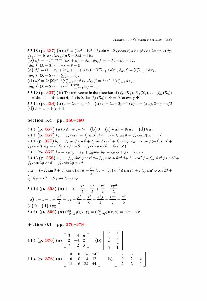
Answers to Selected Exercises 557
5:3:18 (p. 337) (a) df D .3x2C4y2C2y sinxC2xy cos x/ dxC.8xyC2x sinx/ dy,
dX0f D 16 dx, .dX0
f /.X X0/ D 16x(b) df D exy´ .dx C dy C d´/, dX0
f D dx dy d´,
.dX0f /.X X0/ D x y ´
(c) df D .1C x1 C 2x2 C C nxn/1Pn
j D1 j dxj , dX0f D
Pnj D1 j dxj ,
.dX0f /.X X0/ D
Pnj D1 jxj ,
(d) df D 2r jXj2r2Pn
j D1 xj dxj , dX0f D 2rnr1
Pnj D1 dxj ,
.dX0f /.X X0/ D 2rnr1
Pnj D1.xj 1/,
5:3:19 (p. 337) (b) The unit vector in the direction of .fx1.X0/; fx2
.X0/; : : : ; fxn.X0//
provided that this is not 0; if it is 0, then @f .X0/=@ˆ D 0 for every ˆ.
5:3:24 (p. 338) (a) ´ D 2xC4y6 (b) ´ D 2xC3yC1 (c) ´ D .x/=2Cy=2(d) ´ D x C 10y C 4
Section 5.4 pp. 356–360
5:4:2 (p. 357) (a) 5 duC 34 dv (b) 0 (c) 6 du 18 dv (d) 8 du
5:4:3 (p. 357) hr D fx cos C fy sin , h D r.fx sin C fy cos /, h´ D f´
5:4:4 (p. 357) hr D fx sin cos Cfy sin sin Cf´ cos , h D r sin .fx sin Cfy cos /, h D r.fx cos cos C fy cos sin f´ sin/
5:4:6 (p. 357) hy D gxxy C gy C gwwy , h´ D gxx´C g´ C gww´
5:4:13 (p. 358) hrr D fxx sin2 cos2 Cfyy sin2 sin2 Cf´´ cos2 Cfxy sin2 sin 2Cfy´ sin 2 sin C fx´ sin 2 cos ,
hr D .fx sin C fy cos / sin C r
2.fyy fxx/ sin2 sin 2 C rfxy sin2 cos 2 C
r
2.f´y cos f´x sin / sin 2
5:4:16 (p. 358) (a) 1C x C x2
2 y
2
2C x3
6 xy
2
2
(b) 1 x y C x2
2C xy C y2
2 x
3
6 x
2y
2 xy
2
2 y
3
6(c) 0 (d) xy´
5:4:21 (p. 359) (a) .d 2.0;0/
p/.x; y/ D .d 2.0;0/
q/.x; y/ D 2.x y/2
Section 6.1 pp. 376–378
6:1:3 (p. 376) (a)
243 4 6
2 4 2
7 2 3
35 (b)
2664
2 4
3 27 46 1
3775
6:1:4 (p. 376) (a)
24
8 8 16 24
0 0 4 12
12 16 28 44
35 (b)
242 6 0
0 2 42 2 6
35
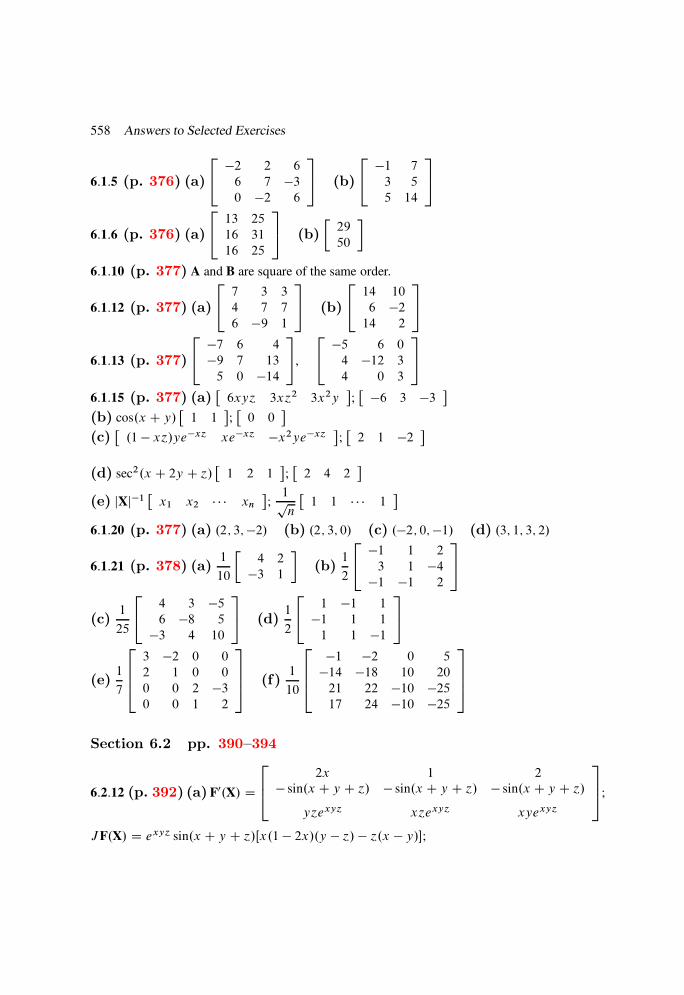
558 Answers to Selected Exercises
6:1:5 (p. 376) (a)
242 2 6
6 7 30 2 6
35 (b)
241 7
3 5
5 14
35
6:1:6 (p. 376) (a)
2413 25
16 31
16 25
35 (b)
29
50
6:1:10 (p. 377) A and B are square of the same order.
6:1:12 (p. 377) (a)
247 3 3
4 7 7
6 9 1
35 (b)
2414 10
6 214 2
35
6:1:13 (p. 377)
247 6 4
9 7 13
5 0 14
35,
245 6 0
4 12 3
4 0 3
35
6:1:15 (p. 377) (a)6xy´ 3x´2 3x2y
;6 3 3
(b) cos.x C y/1 1
;0 0
(c).1 x´/yex´ xex´ x2yex´
;2 1 2
(d) sec2.x C 2y C ´/1 2 1
;2 4 2
(e) jXj1x1 x2 xn
;1pn
1 1 1
6:1:20 (p. 377) (a) .2; 3;2/ (b) .2; 3; 0/ (c) .2; 0;1/ (d) .3; 1; 3; 2/
6:1:21 (p. 378) (a)1
10
4 2
3 1
(b)
1
2
241 1 2
3 1 41 1 2
35
(c)1
25
24
4 3 56 8 5
3 4 10
35 (d)
1
2
24
1 1 1
1 1 1
1 1 1
35
(e)1
7
2664
3 2 0 0
2 1 0 0
0 0 2 30 0 1 2
3775 (f)
1
10
2664
1 2 0 5
14 18 10 20
21 22 10 2517 24 10 25
3775
Section 6.2 pp. 390–394
6:2:12 (p. 392) (a) F0.X/ D
264
2x 1 2
sin.x C y C ´/ sin.x C y C ´/ sin.x C y C ´/
y´exy´ x´exy´ xyexy´
375;
JF.X/ D exy´ sin.x C y C ´/Œx.1 2x/.y ´/ ´.x y/;
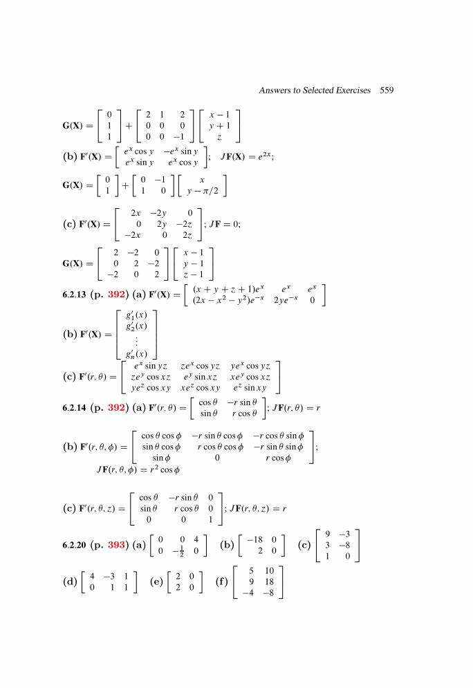
Answers to Selected Exercises 559
G.X/ D
240
1
1
35C
242 1 2
0 0 0
0 0 1
3524x 1y C 1´
35
(b) F0.X/ Dex cos y ex siny
ex sin y ex cosy
; JF.X/ D e2x;
G.X/ D0
1
C0 11 0
x
y =2
(c) F0.X/ D
24
2x 2y 0
0 2y 2´2x 0 2´
35; JF D 0;
G.X/ D
24
2 2 0
0 2 22 0 2
3524x 1y 1´ 1
35
6:2:13 (p. 392) (a) F0.X/ D.x C y C ´C 1/ex ex ex
.2x x2 y2/ex 2yex 0
(b) F0.X/ D
26664
g01.x/
g02.x/:::
g0n.x/
37775
(c) F0.r; / D
24
ex siny´ ´ex cosy´ yex cosy´
´ey cos x´ ey sin x´ xey cos x´
ye´ cos xy xe´ cos xy e´ sinxy
35
6:2:14 (p. 392) (a) F0.r; / D
cos r sin
sin r cos
; JF.r; / D r
(b) F0.r; ; / D
24
cos cos r sin cos r cos sin
sin cos r cos cos r sin sin
sin 0 r cos
35;
JF.r; ; / D r2 cos
(c) F0.r; ; ´/ D
24
cos r sin 0
sin r cos 0
0 0 1
35; JF.r; ; ´/ D r
6:2:20 (p. 393) (a)
0 0 4
0 12
0
(b)
18 0
2 0
(c)
249 33 81 0
35
(d)
4 3 1
0 1 1
(e)
2 0
2 0
(f)
24
5 10
9 18
4 8
35
560 Answers to Selected Exercises
Section 6.3 pp. 414–417
6:3:4 (p. 414) (a) Œ1; =2 (b) Œ1; 2 (c) Œ1; (d) Œ2p2; 9=4 (e)
Œp2; 3=4
6:3:5 (p. 414) (a) Œ1;3=2 (b) Œ1;2 (c) Œ1; (d) Œ2p2;7=4
(e) Œp2;5=4
6:3:6 (p. 414) (b) Let f .x/ D x .0 x 12/, f .x/ D x 1
2.1
2< x 1/; then f is
locally invertible but not invertible on Œ0; 1.
6:3:7 (p. 414) F.S/ D˚.u; v/
ˇ C 2 < arg.u; v/ < C 2
, where is an argu-
ment of .a; b/;
F1S.u; v/ D .u2 C v2/1=4
"cos.arg.u; v/=2/
sin.arg.u; v/=2/
#; 2 < arg.u; v/ < 2 C
6:3:10 (p. 415) (a)
x
y
D 1
10
u 2v3uC 4v
; .F1/0 D 1
10
1 23 4
(b)
24x
y
´
35 D 1
2
24uC 2v C 3w
u wuC v C 2w
35; .F1/0 D 1
2
241 2 3
1 0 11 1 2
35
6:3:12 (p. 415) G1.u; v/ D1p2
puC vpu v
, G0
1.u; v/ D1
2p2
1=puC v 1=
puC v
1=pu v 1=
pu v
G2.u; v/ D1p2
puC vpu v
, G0
2.u; v/ D1
2p2
1=puC v 1=
puC v
1=pu v 1=
pu v
G3.u; v/ D1p2
puC v
pu v
, G0
3.u; v/ D1
2p2
1=puC v 1=
puC v
1=pu v 1=
pu v
G4.u; v/ D1p2
puC v
pu v
, G0
4.u; v/ D1
2p2
1=puC v 1=
puC v
1=pu v 1=
pu v
6:3:15 (p. 416) From solving x D r cos , y D r sin for D arg.x; y/. Each equation
is satisfied by angles that are not arguments of .x; y/, since none of the formulas identifies
the quadrant of .x; y/ uniquely. Moreover, (c) does not hold if x D 0.
6:3:16 (p. 416)
x
y
D G.u; v/ D .u2 C v2/1=4
"cosΠ1
2arg.u; v/
sin.arg.u; v/=2/
#,
where ˇ =2 < arg.u; v/ < ˇ C =2 and ˇ is an argument of .a; b/;
G0.u; v/ D 1
2.x2 C y2/
x y
y x
6:3:19 (p. 416) If F.x1; x2; : : : ; xn/ D .x31 ; x
32; : : : ; x
3n/, then F is invertible, but
JF.0/ D 0.
6:3:20 (p. 416) (a) A.U/ D
1
1
1
25
5 5
3 8
uC 5v 4

Answers to Selected Exercises 561
(b) A.U/ D1
1
C 1
6
4 23 3
u 2v 3
(c) A.U/ D
240
1
1
35C
24
0 1 1
1 1 0
1 0 0
3524u 1v 1w 2
35
(d) A.U/ D
24
1
=2
35C
240 1 0
1 0 0
0 0 1
3524
u
v C 1w
35
6:3:21 (p. 417) G0.x; y; ´/ D
266664
cos cos sin cos sin
sin
r cos
cos
r cos0
1r
cos sin 1r
sin sin 1
rcos
377775
6:3:22 (p. 417) G0.x; y; ´/ D
26664
cos sin 0
1r
sin 1
rcos 0
0 0 1
37775
Section 6.4 pp. 431–434
6:4:1 (p. 431) (a)
u
v
D 1
2
3 4
1 2
x
y
(b)
24u
v
w
35 D 1
2
24
3 3
1 2
2 3
35x
y
(c)
u
v
D 1
5
2 11 3
y C sinx
x C siny
(d) u D x, v D y, ´ D w
6:4:3 (p. 431) fi .X;U/ D
0@
nX
j D1
aij .xj xj 0/
1A
r
.ui ui0/s , 1 i m, where r
and s are positive integers and not all aij D 0. (a) r D s D 3; (b) r D 1, s D 3; (c)r D s D 26:4:4 (p. 431) ux.1; 1/ D 5
8, uy.1; 1/ D 1
2
6:4:5 (p. 431) ux.1; 1; 1/ D 58
, uy.1; 1; 1/ D 98
, u´.1; 1; 1/ D 12
6:4:6 (p. 431) (a) u.1; 2/ D 0, ux.1; 2/ D uy .1; 2/ D 4(b) u.1;2/ D 2, ux.1;2/ D 1, uy .1;2/ D 1
2
(c) u.=2; =2/ D ux.=2; =2/D uy.=2; =2/ D 0(d) u.1; 1/ D 1, ux.1; 1/ D uy.1; 1/ D 1
6:4:7 (p. 431) (a) u1.1; 1/ D 1,@u1.1; 1/
@xD 5,
@u1.1; 1/
@yD 2
562 Answers to Selected Exercises
u2.1; 1/ D 2,@u2.1; 1/
@xD 14;
@u2.1; 1/
@yD 2
(b) uk.0; / D .2k C 1/=2,@uk.0; /
@xD 0,
@uk.0; /
@yD 1, k D integer
6:4:8 (p. 432)1
5
1 2 1
1 2 1
6:4:9 (p. 432) u0.0/ D 3, v0.0/ D 1
6:4:10 (p. 432)1
6
24
5 5
5 56 6
35
6:4:11 (p. 432) U1.1; 1/ D3
1
, U0
1.1; 1/ D
1 3
1 2
;
U2.1; 1/ D 3
1
, U0
2.1; 1/ D
1 3
1 2
6:4:12 (p. 432) ux.0; 0; 0/ D 2, vx.0; 0; 0/ D wx.0; 0; 0/ D 2
6:4:13 (p. 433) yx D
@.f; g; h/
@.x; ´; u/
@.f; g; h/
@.y; ´; u/
, yv D
@.f; g; h/
@.v; ´; u/
@.f; g; h/
@.y; ´; u/
, ´x D
@.f; g; h/
@.y; x; u/
@.f; g; h/
@.y; ´; u/
,
´v D
@.f; g; h/
@.y; v; u/
@.f; g; h/
@.y; ´; u/
, ux D
@.f; g; h/
@.y; ´; x/
@.f; g; h/
@.y; ´; u/
, uv D
@.f; g; h/
@.y; ´; v/
@.f; g; h/
@.y; ´; u/
6:4:14 (p. 433) x D 2y u, ´ D 2v; x D 2y u, v D ´2
; y D x2 u2
,
´ D 2v; y D x2 u2
, v D ´2
; ´ D 2v, u D x 2y; u D x 2y, v D ´2
6:4:15 (p. 433) yx.1;1;2/ D 12
, vu.1;1;2/ D 16:4:16 (p. 433) uw .0;1/ D 5
6, uy .0;1/ D 0, vw.0;1/ D 5
6, vy.0;1/ D 0,
xw.0;1/ D 1, xy.0;1/ D 16:4:18 (p. 434) ux.1; 1/ D 0, uy.1; 1/ D 0, vx.1; 1/ D 1, vy .1; 1/ D 1, uxx .1; 1/ D2,
uxy .1; 1/ D 1, uyy.1; 1/ D 2, vxx.1; 1/ D 2, vxy.1; 1/ D 1, vyy.1; 1/ D 2
6:4:19 (p. 434) ux.1;1/ D 0, uy .1;1/ D1
2, vx.1;1/ D
1
2, vy.1;1/ D 0,
uxx.1;1/ D 1
8, uxy.1;1/ D
1
8, uyy.1;1/ D
1
8, vxx.1;1/ D
1
8,
vxy.1;1/ D 1
8, vyy.1;1/ D
1
8

Index 563
Section 7.1 pp. 459–462
7:1:2 (p. 459) (a) 28 (b) 14
6 (p. ??) 3.b a/.d c/, 0 13 (p. ??)˚.m; n/
ˇm; n D integers
Section 7.2 pp. 480–484
7:2:1 (p. 480) (a) 12 (b) 7920
(c) 1 (d) .1 log 2/=2
7:2:5 (p. 481) (a) 74
(b) 17 (c) 23.p2 1/ (d) 1=4
7:2:7 (p. 481) (a) 38
, 58
(b) 38
, 58
7:2:8 (p. 482) (a) 34
, 54
(b) 34
´C 1
2
,
54
´C 1
2
(c) ´C 1
2, 1
7:2:11 (p. 482) (a) 285 (b) 0 (c) 0 (d) 14.e 5
2/
7:2:12 (p. 483) (a) 324 (b) 16
(c) 1 7:2:13 (p. 483) 5215
7:2:14 (p. 483) (a) 36 (b) 1 (c) 643
(d) .e6 C 17/=27:2:17 (p. 483) (a) 2
27(b) 1
2.e 5
2/ (c) 1
24(d) 1
36
7:2:18 (p. 483) (a) 16 (b) 16
(c) 12821
(d) 2
7:2:19 (p. 484) (a) 12.b1 a1/ .bn an/
Pnj D1.aj C bj /
(b) 13.b1 a1/ .bn an/
Pnj D1.a
2j C aj bj C b2
j /
(c) 2n.b21 a2
1/ .b2n a2
n/
7:2:20 (p. 484)Rp
3=2
p
3=2dxRp
1x2
1=2 f .x; y/ dy 7:2:22 (p. 484) 12
Section 7.3 pp. 514–517
7:3:1 (p. 514) Let S1 and S2 be dense subsets of R such that S1 [ S2 D R.
7:3:7 (p. 514) (a) 1; c (constant); 1 9 (p. ??) .u2 u1/.v2 v1/=jad bcj7:3:10 (p. 515) 5
67:3:14 (p. 515) (a) 4
9(b) log 5
27:3:15 (p. 516) 3
7:3:16 (p. 516) 12
7:3:17 (p. 516) 54e.e 1/
7:3:18 (p. 516) 43abc 7:3:19 (p. 516) 2.e25 e9/ 7:3:20 (p. 516) 16=3
7:3:21 (p. 516) 21=64
7:3:22 (p. 516) (a) .=8/ log 5 (b) .=4/.e4 1/ (c) 2=15
7:3:23 (p. 517) 2a4=2
7:3:24 (p. 517) (a) .ˇ1 ˛1/ .ˇn ˛n/=j det.A/j 25 (p. ??) ja1a2 anjVn
Index
AAbel’s test, 219
Abel’s theorem, 273, 279
Absolute convergence, 215
of an improper integral, 160
of a series of constants, 215
of a series of functions, 247
Absolute integrability, 160
Absolute uniform convergence, 247, 255
(Exercises 4.4.17 and 4.4.20),
256 (Exercise 4.4.21)
of a power series, 257
Absolute value, 2
Addition of power series, 267
Adjoint matrix, 370
Affine transformation, 380
Alternating series, 203
test, 203, 219
Analytic transformation, 416 (Exercise 6.3.17)
Angle between two vectors, 286
Antiderivative, 143, 150 (Exercise 3.3.16)
Archimedean property, 5
Area under a curve, 116
Argument, 398
branch of, 409, 410, 415 (Exercise 6.3.14)
Ascoli–Arzela theorem, 541
Associative laws
for the real numbers, 2 (see p. 1)
for vector addition, 283
BBessel function, 277 (Exercise 4.5.11)
Binomial coefficient, 17 (Exercise 1.2.19),
102, 194 (Exercise 4.1.35)
Binomial series, 266
Binomial theorem, 17 (Exercise 1.2.19)
Bolzano–Weierstrass theorem, 27, 294,
301 (Exercise 5.1.22)
Bound
lower, 7
upper, 3
Boundary, 526
point, 289, 526
of a set, 23, 289
Bounded convergence theorem, 243
Bounded function, 47, 60, 313
Boundedness of a continuous function
on a closed interval, 62, 199
on a compact set, 313
Boundedness of an integrable function,
119
on a metric space, 536
Bounded sequence, 181, 197, 292
Bounded set
above, 3, 313
below 7, 313
Bounded variation, 134–135 (Exercises 3.2.7,
3.2.9, 3.2.10)
Branch
of an argument, 409, 415
of an inverse, 409
CC[a,b], 521
equicontinuous subset of, 539
564
Index 565
uniformly bounded subset of, 539
Cartesian product, 31, 435
Cauchy product of series, 226, 233 (Ex-
ercise 4.3.40), 280 (Exercise 4.5.32)
Cauchy sequence, 527
Cauchy’s convergence criterion
for sequences of real numbers, 190
for sequences of vectors, 292
for series of real numbers, 204
Cauchy’s root test, 215
Cauchy’s uniform convergence criterion
for sequences, 239
for series, 246
Chain rule, 77, 340, 388
Change of variable, 145, 147
in an improper integral, 164
in a multiple integral, 496
formulation of the rule for, 494
in an ordinary integral, 145, 147
Changing the order of integration, 478
Characteristic function, 70 (Exercise 2.2.9),
485
Closed
under scalar multiplication, 519
under vector addition, 519
Closed interval, 23
Closed n-ball, 291
Closed set, 21, 289, 525
Closure of a set, 23, 289
Cofactor, 370
expanding a determinant in, 371–372
Commutative laws
for the reals, 2 (See p. 1)
for vector addition, 283
Compact set, 20, 293, 536
Comparison test
for improper integrals, 156
for series, 206
Complement of a set, 20
Complete metric space, 527
Completeness axiom, 4
Complete ordered field, 4
Component function, 311
Components, 284 (see p. 281)
of a vector-valued function, 311, 362
Composite function, 58, 311
continuity of, 59, 311
differentiability of, 77, 340
higher derivatives of, 345
Taylor polynomial of, 109–110
(Exercise 2.5.11)
Composition of functions, 58
Conditional convergence
of an improper integral, 162
of a series, 217
Conditionally integrable, 162
Connected metric space, 547 (Exercise 8.3.2)
Connected set, 295
polygonally, 296
Containment of a set, 19
Content, 453
of a coordinate rectangle, 437
of a set, 485
zero, 448, 514 (Exercise refexer:7.3.2)
Continuity, 54, 302
of a composite function, 59, 311
of a differentiable function, 76, 325
of a function of n variables, 309
of a function of one variable, 54
on an interval, 55
from the left, 54
of a monotonic function, 67
piecewise, 56
from the right, 54
on a set, 56, 311
of a sum, difference, product, and
quotient, 57, 311
in terms of sequences, 198
of a transformation, 379
uniform, 64, 66, 314, 392 (Exercise 6.2.10)
of a uniform limit, 242
of a uniformly convergent series, 250
Continuous function 54, 309
boundedness of, 62, 313
extreme values of on a closed inter-
val, 62
integrability of, 133
intermediate values of, 63, 313
on a metric space, 543
Continuous transformation, 379
566 Index
Continuously differentiable, 73, 80, 329,
385, 409
Contraction mapping theorem, 545
Convergence
absolute
of an improper integral, 160
of a series of constants, 215
absolute uniform, 247
conditional
of a series, 217
of an improper integral, 162
of an improper integral, 152
of an infinite series, 201
interval of, 258
pointwise
of a sequence of functions, 234,
238
of a series of functions, 244
of a power series, 257
radius of, 258
of a sequence in a metric space, 526
of a sequence in Rn, 292
of a sequence of real numbers, 179
of a series of constants, 200
of a sum, difference, or product of
sequences, 184
of a Taylor series, 264
uniform, 246
of a sequence, 237
of a series, 246
Coordinate cube, 437
degenerate, 437
nondegenerate, 437
Coordinate rectangle, 437
Coordinates,
polar, 397, 502, 505
spherical, 507
Covering, open, 25, 293, 535
Cramer’s rule, 373
Critical point, 81, 335
Curve, differentiable, 453
DDecreasing sequence, 182
Dedekind cut, 9 (Exercise 1.1.8)
Dedekind’s theorem, 9 (Exercise 1.1.8)
Defined inductively, 12
Degree
of a homogeneous polynomial, 352
of a polynomial, 98
Deleted -neighborhood, 22
Deleted neighborhood, 525
Dense set, 6, 29 (Exercise 1.3.22), 70 (Ex-
ercise 2.2.10)
Density of the rationals, 6, 392 (Esercise 6.2.11)
Density of the irrationals, 6
Denumerable set, 176
Derivative, 73
of a composite function, 77
directional, 317
infinite, 88 (Exercise 2.3.26)
of an inverse function, 86 (Exercise 2.3.14)
left-hand, 79
nth, 73
one-sided, 79
ordinary, 317
partial, 317
of a power series, 261–262
right-hand, 79
r th order, 319
second, 73
of a sum, difference, product, and
quotient, 77
zeroth, 73
Determinant, 368 (see p. 369)
expanding in cofactors, 371–372
of a product of square matrices, 370
Diameter of a set, 292, 586
Difference quotient, 73
Differentiability
of a composite function, 340
continuous, 329
of a function of one variable, 73
of a function of several variables, 323
of the limit of a sequence, 243
of a power series, 260–262
of a series, 252
Differentiable 73, 323
continuously, 73, 80, 409
curve, 453
Index 567
function, continuity of, 76, 325, 385
on an interval, 80
on a set, 73
surface, 453
transformation, 380
vector-valued function, 339
Differential, 326
higher, 348
of a linear transformation, 367
matrix, 367, 381
of a real-valued function, 326
of a sum, difference, product, and
quotient, 328
of a transformation, 381
Differential equation, 170–171
(Exercises 3.4.27–3.4.29)
Directional derivative, 317
Dirichlet’s test
for improper integrals, 163
for series of constants, 217
for uniform convergence of series,
248
Disconnected set, 295
Discontinuity
jump, 56
removable, 58
Discrete metric, 519
Disjoint sets, 20
Distance
in a metric space, 518
from a point to a set, 301
(Exercise 5.1.24)
between subsets of a metric space,
547 (Exercise 8.3.3)
between two sets, 301
(Exercise 5.1.25)
between two vectors, 283
Distributive law, 2 (see p. 1)
Divergence, unconditional, 233
(Exercise 4.3.38)
Divergent improper integral, 152
Divergent sequence, 179
Divergent series, 201
Domain of a function, 31 (see p. 30), 543
Double integral, 438
EEdge lengths of a coordinate rectangle,
437
Elementary matrix, 488
Empty set, 4
Entries of a matrix, 364
-neighborhood, 21, 289, 525
-net, 538
Equicontinuous subset of CŒa; b, 539
Equivalent metrics, 529
Error in approximating derivatives, 112
(Exercises 112–112)
Euclidean n-space, 282 (see p. 281)
Euler’s constant, 230 (Exercise 4.3.14)
Euler’s theorem, 357–358 (Exercise 2.4.8)
Existence of an improper integral, 152
Existence theorem, 420
Expanding a determinant, 362–372
Exponential function, 70 (Exercise 2.2.12),
72 (Exercise 2.2.33), 228, 273
Extended mean value theorem, 106
Extended reals, 7,
Exterior point, 289, 526
Exterior of a set, 23, 289, 526
FFaa di Bruno’s formula, 109
(Exercise 2.5.11)
Fibonnacci numbers, 17 (Exercise 1.2.17)
Field
complete ordered, 4
ordered, 2
properties, 2 (see p. 1)
Finite real, 7
First mean value theorem for integrals,
139
Forward differences, 104, 71 (Example 2.2.18),
112 (Exercises 2.5.19–2.5.22)
Fredholm’s integral equation, 546
Function 31, 32
absolutely integrable, 160
Bessel, 277 (Exercise 277)
bounded, 47, 60, 313
above, 60, 313
below, 60, 313
568 Index
of bounded variation, 134 (Exercise 3.2.7)
characteristic, 70 (Exercise 2.2.9), 485
composite, 58, 311
decreasing, 44
differentiable at a point, 73, 323
domain of, 31, 32
exponential, 70 (Exercise 2.2.12), 72
(Exercise 2.2.33), 227, 273
generating, 278 (Exercise 4.5.26)
homogeneous, 357 (Exercise 5.4.8)
increasing, 44
infimum of, 55, 313
inverse of, 68
linear, 325
locally integrable, 152
maximum of, 60
monotonic, 44, 67
nondecreasing, 44
nonincreasing, 44
nonoscillatory at a point, 162
nth power of, 33
oscillation of, 171
piecewise continuous, 56
range of, 31, 32
rational, 33, 232, (Exercise 4.3.28),
276 (Exercise 4.5.4)
real-valued, 302
restriction of, 399
Riemann integrable, 114, 438
Riemann–Stieltjes integrable, 125
strictly monotonic, 44
supremum of, 313
value of, 31, 32
vector-valued, 311
Functions,
composition of, 58, 311
difference of, 32
product of, 32
quotient of, 32
sum of, 32
Fundamental theorem of calculus, 143
GGeneralized mean value theorem, 83
Generating function, 278 (Exercise 4.5.26)
Geometric series, 202
Grouping terms of series, 220
HHeine–Borel property,
Heine–Borel theorem, 172, 66, 172, 293
Higher derivatives of a composite func-
tion, 345
Higher differential, 348
Homogeneous function, 357 (Exercise 5.4.8),
359 (Exercise 5.4.23)
Homogeneous polynomial, 359 (Exercise 5.4.22),
Homogeneous system, 375
Hypercube, 295 (see p. 294)
Hölder’s inequality, 521
IIdentity matrix, 370
Image, 394
Implicit function theorem, 420, 423
Improper integrability, 146
Improper integral, 152
absolutely convergent, 160
change of variable in, 164
conditionally convergent, 162
convergence of, 152
divergence of, 152
existence of, 152
of a nonnegative function, 156
Incompleteness of the rationals, 6
Increasing sequence, 182
Indeterminate forms, 91, 93–95
Induction assumption, 12
Induction proof, 12
Inequality,
Hölder, 521
Minkowski, 522
Schwarz, 284
triangle, 2, 285
Infimum
of a function, 60, 313
of a set, 7
existence and uniqueness of, 7, 9
(Exercise 1.1.6)

Index 569
Infinite derivative, 88 (Exercise 2.3.26)
Infinite limits, 42, 306, 317, 316(Exercise 5.2.6)
Infinite sequence, 179
in a metric space, 526
Infinite series, 210, 244
convergence of, 201
integrability of, 251
oscillatory, 201
Infinity norm, 496, 523, 524
Inner product, 284
Instantaneous
rate of change, 74
velocity, 74
Integrability
conditional, 162
of a continuous function, 133
of a function of bounded variation,
134 (Exercise 3.2.7)
improper, 152
of an infinite series, 251
local, 152
of a monotonic function, 133
of a power series, 264
Integrable
Riemann, 114, 438
Riemann–Stieltjes, 125
Integral
over an arbitrary set in Rn, 452
of a constant times a function, 136,
456
double, 439
improper, 151
iterated, 462
lower
for Riemann integral, 120, 442
for Riemann–Stieltjes integral 128
(Exercise 3.1.17)
multiple, 439
ordinary, 439
of a product, 138, 456
proper, 153
over a rectangle in Rn, 436 (See p. 435)
Riemann, 114, 438
Riemann–Stieltjes, 125, 127 (Exer-
cise 3.1.16), 135 (Exercises 3.2.8–
3.2.10), 151 (Exercise 3.3.23)
over subsets of Rn, 436 (See p. 435),
450, 452, 471–472
of a sum, 136, 456
test, 207
triple, 439
Integration by parts, 144
for Riemann–Stieltjes integrals, 135
(Exercise 3.2.8)
Interior of a set, 21, 289
Interior point, 21, 289, 525
Intermediate value theorem
for continuous functions, 63, 313
for derivatives 82
Intersection of sets, 20
Interval
closed, 23
half closed, 23
half open, 23
open, 21
semi-infinite, 21, 23
Interval of convergence, 258
for derivatives, 82
Inverse function, 68
branch of, 409
derivative of, 86 (Exercise. 2.3.14)
of a function restricted to a set, 399
of a matrix, 370
of a transformation, 396
Inverse function theorem, 412
Invertible, locally, 400
Invertible transformation, 396
Irrational number, 6
Isolated point, 23, 289, 526
Iterated integral, 462
Iterated logarithm, 97 (Example 2.4.42),
167 (Exercise 3.4.10), 208 230
(Exercise 4.3.11), 230 (Exercise 4.3.16)
JJacobian, 384, 426
Jordan content, 485
changed by linear transformation, 488
570 Index
Jordan measurable set, 485, 488
Jump discontinuity, 56
LLebesgue measure zero, 175, 177 (Exer-
cises 3.5.7, 3.5.8)
Lebesgue’s existence criterion, 176
Left limit inferior, 47
Left limit superior, 47
Left-hand derivative, 79
Left-hand limit, 38
Legendre polynomial, 278 (Exercise 4.5.27)
Leibniz’s rule, 86, (Exercise. 2.3.12)
Length of a vector, 283
l’Hospital’s rule, 88
Limit of a real-valued function, 302
Limit
along a curve, 315 (Exercise 5.2.3)
in the extended reals, 43
inferior of a sequence, 188
left, 47
infinite, 42, 306, 316 (Exercise 5.2.6)
at infinity, 307, 316 (Exercise 5.2.6)
left-hand, 38
one-sided, 37, 40
point, 23, 289, 526
pointwise, 234, 238, 244
at ˙1, 40
of a real-valued function
as x approaches x0, 34
as x approaches1, 40
as x approaches 1, 50 (Exer-
cise 2.1.14)
right-hand, 39
of a sequence, 179, 292
uniqueness of, 35, 305
of a sum, product, or quotient, 35,
305
superior, left, 47
superior of a sequence, 188
uniform, 237
uniqueness of, 35, 305
Line segments in Rn, 288
Line, parametric representation of, 288–
289
Linear function, 325
Linear transformation, 362
change of content under, 490
differential of, 367
matrix of, 363
Lipschitz condition, 84, 87 (Exercise 2.3.24),
140
Local extreme point, 80, 334
Local extreme value, 80
Local integrability, 152
Local maximum point, 80, 334
Local minimum point, 80, 334
Locally invertible, 400
Lower bound, 7
Lower integral, 120, 442
Lower sum, 120, 442
MMaclaurin’s series, 264
Magnitude, 2
Main diagonal of a matrix, 370
Mathematical induction, 10, 13
Matrices
product of, 364
sum of, 364
Matrix
adjoint, 370
of a composition of linear transfor-
mations, 366
differential, 367, 381
elementary, 488
identity, 370
inverse, 370
of a linear transformation, 363
main diagonal of, 370
nonsingular, 370
norm of, 368
scalar multiple of, 364
singular, 370
square, 368 (See p. 369)
transpose of, 370
Maximum value, local, 80
Maximum of a function, 60
Mean value theorem, 83, 347
extended, 106

Index 571
generalized, 83
for integrals, 138, 144
Metric, 518
discrete, 519
induced by a norm, 520
Metrics, equivalent, 529
Metric space, 518
complete, 527
connected, 547 (Exercise 8.3.2)
Minimum of a function, 60
Minimum value, local, 80
Minkowski’s inequality, 522
Monotonic function, 44, 67, 84
integrability of, 133
Monotonic sequence, 182
Multinomial coefficient, 322, 336 (Exer-
cise 5.3.12)
Multiple integral, 439
Multiplication
of matrices, 364
of series, 223
scalar, 519
Multiplicityof a zero, 87 (Exercise. 2.3.21),
108 (Exercises 2.5.5–2.5.7)
NNatural numbers, 10
n-ball, 290–291
Negative definite polynomial, 353
Negative semidefinite polynomial, 353
Neighborhood, 21, 289, 525
deleted, 22, 525
deleted , 22
, 21
Nested sets, 292, 529
principle of, 292, 529
Nondecreasing sequence, 182
Nondegenerate coordinate cube, 437
Nondenumerable set, 176
Nonempty set, 4
Nonincreasing sequence, 182
Nonoscillatory at a point, 162
Nonsingular matrix, 370
Nontrivial solution, 375
Norm
infinity, 496, 523, 524
of a matrix, 368
metric induced by, 520
of a partition, 114, 437
on a vector space, 519
Normed vector space, 519
nth derivative, 73
nth partial sum of a series, 201
nth term of a series, 201
Number, natural, 10
Number, prime, 15
OOne-sided derivative, 79
One-sided limit, 37
One-to-one transformation, 396
Open ball, 525
Open covering, 25, 293, 535
Open interval, 21
Open n-ball, 290
Open set, 21, 289, 525
Ordered field, 2
complete, 4
Order relation, 2
Ordinary derivative, 317
Ordinary integral, 439
Origin of Rn, 283
Oscillation of a function, 171
at a point, 172
Oscillatory infinite series, 201
PParametric representation of a line, 288,
289
Partial derivative, 317
r th order, 319
Partial sums, 244
Partition, 114, 437
norm of, 114, 437
points, 114
refinement of, 114, 438
Path, polygonal, 296
Peano’s postulates, 10–11
Piecewise continuous function, 56
Point, 19
572 Index
boundary, 23, 289, 526
critical, 81, 335
exterior, 23, 289, 526
at infinity, 7
interior, 21, 289
isolated, 23, 289, 526
limit, 23, 289, 526
local extreme, 80, 334
local maximum, 80, 334
local minimum, 80, 334
in terms of sequences, 197
Pointwise convergence
of a sequence of functions, 234, 238
of a series, 244
Pointwise limit, 234, 238, 244
Polar coordinates, 397, 502, 505
Polygonal path, 296
Polygonally connected, 296
Polynomial, 33, 98
homogeneous, 352
negative definite, 353
negative semidefinite, 353
positive definite, 353
positive semidefinite, 353
semidefinite, 353
Taylor, 99, 351
Power series, 257
arithmetic operations with, 267
continuity of, 260–261
convergence of, 257
differentiability of, 260–261
integration of, 264
of a product, 268
of a reciprocal, 271
of a quotient, 269
uniqueness of, 263
Prime, 15
Principal value, 155
Principle of mathematical induction, 11,
14
Principle of nested sets, 529
Product
Cartesian, 31, 436 (see p. 435)
Cauchy, 226, 233 (Example 4.3.40)
inner, 284
of matrices, 364
of power series, 268
of series, 223
Proper integral, 153
RR
n, 282 (see p. 281)
r th order partial derivative, 319
Raabe’s test, 212
Radius of convergence, 258
Range of a function, 31, 32, 543
Ratio of a geometric series, 202
Ratio test, 210
Rational function, 33, 232 (Exercise 4.3.28),
276 (Exercise 4.5.4)
Rational numbers, 2
density of, 6
incompleteness of, 6
Real line, 19
Real number system, 19
Real-valued function,
of n variables, 302
of a real variable, 31
Reals, extended, 7
Rearrangement of series, 221
Rectangle, coordinate, 437
Refinement of a partition, 114, 438
Region, 295, 297
Region of integration, 476
Regular transformation, 405
Remainder in Taylor’s formula, 405
Removable discontinuity, 58
Restriction of a function, 399
Riemann integrable, 114, 438
Riemann integral 114 (see p. 113), 438
uniqueness of, 125 (Exercise 3.1.1)
Riemann sum, 114, 438
Riemann–Stieltjes integral, 125
integration by parts for, 135 (Exer-
cise 3.2.8)
Riemann–Stieltjes sum, 125
Right limit inferior, 53 (Exercise 2.1.39)
Right limit superior, 53 (Exercise 2.1.39)
Right-hand derivative, 79
Right-hand limit, 39
Index 573
Rolle’s theorem, 82
SScalar multiple, 282
Scalar multiplication, 519
Schwarz’s inequality, 284
Secant plane, 332–333
Second derivative, 73
Second derivative test, 103
Second mean value theorem for integrals,
144
Sequence, 179, 526
bounded, 181, 292
bounded above, 181
bounded below, 181
Cauchy, 527
convergence of, 179, 292, 526
decreasing, 182
divergent, 179
to˙1, 181
of functional values, 183
of functions,
pointwise, 234
increasing, 182
limit of, 179, 292
uniform, 237
limit inferior of, 188
limit superior of, 188
monotonic, 182
nondecreasing, 182
nonincreasing, 182
nth term of, 179
terms of, 179
unbounded, 292
uniformly convergent, 237
Series
alternating, 203
binomial, 266
Cauchy product of, 226, 233 (Exer-
cise 4.3.40), 280 (Exercise 4.5.32)
differentiability of, 252
divergent, 201
geometric, 202
grouping terms in, 220
Maclaurin, 264
multiplication of, 223
of nonnegative terms, 205
partial sums of, 244
power, 257
product of, 218
rearrangement of, 221
Taylor, 223
term by term differentiation of, 252
term by term integration of, 251
uniformly convergent, 246
Set
boundary of, 23, 289, 526
bounded, 7, 536
above, 3
below, 7
closed, 21, 289, 525
closure of, 23, 289, 526
compact, 26, 293, 536
complement of, 20
connected, 295
containment of, 19
content of, 485
dense, 6, 29 (Example 1.3.22), 70
(Exercise 2.2.10)
denumerable, 176
diameter of, 292, 536
disconnected, 295
empty, 4
exterior of, 23, 289, 526
interior of, 21, 289, 525
nondenumerable, 176
nonempty, 4
open, 21, 289, 525
singleton, 20
strict containment of, 20
subset of, 19
totally bounded, 538
unbounded below, 7
uniformly bounded, 539
universal, 19
Sets
disjoint, 20
equality of, 19
intersection of, 20
nested, 529
574 Index
union of, 20
Simple zero, 108 (Exercise 2.5.5)
Singleton set, 20
Singular matrix, 370
Solution of a system of linear equations
nontrivial, 375
trivial, 375
Space
metric, 518
vector, 519
Spherical coordinates, 507
Square matrix, 368 (see p. 369)
Subsequence, 195
of a convergent sequence, 196, 527
Subset, 19
Subspace of a vector space, 519
Successor, 11
Sum
of matrices, 364
Riemann, 114, 438
lower, 120, 442
upper, 120, 442
Riemann–Stieltjes, 125
of vectors, 282
Summation by parts, 218
Supremum
of a function, 60, 313
of a set, 3
existence and uniqueness of, 4
Surface, 331
differentiable, 453
TTangent
to a curve, 75
line, 75
plane, 332
Taylor polynomial, 99, 351
of a composite function, 109 (Exer-
cise 2.5.11)
of a product, 109 (Exercise 2.5.10)
of a reciprocal, 110 (Exercise 2.5.12)
Taylor series, 264
convergence of, 264
Taylor’s theorem
for functions of n variables, 350
for a function of one variable, 104
Terms of a sequence, 179
Term by term differentiation, 252
Term by term integration, 251
Test
Cauchy’s root, 215
comparison
for improper integrals, 156
for series, 206
integral, 207
Raabe, 212
ratio, 210
second derivative, 103
Topological properties of Rn, 282 (See
p. 281)
Topological space, 26
Total variation, 134 (Exercise 3.2.7)
Totally bounded, 538
Transformation, 362
affine, 380
analytic, 416 (Exercise 6.3.17)
continuous, 379
differentiable, 339, 379–380
differential of, 381
inverse of, 396
invertible, 396396
linear, 362
one-to-one, 396
regular, 405
Transitivity of <, 31
Transpose of a matrix, 370
Triangle inequality, 2, 285
in a metric space, 518
Triple integral, 439
Trivial solution, 375
UUnbounded
above, 7
below, 7
sequence, 292
Unconditional divergence, 233 (Exercise 4.3.38)
Uniform continuity, 64, 72 (Exercises 2.2.30–
2.2.32), 544

Index 575
for functions of n variables, 314, 392
(Exercise 6.2.10)
Uniform convergence
properties preserved by
continuity, 242
differentiability, 243
integrability, 242
of a sequence, 236
of a series, 246
Uniformly bounded set in CŒa; b, 539
Union of sets, 20
Uniqueness
of infimum, 7
of limit, 35, 305, 527
of power series, 263
of prime factorization, 16 (Exercise 1.2.14)
of Riemann integral, 125 (Exercise 3.1.1)
of supremum, 4
Uniform continuity, 64, 66, 72 (Exercises 2.2.30–
2.2.32)
Unit vector, 283
Universal set, 19
Upper bound, 3
Upper integral, 120, 442
Upper sum, 120, 442
VValue
of a function, 31, 32
local maximum, 80
local minimum, 80
principal, 155
Variation, total, 134 (Exercise 3.2.7)
Vector, 283, 519
Vector space, 283, 519
normed, 519
subspace of, 519
Vector sum, 282
Vector, unit, 283
Vector-valued function, 362 (see p. 361)
continuous, 379
differentiable, 379–380
WWeighted average, 139
Weierstrass’s test, 246
ZZero content, 448, 460 (Exercises 7.1.14,
7.1.15), 461 (Exercises 7.1.16–
7.1.19), 487, 514 (Exercise 7.3.2),
515 (Exercise. 7.3.11)
Zero
multiplicityof, 108 (Exercises 2.5.5–
2.5.7)
simple 108 (Exercise 2.5.5)
Zeroth derivative, 73
FUNCTIONS DEFINED BY
IMPROPER INTEGRALS
William F. TrenchProfessor Emeritus
Department of Mathematics
Trinity University
San Antonio, Texas, USA
©Copyright May 2012, William F. Trench
This is a supplement to the author’s
Introduction to Real Analysis
1 Foreword
This is a revised version of Section 7.5 of my Advanced Calculus (Harper & Row,
1978). It is a supplement to my textbook Introduction to Real Analysis, which is refer-
enced several times here. You should review Section 3.4 (Improper Integrals) of that
book before reading this document.
2 Introduction
In Section 7.2 (pp. 462–484) we considered functions of the form
F.y/ DZ b
a
f .x; y/ dx; c y d:
We saw that if f is continuous on Œa; b Œc; d , then F is continuous on Œc; d (Exer-
cise 7.2.3, p. 481) and that we can reverse the order of integration in
Z d
c
F.y/ dy DZ d
c
Z b
a
f .x; y/ dx
!
dy
to evaluate it asZ d
c
F.y/ dy DZ b
a
Z d
c
f .x; y/ dy
!
dx
(Corollary 7.2.3, p. 466).
Here is another important property of F .
Theorem 1 If f and fy are continuous on Œa; b Œc; d ; then
F.y/ DZ b
a
f .x; y/ dx; c y d; (1)
is continuously differentiable on Œc; d and F 0.y/ can be obtained by differentiating (1)
under the integral sign with respect to yI that is,
F 0.y/ DZ b
a
fy.x; y/ dx; c y d: (2)
Here F 0.a/ and fy .x; a/ are derivatives from the right and F 0.b/ and fy .x; b/ are
derivatives from the left:
Proof If y and y C y are in Œc; d and y ¤ 0, then
F.y C y/ F.y/
yDZ b
a
f .x; y C y/ f .x; y/
ydx: (3)
From the mean value theorem (Theorem 2.3.11, p. 83), if x 2 Œa; b and y, y C y 2Œc; d , there is a y.x/ between y and y C y such that
f .x; yCy/f .x; y/ D fy.x; y/y D fy.x; y.x//yC.fy .x; y.x/fy .x; y//y:
2

From this and (3),ˇ
ˇ
ˇ
ˇ
ˇ
F.y C y/ F.y/
yZ b
a
fy.x; y/ dx
ˇ
ˇ
ˇ
ˇ
ˇ
Z b
a
jfy.x; y.x// fy.x; y/j dx: (4)
Now suppose > 0. Since fy is uniformly continuous on the compact set Œa; bŒc; d
(Corollary 5.2.14, p. 314) and y.x/ is between y and y C y, there is a ı > 0 such
that if jj < ı then
jfy.x; y/ fy.x; y.x//j < ; .x; y/ 2 Œa; b Œc; d :
This and (4) imply that
ˇ
ˇ
ˇ
ˇ
ˇ
F.y C y F.y//
yZ b
a
fy.x; y/ dx
ˇ
ˇ
ˇ
ˇ
ˇ
< .b a/
if y and y C y are in Œc; d and 0 < jyj < ı. This implies (2). Since the integral
in (2) is continuous on Œc; d (Exercise 7.2.3, p. 481, with f replaced by fy), F 0 is
continuous on Œc; d .
Example 1 Since
f .x; y/ D cos xy and fy.x; y/ D x sin xy
are continuous for all .x; y/, Theorem 1 implies that if
F.y/ DZ
0
cos xy dx; 1 < y < 1; (5)
then
F 0.y/ D Z
0
x sin xy dx; 1 < y < 1: (6)
(In applying Theorem 1 for a specific value of y, we take R D Œ0; Œ; , where
> jyj.) This provides a convenient way to evaluate the integral in (6): integrating the
right side of (5) with respect to x yields
F.y/ Dsin xy
y
ˇ
ˇ
ˇ
ˇ
xD0
Dsin y
y; y ¤ 0:
Differentiating this and using (6) yields
Z
0
x sin xy dx D sin y
y2 cos y
y; y ¤ 0:
To verify this, use integration by parts.
We will study the continuity, differentiability, and integrability of
F.y/ DZ b
a
f .x; y/ dx; y 2 S;
3
where S is an interval or a union of intervals, and F is a convergent improper integral
for each y 2 S . If the domain of f is Œa; b/ S where 1 < a < b 1, we say
that F is pointwise convergent on S or simply convergent on S , and write
Z b
a
f .x; y/ dx D limr!b
Z r
a
f .x; y/ dx (7)
if, for each y 2 S and every > 0, there is an r D r0.y/ (which also depends on )
such that
ˇ
ˇ
ˇ
ˇ
F.y/ Z r
a
f .x; y/ dx
ˇ
ˇ
ˇ
ˇ
Dˇ
ˇ
ˇ
ˇ
ˇ
Z b
r
f .x; y/ dx
ˇ
ˇ
ˇ
ˇ
ˇ
< ; r0.y/ y < b: (8)
If the domain of f is .a; b S where 1 a < b < 1, we replace (7) by
Z b
a
f .x; y/ dx D limr!aC
Z b
r
f .x; y/ dx
and (8) by
ˇ
ˇ
ˇ
ˇ
ˇ
F.y/ Z b
r
f .x; y/ dx
ˇ
ˇ
ˇ
ˇ
ˇ
Dˇ
ˇ
ˇ
ˇ
Z r
a
f .x; y/ dx
ˇ
ˇ
ˇ
ˇ
< ; a < r r0.y/:
In general, pointwise convergence of F for all y 2 S does not imply that F is
continuous or integrable on Œc; d , and the additional assumptions that fy is continuous
andR b
afy.x; y/ dx converges do not imply (2).
Example 2 The function
f .x; y/ D yejyjx
is continuous on Œ0; 1/ .1; 1/ and
F.y/ DZ 1
0
f .x; y/ dx DZ 1
0
yejyjx dx
converges for all y, with
F.y/ D
8
ˆ
<
ˆ
:
1 y < 0;
0 y D 0;
1 y > 0Itherefore, F is discontinuous at y D 0.
Example 3 The function
f .x; y/ D y3ey2x
is continuous on Œ0; 1/ .1; 1/. Let
F.y/ DZ 1
0
f .x; y/ dx DZ 1
0
y3ey2x dx D y; 1 < y < 1:
4
Then
F 0.y/ D 1; 1 < y < 1:
However,
Z 1
0
@
@y.y3ey2x/ dx D
Z 1
0
.3y2 2y4x/ey2x dx D(
1; y ¤ 0;
0; y D 0;
so
F 0.y/ ¤Z 1
0
@f .x; y/
@ydx if y D 0:
3 Preparation
We begin with two useful convergence criteria for improper integrals that do not involve
a parameter. Consistent with the definition on p. 152, we say that f is locally integrable
on an interval I if it is integrable on every finite closed subinterval of I .
Theorem 2 (Cauchy Criterion for Convergence of an Improper Integral I) Suppose
g is locally integrable on Œa; b/ and denote
G.r/ DZ r
a
g.x/ dx; a r < b:
Then the improper integralR b
a g.x/ dx converges if and only if; for each > 0; there
is an r0 2 Œa; b/ such that
jG.r/ G.r1/j < ; r0 r; r1 < b: (9)
Proof For necessity, supposeR b
ag.x/ dx D L. By definition, this means that for
each > 0 there is an r0 2 Œa; b/ such that
jG.r/ Lj <
2and jG.r1/ Lj <
2; r0 r; r1 < b:
Therefore
jG.r/ G.r1/j D j.G.r/ L/ .G.r1/ L/j jG.r/ Lj C jG.r1/ Lj < ; r0 r; r1 < b:
For sufficiency, (9) implies that
jG.r/j D jG.r1/ C .G.r/ G.r1//j < jG.r1/j C jG.r/ G.r1/j jG.r1/j C ;
r0 r r1 < b. Since G is also bounded on the compact set Œa; r0 (Theorem 5.2.11,
p. 313), G is bounded on Œa; b/. Therefore the monotonic functions
G.r/ D sup˚
G.r1/ˇ
ˇ r r1 < b
and G.r/ D inf˚
G.r1/ˇ
ˇ r r1 < b
5
are well defined on Œa; b/, and
limr!b
G.r/ D L and limr!b
G.r/ D L
both exist and are finite (Theorem 2.1.11, p. 47). From (9),
jG.r/ G.r1/j D j.G.r/ G.r0// .G.r1/ G.r0//j jG.r/ G.r0/j C jG.r1/ G.r0/j < 2;
so
G.r/ G.r/ 2; r0 r; r1 < b:
Since is an arbitrary positive number, this implies that
limr!b
.G.r/ G.r// D 0;
so L D L. Let L D L D L. Since
G.r/ G.r/ G.r/;
it follows that limr!b G.r/ D L.
We leave the proof of the following theorem to you (Exercise 2).
Theorem 3 (Cauchy Criterion for Convergence of an Improper Integral II) Suppose
g is locally integrable on .a; b and denote
G.r/ DZ b
r
g.x/ dx; a r < b:
Then the improper integralR b
ag.x/ dx converges if and only if; for each > 0; there
is an r0 2 .a; b such that
jG.r/ G.r1/j < ; a < r; r1 r0:
To see why we associate Theorems 2 and 3 with Cauchy, compare them with The-
orem 4.3.5 (p. 204)
4 Uniform convergence of improper integrals
Henceforth we deal with functions f D f .x; y/ with domains I S , where S is an
interval or a union of intervals and I is of one of the following forms:
Œa; b/ with 1 < a < b 1;
.a; b with 1 a < b < 1;
.a; b/ with 1 a b 1.
6

In all cases it is to be understood that f is locally integrable with respect to x on I .
When we say that the improper integralR b
af .x; y/ dx has a stated property “on S” we
mean that it has the property for every y 2 S .
Definition 1 If the improper integral
Z b
a
f .x; y/ dx D limr!b
Z r
a
f .x; y/ dx (10)
converges on S; it is said to converge uniformly .or be uniformly convergent/ on S if;
for each > 0; there is an r0 2 Œa; b/ such that
ˇ
ˇ
ˇ
ˇ
ˇ
Z b
a
f .x; y/ dx Z r
a
f .x; y/ dx
ˇ
ˇ
ˇ
ˇ
ˇ
< ; y 2 S; r0 r < b;
or; equivalently;
ˇ
ˇ
ˇ
ˇ
ˇ
Z b
r
f .x; y/ dx
ˇ
ˇ
ˇ
ˇ
ˇ
< ; y 2 S; r0 r < b: (11)
The crucial difference between pointwise and uniform convergence is that r0.y/ in
(8) may depend upon the particular value of y, while the r0 in (11) does not: one choice
must work for all y 2 S . Thus, uniform convergence implies pointwise convergence,
but pointwise convergence does not imply uniform convergence.
Theorem 4 .Cauchy Criterion for Uniform Convergence I/ The improper integral
in (10) converges uniformly on S if and only if; for each > 0; there is an r0 2 Œa; b/
such thatˇ
ˇ
ˇ
ˇ
Z r1
r
f .x; y/ dx
ˇ
ˇ
ˇ
ˇ
< ; y 2 S; r0 r; r1 < b: (12)
Proof SupposeR b
af .x; y/ dx converges uniformly on S and > 0. From Defini-
tion 1, there is an r0 2 Œa; b/ such that
ˇ
ˇ
ˇ
ˇ
ˇ
Z b
r
f .x; y/ dx
ˇ
ˇ
ˇ
ˇ
ˇ
<
2and
ˇ
ˇ
ˇ
ˇ
ˇ
Z b
r1
f .x; y/ dx
ˇ
ˇ
ˇ
ˇ
ˇ
<
2; y 2 S; r0 r; r1 < b: (13)
SinceZ r1
r
f .x; y/ dx DZ b
r
f .x; y/ dx Z b
r1
f .x; y/ dx;
(13) and the triangle inequality imply (12).
For the converse, denote
F.y/ DZ r
a
f .x; y/ dx:
7
Since (12) implies that
jF.r; y/ F.r1; y/j < ; y 2 S; r0 r; r1 < b; (14)
Theorem 2 with G.r/ D F.r; y/ (y fixed but arbitrary in S ) implies thatR b
a f .x; y/ dx
converges pointwise for y 2 S . Therefore, if > 0 then, for each y 2 S , there is an
r0.y/ 2 Œa; b/ such thatˇ
ˇ
ˇ
ˇ
ˇ
Z b
r
f .x; y/ dx
ˇ
ˇ
ˇ
ˇ
ˇ
< ; y 2 S; r0.y/ r < b: (15)
For each y 2 S , choose r1.y/ maxŒr0.y/; r0. (Recall (14)). Then
Z b
r
f .x; y/ dx DZ r1.y/
r
f .x; y/ dx CZ b
r1.y/
f .x; y/ dx;
so (12), (15), and the triangle inequality imply thatˇ
ˇ
ˇ
ˇ
ˇ
Z b
r
f .x; y/ dx
ˇ
ˇ
ˇ
ˇ
ˇ
< 2; y 2 S; r0 r < b:
In practice, we don’t explicitly exhibit r0 for each given . It suffices to obtain
estimates that clearly imply its existence.
Example 4 For the improper integral of Example 2,ˇ
ˇ
ˇ
ˇ
Z 1
r
f .x; y/ dx
ˇ
ˇ
ˇ
ˇ
DZ 1
r
jyjejyjx D er jyj; y ¤ 0:
If jyj , thenˇ
ˇ
ˇ
ˇ
Z 1
r
f .x; y/ dx
ˇ
ˇ
ˇ
ˇ
er;
soR1
0f .x; y/ dx converges uniformly on .1; [ Œ; 1/ if > 0; however, it
does not converge uniformly on any neighborhood of y D 0, since, for any r > 0,
er jyj > 12
if jyj is sufficiently small.
Definition 2 If the improper integral
Z b
a
f .x; y/ dx D limr!aC
Z b
r
f .x; y/ dx
converges on S; it is said to converge uniformly .or be uniformly convergent/ on S if;
for each > 0; there is an r0 2 .a; b such thatˇ
ˇ
ˇ
ˇ
ˇ
Z b
a
f .x; y/ dx Z b
r
f .x; y/ dx
ˇ
ˇ
ˇ
ˇ
ˇ
< ; y 2 S; a < r r0;
or; equivalently;ˇ
ˇ
ˇ
ˇ
Z r
a
f .x; y/ dx
ˇ
ˇ
ˇ
ˇ
< ; y 2 S; a < r r0:
8
We leave proof of the following theorem to you (Exercise 3).
Theorem 5 .Cauchy Criterion for Uniform Convergence II/ The improper integral
Z b
a
f .x; y/ dx D limr!aC
Z b
r
f .x; y/ dx
converges uniformly on S if and only if; for each > 0; there is an r0 2 .a; b such
thatˇ
ˇ
ˇ
ˇ
Z r
r1
f .x; y/ dx
ˇ
ˇ
ˇ
ˇ
< ; y 2 S; a < r; r1 r0:
We need one more definition, as follows.
Definition 3 Let f D f .x; y/ be defined on .a; b/ S; where 1 a < b 1:
Suppose f is locally integrable on .a; b/ for all y 2 S and let c be an arbitrary point
in .a; b/: ThenR b
af .x; y/ dx is said to converge uniformly on S if
R c
af .x; y/ dx and
R b
cf .x; y/ dx both converge uniformly on S:
We leave it to you (Exercise 4) to show that this definition is independent of c;
that is, ifR c
af .x; y/ dx and
R b
cf .x; y/ dx both converge uniformly on S for some
c 2 .a; b/, then they both converge uniformly on S for every c 2 .a; b/.
We also leave it you (Exercise 5) to show that if f is bounded on Œa; b Œc; d
andR b
af .x; y/ dx exists as a proper integral for each y 2 Œc; d , then it converges
uniformly on Œc; d according to all three Definitions 1–3.
Example 5 Consider the improper integral
F.y/ DZ 1
0
x1=2exy dx;
which diverges if y 0 (verify). Definition 3 applies if y > 0, so we consider the
improper integrals
F1.y/ DZ 1
0
x1=2exy dx and F2.y/ DZ 1
1
x1=2exy dx
separately. Moreover, we could just as well define
F1.y/ DZ c
0
x1=2exy dx and F2.y/ DZ 1
c
x1=2exy dx; (16)
where c is any positive number.
Definition 2 applies to F1. If 0 < r1 < r and y 0, then
ˇ
ˇ
ˇ
ˇ
Z r1
r
x1=2exy dx
ˇ
ˇ
ˇ
ˇ
<
Z r
r1
x1=2 dx < 2r1=2;
so F1.y/ converges for uniformly on Œ0; 1/.
9
Definition 1 applies to F2. Since
ˇ
ˇ
ˇ
ˇ
Z r1
r
x1=2exy dx
ˇ
ˇ
ˇ
ˇ
< r1=2
Z 1
r
exy dx D ery
yr1=2;
F2.y/ converges uniformly on Œ; 1/ if > 0. It does not converge uniformly on
.0; /, since the change of variable u D xy yields
Z r1
r
x1=2exy dx D y1=2
Z r1y
ry
u1=2eu du;
which, for any fixed r > 0, can be made arbitrarily large by taking y sufficiently small
and r D 1=y. Therefore we conclude that F.y/ converges uniformly on Œ; 1/ if
> 0:
Note that that the constant c in (16) plays no role in this argument.
Example 6 Suppose we take
Z 1
0
sin u
udu D
2(17)
as given (Exercise 31(b)). Substituting u D xy with y > 0 yields
Z 1
0
sin xy
xdx D
2; y > 0: (18)
What about uniform convergence? Since .sin xy/=x is continuous at x D 0, Defini-
tion 1 and Theorem 4 apply here. If 0 < r < r1 and y > 0, then
Z r1
r
sin xy
xdx D 1
y
cos xy
x
ˇ
ˇ
ˇ
ˇ
r1
r
CZ r1
r
cos xy
x2dx
; so
ˇ
ˇ
ˇ
ˇ
Z r1
r
sin xy
xdx
ˇ
ˇ
ˇ
ˇ
<3
ry:
Therefore (18) converges uniformly on Œ; 1/ if > 0. On the other hand, from (17),
there is a ı > 0 such that
Z 1
u0
sin u
udu >
4; 0 u0 < ı:
This and (18) imply that
Z 1
r
sin xy
xdx D
Z 1
yr
sin u
udu >
4
for any r > 0 if 0 < y < ı=r . Hence, (18) does not converge uniformly on any interval
.0; with > 0.
10
5 Absolutely Uniformly Convergent Improper Integrals
Definition 4 .Absolute Uniform Convergence I/ The improper integral
Z b
a
f .x; y/ dx D limr!b
Z r
a
f .x; y/ dx
is said to converge absolutely uniformly on S if the improper integral
Z b
a
jf .x; y/j dx D limr!b
Z r
a
jf .x; y/j dx
converges uniformly on S ; that is, if, for each > 0, there is an r0 2 Œa; b/ such that
ˇ
ˇ
ˇ
ˇ
ˇ
Z b
a
jf .x; y/j dx Z r
a
jf .x; y/j dx
ˇ
ˇ
ˇ
ˇ
ˇ
< ; y 2 S; r0 < r < b:
To see that this definition makes sense, recall that if f is locally integrable on Œa; b/
for all y in S , then so is jf j (Theorem 3.4.9, p. 161). Theorem 4 with f replaced by
jf j implies thatR b
af .x; y/ dx converges absolutely uniformly on S if and only if, for
each > 0, there is an r0 2 Œa; b/ such that
Z r1
r
jf .x; y/j dx < ; y 2 S; r0 r < r1 < b:
Sinceˇ
ˇ
ˇ
ˇ
Z r1
r
f .x; y/ dx
ˇ
ˇ
ˇ
ˇ
Z r1
r
jf .x; y/j dx;
Theorem 4 implies that ifR b
af .x; y/ dx converges absolutely uniformly on S then it
converges uniformly on S .
Theorem 6 .Weierstrass’s Test for Absolute Uniform Convergence I/ Suppose M DM.x/ is nonnegative on Œa; b/;
R b
aM.x/ dx < 1; and
jf .x; y/j M.x/; y 2 S; a x < b: (19)
ThenR b
af .x; y/ dx converges absolutely uniformly on S:
Proof DenoteR b
aM.x/ dx D L < 1. By definition, for each > 0 there is an
r0 2 Œa; b/ such that
L <
Z r
a
M.x/ dx L; r0 < r < b:
Therefore, if r0 < r r1; then
0 Z r1
r
M.x/ dx DZ r1
a
M.x/ dx L
Z r
a
M.x/ dx L
<
11
This and (19) imply that
Z r1
r
jf .x; y/j dx Z r1
r
M.x/ dx < ; y 2 S; a r0 < r < r1 < b:
Now Theorem 4 implies the stated conclusion.
Example 7 Suppose g D g.x; y/ is locally integrable on Œ0; 1/ for all y 2 S and, for
some a0 0, there are constants K and p0 such that
jg.x; y/j Kep0x ; y 2 S; x a0:
If p > p0 and r a0, then
Z 1
r
epx jg.x; y/j dx DZ 1
r
e.pp0/xep0xjg.x; y/j dx
K
Z 1
r
e.pp0/x dx D Ke.pp0/r
p p0
;
soR1
0epxg.x; y/ dx converges absolutely on S . For example, since
jx˛ sin xyj < ep0x and jx˛ cos xyj < ep0x
for x sufficiently large if p0 > 0, Theorem 4 implies thatR1
0epxx˛ sin xy dx
andR1
0 epxx˛ cos xy dx converge absolutely uniformly on .1; 1/ if p > 0 and
˛ 0. As a matter of fact,R1
0epxx˛ sin xy dx converges absolutely on .1; 1/
if p > 0 and ˛ > 1. (Why?)
Definition 5 .Absolute Uniform Convergence II/ The improper integral
Z b
a
f .x; y/ dx D limr!aC
Z b
r
f .x; y/ dx
is said to converge absolutely uniformly on S if the improper integral
Z b
a
jf .x; y/j dx D limr!aC
Z b
r
jf .x; y/j dx
converges uniformly on S ; that is, if, for each > 0, there is an r0 2 .a; b such that
ˇ
ˇ
ˇ
ˇ
ˇ
Z b
a
jf .x; y/j dx Z b
r
jf .x; y/j dx
ˇ
ˇ
ˇ
ˇ
ˇ
< ; y 2 S; a < r < r0 b:
We leave it to you (Exercise 7) to prove the following theorem.
Theorem 7 .Weierstrass’s Test for Absolute Uniform Convergence II/ Suppose
M D M.x/ is nonnegative on .a; b;R b
aM.x/ dx < 1; and
jf .x; y/j M.x/; y 2 S; x 2 .a; b:
ThenR b
af .x; y/ dx converges absolutely uniformly on S .
12
Example 8 If g D g.x; y/ is locally integrable on .0; 1 for all y 2 S and
jg.x; y/j Axˇ ; 0 < x x0;
for each y 2 S , thenZ 1
0
x˛g.x; y/ dx
converges absolutely uniformly on S if ˛ > ˇ 1. To see this, note that if 0 < r <
r1 x0, then
Z r
r1
x˛jg.x; y/j dx A
Z r
r1
x˛ˇ dx D Ax˛ˇC1
˛ ˇ C 1
ˇ
ˇ
ˇ
ˇ
r
r1
<Ar˛ˇC1
˛ ˇ C 1:
Applying this with ˇ D 0 shows that
F.y/ DZ 1
0
x˛ cos xy dx
converges absolutely uniformly on .1; 1/ if ˛ > 1 and
G.y/ DZ 1
0
x˛ sin xy dx
converges absolutely uniformly on .1; 1/ if ˛ > 2.
By recalling Theorem 4.4.15 (p. 246), you can see why we associate Theorems 6
and 7 with Weierstrass.
6 Dirichlet’s Tests
Weierstrass’s test is useful and important, but it has a basic shortcoming: it applies
only to absolutely uniformly convergent improper integrals. The next theorem applies
in some cases whereR b
af .x; y/ dx converges uniformly on S , but
R b
ajf .x; y/j dx
does not.
Theorem 8 .Dirichlet’s Test for Uniform Convergence I/ If g; gx ; and h are con-
tinuous on Œa; b/ S; thenZ b
a
g.x; y/h.x; y/ dx
converges uniformly on S if the following conditions are satisfiedW
(a) limx!b
(
supy2S
jg.x; y/j)
D 0I
(b) There is a constant M such that
supy2S
ˇ
ˇ
ˇ
ˇ
Z x
a
h.u; y/ du
ˇ
ˇ
ˇ
ˇ
< M; a x < bI
13

(c)R b
ajgx.x; y/j dx converges uniformly on S:
Proof If
H.x; y/ DZ x
a
h.u; y/ du; (20)
then integration by parts yields
Z r1
r
g.x; y/h.x; y/ dx DZ r1
r
g.x; y/Hx .x; y/ dx
D g.r1; y/H.r1; y/ g.r; y/H.r; y/ (21)
Z r1
r
gx.x; y/H.x; y/ dx:
Since assumption (b) and (20) imply that jH.x; y/j M; .x; y/ 2 .a; bS , Eqn. (21)
implies that
ˇ
ˇ
ˇ
ˇ
Z r1
r
g.x; y/h.x; y/ dx
ˇ
ˇ
ˇ
ˇ
< M
2 supxr
jg.x; y/j CZ r1
r
jgx.x; y/j dx
(22)
on Œr; r1 S .
Now suppose > 0. From assumption (a), there is an r0 2 Œa; b/ such that
jg.x; y/j < on S if r0 x < b. From assumption (c) and Theorem 6, there is
an s0 2 Œa; b/ such that
Z r1
r
jgx.x; y/j dx < ; y 2 S; s0 < r < r1 < b:
Therefore (22) implies that
ˇ
ˇ
ˇ
ˇ
Z r1
r
g.x; y/h.x; y/
ˇ
ˇ
ˇ
ˇ
< 3M; y 2 S; max.r0; s0/ < r < r1 < b:
Now Theorem 4 implies the stated conclusion.
The statement of this theorem is complicated, but applying it isn’t; just look for a
factorization f D gh, where h has a bounded antderivative on Œa; b/ and g is “small”
near b. Then integrate by parts and hope that something nice happens. A similar
comment applies to Theorem 9, which follows.
Example 9 Let
I.y/ DZ 1
0
cos xy
x C ydx; y > 0:
The obvious inequalityˇ
ˇ
ˇ
ˇ
cos xy
x C y
ˇ
ˇ
ˇ
ˇ
1
x C y
is useless here, sinceZ 1
0
dx
x C yD 1:
14

However, integration by parts yields
Z r1
r
cos xy
x C ydx D sin xy
y.x C y/
ˇ
ˇ
ˇ
ˇ
r1
r
CZ r1
r
sin xy
y.x C y/2dx
D sin r1y
y.r1 C y/ sin ry
y.r C y/CZ r1
r
sin xy
y.x C y/2dx:
Therefore, if 0 < r < r1, then
ˇ
ˇ
ˇ
ˇ
Z r1
r
cos xy
x C ydx
ˇ
ˇ
ˇ
ˇ
<1
y
2
r C yCZ 1
r
1
.x C y/2
3
y.r C y/2 3
.r C /
if y > 0. Now Theorem 4 implies that I.y/ converges uniformly on Œ; 1/ if
> 0.
We leave the proof of the following theorem to you (Exercise 10).
Theorem 9 .Dirichlet’s Test for Uniform Convergence II/ If g; gx ; and h are con-
tinuous on .a; b S; thenZ b
a
g.x; y/h.x; y/ dx
converges uniformly on S if the following conditions are satisfiedW
(a) limx!aC
(
supy2S
jg.x; y/j)
D 0I
(b) There is a constant M such that
supy2S
ˇ
ˇ
ˇ
ˇ
ˇ
Z b
x
h.u; y/ du
ˇ
ˇ
ˇ
ˇ
ˇ
M; a < x bI
(c)R b
ajgx.x; y/j dx converges uniformly on S .
By recalling Theorems 3.4.10 (p. 163), 4.3.20 (p. 217), and 4.4.16 (p. 248), you
can see why we associate Theorems 8 and 9 with Dirichlet.
7 Consequences of uniform convergence
Theorem 10 If f D f .x; y/ is continuous on either Œa; b/ Œc; d or .a; b Œc; d
and
F.y/ DZ b
a
f .x; y/ dx (23)
converges uniformly on Œc; d ; then F is continuous on Œc; d : Moreover;
Z d
c
Z b
a
f .x; y/ dx
!
dy DZ b
a
Z d
c
f .x; y/ dy
!
dx: (24)
15
Proof We will assume that f is continuous on .a; b Œc; d . You can consider the
other case (Exercise 14).
We will first show that F in (23) is continuous on Œc; d . Since F converges uni-
formly on Œc; d , Definition 1 (specifically, (11)) implies that if > 0, there is an
r 2 Œa; b/ such thatˇ
ˇ
ˇ
ˇ
ˇ
Z b
r
f .x; y/ dx
ˇ
ˇ
ˇ
ˇ
ˇ
< ; c y d:
Therefore, if c y; y0 d, then
jF.y/ F.y0/j Dˇ
ˇ
ˇ
ˇ
ˇ
Z b
a
f .x; y/ dx Z b
a
f .x; y0/ dx
ˇ
ˇ
ˇ
ˇ
ˇ
ˇ
ˇ
ˇ
ˇ
Z r
a
Œf .x; y/ f .x; y0/ dx
ˇ
ˇ
ˇ
ˇ
Cˇ
ˇ
ˇ
ˇ
ˇ
Z b
r
f .x; y/ dx
ˇ
ˇ
ˇ
ˇ
ˇ
Cˇ
ˇ
ˇ
ˇ
ˇ
Z b
r
f .x; y0/ dx
ˇ
ˇ
ˇ
ˇ
ˇ
;
so
jF.y/ F.y0/j Z r
a
jf .x; y/ f .x; y0/j dx C 2: (25)
Since f is uniformly continuous on the compact set Œa; r Œc; d (Corollary 5.2.14,
p. 314), there is a ı > 0 such that
jf .x; y/ f .x; y0/j <
if .x; y/ and .x; y0/ are in Œa; r Œc; d and jy y0j < ı. This and (25) imply that
jF.y/ F.y0/j < .r a/ C 2 < .b a C 2/
if y and y0 are in Œc; d and jy y0j < ı. Therefore F is continuous on Œc; d , so the
integral on left side of (24) exists. Denote
I DZ d
c
Z b
a
f .x; y/ dx
!
dy: (26)
We will show that the improper integral on the right side of (24) converges to I . To
this end, denote
I.r/ DZ r
a
Z d
c
f .x; y/ dy
!
dx:
Since we can reverse the order of integration of the continuous function f over the
rectangle Œa; r Œc; d (Corollary 7.2.2, p. 466),
I.r/ DZ d
c
Z r
a
f .x; y/ dx
dy:
16

From this and (26),
I I.r/ DZ d
c
Z b
r
f .x; y/ dx
!
dy:
Now suppose > 0. SinceR b
af .x; y/ dx converges uniformly on Œc; d , there is an
r0 2 .a; b such thatˇ
ˇ
ˇ
ˇ
ˇ
Z b
r
f .x; y/ dx
ˇ
ˇ
ˇ
ˇ
ˇ
< ; r0 < r < b;
so jI I.r/j < .d c/ if r0 < r < b. Hence,
limr!b
Z r
a
Z d
c
f .x; y/ dy
!
dx DZ d
c
Z b
a
f .x; y/ dx
!
dy;
which completes the proof of (24).
Example 10 It is straightforward to verify thatZ 1
0
exy dx D 1
y; y > 0;
and the convergence is uniform on Œ; 1/ if > 0. Therefore Theorem 10 implies that
if 0 < y1 < y2, thenZ y2
y1
dy
yD
Z y2
y1
Z 1
0
exy dx
dy DZ 1
0
Z y2
y1
exy dy
dy
DZ 1
0
exy1 exy2
xdx:
SinceZ y2
y1
dy
yD log
y2
y1
; y2 y1 > 0;
it follows thatZ 1
0
exy1 exy2
xdx D log
y2
y1
; y2 y1 > 0:
Example 11 From Example 6,Z 1
0
sin xy
xdx D
2; y > 0;
and the convergence is uniform on Œ; 1/ if > 0. Therefore, Theorem 10 implies
that if 0 < y1 < y2, then
2.y2 y1/ D
Z y2
y1
Z 1
0
sin xy
xdx
dy DZ 1
0
Z y2
y1
sin xy
xdy
dx
DZ 1
0
cos xy1 cos xy2
x2dx: (27)
17
The last integral converges uniformly on .1; 1/ (Exercise 10(h)), and is therefore
continuous with respect to y1 on .1; 1/, by Theorem 10; in particular, we can let
y1 ! 0C in (27) and replace y2 by y to obtain
Z 1
0
1 cos xy
x2dx D y
2; y 0:
The next theorem is analogous to Theorem 4.4.20 (p. 252).
Theorem 11 Let f and fy be continuous on either Œa; b/ Œc; d or .a; b Œc; d :
Suppose that the improper integral
F.y/ DZ b
a
f .x; y/ dx
converges for some y0 2 Œc; d and
G.y/ DZ b
a
fy.x; y/ dx
converges uniformly on Œc; d : Then F converges uniformly on Œc; d and is given ex-
plicitly by
F.y/ D F.y0/ CZ y
y0
G.t/ dt; c y d:
Moreover, F is continuously differentiable on Œc; d ; specifically,
F 0.y/ D G.y/; c y d; (28)
where F 0.c/ and fy.x; c/ are derivatives from the right, and F 0.d/ and fy.x; d/ are
derivatives from the left:
Proof We will assume that f and fy are continuous on Œa; b/ Œc; d . You can
consider the other case (Exercise 15).
Let
Fr.y/ DZ r
a
f .x; y/ dx; a r < b; c y d:
Since f and fy are continuous on Œa; r Œc; d , Theorem 1 implies that
F 0r .y/ D
Z r
a
fy.x; y/ dx; c y d:
Then
Fr .y/ D Fr .y0/ CZ y
y0
Z r
a
fy.x; t/ dx
dt
D F.y0/ CZ y
y0
G.t/ dt
C.Fr .y0/ F.y0// Z y
y0
Z b
r
fy.x; t/ dx
!
dt; c y d:
18
Therefore,ˇ
ˇ
ˇ
ˇ
Fr .y/ F.y0/ Z y
y0
G.t/ dt
ˇ
ˇ
ˇ
ˇ
jFr.y0/ F.y0/j
Cˇ
ˇ
ˇ
ˇ
ˇ
Z y
y0
Z b
r
fy.x; t/ dx
ˇ
ˇ
ˇ
ˇ
ˇ
dt: (29)
Now suppose > 0. Since we have assumed that limr!b Fr.y0/ D F.y0/ exists,
there is an r0 in .a; b/ such that
jFr.y0/ F.y0/j < ; r0 < r < b:
Since we have assumed that G.y/ converges for y 2 Œc; d , there is an r1 2 Œa; b/ such
thatˇ
ˇ
ˇ
ˇ
ˇ
Z b
r
fy.x; t/ dx
ˇ
ˇ
ˇ
ˇ
ˇ
< ; t 2 Œc; d ; r1 r < b:
Therefore, (29) yieldsˇ
ˇ
ˇ
ˇ
Fr.y/ F.y0/ Z y
y0
G.t/ dt
ˇ
ˇ
ˇ
ˇ
< .1 C jy y0j/ .1 C d c/
if max.r0; r1/ r < b and t 2 Œc; d . Therefore F.y/ converges uniformly on Œc; d
and
F.y/ D F.y0/ CZ y
y0
G.t/ dt; c y d:
Since G is continuous on Œc; d by Theorem 10, (28) follows from differentiating this
(Theorem 3.3.11, p. 141).
Example 12 Let
I.y/ DZ 1
0
eyx2
dx; y > 0:
SinceZ r
0
eyx2
dx D 1p
y
Z rp
y
0
et2
dt;
it follows that
I.y/ D 1p
y
Z 1
0
et2
dt;
and the convergence is uniform on Œ; 1/ if > 0 (Exercise 8(i)). To evaluate the last
integral, denote J./ DR
0et2
dt ; then
J 2./ DZ
0
eu2
du
Z
0
ev2
dv
DZ
0
Z
0
e.u2Cv2/ du dv:
Transforming to polar coordinates r D r cos , v D r sin yields
J 2./ DZ =2
0
Z
0
rer2
dr d D .1 e2
/
4; so J./ D
q
.1 e2/
2:
19
Therefore
Z 1
0
et2
dt D lim!1
J./ Dp
2and
Z 1
0
eyx2
dx D 1
2
r
y; y > 0:
Differentiating this n times with respect to y yields
Z 1
0
x2neyx2
dx D 1 3 .2n 1/p
2nynC1=2y > 0; n D 1; 2; 3; : : : ;
where Theorem 11 justifies the differentiation for every n, since all these integrals
converge uniformly on Œ; 1/ if > 0 (Exercise 8(i)).
Some advice for applying this theorem: Be sure to check first that F.y0/ DR b
af .x; y0/ dx converges for at least one value of y. If so, differentiate
R b
af .x; y/ dx
formally to obtainR b
afy.x; y/ dx. Then F 0.y/ D
R b
afy.x; y/ dx if y is in some
interval on which this improper integral converges uniformly.
8 Applications to Laplace transforms
The Laplace transform of a function f locally integrable on Œ0; 1/ is
F.s/ DZ 1
0
esxf .x/ dx
for all s such that integral converges. Laplace transforms are widely applied in mathe-
matics, particularly in solving differential equations.
We leave it to you to prove the following theorem (Exercise 26).
Theorem 12 Suppose f is locally integrable on Œ0; 1/ and jf .x/j Mes0x for suf-
ficiently large x. Then the Laplace transform of F converges uniformly on Œs1; 1/ if
s1 > s0.
Theorem 13 If f is continuous on Œ0; 1/ and H.x/ DR1
0es0uf .u/ du is bounded
on Œ0; 1/; then the Laplace transform of f converges uniformly on Œs1; 1/ if s1 > s0:
Proof If 0 r r1,
Z r1
r
esxf .x/ dx DZ r1
r
e.ss0/xes0xf .x/ dt DZ r1
r
e.ss0/t H 0.x/ dt:
Integration by parts yields
Z r1
r
esxf .x/ dt D e.ss0/xH.x/
ˇ
ˇ
ˇ
ˇ
r1
r
C .s s0/
Z r1
r
e.ss0/xH.x/ dx:
20
Therefore, if jH.x/j M , thenˇ
ˇ
ˇ
ˇ
Z r1
r
esxf .x/ dx
ˇ
ˇ
ˇ
ˇ
M
ˇ
ˇ
ˇ
ˇ
e.ss0/r1 C e.ss0/r C .s s0/
Z r1
r
e.ss0/x dx
ˇ
ˇ
ˇ
ˇ
3Me.ss0/r 3Me.s1s0/r ; s s1:
Now Theorem 4 implies that F.s/ converges uniformly on Œs1; 1/.
The following theorem draws a considerably stonger conclusion from the same
assumptions.
Theorem 14 If f is continuous on Œ0; 1/ and
H.x/ DZ x
0
es0uf .u/ du
is bounded on Œ0; 1/; then the Laplace transform of f is infinitely differentiable on
.s0; 1/; with
F .n/.s/ D .1/n
Z 1
0
esxxnf .x/ dxI (30)
that is, the n-th derivative of the Laplace transform of f .x/ is the Laplace transform
of .1/nxnf .x/.
Proof First we will show that the integrals
In.s/ DZ 1
0
esxxnf .x/ dx; n D 0; 1; 2; : : :
all converge uniformly on Œs1; 1/ if s1 > s0. If 0 < r < r1, thenZ r1
r
esxxnf .x/ dx DZ r1
r
e.ss0/xes0xxnf .x/ dx DZ r1
r
e.ss0/xxnH 0.x/ dx:
Integrating by parts yieldsZ r1
r
esxxnf .x/ dx D rn1 e.ss0/r1H.r/ rne.ss0/rH.r/
Z r1
r
H.x/
e.ss0/xxn0
dx;
where 0 indicates differentiation with respect to x. Therefore, if jH.x/j M 1 on
Œ0; 1/, thenˇ
ˇ
ˇ
ˇ
Z r1
r
esxxnf .x/ dx
ˇ
ˇ
ˇ
ˇ
M
e.ss0/r rn C e.ss0/rrn CZ 1
r
j.e.ss0/x/xn/0j dx
:
Therefore, since e.ss0/r rn decreases monotonically on .n; 1/ if s > s0 (check!),ˇ
ˇ
ˇ
ˇ
Z r1
r
esxxnf .x/ dx
ˇ
ˇ
ˇ
ˇ
< 3Me.ss0/r rn; n < r < r1;
so Theorem 4 implies that In.s/ converges uniformly Œs1; 1/ if s1 > s0. Now The-
orem 11 implies that FnC1 D F 0n, and an easy induction proof yields (30) (Exer-
cise 25).
21

Example 13 Here we apply Theorem 12 with f .x/ D cos ax (a ¤ 0) and s0 D 0.
SinceZ x
0
cos au du Dsin ax
a
is bounded on .0; 1/, Theorem 12 implies that
F.s/ DZ 1
0
esx cos ax dx
converges and
F .n/.s/ D .1/n
Z 1
0
esxxn cos ax dx; s > 0: (31)
(Note that this is also true if a D 0.) Elementary integration yields
F.s/ Ds
s2 C a2:
Hence, from (31),
Z 1
0
esxxn cos ax D .1/n d n
dsn
s
s2 C a2; n D 0; 1; : : : :
22
9 Exercises
1. Suppose g and h are differentiable on Œa; b, with
a g.y/ b and a h.y/ b; c y d:
Let f and fy be continuous on Œa; b Œc; d . Derive Liebniz’s rule:
d
dy
Z h.y/
g.y/
f .x; y/ dx D f .h.y/; y/h0.y/ f .g.y/; y/g0 .y/
CZ h.y/
g.y/
fy.x; y/ dx:
(Hint: Define H.y; u; v/ DR v
uf .x; y/ dx and use the chain rule.)
2. Adapt the proof of Theorem 2 to prove Theorem 3.
3. Adapt the proof of Theorem 4 to prove Theorem 5.
4. Show that Definition 3 is independent of c; that is, ifR c
af .x; y/ dx and
R b
cf .x; y/ dx
both converge uniformly on S for some c 2 .a; b/, then they both converge uni-
formly on S and every c 2 .a; b/.
5. (a) Show that if f is bounded on Œa; b Œc; d andR b
af .x; y/ dx exists as a
proper integral for each y 2 Œc; d , then it converges uniformly on Œc; d
according to all of Definition 1–3.
(b) Give an example to show that the boundedness of f is essential in (a).
6. Working directly from Definition 1, discuss uniform convergence of the follow-
ing integrals:
(a)
Z 1
0
dx
1 C y2x2dx (b)
Z 1
0
exyx2 dx
(c)
Z 1
0
x2neyx2
dx (d)
Z 1
0
sin xy2 dx
(e)
Z 1
0
.3y2 2xy/ey2x dx (f)
Z 1
0
.2xy y2x2/exy dx
7. Adapt the proof of Theorem 6 to prove Theorem 7.
8. Use Weierstrass’s test to show that the integral converges uniformly on S W
(a)
Z 1
0
exy sin x dx, S D Œ; 1/, > 0
(b)
Z 1
0
sin x
xydx, S D Œc; d , 1 < c < d < 2
23

(c)
Z 1
1
epx sin xy
xdx, p > 0, S D .1; 1/
(d)
Z 1
0
exy
.1 x/ydx, S D .1; b/, b < 1
(e)
Z 1
1
cos xy
1 C x2y2dx, S D .1; [ Œ; 1/, > 0.
(f)
Z 1
1
ex=y dx, S D Œ; 1/, > 0
(g)
Z 1
1exyex2
dx, S D Œ; , > 0
(h)
Z 1
0
cos xy cos ax
x2dx, S D .1; 1/
(i)
Z 1
0
x2neyx2
dx, S D Œ; 1/, > 0, n D 0, 1, 2,. . .
9. (a) Show that
.y/ DZ 1
0
xy1ex dx
converges if y > 0, and uniformly on Œc; d if 0 < c < d < 1.
(b) Use integration by parts to show that
.y/ D .y C 1/
y; y 0;
and then show by induction that
.y/ D .y C n/
y.y C 1/ .y C n 1/; y > 0; n D 1; 2; 3; : : : :
How can this be used to define .y/ in a natural way for all y ¤ 0, 1,
2, . . . ? (This function is called the gamma function.)
(c) Show that .n C 1/ D nŠ if n is a positive integer.
(d) Show that
Z 1
0
est t˛ dt D s˛1 .˛ C 1/; ˛ > 1; s > 0:
10. Show that Theorem 8 remains valid with assumption (c) replaced by the as-
sumption that jgx.x; y/j is monotonic with respect to x for all y 2 S .
11. Adapt the proof of Theorem 8 to prove Theorem 9.
12. Use Dirichlet’s test to show that the following integrals converge uniformly on
S D Œ; 1/ if > 0:
24

(a)
Z 1
1
sin xy
xydx (b)
Z 1
2
sin xy
log xdx
(c)
Z 1
0
cos xy
x C y2dx (d)
Z 1
1
sin xy
1 C xydx
13. Suppose g; gx and h are continuous on Œa; b/ S; and denote H.x; y/ DR x
ah.u; y/ du; a x < b: Suppose also that
limx!b
(
supy2S
jg.x; y/H.x; y/j)
D 0 and
Z b
a
gx.x; y/H.x; y/ dx
converges uniformly on S: Show thatR b
a g.x; y/h.x; y/ dx converges uniformly
on S .
14. Prove Theorem 10 for the case where f D f .x; y/ is continuous on .a; b Œc; d .
15. Prove Theorem 11 for the case where f D f .x; y/ is continuous on .a; b Œc; d .
16. Show that
C.y/ DZ 1
1f .x/ cos xy dx and S.y/ D
Z 1
1f .x/ sin xy dx
are continuous on .1; 1/ if
Z 1
1jf .x/j dx < 1:
17. Suppose f is continuously differentiable on Œa; 1/, limx!1 f .x/ D 0, and
Z 1
a
jf 0.x/j dx < 1:
Show that the functions
C.y/ DZ 1
a
f .x/ cos xy dx and S.y/ DZ 1
a
f .x/ sin xy dx
are continuous for all y ¤ 0. Give an example showing that they need not be
continuous at y D 0.
18. Evaluate F.y/ and use Theorem 11 to evaluate I :
(a) F.y/ DZ 1
0
dx
1 C y2x2, y ¤ 0; I D
Z 1
0
tan1 ax tan1 bx
xdx,
a, b > 0
25
(b) F.y/ DZ 1
0
xy dx, y > 1; I DZ 1
0
xa xb
log xdx, a, b > 1
(c) F.y/ DZ 1
0
exy cos x dx, y > 0
I DZ 1
0
eax ebx
xcos x dx, a, b > 0
(d) F.y/ DZ 1
0
exy sin x dx, y > 0
I DZ 1
0
eax ebx
xsin x dx, a, b > 0
(e) F.y/ DZ 1
0
ex sin xy dx; I DZ 1
0
ex 1 cos ax
xdx
(f) F.y/ DZ 1
0
ex cos xy dx; I DZ 1
0
ex sin ax
xdx
19. Use Theorem 11 to evaluate:
(a)
Z 1
0
.log x/nxy dx, y > 1, n D 0, 1, 2,. . . .
(b)
Z 1
0
dx
.x2 C y/nC1dx, y > 0, n D 0, 1, 2, . . . .
(c)
Z 1
0
x2nC1eyx2
dx, y > 0, n D 0, 1, 2,. . . .
(d)
Z 1
0
xyx dx, 0 < y < 1.
20. (a) Use Theorem 11 and integration by parts to show that
F.y/ DZ 1
0
ex2
cos 2xy dx
satisfies
F 0 C 2yF D 0:
(b) Use part (a) to show that
F.y/ Dp
2ey2
:
21. Show thatZ 1
0
ex2
sin 2xy dx D ey2
Z y
0
eu2
du:
(Hint: See Exercise 20.)
22. State a condition implying that
C.y/ DZ 1
a
f .x/ cos xy dx and S.y/ DZ 1
a
f .x/ sin xy dx
26
are n times differentiable on for all y ¤ 0. (Your condition should imply the
hypotheses of Exercise 16.)
23. Suppose f is continuously differentiable on Œa; 1/,
Z 1
a
j.xkf .x//0j dx < 1; 0 k n;
and limx!1 xnf .x/ D 0. Show that if
C.y/ DZ 1
a
f .x/ cos xy dx and S.y/ DZ 1
a
f .x/ sin xy dx;
then
C .k/.y/ DZ 1
a
xkf .x/ cos xy dx and S .k/.y/ DZ 1
a
xkf .x/ sin xy dx;
0 k n.
24. Differentiating
F.y/ DZ 1
1
cosy
xdx
under the integral sign yields
Z 1
1
1
xsin
y
xdx;
which converges uniformly on any finite interval. (Why?) Does this imply that
F is differentiable for all y?
25. Show that Theorem 11 and induction imply Eq. (30).
26. Prove Theorem 12.
27. Show that if F.s/ DR1
0esxf .x/ dx converges for s D s0, then it converges
uniformly on Œs0; 1/. (What’s the difference between this and Theorem 13?)
28. Prove: If f is continuous on Œ0; 1/ andR1
0es0xf .x/ dx converges, then
lims!s0C
Z 1
0
esxf .x/ dx DZ 1
0
es0xf .x/ dx:
(Hint: See the proof of Theorem 4.5.12, p. 273.)
29. Under the assumptions of Exercise 28, show that
lims!s0C
Z 1
r
esxf .x/ dx DZ 1
r
es0xf .x/ dx; r > 0:
27

30. Suppose f is continuous on Œ0; 1/ and
F.s/ DZ 1
0
esxf .x/ dx
converges for s D s0. Show that lims!1 F.s/ D 0. (Hint: Integrate by parts.)
31. (a) Starting from the result of Exercise 18(d), let b ! 1 and invoke Exer-
cise 30 to evaluate
Z 1
0
eax sin x
xdx; a > 0:
(b) Use (a) and Exercise 28 to show that
Z 1
0
sin x
xdx D
2:
32. (a) Suppose f is continuously differentiable on Œ0; 1/ and
jf .x/j Mes0x ; 0 x 1:
Show that
G.s/ DZ 1
0
esxf 0.x/ dx
converges uniformly on Œs1; 1/ if s1 > s0. (Hint: Integrate by parts.)
(b) Show from part (a) that
G.s/ DZ 1
0
esxxex2
sin ex2
dx
converges uniformly on Œ; 1/ if > 0. (Notice that this does not follow
from Theorem 6 or 8.)
33. Suppose f is continuous on Œ0; 1/,
limx!0C
f .x/
x
exists, and
F.s/ DZ 1
0
esxf .x/ dx
converges for s D s0. Show that
Z 1
s0
F.u/ du DZ 1
0
es0x f .x/
xdx:
28

10 Answers to selected exercises
5. (b) If f .x; y/ D 1=y for y ¤ 0 and f .x; 0/ D 1, thenR b
af .x; y/ dx does not
converge uniformly on Œ0; d for any d > 0.
6. (a), (d), and (e) converge uniformly on .1; [ Œ; 1/ if > 0; (b), (c), and (f)
converge uniformly on Œ; 1/ if > 0.
17. Let C.y/ DZ 1
1
cos xy
xdx and S.y/ D
Z 1
1
sin xy
xdx. Then C.0/ D 1 and
S.0/ D 0, while S.y/ D =2 if y ¤ 0.
18. (a) F.y/ D
2jyj; I D
2log
a
b(b) F.y/ D 1
y C 1; I D log
a C 1
b C 1
(c) F.y/ D y
y2 C 1; I D 1
2
b2 C 1
a2 C 1
(d) F.y/ D 1
y2 C 1; I D tan1 b tan1 a
(e) F.y/ D y
y2 C 1; I D 1
2log.1 C a2/
(f) F.y/ D 1
y2 C 1; I D tan1 a
19. (a) .1/nnŠ.y C 1/n1 (b) 22n1
2n
n
!
yn1=2
(c)nŠ
2ynC1.log y/2 (d)
1
.log x/2
22.
Z 1
1jxnf .x/j dx < 1
24. No; the integral defining F diverges for all y.
31. (a)
2 tan1 a
29