Introduction to Risk Management - Texas Christian …sbufaculty.tcu.edu/mann/!_AdvInv-Fall2016/solution/Chapter 04.pdf · Chapter 4/Introduction to Risk Management 45 ©2013 Pearson

44 ©2013 Pearson Education, Inc. Publishing as Prentice Hall

Chapter 4

Introduction to Risk Management

Question 4.1

The following table summarizes the unhedged and hedged profit calculations:

Copper price in one year Total cost Unhedged profit

Profit on short forward

Net income on hedged profit

$0.70 $0.90 −$0.20 $0.30 $0.10

$0.80 $0.90 −$0.10 $0.20 $0.10

$0.90 $0.90 0 $0.10 $0.10

$1.00 $0.90 $0.10 0 $0.10

$1.10 $0.90 $0.20 −$0.10 $0.10

$1.20 $0.90 $0.30 −$0.20 $0.10

We obtain the following profit diagram:

Chapter 4/Introduction to Risk Management 45

©2013 Pearson Education, Inc. Publishing as Prentice Hall

Question 4.2

If the forward price were $0.80 instead of $1, we would get the following table:

Copper price in one year Total cost

Unhedged profit



$0.70 $0.90 −$0.20 $0.10 −$0.10

$0.80 $0.90 −$0.10 $0 −$0.10

$0.90 $0.90 0 −$0.10 −$0.10

$1.00 $0.90 $0.10 −$0.20 −$0.10

$1.10 $0.90 $0.20 −$0.30 −$0.10

$1.20 $0.90 $0.30 −$0.40 −$0.10

With a forward price of $0.45, we have:


Unhedged profit



$0.70 $0.90 −$0.20 −$0.25 −$0.45

$0.80 $0.90 −$0.10 −$0.35 −$0.45

$0.90 $0.90 0 −$0.45 −$0.45

$1.00 $0.90 $0.10 −$0.55 −$0.45

$1.10 $0.90 $0.20 −$0.65 −$0.45

$1.20 $0.90 $0.30 −$0.75 −$0.45

Although the copper forward price of $0.45 is below our total costs of $0.90, it is higher than the variable cost of $0.40. It still makes sense to produce copper because even at a price of $0.45 in one year, we will be able to partially cover our fixed costs.

Question 4.3

Please note that we have given the continuously compounded rate of interest as 6 percent. Therefore, the effective annual interest rate is exp(0.06) − 1 = 0.062. In this exercise, we need to find the future value of the put premia. For the $1-strike put, it is: $0.0376 × 1.062 = $0.04. The table on the following page shows the profit calculations for the $1.00-strike put. The calculations for the two other puts are exactly similar. The figure on the next page compares the profit diagrams of all three possible hedging strategies.

46 Part One/Insurance, Hedging, and Simple Strategies


Copper price in one year

Total cost

Unhedged profit

Profit on long $1.00-strike put

option Put

premium Net income on hedged profit

$0.70 $0.90 −$0.20 $0.30 $0.04 $0.06

$0.80 $0.90 −$0.10 $0.20 $0.04 $0.06

$0.90 $0.90 0 $0.10 $0.04 $0.06

$1.00 $0.90 $0.10 0 $0.04 $0.06

$1.10 $0.90 $0.20 0 $0.04 $0.16

$1.20 $0.90 $0.30 0 $0.04 $0.26

Profit diagram of the different put strategies:



Question 4.4

We will explicitly calculate the profit for the $1.00-strike and show figures for all three strikes. The future value of the $1.00-strike call premium amounts to: $0.0376 × 1.062 = $0.04.


Unhedged profit

Profit on short $1.00-strike call

option Call premium

received

Net income on hedged

profit

$0.70 $0.90 −$0.20 0 $0.04 −$0.16

$0.80 $0.90 −$0.10 0 $0.04 −$0.06

$0.90 $0.90 0 0 $0.04 $0.04

$1.00 $0.90 $0.10 0 $0.04 $0.14

$1.10 $0.90 $0.20 −$0.10 $0.04 $0.14

$1.20 $0.90 $0.30 −$0.20 $0.04 $0.14

We obtain the following payoff graphs:



Question 4.5

XYZ will buy collars, which means that they buy the put leg and sell the call leg. We have to compute for each case the net option premium position, and find its future value. We have for

a) ($0.0178 − $0.0376) × 1.062 = −$0.021

b) ($0.0265 − $0.0274) × 1.062 = −$0.001

c) ($0.0665 − $0.0194) × 1.062 = $0.050

a)


Profit on $0.95 put

Profit on short $1.00

call Net

premium Hedged profit

$0.70 $0.90 $0.25 0 −$0.021 $0.0710

$0.80 $0.90 $0.15 0 −$0.021 $0.0710

$0.90 $0.90 $0.05 0 −$0.021 $0.0710

$1.00 $0.90 $0 0 −$0.021 $0.1210

$1.10 $0.90 0 −$0.10 −$0.021 $0.1210

$1.20 $0.90 0 −$0.20 −$0.021 $0.1210

Profit diagram:



b)


Profit on $0.975 put


call Net


$0.70 $0.90 $0.275 0 −$0.001 $0.0760

$0.80 $0.90 $0.175 0 −$0.001 $0.0760

$0.90 $0.90 $0.075 0 −$0.001 $0.0760

$1.00 $0.90 $0 0 −$0.001 $0.1010

$1.10 $0.90 0 −$0.0750 −$0.001 $0.1260

$1.20 $0.90 0 −$0.1750 −$0.001 $0.1260

Profit diagram:

c)


Profit on $1.05 put

Profit on short $1.05 call

Net premium

Hedged profit

$0.70 $0.90 $0.35 0 $0.05 $0.1

$0.80 $0.90 $0.25 0 $0.05 $0.1

$0.90 $0.90 $0.15 0 $0.05 $0.1

$1.00 $0.90 $0.05 0 $0.05 $0.1

$1.10 $0.90 0 −$0.050 $0.05 $0.1

$1.20 $0.90 0 −$0.150 $0.05 $0.1



We see that we are completely and perfectly hedged. Buying a collar where the put and call leg have equal strike prices perfectly offsets the copper price risk.

Profit diagram:

Question 4.6

a)



put

Profit on two long $0.975

puts Net


$0.70 $0.90 −$0.325 $0.55 $0.0022 $0.0228

$0.80 $0.90 −$0.225 $0.35 $0.0022 $0.0228

$0.90 $0.90 −$0.125 $0.150 $0.0022 $0.0228

$1.00 $0.90 −$0.025 0 $0.0022 $0.0728

$1.10 $0.90 0 0 $0.0022 $0.1978

$1.20 $0.90 0 0 $0.0022 $0.2978

We can see from the profit diagram on the following page (and the above table) that in the case of a favorable increase in copper prices, the hedged profit is almost identical to the unhedged profit.



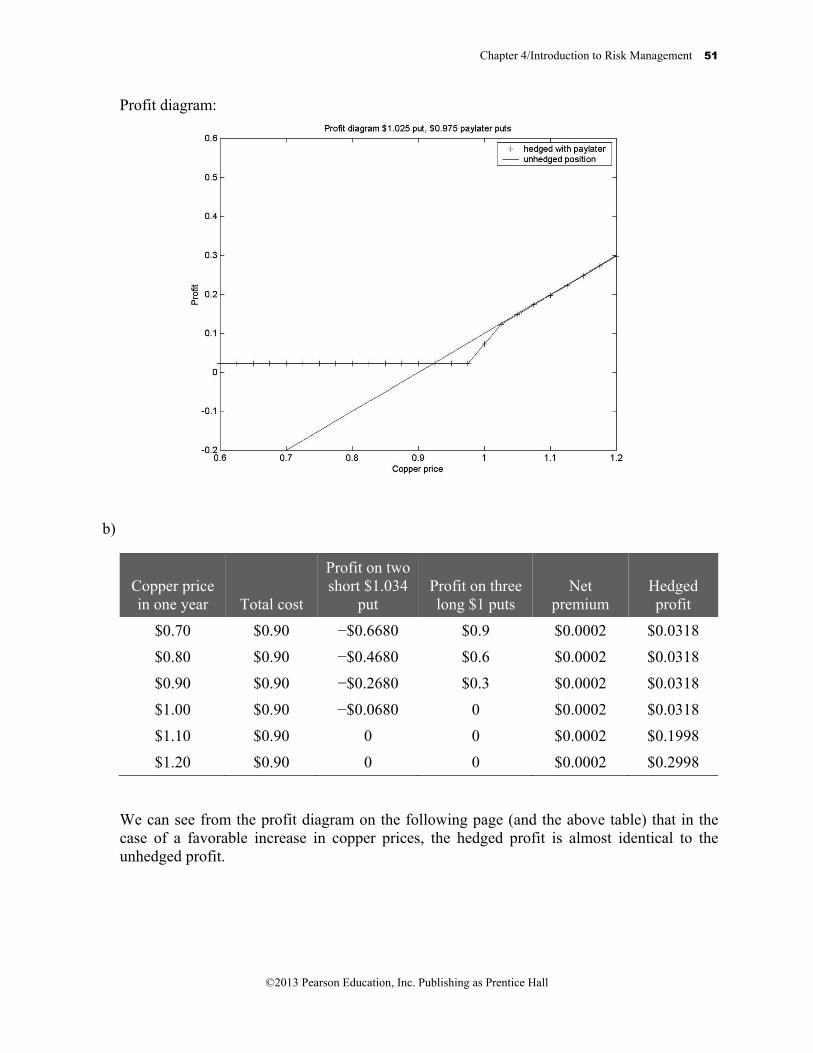
Profit diagram:

b)


Profit on two short $1.034

put Profit on three long $1 puts

Net premium

Hedged profit

$0.70 $0.90 −$0.6680 $0.9 $0.0002 $0.0318

$0.80 $0.90 −$0.4680 $0.6 $0.0002 $0.0318

$0.90 $0.90 −$0.2680 $0.3 $0.0002 $0.0318

$1.00 $0.90 −$0.0680 0 $0.0002 $0.0318

$1.10 $0.90 0 0 $0.0002 $0.1998

$1.20 $0.90 0 0 $0.0002 $0.2998

We can see from the profit diagram on the following page (and the above table) that in the case of a favorable increase in copper prices, the hedged profit is almost identical to the unhedged profit.



Profit diagram:

Question 4.7

Telco assigned a fixed revenue of $6.20 for each unit of wire. It can buy one unit of wire for $5 plus the price of copper. Therefore, Telco’s profit in one year is $6.20 less $5.00 less the price of copper after one year.

Copper price in one year Total cost Unhedged profit

Profit on one long forward Hedged profit

$0.70 $5.70 $0.50 −$0.3 $0.20

$0.80 $5.80 $0.40 −$0.2 $0.20

$0.90 $5.90 $0.30 −$0.1 $0.20

$1.00 $6.00 $0.20 0 $0.20

$1.10 $6.10 $0.10 $0.10 $0.20

$1.20 $6.20 0 $0.20 $0.20



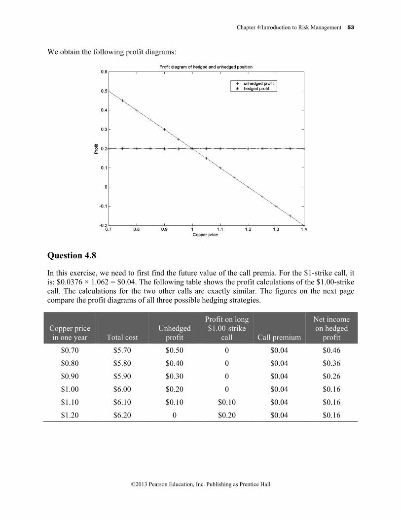
We obtain the following profit diagrams:

Question 4.8

In this exercise, we need to first find the future value of the call premia. For the $1-strike call, it is: $0.0376 × 1.062 = $0.04. The following table shows the profit calculations of the $1.00-strike call. The calculations for the two other calls are exactly similar. The figures on the next page compare the profit diagrams of all three possible hedging strategies.


Unhedged profit

Profit on long $1.00-strike

call Call premium

Net income on hedged

profit

$0.70 $5.70 $0.50 0 $0.04 $0.46

$0.80 $5.80 $0.40 0 $0.04 $0.36

$0.90 $5.90 $0.30 0 $0.04 $0.26

$1.00 $6.00 $0.20 0 $0.04 $0.16

$1.10 $6.10 $0.10 $0.10 $0.04 $0.16

$1.20 $6.20 0 $0.20 $0.04 $0.16




Question 4.9

For the $1-strike put, we receive a premium of: $0.0376 × 1.062 = $0.04. The following table shows the profit calculations of the $1.00-strike put. The calculations for the two other puts are exactly the same. The figures on the next page compare the profit diagrams of all three possible strategies.


Unhedged profit

Profit on short $1.00-strike put

Received premium


$0.70 $5.70 $0.50 −$0.30 $0.04 $0.24

$0.80 $5.80 $0.40 −$0.20 $0.04 $0.24

$0.90 $5.90 $0.30 −$0.10 $0.04 $0.24

$1.00 $6.00 $0.20 0 $0.04 $0.24

$1.10 $6.10 $0.10 0 $0.04 $0.14

$1.20 $6.20 0 0 $0.04 $0.04




Question 4.10

Telco will sell collars, which means that they buy the call leg and sell the put leg. We have to compute for each case the net option premium position, and find its future value. We have for:

a) ($0.0376 − $0.0178) × 1.062 = $0.021

b) ($0.0274 − $0.0265) × 1.062 = $0.001

c) ($0.0649 − $0.0178) × 1.062 = $0.050



a)

Copper price in one

year Total cost

Unhedged profit


put

Profit on long $1.00

call Net


$0.70 $5.70 $0.50 −$0.25 0 $0.021 $0.2290

$0.80 $5.80 $0.40 −$0.15 0 $0.021 $0.2290

$0.90 $5.90 $0.30 −$0.05 0 $0.021 $0.2290

$1.00 $6.00 $0.20 $0 0 $0.021 $0.1790

$1.10 $6.10 $0.10 0 $0.10 $0.021 $0.1790

$1.20 $6.20 0 0 $0.20 $0.021 $0.1790

Profit diagram:

b)

Copper price in one

year Total cost

Unhedged profit


put

Profit on long

$1.025 call Net


$0.70 $5.70 $0.50 −$0.275 0 $0.001 $0.2240

$0.80 $5.80 $0.40 −$0.175 0 $0.001 $0.2240

$0.90 $5.90 $0.30 −$0.075 0 $0.001 $0.2240

$1.00 $6.00 $0.20 $0 0 $0.001 $0.1990

$1.10 $6.10 $0.10 0 $0.0750 $0.001 $0.1740

$1.20 $6.20 0 0 $0.1750 $0.001 $0.1740



Profit diagram:

c)

Copper price in one

year Total cost Unhedged

profit


put

Profit on long

$0.95 call Net


$0.70 $5.70 $0.50 −$0.25 0 $0.05 $0.2

$0.80 $5.80 $0.40 −$0.15 0 $0.05 $0.2

$0.90 $5.90 $0.30 −$0.05 0 $0.05 $0.2

$1.00 $6.00 $0.20 0 $0.050 $0.05 $0.2

$1.10 $6.10 $0.10 0 $0.150 $0.05 $0.2

$1.20 $6.20 0 0 $0.250 $0.05 $0.2

We see that we are completely and perfectly hedged. Buying a collar where the put and call leg have equal strike prices perfectly offsets the copper price risk.



Profit diagram:

Question 4.11

a)

Copper price in one

year Total cost Unhedged

profit

Profit on short

$0.975 call

Profit on two long

$1.034 calls Net


$0.70 $5.70 $0.50 0 0 −$0.0015 $0.5015

$0.80 $5.80 $0.40 0 0 −$0.0015 $0.4015

$0.90 $5.90 $0.30 0 0 −$0.0015 $0.3015

$1.00 $6.00 $0.20 −$0.025 0 −$0.0015 $0.1765

$1.10 $6.10 $0.10 −$0.125 $0.13200 −$0.0015 $0.1085

$1.20 $6.20 0 −$0.225 $0.33200 −$0.0015 $0.1085

We can see from the profit diagram on the following page (and the previous table) that in the case of a favorable decrease in copper prices, the hedged profit is almost identical to the unhedged profit.



Profit diagram:

b)

Copper price in one year

Total cost

Unhedged profit

Profit on 2 short $1

call

Profit on three long

$1.034 calls

Net premium

Hedged profit

$0.70 $5.70 $0.50 0 0 −$0.0024 $0.5024

$0.80 $5.80 $0.40 0 0 −$0.0024 $0.4024

$0.90 $5.90 $0.30 0 0 −$0.0024 $0.3024

$1.00 $6.00 $0.20 0 0 −$0.0024 $0.2024

$1.10 $6.10 $0.10 −$0.200 $0.1980 −$0.0024 $0.1004

$1.20 $6.20 0 −$0.400 $0.4980 −$0.0024 $0.1004

We can see from the profit diagram on the next page (and the above table) that in the case of a favorable decrease in copper prices, the hedged profit is almost identical to the unhedged profit.



Profit diagram:

Question 4.12

This is a very important exercise to really understand the benefits and pitfalls of hedging strategies. Wirco needs copper as an input, which means that its costs increase with the price of copper. We may, therefore, think that they need to hedge against increases in the copper price. However, we must not forget that the price of wire, the source of Wirco’s revenues, also depends positively on the price of copper: The price Wirco can obtain for one unit of wire is $50 plus the price of copper. We will see that those copper price risks cancel each other out. Mathematically,

Wirco’s cost per unit of wire: $3 + $1.50 + ST

Wirco’s revenue per unit of wire: $5 + ST

and ST is the price of copper after one year. Therefore, we can determine Wirco’s profits as:

Profit = Revenue – Cost = $5 + ST − ($3 + $1.50 + ST ) = $0.50

We see that the profits of Wirco do not depend on the price of copper. Cost and revenue copper price risk cancel each other out. In this situation, if we buy a long forward contract, we do in fact introduce copper price risk! To understand this, add a long forward contract to the profit equation:

Profit with forward: = $5 + ST − ($3 + $1.50 + ST ) + ST − $1 = ST − $0.50



To summarize,

Copper price in one year Total cost Total revenue

Unhedged profit

Profit on long forward

Net income on ‘hedged’

profit

$0.70 $5.20 $5.70 $0.50 −$0.30 $0.20

$0.80 $5.30 $5.80 $0.50 −$0.20 $0.30

$0.90 $5.40 $5.90 $0.50 −$0.10 $0.40

$1.00 $5.50 $6.00 $0.50 0 $0.50

$1.10 $5.60 $6.10 $0.50 $0.10 $0.60

$1.20 $5.70 $6.20 $0.50 $0.20 $0.70

Question 4.13

We do in fact introduce copper price risk no matter what strategy we undertake. Therefore, no matter which instrument we are using, we increase the price variability of Wirco’s profits. Although this is a simple example, it is important to keep in mind that a company’s risk management should always take place on an aggregate level otherwise offsetting positions may be hedged twice.

Question 4.14

Hedging should never be thought of as a profit increasing action. A company that hedges merely shifts profits from good to bad states of the relevant price risk that the hedge seeks to diminish.

The value of the reduced profits, should the gold price rise, subsidizes the payment to Golddiggers should the gold price fall. Therefore, a company may use a hedge for one of the reasons stated in the textbook; however, it is not correct to compare hedged and unhedged companies from an accounting perspective.



Question 4.15

If losses are tax deductible (and the company has additional income to which the tax credit can be applied), then each dollar of losses bears a tax credit of $0.40. Therefore,

Price = $9 Price = $11.20

(1) Pre-Tax Operating Income −$1 $1.20

(2) Taxable Income 0 $1.20

(3) Tax @ 40% 0 $0.48

(3b) Tax Credit $0.40 0

After-Tax Income (including Tax credit) −$0.60 $0.72

In particular, this gives an expected after-tax profit of:

E[Profit] = 0.5 × (−$0.60) + 0.5 × ($0.72) = $0.06

and the inefficiency is removed: We obtain the same payoffs as in the hedged case, Table 4.7.

Question 4.16

a) Expected pre-tax profit

Firm A: E[Profit] = 0.5 × ($1, 000) + 0.5 × (−$600) = $200

Firm B: E[Profit] = 0.5 × ($300) + 0.5 × ($100) = $200

Both firms have the same pre-tax profit.

b) Expected after tax profit. Firm A:

Bad state Good state

(1) Pre-Tax Operating Income −$600 $1,000

(2) Taxable Income $0 $1,000

(3) Tax @ 40% 0 $400

(3b) Tax Credit $240 0

After-Tax Income (including Tax credit) −$360 $600

This gives an expected after-tax profit for firm A of:

E[Profit] = 0.5 × (−$360) + 0.5 × ($600) = $120



Firm B:


(1) Pre-Tax Operating Income $100 $300

(2) Taxable Income $100 $300

(3) Tax @ 40% $40 $120

(3b) Tax Credit 0 0

After-Tax Income (including Tax credit) $60 $180

This gives an expected after-tax profit for firm B of:

E[Profit] = 0.5 × ($60) + 0.5 × ($180) = $120

If firms receive full credit for tax losses, the tax code does not have an effect on the expected after-tax profits of firms that have the same expected pre-tax profits but different cash-flow variability.

Question 4.17

a) The pre-tax expected profits are the same as in exercise 4.16. (a).

b) While the after-tax profits of company B stay the same, those of company A change because they do not receive tax credit on the loss anymore.

c) We have for firm A:


(1) Pre-Tax Operating Income −$600 $1,000

(2) Taxable Income $0 $1,000

(3) Tax @ 40% 0 $400

(3b) Tax Credit no tax credit 0

After-Tax Income (including Tax credit) −$600 $600

And consequently, an expected after-tax return for firm A of:

E[Profit] = 0.5 × (−$600) + 0.5 × ($600) = $0

Company B would not pay anything because it makes always positive profits, which means that the lack of a tax credit does not affect them.

Company A would be willing to pay the discounted difference between its after-tax profits calculated in 4.16. (b) and its new after-tax profits, $0 from 4.17. It is thus willing to pay: $120 ÷ 1.1 = $109.09.



Question 4.18

Auric Enterprises is using gold as an input. Therefore, it would like to hedge against price increases in gold.

a) The cost of this collar today is the premium of the purchased 440-strike call ($2.49) less the premium for the sold 400-strike put. We calculate a cost of $2.49 − $2.21 = −$0.28, which means that Auric in fact generates a revenue from entering into this collar.

b) The values of part (a) are a good starting point. You see that both put and call are worth

approximately the same; therefore, start shrinking the 440 – 400 span symmetrically until you get a difference of 30 and then do some trial and error. This should bring you the following values: The call strike is 435.52, and the put strike is 405.52. Both call and put have a premium of $3.425.

Question 4.19

As we buy the call, we will buy it at the ask price, which is $0.25 above the Black-Scholes price, and we sell the put at the bid, which is $0.25 below the Black-Scholes price. Our new equal premium condition is: C + $0.25 – (P − $0.25) = 0, or C + $0.50 – P = 0. Since we know that the value of a call is decreasing in the strike, and we need a Black-Scholes call price that is $.50 less valuable than the Black-Scholes put, we know that we have to look for a pair of higher strike prices. Trial and error brings us to a call strike of 436.53 and a put strike of 406.53. The Black-Scholes call premium is $3.1938, and the put has a premium of $3.6938.



Question 4.20

a) Since we know that the value of a call is decreasing in the strike and we need to sell two call options, the Black-Scholes prices that equal the 440-strike call price, we know that we have to look for a higher strike price. Trial and error results in a strike price of 448.93. The premium of the 440-strike call is $2.4944, and indeed the Black-Scholes premium of the 448.93 strike call is $1.2472.

b) Profit diagram:

Question 4.21

If you do not know how to run a regression, or if you forgot what a regression is, you may want to type the keyword “regression” in Microsoft Excel’s help menu. It will show you how to run a regression in Excel, as well as explain to you the key features of a regression.

Running a regression, we obtain a constant of 2,100,000 and a coefficient on price of 100,000.



Question 4.22

a) We have the following table:

Price Quantity Revenue 3 1.5 4.5 3 0.8 2.4 2 1 2 2 0.6 1.2

Using Excel’s function STDEVP(4.5,2.4,2,1.2), we obtain a value of 1.2194 for the standard deviation of total revenue for Scenario C.

b) Using any standard software’s command (or doing it by hand!) to determine the correlation coefficient, we obtain a value of 0.7586.

Question 4.23

a) Using equation (4.7) and the values of the correlation coefficient and standard deviation of the revenue we calculated in question 4.22, we obtain the following value for the variance minimizing hedge ratio:

0.7586 1.2194 1.850070.5

H ×= − =

It is thus optimal to short 1.85 million bushels of corn.

b) If you do not know how to run a regression, or if you forgot what a regression is, you may want to type the keyword “regression” in Microsoft Excel’s help menu. It will show you how to run a regression in Excel, as well as explain to you the key features of a regression.

Running such a regression, we obtain a constant of −2,100,000 and a coefficient on price of 1,850,000, thus yielding the same results as part (a).

c)

Price Quantity Unhedged revenue Futures gain Total

3 1.5m 4.5m −0.5 × 1.85m 3.575m

= −0.925m

3 0.8m 2.4m −0.5 × 1.85m 1.475m

= −0.925m

2 1m 2m +0.5 × 1.85m 2.925m

= +0.925m

2 0.6m 1.2m +0.5 × 1.85m 2.125m

= +0.925m



Using Excel’s function STDEVP(3.575,1.475,2.925,2.125), we obtain a value of 0.7945 for the standard deviation of the optimally hedged revenue for Scenario C. We see that we were able to significantly reduce the variance of our revenues.

Question 4.24

a) The expected quantity of production is 0.25 × (1.5 + 0.8 + 1 + 0.6) = 0.975 million bushels of corn.

b)

Price Quantity Unhedged revenue

Futures gain from shorting 0.975m contracts Total

3 1.5m 4.5m −0.5 × 0.975m 4.0125m

= −0.4875m

3 0.8m 2.4m −0.5 × 0.975m 1.9125m

= −0.4875m

2 1m 2m 0.5 × 0.975m 2.4875m

= 0.4875m

2 0.6m 1.2m 0.5 × 0.975m 1.6875m

= 0.4875m

Using Excel’s function STDEVP(4.0125, 1.9125, 2.4875, 1.6875), we obtain a value of 0.907004 for the standard deviation of the optimally hedged revenue for Scenario C. We see that we were able to reduce the variance of our revenues, albeit to a lesser degree than with the optimally hedged portfolio.

Question 4.25

a) The expected quantity is: 0.5 × (0.6 + 0.934) = 0.767 million bushels. We have:

Price Quantity Unhedged revenue Futures gain from shorting 0.767m contracts Total

2 0.6m 1.2m +0.5 × 0.767m 1.5835m

= 0.3835m

3 0.934m 2.802m −0.5 × 0.767m 2.4185m

= −0.3835m



b) The minimum quantity is 0.6 million bushels. Therefore:


2 0.6m 1.2m +0.5 × 0.6m 1.5m

= 0.3m

3 0.934m 2.802m −0.5 × 0.6m 2.502m

= −0.3m

c) The maximum quantity is 0.934 million bushels. Therefore:


2 0.6m 1.2m +0.5 × 0.934m 1.667m

= 0.467m

3 0.934m 2.802m −0.5 × 0.934m 2.335m

= −0.467m

d) The hedge position that eliminates price variability shifts enough revenue from the good state to the bad state so that you make the same money in both states of the world (which are either a price of three or a price of two).

We have to solve:

1.2m + 0.5 × = 2.802m − 0.5 × X

⇔ X = 1.602m

This leads to the following table:


2 0.6m 1.2m +0.5 × 1.602m 2.001m

= 0.801m

3 0.934m 2.802m −0.5 × 1.602m 2.001m

= −0.801m

We see again that we have to short more contracts than our maximum production is. The fact that quantity goes up when prices go up is responsible for this extensive amount of hedging.

Documents

Introduction to Risk Management - Texas Christian …sbufaculty.tcu.edu/mann/!_AdvInv-Fall2016/solution/Chapter 04.pdf · Chapter 4/Introduction to Risk Management 45 ©2013 Pearson