Introduction to runoff modeling Introduction to runoff modeling on the North Slope of Alaska on the North Slope of Alaska

using the Swedish HBVusing the Swedish HBVModelModel

Emily Youcha, Douglas KaneEmily Youcha, Douglas Kane

University of Alaska FairbanksWater & Environmental Research Center

PO Box 755860Fairbanks, AK 99775

ObjectiveObjective

Use existing Use existing meteorological meteorological datasets and datasets and develop HBV develop HBV model parameters model parameters to simulate runoff to simulate runoff in both small and in both small and large North Slope large North Slope BasinsBasins

Kuparuk

Sag

Kavik

Upper Kuparuk

ApproachApproach Begin runoff simulations on North Begin runoff simulations on North

Slope streams with abundance of Slope streams with abundance of datadataImnaviat Cr, 2.2 kmImnaviat Cr, 2.2 km22 (1985-present) (1985-present)Upper Kuparuk River, 146 kmUpper Kuparuk River, 146 km22 (1993- (1993-

present)present)– Putuligayuk River, 417 kmPutuligayuk River, 417 km22 (1970-1979, (1970-1979,

1982-1986, 1999-2007) 1982-1986, 1999-2007) – Kuparuk River, 8140 kmKuparuk River, 8140 km22 (1971-present) (1971-present)

Develop parameter sets and apply to Develop parameter sets and apply to other rivers (ungauged?)other rivers (ungauged?)

HBV ModelHBV Model Rainfall-runoff model, commonly used for forecasting in Rainfall-runoff model, commonly used for forecasting in

SwedenSweden Developed by Swedish Meteorological and Hydrological Developed by Swedish Meteorological and Hydrological

InstituteInstitute Semi-distributed conceptual modelSemi-distributed conceptual model

– Divide into sub-basinsDivide into sub-basins– Precipitation and temperature may be spatially distributed by Precipitation and temperature may be spatially distributed by

applying areal-based weights to station data applying areal-based weights to station data – Use of elevation and vegetation zonesUse of elevation and vegetation zones

Required data inputs (hourly or daily) include: Required data inputs (hourly or daily) include: – Precipitation (maximum end-of-winter SWE and summer Precipitation (maximum end-of-winter SWE and summer

precipitation) precipitation) – Air temperatureAir temperature– Evapotranspiration (pan evaporation or estimated) daily or Evapotranspiration (pan evaporation or estimated) daily or

monthlymonthly Routines include:Routines include:

– SnowSnow– Soil Moisture AccountingSoil Moisture Accounting– ResponseResponse– TransformationTransformation

HBV Routines and Input DataHBV Routines and Input Data

Soil Moisture RoutineInputs: Potential Evapotranspiration,

Precipitation, Snowmelt

Snow RoutineInputs: Precipitation, Temperature

Response RoutineInput: Ground-Water Recharge/Excess soil

moisture

Transformation RoutineInput: Runoff

Simulated Runoff

Outputs: Snowpack, Snowmelt

Outputs: Actual Evapotranspiration, Soil Moisture,

Ground-Water Recharge

Output: Runoff, Ground-Water Levels

SMHI

Routines and Parameters:

Snow: 4 + parameters

Degree-day method: Snowmelt = CFMAX * (T –TT)

CFMAX=melting factor (mm/C-day)

TT=threshold temperature (C) (snow vs. rain)

CFR=refreezing factor to refreeze melt water

WHC=water-holding capacity of snow (meltwater is retained in snowpack until it exceeds the WHC)

Soil Moisture Accounting : 3+ parameters

Modified bucket approach

Shape coefficient (BETA) controls the contribution to the response function (runoff ratio)

Limit of potential evapotranspiration (LP), the soil moisture value

above which ET reaches Potential ET

Maximum soil moisture (FC)

Response 4+ parameters

Transforms excess water from soil moisture zone to runoff. Includes both linear and non-linear functions. Upper reservoirs represent quickflow, lower reservoir represent slow runoff (baseflow). Lakes are considered as part of the lower reservoir. Lower reservoir may not be used (PERC parameter is set to zero due to presence of continuous permafrost).

Transformation/Routing

To obtain the proper shape of the hydrograph, parameter= MAXBAS (/d)

SMHI Manual, 2005

UZL0

UZL1

Q0=K0 * (SZ- UZL0)

Q1=K1 * (SZ- UZL1)

Q2=K3 * SZ

SZ

Recharge: input from soil routine (mm/day)SZ: Storage in zone (mm)UZL:Threshold parameterKi: Recession coefficient (/day)Qi: Runoff component (mm/day)

recharge

Modified from Siebert, 2005

Response Routine

Runoff

Soil Moisture Routine

Transformation Routine

HBV CalibrationHBV Calibration Each model routine has parameters requiring model calibrationEach model routine has parameters requiring model calibration

– over 20 parameters, and may be varied throughout the over 20 parameters, and may be varied throughout the simulated period (i.e. spring vs. summer)simulated period (i.e. spring vs. summer)

Explained variance (observed vs. simulated) is the Nash-Explained variance (observed vs. simulated) is the Nash-Sutcliffe (1970) model efficiency criterion good model fit is Sutcliffe (1970) model efficiency criterion good model fit is R-efficiency=1. Also looked at accumulative volume R-efficiency=1. Also looked at accumulative volume difference and visually inspect the hydrograph.difference and visually inspect the hydrograph.

Used the commercially available HBV software to manually Used the commercially available HBV software to manually calibrate the model by trial and errorcalibrate the model by trial and error

We tried HBV automated calibration to estimate parameters We tried HBV automated calibration to estimate parameters (Monte Carlo procedure using “HBV-light” by Siebert, 1997). (Monte Carlo procedure using “HBV-light” by Siebert, 1997). Produced many different parameter sets that would solve the Produced many different parameter sets that would solve the problem. Many parameters were not well definedproblem. Many parameters were not well defined

Most of the time, model validation results not very good. Most of the time, model validation results not very good.

2

2

1QobsQobs

QobsQsim

GUI – easy to GUI – easy to use and view use and view results quickly results quickly

(sort of)(sort of)

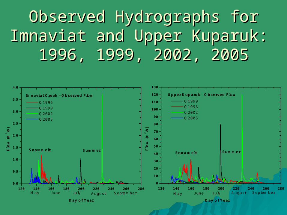
Observed Hydrographs for Imnaviat Observed Hydrographs for Imnaviat and Upper Kuparuk: and Upper Kuparuk:

1996, 1999, 2002, 20051996, 1999, 2002, 2005

120 140 160 180 200 220 240 260 2800

10

20

30

40

50

60

70

80

90

100

110

120

130

SeptemberAugustJulyMay June

SummerSnowmelt

Upper Kuparuk - Observed Flow

Flo

w (

m3 /s

)

Day of Year

Q1999 Q1996 Q2002 Q2005

120 140 160 180 200 220 240 260 2800.0

0.5

1.0

1.5

2.0

2.5

3.0

3.5

4.0

SummerSnowmelt

May June July SeptemberAugust

Imnaviat Creek - Observed Flow

Flo

w (

m3 /s

)

Day of Year

Q1996 Q1999 Q2002 Q2005

Example: Example: Upper Upper

Kuparuk, Kuparuk, 21 21

parameters parameters to calibrate!to calibrate!

HBV Parameter 1996 1999 2002 2005

Snow Routine

TT (C) 1 1 1 1

SFCF 1 1 1 1

WHC 0.1 0.1 0.1 0.1

CFMAX (mm/C-d) 4 4 4 4

CFR 0.05 0.05 0.05 0.05

PCORR 1 1 1 1

RFCF 1 1 1 1

PCALT 0.1 0.1 0.1 0.1

TCALT 0.6 0.6 0.6 0.6

Soil Moisture Routine

BETA spring 0.2 0.2 0.2 0.2

BETA summer 0.2 0.2 0.2 0.2

FC (mm)spring 10 10 10 10

FC (mm)summer 50 50 50 50

LP 0.9 0.9 0.9 0.9

ECALT 0.1 0.1 0.1 0.1

CFLUX 1 1 1 1

Response Routine

k0 (/d) spring 0.4 0.4 0.4 0.4

k0 (/d) summer 0.9 0.9 0.9 0.9

k1 (/d) spring 0.1 0.1 0.1 0.1

k1 (/d) summer 0.5 0.5 0.5 0.5

k3 (/d) spring 0.06 0.06 0.06 0.06

k3 (/d) summer 0.09 0.09 0.09 0.09

UZL0 (mm) spring 40 40 40 40

UZL0 (mm) summer 30 30 30 30

UZL1 (mm) spring 10 10 10 10

UZL1 (mm) summer

PERC 0 0 0 0

Transformation Routine

MAXBAS (d) spring 1.5 1.5 1.5 1.5

MAXBAS (d) summer 1.5 1.5 1.5 1.5

Preliminary Automated Calibration Preliminary Automated Calibration Results (Monte Carlo Procedure)Results (Monte Carlo Procedure)

Dotty plots – look for parameters that Dotty plots – look for parameters that are well definedare well defined

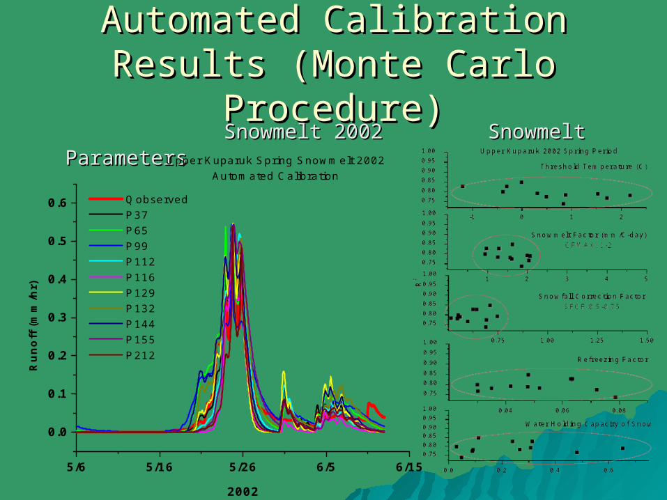
Automated Calibration Results Automated Calibration Results (Monte Carlo Procedure)(Monte Carlo Procedure)

Snowmelt 2002Snowmelt 2002 Snowmelt ParametersSnowmelt Parameters

5/6 5/16 5/26 6/5 6/15

0.0

0.1

0.2

0.3

0.4

0.5

0.6

Upper Kuparuk Spring Snowmelt 2002Automated Calibration

Ru

no

ff (

mm

/hr)

2002

Qobserved P37 P65 P99 P112 P116 P129 P132 P144 P155 P212

5/1 5/16 5/31 6/15 6/30 7/15 7/30 8/14 8/29 9/13 9/280

10

20

30

40

50

SnowmeltR-efficiency=0.85Accum Diff = -4 mmRel. Accum Diff =-3%

SummerR-efficiency=0.42Accum Diff = -18 mmRel. Accum Diff =-19%

R-efficiency=0.85Accum Diff = -23 mmRel. Accum Diff =-9%

Qsimulated Qobserved

Run

off

(m3 /s

)

1996

0

20

40

60

80

100

120

Simulated SnowS

now

Wat

er E

quiv

alen

t (m

m)

-60-50-40-30-20-1001020

Accum. Diff.

Acc

um.

Diff

. (m

m)

5/1 5/16 5/31 6/15 6/30 7/15 7/30 8/14 8/29 9/13 9/280

102030405060708090

SummerR-efficiency=0.56Accum Diff = 23 mmRel. Accum Diff = 15%

SnowmeltR-efficiency=-1.17Accum Diff = 15 mmRel. Accum Diff = 49%

R-efficiency=0.55Accum Diff = 39 mmRel. Accum Diff = 20%

Qsimulated Qobserved

Run

off

(m3 /s

)

1999

0

20

40

60

Simulated Snow Observed Snow UKmet

Sno

w W

ater

Equ

ival

ent

(mm

)

-10

0

10

20

30

40

50

60 Accum. Diff.

Acc

um.

Diff

. (m

m)

5/1 5/16 5/31 6/15 6/30 7/15 7/30 8/14 8/29 9/13 9/280

20

40

60

80

100

120

SummerR-efficiency=0.25Accum Diff = -83 mmRel. Accum Diff = -37%

SnowmeltR-efficiency=0.51Accum Diff = 20 mmRel. Accum Diff = -41 %

R-efficiency=0.29Accum Diff = -60 mmRel. Accum Diff = -22%

Qsimulated Qobserved

Ru

noff

(m

3 /s)

2002

020406080

100120140160180

Simulated Snow Observed Snow UKmet

Sn

ow W

ate

r E

qu

ival

ent

(mm

)

-80

-60

-40

-20

0

20 Accum. Diff.

Acc

um.

Diff

. (m

m)

5/1 5/16 5/31 6/15 6/30 7/15 7/30 8/14 8/29 9/13 9/280

5

10

15

SummerR-efficiency=0.82Accum Diff = -13 mmRel. Accum Diff = -28%

SnowmeltR-efficiency=0.40Accum Diff = 28 mmRel. Accum Diff = 49%

R-efficiency=0.64Accum Diff = 16 mmRel. Accum Diff = 16%

Qsimulated Qobserved

Run

off

(m3 /s

)

2005

020406080

100120140160

Simulated Snow Observed Snow UKmet

Sno

w W

ater

Equ

ival

ent

(mm

)

-10

0

10

20

30

40

50 Accum. Diff.

Acc

um.

Diff

. (m

m)

SummarySummary Need an automated calibration procedure to Need an automated calibration procedure to

develop unique parameter setsdevelop unique parameter sets For Upper Kuparuk, model generally For Upper Kuparuk, model generally

predicted timing of events (onset of predicted timing of events (onset of snowmelt and timing of peak events). When snowmelt and timing of peak events). When it did not predict the proper timing, the it did not predict the proper timing, the model efficiency was poor.model efficiency was poor.

For Upper Kuparuk, model overpredicted For Upper Kuparuk, model overpredicted snowmelt flow volume and underpredicted snowmelt flow volume and underpredicted extreme peak runoff events during summerextreme peak runoff events during summer

For both Upper Kuparuk and Imnavait, model For both Upper Kuparuk and Imnavait, model did not predict the magnitude of peak flowdid not predict the magnitude of peak flow

Problems may be attributed to not using a Problems may be attributed to not using a long enough simulation periodlong enough simulation period

Many improvements are needed to increase Many improvements are needed to increase the Nash-Sutcliffe model efficiencythe Nash-Sutcliffe model efficiency