Introduction to software tools for Automotive Electronics lab

BE électronique automobile 5e année ESPE

Introduction to software tools for Automotive Electronics

lab

http://www.alexandre-boyer.fr

Alexandre Boyer

Patrick Tounsi

5e année ESPE

November 2020

http://www.alexandre-boyer.fr/


2

I - Getting started S32 Design Studio for Power Architecture IDE (version 2.1) .................. 4

1. Overview of S32DS for Power architecture .................................................................... 4 2. Define your Workspace ................................................................................................... 5 3. Create a project from scratch .......................................................................................... 5 4. Import an existing project in a workspace ...................................................................... 7 5. Remove a project from the workspace ............................................................................ 7

6. Compile and build your project ....................................................................................... 8

7. Programming the MCU ................................................................................................... 8

8. Debugging your application .......................................................................................... 10 9. Installing and using SDK .............................................................................................. 11

II - Presentation of Matlab/Simulink for motor control simulation .................................... 12 1. Creating model in Simulink .......................................................................................... 12

2. Creation of variables ..................................................................................................... 14 3. Placing scopes ............................................................................................................... 14

4. Configuration of simulation .......................................................................................... 15 5. Launching simulation .................................................................................................... 15 6. The main common libraries ........................................................................................... 16

a. Commonly used blocks ............................................................................................. 17 b. Continuous ............................................................................................................. 17

c. Discrete ...................................................................................................................... 17 d. Math operation ....................................................................................................... 18

e. Ports and subsystem ................................................................................................... 18 f. Signal attributes ......................................................................................................... 18 g. Signal routing ......................................................................................................... 19

h. Sinks ....................................................................................................................... 19

i. Sources ....................................................................................................................... 19 j. User-defined function ................................................................................................ 20

III - Presentation of FREEMASTER .................................................................................... 20 1. Overview ....................................................................................................................... 20 2. Adding FREEMASTER communication driver to S32DS project ............................... 21

a. The main macros and functions of FREEMASTER API .......................................... 21 b. Configuration of FREEMASTER driver in C code application ............................ 22

3. Configuring FREEMASTER application as an oscilloscope ........................................ 23 4. Saving captured data by Freemaster running as an oscilloscope .................................. 27 5. Debug FREEMASTER ................................................................................................. 28

IV - Presentation of Automotive Math and Motor Control Library for MPC574xP ............ 29 1. Overview ....................................................................................................................... 29

2. Types provided by AMMCLIB ..................................................................................... 31 3. Brief presentation of the functions ................................................................................ 31

a. Math Function library (MLIB) .................................................................................. 32 b. General Functions library (GFLIB) ....................................................................... 32 c. General Digital Filters library (GDFLIB) ................................................................. 33 d. General Motor Control library (GMCLIB) ............................................................ 33


3

4. Using in S32DS environment ........................................................................................ 34

a. Setting the implementation ........................................................................................ 34 b. Calling mathematical function ............................................................................... 34

5. Using in Matlab/Simulink environment ........................................................................ 35 V - References ..................................................................................................................... 35


4

This document aims at providing basic support for the different software tools used to achieve

the motor application project in Automotive Electronics lab:

▪ S32 Design Studio (S32DS) IDE: the integrated development environment provided

by NXP for Power Architecture MCU

▪ Matlab / Simulink: As NXP provides Simulink toolbox for modeling and simulation of

the motor and its command

▪ FREEMASTER: NXP proposes this tool to communicate with embedded applications

and monitor/visualize in real-time internal variables of embedded applications

In order to facilitate the development, simulation and debugging of motor control applications,

NXP also provides Automotive Math and Motor Control Library (AMMCLIB) for NXP

MPC574xP. This library is compatible with both S32DS and Matlab/Simulink as a toolbox. It

contains basic and complex mathematical functions dedicated to motor control applications

(basic mathematical operation, digital filtering, Park transform, SVM, etc…)

The purpose of this document is to help you to start development with these tools rapidly and

underlines the functionality offered by these tools in order to help you to choose the more

appropriate design flow.

This document is intended for motor control application development on MPC5744P

microcontroller, mounted on the DEVKIT-MPC5744P development kit.

This document is not exhaustive. More information about the different tools, toolbox and

library can be found in the references provided in the part Links.

I - Getting started S32 Design Studio for Power Architecture IDE (version 2.1)

1. Overview of S32DS for Power architecture

S32DS for Power architecture is the integrated development

environment provided by NXP for Power Architecture microcontroller

(MCU) and automotive applications. The S32 Design Studio is based on

the Eclipse open development platform and integrates the Eclipse IDE,

GNU Compiler Collection (GCC), GNU Debugger (GDB).

It also provides in-situ debugger through several interfaces: P&E

Multilink/Cyclone/OpenSDA and supports two software design kits (SDK) that will be used

in this lab: FREEMASTER serial communication drivers and Automotive Math and Motor

Control Libraries (AMMCLIB).

In this part, the main steps to launch S32DS, create a new project, compile, build, debug and

flash your application in the MCU will be described. Here, the MCU MPC5744P is

considered.


5

2. Define your Workspace

As S32DS is based on Eclipse environment, all the projects must be defined according to a

common workspace. All the new projects will be created in the associated folder. When

S32DS is launched, the following window is opened to select the Workspace.

Figure 1 – Selection of the Workspace

Tips: manage the different projects within a workspace directly from S32DS IDE, not from

Windows Explorer !

3. Create a project from scratch

Launch the S32 Design Studio for Power Architecture. A dialog window opens in order to

select your workspace. All the S32 project saved in this workspace will be imported.

The window shown in Figure 2 opens. If some existing projects are in the workspace, they

will appear in the Project Explorer. The organization of the window is configurable with the

menu Window.

Project explorer

Commands

Menu bar

Perspective Switch (C/C++ or debug view)

Code editor

Console

Tool bar

Figure 2 - Main window of S32DS IDE

To open an existing project, write click on its name in the project explorer and select Open

Project. You can open source files (.c or .h) and modify them in the Code editor part. Several

commands available either in the menu bar, tool bar or Commands window launch the

compilation, building, debugging and flashing process. They will be presented later.


6

In order to create a project from scratch for MPC5744P, follow the procedure described below:

▪ In the menu bar, click on File > New > S32DS Application project. The window

below opens to setting the target MCU and the project options

▪ Enter the name of the project in Project Name and its location (by default, in your

workspace). In the Elf S32DS project window, select the target microcontroller:

Family MPC574xP > MPC5744P. Click on Next button.

Figure 3 - Creating a new S32DS project from scratch

▪ Select the project options (language, import Software Design Kits (SDK), type of

debugger, …). The default configurations are sufficient for this project, except if you

need to import SDK (e.g. AMMCLIB or FREEMASTER). This point will be

addressed in 5).

▪ Click on Finish to generate the project

S32DS generates the project with all the necessary libraries, start-up, debugger and linker

codes. The project folder is visible in the Project Explorer. By default, the Perspective Switch

is in C/C++ mode for code development. The target memory is written just after the name

of the project:

▪ debug: the executable code will be downloaded in the Flash memory of the MCU

▪ debug RAM: the executable code will be downloaded in the SRAM of the MCU

Tips: select Flash to store your program in non-volatile memory. Programming Flash is a

little longer than programming RAM. During debug stage, it can be more convenient to

download your code in RAM.

The project structure is organized as follows:

▪ Project_Settings: this folder contains all the required files to compile the project, link

the files and the start-up code.

▪ Include: it contains all the header files .h of the project.

▪ src: it contains all the C/C++ source file of the project. By default, the following files

are added after the creation of a new project:

o main.c: your main code

o intc_SW_mode_isr_vectors_MPC5744P.c: this file defines the interrupt vector

table


7

o MPC57xx__Interrupt_Init.c, vector.c and intc_sw_handlers.s: these files define

all the function requires for interrupt management

▪ Debug: this folder contains all the executable source files that will be downloaded into

Flash memory. The .elf file is the executable file and the .map file provides the

memory location of the code.

▪ Debug_RAM: this folder contains all the executable source files that will be

downloaded into SRAM. The .elf file is the executable file and the .map file provides

the memory location of the code.

A default main.c file is opened in the code editor. You can write your own code in this file.

Existing files can be copied and pasted from one project to another directly by right clicking

on them and selecting Copy or Paste. You can create new source C file by clicking on src

folder in your own project and clicking on File > New > Source File or on the icon . Type

the name of the new source file (give .c as extension). Do not forget to create also the

associated header file (.h) that must be included in the folder include. Click on include folder

in your own project and clicking on File > New > Header File or on the icon .

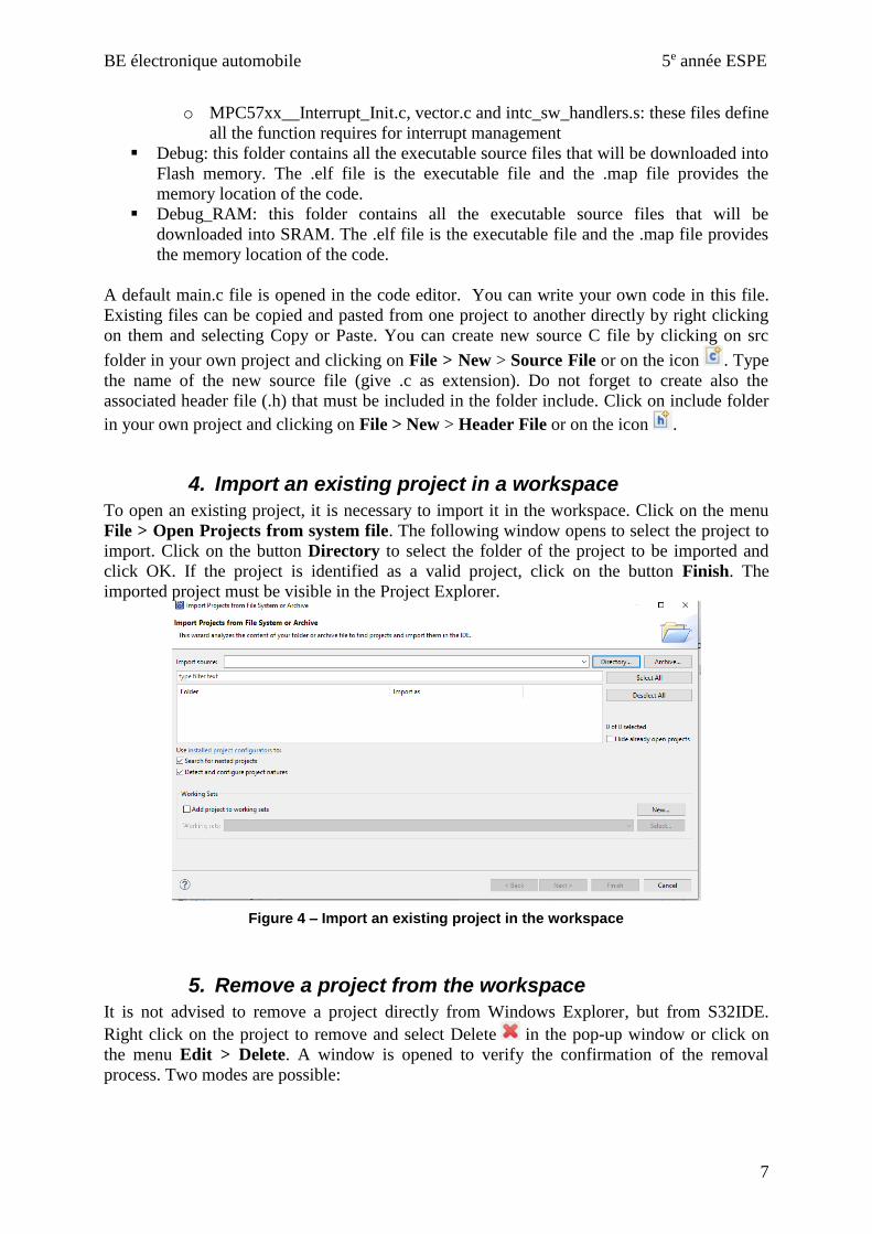
4. Import an existing project in a workspace

To open an existing project, it is necessary to import it in the workspace. Click on the menu

File > Open Projects from system file. The following window opens to select the project to

import. Click on the button Directory to select the folder of the project to be imported and

click OK. If the project is identified as a valid project, click on the button Finish. The

imported project must be visible in the Project Explorer.

Figure 4 – Import an existing project in the workspace

5. Remove a project from the workspace

It is not advised to remove a project directly from Windows Explorer, but from S32IDE.

Right click on the project to remove and select Delete in the pop-up window or click on

the menu Edit > Delete. A window is opened to verify the confirmation of the removal

process. Two modes are possible:


8

▪ If the option “Delete project contents on disk (cannot be undone)” is not selected, the

project is removed from the workspace, but it is not permanently deleted. It can be

imported again if necessary.

▪ If the option “Delete project contents on disk (cannot be undone)” is selected, the

project is removed from the workspace and permanently deleted. Be careful if you

select this option !

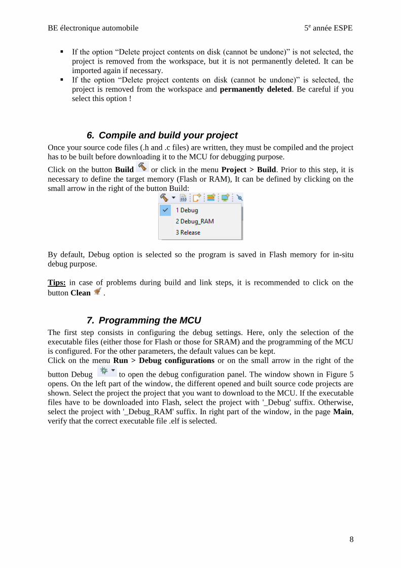
6. Compile and build your project

Once your source code files (.h and .c files) are written, they must be compiled and the project

has to be built before downloading it to the MCU for debugging purpose.

Click on the button Build or click in the menu Project > Build. Prior to this step, it is

necessary to define the target memory (Flash or RAM), It can be defined by clicking on the

small arrow in the right of the button Build:

By default, Debug option is selected so the program is saved in Flash memory for in-situ

debug purpose.

Tips: in case of problems during build and link steps, it is recommended to click on the

button Clean .

7. Programming the MCU

The first step consists in configuring the debug settings. Here, only the selection of the

executable files (either those for Flash or those for SRAM) and the programming of the MCU

is configured. For the other parameters, the default values can be kept.

Click on the menu Run > Debug configurations or on the small arrow in the right of the

button Debug to open the debug configuration panel. The window shown in Figure 5

opens. On the left part of the window, the different opened and built source code projects are

shown. Select the project the project that you want to download to the MCU. If the executable

files have to be downloaded into Flash, select the project with '_Debug' suffix. Otherwise,

select the project with '_Debug_RAM' suffix. In right part of the window, in the page Main,

verify that the correct executable file .elf is selected.


9

Figure 5 - Debug configuration panel (Run > Debug configurations)

Then, go to the page Debugger. The list Interface contains all the supported programming

interfaces, as shown below. In this lab, you will use development board DEVKIT_MPC5744P.

An on-board programming interface, called Open-Standard Serial and Debug Adapter

(OpenSDA) is mounted on the board, offering an economical programming interface for the

user. You will use this interface primarily. Thus select OpenSDA Embedded Debug- USB

Port in the list. If the board is connected on a USB port of your computer, information about

the port number and the device mounted on the development kit should appear in the fields

Port, Device Name and Core.

A programming interface alternative is the USB Multilink. This external programming

interface is available in this lab.

Figure 6 - Selection of the programming interface (Run > Debug configurations)

Finally, you can click on the button Debug to start the downloading of the code into MCU

memory.

You are not forced to return to the Debug configurations to start the programming of the

MCU. Once it has been configuring, you can click on the menu Run > Debug (F11) or on the

button .


10

8. Debugging your application

Once you click on the button Debug, the downloading of the executable files into the MCU

starts. Ensure that the MCU board is connected to your computer through a programming

interface and correctly powered. The process can last several tens of seconds. As explained

before, programming the Flash memory is longer than the programming of the RAM.

During the downloading process, the Perspective Switch changes from C/C++ to Debug mode

and window shown in Figure 7 appears.

Source code

Variable/Register content display

Console (messages, memory content)

Tool bar Perspective switch

Figure 7 - In-situ debugging interface

The debugging process is controlled by the commands provided in the Tool bar (Figure 8).

The Run button starts the execution of the embedded program. The execution can be paused

by clicking on the button Pause. The execution can be performed step-by-step by clicking on

the step buttons.

Disable all breakpoints

Run

Pause

Stop Step into

Step over

Step return

Figure 8 - Debug toolbar

Breakpoints can be inserted in the source code by double clicking on the source code line

where you want to insert the breakpoint. You can also right click and select Add Breakpoint.

The breakpoint is removed by double clicking on it or right clicking and select sur Toggle

Breakpoint. It can be deactivated by clicking on Disable breakpoint and reactivated with

Enable Breakpoint. Each time the execution pauses (due to a breakpoint or a click on button

Pause), the memory content is refreshed.

At the end of in-situ debug operation, you have to stop the debugger by clicking on the button

Stop. Then, click on the perspective switch to return in C/C++ mode.


11

Tips : do not forget to stop the debugger before returning in C/C++ Perspective. Otherwise,

the debugger will continue to run. The next time you will try to reprogram the MCU, an error

message will be displayed to warn you that a in-situ debug is still on-going.

9. Installing and using SDK

In this lab, you will certainly use two software design kits (SDK) provided by NXP:

▪ FREEMASTER communication drivers

▪ Automotive Math and Motor Control Libraries (AMMCLIB)

Both SDK are free but they are not installed in S32DS by default. Here, we explain how to

install SDK and use the provided source codes and drivers. The downloading links and the

contents of these SDK will be detailed in part III and V of this document.

SDK have to be selected during the project creation, in order to import all the library files.

When you create a new project with S32DS, as explained in part I.2, click on the button

in the field SDK of the window New S32DS Project. The window shown in Figure 9 opens.

All the SDK installed in your PC are listed (in this example, Freemaster and AMMCLIB are

installed). Select the SDK that you want to use and click OK. In the window New S32DS

Project, click on Finish. A new project is automatically generated. In the Project Explorer,

you can verity that source files associated to the SDK have been added.

Figure 9 - Selecting SDK in a S32DS project


12

II - Presentation of Matlab/Simulink for motor control simulation

Simulink is dedicated to the modeling and simulation of dynamic multidomain systems,

operating in continuous or discrete time, or mixed. For this reason, it is widely used in motor

control design in order to fit the parameters of the controllers and anticipate the performance

of the command. That's why we use it also in this Automotive Lab. In this chapter, a rapid

description of the steps to create and simulate Simulink models is provided. The most

important Simulink libraries for the project are presented briefly.

1. Creating model in Simulink

In Matlab, the first step before the creation of any model files is the definition of a workspare,

where all your models and associated data will be saved.

From Matlab, you can launch Simulink by clicking on Simulink icon (in Home) or in the

menu Home > New > Simulink model. You can also click on the icon New and select

Simulink model. If existing Simulink models exist in your workspace, you can directly click

on them to launch Simulink.

Simulink opens after several seconds. In order to create a new model, click on the menu

File > New > Blank model or on the icon . A Simulink model consists in a set of

interconnected blocks which models a continuous, discrete or mixed systems. Existing blocks

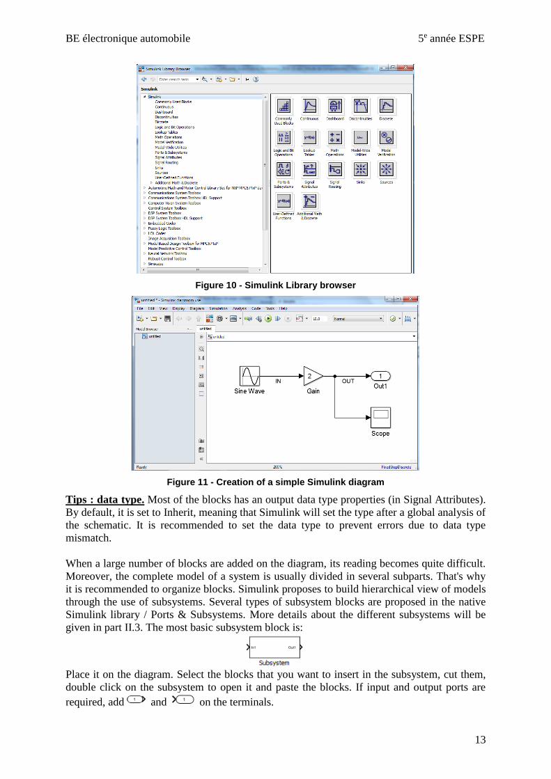
can be found in libraries and toolboxes installed on your working environment. Click on the

menu View > Library browser or on the icon to open the library browser, which lists

all the installed libraries, as shown in Figure 10. The main common libraries for the

Automotive electronics lab will be briefly presented in part II.2.

To place a block in the model diagram, click on the library to open it. Then, select the correct

category and the desired block. Finally, drag and drop it on the model schematic. Place as

many blocks on the diagram.

Each block has a name, which appears on the bottom side of the block. You can change it by

clicking on the name. The properties of the model associated to the block can be modified by

double clicking on the block. A window opens to modify the model properties (model

parameters, data type, min/max value…). Graphical properties can be modified by right

clicking on the block and select Properties in the pop-up window. The different blocks can

be interconnected by clicking on one terminal of a block. A wire starts to be plotted. It

finishes at the position where you release the mouse cursor. If you double click on a wire, you

can give a label to the wire.


13

Figure 10 - Simulink Library browser

Figure 11 - Creation of a simple Simulink diagram

Tips : data type. Most of the blocks has an output data type properties (in Signal Attributes).

By default, it is set to Inherit, meaning that Simulink will set the type after a global analysis of

the schematic. It is recommended to set the data type to prevent errors due to data type

mismatch.

When a large number of blocks are added on the diagram, its reading becomes quite difficult.

Moreover, the complete model of a system is usually divided in several subparts. That's why

it is recommended to organize blocks. Simulink proposes to build hierarchical view of models

through the use of subsystems. Several types of subsystem blocks are proposed in the native

Simulink library / Ports & Subsystems. More details about the different subsystems will be

given in part II.3. The most basic subsystem block is:

Place it on the diagram. Select the blocks that you want to insert in the subsystem, cut them,

double click on the subsystem to open it and paste the blocks. If input and output ports are

required, add and on the terminals.


14

The main icons to interact with diagram are summarized in the following table:

View fil all (space bar) Add image

View in (CTRL + '+'). View out =

CTRL + '-'. To return to the higher level in the

diagram hierarchy

Add text annotation

Back/forward = return to the

previous/next view

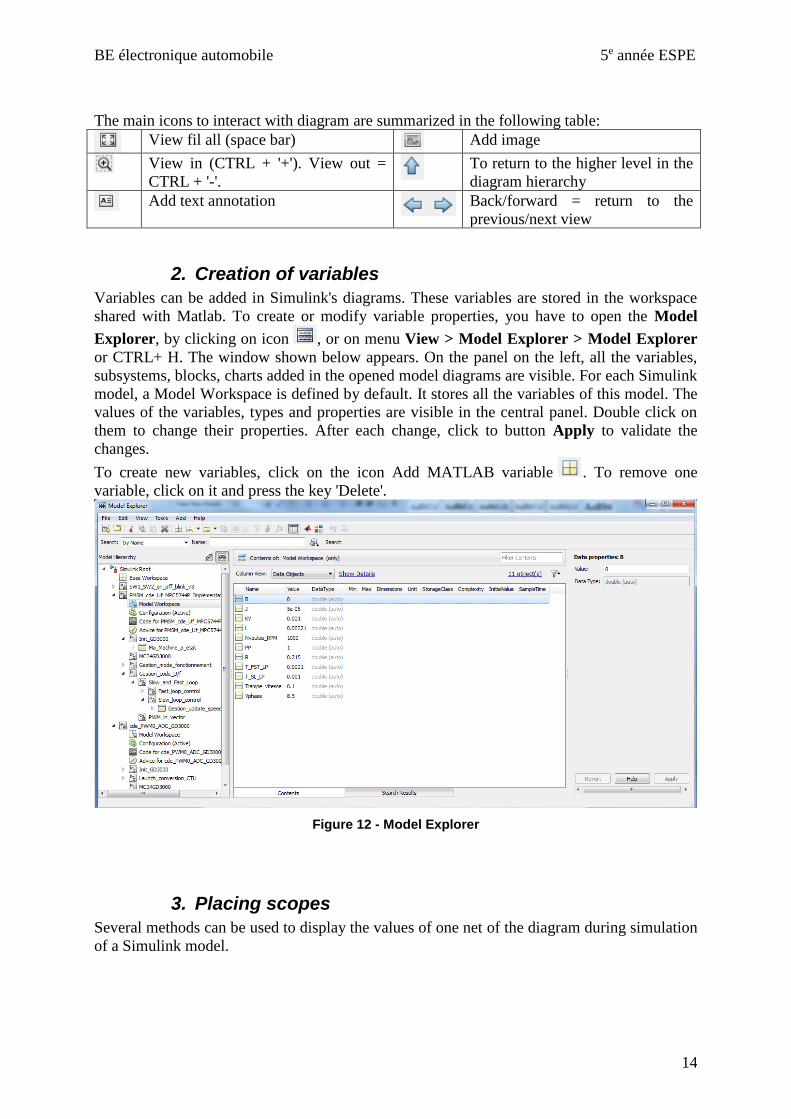
2. Creation of variables

Variables can be added in Simulink's diagrams. These variables are stored in the workspace

shared with Matlab. To create or modify variable properties, you have to open the Model

Explorer, by clicking on icon , or on menu View > Model Explorer > Model Explorer

or CTRL+ H. The window shown below appears. On the panel on the left, all the variables,

subsystems, blocks, charts added in the opened model diagrams are visible. For each Simulink

model, a Model Workspace is defined by default. It stores all the variables of this model. The

values of the variables, types and properties are visible in the central panel. Double click on

them to change their properties. After each change, click to button Apply to validate the

changes.

To create new variables, click on the icon Add MATLAB variable . To remove one

variable, click on it and press the key 'Delete'.

Figure 12 - Model Explorer

3. Placing scopes

Several methods can be used to display the values of one net of the diagram during simulation

of a Simulink model.


15

The first method consists in placing a scope connected to the net. Only the net connected to

the block can be observed with this method. Scope block is available in the native Simulink

library / Sinks . Click on this block to configure the scope settings.

In complex diagrams, it is usually necessary to observe numerous signals simultaneously and

plot them either on the same graphs or one different subwindows. It is possible with Floating

scope, which is also available in Sinks library . You can place it anywhere on the

diagram. Double click on this block to edit its properties. Click on View > Layout to select

the number of subwindows. Click on Simulation > Signal selector to select the signals to be

plotted and the destination subwindows (or axes).

4. Configuration of simulation

The simulation must be configured before the first launching. Click on Simulation > Model

Configuration Parameters or on the icon to open the simulation configuration window,

as shown in Figure 13. Select the pane Solver. By default, the solver is automatically chosen

by Simulink and only the start and stop times can be configured. The solver can be chosen

and also the step type (fixed or variable). In the pane Diagnostics, various sources of errors

can be configured to trigger simulation errors or be ignored.

Figure 13 - Configuration Parameters window

5. Launching simulation

The simulation can be launched by clicking on Simulation > Run or on the icon .

Simulink starts the simulation process by a compilation of the model and, if no errors are

detected, launches the simulation. It ends when the stop time is reached. The simulation can


16

be also done step-by-step by clicking on the icon . It can be stopped by clicking on the icon

.

Results are displayed in real-time on all the opened oscilloscopes. For example, Figure 14

shows simulation results plotted on a floating oscilloscope, configured with three subwindows.

The menu and toolbar aim at controlling simulation, selecting the curves to be plotted,

modifying graphical parameters and placing cursors.

Figure 14 - Example of simulation results plotted on a floating oscilloscope

In View > Configuration Properties …, the main properties of the graph window can be

modified. For example, click on the panel Display and check the box Show Legend to display

the legend of the plotted curves. Click on Tools > Measurements > Curve measurements to

display cursors on the graph. The cursor panel is displayed on the right of the graph, as shown

in Figure 14.

6. The main common libraries

In this part, the most important library for the Automotive Lab are presented briefly. More

details can be found in the on-line help of Simulink. These libraries are present by default in

Simulink. These are those shown in Figure 10.


17

a. Commonly used blocks

The sublibrary lists the mostly used blocks. These

blocks are available in other sublibraries.

b. Continuous

This sublibrary proposes all the basic blocks to

define linear system behavior in continuous

time: derivator, integrator, transfer function in

Laplace domain, PID controller, state-space

model…

c. Discrete

This sublibrary proposes all the basic

blocks to define linear system behavior in

discrete time: discrete-time derivator,

discrete-time integrator, delay, transfer

function in Z-domain, discrete PID

controller, …

Discrete-time blocks can coexist with

continuous-time blocks. Use of discrete-

time function requires sampling time,

which must be in accordance with

simulation step time.

Two discrete-time blocks which operate at two different sampling times can be connected, if

Rate transition block (available in Signal Attributes sublibrary) is inserted within

the interconnection.


18

d. Math operation

:

This sublibrary proposes all the basic

mathematical operations: add, substract,

multiply, gain, sign, sqrt…

.

e. Ports and subsystem

This sublibrary proposes all the

elements to build subsystems (refer to

part 1), to define their ports and call

them.

Submodels inserted in a block

Subsystem are executed all the time.

Submodels inserted in Function-Call

Subsystem are executed only when a

function-call trigger them. Function-call

generator can be inserted in a

subsystem to trigger a function-call

when the subsystem is executed.

Function-call signals is a specific signal in Simulink which cannot be processed as the other

signals (whatever their types). Blocks as Function-call Split are useful to deliver the

same function-call signal to several subsystems.

f. Signal attributes

This sublibrary provides blocks to

manipulate signal properties: data type

conversion, rate transition (when two

interconnected blocks operate at two

different sampling times)…


19

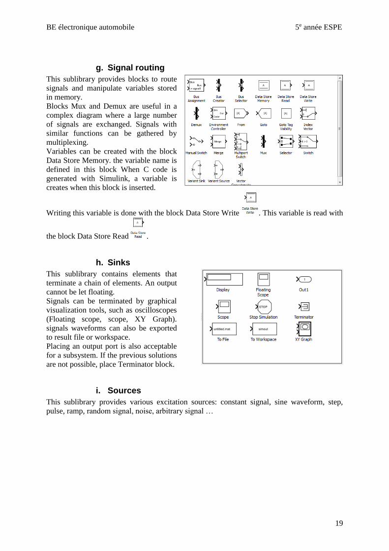
g. Signal routing

This sublibrary provides blocks to route

signals and manipulate variables stored

in memory.

Blocks Mux and Demux are useful in a

complex diagram where a large number

of signals are exchanged. Signals with

similar functions can be gathered by

multiplexing.

Variables can be created with the block

Data Store Memory. the variable name is

defined in this block When C code is

generated with Simulink, a variable is

creates when this block is inserted.

Writing this variable is done with the block Data Store Write . This variable is read with

the block Data Store Read .

h. Sinks

This sublibrary contains elements that

terminate a chain of elements. An output

cannot be let floating.

Signals can be terminated by graphical

visualization tools, such as oscilloscopes

(Floating scope, scope, XY Graph).

signals waveforms can also be exported

to result file or workspace.

Placing an output port is also acceptable

for a subsystem. If the previous solutions

are not possible, place Terminator block.

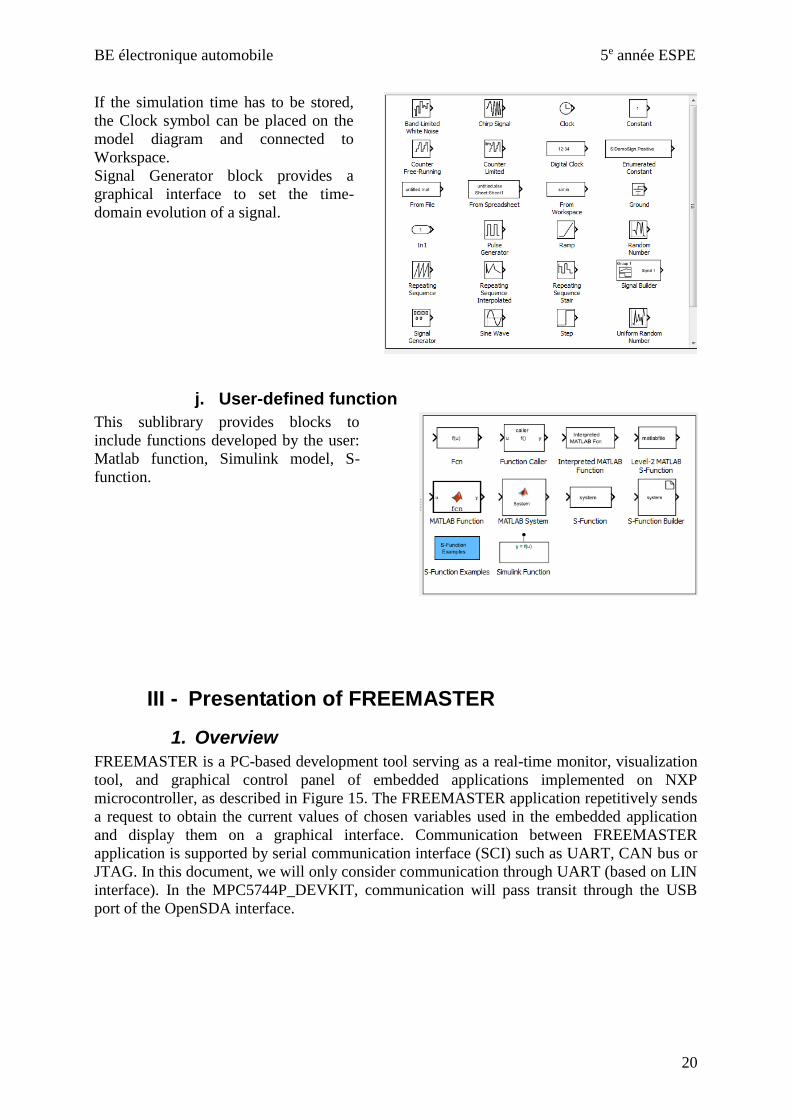
i. Sources

This sublibrary provides various excitation sources: constant signal, sine waveform, step,

pulse, ramp, random signal, noise, arbitrary signal …


20

If the simulation time has to be stored,

the Clock symbol can be placed on the

model diagram and connected to

Workspace.

Signal Generator block provides a

graphical interface to set the time-

domain evolution of a signal.

j. User-defined function

This sublibrary provides blocks to

include functions developed by the user:

Matlab function, Simulink model, S-

function.

III - Presentation of FREEMASTER

1. Overview

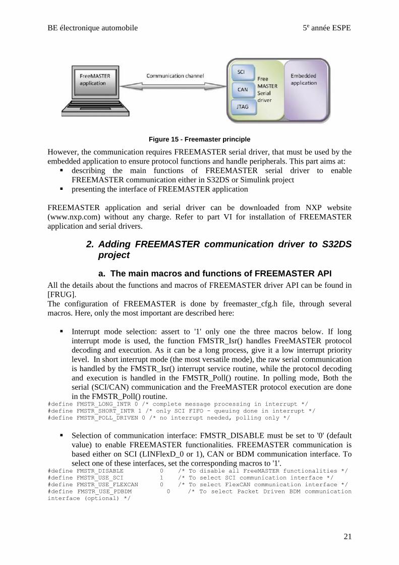
FREEMASTER is a PC-based development tool serving as a real-time monitor, visualization

tool, and graphical control panel of embedded applications implemented on NXP

microcontroller, as described in Figure 15. The FREEMASTER application repetitively sends

a request to obtain the current values of chosen variables used in the embedded application

and display them on a graphical interface. Communication between FREEMASTER

application is supported by serial communication interface (SCI) such as UART, CAN bus or

JTAG. In this document, we will only consider communication through UART (based on LIN

interface). In the MPC5744P_DEVKIT, communication will pass transit through the USB

port of the OpenSDA interface.


21

Figure 15 - Freemaster principle

However, the communication requires FREEMASTER serial driver, that must be used by the

embedded application to ensure protocol functions and handle peripherals. This part aims at:

▪ describing the main functions of FREEMASTER serial driver to enable

FREEMASTER communication either in S32DS or Simulink project

▪ presenting the interface of FREEMASTER application

FREEMASTER application and serial driver can be downloaded from NXP website

(www.nxp.com) without any charge. Refer to part VI for installation of FREEMASTER

application and serial drivers.

2. Adding FREEMASTER communication driver to S32DS project

a. The main macros and functions of FREEMASTER API

All the details about the functions and macros of FREEMASTER driver API can be found in

[FRUG].

The configuration of FREEMASTER is done by freemaster_cfg.h file, through several

macros. Here, only the most important are described here:

▪ Interrupt mode selection: assert to '1' only one the three macros below. If long

interrupt mode is used, the function FMSTR_Isr() handles FreeMASTER protocol

decoding and execution. As it can be a long process, give it a low interrupt priority

level. In short interrupt mode (the most versatile mode), the raw serial communication

is handled by the FMSTR_Isr() interrupt service routine, while the protocol decoding

and execution is handled in the FMSTR_Poll() routine. In polling mode, Both the

serial (SCI/CAN) communication and the FreeMASTER protocol execution are done

in the FMSTR_Poll() routine. #define FMSTR_LONG_INTR 0 /* complete message processing in interrupt */

#define FMSTR_SHORT_INTR 1 /* only SCI FIFO - queuing done in interrupt */

#define FMSTR_POLL_DRIVEN 0 /* no interrupt needed, polling only */

▪ Selection of communication interface: FMSTR_DISABLE must be set to '0' (default

value) to enable FREEMASTER functionalities. FREEMASTER communication is

based either on SCI (LINFlexD_0 or 1), CAN or BDM communication interface. To

select one of these interfaces, set the corresponding macros to '1'. #define FMSTR_DISABLE 0 /* To disable all FreeMASTER functionalities */

#define FMSTR_USE_SCI 1 /* To select SCI communication interface */

#define FMSTR_USE_FLEXCAN 0 /* To select FlexCAN communication interface */

#define FMSTR_USE_PDBDM 0 /* To select Packet Driven BDM communication

interface (optional) */


22

▪ Definition of communication interface memory address for SCI and CAN interface:

refer to memory address map of the microcontroller and write the starting memory

address corresponding to communication interface. Any errors in memory address will

result in unpredictable application error. #define FMSTR_SCI_BASE 0xFFE90000UL /* LINFlex1 base on MPC574xP */

#define FMSTR_CAN_BASE 0xFFEC0000UL /* FlexCAN0 base on MPC574xP */

For the other macros, the default values are sufficient for the application developed in the

Automotive Electronics lab.

FREEMASTER API contains numerous functions. However, in order to initialize and launch

communication with FREEMASTER application, only three functions are required, which

have to be called by the embedded C code:

▪ FMSTR_init(): it initializes internal variables of the FreeMASTER driver and enables

the communication interface (SCI, JTAG or CAN). It does not change the

configuration of the selected communication module. The user must initialize the

communication module (LINFlex as UART, JTAG or CAN) before the FMSTR_Init()

function is called.

▪ FMSTR_Poll(): in poll-driven or short interrupt modes, this function handles the

protocol decoding and execution. In the poll-driven mode, this function also handles

the interface communication with the PC. Typically, FMSTR_Poll() is called during

the 'idle' time in the main application loop.

▪ FMSTR_Isr(): it is the interface to the interrupt service routine of the FreeMASTER

serial driver. In long or short interrupt modes, this function must be set as the interrupt

vector calling address when a transmission or reception is performed by the

communication module (LIN, CAN or JTAG). On platforms where interface

processing is split into multiple interrupts, this function should be set as a vector for

each such interrupt.

Besides, two additional functions can be used if the recorder functionality is used:

▪ FMSTR_Recorder(): it takes one sample of the variables being recorded using the

FreeMASTER recorder. If the recorder is not active at the moment when

FMSTR_Recorder is called, the function returns immediately. When the recorder is

initialized and active, the values of the variables being recorded are copied to the

recorder buffer and the trigger condition is evaluated.

▪ FMSTR_TriggerRec(): it forces the recorder trigger condition to happen, which causes

the recorder to be automatically de-activated after post-trigger samples are sampled.

This function can be used in the application when it needs to have the trigger

occurrence under its control. This function is optional. The recorder can also be

triggered by the PC tool or when the selected variable exceeds a threshold value.

It is not necessary to indicate which variables will be transferred from the MCU to the

FREEMASTER PC-application. All the global variables can be transferred to FREEMASTER

application, if these variables have been selected to be watched.

b. Configuration of FREEMASTER driver in C code application

FREEMASTER serial drivers are provided as a SDK. In order to use FREEMASTER

communication in a new S32DS project, FREEMASTER SDK has to be imported first. Refer

to part I.7 for this action.


23

The header file freemaster_cfg.h is automatically added in the folder include of S32DS

project. The macros should be updated following the explanation given in part III.2.a. Include

the header file freemaster.h in all the source code file where a FREEMASTER API function is

used.

The four main steps are:

1. Configure all the necessary peripherals required for the FREEMASTER

communication (clock gating, interrupt controller, initialization of the UART (SCI or

CAN) and the used external pins). Ensure that the UART, its pins and its timing

parameters are correctly set.

2. Initialize FREEMASTER by calling FMSTR_Init() just once at the code start,

typically after the start-up code, at the beginning of the main function.

3. Call FMSTR_Poll(void) periodically in your code. A typical place is in the main loop.

4. FMSTR_Isr() must be assigned to the used UART interrupt vectors (e.g. interrupt

vectors associated to transmission and reception of the used UART). Configure also

the interrupt priority level associated to these interrupt requests. Use a low priority

level to ensure that FREEMASTER will not affect your application. In S32DS project,

the interrupt vectors are defined in the file intc_SW_mode_isr_vectors_MPC5744P.c.

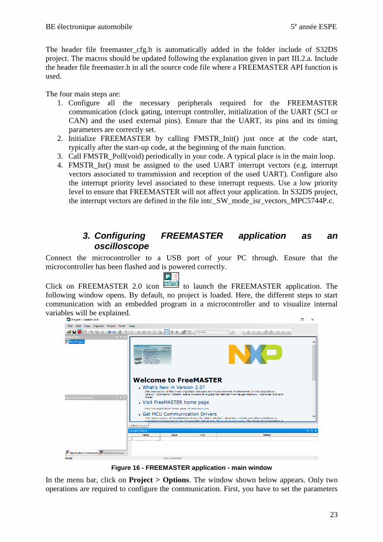
3. Configuring FREEMASTER application as an oscilloscope

Connect the microcontroller to a USB port of your PC through. Ensure that the

microcontroller has been flashed and is powered correctly.

Click on FREEMASTER 2.0 icon to launch the FREEMASTER application. The

following window opens. By default, no project is loaded. Here, the different steps to start

communication with an embedded program in a microcontroller and to visualize internal

variables will be explained.

Figure 16 - FREEMASTER application - main window

In the menu bar, click on Project > Options. The window shown below appears. Only two

operations are required to configure the communication. First, you have to set the parameters


24

of the communication port. In the tab Comm., select the communication port on which the

microcontroller board is connected. If you do not know it, in Window start menu, go to

Control Panel > Device manager > Ports (COM & LPT) and find the number of the Com

port. Then, set the correct baud rate. Secondly, the executable file (.elf) embedded in the

microcontroller must be provided to FREEMASTER to make the link with variables read

continuously. In the tab MAP Files, select the .elf file in the field Default symbol file.

Tips: ensure that the .elf file corresponds to the actual code embedded in the microcontroller.

Otherwise, communication may fail.

Figure 17 - FREEMASTER application - configuration of the communication port (on the left) and selection of the executable file (on the right)

Click on the button OK. A new project was created, visible in the Project tree. Click in the

menu File > Save Project or on icon to save it. The extension of the file is .pmp. The

communication port configuration and visualized variables are saved. The next time you will

connect to the microcontroller, you will import the .pmp file directly.

In order to launch the communication with the microcontroller, click on the button Start/stop

communication . The status of the communication is displayed in the message bar, in the

bottom part of the main window. If the communication is active, the COM port, and the baud

rate must be written. Otherwise, the message "Not connected" is written and an error message

shown below appears. Refer to the following part to solve this issue.

Once the .elf file has been loaded, the variables to be visualized can be selected. To select

variables, click on the menu Project > Variables. A window opens with all the list of

selected variables Click on the button New to add a new variable to observe. The following

window appears. In the list Type, select the type of the variable. In the list Address, select the

variable to be visualized. Give it an arbitrary name in Variable name. Set the Sampling

period. If the visualization must be refreshed as fast as possible, select Fastest. Select also the

format of the visualized variable (decimal, hexadecimal, binary…) in the list Show as.


25

1. Internal variable selection

2. Select type and size of the variable

3. Give a name to the observed variable

4. Set the sampling period

5. Set the displayed format of the observed variable

Figure 18 - Selection of a new variable to be visualized with FREEMASTER

Click on OK. The new variable is added in the table Variable Watch, as shown in Figure 19.

When the communication is active, they could be updated in real-time. Repeat the operation

for all the variables that you want to visualize. To delete one variable, select the variables and

click on the button Delete. To modify it, click on the button Edit.

Figure 19 - List of variables to be observed

FREEMASTER application proposes also to visualize time domain evolution of variables in a

2D graph, called Scope, similarly to an oscilloscope. It requires two operations:

▪ first, the creation of a Block (of variables)

▪ then, the creation of one or several Scopes within a block.

In Project tree, right click on the project name and select Create Subblock to create a new

Block and edit its properties. The following window opens. In the tab Main, enter the name of

the Block. In the tab Watch, all the selected variables in the previous step are in the left part

of the window initially (in the column Available Variables). Select the variables to be

observed and click on the button Add →. The selected variables jump to the right column,

Watched variables. Inversely, to remove variables from a block, select them in the right

column and click on the button Remove. Finally click OK.


26

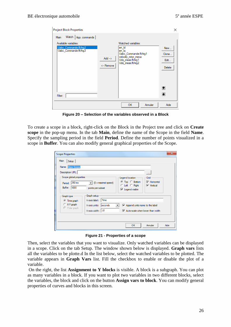
Figure 20 – Selection of the variables observed in a Block

To create a scope in a block, right-click on the Block in the Project tree and click on Create

scope in the pop-up menu. In the tab Main, define the name of the Scope in the field Name.

Specify the sampling period in the field Period. Define the number of points visualized in a

scope in Buffer. You can also modify general graphical properties of the Scope.

Figure 21 - Properties of a scope

Then, select the variables that you want to visualize. Only watched variables can be displayed

in a scope. Click on the tab Setup. The window shown below is displayed. Graph vars lists

all the variables to be plotte.d In the list below, select the watched variables to be plotted. The

variable appears in Graph Vars list. Fill the checkbox to enable or disable the plot of a

variable.

On the right, the list Assignment to Y blocks is visible. A block is a subgraph. You can plot

as many variables in a block. If you want to plot two variables in two different blocks, select

the variables, the block and click on the button Assign vars to block. You can modify general

properties of curves and blocks in this screen.


27

Figure 22 - Selection of plotted variables in a Scope

Click on OK. The graph appears. If the communication is active, the selected watched

variables are plotted directly. Their evolution is plotted in real-time, as shown in the figure

below.

Figure 23 - Observation of the time-domain evolution of three variables in a Scope

Do not forget to save the project before closing FREEMASTER application.

4. Saving captured data by Freemaster running as an oscilloscope

All the captured variables of a block can be saved in a text file. A Scope view has to be

defined. To configure the file where the data will be saved, click on the menu Scope > Data

Capture Setup (Figure 24). Ensure that the Scope window was opened, otherwise the menu

Scope is not available. Define the directory in the Oscilloscope part of the window. Check the


28

box “Close the file (open new) when data capture is paused” to stop data acquisition when

Freemaster is paused. Click OK.

Figure 24 – Capture setup

If not done yet, Launch Freemaster acquisition by clicking on Start/stop communication .

In the menu Scope, click on Toggle Data Capture On/Off or on the button to start the

recording of all the variables of the block in the text file. To stop the recording, click once

again on Toggle Data Capture On/Off or on the button . The saved data are available In

the text file defined previously.

5. Debug FREEMASTER

Wrong configurations will result in loss of communications between the MCU board and

FREEMASTER PC application, shown by this error message :

Freemaster is usually not able to communicate with the board in the five following situations:

▪ FREEMASTER drivers have not been called in the embedded application (or

incorrectly called)

▪ the associated UART has not been correctly configured (baud rate, I/O pads not

configured, …)

▪ FMSTR_Isr() function has not been linked to interrupts vectors associated to the

UART (for TX and RX)

▪ port and baud rate specified in FREEMASTER application are wrong

▪ the communication port between your PC and the microcontroller board is already

used by another application (e.g. S32DS in-situ debugger).

▪ the embedded application was compiled and built, but it results in wrong operation

(e.g. crash due to a critical interrupt request).


29

If the first four reasons have been verified, then you can conclude that FREEMASTER is

correctly configured, but your embedded application is not operational.

IV - Presentation of Automotive Math and Motor Control Library for MPC574xP

This Matlab/Simulink toolbox is compatible only from R2014.a release. In this document, the

version 2.2 for MPC574xP MCU is considered. More information about the mathematical

functions provided by this toolbox can be found in [AMMC]. Model-Based Design Toolbox

can be downloaded here: http://www.nxp.com/support/developer-resources/run-time-

software/automotive-software-and-tools/model-based-design-toolbox:MC_TOOLBOX

1. Overview

The NXP’s Automotive Math and Motor Control Library (AMMCLIB) provides a list of

mathematical functions dedicated to motor control, which supports different number

representations (fixed or floating point). This library is supported by S32DS compiler so it

appears as a SDK for S32DS. Moreover, models compatible with Simulink are also available.

Thus it can be used as a Matlab/Simulink's toolbox.

The AMMCLIB for NXP MPC574xP devices is organized in several sub-libraries, as

depicted in Figure 25:

▪ Mathematical Function Library (MLIB) - it comprises basic mathematical operations

such as addition, multiplication, etc.

▪ General Function Library (GFLIB) - it comprises basic trigonometric and general

math functions such as sine, cosine, tan, hysteresis, limit, etc.

▪ General Digital Filters Library (GDFLIB) - it includes digital IIR and FIR filters

designed to be used in a motor control application

▪ General Motor Control Library (GMCLIB) - it includes standard algorithms used for

motor control such as Clarke/Park transformations, Space Vector Modulation, etc.

▪ Advanced Motor Control Function Library (AMCLIB) - it comprises advanced

algorithms used for motor control purposes

http://www.nxp.com/support/developer-resources/run-time-software/automotive-software-and-tools/model-based-design-toolbox:MC_TOOLBOX

http://www.nxp.com/support/developer-resources/run-time-software/automotive-software-and-tools/model-based-design-toolbox:MC_TOOLBOX


30

Figure 25 - Organization of sublibraries of AMMCLIB [AMMC]

The AMMCLIB for NXP MPC574xP devices was developed to support three major

implementations:

▪ Fixed-point 32-bit fractional (suffix F32) or Q1.31 format: in this format, the number

are comprised between -1 and 1-2-31. The minimum positive value is normalized to 2-

31. Using the format requires a scaling of number to the interval [-1;+1] beforehand.

▪ Fixed-point 16-bit fractional (suffix F16) or Q1.15 format : in this format, the number

are comprised between -1 and 1-2-15. The minimum positive value is normalized to 2-15.

Using the format requires a scaling of number to the interval [-1;+1] beforehand.

▪ Single precision (32 bits) floating point (suffix FLT): in this format, the number are

comprised between -2128 and 2128, with a minimum positive value normalized to 2-128.

The MSB is the sign, the next 24 bits are the mantissa and the 7 last bits form the

exponent.

The fixed-point 32-bit fractional and fixed-point 16-bit rational functions are implemented

based on the unity model. It means that, before using blocks based on these formats, numbers

must be normalized so that their values remain in the range [-1 ; +1]. Most of the functions do

not integrate saturation function: any output that exceed this range induce an overflow

condition.

Tips: converting binary code to decimal number in Q1.31 format: evaluation by the hand

the number coded by a binary or hexadecimal in Q1.31 representation can be quite tedious. In

Matlab, the function dec2hex() can be used to convert decimal number to hexadecimal

representation, while the function hex2dec() aims at converting hexadecimal to decimal

representation. Based on this two functions and on scaling transform, the conversion between

decimal and Q1.31 is possible:

▪ Conversion from decimal to Q1.31 format:


31

o if the number is positive, use the following command:

dec2hex(floor(number*231)).

o if the number is negative, the sign is indicated by the MSB while the other bits

code the shift from -1. Use the following command: dec2hex(floor((1-

number)*231)).

▪ Conversion from Q1.31 format to decimal:

o if the number is positive (MSB = '0'), use the following command:

hex2dec('hexa_code')/231.

o if the number is negative (MSB = '1'), remove the MSB and use the following

command: hex2dec('hexa_code')/231-1

2. Types provided by AMMCLIB

Numerous types are defined in AMMCLIB files. The basic types are summarized in the

following table. Boolean, unsigned/signed integer or floating number formats are provided.

Fixed-point 32-bit fractional type is called tFrac32, while tFrac16 is the type for fixed-pont 16

bit fractional number.

Numerous compound types also exist. They are detailed in part 7 of the AMMCLIB reference

document [AMMC].

3. Brief presentation of the functions

Functions of Advanced Motor Control sublibrary are not presented in this document as they

will not be used in the Automotive Electronics lab. The full list of functions is given in

chapter 4 (p 151) of [AMMC].

Read carefully the MMCLIB User's guide [AMMC] to verify the performed mathematical

operations, the input and output types and the required conditions. Any violation of these

conditions may result in bug of Simulink simulation or code compilation (best case), or in

unpredictable behavior of the embedded application (worst case).

In the following paragraphs, the list of functions in each sublibrary is given. Each function is

terminated by a suffix F16, F32 or FLT to indicate the supported format. As all the functions

support these three formats, the suffix is omitted in the next parts.


32

a. Math Function library (MLIB)

All these functions start with the prefix MLIB_. Details can be found between pages 531 and

650 of [AMMC].

Name Description Abs Absolute value of input parameter

AbsSat Absolute value of input parameter with saturation on output

Add Addition of the two input parameters

AddSat Addition of the two input parameters with saturation on output

Convert_FaFb Conversion between type Fa and type Fb. The conversion functions

exist for the three supported types of the library

Div Division of the two input parameters

DivSat Division of the two input parameters with saturation on output

Mac Multiply - accumulate function

MacSat Multiply - accumulate function with saturation on output

Mnac Multiply - substract function

Msu Multiply - substract function

Mul Multiplication of the two input parameters

MulSat Multiplication of the two input parameters with saturation on output

Neg Negative value of the input parameter

NegSat Negative value of the input parameter with saturation on output

RndSat Round the input parameter

Round Round the input parameter with saturation on output

ShBi Shift to the left or right

ShBiSat Shift to the left or right with saturation on output

ShL Shift to the left

ShLSat Shift to the left with saturation on output

ShR Shift to the right

Sub Substrate the two input parameters

SubSat Substrate the two input parameters with saturation on output

VMac Vector multiply accumulate function

b. General Functions library (GFLIB)

All these functions start with the prefix GFLIB_. Details can be found between pages 255 and

469 of [AMMC].

Name Description

Acos Arccosine function

Asin Arcsine function

Atan Arctangent function

AtanYX Arctangent function applied on two input arguments

AtanYXShifted Calculate the angle of two sinusoidal signals, one shifted in phase to

the other.

ControllerPip Parallel form of the Proportional-Integral controller, without integral

anti-windup

ControllerPipAW Parallel form of the Proportional-Integral controller, with integral

anti-windup


33

ControllerPir Standard recurrent form of the Proportional-Integral controller,

without integral anti-windup

ControllerPirAW Standard recurrent form of the Proportional-Integral controller, with

integral anti-windup

Cos Cosine function

Hyst Calculation of a hysteresis function

IntegratorTR Discrete implementation of the integrator (sum)

Limit Test whether the input value is within the upper and lower limits

LowerLimit Test whether the input value is above the lower limit

Lut1D Implementation of a one-dimensional look-up table

Lut2D Implementation of a two-dimensional look-up table

Ramp Up/down ramp with a step increment/decrement

Sign Sign of the input argument

Sin Sine function

SinCos Return Sine and Cosine functions

Sqrt Square-root function

Tan Tangent function

UpperLimit Test whether the input value is below the upper limit

VectorLimit Limit the magnitude of the input vector

c. General Digital Filters library (GDFLIB)

All these functions start with the prefix GDFLIB_. Details can be found between pages 208

and 254 of [AMMC].

Name Description FilterFIRInit Initialization of FIR filter buffer

FilterFIR Performs a single iteration of an FIR filter

FilterIIR1Init Initialization of first order IIR filter buffer

FilterIIR1 Implements the first order IIR filter

FilterIIR2Init Initialization of second order IIR filter buffer

FilterIIR2 Implements the second order IIR filter

FilterMAInit Clears the internal filter accumulator

FilterMA Implements an exponential moving average filter

d. General Motor Control library (GMCLIB)

All these functions start with the prefix GMCLIB_. Not all the functions are listed below.

More details can be found between pages 474 and 526 of [AMMC].

Name Description ClarkInv Compute inverse Clark transform

Clark Compute Clark transform

ParkInv Compute inverse Park transform

Park Compute Park transform

SvmStd Duty-cycle ratios using the Standard Space Vector Modulation

technique


34

4. Using in S32DS environment

The first step is the import of AMMCLIB SDK during the creation of S32DS project. Refer to

part I.7 of this document for SDK import.

a. Setting the implementation

By default the support of all implementations is turned off, thus the error message "Define at

least one supported implementation in SWLIBS_Config.h file." is displayed during the

compilation if no implementation is selected, preventing the user application building.

Following are the macro definitions enabling or disabling the implementation support:

▪ SWLIBS_SUPPORT_F32 for 32-bit fixed-point implementation support selection

▪ SWLIBS_SUPPORT_F16 for 16-bit fixed-point implementation support selection

▪ SWLIBS_SUPPORT_FLT for single precision floating-point implementation support

selection

These macros are defined in the SWLIBS_Config.h file located in Common directory of the

AMMCLIB for NXP MPC574xP devices installation destination. To enable the support of

each individual implementation the relevant macro definition has to be set to

SWLIBS_STD_ON.

Moreover, the SWLIBS_DEFAULT_IMPLEMENTATION macro definition has to be setup

properly. This macro definition is not defined by default thus the error message "Define

default implementation in SWLIBS_Config.h file." is displayed during the compilation,

preventing the user application building. The SWLIBS_DEFAULT_IMPLEMENTATION

macro is defined in the SWLIBS_Config.h file located in Common directory of the

AMMCLIB for NXP MPC574xP devices installation destination. The

SWLIBS_DEFAULT_IMPLEMENTATION can be defined as the one of the following

supported implementations:

▪ SWLIBS_DEFAULT_IMPLEMENTATION_F32 for 32-bit fixed-point

implementation

▪ SWLIBS_DEFAULT_IMPLEMENTATION_F16 for 16-bit fixed-point

implementation

▪ SWLIBS_DEFAULT_IMPLEMENTATION_FLT for single precision floating point

implementation

b. Calling mathematical function

After proper definition of SWLIBS_DEFAULT_IMPLEMENTATION macro, the AMMCLIB

for NXP MPC574xP devices functions can be called using standard legacy API convention:

'Sublibrary_name'_'Function_name'_'Format_suffix'. For example if the

SWLIBS_DEFAULT_IMPLEMENTATION macro definition is set to

SWLIBS_DEFAULT_IMPLEMENTATION_F32, the 32-bit fixed-point implementation of

sine function is invoked after the GFLIB_Sin(x) API call. The command GFLIB_Sin_F32(x)

has to be added in the C code. Moreover, the header file where the used mathematical

function is declared must be included in the C code file which uses the function. For example,

if the GFLIB_Sin_F32(x) is used, the directive '#include gflib.h' must be added in the C code.


35

5. Using in Matlab/Simulink environment

The functions provided by the library can be used in Simulink directly (once the library has

been installed).

Figure 26 - AMMCLIB library in Simulink

V - References [FRUG] FreeMASTER Serial Communication Driver, User's Guide, Rev. 3.0, August

2016, NXP Semiconductors, www.nxp.com/docs/en/user-

guide/FMSTRSCIDRVUG.pdf [AMMC] Automotive Math and Motor Control Library Set for NXP MPC574xP devices, User's

Guide, Rev. 12, MPC574XPMCLUG, www.nxp.com

Documents

Introduction to software tools for Automotive Electronics lab