Embed Size (px)
Citation preview

Complete Solutions Manual
to Accompany
Introduction to Statistics & Data
Analysis
FIFTH EDITION
Roxy Peck California Polytechnic State University,
San Luis Obispo, CA
Chris Olsen Grinnell College
Grinnell, IA
Jay Devore California Polytechnic State University,
San Luis Obispo, CA
Prepared by
Michael Allwood Brunswick School, Greenwich, CT
Australia • Brazil • Mexico • Singapore • United Kingdom • United States
© C
engag
e L
earn
ing.
All
rig
hts
res
erv
ed.
No
dis
trib
uti
on
all
ow
ed w
ith
ou
t ex
pre
ss a
uth
ori
zati
on
.
Printed in the United States of America
1 2 3 4 5 6 7 17 16 15 14 13
© 2016 Cengage Learning ALL RIGHTS RESERVED. No part of this work covered by the copyright herein may be reproduced, transmitted, stored, or used in any form or by any means graphic, electronic, or mechanical, including but not limited to photocopying, recording, scanning, digitizing, taping, Web distribution, information networks, or information storage and retrieval systems, except as permitted under Section 107 or 108 of the 1976 United States Copyright Act, without the prior written permission of the publisher except as may be permitted by the license terms below.
For product information and technology assistance, contact us at
Cengage Learning Customer & Sales Support, 1-800-354-9706.
For permission to use material from this text or product, submit
all requests online at www.cengage.com/permissions Further permissions questions can be emailed to
ISBN-13: 978-130526581-3 ISBN-10: 1-305-26581-5 Cengage Learning 20 Channel Center Street Fourth Floor Boston, MA 02210 USA Cengage Learning is a leading provider of customized learning solutions with office locations around the globe, including Singapore, the United Kingdom, Australia, Mexico, Brazil, and Japan. Locate your local office at: www.cengage.com/global. Cengage Learning products are represented in Canada by Nelson Education, Ltd. To learn more about Cengage Learning Solutions, visit www.cengage.com. Purchase any of our products at your local college store or at our preferred online store www.cengagebrain.com.
NOTE: UNDER NO CIRCUMSTANCES MAY THIS MATERIAL OR ANY PORTION THEREOF BE SOLD, LICENSED, AUCTIONED,
OR OTHERWISE REDISTRIBUTED EXCEPT AS MAY BE PERMITTED BY THE LICENSE TERMS HEREIN.
READ IMPORTANT LICENSE INFORMATION
Dear Professor or Other Supplement Recipient: Cengage Learning has provided you with this product (the “Supplement”) for your review and, to the extent that you adopt the associated textbook for use in connection with your course (the “Course”), you and your students who purchase the textbook may use the Supplement as described below. Cengage Learning has established these use limitations in response to concerns raised by authors, professors, and other users regarding the pedagogical problems stemming from unlimited distribution of Supplements. Cengage Learning hereby grants you a nontransferable license to use the Supplement in connection with the Course, subject to the following conditions. The Supplement is for your personal, noncommercial use only and may not be reproduced, posted electronically or distributed, except that portions of the Supplement may be provided to your students IN PRINT FORM ONLY in connection with your instruction of the Course, so long as such students are advised that they
may not copy or distribute any portion of the Supplement to any third party. You may not sell, license, auction, or otherwise redistribute the Supplement in any form. We ask that you take reasonable steps to protect the Supplement from unauthorized use, reproduction, or distribution. Your use of the Supplement indicates your acceptance of the conditions set forth in this Agreement. If you do not accept these conditions, you must return the Supplement unused within 30 days of receipt. All rights (including without limitation, copyrights, patents, and trade secrets) in the Supplement are and will remain the sole and exclusive property of Cengage Learning and/or its licensors. The Supplement is furnished by Cengage Learning on an “as is” basis without any warranties, express or implied. This Agreement will be governed by and construed pursuant to the laws of the State of New York, without regard to such State’s conflict of law rules. Thank you for your assistance in helping to safeguard the integrity of the content contained in this Supplement. We trust you find the Supplement a useful teaching tool.

Table of Contents
Chapter 1 The Role of Statistics and the Data Analysis Process 1
Chapter 2 Collecting Data Sensibly 14
Chapter 3 Graphical Methods for Describing Data 29
Chapter 4 Numerical Methods for Describing Data 79
Chapter 5 Summarizing Bivariate Data 98
Chapter 6 Probability 148
Chapter 7 Random Variables and Probability Distributions 179
Chapter 8 Sampling Variability and Sampling Distributions 229
Chapter 9 Estimation Using a Single Sample 241
Chapter 10 Hypothesis Testing Using a Single Sample 261
Chapter 11 Comparing Two Populations or Treatments 296
Chapter 12 The Analysis of Categorical Data and Goodness-of-Fit Tests 353
Chapter 13 Simple Linear Regression and Correlation: Inferential Methods 376
Chapter 14 Multiple Regression Analysis 424
Chapter 15 Analysis of Variance 463
Chapter 16 Nonparametric (Distribution-Free) Statistical Methods 496

1
Chapter 1 The Role of Statistics and the Data Analysis Process
1.1 Descriptive statistics is the branch of statistics that involves the organization and summary of the values in a data set. Inferential statistics is the branch of statistics concerned with reaching conclusions about a population based on the information provided by a sample.
1.2 The population is the entire collection of individuals or objects about which information is
required. A sample is a subset of the population selected for study in some prescribed manner. 1.3 The proportions are stated as population values (although they were very likely calculated from
sample results). 1.4 The sample is the set of 2121 children used in the study. The population is the set of all children
between the ages of one and four. 1.5 a The population of interest is the set of all 15,000 students at the university. b The sample is the 200 students who are interviewed. 1.6 The estimates given were computed using data from a sample. 1.7 The population is the set of all 7000 property owners. The sample is the 500 owners included in
the survey. 1.8 The population is the set of all 2014 Toyota Camrys. The sample is the set of six cars that are
tested. 1.9 The population is the set of 5000 used bricks. The sample is the set of 100 bricks she checks. 1.10 a The researchers wanted to know whether the new surgical approach would improve memory
functioning in Alzheimer’s patients. They hoped that the negative effects of the disease could be reduced by toxins being drained from the fluid filled space that cushions the brain.
b First, it is not stated that the patients were randomly assigned to the treatments (new approach
and standard care); this would be necessary in a well designed study. Second, it would help if the experiment could have been designed so that the patients did not know whether they were receiving the new approach or the standard care; otherwise, it is possible that the patients’ knowledge that they were receiving a new treatment might in itself have brought about an improvement in memory. Third, as stated in the investigators’ conclusion, it would have been useful if the experiment had been conducted on a sufficient number of patients so that any difference observed between the two treatments could not have been attributed to chance.
1.11 a The researchers wanted to find out whether taking a garlic supplement reduces the likelihood
that you will get a cold. They wanted to know whether a significantly lower proportion of people who took a garlic supplement would get a cold than those who did not take a garlic supplement.

2 Chapter 1: The Role of Statistics and the Data Analysis Process
b It is necessary that the participants were randomly assigned to the treatment groups. If this was the case, it seems that the study was conducted in a reasonable way.
1.12 a Numerical (discrete) b Categorical c Numerical (continuous) d Numerical (continuous) e Categorical 1.13 a Categorical b Categorical c Numerical (discrete) d Numerical (continuous) e Categorical f Numerical (continuous) 1.14 a Discrete b Continuous c Discrete d Discrete 1.15 a Continuous b Continuous c Continuous d Discrete 1.16 For example: a Ford, Toyota, Ford, General Motors, Chevrolet, Chevrolet, Honda, BMW, Subaru, Nissan. b 3.23, 2.92, 4.0, 2.8, 2.1, 3.88, 3.33, 3.9, 2.3, 3.56, 3.32, 2.4, 2.8, 3.9, 3.12. c 4, 2, 0, 6, 3, 3, 2, 4, 5, 0, 8, 2, 5, 3, 4, 7, 3, 2, 0, 1 d 50.27, 50.67, 48.98, 50.58, 50.95, 50.95, 50.21, 49.70, 50.33, 49.14, 50.83, 49.89 e In minutes: 10, 10, 18, 0, 17, 17, 0, 17, 12, 19, 12, 13, 15, 15, 15

Chapter 1: The Role of Statistics and the Data Analysis Process 3
1.17 a Gender of purchaser, brand of motorcycle, telephone area code b Number of previous motorcycles c Bar chart d Dotplot 1.18 a
Definitely noProbably noProbably yesDefinitely yes
0.5
0.4
0.3
0.2
0.1
0.0
Response
Relative Frequency
b “Large Majority of Seniors Say They’d Choose the Same College Again” 1.19 a
7.06.56.05.55.04.54.03.53.02.52.01.5Cost (cents per gram of protein)
b The costs per gram of protein for the meat and poultry items are represented by squares in the
dotplot above. With every one of the meat and poultry items included in the lowest seven cost per gram values, meat and poultry items appear to be relatively low cost sources of protein.
1.20 a
5404804203603002401801202008 Sales (millions of dollars)
A typical sales figure for 2008 was around 150 million dollars. There is one extreme result at
the upper end of the distribution. If this point is disregarded then the values range from 127.5 to 318.4. The greatest density of points is at the lower end of the distribution.

4 Chapter 1: The Role of Statistics and the Data Analysis Process
b
5404804203603002401801202007 Sales (millions of dollars)
A typical sales figure for 2007 was around 210 million dollars, with sales figures ranging
from around 128 to around 337 million dollars. The greatest density of points was at the lower end of the distribution. There were no extreme results in 2007.
c Sales figures were generally speaking higher in 2007 than in 2008. There was one extreme
result in 2008, and no extreme result in 2007. If the extreme sales figure is taken into account, the variation in the sales figures (among the top 20 movies) was far greater in 2008 than in 2007. However, if the extreme result is disregarded, the variation was greater in 2007. The distributions are similar in shape, with the greatest density of points being at the lower end of the distribution in both cases.
1.21 a
Oth
er
Trav
el
Mov
ing
Taki
ng a
bre
ak
Fam
ily is
sues
Empl
oym
ent
Hea
lth
Fina
ncia
l
20
15
10
5
0
Primary Reason for Leaving
Frequency
b The most common reason was financial, this accounting for 30.2% of students who left for non-academic reasons. The next two most common reasons were health and other personal reasons, these accounting for 19.0% and 15.9%, respectively, of the students who left for non-academic reasons.
1.22 a Categorical b Since the variable being graphed is categorical, a dotplot would not be suitable. c If you add up the relative frequencies you get 107%. This total should be 100%, so a mistake
has clearly been made.

Chapter 1: The Role of Statistics and the Data Analysis Process 5
1.23 a The dotplot shows that there were two sites that received far greater numbers of visits than
the remaining 23 sites. Also, it shows that the distribution of the number of visits has the greatest density of points for the smaller numbers of visits, with the density decreasing as the number of visits increases. This is the case even when only the 23 less popular sites are considered.
b Again, it is clear from the dotplot that there were two sites that were used by far greater
numbers of individuals (unique visitors) than the remaining 23 sites. However, these two sites are less far above the others in terms of the number of unique visitors than they are in terms of the total number of visits. As with the distribution of the total number of visits, the distribution of the number of unique visitors has the greatest density of points for the smaller numbers of visitors, with the density decreasing as the number of unique visitors increases. This is the case even when only the 23 less popular sites are considered.
c The statistic “visits per unique visitor” tells us how heavily the individuals are using the sites.
Although the table tells us that the most popular site (Facebook) in terms of the other two statistics also has the highest value of this statistic, the dotplot of visits per unique visitor shows that no one or two individual sites are far ahead of the rest in this respect.
1.24 a It would not be appropriate to use a dotplot because rating is a categorical variable. b
Wet Weather Rating Frequency Relative Frequency A+ 4 0.286 A 2 0.143 B 2 0.143 C 2 0.143 D 2 0.143 F 2 0.143
FDCBAA+
0.30
0.25
0.20
0.15
0.10
0.05
0.00
Wet Weather Rating
Relative Frequency

6 Chapter 1: The Role of Statistics and the Data Analysis Process
c Dry Weather Rating Frequency Relative Frequency
A+ 1 0.071 A 9 0.643 B 3 0.214 F 1 0.071
FBAA+
0.7
0.6
0.5
0.4
0.3
0.2
0.1
0.0
Dry Weather Rating
Relative Frequency
d Yes. Apart the greater proportion of “A+” ratings for wet weather than for dry weather, the
beaches on the whole receive higher ratings in dry weather than in wet weather, with only 28.6% of beaches receiving below an A in dry weather, compared to 57.1% in wet weather.
1.25 a
252015105
E
M
W
Wireless %
b Looking at the dotplot we can see that Eastern states have, on average, lower wireless
percents than states in the other two regions. The West and Middle states regions have, on average, roughly equal wireless percents.
1.26 a
302520151050Number of Violent Crimes

Chapter 1: The Role of Statistics and the Data Analysis Process 7
Five schools seem to stand out from the rest, these being, in increasing order of number of
crimes, Florida International, Florida A&M, University of Florida, University of Central Florida, and Florida State University.
b
University/College Violent Crime Rate Per 1000 Students
Edison State College 0.234 Florida A&M University 1.060 Florida Atlantic University 0.158 Florida Gulf Coast University 0.233 Florida International University 0.202 Florida State University 0.755 New College of Florida 1.183 Pensacola State College 0.260 Santa Fe College 0.065 Tallahassee Community College 0.133 University of Central Florida 0.445 University of Florida 0.363 University of North Florida 0.123 University of South Florida 0.464 University of West Florida 0.167
1.120.960.800.640.480.320.16Violent Crimes per 1000 Students
The colleges that stand out in violent crimes per 1000 students are, in increasing order of
crime rate, Florida State University, Florida A&M University, and New College of Florida. Only Florida A&M stands out in both boxplots.
c For the number of violent crimes, there are five schools that stand out by having high
numbers of crimes, with the majority of the schools having similar, and low, numbers of crimes. There seems to be greater consistency for crime rate (per 1000 students) among the 15 schools than there is for number of crimes, with just three schools standing out as having high crime rates, and no schools with crime rates that stand out as being low.
1.27 a When ranking the airlines according to delayed flights, one airline would be ranked above
another if the probability of a randomly chosen flight being delayed is smaller for the first airline than it is for the second airline. These probabilities are estimated using the rate per 10,000 flights values, and so these are the data that should be used for this ranking. (Note that the total number of flights values are not suitable for this ranking. Suppose that one airline had a larger number of delayed flights than another airline. It is possible that this could be accounted for merely through the first airline having more flights than the second.)
b There are two airlines, ExpressJet and Continental, which, with 4.9 and 4.1 of every 10,000
flights delayed, stand out as the worst airlines in this regard. There are two further airlines that stand out above the rest: Delta and Comair, with rates of 2.8 and 2.7 delayed flights per

8 Chapter 1: The Role of Statistics and the Data Analysis Process
10,000 flights. All the other airlines have rates below 1.6, with the best rating being for Southwest, with a rate of only 0.1 delayed flights per 10,000.
1.28 a
>$20,000$10,000-$20,000<$10,000None
0.7
0.6
0.5
0.4
0.3
0.2
0.1
0.0
Debt
Relative Frequency
b Most public community college graduates have no debt at all, and a debt of $10,000 or less
accounts for 85% of the graduates. Among the small minority (15%) of the graduates who have a debt of more than $10,000, only one third (5% of all graduates) have a debt of more than $20,000.
1.29 a
Didn't b
uy te
xtboo
ks
Mostly e
Books
Rented
textbo
oks
Off-cam
pus b
ooks t
ore
Other o
nline b
ookst
ore
Campu
s book
store
website
Campu
s boo
kstore
600
500
400
300
200
100
0
Where Books Purchased
Frequency
b By far the most popular place to buy books is the campus bookstore, with half of the students
in the sample buying their books from that source. The next most popular sources are online bookstores other than the online version of the campus bookstore and off-campus bookstores, with these two sources accounting for around 35% of students. Purchasing mostly eBooks was the least common response.
Chapter 1: The Role of Statistics and the Data Analysis Process 9
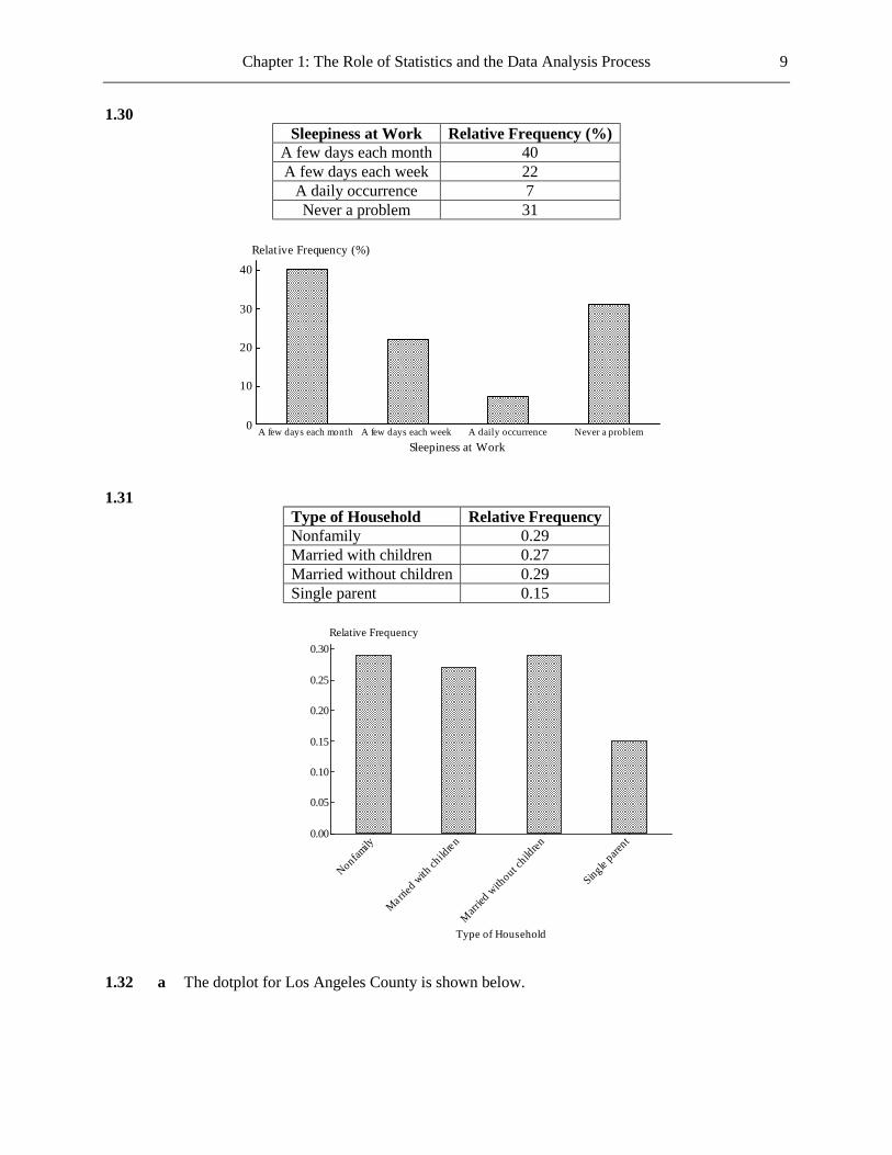
1.30
Sleepiness at Work Relative Frequency (%) A few days each month 40 A few days each week 22
A daily occurrence 7 Never a problem 31
Never a problemA daily occurrenceA few days each weekA few days each month
40
30
20
10
0
Sleepiness at Work
Relative Frequency (%)
1.31
Type of Household Relative Frequency Nonfamily 0.29 Married with children 0.27 Married without children 0.29 Single parent 0.15
Single pare
nt
Marr
ied with
out child
ren
Married with
child
ren
Nonfamily
0.30
0.25
0.20
0.15
0.10
0.05
0.00
Type of Household
Relative Frequency
1.32 a The dotplot for Los Angeles County is shown below.

10 Chapter 1: The Role of Statistics and the Data Analysis Process
42363024181260Percent Failing (Los Angeles County)
A typical percent of tests failing for Los Angeles County is around 16. There is one value that
is unusually high (43), with the other values ranging from 2 to 33. There is a greater density of points toward the lower end of the distribution than toward the upper end.
b The dotplot for the other counties is shown below.
42363024181260Percent Failing (Other Counties)
A typical percent of tests failing for the other counties is around 3. There is one extreme
result at the upper end of the distribution (40); the other values range from 0 to 17. The density of points is highest at the left hand end of the distribution and decreases as the percent failing values increase.
c The typical value for Los Angeles County (around 16) is greater than for the other counties
(around 3) and, disregarding the one extreme value in each case, there is a greater variability in the values for Los Angeles County than for the other counties. In the distribution for Los Angeles County the points are closer to being uniformly distributed than in the distribution for the other counties, where there is a clear tail-off of density of points as you move to the right of the distribution.

Chapter 1: The Role of Statistics and the Data Analysis Process 11
1.33 a Categorical b
ProficientIntermediateBasicBelow Basic
50
40
30
20
10
0
Literacy Level
Relative Frequency (%)
c No, since dotplots are used for numerical data. 1.34
Strongly agreeAgreeNot sureDisagreeStrongly disagree
140
120
100
80
60
40
20
0
Response
Frequency

12 Chapter 1: The Role of Statistics and the Data Analysis Process
1.35 a
Other
Hazardous m
aterials
Flight o
perations
Maintenance
Security
0.4
0.3
0.2
0.1
0.0
Type of Violation
Relative Frequency
b By far the most frequently occurring violation categories were security (43%) and
maintenance (39%). The least frequently occurring violation categories were flight operations (6%) and hazardous materials (3%).
1.36 a
5045403530252015Acceptance Rate (%)
b A typical acceptance rate for these top 25 schools is around 30, with the great majority of
acceptance rates being between 19 and 39. There are no particularly extreme values. The pattern of the points is roughly symmetrical.

Chapter 1: The Role of Statistics and the Data Analysis Process 13
1.37
Other
Don't n
eed e
ducati
on
Easy l
ife
Like s
ports
Attract
women
Money
Fame a
nd cele
brity
9080706050403020100
Response
Frequency

261
Chapter 10 Hypothesis Testing Using a Single Sample
Note: In this chapter, numerical answers to questions involving the normal and t distributions were found using values from a calculator. Students using statistical tables will find that their answers differ slightly from those given. 10.1 Legitimate hypotheses concern population characteristics; x is a sample statistic. 10.2 a Does not comply. The alternative hypothesis must involve an inequality. b Does not comply. The inequality in the alternative hypothesis must refer to the hypothesized
value. c Does comply. d Does not comply. The alternative hypothesis must involve an inequality referring to the
hypothesized value. e Does not comply, since p is not a population characteristic. 10.3 Because so much is at stake at a nuclear power plant, the inspection team needs to obtain
convincing evidence that everything is in order. To put this another way, the team needs not only to obtain a sample mean greater than 100 but, beyond that, to be sure that sample mean is sufficiently far above 100 to provide convincing evidence that the true mean weld strength is greater than 100. Hence an alternative hypothesis of : 100aH µ > will be used.
10.4 a The conclusion is consistent with testing H0: concealed weapons laws do not reduce crime versus Ha: concealed weapons laws reduce crime. The hypothesis that concealed weapons do not reduce crime is equivalent to the statement
that the crime rate when the laws are in place is equal to the crime rate when the laws are not in place, and therefore is essentially an equality. Thus this statement is suitable as the null hypothesis. The hypothesis that concealed weapons reduce crime is equivalent to the statement that the crime rate when the laws are in place is less than the crime rate when the laws are not in place, and therefore is essentially an inequality. Thus this statement is suitable as the alternative hypothesis.
b The null hypothesis was not rejected, since no evidence was found that the laws were
reducing crime. 10.5 We are clearly talking here about a situation where, in a sample of children who had received the
MMR vaccine, a higher incidence of autism was observed than the incidence of autism in children in general. The process of the hypothesis test is then to assume that the incidence of autism is the same amongst the population of children who have had the MMR vaccine as it is amongst children in general, and then to find out whether, on that basis, a result such as the one

262 Chapter 10: Hypothesis Testing Using a Single Sample
obtained in the sample would be very unusual, or not particularly unusual. If such a result would be very unusual, then the sample result is providing convincing evidence of a higher incidence of autism amongst the population of children who have received the MMR vaccine than in children in general. If the sample result would not be particularly unusual, then it would not provide convincing evidence of this. However, since the incidence of autism amongst children in the sample was observed to be higher than it is known to be in children in general, there’s no way that this result can provide evidence that MMR does not cause autism.
10.6 H0: p = 1/3 versus Ha: p > 1/3, where p is the proportion of employers who have sent an employee
home to change clothes 10.7 H0: p = 0.1 versus Ha: p < 0.1 10.8 H0: 170µ = versus Ha: 170.µ < 10.9 Let p be the proportion of all constituents who favor spending money for the new sewer system.
She should test H0: 0.5p = versus Ha: 0.5.p > 10.10 H0: μ = 10.3 versus Ha: μ > 10.3 10.11 H0: p = 0.83 versus Ha: p ≠ 0.83 10.12 a Type I b A Type I error is coming to the conclusion that cancer is present when, in fact, it is not.
Treatment may be started when, in fact, no treatment is necessary. c A Type II error is coming to the conclusion that no cancer is present when, in fact, the illness
is present. No treatment will be prescribed when, in fact, treatment is necessary. d In terms of adjustment of α levels, decreasing the probability of a Type II error involves
increasing the probability of a Type I error. 10.13 a This is a Type I error. Its probability is 3 33 .= 0.091 b A Type II error would be coming to the conclusion that the woman has cancer in the other
breast when in fact she does not have cancer in the other breast. The probability that this happens is 91 936 . .= 0 097
10.14 a A Type I error is coming to the conclusion that the symptoms are due to disease when in fact
the symptoms are due to child abuse. A Type II error is coming to the conclusion that the symptoms are due to child abuse when in fact the symptoms are due to disease.
b The doctor considers the presence of child abuse more serious than the presence of disease.
Thus, according to the doctor, undetected child abuse is more serious than undetected disease, and a Type I error is the more serious.

Chapter 10: Hypothesis Testing Using a Single Sample 263
10.15 a A Type I error would be coming to the conclusion that the man is not the father when in fact
he is. A Type II error would be not coming to the conclusion that the man is not the father when in fact he is not the father.
b 0.001, 0.α β= = c A “false positive” is coming to the conclusion that the man is the father when in fact he is not
the father. This is a Type II error, and its probability is 0.008β = . 10.16 a A Type I error would be obtaining convincing evidence that less than 90% of the TV sets
need no repair when in fact (at least) 90% need no repair. The consumer agency might take action against the manufacturer when in fact the manufacturer is not at fault. A Type II error would be not obtaining convincing evidence that less than 90% of the TV sets need no repair when in fact less than 90% need no repair. The consumer agency would not take action against the manufacturer when in fact the manufacturer is making untrue claims about the reliability of the TV sets.
b Taking action against the manufacturer when in fact the manufacturer is not at fault could
involve large and unnecessary legal costs to the consumer agency. Thus a Type I error could be considered serious, whereas a Type II error would only involve not catching a manufacturer who is making false claims. Therefore, in order to reduce the probability of a Type I error, a procedure using 0.01α = should be recommended.
10.17 a A Type I error is obtaining convincing evidence that more than 1% of a shipment is defective
when in fact (at least) 1% of the shipment is defective. A Type II error is not obtaining convincing evidence that more than 1% of a shipment is defective when in fact more than 1% of the shipment is defective.
b The consequence of a Type I error would be that the calculator manufacturer returns a
shipment when in fact it was acceptable. This will do minimal harm to the calculator manufacturer’s business. However, the consequence of a Type II error would be that the calculator manufacturer would go ahead and use in the calculators circuits that are defective. This will then lead to faulty calculators and would therefore be harmful to the manufacturer’s business. A Type II error would be the more serious for the calculator manufacturer.
c At least in the short term, a Type II error would not be harmful to the supplier’s business;
payment would be received for a shipment that was in fact faulty. However, if a Type I error were to occur, the supplier would receive back, and not be paid for, a shipment of circuits that was in fact acceptable. A Type I error would be the more serious for the supplier.
10.18 a A Type I error is obtaining convincing evidence that the mean water temperature is greater
than 150°F when in fact it is (at most) 150°F. A Type II error is not obtaining convincing evidence that the mean water temperature is greater than 150°F when in fact it is greater than 150°F.
b If a Type II error occurs, then the ecosystem will be harmed and no action will be taken. This
could be considered more serious than a Type I error, where a company will be required to change its practices when in fact it is not contravening the regulations. A Type II error is more serious.

264 Chapter 10: Hypothesis Testing Using a Single Sample
10.19 The probability of a Type I error is equal to the significance level. Here the aim is to reduce the probability of a Type I error, so a small significance level (such as 0.01) should be used.
10.20 a The area will be closed to fishing if the fish are determined to have an unacceptably high
mercury content. Thus we should test H0: 5µ = versus Ha: 5.µ > b If a Type II error occurs, then an unacceptably high mercury level will go undetected, and
people will continue to fish in the area. This could be considered more serious than a Type I error, where fishing will be prohibited in an area where the mercury level is in fact acceptable. We thus wish to reduce the probability of a Type II error, and therefore a significance level of 0.1 should be used.
10.21 a The researchers failed to reject H0. b If the researchers were incorrect in their conclusion, then they would be failing to reject H0
when H0 was in fact true. This is a Type II error. c Yes. The study did not provide convincing evidence that there is a higher cancer death rate
for people who live close to nuclear facilities. However, this does not mean that there was no such effect, and this would be the case for any study with the same outcome.
10.22 a The conversion will be undertaken only if there is strong evidence that the proportion of
defective installations is lower for the robots than for human assemblers. Thus the manufacturer should test H0: 0.02p = versus Ha: 0.02.p <
b A Type I error would be obtaining convincing evidence that the proportion of defective
installations for the robots is less than 0.02 when in fact it is (at least) 0.02. A Type II error would be not obtaining convincing evidence that the proportion of defective installations for the robots is less than 0.02 when in fact it is less than 0.02.
c If a Type I error occurred, then people would lose their jobs and the company would install a
costly new system that does not perform any better than its former employees. If a Type II error occurred, then people would keep their jobs but the company would maintain a production process less effective than would be achieved with the proposed new system. Since the Type I error, with people losing their jobs, appears to be more serious than a Type II error, the probability of a Type I error should be reduced, and a significance level of 0.01 should be used.
10.23 a A P-value of 0.0003 means that it is very unlikely (probability = 0.0003), assuming that H0 is
true, that you would get a sample result at least as inconsistent with H0 as the one obtained in the study. Thus H0 is rejected.
b A P-value of 0.350 means that it is not particularly unlikely (probability = 0.350), assuming
that H0 is true, that you would get a sample result at least as inconsistent with H0 as the one obtained in the study. Thus there is no reason to reject H0.
10.24 The null hypothesis will be rejected if the P-value is less than or equal to 0.05. a The null hypothesis will be rejected. b The null hypothesis will be rejected.

Chapter 10: Hypothesis Testing Using a Single Sample 265
c The null hypothesis will not be rejected. d The null hypothesis will be rejected. e The null hypothesis will not be rejected. 10.25 a H0 is not rejected. b H0 is not rejected. c H0 is not rejected. d H0 is rejected. e H0 is not rejected. f H0 is not rejected. 10.26 a -value ( 1.40) .P P z= > = 0.081 b -value ( 0.93) .P P z= > = 0.176 c -value ( 1.96) .P P z= > = 0.025 d -value ( 2.45) .P P z= > = 0.007 e -value ( 0.17) .P P z= > − = 0.567 10.27 a The large-sample z test is not appropriate since 25(0.2) 5 10.np = = < b The large-sample z test is appropriate since 210(0.6) 126 10np = = ≥ and
(1 ) 210(0.4) 84 10.n p− = = ≥ c The large-sample z test is appropriate since 100(0.9) 90 10np = = ≥ and
(1 ) 100(0.1) 10 10.n p− = = ≥ d The large-sample z test is not appropriate since 75(0.05) 3.75 10.np = = < 10.28 1. p = proportion of all employers in the U.S. who have sent an employee home to change
clothes 2. H0: p = 1/3 3. Ha: p > 1/3 4. 0.05α =
5. ( )( )
ˆ ˆ 1 3(1 ) 1 3 2 3
2765
p p pzp p
n
− −= =
−
6. We are told to assume that it is reasonable to regard the sample as representative of employers in the U.S. The sample size is much smaller than the population size (the number

266 Chapter 10: Hypothesis Testing Using a Single Sample
of employers in the U.S.). Furthermore, ( )2765 1 3 921.7 10np = = ≥ and
( )(1 ) 2765 2 3 1843.3 10n p− = = ≥ , so the sample is large enough. Therefore the large sample test is appropriate.
7. ( )( ) ( )( )
ˆ 1 3 968 2765 1 3 1.8691 3 2 3 1 3 2 3
2765 2765
pz − −= = =
8. -value ( 1.869) 0.031P P Z= > = 9. Since -value 0.031 0.05P = < we reject H0. We have convincing evidence that more than one-
third of employers have sent an employee home to change clothes. 10.29 a 1. p = proportion of all women who work full time, age 22 to 35, who would be willing to
give up some personal time in order to make more money. 2. H0: p = 0.5 3. Ha: p > 0.5 4. 0.01α =
5. ˆ ˆ 0.5(1 ) (0.5)(0.5)
1000
p p pzp p
n
− −= =
−
6. The sample was selected in a way that was designed to produce a sample that was representative of women in the targeted group, so it is reasonable to treat the sample as a random sample from the population. The sample size is much smaller than the population size (the number of women age 22 to 35 who work full time). Furthermore,
1000(0.5) 500 10np = = ≥ and (1 ) 1000(0.5) 500 10n p− = = ≥ , so the sample is large enough. Therefore the large sample test is appropriate.
7. 540 1000 0.5 2.52982(0.5)(0.5)
1000
z −= =
8. -value ( 2.52982) 0.00571P P Z= > = 9. Since -value 0.00571 0.01P = < we reject H0. We have convincing evidence that a
majority of women age 22 to 35 who work full time would be willing to give up some personal time for more money.
b No. The survey only covered women age 22 to 35. 10.30 a 1. p = proportion of all adult Americans who would answer the question correctly 2. H0: p = 0.4 3. Ha: p < 0.4 4. 0.05α =
5. ˆ ˆ 0.4(1 ) (0.4)(0.6)
1000
p p pzp p
n
− −= =
−
6. The sample size is much smaller than the population size (the number of adult Americans). Furthermore, 1000(0.4) 400 10np = = ≥ and
(1 ) 1000(0.6) 600 10n p− = = ≥ , so the sample is large enough. We are told to assume that the sample is representative of adult Americans. Thus the large sample test is appropriate.

Chapter 10: Hypothesis Testing Using a Single Sample 267
7. 354 1000 0.4 2.969(0.4)(0.6)
1000
z −= = −
8. -value ( 2.969) 0.001P P Z= < − = 9. Since -value 0.001 0.05P = < we reject H0. We have convincing evidence that the
proportion of all adult Americans who would answer the question correctly is less than 0.4.
b 1. p = proportion of all adult Americans who would select a wrong answer 2. H0: p = 1/3 3. Ha: p > 1/3 4. 0.05α =
5. ( )( )
ˆ ˆ 1 3(1 ) 1 3 2 3
1000
p p pzp p
n
− −= =
−
6. The sample size is much smaller than the population size (the number of adult Americans). Furthermore, ( )1000 1 3 33.3 10np = = ≥ and
( )(1 ) 1000 2 3 66.7 10n p− = = ≥ , so the sample is large enough. We are told to assume that the sample is representative of adult Americans. Thus the large sample test is appropriate.
7. ( )( )
0.378 1 3 2.9961 3 2 3
1000
z −= =
8. -value ( 2.996) 0.001P P Z= > = 9. Since -value 0.001 0.05P = < we reject H0. We have convincing evidence that more than
one-third of adult Americans would select a wrong answer. 10.31 1. p = proportion of all adult Americans who would prefer to live in a hot climate rather than a
cold climate 2. H0: p = 0.5 3. Ha: p > 0.5 4. 0.01α =
5. ˆ ˆ 0.5(1 ) (0.5)(0.5)
2260
p p pzp p
n
− −= =
−
6. The sample was nationally representative, so it is reasonable to treat the sample as a random sample from the population. The sample size is much smaller than the population size (the number of adult Americans). Furthermore, 2260(0.5) 1130 10np = = ≥ and
(1 ) 2260(0.5) 1130 10n p− = = ≥ , so the sample is large enough. Therefore the large sample test is appropriate.
7. 1288 2260 0.5 6.64711(0.5)(0.5)
2260
z −= =
8. -value ( 6.64711) 0P P Z= > ≈

268 Chapter 10: Hypothesis Testing Using a Single Sample
9. Since -value 0 0.01P ≈ < we reject H0. We have convincing evidence that a majority of adult Americans would prefer a hot climate over a cold climate.
10.32 1. p = proportion of all adult Americans who were somewhat interested or very interested in
having Web access in their cars 2. H0: p = 0.5 3. Ha: p < 0.5 4. 0.05α =
5. ˆ ˆ 0.5(1 ) (0.5)(0.5)
1005
p p pzp p
n
− −= =
−
6. The sample size is much smaller than the population size (the number of adult Americans). Furthermore, 1005(0.5) 502.5 10np = = ≥ and (1 ) 1005(0.5) 502.5 10n p− = = ≥ , so the sample is large enough. We are told to assume that the sample can be considered as representative of adult Americans. Thus the large sample test is appropriate.
7. ˆ 0.5 0.46 0.5 2.536(0.5)(0.5) (0.5)(0.5)
1005 1005
pz − −= = = −
8. -value ( 2.536) 0.006P P Z= < − = 9. Since -value 0.006 0.05P = < we reject H0. We have convincing evidence that the proportion
of all adult Americans who want car Web access is less than 0.5. The marketing manager is not correct in his claim.
10.33 1. p = proportion of all 16- to 17-year-old Americans who have sent a text message while
driving 2. H0: p = 0.25 3. Ha: p > 0.25 4. α = 0.01
5. ( )( )
ˆ ˆ 0.25(1 ) 0.25 0.75
283
p p pzp p
n
− −= =
−
6. We are told to assume that this sample is a random sample of 16- to 17-year-old Americans. The sample size is much smaller than the population size (the number of 16- to 17-year-old Americans). Furthermore, ( )283 0.25 70.75 10np = = ≥ and ( )(1 ) 283 0.75 212.25n p− = = ≥ 10, so the sample is large enough. Therefore the large sample test is appropriate.
7. ( )( ) ( )( )
ˆ 0.25 74 283 0.25 0.4460.25 0.75 0.25 0.75
283 283
pz − −= = =
8. -value ( 0.446) 0.328P P Z= > = 9. Since -value 0.328 0.01P = > we do not reject H0. We do not have convincing evidence that
more than a quarter of Americans age 16 to 17 have sent a text message while driving. 10.34 H0: p = 0.37 versus Ha: p ≠ 0.37, where p = proportion of teens at the high school who access the
Internet from a mobile phone 10.35 1. p = proportion of all cell phone users in 2004 who had received commercial messages or ads 2. H0: p = 0.13

Chapter 10: Hypothesis Testing Using a Single Sample 269
3. Ha: p > 0.13 4. 0.05α =
5. ˆ ˆ 0.13(1 ) (0.13)(0.87)
5500
p p pzp p
n
− −= =
−
6. The sample size is much smaller than the population size (the number of cell phone users in 2004). Furthermore, 5500(0.13) 715 10np = = ≥ and (1 ) 5500(0.87) 4785 10n p− = = ≥ , so the sample is large enough. Therefore, if we assume that the sample was a random sample from the population, the large sample test is appropriate.
7. 0.2 0.13 15.436(0.13)(0.87)
5500
z −= =
8. -value ( 15.436) 0P P Z= > ≈ 9. Since -value 0 0.05P ≈ < we reject H0. We have convincing evidence that the proportion of
cell phone users in 2004 who had received commercial messages or ads is more than 0.13. 10.36 1. p = proportion of U.S. adults who would not be bothered if the National Security Agency
collected records of their personal phone calls 2. H0: p = 0.5 3. Ha: p > 0.5 4. 0.01α =
5. ˆ ˆ 0.5(1 ) (0.5)(0.5)
502
p p pzp p
n
− −= =
−
6. The sample size is much smaller than the population size (the number of U.S. adults). Furthermore, 502(0.5) 251 10np = = ≥ and (1 ) 502(0.5) 251 10n p− = = ≥ , so the sample is large enough. Therefore, since we are told that the sample was randomly selected, the large sample test is appropriate.
7. 331 502 0.5 7.141(0.5)(0.5)
502
z −= =
8. -value ( 7.141) 0P P Z= > ≈ 9. Since -value 0 0.01P ≈ < we reject H0. We have convincing evidence that a majority of U.S.
adults would not be bothered if the National Security Agency collected records of their personal phone calls.
10.37 1. p = proportion of all adult Americans who believe that playing the lottery would be the best
way of accumulating $200,000 in net wealth 2. H0: p = 0.2 3. Ha: p > 0.2 4. 0.05α =
5. ˆ ˆ 0.2(1 ) (0.2)(0.8)
1000
p p pzp p
n
− −= =
−
6. We are told to assume that the sample was a random sample from the population. The sample size is much smaller than the population size (the number of adult Americans). Furthermore,

270 Chapter 10: Hypothesis Testing Using a Single Sample
1000(0.2) 200 10np = = ≥ and (1 ) 1000(0.8) 800 10n p− = = ≥ , so the sample is large enough. Therefore the large sample test is appropriate.
7. 210 1000 0.2 0.79057(0.2)(0.8)
1000
z −= =
8. -value ( 0.79057) 0.21460P P Z= > = 9. Since -value 0.21460 0.05P = > we do not reject H0. We do not have convincing evidence
that more than 20% of adult Americans believe that playing the lottery would be the best strategy for accumulating $200,000 in net wealth.
10.38 a Here np = 728(0.25) = 182 ≥ 10 and n(1 – p) = 728(0.75) = 546 ≥ 10. So the sampling
distribution of p is approximately normal. The sampling distribution of p has mean p = 0.25 and standard deviation (1 ) (0.25)(0.75) 728 0.016p p n− = = .
b ˆ( 0.27) ( (0.27 0.25) 0.016) ( 1.246) 0.106P p P Z P Z≥ = ≥ − = ≥ = . This probability is not
particularly small, so it would not be particularly surprising to observe a sample proportion as large as ˆ 0.27p = if the null hypothesis were true.
c ˆ( 0.31) ( (0.31 0.25) 0.016) ( 3.739) 0.0001P p P Z P Z≥ = ≥ − = ≥ = . This probability is small,
so it would be surprising to observe a sample proportion as large as ˆ 0.31p = if the null hypothesis were true.
10.39 If the null hypothesis, H0: p = 0.25, is true, ˆ( 0.33) ( (0.33 0.25) 0.016)P p P Z≥ = ≥ −
( 4.985) 0P Z= ≥ ≈ . This means that it is very unlikely that you would observe a sample proportion as large as 0.33 if the null hypothesis is true. So, yes, there is convincing evidence that more than 25% of law enforcement agencies review social media activity as part of background checks.
10.40 a 1. p = proportion of U.S. businesses who monitor employees’ web site visits 2. H0: p = 0.6 3. Ha: p > 0.6 4. 0.01α =
5. ˆ ˆ 0.6(1 ) (0.6)(0.4)
304
p p pzp p
n
− −= =
−
6. We are told to regard the sample as representative of U.S businesses, and it is therefore reasonable to treat the sample as a random sample from that population. The sample size is much smaller than the population size (the number of U.S. businesses). Furthermore,
304(0.6) 182.4 10np = = ≥ and (1 ) 304(0.4) 121.6 10n p− = = ≥ , so the sample is large enough. Therefore the large sample test is appropriate.
7. 201 304 0.6 2.178(0.6)(0.4)
304
z −= =
8. -value ( 2.178) 0.015P P Z= > = 9. Since -value 0.015 0.01P = > we do not reject H0. We do not have convincing evidence
that more than 60% of U.S. businesses monitor employees’ web site visits.

Chapter 10: Hypothesis Testing Using a Single Sample 271
b 1. p = proportion of U.S. businesses who monitor employees’ web site visits 2. H0: p = 0.5 3. Ha: p > 0.5 4. 0.01α =
5. ˆ ˆ 0.5(1 ) (0.5)(0.5)
304
p p pzp p
n
− −= =
−
6. We are told to regard the sample as representative of U.S businesses, and it is therefore reasonable to treat the sample as a random sample from that population. The sample size is much smaller than the population size (the number of U.S. businesses). Furthermore,
304(0.5) 152 10np = = ≥ and (1 ) 304(0.5) 152 10n p− = = ≥ , so the sample is large enough. Therefore the large sample test is appropriate.
7. 201 304 0.5 5.621(0.5)(0.5)
304
z −= =
8. -value ( 5.621) 0P P Z= > ≈ 9. Since -value 0 0.01P ≈ < we reject H0. We have convincing evidence that a majority of
U.S. businesses monitor employees’ web site visits. 10.41 The “38%” value given in the article is a proportion of all felons; in other words, it is a
population proportion. Therefore we know that the population proportion is less than 0.4, and there is no need for a hypothesis test.
10.42 a 8-value ( 2.0) . .P P t= > = 0 040 b 13-value ( 3.2) . .P P t= > = 0 003 c 10-value ( 2.4) . .P P t= < − = 0 019 d 21-value ( 4.2) . .P P t= < − = 0 000 e 15-value 2 ( 1.6) . .P P t= ⋅ < − = 0 130 f 15-value 2 ( 1.6) . .P P t= ⋅ > = 0 130 g 15-value 2 ( 6.3) . .P P t= ⋅ > = 0 000 10.43 a 9-value 2 ( 0.73) . .P P t= ⋅ > = 0 484 b 10-value ( 0.5) . .P P t= > − = 0 686 c 19-value ( 2.1) . .P P t= < − = 0 025 d 19-value ( 5.1) . .P P t= < − = 0 000 e 39-value 2 ( 1.7) . .P P t= ⋅ > = 0 097

272 Chapter 10: Hypothesis Testing Using a Single Sample
10.44 14-value ( 3.2) . .P P t= > = 0 003 a Since 0.003 < 0.05 we reject H0. We have convincing evidence that the mean reflectometer
reading for the new type of paint is greater than 20. b Since 0.003 < 0.01 we reject H0. We have convincing evidence that the mean reflectometer
reading for the new type of paint is greater than 20. c Since 0.003 > 0.001 we do not reject H0. We do not have convincing evidence that the mean
reflectometer reading for the new type of paint is greater than 20. 10.45 a 17-value ( 2.3) 0.017 0.05.P P t= < − = < H0 is rejected. We have convincing evidence that the
mean writing time for all pens of this type is less than 10 hours. b 17-value ( 1.83) 0.042 0.01.P P t= < − = > H0 is not rejected. We do not have convincing
evidence that the mean writing time for all pens of this type is less than 10 hours. c Since t is positive, the sample mean must have been greater than 10. Therefore, we certainly
do not have convincing evidence that the mean writing time for all pens of this type is less than 10 hours. H0 is certainly not rejected.
10.46 a 12-value 2 ( 1.6) . .P P t= ⋅ > = 0 136 Since 0.136 > 0.05 we do not reject H0. We do not have
convincing evidence that the mean diameter of ball bearings of this type is not equal to 0.5. b 12-value 2 ( 1.6) . .P P t= ⋅ < − = 0 136 Since 0.136 > 0.05 we do not reject H0. We do not have
convincing evidence that the mean diameter of ball bearings of this type is not equal to 0.5. c 24-value 2 ( 2.6) . .P P t= ⋅ < − = 0 016 Since 0.016 > 0.01 we do not reject H0. We do not have
convincing evidence that the mean diameter of ball bearings of this type is not equal to 0.5. d 24-value 2 ( 3.6) . .P P t= ⋅ < − = 0 001 Since the P-value is very small, we reject H0 at any
reasonable significance level. We have convincing evidence that the mean diameter of ball bearings of this type is not equal to 0.5.
10.47 a 1. µ = mean heart rate after 15 minutes of Wii Bowling for all boys age 10 to 13 2. H0: 98µ = 3. Ha: 98µ ≠ 4. 0.01α =
5. 98x xts n s n
µ− −= =
6. We are told to assume that it is reasonable to regard the sample of boys as representative of boys age 10 to 13. Under this assumption, it is reasonable to treat the sample as a random sample from the population. We are also told to assume that the distribution of heart rates after 15 minutes of Wii Bowling is approximately normal. So we can proceed with the t test.
7. 101 98 0.7483315 14
t −= =
8. 13-value 2 ( 0.74833) 0.468P P t= ⋅ > =

Chapter 10: Hypothesis Testing Using a Single Sample 273
9. Since -value 0.468 0.01P = > we do not reject H0. We do not have convincing evidence
that the mean heart rate after 15 minutes of Wii Bowling is not equal to 98 beats per minute.
b 1. µ = mean heart rate after 15 minutes of Wii Bowling for all boys age 10 to 13 2. H0: 66µ = 3. Ha: 66µ > 4. 0.01α =
5. 66x xts n s n
µ− −= =
6. We are told to assume that it is reasonable to regard the sample of boys as representative of boys age 10 to 13. Under this assumption, it is reasonable to treat the sample as a random sample from the population. We are also told to assume that the distribution of heart rates after 15 minutes of Wii Bowling is approximately normal. So we can proceed with the t test.
7. 101 66 8.73115 14
t −= =
8. 13-value ( 8.731) 0P P t= > ≈ 9. Since -value 0 0.01P ≈ < we reject H0. We have convincing evidence that the mean heart
rate after 15 minutes of Wii Bowling is greater than 66 beats per minute. c It is known that treadmill walking raises the heart rate over the resting heart rate, and the
study provided convincing evidence that Wii Bowling does so, also. Although the sample mean heart rate for Wii Bowling was higher than the known population mean heart rate for treadmill walking, the study did not provide convincing evidence of a difference of the population mean heart rate for Wii Bowling from the known population mean for the treadmill.
10.48 a The large standard deviation tells us that there is great variability in the number of calories
consumed. b Using the sample mean and standard deviation as approximations to the population mean and
standard deviation we see that zero is just over one standard deviation below the mean. If the distribution of the number of calories consumed were normal, then a significant proportion of people would be consuming negative numbers of calories. Since this is not possible, we see that the distribution of the number of calories consumed must be positively skewed, and therefore that the assumption of normality is not valid.
c 1. µ = mean number of calories in a New York City hamburger chain lunchtime purchase 2. H0: 750µ = 3. Ha: 750µ > 4. 0.01α =
5. 750x xts n s n
µ− −= =
6. We are told to regard the sample of 3857 fast-food purchases as representative of all hamburger chain lunchtime purchases in New York City. Also, 3857 30.n = ≥ So we can proceed with the t test.

274 Chapter 10: Hypothesis Testing Using a Single Sample
7. 857 750 9.816677 3857
t −= =
8. 3856-value ( 9.816) 0P P t= > ≈ 9. Since -value 0 0.01P ≈ < we reject H0. We have convincing evidence that the mean
number of calories consumed is above the recommendation of 750. d No. The study was conducted in New York City only, and therefore the results cannot be
generalized to the lunchtime fast food purchases of all adult Americans. e If you ask the customers what they purchased, some customers might misremember or might
give false answers. By looking at the receipt, you know that you are receiving an accurate response.
f Yes. It is possible that knowing that a record of their lunch order was going to be seen might
have influenced the amount of food customers ordered. For example, this knowledge might cause customers to order less, out of the fear of embarrassment at people seeing the sizes of their orders.
10.49 1. µ = mean salary offering for accounting graduates at this university 2. H0: 48722µ = 3. Ha: 48722µ > 4. 0.05α =
5. 48722x xts n s n
µ− −= =
6. The sample was a random sample from the population. Also, 50 30.n = ≥ So we can proceed with the t test.
7. 49850 48722 2.417023300 50
t −= =
8. 49-value ( 2.41702) 0.010P P t= > = 9. Since -value 0.010 0.05P = < we reject H0. We have convincing evidence that the mean
salary offer for accounting graduates of this university is higher than the 2010 national average of $48,722.
10.50 1. µ = mean price of a Big Mac in Europe 2. H0: 4.62µ = 3. Ha: 4.62µ > 4. 0.05α =
5. 4.62x xts n s n
µ− −= =
6. We are told to assume that it is reasonable to regard the sample as representative of European McDonald’s restaurants, and therefore we can treat the sample as a random sample from that population. The sample values are summarized in the boxplot below.

Chapter 10: Hypothesis Testing Using a Single Sample 275
5.65.45.25.04.84.64.44.24.0Price ($)
The boxplot is roughly symmetrical and the sample contains no outliers, so we are justified in
assuming that the distribution of Big Mac prices across all McDonald’s restaurants in Europe is approximately normal. Thus we can proceed with the t test.
7. 4.88, 0.462, 12, df 11x s n= = = =
4.88 4.62 1.9480.462 12
t −= =
8. 11-value ( 1.948) 0.039P P t= > = 9. Since -value 0.039 0.05P = < we reject H0. We have convincing evidence that the mean price
of a Big Mac in Europe is greater than $4.62. 10.51 1. µ = mean number of credit cards carried by undergraduates 2. H0: 4.09µ = 3. Ha: 4.09µ < 4. 0.05α =
5. 4.09x xts n s n
µ− −= =
6. The sample was a random sample from the population. Also, 132 30.n = ≥ So we can proceed with the t test.
7. 2.6 4.09 14.2661.2 132
t −= = −
8. 131-value ( 14.266) 0P P t= < − ≈ 9. Since -value 0 0.05P ≈ < we reject H0. We have convincing evidence that the mean number
of credit cards carried by undergraduates is less than the credit bureau’s figure of 4.09. 10.52 1. µ = mean wrist extension for all people using the new mouse design 2. H0: 20µ = 3. Ha: 20µ > 4. 0.05α =
5. 20x xts n s n
µ− −= =
6. We need to assume that the 24 students used in the study form a random sample from the set of all people using this new mouse design. The sample values are summarized in the boxplot below.

276 Chapter 10: Hypothesis Testing Using a Single Sample
31302928272625242322Wrist Extension (degrees)
As shown in the boxplot, there is an outlier. The boxplot shows a roughly symmetrical shape.
Despite the presence of the outlier, we assume that the distribution of wrist extensions for the population is normal, and proceed with the t test.
7. 25.917, 1.954, 24, df 23x s n= = = =
25.917 20 14.8361.954 24
t −= =
8. 23-value ( 14.836) 0P P t= > ≈ 9. Since -value 0 0.05P ≈ < we reject H0. We have convincing evidence that the mean wrist
extension for all people using the new mouse design is greater than 20 degrees. To generalize the result to the population of Cornell students, we need to assume that the 24
students used in the study are representative of all students at the university. To generalize the result to the population of all university students, we need to assume that the 24 students used in the study are representative of all university students.
10.53 1. µ = mean minimum purchase amount for which Canadians consider it acceptable to use a
debit card 2. H0: 10µ = 3. Ha: 10µ < 4. 0.01α =
5. 10x xts n s n
µ− −= =
6. The sample was a random sample from the population. Also, 2000 30.n = ≥ So we can proceed with the t test.
7. 9.15 10 5.0017.6 2000
t −= = −
8. 1999-value ( 5.001) 0P P t= < − ≈ 9. Since -value 0 0.01P ≈ < we reject H0. We have convincing evidence that the mean minimum
purchase amount for which Canadians consider it acceptable to use a debit card is less than $10.
10.54 Since the sample was large, it was possible for the hypothesis test to provide convincing evidence
that the mean score for the population of children who spent long hours in child care was greater than the mean score for third graders in general, even though the obtained sample mean didn’t differ greatly from the known mean for third graders in general.
10.55 a 1. µ = mean weekly time spent using the Internet by Canadians 2. H0: 12.5µ = 3. Ha: 12.5µ >

Chapter 10: Hypothesis Testing Using a Single Sample 277
4. 0.05α =
5. 12.5x xts n s n
µ− −= =
6. The sample was a random sample from the population. Also, 1000 30.n = ≥ So we can proceed with the t test.
7. 12.7 12.5 1.264915 1000
t −= =
8. 999-value ( 1.26491) 0.103P P t= > = 9. Since -value 0.103 0.05P = > we do not reject H0. We do not have convincing evidence
that the mean weekly time spent using the Internet by Canadians is greater than 12.5 hours.
b Now 12.7 12.5 3.16228,2 1000
t −= = which gives 999-value ( 3.16228) 0.001.P P t= > = Since
-value 0.001 0.05P = < we reject H0. We have convincing evidence that the mean weekly time spent using the Internet by Canadians is greater than 12.5 hours.
c The sample standard deviation of 2 in Part (b) means that the population of weekly Internet
times has a standard deviation of around 2. Likewise, the sample standard deviation of 5 in Part (a) means that the population of weekly Internet times has a standard deviation of around 5. Assuming that the population of weekly Internet times has a mean of 12.5, it is far less likely to get a sample mean of 12.7 if the population standard deviation is 2 than if the population standard deviation is 5, since greater deviations from the mean are expected when the population standard deviation is larger. This explains why H0 is rejected when the sample standard deviation is 2, but not when the sample standard deviation is 5.
10.56 By saying that listening to music reduces pain levels the authors are telling us that the study
resulted in convincing evidence that pain levels are reduced when music is being listened to. (In other words, the results of the study were statistically significant.) By saying, however, that the magnitude of the positive effects was small, the authors are telling us that the effects were not practically significant.
10.57 a Yes. Since the pattern in the normal probability plot is roughly linear, and since the sample
was a random sample from the population, the t test is appropriate. b The boxplot shows a median of around 245, and since the distribution is roughly symmetrical
distribution, this tells us that the sample mean is around 245, also. This might initially suggest that the population mean differs from 240. But when you consider the fact that the sample is relatively small, and that the sample values range all the way from 225 to 265, you realize that such a sample mean would still be feasible if the population mean were 240.
c 1. µ = mean calorie content for frozen dinners of this type 2. H0: 240µ = 3. Ha: 240µ ≠ 4. 0.05α =
5. 240x xts n s n
µ− −= =
6. As explained in Part (a), the conditions for performing the t test are met.

278 Chapter 10: Hypothesis Testing Using a Single Sample
7. The mean and standard deviation of the sample values are 244.33333 and 12.38278,
respectively. So 244.33333 240 1.21226.12.38278 12
t −= =
8. 11-value 2 ( 1.21226) 0.251P P t= ⋅ > = 9. Since -value 0.251 0.05P = > we do not reject H0. We do not have convincing evidence
that the mean calorie content for frozen dinners of this type differs from 240. 10.58 1. µ = mean rate of uptake for cultures with nitrates 2. H0: 8000µ = 3. Ha: 8000µ < 4. 0.1α =
5. 8000x xts n s n
µ− −= =
6. We need to assume that the cultures used in this study form a random sample from the set of all possible such cultures. The sample values are summarized in the boxplot below.
100009000800070006000Rate of Uptake (dpm)
The boxplot is roughly symmetrical and the sample contains no outliers, so we are justified in
assuming that the population distribution of rates of uptake is approximately normal. Thus we can proceed with the t test.
7. 778.8, 1002.431, 15, df 14x s n= = = =
778.8 8000 0.8161002.431 15
t −= = −
8. 14-value ( 0.816) 0.214P P t= < − = 9. Since -value 0.214 0.1P = > we do not reject H0. We do not have convincing evidence that
the mean rate of uptake is reduced by the addition of nitrates. 10.59 a Increasing the sample size increases the power. b Increasing the significance level increases the power. 10.60 a The z statistic should be used because we know the population standard deviation, σ . b A Type I error is obtaining convincing evidence that the mean water temperature is greater
than 150°F when in fact it is (at most) 150°F. A Type II error is not obtaining convincing evidence that the mean water temperature is greater than 150°F when in fact it is greater than 150°F.
c ( 1.8) . .P zα = > = 0 036 d Since 153,µ = Ha is true, and a Type II error would consist of failing to reject H0.
Now,

Chapter 10: Hypothesis Testing Using a Single Sample 279
150 .xz
nσ−
=
So, for 1.8,z = 1501.8 .
10 50x −
=
This gives 10150 1.8 152.546.50
x = + =
Thus, H0 will be rejected for values of x greater than 152.546, and H0 will not be rejected for values of x less than 152.546. The required sketch is shown below.
155153151149 X-bar
Density
152.55
e A Type II error occurs when H0 is not rejected, and, as shown in the sketch, H0 will not be
rejected for values of x less than 152.546. Thus, 152.546 153area under standard normal curve to the left of
10 50area under standard normal curve to the left of 0.3213
. .
β−
=
= −= 0 374
f Again, H0 will not be rejected for values of x less than 152.546. Thus,
152.546 160area under standard normal curve to the left of 10 50
area under standard normal curve to the left of 5.271.
β−
=
= −≈ 0
g Since 152.4 < 152.546, H0 will not be rejected, and a Type II error could have occurred. 10.61 a area under standard normal curve to the left of 1.28 .α = − = 0.1 b When 1.28, 10 ( 1.28)(.1) 9.872.z x= − = + − = So H0 is rejected for values of 9.872x ≤ .

280 Chapter 10: Hypothesis Testing Using a Single Sample
If 9.8,µ = then x is normally distributed with mean 9.8 and standard deviation 0.1. So 0( is rejected) ( 9.872)
area under standard normal curve to left of (9.872 9.8) 0.1area under standard normal curve to left of 0.720.7642.
P H P x= ≤= −==
So 0( not rejected) 1 0.7642 .P Hβ = = − = 0.2358 c H0 states that 10µ = and Ha states that 10µ < . Since 9.5 is further from 10 (in the direction
indicated by Ha), β is less for 9.5µ = than for 9.8µ = . For 9.5µ = ,
0( is rejected) ( 9.872)area under standard normal curve to left of (9.872 9.5) 0.1area under standard normal curve to left of 3.720.9999.
P H P x= ≤= −==
So 0( not rejected) 1 0.9999 .P Hβ = = − = 0.0001 d Power when 9.8µ = is 1 0.2358 . .− = 0 7642 Power when 9.5µ = is 1 0.0001 . .− = 0 9999
10.62 a Testing H0: p = 0.75 against Ha: p > 0.5 we have 102 125 0.75 1.704,(0.75)(0.25)
125
z −= = and so the P-
value is ( 1.704) 0.044,P Z > = which is less than 0.05. Thus H0 is rejected, and we have convincing evidence that more than 75% of apartments exclude children.
b This is a one-tailed test with 0.05,α = so H0 is rejected for values of 1.6449.z ≥ Now
ˆ 0.75 ,(0.75)(0.25)
125
pz −=
so when 1.6449,z = (0.75)(0.25)ˆ 0.75 1.6449 0.8137.
125p = + =
Thus we need ˆ( 0.8137)P p ≥ when 0.8.p = Now, when 0.8,p = the distribution of p is approximately normal with mean 0.8 and standard deviation (0.8)(0.2) 125. So we require the area under the standard normal curve
to the right of 0.8137 0.8 ,(0.8)(0.2) 125
− that is, the area to the right of 0.3831. This area is 0.351.
10.63 a 0.0372 0.035 0.46565.0.0125 7
t −= = So 6-value ( 0.46565) 0.329 0.05.P P t= > = > Therefore, H0 is
not rejected, and we do not have convincing evidence that 0.035.µ >

Chapter 10: Hypothesis Testing Using a Single Sample 281
b 0.04 0.035
0.4.0.0125
d−
= = Using Appendix Table 5, for a one-tailed test, 0.05,α = 6 degrees
of freedom, we get .β ≈ 0.75 c Power 1 0.75 . .≈ − = 0 25 10.64 a df 10 1 9= − =
i 52 50
0.2.10
d−
= = Using Appendix Table 5 for a one-tailed test at 0.05,α = .β ≈ 0.84
ii 55 50
0.5.10
d−
= = Using Appendix Table 5 for a one-tailed test at 0.05,α = .β ≈ 0.57
iii 60 50
1.10
d−
= = Using Appendix Table 5 for a one-tailed test at 0.05,α = .β ≈ 0.10
iv 70 50
2.10
d−
= = Using Appendix Table 5 for a one-tailed test at 0.05,α = .β ≈ 0
b When σ increases, each d value decreases, and, looking at the graphs in Appendix Table 5,
we see that each value of β will be greater than in Part (a). 10.65 Using Appendix Table 5:
a 0.52 0.5
1,0.02
d−
= = .β ≈ 0.04
b 0.48 0.5
1,0.02
d−
= = .β ≈ 0.04
c 0.52 0.5
1,0.02
d−
= = .β ≈ 0.24
d 0.54 0.5
2,0.02
d−
= = .β ≈ 0
e 0.54 0.5
1,0.04
d−
= = .β ≈ 0.04
f 0.54 0.5
1,0.04
d−
= = .β ≈ 0.01
g Comparing Part (b) with Part (a), it makes sense that true values of µ equal distances to the
right and left of the hypothesized value will give equal probabilities of a Type II error. Comparing Part (c) with Part (a), it makes sense that a smaller significance level will give a
larger probability of a Type II error (since with a smaller significance level you are less likely to reject H0, and therefore more likely to fail to reject H0).

282 Chapter 10: Hypothesis Testing Using a Single Sample
Comparing Part (d) with Part (a), it makes sense that an alternative value of µ further from the hypothesized value will give a smaller probability of a Type II error (since the test is more likely to correctly detect a true value of µ that is further from the hypothesized value of µ ).
Comparing Part (e) with Part (a), it makes sense that an alternative value of µ twice as far from the hypothesized value combined with a population standard deviation that is twice as large will give the same probability of a Type II error.
Comparing Part (f) with Part (e), it makes sense that a larger sample size will give a smaller probability of a Type II error (since a larger sample is more likely to detect that the true value of µ is not equal to the hypothesized value of µ ).
10.66 The article states that the FDA approved a benchmark in which Liberte could be up to three
percentage points worse than Express. Thus, if the reclogging rate for the Express stent is 7%, Boston Scientific has to find convincing evidence that Liberte’s rate of reclogging is less than 10%. Thus the given hypotheses are appropriate.
10.67 a 1. p = proportion of all women who would like to choose a baby’s sex who would choose a
girl. 2. H0: p = 0.5 3. Ha: 0.5p ≠ 4. 0.05α =
5. ˆ ˆ 0.5(1 ) (0.5)(0.5)
229
p p pzp p
n
− −= =
−
6. We need to assume that the sample was a random sample from the population of women who would like to choose the sex of a baby. The sample size is presumably much smaller than the population size (the number of women who would like to choose the sex of a baby). Also, 229(0.5) 114.5 10np = = ≥ and (1 ) 229(0.5) 114.5 10n p− = = ≥ , so the sample is large enough. Therefore the large sample test is appropriate.
7. 140 229 0.5 3.370(0.5)(0.5)
229
z −= =
8. -value ( 3.370) 0.0004P P Z= > = 9. Since -value 0.0004 0.05P = < we reject H0. We have convincing evidence that the
proportion of all women who would like to choose a baby’s sex who would choose a girl is not equal to 0.5. (This contradicts the statement in the article.)
b The survey was conducted only on women who had visited the Center for Reproductive
Medicine at Brigham and Women’s Hospital. It is quite possible that women who choose this institution have views on the matter that are different from those of women in general. (This is selection bias.) Also, with only 561 of the 1385 women responding, it is quite possible that the majority who did not respond had different views from those who did. (This is nonresponse bias.) For these two reasons it seems unreasonable to generalize the results to a larger population.
10.68 1. p = proportion of adult Americans who can name at least one justice who is currently serving
on the U.S. Supreme Court. 2. H0: p = 0.5 3. Ha: p < 0.5

Chapter 10: Hypothesis Testing Using a Single Sample 283
4. 0.01α =
5. ˆ ˆ 0.5(1 ) (0.5)(0.5)
1000
p p pzp p
n
− −= =
−
6. We are told that the sample was representative of adult Americans, so it is reasonable to treat the sample as a random sample from the population. The sample size is much smaller than the population size (the number of adult Americans). Furthermore, 1000(0.5) 500 10np = = ≥ and (1 ) 1000(0.5) 500 10n p− = = ≥ , so the sample is large enough. Therefore the large sample test is appropriate.
7. 430 1000 0.5 4.427(0.5)(0.5)
1000
z −= = −
8. -value ( 4.427) 0.P P Z= < − ≈ 9. Since -value 0 0.01P ≈ < we reject H0. We have convincing evidence that fewer than half of
adult Americans can name at least one justice who is currently serving on the U.S. Supreme Court.
10.69 1. p = proportion of all U.S. adults who believe that rudeness is a worsening problem 2. H0: p = 0.75 3. Ha: p < 0.75 4. 0.05α =
5. ˆ ˆ 0.75(1 ) (0.75)(0.25)
2013
p p pzp p
n
− −= =
−
6. We need to assume that the sample was a random sample from the population of U.S. adults. The sample size is much smaller than the population size (the number of U.S. adults). Furthermore, 2013(0.75) 1509.75 10np = = ≥ and (1 ) 2013(0.25) 503.25 10n p− = = ≥ , so the sample is large enough. Therefore the large sample test is appropriate.
7. 1283 2013 0.75 11.671(0.75)(0.25)
2013
z −= = −
8. -value ( 11.671) 0P P Z= < − ≈ 9. Since -value 0 0.05P ≈ < we reject H0. We have convincing evidence that less than three-
quarters of all U.S. adults believe that rudeness is a worsening problem. 10.70 a 1. p = proportion of spins that land heads up 2. H0: p = 0.5 3. Ha: p ≠ 0.5 4. 0.01α =
5. ˆ ˆ 0.5(1 ) (0.5)(0.5)
250
p p pzp p
n
− −= =
−
6. We need to assume that the coin-spins in the study formed a random sample of all coin-spins of Euro coins of this sort. Also, 250(0.5) 125 10np = = ≥ and
(1 ) 250(0.5) 125 10n p− = = ≥ , so the sample is large enough. Therefore the large sample test is appropriate.

284 Chapter 10: Hypothesis Testing Using a Single Sample
7. 140 250 0.5 1.897(0.5)(0.5)
250
z −= =
8. -value 2 ( 1.897) 0.058.P P Z= ⋅ > = 9. Since -value 0.058 0.01P = > we do not reject H0. We do not have convincing evidence
that the proportion of the time this type of coin lands heads up is not 0.5. b With a significance level of 0.05, the conclusion would be the same, since the P-value is
greater than 0.05. 10.71 1. µ = mean time to distraction for Australian teenage boys 2. H0: 5µ = 3. Ha: 5µ < 4. 0.01α =
5. 5x xts n s n
µ− −= =
6. We are told to assume that the sample was a random sample from the population. Also, 50 30.n = ≥ So we can proceed with the t test.
7. 4 5 5.0511.4 50
t −= = −
8. 49-value ( 5.051) 0P P t= < − ≈ 9. Since -value 0 0.01P ≈ < we reject H0. We have convincing evidence that the mean time to
distraction for Australian teenage boys is less than 5 minutes. 10.72 1. p = proportion of smokers who view themselves as being at increased risk of cancer. 2. H0: p = 0.5 3. Ha: p < 0.5 4. 0.05α =
5. ˆ ˆ 0.5(1 ) (0.5)(0.5)
737
p p pzp p
n
− −= =
−
6. We are told that the sample of smokers was selected at random from U.S. households with telephones; we need to treat this as a random sample from the set of all smokers. The sample size is much smaller than the population size (the number of smokers). Furthermore,
737(0.5) 368.5 10np = = ≥ and (1 ) 737(0.5) 368.5 10n p− = = ≥ , so the sample is large enough. Therefore the large sample test is appropriate.
7. 295 737 0.5 5.415(0.5)(0.5)
737
z −= = −
8. -value ( 5.415) 0.P P Z= < − ≈ 9. Since -value 0 0.05P ≈ < we reject H0. We have convincing evidence that the proportion of
smokers who view themselves as being at increased risk of cancer is less than 0.5. 10.73 1. p = proportion of all U.S. adults who approve of casino gambling 2. H0: p = 2/3 3. Ha: p > 2/3

Chapter 10: Hypothesis Testing Using a Single Sample 285
4. 0.05α =
5. ˆ ˆ 2 3(1 ) (2 3)(1 3)
1523
p p pzp p
n
− −= =
−
6. We need to assume that the sample selected at random from households with telephones was a random sample from the population of U.S. adults. The sample size is much smaller than the population size (the number of U.S. adults). Furthermore, 1523(2 3) 1015 10np = = ≥ and
(1 ) 1523(1 3) 508 10n p− = = ≥ , so the sample is large enough. Therefore the large sample test is appropriate.
7. 1035 1523 2 3 1.06902(2 3)(1 3)
1523
z −= =
8. -value ( 1.06902) 0.143P P Z= > = 9. Since -value 0.143 0.05P = > we do not reject H0. We do not have convincing evidence that
more than two-thirds of all U.S. adults approve of casino gambling. 10.74 1. p = proportion of APL patients receiving arsenic who go into remission 2. H0: p = 0.15 3. Ha: p > 0.15 4. 0.01α =
5. ˆ ˆ 0.15(1 ) (0.15)(0.85)
100
p p pzp p
n
− −= =
−
6. We need to assume that the people used in the study form a random sample of APL sufferers. The sample size is much smaller than the population size (the number of APL sufferers). Furthermore, 100(0.15) 15 10np = = ≥ and (1 ) 100(0.85) 85 10n p− = = ≥ , so the sample is large enough. Therefore the large sample test is appropriate.
7. 0.42 0.15 7.562(0.15)(0.85)
100
z −= =
8. -value ( 7.562) 0P P Z= > ≈ 9. Since -value 0 0.01P ≈ < we reject H0. We have convincing evidence that the proportion in
remission for the arsenic treatment is greater than 0.15. 10.75 1. p = proportion of all U.S. adults who believe that an investment of $25 per week over 40
years with a 7% annual return would result in a sum of over $100,000 2. H0: p = 0.4 3. Ha: p < 0.4 4. 0.05α =
5. ˆ ˆ 0.4(1 ) (0.4)(0.6)
1010
p p pzp p
n
− −= =
−
6. The sample was random sample from the population of U.S. adults. The sample size is much smaller than the population size (the number of U.S. adults). Furthermore,
1010(0.4) 404 10np = = ≥ and (1 ) 1010(0.6) 606 10n p− = = ≥ , so the sample is large enough. Therefore the large sample test is appropriate.
286 Chapter 10: Hypothesis Testing Using a Single Sample
7. 374 1010 0.4 1.92688(0.4)(0.6)
1010
z −= = −
8. -value ( 1.92688) 0.027P P Z= < − = 9. Since -value 0.027 0.05P = < we reject H0. We have convincing evidence that less than 40%
of all U.S. adults believe that an investment of $25 per week over 40 years with a 7% annual return would result in a sum of over $100,000.
10.76 1. p = proportion of all U.S. adults who see a lottery or sweepstakes win as their best chance of
accumulating $500,000 2. H0: p = 0.25 3. Ha: p > 0.25 4. 0.01α =
5. ˆ ˆ 0.25(1 ) (0.25)(0.75)
1010
p p pzp p
n
− −= =
−
6. The sample was random sample from the population of U.S. adults. The sample size is much smaller than the population size (the number of U.S. adults). Furthermore,
1010(0.25) 252.5 10np = = ≥ and (1 ) 1010(0.75) 757.5 10n p− = = ≥ , so the sample is large enough. Therefore the large sample test is appropriate.
7. 0.28 0.25 2.202(0.25)(0.75)
1010
z −= =
8. -value ( 2.202) 0.014P P Z= > = 9. Since -value 0.014 0.01P = > we do not reject H0. We do not have convincing evidence that
more than one-fourth of U.S. adults see a lottery or sweepstakes win as their best chance of accumulating $500,000.
10.77 1. µ = mean weight for non-top-20 starters 2. H0: 105µ = 3. Ha: 105µ < 4. 0.05α =
5. 105x xts n s n
µ− −= =
6. The sample was a random sample from the population. Also, 33 30.n = ≥ So we can proceed with the t test.
7. 103.3 105 0.5991316.3 33
t −= = −
8. 32-value ( 0.59913) 0.277P P t= < − = 9. Since -value 0.277 0.01P = > we do not reject H0. We do not have convincing evidence that
the mean weight for non-top-20 starters is less than 105 kg. 10.78 1. p = proportion of all local residents who oppose hunting on Morro Bay 2. H0: p = 0.5 3. Ha: p > 0.5 4. 0.01α =

Chapter 10: Hypothesis Testing Using a Single Sample 287
5. ˆ ˆ 0.5(1 ) (0.5)(0.5)
750
p p pzp p
n
− −= =
−
6. We are told that the sample was a random sample of local residents. The sample size is much smaller than the population size (the number of local residents). Furthermore,
750(0.5) 375 10np = = ≥ and (1 ) 750(0.5) 375 10n p− = = ≥ , so the sample is large enough. Therefore the large sample test is appropriate.
7. 560 750 0.5 13.510(0.5)(0.5)
750
z −= =
8. -value ( 13.510) 0P P Z= > ≈ 9. Since -value 0 0.01P ≈ < we reject H0. We have convincing evidence that a majority of local
residents oppose hunting on Morro Bay. 10.79 1. p = proportion of all people who would respond if the distributor is fitted with an eye patch 2. H0: p = 0.4 3. Ha: p > 0.4 4. 0.05α =
5. ˆ ˆ 0.4(1 ) (0.4)(0.6)
200
p p pzp p
n
− −= =
−
6. We have to assume that the sample was random sample from the population of people who could be approached with a questionnaire. The sample size is much smaller than the population size. Furthermore, 200(0.4) 80 10np = = ≥ and (1 ) 200(0.6) 120 10n p− = = ≥ , so the sample is large enough. Therefore the large sample test is appropriate.
7. 109 200 0.4 4.186(0.4)(0.6)
200
z −= =
8. -value ( 4.186) 0P P Z= > ≈ 9. Since -value 0 0.05P ≈ < we reject H0. We have convincing evidence that more than 40% of
all people who could be approached with a questionnaire will respond when the distributor wears an eye patch.
10.80 1. µ = mean fuel efficiency under these circumstances 2. H0: 30µ = 3. Ha: 30µ < 4. 0.05α =
5. 30x xts n s n
µ− −= =
6. We need to assume that the five drives in the study form a random sample from the set of all possible such drives. We are told to assume that fuel efficiency is normally distributed under these circumstances. Thus we can proceed with the t test.
7. 29.333, 1.408, 6, df 5x s n= = = =
29.333 30 1.1601.408 6
t −= = −

288 Chapter 10: Hypothesis Testing Using a Single Sample
8. 5-value ( 1.160) 0.149P P t= < − = 9. Since -value 0.149 0.05P = > we do not reject H0. We do not have convincing evidence that
the mean fuel efficiency under these circumstances is less than 30 miles per gallon. 10.81 1. µ = mean daily revenue since the change 2. H0: 75µ = 3. Ha: 75µ < 4. 0.05α =
5. 75x xts n s n
µ− −= =
6. The sample was a random sample of days. In order to proceed with the t test we must assume that the distribution of daily revenues since the change is normal.
7. 70 75 5.3244.2 20
t −= = −
8. 19-value ( 5.324) 0P P t= < − ≈ 9. Since -value 0 0.05P ≈ < we reject H0. We have convincing evidence that the mean daily
revenue has decreased since the price increase. 10.82 1. µ = mean time to 100°F 2. H0: 15µ = 3. Ha: 15µ > 4. 0.05α =
5. 15x xts n s n
µ− −= =
6. The sample was a random sample from the population. Since the sample was relatively small, we need to assume that the population distribution of times to 100°F is normal.
7. 17.5 15 5.6822.2 25
t −= =
8. 24-value ( 5.682) 0P P t= > ≈ 9. Since -value 0 0.05P ≈ < we reject H0. We have convincing evidence that the mean time to
100°F is greater than 15.

Chapter 10: Hypothesis Testing Using a Single Sample 289
Cumulative Review Exercises
CR10.1 Gather a set of volunteer older people with knee osteoarthritis (we will assume that 40 such
volunteers are available). Have each person rate his/her knee pain on a scale of 1-10, where 10 is the worst pain. Randomly assign the volunteers to two groups, A and B, of equal sizes. (This can be done by writing the names of the volunteers onto slips of paper. Place the slips into a hat, and pick 20 at random. These 20 people will go into Group A, and the remaining 20 people will go into Group B.) The volunteers in Group A will attend twice weekly sessions of one hour of tai chi. The volunteers in Group B will simply continue with their lives as they usually would. After 12 weeks, each volunteer should be asked to rate his/her pain on the same scale as before. The mean reduction in pain for Group A should then be compared to the mean reduction in pain for Group B.
CR10.2 No. It seems that the designer of the display is intending the lines without the arrow heads to
represent the percentages. However, a person looking at the display could think that the proportions are represented by the lines including the arrow heads, and as a result the display is misleading. For example, when the arrow heads are included the length of the arrow representing 2% is much more than 2/13 of the length of the arrow representing 13%.
CR10.3
a
8470564228140Number of flights delayed more than 3 hours
There are three airlines that stand out from the rest by having large numbers of delayed
flights. These airlines are ExpressJet, Delta, and Continental, with 93, 81, and 72 delayed flights, respectively.
b
4.94.23.52.82.11.40.70.0Rate per 100,000 flights
A typical number of flights delayed per 10,000 flights is around 1.1, with most rates lying
between 0 and 1.6. There are four airlines that standout from the rest by having particularly high rates, with two of those four having particularly high rates.
c The rate per 100,000 flights data should be used, since this measures the likelihood of any
given flight being late. An airline could standout in the number of flights delayed data purely as a result of having a large number of flights.
CR10.4 Median = 19.2, Lower Quartile = 14.4, Upper Quartile = 23.4, IQR = 9.
Lower Quartile − 1.5(IQR) = 0.9 Upper Quartile + 1.5(IQR) = 36.9 Upper Quartile + 3(IQR) = 50.4

290 Chapter 10: Hypothesis Testing Using a Single Sample
Since 49.6 is greater than 36.9, this value of 49.6 (for Boston) is an outlier. There are no other values greater than 36.9 or less than 0.9, so there are no other outliers. The boxplot is shown below.
5040302010Average Wait Time
CR10.5 a The number of people in the sample who change their passwords quarterly is binomially
distributed with 20n = and 0.25.p = So, using Appendix Table 9, (3) .p = 0.134 b Using Appendix Table 9, (more than 8 change passwords quarterly)P
0.027 0.010 0.003 0.001 .= + + + = 0.041 c 100(0.25)x npµ = = = 25 , (1 ) 100(0.25)(0.75) .x np pσ = − = = 4.330 d Since 100(0.25) 25 10np = = ≥ and (1 ) 100(0.75) 75 10n p− = = ≥ the normal approximation
to the binomial distribution can be used. Thus, 19.5 25( 20) ( 1.27017) .4.33013
P x P z P z− < ≈ ≤ = ≤ − =
0.102
CR10.6
2 21.96 1.96(1 ) 0.25 2401.
0.02n p p
B = − = =
A sample size of 2401 is required.
CR10.7 a ( ) .P O = 0.4 b Anyone who accepts a job offer must have received at least one job offer, so
( ) ( ) ( | ) ( ) (0.45)(0.4) .P A P O A P A O P O= ∩ = = = 0.18 c ( ) .P G = 0.26 d ( | ) .P A O = 0.45 e Since anyone who accepts a job offer must have received at least one job offer, ( | ) .P O A = 1 f ( ) ( ) .P A O P A∩ = = 0.18 CR10.8 a Check of Conditions 1. Since ˆ 200(0.173) 34.6 10np = = ≥ and ˆ(1 ) 200(0.827) 165.4 10,n p− = = ≥ the sample is
large enough.

Chapter 10: Hypothesis Testing Using a Single Sample 291
2. The sample size of n = 200 is much smaller than 10% of the population size (the number
of adults in the U.S.). 3. The sample was said to be selected in a way that would produce a set of people
representative of adults in the U.S., so we are justified in assuming that the sample was a random sample from that population.
Calculation The 95% confidence interval for p is
ˆ ˆ(1 ) (0.173)(0.827)ˆ 1.96 0.173 1.96 ( . , . ).200
p ppn−
± = ± = 0 121 0 225
Interpretation We are 95% confident that the proportion of all U.S. adults who planned to buy a Valentine’s
Day gift for their pet was between 0.121 and 0.225. b The confidence interval would be narrower. c 1. p = proportion of all U.S. adults who planned to buy a Valentine’s Day gift for their pet
in 2010. 2. H0: p = 0.15 3. Ha: p > 0.15 4. 0.05α =
5. ˆ ˆ 0.15(1 ) (0.15)(0.85)
200
p p pzp p
n
− −= =
−
6. The sample size is much smaller than the population size (the number of adults in the U.S. in 2010). Furthermore, 200(0.15) 30 10np = = ≥ and
(1 ) 200(0.85) 170 10n p− = = ≥ , so the sample is large enough. The sample was said to be selected in a way that would produce a set of people representative of adults in the U.S., so we are justified in assuming that the sample was a random sample from that population. Therefore the large sample test is appropriate.
7. 0.173 0.15 0.911(0.15)(0.85)
200
z −= =
8. -value ( 0.911) 0.181P P Z= > = 9. Since -value 0.181 0.05P = > we do not reject H0. We do not have convincing evidence
that the proportion of adults in the U.S. in 2010 who planned to buy a Valentine’s Day gift for their pet was greater than 0.15.
CR10.9 a Check of Conditions 1. Since ˆ 115(38 115) 38 10np = = ≥ and ˆ(1 ) 2002(77 2002) 77 10,n p− = = ≥ the sample
size is large enough. 2. The sample size of n = 115 is much smaller than 10% of the population size (the number
of U.S. medical residents). 3. We are told to regard the sample as a random sample from the population. Calculation The 95% confidence interval for p is
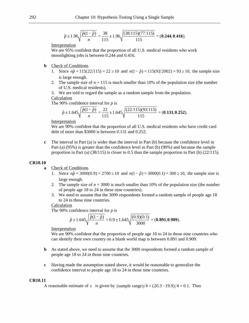
292 Chapter 10: Hypothesis Testing Using a Single Sample
ˆ ˆ(1 ) 38 (38 115)(77 115)ˆ 1.96 1.96 ( . , . ).115 115
p ppn−
± = ± = 0 244 0 416
Interpretation We are 95% confident that the proportion of all U.S. medical residents who work
moonlighting jobs is between 0.244 and 0.416. b Check of Conditions 1. Since ˆ 115(22 115) 22 10np = = ≥ and ˆ(1 ) 115(93 2002) 93 10,n p− = = ≥ the sample size
is large enough. 2. The sample size of n = 115 is much smaller than 10% of the population size (the number
of U.S. medical residents). 3. We are told to regard the sample as a random sample from the population. Calculation The 90% confidence interval for p is
ˆ ˆ(1 ) 22 (22 115)(93 115)ˆ 1.645 1.645 ( . , . ).115 115
p ppn−
± = ± = 0 131 0 252
Interpretation We are 90% confident that the proportion of all U.S. medical residents who have credit card
debt of more than $3000 is between 0.131 and 0.252. c The interval in Part (a) is wider than the interval in Part (b) because the confidence level in
Part (a) (95%) is greater than the confidence level in Part (b) (90%) and because the sample proportion in Part (a) (38/115) is closer to 0.5 than the sample proportion in Part (b) (22/115).
CR10.10 a Check of Conditions 1. Since ˆ 3000(0.9) 2700 10np = = ≥ and ˆ(1 ) 3000(0.1) 300 10,n p− = = ≥ the sample size is
large enough. 2. The sample size of n = 3000 is much smaller than 10% of the population size (the number
of people age 18 to 24 in these nine countries). 3. We need to assume that the 3000 respondents formed a random sample of people age 18
to 24 in those nine countries. Calculation The 90% confidence interval for p is
ˆ ˆ(1 ) (0.9)(0.1)ˆ 1.645 0.9 1.645 ( . , . ).3000
p ppn−
± = ± = 0 891 0 909
Interpretation We are 90% confident that the proportion of people age 18 to 24 in those nine countries who
can identify their own country on a blank world map is between 0.891 and 0.909. b As stated above, we need to assume that the 3000 respondents formed a random sample of
people age 18 to 24 in those nine countries. c Having made the assumption stated above, it would be reasonable to generalize the
confidence interval to people age 18 to 24 in those nine countries. CR10.11
A reasonable estimate of σ is given by (sample range) 4 (20.3 19.9) 4 0.1.= − = Thus

Chapter 10: Hypothesis Testing Using a Single Sample 293
2 21.96 1.96 0.1 384.16.
0.01n
Bσ ⋅ = = =
So we need a sample size of 385. CR10.12 1. p = proportion of all adult Americans who plan to alter their shopping habits if gas prices
remain high 2. H0: p = 0.75 3. Ha: p > 0.75 4. 0.05α =
5. ˆ ˆ 0.75(1 ) (0.75)(0.25)
1813
p p pzp p
n
− −= =
−
6. We are told to regard the sample as representative of adult Americans, so it is reasonable to treat the sample as a random sample from that population. The sample size is much smaller than the population size (the number of adult Americans). Furthermore,
1813(0.75) 1359.75 10np = = ≥ and (1 ) 1813(0.25) 453.25 10n p− = = ≥ , so the sample is large enough. Therefore the large sample test is appropriate.
7. 1432 1813 0.75 3.919(0.75)(0.25)
1813
z −= =
8. -value ( 3.919) 0P P Z= > ≈ 9. Since -value 0 0.05P ≈ < we reject H0. We have convincing evidence that more than three-
quarters of adult Americans plan to alter their shopping habits if gas prices remain high. CR10.13 1. p = proportion of all baseball fans who believe that the designated hitter rule should either be
expanded to both baseball leagues or eliminated 2. H0: p = 0.5 3. Ha: p > 0.5 4. 0.05α =
5. ˆ ˆ 0.5(1 ) (0.5)(0.5)
394
p p pzp p
n
− −= =
−
6. The sample was a random sample from the population. The sample size is much smaller than the population size (the number of baseball fans). Furthermore, 394(0.5) 197 10np = = ≥ and
(1 ) 394(0.5) 197 10n p− = = ≥ , so the sample is large enough. Therefore the large sample test is appropriate.
7. 272 394 0.5 7.557(0.5)(0.5)
394
z −= =
8. -value ( 7.557) 0P P Z= > ≈ 9. Since -value 0 0.05P ≈ < we reject H0. We have convincing evidence that a majority of
baseball fans believe that the designated hitter rule should either be expanded to both baseball leagues or eliminated.

294 Chapter 10: Hypothesis Testing Using a Single Sample
CR10.14 1. p = proportion of religion surfers who belong to a religious community 2. H0: p = 0.68 3. Ha: p ≠ 0.68 4. 0.05α =
5. ˆ ˆ 0.68(1 ) (0.68)(0.32)
512
p p pzp p
n
− −= =
−
6. The sample size is much smaller than the population size (the number of religion surfers). Furthermore, 512(0.68) 348.16 10np = = ≥ and (1 ) 512(0.32) 163.84 10n p− = = ≥ , so the sample is large enough. Therefore, if we assume that the sample was a random sample from the population of religion surfers, the large sample test is appropriate.
7. 0.84 0.68 7.761(0.68)(0.32)
512
z −= =
8. -value 2 ( 7.761) 0P P Z= ⋅ > ≈ 9. Since -value 0 0.05P ≈ < we reject H0. We have convincing evidence that the proportion of
religion surfers who belong to a religious community is different from 0.68. CR10.15 a With a sample mean of 14.6, the sample standard deviation of 11.6 places zero just over one
standard deviation below the mean. Since no teenager can spend a negative time online, to get a typical deviation from the mean of just over 1, there must be values that are substantially more than one standard deviation above the mean. This suggests that the distribution of online times in the sample is positively skewed.
b 1. µ = mean weekly time online for teenagers 2. H0: 10µ = 3. Ha: 10µ > 4. 0.05α =
5. 10x xts n s n
µ− −= =
6. The sample was a random sample of teenagers. Also, 534 30.n = ≥ Therefore we can proceed with the t test.
7. 14.6 10 9.164.11.6 534
t −= =
8. 533-value ( 9.164) 0P P t= > ≈ 9. Since -value 0 0.05P ≈ < we reject H0. We have convincing evidence that the mean
weekly time online for teenagers is greater than 10 hours. CR10.16 a 1. µ = mean number of hours Canadian parents of teens think their teens spend online 2. H0: 10µ = 3. Ha: 10µ < 4. 0.05α =

Chapter 10: Hypothesis Testing Using a Single Sample 295
5. 10x xts n s n
µ− −= =
6. We are told that the sample formed a random sample from the population of Canadian parents of teens. Also, 676 30.n = ≥ So we can proceed with the t test.
7. 6.5 10 10.5818.6 676
t −= = −
8. 675-value ( 10.581) 0P P t= < − ≈ 9. Since -value 0 0.05P ≈ < we reject H0. We have convincing evidence that the mean
number of hours Canadian parents of teens think their teens spend online is less than 10 per week.
b In the previous exercise, we found that there was convincing evidence that the mean of the
time the teens say they spend online is greater than 10. In Part (a) of this exercise we found that there was convincing evidence that the mean time the parents say they think their teens spend online is less than 10. Thus it is clear that either the parents have an unrealistic view of their teens’ Internet use, or the teens themselves are unclear as to the actual time they spend online, or a combination of the two.

296
Chapter 11 Comparing Two Populations or Treatments
Note: In this chapter, numerical answers to questions involving the normal and t distributions were found using values from a calculator. Students using statistical tables will find that their answers differ slightly from those given. 11.1 Since 1n and 2n are large, the distribution of 1 2x x− is approximately normal. Its mean is
1 2 30 25µ µ− = − = 5 and its standard deviation is 2 2 2 21 2
1 2
2 3 . .40 50n n
σ σ+ = + = 0 529
11.2 a H0: 1 2 10µ µ− = versus Ha: 1 2 10µ µ− > b H0: 1 2 10µ µ− = − versus Ha: 1 2 10µ µ− < − 11.3 1. 1µ = mean wait time for males 2µ = mean wait time for females 2. H0: 1 2 0µ µ− = 3. Ha: 1 2 0µ µ− ≠ 4. 0.05α =
5. 1 2 1 22 2 2 21 2 1 2
1 2 1 2
( ) (hypothesized value) ( ) 0x x x xts s s sn n n n
− − − −= =
+ +
6. We are told to assume that the two samples are representative of the populations of wait times for male and female coffee shop customers. Also 1 145 30n = ≥ and 2 141 30n = ≥ , so we can proceed with the two-sample t test.
7. 2 2
85.2 113.7 3.77050 145 75 141
t −= = −
+
8. df = 243.028 243.028-value 2 ( 3.770) 0.0002P P t= ⋅ ≤ − = 9. Since -value 0.0002 0.05P = < we reject H0. We have convincing evidence that the mean
wait time differs for males and females. 11.4 1. 1µ = mean happiness rating for those recalling an experiential purchase 2µ = mean happiness rating for those recalling a material purchase 2. H0: 1 2 0µ µ− = 3. Ha: 1 2 0µ µ− > 4. 0.05α =
5. 1 2 1 22 2 2 21 2 1 2
1 2 1 2
( ) (hypothesized value) ( ) 0x x x xts s s sn n n n
− − − −= =
+ +

Chapter 11: Comparing Two Populations or Treatments 297
6. The people were randomly assigned to the groups. Also 1 92 30n = ≥ and 2 93 30n = ≥ , so we
can proceed with the two-sample t test. 7. 2.40t = 8. df = 175 -value 0.009P = 9. Since -value 0.009 0.05P = < we reject H0. We have convincing evidence that the mean
happiness rating for those recalling an experiential purchase is greater than the mean happiness rating for those recalling a material purchase. This supports the authors’ conclusion.
11.5 a
1999
2009
10987654Time per day using electronic media
We need to assume that the population distributions of time per day using electronic media
are normal. Since the boxplots are roughly symmetrical and since there is no outlier in either sample this assumption is justified, and it is therefore reasonable to carry out a two-sample t test.
b 1. 1µ = mean time using electronic media for all kids age 8 to 18 in 2009 2µ = mean time using electronic media for all kids age 8 to 18 in 1999 2. H0: 1 2 0µ µ− = 3. Ha: 1 2 0µ µ− > 4. 0.01α =
5. 1 2 1 22 2 2 21 2 1 2
1 2 1 2
( ) (hypothesized value) ( ) 0x x x xts s s sn n n n
− − − −= =
+ +
6. We are told to assume that it is reasonable to regard the two samples as representative of kids age 8 to 18 in each of the two years when the surveys were conducted. We can then treat the samples as random samples from their respective populations. Also, as discussed in Part (a), the boxplots show that it is reasonable to assume that the population distributions are normal. So we can proceed with a two-sample t test.
7. 1 1 2 27.6 1.595 5.933 1.100x s x s= = = =
2 2
7.6 5.933 3.3321.595 1.100
15 15
t −= =
+
8. df = 24.861 24.861-value ( 3.332) 0.001P P t= > =

298 Chapter 11: Comparing Two Populations or Treatments
9. Since -value 0.001 0.01P = < we reject H0. We have convincing evidence that the mean number of hours per day spent using electronic media was greater in 2009 than in 1999.
c As explained in Parts (a) and (b), the conditions for the two-sample t test or interval are
satisfied. A 98% confidence interval for 1 2µ µ− is 2 21 2
1 21 2
2 2
( ) ( critical value)
1.595 1.100(7.6 5.93333) 2.4860515 15
( . , . )
s sx x tn n
− ± +
= − ± +
= 0 423 2 910
We are 98% confident that the difference between the mean number of hours per day spent using electronic media in 2009 and 1999 is between 0.423 and 2.910.
11.6 1. 1µ = mean number of correct answers for children who were not taught the gesturing 2µ = mean number of correct answers for children who were taught the gesturing 2. H0: 1 2 0µ µ− = 3. Ha: 1 2 0µ µ− < 4. 0.01α =
5. 1 2 1 22 2 2 21 2 1 2
1 2 1 2
( ) (hypothesized value) ( ) 0x x x xts s s sn n n n
− − − −= =
+ +
6. The children were randomly assigned to the treatments. Also 1 42 30n = ≥ and 2 43 30n = ≥ , so we can proceed with the two-sample t test.
7. 2 2
1.3 2.2 11.7530.3 0.442 43
t −= = −
+
8. df = 77.854 77.854-value ( 11.753) 0P P t= < − ≈ 9. Since -value 0 0.01P ≈ < we reject H0. We have convincing evidence that learning the
gesturing approach to solving problems of this type results in a higher mean number of correct responses.
11.7 1. 1µ = mean food intake for the 4-hour sleep treatment 2µ = mean food intake for the 8-hour sleep treatment 2. H0: 1 2 0µ µ− = 3. Ha: 1 2 0µ µ− ≠ 4. 0.05α =
5. 1 2 1 22 2 2 21 2 1 2
1 2 1 2
( ) (hypothesized value) ( ) 0x x x xts s s sn n n n
− − − −= =
+ +

Chapter 11: Comparing Two Populations or Treatments 299
6.
8-hour sleep group
4-hour sleep group
60005000400030002000Food intake
The experimental subjects were randomly assigned to the two sleep conditions. Also, since
the two boxplots are roughly symmetrical and there was no outlier in either group we are justified in assuming that the food intake distributions for the two treatments are normal. Thus, we can proceed with the two-sample t test.
7. 1 1 2 23924 829.668 4069.267 952.896x s x s= = = =
2 2
3924 4069.267 0.445829.668 952.896
15 15
t −= = −
+
8. df = 27.480 27.480-value 2 ( 0.445) 0.660P P t= ⋅ < − = 9. Since -value 0.660 0.05P = > we do not reject H0. We do not have convincing evidence of a
difference in the means for the two sleep treatments. 11.8 The treatment groups were small (10 people in each group) and so in order to use the two-sample
t test it is necessary to assume that the population distributions of estimated times for those given the easy font and for those given the difficult font are normal. However, in both samples zero is about one-and-a-half standard deviations below the mean. If we assume that the populations have means and standard deviations equal to the sample means and standard deviations, this would imply that a significant proportion of people in each population have negative estimated times. Since no-one will, in fact, estimate the time to be negative, this tells us that the populations are unlikely to be approximately normally distributed. Thus the two-sample t test is not appropriate.
11.9 a If the vertebroplasty group had been compared to a group of patients who did not receive any
treatment, and if, for example, the people in the vertebroplasty group experienced a greater pain reduction on average than the people in the “no treatment” group, then it would be impossible to tell whether the observed pain reduction in the vertebroplasty group was caused by the treatment or merely by the subjects’ knowledge that some treatment was being applied. By using a placebo group it is ensured that the subjects in both groups have the knowledge of some “treatment,” so that any differences between the pain reduction in the two groups can be attributed to the nature of the vertebroplasty treatment.
b Check of Conditions Since 1 68 30n = ≥ and 2 63 30,n = ≥ if we assume that the subjects were randomly assigned
to the treatments, we can proceed with construction of a two-sample t interval. Calculation df = 127.402. The 95% confidence interval for 1 2µ µ− is

300 Chapter 11: Comparing Two Populations or Treatments
2 21 2
1 21 2
2 2
( ) ( critical value)
2.8 2.9(4.2 3.9) 1.97968 63
( . , . )
s sx x tn n
− ± +
= − ± +
= −0 687 1 287
Interpretation We are 95% confident that the difference in mean pain intensity 3 days after treatment for the
vertebroplasty treatment and the fake treatment is between −0.687 and 1.287. c 14 days: Check of Conditions See Part (b). Calculation df = 128.774. The 95% confidence interval for 1 2µ µ− is
2 21 2
1 21 2
2 2
( ) ( critical value)
2.9 2.8(4.3 4.5) 1.97968 63
( , . )
s sx x tn n
− ± +
= − ± +
= −1.186 0 786
Interpretation We are 95% confident that the difference in mean pain intensity 14 days after treatment for
the vertebroplasty treatment and the fake treatment is between −1.186 and 0.786. 1 month: Check of Conditions See Part (b). Calculation df = 127.435. The 95% confidence interval for 1 2µ µ− is
2 21 2
1 21 2
2 2
( ) ( critical value)
2.9 3.0(3.9 4.6) 1.97968 63
( , . )
s sx x tn n
− ± +
= − ± +
= −1.722 0 322
Interpretation We are 95% confident that the difference in mean pain intensity 1 month after treatment for
the vertebroplasty treatment and the fake treatment is between −1.722 and 0.322. d The fact that all of the intervals contain zero tells us that we do not have convincing evidence
at the 0.05 level of a difference in the mean pain intensity for the vertebroplasty treatment and the fake treatment at any of the three times.
11.10 1. 1µ = mean time spent using a computer per day for males 2µ = mean time spent using a computer per day for females 2. H0: 1 2 0µ µ− =
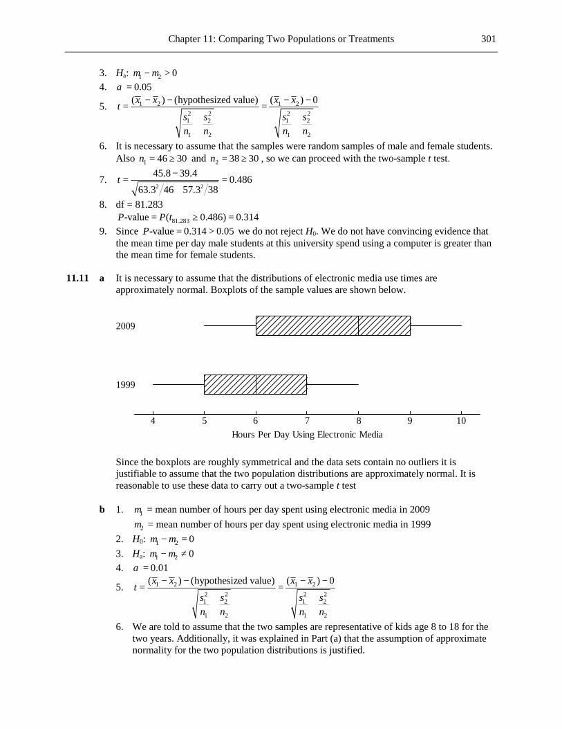
Chapter 11: Comparing Two Populations or Treatments 301
3. Ha: 1 2 0µ µ− > 4. 0.05α =
5. 1 2 1 22 2 2 21 2 1 2
1 2 1 2
( ) (hypothesized value) ( ) 0x x x xts s s sn n n n
− − − −= =
+ +
6. It is necessary to assume that the samples were random samples of male and female students. Also 1 46 30n = ≥ and 2 38 30n = ≥ , so we can proceed with the two-sample t test.
7. 2 2
45.8 39.4 0.48663.3 46 57.3 38
t −= =
+
8. df = 81.283 81.283-value ( 0.486) 0.314P P t= ≥ = 9. Since -value 0.314 0.05P = > we do not reject H0. We do not have convincing evidence that
the mean time per day male students at this university spend using a computer is greater than the mean time for female students.
11.11 a It is necessary to assume that the distributions of electronic media use times are
approximately normal. Boxplots of the sample values are shown below.
1999
2009
10987654Hours Per Day Using Electronic Media
Since the boxplots are roughly symmetrical and the data sets contain no outliers it is
justifiable to assume that the two population distributions are approximately normal. It is reasonable to use these data to carry out a two-sample t test
b 1. 1µ = mean number of hours per day spent using electronic media in 2009 2µ = mean number of hours per day spent using electronic media in 1999 2. H0: 1 2 0µ µ− = 3. Ha: 1 2 0µ µ− ≠ 4. 0.01α =
5. 1 2 1 22 2 2 21 2 1 2
1 2 1 2
( ) (hypothesized value) ( ) 0x x x xts s s sn n n n
− − − −= =
+ +
6. We are told to assume that the two samples are representative of kids age 8 to 18 for the two years. Additionally, it was explained in Part (a) that the assumption of approximate normality for the two population distributions is justified.

302 Chapter 11: Comparing Two Populations or Treatments
7. 2 2
7.6 5.933 3.3321.595 15 1.100 15
t −= =
+
8. df = 24.861 24.861-value 2 ( 3.332) 0.003P P t= ⋅ ≥ = 9. Since -value 0.003 0.01P = < we reject H0. There is convincing evidence that the mean
number of hours per day spent using electronic media was different for the two years. 11.12 Check of Conditions Since 1 311 30n = ≥ and 2 620 30,n = ≥ and it is believed that the two samples were representative
of the two populations of interest, we can proceed with construction of a two-sample t interval. Calculation df = 421.543. The 90% confidence interval for 1 2µ µ− is
2 21 2
1 21 2
2 2
( ) ( critical value)
14.83 8.76(8.39 5.39) 1.648311 620
s sx x tn n
− ± +
= − ± +
= (1.497,4.503)
Interpretation We are 90% confident that the difference in mean number of servings of chocolate per month for
people who would and would not screen positive for depression is between 1.497 and 4.503. 11.13 a 1µ = mean payment for claims not involving errors 2µ = mean payment for claims involving errors H0: 1 2 0µ µ− = Ha: 1 2 0µ µ− < b Answer: (ii) 2.65. Since the samples are large, we are using a t distribution with a large
number of degrees of freedom, which can be approximated with the standard normal distribution. ( 2.65) 0.004,P Z > = which is the P-value given. None of the other possible values of t gives the correct P-value.
11.14 1. 1µ = mean number of hours spent studying per day for Facebook users 2µ = mean number of hours spent studying per day students who are not Facebook users 2. H0: 1 2 0µ µ− = 3. Ha: 1 2 0µ µ− < 4. 0.01α =
5. 1 2 1 22 2 2 21 2 1 2
1 2 1 2
( ) (hypothesized value) ( ) 0x x x xts s s sn n n n
− − − −= =
+ +
6. The samples were selected to be representative of the two populations. Also 1 141 30n = ≥ and 2 68 30n = ≥ . So we can proceed with the two-sample t test.

Chapter 11: Comparing Two Populations or Treatments 303
7. 2 2
1.47 2.76 9.2860.83 141 0.99 68
t −= = −
+
8. df = 113.861 113.861-value ( 9.286) 0P P t= ≤ − ≈ 9. Since -value 0 0.01P ≈ < we reject H0. We have convincing evidence that the mean time
spent studying for Facebook users at this university is less than the mean time spent studying by students at the university who do not use Facebook.
11.15 Check of Conditions Since 1 1000 30n = ≥ and 2 1000 30,n = ≥ and the samples were representative of the two
populations of interest, we can proceed with construction of a two-sample t interval. Calculation df = 1852.745. The 99% confidence interval for 1 2µ µ− is
2 21 2
1 21 2
2 2
( ) ( critical value)
60 80(576 646) 2.5781000 1000
s sx x tn n
− ± +
= − ± +
= (-78.154,- 61.846)
Interpretation We are 99% confident that the difference in mean time spent watching time-shifted television for
2010 and 2011 (2010 minus 2011) is between −78.154 and −61.846. 11.16 1. 1µ = mean time spent watching TV per day for males 2µ = mean time spent watching TV per day for females 2. H0: 1 2 0µ µ− = 3. Ha: 1 2 0µ µ− < 4. 0.05α =
5. 1 2 1 22 2 2 21 2 1 2
1 2 1 2
( ) (hypothesized value) ( ) 0x x x xts s s sn n n n
− − − −= =
+ +
6. The samples were selected to be representative of the two populations. Also 1 46 30n = ≥ and
2 38 30n = ≥ . So we can proceed with the two-sample t test.
7. 2 2
68.2 93.5 1.44267.5 46 89.1 38
t −= = −
+
8. df = 67.859 67.859-value ( 1.442) 0.077P P t= ≤ − = 9. Since -value 0.077 0.05P = > we do not reject H0. We do not have convincing evidence that
the mean time female students at this university spend watching TV is greater than the mean time for male students.
11.17 a 1. 1µ = mean percentage of time playing with police car for male monkeys 2µ = mean percentage of time playing with police car for female monkeys 2. H0: 1 2 0µ µ− =
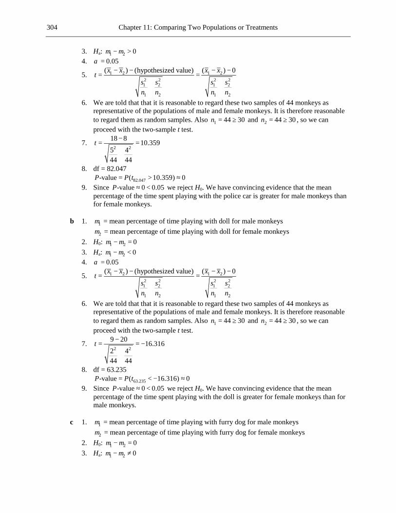
304 Chapter 11: Comparing Two Populations or Treatments
3. Ha: 1 2 0µ µ− > 4. 0.05α =
5. 1 2 1 22 2 2 21 2 1 2
1 2 1 2
( ) (hypothesized value) ( ) 0x x x xts s s sn n n n
− − − −= =
+ +
6. We are told that that it is reasonable to regard these two samples of 44 monkeys as representative of the populations of male and female monkeys. It is therefore reasonable to regard them as random samples. Also 1 44 30n = ≥ and 2 44 30n = ≥ , so we can proceed with the two-sample t test.
7. 2 2
18 8 10.3595 444 44
t −= =
+
8. df = 82.047 82.047-value ( 10.359) 0P P t= > ≈ 9. Since -value 0 0.05P ≈ < we reject H0. We have convincing evidence that the mean
percentage of the time spent playing with the police car is greater for male monkeys than for female monkeys.
b 1. 1µ = mean percentage of time playing with doll for male monkeys 2µ = mean percentage of time playing with doll for female monkeys 2. H0: 1 2 0µ µ− = 3. Ha: 1 2 0µ µ− < 4. 0.05α =
5. 1 2 1 22 2 2 21 2 1 2
1 2 1 2
( ) (hypothesized value) ( ) 0x x x xts s s sn n n n
− − − −= =
+ +
6. We are told that that it is reasonable to regard these two samples of 44 monkeys as representative of the populations of male and female monkeys. It is therefore reasonable to regard them as random samples. Also 1 44 30n = ≥ and 2 44 30n = ≥ , so we can proceed with the two-sample t test.
7. 2 2
9 20 16.3162 444 44
t −= = −
+
8. df = 63.235 63.235-value ( 16.316) 0P P t= < − ≈ 9. Since -value 0 0.05P ≈ < we reject H0. We have convincing evidence that the mean
percentage of the time spent playing with the doll is greater for female monkeys than for male monkeys.
c 1. 1µ = mean percentage of time playing with furry dog for male monkeys 2µ = mean percentage of time playing with furry dog for female monkeys 2. H0: 1 2 0µ µ− = 3. Ha: 1 2 0µ µ− ≠

Chapter 11: Comparing Two Populations or Treatments 305
4. 0.05α =
5. 1 2 1 22 2 2 21 2 1 2
1 2 1 2
( ) (hypothesized value) ( ) 0x x x xts s s sn n n n
− − − −= =
+ +
6. We are told that that it is reasonable to regard these two samples of 44 monkeys as representative of the populations of male and female monkeys. It is therefore reasonable to regard them as random samples. Also 1 44 30n = ≥ and 2 44 30n = ≥ , so we can proceed with the two-sample t test.
7. 2 2
25 20 4.6905 544 44
t −= =
+
8. df = 86 86-value 2 ( 4.690) 0P P t= ⋅ > ≈ 9. Since -value 0 0.05P ≈ < we reject H0. We have convincing evidence that the mean
percentage of the time spent playing with the furry dog is not the same for male monkeys as it is for female monkeys.
d The results do seem to provide convincing evidence of a gender basis in the monkeys’
choices of how much time to spend playing with each toy, with the male monkeys spending significantly more time with the “masculine toy” than the female monkeys, and with the female monkeys spending significantly more time with the “feminine toy” than the male monkeys. However, the data also provide convincing evidence of a difference between male and female monkeys in the time they choose to spend playing with a “neutral toy.” It is possible that it was some attribute other than masculinity/femininity in the toys that was attracting the different genders of monkey in different ways.
e The given mean time playing with the police car and mean time playing with the doll for
female monkeys are sample means for the same sample of female monkeys. The two-sample t test can only be performed when there are two independent random samples.
11.18 a 1. 1µ = mean amount by which speed limit was exceeded for male drivers 2µ = mean amount by which speed limit was exceeded for female drivers 2. H0: 1 2 0µ µ− = 3. Ha: 1 2 0µ µ− > 4. 0.01α =
5. 1 2 1 22 2 2 21 2 1 2
1 2 1 2
( ) (hypothesized value) ( ) 0x x x xts s s sn n n n
− − − −= =
+ +

306 Chapter 11: Comparing Two Populations or Treatments
6.
Female Driver
Male Driver
3.02.52.01.51.00.50.0Amount by which Speed Limit was Exceeded
Any lack of symmetry in the boxplots is acceptable for samples of this size, and neither
data set contains outliers, so we are justified in assuming normal distributions for the populations. We are told to regard the teen drivers in the study as representative of teen drivers in general, so it is reasonable to treat the samples as random samples from the populations of male and female teen drivers. Thus we can proceed with the two-sample t test.
7. 2 2
(1.46 0.64) (0) 2.9860.740 0.455
10 10
t − −= =
+
8. df = 14.960 14.960-value ( 2.986) 0.005P P t= > = 9. Since -value 0.005 0.01P = < we reject H0. We have convincing evidence that, on
average, male teenage drivers exceed the speed limit by more than do female teenage drivers.
b In the hypothesis tests that follow, we need to assume that the samples are random samples
from their respective populations. The samples (size 40) are large enough to justify use of the two-sample t test.
i 1. 1µ = mean amount by which speed limit was exceeded for male drivers with male passengers
2µ = mean amount by which speed limit was exceeded for male drivers with female passengers
2. H0: 1 2 0µ µ− = 3. Ha: 1 2 0µ µ− > 4. 0.01α =
5. 1 2 1 22 2 2 21 2 1 2
1 2 1 2
( ) (hypothesized value) ( ) 0x x x xts s s sn n n n
− − − −= =
+ +
6. The conditions were checked above.
7. 2 2
(5.2 0.3) (0) 27.3920.8 0.840 40
t − −= =
+
8. df = 78 78-value ( 27.392) 0P P t= > ≈

Chapter 11: Comparing Two Populations or Treatments 307
9. Since -value 0 0.01P ≈ < we reject H0. We have convincing evidence that the
average number of miles per hour over the speed limit is greater for male drivers with male passengers than for male drivers with female passengers.
ii 1. 1µ = mean amount by which speed limit was exceeded for female drivers with male
passengers 2µ = mean amount by which speed limit was exceeded for female drivers with
female passengers 2. H0: 1 2 0µ µ− = 3. Ha: 1 2 0µ µ− > 4. 0.01α =
5. 1 2 1 22 2 2 21 2 1 2
1 2 1 2
( ) (hypothesized value) ( ) 0x x x xts s s sn n n n
− − − −= =
+ +
6. The conditions were checked above.
7. 2 2
(2.3 0.6) (0) 9.5030.8 0.840 40
t − −= =
+
8. df = 78 78-value ( 9.503) 0P P t= > ≈ 9. Since -value 0 0.01P ≈ < we reject H0. We have convincing evidence that the
average number of miles per hour over the speed limit is greater for female drivers with male passengers than for female drivers with female passengers.
iii 1. 1µ = mean amount by which speed limit was exceeded for male drivers with female
passengers 2µ = mean amount by which speed limit was exceeded for female drivers with male
passengers 2. H0: 1 2 0µ µ− = 3. Ha: 1 2 0µ µ− < 4. 0.01α =
5. 1 2 1 22 2 2 21 2 1 2
1 2 1 2
( ) (hypothesized value) ( ) 0x x x xts s s sn n n n
− − − −= =
+ +
6. The conditions were checked above.
7. 2 2
(0.3 2.3) (0) 11.1800.8 0.840 40
t − −= = −
+
8. df = 78 78-value ( 11.180) 0P P t= < − ≈ 9. Since -value 0 0.01P ≈ < we reject H0. We have convincing evidence that the
average number of miles per hour over the speed limit is smaller for male drivers with female passengers than for female drivers with male passengers.
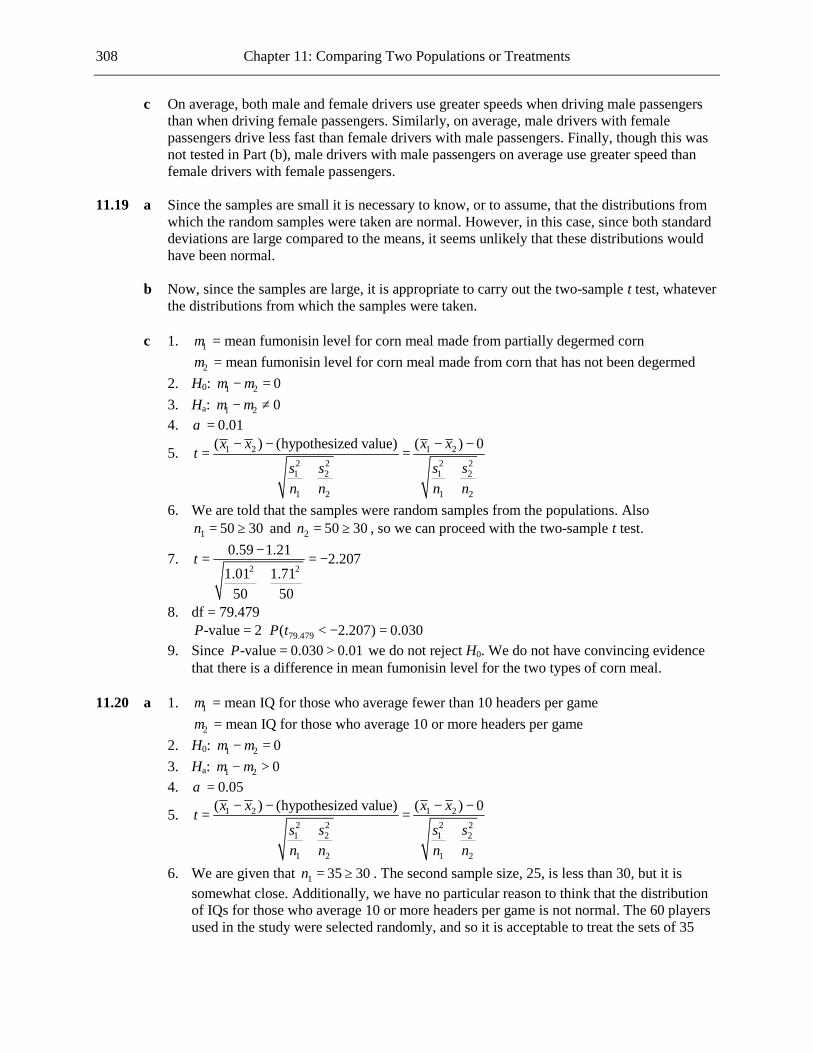
308 Chapter 11: Comparing Two Populations or Treatments
c On average, both male and female drivers use greater speeds when driving male passengers than when driving female passengers. Similarly, on average, male drivers with female passengers drive less fast than female drivers with male passengers. Finally, though this was not tested in Part (b), male drivers with male passengers on average use greater speed than female drivers with female passengers.
11.19 a Since the samples are small it is necessary to know, or to assume, that the distributions from
which the random samples were taken are normal. However, in this case, since both standard deviations are large compared to the means, it seems unlikely that these distributions would have been normal.
b Now, since the samples are large, it is appropriate to carry out the two-sample t test, whatever
the distributions from which the samples were taken. c 1. 1µ = mean fumonisin level for corn meal made from partially degermed corn 2µ = mean fumonisin level for corn meal made from corn that has not been degermed 2. H0: 1 2 0µ µ− = 3. Ha: 1 2 0µ µ− ≠ 4. 0.01α =
5. 1 2 1 22 2 2 21 2 1 2
1 2 1 2
( ) (hypothesized value) ( ) 0x x x xts s s sn n n n
− − − −= =
+ +
6. We are told that the samples were random samples from the populations. Also 1 50 30n = ≥ and 2 50 30n = ≥ , so we can proceed with the two-sample t test.
7. 2 2
0.59 1.21 2.2071.01 1.71
50 50
t −= = −
+
8. df = 79.479 79.479-value 2 ( 2.207) 0.030P P t= ⋅ < − = 9. Since -value 0.030 0.01P = > we do not reject H0. We do not have convincing evidence
that there is a difference in mean fumonisin level for the two types of corn meal. 11.20 a 1. 1µ = mean IQ for those who average fewer than 10 headers per game 2µ = mean IQ for those who average 10 or more headers per game 2. H0: 1 2 0µ µ− = 3. Ha: 1 2 0µ µ− > 4. 0.05α =
5. 1 2 1 22 2 2 21 2 1 2
1 2 1 2
( ) (hypothesized value) ( ) 0x x x xts s s sn n n n
− − − −= =
+ +
6. We are given that 1 35 30n = ≥ . The second sample size, 25, is less than 30, but it is somewhat close. Additionally, we have no particular reason to think that the distribution of IQs for those who average 10 or more headers per game is not normal. The 60 players used in the study were selected randomly, and so it is acceptable to treat the sets of 35

Chapter 11: Comparing Two Populations or Treatments 309
and 25 players as random samples from their respective populations. Thus we can proceed with the two-sample t test.
7. 2 2
112 103 3.86710 835 25
t −= =
+
8. df = 57.185 57.185-value ( 3.867) 0P P t= > ≈ 9. Since -value 0 0.05P ≈ < we reject H0. We have convincing evidence that the mean IQ for
those who average fewer than 10 headers per game is greater than the mean IQ for those who average 10 or more headers per game.
b No. Since this was an observational study, we cannot conclude that heading the ball causes
lower IQ. 11.21 a 1. 1µ = mean oxygen consumption for noncourting pairs 2µ = mean oxygen consumption for courting pairs 2. H0: 1 2 0µ µ− = 3. Ha: 1 2 0µ µ− < 4. 0.05α =
5. 2 2
1 2 1 2 1 1 2 22 2 2 2
1 2
1 2 1 2
( ) (hypothesized value) ( ) 0 ( 1) ( 1), where 2p
p p p p
x x x x n s n st sn ns s s s
n n n n
− − − − − + −= = =
+ −+ +
6. We need to assume that the samples were random samples from the populations, and that the population distributions are normal. Additionally, the similar sample standard deviations justify our assumption that the populations have equal standard deviations.
7. 2 2
2 2
10(0.0066) 14(0.0071) 0.072 0.0990.00690, 9.86324 0.00690 0.00690
11 15
ps t+ −= = = = −
+
8. df = 24 24-value ( 9.863) 0P P t= < − ≈ 9. Since -value 0 0.05P ≈ < we reject H0. We have convincing evidence that the mean
oxygen consumption for courting pairs is higher than the mean oxygen consumption for noncourting pairs.
b For the two-sample t test, 9.979, df 22.566, and -value 0.t P= − = ≈ Thus the conclusion is
the same. 11.22 a Gather a number of volunteers who suffer from glaucoma in both eyes. Measure the pressure
in each eye of each participant before the treatments begin. For each experimental subject, randomly assign the treatments to the eyes (so that one eye receives the standard treatment and the other receives the drug that is being evaluated). Once the patients have applied the treatments for a fixed time, measure again the pressures in all the eyes, and compare the mean reduction in pressure for the eyes that have received the new treatment with the mean reduction in pressure for those that have received the standard treatment.

310 Chapter 11: Comparing Two Populations or Treatments
b Yes, since, for example, the reduction in pressure for the eye that receives the new treatment for the first patient is paired with the reduction in pressure for the eye that receives the standard treatment for the first patient.
c The design given in Part (a) could be used, with the modification that each participant
receives the same treatment in both eyes, and the treatments are randomly assigned to the participants. This design is not as informative as the paired design, since, in the paired design, the set of eyes to which the new treatment is applied is almost identical to the set of eyes to which the standard treatment is applied, which is not the case in the other design. What is more, the analysis of the results for the paired design takes into account, for example, that the result for the new treatment for the first patient is paired with the result for the standard treatment for the first patient.
11.23
Subject Clockwise Counter- clockwise Difference
1 57.9 44.2 13.7 2 35.7 52.1 −16.4 3 54.5 60.2 −5.7 4 56.8 52.7 4.1 5 51.1 47.2 3.9 6 70.8 65.6 5.2 7 77.3 71.4 5.9 8 51.6 48.8 2.8 9 54.7 53.1 1.6 10 63.6 66.3 −2.7 11 59.2 59.8 −0.6 12 59.2 47.5 11.7 13 55.8 64.5 −8.7 14 38.5 34.5 4
1. dµ = mean of the neck rotation difference (clockwise − counterclockwise) 2. H0: 0dµ = 3. Ha: 0dµ > 4. 0.01α =
5. hypothesized valued
d
xts n
−=

Chapter 11: Comparing Two Populations or Treatments 311
6.
151050-5-10-15-20Difference
The boxplot shows that the distribution of the differences in the sample is roughly
symmetrical and has no outliers, so we are justified in assuming that the population distribution of differences is normal. Additionally, we are told to assume that the 14 subjects are representative of the population of adult Americans.
7. 1.343, 7.866d dx s= =
1.343 0 0.6397.866 14
t −= =
8. df = 13 13-value ( 0.639) 0.267P P t= ≥ = 9. Since -value 0.267 0.01P = > we do not reject H0. We do not have convincing evidence that
mean neck rotation is greater in the clockwise direction than in the counterclockwise direction.
11.24
Cyclist
Chocolate Milk
Carbohydrate Replacement
Difference
1 24.85 10.02 14.83 2 50.09 29.96 20.13 3 38.3 37.4 0.9 4 26.11 15.52 10.59 5 36.54 9.11 27.43 6 26.14 21.58 4.56 7 36.13 31.23 4.9 8 47.35 22.04 25.31 9 35.08 17.02 18.06
1. dµ = mean of the time to exhaustion difference (chocolate mile − carbohydrate replacement) 2. H0: 0dµ = 3. Ha: 0dµ > 4. 0.05α =
5. hypothesized valued
d
xts n
−=

312 Chapter 11: Comparing Two Populations or Treatments
6.
302520151050Difference
The boxplot shows that the distribution of the differences in the sample is roughly
symmetrical and has no outliers, so we are justified in assuming that the population distribution of differences is normal. Additionally, we need to assume that the set of cyclists used in the study was randomly selected.
7. 14.079, 9.475d dx s= =
14.079 0 4.4589.475 9
t −= =
8. df = 8 8-value ( 4.458) 0.001P P t= > = 9. Since -value 0.001 0.05P = < we reject H0. We have convincing evidence that the mean time
to exhaustion is greater after chocolate milk than after carbohydrate replacement drink. 11.25
Swimmer Water Guar Syrup Difference 1 0.9 0.92 −0.02 2 0.92 0.96 −0.04 3 1 0.95 0.05 4 1.1 1.13 −0.03 5 1.2 1.22 −0.02 6 1.25 1.2 0.05 7 1.25 1.26 −0.01 8 1.3 1.3 0 9 1.35 1.34 0.01
10 1.4 1.41 −0.01 11 1.4 1.44 −0.04 12 1.5 1.52 −0.02 13 1.65 1.58 0.07 14 1.7 1.7 0 15 1.75 1.8 −0.05 16 1.8 1.76 0.04 17 1.8 1.84 −0.04 18 1.85 1.89 −0.04 19 1.9 1.88 0.02 20 1.95 1.95 0
1. dµ = mean swimming velocity difference (water − guar syrup) 2. H0: 0dµ = 3. Ha: 0dµ ≠ 4. 0.01α =

Chapter 11: Comparing Two Populations or Treatments 313
5. hypothesized valued
d
xts n
−=
6.
0.0750.0500.0250.000-0.025-0.050Difference
The boxplot shows that the distribution of the differences is roughly symmetrical and has no
outliers, so we are justified in assuming that the population distribution of differences is normal. Additionally, we need to assume that this set of differences forms a random sample from the set of differences for all swimmers.
7. 0.004, 0.035d dx s= − =
0.004 0 0.5150.035 20
t − −= = −
8. df = 19 19-value 2 ( 0.515) 0.612P P t= ⋅ < − = 9. Since -value 0.612 0.01P = > we do not reject H0. We do not have convincing evidence of a
difference between the mean swimming speeds in water and guar syrup. The given data are consistent with the authors’ conclusion.
11.26 1. dµ = mean rating difference ($90 − $10) 2. H0: 0dµ = 3. Ha: 0dµ > 4. 0.01α =
5. hypothesized valued
d
xts n
−=
6.
43210-1Difference
The boxplot shows that the sample distribution of differences is roughly symmetrical and has
no outliers, so we are justified in assuming that the population of differences is normal distributed. Additionally we need to assume that the participants in the experiment formed a random sample from the population in question.
7. 1.6, 1.353d dx s= =
1.6 0 5.2871.353 20
t −= =
8. df = 19

314 Chapter 11: Comparing Two Populations or Treatments
19-value ( 5.287) 0P P t= > ≈ 9. Since -value 0 0.01P ≈ < we reject H0. We have convincing evidence that the mean rating
assigned when the cost is described as $90 is greater than the mean rating assigned when the cost is described as $10.
11.27
Worker Conventional Perforated Difference 1 0.0011 0.0011 0 2 0.0014 0.001 0.0004 3 0.0018 0.0019 −0.0001 4 0.0022 0.0013 0.0009 5 0.001 0.0011 −0.0001 6 0.0016 0.0017 −0.0001 7 0.0028 0.0024 0.0004 8 0.002 0.002 0 9 0.0015 0.0013 0.0002 10 0.0014 0.0013 0.0001 11 0.0023 0.0017 0.0006 12 0.0017 0.0015 0.0002 13 0.002 0.0013 0.0007
1. dµ = mean of the energy expenditure difference (conventional − perforated) 2. H0: 0dµ = 3. Ha: 0dµ > 4. 0.05α =
5. hypothesized valued
d
xts n
−=
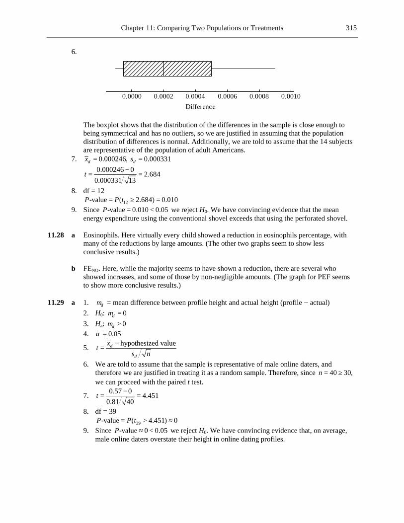
Chapter 11: Comparing Two Populations or Treatments 315
6.
0.00100.00080.00060.00040.00020.0000Difference
The boxplot shows that the distribution of the differences in the sample is close enough to
being symmetrical and has no outliers, so we are justified in assuming that the population distribution of differences is normal. Additionally, we are told to assume that the 14 subjects are representative of the population of adult Americans.
7. 0.000246, 0.000331d dx s= =
0.000246 0 2.6840.000331 13
t −= =
8. df = 12 12-value ( 2.684) 0.010P P t= ≥ = 9. Since -value 0.010 0.05P = < we reject H0. We have convincing evidence that the mean
energy expenditure using the conventional shovel exceeds that using the perforated shovel. 11.28 a Eosinophils. Here virtually every child showed a reduction in eosinophils percentage, with
many of the reductions by large amounts. (The other two graphs seem to show less conclusive results.)
b FENO. Here, while the majority seems to have shown a reduction, there are several who
showed increases, and some of those by non-negligible amounts. (The graph for PEF seems to show more conclusive results.)
11.29 a 1. dµ = mean difference between profile height and actual height (profile − actual) 2. H0: 0dµ = 3. Ha: 0dµ > 4. 0.05α =
5. hypothesized valued
d
xts n
−=
6. We are told to assume that the sample is representative of male online daters, and therefore we are justified in treating it as a random sample. Therefore, since 40 30,n = ≥ we can proceed with the paired t test.
7. 0.57 0 4.4510.81 40
t −= =
8. df = 39 39-value ( 4.451) 0P P t= > ≈ 9. Since -value 0 0.05P ≈ < we reject H0. We have convincing evidence that, on average,
male online daters overstate their height in online dating profiles.

316 Chapter 11: Comparing Two Populations or Treatments
b Check of Conditions We are told to assume that the sample is representative of female online daters, and therefore
we are justified in treating it as a random sample. Therefore, since 40 30,n = ≥ we can proceed with the paired t interval.
Calculation df = 39. The 95% confidence interval for dµ is
0.75( critical value) 0.03 2.023 ( . , . )40
dd
sx tn
± = ± = −0 210 0 270
Interpretation We are 95% confident that the difference between the mean online dating profile height and
mean actual height for female online daters is between −0.210 and 0.270. c 1. mµ = mean height difference (profile − actual) for male online daters fµ = mean height difference (profile − actual) for female online daters 2. H0: 0m fµ µ− = 3. Ha: 0m fµ µ− > 4. 0.05α =
5. 2 22 2
( ) (hypothesized value) ( ) 0m f m f
f fm m
m f m f
x x x xt
s ss sn n n n
− − − −= =
+ +
6. We are told to assume that the samples were representative of the populations, and therefore we are justified in assuming that they are random samples. Also 40 30mn = ≥ and 40 30fn = ≥ , so we can proceed with the two-sample t test.
7. 2 2
0.57 0.03 3.0940.81 0.75
40 40
t −= =
+
8. df = 77.543 77.543-value ( 3.094) 0.001P P t= > = 9. Since -value 0.001 0.05P = < we reject H0. We have convincing evidence that
0m fµ µ− > . d In Part (a), the male profile heights and the male actual heights are paired (according to which
individual has the actual height and the height stated in the profile), and with paired samples we use the paired t test. In Part (c) we were dealing with two independent samples (the sample of males and the sample of females), and therefore the two-sample t test was appropriate.
11.30 Since the data are given for every NCAA Division I university with a basketball program, they
are population data, not sample data, and so there is no need for a hypothesis test.

Chapter 11: Comparing Two Populations or Treatments 317
11.31
Subject B P Difference 1 1928 2126 -198 2 2549 2885 -336 3 2825 2895 -70 4 1924 1942 -18 5 1628 1750 -122 6 2175 2184 -9 7 2114 2164 -50 8 2621 2626 -5 9 1843 2006 -163 10 2541 2627 -86
1. dµ = mean bone mineral content difference (breast feeding − postweaning) 2. H0: 25dµ = − 3. Ha: 25dµ < − 4. 0.05α =
5. hypothesized valued
d
xts n
−=
6.
0-50-100-150-200-250-300-350Difference
The boxplot shows that the distribution of the sample differences is negatively skewed, but
for a relatively small sample this distribution is not inconsistent with a population that is normally distributed. Additionally, the sample distribution of differences has no outliers. We need to assume that the mothers used in the study formed a random sample from the population of mothers.
7. 105.7, 103.845d dx s= − =
105.7 ( 25) 2.457103.845 10
t − − −= = −
8. df = 9 9-value ( 2.457) 0.018P P t= < − = 9. Since -value 0.018 0.05P = < we reject H0. We have convincing evidence that the average
total body bone mineral content during postweaning is greater than that during breast feeding by more than 25 grams.

318 Chapter 11: Comparing Two Populations or Treatments
11.32 The differences applicable to Parts (a) and (b) are shown in the table below.
Player
Dominant Arm
Nondominant Arm
Difference
Pitcher
Dominant Arm
Nondominant Arm
Difference
1 30.31 32.54 -2.23 1 27.63 24.33 3.3 2 44.86 40.95 3.91 2 30.57 26.36 4.21 3 22.09 23.48 -1.39 3 32.62 30.62 2 4 31.26 31.11 0.15 4 39.79 33.74 6.05 5 28.07 28.75 -0.68 5 28.5 29.84 -1.34 6 31.93 29.32 2.61 6 26.7 26.71 -0.01 7 34.68 34.79 -0.11 7 30.34 26.45 3.89 8 29.1 28.87 0.23 8 28.69 21.49 7.2 9 25.51 27.59 -2.08 9 31.19 20.82 10.37
10 22.49 21.01 1.48 10 36 21.75 14.25 11 28.74 30.31 -1.57 11 31.58 28.32 3.26 12 27.89 27.92 -0.03 12 32.55 27.22 5.33 13 28.48 27.85 0.63 13 29.56 28.86 0.7 14 25.6 24.95 0.65 14 28.64 28.58 0.06 15 20.21 21.59 -1.38 15 28.58 27.15 1.43 16 33.77 32.48 1.29 16 31.99 29.46 2.53 17 32.59 32.48 0.11 17 27.16 21.26 5.9 18 32.6 31.61 0.99 19 29.3 27.46 1.84
a Check of Conditions
15.012.510.07.55.02.50.0Difference
The boxplot shows that the distribution of the differences (dominant − nondominant, for
pitchers) is positively skewed and has an outlier. Having assumed that the sample was a random sample of pitchers, we will nonetheless proceed with calculation of the confidence interval.
Calculation 4.066, 3.955, 17, df 16d dx s n= = = = The 95% confidence interval for dµ is
3.955( critical value) 4.066 2.120 ( , . )17
dd
sx tn
± = ± = 2.033 6 100
Interpretation We are 95% confident that the true average difference in translation between dominant and
nondominant arms for pitchers is between 2.033 and 6.100 mm.
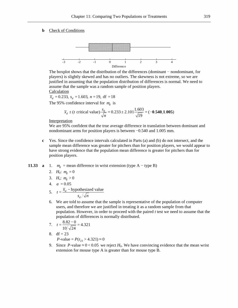
Chapter 11: Comparing Two Populations or Treatments 319
b Check of Conditions
43210-1-2-3Difference
The boxplot shows that the distribution of the differences (dominant − nondominant, for players) is slightly skewed and has no outliers. The skewness is not extreme, so we are justified in assuming that the population distribution of differences is normal. We need to assume that the sample was a random sample of position players.
Calculation 0.233, 1.603, 19, df 18d dx s n= = = = The 95% confidence interval for dµ is
1.603( critical value) 0.233 2.101 ( . , . )19
dd
sx tn
± = ± = −0 540 1 005
Interpretation We are 95% confident that the true average difference in translation between dominant and
nondominant arms for position players is between −0.540 and 1.005 mm. c Yes. Since the confidence intervals calculated in Parts (a) and (b) do not intersect, and the
sample mean difference was greater for pitchers than for position players, we would appear to have strong evidence that the population mean difference is greater for pitchers than for position players.
11.33 a 1. dµ = mean difference in wrist extension (type A − type B) 2. H0: 0dµ = 3. Ha: 0dµ > 4. 0.05α =
5. hypothesized valued
d
xts n
−=
6. We are told to assume that the sample is representative of the population of computer users, and therefore we are justified in treating it as a random sample from that population. However, in order to proceed with the paired t test we need to assume that the population of differences is normally distributed.
7. 8.82 0 4.32110 24
t −= =
8. df = 23 23-value ( 4.321) 0P P t= > ≈ 9. Since -value 0 0.05P ≈ < we reject H0. We have convincing evidence that the mean wrist
extension for mouse type A is greater than for mouse type B.

320 Chapter 11: Comparing Two Populations or Treatments
b Now 8.82 0 1.662,26 24
t −= = and so 23-value ( 1.662) 0.055P P t= > = . Since
-value 0.055 0.05P = > we do not reject H0. We do not have convincing evidence that the mean wrist extension for mouse type A is greater than for mouse type B.
c A lower standard deviation in the sample of differences means that we have a lower estimate of the standard deviation of the population of differences. Assuming that the mean wrist extensions for the two mouse types are the same (in other words, that the mean of the population of differences is zero), a sample mean difference of as much as 8.82 is much less likely when the standard deviation of the population of differences is around 10 than when the standard deviation of the population of differences is around 26.
11.34
Subject Mini Wright Meter
Wright Meter Difference
1 512 494 18 2 430 395 35 3 520 516 4 4 428 434 −6 5 500 476 24 6 600 557 43 7 364 413 −49 8 380 442 −62 9 658 650 8 10 445 433 12 11 432 417 15 12 626 656 −30 13 260 267 −7 14 477 478 −1 15 259 178 81 16 350 423 −73 17 451 427 24
1. dµ = mean difference in reading (mini-Wright meter – Wright meter) 2. H0: 0dµ = 3. Ha: 0dµ ≠ 4. 0.05α =
5. hypothesized valued
d
xts n
−=
6.
100500-50Difference

Chapter 11: Comparing Two Populations or Treatments 321
The boxplot shows that the distribution of the differences in the sample is roughly
symmetrical and has no outliers, so we are justified in assuming that the population distribution of differences is normal. Additionally, we need to assume that the 17 subjects form a random sample from the population in question.
7. 2.118, 38.765d dx s= =
2.118 0 0.22538.765 17
t −= =
8. df = 16 16-value 2 ( 0.225) 0.825P P t= ⋅ ≥ = 9. Since -value 0.825 0.05P = > we do not reject H0. We do not have convincing evidence that
the mean reading differs for the two instruments. 11.35 dµ = mean difference between verbal ability score at age 8 and verbal ability score at age 3
(age 8 − age 3) H0: 0dµ = Ha: 0dµ > 0.05α = We are told to assume that the sample is a random sample from the population of children born
prematurely. Therefore, since 50 30,n = ≥ we can proceed with the paired t test. -value 0.001P = Since -value 0.001 0.05P = < we reject H0. We have convincing evidence that the mean verbal
ability score for children born prematurely increases between age 3 and age 8. 11.36
Athlete X-ray Ultrasound Difference 1 5 4.75 0.25 2 7 3.75 3.25 3 9.25 9 0.25 4 12 11.75 0.25 5 17.25 17 0.25 6 29.5 27.5 2 7 5.5 6.5 −1 8 6 6.75 −0.75 9 8 8.75 −0.75 10 8.5 9.5 −1 11 9.25 9.5 −0.25 12 11 12 −1 13 12 12.25 −0.25 14 14 15.5 −1.5 15 17 18 −1 16 18 18.25 −0.25

322 Chapter 11: Comparing Two Populations or Treatments
Check of Conditions
3210-1-2Difference
The boxplot shows that the distribution of the differences has an outlier, while the distribution is
roughly symmetrical if the outlier is ignored. The outlier should lead us to question the normality of the population distribution. However, the sample is relatively small, and outliers can occur in samples from normal distributions when the sample is small. So we will proceed with the assumption that the population distribution of differences is normal. Additionally, we are told to assume that the 16 athletes who participated in this study are representative of the population of athletes.
Calculation df = 15. The 95% confidence interval for dµ is
1.217( critical value) 0.09375 2.13116
dd
sx tn
± ⋅ = − ± ⋅ = (-0.743,0.555)
Interpretation We are 95% confident that the difference in mean body fat percentage measurement for the two
methods (X-ray – ultrasound) is between −0.743 and 0.555. 11.37 1. 1p = proportion of people receiving liquid nitrogen treatment for whom wart is successfully
removed 2p = proportion of people receiving duct tape treatment for whom wart is successfully
removed 2. H0: 1 2 0p p− = 3. Ha: 1 2 0p p− < 4. 0.01α =
5. 1 2
1 2
ˆ ˆˆ ˆ ˆ ˆ(1 ) (1 )c c c c
p pzp p p p
n n
−=
− −+
6. We are told that the patients were randomly assigned to the treatments. Also 1 1ˆ 100(60 100) 60 10,n p = = ≥ 1 1ˆ(1 ) 100(40 100) 40 10,n p− = = ≥
2 2ˆ 104(88 104) 88 10,n p = = ≥ and 2 2ˆ(1 ) 104(16 104) 16 10,n p− = = ≥ so the treatment groups are large enough.
7. 1 1 2 2
1 2
ˆ ˆ 60 88ˆ 0.725100 104c
n p n ppn n
+ += = =
+ +
60 100 88 104 3.938(0.725)(0.275) (0.725)(0.275)
100 104
z −= = −
+
8. -value ( 3.938) 0P P Z= < − ≈ 9. Since -value 0 0.01P ≈ < we reject H0. We have convincing evidence that the proportion of
people for whom the wart is successfully removed is less for the liquid nitrogen treatment than for duct tape treatment.

Chapter 11: Comparing Two Populations or Treatments 323
11.38 1. 1p = proportion of Dutch boys who listen to music at high volume 2p = proportion of Dutch girls who listen to music at high volume 2. H0: 1 2 0p p− = 3. Ha: 1 2 0p p− > 4. 0.01α =
5. 1 2
1 2
ˆ ˆˆ ˆ ˆ ˆ(1 ) (1 )c c c c
p pzp p p p
n n
−=
− −+
6. We are told that the samples were independent random samples from the populations. Also 1 1ˆ 764(397 764) 397 10,n p = = ≥ 1 1ˆ(1 ) 764(367 764) 367 10,n p− = = ≥
2 2ˆ 748(331 748) 331 10,n p = = ≥ and 2 2ˆ(1 ) 748(417 748) 417 10,n p− = = ≥ so the samples are large enough.
7. 397 331 728ˆ764 748 1512cp +
= =+
397 764 331 748 3.001(728 1512)(784 1512) (728 1512)(784 1512)
764 748
z −= =
+
8. -value ( 3.001) 0.001P P Z= > = 9. Since -value 0.001 0.01P = < we reject H0. We have convincing evidence that the proportion
of Dutch boys who listen to music at high volume is greater than the proportion of Dutch girls who listen to music at high volume.
11.39 a 1. 1p = proportion of Gen Y respondents who donated by text message 2p = proportion of Gen X respondents who donated by text message 2. H0: 1 2 0p p− = 3. Ha: 1 2 0p p− > 4. 0.01α =
5. 1 2
1 2
ˆ ˆˆ ˆ ˆ ˆ(1 ) (1 )c c c c
p pzp p p p
n n
−=
− −+
6. We are told to regard the samples as representative of the Gen Y and Gen X populations, so it is reasonable to treat them as independent random samples from the populations. Also 1 1ˆ 400(0.17) 68 10,n p = = ≥ 1 1ˆ(1 ) 400(0.83) 332 10,n p− = = ≥
2 2ˆ 400(0.14) 56 10,n p = = ≥ and 2 2ˆ(1 ) 400(0.86) 344 10,n p− = = ≥ so the samples are large enough.
7. 1 1 2 2
1 2
ˆ ˆ 400(0.17) 400(0.14)ˆ 0.155400 400c
n p n ppn n
+ += = =
+ +
0.17 0.14 1.172(0.155)(0.845) (0.155)(0.845)
400 400
z −= =
+
8. -value ( 1.172) 0.121P P Z= > =

324 Chapter 11: Comparing Two Populations or Treatments
9. Since -value 0.121 0.01P = > we do not reject H0. We do not have convincing evidence that the proportion of those in Gen Y who donated to Haiti relief via text message is greater than the proportion of those in Gen X.
b Check of Conditions See Part (a). Calculation The 99% confidence interval for 1 2p p− is
1 1 2 21 2
1 2
ˆ ˆ ˆ ˆ(1 ) (1 )ˆ ˆ( ) ( critical value)
(0.17)(0.83) (0.14)(0.86)(0.17 0.14) 2.576400 400
( . , . )
p p p pp p zn n− −
− ± +
= − ± +
= −0 036 0 096
Interpretation of Interval We are 99% confident that the difference between the proportion of Gen Y and the proportion
of Gen X who made a donation via text message is between −0.036 and 0.096. Interpretation of Confidence Level In repeated sampling with random samples of size 400, 99% of the resulting confidence
intervals would contain the true difference in proportions who donated via text message. 11.40 a 1. 1p = proportion of teens who report that they check a social networking site more than
10 times a day 2p = proportion of parents of teens who think their teens check more than 10 times a day 2. H0: 1 2 0p p− = 3. Ha: 1 2 0p p− > 4. 0.01α =
5. 1 2
1 2
ˆ ˆˆ ˆ ˆ ˆ(1 ) (1 )c c c c
p pzp p p p
n n
−=
− −+
6. We are told that the samples were independently selected and representative of the populations. We are therefore justified in treating them as independent random samples from the populations. Also 1 1ˆ 1000(220 1000) 220 10,n p = = ≥
1 1ˆ(1 ) 1000(780 1000) 780 10,n p− = = ≥ 2 2ˆ 1000(40 1000) 40 10,n p = = ≥ and
2 2ˆ(1 ) 1000(960 1000) 960 10,n p− = = ≥ so the samples are large enough.
7. 220 40 260ˆ 0.131000 1000 2000cp +
= = =+
220 1000 40 1000 11.968(0.13)(0.87) (0.13)(0.87)
1000 1000
z −= =
+
8. -value ( 11.968) 0P P Z= > ≈ 9. Since -value 0 0.01P ≈ < we reject H0. We have convincing evidence that the proportion
of teens who report that they check a social networking site more than 10 times a day is greater than the proportion of parents of teens who think their teens check more than 10 times a day.

Chapter 11: Comparing Two Populations or Treatments 325
b No. Here we’re comparing a single sample proportion to a hypothesized population
proportion, so a one-sample test for a proportion should be used. c 1. p = proportion of all teens who say they have posted something that they later regretted 2. H0: p = 1/3 3. Ha: p > 1/3 4. 0.05α =
5. ( )( )
ˆ ˆ 1 3(1 ) 1 3 2 3
1000
p p pzp p
n
− −= =
−
6. We are told that the sample was representative of the population, so we are justified in treating it as a random sample from the population. The sample size is much smaller than the population size (the number of American teens). Furthermore,
( )1000 1 3 333 10np = = ≥ and ( )(1 ) 1000 2 3 667 10n p− = = ≥ , so the sample is large enough. Therefore the large sample test is appropriate.
7. ( )( )
390 1000 1 3 3.8011 3 2 3
1000
z −= =
8. -value ( 3.801) 0P P Z= > ≈ 9. Since -value 0 0.05P ≈ < we reject H0. We have convincing evidence that more than one-
third of American teens have posted something they later regretted. 11.41 a 1. 1p = proportion of American teenage girls who say that newspapers are boring 2p = proportion of American teenage boys who say that newspapers are boring 2. H0: 1 2 0p p− = 3. Ha: 1 2 0p p− ≠ 4. 0.05α =
5. 1 2
1 2
ˆ ˆˆ ˆ ˆ ˆ(1 ) (1 )c c c c
p pzp p p p
n n
−=
− −+
6. The samples were representative of the populations, so it is reasonable to treat them as independent random samples from the populations. Also 1 1ˆ 58(0.41) 24 10,n p = = ≥
1 1ˆ(1 ) 58(0.59) 34 10,n p− = = ≥ 2 2ˆ 41(0.44) 18 10,n p = = ≥ and
2 2ˆ(1 ) 41(0.56) 23 10,n p− = = ≥ so the samples are large enough.
7. 1 1 2 2
1 2
ˆ ˆ 58(0.41) 41(0.44)ˆ 0.42258 41c
n p n ppn n
+ += = =
+ +
0.41 0.44 0.298(0.422)(0.578) (0.422)(0.578)
58 41
z −= = −
+
8. -value 2 ( 0.298) 0.766P P Z= ⋅ < − = 9. Since -value 0.766 0.05P = > we do not reject H0. We do not have convincing evidence
that the proportion of girls who say that newspapers are boring is different from the proportion of boys who say that newspapers are boring.

326 Chapter 11: Comparing Two Populations or Treatments
b Since the samples are larger than in Part (a), the conditions for performing the test are also satisfied here. The calculations will change to the following:
1 1 2 2
1 2
ˆ ˆ 2000(0.41) 2500(0.44)ˆ 0.4272000 2500c
n p n ppn n
+ += = =
+ +
0.41 0.44 2.022(0.427)(0.573) (0.427)(0.573)
2000 2500
z −= = −
+
-value 2 ( 2.022) 0.043P P Z= ⋅ < − = Since -value 0.043 0.05P = < we reject H0. We have convincing evidence that the proportion
of girls who say that newspapers are boring is different from the proportion of boys who say that newspapers are boring.
c Assuming that the population proportions are equal, you are much less likely to get a
difference in sample proportions as large as the one given when the samples are very large than when the samples are relatively small, since large samples are likely to give more accurate estimates of the population proportions. Therefore, when the given difference in sample proportions was based on larger samples, this produced stronger evidence of a difference in population proportions.
11.42 Check of Conditions We are told that the samples were representative of the populations in question. Also,
1 1ˆ 1200(0.125) 150 10,n p = = ≥ 1 1ˆ(1 ) 1200(0.875) 1050 10,n p− = = ≥
2 2ˆ 1000(0.151) 151 10,n p = = ≥ and 2 2ˆ(1 ) 1000(0.849) 849 10,n p− = = ≥ so the samples are large enough.
Calculation The 90% confidence interval for 1 2p p− is
1 1 2 21 2
1 2
ˆ ˆ ˆ ˆ(1 ) (1 )ˆ ˆ( ) ( critical value)
(0.125)(0.875) (0.151)(0.849)(0.125 0.151) 1.6451200 1000
( 0.050, 0.002)
p p p pp p zn n− −
− ± +
= − ± +
= − −
Interpretation of Interval We are 90% confident that the difference in the proportions living in poverty for men and women
(men – women) is between −0.050 and −0.002. 11.43 a Check of Conditions We are told to regard the samples as representative of teens before and after the ban, so it is
reasonable to treat them as independent random samples from these populations. Also 1 1ˆ 200(0.11) 22 10,n p = = ≥ 1 1ˆ(1 ) 200(0.89) 178 10,n p− = = ≥ 2 2ˆ 150(0.12) 18 10,n p = = ≥
and 2 2ˆ(1 ) 150(0.88) 132 10,n p− = = ≥ so the samples are large enough. Calculation The 95% confidence interval for 1 2p p− is
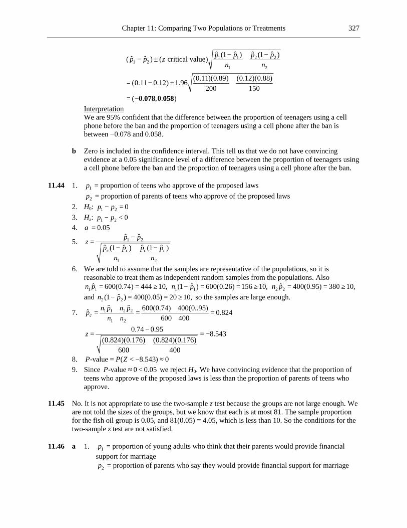
Chapter 11: Comparing Two Populations or Treatments 327
1 1 2 21 2
1 2
ˆ ˆ ˆ ˆ(1 ) (1 )ˆ ˆ( ) ( critical value)
(0.11)(0.89) (0.12)(0.88)(0.11 0.12) 1.96200 150
( . , . )
p p p pp p zn n− −
− ± +
= − ± +
= −0 078 0 058
Interpretation We are 95% confident that the difference between the proportion of teenagers using a cell
phone before the ban and the proportion of teenagers using a cell phone after the ban is between −0.078 and 0.058.
b Zero is included in the confidence interval. This tell us that we do not have convincing
evidence at a 0.05 significance level of a difference between the proportion of teenagers using a cell phone before the ban and the proportion of teenagers using a cell phone after the ban.
11.44 1. 1p = proportion of teens who approve of the proposed laws 2p = proportion of parents of teens who approve of the proposed laws 2. H0: 1 2 0p p− = 3. Ha: 1 2 0p p− < 4. 0.05α =
5. 1 2
1 2
ˆ ˆˆ ˆ ˆ ˆ(1 ) (1 )c c c c
p pzp p p p
n n
−=
− −+
6. We are told to assume that the samples are representative of the populations, so it is reasonable to treat them as independent random samples from the populations. Also
1 1ˆ 600(0.74) 444 10,n p = = ≥ 1 1ˆ(1 ) 600(0.26) 156 10,n p− = = ≥ 2 2ˆ 400(0.95) 380 10,n p = = ≥ and 2 2ˆ(1 ) 400(0.05) 20 10,n p− = = ≥ so the samples are large enough.
7. 1 1 2 2
1 2
ˆ ˆ 600(0.74) 400(0..95)ˆ 0.824600 400c
n p n ppn n
+ += = =
+ +
0.74 0.95 8.543(0.824)(0.176) (0.824)(0.176)
600 400
z −= = −
+
8. -value ( 8.543) 0P P Z= < − ≈ 9. Since -value 0 0.05P ≈ < we reject H0. We have convincing evidence that the proportion of
teens who approve of the proposed laws is less than the proportion of parents of teens who approve.
11.45 No. It is not appropriate to use the two-sample z test because the groups are not large enough. We
are not told the sizes of the groups, but we know that each is at most 81. The sample proportion for the fish oil group is 0.05, and 81(0.05) = 4.05, which is less than 10. So the conditions for the two-sample z test are not satisfied.
11.46 a 1. 1p = proportion of young adults who think that their parents would provide financial
support for marriage 2p = proportion of parents who say they would provide financial support for marriage
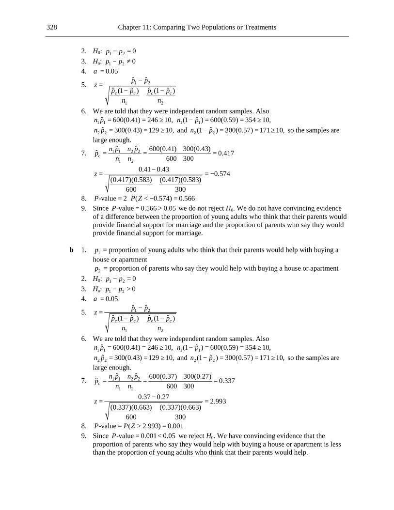
328 Chapter 11: Comparing Two Populations or Treatments
2. H0: 1 2 0p p− = 3. Ha: 1 2 0p p− ≠ 4. 0.05α =
5. 1 2
1 2
ˆ ˆˆ ˆ ˆ ˆ(1 ) (1 )c c c c
p pzp p p p
n n
−=
− −+
6. We are told that they were independent random samples. Also 1 1ˆ 600(0.41) 246 10,n p = = ≥ 1 1ˆ(1 ) 600(0.59) 354 10,n p− = = ≥
2 2ˆ 300(0.43) 129 10,n p = = ≥ and 2 2ˆ(1 ) 300(0.57) 171 10,n p− = = ≥ so the samples are large enough.
7. 1 1 2 2
1 2
ˆ ˆ 600(0.41) 300(0.43)ˆ 0.417600 300c
n p n ppn n
+ += = =
+ +
0.41 0.43 0.574(0.417)(0.583) (0.417)(0.583)
600 300
z −= = −
+
8. -value 2 ( 0.574) 0.566P P Z= ⋅ < − = 9. Since -value 0.566 0.05P = > we do not reject H0. We do not have convincing evidence
of a difference between the proportion of young adults who think that their parents would provide financial support for marriage and the proportion of parents who say they would provide financial support for marriage.
b 1. 1p = proportion of young adults who think that their parents would help with buying a
house or apartment 2p = proportion of parents who say they would help with buying a house or apartment 2. H0: 1 2 0p p− = 3. Ha: 1 2 0p p− > 4. 0.05α =
5. 1 2
1 2
ˆ ˆˆ ˆ ˆ ˆ(1 ) (1 )c c c c
p pzp p p p
n n
−=
− −+
6. We are told that they were independent random samples. Also 1 1ˆ 600(0.41) 246 10,n p = = ≥ 1 1ˆ(1 ) 600(0.59) 354 10,n p− = = ≥
2 2ˆ 300(0.43) 129 10,n p = = ≥ and 2 2ˆ(1 ) 300(0.57) 171 10,n p− = = ≥ so the samples are large enough.
7. 1 1 2 2
1 2
ˆ ˆ 600(0.37) 300(0.27)ˆ 0.337600 300c
n p n ppn n
+ += = =
+ +
0.37 0.27 2.993(0.337)(0.663) (0.337)(0.663)
600 300
z −= =
+
8. -value ( 2.993) 0.001P P Z= > = 9. Since -value 0.001 0.05P = < we reject H0. We have convincing evidence that the
proportion of parents who say they would help with buying a house or apartment is less than the proportion of young adults who think that their parents would help.
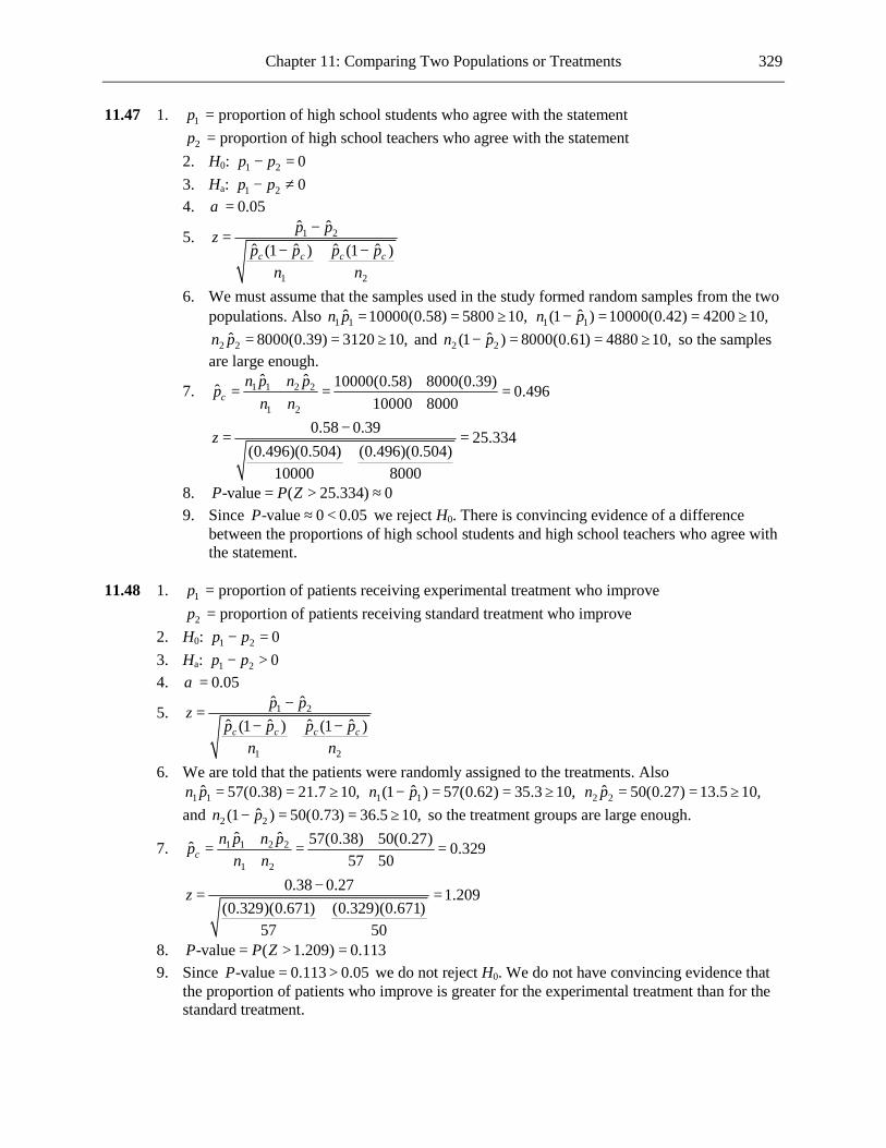
Chapter 11: Comparing Two Populations or Treatments 329
11.47 1. 1p = proportion of high school students who agree with the statement 2p = proportion of high school teachers who agree with the statement 2. H0: 1 2 0p p− = 3. Ha: 1 2 0p p− ≠ 4. 0.05α =
5. 1 2
1 2
ˆ ˆˆ ˆ ˆ ˆ(1 ) (1 )c c c c
p pzp p p p
n n
−=
− −+
6. We must assume that the samples used in the study formed random samples from the two populations. Also 1 1ˆ 10000(0.58) 5800 10,n p = = ≥ 1 1ˆ(1 ) 10000(0.42) 4200 10,n p− = = ≥
2 2ˆ 8000(0.39) 3120 10,n p = = ≥ and 2 2ˆ(1 ) 8000(0.61) 4880 10,n p− = = ≥ so the samples are large enough.
7. 1 1 2 2
1 2
ˆ ˆ 10000(0.58) 8000(0.39)ˆ 0.49610000 8000c
n p n ppn n
+ += = =
+ +
0.58 0.39 25.334(0.496)(0.504) (0.496)(0.504)
10000 8000
z −= =
+
8. -value ( 25.334) 0P P Z= > ≈ 9. Since -value 0 0.05P ≈ < we reject H0. There is convincing evidence of a difference
between the proportions of high school students and high school teachers who agree with the statement.
11.48 1. 1p = proportion of patients receiving experimental treatment who improve 2p = proportion of patients receiving standard treatment who improve 2. H0: 1 2 0p p− = 3. Ha: 1 2 0p p− > 4. 0.05α =
5. 1 2
1 2
ˆ ˆˆ ˆ ˆ ˆ(1 ) (1 )c c c c
p pzp p p p
n n
−=
− −+
6. We are told that the patients were randomly assigned to the treatments. Also 1 1ˆ 57(0.38) 21.7 10,n p = = ≥ 1 1ˆ(1 ) 57(0.62) 35.3 10,n p− = = ≥ 2 2ˆ 50(0.27) 13.5 10,n p = = ≥
and 2 2ˆ(1 ) 50(0.73) 36.5 10,n p− = = ≥ so the treatment groups are large enough.
7. 1 1 2 2
1 2
ˆ ˆ 57(0.38) 50(0.27)ˆ 0.32957 50c
n p n ppn n
+ += = =
+ +
0.38 0.27 1.209(0.329)(0.671) (0.329)(0.671)
57 50
z −= =
+
8. -value ( 1.209) 0.113P P Z= > = 9. Since -value 0.113 0.05P = > we do not reject H0. We do not have convincing evidence that
the proportion of patients who improve is greater for the experimental treatment than for the standard treatment.

330 Chapter 11: Comparing Two Populations or Treatments
11.49 Check of Conditions We are told that the samples were representative of college graduates in the two years. Also,
1 1ˆ 500(0.026) 13 10,n p = = ≥ 1 1ˆ(1 ) 500(0.974) 487 10,n p− = = ≥ 2 2ˆ 500(0.046) 23 10,n p = = ≥ and 2 2ˆ(1 ) 500(0.934) 477 10,n p− = = ≥ so the samples are large enough.
Calculation The 95% confidence interval for 1 2p p− is
1 1 2 21 2
1 2
ˆ ˆ ˆ ˆ(1 ) (1 )ˆ ˆ( ) ( critical value)
(0.026)(0.974) (0.046)(0.954)(0.026 0.046) 1.96500 500
p p p pp p zn n− −
− ± +
= − ± +
= (-0.043,0.003)
Interpretation of Interval We are 95% confident that the difference in the proportions of college graduates who were
unemployed in these two years (2008 minus 2009) is between −0.043 and 0.003. 11.50 a Check of Conditions We are told that the samples were independently selected and representative of high school
graduates in the two years. Also, 1 1ˆ 400(0.057) 22.8 10,n p = = ≥
1 1ˆ(1 ) 400(0.943) 377.2 10,n p− = = ≥ 2 2ˆ 400(0.097) 38.8 10,n p = = ≥ and
2 2ˆ(1 ) 500(0.903) 451.5 10,n p− = = ≥ so the samples are large enough. Calculation The 99% confidence interval for 1 2p p− is
1 1 2 21 2
1 2
ˆ ˆ ˆ ˆ(1 ) (1 )ˆ ˆ( ) ( critical value)
(0.057)(0.943) (0.097)(0.903)(0.057 0.097) 2.576400 400
p p p pp p zn n− −
− ± +
= − ± +
= (-0.088,0.008)
Interpretation of Interval We are 99% confident that the difference in the proportions of high school graduates who
were unemployed in these two years (2008 minus 2009) is between −0.088 and 0.008. b The width of the confidence interval in the previous exercise is 0.003 + 0.043 = 0.046.
The width of the confidence interval in Part (a) is 0.008 + 0.088 = 0.096. The confidence interval in Part (a) is wider, because the confidence level is greater than in the previous exercise and the samples were smaller than in the previous exercise.
11.51 1. 1p = proportion of parents who think that science and higher math are essential 2p = proportion of students in grades 6–12 who think that science and higher math are
essential 2. H0: 1 2 0p p− = 3. Ha: 1 2 0p p− ≠ 4. 0.05α =

Chapter 11: Comparing Two Populations or Treatments 331
5. 1 2
1 2
ˆ ˆˆ ˆ ˆ ˆ(1 ) (1 )c c c c
p pzp p p p
n n
−=
− −+
6. We are told that the samples were independently selected, but we need to assume that they were independent random samples from the populations. Also 1 1ˆ 1379(0.62) 855 10,n p = = ≥
1 1ˆ(1 ) 1379(0.38) 524 10,n p− = = ≥ 2 2ˆ 1342(0.5) 671 10,n p = = ≥ and
2 2ˆ(1 ) 1342(0.5) 671 10,n p− = = ≥ so the samples are large enough.
7. 1 1 2 2
1 2
ˆ ˆ 1379(0.62) 1342(0.5)ˆ 0.5611379 1342c
n p n ppn n
+ += = =
+ +
0.62 0.5 6.306(0.561)(0.439) (0.561)(0.439)
1379 1342
z −= =
+
8. -value 2 ( 6.306) 0P P Z= ⋅ > ≈ 9. Since -value 0 0.05P ≈ < we reject H0. We have convincing evidence that the proportion of
parents who regard science and mathematics as crucial is different from the corresponding proportion of students in grades 6–12.
11.52 a It is quite possible that a patient’s knowledge of being given one of the treatments will itself
contribute positively to the health of the patient, and that the effect of the knowledge of being given an injection might be greater than the corresponding effect of the knowledge of being given a nasal spray (or vice versa). Therefore, if the patients were given only one treatment or the other, then the greater effect of the knowledge of being given one treatment over the knowledge of being given the other might be confounded with the differing effects of the two ways of giving the vaccine.
b Check of Conditions We need to assume that the 8000 children were randomly assigned to the two treatments.
Also, we have 1 1ˆ 4000(0.086) 344 10,n p = = ≥ 1 1ˆ(1 ) 4000(0.914) 3656 10,n p− = = ≥
2 2ˆ 4000(0.039) 156 10,n p = = ≥ and 2 2ˆ(1 ) 4000(0.961) 3844 10,n p− = = ≥ so the samples are large enough.
Calculation The 99% confidence interval for 1 2p p− is
1 1 2 21 2
1 2
ˆ ˆ ˆ ˆ(1 ) (1 )ˆ ˆ( ) ( critical value)
(0.086)(0.914) (0.039)(0.961)(0.086 0.039) 2.5764000 4000
( . , . )
p p p pp p zn n− −
− ± +
= − ± +
= 0 033 0 061
Interpretation We are 99% confident that the proportion of children who get sick with the flu after being
vaccinated with an injection minus the proportion of children who get sick with the flu after being vaccinated with the nasal spray is between 0.033 and 0.061.
c Yes. Since zero is not included in the interval, we have convincing evidence at the 0.01
significance level that the proportions of children who get the flu are different for the two vaccination methods.

332 Chapter 11: Comparing Two Populations or Treatments
11.53 1. 1p = proportion of college graduates who have sunburn 2p = proportion of people without a high school degree who have sunburn 2. H0: 1 2 0p p− = 3. Ha: 1 2 0p p− > 4. 0.05α =
5. 1 2
1 2
ˆ ˆˆ ˆ ˆ ˆ(1 ) (1 )c c c c
p pzp p p p
n n
−=
− −+
6. We are told to assume that the samples were random samples from the populations. Also 1 1ˆ 200(0.43) 86 10,n p = = ≥ 1 1ˆ(1 ) 200(0.57) 114 10,n p− = = ≥ 2 2ˆ 200(0.25) 50 10,n p = = ≥
and 2 2ˆ(1 ) 200(0.75) 150 10,n p− = = ≥ so the samples are large enough.
7. 1 1 2 2
1 2
ˆ ˆ 200(0.43) 200(0.25)ˆ 0.34200 200c
n p n ppn n
+ += = =
+ +
0.43 0.25 3.800(0.34)(0.66) (0.34)(0.66)
200 200
z −= =
+
8. -value ( 3.800) 0P P Z= > ≈ 9. Since -value 0 0.05P ≈ < we reject H0. We have convincing evidence that the proportion
experiencing sunburn is greater for college graduates than it is for those without a high school degree.
11.54 a If 1ˆ sample proportion of Americans reporting major depression 0.09,p = = then
1 1 2 2
1 2
ˆ ˆ 5183(0.09) 3505(0.082)ˆ 0.087.5183 3505c
n p n ppn n
+ += = =
+ + Thus
0.09 0.082 1.300,(0.087)(0.913) (0.087)(0.913)
5183 3505
z −= =
+ and so -value ( 1.300) 0.097.P P Z= > =
Since this P-value is greater than 0.05, the difference in proportions is not significant, which is as stated in the article. Therefore, yes, the sample proportion of Americans reporting major depression could have been as large as 0.09.
b If 1ˆ sample proportion of Americans reporting major depression 0.1,p = = then
1 1 2 2
1 2
ˆ ˆ 5183(0.1) 3505(0.082)ˆ 0.093.5183 3505c
n p n ppn n
+ += = =
+ + Thus
0.1 0.082 2.838,(0.093)(0.907) (0.093)(0.907)
5183 3505
z −= =
+ and so -value ( 2.838) 0.0023.P P Z= > =
Since this P-value is less than 0.05, the difference in proportions is significant, which is not as is stated in the article. Therefore, no, the sample proportion of Americans reporting major depression could not have been as large as 0.10.
11.55 a 1. 1p = proportion of Austrian avid mountain bikers who have a low sperm count 2p = proportion of Austrian nonbikers who have a low sperm count

Chapter 11: Comparing Two Populations or Treatments 333
2. H0: 1 2 0p p− = 3. Ha: 1 2 0p p− > 4. 0.05α =
5. 1 2
1 2
ˆ ˆˆ ˆ ˆ ˆ(1 ) (1 )c c c c
p pzp p p p
n n
−=
− −+
6. We are told to assume that the percentages were based on independent samples and that the samples were representative of Austrian avid mountain bikers and nonbikers. So it is reasonable to assume that the samples were independent random samples. Also
1 1ˆ 100(0.9) 90 10,n p = = ≥ 1 1ˆ(1 ) 100(0.1) 10 10,n p− = = ≥ 2 2ˆ 100(0.26) 26 10,n p = = ≥ and 2 2ˆ(1 ) 100(0.74) 74 10,n p− = = ≥ so the samples are large enough.
7. 1 1 2 2
1 2
ˆ ˆ 100(0.9) 100(0.26)ˆ 0.58100 100c
n p n ppn n
+ += = =
+ +
0.9 0.26 9.169(0.58)(0.42) (0.58)(0.42)
100 100
z −= =
+
8. -value ( 9.169) 0P P Z= > ≈ 9. Since -value 0 0.05P ≈ < we reject H0. We have convincing evidence that the proportion
of Austrian avid mountain bikers with a low sperm count is higher than the equivalent proportion for Austrian nonbikers.
b No. Since this is an observational study, causation cannot be inferred from the result. It could
be suggested that, for example, Austrian men who have low sperm counts have a tendency to choose mountain biking as a hobby.
11.56 Letting 1 proportion of women receiving a mastectomy who survive for 20 yearsp = and
2 proportion of women receiving a lumpectomy who survive for 20 years,p = the hypotheses tested would have been H0: 1 2 0p p− = versus Ha: 1 2 0.p p− ≠ The null hypothesis was not rejected.
11.57 Since the data given are population characteristics an inference procedure is not applicable. It is
known that the rate of Lou Gehrig’s disease amongst soldiers sent to the war is higher than for those not sent to the war.
11.58 a Random assignment is important in order to create comparable treatment groups in terms of
the participants’ attitudes to money. Also, random assignment is required for the hypothesis test used to analyze the results.
b 1 22 2 2 21 2
1 2
( ) 0 0.77 1.34 2.1220.74 1.02
22 22
x xts sn n
− − −= = = −
+ +

334 Chapter 11: Comparing Two Populations or Treatments
( ) ( ) ( ) ( )
2 22 2 2 21 2
1 22 2 2 22 2 2 2
1 1 2 2
1 2
0.74 1.0222 22
df 38.3110.74 22 1.02 22
1 1 21 21
s sn n
s n s nn n
+ +
= = =
+ +− −
Hence, 38.311-value ( 2.122) 0.020,P P t= < − = which is less than 0.05, as stated. c Since neither of the treatment groups was of size greater than 30, we need to assume that the
two population distributions of donation amounts are approximately normal. This seems to be an invalid assumption in both cases, since the distance of zero below the sample mean is as little as 1.0 sample standard deviations for the “money primed” group and as little as 1.3 sample standard deviations for the control group, and since negative donations are not possible.
11.59 a First hypothesis test 1p = proportion of those receiving the intervention whose references to sex decrease to zero 2p = proportion of those not receiving the intervention whose references to sex decrease to
zero H0: 1 2 0p p− = Ha: 1 2 0p p− ≠ (Note: We know that the researchers were using two-sided alternative hypotheses, otherwise
the P-value greater than 0.5 in the second hypothesis test would not have been possible for the given results.)
Since P-value = 0.05, H0 is rejected at the 0.05 level. Second hypothesis test 1p = proportion of those receiving the intervention whose references to substance abuse
decrease to zero 2p = proportion of those not receiving the intervention whose references to substance abuse
decrease to zero H0: 1 2 0p p− = Ha: 1 2 0p p− ≠ Since P-value = 0.61, H0 is not rejected at the 0.05 level. Third hypothesis test 1p = proportion of those receiving the intervention whose profiles are set to “private” at
follow-up 2p = proportion of those not receiving the intervention whose profiles are set to “private” at
follow-up H0: 1 2 0p p− = Ha: 1 2 0p p− ≠ Since P-value = 0.45, H0 is not rejected at the 0.05 level. Fourth hypothesis test 1p = proportion of those receiving the intervention whose profiles show any of the three
protective changes

Chapter 11: Comparing Two Populations or Treatments 335
2p = proportion of those not receiving the intervention whose profiles show any of the three
protective changes H0: 1 2 0p p− = Ha: 1 2 0p p− ≠ Since P-value = 0.07, H0 is not rejected at the 0.05 level. b If we want to know whether the email intervention reduces (as opposed to changes)
adolescents’ display of risk behavior in their profiles, then we use one-sided alternative hypotheses and the P-values are halved. If that is the case, using a 0.05 significance level, we are convinced that the intervention is effective with regard to reduction of references to sex and that the proportion showing any of the three protective changes is greater for those receiving the email intervention. Each of the other two apparently reduced proportions could have occurred by chance.
11.60 a 1. 1µ = mean cohabitation endorsement for emerging adult men 2µ = mean cohabitation endorsement for emerging adult women 2. H0: 1 2 0µ µ− = 3. Ha: 1 2 0µ µ− > 4. 0.05α =
5. 1 2 1 22 2 2 21 2 1 2
1 2 1 2
( ) (hypothesized value) ( ) 0x x x xts s s sn n n n
− − − −= =
+ +
6. We need to assume that the samples of men and women were selected in such a way as to be representative of men and women at these five colleges (which then justifies our treating the samples as random samples from these populations). Also 1 307 30n = ≥ and
2 481 30n = ≥ , so we can proceed with the two-sample t test.
7. 2 2
3.75 3.39 4.1251.21 1.17307 481
t −= =
+
8. df = 635.834 635.834-value ( 4.125) 0P P t= > ≈ 9. Since -value 0 0.05P ≈ < we reject H0. We have convincing evidence that the mean
cohabitation endorsement for emerging adult women is less than the mean for emerging adult men, for students at these five colleges.
b In order to generalize the conclusion to all college students we would need to know, in
addition to the assumption in Step 6 above, that students at the five colleges were representative of students in general.
11.61 a 1. 1µ = mean appropriateness score assigned to wearing a hat in class for students 2µ = mean appropriateness score assigned to wearing a hat in class for faculty 2. H0: 1 2 0µ µ− = 3. Ha: 1 2 0µ µ− ≠ 4. 0.05α =

336 Chapter 11: Comparing Two Populations or Treatments
5. 1 2 1 22 2 2 21 2 1 2
1 2 1 2
( ) (hypothesized value) ( ) 0x x x xts s s sn n n n
− − − −= =
+ +
6. We are told that the samples were random samples from the populations. Also 1 173 30n = ≥ and 2 98 30n = ≥ , so we can proceed with the two-sample t test.
7. 2 2
2.80 3.63 6.5651.0 1.0173 98
t −= = −
+
8. df = 201.549 201.549-value 2 ( 6.565) 0P P t= ⋅ < − ≈ 9. Since -value 0 0.05P ≈ < we reject H0. We have convincing evidence that the mean
appropriateness score assigned to wearing a hat in class differs for students and faculty. b 1. 1µ = mean appropriateness score assigned to addressing an instructor by his/her first
name for students 2µ = mean appropriateness score assigned to addressing an instructor by his/her first
name for faculty 2. H0: 1 2 0µ µ− = 3. Ha: 1 2 0µ µ− > 4. 0.05α =
5. 1 2 1 22 2 2 21 2 1 2
1 2 1 2
( ) (hypothesized value) ( ) 0x x x xts s s sn n n n
− − − −= =
+ +
6. We are told that the samples were random samples from the populations. Also 1 173 30n = ≥ and 2 98 30n = ≥ , so we can proceed with the two-sample t test.
7. 2 2
2.90 2.11 6.2491.0 1.0173 98
t −= =
+
8. df = 201.549 201.549-value ( 6.249) 0P P t= > ≈ 9. Since -value 0 0.05P ≈ < we reject H0. We have convincing evidence that the mean
appropriateness score assigned to addressing an instructor by his/her first name is greater for students than for faculty.
c 1. 1µ = mean appropriateness score assigned to talking on a cell phone in class for students 2µ = mean appropriateness score assigned to talking on a cell phone in class for faculty 2. H0: 1 2 0µ µ− = 3. Ha: 1 2 0µ µ− ≠ 4. 0.05α =
5. 1 2 1 22 2 2 21 2 1 2
1 2 1 2
( ) (hypothesized value) ( ) 0x x x xts s s sn n n n
− − − −= =
+ +

Chapter 11: Comparing Two Populations or Treatments 337
6. We are told that the samples were random samples from the populations. Also
1 173 30n = ≥ and 2 98 30n = ≥ , so we can proceed with the two-sample t test.
7. 2 2
1.11 1.10 0.0791.0 1.0173 98
t −= =
+
8. df = 201.549 201.549-value 2 ( 0.079) 0.937P P t= ⋅ > = 9. Since -value 0.469 0.05P = > we do not reject H0. We do not have convincing evidence
that the mean appropriateness score assigned to talking on a cell phone in class differs for students and faculty.
d No, the result does not imply that students and faculty consider it acceptable to talk on a cell
phone during class. In fact, the low sample mean ratings for both students and faculty show that both groups on the whole feel that the behavior is inappropriate.
11.62 a Check of Conditions First, 1 203 30n = ≥ and 2 224 30.n = ≥ Second, we are told that the samples were randomly
selected. Thus we can proceed with construction of a two-sample t interval. Calculation df = 409.204. The 99% confidence interval for 1 2µ µ− is
2 21 2
1 21 2
2 2
( ) ( critical value)
1.49 1.35(3.42 2.42) 2.588203 224
( . , . )
s sx x tn n
− ± +
= − ± +
= 0 643 1 357
Interpretation We are 99% confident that the mean intended number of science courses for males minus the
mean intended number of science courses for females is between 0.643 and 1.357. b Since zero is not included in the confidence interval, we can be very confident that girls are
inclined to enroll in fewer science courses than boys.

338 Chapter 11: Comparing Two Populations or Treatments
11.63 Initial After 9 Days
Treatment Control Treatment Control Difference (Init − 9 Day, for Trtmnt Grp)
Difference (Init − 9 Day, for Cntrl Grp)
11.4 9.1 138.3 9.3 -126.9 -0.2 9.6 8.7 104 8.8 -94.4 -0.1 10.1 9.7 96.4 8.8 -86.3 0.9 8.5 10.8 89 10.1 -80.5 0.7 10.3 10.9 88 9.6 -77.7 1.3 10.6 10.6 103.8 8.6 -93.2 2 11.8 10.1 147.3 10.4 -135.5 -0.3 9.8 12.3 97.1 12.4 -87.3 -0.1 10.9 8.8 172.6 9.3 -161.7 -0.5 10.3 10.4 146.3 9.5 -136 0.9 10.2 10.9 99 8.4 -88.8 2.5 11.4 10.4 122.3 8.7 -110.9 1.7 9.2 11.6 103 12.5 -93.8 -0.9 10.6 10.9 117.8 9.1 -107.2 1.8 10.8 121.5 -110.7 8.2 93 -84.8
a 1. dµ = mean difference in selenium level (initial level − 9-day level) for cows receiving
supplement 2. H0: 0dµ = 3. Ha: 0dµ < 4. 0.05α =
5. hypothesized valued
d
xts n
−=
6.
-70-80-90-100-110-120-130-140-150-160Difference
The boxplot shows a distribution of sample differences that is negatively skewed, but in a
small sample (along with the fact that there are no outliers) this is nonetheless consistent with an assumption of normality in the population of differences. Additionally, we need to assume that the cows who received the supplement form a random sample from the set of all cows.
7. 104.731, 24.101d dx s= − =
104.731 0 17.38224.101 16
t − −= = −
8. df = 15 15-value ( 17.382) 0P P t= < − ≈

Chapter 11: Comparing Two Populations or Treatments 339
9. Since -value 0 0.05P ≈ < we reject H0. We have convincing evidence that the mean
selenium concentration is greater after 9 days of the selenium supplement. b 1. dµ = mean difference in selenium level (initial level − 9-day level) for cows not
receiving supplement 2. H0: 0dµ = 3. Ha: 0dµ ≠ 4. 0.05α =
5. hypothesized valued
d
xts n
−=
6.
3210-1Difference
Since the boxplot is roughly symmetrical and there are no outliers we are justified in
assuming a normal distribution for the population of differences. Additionally, we need to assume that the cows who did not receive the supplement form a random sample from the set of all cows.
7. 0.693, 1.062d dx s= =
0.693 0 2.4401.062 14
t −= =
8. df = 13 13-value 2 ( 2.440) 0.030P P t= ⋅ > = 9. Since -value 0.030 0.05P = < we reject H0. At the 0.05 level the results are inconsistent
with the hypothesis of no significant change in mean selenium concentration over the 9-day period for cows that did not receive the supplement.
c No, the paired t test would not be appropriate since the treatment and control groups were not
paired samples. 11.64
Hospital
Inpatient Ratio
Outpatient Ratio
Difference
1 68 54 14 2 100 75 25 3 71 53 18 4 74 56 18 5 100 74 26 6 83 71 12
1. dµ = mean difference in ratios (inpatient − outpatient) 2. H0: 0dµ = 3. Ha: 0dµ >

340 Chapter 11: Comparing Two Populations or Treatments
4. 0.05α =
5. hypothesized valued
d
xts n
−=
6.
262422201816141210Difference
The boxplot shows that the distribution of the differences is roughly symmetrical and has no
outliers, so we are justified in assuming that the population of differences is normally distributed. Additionally, we need to assume that this set of hospitals was randomly selected from the set of all hospitals in Oregon.
7. 18.833, 5.672d dx s= =
18.833 0 8.1345.672 6
t −= =
8. df = 5 5-value ( 8.134) 0P P t= > ≈ 9. Since -value 0 0.05P ≈ < we reject H0. We have convincing evidence that the mean cost-to-
charge ratio for Oregon hospitals is lower for outpatient care than for inpatient care. 11.65 1. 1p = proportion of resumes with “white-sounding” names that receive responses 2p = proportion of resumes with “black-sounding” names that receive responses 2. H0: 1 2 0p p− = 3. Ha: 1 2 0p p− > 4. 0.05α =
5. 1 2
1 2
ˆ ˆˆ ˆ ˆ ˆ(1 ) (1 )c c c c
p pzp p p p
n n
−=
− −+
6. We need to assume that the 5000 jobs applied for were randomly assigned to the names used. Also, 1 1ˆ 2500(250 2500) 250 10,n p = = ≥ 1 1ˆ(1 ) 2500(2250 2500) 2250 10,n p− = = ≥
2 2ˆ 2500(167 2500) 167 10,n p = = ≥ and 2 2ˆ(1 ) 2500(2333 2500) 2333 10,n p− = = ≥ so the samples are large enough.
7. 250 167 417ˆ2500 2500 5000cp +
= =+
250 2500 167 2500 4.245(417 5000)(4583 5000) (417 5000)(4583 5000)
2500 2500
z −= =
+
8. -value ( 4.245) 0P P Z= > ≈ 9. Since -value 0 0.05P ≈ < we reject H0. We have convincing evidence that the proportion
eliciting responses is higher for “white-sounding” first names.
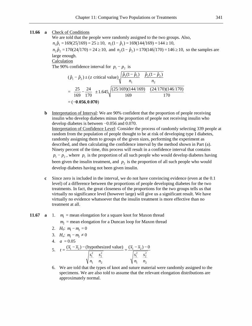
Chapter 11: Comparing Two Populations or Treatments 341
11.66 a Check of Conditions We are told that the people were randomly assigned to the two groups. Also,
1 1ˆ 169(25 169) 25 10,n p = = ≥ 1 1ˆ(1 ) 169(144 169) 144 10,n p− = = ≥
2 2ˆ 170(24 170) 24 10,n p = = ≥ and 2 2ˆ(1 ) 170(146 170) 146 10,n p− = = ≥ so the samples are large enough.
Calculation The 90% confidence interval for 1 2p p− is
1 1 2 21 2
1 2
ˆ ˆ ˆ ˆ(1 ) (1 )ˆ ˆ( ) ( critical value)
25 24 (25 169)(144 169) (24 170)(146 170)1.645169 170 169 170
( . , . )
p p p pp p zn n− −
− ± +
= − ± +
= −0 056 0 070
b Interpretation of Interval: We are 90% confident that the proportion of people receiving
insulin who develop diabetes minus the proportion of people not receiving insulin who develop diabetes is between −0.056 and 0.070. Interpretation of Confidence Level: Consider the process of randomly selecting 339 people at random from the population of people thought to be at risk of developing type I diabetes, randomly assigning them to groups of the given sizes, performing the experiment as described, and then calculating the confidence interval by the method shown in Part (a). Ninety percent of the time, this process will result in a confidence interval that contains
1 2p p− , where 1p is the proportion of all such people who would develop diabetes having been given the insulin treatment, and 2p is the proportion of all such people who would develop diabetes having not been given insulin.
c Since zero is included in the interval, we do not have convincing evidence (even at the 0.1
level) of a difference between the proportions of people developing diabetes for the two treatments. In fact, the great closeness of the proportions for the two groups tells us that virtually no significance level (however large) will give us a significant result. We have virtually no evidence whatsoever that the insulin treatment is more effective than no treatment at all.
11.67 a 1. 1µ = mean elongation for a square knot for Maxon thread 2µ = mean elongation for a Duncan loop for Maxon thread 2. H0: 1 2 0µ µ− = 3. Ha: 1 2 0µ µ− ≠ 4. 0.05α =
5. 1 2 1 22 2 2 21 2 1 2
1 2 1 2
( ) (hypothesized value) ( ) 0x x x xts s s sn n n n
− − − −= =
+ +
6. We are told that the types of knot and suture material were randomly assigned to the specimens. We are also told to assume that the relevant elongation distributions are approximately normal.

342 Chapter 11: Comparing Two Populations or Treatments
7. 2 2
10 11 11.9520.1 0.310 15
t −= = −
+
8. df = 18.266 18.266-value 2 ( 11.952) 0P P t= ⋅ < − ≈ 9. Since -value 0 0.05P ≈ < we reject H0. We have convincing evidence that the mean
elongations for the square knot and the Duncan loop for Maxon thread are different. b 1. 1µ = mean elongation for a square knot for Ticron thread 2µ = mean elongation for a Duncan loop for Ticron thread 2. H0: 1 2 0µ µ− = 3. Ha: 1 2 0µ µ− ≠ 4. 0.05α =
5. 1 2 1 22 2 2 21 2 1 2
1 2 1 2
( ) (hypothesized value) ( ) 0x x x xts s s sn n n n
− − − −= =
+ +
6. We are told that the types of knot and suture material were randomly assigned to the specimens. We are also told to assume that the relevant elongation distributions are approximately normal.
7. 2 2
2.5 10.9 68.8030.06 0.4
10 11
t −= = −
+
8. df = 10.494 10.494-value 2 ( 68.803) 0P P t= ⋅ < − ≈ 9. Since -value 0 0.05P ≈ < we reject H0. We have convincing evidence that the mean
elongations for the square knot and the Duncan loop for Ticron thread are different. c 1. 1µ = mean elongation for a Duncan loop for Maxon thread 2µ = mean elongation for a Duncan loop for Ticron thread 2. H0: 1 2 0µ µ− = 3. Ha: 1 2 0µ µ− ≠ 4. 0.05α =
5. 1 2 1 22 2 2 21 2 1 2
1 2 1 2
( ) (hypothesized value) ( ) 0x x x xts s s sn n n n
− − − −= =
+ +
6. We are told that the types of knot and suture material were randomly assigned to the specimens. We are also told to assume that the relevant elongation distributions are approximately normal.
7. 2 2
11 10.9 0.6980.3 0.415 11
t −= =
+
8. df = 17.789 17.789-value 2 ( 0.698) 0.494P P t= ⋅ > =

Chapter 11: Comparing Two Populations or Treatments 343
9. Since -value 0.697 0.05P = > we do not reject H0. We do not have convincing evidence
that the mean elongations for the Duncan loop for Maxon thread and Ticron thread are different.
11.68 a Yes. The p value for this test is given to be less than 0.001. b Yes. The p value for this test is given to be less than 0.05. c No. We are only given information concerning the distance apart of the means for male trial
and nontrial lawyers and the distance apart of the means for female trial and nontrial lawyers. We have no information concerning a comparison of the two sexes. In order to conduct the test we would need the values of the sample means for male and female trial lawyers, along with the associated sample standard deviations.
11.69
Subject 1 2 3 4 5 6 7 8 1 hr later 14 12 18 7 11 9 16 15 24 hr later 10 4 14 6 9 6 12 12 Difference 4 8 4 1 2 3 4 3
1. dµ = mean difference in number of objects remembered (1 hr − 24 hours) 2. H0: 3dµ = 3. Ha: 3dµ > 4. 0.01α =
5. hypothesized valued
d
xts n
−=
6.
876543210Difference
The boxplot is roughly symmetrical but there is one outlier. Nonetheless we will assume that
the population distribution of differences is normal. We are told that the eight students were selected at random from the large psychology class.
7. 3.625, 2.066d dx s= =
3.625 3 0.8562.066 8
t −= =
8. df = 7 7-value ( 0.856) 0.210P P t= > = 9. Since -value 0.210 0.01P = > we do not reject H0. We do not have convincing evidence that
the mean number of words recalled after 1 hour exceeds the mean number recalled after 24 hours by more than 3.
11.70 a In each case the standard deviation of the differences is large compared to the magnitude of
the mean. This can be the case, since differences can be negative. (Also, the large standard
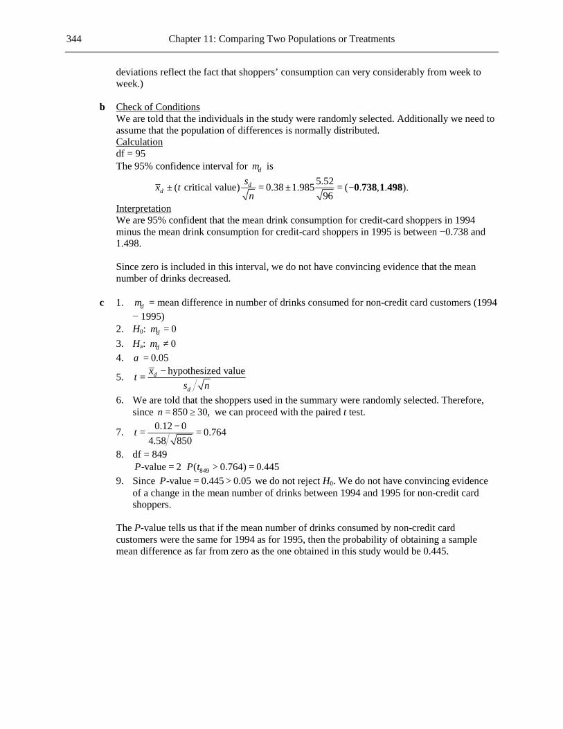
344 Chapter 11: Comparing Two Populations or Treatments
deviations reflect the fact that shoppers’ consumption can very considerably from week to week.)
b Check of Conditions We are told that the individuals in the study were randomly selected. Additionally we need to
assume that the population of differences is normally distributed. Calculation df = 95 The 95% confidence interval for dµ is
5.52( critical value) 0.38 1.985 ( . , . ).96
dd
sx tn
± = ± = −0 738 1 498
Interpretation We are 95% confident that the mean drink consumption for credit-card shoppers in 1994
minus the mean drink consumption for credit-card shoppers in 1995 is between −0.738 and 1.498. Since zero is included in this interval, we do not have convincing evidence that the mean number of drinks decreased.
c 1. dµ = mean difference in number of drinks consumed for non-credit card customers (1994
− 1995) 2. H0: 0dµ = 3. Ha: 0dµ ≠ 4. 0.05α =
5. hypothesized valued
d
xts n
−=
6. We are told that the shoppers used in the summary were randomly selected. Therefore, since 850 30,n = ≥ we can proceed with the paired t test.
7. 0.12 0 0.7644.58 850
t −= =
8. df = 849 849-value 2 ( 0.764) 0.445P P t= ⋅ > = 9. Since -value 0.445 0.05P = > we do not reject H0. We do not have convincing evidence
of a change in the mean number of drinks between 1994 and 1995 for non-credit card shoppers.
The P-value tells us that if the mean number of drinks consumed by non-credit card
customers were the same for 1994 as for 1995, then the probability of obtaining a sample mean difference as far from zero as the one obtained in this study would be 0.445.

Chapter 11: Comparing Two Populations or Treatments 345
11.71
Specimen Direct Stratified Difference 1 24 8 16 2 32 36 -4 3 0 8 -8 4 60 56 4 5 20 52 -32 6 64 64 0 7 40 28 12 8 8 8 0 9 12 8 4 10 92 100 -8 11 4 0 4 12 68 56 12 13 76 68 8 14 24 52 -28 15 32 28 4 16 0 0 0 17 36 36 0 18 16 12 4 19 92 92 0 20 4 12 -8 21 40 48 -8 22 24 24 0 23 0 0 0 24 8 12 -4 25 12 40 -28 26 16 12 4 27 40 76 -36
1. dµ = mean difference in number of seeds detected (direct − stratified) 2. H0: 0dµ = 3. Ha: 0dµ ≠ 4. 0.05α =
5. hypothesized valued
d
xts n
−=
6.
20100-10-20-30-40Difference
The boxplot shows a distribution of differences that is negatively skewed and has three
outliers, and so the assumption that the population distribution of differences is normal is dubious. Nonetheless we will proceed with caution. Additionally, we need to assume that this set of 27 soil samples forms a random sample from the population of soil samples.

346 Chapter 11: Comparing Two Populations or Treatments
7. 3.407, 13.253d dx s= − =
3.407 0 1.33613.253 27
t − −= = −
8. df = 26 26-value 2 ( 1.336) 0.193P P t= ⋅ < − = 9. Since -value 0.193 0.05P = > we do not reject H0. We do not have convincing evidence that
the mean number of seeds detected differs for the two methods. 11.72 Check of Conditions We are told that the samples were randomly selected from the two populations. Also,
1 1ˆ 94(50 94) 50 10,n p = = ≥ 1 1ˆ(1 ) 94(44 94) 44 10,n p− = = ≥ 2 2ˆ 94(56 94) 56 10,n p = = ≥ and
2 2ˆ(1 ) 94(38 94) 38 10,n p− = = ≥ so the samples are large enough. Calculation The 95% confidence interval for 1 2p p− is
1 1 2 21 2
1 2
ˆ ˆ ˆ ˆ(1 ) (1 )ˆ ˆ( ) ( critical value)
50 56 (50 94)(44 94) (56 94)(38 94)1.9694 94 94 94
( . , . )
p p p pp p zn n− −
− ± +
= − ± +
= −0 205 0 078
Interpretation of Interval We are 95% confident that 1 2p p− lies between −0.205 and 0.078, where 1p is the proportion of
all students who did not participate in an orientation course who returned for a second year and 2p is the proportion of all students who did take an orientation course who returned for a second
year.
11.73 1. 1p = proportion of high school seniors exposed to the drug program who use marijuana 2p = proportion of high school seniors not exposed to the drug program who use marijuana 2. H0: 1 2 0p p− = 3. Ha: 1 2 0p p− < 4. 0.05α =
5. 1 2
1 2
ˆ ˆˆ ˆ ˆ ˆ(1 ) (1 )c c c c
p pzp p p p
n n
−=
− −+
6. We are told that the samples were random samples from the populations. Also 1 1ˆ 288(141 288) 141 10,n p = = ≥ 1 1ˆ(1 ) 288(147 288) 147 10,n p− = = ≥
2 2ˆ 335(181 335) 181 10,n p = = ≥ and 2 2ˆ(1 ) 335(154 335) 154 10,n p− = = ≥ so the samples are large enough.
7. 141 181 322ˆ288 335 623cp +
= =+
141 288 181 335 1.263(322 623)(301 623) (322 623)(301 623)
288 335
z −= = −
+
8. -value ( 1.263) 0.103P P Z= < − =

Chapter 11: Comparing Two Populations or Treatments 347
9. Since -value 0.103 0.05P = > we do not reject H0. We do not have convincing evidence that
the proportion using marijuana is lower for students exposed to the DARE program. 11.74 a 1. 1p = proportion of games with stationary bases where a player suffers a sliding injury 2p = proportion of games with breakaway bases where a player suffers a sliding injury 2. H0: 1 2 0p p− = 3. Ha: 1 2 0p p− > 4. 0.01α =
5. 1 2
1 2
ˆ ˆˆ ˆ ˆ ˆ(1 ) (1 )c c c c
p pzp p p p
n n
−=
− −+
6. We need to assume that the 2500 games used in the study were randomly assigned to the two treatments (stationary bases and breakaway bases). Also, we have
1 1ˆ 1250(90 1250) 90 10,n p = = ≥ 1 1ˆ(1 ) 1250(1160 1250) 1160 10,n p− = = ≥
2 2ˆ 1250(20 1250) 20 10,n p = = ≥ and 2 2ˆ(1 ) 1250(1230 1250) 1230 10,n p− = = ≥ so the samples are large enough.
7. 90 20 110ˆ1250 1250 2500cp +
= =+
90 1250 20 1250 6.826(110 2500)(2390 2500) (110 2500)(2390 2500)
1250 1250
z −= =
+
8. -value ( 6.826) 0P P Z= > ≈ 9. Since -value 0 0.01P ≈ < we reject H0. We have convincing evidence that the use of
breakaway bases reduces the proportion of games with a player suffering a sliding injury. b Since the conclusion states that use of breakaway bases reduces the proportion of games with
a player suffering a sliding injury (that is, causes a lower proportion of games with sliding injuries), we need to assume that this was an experiment in which the 2500 games were randomly assigned to the two treatments (stationary bases and breakaway bases). It seems more likely that the treatments were assigned by league (or by region of the country), in which case it would be difficult to argue that each treatment group was representative of all games in terms of sliding injuries.
11.75 Check of Conditions We are told that the samples were random samples from the two communities. Also,
1 1ˆ 119(67 119) 67 10,n p = = ≥ 1 1ˆ(1 ) 119(52 119) 52 10,n p− = = ≥
2 2ˆ 143(106 143) 106 10,n p = = ≥ and 2 2ˆ(1 ) 143(37 143) 37 10,n p− = = ≥ so the samples are large enough.
Calculation The 90% confidence interval for 1 2p p− is
1 1 2 21 2
1 2
ˆ ˆ ˆ ˆ(1 ) (1 )ˆ ˆ( ) ( critical value) p p p pp p zn n− −
− ± +
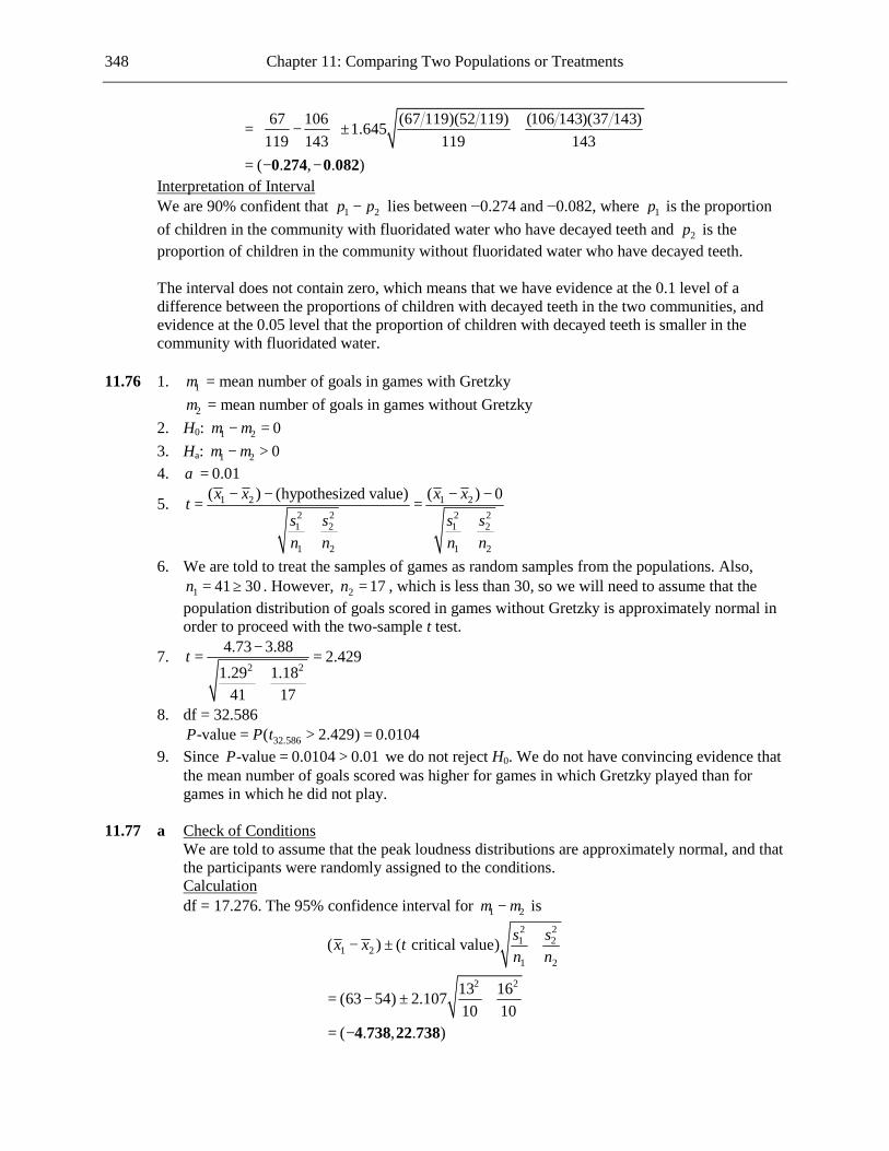
348 Chapter 11: Comparing Two Populations or Treatments
67 106 (67 119)(52 119) (106 143)(37 143)1.645119 143 119 143
( . , . )
= − ± +
= − −0 274 0 082
Interpretation of Interval We are 90% confident that 1 2p p− lies between −0.274 and −0.082, where 1p is the proportion
of children in the community with fluoridated water who have decayed teeth and 2p is the proportion of children in the community without fluoridated water who have decayed teeth.
The interval does not contain zero, which means that we have evidence at the 0.1 level of a
difference between the proportions of children with decayed teeth in the two communities, and evidence at the 0.05 level that the proportion of children with decayed teeth is smaller in the community with fluoridated water.
11.76 1. 1µ = mean number of goals in games with Gretzky 2µ = mean number of goals in games without Gretzky 2. H0: 1 2 0µ µ− = 3. Ha: 1 2 0µ µ− > 4. 0.01α =
5. 1 2 1 22 2 2 21 2 1 2
1 2 1 2
( ) (hypothesized value) ( ) 0x x x xts s s sn n n n
− − − −= =
+ +
6. We are told to treat the samples of games as random samples from the populations. Also, 1 41 30n = ≥ . However, 2 17n = , which is less than 30, so we will need to assume that the
population distribution of goals scored in games without Gretzky is approximately normal in order to proceed with the two-sample t test.
7. 2 2
4.73 3.88 2.4291.29 1.18
41 17
t −= =
+
8. df = 32.586 32.586-value ( 2.429) 0.0104P P t= > = 9. Since -value 0.0104 0.01P = > we do not reject H0. We do not have convincing evidence that
the mean number of goals scored was higher for games in which Gretzky played than for games in which he did not play.
11.77 a Check of Conditions We are told to assume that the peak loudness distributions are approximately normal, and that
the participants were randomly assigned to the conditions. Calculation df = 17.276. The 95% confidence interval for 1 2µ µ− is
2 21 2
1 21 2
2 2
( ) ( critical value)
13 16(63 54) 2.10710 10
( . , . )
s sx x tn n
− ± +
= − ± +
= −4 738 22 738

Chapter 11: Comparing Two Populations or Treatments 349
Interpretation We are 95% confident that the difference in mean loudness for open mouthed and closed
mouthed eating of potato chips is between −4.738 and 22.738. b 1. 1µ = mean loudness for potato chips (closed-mouth chewing) 2µ = mean loudness for tortilla chips (closed-mouth chewing) 2. H0: 1 2 0µ µ− = 3. Ha: 1 2 0µ µ− ≠ 4. 0.01α =
5. 1 2 1 22 2 2 21 2 1 2
1 2 1 2
( ) (hypothesized value) ( ) 0x x x xts s s sn n n n
− − − −= =
+ +
6. We are told to assume that the peak loudness distributions are approximately normal, and that the participants were randomly assigned to the conditions.
7. 2 2
54 53 0.14016 1610 10
t −= =
+
8. df = 18 18-value 2 ( 0.140) 0.890P P t= ⋅ > = 9. Since -value 0.890 0.01P = > we do not reject H0. We do not have convincing evidence
of a difference between potato chips and tortilla chips with respect to mean peak loudness (closed-mouth chewing).
c 1. 1µ = mean loudness for stale tortilla chips (closed-mouth chewing) 2µ = mean loudness for fresh tortilla chips (closed-mouth chewing) 2. H0: 1 2 0µ µ− = 3. Ha: 1 2 0µ µ− < 4. 0.05α =
5. 1 2 1 22 2 2 21 2 1 2
1 2 1 2
( ) (hypothesized value) ( ) 0x x x xts s s sn n n n
− − − −= =
+ +
6. We are told to assume that the peak loudness distributions are approximately normal, and that the participants were randomly assigned to the conditions.
7. 2 2
53 56 0.44616 1410 10
t −= = −
+
8. df = 17.688 17.688-value ( 0.446) 0.330P P t= < − = 9. Since -value 0.330 0.05P = > we do not reject H0. We do not have convincing evidence
that fresh tortilla chips are louder than stale tortilla chips. 11.78 1. 1µ = mean number of imitations with a human model 2µ = mean number of imitations with doll model

350 Chapter 11: Comparing Two Populations or Treatments
2. H0: 1 2 0µ µ− = 3. Ha: 1 2 0µ µ− > 4. 0.01α =
5. 1 2 1 22 2 2 21 2 1 2
1 2 1 2
( ) (hypothesized value) ( ) 0x x x xts s s sn n n n
− − − −= =
+ +
6. We need to assume that the infants were randomly assigned to the treatments (human model and doll model). Both of the sample sizes were less than 30, so we need to assume, also, that the population distributions of numbers of imitations are approximately normal.
7. 2 2
5.14 3.46 2.9421.6 1.312 15
t −= =
+
8. df = 21.069 21.069-value ( 2.942) 0.004P P t= > = 9. Since -value 0.004 0.01P = < we reject H0. We have convincing evidence that the mean
number of imitations is higher for infants who watch a human model than for infants who watch a doll.
11.79 a 1. dµ = mean difference in systolic blood pressure between dental setting and medical
setting (dental − medical) 2. H0: 0dµ = 3. Ha: 0dµ > 4. 0.01α =
5. hypothesized valued
d
xts n
−=
6. We need to assume that the subjects formed a random sample of patients. With this assumption, since 60 30,n = ≥ we can proceed with the paired t test.
7. 4.47 0 3.9488.77 60
t −= =
8. df = 59 59-value ( 3.948) 0P P t= > ≈ 9. Since -value 0 0.01P ≈ < we reject H0. We have strong evidence that the mean blood
pressure is higher in a dental setting than in a medical setting. b 1. dµ = mean difference in pulse rate between dental setting and medical setting (dental −
medical) 2. H0: 0dµ = 3. Ha: 0dµ ≠ 4. 0.05α =
5. hypothesized valued
d
xts n
−=
6. We need to assume that the subjects formed a random sample of patients. With this assumption, since 60 30,n = ≥ we can proceed with the paired t test.

Chapter 11: Comparing Two Populations or Treatments 351
7. 1.33 0 1.1658.84 60
t − −= = −
8. df = 59 59-value 2 ( 1.165) 0.249P P t= ⋅ < − = 9. Since -value 0.249 0.05P = > we do not reject H0. We do not have convincing evidence
that the mean pulse rate in a dental setting is different from the mean pulse rate in a medical setting.
11.80 No procedure from the chapter can be used to answer the question. The question calls for a
comparison of proportions, and the two-proportion z test introduced in this chapter requires independent random samples. The given proportions arise from the same set of people, and therefore the two-proportion z test cannot be used.
11.81 1. 1p = proportion of adults who were born deaf who remove the implant 2p = proportion of adults who became deaf after learning to speak who remove the implant 2. H0: 1 2 0p p− = 3. Ha: 1 2 0p p− ≠ 4. 0.01α =
5. 1 2
1 2
ˆ ˆˆ ˆ ˆ ˆ(1 ) (1 )c c c c
p pzp p p p
n n
−=
− −+
6. We need to assume that the samples were independent random samples from the populations. Also, 1 1ˆ 250(75 250) 75 10,n p = = ≥ 1 1ˆ(1 ) 250(175 250) 175 10,n p− = = ≥
2 2ˆ 250(25 250) 25 10,n p = = ≥ and 2 2ˆ(1 ) 250(225 250) 225 10,n p− = = ≥ so the samples are large enough.
7. 75 25ˆ 0.2250 250cp +
= =+
75 250 25 250 5.590(0.2)(0.8) (0.2)(0.8)
250 250
z −= =
+
8. -value 2 ( 5.590) 0P P Z= ⋅ > ≈ 9. Since -value 0 0.01P ≈ < we reject H0. We have convincing evidence that the proportion of
adults who were born deaf who remove the implant is different from the proportion of adults who became deaf after learning to speak who remove the implant.
11.82 a
Location 1 2 3 4 5 6 7 8 Surface pH 6.55 5.98 5.59 6.17 5.92 6.18 6.43 5.68 Subsoil pH 6.78 6.14 5.8 5.91 6.1 6.01 6.18 5.88 Difference -0.23 -0.16 -0.21 0.26 -0.18 0.17 0.25 -0.2

352 Chapter 11: Comparing Two Populations or Treatments
Check of Conditions
0.30.20.10.0-0.1-0.2-0.3Difference
The boxplot shows a sample distribution of differences that, when we look at the middle 50%
of the data, is positively skewed. However, for a small sample this is not inconsistent with the assumption of normality in the population of differences (especially since there are no outliers in the sample of differences). Additionally, we are told that the agricultural locations were randomly selected.
Calculation df = 7. The 90% confidence interval for dµ is
0.221( critical value) 0.0375 1.895 ( . , . )8
dd
sx tn
± = − ± = −0 186 0 111
Interpretation We are 90% confident that the mean difference between surface and subsoil pH is between
−0.186 and 0.111. b As stated in Part (a), we must assume that the distribution of differences across all locations is
normal.

353
Chapter 12 The Analysis of Categorical Data and Goodness-of-Fit Tests
Note: In this chapter, numerical answers were found using values from a calculator. Students using statistical tables will find that their answers differ slightly from those given. 12.1 a The number of degrees of freedom is 4 – 1 = 3. 2
3( 6.4) 0.094.P χ ≥ = This is greater than 0.05. In other words, if the population of purchases were equally divided between the four colors it would not be particularly unlikely that you would get an X2 value as large as 6.4. So you conclude that there is not convincing evidence that the purchases are not equally divided between the four colors.
b 2
3( 15.3) 0.002P χ ≥ = , which is less than 0.01. So you would conclude that there is convincing evidence that the purchases are not equally divided between the four colors.
c df = 6 – 1 = 5. 2
5( 13.7) 0.018P χ ≥ = , which is less than 0.05. So you would conclude that there is convincing evidence that the purchases are not equally divided between the four colors.
12.2 a 2
2-value ( 7.5) . .P P χ= > = 0 024 H0 is not rejected. b 2
6-value ( 13.0) . .P P χ= > = 0 043 H0 is not rejected. c 2
9-value ( 18.0) . .P P χ= > = 0 035 H0 is not rejected. d 2
4-value ( 21.3) . .P P χ= > = 0 0002 H0 is rejected. e 2
3-value ( 5.0) . .P P χ= > = 0 172 H0 is not rejected. 12.3
Twitter Type IS OC RT ME O Observed Count 51 61 64 101 73 Expected Count 70 70 70 70 70
1. Let 1 2 3 4 5, , , , and p p p p p be the proportions of the five Twitter types among the population
of Twitter users. 2. H0: 1 2 3 4 5 0.2p p p p p= = = = = 3. Ha: H0 is not true 4. α = 0.05
5. 2
2
all cells
(observed cell count expected cell count)expected cell count
X −= ∑
6. We are told that the 350 Twitter users included in the study formed a random sample from the population of Twitter users. All the expected counts are greater than 5.

354 Chapter 12: The Analysis of Categorical Data and Goodness-of-Fit Tests
7. 2 2
2 (51 70) (73 70) 20.68670 70
X − −= + + =L
8. df = 4 2
4-value ( 20.686) 0.0004P P χ= ≥ = 9. Since -value 0.0004 0.05P = < we reject H0. We have convincing evidence that the
proportions of Twitter users falling into the five categories are not all the same. 12.4 a
Direction
Observed Count
Expected Count
Left Field 18 17.4 Left Center 10 17.4 Center 7 17.4 Right Center 18 17.4 Right Field 34 17.4
1. Let 1 2 3 4 5, , , and p p p p p be the proportions of home runs in the given five directions. 2. H0: 1 2 3 4 5 0.2p p p p p= = = = = 3. Ha: H0 is not true 4. 0.05α =
5. 2
2
all cells
(observed cell count expected cell count)expected cell count
X −= ∑
6. We are told to regard the 87 home runs as representative of home runs hit at Yankee Stadium, and therefore it is reasonable to assume that the sample is a random sample from that population. All the expected counts are greater than 5.
7. 2 2
2 (18 17.4) (34 17.4) 25.24117.4 17.4
X − −= + + =L
8. df = 4 2
4-value ( 25.241) 0P P χ= > ≈ 9. Since -value 0 0.05P ≈ < we reject H0. We have convincing evidence that the proportions
of home runs hit are not the same for all five directions. b For home runs going to left center and center field the observed counts are significantly lower
than the numbers that would have been expected if the proportion of home runs hit was the same for all five directions, while for right field the observed count is much high than the number that would have been expected.
12.5
Ethnicity African-American Asian Caucasian Hispanic Observed Count 57 11 330 6 Expected Count 71.508 12.928 296.536 23.028
1. Let 1 2 3 4, , , and p p p p be the proportions of appearances of the four ethnicities across all
commercials. 2. H0: 1 2 3 40.177, 0.032, 0.734, 0.057p p p p= = = = 3. Ha: H0 is not true 4. 0.01α =

Chapter 12: The Analysis of Categorical Data and Goodness-of-Fit Tests 355
5. 2
2
all cells
(observed cell count expected cell count)expected cell count
X −= ∑
6. We need to assume that the set of commercials included in the study form a random sample from the population of commercials. All the expected counts are greater than 5.
7. 2 2
2 (57 71.508) (6 23.028) 19.59971.508 23.028
X − −= + + =L
8. df = 3 2
3-value ( 19.599) 0P P χ= > ≈ 9. Since -value 0 0.01P ≈ < we reject H0. We have convincing evidence that the proportions of
appearances in commercials are not the same as the census proportions.
12.6 a 22(0)
3p = =
49
2! 1 2(1)1!1! 3 3
p = =
49
21(2)
3p = =
19
b
Number Correct 0 1 2 Observed Count 21 10 13 Expected Count 19.556 19.556 4.889
1. Let 0 1 2, , and p p p be the proportions of the given numbers of correct identifications 2. H0: 0 1 24 9, 4 9, 1 9p p p= = = 3. Ha: H0 is not true 4. 0.05α =
5. 2
2
all cells
(observed cell count expected cell count)expected cell count
X −= ∑
6. One of the expected counts is a little less than 5, but, as instructed in the question, we will proceed. (Note that no assumption of randomness is necessary, since we are simply asking whether observed counts as far from the expected counts as those obtained would be feasible if the students were purely guessing.)
7. 2 2
2 (21 19.556) (13 4.889) 18.23319.556 4.889
X − −= + + =L
8. df = 2 2
2-value ( 18.233) 0P P χ= > ≈ 9. Since -value 0 0.05P ≈ < we reject H0. The numbers of correct identifications are
significantly different from those that would have been expected by guessing. 12.7 Since the P-value is small, there is convincing evidence that the population proportions of people
who respond “Monday” and “Friday” are not equal.
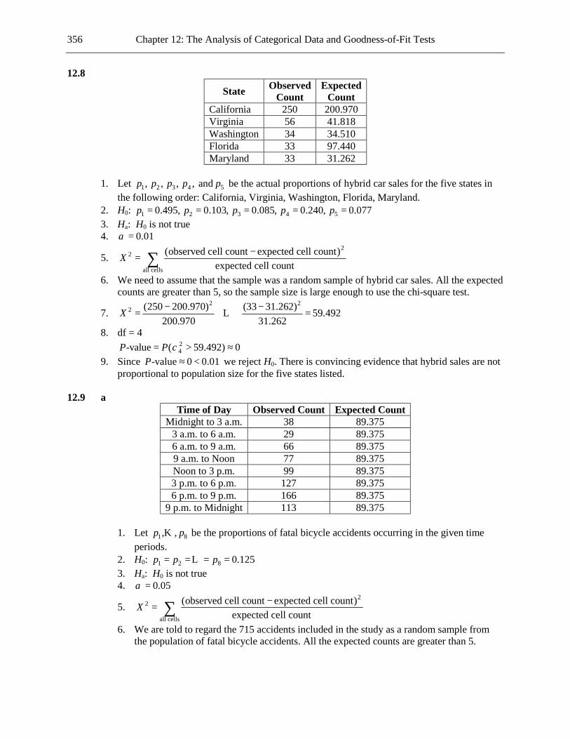
356 Chapter 12: The Analysis of Categorical Data and Goodness-of-Fit Tests
12.8
State Observed Count
Expected Count
California 250 200.970 Virginia 56 41.818 Washington 34 34.510 Florida 33 97.440 Maryland 33 31.262
1. Let 1 2 3 4 5, , , , and p p p p p be the actual proportions of hybrid car sales for the five states in
the following order: California, Virginia, Washington, Florida, Maryland. 2. H0: 1 2 3 4 50.495, 0.103, 0.085, 0.240, 0.077p p p p p= = = = = 3. Ha: H0 is not true 4. 0.01α =
5. 2
2
all cells
(observed cell count expected cell count)expected cell count
X −= ∑
6. We need to assume that the sample was a random sample of hybrid car sales. All the expected counts are greater than 5, so the sample size is large enough to use the chi-square test.
7. 2 2
2 (250 200.970) (33 31.262) 59.492200.970 31.262
X − −= + + =L
8. df = 4 2
4-value ( 59.492) 0P P χ= > ≈ 9. Since -value 0 0.01P ≈ < we reject H0. There is convincing evidence that hybrid sales are not
proportional to population size for the five states listed. 12.9 a
Time of Day Observed Count Expected Count Midnight to 3 a.m. 38 89.375
3 a.m. to 6 a.m. 29 89.375 6 a.m. to 9 a.m. 66 89.375 9 a.m. to Noon 77 89.375 Noon to 3 p.m. 99 89.375 3 p.m. to 6 p.m. 127 89.375 6 p.m. to 9 p.m. 166 89.375
9 p.m. to Midnight 113 89.375 1. Let 1 8, ,p pK be the proportions of fatal bicycle accidents occurring in the given time
periods. 2. H0: 1 2 8 0.125p p p= = = =L 3. Ha: H0 is not true 4. 0.05α =
5. 2
2
all cells
(observed cell count expected cell count)expected cell count
X −= ∑
6. We are told to regard the 715 accidents included in the study as a random sample from the population of fatal bicycle accidents. All the expected counts are greater than 5.

Chapter 12: The Analysis of Categorical Data and Goodness-of-Fit Tests 357
7. 2 2
2 (38 89.375) (113 89.375) 166.95889.375 89.375
X − −= + + =L
8. df = 7 2
7-value ( 166.958) 0P P χ= > ≈ 9. Since -value 0 0.05P ≈ < we reject H0. We have convincing evidence that fatal bicycle
accidents are not equally likely to occur in each of the 3-hour time periods given. b
Time of Day Observed Count Expected Count Midnight to Noon 210 238.333 Noon to Midnight 505 476.667
1. Let 1 2 and p p be the proportions of fatal bicycle accidents occurring between midnight
and noon and between noon and midnight, respectively. 2. H0: 1 21 3, 2 3p p= = 3. Ha: H0 is not true 4. 0.05α =
5. 2
2
all cells
(observed cell count expected cell count)expected cell count
X −= ∑
6. We are told to regard the 715 accidents included in the study as a random sample from the population of fatal bicycle accidents. Both of the expected counts are greater than 5.
7. 2 2
2 (210 238.333) (505 476.667) 5.052238.333 476.667
X − −= + =
8. df = 1 2
1-value ( 5.052) 0.025P P χ= > = 9. Since -value 0.025 0.05P = < we reject H0. Using a 0.05 significance level, we have
convincing evidence that fatal bicycle accidents do not occur as stated in the hypothesis. 12.10 a
Month
Observed Count
Expected Count
January 38 59.917 February 32 59.917 March 43 59.917 April 59 59.917 May 78 59.917 June 74 59.917 July 98 59.917 August 85 59.917 September 64 59.917 October 66 59.917 November 42 59.917 December 40 59.917
1. Let 1 12, ,p pK be the proportions of fatal bicycle accidents occurring in the given months. 2. H0: 1 2 12 1 12p p p= = = =L

358 Chapter 12: The Analysis of Categorical Data and Goodness-of-Fit Tests
3. Ha: H0 is not true 4. 0.01α =
5. 2
2
all cells
(observed cell count expected cell count)expected cell count
X −= ∑
6. We need to assume that the 719 accidents included in the study form a random sample from the population of fatal bicycle accidents. All the expected counts are greater than 5.
7. 2 2
2 (38 59.917) (40 59.917) 82.16359.917 59.917
X − −= + + =L
8. df = 11 2
11-value ( 82.163) 0P P χ= > ≈ 9. Since -value 0 0.01P ≈ < we reject H0. We have convincing evidence that fatal bicycle
accidents are not equally likely to occur in each of the months. b Defining 1 12, ,p pK as in Part (a), the hypotheses are: H0: 1 2 3 4 5 631 366, 29 366, 31 366, 30 366, 31 366, 30 366,p p p p p p= = = = = =
7 8 9 10 11 1231 366, 31 366, 30 366, 31 366, 30 366, 31 366 p p p p p p= = = = = = Ha: H0 is not true c
Month
Observed Count
Expected Count
January 38 60.899 February 32 56.970 March 43 60.899 April 59 58.934 May 78 60.899 June 74 58.934 July 98 60.899 August 85 60.899 September 64 58.934 October 66 60.899 November 42 58.934 December 40 60.899
0.05α =
2
2
all cells
(observed cell count expected cell count)expected cell count
X −= ∑
We need to assume that the 719 accidents included in the study form a random sample from the population of fatal bicycle accidents. All the expected counts are greater than 5.
2 2
2 (38 60.899) (40 60.899) 78.51160.899 60.899
X − −= + + =L
df = 11 2
11-value ( 78.511) 0P P χ= > ≈ Since -value 0 0.05P ≈ < we reject H0. We have convincing evidence that fatal bicycle
accidents do not occur in the twelve months in proportion to the lengths of the months.

Chapter 12: The Analysis of Categorical Data and Goodness-of-Fit Tests 359
12.11
Age Observed Count Expected Count 18–34 36 70 35–64 130 102
65 and over 34 28 1. Let 1 2 3, , and p p p be the proportions of lottery ticket purchasers who fall into the given age
catergories. 2. H0: 1 2 30.35, 0.51, 0.14p p p= = = 3. Ha: H0 is not true 4. 0.05α =
5. 2
2
all cells
(observed cell count expected cell count)expected cell count
X −= ∑
6. We are told to assume that the 200 people in the study form a random sample of lottery ticket purchasers. All the expected counts are greater than 5.
7. 2 2
2 (36 70) (34 28) 25.48670 28
X − −= + + =L
8. df = 2 2
2-value ( 25.486) 0P P χ= > ≈ 9. Since -value 0 0.05P ≈ < we reject H0. We have convincing evidence that one or more of
these three age groups buys a disproportionate share of lottery tickets. 12.12 a 1. Let 1 2 3, , and p p p be the proportions of the three phenotypes for this particular plant. 2. H0: 1 2 30.25, 0.5, 0.25p p p= = = 3. Ha: H0 is not true 4. 0.05α =
5. 2
2
all cells
(observed cell count expected cell count)expected cell count
X −= ∑
6. We are told that the 200 plants included in the study form a random sample from the population of this type of plant. Since 200(0.25) 50 5 and 200(0.5) 100 5,= > = > all the expected counts are greater than 5.
7. 2 4.63X = 8. df = 2 2
2-value ( 4.63) 0.099P P χ= > = 9. Since -value 0.099 0.05P = > we do not reject H0. We do not have convincing evidence
that the theory is incorrect. b The analysis and conclusion would be the same. 12.13
Phenotype 1 2 3 4 Observed Count 926 288 293 104 Expected Count 906.1875 302.0625 302.0625 100.6875
1. Let 1 2 3 4, , , and p p p p be the proportions of phenotypes resulting from the given process.
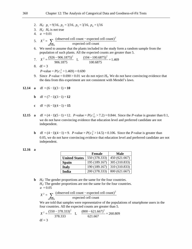
360 Chapter 12: The Analysis of Categorical Data and Goodness-of-Fit Tests
2. H0: 1 2 3 49 16, 3 16, 3 16, 1 16p p p p= = = = 3. Ha: H0 is not true 4. 0.01α =
5. 2
2
all cells
(observed cell count expected cell count)expected cell count
X −= ∑
6. We need to assume that the plants included in the study form a random sample from the population of such plants. All the expected counts are greater than 5.
7. 2 2
2 (926 906.1875) (104 100.6875) 1.469906.1875 100.6875
X − −= + + =L
8. df = 3 2
3-value ( 1.469) 0.690P P χ= > = 9. Since -value 0.690 0.01P = > we do not reject H0. We do not have convincing evidence that
the data from this experiment are not consistent with Mendel’s laws. 12.14 a df (6 1)(3 1)= − − = 10 b df (7 1)(3 1)= − − = 12 c df (6 1)(4 1)= − − = 15 12.15 a df (4 1)(5 1) 12.= − − = 2
12-value ( 7.2) 0.844.P P χ= > = Since the P-value is greater than 0.1, we do not have convincing evidence that education level and preferred candidate are not independent.
b df (4 1)(4 1) 9.= − − = 2
9-value ( 14.5) 0.106.P P χ= > = Since the P-value is greater than 0.05, we do not have convincing evidence that education level and preferred candidate are not independent.
12.16 a
Female Male United States 550 (378.333) 450 (621.667) Spain 195 (189.167) 305 (310.833) Italy 190 (189.167) 310 (310.833) India 200 (378.333) 800 (621.667)
b H0: The gender proportions are the same for the four countries. Ha: The gender proportions are not the same for the four countries. 0.05α =
2
2
all cells
(observed cell count expected cell count)expected cell count
X −= ∑
We are told that samples were representative of the populations of smartphone users in the four countries. All the expected counts are greater than 5.
2 2
2 (550 378.333) (800 621.667) 260.809378.333 621.667
X − −= + + =L
df = 3

Chapter 12: The Analysis of Categorical Data and Goodness-of-Fit Tests 361
2
3-value ( 260.809) 0P P χ= ≥ ≈ Since -value 0 0.05P ≈ < we reject H0. There is convincing evidence that the gender
proportions are not the same for the four countries. 12.17
Body Piercings Only
Tattoos Only
Both Body Piercing and Tattoos
No Body Art
Freshman 61 (49.714) 7 (15.086) 14 (18.514) 86 (84.686) Sophomore 43 (37.878) 11 (11.494) 10 (14.106) 64 (64.522)
Junior 20 (23.378) 9 (7.094) 7 (8.706) 43 (39.822) Senior 21 (34.031) 17 (10.327) 23 (12.673) 54 (57.969)
H0: Class standing and body art response are independent Ha: Class standing and body art response are not independent 0.01α =
2
2
all cells
(observed cell count expected cell count)expected cell count
X −= ∑
We are told to regard the sample as representative of the students at this university, so we are justified in treating it as a random sample from that population. All the expected counts are greater than 5.
2 2
2 (61 49.714) (54 57.969) 29.50749.714 57.969
X − −= + + =L
df = 9 2
9-value ( 29.507) 0.001P P χ= > = Since -value 0.001 0.01P = < we reject H0. We have convincing evidence of an association
between class standing and response to the body art question. 12.18
Degree of Spirituality Very Moderate Slightly Not at All
Natural Scientists 56 (50.594) 162 (173.916) 198 (199.213) 211 (203.278) Social Scientists 56 (61.406) 223 (211.084) 243 (241.787) 239 (246.722)
H0: The spirituality category proportions are the same for natural scientists and social scientists. Ha: The spirituality category proportions are not all the same for natural scientists and social
scientists. 0.01α =
2
2
all cells
(observed cell count expected cell count)expected cell count
X −= ∑
We are told to regard the two samples as representative of natural and social scientists at research universities, and so we are justified in assuming that they were random samples from those populations. All the expected counts are greater than 5.
2 2
2 (56 50.594) (239 246.722) 3.09150.594 246.722
X − −= + + =L
df = 3 2
3-value ( 3.091) 0.378P P χ= > =

362 Chapter 12: The Analysis of Categorical Data and Goodness-of-Fit Tests
Since -value 0.378 0.01P = > we do not reject H0. We do not have convincing evidence that the spirituality category proportions are not all the same for natural scientists and social scientists.
12.19 a H0: Field of study and smoking status are independent Ha: Field of study and smoking status are not independent 0.01α =
2
2
all cells
(observed cell count expected cell count)expected cell count
X −= ∑
We are told that the sample was a random sample from the population. All the expected counts are greater than 5.
2 90.853X = df = 8 -value 0P ≈ Since -value 0 0.01P ≈ < we reject H0. We have convincing evidence that smoking status and
field of study are not independent. b The particularly high contributions to the chi-square statistic (in order of importance) come
from the field of communication, languages, and cultural studies, where there was a disproportionately high number of smokers, the field of mathematics, engineering, and sciences, where there was a disproportionately low number of smokers, and the field of social science and human services, where there was a disproportionately high number of smokers.
12.20
Character Type Sex Positive Negative Neutral Male 255 (262.072) 106 (90.954) 130 (137.973) Female 85 (77.928) 12 (27.046) 49 (41.027)
H0: Sex and character type are independent Ha: Sex and character type are not independent 0.05α =
2
2
all cells
(observed cell count expected cell count)expected cell count
X −= ∑
We are told to regard the sample as representative of smoking movie characters, so we are justified in treating it as a random sample from that population. All the expected counts are greater than 5.
2 2
2 (255 262.072) (49 41.027) 13.702262.072 41.027
X − −= + + =L
df = 2 2
2-value ( 13.702) 0.001P P χ= > = Since -value 0.001 0.05P = < we reject H0. We have convincing evidence of an association
between sex and character type for movie characters who smoke. 12.21 a
Usually Eat 3 Meals a Day
Rarely Eat 3 Meals a Day
Male 26 (21.755) 22 (26.245) Female 37 (41.245) 54 (49.755)

Chapter 12: The Analysis of Categorical Data and Goodness-of-Fit Tests 363
H0: The proportions falling into the two response categories are the same for males and
females. Ha: The proportions falling into the two response categories are not the same for males and
females. 0.05α =
2
2
all cells
(observed cell count expected cell count)expected cell count
X −= ∑
We are told to assume that the samples of male and female students were random samples from the populations. All the expected counts are greater than 5.
2 2
2 (26 21.755) (54 49.755) 2.31421.755 49.755
X − −= + + =L
df = 1 2
1-value ( 2.314) 0.128P P χ= > = Since -value 0.128 0.05P = > we do not reject H0. We do not have convincing evidence that
the proportions falling into the two response categories are not the same for males and females.
b Yes. c Yes. Since -value 0.127 0.05P = > we do not reject H0. We do not have convincing evidence
that the proportions falling into the two response categories are not the same for males and females.
d The two P-values are almost equal, in fact the difference between them is only due to
rounding errors in the MINITAB program. In other words, if complete accuracy had been maintained throughout, the two P-values would have been exactly equal. (Also, the chi-square statistic in Part (a) is the square of the z statistic in Part (c).) It should not be surprising that the P-values are at least similar, since both measure the probability of getting sample proportions at least as far from the expected proportions, given that the proportions who usually eat three meals per day are the same for the two populations.
12.22
Distance of College from Home (in Miles) Student Group
Less than 40 40 to 99 100 to 199 200 to 399 400 or More
Academic Superstars
157 (171.378) 157 (165.469) 141 (146.427) 149 (140.517) 224 (204.209)
Solid Performers
104 (89.622) 95 (86.531) 82 (76.573) 65 (73.483) 87 (106.791)
H0: The proportions falling into the distance categories are the same for the two student groups. Ha: The proportions falling into the distance categories are not all the same for the two student
groups. 0.05α =
2
2
all cells
(observed cell count expected cell count)expected cell count
X −= ∑
We are told to treat the two samples as random samples from the populations. All the expected counts are greater than 5.

364 Chapter 12: The Analysis of Categorical Data and Goodness-of-Fit Tests
2 2
2 (157 171.378) (87 106.791) 12.438171.378 106.791
X − −= + + =L
df = 4 2
4-value ( 12.438) 0.014P P χ= > = Since -value 0.014 0.05P = < we reject H0. We have convincing evidence that the proportions
falling into the distance categories are not all the same for the two student groups. 12.23 a
Donation No Donation No Gift 397 (514.512) 2865 (2747.488) Small Gift 465 (510.569) 2772 (2726.431) Large Gift 691 (527.919) 2656 (2819.081)
H0: The proportions falling into the two donation categories are the same for all three gift
treatments. Ha: The proportions falling into the two donation categories are not the same for all three gift
treatments. 0.01α =
2
2
all cells
(observed cell count expected cell count)expected cell count
X −= ∑
We are told that the three treatments were assigned at random. All the expected counts are greater than 5.
2 2
2 (397 514.512) (2656 2819.081) 96.506514.512 2819.081
X − −= + + =L
df = 2 2
2-value ( 96.506) 0P P χ= > ≈ Since -value 0 0.01P ≈ < we reject H0. We have convincing evidence that the proportions
falling into the two donation categories are not the same for all three gift treatments. b The result of Part (a) tells us that the level of the gift seems to make a difference. Looking at
the data given, 12% of those receiving no gift made a donation, 14% of those receiving a small gift made a donation, and 21% of those receiving a large gift made a donation. (These percentages can be compared to 16% making donations amongst the expected counts.) So it seems that the most effective strategy is to include a large gift, with the small gift making very little difference compared to no gift at all.
12.24
Locus of Control Internal External Compulsive Buyer?
Yes 3 (7.421) 14 (9.579) No 52 (47.579) 57 (61.421)
H0: Locus of control and compulsive buyer behavior are independent Ha: Locus of control and compulsive buyer behavior are not independent 0.01α =
2
2
all cells
(observed cell count expected cell count)expected cell count
X −= ∑

Chapter 12: The Analysis of Categorical Data and Goodness-of-Fit Tests 365
We are told to regard the sample as representative of college students at mid-western public
universities, so we are justified in treating it as a random sample from that population. All the expected counts are greater than 5.
2 2
2 (3 7.421) (57 61.421) 5.4027.421 61.421
X − −= + + =L
df = 1 2
1-value ( 5.402) 0.020P P χ= > = Since -value 0.020 0.01P = > we do not reject H0. We do not have convincing evidence of an
association between locus of control and compulsive buyer behavior. 12.25
Alcohol Exposure Group 1 2 3 4 School Performance
Excellent 110 (79.25) 93 (79.25) 49 (79.25) 65 (79.25) Good 328 (316) 325 (316) 316 (316) 295 (316)
Average/Poor 239 (281.75) 259 (281.75) 312 (281.75) 317 (281.75) H0: Alcohol exposure and school performance are independent Ha: Alcohol exposure and school performance are not independent 0.05α =
2
2
all cells
(observed cell count expected cell count)expected cell count
X −= ∑
We are told to regard the sample as a random sample of German adolescents. All the expected counts are greater than 5.
2 2
2 (110 79.25) (317 281.75) 46.51579.25 281.75
X − −= + + =L
df = 6 2
6-value ( 46.515) 0P P χ= > ≈ Since -value 0 0.05P ≈ < we reject H0. We have convincing evidence of an association between
alcohol exposure and school performance. 12.26 a
Current Hormone Use
None
Esterified Estrogen
Conjugated Equine Estrogen
Venous Thrombosis 372 (371.569) 86 (123.309) 121 (84.121) No Venous Thrombosis 1439 (1439.431) 515 (477.691) 289 (325.879)
H0: The proportions falling into the hormone use categories are the same for women who
have been diagnosed with venous thrombosis as for those who have not. Ha: The proportions falling into the hormone use categories are not all the same for women
who have been diagnosed with venous thrombosis as for those who have not. 0.05α =
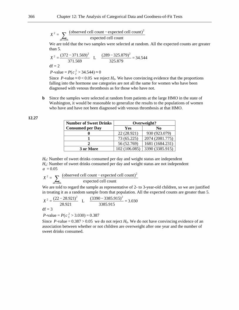
366 Chapter 12: The Analysis of Categorical Data and Goodness-of-Fit Tests
2
2
all cells
(observed cell count expected cell count)expected cell count
X −= ∑
We are told that the two samples were selected at random. All the expected counts are greater than 5.
2 2
2 (372 371.569) (289 325.879) 34.544371.569 325.879
X − −= + + =L
df = 2 2
2-value ( 34.544) 0P P χ= > ≈ Since -value 0 0.05P ≈ < we reject H0. We have convincing evidence that the proportions
falling into the hormone use categories are not all the same for women who have been diagnosed with venous thrombosis as for those who have not.
b Since the samples were selected at random from patients at the large HMO in the state of
Washington, it would be reasonable to generalize the results to the populations of women who have and have not been diagnosed with venous thrombosis at that HMO.
12.27
Number of Sweet Drinks Consumed per Day
Overweight? Yes No
0 22 (28.921) 930 (923.079) 1 73 (65.225) 2074 (2081.775) 2 56 (52.769) 1681 (1684.231)
3 or More 102 (106.085) 3390 (3385.915) H0: Number of sweet drinks consumed per day and weight status are independent Ha: Number of sweet drinks consumed per day and weight status are not independent 0.05α =
2
2
all cells
(observed cell count expected cell count)expected cell count
X −= ∑
We are told to regard the sample as representative of 2- to 3-year-old children, so we are justified in treating it as a random sample from that population. All the expected counts are greater than 5.
2 2
2 (22 28.921) (3390 3385.915) 3.03028.921 3385.915
X − −= + + =L
df = 3 2
3-value ( 3.030) 0.387P P χ= > = Since -value 0.387 0.05P = > we do not reject H0. We do not have convincing evidence of an
association between whether or not children are overweight after one year and the number of sweet drinks consumed.

Chapter 12: The Analysis of Categorical Data and Goodness-of-Fit Tests 367
12.28 a
Gender Days of Vacation Male Female None 51 (50.055) 42 (42.945) 1–5 21 (24.758) 25 (21.242) 6–10 67 (78.581) 79 (67.419) 11–15 111 (110.336) 94 (94.664) 16–20 71 (75.889) 70 (65.111) 21–25 82 (75.351) 58 (64.649) More than 25 118 (106.030) 79 (90.970)
H0: Gender and the number of vacation days taken are independent Ha: Gender and the number of vacation days taken are not independent 0.05α =
2
2
all cells
(observed cell count expected cell count)expected cell count
X −= ∑
It is stated that the adults in the study formed a random sample. All the expected counts are greater than 5.
2 2
2 (51 50.055) (79 90.970) 9.85850.055 90.970
X − −= + + =L
df = 6 2
6-value ( 9.858) 0.131P P χ= > = Since -value 0.131 0.05P = > , H0 is not rejected. The data do not provide convincing
evidence of an association between gender and the number of vacation days taken. b The poll was of working adults in Canada, the results can be generalized to that population. 12.29
City Vehicle Type
Concord
Pleasant Hills
North San Francisco
Small 68 (89.060) 83 (107.019) 221 (175.921) Compact 63 (56.740) 68 (68.181) 106 (112.079) Midsize 88 (84.511) 123 (101.553) 142 (166.936) Large 24 (12.689) 18 (15.247) 11 (25.064)
H0: City of residence and vehicle type are independent Ha: City of residence and vehicle type are not independent 0.05α =
2
2
all cells
(observed cell count expected cell count)expected cell count
X −= ∑
We are told to regard the sample as a random sample of Bay area residents. All the expected counts are greater than 5.
2 2
2 (68 89.060) (11 25.064) 49.81389.060 25.064
X − −= + + =L
df = 6 2
6-value ( 49.813) 0P P χ= > ≈

368 Chapter 12: The Analysis of Categorical Data and Goodness-of-Fit Tests
Since -value 0 0.05P ≈ < we reject H0. We have convincing evidence of an association between city of residence and vehicle type.
12.30
Picture Response
Provocative
Conservative
No Picture
Rape 80 (99.580) 104 (90.955) 92 (85.466) Not Rape 47 (27.420) 12 (25.045) 17 (23.534)
H0: The proportions who believe that the story described a rape are the same for the three photo
treatments. Ha: The proportions who believe that the story described a rape are not the same for the three
photo treatments. 0.01α =
2
2
all cells
(observed cell count expected cell count)expected cell count
X −= ∑
We need to assume that the students were randomly assigned to the photo treatments. All the expected counts are greater than 5.
2 2
2 (80 99.580) (17 23.534) 28.81099.580 23.534
X − −= + + =L
df = 2 2
2-value ( 28.810) 0P P χ= > ≈ Since -value 0 0.01P ≈ < we reject H0. We have convincing evidence that the proportions who
believe that the story described a rape are not the same for the three photo treatments. 12.31
View Sex ID
Front
Profile
Three- Quarter
Correct 23 (26) 26 (26) 29 (26) Incorrect 17 (14) 14 (14) 11 (14)
H0: The proportions of correct sex identifications are the same for all three nose views. Ha: The proportions of correct sex identifications are not the same for all three nose views. 0.05α =
2
2
all cells
(observed cell count expected cell count)expected cell count
X −= ∑
We need to assume that the students were randomly assigned to the nose views. All the expected counts are greater than 5.
2 2
2 (23 26) (11 14) 1.97826 14
X − −= + + =L
df = 2 2
2-value ( 1.978) 0.372P P χ= > = Since -value 0.372 0.05P = > we do not reject H0. We do not have convincing evidence that the
proportions of correct sex identifications are not the same for all three nose views.

Chapter 12: The Analysis of Categorical Data and Goodness-of-Fit Tests 369
12.32 a H0: Gender and number of servings of water consumed per day are independent Ha: Gender and number of servings of water consumed per day are not independent df (5 1)(2 1)= − − = 4 b The P-value for the test was 0.086, which is greater than the new significance level of 0.05.
So, for a significance level of 0.05, we do not have convincing evidence of a difference between males and females with regard to water consumption.
c H0: Gender and number of consumptions of fried potatoes are independent Ha: Gender and number of consumptions of fried potatoes are not independent 0.05α =
2
2
all cells
(observed cell count expected cell count)expected cell count
X −= ∑
No assumption regarding the randomness of the sample is necessary since we are merely asking whether there is a significant association between the two variables for this set of students. All the expected counts (shown in the output) are greater than 5.
2 15.153X = df = 5 -value 0.015P = Since -value 0.015 0.05P = < we reject H0. We have convincing evidence of an association
between gender and number of consumptions of fried potatoes. This agrees with the authors’ conclusion that there was a significant association between gender and consumption of fried potatoes.
12.33 a The number of men in the sample who napped is 744(0.38) = 282.72, which we round to 283,
since the number of men who napped must be a whole number. The number of men who did not nap is therefore 744 283 461.− = The observed frequencies for the women are calculated in a similar way. (The table below also shows the expected frequencies in parentheses.)
Napped Did Not Nap Row Total
Men 283 (257) 461 (487) 744 Women 231 (257) 513 (487) 744
b H0: Gender and napping are independent Ha: Gender and napping are not independent 0.01α =
2
2
all cells
(observed cell count expected cell count)expected cell count
X −= ∑
We are told that the sample was nationally representative, so we are justified in treating it as a random sample from the population of American adults. All the expected counts are greater than 5.
2 2
2 (283 257) (513 487) 8.034257 487
X − −= + + =L
df = 1 2
1-value ( 8.034) 0.005P P χ= > = Since -value 0.005 0.01P = < we reject H0. We have convincing evidence of an association
between gender and napping.

370 Chapter 12: The Analysis of Categorical Data and Goodness-of-Fit Tests
c Yes. We have convincing evidence at the 0.01 significance level of an association between gender and napping in the population. This is equivalent to saying that we have convincing evidence at the 0.01 significance level that the proportions of men and women who nap are different (a two-tailed test of a difference of the proportions). Thus, converting this to a one-tailed test, since in the sample the proportion of men who napped was greater than the proportion of women who napped, we have convincing evidence at the 0.005 level that a greater proportion of men nap than women.
12.34 It is not possible to decide which, if either, of the two conclusions is correct. Since the results
were obtained from an observational study, no conclusion regarding causality can be reached. 12.35
Day
Observed Count
Expected Count
Sunday 14 14.286 Monday 13 14.286 Tuesday 12 14.286 Wednesday 15 14.286 Thursday 14 14.286 Friday 17 14.286 Saturday 15 14.286
1. Let 1 7, ,p pK be the proportions of all fatal bicycle accidents occurring on the seven days. 2. H0: 1 2 7 1 7p p p= = = =L 3. Ha: H0 is not true 4. 0.05α =
5. 2
2
all cells
(observed cell count expected cell count)expected cell count
X −= ∑
6. We are told that the 100 accidents formed a random sample from the population of fatal bicycle accidents. All the expected counts are greater than 5.
7. 2 2
2 (14 14.286) (15 14.286) 1.0814.286 14.286
X − −= + + =L
8. df = 6 2
6-value ( 1.08) 0.982P P χ= > = 9. Since -value 0.982 0.05P = > we do not reject H0. We do not have convincing evidence that
the proportion of accidents is not the same for all days of the week. 12.36
Color
Observed Count
Expected Count
Blue 16 8.25 Green 8 8.25 Yellow 6 8.25 Red 3 8.25
1. Let 1 2 3 4, , , and p p p p be the proportions of first pecks for the colors given. 2. H0: 1 2 3 4 0.25p p p p= = = =

Chapter 12: The Analysis of Categorical Data and Goodness-of-Fit Tests 371
3. Ha: H0 is not true 4. 0.01α =
5. 2
2
all cells
(observed cell count expected cell count)expected cell count
X −= ∑
6. We need to assume that the birds in the study formed a random sample of 1-day-old bobwhites. All the expected counts are greater than 5.
7. 2 2
2 (16 8.25) (3 8.25) 11.2428.25 8.25
X − −= + + =L
8. df = 3 2
3-value ( 11.242) 0.0105P P χ= > = 9. Since -value 0.0105 0.01P = > we do not reject H0. We do not have convincing evidence of a
color preference. 12.37
Response Country Never Rarely Sometimes Often Not Sure Italy 600 (400) 140 (222) 140 (244) 90 (90) 30 (44) Spain 540 (400) 160 (222) 140 (244) 70 (90) 90 (44) France 400 (400) 250 (222) 200 (244) 120 (90) 30 (44) United States 360 (400) 230 (222) 270 (244) 110 (90) 30 (44) South Korea 100 (400) 330 (222) 470 (244) 60 (90) 40 (44)
H0: The proportions falling into the response categories are all the same for all five countries. Ha: The proportions falling into each of the response categories are not all the same for all five
countries. 0.01α =
2
2
all cells
(observed cell count expected cell count)expected cell count
X −= ∑
We are told that the samples were random samples from the populations. All the expected counts are greater than 5.
2 2
2 (600 400) (40 44) 881.360400 44
X − −= + + =L
df = 16 2
16-value ( 881.360) 0P P χ= > ≈ Since -value 0 0.01P ≈ < we reject H0. We have convincing evidence that the response
proportions are not all the same for all five countries. 12.38
Ethnic Group
Observed Count
Expected Count
White 679 507 Black 51 66 Hispanic 77 306 Asian 190 108 Other 3 13

372 Chapter 12: The Analysis of Categorical Data and Goodness-of-Fit Tests
1. Let 1 2 3 4 5, , , and p p p p p be the proportions of students graduating from California colleges and universities in 1998 in the given ethnic groups.
2. H0: 1 2 3 4 50.507, 0.066, 0.306, 0.108, 0.013p p p p p= = = = = 3. Ha: H0 is not true 4. 0.01α =
5. 2
2
all cells
(observed cell count expected cell count)expected cell count
X −= ∑
6. We are told that the students in the study formed a random sample of students graduating from California colleges and universities in 1998. All the expected counts are greater than 5.
7. 2 2
2 (679 507) (3 13) 303.088507 13
X − −= + + =L
8. df = 4 2
4-value ( 303.088) 0P P χ= > ≈ 9. Since -value 0 0.01P ≈ < we reject H0. We have convincing evidence that the proportions of
students graduating from colleges and universities in California for these ethnic group categories differed from the respective proportions in the population of California.
12.39
Season Winter Spring Summer Fall Observed Count 328 334 372 327 Expected Count 340.25 340.25 340.25 340.25
1. Let 1 2 3 4, , , and p p p p be the proportions of homicides occurring in the four seasons. 2. H0: 1 4 0.25p p= = =L 3. Ha: H0 is not true 4. 0.05α =
5. 2
2
all cells
(observed cell count expected cell count)expected cell count
X −= ∑
6. We need to assume that the 1361 homicides form a random sample from the population of homicides. All the expected counts are greater than 5.
7. 2 2
2 (328 340.25) (327 340.25) 4.035340.25 340.25
X − −= + + =L
8. df = 3 2
3-value ( 4.035) 0.258P P χ= > = 9. Since -value 0.258 0.05P = > we do not reject H0. We do not have convincing evidence that
the homicide rate is not the same over the four seasons. 12.40 a
Smoker Nonsmoker Likes Risky Things 45 (26.325) 46 (64.675)
Doesn’t Like Risky Things 36 (54.675) 153 (134.325)
H0: Smoking status and desire to do risky things are independent Ha: Smoking status and desire to do risky things are not independent

Chapter 12: The Analysis of Categorical Data and Goodness-of-Fit Tests 373
0.05α =
2
2
all cells
(observed cell count expected cell count)expected cell count
X −= ∑
We are told to regard the sample as a random sample of Mexican-American male adolescents. All the expected counts are greater than 5.
2 2
2 (45 26.325) (153 134.325) 27.61626.325 134.325
X − −= + + =L
df = 1 2
1-value ( 27.616) 0P P χ= > ≈ Since -value 0 0.05P ≈ < we reject H0. We have convincing evidence of an association
between smoking status and desire to do risky things. b No. Since this was an observational study, no conclusion regarding causality can be reached. 12.41 a
Role Position
Initiate Chase
Participate in Chase
Center 28 (39.038) 48 (36.962) Wing 66 (54.962) 41 (52.038)
H0: Position and role are independent Ha: Position and role are not independent 0.01α =
2
2
all cells
(observed cell count expected cell count)expected cell count
X −= ∑
Each of the 183 observations in the sample is a particular lioness on a particular hunt. (Presumably several observations could have been gathered for a single lioness, each for a different hunt. Likewise, several observations could have been gathered from a single hunt, each for a different lioness.) It is necessary to assume that these 183 observations form a random sample of lioness-hunts. All the expected counts are greater than 5.
2 2
2 (28 39.038) (41 52.038) 10.97639.038 52.038
X − −= + + =L
df = 1 2
1-value ( 10.976) 0.001P P χ= > = Since -value 0.001 0.01P = < we reject H0. We have convincing evidence of an association
between position and role. b As stated in Part (a), it is necessary to assume that these 183 observations form a random
sample of lioness-hunts.

374 Chapter 12: The Analysis of Categorical Data and Goodness-of-Fit Tests
12.42 Age of Children Response Preteen Teen Very Effective 126 (139.073) 149 (135.927) Somewhat Effective 44 (42.986) 41 (42.014) Not at All Effective or Don’t Know 51 (38.941) 26 (38.059)
H0: Age of children and parental response are independent Ha: Age of children and parental response are not independent 0.05α =
2
2
all cells
(observed cell count expected cell count)expected cell count
X −= ∑
We need to assume that the sample is a random sample of parents with preteen and teenage children. All the expected counts are greater than 5.
2 2
2 (126 139.073) (26 38.059) 10.091139.073 38.059
X − −= + + =L
df = 2 2
2-value ( 10.091) 0.006P P χ= > = Since -value 0.006 0.05P = < we reject H0. We have convincing evidence of an association
between age of children and parental response. 12.43
Response Region Agree Disagree Northeast 130 (150.350) 59 (38.650) West 146 (149.554) 42 (38.446) Midwest 211 (209.217) 52 (53.783) South 291 (268.879) 47 (69.121)
H0: Response (agree/disagree) and region of residence are independent Ha: Response (agree/disagree) and region of residence are not independent 0.01α =
2
2
all cells
(observed cell count expected cell count)expected cell count
X −= ∑
We are told that the sample was a random sample of adults. All the expected counts are greater than 5.
2 2
2 (130 150.350) (47 69.121) 22.855150.350 69.121
X − −= + + =L
df = 3 2
3-value ( 22.855) 0P P χ= > ≈ Since -value 0 0.01P ≈ < we reject H0. We have convincing evidence of an association between
response and region of residence. 12.44 a Since the study was conducted using separate random samples of male and female inmates,
this is a test for homogeneity.

Chapter 12: The Analysis of Categorical Data and Goodness-of-Fit Tests 375
b
Gender Type of Crime Male Female Violent 117 (91.5) 66 (91.5) Property 150 (155) 160 (155) Drug 109 (138.5) 168 (138.5) Public-Order 124 (115) 106 (115)
H0: The proportions falling into the crime categories are the same for male and female
inmates. Ha: The proportions falling into the crime categories are not all the same for male and female
inmates. 0.05α =
2
2
all cells
(observed cell count expected cell count)expected cell count
X −= ∑
We are told that the samples were random samples of male and female inmates. All the expected counts are greater than 5.
2 2
2 (117 91.5) (106 115) 28.51191.5 115
X − −= + + =L
df = 3 2
3-value ( 28.511) 0P P χ= > ≈ Since -value 0 0.05P ≈ < we reject H0. We have convincing evidence that the proportions
falling into the crime categories are not all the same for male and female inmates.

376
Chapter 13 Simple Linear Regression and Correlation: Inferential Methods
Note: In this chapter, numerical answers to questions involving the normal, t, and chi square distributions were found using values from a calculator. Students using statistical tables will find that their answers differ slightly from those given. 13.1 a 5.0 0.017y x= − + b When 1000, 5 0.017(1000) 12.x y= = − + = When 2000, 5 0.017(2000) 29.x y= = − + =
-505
1015202530354045
0 1000 2000 3000
x
y
c When 2100,x = 5 0.017(2100) 30.7.y = − + = The mean gas usage for houses with 2100
square feet of space is 30.7 therms. d 0.017 therms e 100(0.017) = 1.7 therms f No. The given relationship only applies to houses whose sizes are between 1000 and 3000
square feet. The size of this house, 500 square feet, lies outside this range. 13.2 a For 10,x = 0.12 0.095(10) .y = − + = 0.83
For 15,x = 0.12 0.095(15) .y = − + = 1.305 b Since the slope of the population regression line is 0.095, the average increase in flow rate
associated with a 1-inch increase in pressure drop is 0.095. 13.3 a When 15, 0.135 0.003(15) . micrometersyx µ= = + = 0 18 When 17, 0.135 0.003(17) micrometersyx µ= = + = 0.186 b When 15, =0.18, so ( 0.18) . .yx P yµ= > = 0 5

Chapter 13: Simple Linear Regression and Correlation: Inferential Methods 377
c When 14, 0.135 0.003(14) 0.177, yx µ= = + =
0.175 0.177so ( 0.175) ( 0.4) . .0.005
P y P z P z− > = > = > − =
0 655
0.178 0.177( 0.178) ( 0.2) . .0.005
P y P z P z− < = < = < =
0 579
13.4 a For each one-unit increase in horsepower the predicted fuel efficiency decreases by
0.150 mpg. b The number ˆ 29.0y = is both an estimate of the mean fuel efficiency when the horsepower is
100 and a prediction for the horsepower of a car whose horsepower is 100. c When 300,x = ˆ 44.0 0.15(300) 1.0.y = − = − This result cannot be valid, since it is not
possible to have a car whose fuel efficiency is negative. This has probably occurred because 300 is outside the range of horsepower ratings for the small cars used in the sample; the estimated regression equation is not valid for values outside this range.
d This tells us that 68.0% of the variation in fuel efficiency is attributable to the approximate
linear relationship between horsepower and fuel efficiency. e This tells us that 3.0 mpg is a typical deviation of the fuel efficiency of a car in the sample
from the value predicted by the least-squares line. 13.5 a Average change in price associated with one extra square foot of space = $47. Average change in price associated with 100 extra square feet of space = 100(47) = $4700. b When 1800, 23000 47(1800) 107600.yx µ= = + =
So 110000 107600( 110000) ( 0.48) .5000
P y P z P z− > = > = > =
0.316
100000 107600( 100000) ( 1.52) . .5000
P y P z P z− < = < = < − =
0 064
13.6 a y xα β= + is the equation of the population regression line, which relates the mean value of
y to the value of x. y a bx= + is the equation of an estimated regression line, which is an estimate of the
population regression line obtained from a particular set of ( , )x y observations. b β is the slope of the population regression line.
b is an estimate of β obtained from a particular set of ( , )x y observations. c ( *)xα β+ is the mean value of y when *.x x=
( *)a b x+ is an estimate of the mean value of y (and also a predicted y value) when *.x x= d The simple linear regression model assumes that for any fixed value of x, the distribution of y
is normal with mean xα β+ and standard deviation σ . Thus σ is the shared standard

378 Chapter 13: Simple Linear Regression and Correlation: Inferential Methods
deviation of these y distributions. The quantity es is an estimate of σ obtained from a particular set of ( , )x y observations.
13.7 a 2 SSResid 0.3131 1 . .SSTo 0.356
r = − = − = 0 121
b A point estimate of SSResid 0.313 is .2 13es
nσ = = =
−0.155 This is a typical deviation of a
bone mineral density value in the sample from the value predicted by the least-squares line. c 0.009 g/cm2. d When 260, estimate of mean BMD 0.558 0.009(60) 1.098 g/cm .x = = + = 13.8 a The equation of the estimated regression line is ˆ 45.572 1.335 ,y x= + where x = percent of
women using HRT and y = breast cancer incidence. b 1.335 cases per 100,000 women. c For 40,x = ˆ 45.572 1.335(40)y = + = 98.990 cases per 100,000 women. d No. This is not advisable as 20 is not within the range of the x-values in the original data set,
and we have no reason to believe that the relationship summarized by the estimated regression line applies outside this range.
e 2 0.830.r = Eighty-three percent of the variability in breast cancer incidence can be
explained by the approximate linear relationship between breast cancer incidence and percent of women using HRT.
f 4.154.es = This is a typical deviation of breast cancer incidence value in this data set from
the value predicted by the estimated regression line.
13.9 a The required proportion is 2 SSResid 2620.571 1 . .SSTo 22398.05
r = − = − = 0 883
b SSResid 2620.57 . .2 14es
n= = =
−13 682 The number of degrees of freedom associated with
this estimate is 2 16 2 .n − = − = 14
13.10 a The point estimate of σ is SSResid 1235.470 .2 13es
n= = =
−9.749
df = 13.
b 2 SSResid 1235.4701 1 .SSTo 25321.368
r = − = − = 0.951 So the required percentage is 95.1%.

Chapter 13: Simple Linear Regression and Correlation: Inferential Methods 379
13.11 a
0.110.100.090.080.070.060.050.04
0.14
0.12
0.10
0.08
0.06
0.04
x
y
The plot shows a linear pattern, and the vertical spread of points does not appear to be
changing over the range of x values in the sample. If we assume that the distribution of errors at any given x value is approximately normal, then the simple linear regression model seems appropriate.
b ˆ 0.00227 1.247y x= − + When ˆ0.09, 0.00227 1.247(0.09) . .x y= = − + = 0 110 c 2 .r = 0.436 This tells us that 43.6% of the variation in market share can be explained by the
linear regression model relating market share and advertising share.
d A point estimate of SSResid 0.00551 is .2 8es
nσ = = =
−0.026 The number of degrees of
freedom associated with this estimate is 2 10 2 .n − = − = 8 13.12 The simple linear regression model assumes that for any fixed value of x, the distribution of y is
normal with mean xα β+ and standard deviation σ . Thus σ is the shared standard deviation of these y distributions. To understand the meaning of the symbol bσ , consider the process, for a given set of x values, of randomly selecting a set of y values (one for each x value), and calculating the slope, b, of the least-squares regression line for the set of ( , )x y observations obtained. The quantity bσ is the standard deviation of the set of all possible such values of b. The quantity bs is an estimate, from a particular set of ( , )x y observations, of bσ .
13.13 a Yes. The P-value for the hypothesis test of H0: β = 0 versus Ha: β ≠ 0 is 0.023. Since this
value is less than 0.05, we have convincing evidence at the 0.05 significance level of a useful linear relationship between shrimp catch per tow and oxygen concentration density.
b Yes. The value of the correlation coefficient for the sample is 0.496 0.704r = = . So there is
a moderate to strong linear relationship for the values in the sample.

380 Chapter 13: Simple Linear Regression and Correlation: Inferential Methods
c We must assume that the conditions for inference are met. df = 10 – 2 = 8. The 95% confidence interval for β is
( critical value) 97.22 (2.306)(34.63) (17.363,177.077).bb t s± ⋅ = ± = We are 95% confident that the slope of the population regression line relating mean catch per
tow to O2 saturation is between 17.363 and 177.077. 13.14 Yes. We know that 2( )b x xσ σ= −∑ . Therefore, the larger the spread of the x values, the
smaller the variability of the statistic b. The set of x values given in the question has a greater spread than the set of x values given in the example, and therefore is likely to give a more reliable estimate for β than the one obtained in the example.
13.15 a SSResid 1235.470 9.749.2 13es
n= = =
−
9.749 . .4024.2
eb
xx
ssS
= = = 0 154
b We must assume that the conditions for inference are met.
df = 13. The 95% confidence interval for β is
( critical value) 2.5 (2.160)(0.154) ( . , . ).bb t s± ⋅ = ± = 2 168 2 832 We are 95% confident that the slope of the population regression line relating hardness of
molded plastic and time elapsed since the molding was completed is between 2.168 and 2.832.
c Yes. Since the confidence interval is relatively narrow it seems that β has been somewhat
precisely estimated.
13.16 a The required proportion is 2 SSResid 561.461 1 .SSTo 2401.85
r = − = − = 0.766
b SSResid 561.46 .2 13es
n= = =
−6.572
( )22
2 14.113.92 0.666.15xx
xS x
n= − = − =∑∑
6.572 .0.666
eb
xx
ssS
= = = 8.053
c We must assume that the conditions for inference are met.
df = 13. ( )( ) (14.1)(1438.5)1387.20 35.01.
15xy
x yS xy
n= − = − =∑ ∑∑

Chapter 13: Simple Linear Regression and Correlation: Inferential Methods 381
35.01 52.5680.666
xy
xx
Sb
S= = =
The 90% confidence interval for β is ( critical value) 52.568 (1.771)(8.053) ( . , . ).bb t s± ⋅ = ± = 38 306 66 829
We are 90% confident that the average change in revenue associated with a $1000 increase in advertising expenditure is between 38.306 and 66.829.
13.17 a ( )( ) (50)(16705)44194 2431.5
20xy
x yS xy
n= − = − =∑ ∑∑
( )22
2 (50)150 25.20xx
xS x
n= − = − =∑∑
50 167052.5, 835.2520 20
x y= = = =
The slope of the population regression line is estimated by 2431.5 .25
xy
xx
Sb
S= = = 97.26
The y intercept of the population regression line is estimated by a y bx= − 835.25 97.26(2.5) .= − = 592.1
b When ˆ2, 592.1 97.26(2) . .x y a bx= = + = + = 786 62 ˆResidual 757 786.62 .y y= − = − = −29.62 c We require a 99% confidence interval for β .
We must assume that the conditions for inference are met. 2SSResid 14194231 592.1(16705) 97.26(44194) 4892.06.y a y b xy= − − = − − =∑ ∑ ∑
SSResid 4892.06 16.486.2 18es
n= = =
−
16.486 3.297.25
eb
xx
ssS
= = =
df = 18. The 99% confidence interval for β is
( critical value) 97.26 (2.878)(3.297) ( . , . )bb t s± ⋅ = ± = 87 769 106 751 We are 99% confident that the slope of the population regression line relating amount of
oxygen consumed and time spent exercising is between 87.769 and 106.751. 13.18 a 1. β = slope of the population regression line relating typing speed to surface angle. 2. H0: 0β = 3. Ha: 0β ≠ 4. 0.05α =
5. (hypothesized value) 0b b
b bts s
− −= =
6. We are told to assume that the basic assumptions of the simple linear regression model are reasonably met.

382 Chapter 13: Simple Linear Regression and Correlation: Inferential Methods
7. 0.09t = 8. df = 3 -value 0.931P = 9. Since -value 0.931 0.05P = > we do not reject H0. We do not have convincing evidence
of a useful linear relationship between typing speed and surface angle. b Since 2 0.003,r = virtually none of the variation in typing speed can be attributed to the
approximate linear relationship between typing speed and surface angle as represented by the estimated regression line. This is consistent with our conclusion that we do not have convincing evidence of a useful linear relationship between the two variables. Now 0.512.es = This value is relatively small when compared to typing speeds of around 60, and tells us that the y values are typically deviating by around only 0.5 from the values predicted by the virtually horizontal estimated regression line. This is not inconsistent with the conclusion from Part (a).
13.19 1. β = slope of the population regression line relating brain volume change with mean
childhood blood lead level. 2. H0: 0β = 3. Ha: 0β ≠ 4. 0.05α =
5. (hypothesized value) 0b b
b bts s
− −= =
6. We are told to assume that the basic assumptions of the simple linear regression model are reasonably met.
7. 3.66t = − 8. -value 0P ≈ 9. Since -value 0 0.05P ≈ < we reject H0. We have convincing evidence that the slope of the
population regression line relating brain volume change with mean childhood blood lead level is not equal to zero, that is, that there is a useful linear relationship between these two variables.
13.20 1. β = slope of the population regression line relating log(weekly gross earnings in dollars) to
height. 2. H0: 0β = 3. Ha: 0β ≠ 4. 0.05α =
5. (hypothesized value) 0b b
b bts s
− −= =
6. We are told to assume that the basic assumptions of the simple linear regression model are reasonably met.
7. 0.023 0 5.750.004
t −= =
8. The number of degrees of freedom is large, and so the normal distribution can be used. -value 2 ( 5.75) 0P P Z= ⋅ > ≈ 9. Since -value 0 0.05P ≈ < we reject H0. We have convincing evidence of a useful linear
relationship between height and the logarithm of weekly earnings.
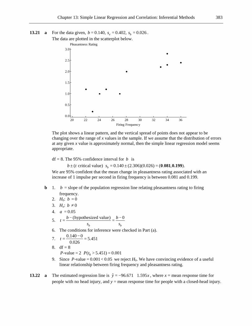
Chapter 13: Simple Linear Regression and Correlation: Inferential Methods 383
13.21 a For the data given, 0.140, 0.402, 0.026e bb s s= = = . The data are plotted in the scatterplot below.
363432302826242220
3.0
2.5
2.0
1.5
1.0
0.5
0.0
Firing Frequency
Pleasantness Rating
The plot shows a linear pattern, and the vertical spread of points does not appear to be
changing over the range of x values in the sample. If we assume that the distribution of errors at any given x value is approximately normal, then the simple linear regression model seems appropriate.
df = 8. The 95% confidence interval for β is
( critical value) 0.140 (2.306)(0.026) ( . , ).bb t s± ⋅ = ± = 0 081 0.199 We are 95% confident that the mean change in pleasantness rating associated with an
increase of 1 impulse per second in firing frequency is between 0.081 and 0.199. b 1. β = slope of the population regression line relating pleasantness rating to firing
frequency. 2. H0: 0β = 3. Ha: 0β ≠ 4. 0.05α =
5. (hypothesized value) 0b b
b bts s
− −= =
6. The conditions for inference were checked in Part (a).
7. 0.140 0 5.4510.026
t −= =
8. df = 8 8-value 2 ( 5.451) 0.001P P t= ⋅ > = 9. Since -value 0.001 0.05P = < we reject H0. We have convincing evidence of a useful
linear relationship between firing frequency and pleasantness rating. 13.22 a The estimated regression line is ˆ 96.671 1.595y x= − + , where x = mean response time for
people with no head injury, and y = mean response time for people with a closed-head injury.

384 Chapter 13: Simple Linear Regression and Correlation: Inferential Methods
b 1. β = slope of the population regression line relating mean response time for people with a closed-head injury to mean response time for people with no head injury.
2. H0: 0β = 3. Ha: 0β ≠ 4. 0.05α =
5. (hypothesized value) 0b b
b bts s
− −= =
6. The data are plotted in the scatterplot below.
12001000800600400200
2000
1500
1000
500
Control
CHI
The plot shows a linear pattern, and the vertical spread of points does not appear to be
changing over the range of x values in the sample. If we assume that the distribution of errors at any given x value is approximately normal, then the simple linear regression model seems appropriate.
7. 53.669, 835860, 0.05870e xx bs S s= = = 1.595 0 27.1650.05870
t −= =
8. df = 8 8-value 2 ( 27.165) 0P P t= ⋅ > ≈ 9. Since -value 0 0.05P ≈ < we reject H0. We have convincing evidence of a useful linear
relationship between mean response time for people with no head injury and mean response time for people with a closed-head injury.
c For any given task, people with a closed-head injury are predicted to have an average reaction
time that is 1.48 times as great as the average reaction time for people with no head injury. 13.23 a 1. β = average change in sales revenue associated with a 1-unit increase in advertising
expenditure. 2. H0: 0β = 3. Ha: 0β ≠ 4. 0.05α =
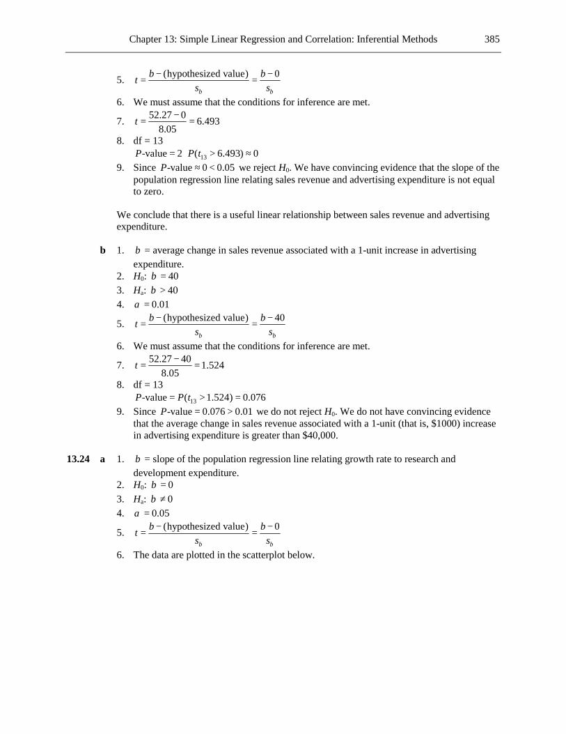
Chapter 13: Simple Linear Regression and Correlation: Inferential Methods 385
5. (hypothesized value) 0b b
b bts s
− −= =
6. We must assume that the conditions for inference are met.
7. 52.27 0 6.4938.05
t −= =
8. df = 13 13-value 2 ( 6.493) 0P P t= ⋅ > ≈ 9. Since -value 0 0.05P ≈ < we reject H0. We have convincing evidence that the slope of the
population regression line relating sales revenue and advertising expenditure is not equal to zero.
We conclude that there is a useful linear relationship between sales revenue and advertising
expenditure. b 1. β = average change in sales revenue associated with a 1-unit increase in advertising
expenditure. 2. H0: 40β = 3. Ha: 40β > 4. 0.01α =
5. (hypothesized value) 40b b
b bts s
− −= =
6. We must assume that the conditions for inference are met.
7. 52.27 40 1.5248.05
t −= =
8. df = 13 13-value ( 1.524) 0.076P P t= > = 9. Since -value 0.076 0.01P = > we do not reject H0. We do not have convincing evidence
that the average change in sales revenue associated with a 1-unit (that is, $1000) increase in advertising expenditure is greater than $40,000.
13.24 a 1. β = slope of the population regression line relating growth rate to research and
development expenditure. 2. H0: 0β = 3. Ha: 0β ≠ 4. 0.05α =
5. (hypothesized value) 0b b
b bts s
− −= =
6. The data are plotted in the scatterplot below.
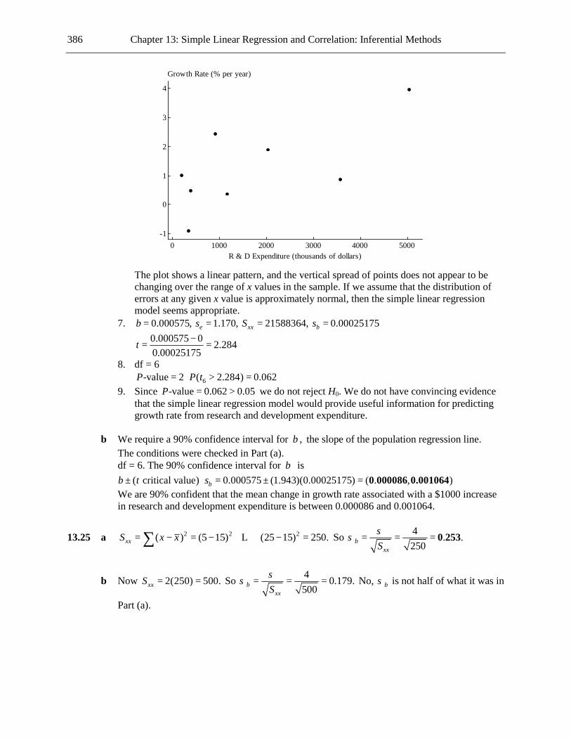
386 Chapter 13: Simple Linear Regression and Correlation: Inferential Methods
500040003000200010000
4
3
2
1
0
-1
R & D Expenditure (thousands of dollars)
Growth Rate (% per year)
The plot shows a linear pattern, and the vertical spread of points does not appear to be
changing over the range of x values in the sample. If we assume that the distribution of errors at any given x value is approximately normal, then the simple linear regression model seems appropriate.
7. 0.000575, 1.170, 21588364, 0.00025175e xx bb s S s= = = = 0.000575 0 2.2840.00025175
t −= =
8. df = 6 6-value 2 ( 2.284) 0.062P P t= ⋅ > = 9. Since -value 0.062 0.05P = > we do not reject H0. We do not have convincing evidence
that the simple linear regression model would provide useful information for predicting growth rate from research and development expenditure.
b We require a 90% confidence interval for ,β the slope of the population regression line.
The conditions were checked in Part (a). df = 6. The 90% confidence interval for β is
( critical value) 0.000575 (1.943)(0.00025175) ( . , )bb t s± ⋅ = ± = 0 000086 0.001064 We are 90% confident that the mean change in growth rate associated with a $1000 increase
in research and development expenditure is between 0.000086 and 0.001064.
13.25 a 2 2 2( ) (5 15) (25 15) 250.xxS x x= − = − + + − =∑ L So 4 . .250b
xxSσ
σ = = = 0 253
b Now 2(250) 500.xxS = = So 4 0.179.500b
xxSσ
σ = = = No, bσ is not half of what it was in
Part (a).

Chapter 13: Simple Linear Regression and Correlation: Inferential Methods 387
c Four observations should be taken at each of the x values, since then xxS would be
multiplied by 4, and so bσ would be divided by 2. To verify, 4(250) 1000,xxS = = so
( )4 0.126 1 2 (0.253).1000b
xxSσ
σ = = = =
13.26 1. β = slope of the population regression line relating cranial capacity to chord length. 2. H0: 20β = 3. Ha: 20β ≠ 4. 0.05α =
5. (hypothesized value) 20b b
b bts s
− −= =
6. The data are plotted in the scatterplot below.
87.585.082.580.077.575.0
1050
1000
950
900
850
800
750
Chord Length (mm)
Cranial Capacity (cubic centimeters)
The plot shows a linear pattern, and the vertical spread of points does not appear to be
changing over the range of x values in the sample. If we assume that the distribution of errors at any given x value is approximately normal, then the simple linear regression model seems appropriate.
7. 22.257, 55.575, 123.429, 5.002e xx bb s S s= = = = 22.257 20 0.451
5.002t −
= =
8. df = 5 5-value 2 ( 0.451) 0.671P P t= ⋅ > = 9. Since -value 0.671 0.05P = > we do not reject H0. We do not have convincing evidence that
the increase in cranial capacity associated with a 1-mm increase in chord length is not 20 cm3. 13.27 There is a random scatter of points in the residual plot, implying that a linear model relating
squirrel population density to percentage of logging is appropriate. The residual plot shows no tendency for the size (magnitude) of the residuals to either increase of decrease as percentage of logging increases. So it is justifiable to assume that the vertical deviations from the population regression line have equal standard deviations. The last condition is that the vertical deviations be

388 Chapter 13: Simple Linear Regression and Correlation: Inferential Methods
normally distributed. The fact that the boxplot of the residuals is roughly symmetrical and shows no outliers suggests that this condition is satisfied.
13.28 a
363432302826242220
1.5
1.0
0.5
0.0
-0.5
-1.0
-1.5
-2.0
Firing Frequency
Standardized Residual
There are no particularly unusual features in the standardized residual plot. The only slightly
unusual feature is the point whose standardized residual is −1.83, which is relatively far from zero, but not particularly extreme. The plot supports the assumption that the simple linear regression model applies.
b Yes. Since the normal probability plot shows a roughly linear pattern we can conclude that is
it reasonable to assume that the error distribution is approximately normal. 13.29 The standardized residual plot is shown below.
403020100
1.5
1.0
0.5
0.0
-0.5
-1.0
-1.5
-2.0
Sunflower Meal (%)
Standardized Residual
There is clear indication of a curve in the standardized residual plot, suggesting that the simple
linear regression model is not adequate.

Chapter 13: Simple Linear Regression and Correlation: Inferential Methods 389
13.30 a Letting x = minimum width and y = maximum width, the least-squares regression line is
ˆ 0.939 0.873 .y x= + b The residuals and the standardized residuals are shown in the table below.
Product Minimum Width
Maximum Width
Residual Standardized Residual
1 1.8 2.5 -0.011 -0.016 2 2.7 2.9 -0.397 -0.601 3 2 2.15 -0.535 -0.816 4 2.6 2.9 -0.309 -0.469 5 3.15 3.2 -0.489 -0.742 6 1.8 2 -0.511 -0.780 7 1.5 1.6 -0.649 -0.996 8 3.8 4.8 0.543 0.825 9 5 5.9 0.595 0.918 10 4.75 5.8 0.714 1.096 11 2.8 2.9 -0.484 -0.734 12 2.1 2.45 -0.323 -0.491 13 2.2 2.6 -0.260 -0.396 14 2.6 2.6 -0.609 -0.924 15 2.6 2.7 -0.509 -0.773 16 2.9 3.1 -0.371 -0.563 17 5.1 5.1 -0.292 -0.451 18 10.2 10.2 0.355 0.748 19 3.5 3.5 -0.495 -0.751 20 1.2 2.7 0.713 1.100 21 1.7 3 0.577 0.882 22 1.75 2.7 0.233 0.356 23 1.7 2.5 0.077 0.117 24 1.2 2.4 0.413 0.637 25 1.2 4.4 2.413 3.721 26 7.5 7.5 0.013 0.021 27 4.25 4.25 -0.400 -0.610
The standardized residual plot is shown below.

390 Chapter 13: Simple Linear Regression and Correlation: Inferential Methods
1086420
4
3
2
1
0
-1
Minimum Width
Standardized Residual
The standardized residual plot shows that there is one point that is a clear outlier (the point
whose standardized residual is 3.721). This is the point for product 25. c The equation of the least-squares regression line is now ˆ 0.703 0.918 .y x= +
A computer analysis gives 0.065bs = . Thus the change in slope from 0.873 to 0.918 expressed in standard deviations is (0.918 0.873) 0.065 0.692.− = Removal of the point resulted in a reasonably substantial change in the equation of the estimated regression line.
d For every 1-cm increase in minimum width, the mean maximum width is estimated to
increase by 0.918 cm. The intercept would be an estimate of the mean maximum width when the minimum width is zero. It is clearly impossible to have a container whose minimum width is zero.
e
1086420
2.0
1.5
1.0
0.5
0.0
-0.5
-1.0
Minimum Width
Standardized Residual

Chapter 13: Simple Linear Regression and Correlation: Inferential Methods 391
The standardized residual plot for the data with the Coke bottle removed is shown above. The
pattern in this plot suggests that the variances of the y distributions decrease as x increases, and therefore that the assumption of constant variance is not valid.
13.31 There is no clear curve in the standardized residual plot, initially suggesting that the assumptions
of the simple linear regression model might be satisfied. Furthermore, there is no point with an extreme x value (a point with an extreme x value would be potentially influential, and therefore undesirable), and there is no one point particularly far-removed from the other points in the standardized residual plot. However, there does seem to be a tendency for points with more central x values to have larger standardized residuals (positive or negative) than points with larger or smaller x values, and there is one point with a standardized residual quite a bit larger than 2. These two facts suggest that the assumptions of the simple linear regression model might not be satisfied.
13.32 a
25201510
150
100
50
0
-50
-100
Traffic flow (thousands of cars per 24 hrs)
Residual
0
There is the smallest hint of a curve in the residual plot, but this is not strong enough to
suggest that the simple linear regression model is inappropriate.

392 Chapter 13: Simple Linear Regression and Correlation: Inferential Methods
b
25201510
1.5
1.0
0.5
0.0
-0.5
-1.0
Traffic flow (thousands of cars per 24 hrs)
Standardized residual
0
This plot is very similar in appearance to the one in Part (a).
Online Exercises 13.33 Suppose we constructed a 95% confidence interval for the mean value of y when x = x*. We
would then be 95% confident that the mean value of y was within that interval. If we were to construct the 95% prediction interval at x = x* we would be 95% confident that an observed y value, y*, at that value of x will be within the interval. The 95% confidence level for the prediction interval is interpreted as follows. The prediction interval is constructed using a set of independent y values for a given set of x values. Imagine this being done a large number of times, with the prediction interval at *x x= being calculated for each set of ( , )x y points. Imagine, also, a large number of y values being selected at x = x*. Then if one interval is chosen at random, and one y value is chosen at random, on average 95 times out of 100 the y value will be within the interval.
13.34 If a confidence interval for β is required, you are asked for a confidence interval either for the
slope of the regression line or for the mean increase in y associated with a one-unit increase in x. If a confidence interval for *xα β+ is required, you are given a value of x and asked to find a confidence interval for the mean value of y at that value of x.
13.35 a We use 2
*1 ( * )
a bx exx
x xs sn S+
−= + .
Here 2
(2.0)1 (2 2.5)16.486 .20 25a bs +
−= + = 4.038
b Since 3 is the same distance from 2.5 as is 2, (3.0) (2.0) .a b a bs s+ += = 4.038

Chapter 13: Simple Linear Regression and Correlation: Inferential Methods 393
c 2
(2.8)1 (2.8 2.5)16.486 . .20 25a bs +
−= + = 3 817
d The estimated standard deviation of *a bx+ is smallest for * 2.5,x = since the distance of
this value from the mean value of x is zero. 13.36 The scatterplot given in the example shows a linear pattern that is consistent with the assumptions
of the simple linear regression model. The point estimate of (0.6)α β+ is (0.6) 0.6678 1.3957(0.6) 0.16962.a b+ = − + =
( )22
2 (5.82)3.1804 0.3577.12xx
xS x
n= − = − =∑∑
The estimated standard deviation of (0.6)a b+ is 2 21 (0.6 ) 1 (0.6 5.82 12)0.285 0.034287.
12 0.3577exx
xsn S
− −+ = + =
The critical value of the t distribution with 10 degrees of freedom for a 95% confidence interval is 2.228. So the required confidence interval is 0.16962 2.228(0.034287) ( . , . ).± = 0 093 0 246 We are 95% confident that the mean vote-difference proportion for congressional races where 60% judge candidate A as more competent is between 0.093 and 0.246.
13.37 a The equation of the estimated regression line is ˆ 0.001790 0.0021007 ,y x= − − where x =
mean childhood blood lead level and y = brain volume change. b We need to assume that the conditions for inference are met.
The point estimate of (20)α β+ is (20) 0.001790 0.0021007(20) 0.043804.a b+ = − − = − The estimated standard deviation of (20)a b+ is
2 21 (20 ) 1 (20 11.5)0.031 0.0069979.100 1764e
xx
xsn S
− −+ = + =
The critical value of the t distribution with 98 degrees of freedom for a 90% confidence interval is 1.661. So the required confidence interval is 0.043804 1.661(0.0069979) ( . , . ).− ± = − −0 055 0 032 We are 90% confident that the mean brain volume change for people with a childhood blood lead level of 20 μg/dL is between −0.055 and −0.032.
c The estimated standard deviation of the amount by which a single y observation deviates
from the value predicted by an estimated regression line is 2 2 2 2
* 0.031 0.0069979 0.03178.e a bxs s ++ = + = The critical value of the t distribution with 98 degrees of freedom for a 90% confidence interval is 1.661. So the required confidence interval is 0.043804 1.661(0.03178) ( . , . ).− ± = −0 097 0 009 We are 90% confident that the brain volume change for a person with a childhood blood lead level of 20 μg/dL will be between −0.097 and 0.009.
d The answer to Part (b) gives an interval in which we are 90% confident that the mean brain
volume change for a person with a childhood blood lead level of 20 μg/dL lies. The answer to

394 Chapter 13: Simple Linear Regression and Correlation: Inferential Methods
Part (c) states that if we were to find the brain volume change for one person with a childhood blood lead level of 20 μg/dL, we are 90% confident that this value will lie within the interval found.
13.38 a The required proportion is 2 .r = 0.630 b Yes. The P-value of 0.000 indicates that the data provide convincing evidence that the slope
of the population regression line is not equal to zero. c We need to assume that the conditions for inference are met.
The point estimate of (200)α β+ is (200) 4.7896 0.014388(200) 7.6672.a b+ = + = We are given that (200) 0.347.a bs + = The critical value of the t distribution with 15 degrees of freedom for a 95% confidence interval is 2.131. So the required confidence interval is 7.6672 2.131(0.347) ( . , . ).± = 6 928 8 407 We are 95% confident that the mean time necessary when the depth is 200 feet is between 6.928 and 8.407 minutes.
d We need to assume that the conditions for inference are met.
The point estimate of (200)α β+ is (200) 4.7896 0.014388(200) 7.6672.a b+ = + = We are given that (200) 0.347.a bs + = Thus, the estimated standard deviation of the amount by which a single y observation deviates from the value predicted by an estimated regression line is 2 2 2 2
* 1.432 0.347 1.47344.e a bxs s ++ = + = The critical value of the t distribution with 15 degrees of freedom for a 95% confidence interval is 2.131. So the required confidence interval is 7.6672 2.131(1.47344) ( . , . ).± = 4 527 10 808 We are 95% confident that the time necessary when the depth is 200 feet will be between 4.527 and 10.808 minutes.
e The critical value of the t distribution with 15 degrees of freedom for a 95% confidence
interval is 2.131. The critical value of the t distribution with 15 degrees of freedom for a 99% confidence interval is 2.947. Thus the required interval will have the same center as the given interval and will have a width that is 2.947 2.131 times the width of the given interval. Therefore, the required interval will have center (8.147 10.065) 2 9.106+ = and the distance from this center to the top and the bottom of the required interval will be ( )( )2.947 2.131 10.065 9.106 1.326.− = So the required interval is 9.106 1.326 ( . , . )± = 7 780 10 432
13.39 a The equation of the regression line is ˆ 133.02 5.919 ,y x= − + where x = snout vent length and
y = clutch size. b .bs = 1.127

Chapter 13: Simple Linear Regression and Correlation: Inferential Methods 395
c Yes. Since the estimated slope is positive and since the P-value is small (given as 0.000 in the
output) we have convincing evidence that the slope of the population regression line is positive.
d We need to assume that the conditions for inference are met. The point estimate of (65)α β+ is (65) 133.02 5.919(65) 251.715.a b+ = − + =
2 2 245958 14(56.5) 1266.5.xxS x nx= − = − =∑ The estimated standard deviation of (65)a b+ is
2 21 (65 ) 1 (65 56.5)33.90 12.151.14 1266.5e
xx
xsn S
− −+ = + =
Therefore, the estimated standard deviation of the amount by which a single y observation deviates from the value predicted by an estimated regression line is
2 2 2 2* 33.90 12.151 36.012.e a bxs s ++ = + =
The critical value of the t distribution with 12 degrees of freedom for a 95% confidence interval is 2.179. So the required confidence interval is 251.715 2.179(36.012) ( . , . ).± = 173 252 330 178 We are 95% confident that the clutch size for a salamander whose snout-vent length is 65 will be between 173.252 and 330.178.
e It would not be appropriate to use the estimated regression line to predict the clutch size for a
salamander with a snout-vent length of 105, since 105 is a long way outside the range of the x values in the original data set.
13.40 a 1. β = slope of the population regression line relating maximum width to minimum width. 2. H0: 0β = 3. Ha: 0β > 4. 0.05α =
5. (hypothesized value) 0b b
b bts s
− −= =
6. The standardized residual plot given in the solution to the earlier exercise shows one point with a large standardized residual. We will nonetheless assume that the conditions for the simple linear regression model apply, and proceed with the hypothesis test.
7. 0.87310, 0.67246, 108.64963, 0.06451e xx bb s S s= = = = 0.87310 0 13.534
0.06451t −
= =
8. df = 25 25-value ( 13.534) 0P P t= > ≈ 9. Since -value 0 0.05P ≈ < we reject H0. We have convincing evidence of a positive linear
relationship between minimum width and maximum width. b .es = 0.672 This is a typical deviation of a maximum width in the sample from the value
predicted by the least-squares regression line. c We proceed with calculation of the confidence interval even though the standardized residual
plot shows that there is a point with a large standardized residual. The point estimate of (6)α β+ is (6) 0.939 0.873(6) 6.178.a b+ = + =

396 Chapter 13: Simple Linear Regression and Correlation: Inferential Methods
The estimated standard deviation of (6)a b+ is 2 21 (6 ) 1 (6 3.096)0.672 0.228.
27 108.650exx
xsn S
− −+ = + =
The critical value of the t distribution with 25 degrees of freedom for a 95% confidence interval is 2.060. So the required confidence interval is 6.178 2.060(0.228) ( . , ).± = 5 709 6.647 We are 95% confident that the mean maximum width when the minimum width is 6 cm is between 5.709 and 6.647. (Note that some values in this interval are not actually possible for this mean, since, when the minimum width is 6 cm, the maximum width can’t be less than 6 cm.)
d We proceed with calculation of the confidence interval even though the standardized residual
plot shows that there is a point with a large standardized residual. As calculated in Part (c), the point estimate of (6)α β+ is 6.178, and the estimated standard deviation of (6)a b+ is 0.228. Therefore, the estimated standard deviation of the amount by which a single y observation deviates from the value predicted by an estimated regression line is
2 2 2 2* 0.672 0.228 0.710.e a bxs s ++ = + =
The critical value of the t distribution with 25 degrees of freedom for a 95% confidence interval is 2.060. So the required confidence interval is 6.178 2.060(0.710) ( . , . ).± = 4 716 7 640 We are 95% confident that, when the minimum width is 6 cm, the maximum width will be between 4.716 and 7.640. (Note that some values in this interval are not actually possible for this predicted value, since, when the minimum width is 6 cm, the maximum width can’t be less than 6 cm.)
13.41 a The equation of the estimated regression line is ˆ 2.78551 0.04462 ,y x= + where x = time on
shelf and y = moisture content. b β = slope of the population regression line relating moisture content to shelf time. H0: 0β = Ha: 0β ≠ 0.05α =
(hypothesized value) 0b b
b bts s
− −= =
A standardized residual plot is shown below.

Chapter 13: Simple Linear Regression and Correlation: Inferential Methods 397
403020100
2
1
0
-1
-2
-3
Shelf Time (days)
Standardized Residual
Apart from one outlier, the standardized residual plot shows a random pattern that is
consistent with the simple regression model.
( )22
2 (269)7445 2276.357.14xx
xS x
n= − = − =∑∑
0.196246es =
0.00411eb
xx
ssS
= =
0.04462 0 10.8480.00411
t −= =
df = 12 12-value 2 ( 10.848) 0P P t= ⋅ > ≈ Since -value 0 0.05P ≈ < we reject H0. We have convincing evidence that the simple
regression model provides useful information for predicting moisture content from knowledge of shelf time.
c The conditions for inference were checked in Part (b). The point estimate of (30)α β+ is (30) 2.78551 0.04462(30) 4.124.a b+ = + =
2 2 27745 14(269 14) 2576.357.xxS x nx= − = − =∑ 0.196246.es =
The estimated standard deviation of (30)a b+ is 2 21 (30 ) 1 (30 19.214286)0.196246 0.067006.
14 2576.357exx
xsn S
− −+ = + =
Therefore, the estimated standard deviation of the amount by which a single y observation deviates from the value predicted by an estimated regression line is
2 2 2 2* 0.196246 0.067006 0.207.e a bxs s ++ = + =
The critical value of the t distribution with 12 degrees of freedom for a 95% confidence interval is 2.179. So the required confidence interval is 4.124 2.179(0.207) ( . , ).± = 3 672 4.576

398 Chapter 13: Simple Linear Regression and Correlation: Inferential Methods
We are 95% confident that the moisture content for a box of cereal that has been on the shelf for 30 days will be between 3.672 and 4.576 percent.
d Since 4.1 is included in the confidence interval constructed in Part (c), a moisture content
exceeding 4.1 percent is quite plausible when the shelf time is 30 days. 13.42 Since 17 is further from the mean than is 20, both the confidence interval and the prediction
interval will be wider for * 17x = than for * 20.x = 13.43 The data are displayed in the scatterplot below.
959085807570
17.5
15.0
12.5
10.0
7.5
5.0
Maximum outdoor temperature
Hours of chiller operation per day
The scatterplot shows a linear pattern that is consistent with the assumptions of the simple linear
regression model. 6, 82.667, 269.333xxn x S= = =
46.410, 0.702, (82) 11.132a b a b= − = + = 0.757es =
2 2
(82)1 (82 ) 1 (82 82.667)0.757 0.311
6 269.333a b exx
xs sn S+
− −= + = + =
(82)
(82) 12 11.132 12 2.7940.311a b
a bts +
+ − −= = = −
4-value ( 2.794) 0.025P P t= < − = Since this P-value is greater than 0.01, we do not reject H0. We do not have convincing evidence at the 0.01 level that, when the maximum output is 82°F, the mean number of hours of chiller operation is less than 12.
13.44 The statistic r is the correlation coefficient for a sample, while ρ denotes the correlation
coefficient for the population. 13.45 The first statement is not correct. It is theoretically possible, by chance, to obtain a sample
correlation coefficient of 1 when the population correlation coefficient is not 1. This occurs when the points representing the sample values just happen to lie in a perfect straight line. (Also, in the

Chapter 13: Simple Linear Regression and Correlation: Inferential Methods 399
special case when the sample size is 2, the value of r will necessarily be 1, whatever the value of ρ .) The second statement is correct. If the population correlation coefficient is 1, then all the points in the population lie on a perfect straight line. Thus, when a sample is taken from that population, all the points in the sample will lie on that same straight line. As a result, the sample correlation coefficient is equal to 1.
13.46 1. ρ = the correlation between teaching evaluation index and annual raise for the population
from which the sample was selected. 2. H0: 0ρ = 3. Ha: 0ρ ≠ 4. 0.05α =
5. 212
rtr
n
=−−
6. We must assume that the variables have a bivariate normal distribution and that the sample was a random sample from the population.
7. 2
0.11 2.0731 0.11
351
t = =−
8. df = 351 351-value 2 ( 2.073) 0.039P P t= ⋅ > = 9. Since -value 0.039 0.05P = < we reject H0. We have convincing evidence of a linear
association between teaching evaluation index and annual raise. This result might be initially surprising, since 0.11 seems to be a relatively small value for the
sample correlation coefficient. However, what the result shows is that for a sample size as large as 353, a sample correlation as large as 0.11 would be very unlikely if the population correlation were zero.
13.47 1. ρ = the correlation between annual dollar rent per square foot and annual dollar sales per
square foot. 2. H0: 0ρ = 3. Ha: 0ρ > 4. 0.05α =
5. 212
rtr
n
=−−
6. We must assume that the variables have a bivariate normal distribution. We are told that the sample was randomly selected.
7. 2
0.37 2.8441 0.37
51
t = =−
8. df = 51 51-value ( 2.844) 0.003P P t= > =
400 Chapter 13: Simple Linear Regression and Correlation: Inferential Methods
9. Since -value 0.003 0.05P = < we reject H0. We have convincing evidence of a positive linear association between annual dollar rent per square foot and annual dollar sales per square foot for the population of all such stores.
13.48 a 1. ρ = the correlation between time spent watching television and grade point average for
the population from which the sample was selected. 2. H0: 0ρ = 3. Ha: 0ρ < 4. 0.01α =
5. 212
rtr
n
=−−
6. We must assume that the variables have a bivariate normal distribution. We are told that the sample was a random sample.
7. 2
0.26 6.1751 ( 0.26)
526
t −= = −
− −
8. df = 526 526-value ( 6.175) 0P P t= < − ≈ 9. Since -value 0 0.01P ≈ < we reject H0. We have convincing evidence of a negative
correlation between time spent watching television and grade point average. b Since 2 2( 0.26) 0.0676,r = − = only 6.76% of the observed variation in grade point average
would be explained by the regression line. This is not a substantial percentage.
13.49 a We first calculate the value of r using .xy
xx yy
Sr
S S=
This formula can be proved as follows:
( ) ( )( ).
1 1 ( 1)( 1)
1 1
x yx y xy xy
x y xx yyyyxx
x x y ys sz z x x y y S S
rn n n s s S SSSn
n n
− − − − = = = = =
− − −−
− −
∑∑ ∑
According to the summary statistics given we have
( )22
2 (860)56700 7393.33315xx
xS x
n= − = − =∑∑
( )22
2 (348)8954 880.415yy
yS y
n= − = − =∑∑
( )( ) (860)(348)22265 231315xy
x yS xy
n= − = − =∑ ∑∑
So 2313 0.907.(7393.333)(880.4)
xy
xx yy
Sr
S S= = =

Chapter 13: Simple Linear Regression and Correlation: Inferential Methods 401
1. ρ = the correlation between particulate pollution and luminance for the population from
which the sample was selected. 2. H0: 0ρ = 3. Ha: 0ρ > 4. 0.05α =
5. 212
rtr
n
=−−
6. We must assume that the variables have a bivariate normal distribution. We are told that the sample was representative of the population, so we can treat it as a random sample.
7. 2
0.907 7.7461 0.907
13
t = =−
8. df = 13 13-value ( 7.746) 0P P t= > ≈ 9. Since -value 0 0.05P ≈ < we reject H0. We have convincing evidence of a positive
correlation between particulate pollution and luminance for the population from which the sample was selected.
b The required proportion is 2 20.907 .r = = 0.822 13.50 1. ρ = the correlation between surface and subsurface concentration. 2. H0: 0ρ = 3. Ha: 0ρ ≠ 4. 0.05α =
5. 212
rtr
n
=−−
6. We must assume that the sample was a random sample from the population under consideration.

402 Chapter 13: Simple Linear Regression and Correlation: Inferential Methods
1.51.00.50.0-0.5-1.0-1.5
50
40
30
20
10
0
Normal Score
Surface
1.51.00.50.0-0.5-1.0-1.5
7
6
5
4
3
Normal Score
Subsurface
The curved pattern in the first normal probability plot tells us that it is unlikely that the
variables have a bivariate normal distribution, but we will nevertheless proceed with the hypothesis test.
7. 0.574r =
2
0.574 1.8551 0.574
7
t = =−
8. df = 7 7-value 2 ( 1.855) 0.106P P t= ⋅ > = 9. Since -value 0.106 0.05P = > we do not reject H0. We do not have convincing evidence of a
linear relationship between surface and subsurface concentration. 13.51 1. ρ = population correlation 2. H0: 0ρ = 3. Ha: 0ρ ≠
Chapter 13: Simple Linear Regression and Correlation: Inferential Methods 403
4. 0.05α =
5. 212
rtr
n
=−−
6. We must assume that the variables have a bivariate normal distribution and that the sample was randomly selected from the population.
7. 2
0.022 2.2001 0.022
9998
t = =−
8. df = 9998 9998-value 2 ( 2.200) 0.028.P P t= ⋅ > = 9. Since -value 0.028 0.05P = < we reject H0. We have convincing evidence that 0ρ ≠ . This tells us that, although the sample correlation coefficient was apparently close to 0, the
sample is large enough for the result to convince us nonetheless that the population correlation coefficient is not zero.
13.52 a The slope of the estimated regression line for y = verbal language score against x = height
gain from age 11 to 16 is 2.0. This tells us that for each extra inch of height gain the average verbal language score at age 11 increased by 2.0 percentage points. The equivalent results for nonverbal language scores and math scores were 2.3 and 3.0. Thus the reported slopes are consistent with the statement that each extra inch of height gain was associated with an increase in test scores of between 2 and 3 percentage points.
b The slope of the estimated regression line for y = verbal language score against x = height
gain from age 16 to 33 is −3.1. This tells us that for each extra inch of height gain the average verbal language score at age 11 decreased by 3.1 percentage points. The equivalent results for nonverbal language scores and math scores were both −3.8. Thus the reported slopes are consistent with the statement that each extra inch of height gain was associated with a decrease in test scores of between 3.1 and 3.8 percentage points.
c Between the ages of 11 and 16 the first boy grew 5 inches more than the second boy. So the
first boy’s age 11 math score is predicted to be 5 3 15⋅ = percentage points higher than that of the second boy. Between the ages of 16 and 33 the second boy grew 5 inches more than the first boy. According to this information the first boy’s age 11 math score is predicted to be 5 3.8 19⋅ = percentage points higher than that of the second boy. These two results are consistent with the conclusion that on the whole boys who did their growing early had higher cognitive scores at age 11 than those whose growth occurred later.
13.53 a For a 1-day increase in elapsed time, the average biomass concentration is estimated to
decrease by 0.640 g/cm3. b When 40,x = 3ˆ 106.3 0.640(40) g/cm .y = − = 80.7 c 1. β = slope of the population regression line relating biomass concentration to elapsed
time. 2. H0: 0β =

404 Chapter 13: Simple Linear Regression and Correlation: Inferential Methods
3. Ha: 0β ≠ 4. 0.05α =
5. (hypothesized value) 0b b
b bts s
− −= =
6. We need to assume that the assumptions of the simple linear regression model apply. 7. Since the slope of the estimated regression line is negative, 0.470 0.686.r = − = −
As explained at the end of Section 13.5, 2
0 .1
2b
b rts r
n
−= =
−−
So here, 0.6861 0.470
56
t −== = −
−7.047
8. df = 56 56-value 2 ( 7.047) 0P P t= ⋅ < − ≈ 9. Since -value 0 0.05P ≈ < we reject H0. We have convincing evidence of a useful linear
relationship between elapsed time and biomass concentration.
13.54 a 2 2
0.18 3.399.1 1 ( 0.18)
2 345
rtr
n
−= = = −
− − −−
Thus, for a two-tailed test, the P-value is 3452 ( 3.399) 0.001.P t⋅ < − = Since the P-value for a one-tailed test would be a half of this, it is indeed correct, whether this be a one- or two-tailed test, that P-value < 0.05.
b Yes. One would expect, generally speaking, that those with greater coping humor ratings
would have smaller depression ratings. c No. Since 2 2( 0.18) 0.0324,r = − = we know that only 3.2% of the variation in depression
scale values is attributable to the approximate linear relationship with the coping humor scale. So the linear regression model will generally not give accurate predictions.
13.55 a 1. ρ = the correlation between soil hardness and trail length for the population of penguin
burrows. 2. H0: 0ρ = 3. Ha: 0ρ < 4. 0.05α =
5. 212
rtr
n
=−−
6. We must assume that the variables have a bivariate normal distribution and that the sample was a random sample of penguin burrows.

Chapter 13: Simple Linear Regression and Correlation: Inferential Methods 405
7. 0.386 0.621.r = − = − (We know that 0r < since the slope of the least-squares line is
negative.)
2
0.621 6.0901 ( 0.621)
59
t −= = −
− −
8. df = 59 59-value ( 6.090) 0P P t= < − ≈ 9. Since -value 0 0.05P ≈ < we reject H0. We have convincing evidence of a negative
correlation between soil hardness and trail length. b We need to assume that the conditions for inference are met.
The point estimate of (6.0)α β+ is (6.0) 11.607 1.4187(6.0) 3.0948.a b+ = − = The estimated standard deviation of (6.0)a b+ is
2 21 (6.0 ) 1 (6.0 4.5)2.35 0.374.61 250e
xx
xsn S
− −+ = + =
Therefore, the estimated standard deviation of the amount by which a single y observation deviates from the value predicted by an estimated regression line is
2 2 2 2* 2.35 0.374 2.380.e a bxs s ++ = + =
The critical value of the t distribution with 59 degrees of freedom for a 95% confidence interval is 2.001. So the required prediction interval is 3.0948 2.001(2.380) ( . , . ).± = −1 667 7 856 We are 95% confident that the trail length when the soil hardness is 6.0 will be between −1.667 and 7.856.
c No. For 10x = the least-squares line predicts 2.58.y = − Since it is not possible to have a
negative trail length, it is clear that the simple linear regression model does not apply at 10.x = So the simple linear regression model is not suitable for this prediction.
13.56 a
30252015105
1.4
1.2
1.0
0.8
0.6
0.4
0.2
0.0
Percentage of light absorption
Peak photovoltage
The scatterplot suggests that the simple linear regression model might be appropriate.
406 Chapter 13: Simple Linear Regression and Correlation: Inferential Methods
b The equation of the estimated regression line is ˆ 0.0826 0.0446 ,y x= − + where x = percentage of light absorption and y = peak photovoltage.
c The required proportion is 2 .r = 0.983 d When 19.1,x = ˆ 0.0826 0.0446(19.1) .y = − + = 0.770 The peak photovoltage is predicted to
be 0.770. The residual is ˆ 0.68 0.770 .y y− = − = −0.090 e 1. β = slope of the population regression line relating peak photovoltage to percentage of
light absorption. 2. H0: 0β = 3. Ha: 0β ≠ 4. 0.05α =
5. (hypothesized value) 0b b
b bts s
− −= =
6. We are told in Part (b) to assume that the simple linear regression model is appropriate. 7. 0.0446, 0.0611, 746.4, 0.00224e xx bb s S s= = = =
0.0446 0 19.9590.00224
t −= =
8. df = 7 7-value 2 ( 19.959) 0P P t= ⋅ > ≈ 9. Since -value 0 0.05P ≈ < we reject H0. We have convincing evidence of a useful linear
relationship between percent light absorption and peak photovoltage. f We are told in Part (b) to assume that the simple linear regression model is appropriate.
df = 7. The 95% confidence interval for β is ( critical value) 0.0446 (2.365)(0.00224) ( . , . ).bb t s± ⋅ = ± = 0 039 0 050
We are 95% confident that the mean increase in peak photovoltage associated with a 1-percentage point increase in light absorption is between 0.039 and 0.050.
g We are told in Part (b) to assume that the simple linear regression model is appropriate.
The point estimate of (20)α β+ is (20) 0.08259 0.04465(20) 0.810.a b+ = − + = The estimated standard deviation of (20)a b+ is
2 21 (20 ) 1 (20 19.967)0.06117 0.0204.9 746.4e
xx
xsn S
− −+ = + =
The critical value of the t distribution with 7 degrees of freedom for a 95% confidence interval is 2.365. So the required confidence interval is 0.810 2.365(0.0204) ( . , . ).± = 0 762 0 859 We are 95% confident that the mean peak photovoltage when the percentage of light absorption is 20 is between 0.762 and 0.859.
13.57 a 1. β = slope of the population regression line relating x = age and y = percentage of the
cribriform area of the lamina scleralis occupied by pores. 2. H0: 0.5β = − 3. Ha: 0.5β ≠ −
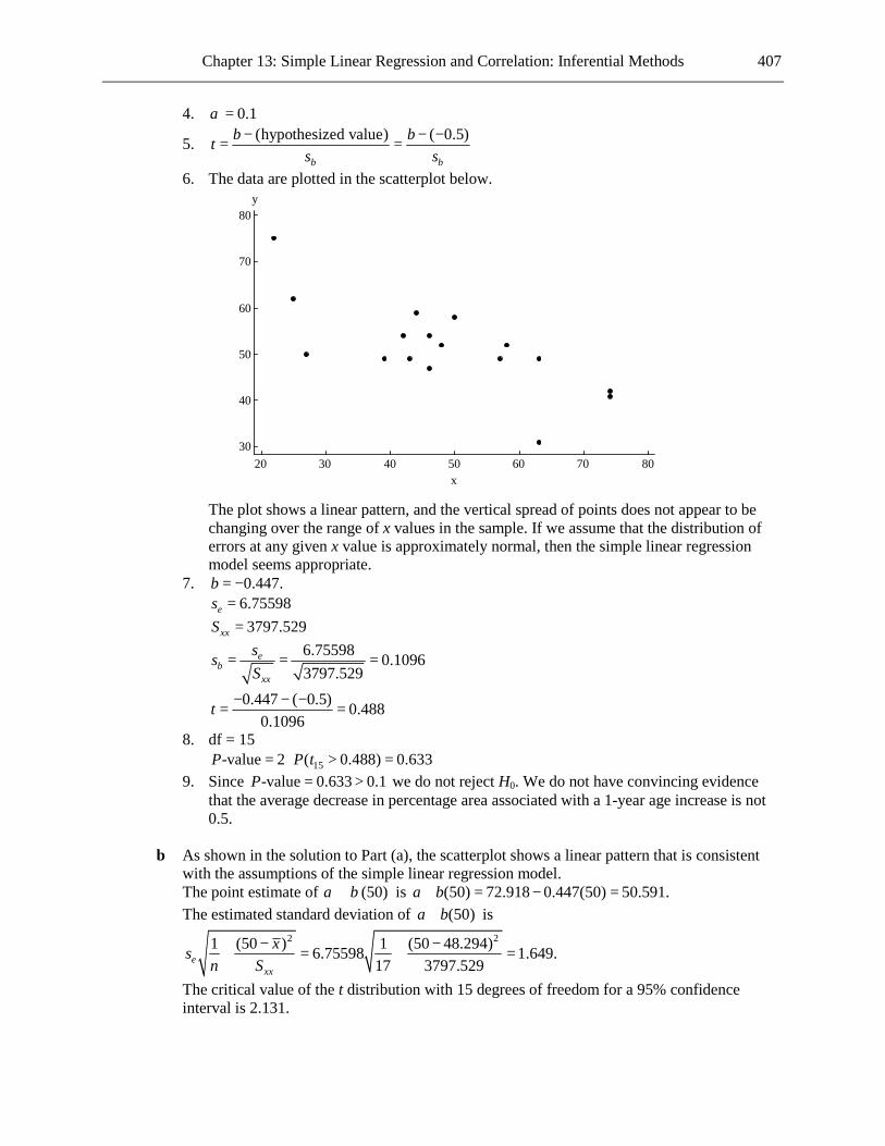
Chapter 13: Simple Linear Regression and Correlation: Inferential Methods 407
4. 0.1α =
5. (hypothesized value) ( 0.5)b b
b bts s
− − −= =
6. The data are plotted in the scatterplot below.
80706050403020
80
70
60
50
40
30
x
y
The plot shows a linear pattern, and the vertical spread of points does not appear to be
changing over the range of x values in the sample. If we assume that the distribution of errors at any given x value is approximately normal, then the simple linear regression model seems appropriate.
7. 0.447.b = − 6.75598es = 3797.529xxS =
6.75598 0.10963797.529
eb
xx
ssS
= = =
0.447 ( 0.5) 0.4880.1096
t − − −= =
8. df = 15 15-value 2 ( 0.488) 0.633P P t= ⋅ > = 9. Since -value 0.633 0.1P = > we do not reject H0. We do not have convincing evidence
that the average decrease in percentage area associated with a 1-year age increase is not 0.5.
b As shown in the solution to Part (a), the scatterplot shows a linear pattern that is consistent
with the assumptions of the simple linear regression model. The point estimate of (50)α β+ is (50) 72.918 0.447(50) 50.591.a b+ = − = The estimated standard deviation of (50)a b+ is
2 21 (50 ) 1 (50 48.294)6.75598 1.649.17 3797.529e
xx
xsn S
− −+ = + =
The critical value of the t distribution with 15 degrees of freedom for a 95% confidence interval is 2.131.

408 Chapter 13: Simple Linear Regression and Correlation: Inferential Methods
So the required confidence interval is 50.591 2.131(1.649) ( . , . ).± = 47 076 54 106 We are 95% confident that the mean percentage area at age 50 is between 47.076 and 54.106.
13.58 a The estimated regression line is ˆ 1.752 0.685 ,y x= − + where x = actual air temperature and y
= temperature as measured by a satellite.
b 2 21 (0 ) 1 (0 2.5)0.804 .
10 82.5a exx
xs sn S
− −= + = + = 0.337
H0: 0α = Ha: 0α ≠ We need to assume that the assumptions of the simple linear regression model apply.
0 1.752 5.1990.337a
ats− −
= = = −
8-value 2 ( 5.199) 0.001P P t= ⋅ < − = Since -value 0.001 0.05P = < we reject H0. We have convincing evidence that the y intercept of the population regression line differs from zero.
c We need to assume that the assumptions of the linear regression model apply.
The 95% confidence interval for α is ( critical value) 1.752 (2.306)(0.337) ( . , . ).aa t s± = − ± = − −2 529 0 975
We are 95% confident that the y intercept of the population regression line lies between −2.529 and −0.975. The fact that zero does not lie within this interval tells us, exactly as concluded in Part (b), that we have convincing evidence at the 0.05 level that the y intercept of the population regression differs from zero.
13.59 For leptodactylus:
SSResid 0.30989= Sample size = 9
0.31636b = 42.82xxS =
For bufa: SSResid 0.12792= Sample size = 8
0.35978b = 34.54875xxS =
2 0.30989 0.12792 0.03368
7 6s +
= =+
H0: β β ′= Ha: β β ′≠ 0.05α =
2 2
0.31636 0.35978 1.034570.03368 0.0336842.82 34.54875
xx xx
b bts sS S
′− −= = = −
++′

Chapter 13: Simple Linear Regression and Correlation: Inferential Methods 409
df = 13 13-value 2 ( 1.03457) 0.320P P t= ⋅ < − = Since -value 0.319 0.05P = > we do not reject H0. We do not have convincing evidence that the
slopes of the population regression lines for the two different frog populations are not equal. 13.60 a
15.012.510.07.55.0
11
10
9
8
7
6
5
4
x1
y1
The scatterplot of the first data set (above) shows no apparent curve, no extreme residuals, no
clear change in the variance of the y values as the x values change, and no influential points. Therefore the simple linear regression model seems appropriate.
15.012.510.07.55.0
10
9
8
7
6
5
4
3
x1
y2
The plot for the second data set (above) shows a clear curve, and so it seems that the assumptions
of the simple linear regression model do not apply.

410 Chapter 13: Simple Linear Regression and Correlation: Inferential Methods
15.012.510.07.55.0
13
12
11
10
9
8
7
6
5
x1
y3
The scatterplot for the third data set (above) shows one point that has a very large residual, and
therefore it seems that the assumptions of the simple linear regression model do not apply.
2018161412108
13
12
11
10
9
8
7
6
5
x4
y4
The scatterplot for the fourth data set (above) shows one point that is clearly influential, and
therefore it seems that the assumptions of the simple linear regression model do not apply. 13.61 If the point (20, 33000) is not included, then the slope of the least-squares line would be relatively
small and negative (appearing close to horizontal when drawn to the scales of the scatterplot given in the question). If the point is included then the slope of the least-squares line would still be negative, but much further from zero.
13.62 a The equation of the estimated regression line is ˆ 57.964 0.0357 ,y x= + where x =
fermentation time and y = glucose concentration. b 1. β = slope of the population regression line relating glucose concentration to fermentation
time.

Chapter 13: Simple Linear Regression and Correlation: Inferential Methods 411
2. H0: 0β = 3. Ha: 0β ≠ 4. 0.1α =
5. (hypothesized value) 0b b
b bts s
− −= =
6. We need to assume that the assumptions of the simple linear regression model apply. 7. 0.03571, 9.8896, 42, 1.5260e xx bb s S s= = = =
0.03571 0 0.02341.5260
t −= =
8. df = 6 6-value 2 ( 0.0234) 0.982P P t= ⋅ > = 9. Since -value 0.982 0.1P = > we do not reject H0. We do not have convincing evidence of
a useful linear relationship between fermentation time and glucose concentration. c The residuals are shown in the table below.
x y Residual 1 74 16.000 2 54 -4.036 3 52 -6.071 4 51 -7.107 5 52 -6.143 6 53 -5.179 7 58 -0.214 8 71 12.750
The residual plot is shown below.
876543210
15
10
5
0
-5
-10
Fermentation time
Residual
d The residual plot shows a clear curve, and so the simple linear regression model seems not to
be appropriate.

412 Chapter 13: Simple Linear Regression and Correlation: Inferential Methods
13.63 The small P-value indicates that there is convincing evidence of a useful linear relationship between percentage raise and productivity.
13.64 The points appear to be varying further from the regression line as the values of x increase, and
there are some points with comparatively very large residuals, and so it seems that the simple linear regression model is not appropriate. A plot of the standardized residuals will show points close to the horizontal axis for small values of x, and points spreading further from the horizontal axis for larger values of x. There will be three points with large magnitudes of standardized residuals.
13.65 a The values 1, , ne eK are the vertical deviations of the y observations from the population
regression line. The residuals are the vertical deviations from the sample regression line. b False. The simple linear regression model states that the mean value of y is equal to .xα β+ c No. You only test hypotheses about population characteristics; b is a sample statistic. d Strictly speaking this statement is false, since a set of points lying exactly on a straight line
will give a zero result for SSResid. However, it is certainly true to say that, since SSResid is a sum of squares, its value must be nonnegative.
e This is not possible, since the sum of the residuals is always zero. f This is not possible, since SSResid (here said to be equal to 731) is always less than or equal
to SSTo (here said to be 615).

Chapter 13: Simple Linear Regression and Correlation: Inferential Methods 413
Cumulative Review Exercises
CR13.1 Randomly assign the 400 students to two groups of equal size, Group A and Group B. (This can
be done by writing the names of the students onto slips of paper, placing the slips into a hat, and picking 200 at random. These 200 people will go into Group A, and the remaining 200 people will go into Group B.) Have the 400 students take the same course, attending the same lectures and being given the same homework assignments. The only difference between the two groups should be that the students in Group A should be given daily quizzes and the students in Group B should not. (This could be done by having the students in Group A take their quizzes in class after the students in Group B have been dismissed.) After the final exam the exam scores for the students in Group A should be compared to the exam scores for the students in Group B.
CR13.2 a The two samples are paired, since the two sets of blood cholesterol measurements were
conducted on the same set of subjects. b 1. dµ = mean difference in total cholesterol (regular diet − pistachio diet) 2. H0: 0dµ = 3. Ha: 0dµ > 4. 0.01α =
5. hypothesized valued
d
xts n
−=
6. We are told to assume that the sample is representative of adults with high cholesterol, and therefore we are justified in treating it as a random sample from that population. We are also told to assume that total cholesterol differences are approximately normally distributed. Therefore we can proceed with the paired t test.
7. 11 0 1.77524 15
t −= =
8. df = 14 14-value ( 1.775) 0.049P P t= > = 9. Since -value 0.049 0.01P = > we do not reject H0. We do not have convincing evidence
that eating the pistachio diet for four weeks is effective in reducing total cholesterol level. CR13.3 a Median = 2
Lower quartile = 1.5 Upper quartile = 6.5 IQR = 6.5 − 1.5 = 5
403020100Number of Fines
Two of the observations, 23 and 36, are (extreme) outliers.

414 Chapter 13: Simple Linear Regression and Correlation: Inferential Methods
b The two airlines with the highest numbers of fines assessed may not be the worst in terms of maintenance violations since these airlines might have more flights than the other airlines.
CR13.4 a We would expect 400(0.05) = 20 to be steroid users and 400(0.95) = 380 to be non-users. b We would expect 20(0.95) = 19 of the steroid users to test positive. c We would expect 380(0.05) = 19 of the non-users to test positive.
d The proportion of those who test positive who are users is 19 19 . .19 19 38
= =+
0 5
e The players who test positive consist of 95% of the 5% of players who use steroids and 5% of
the 95% who do not. Thus one-half (not 0.95) of those who test positive use steroids. CR13.5 a Check of Conditions 1. Since ˆ 1003(0.68) 682 10np = = ≥ and ˆ(1 ) 1003(0.32) 321 10,n p− = = ≥ the sample size
is large enough. 2. The sample size of n = 1003 is much smaller than 10% of the population size (the number
of adult Americans). 3. We are told that the survey was nationally representative, so it is reasonable to regard the
sample as a random sample from the population of adult Americans. Calculation The 95% confidence interval for p is
ˆ ˆ(1 ) (0.68)(0.32)ˆ 1.96 0.68 1.96 ( . , . ).1003
p ppn−
± = ± = 0 651 0 709
Interpretation We are 95% confident that the proportion of all adult Americans who view a landline phone
as a necessity is between 0.651 and 0.709. b 1. p = proportion of all adult Americans who considered a TV set a necessity 2. H0: p = 0.5 3. Ha: p > 0.5 4. 0.05α =
5. ˆ ˆ 0.5(1 ) (0.5)(0.5)
1003
p p pzp p
n
− −= =
−
6. The sample was nationally representative, so it is reasonable to treat the sample as a random sample from the population. The sample size is much smaller than the population size (the number of adult Americans). Furthermore, 1003(0.5) 501.5 10np = = ≥ and
(1 ) 1003(0.5) 501.5 10n p− = = ≥ , so the sample is large enough. Therefore the large sample test is appropriate.
7. 0.52 0.5 1.267(0.5)(0.5)
1003
z −= =
8. -value ( 1.267) 0.103P P Z= > =

Chapter 13: Simple Linear Regression and Correlation: Inferential Methods 415
9. Since -value 0.103 0.05P = > we do not reject H0. We do not have convincing evidence
that a majority of adult Americans consider a TV set a necessity. c 1. 1p = proportion of adult Americans in 2003 who regarded a microwave oven as a
necessity 2p = proportion of adult Americans in 2009 who regarded a microwave oven as a
necessity 2. H0: 1 2 0p p− = 3. Ha: 1 2 0p p− > 4. 0.01α =
5. 1 2
1 2
ˆ ˆˆ ˆ ˆ ˆ(1 ) (1 )c c c c
p pzp p p p
n n
−=
− −+
6. We are told that the 2009 survey was nationally representative, so it is reasonable to treat the sample in 2009 as a random sample from the population. We need to assume that the sample in 2003 was a random sample from the population. Also,
1 1ˆ 1003(0.68) 682 10,n p = = ≥ 1 1ˆ(1 ) 1003(0.32) 321 10,n p− = = ≥
2 2ˆ 1003(0.47) 471 10,n p = = ≥ and 2 2ˆ(1 ) 1003(0.53) 532 10,n p− = = ≥ so the samples are large enough.
7. 1 1 2 2
1 2
ˆ ˆ 1003(0.68) 1003(0.47)ˆ 0.5751003 1003c
n p n ppn n
+ += = =
+ +
0.68 0.47 9.513(0.575)(0.425) (0.575)(0.425)
1003 1003
z −= =
+
8. -value ( 9.513) 0P P Z= > ≈ 9. Since -value 0 0.01P ≈ < we reject H0. We have convincing evidence that the proportion
of adult Americans who regarded a microwave oven as a necessity decreased between 2003 and 2009.
CR13.6 The angles are distorted by the fact that the somewhat circular shape is viewed at a slant.
Nonetheless, the display does an acceptable job of representing the proportions in this study. CR13.7 a ( 0) 1 0.38 .P x = = − = 0.62 b (2 5) 0.5(0.38) 0.19.P x≤ ≤ = =
( 5) 0.18(0.38) 0.0684.P x > = = So ( 1) 0.38 0.19 0.0684 .P x = = − − = 0.1216
c 0.19 d 0.0684

416 Chapter 13: Simple Linear Regression and Correlation: Inferential Methods
CR13.8
Number of Checked Bags 0 1 2 Before Fees 7 (14.5) 70 (67) 23 (18.5) After Fees 22 (14.5) 64 (67) 14 (18.5)
H0: The proportions of passengers falling into the three “number of checked bags” categories
were the same before and after fees were imposed. Ha: H0 is not true. 0.05α =
2
2
all cells
(observed cell count expected cell count)expected cell count
X −= ∑
The samples were random samples from the populations of passengers before and after fees were imposed. All the expected counts are greater than 5.
2 2
2 (7 14.5) (14 18.5) 10.21614.5 18.5
X − −= + + =L
df = 2 2
2-value ( 10.216) 0.006P P χ= > = Since -value 0.006 0.05P = < we reject H0. We have convincing evidence that the proportions
falling into the three “number of checked bags” categories were not the same before and after fees were imposed.
CR13.9 a
403020100
800
700
600
500
400
300
200
100
0
Number of Months
Number of Songs
Yes, the relationship looks approximately linear. b The equation of the estimated regression line is ˆ 12.887 21.126 ,y x= − + where x = number of
months the user has owned the MP3 player and y = number of songs stored.

Chapter 13: Simple Linear Regression and Correlation: Inferential Methods 417
c
403020100
2
1
0
-1
-2
Number of Months
Standardized Residual
There is a random pattern in the standardized residual plot, and there is no suggestion that the
variance of y is not the same at each x value. There are no outliers. The assumptions of the simple linear regression model would therefore seem to be reasonable.
d 1. β = slope of the population regression line relating the number of songs to the number of
months. 2. H0: 0β = 3. Ha: 0β ≠ 4. 0.05α =
5. (hypothesized value) 0b b
b bts s
− −= =
6. As explained in Part (c), the assumptions of the simple linear regression model seem to be reasonable.
7. 0.994bs = 21.126 0 21.263
0.994t −
= =
8. df = 13 13-value 2 ( 21.263) 0P P t= ⋅ > ≈ 9. Since -value 0 0.05P ≈ < we reject H0. We have convincing evidence of a useful linear
relationship between the number of songs stored and the number of months the MP3 player has been owned.
CR13.10 1. 1µ = mean score for those given ginkgo 2µ = mean score for those given the placebo 2. H0: 1 2 0µ µ− = 3. Ha: 1 2 0µ µ− > 4. 0.05α =

418 Chapter 13: Simple Linear Regression and Correlation: Inferential Methods
5. 1 2 1 22 2 2 21 2 1 2
1 2 1 2
( ) (hypothesized value) ( ) 0x x x xts s s sn n n n
− − − −= =
+ +
6. We are told that the participants were randomly assigned to the treatment groups. Also 1 104 30n = ≥ and 2 115 30n = ≥ , so we can proceed with the two-sample t test.
7. 2 2
5.6 5.5 1.2320.6 0.6104 115
t −= =
+
8. df = 214.807 214.807-value ( 1.232) 0.110P P t= > = 9. Since -value 0.110 0.05P = > we do not reject H0. We do not have convincing evidence that
taking 40 mg of ginkgo three times a day is effective in increasing mean performance on the Wechsler Memory Scale.
CR13.11
Year Political Affiliation 2005 2004 2003 Democrat 397 (379.706) 409 (375.647) 325 (375.647) Republican 301 (343.448) 349 (339.776) 373 (339.776) Independent/Unaffiliated 458 (440.473) 397 (435.764) 457 (435.764) Other 60 (52.373) 48 (51.813) 48 (51.813)
H0: The proportions falling in each of the response categories are the same for the three years. Ha: H0 is not true. 0.05α =
2
2
all cells
(observed cell count expected cell count)expected cell count
X −= ∑
The samples were considered to be representative of the populations of undergraduates for the given years, and so it is reasonable to assume that they were random samples from those populations. All the expected counts are greater than 5.
2 2
2 (397 379.706) (48 51.813) 26.175379.706 51.813
X − −= + + =L
df = 6 2
6-value ( 26.175) 0P P χ= > ≈ Since -value 0 0.05P ≈ < we reject H0. We have convincing evidence that the distribution of
political affiliation is not the same for all three years for which the data are given. CR13.12
Year Response 2005 2002
All of the time 132 (155.478) 180 (156.522) Most of the time 337 (431.054) 528 (433.946) Some of the time 554 (473.411) 396 (476.589)
Never 169 (132.057) 96 (132.943) H0: The proportions falling into the four response categories are the same for the two years.

Chapter 13: Simple Linear Regression and Correlation: Inferential Methods 419
Ha: The proportions falling into the four response categories are not all the same for the two
years. 0.05α =
2
2
all cells
(observed cell count expected cell count)expected cell count
X −= ∑
We are told that the samples were independently selected and representative of the populations, and therefore it is reasonable to treat them as independent random samples. All the expected counts are greater than 5.
2 2
2 (132 155.478) (96 132.943) 95.921155.478 132.943
X − −= + + =L
df = 3 2
3-value ( 95.921) 0P P χ= > ≈ Since -value 0 0.05P ≈ < we reject H0. We have convincing evidence that the proportions falling
into the four response categories are not all the same for the two years. CR13.13
Credit Card? Region
At Least One Credit Card
No Credit Card
Northeast 401 (429.848) 164 (135.152) Midwest 162 (150.637) 36 (47.363) South 408 (397.895) 115 (125.105) West 104 (96.621) 23 (30.379)
H0: Region of residence and having a credit card are independent Ha: Region of residence and having a credit card are not independent 0.05α =
2
2
all cells
(observed cell count expected cell count)expected cell count
X −= ∑
We are told that the sample was a random sample of undergraduates in the US. All the expected counts are greater than 5.
2 2
2 (401 429.848) (23 30.379) 15.106429.848 30.379
X − −= + + =L
df = 3 2
3-value ( 15.106) 0.002P P χ= > = Since -value 0.002 0.05P = < we reject H0. We have convincing evidence that region of residence
and having a credit card are not independent. CR13.14
Balance Over $7000 Region No Yes Northeast 28 (87.341) 537 (477.659) Midwest 162 (53.178) 182 (290.822) South 42 (80.849) 481 (442.151) West 9 (19.632) 118 (107.368)
420 Chapter 13: Simple Linear Regression and Correlation: Inferential Methods
H0: Region of residence and having or not having a credit card balance over $7000 are independent
Ha: Region of residence and having or not having a credit card balance over $7000 are not independent
0.01α =
2
2
all cells
(observed cell count expected cell count)expected cell count
X −= ∑
We are told that the sample was a random sample of undergraduates in the US. All the expected counts are greater than 5.
2 2
2 (28 87.341) (118 107.368) 339.99487.341 107.368
X − −= + + =L
df = 3 2
3-value ( 339.994) 0P P χ= > ≈ Since -value 0 0.01P ≈ < we reject H0. We have convincing evidence of an association between
region of residence and having or not having a credit card balance over $7000. CR13.15 1. 1µ = mean alkalinity upstream 2µ = mean alkalinity downstream 2. H0: 1 2 50µ µ− = − 3. Ha: 1 2 50µ µ− < − 4. 0.05α =
5. 1 2 1 22 2 2 21 2 1 2
1 2 1 2
( ) (hypothesized value) ( ) ( 50)x x x xts s s sn n n n
− − − − −= =
+ +
6. We need to assume that the water specimens were chosen randomly from the two locations. We are given that 1 24n = and 2 24,n = so neither sample size was greater than or equal to 30. We therefore need to assume that the distributions of alkalinity at the two locations are approximately normal.
7. 2 2
(75.9 183.6) ( 50) 113.1691.83 1.70
24 24
t − − −= = −
+
8. df = 45.752 45.752-value ( 113.169) 0P P t= < − ≈ 9. Since -value 0 0.05P ≈ < we reject H0. We have convincing evidence that the mean alkalinity
is higher downstream than upstream by more than 50 mg/L.

Chapter 13: Simple Linear Regression and Correlation: Inferential Methods 421
CR13.16
Flight Method 1 Method 2 Difference 1 27.5 34.4 -6.9 2 41.3 38.6 2.7 3 3.5 3.5 0 4 24.3 21.9 2.4 5 27 24.4 2.6 6 17.7 21.4 -3.7 7 12 11.8 0.2 8 20.9 24.1 -3.2
1. dµ = mean difference between the methods (Method 1 − Method 2) 2. H0: 0dµ = 3. Ha: 0dµ ≠ 4. 0.05α =
5. hypothesized valued
d
xts n
−=
6.
420-2-4-6-8Difference
The boxplot shows that the distribution of the differences is close enough to being
symmetrical and has no outliers, so we are justified in assuming that the population distribution of differences is normal. Additionally, we need to assume that this set of flights was a random sample from the population of flights.
7. 0.7375, 3.526d dx s= − =
0.7375 0 0.5923.526 8
t − −= = −
8. df = 7 7-value 2 ( 0.592) 0.573P P t= ⋅ < − = 9. Since -value 0.573 0.05P = > we do not reject H0. We do not have convincing evidence of a
difference in mean radiation measurement for the two methods.

422 Chapter 13: Simple Linear Regression and Correlation: Inferential Methods
CR13.17 Direction
Observed Count
Expected Count
0° to <45° 12 15 45° to < 90° 16 15 90° to <135° 17 15
135° to <180° 15 15 180° to <225° 13 15 225° to <270° 20 15 270° to <315° 17 15 315° to <360° 10 15
1. Let 1 8, ,p pK be the proportions of homing pigeons choosing the twelve given directions. 2. H0: 1 8 0.125p p= = =L 3. Ha: H0 is not true 4. 0.1α =
5. 2
2
all cells
(observed cell count expected cell count)expected cell count
X −= ∑
6. We need to assume that the study was performed using a random sample of homing pigeons. All the expected counts are greater than 5.
7. 2 2
2 (12 15) (10 15) 4.815 15
X − −= + + =L
8. df = 7 2
7-value ( 4.8) 0.684P P χ= > = 9. Since -value 0.684 0.1P = > we do not reject H0. We do not have convincing evidence that
the birds exhibit a preference. CR13.18 a Check of Conditions We cannot truly treat the samples as random samples from the populations, but we will
nonetheless continue with construction of the confidence interval. We have 1 1ˆ 120(26 120) 26 10,n p = = ≥ 1 1ˆ(1 ) 120(94 120) 94 10,n p− = = ≥
2 2ˆ 419(222 419) 222 10,n p = = ≥ and 2 2ˆ(1 ) 419(197 419) 197 10,n p− = = ≥ so the samples are large enough.
Calculation The 95% confidence interval for 1 2p p− is
1 1 2 21 2
1 2
ˆ ˆ ˆ ˆ(1 ) (1 )ˆ ˆ( ) ( critical value)
26 222 (26 120)(94 120) (222 419)(197 419)1.96120 419 120 419
( . , . )
p p p pp p zn n− −
− ± +
= − ± +
= − −0 401 0 225
Interpretation of Interval We are 95% confident that 1 2p p− lies between −0.401 and −0.225, where 1p is the
proportion of cardiologists who did not know that carbohydrate was the diet component most likely to raise triglycerides and 2p is the proportion of internists who did not know that fact.

Chapter 13: Simple Linear Regression and Correlation: Inferential Methods 423
b Only 16% of those receiving the questionnaire responded, and it’s quite possible that those
who did respond differed from those who did not in some way relevant to the study.

424
Chapter 14 Multiple Regression Analysis
Note: In this chapter, numerical answers to questions involving the normal, t, chi square, and F distributions were found using values from a calculator. Students using statistical tables will find that their answers differ slightly from those given. 14.1 a A deterministic model does not have the random deviation component e, while a probabilistic
model does contain such a component. b y = taxi fare x1 = distance traveled x2 = time taken 1 1 2 2y x xα β β= + + c y = test score x1 = average for previous tests x2 = study time x3 = number of hours of sleep 1 1 2 2 3 3y x x x eα β β β= + + + + 14.2 a 0 1 1 2 2x xβ β β+ + b When the measure of weight-bearing activity is fixed, for a 1-kg increase in body weight, the
mean bone mineral density increases by 0.587 g/cm3. 14.3 a The population regression function is 1 2 330 0.90 0.08 4.50x x x+ + − . b The population regression coefficients are 0.90, 0.08, and −4.50. c When dynamic hand grip endurance and trunk extension ratio are fixed, the mean increase in
rating of acceptable load associated with a 1-cm increase in extent of left lateral bending is 0.90 kg.
d When extent of left lateral bending and dynamic hand grip endurance are fixed, the mean
decrease in rating of acceptable load associated with a 1-N/kg increase in trunk extension ratio is 4.50 kg.
e Mean of 30 0.90(25) 0.08(200) 4.50(10) kg.y = + + − = 23.5 f For these values of the independent variables, the distribution of y is normal, with mean 23.5
and standard deviation 5. We require 13.5 23.5 33.5 23.5(13.5 33.5) ( 2 2) . .
5 5P y P z P z− − < < = < < = − < < =
0 9545

Chapter 14: Multiple Regression Analysis 425
14.4 The multiple regression model suggested is 1 1 2 2 .y x x eα β β= + + + No interaction term is
included, since the article states that the contributions of academic adjustment and race are independent.
14.5 a When 1 20x = and 2 50,x = mean weight 21.658 0.828(20) 0.373(50) 13.552 g.= − + + = b When length is fixed, the mean increase in weight associated with a 1-mm increase in width
is 0.828 g. When width is fixed, the mean increase in weight associated with a 1-mm increase in length is 0.373 g.
14.6 a The predicted ecology score is
ˆ 3.6 0.01(250) 0.01(32) 0.07(0) 0.12(1) 0.02(16) 0.04(1) 0.01(3)0.04(0) 0.02(0) . .
y = − + − + + − −− − = 1 79
b The variable 4x decreases by 1, so the predicted value of y decreases by 0.12. Therefore, the
predicted value of y would be 1.79 0.12 .− = 1.67 c For women, the value of 3x is 1 less than for men. Thus, if all the other variables are
unchanged, the estimated mean ecology score for women is 0.07 more than for men. d If all the other variables are fixed, then the increase in the predicted ecology score associated
with a $1000 increase in income is 0.01. e Consider the ideology variable, 6x . According to the model as it is given, the effect on the
predicted ecology score of a change from, for example, liberal to left of center is the same as the effect of a change from left of center to middle of the road. In reality this might not be the case. A better way of dealing with this variable would be to use in its place four variables. We could then say that if the person is a liberal then the values of all four variables are 0; if the person is left of center then the value of the first variable is 1, and all the other variables are 0; if the person is middle of the road, then the value of the second variable is 1, and all the other variables are 0; and so on. Then the values of the coefficients of these variables in the model would take care of possibly differing effects on the ecology score from the various changes in ideology. A similar argument applies to the social class variable.
14.7 a Mean yield 415.11 6.6(20) 4.5(40) .= − − = 103.11 b Mean yield 415.11 6.6(18.9) 4.5(43) . .= − − = 96 87 c When the average percentage of sunshine is fixed, the mean decrease in yield associated with
a 1-degree increase in average temperature is 6.60. When the average temperature is fixed, the mean decrease in yield associated with a one percentage point increase in average percentage of sunshine is 4.50.
14.8 a Mean value of 1.52 0.02(10) 1.4(0.5) 0.02(50) 0.0006(100) .y = + − + − = 1.96 b Mean value of 1.52 0.02(20) 1.4(0.5) 0.02(10) 0.0006(30) .y = + − + − = 1.402

426 Chapter 14: Multiple Regression Analysis
c When all the other variables are fixed, the mean decrease in error percentage associated with a 1-degree increase in subtense is 1.40. When all the other variables are fixed, the mean increase in error percentage associated with a 1-degree increase in viewing angle is 0.02.
14.9 a
x 2 4 6 8 10 12 Mean of y 354 456 526 564 570 544
12108642
600
550
500
450
400
350
x
Mean of y
b The values calculated in Part (a) show us that the chlorine content is greater for a degree of
delignification value of 10 than for a degree of delignification value of 8. c When 9,x = mean of 571.y =
When degree of delignification increases from 8 to 9, mean chlorine content increases by 7. When degree of delignification increases from 9 to 10, mean chlorine content decreases by 1.
14.10 a The population regression function is 2 2
1 2 1 21.09 0.653 0.0022 0.0206 0.4x x x x2 + + − + . b 1 216, 4.118.x x= =
2 2Mean 1.09 0.653(16) 0.0022(4.118) 0.0206(16) 0.4(4.118) . .y = 2 + + − + = 33 057 c Since 1 0,β > larger values of 1x are expected to lead to larger yields. Thus planting on May
22 is expected to bring about a greater yield. d No, since there is a further term involving 1x .

Chapter 14: Multiple Regression Analysis 427
14.11 a
1086420
14
12
10
8
6
4
2
x2
Mean y
x1=10x1=20x1=30
b
302520151050
54
52
50
48
46
44
42
x1
Mean y
x2=50x2=55x2=60
c The fact that there is no interaction between 1x and 2x is reflected by the fact that in each of
the graph, the lines are parallel.

428 Chapter 14: Multiple Regression Analysis
d
1086420
20
15
10
5
0
x2
Mean y
x1=10x1=20x1=30
302520151050
110
100
90
80
70
60
50
40
x1
Mean y
x2=50x2=55x2=60
The presence of an interaction term causes the lines in the graphs to be nonparallel. 14.12 a To take account of the intake settings we could define the variables 1 2 and x x as shown in
the table below.
Intake setting
x2
x3
Low 0 0 Medium 1 0
High 0 1 Then the model equation will be
1 1 2 2 3 3Mean y x x x eα β β β= + + + + .

Chapter 14: Multiple Regression Analysis 429
1β is the amount by which the particulate matter concentration increases when the flue
temperature increases by 1 degree (the intake setting remaining fixed). 2β is the amount by which the particulate matter concentration increases when the intake
setting is changed from low to medium (the flue temperature remaining fixed) 3β is the amount by which the particulate matter concentration increases when the intake
setting is changed from low to high (the flue temperature remaining fixed). b We would need to add to the model terms involving 1 2x x and 1 3x x . 14.13 a 1 1 2 2 3 3y x x x eα β β β= + + + + b 2 2 2
1 1 2 2 3 3 4 1 5 2 6 3y x x x x x x eα β β β β β β= + + + + + + + c 1 1 2 2 3 3 4 2 3y x x x x x eα β β β β= + + + + +
1 1 2 2 3 3 4 1 3y x x x x x eα β β β β= + + + + +
1 1 2 2 3 3 4 1 2y x x x x x eα β β β β= + + + + + d 2 2 2
1 1 2 2 3 3 4 1 5 2 6 3 7 2 3 8 1 3 9 1 2y x x x x x x x x x x x x eα β β β β β β β β β= + + + + + + + + + + 14.14 a 1 2 3 4Mean value 86.8 0.123 5.09 0.0709 0.001y x x x x= − + − +
286.8 0.123(3200) 5.09(57) 0.0709(57) 0.001(3200)(57) .= − + − + = −64.6241 b No, since there are other terms involving 2x . 14.15 a We need additional variables 3 4 5, , and x x x . The values of these variables could be defined
as shown in the table.
Size Class x3 x4 x5 Subcompact 0 0 0
Compact 1 0 0 Midsize 0 1 0 Large 0 0 1
The model equation is 1 1 2 2 3 3 4 4 5 5y x x x x x eα β β β β β= + + + + + + b The additional predictors are 1 3 1 4 1 5, , and x x x x x x . 14.16 a When all the other variables are fixed, the predicted decrease in fish intake associated with a
1-degree increase in water temperature is 2.18. When all the other variables are fixed, the predicted increase in fish intake associated with a 1-knot increase in speed is 2.32.
b The required proportion is 2 SSResid 2230.21 1 .SSTo 1486.9 2230.2
R = − = − =+
0.400

430 Chapter 14: Multiple Regression Analysis
c The value of σ is estimated using SSResid 2230.2 . .( 1) 26 5
sn k
= = =− + −
10 305
d 2 1 SSResid 26 1 2230.2Adjusted 1 1 .( 1) SSTo 26 5 1486.9 2230.2
nRn k
− − = − = − = − + − + 0.286
The value of the adjusted 2R is considerably smaller than that of 2R , reflecting the fact that the number of predictors used in the model is relatively large.
14.17 a 3,15-value ( 4.23) . .P P F= > = 0 024 b 4,18-value ( 1.95) . .P P F= > = 0 146 c 5,20-value ( 4.10) . .P P F= > = 0 010 d 4,35-value ( 4.58) . .P P F= > = 0 004 14.18 a 2,18-value ( 2.47) . .P P F= > = 0 113 b 8,16-value ( 5.98) . .P P F= > = 0 001 c 5,20-value ( 3.00) . .P P F= > = 0 035 d The model is 2 2
1 1 2 2 3 1 4 2 5 1 2y x x x x x x eα β β β β β= + + + + + + + . Thus, 5.k = So 5,14-value ( 8.25) . .P P F= > = 0 001
e 5,94-value ( 2.33) . .P P F= > = 0 048 14.19 a 1. The model is 1 1 2 2 3 3y x x x eα β β β= + + + + where y = surface area, 1x = weight,
2x = width, and 3x = length. 2. H0: 1 2 3 0β β β= = = 3. Ha: At least one of the iβ ’s is not zero. 4. 0.05α =
5. ( )2
2(1 ) ( 1)R kF
R n k=
− − +
6. Since we do not have the original data set we are unable to check the conditions. We need to assume that the variables are related according to the model given above, and that the random deviations, e, are normally distributed with mean zero and fixed standard deviation.
7. 0.996 3 12118(1 0.996) 146
F = =−
8. 3,146-value ( 12118) 0P P F= > ≈ 9. Since -value 0 0.05P ≈ < we reject H0. We have convincing evidence that the multiple
regression model is useful.
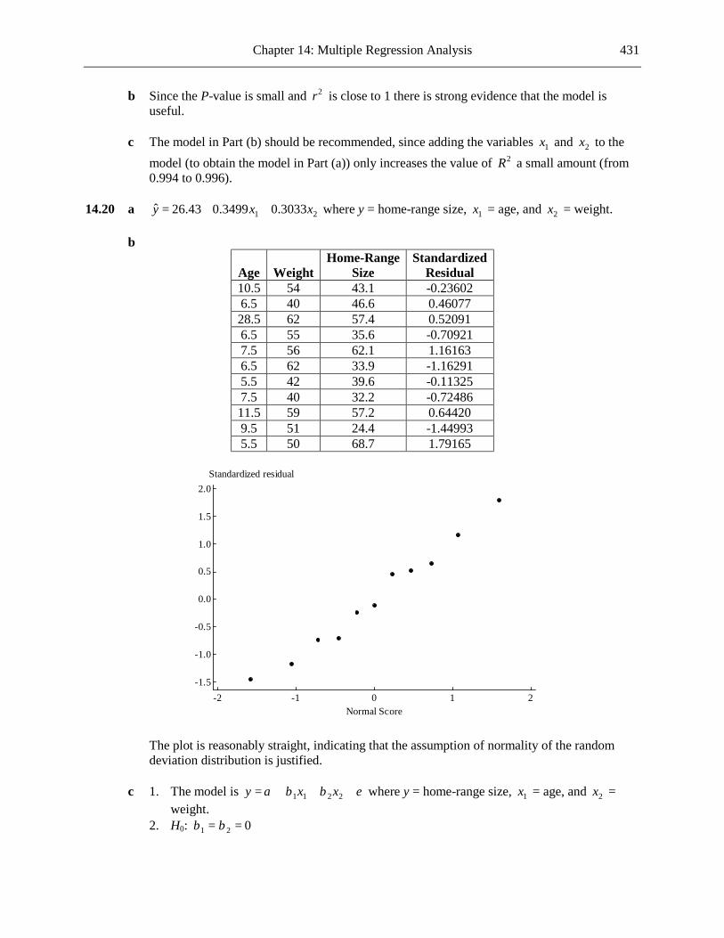
Chapter 14: Multiple Regression Analysis 431
b Since the P-value is small and 2r is close to 1 there is strong evidence that the model is
useful. c The model in Part (b) should be recommended, since adding the variables 1x and 2x to the
model (to obtain the model in Part (a)) only increases the value of 2R a small amount (from 0.994 to 0.996).
14.20 a 1 2ˆ 26.43 0.3499 0.3033y x x= + + where y = home-range size, 1x = age, and 2x = weight. b
Age
Weight
Home-Range Size
Standardized Residual
10.5 54 43.1 -0.23602 6.5 40 46.6 0.46077 28.5 62 57.4 0.52091 6.5 55 35.6 -0.70921 7.5 56 62.1 1.16163 6.5 62 33.9 -1.16291 5.5 42 39.6 -0.11325 7.5 40 32.2 -0.72486 11.5 59 57.2 0.64420 9.5 51 24.4 -1.44993 5.5 50 68.7 1.79165
210-1-2
2.0
1.5
1.0
0.5
0.0
-0.5
-1.0
-1.5
Normal Score
Standardized residual
The plot is reasonably straight, indicating that the assumption of normality of the random
deviation distribution is justified. c 1. The model is 1 1 2 2y x x eα β β= + + + where y = home-range size, 1x = age, and 2x =
weight. 2. H0: 1 2 0β β= =

432 Chapter 14: Multiple Regression Analysis
3. Ha: At least one of 1 2, β β is not zero. 4. 0.05α =
5. ( )2
2(1 ) ( 1)R kF
R n k=
− − +
6. The conditions were checked in Part (b). 7. The computer output gives 0.38.F = 8. The computer output gives -value 0.697.P = 9. Since -value 0.697 0.05P = > we do not reject H0. We do not have convincing evidence
that the predictors age and weight are useful for predicting home-range size. 14.21 1. The model is 1 1 2 2 3 3 4 4 5 5 6 6y x x x x x x eα β β β β β β= + + + + + + + , where y = species richness,
1x = watershed area, 2x = shore width, 3x = drainage, 4x = water color, 5x = sand percentage, and 6 alkalinityx = .
2. H0: 1 2 3 4 5 6 0β β β β β β= = = = = = 3. Ha: At least one of the iβ ’s is not zero. 4. 0.01α =
5. ( )2
2(1 ) ( 1)R kF
R n k=
− − +
6. Since we do not have the original data set we are unable to check the conditions. We need to assume that the variables are related according to the model given above, and that the random deviations, e, are normally distributed with mean zero and fixed standard deviation.
7. 0.83 6 24.412(1 0.83) 30
F = =−
8. 6,30-value ( 24.412) 0P P F= > ≈ 9. Since -value 0 0.01P ≈ < we reject H0. We have convincing evidence that the chosen model
is useful. 14.22 1. The model is 1 1 2 2 3 3 4 4 5 5 6 6 7 7y x x x x x x x eα β β β β β β β= + + + + + + + + , where y = spring
math comprehension, 1x = previous fall test score, 2x = previous fall academic motivation,
3x = age, 4x = number of credit hours, 5x = residence, 6x = hours worked on campus, and
7x = hours worked off campus. 2. H0: 1 2 3 4 5 6 7 0β β β β β β β= = = = = = = 3. Ha: At least one of the iβ ’s is not zero. 4. 0.05α =
5. ( )2
2(1 ) ( 1)R kF
R n k=
− − +
6. Since we do not have the original data set we are unable to check the conditions. We need to assume that the variables are related according to the model given above, and that the random deviations, e, are normally distributed with mean zero and fixed standard deviation.
7. 0.543 7 34.288(1 0.543) 202
F = =−
8. 7,202-value ( 34.288) 0P P F= > ≈
Chapter 14: Multiple Regression Analysis 433
9. Since -value 0 0.05P ≈ < we reject H0. We have convincing evidence that there is a useful
linear relationship between y and at least one of the predictors. 14.23 1. The model is 1 1 2 2 3 3 4 4y x x x x eα β β β β= + + + + + , where y = fish intake, 1x = water
temperature, 2x = number of pumps running, 3x = sea state, and 4x = speed. 2. H0: 1 2 3 4 0β β β β= = = = 3. Ha: At least one of the iβ ’s is not zero. 4. 0.1α =
5. ( )
SSRegrSSResid ( 1)
kFn k
=− +
6. Since we do not have the original data set we are unable to check the conditions. We need to assume that the variables are related according to the model given above, and that the random deviations, e, are normally distributed with mean zero and fixed standard deviation.
7. 1486.9 4 3.5002230.2 21
F = =
8. 4,21-value ( 3.500) 0.024P P F= > = 9. Since -value 0.024 0.1P = < we reject H0. We have convincing evidence that the model is
useful. 14.24 a The estimated regression equation is
1 2 3 4ˆ 86.85 0.12297 5.090 0.07092 0.0015380y x x x x= − + − + , where y = tar content, 1x = rotor speed, 2x = gas inlet temperature, 2
3 2 ,x x= and 4 1 2x x x= . b 1. The model is 1 1 2 2 3 3 4 4y x x x x eα β β β β= + + + + + , where the variables are defined as
above. 2. H0: 1 2 3 4 0β β β β= = = = 3. Ha: At least one of the iβ ’s is not zero. 4. 0.01α =
5. ( )
SSRegrSSResid ( 1)
kFn k
=− +
6. Since we do not have the original data set we are unable to check the conditions. We need to assume that the variables are related according to the model given above, and that the random deviations, e, are normally distributed with mean zero and fixed standard deviation.
7. SSRegr 4 5896.6 4 64.4SSResid 26 595.1 26
F = = =
8. 4,26-value ( 64.4) 0P P F= > ≈ 9. Since -value 0 0.01P ≈ < we reject H0. We have convincing evidence that the multiple
regression model is useful. c 2 0.908R = . This is the proportion of the observed variation in tar content that can be
explained by the fitted model. 4.784es = . This is a typical deviation of a tar content value in the sample from the value
predicted by the estimated regression equation.

434 Chapter 14: Multiple Regression Analysis
14.25 1. The model is 1 1 2 2 3 3 4 4 5 5 6 6 7 7 8 8 9 9y x x x x x x x x x eα β β β β β β β β β= + + + + + + + + + + , where y = ecology score, 1x = age times 10, 2x = income, 3x = gender, 4x = race, 5x = number of years of education, 6x = ideology, 7x = social class, 8x = postmaterialist (0 or 1), and 9x = materialist (0 or 1).
2. H0: 1 2 3 4 5 6 7 8 9 0β β β β β β β β β= = = = = = = = = 3. Ha: At least one of the iβ ’s is not zero. 4. 0.05α =
5. ( )2
2(1 ) ( 1)R kF
R n k=
− − +
6. Since we do not have the original data set we are unable to check the conditions. We need to assume that the variables are related according to the model given above, and that the random deviations, e, are normally distributed with mean zero and fixed standard deviation.
7. We have 1136n = and 9.k = So 0.06 9 7.986(1 0.06) 1126
F = =−
.
8. 9,1126-value ( 7.986) 0P P F= > ≈ 9. Since -value 0 0.05P ≈ < we reject H0. We have convincing evidence that the multiple
regression model is useful. 14.26 a The MINITAB output is shown below.
The regression equation is Weight = - 511 + 3.06 Length - 1.11 Age Predictor Coef SE Coef T P Constant -510.9 286.1 -1.79 0.096 Length 3.0633 0.8254 3.71 0.002 Age -1.113 9.040 -0.12 0.904 S = 94.2379 R-Sq = 59.3% R-Sq(adj) = 53.5% Analysis of Variance Source DF SS MS F P Regression 2 181364 90682 10.21 0.002 Residual Error 14 124331 8881 Total 16 305695
The estimated regression equation is 1 2ˆ 510.9 3.0633 1.113 ,y x x= − + − where y = weight, 1x =
length, and 2x = age. b 1. The model is 1 1 2 2y x x eα β β= + + + , with the variables as defined above. 2. H0: 1 2 0β β= = 3. Ha: At least one of the iβ ’s is not zero. 4. 0.05α =
5. ( )2
2(1 ) ( 1)R kF
R n k=
− − +

Chapter 14: Multiple Regression Analysis 435
6. The normal probability plot of the standardized residuals is shown below.
210-1-2
3
2
1
0
-1
-2
Normal Score
Standardized Residual
The plot at first seems to show a slight curve, but this curvature can be attributed to just
one point. We are justified in assuming that the random deviations are normally distributed.
7. 10.21F = 8. -value 0.002.P = 9. Since -value 0.002 0.05P = < we reject H0. We have convincing evidence that the
predictors length and age, together, are useful for predicting weight. 14.27 a The MINITAB output is shown below.
The regression equation is Catch Time = 1.44 - 0.0523 Prey Length + 0.00397 Prey Speed Predictor Coef SE Coef T P Constant 1.43958 0.08325 17.29 0.000 Prey Length -0.05227 0.01459 -3.58 0.002 Prey Speed 0.0039700 0.0006194 6.41 0.000 S = 0.0930752 R-Sq = 75.0% R-Sq(adj) = 71.9% Analysis of Variance Source DF SS MS F P Regression 2 0.41617 0.20809 24.02 0.000 Residual Error 16 0.13861 0.00866 Total 18 0.55478
The estimated regression equation is 1 2ˆ 1.43958 0.05227 0.0039700y x x= − + , where y = catch time, 1x = prey length, and 2x = prey speed.
b When 1 6x = and 2 50,x = ˆ 1.43958 0.05227(6) 0.0039700(50) seconds.y = − + = 1.324
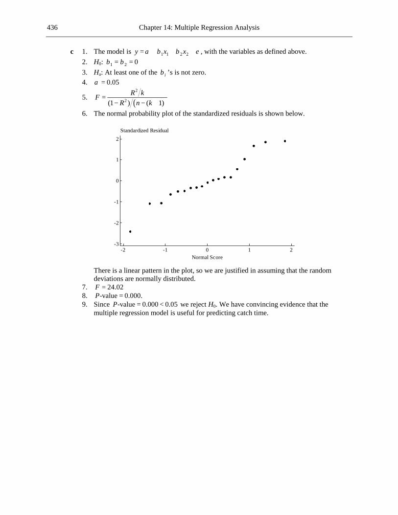
436 Chapter 14: Multiple Regression Analysis
c 1. The model is 1 1 2 2y x x eα β β= + + + , with the variables as defined above. 2. H0: 1 2 0β β= = 3. Ha: At least one of the iβ ’s is not zero. 4. 0.05α =
5. ( )2
2(1 ) ( 1)R kF
R n k=
− − +
6. The normal probability plot of the standardized residuals is shown below.
210-1-2
2
1
0
-1
-2
-3
Normal Score
Standardized Residual
There is a linear pattern in the plot, so we are justified in assuming that the random
deviations are normally distributed. 7. 24.02F = 8. -value 0.000.P = 9. Since -value 0.000 0.05P = < we reject H0. We have convincing evidence that the
multiple regression model is useful for predicting catch time.

Chapter 14: Multiple Regression Analysis 437
d The values of the new variable are shown in the table below.
Prey Length
Prey Speed
Catch Time
x
7 20 1.10 0.3500 6 20 1.20 0.3000 5 20 1.23 0.2500 4 20 1.40 0.2000 3 20 1.50 0.1500 3 40 1.40 0.0750 4 40 1.36 0.1000 6 40 1.30 0.1500 7 40 1.28 0.1750 7 80 1.40 0.0875 6 60 1.38 0.1000 5 80 1.40 0.0625 7 100 1.43 0.0700 6 100 1.43 0.0600 7 120 1.70 0.0583 5 80 1.50 0.0625 3 80 1.40 0.0375 6 100 1.50 0.0600 3 120 1.90 0.0250
The MINITAB output is shown below.
The regression equation is Catch Time = 1.59 - 1.40 x Predictor Coef SE Coef T P Constant 1.58648 0.04803 33.03 0.000 x -1.4044 0.3124 -4.50 0.000 S = 0.122096 R-Sq = 54.3% R-Sq(adj) = 51.6% Analysis of Variance Source DF SS MS F P Regression 1 0.30135 0.30135 20.22 0.000 Residual Error 17 0.25342 0.01491 Total 18 0.55478
The estimated regression equation is ˆ 1.58648 1.4044y x= − . e Since both the 2R and the adjusted 2R values shown in the computer outputs are greater for
the first model than for the second, the first model is preferable to the second. The first model is the one that accounts for the greater proportion of the observed variation in catch time.
14.28 a The MINITAB output is shown below.

438 Chapter 14: Multiple Regression Analysis
The regression equation is Volume = - 859 + 23.7 Minimum Width + 226 Maximum Width + 225 Elongation Predictor Coef SE Coef T P Constant -859.2 272.9 -3.15 0.005 Minimum Width 23.72 85.66 0.28 0.784 Maximum Width 225.81 85.76 2.63 0.015 Elongation 225.24 90.65 2.48 0.021 S = 286.974 R-Sq = 67.6% R-Sq(adj) = 63.4% Analysis of Variance Source DF SS MS F P Regression 3 3960700 1320233 16.03 0.000 Residual Error 23 1894141 82354 Total 26 5854841
The estimated regression equation is 1 2 3ˆ 859.2 23.72 225.81 225.24y x x x= − + + + , where y =
volume, 1x = minimum width, 2x = maximum width, and 3x = elongation score. b We should use adjusted 2R because it takes into account the number of predictors used in the
model. c 1. The model is 1 1 2 2 3 3y x x x eα β β β= + + + + , with the variables as defined above. 2. H0: 1 2 3 0β β β= = = 3. Ha: At least one of the iβ ’s is not zero. 4. 0.05α =
5. ( )2
2(1 ) ( 1)R kF
R n k=
− − +
6. The normal probability plot of the standardized residuals is shown below.
210-1-2
5
4
3
2
1
0
-1
-2
-3
-4
Normal Score
Standardized Residual

Chapter 14: Multiple Regression Analysis 439
There seems to be a nonlinear pattern at the ends of the plot, but we will nonetheless
proceed with the assumption that the random deviations are normally distributed. 7. 16.03F = 8. -value 0.000.P = 9. Since -value 0.000 0.05P = < we reject H0. We have convincing evidence that the
multiple regression model is useful. 14.29 a SSResid , SSTo , SSRegr 1618.209 390.435 .= = = − =390.435 1618.209 1227.775
b 2 SSResid 390.4351 1 .SSTo 1618.209
R = − = − = 0.759
This tells us that 75.9% of the observed variation in shear strength can be explained by the fitted model.
c 1. The model is 1 1 2 2 3 3 4 4 5 5y x x x x x eα β β β β β= + + + + + + , where y = shear strength, 1x =
depth, 2x = water content, 23 1x x= , 2
4 2x x= , and 5 1 2x x x= . 2. H0: 1 2 3 4 5 0β β β β β= = = = = 3. Ha: At least one of the iβ ’s is not zero. 4. 0.05α =
5. ( )2
2(1 ) ( 1)R kF
R n k=
− − +
6. The normal probability plot of the standardized residuals is shown below.
210-1-2
2
1
0
-1
-2
Normal Score
Standardized Residual
The plot shows a linear pattern, so we are justified in assuming that the random
deviations are normally distributed.
7. 0.759 5 5.0310.241 8
F = =
8. 5,8-value ( 5.031) 0.022P P F= > = 9. Since -value 0.022 0.05P = < we reject H0. We have convincing evidence that the
multiple regression model is useful.

440 Chapter 14: Multiple Regression Analysis
14.30 a 2 SSResid 20.01 1 0.490.SSTo 19.2 20.0
R = − = − =+
1. The model is 1 1 2 2 3 3 4 4y x x x x eα β β β β= + + + + + where y = error percentage, 1x = level of backlight, 2x = character subtense, 3x = viewing angle, and 4x = level of ambient light.
2. H0: 1 2 3 4 0β β β β= = = = 3. Ha: At least one of the iβ ’s is not zero. 4. 0.05α =
5. ( )2
2(1 ) ( 1)R kF
R n k=
− − +
6. Since we do not have the original data set we are unable to check the conditions. We need to assume that the variables are related according to the model given above, and that the random deviations, e, are normally distributed with mean zero and fixed standard deviation.
7. 0.490 4 6.000(1 0.490) 25
F = =−
8. 4,25-value ( 6.000) 0.002P P F= > = 9. Since -value 0.002 0.05P = < we reject H0. We have convincing evidence that the
multiple regression model is useful. b 2 .R = 0.490 This tells us that 49.0% of the observed variation in error percentage can be
explained by the fitted model. SSResid 20 . .
( 1) 25esn k
= = =− +
0 894 This is a typical deviation of an error percentage value in
the sample from the value predicted by the estimated regression equation.
c Noting that 0.894,es = we see that error percentages predicted by the model are typically within one percentage point of the true values, which would seem to imply that the estimated regression equation is providing reasonably accurate predictions. However, looking at the 2R value, we see that the model accounts for only 49% of the observed variation in error percentage. This comes about as a result of the fact that the error percentages in the study were low (for example, around 2%), and so a deviation of one percentage point is proportionately large. We conclude that the estimated regression equation is not providing particularly accurate predictions.
14.31 1. The model is 1 1 2 2y x x eα β β= + + + , where y = yield, 1x = defoliation level, and 2
2 1 .x x= 2. H0: 1 2 0β β= = 3. Ha: At least one of the iβ ’s is not zero. 4. 0.01α =
5. ( )2
2(1 ) ( 1)R kF
R n k=
− − +
6. Since we do not have the original data set we are unable to check the conditions. We need to assume that the variables are related according to the model given above, and that the random deviations, e, are normally distributed with mean zero and fixed standard deviation.

Chapter 14: Multiple Regression Analysis 441
7. 0.902 2 96.643(1 0.902) 21
F = =−
8. 2,21-value ( 96.643) 0P P F= > ≈ 9. Since -value 0 0.01P ≈ < we reject H0. We have convincing evidence that the quadratic
model specifies a useful relationship between y and x.
14.32 ( ) ( )2
20.9 9(14 ) .
0.1 15 ( 1)(1 ) ( 1)R k k kF
k kR n k−
= = =− +− − +
Using the above formula and Appendix Table 6 the following table is obtained. (The critical values shown are for a 0.05 significance level.)
k
F
df1
df2
Critical Value
1 117 1 13 4.67 2 54 2 12 3.89 3 33 3 11 3.59 4 22.5 4 10 3.48 5 16.2 5 9 3.48 6 12 6 8 3.58 7 9 7 7 3.79 8 6.75 8 6 4.15 9 5 9 5 4.77 10 3.6 10 4 5.96
For 9k ≤ the value of the F statistic is greater than the critical value, and so there is convincing evidence that the model is useful. For 10k = the value of the F statistic is less than the critical value. Moreover, for 10k ≥ the value of F continues to decrease and we presume that the critical value continues to increase, and thus for 10k ≥ there is not convincing evidence that the model is useful. So the model would be judged to be useful for 9k ≤ , and this large value of 2R does not necessarily imply a useful model.
14.33 The MINITAB output is shown below.
The regression equation is y = - 151 - 16.2 x1 + 13.5 x2 + 0.0935 x3 - 0.253 x4 + 0.492 x5 Predictor Coef SE Coef T P Constant -151.4 134.1 -1.13 0.292 x1 -16.216 8.831 -1.84 0.104 x2 13.476 8.187 1.65 0.138 x3 0.09353 0.07093 1.32 0.224 x4 -0.2528 0.1271 -1.99 0.082 x5 0.4922 0.2281 2.16 0.063 S = 6.98783 R-Sq = 75.9% R-Sq(adj) = 60.8% Analysis of Variance

442 Chapter 14: Multiple Regression Analysis
Source DF SS MS F P Regression 5 1227.57 245.51 5.03 0.022 Residual Error 8 390.64 48.83 Total 13 1618.21
This verifies the estimated regression equation given in the question. 14.34 a The MINITAB output is shown below.
The regression equation is y = 76.4 - 7.3 x1 + 9.6 x2 - 0.91 x3 + 0.0963 x4 - 13.5 x1^2 + 2.80 x2^2 + 0.0280 x3^2 - 0.000320 x4^2 + 3.75 x1x2 - 0.750 x1x3 + 0.142 x1x4 + 2.00 x2x3 - 0.125 x2x4 + 0.00333 x3x4 Predictor Coef SE Coef T P Constant 76.437 9.082 8.42 0.000 x1 -7.35 10.80 -0.68 0.506 x2 9.61 10.80 0.89 0.387 x3 -0.915 1.068 -0.86 0.404 x4 0.09632 0.09834 0.98 0.342 x1^2 -13.452 6.599 -2.04 0.058 x2^2 2.798 6.599 0.42 0.677 x3^2 0.02798 0.06599 0.42 0.677 x4^2 -0.0003201 0.0002933 -1.09 0.291 x1x2 3.750 8.823 0.43 0.676 x1x3 -0.7500 0.8823 -0.85 0.408 x1x4 0.14167 0.05882 2.41 0.028 x2x3 2.0000 0.8823 2.27 0.038 x2x4 -0.12500 0.05882 -2.13 0.049 x3x4 0.003333 0.005882 0.57 0.579 S = 0.352900 R-Sq = 88.5% R-Sq(adj) = 78.3% Analysis of Variance Source DF SS MS F P Regression 14 15.2642 1.0903 8.75 0.000 Residual Error 16 1.9926 0.1245 Total 30 17.2568
The estimated regression equation is
2 21 2 3 4 1 2
2 23 4 1 2 1 3 1 4
2 3 2 4 3 4
ˆ 76.437 7.35 9.61 0.915 0.09632 13.452 2.798
0.02798 0.0003201 3.750 0.7500 0.141672.0000 0.125 0.003333 .
y x x x x x x
x x x x x x x xx x x x x x
= − + − + − +
+ − + − ++ − +
b 1. The model is
2 2 2 21 1 2 2 3 3 4 4 5 1 6 2 7 3 8 4 9 1 2 10 1 3
11 1 4 12 2 3 13 2 4 14 3 4 .y x x x x x x x x x x x x
x x x x x x x x eα β β β β β β β β β ββ β β β
= + + + + + + + + + ++ + + + +
2. H0: 1 14 0β β= = =L 3. Ha: At least one of the iβ ’s is not zero. 4. 0.05α =

Chapter 14: Multiple Regression Analysis 443
5. ( )2
2(1 ) ( 1)R kF
R n k=
− − +
6. The normal probability plot of the standardized residuals is shown below.
210-1-2
4
3
2
1
0
-1
-2
-3
Normal Score
Standardized Residual
The plot shows a linear pattern, so we are justified in assuming that the random
deviations are normally distributed. 7. 8.75F = 8. -value 0.000P = 9. Since -value 0.000 0.05P = < we reject H0. We have convincing evidence that the
multiple regression model is useful. c SSResid 1.9926.= This is the sum of the squares of the deviations of the actual brightness
values from the values predicted by the fitted model. 0.352900.es = This is a typical deviation of a brightness value in the sample from the value
predicted by the fitted model. 2 0.885.R = This is the proportion of the observed variation in brightness that can be
explained by the fitted model. 14.35 The MINITAB output is shown below.
The regression equation is y = 35.8 - 0.68 x1 + 1.28 x2 Predictor Coef SE Coef T P Constant 35.83 53.54 0.67 0.508 x1 -0.676 1.436 -0.47 0.641 x2 1.2811 0.4243 3.02 0.005 S = 22.9789 R-Sq = 55.0% R-Sq(adj) = 52.1% Analysis of Variance

444 Chapter 14: Multiple Regression Analysis
Source DF SS MS F P Regression 2 20008 10004 18.95 0.000 Residual Error 31 16369 528 Total 33 36377
The estimated regression equation is 1 2ˆ 35.83 0.676 1.2811y x x= − + , where y = infestation rate,
1x = mean temperature, and 2x = mean relative humidity. 1. The model is 1 1 2 2y x x eα β β= + + + , with the variables defined as above. 2. H0: 1 2 0β β= = 3. Ha: At least one of the iβ ’s is not zero. 4. 0.05α =
5. ( )2
2(1 ) ( 1)R kF
R n k=
− − +
6. The normal probability plot of the standardized residuals is shown below.
210-1-2
2
1
0
-1
-2
Normal Score
Standardized Residual
The plot shows a linear pattern, so we are justified in assuming that the random deviations are
normally distributed. 7. 18.95F = 8. -value 0.000P = 9. Since -value 0.000 0.05P = < we reject H0. We have convincing evidence that the multiple
regression model is useful. Online Exercises 14.36 It is possible that the proposed predictors, when used in linear combination, actually have
virtually no relationship to the response variable – in other words, that just using the mean value of the response variable in the sample would be as good as any attempt to fit a model using the proposed predictors. If this is the case, then there is little point in using those variables as predictors. However, the model utility test can establish (beyond all reasonable doubt) that there

Chapter 14: Multiple Regression Analysis 445
is a useful relationship between the given set of variables and the response variable, and therefore that it is worthwhile to use them as predictors.
14.37 a We need to assume that the mean value of a vacant lot is related to the predictors according to
the multiple regression model, and that the random deviations from the model are normally distributed with mean zero and fixed standard deviation. df ( 1) 100 8 92.n k= − + = − = The required confidence interval is
22 ( critical value) 0.489 (1.986)(0.1044) ( , ).bb t s± = − ± = − −0.696 0.282 We are 95% confident that, when all the other predictors are fixed, the average decrease in
value of a vacant lot associated with a one-unit increase in the distance from the city’s major east-west thoroughfare is between 0.282 and 0.696.
b 1. 1β is the mean increase in value of a vacant lot for a one unit increase in the “residential
use” variable when all the other predictors are held fixed. 2. H0: 1 0β = 3. Ha: 1 0β ≠ 4. 0.05α =
5. 1
1
b
bts
=
6. We need to assume that the mean value of a vacant lot is related to the predictors according to the multiple regression model, and that the random deviations from the values given by the population regression function are normally distributed with mean zero and fixed standard deviation.
7. 1
1 0.183 0.5990.3055b
bts
−= = = −
8. df ( 1) 100 8 92n k= − + = − = 92-value 2 ( 0.599) 0.551P P t= ⋅ < − = 9. Since -value 0.551 0.05P = > we do not reject H0. We do not have convincing evidence
that the predictor that indicates whether the lot was zoned for residential use provides useful information about the value of a vacant lot, over and above the information contained in the other predictors.
14.38 a We need to assume that the number of fish at intake is related to the predictors according to
the multiple regression model, and that the random deviations from the model are normally distributed with mean zero and fixed standard deviation. df ( 1) 26 5 21.n k= − + = − = The required confidence interval is
33 ( critical value) 9.378 (2.080)(4.356) ( . , . ).bb t s± = − ± = − −18 437 0 319 We are 95% confident that, when all the other predictors are fixed, the average decrease in
the number of fish at intake associated with a one-unit increase in sea state is between 0.319 and 18.437.
b We require a 90% confidence interval for 1β .
We need to assume that the number of fish at intake is related to the predictors according to the multiple regression model, and that the random deviations from the model are normally distributed with mean zero and fixed standard deviation.

446 Chapter 14: Multiple Regression Analysis
df ( 1) 26 5 21.n k= − + = − = The required confidence interval is
11 ( critical value) 2.179 (1.721)(1.087) ( . , . ).bb t s± = − ± = − −4 049 0 309 We are 90% confident that, when all the other predictors are fixed, the average decrease in
the number of fish at intake associated with a 1° increase in temperature is between 0.309 and 4.049.
14.39 a 1. The model is 2
1 2y x x eα β β= + + + , where y = MDH activity and x = electrical conductivity.
2. H0: 1 2 0β β= = 3. Ha: At least one of the iβ ’s is not zero. 4. 0.05α =
5. ( )2
2(1 ) ( 1)R kF
R n k=
− − +
6. Since we do not have the original data set we are unable to check the conditions. We need to assume that the variables are related according to the model given above, and that the random deviations, e, are normally distributed with mean zero and fixed standard deviation.
7. 0.860 2 144.357(1 0.860) 47
F = =−
8. 2,47-value ( 144.357) 0P P F= > ≈ 9. Since -value 0 0.05P ≈ < we reject H0. We have convincing evidence that the quadratic
model is useful. b 1. 2β is defined as in Part (a). 2. H0: 2 0β = 3. Ha: 2 0β ≠ 4. 0.01α =
5. 2
2
b
bts
=
6. We need to assume that the mean MDH activity is related to electrical conductivity according to the quadratic model given in Part (a), and that the random deviations from the values given by the quadratic regression function are normally distributed with mean zero and fixed standard deviation.
7. 2
2 0.0446 4.3300.0103b
bts
= = =
8. df ( 1) 50 3 47n k= − + = − = 47-value 2 ( 4.330) 0P P t= ⋅ > ≈ 9. Since -value 0 0.01P ≈ < we reject H0. We have convincing evidence that the quadratic
predictor 2x is important. c We need to make the same assumptions as in Parts (a) and (b).
When 2ˆ40, 0.1838 0.0272(40) 0.0446(40) 72.2642.x y= = − + + =

Chapter 14: Multiple Regression Analysis 447
df ( 1) 50 3 47.n k= − + = − = The required confidence interval is
ˆˆ ( critical value) 72.2642 (1.678)(0.120) ( . , . ).yy t s± = ± = 72 063 72 466 We are 90% confident that the mean MDH activity when the conductivity is 40 is between
72.063 and 72.466. 14.40 a The MINITAB output is shown below.
The regression equation is Volume = - 859 + 23.7 Minimum Width + 226 Maximum Width + 225 Elongation Predictor Coef SE Coef T P Constant -859.2 272.9 -3.15 0.005 Minimum Width 23.72 85.66 0.28 0.784 Maximum Width 225.81 85.76 2.63 0.015 Elongation 225.24 90.65 2.48 0.021 S = 286.974 R-Sq = 67.6% R-Sq(adj) = 63.4% Analysis of Variance Source DF SS MS F P Regression 3 3960700 1320233 16.03 0.000 Residual Error 23 1894141 82354 Total 26 5854841
Since the P-value associated with the coefficient of minimum width is as large as 0.784, this
variable could be eliminated from the regression. b When 1 2 32.5, 3.0, and 1.55,x x x= = =
ˆ 859.2 23.72(2.5) 225.81(3.0) 225.24(1.55) . .y = − + + + = 226 652 c The standardized residual plot shown in the solution to the earlier exercise shows a curved
shape at its ends, but we will nonetheless proceed with construction of the prediction interval. df ( 1) 27 4 23.n k= − + = − = The standard error of y is 73.8. The required prediction interval is
2 2ˆ
2 2
ˆ ( critical value)
226.652 (2.069) 286.974 73.8 )( 386.315, 839.619).
e yy t s s± +
= ± += −
However, since negative volumes are not possible, the interval is adjusted to (0, 839.619). We are 95% confident that, when the minimum width is 2.5, the maximum width is 3.0, and the elongation is 1.55, the volume will be between 0 and 839.619 ml.
14.41 a The value 0.469 is an estimate of the increase in mean exam score associated with a one-point
increase in expected score on the exam, when time spent studying and GPA are fixed. b 1. The model is 1 1 2 2 3 3y x x x eα β β β= + + + + , with variables as defined in the question.

448 Chapter 14: Multiple Regression Analysis
2. H0: 1 2 3 0β β β= = = 3. Ha: At least one of the iβ ’s is not zero. 4. 0.05α =
5. ( )2
2(1 ) ( 1)R kF
R n k=
− − +
6. Since we do not have the original data set we are unable to check the conditions. We need to assume that the variables are related according to the model given above, and that the random deviations, e, are normally distributed with mean zero and fixed standard deviation.
7. 0.686 3 75.008(1 0.686) 103
F = =−
8. 3,103-value ( 75.008) 0P P F= > ≈ 9. Since -value 0 0.05P ≈ < we reject H0. We have convincing evidence that there is a
useful linear relationship between exam score and at least one of the three predictors. c We need to assume that the exam score is related to the predictors according to the multiple
regression model, and that the random deviations from the model are normally distributed with mean zero and fixed standard deviation. df ( 1) 107 4 103.n k= − + = − = The required confidence interval is
22 ( critical value) 3.369 (1.983)(0.456) ( . , . ).bb t s± = ± = 2 464 4 273 We are 95% confident that, when all the other predictors are fixed, the average increase in
exam score associated with a 1-hour increase in study time is between 2.464 and 4.273. d 1 2 3 ˆWhen 75, 8, and 2.8, 2.178 0.469(75) 3.369(8) 3.054(2.8) .x x x y= = = = + + + = 72.856 e We need to make the same assumptions as in Part (c).
df ( 1) 107 4 103.n k= − + = − = To calculate :es
2 SSResid1 .SSTo
R = − So here SSResid0.686 1 ,10200
= − giving
SSResid 10200(1 0.686) 3202.8.= − =
So SSResid 3202.8 5.576.( 1) 103es
n k= = =
− +
The required prediction interval is 2 2
ˆ
2 2
ˆ ( critical value)
72.856 (1.983) 5.576 1.2 )( . , . ).
e yy t s s± +
= ± += 61 544 84 169
Our estimate of the interval containing 95% of scores of students with the given predictor values is 61.544 to 84.169.

Chapter 14: Multiple Regression Analysis 449
14.42 a 2 1 SSResidAdjusted 1 .( 1) SSTo
nRn k
− = − − +
So here, 299 SSResid0.774 1 ,296 SSTo
= −
which gives SSResid 296 (1 0.774) 0.224.SSTo 299
= − =
From this we get 2 SSResid1 1 0.224 0.776.SSTo
R = − = − =
Thus, for the model utility test we get ( )2
20.776 3 342.336.
(1 0.776) 296(1 ) ( 1)R kF
R n k= = =
−− − +
Therefore, 3,296-value ( 342.336) 0P P F= > ≈ , telling us that at least one of the three predictors provides useful information about y.
b 1. 3β is the mean increase in benevolence payments for a one unit increase in the
urban/nonurban variable when all the other predictors are held fixed. 2. H0: 3 0β = 3. Ha: 3 0β ≠ 4. 0.05α =
5. 3
3
b
bts
=
6. We need to assume that the mean of the benevolence payments is related to the predictors according to the multiple regression model, and that the random deviations from the values given by the population regression function are normally distributed with mean zero and fixed standard deviation.
7. 3
3 101.1 0.162625.8b
bts
= = =
8. df ( 1) 300 4 296n k= − + = − = 296-value 2 ( 0.162) 0.872P P t= ⋅ > = 9. Since -value 0.872 0.05P = > we do not reject H0. We do not have convincing evidence
that the indicator should be retained in the model. 14.43 1. 3β is the coefficient of 1 2x x in the population regression function relating y to 1x , 2x , and
1 2x x , with variables as defined in the question. 2. H0: 3 0β = 3. Ha: 3 0β ≠ 4. 0.05α =
5. 3
3
b
bts
=
6. We need to assume that the mean number of indictments disposed of in a given month is related to the predictors according to the multiple regression model, and that the random deviations from the values given by the population regression function are normally distributed with mean zero and fixed standard deviation.
7. 3
3 0.00002 2.2220.000009b
bts
= = =
8. df ( 1) 367 4 363n k= − + = − =

450 Chapter 14: Multiple Regression Analysis
363-value 2 ( 2.222) 0.027P P t= ⋅ > = 9. Since -value 0.027 0.05P = < we reject H0. We have convincing evidence that the interaction
predictor is important. 14.44 1. 2β is the coefficient of 2x in the population regression function relating y to x and 2x ,
with variables as defined in the question. 2. H0: 2 0β = 3. Ha: 2 0β ≠ 4. 0.05α =
5. 2
2
b
bts
=
6. A normal probability plot of the standardized residuals is shown below.
1.51.00.50.0-0.5-1.0
1.5
1.0
0.5
0.0
-0.5
-1.0
Normal Score
Standardized residual
The plot is quite straight, indicating that normality of the random error distribution is
plausible.
7. 2
2 1.7155 8.4260.2036b
bts
−= = = −
8. df ( 1) 7 3 4n k= − + = − = 4-value 2 ( 8.426) 0.001P P t= ⋅ < − = 9. Since -value 0.001 0.05P = < we reject H0. We have convincing evidence that the quadratic
predictor is important. 14.45 a 1. The model is 1 1 2 2 3 3y x x x eα β β β= + + + + , with variables as defined in the question. 2. H0: 1 2 3 0β β β= = = 3. Ha: At least one of the iβ ’s is not zero. 4. 0.05α =
5. ( )2
2(1 ) ( 1)R kF
R n k=
− − +

Chapter 14: Multiple Regression Analysis 451
6. Since we do not have the original data set we are unable to check the conditions. We need
to assume that the variables are related according to the model given above, and that the random deviations, e, are normally distributed with mean zero and fixed standard deviation.
7. 0.732 3 5.463(1 0.732) 6
F = =−
8. 3,6-value ( 5.463) 0.038P P F= > = 9. Since -value 0.038 0.05P = < we reject H0. We have convincing evidence that the
multiple regression model is useful. b 1. 3β is the coefficient of 1 2x x in the population regression function relating y to 1x , 2x ,
and 1 2x x , with variables as defined in the question. 2. H0: 3 0β = 3. Ha: 3 0β ≠ 4. 0.05α =
5. 3
3
b
bts
=
6. We need to assume that the mean value of y is related to the predictors according to the multiple regression model, and that the random deviations from the values given by the population regression function are normally distributed with mean zero and fixed standard deviation.
7. 3
3 0.04b
bts
= =
8. df ( 1) 10 4 6n k= − + = − = 6-value 2 ( 0.04) 0.969P P t= ⋅ > = 9. Since -value 0.969 0.05P = > we do not reject H0. We do not have convincing evidence
that the interaction predictor is important. c No. The model utility test indicates that all the predictors together provide a useful model.
The fact that the t ratio values are small indicates that any one of the predictors could be dropped from the model as long as the other predictors are retained.
14.46 a 1. The model is 1 1 2 2y x x eα β β= + + + , with variables as defined in the question. 2. H0: 1 2 0β β= = 3. Ha: At least one of the iβ ’s is not zero. 4. 0.05α =
5. ( )2
2(1 ) ( 1)R kF
R n k=
− − +
6. Since we do not have the original data set we are unable to check the conditions. We need to assume that the variables are related according to the model given above, and that the random deviations, e, are normally distributed with mean zero and fixed standard deviation.
7. 0.964 2 334.722(1 0.964) 25
F = =−

452 Chapter 14: Multiple Regression Analysis
8. 2,25-value ( 334.722) 0P P F= > ≈ 9. Since -value 0 0.05P ≈ < we reject H0. We have convincing evidence that the multiple
regression model is useful. b Since we do not have the original data set we are unable to check the conditions. We need to
assume that the variables are related according to the model given in Part (a), and that the random deviations, e, are normally distributed with mean zero and fixed standard deviation. df ( 1) 28 3 25.n k= − + = − = The required confidence interval is
22 ( critical value) 0.33563 (2.060)(0.01814) ( . , ).bb t s± = ± = 0 298 0.373 We are 95% confident that, when all the other predictors are fixed, the average decrease in y
associated with a one-unit increase in 2x is between 0.298 and 0.373. c i 1. 1β is the mean increase in y for a one unit increase 1x when all the other predictors
are held fixed. 2. H0: 1 0β = 3. Ha: 1 0β ≠ 4. 0.05α =
5. 1
1
b
bts
=
6. We need to assume that the mean value of y is related to the predictors according to the multiple regression model, and that the random deviations from the values given by the population regression function are normally distributed with mean zero and fixed standard deviation.
7. 6.95t = 8. -value 0.000P = 9. Since -value 0.000 0.05P = < we reject H0. We have convincing evidence that
1 0β ≠ . ii 1. 2β is the mean increase in y for a one unit increase 2x when all the other predictors
are held fixed. 2. H0: 2 0β = 3. Ha: 2 0β ≠ 4. 0.05α =
5. 2
2
b
bts
=
6. We need to assume that the mean value of y is related to the predictors according to the multiple regression model, and that the random deviations from the values given by the population regression function are normally distributed with mean zero and fixed standard deviation.
7. 18.51t = 8. -value 0.000P = 9. Since -value 0.000 0.05P = < we reject H0. We have convincing evidence that
2 0β ≠ .

Chapter 14: Multiple Regression Analysis 453
d Yes. Since we have convincing evidence that 1 0β ≠ and that 2 0β ≠ , we conclude that both
independent variables are important. e We need to assume that the mean value of y is related to the predictors according to the
multiple regression model, and that the random deviations from the values given by the population regression function are normally distributed with mean zero and fixed standard deviation. When 1 2 ˆ11.7 and 57, 19.440 1.4423(11.7) 0.33563(57) 55.446.x x y= = = + + = df ( 1) 28 3 25.n k= − + = − = The required confidence interval is
ˆˆ ( critical value) 55.446 (1.708)(0.522) ( . , . ).yy t s± = ± = 54 554 56 337 We are 90% confident that the mean water absorption for wheat with 11.7% protein and a
starch damage of 57 is between 54.554 and 56.337. f We need to assume that the mean value of y is related to the predictors according to the
multiple regression model, and that the random deviations from the values given by the population regression function are normally distributed with mean zero and fixed standard deviation.
1.094es = The required prediction interval is
2 2ˆ
2 2
ˆ ( critical value)
55.446 (1.708) 1.094 0.522 )( . , . ).
e yy t s s± +
= ± += 53 375 57 516
Our estimate of the interval containing 90% of water absorption values when the predictors have the given values is 53.375 to 57.516.
14.47 a Referring to the solution to the earlier question, the P-value associated with the coefficient of
length is 0.002, which is small, and so length should not be eliminated. The P-value associated with the coefficient of age is 0.904, which is large, and so age could be eliminated from the model.
b Let the indicator variable for year caught take the value 0 for Year 1 and 1 for Year 2.
The MINITAB output for the required multiple regression model is shown below.
The regression equation is Weight = - 1516 + 5.71 Length + 2.48 Age - 238 Year Predictor Coef SE Coef T P Constant -1515.8 290.8 -5.21 0.000 Length 5.7149 0.7972 7.17 0.000 Age 2.479 5.925 0.42 0.683 Year -237.95 52.96 -4.49 0.001 S = 61.2044 R-Sq = 84.1% R-Sq(adj) = 80.4% Analysis of Variance Source DF SS MS F P

454 Chapter 14: Multiple Regression Analysis
Regression 3 256997 85666 22.87 0.000 Residual Error 13 48698 3746 Total 16 305695
1. 3β is the increase in weight associated with a one-unit increase in year, when all the
other predictors are fixed. 2. H0: 3 0β = 3. Ha: 3 0β ≠ 4. 0.05α =
5. 3
3
b
bts
=
6. A normal probability plot of the standardized residuals is shown below.
210-1-2
4
3
2
1
0
-1
-2
Normal Score
Standardized Residual
Apart from the first and last points, the plot is quite straight, and so the assumption of
normality of the random error distribution is acceptable. 7. 4.49t = − 8. -value 0.001P = 9. Since -value 0.001 0.05P = < we reject H0. We have convincing evidence that year is a
useful predictor given that length and age are included in the model. 14.48 a 1. The model is 1 1 2 2y x x eα β β= + + + , with variables as defined in the question. 2. H0: 1 2 0β β= = 3. Ha: At least one of the iβ ’s is not zero. 4. 0.1α =
5. ( )
SSRegrSSResid ( 1)
kFn k
=− +
6. Since we do not have the original data set we are unable to check the conditions. We need to assume that the variables are related according to the model given above, and that the random deviations, e, are normally distributed with mean zero and fixed standard deviation.

Chapter 14: Multiple Regression Analysis 455
7. 649.75 2 9.057538.03 15
F = =
8. 2,15-value ( 9.057) 0.003P P F= > = 9. Since -value 0.003 0.1P = < we reject H0. We have convincing evidence that the multiple
regression model is useful. b We need to assume that maximum heart rate is related to the predictors according to the
multiple regression model, and that the random deviations from the values given by the regression function are normally distributed with mean zero and fixed standard deviation. df ( 1) 18 3 15.n k= − + = − = The required confidence interval is
11 ( critical value) 0.8 (2.131)(0.280) ( . , . ).bb t s± = − ± = − −1 396 0 203 We are 95% confident that, when all the other predictors are fixed, the average decrease in
maximum heart rate associated with a one-year increase in age is between 0.203 and 1.396. c We need to assume that maximum heart rate is related to the predictors according to the
multiple regression model, and that the random deviations from the values given by the regression function are normally distributed with mean zero and fixed standard deviation. When 1 2 ˆ43 and 65, 179 0.8(43) 0.5(65) 177.1.x x y= = = − + = df ( 1) 18 3 15.n k= − + = − =
SSResid 538.03 5.989.( 1) 15es
n k= = =
− +
The required prediction interval is 2 2
ˆ
2 2
ˆ ( critical value)
177.1 (2.947) 5.989 3.52( . , ).
e yy t s s± +
= ± += 156 630 197.570
Our estimate of the interval containing 99% of maximum heart rates for marathon runners with the given predictor values is 156.630 to 197.570.
d We need to assume that maximum heart rate is related to the predictors according to the multiple regression model, and that the random deviations from the values given by the regression function are normally distributed with mean zero and fixed standard deviation. When 1 2 ˆ30 and 77.2, 179 0.8(30) 0.5(77.2) 193.6.x x y= = = − + = df ( 1) 18 3 15.n k= − + = − = The required confidence interval is
ˆˆ ( critical value) 193.6 (1.753)(2.97) ( . , . ).yy t s± = ± = 188 393 198 807 We are 90% confident that the mean maximum heart rate for marathon runners with the given
predictor values is between 188.393 and 198.807 e The prediction interval will be wider than the interval computed in Part (d), since the
prediction interval is for the actual value (rather than the mean value) of the maximum heart rate for a runner who has the given predictor values, and therefore the prediction interval has to take into account the fact that the actual maximum heart rate value will have some deviation from the mean maximum heart rate value.

456 Chapter 14: Multiple Regression Analysis
14.49 a For the model utility test, ( )
SSRegr 237.520 2 30.812SSResid ( 1) 26.980 7
kFn k
= = =− +
.
So 2,7-value ( 30.812) 0P P F= > ≈ . Since this P-value is small, we have convincing evidence that the quadratic model is useful.
b The t ratios associated with the coefficients of both of these predictors are large, and so
neither could be eliminated from the model. c We need to assume that plant height is related to the predictors according to the multiple
regression model, and that the random deviations from the values given by the regression function are normally distributed with mean zero and fixed standard deviation. When ˆ2, 41.7422 6.581(2) 2.3621(4) 45.4558.x y= = + − = df ( 1) 7.n k= − + = The required confidence interval is
ˆˆ ( critical value) 45.4558 (2.365)(1.037) ( . , . ).yy t s± = ± = 43 004 47 908 We are 95% confident that the mean plant height when 2x = is between 43.004 and 47.908. d We need to assume that plant height is related to the predictors according to the multiple
regression model, and that the random deviations from the values given by the regression function are normally distributed with mean zero and fixed standard deviation. When ˆ1, 41.7422 6.581(1) 2.3621(1) 45.9611.x y= = + − = df ( 1) 7.n k= − + = The required confidence interval is
ˆˆ ( critical value) 45.9611 (1.895)(1.031) ( . , ).yy t s± = ± = 44 008 47.914 We are 90% confident that the mean plant height when the wheat is treated with 10 Mµ of
Mn is between 44.008 and 47.914. 14.50 a The MINITAB output is shown below.
The regression equation is y = 110 - 2.29 x + 0.0329 x^2 Predictor Coef SE Coef T P Constant 109.771 1.273 86.26 0.000 x -2.2943 0.1508 -15.22 0.004 x^2 0.032857 0.003614 9.09 0.012 S = 1.35225 R-Sq = 99.7% R-Sq(adj) = 99.3% Analysis of Variance Source DF SS MS F P Regression 2 1111.54 555.77 303.94 0.003 Residual Error 2 3.66 1.83 Total 4 1115.20

Chapter 14: Multiple Regression Analysis 457
The estimated regression equation is 2ˆ 109.771 2.2943 0.032857 ,y x x= − + where x = distance
from fertilizer band and y = plant height. b 1. The model is 2
1 2y x x eα β β= + + + , with variables as defined in the question. 2. H0: 1 2 0β β= = 3. Ha: At least one of the iβ ’s is not zero. 4. 0.05α =
5. ( )
SSRegrSSResid ( 1)
kFn k
=− +
6. Since we do not have the original data set we are unable to check the conditions. We need to assume that the variables are related according to the model given above, and that the random deviations, e, are normally distributed with mean zero and fixed standard deviation.
7. 303.94F = 8. 2,2-value ( 303.94) 0.003P P F= > = 9. Since -value 0.003 0.05P = < we reject H0. We have convincing evidence that the
quadratic regression model is useful. c 2 0.997R = . This is the proportion of the observed variation in plant Mn that can be
explained by the fitted model. 1.352.es = This is a typical deviation of a plant Mn value in the sample from the value
predicted by the estimated regression equation. d 1. 1β is the coefficient of x in the population regression function relating y to x and 2x ,
with variables as defined in the question. 2. H0: 1 0β = 3. Ha: 1 0β ≠ 4. 0.05α =
5. 1
1
b
bts
=
6. A normal probability plot of the standardized residuals is shown below.

458 Chapter 14: Multiple Regression Analysis
1.00.50.0-0.5-1.0-1.5
1.5
1.0
0.5
0.0
-0.5
-1.0
Normal Score
Standardized residual
The plot is quite straight, indicating that normality of the random error distribution is
plausible. 7. 15.22t = − 8. -value 0.004P = 9. Since -value 0.004 0.05P = < we reject H0. We have convincing evidence that the linear
predictor is important. 1. 2β is the coefficient of 2x in the population regression function relating y to x and 2x ,
with variables as defined in the question. 2. H0: 2 0β = 3. Ha: 2 0β ≠ 4. 0.05α =
5. 2
2
b
bts
=
6. A normal probability plot of the standardized residuals is shown below.

Chapter 14: Multiple Regression Analysis 459
1.00.50.0-0.5-1.0-1.5
1.5
1.0
0.5
0.0
-0.5
-1.0
Normal Score
Standardized residual
The plot is quite straight, indicating that normality of the random error distribution is
plausible. 7. 9.09t = 8. -value 0.012P = 9. Since -value 0.012 0.05P = < we reject H0. We have convincing evidence that the
quadratic predictor is important. We have convincing evidence that both of the predictors are important. e When 2ˆ30, 109.771 2.2943(30) 0.032857(30) 70.5133.x y= = − + =
MINITAB tells us that the standard error associated with this estimate is 0.824. df ( 1) 5 3 2.n k= − + = − = The required confidence interval is
ˆˆ ( critical value) 70.5133 (2.920)(0.824) ( . , . ).yy t s± = ± = 68 107 72 919 We are 90% confident that the mean plant Mn for plants that are 30 cm from the fertilizer
band is between 68.107 and 72.919. 14.51 It is possible that some sort of stepwise procedure was used. For example, the authors might have
started with the model that includes all independent variables, all quadratic terms, and all interaction terms (twenty predictors in all), and then used backward elimination to arrive at the given estimated regression equation.
14.52 The model with the largest value of adjusted 2R is the one with predictors
1 2 3 5 6 7 8, , , , , , and .x x x x x x x So we should consider that model and any others whose adjusted 2R values are nearly as large. The model with predictors 3 5 and x x has an adjusted 2R value that
is almost as large as the one mentioned above, but has only two predictors. Therefore, the model with predictors 3 5 and x x could be considered the best choice.
14.53 The model with the largest value of adjusted 2R is the one with predictors 3 5 6 9 10, , , , and .x x x x x
So we should consider that model and any others whose adjusted 2R values are nearly as large. The model with predictors 3 9 10, , and x x x has an adjusted 2R value that is almost as large as the
460 Chapter 14: Multiple Regression Analysis
one mentioned above, but has only three predictors. Therefore, the model with predictors 3 9 10, , and x x x could be considered the best choice.
14.54 The first candidate for elimination would be 1x , since the t ratio associated with that variable is
the one closest to zero. Since the t ratio for that variable, −0.155, is between −2 and 2, use of the criterion 2 ratio 2t− ≤ ≤ would lead to elimination of the variable 1x .
14.55 a 1. The model is 1 1 2 2 3 3 4 4 5 5 6 6 7 7 8 8 9 9y x x x x x x x x x eα β β β β β β β β β= + + + + + + + + + + . 2. H0: 1 2 3 4 5 6 7 8 9 0β β β β β β β β β= = = = = = = = = 3. Ha: At least one of the iβ ’s is not zero. 4. 0.05α =
5. ( )2
2(1 ) ( 1)R kF
R n k=
− − +
6. Since we do not have the original data set we are unable to check the conditions. We need to assume that the variables are related according to the model given above, and that the random deviations, e, are normally distributed with mean zero and fixed standard deviation.
7. 0.3092 9 91.807(1 0.3092) 1846
F = =−
8. 9,1846-value ( 91.807) 0P P F= > ≈ 9. Since -value 0 0.05P ≈ < we reject H0. We have convincing evidence that the multiple
regression model is useful. b The single predictor that resulted in the largest 2r value was smoking habits. When all of the
two-predictor models consisting of smoking habits and one other variable were considered, the one with the largest 2R value was the one consisting of smoking habits and alcohol consumption. Then, when each three-predictor model consisting of these two predictors and one other predictor was considered, it was found that none of these three-predictor models produced an 2R value that was much larger than the one for the model that used smoking habits and alcohol consumption as predictors.
14.56 a The t-ratio (given by
ii bb s ) closest to zero is the one for 7x ( 0.333)t = − . Since 2 0.333 2,− ≤ − ≤ the predictor would be eliminated.
b No. Since we don’t know the t ratios for the new (eight-predictor) model, it is not possible to
tell what the second candidate for elimination would be. 14.57 a Yes. The two regressions show similar patterns, with the intercept and each of the
coefficients having the same order of value in the two cases. b Each t ratio is given by .
ii i bt b s= So, for log of sales in 1992, 2
6.56 0.372 ,bs= giving
20.372 6.56 .bs = = 0.057
c The variable that would be considered first is return on equity, since this is the variable whose
t ratio, 0.33, is closest to zero. It would be eliminated because its t ratio is between −2 and 2.

Chapter 14: Multiple Regression Analysis 461
d No. For the 1991 regression the first variable to be considered for elimination would be CEO
tenure. e df ( 1) 160 7 153.n k= − + = − =
153-value ( 1.73) .P P t= < − = 0.043 14.58 Yes. Multicollinearity might well be a problem, since there is likely to be a strong correlation
between any two of the three predictors given. 14.59 At Step 1, 1x was eliminated, since this variable has the t value closest to zero, and that t value is
between −2 and 2. At Step 2, 2x was eliminated, since this variable has the t value closest to zero, and that t value is between −2 and 2. At Step 3, no variable was eliminated, since both of the remaining variables have t values whose magnitudes are greater than 2.
14.60 A relevant MINITAB output is shown below.
Response is y Mallows x x x x Vars R-Sq R-Sq(adj) Cp S 1 2 3 4 1 82.4 81.9 14.0 3.0573 X 1 69.8 69.0 48.4 4.0059 X 2 87.2 86.5 2.9 2.6450 X X 2 85.2 84.3 8.5 2.8490 X X 3 87.9 86.8 3.1 2.6139 X X X 3 87.5 86.4 4.1 2.6522 X X X 4 87.9 86.5 5.0 2.6474 X X X X
Looking at the adjusted 2R values we see that the best two-predictor model offers significant
improvement over the best one-predictor model. However, the best three-predictor model offers little improvement over the best two-predictor model. Thus we would choose the best two-predictor model, which is the one using 2x and 4x as predictors. This is a different model from the one chosen by the backward elimination method.
14.61 A relevant MINITAB output is shown below.
Response is y Mallows x x x x x Vars R-Sq R-Sq(adj) Cp S 1 2 3 4 5 1 6.7 2.6 5.8 12.144 X 2 11.1 3.1 6.6 12.116 X X 3 22.1 11.0 5.4 11.609 X X X 4 29.3 15.1 5.4 11.337 X X X X 5 34.0 16.6 6.0 11.239 X X X X X
Looking at the adjusted 2R values we see that the best three-predictor model offers significant
improvement over the best one- and two-predictor models. The best four-predictor model offers some improvement over the best three-predictor model, but it is arguable as to whether this improvement is worthwhile when considering the increase in the number of predictors. The best

462 Chapter 14: Multiple Regression Analysis
five-predictor model does not offer significant improvement over the best four-predictor model. Thus, we would choose either the model with predictors 1x , 3x , and 4x , or the model with predictors 1x , 3x , 4x and 5x .
14.62 a Since the predictors included in both of the models whose 2R values we know are included
in the model introduced in this part of the question, the 2R value for the model introduced in this part of the question must be greater than or equal to both of the 2R values for the models whose 2R values we know. Thus the required 2R value is greater than or equal to 0.723.
b Since both of the predictors included in the model introduced in this part of the question are
included in the model whose 2R value is 0.723, we know that the required 2R value is less than or equal to 0.723.

463
Chapter 15 Analysis of Variance
Note: In this chapter, numerical answers to questions involving the normal, t, chi square, and F distributions were found using values from a calculator. Students using statistical tables will find that their answers differ slightly from those given. 15.1 a 4,15-value ( 5.37) . .P P F= > = 0 007 b 4,15-value ( 1.90) . .P P F= > = 0 163 c 4,15-value ( 4.89) . .P P F= > = 0 010 d 3,20-value ( 14.48) . .P P F= > = 0 000 e 3,20-value ( 2.69) . .P P F= > = 0 074 f 4,50-value ( 3.24) . .P P F= > = 0 019 15.2 a 1 2df 1 4, df 20 5 15.k N k= − = = − = − =
4,15-value ( 5.37) . .P P F= > = 0 007 b 1 2df 1 4, df 23 5 18.k N k= − = = − = − =
4,18-value ( 2.83) . .P P F= > = 0 055 c 1 2df 1 2, df 15 3 12.k N k= − = = − = − =
2,12-value ( 5.02) . .P P F= > = 0 026 d 1 2df 1 2, df 14 3 11.k N k= − = = − = − =
2,11-value ( 15.90) . .P P F= > = 0 001 e 1 2df 1 3, df 52 4 48.k N k= − = = − = − =
3,48-value ( 1.75) . .P P F= > = 0 169 15.3 a Let 1 2 3 4, , , µ µ µ µ be the mean lengths of stay for people participating in the four health
plans. H0: 1 2 3 4µ µ µ µ= = = Ha: At least two among 1 2 3 4, , , µ µ µ µ are different.
b 1 2df 1 3, df 32 4 28.k N k= − = = − = − =
3,28-value ( 4.37) . .P P F= > = 0 012 Since -value 0.012 0.01P = > we do not reject H0. We do not have convincing evidence that mean length of stay is related to health plan.

464 Chapter 15: Analysis of Variance
c 1 2df 1 3, df 32 4 28.k N k= − = = − = − =
3,28-value ( 4.37) . .P P F= > = 0 012 Since -value 0.012 0.01P = > we do not reject H0. We do not have convincing evidence that mean length of stay is related to health plan.
15.4 1. Let 1 2 3 4, , , µ µ µ µ be the mean social marginality scores for the four given populations. 2. H0: 1 2 3 4µ µ µ µ= = = 3. Ha: At least two among 1 2 3 4, , , µ µ µ µ are different. 4. 0.01α =
5. MSTrMSE
F =
6. We are told to regard the four samples as representative of their respective populations, and so it is reasonable to treat the samples as random samples from those populations. Also, we are told to assume that the population social marginality distributions are approximately normal with the same standard deviation.
7. 106 255 314 36 711N = + + + = Grand total 106(2.00) 255(3.4) 314(3.07) 36(2.84) 2145.22= + + + =
2145.22 3.017711
x = = 2 2 2 2
1 1 2 2 3 3 4 42 2 2 2
SSTr ( ) ( ) ( ) ( )
106(2.00 3.017) 255(3.40 3.017) 314(3.07 3.017) 36(2.84 3.017)149.050
n x x n x x n x x n x x= − + − + − + −
= − + − + − + −=
Treatment df 1 3k= − = 2 2 2 2
1 1 2 2 3 3 4 42 2 2 2
SSE ( 1) ( 1) ( 1) ( 1)
105(1.56) 254(1.68) 313(1.66) 35(1.89)1959.9439
n s n s n s n s= − + − + − + −
= + + +=
Error df 711 4 707N k= − = − = MSTr SSTr treatment df 149.050 3 17.922MSE SSE error df 1959.9439 707
F = = = =
8. 3,707-value ( 17.922) 0P P F= > ≈ 9. Since -value 0 0.01P ≈ < we reject H0. We have convincing evidence that the mean social
marginality score is not the same for all four age groups. 15.5 Summary statistics are given in the table below.
7+ label 12+ label 16+ label 18+ label n 10 10 10 10 x 4.8 6.8 7.1 8.1 s 2.098 1.619 1.524 1.449
2s 4.4 2.622 2.322 2.1 1. Let 1 2 3 4, , , µ µ µ µ be the mean ratings for the four restrictive rating labels. 2. H0: 1 2 3 4µ µ µ µ= = = 3. Ha: At least two among 1 2 3 4, , , µ µ µ µ are different.
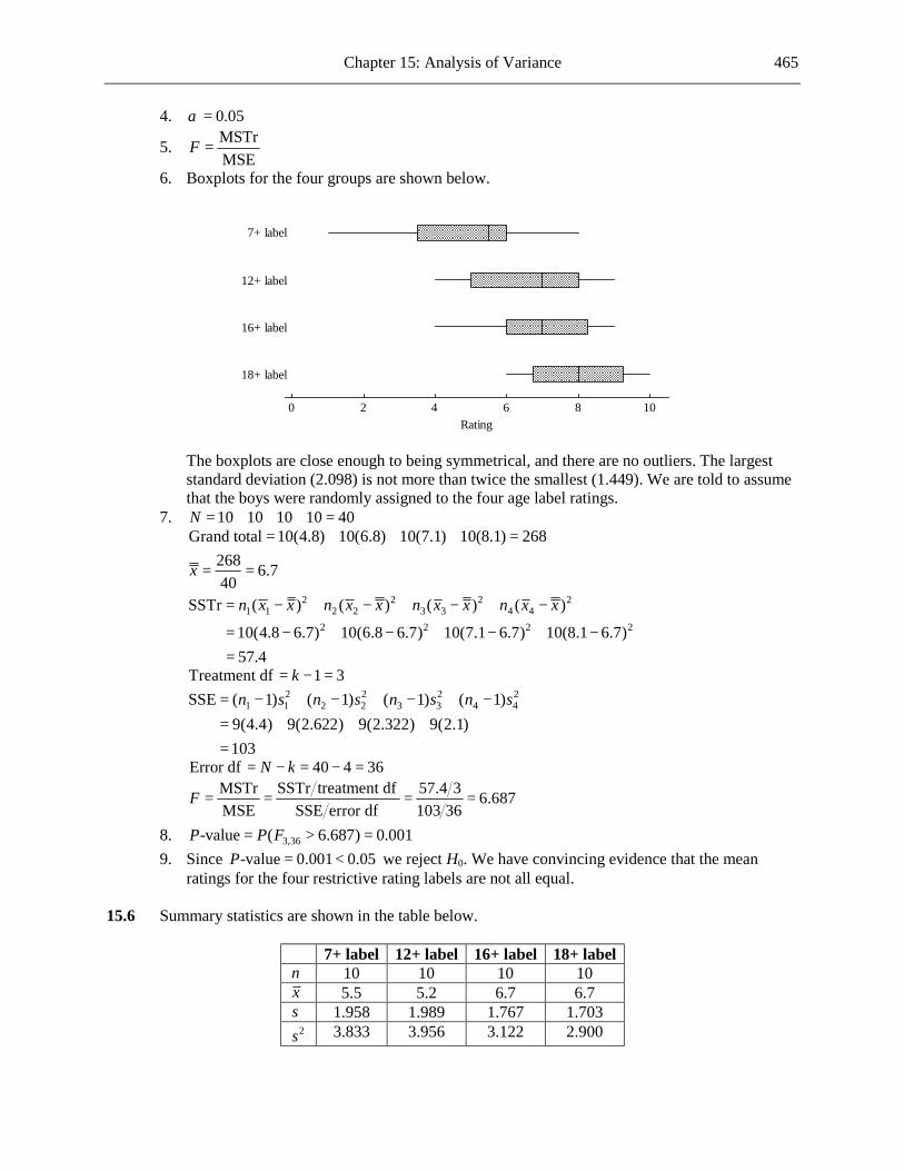
Chapter 15: Analysis of Variance 465
4. 0.05α =
5. MSTrMSE
F =
6. Boxplots for the four groups are shown below.
18+ label
16+ label
12+ label
7+ label
1086420Rating
The boxplots are close enough to being symmetrical, and there are no outliers. The largest
standard deviation (2.098) is not more than twice the smallest (1.449). We are told to assume that the boys were randomly assigned to the four age label ratings.
7. 10 10 10 10 40N = + + + = Grand total 10(4.8) 10(6.8) 10(7.1) 10(8.1) 268= + + + =
268 6.740
x = = 2 2 2 2
1 1 2 2 3 3 4 42 2 2 2
SSTr ( ) ( ) ( ) ( )
10(4.8 6.7) 10(6.8 6.7) 10(7.1 6.7) 10(8.1 6.7)57.4
n x x n x x n x x n x x= − + − + − + −
= − + − + − + −=
Treatment df 1 3k= − = 2 2 2 2
1 1 2 2 3 3 4 4SSE ( 1) ( 1) ( 1) ( 1)9(4.4) 9(2.622) 9(2.322) 9(2.1)103
n s n s n s n s= − + − + − + −= + + +=
Error df 40 4 36N k= − = − = MSTr SSTr treatment df 57.4 3 6.687MSE SSE error df 103 36
F = = = =
8. 3,36-value ( 6.687) 0.001P P F= > = 9. Since -value 0.001 0.05P = < we reject H0. We have convincing evidence that the mean
ratings for the four restrictive rating labels are not all equal. 15.6 Summary statistics are shown in the table below.
7+ label 12+ label 16+ label 18+ label n 10 10 10 10 x 5.5 5.2 6.7 6.7 s 1.958 1.989 1.767 1.703
2s 3.833 3.956 3.122 2.900
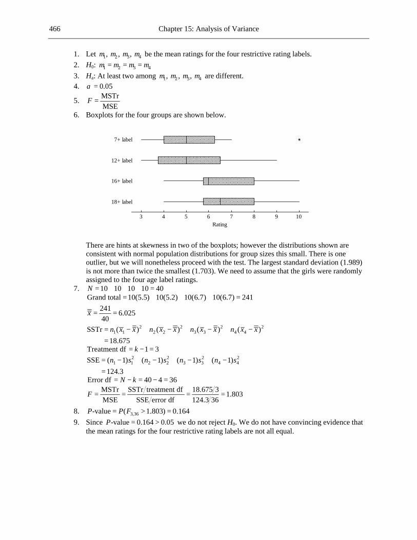
466 Chapter 15: Analysis of Variance
1. Let 1 2 3 4, , , µ µ µ µ be the mean ratings for the four restrictive rating labels. 2. H0: 1 2 3 4µ µ µ µ= = = 3. Ha: At least two among 1 2 3 4, , , µ µ µ µ are different. 4. 0.05α =
5. MSTrMSE
F =
6. Boxplots for the four groups are shown below.
18+ label
16+ label
12+ label
7+ label
109876543Rating
There are hints at skewness in two of the boxplots; however the distributions shown are
consistent with normal population distributions for group sizes this small. There is one outlier, but we will nonetheless proceed with the test. The largest standard deviation (1.989) is not more than twice the smallest (1.703). We need to assume that the girls were randomly assigned to the four age label ratings.
7. 10 10 10 10 40N = + + + = Grand total 10(5.5) 10(5.2) 10(6.7) 10(6.7) 241= + + + =
241 6.02540
x = =
2 2 2 21 1 2 2 3 3 4 4SSTr ( ) ( ) ( ) ( )
18.675n x x n x x n x x n x x= − + − + − + −
=
Treatment df 1 3k= − = 2 2 2 2
1 1 2 2 3 3 4 4SSE ( 1) ( 1) ( 1) ( 1)124.3n s n s n s n s= − + − + − + −
=
Error df 40 4 36N k= − = − = MSTr SSTr treatment df 18.675 3 1.803MSE SSE error df 124.3 36
F = = = =
8. 3,36-value ( 1.803) 0.164P P F= > = 9. Since -value 0.164 0.05P = > we do not reject H0. We do not have convincing evidence that
the mean ratings for the four restrictive rating labels are not all equal.

Chapter 15: Analysis of Variance 467
15.7 Summary statistics are shown in the table below.
Treatment 1 Treatment 2 Treatment 3 Treatment 4 n 18 25 17 14 x 5.778 6.480 3.529 2.929 s 4.081 3.441 2.401 2.129
2s 16.654 11.843 5.765 4.533 1. Let 1 2 3 4, , , µ µ µ µ be the mean numbers of pretzels consumed for the four treatments. 2. H0: 1 2 3 4µ µ µ µ= = = 3. Ha: At least two among 1 2 3 4, , , µ µ µ µ are different. 4. 0.05α =
5. MSTrMSE
F =
6. Boxplots for the four groups are shown below.
Treatment 4
Treatment 3
Treatment 2
Treatment 1
14121086420Number of Pretzels Consumed
The boxplots are roughly symmetric, and there are no outliers. The largest standard deviation
(4.081) is not more than twice the smallest (2.129). We are told that the men were randomly assigned to the four treatments.
7. 1 2 3 4 74N n n n n= + + + =
1 1 2 2 3 3 4 4Grand total 367n x n x n x n x= + + + = grand total 4.959x
N= =
2 2 2 21 1 2 2 3 3 4 4SSTr ( ) ( ) ( ) ( )
162.363n x x n x x n x x n x x= − + − + − + −
=
Treatment df 1 3k= − = 2 2 2 2
1 1 2 2 3 3 4 4SSE ( 1) ( 1) ( 1) ( 1)718.515n s n s n s n s= − + − + − + −
=

468 Chapter 15: Analysis of Variance
Error df 70N k= − = MSTr SSTr treatment df 5.273MSE SSE error df
F = = =
8. 3,70-value ( 5.273) 0.002P P F= > = 9. Since -value 0.002 0.05P = < we reject H0. We have convincing evidence that the mean
numbers of pretzels consumed for the four treatments are not all equal. 15.8 The summary statistics are given in the table below.
Semester 1 2 3 4 5 n 39 42 32 32 34 x 6.31 3.31 1.79 1.83 1.5 s 3.75 3.06 3.25 3.13 2.37
2s 14.0625 9.3636 10.5625 9.7969 5.6169 1. Let 1 2 3 4 5, , , ,µ µ µ µ µ be the mean percentages of words that are plagiarized for the five
semesters. 2. H0: 1 2 3 4 5µ µ µ µ µ= = = = 3. Ha: At least two among 1 2 3 4 5, , , ,µ µ µ µ µ are different. 4. 0.05α =
5. MSTrMSE
F =
6. We are told to assume that the conditions necessary for the ANOVA F test are reasonable. 7. 1 2 3 4 5 179N n n n n n= + + + + =
1 1 2 2 3 3 4 4 5 5Grand total 551.95n x n x n x n x n x= + + + + = grand total 3.084x
N= =
2 2 2 21 1 2 2 3 3 4 4SSTr ( ) ( ) ( ) ( )
597.231n x x n x x n x x n x x= − + − + − + −
=
Treatment df 1 4k= − = 2 2 2 2
1 1 2 2 3 3 4 4SSE ( 1) ( 1) ( 1) ( 1)1734.782n s n s n s n s= − + − + − + −
=
Error df 174N k= − = MSTr SSTr treatment df 14.976MSE SSE error df
F = = =
8. 4,174-value ( 14.976) 0P P F= > ≈ 9. Since -value 0 0.05P ≈ < we reject H0. We have convincing evidence that the mean
percentages of words that are plagiarized are not the same for all five semesters. 15.9 1. Let 1 2 3 4, , , µ µ µ µ be the mean changes in body fat mass for the four treatments. 2. H0: 1 2 3 4µ µ µ µ= = = 3. Ha: At least two among 1 2 3 4, , , µ µ µ µ are different. 4. 0.05α =

Chapter 15: Analysis of Variance 469
5. MSTrMSE
F =
6. Boxplots for the four groups are shown below.
G + S
G + P
P + S
P + P
210-1-2-3-4-5-6-7Change in body fat mass
The boxplots are roughly symmetric, and there are no outliers. The largest standard deviation
(1.443) is not more than twice the smallest (1.122). We are told that the men were randomly assigned to the four treatments.
7. 74N = Grand total 158.3= −
grand total 2.139xN
= = −
2 2 2 21 1 2 2 3 3 4 4SSTr ( ) ( ) ( ) ( )
247.403n x x n x x n x x n x x= − + − + − + −
=
Treatment df 1 3k= − = 2 2 2 2
1 1 2 2 3 3 4 4SSE ( 1) ( 1) ( 1) ( 1)107.314n s n s n s n s= − + − + − + −
=
Error df 70N k= − = MSTr SSTr treatment df 53.793MSE SSE error df
F = = =
8. 3,70-value ( 53.793) 0P P F= > ≈ 9. Since -value 0 0.05P ≈ < we reject H0. We have convincing evidence that the mean change in
body fat differs for the four treatments. 15.10 1. Let 1 2 3 4, , , µ µ µ µ be the mean compression strength for the four types of box. 2. H0: 1 2 3 4µ µ µ µ= = = 3. Ha: At least two among 1 2 3 4, , , µ µ µ µ are different. 4. 0.01α =
5. MSTrMSE
F =
6. Boxplots for the four samples are shown below.

470 Chapter 15: Analysis of Variance
4
3
2
1
800750700650600550500Compression strength (pounds)
For the small sample sizes the boxplots are reasonably close to being symmetrical, and there
are no outliers. The largest standard deviation (46.55) is not more than twice the smallest (37.20). We need to assume that the samples used were random samples from their respective populations.
7. 1 2 3 4 6 6 6 6 24N n n n n= + + + = + + + =
1 1 2 2 3 3 4 4Grand total 16380.1n x n x n x n x= + + + = grand total 682.504x
N= =
2 2 2 21 1 2 2 3 3 4 4SSTr ( ) ( ) ( ) ( )
127374.755n x x n x x n x x n x x= − + − + − + −
=
Treatment df 1 3k= − = 2 2 2 2
1 1 2 2 3 3 4 4SSE ( 1) ( 1) ( 1) ( 1)33838.975n s n s n s n s= − + − + − + −
=
Error df 20N k= − = MSTr SSTr treatment df 25.094MSE SSE error df
F = = =
8. 3,20-value ( 25.094) 0P P F= > ≈ 9. Since -value 0 0.01P ≈ < we reject H0. We have convincing evidence that the mean
compression strength is not the same for all four box types. 15.11 1. Let 1 2 3, , µ µ µ be the mean Hopkins scores for the three populations. 2. H0: 1 2 3µ µ µ= = 3. Ha: At least two among 1 2 3, , µ µ µ are different. 4. 0.05α =
5. MSTrMSE
F =
6. We are told to treat the samples as random samples from their respective populations. We have to assume that the population Hopkins score distributions are approximately normal with the same standard deviation.
7. 1 2 3 234N n n n= + + =
1 1 2 2 3 3Grand total 7064.66n x n x n x= + + =

Chapter 15: Analysis of Variance 471
grand total 30.191x
N= =
2 2 21 1 2 2 3 3SSTr ( ) ( ) ( )
100.786n x x n x x n x x= − + − + −
=
Treatment df 1 2k= − = 2 2 2 2
1 1 2 2 3 3 4 4SSE ( 1) ( 1) ( 1) ( 1)4409.036n s n s n s n s= − + − + − + −
=
Error df 231N k= − = MSTr SSTr treatment df 2.640MSE SSE error df
F = = =
8. 2,231-value ( 2.640) 0.074P P F= > = 9. Since -value 0.074 0.05P = > we do not reject H0. We do not have convincing evidence that
the mean Hopkins scores are not the same for all three student populations. 15.12 a 1 2 3 4 6 6 6 6 24N n n n n= + + + = + + + =
The four sample means are 57.49333333, 57.95166667, 59.55333333, 60.33833333. The four sample standard deviations are 1.37481150, 1.32888550, 0.89694296, 1.45590407.
1 1 2 2 3 3 4 4Grand total 1412.02000000n x n x n x n x= + + + = grand total 58.83416667x
N= =
2 2 2 21 1 2 2 3 3 4 4SSTr ( ) ( ) ( ) ( )
32.13815000n x x n x x n x x n x x= − + − + − + −
=
Treatment df 1 3k= − = 2 2 2 2
1 1 2 2 3 3 4 4SSE ( 1) ( 1) ( 1) ( 1)32.90103333n s n s n s n s= − + − + − + −
=
Error df 20N k= − = Thus the sums of squares and df’s are as given in the ANOVA table.
b 1. Let 1 2 3 4, , , µ µ µ µ be the mean calcium contents for the four storage times. 2. H0: 1 2 3 4µ µ µ µ= = = 3. Ha: At least two among 1 2 3 4, , , µ µ µ µ are different. 4. 0.05α =
5. MSTrMSE
F =
6. Boxplots for the four groups are shown below.

472 Chapter 15: Analysis of Variance
3 months
2 months
1 month
0 months
636261605958575655Calcium content
The boxplots are roughly symmetrical, and there are no outliers. The largest standard
deviation (1.456) is not more than twice the smallest (0.897). We need to assume that the four wheat specimens were randomly assigned to the four storage times.
7. 6.51F = 8. 3,20-value ( 6.51) 0.003P P F= > = 9. Since -value 0.003 0.05P = < we reject H0. We have convincing evidence that the mean
calcium content for the four storage times are not all equal. 15.13 4, 20.k N= = Treatment df 1 3. Error df 16.k N k= − = = − =
SSTr SSTo SSE 310500.76 235419.04 75081.72.= − = − = The completed table is shown below.
Source of Variation
df
Sum of Squares
Mean Square
F
Treatments 3 75081.72 25027.24 1.701 Error 16 235419.04 14713.69 Total 19 310500.76
1. Let 1 2 3 4, , , µ µ µ µ be the mean number of miles until failure for the four given brands of
spark plug. 2. H0: 1 2 3 4µ µ µ µ= = = 3. Ha: At least two among 1 2 3 4, , , µ µ µ µ are different. 4. 0.05α =
5. MSTrMSE
F =
6. We need to treat the samples as random samples from their respective populations, and assume that the population distributions are approximately normal with the same standard deviation.
7. 1.701F = 8. 3,16-value ( 1.701) 0.207P P F= > =

Chapter 15: Analysis of Variance 473
9. Since -value 0.207 0.05P = > we do not reject H0. We do not have convincing evidence that
the mean number of miles to failure is not the same for all four brands of spark plug. 15.14 Since the interval for 2 3µ µ− is the only one that contains zero, we have evidence of a difference
between 1µ and 2µ , and between 1µ and 3µ , but not between 2µ and 3µ . Thus, statement c is the correct choice.
15.15 Since there is a significant difference in all three of the pairs we need a set of intervals none of
which includes zero. Set 3 is therefore the required set. 15.16 In increasing order of the resulting mean numbers of pretzels eaten the treatments were: slides
with related text, slides with no text, no slides, and slides with unrelated text. There were no significant differences between the results for slides with related text and slides with no text, or for no slides and slides with unrelated text. However, there was a significant difference between the mean numbers of pretzels eaten for no slides and slides with no text (and also between the results for no slides and slides with related text). Likewise, there was a significant difference between the mean numbers of pretzels eaten for slides with unrelated text and slides with no text (and also between the results for slides with unrelated text and slides with related text).
15.17 a In decreasing order of the resulting mean numbers of pretzels eaten the treatments were:
slides with related text, slides with no text, slides with unrelated text, and no slides. There were no significant differences between the results for slides with no text and slides with unrated text, and for slides with unrelated text and no slides. However there was a significant difference between the results for slides with related text and each one of the other treatments, and between the results for no slides and for slides with no text (and for slides with related text).
b The results for the women and men are almost exactly the reverse of one another, with, for
example, slides with related text (treatment 2) resulting in the smallest mean number of pretzels eaten for the women and the largest mean number of pretzels eaten for the men. For the men, treatment 2 was significantly different from all the other treatments; however for women treatment 2 was not significantly different from treatment 1. For both women and men there was a significant difference between treatments 1 and 4 and no significant difference between treatments 3 and 4. However, between treatments 1 and 3 there was a significant difference for the women but no significant difference for the men.
15.18 a The sample sizes and means are given in the table below.
7+ label 12+ label 16+ label 18+ label n 10 10 10 10 x 4.8 6.8 7.1 8.1
As calculated in Exercise 15.5, MSE = 103/36 = 2.861 and Error df = 36.
Thus the T-K interval for i jµ µ− (using Error df = 40 in Appendix Table 7) is
1 2
MSE 1 1 MSE 2.8613.792 10i j i j i jx x q x x q x x
n n n
− ± + = − ± = − ±
.
So the intervals are as shown below.

474 Chapter 15: Analysis of Variance
Difference Interval Includes 0? 1 2µ µ− (−4.027, 0.027) Yes
1 3µ µ− (−4.327, −0.273) No
1 4µ µ− (−5.327, −1.273) No
2 3µ µ− (−2.327, 1.727) Yes
2 4µ µ− (−3.327, 0.727) Yes
3 4µ µ− (−3.027, 1.027) Yes 7+ label 12+ label 16+ label 18+ label Sample mean 4.8 6.8 7.1 8.1
b Certainly the more restrictive the age label on the video game the higher the sample mean
rating given by the boys used in the experiment. However, according to the T-K intervals the only significant differences were between the means for the 7+ label and the 16+ label, and between the means for the 7+ label and the 18+ label.
15.19 a Driving Shooting Fighting Sample mean 3.42 4.00 5.30 b Driving Shooting Fighting Sample mean 2.81 3.44 4.01
15.20 The sample means for the five different fabrics are: 16.350, 11.633, 10.500, 14.960, 12.300.
Therefore, the fabric types, listed in order of their sample means, are: 3, 2, 5, 4, 1. The significant differences are between 1µ and 2µ , 1µ and 3µ , 1µ and 5µ , 2µ and 4µ , 3µ and
4µ , 4µ and 5µ . The underscoring pattern is shown below.
Fabric 3 Fabric 2 Fabric 5 Fabric 4 Fabric 1 Sample mean 10.5 11.633 12.3 14.96 16.35 15.21 a 1 2 3 4 80N n n n n= + + + =
1 1 2 2 3 3 4 4Grand total 158n x n x n x n x= + + + = grand total 1.975x
N= =
2 2 2 21 1 2 2 3 3 4 4SSTr ( ) ( ) ( ) ( )
13.450n x x n x x n x x n x x= − + − + − + −
=
Treatment df 1 3k= − = 2 2 2 2
1 1 2 2 3 3 4 4SSE ( 1) ( 1) ( 1) ( 1)7.465n s n s n s n s= − + − + − + −
=
Error df 76N k= − =

Chapter 15: Analysis of Variance 475
MSTr SSTr treatment df 45.644MSE SSE error df
F = = =
The ANOVA table is shown below.
Source of Variation
df
Sum of Squares
Mean Square
F
Treatments 3 13.450 4.483 45.644 Error 76 7.465 0.098 Total 79 20.915
1. Let 1 2 3 4, , , µ µ µ µ be the mean numbers of seeds germinating for the four treatments. 2. H0: 1 2 3 4µ µ µ µ= = = 3. Ha: At least two among 1 2 3 4, , , µ µ µ µ are different. 4. 0.05α =
5. MSTrMSE
F =
6. We need to assume that the samples of 100 seeds collected from each treatment were random samples from those populations, and that the population distributions of numbers of seeds germinating are approximately normal with the same standard deviation.
7. 45.644F = 8. 3,76-value ( 45.644) 0P P F= > ≈ 9. Since -value 0 0.05P ≈ < we reject H0. We have convincing evidence that the mean
number of seeds germinating is not the same for all four treatments. b We will construct the T-K interval for 2 3µ µ− .
Appendix Table 7 gives the 95% Studentized range critical value 3.74q = (using 4k = and error df = 60, the closest tabled value to df 76n k= − = ). The T-K interval for 2 3µ µ− is
0.098 1 1(2.35 1.70) 3.74 (0.388, 0.912).2 20 20
− ± + =
Since this interval does not contain zero, we have convincing evidence that seeds eaten and then excreted by lizards germinate at a different rate from those eaten and then excreted by birds. Therefore, since the sample mean was higher for the lizard dung treatment than for the bird dung treatment, we have convincing evidence that seeds eaten and then excreted by lizards germinate at a higher rate from those eaten and then excreted by birds.
15.22 a Summary statistics are shown in the table below.
Imperial Parkay Blue Bonnet Chiffon Mazola Fleischmann’s n 4 5 4 4 5 4 x 14.1 12.8 13.825 13.1 17.14 18.1 s 0.356 0.430 0.443 0.594 0.598 0.648
2s 0.127 0.185 0.196 0.353 0.358 0.420 1. Let 1 2 3 4 5 6, , , , , µ µ µ µ µ µ be the mean PAPUFA percentages for the six brands. 2. H0: 1 2 3 4 5 6µ µ µ µ µ µ= = = = = 3. Ha: At least two among 1 2 3 4 5 6, , , , , µ µ µ µ µ µ are different.

476 Chapter 15: Analysis of Variance
4. 0.05α =
5. MSTrMSE
F =
6. Boxplots for the four groups are shown below.
Fleischmann’s
Mazola
Chiffon
Blue Bonnet
Parkay
Imperial
1918171615141312PAPUFA percentage
The boxplots are roughly symmetric, and there are no outliers. The largest standard
deviation (0.420) is more than twice the smallest (0.127), but we will nonetheless proceed. We need to assume that the specimens of margarine used formed random samples from their respective populations.
7. 1 2 3 4 5 6 26N n n n n n n= + + + + + =
1 1 2 2 3 3 4 4 5 5 6 6Grand total 386.2n x n x n x n x n x n x= + + + + + = grand total 14.854x
N= =
2 2 2 2 2 21 1 2 2 3 3 4 4 5 5 6 6SSTr ( ) ( ) ( ) ( ) ( ) ( )
108.185n x x n x x n x x n x x n x x n x x= − + − + − + − + − + −
=
Treatment df 1 5k= − = 2 2 2 2 2 2
1 1 2 2 3 3 4 4 5 5 6 6SSE ( 1) ( 1) ( 1) ( 1) ( 1) ( 1)5.459n s n s n s n s n s n s= − + − + − + − + − + −
=
Error df 20N k= − = MSTr SSTr treatment df 79.264MSE SSE error df
F = = =
8. 5,20-value ( 79.264) 0P P F= > ≈ 9. Since -value 0 0.05P ≈ < we reject H0. We have convincing evidence that the mean
PAPUFA percentages for the six brands are not all equal. b The confidence intervals are as follows:
1 20.272975 1 1: (14.1 12.8) 4.45 ( , )
2 4 5µ µ − − ± + =
0.197 2.403

Chapter 15: Analysis of Variance 477
1 30.272975 1 1: (14.1 13.825) 4.45 ( , )
2 4 4µ µ − − ± + = −
0.887 1.437
1 40.272975 1 1: (14.1 13.1) 4.45 ( , )
2 4 4µ µ − − ± + = −
0.162 2.162
1 50.272975 1 1: (14.1 17.14) 4.45 ( , )
2 4 5µ µ − − ± + = − −
4.143 1.937
1 60.272975 1 1: (14.1 18.1) 4.45 ( . , . )
2 4 4µ µ − − ± + = − −
5 162 2 838
2 30.272975 1 1: (12.8 13.825) 4.45 ( . , . )
2 5 4µ µ − − ± + = −
2 128 0 078
2 40.272975 1 1: (12.8 13.1) 4.45 ( . , . )
2 5 4µ µ − − ± + = −
1 403 0 803
2 50.272975 1 1: (12.8 17.14) 4.45 ( . , . )
2 5 5µ µ − − ± + = − −
5 380 3 300
2 60.272975 1 1: (12.8 18.1) 4.45 ( . , . )
2 5 4µ µ − − ± + = − −
6 403 4 197
3 40.272975 1 1: (13.825 13.1) 4.45 ( . , . )
2 4 4µ µ − − ± + = −
0 437 1 887
3 50.272975 1 1: (13.825 17.14) 4.45 ( . , )
2 4 5µ µ − − ± + = − −
4 418 2.212
3 60.272975 1 1: (13.825 18.1) 4.45 ( . , . )
2 4 4µ µ − − ± + = − −
5 437 3 113
4 50.272975 1 1: (13.1 17.14) 4.45 ( . , )
2 4 5µ µ − − ± + = − −
5 143 2.937
4 60.272975 1 1: (13.1 18.1) 4.45 ( . , . )
2 4 4µ µ − − ± + = − −
6 162 3 838
5 60.272975 1 1: (17.14 18.1) 4.45 ( . , . )
2 5 4µ µ − − ± + = −
2 063 0 143
The underscoring pattern is shown below. Parkay Chiffon Blue Bonnet Imperial Mazola Fleischmann’s Sample mean 12.8 13.1 13.825 14.1 17.14 18.1
Online Exercises 15.23 A randomized block experiment was used to control the factor value of house, which definitely
affects the assessors’ appraisals. If a completely randomized experiment had been done, then there would have been danger of having the assessors appraising houses which were not of

478 Chapter 15: Analysis of Variance
similar values. Therefore, differences between assessors would be partly due to the fact that the homes were dissimilar, as well as to systematical differences in the appraisals made.
15.24 a
Source of Variation
Degrees of Freedom
Sum of Squares
Mean Square
F
Treatments
2
11.7
5.85
0.37
Blocks
4
113.5
28.375
Error
8
125.6
15.7
Total
14
250.8
b Ho: The mean appraised value does not depend on which assessor is doing the appraisal. Ha: The mean appraised value does depend on which assessor is doing the appraisal. α = 0.05
Test statistic: MSTr MSE
F =
df1 = k − 1 = 2 df2 = (k− 1)(l − 1) = 8. From the ANOVA table, F = 0.37. From Appendix Table 6, P-value > 0.10.
Since the P-value exceeds α, the null hypothesis is not rejected. The mean appraised value does not seem to depend on which assessor is doing the appraisal.
15.25 Ho: The mean lead concentration does not depend on proportion of ash. Ha: The mean lead concentration does depend on proportion of ash. α = 0.01
Test statistic: MSTrF = MSE
Computations:
Source of Variation
Degrees of Freedom
Sum of Squares
Mean Square
F
Treatment 2 1395.61 697.806 117.36 Block 3 7.08 2.361 Error 6 35.68 5.946 Total 11 1438.37

Chapter 15: Analysis of Variance 479
df1 = 2 , df2 = 6 and F = 117.36. From Appendix Table 6, P-value < 0.001. Since the P-value is less than α, the null hypothesis is rejected. There is convincing evidence that
the mean lead concentration differs for the three ash concentrations. 15.26 Ho: 1 2 3µ µ µ= = Ha: The three means are not all equal α = 0.05
Test statistic: MSTrF = MSE
Computations:
Source of Variation
Degrees of Freedom
Sum of Squares
Mean Square
F
Treatment 2 3199140 1599570 641.49 Block 9 15028 1670 Error 18 44883 2494 Total 29 3259052
df1 = 2 , df2 = 18 and F = 641.49. From Appendix Table 6, P-value < 0.001. Since the P-value is less than α, there is evidence that the null hypothesis should be rejected. 15.27 Ho: The mean soil moisture is the same for the three treatments. Ha: The mean soil moisture is not the same for all three treatments. α = 0.05
Test statistic: MSTrF = MSE
Computations:
Source of Variation
Degrees of Freedom
Sum of Squares
Mean Square
F
Treatment 2 7.541 3.77033 0.42 Block 9 47.112 5.23467 Error 18 162.246 9.01367 Total 29 216.899

480 Chapter 15: Analysis of Variance
df1 = 2 , df2 = 18 and F = 0.42. From Appendix Table 6, P-value > 0.1. Since the P-value exceeds α, the null hypothesis is not rejected. We do not have convincing
evidence that the mean soil moisture is not the same for all three treatments. 15.28 Ho: The mean soil moisture is the same for the three treatments. Ha: The mean soil moisture is not the same for all three treatments. α = 0.05
Test statistic: MSTrF = MSE
Computations:
Source of Variation
Degrees of Freedom
Sum of Squares
Mean Square
F
Treatment 2 7.046 3.523 0.95 Block 9 37.52 4.16893 1.13 Error 18 66.641 3.70226 Total 29 111.207
df1 = 2 , df2 = 18 and F = 0.95. From Appendix Table 6, P-value > 0.1. Since the P-value exceeds α, the null hypothesis is not rejected. We do not have convincing
evidence that the mean soil temperature is not the same for all three treatments. 15.29 The statement indicates that there is interaction between caffeine consumption and exercise. The
protective effect of increasing exercise by a particular amount is greater for higher levels of caffeine consumption.
15.30 a The graph is shown below.

Chapter 15: Analysis of Variance 481
The graph does not seem to support the conclusion of no interaction. It appears that for
students who did not study the increase from 4 to 6 choices resulted in an increase in mean percentage correct, this not being the case for students who studied (with or without review).
b Ho: There are no prior study main effects. Ha: There are prior study main effects. α = 0.05
Test statistic: AMSAF = MSE
df1 = k − 1 = 3 − 1 = 2, df2 = 69, and FA = 66.25. From Appendix Table 6,
P-value < 0.001.
Since the P-value is less than α, the null hypothesis of no prior study main effects is rejected. The conclusion of significant main effects for prior study is justified.
Ho: There are no number of choices main effects. Ha: There are number of choices main effects. α = 0.05
Test statistic: BMSB = F MSE
df1 = l − 1 = 3 − 1 = 2, df2 = 69, and FB = 73.76. From Appendix Table 6,
P-value < 0.001.
Since the P-value is less than α, the null hypothesis of no number of choices main effects is rejected. The conclusion of significant main effects for number of choices is justified.

482 Chapter 15: Analysis of Variance
c The conclusion of the authors mentioned in Part (a) tells us that the effect of changing the number of answer choices from 2 to 4 and from 4 to 6 is not significantly changed according to the level of prior study. From the graph we can see that increasing the number of answer choices resulted in a decrease, on average, of the percentage correct on the exam, and the authors’ conclusion implies that this effect is roughly equal for all levels of prior study. The conclusion of the first hypothesis test in Part (b) is that this effect is significant. We also see from the graph that whatever the number of answer choices, an increase in the level of study is associated with an increase in the percentage correct, and that this applies for all numbers of answer choices. The conclusion of the second hypothesis test in Part (b) tells us that this effect is significant.
15.31 a Yes. The roughly horizontal lines for “low approach” show that the level of thoughts of
passion has very little effect on the satisfaction level for people in that category. The small positive slope for “average approach” shows that an increase in thoughts of passion results in a relatively small increase in satisfaction for people in that category. However, the greater slope for “high approach” shows that an increase in thoughts of passion results in a larger increase in satisfaction for people in that category.
b Yes. The small positive slope for “low avoidance” shows that an increase in thoughts of
insecurity results in a small increase in satisfaction for people in that category. The small negative slope for “average avoidance” shows that an increase in thoughts of insecurity results in a small decrease in satisfaction for people in that category. The larger negative slope for “high avoidance” shows that an increase in thoughts of insecurity results in a larger decrease in satisfaction for people in that category.
c Yes. In the top graph the slope for “high approach” is more positive than that of either of
the other two categories, and in the bottom graph the slope for “high avoidance” is more negative than that of either of the other two categories.
15.32 a
b The graphs for males and females are very nearly parallel. There does not appear to be an

Chapter 15: Analysis of Variance 483
interaction between gender and type of odor. 15.33 When an AB interaction is present, the change in mean response, when going from one level of
factor A to another, depends upon which level of factor B is being used. Since these effects are different for different levels of factor B, the individual effects of factor A or factor B cannot be interpreted.
15.34 a The completed ANOVA table is shown below.
Source of Variation
Degrees of Freedom
Sum of Squares
Mean Square
F
Status (A)
2
0.34776
0.17388
14.49
Gender (B)
1
0.00180
0.00180
0.15
Status by Gender
2
0.02280
0.01140
0.95
Error
66
0.79200
0.01200
Total
71
1.16436
b Ho: There is no interaction between status (A) and gender (B). Ha: There is interaction between status (A) and gender (B). α = 0.05 (for illustration)
The test statistic is: ABMSAB = F MSE
.
df1 = 2 , df2 = 66, FAB = 0.95. From Appendix Table 6, P-value > 0.10.
Since the P-value is greater than α, the null hypothesis is not rejected. The data do not suggest existence of an interaction between status and gender. Hence tests about main effects may be performed.
c Ho: There are no gender main effects. Ha: There are gender main effects. α = 0.05 (for illustration)
The test statistic is: BMSBMSE
= F .
df1 = 1, df2 = 66, and FB = 0.15 From Appendix Table 6, P-value > 0.10.

484 Chapter 15: Analysis of Variance
Since the P-value exceeds α, the null hypothesis of no gender main effects is not rejected. The data do not suggest the existence of a difference between mean “Rate of Talk” scores for girls and boys.
d Ho: There are no status main effects. Ha: There are status main effects. α = 0.05 (for illustration)
The test statistic is: AMSA
MSEF = .
df1 = 2, df2 = 66, and FA = 14.49 From Appendix Table 6, 0.001 > P-value.
Since the P-value is smaller than α, the null hypothesis of no status main effects is rejected. The data provide evidence to conclude that there is a difference among the mean “Rate of Talk” scores across the three status groups.
15.35
Source of Variation
Degrees of Freedom
Sum of Squares
Mean Square
F
Size (A)
2
0.088
0.044
4.00
Species (B)
1
0.048
0.048
4.364
Size by Species
2
0.048
0.024
2.18
Error
12
0.132
0.011
Total
17
0.316
Ho: There is no interaction between Size (A) and Species (B). Ha: There is interaction between Size and Species. α = 0.01
The test statistic is: ABMSAB = F MSE
.
df1 = 2 , df2 = 12, and FAB = 2.18 From Appendix Table 6, P-value > 0.10. Since the P-value exceeds α, the null hypothesis is not rejected. The data are consistent with the
hypothesis of no interaction between Size and Species. Hence, hypothesis tests on main effects will be done.

Chapter 15: Analysis of Variance 485
Ho: There are no size main effects. Ha: There are size main effects. α = 0.01
The test statistic is: AMSA = F MSE
.
df1 = 2, df2 = 12, and FA = 4.00. From Appendix Table 6, 0.05 > P-value > 0.01. Since the P-value exceeds α, the null hypothesis of no size main effects is not rejected. When
using α=0.01, the data do not support the conclusion that there are differences between the mean preference indices for the three sizes of bass.
Ho: There are no species main effects. Ha: There are species main effects. α = 0.01
The test statistic is: BMSB = F MSE
.
df1 = 1, df2 = 12, and FB = 4.364 From Appendix Table 6, P-value > 0.05. Since the P-value exceeds α, the null hypothesis of no species main effects is not rejected. At a
significance level of α = 0.01, the data are consistent with the hypothesis that there are no differences between the mean preference indices for the three species of bass.
15.36 a There are two age classes. b There were twenty-one observations made for each age-sex combination. c
Source of Variation
Degrees of Freedom
Sum of Squares
Mean Square
F
Age (A)
1
0.614
0.6140
8.73
Sex (B)
1
1.754
1.7540
24.95
Age by Sex
(AB)
1
0.146
0.1460
2.08
Error
80
5.624
0.0703
Total
83
8.138

486 Chapter 15: Analysis of Variance
Ho: There is no interaction between age (A) and sex (B). Ha: There is interaction between age and sex. α = 0.01 (for illustration)
Test statistic: ABMSAB = F MSE
df1 = 1 , df2 = 80 , and FAB = 2.08. From Appendix Table 6, P-value > 0.10.
Since the P-value exceeds α, the null hypothesis is not rejected. The data are consistent with the hypothesis of no interaction between age and sex. Hence, hypothesis tests on main effects will be done.
Ho: There are no age main effects. Ha: There are age main effects. α = 0.01
Test statistic: AMSA = F MSE
df1 = 1 , df2 = 80 , and FA = 8.73. From Appendix Table 6, 0.01 > P-value > 0.001.
Since the P-value is less than α, the null hypothesis of no age main effects is rejected. The data supports the conclusion that there is a difference between the mean values of the preference index for the two age groups.
Ho: There are no sex main effects. Ha: There are sex main effects. α = 0.01
Test statistic: BMSB = F MSE
df1 = 1 , df2 = 80 , and FB = 24.95. From Appendix Table 6, 0.001 > P-value.
Since the P-value is less than α, the null hypothesis of no sex main effects is rejected. The data supports the conclusion that there is a difference between the mean territory size for the two sexes.
15.37 a
Source of Variation
Degrees of Freedom
Sum of Squares
Mean Square
F
Race
1
857
857
5.57

Chapter 15: Analysis of Variance 487
Ho: There is no interaction between race and sex. Ha: There is interaction between race and sex. α = 0.01
Test statistic: ABMSAB = F MSE
df1 = 1 , df2 = 36 , and FAB = 0.21. From Appendix Table 6, P-value > 0.10.
Since the P-value exceeds α, the null hypothesis of no interaction between race and sex is not rejected. Thus, hypothesis tests for main effects are appropriate.
b Ho: There are no race main effects. Ha: There are race main effects. α = 0.01
Test statistic: AMSA = F MSE
df1 = 1 , df2 = 36 , and FA = 5.57. From Appendix Table 6, 0.05 > P-value > 0.01
Since the P-value exceeds α, the null hypothesis of no race main effects is not rejected. The data are consistent with the hypothesis that the true average lengths of sacra do not differ for the two races.
c Ho: There are no sex main effects. Ha: There are sex main effects. α = 0.01
Test statistic: BMSB = F MSE
df1 = 1 , df2 = 36 , and FB = 1.89. From Appendix Table 6, P-value > 0.10.
Sex 1 291 291 1.89 Race by
Sex
1
32
32
0.21
Error
36
5541
153.92
Total
39
6721

488 Chapter 15: Analysis of Variance
Since the P-value exceeds α, the null hypothesis of no sex main effects is not rejected. The data are consistent with the hypothesis that the true average lengths of sacra do not differ for males and females.
15.38 a The required boxplot obtained using MINITAB is shown below. Price per acre values
appear to be similar for 1996 and 1997 but 1998 values are higher. The mean price per acre values for each year are also plotted as a solid square within each box plot.
500004000030000
1998
1997
1996
Price
Year
b Let µi denote the mean price per acre for vineyards in year i (i = 1, 2, 3). Ho: µ1 = µ2 = µ3 Ha: At least two of the three µi's are different. α = 0.05
Test statistic: MSTrF = MSE
df1 = k − 1 = 2 df2 = N − k = 15-3 = 12. 1 2 335600, 36000, 43600x x x= = =
[5(35600) + 5(36000) + 5(43600) ]= (15)
x = 38400
MSTr = [5(35600 − 38400)2 + 5(36000 − 38400)2 + 5(43600 − 38400)2 ]/2 = 101600000 1 2 33847.077, 3807.887, 3911.521s s s= = = MSE = [(5-1)(3847.077)2 + (5-1)(3807.887)2 + (5-1)(3911.521)2 ]/12 = 14866667

Chapter 15: Analysis of Variance 489
MSTr 101600000F = = = 6.83MSE 14866667
From Appendix Table 6, 0.05 > P-value > 0.01.
Since the P-value is less than α, the null hypothesis is rejected. At a significance level of α = 0.05, the data support the claim that the true mean price per acre for the three years under consideration are not all the same.
15.39 a From the given information:
2 2
1 1 1 2 2 22 2
3 3 3 4 4 4
6, 10.125, 2.093750 6, 11.375, 3.59375
6, 11.708333, 2.310417 5, 12.35, .925
n x s n x s
n x s n x s
= = = = = =
= = = = = =
261 11.34782623
TxN
= = =
SSTr = 6(10.125 − 11.347826)2 + 6(11.375 − 11.347826)2 + 6(11.708333 − 11.347826)2 + 5(12.35 − 11.347826)2 = 8.971822 + 0.004431 + 0.779791 + 5.021763 = 14.7778 SSE = 5(2.093750) + 5(3.59375) + 5(2.310417) + 4(0.925) = 43.689585. df1 = k − 1 = 4 − 1 = 3 df2 = (6 + 6 + 6 + 5) − 4 = 19
SSTr 14.7778MSTr 4.9259331 3k
= = =−
SSE 43.689585MSE 2.29945219N k
= = =−
MSTr 4.925933 2.142MSE 2.299452
F = = =
From Appendix Table 6, P-value > 0.10. b Ho: µ1 = µ2 = µ3 = µ4 Ha: At least two of the four µi's are different. α = 0.05
Test statistic: MSTrF = 2.142MSE
=
df1 = k − 1 = 3 df2 = N − k = 19. From the ANOVA table, F = 2.142. From Appendix Table 6, P-value > 0.10.

490 Chapter 15: Analysis of Variance
Since the P-value exceeds α, the null hypothesis is not rejected. The data do not suggest
that there are differences in true average responses among the treatments. 15.40 The interval for µ1 − µ2 contains zero, and hence µ1 and µ2 are judged not different. The intervals
for µ1 − µ3 and µ2 − µ3 do not contain zero, so µ1 and µ3 are judged to be different and µ2 and µ3 are judged to be different. Hence there is evidence that µ3 is different from the other two means.
15.41 a Ho: µ1 = µ2 = µ3 = µ4 = µ5 Ha: At least two of the five µi's are different. α = 0.05
Test statistic: MSTrF = MSE
df1 = k − 1 = 4 df2 = N − k = 15. From the data, the following statistics were calculated.
Hormone 1 2 3 4 5 n 4 4 4 4 4 mean 12.75 17.75 17.50 11.50 10.00 Total 51 71 70 46 40 variance 17.58 12.917 8.333 21.667 15.333
278 13.920
TxN
= = =
SSTr = 4(12.75 − 13.9)2 + 4(17.75 − 13.9)2 + 4(17.50 − 13.9)2 + 4(11.5 − 13.9)2 + 4(10 − 13.9)2 = 5.29 + 59.29 + 51.84 + 23.04 + 60.840 = 200.3 SSE = 3(17.583) + 3(12.917) + 3(8.333) + 3(21.667) + 3(15.333) = 227.499 df1 = k − 1 = 5 − 1 = 4 df2 = (4 + 4 + 4 + 4 + 4) − 5 = 15
SSTr 200.3MSTr 50.0751 4k
= = =−
227.499 15.166615
SSEMSEN k
= = =−
50.075 3.3015.1666
MSTrFMSE
= = =
From Appendix Table 6, 0.05 > P-value > 0.01.
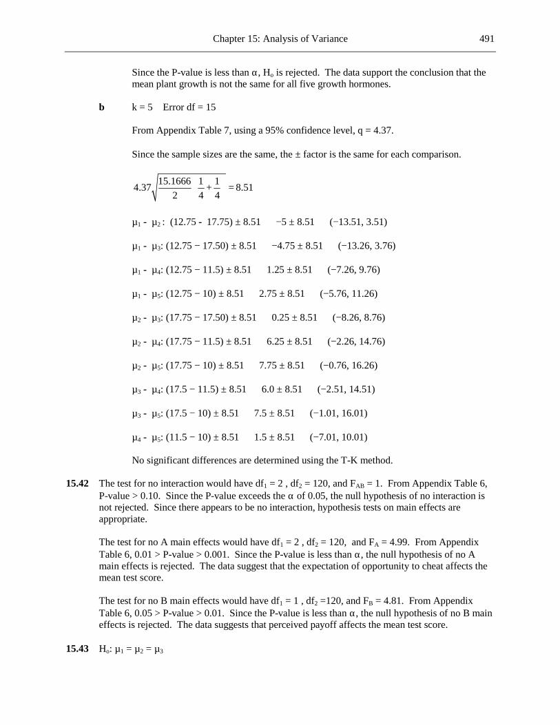
Chapter 15: Analysis of Variance 491
Since the P-value is less than α, Ho is rejected. The data support the conclusion that the
mean plant growth is not the same for all five growth hormones. b k = 5 Error df = 15 From Appendix Table 7, using a 95% confidence level, q = 4.37. Since the sample sizes are the same, the ± factor is the same for each comparison.
15.1666 1 14.37 + 8.512 4 4
=
µ1 − µ2 : (12.75 − 17.75) ± 8.51 ⇒ −5 ± 8.51 ⇒ (−13.51, 3.51) µ1 − µ3: (12.75 − 17.50) ± 8.51 ⇒ −4.75 ± 8.51 ⇒ (−13.26, 3.76) µ1 − µ4: (12.75 − 11.5) ± 8.51 ⇒ 1.25 ± 8.51 ⇒ (−7.26, 9.76) µ1 − µ5: (12.75 − 10) ± 8.51 ⇒ 2.75 ± 8.51 ⇒ (−5.76, 11.26) µ2 − µ3: (17.75 − 17.50) ± 8.51 ⇒ 0.25 ± 8.51 ⇒ (−8.26, 8.76) µ2 − µ4: (17.75 − 11.5) ± 8.51 ⇒ 6.25 ± 8.51 ⇒ (−2.26, 14.76) µ2 − µ5: (17.75 − 10) ± 8.51 ⇒ 7.75 ± 8.51 ⇒ (−0.76, 16.26) µ3 − µ4: (17.5 − 11.5) ± 8.51 ⇒ 6.0 ± 8.51 ⇒ (−2.51, 14.51) µ3 − µ5: (17.5 − 10) ± 8.51 ⇒ 7.5 ± 8.51 ⇒ (−1.01, 16.01) µ4 − µ5: (11.5 − 10) ± 8.51 ⇒ 1.5 ± 8.51 ⇒ (−7.01, 10.01) No significant differences are determined using the T-K method. 15.42 The test for no interaction would have df1 = 2 , df2 = 120, and FAB = 1. From Appendix Table 6,
P-value > 0.10. Since the P-value exceeds the α of 0.05, the null hypothesis of no interaction is not rejected. Since there appears to be no interaction, hypothesis tests on main effects are appropriate.
The test for no A main effects would have df1 = 2 , df2 = 120, and FA = 4.99. From Appendix
Table 6, 0.01 > P-value > 0.001. Since the P-value is less than α, the null hypothesis of no A main effects is rejected. The data suggest that the expectation of opportunity to cheat affects the mean test score.
The test for no B main effects would have df1 = 1 , df2 =120, and FB = 4.81. From Appendix
Table 6, 0.05 > P-value > 0.01. Since the P-value is less than α, the null hypothesis of no B main effects is rejected. The data suggests that perceived payoff affects the mean test score.
15.43 Ho: µ1 = µ2 = µ3

492 Chapter 15: Analysis of Variance
Ha: at least two among µ1, µ2, µ3 are not equal.
MSTrF = MSE
N = 90, df1 = 2 df2 = 87 T = 30(9.40 + 11.63 + 11.00) = 960 .9
960.9 10.67790
TxN
= = =
SSTr = 30[(9.40 − 10.677)2 + (11.63 − 10.677)2 + (11.00 − 10.677)2 ] = 30[1.630729 + 0.908209 + 0.104329] = 79.298
79.298 39.6492
MSTr = =
749.85 8.61987
MSE = =
MSTr 39.649F = 4.60MSE 8.619
= =
From Appendix Table 6, 0.05 > P-value > 0.01. If α = 0.05 is used, then the P-value is less than α and the null hypothesis would be rejected. The
conclusion would be that the true population mean score is not the same for the three types of students.
If α = 0.01 is used, then the P-value exceeds α and the null hypothesis would not be rejected.
The conclusion would be that the data are consistent with the hypothesis that the mean score is the same for the three types of students.
15.44 a Ho: µ1 = µ2 = µ3 = µ4
Ha: at least two among µ1, µ2, µ3, µ4 are not equal. α = 0.05
MSTrF = MSE
2 2
1 1 1 2 2 22 2
3 3 3 4 4 4
6, 4.923, .000107 6, 4.923, .000067
6, 4.917, .000147 6, 4.902, .000057
n x s n x s
n x s n x s
= = = = = =
= = = = = =
T = 6(4.923) + 6(4.923) + 6(4.917) + 6(4.902) = 117.99
117.99 4.91624
x = =

Chapter 15: Analysis of Variance 493
SSTr = 6(4.923 − 4.916)2 + 6(4.923 − 4.916)2 + 6(4.917 − 4.916)2 + 6(4.902 − 4.916)2 = 0.000294 + 0.000294 + 0.000006 + 0.001176 = 0.001770 SSE = 5(0.000107) + 5(0.000067) + 5(0.000147) + 5(0.000057) = 0.001890
.001770 .000591 3
SSTrMSTrk
= = =−
.001890 .000094524 4
SSEMSEN k
= = =− −
MSTr .00059F = 6.24MSE .0000945
= =
df1 = 3 , df2 = 20. From Appendix Table 6, 0.01 > P-value > 0.001.
Since the P-value is less than α, the null hypothesis is rejected. The sample data support the conclusion that there are differences in the true average iron content for the four storage periods.
b k = 4 , Error df = 20. From Appendix Table 7, for a 95% confidence level, q = 3.96.
Since the sample sizes are equal, the ± factor is the same for each comparison.
.0000945factor 3.96 .01576
± = =
Storage Period 4 2 1 0 Mean 4.902 4.917 4.923 4.923
The mean for the 4-month storage period differs significantly from the means for the 1-month and 0 storage periods. No other significant differences are present.
15.45
Source of Variation
Degrees of Freedom
Sum of Squares
Mean Square
F
Locations
14
0.6
0.04286
1.89
Months
11
2.3
0.20909
9.20
Error
154
3.5
0.02273
Total
179
6.4
Test for locations effects: α = 0.05

494 Chapter 15: Analysis of Variance
df1 = 14 and df2 = 154. The F ratio to test for locations is F = 1.89. From Appendix Table 6, 0.05 > P-value > 0.01. Since the P-value is less than α, the null hypothesis of no location main effects is rejected. The data suggest that the true concentration differs by location.
Test for months effects: α = 0.05 df1 = 11 and df2 = 154. The F ratio to test for months is F = 9.20. From Appendix Table 6, 0.001 > P-value. Since the P-value is less than α, the null hypothesis of no month main effects is
rejected. The data suggest that the true mean concentration differs by month of year. 15.46 Multiplying each observation in a single-factor ANOVA will change x xi , , and si by a factor of
c. Hence, MSTr and MSE will be also changed, but by a factor of c2. However, the F ratio remains unchanged because c2MSTr/c2MSE = MSTr/MSE. That is, the c2 in the numerator and denominator cancel. It is reasonable to expect a test statistic not to depend on the unit of measurement.
15.47 Let µ1, µ2, and µ3 denote the mean lifetime for brands 1, 2 and 3 respectively. Ho: µ1 = µ2 = µ3 Ha: At least two of the three µi's are different. α = 0.05
Test statistic: MSTrF = MSE
Computations: 2
1= 45171, 46.1429, = 44.571, x x x∑ = 2 345.857, 48x x= = SSTo = 45,171 − 21(46.1429)2 = 45171 − 44712.43 = 458.57 SSTr = 7(44.571)2 + 7(45.857)2 + 7(48)2 − 44712.43 = 44754.43 − 44712.43 = 42 SSE = SSTo − SSTr = 458.57 − 42 = 416.57
Source of Variation
Degrees of Freedom
Sum of Squares
Mean Square
F
Treatments
2
42
21
0.907
Error
18
416.57
23.14
Total
20
458.57
df1 = 2 and df2 = 18. The F ratio is 0.907. From Appendix Table 6, P-value > 0.10. Since the P-value exceeds α, Ho is not rejected at level of significance 0.05. The data are consistent with
the hypothesis that there are no differences in true mean lifetimes of the three brands of batteries. 15.48 1 2 31, .5, .5c c c= = − = −

Chapter 15: Analysis of Variance 495
1 1 2 2 3 3 44.571 .5(45.857) .5(48) 2.3575c x c x c x+ + = − − = −
22 2 2 231 2
1 2 3
1 ( .5) ( .5)23.14 23.14(.2143) 4.95867 7 7
cc cMSEn n n
− −+ + = + + = =
t critical = 2.10 The desired confidence interval is: −2.3575 ± 2.10 4.9586 ⇒ −2.3575 ± 2.10(2.2268) ⇒ −2.3575 ± 4.6762 ⇒ (−7.0337, 2.3187). 15.49 The transformed data are:
mean Brand 1 3.162 3.742 2.236 3.464 2.828 3.0864 Brand 2 4.123 3.742 2.828 3.000 3.464 3.4314 Brand 3 3.606 4.243 3.873 4.243 3.162 3.8254 Brand 4 3.742 4.690 3.464 4.000 4.123 4.0038
SSTo = 264.001 − 20(3.58675)2 = 264.001 − 257.2955 = 6.7055 SSTr = [5(3.0864)2 + 5(3.4314)2 + 5(3.8254)2 + 5(4.0038)2] − 257.2955 = 259.8409 − 257.2955 = 2.5454 SSE = 6.7055 − 2.5454 = 4.1601 Let µ1, µ2, µ3, µ4 denote the mean of the square root of the number of flaws for brand 1, 2, 3 and 4
of tape, respectively. Ho: µ1 = µ2 = µ3 = µ4 Ha: At least two of the four µi's are different. α = 0.01
MSTrF = MSE
df1 = 3 and df2 = 16.
2.5454 / 3 = 3.264.1601/16
F =
From Appendix Table 6, P-value > 0.01. Since the P-value exceeds α, H0 is not rejected. The data are consistent with the hypothesis that
there are no differences in true mean square root of the number of flaws for the four brands of tape.

496
Chapter 16 Nonparametric (Distribution-Free) Statistical Methods
Online Exercises 16.1 Let 1µ denote the mean fluoride concentration for livestock grazing in the polluted region and 2µ
denote the mean fluoride concentration for livestock grazing in the unpolluted regions. 0H : 21 µµ − = 0 aH : 21 µµ − > 0 α = 0.05 The test statistic is: rank sum for polluted area (sample 1).
Sample Ordered Data Rank 2 14.2 1 1 16.8 2 1 17.1 3 2 17.2 4 2 18.3 5 2 18.4 6 1 18.7 7 1 19.7 8 2 20.0 9 1 20.9 10 1 21.3 11 1 23.0 12
Rank sum = (2 + 3 + 7 + 8 + 10 + 11 + 12) = 53 P-value: This is an upper-tail test. With 1n = 7 and 2n = 5, Chapter 16 Appendix Table 1 tells us
that the P-value > 0.05. Since the P-value exceeds α, Ho is not rejected. The data do not support the conclusion that there
is a larger average fluoride concentration for the polluted area than for the unpolluted area. 16.2 Let 1µ denote the true average developing time without modification and 2µ the true average
developing time with modification. 0H : 21 µµ − = 1 aH : 21 µµ − > 1 α = 0.05 The test statistic is: rank sum for (unmodified times - 1).
(A) original process − 1 7.6 4.1 3.5 4.4 5.3 5.6 4.7 7.5 (B) modified process 5.5 4.0 3.8 6.0 5.8 4.9 7.0 5.7

Chapter 16: Nonparametric (Distribution-Free) Statistical Methods 497
Sample Ordered Data Rank A 3.5 1 B 3.8 2 B 4.0 3 A 4.1 4 A 4.4 5 A 4.7 6 B 4.9 7 A 5.3 8 B 5.5 9 A 5.6 10 B 5.7 11 B 5.8 12 B 6.0 13 B 7.0 14 A 7.5 15 A 7.6 16
Rank sum = 1 + 4 + 5 + 6 + 8 + 10 + 15 + 16 = 65 P-value: This is an upper-tail test. With n1 = 8 and n2 = 8, Chapter 16 Appendix Table 1 tells us
that the P-value is greater than 0.05. Since the P-value exceeds α , 0H is not rejected. There is not enough evidence suggesting that
the mean reduction in development time resulting from the modification exceeds 1 second. 16.3 a Let 1µ denote the true average ascent time using the lateral gait and 2µ denote the true
average ascent time using the four-beat diagonal gait 0H : 21 µµ − = 0 aH : 21 µµ − =/ 0
A value for α was not specified in the problem, so a value of 0.05 was chosen for illustration.
The test statistic is: Rank sum for diagonal gait.
Gait Ordered Data Rank D 0.85 1 L 0.86 2 L 1.09 3 D 1.24 4 D 1.27 5 L 1.31 6 L 1.39 7 D 1.45 8 L 1.51 9 L 1.53 10 L 1.64 11 D 1.66 12 D 1.82 13
Rank sum = 2 + 3 + 6 + 7 + 9 + 10 + 11 = 48

498 Chapter 16: Nonparametric (Distribution-Free) Statistical Methods
P-value: This is a two-tailed test. With 1n = 7 and 2n = 6, Chapter 16 Appendix Table 1 tells us that the P-value > 0.05.
Since the P-value exceeds α, Ho is not rejected. The data do not provide sufficient
evidence that there is a difference in mean ascent time for the diagonal and lateral gaits.
b We can be at least 95% confident (actually 96.2% confident) that the difference in the mean ascent time using lateral gait and the mean ascent time using diagonal gait may be as small as −.43 to as large as 0.3697.
16.4 Let 1µ and 2µ denote the mean conduction velocity of workers who are exposed to lead and not
exposed to lead, respectively. 0H : 21 µµ − = 0 aH : 21 µµ − =/ 0 α = 0.05 The test statistic is: Rank sum of the exposed group.
Group Ordered Data Rank E 31 1 E 36 2 E 38 3 E 41 4.5 N 41 4.5 N 42 6 E 43 7 N 44 8 N 45 9 N 46 10.5 E 46 10.5 E 46.5 12 N 50.5 13 N 54 14
Rank sum = 1 + 2 + 3 + 4.5 + 7 + 10.5 + 12 = 40
P-value: This is a two-sided test. With 1n = 7 and 2n = 7, Chapter 16 Appendix Table 1 tells us that P-value > 0.05.
Since the P-value exceeds α, 0H is not rejected. There is not sufficient evidence to conclude that
mean conduction velocity for those exposed to lead differs from the mean conduction velocity for those not exposed to lead.
16.5 Let 1µ denote the mean number of binges per week for people who use a placebo and 2µ denote
the mean number of binges per week for people who use Imipramine. 0H : 21 µµ − = 0 aH : 21 µµ − > 0 α = 0.05

Chapter 16: Nonparametric (Distribution-Free) Statistical Methods 499
The test statistic is: Rank sum for the Imipramine group.
Group Ordered Data
Rank Group Ordered Data
Rank
I 1 1.5 P 4 8.5 I 1 1.5 I 5 10 I 2 3.5 P 6 11 I 2 3.5 I 7 12 I 3 6 P 8 13 P 3 6 P 10 14 P 3 6 I 12 15 P 4 8.5 P 15 16
Rank sum = 6 + 6 + 8.5 + 8.5 + 11 + 13 + 14 + 16 = 83 P-value: This is an upper-tail test. With 1n = 8 and 2n = 8, Chapter 16 Appendix Table 1 tells us
that the P-value > 0.05. Since the P-value exceeds α, 0H is not rejected. The data does not provide enough evidence to
suggest that Imipramine is effective in reducing the mean number of binges per week. 16.6 The 90.5% C.I. for 1 2µ µ− is given as (16.00, 95.98). Based on the sample information, we
estimate with 90.5% confidence that the difference between the bond strength of Adhesive 1 and Adhesive 2 is that Adhesive 1 is stronger by, on average, between 16.00 units and 95.98 units.
16.7 The 95.5% C.I. for 1 2µ µ− is given as (-0.4998, 0.5699). The confidence interval indicates that
with 95.5% confidence the mean burning time of oak may be as much as 0. 5699 hours longer than pine; but also that the mean burning time of oak may be as much as 0.4998 hours shorter than pine.
16.8 Let dµ denote the true mean difference of Peptide secretion of children with autistic syndrome
(Before – After). 0 :H 0dµ = :aH 0dµ > Test statistic is the signed-rank sum. With n = 10 and α = 0.01, reject 0H if the signed rank sum is greater than or equal to 45.
(Critical Value from Chapter 16 Appendix Table 2.) The differences and signed ranks are: Differences: 5, 7, 13, 15, 16, 22, 31, 55, 58, 77 Signed-ranks: 1, 2, 3, 4, 5, 6, 7, 8, 9, 10 Signed-rank sum = 55 Since the signed-rank sum of 55 exceeds the critical value of 45, the null hypothesis is rejected.
There is sufficient evidence to conclude that the restricted diet is successful in reducing Peptide secretion.
16.9 Let dµ denote the true mean difference of in peak force on the hand (Post – Pre).

500 Chapter 16: Nonparametric (Distribution-Free) Statistical Methods
0 :H 6dµ = :aH 6dµ > Test statistic is the signed-rank sum. With n = 6 and α = 0.109, reject 0H if the signed rank sum is greater than or equal to 13.
(Critical Value from Chapter 16 Appendix Table 2.) Differences = (Post – Pre) - 6 The differences and signed ranks are: Differences: 5.5, −3.1, 1.1, 1.9, 11.3, −4.9. Signed-ranks: 5, −3, 1, 2, 6, −4. Signed-rank sum = 7 Since the signed-rank sum of 7 is less than the critical value of 13, the null hypothesis is not
rejected. There is not sufficient evidence to conclude that the mean postimpact force is greater than the mean preimpact force by more than 6 Newtons.
16.10 Let dµ denote the true mean difference in epinephrine concentration for the two anesthetics
(isoflurane − halothane). 0 :H 0dµ = :aH 0dµ ≠ Test statistic is the signed-rank sum. With n = 10 and α = 0.048, reject 0H if the signed rank sum is less than or equal to -39, or
greater than or equal to 39. (Critical Value from Chapter 16 Appendix Table 2.) The differences and signed ranks are: Differences: 0.21, 0.61, -0.24, -0.09, 0.15, -0.56, 0.3, -0.34, 0.01, -0.14 Signed-ranks: 5, 10, -6, -2, 4, -9, 7, -8, 1, -3 Signed-rank sum = -1 Since the calculated value of the test statistic does not fall into the rejection region, the null
hypothesis is not rejected. The data do not suggest that there is a difference in the mean epinephrine concentration for the two anesthetics.
The assumption that must be made is that the population distribution of differences of epinephrine
concentration (isoflurane − halothane) is symmetrical. 16.11 Let dµ denote the true mean difference in concentration of strontium-90 (nonfat minus 2% fat). 0 :H 0dµ = :aH 0dµ < Test statistic is the signed-rank sum. With n = 5 and α = 0.031, reject 0H if the signed rank sum is less than or equal to -15. (Critical
Value from Chapter 16 Appendix Table 2.) The differences and signed ranks are:
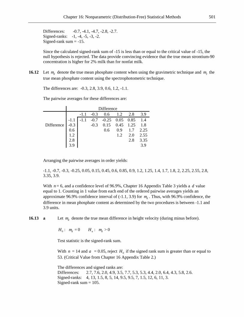
Chapter 16: Nonparametric (Distribution-Free) Statistical Methods 501
Differences: -0.7, -4.1, -4.7, -2.8, -2.7. Signed-ranks: -1, -4, -5, -3, -2. Signed-rank sum = -15. Since the calculated signed-rank sum of -15 is less than or equal to the critical value of -15, the
null hypothesis is rejected. The data provide convincing evidence that the true mean strontium-90 concentration is higher for 2% milk than for nonfat milk.
16.12 Let dµ denote the true mean phosphate content when using the gravimetric technique and 2µ the
true mean phosphate content using the spectrophotometric technique. The differences are: -0.3, 2.8, 3.9, 0.6, 1.2, -1.1. The pairwise averages for these differences are:
Difference -1.1 -0.3 0.6 1.2 2.8 3.9 -1.1 -1.1 -0.7 -0.25 0.05 0.85 1.4
Difference -0.3 -0.3 0.15 0.45 1.25 1.8 0.6 0.6 0.9 1.7 2.25 1.2 1.2 2.0 2.55 2.8 2.8 3.35 3.9 3.9
Arranging the pairwise averages in order yields: -1.1, -0.7, -0.3, -0.25, 0.05, 0.15, 0.45, 0.6, 0.85, 0.9, 1.2, 1.25, 1.4, 1.7, 1.8, 2, 2.25, 2.55, 2.8,
3.35, 3.9. With n = 6, and a confidence level of 96.9%, Chapter 16 Appendix Table 3 yields a d value
equal to 1. Counting in 1 value from each end of the ordered pairwise averages yields an approximate 96.9% confidence interval of (-1.1, 3.9) for dµ . Thus, with 96.9% confidence, the difference in mean phosphate content as determined by the two procedures is between -1.1 and 3.9 units.
16.13 a Let dµ denote the true mean difference in height velocity (during minus before). 0 :H 0dµ = :aH 0dµ > Test statistic is the signed-rank sum.
With n = 14 and α = 0.05, reject 0H if the signed rank sum is greater than or equal to 53. (Critical Value from Chapter 16 Appendix Table 2.)
The differences and signed ranks are: Differences: 2.7, 7.6, 2.0, 4.9, 3.5, 7.7, 5.3, 5.3, 4.4, 2.0, 6.4, 4.3, 5.8, 2.6. Signed-ranks: 4, 13, 1.5, 8, 5, 14, 9.5, 9.5, 7, 1.5, 12, 6, 11, 3. Signed-rank sum = 105.

502 Chapter 16: Nonparametric (Distribution-Free) Statistical Methods
Since the calculated signed-rank sum of 105 exceeds the critical value of 53, the null hypothesis is rejected. The data provide evidence that the growth hormone therapy is successful in increasing the mean height velocity. b We need to assume that the population distribution of height velocity differences is
symmetrical. 16.14 a Let dµ denote the true mean difference in time from entry to first stroke (hole minus
flat). 0 :H 0dµ = :aH 0dµ ≠ Test statistic is the signed-rank sum.
With n = 10 and α = 0.02, reject 0H if the signed rank sum is less than or equal to -45, or greater than or equal to 45. (Critical Value from Chapter 16 Appendix Table 2.)
The differences and signed ranks are: Differences: 0.12, -0.13, 0.11, -0.07, -0.17, 0.14, 0.18, -0.25, -0.01, -0.11. Signed-ranks: 5, -6, 3.5, -2, -8, 7, 9, -10, -1, -3.5. Signed-rank sum = -6.
Since the calculated value of -6 does not fall in the rejection region for α = 0.02, it does not fall in the rejection region for α = 0.01, and so 0H is not rejected. Thus, the data do not provide convincing evidence that there is a difference in mean time from entry to first stroke for the two entry methods.
b Let dµ denote the true mean difference in initial velocity (hole minus flat). 0 :H 0dµ = :aH 0dµ ≠ Test statistic is the signed-rank sum. The differences and signed ranks are: Differences: -1.1, 0.1, -2.4, -1.0, -3.0. -0.9, -1.4, -1.7, 1.2. Signed-ranks: -4, 1, -8, -3, -9, -2, -6, -7, -5. Signed-rank sum = -33
Chapter 16 Appendix Table 2 tells us that the critical region for a two-tailed 0.054 test starts at 33 and at −33. Thus our signed-rank sum of −33 is significant at the 0.054 level. At the 0.054 level the data provide convincing evidence that there is a difference in the mean initial velocity for the two entry methods.
16.15 Let dµ denote the true mean difference in cholesterol synthesis rates (potato minus rice). 0 :H 0dµ = :aH 0dµ ≠

Chapter 16: Nonparametric (Distribution-Free) Statistical Methods 503
Test statistic is the signed-rank sum.
With n = 8 and α = 0.054, reject 0H if the signed rank sum is less than or equal to -28, or greater than or equal to 28. (Critical Value from Chapter 16 Appendix Table 2.)
The differences and signed ranks are: Differences: 0.18, -1.24, 0.25, -0.56, 1.01, 0.96, 0.60, 0.16 Signed-ranks: 2, -8, 3, -4, 7, 6, 5, 1. Signed-rank sum = 12
Since the calculated value of 12 does not fall into the rejection region, 0H is not rejected. The data
do not provide evidence that there is a difference in the true mean cholesterol synthesis for the two sources of carbohydrates.
16.16 Let dµ denote the true mean difference in lung capacity (post-operative minus pre-operative). 0 :H 0dµ = :aH 0dµ >
Test statistic is signed-rank sumn(n+1)(2n+1)
6
z = .
For α = 0.05, reject 0H if z > 1.645.
The differences and signed ranks are: Differences: 80, 340, 350, 100, 640, -115, 545, 220, 630, 800, 120, 240, -20, 880, 570, 40, -
20, 580, 130, 70, 450, 110. Signed-ranks: 5, 13, 14, 6, 20, -8, 16, 11, 19, 21, 9, 12, -1.5, 22, 17, 3, -1.5, 18, 10, 4, 15, 7. Signed-rank sum = 231
231 3.7522(23)(45)
6
z = =
Since the calculated value of z exceeds the z critical value of 1.645, 0H is rejected. The data
provide convincing evidence that surgery increases the mean lung capacity.

504 Chapter 16: Nonparametric (Distribution-Free) Statistical Methods
16.17 Using dµ as defined in Exercise 16.13, and the differences computed there, the pairwise averages are:
2.0 2.0 2.6 2.7 3.5 4.3 4.4 4.9 5.3 5.3 5.8 6.4 7.6 7.7
2.0 2.0 2.0 2.3 2.35 2.75 3.15 3.2 3.45 3.65 3.65 3.9 4.2 4.8 4.85 2.0 2.0 2.3 2.35 2.75 3.15 3.2 3.45 3.65 3.65 3.9 4.2 4.8 4.85 2.6 2.6 2.65 3.05 3.45 3.5 3.75 3.95 3.95 4.2 4.5 5.1 5.15 2.7 2.7 3.1 3.5 3.55 3.8 4.0 4.0 4.25 4.55 5.15 5.20 3.5 3.5 3.9 3.95 4.2 4.4 4.4 4.65 4.95 5.55 5.60 4.3 4.3 4.35 4.6 4.8 4.8 5.05 5.35 5.95 6.0 4.4 4.4 4.65 4.85 4.85 5.1 5.4 6 6.05 4.9 4.9 5.1 5.1 5.35 5.65 6.25 6.3 5.3 5.3 5.3 5.55 5.85 6.45 6.5 5.3 5.3 5.55 5.85 6.45 6.5 5.8 5.8 6.1 6.7 6.75 6.4 6.4 7.0 7.05 7.6 7.6 7.65 7.7 7.7
With n = 14, and a confidence level of 89.6%, d = 27. Counting in 27 averages from each end of
the ordered pairwise averages yields the confidence interval of (3.65, 5.55). Thus, with 89.6% confidence, the true mean difference in height velocity is estimated to be between 3.65 and 5.55 units.
16.18 Let µ denote the true mean processing time. 0 :H 2µ = :aH 2µ > The test statistic is the signed rank sum. With n = 10, and α = 0.053, 0H is rejected if the calculated signed rank is greater than or equal
to 33. Process Time: 1.4, 2.1, 1.9, 1.7, 2.4, 2.9, 1.8, 1.9, 2.6, 2.2. Process time minus 2: -0.6, .0.1, -0.1, -0.3, 0.4, 0.9, -0.2, -0.1, 0.6, 0.2. Signed Rank: -8.5, 2, -2, -6, 7, 10, -4.5, -2, 8.5, 4.5. Signed Rank Sum = 9 Since the signed-rank sum of 9 does not exceed the critical value of 33, the null hypothesis is not
rejected. There is not sufficient evidence to conclude that the mean processing time exceeds two minutes.
16.19 Let 1µ , 2µ , and 3µ denote the mean importance scores for lower, middle, and upper social class,
respectively. 0 :H 1 2 3µ µ µ= = :aH at least two of the three iµ ’s are different Test statistic: Kruskal Wallis

Chapter 16: Nonparametric (Distribution-Free) Statistical Methods 505
Rejection region: The number of df for the chi-squared approximation is k – 1 = 2. For α = 0.05,
Chapter 16 Appendix Table 4 gives 5.99 as the critical value. 0H will be rejected if KW > 5.99. KW = .17 as given. Since this computed value does not exceed the critical value of 5.99, the null
hypothesis is not rejected. The data do not provide enough evidence for concluding that the mean importance scores for lower, middle and upper social classes are not all the same.
16.20 Let 1µ , 2µ , and 3µ denote the true mean protoporphyrin levels for the normal workers,
alcoholics with sideroblasts and alcoholics without sideroblasts, respectively, 0 :H 1 2 3µ µ µ= = :aH at least two of the three iµ ’s are different Test statistic: Kruskal Wallis Rejection region: The number of df for the chi-squared approximation is k – 1 = 2. For α = 0.05,
Chapter 16 Appendix Table 4 gives 5.99 as the critical value. 0H will be rejected if KW > 5.99.
RANKS Normal Workers Alcoholics
w/sideroblasts Alcoholics
w/o sideroblasts 5 29.5 14.5 6 35 7.5 20.5 37 16.5 10.5 31 19 16.5 38 20.5 29.5 39 9 7.5 36 12 25 41 4 27 32 26 24 34 3 10.5 40 14.5 18 1 23 28 22 33 13 2
Sum of Ranks 258 392.5 210.5 in 15 11 15
ir 17.2 35.68 14.03
2 2 212 15(17.2 21) 11(35.68 21) 15(14.03 21) 23.11(41)(42)
KW = − + − + − =
Since 23.11 > 5.99, the null hypothesis is rejected. The data strongly suggest that mean
protoporphyrin levels are not the same for all three groups. 16.21. Let 1µ , 2µ , 3µ and 4µ denote the true mean phosphorous concentrations for the four soil
treatments.
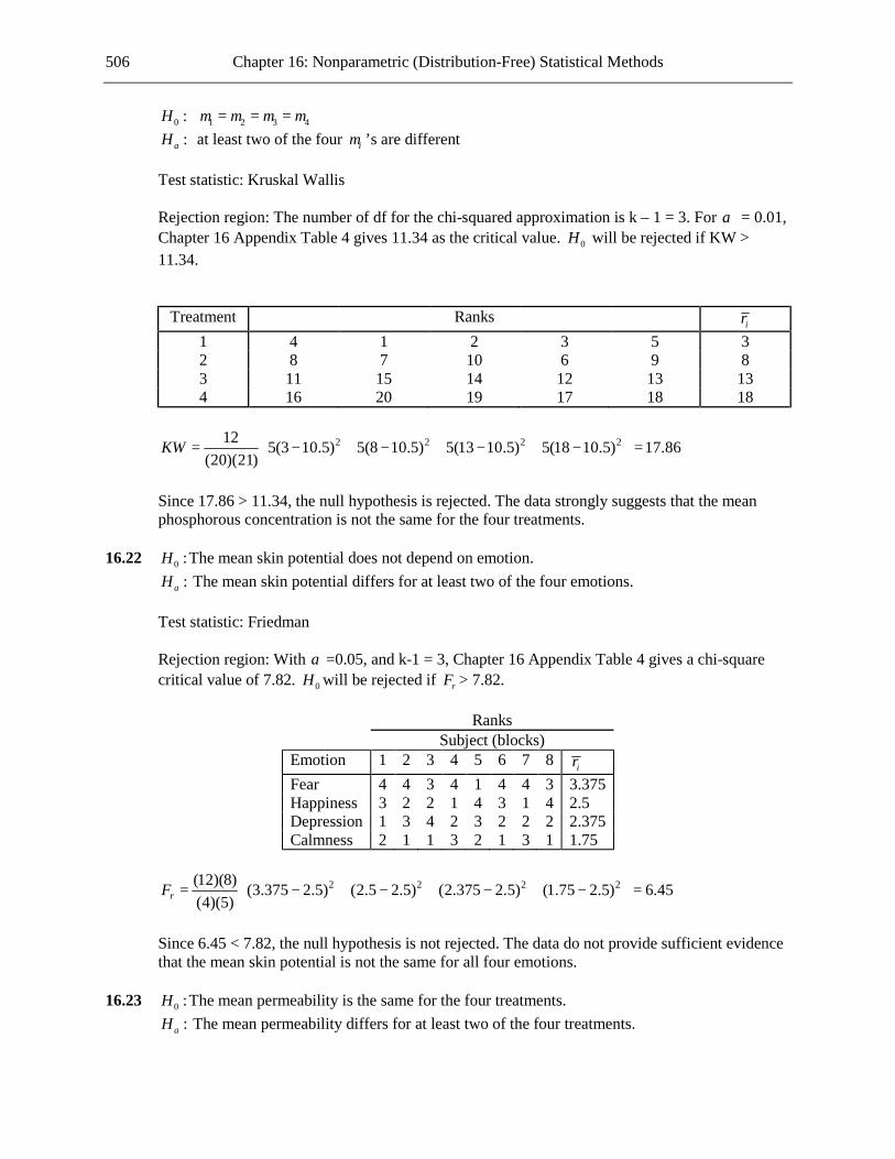
506 Chapter 16: Nonparametric (Distribution-Free) Statistical Methods
0 :H 1 2 3 4µ µ µ µ= = = :aH at least two of the four iµ ’s are different Test statistic: Kruskal Wallis Rejection region: The number of df for the chi-squared approximation is k – 1 = 3. For α = 0.01,
Chapter 16 Appendix Table 4 gives 11.34 as the critical value. 0H will be rejected if KW > 11.34.
Treatment Ranks ir 1 4 1 2 3 5 3 2 8 7 10 6 9 8 3 11 15 14 12 13 13 4 16 20 19 17 18 18
2 2 2 212 5(3 10.5) 5(8 10.5) 5(13 10.5) 5(18 10.5) 17.86(20)(21)
KW = − + − + − + − =
Since 17.86 > 11.34, the null hypothesis is rejected. The data strongly suggests that the mean
phosphorous concentration is not the same for the four treatments. 16.22 0 :H The mean skin potential does not depend on emotion. :aH The mean skin potential differs for at least two of the four emotions. Test statistic: Friedman Rejection region: With α =0.05, and k-1 = 3, Chapter 16 Appendix Table 4 gives a chi-square
critical value of 7.82. 0H will be rejected if rF > 7.82.
Ranks Subject (blocks) Emotion 1 2 3 4 5 6 7 8 ir Fear 4 4 3 4 1 4 4 3 3.375 Happiness 3 2 2 1 4 3 1 4 2.5 Depression 1 3 4 2 3 2 2 2 2.375 Calmness 2 1 1 3 2 1 3 1 1.75
2 2 2 2(12)(8) (3.375 2.5) (2.5 2.5) (2.375 2.5) (1.75 2.5) 6.45(4)(5)rF = − + − + − + − =
Since 6.45 < 7.82, the null hypothesis is not rejected. The data do not provide sufficient evidence
that the mean skin potential is not the same for all four emotions. 16.23 0 :H The mean permeability is the same for the four treatments. :aH The mean permeability differs for at least two of the four treatments.

Chapter 16: Nonparametric (Distribution-Free) Statistical Methods 507
Test statistic: Friedman Rejection region: With α = 0.01, and k − 1 = 3, Chapter 16 Appendix Table 4 gives a chi-square
critical value of 11.34. 0H will be rejected if rF > 11.34.
Ranks Subject (blocks) Treatment 1 2 3 4 5 6 7 8 9 10 ir
1 2 2 2 2 2 2 2 2 2 2 2 2 1 1 1 1 1 1 1 1 1 1 1 3 4 4 4 4 3 4 4 4 4 4 3.9 4 3 3 3 3 4 3 3 3 3 3 3.1
2 2 2 2(12)(10) (2 2.5) (1 2.5) (3.9 2.5) (3.1 2.5) 28.92(4)(5)rF = − + − + − + − =
Since 28.92 > 11.34, the null hypothesis is rejected. The data provide convincing evidence that
the mean permeability is not the same for all four treatments. 16.24 0 :H The mean food consumption is the same for the three experimental conditions. :aH The mean food consumption differs for at least two of the three experimental conditions. Test statistic: Friedman Rejection region: With α = 0.01, and k − 1 = 2, Chapter 16 Appendix Table 4 gives a chi-square
critical value of 9.21. 0H will be rejected if rF > 9.21.
Ranks Rats (blocks) Hours 1 2 3 4 5 6 7 8 ir
0 1 1 1 1 1 1 1 1 1 24 2 2 2.5 3 2 3 2 2.5 2.375 72 3 3 2.5 2 3 2 3 2.5 2.625
2 2 2(12)(8) (1 2) (2.375 2) (2.625 2) 12.25(3)(4)rF = − + − + − =
Since 12.25 > 9.21, the null hypothesis is rejected. The data provide convincing evidence that the
mean food consumption depends on the number of hours of food deprivation. 16.25 0 :H The mean survival rate does not depend on storage temperature. :aH The mean survival rate does depend on storage temperature. Test statistic: Friedman

508 Chapter 16: Nonparametric (Distribution-Free) Statistical Methods
Rejection region: With α = 0.05, and k − 1 = 3, Chapter 16 Appendix Table 4 gives a chi-square critical value of 7.82. 0H will be rejected if rF > 7.82.
Ranks Storage Time Temperature 6 24 48 120 168 ir
15.6 3 3 3 3 3 3 21.1 4 4 4 4 4 4 26.7 2 2 2 2 2 2 32.2 1 1 1 1 1 1
2 2 2 2(12)(5) (3 2.5) (4 2.5) (2 2.5) (1 2.5) 15(4)(5)rF = − + − + − + − =
Since 15 > 7.82, the null hypothesis is rejected. The data provide convincing evidence that the
mean survival rate differs for at least two of the different storage temperatures.

14
Chapter 2 Collecting Data Sensibly
2.1 This is an observational study. The treatments (length of stay) were determined by the condition of the patients. (In an experiment the patients would be assigned to the various lengths of stay by the investigators, usually using random assignment.)
2.2 This was an experiment, since the investigators (not the students) determined which discussion
sections received the chocolate and which did not. 2.3 This was an experiment, since the professor (not the students) determined who was supplying a
buying price and who was supplying a selling price. 2.4 a This is an observational study. b No. It is quite possible, for example, that those children who averaged more than two hours of
television viewing per day received, generally speaking, a less good education than those who did not, and that it is the less good education, and not the television viewing, that caused the lower reading scores.
2.5 a This is an experiment since it was decided by the researchers (in this case by random
assignment) which participants would receive which treatments. b Yes. Since the participants were randomly assigned to the treatments it is reasonable to
conclude that receiving either real or fake acupuncture was the cause of the observed reductions in pain.
2.6 a This is an observational study. b Yes. Since the researchers looked at a random sample of publically accessible MySpace web
profiles posted by 18-year-olds, it is reasonable to generalize the stated conclusion to all 18-year-olds with publically accessible MySpace profiles.
c No, it is not reasonable to generalize the stated conclusion to all 18-year-old MySpace users
since no users without publically accessible profiles were included in the study. d No, it is not reasonable to generalize the stated conclusion to all MySpace users with
publically accessible profiles since only 18-year-olds were included in the study. 2.7 a This is an experiment. b Yes. Since the participants were randomly assigned to the treatments the researcher can
reasonably claim that the music played was the cause of the higher rating. 2.8 It is quite possible, for example, that 3- and 4-year olds who drink something sweet once or twice
a day generally speaking consume larger amounts of fat than those who do not, and that it is the fat that is causing the weight problems a year later, rather than the consumption of the sweet drinks.

Chapter 2: Collecting Data Sensibly 15
2.9 We are told that moderate drinkers, as a group, tended to be better educated, wealthier, and more
active than nondrinkers. It is therefore quite possible that the observed reduction in the risk of heart disease amongst moderate drinkers is caused by one of these attributes and not by the moderate drinking.
2.10 a No. It is quite possible, for example, that women who choose to watch Oprah generally
speaking have a more health oriented outlook than those who watch other daytime talk shows, and it is this health oriented outlook that causes the decrease in craving for fattening foods, not the watching of Oprah.
b Neither generalization would be reasonable since the survey was conducted on the
DietSmart.com website. It is unlikely that users of this website would be representative of the population of women in the United States or of the population of women who watch daytime talk shows.
2.11 a The data would need to be collected from a simple random sample of affluent Americans. b No. Since the survey included only affluent Americans the result cannot be generalized to all
Americans. 2.12 It is possible, for example, that people who live in the South generally speaking eat less healthy
food and exercise less than people who live in other regions of the country, and that the greater percentage of high blood pressure is caused not by living in the South but by the less healthy food and the lack of exercise.
2.13 The following is one possible method. Use a computer list of all the students at the college.
Assign to each student a 10-digit decimal number. Sort the students according to the numbers assigned, smallest to largest. The first 100 students on the sorted list will form the sample.
2.14 Method 1: Using a computer list of the graduates, number the graduates 1-140. Use a random
number generator on a calculator or computer to randomly select a whole number between 1 and 140. The number selected represents the first graduate to be included in the sample. Repeat the number selection, ignoring repeated numbers, until 20 graduates have been selected.
Method 2: Using a computer list of the graduates, number the graduates 001-140. Take the first three digits from the left hand end of a row from a table of random digits. If the three-digit number formed is between 001 and 140 inclusive, the graduate with that number should be the first graduate in the sample. If the number formed is not between 001 and 140 inclusive, the number should be ignored. Repeat the process described for the next three digits in the random number table, and continue in the same way until 20 graduates have been selected. (Three-digit numbers that are repeats of numbers previously selected should be ignored.)
2.15 The following is one possible method. Number the signatures 1-500. Use a random number
generator on a calculator or computer to randomly select a whole number between 1 and 500. The number selected represents the first signature to be included in the sample. Repeat the number selection, ignoring repeated numbers, until 30 signatures have been selected.
2.16 a The 716 bicycle fatalities constitute all bicycle fatalities in 2008, and so the group represents
a census. b The average age of 41 years is a population characteristic, since it is the average for all
bicycle fatalities in 2008.

16 Chapter 2: Collecting Data Sensibly
2.17 a The population is all American women. b No. The sample included women only from Maryland, Minnesota, Oregon, and Pennsylvania.
It is quite possible that the relationship between exercise and cognitive impairment is different for women in other states.
c No. As mentioned in Part (b), it is quite possible that the relationship between exercise and
cognitive impairment is different for women in other states. For example, other states might contain a different racial mix from the four included in the study, and it is possible that women of different racial origins respond differently to exercise in terms of cognitive impairment.
d The inadequate sampling method used in this study is an example of selection bias. Women
in the other 46 states were excluded from the study. 2.18 a Cluster sampling b Stratified random sampling c Convenience sampling d Simple random sampling e Systematic sampling 2.19 a Using the list, first number the part time students 1-3000. Use a random number generator on
a calculator or computer to randomly select a whole number between 1 and 3000. The number selected represents the first part time student to be included in the sample. Repeat the number selection, ignoring repeated numbers, until 10 part time students have been selected. Then number the full time students 1-3500 and select 10 full time students using the same procedure.
b No. With 10 part time students being selected out of a total of 3000 part time students, the
probability of any particular part time student being selected is 10/3000 = 1/300. Applying a similar argument to the full time students, the probability of any particular full time student being selected is 10/3500 = 1/350. Since these probabilities are different, it is not the case that every student has the same chance of being included in the sample.
2.20 Convenience samples are, by nature, very unlikely to be representative of the population. 2.21 a The pages of the book have already been numbered between 1 and the highest page number
in the book. Use a random number generator on a calculator or computer to randomly select a whole number between 1 and the highest page number in the book. The number selected will be the first page to be included in the sample. Repeat the number selection, ignoring repeated numbers, until the required number of pages has been selected.
b Pages that include exercises tend to contain more words than pages that do not include
exercises. Therefore, it would be sensible to stratify according to this criterion. Assuming that 20 non-exercise pages and 20 exercise pages will be included in the sample, the sample should be selected as follows. Use a random number generator to randomly select a whole number between 1 and the highest page number in the book. The number selected will be the

Chapter 2: Collecting Data Sensibly 17
first page to be included in the sample. Repeat the number selection, ignoring repeated numbers and keeping track of the number of pages of each type selected, until 20 pages of one type have been selected. Then continue in the same way, but ignore numbers corresponding to pages of that type. When 20 pages of the other type have been selected, stop the process.
c Randomly select one page from the first 20 pages in the book. Include in your sample that
page and every 20th page from that page onwards. d Roughly speaking, in terms of the numbers of words per page, each chapter is representative
of the book as a whole. It is therefore sensible for the chapters to be used as clusters. Using a random number generator randomly choose three chapters. Then count the number of words on each page in those three chapters.
e Answers will vary. f Answers will vary. 2.22 It is not the proportion of voters that is important, but the number of voters in the sample – and
1000 is an adequate number. 2.23 The researchers should be concerned about nonresponse bias. Only a small proportion (20.7%) of
the selected households completed the interview, and it is quite possible that those households who did complete the interview are different in some relevant way concerning Internet use from those who did not.
2.24 a This was a convenience sample. The study simply used students from one psychology class. b The students in this psychology class, and at this particular small college, are unlikely to be
representative of the set of all college students in the U.S. Also, since the survey was about illegal drug use, we cannot be sure that the students were giving truthful answers to the questions.
2.25 First, the participants in the study were all students in an upper-division communications course
at one particular university. It is not reasonable to consider these students to be representative of all students with regard to their truthfulness in the various forms of communication. Second, the students knew during the week’s activity that they were surveying themselves as to the truthfulness of their interactions. This could easily have changed their behavior in particular social contexts and therefore could have distorted the results of the study.
2.26 a No. The games used in the study were the 20 most popular for each of three games systems
and therefore are not likely to be representative of the population of all video games with respect to the number of violent interactions.
b No. The sample is not likely to have been representative of the population of all video games with respect to the number of violent interactions and therefore it would not be reasonable to generalize the researchers’ conclusion to all video games.
2.27 First, the people who responded to the print and online advertisements might be different in some
way relevant to the study from the population of people who have online dating profiles. Second, only the Village Voice and Craigslist New York City were used for the recruitment. It is quite possible that people who read that newspaper or access those websites differ from the population

18 Chapter 2: Collecting Data Sensibly
in some relevant way, particularly considering that they are both New York City based publications.
2.28 No. First, only 132 of the 1260 students who were sent the survey responded, and it is quite likely
that those who chose to respond differ in some relevant way from those who did not. (This is nonresponse bias.) Second, those students who did respond might not have been fully honest about their financial condition. (This is response bias.)
2.29 a Yes. It is possible that students of a given class standing tend to be similar in the amounts of
money they spend on textbooks. b Yes. It is possible that students who pursue a certain field of study tend to be similar in the
amounts of money they spend on textbooks. c No. It is unlikely that stratifying in this way will produce groups that are homogeneous in
terms of the students’ spending on textbooks. 2.30 The individuals within each stratum should on the whole be similar in terms of the topic of the
study. This is true of the proposed strata in Scheme 2, since it is likely that college students will on the whole be similar in their opinions regarding the possible tax increase; likewise nonstudents who work full time will on the whole be similar in their opinions regarding the possible tax increase, and nonstudents who do not work full time will on the whole be similar in their opinions regarding the possible tax increase. Scheme 1, however, is not suitable since we have no reason to believe that people within the proposed first-letter-of-last-name strata will be similar in terms of their attitudes to the possible tax increase. Similarly the suggested stratification in Scheme 3 is very unlikely to produce homogeneous groups.
2.31 It is not reasonable to generalize these results to the population of U.S. adults since the people
who sent their hair for testing did so voluntarily. It is quite possible that people who would choose to participate in a study of this sort differ in their mercury levels from the population as a whole.
2.32 Different subsets of the population might have responded by different methods. For example, it is
quite possible that younger people (who might generally be in favor of continuing the parade) chose to respond via the Internet while older people (who might on the whole be against the parade) chose to use the telephone to make their responses.
2.33 a Binding strength b Type of glue c The extraneous variables mentioned are the number of pages in the book and whether the
book is bound as a hardback or a paperback. Further extraneous variables that might be considered include the weight of the material used for the cover and the type of paper used.
2.34 a Use two IQ tests (Test 1 and Test 2) of equal levels of difficulty. Randomly select 50 students
from the school. Randomly assign the 50 students to two groups, Group A and Group B. The experiment will be conducted over two days. On the first day, students in Group A will do an IQ test without listening to any music and students in Group B will do an IQ test after listening to a Mozart piano sonata. On the second day the activities of the two groups will be switched. For each student decide randomly whether he/she will take Test 1 on the first day

Chapter 2: Collecting Data Sensibly 19
and Test 2 on the second day, or vice versa. All conditions (temperature, time of day, amount of light, etc. – everything apart from the presence of the music or not) should be kept equal between the two days and between the two groups. In particular, the students taking the test without listening to the music should nonetheless sit quietly in a room for the length of time of the piano sonata. At the end of the experiment the after-music IQ scores should be compared to the no-music IQ scores.
b Yes, the fact that all conditions are kept the same is direct control. c By having each student take IQ tests under both experimental conditions we are using a
matched pairs design, and matched pairs is a form of blocking. d The students were randomly assigned to the two orders of the treatments (no music then
music, or music then no music). Also it was decided randomly for each student whether Test 1 or Test 2 would be taken first.
2.35 The following is one possible method. Write the names of the subjects on identical slips of paper,
and place the slips in a hat. Mix the slips, and randomly select ten slips from the hat. The names on those ten slips are the people who will dry their hands by the first method. Randomly select a further ten slips from the hat. The names on those ten slips are the people who will dry their hands by the second method. The remaining ten people will dry their hands by the third method.
2.36 Random assignment should have been used to determine, for each cyclist, which drink would be
consumed during which break. 2.37 a Blocking b Direct control 2.38 We rely on random assignment to produce comparable experimental groups. If the researchers
had hand-picked the treatment groups, they might unconsciously have favored one group over the other in terms of some variable that affects the subjects’ ability to deal with multiple inputs.
2.39 The figure shows that comparable groups in terms of age have been formed. (Differences
between the age distributions in the groups can be seen: there are one or two children in the LR group who are younger than all those in the OR group, and also there is a greater number of children over 14 years old in the LR group. It is inevitable that there will be some differences between the groups under random assignment.)
2.40 a If the participants had been able to choose their own avatars, then it is quite possible, for
example, that people with a lot of self confidence would tend to choose the attractive avatar while those with less self confidence would tend to choose the unattractive avatar. Then, if the same result was obtained as the one described in the paper, it would be impossible to tell whether the greater closeness achieved by those with the attractive avatar came about as a result of the avatar or as a result of those people’s greater self confidence.

20 Chapter 2: Collecting Data Sensibly
b
2.41 We rely on random assignment to produce comparable experimental groups. If the researchers
had hand-picked the treatment groups, they might unconsciously have favored one group over the other in terms of some variable that affects the subjects’ ability to learn through video gaming activity.
2.42
Subjects
Construct sentences
using words relating to politeness
Construct sentences
using words relating to rudeness
Measure
politeness
Measure
politeness
Compare politeness
for the two treatments
Random A
ssignment
Participants
Attractive avatar
Unattractive avatar
Measure closeness
Measure closeness
Compare closeness for attractive avatar
vs. unattractive avatar
Random A
ssignment

Chapter 2: Collecting Data Sensibly 21
2.43
2.44 How many bottles of water were used in the experiment? Were the bottles identical? Was there a
control group in which the bottles had identical labels to those used in the treatment group but without the positive words? Were the bottles randomly assigned to the groups? Was the state of the water measured both before and after the experiment? Did the people who measured the water’s structure know which bottles were in which group?
2.45 a This is an experiment. The researchers assigned the students to the treatments. b No. The subjects were randomly assigned to the treatments, but there was no random
selection from a population of interest. c Yes. d If the performance was significantly better for the group that read the material in the
landscape orientation then, yes, for the set of subjects used in the experiment, reasoning was improved by turning the screen to landscape orientation. The subjects were randomly assigned to the treatment groups, and a significant difference in the results of the two groups means that the observed difference is unlikely to have occurred by chance.
e No. The students used in the study were all undergraduates taking psychology at a large
university, and therefore cannot be considered to be representative of any larger population. 2.46 a The treatments are the names – Ann Clark and Andrew Clark – given to the participants. b The response variables are the participants’ answers to the questions given. c Selecting a random sample of 1161 voters and giving them the female name, and then
selecting a second random sample 1139 voters and giving them the male name, is exactly equivalent to selecting a random sample of 2300 voters, and then randomly assigning 1161 of them to the female name and the remainder to the male name. (It is assumed here that in the study given in the question it was ensured that there was no overlap between the two samples.)
30 trials
Additive 1
Additive 2
Measure distance traveled
Measure distance traveled
Compare distances traveled for the three additives
Additive 3
Measure distance traveled
Random A
ssignment

22 Chapter 2: Collecting Data Sensibly
2.47 a Red wine, yellow onions, black tea b Absorption of flavonols c Alcohol tolerance, amount of flavonols in the diet (other than from red wine, yellow onions,
and black tea), gender 2.48 Suppose that an experiment is conducted in which people are given either a drug or a placebo,
and that those who are given the drug do significantly better, on average, than those who are given the placebo. Since both groups experience the placebo effect (the psychological effect of taking a tablet) we are able to attribute the greater improvement of those who took the drug to the chemicals in the drug. However we are unable to tell just how much of a placebo effect is being experienced by all the subjects. By adding a control group (a group that is given nothing) and comparing the results for this group with the results for the placebo group we can measure the extent of the placebo effect.
2.49 “Blinding” is ensuring that the experimental subjects do not know which treatment they were
given and/or ensuring that the people who measure the response variable do not know who was given which treatment. When this is possible to implement, it is useful that the subjects do not know which treatments they were given since, if a person knows what treatment he/she was given, this knowledge could influence the person’s perception of the response variable, or even, through psychological processes, have a direct effect on the response variable. If the response variable is to be measured by a person other than the experimental subjects it is useful if this person doesn’t know who received which treatment since, if this person does know who received which treatment, then this could influence the person’s perception of the response variable.
2.50 Answers will vary. 2.51 a In order to know that the results of this experiment are valid it is necessary to know that the
assignment of the women to the groups was done randomly. For suppose, for example, that the women were allowed to choose which groups they went into. Then it would be quite possible, for instance, that women who are particularly social by nature, and therefore whose health would be enhanced by any regular social gathering, would choose the more interesting sounding art discussions, while those less social by nature (and therefore less likely to be helped by social gatherings) would choose the more conventional discussions of hobbies and interests. Then it would be impossible to tell whether the stated results were caused by the discussions of art or by the greater social nature of the women in the art discussion group.
b Suppose that all the women took part in weekly discussions of art, and that generally an
improvement in the medical conditions mentioned was observed amongst the subjects. Then it would be impossible to tell whether these health improvements had been caused by the discussions of art or by some factor that was affecting all the subjects, such as an improvement in the weather over the four months. By including a control group, and by observing that the improvements did not take place (generally speaking) for those in the control group, factors such as this can be discounted, and the discussions of art are established as the cause of the improvements.
2.52 a It is very possible that the nurses might have preconceptions about the two forms of surgery
in terms of the amount of pain and nausea caused. Therefore, if the nurses know which children have been given which form of surgery, this might affect the amounts of medication

Chapter 2: Collecting Data Sensibly 23
they give. By making sure that the nurses do not have this knowledge, this possible effect is avoided.
b Since the incisions made under the two procedures are different the patients and/or their
parents would know which method had been used. 2.53 We will assume that only four colors will be compared, and that only headache sufferers will be
included in the study. Prepare a supply of “Regular Strength” Tylenol in four different colors: white (the current color
of the medication, and therefore the “control”), red, green, and blue. Recruit 20 volunteers who suffer from headaches. Instruct each volunteer not to take any pain relief medication for a week. After that week is over, issue each volunteer a supply of all four colors. Give each volunteer an order in which to use the colors (this order would be determined randomly for each volunteer). Instruct the volunteers to use one fixed dose of the medication for each headache over a period of four weeks, and to note on a form the color used and the pain relief achieved (on a scale of 0-10, where 0 is no pain relief and 10 is complete pain relief). At the end of the four weeks gather the results and compare the pain relief achieved by the four colors.
2.54 a Randomly assigning 852 children to the book group and the rest to the control group consists
of randomly selecting 852 to be in the book group and putting the remaining children in the control group.
b If no control group had been included in the study, then the only results available to the
researchers would be the reading scores of the children who had been given the reading books. There would be no way of telling whether these scores were any better than the scores for children who were not given reading books.
2.55 Of the girls, randomly assign 350 to the book group and 350 to the no-book group. (You could do
this by starting with a computer list of the names of the 700 girls. Assign to each name a random 10-digit number. Sort the names according to the numbers, from smallest to largest. The first 350 names on the sorted list are assigned to the book group, and the remainder to the no-book group.) Using a similar method, randomly assign 315 of the boys to the book group and 315 to the no-book group.
2.56 Suppose that the dog handlers and/or the experimental observers had known which patients did
and did not have cancer. It would then be possible for some sort of (conscious or unconscious) communication to take place between these people and the dogs so that the dogs would pick up the conditions of the patients from these people rather than through their perception of the patients’ breath. By making sure that the dog handlers and the experimental observers do not know who has the disease and who does not it is ensured that the dogs are getting the information from the patients.
2.57 a If the judges had known which chowder came from which restaurant then it is unlikely that
Denny’s chowder would have won the contest, since the judges would probably be conditioned by this knowledge to choose chowders from more expensive restaurants.
b In experiments, if the people measuring the response are not blinded they will often be
conditioned to see different responses to some treatments over other treatments, in the same way as the judges would have been conditioned to favor the expensive restaurant chowders. It

24 Chapter 2: Collecting Data Sensibly
is therefore necessary that the people measuring the response should not know which subject received which treatment, so that the treatments can be compared on their own merits.
2.58 This describes the placebo effect. The implication is that the experiments have included patients
who have been given a placebo in place of the antidepressants. 2.59 a A placebo group would be necessary if the mere thought of having amalgam fillings could
produce kidney disorders. However, since the experimental subjects were sheep the researchers do not need to be concerned that this would happen.
b A resin filling treatment group would be necessary in order to provide evidence that it is the
material in the amalgam fillings, rather than the process of filling the teeth, or just the presence of foreign bodies in the teeth, that is the cause of the kidney disorders. If the amalgam filling group developed the kidney disorders and the resin filling group did not, then this would provide evidence that it is some ingredient in the amalgam fillings that is causing the kidney problems.
c Since there is concern about the effect of amalgam fillings it would be considered unethical to
use humans in the experiment. 2.60 Answers will vary. 2.61 a This is an observational study. b In order to evaluate the study, we need to know whether the sample was a random sample. c No. Since the sample used in the Healthy Steps study was known to be nationally
representative, and since the paper states that, compared with the HS trial, parents in the study sample were disproportionately older, white, more educated, and married, it is clear that it is not reasonable to regard the sample as representative of parents of all children at age 5.5 years.
d The potential confounding variable mentioned is what the children watched. e The quotation from Kamila Mistry makes a statement about cause and effect and therefore is
inconsistent with the statement that the study can’t show that TV was the cause of later problems.
2.62 Answers will vary. 2.63 Answers will vary. 2.64 Study 1 1. Observational study 2. No 3. No
4. No. The fact that calcium takers were more common among the heart attack patients implies mathematically that calcium takers were more likely to be heart attack patients than non-calcium takers. However, it is quite possible that people who take a calcium supplement very often also take another supplement, and it is this other supplement that is causing heart attacks, not the calcium.

Chapter 2: Collecting Data Sensibly 25
5. No. The hospital at which this study was conducted cannot be considered to be representative
of any larger population. Study 2 1. Observational study 2. Yes 3. No 4. No. It is quite possible that people who take a calcium supplement very often also take
another supplement, and it is this other supplement that is causing heart attacks, not the calcium.
5. The conclusions can only be generalized to the population of people living in Minneapolis who receive Social Security.
Study 3 1. Experiment 2. Yes 3. No 4. No 5. No reasonable conclusion can be drawn from the study. Study 4 1. Experiment 2. No 3. Yes 4. Yes 5. No. The participants were volunteers. 2.65 By randomly selecting the phone numbers, calling back those where there are no answers, and
asking for the adult in the household with the most recent birthday the researchers are avoiding selection bias. However, selection bias could come about as a result of the fact that not all Californians have phones. Also, by selecting the adult with the most recent birthday certain birth dates are being favored, and it could be suggested that different attributes of people born at different times of the year could introduce further selection bias. Further to that, there is always the concern that people might not answer truthfully. This is response bias.
2.66 Answers will vary. 2.67 We rely on random assignment to produce comparable experimental groups. If the researchers
had hand-picked the treatment groups, they might unconsciously have favored one group over the other in terms of some variable that affects the ability of the people at the centers to respond to the materials provided.
2.68 Yes. It seems quite possible that “rate of talk” would be related to gender and therefore that
gender would be a sensible blocking variable. 2.69 a Observational study b It is quite possible that the children who watched large amounts of TV in their early years
were also those, generally speaking, who received less attention from their parents, and it was the lack of attention from their parents that caused the later attention problems, not the TV-watching.

26 Chapter 2: Collecting Data Sensibly
2.70 a Observational study b No. As Mr. Adamson pointed out, it is quite possible that women who drink a lot of soda
generally have less healthy lifestyles than those who do not, and that it’s the unhealthy lifestyles that are causing the diabetes, not the consumption of soda or fruit punch.
2.71 a It cannot be concluded from the results of the study that being single causes an increased risk
of violent crime. b It is possible, for example, that the kind of people who get married are the kind of people,
generally speaking, who are more careful about where they walk alone. It is this carefulness that is reducing the likelihood of being a victim of violent crime, not the fact that these people are married.
2.72 Nonresponse bias: it is likely that those who responded differed in some important way from
those who did not. Also there is a possibility of response bias in that those who did respond might not have been answering truthfully.
2.73 All the participants were women, from Texas, and volunteers. All three of these facts tell us that it
is likely to be unreasonable to generalize the results of the study to all college students. 2.74 a The design is good in that it includes a large number of doctors (adequate replication) and
directly controls the clothing and gestures. In order for the design to be correct it is important to know that the doctors were randomly assigned to the eight tapes.
b A greater number of actors should have been used. It is possible that particular attributes of
the individual actors (apart from their race and gender) might have influenced the doctors’ decisions, while use of a greater number of actors would have reduced the effect of such individual differences.
2.75 a The extraneous variables identified are gender, age, weight, lean body mass, and capacity to
lift weights. They were dealt with by direct control: all the volunteers were male, about the same age, and similar in weight, lean body mass, and capacity to lift weights.
b Yes, it is important that the men were not told which treatment they were receiving, otherwise
the effect of giving a placebo would have been removed. If the participants were told which treatment they were receiving, then those taking the creatine would have the additional effect of the mere taking of a supplement thought to be helpful (the placebo effect) and those getting the fake preparation would not get this effect. It would then be impossible to distinguish the influence of the placebo effect from the effect of the creatine itself.
c Yes, it would have been useful if those measuring the increase in muscle mass had not know
who received which treatment. It is possible that, through having this knowledge, the people would have been unconsciously influenced into exaggerating the increase in muscle mass for those who took the creatine.
2.76 a The treatments are standing and squatting. The response variable is the amount of the tip
(probably expressed as a percentage of the amount of the bill). b There are many variables affecting the amount of the tip, and most of these are dealt with by
the use of the coin to decide which treatment to use. However extraneous factors relating to
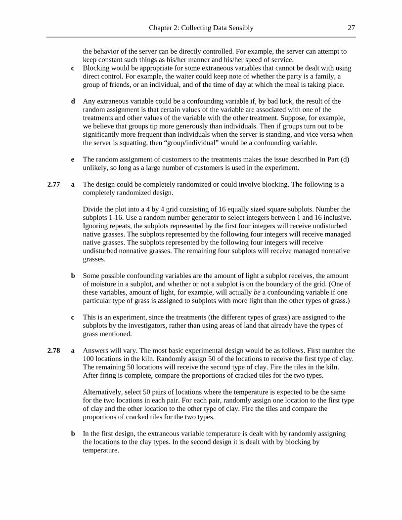
Chapter 2: Collecting Data Sensibly 27
the behavior of the server can be directly controlled. For example, the server can attempt to keep constant such things as his/her manner and his/her speed of service.
c Blocking would be appropriate for some extraneous variables that cannot be dealt with using direct control. For example, the waiter could keep note of whether the party is a family, a group of friends, or an individual, and of the time of day at which the meal is taking place.
d Any extraneous variable could be a confounding variable if, by bad luck, the result of the
random assignment is that certain values of the variable are associated with one of the treatments and other values of the variable with the other treatment. Suppose, for example, we believe that groups tip more generously than individuals. Then if groups turn out to be significantly more frequent than individuals when the server is standing, and vice versa when the server is squatting, then “group/individual” would be a confounding variable.
e The random assignment of customers to the treatments makes the issue described in Part (d)
unlikely, so long as a large number of customers is used in the experiment. 2.77 a The design could be completely randomized or could involve blocking. The following is a
completely randomized design. Divide the plot into a 4 by 4 grid consisting of 16 equally sized square subplots. Number the
subplots 1-16. Use a random number generator to select integers between 1 and 16 inclusive. Ignoring repeats, the subplots represented by the first four integers will receive undisturbed native grasses. The subplots represented by the following four integers will receive managed native grasses. The subplots represented by the following four integers will receive undisturbed nonnative grasses. The remaining four subplots will receive managed nonnative grasses.
b Some possible confounding variables are the amount of light a subplot receives, the amount
of moisture in a subplot, and whether or not a subplot is on the boundary of the grid. (One of these variables, amount of light, for example, will actually be a confounding variable if one particular type of grass is assigned to subplots with more light than the other types of grass.)
c This is an experiment, since the treatments (the different types of grass) are assigned to the
subplots by the investigators, rather than using areas of land that already have the types of grass mentioned.
2.78 a Answers will vary. The most basic experimental design would be as follows. First number the
100 locations in the kiln. Randomly assign 50 of the locations to receive the first type of clay. The remaining 50 locations will receive the second type of clay. Fire the tiles in the kiln. After firing is complete, compare the proportions of cracked tiles for the two types.
Alternatively, select 50 pairs of locations where the temperature is expected to be the same
for the two locations in each pair. For each pair, randomly assign one location to the first type of clay and the other location to the other type of clay. Fire the tiles and compare the proportions of cracked tiles for the two types.
b In the first design, the extraneous variable temperature is dealt with by randomly assigning
the locations to the clay types. In the second design it is dealt with by blocking by temperature.

28 Chapter 2: Collecting Data Sensibly
2.79 a There are many possible designs. We will describe here a design that blocks for the day of the week and the section of the newspaper in which the advertisement appears. For the sake of argument we will assume that the mortgage lender is interested in advertising on only two days of the week (Monday and Tuesday) and that there are three sections in the newspaper (A, B, and C). We will refer to the three types of advertisement as Ad 1, Ad 1, and Ad 3.
The experimental units are 18 issues of the newspaper (that is, 18 dates) consisting of
Mondays and Tuesdays over 9 weeks. Use a random process to decide which three Mondays will receive advertisements in Section A, which three Mondays will receive advertisements in Section B, and which three Mondays will receive advertisements in Section C. Do the same for the nine Tuesdays. We have now effectively split the 18 issues into the six blocks shown below. (There are 3 issues in each block.)
Mon, Sect A Mon, Sect B Mon, Sect C Tue, Sect A Tue, Sect B Tue, Sect C
Now randomly assign the three issues in each block to the three advertisements. (Ad 1 is then
appearing on three Mondays, once in each section, and on three Tuesdays, once in each section. The same applies to Ad 2 and Ad 3.) The response levels for the three advertisements can now be compared (as can the three different sections and the two different days).
b Within each block, the three issues of the newspaper were randomly assigned to the three
advertisements. Online Exercises 2.80 a “forests are being destroyed…80 acres per minute” b “vanishing tropical forests” c “man-made extinction” d “destruction of tropical forests” 2.81 Answers will vary. 2.82 Answers will vary. 2.83 Answers will vary. 2.84 Answers will vary. 2.85 Answers will vary.

29
Chapter 3 Graphical Methods for Describing Data
3.1
Out of shape27.0%
Flabby55.0%
Toned and fit18.0%
3.2 Segmented bar graph 3.3 a The second and third categories (“Permitted for business purposes only” and “Permitted for
limited personal use” were combined into one category (“No, but some limits apply”). b
Responses
1.0
0.8
0.6
0.4
0.2
0.0
Don’t knowPermitted for personal useLimited personal useBusiness purposes onlyProhibited
Response Category
c Pie chart, regular bar graph

30 Chapter 3: Graphical Methods for Describing Data
3.4 No Answer
4.0%
Yes41.0% No
55.0%
3.5 a
Don't knowStrongly agreeAgreeDisagreeStrongly disagree
30
25
20
15
10
5
0
Response
Relat
ive
Freq
uenc
y (%
)
b “Majority of Students Don’t Want Textbooks in E-format” 3.6 a Overall score is a numerical variable and grade is a categorical variable. b The shaded regions representing the various grades have areas that are proportional to the
relative frequencies for those grades, just as in a segmented bar graph. c
8580757065605550454035Overall Score
One possibility would be to require 72 or higher for “top of the class,” 63 or higher for
“passing,” 59 or higher for “barely passing,” and below 59 for “failing.” This makes a clear separation between the jurisdictions in the four grade categories. (Since this makes it easier to be rated as “top of the class,” it could be considered more appropriate to leave the grade boundaries as they are.)
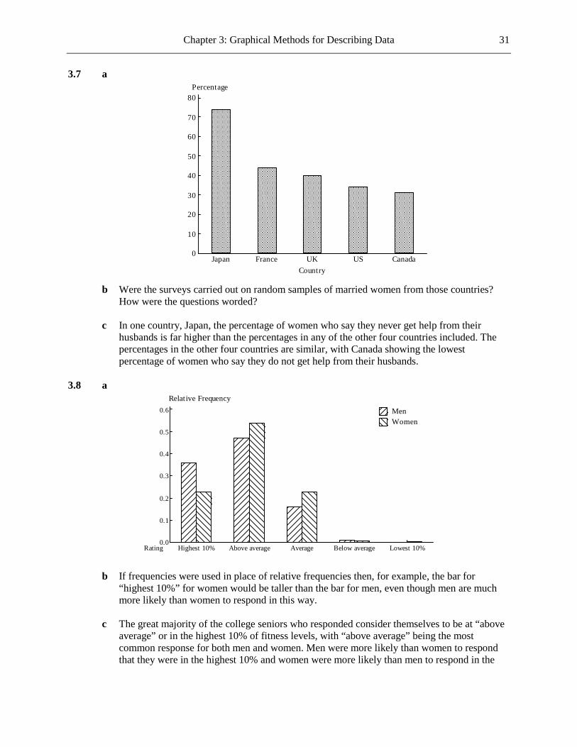
Chapter 3: Graphical Methods for Describing Data 31
3.7 a
CanadaUSUKFranceJapan
80
70
60
50
40
30
20
10
0
Country
Percentage
b Were the surveys carried out on random samples of married women from those countries?
How were the questions worded? c In one country, Japan, the percentage of women who say they never get help from their
husbands is far higher than the percentages in any of the other four countries included. The percentages in the other four countries are similar, with Canada showing the lowest percentage of women who say they do not get help from their husbands.
3.8 a
Rating Lowest 10%Below averageAverageAbove averageHighest 10%
0.6
0.5
0.4
0.3
0.2
0.1
0.0
Relative FrequencyMenWomen
b If frequencies were used in place of relative frequencies then, for example, the bar for
“highest 10%” for women would be taller than the bar for men, even though men are much more likely than women to respond in this way.
c The great majority of the college seniors who responded consider themselves to be at “above
average” or in the highest 10% of fitness levels, with “above average” being the most common response for both men and women. Men were more likely than women to respond that they were in the highest 10% and women were more likely than men to respond in the
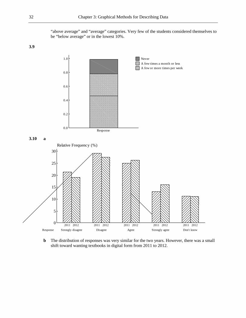
32 Chapter 3: Graphical Methods for Describing Data
“above average” and “average” categories. Very few of the students considered themselves to be “below average” or in the lowest 10%.
3.9
Response
1.0
0.8
0.6
0.4
0.2
0.0
NeverA few times a month or lessA few or more times per week
3.10 a
Response Don't knowStrongly agreeAgreeDisagreeStrongly disagree2012201120122011201220112012201120122011
30
25
20
15
10
5
0
Relative Frequency (%)
b The distribution of responses was very similar for the two years. However, there was a small
shift toward wanting textbooks in digital form from 2011 to 2012.

Chapter 3: Graphical Methods for Describing Data 33
3.11 a
AdultAdolescentFemaleMaleFemaleMale
35
30
25
20
15
10
5
0
Percent Unfit
b The comparative bar graph shows that a much higher proportion of adolescents are unfit than
adults. It also shows that while amongst adolescents the rates of unfitness are roughly the same for females and males, amongst adults the rate is significantly higher for females than it is for males.
3.12 a
Not sure1.0%Not at all
4.0%Not too
11.0%
Somewhat53.0%
Very27.0%
Extremely4.0%

34 Chapter 3: Graphical Methods for Describing Data
b
Not sureNot at allNot tooSomewhatVeryExtremely
60
50
40
30
20
10
0
Response
Relative Frequency (%)
c The bar graph is preferable since the categories have a particular order. 3.13 a
Loan Status
For-p
rofit
Privat
e Non
-profi
tPub
lic
In Defa
ult
Good S
tandin
g
In Defa
ult
Good S
tandin
g
In Defa
ult
Good S
tandin
g
1.0
0.8
0.6
0.4
0.2
0.0
Relative Frequency
b The “in default” bar is taller in the “for-profit” category than in either of the other two
categories.

Chapter 3: Graphical Methods for Describing Data 35
3.14
OtherEmployment fraudBank fraudPhone or utilities fraudCredit card fraud
30
25
20
15
10
5
0
Type of Complaint
Relative Frequency (%)
Apart from “other” (22%), the most common types of identity theft complaint are credit card
fraud (28%) and phone or utilities fraud (19%). 3.15
10 578 11 79 12 1114 13 001122478899 14 0011112235669 15 11122445599 16 1227 17 1 18 19 Stem: Ones 20 8 Leaf: Tenths
A typical number of births per thousand of the population is around 14, with most birth rates
concentrated in the 13.0 to 15.9 range. The distribution has just one peak (at the 14-15 class). There is an extreme value, 20.8, at the high end of the data set, and this is the only birth rate above 17.1. The distribution is not symmetrical, since it has a greater spread to the right of its center than to the left.
3.16 a
0 111112222233344456777788 1 01122233444567778 2 235 3 112 4 13 5 5 Stem: Thousands (of thousands) 6 7 Leaf: Hundreds (of thousands)

36 Chapter 3: Graphical Methods for Describing Data
b The distribution has just one peak (at the lowest class) and tails off for values above that class. There are four unusual observations (4107, 4392, 5533, and 6751) at the high end of the data set.
c No. Since these four states have large populations, the large values given do not necessarily
reflect a problem relative to other states. d No. It would be more sensible to use data giving the number of tobacco users per 1000 people
in each state. 3.17 a
0H 55567889999 1L 0000111113334 1H 556666666667789 2L 00001122233 Stem: Tens 2H 5 Leaf: Ones
A typical percentage of households with only a wireless phone is around 15. b
West East
998 0H 555789 110 1L 00011134
8766 1H 666 21 2L 00 Stem: Tens 5 2H Leaf: Ones
A typical percentage of households with only a wireless phone for the West is around 16,
which is greater than for the East (around 11). There is a slightly greater spread of values in the West than in the East, with values in the West ranging from 8 to 25 (a range of 17) and values in the East ranging from 5 to 20 (a range of 15). The distribution for the West is roughly symmetrical, while the distribution in the East shows a slightly greater spread to the right of its center than to the left. Neither distribution has any outliers.
3.18 a The largest is 43.5 and the smallest is 18.5. b If the stems were ones then there would be 26 stems, which would be too many. One sensible
strategy would be for the stems to be tens, splitting each into two, one taking the lower leaves (0-4) and the other taking the higher leaves (5-9). This would produce 6 stems: 1H, 2L, 2H, 3L, 3H, 4L.
3.19 a
0H 8 1L 44 1H 67788999 2L 00001122233333444 2H 5557778 3L 012223344 3H 57 4L 024 Stem: Tens 4H 58 Leaf: Ones

Chapter 3: Graphical Methods for Describing Data 37
b Gasoline taxes center around 24 cents per gallon and range from 8 to 48 cents per gallon. c No values stand out as particularly unusual. The lowest gasoline tax is 8 cents per gallon
(Alaska) and the highest is 48.6 cents per gallon (California). 3.20 a
Very Large Large Urban Areas Urban Areas
1 023478 2 369
8 3 0033589 99 4 0366
8711 5 012355 9730 6
2 7 8 Stem: tens
3 9 Leaf: ones b The statement is not correct, since the extra travel time is not ordered strictly according to the
size of the urban area. However, it is certainly true to say that a typical travel time for an urban area classified as “very large” is greater than a typical travel time for an urban area classified as “large.”
3.21
0f 4455555 0s 66677777 0* 888888888999999999 1 00001111 1t 222223 Stem: Tens 1f 445 Leaf: Ones
The stem-and-leaf display shows that the distribution of high school dropout rates is slightly skewed to the right. A typical dropout rate is 9%. The dropout rates range from 4% to 15%.

38 Chapter 3: Graphical Methods for Describing Data
3.22 a
70006000500040003000200010000
9
8
7
6
5
4
3
2
1
0
College Enrollment (per 100,000)
Frequency
b A typical college enrollment (per 100,000) is around 4200. The smallest value is 837 and the
largest is 6585, giving a range of 6585 – 837 = 5748. The distribution is negatively skewed. 3.23 a
656055504540353025
14
12
10
8
6
4
2
0
Max Wind Speed (m/s)
Frequency
b The distribution of maximum wind speeds is positively skewed c The distribution is bimodal, with peaks at the 35-40 and 60-65 intervals.

Chapter 3: Graphical Methods for Describing Data 39
3.24 a
800700600500400300200
30
25
20
15
10
5
0
SAT Score
Relative Frequency (Percent)
b
800700600500400300200
35
30
25
20
15
10
5
0
SAT Score
Relative Frequency (Percent)
c The center of the distribution for the males is between 500 and 600, and is greater than the
center for the females (between 400 and 500). Both distributions are roughly symmetrical. The spreads of the two distributions are roughly equal.

40 Chapter 3: Graphical Methods for Describing Data
3.25 a
2520151050
18
16
14
12
10
8
6
4
2
0
Percentage of Workers who Belong to a Union
Frequency
b
2520151050Percentage of Workers who Belong to a Union
A typical percentage of workers belonging to a union is around 11, with values ranging from 3.5 to 24.9. There are three states whose percentages stand out as being higher than those of the rest of the states. The distribution is positively skewed.
c The dotplot is more informative as it shows where the data points actually lie. For example,
in the histogram we can tell that there are 3 observations in the 20 to 25 interval, but we don’t see the actual values and miss the fact that these values are actually considerably higher than the other values in the data set.

Chapter 3: Graphical Methods for Describing Data 41
d
25.022.520.017.515.012.510.07.55.02.5
12
10
8
6
4
2
0
Percentage of Workers who Belong to a Union
Frequency
The histogram in part (a) could be taken to imply that there are states with a percent of
workers belonging to a union near zero. It is clear from this second histogram that this is not the case. Also, the second histogram shows that there is a gap at the high end and that the three largest values are noticeably higher than those of the other states. This fact is not clear from the histogram in part (a).
3.26 a
Class Interval Frequency Relative Frequency 0 to <3 7 0.137 3 to <6 3 0.059 6 to <9 15 0.294
9 to <12 11 0.216 12 to <15 8 0.157 15 to <18 4 0.078 18 to <21 3 0.059
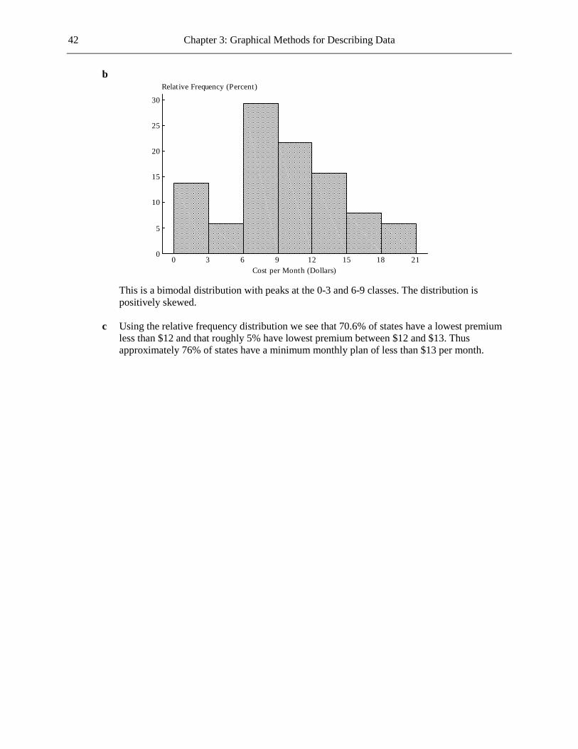
42 Chapter 3: Graphical Methods for Describing Data
b
211815129630
30
25
20
15
10
5
0
Cost per Month (Dollars)
Relative Frequency (Percent)
This is a bimodal distribution with peaks at the 0-3 and 6-9 classes. The distribution is
positively skewed. c Using the relative frequency distribution we see that 70.6% of states have a lowest premium
less than $12 and that roughly 5% have lowest premium between $12 and $13. Thus approximately 76% of states have a minimum monthly plan of less than $13 per month.
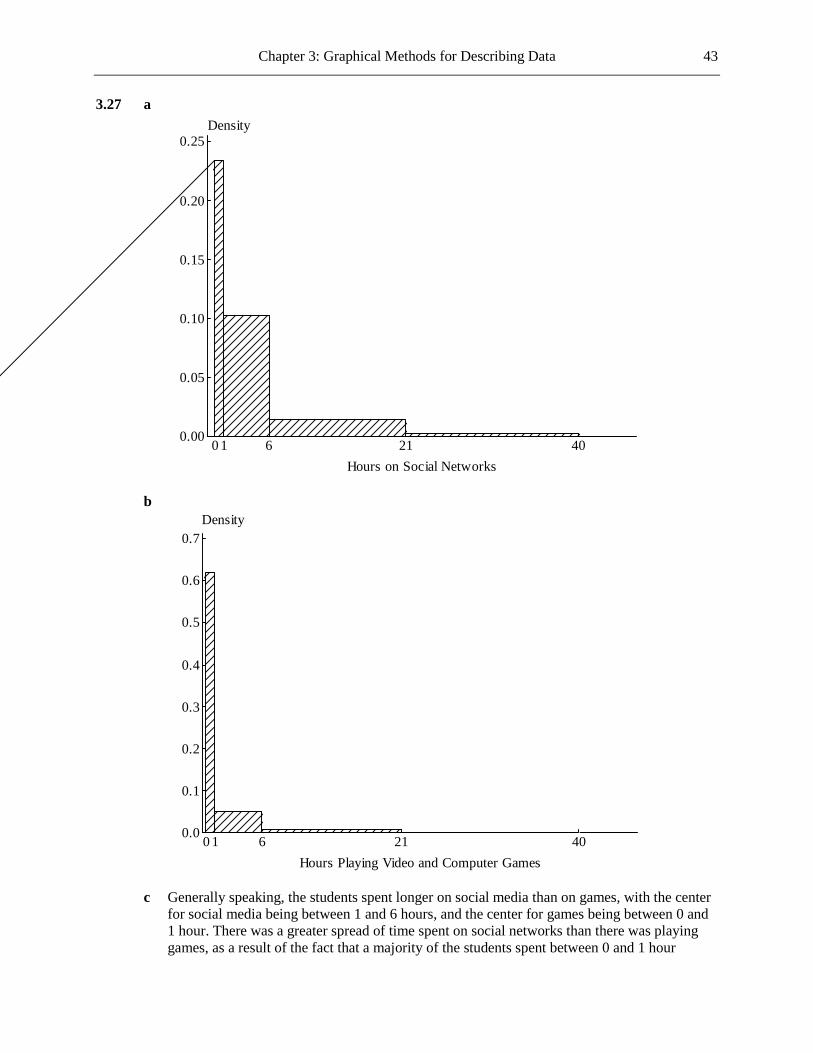
Chapter 3: Graphical Methods for Describing Data 43
3.27 a
4021610
0.25
0.20
0.15
0.10
0.05
0.00
Hours on Social Networks
Density
b
4021610
0.7
0.6
0.5
0.4
0.3
0.2
0.1
0.0
Hours Playing Video and Computer Games
Density
c Generally speaking, the students spent longer on social media than on games, with the center
for social media being between 1 and 6 hours, and the center for games being between 0 and 1 hour. There was a greater spread of time spent on social networks than there was playing games, as a result of the fact that a majority of the students spent between 0 and 1 hour

44 Chapter 3: Graphical Methods for Describing Data
playing games and there was no time interval containing a majority of students for social media use. Both distributions are positively skewed.
3.28 a In order to show necessary detail at the lower end of the distribution it was necessary to use
class intervals as narrow as 5 minutes. However, to use this class width throughout would result in too large a number of intervals. Therefore wider intervals were used for the higher commute times where the results were more scarce.
b
Commute Time Frequency Relative
Frequency Density Cumulative Relative Frequency
0 to <5 5200 0.052 0.0104 0.052 5 to <10 18200 0.181 0.0363 0.233 10 to <15 19600 0.195 0.0390 0.428 15 to <20 15400 0.153 0.0307 0.581 20 to <25 13800 0.137 0.0275 0.718 25 to <30 5700 0.057 0.0114 0.775 30 to <35 10200 0.102 0.0203 0.877 35 to <40 2000 0.020 0.0040 0.897 40 to <45 2000 0.020 0.0040 0.917 45 to <60 4000 0.040 0.0027 0.957 60 to <90 2100 0.021 0.0007 0.978
90 to <120 2200 0.022 0.0007 1.000 c
12060403020100
0.04
0.03
0.02
0.01
0.00
Commute T ime (minutes)
Density
A typical commute time is between 15 and 20 minutes, and the great majority of commute
times lie between 5 and 35 minutes. The distribution is positively skewed, and has an unexpected trough, with the 25-30 class occurring less frequently than the two adjacent classes.
d (The cumulative relative frequencies are shown in the table in part (b).)

Chapter 3: Graphical Methods for Describing Data 45
120100806040200
1.0
0.8
0.6
0.4
0.2
0.0
Commute T ime
Cumulative Relative Frequency
e i 0.93 ii 1 − 0.64 = 0.36 iii 17 minutes 3.29 a
4842363024181260
50
40
30
20
10
0
Tuition and Fees (Thousands)
Relative Frequency (%)
A typical value for tuition and fees for a student at a public four-year college is between
$6,000 and $9,000. Tuition and fees for these colleges range from close to zero to $42,000. The distribution is positively skewed.

46 Chapter 3: Graphical Methods for Describing Data
b
4842363024181260
50
40
30
20
10
0
Tuition and Fees (Thousands)
Relative Frequency (%)
A typical value for tuition and fees for a student at a private not-for-profit four-year college is
between $30,000 and $33,000. Tuition and fees at these colleges range from around $3,000 to $48,000. The distribution is slightly negatively skewed, and seems to have peaks between $3,000 and $6,000, between $24,000 and $36,000, and between $42,000 and $45,000.
c Tuition and fees tend to be higher at private not-for-profit four-year colleges than at public
four-year colleges. Tuition and fees are also more variable among private not-for-profit four-year colleges than among public four-year colleges. The two distributions have very different shapes, with a simple positively skewed distribution for public four-year colleges and a distribution that could be considered to have three peaks for private not-for-profit four-year colleges.
3.30 a The distribution is likely to be negatively skewed. There will be a high density of scores close
to 100, with no score greater than 100, and the density of scores tailing off to the left. b So long as there is no cutoff at the lower end the distribution is likely to be roughly
symmetrical. For example, the greatest density of points might be around 65, with the density tailing off equally to the left and to the right of that value. (It could also be suggested that the distribution would be positively skewed, since certain students will always get high scores however tough the exam.)
c In this case a bimodal distribution would be likely. There would a clustering of points around,
say, 65 for the students with less math knowledge and another clustering around, say, 95, for those who have had calculus.

Chapter 3: Graphical Methods for Describing Data 47
3.31
109876543210
0.4
0.3
0.2
0.1
0.0
Number of attempts
Density
3.32 a
Rainfall (inches) Frequency Relative Frequency Cumulative Relative Frequency
10 to <12 2 0.034 0.034 12 to <14 4 0.068 0.102 14 to <16 8 0.136 0.237 16 to <18 6 0.102 0.339 18 to <20 16 0.271 0.610 20 to <22 10 0.169 0.780 22 to <24 6 0.102 0.881 24 to <26 1 0.017 0.898 26 to <28 0 0 0.898 28 to <30 4 0.068 0.966 30 to <32 2 0.034 1.000

48 Chapter 3: Graphical Methods for Describing Data
b
322824201612
30
25
20
15
10
5
0
Rainfall (inches)
Relative Frequency (percent)
The histogram shows a distribution that is slightly positively skewed with a trough between
24 and 28. 3.33 a (The cumulative relative frequencies are shown in the table in Part (a).)
353025201510
1.0
0.8
0.6
0.4
0.2
0.0
Rainfall (inches)
Cumulative Relative Frequency
b i 0.20 ii 0.89 iii 0.89 − 0.31 = 0.58

Chapter 3: Graphical Methods for Describing Data 49
3.34 a
181614121086420
1.0
0.8
0.6
0.4
0.2
0.0
Years Survived
Cumulative Relative Frequency
b i 0.53 ii 0.62 iii 1 − 0.68 = 0.32 3.35 a
Years Survived Relative Frequency 0 - < 2 .10 2 - < 4 .42 4 - < 6 .02 6 - < 8 .10
8 - < 10 .04 10 - < 12 .02 12 - < 14 .02 14 - < 16 .28
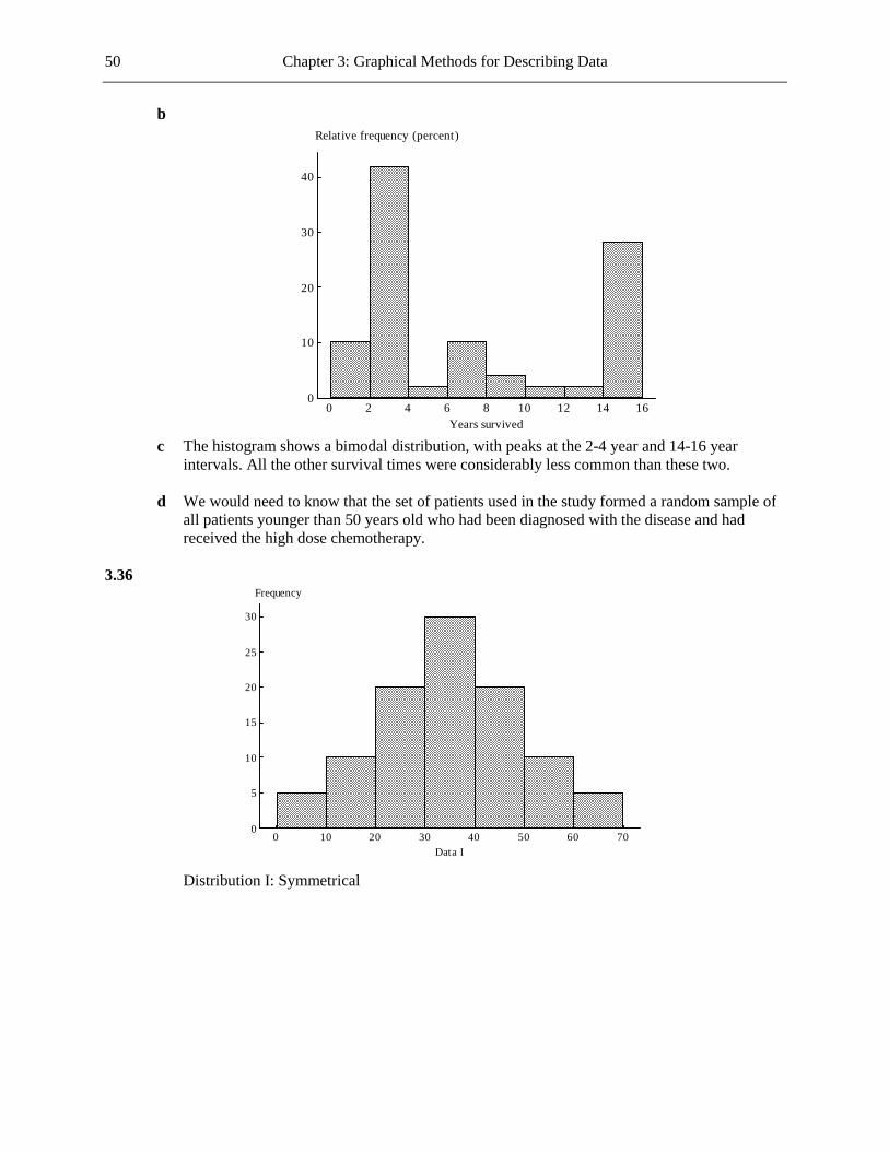
50 Chapter 3: Graphical Methods for Describing Data
b
1614121086420
40
30
20
10
0
Years survived
Relative frequency (percent)
c The histogram shows a bimodal distribution, with peaks at the 2-4 year and 14-16 year
intervals. All the other survival times were considerably less common than these two. d We would need to know that the set of patients used in the study formed a random sample of
all patients younger than 50 years old who had been diagnosed with the disease and had received the high dose chemotherapy.
3.36
706050403020100
30
25
20
15
10
5
0
Data I
Frequency
Distribution I: Symmetrical
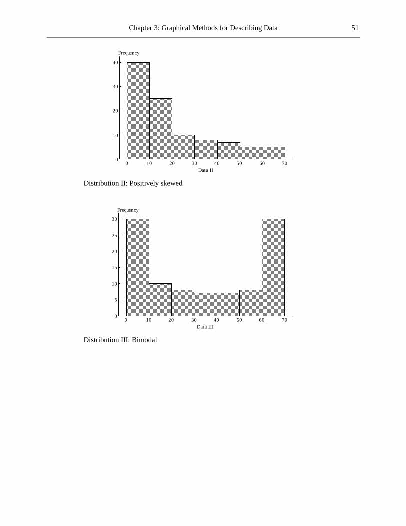
Chapter 3: Graphical Methods for Describing Data 51
706050403020100
40
30
20
10
0
Data II
Frequency
Distribution II: Positively skewed
706050403020100
30
25
20
15
10
5
0
Data III
Frequency
Distribution III: Bimodal

52 Chapter 3: Graphical Methods for Describing Data
706050403020100
25
20
15
10
5
0
Data IV
Frequency
Distribution IV: Bimodal
706050403020100
40
30
20
10
0
Data V
Frequency
Distribution V: Negatively skewed 3.37 Answers will vary. One possibility for each part is shown below. a
Class Interval 100 to <120 120 to <140 140 to <160 160 to <180 180 to <200 Frequency 5 10 40 10 5
b
Class Interval 100 to <120 120 to <140 140 to <160 160 to <180 180 to <200 Frequency 20 10 4 25 11
c
Class Interval 100 to <120 120 to <140 140 to <160 160 to <180 180 to <200 Frequency 33 15 10 7 5

Chapter 3: Graphical Methods for Describing Data 53
d
Class Interval 100 to <120 120 to <140 140 to <160 160 to <180 180 to <200 Frequency 5 7 10 15 33
3.38 a
1701601501401301201101009080
880
860
840
820
800
780
760
740
720
Quality Rating
APEAL Rating
b No. Customer satisfaction does not seem to be related to car quality. The scatterplot shows
what seems to be a random scatter of points. (It could be argued that there is a slight tendency for APEAL rating to be lower for higher quality ratings.)
3.39 a
9876543210
700
600
500
400
300
200
100
Fat
Calories
As expected there is a positive relationship between the amount of fat and the number of
calories. The relationship is weak.
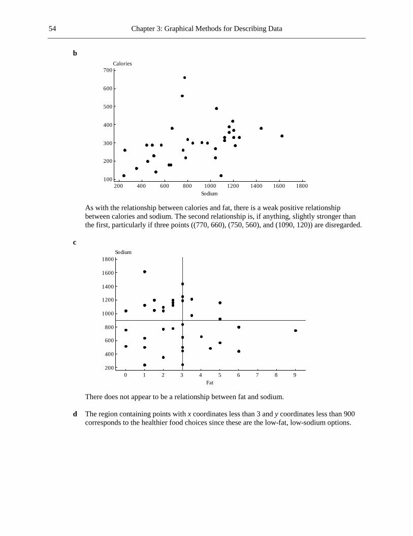
54 Chapter 3: Graphical Methods for Describing Data
b
18001600140012001000800600400200
700
600
500
400
300
200
100
Sodium
Calories
As with the relationship between calories and fat, there is a weak positive relationship
between calories and sodium. The second relationship is, if anything, slightly stronger than the first, particularly if three points ((770, 660), (750, 560), and (1090, 120)) are disregarded.
c
9876543210
1800
1600
1400
1200
1000
800
600
400
200
Fat
Sodium
There does not appear to be a relationship between fat and sodium. d The region containing points with x coordinates less than 3 and y coordinates less than 900
corresponds to the healthier food choices since these are the low-fat, low-sodium options.

Chapter 3: Graphical Methods for Describing Data 55
3.40 a
YearMonth
2008200720062005DecJunDecJunDecJunDecJun
20
15
10
5
0
Perc
ent w
ith W
irele
ss O
nly
The graph shows an upward trend in the percentage of homes with only a wireless phone
service from June 2005 to December 2008.
b The increase has been at a roughly steady rate, with only the periods June to December 2005 and December 2006 to June 2007 showing a slightly lower rate of growth.
3.41 a
50454035302520
65
60
55
50
45
40
35
30
Cost
Rating
b There appears to be a very weak positive relationship between cost and quality rating. The
scatterplot only very weakly supports the statement.

56 Chapter 3: Graphical Methods for Describing Data
3.42 a
1101009080706050403020
70
65
60
55
50
Cost
Ratin
g
There is a weak relationship between cost and quality rating, with higher costs being loosely
associated with lower ratings. b
1101009080706050403020
70
65
60
55
50
Cost
Ratin
g
Men'sWomen's
Type
The range of costs for men’s athletic shoes is slightly greater than for women’s (with just one
type of men’s shoe providing a cheaper option). For any given cost, there is generally speaking a greater spread of ratings for men’s shoes than for women’s, with the women’s shoes tending to show slightly higher ratings than the men’s.
c For men’s shoes the relationship between cost and quality rating is very weak. For women’s
shoes the relationship is stronger than for the men’s (and stronger than for the combined data set).

Chapter 3: Graphical Methods for Describing Data 57
3.43
2005200420032002200120001999199819971996199519941993199219911990
60
50
40
30
20
10
0
Year
Recy
cled
Was
te (m
illio
ns o
f ton
s)
The plot shows that the amount of waste collected for recycling had grown substantially (not
slowly, as is stated in the article) in the years 1990 to 2005. The amount increased from under 30 million tons to nearly sixty million tons in that period, which means that the amount had almost doubled.
3.44 a
2005200019951990198519801975197019651960
44
42
40
38
36
34
32
30
Index
Percent Who Smoke
For people who did not graduate from high school, there was a steady decrease over time in
the percent who smoked.

58 Chapter 3: Graphical Methods for Describing Data
b
2005200019951990198519801975197019651960
50
40
30
20
10
Year
Percent Who Smoke
Not a High School GraduateHigh Sch Grad but No CollegeSome CollegeBachelor or Higher
Variable
c All four categories showed a steady decline in the percent who smoked during the time period
of this study (with a slight tail-off in rate of decline between 2000 and 2005 for both non-high school graduates and high school graduates with no college). The most dramatic decrease was for people with bachelor’s degrees or higher, with the percentage decreasing from 44% in 1960 to 10% in 2005. In 1960, the category with the highest percentage of smokers was those with some college, but that was the category with the second-lowest percentage of smokers by 2005.
3.45 According to the 2001 and 2002 data, there are seasonal peaks at weeks 4, 9, and 14, and seasonal
lows at weeks 2, 6, 10-12, and 18. 3.46 For 12-year-olds to 17-year-olds, the percentage owning cell phones increased with age at each of
the years 2004, 2006, and 2008. Also, in each age group the percentage owning cell phones increased from 2004 to 2006 and from 2006 to 2008. Amongst 12-year-olds the percentage increased from 18% to 51% between 2004 and 2008, and amongst 17-year-olds the percentage increased from 64% to 84% over the same period.

Chapter 3: Graphical Methods for Describing Data 59
3.47 a
Enrollment
1.0
0.8
0.6
0.4
0.2
0.0
Unknown/OtherNative AmericanAfrican AmericanHispanic/LatinoAsian AmericanWhite
b The graphical display created in Part (a) is more informative, since it gives an accurate
representation of the proportions of the ethnic groups. c The people who designed the original display possibly felt that the four ethnic groups shown
in the segmented bar section might seem to be underrepresented at the college if they used a single pie chart.
3.48 a
Local CommunityWorldNation
40
30
20
10
0
Relative Frequency
MenWomen
b The USA Today graph is constructed so that the sleeves and the hands together have heights
that are in proportion to the relative frequencies. However many readers could think that the sleeves (which could be thought to look like the bars of a bar chart) are supposed to represent the relative frequencies, and the lengths of the sleeves are not in the correct proportion for these quantities. Also, given that the six hands all have equal areas and that the heights of the sleeve-hand combinations are in proportion to the relative frequencies, the areas of the sleeve-hand combinations will not be proportional to the relative frequencies, whereas in the

60 Chapter 3: Graphical Methods for Describing Data
traditional comparative bar graph the areas of the bars are in proportion to the relative frequencies.
3.49 The first graphical display is not drawn appropriately. The Z’s have been drawn so that their
heights are in proportion to the percentages shown. However, the widths and the perceived depths are also in proportion to the percentages, and so neither the areas nor the perceived volumes of the Z’s are proportional to the percentages. The graph is therefore misleading to the reader. In the second graphical display, however, only the heights of the cars are in proportion to the percentages shown. The widths of the cars are all equal. Therefore the areas of the cars are in proportion to the percentages, and this is an appropriately drawn graphical display.
3.50 The display is misleading. The cones are drawn so that their heights are in proportion to the
relative frequencies. However this means that their areas are not in proportion to the relative frequencies. A more suitable display is shown below.
Preference OtherSandwichSundaeConeCup
50
40
30
20
10
0
Relative Frequency (percent)
MenWomen
3.51 The piles of cocaine have been drawn so that their heights are in proportion to the percentages
shown. However, the widths are also in proportion to the percentages, and therefore neither the areas (nor the perceived volumes) are in proportion to the percentages. The graph is therefore misleading to the reader.
3.52 a The relative frequencies are given in the table below.
Perceived Risk of
Smoking Relative Frequency
Smokers Former Smokers Nonsmokers Very harmful 0.602 0.782 0.861
Somewhat harmful 0.299 0.161 0.100 Not too harmful 0.071 0.038 0.030
Not at all harmful 0.029 0.019 0.010

Chapter 3: Graphical Methods for Describing Data 61
Pcvd Risk Not at all harmfulNot too harmfulSomewhat harmfulVery harmful
2.0
1.5
1.0
0.5
0.0
Relative Frequency
SmokersFormer SmokersNonsmokers
b In all three groups the ranking of the perceived risks is the same. Nonsmokers are easily the
most likely group to have the belief that smoking is very harmful, with former smokers being the next most likely to have that opinion. Looking at the other three opinions the differences between the three groups are less marked, with “somewhat harmful” being most often responded by smokers, followed by nonsmokers.
3.53
Language other than EnglishEnglish and anotherEnglish
500
400
300
200
100
0
First Language
Average Verbal SAT

62 Chapter 3: Graphical Methods for Describing Data
3.54 a
Language other than EnglishEnglish and anotherEnglish
500
400
300
200
100
0
Average SAT Score
VerbalMath
b For the group whose first language is English the average scores in the two sections of the
SAT were very similar. In the other two groups the math scores were higher than the verbal scores, with the difference being most marked in the “language other than English” group. The average math scores were roughly the same for the three groups, while the verbal scores were lower for the “English and another” group than for the “English” group, and still lower for the “language other than English” group.
3.55 a
1 9 2 23788999 3 0011112233459 Stem: Tens 4 0123 Leaf: Ones
b A typical calorie content for these light beers is 31 calories per 100 ml, with the great
majority lying in the 22-39 range. The distribution is negatively skewed, with one peak (in the 30-39 range). There are no gaps in the data.
3.56
1H 9 2L 23 2H 788999 3L 00111122334 3H 59 Stem: Tens 4L 0123 Leaf: Ones

Chapter 3: Graphical Methods for Describing Data 63
3.57 a
0 0033344555568888888999999 1 0001223344567 2 001123689 3 0 4 0 5 Stem: Tens 6 6 Leaf: Ones
b A typical percentage population increase is around 10, with the great majority of states in the
0-29 range. The distribution is positively skewed, with one peak (in the 0-9 range). There are two states showing significantly greater increases than the other 48 states: one at 40 (Arizona) and one at 66 (Nevada).
c
West East 9988880 0 033344555568889999
432 1 0001234567 982100 2 136
0 3 0 4
5 Stem: Tens 6 6 Leaf: Ones
On average, the percentage population increases in the West were greater than those for the
East, with a typical value for the West being around 14 and a typical value for the East being around 9. There is a far greater spread in the values in the West, with values ranging from 0 to 66, than in the East where values ranged from 0 to 26. Both distributions are positively skewed, with a single peak for the East data, and two peaks for the West. In the West there are two states showing significantly greater increases than the remaining states, with values at 40 and 60. There are no such extreme values in the East.
3.58 a
Number of impairments 0 1 2 3 4 5 6 Frequency 100 43 36 17 24 9 11 Relative frequency 0.41667 0.17917 0.15000 0.07083 0.10000 0.03750 0.04583
b 0.41667 + 0.17917 + 0.15000 = 0.746 c 1 − 0.746 = 0.254 d 0.100 + 0.03750 + 0.04583 = 0.183 3.59 a High graft weight ratios are clearly associated with low body weights (and vice versa), and
the relationship is not linear. (In fact there seems to be, roughly speaking, an inverse proportionality between the two variables, apart from a small increase in the graft weight ratios for increasing body weights amongst those recipients with the greater body weights. This is interesting in that an inverse proportionality between the variables would imply that

64 Chapter 3: Graphical Methods for Describing Data
the actual weights of transplanted livers are chosen independently of the recipients’ body weights.)
b A likely reason for the negative relationship is that the livers to be transplanted are probably
chosen according to whatever happens to be available at the time. Therefore, lighter patients are likely to receive livers that are too large and heavier patients are likely to receive livers that are too small.
3.60 a
2000199519901985
50
40
30
20
10
Year
Percentage of Households with Computer
b The percentage of households with a computer increased with time, and since 1995 the rate of
increase has itself become larger over time. 3.61 a
2003199019701950
2500
2000
1500
1000
500
0
Year
Average Home Size (sq. feet)
b Continuing the growth trend, we estimate that the average home size in 2010 will be
approximately 2500 square feet.

Chapter 3: Graphical Methods for Describing Data 65
3.62
Gender
1.0
0.8
0.6
0.4
0.2
0.0
Relative FrequencyFemaleMale
3.63 a
Disney Other 975332100 0 0001259
765 1 156 920 2 0
3 4 Stem: Hundreds
4 5 Leaf: Tens b On average, the total tobacco exposure times for the Disney movies are higher than the
others, with a typical value for Disney being around 90 seconds and a typical value for the other companies being around 50 seconds. Both distributions have one peak and are positively skewed. There is one extreme value (548) in the Disney data, and no extreme value in the data for the other companies. There is a greater spread in the Disney data, with values ranging from 6 seconds to 540 seconds, than for the other companies, where the values range from 1 second to 205 seconds.
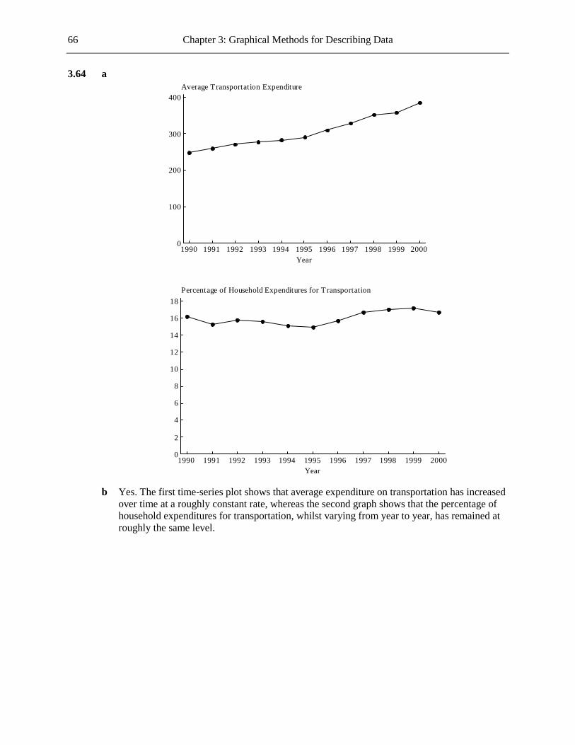
66 Chapter 3: Graphical Methods for Describing Data
3.64 a
20001999199819971996199519941993199219911990
400
300
200
100
0
Year
Average Transportation Expenditure
20001999199819971996199519941993199219911990
18
16
14
12
10
8
6
4
2
0
Year
Percentage of Household Expenditures for Transportation
b Yes. The first time-series plot shows that average expenditure on transportation has increased
over time at a roughly constant rate, whereas the second graph shows that the percentage of household expenditures for transportation, whilst varying from year to year, has remained at roughly the same level.

Chapter 3: Graphical Methods for Describing Data 67
3.65 a
All of the time Most of the time
Some of the time
Never
b
Response
1.0
0.8
0.6
0.4
0.2
0.0
All of the timeMost of the timeSome of the timeNever
Response
c The segmented bar graph is slightly preferable in that it is a little easier than in the pie chart
to see that the proportion of children responding “Most of the time” was slightly higher than the proportion responding “Some of the time.”
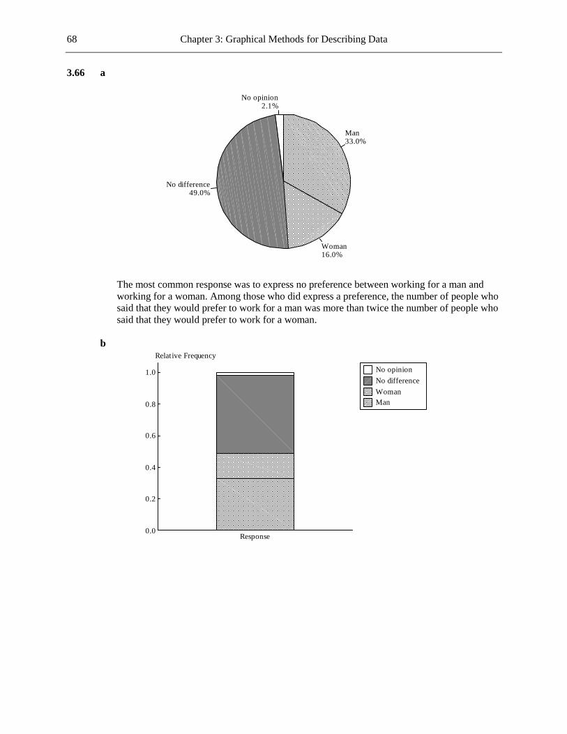
68 Chapter 3: Graphical Methods for Describing Data
3.66 a
No opinion2.1%
No difference49.0%
Woman16.0%
Man33.0%
The most common response was to express no preference between working for a man and
working for a woman. Among those who did express a preference, the number of people who said that they would prefer to work for a man was more than twice the number of people who said that they would prefer to work for a woman.
b
Response
1.0
0.8
0.6
0.4
0.2
0.0
Relative Frequency
No opinionNo differenceWomanMan

Chapter 3: Graphical Methods for Describing Data 69
3.67 a
200620042002200019981996199419921990
60
50
40
30
20
10
0
Year
Cost (billions of dollars)
b The peaks were probably caused by the incidence of major hurricanes in those years. 3.68
Rural19.0%
Suburban42.0%
Urban39.0%

70 Chapter 3: Graphical Methods for Describing Data
3.69 a
20012000199919981997199619951994
4000
3750
3500
3250
3000
2750
2500
Year
Number of transplants
b The number of transplants increased every year, with particularly dramatic increases between
1994 and 1995, and between 1999 and 2001. c
20012000199919981997199619951994
4000
3000
2000
1000
0
Number of transplants
RelatedUnrelated
d In every year the number of related donors was much greater than the number of unrelated
donors. In both categories the number of transplants increased every year, but proportionately the increases in unrelated donors were greater than the increases in related donors.
3.70 a Yes. The first histogram gives the impression of a distribution that is negatively skewed,
while the second histogram gives an impression of a distribution that is positively skewed. Also, the second histogram shows a decrease in density of points in the second and third class intervals as compared to the first and fourth intervals: this feature of the shape of the distribution is not at all evident in the first histogram.

Chapter 3: Graphical Methods for Describing Data 71
b According to the first histogram the proportion of observations less than 800 is approximately
(6 7 (0.5)10) 27 0.667+ + = . According to the second histogram this proportion is approximately (6 5 5 (1 / 3)6) 27 0.667+ + + = , also. The true proportion of observations less than 800 is 18 27 0.667= . The approximations according to the two histograms are both correct.
3.71 a
Skeletal Retention Frequency
0.15 to <0.20 4 0.20 to <0.25 2 0.25 to <0.30 5 0.30 to <0.35 21 0.35 to <0.40 9 0.40 to <0.45 9 0.45 to <0.50 4 0.50 to <0.55 0 0.55 to <0.60 1
0.600.550.500.450.400.350.300.250.200.15
20
15
10
5
0
Skeletal retention
Frequency
b The histogram is centered at approximately 0.34, with values ranging from 0.15 to 0.5, plus
one extreme value in the 0.55-0.6 range. The distribution has a single peak and is slightly positively skewed.

72 Chapter 3: Graphical Methods for Describing Data
Cumulative Review Exercises CR3.1 No. It is quite possible, for example, that men who ate a high proportion of cruciferous vegetables
generally speaking also had healthier lifestyles than those who did not, and that it was the healthier lifestyles that were causing the lower incidence of prostate cancer, not the eating of cruciferous vegetables.
CR3.2 Neither the conclusion nor the headline is appropriate. Since this is an observational study, we
can only conclude that there is an association between religious activity and blood pressure, not that religious activity causes reduced blood pressure. It is quite possible, for example, that people who attend a religious service once a week and pray or study the Bible at least once a day also have more exercise than people who do not engage in these activities, and that it is the exercise not the religious activity that is causing the reduced blood pressure.
CR3.3 Very often those who choose to respond generally have a different opinion on the subject of the
study from those who do not respond. (In particular, those who respond often have strong feelings against the status quo.) This can lead to results that are not representative of the population that is being studied.
CR3.4 The survey was conducted using people who chose to attend a budget workshop and so we have
no reason to think that this set of people was representative of the population as a whole. (Also, there is no reason to think that people who are not exposed to the content of the workshop would have the same opinion regarding the proposed sales tax increase.)
CR3.5 Only a small proportion (around 11%) of the doctors responded, and it is quite possible that those
who did respond had different opinions regarding managed care from the majority who did not. Therefore the results could have been very inaccurate for the population of doctors in California.
CR3.6 a Answers will vary. A completely randomized design (no blocking) should include randomly
choosing which exiting cars should have a car waiting for the space and which should not. b The response variable is the time taken to exit the parking space. c Possible extraneous variables include the time of day, the gender of the exiting driver, and the
location of the parking space. CR3.7 Suppose, for example, the women had been allowed to choose whether or not they participated in
the program. Then it is quite possible that generally speaking those women with more social awareness would have chosen to participate, and those with less social awareness would have chosen not to. Then it would be impossible to tell whether the stated results came about as a result of the program or of the greater social awareness amongst the women who participated. By randomly assigning the women to participate or not, comparable groups of women would have been obtained.
CR3.8 a Randomly assign the 100 female volunteers to two groups, A and B. (This could be done by
writing the names of the volunteers on slips of paper, placing the slips in a hat, mixing them, and randomly picking one slip at a time. The first 50 names picked will go into Group A and the remainder into Group B.) At the beginning of the experiment, by means of a questionnaire, the PMS symptoms of the volunteers will be assessed. Then the women in Group A will be given the nasal spray containing the pheromones and the women in Group B

Chapter 3: Graphical Methods for Describing Data 73
will be given a nasal spray that in appearance and sensation is identical to the first one but contains no active ingredient. (No volunteer will be told which treatment she is receiving.) Then all the women will be instructed to use the spray over a period of a few months. At the end of the experiment the women’s PMS symptoms will be reassessed and the reduction in PMS symptoms for the two groups will be compared.
b Yes. If Group B were to receive no spray at all, and if there were a greater improvement in
symptoms for Group A than for Group B, then it would be impossible to tell whether this improvement took place as a result of the pheromones or as a result of the psychological effect of using the spray.
c The design is single blind, since the women are not told what treatment they are receiving. A
double blind design would be one in which, additionally, the people who measure the PMS symptoms do not know who received which treatment. In the design given in part (a) the women are required to assess their own symptoms, however it would certainly be useful if the people who collate the information given in the questionnaires were not to know who received which treatment.
CR3.9 a
200420032002
90
80
70
60
50
40
30
20
10
0
Pass Rate (%)San Luis Obispo High SchoolSan Luis Obispo CountyState of California
District
b Between 2002 and 2003 and between 2003 and 2004 the pass rates rose for both the high
school and the state, with a particularly sharp rise between 2003 and 2004 for the state. However, for the county the pass rate fell between 2002 and 2003 and then rose between 2003 and 2004.
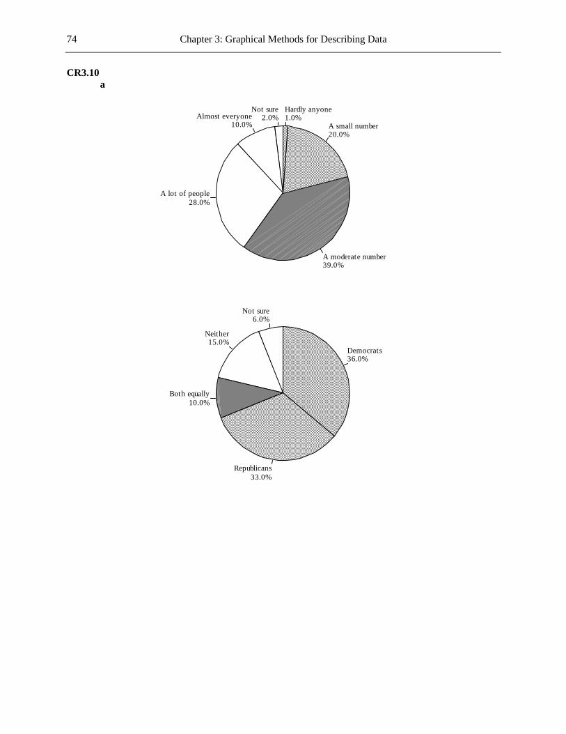
74 Chapter 3: Graphical Methods for Describing Data
CR3.10 a
Not sure2.0%Almost everyone
10.0%
A lot of people28.0%
A moderate number39.0%
A small number20.0%
Hardly anyone1.0%
Not sure6.0%
Neither15.0%
Both equally10.0%
Republicans33.0%
Democrats36.0%

Chapter 3: Graphical Methods for Describing Data 75
b
Response
1.0
0.8
0.6
0.4
0.2
0.0
Relative Frequency
Not sureAlmost everyoneA lot of peopleA moderate numberA small numberHardly anyone
Response
1.0
0.8
0.6
0.4
0.2
0.0
Relative Frequency
Not sureNeitherBoth equallyRepublicansDemocrats
c In both cases, but particularly for the first data set, since there is a relatively large number of
categories the segmented bar graph does a better job of presenting the data. Also, in the first data set the order in which the six possible responses are listed is important. This order is clearly reflected in the segmented bar graph but not in the pie chart.
CR3.11 a
0 123334555599 1 00122234688 2 1112344477 3 0113338 4 37 Stem: Thousands 5 23778 Leaf: Hundreds

76 Chapter 3: Graphical Methods for Describing Data
The stem-and-leaf display shows a positively skewed distribution with a single peak. There are no extreme values. A typical total length is around 2100 and the great majority of total lengths lie in the 100 to 3800 range.
b
6000500040003000200010000
12
10
8
6
4
2
0
Total Length
Frequency
c The number of subdivisions that have total lengths less than 2000 is 12 + 11 = 23, and so the
proportion of subdivisions that have total lengths less than 2000 is 23/47 = 0.489. The number of subdivisions that have total lengths between 2000 and 4000 is 10 + 7 = 17,
and so the proportion of subdivisions that have total lengths between 2000 and 4000 is 17/47 = 0.361.
CR3.12 a
Class Interval Frequency Relative Frequency Cumulative Relative Frequency 0 to <6 2 0.022 0.022
6 to <12 10 0.112 0.135 12 to <18 21 0.236 0.371 18 to <24 28 0.315 0.685 24 to <30 22 0.247 0.933 30 to <36 6 0.067 1.000
b The relative frequencies and the cumulative relative frequencies are shown in the table in Part
(a). c (Relative frequency for 12 to <18) = (cum rel freq for 12 to <18) − (cum rel freq for 6 to <12) = 0.371 − 0.135 = 0.236. d i 1 − 0.135 = 0.865. ii 0.236 + 0.315 = 0.561

Chapter 3: Graphical Methods for Describing Data 77
e
403020100
1.0
0.8
0.6
0.4
0.2
0.0
Time to First Malfunction (months)
Cumulative Relative Frequency
i 20 months ii 29 months CR3.13 a The histogram shows a smooth positively skewed distribution with a single peak. There are
around three values that could be considered extreme, with those values lying in the 650 to 750 range. The majority of time differences lie between 50 and 350 seconds.
b A typical time difference between the two phases of the race is 150 seconds. c Estimating the frequencies from the histogram we see that approximately 920 runners were
included in the study and that approximately 8 of those runners ran the late distance more quickly than the early distance (indicated by a negative time difference). Therefore the proportion of runners who ran the late distance more quickly than the early distance is approximately 8/920 = 0.009.
CR3.14 a Generally speaking, states with higher poverty rates have higher dropout rates, but the
relationship is not strong. There are two states with relatively low poverty rates (between 10% and 15%) but high dropout rates (over 15%).
b There is a weak positive relationship between poverty rate and dropout rate. CR3.15 There is a strong negative linear relationship between racket resonance frequency and sum of
peak-to-peak accelerations. There are two rackets whose data points are separated from the remaining data points. Those two rackets have very high resonance frequencies and their peak-to-peak accelerations are lower than those of all the other rackets.

78 Chapter 3: Graphical Methods for Describing Data
CR3.16 a
200520001995199019851980
80
70
60
50
40
30
20
Date
Percentage
Good TimeBad Time
b The new line has been added to the plot in Part (a). c The time series plot is more effective as its horizontal axis shows an actual time scale, which
is not present in the bar graph.

79
Chapter 4 Numerical Methods for Describing Data
4.1 a ( )1480 1071 2291 1688 1124 3476 3701 7x = + + + + + + = $2118.71. To calculate the median, we first list the data values in order of size:
1071 1124 1480 1688 2291 3476 3701
The median is the middle value in this list, $1688. b The mean is much larger than the median since the distribution of these seven values is
positively skewed. The two largest values are greatly separated from the remaining five values.
c The median is better as a description of a typical value since it is not influenced by the two
extreme values. 4.2 a ( )9.6 10.0 10.0 9.0 10.9 8.9 9.5 9.1 8x = + + + + + + + = 9.625 mg/oz. b The caffeine concentration of top-selling energy drinks is much greater than that of colas. 4.3 The mean caffeine concentration for the brands of coffee listed is
140 195 155 115 195 180 110 110 130 55 60 6012
+ + + + + + + + + + + = 125.417 mg/cup.
Therefore the mean caffeine concentration of the coffee brands in mg/oz is (125.417)/8 = 15.677.
This is significantly greater than the mean caffeine concentration of the energy drinks given in the previous exercise.
4.4 a
2402101801501209060Sodium Content (mg)
The distribution is roughly symmetrical. One brand of peanut butter has an unusually high
sodium content (250). If this value is disregarded, then the distribution is negatively skewed. b (120 110) 11 .x = + + = 134.091L The values listed in order are: 50 65 110 120 120 140 150 150 150 170 250 Median = 6th value = 140. c The values of the mean and the median are similar because the distribution is roughly
symmetrical.

80 Chapter 4: Numerical Methods for Describing Data
4.5 The fact that the mean is so much greater than the median tells us that a small number of individuals who donate a large amount of time are greatly increasing the mean.
4.6 A dotplot of the data set is shown below.
300250200150100500Number of Minutes
Since the distribution is not symmetrical, the median would be a preferable measure of center. 4.7 a There are some unusually large circulation values that make the mean greater than the
median. b The sum of the circulation values given is 13666304, and so the mean is
(13666304)/20 = 683315.2. The values are already given in descending order, and so to find the median we only need to
find the average of the two middle values: (438722 427771) 2+ = 433246.5. c The median is does the better job of describing a typical value as it is not affected by the
small number of unusually large values in the data set. d This sample is in no way representative of the population of daily newspapers in the US since
it consists of the top 20 newspapers in the country. 4.8 a The number in the sample who are registered to vote is 12, in a sample of 20 students. So the
proportion of successes is 12/20 = 0.6. b This generalization could be made if the sample were a simple random sample of seniors at
the university. 4.9 a The sum of the values given is 8966, and so the mean is 8966/20 = 448.3. b Median = (446 + 446)/2 = 446. c This sample represents the 20 days with the highest number of speeding-related fatalities, and
so it is not reasonable to generalize from this sample to the other 365 days of the year. 4.10 Both means are greater than the respective medians, suggesting that both distributions are
positively skewed. The fact that the median is greater for angioplasty and the mean is greater for bypass surgery tells us that the median-to-mean increase is greater in the case of bypass surgery, suggesting that the positive skew is more pronounced for bypass surgery than for angioplasty.
4.11 Neither statement is correct. Regarding the first statement it should be noted that, unless the
“fairly expensive houses” constitute a majority of the houses selling, these more costly houses will not have an effect on the median. Turning to the second statement, we point out that the

Chapter 4: Numerical Methods for Describing Data 81
small number of very high or very low prices will have no effect on the median, whatever the number of sales. Both statements can be corrected by replacing the median with the mean.
4.12 Here the word “average” refers to the mean and, yes, it is possible that 65% of the residents
would earn less than that value. If the distribution of wages is positively skewed then the mean will be greater than the median, which tells us that more than 50% (and therefore possibly 65%) of residents will earn less than the mean.
4.13 The two possible solutions are 5x = 32 and 5 39.5.x = 4.14 a ˆ 7 10 .p = = 0.7 b (1 1 0 1 1 1 0 0 1 1) 10 .x = + + + + + + + + + = 0.7 The values of x and p are the same. c The sample size is now 10 + 15 = 25. We need the number of successes to be (0.8)(25) = 20.
Therefore we need 13 of these 15 observations to be successes. 4.15 The only measure of center discussed in this section that can be calculated is the median. To find the median we first list the data values in order:
170 290 350 480 570 790 860 920 1000+ 1000+ The median is the mean of the two middle values: (570 + 790)/2 = 680 hours. 4.16 The total score after 19 students is (19)(70) = 1330. For the average for all 20 students to be 71,
we need the total for all 20 students to be (20)(71) = 1420. So the last student needs to score 1420 − 1330 = 90. For the average for all 20 students to be 72, we need the total for all 20 students to be (20)(72) = 1440. So the last student needs to score 1440 − 1330 = 110, which is not possible.
4.17 a (29 62 37 41 70 82 47 52 49) 9 52.111.x = + + + + + + + + =
2 2(29 52.111) (49 52.111)Variance .
8− + + −
= = 279.111L
279.111 .s = = 16.707 b The addition of the very expensive cheese would increase the values of both the mean and the
standard deviation. 4.18 Cereals rated very good: Median = 47.5, upper quartile = 62, lower quartile = 41, iqr = 21. Cereals rated good: Median = 53, upper quartile = 60.5, lower quartile = 36.5, iqr = 24. The median cost per serving is higher for cereals rated good than for cereals rated very good. The
interquartile range is higher for cereals rated good than for cereals rated very good, reflecting a greater spread in the distribution for cereals rated good.

82 Chapter 4: Numerical Methods for Describing Data
4.19 a The complete data set, listed in order, is: 19 28 30 41 43 46 48 49 53 53 54
62 67 71 77 Lower quartile = 4th value = 41. Upper quartile = 12th value = 62. Iqr = 21. b The iqr for cereals rated good (calculated in exercise 4.18) is 24. This is greater than the value
calculated in Part (a). 4.20 This question can be answered by comparing standard deviations (or variances) or interquartile
ranges. The standard deviation for the high caffeine energy drinks (8.311) is much larger than the
standard deviation for the top selling energy drinks (0.667). The high caffeine drinks are the more variable with respect to caffeine per ounce.
Likewise, the interquartile range for the high caffeine energy drinks (31.3 − 15.0 = 16.3) is much
larger than the interquartile range for the top selling energy drinks (10.0 − 9.05 = 0.95). This, too, tells us that the high caffeine drinks are the more variable with respect to caffeine per ounce.
4.21 (44.0 21.4) 18x = + + = 51.333L
A typical amount poured into a tall, slender glass is 51.333 ml.
2 2(44.0 51.333) (21.4 51.333)17
s − + + −= = 15.216L
A typical deviation from the mean amount poured is 15.216 ml. 4.22 a (89.2 57.8) 18x = + + = 59.233L
A typical amount poured into a short, wide glass is 59.233 ml.
2 2(89.2 59.233) (57.8 59.233)17
s − + + −= = 16.715L
A typical deviation from the mean amount poured is 16.715 ml. b The mean amount for a short, wide glass (59.233 ml) is greater than the mean amount for a
tall, slender glass (51.333 ml). This suggests that bartenders tend to pour more into a short, wide glass than into a tall, slender glass.
4.23 a (1480 3701) 7 2118.71429x = + + =L 2Variance ((1480 2118.71429) (3701 2118.71429) ) 6= − + + − = 1176027.905L . Standard deviation 1176027.905 .= = 1084.448 b The fairly large value of the standard deviation tells us that there is considerable variation
between repair costs. 4.24 For minivans, mean = 1355.833, variance = 93698.967, and standard deviation = 306.103. The mean repair cost for minivans is less than for the smaller cars, showing a lower typical repair
cost for the minivans. The standard deviation for minivans is considerably less than for the smaller cars, showing a lower repair cost variability for the minivans.

Chapter 4: Numerical Methods for Describing Data 83
4.25 a The data values, listed in order, are: 0 0 0 0 0 0 0 59 71 83 106
130 142 142 165 177 189 189 189 201 212 224 236 236 306
Lower quartile = average of 6th and 7th values = (0 + 0)/2 = 0. Upper quartile = average of 19th and 20th values = (189 + 201)/2 = 195. Interquartile range = 195 − 0 = 195. b The lower quartile is equal to the minimum value for this data set because there are a large
number of equal values (zero in this case) at the lower end of the distribution. In most data sets this is not the case and therefore, generally speaking, the lower quartile is not equal to the minimum value.
4.26 Answers will vary. 4.27 The volatility of a portfolio is the amount by which its return varies, and the standard deviation of
the annual returns measures exactly that. A lower risk portfolio is one in which the return is less variable. This is can be interpreted in terms of a low standard deviation of annual returns.
4.28 a (141 70) 10 147.5.x = + + =L 2 2Variance ((141 147.5) (70 147.5) ) 9 2505.83333.= − + + − =L Standard deviation 2505.83333 .= = 50.058 b The Memorial Day data are a great deal more consistent than the New Year’s Day data, and
therefore the standard deviation for Memorial Day would be smaller than the standard deviation for New Year’s Day.
c The standard deviations are given in the table below.
Holiday Standard Deviation New Year's Day 50.058 Memorial Day 18.224 July 4th 47.139 Labor Day 17.725 Thanksgiving 15.312 Christmas 52.370
The standard deviations for Memorial Day, Labor Day, and Thanksgiving are 18.224, 17.725,
and 15.312, respectively. The standard deviations for the other three holidays are 50.058, 47.139, and 52.370. The standard deviations for the same day of the week holidays are all smaller than all of the standard deviations for the holidays that can occur on different days. There is less variability for the holidays that always occur on the same day of the week.
4.29 a i. The lower quartile must be less than the median. b iii. Only 10% of the bypass surgeries took longer than 42 days to be completed, and so the
upper quartile must be between the median (13) and this value.

84 Chapter 4: Numerical Methods for Describing Data
c iv. The number of days for which only 5% of the bypass surgery wait times were longer must be greater than the number of days for which 10% of the bypass surgery wait times were longer, which was 42.
4.30 The mean of the values given is 747.370 and the standard deviation is 606.894. Thus the
maximum amount that could be awarded under the “2-standard deviations” rule is 747.370 + 2(606.894) = 1961.158 thousands of dollars.
4.31 a
Mean Standard Deviation
Coef. of Variation
Sample 1 7.81 0.398 5.102 Sample 2 49.68 1.739 3.500
b The values of the coefficient of variation are given in the table in Part (a). The fact that the
coefficient of variation is smaller for Sample 2 than for Sample 1 is not surprising since, relative to the actual amount placed in the containers, it is easier to be accurate when larger amounts are being placed in the containers.
4.32 a Since the mean is greater than the median, the distribution is likely to be positively skewed. b
200150100500Travel T ime (minutes)
c There are clearly no outliers at the lower end. There are extreme outliers at the upper end if
there are travel times more than 3(iqr) above the upper quartile. Here
(upper quartile) + 3(iqr) = 31 + 3(31 − 7) = 31 + 3(24) = 103. Therefore, since we are assuming that the maximum travel time is 205 minutes and 205 is
greater than 103, there are extreme outliers in this data set, and knowing these data came from a large sample we can be confident that there are mild outliers, also.
4.33 a Median = average of 25th and 26th values = (57.3 + 58.7)/2 = 58. Lower quartile = 13th value = 53.5. Upper quartile = 38th value = 64.4. b (Lower quartile) − 1.5(iqr) = 53.5 − 1.5(10.9) = 37.15. Since 28.2 and 35.7 are both less than 37.15, they are both outliers.
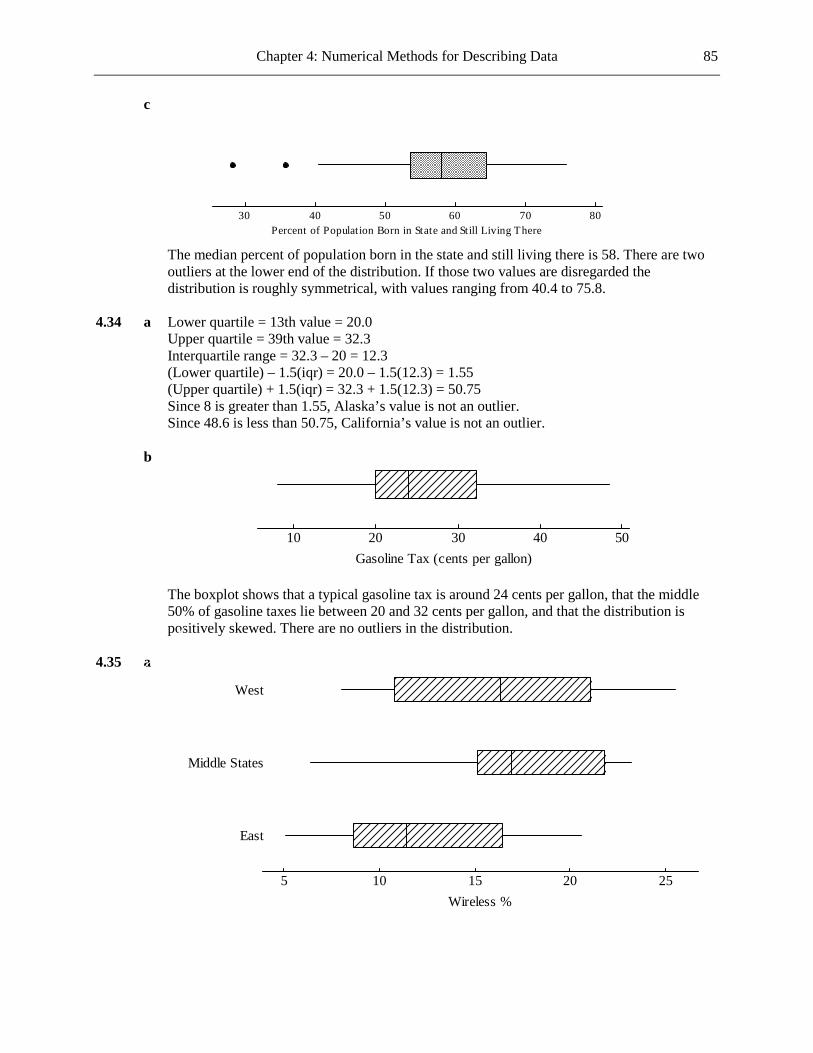
Chapter 4: Numerical Methods for Describing Data 85
c
807060504030Percent of Population Born in State and Still Living There
The median percent of population born in the state and still living there is 58. There are two
outliers at the lower end of the distribution. If those two values are disregarded the distribution is roughly symmetrical, with values ranging from 40.4 to 75.8.
4.34 a Lower quartile = 13th value = 20.0
Upper quartile = 39th value = 32.3 Interquartile range = 32.3 – 20 = 12.3 (Lower quartile) – 1.5(iqr) = 20.0 – 1.5(12.3) = 1.55 (Upper quartile) + 1.5(iqr) = 32.3 + 1.5(12.3) = 50.75 Since 8 is greater than 1.55, Alaska’s value is not an outlier. Since 48.6 is less than 50.75, California’s value is not an outlier.
b
5040302010Gasoline Tax (cents per gallon)
The boxplot shows that a typical gasoline tax is around 24 cents per gallon, that the middle
50% of gasoline taxes lie between 20 and 32 cents per gallon, and that the distribution is positively skewed. There are no outliers in the distribution.
4.35 a
East
Middle States
West
252015105Wireless %

86 Chapter 4: Numerical Methods for Describing Data
b The median for the East (11.4%) is lower than for the other two regions (16.3% and 16.9%, respectively). The three regions have similar interquartile ranges. The distributions are similar in shape except that the middle states region has some percentages that are far below the median for that region.
4.36 a The fiber data listed in order are: 7 7 7 7 7 8 8 8 8 8 10 10 10 12 12 12 13 14 Median = average of 9th and 10th values = (8 + 8)/2 = 8 Lower quartile = 5th value = 7 Upper quartile = 14th value = 12 Interquartile range = 12 − 7 = 5 b The sugar data listed in order are:
0 0 5 6 6 9 9 10 10 10 10 11 11 13 14 17 18 19
Median = average of 9th and 10th values = (10 + 10)/2 = 10 Lower quartile = 5th value = 6 Upper quartile = 14th value = 13 Interquartile range = 13 − 6 = 7 c For the sugar data, (Upper quartile) + 1.5(iqr) = 13 + 1.5(7) = 23.5 (Lower quartile) − 1.5(iqr) = 6 − 1.5(7) = −4.5 There are no values less than −4.5 or greater than 23.5 and therefore there are no outliers. d The minimum and lower quartile for the fiber data set are both equal to 7 since the five
smallest values (that is, more than a quarter of the data values) are all equal to 7. e
Sugar Content
Fiber Content
20151050
Generally speaking, there are more grams per serving of sugar content than of fiber content in these cereals, with the median sugar content being 10 and the median fiber content being 8. The sugar content is also more variable, with both the interquartile range and the range (7 and 19, respectively) for the sugar data being larger than for the fiber data (5 and 7, respectively).

Chapter 4: Numerical Methods for Describing Data 87
The distribution of the sugar content is roughly symmetrical, whereas the fiber content distribution seems to be positively skewed. Neither distribution contains outliers.
4.37 a Since there are outliers in the data set (152 and 43), it would be more appropriate to use the
interquartile range than the standard deviation. b Lower quartile = 81.5, upper quartile = 94, iqr = 12.5. (Lower quartile) − 3(iqr) = 81.5 − 3(12.5) = 44 (Lower quartile) − 1.5(iqr) = 81.5 − 1.5(12.5) = 62.75 (Upper quartile) + 1.5(iqr) = 94 + 1.5(12.5) = 112.75 (Upper quartile) + 3(iqr) = 94 + 3(12.5) = 131.5 Since the value for students (152) is greater than 131.5, this is an extreme outlier. Since the value for farmers (43) is less than 44, this is an extreme outlier. There are no non-extreme outliers. c
1501251007550Accidents per 1000
d The insurance company might decide only to offer discounts to occupations that are outliers
at the lower end of the distribution, in which case only farmers would receive the discount. If the company was willing to offer discounts to the quarter of occupations with the lowest accident rates then the last 10 occupations on the list should be the ones to receive discounts.
4.38 a Value 1 standard deviation above mean = 40 min. Value 1 standard deviation below mean = 30 min. Value 2 standard deviations above mean = 45 min. Value 2 standard deviations below mean = 25 min. b The values 25 and 45 are 2 standard deviations from the mean. Therefore, by Chebyshev’s
Rule, at least 100(1 − 1/22)% = 75% of the times are between these two values. c The values 20 and 50 are both 3 standard deviations from the mean, so by Chebyshev’s Rule
at most 100(1/32)% = 11.1% of the times are either less than 20 min or more than 50 min. d Assuming that the distribution of times is normal, approximately 95% of the times are
between 25 and 45 min., approximately 0.3% of the times are either less than 20 min. or greater than 50 min., and approximately 0.15% of the times are less than 20 min.
4.39 a Since the values given are 1 standard deviation above and below the mean, roughly 68% of
speeds would have been between those two values. b (1 − 0.68)/2 = 0.16. Roughly 16% of speeds would exceed 57 mph.

88 Chapter 4: Numerical Methods for Describing Data
4.40 a
2001000
0.035
0.030
0.025
0.020
0.015
0.010
0.005
0.000
Travel T ime (minutes)
Density
b The center of the distribution of travel times is around 20 minutes, with the great majority of
travel times being between 5 and 45 minutes. The distribution is positively skewed. c No. The distribution of travel times is not approximately normal and therefore the Empirical
Rule is not applicable. d Since the mean of the distribution is 27 minutes and the standard deviation is 24 minutes, 0 is
just over 1 standard deviation below the mean. Therefore, if the distribution were approximately normal, then just under (100 − 68)/2 = 16% of travel times would be less than 0, which is clearly not the case. Thus the distribution cannot be well approximated by a normal curve.
e i Since the mean of the distribution is 27 and the standard deviation is 24, 75 is 2 standard
deviations above the mean and the point 2 standard deviations below the mean is −21. Therefore by Chebyshev’s Rule at least 75% of travel times are between these two values. However, since travel times cannot be less than zero, we can conclude that at least 75% of travel times are between 0 and 75 minutes.
ii A travel time of 47 minutes is (47 − 27)/24 = 0.833 standard deviations above the mean.
A travel time of 0 is 27/24 = 1.125 standard deviations below the mean. Since 1.125 is larger than 0.833, we can conclude that at least 100(1 − 1/1.1252)% = 21% of travel times are between 0 and 47 minutes.
f The actual percentage of travel times between 0 and 75 minutes is approximately
(100 − 2 − 2.5)% = 95.5%, which is a lot more than the 75% minimum given by Chebyshev’s Rule. The actual percentage of travel times between 0 and 47 minutes is approximately (100 − 2 − 5 − 5)% = 88%, which is again a lot more than the 21% minimum given by Chebyshev’s Rule.
4.41 a The values given are two standard deviations below and above the mean. Therefore by
Chebyshev’s Rule at least 75% of observations must lie between those two values.

Chapter 4: Numerical Methods for Describing Data 89
b By Chebyshev’s Rule at least 89% of observations must lie within 3 standard deviations of
the mean. So the required interval is 36.92 3(11.34) ( , )± = 2.90 70.94 . c If the distribution were approximately normal then roughly 2.5% of observations would be
more than 2 standard deviations below the mean. However, here 2x s− is negative, and so this cannot be the case. Therefore the distribution cannot be approximately normal.
4.42 First note that 0 is 3.15/6.09 = 0.517 standard deviations below the mean. If the distribution were
approximately normal then the Empirical Rule would tell us that considerably more than (100 − 68)/2 = 16% of adults consume less than zero gallons of wine per year. This is obviously not possible, so the distribution cannot be approximately normal. Therefore use of the Empirical Rule to calculate the proportion of adults who consume more than 9.24 gallons is not appropriate.
4.43 For the first test z = (625 − 475)/100 = 1.5 and for the second test z = (45 − 30)/8 = 1.875. Since
the student’s z score in the second test is higher than in the first, the student did better relative to the other test takers in the second test.
4.44 Of students taking the SAT, 83% scored at or below her score on the verbal section and 94%
scored at or below her score on the math section. 4.45 At least 10% of the students owe nothing.
In fact, at least 25% of the students owe nothing. 50% of the students owe $11,000 or less. 75% of the students owe $24,600 or less. 90% of the students owe $39,300 or less.
4.46 a
262524232221201918171615
0.5
0.4
0.3
0.2
0.1
0
Travel T ime (minutes)
Relative frequency
b i 21 minutes ii 18 minutes iii 21.7 minutes iv 25.4 minutes v 17.6 minutes

90 Chapter 4: Numerical Methods for Describing Data
4.47 We require the proportion of observations between 49.75 and 50.25. At 49.75, z = (49.75 − 49.5)/0.1 = 2.5. Chebyshev’s Rule tells us that at most 21 2.5 0.16= of observations lie more than 2.5 standard deviations from the mean. Therefore, since we know nothing about the distribution of weight readings, the best conclusion we can reach is that at most 16% of weight readings will be between 49.75 and 50.25.
4.48 a My score was 2.2 standard deviations above the mean. Less than 2.5% of students did better
than I did. b My score was 0.4 standard deviations above the mean. I was easily in the top half of the
scores. c My score was 1.8 standard deviations above the mean. I was a little under the 97th percentile
on this exam. d My score was 1 standard deviation above the mean. I was around the 84th percentile on this
exam. (The Empirical Rule tells us that approximately 68% of scores are within 1 standard deviation of the mean. Therefore approximately 32% of scores are more than 1 standard deviation away from the mean, and approximately 16% of scores are more than 1 standard deviation above the mean. This puts the score roughly at the 84th percentile.)
e My score was roughly equal to the mean and the median on this exam. 4.49 The value of the standard deviation tells us that a typical deviation of the number of answers
changed from right to wrong from the mean of this variable is 1.5. However, 0 is only 1.4 below the mean and negative values are not possible, and so for a typical deviation to be 1.5 there must be some values more than 1.5 above the mean, that is, values above 2.9. This suggests that the distribution is positively skewed.
The value 6 is the lowest whole number value more than 3 standard deviations above the mean.
Therefore, using Chebyshev’s Rule, we can conclude that at most 1/32 = 1/9 of students, that is, at most 162/9 = 18 students, changed at least six answers from correct to incorrect.
4.50 a z = (320 − 450)/70 = −1.857 b z = (475 − 450)/70 = 0.357 c z = (420 − 450)/70 = −0.429 d z = (610 − 450)/70 = 2.286

Chapter 4: Numerical Methods for Describing Data 91
4.51 a
Per Capita Expenditure Frequency 0 to <2 13 2 to <4 18 4 to <6 10 6 to <8 5 8 to <10 1
10 to <12 2 12 to <14 0 14 to <16 0 16 to <18 2
181614121086420
20
15
10
5
0
Per Capita Expenditure on Libraries
Frequency
b i 3.4 ii 5.0 iii 0.8 iv 8.0 v 2.8 4.52 For the first stimulus, z = (4.2 − 6)/1.2 = −1.5. For the second stimulus,
z = (1.8 − 3.6)/0.8 = −2.25. Since a lower z score is obtained for the second stimulus, the person is reacting relatively more quickly to the second stimulus.
4.53 a There is no lower whisker because the minimum value and the lower quartile were both 1. b The minimum, the lower quartile, and the median are all equal because more than half of the
data values were equal to the minimum value. c The boxplot shows that 2 is between the median and the upper quartile. Therefore between
25% and 50% of patients had unacceptable times to defibrillation. d (Upper quartile) + 3(iqr) = 3 + 3(2) = 9. Since 7 is less than 9, 7 must be a mild outlier.

92 Chapter 4: Numerical Methods for Describing Data
4.54 a The sample doesn’t offer a good representation of young adults since it consisted only of students taking one particular course at one particular university.
b By reporting the mean, the author is giving information about the center of the distribution of
cell phone use times. If the standard deviation had been quoted then we would also have an idea of the spread of the distribution.
4.55 a (497 270) 7x = + + = 287.714L . The seven deviations are 209.286, -94.714, 40.286, -132.714, 38.286, -42.714, -17.714. b The sum of the rounded deviations is 0.002. c ( )2 2Variance (497 287.71429) (270 287.71429) 6 .= − + + − = 12601.905L
12601.905 .s = = 112.258 4.56 a
160140120100806040200Nitrous Oxide Emissions (thousands of tons)
b The median nitrous oxide emissions is 33.5 thousands of tons, with the middle 50% of the
data extending from 14 to 63 (giving an interquartile range of 63 − 14 = 49). The distribution appears to be positively skewed with one mild outlier at the upper end (a state that has nitrous oxide emissions of 151 thousand tons).
4.57 a This is the median, and its value is (4443 + 4129)/2 = $4286. b The other measure of center is the mean, and its value is $3968.67. This is smaller than the
median and therefore less favorable to the supervisors. 4.58 a
32 55 33 49 34 35 6699 36 34469 37 03345 38 9 39 2347 40 23 41 Stem: Tens 42 4 Leaf: Ones
Since the distribution is slightly positively skewed the mean will be a little larger than the
median.

Chapter 4: Numerical Methods for Describing Data 93
b With n = 26, the median is the average of the 13th and 14th values, which is
(369 + 370)/2 = 369.5 seconds. The mean is the sum of all the values divided by 26, which is 370.692 seconds.
c The largest value could be increased by any amount without affecting the sample median.
Decreasing the largest value to anything greater than or equal to 370 will also leave the median unchanged.
4.59 a This is a correct interpretation of the median. b Here the word “range” is being used to describe the interval from the minimum value to the
maximum value. The statement claims that the median is defined to be the midpoint of this interval, which is not true.
c If there is no home below $300,000 then certainly the median will be greater than $300,000
(unless more than half of the homes cost exactly $300,000). 4.60 a (62 83) 11x = + + =L 48.364 cm. b 2 2Variance (62 48.364) (83 48.364) 10 = − + + − = L 327.055 cm2.
327.055s = = 18.085 cm. The variance can be interpreted as the mean squared deviation of the distance at which a bat
first detected a nearby insect from the mean distance at which a bat first detected a nearby insect. The standard deviation can be interpreted as a typical deviation of the distance at which a bat first detected a nearby insect from the mean distance at which a bat first detected a nearby insect.
4.61 The new mean is (52 73) 11 38.364.x = + + =L The new values and their deviations from the mean are shown in the table below.
Value Deviation 52 13.636 13 −25.364 17 −21.364 46 7.636 42 3.636 24 −14.364 32 −6.364 30 −8.364 58 19.636 35 −3.364
The deviations are the same as the deviations in the original sample. Therefore the value of 2s
for the new values is the same as for the old values. In general, subtracting (or adding) the same number from/to each observation has no effect on 2s or on s, since the mean is decreased (or increased) by the same amount as the values, and so the deviations from the mean remain the same.

94 Chapter 4: Numerical Methods for Describing Data
4.62 (620 830) 11x = + + =L 483.636 cm. 2 2Variance (620 483.636) (830 483.636) 10 = − + + − = L 32705.455.
32705.455s = = 180.846. The value of s for the new values is 10 times the value of s for the old values. More generally,
when each observation is multiplied by the positive constant c, the value of s is multiplied by c, also.
4.63 a Lower quartile = 44, upper quartile = 53, iqr = 9. (Lower quartile) − 1.5(iqr) = 44 − 1.5(9) = 30.5 (Upper quartile) + 1.5(iqr) = 53 + 1.5(9) = 66.5 Since there are no data values less than 30.5 and no data values greater than 66.5, there are no
outliers in this data set. b
60555045403530Percentage of Juice Lost
The median of the distribution is 46. The middle 50% of the data range from 44 to 53 and the
whole data set ranges from 33 to 60. There are no outliers. The lower half of the middle 50% of data values shows less spread than the upper half of the middle 50% of data values. The spreads of the lowest 25% of data values is slightly greater than the spread of the highest 25% percent of data values.
4.64 a (15.2 8.3) 12x = + + =L 11.608. The data, in ascending order, are: 7.6 8.3 9.3 9.4 9.4 9.7 10.4 11.5 11.9
15.2 16.2 20.4 The median is the average of the 6th and 7th values = (9.7 + 10.4)/2 = 10.05. b The mean is influenced by the three extreme values at the upper end of the distribution. The
median is unaffected by these values and therefore is more representative of the sample as a whole.
4.65 a (244 200) 14 .x = + + = 192.571L This is a measure of center that incorporates all the
sample values. The data values, listed in order, are:
160 174 176 180 180 183 187 191 194 200 205 211 211 244

Chapter 4: Numerical Methods for Describing Data 95
Median = average of 7th and 8th values = (187 + 191)/2 = 189. This is a measure of center
that is the “middle value” in the sample. b The mean would decrease and the median would remain the same. 4.66 The sum of the 13 values is 13(119.7692) = 1557. Therefore, for the entire sample,
(1557 159) 14x = + = 122.571. 4.67
5004003002001000Aluminum Contamination (ppm)
The median aluminum contamination is 119. There is one (extreme) outlier, a value of 511.
Disregarding the outlier the data values range from 30 to 291. The middle 50% of data values range from 87 to 182. Even disregarding the outlier the distribution is positively skewed.
4.68
1.051.000.950.900.850.80Cadence (strides per second)
The median cadence was 0.93, with the middle 50% of the data values ranging from 0.855 to 0.96
(making an interquartile range of 0.96 − 0.855 = 0.105). Looking at the middle 50% of the data the distribution seems to be negatively skewed, however the tails are of approximately equal lengths. There are no outliers in the data set.
4.69
First-class
Midrange
Budget
10987654321Franchise Cost as Percentage of Total Room Revenue
The medians for the three different types of hotel are roughly the same, the median for the
midrange hotels being slightly higher than the other two medians. The midrange hotels have two
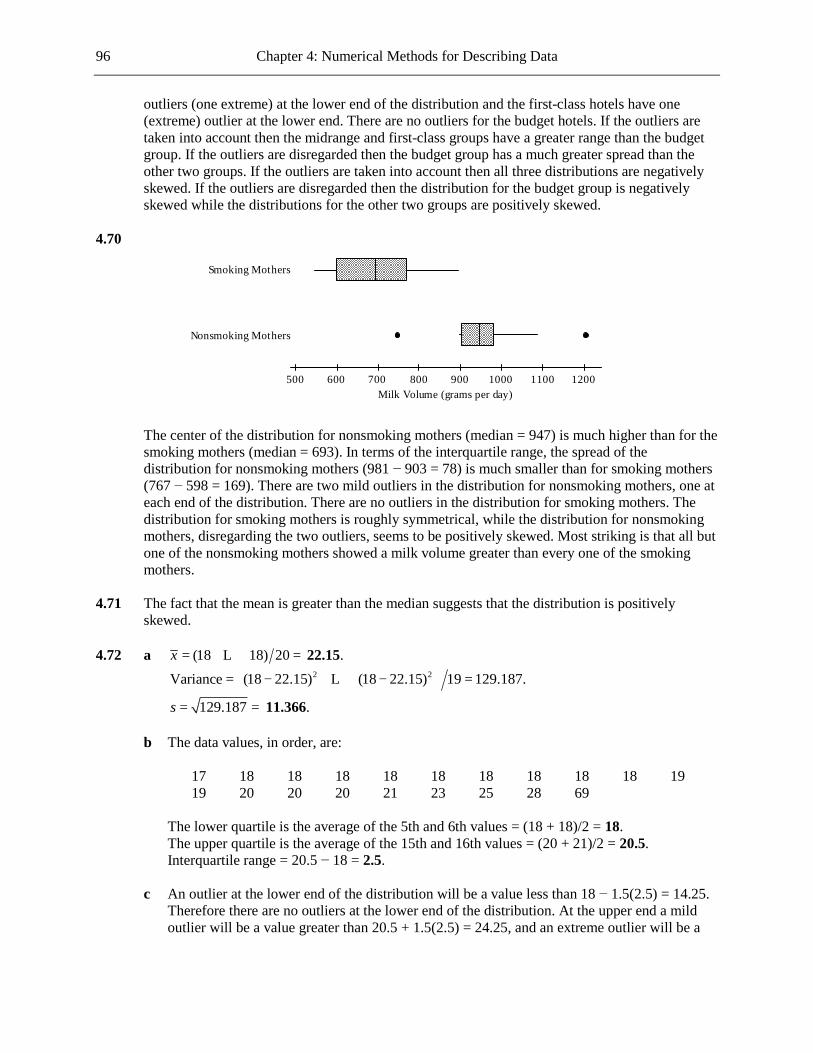
96 Chapter 4: Numerical Methods for Describing Data
outliers (one extreme) at the lower end of the distribution and the first-class hotels have one (extreme) outlier at the lower end. There are no outliers for the budget hotels. If the outliers are taken into account then the midrange and first-class groups have a greater range than the budget group. If the outliers are disregarded then the budget group has a much greater spread than the other two groups. If the outliers are taken into account then all three distributions are negatively skewed. If the outliers are disregarded then the distribution for the budget group is negatively skewed while the distributions for the other two groups are positively skewed.
4.70
Nonsmoking Mothers
Smoking Mothers
120011001000900800700600500Milk Volume (grams per day)
The center of the distribution for nonsmoking mothers (median = 947) is much higher than for the
smoking mothers (median = 693). In terms of the interquartile range, the spread of the distribution for nonsmoking mothers (981 − 903 = 78) is much smaller than for smoking mothers (767 − 598 = 169). There are two mild outliers in the distribution for nonsmoking mothers, one at each end of the distribution. There are no outliers in the distribution for smoking mothers. The distribution for smoking mothers is roughly symmetrical, while the distribution for nonsmoking mothers, disregarding the two outliers, seems to be positively skewed. Most striking is that all but one of the nonsmoking mothers showed a milk volume greater than every one of the smoking mothers.
4.71 The fact that the mean is greater than the median suggests that the distribution is positively
skewed. 4.72 a (18 18) 20x = + + =L 22.15. 2 2Variance (18 22.15) (18 22.15) 19 = − + + − = L 129.187.
129.187s = = 11.366. b The data values, in order, are: 17 18 18 18 18 18 18 18 18 18 19
19 20 20 20 21 23 25 28 69 The lower quartile is the average of the 5th and 6th values = (18 + 18)/2 = 18. The upper quartile is the average of the 15th and 16th values = (20 + 21)/2 = 20.5. Interquartile range = 20.5 − 18 = 2.5. c An outlier at the lower end of the distribution will be a value less than 18 − 1.5(2.5) = 14.25.
Therefore there are no outliers at the lower end of the distribution. At the upper end a mild outlier will be a value greater than 20.5 + 1.5(2.5) = 24.25, and an extreme outlier will be a

Chapter 4: Numerical Methods for Describing Data 97
value greater than 20.5 + 3(2.5) = 28. Thus the values 25 and 28 are mild outliers and 69 is an extreme outlier.
d
70605040302010Age (years)
4.73 a The distribution is roughly symmetrical and 0.84 = 1 − 0.16, and so the 84th percentile is the
same distance above the mean as the 16th percentile is below the mean. The 16th percentile is 20 units below the mean and so the 84th percentile is 20 units above the mean. Therefore the 84th percentile is 120.
b The proportion of scores below 80 is 16% and the proportion above 120 is 16%. Therefore
the proportion between 80 and 120 is 100 − 2(16) = 68%. So by the Empirical Rule 80 and 120 are both 1 standard deviation from the mean, which is 100. This tells us that the standard deviation is approximately 20.
c z = (90 − 100)/20 = −0.5. d A score of 140 is 2 standard deviations above the mean. By the Empirical Rule approximately
5% of scores are more than 2 standard deviations from the mean. So approximately 5/2 = 2.5% of scores are greater than 140. Thus 140 is at approximately the 97.5th percentile.
e A score of 40 is 3 standard deviations below the mean, and so the proportion of scores below
40 would be approximately (100 − 99.7)/2 = 0.15%. Therefore there would be very few scores below 40.

98
Chapter 5 Summarizing Bivariate Data
5.1 Scatterplot 1 (i) Yes (ii) Yes (iii) Positive Scatterplot 2 (i) Yes (ii) Yes (iii) Negative Scatterplot 3 (i) Yes (ii) No (iii) - Scatterplot 4 (i) Yes (ii) Yes (iii) Negative 5.2 a Positive. As temperatures increase, cooling costs are likely to increase. b Negative. As interest rates rise, fewer people are likely to apply for loans. c Positive. Husbands and wives tend to come from similar backgrounds, and therefore have
similar expectations in terms of income. d Close to zero. There is no reason to believe that there is an association between height and
IQ. e Positive. People with large feet tend to be taller than people with small feet. f Positive. People who are smart and/or well educated tend to do well on both sections, with
those lacking these attributes doing less well on both sections. g Negative. Those who spend a lot of time on their homework are likely to spend little time
watching television, and vice versa. h Close to zero. The points in the scatterplot will form an inverted “U” shape, making a
correlation close to zero. 5.3 No. A correlation coefficient of 0 implies that there is no linear relationship between the
variables. There could still be a nonlinear relationship. 5.4 Scatterplot for which r = 1:
x
y

Chapter 5: Summarizing Bivariate Data 99
Scatterplot for which r = −1:
x
y
5.5 a
1701601501401301201101009080
880
860
840
820
800
780
760
740
720
Quality Rating
Satis
fact
ion
Ratin
g
There does not appear to be a relationship between quality rating and satisfaction rating. b r = −0.239. The linear relationship between quality rating and satisfaction rating is weak and
negative. 5.6 a Using a calculator or statistical software package we get r = 0.204. There is a weak positive
linear relationship between cost per serving and fiber per serving. b Using a calculator or statistical software package we get r = 0.241. This correlation
coefficient is slightly greater than the correlation coefficient for the per serving data. 5.7 a There is a weak negative linear relationship between average hopping height and arch height.
The negative correlation tells us that large arch heights are (weakly) associated with small hopping heights, and vice versa.
b Yes. Since all five correlation coefficients are close to zero, the results imply that there is
very little relationship between arch height and the motor skills measured.

100 Chapter 5: Summarizing Bivariate Data
5.8 The fact that the correlation coefficient for college GPA and academic self worth was 0.48 tells us that among these athletes there was a weak to moderate positive linear relationship between GPA and self worth. Those with higher grades tended to feel better about themselves in an academic sense than those with lower grades. The correlation coefficient of 0.46 between college GPA and high school GPA gives us the same information about those variables. However, the correlation coefficient of −0.36 between college GPA and the procrastination measure tells us that there was a weak negative linear relationship between those variables. Those who had a tendency to procrastinate generally speaking had lower grades than those without that tendency.
5.9 a Using a calculator or statistical software package we get r = 0.118. b
8.07.57.06.56.0
6.3
6.2
6.1
6.0
5.9
5.8
5.7
Consumer Debt
Household Debt
Yes. Looking at the scatterplot there does not seem to be a strong relationship between the
variables. 5.10 a 0.335.r = There is a weak positive linear relationship between timber sales and acres burned. b It does seem that heavier logging was (weakly) associated with larger forest fires, however it
is not justified to claim that the greater logging caused the larger fires. 5.11
2 2
(88.8)(86.1)281.1 85.05739 .(9.263)(9.824)88.8 86.1288 286.6
39 39
r−
= = =
− −
0.935
There is a strong positive linear relationship between the concentrations of neurolipofuscin in the
right and left eye storks. 5.12 No, because “artist” is a categorical variable. 5.13 The time needed is related to the speed by the equation

Chapter 5: Summarizing Bivariate Data 101
distancetimespeed
= ,
where the distance is constant. Using this relationship, and plotting the times (over a fixed
distance) for various feasible speeds, a scatterplot is obtained like the one below.
Speed
Time
These points show a strong negative correlation, and therefore the correlation coefficient is most
likely to be close to −0.9. 5.14 Scatterplot 1 seems to show a linear relationship between x and y, while Scatterplot 2 shows a
curved relationship between the two variables. So it makes sense to use the least squares regression line to summarize the relationship between x and y for the data set in Scatterplot 1, but not for the data set in Scatterplot 2.
5.15 a The equation of the least squares regression line is ˆ 11.482 0.970y x= + , where x = mini-
Wright meter reading and y = Wright meter reading. b When x = 500, y = 496.454 . The least squares regression line predicts a Wright meter
reading of 496.454 for a person whose mini-Wright meter reading was 500. c When x = 300, y = 302.465 . The least squares regression line predicts a Wright meter
reading of 302.465 for a person whose mini-Wright meter reading was 500. However, 300 is well outside the range of mini-Wright meter readings in the data set, so this prediction involves extrapolation and is therefore not reliable.

102 Chapter 5: Summarizing Bivariate Data
5.16 a
20.017.515.012.510.07.55.0
0.3
0.2
0.1
0.0
-0.1
-0.2
Mean Temperature
Net Directionality
There is one point, (8.06, 0.25), which is separated from the general pattern of the data. If this
point is disregarded then there is a somewhat strong positive linear relationship between mean temperature and net directionality. Even if this point is included, there is still a moderate linear relationship between the two variables.
b Using a calculator or statistical software package we find that the equation of the least-
squares regression line is ˆ 0.14282 0.016141y x= − + , where x = mean water temperature and y = net directionality.
c When x = 15, ˆ 0.14282 0.016141(15)y = − + = 0.0993 . d The scatterplot and the least-squares line support the fact that, generally speaking, the higher
the temperature the greater the proportion of larvae that were captured moving upstream. e Approximately the same number of larvae moving upstream as downstream is represented by
a net directionality of zero. According to the least-squares line this will happen when the mean temperature is approximately 8.8°C.
5.17 a The dependent variable is the number of fruit and vegetable servings per day, and the
predictor variable is the number of hours of television viewed per day. b Negative. As the number of hours of TV watched per day increases, the number of fruit and
vegetable servings per day (on average) decreases. 5.18 a Negative. As the patient-to-nurse ratio increases we would expect nurses’ stress levels to
increase and therefore their job satisfaction to decrease. b Negative. As the patient-to-nurse ratio increases we would expect patient satisfaction to
decrease. c Negative. As the patient-to-nurse ratio increases we would expect quality of care to decrease.

Chapter 5: Summarizing Bivariate Data 103
5.19 The equation of the least-squares regression line is ˆ 0.884 0.699y x= + , where x = passenger
complaint rank and y = J.D. Powers quality score. 5.20 When x = 3, ˆ 2.982y = , and when x = 9, ˆ 7.178y = . The J.D. Powers quality scores predicted for
Hawaiian Airlines and Northwest Airlines are 2.982 and 7.178, respectively. 5.21 a
12108642
90
80
70
60
50
40
30
20
10
0
Mean Call-to-Shock Time (minutes)
Survival Rate (percent)
There is a strong negative relationship between mean call-to-shock time and survival rate.
The relationship is close to being linear, particularly if the point with the highest x value is disregarded. If that point is included then there is the suggestion of a curve.
b ˆ 101.32847 9.29562y x= − , where x is the mean call-to-shock time and y is the survival rate. c When x = 10, ˆ 101.32847 9.29562(10) .y = − = 8.372 5.22 Since the slope of the least-squares line is −9.30, we can say that every extra minute waiting for
paramedics to arrive with a defibrillator lowers the chance of survival by 9.3 percentage points. 5.23 The slope would be −4000, since the slope of the least-squares line is the increase in the average y
value for each increase of one unit in x. Here the average home price decreases by $4000 for each increase of 1 mile in the distance east of the bay.
5.24 a Using a calculator or a statistical software package we find that the correlation coefficient
between sale price and size is 0.700. There is a moderate linear relationship between sale price and size.
b Using a calculator or a statistical software package we find that the correlation coefficient
between sale price and land-to-building ratio is −0.332. There is a weak negative linear relationship between sale price and land-to-building ratio.
c Size is the better predictor of sale price since the absolute value of the correlation between
sale price and size is closer to 1 than the absolute value of the correlation between sale price and land-to-building ratio.

104 Chapter 5: Summarizing Bivariate Data
d Using a calculator or statistical software package we find that the least-squares regression line for predicting y = sale price from x = size is ˆ 1.3281 0.0053y x= + .
5.25 The least-squares line is based on the x values contained in the sample. We do not know that the
same linear relationship will apply for x values outside this range. Therefore the least-squares line should not be used for x values outside the range of values in the sample.
5.26 a Since the x value is 2 standard deviations above the mean, the y value will be
2 (0.75)(2) 1.5r ⋅ = = standard deviations above the mean. b 1 1.5 .r = = 0.667 5.27 We know (as stated in the text) that ( / )y xb r s s= , where ys and xs are the standard deviations of
the y values and the x values, respectively. Since standard deviations are always positive we know that b and r must always have the same sign.
5.28 a Since all the y values are multiplied by 0.4536, all the predicted y values will be multiplied by
the same factor. Therefore, for the new y values, the least-squares line is ˆ 0.4536( 936.22 8.577 ) 424.67 3.89 .y x x= − + = − +
b Since each y value is multiplied by c, y will be multiplied by c, also. Thus
( )2 2
( )( )( )( )(New ) (Old )
( ) ( )
c x x y yx x cy cyb c b
x x x x
− −− −= = =
− −∑∑
∑ ∑.
Also, (New ) ( ) (Old ).a cy cbx c y bx c a= − = − = Thus a and b are both multiplied by c. This verifies the notion that the whole right side of the
regression equation is multiplied by c. 5.29 a The equation of the least squares regression line is ˆ 9.071 1.571y x= − + , where x = years of
schooling and y = median hourly wage gain. When x = 15, y = 14.5 . The least squares regression line predicts a median hourly wage gain of 14.5 percent for the 15th year of schooling.
b The actual wage gain percent is very close to the value predicted in Part (a).
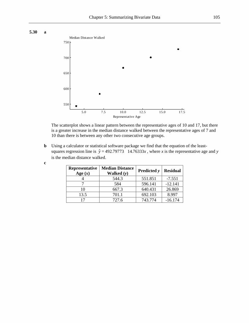
Chapter 5: Summarizing Bivariate Data 105
5.30 a
17.515.012.510.07.55.0
750
700
650
600
550
Representative Age
Median Distance Walked
The scatterplot shows a linear pattern between the representative ages of 10 and 17, but there
is a greater increase in the median distance walked between the representative ages of 7 and 10 than there is between any other two consecutive age groups.
b Using a calculator or statistical software package we find that the equation of the least-
squares regression line is ˆ 492.79773 14.76333y x= + , where x is the representative age and y is the median distance walked.
c Representative
Age (x) Median Distance
Walked (y) Predicted y Residual
4 544.3 551.851 -7.551 7 584 596.141 -12.141
10 667.3 640.431 26.869 13.5 701.1 692.103 8.997 17 727.6 743.774 -16.174

106 Chapter 5: Summarizing Bivariate Data
17.515.012.510.07.55.0
30
20
10
0
-10
-20
Representative Age
Residual
The residual plot reflects the sharp increase in the median distance walked between the
representative ages of 7 and 10, with a clear negative residual at 7x = and large positive residual at 10x = .
5.31 a
17.515.012.510.07.55.0
680
660
640
620
600
580
560
540
520
500
Representative Age
Median Six-Minute Walk Distance
b In the last three age categories, the median distance walked for girls increases only slightly,
whereas for boys it increases at a rate only slightly smaller than the rate that applies to the first two age categories. Also, the scatterplot for the girls shows clearer evidence of a curved relationship between the variables than does the scatterplot for the boys.
c ˆ 479.997 12.525y x= + , where x is the representative age and y is the median distance
walked.

Chapter 5: Summarizing Bivariate Data 107
d
Representative Age (x)
Median Distance Walked (y) Predicted y Residual
4 492.4 530.095 -37.695 7 578.3 567.669 10.631
10 655.8 605.243 50.557 13.5 657.6 649.079 8.521 17 660.9 692.915 -32.015
17.515.012.510.07.55.0
50
25
0
-25
-50
Representative Age
Residual
e The authors’ decision to use a curve is supported by the clear curved pattern in the residual
plot. 5.32 a
0.250.200.150.100.050.00
0.125
0.100
0.075
0.050
0.025
0.000
-0.025
-0.050
Nitrogen Intake (grams)
Nitrogen Retention (grams)
b ˆ 0.03443 0.58026y x= − + , where x is the nitrogen intake and y is the nitrogen retention.

108 Chapter 5: Summarizing Bivariate Data
c When x = 0.06, ˆ 0.03443 0.58026(0.06)y = − + = 0.00039 . d ˆResidual 0.01 0.00039 .y y= − = − = 0.00961 e The observation (0.25, 0.11) is potentially influential since its x value is far separated from
the x values of the other points. f Using the new regression equation, when x = 0.06, ˆ 0.037 0.627(0.06) .y = − + = 0.00062 The
difference between the two predictions is 0.00062 − 0.00039 = 0.00023. This is only a small difference.
5.33 a The equation of the least-squares regression line is ˆ 232.258 2.926y x= − , where x = rock
surface area and y = algae colony density. b 2r = 0.300 . Thirty percent of the variation in algae colony density can be attributed to the
approximate linear relationship between rock surface area and algae colony density. c es = 63.315 . This is a typical deviation of an algae colony density value from the value
predicted by the least-squares regression line. d r = −0.547. The linear relationship between rock surface area and algae colony density is
moderate and negative. 5.34 a
20000150001000050000
80
70
60
50
40
30
20
Total Number
Percent Transported
b Yes, there appears to be a strong linear relationship between the total number of salmon in the
stream and the percent of salmon killed by bears that are transported away from the stream. c The equation of the least-squares regression line is ˆ 18.483 0.00287y x= + , where x is the
total number of salmon in a creek and y is the percent of salmon killed by bears that were transported away from the stream prior to the bear eating. The regression line has been drawn on the scatterplot in Part (a).

Chapter 5: Summarizing Bivariate Data 109
d The point (3928, 46.8) is unlikely to be influential as its x value does not differ greatly from
the others in the data set. e The two points are not influential since the least-squares line provides a good fit for the
remaining 8 points. Removing the two points will make only a small change in the regression line.
f .es = 9.16217 This is a typical deviation of a percent transported value from the value
predicted by the regression line. g 2 .r = 0.832 This is a large value of 2r , and means that 83.2% of the variation in the percent
transported values can be attributed to the approximate linear relationship between total number and percent transported.
5.35 a ˆ 4788.839 29.015y x= − , where x is the representative age and y is the average swim
distance. b
Representative Age (x)
Average Swim Distance (y) Predicted y Residual
25 3913.5 4063.464 −149.964 35 3728.8 3773.314 −44.514 45 3579.4 3483.164 96.236 55 3361.9 3193.014 168.886 65 3000.1 2902.864 97.236 75 2649 2612.714 36.286 85 2118.4 2322.564 −204.164
9080706050403020
200
100
0
-100
-200
Representative Age
Residual
c The clear curve in the residual plot suggests that a linear model is not appropriate for the
relationship between representative age and swim distance. d No. The least-squares line in Part (a) was calculated using the data for men, and we have no
reason to believe that this line will also apply to women.

110 Chapter 5: Summarizing Bivariate Data
5.36 a The observation for Hospital 11 is unlikely to be particularly influential, since its x value is not extreme in either direction. Removal of this point changes the slope of the least-squares regression line from 1.29 to 1.51, which is not a large change, and so the point is not influential.
b It is clear that the point for Hospital 11 will have a large residual when the least-squares
regression line is drawn. Thus this point is an outlier. c When ˆ75, 1.1 1.29(75) 95.65x y= = − + = . Since the y value for Hospital 5 is not far from the
value predicted by the least-squares regression line, the point for Hospital 5 is not influential. d Since the y value for Hospital 5 is not far from the value predicted by the least-squares
regression line, the point for Hospital 5 does not have a large residual, and therefore is not considered an outlier.
5.37 a The value of 2r would be 0.154. b No, since the 2r value for y = first year college GPA and x = SAT II score was 0.16, which is
not large. Only 16% of the variation in first year college GPA could be attributed to the approximate linear relationship between SAT II score and first year college GPA.
5.38 a The equation of the least-squares regression line is ˆ 1.339 0.00766 ,y x= − where x =
perceived stress and y = telomere length. b 2 .r = 0.099 c The linear relationship accounts for only 9.9% of the variability in telomere length. This is a
small proportion. 5.39 a
7000006000005000004000003000002000001000000
150
125
100
75
50
Total Park Size (Acres)
Number of Employees

Chapter 5: Summarizing Bivariate Data 111
b Using a graphing calculator or computer software package we see that the equation of the
least-squares line is ˆ 85.334 0.0000259y x= − , where x is the total park size in acres and y is the number of employees.
c 2r = 0.016. With only 1.6% of the variation of the number of employees being attributable to
the least-squares line, the line will not give accurate predictions. d Deleting the point (620231, 67), the equation of the least-squares line is now
ˆ 83.402 0.0000387y x= + . Yes, removal of the point does greatly affect the equation of the line, since it changes the slope from negative to positive.
5.40 a The equation of the least-squares regression line is ˆ 27.709 0.201 ,y x= + where y = percent of
operating costs covered by park revenues and x = number of employees. b Since 2 0.053,r = we know that only 5.3% of the variability in operating costs is attributable
to the least-squares regression line. Therefore the least-squares line does not do a good job of describing the relationship. Also, with 24.148es = being of the same order of size as the y values themselves, we see again that the line does not do a good job of describing the relationship.
c The points (69, 80), (87, 97), and (112, 108) are outliers. No, the three observations with the
largest residuals are not for the three districts with the largest numbers of employees. However, generally speaking districts with larger numbers of employees tend to have larger residuals.
5.41 The coefficient of determination is ( ) ( )2 1 SSResid SSTo 1 1235.470 25321.368 .r = − = − = 0.951
This tells us that 95.1% of the variation in hardness is attributable to the approximate linear relationship between time elapsed and hardness.
5.42 a For a given value of 2r a scatterplot can be constructed with any value of es you care to
specify. For example, suppose you have a scatterplot with 2 0.984r = and 0.42.es = If you multiply the y values by 10 you obtain a scatterplot with 2 0.984r = and 4.2.es = If you multiply the original y values by 100 you obtain a scatterplot with 2 0.984r = and 42.es = Likewise, by multiplying the y values by a positive number less than 1 you obtain a scatterplot with a smaller value of es .
Now, suppose that you were using a least-squares line to predict the prices, y, of objects that cost in the region of $3. A value of es of around 0.8 would be considered large, since this means that the deviations of the true prices from predicted prices tend to be around 80 cents, which is quite a large amount when the prices of the objects are around $3. If, however, the least-squares line were being used to predict the prices of objects that cost in the region of $300, then a value of es of around 0.8 would be considered small. Thus we can conclude that, for a given value of 2 ,r however large or small, it is possible to have both large and small values of es .
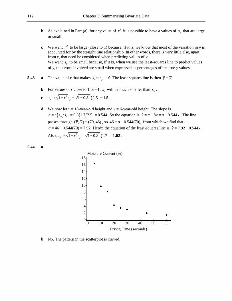
112 Chapter 5: Summarizing Bivariate Data
b As explained in Part (a), for any value of 2r it is possible to have a values of es that are large or small.
c We want 2r to be large (close to 1) because, if it is, we know that most of the variation in y is
accounted for by the straight line relationship. In other words, there is very little else, apart from x, that need be considered when predicting values of y. We want es to be small because, if it is, when we use the least-squares line to predict values of y, the errors involved are small when expressed as percentages of the true y values.
5.43 a The value of r that makes e ys s≈ is 0. The least-squares line is then y y= . b For values of r close to 1 or −1, es will be much smaller than ys .
c ( )2 21 1 0.8 2.5e ys r s≈ − = − = 1.5 . d We now let x = 18-year-old height and y = 6-year-old height. The slope is
( ) ( )0.8 1.7 2.5 0.544.y xb r s s= = = So the equation is ˆ 0.544y a bx a x= + = + . The line passes through ( , ) (70, 46)x y = , so 46 0.544(70),a= + from which we find that
46 0.544(70) 7.92.a = − = Hence the equation of the least-squares line is ˆ 7.92 0.544y x= + .
Also, ( )2 21 1 0.8 1.7e ys r s≈ − = − = 1.02 . 5.44 a
6050403020100
18
16
14
12
10
8
6
4
2
0
Frying Time (seconds)
Moisture Content (%)
b No. The pattern in the scatterplot is curved.

Chapter 5: Summarizing Bivariate Data 113
c
1.81.61.41.21.00.80.6
1.2
1.0
0.8
0.6
0.4
0.2
0.0
Log(x)
Log(y)
The relationship between log(x) and log (y) seems to be linear. d The value of r2 is large (0.973) and the value of se is relatively small (0.0657), indicating that
a line is a good fit for the data. e The regression equation is
Predicted(log( )) 2.01780 1.05171 log( )y x= − ⋅ . When x = 35, log(x) = 1.544. So then,
Predicted(log( )) 2.01780 1.05171 1.544 0.394y = − ⋅ = So 0.394ˆ 10 2.477y = = . The predicted moisture content for a frying time of 35 seconds is
2.477%. 5.45 a
76543210
70
60
50
40
30
20
10
0 x
y

114 Chapter 5: Summarizing Bivariate Data
There seems to be a curved relationship between the two variables. b
2.52.01.51.00.50.0
9
8
7
6
5
4
3
2
sqrt(x)
sqrt(y)
The curved pattern is not as pronounced as in the scatterplot from Part (a), but there is still
curvature in the plot. c Answers will vary. One possible answer is to use ' log( )y y= and ' log( )x x= . (See
scatterplot below.)
2.52.01.51.00.50.0
2.00
1.75
1.50
1.25
1.00
0.75
0.50
sqrt(x)
log(y)
This transformation would be preferred over the transformation in Part (b) because this
scatterplot is closer to being linear. 5.46 Answers will vary. Scatterplot (b) shows a curve that tends to follow the pattern of points in the
scatterplot.

Chapter 5: Summarizing Bivariate Data 115
5.47 a
2.52.01.51.00.5
100
90
80
70
60
50
40
30
Energy of Shock
Success (%)
The relationship appears to be nonlinear. b ˆ 22.48 34.36y x= + . The residuals are: −6.36, 1.46, 7.78, 5.5, −8.38.
2.52.01.51.00.5
10
5
0
-5
-10
Energy of Shock
Residual
Yes. There is a curved pattern in the residual plot. c The residual plot for the square root transformation is shown below.

116 Chapter 5: Summarizing Bivariate Data
1.61.41.21.00.80.6
5.0
2.5
0.0
-2.5
-5.0
Sqrt(x)
Residual
The residual plot for the natural log transformation is shown below.
1.00.50.0-0.5
4
3
2
1
0
-1
-2
-3
-4
-5
Ln(x)
Residual
The residual plot for the square root transformation shows a curved pattern of points, while
the residual plot for the natural log transformation shows what would seem to be a random scatter of points. So the log transformation is more successful in producing a linear relationship.
d The regression equation is ˆ 62.417 43.891 ln( )y x= + ⋅ . e When x = 1.75, ˆ 62.417 43.891 ln(1.75) 86.979y = + ⋅ = . The predicted success level is
86.979%. When x = 0.8, ˆ 62.417 43.891 ln(0.8) 52.623y = + ⋅ = . The predicted success level is 52.623%.

Chapter 5: Summarizing Bivariate Data 117
5.48 a
1086420
70
60
50
40
30
20
Year
Number Waiting for Transplant (thousands)
From 1990 to 1999 the number of people waiting for transplants increased, with the number
increasing by a greater amount each year. b After much trial and error it is found that the transformation 0.15y y′ = (with x x′ = ) produces
a linear pattern in the scatterplot and a random pattern in the residual plot. The scatterplot is shown below.
1086420
1.90
1.85
1.80
1.75
1.70
1.65
1.60
Year
(Number Waiting) ^ (0.15)
c The least-squares line relating the transformed variables is 0.15ˆ 1.552753 0.034856y x= + ,
where x is the year (1990 represented by 1) and y is the number waiting (in thousands). When x = 11, 0.15ˆ 1.552753 0.034856(11) 1.936164y = + = . From this,
1 0.15ˆ (1.936164) 81.837y = = . The least-squares line predicts that in 2000 the number of patients waiting will be around 81,800.
d We have to be confident that the pattern observed between 1990 and 1999 will continue up to
2000. This is reasonable so long as circumstances remain basically the same. To expect the same pattern to continue to 2010, however, would be unreasonable.
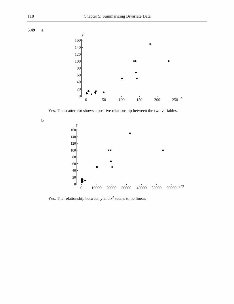
118 Chapter 5: Summarizing Bivariate Data
5.49 a
250200150100500
160
140
120
100
80
60
40
20
0 x
y
Yes. The scatterplot shows a positive relationship between the two variables. b
6000050000400003000020000100000
160
140
120
100
80
60
40
20
0 x^2
y
Yes. The relationship between y and x2 seems to be linear.

Chapter 5: Summarizing Bivariate Data 119
c
250200150100500
2.25
2.00
1.75
1.50
1.25
1.00
0.75
0.50 x
log(y)
This transformation straightens the plot. In addition, the variability in log(y) does not seem to
increase as x increases, as was the case in Part (b). d
6000050000400003000020000100000
2.25
2.00
1.75
1.50
1.25
1.00
0.75
0.50 x^2
log(y)
No. There is obvious curvature in the scatterplot.

120 Chapter 5: Summarizing Bivariate Data
5.50
6543210
700
600
500
400
300
200
100
0
Age (years)
Canal Length (mm)
The relationship between age and canal length is not linear. A transformation that makes the plot
roughly linear is 1x x′ = (with y y′ = ). The resulting scatterplot and residual plot are shown below.
2.001.751.501.251.000.750.50
700
600
500
400
300
200
100
0
Age^(-0.5)
Canal Length (mm)

Chapter 5: Summarizing Bivariate Data 121
2.001.751.501.251.000.750.50
100
50
0
-50
-100
-150
Age^(-0.5)
Residual
5.51 a Any image plotted between the dashed lines would be associated with Cal Poly by roughly
the same percentages of enrolling and non-enrolling students. b The images that were more commonly associated with non-enrolling students than with
enrolling students were “Average,” “Isolated,” and “Back-up school,” with “Back-up school” being the most common of these amongst non-enrolling students. The images that were more commonly associated with enrolling students than with non-enrolling students were (in increasing order of commonality amongst enrolling students) “Excitingly different,” “Personal,” “Selective,” “Prestigious,” “Exciting,” “Intellectual,” “Challenging,” “Comfortable,” “Fun,” “Career-oriented,” “Highly respected,” and “Friendly,” with this last image being marked by over 60% of students who enrolled and over 45% of students who didn’t enroll. The most commonly marked image amongst students who didn’t enroll was “Career-oriented.”
5.52
1101009080706050403020
30
25
20
15
10
Speed (mph)
Fuel Efficiency (mpg)

122 Chapter 5: Summarizing Bivariate Data
As illustrated in the graph above, it is quite possible that the relationship between speed and fuel efficiency is modeled by a curve (in particular, by a quadratic curve), and that for greater speeds the fuel efficiency is negatively related to the speed.
5.53 a 0.89 .r = = 0.943 (Note that r is 0.943 rather than −0.943 since the slope of the least-
squares line is positive.) There is a very strong positive linear relationship between assault rate and lead exposure 23 years prior. No, we cannot conclude that lead exposure causes increased assault rates, since the value of r close to 1 tells us that there is a strong linear association between lead exposure and assault rate, but tells us nothing about causation.
b The equation of the least-squares regression line is ˆ 24.08 327.41y x= − + , where y is the
assault rate and x is the lead exposure 23 years prior. When x = 0.5, ˆ 24.08 327.41(0.5)y = − + 139.625= assaults per 100,000 people.
c 89% of the year-to-year variability in assault rates can be explained by the relationship
between assault rate and gasoline lead exposure 23 years earlier. d The two time series plots, generally speaking, move together. That is, generally when one
goes up the other goes up and when one goes down the other goes down. Thus high assault rates are associated with high lead exposures 23 years earlier and low assault rates are associated with low lead exposures 23 years earlier.
5.54 Consider the scatterplot for the combined group. Between x = 0 and x = 1 the points form an
approximately linear pattern with a slope of 6.93, while between x = 1 and x = 10 the points form an approximately linear pattern with a slope of just over 3. Clearly this pattern could not be modeled with a single straight line; a curve would be more appropriate.
5.55 a r = −0.981. This suggests a very strong linear relationship between the amount of catalyst and
the resulting reaction time. b
54321
50
45
40
35
30
25
Amount of Catalyst
Reaction Time
The word linear does not provide the most effective description of the relationship. There are
curves that would provide a much better fit.

Chapter 5: Summarizing Bivariate Data 123
5.56 a .r = 0.944 There is a strong, positive linear relationship between depression rate and sugar
consumption. b No. Since this was an observational study, no conclusion relating to causation may be drawn. c Yes. Since the set of countries used was not a random sample from the set of all countries
(nor do we have any reason to think that these countries are representative of the set of all countries), we cannot generalize the conclusions to countries in general.
5.57 a
2520151050
80
70
60
50
40
Test Anxiety
Exam Score
There is one point, (0, 77), that is far separated from the other points in the plot. There is a
clear negative relationship between scores on the measure of test anxiety and exam scores. b There appears to be a very strong negative linear relationship between test anxiety and exam
score. (However, without the point (0, 77) the relationship would be significantly less strong.) c r = −0.912. This is consistent with the observations given in Part (b). d No, we cannot conclude that test anxiety caused poor exam performance. Correlation
measures the strength of the linear relationship between the two variables, but tells us nothing about causation.

124 Chapter 5: Summarizing Bivariate Data
5.58 a
1211109876
90
80
70
60
50
40
30
Grade
Percentage More Likely to Purchase
Yes, the relationship appears linear. b The equation of the least-squares line is ˆ 22.37 9.08y x= − + , where x = grade and y =
percentage who said they were more likely to purchase. 5.59 a
2422201816141210
40
35
30
25
20
15
10
4th Grade (1996)
8th Grade (2000)
There is a clear positive relationship between the percentages of students who were proficient
at the two times. There is the suggestion of a curve in the plot. b The equation of the least-squares line is ˆ 3.13603 1.52206y x= − + , where x is the percentage
proficient in 4th grade (1996) and y is the percentage proficient in 8th grade (2000). c When x = 14, ˆ 3.13603 1.52206(14)y = − + = 18.173 . This is slightly lower than the actual
value of 20 for Nevada.

Chapter 5: Summarizing Bivariate Data 125
5.60 a
1086420
22
21
20
19
18
17
16
15
Year
Number of Transplants (thousands)
The equation of the least-squares line is ˆ 14.213 0.790y x= + , where x = year and y = number
of transplants performed (in thousands). b From 1990 to 1999 the number of transplants increased at a roughly constant rate. c
Year
Number of Transplants
Residual
1 15.0 −0.004 2 15.7 −0.094 3 16.1 −0.484 4 17.6 0.225 5 18.3 0.135 6 19.4 0.445 7 20.0 0.255 8 20.3 −0.236 9 21.4 0.074 10 21.8 −0.316

126 Chapter 5: Summarizing Bivariate Data
1086420
0.50
0.25
0.00
-0.25
-0.50
Year
Residual
d There is no strong enough pattern in the residual plot to indicate that a straight line model
would be inappropriate. 5.61 a When x = 25, ˆ 62.9476 0.54975(25) 49.204y = − = . So the residual is
ˆ 70 49.204y y− = − = 20.796 . b 0.57r = − = -0.755 (The correlation coefficient is negative since the slope of the least-
squares regression line is negative.) c We know that 2 1 SSResid SSTor = − . Solving for SSResid we get
2SSResid SSTo(1 ) 2520(1 0.57) 1083.6r= − = − = . Therefore SSResid ( 2) 1083.6 8es n= − = = 11.638 .
5.62 a
76543210
70
60
50
40
30
20
10
0
Salmon Availability
Percentage of Eagles in the Air

Chapter 5: Summarizing Bivariate Data 127
There seems to be a curved relationship between percentage of eagles in the air and salmon
availability. b The scatterplot in Part (c) shows that the transformation is partially successful in finding a
linear relationship. c
98765432
2.5
2.0
1.5
1.0
0.5
0.0
sqrt(y)
sqrt(x)
Yes, the plot is straighter than the one in Part (a). d Taking the cube roots of both variables might be successful in straightening the plot. (In fact,
this transformation does seem to result in a more linear relationship, as shown in the scatterplot below.)
4.03.53.02.52.0
2.0
1.5
1.0
0.5
0.0
cube root (y)
cube root (x)
5.63 a 0.717r = −
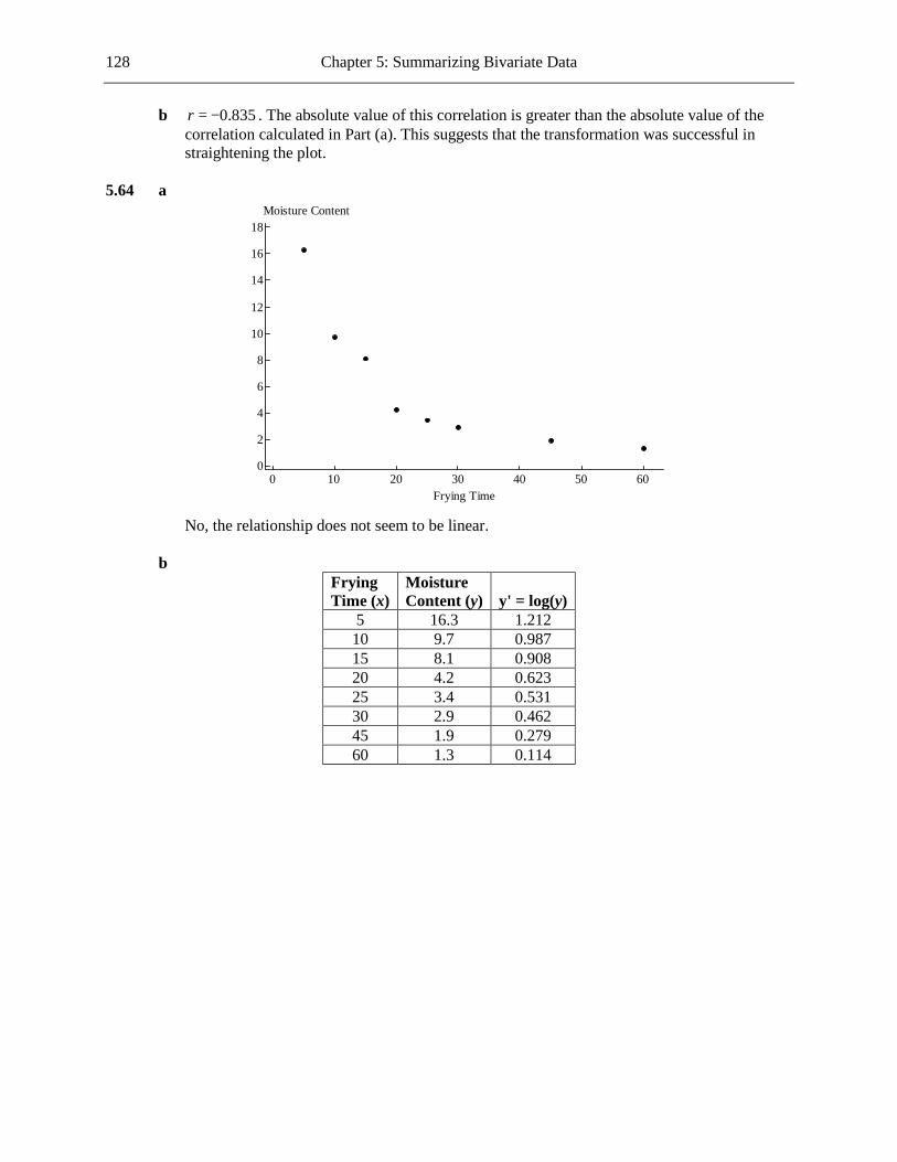
128 Chapter 5: Summarizing Bivariate Data
b 0.835r = − . The absolute value of this correlation is greater than the absolute value of the correlation calculated in Part (a). This suggests that the transformation was successful in straightening the plot.
5.64 a
6050403020100
18
16
14
12
10
8
6
4
2
0
Frying Time
Moisture Content
No, the relationship does not seem to be linear. b
Frying Time (x)
Moisture Content (y)
y' = log(y)
5 16.3 1.212 10 9.7 0.987 15 8.1 0.908 20 4.2 0.623 25 3.4 0.531 30 2.9 0.462 45 1.9 0.279 60 1.3 0.114

Chapter 5: Summarizing Bivariate Data 129
6050403020100
1.2
1.0
0.8
0.6
0.4
0.2
0.0
Frying Time
Log(y)
Yes, the transformed relationship is closer to being linear than the relationship shown in Part
(a). c The least-squares line predicts 1.143 0.0192y x′ = − , where x = frying time and y′ is
log(moisture content). d For x = 35, the least-squares line predicts log 1.143 0.0192(35) 0.472.y y′ = = − = So the
predicted moisture content is 0.47210 %= 2.964 . 5.65 a
100806040200
70
60
50
40
30
20
10
x
y

130 Chapter 5: Summarizing Bivariate Data
2.01.51.00.50.0-0.5
70
60
50
40
30
20
10
log(x)
y
2.01.51.00.50.0-0.5
1.8
1.7
1.6
1.5
1.4
1.3
1.2
1.1
1.0
log(x)
log(y)
3.53.02.52.01.51.00.50.0
0.10
0.09
0.08
0.07
0.06
0.05
0.04
0.03
0.02
0.01
1/x
1/y
Chapter 5: Summarizing Bivariate Data 131
b Plotting log( )y against log( )x does the best job of producing an approximately linear
relationship. The least-squares line of log( )y on log( )x is ˆlog( ) 1.61867 0.31646log( )y x= − . So when x = 25, ˆlog( ) 1.61867 0.31646log(25) 1.17629y = − = . Therefore
1.17629ˆ 10 15.007y = = . The predicted lead content is 15.007 parts per million. 5.66 a Initially the scatterplot might suggest a linear relationship between the variables, but it
becomes clear that this relationship is dependent on one highly influential point. If that point is removed the scatterplot suggests very little relationship between the variables.
b The equation of the least-squares line is ˆ 11.37 1.0906y x= − + , where x = treadmill
consumption and y = fire-suppression simulation consumption. When x = 40, ˆ 11.37 1.0906(40) ml per kg per min.y = − + = 32.254
c Since 2 0.595,r = we know that 59.5% of the variation in fire-suppression simulation
consumption is accounted for by the approximate straight line relationship between the two variables. This is a reasonably high percentage, but it should be remembered that this linear relationship is entirely dependent on the one influential point.
d The new regression equation is ˆ 36.418 0.198y x= − and the new value of 2r is 0.027. The
large change in the slope of the regression line shows how very influential the point for Firefighter 1 was, and the very small new value of 2r tells us that there is effectively no linear relationship between the two variables when the data point for Firefighter 1 is omitted.
5.67 a r = 0 b For example, adding the point (6, 1) gives 0.510r = . (Any y-coordinate greater than 0.973
will work.) c For example, adding the point (6, −1) gives 0.510r = − . (Any y-coordinate less than −0.973
will work.) Online Exercises 5.68 The least-squares line for the transformed data is 4.587 0.0658y x′ = − , where x is the peak
intake. Thus the logistic regression equation is 4.587 0.0658
4.587 0.0658 .1
x
xep
e
−
−=+
For 40,x = the equation predicts 4.587 0.0658(40)
4.587 0.0658(40) 0.876.1
epe
−
−= =+
5.69 Calculating the least-squares line for ( )ln (1 )y p p′ = − against x = high school GPA we get
2.89399 1.70586y x′ = − + . Thus the logistic regression equation is 2.89399 1.70586
2.89399 1.70586 .1
x
xep
e
− +
− +=+
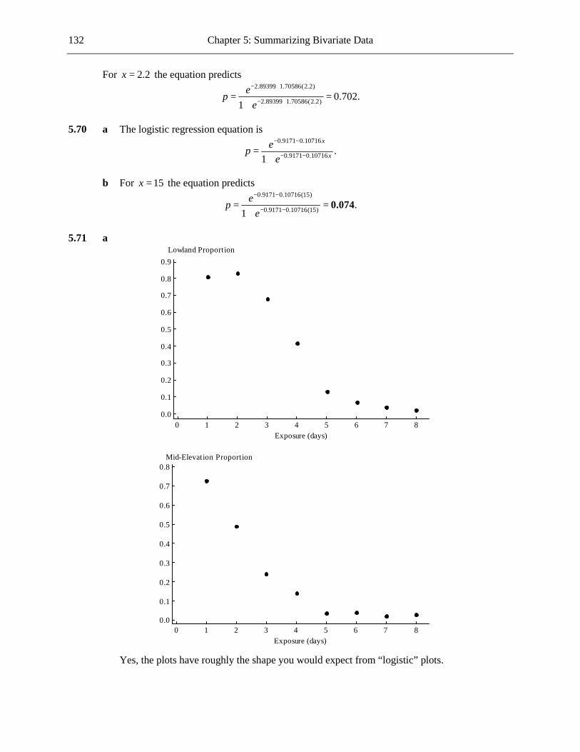
132 Chapter 5: Summarizing Bivariate Data
For 2.2x = the equation predicts 2.89399 1.70586(2.2)
2.89399 1.70586(2.2) 0.702.1
epe
− +
− += =+
5.70 a The logistic regression equation is
0.9171 0.10716
0.9171 0.10716 .1
x
xep
e
− −
− −=+
b For 15x = the equation predicts
0.9171 0.10716(15)
0.9171 0.10716(15) .1
epe
− −
− −= =+
0.074
5.71 a
876543210
0.9
0.8
0.7
0.6
0.5
0.4
0.3
0.2
0.1
0.0
Exposure (days)
Lowland Proportion
876543210
0.8
0.7
0.6
0.5
0.4
0.3
0.2
0.1
0.0
Exposure (days)
Mid-Elevation Proportion
Yes, the plots have roughly the shape you would expect from “logistic” plots.

Chapter 5: Summarizing Bivariate Data 133
b
Exposure (days) (x) Cloud Forest Proportion (p) y' = ln(p/(1−p)) 1 0.75 1.09861 2 0.67 0.70819 3 0.36 -0.57536 4 0.31 -0.80012 5 0.14 -1.81529 6 0.09 -2.31363 7 0.06 -2.75154 8 0.07 -2.58669
The least-squares line relating y′ and x (where x is the exposure time in days) is
1.51297 0.58721y x′ = − . The negative slope reflects the fact that as exposure time increases the hatch rate decreases.
c The logistic regression equation is
1.51297 0.58721
1.51297 0.58721 .1
x
xep
e
−
−=+
For 3x = the equation predicts
1.51297 0.58721(3)
1.51297 0.58721(3) .1
epe
−
−= =+
0.438
For 5x = the equation predicts
1.51297 0.58721(5)
1.51297 0.58721(5) .1
epe
−
−= =+
0.194
d When p = 0.5, ( ) ( )ln (1 ) ln 0.5 (1 0.5) 0y p p′ = − = − = . So, solving 1.51297 0.58721 0x− =
we get 1.51297 0.58721 days.x = = 2.577 5.72 a As elevation increases, the species becomes less common. This is made clear in the table by
the fact that the proportion of plots with the lichen decreases as the elevation values increase. b
Elevation
Proportion of Plots with Lichen (p)
y' = ln(p/(1−p))
400 0.99 4.595 600 0.96 3.178 800 0.75 1.099
1000 0.29 -0.895 1200 0.077 -2.484 1400 0.035 -3.317 1600 0.01 -4.595
The least-squares line is 7.537 0.00788y x′ = − , where x = elevation. c The logistic regression equation is

134 Chapter 5: Summarizing Bivariate Data
7.537 0.00788
7.537 0.00788 .1
x
xep
e
−
−=+
For 900x = the equation predicts
7.537 0.00788(900)
7.537 0.00788(900) .1
epe
−
−= =+
0.609
5.73 a
Concentration (g/cc)
Number of Mosquitoes
Number Killed
Proportion Killed
y' = ln(p/(1−p))
0.10 48 10 0.208333 -1.33500 0.15 52 13 0.250000 -1.09861 0.20 56 25 0.446429 -0.21511 0.30 51 31 0.607843 0.43825 0.50 47 39 0.829787 1.58412 0.70 53 51 0.962264 3.23868 0.95 51 49 0.960784 3.19867
1.00.90.80.70.60.50.40.30.20.1
1.0
0.9
0.8
0.7
0.6
0.5
0.4
0.3
0.2
Concentration (g/cc)
Proportion Killed
b The least-squares line relating y′ and x (where x is the concentration in g/cc) is
ˆ 1.55892 5.76671y x′ = − + . The positive slope reflects the fact that as the concentration increases the proportion of mosquitoes that die increases.
c When p = 0.5, ( ) ( )ln (1 ) ln 0.5 (1 0.5) 0y p p′ = − = − = . So, solving 1.55892 5.76671 0x− + =
we get 1.55892 5.76671x = = 0.270 . LD50 is estimated to be around 0.270 g/cc.

Chapter 5: Summarizing Bivariate Data 135
5.74 a
9080706050403020100
0.4
0.3
0.2
0.1
0.0
Load(lb/sq in.)
Proportion Failing
b
Load
Proportion Failing
y' = ln(p/(1−p))
5 0.02 -3.892 15 0.04 -3.178 35 0.2 -1.386 50 0.23 -1.208 70 0.32 -0.754 80 0.34 -0.663 90 0.43 -0.282
The least-squares line is 3.579 0.03968y x′ = − + , where x = load applied. c The logistic regression equation is
3.579 0.03968
3.579 0.03968 .1
x
xep
e
− +
− +=+
For 60x = the equation predicts
3.579 0.03968(60)
3.579 0.03968(60) .1
epe
− +
− += =+
0.232
d For 0.05,p = ln(0.05 0.95) 2.944.y′ = = − So we need 3.579 0.03968 2.944.x− + = − Solving
for x we get ( 2.944 3.579) 0.03968 lb/sq in.x = − + = 15.989

136 Chapter 5: Summarizing Bivariate Data
Cumulative Review Exercises CR5.1 Here is one possible design. Gather a number of volunteers (around 50, for example) who are
willing to take part in an experiment involving exercise. Establish some measure of fitness, involving such criteria as strength, endurance, and muscle mass. Measure the fitness of each person. Randomly assign the 50 people to two groups, Group A and Group B. (This can be done by writing the names of the 50 people on identical slips of paper, placing the slips of paper in a hat, mixing them, and picking 25 names at random. Those 25 people will be put into Group A and the remainder will be put into Group B.) People in Group A should be instructed on a program of exercise that does not involve the sort of activity one would engage in at the gym, and this exercise should be undergone wearing the new sneakers. People in Group B should be instructed on an equivalent program of exercise that primarily involves gym-based activities, and this exercise should be undergone without the wearing of the new sneakers. At the end of the program the fitness of all the participants should be measured and a comparison should be made regarding the increase in fitness of the people in the two groups.
This is an experiment since the participants are assigned to the groups by the experimenters. CR5.2 The first histogram below shows the distribution of the amount planned to spend for respondents
age 50–64, and the second shows the distribution of the amount planned to spend for respondents age 65 and older.
10005004003002001000
0.0020
0.0015
0.0010
0.0005
0.0000
Amount Plan to Spend
Density

Chapter 5: Summarizing Bivariate Data 137
10005004003002001000
0.004
0.003
0.002
0.001
0.000
Amount Plan to Spend
Density
The center of the distribution for the younger age group (around 300) is larger than the center of
the distribution for the older age group (around 220). As a result of the way the information has been summarized it is difficult to compare the spreads of the two distributions, however it seems likely, looking at the histograms, that the spread is a little greater for the younger age group. Both distributions are positively skewed.
CR5.3 The peaks in rainfall do seem to be followed by peaks in the number of E. coli cases, with rainfall
peaks around May 12, May 17, and May 23 being followed by peaks in the number of cases on May 17, May 23, and May 28th. (The incubation period seems to be more like 5 days than the 3 to 4 days mentioned in the caption.) Thus the graph does show a close connection between unusually heavy rainfall and the incidence of the infection. The storms may not be responsible for the increased illness levels, however, since the graph can only show us association, not causation.
CR5.4 For broadband users the mean is only very slightly larger than the median telling us that the
distribution of amounts paid is roughly symmetrical (maybe slightly positively skewed). However, in the case of dial-up users the mean is significantly larger than the median, suggesting a positively skewed distribution.

138 Chapter 5: Summarizing Bivariate Data
CR5.5
660640620600580560540520500
130
120
110
100
90
Mare Weight (kg)
Foal weight (kg)
The apparently random pattern in the scatterplot shows that there is very little relationship
between the weight of the mare and the weight of her foal. This is supported by the value of the correlation coefficient. A value so close to zero shows that there is little to no linear relationship between the weight of the mare and the weight of the foal.
CR5.6 The fact that the mean is so much larger than the median tells us that the distribution of amounts
spent was strongly positively skewed. CR5.7 a
9.68.47.26.04.83.62.4Copper Content (%)
b (2.0 10.1) 26x = + + = 3.654L . The mean copper content is 3.654%. Median = average of 13th and 14th values = (3.3 + 3.4)/2 = 3.35. The median copper content
is 3.35%. c With a sample size of 26, the 8% trimmed mean removes 2 values from each end, since 8%
of 26 is approximately 2. Removing 10.1 and 5.3 from the upper end will result in a noticeable reduction in the mean since 10.1 is an extreme value, while removing 2.0 and 2.4 from the lower end will have less effect on the mean. Therefore the trimmed mean will be smaller than the mean.
CR5.8 a The median premium cost in Colorado cannot be determined since we are only told the
maximum and the minimum monthly premiums for each state. b The number of plan choices in Virginia cannot be determined since the table does not give
any information about the number of plans. c The states with the largest difference in cost are Iowa, Minnesota, Montana, Nebraska, North
Dakota, South Dakota, and Wyoming, each with a difference of $98.03.
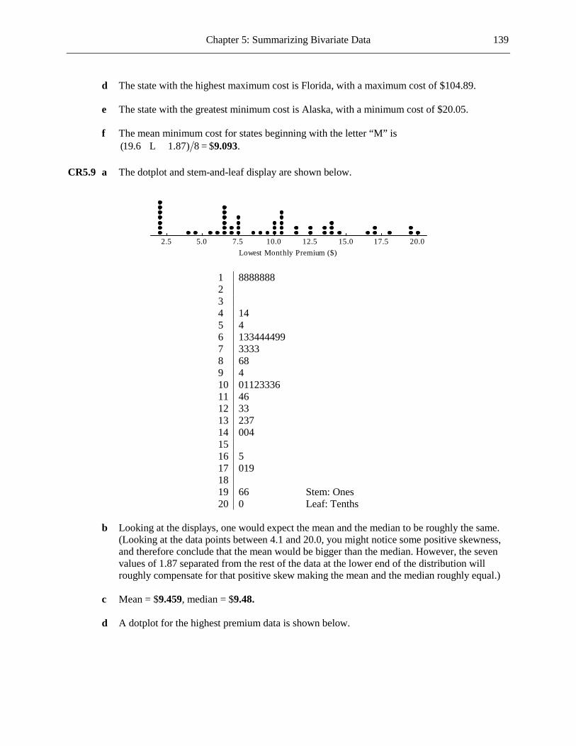
Chapter 5: Summarizing Bivariate Data 139
d The state with the highest maximum cost is Florida, with a maximum cost of $104.89. e The state with the greatest minimum cost is Alaska, with a minimum cost of $20.05. f The mean minimum cost for states beginning with the letter “M” is
(19.6 1.87) 8 $ .+ + = 9.093L CR5.9 a The dotplot and stem-and-leaf display are shown below.
20.017.515.012.510.07.55.02.5Lowest Monthly Premium ($)
1 8888888 2 3 4 14 5 4 6 133444499 7 3333 8 68 9 4 10 01123336 11 46 12 33 13 237 14 004 15 16 5 17 019 18 19 66 Stem: Ones 20 0 Leaf: Tenths
b Looking at the displays, one would expect the mean and the median to be roughly the same.
(Looking at the data points between 4.1 and 20.0, you might notice some positive skewness, and therefore conclude that the mean would be bigger than the median. However, the seven values of 1.87 separated from the rest of the data at the lower end of the distribution will roughly compensate for that positive skew making the mean and the median roughly equal.)
c Mean = $9.459, median = $9.48. d A dotplot for the highest premium data is shown below.

140 Chapter 5: Summarizing Bivariate Data
102969084787266Highest Monthly Premium ($)
e Mean = $72.846, median = $68.61. CR5.10 The data, in ascending order, are:
8457 8758 9116 10047 10108 10426 10478 10591 10680 10788 10815 10912 11040 11092 11145 11495 11644 11663 11673 11778 11781 12148 12353 12605 12962 13226
Lower quartile = 7th value = 10478 mg/kg. Upper quartile = 20th value = 11778 mg/kg. Interquartile range = 11778 − 10478 = 1300 mg/kg. CR5.11 a (3099 3700) 10x = + + = 2965.2L . ( )2 2Variance (3099 2965.2) (3700 2965.2) 9 294416.622= − + + − =L .
294416.622s = = 542.602 . The data values listed in order are:
2297 2401 2510 2682 2824 3068 3099 3112 3700 3959 Lower quartile = 3rd value = 2510. Upper quartile = 8th value = 3112. Interquartile range = 3112 − 2510 = 602. b The interquartile range for the chocolate pudding data (602) is less than the interquartile
range for the tomato catsup data (1300). So there is less variability in sodium content for the chocolate pudding data than for the tomato catsup data.
CR5.12 a Mean = (98 40) 13 .+ + = 59.846L
The data, listed in order, are: 40 48 49 50 53 54 55 61 64 65 66
75 98 Median = 7th value = 55.

Chapter 5: Summarizing Bivariate Data 141
Since the mean is greater than the median, the distribution of extra travel hours is likely to be
positively skewed. b
100908070605040Extra Hours per Traveler
There is one outlier (Los Angeles, with 98 extra travel hours per traveler). The median
number of extra hours of travel per traveler is 55, and, apart from the one outlier, the values range from 40 to 75. The distribution is positively skewed.
CR5.13 a (4.8 3.7) 20 .x = + + = 4.93L The data, listed in order are: 0.4 0.9 1.4 1.4 2.1 2.4 2.9 3.3 3.4 3.5 3.7
4.8 5 5 5.4 6.1 7.5 10.8 13.8 14.8 Median = average of 10th and 11th = (3.5 + 3.7)/2 = 3.6. b The mean is greater than the median. This is explained by the fact that the distribution of
blood lead levels is positively skewed. c
African Americans
Whites
1614121086420Blood Lead Level (micrograms per decilliter)
d The median blood lead level for the African Americans (3.6) is slightly higher than for the
Whites (3.1). Both distributions seem to be positively skewed. There are two outliers in the data set for the African Americans. The distribution for the African Americans shows a greater range than the distribution for the Whites, even if you discount the two outliers.

142 Chapter 5: Summarizing Bivariate Data
CR5.14 a 0.730.r =
1009080706050
75
70
65
60
55
50
45
Inpatient Cost-to-Charge Ratio
Outpatient Cost-to-Charge Ratio
Based on the correlation coefficient value of 0.730 and the scatterplot, there is a moderate
linear relationship between the cost-to-charge ratio for inpatient and outpatient services. Looking at the scatterplot, it is clear that one outlier is affecting the correlation. If that point were removed, there would be a strong linear relationship between the variables.
b As mentioned above, there is an outlier (the point for Harney District). c If the outlying point were removed then the linear relationship would be much stronger, and
the value of r would therefore be greater. CR5.15 a Yes, it appears that the variables are highly correlated. b There is a strong positive linear relationship between the observations by the standard
spectrophotometric method and the new, simpler method. c Perfect correlation would result in the points lying exactly on some straight line, but not
necessarily on the line described. CR5.16 a The y intercept is −147. b The slope is 6.175. For every 1-cm increase in the snout-vent length the predicted clutch size
increases by 6.175. c It would be inadvisable to use the least-squares line to predict the clutch size when the snout-
vent length is 22, since 22 is well outside the range of the x values in the original data set, and we have no reason to think that the observed linear relationship applies outside this range.

Chapter 5: Summarizing Bivariate Data 143
CR5.17 a This value of 2r tells us that 76.64% of the variability in clutch size can be attributed to the
approximate linear relationship between snout-vent length and clutch size. b Using 2 1 SSResid SSTor = − we see that 2SSResid SSTo(1 )r= − . So here
SSResid 43951(1 0.7664) 10266.9536.= − = Therefore SSResid 10266.9536 .
2 12esn
= = =−
29.250 This is a typical deviation of an observed clutch
size from the clutch size predicted by the least-squares line. CR5.18 a
2.52.01.51.00.5
100
90
80
70
60
50
40
30
Energy of Shock
Success (%)
The relationship appears to be nonlinear. b The equation of the least-squares line is ˆ 22.48 34.36 ,y x= + where y = success and x =
energy of shock. The residuals are shown in the table below.
Energy of Shock
Success
Residual
0.5 33.3 -6.36 1 58.3 1.46
1.5 81.8 7.78 2 96.7 5.5
2.5 100 -8.38 The residual plot is shown below.

144 Chapter 5: Summarizing Bivariate Data
2.52.01.51.00.5
10
5
0
-5
-10
Energy of Shock
Residual
The clear curve in the residual plot supports the conclusion that the relationship is nonlinear. c The scatterplot for x x′ = is shown below.
1.61.41.21.00.80.6
100
90
80
70
60
50
40
30
Sqrt(x)
Success (%)
The scatterplot for log( )x x′′ = is shown below.

Chapter 5: Summarizing Bivariate Data 145
0.40.30.20.10.0-0.1-0.2-0.3
100
90
80
70
60
50
40
30
Log(x)
Success (%)
The second transformation seems to have been more successful in straightening the plot. This
is confirmed by the random pattern in the residual plot, as shown below.
0.40.30.20.10.0-0.1-0.2-0.3
4
3
2
1
0
-1
-2
-3
-4
-5
Log(x)
Residual
d The equation of the least-squares line is ˆ 62.417 101.063 ,y x′′= + where
log(energy of shock)x′′ = and y = success. e At 1.75,x = ˆ 62.417 101.063log(1.75) %y = + = 86.979 .
At 0.8,x = ˆ 62.417 101.063log(0.8) %y = + = 52.623 .

146 Chapter 5: Summarizing Bivariate Data
CR5.19 a
250200150100500
160
140
120
100
80
60
40
20
0
Population Density
Agricultural Intensity
Yes, the scatterplot shows a strong positive association between population density and
agricultural intensity. b
6000050000400003000020000100000
160
140
120
100
80
60
40
20
0
(Population Density)^2
Agricultural Intensity
The plot now seems to be straight, particularly if you disregard the point with the greatest x
value.

Chapter 5: Summarizing Bivariate Data 147
c
250200150100500
2.25
2.00
1.75
1.50
1.25
1.00
0.75
0.50
Population Density
Log(Agricultural Intensity)
This transformation seems to have been successful in straightening the plot. Also, unlike the
plot in Part (b), the variability of the quantity measured on the vertical axis does not seem to increase as x increases.
d
6000050000400003000020000100000
2.25
2.00
1.75
1.50
1.25
1.00
0.75
0.50
(Population Density)^2
Log(Agricultural Intensity)
No, this transformation has not been successful in producing a linear relationship. There is a
clear curve in the plot.

148
Chapter 6 Probability
6.1 A chance experiment is any activity or situation in which there is uncertainty about which of two or more possible outcomes will result. For example, a random number generator is used to select a whole number between 1 and 4, inclusive.
6.2 The sample space is the collection of all possible outcomes of a chance experiment. The sample
space for Exercise 6.1 is {1, 2, 3, 4}. 6.3 a {AA, AM, MA, MM} b
c i B = {AA, AM, MA} ii C = {AM, MA} iii D = {MM}. D is a simple event. d B and C = {AM, MA} B or C = {AA, AM, MA} 6.4 a A = {Head oversize, Prince oversize, Slazenger oversize, Wimbledon oversize, Wilson
oversize} b B = {Wimbledon midsize, Wilson midsize, Wimbledon oversize, Wilson oversize} c not B = {Head midsize, Prince midsize, Slazenger midsize, Head oversize, Prince oversize,
Slazenger oversize} d B or C = {Head midsize, Prince midsize, Wimbledon midsize, Wilson midsize, Head
oversize, Prince oversize, Wimbledon oversize, Wilson oversize} e B and C = {Wilson midsize, Wilson oversize}
A
M
A
M
A
M

Chapter 6: Probability 149
f
6.5 a
b i AC = {(15, 50), (15, 100), (15, 150), (15, 200)}
Prince
Slazenger
Wimbledon
Wilson
Head
Midsize
Oversize
Midsize
Oversize
Midsize
Oversize
Midsize
Oversize
Oversize
Midsize
10
12
50
150
15
100
200
50
150
100
200
50
150
100
200
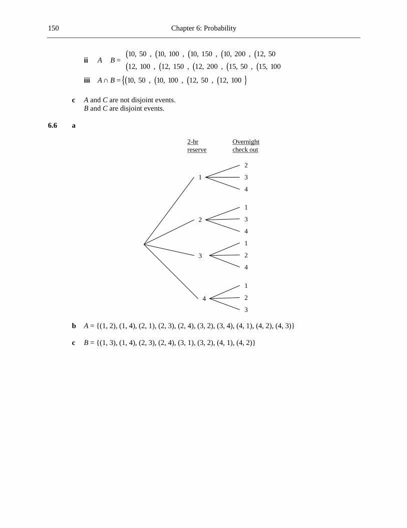
150 Chapter 6: Probability
ii ( ) ( ) ( ) ( ) ( )( ) ( ) ( ) ( ) ( )10, 50 , 10, 100 , 10, 150 , 10, 200 , 12, 50
12, 100 , 12, 150 , 12, 200 , 15, 50 , 15, 100A B
∪ =
iii ( ) ( ) ( ) ( ){ }10, 50 , 10, 100 , 12, 50 , 12, 100A B∩ = c A and C are not disjoint events. B and C are disjoint events. 6.6 a
b A = {(1, 2), (1, 4), (2, 1), (2, 3), (2, 4), (3, 2), (3, 4), (4, 1), (4, 2), (4, 3)} c B = {(1, 3), (1, 4), (2, 3), (2, 4), (3, 1), (3, 2), (4, 1), (4, 2)}
2
3
4
1
2
3
4
1
3
4
1
2
4
1
2
3
2-hr reserve
Overnight check out

Chapter 6: Probability 151
6.7 a
b A = {(3), (4), (5)} c C = {1 2 5, 1 5, 2 1 5, 2 5, 5} 6.8 a For example: N, DN, DDN, DDDN, DDDDN b There is an infinite number of outcomes. c E = {DN, DDDN, DDDDDN, DDDDDDDN, …} 6.9 a A = {NN, DNN} b B = {DDNN} c There are an infinite number of outcomes. 6.10 a The 27 possible outcomes are (1,1,1), (1,1,2), (1,1,3), (1,2,1), (1,2,2), (1,2,3), (1,3,1), (1,3,2),
(1,3,3), (2,1,1), (2,1,2), (2,1,3), (2,2,1), (2,2,2), (2,2,3), (2,3,1), (2,3,2), (2,3,3), (3,1,1), (3,1,2), (3,1,3), (3,2,1), (3,2,2), (3,2,3), (3,3,1), (3,3,2), (3,3,3).
b A = {(1,1,1), (2,2,2), (3,3,3)} c B = {(1,2,3), (1,3,2), (2,1,3), (2,3,1), (3,1,2), (3,2,1)} d C = {(1,1,1), (1,1,3), (1,3,1), (1,3,3), (3,1,1), (3,1,3), (3,3,1), (3,3,3)} e i CB = {(1,1,1), (1,1,2), (1,1,3), (1,2,1), (1,2,2), (1,3,1), (1,3,3), (2,1,1), (2,1,2), (2,2,1),
(2,2,2), (2,2,3), (2,3,2), (2,3,3), (3,1,1), (3,1,3), (3,2,2), (3,2,3), (3,3,1), (3,3,2), (3,3,3)}
2
3
4
5
1
2
3
4
5
1
3
4
5
3
4
5
3
4
5

152 Chapter 6: Probability
ii CC = {(1,1,2), (1,2,1), (1,2,2), (1,2,3), (1,3,2), (2,1,1), (2,1,2), (2,1,3), (2,2,1), (2,2,2),
(2,2,3), (2,3,1), (2,3,2), (2,3,3), (3,1,2), (3,2,1), (3,2,2), (3,2,3), (3,3,2)} iii A B∪ = {(1,1,1), (2,2,2), (3,3,3), (1,2,3), (1,3,2), (2,1,3), (2,3,1), (3,1,2), (3,2,1)} iv A B∩ = ∅ v {(1,1,1), (3,3,3)}A C∩ =
6.11 a
b
c
d
e
f
6.12 a The event ( )CA B∪ is shaded in the Venn diagram below.

Chapter 6: Probability 153
The event C CA B∩ is shaded in the Venn diagram below.
The two events are the same event. b The event ( )CA B∩ is shaded in the Venn diagram below.
The event C CA B∪ is shaded in the Venn diagram below.
The two events are the same event.

154 Chapter 6: Probability
6.13 a The sample space is {expedited overnight delivery, expedited second business day delivery, standard delivery, delivery to the nearest store for customer pick-up}.
b i 1 − 0.1 − 0.3 − 0.4 = 0.2 ii 0.1 + 0.3 = 0.4 iii 0.4 + 0.2 = 0.6 6.14 a 0.45 + 0.25 + 0.1 = 0.8 b (at most 3) 0.45 0.25 0.1 .P = + + = 0.8 This probability is the same as the one in Part (a). c 0.07 + 0.03 = 0.1 d 0.45 + 0.25 = 0.7 e (more than 2) 0.1 0.1 0.07 0.03 .P = + + + = 0.3
(more than 2) 1 (2 or fewer) 1 0.7 .P P= − = − = 0.3 6.15 a The sample space is {fiction hardcover, fiction paperback, fiction digital, fiction audio,
nonfiction hardcover, nonfiction paperback, nonfiction digital, nonfiction audio} b No. For example, a customer is more likely to buy a paperback than a hardcover book. c 0.15 + 0.08 + 0.45 + 0.04 = 0.72 d 0.1 + 0.02 + 0.1 + 0.06 = 0.28; 1 − 0.72 = 0.28 e 0.15 + 0.45 + 0.1 + 0.1 = 0.8 6.16 a A = {(C, N), (N, C), (N, N)}. ( ) 0.09 0.09 0.01 .P A = + + = 0.19 b B = {(C, C), (N, N)}.
( ) 0.81 0.01 .P B = + = 0.82 6.17 a P(Red) = 18/38 = 0.474. b No. If the segments were rearranged, there would still be 18 red segments out of a total of 38
segments, and so the probability of landing in a red segment would still be 18/38 = 0.474. c 1000(0.474) = 474. So, if the wheel is balanced you would expect the resulting color to be red
on approximately 474 of the 1000 spins. If the number of spins resulting in red is very different from 474, then you would suspect that the wheel is not balanced.
6.18 a P(Phoenix is final destination) = 1800/8000 = 0.225. b P(Phoenix is not final destination) = 1 – 0.225 = 0.775. c P(Connecting and missed flight) = 480/8000 = 0.06.

Chapter 6: Probability 155
d P(Connecting and did not miss flight) = (6200 – 480)/8000 = 0.715. e P(Either had Phoenix as final destination or delayed overnight) = (1800 + 75)/8000 = 0.234. f We know that 50 of the 8000 passengers will be selected, and 50/8000 = 1/160. In other
words, 1 in every 160 passengers will be selected. So, of the 75 passengers who were delayed overnight, you would expect 75(1/160) = 0.47 to be included in the survey. So it is very likely that none, or just one, of the passengers who were delayed overnight will be included in the survey, and so the airline has little need to worry.
6.19 a The number of ways of selecting two problems from the five is 10. (The easiest way to see
this is to list the possibilities. Calling the problems A, B, C, D, E, the possibilities are: AB, AC, AD, AE, BC, BD, BE, CD, CE, DE.)
Suppose now that you completed problems A, B, and C. The number of ways of selecting two
of these problems to be graded is 3. (The possibilities are: AB, AC, BC.) So the probability that the two problems selected are from the three you completed is 3/10
= 0.3. b No. The problems to be graded will be selected at random, so the probability of being able to
turn in both of the selected problems is the same whatever your choice of three problems to complete.
c If you complete four problems, the number of ways of selecting two from the ones you
completed is 6. (Suppose you completed problems A, B, C, and D. The possibilities for the two selected are: AB, AC, AD, BC, BD, CD.) As in Part (a), there are 10 ways of selecting the two to be graded from the 5 problems assigned. So the probability that you are able to turn in both problems is now 6/10 = 0.6.
6.20 a 500000/42005100 = 0.0119 b 100/42005100 = 0.00000238 c 505100/42005100 = 0.0120 6.21 P(credit card used) = 37100/80500 = 0.461. 6.22 If the events were mutually exclusive, then P(T or P) would be 0.83 + 0.56 = 1.39. This is greater
than 1, which is not possible. So the two events cannot be mutually exclusive. 6.23 a P(female) = 488142/787325 = 0.620. b P(male) = 1 – 0.620 = 0.380. 6.24 a P(Associate) = 97921/274515 = 0.357 b P(graduate or professional) = (274515 – 97921 – 129526)/274515 = 47068/274515 = 0.171 c P(not Bachelor’s) = 1 – 129526/274515 = 0.528

156 Chapter 6: Probability
6.25 a ( just spades) 1287 2598960 .P = = 0.000495 Since there are 1287 hands consisting entirely of spades, there are also 1287 hands consisting
entirely of clubs, 1287 hands consisting entirely of diamonds, and 1287 hands consisting entirely of hearts. So the number of possible hands consisting of just one suit is 4(1287) = 5148. Thus, (single suit) 5148 2598960 .P = = 0.00198
b (entirely spades and clubs with both suits represented) 63206 2598960 .P = = 0.024 c The two suits could be spades and clubs, spades and diamonds, spades and hearts, clubs and
diamonds, clubs and hearts, or diamonds and hearts. So there are six different combinations of two suits, with 63,206 possible hands for each combination. Therefore,
(exactly two suits) 6(63206) 2598960 .P = = 0.146 6.26 a The 24 outcomes (including the given outcome) are:
(1, 2, 3, 4), (1, 2, 4, 3), (1, 3, 2, 4), (1, 3, 4, 2), (1, 4, 2, 3), (1, 4, 3, 2), (2, 1, 3, 4), (2, 1, 4, 3), (2, 3, 1, 4), (2, 3, 4, 1), (2, 4, 1, 3), (2, 4, 3, 1), (3, 1, 2, 4), (3, 1, 4, 2), (3, 2, 1, 4), (3, 2, 4, 1), (3, 4, 1, 2), (3, 4, 2, 1), (4, 1, 2, 3), (4, 1, 3, 2), (4, 2, 1, 3), (4, 2, 3, 1), (4, 3, 1, 2), (4, 3, 2, 1).
b The event is {(1, 2, 4, 3), (1, 4, 3, 2), (1, 3, 2, 4), (4, 2, 3, 1), (3, 2, 1, 4), (2, 1, 3, 4)}.
The required probability is 6/24 = 1/4. c The outcomes associated with this event are:
(1, 3, 4, 2), (1, 4, 2, 3), (3, 2, 4, 1), ( 4, 2, 1, 3), (2, 4, 3, 1), (4, 1, 3, 2), (2, 3, 1, 4), (3, 1, 2, 4). The required probability is 8/24 = 1/3.
d It is not possible that exactly three receive their own books, because if three students have
their own books, then the fourth student must receive his/her own, also. Thus the required probability is 0.
e (at least 2 get the correct books)P
(2 get the correct books) (4 get the correct books) 1 4 1 24 .P P= + = + = 7 24 6.27 a BC, BM, BP, BS, CM, CP, CS, MP, MS, PS b 1/10 = 0.1 c 4/10 = 0.4 d There are three outcomes in which both representatives come from laboratory science
subjects: BC, BP, and CP. Thus (both from laboratory science) 3 10 .P = = 0.3 6.28 a Denoting the three math majors as M1, M2, and M3, and the two statistics majors by S1 and S2,
the ten possible outcomes for the pair of students chosen are: M1M2, M1M3, M1S1, M1S2, M2M3, M2S1, M2S2, M3S1, M3S2, S1S2. There is only one outcome for which both students chosen are statistics majors, and so the required probability is 1/10 = 0.1.
b Three of the ten outcomes satisfy this criterion, so the required probability is 0.3.

Chapter 6: Probability 157
c Seven of the ten outcomes satisfy this criterion, so the required probability is 0.7. d Six of the ten outcomes satisfy this criterion, so the required probability is 0.6. 6.29 a From 2 2 2 1p p p p p p+ + + + + = we see that 9 1p = , and so 1 9p = . Therefore,
1 3 5( ) ( ) ( ) 1 9P O P O P O= = = and 2 4 6( ) ( ) ( )P O P O P O= = = 2 9 . b 1 3 5(odd) ( ) ( ) ( ) 1 9 1 9 1 9P P O P O P O= + + = + + = 1 3 . 1 2 3(at most 3) ( ) ( ) ( ) 1 9 2 9 1 9 .P P O P O P O= + + = + + = 4 9 c From 2 3 4 5 6 1c c c c c c+ + + + + = we see that 21 1c = , and so 1 21c = . Thus 1 2 3 4( ) 1 21, ( ) 2 21, ( ) 3 21 1 7, ( ) 4 21,P O P O P O P O= = = = = 5 6( ) 5 21, ( ) 6 21 2 7.P O P O= = = Therefore,
1 3 5(odd) ( ) ( ) ( ) 1 21 3 21 5 21P P O P O P O= + + = + + = 9 21 and
1 2 3(at most 3) ( ) ( ) ( ) 1 21 2 21 3 21 6 21 .P P O P O P O= + + = + + = = 2 7
6.30 a ( ) 0.54( | ) .( ) 0.6
P E FP E FP F
∩= = = 0.9
b ( ) 0.54( | ) .( ) 0.7
P F EP F EP E
∩= = = 0.771
6.31 a (tattoo) 24 100P = = 0.24 b (tattoo | age 18-29) 18 50P = = 0.36 c (tattoo | age 30-50) 6 50P = = 0.12 d (age 18-29 | tattoo) 18 24P = = 0.75 6.32 The row and column totals are given in the table below.
Hybrid Not Hybrid Total Male 77 117 194 Female 34 83 117 Total 111 200 311
a i 194 311 = 0.624 ii 111 311 = 0.357 iii 77 194 = 0.397 iv 34 117 = 0.291 v 34 111 = 0.306 b i If a person who purchased a Honda Civic is chosen at random, the probability that this
person is a male is 0.624.

158 Chapter 6: Probability
ii If a person who purchased a Honda Civic is chosen at random, the probability that this person purchased a hybrid is 0.357.
iii If a male who purchased a Honda Civic is chosen at random, the probability that he purchased a hybrid is 0.397.
iv If a female who purchased a Honda Civic is chosen at random, the probability that she purchased a hybrid is 0.291.
v If a person who purchased a hybrid Honda Civic is chosen at random, the probability that this person is female is 0.306.
c (hybrid | male) 0.397.P =
(male | hybrid) 0.694.P = These probabilities are not equal. The first is the proportion of males who bought hybrids, and the second is the proportion of hybrid buyers who were males; they are different quantities.
6.33 a 0.72 b The value 0.45 is the conditional probability that the selected individual drinks 2 or more
cups a day given that he or she drinks coffee. We know this because the percentages given in the display add to 100, and yet we know that only 72% of Americans drink coffee. So the percentages given in the table must be the proportions of coffee drinkers who drink the given amounts.
6.34 The row and column totals are given in the table below.
Diagnosis Delayed
Diagnosis Not Delayed
Total
Mammogram Report Benign 32 89 121 Mammogram Report Suspicious
8 304 312
Total 40 393 433 a i ( ) 121 433 .P B = = 0.279 The probability that the report is benign is 0.279. ii ( ) 312 433 .P S = = 0.721 The probability that the report is suspicious is 0.721. iii ( | ) 32 121 .P D B = = 0.264 If the report is benign the probability that the diagnosis is
delayed is 0.264. iv ( | ) 8 312 .P D S = = 0.026 If the report is suspicious the probability that the diagnosis is
delayed is 0.026. b Comparison of the answers to (iii) and (iv) above tells us that the diagnosis is more likely to
be delayed if the report is benign. Thus the error of a benign report is related to delayed diagnosis.
6.35 a i If a person has been out of work for 1 month then the probability that the person will find
work within the next month is 0.3. ii If a person has been out of work for 6 months then the probability that the person will
find work within the next month is 0.19.
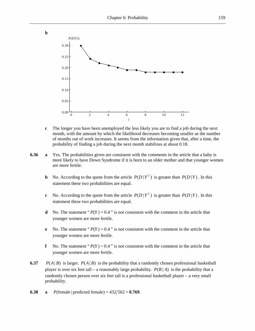
Chapter 6: Probability 159
b
121086420
0.30
0.25
0.20
0.15
0.10
0.05
0.00
i
P(E|Ti)
c The longer you have been unemployed the less likely you are to find a job during the next
month, with the amount by which the likelihood decreases becoming smaller as the number of months out of work increases. It seems from the information given that, after a time, the probability of finding a job during the next month stabilizes at about 0.18.
6.36 a Yes. The probabilities given are consistent with the comments in the article that a baby is
more likely to have Down Syndrome if it is born to an older mother and that younger women are more fertile.
b No. According to the quote from the article ( | )CP D Y is greater than ( | )P D Y . In this
statement these two probabilities are equal. c No. According to the quote from the article ( | )CP D Y is greater than ( | )P D Y . In this
statement these two probabilities are equal. d No. The statement “ ( ) 0.4P Y = ” is not consistent with the comment in the article that
younger women are more fertile. e No. The statement “ ( ) 0.4P Y = ” is not consistent with the comment in the article that
younger women are more fertile. f No. The statement “ ( ) 0.4P Y = ” is not consistent with the comment in the article that
younger women are more fertile. 6.37 ( | )P A B is larger. ( | )P A B is the probability that a randomly chosen professional basketball
player is over six feet tall – a reasonably large probability. ( | )P B A is the probability that a randomly chosen person over six feet tall is a professional basketball player – a very small probability.
6.38 a (female | predicted female) 432 562 .P = = 0.769
160 Chapter 6: Probability
b (male | predicted male) 390 438 .P = = 0.890 c Since the conditional probabilities in (a) and (b) are not equal, we see that a prediction that a
baby is male and a prediction that a baby is female are not equally reliable. 6.39 a (former smoker) 99 294 .P = = 0.337 b (very harmful) 224 294 .P = = 0.762 c (very harmful | current smoker) 60 96 .P = = 0.625 d (very harmful | former smoker) 78 99 .P = = 0.788 e (very harmful | never smoked) 86 99 .P = = 0.869 f Of the three smoking statuses, current smokers are the least likely to believe that smoking is
very harmful and those who have never smoked are the most likely to think that smoking is very harmful. This is not surprising since you would expect those who smoke to be the most confident about the health prospects of a smoker, with those who formally smoked being a little more concerned, and those who have never smoked being the most concerned.
6.40 The row and column totals are given in the table below.
Male Female Total Uses Seat Belts Regularly 0.1 0.175 0.275 Does Not Use Seat Belts Regularly 0.4 0.325 0.725 Total 0.5 0.5 1
a 0.275 b 0.1 0.5 = 0.2 c 0.325 0.5 .= 0.65 d 0.325 0.725 .= 0.448 e No. The answer to Part (c) is the proportion of females who are not seat belt wearers, whereas
the answer to Part (d) is the proportion of people who don’t wear seat belts who are female. We have no reason to think that these two quantities will be equal.

Chapter 6: Probability 161
6.41 a
Age Does Not Use Regularly
Uses Regularly Total
18-24 0.09833 0.06833 0.16667 25-34 0.12167 0.04500 0.16667 35-44 0.12333 0.04333 0.16667 45-54 0.11667 0.05000 0.16667 55-64 0.11667 0.05000 0.16667
65 and older 0.13667 0.03000 0.16667 Total 0.71333 0.28667 1.00000
i 1( )P A = 0.167 ii 1( )P A S∩ = 0.068 iii 1 1( | ) ( ) ( ) 0.06833 0.28667P A S P A S P S= ∩ = = 0.238 iv 1 1( ) 1 ( ) 1 0.16667P not A P A= − = − = 0.833 v 1 1 1( | ) ( ) ( ) 0.06833 0.16667P S A P S A P A= ∩ = = 0.41 vi 6 6 6( | ) ( ) ( ) 0.03 0.16667P S A P S A P A= ∩ = = 0.18 b The conditional probabilities tell us that 18–24-year-olds are more likely than seniors to
regularly wear seat belts. 6.42 a i ( ) 456 600 .P S = = 0.76 ii ( | ) 215 300 .P S A = = 0.717 iii ( | ) 241 300 .P S B = = 0.803 iv Treatment B appears to be better, since the probability of survival given that the patient
receives treatment B is greater than the probability of survival given that the patient receives treatment A.
b i ( ) 140 240 .P S = = 0.583 ii ( | ) 120 200 .P S A = = 0.6 iii ( | ) 20 40 .P S B = = 0.5 iv Treatment A appears to be better, since the probability of survival given that the patient
receives treatment A is greater than the probability of survival given that the patient receives treatment B.
c i ( ) 316 360 .P S = = 0.878 ii ( | ) 95 100 .P S A = = 0.95 iii ( | ) 221 260 .P S B = = 0.85 iv Treatment A appears to be better, since the probability of survival given that the patient
receives treatment A is greater than the probability of survival given that the patient receives treatment B.
d Women respond better to these treatments than men do. Moreover, treatment A was given to
far more men than women and treatment B was given to far more women than men. As a result, even though treatment A is the better one for both men and women, when the results are combined the greater number of women receiving treatment B artificially increases the
162 Chapter 6: Probability
apparent efficacy of treatment B and the greater number of men receiving treatment A artificially decreases the apparent efficacy of treatment A. The combined results are in this way distorted in favor of treatment B.
6.43 a Eighty-five percent of all calls to the station are for medial assistance. b 0.15 c (0.85)(0.85) = 0.7225 d (0.85)(0.15) = 0.1275 e (exactly one for medical assistance)P
(1st for medical 2nd not for medical) (1st not for medical 2nd for medical)
(0.85)(0.15) (0.15)(0.85) .P P= ∩ + ∩
= + = 0.255
f It would seem reasonable to assume that the outcomes of successive calls (for medical assistance or not) do not affect each other. However, it is likely that at certain times of the day calls are more likely to be for medical assistance than at other times of the day. Therefore, if a call is chosen at random and found to be for medical assistance, then it becomes more likely that this call was received at one of these times. The next call, being at roughly the same time of the day, then has a more than 0.85 probability of being for medical assistance. Therefore it is not reasonable to assume that the outcomes of successive calls are independent.
6.44 a
Does Not Use Complementary Therapies
Does Use Complementary Therapies
Total
Convention Medications Usually Help 0.758 0.122 0.879
Convention Medications Usually Do Not Help 0.096 0.025 0.121
Total 0.853 0.147 1 b The cell entry 0.122 represents the probability of (conventional medicines usually help and
does use complementary therapies). The cell entry 0.096 represents the probability of (conventional medicines usually do not help and does not use complementary therapies). The cell entry 0.025 represents the probability of (conventional medicines usually do not help and does use complementary therapies).
c ( ) 0.12163( | ) 0.829,( ) 0.14670
P CH CTP CH CTP CT
∩= = = and ( ) 0.879.P CH = Since these two
probabilities are not equal the two events are not independent. 6.45 ( ) ( ) (0.58)(0.5) 0.29 ( ).P L P F P L F⋅ = = ≠ ∩ Therefore the events L and F are not independent. 6.46 a If an accident results in death, the probability that it was a single vehicle rollover is 0.3.

Chapter 6: Probability 163
b If an accident results in death, the probability that it was a frontal collision is 0.54. c ( ) 0.06P R = and ( | ) 0.3P R D = . Since these probabilities are not equal, the events R and D
are not independent. d No. If ( )P F D∩ were equal to ( ) ( ),P F P D then F and D would be independent. But we
know that F and D are not independent, since ( | ) ( )P F D P F≠ . Thus ( )P F D∩ cannot be equal to ( ) ( ).P F P D
e No. If F were equal to ,CR then ( ) ( )P F P R+ would be equal to 1. But
( ) ( ) 0.6 0.06 0.66 1,P F P R+ = + = ≠ so .CF R≠ 6.47 No. The events are not independent because the probability of experiencing pain daily given that
the person is male is not equal to the probability of experiencing pain daily given that the person is not male.
6.48 a (selected in each of the next two years) (0.15)(0.15) .P = = 0.0225
b (selected in each of the next three years) (0.15)(0.15)(0.15) .P = = 0.003375 6.49 a (0.1) (0.1) (0.1) = 0.001. We have to assume that she deals with the three errands
independently. b (remembers at least one) 1 (forgets them all) 1 0.001 .P P= − = − = 0.999 c (remembers 1st, forgets 2nd, forgets 3rd) (0.9)(0.1)(0.1) .P = = 0.009 6.50 a 10(0.7) = 0.028 b We had to assume that the results of the calls were independent. c (at least one results in reservation) 1 (none results in reservation) 1 0.028 .P P= − = − = 0.972 6.51 a (1-2 subsystem works) (0.9)(0.9) .P = = 0.81 b (1-2 subsystem doesn't work) 1 0.81 .P = − = 0.19 (3-4 subsystem doesn't work) .P = 0.19 c (system won't work) (0.19)(0.19) .P = = 0.0361 (system will work) 1 0.0361 .P = − = 0.9639 d (system won't work) (0.19)(0.19)(0.19) .P = = 0.006859 So (system will work) 1 0.006859 .P = − = 0.993141 e The probability that one particular subsystem will work is now (0.9) (0.9) (0.9) = 0.729. So
the probability that the subsystem won’t work is 1 0.729 0.271− = . Therefore the probability

164 Chapter 6: Probability
that neither of the two subsystems works (and so the system doesn’t work) is (0.271) (0.271) = 0.073441. So the probability that the system works is 1 0.073441 0.926559.− =
6.52 a i 0.51 ii 0.56 iii 0.45 iv 0.36 v 0.72 b No, since ( ) ( | ).P F P F C≠ c No, since ( ) ( | ).P F P F O≠ 6.53 a The expert was assuming that there was a 1 in 12 chance of a valve being in any one of the 12
clock positions and that the positions of the two air valves were independent. b Since the car’s wheels are probably the same size, if one of the wheels happens to have its air
valve in the same position as before then the other wheel is likely also to have its air valve in the same position as before. Thus the positions of the two air valves are not independent.
c Assuming independence makes the probability smaller. d 1/144 is smaller than the correct probability. 6.54 a (0.7)(0.8)(0.6) = 0.336 b (0.7)(0.8) = 0.56 c (0.3)(0.2) = 0.06 d (each person wins one match)P
(A beats B, C beats A, and B beats C) (B beats A, A beats C, and C beats B)P P= + (0.7)(0.2)(0.6) (0.3)(0.8)(0.4) .= + = 0.18
6.55 a No. If the first board selected is defective then it is less likely that the second board is
defective than if the first board had not been defective. b 1 1( ) 1 ( ) 1 40 5000 .P not E P E= − = − = 0.992 c If the first board is defective then 39 of the remaining 4999 boards are defective. So
2 1( | ) 39 4999 0.00780.P E E = = If the first board is not defective then 40 of the remaining 4999 boards are defective. So 2 1( | ) 40 4999 0.00800.P E not E = = If the first board is defective then it is slightly less likely that the second board will be defective than if the first board is not defective.
d Yes. Since the two probabilities calculated in Part (c) are roughly equal, it would be
reasonable to say that the events 1E and 2E are approximately independent.

Chapter 6: Probability 165
6.56 1 1( ) ( ) ( ) (0.4)(0.3) 0.12.P B S P B P S∩ = = =
The required probabilities are given in the table below.
S M L B1 0.12 0.2 0.08 B2 0.18 0.3 0.12
6.57 a (both correct) (50 800)(50 800) .P = = 0.00391 b (2nd is correct |1st is correct) (2nd is correct 1st is correct) (1st is correct).P P P= ∩ So
( )( )(1st is correct 2nd is correct) (1st is correct) (2nd is correct |1st is correct)
50 800 49 799 .P P P∩ = ⋅
= = 0.00383
This probability is slightly smaller than the one in Part (a). 6.58 a (both correct) (50 100)(50 100) .P = = 0.25 b (both correct) (50 100)(49 99) .P = = 0.247 6.59 a 6/10 = 0.6 b ( | ) .P F E = 5 9 c ( | ) ( ) ( ).P F E P F E P E= ∩ So ( ) ( ) ( ) ( | ) (6 10)(5 9) .P E and F P F E P E P F E= ∩ = ⋅ = = 1 3 6.60 a (0.4)(0.3) = 0.12 b (0.6)(0.7) = 0.42 c (at least one successful) 1 (neither is successful) 1 0.42 .P P= − = − = 0.58 6.61 a ( ) ( ) ( ) ( ) 0.4 0.3 0.15 .P E F P E P F P E F∪ = + − ∩ = + − = 0.55 b The Venn diagram is shown below.

166 Chapter 6: Probability
(needn't stop at either light) 1 ( ) 1 0.55 .P P E F= − ∪ = − = 0.45 c (stops at exactly one) 0.25 0.15 .P = + = 0.4 d (stops at just the first light) .P = 0.25 6.62 The event E F∩ is the event that the randomly chosen registered voter has signed the petition
and votes in the recall election. ( ) ( | ) ( ) (0.8)(0.1) .P E F P E F P F∩ = ⋅ = = 0.08
6.63 a P(at least one food allergy and severe reaction) = (0.08)(0.39) = 0.0312. b P(allergic to multiple foods) = (0.08)(0.3) = 0.024. 6.64
(blue and identified as blue) (0.15)(0.8)(blue | identified as blue)(identified as blue) (0.15)(0.8) (0.85)(0.2)
PPP
= = =+
0.414 .
6.65 For a randomly selected customer, let T be the event that the customer subscribes to cable TV
service, I be the event that the customer subscribes to Internet service, and P be the event that the customer subscribes to telephone service. The three events are shown in the Venn diagram below, and letters have been used to denote the probabilities of four events. (Please note that x represents the probability that the customer subscribes to the phone and Internet services but not to the cable TV service. The quantities y and z are similarly defined.)
The information we have been given can be summarized as follows:

Chapter 6: Probability 167
( ) 0.8( ) 0.42( ) 0.32
0.250.210.230.15
P TP IP Pw zw yw x
w
===
+ =+ =+ =
=
Using the last four results we can conclude that 0.08, 0.06, and 0.1.x y z= = =
a (cable TV only) 0.8 ( ) 0.8 (0.06 0.1 0.15) .P y z w= − + + = − + + = 0.49 The probability that a randomly chosen customer subscribes only to the cable TV service is 0.49.
b ( ) 0.25(Internet | cable TV) ( | ) .( ) 0.8
P I TP P I TP T
∩= = = = 0.3125
If a customer is chosen at random from those who subscribe to the cable TV service, the probability that this customer will subscribe to the Internet service is 0.3125.
c (exactly two services) 0.08 0.06 0.1 .P x y z= + + = + + = 0.24 The probability that a randomly chosen customer subscribes to exactly two services is 0.24.
d (Internet and cable TV only) .P z= = 0.1
The probability that a randomly chosen customer subscribes only to the Internet and cable TV services is 0.1.
6.66 a Yes. Since it is a large cable company, meaning that it has many customers, the outcome for
the first customer (cable TV or not) will have little effect on the outcome for the second customer.
b 1 2( ) (0.8)(0.8) .P C C∩ = = 0.64 6.67 a ( ) (0.261)(0.375) (0.739)(0.073) 0.152.P H = + =
( ) (0.261)(0.375) 0.098.P C H∩ = = ( ) 0.098( | ) .
( ) 0.152P C HP C H
P H∩
= = = 0.645
b ( ) (0.495)(0.537) (0.505)(0.252) 0.393.P H = + =
( ) (0.495)(0.537) 0.266.P C H∩ = = ( ) 0.266( | ) .
( ) 0.393P C HP C H
P H∩
= = = 0.676
The result is a little higher for faculty than for students. A faculty member who has high confidence in a correct diagnosis is slightly more likely actually to be correct that a student who has the same high confidence.

168 Chapter 6: Probability
6.68 a (37 14 16 11) 79+ + + = 0.987 b (37 14) 79+ = 0.646 c (14 16) 79+ = 0.380 d (14 16) (14 16 37 11) 30 78+ + + + = = 0.385 e 30 30 = 1 6.69 a i ( ) .P T = 0.307 ii ( ) .CP T = 0.693 iii ( | ) .P C T = 0.399 iv ( | ) .P L T = 0.275 v ( ) (0.307)(0.399) .P C T∩ = = 0.122 b 30.7% of faculty members use Twitter. 69.3% of faculty members do not use Twitter. 39.9% of faculty members who use Twitter also use it to communicate with students. 27.5% of faculty members who use Twitter also use it as a learning tool in the classroom. 12.2% of faculty members use Twitter and use it to communicate with students. c By the law of total probability, ( ) ( ) ( ).CP C P C T P C T= ∩ + ∩ However, faculty members
who do not use Twitter cannot possibly use it to communicate with students. Therefore ( ) 0.CP C T∩ = Thus ( ) ( ) .P C P C T= ∩ = 0.122
d Since faculty members who use Twitter as a learning tool must use Twitter,
( ) ( ) ( ) ( | ) (0.307)(0.275) .P L P L T P T P L T= ∩ = ⋅ = = 0.084 6.70 a
Uses Alternative Therapies
Does Not Use Alternative Therapies
Total
High School or Less 315 7005 7320
College – 1 to 4 years 393 4400 4793
College – 5 or more years 120 975 1095
Total 828 12380 13208

Chapter 6: Probability 169
b
Uses Alternative Therapies
Does Not Use Alternative Therapies
Total
High School or Less 0.024 0.530 0.554
College – 1 to 4 years 0.030 0.333 0.363
College – 5 or more years 0.009 0.074 0.083
Total 0.063 0.937 1.000 c i 0.083 ii 0.063
iii 0.009 1200.083 1095
= = 0.110
iv 0.024 3150.554 7320
= = 0.043
v 0.024 3150.063 828
= = 0.380
vi 0.030 0.009 393 1200.363 0.083 4793 1095
+ += =
+ +0.087
d ( | ) 0.043 and ( ) 0.063.P A H P A= = Since these two probabilities are different, the events A
and H are not independent. 6.71 The reason that ( )P C is not the average of the three conditional probabilities is that there are
different numbers of people driving the three different types of vehicle (and also that there are some drivers who are driving vehicles not included in those three types).
6.72 a i 4.5( ) .8.6
P F = = 0.523
ii 4.1( ) .8.6
P S = = 0.477
iii ( | ) .P R F = 0.018 iv ( | ) .P R S = 0.03
b ( ) (0.523)(0.018) (0.477)(0.03) 0.024.P R = + =
( ) (0.477)(0.03)( | ) .( ) 0.024
P S RP S RP R
∩= = = 0.603
If a gun purchase is rejected, the probability that this happened through a state or local agency is 0.603.

170 Chapter 6: Probability
6.73 Radiologist 1 Predicted
Male Predicted Female Total
Baby Is Male 74 12 86 Baby Is Female 14 59 73 Total 88 71 159
a P(prediction is male | baby is male) = 74/86 = 0.860. b P(prediction is female | baby is female) = 59/73 = 0.808. c Yes. Since the answer to (a) is greater than the answer to (b), the prediction is more likely to
be correct when the baby is male. d The radiologist was correct for 74 + 59 = 133 of the 159 babies in the study. So P(correct)
= 133/159 = 0.836. 6.74 Radiologist 2
Predicted Male
Predicted Female Total
Baby Is Male 81 8 89 Baby Is Female 7 58 65 Total 88 66 154
For Radiologist 1, P(prediction is male | baby is male) = 0.860. For Radiologist 2, P(prediction is male | baby is male) = 81/89 = 0.910. So Radiologist 2 is better than Radiologist 1 at predicting the gender when the baby is male. For Radiologist 1, P(prediction is female | baby is female) = 0.808. For Radiologist 2, P(prediction is female | baby is female) = 58/65 = 0.892. So Radiologist 2 is also better than Radiologist 1 at predicting the gender when the baby is
female. Indeed, Radiologist 2’s overall success rate is (81 + 58)/154 = 0.903, which is higher than
Radiologist 1’s success rate of 0.836. 6.75 a i 0.99 ii 0.01 iii 0.99 iv 0.01 b ( ) ( ) ( )P TD P TD C P TD D= ∩ + ∩
( ) ( | ) ( ) ( | )
(0.99)(0.01) (0.01)(0.99) .P C P TD C P D P TD D= ⋅ + ⋅
= + = 0.0198
c ( | ) ( ) ( ) (0.99)(0.01) 0.0198 .P C TD P C TD P TD= ∩ = = 0.5 Yes. The quote states that half of the dirty tests are false. The above probability states that
half of the dirty tests are on people who are in fact clean. This confirms the statement in the quote.
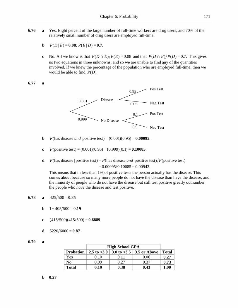
Chapter 6: Probability 171
6.76 a Yes. Eight percent of the large number of full-time workers are drug users, and 70% of the
relatively small number of drug users are employed full-time. b ( | ) ; ( | ) .P D E P E D= =0.08 0.7 c No. All we know is that ( ) ( ) 0.08P D E P E∩ = and that ( ) ( ) 0.7.P D E P D∩ = This gives
us two equations in three unknowns, and so we are unable to find any of the quantities involved. If we knew the percentage of the population who are employed full-time, then we would be able to find ( ).P D
6.77 a
b (has disease positive test) (0.001)(0.95) .P and = = 0.00095 c (positive test) (0.001)(0.95) (0.999)(0.1) .P = + = 0.10085 d (has disease | positive test) (has disease positive test) (positive test)P P and P= 0.00095 0.10085 0.00942.= = This means that in less than 1% of positive tests the person actually has the disease. This
comes about because so many more people do not have the disease than have the disease, and the minority of people who do not have the disease but still test positive greatly outnumber the people who have the disease and test positive.
6.78 a 425 500 = 0.85 b 1 405 500− = 0.19 c (415 500)(415 500) = 0.6889 d 5220 6000 = 0.87 6.79 a
High School GPA Probation 2.5 to <3.0 3.0 to <3.5 3.5 or Above Total Yes 0.10 0.11 0.06 0.27 No 0.09 0.27 0.37 0.73 Total 0.19 0.38 0.43 1.00
b 0.27
0.9
0.1
0.05
0.95
0.999
0.001 Disease
No Disease
Pos Test
Neg Test
Pos Test
Neg Test
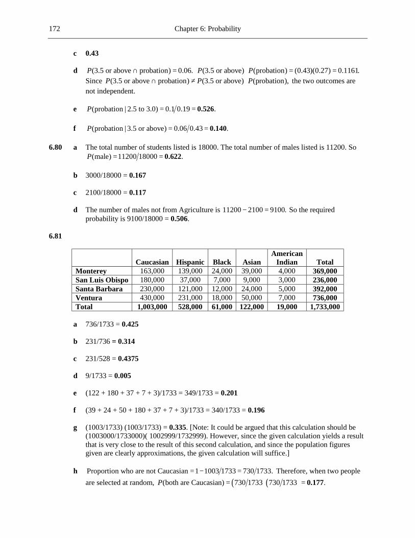
172 Chapter 6: Probability
c 0.43 d (3.5 or above probation) 0.06.P ∩ = (3.5 or above) (probation) (0.43)(0.27) 0.1161.P P⋅ = =
Since (3.5 or above probation) (3.5 or above) (probation),P P P∩ ≠ ⋅ the two outcomes are not independent.
e (probation | 2.5 to 3.0) 0.1 0.19 .P = = 0.526 f (probation | 3.5 or above) 0.06 0.43 .P = = 0.140 6.80 a The total number of students listed is 18000. The total number of males listed is 11200. So
(male) 11200 18000 .P = = 0.622 b 3000/18000 = 0.167 c 2100/18000 = 0.117 d The number of males not from Agriculture is 11200 2100 9100.− = So the required
probability is 9100/18000 = 0.506. 6.81
Caucasian Hispanic Black Asian
American Indian Total
Monterey 163,000 139,000 24,000 39,000 4,000 369,000 San Luis Obispo 180,000 37,000 7,000 9,000 3,000 236,000 Santa Barbara 230,000 121,000 12,000 24,000 5,000 392,000 Ventura 430,000 231,000 18,000 50,000 7,000 736,000 Total 1,003,000 528,000 61,000 122,000 19,000 1,733,000
a 736/1733 = 0.425 b 231/736 = 0.314 c 231/528 = 0.4375 d 9/1733 = 0.005 e (122 + 180 + 37 + 7 + 3)/1733 = 349/1733 = 0.201 f (39 + 24 + 50 + 180 + 37 + 7 + 3)/1733 = 340/1733 = 0.196 g (1003/1733) (1003/1733) = 0.335. [Note: It could be argued that this calculation should be
(1003000/1733000)( 1002999/1732999). However, since the given calculation yields a result that is very close to the result of this second calculation, and since the population figures given are clearly approximations, the given calculation will suffice.]
h Proportion who are not Caucasian 1 1003 1733 730 1733.= − = Therefore, when two people
are selected at random, ( )( )(both are Caucasian) 730 1733 730 1733 .P = = 0.177

Chapter 6: Probability 173
i (1003/1733)(730/1733) + (730/1733)( 1003/1733) = 0.488 j (369/1733)( 369/1733) + (236/1733)( 236/1733) + (392/1733)( 392/1733) + (736/1733)( 736/1733) = 0.295 k ( )( ) ( )( )(same ethnic group) 1003 1733 1003 1733 528 1733 528 1733P = + ( )( ) ( )( ) ( )( )61 1733 61 1733 122 1733 122 1733 19 1733 19 1733 0.434.+ + + = So (different ethnic groups) 1 0.434 .P = − = 0.566 6.82 Answers will vary. 6.83 a The simulation could be designed as follows. Number the 20 companies/individuals applying
for licenses 01–20, with the applications for 3 licenses coming from 01–06, the applications for 2 licenses coming from 07–15, and the applications for single licenses coming from 16–20. Assume that the individual with whom this question is concerned is numbered 16.
One run of the simulation is conducted as follows. Use two consecutive digits from a random
number table to select a number between 01 and 20. (Ignore pairs of digits from the random number table that give numbers outside this range.) The number selected indicates the company/individual whose request is granted. Repeat the number selection, ignoring repeated numbers, until there are no licenses left. Make a note of whether or not individual 16 was awarded a license.
Perform the above simulation a large number of times. The probability that this particular
individual is awarded a license is approximated by (Number of runs in which 16 is awarded a license) (Total number of runs).
b This does not seem to be a fair way to distribute licenses, since any given company applying
for multiple licenses has roughly the same chance of obtaining all of its licenses as an individual applying for a single license has of obtaining his/her license. It might be fairer for companies who require two licenses to submit two separate applications and companies who require three licenses to submit three separate applications (with individuals/companies applying for single licenses submitting applications as before). Then 10 of the applications would be randomly selected and licenses would be awarded accordingly.
6.84 Results of the simulation will vary. The correct probability that the project is completed on time
is 0.8504. 6.85 Results of the simulation will vary. The correct probability that the project is completed on time
is 0.8468. 6.86 a Results of the simulation will vary. The correct probability that the project is completed on
time is 0.6504. b Jacob’s change makes the bigger change in the probability that the project will be completed
on time.
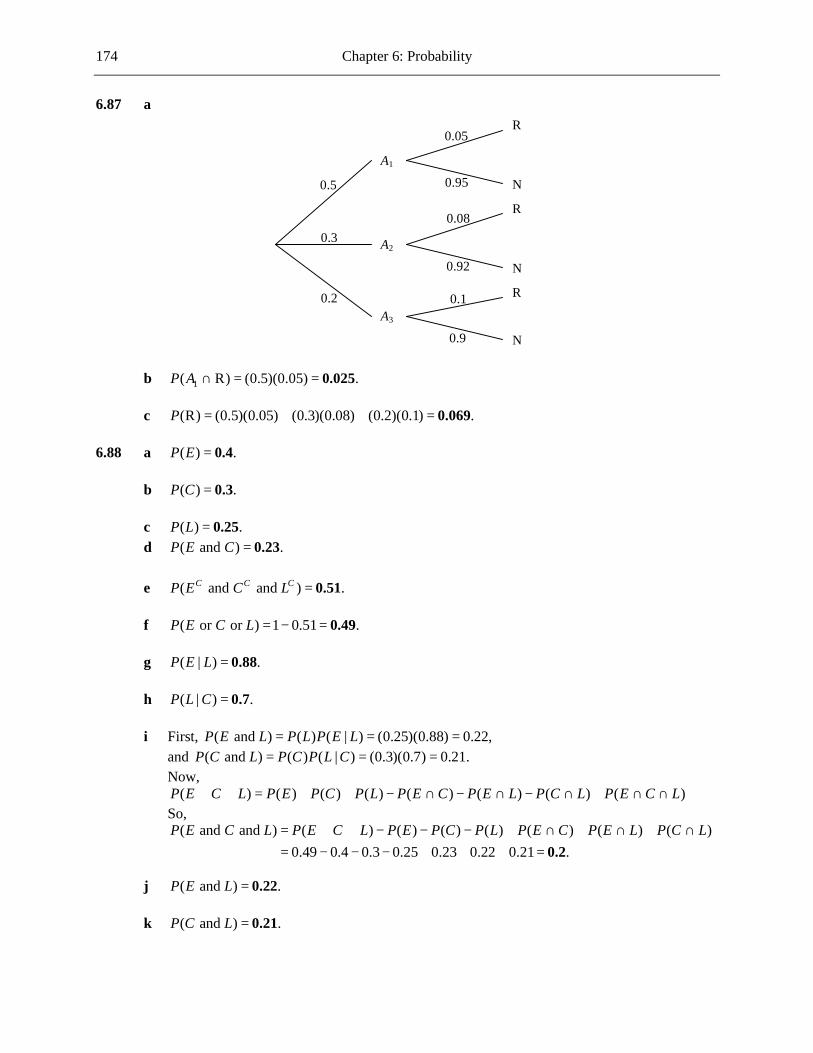
174 Chapter 6: Probability
6.87 a
b 1( R) (0.5)(0.05) .P A ∩ = = 0.025 c (R) (0.5)(0.05) (0.3)(0.08) (0.2)(0.1) .P = + + = 0.069 6.88 a ( ) .P E = 0.4 b ( ) .P C = 0.3 c ( ) .P L = 0.25 d ( and ) .P E C = 0.23 e ( and and ) .C C CP E C L = 0.51 f ( or or ) 1 0.51 .P E C L = − = 0.49 g ( | ) .P E L = 0.88 h ( | ) .P L C = 0.7 i First, ( and ) ( ) ( | ) (0.25)(0.88) 0.22,P E L P L P E L= = =
and ( and ) ( ) ( | ) (0.3)(0.7) 0.21.P C L P C P L C= = = Now,
( ) ( ) ( ) ( ) ( ) ( ) ( ) ( )P E C L P E P C P L P E C P E L P C L P E C L∪ ∪ = + + − ∩ − ∩ − ∩ + ∩ ∩ So,
( and and ) ( ) ( ) ( ) ( ) ( ) ( ) ( )0.49 0.4 0.3 0.25 0.23 0.22 0.21 .
P E C L P E C L P E P C P L P E C P E L P C L= ∪ ∪ − − − + ∩ + ∩ + ∩= − − − + + + = 0.2
j ( and ) .P E L = 0.22 k ( and ) .P C L = 0.21
0.08
0.92
0.1
0.9
0.95
0.05
0.2
0.3
0.5
A1
A2
R
A3
N
R
N
R
N

Chapter 6: Probability 175
l ( ) 0.2( | ( and )) .( ) 0.22
P C E LP C E LP E L
∩ ∩= = =
∩0.909
6.89 a ( ) 27 193 .P C = = 0.140 14.0% of chat room users have criticized others. b ( ) 42 193 .P O = = 0.218 21.8% of chat room users have been personally criticized. c ( ) 19 193 .P C O∩ = = 0.098 9.8% of chat room users have criticized others and have been
personally criticized. d ( | ) 19 42 .P C O = = 0.452 45.2% of chat room users who have been personally criticized have
criticized others. e ( | ) 19 27 .P O C = = 0.704 70.4% of chat room users who have criticized others have been
personally criticized. 6.90 They are dependent events, since the probability that the selected student has TB given that the
student is a recent immigrant is not equal to the (unconditional) probability that the student has TB.
6.91 They are dependent events, since someone who is attempting to quit is slightly more likely to
return to smoking within two weeks if he/she does not use a nicotine aid than if he/she does use a nicotine aid.
6.92 (0.4)(0.02) = 0.008 6.93 a
( ) (0.4)(0.02) (0.5)(0.01) (0.1)(0.05) .P L = + + = 0.018 b 1 1( | ) ( ) ( ) (0.4)(0.02) 0.018 .P A L P A L P L= ∩ = = 0.444 c 2 2( | ) ( ) ( ) (0.5)(0.01) 0.018 .P A L P A L P L= ∩ = = 0.278 d 3 3( | ) ( ) ( ) (0.1)(0.05) 0.018 .P A L P A L P L= ∩ = = 0.278
0.01
0.99
0.05
0.95
0.98
0.02
0.1
0.5
0.4
A1
A2
L
A3
LC
L
LC
L
LC

176 Chapter 6: Probability
6.94 a 5( wins in 5 games) (0.3) .P A = = 0.00243 b 5 5(5 games to obtain champion) (0.3) (0.2) .P = + = 0.00275 c A random number table could be used. The digits 0–2 will represent A winning the game,
3–4 will represent B winning, and 5–9 will represent the game resulting in a draw. Use digits one at a time from the random number table, noting the results of the simulated games, and keeping a tally of scores according to the plan given in the question. When one of the competitors reaches a total score of 5, that person is the winner. If both competitors reach 5 at the same time, then the championship ends in a draw. Repeat the simulation above a large number of times. The probability that A wins the championship is estimated by the fraction
number of runs in which A wins .
total number of runs
6.95 In Parts (a)–(c) below, examples of possible simulation plans are given. a Use a single-digit random number to represent the outcome of the game. The digits 0–7 will
represent a win for seed 1, and digits 8–9 will represent a win for seed 4. b Use a single-digit random number to represent the outcome of the game. The digits 0–5 will
represent a win for seed 2, and digits 6–9 will represent a win for seed 3. c Use a single-digit random number to represent the outcome of the game. If seed 1 won game 1 and seed 2 won game 2, the digits 0–5 will represent a win for seed 1,
and digits 6–9 will represent a win for seed 2. If seed 1 won game 1 and seed 3 won game 2, the digits 0–6 will represent a win for seed 1,
and digits 7–9 will represent a win for seed 3. If seed 4 won game 1 and seed 2 won game 2, the digits 0–6 will represent a win for seed 2,
and digits 7–9 will represent a win for seed 4. If seed 4 won game 1 and seed 3 won game 2, the digits 0–5 will represent a win for seed 3,
and digits 6–9 will represent a win for seed 4. d Answers will vary. e Answers will vary. f Answers will vary. g The estimated probabilities from Parts (e) and (f) will differ because they are based on
different sets of simulations. The estimate from Part (f) is likely to be the better one, since it is based on more runs of the simulation than the estimate from Part (e).
6.96 a ( ) 1 ( ) 1 0.6 .CP E P E= − = − = 0.4 b Since ( ) 0,P E F∩ = ( ) ( ) ( ) 0.6 0.15 .P E F P E P F∪ = + = + = 0.75 c ( ) 1 ( ) 1 0.75 .C CP E F P E F∩ = − ∪ = − = 0.25

Chapter 6: Probability 177
6.97
Individuals Chosen (by Years of Experience)
Total Number of Years’ Experience
At least 15 years?
3, 6 9 No 3, 7 10 No
3, 10 13 No 3, 14 17 Yes 6, 7 13 No
6, 10 16 Yes 6, 14 20 Yes 7, 10 17 Yes 7, 14 21 Yes 10, 14 24 Yes
(at least 15 years' experience) 6 10 .P = = 0.6 6.98 (at least one) ( or or ) 0.14 0.23 0.37 0.08 0.09 0.13 0.05 .P P A B C= = + + − − − + = 0.49 6.99 a (179 + 87)/2517 = 0.106 b (420 + 323 + 179 + 114 + 87)/2517 = 0.446 c 1 (600 196 205 139) 2517− + + + = 0.547 6.100 Since the total number of viewers was 2517 and the number of viewers of R-rated movies was
1140, 2 1( | ) 1139 2516P R R = and 2 1( | ) 1140 2516CP R R = . These probabilities are not equal, so the events 1 2 and R R are not independent. However, as a result of the fact that the total number of viewers is large, the two probabilities are very close, and therefore from a practical point of view the events may be regarded as independent.
6.101 a ( ) 20 25 .P E = = 4 5 b ( | ) .P F E = 19 24 c ( | ) .P G E F∩ = 18 23 d ( )( )( )(all good) 20 25 19 24 18 23 .P = = 0.496
6.102 a 20 19 18 17(all 4 are good) .25 24 23 22
P = =
0.383
b (at least one is bad) 1 (all 4 are good) 1 0.383 .P P= − = − = 0.617 6.103 a (0.8)(0.8)(0.8) = 0.512

178 Chapter 6: Probability
b The possible sequences and their probabilities are shown in the table below.
Sent by Transmitter
Sent by Relay 1
Sent by Relay 2
Sent by Relay 3
Probability
1 0 0 1 (0.2)(0.8)(0.2) 1 0 1 1 (0.2)(0.2)(0.8) 1 1 0 1 (0.8)(0.2)(0.2) 1 1 1 1 (0.8)(0.8)(0.8)
(1 is received) (0.2)(0.8)(0.2) (0.2)(0.2)(0.8) (0.8)(0.2)(0.2) (0.8)(0.8)(0.8).
P = + + += 0.608

179
Chapter 7 Random Variables and Probability Distributions
Note: In this chapter, numerical answers to questions involving the normal distribution were found using statistical tables. Students using calculators or computers will find that their answers differ slightly from those given. 7.1 a Discrete b Continuous c Discrete d Discrete e Continuous 7.2 a Continuous b Continuous c Continuous d Discrete e Continuous f Continuous g Discrete 7.3 a The possible y values are the positive integers. b (Answers will vary.) 7.4 a The random variable x takes values between 0 and 2 1.414= . b Continuous 7.5 a The possible values of y are the real numbers between 0 and 100, inclusive. b Continuous 7.6 a The variable y can take any positive even integer value b Discrete 7.7 a 3, 4, 5, 6, 7 b 3, 2, 1, 0, 1, 2, 3− − −

180 Chapter 7: Random Variables and Probability Distributions
c 0, 1, 2 d 0, 1 7.8 a 0.25 b 0.02 + 0.03 + 0.09 + 0.25 = 0.39 c ( 5) 0.02 0.03 0.09 0.25 0.40 . .P x ≤ = + + + + = 0 79 d (student is taking at least 5 courses) ( 5) 0.4 0.16 0.05 . .P P x= ≥ = + + = 0 61
(student is taking more than 5 courses) ( 5) 0.16 0.05 . .P P x= > = + = 0 21 e (3 6) 0.09 0.25 0.4 0.16 .P x≤ ≤ = + + + = 0.9
(3 6) 0.25 0.4 .P x< < = + = 0.65 The second probability is smaller (and therefore the two probabilities are not equal) because the second probability does not include the possibility of a student taking 3 or 6 courses, while the first does include this possibility.
7.9 a (4) 1 0.65 0.2 0.1 0.04 .p = − − − − = 0.01 b Over a large number of cartons, 20% will contain 1 broken egg. c ( 2) 0.65 0.2 0.1 . .P y ≤ = + + = 0 95 Over a large number of cartons, 95% will contain at most 2
broken eggs. d ( 2) 0.65 0.2 . .P y < = + = 0 85 This probability is smaller than the one in Part (c) since it does
not include the possibility of 2 broken eggs. e (exactly 10 unbroken) (exactly 2 broken) .P P= = 0.1 f ( 10 unbroken) ( 2 broken) .P P≥ = ≤ = 0.95 7.10 a You would expect roughly 450 of the graduates to donate nothing, roughly 300 to donate $10,
roughly 200 to donate $25, and roughly 50 to donate $50. The frequencies would be close to, but not exactly, these values. The four frequencies would add to 1000.
b The most common value of x is 0. c P(x ≥ 25) = 0.20 + 0.05 = 0.25. d P(x > 0) = 0.30 + 0.20 + 0.05 = 0.55. 7.11 a The probability that everyone who shows up can be accommodated is
( 100) 0.05 0.1 0.12 0.14 0.24 0.17 . .P x ≤ = + + + + + = 0 82 b 1 0.82 . .− = 0 18
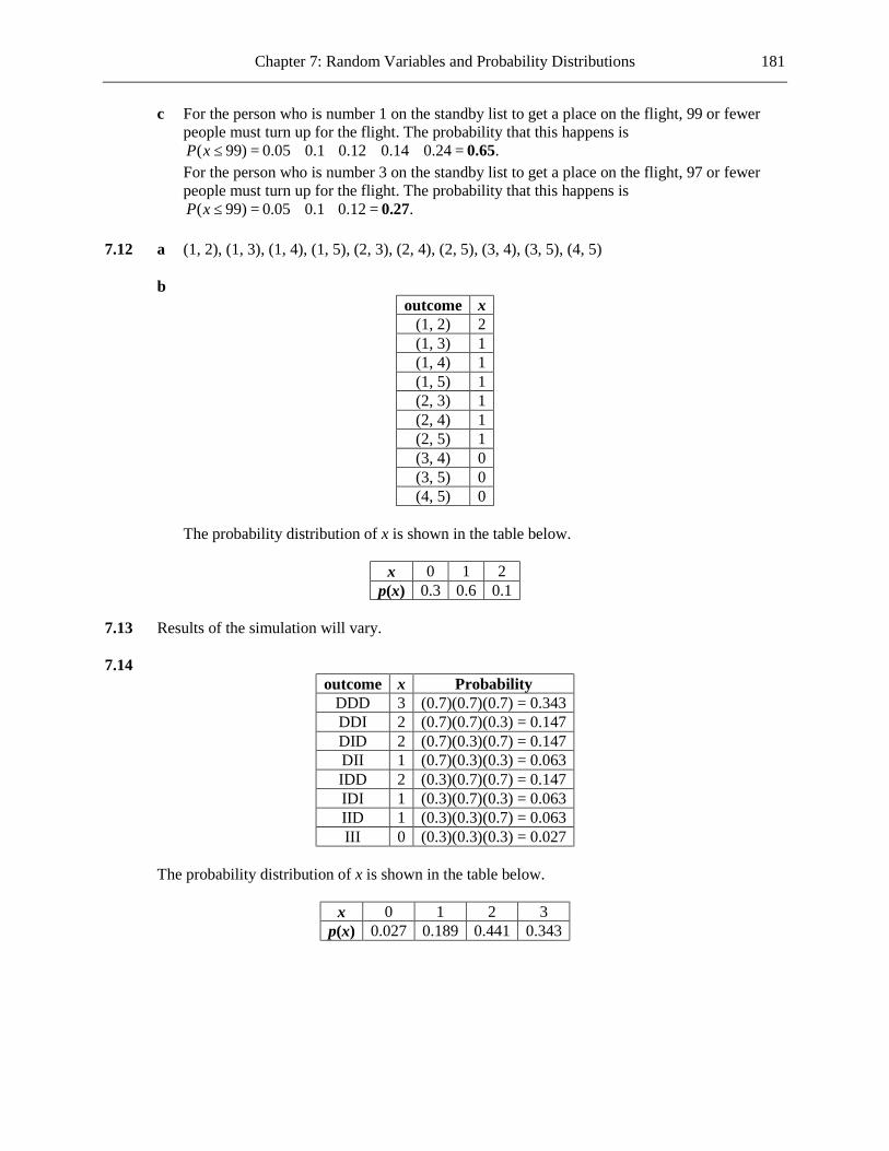
Chapter 7: Random Variables and Probability Distributions 181
c For the person who is number 1 on the standby list to get a place on the flight, 99 or fewer
people must turn up for the flight. The probability that this happens is ( 99) 0.05 0.1 0.12 0.14 0.24 .P x ≤ = + + + + = 0.65
For the person who is number 3 on the standby list to get a place on the flight, 97 or fewer people must turn up for the flight. The probability that this happens is
( 99) 0.05 0.1 0.12 .P x ≤ = + + = 0.27 7.12 a (1, 2), (1, 3), (1, 4), (1, 5), (2, 3), (2, 4), (2, 5), (3, 4), (3, 5), (4, 5) b
outcome x (1, 2) 2 (1, 3) 1 (1, 4) 1 (1, 5) 1 (2, 3) 1 (2, 4) 1 (2, 5) 1 (3, 4) 0 (3, 5) 0 (4, 5) 0
The probability distribution of x is shown in the table below.
x 0 1 2 p(x) 0.3 0.6 0.1
7.13 Results of the simulation will vary. 7.14
outcome x Probability DDD 3 (0.7)(0.7)(0.7) = 0.343 DDI 2 (0.7)(0.7)(0.3) = 0.147 DID 2 (0.7)(0.3)(0.7) = 0.147 DII 1 (0.7)(0.3)(0.3) = 0.063 IDD 2 (0.3)(0.7)(0.7) = 0.147 IDI 1 (0.3)(0.7)(0.3) = 0.063 IID 1 (0.3)(0.3)(0.7) = 0.063 III 0 (0.3)(0.3)(0.3) = 0.027
The probability distribution of x is shown in the table below.
x 0 1 2 3 p(x) 0.027 0.189 0.441 0.343

182 Chapter 7: Random Variables and Probability Distributions
7.15 a The sixteen possible outcomes, their probabilities, and the associated values of x, are shown in the table below.
Outcome Probability x
SSSS (0.2)(0.2)(0.2)(0.2) = 0.0016 4 SSSF (0.2)(0.2)(0.2)(0.8) = 0.0064 3 SSFS (0.2)(0.2)(0.8)(0.2) = 0.0064 3 SSFF (0.2)(0.2)(0.8)(0.8) = 0.0256 2 SFSS (0.2)(0.8)(0.2)(0.2) = 0.0064 3 SFSF (0.2)(0.8)(0.2)(0.8) = 0.0256 2 SFFS (0.2)(0.8)(0.8)(0.2) = 0.0256 2 SFFF (0.2)(0.8)(0.8)(0.8) = 0.1024 1 FSSS (0.8)(0.2)(0.2)(0.2) = 0.0064 3 FSSF (0.8)(0.2)(0.2)(0.8) = 0.0256 2 FSFS (0.8)(0.2)(0.8)(0.2) = 0.0256 2 FSFF (0.8)(0.2)(0.8)(0.8) = 0.1024 1 FFSS (0.8)(0.8)(0.2)(0.2) = 0.0256 2 FFSF (0.8)(0.8)(0.2)(0.8) = 0.1024 1 FFFS (0.8)(0.8)(0.8)(0.2) = 0.1024 1 FFFF (0.8)(0.8)(0.8)(0.8) = 0.4096 0
The probability distribution of x is given in the table below.
x 0 1 2 3 4 p(x) 0.4096 0.4096 0.1536 0.0256 0.0016
b There are two most likely values of x: 0 and 1. c ( 2) 0.1536 0.0256 0.0016 .P x ≥ = + + = 0.1808 7.16 The value of w for each pair of slips picked is shown in the table below.
$1 $1 $1 $10 $25 $1 $1 1 $1 1 1 $10 10 10 10 $25 25 25 25 25
Each of the ten outcomes shown above is equally likely. Thus the probability distribution of w is
as given in the table below.
w 1 10 25 p(w) 0.3 0.3 0.4
7.17 a The smallest possible y value is 1, and the corresponding outcome is S. The second smallest y value is 2, and the corresponding outcome is FS.

Chapter 7: Random Variables and Probability Distributions 183
b The set of positive integers c ( 1) (S)P y P= = = 0.7 ( 2) (FS) (0.3)(0.7) .P y P= = = = 0.21 ( 3) (FFS) (0.3)(0.3)(0.7) .P y P= = = = 0.063 ( 4) (FFFS) (0.3)(0.3)(0.3)(0.7) .P y P= = = = 0.0189 ( 5) (FFFFS) (0.3)(0.3)(0.3)(0.3)(0.7) .P y P= = = = 0.00567 The formula is 1( ) (0.3) (0.7), for 1, 2, 3,yp y y−= = K 7.18 a The probability distribution of y (with probabilities in terms of k) is as shown below.
y 1 2 3 4 5 p(y) k 2k 3k 4k 5k
Since all the probabilities must add to 1 we have 2 3 4 5 1,k k k k k+ + + + = and so 15 1.k =
Thus .k = 1 15 b Since 1 15k = , the probability distribution of y is as shown below.
y 1 2 3 4 5
p(y) 1/15 2/15 3/15 4/15 5/15
Thus, 1 2 3(at most three forms are required) ( 3) . .15 15 15
P P y= ≤ = + + = 0 4
c 2 3 4(between 2 and 4 inclusive) (2 4) . .15 15 15
P P y= ≤ ≤ = + + = 0 6
d If 2( ) 50p y y= then the probability distribution of y would be as shown below.
y 1 2 3 4 5 p(y) 1/50 4/50 9/50 16/50 25/50
However, the probabilities would then not add to 1, and so the given probability distribution
is not possible. 7.19
1st Magazine W T F S
2nd Magazine
W y = 0 prob = 0.16
y = 1 prob = 0.12
y = 2 prob = 0.08
y = 3 prob = 0.04
T y = 1 prob = 0.12
y = 1 prob = 0.09
y = 2 prob = 0.06
y = 3 prob = 0.03
F y = 2 prob = 0.08
y = 2 prob = 0.06
y = 2 prob = 0.04
y = 3 prob = 0.02
S y = 3 prob = 0.04
y = 3 prob = 0.03
y = 3 prob = 0.02
y = 3 prob = 0.01

184 Chapter 7: Random Variables and Probability Distributions
The probability distribution of y is shown below.
y 0 1 2 3 p(y) 0.16 0.33 0.32 0.19
7.20 a
b
c
d
e
7.21 a ( )( )( 5) 1 10 5 0 . .P x ≤ = − = 0 5 b ( )( )(3 5) 1 10 5 3 .P x≤ ≤ = − = 0.2
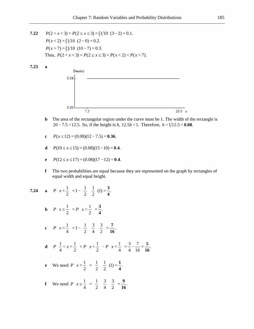
Chapter 7: Random Variables and Probability Distributions 185
7.22 ( )(2 3) (2 3) 1 10 (3 2) 0.1.P x P x< < = ≤ ≤ = − =
( )( 2) 1 10 (2 0) 0.2.P x < = − =
( )( 7) 1 10 (10 7) 0.3.P x > = − = Thus, (2 3) (2 3) ( 2) ( 7).P x P x P x P x< < = ≤ ≤ < < < >
7.23 a
b The area of the rectangular region under the curve must be 1. The width of the rectangle is
20 7.5 12.5.− = So, if the height is h, 12.5 1.h = Therefore, 1 12.5 .h = = 0.08 c ( 12) (0.08)(12 7.5) .P x ≤ = − = 0.36 d (10 15) (0.08)(15 10) . .P x≤ ≤ = − = 0 4 e (12 17) (0.08)(17 12) . .P x≤ ≤ = − = 0 4 f The two probabilities are equal because they are represented on the graph by rectangles of
equal width and equal height.
7.24 a 1 1 11 (1) .2 2 2
P x < = − =
34
b 1 1 .2 2
P x P x ≤ = < =
34
c 1 1 3 31 .4 2 4 2
P x < = − =
716
d 1 1 1 1 3 7 .4 2 2 4 4 16
P x P x P x < < = < − < = − =
516
e We need 1 1 1 (1) .2 2 2
P x > = =
14
f We need 1 1 3 3 .4 2 4 2
P x ≥ = =
916

186 Chapter 7: Random Variables and Probability Distributions
7.25 a ( 10) 0.05(10 0) .P x < = − = 0.5 ( 15) 0.05(20 15) . .P x > = − = 0 25 b (7 12) 0.05(12 7) . .P x< < = − = 0 25 c 0.05( 0) 0.9,c − = so 0.9 0.05 .c = = 18
7.26 a ( )( )1Area 40 0.05 12
= = , as required.
b ( )( )1( 20) 20 0.05 . .2
P w < = = 0 5
c 1( 10) (10)(0.025) .2
P w < = = 0.125
d 1( 30) (10)(0.025) .2
P w > = = 0.125
e (10 30) 1 ( 10) ( 30) 1 0.125 0.125 .P w P w P w< < = − < − > = − − = 0.75 7.27 μx = (1)(.140) + (2)(.175) + (3)(.220) + (4)(.260) + (5)(.155) + (6)(.025) + (7)(.015) + (8)(.005)
+ (9)(.004) + (10)(.001) = 3.306. 7.28 a 0(0.54) 1(0.16) 2(0.06) 3(0.04) 4(0.2) .xµ = + + + + = 1.2 b ( ) ( 1.2) ( 2) 0.06 0.04 0.2 . .xP x P x P xµ> = > = ≥ = + + = 0 3 7.29 a 0(0.65) 1(0.2) 2(0.1) 3(0.04) 4(0.01) . .yµ = + + + + = 0 56 Over a large number of cartons, the
mean number of broken eggs per carton will be 0.56. b ( ) ( 0.56) ( 0) 0.65.yP y P y P yµ< = < = = = In 65% of cartons, the number of broken eggs
will be less than yµ . This result is greater than 0.5 because the distribution of y is positively skewed.
c The mean is not (0 1 2 3 4) 5+ + + + since, for example, far more cartons have 0 broken eggs
than 4 broken eggs, and so 0 needs a much greater weighting than 4 in the calculation of the mean.
7.30 12z y= − , so 12 12 0.56 .z yµ µ= − = − = 11.44 7.31 a 0.02 + 0.03 + 0.09 = 0.14. b 2 4.66 2(1.2) 2.26µ σ− = − = ; 2 4.66 2(1.2) 7.06.µ σ+ = + = The values of x more than 2
standard deviations away from the mean are 1 and 2. c 0.02 + 0.03 = 0.05.
Chapter 7: Random Variables and Probability Distributions 187
7.32 Let x be the number of flaws in a randomly selected panel from the first supplier, and let y be the
number of flaws in a randomly selected panel from the second supplier. As shown in Examples 7.11 and 7.12, 1,xµ = 1,yµ = 1,xσ = and 0.632.yσ = Therefore, in terms of the mean number of flaws per panel, the two suppliers are equal. However, since the standard deviation for the second supplier is smaller than that for the first, the second supplier is more consistent in terms of the number of flaws per panel than the first supplier. It could be argued that greater consistency is desirable in this context, and so for this reason the second supplier should be recommended.
7.33 a 0(0.05) 1(0.1) 5(0.1) .xµ = + + + = 2.8L 2 2 2(0 2.8) (0.5) (5 2.8) (0.1) 1.66.xσ = − + + − =L So 1.66 .xσ = = 1.288 b 0(0.5) 1(0.3) 2(0.2) .yµ = + + = 0.7
2 2 2 2(0 0.7) (0.5) (1 0.7) (0.3) (2 0.7) (0.2) 0.61.yσ = − + − + − =
So 0.61 .yσ = = 0.781 c The amount of money collected in tolls from cars is (number of cars)($3) = 3x. 3 3 3(2.8) .x xµ µ= = = 8.4 2 2 2
3 3 9(1.66) .x xσ σ= = = 14.94 d The amount of money collected in tolls from buses is (number of buses)($10) = 10y. 10 10 10(0.7) .y yµ µ= = = 7
2 2 210 10 100(0.61) .y yσ σ= = = 61
e 2.8 0.7 .z x y x yµ µ µ µ+= = + = + = 3.5
2 2 2 2 1.66 0.61 .z x y x yσ σ σ σ+= = + = + = 2.27 f 3 10 3 10 8.4 7 .w x y x yµ µ µ µ+= = + = + = 15.4
2 2 2 23 10 3 10 14.94 61 .w x y x yσ σ σ σ+= = + = + = 75.94
7.34 a 1(0.05) 2(0.1) 3(0.12) 4(0.3) 5(0.3) 6(0.11) 7(0.01) 8(0.01) .xµ = + + + + + + + = 4.12 b 2 2 2 2 2(1 4.12) (0.05) (2 4.12) (0.1) (3 4.12) (0.12) (4 4.12) (0.3)xσ = − + − + − + −
2 2 2 2(5 4.12) (0.3) (6 4.12) (0.11) (7 4.12) (0.01) (8 4.12) (0.01) .+ − + − + − + − = 1.9456 1.9456 .xσ = = 1.395
The mean squared deviation of the number of systems sold in a month from the mean number of systems sold in a month is 1.9456. A typical deviation of the number of systems sold in a month from the mean number of systems sold in a month is 1.395.
c 4.12 1.395 2.725.x xµ σ− = − =
4.12 1.395 5.515.x xµ σ+ = + = So we need (2.725 5.515) (3 5) 0.12 0.3 0.3 .P x P x< < = ≤ ≤ = + + = 0.72

188 Chapter 7: Random Variables and Probability Distributions
d 2 4.12 2(1.395) 1.33.x xµ σ− = − = 2 4.12 2(1.395) 6.91.x xµ σ+ = + =
So we need ( 1.33) ( 6.91) ( 1) ( 7) 0.05 0.01 0.01 .P x P x P x P x< + > = ≤ + ≥ = + + = 0.07 7.35 a ( ) 15(0.1) 30(0.3) 60(0.6) seconds.E x = + + = 46.5 b The probability distribution of y is shown below.
y 500 800 1000 p(y) 0.1 0.3 0.6
( ) 500(0.1) 800(0.3) 1000(0.6) 890.E y = + + = The average amount paid is $890. 7.36 Since 1000(0.05) 5000(0.3) 10000(0.4) 20000(0.25) 10550,xµ = + + + = the author expects to
make slightly more under the royalty plan than by accepting the flat payment of $10,000. However, since the royalty plan could result in payments as low as $1000 and as high as $20,000, the author might opt for the less risky (less variable) option of the flat payment.
7.37 For the first distribution shown below, 3 and 1.414,x xµ σ= = while for the second distribution
3 and 1.x xµ σ= =
x 1 2 3 4 5 p(x) 0.2 0.2 0.2 0.2 0.2
x 1 2 3 4 5 p(x) 0.1 0.1 0.6 0.1 0.1
7.38 a 13.5(0.2) 15.9(0.5) 19.1(0.3) . .xµ = + + = 16 38
2 2 2 2(13.5 16.38) (0.2) (15.9 16.38) (0.5) (19.1 16.38) (0.3) 3.9936.xσ = − + − + − = 3.9936 .xσ = = 1.998
b Price 25(16.38) 8.5 401.µ = − = The mean of the price paid by the next customer is $401. c Price 25(1.998) 49.960.σ = = The standard deviation of the price paid by the next customer is
$49.960. 7.39 a Whether y is positive or negative tells us whether or not the peg will fit into the hole. b
2 10.253 0.25 .y x xµ µ µ= − = − = 0.003
c
1 2
2 2 2 2(0.006) (0.002) .y x xσ σ σ= + = + = 0.00632 d Yes. Since we have no reason to believe that the pegs are being specially selected to match
the holes (or vice versa), it is reasonable to think that 1x and 2x are independent.

Chapter 7: Random Variables and Probability Distributions 189
e Since 0 is less than half a standard deviation from the mean in the distribution of y, it is
relatively likely that a value of y will be negative, and therefore that the peg will be too big to fit the hole.
7.40 a 1 2
1 110 (40) .4 4y x xµ µ µ= − = − = 0
If a student guesses the answer to every question, we would expect 1/5 of the questions to be answered correctly and 4/5 to be answered incorrectly. Under this scheme, the student is awarded one point for every correct answer and −1/4 of a point for every incorrect answer. So if the test contains 50 questions then if the student guesses completely at random we expect 10 correct answers and 40 incorrect answers, and thus a total score of 0.
b Since 1 250x x= − , the value of 1x is completely determined by the value of 2 ,x and thus 1x
and 2x are not independent. The formulas in this section for computing variances and standard deviations of combinations of random variables require the random variables to be independent.
7.41 a ( ) ( )1 1 6 6 1 6 .
Rxµ = + + = 3.5L
( ) ( )2 2 2(1 3.5) 1 6 (6 3.5) 1 6 .Rxσ = − + + − = 2.917L
2.917 . .Rxσ = = 1 708
b ,
Bxµ = 3.5 2 ,Bxσ = 2.917 and . .
Bxσ = 1 708 c
17 3.5 3.5 7 .
R Bw x xµ µ µ= + − = + − = 0
1
2 2 2.917 2.917 .R Bw x xσ σ σ= + = + = 2.415
d 2 3 3R Bw x x= −
23 3 3(3.5) 3(3.5) .
R Bw x xµ µ µ= − = − = 0
2
2 29 9 9(2.917) 9(2.917) . .R Bw x xσ σ σ= + = + = 7 246
e For both of the games the mean of the money gained is 0. The choice of games is therefore
governed by the amount of risk the player is willing to undergo. If you are willing to win or lose larger amounts, Game 2 should be chosen. If less risk is desired, Game 1 should be chosen.
7.42 a
d1 0 650 2000 p(d1) 1/3 1/3 1/3
b 1( ) 0(1 3) 650(1 3) 2000(1 3) . .E d = + + = 883 333 c
1
2 2 2 2(0 883.333) (1 3) (650 883.333) (1 3) (2000 883.333) (1 3) 693888.889.dσ = − + − + − =
So 1
693888.889 .dσ = = 833.000

190 Chapter 7: Random Variables and Probability Distributions
d The probability distributions of 2d and 3d are shown below.
d2 0 650 1350 p(d2) 1/3 1/3 1/3
d3 0 1350 2000 p(d3) 1/3 1/3 1/3
Neither of these probability distributions is the same as the probability distribution of 1.d e The possible values of t are calculated in the table below.
Where meeting held d1 d2 t Probability Columbus 0 650 650 1/3 Des Moines 650 0 650 1/3 Boise 2000 1350 3350 1/3
This tells us that the probability distribution of t is as shown below.
t 650 3350 p(t) 2/3 1/3
f The probability distribution of d2 is given below.
d2 0 650 1350 p(d2) 1/3 1/3 1/3
From this we get 2( ) 666.667E d = and
2551.261.dσ =
From the probability distribution of t we get ( ) 1550E t = and 1272.792.tσ = i 1 2( ) ( ) 883.333 666.667 1550 ( ),E d E d E t+ = + = = so the statement is true. (Note that the
statement has to be true, since 1 2t d d= + , and since for any two random variables x and y, regardless of whether or not they are independent, ( ) ( ) ( ).E x y E x E y+ = + )
ii 1 2
2 2 2 2883.000 551.261 303888.889 693888.889 997777.778,d dσ σ+ = + = + = but 2 21272.792 1620000.tσ = = So the statement is false.
7.43 The distribution of x is binomial with n = 10 and p = 1/20 = 0.05. a ( 3) ( 0) ( 1) ( 2)P x P x P x P x< = = + = + =
10 1 9 2 810! 10!(0.95) (0.05) (0.95) (0.05) (0.95)1!9! 2!8!
= + +
= 0.988.

Chapter 7: Random Variables and Probability Distributions 191
b ( 3) ( 0) ( 1) ( 2) ( 3)P x P x P x P x P x≤ = = + = + = + =
10 1 9 2 8 3 710! 10! 10!(0.95) (0.05) (0.95) (0.05) (0.95) (0.05) (0.95)1!9! 2!8! 3!7!
= + + +
= 0.999 c ( 4) 1 ( 3) 1 0.999P x P x≥ = − ≤ = − = 0.001 d (1 3) ( 1) ( 2) ( 3)P x P x P x P x≤ ≤ = = + = + =
1 9 2 8 3 710! 10! 10!(0.05) (0.95) (0.05) (0.95) (0.05) (0.95)1!9! 2!8! 3!7!
= + +
= 0.400 . 7.44 Let x be the number of vehicles out of 15 that involve a single vehicle. Then x is binomially
distributed with n = 15 and p = 0.7.
a 4 1115!( 4) (0.7) (0.3)4!11!
P x = = = 0.001 .
b Using Appendix Table 9, ( 4) 0.001 0.000 0.000P x ≤ = + + + = 0.001L .
c 9 615!(exactly 6 involve multiple vehicles) ( 9) (0.7) (0.3)9!6!
P P x= = = = 0.147 .
7.45 a ( ) 4 2(4) 6! (4!2!) (0.8) (0.2) .p = = 0.246 Over a large number of random selections of 6
passengers, 24.6% will have exactly four people resting or sleeping. b 6(6) (0.8) .p = = 0.262 c ( ) ( )4 2 5 1 6( 4) (4) (5) (6) 6! (4!2!) (0.8) (0.2) 6! (5!1!) (0.8) (0.2) (0.8)P x p p p≥ = + + = + + . .= 0 901 7.46 a (8) .p = 0.302 b ( 7) 1 ( 8) 1 (0.302 0.268 0.107) .P x P x≤ = − ≥ = − + + = 0.323 c (more than half rested or slept) ( 6) 0.088 0.201 0.302 0.268 0.107 .P P x= ≥ = + + + + = 0.966 7.47 a ( ) 2 3(2) 5! (2!3!) (0.25) (0.75) .p = = 0.264 b ( 1) (0) (1) 0.23730 0.39551 . .P x p p≤ = + = + = 0 633 c (2 ) ( 2) 1 ( 1) 1 0.633 .P x P x P x≤ = ≥ = − ≤ = − = 0.367 d ( 2) 1 ( 2) 1 0.264 . .P x P x≠ = − = = − = 0 736

192 Chapter 7: Random Variables and Probability Distributions
7.48 a 0, 1, 2, 3, 4, 5. b The probabilities in the table below were calculated using the formula
55!( ) (0.25) (0.75)!(5 )!
x xp xx x
−=−
.
x p(x) 0 0.237 1 0.396 2 0.264 3 0.088 4 0.015 5 0.001
c
543210
0.4
0.3
0.2
0.1
0.0
x
p(x)
7.49 a Using Appendix Table 9, ( 15 have firewall) (16) (17) (18) (19) (20)P p p p p p> = + + + + 0.218 0.205 0.137 0.058 0.012 .= + + + + = 0.630 b Using Appendix Table 9, ( 15 have firewall) (16) (17) (18) (19) (20)P p p p p p> = + + + + 0.000 0.000 0.000 0.000 0.000 0.000.= + + + + = The required probability is 0.000 when
rounded to the nearest one-thousandth. c If the true proportion of computer owners who have a firewall installed is 0.4 then
( ) 14 6(14) 20! (14!6!) (0.4) (0.6) 0.005.p = = If the true proportion of computer owners who
have a firewall installed is 0.8 then ( ) 14 6(14) 20! (14!6!) (0.8) (0.2) 0.109.p = = So if, in a random sample of 20 computer owners, 14 are observed to have a firewall installed, it is more likely that the true proportion of computer owners who have a firewall installed is 0.8.
7.50 The probabilities in the table below are calculated using the formula
Chapter 7: Random Variables and Probability Distributions 193
55!( ) (0.5) (0.5)
!(5 )!r rP x r
r r−= =
−.
x 0 1 2 3 4 5
p(x) 0.03125 0.15625 0.3125 0.3125 0.15625 0.03125 7.51 a 10(all 10 pass) (0.85) . .P = = 0 197 b ( )( 2 fail) 1 ( 2 fail) 1 (0 fail) (1 fails) (2 fail)P P P P P> = − ≤ = − + +
10 9 2 810! 10!1 (0.85) (0.15)(0.85) (0.15) (0.85) . .1!9! 2!8!
= − + + =
0 180
c 500(0.15) .xµ = = 75 500(0.15)(0.85) .xσ = = 7.984 d The value 25 is more than 6 standard deviations below the mean in the distribution of x. It is
therefore surprising that fewer than 25 are said to have failed the test. 7.52 a 20, 0.05.n p= = Using Appendix Table 9,
(acceptance) (0) (1) 0.358 0.377 .P p p= + = + = 0.735 b 20, 0.1.n p= = Using Appendix Table 9,
(acceptance) (0) (1) 0.122 0.270 .P p p= + = + = 0.392 c 20, 0.2.n p= = Using Appendix Table 9,
(acceptance) (0) (1) 0.012 0.058 .P p p= + = + = 0.070 7.53 a Expected number showing damage 2000(0.1) .= = 200 b Standard deviation 2000(0.1)(0.9) .= = 13.416 7.54 Let x = number of cars failing the inspection. a 15, 0.3.n p= = Using Appendix Table 9,
( 5) 0.206 0.219 0.170 0.092 0.031 0.005 .P x ≤ = + + + + + = 0.723 b 15, 0.3.n p= = Using Appendix Table 9,
(5 10) 0.206 0.147 0.081 0.035 0.012 0.003 .P x≤ ≤ = + + + + + = 0.484 c Let y = number that pass the inspection. Then y is binomially distributed with
25 and 0.7.n p= = 25(0.7) .x npµ = = = 17.5 (1 ) 25(0.7)(0.3) .x np pσ = − = = 2.291 d 17.5 2.291 15.209.x xµ σ− = − =
17.5 2.291 19.791.x xµ σ+ = + = So, using Appendix Table 9, the required probability is
(15.209 19.791) (16 19) 0.134 0.165 0.171 0.147 .P x P x< < = ≤ ≤ = + + + = 0.617

194 Chapter 7: Random Variables and Probability Distributions
7.55 a Binomial distribution with 100 and 0.2n p= = b Expected score 100(0.2) .= = 20 c 2 100(0.2)(0.8) , 16 .x xσ σ= = = =16 4 d A score of 50 is (50 20) 4 7.5− = standard deviations from the mean in the distribution of x.
So a score of over 50 is very unlikely. 7.56 Since 2000/10000 = 0.2, 20% of the population is being sampled, which is greater than 5%. Thus
the binomial distribution would not be a good model for the number of invalid signatures. 7.57 a Using Appendix Table 9, (program is implemented) ( 15) 0.012 0.004 0.001P P x= ≤ = + + .= 0.017 b Using Appendix Table 9, if 0.7,p = (program is implemented) ( 15)P P x= ≤ 0.091 0.054 0.027 0.011 0.004 0.002 0.189.= + + + + + = So
(program is not implemented) 1 0.189 .P = − = 0.811 c Using Appendix Table 9, if 0.6,p = (program is not implemented) ( 15)P P x= > 0.151 0.120 0.080 0.045 0.020 0.007 0.002 . .= + + + + + + = 0 425 d The error probability when 0.7p = is now 0.811 (15) 0.811 0.092 .p+ = + = 0.903
The error probability when 0.6p = is now 0.424 (15) 0.424 0.161 .p+ = + = 0.585 7.58 Let x = number of voters who favor the ban. Then x is binomially distributed with
25 and 0.9.n p= = a Using Appendix Table 9, ( 20) 0.138 0.226 0.266 0.199 0.072 .P x > = + + + + = 0.901 b Using Appendix Table 9, ( 20) 0.065 0.138 0.226 0.266 0.199 0.072 .P x ≥ = + + + + + = 0.966 c 25(0.9) .x npµ = = = 22.5 (1 ) 25(0.9)(0.1) . .x np pσ = − = = 1 5 d Assuming that 90% of the populace favors the ban,
( 20) 1 ( 20) 1 0.966 0.034,P x P x< = − ≥ = − = which is small. This tells us that if 90% of the populace favored the ban it would be unlikely that fewer than 20 people in the sample would favor the ban. Thus if fewer than 20 people out of a sample of 25 favored the ban we would reject the assertion that 90% of the populace favors the ban.
7.59 a For a random variable to be binomially distributed, it must represent the number of
“successes” in a fixed number of trials. This is not the case for the random variable x described.
b The distribution of x is geometric with 0.08p = . i 3(4) (0.92) (0.08) .p = = 0.062

Chapter 7: Random Variables and Probability Distributions 195
ii 2 3( 4) (1) (2) (3) (4) 0.08 (0.92)(0.08) (0.92) (0.08) (0.92) (0.08)P x p p p p≤ = + + + = + + + . .= 0 284 iii ( 4) 1 ( 4) 1 0.284 . .P x P x> = − ≤ = − = 0 716 iv ( 4) (4) ( 4) 0.06230 0.71639 . .P x p P x≥ = + > = + = 0 779 c The process described is for songs to be randomly selected until a song by the particular artist
is played. i If the process were to be repeated many times, on 6.2% of occasions exactly four songs
would be played up to and including the first song by this artist. ii If the process were to be repeated many times, on 28.4% of occasions at most four songs
would be played up to and including the first song by this artist. iii If the process were to be repeated many times, on 71.6% of occasions more than four
songs would be played up to and including the first song by this artist. iv If the process were to be repeated many times, on 77.9% of occasions at least four songs
would be played up to and including the first song by this artist. The differences between the four probabilities lie in the underlined phrases. 7.60 a Geometric b (0.9)(0.1) = 0.09 c The probability that it takes Sophie more than three tosses to catch the ball is the probability
that Sophie fails to catch each of the first three tosses, which is (0.9)(0.9)(0.9) = 0.729. 7.61 a ( 2) (1) (2) 0.05 (0.95)(0.05) . .P x p p≤ = + = + = 0 0975 b 3(4) (0.95) (0.05) . .p = = 0 043 c ( )2 3( 4) 1 ( 4) 1 (0.05) (0.95)(0.05) (0.95) (0.05) (0.95) (0.05) .P x P x> = − ≤ = − + + + = 0.815 (Alternatively, note that for more than four boxes to be purchased, the first four boxes bought
must not contain a prize. So 4( 4) (0.95) .P x > = = 0.815 ) 7.62 a Geometric, with 0.15p = b (0.85)(0.85)(0.15) = 0.108 c 2( 4) (1) (2) (3) 0.15 (0.85)(0.15) (0.85) (0.15) . .P x p p p< = + + = + + = 0 386 d ( 3) ( 4) 1 ( 4) 1 0.386 .P x P x P x> = ≥ = − < = − = 0.614 7.63 a 0.9599 b 0.2483 c 1 0.8849 . .− = 0 1151 d 1 0.0024 . .− = 0 9976

196 Chapter 7: Random Variables and Probability Distributions
e 0.7019 0.0132 .− = 0 6887 f 0.8413 0.1587 . .− = 0 6826 g 1.0000 7.64 a 0.1003 b 0.1003 c 0.9772 0.1587− = 0.8185 d 0.5 e 1.0000 f 0.9938 0.0548− = 0.9390 g 0.5910 7.65 a 0.9909 b 0.9909 c 0.1093 d 0.9996 0.8729− = 0.1267 e 0.2912 0.2206− = 0.0706 f 1 0.9772− = 0.0228 g 1 0.0004 .− = 0 9996 h 1.0000 7.66 a 0.5398 b 0.4602 c 0.8023 0.6554− = 0.1469 d 0.1469 e 0.8023 0.3446 .− = 0 4577 f 1 0.1056− = 0.8944 g 0.0668 (1 0.9938) .+ − = 0 0730

Chapter 7: Random Variables and Probability Distributions 197
7.67 a .−1 96 b −2.33 c −1.645 d ( *) 1 0.02 0.98.P z z< = − = So * .z = 2.05 e ( *) 1 0.01 0.99.P z z< = − = So * .z = 2.33 f ( *) 0.2 2 0.1.P z z> = = So ( *) 1 0.1 0.9.P z z< = − = Therefore * . .z = 1 28 7.68 a If ( *) 0.03P z z> = then ( *) 0.97.P z z< = So * . .z = 1 88 b If ( *) 0.01P z z> = then ( *) 0.99.P z z< = So * . .z = 2 33 c If ( *) 0.04P z z< = then * . .z = −1 75 d If ( *) 0.1P z z< = then * . .z = −1 28 7.69 a ( *) 0.05 2 0.025. So ( *) 1 0.025 0.975.P z z P z z> = = < = − = So * . .z = 1 96 b ( *) 0.1 2 0.05. So ( *) 1 0.05 0.95.P z z P z z> = = < = − = So * . .z = 1 645 c ( *) 0.02 2 0.01. So ( *) 1 0.01 0.99.P z z P z z> = = < = − = So * . .z = 2 33 d ( *) 0.08 2 0.04. So ( *) 1 0.04 0.96.P z z P z z> = = < = − = So * .z = 1.75 7.70 a ( *) 0.91,P z z< = so * .z = 1.34 b ( *) 0.77,P z z< = so * .z = 0.74 c ( *) 0.5,P z z< = so * .z = 0 d ( *) 0.09,P z z< = so * .z = −1.34 e The 30th percentile is negative the 70th percentile. 7.71 a ( )( 5) (5 5) 0.2 ( 0) . .P x P z P z< = < − = < = 0 5 b ( )( 5.4) (5.4 5) 0.2 ( 2) . .P x P z P z< = < − = < = 0 9772 c ( 5.4) ( 5.4) . .P x P x≤ = < = 0 9772 d ( )(4.6 5.2) (4.6 5) 0.2 (5.2 5) 0.2 ( 2 1) 0.8413 0.0228P x P z P z< < = − < < − = − < < = − .= 0.8185

198 Chapter 7: Random Variables and Probability Distributions
e ( )( 4.5) (4.5 5) 0.2 ( 2.5) 1 ( 2.5) 1 0.0062 . .P x P z P z P z> = > − = > − = − < − = − = 0 9938 f ( )( 4.0) (4.0 5) 0.2 ( 5) 1 ( 5) 1 0.0000 . .P x P z P z P z> = > − = > − = − < − = − = 1 0000 7.72 a ( )( 4000) (4000 3500) 600 ( 0.83) .P x z P z> = > − = > = 0.2033 b ( )(3000 4000) (3000 3500) 600 (4000 3500) 600 ( 0.83 0.83)P x P z P z< < = − < < − = − < <
0.7967 0.2033 .= − = 0.5934 c ( )( 2000) (2000 3500) 600 ( 2.5) 0.0062.P x P z P z< = < − = < − =
( )( 5000) (5000 3500) 600 ( 2.5) 0.0062.P x P z P z> = > − = > = So ( 2000 or 5000) 0.0062 0.0062 .P x x< > = + = 0.0124
d 7 lb = 7(453.59) g = 3175.13 g.
( )( 3175.13) (3175.13 3500) 600 ( 0.54) .P x P z P z> = > − = > − = 0.7054 e If ( *) 0.0005 then * 3.29.P z z z> = = So the most extreme 0.1% of birth weights are at least
3.29 standard deviations above or below the mean. Now 3500 + 3.29(600) = 5474 and 3500 3.29(600) 1526.− = So the most extreme 0.1% of birth weights consist of those greater than 5474 and those less than 1526 grams.
f If y is the weight of a baby in pounds, then 453.59.y x= So the mean of y is
3500 453.59 7.71622= , the standard deviation of y is 600 453.59 1.32278,= and y is normally distributed.
( )( 7) (7 7.71622) 1.32278 ( 0.54) . .P y P z P z> = > − = > − = 0 7054 This is the same as the probability calculated in Part (c).
7.73 If ( *) 0.1 then ( *) 0.9; so * 1.28.P z z P z z z> = < = = Thus ( *) 1.6 (1.28)(0.4)x zµ σ= + = +
2.113.= The worst 10% of vehicles are those with emission levels greater than 2.113 parts per billion.
7.74 For a distribution with mean 9.9 and standard deviation 6.2, the value 0 is around 1.6 standard
deviations below the mean. Therefore, if the distribution were normal, a substantial proportion of observations would be negative. Clearly you can’t have a negative processing time, and so the normal distribution cannot be an appropriate model for this variable.
7.75 a Let the left atrial diameter be x. ( )( 24) (24 26.4) 4.2 ( 0.57) .P x P z P z< = < − = < − = 0.2843 b ( )( 32) (32 26.4) 4.2 ( 1.33) .P x P z P z> = > − = > = 0.0918 c ( )(25 30) (25 26.4) 4.2 (30 26.4) 4.2 ( 0.33 0.86)P x P z P z< < = − < < − = − < <
0.8051 0.3707 .= − = 0.4344 d If ( *) 0.2, then ( *) 0.8; so * 0.84.P z z P z z z> = < = = Thus ( *) 26.4 (0.84)(4.2)x zµ σ= + = +
mm.= 29.928

Chapter 7: Random Variables and Probability Distributions 199
7.76 Let the left atrial diameter be x. a ( )( 25) (25 28) 4.7 ( 0.64) .P x P z P z< = < − = < − = 0.2611 b ( )( 32) (32 28) 4.7 ( 0.85) 1 ( 0.85) 1 0.8023 .P x P z P z P z> = > − = > = − < = − = 0.1977 c ( )(25 30) (25 28) 4.7 (30 28) 4.7 ( 0.64 0.43)P x P z P z< < = − < < − = − < <
0.6664 0.2611 .= − = 0.4053 d ( )( 26.4) (26.4 28) 4.7 ( 0.34) 1 ( 0.34) 1 0.3669 .P x P z P z P z> = > − = > − = − < − = − = 0.6331 7.77 Let the carbon monoxide exposure be x.
a ( )( 20) (20 18.6) 5.7 ( 0.25) 1 ( 0.25) 1 0.5987P x P z P z P z> = > − = > = − < = − = 0.4013
b ( )( 25) (25 18.6) 5.7 ( 1.12) 1 ( 1.12) 1 0.8686P x P z P z P z> = > − = > = − < = − = 0.1314
7.78 Let the diameter of the cork produced be x.
( )(2.9 3.1) (2.9 3) 0.1 (3.1 3) 0.1 ( 1 1) 0.8413 0.1587 0.6826.P x P z P z< < = − < < − = − < < = − = So the proportion of corks that are defective is 1 0.6826 .− = 0.3174
7.79 Let the diameter of the cork produced be x.
( )(2.9 3.1) (2.9 3.05) 0.01 (3.1 3.05) 0.01 ( 15 5) 1.0000.P x P z P z< < = − < < − = − < < = A cork made by the machine in this exercise is almost certain to meet the specifications. This machine is therefore preferable to the one in the Exercise 7.78.
7.80 a 14.8 15( 14.8) ( 2) .0.1
P x P z P z− ≤ = ≤ = ≤ − =
0.0228
b 14.7 15 15.1 15(14.7 15.1) ( 3 1) 0.8413 0.0013 .0.1 0.1
P x P z P z− − < < = < < = − < < = − =
0.8400
c ( 15) 0.5.P x ≤ =
So (both hold at most 15) (0.5)(0.5) . .P = = 0 25 7.81 The fastest 10% of applicants are those with the lowest 10% of times. If ( *) 0.1,P z z< = then
* 1.28.z = − The corresponding time is ( *) 120 ( 1.28)(20) 94.4.zµ σ+ = + − = Those with times less than 94.4 seconds qualify for advanced training.
7.82 a 0.5 b 0.5

200 Chapter 7: Random Variables and Probability Distributions
c 45 60 90 60(45 90) ( 1 2) 0.9772 0.1587 . .15 15
P x P z P z− − < < = < < = − < < = − =
0 8185
d 105 60( 105) ( 3) 1 ( 3) 1 0.9987 .15
P x P z P z P z− > = > = > = − < = − =
0.0013
e 75 60( 75) ( 1) 0.1587.15
P x P z P z− > = > = > =
So the probability that both typists have
rates exceeding 75 wpm is 2(0.1587) . .= 0 025 f ( *) 0.2,P z z< = then 0.84.z = − The corresponding typing speed is ( *)zµ σ+
60 ( 0.84)(15) 47.4.= + − = People with typing speeds of 47 wpm and below would qualify for the training.
7.83 a
210-1-2
14
12
10
8
6
4
2
0
Normal Score
Fussing Time
b The clear curve in the normal probability plot tells us that the distribution of fussing times is
not normal. c The square roots of the data values are shown in the table below.

Chapter 7: Random Variables and Probability Distributions 201
Fussing Time Normal Score sqrt(Fussing Time) 0.05 -1.739 0.22361 0.10 -1.245 0.31623 0.15 -0.946 0.38730 0.40 -0.714 0.63246 0.70 -0.515 0.83666 1.05 -0.333 1.02470 1.95 -0.165 1.39642 2.15 0.000 1.46629 3.70 0.165 1.92354 3.90 0.335 1.97484 4.50 0.515 2.12132 6.00 0.714 2.44949 8.00 0.946 2.82843
11.00 1.245 3.31662 14.00 1.739 3.74166
210-1-2
4
3
2
1
0
Normal Score
sqrt(Fussing Time)
d The transformation results in a pattern that is much closer to being linear than the pattern in
Part (a).
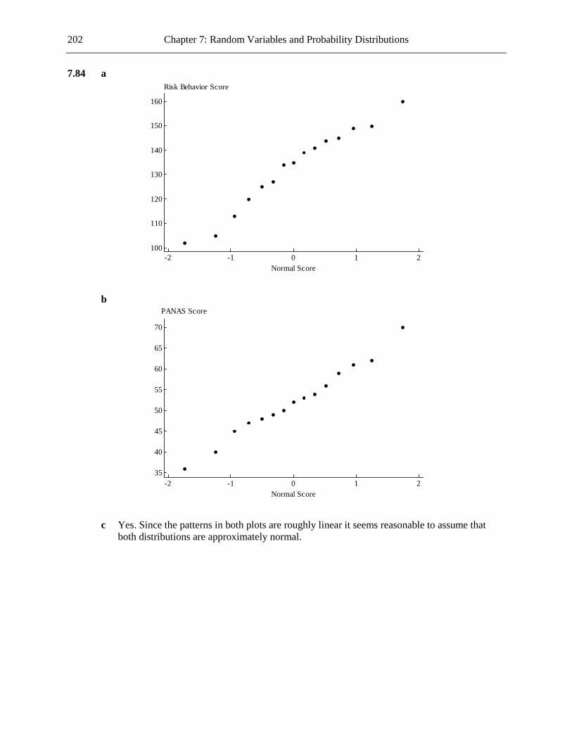
202 Chapter 7: Random Variables and Probability Distributions
7.84 a
210-1-2
160
150
140
130
120
110
100
Normal Score
Risk Behavior Score
b
210-1-2
70
65
60
55
50
45
40
35
Normal Score
PANAS Score
c Yes. Since the patterns in both plots are roughly linear it seems reasonable to assume that
both distributions are approximately normal.

Chapter 7: Random Variables and Probability Distributions 203
7.85 a
686460565248
7
6
5
4
3
2
1
0
x
Frequency
b No. The distribution of x is positively skewed. c
1.841.801.761.721.68
9
8
7
6
5
4
3
2
1
0
log(x)
Frequency
d Yes. The histogram shows a distribution that is slightly closer to being symmetric than the
distribution of the untransformed data.

204 Chapter 7: Random Variables and Probability Distributions
e
8.17.87.57.26.9
7
6
5
4
3
2
1
0
sqrt(x)
Frequency
f Both transformations produce histograms that are closer to being symmetric than the
histogram of the untransformed data, but neither transformation produces a distribution that is truly close to being normal.
7.86 a
210-1-2
0.8
0.7
0.6
0.5
0.4
0.3
0.2
0.1
0.0
Normal Score
sFasL Level
b The normal probability plot appears curved.

Chapter 7: Random Variables and Probability Distributions 205
c
210-1-2
0.9
0.8
0.7
0.6
0.5
0.4
Normal Score
Cube root of x
Yes. This normal probability plot appears more linear than the plot for the untransformed
data. 7.87 Yes. The curve in the normal probability plot suggests that the distribution is not normal. 7.88
210-1-2
450
400
350
300
250
200
150
Normal Score
Lifetime (hrs)
Since the normal probability plot shows a clear curve, the normal distribution is not a plausible
model for power supply lifetime. (However, it is worth noting that most of the apparent curved pattern is brought about by the single point with coordinates (1.539, 422.6).)

206 Chapter 7: Random Variables and Probability Distributions
7.89
210-1-2
16.3
16.2
16.1
16.0
15.9
15.8
15.7
15.6
Normal score
Diameter
Since the pattern in the normal probability plot is very close to being linear, it is plausible that
disk diameter is normally distributed. 7.90
1.81.51.20.90.6
9
8
7
6
5
4
3
2
1
0
Cuberoot(precipitation)
Frequency
The cube-root transformation appears to result in the more symmetrical histogram.
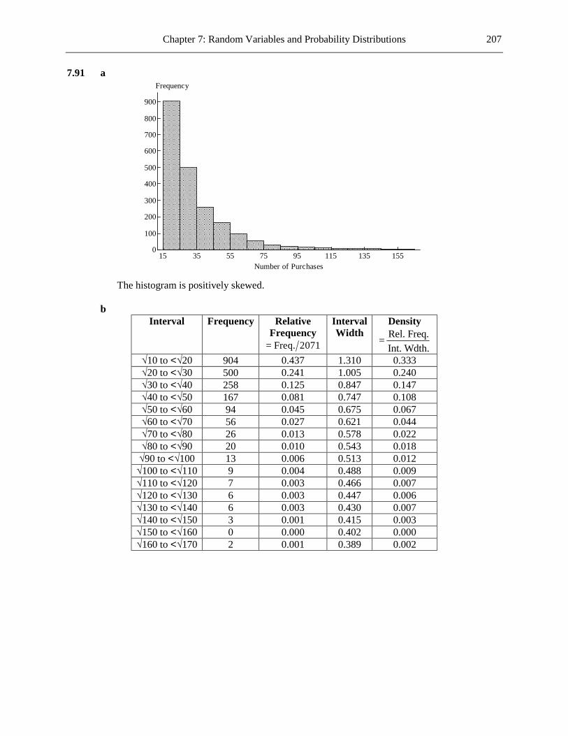
Chapter 7: Random Variables and Probability Distributions 207
7.91 a
1551351159575553515
900
800
700
600
500
400
300
200
100
0
Number of Purchases
Frequency
The histogram is positively skewed. b
Interval Frequency Relative Frequency Freq. 2071=
Interval Width
Density Rel. Freq.Int. Wdth.
=
√10 to <√20 904 0.437 1.310 0.333 √20 to <√30 500 0.241 1.005 0.240 √30 to <√40 258 0.125 0.847 0.147 √40 to <√50 167 0.081 0.747 0.108 √50 to <√60 94 0.045 0.675 0.067 √60 to <√70 56 0.027 0.621 0.044 √70 to <√80 26 0.013 0.578 0.022 √80 to <√90 20 0.010 0.543 0.018 √90 to <√100 13 0.006 0.513 0.012 √100 to <√110 9 0.004 0.488 0.009 √110 to <√120 7 0.003 0.466 0.007 √120 to <√130 6 0.003 0.447 0.006 √130 to <√140 6 0.003 0.430 0.007 √140 to <√150 3 0.001 0.415 0.003 √150 to <√160 0 0.000 0.402 0.000 √160 to <√170 2 0.001 0.389 0.002

208 Chapter 7: Random Variables and Probability Distributions
13119753
0.35
0.30
0.25
0.20
0.15
0.10
0.05
0.00
sqrt(Number of Purchases)
Density
No. The transformation has resulted in a histogram which is still clearly positively skewed. 7.92 a
500503020100
0.05
0.04
0.03
0.02
0.01
0.00
Body Mass (grams)
Density
Yes. If a symmetrical distribution is required, a transformation is desirable. b The logarithms of the body mass values and the resulting histogram are shown below.
Body Mass Log(Body Mass) 1/sqrt(Body Mass) 7.7 0.88649 0.360375 10.1 1.00432 0.314658 21.6 1.33445 0.215166 8.6 0.93450 0.340997 12.0 1.07918 0.288675 11.4 1.05690 0.296174 16.6 1.22011 0.245440 9.4 0.97313 0.326164

Chapter 7: Random Variables and Probability Distributions 209
11.5 1.06070 0.294884 9.0 0.95424 0.333333 8.2 0.91381 0.349215 20.2 1.30535 0.222497 48.5 1.68574 0.143592 21.6 1.33445 0.215166 26.1 1.41664 0.195740 6.2 0.79239 0.401610 19.1 1.28103 0.228814 21.0 1.32222 0.218218 28.1 1.44871 0.188646 10.6 1.02531 0.307148 31.6 1.49969 0.177892 6.7 0.82607 0.386334 5.0 0.69897 0.447214 68.8 1.83759 0.120561 23.9 1.37840 0.204551 19.8 1.29667 0.224733 20.1 1.30320 0.223050 6.0 0.77815 0.408248 99.6 1.99826 0.100201 19.8 1.29667 0.224733 16.5 1.21748 0.246183 9.0 0.95424 0.333333
448.0 2.65128 0.047246 21.3 1.32838 0.216676 17.4 1.24055 0.239732 36.9 1.56703 0.164622 34.0 1.53148 0.171499 41.0 1.61278 0.156174 15.9 1.20140 0.250785 12.5 1.09691 0.282843 10.2 1.00860 0.313112 31.0 1.49136 0.179605 21.5 1.33244 0.215666 11.9 1.07555 0.289886 32.5 1.51188 0.175412 9.8 0.99123 0.319438 93.9 1.97267 0.103197 10.9 1.03743 0.302891 19.6 1.29226 0.225877 14.5 1.16137 0.262613

210 Chapter 7: Random Variables and Probability Distributions
2.82.42.01.61.20.8
18
16
14
12
10
8
6
4
2
0
Log(Body Mass)
Frequency
The distribution is closer to being symmetrical than the original distribution, but is
nonetheless positively skewed. c The transformed values are shown in the table in Part (c). The resulting histogram is shown
below.
0.40.30.20.10.0
16
14
12
10
8
6
4
2
0
1/sqrt(Body Mass)
Frequency
The shape in the histogram roughly resembles that of a normal curve. Certainly, this
transformation was more successful than the other one in producing an approximately normal distribution.
7.93 Yes. In each case the transformation has resulted in a histogram that is much closer to being
symmetric than the original histogram.
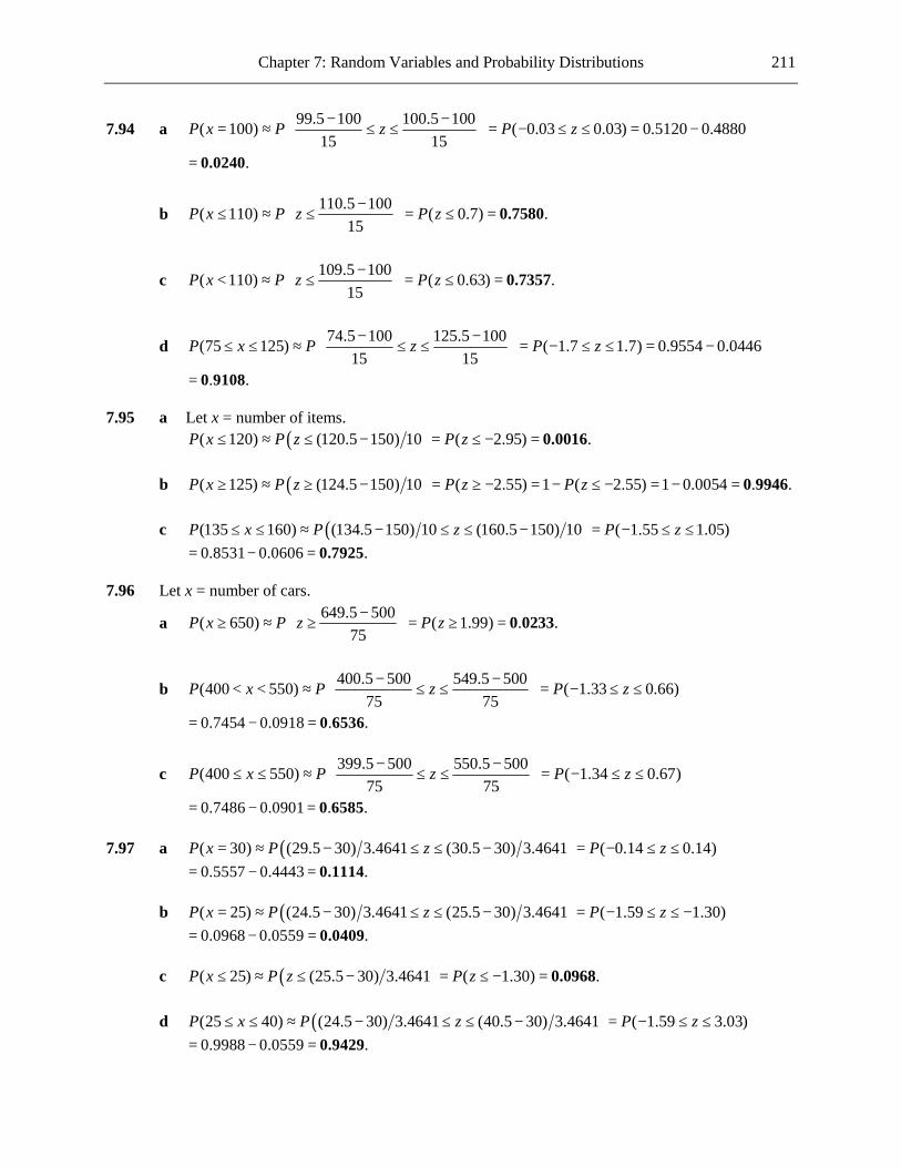
Chapter 7: Random Variables and Probability Distributions 211
7.94 a 99.5 100 100.5 100( 100) ( 0.03 0.03) 0.5120 0.488015 15
P x P z P z− − = ≈ ≤ ≤ = − ≤ ≤ = −
.= 0.0240
b 110.5 100( 110) ( 0.7) .15
P x P z P z− ≤ ≈ ≤ = ≤ =
0.7580
c 109.5 100( 110) ( 0.63) .15
P x P z P z− < ≈ ≤ = ≤ =
0.7357
d 74.5 100 125.5 100(75 125) ( 1.7 1.7) 0.9554 0.044615 15
P x P z P z− − ≤ ≤ ≈ ≤ ≤ = − ≤ ≤ = −
. .= 0 9108 7.95 a Let x = number of items. ( )( 120) (120.5 150) 10 ( 2.95) .P x P z P z≤ ≈ ≤ − = ≤ − = 0.0016 b ( )( 125) (124.5 150) 10 ( 2.55) 1 ( 2.55) 1 0.0054 . .P x P z P z P z≥ ≈ ≥ − = ≥ − = − ≤ − = − = 0 9946 c ( )(135 160) (134.5 150) 10 (160.5 150) 10 ( 1.55 1.05)P x P z P z≤ ≤ ≈ − ≤ ≤ − = − ≤ ≤
0.8531 0.0606 .= − = 0.7925 7.96 Let x = number of cars.
a 649.5 500( 650) ( 1.99) . .75
P x P z P z− ≥ ≈ ≥ = ≥ =
0 0233
b 400.5 500 549.5 500(400 550) ( 1.33 0.66)75 75
P x P z P z− − < < ≈ ≤ ≤ = − ≤ ≤
0.7454 0.0918 . .= − = 0 6536
c 399.5 500 550.5 500(400 550) ( 1.34 0.67)75 75
P x P z P z− − ≤ ≤ ≈ ≤ ≤ = − ≤ ≤
0.7486 0.0901 . .= − = 0 6585 7.97 a ( )( 30) (29.5 30) 3.4641 (30.5 30) 3.4641 ( 0.14 0.14)P x P z P z= ≈ − ≤ ≤ − = − ≤ ≤
0.5557 0.4443 .= − = 0.1114 b ( )( 25) (24.5 30) 3.4641 (25.5 30) 3.4641 ( 1.59 1.30)P x P z P z= ≈ − ≤ ≤ − = − ≤ ≤ −
0.0968 0.0559 .= − = 0.0409 c ( )( 25) (25.5 30) 3.4641 ( 1.30) .P x P z P z≤ ≈ ≤ − = ≤ − = 0.0968 d ( )(25 40) (24.5 30) 3.4641 (40.5 30) 3.4641 ( 1.59 3.03)P x P z P z≤ ≤ ≈ − ≤ ≤ − = − ≤ ≤
0.9988 0.0559 .= − = 0.9429

212 Chapter 7: Random Variables and Probability Distributions
e ( )(25 40) (25.5 30) 3.4641 (39.5 30) 3.4641 ( 1.30 2.74)P x P z P z< < ≈ − ≤ ≤ − = − ≤ ≤ 0.9969 0.0968 .= − = 0.9001
7.98 a Since 60(0.7) 42 10np = = ≥ and (1 ) 60(0.3) 18 10n p− = = ≥ the normal approximation to
the binomial distribution is appropriate. b 60(0.7) 42xµ = = and (1 ) 60(0.7)(0.3) 3.550.x np pσ = − = =
i 41.5 42 42.5 42( 42) ( 0.14 0.14) 0.5557 0.44433.550 3.550
P x P z P z− − = ≈ < < = − < < = −
.= 0.1114
ii 41.5 42( 42) ( 0.14) .3.550
P x P z P z− < ≈ < = < − =
0.4443
iii 42.5 42( 42) ( 0.14) .3.550
P x P z P z− ≤ ≈ < = < =
0.5557
c The probability in (i) is an approximation to the probability that x is exactly 42. The
probability in (ii) is an approximation to the sum of the probabilities of values of x less than 42. The probability in (iii) is an approximation to the sum of the probabilities of values of x less than or equal to 42. These are different quantities.
d When 0.96, (1 ) 60(0.04) 2.4,p n p= − = = which is less than 10, and so the normal
approximation to the binomial distribution cannot be used. Therefore the binomial formula must be used when 0.96.p =
e For a person who is not faking the test, a score of 42 or less is extremely unlikely (a
probability of 0.000000000013 ). Therefore, if someone does get a score of 42 or less, we have convincing evidence that the person is faking the test.
7.99 a There is a fixed number of trials, where the probability of an undetected tumor is the same in
each trial, and the outcomes of the trials are independent since the sample is random. Thus it is reasonable to think that the distribution of x is binomial.
b Yes, since 500(0.031) 15.5 10np = = ≥ and (1 ) 500(0.969) 484.5 10.n p− = = ≥ c 500(0.031) 15.5npµ = = = and (1 ) 500(0.031)(0.969) 3.8755np pσ = − = = .
i ( )( 10) (9.5 15.5) 3.8755 ( 1.55) .P x P z P z< ≈ ≤ − = ≤ − = 0.0606 ii ( )(10 25) (9.5 15.5) 3.8755 (25.5 15.5) 3.8755 ( 1.55 2.58)P x P z P z≤ ≤ ≈ − ≤ ≤ − = − ≤ ≤
0.9951 0.0606 . .= − = 0 9345 iii ( )( 20) (20.5 15.5) 3.8755 ( 1.29) 1 ( 1.29) 1 0.9015P x P z P z P z> ≈ ≥ − = ≥ = − ≤ = −
.= 0.0985 d i In a large number of random samples of 500 women diagnosed with cancer in one breast,
approximately 6.06% will contain less than 10 women with an undetected tumor in the other breast.

Chapter 7: Random Variables and Probability Distributions 213
ii In a large number of random samples of 500 women diagnosed with cancer in one breast,
approximately 93.45% will contain between 10 and 25 (inclusive) women with an undetected tumor in the other breast.
iii In a large number of random samples of 500 women diagnosed with cancer in one breast, approximately 9.85% will contain more than 20 women with an undetected tumor in the other breast.
7.100 a Let x = number of bikes out of 100 that are mountain bikes.
100(0.7) 70,x npµ = = = and (1 ) 100(0.7)(0.3) 4.5826.x np pσ = − = = The normal approximation is valid since 70 10np = ≥ and (1 ) 100(0.3) 30 10.n p− = = ≥
75.5 70( 75) ( 1.20) . .4.5826
P x P z P z− ≤ ≈ ≤ = ≤ =
0 8849
b 59.5 70 75.5 70(60 75) ( 2.29 1.20) 0.8849 0.01104.5826 4.5826
P x P z P z− − ≤ ≤ ≈ ≤ ≤ = − ≤ ≤ = −
. .= 0 8739
c 80.5 70( 80) ( 2.29) . .4.5826
P x P z P z− > ≈ ≥ = ≥ =
0 0110
d (at most 30 are not mountain bikes) (at least 70 are mountain bikes) ( 70)P P P x= = ≥
69.5 70 ( 0.11) . .4.5826
P z P z− ≈ ≥ = ≥ − =
0 5438
7.101 The normal approximation is reasonable since 100(0.25) 25 10np = = ≥ and (1 ) 100(0.75)n p− =
75 10= ≥ . Also, 25npµ = = and (1 ) 100(0.25)(0.75) 4.3301.np pσ = − = = a ( )(20 30) (19.5 25) 4.3301 (30.5 25) 4.3301 ( 1.27 1.27)P x P z P z≤ ≤ ≈ − ≤ ≤ − = − ≤ ≤
0.8980 0.1010 . .= − = 0 7970 b ( )(20 30) (20.5 25) 4.3301 (29.5 25) 4.3301 ( 1.04 1.04)P x P z P z< < ≈ − ≤ ≤ − = − ≤ ≤
0.8508 0.1492 .= − = 0.7016 c ( )( 35) (34.5 25) 4.3301 ( 2.19) 1 ( 2.19) 1 0.9857 .P x P z P z P z≥ ≈ ≥ − = ≥ = − ≤ = − = 0.0143 d 2 25 2(4.3301) 16.3398,µ σ− = − = and 2 25 2(4.3301) 33.6602.µ σ+ = + = So ( is less than two st. devs. from mean) (16.3398 33.6602) (17 33)P x P x P x= ≤ ≤ = ≤ ≤
( )(16.5 25) 4.3301 (33.5 25) 4.3301 ( 1.96 1.96) 0.9750 0.0250P z P z≈ − ≤ ≤ − = − ≤ ≤ = − 0.9500.= Therefore the probability that x is more than 2 standard deviations from its mean is
1 0.9500 .− = 0.05 7.102 a Let x = number of voters out of 225 who favor the waiting period.
225(0.65) 146.25,x npµ = = = and (1 ) 225(0.65)(0.35) 7.1545.x np pσ = − = = The normal approximation is valid since 146.25 10np = ≥ and

214 Chapter 7: Random Variables and Probability Distributions
(1 ) 225(0.35) 78.75 10.n p− = = ≥ 149.5 146.25( 150) ( 0.45) .
7.1545P x P z P z− ≥ ≈ ≥ = ≥ =
0.3264
b 150.5 146.25( 150) ( 0.59) .7.1545
P x P z P z− > ≈ ≥ = ≥ =
0.2776
c 124.5 146.25( 125) ( 3.04) . .7.1545
P x P z P z− < ≈ < = < − =
0 0012
7.103 a No, since 50(0.05) 2.5 10.np = = < b Now 500n = and 0.05,p = so 500(0.05) 25 10.np = = ≥ So the techniques of this section
can be used. Using 25npµ = = and (1 ) 500(0.05)(0.95) 4.8734,np pσ = − = =
( )(at least 20 are defective) (19.5 25) 4.8734 ( 1.13) 1 ( 1.13)P P z P z P z≈ ≥ − = ≥ − = − ≤ − 1 0.1292 .= − = 0.8708
7.104 a Let x = number of mufflers out of 400 that are replaced.
400(0.2) 80.x npµ = = = (1 ) 400(0.2)(0.8) 8.x np pσ = − = =
The normal approximation is valid since 80 10np = ≥ and (1 ) 400(0.8) 320 10.n p− = = ≥ 74.5 80 100.5 80(75 100) ( 0.69 2.56) 0.9948 0.2451 . .
8 8P x P z P z− − ≤ ≤ ≈ ≤ ≤ = − ≤ ≤ = − =
0 7497
b 70.5 80( 70) ( 1.19) . .8
P x P z P z− ≤ ≈ ≤ = ≤ − =
0 1170
c 49.5 80( 50) ( 3.81) 0.0001.8
P x P z P z− < ≈ ≤ = ≤ − =
This tells us that fewer than 50
mufflers being replaced in a sample of 400 is unlikely, assuming that 20% of all mufflers are being replaced. Therefore, yes, the 20% figure would be questioned.
7.105 a ( )(250 300) (250 266) 16 (300 266) 16 ( 1 2.125)P x P z P z< < = − < < − = − < <
0.9832 0.1587 .= − = 0.8245 b ( )( 240) (240 266) 16 ( 1.625) .P x P z P z≤ = ≤ − = ≤ − = 0.0521 c Sixteen days is 1 standard deviation, so we need ( 1 1) 0.8413 0.1587 .P z− < < = − = 0.6826 d ( )( 310) (310 266) 16 ( 2.75) 1 ( 2.75) 1 0.9970 .P x P z P z P z≥ = ≥ − = ≥ = − ≤ = − = 0.0030
This should make us skeptical of the claim, since it is very unlikely that a pregnancy will last at least 310 days.

Chapter 7: Random Variables and Probability Distributions 215
e The insurance company will refuse to pay if the birth occurs within 275 days of the beginning
of the coverage. If the conception took place after coverage began, then the insurance company will refuse to pay if the pregnancy is less than or equal to 275 14 261− = days.
( )( 261) (261 266) 16 ( 0.31) .P x P z P z≤ = ≤ − = ≤ − = 0.3783 7.106 The distribution of x is binomial with 15n = and 0.6.p = Using Appendix Table 9, the required
probability is (5 10) 0.024 0.061 0.118 0.177 0.207 0.186 . .P x≤ ≤ = + + + + + = 0 773 7.107 a ( 3) 0.1 0.15 0.2 0.25 .P x ≤ = + + + = 0.7 b ( 3) 0.1 0.15 0.2 .P x < = + + = 0.45 c ( 3) 1 ( 3) 1 0.45 .P x P x≥ = − < = − = 0.55 d (2 5) 0.2 0.25 0.2 0.06 .P x≤ ≤ = + + + = 0.71 e If 2 lines are not in use, then 4 lines are in use. If 3 lines are not in use, then 3 lines are in use. If 4 lines are not in use, then 2 lines are in use. So the required probability is (2 4) 0.2 0.25 0.2 .P x≤ ≤ = + + = 0.65 f If 4 lines are not in use, then 2 lines are in use. If 5 lines are not in use, then 1 line is in use. If 6 lines are not in use, then 0 lines are in use. So the required probability is (0 2) 0.1 0.15 0.2 . .P x≤ ≤ = + + = 0 45 7.108 a 0(0.1) 1(0.15) 6(0.04) . .xµ = + + + = 2 64L
2 2 2(0 2.64) (0.1) (6 2.64) (0.04) 2.3704.xσ = − + + − =L 2.3704 . .xσ = = 1 540
b 3 2.64 3(1.540) 1.98.x xµ σ− = − = −
3 2.64 3(1.540) 7.26.x xµ σ+ = + = Since all the possible values of x lie between these two values, the required probability is 0.
7.109 a (2) (0.8)(0.8) .p = = 0.64 b (3) (UAA or AUA) (0.2)(0.8)(0.8) (0.8)(0.2)(0.8) . .p P= = + = 0 256 c For y to be 5, the fifth battery’s voltage must be acceptable. The four outcomes are UUUAA,
UUAUA, UAUUA, AUUUA. So (5) 4(0.2)(0.2)(0.2)(0.8)(0.8) . .p = = 0 02048 d In order for it to take y selections to find two acceptable batteries, the first 1y − batteries
must include exactly 1 acceptable battery (and therefore 2y − unacceptable batteries), and the yth battery must be acceptable. There are 1y − ways in which the first 1y − batteries can

216 Chapter 7: Random Variables and Probability Distributions
include exactly 1 acceptable battery. So 1 2( ) ( 1)(0.8) (0.2) (0.8)yp y y −= − ⋅ 2 2( 1)(0.2) (0.8) .yy −= −
7.110 a Let x = amount of cheese on a medium pizza.
0.525 0.5 0.550 0.5(0.525 0.550) (1 2) 0.9772 0.8413 . .0.025 0.025
P x P z P z− − < < = < < = < < = − =
0 1359
b The required probability is ( 2) 1 ( 2) 1 0.9772 . .P z P z> = − ≤ = − = 0 0228 c ( 0.475) ( 1) 0.8413.P x P z≥ = ≥ − = So the required probability is 3(0.8413) .= 0.595 7.111 Let the fuel efficiency of a randomly selected car of this type be x. a ( ) ( )(29 31) (29 30) 1.2 (31 30) 1.2 0.83 0.83P x P z P z< < = − < < − = − < <
0.7967 0.2033 . .= − = 0 5934 b ( ) ( )( 25) (25 30) 1.2 4.17 0.0000.P x P z P z< = < − = < − = Yes, you are very unlikely to
select a car of this model with a fuel efficiency of less than 25 mpg. c ( ) ( )( 32) (32 30) 1.2 1.67 0.0475.P x P z P z> = > − = > = So, if 3 cars are selected, the
probability that they all have fuel efficiencies more than 32 mpg is 3(0.0475) .= 0.0001 d If ( *) 0.95,P z z> = then * 1.645.z = − So ( *) 30 (1.645)(1.2) .c zµ σ= + = − = 28.026 7.112 a If the coin is fair then the distribution of x is binomial with 25n = and 0.5.p = The
probability that it is judged to be biased is ( 7) ( 18).P x P x≤ + ≥ Using Appendix Table 9, ( 7) 0.014 0.005 0.002 0.021.P x ≤ = + + = ( 18) 0.014 0.005 0.002 0.021.P x ≥ = + + =
So the probability that the coin is judged to be biased is 0.021 0.021 .+ = 0.042 b Now the distribution of x is binomial with 25n = and 0.9.p = The probability that the coin
is judged to be biased is ( 7) ( 18).P x P x≤ + ≥ Using Appendix Table 9, ( 7) 0.000.P x ≤ = ( 18) 0.007 0.024 0.065 0.138 0.226 0.266 0.199 0.072 0.997.P x ≥ = + + + + + + + =
So the probability that the coin is judged to be fair is 1 0.997 . .− = 0 003 When ( ) 0.1,P H = the distribution of x is binomial with 25n = and 0.1.p = The probability that the coin is judged to be biased is ( 7) ( 18).P x P x≤ + ≥ Using Appendix Table 9,
( 7) 0.007 0.024 0.065 0.138 0.227 0.266 0.199 0.072 0.998.P x ≤ = + + + + + + + = ( 18) 0.000.P x ≥ =
So the probability that the coin is judged to be fair is 1 0.998 . .− = 0 002 c When ( ) 0.6,P H = the distribution of x is binomial with 25n = and 0.6.p = The probability
that the coin is judged to be biased is ( 7) ( 18).P x P x≤ + ≥ Using Appendix Table 9,

Chapter 7: Random Variables and Probability Distributions 217
( 7) 0.001.P x ≤ = ( 18) 0.080 0.044 0.020 0.007 0.002 0.153.P x ≥ = + + + + =
So the probability that the coin is judged to be fair is 1 0.153 . .− = 0 847 Likewise, by symmetry, when ( ) 0.4,P H = the probability that the coin is judged to be fair is0.847. These probabilities are larger than those in Part (b), since, when ( ) 0.6P H = or ( ) 0.4,P H = the probability of getting a head is closer to 0.5 than when ( ) 0.9P H = or ( ) 0.1.P H = Thus it is more likely that the coin will be judged to be fair when ( ) 0.6P H = or ( ) 0.4.P H =
d It is now more likely that the coin will be judged to be fair, and so the error probabilities are
increased. This would seem to make the rule less good, however this rule makes it more likely that the coin will be judged to be fair when in fact it is fair.
7.113 2 2 2(0 1.2) (0.54) (4 1.2) (0.2) .xσ = − + + − = 2.52L 2.52 .xσ = = 1.587 7.114 a Let x = amount of time spent.
45 60( 45) ( 1.5) .10
P x P z P z− > = > = > − =
0.9332
b If ( *) 0.1,P z z> = 1.28.z = So ( *) 60 1.28(10) minutes.x zµ σ= + = + = 72.8
c Letting y = revenue, we have ( ) 510 50 60 10 .6
y x x= + = + So the mean revenue is
510 (60) 60.6yµ = + = The mean revenue is $60.
7.115 Let the life of a randomly chosen battery be x. a ( )( 4) (4 6) 0.8 ( 2.5) 0.9938.P x P z P z> = > − = > − = For the player to function for at least 4
hours, both batteries have to last for at least 4 hours. The probability that this happens is 2(0.9938) .= 0.9876
b ( )( 7) (7 6) 0.8 ( 1.25) 0.1056.P x P z P z> = > − = > = For the player to function for at least 7
hours, both batteries have to last for at least 7 hours. The probability that this happens is 2(0.1056) 0.0112.= So the probability that the player works for at most 7 hours is
1 0.0112 .− = 0.9888 c We need the probability that both batteries last longer than c hours to be 0.05. So for either
one of the two batteries, we need the probability that it lasts longer than c hours to be 0.05 0.2236= (so that the probability that both batteries last longer than c hours is
2(0.2236) 0.05= ). Now, if ( *) 0.2236,P z z> = then 0.76.z = So ( *)c zµ σ= + 6 (0.76)(0.8) . .= + = 6 608
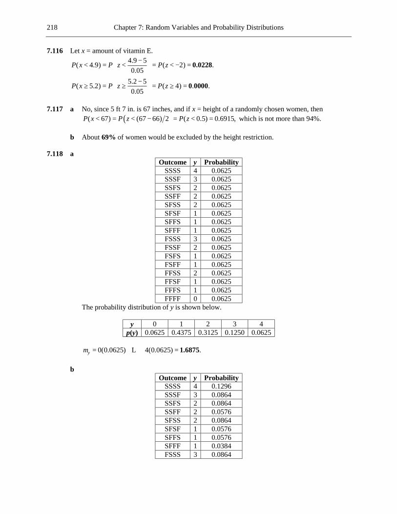
218 Chapter 7: Random Variables and Probability Distributions
7.116 Let x = amount of vitamin E. 4.9 5( 4.9) ( 2) .0.05
P x P z P z− < = < = < − =
0.0228
5.2 5( 5.2) ( 4) . .0.05
P x P z P z− ≥ = ≥ = ≥ =
0 0000
7.117 a No, since 5 ft 7 in. is 67 inches, and if x = height of a randomly chosen women, then
( )( 67) (67 66) 2 ( 0.5) 0.6915,P x P z P z< = < − = < = which is not more than 94%. b About 69% of women would be excluded by the height restriction. 7.118 a
Outcome y Probability SSSS 4 0.0625 SSSF 3 0.0625 SSFS 2 0.0625 SSFF 2 0.0625 SFSS 2 0.0625 SFSF 1 0.0625 SFFS 1 0.0625 SFFF 1 0.0625 FSSS 3 0.0625 FSSF 2 0.0625 FSFS 1 0.0625 FSFF 1 0.0625 FFSS 2 0.0625 FFSF 1 0.0625 FFFS 1 0.0625 FFFF 0 0.0625
The probability distribution of y is shown below.
y 0 1 2 3 4 p(y) 0.0625 0.4375 0.3125 0.1250 0.0625
0(0.0625) 4(0.0625) .yµ = + + = 1.6875L b
Outcome y Probability SSSS 4 0.1296 SSSF 3 0.0864 SSFS 2 0.0864 SSFF 2 0.0576 SFSS 2 0.0864 SFSF 1 0.0576 SFFS 1 0.0576 SFFF 1 0.0384 FSSS 3 0.0864

Chapter 7: Random Variables and Probability Distributions 219
FSSF 2 0.0576 FSFS 1 0.0576 FSFF 1 0.0384 FFSS 2 0.0576 FFSF 1 0.0384 FFFS 1 0.0384 FFFF 0 0.0256
The probability distribution of y is shown below.
y 0 1 2 3 4 p(y) 0.0256 0.3264 0.3456 0.1728 0.1296
0(0.0256) 4(0.1296) . .yµ = + + = 2 0544L
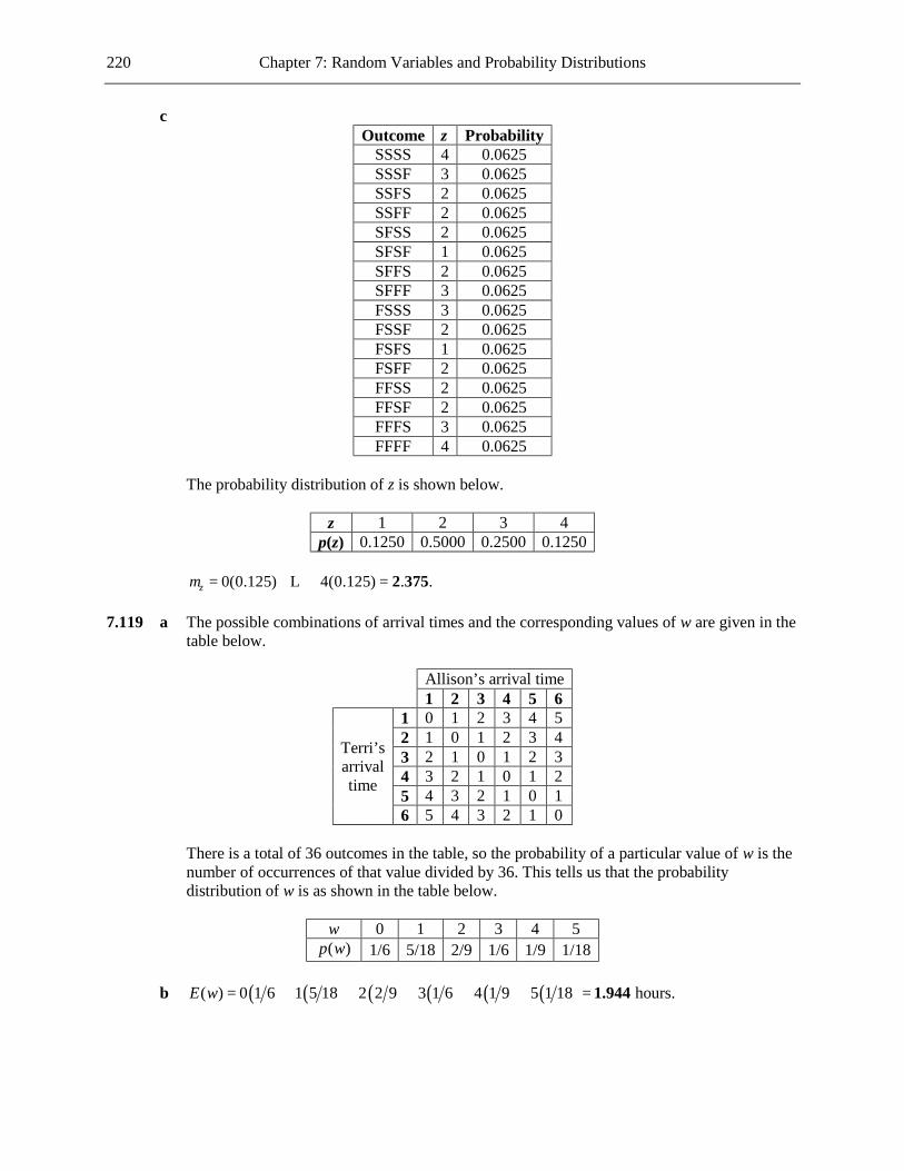
220 Chapter 7: Random Variables and Probability Distributions
c Outcome z Probability
SSSS 4 0.0625 SSSF 3 0.0625 SSFS 2 0.0625 SSFF 2 0.0625 SFSS 2 0.0625 SFSF 1 0.0625 SFFS 2 0.0625 SFFF 3 0.0625 FSSS 3 0.0625 FSSF 2 0.0625 FSFS 1 0.0625 FSFF 2 0.0625 FFSS 2 0.0625 FFSF 2 0.0625 FFFS 3 0.0625 FFFF 4 0.0625
The probability distribution of z is shown below.
z 1 2 3 4 p(z) 0.1250 0.5000 0.2500 0.1250
0(0.125) 4(0.125) . .zµ = + + = 2 375L 7.119 a The possible combinations of arrival times and the corresponding values of w are given in the
table below.
Allison’s arrival time 1 2 3 4 5 6
Terri’s arrival time
1 0 1 2 3 4 5 2 1 0 1 2 3 4 3 2 1 0 1 2 3 4 3 2 1 0 1 2 5 4 3 2 1 0 1 6 5 4 3 2 1 0
There is a total of 36 outcomes in the table, so the probability of a particular value of w is the
number of occurrences of that value divided by 36. This tells us that the probability distribution of w is as shown in the table below.
w 0 1 2 3 4 5 ( )p w 1/6 5/18 2/9 1/6 1/9 1/18
b ( ) ( ) ( ) ( ) ( ) ( )( ) 0 1 6 1 5 18 2 2 9 3 1 6 4 1 9 5 1 18 hours.E w = + + + + + = 1.944

Chapter 7: Random Variables and Probability Distributions 221
7.120 1( 1) (a or b picked first) .2
P x P= = =
1 2 1 2 1( 2) (c then not d) (d then not c) .4 3 4 3 3
P x P P = = + = + =
1 1 1( 3) 1 .2 3 6
P x = = − − =
These results are summarized in the table below.
x 1 2 3 p(x) 1/2 1/3 1/6
7.121 a 4 4(4) (KKKK) (LLLL) (0.4) (0.6) .p P P= + = + = 0.1552 b 3 3
in any order in any order(5) ( LLLK L) ( KKKL K) 4(0.6) (0.4)(0.6) 4(0.4) (0.6)(0.4) .p P P= + = + = 0.2688123 123
c 3 2 3 2
5 3 5 3in any order in any order
(6) (LLLKK L) (KKKLLK) (0.6) (0.4) (0.6) (0.4) (0.6) (0.4) 0.29952.p P P C C= + = + =14243 14243
3 3 3 36 3 6 3
in any order in any order(7) (LLLKKK L) (LLLKKK K) (0.6) (0.4) (0.6) (0.6) (0.4) (0.4)p P P C C= + = +14243 14243
0.27648.= So the probability distribution of x is as shown below.
x 4 5 6 7 p(x) 0.1552 0.2688 0.29952 0.27648
d ( ) 4(0.1552) 5(0.2688) 6(0.29952) 7(0.27648) . .E x = + + + = 5 697 7.122 The total number of games played is x, and the winning player always plays 4 games. So the
losing player plays 4x − games. That is, 4.y x= − Thus the probability distribution of y is as shown below.
y 0 1 2 3
p(y) 0.1552 0.2688 0.29952 0.27648 7.123 If ( *) 0.15,P z z≥ = then * 1.04.z = So the lowest score to be designated an A is given by
( *) 78 (1.04)(7) 85.28.zµ σ+ = + = Since 89 85.28,> yes, I received an A. 7.124 Let the pH of the randomly selected soil sample be x. a ( )(5.9 6.15) (5.9 6) 0.1 (6.15 6) 0.1 ( 1 1.5)P x P z P z< < = − < < − = − < <
0.9332 0.1587 .= − = 0.7745 b ( )( 6.10) (6.10 6) 0.1 ( 1) 1 ( 1) 1 0.8413 .P x P z P z P z> = > − = > = − ≤ = − = 0.1587
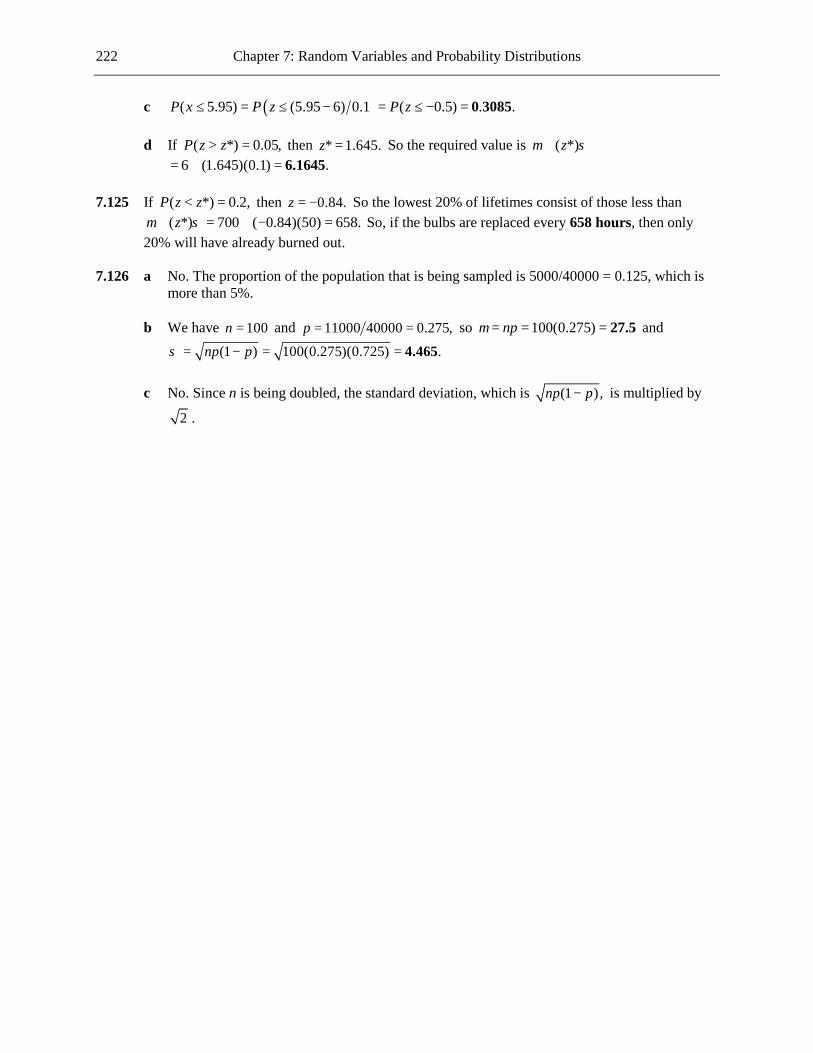
222 Chapter 7: Random Variables and Probability Distributions
c ( )( 5.95) (5.95 6) 0.1 ( 0.5) . .P x P z P z≤ = ≤ − = ≤ − = 0 3085 d If ( *) 0.05,P z z> = then * 1.645.z = So the required value is ( *)zµ σ+
6 (1.645)(0.1) .= + = 6.1645 7.125 If ( *) 0.2,P z z< = then 0.84.z = − So the lowest 20% of lifetimes consist of those less than
( *) 700 ( 0.84)(50) 658.zµ σ+ = + − = So, if the bulbs are replaced every 658 hours, then only 20% will have already burned out.
7.126 a No. The proportion of the population that is being sampled is 5000/40000 = 0.125, which is
more than 5%. b We have 100n = and 11000 40000 0.275,p = = so 100(0.275)npµ = = = 27.5 and
(1 ) 100(0.275)(0.725) .np pσ = − = = 4.465 c No. Since n is being doubled, the standard deviation, which is (1 ),np p− is multiplied by
2 .

Chapter 7: Random Variables and Probability Distributions 223
Cumulative Review Exercises
CR7.1 Obtain a group of volunteers (we’ll assume that 60 people are available for this). Randomly
assign the 60 people to two groups, A and B. (This can be done by writing the people’s names on slips of paper, placing the slips in a hat, and drawing 30 slips at random. The people whose names are on those slips should be placed in Group A. The remaining people should be placed in Group B.) Meet with each person individually. For people in Group A offer an option of being given $5 or for a coin to be flipped. Tell the person that if the coin lands heads, he/she will be given $10, but if the coin lands tails, he/she will not be given any money. Note the person’s choice, and then proceed according to the option the person has chosen. For people in Group B, give the person two $5 bills, and then offer a choice of returning one of the $5 bills, or flipping a coin. Tell the person that if the coin lands heads, he/she will keep both $5 bills, but if the coin lands tails, he/she must return both of the $5 bills. Note the person’s choice, and then proceed according to the option the person has chosen. Once you have met with all the participants, compare the two groups in terms of the proportions choosing the gambling options.
CR7.2 a Median = 87
Lower quartile = 69 Upper quartile = 96 Interquartile range = 96 − 69 = 27
35030025020015010050Water Consumption (gallons per person per day)
The center of the water consumption distribution is around 87, with the majority of values
lying between 70 and 114. There are four outliers, three of which are extreme outliers. If the outliers are included the distribution is positively skewed; without the outliers the distribution is roughly symmetrical.
b (49 334) 27 .x = + + = 104.222L
2 2(49 104.222) (334 104.222) .26xs − + + −
= = 71.580L
c If the two largest values were removed the standard deviation would be smaller, since the
spread of the data would be reduced. d The mean (104.222) is greater than the median (87). This is consistent with the fact that the
distribution is positively skewed. CR7.3 No. The percentages given in the graph are said to be, for each year, the “percent increase in the
number of communities installing” red-light cameras. This presumably means the percent increase in the number of communities with red-light cameras installed, in which case the positive results for all of the years 2003 to 2009 show that a great many more communities had red-light cameras installed in 2009 than in 2002.

224 Chapter 7: Random Variables and Probability Distributions
CR7.4 a ( | ) 0.57,P I W = while we can infer from the larger proportions of blacks and Hispanics who rated the Census as “very important” that ( | )CP I W is larger than 0.57. Hence I and W are dependent events.
b Answers will vary. CR7.5 We need 1 2(15.8 15.9).P b b≤ + ≤ Since
1 28,b bµ µ= = and
1 20.2,b bσ σ= =
1 28 8 16b bµ + = + =
and 1 2
2 2(0.2) (0.2) 0.2828.b bσ + = + =
So ( )1 2(15.8 15.9) (15.8 16) 0.2828 (15.9 16) 0.2828P b b P z≤ + ≤ = − ≤ ≤ − ( 0.71 0.35) 0.3632 0.2389 .P z= − ≤ ≤ − = − = 0.1243
CR7.6
19951990198519801975
200
150
100
50
0
Year
Number of Manatee Deaths
The trend was for the number of manatee deaths per year to increase. Allowing for year-to-year
variations, the number of deaths per year seems to have increased at a roughly constant rate. CR7.7 ( )(Service 1 | Late) (Service 1 Late) (Late) (0.3)(0.1) (0.3)(0.1) (0.7)(0.08) 0.349.P P P= ∩ = + =
So (Service 2 | Late) 1 0.349 0.651.P = − = Thus Service 2 is more likely to have been used. CR7.8 First, the median is approximately equal to the mean, implying a roughly symmetrical
distribution. Second, consider the comparison of z values given below.
Statistic z value in this distribution z value in normal distribution Median 0.15 0 5th percentile −1.46 −1.645 Lower quartile −0.88 −0.67 Upper quartile 0.62 0.67 95th percentile 1.73 1.645

Chapter 7: Random Variables and Probability Distributions 225
Although the z values do not agree exactly, they are somewhat close, and therefore it would seem
reasonable to suggest that the distribution could have been approximately normal. CR7.9 1. ( ) 0.021.P M = 2. ( | ) 0.043.P M B = 3. ( | ) 0.07.P M W = CR7.10 a i 135/182 = 0.742 ii (173 + 206)/(210 + 231) = 379/441 = 0.859 b
CR7.11 To say that a quantity x is 30% more than a quantity y means that the amount by which x exceeds
y is 30% of y; that is, in mathematical notation, that 0.3 .y x y− = Dividing both sides by 0.3, we see that this can be written as ( ) 0.3y x y− = . Here we are told that drivers who live within one mile of a restaurant are 30% more likely to have an accident than those who do not live within one mile of a restaurant; in other words, that ( | )P A R is 30% more than ( | )CP A R . Thus
statement iv is correct: ( )( | ) ( | ) ( | ) 0.3.C CP A R P A R P A R− = None of the other statements is correct.
CR7.12 They are dependent events, since the probability that an adult favors stricter gun control given
that the adult is female (0.66) is greater than the (unconditional) probability that the adult favors stricter gun control (0.56).
Iowa City (city)
Iowa City (interstate)
Properly Restrained
Not Properly Restrained
Properly Restrained
Not Properly Restrained

226 Chapter 7: Random Variables and Probability Distributions
CR7.13
a (Drug Positive) (0.1)(0.9) .P ∩ = = 0.09 b (No Drug Positive) (0.9)(0.05) .P ∩ = = 0.045 c (Positive) 0.09 0.045 .P = + = 0.135 d (Drug | Positive) (Drug Positive) (Positive) 0.09 0.135 .P P P= ∩ = = 0.667 CR7.14 a (0.1)(0.9)(0.9) = 0.081. b (0.1)(0.9)(0.9) + (0.9)(0.05)(0.05) = 0.08325.
c (drug positive twice) 0.081(drug | positive twice) . .(positive twice) 0.08325
PPP
∩= = = 0 973
d (not positive twice | drug) 1 (positive twice | drug) 1 (0.9)(0.9) .P P= − = − = 0.19 e The retest scheme is preferable in that the probability that someone uses drugs given that the
person has tested positive twice is 0.973, which is much greater than the probability that someone uses drugs given a single positive test (0.667). However, under the retest scheme it is more likely that someone who uses drugs will not get caught (a probability of 0.19 under the retest scheme as opposed to 0.1 under the single test scheme).
CR7.15 a 1(0.2) 4(0.1) . .xµ = + + = 2 3L b 2 2 2(1 2.3) (0.2) (4 2.3) (0.1) . .xσ = − + + − = 0 81L 0.81 .xσ = = 0 9 CR7.16 100 5y x= − .
So 100 5 100 5(2.3)y xµ µ= − = − = 88.5 ,
0.95
0.05
0.1
0.9
0.9
0.1 Drug
No Drug
Positive
Negative
Positive
Negative

Chapter 7: Random Variables and Probability Distributions 227
and 5 5(0.9) 4.5y xσ σ= = = .
So 2 2(4.5)yσ = = 20.25 . CR7.17 Let x be the number of correct identifications. Assume that the graphologist was merely guessing,
in other words that the probability of success on each trial was 0.5. Then, using Appendix Table 9 (with 15, 0.5n p= = ), ( 6) 0.205 0.117 0.044 0.010 0.001 0.377.P x ≥ = + + + + = Since this probability is not particularly small, this tells us that, if the graphologist was guessing, then it would not have been unlikely for him/her to get 6 or more correct identifications. Thus no ability to distinguish the handwriting of psychotics is indicated.
CR7.18 A ball bearing is acceptable if its diameter is between 0.496 and 0.504 inches. Under the new
setting, ( )(0.496 diameter 0.504) (0.496 0.499) 0.002 (0.504 0.499) 0.002P P z< < = − ≤ ≤ − ( 1.5 2.5) 0.9938 0.0668 0.9270.P z= − ≤ ≤ = − = So the probability that a ball bearing is
unacceptable is 1 0.9270 0.0730.− = Therefore, 7.3% of the ball bearings will be unacceptable. CR7.19 a ( )( 50) (50 45) 5 ( 1) .P x P z P z> = > − = > = 0.1587 b If ( *) 0.9P z z< = then * 1.28.z = So the required time is ( *) 45 (1.28)(5)zµ σ+ = +
minutes.= 51.4 c If ( *) 0.25P z z< = then * 0.67.z = − So the required time is ( *) 45 ( 0.67)(5)zµ σ+ = + −
. minutes.= 41 65 CR7.20
210-1-2
400
300
200
100
0
Normal Score
x
Yes. Since the pattern in the normal probability plot is relatively straight, normality is plausible.

228 Chapter 7: Random Variables and Probability Distributions
CR7.21 a
Survival Time (days) Frequency Relative Frequency 0 to <300 8 0.186
300 to <600 12 0.279 600 to <900 5 0.116 900 to <1200 5 0.116 1200 to <1500 3 0.070 1500 to <1800 3 0.070 1800 to <2100 4 0.093 2100 to <2400 1 0.023 2400 to <2700 2 0.047
2400180012006000
30
25
20
15
10
5
0
Survival Time (days)
Relative Frequency (%)
b Positive c Yes. If a symmetrical distribution were required then a transformation would be advisable.

229
Chapter 8 Sampling Variability and Sampling Distributions
Note: In this chapter, numerical answers to questions involving the normal distribution were found using statistical tables. Students using calculators or computers will find that their answers differ slightly from those given. 8.1 A population characteristic is a quantity that summarizes the whole population. A statistic is a
quantity calculated from the values in a sample. 8.2 The quantity x is the mean of a sample, while the quantity µ is the mean of a population. The
quantity s is the standard deviation of a sample, while the quantity σ is the standard deviation of a population.
8.3 a Population characteristic b Statistic c Population characteristic d Population characteristic e Statistic 8.4 a (8 + 14 + 16 + 10 + 11)/5 = 11.8. b Answers will vary. c Answers will vary. d Answers will vary. 8.5 Answers will vary. 8.6 a The x values would be more densely congregated than in Example 8.1. b The histogram would have a similar shape to the one in Example 8.1, and the distribution of
the x values would have approximately the same center.

230 Chapter 8: Sampling Variability and Sampling Distributions
8.7 a Sample Sample mean
1, 2 1.5 1, 3 2 1, 4 2.5 2, 1 1.5 2, 3 2.5 2, 4 3 3, 1 2 3, 2 2.5 3, 4 3.5 4, 1 2.5 4, 2 3 4, 3 3.5
b The sampling distribution of the sample mean, x , is shown below.
x 1.5 2 2.5 3 3.5 ( )p x 1/6 1/6 1/3 1/6 1/6
3.53.02.52.01.5
0.7
0.6
0.5
0.4
0.3
0.2
0.1
0.0
Sample Mean
Density

Chapter 8: Sampling Variability and Sampling Distributions 231
c
Sample Sample Mean 1, 1 1 1, 2 1.5 1, 3 2 1, 4 2.5 2, 1 1.5 2, 2 2 2, 3 2.5 2, 4 3 3, 1 2 3, 2 2.5 3, 3 3 3, 4 3.5 4, 1 2.5 4, 2 3 4, 3 3.5 4, 4 4
The sampling distribution of the sample mean, x , is shown below.
x 1 1.5 2 2.5 3 3.5 4 ( )p x 1/16 1/8 3/16 1/4 3/16 1/8 1/16
4.03.53.02.52.01.51.0
0.5
0.4
0.3
0.2
0.1
0.0
Sample Mean
Density
d Both distributions are symmetrical, and their means are equal (2.5). However, the “with
replacement” version has a greater spread than the first distribution, with values ranging from 1 to 4 in the “with replacement” distribution, and from 1.5 to 3.5 in the “without replacement” distribution. The stepped pattern of the “with replacement” distribution more closely resembles a normal distribution than does the shape of the “without replacement” distribution.
8.8 Answers will vary.
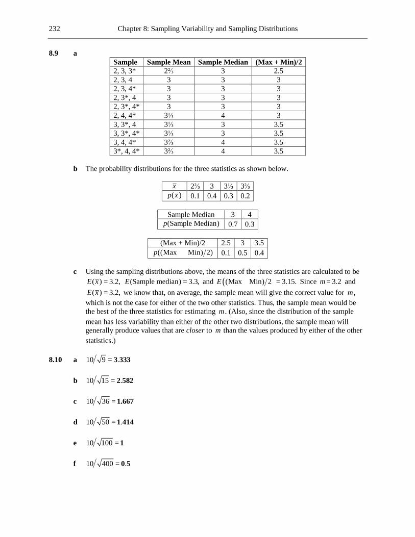
232 Chapter 8: Sampling Variability and Sampling Distributions
8.9 a Sample Sample Mean Sample Median (Max + Min)/2 2, 3, 3* 2⅔ 3 2.5 2, 3, 4 3 3 3 2, 3, 4* 3 3 3 2, 3*, 4 3 3 3 2, 3*, 4* 3 3 3 2, 4, 4* 3⅓ 4 3 3, 3*, 4 3⅓ 3 3.5 3, 3*, 4* 3⅓ 3 3.5 3, 4, 4* 3⅔ 4 3.5 3*, 4, 4* 3⅔ 4 3.5
b The probability distributions for the three statistics as shown below.
x 2⅔ 3 3⅓ 3⅔ ( )p x 0.1 0.4 0.3 0.2
Sample Median 3 4 (Sample Median)p 0.7 0.3
(Max + Min)/2 2.5 3 3.5
((Max Min) 2)p + 0.1 0.5 0.4 c Using the sampling distributions above, the means of the three statistics are calculated to be
( ) 3.2,E x = (Sample median) 3.3,E = and ( )(Max Min) 2 3.15.E + = Since 3.2µ = and ( ) 3.2,E x = we know that, on average, the sample mean will give the correct value for µ ,
which is not the case for either of the two other statistics. Thus, the sample mean would be the best of the three statistics for estimating µ . (Also, since the distribution of the sample mean has less variability than either of the other two distributions, the sample mean will generally produce values that are closer to µ than the values produced by either of the other statistics.)
8.10 a 10 9 .= 3 333 b 10 15 .= 2 582 c 10 36 = 1.667 d 10 50 .= 1 414 e 10 100 = 1 f 10 400 .= 0 5

Chapter 8: Sampling Variability and Sampling Distributions 233
8.11 The sampling distribution of x will be approximately normal for the sample sizes in Parts (c)‒(f),
since those sample sizes are all greater than or equal to 30. 8.12 The quantity µ is the population mean, while the quantity xµ is the mean of all possible sample
means. The quantity σ is the population standard deviation, while the quantity xσ is the standard deviation of all the possible sample means.
8.13 a ,xµ = 40 and 5 64 .x nσ σ= = = 0.625 Since 64 30,n = ≥ the distribution of x will be
approximately normal. b Since 0.5 40 0.5 39.5µ − = − = and 0.5 40 0.5 40.5,µ + = + = the required probability is
( )(39.5 40.5) (39.5 40) 0.625 (40.5 40) 0.625 ( 0.8 0.8)P x P z P z< < = − < < − = − < < 0.7881 0.2119 .= − = 0.5762
c Since 0.7 40 0.7 39.3µ − = − = and 0.7 40 0.7 40.7,µ + = + = the probability that x will be
within 0.7 of µ is ( )(39.3 40.7) (39.3 40) 0.625 (40.7 40) 0.625P x P z< < = − < < − ( 1.12 1.12) 0.8686 0.1314 0.7372.P z= − < < = − = Therefore, the probability that x will be
more than 0.7 from µ is 1 0.7372 . .− = 0 2628 8.14 a .xµ µ= = 0.5
0.289 .16x n
σσ = = = 0.07225
b When 50,n = xµ µ= = 0.5 and 0.289 . .50x n
σσ = = = 0 041
c Since 30n ≥ the distribution of x is approximately normal.
0.650.600.550.500.450.40
10
8
6
4
2
0
Sample Mean
Density

234 Chapter 8: Sampling Variability and Sampling Distributions
8.15 a xµ = 2 and 0.8 9 . .x nσ σ= = = 0 267 b In each case xµ = 2 . When 20,n = 0.8 20 . .x nσ σ= = = 0 179 When 100,n = 0.8 100 . .x nσ σ= = = 0 08 The centers of the distributions of the sample mean are all at the population mean, while the
standard deviations (and therefore spreads) of these distributions are smaller for larger sample sizes.
c The sample size of 100n = is most likely to result in a sample mean close to µ , since this is
the sample size that results in the smallest standard deviation of the distribution of x . 8.16 a 150 lb
b 27 lb.16x n
σσ = = = 6.75
c 2500 lb.16
x = = 156.25
d 156.25 150( 156.25) ( 0.93) . .6.75
P x P z P z− > = > = > =
0 1762
8.17 a Since the distribution of interpupillary distances is normal, the distribution of x is normal,
also.
( ) ( )64 65 67 65(64 67) ( 1 2) 0.9772 0.1587 .5 25 5 25
P x P z P z − − < < = < < = − < < = − =
0.8185
( )68 65( 68) ( 3) . .5 25
P x P z P z − ≥ = ≥ = ≥ =
0 0013
b Since 100 30,n = ≥ the distribution of x is approximately normal.
( ) ( )64 65 67 65(64 67) ( 2 4) 1.0000 0.0228 .5 100 5 100
P x P z P z − − < < = < < = − < < = − =
0.9772
( )68 65( 68) ( 6) . .5 100
P x P z P z − ≥ = ≥ = ≥ =
0 0000
8.18 a 10 1.100x n
σσ = = = Thus ( is within 1 of ) ( 1 1) 0.8413 0.1587 .P x P zµ = − < < = − = 0.6826

Chapter 8: Sampling Variability and Sampling Distributions 235
b i Approximately 95% of the time, x will be within 2 xσ of .µ Therefore, approximately
95% of the time, x will be within 2 of .µ ii Approximately 99.7% of the time, x will be within 3 xσ of .µ Therefore, approximately
0.3% of the time, x will be farther than 3 from .µ 8.19 Given that the true process mean is 0.5, the probability that x is not in the shutdown range is
0.49 0.5 0.51 0.5(0.49 0.51) ( 3 3) 0.9987 0.0013 0.9974.0.2 36 0.2 36
P x P z P z − −
< < = < < = − < < = − =
So the probability that the manufacturing line will be shut down unnecessarily is 1 0.9974− .= 0.0026
8.20 a In the sketch given below, the horizontal axis represents x (the number of checks written) and
the vertical axis represents density.
b ,xµ µ= = 22 and 16.5 .
100x nσ
σ = = = 1.65
Since 100 30,n = ≥ the distribution of x is approximately normal.
28262422201816Sample Mean
Density
c 20 22( 20) ( 1.21) . .1.65
P x P z P z− ≤ ≈ ≤ = ≤ − =
0 1131
25 22( 25) ( 1.82) . .1.65
P x P z P z− ≥ ≈ ≥ = ≥ =
0 0344
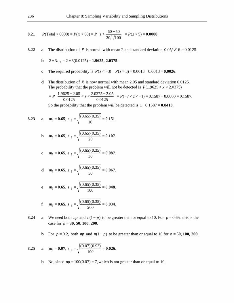
236 Chapter 8: Sampling Variability and Sampling Distributions
8.21 60 50(Total 6000) ( 60) ( 5) . .20 100
P P x P z P z −
> = > = > = > =
0 0000
8.22 a The distribution of x is normal with mean 2 and standard deviation 0.05 16 0.0125.= b 2 3 2 3(0.0125) .xσ± = ± = 1.9625, 2.0375 c The required probability is ( 3) ( 3) 0.0013 0.0013 .P z P z< − + > = + = 0.0026 d The distribution of x is now normal with mean 2.05 and standard deviation 0.0125.
The probability that the problem will not be detected is (1.9625 2.0375)P x< < 1.9625 2.05 2.0375 2.05 ( 7 1) 0.1587 0.0000 0.1587.
0.0125 0.0125P z P z− − = < < = − < < − = − =
So the probability that the problem will be detected is 1 0.1587 .− = 0.8413
8.23 a ˆ ˆ(0.65)(0.35), . .
10p pµ σ= = =0.65 0 151
b ˆ ˆ(0.65)(0.35), . .
20p pµ σ= = =0.65 0 107
c ˆ ˆ(0.65)(0.35), . .
30p pµ σ= = =0.65 0 087
d ˆ ˆ(0.65)(0.35), . .
50p pµ σ= = =0.65 0 067
e ˆ ˆ(0.65)(0.35), . .
100p pµ σ= = =0.65 0 048
f ˆ ˆ(0.65)(0.35), . .
200p pµ σ= = =0.65 0 034
8.24 a We need both np and (1 )n p− to be greater than or equal to 10. For 0.65,p = this is the
case for .n = 30, 50, 100, 200 b For 0.2,p = both np and (1 )n p− to be greater than or equal to 10 for .n = 50, 100, 200
8.25 a ˆ ˆ(0.07)(0.93), . .
100p pµ σ= = =0.07 0 026
b No, since 100(0.07) 7,np = = which is not greater than or equal to 10.

Chapter 8: Sampling Variability and Sampling Distributions 237
c The mean is unchanged since the mean of the distribution of the sample proportion is always
equal to the population proportion, but the standard deviation changes to
ˆ(0.07)(0.93) . .
200pσ = = 0 018
d Yes, since 200(0.07) 14 and (1 ) 200(0.93) 186,np n p= = − = = which are both greater than or
equal to 10.
e 0.1 0.07ˆ( 0.1) ( 1.66) . .(0.07)(0.93) 200
P p P z P z −
> = > = > =
0 0485
8.26 a ˆ ˆ(0.15)(0.85), . .
100p pµ σ= = =0.15 0 036
b Yes, since 100(0.15) 15np = = and (1 ) 100(0.85) 85n p− = = which are both greater than or
equal to 10. c The mean is unchanged since the mean of the distribution of the sample proportion is always
equal to the population proportion, but the standard deviation changes to
ˆ(0.15)(0.85) . .
200pσ = = 0 025
d Yes, since 200(0.15) 30np = = and (1 ) 200(0.85) 170,n p− = = which are both greater than
or equal to 10.
e 0.1 0.15ˆ( 0.1) ( 1.98) . .(0.15)(0.85) 200
P p P z P z −
> = > = > − =
0 9761
8.27 a ˆ ˆ1 (0.005)(0.995), . .
200 100p pµ σ= = = =0.005 0 007
b No, since 100(0.005) 0.5,np = = which is not greater than or equal to 10. c We need both np and (1 )n p− to be greater than or equal to 10, and since p q< it will be
sufficient to ensure that 10.np ≥ So we need (0.005) 10,n ≥ that is 10 0.005 .n ≥ = 2000 8.28 a No, since 10(0.3) 3,np = = which is not greater than or equal to 10.
b ˆ .p pµ = = 0.3 ˆ(1 ) (0.3)(0.7) . .
400pp p
nσ
−= = = 0 0229
c Since 400(0.3) 120 10np = = ≥ and (1 ) 400(0.7) 280 10,n p− = = ≥ the distribution of p is
approximately normal.

238 Chapter 8: Sampling Variability and Sampling Distributions
0.25 0.3 0.35 0.3ˆ(0.25 0.35) ( 2.18 2.18) 0.9854 0.0146 . .0.0229 0.0229
P p z P z− − ≤ ≤ = ≤ ≤ = − ≤ ≤ = − =
0 9708
d In a sample of size 500 it is more likely that the sample proportion will be close to the
population proportion than in a sample of size 400. Therefore, the probability calculated in Part (c) is smaller than would be the case if 500.n =
8.29 a If 0.5,p = ˆ ˆ(0.5)(0.5), . .
225p pµ σ= = =0.5 0 0333 Also 225(0.5) 112.5 10np = = ≥ and
(1 ) 225(0.5) 112.5 10,n p− = = ≥ and so p has an approximately normal distribution.
If 0.6,p = ˆ ˆ(0.6)(0.4), . .
225p pµ σ= = =0.6 0 0327 Also 225(0.6) 135 10np = = ≥ and
(1 ) 225(0.4) 90 10,n p− = = ≥ and so p has an approximately normal distribution.
b If 0.5,p = 0.6 0.5ˆ( 0.6) ( 3) . .(0.5)(0.5) 225
P p P z P z −
≥ = ≥ = ≥ =
0 0013
If 0.6,p = 0.6 0.6ˆ( 0.6) ( 0) . .(0.6)(0.4) 225
P p P z P z −
≥ = ≥ = ≥ =
0 5
c For a larger sample size, the value of p is likely to be closer to p. So, for 400,n = when
0.5,p = ˆ( 0.6)P p ≥ will be smaller. When 0.6,p = ˆ( 0.6)P p ≥ will still be 0, that is, it will remain the same.
8.30 Since 500(0.48) 240 10np = = ≥ and (1 ) 500(0.52) 260 10,n p− = = ≥ the distribution of p is
approximately normal. 0.5 0.48ˆ( 0.5) ( 0.90) . .
(0.48)(0.52) 500P p P z P z
−> = > = > =
0 1841
8.31 a 0.02 0.05ˆ(Returned) ( 0.02) ( 1.95) .(0.05)(0.95) 200
P P p P z P z −
= > = > = > − =
0.9744
b 0.02 0.1ˆ(Returned) ( 0.02) ( 3.77) 0.9999.(0.1)(0.9) 200
P P p P z P z −
= > = > = > − =
So the
probability that the shipment is not returned is 1 0.9999 .− = 0.0001 8.32 Since 100 30,n = ≥ the distribution of x is approximately normal.
0.8xµ µ= = and 0.1 0.01.100x n
σσ = = =
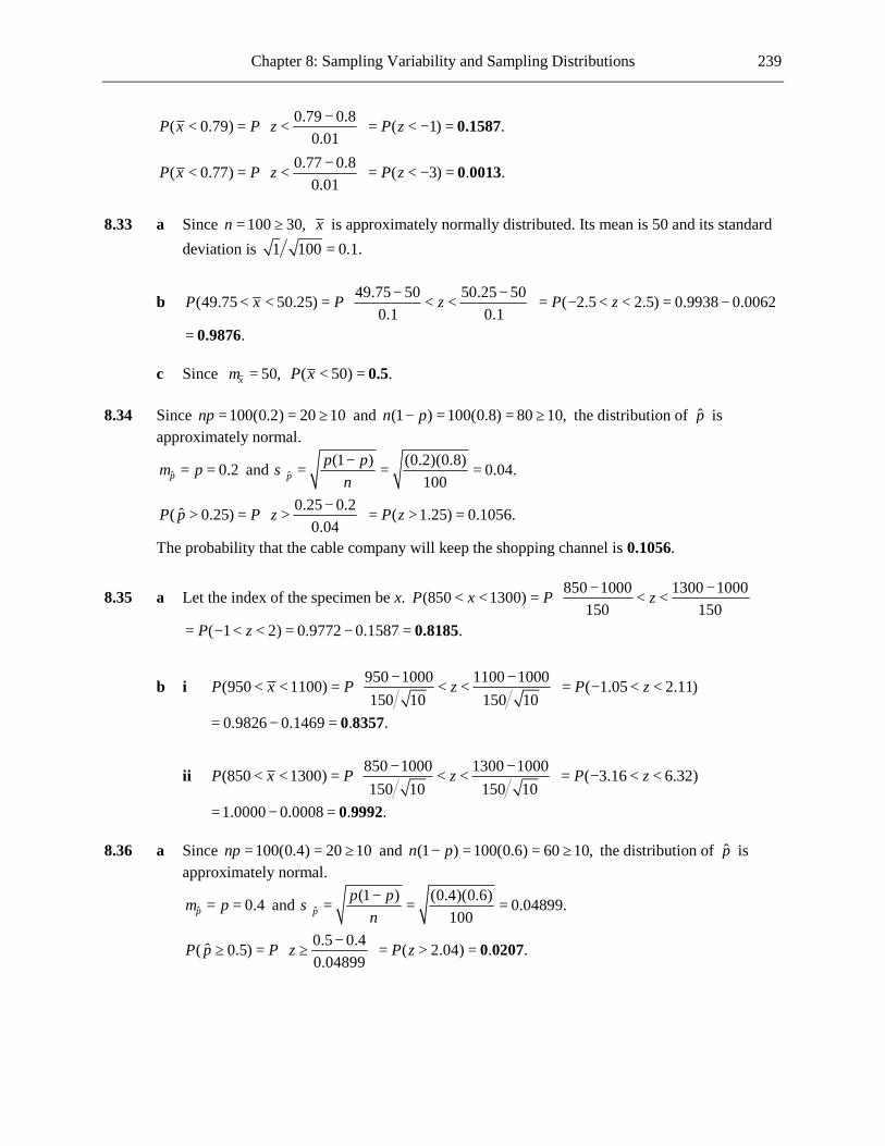
Chapter 8: Sampling Variability and Sampling Distributions 239
0.79 0.8( 0.79) ( 1) .
0.01P x P z P z− < = < = < − =
0.1587
0.77 0.8( 0.77) ( 3) . .0.01
P x P z P z− < = < = < − =
0 0013
8.33 a Since 100 30,n = ≥ x is approximately normally distributed. Its mean is 50 and its standard
deviation is 1 100 0.1.=
b 49.75 50 50.25 50(49.75 50.25) ( 2.5 2.5) 0.9938 0.00620.1 0.1
P x P z P z− − < < = < < = − < < = −
.= 0.9876 c Since 50,xµ = ( 50) .P x < = 0.5 8.34 Since 100(0.2) 20 10np = = ≥ and (1 ) 100(0.8) 80 10,n p− = = ≥ the distribution of p is
approximately normal.
ˆ 0.2p pµ = = and ˆ(1 ) (0.2)(0.8) 0.04.
100pp p
nσ
−= = =
0.25 0.2ˆ( 0.25) ( 1.25) 0.1056.0.04
P p P z P z− > = > = > =
The probability that the cable company will keep the shopping channel is 0.1056.
8.35 a Let the index of the specimen be x. 850 1000 1300 1000(850 1300)150 150
P x P z− − < < = < <
( 1 2) 0.9772 0.1587 .P z= − < < = − = 0.8185
b i 950 1000 1100 1000(950 1100) ( 1.05 2.11)150 10 150 10
P x P z P z − −
< < = < < = − < <
0.9826 0.1469 . .= − = 0 8357
ii 850 1000 1300 1000(850 1300) ( 3.16 6.32)150 10 150 10
P x P z P z − −
< < = < < = − < <
1.0000 0.0008 . .= − = 0 9992 8.36 a Since 100(0.4) 20 10np = = ≥ and (1 ) 100(0.6) 60 10,n p− = = ≥ the distribution of p is
approximately normal.
ˆ 0.4p pµ = = and ˆ(1 ) (0.4)(0.6) 0.04899.
100pp p
nσ
−= = =
0.5 0.4ˆ( 0.5) ( 2.04) . .0.04899
P p P z P z− ≥ = ≥ = > =
0 0207

240 Chapter 8: Sampling Variability and Sampling Distributions
b If 0.4,p = 0.6 0.4ˆ( 0.6) ( 4.08) 0.0000.0.04899
P p P z P z− > = > = > =
This tells us that, if 40% of people in a state participate in a “self-insurance” plan then it is very unlikely that more than 60 people in a sample of 100 would participate in such a plan. Therefore, if more than 60 people in a sample of 100 were found to participate in this type of plan, we would strongly doubt that 0.4p = for that state.
8.37 106 100(Total 5300) ( 5300 50) ( 106) ( 1.41) . .30 50
P P x P x P z P z −
> = > = > = > = > =
0 0793
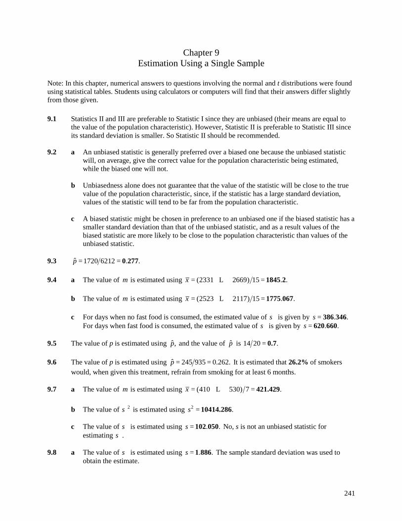
241
Chapter 9 Estimation Using a Single Sample
Note: In this chapter, numerical answers to questions involving the normal and t distributions were found using statistical tables. Students using calculators or computers will find that their answers differ slightly from those given. 9.1 Statistics II and III are preferable to Statistic I since they are unbiased (their means are equal to
the value of the population characteristic). However, Statistic II is preferable to Statistic III since its standard deviation is smaller. So Statistic II should be recommended.
9.2 a An unbiased statistic is generally preferred over a biased one because the unbiased statistic
will, on average, give the correct value for the population characteristic being estimated, while the biased one will not.
b Unbiasedness alone does not guarantee that the value of the statistic will be close to the true
value of the population characteristic, since, if the statistic has a large standard deviation, values of the statistic will tend to be far from the population characteristic.
c A biased statistic might be chosen in preference to an unbiased one if the biased statistic has a
smaller standard deviation than that of the unbiased statistic, and as a result values of the biased statistic are more likely to be close to the population characteristic than values of the unbiased statistic.
9.3 ˆ 1720 6212 . .p = = 0 277 9.4 a The value of µ is estimated using (2331 2669) 15 . .x = + + = 1845 2L b The value of µ is estimated using (2523 2117) 15 . .x = + + = 1775 067L c For days when no fast food is consumed, the estimated value of σ is given by . .s = 386 346
For days when fast food is consumed, the estimated value of σ is given by . .s = 620 660 9.5 The value of p is estimated using ˆ ,p and the value of p is 14 20 .= 0.7 9.6 The value of p is estimated using ˆ 245 935 0.262.p = = It is estimated that 26.2% of smokers
would, when given this treatment, refrain from smoking for at least 6 months. 9.7 a The value of µ is estimated using (410 530) 7 .x = + + = 421.429L b The value of 2σ is estimated using 2 .s = 10414.286 c The value of σ is estimated using . .s = 102 050 No, s is not an unbiased statistic for
estimating σ . 9.8 a The value of σ is estimated using . .s = 1 886 The sample standard deviation was used to
obtain the estimate.

242 Chapter 9: Estimation Using a Single Sample
b The value of µ is estimated using (11.3 12) 12 11.967.x = + + =L So the required percentile is estimated to be 11.967 1.28(1.886) .+ = 14.381
9.9 a The value of Jµ is estimated using (103 99) 10 . therms.x = + + = 120 6L b The value of τ is estimated to be 10000(120.6) = 1,206,000 therms. c The value of p is estimated using ˆ 8 10 .p = = 0.8 d The population median is estimated using the sample median, which is 120 therms. 9.10 a For any given sample, the 95% confidence interval is wider than the 90% confidence interval.
The interval needs to be wider in order to have greater confidence that the interval contains the true value of p.
b The sample of size n = 100 is likely to result in a wider confidence interval. The formula for
the confidence interval is ˆ ˆ(1 )ˆ 1.96 p ppn−
± , and so a smaller value of n is likely to result in
a wider confidence interval. 9.11 a 1.96 b 1.645 c 2.58 d 1.28 e 1.44 9.12 In order for the interval to be appropriate, we need 10np ≥ and (1 ) 10.n p− ≥ a Yes, since 50(0.3) 15 10np = = ≥ and (1 ) 50(0.7) 35 10.n p− = = ≥ b No, since 50(0.05) 2.5,np = = which is not greater than or equal to 10. c No, since 15(0.45) 6.75,np = = which is not greater than or equal to 10. d No, since 100(0.01) 1,np = = which is not greater than or equal to 10. e Yes, since 100(0.7) 70 10np = = ≥ and (1 ) 100(0.3) 30 10.n p− = = ≥ f Yes, since 40(0.25) 10 10np = = ≥ and (1 ) 40(0.75) 30 10.n p− = = ≥ g Yes, since 60(0.25) 15 10np = = ≥ and (1 ) 60(0.75) 45 10.n p− = = ≥ h No, since 80(0.1) 8,np = = which is not greater than or equal to 10.

Chapter 9: Estimation Using a Single Sample 243
9.13 a The larger the confidence level the wider the interval. b The larger the sample size the narrower the interval. c Values of p further from 0.5 give smaller values of ˆ ˆ(1 ).p p− Therefore, the further the
value of p from 0.5, the narrower the interval. 9.14 Check of Conditions 1. Since ˆ 2667(1200 2667) 1200 10np = = ≥ and ˆ(1 ) 2667(1467 2667) 1467 10,n p− = = ≥ the
sample is large enough. 2. The sample size of n = 2667 is much smaller than 10% of the population size (the number of
hiring managers and human resource professionals). 3. We are told to assume that the sample is representative of the population of hiring managers
and human resource professionals. Having made this assumption it is reasonable to regard the sample as a random sample from the population.
Calculation The 95% confidence interval for p is
ˆ ˆ(1 ) 1200 (1200 2667)(1467 2667)ˆ 1.96 1.96 ( . , . ).2667 2667
p ppn−
± = ± = 0 431 0 469
Interpretation We are 95% confident that the proportion of all hiring managers and human resource professionals who use social networking sites to research job applicants is between 0.431 and 0.469.
9.15 If a large number of random samples of size 1200 were to be taken, 90% of the resulting
confidence intervals would contain the true proportion of all Facebook users who would say it is not OK to “friend” someone who reports to you at work.
9.16 a We need to assume that the 722 people formed a random sample of adult Americans. b Check of Conditions 1. Since ˆ 4013(722 4013) 722 10np = = ≥ and ˆ(1 ) 4013(3291 4013) 3291 10,n p− = = ≥ the
sample is large enough. 2. The sample size of n = 4013 is much smaller than 10% of the population size (the number
of adult Americans). 3. As stated in Part (a), we need to assume that the 722 people formed a random sample of
adult Americans. Calculation The 90% confidence interval for p is
ˆ ˆ(1 ) 722 (722 4013)(3291 4013)ˆ 1.645 1.645 ( . , . ).4013 4013
p ppn−
± = ± = 0 170 0 190
Interpretation We are 90% confident that the proportion of all adult Americans who have seen or been with
a ghost is between 0.170 and 0.190. c A 99% confidence interval the proportion of all adult Americans who have seen or been with
a ghost would be wider than the interval constructed in Part (b). In order to be 99% (rather than 90%) confident that the interval is capturing the true proportion, the interval needs to be wider.

244 Chapter 9: Estimation Using a Single Sample
9.17 a Let p be the proportion of all coastal residents who would evacuate. Check of Conditions 1. Since ˆ 5046(0.69) 3482 10np = = ≥ and ˆ(1 ) 5046(0.31) 1564 10,n p− = = ≥ the sample
size is large enough. 2. The sample size of n = 5046 is much smaller than 10% of the population size (the number
of people who live within 20 miles of the coast in high hurricane risk counties of these eight southern states).
3. The sample was selected in a way designed to produce a representative sample. So, it is reasonable to regard the sample as a random sample from the population.
Calculation The 98% confidence interval for p is
ˆ ˆ(1 ) (0.69)(0.31)ˆ 2.33 0.69 2.33 ( . , . ).5046
p ppn−
± = ± = 0 675 0 705
b Interpretation of the Confidence Interval We are 98% confident that the proportion of all coastal residents who would evacuate is
between 0.675 and 0.705. Interpretation of the Confidence Level If we were to take a large number of random samples of size 5046, 98% of the resulting
confidence intervals would contain the true proportion of all coastal residents who would evacuate.
9.18 Check of Conditions 1. Since ˆ 300(0.47) 141 10np = = ≥ and ˆ(1 ) 300(0.53) 159 10,n p− = = ≥ the sample is large
enough. 2. The sample size of n = 300 is much smaller than 10% of the population size (the number of
Internet users). 3. We are told that the sample was a random sample of Internet users. Calculation The 90% confidence interval for p is
ˆ ˆ(1 ) (0.47)(0.53)ˆ 1.645 0.47 1.645 ( . , . ).300
p ppn−
± = ± = 0 423 0 517
Interpretation We are 90% confident that the proportion of all Internet users who have searched online for
information about themselves is between 0.423 and 0.517. 9.19 a Check of Conditions 1. Since ˆ 2002(1321 2002) 1321 10np = = ≥ and ˆ(1 ) 2002(681 2002) 681 10,n p− = = ≥ the
sample size is large enough. 2. The sample size of n = 2002 is much smaller than 10% of the population size (the number
of Americans age 8 to 18). 3. The sample was selected in a way designed to produce a representative sample. So, it is
reasonable to regard the sample as a random sample from the population. Calculation The 90% confidence interval for p is
ˆ ˆ(1 ) 1321 (1321 2002)(681 2002)ˆ 1.645 1.645 ( . , . ).2002 2002
p ppn−
± = ± = 0 642 0 677

Chapter 9: Estimation Using a Single Sample 245
Interpretation We are 90% confident that the proportion of all Americans age 8 to 18 who own a cell phone
is between 0.642 and 0.677. b Check of Conditions 1. Since ˆ 2002(1522 2002) 1522 10np = = ≥ and ˆ(1 ) 2002(480 2002) 480 10,n p− = = ≥ the
sample size is large enough. 2. The sample size of n = 2002 is much smaller than 10% of the population size (the number
of Americans age 8 to 18). 3. The sample was selected in a way designed to produce a representative sample. So it is
reasonable to regard the sample as a random sample from the population. Calculation The 90% confidence interval for p is
ˆ ˆ(1 ) 1522 (1522 2002)(480 2002)ˆ 1.645 1.645 ( . , . ).2002 2002
p ppn−
± = ± = 0 745 0 776
Interpretation We are 90% confident that the proportion of all Americans age 8 to 18 who own an MP3
player is between 0.745 and 0.776. c The interval in Part (b) is narrower than the interval in Part (a) because the sample proportion
in Part (b) is further from 0.5, thus reducing the value of the estimated standard deviation of the sample proportion (given by the expression ˆ ˆ(1 )p p n− ).
9.20 a Check of Conditions 1. Since ˆ 1000(0.37) 370 10np = = ≥ and ˆ(1 ) 1000(0.63) 630 10,n p− = = ≥ the sample size
is large enough. 2. The sample size of n = 1000 is much smaller than 10% of the population size (the number
of college freshmen). 3. We are told to assume that the sample was a random sample from the population. Calculation The 90% confidence interval for p is
ˆ ˆ(1 ) (0.37)(0.63)ˆ 1.645 0.37 1.645 ( . , . ).1000
p ppn−
± = ± = 0 345 0 395
Interpretation We are 90% confident that the proportion of all college freshmen who carry a credit card
balance from month to month is between 0.345 and 0.395. b Check of Conditions 1. Since ˆ 1000(0.48) 480 10np = = ≥ and ˆ(1 ) 1000(0.52) 520 10,n p− = = ≥ the sample size
is large enough. 2. The sample size of n = 1000 is much smaller than 10% of the population size (the number
of college seniors). 3. We are told to assume that the sample was a random sample from the population. Calculation The 90% confidence interval for p is
ˆ ˆ(1 ) (0.48)(0.52)ˆ 1.645 0.48 1.645 ( , . ).1000
p ppn−
± = ± = 0.454 0 506

246 Chapter 9: Estimation Using a Single Sample
Interpretation We are 90% confident that the proportion of all college seniors who carry a credit card
balance from month to month is between 0.454 and 0.506. c The widths of the two confidence intervals are different since the values of the estimated
standard deviations of the sampling distributions of p, given by the expression ˆ ˆ(1 )p p n− , are different in the two cases.
9.21 a Check of Conditions 1. Since ˆ 500(350 500) 350 10np = = ≥ and ˆ(1 ) 500(150 500) 150 10,n p− = = ≥ the sample
size is large enough. 2. The sample size of n = 500 is much smaller than 10% of the population size (the number
of potential jurors). 3. We are told to assume that the sample is representative of the population of potential
jurors. Having made this assumption it is reasonable to regard the sample as a random sample from the population.
Calculation The 95% confidence interval for p is
ˆ ˆ(1 ) 350 (350 500)(150 500)ˆ 1.96 1.96 ( . , . ).500 500
p ppn−
± = ± = 0 660 0 740
Interpretation We are 95% confident that the proportion of all potential jurors who regularly watch at least
one crime-scene investigation series is between 0.660 and 0.740. b Wider 9.22 a Check of Conditions 1. Since ˆ 1000(230 1000) 230 10np = = ≥ and ˆ(1 ) 1000(770 1000) 770 10,n p− = = ≥ the
sample size is large enough. 2. The sample size of n = 1000 is much smaller than 10% of the population size (the number
of adults in the United States). 3. We are told that the sample was a random sample from the population of adults in the
United States. Calculation The 95% confidence interval for p is
ˆ ˆ(1 ) 230 (230 1000)(770 1000)ˆ 1.96 1.96 ( . , . ).1000 1000
p ppn−
± = ± = 0 204 0 256
Interpretation We are 95% confident that the proportion of all adults in the United States for whom math
was the favorite subject is between 0.204 and 0.256. b Check of Conditions 1. Since ˆ 1000(370 1000) 370 10np = = ≥ and ˆ(1 ) 1000(630 1000) 630 10,n p− = = ≥ the
sample size is large enough. 2. The sample size of n = 1000 is much smaller than 10% of the population size (the number
of adults in the United States). 3. We are told that the sample was a random sample from the population of adults in the
United States.

Chapter 9: Estimation Using a Single Sample 247
Calculation The 95% confidence interval for p is
ˆ ˆ(1 ) 370 (370 1000)(630 1000)ˆ 1.96 1.96 ( . , . ).1000 1000
p ppn−
± = ± = 0 340 0 400
Interpretation We are 95% confident that the proportion of all adults in the United States for whom math
was the least favorite subject is between 0.340 and 0.400. 9.23 a Check of Conditions 1. Since ˆ 526(137 526) 137 10np = = ≥ and ˆ(1 ) 526(389 526) 389 10,n p− = = ≥ the sample
size is large enough. 2. The sample size of n = 526 is much smaller than 10% of the population size (the number
of U.S. businesses). 3. We must assume that the sample is a random sample of U.S. businesses. Calculation The 95% confidence interval for p is
ˆ ˆ(1 ) 137 (137 526)(389 526)ˆ 1.96 1.96 ( . , . ).526 526
p ppn−
± = ± = 0 223 0 298
Interpretation We are 95% confident that the proportion of all U.S. businesses that have fired workers for
misuse of the Internet is between 0.223 and 0.298. b The sample proportion of businesses that had fired workers for misuse of email is further
from 0.5 than the sample proportion of businesses that had fired workers for misuse of the Internet, making the value of ˆ ˆ(1 )p p n− smaller. This makes the confidence interval narrower. Additionally, the critical value of z for a 90% confidence interval is smaller than the critical value of z for a 95% confidence interval, also making the second confidence interval narrower.
9.24 a Check of Conditions 1. Since ˆ 1000(394 1000) 394 10np = = ≥ and ˆ(1 ) 1000(606 1000) 606 10,n p− = = ≥ the
sample size is large enough. 2. The sample size of n = 1000 is much smaller than 10% of the population size (the number
of adults in the United States). 3. We are told that the sample was a random sample from the population of adults in the
United States. Calculation The 95% confidence interval for p is
ˆ ˆ(1 ) 394 (394 1000)(606 1000)ˆ 1.96 1.96 ( . , . ).1000 1000
p ppn−
± = ± = 0 364 0 424
Interpretation We are 95% confident that the proportion of all adults in the United States who consider
themselves to be baseball fans is between 0.364 and 0.424. b Check of Conditions 1. Since ˆ 394(272 394) 272 10np = = ≥ and ˆ(1 ) 394(122 394) 122 10,n p− = = ≥ the sample
size is large enough.

248 Chapter 9: Estimation Using a Single Sample
2. The sample size of n = 394 is much smaller than 10% of the population size (the number of adults in the United States who are baseball fans).
3. We are told that the original sample was a random sample from the population of adults in the United States, and so it follows that these 394 people form a random sample of baseball fans.
Calculation The 95% confidence interval for p is
ˆ ˆ(1 ) 272 (272 394)(122 394)ˆ 1.96 1.96 ( . , . ).394 394
p ppn−
± = ± = 0 645 0 736
Interpretation We are 95% confident that the proportion of all adult baseball fans in the United States who
think that the designated hitter rule should be expanded to both leagues or eliminated is between 0.645 and 0.736.
c The widths of the confidence intervals are different because the sample sizes were different
and because the sample proportions were different. 9.25 Check of Conditions 1. Since ˆ 1002(0.82) 822 10np = = ≥ and ˆ(1 ) 1002(0.18) 180 10,n p− = = ≥ the sample size is
large enough. 2. The sample size of n = 1002 is much smaller than 10% of the population size (the number of
adults in the country). 3. We are told that the sample was a random sample from the population. Calculation When the sample proportion of 0.82 is used as an estimate of the population proportion, the 95%
error bound on this estimate is ˆ ˆ(1 ) (0.82)(0.18)1.96 1.96 0.024.
1002p p
n−
= =
Interpretation We are 95% confident that proportion of all adults who believe that the shows are either “totally
made up” or “mostly distorted” is within 2.4% of the sample proportion of 82%. 9.26 a Check of Conditions 1. Since ˆ 1000(520 1000) 520 10np = = ≥ and ˆ(1 ) 1000(480 1000) 480 10,n p− = = ≥ the
sample size is large enough. 2. The sample size of n = 1000 is much smaller than 10% of the population size (the number
of adult Americans). 3. We are told that the sample was a random sample from the population of adult
Americans. Calculation The 90% confidence interval for p is
ˆ ˆ(1 ) 520 (520 1000)(480 1000)ˆ 1.645 1.645 ( . , . ).1000 1000
p ppn−
± = ± = 0 494 0 546
Interpretation We are 90% confident that the proportion of all adult Americans who think that lying is never
justified is between 0.494 and 0.546.

Chapter 9: Estimation Using a Single Sample 249
b Check of Conditions 1. Since ˆ 1000(650 1000) 650 10np = = ≥ and ˆ(1 ) 1000(350 1000) 350 10,n p− = = ≥ the
sample size is large enough. 2. The sample size of n = 1000 is much smaller than 10% of the population size (the number
of adult Americans). 3. We are told that the sample was a random sample from the population of adult
Americans. Calculation The 90% confidence interval for p is
ˆ ˆ(1 ) 650 (650 1000)(350 1000)ˆ 1.645 1.645 ( . , . ).1000 1000
p ppn−
± = ± = 0 625 0 675
Interpretation We are 90% confident that the proportion of all adult Americans who think that it is often or
sometimes OK to lie to avoid hurting someone’s feelings is between 0.625 and 0.675. c Since 520 + 650 is more than 1000, it is clear that some people were responding both that
lying is never justified and that it is often or sometimes OK to lie to avoid hurting someone’s feelings. These are contradictory responses.
9.27 We are 95% confident that proportion of all adult drivers who would say that they often or
sometimes talk on a cell phone while driving is within ˆ ˆ1.96 (1 )p p n−
1.96 (0.36)(0.64) 1004 0.030= = , that is, 3.0 percentage points, of the sample proportion of 36%. The reported bound on error is slightly inaccurate, in that it is wrong by one tenth of a percentage point.
9.28 We have 1002n = and ˆ 0.25.p = So the margin of error is (0.25)(0.75)1.96 0.0271002
= ; thus the
margin of error is approximately 3 percentage points, as stated. 9.29 a Check of Conditions 1. Since ˆ 89(18 89) 18 10np = = ≥ and ˆ(1 ) 89(71 89) 71 10,n p− = = ≥ the sample size is
large enough. 2. The sample size of n = 89 is much smaller than 10% of the population size (the number
of people under 50 years old who use this type of defibrillator). 3. We are told to assume that the sample is representative of patients under 50 years old
who receive this type of defibrillator. Having made this assumption it is reasonable to regard the sample as a random sample from the population.
Calculation The 95% confidence interval for p is
ˆ ˆ(1 ) 18 (18 89)(71 89)ˆ 1.96 1.96 ( . , . ).89 89
p ppn−
± = ± = 0 119 0 286
Interpretation We are 95% confident that the proportion of all patients under 50 years old who experience a
failure within the first two years after receiving this type of defibrillator is between 0.119 and 0.286.

250 Chapter 9: Estimation Using a Single Sample
b Check of Conditions 1. Since ˆ 362(13 362) 13 10np = = ≥ and ˆ(1 ) 362(349 362) 349 10,n p− = = ≥ the sample
size is large enough. 2. The sample size of n = 362 is much smaller than 10% of the population size (the number
of people age 50 or older who use this type of defibrillator). 3. We are told to assume that the sample is representative of patients age 50 or older who
receive this type of defibrillator. Having made this assumption it is reasonable to regard the sample as a random sample from the population.
Calculation The 99% confidence interval for p is
ˆ ˆ(1 ) 13 (13 362)(349 362)ˆ 2.58 2.58 ( . , . ).362 362
p ppn−
± = ± = 0 011 0 061
Interpretation We are 99% confident that the proportion of all patients age 50 or older who experience a
failure within the first two years after receiving this type of defibrillator is between 0.011 and 0.061.
c Using the estimate of p from the study, 18 89 , the required sample size is given by
2 21.96 18 71 1.96(1 ) 688.685.89 89 0.03
n p pB
= − = =
So a sample of size at least 689 is required. 9.30 Assuming a 95% confidence level, the margin of error is
ˆ ˆ(1 ) (0.64)(0.36)1.96 1.96 .511
p pn−
= = 0.042
9.31 2 21.96 1.96(1 ) 0.25 2401.
0.02n p p
B = − = =
A sample size of 2401 is required.
9.32 a 2 21.96 1.96(1 ) (0.3)(0.7) 2016.84.
0.02n p p
B = − = =
A sample size of 2017 is required.
b 22.58(1 )n p p
B = −
c 2 22.58 2.58(1 ) (0.3)(0.7) 3494.61.
0.02n p p
B = − = =
A sample size of 3495 is required.
9.33 Assuming a 95% confidence level, and using p = 0.32,
2 21.96 1.96(1 ) (0.32)(0.68) 334.4.0.05
n p pB
= − = =
A sample size of 335 is required.
Using the conservative value, p = 0.5, 2 21.96 1.96(1 ) (0.5)(0.5) 384.2.
0.05n p p
B = − = =
A sample size of 385 is required.

Chapter 9: Estimation Using a Single Sample 251
As always, the conservative estimate of p gives the larger sample size. Since the relevant proportion could have changed significantly since 2011, it would be sensible to use a sample size of 385.
9.34 a 90% b 95% c 95% d 99% e 1% f 0.5% g 5% 9.35 a 2.12 b 1.80 c 2.81 d 1.71 e 1.78 f 2.26 9.36 a (114.4 115.6) 2 Hertz.x = + = 115.0 b The 99% confidence interval is wider than the 90% confidence interval, since the interval
needs to be wider in order that there be greater confidence that the interval contains the population proportion. Thus the 90% interval is (114.4, 115.6) and the 99% interval is (114.1, 115.9).
9.37 The width of the first interval is 52.7 51.3 1.4.− = The width of the second interval is
50.6 49.4 1.2.− = Since the confidence interval is given by ( )( critical value) ,x t s n± the
width of the confidence interval is given by ( )2 ( critical value)t s n⋅ . Therefore, for samples of
equal standard deviations, the larger the sample size the narrower the interval. Thus it is the second interval that is based on the larger sample size.
9.38 a We need to assume that the 30 students formed a random sample of all students at this
university. b No. It is very unlikely that the 30 students from the upper division communications course
are representative of all students at the university, so the assumption of randomness is not valid, and the t confidence interval should not be used.
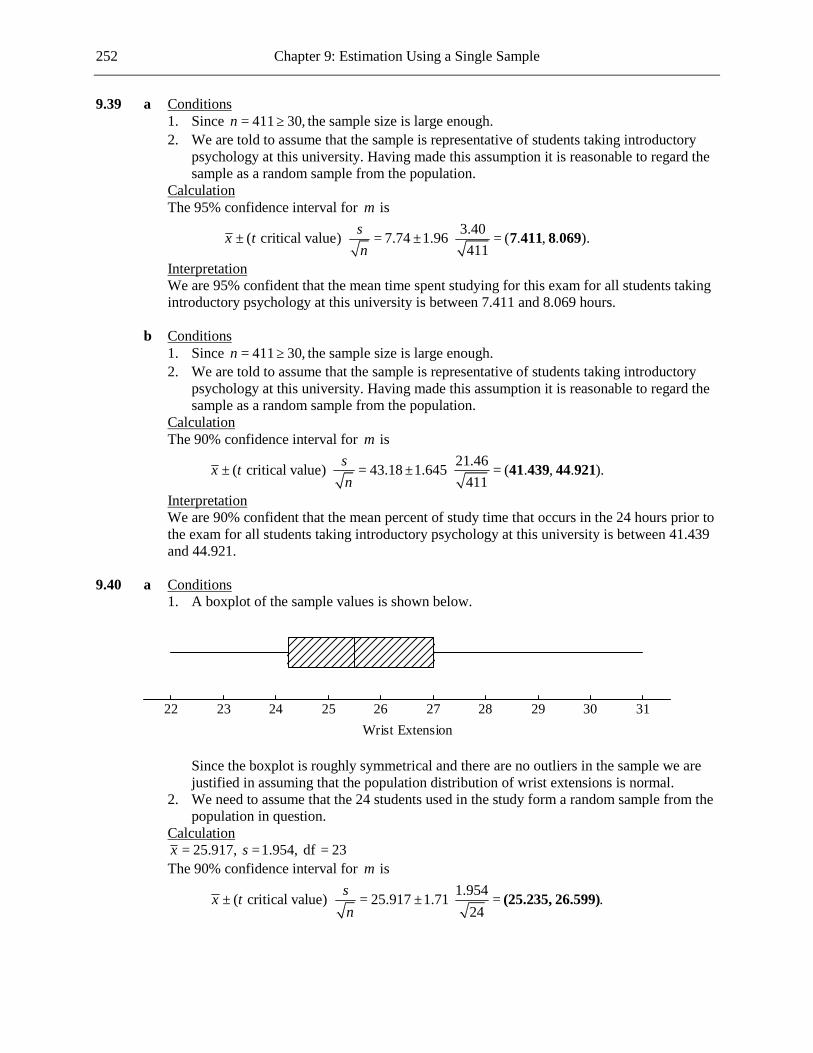
252 Chapter 9: Estimation Using a Single Sample
9.39 a Conditions 1. Since 411 30,n = ≥ the sample size is large enough. 2. We are told to assume that the sample is representative of students taking introductory
psychology at this university. Having made this assumption it is reasonable to regard the sample as a random sample from the population.
Calculation The 95% confidence interval for µ is
3.40( critical value) 7.74 1.96 ( . , . ).411
sx tn
± ⋅ = ± ⋅ = 7 411 8 069
Interpretation We are 95% confident that the mean time spent studying for this exam for all students taking
introductory psychology at this university is between 7.411 and 8.069 hours. b Conditions 1. Since 411 30,n = ≥ the sample size is large enough. 2. We are told to assume that the sample is representative of students taking introductory
psychology at this university. Having made this assumption it is reasonable to regard the sample as a random sample from the population.
Calculation The 90% confidence interval for µ is
21.46( critical value) 43.18 1.645 ( . , . ).411
sx tn
± ⋅ = ± ⋅ = 41 439 44 921
Interpretation We are 90% confident that the mean percent of study time that occurs in the 24 hours prior to
the exam for all students taking introductory psychology at this university is between 41.439 and 44.921.
9.40 a Conditions 1. A boxplot of the sample values is shown below.
31302928272625242322Wrist Extension
Since the boxplot is roughly symmetrical and there are no outliers in the sample we are
justified in assuming that the population distribution of wrist extensions is normal. 2. We need to assume that the 24 students used in the study form a random sample from the
population in question. Calculation 25.917, 1.954, df 23x s= = = The 90% confidence interval for µ is
1.954( critical value) 25.917 1.71 .24
sx tn
± ⋅ = ± ⋅ = (25.235, 26.599)

Chapter 9: Estimation Using a Single Sample 253
Interpretation We are 90% confident that the population mean wrist extension is between 25.235 and
26.599. b In order to generalize the estimate to the population of Cornell students the assumption would
have to be made that the 24 students in the study formed a random sample of Cornell students. To generalize the estimate to all university students you would have to assume that the 24 students in the study formed a random sample of university students.
c Yes. The entire confidence interval is above 20, so the results of the study would be very
unlikely if the population mean wrist extension were as low as 20. 9.41 a The fact that the mean is much greater than the median suggests that the distribution of times
spent volunteering in the sample was positively skewed. b With the sample mean being much greater than the sample median, and with the sample
being regarded as representative of the population, it seems very likely that the population is strongly positively skewed, and therefore not normally distributed.
c Since 1086 30,n = ≥ the sample size is large enough for us to use the t confidence interval,
even though the population distribution is not approximately normal. d In addition to observing that the sample is large, we need to point out that the sample was
selected in a way that makes it reasonable to regard it as representative of the population, and therefore that it is reasonable to regard the sample as random. This justifies use of the t confidence interval. The 98% confidence interval for µ is then
5.2( critical value) 5.6 2.33 ( . , . ).1086
sx tn
± ⋅ = ± ⋅ = 5 232 5 968
We are 98% confident that the mean time spent volunteering for the population of parents of school age children is between 5.232 and 5.968 hours.
9.42 a Conditions 1. Since 48 30,n = ≥ the sample is large enough. 2. We need to assume that the subjects formed a random sample from the population of
drivers. Calculation The 95% confidence interval for µ is
70( critical value) 530 2.01 ( . , . ).48
sx tn
± ⋅ = ± ⋅ = 509 692 550 308
Interpretation We are 95% confident that the mean time to react to a red light while talking on a cell phone
is between 509.692 and 550.308 milliseconds. b As mentioned in Part (a), we need to assume that the subjects of the experiment formed a
random sample from the population of drivers.
c 2 21.96 1.96 70 752.954.
5n
Bσ ⋅ = = =
A sample size of 753 is required.

254 Chapter 9: Estimation Using a Single Sample
9.43 a The 90% confidence interval would be narrower. In order to be only 90% confident that the interval captures the true population mean, the interval does not have to be as wide as it would in order to be 95% confident of capturing the true population mean.
b The statement is not correct. The population mean, µ , is a constant, and therefore we cannot
talk about the probability that it falls within a certain interval. c The statement is not correct. We can say that on average 95 out of every 100 samples will
result in confidence intervals that will contain µ , but we cannot say that in 100 such samples, exactly 95 will result in confidence intervals that contain µ .
9.44 Conditions 1. We are told that it is reasonable to believe that the distribution of breaking forces is
approximately normal. 2. We need to assume that the six specimens formed a random sample from the population of
such specimens. Calculation df = 5.
The 95% confidence interval for µ is 41.97( critical value) 306.09 2.57 ( . , . ).
6sx tn
± ⋅ = ± ⋅ = 262 055 350 125
Interpretation We are 95% confident that the mean breaking force for acrylic bone cement under the specified
conditions is between 262.055 and 350.125 Newtons. 9.45 a For samples of equal sizes, those with greater variability will result in wider confidence
intervals. The 12 to 23 month and 24 to 35 month samples resulted in confidence intervals of width 0.4, while the less than 12 month sample resulted in a confidence interval of width 0.2. So the 12 to 23 month and 24 to 35 month samples are the ones with the greater variability.
b For samples of equal variability, those with greater sample sizes will result in narrower
confidence intervals. Thus the less than 12 month sample is the one with the greater sample size.
c Since the new interval is wider than the interval given in the question, the new interval must
be for a higher confidence level. (By obtaining a wider interval, we have a greater confidence that the interval captures the true population mean.) Thus the new interval must have a 99% confidence level.
9.46 a It is possible that the distribution of the sample values was heavily skewed to the right, thus
making the standard deviation of the sample anticipated expenses greater than the sample mean.
b No. Since the distribution of sample values is strongly skewed to the right, it is very unlikely
that the variable anticipated Halloween expense is approximately normally distributed. c Yes, since the sample is large.

Chapter 9: Estimation Using a Single Sample 255
d Conditions 1. Since 1000 30,n = ≥ the sample is large enough. 2. We are told that the sample was randomly selected from the population of Canadian
residents. Calculation df = 999. The 99% confidence interval for µ is
83.70( critical value) 46.65 2.58 ( , . ).1000
sx tn
± ⋅ = ± ⋅ = 39.821 53 479
Interpretation We are 99% confident that the mean anticipated Halloween expense for the population of
Canadian residents is between 39.821 and 53.479 hours. 9.47 a Conditions 1. Since 100 30,n = ≥ the sample size is large enough. 2. We are told to assume that the sample was a random sample of passengers. Calculation The t critical value for 99 degrees of freedom (for a 95% confidence level) is between 1.98
and 2.00. We will use an estimate of 1.99. Thus, the 95% confidence interval for µ is 20( critical value) 183 1.99 ( . , . ).100
sx tn
± ⋅ = ± ⋅ = 179 02 186 98
Interpretation We are 95% confident that the mean summer weight is between 179.02 and 186.98 lb. b Conditions 1. Since 100 30,n = ≥ the sample size is large enough. 2. We are told to assume that the sample was a random sample. Calculation The 95% confidence interval for µ is
23( critical value) 190 1.99 ( . , . ).100
sx tn
± ⋅ = ± ⋅ = 185 423 194 577
Interpretation We are 95% confident that the mean winter weight is between 185.423 and 194.577 lb. c Based on the Frontier Airlines data, neither recommendation is likely to be an accurate
estimate of the mean passenger weight, since 190 is not contained in the confidence interval for the mean summer weight and 95 is not contained in the confidence interval for the mean winter weight.
9.48 a Conditions 1. A boxplot of the sample values is shown below.

256 Chapter 9: Estimation Using a Single Sample
285280275270265260255Airborne Time
Since the boxplot is roughly symmetrical and there are no outliers in the sample we are
justified in assuming that the population distribution of airborne times is normal. 2. We are told that the sample was a random sample from the population of flights. Calculation 270.3, 9.141, df 9x s= = = The 90% confidence interval for µ is
9.141( critical value) 270.3 1.83 ( . , . ).10
sx tn
± ⋅ = ± ⋅ = 265 010 275 590
Interpretation We are 90% confident that the mean airborne time is between 265.010 and 275.590 minutes. b If we were to take a large number of random samples of size 10, 90% of the resulting
confidence intervals would contain the true mean airborne time. c The sample mean airborne time is 270.3 and the sample standard deviation is 9.141.
Assuming these values for the population mean and standard deviation, and assuming that the population of airborne times is normal, approximately 5% of airborne times will be greater than 270.3 1.96(9.141) 288.+ = The time 290 minutes after 10 a.m. is 2.50 p.m. Thus, if the arrival time is published as 2.50 p.m., we can expect less than 5% of flights to be late. (This is assuming that all flights actually do depart at 10 a.m. Note, also, that many approximations have been made in this calculation. The airline might wish to use a more conservative method of calculation, that is, one that results in a later published arrival time.)
9.49 A boxplot of the sample values is shown below.
17.515.012.510.07.55.0Fat Content (grams)
The boxplot shows that the distribution of the sample values is negatively skewed, and this leads
us to suspect that the population is not approximately normally distributed. Therefore, since the sample is small, it is not appropriate to use the t confidence interval method of this section.
9.50 Conditions 1. A boxplot of the sample values is shown below.

Chapter 9: Estimation Using a Single Sample 257
30252015105Number of Months
Since the boxplot is roughly symmetrical and there are no outliers in the sample we are
justified in assuming that the population distribution of the number of months since the last visit is normal.
2. We are told to assume that the sample was a random sample from the population of students participating in the free checkup program.
Calculation 17, 9.0277, df 4x s= = = The 95% confidence interval for µ is
9.0277( critical value) 17 2.78 ( . , . ).5
sx tn
± ⋅ = ± ⋅ = 5 776 28 224
Interpretation We are 95% confident that the mean number of months elapsed since the last visit for the
population of students participating in the program is between 5.776 and 28.224. 9.51 A reasonable estimate of σ is given by (sample range) 4 (700 50) 4 162.5.= − = Thus
2 21.96 1.96 162.5 1014.4225.10
nB
σ ⋅ = = =
So we need a sample size of 1015.
9.52 For a 90% confidence level, the formula is 21.645 .n
Bσ =
For a 98% confidence level, the formula is 22.33 .n
Bσ =
9.53 First, we need to know that the information is based on a random sample of middle-income
consumers aged 65 and older. Second, it would be useful if some sort of margin of error were given for the estimated mean of $10,235.
9.54 The margins of error are different because the sample sizes are different and the sample
proportions are different. 9.55 a The paper states that Queens flew for an average of 24.2 9.21± minutes on their mating
flights, and so this interval is a confidence interval for a population mean. b Conditions 1. Since 30 30,n = ≥ the sample size is large enough.

258 Chapter 9: Estimation Using a Single Sample
2. We are told to assume that the 30 queen honeybees are representative of the population of queen honeybees. It is then reasonable to treat the sample as a random sample from the population.
Calculation The 95% confidence interval for µ is
3.47( critical value) 4.6 2.05 ( . , . ).30
sx tn
± ⋅ = ± ⋅ = 3 301 5 899
Interpretation We are 95% confident that the mean number of partners is between 3.301 and 5.899. 9.56 Conditions 1. Since 2815 30,n = ≥ the sample is large enough. 2. The sample was selected in a way designed to be representative of adult Americans who
purchased graduation gifts in 2007. It is therefore reasonable to regard it as a random sample from the population.
Calculation The 98% confidence interval for µ is
20( critical value) 55.05 2.33 ( . , ).2815
sx tn
± ⋅ = ± ⋅ = 54 172 55.928
Interpretation We are 98% confident that the mean amount of money spent per graduation gift in 2007 was
between $54.172 and $55.928. 9.57 a Check of Conditions 1. Since ˆ 52(18 52) 18 10np = = ≥ and ˆ(1 ) 52(34 52) 34 10,n p− = = ≥ the sample size is
large enough. 2. The sample size of n = 52 is much smaller than 10% of the population size (the number
of young adults with pierced tongues). 3. It is necessary to assume that the sample of 52 was a random sample from the population
of young adults with pierced tongues. Calculation The 95% confidence interval for p is
ˆ ˆ(1 ) 18 (18 52)(34 52)ˆ 1.96 1.96 ( . , . ).52 52
p ppn−
± = ± = 0 217 0 475
Interpretation We are 95% confident that the proportion of all young people with pierced tongues who have receding gums is between 0.217 and 0.475.
b As mentioned in Part (a), it is necessary to assume that the sample of 52 was a random sample from the population of young adults with pierced tongues.
9.58 a Check of Conditions 1. Since ˆ 1710(1060 1710) 1060 10np = = ≥ and ˆ(1 ) 1710(650 1710) 650 10,n p− = = ≥ the
sample is large enough. 2. The sample size of n = 1710 is much smaller than 10% of the population size (the number
of schoolchildren in Australia). 3. It is necessary to assume that the 1710 children used in the study formed a random
sample from the population of schoolchildren in Australia.

Chapter 9: Estimation Using a Single Sample 259
Calculation The 95% confidence interval for p is
ˆ ˆ(1 ) 1060 (1060 1710)(650 1710)ˆ 1.96 1.96 ( . , . ).1710 1710
p ppn−
± = ± = 0 597 0 643
Interpretation We are 95% confident that the proportion of all schoolchildren in Australia who say they watch TV before school is between 0.597 and 0.643.
b As stated in Part (a), it is necessary to assume that the 1710 children used in the study formed a random sample from the population of schoolchildren in Australia.
9.59 The standard error for the mean cost for Native Americans is much larger than that for Hispanics
since the sample size was much smaller for Native Americans.
9.60 a Using 0.27p = we have 2 21.96 1.96(1 ) (0.27)(0.73) 302.87.
0.05n p p
B = − = =
A sample
size of 303 is required.
Using 0.5p = we have 2 21.96 1.96(1 ) (0.5)(0.5) 384.16.
0.05n p p
B = − = =
A sample size of
385 is required. b Use of the conservative value of 0.5 results in a larger required sample size. Since we expect
the proportion in our own area to be different from the national one, a sample size of 385 would be advisable.
9.61 a Conditions 1. Since 77 30,n = ≥ the sample is large enough. 2. We are told to treat the group of 77 students as a random sample from the population of
students at this university. Calculation df = 76. The 95% confidence interval for µ is
0.4( critical value) 0.5 1.99 ( . , . ).77
sx tn
± ⋅ = ± ⋅ = 0 409 0 591
Interpretation We are 95% confident that the mean number of lies per conversation for this population is
between 0.409 and 0.591 hours. b No. It means that we are very confident that at least some students lie to their mothers.
9.62 2 21.96 1.96(1 ) (0.5)(0.5) 96.04.
0.1n p p
B = − = =
A sample size of 97 is required.
9.63 The margin of error is ˆ ˆ(1 ) (0.43)(0.57)1.96 1.96 0.032.930
p pn−
= = Thus the sample proportion
of 43% is within about 3 percentage points of the true proportion of residents who feel that their financial situation has improved.

260 Chapter 9: Estimation Using a Single Sample
9.64 2 21.96 1.96 0.8 245.862.
0.1n
Bσ ⋅ = = =
A sample size of 246 is required.
9.65 Check of Conditions 1. Since ˆ 900(0.71) 639 10np = = ≥ and ˆ(1 ) 900(0.29) 261 10,n p− = = ≥ the sample is large
enough. 2. The sample size of n = 900 is much smaller than 10% of the population size (the number of
Californians). 3. We are told that the sample was a random sample from the population of Californians. Calculation The 99% confidence interval for p is
ˆ ˆ(1 ) (0.71)(0.29)ˆ 2.58 0.71 2.58 ( . , . ).900
p ppn−
± = ± = 0 671 0 749
Interpretation We are 99% confident that the proportion of Californians who favor the 10–2 verdict is between
0.671 and 0.749. 9.66 The 99% upper confidence bound for the mean wait time for bypass surgery is
( )19 2.33 10 539 . days.+ = 20 004
9.67 The 95% confidence interval for the population standard deviation of wait time (in days) for
angiography is
99 1.96 .2(847)
± =
(8.571,9.429)
9.68 The new 95% interval has width ( ) ( )(1.75 2.33) (4.08) .n nσ σ+ = The 95% interval
discussed in the text has width ( ) ( )2(1.96) (3.92) .n nσ σ= Therefore, the new interval
would not be recommended, since it is wider than the interval discussed in the text. 9.69 Conditions 1. We have to assume that the distribution of the time taken to eat a frog over all Indian false
vampire bats is normally distributed. 2. We have to assume, also, that the sample of 12 bats is a random sample from the population
of Indian false vampire bats. Calculation The 90% confidence interval for µ is
7.7( critical value) 21.9 1.80 ( . , . ).12
sx tn
± ⋅ = ± ⋅ = 17 899 25 901
Interpretation We are 90% confident that the mean suppertime for a vampire bat whose meal consists of a frog
is between 17.899 and 25.901 minutes.