Section 3.1

Introduction to Statistics

Statistics is the science of making effective use of numerical data relating to groups of

individuals or experiments.

It is important to note that those who gather data and report statistics, whether they are

professional statisticians or, have an ethical responsibility to be as honest as possible.

Population and Sample

A population is a collection or set of individuals, objects, or events whose properties, called

variables, are to be analyzed. A sample is a subset of that population.

Example 1

In a recent study at Radford University, freshman students at Radford University were part of

study on effect the hours of sleep the night before the test has on test performance. 100 freshman

students were randomly selected for a survey that indicated that students that got 8 hours or more

of sleep the night before the test did 20 % better on their test scores than students that did get as

much sleep the night before the test.

Identify the population in the problem.

Solution: The 100 freshman students that were surveyed.

Parameter and statistic

A value that represents the entire population is called a parameter.

A value that is a measure of the sample is called a statistic.

Example 2

Determine if the numerical value is a parameter or statistic.

a) The population of Virginia is 7,650,000

b) In a sample of US House Holds,62 % had internet service.

Solution:

a) Parameter is 7,650,000

b) Statistic is 62%

Sampling

The goal is to find a sample that accurately represents the population from which it is drawn. To

achieve this goal, we use random sampling.

To obtain a simple random sample we assign a number to each item in the population and then

use a random number generator, usually a computer program, to choose n of the assigned

numbers.

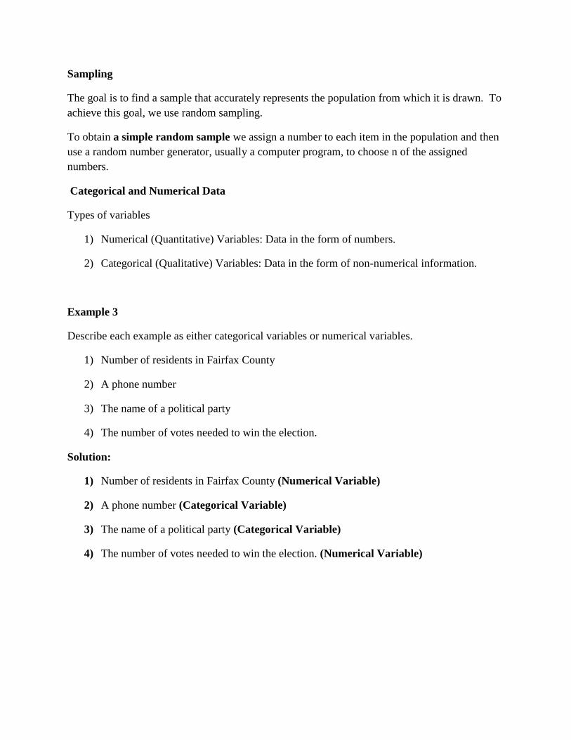
Categorical and Numerical Data

Types of variables

1) Numerical (Quantitative) Variables: Data in the form of numbers.

2) Categorical (Qualitative) Variables: Data in the form of non-numerical information.

Example 3

Describe each example as either categorical variables or numerical variables.

1) Number of residents in Fairfax County

2) A phone number

3) The name of a political party

4) The number of votes needed to win the election.

Solution:

1) Number of residents in Fairfax County (Numerical Variable)

2) A phone number (Categorical Variable)

3) The name of a political party (Categorical Variable)

4) The number of votes needed to win the election. (Numerical Variable)

Section 3.2 Graphing Categorical Data

Bar Graphs and Pie Charts

How do we know what is the best way to display or analyze data? Statisticians typically know

several ways to analyze data. It is their responsibility to choose the best way to analyze a

particular data set. Usually the best way to analyze a set data depends on the data.

Graphs are an excellent tool for analyzing data.

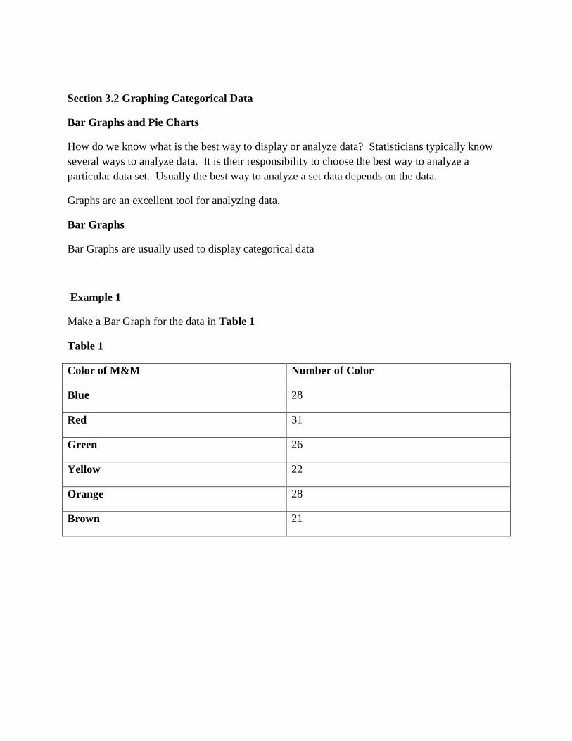
Bar Graphs

Bar Graphs are usually used to display categorical data

Example 1

Make a Bar Graph for the data in Table 1

Table 1

Color of M&M Number of Color

Blue 28

Red 31

Green 26

Yellow 22

Orange 28

Brown 21

Solution:

Example 2:

Use the data from table 1, create a bar graph which shows the percentage of each color of M&M.

Color of

M&M

Number of Color Percentage

Blue 28 18 %

Red 31 20 %

Green 26 17 %

Yellow 22 14 %

Orange 28 18 %

Brown 21 13 %

Total 156 100 %

Solution:

Pie Charts

Example 3

Use the data from the Table 2 to make a pie chart

Hybrid Car Number of Hyrids Sold Percentage of Hybrids Sold

Prius 34 23

Camry 45 31

Highlander 15 10

Malibu 25 17

Tahoe 12 8

Escape 16 11

Total 147 100

Solution:

Using Excel Spreadsheet will give the following pie chart.

Example 4

Given the data in table 3, construct a pie chart.

Math Course Percent of Freshman enrolled

in math course (Fall Semester)

Calculus II 3 %

Calculus I 15 %

Pre-Calculus 10 %

College Algebra 20 %

Core Math Courses 35 %

None 17 %

Solution:

Section 3.3

Line Graphs

Suppose you were given the following information and ask to display the data as a line graph.

Average rain fall in Blacksburg, Virginia

Month Rainfall in inches.

January 1.2

February 1.0

March 2.7

April 3.1

May 2.5

June 1.6

July 1.2

August 1.1

September 2.1

October 1.7

November 2.5

December 2.3

Solution: First you decide what information you want to pull on each axis. If one of variables is

categorical, it should be displayed on the horizontal axis which leaves rainfall in inches on the

vertical axis. Next, you should scale the vertical axis so that all the data will fit on that axis.

Since the rainfall varies from 1.1 inches to 3.1 inches, we can scale the vertical axis from 0

inches to 3.5 inches.

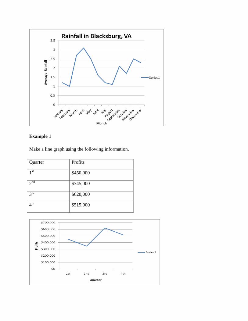
Example 1

Make a line graph using the following information.

Quarter Profits

1st $450,000

2nd

$345,000

3rd

$620,000

4th

$515,000

Double Line Graphs

Example 2

Make a double line graph of the following data.

Year Blacksburg Christiansburg

1970 10,000 13,000

1980 21,000 14,000

1990 30,000 14,000

2000 38,000 16,000

Section 3.5

Measures of Central Tendency

Averages

The mean, or average, is the most common way to measure the center of the data.

Key Formulas and Variables

n

x

x

n

i

i 1

indexthei

termithex

setdatainvaluesofnumberthen

meansamplex

th

i

Example 1

Suzy has six 100 point grades in her Math 114 class which are 91, 87, 86, 97, 95, and 84. Find

the mean (average) of Suzy’s grade in Math 114.

First, find

6

1i

ix . There are 6 data points in the data set. 6n , 911 x , 876 x , 862 x ,

973 x , 951 x , and 841 x .

Therefore,

6

1

654321 540849597868791i

i xxxxxxx

906

540

6

1

n

x

x i

i

The mean of the data set is 90

Example 2

Find the mean of the data set

12, 15, 16, 18, 19, 21, 23, 25, 26

229

198

9

2625232119181615121

n

x

x

n

i

i

Average = 22

Example 3

Below is the points scored by Johnny Dunksalot in his first 5 games. Find the Johnny’s scoring

average for his first 5 games.

21, 13, 17, 33, 9, 12, 18

6.177

123

7

18129331713211

n

x

x

n

i

i

The median

The median is the middle score of a data set.

Example 4

Find the median of the following set of test scores

61 72 88 77 83 91 80 98 87 96 99

First, put the numbers in order of lowest to highest.

61 72 77 80 83 87 88 91 96 98 99

Now, find the middle score

The median is 87

Example 5

Find the median and mean of the data set.

8, 7, 12, 14, 8, 9, 11, 13, 18, 21, 23, 29

Solution:

Put the number in order of lowest to highest.

7, 8, 8, 9, 11, 12, 13, 14, 18, 21, 23, 29

Since there is an even number of score, you will average the middle to scores.

5.122

25

2

1312

median

Now, find the mean

4.147

173

12

292321181413121198871

n

x

x

n

i

i

The mode is the most frequent score.

Example 6

Find the median of the following data set

8, 7, 12, 14, 8, 9, 11, 13, 18, 21, 23, 29

The most frequent score is 8. Therefore the mode is 8.

Example 7

Find the mean, median, and mode of the data set.

10, 11, 14, 10, 9, 10, 14

Solution:

Mean:

1.117

78

7

14109101411101

n

x

x

n

i

i

Median:

9, 10, 10, 10, 11, 14, 14

Median = 14

Mode:

10 occurs the most (3 times)

Mode = 10

Section 3.6

Variance and Standard Deviation

The next three measures of central tendency are range, variance, and standard deviation. The

range of a set of numbers is the difference between the highest score and the lowest score. The

variance is the measure of the spread of the data in terms of their squares. The standard

deviation is the square root of the variance.

Key Formulas

scorelowestscorehighestRange

Sample Variance and Standard Deviation

Sample Variance:

1

2

12

n

xx

s

n

i

i

Population Standard Deviation: 2ss

Population Variance and Standard Deviation

Population Variance:

n

xxn

i

i

2

12

Population Standard Deviation: 2

Now, let’s look at an example.

Example 1

Find the range of the following data set.

23, 30, 37, 39, 43, 45, 50, 60, 71, 82

Solution: 592382 scorelowestscorehighestRange

Example 2 (Sample Variance)

Find the variance and standard deviation.

9, 11, 15, 13, 14, 17

First, find the mean of the data set

2.136

79

6

171413151191

n

x

x

n

i

i

Next, find the variance by subtracting the mean from each data point and squaring this value.

After squaring each of these terms, take their sum and divide by the number of scores.

Variance:

49.7

5

44.37

5

44.1464.04.24.344.164.17

5

8.38.2.8.12.12.4

16

2.13172.13142.13132.13152.12112.139

1

2

2

2

222222

2

222222

2

2

12

s

s

s

s

s

n

xx

s

n

i

i

Standard Deviation:

73.249.72 ss

Example 3 (Population Variance)

Find the variance and standard deviation of the following data set

5, 6, 3, 7, 8, 7

Variance:

Find the mean: 66

36

6

7873651

n

x

x

n

i

i

67.2

6

16

6

141901

6

121301

6

676867636665

2

2

2

222222

2

222222

2

2

12

n

xxn

i

i

Standard Deviation:

63.167.22

You can also use tables to find the standard deviation and variance if you have problem with

summation notation.

Here is an example that uses tables to find the variance and standard deviation.

Example 4 (Sample Variance)

Find the variance and standard deviation of the following data set.

8, 10, 9, 12, 9, 10, 5

First, find the mean.

97

63

7

5109129108

x

Value of x x xxi 2xxi

8 9 198 112

10 9 1910 112

9 9 099 002

12 9 3912 932

10 9 1910 112

5 9 495 1642

Total - - 28

28

2

1

n

i

i xx

16.266.4

66.46

28

1

1

2

2

s

n

xx

s

n

i

i

Example 5 (Sample Variance)

Given the following test scores find the mean, median, variance, and standard deviation.

60,71,78,82,86,88,90,93,97,98

Mean: 3.8410

843

10

989793908886827871601

n

x

x

n

i

i

Median: 872

174

2

8886

median

Value of x x xxi 2xxi

60 84.3 3.243.8460 59.5903.242

71 84.3 3.133.8471 89.1763.132

78 84.3 3.63.8478 69.393.62

82 84.3 3.23.8482 29.53.22

86 84.3 7.13.8486 89.27.12

90 84.3 7.53.8490 49.327.52

93 84.3 7.83.8493 69.757.82

97 84.3 7.123.8497 29.1617.122

98 84.3 7.133.8498 69.1877.132

Total 1272.51

51.1272

2

1

n

i

i xx

Variance:

39.141

9

51.1272

110

51.1272

1

2

12

n

xx

s

n

i

i

Standard Deviation: 9.1139.141 s

Section 3.8/ Section 3.9

Graphing Numerical Data

Stem-and-Leaf Diagrams

Example 1

Make a stem and leaf plot of the given data

11,14,15,16,17,21,23,24,25,26,26,31,32,34,34,35,38,39,40,41,42,45,50,52,53,54,57,60,61,62,66,

67

Stem Leaf

1 1 4 5 6 7

2 1 3 4 5 6 6

3 1 2 4 4 5 8 9

4 0 1 2 5

5 0 2 3 4 7

6 1 2 6

Example 2

Make a stem and leaf plot of the given data

62,73,76,77,81,83,85,88,89,90,91,92,93,95,96,99

Stem Leaf

6 1

7 3 6 7

8 1 3 5 8 9

9 0 2 3 5 6 9

Example 3

Use the stem and leaf plot from example 2 to find the median.

Since there are 15 numbers in the data set, the median will the 8th

term in the stem and leaf plot.

Recall that the stem and leaf puts the numbers in ascending order.

Therefore, the median of the data is 8.

Frequency Tables

A frequency table shows a list of numbers between the minimum and maximum data values.

Here is an example of a frequency table.

Example 4

Use the data listed below to create a frequency table.

5,6,6,7,7,7,8,9,9,10,11,11,11,12,13,13,13,14,14

Value Frequency

5 1

6 2

8 1

9 2

10 1

11 3

14 2

Frequency Table with Intervals

Example 5

Use the data listed below to create a frequency table using intervals.

11,12,13,13,14,15,17,20,21,23,24,28,29,31,33,34,35,37,38,41,42,44,50,51,55,56,59,60,62,64,65

Interval Frequency

0 - 10 0

10-20* 7

20-30 6

30-40 6

40-50 3

50-60 5

60-70 4

Histograms

A histogram is a form of a bar graph where the data is numerical instead of categorical.

Here is an example of data displayed as a histogram.

Example 6

Make a histogram for the given data in example 5

First make a frequency table from the given data.

11,12,13,13,14,15,17,20,21,23,24,28,29,31,33,34,35,37,38,41,42,44,50,51,55,56,59,60,62,64,65

Interval Frequency

0 - 10 0

10-20* 7

20-30 6

30-40 6

40-50 3

50-60 5

60-70 4

Histogram of Example 6

Example 7

Make a histogram of the frequency table that represents the heights of preschool children.

Midpoint Frequency

34.5 2

35.5 7

36.5 8

37.3 14

38.5 16

39.5 17

40.5 21

41.5 23

42.5 18

43.5 14

44.5 6

45.5 3

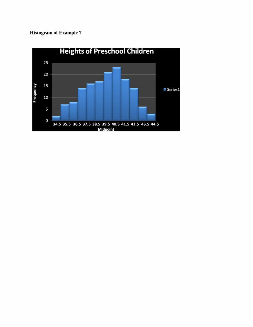
Histogram of Example 7