Introduction to STRUCTURAL EQUATION MODELING USING …

Introduction toSTRUCTURAL

EQUATION MODELING

USING IBM SPSS STATISTICS AND EQS

NIELS J. BLUNCH

00_Blunch_Prelims.indd 3 9/22/2015 2:43:42 PM

SAGE Publications Ltd1 Oliver’s Yard 55 City RoadLondon EC1Y 1SP

SAGE Publications Inc.2455 Teller RoadThousand Oaks, California 91320

SAGE Publications India Pvt LtdB 1/I 1 Mohan Cooperative Industrial AreaMathura RoadNew Delhi 110 044

SAGE Publications Asia-Pacific Pte Ltd3 Church Street#10-04 Samsung HubSingapore 049483

Editor: Jai SeamanAssistant editor: James PiperProduction editor: Victoria NicholasCopyeditor: Neville HankinsProofreader: Kate CampbellIndexer: David RudeforthMarketing manager: Sally RansomCover design: Shaun MercierTypeset by: C&M Digitals (P) Ltd, Chennai, IndiaPrinted and bound by CPI Group (UK) Ltd, Croydon, CR0 4YY

Niels J. Blunch 2016

Apart from any fair dealing for the purposes of research or private study, or criticism or review, as permitted under the Copyright, Designs and Patents Act, 1988, this publication may be reproduced, stored or transmitted in any form, or by any means, only with the prior permission in writing of the publishers, or in the case of reprographic reproduction, in accordance with the terms of licences issued by the Copyright Licensing Agency. Enquiries concerning reproduction outside those terms should be sent to the publishers.

Library of Congress Control Number: 2015934011

British Library Cataloguing in Publication data

A catalogue record for this book is available from the British Library

ISBN 978-1-47391-621-0ISBN 978-1-47391-622-7 (pbk)

At SAGE we take sustainability seriously. Most of our products are printed in the UK using FSC papers and boards. When we print overseas we ensure sustainable papers are used as measured by the Egmont grading system. We undertake an annual audit to monitor our sustainability.

00_Blunch_Prelims.indd 4 9/22/2015 2:43:42 PM

1Introduction

After a presentation and an overview of the contents of the whole book, this chapter continues with an intuitive introduction to structural equation modeling (SEM) by presenting a few examples of such modeling.

These models are very simple, but are chosen to illustrate the broad spectrum of research problems that can be analyzed by the collection of tools in the bag called SEM. This will not only acquaint you with prototypes of problems and mod-els discussed in more depth in later chapters, but also stress the way SEM solves the problem of measuring the vague concepts often met in the social and behav-ioral sciences (intelligence, preference, social status, attitude, literacy and the like), for which no generally accepted measuring instruments exist.

A short outline of the history of SEM follows subsequently.Then you will learn how to cope with another problem. Unlike the natural sci-

ences, the ideal way of doing causal research, namely experimentation, is more often than not impossible to implement in the social and behavioral sciences. This being the case, we face a series of difficulties of a practical as well as a philo-sophical nature.

You will also find a short introduction to the matrices appearing in the output from EQS, the computer program used in this book.

Rather than presenting a deep discussion of the mathematical and statistical calculations, which are the basis for SEM estimation, a brief, intuitive explanation of the principles is presented instead.

1 Purpose and Plan of the Book

As you can see from the title, this book is an introduction to structural equation modeling – or SEM for short. SEM is a very large subject indeed. It is not just one statistical method, such as regression analysis or analysis of variance, that you should know from your introductory course in statistics. In fact these two statistical techniques can be shown to be special cases of SEM, and the same goes for more advanced statistical models that you might have met, such as MANOVA, discriminant analysis and canonical correlation.

So you can see that general SEM is a rather large toolbox that can serve you in lots of different data analysis situations. This means that it is impossible to cover, in a rather slim volume like this one, the more advanced and complicated topics in this rapid developing area.

01_Blunch_Ch-01_Part-1.indd 3 9/22/2015 2:47:28 PM

4 Chapter 1 Introduction

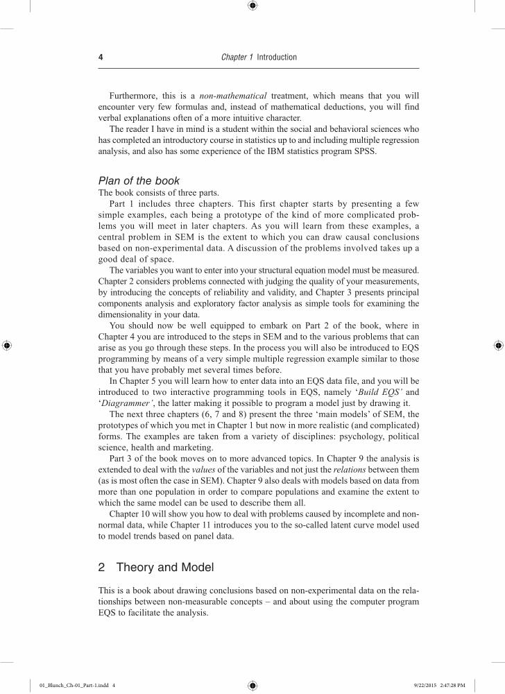
Furthermore, this is a non-mathematical treatment, which means that you will encounter very few formulas and, instead of mathematical deductions, you will find verbal explanations often of a more intuitive character.

The reader I have in mind is a student within the social and behavioral sciences who has completed an introductory course in statistics up to and including multiple regression analysis, and also has some experience of the IBM statistics program SPSS.

Plan of the bookThe book consists of three parts.

Part 1 includes three chapters. This first chapter starts by presenting a few simple examples, each being a prototype of the kind of more complicated prob-lems you will meet in later chapters. As you will learn from these examples, a central problem in SEM is the extent to which you can draw causal conclusions based on non-experimental data. A discussion of the problems involved takes up a good deal of space.

The variables you want to enter into your structural equation model must be measured. Chapter 2 considers problems connected with judging the quality of your measurements, by introducing the concepts of reliability and validity, and Chapter 3 presents principal components analysis and exploratory factor analysis as simple tools for examining the dimensionality in your data.

You should now be well equipped to embark on Part 2 of the book, where in Chapter 4 you are introduced to the steps in SEM and to the various problems that can arise as you go through these steps. In the process you will also be introduced to EQS programming by means of a very simple multiple regression example similar to those that you have probably met several times before.

In Chapter 5 you will learn how to enter data into an EQS data file, and you will be introduced to two interactive programming tools in EQS, namely ‘Build EQS’ and ‘Diagrammer’, the latter making it possible to program a model just by drawing it.

The next three chapters (6, 7 and 8) present the three ‘main models’ of SEM, the prototypes of which you met in Chapter 1 but now in more realistic (and complicated) forms. The examples are taken from a variety of disciplines: psychology, political science, health and marketing.

Part 3 of the book moves on to more advanced topics. In Chapter 9 the analysis is extended to deal with the values of the variables and not just the relations between them (as is most often the case in SEM). Chapter 9 also deals with models based on data from more than one population in order to compare populations and examine the extent to which the same model can be used to describe them all.

Chapter 10 will show you how to deal with problems caused by incomplete and non-normal data, while Chapter 11 introduces you to the so-called latent curve model used to model trends based on panel data.

2 Theory and Model

This is a book about drawing conclusions based on non-experimental data on the rela-tionships between non-measurable concepts – and about using the computer program EQS to facilitate the analysis.


1.2 Theory and Model 5

Scientific work is characterized by the fact that a scientist works with models, i.e. simpli-fied descriptions of the phenomenon in ‘the real world’ that is the object of the research. An example of such a model is the hierarchy-of-effects model depicting the various stages through which a recipient of an advertising message is supposed to move from awareness to (hopefully) the final purchase (e.g. Lavidge & Steiner, 1961). See Figure 1a.

Another example comes from the theory of the pioneering French sociologist and philosopher Emile Durkheim: that living an isolated life increases the probability of suicide (Durkheim, 2002 [1897]). This theory can be depicted as in Figure 1b.

We can see that a scientific theory may be depicted as a graphic model in which the hypothesized connections among the concepts of the theory are shown as arrows.

What then is SEM?SEM is a collection of tools for analyzing connections between various concepts in

cases where these connections are relevant either for expanding our general knowledge or for solving some problem.

Examples of such problems are as follows:

1. Health officials might be interested in mapping a possible connection between smoking during pregnancy and infant health.

2. School authorities might be interested in examining the effects of various factors having a possible impact on students’ academic achievement.

3. A psychologist might be interested in developing a questionnaire that could ‘measure’ the respondent’s ‘style of information processing’, i.e. whether the respondent prefers a verbal and/or visual modality of processing information about his or her environment. In that connection the psychologist is interested in mapping the possible connection between a person’s ‘style of information pro-cessing’ and the same person’s answers to the various proposed questions.

4. A health researcher might be interested in mapping a possible connection between a person’s psychical well-being and the same person’s physical reactions.

5. An advertising manager or a health official might (for different reasons) be interested in mapping a possible connection between cigarette advertising and cigarette sales.

The key term is the word possible. We are not sure that a connection exists, but we want to find out whether it exists and, if so, to measure the strengths of the connection in numerical form.

So, SEM is a set of tools for verifying theories. In principle we start out with an a priori theory about the system we want to map, and then use SEM to test our model against empirical data. SEM is a confirmatory rather than an exploratory technique.

Exposure

Isolated life Suicide

KnowledgePositiveattitude

Buy(a)

(b)

Figure 1 (a) The hierarchy-of-effects model; (b) Durkheim’s suicide model



Our hope is that we can confirm our model and as a result be able to measure the strength of the various connections and in that way answer questions such as ‘By how much can we expect each extra pack of cigarettes smoked during pregnancy to reduce birth weight?’

However, this does not exclude the possibility that our analysis might lead to modifica-tions of the original model as we gain more insight while working with our model – so the distinction between confirmatory and exploratory is not a sharp one.

As the name ‘structural equation modeling’ suggests, the first step is to form a graphic depiction – a model – showing how the various concepts fit together.

Let us look at the examples above.

Example 1Cigarette smoking during pregnancy and infant health(Mullahy, 1997)

If we measure cigarette smoking in ‘total number of cigarettes smoked during pregnancy’ and infant health by ‘birth weight’ we can suggest the model shown in Figure 2a. The concepts are shown in rectangles and the ‘connection’ between them is depicted as an arrow indicating the direction of a possible causal effect: we suspect the mother’s cigarette smoking affects the child’s birth weight and not the other way round.

In this example it is easy to decide on the direction of a (possible) effect, but at times this can be more problematic – for example, Example 5 in the list above, where an advertising manager hopes that advertising will promote sales but cannot rule out the possibility that a positive covariation between advertising and sales figures could be due to the way the advertising budget is compiled, e.g. using a fixed percentage of sales income for advertising. That is why I have avoided words like ‘cause’ and ‘effect’ in the list of examples above and used the more vague expression ‘connection’. As you will learn in Section 4, it takes more than covariation to confirm a possible causal effect, and SEM is (in principle) only the analysis of covariations.

b is a measure of the strength of the connection and δ (disturbance) depicts the combined effect of all other factors influencing the child’s birth weight.

Number of cigarettessmoked during pregnancy

Number of cigarettessmoked during pregnancy

Birthweight

Birthweight

Family income

(b)

(a)β

β

β

δ

δ

2

1

Figure 1.2 Example 1: a traditional regression model



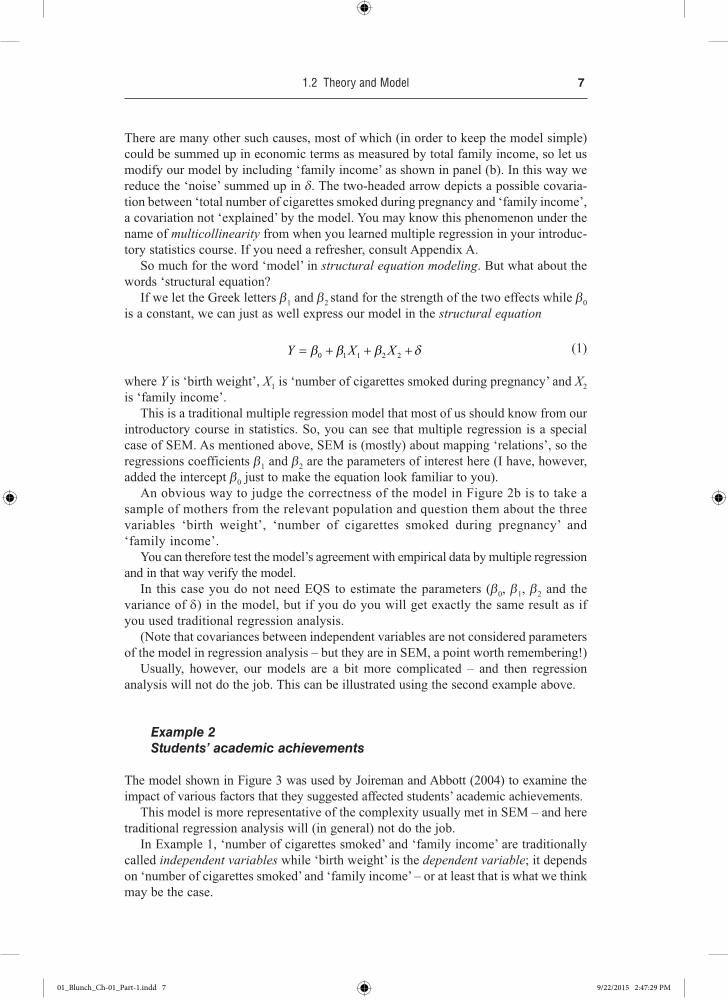
There are many other such causes, most of which (in order to keep the model simple) could be summed up in economic terms as measured by total family income, so let us modify our model by including ‘family income’ as shown in panel (b). In this way we reduce the ‘noise’ summed up in d. The two-headed arrow depicts a possible covaria-tion between ‘total number of cigarettes smoked during pregnancy and ‘family income’, a covariation not ‘explained’ by the model. You may know this phenomenon under the name of multicollinearity from when you learned multiple regression in your introduc-tory statistics course. If you need a refresher, consult Appendix A.

So much for the word ‘model’ in structural equation modeling. But what about the words ‘structural equation?

If we let the Greek letters b1 and b2 stand for the strength of the two effects while b0 is a constant, we can just as well express our model in the structural equation

Y X X= + + +β β β δ0 1 1 2 2 (1)

where Y is ‘birth weight’, X1 is ‘number of cigarettes smoked during pregnancy’ and X2 is ‘family income’.

This is a traditional multiple regression model that most of us should know from our introductory course in statistics. So, you can see that multiple regression is a special case of SEM. As mentioned above, SEM is (mostly) about mapping ‘relations’, so the regressions coefficients b1 and b2 are the parameters of interest here (I have, however, added the intercept b0 just to make the equation look familiar to you).

An obvious way to judge the correctness of the model in Figure 2b is to take a sample of mothers from the relevant population and question them about the three variables ‘birth weight’, ‘number of cigarettes smoked during pregnancy’ and ‘family income’.

You can therefore test the model’s agreement with empirical data by multiple regression and in that way verify the model.

In this case you do not need EQS to estimate the parameters (b0, b1, b2 and the variance of d) in the model, but if you do you will get exactly the same result as if you used traditional regression analysis.

(Note that covariances between independent variables are not considered parameters of the model in regression analysis – but they are in SEM, a point worth remembering!)

Usually, however, our models are a bit more complicated – and then regression analysis will not do the job. This can be illustrated using the second example above.

Example 2Students’ academic achievements

The model shown in Figure 3 was used by Joireman and Abbott (2004) to examine the impact of various factors that they suggested affected students’ academic achievements.

This model is more representative of the complexity usually met in SEM – and here traditional regression analysis will (in general) not do the job.

In Example 1, ‘number of cigarettes smoked’ and ‘family income’ are traditionally called independent variables while ‘birth weight’ is the dependent variable; it depends on ‘number of cigarettes smoked’ and ‘family income’ – or at least that is what we think may be the case.



A glance at the model in Figure 3 reveals that here things are a bit more complicated. Looking only at the connection between ‘mother’s education’ and ‘homework’, you could say that ‘mother’s education’ is the independent variable and ‘homework’ the dependent variable. However, ‘mother’s education’ is dependent on ‘ethnicity’, so it is also a dependent variable.

This shows that we have to draw a very important distinction between exogenous variables, whose values are determined by variables not included in the model, and endog-enous variables, the values of which are determined by other variables in the model.

In the model in Figure 3 (apart from δ-variables) the only exogenous variable is ‘ethnicity’ – all other variables are endogenous.

Example 3Constructing a measuring instrument

A psychologist is constructing a questionnaire that can measure a person’s ‘style of processing’, i.e. the person’s preference to engage in a verbal and/or visual modality of processing information about his or her environment.

The psychologist decides to use a summated scale.A summated scale is compiled by adding up scores obtained from answering a

series of questions. One of the most popular scales is the Likert scale. Here the respondents are asked to indicate their agreement with a series of statements by checking a scale from, say, 1 (strongly disagree) to 5 (strongly agree) and the scores are then added to make up the scale. The scale values are in the opposite direction for statements that are favorably worded versus unfavorably worded in regard to the concept being measured.

Examples of such questions – or items as they are called in this connection – to measure ‘style of processing’ are as follows:

Time spenton watching

TV

Father’seducation

EthnicityEngagement

in schoolactivities

Mother’seducation

Homework

Achievement

δ1 δ3

δ2 δ5

δ4 δ6

Figure 3 Example 2: model used to explain the impact of factors affecting students’ academic achievements



1. I enjoy work that requires the use of words.2. There are some special times in my life that I like to relive by mentally ‘picturing’

just how everything looked.3. When I’m trying to learn something new, I’d rather watch a demonstration than

read how to do it.

The psychologist has formulated around 50 such items (statements) and is now won-dering which of them should be chosen for inclusion in the questionnaire – the criteria of course being that the ones with the strongest ‘connection’ to the concept ‘style of processing’ should be the preferred ones.

The problem can be modeled as shown in Figure 4.

The X-variables in the figure are three items supposed to measure ‘style of processing’, and the three ε-variables indicate that factors other than the variable ‘style of processing,’ affect how people answer a question. e is the combined effect of all such ‘disturbing’ effects. In other words, e is the measurement error of the item in question.

You may wonder why the variable ‘style of processing’ in the model in Figure 4 is shown as an ellipse (just like the concepts in Figure 1), while the concepts in Figure 2 are depicted as rectangles. This is done because there is a fundamental difference between ‘number of cigarettes’, ‘family income’ and ‘birth weight’ on the one hand, and ‘style of processing’ on the other.

The first-mentioned concepts are measurable, i.e. there exist well-defined ways of measuring them. They are measured in number of cigarettes, in dollars (or whatever currency is relevant) and in pounds or kilograms. Such measurable variables are called manifest variables, and they are traditionally depicted as squares or rectangles.

A characteristic of the concept ‘style of processing’ in the model in Figure 4 is that it is not directly measurable by a generally accepted measuring instrument, a character-istic it shares with many concepts from the social and behavioral sciences – satisfaction, preference, intelligence, lifestyle, social class and literacy, just to mention a few. Such non-measurable variables are called latent variables. Latent variables are traditionally depicted as circles or ellipses

As such concepts cannot be measured directly, they are measured indirectly by indicators – in this case items in a Likert scale – and such indicators are manifest variables.

Figure 4 Example 3: model used in scale development

Style ofprocessing

X1

X2

X3 ε3

ε2

ε1



The arrows connecting a latent variable to its manifest variables should be interpreted as follows:

If a latent variable were measurable on a continuous scale – which of course is not the case as a latent variable is not (directly) measurable on any scale – variations in a person’s (or whatever the analytical unit may be) position on this scale would be mir-rored in variations in its manifest variables. This is the reason why the arrows point from the latent variable towards its manifest indicators and not the other way round.

The purpose is now to estimate the parameters in the model in Figure 4, these para-meters being the three regression coefficients and the variances of the ε-variables, and then use the result to select the ‘best’ items (i.e. the ones with the strongest connection to ‘style of processing’) for use in the summated Likert scale.

In this case we cannot use traditional regression analysis, because one of the vari-ables is latent, but EQS can do the job.

In fact, the three items in this example are taken from the 22-item SOP (Style of Processing) scale by Childers, Houston & Heckler (1985). We will return to this example in Chapter 7.

The selection of items for summated and non-summated scales is discussed in the next chapter.

Example 4The effects of depression on the immune system

A health researcher is interested in evaluating the (possible) connection between depression and the state of the immune system, and tentatively suggests the model shown in Figure 5 (this figure is part of a more complicated model, to which we will return in Chapter 8).

As can be seen, the model contains the hypothesized effect of ‘depression’ on ‘immune system’ as well as the connections between the two latent (non-measurable) variables and their manifest (measurable) indicators.

The model thus consists of two parts:

1. The structural model describing the (causal?) connections between the latent variables. Mapping of this connection is the main purpose of the analysis.

2. The measurement model describing the connections between the latent variables and their manifest indicators.

Figure 5 Example 4: a model with latent variables

1

1

1 DepressionImmunesystem

1

1

1

1δX3ε3

ε2

ε1 ε4

ε5

ε6

X2

X1 X4

X5

X6

23θ λ32

λ22 β12

λ12 λ41

λ61

λ51

F2 F1



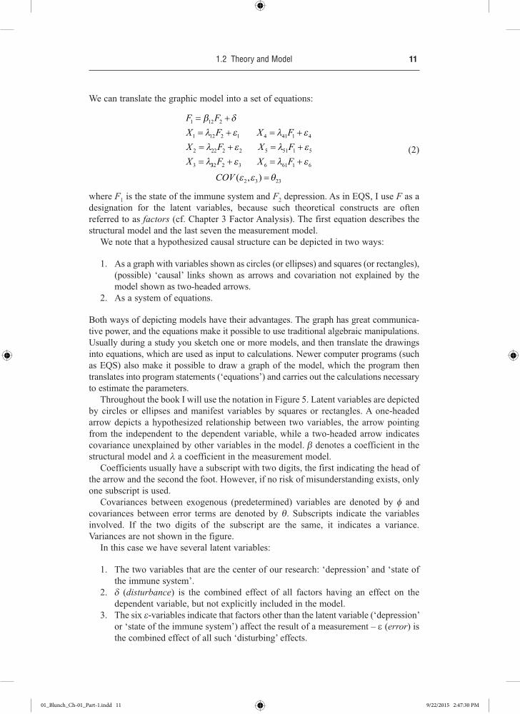
We can translate the graphic model into a set of equations:

F

X

X

X

1 12 2

1 12 2 1 4 41 1 4

2 22 2 2 5 51 1 5

3

= += + = += + = +=

β δλ ε λ ελ ε λ ελ

F

X F F

X F F

332 2 3 6 61 1 6

2 3 23

F X F

COV

+ = +

=

ε λ ε

ε ε θ( ),

(2)

where F1 is the state of the immune system and F2 depression. As in EQS, I use F as a designation for the latent variables, because such theoretical constructs are often referred to as factors (cf. Chapter 3 Factor Analysis). The first equation describes the structural model and the last seven the measurement model.

We note that a hypothesized causal structure can be depicted in two ways:

1. As a graph with variables shown as circles (or ellipses) and squares (or rectangles), (possible) ‘causal’ links shown as arrows and covariation not explained by the model shown as two-headed arrows.

2. As a system of equations.

Both ways of depicting models have their advantages. The graph has great communica-tive power, and the equations make it possible to use traditional algebraic manipulations. Usually during a study you sketch one or more models, and then translate the drawings into equations, which are used as input to calculations. Newer computer programs (such as EQS) also make it possible to draw a graph of the model, which the program then translates into program statements (‘equations’) and carries out the calculations necessary to estimate the parameters.

Throughout the book I will use the notation in Figure 5. Latent variables are depicted by circles or ellipses and manifest variables by squares or rectangles. A one-headed arrow depicts a hypothesized relationship between two variables, the arrow pointing from the independent to the dependent variable, while a two-headed arrow indicates covariance unexplained by other variables in the model. b denotes a coefficient in the structural model and l a coefficient in the measurement model.

Coefficients usually have a subscript with two digits, the first indicating the head of the arrow and the second the foot. However, if no risk of misunderstanding exists, only one subscript is used.

Covariances between exogenous (predetermined) variables are denoted by f and covariances between error terms are denoted by q. Subscripts indicate the variables involved. If the two digits of the subscript are the same, it indicates a variance. Variances are not shown in the figure.

In this case we have several latent variables:

1. The two variables that are the center of our research: ‘depression’ and ‘state of the immune system’.

2. d (disturbance) is the combined effect of all factors having an effect on the dependent variable, but not explicitly included in the model.

3. The six e-variables indicate that factors other than the latent variable (‘depression’ or ‘state of the immune system’) affect the result of a measurement – e (error) is the combined effect of all such ‘disturbing’ effects.



Depression could be measured by Likert items such as:

X1: I am sad all the time and I cannot snap out of it.

X2: I am so restless and agitated that I have to keep moving or doing something.

X3: I have as much energy as ever.

Most often you will have more than three items in a scale, but three will do as an illustration (in fact the three items mentioned above are taken from one of the most widespread scales for measuring the strength of depression: ‘Beck’s Depression Inventory’ (Beck, Ward, Mendelson, & Erbaugh, 1961)). Observe that the variables X1 to X3 are expected to correlate, because they are all functions of the same variable ‘depression’ – they are measuring the same concept. However, a glance at the wording of X2 and X3 shows that they are indeed very similar, and they could be expected to correlate more than by their mutual cause ‘depression’. If that should be the case X2 and X3 measure not only the same latent variable ‘depression’, but also the same aspect of that concept, hence the two-headed arrow in Figure 5.

A characteristic of the summated scale is that in taking an unweighted sum of the various scores you implicitly assume that all the questions (or items) making up the scale measure the concept to the same precision. An advantage of SEM is that instead of summing the various items, you can use the items separately, and in that way weight them in accordance with their quality in measuring the concept in question.

Now, we cannot measure the state of the immune system by using a questionnaire. Instead we carry out a few tests to measure variables that could be used as indicators, such as number of leukocytes, number of lymphocytes and PHA-stimulated T-cell proliferation.

To sum up, a theory is a number of hypothesized connections among conceptually defined variables. These variables are often latent, i.e. they are not directly measurable and must be operationalized in a series of manifest variables.

These manifest variables and their interrelations are all we have at our disposal to uncover the connections among the latent variables.

The benefits of using latent variablesThe variables with which the social science researcher works are usually more diffuse than concepts such as weight, length and the like, for which well-defined and generally accepted measuring methods exist. Rather, the social scientist works with concepts such as attitudes, literacy, alienation, social status, etc. Concepts that are not directly measurable and therefore must be measured indirectly via indicators, whether they are questions in a questionnaire or some sort of test.

If we compare SEM with a traditional regression model such as

Y Xi i i= + +β β δ0 1 (3)

it is obvious that the latter is based on an assumption which is rarely mentioned but is nevertheless usually unrealistic: that all variables are measured without error. (The assumption of no measurement error always applies to the independent variable, whereas you can assume that di includes measurement error in the dependent variable as well as the effect of excluded variables.)


1.3 A Short History of SEM 13

An assumption of error-free measurements is of course always wrong in principle, but it will serve as a reasonable simplification when measuring, for example, weight, volume, temperature and other variables for which generally agreed measurement units and measuring instruments exist.

On the other hand, such an assumption is clearly unrealistic when the variables are lifestyle, intelligence, attitudes and the like. Any measurement will be an imperfect indicator of such a concept. Using more than one indicator per latent variable makes it possible to assess the connection between an indicator and the concept it is assumed to measure, and in this way evaluate the quality of the measuring instrument.

Introducing measurement models has the effect of freeing the estimated parameters in the structural model from the influence of measurement errors. Or – put another way – the errors in the structural model (‘errors in equations’ d) are separated from the errors in the measurement model (‘errors in variables’ e).

What then is SEM?As should be clear from the examples, SEM is not a single statistical model, but rather a collection of models originated in different disciplines at different times and brought together, because they can be shown to be special cases of a general model.

In Example 1 you met the traditional regression model that you should already know from your introductory statistics course, and in Example 2 several such models were put together to form a system of regression functions. Such systems are known in psy-chology and related fields as path models and in economics as simultaneous equation models or econometric models.

The model in Example 3 is generally known as the confirmatory factor model, and in Example 4 the path model and the confirmatory factor model are brought together to form the general structural equation model, of which the models in the first three examples are special cases. In fact, the general model can be shown to include many of the linear models that are bases for statistical techniques you may already know: analy-sis of variance, canonical correlation and discriminant analysis, to mention a few. So the structural equation model is very general indeed and well suited for analyzing a broad spectrum of problems in many disciplines.

3 A Short History of SEM

SEM can trace its history back more than 100 years.At the beginning of the twentieth century C. Spearman laid the foundation for factor

analysis and thereby for the measurement model in SEM (Spearman, 1904). He tried to trace the different dimensions of intelligence back to a general intelligence factor. In the 1930s L.L. Thurstone invented multi-factor analysis and factor rotation (more or less in opposition to Spearman) and thereby founded modern factor analysis where intelli-gence, for instance, was thought of as being composed of several different intelligence dimensions (Thurstone, 1947; Thurstone & Thurstone, 1941).

About 20 years after Spearman, S. Wright developed so-called path analysis (Wright, 1918, 1921). Based on box and arrow diagrams like those in Figure 3, he formulated a series of rules that connected correlations among the variables to



parameters in a model of the assumed data-generating process. Most of his work was on models with only manifest variables, but a few also included models with latent variables.

Wright was a biometrician and it is amazing that his work was more or less unknown to scientists outside this area, until it was taken up by social researchers in the 1960s (Blalock, 1961, 1971; Duncan, 1975).

In economics a parallel development took place in what came to be known as econometrics. However, this development was unaffected by Wright’s ideas and was characterized by an absence of latent variables – at least in the sense of the word used in this book. However, in the 1950s econometricians became aware of Wright’s work, and some of them found to their surprise that he had pioneered the estimation of sup-ply and demand functions and in several respects was far ahead of econometricians of that time (Goldberger, 1972).

In the early 1970s path analysis and factor analysis were combined to form the gen-eral SEM of today. Foremost in its development was K.G. Jöreskog, who created the well-known LISREL (LInear Structural RELations) program for analyzing such models (Jöreskog, 1973).

However, LISREL is not alone in this. Among other similar computer programs, mention can be made of RAM (Reticular Action Model) (McArdle & McDonald, 1984), included in the SYSTAT package of statistics programs under the name RAMONA (Reticular Action Model Or Near Approximation), AMOS (Analysis of MOment Structures (Arbuckle, 1989) and of course EQS (EQuationS) (Bentler, 1985).

Jöreskog was a statistician but published much of his research in psychological journals. No wonder then that psychology was the area where this ‘new’ way of thinking first gained widespread use.

The first discipline to ‘import’ SEM – and the area where it has found most use outside of psychology – is marketing. One of the first articles on SEM in the Journal of Marketing Research was by Bagozzi (1977), and three years later this author published a book on the use of SEM in marketing (Bagozzi, 1980).

Since then there has hardly been an area within the social and life sciences where SEM has not gained more and more appreciation.

The reasons for this are very simple: we often have to struggle with measurement problems; and the possibilities to perform experiments are often limited.

Last but not least, SEM forces you to think in terms of hypotheses, models and verification, i.e. it speaks the language of science and forces you to think as a scientist.

There is an exception to the development sketched above, namely economics, where the use of latent variables (in the SEM sense) is not apparent, despite modern econo-mists spending more and more time analyzing ‘soft’ variables like health, values, etc.

4 The Problem of Non-experimental Data

Basing causal conclusions on non-experimental data usually necessitates statistical mod-els comprising several equations as opposed to traditional regression analysis and analysis of variance, which serve us so well in the simpler situations we meet when we analyze experimental data. Besides, the statistical assumptions underlying the models used are more difficult to fulfill in non-experimental research, and, last but not least, the concept of causality must be used with greater care in non-experimental research.


1.4 The Problem of Non-experimental Data 15

As is well known, we are not able to observe causation – considered as a ‘force’ from cause to effect. What we can observe is:

1. Co-variation – the fact that two factors A and B covary is an indication of the possible existence of a causal relationship, in one direction or the other.

2. The time sequence – the fact that the occurrence of A is generally followed by the occurrence of B is an indication of A being a cause of B (and not the other way round).

However (and this is a crucial requirement):

3. These observations must be made under conditions that rule out all other expla-nations of the observations than that of the hypothesized causation.

These three points could be used as building blocks in an operational definition of the concept of causation, even if this concept ‘in the real world’ is somewhat dim and per-haps meaningless except as a common experience facilitating communication between people (Hume, 2000 [1739]).

It is clear from the above that we can never prove a causal relationship; we can only render it probable. It is not possible to rule out all other explanations, but we can try to rule out the ones deemed most ‘probable’ to the extent that makes the claimed explanation ‘A is the cause of B’ the most probable.

The extent to which this can be done depends on the nature of the data from which the conclusions are drawn.

The dataThe necessary data can be obtained in one of two different ways:

1. Data can be ‘historical’ in the sense that they mirror ‘the real world’, e.g. the actual consequences that a firm’s pricing policy has had on sales.

2. Data can be experimental: you can make your own ‘world’ in which you can manipulate the variables whose effects you want to investigate.

Historical data are often called observational data in order to indicate that while in an experiment you deliberately manipulate the independent variables, you do not inter-fere with the variables in non-experimental research more than necessary in order to observe (i.e. measure) them.

The necessity of a closed systemTo rule out all possible explanations except one is of course impossible, and since we can examine only a subset of (possible) explanations it is obvious that causal relation-ships can only be mapped in isolated systems. Clearly, experimental data are to be preferred to non-experimental data, because in an experiment we create our own world in accordance with an experimental plan designed to reduce outside influences.

It is much more difficult to cut out disturbing effects in a non-experimental study. In an experiment we create our own little world, but when we base our study on the



real world we must accept the world as it is. We deal with historical data and cannot change the past.

While it seems obvious that causality can only be established – or according to Hume (2000 [1739]) only be meaningful – in a scientific model which constitutes a closed system, it is a little more complicated to define ‘closed’.

Example 5The determinants of cigarette sales

In Figure 6 – inspired by Bass (1969) – some of the factors determining cigarette sales are depicted. There are an enormous number of possible factors influencing cigarette sales – many more than shown in the figure. It would not be very difficult to expand the model to cover several pages of this book. In causal research it is necessary to keep down the number of variables – in this example (as Bass did) to the variables on the gray background.

Figure 6 Example 5: the demand for cigarettes (d-terms not shown)

Distribution

IncomeSales of lter

cigarettesAdvertising for lter cigarettes

Relative price of lter cigarettes

Sales of non- ltercigarettes

Taxes Distribution

Advertising fornon- lter cigarettes

Anti-smokingcampaign

As any limit on the number of variables must necessarily cut causal relations, we cannot demand that the system has no relation to the surrounding world. What we require is that all effects on a variable in the model, from outside the model, can be summarized in one variable which is of purely random (i.e. non-systematic) nature, and with a



variance small enough not to ‘drown’ effects from variables in the model in ‘noise’. If we use the Greek letter δ (disturbance) to designate the combined effects of excluded independent variables (noise), we can write

Y f X X X X Xj p= +( , , ,..., ,..., )1 2 3 δ (4a)

where Y is the dependent variable in the model, and Xj j (j = 1, 2, …, p) are exoge-nous variables included in the model and supposed to influence Y. If the model is really ‘closed’, Xj (for j = 1, 2, ….p) and d must be stochastically independent. This is the same as demanding that for each and every value of Xj the expected value of d is the same and consequently the same as the unconditional expected value of d. This can be written as

E X E jj( | ) ( )δ δ= = 0 forallvaluesof (4b)

(for a definition of expected value, see Appendix A).If condition (4b) is not met, a ceteris paribus interpretation of the parameters indi-

cating the influence of the various independent variables is not possible, because the effects of variables included in the model are then mixed up with the effects of variables not included in the model.

Simon (1953, 1954) has given Hume’s operational definition of causality a modern formulation.

Example 6The disturbance must be independent of exogenous variables

As is well known (Appendix A), least squares estimation in traditional regression analysis forces δ to be independent of the exogenous variables X1 , …, Xj , …, Xp in the model – and so do the estimation methods used in EQS. But the point is that this condi-tion must hold in the population and not just in our model. So, be careful in specifying your model.

Consider the following model:

score obtained at exam = f (number of classes attended) + d

Think about what variables are contained in d: intelligence, motivation, age and earlier education, to name but a few. Do you think that it is likely that the ‘number of classes attended’ does not depend on any of these factors?

Three different causal modelsFigure 7 shows three causal models from marketing, depicting three fundamentally dif-ferent causal structures.

Dominick (1952) reported an in-store experiment concerning the effect on sales of four different packages for McIntosh apples. The experiment ran for four days in four retail stores. The causal model is shown in Figure 7a. In order to reduce the noise d, the most influencing factors affecting sales (apart from the package) were included in the



experiment, namely the effects on sales caused by differences among the shops in which the experiment was conducted, the effects caused by variations in sales over time, and the varying number of customers in the shops during the testing period.

Figure 7 Three types of causal models (d-terms not shown)

Package

Shop

Sales (a)Time

Number ofcustomers

Model 1: hierarchy-of-effects model

Model 2: low-involvement model

Exposure Awareness Attitude

Price(b)

(c)

Market share

Market shareExposure Awareness

Price

Attitude

X1

X1 = average income for persons ≥ 20 yearsX2 = relative price of non-�lter cigarettesY1 = sales of �lter cigarettes to persons ≥ 20 yearsY2 = sales of non-�lter cigarettes to persons ≥ 20 yearsY3 = advertising expenditures for �lter cigarettes/number of persons ≥ 20 yearsY4 = advertising expenditures for non-�lter cigarettes/number of persons ≥ 20 years

Y1 Y3

X2 Y2 Y4

Aaker and Day (1971) tried to decide which of the two models in Figure 7b best describe buying behavior in regard to coffee. The question is whether buying coffee is considered a high-involvement activity (in which an attitude towards a brand is founded



on assimilated information prior to the actual buying decision), or a low-involvement activity (where the attitude towards the brand is based on the actual use of the product). The non-experimental data came partly from a store panel (market shares and prices) and partly from telephone interviews (awareness and attitude). The models in the figure are somewhat simplified compared with Aaker and Day’s original models, which addi-tionally included a time dimension showing how the various independent variables extend their effects over subsequent periods of time.

Bass (1969) analyzed the effects of advertising on cigarette sales using the model in Figure 7c based on time series data.

The three examples illustrate three types of causal models of increasing complexity.The model in Figure 7a has only one box with ingoing arrows. Such models are

typical of studies based on experimental data, and the analysis is uncomplicated since:

1. There is no doubt about the orientation of the arrows – they depart from the variables being manipulated and from variables incorporated in the model in order to reduce the amount of noise.

2. The model can be expressed in only one equation.3. The parameters in this equation can (subject to the usual assumptions) be

estimated with regression analysis or analysis of variance (or in this case, analysis of covariance) – simple statistical techniques which can be found in any introductory statistics text.

In Figures 7b and c there are several boxes with both ingoing and outgoing arrows, so the model translates into more than one equation, because every box with an ingoing arrow is a dependent variable, and for every dependent variable there is an equation. For example, the hierarchy-of-effects model can be expressed by the following equations:

awareness = f1(exposure) + d1

attitude = f2(exposure, awareness) + d2

market share = f3(attitude, price) + d3

Such a system of equations, where some of the variables appear as both dependent and independent variables, is typical of causal models based on non-experimental data. This complicates the analysis, because it is not obvious a priori that the various equations are independent with regard to estimation, so can we then estimate the equations one by one using traditional regression analysis?

While the graphs in Figure 7b are acyclic (i.e. it is not possible to pass through the same box twice by following the arrows), the graph in 7c is cyclic: you can walk your way through the graph by following the arrows and pass through the same box several times. In a way you could say that such a variable has an effect on itself – a problem that I return to in Chapter 6. In the example the cyclic nature comes from reciprocal effects between advertising and sales: not only does advertising influence sales – which is the purpose – but sales could also influence advertising through budgeting routines.

We therefore have two (possible) causal relationships between advertising and sales, and the problem is to separate them analytically – to identify the two relationships.



This identification problem does not arise in acyclic models, at least not under certain reasonable assumptions. The causal chain is a ‘one-way street’, just as in an experiment. This means that not only is the statistical analysis simpler, but also the same thing applies to the substantive interpretation and the use of the results.

Causality in non-experimental researchCare must be taken in interpreting the coefficients in a regression equation when using non-experimental data.

To take a simple example from marketing research, suppose a market researcher wants to find the influence of price on sales of a certain product. The researcher decides to run an experiment in a retail store by varying the price and noting the amount sold. The data are then analyzed by regression analysis, and the result is

sales a a price= +0 1( ) (5a)

where a0 and a1 are the estimated coefficients.Suppose the same researcher also wants to estimate the influence of income on sales

of the same product. Now, the researcher cannot experiment with people’s income, so he or she takes a representative sample from the relevant population and asks the respondents – among other things – how much of the product they have bought in the last week, and also asks them about their annual income. The researcher then runs a regression analysis, the result of which is

sales b b income= +0 1( ) (5b)

How do we interpret the regression coefficients a1 and b1 in the two cases?The immediate answer we would get by asking anyone with a knowledge of

regression analysis is that a1 shows by how many units sales would change if the price were changed by one unit and b1 by how many units sales would change if income were changed one unit.

However, this interpretation is only valid in the first case, where prices were actually changed.

In the second case, income is not actually changed, and b1 depicts by how many units we can expect a household’s purchase to change if it is replaced by another household with an income one unit different from the first.

Therefore the word ‘causality ’ must be used with great care in non-experimental research, if we cannot rule out the possibility that, by replacing a household (or whatever the analytical unit may be) with another, the two units could differ on other variables than the one that is of immediate interest.

This is exactly the reason why an earlier name for SEM, – ‘causal modeling’ – went out of use.

It is only fair to mention that the use of SEM is in no way restricted to non-experimental research, although this is by far its most common use. Readers interested in exploring the possible advantages of using SEM in experimental research are referred to Bagozzi (1977) and Bagozzi and Yi (1994).

However, in this book you will find SEM used only on non-experimental data. The point to remember is that SEM is based on relations among the manifest variables


1.5 The Data Matrix and Other Matrices 21

measured as covariances, and (as you have probably heard several times before) ‘correlation is not causation’. Therefore – as pointed out at the beginning of this section – it takes more than statistically significant relations to ‘prove’ causation.

If time series data are available you can also use the time sequence to support your theory, but – and this is the crucial condition – you cannot for pure statistical reasons rule out the possibility that other mechanisms could have given rise to your observations.

A claimed causal connection should be based on substantiated theoretical arguments.

5 The Data Matrix and Other Matrices

In the computer output from EQS, in the EQS manual and whenever you read an article where SEM is used, you will come across a wide variety of matrices. Therefore a few words on vectors and matrices are in order.

A matrix is a rectangular arrangement of numbers in rows and columns. In the data matrix in Table 1, Xij is the value of variable j on observation i. In this book the observation is most often a person, and the variable is an answer to a question in a questionnaire.

The need to be able to describe manipulations, not of single numbers but of whole data matrices, has resulted in the development of matrix algebra. Matrix algebra can be considered a form of shorthand, where every single operator (e.g. + or –) describes a series of mathematical operations performed on the elements of the matrices involved. So, matrix algebra does not make it easier to do actual calculations, but does make it easier to describe the calculations.

Table 1 Data matrix

Variable →Observation ↓

1 2 … j … p

1 X11 X12 … X1j … X1p

2 X21 X22 … X2j … X2p

i Xi1 Xi 2 … Xij … Xip

n Xn1 Xn2 … Xnj … Xnp

In matrix notation the data matrix is

X =

x x x x

x x x x

x x x x

x x x x

j p

j p

i i ij ip

n n nj np

11 12 1 1

21 22 2 2

1 2

1 2

(6)



Matrices are denoted by uppercase boldface letters and ordinary numbers (called scalars) by lowercase italicized letters. The matrix X is an n × p matrix, i.e. it has n rows and p columns.

A single row in the matrix could be considered as a 1 × p matrix or a row vector, the elements of which indicate the coordinates of a point in a p-dimensional coordinate system in which the axes are the variables and the point indicates an observation. In this way we can map the data matrix as n points in a p-dimensional space – the variable space. Vectors are denoted by lowercase boldface letters:

xi i i ij npx x x x= 1 2 (7)

Alternatively, we could consider the data matrix as composed of p column vectors and map the data as p points each representing a variable in an n-dimensional coordinate system – the observation space – the axes of which refer to each of the n observations:

x j

j

j

ij

nj

x

x

x

x

=

1

2

(8)

It is often an advantage to base arguments on such geometrical interpretations.In addition to the data matrix you will meet a few other matrices. The sum of cross-

products (SCP) for two variables Xj and Xk is defined as

SCP = − −=i

n

ij j ik kX X X X1ΣΣ( )( ) (9)

If j = k we obtain the sum of squares (SS). The p × p matrix

C =

SS SCP SCP SCP

SCP SS SCP SCP

SCP SCP

11 12 1 1

21 22 2 2

1 2

… …… …

� � � �

j p

j p

i i …… …� � � �

… …

SCP SCP

SCP SCP SCP SS

ij ip

p p pj pp1 2

(10)

containing the SCP and – on the main diagonal (the northwest–southeast diagonal) – the SS of p variables is usually called the sum of squares and cross-products (SSCP) matrix.

If all elements in C are divided by the degrees of freedom n – 1 (see Appendix A), we obtain the covariance matrix S, containing all covariances and, on the main diagonal, the variances of the p variables:


1.6 How Do We Estimate the Parameters of a Model? 23

s =

s s s s

s s s s

s s s s

s s

j p

j p

i i ij ip

n n

11 12 1 1

21 22 2 2

1 2

1 2

… …… …

� � � �… …

� � � �…… …s snj np

(11)

If all variables are standardized

XX X

sstdij j

j=

− (12)

where X j is the mean and sj the standard deviation of Xj, to have mean 0 and variance 1.00 before these calculations, S becomes the correlation matrix R:

R =

1

1

12 1 1

21 2 2

1 2

1 2

r r r

r r r

r r r r

r r r

j p

j p

i i ij ip

n n nj

… …… …

� � � �… …

� � � �… …… 1

(13)

6 How Do We Estimate the Parameters of a Structural Equation Model?

At first it seems impossible to estimate, for example, the regression coefficient b12 in Figure 5. After all, b12 connects two latent (i.e. non-measurable) variables. To give you an intuitive introduction to the principle on which estimation of parameters in models with latent variables is based, consider the simple regression model

Y X= +β δ (14)

where both X and Y are measurable, and assume – without loss of generality – that both variables are measured as deviations from their mean. Under this assumption we have the following expected values E (see Appendix A):

E Y E X E( ) ( ) ( )= = =δ 0 (15)

Further,

Var Y E Y( ) ( )= 2 (16a)

Var X E X( ) ( )= 2 (16b)

Cov YX E YX( ) ( )= (16c)



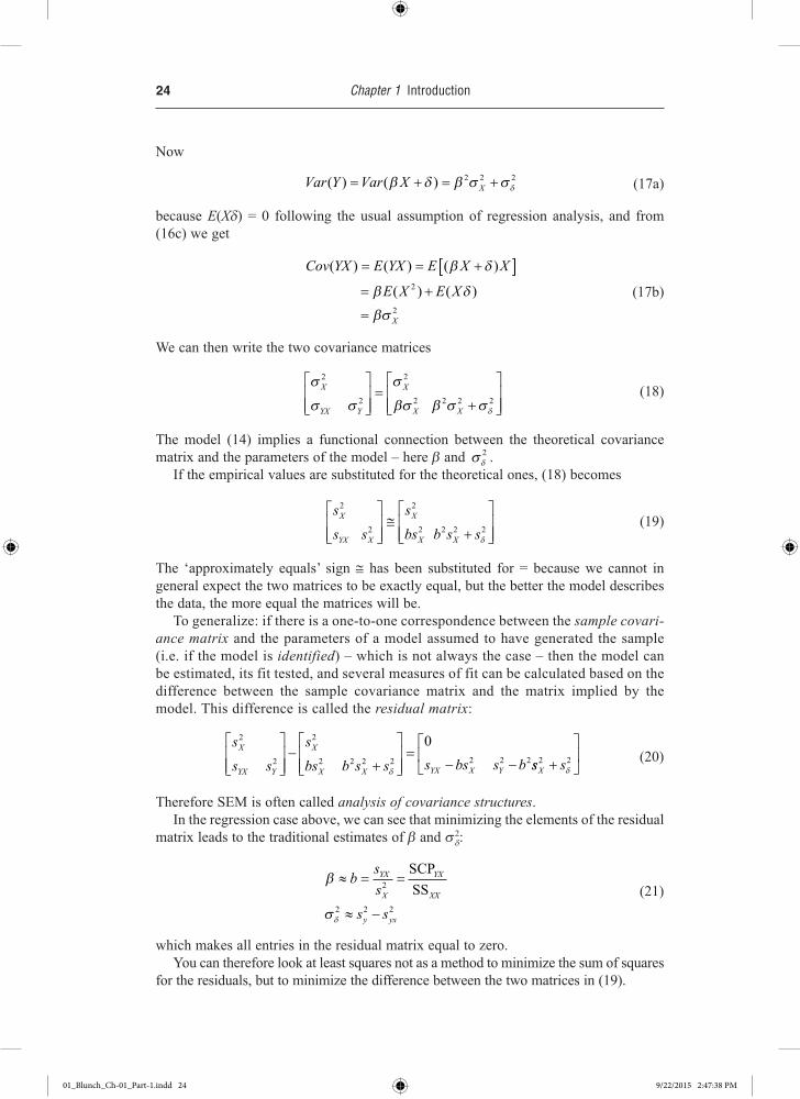
Now

Var Y Var X X( ) ( )= + = +β δ β σ σδ2 2 2 (17a)

because E(Xd) = 0 following the usual assumption of regression analysis, and from (16c) we get

Cov YX E YX E X X

E X E X

X

( ) ( ) ( )

( ) ( )

= = +[ ]= +

=

β δ

β δ

βσ

2

2

(17b)

We can then write the two covariance matrices

σ

σ σ

σ

βσ β σ σδ

X

YX Y

X

X X

2

2

2

2 2 2 2

=

+

(18)

The model (14) implies a functional connection between the theoretical covariance matrix and the parameters of the model – here b and σδ

2 .If the empirical values are substituted for the theoretical ones, (18) becomes

s

s s

s

bs b s s

X

YX X

X

X X

2

2

2

2 2 2 2

≅

+

δ

(19)

The ‘approximately equals’ sign @ has been substituted for = because we cannot in general expect the two matrices to be exactly equal, but the better the model describes the data, the more equal the matrices will be.

To generalize: if there is a one-to-one correspondence between the sample covari-ance matrix and the parameters of a model assumed to have generated the sample (i.e. if the model is identified) – which is not always the case – then the model can be estimated, its fit tested, and several measures of fit can be calculated based on the difference between the sample covariance matrix and the matrix implied by the model. This difference is called the residual matrix:

s

s s

s

bs b s s s bs s bX

YX Y

X

X X YX X Y

2

2

2

2 2 2 2 2 2 2

0

−

+

=

− −δ ss sX2 2+

δ (20)

Therefore SEM is often called analysis of covariance structures.In the regression case above, we can see that minimizing the elements of the residual

matrix leads to the traditional estimates of b and s2d:

β

σδ

≈ = =

≈ −

bs

s

s s

YX

X

YX

XX

y yx

2

2 2 2

SCP

SS (21)

which makes all entries in the residual matrix equal to zero.You can therefore look at least squares not as a method to minimize the sum of squares

for the residuals, but to minimize the difference between the two matrices in (19).


Questions 25

This is the basis on which estimation in SEM is built. Every model formulation implies a certain form for the covariance matrix of the manifest variables, and the parameters are estimated as the values that minimize the difference between the sample covariance matrix and the implied covariance matrix, i.e. the residual matrix – or to put it more precisely, a function of the residual matrix is minimized.

In this chapter you met the following concepts:

• theory and model • exogenous and endogenous

variable • summated scale, Likert scale • manifest and latent variables • structural model and

measurement model • cyclic and acyclic models

• data matrix, SSCP matrix, covariance matrix and correlation matrix

• population and sample covariance matrix

• implied covariance matrix • residual matrix

Questions

1. Why should a researcher prefer to work with latent variables? (List all the reasons you can.)

2. Explain the concepts ‘measurement model’ and ‘structural model’.

3. To what extent is it possible to support a hypothesis of causal connections using SEM?

4. Explain the difference between cyclic and acyclic models.

5. Explain the various matrices X, C, S and R.

6. Look at Figure 3. Do you have any comments on the model? Do you have any suggestions for modifications of the model?

References

Aaker, D. A., & Day, D. A. (1971). A recursive model of communication processes. In D. A. Aaker (Ed.), Multivariate analysis in marketing. Belmont, CA: Wadsworth.

Arbuckle, J. L. (1989). AMOS: Analysis of moment structures. The American Statistician, 43, 66–67.

Bagozzi, R. P. (1977). Structural equation models in experimental research. Journal of Marketing Research, 14, 202–226.

Bagozzi, R. P. (1980). Causal models in marketing. New York: Wiley.Bagozzi, R. P., & Yi, Y. (1994). Advanced topics in structural equation models. In R. P. Bagozzi

(Ed.), Advanced methods of marketing research (pp. 1–51). Oxford: Blackwell.Bass, F. M. (1969). A simultaneous study of advertising and sales – analysis of cigarette data.

Journal of Marketing Research, 6(3), 291–300.Beck, A. T., Ward, C. H., Mendelson, M., & Erbaugh, J. (1961). An inventory for measuring

depression. Archives of General Psychiatry, 4, 561–571.



Bentler, P. M. (1985). Theory and implementation of EQS: A structural equation program. Los Angeles: BMDP Statistical Software.

Blalock, H. M. (1961). Causal inferences in non-experimental research. Chapel Hill, NC: University of North Carolina Press.

Blalock, H. M. (1971). Causal models in the social sciences. Chicago: Aldine-Atherton.Childers, T. L., Houston, M. J., & Heckler, S. (1985). Measurement of individual differences in

visual versus verbal information processing. Journal of Consumer Research, 12, 124–134.Dominick, B. A. (1952). An illustration of the use of the Latin square in measuring the effective-

ness of retail merchandising practices. Ithaca, NY: Department of Agricultural Economics, Cornell University Agricultural Experiment Station, New York State College of Agriculture, Cornell University.

Duncan, O. D. (1975). Introduction to structural equation models. New York: Academic Press. Durkheim, E. (2002 [1897]). Suicide. London: Routledge.Goldberger, A. S. (1972). Structural equation methods in the social sciences. Econometrica, 40,

979–1001.Hume, D. (2000 [1739]). A treatise of human nature. Ed. D. Norton. Oxford: Oxford University

Press.Joireman, J., & Abbott, M. (2004). Structural Equation Models Assessing Relationships Among

Student Activities, Ethnicity, Poverty, Parents’ Education, and Academic Achievement (Technical Report #6). Seattle, OR: Washington School Research Center.

Jöreskog, K. G. (1973). A general method for estimating a linear structural equation system. In A. S. Goldberger & O. D. Duncan (Eds.), Structural equation models in the social sciences (pp. 85–112). New York: Seminar Press.

Lavidge, R. C., & Steiner, G. A. (1961). A model for predictive measurement of advertising effectiveness. Journal of Marketing, 25(Oct.), 59–62.

McArdle, J. J., & McDonald, R. P. (1984). Some algebraic properties of the Reticular Action Model for moment structures. British Journal of Mathematical and Statistical Psychology, 37, 234–251.

Mullahy, J. (1997). Instrumental-variable estimation of count data models: Applications to models of cigarette smoking behavior. Review of Economics and Statistics, 79, 586–593.

Simon, H. A. (1953). Causal ordering and identifiability. In W. C. Hood & T. C. Koopmans (Eds.), Studies in Econometric Method. New York: Wiley.

Simon, H. A. (1954). Spurious correlation: A causal interpretation. Journal of the American Statistical Association, 49(Sept.), 467–479.

Spearman, C. (1904). General intelligence, objectively determined and measured. American Journal of Psychology, 15, 201–293.

Thurstone, L. L. (1947). Multiple factor analysis. Chicago: University of Chicago Press.Thurstone, L. L., & Thurstone, T. (1941). Factorial studies of intelligence. Chicago: University

of Chicago Press.Wright, S. (1918). On the nature of size factors. Genetics, 3, 367–374.Wright, S. (1921). Correlation and causation. Journal of Agricultural Research, 20, 557–585.


Documents

Introduction to STRUCTURAL EQUATION MODELING USING …