Introduction to theCurvelet Transform

By

Zvi Devir and Yanai Shpinner

IntroductionCurvelet Transform is a new multi-scale representation most suitable for objects with curves.

Developed by Candès and Donoho (1999).

Still not fully matured.

Seems promising, however.

Approximation RatesHaving an object in the domain [0,1][0,1], how ‘fast’ can we approximate it using certain system of functions?

Using the Fourier Transform:

Using the Wavelet Transform:

Using the Curvelet Transform:

212

2

~ mOff m

12

2

~ mOff m

2322

2log

~ mOmmOff m

Point and Curve DiscontinuitiesA discontinuity point affects all the Fourier coefficients in the domain. Hence the FT doesn’t handle points discontinuities well.

Using wavelets, it affects only a limited number of coefficients. Hence the WT handles point discontinuities well.

Discontinuities across a simple curve affect all the wavelets coefficients on the curve. Hence the WT doesn’t handle curves discontinuities well.

Curvelets are designed to handle curves using only a small number of coefficients. Hence the CvT handles curve discontinuities well.

Curvelet TransformThe Curvelet Transform includes four stages:

Sub-band decomposition

Smooth partitioning

Renormalization

Ridgelet analysis

Sub-band Decomposition

Dividing the image into resolution layers.

Each layer contains details of different frequencies: P0 – Low-pass filter.

1, 2, … – Band-pass (high-pass) filters.

The original image can be reconstructed from the sub-bands:

Energy preservation

s

ss ffPPf 00

s

s ffPf2

2

2

20

2

2

,,, 210 fffPf

Sub-band Decomposition

fP0 f1 f2

f

,,, 210 fffPf

Sub-band DecompositionLow-pass filter 0 deals with low frequencies near ||1.

Band-pass filters 2s deals with frequencies near domain ||[22s, 22s+2]. Recursive construction – 2s(x) = 24s (22sx).

The sub-band decomposition is simply applying a convolution operator:

ffffP ss 200

Sub-band DecompositionThe sub-band decomposition can be approximated using the well known wavelet transform: Using wavelet transform, f is decomposed into S0,

D1, D2, D3, etc.

P0 f is partially constructed from S0 and D1, and may include also D2 and D3.

s f is constructed from D2s and D2s+1.

Sub-band DecompositionP0 f is “smooth” (low-pass), and can be efficiently represented using wavelet base.

The discontinuity curves effect the high-pass layers s f. Can they be represented efficiently? Looking at a small fragment of the curve, it appears

as a relatively straight ridge. We will dissect the layer into small partitions.

Smooth Partitioning

Smooth PartitioningA grid of dyadic squares is defined:

Qs – all the dyadic squares of the grid.

Let w be a smooth windowing function with ‘main’ support of size 2-s2-s.

For each square, wQ is a displacement of w localized near Q.

Multiplying s f with wQ (QQs) produces a smooth dissection of the function into ‘squares’. fwh sQQ

skkkk

kks ssssQ Q

2

1

22

1

2,,2211

21,,

Smooth PartitioningThe windowing function w is a nonnegative smooth function.Partition of the energy: The energy of certain pixel (x1,x2) is divided

between all sampling windows of the grid.

Example: An indicator of the dyadic square

(but not smooth!!). Smooth window function with

an extended compact support:

Expands the number of coefficients.

1,21 ,

22112

kk

kxkxw

Smooth PartitioningPartition of the energy:

Reconstruction:

Parserval relation:

hhwhwss Q

QQ

QQ QQ

2

2

2

222222

2hhhwhwh

sss QQ

QQ

QQ

QQQ

1,21 ,

22112

kk

kxkxw

12 sQ

QwQ

RenormalizationRenormalization is centering each dyadic square to the unit square [0,1][0,1].

For each Q, the operator TQ is defined as:

Each square is renormalized:

221121 2,22, kxkxfxxfT sssQ

QQQ hTg 1

Before the Ridgelet Transform The s f layer contains objects with frequencies near domain ||[22s, 22s+2]. We expect to find ridges with width 2-2s.

Windowing creates ridges of width 2-2s and length 2-s.

The renormalized ridges has an aspect ratio of width length2.

We would like to encode those ridges efficiently Using the Ridgelet Transform.

The Ridgelet TransformRidgelet are an orthonormal set {} for L2(2).Developed by Candès and Donoho (1998).

Ridge in Square

2-s

2-2s

Ridge in Square

1

2-s

It’s Fourier Transform

2s

Ridgelet Tiling

radius 2s

2s

divisions

It’s Fourier Transform Ridgelet Tiling

Divides the frequency domain to dyadic coronae ||[2s, 2s+1].

In the angular direction, samples the s-th corona at least 2s times.

In the radial direction, samples using local wavelets.

Fourier Transform within Tiling

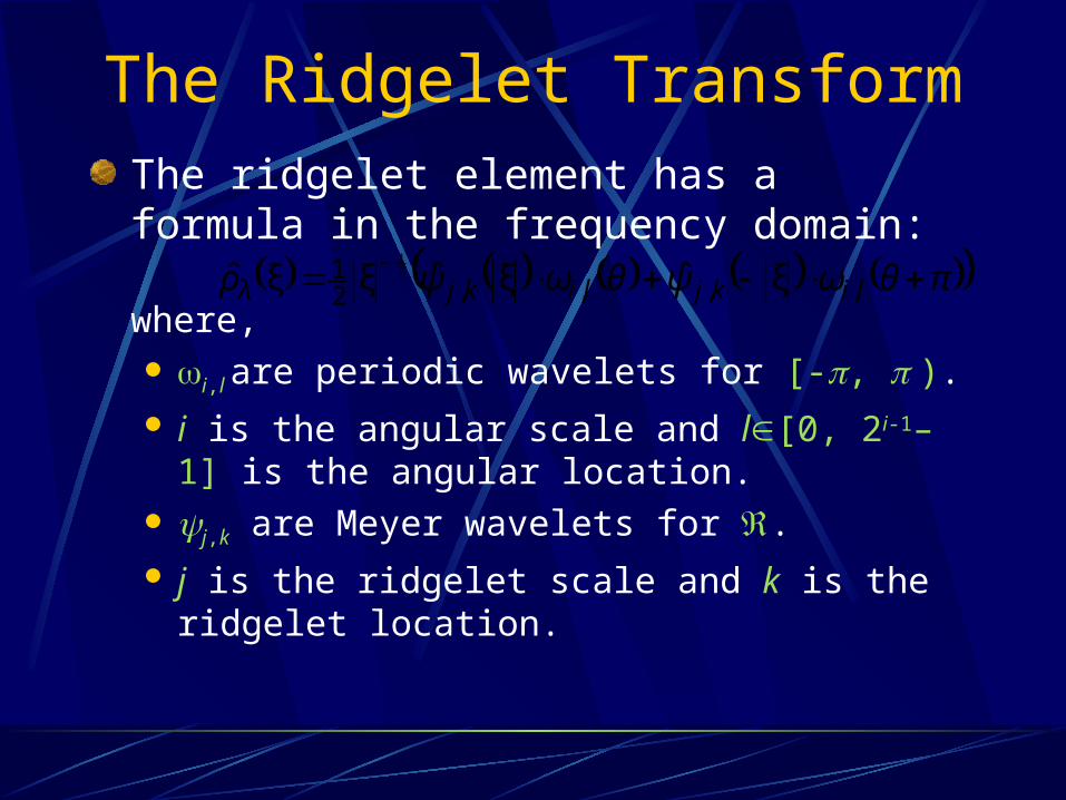
The Ridgelet TransformThe ridgelet element has a formula in the frequency domain:

where, i,l are periodic wavelets for [-, ). i is the angular scale and l[0, 2i-1–1] is the

angular location. j,k are Meyer wavelets for . j is the ridgelet scale and k is the ridgelet location.

πθωψθωψρ likjlikjλ ,,,,2

1 ξˆξˆξξˆ 21

Ridgelet AnalysisEach normalized square is analyzed in the ridgelet system:

The ridge fragment has an aspect ratio of 2-2s2-s.

After the renormalization, it has localized frequency in band ||[2s, 2s+1].

A ridge fragment needs only a very few ridgelet coefficients to represent it.

λQQ,λ ρgα ,

Digital Ridgelet Transform (DRT)

Unfortunately, the (current) DRT is not truly orthonormal.

An array of nn elements cannot be fully reconstructed from nn coefficients.

The DRT uses n2n coefficients for almost perfect reconstruction

Still a lot of research need to be done…

Curvelet TransformThe four stages of the Curvelet Transform were:

Sub-band decomposition

Smooth partitioning

Renormalization

Ridgelet analysis

,,, 210 fffPf

fwh sQQ

QQQ hTg 1

λQQ,λ ρgα ,

Image ReconstructionThe Inverse of the Curvelet Transform:

Ridgelet Synthesis

Renormalization

Smooth Integration

Sub-band Recomposition

λλ

Q,λQ ραg

QQQ gTh

sQ

QQs hwfQ

s

ss ffPPf 00

Example: Roy Lichtenstein: “In The Car” 1963

Original ImageOriginal Image(256(256256)256)

Approximation with Approximation with onlyonly64 wavelets and 256 curvelets64 wavelets and 256 curvelets

(about 0.5% of the coefficients)(about 0.5% of the coefficients)

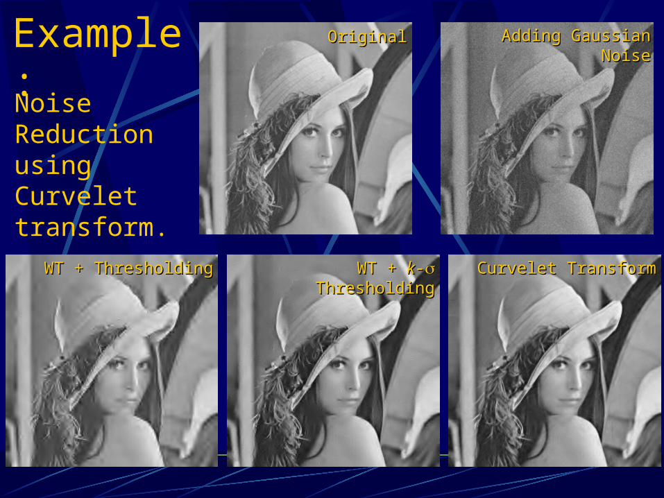
OriginalOriginal Adding Gaussian NoiseAdding Gaussian Noise

WT + ThresholdingWT + Thresholding WT + WT + kk-- Thresholding Thresholding Curvelet TransformCurvelet Transform

Example: Noise Reduction using Curvelet transform.

OriginalOriginal Adding Gaussian NoiseAdding Gaussian Noise

WT + ThresholdingWT + Thresholding WT + WT + kk-- Thresholding Thresholding Curvelet TransformCurvelet Transform

Example: Noise Reduction using Curvelet transform.

References[1] D.L. Donoho and M.R. Duncan. Digital Curvelet Transform:

Strategy, Implementation and Experiments; Technical Report, Stanford University 1999

[2] E.J. Candès and D.L. Donoho. Curvelets – A Surprisingly Effective Non-adaptive Representation for Objects with Edges; Curve and Surface Fitting: Saint Malo 1999

[3] Lenna examples fromhttp://www-stat.stanford.edu/~jstarck/comp.html