Introduction

to the gradient analysis

Community concept

(from Mike Austin)

Continuum concept

(from Mike Austin)

The real situation is somewhere between and more complicated

Originally (and theoretically)

• Community concept as a basis for classification

• Continuum concept as a basis for ordination or gradient analysis

In practice

• I need a vegetation map (or categories for nature conservation agency) - I will use classification

• I am interested in transitions, gradients, etc. - lets go for the gradient analysis (ordination)

Methods of the gradient analysis

pH

CO

VE

R

0

10

20

30

40

5 6 7 8 9

No. of environmental variables

No. of species

1, n 1 no Regression Dependence of the species on environmental variables

None n yes Calibration Estimates of environmental values

None n no Ordination Axes of variability in species composition

1, n n no Constrained ordination

Variability in species composition explained by environmental variables and Relationship of environmental variables to the species data

Data used in calculations A priori

knowledge of species-environment relationships

Method Result

Over a short gradient, the linear response is good approximation, over a long gradient, it is not.

However

• In most cases, neither the linear, nor the unimodal response models are sufficient description of reality for all the species

• I use a methods based on either of the models not because I would believe that all the species behave according to those models, but because I see them as a reasonable compromise between reality and clarity.

Estimating species optima by the weighted averaging method

n

ii

n

iii

Abund

AbundEnvSpWA

1

1)(

n

ii

n

iii

Abund

AbundSpWAEnvDS

1

1

2))((..

Optimum Tolerance

Environmental variable

Sp

eci

es

ab

un

da

nce

0

1

2

3

4

5

0 20 40 60 80 100 120 140 160 180 200

604.9/564)(

1

1

n

ii

n

iii

Abund

AbundEnvSpWA

Environmental variable

Sp

eci

es

ab

un

da

nce

0

1

2

3

4

5

0 20 40 60 80 100 120 140 160 180 200

The techniques based on the linear response model are suitable for homogeneous data sets, the weighted averaging techniques are suitable for more heterogeneous data.

s

ii

s

iii

Abund

AbundIVSampWA

1

1)(

Calibrations (using weighted averages)

Nitrogen IV Sample 1 IV x abund. Sample 2 IV x abund.Drosera rotundifolia 1 2 2 0 0

Andromeda polypofila 1 3 3 0 0Vaccinium oxycoccus 1 5 5 0 0Vaccinium uliginosum 3 2 6 1 3

Urtica dioica 8 0 0 5 40Phalaris arundinacea 7 0 0 5 35

Total 12 16 11 78Nitrogen (WA): 1.333

(=16/12)7.090

(=78/11)

Cactus Nymphea

Urtica

Drosera

Menyanthes

Comarum

Chenopodium

Aira

Ordination diagram

Cactus Nymphea

Urtica

Drosera

Menyanthes

Comarum

Chenopodium

Aira

Ordination diagram

Nutrients

Water

Proximity means similarity

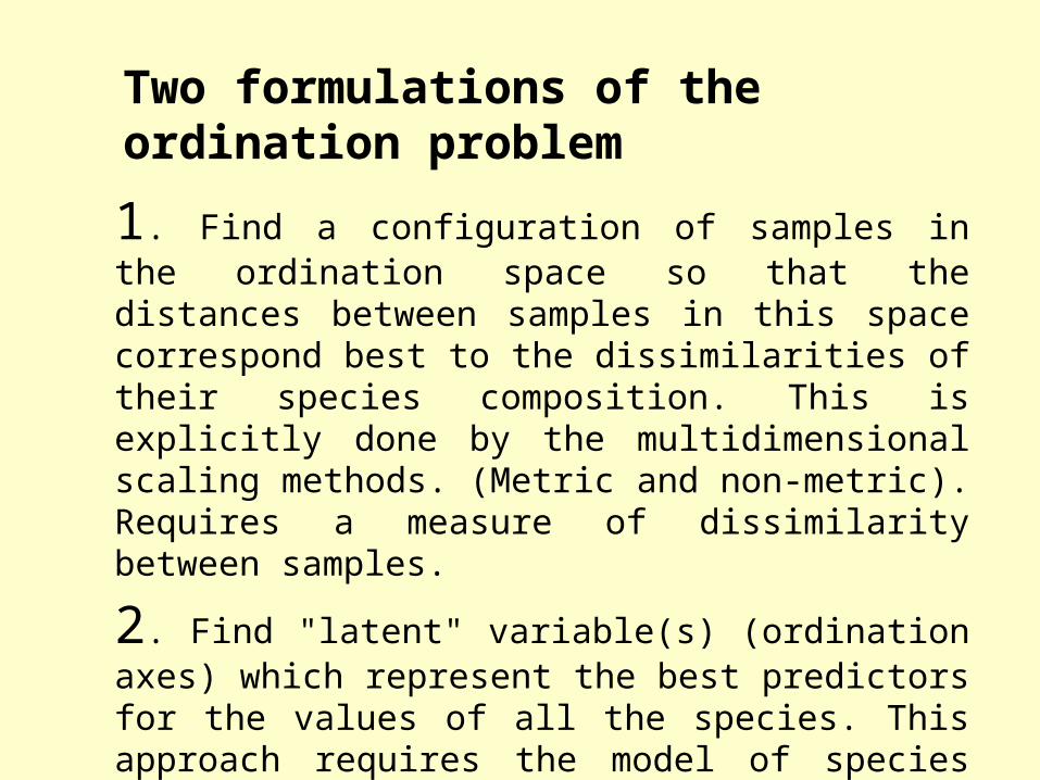
1. Find a configuration of samples in the ordination space so that the distances between samples in this space correspond best to the dissimilarities of their species composition. This is explicitly done by the multidimensional scaling methods. (Metric and non-metric). Requires a measure of dissimilarity between samples.

2. Find "latent" variable(s) (ordination axes) which represent the best predictors for the values of all the species. This approach requires the model of species response to such latent variables to be explicitly specified.

Two formulations of the ordination problem

The linear response model is used for linear ordination methods, the unimodal response model for weighted averaging methods. In linear methods, the sample score is a linear combination (weighted sum) of the species scores. In weighted averaging methods, the sample score is a weighted average of the species scores (after some rescaling).

Note: The weighted averaging algorithm contains an implicit standardization by both samples and species. In contrast, we can select in linear ordination the standardized and non-standardized forms.

Transformation is an algebraic function Xij’=f(Xij) which is applied independently of the other values. Standardization is done either with respect to the values of other species in the sample (standardization by samples) or with respect to the values of the species in other samples (standardization by species).

Quantitative data

Centering means the subtraction of a mean so that the resulting variable (species) or sample has a mean of zero. Standardization usually means division of each value by the sample (species) norm or by the total of all the values in a sample (species).

2,2

1,12,1 )( j

s

jj XXED

Euclidean distance - used in linear methods

For ED, standardize by sample norm, not by total

The samples with t contain values standardized by the total, those with n samples standardized by sample norm. For samples standardized by total, ED12 = 1.41 (√2), whereas ED34=0.82, whereas for samples standardized by sample norm, ED12=ED34=1.41

)(

),min(2

12,2

1,1

,21

,1

j

s

jj

j

s

jj

XX

XX

PS

Percentual similarity (quantitative Sörensen) - no counterpart in either linear or WA methods, can be used in mutlidimensional scaling

C h i - s q u a r e d d i s t a n c e

s

j

jj

j S

X

S

X

S1

2

2

2

1

1212

1

w h e r e S + j i s t o t a l o f j - t h s p e c i e s v a l u e s o v e r a l l t h es a m p l e s

n

iijj XS

1

a n d S i + i s t o t a l o f a l l t h e s p e c i e s v a l u e s i n t h e i - t hs a m p l e

s

iiji XS

1

Weighted averaging methods correspond to the use of

The two formulations may lead to the same solution. (When samples of similar species composition would be distant on an ordination axis, this axis could hardly serve as a good predictor of their species composition.) For example, principal component analysis can be formulated as a projection in Euclidean space, or as a search for latent variable when linear response is assumed.

By specifying species response, we specify the (dis)similarity measure

Species 1

Species 2

Species 1

Species 2

Species 1

Species 2Sp1 Sp2

Sp1 Sp2

The result of the ordination will be the values of this latent variable for each sample (called the sample scores) and the estimate of species optimum on that variable for each species (the species scores). Further, we require that the species optima be correctly estimated from the sample scores (by weighted averaging) and the sample scores be correctly estimated as weighted averages of the species scores (species optima). This can be achieved by the following iterative algorithm:

Step 1 Start with some (arbitrary) initial site scores {xi}Step 2 Calculate new species scores {yi} by [weighted averaging] regression from {xi}Step 3 Calculate new site scores {xi} by [weighted averaging] calibration from {yi}Step 4 Remove the arbitrariness in the scale by standardizing site scores (stretch the axis)Step 5 Stop on convergence, else GO TO Step 2

length

xx minmax =eigenvalue

The larger the eigenvalue, the better is the explanatory power of the axis. Amount of variability explained is proportional to the eigenvalue.

In weighted averaging, eigenvalues < 1 (=1 only for perfect partitioning).

In CANOCO, linear methods are scaled so that total of eigenvalues = 1 (not in some other programs)

00x x 0 x x

x x x 0 x

x 0 x x 0 x x x 0 x

samples

spec

ies

perfect partitioning

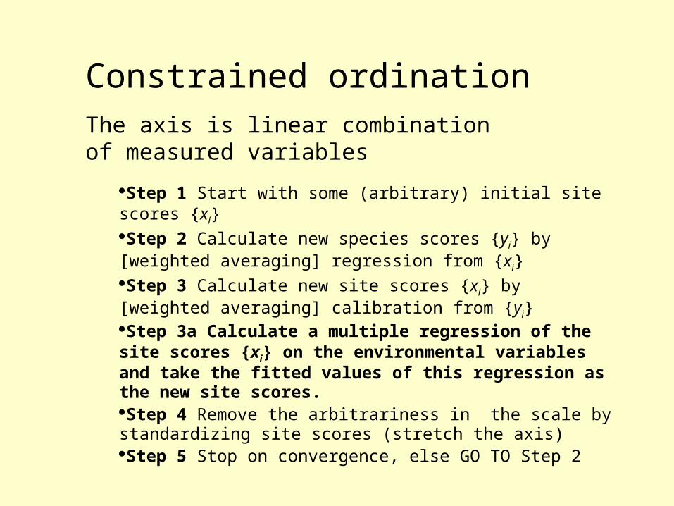
Constrained ordinationThe axis is linear combination of measured variables

Step 1 Start with some (arbitrary) initial site scores {xi}Step 2 Calculate new species scores {yi} by [weighted averaging] regression from {xi}Step 3 Calculate new site scores {xi} by [weighted averaging] calibration from {yi}

Step 4 Remove the arbitrariness in the scale by standardizing site scores (stretch the axis)Step 5 Stop on convergence, else GO TO Step 2

Constrained ordinationThe axis is linear combination of measured variables

Step 1 Start with some (arbitrary) initial site scores {xi}Step 2 Calculate new species scores {yi} by [weighted averaging] regression from {xi}Step 3 Calculate new site scores {xi} by [weighted averaging] calibration from {yi}Step 3a Calculate a multiple regression of the site scores {xi} on the environmental variables and take the fitted values of this regression as the new site scores. Step 4 Remove the arbitrariness in the scale by standardizing site scores (stretch the axis)Step 5 Stop on convergence, else GO TO Step 2

Linear methods Weighted averaging

Unconstrained Principal ComponentsAnalysis (PCA)

Correspondence Analysis (CA)

Constrained Redundancy Analysis(RDA)

Canonical CorrespondenceAnalysis (CCA)

Basic ordination techniques

Detrending

Hybrid analyses

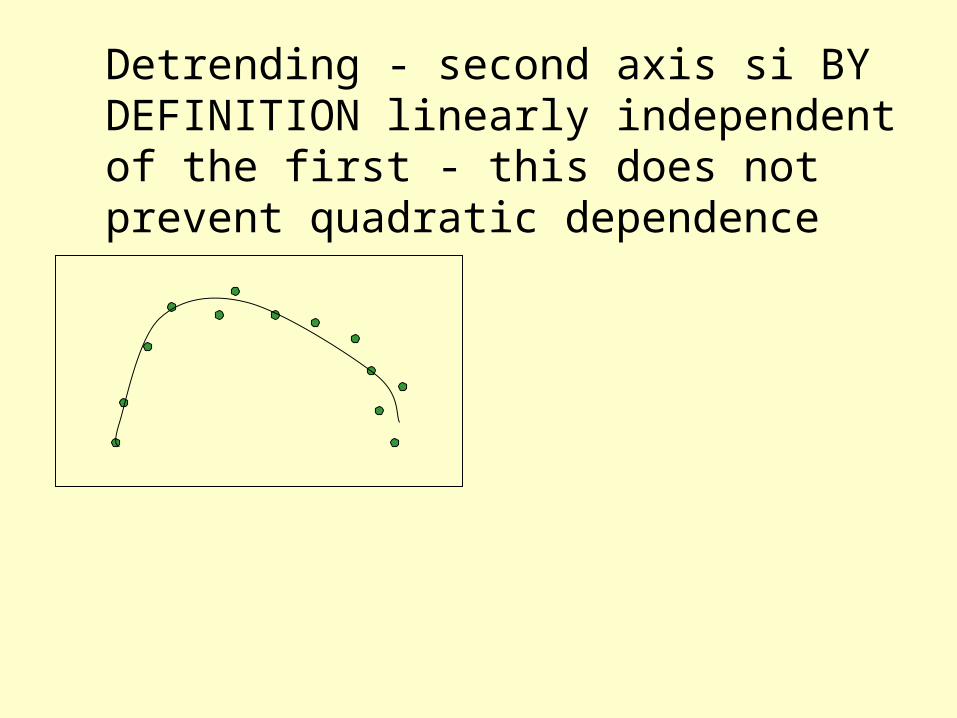
Detrending - second axis si BY DEFINITION linearly independent of the first - this does not prevent quadratic dependence

Let’s take a hammer

Done in each iteration

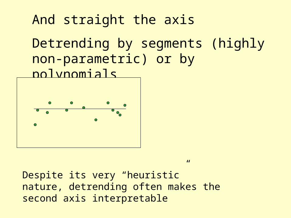
And straight the axis

Detrending by segments (highly non-parametric) or by polynomials

Despite its very “heuristic” nature, detrending often makes the second axis interpretable

PCA CA

RDA CCA

Two approachesHaving both environmental data and data on species composition, we can first calculate an unconstrained ordination and then calculate a regression of the ordination axes on the measured environmental variables (i.e. to project the environmental variables into the ordination diagram) or we can calculate directly a constrained ordination. The two approaches are complementary and both should be used! By calculating the unconstrained ordination first, we do not miss the main part of the variability in species composition, but we can miss that part of the variability that is related to the measured environmental variables. By calculating a constrained ordination, you do not miss the main part of the biological variability explained by the environmental variables, but we can miss the main part of the variability that is not related to the measured environmental variables.

What shall we do with categorial variables?

Scatterplot (Spreadsheet1 10v*10c)

Var2 = 4.2+3.6*x

-0.2 0.0 0.2 0.4 0.6 0.8 1.0 1.2

Var1

0

2

4

6

8

10

12

Var2

ANOVA grouping=var4

Regression Summary for Dependent Variable: Var7 (Spreadsheet1) Independent Var5 and Var6R= .88898086 R2= .79028698 Adjusted R2= .73036897F(2,7)=13.189 p<.00422 Std.Error of estimate: 1.3452

4groundrock

5basalt

6granit

7limestone

8biomass

123456789

10

basalt 1 0 0 2basalt 1 0 0 3basalt 1 0 0 4granit 0 1 0 2granit 0 1 0 5granit 0 1 0 6limestone 0 0 1 7limestone 0 0 1 8limestone 0 0 1 9limestone 0 0 1 8

Dummy variables

Predictors and response are correlated, distribution usually

non-normal. Use the distribution free

Monte Carlo permutation test.

Plantheight

Nitrogen(as

measured)

1-stpermutation

2-ndpermutation

3-rdpermutation

4-thpermutation

5-thetc

5 3 3 8 5 5 ...

7 5 8 5 5 8 ...

6 5 4 4 3 4 ...

10 8 5 3 8 5 ...

3 4 5 5 4 3 ...

F-value 10.058 0.214 1.428 4.494 0.826 0.###

nspermutatioofnumbertotal

Fwherenspermutatioofno

1

)058.10(.1

Monte Carlo permutation test