Embed Size (px)
Citation preview
Sandmeier geophysical software - REFLEXW guide
Introduction to the traveltime tomography and prestack migration for
borehole-data within REFLEXW
In the following the use of the traveltime tomography and the prestack-migration for different types of
borehole data is described. The traveltime tomography allows to build a velocity model from the first
arrival traveltimes. The prestack migration allows to trace back the wavefield of single shots or
constant offset data to their "source". The migration takes into account arbitrary shot/receiver offsets
in contrast to the other migration methods within Reflexw which need zero offset
data as input. The following borehole geometries are supported:
- shots or receivers are located along the x-axis and shots or receivers are located
along the y(z)-axis (borehole) - walk away vertical seismic profile (WVSP) - see
chap. I
- shots and receivers are both located along the y(z) axis within different
boreholes which have a distinct x-offset - crosshole - see chap. II
The prestack migration tool automatically controls the correct geometry.
I. Walk away VSP data
The used dataset is a synthetic seismic dataset which allows to get
informations about the benefits und the critical parameters of the
prestack migration.
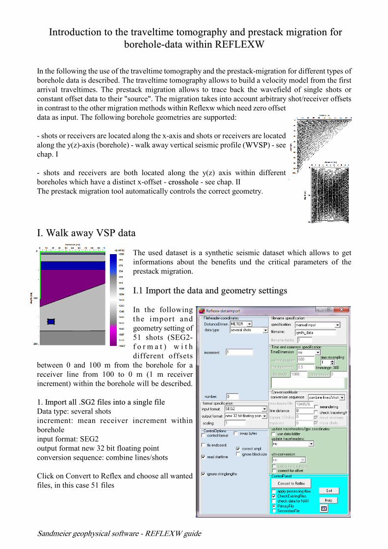
I.1 Import the data and geometry settings
In the following
the import and
geometry setting of
51 shots (SEG2-
f o r m a t ) w i t h
different offsets
between 0 and 100 m from the borehole for a
receiver line from 100 to 0 m (1 m receiver
increment) within the borehole will be described.
1. Import all .SG2 files into a single file
Data type: several shots
increment: mean receiver increment within
borehole
input format: SEG2
output format new 32 bit floating point
conversion sequence: combine lines/shots
Click on Convert to Reflex and choose all wanted
files, in this case 51 files

Sandmeier geophysical software - REFLEXW guide
2) Set the geometry within the CMP-geometry panel
The positions of the shot and the receivers in real z-direction may be stored on the y- or on the z-
traceheader coordinates. The x-offsets are stored on the x-traceheader coordinates. In the following the
y-traceheader coordinates are used because the CMP-geometry setting only allows to set the x- and y-
traceheader coordinates. If wanted it is possible to exchange the y- and z-traceheader coordinates
afterwards within the edit/traceheader tabella menu (option y<-> z).
- Click on CMP and then on geometry
- set the standard geometry for a fixed receiver line within the borehole from 100 to 0 m with an
increment of 1 m. The shots are located at the surface starting from 0 m to 100 m with an increment of
2 m.
As standard line direction choose y-direction rec. The receiver increment must be negative because the
first receiver has been located at 100 m and the last at 0 m. The nr. of channels is 101 (101 receiver
positions).
- click on apply std.geometry and then on save geometry
- use the option edit single traces in order to check the correct geometry.
Another check may be done using the option view/profile line (traceheader coor.) Click show shot
position and move mouse over the shot record in the background from left to right to check the
geometry.

Sandmeier geophysical software - REFLEXW guide

Sandmeier geophysical software - REFLEXW guide
I.2 Generate a 2D-velocity file for the subsequent migration
The prestack migration needs either a constant velocity or a 2D-velocity distribution. If no other
informations are available the 2D-velocity distribution may be generated either from one VSP-data
shot using the CMP-vel.analysis module or from a tomographic inversion of the first arrivals of the
direct wave.
I.2.1 2D-velocity distribution using
the CMP-vel.analysis
1. Enter the 2D-dataanalysis module:
Import one VSP-data shot:
- data type: single shot/borehole
- set the offset, receiver start and end
and shot offset and position.
- conversion sequence set to no
Convert to Reflex this single file. If
receiver start is bigger than end
coordinate the file will be automatically
flipped (first trace at top and last trace at
bottom).
Optionally you may pick the first
arrivals.
2. Perform the VSP-velocity inversion within the CMP-
vel.analysis module
- load the VSP-data shot.
- If the shot has an offset you must enter the correct
shot offset.
- Optionally you also may load the picked first
arrivals.
- activate VSP and adapt the first arrivals
- if picked traveltimes have been loaded a direct
inversion (option invert local velocities) is possible
- save the final 1D-model
- activate the option 2D-model
- click on create and load the saved 1D-model
- enter the filename for the 2D-velocity distribution
The resulting 2D-velocity distribution is laterally
homogeneous.

Sandmeier geophysical software - REFLEXW guide
I.2.2 2D-velocity distribution using a tomographic inversion of the first arrivals
1. Enter the 2D-dataanalysis.
Load the combined data which still include the
direct wave (without fk-filtering for example).
Pick the first arrivals and store them using the
ASCII-3D-tomography format.
2. Enter the modelling module.
Create a start model with a constant velocity
(e.g. 1000 m/s) and the necessary min/max. x-
and z-coordinates which cover the whole data
range, in this case x from 0 to 100 m and z
from 0 to 100.
Load the traveltime data and set the
tomography parameters. The parameters for the tomography may be changed depending on your needs.
The space increment should be within the range or smaller than the receiver increment. Max.def.
Change should be large enough to ensure strong enough velocity changes. Straight rays are faster and
lead to a less smoothed model than curved rays. Averaging should be done in x-direction because the
covering is much higher in z-direction than in x-direction. Min. and max.velocity restrict the range of
the inverted velocities.
Start the tomography.

Sandmeier geophysical software - REFLEXW guide
I.3 processing before applying the prestack migration
The aim of the pre-migration filtering is to prepare the dataset for the subsequent prestack migration.
The most important processing steps are:
- energy normalization
- elimination or suppression of the direct waves and other non desired waves
The energy normalization should be the first filter step especially if you are using multi-channel filters
(e.g. FK-filter) for the suppression of non desired waves. This filter step is applied to correct for the
amplitude effects of wavefront divergence and damping. It is also necessary if a subsequent filter shall
be applied for eliminating the surface waves.
The easiest way would be a manual gain function, e.g. manual gain (y) or the div. compensation filter.
In the case of different coupling conditions this gain recovery function is not very suitable. In this case
the filter scaled windowgain(x) may be a good choice.
To bo considered: Filtering and stacking are always done on the true amplitude data. The option
tracenormalize within the plotoptions is only a plotoption and does not effect the filtering/stacking
process. Therefore the option tracenormalize within the plotoptions should be deactivated because
otherwise the effect of the energy normalization may not be controlled correctly.
The second filter step consists of the elimination of the direct waves and other non desired waves. For
that purpose you may distinguish between editing and 2D-filter steps.
Editing may be used for muting (set to zero) special data parts or to delete single traces or trace ranges.
2D-filters may be used to suppress unwanted signals. A FK-filter may be a good choice.
1. Energy normalization
Here a div. compensation filter has been applied on the data.

Sandmeier geophysical software - REFLEXW guide
2. Direct wave suppression
For the direct wave suppression here a fk-filtering has been
used - option Processing/FK-filter/FK-spectrum.
The FK-filter/FK-spectrum window appears. Enter the
following parameters or options:
- activate the option fk filter-lineparts
- enter the filterparameter tracenumber (corresponds to the
number of traces per shot) - in this case 101
- activate the option generate fk-spectrum
A new FK-filter/FK-spectrum window appears. The direct
wave is located within a different kx range than the
reflections which shall be included for the prestack migration
of VSP data. The direct waves are located within the negative kx-range in this case as the receiver line
goes from larger values to smaller ones (100 m to 0 m). Therefore the pos. fk-range has been chosen
for filtering the data.

Sandmeier geophysical software - REFLEXW guide
I.4 Perform the prestack migration
The prestack migration needs either a
constant velocity or a 2D-velocity
distribution. Depending on the choice
of the 2D-velocity distribution (see
chap. I.3) the velocities may be
determined from
a. CMP-analysis (chap. I.3.1)
b. rasterfile layer using the inverted
tomogram (chap. I.3.2). Reflections
originating from below the defined
velocity tomogram are migrated with
an extrapolated velocity equal to the
veloci ty at the bot tom of the
tomogram.
Parameter settings:
maxdepth: defines the maximum depth
range for the depth migration. The
value may be set to larger depths than
the borehole depth in order to also
include deeper reflections. The value
should not exceed the maximum
reached depth defined by the acquisition time range.
velocity: defines the velocity in case of const.velocity migration and will be used for the smooth option
if a depth migration will be performed.
min. and max. offset: restrict the range for the summation
activated option smooth: the summation is done over a depth range corresponding to the real
wavelength. The parameter velocity is used for the calculation of the wavelength. A very high value
will lead to a strong smoothig, a smaller value will decrease the smoothing.
activated option Kirchhoff: weighted factors are used for the summation

Sandmeier geophysical software - REFLEXW guide
I.5 Overlay tomogram and prestack migration result
The prestack migration may be overlaid with the tomogram. For this purpose you must perform the
following steps:
1. Set the correct plot settings both for the migrated section and the tomogram and save them within
the fileheader.
• tomogram - load the tomogram, enter
the plotopt ions menu and set
pointmode and the wanted plot
interval (in this case min.value to 750
m/s and max.value to 1700 m/s, if the
depth of the tomogram is smaller than
the max.depth of the migrated section
you may set min.value to a smaller
value than the min.tomogram velocity
in order to use a white color for this
value range and below), click on save
in fileheader
• migrated section - load the migrated
section, enter the plotoptions menu
and set wigglemode and the wanted
wiggle scale (in this case 0.001) and
fill to positive, click on save in fileheader
2. Load the migrated section as a primary file and the tomogram as a secondary file
3. Select “always each file” within the plotoption
4. Select the overlay button either within the plotoptions or within the control panel
Model used for the generation of the synthetic
dataset
Prestack migration based on the inital model
which has been underlaid

Sandmeier geophysical software - REFLEXW guide
A better result is achieved if the VSP-inverted 1D-velocity distribution is used because of the
smoothing of the tomographic inversion. The lower reflections (diffractions) below the borehole are
only reconstructed if the correct velocity is used. Therefore additional informations about the velocity
there is needed. The migration result based on the VSP-inverted 1D-velocity distribution including the
velocity decrease below 100 m shows a very good reconstruction of all elements within the initial
model.
Prestack migration based on the inverted
tomogram with manual change of the lower
velocities (below 100 m,) to 1000 m/s
Prestack migration based on the inverted
tomogram without adapting the velocities below
100 m (end of borehole and therefore end of
tomographic inversion)
Prestack migration based on the VSP-inverted
1D-velocity distribution including lower
velocities of 1000 m/s below 110 m
Prestack migration based on the VSP-inverted
1D-velocity distribution. Again below 100 m
the velocity has been simply extrapolated

Sandmeier geophysical software - REFLEXW guide
II. Crosshole data
The used dataset is a synthetic GPR dataset (model see right picture)
which allows to get informations about the benefits und the critical
parameters of the prestack migration.
II.1 Import the data and geometry settings
In the following the import and geometry setting of 101 shots (SEG2-
format) located within borehole 1 at different depths starting at 0 m
until 20 m for a receiver line within borehole 2 (separated by 10 m
from borehole 1) from 20 to 0 m (0.2 m receiver increment) will be
described.
1. Import all .SG2 files into a single file
Data type: several shots
increment: mean receiver increment within
borehole
input format: SEG2
output format new 32 bit floating point
conversion sequence: combine lines/shots
Click on Convert to Reflex and choose all wanted
files, in this case 101 files

Sandmeier geophysical software - REFLEXW guide
2) Set the geometry within the CMP-geometry panel
The positions of the shot and the receivers in real z-direction may be stored on the y- or on the z-
traceheader coordinates. The x-offsets are stored on the x-traceheader coordinates. In the following the
y-traceheader coordinates are used because the CMP-geometry setting only allows to set the x- and y-
traceheader coordinates. If wanted it is possible to exchange the y- and z-traceheader coordinates
afterwards within the edit/traceheader tabella menu (option y<-> z).
- Click on CMP and then on geometry
- set the standard geometry for a fixed receiver line within the borehole 2 at an offset of 10 m from 20
to 0 m with an increment of 0.2 m. The shots are located within borehole 1 at an offset of 0 m starting
from 0 m to 20 m with an increment of 0.2 m.
As standard line direction choose y-direction shots/rec. The receiver increment must be negative
because the first receiver has been located at 20 m and the last at 0 m. The nr. of channels is 101 (101
receiver positions).
- click on apply std.geometry and then on save geometry
- use the option edit single traces in order to check the correct geometry.
Another check may be done using the option view/profile line (traceheader coor.) Click show shot
position and move mouse over the shot record in the background from left to right to check the
geometry.
Sandmeier geophysical software - REFLEXW guide
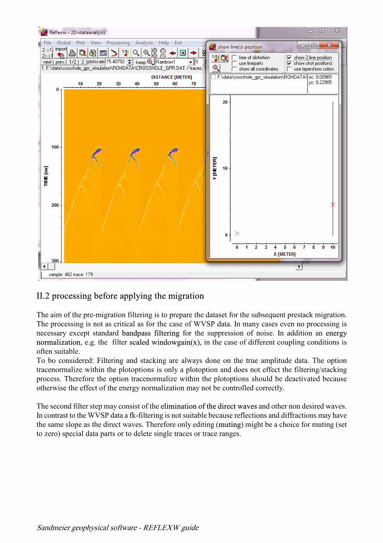
II.2 processing before applying the migration
The aim of the pre-migration filtering is to prepare the dataset for the subsequent prestack migration.
The processing is not as critical as for the case of WVSP data. In many cases even no processing is
necessary except standard bandpass filtering for the suppression of noise. In addition an energy
normalization, e.g. the filter scaled windowgain(x), in the case of different coupling conditions is
often suitable.
To bo considered: Filtering and stacking are always done on the true amplitude data. The option
tracenormalize within the plotoptions is only a plotoption and does not effect the filtering/stacking
process. Therefore the option tracenormalize within the plotoptions should be deactivated because
otherwise the effect of the energy normalization may not be controlled correctly.
The second filter step may consist of the elimination of the direct waves and other non desired waves.
In contrast to the WVSP data a fk-filtering is not suitable because reflections and diffractions may have
the same slope as the direct waves. Therefore only editing (muting) might be a choice for muting (set
to zero) special data parts or to delete single traces or trace ranges.

Sandmeier geophysical software - REFLEXW guide
II.3 Generate a 2D-velocity file for the subsequent migration by a tomographic
inversion of the first arrivals
The prestack migration needs either a constant velocity or a 2D-velocity distribution. If no other
informations are available the 2D-velocity distribution may be generated from a tomographic inversion
of the first arrivals of the direct waves.
1. Enter the 2D-dataanalysis.
Load the combined data which still include the
direct wave (without muting for example).
Pick the first arrivals and store them using the
ASCII-3D-tomography format.
2. Enter the modelling module.
Create a start model with a constant velocity (e.g.
2000 m/s) and the necessary min/max. x- and z-
coordinates which cover the whole data range, in this case x from 0 to 100 m and z from 0 to 100.
Load the traveltime data and set the tomography parameters. Use the option check rays in order to
check the shot/receiver geometry.
Start the tomography.
The parameters for the tomography may be changed depending on your needs (see also chap. I.2.2.2).
In this case the max. depth of tomographic inversion has been set to 30 although the boreholes only
reach a depth of 20 m in order to extrapolate the inverted velocity at 20 m depth to larger depths for the
subsequent prestack migration.

Sandmeier geophysical software - REFLEXW guide
II.4 Perform the prestack migration
The prestack migration needs either a constant
velocity or a 2D-velocity distribution. Here we
are choosing
rasterfile layer using the inverted tomogram
(chap. II.3). Reflections originating from below
the defined velocity tomogram are migrated
with an extrapolated velocity equal to the
velocity at the bottom of the tomogram. This
only holds true if the calculation of the
tomogram used a smaller depth than the
maxdepth used for the prestack migration (see
chap. I.4).
Parameter settings:
maxdepth: defines the maximum depth range
for the depth migration. The value may be set
to larger depths than the borehole depth in
order to also include deeper reflections. The
value should not exceed the maximum reached
depth defined by the acquisition time range.
velocity: defines the velocity in case of const.velocity migration and will be used for the smooth option
if a depth migration will be performed.
min. and max. offset: restrict the range for the summation
activated option smooth: the summation is done over a depth range corresponding to the real
wavelength. The parameter velocity is used for the calculation of the wavelength. A very high value
will lead to a strong smoothig, a smaller value will decrease the smoothing.
deactivated option Kirchhoff: no weighted factors are used for the summation
After having started the prestack migration the tomogram is asked for and afterward the trace
increment for which the prestack migration shall be performed. It is recommended to use a smaller
increment than the default which is taken from the receiver increment within the borehole although a
smaller value leads to a greater CPU time.

Sandmeier geophysical software - REFLEXW guide
II.5 Overlay tomogram and prestack migration result
The prestack migration may be overlaid with the tomogram. For this purpose you must perform the
following steps:
1. Set the correct plot settings both for the migrated section and the tomogram and save them within
the fileheader.
• tomogram - load the tomogram, enter the plotoptions menu and set pointmode and the wanted plot
interval (in this case min.value to 4.4 and max.value to 14), click on save in fileheader
• migrated section - load the migrated section, enter the plotoptions menu and set wigglemode and
the wanted wiggle scale (in this case 5) and fill to positive, click on save in fileheader
2. Load the migrated section as a primary file and the tomogram as a secondary file
3. Select “always each file” within the plotoption
4. Select the overlay button either within the plotoptions or within the control panel
It is quite obvious that tha prestack migration gives much more informations than the pure traveltime
inversion (left picture). This is also documented if the initial model used for the creation of the
synthetic dataset is overlaid (right picture).