Introduction to Volume Graphics - Princeton University

Introduction to Volume Graphics

Arie E. Kaufman

Center for Visual Computingand Computer Science Department

State University of New York at Stony BrookStony Brook, NY 11794-4400

[email protected]://www.cs.sunysb.edu/˜ari

Abstract

This paper is a survey of volume graphics.It includes an introduction to volumetric data and to volumemodeling techniques, such as voxelization, texture mapping, amorphous phenomena, block operations,constructive solid modeling, and volume sculpting.A comparison between surface graphics and volumegraphics is given, along with a consideration of volume graphics advantages and weaknesses.The paperconcludes with a discussion on special-purpose volume rendering hardware.

1. Introduction

Volume data are 3D entities that may have information inside them, might not consist of surfaces andedges, or might be too voluminous to be represented geometrically. Volume visualization is a method ofextracting meaningful information from volumetric data using interactive graphics and imaging, and it isconcerned with volume data representation, modeling, manipulation, and rendering [36, 41, 42].Volume data are obtained by sampling, simulation, or modeling techniques.For example, a sequence of2D slices obtained from Magnetic Resonance Imaging (MRI) or Computed Tomography (CT) is 3Dreconstructed into a volume model and visualized for diagnostic purposes or for planning of treatmentor surgery. The same technology is often used with industrial CT for non-destructive inspection ofcomposite materials or mechanical parts.Similarly, confocal microscopes produce data which isvisualized to study the morphology of biological structures.In many computational fields, such as incomputational fluid dynamics, the results of simulation typically running on a supercomputer are oftenvisualized as volume data for analysis and verification. Recently, many traditional geometric computergraphics applications, such as CAD and simulation, have exploited the advantages of volume techniquescalledvolume graphicsfor modeling, manipulation, and visualization.

Volume graphics [38], which is an emerging subfield of computer graphics, is concerned with thesynthesis, modeling, manipulation, and rendering of volumetric geometric objects, stored in a volumebuffer of voxels. Unlike volume visualization which focuses primarily on sampled and computeddatasets, volume graphics is concerned primarily with modeled geometric scenes and commonly withthose that are represented in a regular volume buffer. As an approach, volume graphics has the potentialto greatly advance the field of 3D graphics by offering a comprehensive alternative to traditional surfacegraphics.

We begin in Section 2 with an introduction to volumetric data.In the following sections we describe thevolumetric approach to several common volume graphics modeling techniques. We describe thegeneration of object primitives by voxelization (Section 3), fundamentals of 3D discrete topology(Section 4), binary voxelization (Section 5), 3D antialiasing and multivalued voxelization (Section 6),texture and photo mapping and solid-texturing (Section 7), modeling of amorphous phenomena (Section

Volume Graphics -2- Arie Kaufman

8), modeling by block operations and constructive solid modeling (Section 9), and volume sculpting(Section 10). Then, volume graphics is contrasted with surface graphics (Section 11), and thecorresponding advantages (Section 12) and disadvantages (Section 13) are discussed.In Section 14 wedescribe special-purpose volume rendering hardware.

2. Volumetric Data

Volumetric data is typically a setS of samples (x, y, z, v), representing the valuev of some property ofthe data, at a 3D location (x, y, z). If the value is simply a 0 or 1, with a value of 0 indicatingbackground and a value of 1 indicating the object, then the data is referred to as binary data. The datamay instead be multivalued, with the value representing some measurable property of the data,including, for example, color, density, heat or pressure. The valuev may even be a vector, representing,for example, velocity at each location.

In general, samples may be taken at purely random locations in space, but in most cases the setS isisotropic containingsamples taken at regularly spaced intervals along three orthogonal axes. When thespacing between samples along each axis is a constant, but there may be three different spacingconstants for the three axes, then setS is anisotropic.Since the set of samples is defined on a regulargrid, a 3D array (called alsovolume buffer, cubic frame buffer, 3D raster) is typically used to store thevalues, with the element location indicating position of the sample on the grid.For this reason, the setSwill be referred to as the array of valuesS(x, y, z), which is defined only at grid locations.Alternatively,either rectilinear, curvilinear (structured), or unstructured grids, are employed (e.g., [71]). In arectilinear grid the cells are axis-aligned, but grid spacings along the axes are arbitrary. When such agrid has been non-linearly transformed while preserving the grid topology, the grid becomescurvilinear.Usually, the rectilinear grid defining the logical organization is calledcomputational space, and thecurvilinear grid is calledphysical space. Otherwise the grid is calledunstructured or irr egular. Anunstructured or irregular volume data is a collection of cells whose connectivity has to be specifiedexplicitly. These cells can be of an arbitrary shape such as tetrahedra, hexahedra, or prisms.

The arrayS only defines the value of some measured property of the data at discrete locations in space.A function f (x, y, z) may be defined over R3 in order to describe the value at any continuous location.The function f (x, y, z) = S(x, y, z) if (x, y, z) is a grid location, otherwisef (x, y, z) approximates thesample value at a location (x, y, z) by applying some interpolation function toS. There are manypossible interpolation functions.The simplest interpolation function is known as zero-orderinterpolation, which is actually just a nearest-neighbor function.The value at any location in R3 issimply the value of the closest sample to that location. With this interpolation method there is a regionof constant value around each sample inS. Since the samples inS are regularly spaced, each region isof uniform size and shape.The region of constant value that surrounds each sample is known as avoxelwith each voxel being a rectangular cuboid having six faces, twelve edges, and eight corners.

Higher-order interpolation functions can also be used to definef (x, y, z) between sample points.Onecommon interpolation function is a piecewise function known asfirst-order interpolation, or trilinearinterpolation. With this interpolation function, the value is assumed to vary linearly along directionsparallel to one of the major axes. Let the point P lie at location (xp, yp, zp) within the regularhexahedron, known as acell, defined by samplesA throughH . For simplicity, let the distance betweensamples in all three directions be 1, with sampleA at (0,0, 0) with a value of vA, and sampleH at(1, 1, 1)with a value ofvH . The valuevP, according to trilinear interpolation, is then:


(1)vP = vA (1 − xp)(1 − yp)(1 − zp) + vE (1 − xp)(1 − yp) zp +

vB xp (1 − yp)(1 − zp) + vF xp (1 − yp) zp +

vC (1 − xp) yp (1 − zp) + vG (1 − xp) yp zp +

vD xp yp (1 − zp) + vH xp yp zp

In general,A is at some location (xA, yA, zA), andH is at (xH ,yH ,zH ). In this case,xp in Equation 1

would be replaced by(xp − xA)

(xH − xA), with similar substitutions made foryp andzp.

Over the years many techniques have been developed to visualize 3D data.Since methods fordisplaying geometric primitives were already well-established, most of the early methods involveapproximating a surface contained within the data using geometric primitives [4, 47]. When volumetricdata are visualized using a surface rendering technique, a dimension of information is essentially lost.In response to this, volume rendering techniques were developed that attempt to capture the entire 3Ddata in a single 2D image [12, 36, 45, 62, 79, 86].Volume rendering convey more information thansurface rendering images, but at the cost of increased algorithm complexity, and consequently increasedrendering times.To improve interactivity in volume rendering, many optimization methods as well asseveral special-purpose volume rendering machines have been developed (see Section 14).

The 3D raster representation seems to be more natural for empirical imagery than for geometric objects,due to its ability to represent interiors and digital samples.Nonetheless, the advantages of thisrepresentation are also attracting traditional surface-based applications that deal with the modeling and

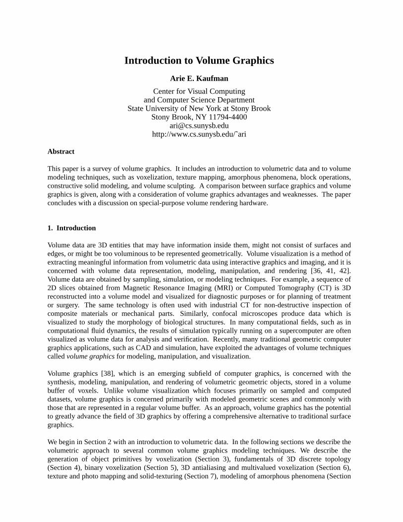
Figure 1: A volume-sampled plane within a volumetric cloud over volumetric model of terrain en-hanced with photo mapping of satellite images.


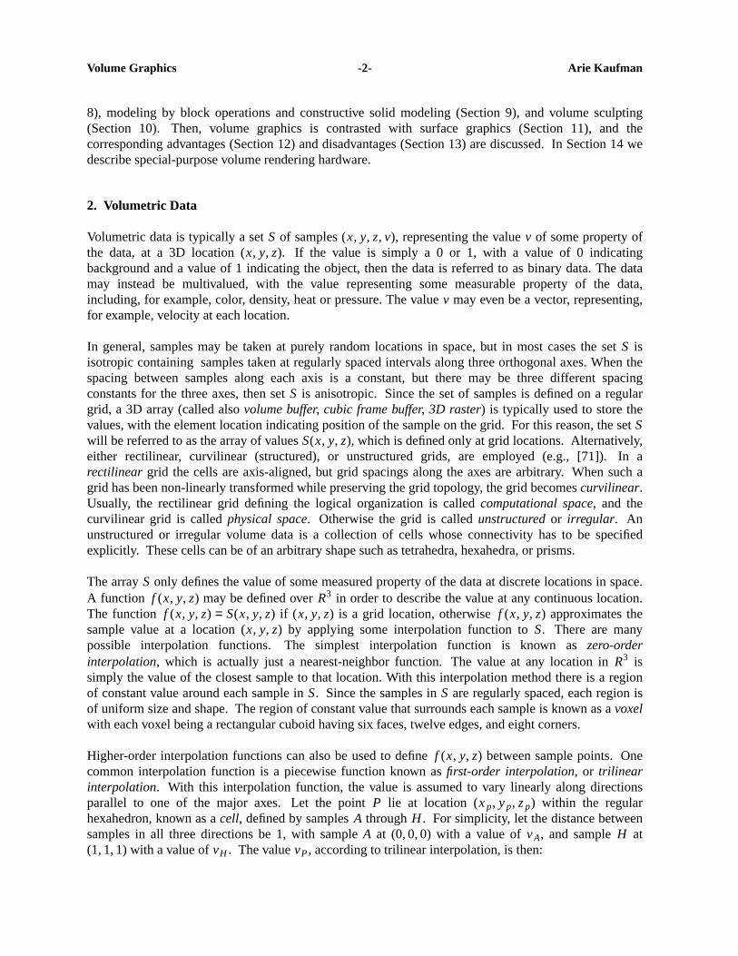
rendering of synthetic scenes made out of geometric models.The geometric model isvoxelized (3Dscan-converted) into a set of voxels that ‘‘best’’ approximate the model.Each of these voxels is thenstored in the volume buffer together with the voxel pre-computed view-independent attributes. Thevoxelized model can be either binary (see [5, 30-32] and Section 5) or volume sampled (see [72, 82] andSection 6) which generates alias-free density voxelization of the model.Some surface-based applicationexamples are the rendering of fractals [51], hyper textures [54], fur [28], gases [15], and other complexmodels [69] including terrain models for flight simulators (see Figures 1 and 2) [6, 38, 81, 87].andCAD models (see Figure 3).Furthermore, in many applications involving sampled data, such as medialimaging, the data need to be visualized along with synthetic objects that may not be available in digitalform, such as scalpels, prosthetic devices, injection needles, radiation beams, and isodose surfaces.These geometric objects can be voxelized and intermixed with the sampled organ in the voxel buffer[35].

3. Voxelization

An indispensable stage in volume graphics is the synthesis of voxel-represented objects from theirgeometric representation.This stage, which is calledvoxelization, is concerned with convertinggeometric objects from their continuous geometric representation into a set of voxels that ‘‘best’’approximates the continuous object.As this process mimics the scan-conversion process that pixelizes(rasterizes) 2D geometric objects, it is also referred to as3D scan-conversion. In 2D rasterization thepixels are directly drawn onto the screen to be visualized and filtering is applied to reduce the aliasingartifacts. However, the voxelization process does not render the voxels but merely generates a databaseof the discrete digitization of the continuous object.

Figure 2: A volumetric model of terrain enhanced with photo mapping of satellite images. The build-ings are synthetic voxel models raised on top of the terrain. The voxelized terrain has been mapped withaerial photos during the voxelization stage.


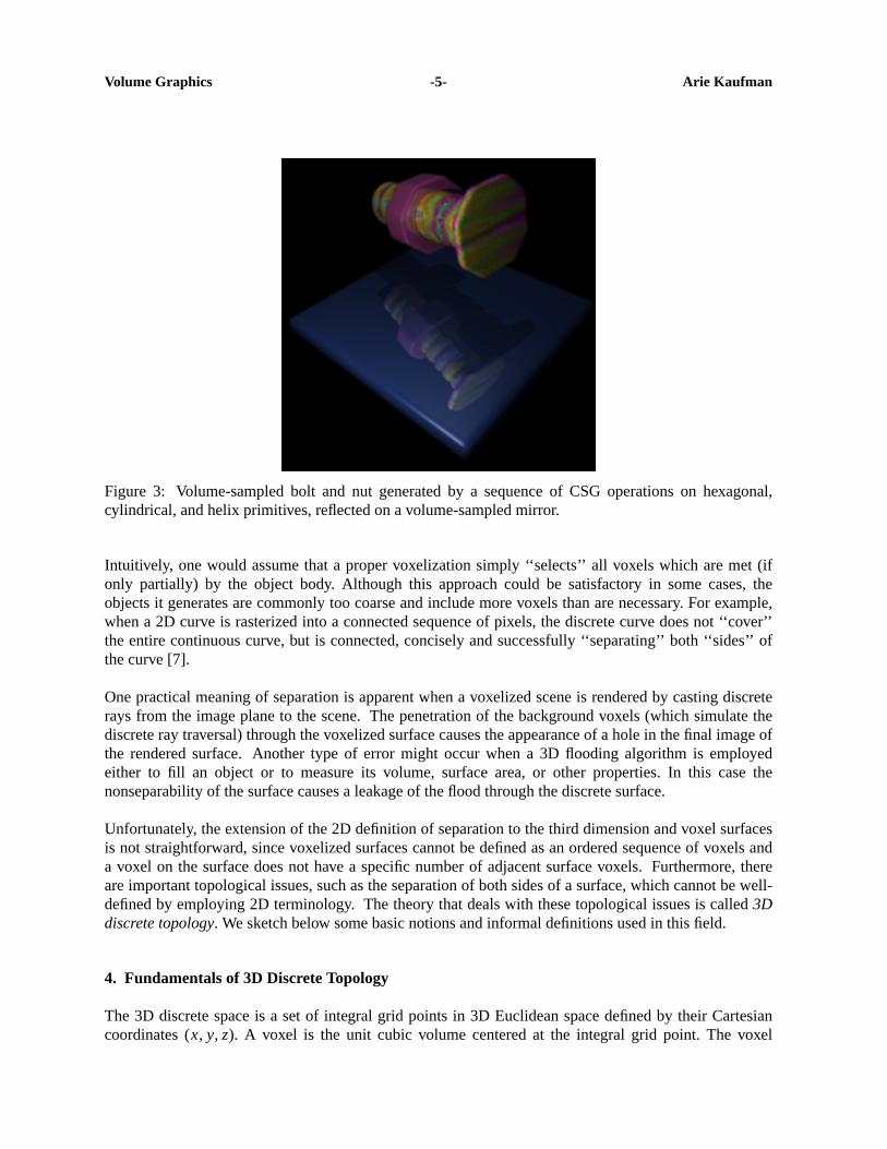
Figure 3: Volume-sampled bolt and nut generated by a sequence of CSG operations on hexagonal,cylindrical, and helix primitives, reflected on a volume-sampled mirror.

Intuitively, one would assume that a proper voxelization simply ‘‘selects’’ all voxels which are met (ifonly partially) by the object body. Although this approach could be satisfactory in some cases, theobjects it generates are commonly too coarse and include more voxels than are necessary. For example,when a 2D curve is rasterized into a connected sequence of pixels, the discrete curve does not ‘‘cover’’the entire continuous curve, but is connected, concisely and successfully ‘‘separating’’ both ‘‘sides’’ ofthe curve [7].

One practical meaning of separation is apparent when a voxelized scene is rendered by casting discreterays from the image plane to the scene.The penetration of the background voxels (which simulate thediscrete ray traversal) through the voxelized surface causes the appearance of a hole in the final image ofthe rendered surface. Anothertype of error might occur when a 3D flooding algorithm is employedeither to fill an object or to measure its volume, surface area, or other properties. In this case thenonseparability of the surface causes a leakage of the flood through the discrete surface.

Unfortunately, the extension of the 2D definition of separation to the third dimension and voxel surfacesis not straightforward, since voxelized surfaces cannot be defined as an ordered sequence of voxels anda voxel on the surface does not have a specific number of adjacent surface voxels. Furthermore,thereare important topological issues, such as the separation of both sides of a surface, which cannot be well-defined by employing 2D terminology. The theory that deals with these topological issues is called3Ddiscrete topology. We sketch below some basic notions and informal definitions used in this field.

4. Fundamentals of 3D Discrete Topology

The 3D discrete space is a set of integral grid points in 3D Euclidean space defined by their Cartesiancoordinates (x, y, z). A voxel is the unit cubic volume centered at the integral grid point. The voxel


value is mapped onto {0,1}: the voxels assigned ‘‘1’ ’ are called the ‘‘black’’ voxels representing opaqueobjects, and those assigned ‘‘0’ ’ are the ‘‘white’’ voxels representing the transparent background.InSection 6 we describe non-binary approaches where the voxel value is mapped onto the interval [0,1]representing either partial coverage, variable densities, or graded opacities. Due to its larger dynamicrange of values, this approach supports 3D antialiasing and thus supports higher quality rendering.

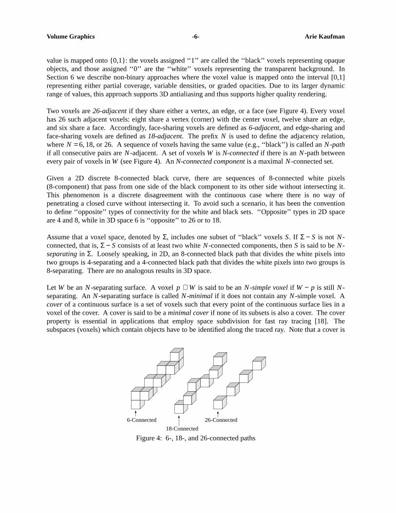
Tw o voxels are26-adjacentif they share either a vertex, an edge, or a face (see Figure 4). Every voxelhas 26 such adjacent voxels: eight share a vertex (corner) with the center voxel, twelve share an edge,and six share a face. Accordingly, face-sharing voxels are defined as6-adjacent, and edge-sharing andface-sharing voxels are defined as18-adjacent. The prefixN is used to define the adjacency relation,whereN = 6, 18,or 26. A sequence of voxels having the same value (e.g., ‘‘black’’) is called anN-pathif all consecutive pairs areN-adjacent. Aset of voxelsW is N-connectedif there is anN-path betweenev ery pair of voxels inW (see Figure 4).An N-connected componentis a maximalN-connected set.

Given a 2D discrete 8-connected black curve, there are sequences of 8-connected white pixels(8-component) that pass from one side of the black component to its other side without intersecting it.This phenomenon is a discrete disagreement with the continuous case where there is no way ofpenetrating a closed curve without intersecting it.To avoid such a scenario, it has been the conventionto define ‘‘opposite’’ types of connectivity for the white and black sets.‘‘ Opposite’’ types in 2D spaceare 4 and 8, while in 3D space 6 is ‘‘opposite’’ to 26 or to 18.

Assume that a voxel space, denoted byΣ, includes one subset of ‘‘black’’ voxels S. If Σ − S is not N-connected, that is,Σ − S consists of at least two white N-connected components, thenS is said to beN-separating in Σ. Loosely speaking, in 2D, an 8-connected black path that divides the white pixels intotwo groups is 4-separating and a 4-connected black path that divides the white pixels into two groups is8-separating. Thereare no analogous results in 3D space.

Let W be anN-separating surface. Avoxel p ∈ W is said to be anN-simple voxelif W − p is still N-separating. AnN-separating surface is calledN-minimal if it does not contain any N-simple voxel. Acover of a continuous surface is a set of voxels such that every point of the continuous surface lies in avoxel of the cover. A cover is said to be aminimal cover if none of its subsets is also a cover. The coverproperty is essential in applications that employ space subdivision for fast ray tracing [18].Thesubspaces (voxels) which contain objects have to be identified along the traced ray. Note that a cover is

6-Connected

18-Connected

26-Connected

Figure 4: 6-, 18-, and 26-connected paths


not necessarily separating, while on the other hand, as mentioned above, it may include simple voxels.In fact, even a minimal cover is not necessarilyN-minimal for any N [7].

5. Binary Voxelization

An early technique for the digitization of solids was spatial enumeration which employs point or cellclassification methods in either an exhaustive fashion or by recursive subdivision [44]. However,subdivision techniques for model decomposition into rectangular subspaces are computationallyexpensive and thus inappropriate for medium or high resolution grids.Instead, objects should bedirectly voxelized, preferably generating anN-separating,N-minimal, and covering set, whereN isapplication dependent. The voxelization algorithms should follow the same paradigm as the 2D scan-conversion algorithms; they should be incremental, accurate, use simple arithmetic (preferably integeronly), and have a complexity that is not more than linear with the number of voxels generated.

The literature of 3D scan-conversion is relatively small. Danielsson [11] and Mokrzycki [49] developedindependently similar 3D curve algorithms where the curve is defined by the intersection of two implicitsurfaces. Voxelization algorithms have been developed for 3D lines [8], 3D circles, and a variety ofsurfaces and solids, including polygons, polyhedra, and quadric objects [30].Efficient algorithms havebeen developed for voxelizing polygons using an integer-based decision mechanism embedded within ascan-line filling algorithm [31] or with an incremental pre-filtered algorithm [10], for parametric curves,surfaces, and volumes using an integer-based forward differencing technique [32], and for quadricobjects such as cylinders, spheres, and cones using ‘‘weaving’’ algorithms by which a discretecircle/line sweeps along a discrete circle/line [5].Figure 2 consists of a variety of objects (polygons,boxes, cylinders) voxelized using these methods.These pioneering attempts should now be followed byenhanced voxelization algorithms that, in addition to being efficient and accurate, will also adhere to thetopological requirements of separation, coverage, and minimality.

6. 3D Antialiasing and Multivalueded Voxelization

The previous section discussed binary voxelization, which generates topologically and geometricallyconsistent models, but exhibits object space aliasing.These algorithms have used a straightforwardmethod of sampling in space, calledpoint sampling. In point sampling, the continuous object isevaluated at the voxel center, and the value of 0 or 1 is assigned to the voxel. Becauseof this binaryclassification of the voxels, the resolution of the 3D raster ultimately determines the precision of thediscrete model.Imprecise modeling results in jagged surfaces, known asobject space aliasing(seeFigure 2). In this section, we first present a 3D object-space antialiasing technique.It performsantialiasing once, on a 3D view-independent representation, as part of the modeling stage.Unlikeantialiasing of 2D scan-converted graphics, where the main focus is on generating aesthetically pleasingdisplays, the emphasis in antialiased 3D voxelization is on producing alias-free 3D models that arestored in the view-independent volume buffer for various volume graphics manipulations, including butnot limited to the generation of aesthetically pleasing displays (see Figure 1).

To reduce object space aliasing, avolume samplingtechnique has been developed [82], which estimatesthe density contribution of the geometric objects to the voxels. Thedensity of a voxel is attenuated by afilter weight function which is proportional to the distance between the center of the voxel and thegeometric primitive. To improve performance, precomputed lookup tables of densities for a predefinedset of geometric primitives can be used to select the density value of each voxel. For each voxel visited


by the binary voxelization algorithm, the distance to the predefined primitive is used as an index into alookup table of densities.

Since voxelized geometric objects are represented as volume rasters of density values, they canessentially be treated as sampled or simulated volume datasets, such as 3D medical imaging datasets,and one of many volume rendering techniques for image generation can be employed. Oneprimaryadvantage of this approach is that volume rendering or volumetric global illumination carries thesmoothness of the volume-sampled objects from object space over into its 2D projection in image space[84]. Hence,the silhouette of the objects, reflections, and shadows are smooth.In addition, CSGoperations between two volume-sampled geometric models are accomplished at the voxel level aftervoxelization, thereby reducing the original problem of evaluating a CSG tree of such operations down toa fuzzy Boolean operation between pairs of non-binary voxels [83] (see Section 9).Volume-sampledmodels are also suitable for intermixing with sampled or simulated datasets, since they can be treateduniformly as one common data representation.Furthermore, volume-sampled models lend themselvesto alias-free multi-resolution hierarchy construction [83].

Further study of filtered voxelization has been conducted by Sramek and Kaufman [72, 74].The basicidea has been that in voxelization filter design one needs to consider the visualization techniques used(i.e., data interpolation and normal estimation).They showed that a combination of first order filters onvoxelization and visualization, with proper parameters, results in rendered images with negligible errorin estimating object surface position and normal direction.More specifically, if a trilinear interpolationis used for reconstruction of the continuous volume, with subsequent surface detection by thresholdingand normal gradient calculation by central differences, best results are obtained if the density of thevoxelized object near its surface is linear along the surface normal direction (e.g., [27, 73]).This linearprofile results from convolution of the object with a 1D box filter applied along a directionperpendicular to the surface, called oriented box filter [72].Furthermore, a Gaussian surface densityprofile combined with tricubic interpolation and Gabor derivative reconstruction outperforms the lineardensity profile, but for a sharp increase in the computation time.

A C++ library for filtered voxelization of objects, vxt, has been developed [75]. It provides the userwith an extensible set of easy-to-use tools and routines for alias-free voxelization of analytically definedmonochromatic and color objects.Thus, resulting volumetric data represent a suitable input for bothsoftware and hardware volume rendering systems.The library provides for voxelization of primitiveobjects; however, when supplemented by a suitable parser, it represents a basis for voxelization ofcomplex models defined in various graphics formats.

7. Texture Mapping

One type of object complexity involves objects that are enhanced with texture mapping, photo mapping,environment mapping, or solid texturing. Texture mapping is commonly implemented during the laststage of the rendering pipeline, and its complexity is proportional to the object complexity. In volumegraphics, however, texture mapping is performed during the voxelization stage, and the texture color isstored in each voxel in the volume buffer.

In photo mapping six orthogonal photographs of the real object are projected back onto the voxelizedobject. Oncethis mapping is applied, it is stored with the voxels themselves during the voxelizationstage, and therefore does not degrade the rendering performance.Te xture and photo mapping are alsoviewpoint independent attributes implying that once the texture is stored as part of the voxel value,


texture mapping need not be repeated.This important feature is exploited, for example, by voxel-basedflight simulators (see Figures 1 and 2) and in CAD systems (see Figure 3).

A central feature of volumetric representation is that, unlike surface representation, it is capable ofrepresenting inner structures of objects, which can be revealed and explored with appropriatemanipulation and rendering techniques.This capability is essential for the exploration of sampled orcomputed objects.Synthetic objects are also likely to be solid rather than hollow. One method formodeling various solid types is solid texturing, in which a function or a 3D map models the color of theobjects in 3D (see Figure 3).During the voxelization phase each voxel belonging to the objects isassigned a value by the texturing function or the 3D map.This value is then stored as part of the voxelinformation. Again, since this value is view independent, it does not have to be recomputed for everychange in the rendering parameters.

8. Amorphous Phenomena

While translucent objects can be represented by surface methods, these methods cannot efficientlysupport the modeling and rendering of amorphous phenomena (e.g., clouds, fire, smoke) that arevolumetric in nature and lack any tangible surfaces. A common modeling and rendering approach isbased on a volumetric function that, for any input point in 3D, calculates some object features such asdensity, reflectivity, or color (see Figure 1).These functions can then be rendered by ray casting, whichcasts a ray from each pixel into the function domain. Along the passage of the ray, at constant intervalsthe function is evaluated to yield a sample. All samples along each ray are combined to form the pixelcolor. Some examples for the use of this or similar techniques are the rendering of fractals [22],hypertextures [54], fur [28], and gases [15].

The process of function evaluation at each sample point in 3D has to be repeated for each imagegenerated. In contrast, the volumetric approach allows the pre-computation of these functions at eachgrid point of the volume buffer. The resulting volumetric dataset can then be rendered from multipleviewpoints without recomputing the modeling function. As in other volume graphics techniques,accuracy is traded for speed, due to the resolution limit.Instead of accurately computing the function ateach sample point, some type of interpolation from the precomputed grid values is employed.

9. Block Operations and Constructive Solid Modeling

The presortedness of the volume buffer naturally lends itself to grouping operations that can beexploited in various ways. For example, by generating multi-resolution volume hierarchy that cansupport time critical and space critical volume graphics applications can be better supported.The basicidea is similar to that of level-of-detail surface rendering which has recently proliferated [16, 25, 61, 65,78], in which the perceptual importance of a given object in the scene determines its appropriate level-of-detail representation.One simple approach is the 3D "mip-map" approach [46, 63], where everylevel of the hierarchy is formed by averaging several voxels from the previous level. A better approachis based on sampling theory, in which an object is modeled with a sequence of alias-free volume buffersat different resolutions using the volume-sampled voxelization approach [23].To accomplish this, highfrequencies that exceed the Nyquist frequency of the corresponding volume buffer are filtered out byapplying an ideal low-pass filter (sinc) with infinite support. In practice, the ideal filter is approximatedby filters with finite support.Low sampling resolution of the volume buffer corresponds to a lowerNyquist frequency, and therefore requires a low-pass filter with wider support for good approximation.


As one moves up the hierarchy, low-pass filters with wider and wider support are applied.Compared tothe level-of-detail hierarchy in surface graphics, the multi-resolution volume buffers are easy to generateand to spatially correspond neighboring levels, and are also free of object space aliasing.Furthermore,arbitrary resolutions can be generated, and errors caused by a non-ideal filter do not propagate andaccumulate from level to lev el. Dependingon the required speed and accuracy, a variety of low-passfilters (zero order, cubic, Gaussian) can be applied.

An intrinsic characteristic of the volume buffer is that adjacent objects in the scene are also representedby neighboring memory cells. Therefore, rasters lend themselves to various meaningful grouping-basedoperations, such asbitblt in 2D, or voxblt in 3D [37]. These include transfer of volume bufferrectangular blocks (cuboids) while supporting voxel-by-voxel operations between source anddestination blocks.Block operations add a variety of modeling capabilities which aid in the task ofimage synthesis and form the basis for the efficient implementation of a 3D ‘‘room manager’’, which isthe extension of window management to the third dimension.

Since the volume buffer lends itself to Boolean operations that can be performed on a voxel-by-voxelbasis during the voxelization stage, it is advantageous to use CSG as the modeling paradigm.Subtraction, union, and intersection operations between two voxelized objects are accomplished at thevoxel lev el, thereby reducing the original problem of evaluating a CSG tree during rendering time downto a 1D Boolean operation between pairs of voxels during a preprocessing stage.

For two point-sampled binary objects the Boolean operations of CSG orvoxblt are trivially defined.However, the Boolean operations applied to volume-sampled models are analogous to those of fuzzy settheory (cf. [13]). The volume-sampled model is a density functiond(x) over R3, whered is 1 inside theobject, 0 outside the object, and 0< d < 1 within the "soft" region of the filtered surface. Someof thecommon operations, intersection, complement, difference, and union, between two objectsA andB aredefined as follows:

(16)dA∩ B(x) ≡ min ( dA(x), dB(x))

(17)dA(x) ≡ 1 − dA(x)

(18)dA−B(x) ≡ min (dA(x), 1 − dB(x))

(19)dA∪ B(x) ≡ max (dA(x), dB(x))

The only law of set theory that is no longer true is the excluded-middle law (i.e., A ∩ A ≠ �and

A ∪ A ≠ Universe). Theuse of the min and max functions causes discontinuity at the region where thesoft regions of the two objects meet, since the density value at each location in the region is determinedsolely by one of the two overlapping objects.

Complex geometric models can be generated by performing the CSG operations in Equations 16-19between volume-sampled primitives. Volume-sampled models can also function as matte volumes [12]for various matting operations, such as performing cut-aways and merging multiple volumes into asingle volume using the union operation.However, in order to preserve continuity on the cut-awayboundaries between the material and the empty space, one should use an alternative set of Booleanoperators based on algebraic sum and algebraic product [13, 20] :

(20)dA∩ B(x) ≡ dA(x) dB(x)


(21)dA(x) ≡ 1 − dA(x)

(22)dA−B(x) ≡ dA(x) − dA(x) dB(x)

(23)dA∪ B(x) ≡ dA(x) + dB(x) − dA(x) dB(x)

Unlike the min and max operators, algebraic sum and product operators result inA ∪ A ≠ A, which isundesirable. Aconsequence, for example, is that during modeling via sweeping, the resulting model issensitive to the sampling rate of the swept path [83].

Once a CSG model has been constructed in voxel representation, it is rendered in the same way anyother volume buffer is. This makes, for example, volumetric ray tracing of constructive solid modelsstraightforward [70] (see Figure 3).

10. Volume Sculpting

Surface-based sculpting has been studied extensively (e.g., [9, 66]), while volume sculpting has beenrecently introduced for clay or wax-like sculptures [17] and for comprehensive detailed sculpting [85].The latter approach is a free-form interactive modeling technique based on the metaphor of sculptingand painting a voxel-based solid material, such as a block of marble or wood. Thereare twomotivations for this approach.First, modeling topologically complex and highly-detailed objects arestill difficult in most CAD systems.Second, sculpting has shown to be useful in volumetricapplications. For example, scientists and physicians often need to explore the inner structures of theirsimulated or sampled datasets by gradually removing material.

Real-time human interaction could be achieved in this approach, since the actions of sculpting (e.g.,carving, sawing) and painting are localized in the volume buffer, a localized rendering can be employedto reproject only those pixels that are affected. Carvingis the process of taking a pre-existing volume-sampled tool to chip or chisel the object bit by bit.Since both the object and tool are represented asindependent volume buffers, the process of sculpting involves positioning the tool with respect to theobject and performing a Boolean subtraction between the two volumes. Sawing is the process ofremoving a whole chunk of material at once, much like a carpenter sawing off a portion of a woodpiece. Unlike carving, sawing requires generating the volume-sampled tool on-the-fly, using a userinterface. To prevent object space aliasing and to achieve interactive speed, 3D splatting is employed.

11. Surface Graphics vs. Volume Graphics

Contemporary 3D graphics has been employing an object-based approach at the expense of maintainingand manipulating a display list of geometric objects and regenerating the frame-buffer after everychange in the scene or viewing parameters.This approach, termedsurface graphics, is supported bypowerful geometry engines which have flourished in the past decade, making surface graphics the state-of-the-art in 3D graphics.

Surface graphics strikingly resembles vector graphics that prevailed in the sixties and seventies, andemployed vector drawing devices. Like vector graphics, surface graphics represents the scene as a set ofgeometric primitives kept in a display list. In surface graphics, these primitives are transformed,mapped to screen coordinates, and converted by scan-conversion algorithms into a discrete set of pixels.Any change to the scene, viewing parameters, or shading parameters requires the image generation


system to repeat this process.Like vector graphics that did not support painting the interior of 2Dobjects, surface graphics generates merely the surfaces of 3D objects and does not support the renderingof their interior.

Instead of a list of geometric objects maintained by surface graphics, volume graphics employs a 3Dvolume buffer as a medium for the representation and manipulation of 3D scenes.A 3D scene isdiscretized earlier in the image generation sequence, and the resulting 3D discrete form is used as adatabase of the scene for manipulation and rendering purposes, which in effect decouples discretizationfrom rendering.Furthermore, all objects are converted into one uniform meta-object − the voxel. Eachvoxel is atomic and represents the information about at most one object that resides in that voxel.

Volume graphics offers similar benefits to surface graphics, with several advantages that are due to thedecoupling, uniformity, and atomicity features.The rendering phase is viewpoint independent andinsensitive to scene complexity and object complexity. It supports Boolean and block operations andconstructive solid modeling. When 3D sampled or simulated data are used, such as that generated bymedical scanners (e.g., CT, MRI) or scientific simulations (e.g., CFD), volume graphic is suitable fortheir representation too. It is capable of representing amorphous phenomena and both the interior andexterior of 3D objects.These features of volume graphics as compared with surface graphics arediscussed in detail in Section 12.Several weaknesses of volume graphics are related to the discretenature of the representation, for instance, transformations and shading are performed in discrete space.In addition, this approach requires substantial amounts of storage space and specialized processing.These weaknessesare discussed in detail in Section 13.

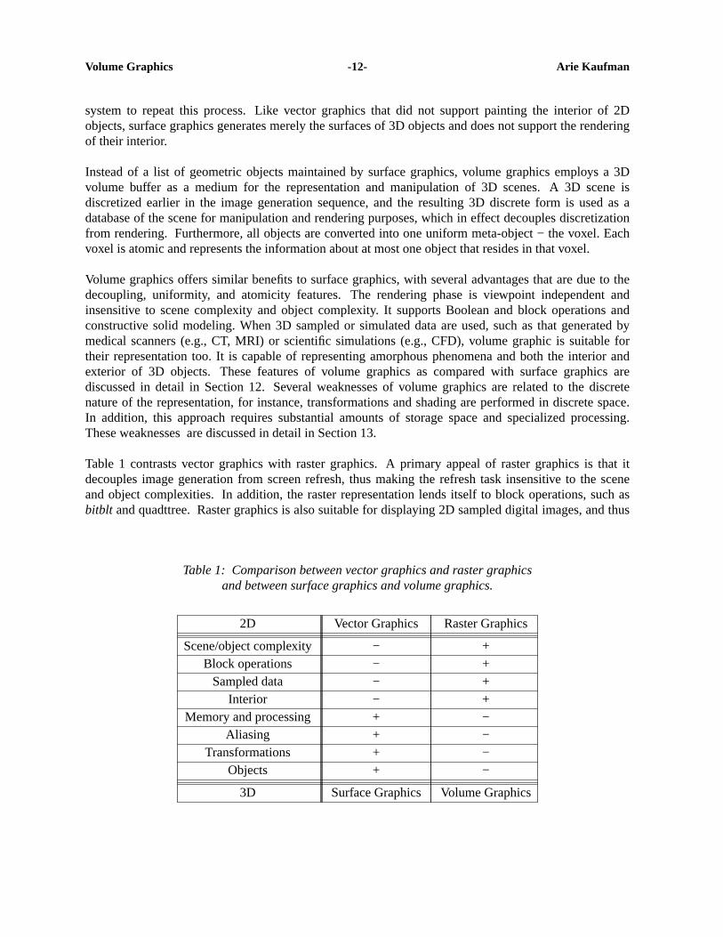
Table 1 contrasts vector graphics with raster graphics.A primary appeal of raster graphics is that itdecouples image generation from screen refresh, thus making the refresh task insensitive to the sceneand object complexities. In addition, the raster representation lends itself to block operations, such asbitblt and quadttree.Raster graphics is also suitable for displaying 2D sampled digital images, and thus

Table 1: Comparison between vector graphics and raster graphicsand between surface graphics and volume graphics.

2D Vector Graphics Raster Graphics

Scene/object complexity − +Block operations − +

Sampled data − +Interior − +

Memory and processing + −Aliasing + −

Transformations + −Objects + −

3D Surface Graphics Volume Graphics


provides the ideal environment for mixing digital images with synthetic graphic. Unlike vector graphics,raster graphics provides the capability to present shaded and textured surfaces, as well as line drawings.These advantages, coupled with advances in hardware and the development of antialiasing methods,have led raster graphics to supersede vector graphics as the primary technology for computer graphics.The main weaknesses of raster graphics are the large memory and processing power it requires for theframe buffer, as well as the discrete nature of the image.These difficulties delayed the full acceptanceof raster graphics until the late seventies when the technology was able to provide cheaper and fastermemory and hardware to support the demands of the raster approach.In addition, the discrete nature ofrasters makes them less suitable for geometric operations such as transformations and accuratemeasurements, and once discretized, the notion of objects is lost.

The same appeal that drove the evolution of the computer graphics world from vector graphics to rastergraphics, once the memory and processing power became available, is driving a variety of applicationsfrom a surface-based approach to a volume-based approach.Naturally, this trend first appeared inapplications involving sampled or computed 3D data, such as 3D medical imaging and scientificvisualization, in which the datasets are in volumetric form. These diverse empirical applications ofvolume visualization still provide a major driving force for advances in volume graphics.

The comparison in Table 1 between vector graphics and raster graphics strikingly resembles acomparison between surface graphics and volume graphics.Actually Table 1 itself is also used tocontrast surface graphics and volume graphics.

12. Volume Graphics Features

One of the most appealing attributes of volume graphics is its insensitivity to the complexity of thescene, since all objects have been pre-converted into a finite size volume buffer. Although theperformance of the pre-processing voxelization phase is influenced by the scene complexity [5, 30-32],rendering performance depends mainly on the constant resolution of the volume buffer and not on thenumber of objects in the scene.Insensitivity to the scene complexity makes the volumetric approachespecially attractive for scenes consisting of a large number of objects.

In volume graphics, rendering is decoupled from voxelization and all objects are first converted into onemeta object, the voxel, which makes the rendering process insensitive to the complexity of the objects.Thus, volume graphics is particularly attractive for objects that are hard to render using conventionalgraphics systems.Examples of such objects include curved surfaces of high order and fractals whichrequire expensive computation of an iterative function for each volume unit [51]. Constructive solidmodels are also hard to render by conventional methods, but are straightforward to render in volumetricrepresentation (see below).

Anti-aliasing and texture mapping are commonly implemented during the last stage of the conventionalrendering pipeline, and their complexity is proportional to object complexity. Solid texturing, whichemploys a 3D texture image, has also a high complexity proportional to object complexity. In volumegraphics, however, anti-aliasing, texture mapping, and solid texturing are performed only once - duringthe voxelization stage - where the color is calculated and stored in each voxel. Thetexture can also bestored as a separate volumetric entity which is rendered together with the volumetric object, as in theVolVis software system for volume visualization [1].

The textured objects in Figure 1, 2 and 3 have been assigned texture during the voxelization stage by


mapping each voxel back to the corresponding value on a texture map or solid.Once this mapping isapplied, it is stored with the voxels themselves during the voxelization stage, which does not degrade therendering performance.In addition, texture mapping and photo mapping are also viewpointindependent attributes, implying that once the texture is stored as part of the voxel value, texturemapping need not be repeated.

In anticipation of repeated access to the volume buffer (such as in animation), all viewpoint independentattributes can be precomputed during the voxelization stage, stored with the voxel, and be readilyaccessible for speeding up the rendering.The voxelization algorithm can generate for each object voxelits color, texture color, normal vector (for visible voxels), antialiasing information [82], and informationconcerning the visibility of the light sources from that voxel. Actually, the viewpoint independent partsof the illumination equation can also be precomputed and stored as part of the voxel value.

Once a volume buffer with precomputed view-independent attributes is available, a rendering algorithmsuch as a discrete ray tracing or a volumetric ray tracing algorithm can be engaged. Eitherray tracingapproach is especially attractive for complex surface scenes and constructive solid models, as well as 3Dsampled or computed datasets (see below). Figure3 shows an example of objects that were ray tracedin discrete voxel space.In spite of the complexity of these scenes, volumetric ray tracing time wasapproximately the same as for much simpler scenes and significantly faster than traditional space-subdivision ray tracing methods.Moreover, in spite of the discrete nature of the volume bufferrepresentation, images indistinguishable from the ones produced by conventional surface-based raytracing can be generated by employing, accurate ray tracing, auxiliary object information, or screensupersampling techniques.

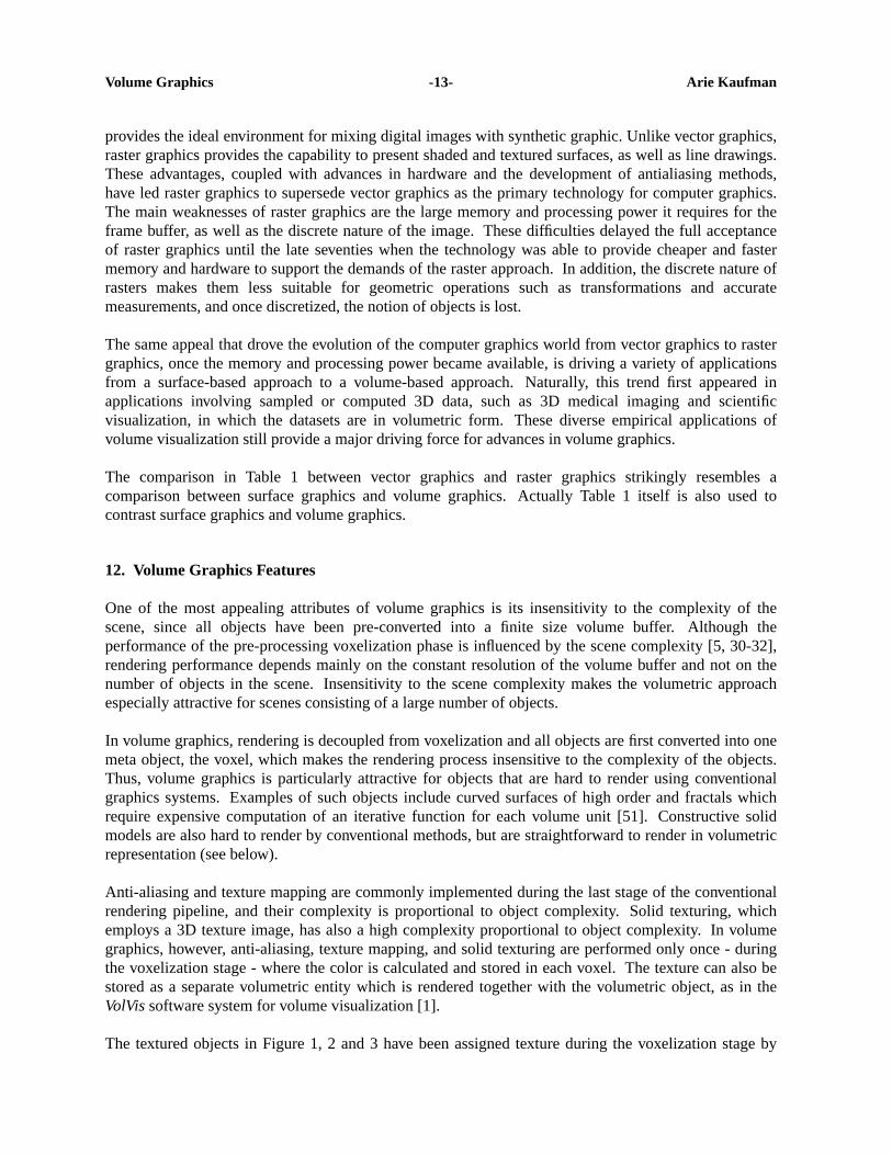
Sampled datasets, such as in 3D medical imaging (see Figure 3), volume microscopy, and geology, andsimulated datasets, such as in computational fluid dynamics, chemistry, and materials simulation areoften reconstructed from the acquired sampled or simulated points into a regular grid of voxels andstored in a volume buffer. Such datasets provide for the majority of applications using the volumetricapproach. Unlike surface graphics, volume graphics naturally and directly supports the representation,manipulation, and rendering of such datasets, as well as providing the volume buffer medium forintermixing sampled or simulated datasets with geometric objects [35], as can be seen in Figure 5.Forcompatibility between the sampled/computed data and the voxelized geometric object, the object can bevolume sampled [82] with the same, but not necessarily the same, density frequency as the acquired orsimulated datasets.In volume sampling the continuous object is filtered during the voxelization stagegenerating alias-free 3D density primitives. Volume graphics also naturally supports the rendering oftranslucent volumetric datasets (see Figures 1 and 5).

A central feature of volumetric representation is that unlike surface representation it is capable ofrepresenting inner structures of objects, which can be revealed and explored with the appropriatevolumetric manipulation and rendering techniques.Natural objects as well as synthetic objects arelikely to be solid rather than hollow. The inner structure is easily explored using volume graphics andcannot be supported by surface graphics (see Figure 5).Moreover, while translucent objects can berepresented by surface methods, these methods cannot efficiently support the translucent rendering ofvolumetric objects, or the modeling and rendering of amorphous phenomena (e.g., clouds, fire, smoke)that are volumetric in nature and do not contain any tangible surfaces (see Figure 1) [15, 28, 54].

An intrinsic characteristic of rasters is that adjacent objects in the scene are also represented byneighboring voxels. Therefore, rasters lend themselves to various meaningful block-based operationswhich can be performed during the voxelization stage.For example, the 3D counterpart of thebitblt


Figure 5: Intermixing of a volume-sampled cone with an MRI head using a union operation.

operations, termedvoxblt (voxel block-transfer), can support transfer of cuboidal voxel blocks with avariety of voxel-by-voxel operations between source and destination blocks [37].This property is veryuseful for voxblt and CSG. Once a CSG model has been constructed in voxel representation, it isrendered like any other volume buffer. This makes rendering of constructive solid modelsstraightforward.

The spatial presortedness of the volume buffer voxels lends itself to other types of grouping oraggregation of neighboring voxels. For example, the terrain image shown in Figure 2 was generated bythe voxel-based Hughes Aircraft Co.flight simulator [87]. It simulates a flight over voxel-representedterrain enhanced with satellite or aerial photo mapping with additional synthetic raised objects, such asbuildings, trees, vehicles, aircraft, clouds and the like. Sincethe information below the terrain surface isinvisible, terrain voxels can be actually represented as tall cuboids extending from sea level to the terrainheight. Theraised and moving objects, however, hav eto be represented in a more conventional voxel-based form.

Similarly, voxels can be aggregated into super-voxels in a pyramid-like hierarchy. For example, in avoxel-based flight simulator, the best resolution can be used for takeoff and landing. As the aircraftascends, fewer and fewer details need to be processed and visualized, and a lower resolution suffices.Furthermore, even in the same view, parts of the terrain close to the observer are rendered at highresolution which deceases towards the horizon. A hierarchical volume buffer can be prepared in advanceor on-the-fly by subsampling or averaging the appropriate size neighborhoods of voxels (see also [23]).

13. Weaknesses of Volume Graphics

A typical volume buffer occupies a large amount of memory. For example, for a medium resolution of5123, two bytes per voxel, the volume buffer consists of 256M bytes. However, since computermemories are significantly decreasing in price and increasing in their compactness and speed, such large


memories are becoming commonplace.This argument echoes a similar discussion when raster graphicsemerged as a technology in the mid-seventies. With the rapid progress in memory price andcompactness, it is safe to predict that, as in the case of raster graphics, memory will soon cease to be astumbling block for volume graphics.

The extremely large throughput that has to be handled requires a special architecture and processingattention (see Section 14 and [36] Chapter 6).Volume engines, analogous to the currently availablegeometry (polygon) engines, are emerging. Becauseof the presortedness of the volume buffer and thefact that only a simple single type of object has to be handled, volume engines are conceptually simplerto implement than current geometry engines (see Section 14).Volume engines will materialize in thenear future, with capabilities to synthesize, load, store, manipulate, and render volumetric scenes in realtime (e.g., 30 frames/sec), configured as accelerators or co-systems to existing geometry engines.

Unlike surface graphics, in volume graphics the 3D scene is represented in discrete form.This is thesource of many of the problems of voxel-based graphics, which are similar to those of 2D rasters [14].The finite resolution of the raster poses a limit on the accuracy of some operations, such as volume andarea measurements, that are based on voxel counting.

Since the discrete data is sampled during rendering, a low resolution volume yields high aliasingartifacts. Thisbecomes especially apparent when zooming in on the 3D raster. When naive renderingalgorithms are used, holes may appear "between" voxels. Nevertheless, this can be alleviated in wayssimilar to those adopted by 2D raster graphics, such as employing either reconstruction techniques, ahigher-resolution volume buffer, or volume sampling.

Manipulation and transformation of the discrete volume are difficult to achieve without degrading theimage quality or losing some information.Rotation of rasters by angles other than 90 degrees isespecially problematic since a sequence of consecutive rotations will distort the image.Again, thesecan be alleviated in ways similar to the 2D raster techniques.

Once an object has been voxelized, the voxels comprising the discrete object do not retain anygeometric information regarding the geometric definition of the object.Thus, it is advantageous, whenexact measurements are required (e.g., distance, area), to employ conventional modeling where thegeometric definition of the object is available. A voxel-based object is only a discrete approximation ofthe original continuous object where the volume buffer resolution determines the precision of suchmeasurements. Onthe other hand, several measurement types are more easily computed in voxel space(e.g., mass property, adjacency detection, and volume computation).

The lack of geometric information in the voxel may inflict other difficulties, such as surface normalcomputation. Invoxel-based models, a discrete shading method is commonly employed to estimate thenormal from a context of voxels. A variety of image-based and object-based methods for normalestimation from volumetric data has been devised (see [90], [36, Chapter 4]) and some have beendiscussed above. Most methods are based on fitting some type of a surface primitive to a smallneighborhood of voxels.

A partial integration between surface and volume graphics is conceivable as part of an object-basedapproach in which an auxiliary object table, consisting of the geometric definition and global attributesof each object, is maintained in addition to the volume buffer. Each voxel consists of an index to theobject table. This allows exact calculation of normal, exact measurements, and intersection verificationfor discrete ray tracing [89].The auxiliary geometric information might be useful also for re-voxelizing


the scene in case of a change in the scene itself.

14. Special-Purpose Volume Rendering Hardware

The high computational cost of direct volume rendering makes it difficult for sequentialimplementations and general-purpose computers to deliver the targeted level of performance. Thissituation is aggravated by the continuing trend towards higher and higher resolution datasets. Forexample, to render a dataset of 10243 16-bit voxels at 30 frames per second requires 2 GBytes ofstorage, a memory transfer rate of 60 GBytes per second and approximately 300 billion instructions persecond, assuming only 10 instructions per voxel per projection.To address this challenge, researchershave tried to achieve interactive display rates on supercomputers and massively parallel architectures[50, 64, 67, 68, 80, 91].However, most algorithms require very little repeated computation on eachvoxel and data movement actually accounts for a significant portion of the overall performanceoverhead. Today’s commercial supercomputer memory systems do not have, nor will they in the nearfuture, adequate latency and memory bandwidth for efficiently transferring the required large amountsof data. Furthermore, supercomputers seldom contain frame buffers and, due to their high cost, arefrequently shared by many users.

The same way as the special requirements of traditional computer graphics lead to high-performancegraphics engines, volume visualization naturally lends itself to special-purpose volume renderers thatseparate real-time image generation from general-purpose processing. This allows for stand-alonevisualization environments that help scientists to interactively view their data on a single userworkstation, either augmented by a volume rendering accelerator or connected to a dedicatedvisualization server. Furthermore, a volume rendering engine integrated in a graphics workstation is anatural extension of raster based systems into 3D volume visualization.

Several researchers have proposed special-purpose volume rendering architectures [36, Chapter 6] [19,26, 34, 48, 52, 76, 77, 88]. Most recent research has focused on accelerators for ray-casting of regulardatasets. Ray-casting offers room for algorithmic improvements while still allowing for high imagequality. Recent architectures [24] include VOGUE, VIRIM, and Cube.

VOGUE [43], a modular add-on accelerator, is estimated to achieve 2.5 frames per second for 2563

datasets. For each pixel a ray is defined by the host computer and sent to the accelerator. The VOGUEmodule autonomously processes the complete ray, consisting of evenly spaced resampling locations, andreturns the final pixel color of that ray to the host. Several VOGUE modules can be combined to yieldhigher performance implementations. For example, to achieve 20 projections per second of 5123

datasets requires 64 boards and a 5.2 GB per second ring-connected cubic network.

VIRIM [21] is a flexible and programmable ray-casting engine. The hardware consists of two separateunits, the first being responsible for 3D resampling of the volume using lookup tables to implementdifferent interpolation schemes. The second unit performs the ray-casting through the resampled datasetaccording to user programmable lighting and viewing parameters. The underlying ray-casting modelallows for arbitrary parallel and perspective projections and shadows. An existing hardwareimplementation for the visualization of 256× 256× 128 datasets at 10 frames per second requires 16processing boards.

The Cube project aims at the realization of high-performance volume rendering systems for largedatasets and pioneered several hardware architectures. Cube-1, a first generation hardware prototype,


was based on a specially interleaved memory organization [33], which has also been used in allsubsequent generations of the Cube architecture. This interleaving of then3 voxel enables conflict-freeaccess to any ray parallel to a main axis ofn voxels. A fully operational printed circuit board (PCB)implementation of Cube-1 is capable of generating orthographic projections of 163 datasets from a finitenumber of predetermined directions in real-time.Cube-2 was a single-chip VLSI implementation ofthis prototype [3].

To achieve higher performance and to further reduce the critical memory access bottleneck, Cube-3introduced several new concepts [55-57].A high-speed global communication network aligns anddistributes voxels from the memory to several parallel processing units and a circular cross-linkedbinary tree of voxel combination units composites all samples into the final pixel color. Estimatedperformance for arbitrary parallel and perspective projections is 30 frames per second for 5123 datasets.Cube-4 [29, 58, 59] has only simple and local interconnections, thereby allowing for easy scalability ofperformance. Instead of processing individual rays, Cube-4 manipulates a group of rays at a time. As aresult, the rendering pipeline is directly connected to the memory. Accumulating compositors replacethe binary compositing tree. A pixel-bus collects and aligns the pixel output from the compositors.Cube-4 is easily scalable to very high resolution of 10243 16-bit voxels and true real-time performanceimplementations of 30 frames per second.

Enhancing the Cube-4 architecture, Mitsubishi Electric has derived EM-Cube (Enhanced MemoryCube-4). Asystem based on EM-Cube consists of a PCI card with four volume rendering chips, four64Mbit SDRAMs to hold the volume data, and four SRAMs to capture the rendered image [53].Theprimary innovation of EM-Cube is the block-skewed memory, where the volume memory is organizedin subcubes (blocks) in such a way that all the voxels of a block are stored linearly in the same DRAMpage. EM-Cubehas been further developed into a commercial product where a volume rendering chip,called vg500, has been developed by Mitsubishi. It computes 500 million interpolated, Phong-illuminated, composited samples per second.The vg500 is the heart of a VolumePro PC card consistingof one vg500 and configurable standard SDRAM memory architectures.The first generation, availablein 1999, supports rendering of a rectangular data set up to 256x256x256 12-bit voxels, in real-time 30frames/sec [60].

Simultaneously, Japan Radio Co. has enhanced Cube-4 and developed a special-purpose architecture U-Cube. U-Cubeis specifically designed for real-time volume rendering of 3D ultrasound data.

The choice of whether one adopts a general-purpose or a special-purpose solution to volume renderingdepends upon the circumstances. If maximum flexibility is required, general-purpose appears to be thebest way to proceed. However, an important feature of graphics accelerators is that they are integratedinto a much larger environment where software can shape the form of input and output data, therebyproviding the additional flexibility that is needed. A good example is the relationship between the needsof conventional computer graphics and special-purpose graphics hardware. Nobody would dispute thenecessity for polygon graphics acceleration despite its obvious limitations. The same argument can bemade for special-purpose volume rendering architectures.

15. Conclusions

The important concepts and computational methods of volume graphics have been presented.Althoughvolumetric representations and visualization techniques seem more natural for sampled or computeddata sets, their advantages are also attracting traditional geometric-based applications.This trend


implies an expanding role for volume visualization, and it has thus the potential to revolutionize the fieldof computer graphics, by providing an alternative to surface graphics, called volume graphics.We hav eintroduced recent trends in volume visualization that brought about the emergence of volume graphics.Volume graphics has advantages over surface graphics by being viewpoint independent, insensitive toscene and object complexity, and lending itself to the realization of block operations, CSG modeling,and hierarchical representation.It is suitable for the representation of sampled or simulated datasets andtheir intermixing with geometric objects, and it supports the visualization of internal structures.Theproblems associated with the volume buffer representation, such as memory size, processing time,aliasing, and lack of geometric representation, echo problems encountered when raster graphicsemerged as an alternative technology to vector graphics and can be alleviated in similar ways.

The progress so far in volume graphics, in computer hardware, and memory systems, coupled with thedesire to reveal the inner structures of volumetric objects, suggests that volume visualization andvolume graphics may develop into major trends in computer graphics.Just as raster graphics in theseventies superseded vector graphics for visualizing surfaces, volume graphics has the potential tosupersede surface graphics for handling and visualizing volumes as well as for modeling and renderingsynthetic scenes composed of surfaces.

Acknowledgments

Special thanks are due to Lisa Sobierajski, Rick Avila, Roni Yagel, Dany Cohen, Sid Wang, TaosongHe, Hanspeter Pfister, and LichanHong who contributed to this paper, co-authored with me relatedpapers [2, 38-40], and helped with theVolVis software. (VolVis can be obtained by sending email to:[email protected].) Thiswork has been supported by the National Science Foundation under grantMIP-9527694 and a grant from the Office of Naval Research N000149710402.The MRI head data inFigure 5 is courtesy of Siemens Medical Systems, Inc., Iselin, NJ.Figure 2 is courtesy of HughesAircraft Company, Long Beach, CA.This image has been voxelized using voxelization algorithms, avoxel-based modeler, and a photo-mapper developed at Stony Brook Visualization Lab.

16. References

1. Avila, R., Sobierajski, L. and Kaufman, A., ‘‘Tow ards a Comprehensive Volume VisualizationSystem’’, Visualization ’92 Proceedings, October 1992, 13-20.

2. Avila, R., He, T., Hong, L., Kaufman, A., Pfister, H., Silva, C., Sobierajski, L. and Wang, S.,‘‘ VolVis: A Diversified Volume Visualization System’’, Visualization ’94 Proceedings,Washington, DC, October 1994, 31-38.

3. Bakalash,R., Kaufman, A., Pacheco, R. and Pfister, H., ‘‘A n Extended Volume VisualizationSystem for Arbitrary Parallel Projection’’, Proceedings of the 1992 Eurographics Workshop onGraphics Hardware, Cambridge, UK, September 1992.

4. Cline,H. E., Lorensen, W. E., Ludke, S., Crawford, C. R. and Teeter, B. C., ‘‘Two Algorithms forthe Three-Dimensional Reconstruction of Tomograms’’, Medical Physics, 15, 3 (May/June 1988),320-327.

5. Cohen,D. and Kaufman, A., ‘‘Scan Conversion Algorithms for Linear and Quadratic Objects’’, inVolume Visualization, A. Kaufman, (ed.), IEEE Computer Society Press, Los Alamitos, CA, 1991,280-301.

6. Cohen,D. and Shaked, A., ‘‘Photo-Realistic Imaging of Digital Terrain’’, Computer GraphicsForum, 12, 3 (September 1993), 363-374.


7. Cohen-Or, D. and Kaufman, A., ‘‘Fundamentals of Surface Voxelization’’, CVGIP: GraphicsModels and Image Processing, 56, 6 (November 1995), 453-461.

8. Cohen-Or, D. and Kaufman, A., ‘‘3D Line Voxelization and Connectivity Control’’, IEEEComputer Graphics & Applications, 1997.

9. Coquillart, S., ‘‘Extended Free-Form Deformation: A Sculpturing Tool for 3D GeometricModeling’’, Computer Graphics, 24, 4 (August 1990), 187-196.

10. Dachille,F. and Kaufman, A., ‘‘Incremental Triangle Voxelization’’, submitted for publication,1999.

11. Danielsson,P. E., ‘‘Incremental Curve Generation’’, IEEE Transactions on Computers, C-19,(1970), 783-793.

12. Drebin,R. A., Carpenter, L. and Hanrahan, P., ‘‘Volume Rendering’’, Computer Graphics (Proc.SIGGRAPH), 22, 4 (August 1988), 65-74.

13. Dubois,D. and Prade, H.,Fuzzy Sets and Systems: Theory and Applications, Academic Press,1980.

14. Eastman,C. M., ‘‘Vector versus Raster: A Functional Comarison of Drawing Technologies’’,IEEE Computer Graphics & Applications, 10, 5 (September 1990), 68-80.

15. Ebert,D. S. and Parent, R. E., ‘‘Rendering and Animation of Gaseous Phenomena by CombiningFast Volume and Scanline A-buffer Techniques’’, Computer Graphics, 24, 4 (August 1990),357-366.

16. Eck,M., DeRose, T., Duchamp, T., Hoppe, H., Lounsbery, M. and Stuetzle, W., ‘‘MultiresolutionAnalysis of Arbitrary Meshes’’, SIGGRAPH’95 Conference Proceedings, August 1995, 173-182.

17. Galyean,T. A. and Hughes, J. F., ‘‘Sculpting: An Interactive Volumetric Medeling Technique’’,Computer Graphics, 25, 4 (July 1991), 267-274.

18. Glassner, A. S., ‘‘Space Subdivision for Fast Ray Tracing’’, IEEE Computer Graphics andApplications, 4, 10 (October 1984), 15-22.

19. Goldwasser, S. M., Reynolds, R. A., Bapty, T., Baraff, D., Summers, J., Talton, D. A. and Walsh,E., ‘‘Physician’s Workstation with Real-Time Performance’’, IEEE Computer Graphics &Applications, 5, 12 (December 1985), 44-57.

20. Goodman,J. R. and Sequin, C. H., ‘‘Hypertree: A Multiprocessor Interconnection Topology’’,IEEE Transactions on Computers, C-30, 12 (December 1981), 923-933.

21. Guenther, T., Poliwoda, C., Reinhard, C., Hesser, J., Maenner, R., Meinzer, H. and Baur, H.,‘‘ VIRIM: A Mssivealy Parallel Processor for Real-Time Volume Visualization in Medicine’’,Proceedings of the 9th Eurographics Hardware Workshop, Oslo, Norway, September 1994,103-108.

22. Hart, J. C., Sandin, D. J. and Kauffman, L. H., ‘‘Ray Tracing Deterministic 3-D Fractals’’,Computer Graphics, 23, 3 (July 1989), 289-296.

23. He,T., Hong, L., Kaufman, A., Varshney, A. and Wang, S., ‘‘Voxel-Based Object Simplification’’,IEEE Visualization ’95 Proceedings, Los Alamitos, CA, October 1995, 296-303.

24. Hesser, J., Maenner, R., Knittel, G., Strasser, W., Pfister, H. and Kaufman, A., ‘‘ThreeArchitectures for Volume Rendering’’, Computer Graphics Forum, 14, 3 (August 1995), 111-122.

25. Hoppe,H., DeRose, T., Duchamp, T., McDonald, J. and Stuetzle, W., ‘‘Mesh Optimization’’,Computer Graphics (SIGGRAPH ’93 Proceedings), 27, (August 1993), 19-26.


26. Jackel, D., ‘‘The Graphics PARCUM System: A 3D Memory Based Computer Architecture forProcessing and Display of Solid Models’’, Computer Graphics Forum, 4, (1985), 21-32.

27. Jones,M. W., ‘‘The Production of Volume Data from Triangular Meshes using Voxelisation’’,Computer Graphics Forum, 14, 5 (December 1996), 311-318.

28. Kajiya, J. T. and Kay, T. L., ‘‘Rendering Fur with Three Dimensional Textures’’, ComputerGraphics, 23, 3 (July 1989), 271-280.

29. Kanus,U., Meissner, M., Strasser, W., Pfister, H., Kaufman, A., Amerson, R., Carter, R. J.,Culbertson, B., Kuekes, P. and Snider, G., ‘‘Implementations of Cube-4 on the Teramac CustomComputing Machine’’, Computers & Graphics, 21, 2 (1997), .

30. Kaufman,A. and Shimony, E., ‘‘3D Scan-Conversion Algorithms for Voxel-Based Graphics’’,Proc. ACM Workshop on Interactive 3D Graphics, Chapel Hill, NC, October 1986, 45-76.

31. Kaufman,A., ‘‘A n Algorithm for 3D Scan-Conversion of Polygons’’, Proc. EUROGRAPHICS’87,Amsterdam, Netherlands, August 1987, 197-208.

32. Kaufman,A., ‘‘Efficient Algorithms for 3D Scan-Conversion of Parametric Curves, Surfaces, andVolumes’’, Computer Graphics, 21, 4 (July 1987), 171-179.

33. Kaufman,A. and Bakalash, R., ‘‘Memory and Processing Architecture for 3-D Voxel-BasedImagery’’, IEEE Computer Graphics & Applications, 8, 6 (November 1988), 10-23.Also inJapanese,Nikkei Computer Graphics, 3, 30, March 1989, pp. 148-160.

34. Kaufman,A. and Bakalash, R., ‘‘CUBE - An Architecture Based on a 3-D Voxel Map’’, inTheoretical Foundations of Computer Graphics and CAD, R. A. Earnshaw, (ed.), Springer-Verlag,1988, 689-701.

35. Kaufman,A., Yagel, R. and Cohen, D., ‘‘Intermixing Surface and Volume Rendering’’, in 3DImaging in Medicine: Algorithms, Systems, Applications, K. H. Hoehne, H. Fuchs and S. M.Pizer, (eds.), June 1990, 217-227.

36. Kaufman,A., Volume Visualization, IEEE Computer Society Press Tutorial, Los Alamitos, CA,1991.

37. Kaufman,A., ‘‘The voxblt Engine: A Voxel Frame Buffer Processor’’, in Advances in GraphicsHardware III , A. A. M. Kuijk, (ed.), Springer-Verlag, Berlin, 1992, 85-102.

38. Kaufman,A., Cohen, D. and Yagel, R., ‘‘Volume Graphics’’, IEEE Computer, 26, 7 (July 1993),51-64. Alsoin Japanese,Nikkei Computer Graphics, 1, No. 88, 148-155 & 2, No. 89, 130-137,1994.

39. Kaufman,A., Yagel, R. and Cohen, D., ‘‘Modeling in Volume Graphics’’, in Modeling inComputer Graphics, B. Falcidieno and T. L. Kunii, (eds.), Springer-Verlag, June 1993, 441-454.

40. Kaufman,A. and Sobierajski, L., ‘‘Continuum Volume Display’’, in Computer Visualization, R. S.Gallagher, (ed.), CRC Press, Boca Raton, FL, 1994, 171-202.

41. Kaufman,A., ‘‘Volume Visualization’’, ACM Computing Surveys, 28, 1 (1996), 165-167.

42. Kaufman,A., ‘‘Volume Visualization’’, in Handbook of Computer Science and Engineering, A.Tucker, (ed.), CRC Press, 1996.

43. Knittel,G. and Strasser, W., ‘‘A Compact Volume Rendering Accelerator’’, Volume VisualizationSymposium Proceedings, Washington, DC, October 1994, 67-74.

44. Lee,Y. T. and Requicha, A. A. G., ‘‘A lgorithms for Computing the Volume and Other IntegralProperties of Solids: I-Known Methods and Open Issues; II-A Family of Algorithms Based onRepresentation Conversion and Cellular Approximation’’, Communications of the ACM, 25, 9


(September 1982), 635-650.

45. Levo y, M., ‘‘Display of Surfaces from Volume Data’’, Computer Graphics and Applications, 8, 5(May 1988), 29-37.

46. Levo y, M. and Whitaker, R., ‘‘Gaze-Directed Volume Rendering’’, Computer Graphics (Proc.1990 Symposium on Interactive 3D Graphics), 24, 2 (March 1990), 217-223.

47. Lorensen,W. E. and Cline, H. E., ‘‘Marching Cubes: A High Resolution 3D Surface ConstructionAlgorithm’’, Computer Graphics, 21, 4 (July 1987), 163-170.

48. Meagher, D. J., ‘‘A pplying Solids Processing Methods to Medical Planning’’, ProceedingsNCGA’85, Dallas, TX, April 1985, 101-109.

49. Mokrzycki, W., ‘‘A lgorithms of Discretization of Algebraic Spatial Curves on HomogeneousCubical Grids’’, Computers & Graphics, 12, 3/4 (1988), 477-487.

50. Molnar, S., Eyles, J. and Poulton, J., ‘‘PixelFlow: High-Speed Rendering Using ImageComposition’’, Computer Graphics, 26, 2 (July 1992), 231-240.

51. Norton,V. A., ‘‘Generation and Rendering of Geometric Fractals in 3-D’’, Computer Graphics,16, 3 (1982), 61-67.

52. Ohashi,T., Uchiki, T. and Tokoro, M., ‘‘A Three-Dimensional Shaded Display Method for Voxel-Based Representation’’, Proceedings EUROGRAPHICS ’85, Nice, France, September 1985,221-232.

53. Osborne,R., Pfister, H., Lauer, H., McKenzie, N., Gibson, S., Hiatt, W. and Ohkami, H., ‘‘EM-Cube: an Architecture for Low-Cost Real-Time Volume Rendering’’, Proceedings of theSIGGRAPH/Eurographics Hardware Workshop, 1997, 131-138.

54. Perlin,K. and Hoffert, E. M., ‘‘Hypertexture’’, Computer Graphics, 23, 3 (July 1989), 253-262.

55. Pfister, H., Wessels, F. and Kaufman, A., ‘‘Sheared Interpolation and Gradient Estimation forReal-Time Volume Rendering’’, 9th Eurographics Workshop on Graphics Hardware Proceedings,Oslo, Norway, September 1994.

56. Pfister, H., Kaufman, A. and Chiueh, T., ‘‘Cube-3: A Real-Time Architecture for High-resolutionVolume Visualization’’, Volume Visualization Symposium Proceedings, Washington, DC, October1994, 75-82.

57. Pfister, H., Wessels, F. and Kaufman, A., ‘‘Sheared Interpolation and Gradient Estimation forReal-Time Volume Rendering’’, Computers & Graphics, 19, 5 (September 1995), 667-677.

58. Pfister, H., Kaufman, A. and Wessels, F., ‘‘Tow ards a Scalable Architecture for Real-TimeVolume Rendering’’, 10th Eurographics Workshop on Graphics Hardware Proceedings,Maastricht, The Netherlands, August 1995.

59. Pfister, H. and Kaufman, A., ‘‘Cube-4: A Scalable Architecture for Real-Time VolumeRendering’’, Volume Visualization Symposium Proceedings, San Francisco, CA, October 1996,47-54.

60. Pfister, H., Hardenbergh, J., Knittel, J., Lauer, H. and Seiler, L., ‘‘The VolumePro Real-Time Ray-Casting System’’, Proceedings SIGGRAPH’99, August 1999.

61. Rossignac,J. and Borrel, P., ‘‘Multi-Resolution 3D Approximations for Rendering ComplexScenes’’, in Modeling in Computer Graphics, B. Falcidieno and T. L. Kunni, (eds.), Springer-Verlag, 1993, 455-465.

62. Sabella,P., ‘‘A Rendering Algorithm for Visualizing 3D Scalar Fields’’, Computer Graphics(Proc. SIGGRAPH), 22, 4 (August 1988), 160-165.


63. Sakas,G. and Hartig, J., ‘‘Interactive Visualization of Large Scalar Voxel Fields’’, ProceedingsVisualization ’92, Boston, MA, October 1992, 29-36.

64. Schroder, P. and Stoll, G., ‘‘Data Parallel Volume Rendering as Line Drawing’’, Workshop onVolume Visualization, Boston, MA, October 1992, 25-32.

65. Schroeder, W. J., Zarge, J. A. and Lorensen, W. E., ‘‘Decimation of Triangle Meshes’’, ComputerGraphics, 26, 2 (July 26-31 1992), 65-70.

66. Sederberg, T. W. and Parry, S. R., ‘‘Free-Form Deformation of Solid Geometry Models’’,Computer Graphics, 20, 4 (August 1986), 151-160.

67. Silva, C. and Kaufman, A., ‘‘Parallel Performance Measures for Volume Ray Casting’’,Visualization ’94 Proceedings, Washington, DC, October 1994, 196-203.

68. Silva, C. T., Kaufman, A. and Pavlakos, C., ‘‘PVR: High-Performance Volume Rendering’’, IEEEComputational Science & Engineering, 3, 4 (December 1996), 16-28.

69. Snyder, J. M. and Barr, A. H., ‘‘Ray Tracing Complex Models Containing Surface Tessellations’’,Computer Graphics, 21, 4 (July 1987), 119-128.

70. Sobierajski,L. and Kaufman, A., ‘‘Volumetric Ray Tracing’’, Volume Visualization SymposiumProceedings, Washington, DC, October 1994, 11-18.

71. Speray, D. and Kennon, S., ‘‘Volume Probes: Interactive Data Exploration on Arbitrary Grids’’,Computer Graphics, 24, 5 (November 1990), 5-12.

72. Sramek,M. and Kaufman, A., ‘‘Object Voxelization by Filtering’’, ACM/IEEE VolumeVisualization ’98 Symposium Proceedings, October 1998, 111-118.

73. Sramek,M., ‘‘V isualization of Volumetric Data by Ray Tracing’’, Proceedings Symposium onVolume Visualization, Austria, 1998.

74. Sramek, M. and Kaufman, A., ‘‘A lias-free Voxelization of Geometric Objects’’, IEEETr ansactions on Visualization and Computer Graphics, 1999.

75. Sramek,M. and Kaufman, A., ‘‘vxt: a C++ Class Library for Object Voxelization’’, InternationalWorkshop on Volume Graphics, Swansea, UK, March 1999, 295-306.

76. Stytz,M. R., Frieder, G. and Frieder, O., ‘‘Three-Dimensional Medical Imaging: Algorithms andComputer Systems’’, ACM Computing Surveys, December 1991, 421-499.

77. Stytz,M. R. and Frieder, O., ‘‘Computer Systems for Three-Dimensional Diagnostic Imaging: AnExamination of the State of the Art’’, Critical Reviews in Biomedical Engineering, August 1991,1-46.

78. Turk, G., ‘‘Re-Tiling Polygonal Surfaces’’, Computer Graphics, 26, 2 (July 26-31 1992), 55-64.

79. Upson,C. and Keeler, M., ‘‘V-BUFFER: Visible Volume Rendering’’, Computer Graphics (Proc.SIGGRAPH), 1988, 59-64.

80. Vezina, G., Fletcher, P. A. and Robertson, P. K., ‘‘Volume Rendering on the MasPar MP-1’’,Workshop on Volume Visualization, Boston, MA, October 1992, 3-8.

81. Wan, M., Qu, H. and Kaufman, A., ‘‘V irtual Flythrough over a Voxel-Based Terrain’’, IEEEVirtual Reality Conference Proceedings, March 1999, 53-60.

82. Wang, S. and Kaufman, A., ‘‘Volume Sampled Voxelization of Geometric Primitives’’,Visualization ’93 Proceedings, San Jose, CA, October 1993, 78-84.

83. Wang, S. and Kaufman, A., ‘‘Volume-Sampled 3D Modeling’’, IEEE Computer Graphics &Applications, 14, 5 (September 1994), 26-32.


84. Wang, S. and Kaufman, A., ‘‘3D Antialiasing’’, Technical Report 94.01.03, Computer Science,SUNY Stony Brook, January 1994.

85. Wang, S. and Kaufman, A., ‘‘Volume Sculpting’’, ACM Symposium on Interactive 3D Graphics,Monterey, CA, April 1995, 151-156.

86. Westover, L., ‘‘Footprint Evaluation for Volume Rendering’’, Computer Graphics (Proc.SIGGRAPH), 24, 4 (August 1990), 144-153.

87. Wright,J. and Hsieh, J., ‘‘A Voxel-Based, Forward Projection Algorithm for Rendering Surfaceand Volumetric Data’’, Proceedings Visualization ’92, Boston, MA, October 1992, 340-348.

88. Yagel, R. and Kaufman, A., ‘‘The Flipping Cube Architecture’’, Tech. Rep. 91.07.26, ComputerScience, SUNY at Stony Brook, July 1991.

89. Yagel, R., Cohen, D. and Kaufman, A., ‘‘Discrete Ray Tracing’’, IEEE Computer Graphics &Applications, 12, 5 (September 1992), 19-28.

90. Yagel, R., Cohen, D. and Kaufman, A., ‘‘Normal Estimation in 3D Discrete Space’’, The VisualComputer, June 1992, 278-291.

91. Yoo, T. S., Neumann, U., Fuchs, H., Pizer, S. M., Cullip, T., Rhoades, J. and Whitaker, R.,‘‘ Direct Visualization of Volume Data’’, IEEE Computer Graphics & Applications, 12, 4 (July1992), 63-71.

Documents

Introduction to Volume Graphics - Princeton University