Introduction - University of MinnesotaMOMENTS OF ORTHOGONAL POLYNOMIALS AND COMBINATORICS 3 These functions are polynomials in x of degree n due to the relation (az,a/z;q)k = kY1 j=0

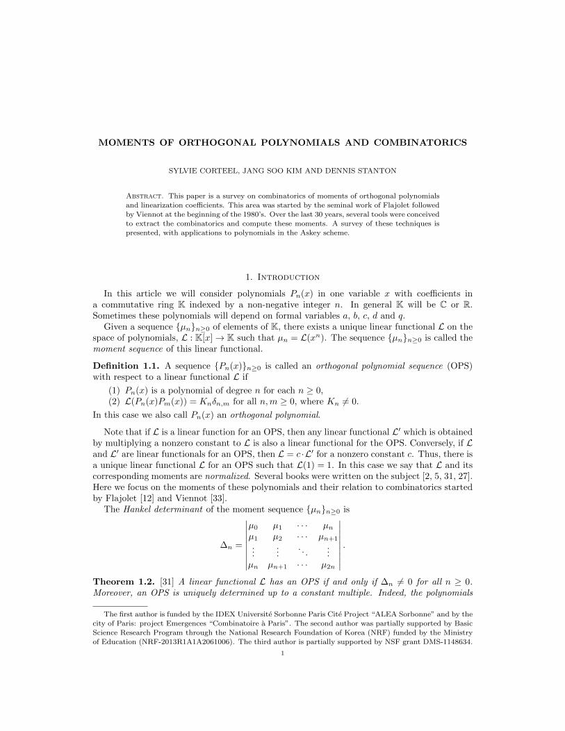
MOMENTS OF ORTHOGONAL POLYNOMIALS AND COMBINATORICS

SYLVIE CORTEEL, JANG SOO KIM AND DENNIS STANTON

Abstract. This paper is a survey on combinatorics of moments of orthogonal polynomialsand linearization coe�cients. This area was started by the seminal work of Flajolet followedby Viennot at the beginning of the 1980’s. Over the last 30 years, several tools were conceivedto extract the combinatorics and compute these moments. A survey of these techniques ispresented, with applications to polynomials in the Askey scheme.

1. Introduction

In this article we will consider polynomials Pn(x) in one variable x with coe�cients ina commutative ring K indexed by a non-negative integer n. In general K will be C or R.Sometimes these polynomials will depend on formal variables a, b, c, d and q.

Given a sequence {µn}n�0 of elements of K, there exists a unique linear functional L on thespace of polynomials, L : K[x] ! K such that µn = L(xn). The sequence {µn}n�0 is called themoment sequence of this linear functional.

Definition 1.1. A sequence {Pn(x)}n�0 is called an orthogonal polynomial sequence (OPS)with respect to a linear functional L if

(1) Pn(x) is a polynomial of degree n for each n � 0,(2) L(Pn(x)Pm(x)) = Kn�n,m for all n, m � 0, where Kn 6= 0.

In this case we also call Pn(x) an orthogonal polynomial.

Note that if L is a linear function for an OPS, then any linear functional L0 which is obtainedby multiplying a nonzero constant to L is also a linear functional for the OPS. Conversely, if Land L0 are linear functionals for an OPS, then L = c ·L0 for a nonzero constant c. Thus, there isa unique linear functional L for an OPS such that L(1) = 1. In this case we say that L and itscorresponding moments are normalized. Several books were written on the subject [2, 5, 31, 27].Here we focus on the moments of these polynomials and their relation to combinatorics startedby Flajolet [12] and Viennot [33].

The Hankel determinant of the moment sequence {µn}n�0 is

�n =

��

µ0 µ1 · · · µn

µ1 µ2 · · · µn+1...

.... . .

...µn µn+1 · · · µ2n

��

.

Theorem 1.2. [31] A linear functional L has an OPS if and only if �n 6= 0 for all n � 0.Moreover, an OPS is uniquely determined up to a constant multiple. Indeed, the polynomials

The first author is funded by the IDEX Universite Sorbonne Paris Cite Project “ALEA Sorbonne” and by thecity of Paris: project Emergences “Combinatoire a Paris”. The second author was partially supported by BasicScience Research Program through the National Research Foundation of Korea (NRF) funded by the Ministryof Education (NRF-2013R1A1A2061006). The third author is partially supported by NSF grant DMS-1148634.

1

2 SYLVIE CORTEEL, JANG SOO KIM AND DENNIS STANTON

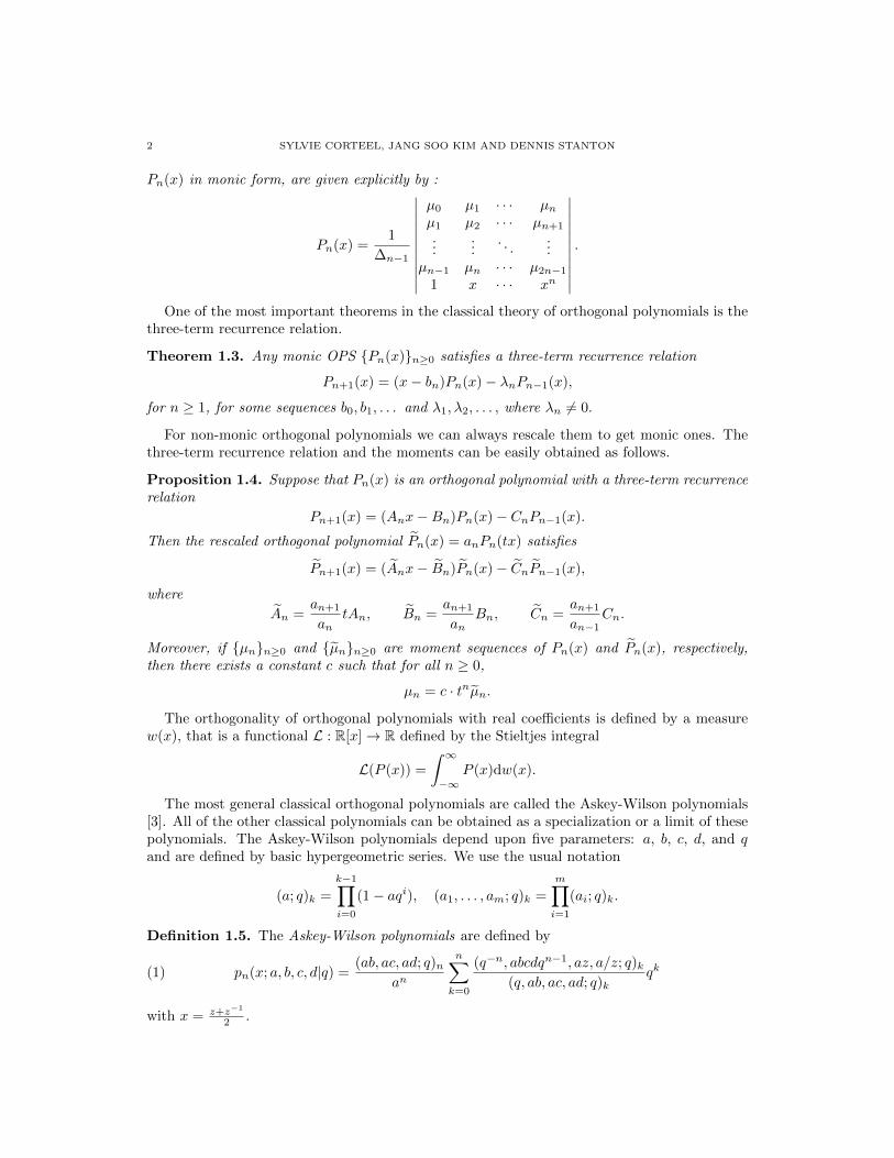
Pn(x) in monic form, are given explicitly by :

Pn(x) =1

�n�1

��

µ0 µ1 · · · µn

µ1 µ2 · · · µn+1...

.... . .

...µn�1 µn · · · µ2n�1

1 x · · · xn

��

.

One of the most important theorems in the classical theory of orthogonal polynomials is thethree-term recurrence relation.

Theorem 1.3. Any monic OPS {Pn(x)}n�0 satisfies a three-term recurrence relation

Pn+1(x) = (x � bn)Pn(x) � �nPn�1(x),

for n � 1, for some sequences b0, b1, . . . and �1,�2, . . . , where �n 6= 0.

For non-monic orthogonal polynomials we can always rescale them to get monic ones. Thethree-term recurrence relation and the moments can be easily obtained as follows.

Proposition 1.4. Suppose that Pn(x) is an orthogonal polynomial with a three-term recurrencerelation

Pn+1(x) = (Anx � Bn)Pn(x) � CnPn�1(x).

Then the rescaled orthogonal polynomial ePn(x) = anPn(tx) satisfies

ePn+1(x) = ( eAnx � eBn) ePn(x) � eCnePn�1(x),

whereeAn =

an+1

antAn, eBn =

an+1

anBn, eCn =

an+1

an�1Cn.

Moreover, if {µn}n�0 and {eµn}n�0 are moment sequences of Pn(x) and ePn(x), respectively,then there exists a constant c such that for all n � 0,

µn = c · tneµn.

The orthogonality of orthogonal polynomials with real coe�cients is defined by a measurew(x), that is a functional L : R[x] ! R defined by the Stieltjes integral

L(P (x)) =

Z 1

�1P (x)dw(x).

The most general classical orthogonal polynomials are called the Askey-Wilson polynomials[3]. All of the other classical polynomials can be obtained as a specialization or a limit of thesepolynomials. The Askey-Wilson polynomials depend upon five parameters: a, b, c, d, and qand are defined by basic hypergeometric series. We use the usual notation

(a; q)k =k�1Y

i=0

(1 � aqi), (a1, . . . , am; q)k =mY

i=1

(ai; q)k.

Definition 1.5. The Askey-Wilson polynomials are defined by

(1) pn(x; a, b, c, d|q) =(ab, ac, ad; q)n

an

nX

k=0

(q�n, abcdqn�1, az, a/z; q)k

(q, ab, ac, ad; q)kqk

with x = z+z�1

2 .

MOMENTS OF ORTHOGONAL POLYNOMIALS AND COMBINATORICS 3

These functions are polynomials in x of degree n due to the relation

(az, a/z; q)k =k�1Y

j=0

(1 � 2axqj + a2q2j).

A representing measure for the Askey-Wilson polynomials may be given for 0 < q < 1 andmax{|a|, |b|, |c|, |d|} < 1. The orthogonality relation is

Z ⇡

0pn(cos ✓; a, b, c, d|q)pm(cos ✓; a, b, c, d|q)w(cos ✓; a, b, c, d|q)d✓ = 0, n 6= m,

where x = cos ✓ and the measure is given by

w(x; a, b, c, d|q) =(z2, z�2; q)1

(az, a/z, bz, b/z, cz, c/z, dz, d/z; q)1.

The enumeration formula and the combinatorics of the moments of these polynomials wererecently presented in [9, 10, 25, 26]. A recent catalog on known enumeration formulas formoments appeared in [28].

In this paper, we will consider the moments of orthogonal polynomials of the Askey scheme,and emphasize their relationship to combinatorial enumeration. In Section 2, we give a generalinterpretation of the orthogonal polynomials and their moments using paths [33]. In Section3, we introduce some basic combinatorics related to the moments of Hermite, Charlier andLaguerre polynomials and their q-analogues. This was first started in the memoir of Viennot[33] and then in a series of papers by several authors. In Section 4, we present an odd-even trickwhich is often useful to compute moments and can also give non-trivial combinatorial results.In Section 5, we focus on the case of the Askey-Wilson moments and their enumeration formula.In Section 6, we present some modified moments coming from the Askey-Wilson basis. We endin Section 7 with linearization coe�cients.

This paper is a survey and contains a collection of diverse results; so that the interested readercan learn a series of important tools built for the study of moments of orthogonal polynomials.

2. Path interpretation of the polynomials and the moments

For general orthogonal polynomials which satisfy Theorem 1.3, the moments µn are alwayspolynomials in the three-term recurrence coe�cients with non-negative integral coe�cients. Forexample,

µ0 = 1, µ1 = b0, µ2 = b20 + �1, µ3 = b3

0 + 2b0�1 + b1�1.

The orthogonal polynomials pn(x) may also be given as polynomials in x and the three-termrecurrence coe�cients, but not necessarily positive. For example,

p0(x) = 1, p1(x) = x � b0, p2(x) = x2 � (b0 + b1)x + (b0b1 � �1).

The purpose of this section is to give combinatorial interpretations for these two phenomenausing paths.

Paths live in the quarter plane ⇧ = N ⇥ N. A path ! is a sequence ! = (s0, . . . , sn) wheresi = (xi, yi) 2 ⇧. The si’s are the vertices of the path. The starting vertex is s0, the endingvertex is sn and (si, si+1) is an elementary step of the path.

The step (si, si+1) is called

• North if xi = xi+1 and yi + 1 = yi+1;• North-North if xi = xi+1 and yi + 2 = yi+1;• North-East if xi + 1 = xi+1 and yi + 1 = yi+1;• South-East if xi + 1 = xi+1 and yi � 1 = yi+1; and• East if xi + 1 = xi+1 and yi = yi+1.


The paths are weighted. There is a partial application wt : ⇧ ⇥ ⇧ ! K which associates toeach step (si, si+1) a weight wt(si, si+1) 2 K. The weight of the path ! is the product of theweight of the steps :

wt(!) =n�1Y

i=0

wt(si, si+1).

Definition 2.1. [33] A Favard path is a path ⌘ = (s0, . . . , sn) starting at s0 = (0, 0) with threetypes of elementary steps: North, North-North and North-East. The weight of the elementarystep (si, si+1) is x if the step is North-East and �bk (resp. ��k+1) if the step is North (resp.North-North) and the y-coordinate of si is k. The length of the path is the y-coordinate of sn.

Let Favn be the set of Favard paths of length n.

Lemma 2.2. [33] Let {Pn(x)} be a sequence of polynomials which satisfies the recurrence ofTheorem 1.3 and with boundary conditions P0(x) = 1 and P1(x) = x � b0. Then

Pn(x) =X

!2Favn

wt(!).

A Motzkin path of length n is a path consisting of North-East steps, East steps, and South-East steps which lies in the first quadrant. Let Motn,k,` be the set of Motzkin paths from (0, k)to (n, `), and let Motn = Motn,0,0.

Suppose that two sequences b = {bn}n�0 and � = {�n}n�1 are given. For a Motzkin pathP , we define wtb,�(P ) to be the product of the weight of every step in P , where the weight ofeach step is defined as follows.

(1) A North-East step has weight 1.(2) An East step has weight bk, where k is the y-coordinate of starting point.(3) A South-East step has weight �k, where k is the y-coordinate of starting point.

For the remainder of this section we assume that Pn(x) are orthogonal polynomials given byP�1(x) = 0, P0(x) = 1, and for n � 1,

Pn+1(x) = (x � bn)Pn(x) � �nPn�1(x),

with the normalized linear functional L and the nth moment µn = L(xn).

Theorem 2.3. [33] We have

µn =X

!2Motn

wtb,�(!).

We will sketch a proof of a generalization of Theorem 2.3 that also gives a combinatorialproof of the orthogonality.

Theorem 2.4. [33] For all n, k, `,

(2) L(xnPk(x)P`(x)) = �1 · · ·�`

X

!2Motn,k,`

wt(!).

Proof. (Sketch [33].) The proof of this theorem uses the combinatorial interpretation of thepolynomials as Favard paths. Let En,k,` be the set of triplets made of

• A Favard path f of length k• A Favard path g of length `• A Motzkin path ! of length n + p(f) + p(g) where p(f) is the number of North-East

steps of f .


Let Fn,k,` be the subset of En,k,` where p(f) = k, p(g) = ` and ! starts with k North-East stepsand ends with ` South-East steps. Proving the theorem is equivalent to defining a sign-reversinginvolution ✓ on En,k,` whose fixed points are exactly the elements in the set Fn,k,`. Let j bethe minimal index such that (sj , sj+1) is an East step or a South-East step in !. If j < kthen let h(!) = yj otherwise h(!) = 1. Let fj be the first step of f which is a North or aNorth-North step. Let h(f) = j if such a j exists otherwise h(f) = 1. If h(!) or h(f) is finite,then if h(f) � 1 is smaller than or equal to h(!), if the h(f)th step of f is North-North, we adda North-East step and a South-East step to ! in position h(f)� 1 and change the North-Northstep to two North-East steps; otherwise (it is a North step), we add an East step to ! in positionh(f). The step in f is changed to one North-East step. Otherwise (h(f) � 1 > h(!)), we takeo↵ the first East step or the first South-East step and its previous North-East step from ! andchange two North-East steps in f by a North-North step or one North-East step in f by aNorth step. One can easily check that this changes the sign. If both h’s are infinite, we apply asimilar algorithm on g and the last ` steps of !. The only triplets where the algorithm cannotbe applied are exactly the ones in Fn,k,`. ⇤

Note that this implies that

L(Pk(x)P`(x)) = �1 . . .�`�k`.

and this gives a proof of the orthogonality relation.Let

Ci(z) =1

1 � b0+iz � �1+iz2

1 � b1+iz � �2+iz2

. . .

.

Using the theory of Flajolet [12] we have

Corollary 2.5. We have

X

n�0

µnzn =1

1 � b0z � �1z2

1 � b1z � �2z2

. . .

= C0(z);

X

n�0

L(xnP`(x))zn = �1 · · ·�`z`Y

i=0

Ci(z);

X

n�0

L(xnP`(x)Pk(x))zn =

min(k,`)X

j=0

�1 · · ·�jCj(z)Y

i=j+1

�izCi(z)kY

i=j+1

�izCi(z).

The last equation in Corollary 2.5 can be proved by observing the fact that we can uniquelydecompose a Motzkin path ! 2 Motn,k,` as

! = !k�jD · · ·!1D!0U!01 · · · U!0

`�j ,

where j is a nonnegative integer, each !i and !0i is a Motzkin path in which the starting and

ending vertices have the smallest y-coordinates, D is a South-East step, and U is a North-Eaststep.


BIJECTIONS ON TWO VARIATIONS OF NONCROSSING

PARTITIONS

JANG SOO KIM

Abstract. We find bijections on 2-distant noncrossing partitions, 12312-avoidingpartitions, 3-Motzkin paths, UH-free Schroder paths and Schroder paths with-out peaks at even height. We also give a direct bijection between 2-distantnoncrossing partitions and 12312-avoiding partitions.

E-mail address: [email protected]

Date: June 18, 2015.2000 Mathematics Subject Classification. 05A18, 05A15.Key words and phrases. noncrossing partition, Motzkin path, Schroder path.

1 2 3 4 5 6 7 8 9

Figure 1. The standard representation of ({1, 4, 8}, {2, 5, 9}, {3}, {6, 7}).

0

2 012

22

1 22

12

� f0

0

2 0

0 2

0 2 2 2 2

2

Figure 2. An example of f0.

1

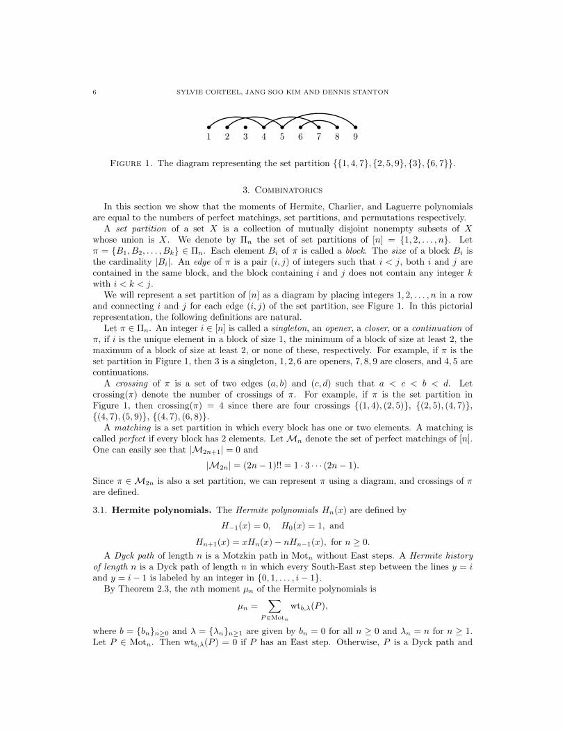
Figure 1. The diagram representing the set partition {{1, 4, 7}, {2, 5, 9}, {3}, {6, 7}}.

3. Combinatorics

In this section we show that the moments of Hermite, Charlier, and Laguerre polynomialsare equal to the numbers of perfect matchings, set partitions, and permutations respectively.

A set partition of a set X is a collection of mutually disjoint nonempty subsets of Xwhose union is X. We denote by ⇧n the set of set partitions of [n] = {1, 2, . . . , n}. Let⇡ = {B1, B2, . . . , Bk} 2 ⇧n. Each element Bi of ⇡ is called a block. The size of a block Bi isthe cardinality |Bi|. An edge of ⇡ is a pair (i, j) of integers such that i < j, both i and j arecontained in the same block, and the block containing i and j does not contain any integer kwith i < k < j.

We will represent a set partition of [n] as a diagram by placing integers 1, 2, . . . , n in a rowand connecting i and j for each edge (i, j) of the set partition, see Figure 1. In this pictorialrepresentation, the following definitions are natural.

Let ⇡ 2 ⇧n. An integer i 2 [n] is called a singleton, an opener, a closer, or a continuation of⇡, if i is the unique element in a block of size 1, the minimum of a block of size at least 2, themaximum of a block of size at least 2, or none of these, respectively. For example, if ⇡ is theset partition in Figure 1, then 3 is a singleton, 1, 2, 6 are openers, 7, 8, 9 are closers, and 4, 5 arecontinuations.

A crossing of ⇡ is a set of two edges (a, b) and (c, d) such that a < c < b < d. Letcrossing(⇡) denote the number of crossings of ⇡. For example, if ⇡ is the set partition inFigure 1, then crossing(⇡) = 4 since there are four crossings {(1, 4), (2, 5)}, {(2, 5), (4, 7)},{(4, 7), (5, 9)}, {(4, 7), (6, 8)}.

A matching is a set partition in which every block has one or two elements. A matching iscalled perfect if every block has 2 elements. Let Mn denote the set of perfect matchings of [n].One can easily see that |M2n+1| = 0 and

|M2n| = (2n � 1)!! = 1 · 3 · · · (2n � 1).

Since ⇡ 2 M2n is also a set partition, we can represent ⇡ using a diagram, and crossings of ⇡are defined.

3.1. Hermite polynomials. The Hermite polynomials Hn(x) are defined by

H�1(x) = 0, H0(x) = 1, and

Hn+1(x) = xHn(x) � nHn�1(x), for n � 0.

A Dyck path of length n is a Motzkin path in Motn without East steps. A Hermite historyof length n is a Dyck path of length n in which every South-East step between the lines y = iand y = i � 1 is labeled by an integer in {0, 1, . . . , i � 1}.

By Theorem 2.3, the nth moment µn of the Hermite polynomials is

µn =X

P2Motn

wtb,�(P ),

where b = {bn}n�0 and � = {�n}n�1 are given by bn = 0 for all n � 0 and �n = n for n � 1.Let P 2 Motn. Then wtb,�(P ) = 0 if P has an East step. Otherwise, P is a Dyck path and


BIJECTIONS ON TWO VARIATIONS OF NONCROSSING

PARTITIONS

JANG SOO KIM

Abstract. We find bijections on 2-distant noncrossing partitions, 12312-avoidingpartitions, 3-Motzkin paths, UH-free Schroder paths and Schroder paths with-out peaks at even height. We also give a direct bijection between 2-distantnoncrossing partitions and 12312-avoiding partitions.


Date: June 18, 2015.2000 Mathematics Subject Classification. 05A18, 05A15.Key words and phrases. noncrossing partition, Motzkin path, Schroder path.

1 2 3 4 5 6 7 8 9

1 2 3 4 5 6 7 8 9 10 11 12�

1

2

0

0

1

0


0

2 012

22

1 22

12

� f0

0

1 0

0 1

0 2 2 1 2

2


1

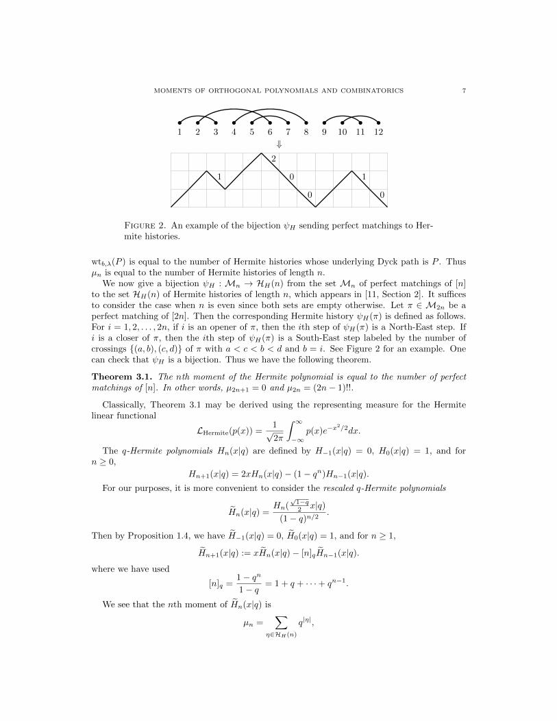
Figure 2. An example of the bijection H sending perfect matchings to Her-mite histories.

wtb,�(P ) is equal to the number of Hermite histories whose underlying Dyck path is P . Thusµn is equal to the number of Hermite histories of length n.

We now give a bijection H : Mn ! HH(n) from the set Mn of perfect matchings of [n]to the set HH(n) of Hermite histories of length n, which appears in [11, Section 2]. It su�cesto consider the case when n is even since both sets are empty otherwise. Let ⇡ 2 M2n be aperfect matching of [2n]. Then the corresponding Hermite history H(⇡) is defined as follows.For i = 1, 2, . . . , 2n, if i is an opener of ⇡, then the ith step of H(⇡) is a North-East step. Ifi is a closer of ⇡, then the ith step of H(⇡) is a South-East step labeled by the number ofcrossings {(a, b), (c, d)} of ⇡ with a < c < b < d and b = i. See Figure 2 for an example. Onecan check that H is a bijection. Thus we have the following theorem.

Theorem 3.1. The nth moment of the Hermite polynomial is equal to the number of perfectmatchings of [n]. In other words, µ2n+1 = 0 and µ2n = (2n � 1)!!.

Classically, Theorem 3.1 may be derived using the representing measure for the Hermitelinear functional

LHermite(p(x)) =1p2⇡

Z 1

�1p(x)e�x2/2dx.

The q-Hermite polynomials Hn(x|q) are defined by H�1(x|q) = 0, H0(x|q) = 1, and forn � 0,

Hn+1(x|q) = 2xHn(x|q) � (1 � qn)Hn�1(x|q).For our purposes, it is more convenient to consider the rescaled q-Hermite polynomials

eHn(x|q) =Hn(

p1�q2 x|q)

(1 � q)n/2.

Then by Proposition 1.4, we have eH�1(x|q) = 0, eH0(x|q) = 1, and for n � 1,

eHn+1(x|q) := x eHn(x|q) � [n]q eHn�1(x|q).where we have used

[n]q =1 � qn

1 � q= 1 + q + · · · + qn�1.

We see that the nth moment of eHn(x|q) is

µn =X

⌘2HH(n)

q|⌘|,


where |⌘| is the sum of labels of South-East steps. The bijection H : Mn ! HH(n) satisfiescrossing(⇡) = | H(⌘)|. Thus we obtain the following theorem.

Theorem 3.2. [19, Eq. (3.8)] The nth moment of the rescaled q-Hermite polynomials eHn(x|q)is

µn =X

⇡2Mn

qcrossing(⇡).

The rescaled discrete q-Hermite polynomials ehn(x; q) are defined by eh�1(x; q) = 0, eh0(x; q) =1, and for n � 0,

ehn+1(x; q) = xehn(x; q) � qn�1[n]qehn�1(x; q).

Again the odd moments are 0. The analogous version to Theorem 3.2 is the next result.

Theorem 3.3. [30, p. 310, (5.4)] The 2nth moment of the rescaled discrete q-Hermite polyno-

mials ehn(x; q) is

µ2n = [1]q[3]q · · · [2n � 1]q =X

⇡2M2n

qcrossing(⇡)+2 nesting(⇡),

where nesting(⇡) is the number of pairs of two edges (a, b) and (c, d) of ⇡ such that a < c < d < b.

3.2. Charlier polynomials. The Charlier polynomials Cn(x) are defined by

Cn+1(x) = (x � n � 1)Cn(x) � nCn�1(x),

for n � 1 with initial conditions C�1(x) = 0 and C0(x) = 1.

Theorem 3.4. The nth moment of the Charlier polynomials is equal to the number of setpartitions of [n].

Theorem 3.4 may be derived using the representing measure for the Charlier linear functional

LCharlier(p(x)) =1

e

1X

n=0

p(n)1

n!.

We will instead prove a generalization of the above theorem using the q-Charlier polynomialsCn(x, a; q) given by

Cn+1(x, a; q) = (x � a � [n]q)Cn(x, a; q) � a[n]qCn�1(x, a; q).

A Charlier history of length n is a Motzkin path of length n in which every South-East stepbetween the lines y = i and y = i � 1 is labeled by an integer in {0, 1, . . . , i � 1} and every Easton the line y = i is either unlabeled or labeled by an integer in {0, 1, . . . , i � 1}.

By Theorem 2.3, the nth moment µn of the Charlier polynomials is

µn =X

P2Motn

wtb,�(P ),

where b = {bn}n�0 and � = {�n}n�1 are given by bn = n + a for all n � 0 and �n = an forn � 1. Let P 2 Motn. Then

wtb,�(P ) =X

⌘

aunlabeled(⌘)q|⌘|,

where the sum is over all Charlier histories ⌘ with underlying Motzkin path P , unlabeled(⌘) isthe number of unlabeled steps of ⌘ and |⌘| is the sum of labels in ⌘.

We now give a bijection C : ⇧n ! HC(n) from the set ⇧n of set partitions of [n] to theset HC(n) of Charlier histories of length n. This map can be considered as a special case of


2 JANG SOO KIM

1 2 3 4 5 6 7 8 9

1 2 3 4 5 6 7 8 9 10 11 12�

1

2

0

0

1

0

1 2 3 4 5 6 7 8 9 10 11 12 13 14�

00

21

0 1

0

1 2 3 4 5 6 7 8 9

��2 +2 +1

(0, 1)

(0, 0)


0

2 012

22

1 22

12

� f0

0

1 0

0 1

0 2 2 1 2

2


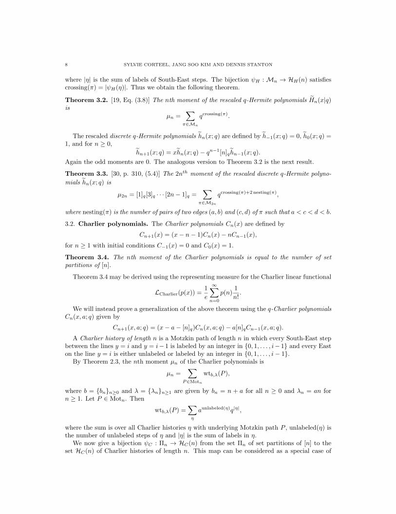
Figure 3. An example of the bijection C sending set partitions to Charlier histories.

Foata and Zeilberger’s map [13], which will be described in the next subsection. Let ⇡ 2 ⇧n bea set partition of [n]. Then the corresponding Charlier history C(⇡) = ⌘ is defined as follows.For i = 1, 2, . . . , n, if i is an opener of ⇡, then the ith step of ⌘ is a North-East step. If i isa closer of ⇡, then the ith step of ⌘ is a South-East step labeled by the number of crossings{(a, b), (c, d)} of ⇡ with a < c < b < d and b = i. If i is a singleton of ⇡, then the ith step of ⌘ isan unlabeled East step. If i is a continuation of ⇡, then the ith step of ⌘ is an East step labeledby the number of crossings {(a, b), (c, d)} of ⇡ with a < c < b < d and b = i. See Figure 3 foran example.

It is easy to see that C is a bijection such that if C(⇡) = ⌘ then unlabeled(⌘) = block(⇡)and |⌘| = crossing(⇡). This implies the following theorem due to Kim, Stanton, and Zeng [24,Theorem 4].

Theorem 3.5. The q-Charlier polynomials Cn(x, a; q) given by

Cn+1(x, a; q) = (x � a � [n]q)Cn(x, a; q) � a[n]qCn�1(x, a; q)

has the nth momentµn =

X

⇡2⇧n

ablock(⇡)qcrossing(⇡).

3.3. Laguerre polynomials. The Laguerre polynomials Ln(x) are defined by

Ln+1(x) = (x � 2n � 1)Ln(x) � n2Ln�1(x).

Theorem 3.6. The nth moment of the Laguerre polynomials Ln(x) is equal to the number ofpermutations of [n], that is, µn = n!.

Theorem 3.6 may be derived using the representing measure for the Laguerre linear functional

LLaguerre(p(x)) =

Z 1

0p(x)e�xdx.

We will consider the following generalization of the above theorem.The q-Laguerre polynomials Ln(x; q) are defined by

Ln+1(x; q) = (x � [n]q � y[n + 1]q)Ln(x; a) � y[n]2qLn�1(x; q).

A Laguerre history of length n is a Motzkin path of length n in which every North-East orSouth-East step between the lines y = i and y = i�1 is labeled by an integer in {0, 1, . . . , i�1}and every East step on the line y = i is either unlabeled or labeled by an integer in {�i, �i +1, . . . , �1, 0, 1, . . . , i � 1}.


2 JANG SOO KIM

1 2 3 4 5 6 7 8 9

1 2 3 4 5 6 7 8 9 10 11 12�

1

2

0

0

1

0

1 2 3 4 5 6 7 8 9 10 11 12 13 14�

00

21

0 1

0

1 2 3 4 5 6 7 8 9 10 11 12 13 14

�

0

1

0 0 0+2

2

1 0 1 �1 �10

1 2 3 4 5 6 7 8 9

��2 +2 +1

(0, 1)

(0, 0)


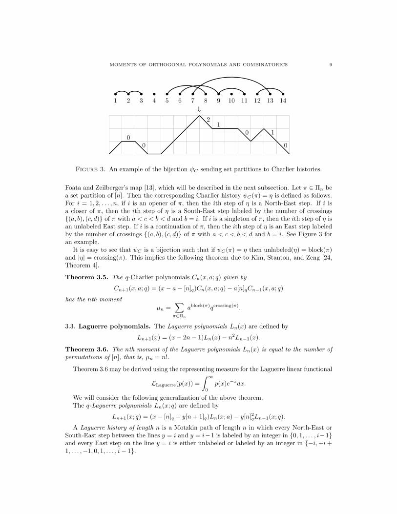
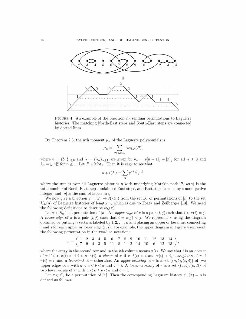
Figure 4. An example of the bijection �L sending permutations to Laguerrehistories. The matching North-East steps and South-East steps are connectedby dotted lines.

By Theorem 2.3, the nth moment µn of the Laguerre polynomials is

µn =X

P2Motn

wtb,�(P ),

where b = {bn}n�0 and � = {�n}n�1 are given by bn = y[n + 1]q + [n]q for all n � 0 and�n = y[n]2q for n � 1. Let P 2 Motn. Then it is easy to see that

wtb,�(P ) =X

⌘

yw(⌘)q|⌘|,

where the sum is over all Laguerre histories ⌘ with underlying Motzkin path P , w(⌘) is thetotal number of North-East steps, unlabeled East steps, and East steps labeled by a nonnegativeinteger, and |⌘| is the sum of labels in ⌘.

We now give a bijection L : Sn ! HL(n) from the set Sn of permutations of [n] to the setHL(n) of Laguerre histories of length n, which is due to Foata and Zeilberger [13]. We needthe following definitions to describe L(⇡).

Let ⇡ 2 Sn be a permutation of [n]. An upper edge of ⇡ is a pair (i, j) such that i < ⇡(i) = j.A lower edge of ⇡ is a pair (i, j) such that i = ⇡(j) < j. We represent ⇡ using the diagramobtained by putting n vertices labeled by 1, 2, . . . , n and placing an upper or lower arc connectingi and j for each upper or lower edge (i, j). For example, the upper diagram in Figure 4 representthe following permutation in the two-line notation:

⇡ =

✓1 2 3 4 5 6 7 8 9 10 11 12 13 147 9 4 3 5 11 8 1 2 14 10 6 12 13

◆,

where the entry in the second row and in the ith column means ⇡(i). We say that i is an openerof ⇡ if i < ⇡(i) and i < ⇡�1(i), a closer of ⇡ if ⇡�1(i) < i and ⇡(i) < i, a singleton of ⇡ if⇡(i) = i, and a transient of ⇡ otherwise. An upper crossing of ⇡ is a set {(a, b), (c, d)} of twoupper edges of ⇡ with a < c < b < d and b = i. A lower crossing of ⇡ is a set {(a, b), (c, d)} oftwo lower edges of ⇡ with a < c b < d and b = i.

Let ⇡ 2 Sn be a permutation of [n]. Then the corresponding Laguerre history L(⇡) = ⌘ isdefined as follows.


For i = 1, 2, . . . , n, if i is an opener of ⇡, then the ith step of ⌘ is a North-East step whoselabel will be determined later. If i is a closer of ⇡, then the ith step of ⌘ is a South-Eaststep. In this case suppose that the jth step and ith step are the matching North-East step andSouth-East step. Then the label of the jth step (resp. ith step) is the number of upper crossings(resp. lower crossings) {(a, b), (c, d)} of ⇡ with a < c < b < d and b = i. If i is a singleton, thenthe ith step of ⌘ is an unlabeled East step. Finally suppose that i is a continuation of ⇡. Thenthe ith step of ⌘ is an East step whose labeled determined as follows. If the vertex i is incidentto two upper edges, then the label is +k, where k is the number of upper crossings {(a, b), (c, d)}of ⇡ with a < c < b < d and b = i. If the vertex i is incident to two lower edges, then thelabel is �k, where k is the number of lower crossings {(a, b), (c, d)} of ⇡ with a < c b < d andb = i. See Figure 4 for an example.

One can check that �L is a bijection such that if �L(⇡) = ⌘ then wex(⇡) = w(⌘) andcrossing(⇡) = |⌘|. Here wex(⇡) is the number of weak excedances, which are integers i suchthat i ⇡(i). Thus we obtain the following theorem, which is shown in [23, Theorem 2]. Anequivalent version of this theorem in terms of continued fractions has been proved earlier, see[30, 6].

Theorem 3.7. The q-Laguerre polynomials Ln(x; q) has the nth moment

µn =X

⇡2Sn

ywex(⇡)qcrossing(⇡).

Corteel et al. [8] showed that the moment has several interpretations in terms of permuta-tions, permutation tableaux, matrix anszatz, etc. Simion and Stanton [30] consider octabasicLaguerre polynomials (whose recurrence relation has eight independent q’s) and express theirmoments using various statistics of permutations.

4. The odd-even trick

In this section we give a relation between moments for two di↵erent sets of orthogonalpolynomials. We call this occurrence the odd-even trick. It occurs for the three cases consideredin Section 3, and o↵ers alternative combinatorial interpretations for the moments. This ideaappears in [5, p. 40].

Definition 4.1. For an orthogonal polynomial satisfying the Theorem 2.4, let

µn = µn({bk}k�0, {�k}k�1)

denote the nth moment.

From Theorem 2.4, µn is a positive polynomial function of the three-term recurrence coe�-cients. The odd-even trick is the observation that if bk = 0 for all k, the polynomials pn(x) arealternately even and odd. Moreover if

p2n(x) = en(x), p2n+1(x) = xon(x2),

the even and polynomials en(x) and on(x) are themselves orthogonal polynomials. The momentsequences for en(x) and on(x) are related to the moment sequence of pn(x).

Proposition 4.2. Given a sequence �k with �0 = 0 we have

µ2n(0, {�k}k�1) =µn({�2k + �2k+1}k�0, {�2k�1�2k}k�1),

µ2n+2(0, {�k}k�1) =�1µn({�2k+1 + �2k+2}k�0, {�2k�2k+1}k�1).

Proof. There are several ways to prove this. We give a sketch of the combinatorial proof dueto Viennot [34]. The first statement is equivalent to a bijection between


• Dyck paths of length 2n where South-East steps starting at y-coordinate k are weightedby �k,

• Motzkin paths of length n where the East steps (resp. South-East steps) starting aty-coordinate k are weighted by �2k + �2k+1 (resp. �2k�2k�1).

Starting with a Dyck path of length 2n, (s0, . . . , s2n). For i from 0 to n � 1, suppose thats2i = (2i, 2k)

• If (s2i, s2i+1) and (s2i+1, s2i+2) are North-East steps, change them to one North-Eaststep;

• If (s2i, s2i+1) and (s2i+1, s2i+2) are South-East steps, change them to one South-Eaststep weighted by �2k�2k�1;

• If (s2i, s2i+1) is a South-East step and (s2i+1, s2i+2) is a North-East step, change themto one East step weighted by �2k;

• If (s2i, s2i+1) is a North-East step and (s2i+1, s2i+2) is a South-East step, change themto one East step weighted by �2k+1.

This gives a Motzkin path of length n with the correct weights. The second statement isequivalent to a bijection between

• Dyck paths of length 2n + 2 where South-East steps starting at y-coordinate k areweighted by �k

• Motzkin paths of length n where the East steps (resp. South-East step) starting aty-coordinate k are weighted by �2k+1 + �2k+2 (resp. �2k+1�2k).

One needs to delete the first and last step of the Dyck path and apply the same bijection andadjust the weights accordingly. ⇤

Example 4.3. The Hermite polynomials have bk = 0, �k = k, so

(2n � 1)!! = µ2n(0, {k}k�1) = µn({4k + 1}k�0, {2k(2k � 1)}k�1).

Example 4.4. The Laguerre polynomials have bk = 2k + 1, �k = k2, so

n! = µn({2k + 1}k�0, {k2}k�1) = µ2n(0, {b(k + 1)/2c}k�1).

Example 4.5. The q-Charlier polynomials have bk = a + [k]q, �k = a[k]q, so in this case

µn({b}k�0, {�k}k�1) = µ2n(0, {⇤k}k�1),

where

⇤k =

([k/2]q, if k is even,

a, if k is odd.

Example 4.6. The renormalized Askey-Wilson polynomials Qn(y) (see Proposition 5.1)

y = a + a�1 � 2x, Qn(y) = (�1)nPn(x)

satisfy Theorem 1.3 withbk = Ak�1 + Ck, �k = AkCk.

In this caseµn({bk}k�0, {�k}k�1) = µ2n(0, {⇤k}k�1),

where

⇤k =

(Ck/2, if k is even,

A(k�1)/2, if k is odd.

The next Theorem follows from Example 4.6.


Theorem 4.7. Let

✓2n = µ2n(0, {⇤k}k�1).

The Askey-Wilson moments satisfy

2nµn(a, b, c, d|q) =nX

s=0

✓n

s

◆(a + 1/a)s(�1)n�s✓2n�2s.

Using the Proposition 4.2 we see

Corollary 4.8. Given a sequence ak for k � 0 with a0 = 0 we have

µn({a2k+1 + a2k}k�0, {a2ka2k�1}k�1) = a1µn�1({a2k+2 + a2k+1}k�0, {a2k+1a2k}k�1).

Example 4.9. The Laguerre polynomials have bk = 2k + 1, �k = k2, so ak = dk/2e(n + 1)! = µn+1({2k + 1}k�0, {k2}k�1) = µn({2k + 2}k�0, {k(k + 1)}k�1).

5. Askey-Wilson moments

In this section we consider the Askey-Wilson polynomials and explicit forms for their mo-ments. Recall that these polynomials in x have five parameters: a, b, c, d, and q. In Sub-section 5.1 we give explicit formulas for the moments. In Subsection 5.2 we use a non-linearchange of variables on the parameters to obtain four new parameters ↵, �, �, and �. Usingthese parameters we give a combinatorial interpretation for the moments as weights of specialtableaux.

Recall from (1.5) that the Askey-Wilson polynomial pn(x; a, b, c, d|q) is not monic and hasthe leading term (abcd; q)n(2x)n. It is true, but not obvious, that the Askey-Wilson polynomialpn(x; a, b, c, d|q) is symmetric in all four parameters a, b, c, and d, not just b, c, and d.

Let

Pn(x) =1

(abcd; q)npn(x; a, b, c, d|q)

be the normalized Askey-Wilson (AW) polynomial whose leading term is (2x)n. The momentsequences for Pn(x) and pn(x; a, b, c, d|q) are the same. For historical reasons, and to agree withthe literature, we keep the 2x.

Proposition 5.1. The normalized Askey-Wilson polynomials Pn(x) satisfy the three-term re-currence relation :

Pn+1(x) = (2x � bn)Pn(x) � �nPn�1(x)

for n � 0 with P�1(x) = 0 and P0(x) = 1,

bn = (a + a�1 � An � Cn), �n = An�1Cn,

where

An =(1 � abqn)(1 � acqn)(1 � adqn)(1 � abcdqn�1)

a(1 � abcdq2n�1)(1 � abcdq2n),

Cn =a(1 � qn)(1 � bcqn�1)(1 � bdqn�1)(1 � cdqn�1)

(1 � abcdq2n�2)(1 � abcdq2n�1).

In this section, we will start by giving enumeration formulas for the moments of these poly-nomials. We will then present the combinatorics coming from staircase tableaux. We will endthe section with some special cases.


5.1. Enumeration formulas. The moments of the AW polynomials, denoted µn(a, b, c, d|q),are not polynomials in a, b, c, d and q. But it was recently proven [25, Proposition 2.1]that 2n(abcd; q)nµn(a, b, c, d|q) are polynomials in a, b, c, d, q with integer coe�cients. Severalexplicit formulas for µn(a, b, c, d|q) are known. The following is the simplest known expressionas a double sum.

Theorem 5.2. [9, Theorem 1.13] We have

µn(a, b, c, d|q) =1

2n

nX

m=0

(ab, ac, ad; q)m

(abcd; q)mqm

mX

j=0

q�j2

a�2j(aqj + q�j/a)n

(q, q1�2j/a2; q)j(q, q2j+1a2; q)m�j.

Theorem 5.2 was proved using techniques built in [17, 18]. The formula has two clear defects.It does not demonstrate the polynomiality of 2n(abcd; q)nµn(a, b, c, d|q) in a, and it not obviouslysymmetric in the four parameters a, b, c, and d.

A fivefold sum formula was found where the polynomiality is clear.

Corollary 5.3. [25, Theorem 5.6] We have


k=0

✓✓n

n�k2

◆�

✓n

n�k2 � 1

◆◆ X

u+v+w+x+2t=k

aubvcwdx

⇥ (ac; q)v(bd; q)w

(abcd; q)v+w(�1)tq(

t+12 )

u + v + w + t

u

�

q

v + w + x + t

v, w, x + t

�

q

u + x + t

x

�

q

,

where the second sum is over all integers u, v, w, x � 0 and �k t k/2 satisfying u + v +w + x + 2t = k.

A combinatorial approach to the proof of Corollary 5.3 is given in Section 7. When d = 0, themoments 2nµn(a, b, c, 0|q) are polynomials and there is an explicit polynomial formula whichalso establishes symmetry.

Corollary 5.4. [25, Theorem 2.3] The Askey-Wilson moments for d = 0 are

2nµn(a, b, c, 0|q) =nX

k=0

✓✓n

n�k2

◆�

✓n

n�k2 � 1

◆◆

⇥X

u+v+w+2t=k

aubvcw(�1)tq(t+12 )

u + v + t

v

�

q

v + w + t

w

�

q

w + u + t

u

�

q

,

where the second sum is over all integers u, v, w � 0 and �k t k/2 satisfying u+v+w+2t =k.

There is a result showing symmetry using very-well poised basic hypergeometric series.

Theorem 5.5. [25, Theorem 2.10] For an arbitrary A,


m=0

(aA, bA, cA, dA; q)m

(A2, abcd; q)m(�q)m

8W7(m)n+1X

s=0

✓✓n

s

◆�

✓n

s � 1

◆◆

⇥n�2s�mX

p=0

A�n+2s+2p

m + p

m

�

q

n � 2s � p

m

�

q

qm(�n+2s+p)+(m2 ),

where

8W7(m) = 8W7(A2/q; A/a, A/b, A/c, A/d, q�m; q, abcdqm),


and [14, Chap. 2.1]

8W7(a0; a1, . . . , a5; q, z) =1X

k=0

(1 � a0q2k)

(1 � a0)

(a0; q)k

(q; q)k

5Y

i=1

(ai; q)k

(qa0/ai; q)kzk.

The expression for 2n(abcd; q)nµn(a, b, c, d|q) in Theorem 5.5 is clearly symmetric in a, b, c,and d. From Theorem 5.5 it may be shown that it is a polynomial in these four parameters. Wedo not give the details here. Instead we o↵er another representation which shows polynomialitybut breaks symmetry

(3)(aA, bA, cA, dA; q)m

(A2; q)m8W7(m) =

mX

j=0

m

j

�

q

(cd)j(A/c, A/d; q)j(ab; q)j

⇥ (Aaqj , Abqj , cd; q)m�j .

The details appear in [25].The results in Corollaries 5.3 and 5.4, and Theorem 5.5, all involve a product of di↵erences

of binomial coe�cients and q-binomial coe�cients. The reason for this unusual behavior isthe form of Theorem 5.2. The power in the numerator leads to binomial coe�cients, while thedenominator terms lead to di↵erences of q-binomial coe�cients. This di↵erence can be switchedto the binomial coe�cients, giving the di↵erences that are displayed.

The proofs of these results are analytic and use properties of the Askey-Wilson functionalLAW. There is a combinatorial proof of the c = 0 case of Corollary 5.4 using weighted Motzkinpaths in [25]. Josuat-Verges also did this case (which is the Al-Salam-Chihara polynomials),see [20, Theorem 6.1.1]. The di↵erences of binomial coe�cients occur naturally in these com-binatorial approaches, see (14). A combinatorial proof of a general result remains open.

5.2. Combinatorics of the moments. We define here a combinatorial object that was definedto study the stationary distribution of the asymmetric exclusion process with open boundaries[32].

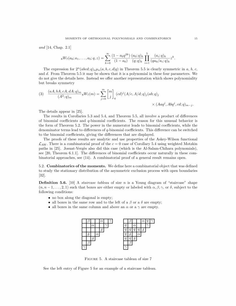
Definition 5.6. [10] A staircase tableau of size n is a Young diagram of “staircase” shape(n, n � 1, . . . , 2, 1) such that boxes are either empty or labeled with ↵,�, �, or �, subject to thefollowing conditions:

• no box along the diagonal is empty;• all boxes in the same row and to the left of a � or a � are empty;• all boxes in the same column and above an ↵ or a � are empty.


where

Bn =1/

py +

py + bn

1 � q, ⇤n =

An�1Cn

(1 � q)2

are given by the Askey-Wilson recurrence with the substitutions a ! a/p

y, b !bp

y, c ! c/p

y, d ! dp

y.

We also know an enumeration formula :

Theorem 6.4. [?]Zn(y; ↵, �, �, �; q) =

This formula is a polynomial in y; ↵, �, �, �; q with 4nn! coe�cients. This is noteasy to see from the previous formula. There are several easy proof that this is truefor y = q = 1.

When y = q = 1 this generating polynomial of the staircase tableau of size n is

(3) Zn(1, ↵, �, �, �, 1) =n�1Y

i=0

(↵ + � + � + � + i(↵ + �)(� + �))

We give here a simple bijective proof based on [?] :

Definition 6.5. • An inversion table of size n is a table T such that fori 2 {1, ..., n}, T [i] is a non-negative integer less than i.

• A colored inversion table of size n is a table T such that for i 2 {1, ..., n},T [i] = (i � 1)x with x 2 {↵, �, �, �} or T [i] = jx,y with 0 j < i � 1,x 2 {↵, �} and y 2 {�, �}.

The weight of a colored inversion table is the product of its colors. Computingthe generating polynomial of the colored inversion table is trivial and it is equalto :

nY

i=1

((↵ + �)(� + �)(i � 1) + ↵ + � + � + �)

��

�

↵�

��

�

↵↵�

��

�

↵�

��

�

↵↵� q

qq q q qqq q

Figure 1. A staircase tableau of size 7

Proposition 6.6. There exists a weight preserving bijection between staircase tableaux(with q = 1) of size n and colored inversion tables of size n.

Proof. Start with a staircase tableau of size n and number the columns from 1 ton from left to right and the rows from 1 to n from top to bottom. The bijection isobtained doing the following steps.

• For each column i, look at the topmost Greek letter in column i and countthe number of cells j directly to its left that does not contain any Greekletter.

Figure 5. A staircase tableau of size 7

See the left entry of Figure 5 for an example of a staircase tableau.


Definition 5.7. [10] The weight wt(T ) of a staircase tableau T is a monomial in ↵,�, �, �,and q, which we obtain as follows. Some blank boxes of T are assigned a q, based on the labelof the closest labeled box to its right in the same row and the label of the closest labeled boxbelow it in the same column, such that:

• every blank box which sees a � to its right gets assigned a q;• every blank box which sees an ↵ or � to its right, and a � or � below it, gets assigned

a q.

After this assignment, the weight of T , wt(T ) is then defined as the product of all labels in allboxes.

The right entry of Figure 5 shows that this staircase tableau has weight ↵3�2�3�3q9. Thetype of the tableau T is the number of ↵’s plus the number of �’s on the diagonal. We denoteit by t(T ).

Let

(4) Zn(y,↵,�, �, �, q) =X

Twt(T )yt(T ),

where the sum is taken on the staircase tableaux of size n.We now link this generating polynomial to the moments of the Askey-Wilson polynomials.

Let

a =1 � q � ↵+ � +

p(1 � q � ↵+ �)2 + 4↵�

2↵,

c =1 � q � ↵+ � � p

(1 � q � ↵+ �)2 + 4↵�

2↵,

b =1 � q � � + � +

p(1 � q � � + �)2 + 4��

2�,

d =1 � q � � + � � p

(1 � q � � + �)2 + 4��

2�.

Proposition 5.8 (see [9]; Theorem 1.11). The generating polynomial Zn(y;↵,�, �, �; q) is

(abcd; q)np

yn(↵�)n ⇥ µn

where µn are the moments of the orthogonal polynomials defined by

Gn+1(x) = (x � Bn)Gn(x) � ⇤nGn�1(x),

where

Bn =1/

py +

py + bn

1 � q, ⇤n =

An�1Cn

(1 � q)2

are given by the Askey-Wilson recurrence with the substitutions a ! a/p

y, b ! bp

y, c ! c/p

y,d ! d

py.

Remark 5.9. This proposition uses a result of [10] that relates the partition function of theASEP and the generating polynomial of the staircase tableaux. The proof is quite complicated.It is still an open problem to find a simple combinatorial proof.

Remark 5.10. The Askey-Wilson moments 2n(abcd; q)nµn(a, b, c, d|q) do not have positivecoe�cients as polynomials in a, b, c, d, and q. The change of variables in the parametersmiraculously does make these moments positive.


We also know an enumeration formula :

Theorem 5.11. [9, Theorem 1.14]

Zn(y;↵,�, �, �; q) = (abcd; q)n

✓↵�

1 � q

◆n nX

k=0

(ab, ac/y, ad; q)k

(abcd; q)kqk

⇥kX

j=0

q�(k�j)2(a2/y)j�k (1 + y + qk�ja + qj�ky/a)n

(q, q2j�2k+1y/a2; q)k�j(q, a2q1�2j+2k/y; q)j.

This formula is a polynomial in y,↵,�, �, �, q with positive coe�cients whose sum of coe�-cients is 4nn!. This is not easy to see from Theorem 5.11. The special case y = q = 1 does makethis clear.

Proposition 5.12. The generating polynomial of the staircase tableau of size n satisfies

(5) Zn(1,↵,�, �, �, 1) =n�1Y

i=0

(↵+ � + � + � + i(↵+ �)(� + �)).

We give here a simple bijective proof based on [7]. A colored inversion table of size n is atable T such that for i 2 {1, ..., n}, T [i] = (i � 1)x with x 2 {↵,�, �, �} or T [i] = jx,y with0 j < i � 1, x 2 {↵, �} and y 2 {�, �}. The weight of a colored inversion table is the productof its colors in {↵,�, �, �}. Computing the generating polynomial of the colored inversion tableis trivial and it is equal to :

n�1Y

i=0

(↵+ � + � + � + i(↵+ �)(� + �)).

Proposition 5.13. There exists a weight preserving bijection between staircase tableaux (withq = 1) of size n and colored inversion tables of size n.

Proof. Start with a staircase tableau of size n and number the columns from 1 to n from leftto right and the rows from 1 to n from top to bottom. The bijection is obtained doing thefollowing steps. For each column i, look at the topmost Greek letter in column i and count thenumber of cells j directly to its left that does not contain any Greek letter.

• If this letter, say x, is topmost and leftmost, record T [i] = ix.• Otherwise let y be the first Greek letter to the left of x and let z be the first Greek

letter under y. Then T [i] = jx,z.

We present the inverse of the algorithm. Start from a colored inversion table T of size n.Mark all the cells of the tableau as free. For i from n down to 1,

• if Ti = (i � 1)x, put an x in in the ith column, as high as possible. Mark all the cellsto its left as reserved.

• Otherwise, Ti is equal to some jx,y. Put an x in the ith column, as high as possible.Mark j boxes to its immediate left as reserved. Suppose that x is inserted in row k.

• Insert a y in column i � j � 1 as high as possible but in a row with a label larger thank (such a cell always exists as one can check that the diagonal box of column i � j � 1is still free). Mark all the cells to its left as reserved.

⇤

For example, we obtain the inversion table T = (0� , 1� , 2↵, 1↵,� , 2↵,�, 2�,�, 1�,�) from thetableau on the left of Figure 5, . Note that the proof of Proposition 5.13 gives a proof of (5).


5.3. Special cases. We give alternative proofs of special cases for Zn(y;↵,�, �, �; q) proven in[9, Table 1]. These were proven using the staircase tableaux and the matrix ansatz. We usehere the moments and the explicit three-term recurrence relation. The first result is new anddoes not have (yet) a combinatorial proof.

Proposition 5.14. If � = ��/y, then

Zn(y;↵,�, �, �; q) =n�1Y

j=0

(↵y + �qj).

Proof. First let’s check that the choice � = ��/y forces ⇤1 = 0, so that in Proposition 5.8µn = Bn

0 .In general we have bd = ��/�. So Proposition 5.1 and Proposition 5.8 imply that ⇤1 has

the numerator factor (1 � bdy) = (1 + y�/�) = 0.Since abcd = ��/↵�, we have

Zn(y;↵,�, �, �; q) = (��/↵�; q)np

yn(↵�)n ⇥ Bn

0 .

Take the version of Proposition 5.1 which uses b instead of a. In this case A(0) = C(0) = 0,and

B0 =1/

py +

py + b

py + 1/b

py

1 � q=

py

�.

⇤

Proposition 5.12 may be shown using the recurrence relation instead of the bijection ofProposition 5.13. We need the fact, which follows from Proposition 1.4, that the rescaledLaguerre polynomials which have

bn = A(2n + ✓ + 1), �n = A2n(n + ✓),

have moments of

µn = AnnY

i=1

(✓ + i).

We do not give these details.The next result can be proven bijectively by adapting the bijection between staircase tableaux

and inversion tables given in the preceding subsection, see [7].

Proposition 5.15. If ↵ = � = 0, then

Zn(y;↵,�, �, �; q) =n�1Y

j=0

(� + ��[j]q + �qj).

Proof. This analogously comes from the q-Laguerre polynomials studied by de Medicis andViennot [11] which have

bn =Aqn ([n]q + B + q + · · · + qn) , �n = A2q2n�1[n]q�B + q + · · · + qn�1

�,

µn =AnnY

j=1

(B + q + · · · + qj�1).

⇤


6. Modified moments

The Askey-Wilson polynomials have the polynomial representation in Definition 1.5 usingthe Askey-Wilson basis of polynomials,

�n(x; a) =n�1Y

k=0

(1 � 2axqk + a2q2k) = (az, a/z; q)n, z = ei✓, x = cos ✓.

However it is not clear how Theorem 1.2 and Theorem 5.2 lead to the explicit formula inDefinition 1.5. One may ask if an analogue of Theorem 1.2 exists for the Askey-Wilson basis�n(x; a) instead of xn. We shall see that for the Askey-Wilson polynomials it does exist. It wasgiven by Wilson in his 1978 thesis and is implicit in [35].

Suppose that polynomial sequences { k(x)}1k=0 and {�k(x)}1

k=0 are given with

deg( k(x)) = deg(�k(x)) = k.

For the linear functional L define a matrix M by

Mi,j = L( i�j).

Proposition 6.1. The orthogonal polynomial pn(x) for L is

pn(x) =1

Bn

��

M0,0 M0,1 · · · M0,n

M1,0 M1,1 · · · M1,n

......

. . ....

Mn�1,0 Mn�1,1 · · · Mn�1,n

�0(x) �1(x) · · · �n(x)

��

,

where

Bn =

��

M0,0 M0,1 · · · M0,n�1

M1,0 M1,1 · · · M1,n�1...

.... . .

...Mn�1,0 Mn�1,1 · · · Mn�1,n�1

��

.

The determinant Bn in Proposition 6.1 is non-zero and pn(x) is a polynomial of exact degreen with leading term �n(x). To prove this, let Dn be the matrix of the determinant �n inTheorem 1.2. Let Y and Z be the n ⇥ n non-singular lower triangular matrices defined by i(x) =

Pis=0 Yisx

s, �j(x) =Pj

t=0 Zjtxt. Then Mi,j is the ij-entry of the matrix Y DnZT ,

which is invertible.Theorem 1.2 is the special case k(x) = �k(x) = xk of Proposition 6.1.Whenever we have two bases of polynomials for which Mi,j may be explicitly computed,

we have a determinantal formula for pn(x). The explicit representation for the polynomials isreduced to evaluating the determinant

det(Mi,j) 0in�10jn,j 6=k

,

(6) pn(x) =1

Bn

nX

k=0

(�1)k�k(x) det(Mij) 0in�10jn,j 6=k


The Askey-Wilson bases provide such an example for the Askey-Wilson polynomials. Weuse a normalized representing measure for 0 < q < 1, 0 |a|, |b|, |c|, |d| < 1, which is [3]

LAW(p(x)) =1

2⇡

(ab, ac, ad, bc, bd, cd; q)1(abcd; q)1

⇥Z ⇡

0p(cos(✓))

(e2i✓, e�2i✓; q)1 d✓

(aei✓, ae�i✓, bei✓, be�i✓, cei✓, ce�i✓, dei✓, de�i✓; q)1.

In this form we have the Askey-Wilson integral

LAW(1) = 1.

Proposition 6.2. If i(x) = �i(x; d), �j(x) = �j(x; a), then

LAW( i�j) = Mi,j =(ab, ac; q)j(bd, cd; q)i(ad; q)i+j

(abcd; q)i+j.

Proof. Finding LAW( i�j) amounts to shifting a to aqj and d to dqi in the Askey-Wilsonintegral. ⇤

To find the coe�cient of �k(x; a) for the Askey-Wilson polynomials in Definition 1.5, thefollowing determinant evaluation of Wilson ([35, p. 1155]) is used in (6).

Proposition 6.3. If 0 k n, we have

det

✓(Aqi; q)j

(Dqi; q)j

◆

0in�1,0jn,j 6=k

= �nn⇡k/⇡n,

where

�nn =n�1Y

r=0

(q, D/A; q)r

(Dqr; q)n�1Arqr(r�1)

⇡k =(q�n, Dqn�1; q)k

(q, A; q)k(�q)k

Proposition 6.3 with A = ad and D = abcd and (6) give the explicit formula in Definition 1.5for the Askey-Wilson polynomials.

Another example occurs with the Hahn polynomials Qn(x;↵,�, N), 0 n N , whosemeasure is purely discrete (the hypergeometric distribution), and is located at the integersx = 0, 1, · · · , N,

w(x;↵,�, N) =

�↵+x

x

��+N�x

N�x

��↵+�+1+N

N

� .

In this case the choices of

i(x) =(�x)i = (�x)(�x + 1) · · · (�x + i � 1),

�j(x) =(�N + x)j = (�N + x)(�N + x + 1) · · · (�N + x + j � 1)

yield

Mi,j =(↵+ 1)i(� + 1)j

(↵+ � + 2)i+j

N !

(N � i � j)!(�1)i+j , for i + j N.

Here another determinant evaluation leads to the explicit hypergeometric representation [27]for Qn(x;↵,�, N).


7. Linearization coefficients

Suppose that {Pn(x)}n�0 is an orthogonal polynomial sequence with respect to a linearfunctional L : K[x] ! K. Since {Pn(x)}n�0 is a basis of the ring K[x], we can express theproduct Pn(x)Pm(x) of two polynomials in the basis as follows:

(7) Pn(x)Pm(x) =n+mX

k=0

ckn,mPk(x).

If we multiply both sides of (7) by P`(x) and apply the linear functional L, then by theorthogonality we obtain

c`n,m =

L(Pn(x)Pm(x)P`(x))

L(P`(x)2).

By Theorem 2.4, L(P`(x)2) is obtained immediately once we know the three-term recur-rence relation. Thus computing the coe�cients c`

n,m is equivalent to computing the quantity

L(Pn(x)Pm(x)P`(x)). Although it is more common to call c`n,m the linearization coe�cient, for

brevity, we will instead call the quantity L(Pn1(x)Pn2(x) · · · Pnk(x)) the linearization coe�cient

of the orthogonal polynomials Pn(x).Using the three-term recurrence relation, Lemma 2.2 allows us to consider orthogonal polyno-

mials Pn(x) as generating functions of Favard paths. By Theorem 2.3, there is a combinatorialmeaning to the moments µn = L(xn) of Pn(x). Therefore it is possible to understand thelinearization coe�cients of Pn(x) combinatorially. When Pn(x) are q-Hermite, q-Charlier, or q-Laguerre polynomials, there is a nice combinatorial expression for the linearization coe�cients.

In this section we will consider the linearization coe�cients of the Hermite polynomials. Thenwe will see a connection between the linearization coe�cients of the q-Hermite polynomials andthe moments of Askey-Wilson polynomials.

Recall that the Hermite polynomials Hn(x) are defined by H�1(x) = 0, H0(x) = 1, and forn � 0,

(8) Hn+1(x) = xHn(x) � nHn�1(x),

and the moment µn = L(xn) is equal to the number of perfect matchings of [n]. Using thethree-term recurrence relation (8), one can easily see that

(9) Hn(x) =X

⇡2Matching(n)

(�1)edge(⇡)xfix(⇡),

where fix(⇡) is the number of singletons in ⇡, which are also called fixed points.Recall that Mn is the set of perfect matchings of [n]. Suppose that n = n1 + n2 + · · · + nk

and for 1 i k, let

(10) Si = {ai�1 + 1, ai�1 + 2, . . . , ai�1 + ni} ,

where ai�1 = n1 + n2 + · · · + ni�1 for i � 2 and a0 = 0. Then [n] is a disjoint union of Si’s. Anedge (i, j) of ⇡ 2 Mn is called homogeneous if i, j 2 Sr for some r 2 [k], and inhomogeneousotherwise. If every edge is inhomogeneous in ⇡ 2 Mn, then we call ⇡ an inhomogeneous perfectmatching. We denote by M(n1, n2, . . . , nk) the set of inhomogeneous perfect matchings of [n].

The following theorem is due to Azor, Gillis, and Victor [4] and Godsil [15].

Theorem 7.1. The linearization coe�cient of the Hermite polynomials is equal to the numberof inhomogeneous perfect matchings:

L(Hn1(x) · · · Hnk(x)) = |M(n1, n2, . . . , nk)|.


Proof. By (9), Hn1(x) · · · Hnk(x) is equal to

X

⇡12Matching(n1)

· · ·X

⇡k2Matching(nk)

(�1)edge(⇡1)+···+edge(⇡k)xfix(⇡1)+···+fix(⇡k).

Since L(xm) is the number of perfect matchings of [m], we have

L(Hn1(x) · · · Hnk(x)) =

X

(⇡1,...,⇡k,⇡0)2X

(�1)edge(⇡1)+···+edge(⇡k),

where X is the set of all (k + 1)-tuples (⇡1, . . . ,⇡k,⇡0) such that

⇡1 2 Matching(n1), . . . ,⇡k 2 Matching(nk),

and ⇡0 is a perfect matching of the union of the sets of fixed points in ⇡1,⇡2, . . . ,⇡k. As beforewe say that an edge (a, b) is homogeneous if (a, b) 2 Si for some 1 i k, and inhomogeneousotherwise, where Si is given in (10). Note that all edges in ⇡1, . . . ,⇡k are homogeneous and ⇡0

may have both homogeneous and inhomogeneous edges.We will construct a sign-reversing involution ⇢ on X. For (⇡1, . . . ,⇡k,⇡0) 2 X, we define

⇢((⇡1, . . . ,⇡k,⇡0)) = (⇡01, . . . ,⇡

0k,⇡0

0) as follow. If ⇡1, . . . ,⇡k are all empty and ⇡0 has onlyinhomogeneous edges, then ⇡0

i = ⇡i for all 0 i k. Otherwise, there is a homogeneous edge(a, b) in one of ⇡1,⇡2, . . . ,⇡k or ⇡0. Take the homogeneous edge (a, b) such that b is minimal.If (a, b) 2 ⇡i for some 1 i k, then let ⇡0

i = ⇡i \ {(a, b)} and ⇡00 = ⇡0 [ {(a, b)}, and ⇡0

j = ⇡j

for j 6= 0, i. If (a, b) 2 ⇡0, then let i be the index for which a, b 2 Si and let ⇡0i = ⇡i [ {(a, b)}

and ⇡00 = ⇡0 \ {(a, b)}, and ⇡0

j = ⇡j for j 6= 0, i.It is not hard to check that ⇢ is a sign-reversing involution on X whose fixed points are the

(k+1)-tuples (⇡1, . . . ,⇡k,⇡0) 2 X such that ⇡1, . . . ,⇡k are all empty and ⇡0 is an inhomogeneousperfect matchings of S1 [ · · · [ Sk. This completes the proof. ⇤

From now on we put x = cos ✓.The generating function for the q-Hermite polynomials Hn(x|q) is given by

H(cos ✓, z) :=1X

n=0

Hn(cos ✓|q)(q; q)n

zn =1

(zei✓; q)1(ze�i✓; q)1.

The orthogonality for the q-Hermite polynomials is

Z ⇡

0Hn(cos ✓|q)Hm(cos ✓|q)v(cos ✓|q)d✓ = 0, n 6= m,

where

v(cos ✓|q) =(q; q)1

2⇡(e2i✓; q)1(e�2i✓; q)1.

We now look at the Askey-Wilson polynomials defined in (1.5). The total mass

(11) I0(a, b, c, d) =(q; q)1

2⇡

Z ⇡

0w(cos ✓, a, b, c, d; q)d✓ =

(abcd; q)1(ab, ac, ad, bc, bd, cd; q)1


of the measure is called the Askey-Wilson integral. Observe that the Askey-Wilson integral isthe generating function for linearization coe�cients of the q-Hermite polynomials

I0(a, b, c, d) =

Z ⇡

0H(cos ✓, a)H(cos ✓, b)H(cos ✓, c)H(cos ✓, d)v(cos ✓|q)d✓

=1X

n1,n2,n3,n4=0

L(Hn1(x|q)Hn2(x|q)Hn3(x|q)Hn4(x|q))

⇥ an1bn2cn3dn4

(q; q)n1(q; q)n2(q; q)n3(q; q)n4

,

where L is the linear function for Hn(x|q) defined by

L(p(x)) =

Z ⇡

0p(cos ✓)v(cos ✓|q)d✓,

Using this observation Ismail, Stanton, and Viennot [19] evaluated the Askey-Wilson integralcombinatorially. More precisely, they considered the rescaled q-Hermite polynomials, whichare more suitable to work with combinatorially, and showed the following generalization ofTheorem 7.1.

Theorem 7.2. [19, Theorem 3.2] Let eL be the normalized linear functional for eHn(x|q). Then

eL( eHn1(x|q) · · · eHnk(x|q)) =

X

⇡2M(n1,...,nk)

qcrossing(⇡),

where M(n1, . . . , nk) is the set of inhomogeneous perfect matchings of [n1] ] · · · ] [nk].

This idea can be extended to compute the moments of the Askey-Wilson polynomials asfollows. Let

(12) In(a, b, c, d) =(q; q)1

2⇡

Z ⇡

0(cos ✓)nw(cos ✓, a, b, c, d; q)d✓.

Then the normalized moment µn(a, b, c, d; q) of the Askey-Wilson polynomials is

(13) µn(a, b, c, d; q) = In(a, b, c, d)/I0(a, b, c, d).

By the same observation as above we have

In(a, b, c, d) =

Z ⇡

0(cos ✓)nH(cos ✓, a)H(cos ✓, b)H(cos ✓, c)H(cos ✓, d)v(cos ✓|q)d✓

=1X

n1,n2,n3,n4=0

L(xnHn1(x|q)Hn2(x|q)Hn3(x|q)Hn4(x|q))

⇥ an1bn2cn3dn4

(q; q)n1(q; q)n2(q; q)n3(q; q)n4

.

Using the above formula Kim and Stanton [25] found the formula for µn(a, b, c, d; q) in Corol-lary 5.3. In what follows we briefly explain the idea of their proof.

First, in [25] they consider the rescaled q-Hermite polynomials and show the following theo-rem.

Theorem 7.3. [25, Theorem 5.1] Let eL be the normalized linear functional for eHn(x|q). Then

eL(xn eHn1(x|q) · · · eHnk(x|q)) =

X

⇡2M(n;n1,...,nk)

qcrossing(⇡),


where M(n; n1, . . . , nk) is the set of perfect matchings ⇡ of S1 [ · · · [ Sk [ Sk+1 such that if ⇡contains a homogeneous edge (a, b) 2 Si, then i = k+1. Here, Si is given in (10) for 1 i k,and

Sk+1 = {n1 + · · · + nk + 1, n1 + · · · + nk + 2, . . . , n1 + · · · + nk + n}.

In order to evaluate the sum in the left hand side of the above theorem, they [25] decompose⇡ 2 M(n; n1, n2, n3, n4) as a pair (⇡0,⇡1) of a matching ⇡0 of [n] with m fixed points andan inhomogeneous perfect matching ⇡1 2 M(m, n1, n2, n3, n4) for some integer m. In thisdecomposition we have crossing(⇡) = crossing⇤(⇡0) + crossing(⇡1), where crossing⇤(⇡0) is thenumber of pairs (e1, e2) such that

• e1 = {a, b} and e2 = {c, d} are edges of ⇡0 with a < c < b < d, or• e1 = {a, b} is an edge of ⇡0 and e2 = {c} is a singleton of ⇡0 with a < c < b.

Then they use the following formula due to Josuat-Verges [22, Proposition 5.1]:

(14) (1 � q)(n�m)/2X

⇡2M⇤(n,m)

qcrossing⇤(⇡)

=X

k�0

✓✓n

n�k2

◆�

✓n

n�k2 � 1

◆◆(�1)(k�m)/2q(

(k�m)/2+12 )

k+m2

k�m2

�

q

,

where M⇤(n, m) is the set of matchings of [n] with m fixed points.The appearance of the di↵erence of binomial coe�cients in (14) can be explained as follows.

A Dyck prefix is a path obtained from a Dyck path by taking the first m steps for some m. Bya similar argument using Hermite histories, the left hand side of (14) is the generating functionfor Dyck prefixes whose South-East steps are labeled by 1 or �qi, where i is the y-coordinateof the starting point. Then we can use Penaud’s idea [29] which decomposes such a labeledDyck prefix into a Dyck prefix and a certain labeled Dyck path. The number of Dyck prefixesis given by a di↵erence of binomial coe�cients.

There are analogous combinatorial interpretations for the linearization coe�cients of q-Charlier polynomials and q-Laguerre polynomials.

Theorem 7.4. [1, p. 127] Let LC be the normalized linear functional for the q-Charlier poly-nomials Ca

n(x; q). Then

LC(Can1

(x; q) · · · Cank

(x; q)) =X

⇡2⇧(n1,...,nk)

ablock(⇡)qcrossing(⇡),

where ⇧(n1, . . . , nk) is the set of partitions of S1 [ · · · [ Sk which do not have homogeneousedges. Here, Si is given in (10) for 1 i k.

Kim, Stanton and Zeng [24] found a combinatorial proof of Theorem 7.4. Kasraoui, Stanton,and Zeng [23] showed the following theorem using recurrence relations.

Theorem 7.5. [23, Theorem 5] Let LL be the normalized linear functional for the q-Laguerrepolynomials Ln(x; q). Then

LL(Ln1(x; q) · · · Lnk(x; q)) =

X

⇡2D(n1,...,nk)

ywex(⇡)qcrossing(⇡),

where D(n1, . . . , nk) is the set of permutations ⇡ of S1 [ · · · [ Sk such that if ⇡(a) = b then aand b are in di↵erent Si’s. Here, Si is given in (10) for 1 i k.


Note that in Theorem 7.5, if n1 = · · · = nk = 1, then D(n1, . . . , nk) becomes the set ofderangements of [k], i.e., permutations with no fixed points. Permutations in D(n1, . . . , nk) arecalled multi-derangements. There is a nice generating function expression for the number ofmulti-derangements, see [16, p. 563] and references therein.

Ismail, Kasraoui, and Zeng [16] found a general approach to find the linearization coe�cientsusing recurrence relations.

References

[1] Michael Anshelevich. Linearization coe�cients for orthogonal polynomials using stochastic processes. Ann.Probab., 33(1):114–136, 2005.

[2] Richard Askey. Orthogonal polynomials and special functions. Society for Industrial and Applied Mathe-matics, Philadelphia, Pa., 1975.

[3] Richard Askey and James Wilson. Some basic hypergeometric orthogonal polynomials that generalize Jacobipolynomials. Mem. Amer. Math. Soc., 54(319):iv+55, 1985.

[4] Ruth Azor, Joseph Gillis, and Jonathan D. Victor. Combinatorial applications of Hermite polynomials.SIAM J. Math. Anal., 13(5):879–890, 1982.

[5] Theodore Chihara. An Introduction to Orthogonal Polynomials. Gordon and Breach Science Publishers,New York-London-Paris, 1978.

[6] Sylvie Corteel. Crossings and alignments of permutations. Adv. in Appl. Math. 38 (2007), no. 2, 149163.[7] Sylvie Corteel and Sandrine Dasse-Hartaut. Statistics on staircase tableaux, Eulerian and Mahonian sta-

tistics. In 23rd International Conference on Formal Power Series and Algebraic Combinatorics (FPSAC2011), Discrete Math. Theor. Comput. Sci. Proc., AO, pages 245–255. Assoc. Discrete Math. Theor. Com-put. Sci., Nancy, 2011.

[8] Sylvie Corteel, Matthieu Josuat-Verges, Thomas Prellberg, and Martin Rubey. Matrix ansatz, lattice pathsand rook placements. DMTCS proc., AK:313–324, 2009.

[9] Sylvie Corteel, Richard Stanley, Dennis Stanton, and Lauren Williams. Formulae for Askey-Wilson momentsand enumeration of staircase tableaux. Trans. Amer. Math. Soc., 364(11):6009–6037, 2012.

[10] Sylvie Corteel and Lauren K. Williams. Tableaux combinatorics for the asymmetric exclusion process andAskey-Wilson polynomials. Duke Math. J., 159(3):385–415, 2011.

[11] Anne de Medicis and Xavier G. Viennot. Moments des q-polynomes de Laguerre et la bijection de Foata-Zeilberger. Adv. in Appl. Math., 15(3):262–304, 1994.

[12] Philippe Flajolet. Combinatorial aspects of continued fractions. Discrete Math., 32(2):125–161, 1980.[13] Dominique Foata and Doron Zeilberger. Denert’s permutation statistic is indeed Euler-Mahonian. Stud.

Appl. Math., 83(1):31–59, 1990.[14] G. Gasper and M. Rahman. Basic Hypergeometric Series, second edition. Cambridge University Press,

Cambridge, 2004[15] Chris Godsil. Hermite polynomials and a duality relation for matching polynomials. Combinatorica,

1(3):257–262, 1981.[16] Mourad E. H. Ismail, Anisse Kasraoui, and Jiang Zeng. Separation of variables and combinatorics of

linearization coe�cients of orthogonal polynomials. J. Combin. Theory Ser. A, 120(3):561–599, 2013.[17] Mourad E. H. Ismail and Dennis Stanton. Expansions in the Askey-Wilson polynomials. J. Math. Anal.

Appl., 424(1):664–674, 2015.[18] Mourad E. H. Ismail and Dennis Stanton, Classical orthogonal polynomials as moments. Canad. J. Math.

49 (1997), no. 3, 520542.[19] Mourad E. H. Ismail, Dennis Stanton, and Gerard Viennot. The combinatorics of q-Hermite polynomials

and the Askey-Wilson integral. European J. Combin., 8(4):379–392, 1987.[20] Matthieu Josuat-Verges. Combinatorics of the three-parameter PASEP partition function. Electron. J.

Combin., 18:#P22, 2011.[21] Matthieu Josuat-Verges and Martin Rubey. Crossings, Motzkin paths and moments. Discrete Math.,

311:2064–2078, 2011.[22] Matthieu Josuat-Verges. Rook placements in Young diagrams and permutation enumeration. Adv. in Appl.

Math., 47:1–22, 2011.[23] Anisse Kasraoui, Dennis Stanton, and Jiang Zeng. The combinatorics of Al-Salam–Chihara q-Laguerre

polynomials. Adv. in Appl. Math., 47(2):216–239, 2011.[24] Dongsu Kim, Dennis Stanton, and Jiang Zeng. The combinatorics of the Al-Salam-Chihara q-Charlier

polynomials. Sem. Lothar. Combin., 54:Art. B54i, 15 pp. (electronic), 2005/07.


[25] Jang Soo Kim and Dennis Stanton. Moments of Askey-Wilson polynomials. J. Combin. Theory Ser. A,125:113–145, 2014.

[26] Jang Soo Kim and Dennis Stanton. Bootstrapping and Askey-Wilson polynomials. J. Math. Anal. Appl.,421(1):501–520, 2015.

[27] Roelof Koekoek, Peter A. Lesky, and Rene F. Swarttouw. Hypergeometric orthogonal polynomials and theirq-analogues. Springer Monographs in Mathematics. Springer-Verlag, Berlin, 2010. With a foreword by TomH. Koornwinder.

[28] Patrick Njionou Sadjang, Wolfram A. Koepf and Mama Foupouagnigni, On moments of classical orthogonalpolynomials. J. Math. Anal. Appl. 424 (2015), no. 1, 122151.

[29] Jean-Guy Penaud. Une preuve bijective d’une formule de Touchard-Riordan. Discrete Math., 139:347–360,1995.

[30] Rodica Simion and Dennis Stanton. Octabasic Laguerre polynomials and permutation statistics. J. Comput.Appl. Math., 68(1-2):297–329, 1996.

[31] Gabor Szego, Orthogonal polynomials. Fourth edition. American Mathematical Society, Colloquium Publi-cations, Vol. XXIII. American Mathematical Society, Providence, R.I., 1975. xiii+432 pp.

[32] Masaru Uchiyama, Tomohiro Sasamoto, and Miki Wadati. Asymmetric simple exclusion process with openboundaries and Askey-Wilson polynomials. J. Phys. A, 37(18):4985–5002, 2004.

[33] Gerard Viennot. Une theorie combinatoire des polynomes orthogonaux. Lecture Notes, UQAM, 1984.http://www.xavierviennot.org/xavier/livres.html

[34] X. G. Viennot. A combinatorial interpretation of the quotient-di↵erence algorithm. Formal Power Seriesand Algebraic Combinatorics (Moscow, 2000), pages 379–390. Springer, Berlin, 2000.

[35] James A. Wilson. Orthogonal functions from Gram determinants. SIAM J. Math. Anal., 22(4):1147–1155,1991.

LIAFA, CNRS et Universit

´

e Paris Diderot, Case 7014, 75205 Paris Cedex 13 France


Department of Mathematics, Sungkyunkwan University (SKKU), 2066 Seobu-ro, Jangan-gu, Su-

won, Gyeonggi-do 440-746, South Korea


School of Mathematics, University of Minnesota, Minneapolis, Minnesota 55455 USA


Documents

Introduction - University of MinnesotaMOMENTS OF ORTHOGONAL POLYNOMIALS AND COMBINATORICS 3 These functions are polynomials in x of degree n due to the relation (az,a/z;q)k = kY1 j=0