Embed Size (px)
Citation preview
CONFIGURATION SPACES AND BRAID GROUPS
FRED COHEN AND JONATHAN PAKIANATHAN
Abstract. The main thrust of these notes is 3-fold: (1) An analysis of certainK(π, 1)’s that arise from the connections between configuration spaces, braidgroups, and mapping class groups, (2) a function space interpretation of theseresults, and (3) a homological analysis of the cohomology of some of thesegroups for genus zero, one, and two surfaces possibly with marked points, aswell as the cohomology of certain associated function spaces.
An example of the type of results given here is an analysis of the spacek particles moving on a punctured torus up to equivalence by the naturalSL(2, Z) action.
1. Introduction
The main thrust of these notes is 3-fold:(1) An analysis of certain K(π, 1)-spaces that arise from the connections betweenconfiguration spaces, braid groups, and mapping class groups.(2) A function space interpretation of these results, and(3) A homological analysis of the cohomology of some of these groups for genuszero, one, and two surfaces (possibly with marked points).
These notes address certain properties of configuration spaces of surfaces, such astheir connections to mapping class groups, as well as their connections to classicalhomotopy theory that emerged over 15 years ago. These constructions have varioususeful properties. For example, they give easy ways to compute the cohomology ofcertain related discrete groups, as well as give interpretations of this cohomologyin terms of related mathematics.
In particular certain explicit models for Eilenberg-MacLane spaces of type K(π, 1)are given for certain kinds of braid groups and mapping class groups. For example,we recall the classical result that configuration spaces of surfaces that are neither the2-sphere nor the real projective plane are K(π, 1) spaces. The analogous configura-tion spaces for the the 2-sphere and the real projective plane are not K(π, 1)’s, butthis is remedied by considering natural actions of certain groups on these surfacesand forming the associated Borel constructions.
For example, the group SO(3) acts on the 2-sphere by rotations. Hence, thisgroup acts on the configuration space. Thus, there is an induced action of S3,the non-trivial double cover of SO(3), on these configuration spaces. A commontheme throughout these notes is the structure of the Borel construction for thesetypes of actions. For example, the case of the S3 Borel construction for the naturalaction of S3 on points in the 2-sphere or the projective plane give K(π, 1) spaces
1
2 FRED COHEN AND JONATHAN PAKIANATHAN
whose fundamental group is the braid group of the 2-sphere or real projective planerespectively. The resulting spaces are elementary flavors of moduli spaces and maybe described in elementary terms as spaces of polynomials. These were investigatedin [].
One feature of the view here is that when calculations “work”, they do so eas-ily, and give global descriptions of certain cohomology groups. For example, thecohomology of the genus zero mapping class group with marked points gives a(sometimes) computable version of cyclic homology. Some concrete calculationsare given.
Also, in genus one, there is a version of a based mapping class group. In this casethe cohomology of these groups with all possible marked points admits an accessibleand simple description. In additon, the genus 2 mapping class group has a verysimple “configuration-like” description from which the torsion in the cohomologyfollows at once. Some of this has found application to the integral cohomology ofSp(4, Z), the 4× 4 integral matrices that preserve the symplectic form of R4. Mostof the work here is directed at calculating torsion in the integral cohomology.
TABLE OF CONTENTS
• Section [1]: Introduction• Section [2]: Definitions of configuration spaces and related spaces• Section [3]: Braid groups and mapping class groups/ Smale’s theorem,
Earle-Eells/ configuration spaces as homogeneous spaces• Section [4]: K(π, 1)’s obtained from configuration spaces• Section [5]: Orbit configuration spaces ala’ Xicotencatl• Section [6]: Function spaces and configuration spaces/Dold-Thom• Section [7]: Labeled configuration spaces• Section [8]: Homological and topological splitings of function spaces• Section [9]: Homological consequences• Section [10]: Homology of function spaces from a surface to the 2-sphere,
and the “generalized Heisenberg group”• Section [11]: Based mapping class groups, particles on a punctured torus,
and automorphic forms• Section [12]: Homological calculations for braid groups• Section [13]: Central extensions• Section [14]: Geometric analogues of central extensions and applications to
mapping class groups• Section [15]: The genus two mapping class group and the unitary group• Section [16]: Lie algebras, and central extensions/ automorphisms of free
groups and Artin’s theorem, Falk-Randell theory• Section [17]: Samelson products, and Vassiliev invariants of braids.
2. Configuration spaces
Throughout these notes, we will assume X is a Hausdorff space and furthermoreif X has a basepoint, we will assume it is non-degenerate. (This means that theinclusion of the basepoint into the space is a cofibration. We will discuss this more
CONFIGURATION SPACES AND BRAID GROUPS 3
when we need it.) We will frequently also assume that X is of the homotopy typeof a CW-complex.
We will use Xk to denote the Cartesian product of k copies of X . We willbe interested in studying certain “configuration spaces” associated to X , so let usdefine these next.
Definition 2.1. Given a topological space X, and a positive integer k, let
F (X, k) = (x1, . . . , xk) ∈ Xk : xi 6= xj for i 6= j.This is the k-configuration space of X.
So we see that elements in the k-configuration space of X , correspond to kdistinct, ordered points from X .
Now, it is easy to see that Σk, the symmetric group on k letters, acts on Xk
by permuting the coordinates. If we restrict this action to F (X, k), it is easy tocheck that it is free (no nonidentity element fixes a point). Thus we can form thequotient space
SF (X, k) = F (X, k)/Σk(1)
and the quotient map π : F (X, k) → SF (X, k) is a covering map. An element ofSF (X, k) is a set of k distinct (unordered) points from X .
Remark 2.2. We have of course that F (X, 1) = SF (X, 1) = X. (In these notes,= will mean homeomorphic and we will use ≃ to stand for homotopy equivalent).
Remark 2.3. It is easy to see that F (−, k) defines a covariant functor from thecategory of topological spaces and continuous injective maps, to itself. This is nota homotopy functor. For example the unit interval, [0, 1], is homotopy equivalentto a point. However F ([0, 1], 2) is a nonempty space while F (point, 2) is an emptyset.
Definition 2.4. Given a space X, we will find it convenient to let Qm denote aset of m distinct points in X.
Notice that for k ≥ m ≥ 1 there is a natural map
πk,m : F (X, k) → F (X, m)
obtained by projecting to the first m factors.This map is very useful in studying the nature of F (X, k) especially when X is
a manifold without boundary. This is due to the following fundamental theorem:
Theorem 2.5 (Fadell and Neuwirth). If M is a manifold without boundary (notnecessarily compact) and k ≥ m ≥ 1, then the map πk,m is a fibration with fiberF (M − Qm, k − m).
We will use this theorem, to get our first insight into the nature of these config-uration spaces.
Definition 2.6. A K(π, 1)-space X is a path connected space where πi(X) = 0 fori ≥ 2 and π1(X) = π. It is well known, that the homotopy type of such a spaceis completely determined by its fundamental group (recall all our spaces are of thehomotopy type of a CW complex).
Let us first look at configuration spaces for 2-dimensional manifolds. Our firstresult, will be to show that most of these are K(π, 1)-spaces.
4 FRED COHEN AND JONATHAN PAKIANATHAN
Theorem 2.7. Let M be either R2 or a closed 2-manifold of genus ≥ 1 (notnecessarily orientable). F (M−Qm, k) has no higher homotopy for all k ≥ 1, m ≥ 0.In other words F (M − Qm, k) is a K(π, 1)-space.
Proof. We will prove it by induction on k. First the case k = 1. If m = 0, wejust have to note that M = F (M, 1) is a K(π, 1)-space and for m ≥ 1, M − Qm ≃bouquet of circles , and so is a K(F, 1)-space where F is a free group of finite rank.
So we can assume k > 1 and that the theorem holds for all smaller values. Bytheorem 2.5, the map π(k,1) : F (M − Qm, k) → F (M − Qm, 1) is a fibration withfiber F (M − Qm+1, k − 1). However, by induction both the base and the fiber ofthis fibration are K(π, 1)-spaces, and so by the homotopy long exact sequence ofthe fibration, we can conclude the total space is also a K(π, 1)-space and so we aredone.
It follows, from theorem 2.7, that for any closed 2-dimensional manifold Mbesides the sphere S2 and the projective plane RP 2, the homotopy type of F (M, k)is completely determined by its fundamental group. So our next goal should be tounderstand that. It turns out there is quite a beautiful picture for the fundamentalgroup of a configuration space in terms of braids and we shall explore this in thenext section.
For now, let us state a lemma that can be used to ensure that a configurationspace is path connected so that one does not have to worry about base points whentalking about the fundamental group.
Lemma 2.8. Let M be a connected manifold (without boundary) such that Mremains connected when punctured at k − 1 ≥ 0 points. Then F (M, k) is pathconnected. So in particular, if M is a connected manifold of dimension at least 2,all of its configuration spaces are path connected.
Proof. The proof is by induction on k. When k = 1, it follows easily from thehypothesis. So we can assume k > 1 and that we have proved it for smallervalues. Then by theorem 2.5, πk,1 : F (M, k) → F (M, 1) is a fibration with fiberF (M−Q1, k−1). Thus by induction, both the base and the fiber are path connectedand hence so is the total space.
3. Braid groups
Let I denote the unit interval [0, 1] ⊂ R. If X is a space, we can view X × 0as the bottom of the “cylinder” X × I, and similarly X × 1 as the top.
Let Ik be the space which consists of k disjoint copies of I where the copies arelabeled from 1 to k. Then let 0i ∈ Ii be the point in the ith copy of I correspondingto 0 and similarly let 1i ∈ Ii be the point in the ith copy of I corresponding to 1.
Let E = (e1, . . . , ek) be an element in F (X, k), and let πI : X × I → I be theprojection map to the second factor. We are now ready to define what we mean bya pure braid in X .
Definition 3.1. A pure k-stranded braid in X (based at E) is a continuous, oneto one map f : Ik → X × I which satisfies:(a) πI f : Ik → I is the identity map on each component of Ik and(b) f(0i) = (ei, 0), f(1i) = (ei, 1) for all 1 ≤ i ≤ k.
CONFIGURATION SPACES AND BRAID GROUPS 5
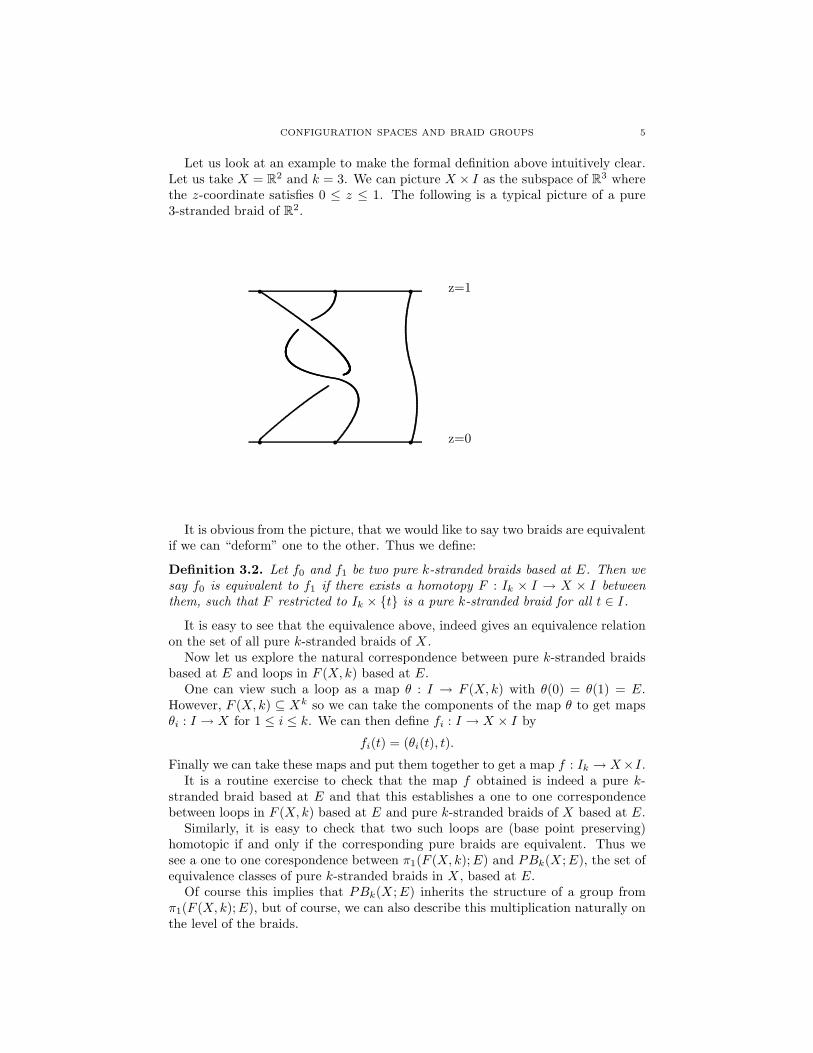
Let us look at an example to make the formal definition above intuitively clear.Let us take X = R2 and k = 3. We can picture X × I as the subspace of R3 wherethe z-coordinate satisfies 0 ≤ z ≤ 1. The following is a typical picture of a pure3-stranded braid of R2.
r r r
r r r
z=0
z=1
It is obvious from the picture, that we would like to say two braids are equivalentif we can “deform” one to the other. Thus we define:
Definition 3.2. Let f0 and f1 be two pure k-stranded braids based at E. Then wesay f0 is equivalent to f1 if there exists a homotopy F : Ik × I → X × I betweenthem, such that F restricted to Ik × t is a pure k-stranded braid for all t ∈ I.
It is easy to see that the equivalence above, indeed gives an equivalence relationon the set of all pure k-stranded braids of X .
Now let us explore the natural correspondence between pure k-stranded braidsbased at E and loops in F (X, k) based at E.
One can view such a loop as a map θ : I → F (X, k) with θ(0) = θ(1) = E.However, F (X, k) ⊆ Xk so we can take the components of the map θ to get mapsθi : I → X for 1 ≤ i ≤ k. We can then define fi : I → X × I by
fi(t) = (θi(t), t).
Finally we can take these maps and put them together to get a map f : Ik → X×I.It is a routine exercise to check that the map f obtained is indeed a pure k-
stranded braid based at E and that this establishes a one to one correspondencebetween loops in F (X, k) based at E and pure k-stranded braids of X based at E.
Similarly, it is easy to check that two such loops are (base point preserving)homotopic if and only if the corresponding pure braids are equivalent. Thus wesee a one to one corespondence between π1(F (X, k); E) and PBk(X ; E), the set ofequivalence classes of pure k-stranded braids in X , based at E.
Of course this implies that PBk(X ; E) inherits the structure of a group fromπ1(F (X, k); E), but of course, we can also describe this multiplication naturally onthe level of the braids.
6 FRED COHEN AND JONATHAN PAKIANATHAN
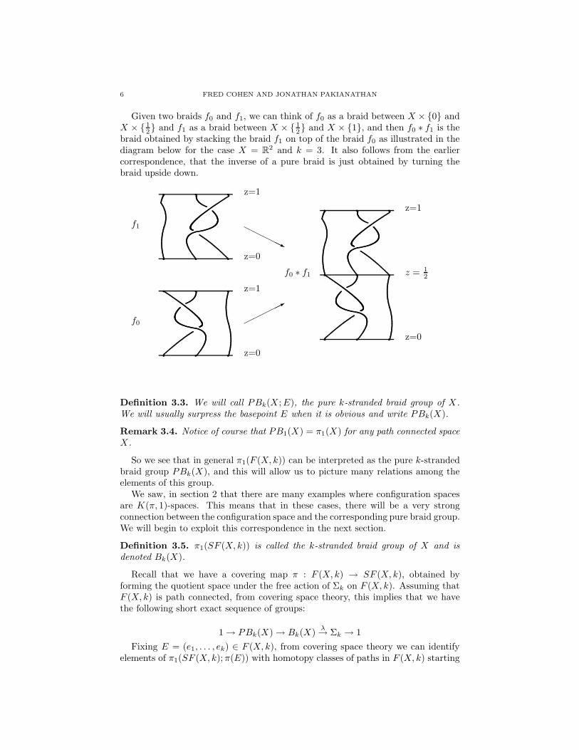
Given two braids f0 and f1, we can think of f0 as a braid between X × 0 andX × 1
2 and f1 as a braid between X × 12 and X × 1, and then f0 ∗ f1 is the
braid obtained by stacking the braid f1 on top of the braid f0 as illustrated in thediagram below for the case X = R2 and k = 3. It also follows from the earliercorrespondence, that the inverse of a pure braid is just obtained by turning thebraid upside down.
f0
q q q
q q q
q q q
q q q
q q q
q q q
q q q
f0 ∗ f1
*
HH
HHHj
z=1
z=0
z=1
z=0
z=1
f1
z=0
z = 12
Definition 3.3. We will call PBk(X ; E), the pure k-stranded braid group of X.We will usually surpress the basepoint E when it is obvious and write PBk(X).
Remark 3.4. Notice of course that PB1(X) = π1(X) for any path connected spaceX.
So we see that in general π1(F (X, k)) can be interpreted as the pure k-strandedbraid group PBk(X), and this will allow us to picture many relations among theelements of this group.
We saw, in section 2 that there are many examples where configuration spacesare K(π, 1)-spaces. This means that in these cases, there will be a very strongconnection between the configuration space and the corresponding pure braid group.We will begin to exploit this correspondence in the next section.
Definition 3.5. π1(SF (X, k)) is called the k-stranded braid group of X and isdenoted Bk(X).
Recall that we have a covering map π : F (X, k) → SF (X, k), obtained byforming the quotient space under the free action of Σk on F (X, k). Assuming thatF (X, k) is path connected, from covering space theory, this implies that we havethe following short exact sequence of groups:
1 → PBk(X) → Bk(X)λ→ Σk → 1
Fixing E = (e1, . . . , ek) ∈ F (X, k), from covering space theory we can identifyelements of π1(SF (X, k); π(E)) with homotopy classes of paths in F (X, k) starting
CONFIGURATION SPACES AND BRAID GROUPS 7
at E and ending at a point of F (X, k) in the same Σk-orbit of E. Using the samecorrespondence that associated loops in F (X, k) with pure braids, we see that thesepaths are naturally associated to k-stranded braids of X which start at the pointse1, . . . , ek at the bottom of X × I and end at the same set of points on the top,but where it is possible that the points get permuted.
It is easy to check that there is a well defined multiplication on the equivalenceclasses of these braids, just as before, which corresponds to the group structure ofπ1(SF (X, k)). Thus Bk(X) is just the group of k-stranded braids in X (based atsome set of k distinct points) which are allowed to induce a permutation of thepoints. The map λ in the short exact sequence above is just the map that assignsto every braid, the permutation it induces on the k points. The pure braids arehence exactly the elements in the kernel of this map.
Definition 3.6. Bk(R2) is called Artin’s k-stranded braid group and correspond-ingly, PBk(R2) is called Artin’s k-stranded pure braid group. It follows from theo-rem 2.7 that
F (R2, k) = K(PBk(R2), 1)
andSF (R2, k) = K(Bk(R2), 1).
4. Cohomology of groups
4.1. Basic concepts. This section is provided to recall the relevant basic factsabout the cohomology of groups that we will need for the sequel. The reader isencouraged to read when these results are needed and used.
Recall for every “nice” topological group G (Lie groups and all groups equippedwith the discrete topology are “nice”), we have a universal principal G-bundle,
EGπ→ BG
where EG is contractible and G acts freely on it. The isomorphism classes of princi-pal G-bundles over any paracompact space X , are then in bijective correspondenceto [X, BG], the free homotopy classes of maps from X into BG. Furthermore, it iswell known that BG is unique up to homotopy equivalence.
Furthermore the correspondence G → BG can be made functorial, so for everyhomomorphism of (topological) groups, λ : G → H we get a map B(λ) : BG → BH .This map is always well defined up to free homotopy.
If G is discrete, then π is a covering map and BG is a K(G, 1)-space. SinceBG is unique up to homotopy equivalence, we may speak of the cohomology of a(discrete) group by defining
H∗(G; M) = H∗((K(G, 1); M).
In general, we will also want to consider “twisted” coefficients in some G-moduleM .
One can also define the cohomology of a group, purely in the language of homo-logical algebra.
Definition 4.1. Given a group G, and a G-module M , we define
H∗(G; M) = Ext∗ZG(Z, M)
andH∗(G; M) = TorZG
∗ (Z, M)
8 FRED COHEN AND JONATHAN PAKIANATHAN
where ZG is the integral group ring of G, and Z is given the structure of a G-modulewhere every element of G acts trivially.
In other words, to calculate the cohomology of a group G, take any projectiveresolution of Z over the ring ZG, apply HomZG(−, M) to it, and calculate thecohomology of the resulting complex.
This definition, is equivalent to the topological one, see for example [B].
Remark 4.2. It is an elementary fact that for any G-module M , one has
H0(G; M) = MG = m ∈ M | gm = m for all g ∈ G.MG is called the group of invariants of the G-module M .
Remark 4.3. It is also easy to see that one has
H0(G; Z) = Z
and
H1(G; Z) = Gab
where Gab is the abelianization of G.
4.2. Examples. Here are some basic calculations:(a) Let G = Z/n be the cyclic group of order n. We can view Z/n as the nth rootsof unity in C and have it act on C∞ by coordinatewise multiplication. This actionrestricts to a free action on S∞, the subspace of unit vectors whose coordinates areeventually zero and the quotient space under this action is an infinite Lens spacewhich is a K(Z/n, 1).
One calculates:
Hk(Z/n; Z) =
Z/n if k > 0, k even
Z if k = 0
0 otherwise .
(b) let G = Fn be a free group of rank n. In this case, a bouquet of n circles isa K(Fn, 1). Since this is 1-dimensional, it is easy to see that H∗(Fn; M) = 0 forall ∗ > 1 and any coefficient M . Furthermore, H1(Fn; Z) is a free abelian group ofrank n.
4.3. Cohomological dimension. As we saw before, the free groups have the prop-erty that H∗(G; M) = 0 when ∗ > 1, so we might say they have cohomologicaldimension 1. In general we define:
Definition 4.4. The cohomological dimension of G is denoted cd(G). It is themaximum dimension n such that H∗(G; M) 6= 0 for some G-module M . Of course,if there is no such maximum n, we say cd(G) = ∞.
Thus we see the cohomological dimension of a nontrivial free group is one whilecd(Z/n) = ∞ for any n ≥ 2.
Again, there is also a more direct description of cohomological dimension usinghomological algebra.
Definition 4.5. Given a ring R, a projective resolution of a R-module M is aexact sequence of R-modules
· · · → Pn → · · · → P1 → P0 → M → 0
CONFIGURATION SPACES AND BRAID GROUPS 9
where the Pi are projective R-modules. If Pn 6= 0 and Pk = 0 for k > n we say theresolution has length n.
Definition 4.6. Given a ring R and an R-module M , we define projR(M), theprojective dimension of M , as the mimimum length of a projective resolution of M .Of course, it is possible projR(M) = ∞.
Proposition 4.7. For any group G,
cd(G) = projZG(Z)
Proof. See [B].
Remark 4.8. Given a G-module M , and a subgroup H ≤ G, we can regard M asa H-module in the obvious way. It is easy to check that if M is a free (projective)ZG-module, then M is also a free (projective) ZH-module.
Proposition 4.9. For any group G, and subgroup H ≤ G we have cd(H) ≤ cd(G).Thus if cd(G) < ∞, G is torsion-free.
Proof. It is easy to check that a projective resolution of Z over ZG restricts toa projective resolution of Z over ZH . So the first statement follows. If G hasnontrivial torsion it contains Z/n for some n ≥ 2 and the second statement followsfrom the first as cd(Z/n) = ∞.
It is an elementary result that the only group that has cohomological dimensionequal to zero is the trivial group. On the other hand we have seen that any nontrivialfree group has cohomological dimension 1. It is a deep result of Stallings and Swanthat the converse is also true, i.e.,
cd(G) ≤ 1 ⇐⇒ G is a free group.
Thus we can think of cd(G) as measuring how far a group G is from being free. Ifcd(G) < ∞, at least it is torsion-free, as we have seen.
We also have the following topological picture of cohomological dimension, givenby the following proposition, whose proof can be found in [B].
Proposition 4.10. Let the geometric dimension of G, denoted by geod(G), be theminimum dimension of a K(G, 1)-CW-complex. Then we have geod(G) = cd(G)except possibly for the case where cd(G) = 2 and geod(G) = 3.
Remark 4.11. Whether the exceptional case cd(G) = 2 and geod(G) = 3 canoccur is unknown. The conjecture that cd(G) = geod(G) in general is known as theEilenberg-Ganea conjecture.
We will also need the following basic theorem on subgroups of finite index whoseproof can be found in [B].
Theorem 4.12. Let G be a torsion-free group and H a subgroup of finite index.Then cd(G) = cd(H).
4.4. FP∞ groups.
Definition 4.13. A group G is of type FPn if there is a projective resolutionPi∞i=0 of Z over ZG such that Pj is finitely generated for j = 0, . . . , n. A groupG is of type FP∞ if it is of type FPn for all n.
10 FRED COHEN AND JONATHAN PAKIANATHAN
It is elementary to show that every group is FP0 and that a group is of typeFP1 if and only if it is finitely generated. So we can think of FPn for higher n asstrengthenings of the condition that G be finitely generated.
It is also true that if G is finitely presented, then G is of type FP2. For a longtime, it was conjectured the converse was true but Bestvina and Brady provided acounterexample - a group that is FP2 but not finitely presented.
Remark 4.14. It follows immediately, that if G is of type FPn then for any G-module M , which is finitely generated as an abelian group, we have Hi(G; M) andHi(G; M) finitely generated for all i ≤ n.
One has the following topological picture:
Proposition 4.15. A finitely presented group G is of type FPn if and only if thereexists a K(G, 1)-CW-complex such that the n-skeleton is finite. If G is finitelypresented, then it is of type FP∞ if and only if there exists a K(G, 1)-CW-complexsuch that the n-skeleton is finite for all n.
Definition 4.16. A group is of type FP if it is of type FP∞ and has finite co-homological dimension. This happens exactly when there is a projective resolutionPi∞i=0 of Z over ZG which has finite length and such that each Pi is finitelygenerated.
If we are given such a finite projective resolution, it does not necessarily meanthat we can find a finite length resolution using free modules of finite rank. Thuswe define:
Definition 4.17. A group is of type FL if there is a resolution of finite length forZ over ZG using finitely generated free modules.
Again, we have a more concrete topological picture.
Proposition 4.18. Let G be a finitely presented group. Then G is of type FP ifand only if there exists a finitely dominated K(G, 1)-CW-complex. Similarly, G isof type FL if and only if there exists a finite K(G, 1)-CW complex.
Thus for example Fn is FL as we can take K(Fn, 1) to be the bouquet of ncircles.
We will also find the following proposition useful:
Proposition 4.19. If we have a short exact sequence of groups
1 → Γ0 → Γ → Γ1 → 1
then if Γ0 and Γ1 are of type FP (respectively FL) then so is Γ.
Definition 4.20. If a group G is of type FP , we define χ(G), the Euler charac-teristic of G to be the Euler characteristic of a K(G, 1). This makes sense sinceH∗(G; Z) is finitely generated in each dimension, and is zero for ∗ > cd(G).
The following proposition recalls well-known facts about subgroups of finite in-dex.
Proposition 4.21. If G is a torsion-free group, and H is a subgroup of finite index.Then G is of type FP if and only if H is. Furthermore in this case,
χ(H) = |G : H |χ(G).
CONFIGURATION SPACES AND BRAID GROUPS 11
4.5. The five lemma. We state a refined form of the five lemma here as a con-venient quick reference. The reader can supply the usual diagram chasing proof ifthey feel inclined!
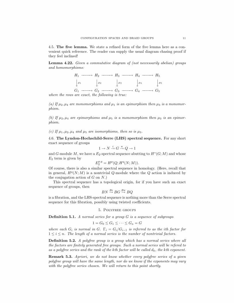
Lemma 4.22. Given a commutative diagram of (not neccessarily abelian) groupsand homomorphisms:
H1 −−−−→ H2 −−−−→ H3 −−−−→ H4 −−−−→ H5
y
µ1
y
µ2
y
µ3
y
µ4
y
µ5
G1 −−−−→ G2 −−−−→ G3 −−−−→ G4 −−−−→ G5
where the rows are exact, the following is true:
(a) If µ2, µ4 are monomorphisms and µ1 is an epimorphism then µ3 is a monomor-phism.
(b) If µ2, µ4 are epimorphisms and µ5 is a monomorphism then µ3 is an epimor-phism.
(c) If µ1, µ2, µ4 and µ5 are isomorphisms, then so is µ3.
4.6. The Lyndon-Hochschild-Serre (LHS) spectral sequence. For any shortexact sequence of groups
1 → Ni→ G
π→ Q → 1
and G-module M , we have a E2-spectral sequence abutting to H∗(G; M) and whoseE2 term is given by
Ep,q2 = Hp(Q; Hq(N ; M)).
Of course, there is also a similar spectral sequence in homology. (Here, recall thatin general, Hq(N ; M) is a nontrivial Q-module where the Q action is induced bythe conjugation action of G on N .)
This spectral sequence has a topological origin, for if you have such an exactsequence of groups, then
BNBi→ BG
Bπ→ BQ
is a fibration, and the LHS-spectral sequence is nothing more than the Serre spectralsequence for this fibration, possibly using twisted coefficients.
5. Polyfree groups
Definition 5.1. A normal series for a group G is a sequence of subgroups
1 = G0 ≤ G1 ≤ · · · ≤ Gn = G
where each Gi is normal in G. Γi = Gi/Gi−1 is referred to as the ith factor for1 ≤ i ≤ n. The length of a normal series is the number of nontrivial factors.
Definition 5.2. A polyfree group is a group which has a normal series where allthe factors are finitely generated free groups. Such a normal series will be refered toas a polyfree series and the rank of the kth factor will be called dk, the kth exponent.
Remark 5.3. Apriori, we do not know whether every polyfree series of a givenpolyfree group will have the same length, nor do we know if the exponents may varywith the polyfree series chosen. We will return to this point shortly.
12 FRED COHEN AND JONATHAN PAKIANATHAN
Our interest in polyfree groups stems from the fact that many of the pure braidgroups we have considered up to now, are polyfree.
Theorem 5.4. Let M be equal to R2 or a closed 2-manifold of genus g ≥ 1. ThenPBk(M−Qm) is polyfree for any m, k ≥ 1. (Notice that we do have to puncture themanifold at least once in general). Furthermore there is a polyfree series of lengthk where the rank of the ith factor is equal to 2g + m − 1 − i + k for 1 ≤ i ≤ k.(These formulas also work for M = R2 if we set g = 1
2).
Proof. As usual, we will induct on k. For k = 1, F (M − Qm, k) = M − Qm is aK(F2g+m−1, 1) where F2g+m−1 is a free group of rank 2g+m−1. Thus the theoremfollows easily in this case. So we may assume k > 1 and that the theorem is provenfor smaller values of k. Then by theorem 2.5, we have
πk,k−1 : F (M − Qm, k) → F (M − Qm, k − 1)
is a fibration with fiber F (M − Qm+k−1, 1). Since these spaces have trivial π2 bytheorem 2.7, we get a short exact sequence of groups
1 → F2g+m−2+k → PBk(M − Qm) → PBk−1(M − Qm) → 1.
By induction PBk−1(M −Qm) has a polyfree series of length k−1 with the claimedexponents and so it follows from the short exact sequence of groups above, thatPBk(M − Qm) has a polyfree series of length k. It is an easy exercise which willbe left to the reader, to check that the factors have the ranks claimed.
Remark 5.5. For k ≥ 2, by considering the map πk,1 : F (R2, k) → F (R2, 1) = R2
we see that
F (R2, k) = R2 × F (R2 − Q1, k − 1)
so it follows that PBk(R2) = PBk−1(R2 − Q1) and so the pure k-stranded Artinbraid group is polyfree with a polyfree series of length k − 1 given by the theoremabove.
So now we have a lot of motivation to study the class of polyfree groups. Let usbegin with some elementary results. First recall the following classical theorem ofP. Hall:
Theorem 5.6 (P. Hall). If
1 → N → G → Q → 1
is a short exact sequence of groups, with N and Q finitely presented, then G isfinitely presented.
Proof. See e.g. [R]
Proposition 5.7. Suppose G is a polyfree group with a polyfree series of length n.Then:(a) cd(G) ≤ n and in particular G is torsion-free.(b) G is of type FL.(c) G is finitely presented.(d) If the exponents for the polyfree series satisfy dk ≥ 2 for all 1 ≤ k ≤ n then Ghas trivial center.
CONFIGURATION SPACES AND BRAID GROUPS 13
Proof. We will induct on n, the length of the polyfree series. If n = 1, then G isfree of rank d1. The theorem then follows readily once we note that a free group ofrank d1 ≥ 2 has trivial center. (Since for example it is a nontrivial free product.)
So we can assume n > 1 and that we have proved the proposition for all smallern. Let 1 = G0 ≤ G1 ≤ · · · ≤ Gn = G be the given polyfree series. Notice we havea short exact sequence
1 → Gn−1 → Gπ→ Fdn
→ 1
and that Gn−1 is polyfree with a series of length n− 1. Thus by induction Gn−1 isFL and finitely presented and hence so is G by theorem 5.6 and proposition 4.19.So we have proven (b) and (c).
For (d), if we assume dk ≥ 2 for all k then by induction Gn−1 has trivial centerand of course so does Fdn
. Now if c ∈ G is a central element, then it is easy tosee that π(c) will be central in Fdn
and hence trivial. Thus c ∈ Gn−1 and so c is acentral element in Gn−1 which finally lets us conclude c = 1. Thus we have proven(d).
So it remains only to prove (a). By induction, cd(Gn−1) ≤ n − 1. Now supposeM is any G-module. Then we can apply the LHS-spectral sequence to the shortexact sequence above. Now Ep,q
2 = Hp(Fdn; Hq(Gn−1; M)) is zero if either p > 1 or
q > n−1, as cd(Gn−1) ≤ n−1. Thus we see there can be no nontrivial differentialsin this spectral sequence and so E2 = E∞.
However this spectral sequence converges to H∗(G; M) and so we can concludeeasily that H∗(G; M) = 0 for ∗ > n. Since this holds for any G-module M , we canconclude cd(G) ≤ n.
Remark 5.8. Given a polyfree group G with a polyfree series of length n, propo-sition 5.7 guarantees the existance of a resolution of Z over ZG of length less thanor equal to n, using finitely generated, free ZG-modules.
A nice resolution of this sort was constructed in [DCS] using Fox free derivativesin the case where the polyfree group satisfies an extra splitting condition which wewill consider later. The naturality of this resolution was also exploited to recovermany interesting representations which we will also look at later.
Next we consider subgroups of finite index in a polyfree group.
Proposition 5.9. Let G be a polyfree group with a polyfree series of length n andlet H be a subgroup of finite index in G. Then H is polyfree with a polyfree seriesof length n.
Proof. We proceed by induction on n. If n = 1 then G is a nontrivial free group offinite rank. It follows then from the Nielsen-Schreier theorem (see [R]) that H isalso free of finite rank and so this case follows.
So we may assume n > 1 and that we have proved the proposition for smallervalues. Let 1 = G0 < G1 < · · · < Gn = G be the polyfree series for G. Then if weset Hi = Gi ∩ H for 0 ≤ i ≤ n, it is easy to check 1 = H0 < H1 < · · · < Hn = H isa normal series for H . Furthermore, if Hi/Hi−1 → Gi/Gi−1 is the map induced byinclusion of H in G, it is easy to check this map is a well defined monomorphism(injection) of groups. On the other hand the image of this map has finite index inGi/Gi−1 as Gi/Hi injects (as sets) into the finite set G/H via the map inducedby inclusion. Thus we see each Hi/Hi−1 can be viewed as a subgroup of finiteindex in the nontrivial finitely generated free group Gi/Gi−1 and hence is itself a
14 FRED COHEN AND JONATHAN PAKIANATHAN
nontrivial free group of finite rank, again by the Nielsen-Schreier theorem. Thus1 = H0 < H1 < · · · < Hn = H is a polyfree series for H of length n.
Remark 5.10. An arbitrary subgroup of a free group of finite rank need not havefinite rank and so we see that arbitrary subgroups of a polyfree group need not bepolyfree.
Now let us show that for any given polyfree group G, all polyfree series for Ghave the same length. First we will need a technical lemma. Let F2 be the fieldwith two elements.
Lemma 5.11. Let G be a polyfree group with a polyfree series 1 = G0 < G1 <· · · < Gn = G of length n. Then there exists a subgroup T of finite index such thatHn(T ; F2) 6= 0. Furthermore, T contains G1 and χ(T ) = χ(G1)χ(T/G1). Thusχ(G) = χ(G1)χ(G/G1).
Proof. As usual we will proceed by induction on n. If n = 1, G is a nontrivial freegroup of finite rank. Thus we can take T = G = G1 as H1(G; F2) = Hom(G; F2)is nonzero. (The statement about Euler characteristics follows as χ(1) = 1.)
So we can assume n > 1 and that we have proved the lemma for smaller n. Thennotice that G/G1 has a polyfree series of length n − 1.
Now G acts by conjugation on G1 and hence on the finite vector space
H1(G1; F2) = Hom(G1, F2).
If we let K be the kernel of this action on H1(G1; F2), then K is normal and offinite index in G and furthermore G1 ⊆ K.
Now K/G1 ⊆ G/G1 is a subgroup of finite index and so by proposition 5.9, K/G1
is polyfree with a polyfree series of length n − 1. So, by hypothesis, we may findT/G1 with Hn−1(T/G1; F2) 6= 0 and T a subgroup of K of finite index. HoweverT/G1 ⊆ G/G1 and so cd(T/G1) ≤ n − 1 by proposition 5.7. So if we look at theLHS-spectral sequence for the short exact sequence
1 → G1 → T → T/G1 → 1
we see that Ep,q2 = Hp(T/G1; H
q(G1; F2)) is zero if p > n − 1 or q > 1 and En−1,12
is nonzero. (Here we use that T ⊆ K so that E∗,∗2 = H∗(T/G1; F2) ⊗ H∗(G1; F2).)
It is easy to see that we must have En−1,12 = En−1,1
∞ and so we can concludeHn(T ; F2) is nonzero. T is obviously of finite index in G so it only remains to provethe statement about χ(T ).
In the spectral sequence above, the E2 term has Euler characteristic
χ(G1)χ(T/G1).
On the other hand the E∞ term abuts to H∗(T ; F2) which has Euler characteristicχ(T ) and so the equality χ(T ) = χ(G1)χ(T/G1) follows from the general factthat the Euler characteristic remains constant on each page of the LHS-spectralsequence. Thus our induction on n goes through.
Finally the equality χ(G) = χ(G1)χ(G/G1) follows from the previous one whichhad T instead of G, theorem 4.21, and the fact that the index of T in G is the sameas the index of T/G1 in G/G1.
CONFIGURATION SPACES AND BRAID GROUPS 15
Proposition 5.12. Let G be a polyfree group with a polyfree series of length n andexponents dk, 1 ≤ k ≤ n. Then cd(G) = n and so every polyfree series of G haslength n. Furthermore χ(G) =
∏nk=1(1 − dk).
Proof. By proposition 5.7, we have cd(G) ≤ n. On the other hand, by lemma 5.11,we have a subgroup T of G of finite index, such that cd(T ) ≥ n. Thus the first partfollows as cd(G) = cd(T ) by proposition 4.12.
Now let us prove the formula for χ(G) by induction on n. For n = 1, it followsas a bouquet of d1 circles is a K(G, 1). So as usual we can assume n > 1 and thatwe have the formula for smaller n.
Again by lemma 5.11, we have χ(G) = χ(G1)χ(G/G1) = (1− d1)χ(G/G1). Theformula now follows readily once we observe that G/G1 has a polyfree series oflength n − 1 with exponents d2, . . . , dn and so by induction,
χ(G/G1) =
n∏
k=2
(1 − dk).
Remark 5.13. So from what we have seen, all polyfree series for a given polyfreegroup G, have the same length which is equal to cd(G). However the exponents ofdifferent polyfree series need not be the same.
For example we saw that PB4(R2) = PB3(R2 − Q1) is polyfree with exponents(3, 2, 1) by theorem 5.4. However it is known that this group also admits a polyfreeseries with exponents (5, 2, 1) (see [DCS]).
However∏n
k=1(1− dk) is independent of the polyfree series chosen as it is equalto χ(G) as we have seen.
6. Configuration spaces for the 2-sphere
We have seen in theorem 2.7 that for any closed 2-dimensional manifold Mbesides the sphere S2 and the projective plane RP 2, F (M, k) is a K(PBk(M), 1).Thus the configuration space is a good model for the pure braid group of M . Nowlet us see what we can say in the case where M is S2 or RP 2. Let us first look atS2. First note that SO(3) acts naturally on R3 and this action preserves the unitsphere S2. Hence SO(3) acts naturally on F (S2, k) for any k via a diagonal action.We will describe these configuration spaces now up to homotopy equivalence (whichwill be denoted by ≃). In fact we will find homotopy equivalences which preservethe SO(3) actions.
Proposition 6.1.
F (S2, k) ≃
S2 if k = 1, 2
SO(3) if k = 3
SO(3) × F (S2 − Q3, k − 3) if k > 3.
Furthermore, there are homotopy equivalences which are equivariant with respectto the natural SO(3) actions on F (S2, k) and the action of SO(3) on itself by leftmultiplication. (Here SO(3) acts on SO(3) × F (S2 − Q3, k − 3) by acting entirelyon the left factor via left multiplication.)
Proof. The k = 1 case is trivial so let us look at the k = 2 case first. By theorem 2.5,π : F (S2, 2) → F (S2, 1) = S2 is a fibration with contractible fiber F (S2 −Q1, 1) =
16 FRED COHEN AND JONATHAN PAKIANATHAN
R2. Thus π is a homotopy equivalence and it is trivial to see it is equivariant withrespect to the natural actions of SO(3) on F (S2, 2) and S2.
Now let us look at the case where k = 3. Again by theorem 2.5, there is afibration
π : F (S2, 3) → S2
obtained by projecting onto the first factor.Fix a point p1 ∈ S2. Let F = π−1(p1), the fiber over the point p1. Then again
by theorem 2.5, since F = F (S2 − Q1, 2) there is a fibration
π : F → (S2 − Q1) = R2
with fiber S2 − Q2, obtained by projecting onto a factor.Since the base space of the fibration π is contractible, we conclude that
F = R2 × (S2 − Q2) ≃ S1.
Now we will define a map λ : SO(3) → F (S2, 3). Fix p = (p1, p2, p3) ∈ F (S2, 3).Specifically, we will take p1 = (0, 0, 1), p2 = −p1 and p3 = (1, 0, 0). Then we canset
λ(α) = (α(p1), α(p2), α(p3))
for all α ∈ SO(3).It is easy to see that λ is a SO(3)-equivariant, continuous map from SO(3) to
F (S2, 3). We now want to show it is a homotopy equivalence. Let I denote theisotropy group of the point p1 ∈ S2 under the SO(3) action. Then I is isomorphicto SO(2) as a topological group and λ|I maps I into F .
Claim 6.2. The map λ|I : I → F is a homotopy equivalence.
Proof. The action of I on S2 is given by rotation about the z-axis fixing p1 whichcan be thought of as the north pole of S2. Notice that since we chose p2 = −p1,any element of I will also fix p2 (which is the south pole). Recall we had a fibrationπ : F → S2 − p1 and let us set F ′ = π−1(p2), the fiber above the point p2. Wesaw above that F ′ = S2 − p1, p2 ≃ S1 and that the inclusion of F ′ into F is ahomotopy equivalence.
Now notice, that λ|I actually maps I into F ′ since any element of I fixes p2. Ifwe let αθ denote the element of I which corresponds to rotation through an angleθ, then the loop αθ : 0 ≤ θ ≤ 2π gets mapped by λ to the generator of π1(F
′).Thus we see that λ|I : I → F ′ is a homotopy equivalence since both I and F ′ arehomotopic to S1 and λ is surjective on the π1 level. Hence λ|I : I → F is a homotopyequivalence since the inclusion of F ′ into F is a homotopy equivalence.
Now one can check easily that we get the following commutative diagram:
I −−−−→ SO(3)f−−−−→ S2
y
λ|I
yλ
yId
F −−−−→ F (S2, 3)π−−−−→ S2
where Id is the identity map and f(α) = α(p1) for α ∈ SO(3). Furthermore,each row is a fibration. Comparing the long exact sequence in homotopy for thetwo fibrations, one sees that the vertical maps induce an isomorphism on homo-topy groups on the base and fiber levels of these fibrations and hence (by the fivelemma) also on the level of total spaces. Thus, λ : SO(3) → F (S2, 3) induces an
CONFIGURATION SPACES AND BRAID GROUPS 17
isomorphism on homotopy groups and hence is a homotopy equivalence and so wehave the result for the case k = 3.
Now for the final case when k > 3. Let p = (p1, . . . , pk) ∈ F (S2, k) extend(p1, p2, p3) chosen in the previous case. Then again we can define a map
λ : SO(3) × F (S2 − p1, p2, p3, k − 3) → F (S2, k)
by
λ(α, (a4, . . . , ak)) = (α(p1), α(p2), α(p3), α(a4), . . . , α(ak))
for α ∈ SO(3) and (a4, . . . , ak) ∈ F (S2 − p1, p2, p3, k − 3).It is easy to see that this map is continuous and SO(3)-equivariant under the
SO(3)-actions described in the statement of this lemma. Furthermore, we get thefollowing commutative diagram:
π−1(Id) −−−−→ SO(3) × F (S2 − p1, p2, p3, k − 3)π−−−−→ SO(3)
Id
yλ
yλ
y
π−1k,3(p1, p2, p3) −−−−→ F (S2, k)
πk,3−−−−→ F (S2, 3)
where as usual Id stands for an identity map and π is projection onto the firstfactor. Furthermore both rows are fibrations. We have seen that the vertical mapon the base level is a homotopy equivalence and also trivially the vertical map onthe fiber level is also a homotopy equivalence and so it follows that λ is indeed ahomotopy equivalence (by looking at the long exact sequences in homotopy for thefibrations, and using the five-lemma). So this concludes the proof of the lemma.
Proposition 6.1 has the following immediate corollary:
Corollary 6.3.
PBk(S2) =
1 if k = 1, 2
Z/2Z if k = 3
Z/2Z × PBk−3(R2 − Q2) if k > 3
Notice that F (S2, k) is never a K(π, 1)-space due to the higher homotopy inSO(3) and S2. However, we will see in the next subsection, that one can performa natural construction to F (S2, k) for k ≥ 3 and obtain a useful K(π, 1)-space.
6.1. The Borel Construction. We will now recall a very important construction.First some elementary definitions:
Definition 6.4. If G is a topological group with identity element e, then a (left) G-space is a space X together with a continuous map µ : G×X → X which satisfies:(a) g1 · (g2 · x) = (g1g2) · x and(b) e · x = xfor all g1, g2 ∈ G, x ∈ X. (Here we use the notation g · x for µ(g, x) and e denotesthe identity element of G). Of course, similarly there is a notion of right G-spacewhere the action is on the right instead of on the left.
Definition 6.5. Keeping the notation above, we say a G-space X is free if g ·x = ximplies that g = e.
18 FRED COHEN AND JONATHAN PAKIANATHAN
Recall that for a “nice” topological group G, there is a universal G-bundle:
G → EG → BG
where EG is a contractible free (right) G-space.
Definition 6.6. Given a (left) G-space X, one can perform the Borel construction:
EG ×G X = EG × X/ ∼
where ∼ is the equivalence relation generated by (tg, x) ∼ (t, gx) for all t ∈ EG, x ∈X, g ∈ G.
Remark 6.7. It is easy to see from this definition, that EG×G G = EG ≃ ∗. HereG is viewed as a left G-space via left multiplication on itself and we are using thestandard notation of ∗ to denote a space which consists of a single point.
The next lemma collects some well-known elementary facts about the Borel con-struction:
Lemma 6.8. Let G be a topological group and X be a G-space then
π1 : EG ×G X → BG = EG/G,
the map induced by projection onto the first factor, is a bundle map with fiber X.Furthermore, if X is a free G-space, then the map
π2 : EG ×G X → X/G,
induced by projection onto the second factor is a bundle map with fiber EG. SinceEG is contractible, this implies π2 is a (weak) homotopy equivalence.
Let G1, G2 be two topological groups and let µ : G1 → G2 be a homomorphismof topological groups. Suppose further that you are given a µ-equivariant map
f : X1 → X2,
where Xi is a left Gi-space for i = 1, 2. In other words, f satisfies:
f(g · x) = µ(g) · f(x)
for all g ∈ G1, x ∈ X1.Furthermore recall, from the functoriality of the construction of the universal
principal G-bundle, one has the map E(µ) : EG1 → EG2 which is also µ-equivariantwhich induces the map B(µ) : BG1 → BG2 on the level of the quotient spaces.
Thus one can look at
E(µ) × f : EG1 × X1 → EG2 × X2.
It is easy to check that this map respects the equivalence relations used in formingthe respective Borel constructions and thus one gets a map:
E(µ)×f : EG1 ×G1X1 → EG2 ×G2
X2.
There is a commutative diagram in this context that is very useful. We state itas the next lemma.
CONFIGURATION SPACES AND BRAID GROUPS 19
Lemma 6.9. Given µ : G1 → G2 a homomorphism of topological groups andf : X1 → X2 a µ-equivariant map one has the following commutative diagram:
X1 −−−−→ EG1 ×G1X1 −−−−→ BG1
y
f
y
E(µ)×f
y
B(µ)
X2 −−−−→ EG2 ×G2X2 −−−−→ BG2
where each row is a fiber bundle. So in particular, if B(µ) and f are weak homotopyequivalences, then so is E(µ)×f .
Proof. It is a routine exercise to check that the diagram commutes. The last sen-tence then follows once again from the five lemma applied to the long exact se-quences in homotopy for the two bundles.
Lemma 6.9 gives us a convenient way to restate part of the results of proposi-tion 6.1.
Proposition 6.10. For k ≥ 3 one has that
ESO(3) ×SO(3) F (S2, k) = K(PBk−3(R2 − Q2), 1).
Here we are using the natural action of SO(3) on F (S2, k) described before. (Weare using the convention, that PB0(X) denotes the trivial group.)
Proof. Fix k ≥ 3, then from proposition 6.1, one has a SO(3)-equivariant homotopyequivalence
λ : SO(3) × Y → F (S2, k).
where we have denoted F (S2 − Q3, k − 3) by Y for convenience. (This means thatY is a point when k = 3.)
Applying lemma 6.9 using Id : SO(3) → SO(3) as µ, and λ as the equivariantmap, one sees immediately that since B(µ) and λ are homotopy equivalences, then
E(Id)×λ : ESO(3) ×SO(3) (SO(3) × Y ) → ESO(3) ×SO(3) F (S2, k)
is a (weak) homotopy equivalence. However,
ESO(3) ×SO(3) (SO(3) × Y ) = (ESO(3) ×SO(3) SO(3)) × Y
= ESO(3) × Y
≃ Y
by remark 6.7 and the contractibility of ESO(3). Theorem 2.7 then gives us thedesired result.
Now notice the following. If X is a left G-space, then F (X, k) is also a G-spacevia a diagonal action (as any group action takes distinct points to distinct points).On the other hand Σk acts on F (X, k) on the right by permuting coordinates. Itis easy to see that the Σk-action on F (X, k) commutes with the G-action. Thus ifwe look at the Σk action on EG×F (X, k) where Σk acts purely on the right factorby permuting coordinates, then it is easy to check that this action descends to anaction of Σk on the Borel construction EG ×G F (X, k). It is also routine to checkthat this action of Σk on the Borel contruction is still free and that
(EG ×G F (X, k))/Σk = EG ×G SF (X, k)
where recall that SF (X, k) denotes F (X, k)/Σk.We summarize this useful fact in the following remark:
20 FRED COHEN AND JONATHAN PAKIANATHAN
Remark 6.11. Let G be a topological group and let X be a left G-space then thereis a natural Σk-covering map:
EG ×G F (X, k)π→ EG ×G SF (X, k)
where the natural diagonal actions of G on F (X, k) and SF (X, k) are used to formthe Borel constructions.
Remark 6.11 and proposition 6.10 have the following immediate corollary:
Corollary 6.12. ESO(3) ×SO(3) SF (S2, k) is a K(π, 1) space for all k ≥ 3.
One bad thing about the Borel constructions so far, is that although they pro-duced K(π, 1) spaces, these spaces did not have PBk(S2) as their fundamentalgroup. We will now fix this point.
If a topological group G has a universal cover G (which we always assume is
connected), then it is elementary to show that G has the structure of a topological
group such that the covering map µ : G → G is a homomorphism of topologicalgroups. G is called the covering group of G.
Now given a (left) G-space X , X can also be viewed as a G-space via µ. Thusthe identity map of X is µ-equivariant in our previous terminology. It then followsfrom lemma 6.9 that we have the following commutative diagram where each rowis a fibration:
X −−−−→ EG ×G X −−−−→ BG
yId
y
E(µ)×Id
y
B(µ)
X −−−−→ EG ×G X −−−−→ BG
We wish to study the vertical map in the middle. To do this, we need to lookat the vertical maps on the sides first. It is obvious that the identity map is ahomotopy equivalence, so let us first look at B(µ). Recall the following elementaryremarks:
Remark 6.13. For any topological group G, BG is always path connected andπn(BG) ∼= πn−1(G) for n > 1.
Proof. We have the universal principal G-bundle EG → BG. The result followsimmediately from the long exact sequence in homotopy for this fibration and thecontractibility of EG.
Remark 6.14. A covering map π : X → X induces isomorphisms between πn(X)and πn(X) for all n > 1.
It follows from these remarks that µ : G → G induces isomorphisms between thehigher homotopy groups (πn for n > 1) and hence that B(µ) induces isomorphisms
in πn for all n 6= 2. (Here recall that we insist that G and hence also G is pathconnected.) Of course it induces the zero map on the π2 level as
π2(BG) = π1(G) = 0.
With this knowledge of B(µ) and by using the usual argument of applying thefive-lemma to the vertical maps between the long exact sequences in homotopy forthe two fibrations, one finds easily that E(µ)×Id induces an isomorphism in πn for
CONFIGURATION SPACES AND BRAID GROUPS 21
all n 6= 1, 2. Using the refined form of the five-lemma (stated in lemma 4.22), italso follows easily that E(µ)×Id induces a monomorphism on the π2 level.
This is the main step in proving the following useful lemma:
Lemma 6.15. Let G be a path connected, topological group. Let G be the universalcovering group with µ : G → G the covering map. Furthermore suppose X is aG-space. Then E(µ)×Id induces isomorphisms
πn(EG ×G X) ∼= πn(EG ×G X)
for all n 6= 1, 2 and a monomorphism
π2(EG ×G X)1−1→ π2(EG ×G X).
Furthermore,
π1(EG ×G X) ∼= π1(X)
Proof. We have already proved everything besides the final isomorphism listed. Toprove this, look at the fiber bundle
X → EG ×G X → BG.
Now we saw, in the paragraph preceding the lemma, that π2(BG) = 0, but one alsohas
π1(BG) ∼= π0(G) = 0.
Using this, it is easy to obtain our desired result from the long exact sequence inhomotopy for the fiber bundle above.
Now it is a well known fact that SO(3) is S3, the group of unit quarternions,which is topologically a 3-sphere. Thus applying lemma 6.15 to this group andusing proposition 6.10 and corollary 6.12, one easily obtains:
Corollary 6.16.
ES3 ×S3 F (S2, k) = K(PBk(S2), 1)
and
ES3 ×S3 SF (S2, k) = K(Bk(S2), 1),
for k ≥ 3.
Thus, once again we see that the configuration space provides a good model (thistime using a Borel construction) for the (pure) braid group of the underlying space.
Thus the only surface whose configuration space we have not studied yet is RP 2.We will do this now, in the next section.
7. Configuration spaces for the real projective plane
7.1. Orbit configuration spaces. In our study of the configuration spaces ofRP 2, we will find the concept of an orbit configuration space quite useful. Thesewere introduced by M. Xicotencatl and are defined as follows:
Definition 7.1. Let G be a group and X a G-space. Then
FG(X, k) = (x1, . . . , xk) ∈ Xk|xi, xj are in different G orbits if i 6= j.FG(X, k) is called the k-fold orbit configuration space of X.
22 FRED COHEN AND JONATHAN PAKIANATHAN
Remark 7.2. Thus we see that FG(X, k) is the space of k-tuples of points whichlie in distinct G orbits of X. Note that FG(X, 1) = X and F1(X, k) = F (X, k) forthe action of the trivial group 1 on X.
We will now prove some elementary but useful properties of these orbit configu-ration spaces. First some necessary definitions.
Definition 7.3. Given two groups G1 and G2, a left G1-space X is said to have acompatible G2 action if(a) X is a left G2-space.(b) For every g1 ∈ G1, g2 ∈ G2, x ∈ X, there exists g′1 ∈ G1 such that
g2 · (g1 · x) = g′1 · (g2 · x).
If it is always possible to take g′1 = g1, we say that the two actions commute.
Remark 7.4. Notice that if a G1-space X has a compatible G2 action then theG2 action takes G1-orbits to G1-orbits and hence induces a G2 action on X/G1.(To guarantee the continuity of this action, one should assume that G2 is locallycompact, Hausdorff so that G2 × X → G2 × X/G1 is a quotient map. This holdsfor all Lie groups and hence discrete groups.)
Remark 7.5. The most important examples of compatible actions are:(a) commuting actions.(b) When G1 = G2 = G and both groups act in the same way on X. These arecompatible actions as
g2 · (g1 · x) = (g2g1g−12 ) · (g2 · x)
and so we can take g′1 = g2g1g−12 .
Lemma 7.6. If X is a G1-space which supports a compatible G2-action, then thereis a natural Gk
2 action on FG1(X, k) defined via
(g1, . . . , gk) · (x1, . . . , xk) = (g1 · x1, . . . , gk · xk)
for all (g1, . . . , gk) ∈ Gk2 and (x1, . . . , xk) ∈ FG1
(X, k). Notice of course, this alsogives a G2 action on FG1
(X, k) obtained by precomposing the above action with thediagonal homomorphism ∆ : G2 → Gk
2 which sends g to (g, · · · , g).
Proof. The proof follows easily from remark 7.4 and is left to the reader.
¿From lemma 7.6, we see that there is always a natural action of Gk on FG(X, k).If the original G-action on X is reasonable, we can say something about this Gk-action on FG(X, k):
Proposition 7.7. If π : X → X/G is a principal G-bundle, there is a map
π : FG(X, k) → F (X/G, k)
which is a principal Gk-bundle, where
π(x1, . . . , xk) = (π(x1), . . . , π(xk))
and the Gk action on FG(X, k) is that which is described in lemma 7.6.
CONFIGURATION SPACES AND BRAID GROUPS 23
Proof. First notice that by taking a k-fold product we get a principal Gk-bundle
Gk → Xk ×π→ (X/G)k.
Then we can take the pullback of this bundle with respect to the inclusion mapi : F (X/G, k) → (X/G)k and hence get the commutative diagram:
Gk −−−−→Id
Gk
y
y
E −−−−→ Xk
yπ
y
×π
F (X/G, k) −−−−→i
(X/G)k
Thus the left hand column is also a principal Gk-bundle and the reader can easilycheck from the definition of a pullback (see [Bre]), that E is naturally identifiedwith FG(X, k) and that with this identification, π has the form stated above andthe Gk action on E = FG(X, k) is that which is described in lemma 7.6.
Remark 7.8. Recall, that when G is discrete, a principal G-bundle is the samething as a regular cover with covering group G. With this, it follows easily fromproposition 7.7, that if G is a finite group and X a free G-space, then there is acovering map
π : FG(X, k) → F (X/G, k)
with covering group Gk.
Proposition 7.7 shows us immediately how orbit configuration spaces can helpus understand the configuration space of RP 2. To see this, we can take S2 as aZ/2Z-space where the nontrivial element of Z/2Z is acting via the antipodal map.Then proposition 7.7 gives us the following covering map
(Z/2Z)k → FZ/2Z(S2, k)π→ F (RP 2, k).
Thus we need to study FZ/2Z(S2, k). To do this, we will need to use the analogueof the Fadell-Neuwirth theorem (theorem 2.5) for orbit configuration spaces. Wewill state and prove this analogue next.
Definition 7.9. Given a free G-space X, we will use the notation Ok to denotethe disjoint union of k distinct G-orbits. Notice X − Ok is hence also a G-space.
Theorem 7.10. Let G be a finite group and X be a free G-space. Suppose furtherthat X is a connected manifold without boundary with dimension ≥ 1. Then for alln > k, there are fibrations
FG(X − Ok, n − k) → FG(X, n)π→ FG(X, k)
where π is projection onto the first k factors.
Proof. Once one has verified that π is a fibration, it is an easy exercise to see thatthe fiber is as described in the statement of this theorem. Thus, we will only showthat π is a fibration.
Since the composition of fibrations is a fibration, it is enough to show that π is afibration in the case when n = k+1, since an arbitrary projection from FG(X, n) to
24 FRED COHEN AND JONATHAN PAKIANATHAN
FG(X, k) can be broken up as a composition of maps of this sort. Thus, we assumethat n = k + 1 from now on.
Let the order of G be s and write G = g1, . . . , gs. Define λ : FG(X, k) →F (X, sk) by
λ(x1, . . . , xk) = (g1x1, g2x1, . . . , gsx1, g1x2, . . . , gsx2, . . . , g1xk, . . . , gsxk).
The following diagram commutes:
F (M − Qks, 1) −−−−→ F (M, ks + 1)µ−−−−→ F (M, ks)
x
Id
x
λ
x
λ
FG(M − Ok, 1) −−−−→ Eµ−−−−→ FG(M, k)
Here the top row is a fibration by theorem 2.5, where µ is projection onto the firstks factors. The bottom row is the pullback of this fibration under the map λ.
Thus µ is a fibration. It remains only to show that the pullback E is naturallyhomeomorphic to FG(M, k + 1). Recall that
E = (x, y) ∈ FG(M, k) × F (M, ks + 1)|λ(x) = µ(y).Define θ : FG(M, k + 1) → FG(M, k) × F (M, ks + 1) by
θ(x1, . . . , xk+1) = ((x1, . . . , xk), (g1x1, . . . , gsx1, . . . , g1xk, . . . , gsxk, xk+1)).
It is easy to check that in fact θ : FG(M, k + 1) → E.Now, θ : FG(M, k + 1) → E has an inverse given by
((x1, . . . , xk), (g1x1, . . . , gsxk, xk+1)) → (x1, . . . , xk, xk+1).
Thus, θ is our desired homeomorphism and furthermore µ θ : FG(X, k + 1) →FG(X, k) is indeed projection onto the first k coordinates. This is a fibration as µis. Thus the theorem is proven.
(The authors would like to thank Dan Cohen for informing us about the niceproof above. Previous proofs consisted of going through the proof of theorem 2.5carefully and doing the necessary modifications, which is considerably more messy.)
7.2. Application of orbit configuration spaces to F (RP 2, k). First, we needto study FZ/2Z(S2, k).
Lemma 7.11. Let S2 be given a Z/2Z action via the antipodal map.Then FZ/2Z(S2 − On, k) is a K(π, 1) space for all n, k ≥ 1.
Furthermore π1(FZ/2Z(S2−On, k)) is a polyfree group of cohomological dimensionk and it has a polyfree series with exponents
(2(n + k − 1) − 1, . . . , 2(n + 1) − 1, 2(n + 0) − 1).
Proof. We will prove this lemma by induction on k. First the case when k = 1.Here we have that
FZ/2Z(S2 − On, 1) = S2 − On = R2 − Q2n−1 = K(F2n−1, 1).
Thus the result follows as F2n−1, the free group on 2n − 1 generators, is polyfree,of cohomological dimension one with the stated exponent.
So without loss of generality, k > 1 and we can assume the theorem is provenfor numbers smaller than k.
CONFIGURATION SPACES AND BRAID GROUPS 25
Now by theorem 7.1, we have a fibration
FZ/2Z(S2 − On+k−1, 1) → FZ/2Z(S2 − On, k) → FZ/2Z(S2 − On, k − 1).
By induction, the fiber and the base space are K(π, 1) spaces and hence, by thelong exact sequence in homotopy, so is the total space.
Furthermore, on the level of fundamental groups, the long exact sequence inhomotopy for the fibration above gives us a short exact sequence of groups:
π1(FZ/2Z(S2 − On+k−1, 1)) → π1(FZ/2Z(S2 − On, k)) → π1(FZ/2Z(S2 − On, k − 1)).
By induction, the base (quotient) group is polyfree, of cohomological dimensionk − 1, with exponents:
(2(n + k − 2) − 1, . . . , 2(n + 0) − 1)
and also the fiber group (kernel) is a free group of rank 2(n + k − 1) − 1. ¿Fromthis, the properties of π1(FZ/2Z(S2 −On, k)) stated in the lemma, follow easily.
Unfortunately, lemma 7.11 does not tell us anything about FZ/2Z(S2, k) directly
- the lemma only applies if at least one Z/2Z-orbit has been removed from S2. Wehave to do some genuine geometric analysis to go any further, so let us analyzeFZ/2Z(S2, 2) and show it is homotopy equivalent to SO(3) in a nice way.
First, let us notice that if we view S2 as the unit vectors in R3, then FZ/2Z(S2, 2)is naturally identified as the space of pairs of linearly independent unit vectors ofR3.
Thus, inside of FZ/2Z(S2, 2) is the subspace
U = (x, y)|x is orthogonal to y and x, y ∈ S2of pairs of orthogonal unit vectors. Notice that U can be naturally identified withthe unit tangent bundle of S2 (We will not need this fact).
SO(3) acts naturally on S2 and this action commutes with the antipodal map,thus by lemma 7.6, SO(3) acts diagonally on FZ/2Z(S2, 2).
It is easy to see that this action preserves the subspace U . In fact, even moreis true. Let ei be the ith standard unit vector of R3 for i = 1, 2, 3. Then given(x, y) ∈ U , since there are elements of O(3) mapping (e1, e2, e3) to any other givenorthonormal basis, it is easy to see that there is an element of SO(3) mapping(e1, e2) to (x, y). In fact this element is unique as any element of SO(3) mapping(e1, e2) to (x, y) would have to map e1 × e2 = e3 to x × y and so is determined ona basis. (Here × stands for the cross product in R3.)
Thus we see that the SO(3) action on U is transitive and free and hence U =SO(3). Furthermore, the SO(3) action on U corresponds to the left multiplicationaction on SO(3) under this correspondence.
Proposition 7.12. The inclusion i : U → FZ/2Z(S2, 2) is a SO(3)-equivarianthomotopy equivalence. Furthermore U = SO(3), with SO(3)-action given by leftmultiplication.
Proof. We have already proven the final sentence of the proposition in the precedingparagraph. It remains only to show that i is a homotopy equivalence.
We will need a bit of notation. For x, y ∈ Rn, let x · y denote the dot product ofx and y. Let ‖ x ‖= √
x · x denote the norm of x.
26 FRED COHEN AND JONATHAN PAKIANATHAN
Now we construct R : FZ/2Z(S2, 2) × I → FZ/2Z(S2, 2) as follows:
R(x, y, t) = (x,y − t(x · y)x
‖ y − t(x · y)x ‖).
Notice R is well defined as y is not a multiple of x. The following properties of Rfollow easily:(a) R(x, y, 0) = (x, y) for all (x, y) ∈ FZ/2Z(S2, 2),(b) R(x, y, 1) ∈ U ,(c) R(x, y, t) = (x, y) for all (x, y) ∈ U, t ∈ I.(d) R(αx, αy, t) = αR(x, y, t) for all (x, y) ∈ FZ/2Z(S2, 2), t ∈ I, α ∈ O(3). Here
O(3) is acting diagonally on FZ/2Z(S2, 2) in the natural way.
Properties (a)-(c) tell us that U is a strong deformation retract of FZ/2Z(S2, 2)which is all we need to finish the proof of the proposition. Property (d) says in fact,that there is a strong deformation through SO(3)-equivariant maps of FZ/2Z(S2, 2)to itself.
(Notice, that R, is in effect, performing a Gram-Schmidt orthogonalization pro-cess globally.)
Corollary 7.13. If FZ/2Z(S2, 2) is given the diagonal SO(3) action induced from
the natural action of SO(3) on S2 then ESO(3) ×SO(3) FZ/2Z(S2, 2) is (weakly)contractible.
Proof. Proposition 7.12 shows that i : U = SO(3) → FZ/2Z(S2, 2) is a SO(3)-equivariant homotopy equivalence. By lemma 6.9, it follows that
Id×i : ESO(3) ×SO(3) U → ESO(3) ×SO(3) FZ/2Z(S2, 2)
is a (weak) homotopy equivalence.On the other hand,
ESO(3) ×SO(3) U = ESO(3) ×SO(3) SO(3) = ESO(3) ≃ ∗
This was the crucial ingredient to the following proposition:
Proposition 7.14. If FZ/2Z(S2, k) is given the diagonal SO(3)-action induced from
the natural SO(3) action on S2 then ESO(3)×SO(3) FZ/2Z(S2, k) is a K(π, 1)-spacefor all k ≥ 2.
Proof. We will prove this by induction on k. The case k = 2 was proven in corol-lary 7.13 so assume k > 2 and that we have proven the proposition for smallernumbers.
Let π : FZ/2Z(S2, k) → FZ/2Z(S2, 2) be projection onto the first 2 factors. Noticethat π is SO(3)-equivariant.
By theorem 7.1, π is a fibration with fiber FZ/2Z(S2−O2, k−2) which is a K(π, 1)-space by lemma 7.11. Thus π induces an isomorphism in πi for i 6= 1, 2. Howeverπ2(FZ/2Z(S2, 2)) = π2(SO(3)) = 0 so in fact in the long exact sequence for the
fibration above, the boundary map from π2(FZ/2Z(S2, 2)) to π1(fiber) necessarilyvanishes and π is an isomorphism on the π2 level also.
CONFIGURATION SPACES AND BRAID GROUPS 27
By lemma 6.9, we have the following commutative diagram
FZ/2Z(S2, k) −−−−→ ESO(3) ×SO(3) FZ/2Z(S2, k) −−−−→ BSO(3)
y
π
yId×π
yId
FZ/2Z(S2, 2) −−−−→ ESO(3) ×SO(3) FZ/2Z(S2, 2) −−−−→ BSO(3)
where each row is a fibration. In the preceding paragraph, we saw that π inducedisomorphisms in πi for all i 6= 1. Thus by the refined form of the five lemmagiven in lemma 4.22, we see that Id×π induces a monomorphism in πi for alli 6= 1. Since πi(ESO(3) ×SO(3) FZ/2Z(S2, 2)) = 0 for all i this lets us conclude
that πi(ESO(3) ×SO(3) FZ/2Z(S2, k)) = 0 for all i 6= 1 which is what we set out toprove.
Now we are finally ready to study the configuration space F (RP 2, k). Recall wehad the covering map:
(Z/2Z)k → FZ/2Z(S2, k)π→ F (RP 2, k).
As before, SO(3) acts diagonally on FZ/2Z(S2, k) using the natural action of SO(3)
on S2. Of course, SO(3) also acts naturally on RP 2 viewed as the space of linesin R3. Hence, SO(3) acts diagonally on F (RP 2, k). Furthermore, it is easy to see,that the covering map π above is SO(3)-equivariant with respect to these actions.(For k = 1, π is just the map taking a unit vector, to the line it spans.)
Being a covering map, π induces isomorphisms in πi for all i 6= 1, and a monomor-phism in π1. We have the usual commutative diagram
FZ/2Z(S2, k) −−−−→ ESO(3) ×SO(3) FZ/2Z(S2, k) −−−−→ BSO(3)
y
π
yId×π
yId
F (RP 2, k) −−−−→ ESO(3) ×SO(3) F (RP 2, k) −−−−→ BSO(3)
where each row is a fibration.¿From the five lemma (lemma 4.22), it follows easily that Id×π induces an epi-
morphism in πi for i 6= 1. Thus from proposition 7.14, it follows that ESO(3)×SO(3)
F (RP 2, k) is a K(π, 1)-space. This is the result we wanted in this section and westate it as:
Theorem 7.15. ESO(3) ×SO(3) F (RP 2, k) is a K(π, 1)-space if k ≥ 2 and fur-thermore
ES3 ×S3 F (RP 2, k) = K(PBk(RP 2), 1)
and
ES3 ×S3 SF (RP 2, k) = K(Bk(RP 2), 1).
Here, the SO(3) action is induced from the natural action of SO(3) on RP 2 viewedas the space of lines in R3. The S3 action is obtained from the SO(3) action usingthat S3 is the universal covering group of SO(3).
Proof. Most of the theorem was proven in the preceding paragraph. The onlything remaining is the statement about the S3 Borel constructions which followsimmediately from lemma 6.15 and remark 6.11.
28 FRED COHEN AND JONATHAN PAKIANATHAN
Remark 7.16. ¿From the fibration,
F (RP 2, k) → ES3 ×S3 F (RP 2, k) → BS3
and the fact that ES3 ×S3 F (RP 2, k) is a K(π, 1)-space, we see easily that
πn(F (RP 2, k)) ∼= πn+1(BS3) ∼= πn(S3)
for n ≥ 2.Thus, F (RP 2, k) has the same higher homotopy as the 3-sphere.
This completes our analysis of F (M, k) for 2-manifolds M without boundary.The conclusion is that these are always K(PBk(M), 1)-spaces except when M isS2 or RP 2. However in these cases, there is an associated Borel construction whichis a K(PBk(M), 1).
For now, these results might seem to be a pretty formal analysis of the homo-topy type of the configuration spaces of surfaces - however we will see their truepower when we begin talking about labeled configuration spaces, and the “classical”connection of these labeled configuration spaces with loop spaces.
Furthermore, Borel constructions will provide a crucial tool in connecting thebraid groups we have studied, to mapping class groups, another important class ofgroups associated to surfaces, which we will introduce and study later on in thesenotes.
8. Mapping class groups
Let M denote an orientable surface and let Top(M) be the group of orientationpreserving homeomorphisms of M. We make it a topological group by giving it thecompact open topology.
Let Qk be a set of k distinct points in M and let Top(M, Qk) be the topologicalsubgroup of Top(M) which leaves the set Qk invariant.
Recall the standard isotopy lemma, (see [?])
Lemma 8.1 (Isotopy Lemma). Let M be a connected smooth manifold of dimensionstrictly bigger than one. Then for (x1, . . . , xk), (y1, . . . , yk) ∈ F (M, k), there exists adiffeomorphism φ : M → M such that φ is isotopic to the identity and φ(xi) = (yi)for 1 ≤ i ≤ k.
¿From the isotopy lemma, there is an orientation preserving homeomorphism ofM carrying one set of k distinct points Qk to any other set of k distinct pointsQ′
k, and thus Top(M, Qk) is conjugate to Top(M, Q′k) in Top(M) and so we will
sometimes write Top(M, k) when the points are understood.We will also look at PTop(M, Qk), the topological subgroup of Top(M, Qk) con-
sisting of homeomorphisms which actually fixe the points of Qk pointwise. ThusPTop(M, Qk) is the kernel of the natural homomorphism from Top(M, Qk) → Σk
induced by sending a homeomorphism leaving the set Qk invariant to the permuta-tion it induces on those points. Again, we will write PTop(M, k) when the pointsQk are understood.
Recall that if M is a surface then the inclusion of the group of orientationpreserving diffeomorphisms Diff+(M) → Top(M) is a homotopy equivalence.Some of the motivation for considering PTop(M, k) is described next.
CONFIGURATION SPACES AND BRAID GROUPS 29
Properties of these subgroups frequently correspond to a lifting question relat-ing branched covering spaces. Namely given a branched cover N → M which isbranched over a finite set Qk, information about Top(M, k) gives information aboutTop(N). That is, homeomorphisms of M which leave the branch set invariant lift(in possibly more than one way) to homeomorphisms of N .
One direction of these notes is to obtain information concerning Top(M, k) inorder to obtain information about Top(N). This approach is carried out in a fewcases in these notes for the specific examples of surfaces of genus 0,1, and 2. Thisapproach dates back to Hurwitz, and has been exploited in [BH], [?]; these classicalmethods have proven to be useful also for cohomological analysis.
In a few of the applications, pointed versions of these constructions are useful.For example, the cohomology of the ”pointed mapping class group” for a genus 1surface with marked points (to be defined below) has a clean cohomological de-scription. The analogous description without the assumption of ”pointed maps”has a technically more complicated description. This structure is analogous to thebehavior of certain function spaces. That is, the space of pointed maps from acircle to a space X, the loop space ΩX is frequently accessible from a homologicalpoint of view. At the same time, the space of free maps from a circle to X, the freeloop space ΛX , is frequently more delicate.
Mapping class groups, in some cases, reflect similar behavior as we will see laterwhen we study the pointed mapping class group for punctured copies of genus zero,one, and two surfaces.
Recall given a topological group G, the path components pi0(G) form a (discrete)group where the group structure is induced from G.
Definition 8.2. Let M be a closed orientable surface of genus g. The mappingclass group Γk
g = π0(Top(M, Qk)).
The pure mapping class group PΓkg is the kernel of the natural homomorphism
Γkg → Σk, induces by sending a homeomorphism to the permutation it induces a
the points Qk.
Definition 8.3. Let M be a closed orientable surface of genus g, Qk a set of kdistinct points of M and p a fixed point in M − Qk.
The pointed mapping class group Γk,1g is the group of path components of the
orientation preserving homeomorphisms which (1) preserve the point p, and(2) leave the set Qk invariant.
The pure pointed mapping class group PΓk,1g is the kernel of the natural homo-
morphism Γk,1g → Σk.
The group Top(M) acts on the configuration space of points in M , F (M, k),diagonally. A ”folk theorem” that has been useful gives (1) there are naturalK(π, 1)′s obtained from the associated Borel construction (homotopy orbit spaces)for groups acting on configuration spaces, and(2) these configuration spaces are analogous to homogeneous spaces in the sense
30 FRED COHEN AND JONATHAN PAKIANATHAN
that they are frequently homeomorphic to a quotient of a topological group by aclosed subgroup.
Namely, let G be a subgroup of Top(M), and consider the diagonal action of Gon F (M, k) together with the homotopy orbit spaces
EG ×G F (M, k)
and
EG ×G F (M, k)/Σk.
Lemma 8.4. Assume that M is a nonempty manifold of dimension at least 1.Then Top(M, k) and PTop(M, k) are closed subgroups of Top(M).
Proof. Given any point f in the complement of Top(M, k) in Top(M), there is atleast one mi ∈ Qk that is taken to a point outside Qk. The open set of continuousfunctions that carry mi to M − Qk in the complement of Top(M, k) in Top(M)is a neighbourhood of f . Thus it follows that the complement of Top(M, k) inTop(M) is open and the lemma follows for Top(M, k). The proof for PTop(M, k)is similar.
Consider the natural evaluation map Top(M) → F (M, k) given by Top(M)acting on the point (m1, m2, ..., mk). Since the isotropy group of the Top(M) actionon F (M, k) at (m1, . . . , mk) is the group Top(M, k), there is an induced map
ρ : Top(M)/Top(M, k) → F (M, k).
By the isotopy lemma, ρ is onto and hence a continuous bijection.In the next theorem, we will show among other things, that in fact the map
ρ above is a homeomorphism. Thus configuration spaces of surfaces are “homoge-neous spaces” of suitable topological groups. (The quotation marks about the wordhomogeneous space is due to the fact that Top(M) is only a topological group, nota Lie group).
The theorem will be proven from a construction in Steenrod’s book ”The topol-ogy of fibre bundles”. Namely, consider
H → G → G/H
where H is a closed subgroup of G, and the map G → G/H admits ”local cross-sections”. Then the induced map BH → BG is the projection map in a fibrebundle with fibre given by the space of left cosets G/H . [Steenrod, page 30]
The definition of ”local cross-sections” is given as follows: Let H be a closedsubgroup of G with natural quotient map p : G → G/H and let x ∈ G/H . A localcross-section of p : G → G/H at x is a continuous function f : V → G where V isan open neighborhood of x in G/H satisfying pf(x) = x for all x ∈ V . [Steenrod,page 30].
Theorem 8.5. Assume that M is an orientable surface without boundary. Then
(1) There is a principal fibration
Top(M, k) → Top(M) → Top(M)/Top(M, k).
CONFIGURATION SPACES AND BRAID GROUPS 31
(2) The map
ρ : Top(M)/Top(M, k) → F (M, k)
is a homeomorphism.(3) The homotopy theoretic fibre of the natural map BTop(M, k) → BTop(M)
is F (M, k), and ETop(M)×Top(M)F (M, k) is homotopy equivalent to BTop(M, k).
The proof of Theorem 8.5 depends on the next lemma. Here, let Dn denote thestandard n-disk, i.e., the points in Rn of euclidean norm at most 1 with interiordenoted Do,n with (0, 0, ..., 0) the origin in Dn. The map θ in the next lemma wasquite useful in the article by Fadell and Neuwirth [FN] while the formula here waswritten explicitly in [X].
Lemma 8.6. (1) There is a continuous mapθ : Do,n × Dn → Dn
such that θ(x,−) fixes the boundary of Dn pointwise, and θ(x, x) =(0, 0, ..., 0) for every x in Do,n.
(2) If M is a surface without boundary, then there exists a basis of open sets Ufor the topology of F (M, k) together with local sections
φ : U → Top(M) such that the composite
Uφ→ Top(M) → Top(M)/Top(M, k)
ρ→ F (M, k)
is a homeomorphism onto U .(3) The natural map ρ : Top(M)/Top(M, k) → F (M, k) is a homeomorphism.
Proof. Define α : Do,n → Rn by the formula α(x) = x/(1 − |x|), and so α−1(z) =z/(1 + |z|).
For a fixed element q in Do,n, define γq : Dn → Dn by the formula
(1) γq(y) = y for y in the boundary of Dn, and(2) γq(y) = α−1(y/(1 − ||y||) − q/(1 − |q|) for y in Do,n.
Define θ : Do,n × Dn → Dn by the formula θ(q, y) = γq(y). Notice that θ iscontinuous, and θ(q, q) = (0, 0, ..., 0), and so part (1) of the lemma follows.
To prove part (2), consider a point (p1, p2, ..., pk) in F (M, k) together with dis-joint open discs Do,2(p1), D
o,2(p2), ...., Do,2(pk) where Do,2(pi) is a disc with center
pi. ( There is a choice of homeomorphism in the identification of each open discwith an open coordinate patch of M; this choice will be suppressed here.) Let U bethe open set in F (M, k) given by the product Do,2(p1) × Do,2(p2) × ... × Do,2(pk).The sets U give a basis for the topology of F (M, k) which depend on the choice ofthe discs Do,2(pi). Define φ : U → Top(M) by the formula φ((y1, y2, ..., yk)) = Hfor H in Top(M) where (y1, y2, ..., yk) is in U = Do,2(p1)×Do,2(p2)× ...×Do,2(pk),and H is the homeomorphism of M given as follows.
(1) H(x) = x if x is in the complement in the union of the∐
1≤i≤k Do,2(pi),and
(2) H(x) = θ(pi, x) if x is in Do,2(pi).
32 FRED COHEN AND JONATHAN PAKIANATHAN
Clearly H is in Top(M). Notice that φ is continuous if an only if the adjoint ofφ, adj(φ) : U × M → M is continuous as all spaces here are locally compact, andHausdorff. But then continuity follows at once from the first part of the lemma asadj(φ)(x, y) = y for y in the boundary of any of the discs Do,2(pi). The secondpart of the lemma follows.
To finish the third part of the lemma, it must be checked that the natural mapρ : Top(M)/Top(M, k) → F (M, k) is a homeomorphism. Notice that part 2 ofthe lemma gives local sections φ : U → Top(M). Thus consider the compositeλ : U → Top(M)/Top(M, k) given by the composite pφ where p : G → G/H isthe natural quotient map. Notice that λ : U → λ(U) is a continuous bijection, andλ(U) = φ−1(U). Thus λ(U) is open, and the map φ is open. Thus ρ is open, andhence a homeomorphism. The lemma follows.
Next, the proof of Theorem 8.5 is given.
Proof. By Lemmas 8.6, and 8.4, Top(M, k) is a closed subgroup of Top(M), andlocal sections exist for Top(M) → Top(M)/Top(M, k) . Thus there is a principalfibration Top(M, k) → Top(M) → Top(M)/Top(M, k), and the first part of thetheorem follows.
Furthermore, the natural evaluation map Top(M) → F (M, k) factors throughthe quotient map Top(M) → Top(M)/Top(M, k). There is the induced mapρ : Top(M)/Top(M, k) → F (M, k) which, by lemma 1.4 , is a homeomorphism,and part 2 of the theorem follows.
The third statement in the theorem follows from a construction in N. Steenrod’sbook [S], at the foot of page 30. Namely, consider H → G → G/H where H is aclosed subgroup of G, and the map G → G/H admits ”local cross-sections”, thenBH → BG is the projection map in a fibre bundle with fibre given by the spaceof left cosets G/H .
As a consequence of Theorem 8.5, we can describe some of the Borel constructionswe have looked at in previous sections as K(π, 1) spaces where the group π is givenby certain mapping class groups.
Theorem 8.7. (1) If q ≥ 3, the spaces ESO(3)×SO(3)F (S2, q), and ESO(3)×SO(3)
F (S2, q)/Σq are respectively K(PΓq0, 1), and K(Γq
0, 1).(2) If M = S1 × S1, and q ≥ 2, the spaces ETop(M) ×Top(M) F (M, q), and
ETop(M) ×Top(M) F (M, q)/Σq are respectively K(PΓq1, 1), and K(Γq
1, 1).Furthermore, in these cases ETop(M)×Top(M) F (M, q) is homotopy equiv-
alent to ESL(2, Z)×SL(2,Z)F (S1×S1−(1, 1), q−1) where SL(2, Z) acts
on S1 × S1 − (1, 1) by the formula
(2)
(
a bc d
) (
uv
)
= (uavb, ucvd)
CONFIGURATION SPACES AND BRAID GROUPS 33
for
(3)
(
uv
)
in S1 × S1.(3) If M is a surface of genus g without boundary ( possibly with punctures ),
and g ≥ 2, the spaces ETop(M) ×Top(M) F (M, q) and ETop(M) ×Top(M)
F (M, q)/Σq are respectively K(PΓqg, 1), and K(Γq
g, 1).(4) Let M be a closed orientable surface of genus g with x a point of M, and N
= M −x. The spaces ETop(N)×Top(N) F (N, q), and ETop(N)×Top(N)
F (N, q)/Σq are respectively K(PΓq,1g , 1), and K(Γq,1
g , 1).
Proof. Notice that Lemma 2 gives that the fundamental group of ETop(M)×Top(M)
F (M, q) is isomorphic to π0(Top(M, k) = PΓkg . Similarly, the fundamental group
of ETop(M) ×Top(M) F (M, q)/Σq is Γkg The main task is now to determine when
ETop(M) ×Top(M) F (M, q) is a K(π, 1). If the genus of M is at least 2, then theresulting space is a K(π, 1), however, if the genus is 0, or 1, there are some smallmodifications described below.
A theorem of Smale [Smale] gives that the natural map SO(3) → Diff+(S2) isa homotopy equivalence. Thus the natural maps SO(3) → Diff+(S2) → Top(S2)as well as the maps induced on the level of the Borel constructions ESO(3)×SO(3)
F (S2, q) → ESO(3)×Top(S2)F (S2, q) are homotopy equivalences. Since ESO(3)×SO(3)
F (S2, q) is a K(π, 1 for q ≥ 3 ( See section ?? in these notes . ), the result for part(1) follows from the above lemma.
To prove part(2) of the theorem, notice that a result of Earle, and Eells [EE], no-tice that there is an exact sequence of groups 1 → Diff0(S
1×S1) → Diff+(S1×S1) → SL(2, Z) → 1 where Diff0(S
1 × S1) is homotopy equivalent to S1 × S1
and so BDiff0(S1 × S1) is homotopy equivalent to CP∞ × CP∞. Furthermore,
the map S1 × S1 → Diff0(S1 × S1) given by rotations is a homotopy equivalence
by [EE]. Thus the Borel construction EG ×G S1 × S1 is K(SL(2, Z), 1) where G= Diff+(S1 × S1).
Consider the Borel construction EG×GF (S1×S1, q) together with the projectionto EG ×G F (S1 × S1, 1) having fibre F (S1 × S1 − Q1, q − 1). Recall that EG ×G
F (S1×S1, 1) is K(SL(2, Z), 1), and observe that the action of SL(2, Z) on F (S1×S1 −(1, 1), q− 1) is the diagonal natural action of SL(2, Z) on S1 ×S1 −(1, 1)where (1, 1) is the identity element in S1 × S1 with the following action:
(4)
(
a bc d
) (
uv
)
= (uavb, ucvd).
Thus, if q ≥ 2, the fibre and base of the projection EG ×G F (S1 × S1, q) →EG×G F (S1 × S1, 1) are K(π, 1)′s. Thus EG×G F (S1 × S1, q) is also a K(π, 1) ifq ≥ 2, and part (3) follows.
34 FRED COHEN AND JONATHAN PAKIANATHAN
To prove part (3), notice that by [EE],each path component of Diff+(M) is con-tractible if M is of genus g ≥ 2. Thus both BTop(M), and F (M, k) are Eilenberg-Mac Lane spaces of type K(π, 1).
Part(4) is analogous as BTop(M) is a K(π, 1) where N = M −x. The theoremfollows.
Recall the definition of the pointed mapping class group: The pointed mappingclass group Γk,1
g is the group of path components of the orientation preservinghomeomorphisms which (1) preserve the point p in the surface, and (2) leave a setof k other distinct points in M invariant, π0(Top(M, p, Qk). The pure pointedmapping class group PΓk
g is the kernel of the natural homomorphism Γk,1g → Σk.
Corollary 8.8. (1) If q ≥ 1, then the fundamental group ofETop(M) ×Top(M) F (M, q + 1)/1 × Σqis isomorphic to Γq,1
g .(2) If M is of genus zero, and q ≥ 2, then ETop(M)×Top(M)F (M, q + 1)/1 ×
Σq is a K(Γq,10 , 1).
(3) If M is of genus one, and q ≥ 1, then ETop(M)×Top(M) F (M, q + 1)/1 ×Σq is a K(Γq,1
g , 1).Furthermore if q ≥ 1, then ETop(M)×Top(M)F (M, q) is homotopy equiv-
alent to ESL(2, Z)×SL(2,Z)F (S1×S1−(1, 1), q−1) where SL(2, Z) acts
on S1 × S1 − (1, 1) by the formula(4) If M is of genus at least two, and q ≥ 1, then ETop(M)×Top(M)F (M, q + 1)/1 ×
Σq is a K(Γq,1g , 1).
Proof. Consider ETop(M)×Top(M)F (M, q + 1)/1 × Σq together with the naturalprojection to ETop(M) ×Top(M) M with fibre F (M − Q1, q)/Σq. Thus the spaceETop(M)×Top(M) is BTop(M, 1) by Theorem 1.2 . Furthermore, the Top(M, 1)-action on F (M − Q1, q)/Σq is induced by the natural diagonal action on M − Q1.Hence the fundamental group is Γq,1
g . The hypotheses on the number of points qgives that the resulting spaces are K(π, 1)′s by Theorem 1.2.
To finish the proof of the corollary, it suffices to notice that ETop(M) ×Top(M)
F (M, q) is homotopy equivalent to ESL(2, Z)×SL(2,Z) F (S1 × S1 −(1, 1), q− 1)
where SL(2, Z) acts on S1 × S1 − (1, 1) where M is of genus 1 by the aboveremarks.
9. The Thom construction
9.1. Basic definitions. In this section, we will be working in the category ofpointed spaces and maps. Recall the basic definitions:
Definition 9.1. A pointed space is a space X together with a fixed basepoint ∗ ∈ X.A map f : X → Y between two pointed spaces is said to be a pointed map if f(∗) = ∗.A homotopy F between two pointed maps f, g : X → Y is said to preserve basepoints
CONFIGURATION SPACES AND BRAID GROUPS 35
if F (∗×I) = ∗ and we write f ≃∗ g. If f and g are homotopic but not necessarily bya homotopy that preserves basepoints, we write f ≃ g and say f is freely homotopicto g.
We recall some basic constructions. See [Bre] for proofs of the basic propertiesof these constructions.
Definition 9.2. Given two pointed spaces X and Y , X ×Y can be made a pointedspace by taking (∗, ∗) as basepoint. Define
X ∨ Y = (x, y) ∈ X × Y such that either x = ∗ or y = ∗.X ∨ Y is called the wedge product of X and Y and is a pointed space consisting ofthe spaces X = X × ∗ and Y = ∗ × Y attached at the basepoint (∗, ∗).
Definition 9.3. Given two pointed spaces X and Y ,
X ∧ Y = X × Y/X ∨ Y
is called the smash product of X and Y and is itself a pointed space where we setthe equivalence class of X ∨ Y as the basepoint.
The following lemma collects some useful facts about the wedge and smash prod-ucts. The proof of these facts is left to the reader and can be found in introductorytexts like [Bre] or [Spa].
Lemma 9.4. Let Top∗ denote the category of pointed spaces and maps. We willwrite X =∗ Y if X and Y are isomorphic in this category. Then(a) −∨− and −∧− are functors from Top∗ to itself, which are covariant in both en-tries. If f : X1 → X2 and g : Y1 → Y2 are two pointed maps we will denote the mapsgiven by these functors as f ∨g : X1 ∨Y1 → X2 ∨Y2 and f ∧g : X1∧Y1 → X2 ∧Y2.(b) −∨− equips the isomorphism classes of objects in Top∗ with the structure of acommutative monoid with identity where the identity is the point space ∗. In otherwords:(i) X ∨ Y =∗ Y ∨ X(ii) (X ∨ Y ) ∨ Z =∗ X ∨ (Y ∨ Z)(iii) X ∨ ∗ =∗ X.(c) − ∧ − equips the isomorphism classes of objects in Top∗ with a commutativemultiplication structure, which together with ∨ gives a commutative semiring struc-ture on Top∗. (A semiring is something which satisfies all the axioms of a ringexcept the existance of additive inverses.) In other words:(i) X ∧ Y =∗ Y ∧ X(ii) (X ∧ Y ) ∧ Z =∗ X ∧ (Y ∧ Z)(iii) X ∧ S0 =∗ X where S0 = 0, 1 with 0 as the basepoint.(iv) (X ∨ Y ) ∧ Z = (X ∧ Z) ∨ (Y ∧ Z).(d) ∨ and ∧ are homotopy functors, i.e., if f ≃∗ f ′ and g ≃∗ g′ then we havef ∨ g ≃∗ f ′ ∨ g′ and f ∧ g ≃∗ f ′ ∧ g′.
Remark 9.5. The reader should be careful in interpreting the semiring structurein lemma 9.4 since the objects of Top∗ do not form a set. However, in practice,this is not a problem as we can always confine ourselves to a suitable set of objectsif we wish to use the semiring structure. The reader can check for example, that the“subsemiring” generated by S0 is naturally identified with the semiring of natural
36 FRED COHEN AND JONATHAN PAKIANATHAN
numbers. In fact, if we confine ourselves to objects in Top∗ where the Euler char-acteristic χ is defined, and where we can identify H∗(X ∧Y ) as H∗(X ×Y, X ∨Y ),then the map taking X to χ(X) − 1 is a semiring morphism to the integers.
Definition 9.6. We use X(k) to stand for the kth power of the pointed space Xunder the smash product multiplication. It is understood then that X(0) = S0 andX(1) = X. Notice that, for k ≥ 1, we have
X(k) = Xk/F
where F = (x1, . . . , xk) ∈ Xk such that xi = ∗ for some i, is the so called fat-tened wedge. Notice that the symmetric group Σk acts on Xk by permuting coor-dinates and that this action preserves F . Thus this induces a natural action of Σk
on X(k) which fixes the basepoint.
Definition 9.7. Given a space X, the unreduced suspension of X, denoted SX,is the quotient space obtained from X × I by identifying X × 0 to a point andX × 1 to another point.Given a pointed space X, the reduced suspension of X, is defined as
ΣX = X × I/(X × 0 ∪ ∗ × I ∪ X × 1).and is given the equivalence class of ∗ × I as the basepoint.
Remark 9.8. We will identify the 1-sphere S1 as the quotient space formed from[0, 1] where we identify 0 and 1 to form a common basepoint. With this, it is easyto see that
S1 ∧ X =∗ ΣX.
Thus (S1)(k) = Sk for all k ≥ 0.
Definition 9.9. A well pointed space X is a pointed space where the inclusion∗ → X is a cofibration. Recall that for such a space, the reduced and unreducedsuspensions are homotopy equivalent. (See [Bre] or [Spa]). Any CW -complex X iswell pointed if we take the basepoint to be an element of the zero skeleton X(0).
9.2. The Thom construction. We now introduce an important construction.Let M be a free right Σk-space and X be a well pointed space. Then from thefinal remark in definition 9.6, there is a natural Σk action on X(k) which fixes thebasepoint. Thus we can form
M ×ΣkX(k) = M × X(k)/ ∼,
where (mσ, x) ∼ (m, σx) for all σ ∈ Σk, x ∈ X(k) and m ∈ M .As in the Borel construction, one can easily show that as the Σk action on M is
free, the map
π : M ×ΣkX(k) → M/Σk,
obtained by projecting on the first factor, is a fiber bundle with fiber X(k). Fur-thermore π has a section σ : M/Σk → M ×Σk
X(k) defined by σ(m) = (m, ∗) where
∗ is the basepoint of X(k). (This section is well defined as ∗ is fixed under the Σk
action on X(k).)Given a field F, we will now set out to find H∗(M ×Σk
X(k); F). To do that usingthe spectral sequence for the fiber bundle described above, we see that we first needto describe H∗(X(k); F). So let us do that now.
CONFIGURATION SPACES AND BRAID GROUPS 37
Recall that if the inclusion of A into X is a cofibration, then we have a naturalisomorphism H∗(X, A; F) ∼= H∗(X/A; F) where the bar signifies reduced cohomol-ogy. (See for example [Bre]).
Now if X and Y are well pointed spaces, then the inclusion of X ∨Y into X ×Yis a cofibration?
Thus H∗(X×Y, X∨Y ; F) ∼= H∗(X∧Y ; F). On the other hand, it is easy to arguethat the long exact sequence in reduced cohomology for the pair (X × Y, X ∨ Y )degenerates into split short exact sequences:
0 → H∗(X × Y, X ∨ Y ; F) → H∗(X × Y ; F)i∗→ H∗(X ∨ Y ; F) → 0
Thus H∗(X ∧ Y ; F) is algebra isomorphic to the kernel of i∗. We are able to geta complete description of this kernel via the Kunneth Theorem in the case whenone of the spaces has finite dimensional F-cohomology in each dimension. (We needthis condition, to apply the cohomology version of Kunneth’s theorem - see [Bre]).
Using this, one easily describes the cohomology algebra of the smash product interms of the cohomology algebras of the original spaces. We state the result as alemma and leave the completion of the details of its proof to the reader.
Lemma 9.10. If X, Y are path connected, well pointed spaces and at least one ofthem has finite dimensional F-cohomology in each dimension, then H∗(X ∧Y ; F) ∼=H∗(X ; F)⊗ H∗(Y ; F) as F-algebras (without identity element).
It follows from lemma 9.10 that for a path connected, well pointed space X ,one has H∗(X(k); F) is isomorphic to the tensor product of k copies of the algebraH∗(X ; F) with itself.
Definition 9.11. Given a graded F-algebra A with A0 = 0 (so A does not havean identity element), we define Tk(A) to be the F-algebra with identity obtainedin the following way. We first take the tensor product of k-copies of A. This hasnothing in degree zero. Finally, we include a 1-dimensional vector space in degreezero generated by an identity element.
Thus we can restate our results as H∗(X(k); F) ∼= Tk(H∗(X ; F)).Fix a label space X . Now as we mentioned before, there is a natural left Σk
action on X(k) induced from the left Σk action on Xk given by σ · (x1, . . . , xk) =(xσ(1), . . . , xσ(k)).
Since cohomology is a contravariant functor, it is easy to check that we get a rightΣk action on H∗(Xk; F). Let us describe this action using the Kunneth theoremto identify H∗(Xk; F) as the tensor product of k copies of H∗(X ; F). It is easy tocheck that an element of the form 1 ⊗ . . . α · · · ⊗ 1 where α is in the ith spot getstaken under σ ∈ Σk to a similar element where α is in the σ−1(i)th spot. (To checkthis note that such elements correspond nicely to elements in the cohomology ofthe k-fold wedge product of X where the statement is clear.)
This describes the right Σk action on H∗(Xk; F) completely as elements of theform 1⊗ . . . α · · ·⊗1 generate this cohomology as an algebra and Σk acts via algebramaps.
It is convenient, to switch this right Σk action to a left Σk action via a standardprocedure. Given a right action of a group G on some object X , one obtains a leftaction of G on X by defining
g · x ≡ x · g−1.
38 FRED COHEN AND JONATHAN PAKIANATHAN
Doing this the left action of Σk on H∗(Xk; F) sends 1 ⊗ . . . α · · · ⊗ 1 where α isin the ith spot to the corresponding element where α is in the σ(i)th spot underσ ∈ Σk.
Thus we have in general that
σ · (α1 ⊗ · · · ⊗ αk) = ±ασ(1) ⊗ · · · ⊗ ασ(k).
The ± sign occurs because of the grading as the following example illustrates:Let k = 2 and σ = (1, 2), then
σ · (α ⊗ β) = σ · (α ⊗ 1 ∪ 1 ⊗ β)
= (σ · (α ⊗ 1)) ∪ (σ · (1 ⊗ β))
= (1 ⊗ α) ∪ (β ⊗ 1)
= (−1)|α||β|(β ⊗ 1) ∪ (1 ⊗ α)
= (−1)|α||β|(β ⊗ α)
Of course, this description of the left Σk action on H∗(Xk; F) restricts to adescription of the left Σk action on H∗(X(k); F) ∼= Tk(H∗(X ; F)).
One of the main cases we will be looking at is when X is Sd, the d-sphere. Inthis case, we can make the sign in the left Σk action on H∗(X(k); F) explicit.
Definition 9.12. A representation of Σk on a F-vector space is said to be trivialif every element acts as the identity map of the vector space.
The sign representation of Σk is a one dimensional F-vector space where theeven elements of Σk act as multiplication by 1 while the odd elements of Σk act asmultiplication by −1.
Notice that if the characteristic of F is two, then the sign representation is ac-tually trivial.
First note, that the reduced cohomology of Sd is zero except in degree d whereit is one dimensional generated by α say.
Thus H∗((Sd)(k); F) is zero except in degree kd where it is one dimensionalgenerated by T = α ⊗ · · · ⊗ α. (In fact in this case we know (Sd)(k) = Sdk but wewill not use that.)
Each element in Σk takes T to ±T . It is easy to see that if d is even, σ(T ) = Tfor all σ ∈ Σk while if d is odd, σ(T ) = (−1)ǫ(σ)T where ǫ is the sign representationof Σk into −1, +1 ⊂ F∗. (F∗ stands for the group of nonzero elements of F.)
Thus we have shown the following useful proposition:
Proposition 9.13. As a left Σk-module, H∗((Sd)(k); F) is concentrated in degreekd and in that degree it is(a) A trivial one dimensional Σk-module if d is even.(b) The one dimensional sign representation if d is odd.
Now let us calculate the cohomology of M ×ΣkX(k) where X = Sd. First recall
that we had a fiber bundle π : M ×ΣkX(k) → M/Σk with fiber X(k). Thus we
have a Serre spectral sequence with
Ep,q2 = Hp(M/Σk; Hq(X(k); F))
abutting to Hp+q(M ×ΣkX(k); F). The reader is warned that the coefficients in
the E2-term are twisted. In fact from the cover M → M/Σk we get a short exact
CONFIGURATION SPACES AND BRAID GROUPS 39
sequence of groups
π1(M) → π1(M/Σk)λ→ Σk.
The action of π1(M/Σk) on the cohomology of the fiber is easily checked to begiven by the composition of λ and the Σk-action on H∗(X(k); F) described in theprevious paragraphs.
Recall that the fiber bundle π had a section σ. This means that in this spectralsequence, no differentials will hit the horizontal line q = 0. Thus for general X ,Ep,0
2 = Ep,0∞ in this spectral sequence.
Now for X = Sd, we have E2 is concentrated on the horizontal lines q = 0 andq = kd. Since we know no differential can hit the line q = 0, we conclude alldiffenrentials are zero in this spectral sequence and E∗,∗
2 = E∗,∗∞ . Thus we conclude
for X = Sd, we have an isomorphism of vector spaces
H∗(M ×Σk(Sd)(k); F) ∼= H∗(M/Σk; F) ⊕ H∗−kd(M/Σk; Hkd((Sd)(k); F))
where again recall that the last summand has a twisted coefficient.The first summand above, is the part of H∗(M ×Σk
X(k); F) coming from theimage of π∗ or in other words coming from the image of our section. It can beshown that the section above is a cofibration, so if we form M ⋊Σk
X(k) the space
obtained from M ×ΣkX(k) by collapsing the image of the section to a basepoint,
we conclude that
H∗(M ⋊Σk(Sd)(k); F) ∼= H∗−kd(M/Σk; Hkd((Sd)(k); F))
as algebras. (Here we notice that in the E∞ term above, once we collapse the imageof the section to a basepoint, we lose the row q = 0 and hence there are no liftingproblems anymore since everything is concentrated in the row q = kd.)
This shows that the algebra structure of H∗(M ⋊Σk(Sd)(k); F) is trivial, i.e., the
product of any two elements is zero.
10. Lie Algebras and Kohno-Falk-Randell Theory
The purpose of this section is to consider the functor from groups to Lie algebrasgiven by sending a group G to the Lie algebra obtained from the descending centralseries for G.
The Lie algebras associated in this way to some pure braid groups as well asthe fundamental groups of orbit configuration spaces appear in several differentmathematical contexts.
In this section, a very useful tool for the analysis of these Lie algebras, obtainedby T. Kohno [?], and Falk, and Randell [?] is described. They used this tool toanalyze the beautiful case where G is the kth pure Artin braid group. This generaltheory is described below along with several examples related to braid groups andelliptic curves.
We begin by defining some preliminary group theoretic concepts.
Definition 10.1. Given two subgroups H, K of a group G, we define [H, K] tobe the subgroup of G generated by commutators [h, k] = h−1k−1hk where h rangesover the elements of H and k ranges over the elements of K.
It is easy to check that [H, K] is normal (characteristic) in G if H and K arenormal (characteristic) in G. (Recall a subgroup of G is called characteristic if itis invariant under every automorphism of G.)
40 FRED COHEN AND JONATHAN PAKIANATHAN
Definition 10.2. We define the descending central series of G,
G = Γ1(G) ≥ Γ2(G) ≥ .... ≥ Γn(G) ≥ . . .
inductively by G = Γ1(G) and Γn(G) = [G, Γn−1(G)] for n > 1.
The following proposition collects some elementary facts about this series, theproofs of which are easy and left to the reader: [references: see Magnus, Karass,Solitar, or Michael Vaughn-Lee]
Proposition 10.3. Let Γn(G) denote the nth term in the descending central series,then:(1) The group Γn(G) is a normal (in fact characteristic) subgroup of G.(2) The quotient group En
0 (G) = Γn(G)/Γn+1(G) is abelian for all n ≥ 1.(3) The map of sets given by the commutator <, >: G × G → G by defining
< x, y >= x−1y−1xy
induces a well-defined bilinear pairing
[·, ·] : En0 (G) ⊗Z Em
0 (G) → En+m0 (G)
which is alternating, i.e.,[a, a] = 0
for all a, and satisfies the Jacobi identity, i.e.,
[[a, b], c] + [[b, c], a] + [[c, a], b] = 0
for all a, b, c.(4) Thus E∗
0 (G) is a quasi-graded Lie algebra in the sense that if a has degree n andb has degree m, then [a, b] has degree n+m. The reader is warned that this notion ofquasi-graded Lie algebra is different from the notion of a graded Lie algebra typicallyused in topology which is defined below for completeness.
Definition 10.4. A graded Lie algebra is a graded abelian group E∗ = ⊕i∈ZEi
together with a bilinear bracket [·, ·] : E∗ ⊗ E∗ → E∗ satisfying:
[a, b] = (−1)|a||b|[b, a]
and(−1)|a||c|[[a, b], c] + (−1)|b||a|[[b, c], a] + (−1)|c||b|[[c, a], b] = 0
for all homogeneous a, b, c ∈ E∗. (Here |a| denotes the degree of a etc.)
The motivation for the definition of a graded Lie algebra given above is that thehomotopy groups πn(X)|n ≥ 2 of a well-pointed space X fit together to give agraded Lie algebra under the Whitehead product. (See [Bre].)
Consider the Lie algebra E∗0 (G) obtained from the descending central series for
the group G as described in proposition 10.3. For each positive integer q, there isa canonical graded Lie algebra E∗
0 (G)q obtained from E∗0 (G), which will be useful
in the next section, and which is defined as follows.
Definition 10.5. Fix a positive integer q and let Γn(G) denote the nth stage ofthe descending central series for G. Define
Ei0(G)q =
En0 (G) if i = 2nq
0 if i 6= 0 mod 2q
Finally define the Lie bracket on E∗0 (G)q to be that induced from the one of E∗
0 (G).
CONFIGURATION SPACES AND BRAID GROUPS 41
We are now ready to look at the main theorem of this section.
Theorem 10.6 (T. Kohno, Falk-Randell). Let
1 → A → B → C → 1
be a split short exact sequence of groups such that the conjugation action of C onH1(A) is trivial.
Then there is a short exact sequence of Lie algebras
0 → E∗0 (A) → E∗
0 (B) → E∗0 (C) → 0
which is split as a sequence of abelian groups. (Thus there is an isomorphism ofabelian groups En
0 (A) ⊕ En0 (C) ∼= En
0 (B) but this isomorphism need not preservethe Lie algebra structure.)
Proof. This proof follows that of Falk-Randell [?] and Xicotentcatl [?]. Considerthe extension
1 → Aj→ B
p→ C → 1
and let σ : C → B be a splitting for p. Observe that p(bσ(p(b−1))) = 1 for allb ∈ B, so there exists a unique element a ∈ A with j(a) = b(σ(p(b−1))) for all b ∈ B.Thus, there is a well-defined function (which is not necessarily a homomorphism)τ : B → A defined by the formula τ(b) = j−1(bσ(p(b−1))).
Notice that the trivial action of C on H1(A) gives
(1) cac−1 = ax for a in A, and x in [A, A],(2) [B, A] is a subgroup of [A, A], and(3) [Γn(B), Γm(A)] is a subgroup of Γm+n(A), and(4) τ(Γn(B)) is contained in Γn(A).
Since τ(Γn(B)) is contained in Γn(A), for all n, there is a well-defined inducedmap of sets τ : En
0 (B) → En0 (A) where τ is defined on an equivalence class of b by
the formula τ([b]) = τ(b) ( as τ(bv) = bv.σp((bv)−1)= τ(b).Γ where v and Γ are inΓn+1(B).
Furthermore if b is in ker(p) ∩ Γn(B), then τ(b) = b. Thus τ restricts to afunction τ |ker(p)∩Γn(B) : ker(p) ∩ Γn(B) → Γn(A), and the homomorphism j :Γn(A) → ker(p)∩ = Γn(B) is a group isomorphism. Thus, there is an exactsequence of groups 1 → Γn(A) → Γn(B) → Γn(C) → 1 which is split by theexistence of σ.
Furthermore, if [b] is in the kernel of En0 (p) : En
0 (B) → En0 (C), then En
0 (τ [b]) =[b]. Hence, there is a split short exact sequence 0 → En
0 (A) → En0 (B) → En
0 (C) →0. The theorem follows from the above.
The additive decomposition in theorem 10.6 may not necessarily preserve theunderlying Lie algebra structure. The Lie product is sometimes ”twisted”, andquite interesting, as shall be seen in examples below. We will now look at someexamples which demonstrate that both hypotheses on the theorem are required(The existance of the splitting on the sequence of groups and the trivial action onhomology.)
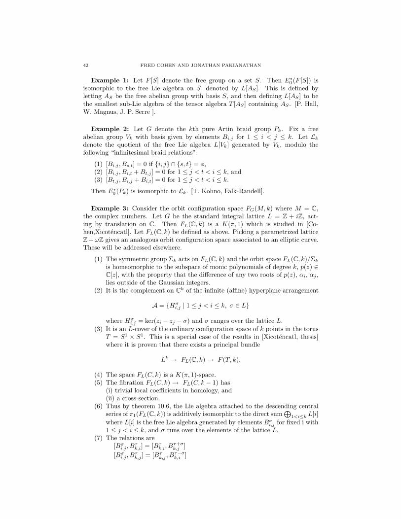
42 FRED COHEN AND JONATHAN PAKIANATHAN
Example 1: Let F [S] denote the free group on a set S. Then E∗0 (F [S]) is
isomorphic to the free Lie algebra on S, denoted by L[AS ]. This is defined byletting AS be the free abelian group with basis S, and then defining L[AS ] to bethe smallest sub-Lie algebra of the tensor algebra T [AS ] containing AS . [P. Hall,W. Magnus, J. P. Serre ].
Example 2: Let G denote the kth pure Artin braid group Pk. Fix a freeabelian group Vk with basis given by elements Bi,j for 1 ≤ i < j ≤ k. Let Lk
denote the quotient of the free Lie algebra L[Vk] generated by Vk, modulo thefollowing “infinitesimal braid relations”:
(1) [Bi,j , Bs,t] = 0 if i, j ∩ s, t = φ,(2) [Bi,j , Bi,t + Bt,j ] = 0 for 1 ≤ j < t < i ≤ k, and(3) [Bt,j , Bi,j + Bi,t] = 0 for 1 ≤ j < t < i ≤ k.
Then E∗0 (Pk) is isomorphic to Lk. [T. Kohno, Falk-Randell].
Example 3: Consider the orbit configuration space FG(M, k) where M = C,the complex numbers. Let G be the standard integral lattice L = Z + iZ, act-ing by translation on C. Then FL(C, k) is a K(π, 1) which is studied in [Co-hen,Xicotencatl]. Let FL(C, k) be defined as above. Picking a parametrized latticeZ + ωZ gives an analogous orbit configuration space associated to an elliptic curve.These will be addressed elsewhere.
(1) The symmetric group Σk acts on FL(C, k) and the orbit space FL(C, k)/Σk
is homeomorphic to the subspace of monic polynomials of degree k, p(z) ∈C[z], with the property that the difference of any two roots of p(z), αi, αj ,lies outside of the Gaussian integers.
(2) It is the complement on Ck of the infinite (affine) hyperplane arrangement
A = Hσi,j | 1 ≤ j < i ≤ k, σ ∈ L
where Hσi,j = ker(zi − zj − σ) and σ ranges over the lattice L.
(3) It is an L-cover of the ordinary configuration space of k points in the torusT = S1 × S1. This is a special case of the results in [Xicotencatl, thesis]where it is proven that there exists a principal bundle
Lk → FL(C, k) → F (T, k).
(4) The space FL(C, k) is a K(π, 1)-space.(5) The fibration FL(C, k) → FL(C, k − 1) has
(i) trivial local coefficients in homology, and(ii) a cross-section.
(6) Thus by theorem 10.6, the Lie algebra attached to the descending centralseries of π1(FL(C, k)) is additively isomorphic to the direct sum
⊕
1<i≤k L[i]
where L[i] is the free Lie algebra generated by elements Bσi,j for fixed i with
1 ≤ j < i ≤ k, and σ runs over the elements of the lattice L.(7) The relations are
[Bσi,j , B
τk,i] = [Bτ
k,i, Bτ+σk,j ]
[Bσi,j , B
τk,j ] = [Bτ
k,j , Bτ−σk,i ]
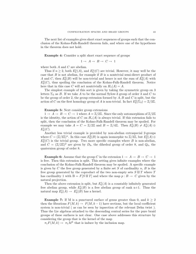
CONFIGURATION SPACES AND BRAID GROUPS 43
The next list of examples gives short exact sequences of groups such that the con-clusion of the Kohno-Falk-Randell theorem fails, and where one of the hypothesesin the theorem does not hold.
Example 4: Consider a split short exact sequence of groups
1 → A → B → C → 1
where both A and C are abelian.Thus if n ≥ 2, both En
0 (A), and En0 (C) are trivial. However, it may well be the
case that B is not abelian, for example if B is a nontrivial semi-direct product ofA and C, then E2
0 (B) will be non-trivial and hence is not the sum of E20(A) with
E20(C), thus spoiling the conclusion of the Kohno-Falk-Randell theorem. Notice
here that in this case C will act nontrivially on H1(A) = A.The simplest example of this sort is given by taking the symmetric group on 3
letters Σ3 as B. If we take A to be the normal Sylow-3 group of order 3 and C tobe the group of order 2, the group extension formed by A, B and C is split, but theaction of C on the first homology group of A is non-trivial. In fact E2
0(Σ3) = Z/3Z.
Example 5: Next consider group extensions1 → A → B → C → 1 where A = Z/2Z. Since the only automorphism of Z/2Z
is the identity, the action of C on H∗(A) is always trivial. If this extension fails tosplit, then the conclusion of the Kohno-Falk-Randell theorem may be spoiled. Forexample we may take A = C = Z/2Z and B = Z/4Z. Then E1
0(B) 6= E10 (A) ⊕
E10(C).Another less trivial example is provided by non-abelian extraspecial 2-groups
where C = (Z/2Z)n. In this case E20(B) is again isomorphic to Z/2Z, but E2
0(A)⊕E2
0(C) is the trivial group. Two more specific examples where B is non-abelian,and C = (Z/2Z)2 are given by D8, the dihedral group of order 8, and Q8, thequaternion group of order 8.
Example 6: Assume that the group C in the extension 1 → A → B → C → 1is free. Then this extension is split. This setting gives infinite examples where theconclusion of the Kohno-Falk-Randell theorem may be spoiled. A specific exampleis given by C the free group generated by a finite set S of cardinality n, B is thefree group generated by the coproduct of the two non-empty sets S ∐ T where Thas cardinality 1 with B = F [S ∐ T ] and where the map p : B → C given by thenatural projection.
Then the above extension is split, but E10(A) is a countably infinitely generated
free abelian group, while E10(B) is a free abelian group of rank n+1. Thus the
natural map E10(A) → E1
0(B) has a kernel.
Example 7: If M is a punctured surface of genus greater than 0, and k ≥ 2then the fibrations F (M, k) → F (M, k − 1) have sections, but the local coefficientsystem is non-trivial ( as can be seen by inpsection of the relevant Dehn twist ).Thus the Lie algebras attached to the descending central series for the pure braidgroups of these surfaces is not clear. One case above addresses this structure byconsidering the group that is the kernel of the map
π1F (M, k) → π1Mk that is induce by the inclusion map.
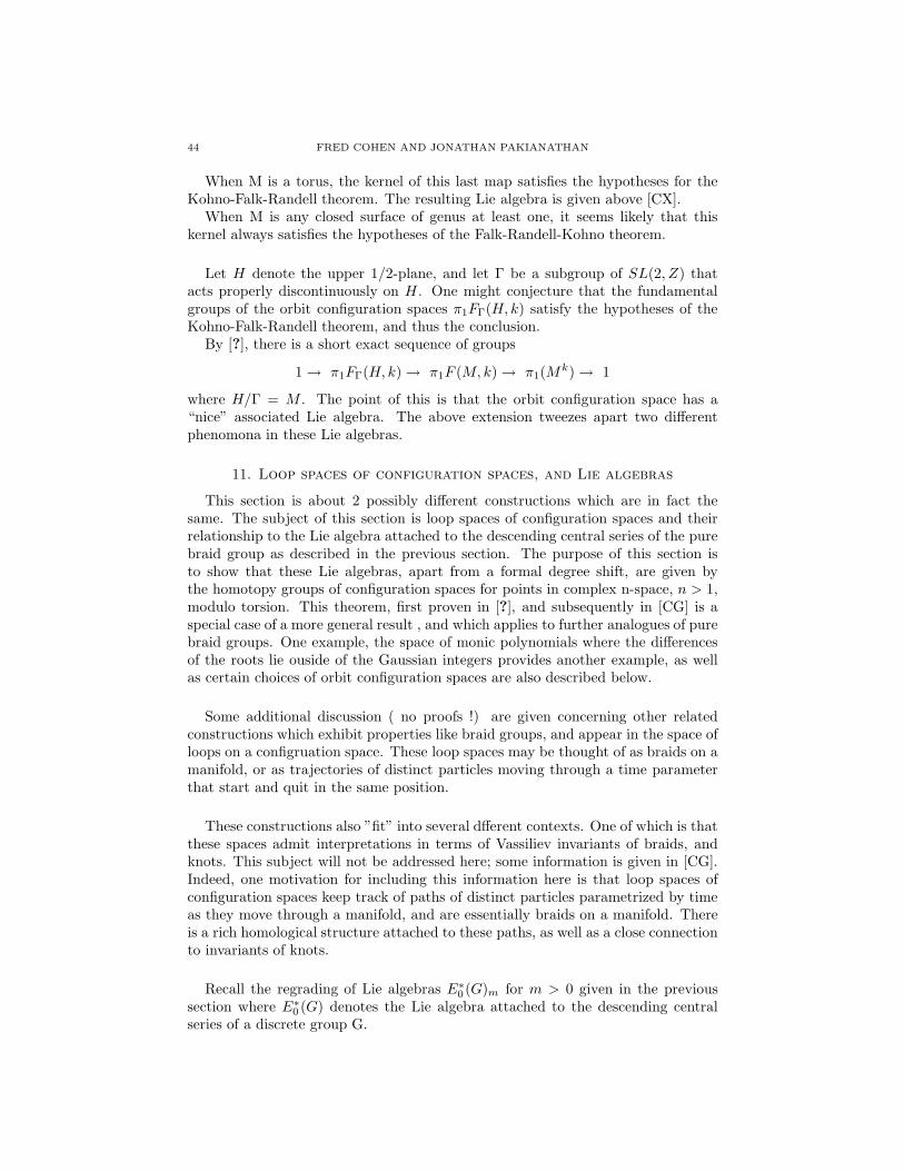
44 FRED COHEN AND JONATHAN PAKIANATHAN
When M is a torus, the kernel of this last map satisfies the hypotheses for theKohno-Falk-Randell theorem. The resulting Lie algebra is given above [CX].
When M is any closed surface of genus at least one, it seems likely that thiskernel always satisfies the hypotheses of the Falk-Randell-Kohno theorem.
Let H denote the upper 1/2-plane, and let Γ be a subgroup of SL(2, Z) thatacts properly discontinuously on H . One might conjecture that the fundamentalgroups of the orbit configuration spaces π1FΓ(H, k) satisfy the hypotheses of theKohno-Falk-Randell theorem, and thus the conclusion.
By [?], there is a short exact sequence of groups
1 → π1FΓ(H, k) → π1F (M, k) → π1(Mk) → 1
where H/Γ = M . The point of this is that the orbit configuration space has a“nice” associated Lie algebra. The above extension tweezes apart two differentphenomona in these Lie algebras.
11. Loop spaces of configuration spaces, and Lie algebras
This section is about 2 possibly different constructions which are in fact thesame. The subject of this section is loop spaces of configuration spaces and theirrelationship to the Lie algebra attached to the descending central series of the purebraid group as described in the previous section. The purpose of this section isto show that these Lie algebras, apart from a formal degree shift, are given bythe homotopy groups of configuration spaces for points in complex n-space, n > 1,modulo torsion. This theorem, first proven in [?], and subsequently in [CG] is aspecial case of a more general result , and which applies to further analogues of purebraid groups. One example, the space of monic polynomials where the differencesof the roots lie ouside of the Gaussian integers provides another example, as wellas certain choices of orbit configuration spaces are also described below.
Some additional discussion ( no proofs !) are given concerning other relatedconstructions which exhibit properties like braid groups, and appear in the space ofloops on a configruation space. These loop spaces may be thought of as braids on amanifold, or as trajectories of distinct particles moving through a time parameterthat start and quit in the same position.
These constructions also ”fit” into several dfferent contexts. One of which is thatthese spaces admit interpretations in terms of Vassiliev invariants of braids, andknots. This subject will not be addressed here; some information is given in [CG].Indeed, one motivation for including this information here is that loop spaces ofconfiguration spaces keep track of paths of distinct particles parametrized by timeas they move through a manifold, and are essentially braids on a manifold. Thereis a rich homological structure attached to these paths, as well as a close connectionto invariants of knots.
Recall the regrading of Lie algebras E∗0 (G)m for m > 0 given in the previous
section where E∗0 (G) denotes the Lie algebra attached to the descending central
series of a discrete group G.
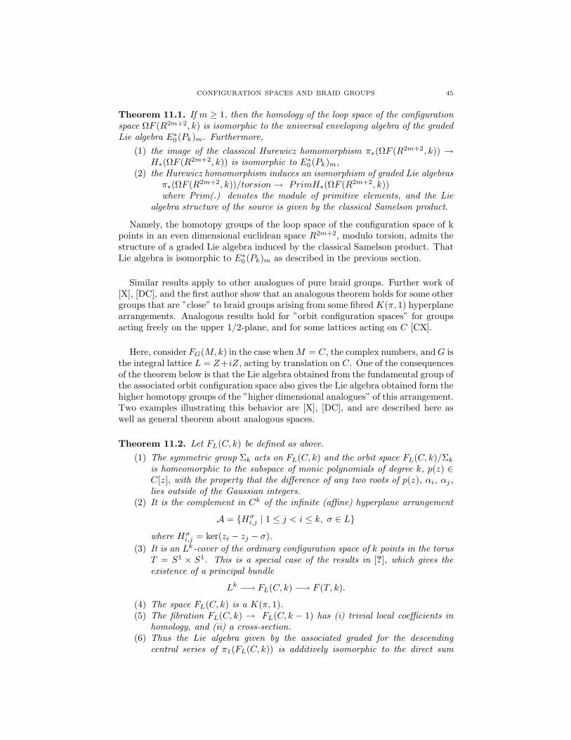
CONFIGURATION SPACES AND BRAID GROUPS 45
Theorem 11.1. If m ≥ 1, then the homology of the loop space of the configurationspace ΩF (R2m+2, k) is isomorphic to the universal enveloping algebra of the gradedLie algebra E∗
0 (Pk)m. Furthermore,
(1) the image of the classical Hurewicz homomorphism π∗(ΩF (R2m+2, k)) →H∗(ΩF (R2m+2, k)) is isomorphic to E∗
0 (Pk)m,(2) the Hurewicz homomorphism induces an isomorphism of graded Lie algebras
π∗(ΩF (R2m+2, k))/torsion → PrimH∗(ΩF (R2m+2, k))where Prim(.) denotes the module of primitive elements, and the Lie
algebra structure of the source is given by the classical Samelson product.
Namely, the homotopy groups of the loop space of the configuration space of kpoints in an even dimensional euclidean space R2m+2, modulo torsion, admits thestructure of a graded Lie algebra induced by the classical Samelson product. ThatLie algebra is isomorphic to E∗
0 (Pk)m as described in the previous section.
Similar results apply to other analogues of pure braid groups. Further work of[X], [DC], and the first author show that an analogous theorem holds for some othergroups that are ”close” to braid groups arising from some fibred K(π, 1) hyperplanearrangements. Analogous results hold for ”orbit configuration spaces” for groupsacting freely on the upper 1/2-plane, and for some lattices acting on C [CX].
Here, consider FG(M, k) in the case when M = C, the complex numbers, and G isthe integral lattice L = Z+iZ, acting by translation on C. One of the consequencesof the theorem below is that the Lie algebra obtained from the fundamental group ofthe associated orbit configuration space also gives the Lie algebra obtained form thehigher homotopy groups of the ”higher dimensional analogues” of this arrangement.Two examples illustrating this behavior are [X], [DC], and are described here aswell as general theorem about analogous spaces.
Theorem 11.2. Let FL(C, k) be defined as above.
(1) The symmetric group Σk acts on FL(C, k) and the orbit space FL(C, k)/Σk
is homeomorphic to the subspace of monic polynomials of degree k, p(z) ∈C[z], with the property that the difference of any two roots of p(z), αi, αj,lies outside of the Gaussian integers.
(2) It is the complement in Ck of the infinite (affine) hyperplane arrangement
A = Hσi,j | 1 ≤ j < i ≤ k, σ ∈ L
where Hσi,j = ker(zi − zj − σ).
(3) It is an Lk-cover of the ordinary configuration space of k points in the torusT = S1 × S1. This is a special case of the results in [?], which gives theexistence of a principal bundle
Lk −→ FL(C, k) −→ F (T, k).
(4) The space FL(C, k) is a K(π, 1).(5) The fibration FL(C, k) → FL(C, k − 1) has (i) trivial local coefficients in
homology, and (ii) a cross-section.(6) Thus the Lie algebra given by the associated graded for the descending
central series of π1(FL(C, k)) is additively isomorphic to the direct sum
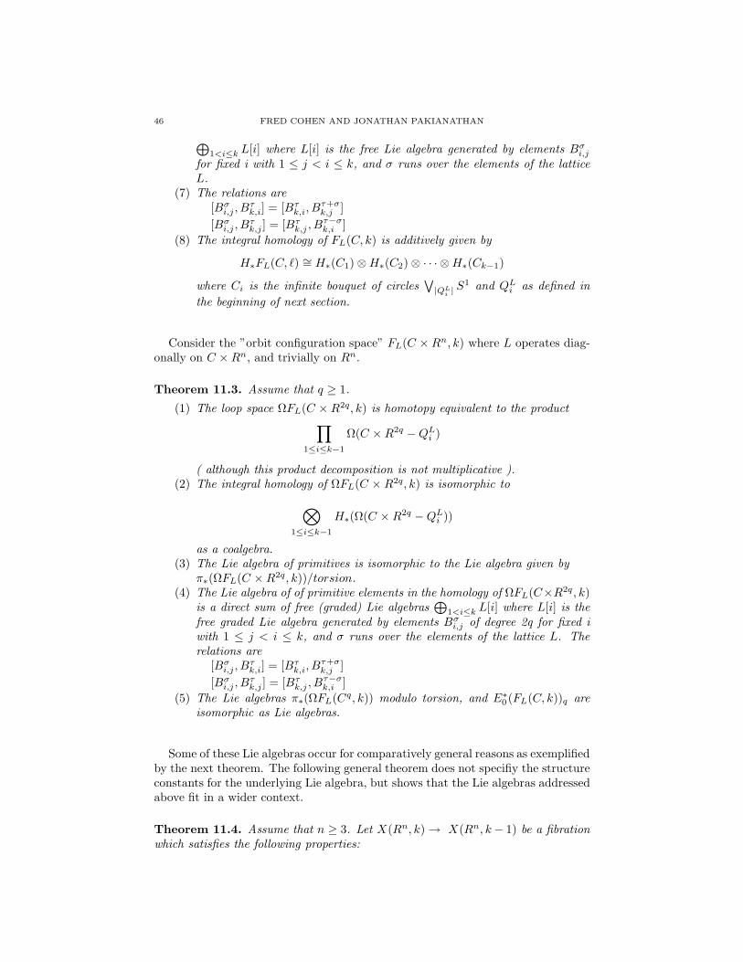
46 FRED COHEN AND JONATHAN PAKIANATHAN
⊕
1<i≤k L[i] where L[i] is the free Lie algebra generated by elements Bσi,j
for fixed i with 1 ≤ j < i ≤ k, and σ runs over the elements of the latticeL.
(7) The relations are[Bσ
i,j , Bτk,i] = [Bτ
k,i, Bτ+σk,j ]
[Bσi,j , B
τk,j ] = [Bτ
k,j , Bτ−σk,i ]
(8) The integral homology of FL(C, k) is additively given by
H∗FL(C, ℓ) ∼= H∗(C1) ⊗ H∗(C2) ⊗ · · · ⊗ H∗(Ck−1)
where Ci is the infinite bouquet of circles∨
|QLi| S
1 and QLi as defined in
the beginning of next section.
Consider the ”orbit configuration space” FL(C × Rn, k) where L operates diag-onally on C × Rn, and trivially on Rn.
Theorem 11.3. Assume that q ≥ 1.
(1) The loop space ΩFL(C × R2q, k) is homotopy equivalent to the product∏
1≤i≤k−1
Ω(C × R2q − QLi )
( although this product decomposition is not multiplicative ).(2) The integral homology of ΩFL(C × R2q, k) is isomorphic to
⊗
1≤i≤k−1
H∗(Ω(C × R2q − QLi ))
as a coalgebra.(3) The Lie algebra of primitives is isomorphic to the Lie algebra given by
π∗(ΩFL(C × R2q, k))/torsion.(4) The Lie algebra of of primitive elements in the homology of ΩFL(C×R2q, k)
is a direct sum of free (graded) Lie algebras⊕
1<i≤k L[i] where L[i] is thefree graded Lie algebra generated by elements Bσ
i,j of degree 2q for fixed iwith 1 ≤ j < i ≤ k, and σ runs over the elements of the lattice L. Therelations are
[Bσi,j , B
τk,i] = [Bτ
k,i, Bτ+σk,j ]
[Bσi,j , B
τk,j ] = [Bτ
k,j , Bτ−σk,i ]
(5) The Lie algebras π∗(ΩFL(Cq, k)) modulo torsion, and E∗0 (FL(C, k))q are
isomorphic as Lie algebras.
Some of these Lie algebras occur for comparatively general reasons as exemplifiedby the next theorem. The following general theorem does not specifiy the structureconstants for the underlying Lie algebra, but shows that the Lie algebras addressedabove fit in a wider context.
Theorem 11.4. Assume that n ≥ 3. Let X(Rn, k) → X(Rn, k − 1) be a fibrationwhich satisfies the following properties:
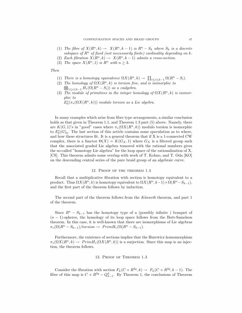
CONFIGURATION SPACES AND BRAID GROUPS 47
(1) The fibre of X(Rn, k) → X(Rn, k − 1) is Rn − Sk where Sk is a discretesubspace of Rn of fixed (not neccessarily finite) cardinality depending on k.
(2) Each fibration X(Rn, k) → X(Rn, k − 1) admits a cross-section.(3) The space X(Rn, 1) is Rn with n ≥ 3.
Then
(1) There is a homotopy equivalence ΩX(Rn, k) → ∏
1≤i≤k−1 Ω(Rn − Si).
(2) The homology of ΩX(Rn, k) is torsion free, and is isomorphic to⊗
1≤i≤k−1 H∗(Ω(Rn − Si)) as a coalgebra.
(3) The module of primitives in the integer homology of ΩX(Rn, k) is isomor-phic toE∗
0 (π∗(ΩX(Rn, k))) modulo torsion as a Lie algebra.
In many examples which arise from fibre type arrangements, a similar conclusionholds as that given in Theorem 1.1, and Theorem 1.3 part (5) above. Namely, thereare K(G, 1)′s in ”good” cases where π∗(ΩX(Rn, k)) modulo torsion is isomorphicto E∗
0 (G)q . The last section of this article contains some speculation as to where,and how these structures fit. It is a general theorem that if X is a 1-connected CWcomplex, there is a functor Θ(X) = K(GX , 1) where GX is a filtered group suchthat the associated graded Lie algebra tensored with the rational numbers givesthe so-called ”homotopy Lie algebra” for the loop space of the rationalization of X.[CS]. This theorem admits some overlap with work of T. Kohno, and T. Oda [KO]on the descending central series of the pure braid group of an algebraic curve.
12. Proof of the theorem 1.4
Recall that a multiplicative fibration with section is homotopy equivalent to aproduct. Thus ΩX(Rn, k) is homotopy equivalent to ΩX(Rn, k−1)×Ω(Rn−Sk−1),and the first part of the theorem follows by induction.
The second part of the theorem follows from the Kunneth theorem, and part 1of the theorem.
Since Rn − Sk−1 has the homotopy type of a (possibly infinite ) bouquet of(n − 1)-spheres, the homology of its loop space follows from the Bott-Samelsontheorem. In this case, it is well-known that there are isomorphisms of Lie algebrasπ∗(Ω(Rn − Sk−1)/torsion → PrimH∗(Ω(Rn − Sk−1).
Furthermore, the existence of sections implies that the Hurewicz homomorphismπ∗(ΩX(Rn, k) → PrimH∗(ΩX(Rn, k)) is a surjection. Since this map is an injec-tion, the theorem follows.
13. Proof of Theorem 1.3
Consider the fibration with section FL(C × R2q, k) → FL(C × R2q, k − 1). Thefibre of this map is C × R2q − QL
k−1. By Theorem 1, the conclusions of Theorem
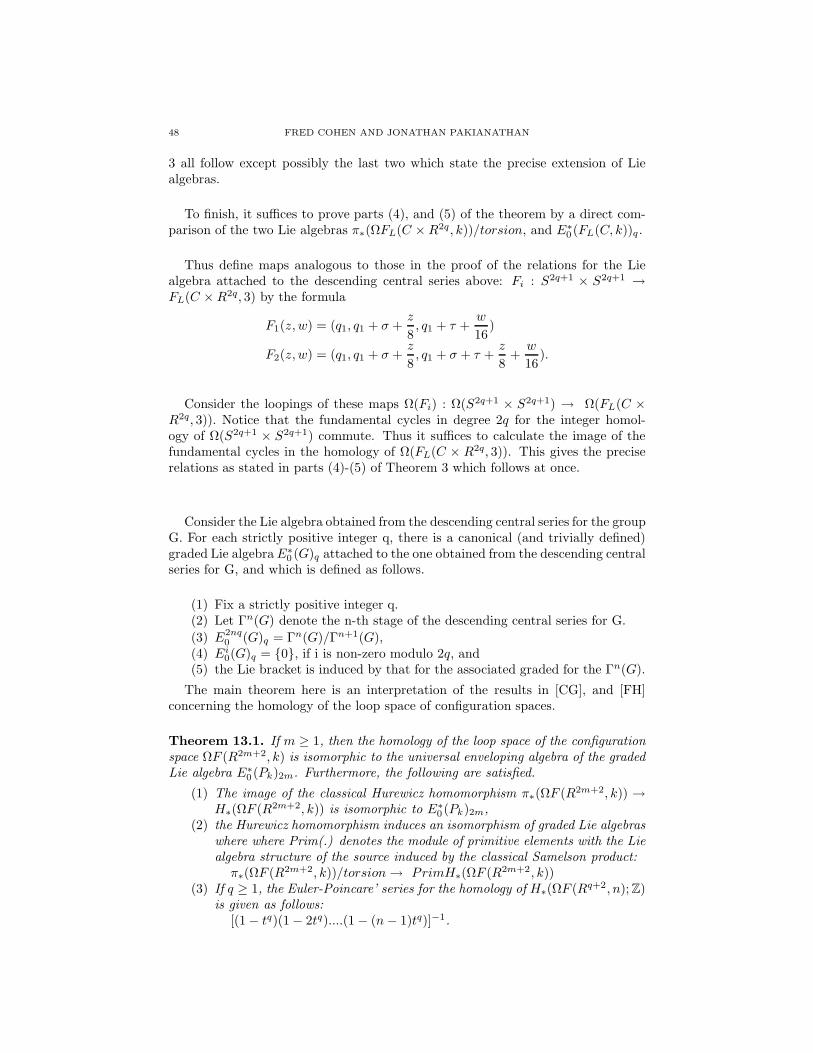
48 FRED COHEN AND JONATHAN PAKIANATHAN
3 all follow except possibly the last two which state the precise extension of Liealgebras.
To finish, it suffices to prove parts (4), and (5) of the theorem by a direct com-parison of the two Lie algebras π∗(ΩFL(C × R2q, k))/torsion, and E∗
0 (FL(C, k))q .
Thus define maps analogous to those in the proof of the relations for the Liealgebra attached to the descending central series above: Fi : S2q+1 × S2q+1 →FL(C × R2q, 3) by the formula
F1(z, w) = (q1, q1 + σ +z
8, q1 + τ +
w
16)
F2(z, w) = (q1, q1 + σ +z
8, q1 + σ + τ +
z
8+
w
16).
Consider the loopings of these maps Ω(Fi) : Ω(S2q+1 × S2q+1) → Ω(FL(C ×R2q, 3)). Notice that the fundamental cycles in degree 2q for the integer homol-ogy of Ω(S2q+1 × S2q+1) commute. Thus it suffices to calculate the image of thefundamental cycles in the homology of Ω(FL(C × R2q, 3)). This gives the preciserelations as stated in parts (4)-(5) of Theorem 3 which follows at once.
Consider the Lie algebra obtained from the descending central series for the groupG. For each strictly positive integer q, there is a canonical (and trivially defined)graded Lie algebra E∗
0 (G)q attached to the one obtained from the descending centralseries for G, and which is defined as follows.
(1) Fix a strictly positive integer q.(2) Let Γn(G) denote the n-th stage of the descending central series for G.
(3) E2nq0 (G)q = Γn(G)/Γn+1(G),
(4) Ei0(G)q = 0, if i is non-zero modulo 2q, and
(5) the Lie bracket is induced by that for the associated graded for the Γn(G).
The main theorem here is an interpretation of the results in [CG], and [FH]concerning the homology of the loop space of configuration spaces.
Theorem 13.1. If m ≥ 1, then the homology of the loop space of the configurationspace ΩF (R2m+2, k) is isomorphic to the universal enveloping algebra of the gradedLie algebra E∗
0 (Pk)2m. Furthermore, the following are satisfied.
(1) The image of the classical Hurewicz homomorphism π∗(ΩF (R2m+2, k)) →H∗(ΩF (R2m+2, k)) is isomorphic to E∗
0 (Pk)2m,(2) the Hurewicz homomorphism induces an isomorphism of graded Lie algebras
where where Prim(.) denotes the module of primitive elements with the Liealgebra structure of the source induced by the classical Samelson product:
π∗(ΩF (R2m+2, k))/torsion → PrimH∗(ΩF (R2m+2, k))(3) If q ≥ 1, the Euler-Poincare’ series for the homology of H∗(ΩF (Rq+2, n); Z)
is given as follows:[(1 − tq)(1 − 2tq)....(1 − (n − 1)tq)]−1.
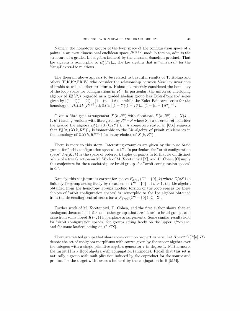
CONFIGURATION SPACES AND BRAID GROUPS 49
Namely, the homotopy groups of the loop space of the configuration space of kpoints in an even dimensional euclidean space R2m+2, modulo torsion, admits thestructure of a graded Lie algebra induced by the classical Samelson product. ThatLie algebra is isomorphic to E∗
0 (Pk)m, the Lie algebra that is ”universal” for theYang-Baxter-Lie relations.
The theorem above appears to be related to beautiful results of T. Kohno andothers [H,K,K2,FR,W] who consider the relationship between Vassiliev invariantsof braids as well as other structures. Kohno has recently considered the homologyof the loop space for configurations in R3. In particular, the universal envelopingalgebra of E∗
0 (Pk) regarded as a graded abelian group has Euler-Poincare’ seriesgiven by [(1 − t)(1 − 2t)....(1− (n− 1)t)]−1 while the Euler-Poincare’ series for thehomology of H∗(ΩF (Rq+2, n); Z) is [(1 − tq)(1 − 2tq)....(1 − (n − 1)tq)]−1.
Given a fibre type arrangement X(k, Rn) with fibrations X(k, Rn) → X(k −1, Rn) having sections with fibre given by Rn −S where S is a discrete set, considerthe graded Lie algebra E∗
0 (π1(X(k, R2)))q. A conjecture stated in [CX] suggeststhat E∗
0 (π1(X(k, R2)))q is isomorphic to the Lie algebra of primitive elements inthe homology of ΩX(k, R2q+2) for many choices of X(k, Rn).
There is more to this story. Interesting examples are given by the pure braidgroups for ”orbit configuration spaces” in C∗. In particular, the ”orbit configurationspace” FG(M, k) is the space of ordered k tuples of points in M that lie on distinctorbits of a free G action on M. Work of M. Xicotencatl [X], and D. Cohen [C] implythis conjecture for the associated pure braid groups for ”orbit configuration spaces”in C∗.
Namely, this conjecture is correct for spaces FZ/qZ (Cn−0, k) where Z/qZ is afinite cyclic group acting freely by rotations on Cn −0. If n > 1, the Lie algebraobtained from the homotopy groups modulo torsion of the loop spaces for thesechoices of ”orbit configuration spaces” is isomorphic to the Lie algebra obtainedfrom the descending central series for π1FZ/qZ (Cn − 0) [C],[X].
Further work of M. Xicotencatl, D. Cohen, and the first author shows that ananalogous theorem holds for some other groups that are ”close” to braid groups, andarise from some fibred K(π, 1) hyperplane arrangements. Some similar results holdfor ”orbit configuration spaces” for groups acting freely on the upper 1/2-plane,and for some lattices acting on C [CX].
There are related groups that share some common properties here. Let Homcoalg(T [v], H)denote the set of coalgebra morphisms with source given by the tensor algebra overthe integers with a single primitive algebra generator v in degree 1. Furthermore,the target H is a Hopf algebra with conjugation (antipode). Recall that this set isnaturally a group with multiplication induced by the coproduct for the source andproduct for the target with inverses induced by the conjugation in H [MM].
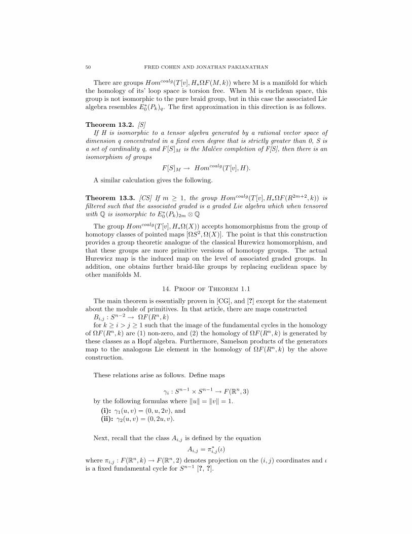
50 FRED COHEN AND JONATHAN PAKIANATHAN
There are groups Homcoalg(T [v], H∗ΩF (M, k)) where M is a manifold for whichthe homology of its’ loop space is torsion free. When M is euclidean space, thisgroup is not isomorphic to the pure braid group, but in this case the associated Liealgebra resembles E∗
0 (Pk)q. The first approximation in this direction is as follows.
Theorem 13.2. [S]If H is isomorphic to a tensor algebra generated by a rational vector space of
dimension q concentrated in a fixed even degree that is strictly greater than 0, S isa set of cardinality q, and F [S]M is the Malcev completion of F[S], then there is anisomorphism of groups
F [S]M → Homcoalg(T [v], H).
A similar calculation gives the following.
Theorem 13.3. [CS] If m ≥ 1, the group Homcoalg(T [v], H∗ΩF (R2m+2, k)) isfiltered such that the associated graded is a graded Lie algebra which when tensoredwith Q is isomorphic to E∗
0 (Pk)2m ⊗ Q
The group Homcoalg(T [v], H∗Ω(X)) accepts homomorphisms from the group ofhomotopy classes of pointed maps [ΩS2, Ω(X)]. The point is that this constructionprovides a group theoretic analogue of the classical Hurewicz homomorphism, andthat these groups are more primitive versions of homotopy groups. The actualHurewicz map is the induced map on the level of associated graded groups. Inaddition, one obtains further braid-like groups by replacing euclidean space byother manifolds M.
14. Proof of Theorem 1.1
The main theorem is essentially proven in [CG], and [?] except for the statementabout the module of primitives. In that article, there are maps constructed
Bi,j : Sn−2 → ΩF (Rn, k)for k ≥ i > j ≥ 1 such that the image of the fundamental cycles in the homology
of ΩF (Rn, k) are (1) non-zero, and (2) the homology of ΩF (Rn, k) is generated bythese classes as a Hopf algebra. Furthermore, Samelson products of the generatorsmap to the analogous Lie element in the homology of ΩF (Rn, k) by the aboveconstruction.
These relations arise as follows. Define maps
γi : Sn−1 × Sn−1 → F (Rn, 3)
by the following formulas where ‖u‖ = ‖v‖ = 1.
(i): γ1(u, v) = (0, u, 2v), and(ii): γ2(u, v) = (0, 2u, v).
Next, recall that the class Ai,j is defined by the equation
Ai,j = π∗i,j(ι)
where πi,j : F (Rn, k) → F (Rn, 2) denotes projection on the (i, j) coordinates and ιis a fixed fundamental cycle for Sn−1 [?, ?].
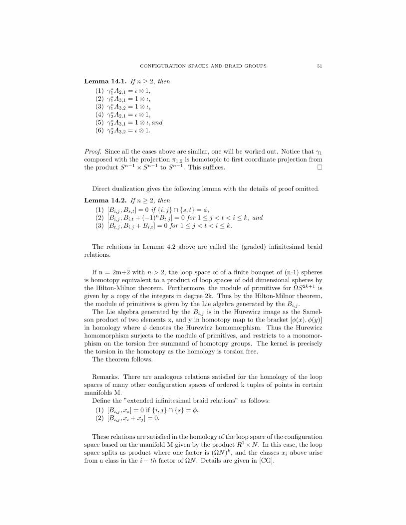
CONFIGURATION SPACES AND BRAID GROUPS 51
Lemma 14.1. If n ≥ 2, then
(1) γ∗1A2,1 = ι ⊗ 1,
(2) γ∗1A3,1 = 1 ⊗ ι,
(3) γ∗1A3,2 = 1 ⊗ ι,
(4) γ∗2A2,1 = ι ⊗ 1,
(5) γ∗2A3,1 = 1 ⊗ ι, and
(6) γ∗2A3,2 = ι ⊗ 1.
Proof. Since all the cases above are similar, one will be worked out. Notice that γ1
composed with the projection π1,2 is homotopic to first coordinate projection fromthe product Sn−1 × Sn−1 to Sn−1. This suffices.
Direct dualization gives the following lemma with the details of proof omitted.
Lemma 14.2. If n ≥ 2, then
(1) [Bi,j , Bs,t] = 0 if i, j ∩ s, t = φ,(2) [Bi,j , Bi,t + (−1)nBt,j ] = 0 for 1 ≤ j < t < i ≤ k, and(3) [Bt,j , Bi,j + Bi,t] = 0 for 1 ≤ j < t < i ≤ k.
The relations in Lemma 4.2 above are called the (graded) infinitesimal braidrelations.
If n = 2m+2 with n > 2, the loop space of of a finite bouquet of (n-1) spheresis homotopy equivalent to a product of loop spaces of odd dimensional spheres bythe Hilton-Milnor theorem. Furthermore, the module of primitives for ΩS2k+1 isgiven by a copy of the integers in degree 2k. Thus by the Hilton-Milnor theorem,the module of primitives is given by the Lie algebra generated by the Bi,j .
The Lie algebra generated by the Bi,j is in the Hurewicz image as the Samel-son product of two elements x, and y in homotopy map to the bracket [φ(x), φ(y)]in homology where φ denotes the Hurewicz homomorphism. Thus the Hurewiczhomomorphism surjects to the module of primitives, and restricts to a monomor-phism on the torsion free summand of homotopy groups. The kernel is preciselythe torsion in the homotopy as the homology is torsion free.
The theorem follows.
Remarks. There are analogous relations satisfied for the homology of the loopspaces of many other configuration spaces of ordered k tuples of points in certainmanifolds M.
Define the ”extended infinitesimal braid relations” as follows:
(1) [Bi,j , xs] = 0 if i, j ∩ s = φ,(2) [Bi,j , xi + xj ] = 0.
These relations are satisfied in the homology of the loop space of the configurationspace based on the manifold M given by the product R1×N . In this case, the loopspace splits as product where one factor is (ΩN)k, and the classes xi above arisefrom a class in the i − th factor of ΩN . Details are given in [CG].
52 FRED COHEN AND JONATHAN PAKIANATHAN
References
[Bre] Bredon, Topology and Geometry, Springer Verlag GTM 139, New York-Heidelberg-Berlin,1993.
[B] K. S. Brown, Cohomology of Groups, Springer Verlag GTM 87, New York-Heidelberg-Berlin, 1994.
[BM] Bergau, and Mennicke[BH] Birman, and H. Hilden,[C1] F. R. Cohen, On the hyperelliptic mapping class groups, SO(3), and Spinc(3), American
J. Math., 115 (1993), 389–434.[C2] F.R. Cohen, On configuration spaces, their homology, and Lie Algebras, Journal of Pure
and Applied Algebra 100 (1995), 19-42.[CG] F.R. Cohen, S. Gitler, (i) On loop spaces of configuration spaces, submitted to the Memoirs
of the AMS, and (ii) Loop spaces of configuration spaces, braid-like groups, and knots, toappear in the Proceedings of the 1998 Barcelona Conference on Algebraic Topology.
[CLM] F.R. Cohen, T.J. Lada and J.P. May, The homology of iterated loop spaces, Lecture Notesin Math., vol. 533, Springer-Verlag (1976).
[CS] F.R. Cohen, T. Sato, in preparation.[CX] F.R. Cohen, M. Xicotencatl, submitted.[DC] D. C. Cohen, Monodromy of fibre-type arrangements and orbit configuration spaces, to
appear in Forum Mathematicum.[DCS] D. C. Cohen, Alexander I. Suciu, Homology of iterated semidirect products of free groups,
J. Pure Appl. Algebra 126 (1998), pg 87-120.[EE] C. Earle, and J. Eells, A fibre bundle description of Teichmuller theory, J. Differential
Geometry 3(1969), 19-43.[FH1] E. Fadell and S. Husseini, The space of loops on configuration spaces and the Majer-
Terracini index, Topol. Methods in Nonlinear Anal., Journal of the Julius Schauder Cen-ter, 11 (1998), 249–271.
[FH2] E. Fadell and S. Husseini, Geometry and Topology of Configuration Spaces, in preparation.[FN] E. Fadell and L. Neuwirth, Configuration spaces, Math. Scand. 10 (1962), 119-126.[FR] M. Falk, and R. Randell, The lower central series of a fiber-type arrangement, Invent.
Math. 82 (1985), 77-88.[H] R. Hain, Infinitesimal presentations of the Torelli group, J. Amer. Math. Soc. 10
(1997),597-691.[K1] T. Kohno, Linear represenations of braid groups and classical Yang-Baxter equations,
Cont. Math. 78 (1988), 339-363.[K2] T. Kohno, Vassiliev invariants and de Rham complex on the space of knots, Cont. Math.
179 (1994), 123-138.[K3] T. Kohno, Elliptic KZ system, braid groups of the torus and Vassiliev invariants, Topology
and its Applications, 78 (1997), 79-94.[KO] T. Kohno, and T. Oda, The lower central series of the pure braid group of an algebraic
curve, Advanced Studies in Pure Mathematics, Galois Represntations and ArithmeticAlgebraic Geometry 12 (1987), 201-219.
[MM] J. W. Milnor, and J.C. Moore, On the structure of Hopf algebras, Ann. of Math. 81
(1965), 211-264.[R] Derek J.S. Robinson, A Course in the Theory of Groups, Springer Verlag GTM 80, New
York-Heidelberg-Berlin, 1995.[S] N. E. Steenrod, The Topology of Fibre Bundles, Princeton University Press.[Sa] T. Sato, On free groups and morphisms of coalgebras, student topology seminar, Univ. of
Roch., Spring 1998, preprint.[Smale] S. Smale, P.A.M.S.[Spa] Edwin H. Spanier, Algebraic Topology, Springer Verlag, New York-Heidelberg-Berlin, 1966.[Wh] Whitehead, Elements of Homotopy Theory, Springer Verlag GTM 61, New York-
Heidelberg-Berlin, .[W] S. Willerton, thesis.[X] M. Xicotencatl, Orbit configuration spaces, infinitesimal braid relations, and equivariant
function spaces, Ph.D. thesis, University of Rochester, Spring 1997.[Xia] Yining Xia,