Embed Size (px)
Citation preview

29/09/2008Ina Dix - 15th Bruker AXS SCD Users Meeting1
Introduction to
Integration – SAINT
Dr. Ina Dix
Bruker AXS Karlsruhe
29/09/2008Ina Dix - 15th Bruker AXS SCD Users Meeting2
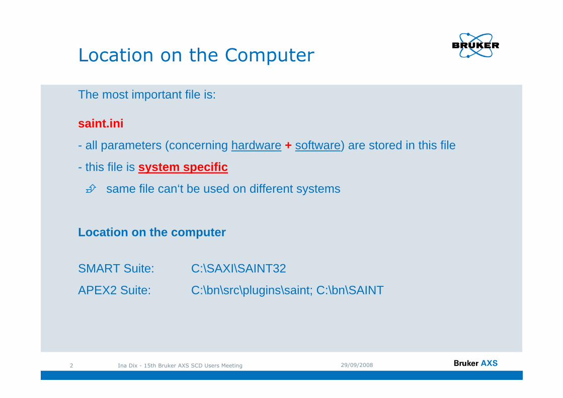
The most important file is:
saint.ini
- all parameters (concerning hardware + software) are stored in this file
- this file is system specific
� same file can‘t be used on different systems
Location on the computer
SMART Suite: C:\SAXI\SAINT32
APEX2 Suite: C:\bn\src\plugins\saint; C:\bn\SAINT
Location on the Computer
29/09/2008Ina Dix - 15th Bruker AXS SCD Users Meeting3
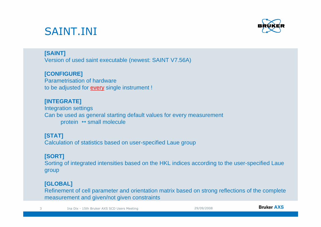
[SAINT]Version of used saint executable (newest: SAINT V7.56A)
[CONFIGURE]Parametrisation of hardware to be adjusted for every single instrument !
[INTEGRATE]Integration settingsCan be used as general starting default values for every measurement
protein � small molecule
[STAT]Calculation of statistics based on user-specified Laue group
[SORT]Sorting of integrated intensities based on the HKL indices according to the user-specified Lauegroup
[GLOBAL]Refinement of cell parameter and orientation matrix based on strong reflections of the complete measurement and given/not given constraints
SAINT.INI
29/09/2008Ina Dix - 15th Bruker AXS SCD Users Meeting4
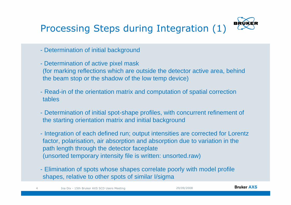
- Determination of initial background
- Determination of active pixel mask (for marking reflections which are outside the detector active area, behind the beam stop or the shadow of the low temp device)
- Read-in of the orientation matrix and computation of spatial correction tables
- Determination of initial spot-shape profiles, with concurrent refinement of the starting orientation matrix and initial background
- Integration of each defined run; output intensities are corrected for Lorentzfactor, polarisation, air absorption and absorption due to variation in the path length through the detector faceplate(unsorted temporary intensity file is written: unsorted.raw)
- Elimination of spots whose shapes correlate poorly with model profile shapes, relative to other spots of similar I/sigma
Processing Steps during Integration (1)
29/09/2008Ina Dix - 15th Bruker AXS SCD Users Meeting5
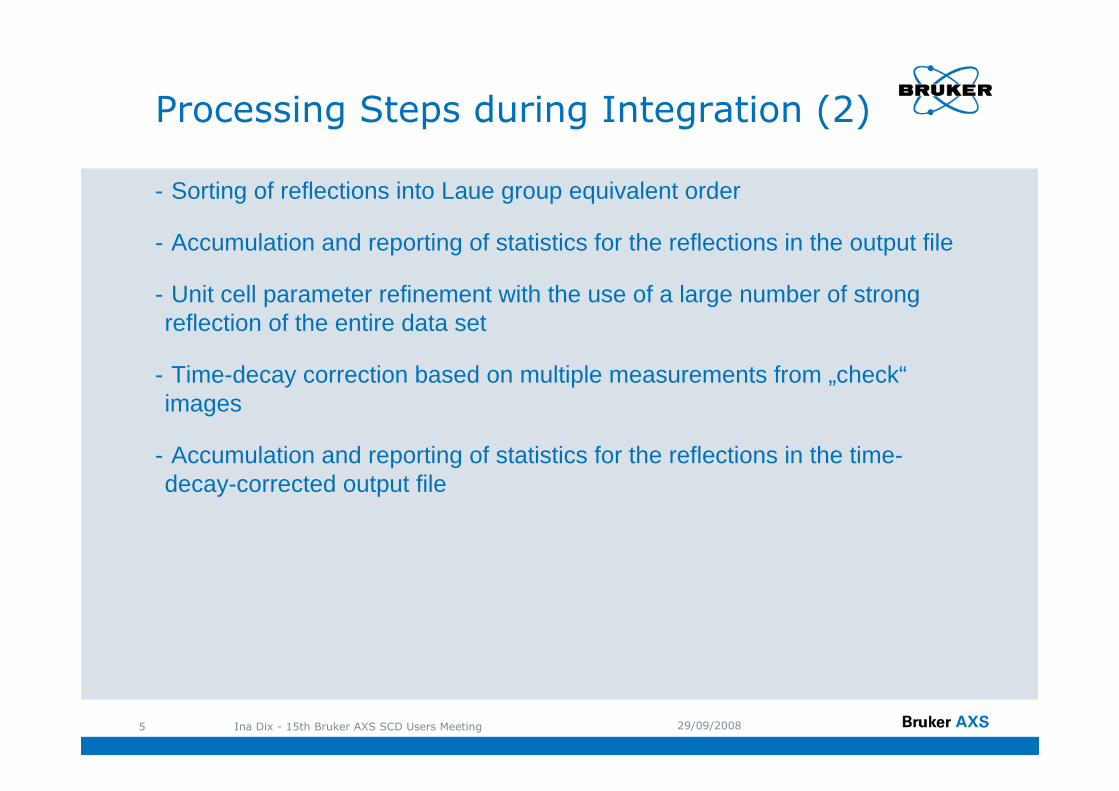
- Sorting of reflections into Laue group equivalent order
- Accumulation and reporting of statistics for the reflections in the output file
- Unit cell parameter refinement with the use of a large number of strong reflection of the entire data set
- Time-decay correction based on multiple measurements from „check“ images
- Accumulation and reporting of statistics for the reflections in the time-decay-corrected output file
Processing Steps during Integration (2)
29/09/2008Ina Dix - 15th Bruker AXS SCD Users Meeting6
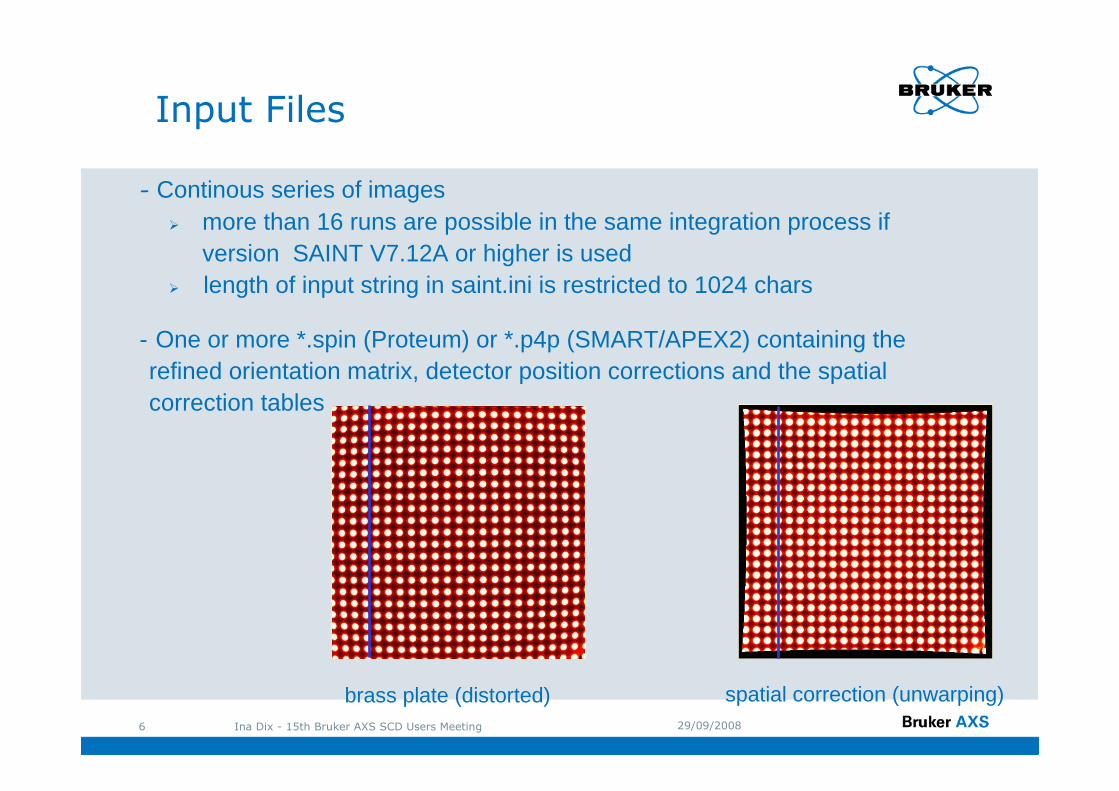
- Continous series of images � more than 16 runs are possible in the same integration process if
version SAINT V7.12A or higher is used� length of input string in saint.ini is restricted to 1024 chars
- One or more *.spin (Proteum) or *.p4p (SMART/APEX2) containing the refined orientation matrix, detector position corrections and the spatial correction tables
brass plate (distorted) spatial correction (unwarping)
Input Files
29/09/2008Ina Dix - 15th Bruker AXS SCD Users Meeting7
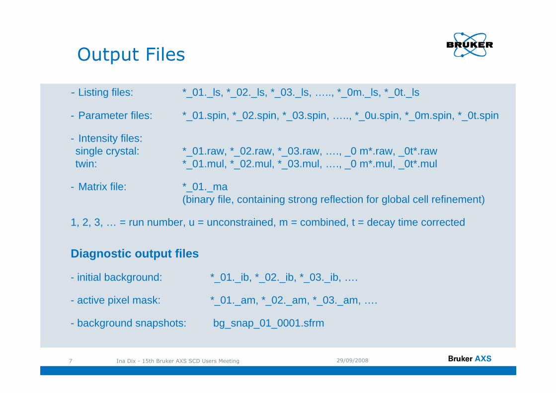
- Listing files: *_01._ls, *_02._ls, *_03._ls, ….., *_0m._ls, *_0t._ls
- Parameter files: *_01.spin, *_02.spin, *_03.spin, ….., *_0u.spin, *_0m.spin, *_0t.spin
- Intensity files: single crystal: *_01.raw, *_02.raw, *_03.raw, …., _0 m*.raw, _0t*.rawtwin: *_01.mul, *_02.mul, *_03.mul, …., _0 m*.mul, _0t*.mul
- Matrix file: *_01._ma (binary file, containing strong reflection for global cell refinement)
1, 2, 3, … = run number, u = unconstrained, m = combined, t = decay time corrected
Diagnostic output files
- initial background: *_01._ib, *_02._ib, *_03._ib, ….
- active pixel mask: *_01._am, *_02._am, *_03._am, ….
- background snapshots: bg_snap_01_0001.sfrm
Output Files
29/09/2008Ina Dix - 15th Bruker AXS SCD Users Meeting8
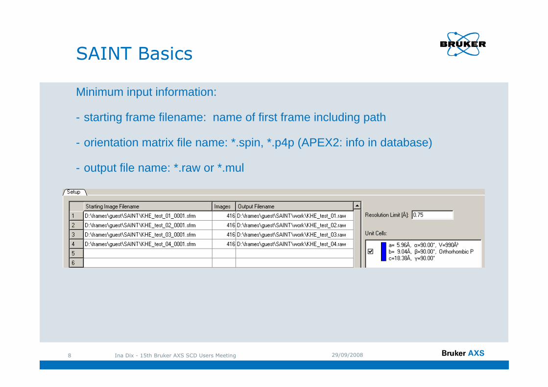
Minimum input information:
- starting frame filename: name of first frame including path
- orientation matrix file name: *.spin, *.p4p (APEX2: info in database)
- output file name: *.raw or *.mul
SAINT Basics
29/09/2008Ina Dix - 15th Bruker AXS SCD Users Meeting9
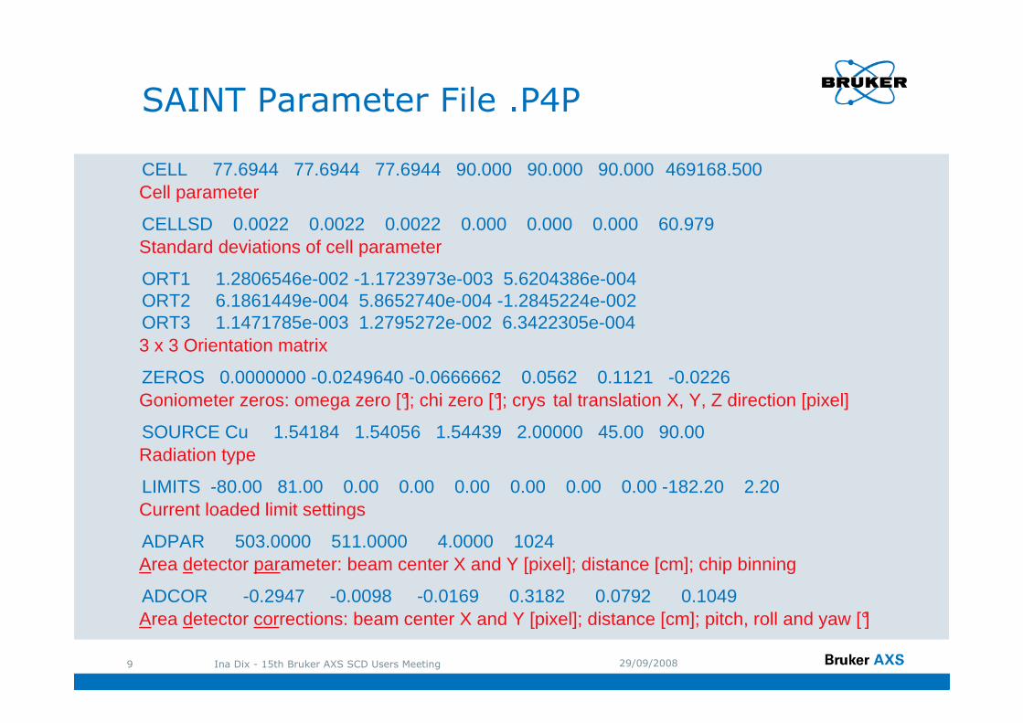
CELL 77.6944 77.6944 77.6944 90.000 90.000 90.000 469168.500
CELLSD 0.0022 0.0022 0.0022 0.000 0.000 0.000 60.979
ORT1 1.2806546e-002 -1.1723973e-003 5.6204386e-004 ORT2 6.1861449e-004 5.8652740e-004 -1.2845224e-002 ORT3 1.1471785e-003 1.2795272e-002 6.3422305e-004
ZEROS 0.0000000 -0.0249640 -0.0666662 0.0562 0.1121 -0.0226
SOURCE Cu 1.54184 1.54056 1.54439 2.00000 45.00 90.00
LIMITS -80.00 81.00 0.00 0.00 0.00 0.00 0.00 0.00 -182.20 2.20
ADPAR 503.0000 511.0000 4.0000 1024
ADCOR -0.2947 -0.0098 -0.0169 0.3182 0.0792 0.1049
Cell parameter
Standard deviations of cell parameter
3 x 3 Orientation matrix
Goniometer zeros: omega zero [°]; chi zero [°]; crys tal translation X, Y, Z direction [pixel]
Radiation type
Current loaded limit settings
Area detector parameter: beam center X and Y [pixel]; distance [cm]; chip binning
Area detector corrections: beam center X and Y [pixel]; distance [cm]; pitch, roll and yaw [°]
SAINT Parameter File .P4P
29/09/2008Ina Dix - 15th Bruker AXS SCD Users Meeting10
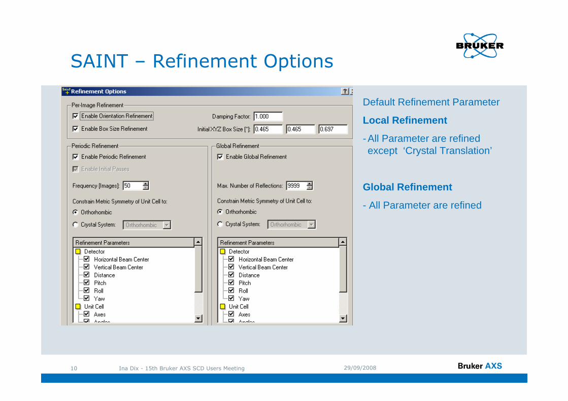
Default Refinement Parameter
Local Refinement
- All Parameter are refined except ‘Crystal Translation’
Global Refinement
- All Parameter are refined
SAINT – Refinement Options
29/09/2008Ina Dix - 15th Bruker AXS SCD Users Meeting11
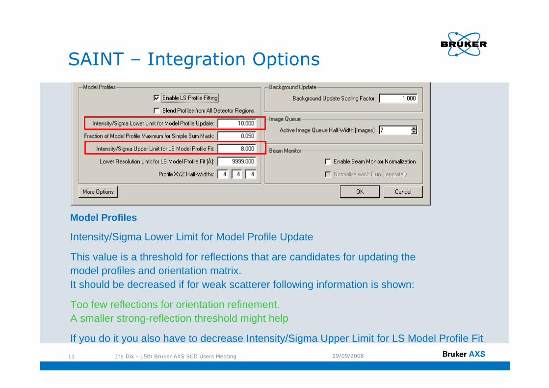
Model Profiles
Intensity/Sigma Lower Limit for Model Profile Update
This value is a threshold for reflections that are candidates for updating themodel profiles and orientation matrix.It should be decreased if for weak scatterer following information is shown:
Too few reflections for orientation refinement. A smaller strong-reflection threshold might help
If you do it you also have to decrease Intensity/Sigma Upper Limit for LS Model Profile Fit
SAINT – Integration Options
29/09/2008Ina Dix - 15th Bruker AXS SCD Users Meeting12
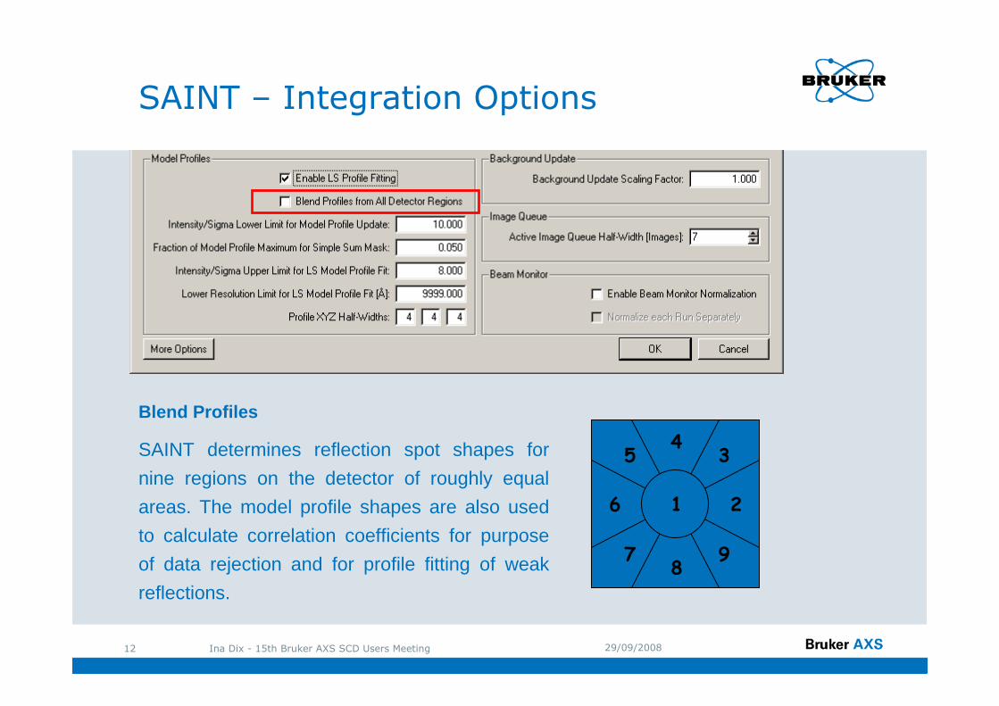
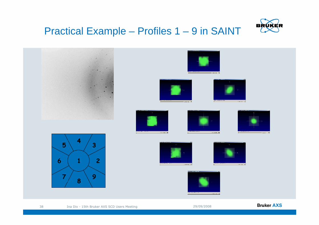
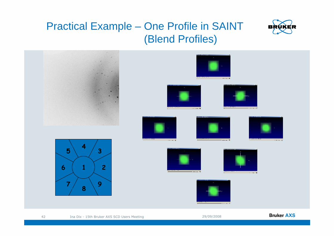
Blend Profiles
SAINT determines reflection spot shapes for
nine regions on the detector of roughly equal
areas. The model profile shapes are also used
to calculate correlation coefficients for purpose
of data rejection and for profile fitting of weak
reflections.
SAINT – Integration Options
7
6
5 3
2
98
1
4
29/09/2008Ina Dix - 15th Bruker AXS SCD Users Meeting13
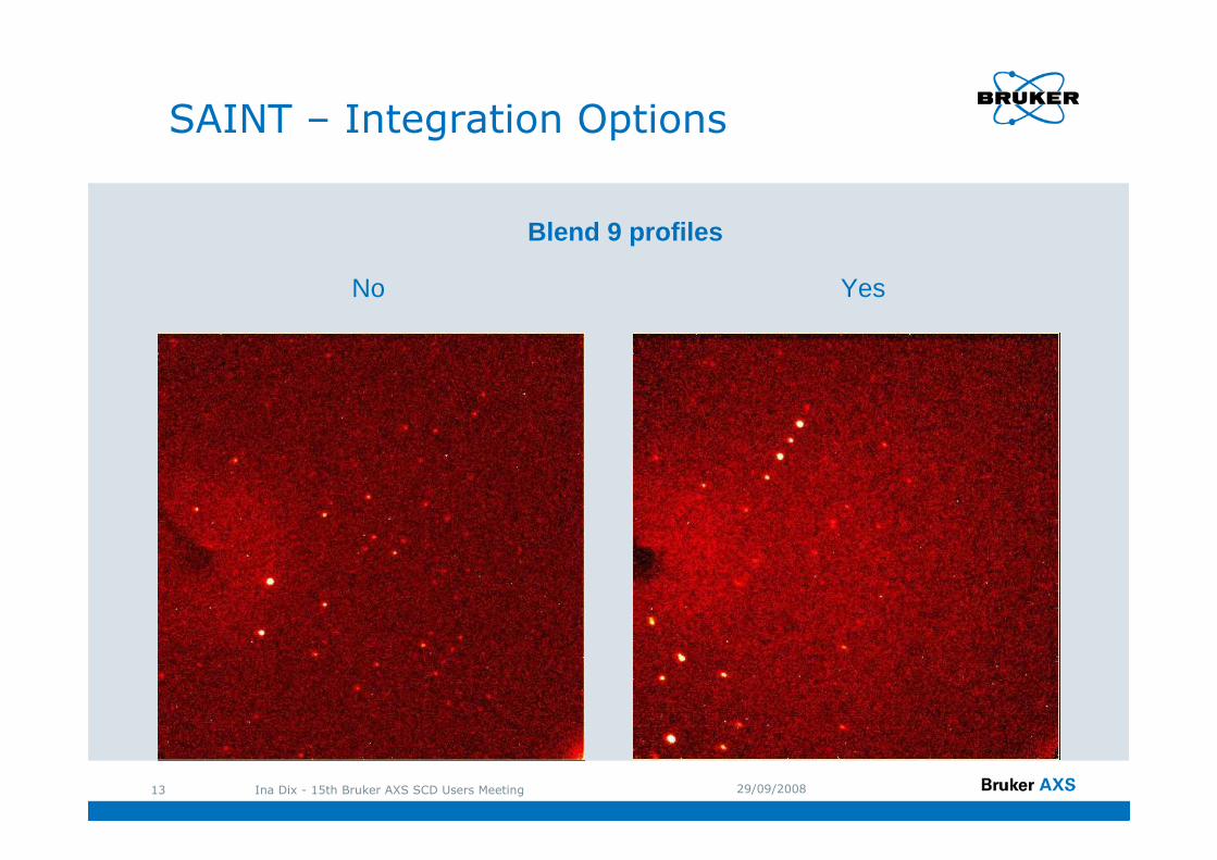
Blend 9 profiles
No Yes
SAINT – Integration Options
29/09/2008Ina Dix - 15th Bruker AXS SCD Users Meeting14
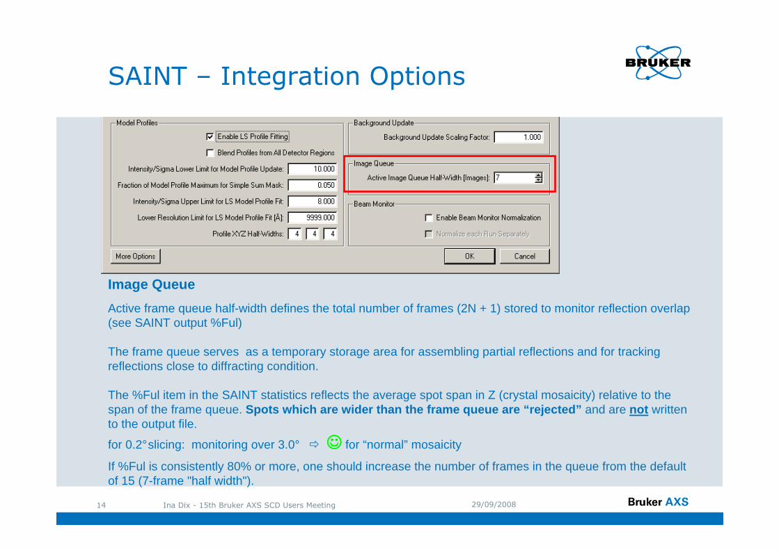
Image Queue
Active frame queue half-width defines the total number of frames (2N + 1) stored to monitor reflection overlap (see SAINT output %Ful)
The frame queue serves as a temporary storage area for assembling partial reflections and for tracking reflections close to diffracting condition.
The %Ful item in the SAINT statistics reflects the average spot span in Z (crystal mosaicity) relative to the span of the frame queue. Spots which are wider than the frame queue are “rej ected” and are not written to the output file.
for 0.2° slicing: monitoring over 3.0° � ☺☺☺☺ for “normal” mosaicity
If %Ful is consistently 80% or more, one should increase the number of frames in the queue from the default of 15 (7-frame "half width").
SAINT – Integration Options
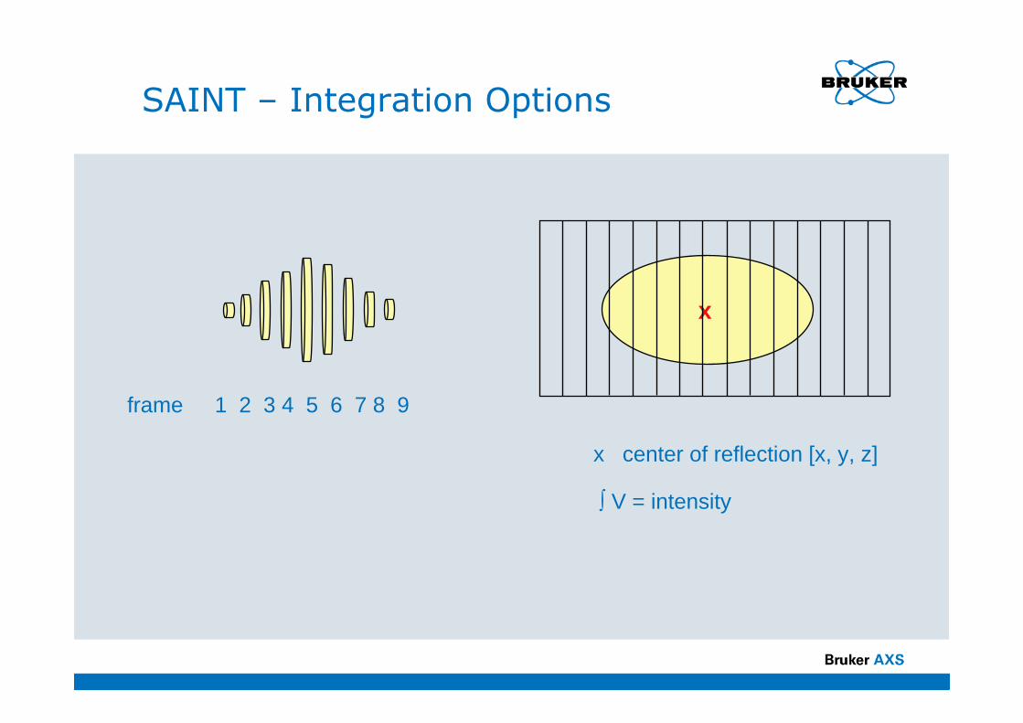
frame 1 2 3 4 5 6 7 8 9
x center of reflection [x, y, z]
∫ V = intensity
x
SAINT – Integration Options
29/09/2008Ina Dix - 15th Bruker AXS SCD Users Meeting16
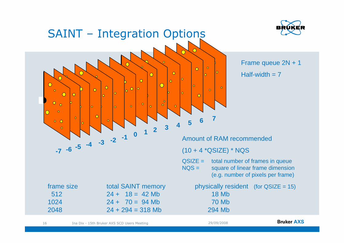
76543210-1-2-3-4-5-6-7
frame size total SAINT memory physically resident (for QSIZE = 15)512 24 + 18 = 42 Mb 18 Mb
1024 24 + 70 = 94 Mb 70 Mb2048 24 + 294 = 318 Mb 294 Mb
Amount of RAM recommended
(10 + 4 *QSIZE) * NQS
QSIZE = total number of frames in queueNQS = square of linear frame dimension
(e.g. number of pixels per frame)
Frame queue 2N + 1
Half-width = 7
SAINT – Integration Options
29/09/2008Ina Dix - 15th Bruker AXS SCD Users Meeting17
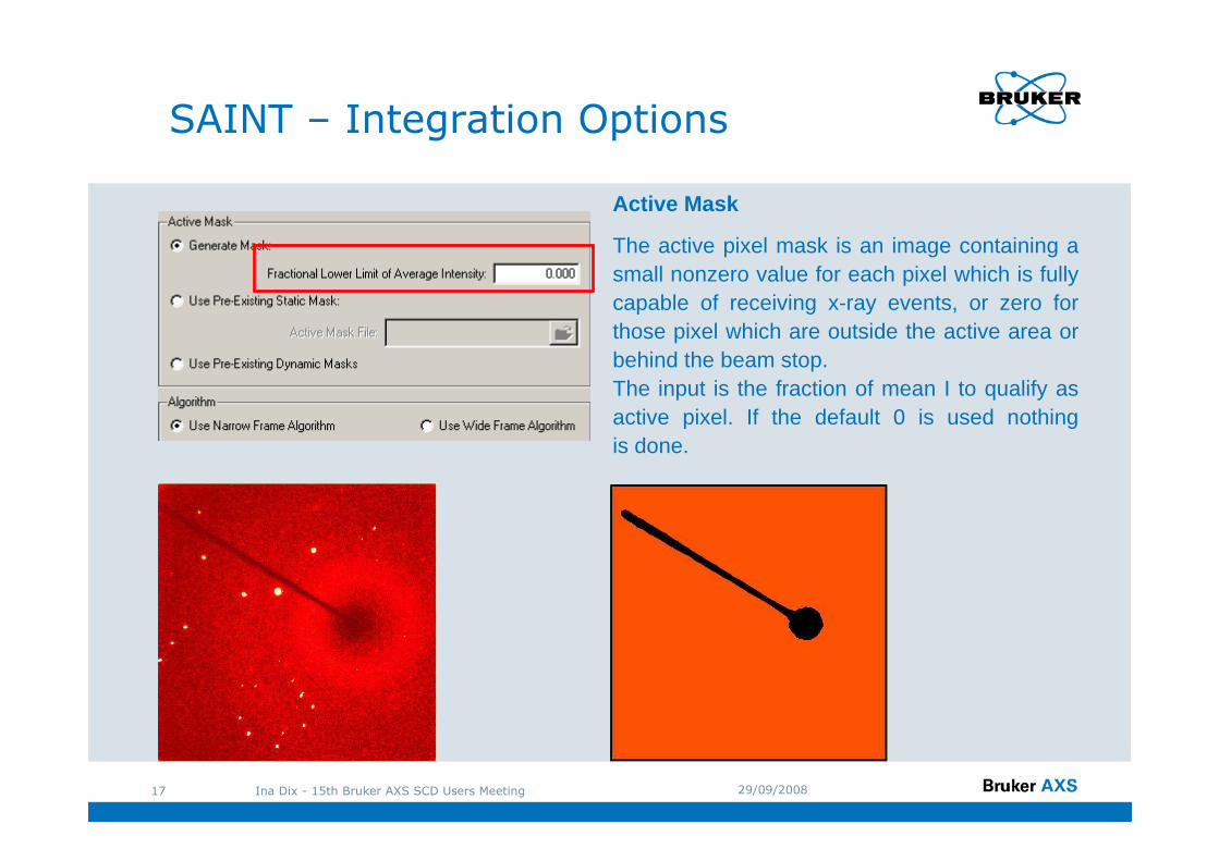
Active Mask
The active pixel mask is an image containing a small nonzero value for each pixel which is fully capable of receiving x-ray events, or zero for those pixel which are outside the active area or behind the beam stop.The input is the fraction of mean I to qualify as active pixel. If the default 0 is used nothingis done.
SAINT – Integration Options
29/09/2008Ina Dix - 15th Bruker AXS SCD Users Meeting18
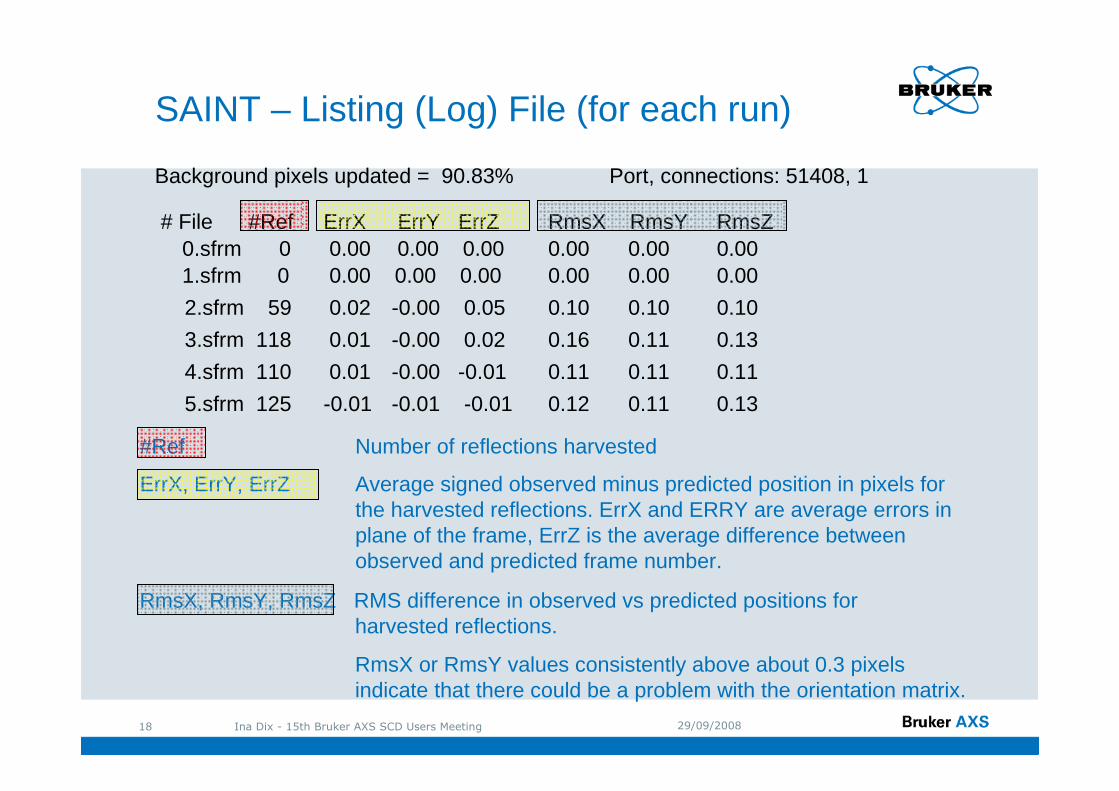
Background pixels updated = 90.83% Port, connections: 51408, 1
# File #Ref ErrX ErrY ErrZ RmsX RmsY RmsZ0.sfrm 0 0.00 0.00 0.00 0.00 0.00 0.001.sfrm 0 0.00 0.00 0.00 0.00 0.00 0.00
2.sfrm 59 0.02 -0.00 0.05 0.10 0.10 0.10
3.sfrm 118 0.01 -0.00 0.02 0.16 0.11 0.13
4.sfrm 110 0.01 -0.00 -0.01 0.11 0.11 0.11
5.sfrm 125 -0.01 -0.01 -0.01 0.12 0.11 0.13
#Ref Number of reflections harvested
ErrX, ErrY, ErrZ Average signed observed minus predicted position in pixels forthe harvested reflections. ErrX and ERRY are average errors inplane of the frame, ErrZ is the average difference between observed and predicted frame number.
RmsX, RmsY, RmsZ RMS difference in observed vs predicted positions forharvested reflections.
RmsX or RmsY values consistently above about 0.3 pixelsindicate that there could be a problem with the orientation matrix.
SAINT – Listing (Log) File (for each run)
29/09/2008Ina Dix - 15th Bruker AXS SCD Users Meeting19
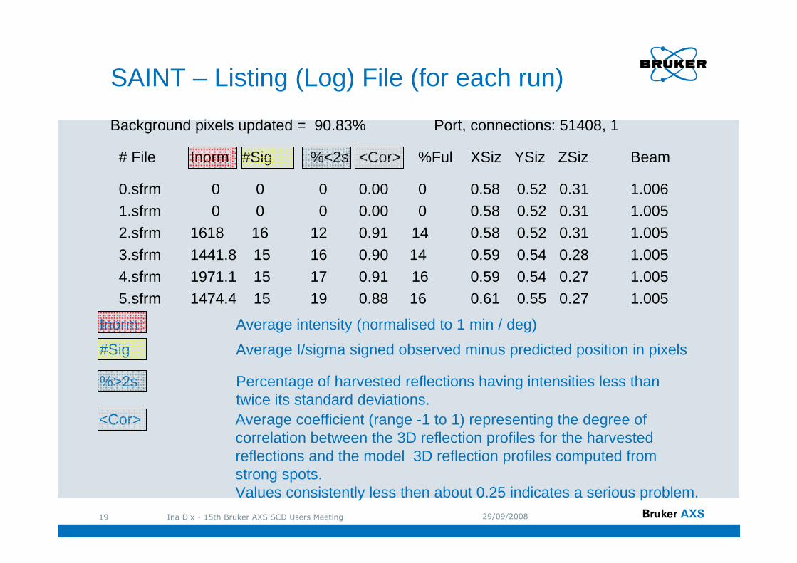
Background pixels updated = 90.83% Port, connections: 51408, 1
# File Inorm #Sig %<2s <Cor> %Ful XSiz YSiz ZSiz Beam
0.sfrm 0 0 0 0.00 0 0.58 0.52 0.31 1.0061.sfrm 0 0 0 0.00 0 0.58 0.52 0.31 1.005
2.sfrm 1618 16 12 0.91 14 0.58 0.52 0.31 1.0053.sfrm 1441.8 15 16 0.90 14 0.59 0.54 0.28 1.005
4.sfrm 1971.1 15 17 0.91 16 0.59 0.54 0.27 1.0055.sfrm 1474.4 15 19 0.88 16 0.61 0.55 0.27 1.005
Inorm Average intensity (normalised to 1 min / deg)
<Cor> Average coefficient (range -1 to 1) representing the degree of correlation between the 3D reflection profiles for the harvestedreflections and the model 3D reflection profiles computed fromstrong spots.Values consistently less then about 0.25 indicates a serious problem.
#Sig Average I/sigma signed observed minus predicted position in pixels
%>2s Percentage of harvested reflections having intensities less thantwice its standard deviations.
SAINT – Listing (Log) File (for each run)
29/09/2008Ina Dix - 15th Bruker AXS SCD Users Meeting20
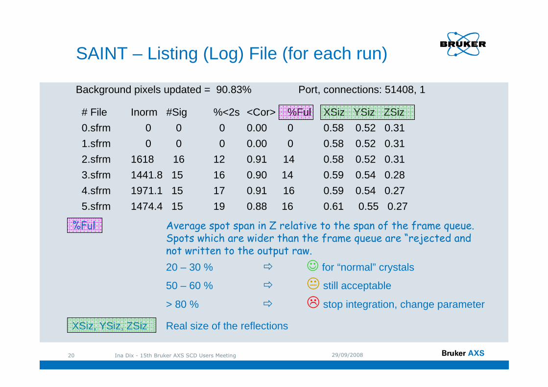
Background pixels updated = 90.83% Port, connections: 51408, 1
# File Inorm #Sig %<2s <Cor> %Ful XSiz YSiz ZSiz
0.sfrm 0 0 0 0.00 0 0.58 0.52 0.31
1.sfrm 0 0 0 0.00 0 0.58 0.52 0.31
2.sfrm 1618 16 12 0.91 14 0.58 0.52 0.31
3.sfrm 1441.8 15 16 0.90 14 0.59 0.54 0.28
4.sfrm 1971.1 15 17 0.91 16 0.59 0.54 0.27
5.sfrm 1474.4 15 19 0.88 16 0.61 0.55 0.27
XSiz, YSiz, ZSiz Real size of the reflections
%Ful Average spot span in Z relative to the span of the frame queue. Spots which are wider than the frame queue are “rejected andnot written to the output raw.
20 – 30 % � ☺ for “normal” crystals
50 – 60 % � � still acceptable
> 80 % � � stop integration, change parameter
SAINT – Listing (Log) File (for each run)
29/09/2008Ina Dix - 15th Bruker AXS SCD Users Meeting21
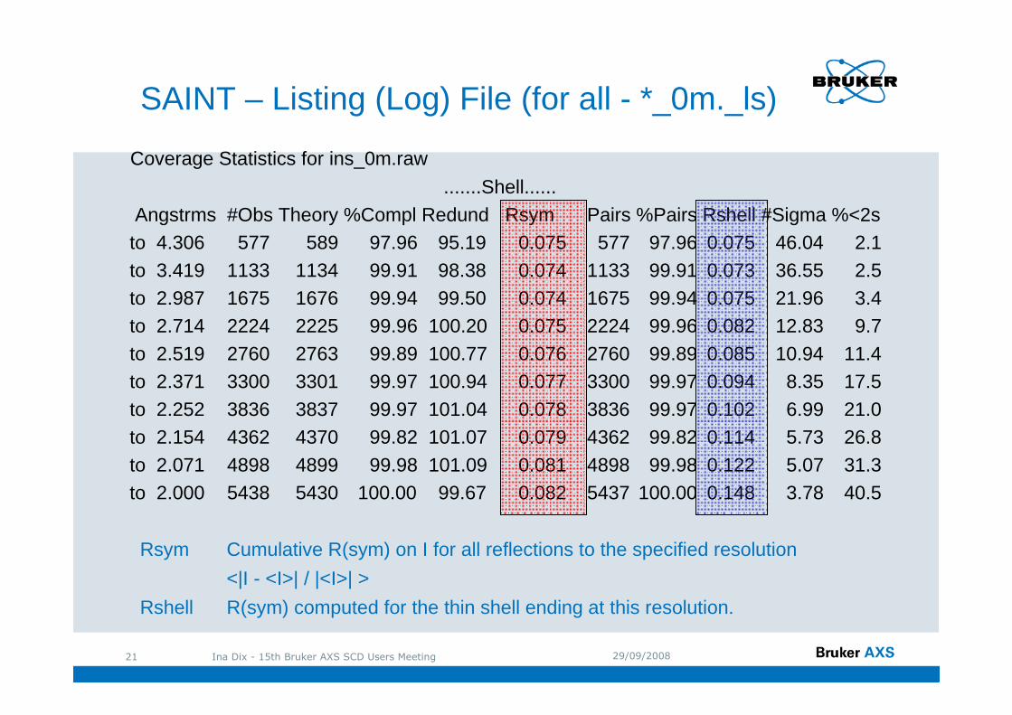
Coverage Statistics for ins_0m.raw
.......Shell......
Angstrms #Obs Theory %Compl Redund Rsym Pairs %Pairs Rshell #Sigma %<2sto 4.306 577 589 97.96 95.19 0.075 577 97.96 0.075 46.04 2.1
to 3.419 1133 1134 99.91 98.38 0.074 1133 99.91 0.073 36.55 2.5to 2.987 1675 1676 99.94 99.50 0.074 1675 99.94 0.075 21.96 3.4to 2.714 2224 2225 99.96 100.20 0.075 2224 99.96 0.082 12.83 9.7
to 2.519 2760 2763 99.89 100.77 0.076 2760 99.89 0.085 10.94 11.4to 2.371 3300 3301 99.97 100.94 0.077 3300 99.97 0.094 8.35 17.5
to 2.252 3836 3837 99.97 101.04 0.078 3836 99.97 0.102 6.99 21.0to 2.154 4362 4370 99.82 101.07 0.079 4362 99.82 0.114 5.73 26.8
to 2.071 4898 4899 99.98 101.09 0.081 4898 99.98 0.122 5.07 31.3to 2.000 5438 5430 100.00 99.67 0.082 5437 100.00 0.148 3.78 40.5
Rsym Cumulative R(sym) on I for all reflections to the specified resolution
<|I - <I>| / |<I>| >
Rshell R(sym) computed for the thin shell ending at this resolution.
SAINT – Listing (Log) File (for all - *_0m._ls)
29/09/2008Ina Dix - 15th Bruker AXS SCD Users Meeting22
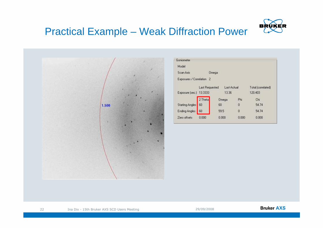
Practical Example – Weak Diffraction Power
29/09/2008Ina Dix - 15th Bruker AXS SCD Users Meeting23
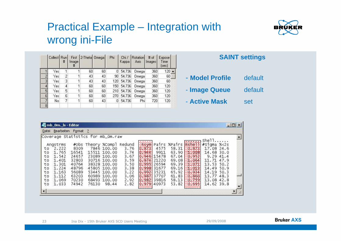
SAINT settings
- Model Profile default
- Image Queue default
- Active Mask set
Practical Example – Integration with wrong ini-File
29/09/2008Ina Dix - 15th Bruker AXS SCD Users Meeting24
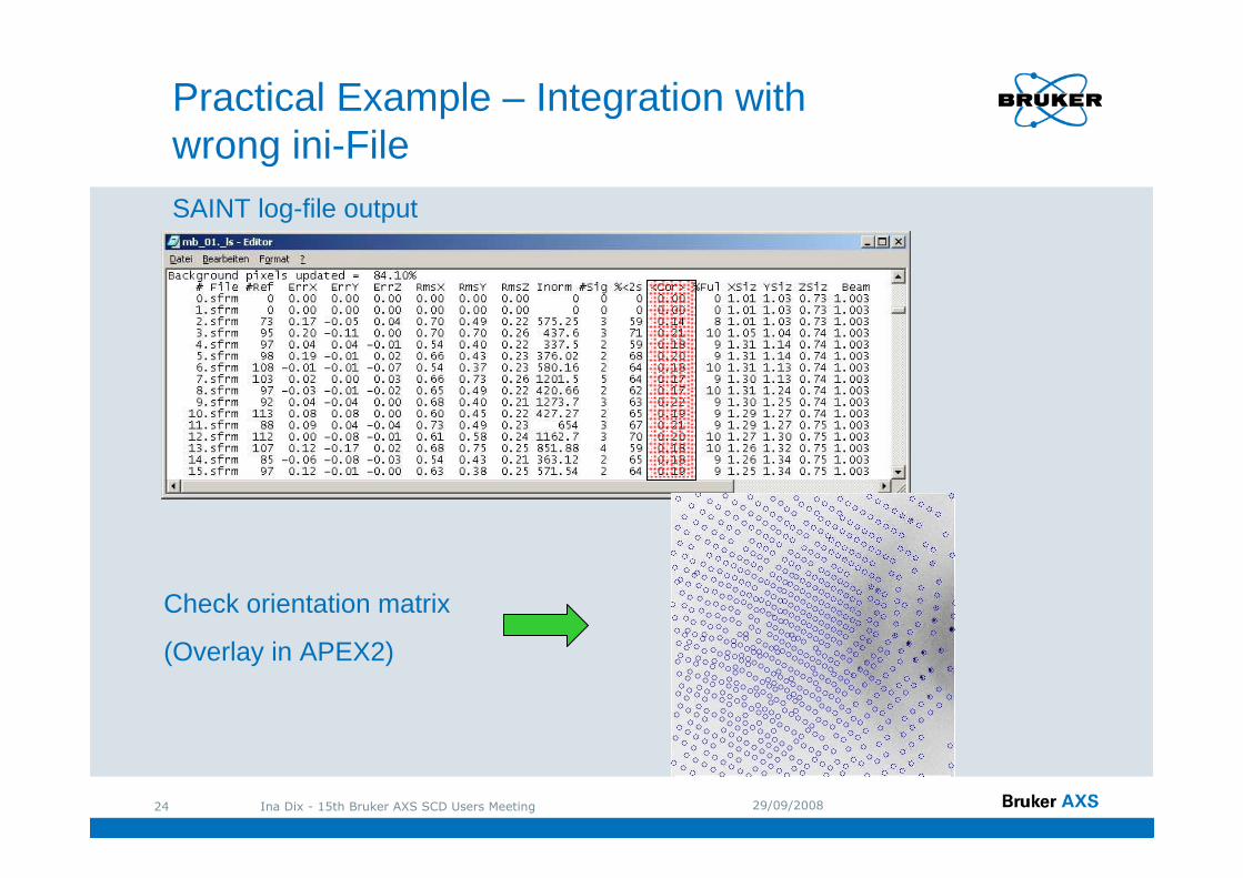
Check orientation matrix
(Overlay in APEX2)
Practical Example – Integration with wrong ini-File
SAINT log-file output
29/09/2008Ina Dix - 15th Bruker AXS SCD Users Meeting25
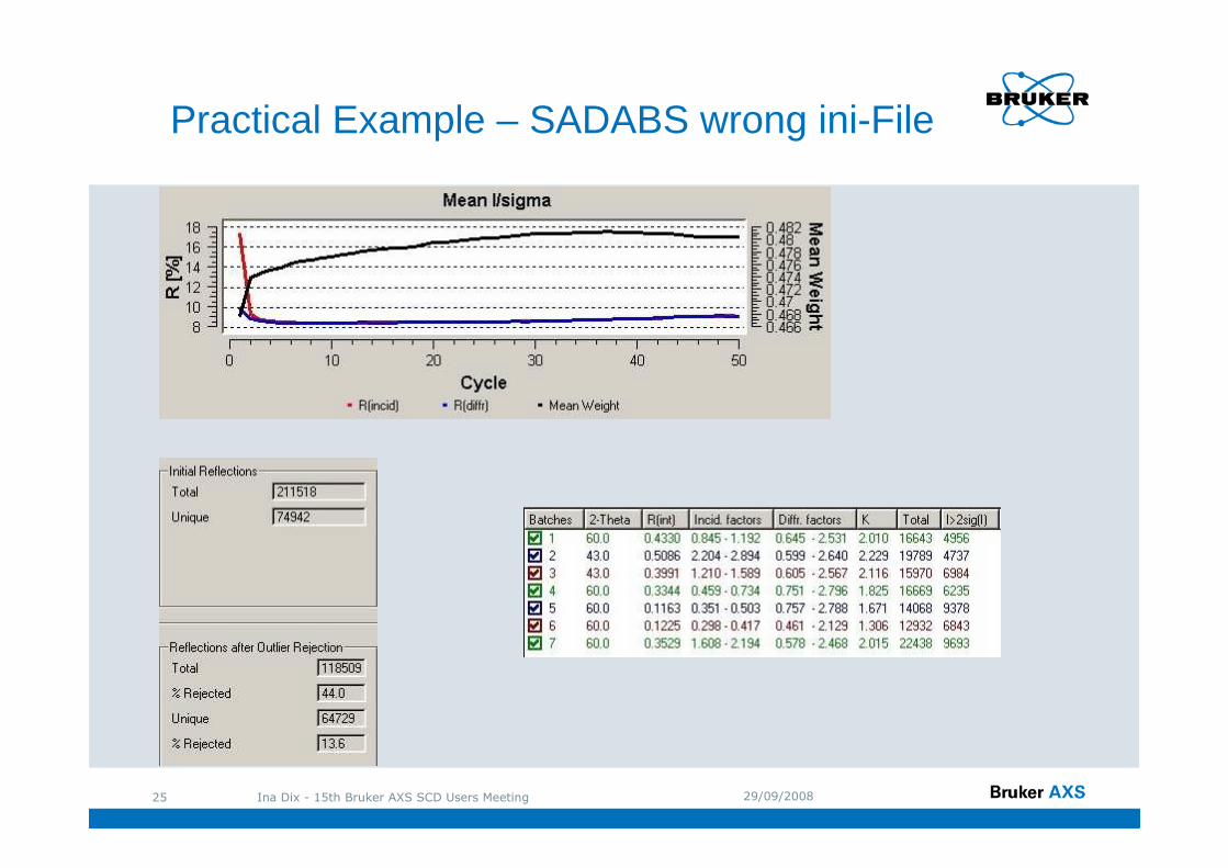
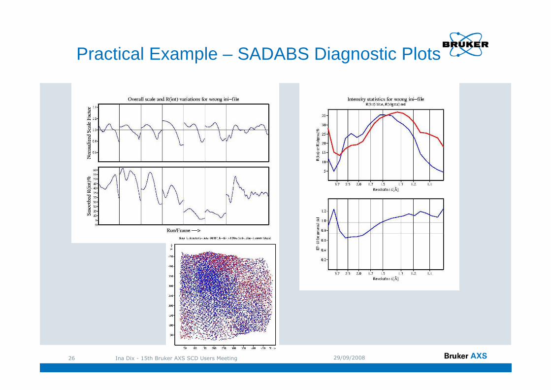
Practical Example – SADABS wrong ini-File
29/09/2008Ina Dix - 15th Bruker AXS SCD Users Meeting26
Practical Example – SADABS Diagnostic Plots
29/09/2008Ina Dix - 15th Bruker AXS SCD Users Meeting27
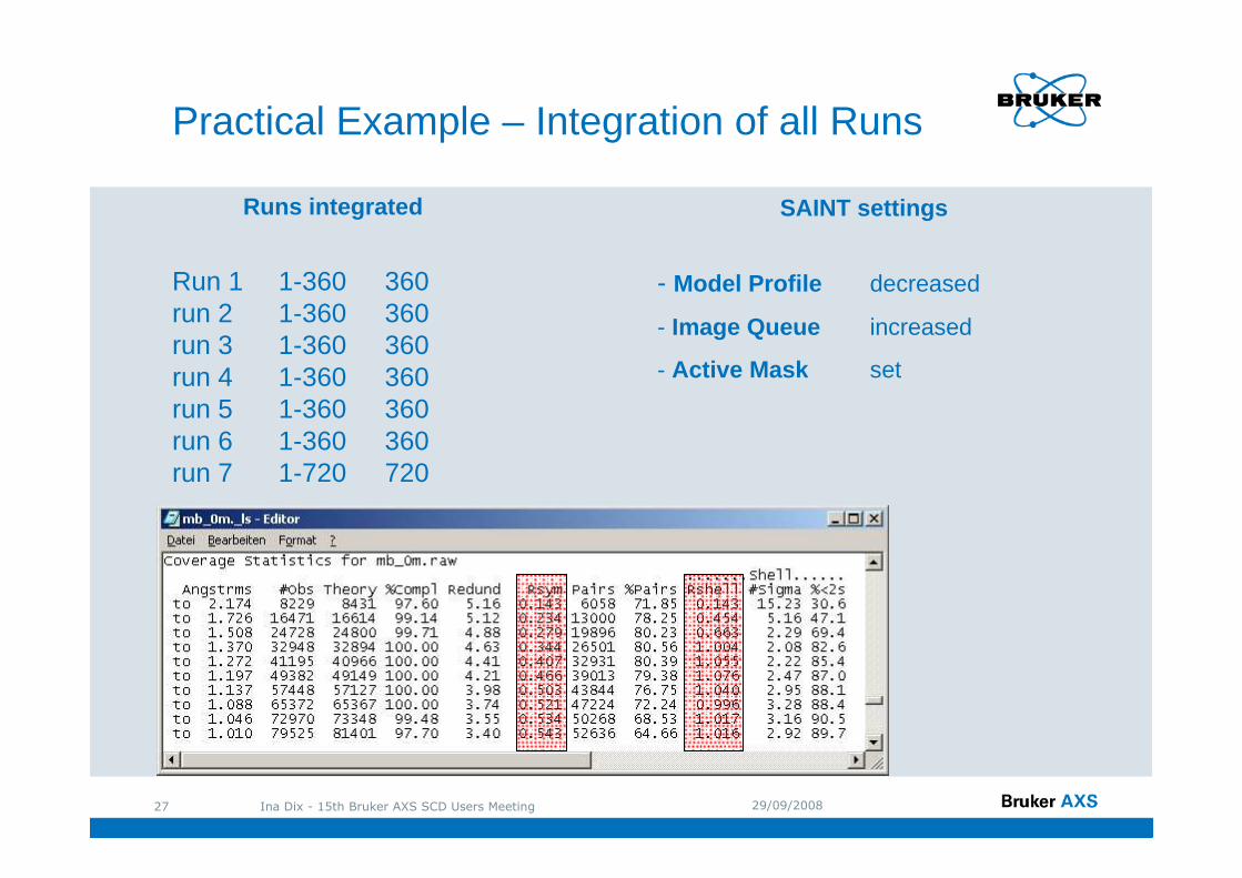
Runs integrated
Run 1 1-360 360run 2 1-360 360run 3 1-360 360run 4 1-360 360run 5 1-360 360run 6 1-360 360run 7 1-720 720
Practical Example – Integration of all Runs
SAINT settings
- Model Profile decreased
- Image Queue increased
- Active Mask set
29/09/2008Ina Dix - 15th Bruker AXS SCD Users Meeting28
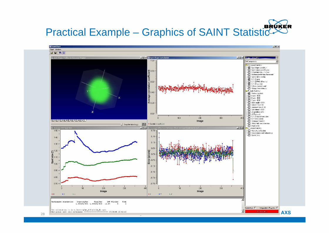
Practical Example – Graphics of SAINT Statistic

29/09/2008Ina Dix - 15th Bruker AXS SCD Users Meeting29
run 1 (correlation coefficient)
run 2 (correlation coefficient) run 3 (correlation coefficient)
run 1 (position error)
Practical Example – Graphics of SAINT Statistic
29/09/2008Ina Dix - 15th Bruker AXS SCD Users Meeting30
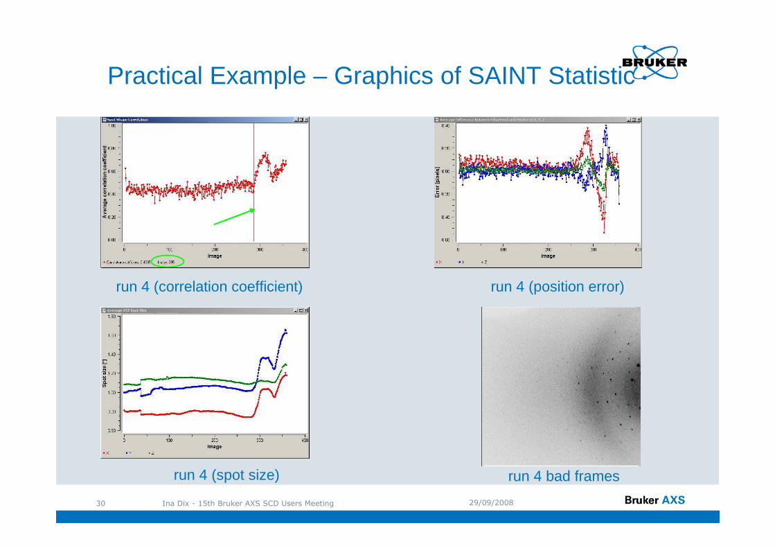
run 4 bad frames
run 4 (correlation coefficient) run 4 (position error)
run 4 (spot size)
Practical Example – Graphics of SAINT Statistic

29/09/2008Ina Dix - 15th Bruker AXS SCD Users Meeting31
run 5 bad frames 1
run 5 (position error)run 5 (correlation coefficient)
run 5 (spot size)
Practical Example – Graphics of SAINT Statistic
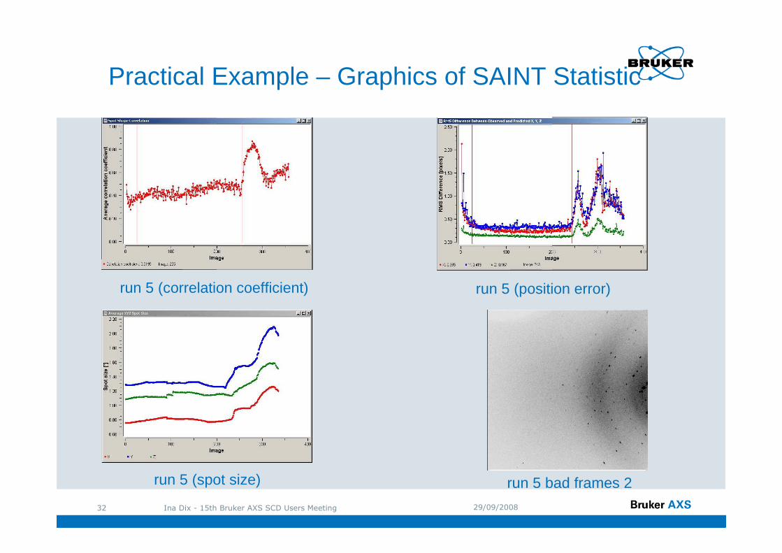
29/09/2008Ina Dix - 15th Bruker AXS SCD Users Meeting32
run 5 bad frames 2
run 5 (correlation coefficient)
run 5 (spot size)
Practical Example – Graphics of SAINT Statistic
run 5 (position error)
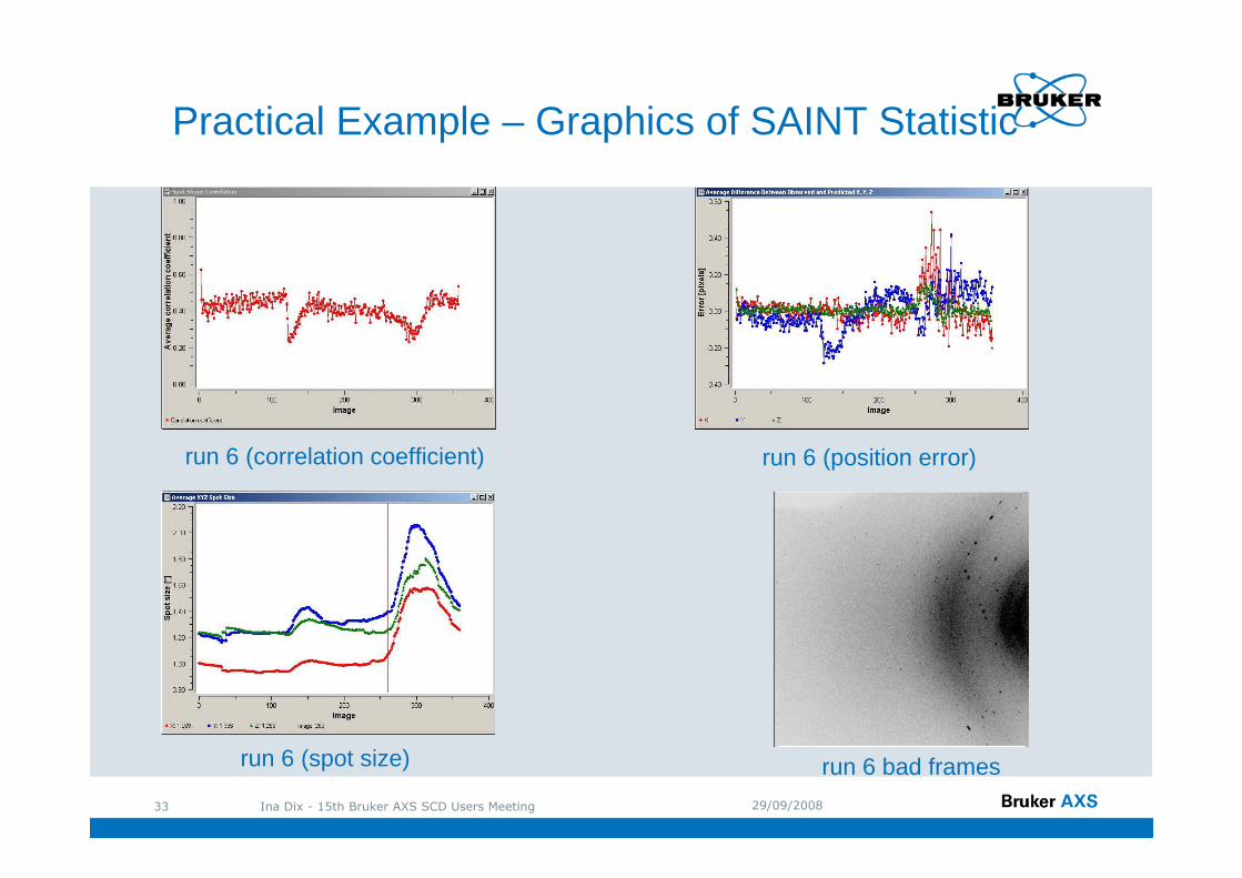
29/09/2008Ina Dix - 15th Bruker AXS SCD Users Meeting33
run 6 (spot size)
run 6 (correlation coefficient) run 6 (position error)
run 6 bad frames
Practical Example – Graphics of SAINT Statistic
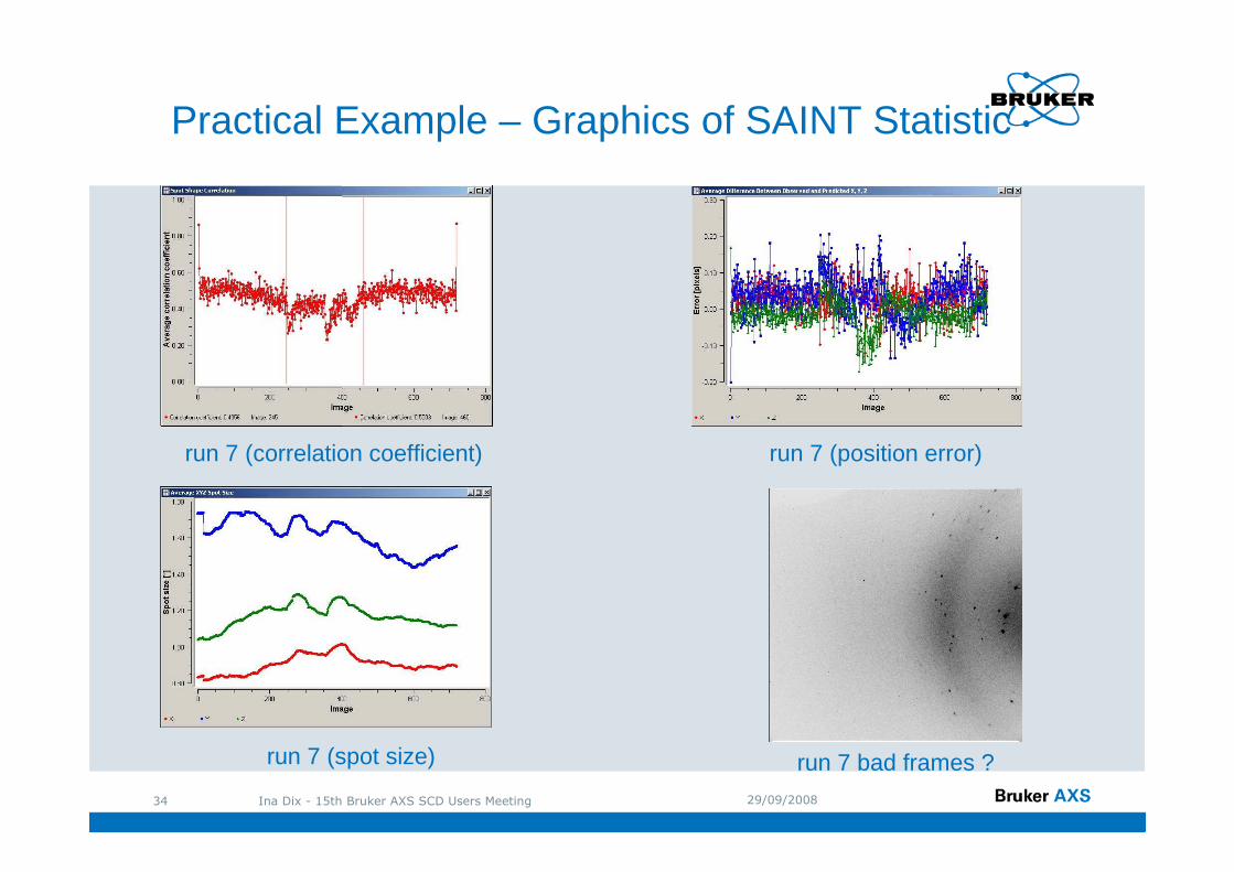
29/09/2008Ina Dix - 15th Bruker AXS SCD Users Meeting34
run 7 bad frames ?
run 7 (correlation coefficient) run 7 (position error)
run 7 (spot size)
Practical Example – Graphics of SAINT Statistic
29/09/2008Ina Dix - 15th Bruker AXS SCD Users Meeting35
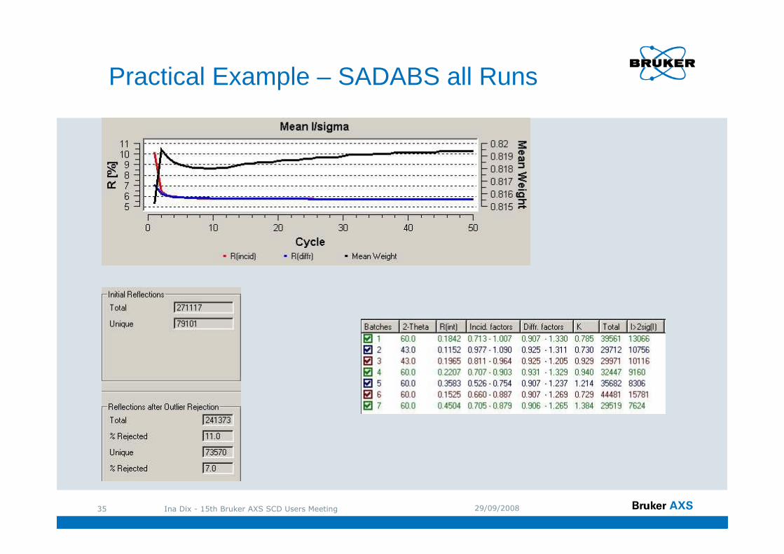
Practical Example – SADABS all Runs
29/09/2008Ina Dix - 15th Bruker AXS SCD Users Meeting36
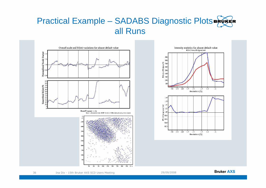
Practical Example – SADABS Diagnostic Plots all Runs
29/09/2008Ina Dix - 15th Bruker AXS SCD Users Meeting37
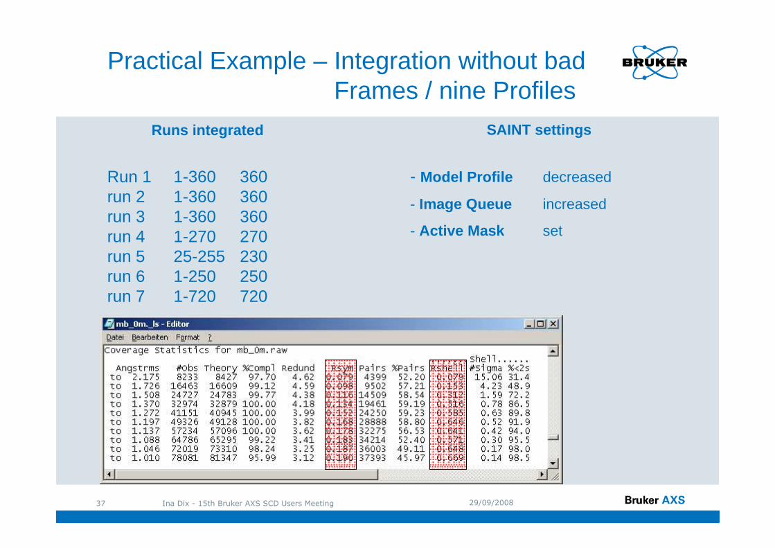
Runs integrated
Run 1 1-360 360run 2 1-360 360run 3 1-360 360run 4 1-270 270run 5 25-255 230run 6 1-250 250run 7 1-720 720
Practical Example – Integration without bad Frames / nine Profiles
SAINT settings
- Model Profile decreased
- Image Queue increased
- Active Mask set
29/09/2008Ina Dix - 15th Bruker AXS SCD Users Meeting38
7
6
5 3
2
98
1
4
Practical Example – Profiles 1 – 9 in SAINT
29/09/2008Ina Dix - 15th Bruker AXS SCD Users Meeting39
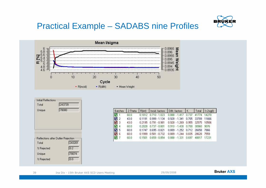
Practical Example – SADABS nine Profiles
29/09/2008Ina Dix - 15th Bruker AXS SCD Users Meeting40
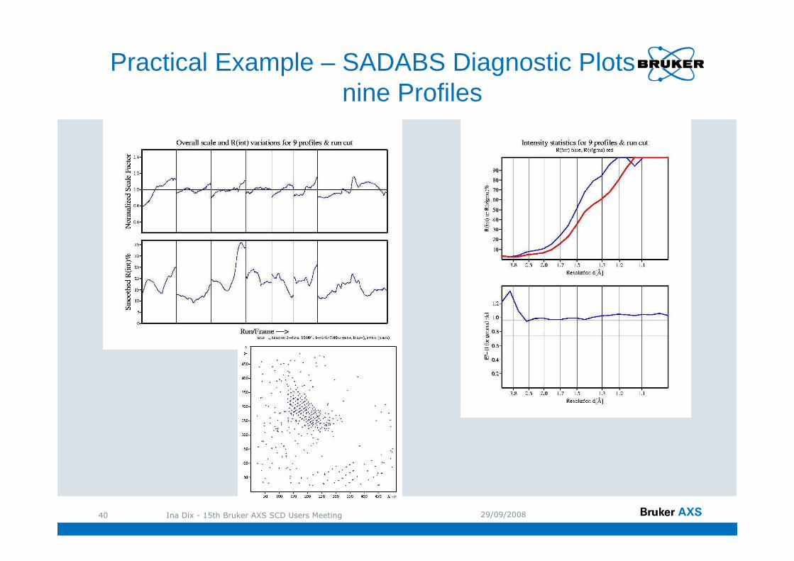
Practical Example – SADABS Diagnostic Plots nine Profiles
29/09/2008Ina Dix - 15th Bruker AXS SCD Users Meeting41
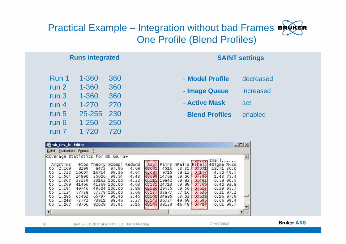
Runs integrated
Run 1 1-360 360run 2 1-360 360run 3 1-360 360run 4 1-270 270run 5 25-255 230run 6 1-250 250run 7 1-720 720
Practical Example – Integration without bad FramesOne Profile (Blend Profiles)
SAINT settings
- Model Profile decreased
- Image Queue increased
- Active Mask set
- Blend Profiles enabled
29/09/2008Ina Dix - 15th Bruker AXS SCD Users Meeting42
7
6
5 3
2
98
1
4
Practical Example – One Profile in SAINT(Blend Profiles)
29/09/2008Ina Dix - 15th Bruker AXS SCD Users Meeting43
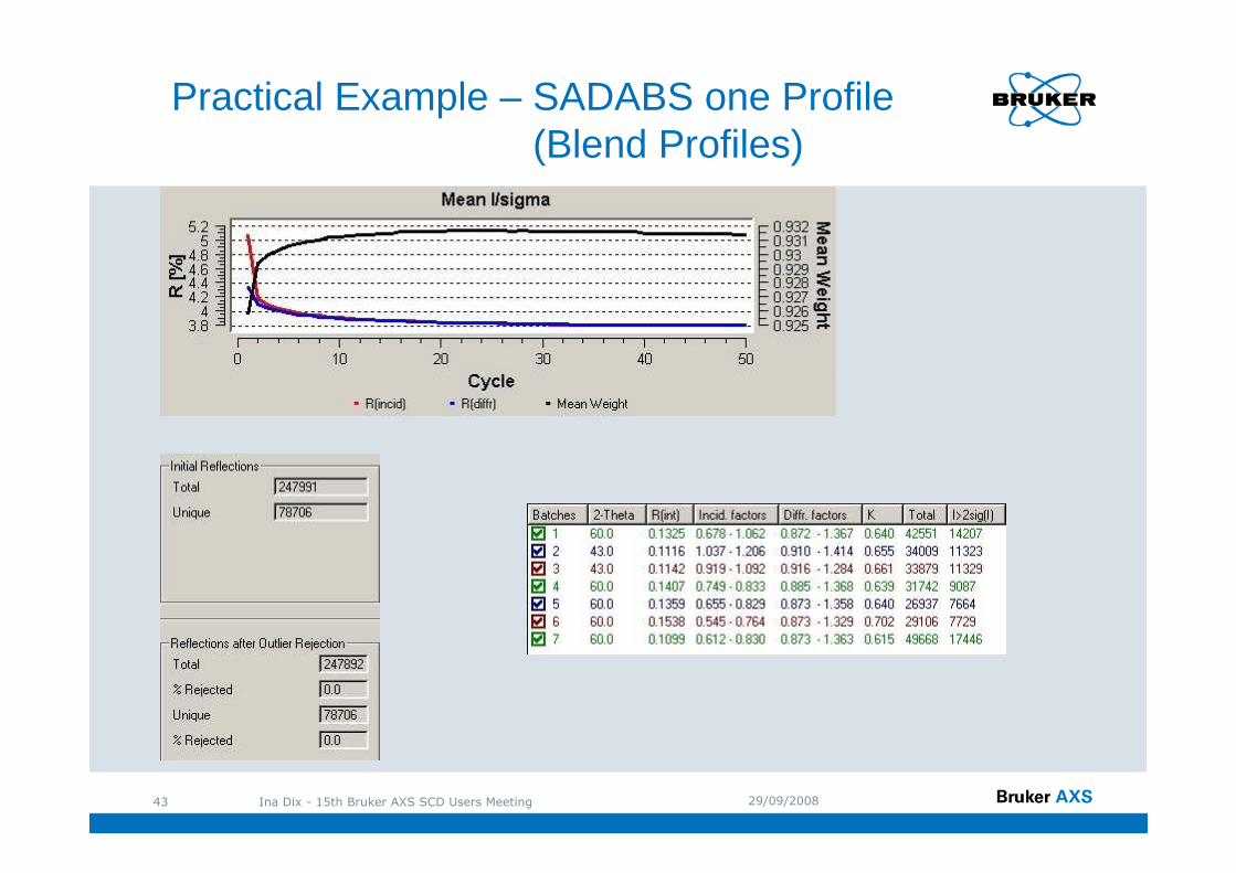
Practical Example – SADABS one Profile(Blend Profiles)
29/09/2008Ina Dix - 15th Bruker AXS SCD Users Meeting44
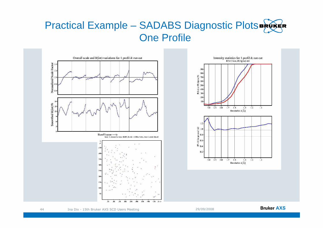
Practical Example – SADABS Diagnostic PlotsOne Profile
29/09/2008Ina Dix - 15th Bruker AXS SCD Users Meeting45
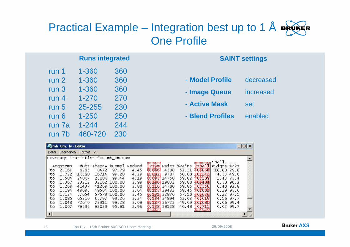
Runs integrated
run 1 1-360 360run 2 1-360 360run 3 1-360 360run 4 1-270 270run 5 25-255 230run 6 1-250 250run 7a 1-244 244run 7b 460-720 230
Practical Example – Integration best up to 1 ÅOne Profile
SAINT settings
- Model Profile decreased
- Image Queue increased
- Active Mask set
- Blend Profiles enabled
29/09/2008Ina Dix - 15th Bruker AXS SCD Users Meeting46
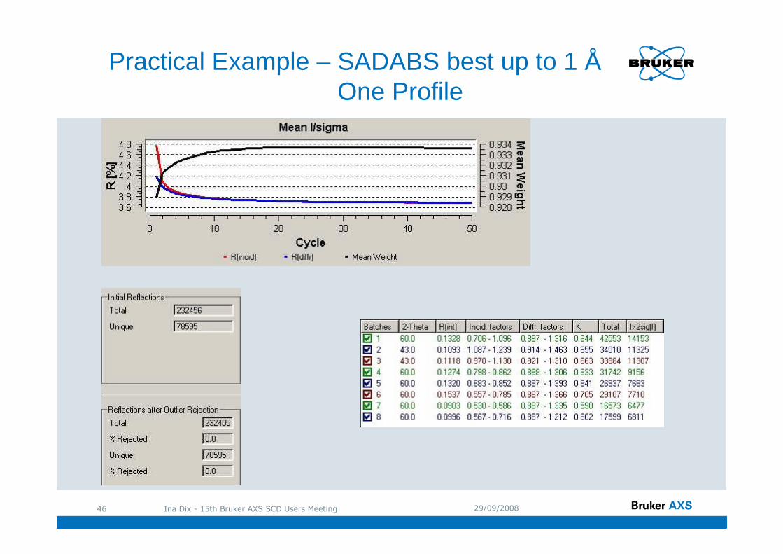
Practical Example – SADABS best up to 1 ÅOne Profile

29/09/2008Ina Dix - 15th Bruker AXS SCD Users Meeting47
Practical Example – SADABS Diagnostic Plots best up to 1 Å
29/09/2008Ina Dix - 15th Bruker AXS SCD Users Meeting48
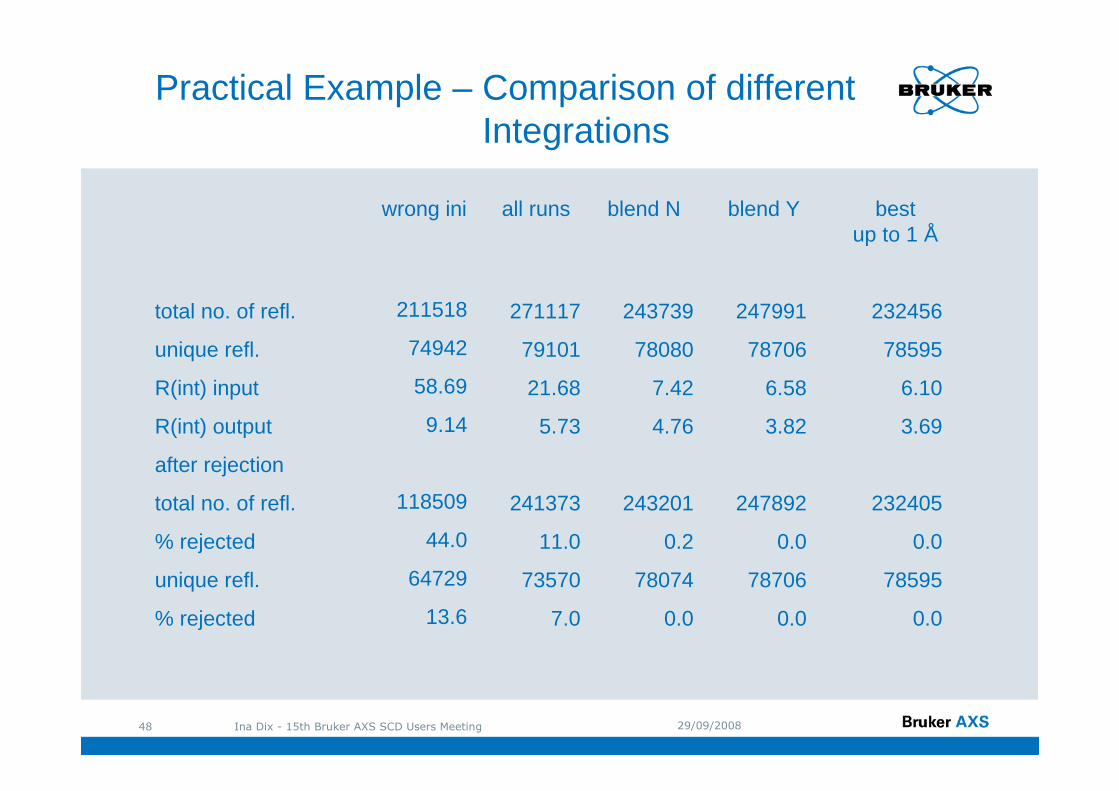
total no. of refl.
unique refl.
R(int) input
R(int) output
after rejection
total no. of refl.
% rejected
unique refl.
% rejected
wrong ini
211518
74942
58.69
9.14
118509
44.0
64729
13.6
all runs
271117
79101
21.68
5.73
241373
11.0
73570
7.0
blend N
243739
78080
7.42
4.76
243201
0.2
78074
0.0
blend Y
247991
78706
6.58
3.82
247892
0.0
78706
0.0
best up to 1 Å
232456
78595
6.10
3.69
232405
0.0
78595
0.0
Practical Example – Comparison of different Integrations