Embed Size (px)
Citation preview
123
With 22 Figures
Introductory Lectures on ´ Fluctuations of Levy Processes with Applications
Andreas E. Kyprianou
ISBN-10ISBN-13 Springer Berlin Heidelberg New York
This work is subject to copyright. All rights are reserved, whether the whole or part of the materialis concerned, specifically the rights of translation, reprinting, reuse of illustrations, recitation,broadcasting, reproduction on microfilm or in any other way, and storage in data banks. Dupli-cation of this publication or parts thereof is permitted only under the provisions of the GermanCopyright Law of September 9, 1965, in its current version, and permission for use must always beobtained from Springer. Violations are liable for prosecution under the German Copyright Law.
Springer is a part of Springer Science+Business Media
Printed in Germany
The use of general descriptive names, registered names, trademarks, etc. in this publication doesnot imply, even in the absence of a specific statement, that such names are exempt from the relevantprotective laws and regulations and therefore free for general use.
Cover design: Erich Kirchner, Heidelbergusing a Springer LATEX macro package
Printed on acid-free paper
Mathematics Subject Classification (2000): 60G50, 60G51, 60G52
Library of Congress Control Number: 2006924567
3-540-31342-7 Springer Berlin Heidelberg New York978-3-540-31342-7
springer.com© Springer-Verlag Berlin Heidelberg 2006
Andreas E. KyprianouDepartment of Mathematical SciencesUniversity of BathBath BA2 7AYUK
The background text on the front cover is written in old (pre-1941) Mongolian scripture.It is a translation of the words ‘stochastic processes with stationary and independentincrements’ and should be read from the top left hand corner of the back cover to the bottom right hand corner of the front cover.
e-mail: [email protected]
Typesetting by the author and SPi
41/3100/SPi - 5 4 3 2 1 0SPIN 11338987
Preface
In 2003 I began teaching a course entitled Levy processes on the Amsterdam-Utrecht masters programme in stochastics and financial mathematics. Quitenaturally, I wanted to expose my students to my own interests in Levyprocesses; that is, the role that certain subtle behaviour concerning their fluc-tuations play in explaining different types of phenomena appearing in a num-ber of classical models of applied probability. Indeed, recent developments inthe theory of Levy processes, in particular concerning path fluctuation, haveoffered the clarity required to revisit classical applied probability models andimprove on well established and fundamental results.
Whilst teaching the course I wrote some lecture notes which have nowmatured into this text. Given the audience of students, who were either en-gaged in their ‘afstudeerfase’1 or just starting a Ph.D., these lecture notes wereoriginally written with the restriction that the mathematics used would notsurpass the level that they should in principle have reached. Roughly speakingthat means the following: experience to the level of third year or fourth yearuniversity courses delivered by a mathematics department on
- foundational real and complex analysis,- basic facts about Lp spaces,- measure theory, integration theory and measure theoretic probability theory,- elements of the classical theory of Markov processes, stopping times and the
Strong Markov Property.- Poisson processes and renewal processes,- Brownian motion as a Markov process and elementary martingale theory in
continuous time.
For the most part this affected the way in which the material was handledcompared to the classical texts and research papers from which almost all ofthe results and arguments in this text originate. A good example of this is
1The afstudeerfase is equivalent to at least a European masters-level programme.
VIII Preface
the conscious exclusion of calculations involving the master formula for thePoisson point process of excursions of a Levy process from its maximum.
There are approximately 80 exercises and likewise these are pitched at alevel appropriate to the aforementioned audience. Indeed several of the exer-cises have been included in response to some of the questions that have beenasked by students themselves concerning curiosities of the arguments givenin class. Arguably the exercises are at times quite long. Such exercises reflectsome of the other ways in which I have used preliminary versions of this text.A small number of students in Utrecht also used the text as an individualreading/self-study programme contributing to their ‘kleinescripite’ (extendedmathematical essay) or ‘onderzoekopdracht’ (research option); in addition,some exercises were used as (take-home) examination questions. The exer-cises in the first chapter in particular are designed to show the reader thatthe basics of the material presented thereafter is already accessible assumingbasic knowledge of Poisson processes and Brownian motion.
There can be no doubt, particularly to the more experienced reader, thatthe current text has been heavily influenced by the outstanding books ofBertoin (1996) and Sato (1999), and especially the former which also takes apredominantly pathwise approach to its content. It should be reiterated how-ever that, unlike the latter two books, this text is not intended as a researchmonograph nor as a reference manual for the researcher.
Writing of this text began whilst I was employed at Utrecht University,The Netherlands. In early 2005 I moved to a new position at Heriot WattUniversity in Edinburgh, Scotland, and in the final stages of completion ofthe book to The University of Bath. Over a period of several months mypresence in Utrecht was phased out and my presence in Edinburgh was phasedin. Along the way I passed through the Technical University of Munich andThe University of Manchester. I should like to thank these four institutes andmy hosts for giving me the facilities necessary to write this text (mostly timeand a warm, dry, quiet room with an ethernet connection). I would especiallylike to thank my colleagues at Utrecht for giving me the opportunity andenvironment in which to develop this course, Ron Doney during his two-monthabsence for lending me the key to his office and book collection whilst minewas in storage and Andrew Cairns for arranging to push my teaching dutiesinto 2006 allowing me the focus to finalise this text.
Let me now thank the many, including several of the students who tookthe course, who have made a number of remarks, corrections and suggestions(minor and major) which have helped to shape this text. In alphabetical orderthese are: Larbi Alili, David Applebaum, Johnathan Bagley, Erik Baurdoux,M.S. Bratiychuk, Catriona Byrne, Zhen-Qing Chen, Gunther Cornelissen,Irmingard Erder, Abdelghafour Es-Saghouani, Serguei Foss, Uwe Franz, ShotaGugushvili, Thorsten Kleinow, Pawel Kliber, Claudia Kluppelberg, V.S.Korolyuk, Ronnie Loeffen, Alexander Novikov, Zbigniew Palmowski, GoranPeskir, Kees van Schaik, Sonja Scheer, Wim Schoutens, Budhi Arta Surya,Enno Veerman, Maaike Verloop, Zoran Vondracek. In particular I would also
Preface IX
like to thank, Peter Andrew, Jean Bertoin, Ron Doney, Niel Farricker, Alexan-der Gnedin, Amaury Lambert, Antonis Papapantoleon and Martijn Pistoriusrooted out many errors from extensive sections of the text and provided valu-able criticism. Antonis Papapantoleon very kindly produced some simulationsof the paths of Levy processes which have been included in Chap. 1. I am mostgrateful to Takis Konstantopoulos who read through earlier drafts of the en-tire text in considerable detail, taking the time to discuss with me at lengthmany of the issues that arose. The front cover was produced in consultationwith Hurlee Gonchigdanzan and Jargalmaa Magsarjav. All further comments,corrections and suggestions on the current text are welcome.
Finally, the deepest gratitude of all goes to Jagaa, Sophia and Sanaa forwhom the special inscription is written.
Edinburgh Andreas E. KyprianouJune 2006
Contents
1 Levy Processes and Applications . . . . . . . . . . . . . . . . . . . . . . . . . . 11.1 Levy Processes and Infinite Divisibility . . . . . . . . . . . . . . . . . . . . . 11.2 Some Examples of Levy Processes . . . . . . . . . . . . . . . . . . . . . . . . . 51.3 Levy Processes and Some Applied Probability Models . . . . . . . . 14Exercises . . . . . . . . . . . . . . . . . . . . . . . . . . . . . . . . . . . . . . . . . . . . . . . . . . . 26
2 The Levy–Ito Decomposition and Path Structure . . . . . . . . . . 332.1 The Levy–Ito Decomposition . . . . . . . . . . . . . . . . . . . . . . . . . . . . . . 332.2 Poisson Random Measures . . . . . . . . . . . . . . . . . . . . . . . . . . . . . . . . 352.3 Functionals of Poisson Random Measures . . . . . . . . . . . . . . . . . . . 412.4 Square Integrable Martingales . . . . . . . . . . . . . . . . . . . . . . . . . . . . . 442.5 Proof of the Levy–Ito Decomposition . . . . . . . . . . . . . . . . . . . . . . 512.6 Levy Processes Distinguished by Their Path Type . . . . . . . . . . . 532.7 Interpretations of the Levy–Ito Decomposition . . . . . . . . . . . . . . 56Exercises . . . . . . . . . . . . . . . . . . . . . . . . . . . . . . . . . . . . . . . . . . . . . . . . . . . 62
3 More Distributional and Path-Related Properties . . . . . . . . . . 673.1 The Strong Markov Property . . . . . . . . . . . . . . . . . . . . . . . . . . . . . 673.2 Duality . . . . . . . . . . . . . . . . . . . . . . . . . . . . . . . . . . . . . . . . . . . . . . . . 733.3 Exponential Moments and Martingales . . . . . . . . . . . . . . . . . . . . . 75Exercises . . . . . . . . . . . . . . . . . . . . . . . . . . . . . . . . . . . . . . . . . . . . . . . . . . . 83
4 General Storage Models and Paths of Bounded Variation . . 874.1 General Storage Models . . . . . . . . . . . . . . . . . . . . . . . . . . . . . . . . . . 874.2 Idle Times . . . . . . . . . . . . . . . . . . . . . . . . . . . . . . . . . . . . . . . . . . . . . . 884.3 Change of Variable and Compensation Formulae . . . . . . . . . . . . 904.4 The Kella–Whitt Martingale . . . . . . . . . . . . . . . . . . . . . . . . . . . . . . 974.5 Stationary Distribution of the Workload . . . . . . . . . . . . . . . . . . . . 1004.6 Small-Time Behaviour and the Pollaczek–Khintchine Formula . 102Exercises . . . . . . . . . . . . . . . . . . . . . . . . . . . . . . . . . . . . . . . . . . . . . . . . . . . 105
XII Contents
5 Subordinators at First Passage and Renewal Measures . . . . 1115.1 Killed Subordinators and Renewal Measures . . . . . . . . . . . . . . . . 1115.2 Overshoots and Undershoots . . . . . . . . . . . . . . . . . . . . . . . . . . . . . . 1195.3 Creeping . . . . . . . . . . . . . . . . . . . . . . . . . . . . . . . . . . . . . . . . . . . . . . . 1215.4 Regular Variation and Tauberian Theorems . . . . . . . . . . . . . . . . . 1265.5 Dynkin–Lamperti Asymptotics . . . . . . . . . . . . . . . . . . . . . . . . . . . . 130Exercises . . . . . . . . . . . . . . . . . . . . . . . . . . . . . . . . . . . . . . . . . . . . . . . . . . . 133
6 The Wiener–Hopf Factorisation . . . . . . . . . . . . . . . . . . . . . . . . . . . . 1396.1 Local Time at the Maximum . . . . . . . . . . . . . . . . . . . . . . . . . . . . . . 1406.2 The Ladder Process . . . . . . . . . . . . . . . . . . . . . . . . . . . . . . . . . . . . . . 1476.3 Excursions . . . . . . . . . . . . . . . . . . . . . . . . . . . . . . . . . . . . . . . . . . . . . . 1546.4 The Wiener–Hopf Factorisation . . . . . . . . . . . . . . . . . . . . . . . . . . . 1576.5 Examples of the Wiener–Hopf Factorisation . . . . . . . . . . . . . . . . . 1686.6 Brief Remarks on the Term “Wiener–Hopf” . . . . . . . . . . . . . . . . . 174Exercises . . . . . . . . . . . . . . . . . . . . . . . . . . . . . . . . . . . . . . . . . . . . . . . . . . . 174
7 Levy Processes at First Passage and Insurance Risk . . . . . . 1797.1 Drifting and Oscillating . . . . . . . . . . . . . . . . . . . . . . . . . . . . . . . . . . 1797.2 Cramer’s Estimate of Ruin . . . . . . . . . . . . . . . . . . . . . . . . . . . . . . . 1857.3 A Quintuple Law at First Passage . . . . . . . . . . . . . . . . . . . . . . . . . 1897.4 The Jump Measure of the Ascending Ladder Height Process . . 1957.5 Creeping . . . . . . . . . . . . . . . . . . . . . . . . . . . . . . . . . . . . . . . . . . . . . . . 1977.6 Regular Variation and Infinite Divisibility . . . . . . . . . . . . . . . . . . 2007.7 Asymptotic Ruinous Behaviour with Regular Variation . . . . . . . 203Exercises . . . . . . . . . . . . . . . . . . . . . . . . . . . . . . . . . . . . . . . . . . . . . . . . . . . 206
8 Exit Problems for Spectrally Negative Processes . . . . . . . . . . . 2118.1 Basic Properties Reviewed . . . . . . . . . . . . . . . . . . . . . . . . . . . . . . . . 2118.2 The One-Sided and Two-Sided Exit Problems . . . . . . . . . . . . . . . 2148.3 The Scale Functions W (q) and Z(q) . . . . . . . . . . . . . . . . . . . . . . . . 2208.4 Potential Measures . . . . . . . . . . . . . . . . . . . . . . . . . . . . . . . . . . . . . . 2238.5 Identities for Reflected Processes . . . . . . . . . . . . . . . . . . . . . . . . . . 2278.6 Brief Remarks on Spectrally Negative GOUs . . . . . . . . . . . . . . . . 231Exercises . . . . . . . . . . . . . . . . . . . . . . . . . . . . . . . . . . . . . . . . . . . . . . . . . . . 233
9 Applications to Optimal Stopping Problems . . . . . . . . . . . . . . . 2399.1 Sufficient Conditions for Optimality . . . . . . . . . . . . . . . . . . . . . . . . 2409.2 The McKean Optimal Stopping Problem . . . . . . . . . . . . . . . . . . . 2419.3 Smooth Fit versus Continuous Fit . . . . . . . . . . . . . . . . . . . . . . . . . 2459.4 The Novikov–Shiryaev Optimal Stopping Problem . . . . . . . . . . . 2499.5 The Shepp–Shiryaev Optimal Stopping Problem . . . . . . . . . . . . . 2559.6 Stochastic Games . . . . . . . . . . . . . . . . . . . . . . . . . . . . . . . . . . . . . . . . 260Exercises . . . . . . . . . . . . . . . . . . . . . . . . . . . . . . . . . . . . . . . . . . . . . . . . . . . 269
Contents XIII
10 Continuous-State Branching Processes . . . . . . . . . . . . . . . . . . . . . 27110.1 The Lamperti Transform . . . . . . . . . . . . . . . . . . . . . . . . . . . . . . . . . 27110.2 Long-term Behaviour . . . . . . . . . . . . . . . . . . . . . . . . . . . . . . . . . . . . 27410.3 Conditioned Processes and Immigration . . . . . . . . . . . . . . . . . . . . 28010.4 Concluding Remarks . . . . . . . . . . . . . . . . . . . . . . . . . . . . . . . . . . . . . 291Exercises . . . . . . . . . . . . . . . . . . . . . . . . . . . . . . . . . . . . . . . . . . . . . . . . . . . 293
Epilogue . . . . . . . . . . . . . . . . . . . . . . . . . . . . . . . . . . . . . . . . . . . . . . . . . . . . . . . 295
Solutions . . . . . . . . . . . . . . . . . . . . . . . . . . . . . . . . . . . . . . . . . . . . . . . . . . . . . . 299
References . . . . . . . . . . . . . . . . . . . . . . . . . . . . . . . . . . . . . . . . . . . . . . . . . . . . . 361
Index . . . . . . . . . . . . . . . . . . . . . . . . . . . . . . . . . . . . . . . . . . . . . . . . . . . . . . . . . . 371
1
Levy Processes and Applications
In this chapter we define a Levy process and attempt to give some indica-tion of how rich a class of processes they form. To illustrate the variety ofprocesses captured within the definition of a Levy process, we explore brieflythe relationship of Levy processes with infinitely divisible distributions. Wealso discuss some classical applied probability models, which are built on thestrength of well-understood path properties of elementary Levy processes.We hint at how generalisations of these models may be approached usingmore sophisticated Levy processes. At a number of points later on in this textwe handle these generalisations in more detail. The models we have chosento present are suitable for the course of this text as a way of exemplifyingfluctuation theory but are by no means the only applications.
1.1 Levy Processes and Infinite Divisibility
Let us begin by recalling the definition of two familiar processes, a Brownianmotion and a Poisson process.
A real-valued process B = Bt : t ≥ 0 defined on a probability space(Ω,F ,P) is said to be a Brownian motion if the following hold:
(i) The paths of B are P-almost surely continuous.(ii) P(B0 = 0) = 1.(iii) For 0 ≤ s ≤ t, Bt −Bs is equal in distribution to Bt−s.(iv) For 0 ≤ s ≤ t, Bt −Bs is independent of Bu : u ≤ s.(v) For each t > 0, Bt is equal in distribution to a normal random variable
with variance t.
A process valued on the non-negative integers N = Nt : t ≥ 0, definedon a probability space (Ω,F ,P), is said to be a Poisson process with intensityλ > 0 if the following hold:
(i) The paths of N are P-almost surely right continuous with left limits.(ii) P(N0 = 0) = 1.
2 1 Levy Processes and Applications
(iii) For 0 ≤ s ≤ t, Nt −Ns is equal in distribution to Nt−s.(iv) For 0 ≤ s ≤ t, Nt −Ns is independent of Nu : u ≤ s.(v) For each t > 0, Nt is equal in distribution to a Poisson random variable
with parameter λt.
On first encounter, these processes would seem to be considerably differentfrom one another. Firstly, Brownian motion has continuous paths whereas aPoisson process does not. Secondly, a Poisson process is a non-decreasingprocess and thus has paths of bounded variation over finite time horizons,whereas a Brownian motion does not have monotone paths and in fact itspaths are of unbounded variation over finite time horizons.
However, when we line up their definitions next to one another, we seethat they have a lot in common. Both processes have right continuous pathswith left limits, are initiated from the origin and both have stationary andindependent increments; that is properties (i), (ii), (iii) and (iv). We mayuse these common properties to define a general class of stochastic processes,which are called Levy processes.
Definition 1.1 (Levy Process). A process X = Xt : t ≥ 0 defined ona probability space (Ω,F ,P) is said to be a Levy process if it possesses thefollowing properties:
(i) The paths of X are P-almost surely right continuous with left limits.(ii) P(X0 = 0) = 1.(iii) For 0 ≤ s ≤ t, Xt −Xs is equal in distribution to Xt−s.(iv) For 0 ≤ s ≤ t, Xt −Xs is independent of Xu : u ≤ s.
Unless otherwise stated, from now on, when talking of a Levy process, weshall always use the measure P (with associated expectation operator E) to beimplicitly understood as its law.
The term “Levy process” honours the work of the French mathematicianPaul Levy who, although not alone in his contribution, played an instrumentalrole in bringing together an understanding and characterisation of processeswith stationary independent increments. In earlier literature, Levy processescan be found under a number of different names. In the 1940s, Levy himselfreferred to them as a sub-class of processus additif (additive processes), that isprocesses with independent increments. For the most part however, researchliterature through the 1960s and 1970s refers to Levy processes simply asprocesses with stationary independent increments. One sees a change in lan-guage through the 1980s and by the 1990s the use of the term “Levy process”had become standard.
From Definition 1.1 alone it is difficult to see just how rich a class ofprocesses the class of Levy processes forms. De Finetti (1929) introducedthe notion of an infinitely divisible distribution and showed that they have anintimate relationship with Levy processes. This relationship gives a reasonably

1.1 Levy Processes and Infinite Divisibility 3
good impression of how varied the class of Levy processes really is. To this end,let us now devote a little time to discussing infinitely divisible distributions.
Definition 1.2. We say that a real-valued random variable Θ has an infinitelydivisible distribution if for each n = 1, 2, ... there exist a sequence of i.i.d.random variables Θ1,n, ..., Θn,n such that
Θd= Θ1,n + · · ·+Θn,n
where d= is equality in distribution. Alternatively, we could have expressedthis relation in terms of probability laws. That is to say, the law µ of a real-valued random variable is infinitely divisible if for each n = 1, 2, ... there existsanother law µn of a real valued random variable such that µ = µ∗nn . (Here µ∗ndenotes the n-fold convolution of µn).
In view of the above definition, one way to establish whether a givenrandom variable has an infinitely divisible distribution is via its characteristicexponent. Suppose that Θ has characteristic exponent Ψ(u) := − log E(eiuΘ)for all u ∈ R. Then Θ has an infinitely divisible distribution if for all n ≥ 1there exists a characteristic exponent of a probability distribution, say Ψn,such that Ψ(u) = nΨn(u) for all u ∈ R.
The full extent to which we may characterise infinitely divisible distribu-tions is described by the characteristic exponent Ψ and an expression knownas the Levy–Khintchine formula.
Theorem 1.3 (Levy–Khintchine formula). A probability law µ of a real-valued random variable is infinitely divisible with characteristic exponent Ψ,∫
Reiθxµ (dx) = e−Ψ(θ) for θ ∈ R,
if and only if there exists a triple (a, σ,Π), where a ∈ R, σ ≥ 0 and Π is ameasure concentrated on R\0 satisfying
∫R(1 ∧ x2
)Π(dx) <∞, such that
Ψ (θ) = iaθ +12σ2θ2 +
∫R(1− eiθx + iθx1(|x|<1))Π(dx)
for every θ ∈ R.
Definition 1.4. The measure Π is called the Levy (characteristic) measure.
The proof of the Levy–Khintchine characterisation of infinitely divisiblerandom variables is quite lengthy and we choose to exclude it in favour ofmoving as quickly as possible to fluctuation theory. The interested reader isreferred to Lukacs (1970) or Sato (1999), to name but two of many possiblereferences.
A special case of the Levy–Khintchine formula was established by Kol-mogorov (1932) for infinitely divisible distributions with second moments.
4 1 Levy Processes and Applications
However it was Levy (1934) who gave a complete characterisation of infinitelydivisible distributions and in doing so he also characterised the general class ofprocesses with stationary independent increments. Later, Khintchine (1937)and Ito (1942) gave further simplification and deeper insight to Levy’s originalproof.
Let us now discuss in further detail the relationship between infinitelydivisible distributions and processes with stationary independent increments.
From the definition of a Levy process we see that for any t > 0, Xt isa random variable belonging to the class of infinitely divisible distributions.This follows from the fact that for any n = 1, 2, ...,
Xt = Xt/n + (X2t/n −Xt/n) + · · ·+ (Xt −X(n−1)t/n) (1.1)
together with the fact that X has stationary independent increments. Supposenow that we define for all θ ∈ R, t ≥ 0,
Ψt (θ) = − log E(eiθXt
)then using (1.1) twice we have for any two positive integers m,n that
mΨ1 (θ) = Ψm (θ) = nΨm/n (θ)
and hence for any rational t > 0,
Ψt (θ) = tΨ1 (θ) . (1.2)
If t is an irrational number, then we can choose a decreasing sequence ofrationals tn : n ≥ 1 such that tn ↓ t as n tends to infinity. Almost sureright continuity of X implies right continuity of exp−Ψt (θ) (by dominatedconvergence) and hence (1.2) holds for all t ≥ 0.
In conclusion, any Levy process has the property that for all t ≥ 0
E(eiθXt
)= e−tΨ(θ),
where Ψ (θ) := Ψ1 (θ) is the characteristic exponent of X1, which has aninfinitely divisible distribution.
Definition 1.5. In the sequel we shall also refer to Ψ (θ) as the characteristicexponent of the Levy process.
It is now clear that each Levy process can be associated with an infinitelydivisible distribution. What is not clear is whether given an infinitely divisibledistribution, one may construct a Levy process X, such that X1 has thatdistribution. This latter issue is affirmed by the following theorem which givesthe Levy–Khintchine formula for Levy processes.
Theorem 1.6 (Levy–Khintchine formula for Levy processes). Sup-pose that a ∈ R, σ ≥ 0 and Π is a measure concentrated on R\0 such that∫
R(1 ∧ x2)Π(dx) <∞. From this triple define for each θ ∈ R,
1.2 Some Examples of Levy Processes 5
Ψ (θ) = iaθ +12σ2θ2 +
∫R(1− eiθx + iθx1(|x|<1))Π(dx).
Then there exists a probability space (Ω,F ,P) on which a Levy process isdefined having characteristic exponent Ψ.
The proof of this theorem is rather complicated but very rewarding as italso reveals much more about the general structure of Levy processes. Later, inChap. 2, we will prove a stronger version of this theorem, which also explainsthe path structure of the Levy process in terms of the triple (a, σ,Π).
1.2 Some Examples of Levy Processes
To conclude our introduction to Levy processes and infinite divisible distrib-utions, let us proceed to some concrete examples. Some of these will also beof use later to verify certain results from the forthcoming fluctuation theorywe will present.
1.2.1 Poisson Processes
For each λ > 0 consider a probability distribution µλ which is concentratedon k = 0, 1, 2... such that µλ(k) = e−λλk/k!. That is to say the Poissondistribution. An easy calculation reveals that∑
k≥0
eiθkµλ(k) = e−λ(1−eiθ)
=[e−
λn (1−eiθ)
]n.
The right-hand side is the characteristic function of the sum of n independentPoisson processes, each of which with parameter λ/n. In the Levy–Khintchinedecomposition we see that a = σ = 0 and Π = λδ1, the Dirac measuresupported on 1.
Recall that a Poisson process, Nt : n ≥ 0, is a Levy process with dis-tribution at time t > 0, which is Poisson with parameter λt. From the abovecalculations we have
E(eiθNt) = e−λt(1−eiθ)
and hence its characteristic exponent is given by Ψ(θ) = λ(1− eiθ) for θ ∈ R.
1.2.2 Compound Poisson Processes
Suppose now that N is a Poisson random variable with parameter λ > 0 andthat ξi : i ≥ 1 is an i.i.d. sequence of random variables (independent of N)
6 1 Levy Processes and Applications
with common law F having no atom at zero. By first conditioning on N , wehave for θ ∈ R,
E(eiθ∑N
i=1ξi) =
∑n≥0
E(eiθ∑n
i=1ξi)e−λ
λn
n!
=∑n≥0
(∫R
eiθxF (dx))n
e−λλn
n!
= e−λ∫
R(1−eiθx)F (dx)
. (1.3)
Note we use the convention here that∑0
1 = 0. We see from (1.3) thatdistributions of the form
∑Ni=1 ξi are infinitely divisible with triple a =
−λ ∫0<|x|<1
xF (dx), σ = 0 and Π(dx) = λF (dx). When F has an atomof unit mass at 1 then we have simply a Poisson distribution.
Suppose now that Nt : t ≥ 0 is a Poisson process with intensity λ andconsider a compound Poisson process Xt : t ≥ 0 defined by
Xt =Nt∑i=0
ξi, t ≥ 0.
Using the fact thatN has stationary independent increments together with themutual independence of the random variables ξi : i ≥ 1, for 0 ≤ s < t <∞,by writing
Xt = Xs +Nt∑
i=Ns+1
ξi
it is clear that Xt is the sum of Xs and an independent copy of Xt−s. Rightcontinuity and left limits of the process N also ensure right continuity andleft limits of X. Thus compound Poisson processes are Levy processes. Fromthe calculations in the previous paragraph, for each t ≥ 0 we may substituteNt for the variable N to discover that the Levy–Khintchine formula for acompound Poisson process takes the form Ψ(θ) = λ
∫R(1 − eiθx)F (dx). Note
in particular that the Levy measure of a compound Poisson process is alwaysfinite with total mass equal to the rate λ of the underlying process N .
Compound Poisson processes provide a direct link between Levy processesand random walks; that is discrete time processes of the form S = Sn : n ≥ 0where
S0 = 0 and Sn =n∑i=1
ξi for n ≥ 1.
Indeed a compound Poisson process is nothing more than a random walkwhose jumps have been spaced out with independent and exponentially dis-tributed periods.
1.2 Some Examples of Levy Processes 7
1.2.3 Linear Brownian Motion
Take the probability law
µs,γ(dx) :=1√
2πs2e−(x−γ)2/2s2dx
supported on R where γ ∈ R and s > 0; the well-known Gaussian distributionwith mean γ and variance s2. It is well known that∫
Reiθxµs,γ(dx) = e−
12 s
2θ2+iθγ
=[e−
12 ( s√
n)2θ2+iθ γ
n
]nshowing again that it is an infinitely divisible distribution, this time witha = −γ, σ = s and Π = 0.
We immediately recognise the characteristic exponent Ψ(θ) = s2θ2/2− iθγas also that of a scaled Brownian motion with linear drift,
Xt := sBt + γt, t ≥ 0,
where B = Bt : t ≥ 0 is a standard Brownian motion; that is to say a linearBrownian motion with parameters σ = 1 and γ = 0. It is a trivial exercise toverify that X has stationary independent increments with continuous pathsas a consequence of the fact that B does.
1.2.4 Gamma Processes
For α, β > 0 define the probability measure
µα,β(dx) =αβ
Γ (β)xβ−1e−αxdx
concentrated on (0,∞); the gamma-(α, β) distribution. Note that when β = 1this is the exponential distribution. We have∫ ∞
0
eiθxµα,β(dx) =1
(1− iθ/α)β
=
[1
(1− iθ/α)β/n
]nand infinite divisibility follows. For the Levy–Khintchine decomposition wehave σ = 0 and Π(dx) = βx−1e−αxdx, concentrated on (0,∞) and a =− ∫ 1
0xΠ(dx). However this is not immediately obvious. The following lemma
8 1 Levy Processes and Applications
proves to be useful in establishing the above triple (a, σ,Π). Its proof isExercise 1.3.
Lemma 1.7 (Frullani integral). For all α, β > 0 and z ∈ C such thatℜz ≤ 0 we have
1(1− z/α)β
= e−∫∞
0(1−ezx)βx−1e−αxdx
.
To see how this lemma helps note that the Levy–Khintchine formula for agamma distribution takes the form
Ψ(θ) = β
∫ ∞
0
(1− eiθx)1x
e−αxdx = β log(1− iθ/α)
for θ ∈ R. The choice of a in the Levy–Khintchine formula is the necessaryquantity to cancel the term coming from iθ1(|x|<1) in the integral with respectto Π in the general Levy–Khintchine formula.
According to Theorem 1.6 there exists a Levy process whose Levy–Khintchine formula is given by Ψ , the so-called gamma process.
Suppose now that X = Xt : t ≥ 0 is a gamma process. Stationary inde-pendent increments tell us that for all 0 ≤ s < t <∞, Xt = Xs + Xt−s whereXt−s is an independent copy of Xt−s. The fact that the latter is strictly pos-itive with probability one (on account of it being gamma distributed) impliesthat Xt > Xs almost surely. Hence a gamma process is an example of a Levyprocess with almost surely non-decreasing paths (in fact its paths are strictlyincreasing). Another example of a Levy process with non-decreasing paths isa compound Poisson process where the jump distribution F is concentratedon (0,∞). Note however that a gamma process is not a compound Poissonprocess on two counts. Firstly, its Levy measure has infinite total mass unlikethe Levy measure of a compound Poisson process, which is necessarily finite(and equal to the arrival rate of jumps). Secondly, whilst a compound Poissonprocess with positive jumps does have paths, which are almost surely non-decreasing, it does not have paths that are almost surely strictly increasing.
Levy processes whose paths are almost surely non-decreasing (or simplynon-decreasing for short) are called subordinators. We will return to a formaldefinition of this subclass of processes in Chap. 2.
1.2.5 Inverse Gaussian Processes
Suppose as usual that B = Bt : t ≥ 0 is a standard Brownian motion.Define the first passage time
τs = inft > 0 : Bt + bt > s, (1.4)
1.2 Some Examples of Levy Processes 9
that is, the first time a Brownian motion with linear drift b > 0 crossesabove level s. Recall that τs is a stopping time1 with respect to the filtrationFt : t ≥ 0 where Ft is generated by Bs : s ≤ t. Otherwise said, sinceBrownian motion has continuous paths, for all t ≥ 0,
τs ≤ t =⋃
u∈[0,t]∩QBu + bu > s
and hence the latter belongs to the sigma algebra Ft.Recalling again that Brownian motion has continuous paths we know that
Bτs+ bτs = s almost surely. From the Strong Markov Property,2 it is known
that Bτs+t + b(τs + t) − s : t ≥ 0 is equal in law to B and hence for all0 ≤ s < t,
τt = τs + τt−s,
where τt−s is an independent copy of τt−s. This shows that the process τ :=τt : t ≥ 0 has stationary independent increments. Continuity of the pathsof Bt + bt : t ≥ 0 ensures that τ has right continuous paths. Further, itis clear that τ has almost surely non-decreasing paths, which guarantees itspaths have left limits as well as being yet another example of a subordinator.According to its definition as a sequence of first passage times, τ is also thealmost sure right inverse of the path of the graph of Bt + bt : t ≥ 0 in thesense of (1.4). From this τ earns its name as the inverse Gaussian process.
According to the discussion following Theorem 1.3 it is now immediatethat for each fixed s > 0, the random variable τs is infinitely divisible. Itscharacteristic exponent takes the form
Ψ(θ) = s(√−2iθ + b2 − b)
for all θ ∈ R and corresponds to a triple a = −2sb−1∫ b0(2π)−1/2e−y
2/2dy,σ = 0 and
Π(dx) = s1√
2πx3e−
b2x2 dx
concentrated on (0,∞). The law of τs can also be computed explicitly as
µs(dx) =s√
2πx3esbe−
12 (s2x−1+b2x)
for x > 0. The proof of these facts forms Exercise 1.6.1We assume that the reader is familiar with the notion of a stopping time for aMarkov process. By definition, the random time τ is a stopping time with respectto the filtration Gt : t ≥ 0 if for all t ≥ 0,
τ ≤ t ∈ Gt.
2The Strong Markov Property will be dealt with in more detail for a general Levyprocess in Chap. 3.
10 1 Levy Processes and Applications
1.2.6 Stable Processes
Stable processes are the class of Levy processes whose characteristic expo-nents correspond to those of stable distributions. Stable distributions wereintroduced by Levy (1924, 1925) as a third example of infinitely divisible dis-tributions after Gaussian and Poisson distributions. A random variable, Y , issaid to have a stable distribution if for all n ≥ 1 it observes the distributionalequality
Y1 + · · ·+ Ynd= anY + bn, (1.5)
where Y1, . . . , Yn are independent copies of Y , an > 0 and bn ∈ R. By sub-tracting bn/n from each of the terms on the left-hand side of (1.5) one seesin particular that this definition implies that any stable random variable isinfinitely divisible. It turns out that necessarily an = n1/α for α ∈ (0, 2]; seeFeller (1971), Sect. VI.1. In that case we refer to the parameter α as the index.A smaller class of distributions are the strictly stable distributions. A randomvariable Y is said to have a strictly stable distribution if it observes (1.5) butwith bn = 0. In that case, we necessarily have
Y1 + · · ·+ Ynd= n1/αY. (1.6)
The case α = 2 corresponds to zero mean Gaussian random variables and isexcluded in the remainder of the discussion as it has essentially been dealtwith in Sect. 1.2.3.
Stable random variables observing the relation (1.5) for α ∈ (0, 1) ∪ (1, 2)have characteristic exponents of the form
Ψ (θ) = c|θ|α(1− iβ tanπα
2sgn θ) + iθη, (1.7)
where β ∈ [−1, 1], η ∈ R and c > 0. Stable random variables observing therelation (1.5) for α = 1, have characteristic exponents of the form
Ψ (θ) = c|θ|(1 + iβ2π
sgn θ log |θ|) + iθη, (1.8)
where β ∈ [−1, 1] η ∈ R and c > 0. Here we work with the definition ofthe sign function sgn θ = 1(θ>0) − 1(θ<0). To make the connection with theLevy–Khintchine formula, one needs σ = 0 and
Π (dx) =c1x
−1−αdx for x ∈ (0,∞)c2|x|−1−αdx for x ∈ (−∞, 0), (1.9)
where c = c1 + c2, c1, c2 ≥ 0 and β = (c1 − c2)/(c1 + c2) if α ∈ (0, 1) ∪ (1, 2)and c1 = c2 if α = 1. The choice of a ∈ R in the Levy–Khintchine formulais then implicit. Exercise 1.4 shows how to make the connection between Πand Ψ with the right choice of a (which depends on α). Unlike the previousexamples, the distributions that lie behind these characteristic exponents areheavy tailed in the sense that the tails of their distributions decay slowlyenough to zero so that they only have moments strictly less than α. The
1.2 Some Examples of Levy Processes 11
value of the parameter β gives a measure of asymmetry in the Levy measureand likewise for the distributional asymmetry (although this latter fact is notimmediately obvious). The densities of stable processes are known explicitlyin the form of convergent power series. See Zolotarev (1986), Sato (1999) and(Samorodnitsky and Taqqu, 1994) for further details of all the facts given inthis paragraph. With the exception of the defining property (1.6) we shallgenerally not need detailed information on distributional properties of stableprocesses in order to proceed with their fluctuation theory. This explains thereluctance to give further details here.
Two examples of the aforementioned power series that tidy up to morecompact expressions are centred Cauchy distributions, corresponding to α =1, β = 0 and η = 0, and stable-1
2 distributions, corresponding to α = 1/2,β = 1 and η = 0. In the former case, Ψ(θ) = c|θ| for θ ∈ R and its law isgiven by
c
π
1(x2 + c2)
dx (1.10)
for x ∈ R. In the latter case, Ψ(θ) = c|θ|1/2(1 − isgn θ) for θ ∈ R and its lawis given by
c√2πx3
e−c2/2xdx.
Note then that an inverse Gaussian distribution coincides with a stable-12
distribution for a = c and b = 0.Suppose that S(c, α, β, η) is the distribution of a stable random variable
with parameters c, α, β and η. For each choice of c > 0, α ∈ (0, 2), β ∈[−1, 1] and η ∈ R Theorem 1.6 tells us that there exists a Levy process,with characteristic exponent given by (1.7) or (1.8) according to this choiceof parameters. Further, from the definition of its characteristic exponent itis clear that at each fixed time the α-stable process will have distributionS(ct, α, β, η).
In this text, we shall henceforth make an abuse of notation and refer to anα-stable process to mean a Levy process based on a strictly stable distribution.
Necessarily this means that the associated characteristic exponent takesthe form
Ψ(θ) =c|θ|α(1− iβ tan πα
2 sgn θ) for α ∈ (0, 1) ∪ (1, 2)c|θ|+ iη. for α = 1,
where the parameter ranges for c and β are as above. The reason for therestriction to strictly stable distribution is essentially that we shall want tomake use of the following fact. If Xt : t ≥ 0 is an α-stable process, then fromits characteristic exponent (or equivalently the scaling properties of strictlystable random variables) we see that for all λ > 0 Xλt : t ≥ 0 has the samelaw as λ1/αXt : t ≥ 0.
12 1 Levy Processes and Applications
1.2.7 Other Examples
There are many more known examples of infinitely divisible distributions (andhence Levy processes). Of the many known proofs of infinitely divisibility forspecific distributions, most of them are non-trivial, often requiring intimateknowledge of special functions. A brief list of such distributions might in-clude generalised inverse Gaussian (see Good (1953) and Jørgensen (1982)),truncated stable (see Tweedie (1984), Hougaard (1986), Koponen (1995), Bo-yarchenko and Levendorskii (2002a) and Carr et al. (2003)), generalised hy-perbolic (see Halgreen (1979)), Meixner (see Schoutens and Teugels (1998)),Pareto (see Steutel (1970) and Thorin (1977a)), F -distributions (see Ismail(1979)), Gumbel (see Johnson and Kotz (1970) and Steutel (1973)), Weibull(see Johnson and Kotz (1970) and Steutel (1970)), lognormal (see Thorin(1977b)) and Student t-distribution (see Grosswald (1976) and Ismail (1977)).
Despite our being able to identify a large number of infinitely divisibledistributions and hence associated Levy processes, it is not clear at this pointwhat the paths of Levy processes look like. The task of giving a mathemat-ically precise account of this lies ahead in Chap. 2. In the meantime let usmake the following informal remarks concerning paths of Levy processes.
Exercise 1.1 shows that a linear combination of a finite number of inde-pendent Levy processes is again a Levy process. It turns out that one mayconsider any Levy process as an independent sum of a Brownian motion withdrift and a countable number of independent compound Poisson processeswith different jump rates, jump distributions and drifts. The superpositionoccurs in such a way that the resulting path remains almost surely finite atall times and, for each ε > 0, the process experiences at most a countablyinfinite number of jumps of magnitude ε or less with probability one and analmost surely finite number of jumps of magnitude greater than ε, over allfixed finite time intervals. If in the latter description there is always an al-most surely finite number of jumps over each fixed time interval then it isnecessary and sufficient that one has the linear independent combination of aBrownian motion with drift and a compound Poisson process. Depending onthe underlying structure of the jumps and the presence of a Brownian motionin the described linear combination, a Levy process will either have paths ofbounded variation on all finite time intervals or paths of unbounded variationon all finite time intervals.
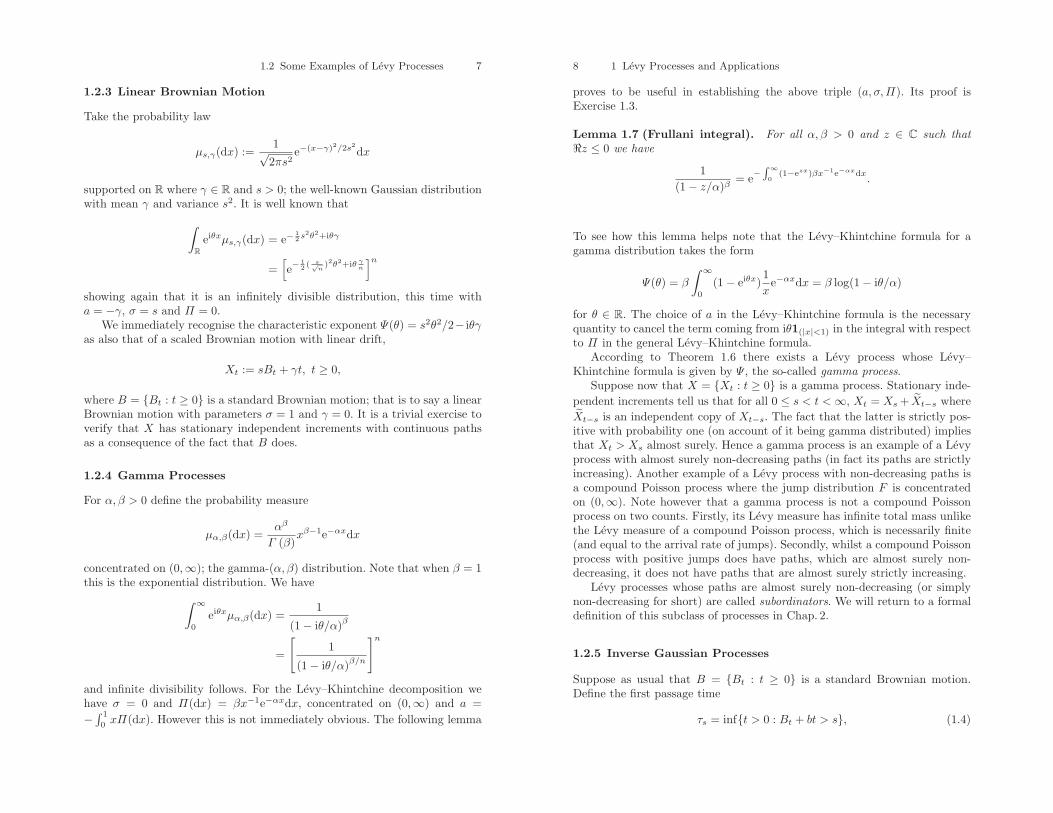
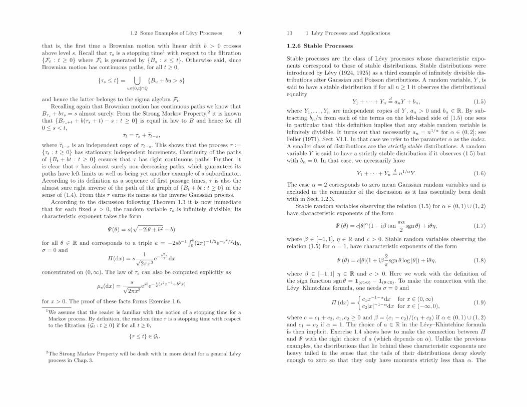
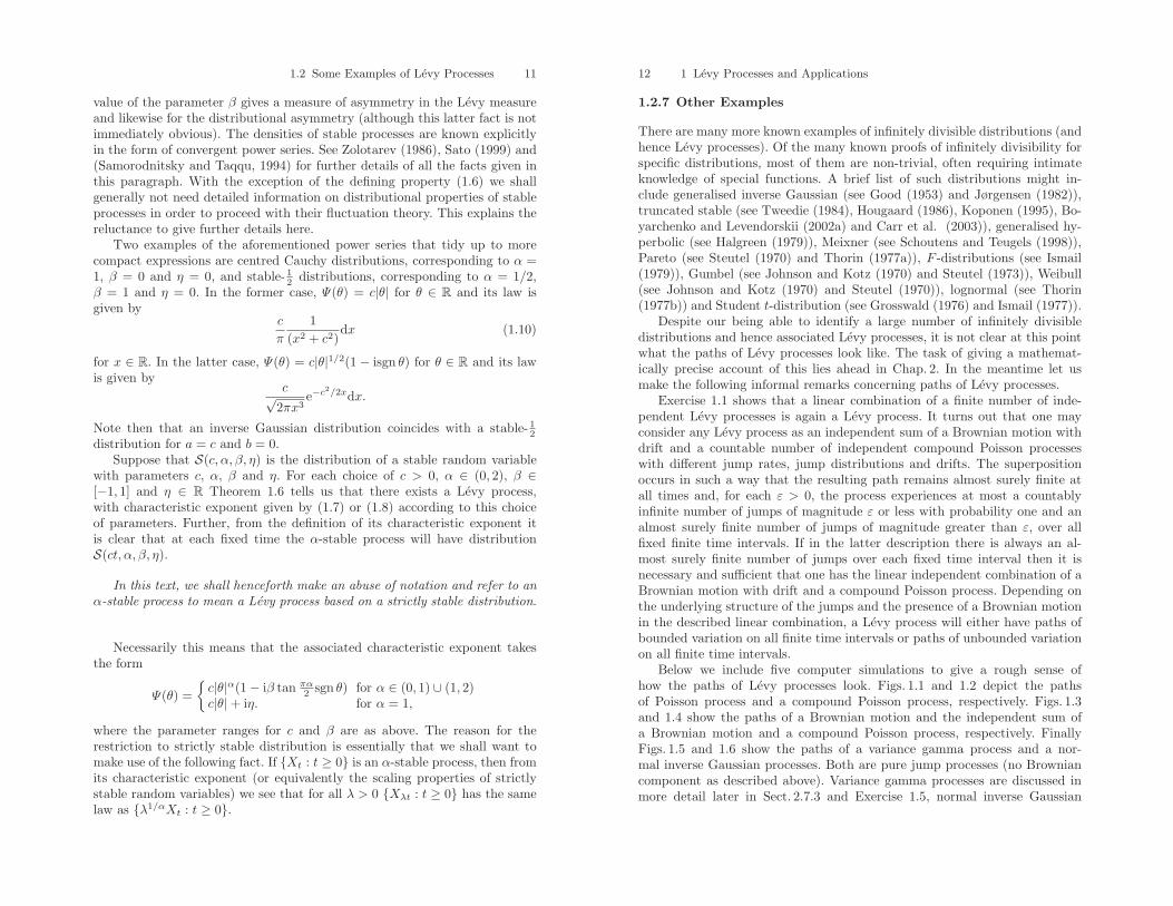
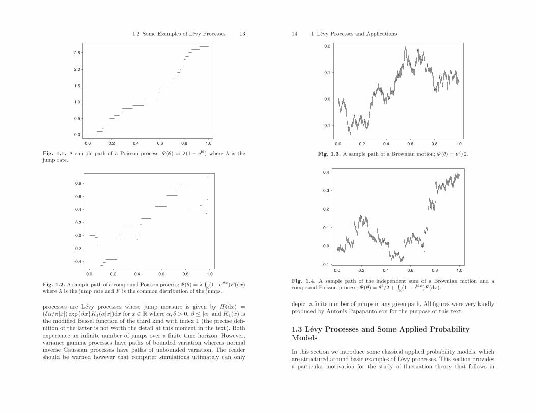
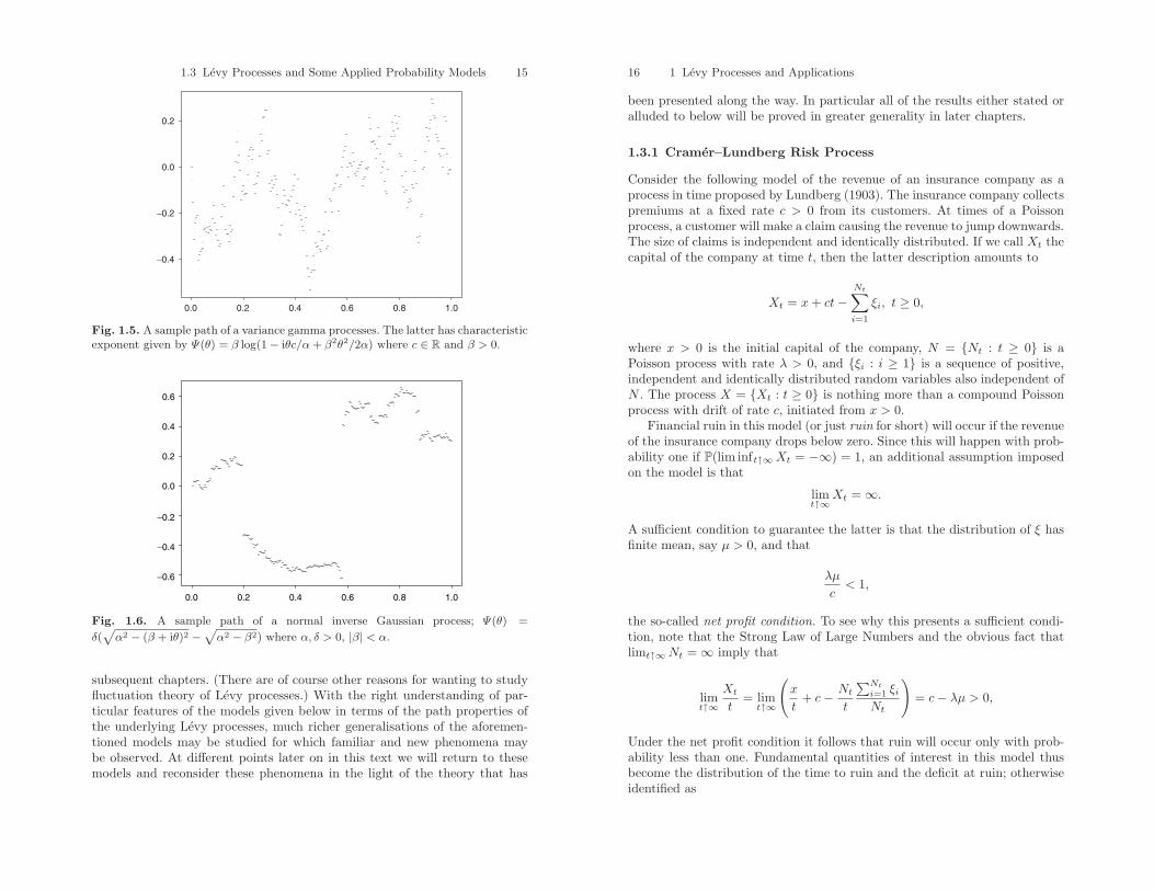
Below we include five computer simulations to give a rough sense ofhow the paths of Levy processes look. Figs. 1.1 and 1.2 depict the pathsof Poisson process and a compound Poisson process, respectively. Figs. 1.3and 1.4 show the paths of a Brownian motion and the independent sum ofa Brownian motion and a compound Poisson process, respectively. FinallyFigs. 1.5 and 1.6 show the paths of a variance gamma process and a nor-mal inverse Gaussian processes. Both are pure jump processes (no Browniancomponent as described above). Variance gamma processes are discussed inmore detail later in Sect. 2.7.3 and Exercise 1.5, normal inverse Gaussian
1.2 Some Examples of Levy Processes 13
0.0 0.2 0.4 0.6 0.8 1.0
0.0
0.5
1.0
1.5
2.0
2.5
Fig. 1.1. A sample path of a Poisson process; Ψ(θ) = λ(1 − eiθ) where λ is thejump rate.
0.0 0.2 0.4 0.6 0.8 1.0
−0.4
−0.2
0.0
0.2
0.4
0.6
0.8
Fig. 1.2. A sample path of a compound Poisson process; Ψ(θ) = λ∫
R(1−eiθx)F (dx)where λ is the jump rate and F is the common distribution of the jumps.
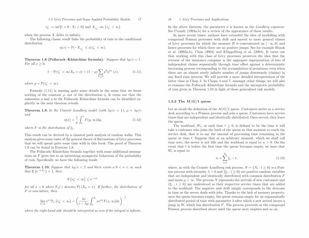
processes are Levy processes whose jump measure is given by Π(dx) =(δα/π|x|) expβxK1(α|x|)dx for x ∈ R where α, δ > 0, β ≤ |α| and K1(x) isthe modified Bessel function of the third kind with index 1 (the precise defi-nition of the latter is not worth the detail at this moment in the text). Bothexperience an infinite number of jumps over a finite time horizon. However,variance gamma processes have paths of bounded variation whereas normalinverse Gaussian processes have paths of unbounded variation. The readershould be warned however that computer simulations ultimately can only
14 1 Levy Processes and Applications
0.0 0.2 0.4 0.6 0.8 1.0
−0.1
0.0
0.1
0.2
Fig. 1.3. A sample path of a Brownian motion; Ψ(θ) = θ2/2.
0.0 0.2 0.4 0.6 0.8 1.0
−0.1
0.0
0.1
0.2
0.3
0.4
Fig. 1.4. A sample path of the independent sum of a Brownian motion and acompound Poisson process; Ψ(θ) = θ2/2 +
∫R(1− eiθx)F (dx).
depict a finite number of jumps in any given path. All figures were very kindlyproduced by Antonis Papapantoleon for the purpose of this text.
1.3 Levy Processes and Some Applied ProbabilityModels
In this section we introduce some classical applied probability models, whichare structured around basic examples of Levy processes. This section providesa particular motivation for the study of fluctuation theory that follows in
1.3 Levy Processes and Some Applied Probability Models 15
0.0 0.2 0.4 0.6 0.8 1.0
−0.4
−0.2
0.0
0.2
Fig. 1.5. A sample path of a variance gamma processes. The latter has characteristicexponent given by Ψ(θ) = β log(1− iθc/α + β2θ2/2α) where c ∈ R and β > 0.
0.0 0.2 0.4 0.6 0.8 1.0
−0.6
−0.4
−0.2
0.0
0.2
0.4
0.6
Fig. 1.6. A sample path of a normal inverse Gaussian process; Ψ(θ) =
δ(√
α2 − (β + iθ)2 −√
α2 − β2) where α, δ > 0, |β| < α.
subsequent chapters. (There are of course other reasons for wanting to studyfluctuation theory of Levy processes.) With the right understanding of par-ticular features of the models given below in terms of the path properties ofthe underlying Levy processes, much richer generalisations of the aforemen-tioned models may be studied for which familiar and new phenomena maybe observed. At different points later on in this text we will return to thesemodels and reconsider these phenomena in the light of the theory that has
16 1 Levy Processes and Applications
been presented along the way. In particular all of the results either stated oralluded to below will be proved in greater generality in later chapters.
1.3.1 Cramer–Lundberg Risk Process
Consider the following model of the revenue of an insurance company as aprocess in time proposed by Lundberg (1903). The insurance company collectspremiums at a fixed rate c > 0 from its customers. At times of a Poissonprocess, a customer will make a claim causing the revenue to jump downwards.The size of claims is independent and identically distributed. If we call Xt thecapital of the company at time t, then the latter description amounts to
Xt = x+ ct−Nt∑i=1
ξi, t ≥ 0,
where x > 0 is the initial capital of the company, N = Nt : t ≥ 0 is aPoisson process with rate λ > 0, and ξi : i ≥ 1 is a sequence of positive,independent and identically distributed random variables also independent ofN . The process X = Xt : t ≥ 0 is nothing more than a compound Poissonprocess with drift of rate c, initiated from x > 0.
Financial ruin in this model (or just ruin for short) will occur if the revenueof the insurance company drops below zero. Since this will happen with prob-ability one if P(lim inft↑∞Xt = −∞) = 1, an additional assumption imposedon the model is that
limt↑∞
Xt = ∞.
A sufficient condition to guarantee the latter is that the distribution of ξ hasfinite mean, say µ > 0, and that
λµ
c< 1,
the so-called net profit condition. To see why this presents a sufficient condi-tion, note that the Strong Law of Large Numbers and the obvious fact thatlimt↑∞Nt = ∞ imply that
limt↑∞
Xt
t= lim
t↑∞
(x
t+ c− Nt
t
∑Nt
i=1 ξiNt
)= c− λµ > 0,
Under the net profit condition it follows that ruin will occur only with prob-ability less than one. Fundamental quantities of interest in this model thusbecome the distribution of the time to ruin and the deficit at ruin; otherwiseidentified as
1.3 Levy Processes and Some Applied Probability Models 17
τ−0 := inft > 0 : Xt < 0 and Xτ−0on τ−0 <∞
when the process X drifts to infinity.The following classic result links the probability of ruin to the conditional
distributionη(x) = P(−Xτ−0
≤ x|τ−0 <∞).
Theorem 1.8 (Pollaczek–Khintchine formula). Suppose that λµ/c < 1.For all x ≥ 0,
1− P(τ−0 <∞|X0 = x) = (1− ρ)∑k≥0
ρkηk∗ (x), (1.11)
where ρ = P(τ−0 <∞).
Formula (1.11) is missing quite some details in the sense that we knownothing of the constant ρ, nor of the distribution η. It turns out that theunknowns ρ and η in the Pollaczek–Khintchine formula can be identified ex-plicitly as the next theorem reveals.
Theorem 1.9. In the Cramer–Lundberg model (with λµ/c < 1), ρ = λµ/cand
η(x) =1µ
∫ x
0
F (y,∞)dy, (1.12)
where F is the distribution of ξ1.
This result can be derived by a classical path analysis of random walks. Thisanalysis gives some taste of the general theory of fluctuations of Levy processesthat we will spend quite some time with in this book. The proof of Theorem1.9 can be found in Exercise 1.8.
The Pollaczek–Khintchine formula together with some additional assump-tions on F gives rise to an interesting asymptotic behaviour of the probabilityof ruin. Specifically we have the following result.
Theorem 1.10. Suppose that λµ/c < 1 and there exists a 0 < ν < ∞ suchthat E
(e−νX1
)= 1, then
P(τ−0 <∞) ≤ e−νx
for all x > 0 where Px(·) denotes P(·|X0 = x). If further, the distribution ofF is non-lattice, then
limx↑∞
eνxPx(τ−0 <∞) =
(λν
c− λµ
∫ ∞
0
xeνxF (x,∞)dx)−1
where the right-hand side should be interpreted as zero if the integral is infinite.
18 1 Levy Processes and Applications
In the above theorem, the parameter ν is known as the Lundberg exponent.See Cramer (1994a,b) for a review of the appearance of these results.
In more recent times, authors have extended the idea of modelling withcompound Poisson processes with drift and moved to more general classesof Levy processes for which the measure Π is concentrated on (−∞, 0) andhence processes for which there are no positive jumps. See for example Huzaket al. (2004a,b), Chan (2004) and Kluppelberg et al. (2004). It turns outthat working with this class of Levy processes preserves the idea that therevenue of the insurance company is the aggregate superposition of lots ofindependent claims sequentially through time offset against a deterministicincreasing process corresponding to the accumulation of premiums, even whenthere are an almost surely infinite number of jumps downwards (claims) inany fixed time interval. We will provide a more detailed interpretation of thelatter class in Chap. 2. In Chaps. 4 and 7, amongst other things, we will alsore-examine the Pollaczek–Khintchine formula and the asymptotic probabilityof ruin given in Theorem 1.10 in light of these generalised risk models.
1.3.2 The M/G/1 queue
Let us recall the definition of the M/G/1 queue. Customers arrive at a servicedesk according to a Poisson process and join a queue. Customers have servicetimes that are independent and identically distributed. Once served, they leavethe queue.
The workload, Wt, at each time t ≥ 0, is defined to be the time it willtake a customer who joins the back of the queue at that moment to reach theservice desk, that is to say the amount of processing time remaining in thequeue at time t. Suppose that at an arbitrary moment, which we shall calltime zero, the server is not idle and the workload is equal to w > 0. On theevent that t is before the first time the queue becomes empty, we have thatWt is equal to
w +Nt∑i=1
ξi − t, (1.13)
where, as with the Cramer–Lundberg risk process, N = Nt : t ≥ 0 is a Pois-son process with intensity λ > 0 and ξi : i ≥ 0 are positive random variablesthat are independent and identically distributed with common distribution Fand mean µ <∞. The process N represents the arrivals of new customers andξi : i ≥ 0 are understood as their respective service times that are addedto the workload. The negative unit drift simply corresponds to the decreasein time as the server deals with jobs. Thanks to the lack of memory property,once the queue becomes empty, the queue remains empty for an exponentiallydistributed period of time with parameter λ after which a new arrival incurs ajump in W, which has distribution F . The process proceeds as the compoundPoisson process described above until the queue next empties and so on.
1.3 Levy Processes and Some Applied Probability Models 19
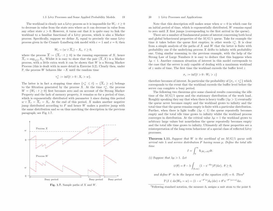
The workload is clearly not a Levy process as it is impossible for Wt : t ≥ 0to decrease in value from the state zero where as it can decrease in value fromany other state x > 0. However, it turns out that it is quite easy to link theworkload to a familiar functional of a Levy process, which is also a Markovprocess. Specifically, suppose we define Xt equal to precisely the same Levyprocess given in the Cramer–Lundberg risk model with c = 1 and x = 0, then
Wt = (w ∨Xt)−Xt, t ≥ 0,
where the process X := Xt : t ≥ 0 is the running supremum of X, henceXt = supu≤tXu. Whilst it is easy to show that the pair (X,X) is a Markovprocess, with a little extra work it can be shown that W is a Strong MarkovProcess (this is dealt with in more detail in Exercise 3.2). Clearly then, underP, the process W behaves like −X until the random time
τ+w := inft > 0 : Xt > w.
The latter is in fact a stopping time since τ+w ≤ t = Xt ≥ w belongs
to the filtration generated by the process X. At the time τ+w , the process
W = Wt : t ≥ 0 first becomes zero and on account of the Strong MarkovProperty and the lack of memory property, it remains so for a period of time,which is exponentially distributed with parameter λ since during this periodw ∨ Xt = Xt = Xt. At the end of this period, X makes another negativejump distributed according to F and hence W makes a positive jump withthe same distribution and so on thus matching the description in the previousparagraph; see Fig. 1.7.
wProcess X
w
Process W
0
0
Busy period Busy period Busy period
Fig. 1.7. Sample paths of X and W .
20 1 Levy Processes and Applications
Note that this description still makes sense when w = 0 in which case foran initial period of time, which is exponentially distributed, W remains equalto zero until X first jumps (corresponding to the first arrival in the queue).
There are a number of fundamental points of interest concerning both localand global behavioural properties of the M/G/1 queue. Take for example thetime it takes before the queue first empties; in other words τ+
w . It is clearfrom a simple analysis of the paths of X and W that the latter is finite withprobability one if the underlying process X drifts to infinity with probabilityone. Using similar reasoning to the previous example, with the help of theStrong Law of Large Numbers it is easy to deduce that this happens whenλµ < 1. Another common situation of interest in this model corresponds tothe case that the server is only capable of dealing with a maximum workloadof z units of time. The first time the workload exceeds the buffer level z
σz := inft > 0 : Wt > ztherefore becomes of interest. In particular the probability of σz < τ+
w whichcorresponds to the event that the workload exceeds the buffer level before theserver can complete a busy period.
The following two theorems give some classical results concerning the idletime of the M/G/1 queue and the stationary distribution of the work load.Roughly speaking they say that when there is heavy traffic (λµ > 1) eventuallythe queue never becomes empty and the workload grows to infinity and thetotal time that the queue remains empty is finite with a particular distribution.Further, when there is light traffic (λµ < 1) the queue repeatedly becomesempty and the total idle time grows to infinity whilst the workload processconverges in distribution. At the critical value λµ = 1 the workload grows toarbitrary large values but nonetheless the queue repeatedly becomes emptyand the total idle time grows to infinity. Ultimately all these properties are areinterpretation of the long-term behaviour of a special class of reflected Levyprocesses.
Theorem 1.11. Suppose that W is the workload of an M/G/1 queue witharrival rate λ and service distribution F having mean µ. Define the total idletime
I =∫ ∞
0
1(Wt=0)dt.
(i) Suppose that λµ > 1. Let
ψ(θ) = θ − λ
∫(0,∞)
(1− e−θx)F (dx), θ ≥ 0,
and define θ∗ to be the largest root of the equation ψ(θ) = 0. Then3
P (I ∈ dx|W0 = w) = (1− e−θ∗w)δ0 (dx) + θ∗e−θ
∗(w+x)dx.3Following standard notation, the measure δ0 assigns a unit atom to the point 0.
1.3 Levy Processes and Some Applied Probability Models 21
(ii) If λµ ≤ 1 then I is infinite with probability one.
Note that the function ψ given above is nothing more than the Laplaceexponent of the underlying Levy process
Xt = t−Nt∑i=1
ξi, t ≥ 0
which drives the process W and fulfils the relation ψ(θ) = log E(eθX1). It iseasy to check by differentiating it twice that ψ is a strictly convex function,which is zero at the origin and tends to infinity at infinity. Further ψ′(0+) < 0under the assumption λµ > 1 and hence θ∗ exists, is finite and is in fact theonly solution to ψ(θ) = 0 other than θ = 0.
Theorem 1.12. Let W be the same as in Theorem 1.11.
(i) Suppose that λµ < 1. Then for all w ≥ 0 the virtual waiting time has astationary distribution,
limt↑∞
P(Wt ≤ x|W0 = w) = (1− ρ)∞∑k=0
ρkη∗k(x),
where
η(x) =1µ
∫ x
0
F (y,∞)dy and ρ = λµ.
(ii) If λµ ≥ 1 then lim supt↑∞Wt = ∞ with probability one.
Some of the conclusions in the above two theorems can already be ob-tained with basic knowledge of compound Poisson processes. Theorem 1.11 isproved in Exercise 1.9 and gives some feeling of the fluctuation theory thatwill be touched upon later on in this text. The remarkable similarity betweenTheorem 1.12 part (i) and the Pollaczek–Khintchine formula is of course no co-incidence. The principles that are responsible for the latter two results are em-bedded within the general fluctuation theory of Levy processes. Indeed we willrevisit Theorems 1.11 and 1.12 but for more general versions of the workloadprocess of the M/G/1 queue known as general storage models. Such general-isations involve working with a general class of Levy process with no positivejumps (that is Π(0,∞) = 0) and defining as before Wt = (w ∨ Xt) − Xt.When there are an infinite number of jumps in each finite time interval thelatter process may be thought of as modelling a processor that deals with anarbitrarily large number of small jobs and occasional large jobs. The preciseinterpretation of such a generalised M/G/1 workload process and issues con-cerning the distribution of the busy period, the stationary distribution of theworkload, time to buffer overflow and other related quantities will be dealtwith later on in Chaps. 2, 4 and 8.
22 1 Levy Processes and Applications
1.3.3 Optimal Stopping Problems
A fundamental class of problems motivated by applications from physics, op-timal control, sequential testing and economics (to name but a few) concernoptimal stopping problems of the form: Find v(x) and a stopping time, τ∗,belonging to a specified family of stopping times, T , such that
v(x) = supτ∈T
Ex(e−qτG(Xτ )) = Ex(e−qτ∗G(Xτ∗)) (1.14)
for all x ∈ R ⊆ R, where X is a R-valued Markov process with probabilitiesPx : x ∈ R (with the usual understanding that Px is the law of X given thatX0 = x), q ≥ 0 and G : R → [0,∞) is a function suitable to the applicationat hand. The optimal stopping problem (1.14) is not the most general classof such problems that one may consider but will suffice for the discussion athand.
In many cases it turns out that the optimal strategy takes the form
τ∗ = inft > 0 : (t,Xt) ∈ D,
where D ⊂ [0,∞) × R is a domain in time–space called the stopping region.Further still, there are many examples within the latter class for which D =[0,∞) × I where I is an interval or the complement of an interval. In otherwords the optimal strategy is the first passage time into I,
τ∗ = inft > 0 : Xt ∈ I. (1.15)
A classic example of an optimal stopping problem in the form (1.14) forwhich the solution agrees with (1.15) is the following taken from McKean(1965),
v(x) = supτ∈T
Ex(e−qτ (K − eXτ )+), (1.16)
where now q > 0, T is the family of stopping times with respect to the fil-tration Ft := σ(Xs : s ≤ t) and Xt : t ≥ 0 is a linear Brownian motion,Xt = σBt + γt, t ≥ 0 (see Sect. 1.2.3). Note that we use here the standardnotation y+ = y ∨ 0. This particular example models the optimal time to sella risky asset for a fixed value K when the asset’s dynamics are those of anexponential linear Brownian motion. Optimality in this case is determined viathe expected discounted gain at the selling time. On account of the under-lying source of randomness being Brownian motion and the optimal strategytaking the simple form (1.15), the solution to (1.16) turns out to be explicitlycomputable as follows.
Theorem 1.13. The solution (v, τ∗) to (1.16) is given by
τ∗ = inft > 0 : Xt < x∗,
1.3 Levy Processes and Some Applied Probability Models 23
where
ex∗
= K
(Φ(q)
1 + Φ(q)
),
Φ(q) = (√γ2 + 2σ2q + γ)/σ2 and
v(x) =
(K − ex) if x < x∗
(K − ex∗)e−Φ(q)(x−x∗) if x ≥ x∗.
The solution to this problem reflects the intuition that the optimal time to stopshould be at a time when X is as negative as possible taking into considerationthat taking too long to stop incurs an exponentially weighted penalty. Notethat in (−∞, x∗) the value function v(x) is equal to the gain function (K −ex)+ as the optimal strategy τ∗ dictates that one should stop immediately. Aparticular curiosity of the solution to (1.16) is the fact that at x∗, the valuefunction v joins smoothly to the gain function. In other words,
v′(x∗−) = −ex∗
= v′(x∗+).
A natural question in light of the above optimal stopping problem iswhether one can characterise the solution to (1.16) when X is replaced bya general Levy process. Indeed, if the same strategy of first passage belowa specified level is still optimal, one is then confronted with needing infor-mation about the distribution of the overshoot of a Levy process when firstcrossing below a barrier in order to compute the function v. The latter is ofparticular interest if one would like to address the question as to whether thephenomenon of smooth fit is still to be expected in the general Levy processsetting.
Later in Chap. 9 we give a brief introduction to some general principlesappearing in the theory of optimal stopping and apply them to a handful ofexamples where the underlying source of randomness is provided by a Levyprocess. The first of these examples being the generalisation of (1.16) as men-tioned above. All of the examples presented in Chap. 9 can be solved (semi-)explicitly thanks to a degree of simplicity in the optimal strategy such as(1.15) coupled with knowledge of fluctuation theory of Levy processes. In ad-dition, through these examples, we will attempt to give some insight into howand when smooth pasting occurs as a consequence of a subtle type of pathbehaviour of the underlying Levy process.
1.3.4 Continuous-State Branching Processes
Originating in part from the concerns of the Victorian British upper classesthat aristocratic surnames were becoming extinct, the theory of branchingprocesses now forms a cornerstone of classical applied probability. Some ofthe earliest work on branching processes dates back to Watson and Galton(1874). However, approximately 100 years later, it was discovered by Heyde
24 1 Levy Processes and Applications
and Seneta (1977) that the less well-exposed work of I.J. Bienayme, datedaround 1845, contained many aspects of the later work of Galton and Watson.The Bienayme–Galton–Watson process, as it is now known, is a discrete timeMarkov chain with state space 0, 1, 2, ... described by the sequence Zn :n = 0, 1, 2, ... satisfying the recursion Z0 > 0 and
Zn =Zn−1∑i=1
ξ(n)i
for n = 1, 2, ... where ξ(n) : i = 1, 2, ... are independent and exponentiallydistributed on 0, 1, 2, .... We use the usual notation
∑0i=1 to represent the
empty sum. The basic idea behind this model is that Zn is the populationcount in the nth generation and from an initial population Z0 (which maybe randomly distributed) individuals reproduce asexually and independentlywith the same distribution of numbers of offspring. The latter reproductiveproperties are referred to as the branching property. Note that as soon asZn = 0 it follows from the given construction that Zn+k = 0 for all k = 1, 2, ...A particular consequence of the branching property is that if Z0 = a+ b thenZn is equal in distribution to Z(1)
n +Z(2)n where Z(1)
n and Z(2)n are independent
with the same distribution as an nth generation Bienayme–Galton–Watsonprocess initiated from population sizes a and b, respectively.
A mild modification of the Bienayme–Galton–Watson process is to set itinto continuous time by assigning life lengths to each individual which areindependent and identically distributed with parameter λ > 0. Individuals re-produce at their moment of death in the same way as described previously forthe Bienayme-Galton-Watson process. If Y = Yt : t ≥ 0 is the 0, 1, 2, ....-valued process describing the population size then it is straightforward to seethat the lack of memory property of the exponential distribution implies thatfor all 0 ≤ s ≤ t,
Yt =Ys∑i=1
Y(i)t−s,
where given Yu : u ≤ s the variables Y (i)t−s : i = 1, ..., Ys are independent
with the same distribution as Yt−s conditional on Y0 = 1. In that case, we maytalk of Y as a continuous-time Markov chain on 0, 1, 2, ..., with probabilities,say, Py : y = 0, 1, 2, ... where Py is the law of Y under the assumption thatY0 = y. As before, the state 0 is absorbing in the sense that if Yt = 0 thenYt+u = 0 for all u > 0. The process Y is called the continuous time Markovbranching process. The branching property for Y may now be formulated asfollows.
Definition 1.14 (Branching property). For any t ≥ 0 and y1, y2 in thestate space of Y , Yt under Py1+y2 is equal in law to the independent sumY
(1)t + Y
(2)t where the distribution of Y (i)
t is equal to that of Yt under Pyifor
i = 1, 2.
So far there appears to be little connection with Levy processes. However aremarkable time transformation shows that the path of Y is intimately linked
1.3 Levy Processes and Some Applied Probability Models 25
to the path of a compound Poisson process with jumps whose distributionis supported in −1, 0, 1, 2, ..., stopped at the first instant that it hits zero.To explain this in more detail let us introduce the probabilities πi : i =−1, 0, 1, 2, ..., where πi = P (ξ = i + 1) and ξ has the same distributionas the typical family size in the Bienayme–Galton–Watson process. To avoidcomplications let us assume that π0 = 0 so that a transition in the state ofY always occurs when an individual dies. When jumps of Y occur, they areindependent and always distributed according to πi : i = −1, 0, 1, .... Theidea now is to adjust time accordingly with the evolution of Y in such a waythat these jumps are spaced out with inter-arrival times that are independentand exponentially distributed. Crucial to the following exposition is the simpleand well-known fact that the minimum of n ∈ 1, 2, ... independent andexponentially distributed random variables is exponentially distributed withparameter λn. Further, that if eα is exponentially distributed with parameterα > 0 then for β > 0, βeα is equal in distribution to eα/β .
Write for t ≥ 0,
Jt =∫ t
0
Yudu
setϕt = infs ≥ 0 : Js > t
with the usual convention that inf ∅ = ∞ and define
Xt = Yϕt(1.17)
with the understanding that when ϕt = ∞ we set Xt = 0. Now observe thatwhen Y0 = y ∈ 1, 2, ... the first jump of Y occurs at a time, say T1 (theminimum of y independent exponential random variables, each with parameterλ > 0) which is exponentially distributed with parameter λy and the size ofthe jump is distributed according to πi : i = −1, 0, 1, 2, .... However, notethat JT1 = yT1 is the first time that the process X = Xt : t ≥ 0 jumps. Thelatter time is exponentially distributed with parameter λ. The jump at thistime is independent and distributed according to πi : i = −1, 0, 1, 2, ....
Given the information G1 = σ(Yt : t ≤ T1), the lack of memory propertyimplies that the continuation YT1+t : t ≥ 0 has the same law as Y under Pywith y = YT1 . Hence if T2 is the time of the second jump of Y then conditionalon G1 we have that T2 − T1 is exponentially distributed with parameter λYT1
and JT2 − JT1 = YT1(T2 − T1) which is again exponentially distributed withparameter λ and further, is independent of G1. Note that JT2 is the time ofthe second jump of X and the size of the second jump is again independentand distributed according to πi : i = −1, 0, 1, .... Iterating in this way itbecomes clear that X is nothing more than a compound Poisson process witharrival rate λ and jump distribution
F (dx) =∞∑
i=−1
πiδi(dx) (1.18)
stopped on first hitting the origin.
26 1 Levy Processes and Applications
A converse to this construction is also possible. Suppose now that X =Xt : t ≥ 0 is a compound Poisson process with arrival rate λ > 0 and jumpdistribution F (dx) =
∑∞i=−1 πiδi(dx). Write
It =∫ t
0
X−1u du
and set
θt = infs ≥ 0 : Is > t. (1.19)
again with the understanding that inf ∅ = ∞. Define
Yt = Xθt∧τ−0
where τ−0 = inft > 0 : Xt < 0. By analysing the behaviour of Y = Yt : t ≥0 at the jump times of X in a similar way to above one readily shows thatthe process Y is a continuous time Markov branching process. The details areleft as an exercise to the reader.
The relationship between compound Poisson processes and continuoustime Markov branching processes described above turns out to have a muchmore general setting. In the work of Lamperti (1967a, 1976b) it is shown thatthere exists a correspondence between a class of branching processes calledcontinuous-state branching processes and Levy processes with no negativejumps (Π(−∞, 0) = 0). In brief, a continuous-state branching process is a[0,∞)-valued Markov process having paths that are right continuous with leftlimits and probabilities Px : x > 0 that satisfy the branching property inDefinition 1.14. Note in particular that now the quantities y1 and y2 maybe chosen from the non-negative real numbers. Lamperti’s characterisationof continuous-state branching processes shows that they can be identified astime changed Levy processes with no negative jumps precisely via the trans-formations given in (1.17) with an inverse transformation analogous to (1.19).We explore this relationship in more detail in Chap. 10 by looking at issuessuch as explosion, extinction and conditioning on survival.
Exercises
1.1. Using Definition 1.1, show that the sum of two (or indeed any finitenumber of) independent Levy processes is again a Levy process.
1.2. Suppose that S = Sn : n ≥ 0 is any random walk and Γp is anindependent random variable with a geometric distribution on 0, 1, 2, ...with parameter p.
(i) Show that Γp is infinitely divisible.(ii) Show that SΓp
is infinitely divisible.
1.3 Exercises 27
1.3 (Proof of Lemma 1.7). In this exercise we derive the Frullani identity.
(i) Show for any function f such that f ′ exists and is continuous and f(0) andf(∞) are finite, that∫ ∞
0
f(ax)− f(bx)x
dx = (f(0)− f(∞)) log(b
a
),
where b > a > 0.(ii) By choosing f(x) = e−x, a = α > 0 and b = α− z where z < 0, show that
1(1− z/α)β
= e−∫∞
0(1−ezx) β
x e−αxdx
and hence by analytic extension show that the above identity is still validfor all z ∈ C such that ℜz ≤ 0.
1.4. Establishing formulae (1.7) and (1.8) from the Levy measure given in(1.9) is the result of a series of technical manipulations of special integrals.In this exercise we work through them. In the following text we will use thegamma function Γ (z), defined by
Γ (z) =∫ ∞
0
tz−1e−tdt
for z > 0. Note the gamma function can also be analytically extended sothat it is also defined on R\0,−1,−2, ... (see Lebedev (1972)). Whilst thespecific definition of the gamma function for negative numbers will not play animportant role in this exercise, the following two facts that can be derived fromit will. For z ∈ R\0,−1,−2, ... the gamma function observes the recursionΓ (1 + z) = zΓ (z) and Γ (1/2) =
√π.
(i) Suppose that 0 < α < 1. Prove that for u > 0,∫ ∞
0
(e−ur − 1)r−α−1dr = Γ (−α)uα
and show that the same equality is valid when −u is replaced by anycomplex number w = 0 with ℜw ≤ 0. Conclude by considering w = i that∫ ∞
0
(1− eir)r−α−1dr = −Γ (−α)e−iπα/2 (1.20)
as well as the complex conjugate of both sides being equal. Deduce (1.7)by considering the integral∫ ∞
0
(1− eiξθr)r−α−1dr
for ξ = ±1 and θ ∈ R. Note that you will have to take a = η −∫R x1(|x|<1)Π (dx), which you should check is finite.
28 1 Levy Processes and Applications
(ii) Now suppose that α = 1. First prove that∫|x|<1
eiθx(1− |x|)dx = 2(
1− cos θθ2
)for θ ∈ R and hence by Fourier inversion,∫ ∞
0
1− cos rr2
dr =π
2.
Use this identity to show that for z > 0,∫ ∞
0
(1− eirz + izr1(r<1))1r2
dr =π
2z + iz log z − ikz
for some constant k ∈ R. By considering the complex conjugate of theabove integral establish the expression in (1.8). Note that you will need adifferent choice of a to part (i).
(iii) Now suppose that 1 < α < 2. Integrate (1.20) by parts to reach∫ ∞
0
(eir − 1− ir)r−α−1dr = Γ (−α)e−iπα/2.
Consider the above integral for z = ξθ, where ξ = ±1 and θ ∈ R anddeduce the identity (1.7) in a similar manner to the proof in (i) and (ii).
1.5. Prove for any θ ∈ R that
expiθXt + tΨ(θ), t ≥ 0
is a martingale where Xt : t ≥ 0 is a Levy process with characteristicexponent Ψ .
1.6. In this exercise we will work out in detail the features of the inverseGaussian process discussed earlier on in this chapter. Recall that τ = τs : s ≥0 is a non-decreasing Levy process defined by τs = inft ≥ 0 : Bt + bt > s,s ≥ 0, where B = Bt : t ≥ 0 is a standard Brownian motion and b > 0.
(i) Argue along the lines of Exercise 1.5 to show that for each λ > 0,
eλBt− 12λ
2t, t ≥ 0
is a martingale. Use Doob’s Optimal Stopping Theorem to obtain
E(e−( 12λ
2+bλ)τs) = e−λs.
Use analytic extension to deduce further that τs has characteristic expo-nent
Ψ(θ) = s(√−2iθ + b2 − b)
for all θ ∈ R.
1.3 Exercises 29
(ii) Defining the measure Π(dx) = (2πx3)−1/2e−xb2/2dx on x > 0, check using
(1.20) from Exercise 1.4 that∫ ∞
0
(1− eiθx)Π(dx) = Ψ(θ)
for all θ ∈ R. Confirm that the triple (a, σ,Π) in the Levy–Khintchineformula are thus σ = 0, Π as above and a = −2sb−1
∫ b0(2π)−1/2e−y
2/2dy.(iii) Taking
µs(dx) =s√
2πx3esbe−
12 (s2x−1+b2x)dx
on x > 0 show that∫ ∞
0
e−λxµs(dx) = ebs−s√b2+2λ
∫ ∞
0
s√2πx3
e−12 ( s√
x−√
(b2+2λ)x)2dx
= ebs−s√b2+2λ
∫ ∞
0
√2λ+ b2
2πue−
12 ( s√
u−√
(b2+2λ)u)2du.
Hence by adding the last two integrals together deduce that∫ ∞
0
e−λxµs(dx) = e−s(√b2+2λ−b)
confirming both that µs(dx) is a probability distribution as well as beingthe probability distribution of τs.
1.7. Show that for a simple Brownian motion B = Bt : t > 0 the firstpassage process τ = τs : s > 0 (where τs = inft ≥ 0 : Bt ≥ s) is a stableprocess with parameters α = 1/2 and β = 1.
1.8 (Proof of Theorem 1.9). As we shall see in this exercise, the proofof Theorem 1.9 follows from the proof of a more general result given by theconclusion of parts (i)–(v) below for random walks.
(i) Suppose that S = Sn : n ≥ 0 is a random walk with S0 = 0 andjump distribution µ. By considering the variables S∗k := Sn − Sn−k fork = 0, 1, ..., n and noting that the joint distributions of (S0, ..., Sn) and(S∗0 , ..., S
∗n) are identical, show that for all y > 0 and n ≥ 1,
P (Sn ∈ dy and Sn > Sj for j = 0, ..., n− 1)= P (Sn ∈ dy and Sj > 0 for j = 1, ..., n).
[Hint: it may be helpful to draw a diagram of the path of the first n stepsof S and to rotate it by 180.]
(ii) Define
T−0 = infn > 0 : Sn ≤ 0 and T+0 = infn > 0 : Sn > 0.
30 1 Levy Processes and Applications
By summing both sides of the equality
P (S1 > 0, ..., Sn > 0, Sn+1 ∈ dx)
=∫
(0,∞)
P (S1 > 0, ..., Sn > 0, Sn ∈ dy)µ(dx− y)
over n show that for x ≤ 0,
P (ST−0 ∈ dx) =∫
[0,∞)
V (dy)µ(dx− y),
where for y ≥ 0,
V (dy) = δ0(dy) +∑n≥1
P (Hn ∈ dy)
and H = Hn : n ≥ 0 is a random walk with H0 = 0 and step distributiongiven by P (ST+
0∈ dz) for z ≥ 0.
(iii) Embedded in the Cramer–Lundberg model is a random walk S whoseincrements are equal in distribution to the distribution of ceλ− ξ1, whereeλ is an independent exponential random variable with mean 1/λ. Noting(using obvious notation) that ceλ has the same distribution as eβ whereβ = λ/c show that the step distribution of this random walk satisfies
µ(z,∞) =(∫ ∞
0
e−βuF (du))
e−βz for z ≥ 0
and
µ(−∞,−z) = E(F (eβ + z)) for z > 0,
where F is the tail of the distribution function F of ξ1 and E is expectationwith respect to the random variable eβ .
(iv) Since upward jumps are exponentially distributed in this random walk,use the lack of memory property to reason that
V (dy) = δ0(dy) + βdy.
Hence deduce from part (iii) that
P (−ST−0 > z) = E
(F (eβ) +
∫ ∞
x
βF (eβ + z)dz)
and so by writing out the latter with the density of the exponential dis-tribution, show that the conclusions of Theorem 1.9 hold.
1.3 Exercises 31
1.9 (Proof of Theorem 1.11). Suppose that X is a compound Poissonprocess of the form
Xt = t−Nt∑i=1
ξi,
where the process N = Nt : t ≥ 0 is a Poisson process with rate λ > 0 andξi : i ≥ 1 positive, independent and identically distributed with commondistribution F having mean µ.
(i) Show by analytic extension from the Levy–Khintchine formula or otherwisethat E(eθXt) = eψ(θ)t for all θ ≥ 0, where
ψ(θ) = θ − λ
∫(0,∞)
(1− e−θx)F (dx).
Show that ψ is strictly convex, is equal to zero at the origin and tends toinfinity at infinity. Further, show that ψ(θ) = 0 has one additional root in[0,∞) other than θ = 0 if and only if ψ′(0) < 0.
(ii) Show that eθXt−ψ(θ)t : t ≥ 0 is a martingale and hence so is eθ∗X
t∧τ+x :
t ≥ 0 where τ+x = inft > 0 : Xt > x, x > 0 and θ∗ is the largest root
described in the previous part of the question. Show further that
P(X∞ > x) = e−θ∗x
for all x > 0.(iii) Show that for all t ≥ 0,∫ t
0
1(Ws=0)ds = (Xt − w) ∨ 0,
where Wt = (w ∨Xt)−Xt.(iv) Deduce that I :=
∫∞0
1(Ws=0)ds = ∞ if λµ ≤ 1.(v) Assume that λµ > 1. Show that
P(I ∈ dx; τ+w = ∞|W0 = w) = (1− e−θ
∗w)δ0(dx).
Next use the lack of memory property to deduce that
P(I ∈ dx; τ+w <∞|W0 = w) = θ∗e−θ
∗(w+x)dx.
1.10. Here we solve a slightly simpler optimal stopping problem than (1.16).Suppose, as in the aforementioned problem, that X is a linear Brownian mo-tion with scaling parameter σ > 0 and drift γ ∈ R. Fix K > 0 and let
v(x) = supa∈R
Ex(e−qτ−a (K − e
Xτ−a )+), (1.21)
32 1 Levy Processes and Applications
where
τ−a = inft > 0 : Xt < a.(i) Following similar arguments to those in Exercise 1.5 shows that expθXt−
ψ(θ)t : t ≥ 0 is a martingale, where ψ(θ) = σ2θ2/2 + γθ.(ii) By considering the martingale in part (i) at the stopping time t∧ τ+
x andthen letting t ↑ ∞, deduce that
E(e−qτ+x ) = e−x(
√γ2+2σ2q−γ)/σ2
and hence deduce that for a ≥ 0,
E(e−qτ−−a) = e−a(
√γ2+2σ2q+γ)/σ2
.
(iii) Let v(x, a) = Ex(e−qτ−−a(K − expXτ−−a
)). For each fixed x differentiatev(x, a) in the variable a and show that the solution to 1.21 is the same asthe solution given in Theorem 1.13.
1.11. In this exercise, we characterise the Laplace exponent of the continuoustime Markov branching process Y described in Sect. 1.3.4.
(i) Show that for φ > 0 and t ≥ 0 there exists some function ut(φ) > 0satisfying
Ey(e−φYt) = e−yut(φ),
where y ∈ 1, 2, .....(ii) Show that for s, t ≥ 0,
ut+s(φ) = us(ut(φ)).
(iii) Appealing to the infinitesimal behaviour of the Markov chain Y showthat
∂ut(φ)∂t
= ψ(ut(φ))
and u0(φ) = φ where
ψ(q) = λ
∫[−1,∞)
(1− e−qx)F (dx)
and F is given in (1.18).
2
The Levy–Ito Decompositionand Path Structure
The main aim of this chapter is to establish a rigorous understanding of thestructure of the paths of Levy processes. The way we shall do this is to provethe assertion in Theorem 1.6 that given any characteristic exponent, Ψ , be-longing to an infinitely divisible distribution, there exists a Levy process withthe same characteristic exponent. This will be done by establishing the so-called Levy–Ito decomposition which describes the structure of a general Levyprocess in terms of three independent auxiliary Levy processes, each with dif-ferent types of path behaviour. In doing so it will be necessary to digress tem-porarily into the theory of Poisson random measures and associated squareintegrable martingales. Understanding the Levy–Ito decomposition will allowus to distinguish a number of important general subclasses of Levy processesaccording to their path type. The chapter is concluded with a discussion ofthe interpretation of the Levy–Ito decomposition in the context of some ofthe applied probability models mentioned in Chap. 1.
2.1 The Levy–Ito Decomposition
According to Theorem 1.3, any characteristic exponent Ψ belonging to an in-finitely divisible distribution can be written, after some simple reorganisation,in the form
Ψ(θ) =
iaθ +12σ2θ2
+
Π(R\(−1, 1))
∫|x|≥1
(1− eiθx)Π(dx)
Π(R\(−1, 1))
+
∫0<|x|<1
(1− eiθx + iθx)Π(dx)
(2.1)
for all θ ∈ R where a ∈ R, σ ≥ 0 and Π is a measure on R\0 satisfying∫R(1 ∧ x2)Π(dx) < ∞. Note that the latter condition on Π implies that
34 2 The Levy–Ito Decomposition and Path Structure
Π(A) < ∞ for all Borel A such that 0 is in the interior of Ac and particularthat Π(R\(−1, 1)) ∈ [0,∞). In the case that Π(R\(−1, 1)) = 0 one shouldthink of the second bracket in (2.1) as absent. Call the three brackets in(2.1) Ψ (1), Ψ (2) and Ψ (3). The essence of the Levy–Ito decomposition revolvesaround showing that Ψ (1), Ψ (2) and Ψ (3) all correspond to the characteristicexponents of three different types of Levy processes. Therefore Ψ may beconsidered as the characteristic exponent of the independent sum of thesethree Levy processes which is again a Levy process (cf. Exercise 1.1). Indeed,as we have already seen in Chap. 1, Ψ (1) and Ψ (2) correspond, respectively, toa linear Brownian motion with drift, X(1) = X(1)
t : t ≥ 0 where
X(1)t = σBt − at, t ≥ 0 (2.2)
and a compound Poisson process, say X(2) = X(2)t : t ≥ 0, where,
X(2)t =
Nt∑i=1
ξi, t ≥ 0, (2.3)
Nt : t ≥ 0 is a Poisson process with rate Π(R\(−1, 1)) and ξi : i ≥ 1 areindependent and identically distributed with distributionΠ(dx)/Π(R\(−1, 1))concentrated on x : |x| ≥ 1 (unless Π(R\(−1, 1)) = 0 in which case X(2) isthe process which is identically zero).
The proof of existence of a Levy process with characteristic exponent givenby (2.1) thus boils down to showing the existence of a Levy process, X(3),whose characteristic exponent is given by Ψ (3). Noting that∫
0<|x|<1
(1− eiθx + iθx)Π(dx)
=∑n≥0
λn
∫2−(n+1)≤|x|<2−n
(1− eiθx)Fn(dx)
+iθλn
(∫2−(n+1)≤|x|<2−n
xFn(dx)
), (2.4)
where λn = Π(x : 2−(n+1) ≤ |x| < 2−n) and Fn(dx) = Π(dx)/λn (againwith the understanding that the nth integral is absent if λn = 0). It would ap-pear from (2.4) that the process X(3) consists of the superposition of (at most)a countable number of independent compound Poisson processes with differ-ent arrival rates and additional linear drift. To understand the mathematicalsense of this superposition we shall need to establish some facts concerningPoisson random measures and related martingales. Hence Sects. 2.2 and 2.3are dedicated to the study of the latter processes. The precise construction ofX(3) is given in Sect. 2.5.
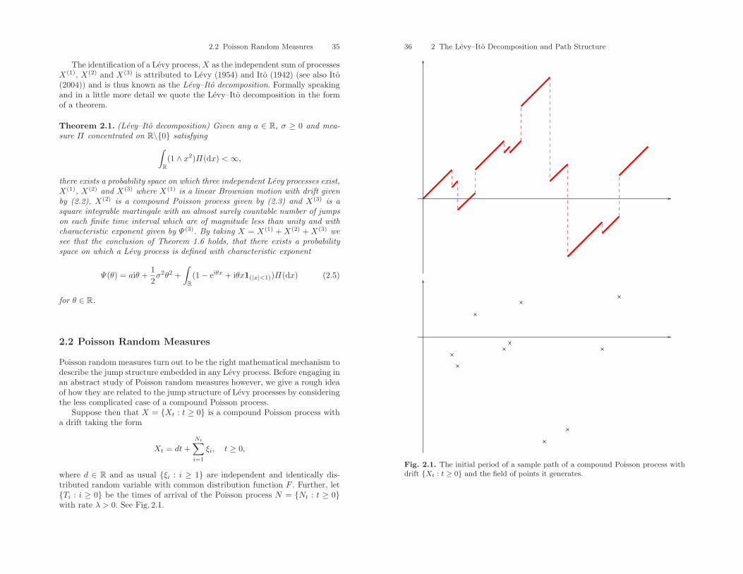
2.2 Poisson Random Measures 35
The identification of a Levy process,X as the independent sum of processesX(1), X(2) and X(3) is attributed to Levy (1954) and Ito (1942) (see also Ito(2004)) and is thus known as the Levy–Ito decomposition. Formally speakingand in a little more detail we quote the Levy–Ito decomposition in the formof a theorem.
Theorem 2.1. (Levy–Ito decomposition) Given any a ∈ R, σ ≥ 0 and mea-sure Π concentrated on R\0 satisfying∫
R(1 ∧ x2)Π(dx) <∞,
there exists a probability space on which three independent Levy processes exist,X(1), X(2) and X(3) where X(1) is a linear Brownian motion with drift givenby (2.2), X(2) is a compound Poisson process given by (2.3) and X(3) is asquare integrable martingale with an almost surely countable number of jumpson each finite time interval which are of magnitude less than unity and withcharacteristic exponent given by Ψ (3). By taking X = X(1) + X(2) + X(3) wesee that the conclusion of Theorem 1.6 holds, that there exists a probabilityspace on which a Levy process is defined with characteristic exponent
Ψ(θ) = aiθ +12σ2θ2 +
∫R(1− eiθx + iθx1(|x|<1))Π(dx) (2.5)
for θ ∈ R.
2.2 Poisson Random Measures
Poisson random measures turn out to be the right mathematical mechanism todescribe the jump structure embedded in any Levy process. Before engaging inan abstract study of Poisson random measures however, we give a rough ideaof how they are related to the jump structure of Levy processes by consideringthe less complicated case of a compound Poisson process.
Suppose then that X = Xt : t ≥ 0 is a compound Poisson process witha drift taking the form
Xt = dt+Nt∑i=1
ξi, t ≥ 0,
where d ∈ R and as usual ξi : i ≥ 1 are independent and identically dis-tributed random variable with common distribution function F . Further, letTi : i ≥ 0 be the times of arrival of the Poisson process N = Nt : t ≥ 0with rate λ > 0. See Fig. 2.1.
36 2 The Levy–Ito Decomposition and Path Structure
Fig. 2.1. The initial period of a sample path of a compound Poisson process withdrift Xt : t ≥ 0 and the field of points it generates.
2.2 Poisson Random Measures 37
Suppose now that we pick any set in A ∈ B[0,∞)× B(R\0). Define
N(A) = #i ≥ 0 : (Ti, ξi) ∈ A =∞∑i=1
1((Ti,ξi)∈A). (2.6)
Clearly since X experiences an almost surely finite number of jumps over afinite period of time it follows that N(A) <∞ almost surely where for t ≥ 0,A ⊆ B[0, t)× B(R\0).
Lemma 2.2. Choose k ≥ 1. If A1, ..., Ak are disjoint sets in B[0,∞) ×B(R\0) then N(A1), ..., N(Ak) are mutually independent and Poisson dis-tributed with parameters λi := λ
∫Ai
dt × F (dx), respectively. Further, forP-almost every realisation of X, N : B[0,∞)×B(R\0) → 0, 1, 2, ...∪∞is a measure.1
Proof. First recall a classic result concerning the Poisson process Nt : t ≥ 0.That is, the law of T1, ..., Tn conditional on the event Nt = n is the sameas the law of an ordered independent sample of size n from the uniform dis-tribution on [0, t]. (Exercise 2.2 has the full details). This latter fact togetherwith the fact that the variables ξi : i = 1, ..., k are independent and identi-cally distributed with common law F implies that conditional on Nt = n,the joint law of the pairs (Ti, ξi) : i = 1, ..., k is that of n independent bivari-ate random variables with common distribution t−1ds × F (dx) on [0, t] × Rordered in time. In particular, for any A ∈ B[0, t] × B(R\0), the randomvariable N(A) conditional on the event Nt = n is a Binomial random vari-able with probability of success given by
∫At−1ds × F (dx). A generalisation
of this latter statement for the k-tuple (N(A1), ..., N(Ak)), where A1, ..., Akare mutually disjoint and chosen from B[0, t]×B(R), is the following. Supposethat A0 = [0, t] × R\A1 ∪ ... ∪ Ak,
∑ki=1 ni ≤ n, n0 = n −∑k
i=1 ni andλ0 =
∫A0
λds × F (dx) = λt − λ1 − ... − λk then (N(A1), ..., N(Ak)) has thefollowing multinomial law
P(N(A1) = n1, ..., N(Ak) = nk|Nt = n)
=n!
n0!n1!...nk!
k∏i=0
(λiλt
)ni
.
1Specifically, P-almost surely, N(∅) = 0 and for disjoint A1, A2, ... in B[0,∞) ×B(R\0) we have
N
(⋃i≥1
Ai
)=∑i≥1
N(Ai).
38 2 The Levy–Ito Decomposition and Path Structure
Integrating out the conditioning on Nt it follows that
P(N(A1) = n1, ..., N(Ak) = nk)
=∑
n≥Σki=1ni
e−λt(λt)n
n!n!
n0!n1!...nk!
k∏i=0
(λiλt
)ni
=∑
n≥Σki=1ni
e−λ0(λ0)(n−Σ
ki=1ni)
(n−Σki=1ni)!
(k∏i=1
e−λi(λi)ni
ni!
)
=k∏i=1
e−λi(λi)ni
ni!
showing that N(A1), ..., N(Ak) are independent and Poisson distributed asclaimed.
To complete the proof for arbitrary disjoint A1, ..., Ak, in other words toremove the restriction on the time horizon, suppose without loss of generalitythat A1 belongs to B[0,∞) × B(R\0). Write A1 as a countable union ofdisjoint sets and recall that the sum of an independent sequence of Poissonrandom variables is Poisson distributed with the sum of their rates. If we agreethat a Poisson random variable with infinite rate is infinite with probabilityone (see Exercise 2.1), then the proof is complete.
Finally the fact that N is a measure P-almost surely follows immediatelyfrom its definition.
Lemma 2.2 shows that N : B[0,∞) × B(R\0) → 0, 1, ... ∪ ∞ fulfilsthe following definition of a Poisson random measure.
Definition 2.3 (Poisson random measure). In what follows we shallassume that (S,S, η) is an arbitrary σ-finite measure space. Let N : S →0, 1, 2, ... ∪ ∞ in such a way that the family N(A) : A ∈ S are randomvariables defined on the probability space (Ω,F ,P). Then N is called a Pois-son random measure on (S,S, η) (or sometimes a Poisson random measureon S with intensity η) if
(i) for mutually disjoint A1, ..., An in S, the variables N(A1), ..., N(An) areindependent,
(ii) for each A ∈ S, N(A) is Poisson distributed with parameter η(A) (herewe allow 0 ≤ η(A) ≤ ∞),
(iii) P-almost surely N is a measure.
In the second condition we note that if η(A) = 0 then it is understoodthat N(A) = 0 with probability one and if η(A) = ∞ then N(A) is infinitewith probability one.
2.2 Poisson Random Measures 39
In the case of (2.6) we have S = [0,∞) × R\0 and dη = λdt × dF .Note also that by construction of the compound Poisson process on someprobability space (Ω,F ,P), all of the random variables 1((Ti,ξi)∈A) for eachA ∈ B[0,∞) × B(R\0) are F-measurable and hence so are the variablesN(A).
We complete this section by proving that a Poisson random measure asdefined above exists. This is done in Theorem 2.4, the proof of which hasmany similarities to the proof of Lemma 2.2.
Theorem 2.4. There exists a Poisson random measure N as in Definition2.3.
Proof. First suppose that S is such that η(S) < ∞. There exists a standardconstruction of an infinite product space, say (Ω,F , P ) on which the indepen-dent random variables
N and υ1, υ2, ...are collectively defined such that N has a Poisson distribution with parameterη(S) and each of the variables υi have distribution η(dx)/η(S) on S. Definefor each A ∈ S,
N(A) =N∑i=1
1(υi∈A)
so that N = N(S). As for each A ∈ S and i ≥ 1, the random variables 1(υi∈A)
are F-measurable, then so are the random variables N(A).When presented with mutually disjoint sets of S, say A1, ..., Ak, a cal-
culation identical to the one given in the proof of Lemma 2.2 shows againthat
P (N(A1) = n1, ..., N(Ak) = nk) =k∏i=1
e−η(Ai)η(Ai)ni
ni!
for non-negative integers n1, n2, ..., nk. Returning to Definition 2.3 it is nowclear from the previous calculation together with the assumption that η isnon-atomic that conditions (i)–(iii) are met by N . In particular, similar tothe case dealt with in Lemma 2.2, the third condition is automatic as N is acounting measure by definition.
Next we turn to the case that (S,S, η) is a σ-finite measure space. Themeaning of σ-finite is that there exists a countable disjoint exhaustive sequenceof sets B1, B2, ... in S such that 0 < η(Bi) < ∞ for each i ≥ 1. Define themeasures ηi(·) = η(· ∩ Bi) for each i ≥ 1. The first part of this proof showsthat for each i ≥ 1 there exists some probability space (Ωi,Fi,Pi) on whichwe can define a Poisson random measure, say Ni, in (Bi,S ∩ Bi, ηi) whereS ∩ Bi = A ∩ Bi : A ∈ S (the reader should verify easily that S ∩ Bi isindeed a sigma algebra on Bi). The idea is now to show that
N (·) =∑i≥1
Ni(· ∩Bi)
40 2 The Levy–Ito Decomposition and Path Structure
is a Poisson random measure on S with intensity η defined on the productspace
(Ω,F ,P) :=∏i≥1
(Ωi,Fi,Pi).
First note that it is again immediate from its definition that N is P-almostsurely a measure. In particular with the help of Fubini’s Theorem, for disjointA1, A2, ..., we have
N
⎛⎝⋃j≥1
Aj
⎞⎠ =∑i≥1
Ni
⎛⎝⋃j
Aj ∩Bi
⎞⎠ =∑i≥1
∑j≥1
N(Aj ∩Bi)
=∑j≥0
∑i≥1
N(Aj ∩Bi)
=∑j≥0
N(Aj).
Next, for each i ≥ 1. we have that Ni(A ∩ Bi) is Poisson distributed withparameter ηi(A ∩Bi); Exercise 2.1 tells us that under P the random variableN (A) is Poisson distributed with parameter η(A). The proof is complete oncewe show that for disjoint A1, ..., Ak in S the variables N(A1), ..., N(Ak) areall independent under P. However this is obvious since the double array ofvariables
Ni(Aj ∩Bi) : i = 1, 2, ... and j = 1, ..., k
is also an independent sequence of variables.
From the construction of the Poisson random measure, the following twocorollaries should be clear.
Corollary 2.5. Suppose that N is a Poisson random measure on (S,S, η).Then for each A ∈ S, N(· ∩A) is a Poisson random measure on (S ∩A,S ∩A, η(· ∩A)). Further, if A,B ∈ S and A∩B = ∅ then N(· ∩A) and N(· ∩B)are independent.
Corollary 2.6. Suppose that N is a Poisson random measure on (S,S, η),then the support of N is P-almost surely countable. If in addition, η is a finitemeasure, then the support is P-almost surely finite.
Finally, note that if η is a measure with an atom at, say, the singletons ∈ S, then it is intuitively obvious from the construction of N in the proofof Theorem 2.4 that P(N(s) ≥ 1) > 0. Conversely, if η has no atoms thenP(N(s) = 0) = 1 for all singletons s ∈ S. For further discussion on thispoint, the reader is referred to Kingman (1993).

2.3 Functionals of Poisson Random Measures 41
2.3 Functionals of Poisson Random Measures
Suppose as in Sect. 2.2 that N is a Poisson random measure on the measurespace (S,S, η). As N is P-almost surely a measure, the classical theory ofLebesgue integration now allows us to talk of∫
S
f(x)N(dx) (2.7)
as a well defined [0,∞]-valued random variable for measurable functions f :S → [0,∞). Further (2.7) is still well defined and [−∞,∞] valued for signedmeasurable f provided at most one the integrals of f+ = f ∨ 0 and f− =(−f)∨ 0 is infinite. Note however, from the construction of the Poisson randommeasure in the proof of Theorem 2.4 the integral in (2.7) may be interpretedas equal in law to ∑
υ∈Υf(υ)mυ,
where Υ is the support of N (which from Corollary 2.6) is countable, and mυ
is the multiplicity of points at υ. Recalling the remarks following Corollary2.6 if η has no atoms then mυ = 1 for all υ ∈ N .
We move to the main theorem of this section which is attributed to King-man (1967) who himself accredits the earlier work of Campbell (1909, 1910).
Theorem 2.7. Suppose that N is a Poisson random measure on (S,S, η). Letf : S → R be a measurable function.
(i) Then
X =∫
f(x)N(dx)
is almost surely absolutely convergent if and only if∫S
(1 ∧ |f(x)|)η(dx) <∞. (2.8)
(ii) When condition (2.8) holds, then (with E as expectation with respect toP)
E(eiβX
)= exp
−∫S
(1− eiβf(x))η(dx)
(2.9)
for any β ∈ R.(iii) Further
E (X) =∫S
f(x)η(dx) when∫S
|f(x)|η(dx) <∞ (2.10)
and
E(X2)
=∫S
f(x)2η(dx) +(∫
S
f(x)η(dx))2
when∫S
f(x)2η(dx) <∞.
(2.11)
42 2 The Levy–Ito Decomposition and Path Structure
Proof. (i) We begin by defining simple functions to be those of the form
f (x) =n∑i=1
fi1Ai(x) ,
where fi is constant and Ai : i = 1, ..., n are disjoint sets in S and furtherη (A1 ∪ ... ∪An) <∞.
For such functions we have
X =n∑i=1
fiN(Ai)
which is clearly finite with probability one since each N(Ai) has a Poissondistribution with parameter η(Ai) < ∞. Now for any θ > 0 we have (usingthe well known fact that the characteristic function of a Poisson distributionwith parameter λ > 0 is exp−λ(1− e−θ)),
E(e−θX
)=
n∏i=1
E(e−θfiN(Ai)
)=
n∏i=1
exp−(1− e−θfi)η(Ai)
= exp
−
n∑i=1
(1− e−θfi)η(Ai)
.
Since 1− e−θf(x) = 0 on S\(A1 ∪ ... ∪An) we may thus conclude that
E(e−θX
)= exp
−∫S
(1− e−θf(x))η(dx).
Next we establish the above equality for a general positive measurablef. For the latter class of f, there exists a pointwise increasing sequence ofpositive simple functions fn : n ≥ 0 such that limn↑∞ fn = f, where thelimit is also understood in the pointwise sense. Since N is an almost surelyσ-finite measure, the monotone convergence theorem now implies that
limn↑∞
∫fn (x)N (dx) =
∫f (x)N (dx) = X
almost surely. An application of bounded convergence followed by an applica-tion of monotone convergence again tells us that for any θ > 0,
E(e−θX
)= E
(exp
−θ∫
f (x)N (dx))
= limn↑∞
E(
exp−θ∫
fn (x)N (dx))
2.3 Functionals of Poisson Random Measures 43
= limn↑∞
exp−∫S
(1− e−θfn(x))η(dx)
= exp−∫S
(1− e−θf(x))η(dx). (2.12)
Note that the integral on the right-hand side of (2.12) is either infinite forall θ > 0 or finite for all θ > 0 accordingly, with the cases that X = ∞with probability one or X = ∞ with probability less than one, respectively. If∫S(1−e−θf(x))η(dx) <∞ for all θ > 0 then as, for each x ∈ S, (1−e−θf(x)) ≤
(1− e−f(x)) for all 0 < θ < 1, dominated convergence implies that
limθ↓0
∫S
(1− e−θf(x))η(dx) = 0
and hence dominated convergence applied again in (2.12) as θ ↓ 0 tells us thatP(X = ∞) = 0.
In conclusion we have that X <∞ if and only if∫S(1−e−θf(x))η(dx) <∞
for all θ > 0 and it can be checked (see Exercise 2.3) that the latter happensif and only if ∫
S
(1 ∧ f(x))η(dx) <∞.
Note that both sides of (2.12) may be analytically extended by replacing θby θ − iβ for β ∈ R. Then taking limits on both sides as θ ↓ 0 we deduce(2.9).
Now we shall remove the restriction that f is positive. Henceforth assumeas in the statement of the theorem that f is a measurable function. We maywrite f = f+−f− where f+ = f ∨0 and f− = (−f)∨0 are both measurable.The sum X can be written X+ −X− where
X+ =∫S
f(x)N+(dx) and X− =∫S
f(x)N−(dx)
and N+ = N(· ∩ x ∈ S : f(x) ≥ 0) and N− = N(· ∩ x ∈ S : f(x) < 0). FromCorollary 2.5 we know that N+ and N− are both Poisson random measureswith respective intensities η(· ∩ f ≥ 0) and η(· ∩ f < 0). Further, theyare independent and hence the same is true of X+ and X−. It is now clearthat X converges absolutely almost surely if and only if X+ and X− areconvergent. The analysis of the case when f is positive applied to the sumsX+ and X− now tells us that absolute convergence of X occurs if and onlyif ∫
S
(1 ∧ |f(x)|)η(dx) <∞ (2.13)
and the proof of (i) is complete.
44 2 The Levy–Ito Decomposition and Path Structure
To complete the proof of (ii), assume that (2.13) holds. Using the inde-pendence of X+ and X− as well as the conclusion of part (i) we have that forany θ ∈ R,
E(eiθX
)= E
(eiθX+
)E(e−iθX−
)= exp
−∫f>0
(1− eiθf+(x))η(dx)
× exp
−∫f<0
(1− e−iθf−(x))η(dx)
= exp−∫S
(1− eiθf(x))η(dx)
and the proof of (ii) is complete.Part (iii) is dealt with similarly as in the above treatment; that is first by
considering positive, simple f , then extending to positive measurable f andthen to a general measurable f by considering its positive and negative parts.The proof is left to the reader.
2.4 Square Integrable Martingales
We shall predominantly use the identities in the Theorem 2.7 for Poissonrandom measures on ([0,∞) × R,B[0,∞) × B(R),dt ×Π(dx)) where Π is ameasure concentrated on R\0. We shall be interested in integrals of theform ∫
[0,t]
∫B
xN(ds× dx), (2.14)
where B ∈ B(R). The relevant integrals appearing in (2.8)–(2.11) for theabove functional of the given Poisson random measure can now be checked totake the form
t
∫B
(1 ∧ |x|)Π(dx), t
∫B
(1− eiβx)Π(dx),
t
∫B
|x|Π(dx), and t
∫B
x2Π(dx),
with the appearance of the factor t in front of each of the integrals being aconsequence of the involvement of Lebesgue measure in the intensity of N .The following two lemmas capture the context in which we use sums of theform (2.14). The first may be considered as a converse to Lemma 2.2 and thesecond shows the relationship with martingales.
Lemma 2.8. Suppose that N is a Poisson random measure on ([0,∞) ×R,B[0,∞)×B(R),dt×Π(dx)) where Π is a measure concentrated on R\0and B ∈ B(R) such that 0 < Π(B) <∞. Then
2.4 Square Integrable Martingales 45
Xt :=∫
[0,t]
∫B
xN(ds× dx), t ≥ 0
is a compound Poisson process with arrival rate Π(B) and jump distributionΠ(B)−1Π(dx)|B.
Proof. First note that since Π(B) <∞ by assumption, from Corollary 2.6 weknow that almost surely, Xt may be written as the sum over finite number ofpoints for each t > 0. This explains why X = Xt : t ≥ 0 is right continuouswith left limits. (One may also see finiteness of Xt from Theorem 2.7 (i)).Next note that for all 0 ≤ s < t <∞,
Xt −Xs =∫
(s,t]
∫B
xN(ds× dx)
which is independent of Xu : u ≤ s as N gives independent counts overdisjoint regions. Further, according to Theorem 2.7 (ii) we have that for allθ ∈ R,
E(eiθXt) = exp−t∫B
(1− eiθx)Π(dx). (2.15)
When put together with the fact that X has independent increments thisshows that
E(eiθ(Xt−Xs)
)=
E(eiθXt)E(eiθXs)
= exp−(t− s)
∫B
(1− eiθx)Π(dx)
= E(eiθXt−s
)and hence that increments are stationary. Finally, we identify from (2.15) thatthe Levy–Khintchine exponent of X corresponds to that of a compound Pois-son process with jump distribution and arrival rate given by Π(B)−1Π(dx)|Band Π(B), respectively. Since two Levy processes with the same incrementdistributions must be equal in law (as all the finite dimensional distributionsare determined by the increment distributions and this in turn determines thelaw of the process) then the Levy process X must be a compound Poissonprocess.
Lemma 2.9. Suppose that N and B are as in the previous lemma with theadditional assumption that
∫B|x|Π(dx) <∞.
(i) The compound Poisson process with drift
Mt :=∫
[0,t]
∫B
xN(ds× dx)− t
∫B
xΠ(dx), t ≥ 0
46 2 The Levy–Ito Decomposition and Path Structure
is a P-martingale with respect to the filtration
Ft = σ (N(A) : A ∈ B[0, t]× B (R)) , t > 0. (2.16)
(ii) If further,∫Bx2Π(dx) <∞ then it is a square integrable martingale.
Proof. (i) First note that the process M = Mt : t ≥ 0 is adapted to thefiltration Ft : t ≥ 0. Next note that for each t > 0,
E(|Mt|) ≤ E
(∫[0,t]
∫B
|x|N(ds× dx) + t
∫B
|x|Π(dx)
)
which, from Theorem 2.7 (iii), is finite because∫B|x|Π(dx) is. Next use the
fact that M has stationary independent increments to deduce that for 0 ≤s ≤ t <∞,
E(Mt −Ms|Fs)= E(Mt−s)
= E
(∫[s,t]
∫B
xN(ds× dx)
)− (t− s)
∫B
xΠ(dx)
= 0
where in the final equality we have used Theorem 2.7 (iii) again.(ii) To see that M is square integrable, we may yet again appeal to The-
orem 2.7 (iii) together with the assumption that∫Bx2Π(dx) <∞ to deduce
that
E
(Mt + t
∫B
xΠ(dx)2)
= t
∫B
x2Π(dx)
+t2(∫
B
xΠ(dx))2
.
Recalling from the martingale property that E(Mt) = 0, it follows by devel-oping the left-hand side in the previous display that
E(M2t ) = t
∫B
x2Π(dx) <∞
as required.
The conditions in both Lemmas 2.8 and 2.9 mean that we may considersets, for example, of the form Bε := (−1,−ε)∪(ε, 1) for any ε ∈ (0, 1). Howeverit is not necessarily the case that we may consider sets of the form B =(−1, 0)∪(0, 1). Consider for example the case thatΠ(dx) = 1(x>0)x
−(1+α)dx+1(x<0)|x|−(1+α) for α ∈ (1, 2). In this case, we have that
∫B|x|Π(dx) = ∞
2.4 Square Integrable Martingales 47
whereas∫Bx2Π(dx) <∞. It will turn out to be quite important in the proof
of the Levy–Ito decomposition to understand the limit of the martingale inLemma 2.8 for sets of the form Bε as ε ↓ 0. For this reason, let us now stateand prove the following theorem.
Theorem 2.10. Suppose that N is as in Lemma 2.8 and∫(−1,1)
x2Π(dx) <∞. For each ε ∈ (0, 1) define the martingale
Mεt =
∫[0,t]
∫Bε
xN(ds× dx)− t
∫Bε
xΠ(dx), t ≥ 0
and let F∗t be equal to the completion of
⋂s>t Fs by the null sets of P where
Ft is given in (2.16). Then there exists a martingale M = Mt : t ≥ 0 withthe following properties,
(i) for each T > 0, there exists a deterministic subsequence εTn : n = 1, 2, ...with εTn ↓ 0 along which
P( limn↑∞
sup0≤s≤T
(MεTns −Ms)2 = 0) = 1,
(ii) it is adapted to the filtration F∗t : t ≥ 0,
(iii) it has right continuous paths with left limits almost surely,(iv) it has, at most, a countable number of discontinuities on [0, T ] almost
surely and(v) it has stationary and independent increments.
In short, there exists a Levy process, which is also a martingale with a count-able number of jumps to which, for any fixed T > 0, the sequence of martin-gales Mε
t : t ≤ T converges uniformly on [0, T ] with probability one along asubsequence in ε which may depend on T .
Before proving Theorem 2.10 we need to remind ourselves of some generalfacts concerning square integrable martingales. In our account we shall recalla number of well established facts coming from quite standard L2 theory,measure theory and continuous time martingale theory. The reader is referredto Sects. 2.4, 2.5 and 9.6 of Ash and Doleans-Dade (2000) for a clear accountof the necessary background.
Fix a time horizon T > 0. Let us assume as in the above theorem that(Ω,F , F∗
t : t ∈ [0, T ],P) is a filtered probability space in which the filtrationF∗
t : t ≥ 0 is complete with respect to the null sets of P and right continuousin the sense that F∗
t =⋂s>t F∗
s .
Definition 2.11. Fix T > 0. Define M2T = M2
T (Ω,F , F∗t : t ∈ [0, T ],P)
to be the space of real valued, zero mean right-continuous, square integrableP-martingales with respect to the given filtration over the finite time period[0, T ].
One luxury that follows from the assumptions on F∗t : t ≥ 0 is that any
zero mean square integrable martingale with respect to the latter filtration
48 2 The Levy–Ito Decomposition and Path Structure
has a right continuous version which is also a member of M2T . Recall that
M ′ = M ′t : t ∈ [0, T ] is a version of M if it is defined on the same probability
space and ∃t ∈ [0, T ] : M ′t = Mt is measurable with zero probability.
It is straightforward to deduce that M2T is a vector space over the real
numbers with zero element Mt = 0 for all t ∈ [0, T ] and all ω ∈ Ω. In fact, aswe shall shortly see, M2
T is a Hilbert space2 with respect to the inner product
〈M,N〉 = E (MTNT ) ,
where M,N ∈M2T . It is left to the reader to verify the fact that 〈·, ·〉 forms an
inner product. The only mild technical difficulty in this verification is showingthat for M ∈ M2
T , 〈M,M〉 = 0 implies that M = 0, the zero element. Notehowever that if 〈M,M〉 = 0 then by Doob’s Maximal Inequality, which saysthat for M ∈M2
T ,
E(
sup0≤s≤T
M2s
)≤ 4E
(M2T
),
we have that sup0≤t≤T Mt = 0 almost surely. Since M ∈ M2T is right con-
tinuous it follows necessarily that Mt = 0 for all t ∈ [0, T ] with probabilityone.
As alluded to above, we can show without too much difficulty that M2T is
a Hilbert space. To do that we are required to show that given M (n) : n =1, 2, ... is a Cauchy sequence of martingales taken from M2
T then there existsan M ∈M2
T such that ∥∥∥M (n) −M∥∥∥→ 0
as n ↑ ∞ where ‖·‖ := 〈·, ·〉1/2 . To this end let us assume that the sequenceof processes
M (n) : n = 1, 2, ...
is a Cauchy sequence, in other words,
E[(M
(m)T −M
(n)T
)2]1/2
→ 0 as m,n ↑ ∞.
Necessarily then the sequence of random variables M (k)T : k ≥ 1 is a Cauchy
sequence in the Hilbert space of zero mean, square integrable random vari-ables defined on (Ω,FT ,P), say L2(Ω,FT ,P), endowed with the inner prod-uct 〈M,N〉 = E(MN). Hence there exists a limiting variable, say MT inL2(Ω,FT ,P) satisfying
E[(M (n)
T −MT )2]1/2
→ 0
2Recall that 〈·, ·〉 : L × L → R is an inner product on a vector space L overthe reals if it satisfies the following properties for f, g ∈ L and a, b ∈ R; (i)〈af + bg, h〉 = a 〈f, h〉 + b 〈g, h〉 for all h ∈ L, (ii) 〈f, g〉 = 〈g, f〉, (iii) 〈f, f〉 ≥ 0and (iv) 〈f, f〉 = 0 if and only if f = 0.
For each f ∈ L let ||f || = 〈f, f〉1/2. The pair (L, 〈·, ·〉) are said to form aHilbert space if all sequences, fn : n = 1, 2, ... in L that satisfy ||fn − fm|| → 0as m, n →∞, so called Cauchy sequences, have a limit which exists in L.
2.4 Square Integrable Martingales 49
as n ↑ ∞. Define the martingale M to be the right continuous version3 of
E (MT |F∗t ) for t ∈ [0, T ]
and note that by definition ∥∥∥M (n) −M∥∥∥→ 0
as n tends to infinity. Clearly it is an F∗t -adapted process and by Jensen’s
inequality
E(M2t
)= E
(E (MT |F∗
t )2)
≤ E(E(M2T |F∗
t
))= E
(M2T
)which is finite. Hence Cauchy sequences converge in M2
T and we see that M2T
is indeed a Hilbert space.
We are now ready to return to Theorem 2.10.
Proof (of Theorem 2.10). (i) Choose 0 < η < ε < 1, fix T > 0 and defineMε = Mε
t : t ∈ [0, T ]. A calculation similar to the one in Lemma 2.9 (ii)gives
E((Mε
T −MηT )2)
= E
⎛⎝∫[0,T ]
∫η≤|x|<ε
xN(ds× dx)
2⎞⎠
= T
∫η≤|x|<ε
x2Π(dx).
Note however that the left-hand side above is also equal to ||Mε − Mη||2(where as in the previous discussion, || · || is the norm induced by the innerproduct on M2
T ).Thanks to the assumption that
∫(−1,1)
x2Π(dx) < ∞, we now have thatlimε↓0 ||Mε −Mη|| = 0 and hence that Mε : 0 < ε < 1 is a Cauchy familyin M2
T . As M2T is a Hilbert space we know that there exists a martingale
M = Ms : s ∈ [0, T ] ∈ M2T such that
limε↓0
||M −Mε|| = 0.
An application of Doob’s maximal inequality tells us that in fact
limε↓0
E[
sup0≤s≤T
(Ms −Mεs )
2
]≤ 4 lim
ε↓0||M −Mε|| = 0. (2.17)
3Here we use the fact that F∗t : t ∈ [0, T ] is complete and right continuous.
50 2 The Levy–Ito Decomposition and Path Structure
From this one may deduce that the limit Ms : s ∈ [0, T ] does not dependon T . Indeed suppose it did and we adjust our notation accordingly so thatMs,T : s ≤ T represents the limit. Then from (2.17) we see that for any0 < T ′ < T ,
limε↓0
E[
sup0≤s≤T ′
(Mεs −Ms,T ′)2
]= 0
as well as
limε↓0
E[
sup0≤s≤T ′
(Mεs −Ms,T )2
]≤ lim
ε↓0E[
sup0≤s≤T
(Mεs −Ms,T )2
]= 0,
where the inequality is the result of a trivial upper bound. Hence using thatfor any two sequences of real numbers an and bn, supn a2
n = (supn |an|)2and supn |an+bn| ≤ supn |an|+supn |bn|, we have together with an applicationof Minkowski’s inequality that
E[
sup0≤s≤T ′
(Ms,T ′ −Ms,T )2]1/2
≤ limε↓0
E[
sup0≤s≤T ′
(Mεs −Ms,T ′)2
]1/2+ lim
ε↓0E[
sup0≤s≤T ′
(Mεs −Ms,T )2
]1/2= 0
thus showing that the processes M·,T and M·,T ′ are almost surely uniformlyequal on [0, T ′]. Since T ′ and T may be arbitrarily chosen, we may now speakof a well defined martingale limit M = Mt : t ≥ 0.
From the limit (2.17) we may also deduce that there exists a deterministicsubsequence εTn : n ≥ 0 along which
limεT
n↓0sup
0≤s≤T(MεT
ns −Ms)2 = 0
P-almost surely. This follows from the well established fact that L2 conver-gence of a sequence of random variables implies almost sure convergence on adeterministic subsequence.
(ii) Fix 0 < t < T . Clearly as MεTnt is F∗
t -measurable, and by part (i) thelatter sequence has an almost sure limit as n ↑ ∞, then by standard measuretheory its limit is also F∗
t -measurable.
(iii) As the paths of Mε are right continuous with left limits, almost sureuniform convergence (along a subsequence) on finite time intervals impliesthat the limiting process, M , also has paths which are right continuous withleft limits. We are using here the fact that, if D[0, 1] is the space of functionsf : [0, 1] → R which are right continuous with left limits, then D[0, 1] is aclosed space under the metric d(f, g) = supt∈[0,1] |f(t)−g(t)| for f, g ∈ D[0, 1].See Exercise 2.4 for a proof of this fact.
2.5 Proof of the Levy–Ito Decomposition 51
(iv) According to Corollary 2.6 there are at most an almost surely count-able number of points in the support of N . Further, as the measure dt×Π(dx)has no atoms then N is necessarily 0, 1 valued on time–space singletons.4
Hence every discontinuity in Ms : s ≥ 0 corresponds to a unique pointin the support of N , it follows that M has at most a countable number ofdiscontinuities. Another way to see there are at most a countable numberof discontinuities is simply to note that functions in the space D[0, 1] havediscontinuities of the first kind5 and hence there are necessarily a countablenumber of such discontinuities; see Exercise 2.4.
(v) Uniform almost sure convergence along a subsequence also guaranteesconvergence in distribution for a collection of fixed times along the same sub-sequence. This shows that M has stationary independent increments since forany 0 ≤ u ≤ v ≤ s ≤ t ≤ T <∞ and θ1, θ2 ∈ R, dominated convergence gives
E(eiθ1(Mv−Mu)eiθ2(Mt−Ms))
= limn↑∞
E(eiθ1(MεT
nv −MεT
nu )eiθ2(M
εTn
t −MεTn
s ))
= limn↑∞
E(eiθ1MεT
nv−u)E(eiθ2M
εTn
t−s)
= E(eiθ1Mv−u)E(eiθ2Mt−s)
thus concluding the proof.
2.5 Proof of the Levy–Ito Decomposition
As previously indicated in Sect. 2, we will take X(1) to be the linear Brownianmotion (2.2) defined now on some probability space (Ω#,F#, P#).
Given Π in the statement of Theorem 2.1 we know from Theorem 2.4 thatthere exists a probability space, say (Ω∗,F∗, P ∗), on which may constructa Poisson random measure N on ([0,∞) × R,B[0,∞) × B(R),dt × Π(dx)).We may think of the points in the support of N as having a time and spaceco-ordinate, or alternatively, as points in R\0 arriving in time.
Now defineX
(2)t =
∫[0,t]
∫|x|≥1
xN(ds× dx), t ≥ 0
and note from Lemma 2.8 that since Π(R\(−1, 1)) < ∞ that it is acompound Poisson process with rate Π(R\(−1, 1)) and jump distribution
4If one reconsiders the construction of a general Poisson random measure on(S,S, η) in the proof of Theorem 2.4, then one sees that if η has atoms, it ispossible that the points which contribute to the support of N may lie on top ofone another. If η has no atoms then the aforementioned points are almost surelydistinct.
5A discontinuity of the first kind of f at x means that f(x+) and f(x−) both existbut are not equal to one another.
52 2 The Levy–Ito Decomposition and Path Structure
Π(R\(−1, 1))−1Π(dx)|R\(−1,1). (We may assume without loss of generalitythat Π(R\(−1, 1)) > 0 as otherwise we may simply take the process X(2) asthe process which is identically zero.)
Next we construct a Levy process having only small jumps. For each 1 >ε > 0 define similarly the compound Poisson process with drift
X(3,ε)t =
∫[0,t]
∫ε≤|x|<1
xN(ds× dx)− t
∫ε≤|x|<1
xΠ(dx), t ≥ 0. (2.18)
(As in the definition of X(2) we shall assume without loss of generality Π(x :|x| < 1) > 0 otherwise the process X(3) may be taken as the process whichis identically zero). Using Theorem 2.7 (ii) we can compute its characteristicexponent,
Ψ (3,ε) (θ) :=∫ε≤|x|<1
(1− eiθx + iθx)Π (dx) .
According to Theorem 2.10 there exists a Levy process, which is also asquare integrable martingale, defined on (Ω∗,F∗, P ∗), to which X(3,ε) con-verges uniformly on [0, T ] along an appropriate deterministic subsequencein ε. Note that it is at this point that we are using the assumption that∫(−1,1)
x2Π(dx) <∞. It is clear that the characteristic exponent of this latterLevy process is equal to
Ψ (3)(θ) =∫|x|<1
(1− eiθx + iθx)Π(dx).
From Corollary 2.5 we know that for each t > 0, N has independent countsover the two domains [0, t] × R\(−1, 1) and [0, t] × (−1, 1). It follows thatX(2) and X(3) are independent. Further the latter two are independent ofX(1) which was defined on another probability space.
To conclude the proof of the Levy–Ito decomposition in line with thestatement of Theorem 2.1, define the process
Xt = X(1)t +X
(2)t +X
(3)t , t ≥ 0. (2.19)
This process is defined on the product space
(Ω,F ,P) = (Ω#,F#, P#)× (Ω∗,F∗, P ∗),
has stationary independent increments, has paths that are right continuouswith left limits and has characteristic exponent
Ψ(θ) = Ψ (1)(θ) + Ψ (2)(θ) + Ψ (3)(θ)
= iaθ +12σ2θ2 +
∫R(1− eiθx + iθx1(|x|<1))Π(dx)
as required.
Let us conclude this section with some additional remarks on the Levy–Itodecomposition.
2.6 Levy Processes Distinguished by Their Path Type 53
Recall from (2.4) that the exponent Ψ (3) appears to have the form ofthe infinite sum of characteristic exponents belonging to compound Poissonprocesses with drift. Thus suggesting that X(3) may be taken as the superpo-sition of such processes. We now see from the above proof that this is exactlythe case. Indeed moving ε to zero through the sequence 2−k : k ≥ 0 showsus that in the appropriate sense of L2 convergence
limk↑∞
X(3,2−k)t = lim
k↑∞
∫[0,t]
∫2−k<|x|<1
xN(ds× dx)− t
∫2−k<|x|<1
xΠ(dx)
= limk↑∞
k−1∑i=0
∫[0,t]
∫2−(i+1)<|x|<2−i
xN(ds× dx)
−t∫
2−(i+1)<|x|<2−i
xΠ(dx)
.
It is also worth remarking that the definition of X(2) and X(3) in the proofof the Levy–Ito decomposition accordingly, with the partition of R\0 intoR\(−1, 1) and (−1, 1)\0 is to some extent arbitrary. The point is that oneneeds to deal with the contribution of N to the path of the Levy process whichcomes from points which are arbitrarily close to the origin in a different wayto points which are at a positive distance from the origin. In this respect onecould have redrafted the proof replacing (−1, 1) by (α, β) for any α < 0 andβ > 0, in which case one would need to choose a different value of a in thedefinition of X(1) in order to make terms add up precisely to the expressiongiven in the Levy–Khintchine exponent. To be more precise, if for exampleα < −1 and β > 1, then one should take X(1)
t = a′t+ σBt where
a′ = a−∫α<|x|≤−1
xΠ(dx)−∫
1≤|x|<βxΠ(dx).
The latter also shows that the Levy–Khintchine formula (2.1) is not a uniquerepresentation and indeed the indicator 1(|x|<1) in (2.1) may be replaced by1(α<x<β) with an appropriate adjustment in the constant a.
2.6 Levy Processes Distinguished by Their Path Type
As is clear from the proof of the Levy–Ito decomposition, we should think ofthe measure Π given in the Levy–Khintchine formula as characterising a Pois-son random measure which encodes the jumps of the associated Levy process.In this section we shall re-examine elements of the proof of the Levy–Ito de-composition and show that, with additional assumptions on Π correspondingto restrictions on the way in which jumps occur, we may further identifyspecial classes of Levy processes embedded within the general class.
54 2 The Levy–Ito Decomposition and Path Structure
2.6.1 Path Variation
It is clear from the Levy–Ito decomposition that the presence of the linearBrownian motion X(1) would imply that paths of the Levy process have un-bounded variation. On the other hand, should it be the case that σ = 0, thenthe Levy process may or may not have unbounded variation. The term X(2),being a compound Poisson process, has only bounded variation. Hence in thecase σ = 0, understanding whether the Levy process has unbounded variationis an issue determined by the limiting process X(3); that is to say the processof compensated small jumps.
Reconsidering the definition of X(3) it is natural to ask under what cir-cumstances
limε↓0
∫[0,t]
∫ε≤|x|<1
xN(ds× dx)
exists almost surely without the need for compensation. Once again, the an-swer is given by Theorem 2.7 (i). Here we are told that∫
[0,t]
∫0<|x|<1
xN(ds× dx) <∞
if and only if∫0<|x|<1
|x|Π(dx) < ∞. In that case we may identify X(3)
directly via
X(3)t =
∫[0,t]
∫0<|x|<1
xN(ds× dx)− t
∫0<|x|<1
xΠ(dx), t ≥ 0.
This also tells us that X(3) will be of bounded variation if and only if∫0<|x|<1
|x|Π(dx) <∞. The latter combined with the general integral condi-tion
∫R(1 ∧ x2)Π(dx) < ∞ in the light of the Levy–Ito decomposition yields
the following Lemma.
Lemma 2.12. A Levy process with Levy–Khintchine exponent correspondingto the triple (a, σ,Π) has paths of bounded variation if and only if
σ = 0 and∫
R(1 ∧ |x|)Π(dx) <∞. (2.20)
Note that the finiteness of the integral in (2.20) also allows for the Levy–Khintchine exponent of any such bounded variation process to be re-writtenas follows
Ψ(θ) = −idθ +∫
R(1− eiθx)Π(dx), (2.21)
where the constant d ∈ R relates to the constant a and Π via
d = −(a+
∫|x|<1
xΠ(dx)
).
2.6 Levy Processes Distinguished by Their Path Type 55
In this case, we may write the Levy process in the form
Xt = dt+∫
[0,t]
∫RxN(ds× dx), t ≥ 0. (2.22)
In view of the decomposition of the Levy–Khintchine formula for a processof bounded variation and the corresponding representation (2.22), the termd is often referred to as the drift. Strictly speaking, one should not talk ofdrift in the case of a Levy process whose jump part is a process of unboundedvariation. If drift is to be understood in terms of a purely deterministic trend,then it is ambiguous on account of the “infinite limiting compensation” thatone sees in X(3) coming from the second term on the right hand side of (2.18).
From the expression given in (1.3) of the Chap. 1 we see that if X is acompound Poisson process with drift then its characterisitic exponent takesthe form of (2.21) with Π(R) <∞. Conversely, suppose that σ = 0 and Π hasfinite total mass, then we know from Lemma 2.8 that (2.22) is a compoundPoisson process with drift d. In conclusion we have the following lemma.
Lemma 2.13. A Levy process is a compound Poisson process with drift if andonly if σ = 0 and Π(R) <∞.
Processes which are of bounded variation but which are not compoundPoisson processes with drift are sometimes referred to as generalised compoundPoisson processes (with drift). This is because they are structurally the sameas compound Poisson processes in that they may be represented in the formof (2.22). This is of course not true for Levy processes of unbounded variation,even if the Gaussian component is zero.
2.6.2 One-Sided Jumps
Suppose now that Π(−∞, 0) = 0. From the proof of the Levy–Ito decomposi-tion, we see that this implies that the corresponding Levy process has no neg-ative jumps. If further we have that
∫(0,∞)
(1∧x)Π(dx) <∞, σ = 0 and, in therepresentation (2.21) of the characteristic exponent, d ≥ 0, then from the rep-resentation (2.22) it becomes clear that the Levy process has non-decreasingpaths. Conversely, suppose that a Levy process has non-decreasing paths thennecessarily it has bounded variation. Hence
∫(0,∞)
(1 ∧ x)Π(dx) < ∞, σ = 0and then it is easy to see that in the representation (2.21) of the characteristicexponent, we necessarily have d ≥ 0. Examples of such a process were givenin Chap. 1 (the gamma process and the inverse Gaussian process) and werenamed subordinators. Summarising we have the following.
Lemma 2.14. A Levy process is a subordinator if and only if Π(−∞, 0) = 0,∫(0,∞)
(1 ∧ x)Π(dx) <∞, σ = 0 and d = −(a+
∫(0,1)
xΠ(dx))≥ 0.
56 2 The Levy–Ito Decomposition and Path Structure
For the sake of clarity, we note that when X is a subordinator, further to(2.21), its Levy-Khinchine formula may be written
Ψ(θ) = −idθ +∫
(0,∞)
(1− eiθx)Π(dx), (2.23)
where necessarily d ≥ 0.If Π(−∞, 0) = 0 and X is not a subordinator, then it is referred to in
general as a spectrally positive Levy process. A Levy process, X, will thenbe referred to as spectrally negative if −X is spectrally positive. Together thelatter two classes of processes are called spectrally one-sided. Spectrally one-sided Levy processes may be of bounded or unbounded variation and, in thelatter case, may or may not possess a Gaussian component. Note in particularthat when σ = 0 it is still possible to have paths of unbounded variation. Whena spectrally positive Levy process has bounded variation then it must takethe form
Xt = −dt+ St, t ≥ 0
where St : t ≥ 0 is a pure jump subordinator and necessarily d > 0 asotherwise X would conform to the definition of a subordinator. Note that theabove decomposition implies that if E(X1) ≤ 0 then E(S1) < ∞ as opposedto the case that E(X1) > 0 in which case it is possible that E(S1) = ∞.
A special feature of spectrally positive processes is that, if τ−x = inft >0 : Xt < x where x < 0, then P(τ−x <∞) > 0 and hence, as there can be nodownwards jumps,
P(Xτ−x= x|τ−x <∞) = 1
with a similar property for first passage upwards being true for spectrallynegative processes. A rigorous proof of the first of the above two facts will begiven in Corollary 3.13 at the end of Sect. 3.3. It turns out that the latter factplays a very important role in the simplification of a number of theorems weshall encounter later on in this text which concern the fluctuations of generalLevy processes.
2.7 Interpretations of the Levy–Ito Decomposition
Let us return to some of the models considered in Chap. 1 and consider howthe understanding of the Levy–Ito decomposition helps to justify working withmore general classes of Levy processes.
2.7.1 The Structure of Insurance Claims
Recall from Sect. 1.3.1 that the Cramer–Lundberg model corresponds to aLevy process with characteristic exponent given by
2.7 Interpretations of the Levy–Ito Decomposition 57
Ψ(θ) = −icθ + λ
∫(−∞,0)
(1− eiθx)F (dx),
for θ ∈ R. In other words, a compound Poisson process with arrival rate λ > 0and negative jumps, corresponds to claims, having common distribution Fas well as a drift c > 0 corresponding to a steady income due to premiums.Suppose instead we work with a general spectrally negative Levy process. Thatis a process for which Π(0,∞) = 0 (but not the negative of a subordinator).In this case, the Levy–Ito decomposition offers an interpretation for largescale insurance companies as follows. The Levy–Khintchine exponent may bewritten in the form
Ψ(θ) =
12σ2θ2
+
−iθc+
∫(−∞,−1]
(1− eiθx)Π(dx)
+
∫(−1,0)
(1− eiθx + iθx)Π(dx)
(2.24)
for θ ∈ R. Assume that Π(−∞, 0) = ∞ so Ψ is genuinely different fromthe characteristic of a Cramer–Lundberg model. The third bracket in (2.24)we may understand as a Levy process representing a countably infinite num-ber of arbitrarily small claims compensated by a deterministic positive drift(which may be infinite in the case that
∫(−1,0)
|x|Π(dx) = ∞) corresponding tothe accumulation of premiums over an infinite number of contracts. Roughlyspeaking, the way in which claims occur is such that in any arbitrarily smallperiod of time dt, a claim of size |x| (for x < 0) is made independently withprobability Π(dx)dt + o(dt). The insurance company thus counterbalancessuch claims by ensuring that it collects premiums in such a way that in anydt, |x|Π(dx)dt of its income is devoted to the compensation of claims of size|x|. The second bracket in (2.24) we may understand as coming from largeclaims which occur occasionally and are compensated against by a steady in-come at rate c > 0 as in the Cramer–Lundberg model. Here “large” is takento mean claims of size one or more and c = −a in the terminology of theLevy–Khintchine formula given in Theorem 1.6. Finally the first bracket in(2.24) may be seen as a stochastic perturbation of the system of claims andpremium income.
Since the first and third brackets in (2.24) correspond to martingales, thecompany may guarantee that its revenues drift to infinity over an infinite timehorizon by assuming the latter behaviour applies to the compensated processof large claims corresponding to the second bracket in (2.24).
2.7.2 General Storage Models
The workload of the M/G/1 queue was presented in Sect. 1.3.2 as a spectrallynegative compound Poisson process with rate λ > 0 and jump distribution F
58 2 The Levy–Ito Decomposition and Path Structure
with positive unit drift reflected in its supremum. In other words, the under-lying Levy process has characteristic exponent
Ψ(θ) = −iθ + λ
∫(−∞,0)
(1− eiθx)F (dx)
for all θ ∈ R. A general storage model, described for example in the classicbooks of Prabhu (1998) and Takacs (1966), consists of working with a generalLevy process which is the difference of a positive drift and a subordinator andthen reflected in its supremum. Its Levy–Khintchine exponent thus takes theform
Ψ(θ) = −idθ +∫
(−∞,0)
(1− eiθx)Π(dx),
where d > 0 and∫(−∞,0)
(1∧ |x|)Π(dx) <∞. As with the case of the M/G/1queue, the reflected process
Wt = (w ∨Xt)−Xt, t ≥ 0
may be thought of the stored volume or workload of some system where Xis the Levy process with characteristic exponent Ψ given above and X is itsrunning supremum. The Levy–Ito decomposition tells us that during the pe-riods of time that X is away from its supremum, there is a natural “drainage”of volume or “processing” of workload, corresponding to the downward move-ment of W in a linear fashion with rate d. At the same time new “volume forstorage” or equivalently new “jobs” arrive independently so that in each dt,one arrives of size |x| (where x < 0) with probability Π(dx)dt + o(dt) (thusgiving similar interpretation to the occurrence of jumps in the insurance riskmodel described above). When Π(−∞, 0) = ∞ the number of jumps arecountably infinite over any finite time interval thus indicating that our modelis processing with “infinite frequency” in comparison to the finite activity ofthe workload of the M/G/1 process.
Of course one may also envisage working with a jump measure which hassome mass on the positive half line. This would correspond negative jumps inthe process W . This, in turn, can be interpreted as follows. Over and abovethe natural drainage or processing at rate d, in each dt there is independentremoval of a “volume” or “processing time of job” of size y > 0 with probabil-ity Π(dy)dt + o(dt). One may also consider moving to models of unboundedvariation. However, in this case, the interpretation of drift is lost.
2.7.3 Financial Models
Financial mathematics has become a field of applied probability which hasembraced the use of Levy processes, in particular, for the purpose of mod-elling the evolution of risky assets. We shall not attempt to give anything like
2.7 Interpretations of the Levy–Ito Decomposition 59
a comprehensive exposure of this topic here, nor elsewhere in this book. Espe-cially since the existing text books of Boyarchenko and Levendorskii (2002b),Schoutens (2003), Cont and Tankov (2004) and Barndorff–Nielsen and Shep-hard (2005) already offer a clear and up-to-date overview between them. It ishowever worth mentioning briefly some of the connections between path prop-erties of Levy processes seen above and modern perspectives within financialmodelling.
One may say that financial mathematics proper begins with the thesis ofLouis Bachellier who proposed the use of linear Brownian motion to model thevalue of a risky asset, say the value of a stock (See Bachelier (1900, 1901)).The classical model, proposed by Samuleson (1965), for the evolution of arisky asset however is generally accepted to be that of an exponential linearBrownian motion with drift;
St = seσBt+µt, t ≥ 0 (2.25)
where s > 0 is the initial value of the asset, B = Bt : t ≥ 0 is a standardBrownian motion, σ > 0 and µ ∈ R. This choice of model offers the featurethat asset values have multiplicative stationarity and independence in thesense that for any 0 ≤ u < t <∞,
St = Su × St−u (2.26)
where St−u is independent of Su and has the same distribution as St−u.Whether this is a realistic assumption in terms of temporal correlations infinancial markets is open to debate. Nonetheless, for the purpose of a the-oretical framework in which one may examine the existence or absence ofcertain economic mechanisms, such as risk-neutrality, hedging and arbitrageas well as giving sense to the value of certain financial products such as optioncontracts, exponential Brownian motion has proved to be the right model tocapture the imagination of mathematicians, economists and financial practi-tioners alike. Indeed, what makes (2.25) “classical” is that Black and Scholes(1973) and Merton (1973) demonstrated how one may construct rational ar-guments leading to the pricing of a call option on a risky asset driven byexponential Brownian motion.
Two particular points (of the many) where the above model of a riskyasset can be shown to be inadequate concern the continuity of the paths andthe distribution of log-returns of the value of a risky asset. Clearly (2.25)has continuous paths and therefore cannot accommodate for jumps whicharguably are present in observed historical data of certain risky assets due toshocks in the market. The feature (2.26) suggests that if one would choose afixed period of time ∆, then for each n ≥ 1, the innovations log(S(n+1)∆/Sn∆)are independent and normally distributed with mean µ∆ and variance σ
√∆.
Empirical data suggests however that the tails of the distribution of the log-returns are asymmetric as well as having heavier tails than those of normal
60 2 The Levy–Ito Decomposition and Path Structure
distributions. The tails of the latter being particularly light as they decay likeexp−x2 for large |x|. See for example the discussion in Schoutens (2003).
Recent literature suggests that a possible remedy for these two points isto work with
St = seXt , t ≥ 0
instead of (2.25) where again s > 0 is the initial value of the risky asset andX = Xt : t ≥ 0 is now a Levy process. This preserves multiplicative station-ary and independent increments as well as allowing for jumps, distributionalasymmetry and the possibility of heavier tails than the normal distributioncan offer. A rather unsophisticated example of how the latter may happen issimply to take for X a compound Poisson process whose jump distribution isasymmetric and heavy tailed. A more sophisticated example however, and in-deed quite a popular model in the research literature, is the so-called variancegamma process, introduced by Madan and Seneta (1990). This Levy processis pure jump, that is to say σ = 0, and has Levy measure given by
Π(dx) = 1(x<0)C
|x|eGxdx+ 1(x>0)
C
xe−Mxdx,
where C,G,M > 0. It is easily seen by computing explicitly the integral∫R\0(1∧|x|)Π(dx) and the total mass Π(R) that the variance gamma process
has paths of bounded variation and further is not a compound Poisson process.It turns out that the exponential weighting in the Levy measure ensures thatthe distribution of the variance gamma process at a fixed time t has expo-nentially decaying tails (as opposed to the much lighter tails of the Gaussiandistribution).
Working with pure jump processes implies that there is no diffusive natureto the evolution of risky assets. Diffusive behaviour is often found attractivefor modelling purposes as it has the taste of a physical interpretation in whichincrements in infinitesimal periods of time are explained as the aggregate ef-fect of many simultaneous conflicting external forces. Geman et al. (2001)argue however the case for modelling the value of risky assets with Levyprocesses which have paths of bounded variation which are not compoundPoisson processes. In their reasoning, the latter has a countable number ofjumps over finite periods of time which correspond to the countable, butnonetheless infinite number of purchases and sales of the asset which collec-tively dictate its value as a net effect. In particular being of bounded variationmeans the Levy process can be written as the difference to two independentsubordinators (see Exercise 2.8). The latter two should be thought of the to-tal prevailing price buy orders and total prevailing price sell orders on thelogarithmic price scale.
Despite the fundamental difference between modelling with bounded vari-ation Levy processes and exponential Brownian motion, Geman et al. (2001)also provide an interesting link to the classical model (2.25) via time change.The basis of their ideas lies with the following lemma.

2.7 Interpretations of the Levy–Ito Decomposition 61
Lemma 2.15. Suppose that X = Xt : t ≥ 0 is a Levy process with char-acteristic exponent Ψ and τ = τs : s ≥ 0 is an independent subordinatorwith characteristic Ξ. Then Y = Xτs
: s ≥ 0 is again a Levy process withcharacteristic exponent Ξ Ψ .
Proof. First let us make some remarks about Ξ. We already know that theformula
E(eiθτs) = e−Ξ(θ)s
holds for all θ ∈ R. However, since τ is a non-negative valued process, viaanalytical extension, we may claim that the previous equality is still valid forθ ∈ z ∈ C : ℑz ≥ 0. Note in particular then that since
ℜΨ(u) =12σ2u2 +
∫R(1− cos(ux))Π(dx) > 0
for all u ∈ R, the equality
E(e−Ψ(u)τs) = e−Ξ(Ψ(u))s (2.27)
holds.Since X and τ have right continuous paths, then so does Y . Next consider
0 ≤ u ≤ v ≤ s ≤ t < ∞ and θ1, θ2 ∈ R. Then by first conditioning on τ andnoting that 0 ≤ τu ≤ τv ≤ τs ≤ τt <∞ we have
E(eiθ1(Yv−Yu)+iθ2(Yt−Ys)
)= E
(e−Ψ(θ1)(τv−τu)−Ψ(θ2)(τt−τs)
)= E
(e−Ψ(θ1)τv−u−Ψ(θ2)τt−s)
)= e−Ξ(Ψ(θ1))(v−u)−Ξ(Ψ(θ2))(t−s)
where in the final equality we have used the fact that τ has stationary inde-pendent increments together with (2.27). This shows that Y has stationaryand independent increments.
Suppose in the above lemma we take for X a linear Brownian motion withdrift as in the exponent of (2.25). By sampling this continuous path processalong the range of an independent subordinator, one recovers another Levyprocess. Geman et al. (2001) suggest that one may consider the value of arisky asset to evolve as the process (2.25) on an abstract time scale suitableto the rate of business transactions called business time. The link betweenbusiness time and real time is given by the subordinator τ . That is to say, oneassumes that the value of a given risky asset follows the process Y = X τbecause at real time s > 0, τs units of business time have passed and hencethe value of the risky asset is positioned at Xτs
.Returning to the example of the variance gamma process given above, it
turns out that one may recover it from a linear Brownian motion by applyinga time change using a gamma subordinator. See Exercise 2.9 for more detailson the facts mentioned here concerning the variance gamma process as wellas Exercise 2.12 for more examples of Levy processes which may be writtenin terms of a subordinated Brownian motion with drift.
62 2 The Levy–Ito Decomposition and Path Structure
Exercises
2.1. The object of this exercise is to give a reminder of the additive propertyof Poisson distributions (which is also the reason why they belong to theclass of infinite divisible distributions). Suppose that Ni : i = 1, 2, ... isan independent sequence of random variables defined on (Ω,F , P ) which arePoisson distributed with parameters λi for i = 1, 2, ..., respectively. Let S =∑
i≥1 Ni. Show that
(i) if∑
i≥1 λi <∞ then S is Poisson distributed with parameter∑
i≥1 λi andhence in particular P (S <∞) = 1,
(ii) if∑
i≥1 λi = ∞ then P (S = ∞) = 1.
2.2. Denote by Ti : i ≥ 1 the arrival times in the Poisson process N = Nt :t ≥ 0 with parameter λ.
(i) By recalling that inter-arrival times are independent and exponential, showthat for any A ∈ B([0,∞)n),
P ((T1, ..., Tn) ∈ A|Nt = n) =∫A
n!tn
1(0≤t1≤...≤tn≤t)dt1 × ...× dtn.
(ii) Deduce that the distribution of (T1, ..., Tn) conditional on Nt = n has thesame law as the distribution of an ordered independent sample of size ntaken from the uniform distribution on [0, t].
2.3. If η is a measure on (S,S) and f : S → [0,∞) is measurable then showthat
∫S(1−e−φf(x))η(dx) <∞ for all φ > 0 if and only if
∫S(1∧f(x))η(dx) <
∞.
2.4. Recall that D[0, 1] is the space of functions f : [0, 1] → R which are rightcontinuous with left limits.
(i) Define the norm ||f || = supx∈[0,1] |f(x)|. Use the triangle inequality todeduce that D[0, 1] is closed under uniform convergence with respect tothe norm || · ||. That is to say, show that if fn : n ≥ 1 is a sequence inD[0, 1] and f : [0, 1] → R such that limn↑∞ ||fn− f || = 0 then f ∈ D[0, 1].
(ii) Suppose that f ∈ D[0, 1] and let ∆ = t ∈ [0, 1] : |f(t)− f(t−)| = 0 (theset of discontinuity points). Show that ∆ is countable if ∆c is countablefor all c > 0 where ∆c = t ∈ [0, 1] : |f(t) − f(t−)| > c. Next fix c > 0.By supposing for contradiction that ∆c has an accumulation point, say x,show that the existence of either a left or right limit at x fails as it wouldimply that there is no left or right limit of f at x. Deduce that ∆c andhence ∆ is countable.
2.5. The explicit construction of a Levy process given in the Levy–Ito de-composition begs the question as to whether one may construct examples ofdeterministic functions which have similar properties to those of the paths
2.7 Exercises 63
of Levy processes. The objective of this exercise is to do precisely that. Thereader is warned however, that this is purely an analytical exercise and oneshould not necessarily think of the paths of Levy processes as being entirelysimilar to the functions constructed below in all respects.
(i) Let us recall the definition of the Cantor function which we shall use toconstruct a deterministic function which has bounded variation and thatis right continuous with left limits. Take the interval C0 := [0, 1] andperform the following iteration. For n ≥ 0 define Cn as the union ofintervals which remain when removing the middle third of each of theintervals which make up Cn−1. The Cantor set C is the limiting object,⋂n≥0 Cn and can be described by
C = x ∈ [0, 1] : x =∑k≥1
αk3k
such that αk ∈ 0, 2 for each k ≥ 1.
One sees then that the Cantor set is simply the points in [0, 1] whichomits numbers whose tertiary expansion contain the digit 1. To describethe Cantor function, for each x ∈ [0, 1] let j(x) be the smallest j for whichαj = 1 in the tertiary expansion of
∑k≥1 αk/3
k of x. If x ∈ C thenj(x) = ∞ and otherwise if x ∈ [0, 1]\C then 1 ≤ j(x) < ∞. The Cantorfunction is defined as follows
f(x) =1
2j(x)+
j(x)−1∑i=1
αj2i+1
for x ∈ [0, 1].
Now consider the function g : [0, 1] → [0, 1] given by g(x) = f−1(x) − atfor a ∈ R. Here we understand f−1(x) = infθ : f(θ) > x. Note that g ismonotone if and only if a ≤ 0. Show that g has only positive jumps andthe value of x for which g jumps form a dense set in [0, 1]. Show furtherthat g has bounded variation on [0, 1].
(ii) Now let us construct an example of a deterministic function which hasunbounded variation and that is right continuous with left limits. Denoteby Q2 the dyadic rationals. Consider a function J : [0,∞) → R as follows.For all x ≥ 0 which are not in Q2, set J(x) = 0. It remains to assign avalue for each x = a/2n where a = 1, 3, 5, ... (even values of a cancel). Let
J(a/2n) =
2−n if a = 1, 5, 9, ...−2−n if a = 3, 7, 11, ...
and definef(x) =
∑s∈[0,x]∩Q2
J(x).
Show that f is uniformly bounded on [0, 1], is right continuous with leftlimits and has unbounded variation over [0, 1].
64 2 The Levy–Ito Decomposition and Path Structure
2.6. Suppose that X is a Levy process with Levy measure Π.
(i) For each n ≥ 2 show that for each t > 0,∫[0,t]
∫RxnN(ds× dx) <∞
almost surely if and only if∫|x|≥1
|x|nΠ(dx) <∞.
(ii) Suppose now that Π satisfies∫|x|≥1
|x|nΠ(dx) <∞ for n ≥ 2. Show that∫[0,t]
∫RxnN(ds× dx)− t
∫RxnΠ(dx), t ≥ 0
is a martingale.
2.7. Let X be a Levy process with Levy measure Π. Denote by N the Poissonrandom measure associated with its jumps.
(i) Show that
P( sup0<s≤t
|Xs −Xs−| > a) = 1− e−tΠ(R\(−a,a))
for a > 0.(ii) Show that the paths of X are continuous if and only if Π = 0.(iii) Show that the paths of X are piece-wise linear if and only if it is a
compound Poisson process with drift if and only if σ = 0 and Π(R) <∞.[Recall that a function f : [0,∞) → R is right continuous and piece-wiselinear if there exist sequence of times 0 = t0 < t1 < ... < tn < ... withlimn↑∞ tn = ∞ such that on [tj−1, tj) the function f is linear].
(iv) Now suppose that Π(R) = ∞. Argue by contradiction that for each pos-itive rational q ∈ Q there exists a decreasing sequence of jump times forX, say Tn(ω) : n ≥ 0, such that limn↑∞ Tn = q. Hence deduce that theset of jump times are dense in [0,∞).
2.8. Show that any Levy process of bounded variation may be written as thedifference of two independent subordinators.
2.9. This exercise gives another explicit example of a Levy process; the vari-ance gamma process, introduced by Madan and Seneta (1990) for modellingfinancial data.
(i) Suppose that Γ = Γt : t ≥ 0 is a gamma subordinator with parametersα, β and that B = Bt : t ≥ 0 is a standard Brownian motion. Show thatfor c ∈ R and σ > 0, the variance gamma process
2.7 Exercises 65
Xt := cΓt + σBΓt, t ≥ 0
is a Levy process with characteristic exponent
Ψ(θ) = β log(1− iθc
α+σ2θ2
2α).
(ii) Show that the variance gamma process is equal in law to the Levy process
Γ (1) − Γ (2) = Γ (1)t − Γ
(2)t : t ≥ 0,
where Γ (1) is a Gamma subordinator with parameters
α(1) =
(√14c2
α2+
12σ2
α+
12c
α
)−1
and β(1) = β
and Γ (2) is a Gamma subordinator, independent of Γ (1), with parameters
α(2) =
(√14c2
α2+
12σ2
α− 1
2c
α
)−1
and β(2) = β.
2.10. Suppose that d is an integer greater than one. Choose a ∈ Rd and letΠ be a measure concentrated on Rd\0 satisfying∫
Rd
(1 ∧ |x|2)Π(dx)
where | · | is the standard Euclidian norm. Show that it is possible to constructa d-dimensional process X = Xt : t ≥ 0 on a probability space (Ω,F ,P)having the following properties.
(i) The paths of X are right continuous with left limits P-almost surely in thesense that for each t ≥ 0, P(lims↓tXs = Xt) = 1 and P(lims↑tXs exists) =1.
(ii) P(X0 = 0) = 1, the zero vector in Rd.(iii) For 0 ≤ s ≤ t, Xt −Xs is independent of σ(Xu : u ≤ s).(iv) For 0 ≤ s ≤ t, Xt −Xs is equal in distribution to Xt−s.(v) For any t ≥ 0 and θ ∈ Rd,
E(eiθ·Xt) = e−Ψ(θ)t
and
Ψ(θ) = ia · θ +12θ ·Aθ +
∫Rd
(1− eiθ·x + i(θ · x)1(|x|<1))Π(dx), (2.28)
where for any two vectors x and y in Rd, x · y is the usual inner productand A is a d× d matrix whose eigenvalues are all non-negative.
66 2 The Levy–Ito Decomposition and Path Structure
2.11. Suppose that X is a subordinator. Show that it has a Laplace exponentgiven by
− log E(e−qX1) = Φ(q) = dq +∫
(0,∞)
(1− e−qx)Π(dx)
for q ≥ 0. Show using integration by parts that
Φ(q) = dq + q
∫ ∞
0
e−qxΠ(x,∞)dx
and hence that the drift term d may be recovered from the limit
limq↑∞
Φ(q)q
= d.
2.12. Here are some more examples of Levy processes which may be writtenas a subordinated Brownian motion.
(i) Let α ∈ (0, 2). Show that a Brownian motion subordinated by a stableprocess of index α/2 is a symmetric stable process of index α.
(ii) Suppose that X = Xt : t ≥ 0 is a compound Poisson process with Levymeasure given by
Π(dx) =1(x<0)e−a|x| + 1(x>0)e−ax
dx
for a > 0. Now let τ = τs : s ≥ 0 be a pure jump subordinator withLevy measure
π(dx) = 1(x>0)2ae−a2xdx.
Show that √2Bτs: s ≥ 0 has the same law as X where B = Bt : t ≥ 0
is a standard Brownian motion independent of τ .(iii) Suppose now that X = Xt : t ≥ 0 is a compound Poisson process with
Levy measure given by
Π(dx) =λ√
2σ√π
e−x2/2σ2
dx
for x ∈ R. Show that σBNt: t ≥ 0 has the same law as X where B is as
in part (ii) and Ns : s ≥ 0 is a Poisson process with rate 2λ independentof B.
Further, the final part gives a simple example of Levy processes which maybe written as a subordinated Levy process.
(iv) Suppose that X is a symmetric stable process of index α ∈ (0, 2). Showthat X can be written as a symmetric stable process of index α/β subor-dinated by an independent stable subordinator of index β ∈ (0, 1).
3
More Distributional and Path-RelatedProperties
In this chapter we consider some more distributional and path-related prop-erties of general Levy processes. Specifically we examine the Strong MarkovProperty, duality, moments and exponential change of measure.
In Chap. 1 it was mentioned that any Levy process X = Xt : t ≥ 0 isassumed to be defined on a probability space (Ω,F ,P). We now broaden thisassumption.
Henceforth any Levy process X is assumed to be defined on a filtered prob-ability space (Ω,F ,F,P) where now the filtration F = Ft : t ≥ 0, defined byFt = σ(F0
t ,O), F0t = σ(Xs : s ≤ t) and O is the set of null sets of P.
Principally what will be of repeated use in making this assumption is theconsequence that the filtration F becomes right continuous.1 That is to sayfor each t ≥ 0,
Ft =⋂s>t
Fs.
The proof of this fact is given in Exercise 3.1.
3.1 The Strong Markov Property
Recall that X = Xt : t ≥ 0 defined on the filtered space (Ω,F ,F,P) is aMarkov Process if for each B ∈ B(R) and s, t ≥ 0,
P(Xt+s ∈ B|Ft) = P(Xt+s ∈ B|σ(Xt)). (3.1)
1It is important to stress that, in general, completing the filtration of a stochasticprocess by the null sets of its measure is not sufficient to induce right continuityin the modified filtration.
68 3 More Distributional and Path-Related Properties
In addition, recall that a non-negative random variable, say τ , defined on thesame filtered probability space (Ω,F ,F,P) is called a stopping time if
τ ≤ t ∈ Ft
for all t > 0. It is possible that a stopping time may have the property thatP(τ = ∞) > 0. In addition, for any stopping time τ ,
τ < t =⋃n≥1
τ ≤ t− 1/n ∈⋃n≥1
Ft−1/n ⊆ Ft.
However, given the right continuity of F, conversely we also have that anyrandom time τ which has the property that τ < t ∈ Ft for all t ≥ 0, mustalso be a stopping time since
τ ≤ t =⋂n≥1
τ < t+ 1/n ∈⋂n≥1
Ft+1/n = Ft+ = Ft,
where in the last equality we use the right continuity of the filtration. In otherwords, for a Levy process whose filtration is right continuous we may also saythat τ is a stopping time if and only if τ < t ∈ Ft for all t ≥ 0.
Associated with a given stopping time is the sigma algebra
Fτ := A ∈ F : A ∩ τ ≤ t ∈ Ft for all t ≥ 0.
(Note, it is a simple exercise to verify that the above set of sets is a sigmaalgebra). A Strong Markov Process satisfies the analog of relation (3.1) inwhich the fixed time t may be replaced by any stopping time τ with respectto F;
P(Xτ+s ∈ B|Fτ ) = P(Xτ+s ∈ B|σ(Xτ )) on τ <∞.It is easy to see that all Levy processes are Markovian. Indeed Levy processessatisfy the stronger condition that the law of Xt+s−Xt is independent of Ft.The next theorem indicates that the continuation of X beyond an F-stoppingtime relative to its stopped position is completely independent of the historyof the process up to that stopping time and is equal in law to X. Hence inparticular, all Levy processes exhibit the strong Markov property.
Theorem 3.1. Suppose that τ is a stopping time. Define on τ < ∞ theprocess X = Xt : t ≥ 0 where
Xt = Xτ+t −Xτ , t ≥ 0.
Then on the event τ < ∞ the process X is independent of Fτ and has thesame law as X and hence in particular is a Levy process.
3.1 The Strong Markov Property 69
Proof. As finite dimensional distributions determine the law of a stochasticprocess, it would suffice to prove that for any 0 ≤ v ≤ u ≤ s ≤ t <∞, H ∈ Fτand θ1, θ2 ∈ R,
E(eiθ1(Xτ+t−Xτ+s)+iθ2(Xτ+u−Xτ+v);H ∩ τ <∞
)= e−Ψ(θ1)(t−s)−Ψ(θ2)(u−v)P (H ∩ τ <∞) ,
where Ψ is the characteristic exponent of X.To this end, define a sequence of stopping times τ (n) : n ≥ 1 by
τ (n) =k2−n if (k − 1) 2−n < τ ≤ k2−n for k = 1, 2, ...
0 if τ = 0. (3.2)
Stationary independent increments together with the fact that H∩τ (n) =k2−n ∈ Fk2−n gives
E(eiθ1(Xτ(n)+t
−Xτ(n)+s
)+iθ2(Xτ(n)+u−X
τ(n)+v);H ∩ τ (n) <∞
)=∑k≥0
E(eiθ1(Xτ(n)+t
−Xτ(n)+s
)+iθ2(Xτ(n)+u−X
τ(n)+v);H ∩ τ (n) = k2−n
)=∑k≥0
E[1(H∩τ(n)=k2−n)
E(
eiθ1(Xk2−n+t−Xk2−n+s)+iθ2(Xk2−n+u−Xk2−n+v)∣∣∣Fk2−n
)]=∑k≥0
E(eiθ1Xt−s+iθ2Xu−v
)P(H ∩ τ (n) = k2−n)
= e−Ψ(θ1)(t−s)−Ψ(θ2)(u−v)P(H ∩ τ (n) <∞).
The paths of X are almost surely right continuous and τ (n) ↓ τ as n tendsto infinity, hence Xτ(n)+s → Xτ+s almost surely for all s ≥ 0 as n tends toinfinity. It follows by the dominated convergence theorem that
P(eiθ1(Xτ+t−Xτ+s)+iθ2(Xτ+u−Xτ+v);H ∩ τ <∞
)= lim
n↑∞E(eiθ1(Xτ(n)+t
−Xτ(n)+s
)+iθ2(Xτ(n)+u−X
τ(n)+v);H ∩ τ (n) <∞
)= lim
n↑∞e−Ψ(θ1)(t−s)−Ψ(θ2)(u−v)P(H ∩ τ (n) <∞)
= e−Ψ(θ1)(t−s)−Ψ(θ2)(u−v)P (H ∩ τ <∞)
showing that X is independent of Fτ on τ <∞ and has the same law as X.
Examples of F-stopping times which will repeatedly occur in the remainingtext are those of the first entrance time and first hitting time of a given open or
70 3 More Distributional and Path-Related Properties
closed set B ⊆ R. They are defined, respectively, as
TB = inft ≥ 0 : Xt ∈ B and τB = inft > 0 : Xt ∈ B.We take the usual definition inf ∅ = ∞ here. Typically throughout this bookwe shall work with the choice of B equal to (x,∞), [x,∞), (−∞, x), (−∞, x]and x where x ∈ R. The two times TB and τB are very closely related.They are equal when X0 ∈ B, however, they may possibly differ in valuewhen X0 ∈ B. Consider for example the case that B = [0,∞) and X is acompound Poisson process with strictly negative drift. When X0 = 0 we haveP(TB = 0) = 1 where as P(τB > 0) = 1.2
To some extent it is intuitively obvious why TB and τB are stopping times.Nonetheless, we complete this section by justifying this claim. The justifica-tion comes in the form of a supporting lemma and a theorem establishingthe claim. The lemma illustrates that there exists a sense of left continuityof Levy processes when appropriately sampling the path with an increasingsequence of stopping times; so called quasi-left-continuity. The proofs of theforthcoming lemma and theorem are quite technical and it will do no harm ifthe reader chooses to bypass their proofs and continue reading on to the nextsection at this point in time. The arguments given are rooted in the works ofDellacherie and Meyer (1975–1993) and Blumenthal and Getoor (1968) whogive a comprehensive and highly detailed account of the theory of Markovprocesses in general.
Lemma 3.2 (Quasi-Left-Continuity). Suppose that T is a F-stopping timeand that Tn: n ≥ 1 is an increasing sequence of F-stopping times such thatlimn↑∞ Tn = T almost surely, then limn↑∞XTn
= XT on T < ∞. Henceif Tn < T almost surely for each n ≥ 1, then X is left continuous at T onT <∞.
Note that for any fixed t > 0, the probability that X jumps at time t iszero. Hence if tn: n = 1, 2, ... is a sequence of deterministic times satisfyingtn → t as n ↑ ∞ then with probability one Xtn → Xt; in other words, t isa point of continuity of X.3 The statement in the above lemma thus assertsthat this property extends to the case of stopping times.
Proof (of Lemma 3.2). First suppose that P(T < ∞) = 1. As the sequenceTn : n ≥ 1 is almost surely increasing we can identify the limit of XTn
:n ≥ 0 by
2As we shall see later, this is a phenomenon which is not exclusive to compoundPoisson processes with strictly negative drift. The same behaviour is experiencedby Levy processes of bounded variation with strictly negative drift.
3It is worth reminding oneself for the sake of clarity that Xtn → Xt as n ↑ ∞means that for all ε > 0 there exists a N > 0 such that |Xtn − Xt| < ε forall n > N and this does not contradict the fact that there might be an infinitenumber of discontinuities in the path of X in an arbitrary small neighbourhoodof t.
3.1 The Strong Markov Property 71
Z = 1AXT + 1AcXT−
where A =⋃n≥1
⋂k≥nTk = T = Tk = T eventually. Suppose that f and
g are two continuous functions with compact supports. Appealing to boundedconvergence and then to bounded convergence again together with the rightcontinuity and left limits of paths we have
limt↓0
limn↑∞
E(f(XTn)g(XTn+t)) = lim
t↓0E(f(Z)g(X(T+t)−))
= E(f(Z)g(XT )). (3.3)
Now write for short Ptg(x) = E(g(x+Xt)) = Ex(g(Xt)) which is uniformlybounded in x and t and, by bounded convergence, continuous in x. Note thatright continuity of X together with bounded convergence also implies thatlimt↓0 Ptg(x) = g(x) for each x ∈ R. These facts together with the Markovproperty applied at time Tn and bounded convergence imply that
limt↓0
limn↑∞
E(f(XTn)g(XTn+t)) = lim
t↓0limn↑∞
E(f(XTn)Ptg(XTn
))
= limt↓0
E(f(Z)Ptg(Z))
= E(f(Z)g(Z)). (3.4)
Equating (3.3) and (3.4) we see that for all uniformly bounded continuousfunctions f and g,
E(f(Z)g(XT )) = E(f(Z)g(Z)).
From this equality we may deduce (using standard measure theory) that
E(h(Z,XT )) = E(h(Z,Z))
for any bounded measurable function h. In particular, if we take h(x, y) =1(x=y) then we deduce that Z = XT almost surely.
When Tn < T almost surely for all n ≥ 1 it is clear that Z = XT− and theconcluding sentence in the statement of the lemma follows for the case thatP(T <∞) = 1.
To remove the requirement that P(T <∞) = 1 recall that for each t > 0,T ∧ t is a finite stopping time. We have that Tn∧ t ↑ T ∧ t as n ↑ ∞ and hence,from the previous part of the proof, limn↑∞XTn∧t = XT∧t almost surely. Inother words, limn↑∞XTn
= XT on T ≤ t. Since we may take t arbitrarilylarge the result follows.
Theorem 3.3. Suppose that B is open or closed. Then,
(i) TB is a stopping time and XTB ∈ B on TB <∞ and(ii) τB is a stopping time and XτB ∈ B on τB <∞(note that B = B when B is closed).
72 3 More Distributional and Path-Related Properties
Proof. (i) First we deal with the case that B is open. Since any Levy processX = Xt : t ≥ 0 has right continuous paths and B is open we may describethe event TB < t in terms of the path of X at rational times. That is tosay,
TB < t =⋃
s∈Q∩[0,t)
Xs ∈ B. (3.5)
Since each of the sets in the union are Ft-measurable and sigma algebras areclosed under countable set operations, then TB < t is also Ft-measurable.Recalling that F is right continuous we have that TB < t is Ft-measurable ifand only if TB ≤ t is Ft-measurable and hence TB fulfills the definition of anF-stopping time. Now note that on TB <∞ we have that either XTB ∈ Bor that at the time TB , X is at the boundary of B and at the next instantmoves into B; that is to say, X moves continuously into B by first approachingits boundary arbitrarily closely. In the latter case, right continuity of pathsimplies that XTB ∈ B. To illustrate this latter case, consider the examplewhereB = (x,∞) for some x > 0 andX is any compound Poisson process withstrictly positive drift and negative jumps. It is clear that P(XT (x,∞) = x) > 0as the process may drift up to the boundary point x and then continue into(x,∞) before, for example, the first jump occurs.
For the case of closed B, the argument given above does not work. Thereason why lies with the possibility that X may enter B simply by touchingits boundary which is now included in B. Further, this may occur in a waythat cannot be described in terms of a countable sequence of events.
We thus employ another technique for the proof of (i) when B is closed.Suppose then that Bn : n ≥ 1 is a sequence of open sets given by
Bn = x ∈ R : |x− y| < 1/n for some y ∈ B.Note that B ⊂ Bn for all n ≥ 1 and
⋂n≥1 Bn = B. From the previous para-
graph we have that TBn are F-stopping times and clearly they are increasing.Denote their limit by T . Since for all t ≥ 0,
T ≤ t = supn≥1
TBn ≤ t =⋂n≥1
TBn ≤ t ∈ Ft,
we see that T is an F-stopping time. Obviously TBn ≤ TB for all n and henceT ≤ TB. On the other hand, according to quasi-left-continuity described inthe previous lemma, limn↑∞XTBn = XT on the event T <∞ showing thatXT ∈ B = B and hence that T ≥ TB on T < ∞. In conclusion we havethat T = TB and XTB ∈ B on TB <∞.
(ii) Suppose now that B is open. Let TBε = inft ≥ ε : Xt ∈ B. Note thatTBε < t = ∅ ∈ Ft for all t < ε and for t ≥ ε,
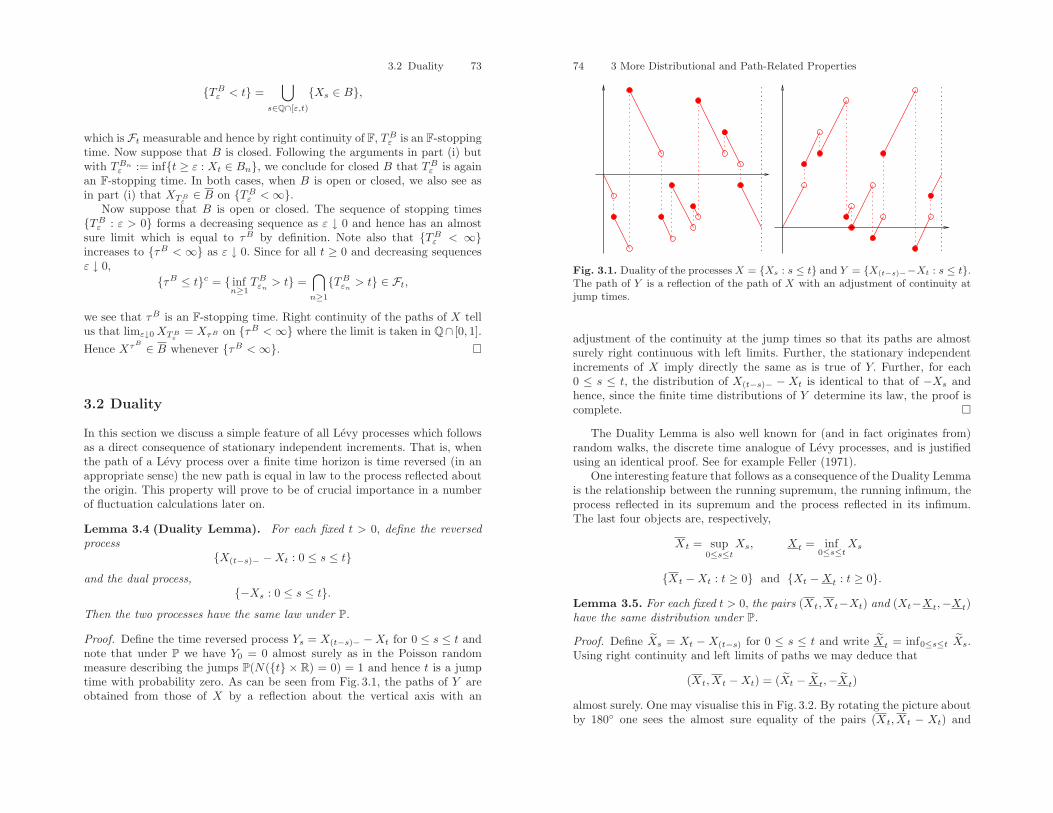
3.2 Duality 73
TBε < t =⋃
s∈Q∩[ε,t)
Xs ∈ B,
which is Ft measurable and hence by right continuity of F, TBε is an F-stoppingtime. Now suppose that B is closed. Following the arguments in part (i) butwith TBn
ε := inft ≥ ε : Xt ∈ Bn, we conclude for closed B that TBε is againan F-stopping time. In both cases, when B is open or closed, we also see asin part (i) that XTB
ε∈ B on TBε <∞.
Now suppose that B is open or closed. The sequence of stopping timesTBε : ε > 0 forms a decreasing sequence as ε ↓ 0 and hence has an almostsure limit which is equal to τB by definition. Note also that TBε < ∞increases to τB < ∞ as ε ↓ 0. Since for all t ≥ 0 and decreasing sequencesε ↓ 0,
τB ≤ tc = infn≥1
TBεn> t =
⋂n≥1
TBεn> t ∈ Ft,
we see that τB is an F-stopping time. Right continuity of the paths of X tellus that limε↓0 XTB
ε= XτB on τB <∞ where the limit is taken in Q∩ [0, 1].
Hence XτB ∈ B whenever τB <∞.
3.2 Duality
In this section we discuss a simple feature of all Levy processes which followsas a direct consequence of stationary independent increments. That is, whenthe path of a Levy process over a finite time horizon is time reversed (in anappropriate sense) the new path is equal in law to the process reflected aboutthe origin. This property will prove to be of crucial importance in a numberof fluctuation calculations later on.
Lemma 3.4 (Duality Lemma). For each fixed t > 0, define the reversedprocess
X(t−s)− −Xt : 0 ≤ s ≤ tand the dual process,
−Xs : 0 ≤ s ≤ t.Then the two processes have the same law under P.
Proof. Define the time reversed process Ys = X(t−s)− −Xt for 0 ≤ s ≤ t andnote that under P we have Y0 = 0 almost surely as in the Poisson randommeasure describing the jumps P(N(t × R) = 0) = 1 and hence t is a jumptime with probability zero. As can be seen from Fig. 3.1, the paths of Y areobtained from those of X by a reflection about the vertical axis with an
74 3 More Distributional and Path-Related Properties
Fig. 3.1. Duality of the processes X = Xs : s ≤ t and Y = X(t−s)−−Xt : s ≤ t.The path of Y is a reflection of the path of X with an adjustment of continuity atjump times.
adjustment of the continuity at the jump times so that its paths are almostsurely right continuous with left limits. Further, the stationary independentincrements of X imply directly the same as is true of Y. Further, for each0 ≤ s ≤ t, the distribution of X(t−s)− − Xt is identical to that of −Xs andhence, since the finite time distributions of Y determine its law, the proof iscomplete.
The Duality Lemma is also well known for (and in fact originates from)random walks, the discrete time analogue of Levy processes, and is justifiedusing an identical proof. See for example Feller (1971).
One interesting feature that follows as a consequence of the Duality Lemmais the relationship between the running supremum, the running infimum, theprocess reflected in its supremum and the process reflected in its infimum.The last four objects are, respectively,
Xt = sup0≤s≤t
Xs, Xt = inf0≤s≤t
Xs
Xt −Xt : t ≥ 0 and Xt −Xt : t ≥ 0.Lemma 3.5. For each fixed t > 0, the pairs (Xt,Xt−Xt) and (Xt−Xt,−Xt)have the same distribution under P.
Proof. Define Xs = Xt −X(t−s) for 0 ≤ s ≤ t and write Xt = inf0≤s≤t Xs.Using right continuity and left limits of paths we may deduce that
(Xt,Xt −Xt) = (Xt − Xt,−Xt)
almost surely. One may visualise this in Fig. 3.2. By rotating the picture aboutby 180 one sees the almost sure equality of the pairs (Xt,Xt − Xt) and
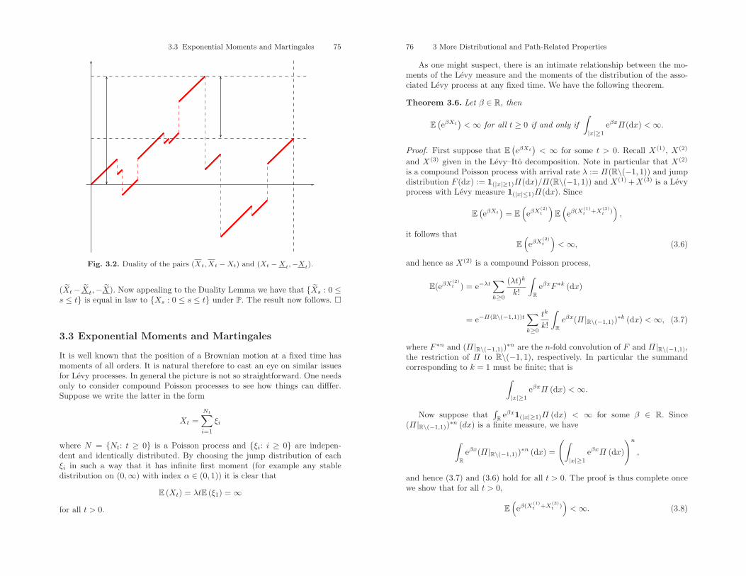
3.3 Exponential Moments and Martingales 75
Fig. 3.2. Duality of the pairs (Xt, Xt −Xt) and (Xt −Xt,−Xt).
(Xt− Xt,−X). Now appealing to the Duality Lemma we have that Xs : 0 ≤s ≤ t is equal in law to Xs : 0 ≤ s ≤ t under P. The result now follows.
3.3 Exponential Moments and Martingales
It is well known that the position of a Brownian motion at a fixed time hasmoments of all orders. It is natural therefore to cast an eye on similar issuesfor Levy processes. In general the picture is not so straightforward. One needsonly to consider compound Poisson processes to see how things can difffer.Suppose we write the latter in the form
Xt =Nt∑i=1
ξi
where N = Nt: t ≥ 0 is a Poisson process and ξi: i ≥ 0 are indepen-dent and identically distributed. By choosing the jump distribution of eachξi in such a way that it has infinite first moment (for example any stabledistribution on (0,∞) with index α ∈ (0, 1)) it is clear that
E (Xt) = λtE (ξ1) = ∞for all t > 0.
76 3 More Distributional and Path-Related Properties
As one might suspect, there is an intimate relationship between the mo-ments of the Levy measure and the moments of the distribution of the asso-ciated Levy process at any fixed time. We have the following theorem.
Theorem 3.6. Let β ∈ R, then
E(eβXt
)<∞ for all t ≥ 0 if and only if
∫|x|≥1
eβxΠ(dx) <∞.
Proof. First suppose that E(eβXt
)< ∞ for some t > 0. Recall X(1), X(2)
and X(3) given in the Levy–Ito decomposition. Note in particular that X(2)
is a compound Poisson process with arrival rate λ := Π(R\(−1, 1)) and jumpdistribution F (dx) := 1(|x|≥1)Π(dx)/Π(R\(−1, 1)) and X(1) +X(3) is a Levyprocess with Levy measure 1(|x|≤1)Π(dx). Since
E(eβXt
)= E
(eβX
(2)t
)E(eβ(X
(1)t +X
(3)t )),
it follows thatE(eβX
(2)t
)<∞, (3.6)
and hence as X(2) is a compound Poisson process,
E(eβX(2)t ) = e−λt
∑k≥0
(λt)k
k!
∫R
eβxF ∗k (dx)
= e−Π(R\(−1,1))t∑k≥0
tk
k!
∫Reβx(Π|R\(−1,1))∗k (dx) <∞, (3.7)
where F ∗n and (Π|R\(−1,1))∗n are the n-fold convolution of F and Π|R\(−1,1),the restriction of Π to R\(−1, 1), respectively. In particular the summandcorresponding to k = 1 must be finite; that is∫
|x|≥1
eβxΠ (dx) <∞.
Now suppose that∫
R eβx1(|x|≥1)Π (dx) < ∞ for some β ∈ R. Since(Π|R\(−1,1))∗n (dx) is a finite measure, we have
∫R
eβx(Π|R\(−1,1))∗n (dx) =
(∫|x|≥1
eβxΠ (dx)
)n,
and hence (3.7) and (3.6) hold for all t > 0. The proof is thus complete oncewe show that for all t > 0,
E(eβ(X
(1)t +X
(3)t ))<∞. (3.8)
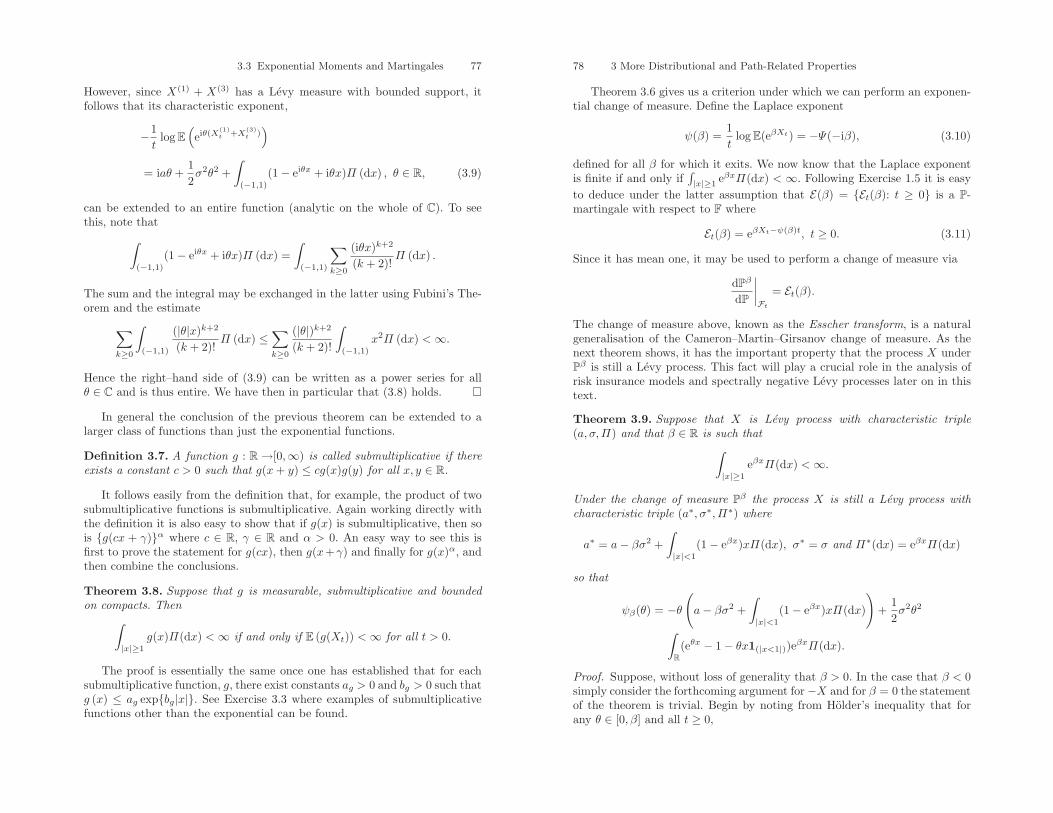
3.3 Exponential Moments and Martingales 77
However, since X(1) + X(3) has a Levy measure with bounded support, itfollows that its characteristic exponent,
−1t
log E(eiθ(X
(1)t +X
(3)t ))
= iaθ +12σ2θ2 +
∫(−1,1)
(1− eiθx + iθx)Π (dx) , θ ∈ R, (3.9)
can be extended to an entire function (analytic on the whole of C). To seethis, note that∫
(−1,1)
(1− eiθx + iθx)Π (dx) =∫
(−1,1)
∑k≥0
(iθx)k+2
(k + 2)!Π (dx) .
The sum and the integral may be exchanged in the latter using Fubini’s The-orem and the estimate∑
k≥0
∫(−1,1)
(|θ|x)k+2
(k + 2)!Π (dx) ≤
∑k≥0
(|θ|)k+2
(k + 2)!
∫(−1,1)
x2Π (dx) <∞.
Hence the right–hand side of (3.9) can be written as a power series for allθ ∈ C and is thus entire. We have then in particular that (3.8) holds.
In general the conclusion of the previous theorem can be extended to alarger class of functions than just the exponential functions.
Definition 3.7. A function g : R →[0,∞) is called submultiplicative if thereexists a constant c > 0 such that g(x+ y) ≤ cg(x)g(y) for all x, y ∈ R.
It follows easily from the definition that, for example, the product of twosubmultiplicative functions is submultiplicative. Again working directly withthe definition it is also easy to show that if g(x) is submultiplicative, then sois g(cx + γ)α where c ∈ R, γ ∈ R and α > 0. An easy way to see this isfirst to prove the statement for g(cx), then g(x+γ) and finally for g(x)α, andthen combine the conclusions.
Theorem 3.8. Suppose that g is measurable, submultiplicative and boundedon compacts. Then∫
|x|≥1
g(x)Π(dx) <∞ if and only if E (g(Xt)) <∞ for all t > 0.
The proof is essentially the same once one has established that for eachsubmultiplicative function, g, there exist constants ag > 0 and bg > 0 such thatg (x) ≤ ag expbg|x|. See Exercise 3.3 where examples of submultiplicativefunctions other than the exponential can be found.
78 3 More Distributional and Path-Related Properties
Theorem 3.6 gives us a criterion under which we can perform an exponen-tial change of measure. Define the Laplace exponent
ψ(β) =1t
log E(eβXt) = −Ψ(−iβ), (3.10)
defined for all β for which it exits. We now know that the Laplace exponentis finite if and only if
∫|x|≥1
eβxΠ(dx) < ∞. Following Exercise 1.5 it is easyto deduce under the latter assumption that E(β) = Et(β): t ≥ 0 is a P-martingale with respect to F where
Et(β) = eβXt−ψ(β)t, t ≥ 0. (3.11)
Since it has mean one, it may be used to perform a change of measure via
dPβ
dP
∣∣∣∣Ft
= Et(β).
The change of measure above, known as the Esscher transform, is a naturalgeneralisation of the Cameron–Martin–Girsanov change of measure. As thenext theorem shows, it has the important property that the process X underPβ is still a Levy process. This fact will play a crucial role in the analysis ofrisk insurance models and spectrally negative Levy processes later on in thistext.
Theorem 3.9. Suppose that X is Levy process with characteristic triple(a, σ,Π) and that β ∈ R is such that∫
|x|≥1
eβxΠ(dx) <∞.
Under the change of measure Pβ the process X is still a Levy process withcharacteristic triple (a∗, σ∗,Π∗) where
a∗ = a− βσ2 +∫|x|<1
(1− eβx)xΠ(dx), σ∗ = σ and Π∗(dx) = eβxΠ(dx)
so that
ψβ(θ) = −θ(a− βσ2 +
∫|x|<1
(1− eβx)xΠ(dx)
)+
12σ2θ2
∫R(eθx − 1− θx1(|x<1|))eβxΠ(dx).
Proof. Suppose, without loss of generality that β > 0. In the case that β < 0simply consider the forthcoming argument for−X and for β = 0 the statementof the theorem is trivial. Begin by noting from Holder’s inequality that forany θ ∈ [0, β] and all t ≥ 0,
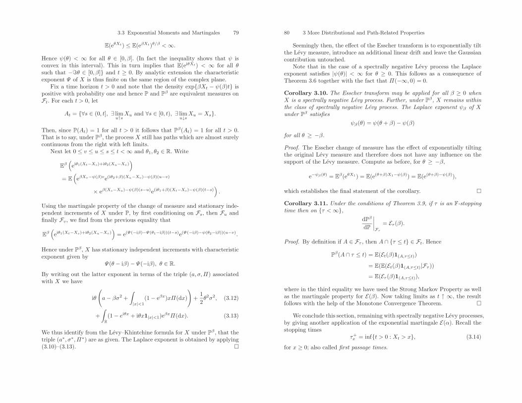
3.3 Exponential Moments and Martingales 79
E(eθXt) ≤ E(eβXt)θ/β <∞.
Hence ψ(θ) < ∞ for all θ ∈ [0, β]. (In fact the inequality shows that ψ isconvex in this interval). This in turn implies that E(eiθXt) < ∞ for all θsuch that −ℑθ ∈ [0, β] and t ≥ 0. By analytic extension the characteristicexponent Ψ of X is thus finite on the same region of the complex plane.
Fix a time horizon t > 0 and note that the density expβXt − ψ(β)t ispositive with probability one and hence P and Pβ are equivalent measures onFt. For each t > 0, let
At = ∀s ∈ (0, t], ∃ limu↑s
Xu and ∀s ∈ [0, t), ∃ limu↓s
Xu = Xs.
Then, since P(At) = 1 for all t > 0 it follows that Pβ(At) = 1 for all t > 0.That is to say, under Pβ , the process X still has paths which are almost surelycontinuous from the right with left limits.
Next let 0 ≤ v ≤ u ≤ s ≤ t <∞ and θ1, θ2 ∈ R. Write
Eβ(eiθ1(Xt−Xs)+iθ2(Xu−Xv)
)= E
(eβXv−ψ(β)ve(iθ2+β)(Xu−Xv)−ψ(β)(u−v)
× eβ(Xs−Xu)−ψ(β)(s−u)e(iθ1+β)(Xt−Xs)−ψ(β)(t−s)).
Using the martingale property of the change of measure and stationary inde-pendent increments of X under P, by first conditioning on Fs, then Fu andfinally Fv, we find from the previous equality that
Eβ(eiθ1(Xt−Xs)+iθ2(Xu−Xv)
)= e(Ψ(−iβ)−Ψ(θ1−iβ))(t−s)e(Ψ(−iβ)−ψ(θ2−iβ))(u−v).
Hence under Pβ , X has stationary independent increments with characteristicexponent given by
Ψ(θ − iβ)− Ψ(−iβ), θ ∈ R.
By writing out the latter exponent in terms of the triple (a, σ,Π) associatedwith X we have
iθ
(a− βσ2 +
∫|x|<1
(1− eβx)xΠ(dx)
)+
12θ2σ2, (3.12)
+∫
R(1− eiθx + iθx1|x|<1)eβxΠ(dx). (3.13)
We thus identify from the Levy–Khintchine formula for X under Pβ , that thetriple (a∗, σ∗,Π∗) are as given. The Laplace exponent is obtained by applying(3.10)–(3.13).
80 3 More Distributional and Path-Related Properties
Seemingly then, the effect of the Esscher transform is to exponentially tiltthe Levy measure, introduce an additional linear drift and leave the Gaussiancontribution untouched.
Note that in the case of a spectrally negative Levy process the Laplaceexponent satisfies |ψ(θ)| < ∞ for θ ≥ 0. This follows as a consequence ofTheorem 3.6 together with the fact that Π(−∞, 0) = 0.
Corollary 3.10. The Esscher transform may be applied for all β ≥ 0 whenX is a spectrally negative Levy process. Further, under Pβ, X remains withinthe class of spectrally negative Levy process. The Laplace exponent ψβ of Xunder Pβ satisfies
ψβ(θ) = ψ(θ + β)− ψ(β)
for all θ ≥ −β.
Proof. The Esscher change of measure has the effect of exponentially tiltingthe original Levy measure and therefore does not have any influence on thesupport of the Levy measure. Compute as before, for θ ≥ −β,
e−ψβ(θ) = Eβ(eθX1) = E(e(θ+β)X1−ψ(β)) = E(e(θ+β)−ψ(β)),
which establishes the final statement of the corollary.
Corollary 3.11. Under the conditions of Theorem 3.9, if τ is an F-stoppingtime then on τ <∞,
dPβ
dP
∣∣∣∣Fτ
= Eτ (β).
Proof. By definition if A ∈ Fτ , then A ∩ τ ≤ t ∈ Ft. Hence
Pβ(A ∩ τ ≤ t) = E(Et(β)1(A,τ≤t))
= E(E(Et(β)1(A,τ≤t)|Fτ ))= E(Eτ (β)1(A,τ≤t)),
where in the third equality we have used the Strong Markov Property as wellas the martingale property for E(β). Now taking limits as t ↑ ∞, the resultfollows with the help of the Monotone Convergence Theorem.
We conclude this section, remaining with spectrally negative Levy processes,by giving another application of the exponential martingale E(α). Recall thestopping times
τ+x = inft > 0 : Xt > x, (3.14)
for x ≥ 0; also called first passage times.
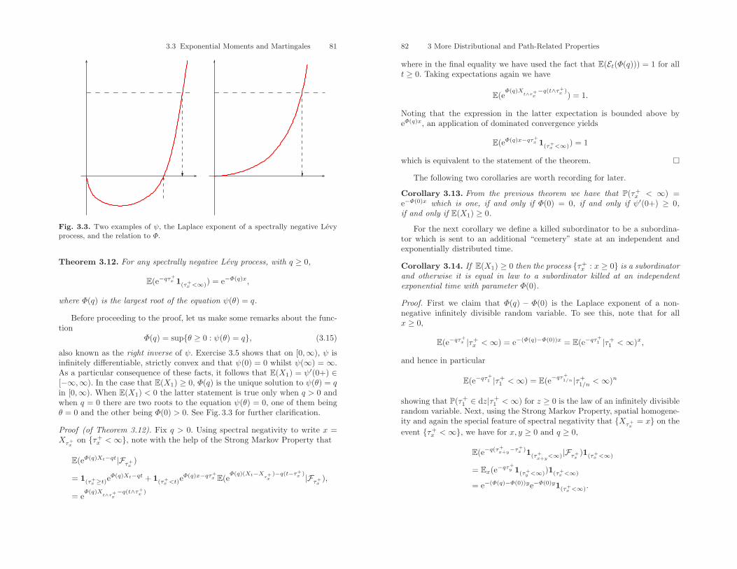
3.3 Exponential Moments and Martingales 81
Fig. 3.3. Two examples of ψ, the Laplace exponent of a spectrally negative Levyprocess, and the relation to Φ.
Theorem 3.12. For any spectrally negative Levy process, with q ≥ 0,
E(e−qτ+x 1(τ+
x <∞)) = e−Φ(q)x,
where Φ(q) is the largest root of the equation ψ(θ) = q.
Before proceeding to the proof, let us make some remarks about the func-tion
Φ(q) = supθ ≥ 0 : ψ(θ) = q, (3.15)
also known as the right inverse of ψ. Exercise 3.5 shows that on [0,∞), ψ isinfinitely differentiable, strictly convex and that ψ(0) = 0 whilst ψ(∞) = ∞.As a particular consequence of these facts, it follows that E(X1) = ψ′(0+) ∈[−∞,∞). In the case that E(X1) ≥ 0, Φ(q) is the unique solution to ψ(θ) = qin [0,∞). When E(X1) < 0 the latter statement is true only when q > 0 andwhen q = 0 there are two roots to the equation ψ(θ) = 0, one of them beingθ = 0 and the other being Φ(0) > 0. See Fig. 3.3 for further clarification.
Proof (of Theorem 3.12). Fix q > 0. Using spectral negativity to write x =Xτ+
xon τ+
x <∞, note with the help of the Strong Markov Property that
E(eΦ(q)Xt−qt|Fτ+x
)
= 1(τ+x ≥t)e
Φ(q)Xt−qt + 1(τ+x <t)
eΦ(q)x−qτ+x E(e
Φ(q)(Xt−Xτ+x
)−q(t−τ+x )|Fτ+
x),
= eΦ(q)X
t∧τ+x−q(t∧τ+
x )
82 3 More Distributional and Path-Related Properties
where in the final equality we have used the fact that E(Et(Φ(q))) = 1 for allt ≥ 0. Taking expectations again we have
E(eΦ(q)X
t∧τ+x−q(t∧τ+
x )) = 1.
Noting that the expression in the latter expectation is bounded above byeΦ(q)x, an application of dominated convergence yields
E(eΦ(q)x−qτ+x 1(τ+
x <∞)) = 1
which is equivalent to the statement of the theorem.
The following two corollaries are worth recording for later.
Corollary 3.13. From the previous theorem we have that P(τ+x < ∞) =
e−Φ(0)x which is one, if and only if Φ(0) = 0, if and only if ψ′(0+) ≥ 0,if and only if E(X1) ≥ 0.
For the next corollary we define a killed subordinator to be a subordina-tor which is sent to an additional “cemetery” state at an independent andexponentially distributed time.
Corollary 3.14. If E(X1) ≥ 0 then the process τ+x : x ≥ 0 is a subordinator
and otherwise it is equal in law to a subordinator killed at an independentexponential time with parameter Φ(0).
Proof. First we claim that Φ(q) − Φ(0) is the Laplace exponent of a non-negative infinitely divisible random variable. To see this, note that for allx ≥ 0,
E(e−qτ+x |τ+
x <∞) = e−(Φ(q)−Φ(0))x = E(e−qτ+1 |τ+
1 <∞)x,
and hence in particular
E(e−qτ+1 |τ+
1 <∞) = E(e−qτ+1/n |τ+
1/n <∞)n
showing that P(τ+1 ∈ dz|τ+
1 <∞) for z ≥ 0 is the law of an infinitely divisiblerandom variable. Next, using the Strong Markov Property, spatial homogene-ity and again the special feature of spectral negativity that Xτ+
x= x on the
event τ+x <∞, we have for x, y ≥ 0 and q ≥ 0,
E(e−q(τ+x+y
−τ+x )1(τ+
x+y<∞)|Fτ+
x)1(τ+
x <∞)
= Ex(e−qτ+y 1(τ+
y <∞))1(τ+x <∞)
= e−(Φ(q)−Φ(0))ye−Φ(0)y1(τ+x <∞).
3.3 Exercises 83
In the first equality we have used standard notation for Markov processes,Ex(·) = E(·|X0 = x). We see then that the increment τ+
x+y−τ+x is independent
of Fτ+x
on τ+x <∞ and has the same law as the subordinator with Laplace
exponent Φ(q) − Φ(0) but killed at an independent exponential time withparameter Φ(0).
When E(X1) ≥ 0 we have that Φ(0) = 0 and hence the concluding state-ment of the previous paragraph indicates that τ+
x : x ≥ 0 is a subordinator(without killing). On the other hand, if E(X1) < 0, or equivalently Φ(0) > 0then the second statement of the corollary follows.
Note that embedded in the previous corollary is the same reasoning whichlies behind the justification of the fact that an inverse Gaussian process is aLevy process. See Sect. 1.2.5 and Exercise 1.6.
Exercises
3.1. Suppose that X is a Levy process defined on (Ω,F ,P) and that Ft is thesigma algebra obtained by completing σ(Xs : s ≤ t) by the null sets of P. Theaim of this exercise is to show that F := Ft : t ≥ 0 is automatically rightcontinuous; that is to say that for all t ≥ 0,
Ft =⋂s>t
Fs.
(i) Fix t2 > t1 ≥ 0 and show that for any t ≥ 0,
limu↓t
E(eiθ1Xt1+iθ2Xt2 |Fu) = E(eiθ1Xt1+iθ2Xt2 |Ft)
almost surely where θ1, θ2 ∈ R.(ii) Deduce that for any sequence of times t1, ..., tn ≥ 0,
E(g(Xt1 , ..., Xtn)|Ft) = E(g(Xt1 , ..., Xtn)|Ft+)
almost surely for all functions g satisfying E(|g(Xt1 , ..., Xtn)|) <∞.(iii) Conclude that for each A ∈ Ft+, E(1A|Ft) = 1A and hence that Ft =
Ft+.
3.2. Show that for any y ≥ 0,
(y ∨Xt)−Xt : t ≥ 0 and Xt − (Xt ∧ (−y)) : t ≥ 0
are [0,∞)-valued strong Markov process.
3.3 (Proof of Theorem 3.8 and examples).
(i) Use the comments under Theorem 3.8 to prove it.
84 3 More Distributional and Path-Related Properties
(ii) Prove that the following functions are submultiplicative: x ∨ 1, xα ∨ 1|x| ∨ 1, |x|α ∨ 1, exp(|x|β), log(|x| ∨ e), log log(|x| ∨ ee) where α > 0 andβ ∈ (0, 1].
(iii) Suppose that X is a stable process of index α ∈ (0, 2). Show thatE(|Xt|η) <∞ for all t ≥ 0 if and only if η ∈ (0, α).
3.4. A generalised tempered stable process is a Levy process with no Gaussiancomponent and Levy measure given by
Π(dx) = 1(x>0)c+
x1+α+ e−γ+x dx+ 1(x<0)
c−
|x|1+α− eγ−x dx,
where c± > 0, α± ∈ (−∞, 2) and γ± > 0. Show that if X is a generalizedstable process, then X may always be written in the form X = X+ − X−
where X+ = X+t : t ≥ 0 and X− = X−
t : t ≥ 0 satisfy the following:
(i) If α± < 0 then X± is a compound Poisson process with drift.(ii) If α± = 0 then X± is a gamma process with drift.(iii) If α± = 1 then X± is a one-sided Cauchy process.(iv) If α± ∈ (0, 1) ∪ (1, 2) then up to the addition of a linear drift X± has
the same law as a spectrally positive stable process with index α± butconsidered under the change of measure P−γ± .
3.5. Suppose that ψ is the Laplace exponent of a spectrally negative Levyprocess. By considering explicitly the formula
ψ(β) = −aβ +12σ2β2 +
∫(−∞,0)
(eβx − 1− βx1(x>−1))Π(dx)
show that on [0,∞), ψ is infinitely differentiable, strictly convex and thatψ(0) = 0 whilst ψ(∞) = ∞.
3.6. Suppose thatX is a spectrally negative Levy process with Levy–Khintchineexponent Ψ . Here we give another proof of the existence of a finite Laplaceexponent for all spectrally negative Levy processes.
(i) Use spectral negativity together with the lack of memory property to showthat for x, y > 0,
P(Xeq> x+ y) = P(Xeq
> x)P(Xeq> y)
where eq is an exponentially distributed random variable4 independent ofX and Xt = sups≤tXs.
4We are making an abuse of notation in the use of the measure P. Strictly speakingwe should work with the measure P × P where P is the probability measure onthe space in which the random variable eq is defined. This abuse of notation willbe repeated for the sake of convenience at various points throughout this text.
3.3 Exercises 85
(ii) Deduce that Xeqis exponentially distributed and hence the Laplace ex-
ponent ψ(β) = −Ψ(−iβ) exists and is finite for all β ≥ 0.(iii) By considering the Laplace transform of the first passage time τ+
x as inSect. 3.3, show that one may also deduce via a different route that Xeq
is exponentially distributed with parameter Φ(q). In particular show thatX∞ is either infinite with probability one or is exponentially distributedaccordingly as E(X1) ≥ 0 or E(X1) < 0. [Hint: reconsider Exercise 3.5].
3.7. For this exercise it will be useful to refer to Sect. 1.2.6. Suppose that Xis a Stable Levy process with index β = 1; that is to say Π(−∞, 0) = 0.
(i) Show that if α ∈ (0, 1) then X is a driftless subordinator with Laplaceexponent satisfying
− log E(e−θX1) = cθα, θ ≥ 0
for some c > 0.(ii) Show that if α ∈ (1, 2), then X has a Laplace exponent satisfying
− log E(e−θX1) = −Cθα, θ ≥ 0
for some C > 0. Confirm that X has no integer moments of order 2 andabove as well as being a process of unbounded variation.
4
General Storage Models and Paths of BoundedVariation
In this chapter we return to the queuing and general storage models discussedin Sects. 1.3.2 and 2.7.2. Predominantly we shall concentrate on the asymp-totic behaviour of the two quantities that correspond to the workload processand the idle time in the M/G/1 queue but now in the general setting de-scribed in Sect. 2.7.2. Along the way we will introduce some new tools whichwill be of help, both in this chapter and in later chapters. Specifically weshall spend some additional time looking at the change of variable and com-pensation formulae. We also spend some time discussing similarities betweenthe mathematical description of the limiting distribution of workload process(when it is non-trivial) and the Pollaczek–Khintchine formula which requires astudy of the small scale behaviour of Levy processes of bounded variation. Westart however by briefly recalling and expanding a little on the mathematicalbackground of general storage models.
4.1 General Storage Models
A general storage model may be considered as consisting of two processes;At : t ≥ 0, the volume of incoming work and Bt : t ≥ 0, the total amountof work that can potentially exit from the system as a result of processing workcontinuously. In the case of the M/G/1 queue we have At =
∑Nt
i=1 ξi whereNt : t ≥ 0 is a Poisson process and ξi : i = 1, 2, ... are the independentservice times of the ordered customers. Further, as the server processes at aconstant unit rate, we have simply that Bt = t. For all t ≥ 0 let Dt = At−Bt.The process D = Dt : t ≥ 0 is clearly related to the workload of thesystem, although it is itself not a suitable candidate to model the workloadas in principle D may become negative and the workload is clearly a non-negative quantity. The work stored in the system, W = Wt : t ≥ 0, is insteaddefined by
Wt = Dt + Lt,
88 4 General Storage Models and Paths of Bounded Variation
where L = Lt : t ≥ 0 is increasing with paths that are right continuous(and left limits are of course automatic by monotonicity) and is added to theprocess D to ensure that Wt ≥ 0 for all t ≥ 0. The process L must onlyincrease when W = 0 so in particular∫ ∞
0
1(Wt>0)dLt = 0.
It is easy to check that we may take Lt = −(infs≤tDs ∧ 0). Indeed with thischoice of L we have that Wt = 0 if and only if Dt = infs≤tDs ∧ 0 if andonly if t is in the support of the measure dL. It can also be proved that thereis no other choice of L fulfilling these requirements (see for example Kella andWhitt 1996).
We are concerned with the case that the process A is a pure jump subor-dinator and B is a linear trend. Specifically, Dt = x−Xt where w ≥ 0 is theworkload already in the system at time t = 0 and X is a spectrally negativeLevy process of bounded variation. A little algebra with the given expressionsfor D and L shows that
Wt = (w ∨Xt)−Xt, t ≥ 0,
where Xt = sups≤tXs.We know from the discussion in Sect. 3.3 (see also Exercise 3.6) that the
process X has Laplace exponent ψ(θ) = log E(eθX1) which is finite for allθ ≥ 0. Writing X in the form dt − St where d > 0 and S = St : t ≥ 0 is apure jump subordinator, it is convenient to write the Laplace exponent of Xin the form
ψ(θ) = dθ −∫
(0,∞)
(1− e−θx)ν(dx),
where ν is the Levy measure of the subordinator S and necessarily∫(0,∞)
(1∧x)ν(dx) <∞. We interpret ν(dx)dt+o(dt) as the probability a job or storagebulk of size x arrives independently in each dt.
4.2 Idle Times
We start by introducing the parameter
ρ :=d− ψ′(0+)
d.
Note that regimes 0 < ρ < 1, ρ = 1 and ρ > 1 correspond precisely to theregimes ψ′(0+) > 0, ψ′(0+) = 0 and ψ′(0+) < 0, respectively. The first twoof these cases thus imply that Φ(0) = 0 and the third case implies Φ(0) > 0where Φ is the right inverse of ψ defined in (3.15). When d = 1 and ν = λFwhere F is a distribution function and λ > 0 is the arrival rate, the processW is the workload of an M/G/1 queue. In that case ρ = λE(ξ) where ξ is arandom variable with distribution F and is called the traffic intensity.
The main purpose of this section is to prove the following result whichgeneralises Theorem 1.11.
4.2 Idle Times 89
Theorem 4.1. Suppose that ρ > 1 then the total time that the storage processspends idle
I :=∫ ∞
0
1(Wt=0)dt,
has the following distribution
P (I ∈ dx) = (1− e−Φ(0)w)δ0 (dx) + Φ(0)e−Φ(0)(w+xd)dx.
Otherwise if 0 < ρ ≤ 1 then I is infinite with probability one.
Proof (of Theorem 4.1). Essentially the proof mimics the steps of Exercise1.9. As one sees for the case of the M/G/1 queue, a key ingredient to theproof is that one may identify the process d ∫ t
01(Ws=0)ds : t ≥ 0 as the
process Xt : t ≥ 0. To see why this is true in the general storage model,recall from the Levy–Ito decomposition that X has a countable number ofjumps over finite intervals of time and hence the same is true of W . Furthersince X has negative jumps, Ws = 0 only if there is no jump at time s. Hence,given that X is the difference of a linear drift with rate d and a subordinatorS, it follows that for each t ≥ 0,
Xt =∫ t
0
1(Xs=Xs)dXs
= d
∫ t
0
1(Xs=Xs)ds−∫ t
0
1(Xs=Xs)dSs
= d
∫ t
0
1(Xs=Xs)ds
almost surely where the final equality follows as a consequence of the fact that∫ t
0
1(Xs=Xs)dSs ≤∫ t
0
1(∆Ss=0)dSs = 0.
It is important to note that the latter calculation only works for spectrallynegative Levy processes of bounded variation on account of the Levy–Itodecomposition.
Now following Exercise 3.6 (iii) we can use the equivalence of the eventsX∞ > x and τ+
x <∞, where τ+x is the first hitting time of (x,∞) defined
in (3.14), to deduce that X∞ is exponentially distributed with parameterΦ(0). When Φ(0) = 0 then the previous statement is understood to mean thatP(X∞ = ∞) = 1. When w = 0 we have precisely that
X∞d
=∫ ∞
0
1(Xs=Xs)ds =∫ ∞
0
1(Ws=0)ds. (4.1)
Hence we see that I is exponentially distributed with parameter dΦ(0). Re-calling which values of ρ imply that Φ(0) > 0 we see that the statement of thetheorem follows for the case w = 0.
90 4 General Storage Models and Paths of Bounded Variation
In general however, when w > 0 the equality (4.1) is not valid. Instead wehave that ∫ ∞
0
1(Ws=0)ds =∫ τ+
w
0
1(Ws=0)ds+∫ ∞
τ+w
1(Ws=0)ds
= 1(τ+w<∞)
∫ ∞
τ+w
1(Ws=0)ds
= 1(X∞≥w)I∗, (4.2)
where I∗ is independent of Fτ+w
on τ+w < ∞ and equal in distribution to∫∞
01(Ws=0)ds when w = 0. Note that the first integral in the right-hand
side of the first equality disappears on account of the fact that Ws > 0 for alls < τ+
w . The statement of the theorem now follows for 0 ≤ ρ ≤ 1 by once againrecalling that in this regime Φ(0) = 0 and hence from (4.2) X∞ = ∞ withprobability one and hence I = I∗. The latter has previously been shown tobe infinite with probability one. On the other hand, when ρ > 1, we see from(4.2) that there is an atom at zero corresponding to the event X∞ < w withprobability 1− e−Φ(0)w. Otherwise, with independent probability e−Φ(0)w, theintegral I has the same distribution as I∗. Again from previous calculationsfor the case w = 0 we have seen that this is exponential with parameter dΦ(0)and the proof is complete.
4.3 Change of Variable and Compensation Formulae
Next we spend a little time introducing the change of variable formula and thecompensation formula. Both formulae pertain to a form of stochastic calculus.The theory of stochastic calculus is an avenue which we choose not to pursuein full generality, choosing instead to make some brief remarks. Our expositionwill suffice to study in more detail the storage processes discussed in Chap. 1as well as a number of other applications in later Chapters.
4.3.1 The Change of Variable Formula
We assume that X = Xt : t ≥ 0 is a Levy process of bounded variation.Referring back to Chap. 2, (2.21) and (2.22) we recall that we may alwayswrite its Levy–Khintchine exponent as
Ψ(θ) = −idθ +∫
R(1− eiθx)Π(dx)
and correspondingly identify X path-wise in the form of a generalised com-pound Poisson process
Xt = dt+∫
[0,t]
∫RxN(ds× dx),
4.3 Change of Variable and Compensation Formulae 91
where d ∈ R and, as usual, N is the Poisson random measure associated withthe jumps of X.
Our goal in this section is to prove the following change of variable formula.
Theorem 4.2. Let C1,1([0,∞)×R) be the space of functions f : [0,∞)×R →R which are continuously differentiable in each variable (in the case of thederivative in the first variable at the origin a right derivative is understood).If f(s, x) belongs to the class C1,1([0,∞)× R) then
f(t,Xt) = f(0, X0) +∫ t
0
∂f
∂s(s,Xs)ds+ d
∫ t
0
∂f
∂x(s,Xs)ds
+∫
[0,t]
∫R(f(s,Xs− + x)− f(s,Xs−))N(ds× dx).
It will become apparent from the proof of this theorem that the finalintegral with respect to N in the change of variable formula is well defined.
It is worth mentioning that the change of variable formula exists in a muchmore general form. For example it is known (cf. Protter 2004 that if V = Vt :t ≥ 0 is any mapping from [0,∞) to R (random or deterministic) of boundedvariation with paths that are right continuous and f(s, x) ∈ C1,1([0,∞)×R)is continuously differentiable, then f(t, Vt) : t ≥ 0 is a mapping from [0,∞)to R of bounded variation which satisfies
f(t, Vt) = f(0, V0) +∫ t
0
∂f
∂s(s, Vs)ds+
∫ t
0
∂f
∂x(s, Vs−)dVs
+∑s≤t
f(s, Vs)− f(s, Vs−)−∆Vs∂f
∂x(s, Vs), (4.3)
where ∆Vs = Vs − Vs−. Note also that since V is of bounded variation thenit has a minimal decomposition as the difference of two increasing functionsmapping [0,∞) to [0,∞) and hence left continuity of V is automatically guar-anteed. This means that V has a countable number of jumps (see Exercise2.4). One therefore may understand the final term on the right-hand side of(4.3) as a convergent sum over the countable discontinuities of V . In the casethat V is a Levy process of bounded variation, it is a straightforward exerciseto deduce that when one represents the discontinuities of V via a Poissonrandom measure then (4.3) and the conclusion of Theorem 4.2 agree.
Proof (of Theorem 4.2). Define for all ε > 0,
Xεt = dt+
∫[0,t]
∫|x|≥ε
xN(ds× dx), t ≥ 0.
As Π(R\(−ε, ε)) <∞ it follows that N counts an almost surely finite numberof jumps over [0, t] × R\(−ε, ε) and Xε = Xε
t : t ≥ 0 is a compoundPoisson process with drift. Suppose the collection of jumps of Xε up to time
92 4 General Storage Models and Paths of Bounded Variation
t are described by the time-space points (Ti, ξi) : i = 1, ..., N where N =N([0, t]× R\(−ε, ε)). Let T0 = 0. Then a simple telescopic sum gives
f(t,Xεt ) = f(0, Xε
0) +N∑i=1
(f(Ti, XεTi
)− f(Ti−1, XεTi−1
))
+(f(t,Xεt )− f(TN , Xε
TN)).
Now noting that Xε is piece-wise linear we have,
f(t,Xεt )
= f(0, Xε0)
+N∑i=1
(∫ Ti
Ti−1
∂f
∂s(s,Xε
s ) + d∂f
∂x(s,Xε
s )ds+ (f(Ti, XεTi− + ξi)− f(Ti, Xε
Ti−))
)
+∫ t
TN
∂f
∂s(s,Xε
s ) + d∂f
∂x(s,Xε
s )ds
= f(0, Xε0) +
∫ t
0
∂f
∂s(s,Xε
s ) + d∂f
∂x(s,Xε
s )ds
+∫
[0,t]
∫R\0
(f(s,Xεs− + x)− f(x,Xε
s−))1(|x|≥ε)N(ds× dx). (4.4)
(Note that the smoothness of f has been used here).From Exercise 2.8 we know that any Levy process of bounded variation
may be written as the difference of two independent subordinators. In thisspirit write Xt = X
(1)t −X
(2)t where
X(1)t = (d ∨ 0)t+
∫[0,t]
∫(0,∞)
xN(ds× dx), t ≥ 0
andX
(2)t = |d ∧ 0|t−
∫[0,t]
∫(−∞,0)
xN(ds× dx), t ≥ 0.
Now letX
(1,ε)t = (d ∨ 0)t+
∫[0,t]
∫[ε,∞)
xN(ds× dx), t ≥ 0
andX
(2,ε)t = |d ∧ 0|t−
∫[0,t]
∫(−∞,−ε]
xN(ds× dx), t ≥ 0
and note by almost sure monotone convergence that for each fixed t ≥ 0,X
(i,ε)t ↑ X(i)
t almost surely for i = 1, 2 as ε ↓ 0. Since Xεt = X
(1,ε)t − X
(2,ε)t
we see that for each fixed t > 0 we have limε↓0 Xεt = Xt almost surely. By
replacing [0, t] by [0, t) in the delimiters of the definitions above it is also clearthat for each fixed t > 0, limε↓0 Xε
t− = Xt− almost surely.
4.3 Change of Variable and Compensation Formulae 93
Now define the random region B = 0 ≤ x ≤ |Xεs | : s ≤ t and ε > 0 and
note that B is almost surely bounded in R since it is contained in
0 ≤ x ≤ X(1)s : s ≤ t ∪ 0 ≥ x ≥ −X(2)
s : s ≤ t
and the latter two are almost surely bounded sets on account of right conti-nuity of paths. Due to the assumed smoothness of f , both derivatives of f areuniformly bounded (by a random value) on [0, t]×B, where B is the closureof the set B. Using the limiting behaviour of Xε in ε and boundedness of thederivatives of f on [0, t]×B together with almost sure dominated convergencewe see that
limε↓0
∫ t
0
∂f
∂s(s,Xε
s ) + d∂f
∂x(s,Xε
s )ds =∫ t
0
∂f
∂s(s,Xs) + d
∂f
∂x(s,Xs)ds.
Again using uniform boundedness of ∂f/∂x but this time on [0, t]× x+B :|x| ≤ 1 we note with the help of the Mean Value Theorem that for all ε > 0and s ∈ [0, t],∣∣(f(s,Xε
s− + x)− f(s,Xεs−))1(ε≤|x|<1),
∣∣ ≤ C |x|1(|x|<1),
where C > 0 is some random variable, independent of s, ε and x. The function|x| integrates against N on [0, t]×(−1, 1) thanks to the assumption that Xhas bounded variation. Now appealing to almost sure dominated convergenceagain we have that
limε↓0
∫[0,t]
∫(−1,1)
(f(s,Xεs− + x)− f(s,Xε
s−))1(|x|≥ε)N(ds× dx)
=∫
[0,t]
∫(−1,1)
f(s,Xs− + x)− f(s,Xs−)N(ds× dx).
A similar limit holds when the delimiters in the double integrals above arereplaced by [0, t]×R\(−1, 1) as there are at most a finite number of atomsin the support of N in this domain. Now taking limits on both sides of (4.4)the statement of the theorem follows.
It is clear from the above proof that one could not expect such a formulato be valid for a general Levy process. In order to write down a change ofvariable formula for a general Levy process, X, one must first progress to theconstruction of stochastic integrals with respect to the X; at the very least,integrals of the form ∫ t
0
g(s,Xs−)dXs (4.5)
for continuous functions g. Roughly speaking the latter integral may be un-derstood as the limit
94 4 General Storage Models and Paths of Bounded Variation
lim||P||↓0
∑i≥1
g(ti−1, Xti−1)(Xt∧ti −Xt∧ti−1),
where P = 0 = t0 ≤ t1 ≤ t2 ≤ ... is a partition of [0,∞), ||P|| = supi≥1(ti−ti−1) and the limit is taken in probability uniformly in t on [0, T ] where T > 0is some finite time horizon. This is not however the only way to make senseof (4.5) although all definitions must be equivalent; see for example Exercise4.5. In the case that X has bounded variation the integral (4.5) takes therecognisable form∫ t
0
g(s,Xs−)dXs = d
∫ t
0
g(s,Xs)ds+∫
[0,t]
∫Rg(s,Xs−)N(ds× dx). (4.6)
Establishing these facts is of course non-trivial and in keeping with thetitle of this book we shy away from them. The reader is otherwise directed toApplebaum (2004) for a focused account of the necessary calculations. Protter(2004) also gives the much broader picture for integration with respect to ageneral semi-martingale. (A Levy process is an example of a broader family ofstochastic processes called semi-martingales which form a natural class fromwhich to construct a theory of stochastic integration). We finish this sectionhowever by simply stating Ito’s formula for a general Levy process1 whichfunctions as a change of variable for the cases not covered by Theorem 4.2.
Theorem 4.3. Let C1,2([0,∞) × R) be the space of functions f : [0,∞) ×R which are continuously differentiable in the first variable (where the rightderivative is understood at the origin) and twice continuously differentiablein the second variable. Then for a general Levy process X with Gaussiancoefficient σ ≥ 0 and f ∈ C1,2([0,∞)× R) we have
f(t,Xt) = f(0, X0) +∫ t
0
∂f
∂s(s,Xs)ds+
∫ t
0
∂f
∂x(s,Xs−)dXs
+∫ t
0
12σ2 ∂
2f
∂x2(s,Xs)ds
+∫
[0,t]
∫R
(f(s,Xs− + x)− f(s,Xs−)− x
∂f
∂x(s,Xs−)
)N(ds× dx).
4.3.2 The Compensation Formula
Although it was indicated that this chapter principally concerns processes ofbounded variation, the compensation formula, which we will shortly estab-lish, is applicable to all Levy processes. Suppose then that X is a generalLevy process with Levy measure Π. Recall our running assumption that X isdefined on the filtered probability space (Ω,F ,F,P) where F = Ft : t ≥ 0
1As with the change of variable formula, a more general form of Ito’s formula existswhich includes the statement of Theorem 4.3. The natural setting as indicatedabove is the case that X is a semi-martingale.
4.3 Change of Variable and Compensation Formulae 95
is assumed to is completed by null sets (and hence is right continuous as Xis a Levy process). As usual, N will denote Poisson random measure withintensity ds× dΠ describing the jumps of X. The main result of this sectionmay be considered as a generalisation of the results in Theorem 2.7.
Theorem 4.4. Suppose φ : [0,∞)× R×Ω → [0,∞) is a random time-spacefunction such that
(i) as a trivariate function φ = φ(t, x)[ω] is measurable,(ii) for each t ≥ 0 φ(t, x)[ω] is Ft × B(R)-measurable and(iii) for each x ∈ R, with probability one, φ(t, x)[ω] : t ≥ 0 is a left contin-
uous process.
Then for all t ≥ 0,
E
(∫[0,t]
∫Rφ(s, x)N(ds× dx)
)= E
(∫ t
0
∫Rφ(s, x)dsΠ(dx)
)(4.7)
with the understanding that the right-hand side is infinite if and only if theleft-hand side is.
Note that for each ε > 0,∫[0,t]
∫R\(−ε,ε)
φ(s, x)N(ds× dx)
is nothing but the sum over a finite number of terms of positive randomobjects and hence, under the first assumption on φ, is measurable in ω. By(almost sure) monotone convergence the integral
∫[0,t]
∫R φ(s, x)N(ds× dx) is
well defined aslimε↓0
∫[0,t]
∫R\(−ε,ε)
φ(s, x)N(ds× dx)
and is measurable in ω (recall when the limit of a sequence of measurablefunctions exists it is also measurable). Hence the left-hand side of (4.7) is welldefined even if infinite in value.
On the other hand, under the first assumption on φ, Fubini’s Theoremimplies that, as a random variable,∫ t
0
∫Rφ(s, x)dsΠ(dx)
is measurable in ω. Hence the expression on the right-hand side of (4.7) is alsowell defined even when infinite in value.
Proof (of Theorem 4.4). Suppose initially that in addition to the assumptionsof the theorem, φ is uniformly bounded by C(1∧x2) for some C > 0. Note thatthis ensures the finiteness of the expressions on the left-hand and right-handside of (4.7). Write
96 4 General Storage Models and Paths of Bounded Variation
φn(t, x) = φ(0, x)1(t=0) +∑k≥0
φ(k/2n, x)1(t∈(k/2n,(k+1)/2n]) (4.8)
noting that φn also satisfies the assumptions (i)–(iii) of the theorem. Hence,as remarked above, for each ε > 0,∫
[0,t]
∫R\(−ε,ε)
φn(s, x)N(ds× dx)
is well defined and measurable in ω. We have
E
(∫[0,t]
∫R\(−ε,ε)
φn(s, x)N(ds× dx)
)
= E
⎛⎝∑k≥0
∫( k2n ,
k+12n ]
∫R\(−ε,ε)
φ(k/2n, x)N(ds× dx)
⎞⎠= E
⎛⎝∑k≥0
E
(∫( k2n ∧t, k+1
2n ∧t]
∫R\(−ε,ε)
φ(k/2n, x)N(ds× dx)
∣∣∣∣∣F k2n ∧t
)⎞⎠= E
⎛⎝∑k≥0
∫( k2n ∧t, k+1
2n ∧t]
∫R\(−ε,ε)
φ(k/2n, x)dsΠ(dx)
⎞⎠= E
(∫[0,t]
∫R\(−ε,ε)
φn(s, x)dsΠ(dx)
), (4.9)
where in the third equality we have used the fact that N has independentcounts on disjoint domains, the measurability of φn(k/2n, x) together withan application of Theorem 2.7 (iii). Since it is assumed that φ is uniformlybounded by C(1∧ x2) we may apply dominated convergence on both sides of(4.9) as n ↑ ∞ together with the fact that limn↑∞ φn(t, x) = φ(t−, x) = φ(t, x)almost surely (by the assumed left continuity of φ) to conclude that
E
(∫[0,t]
∫R\(−ε,ε)
φ(s, x)N(ds× dx)
)= E
(∫ t
0
∫R\(−ε,ε)
φ(s, x)dsΠ(dx)
).
Now take limits as ε ↓ 0 and apply the Monotone Convergence theorem oneach side of the above equality to deduce (4.7) for the case that φ is uniformlybounded by C(1 ∧ x2).
To remove the latter condition, note that it has been established that (4.7)holds for φ ∧ C(1 ∧ x2) where φ is given in the statement of the theorem. Bytaking limits as C ↑ ∞ in the aforementioned equality, again with the help ofthe Monotone Convergence theorem, the required result follows.
Reviewing the proof of this result, there is a rather obvious corollary whichfollows. We leave its proof to the reader as an exercise.
4.4 The Kella–Whitt Martingale 97
Corollary 4.5. Under the same conditions as Theorem 4.4 we have for all0 ≤ u ≤ t <∞,
E
(∫(u,t]
∫Rφ(s, x)N(ds× dx)
∣∣∣∣∣Fu)
= E(∫ t
u
∫Rφ(s, x)dsΠ(dx)
∣∣∣∣Fu) .The last corollary also implies the martingale result below.
Corollary 4.6. Under the same conditions as Theorem 4.4 with the addi-tional assumption that
E
(∫[0,t]
∫R|φ(s, x)|dsΠ(dx)
)<∞,
we have that
Mt :=∫
[0,t]
∫Rφ(s, x)N(ds× dx)−
∫[0,t]
∫Rφ(s, x)dsΠ(dx), t ≥ 0,
is a martingale.
Proof. The additional integrability condition on φ and Theorem 4.4 impliesthat for each t ≥ 0,
E|Mt| ≤ 2E
(∫[0,t]
∫R|φ(s, x)|dsΠ(dx)
)<∞.
For 0 ≤ u ≤ t we see that
E(Mt|Fu) = Mu + E
(∫(u,t]
∫Rφ(s, x)N(ds× dx)
∣∣∣∣∣Fu)
−E(∫ t
u
∫Rφ(s, x)dsΠ(dx)
∣∣∣∣Fu)= Mu
where the last equality is a consequence of Corollary 4.5.
4.4 The Kella–Whitt Martingale
In this section we introduce a martingale, the Kella–Whitt martingale, whichwill prove to be useful for the analysis concerning the existence of a stationarydistribution of the process W . The martingale itself is of implicit interestas far as fluctuation theory of general spectrally negative Levy processes areconcerned since one may derive a number of important identities from it. Theseidentities also appear later in this text as a consequence of other techniquescentred around the Wiener–Hopf factorisation. See in particular Exercise 4.8.
The Kella–Whitt martingale takes its name from Kella and Whitt (1992)and is presented in the theorem below.
98 4 General Storage Models and Paths of Bounded Variation
Theorem 4.7. Suppose that X is a spectrally negative Levy process of boundedvariation as described in the introduction. For each α ≥ 0, the process
ψ(α)∫ t
0
e−α(Xs−Xs)ds+ 1− e−α(Xt−Xt) − αXt, t ≥ 0
is a P-martingale with respect to F.
Proof. The proof of this theorem will rely on the change of variable and com-pensation formulae. To be more precise, we will make use of the slightly moregeneral version of the change of variable formula given in Exercise 4.2 whichlooks like
f(Xt, Xt) = f(X0, X0) + d
∫ t
0
∂f
∂x(Xs, Xs)ds+
∫ t
0
∂f
∂s(Xs, Xs)dXs
+∫
[0,t]
∫R(f(Xs, Xs− + x)− f(Xs, Xs−))N(ds× dx).
for f(s, x) ∈ C1,1([0,∞)× R). From the latter we have that
e−α(Xt−Xt) = 1 + αd
∫ t
0
e−α(Xs−Xs)ds− α
∫ t
0
e−α(Xs−Xs)dXs
+∫
[0,t]
∫(−∞,0)
(e−α(Xs−Xs−−x) − e−α(Xs−Xs−))N(ds× dx)
= 1 + αd
∫ t
0
e−α(Xs−Xs)ds− α
∫ t
0
e−α(Xs−Xs)dXs
+∫ t
0
∫(0,∞)
(e−α(Xs−Xs−+x) − e−α(Xs−Xs−))dsν(dx)
+Mt (4.10)
(recall that ν is the Levy measure of −X, defined at the end of Sect. 4.1)where for each t ≥ 0,
Mt =∫
[0,t]
∫(−∞,0)
(e−α(Xs−Xs−−x) − e−α(Xs−Xs−))N(ds× dx)
−∫ t
0
∫(0,∞)
(e−α(Xs−Xs−+x) − e−α(Xs−Xs−))dsν(dx).
Note that the second integral on the right-hand side of (4.10) can bereplaced by Xt since the process X increases if and only if the integrand isequal to one. Note also that the final integral on the right-hand side of (4.10)also combines with the first integral to give
αd
∫ t
0
e−α(Xs−Xs)ds+∫ t
0
e−α(Xs−Xs)ds∫
(0,∞)
(e−αx − 1)ν(dx)
= ψ(α)∫ t
0
e−α(Xs−Xs)ds.
4.4 The Kella–Whitt Martingale 99
The theorem is thus proved once we show that M = Mt : t ≥ 0 is amartingale. However, this is a consequence of Corollary 4.6.
For the reader who is more familiar with stochastic calculus and Ito’sformula for a general Levy process, the conclusion of the previous theorem isstill valid when we replace X by a general spectrally negative Levy process.See Exercise 4.7. The reader is also encouraged to consult Kella and Whitt(1992) where general complex valued martingales of this type are derived.Similarly in this vein one may consult Kennedy (1976), Jacod and Shiryaev(1987) and Nugyen-Ngoc (2005).
The theorem below, taken from Kyprianou and Palmowski (2005), is anexample of how one may use the Kella–Whitt martingale to study the distri-bution of the running infimum X = Xt : t ≥ 0 where Xt := infs≤tXs.
Theorem 4.8. Suppose that X is a general spectrally negative Levy processwith Laplace exponent ψ and that eq is a random variable which is exponen-tially distributed with parameter q which is independent of X. Then for allβ ≥ 0 and q > 0,
E(e−β(Xeq−Xeq )) =q
Φ(q)β − Φ(q)ψ(β)− q
. (4.11)
Proof. As indicated in the remarks following the proof of Theorem 4.7, thestatement of the latter theorem is still valid when X is a general spectrallynegative Levy process. We will assume this fact without proof here (otherwiserefer to Exercise 4.7).
Since M is a martingale, it follows that E(Meq) = 0. That is to say, for all
α ≥ 0,
ψ(α)E(∫ eq
0
e−α(Xs−Xs)ds)
+ 1− E(e−α(Xeq−Xeq ))− αE(Xeq) = 0. (4.12)
Taking the first of the three expectations note that
E(∫ eq
0
e−α(Xs−Xs)ds)
= E(∫ ∞
0
du · qe−qu∫ ∞
0
1(s≤u)e−α(Xs−Xs)ds)
=1q
E(∫ ∞
0
qe−qse−α(Xs−Xs)ds)
=1q
E(e−α(Xeq−Xeq )
).
To compute the third expectation of (4.12) we recall from Exercise 3.6 thatXeq
is exponentially distributed with parameter Φ(q). Hence the latter expec-tation is equal to 1/Φ(q).
Now returning to (4.12) and using the previous two main observations wemay re-write it as (4.11).
100 4 General Storage Models and Paths of Bounded Variation
Corollary 4.9. In the previous theorem, by taking limits as q ↓ 0 on bothsides of the above equality, we obtain
E(e−β(X∞−X∞)) = (0 ∨ ψ′(0+))β
ψ(β).
In particular this shows that P(X∞−X∞ = ∞) = 1 if and only if ψ′(0+) ≤ 0and otherwise P(X∞ −X∞ <∞) = 1.
Proof. Note that when Φ(0) = 0, equivalently ψ′(0+) ≥ 0,
ψ′(0+) = limθ↓0
ψ(θ)θ
= limq↓0
q
Φ(q).
On the other hand, when Φ(0) > 0, equivalently ψ′(0+) < 0,
limq↓0
q
Φ(q)= 0.
Using these limits in (4.11) the statement of the Corollary follows.
4.5 Stationary Distribution of the Workload
In this section we turn to the stationary distribution of the workload processW , making use of the conclusion in Corollary 4.9 which itself is drawn from theKella–Whitt martingale. The setting is as in the introduction to this chapter.
Theorem 4.10. Suppose that 0 < ρ < 1. Then for all w ≥ 0 the workloadhas a stationary distribution,
limt↑∞
P(Wt ∈ dx|W0 = w) = (1− ρ)∞∑k=0
ρkη∗k(dx), (4.13)
whereη(dx) =
1dρ
ν(x,∞)dx.
Here we understand η∗0(dx) = δ0(dx) so that the distribution of W∞ hasan atom at zero. Otherwise if ρ ≥ 1 then there is no non-trivial stationarydistribution.
Proof. First suppose that ρ ≥ 1. In this case we know that ψ′(0+) ≤ 0and then from Corollary 4.9 P(X∞ − X∞ = ∞) = 1. Next note that Wt =(w ∨Xt)−Xt ≥ Xt −Xt thus showing that P(W∞ = ∞) = 1.
Now suppose that 0 < ρ < 1. In this case ψ′(0+) > 0 and hence fromCorollary 3.14 we know that P(τ+
w < ∞) = 1. It follows that for all t ≥ τ+w ,
Wt = Xt −Xt and so from Corollary 4.9 we see that for all β > 0,
4.5 Stationary Distribution of the Workload 101
limt↑∞
E(e−βWt) = ψ′(0+)β
ψ(β). (4.14)
The remainder of the proof thus requires us to show that the right-hand sideof (4.13) has Laplace–Stieltjes transform equal to the right-hand side of (4.14).
To this end, note using integration by parts in the definition of ψ that
ψ(β)β
= d−∫ ∞
0
e−βxν(x,∞)dx. (4.15)
As ψ′(0+) > 0 we have that d−1∫∞0
ν(x,∞)dx < 1; indeed, for all β ≥ 0 wehave that d−1
∫∞0
e−βxν(x,∞)dx < 1. We may thus develop the right-handside of (4.14) as follows
ψ′(0+)β
ψ(β)=
ψ′(0+)d
∑k≥0
(1d
∫ ∞
0
e−βxν(x,∞)dx)k
.
Now define the measure η(dx) = (dρ)−1ν(x,∞)dx. We have
ψ′(0+)β
ψ(β)=
ψ′(0+)d
∑k≥0
ρk∫ ∞
0
e−βxη∗k(dx) (4.16)
with the understanding that η∗0(dx) = δ0(dx). Noting that ψ′(0+)/d = 1− ρthe result now follows by comparing (4.16) against (4.14). Note in particularthat the stationary distribution, as one would expect, is independent of theinitial value of the workload.
Theorem 4.10 contains Theorem 1.12. To see this simply set d = 1, ν = λFwhere F is the distribution with mean µ.
As noted earlier in Sect. 1.3.2 for the case of the M/G/1 queue, the ex-pression for the stationary distribution given in statement Theorem 4.10 forthe case 0 < ρ < 1 is remarkably similar to the expression for the Pollaczek-Khintchine formula given in Theorem 1.8. The similarity of these two can beexplained simply using Duality Lemma 3.4. Duality implies that for each fixedt ≥ 0, Xt −Xt is equal in distribution to −Xt. As was noted in the proof ofTheorem 4.10, when 0 < ρ < 1, the limit in distribution of W is independentof w and equal to the distributional limit of X−X and hence by the previousremarks, is also equal to the distribution of −X∞. Noting further that
P(−X∞ ≤ x) = Px(τ−0 = ∞),
where τ−0 = inft > 0 : Xt < 0, we see that Theorem 4.10 also reads for allx > 0,
Px(τ−0 = ∞) = (1− ρ)∞∑k=0
ρkη∗k(x)
where now η∗0(x) = 1. However, this is precisely the combined statements ofTheorems 1.8 and 1.9, but now for a general spectrally negative Levy processof bounded variation.
102 4 General Storage Models and Paths of Bounded Variation
4.6 Small-Time Behaviour and the Pollaczek–KhintchineFormula
Either within the context of the stationary distribution of the workloadprocess or the ruin problem, the reason for the appearance of a geometric-type sum in both cases is related to how spectrally negative Levy processesof bounded variation behave at arbitrarily small times and consequently, howthe entire path of the process X decomposes into objects called excursions.This section is dedicated to explaining this phenomenon.
We start the discussion with a Lemma, essentially due to Shtatland (1965);see also Chap. IV of Gikhman and Skorokhod (1975).
Lemma 4.11. Suppose that X is a spectrally negative Levy process of boundedvariation. Then
limt↓0
Xt
t= d
almost surely.
Proof. Recall from the Levy–Ito decomposition that jumps of Levy processesare described by a Poisson random measure with intensity dt × ν(dx). Fromthis it follows that the first jump of X of magnitude greater than δ appears af-ter a length of time which is exponentially distributed with parameter ν(δ,∞).Since we are interested in small-time behaviour, it therefore is of no conse-quence if we assume that ν is concentrated on (0, δ). That is to say, there areno negative jumps of magnitude greater than δ.
Recall that as X is written in the form Xt = dt − St for t ≥ 0 whereS = St : t ≥ 0 is a pure jump subordinator with Levy measure ν. The proofis then completed by showing that
limt↓0
Stt
= 0.
Note however that since S has non-decreasing paths, it follows that whent ∈ [2−(n−1), 2−n), St ≤ S2−n and hence it suffices to prove that
limn↑∞
S2−n
2−(n−1)= 0.
To achieve the latter, set Mn = S2−n/2−n and compute on the one hand
E(Mn+1|M1, ..., Mn) = 2Mn − 2n+1E(S2−n − S2−(n+1) |M1, ..., Mn). (4.17)
On the other hand, time reversing the path St : t ≤ 2−n and using thestationarity and independence of increments we have that the law of S2−n/2−S0 given S2−n , S2−(n−1) , ..., S1/2 is equal in law to the law of S2−n −S2−n/2
given S2−n , S2−(n−1) , ..., S1/2 and hence
E(S2−n − S2−(n+1) |M1, ..., Mn) = E(S2−(n+1) |M1, ..., Mn).
4.6 Small-Time Behaviour and the Pollaczek–Khintchine Formula 103
Substituting back into (4.17) we see that E(Mn+1|M1, ..., Mn) = Mn andhence the sequence M = Mn : n ≥ 1 is a positive P-martingale with re-spect to the filtration generated by M . The Martingale Convergence Theoremimplies that M∞ := limn↑∞Mn exists and Fatou’s Lemma implies that
E(M∞) ≤ E(M1) =∫
(0,δ)
xν(dx).
We have then that
E
(lim supt↓0
Stt
)≤ 1
2E(lim sup
n↑∞Mn) =
12
E(M∞) ≤ 12
∫(0,δ)
xν(dx). (4.18)
Since∫(0,1)
xν(dx) < ∞ the right-hand side above can be made arbitrarilysmall by letting δ ↓ 0. This shows that the expectation on the left-hand sideof (4.18) is equal to zero and hence so is the limsup in the expectation withprobability one.
The Lemma shows that for all sufficiently small times, Xt > 0 and henceP(τ−0 > 0) = 1. That is to say, when starting from zero, it takes a strictlypositive amount of time before X visits (−∞, 0). Compare this with, for ex-ample, the situation of a Brownian motion. It is intuitively clear that it willvisit both sides of the origin immediately. To be rigorous about this, recallfrom Exercise 1.7 that the first passage process of a Brownian motion is astable- 1
2 subordinator. Since the latter subordinator is not a compound Pois-son process, and hence does not remain at the origin for an initial almostsurely strictly positive period of time, first passage strictly above level zero ofB occurs immediately. By symmetry, the same can be said about first passagestrictly below the level zero.
In order to complete our explanation of the geometric-type sum appearingin the Pollaczek–Khinchine formula let us proceed for the sake of convenienceby showing that P(σ+
x = ∞) takes the form given in the right-hand side of(4.13) where now we take Y = −X and for each x ≥ 0, σ+
x = inft > 0 : Yt >x. Lemma 4.11 shows that P(σ+
0 > 0) = 1. This information allows us tomake the following path decomposition.
Define T0 = 0 and H0 = 0. Let T1 := σ+0 and
H1 =XT1 if T1 <∞∞ if T1 = ∞.
Next we construct iteratively the variables T1, T2, ... and H1,H2, ... in such away that
Tn :=
inft > Tn−1 : Xt > Hn−1 if Tn−1 <∞∞ if Tn−1 = ∞
104 4 General Storage Models and Paths of Bounded Variation
and
Hn :=XTn
if Tn <∞∞ if Tn = ∞.
Note in particular that T1 = σ+0 is a stopping time and that for each n ≥ 1,
Tn+1 − Tn is equal in distribution to T1. The Strong Markov Property andstationary independent increments imply that in the event that Tn−1 <∞the path
ǫn = Xt : Tn−1 < t ≤ Tn (4.19)
is independent of FTn−1 and has the same law as
Xt : 0 < t ≤ T1.In particular, the pair (Tn−Tn−1,Hn−Hn−1) are independent of FTn−1 andhave the same distribution as (σ+
0 , Xσ+0) under law P.
The sequence of independent and identically distributed sections of pathǫn : n ≥ 1 are called the excursions of X from its maximum. The sequenceof pairs (T,H) := (Tn,Hn) : n ≥ 0 are nothing more than the jump timesand the consecutive heights of the new maxima of X so long as they are finite.The assumption that X drifts to infinity implies that the distribution of σ+
0
(and hence Xσ+0) under P is defective. To see this, recall that X∞ − X∞ is
equal in distribution to −X∞ which in turn is equal to Y∞. From (4.15) wesee that as limβ↑∞ ψ(β)/β = d. Hence, as it is assumed that 0 < ρ < 1, orequivalently that ψ′(0+) > 0, we see from Corollary 4.9 that
1− ρ =ψ′(0+)
d= lim
β↑∞E(e−βY∞) = P(Y∞ = 0) = E(σ+
0 = ∞).
It follows then that there exists an almost surely finite N for which (Tn,Hn)are all finite for all n ≤ N and infinite for all n > N . We say that theexcursion ǫn is infinite if Tn−Tn−1 = ∞ and otherwise finite. Since excursionsare independent and identically distributed, the total number of excursionsN + 1 is the first time to failure in Bernoulli trials where “failure” means theoccurrence of an infinite excursion and, as noted above, failure has probability1− ρ. That is to say N + 1 is geometrically distributed with parameter 1− ρ.As the process Y is assumed to drift to ∞ the structure of the path of Ymust correspond to the juxtaposition of N finite excursions followed by a finalinfinite excursion. Figure 4.1 gives a symbolic impression of this decompositionleaving out details of the path within excursions.
Using the decomposition of the path of Y into the juxtaposition of inde-pendent and identically distributed excursions from the maximum it is nowclear that the event that there is no ruin corresponds to the event that thereare N finite excursions which when pasted end to end have a right end pointwhich is no higher than x followed by an infinite excursion. Here, as above,N+1 is geometrically distributed with parameter 1−ρ. It follows immediatelythat
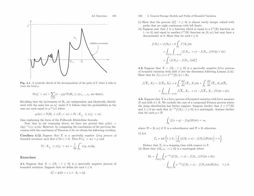
4.6 Exercises 105
x
infinite excursion
Tn− Tn
n
Fig. 4.1. A symbolic sketch of the decomposition of the path of Y when it fails tocross the level x.
P(σ+x = ∞) =
∑n≥0
(1− ρ)ρnP(Hn ≤ x|ǫ1, ..., ǫn are finite).
Recalling that the increments of Hn are independent and identically distrib-uted with the same law as σ+
0 under P it follows that the probabilities in thesum are each equal to µ∗n(x) where
µ(dx) = P(H1 ≤ x|T1 <∞) = P(−Xτ−0≤ x|τ−0 <∞)
thus explaining the form of the Pollaczek–Khintchine formula.Note that in our reasoning above, we have not proved that µ(dx) =
(dρ)−1ν(x,∞)dx. However, by comparing the conclusions of the previous dis-cussion with the conclusion of Theorem 4.10, we obtain the following corollary.
Corollary 4.12. Suppose that X is a spectrally negative Levy process ofbounded variation such that ψ′(0+) > 0. Then P(τ−0 <∞) = ρ and
P(−Xτ−0≤ x|τ−0 <∞) =
1dρ
∫ x
0
ν(y,∞)dy.
Exercises
4.1. Suppose that X = Xt : t ≥ 0 is a spectrally negative process ofbounded variation. Suppose that we define for each t ≥ 0,
L0t = #0 < s ≤ t : Xt = 0.
106 4 General Storage Models and Paths of Bounded Variation
(i) Show that the process L0t : t ≥ 0 is almost surely integer valued with
paths that are right continuous with left limits.(ii) Suppose now that f is a function which is equal to a C1(R) function on
(−∞, 0) and equal to another C1(R) function on (0,∞) but may have adiscontinuity at 0. Show that for each t ≥ 0,
f(Xt) = f(X0) + d
∫ t
0
f ′(Xs)ds
+∫
(0,t]
∫(−∞,0)
(f(Xs− + x)− f(Xs−))N(ds× dx)
+∫ t
0
(f(Xs)− f(Xs−))dL0s.
4.2. Suppose that X = Xt : t ≥ 0 is a spectrally negative Levy processof bounded variation with drift d (see the discussion following Lemma 2.14).Show that for f(s, x) ∈ C1,1([0,∞)× R),
f(Xt, Xt) = f(X0, X0) + d
∫ t
0
∂f
∂x(Xs, Xs)ds+
∫ t
0
∂f
∂s(Xs, Xs)dXs
+∫
[0,t]
∫(−∞,0)
f(Xs, Xs− + x)− f(Xs, Xs−)N(ds× dx).
4.3. Suppose thatX is a Levy process of bounded variation with Levy measureΠ and drift d ∈ R. We exclude the case of a compound Poisson process wherethe jump distribution has lattice support. Suppose further that f ∈ C1(R)and λ ≥ 0 are such that e−λtf(Xt) : t ≥ 0 is a martingale. Assume furtherthat for each y ∈ D, ∫
R|f(x+ y)− f(y)|Π(dx) <∞,
where D = [0,∞) if X is a subordinator and D = R otherwise.
(i) Let
Tn = inft ≥ 0 :
∣∣∣∣∫R(f(Xt + x)− f(Xt))Π(dx)
∣∣∣∣ > n
.
Deduce that Tn is a stopping time with respect to F.(ii) Show that Mt∧Tn
: t ≥ 0 is a martingale where
Mt =∫
[0,t]
∫R
e−λs(f(Xs− + x)− f(Xs−))N(ds× dx)
−∫
[0,t]
∫R
e−λs(f(Xs + x)− f(Xs))dsΠ(dx), t ≥ 0.
4.6 Exercises 107
(iii) Deduce with the help of the change of variable formula that, under theassumption that the support of the distribution of Xs is R for all s > 0,
d∂f
∂y(y) +
∫R(f(y + x)− f(y))Π(dx) = λf(y)
for all y ∈ R.(iv) Assume now that for given β ∈ R,
∫|x|>1
eβxΠ(dx) < ∞. Show that iff(x) = eβx then necessarily λ = ψ(β).
4.4. Suppose that φ fulfils the conditions of Theorem 4.4 and that for eacht > 0, E(
∫[0,t]
∫R |φ(s, x)|dsΠ(dx)) < ∞. If M = Mt : t ≥ 0 is the mar-
tingale given in Corollary 4.6 and further, it is assumed that for all t ≥ 0,E(∫[0,t]
∫R φ(s, x)2dsΠ(dx)) <∞ show that
E(M2t ) = E
(∫[0,t]
∫Rφ(s, x)2dsΠ(dx)
).
4.5. In this exercise, we use ideas coming from the proof of the Levy–Itodecomposition to prove Ito’s formula in Theorem 4.3 but for the case thatσ = 0. Henceforth we will assume that X is a Levy process with no Gaussiancomponent and f(s, x) ∈ C1,2([0,∞)× R) which is uniformly bounded alongwith its first derivative in s and first two derivatives in x.
(i) Suppose that X has characteristic exponent
Ψ(θ) = iθa+∫
R(1− eiθx + iθx1(|x|<1))Π(dx).
For each 1 > ε > 0 let X(ε) = X(ε)t : t ≥ 0 be the Levy process with
characteristic exponent
Ψ (ε)(θ) = iθa+∫
R\(−ε,ε)(1− eiθx + iθx1(|x|<1))Π(dx).
Show that
f(t,X(ε)t )
= f(0, X0) +∫ t
0
∂f
∂s(s,X(ε)
s )ds
+∫
[0,t]
∫|x|>ε
(f(s,X(ε)s− + x)− f(s,X(ε)
s− )− x∂f
∂x(s,X(ε)
s− ))N(ds× dx)
+∫ t
0
∂f
∂x(s,X(ε)
s− )dX(2)s +M
(ε)t , (4.20)
where X(2) is a Levy process with characteristic exponent aiθ+∫|x|≥1
(1−eiθx)Π(dx) and M (ε) = M (ε)
t : t ≥ 0 is a right continuous, squareintegrable martingale with respect to the filtration Ft : t ≥ 0 of Xwhich you should specify.
108 4 General Storage Models and Paths of Bounded Variation
(ii) Fix T > 0. Show that M (ε) : 0 < ε < 1 is a Cauchy family in themartingale space M2
T (see Definition 2.11).(iii) Denote the limiting martingale in part (ii) by M . By taking limits as ε ↓ 0
along a suitable subsequence, show that the Ito formula holds where wemay define ∫ t
0
∂f
∂x(s,Xs−)dXs =
∫ t
0
∂f
∂x(s,Xs−)dX(2) +Mt.
Explain why the left-hand side above is a suitable choice of notation.(iv) Show that if the restrictions of uniform boundedness of f and its deriva-
tives using stopping times are removed then the same conclusion may bedrawn as in (iii) except now there exists an increasing sequence of stop-ping times tending to infinity, say Tn : n ≥ 1 , such that for each n ≥ 1the process M is a martingale when stopped at time Tn. In other words,M is a local martingale and not necessarily a martingale.
4.6. Consider the workload process W of an M/G/1 queue as described inSect. 1.3.2. Suppose that W0 = w = 0 and the service distribution F hasLaplace transform F (β) =
∫(0,∞)
e−βxF (dx).
(i) Show that the first busy period (the time from the moment of first serviceto the first moment thereafter that the queue is again empty), denoted B,fulfils
E(e−βB) = F (Φ(β))
where Φ(β) is the largest solution to the equation
θ −∫
(0,∞)
(1− e−θx)λF (dx) = β.
(ii) When ρ > 1, show that there are a geometrically distributed number ofbusy periods. Hence give another proof of the first part of Theorem 4.1when w = 0 by using this fact.
(iii) Suppose further that the service distribution F is that of an exponentialrandom variable with parameter µ > λ. This is the case of an M/M/1queue. Show that the workload process has limiting distribution given by(
1− λ
µ
)(δ0(dx) + 1(x>0)λe−(µ−λ)xdx
).
4.7. This exercise is only for the reader familiar with the general theoryof stochastic calculus with respect to semi-martingales. Suppose that X isa general spectrally negative Levy process. Recall the notation Et(α) =expαXt − ψ(α)t for t ≥ 0.
(i) If M is the Kella–Whitt martingale, show that
dMt = −e−Xt+ψ(α)tdEt(α)
and hence deduce that M is a local martingale.
4.6 Exercises 109
(ii) Show that E(Xt) <∞ for all t > 0.(iii) Deduce that E(sups≤t |Ms|) <∞ and hence that M is a martingale.
4.8. Suppose thatX is a spectrally negative Levy process of bounded variationwith characteristic exponent Ψ .
(i) Show that for each α, β ∈ R,
Mt = −Ψ(α)∫ t
0
eiα(Xs−Xs)+iβXsds+ 1− eiα(Xt−Xt)+iβXt
−i(α− β)∫ t
0
eiα(Xs−Xs)+iβXsdXs, t ≥ 0
is a martingale. Note, for the reader familiar with general stochastic cal-culus for semi-martingales, one may equally prove that the latter is amartingale for a general spectrally negative Levy process.
(ii) Use the fact that E(Meq) = 0, where eq is an independent exponentially
distributed random variable with parameter q, to show that
E(eiα(Xeq−Xeq )+iβXeq ) =q(Φ(q)− iα)
(Ψ(α) + q)(iβ − Φ(q)), (4.21)
where Φ is the right inverse of the Laplace exponent ψ(β) = −Ψ(−iβ).(iii) Deduce that Xeq
−Xeqand Xeq
are independent.
4.9. Suppose that X is any Levy process of bounded variation with drift d > 0(excluding subordinators).
(i) Show that
limt↓0
Xt
t= d
almost surely.(ii) Define τ−0 = inft > 0 : Xt < 0. By reasoning along similar lines for the
case of a spectrally negative process, show that P(τ−0 > 0) > 0(iii) Suppose now that limt↑∞Xt = ∞. Let η(dx) = P(−Xτ−0
∈ dx|τ−0 <∞).Conclude that the Pollaczek–Khinchine formula
Px(τ−0 = ∞) = (1− ρ)∞∑k=0
ρkη∗k(x)
is still valid under these circumstances.
5
Subordinators at First Passage andRenewal Measures
In this chapter we look at subordinators; Levy processes which have pathsthat are non-decreasing. In addition, we consider killed subordinators. Thatis subordinators which are sent to a “graveyard state” (in other words anadditional point that is not on [0,∞)) at an independent time that is expo-nentially distributed. Principally we are interested in first passage over a fixedlevel and some asymptotic features of the processes as this level tends to in-finity. In particular, the (asymptotic) law of the overshoot and undershoot aswell as the phenomena of crossing a level by hitting it. These three points ofinterest turn out to be very closely related to renewal measures. The resultsobtained in this chapter will be of significance later on when we consider firstpassage of a general Levy process over a fixed level. As part of the presenta-tion on asymptotic first passage, we will review some basic facts about regularvariation. Regular variation will also be of use in later chapters.
5.1 Killed Subordinators and Renewal Measures
Recall that a subordinator is a Levy process with paths which are non-decreasing almost surely. Equivalently, a subordinator is a Levy process ofbounded variation, positive drift d > 0 and jump measure concentrated on(0,∞). In this section we shall consider a slightly more general class of process,killed subordinators. Let Y be a subordinator and eη an independent exponen-tially distributed random variable for some η > 0. Then a killed subordinatoris the process
Xt =Yt if t < eη∂ if t ≥ eη,
where ∂ is a “graveyard state”. We shall also refer to X as “Y killed at rateη”. If we agree that eη = ∞ when η = 0 then the definition of a killed
112 5 Subordinators at First Passage and Renewal Measures
subordinator includes the class of regular subordinators.1 This will prove tobe useful for making general statements. The Laplace exponent of a killedsubordinator X is defined for all θ ≥ 0 by the formula
Φ(η) = − log E(e−θX1) = − log E(e−θY11(1<eη)) = η−log E(e−θY1) = η+Ψ(iθ),
where Ψ is the Levy–Khintchine exponent of Y . From the Levy–Khintchineformula given in the form (2.21) we easily deduce that
Φ(θ) = η + dθ +∫
(0,∞)
(1− e−θx)Π(dx), (5.1)
where d ≥ 0 and∫(0,∞)
(1 ∧ x)Π(dx) <∞; recall Exercise 2.11.With each killed subordinator we associate a family of potential measures.
Define for each q ≥ 0 the q-potential measure by
U (q)(dx) = E(∫ ∞
0
e−qt1(Xt∈dx)dt)
=∫ ∞
0
e−qtP(Xt ∈ dx)dt.
For notational ease we shall simply write U (0) = U and call it the poten-tial measure. Note that the q-potential measure of a killed subordinator withkilling at rate η > 0 is equal to the (q + η)-potential measure of a subordi-nator. Note also that for each q > 0, (q + η)U (q) is a probability measure on[0,∞) and also that for each q ≥ 0 U (q)(x) := U (q)[0, x] is right continuous.Roughly speaking, a q-potential measure is an expected discounted measureof how long the process X occupies different regions of space.2
These potential measures will play an important role in the study of howsubordinators cross fixed levels. For this reason we will devote the remain-der of this section to studying some of their analytical properties. One of themost important facts about q-potential measures is that they are closely re-lated to renewal measures. Recall that the renewal measure associated with adistribution F concentrated on [0,∞) is defined by
V (dx) =∑k≥0
F ∗k(dx), x ≥ 0,
where we understand F ∗0(dx) := δ0(dx). As with potential measures we workwith the notation V (x) := V [0, x]. For future reference let us recall the twoversions of the classical Renewal Theorem.
Theorem 5.1 (Renewal Theorem). Suppose that V is the renewal func-tion given above and assume that µ :=
∫(0,∞)
xF (dx) <∞.
1A killed subordinator is only a Levy process when η = 0 however, it is still aMarkov process even when η > 0.
2From the general theory of Markov processes, U (q) also comes under name ofresolvent measure or Green’s measure.
5.1 Killed Subordinators and Renewal Measures 113
(i) If F does not have lattice support then for all y > 0,
limx↑∞
V (x+ y)− V (x) =y
µ.
(ii) 3If F does not have lattice support and h : R → R is directly Riemannintegrable, then
limx↑∞
∫ x
0
h(x− y)V (dy) =1µ
∫ ∞
0
h(y)dy.
(iii) Without restriction on the support of F ,
limx↑∞
V (x)x
=1µ.
The precise relationship between q-potential measures of subordinatorsand renewal measures is given in the following lemma.
Lemma 5.2. Suppose that X is a subordinator (no killing). Let F = U (1) andlet V be the renewal measure associated with the distribution F . Then V (dx)is equal to the measure δ0(dx) + U(dx) on [0,∞).
Proof. First note that for all θ > 0,∫[0,∞)
e−θxU (1)(dx) =∫ ∞
0
dt · e−t∫
[0,∞)
e−θxP(Xt ∈ dx)
=∫ ∞
0
dt · e−(1+Φ(θ))t
=1
1 + Φ(θ),
where Φ is the Laplace exponent of the underlying subordinator. Note that inthe final equality we have used the fact that Φ(θ) > 0.
Next compute the Laplace transform of V for all θ > 0 as follows,∫[0,∞)
e−θxV (dx) =∑k≥0
(∫[0,∞)
e−θxU (1)(dx)
)k
=∑k≥0
(1
1 + Φ(θ)
)k=
11− (1 + Φ(θ))−1
= 1 +1
Φ(θ). (5.2)
3This part of the theorem is also known on its own as the Key Renewal Theorem.
114 5 Subordinators at First Passage and Renewal Measures
Note that in the third equality we have used the fact that |1/(1+Φ(θ))| < 1.On the other hand, a similar computation to the one in the first paragraph
of this proof shows that the Laplace transform of δ0(dx) + U(dx) equals theright-hand side of (5.2). Since distinct measures have distinct Laplace trans-forms the proof is complete.
The conclusion of the previous Lemma means that the Renewal Theoremcan, and will, be employed at a later stage to understand the asymptoticbehaviour of U . Specifically we have the following two asymptotics.
Corollary 5.3. Suppose that X is a subordinator (no killing) such that µ :=E(X1) <∞.
(i) If U does not have lattice support, then for all y > 0,
limx↑∞
U(x+ y)− U(x) =y
µ.
(ii) Without restriction on the support of U ,
limx↑∞
U(x)x
=1µ.
Proof. The proof is a direct consequence of Theorem 5.1 once one notes that
µ =∫
[0,∞)
xU (1)(dx) =∫ ∞
0
e−tE(Xt)dt =∫ ∞
0
te−tE(X1)dt = E(X1)
and that U (1) has the same support as U .
In the previous corollary, the requirement that U does not have a latticesupport is not a serious restriction as there are analogues to Corollary 5.3(i); see for example Feller (1971). The following theorem, based on standardresults in Blumenthal and Getoor (1968), shows that in principle one can onlyfind examples of potential measures with lattice support when X is a killedcompound Poisson subordinator. The statement of the theorem gives in facta stronger conclusion than the latter.
Theorem 5.4. Suppose that X is a killed subordinator with Levy measure Π.
(i) If Π(0,∞) = ∞ then for any q ≥ 0, U (q) has no atoms.(ii) If Π(0,∞) <∞ and Π has a non-lattice support then for all q ≥ 0, U (q)
does not have a lattice support.(iii) If Π(0,∞) <∞ and Π has a lattice support, then for all q ≥ 0, U (q) has
the same lattice support in (0,∞).
Proof. (i) Recall the definition
U (q)(dx) = E(∫ ∞
0
e−qt1(Xt∈dx)dt)
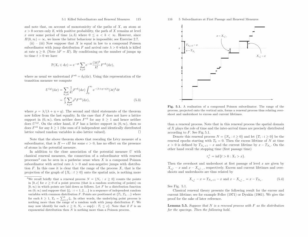
5.1 Killed Subordinators and Renewal Measures 115
and note that, on account of monotonicity of the paths of X, an atom atx > 0 occurs only if, with positive probability, the path of X remains at levelx over some period of time (a, b) where 0 ≤ a < b < ∞. However, sinceΠ(0,∞) = ∞, we know the latter behaviour is impossible; see Exercise 2.7.
(ii) – (iii) Now suppose that X is equal in law to a compound Poissonsubordinator with jump distribution F and arrival rate λ > 0 which is killedat rate η ≥ 0. (Note λF = Π). By conditioning on the number of jumps upto time t > 0 we have
P(Xt ∈ dx) = e−ηt∑k≥0
e−λt(λt)k
k!F ∗k(dx),
where as usual we understand F ∗0 = δ0(dx). Using this representation of thetransition measure we compute
U (q)(dx) =∑k≥0
1k!F ∗k(dx)
∫ ∞
0
e−(λ+q+η)t(λt)kdt
=ρ
λ
∑k≥0
ρkF ∗k(dx), (5.3)
where ρ = λ/(λ + η + q). The second and third statements of the theoremnow follow from the last equality. In the case that F does not have a latticesupport in (0,∞), then neither does F ∗k for any k ≥ 1 and hence neitherdoes U (q). On the other hand, if F has a lattice support in (0,∞), then sodoes F ∗k for any k ≥ 1 (the sum of k independent and identically distributedlattice valued random variables is also lattice valued).
Note that the above theorem shows that rescaling the Levy measure of asubordinator, that is Π → cΠ for some c > 0, has no effect on the presenceof atoms in the potential measure.
In addition to the close association of the potential measure U withclassical renewal measures, the connection of a subordinator with renewalprocesses4 can be seen in a pathwise sense when X is a compound Poissonsubordinator with arrival rate λ > 0 and non-negative jumps with distribu-tion F . In this case it is clear that the range of the process X, that is theprojection of the graph of Xt : t ≥ 0 onto the spatial axis, is nothing more
4We recall briefly that a renewal process N = Nx : x ≥ 0 counts the pointsin [0, x] for x ≥ 0 of a point process (that is a random scattering of points) on[0,∞) in which points are laid down as follows. Let F be a distribution functionon (0,∞) and suppose that ξi : i = 1, 2, ... is a sequence of independent randomvariables with common distribution F . Points are positioned at T1, T2, ... where
for each k ≥ 1, Tk =∑k
i=1ξi. In other words, the underlying point process is
nothing more than the range of a random walk with jump distribution F . Wemay now identify for each x ≥ 0, Nx = supi : Ti ≤ x. Note that if F is anexponential distribution then N is nothing more than a Poisson process.
116 5 Subordinators at First Passage and Renewal Measures
TNx+1 − x
x − TNx
x − Xτx+
−
Xτx+ − x
x
Fig. 5.1. A realisation of a compound Poisson subordinator. The range of theprocess, projected onto the vertical axis, forms a renewal process thus relating over-shoot and undershoot to excess and current lifetimes.
than a renewal process. Note that in this renewal process the spatial domainof X plays the role of time and the inter-arrival times are precisely distributedaccording to F . See Fig. 5.1.
Denote this renewal process N = Nx : t ≥ 0 and let Ti : i ≥ 0 be therenewal epochs starting with T0 = 0. Then the excess lifetime of N at timex > 0 is defined by TNx+1 − x and the current lifetime by x − TNx
. On theother hand recall the stopping time (first passage time)
τ+x = inft > 0 : Xt > x.
Then the overshoot and undershoot at first passage of level x are given byXτ+
x− x and x −Xτ+
x −, respectively. Excess and current lifetimes and over-shoots and undershoots are thus related by
Xτ+x− x = TNx+1 − x and x−Xτ+
x − = x− TNx. (5.4)
See Fig. 5.1.Classical renewal theory presents the following result for the excess and
current lifetime; see for example Feller (1971) or Dynkin (1961). We give theproof for the sake of later reference.
Lemma 5.5. Suppose that N is a renewal process with F as the distributionfor the spacings. Then the following hold.
5.1 Killed Subordinators and Renewal Measures 117
(i) For u > 0 and y ∈ (0, x],
P(TNx+1 − x ∈ du, x− TNx∈ dy) = V (x− dy)F (du+ y), (5.5)
where V is the renewal measure constructed from F .(ii) Suppose that F has mean µ < ∞ and is non-lattice, then for u > 0 and
y > 0,
limx↑∞
P(TNx+1 − x > u, x− TNx> y) =
1µ
∫ ∞
u+y
F (z)dz,
where F (x) = 1− F (x).
Proof. (i) The key to the proof of the first part is to condition on the numberof renewal epochs at time x. We have for k ≥ 0,
P(TNx+1 − x > u, x− TNx> y|Nx = k) =
∫[0,x−y)
F ∗k(dv)F (x− v + u)
as the probability on the left-hand side requires that the kth renewal epochoccurs sometime before x−y. Further, this epoch occurs in dv with probabilityF ∗k(dv) and hence the probability that the excess exceeds u requires that thenext inter-arrival time exceeds x−v+u with probability F (x−v+u). Summingover k and changing variable in the integral via z = x− v gives
P(TNx+1 − x > u, x− TNx> y) =
∫(y,x]
V (x− dz)F (z + u).
In differential form this gives the distribution given in the statement of part(i).
(ii) From part (i) we may write for u > 0 and y ∈ [0, x),
P(TNx+1 − x > u, x− TNx> y)
=∫
(u,∞)
∫[0,x−y)
V (dv)F (x− v + dθ)
=∫
(0,∞)
F (dt)∫
[0,x)
V (dv)1(t>u+x−v)1(v∈[0,x−y))
=∫
(0,∞)
F (dt)∫
[0,x)
V (dv)1(v>u+x−t)1(v∈[0,x−y)),
where we have applied the change of variables t = θ + x − v in the secondequality. Now note that the indicators and integral delimiters require that
v ≥ (u+ x− t) ∨ 0 and u+ x− t ≤ x− y.
118 5 Subordinators at First Passage and Renewal Measures
Hence for u > 0 and y ∈ [0, x),
P(TNx+1 − x > u, x− TNx> y)
=∫
(0,∞)
F (dt)V (x− y)− V ((u+ x− t) ∨ 0)1(t≥u+y)
=∫
(u+y,∞)
F (dt)V (x− y)− V (u+ x− t)1(t<u+x)
+∫
[u+x,∞)
F (dt)V (x− y). (5.6)
To deal with the second term on the right-hand side of (5.6) we may use theRenewal Theorem 5.1 (iii) to show that for some ε > 0 and x sufficiently large∫
(u+x,∞)
F (dt)V (x− y) ≤ 1 + ε
µ
∫(u+x,∞)
tF (dt)
which tends to zero as x tends to infinity as µ =∫(0,∞)
tF (dt) <∞.For the first term on the right-hand side of (5.6) suppose that X is a
compound Poisson subordinator whose jump distribution is F and arrivalrate is 1, then for this subordinator
E(τ+x ) =
∫ ∞
0
P(τ+x > t)dt =
∫ ∞
0
P(Xt ≤ x)dt = V (x),
where the final equality follows from (5.3) with q = η = 0 and λ = 1. Nowapplying the strong Markov property we can establish that
V (x+ y) = E(τ+x+y)
= E(τ+x + EX
τ+x
(τ+x+y))
≤ E(τ+x ) + E(τ+
y )= V (x) + V (y).
Using then the bound V (x−y)−V (u+x−t) ≤ V (t−u−y), the right continuityof V and the Renewal Theorem 5.1 (iii) we know that the integrand in firstterm on the hand side of (5.6) is bounded by a constant times t. Hence as∫(0,∞)
tF (dt) <∞ dominated convergence applies together with Theorem 5.1(i) to give
limx↑∞
∫(u+y,∞)
F (dt)V (x− y)− V (u+ x− t)1(t<u+x)
=1µ
∫(u+y,∞)
(t− u− y)F (dt)
=1µ
∫ ∞
u+y
F (t)dt,
where the final equality follows on integration by parts.
5.2 Overshoots and Undershoots 119
In light of (5.4) we see that Lemma 5.5 gives the exact and asymptoticdistribution of the overshoot and undershoot at first passage of a compoundPoisson subordinator with jump distribution F (with finite mean and non-lattice support in the case of the asymptotic behaviour). In this spirit, theaim of the remainder of this chapter is to study the exact and asymptoticjoint distributions of the overshoot and undershoot of a killed subordinatorat first passage.
There are a number of differences in the range of a killed subordinatorcompared to the range of a compound Poisson subordinator which createadditional difficulties to the situation described above. Firstly, in the case ofa killed subordinator, the process may be killed before reaching a specifiedfixed level and hence one should expect an atom in the distribution of theovershoot at ∞. Secondly, the number of jumps over a finite time horizonmay be infinite, which occurs if and only if Π(0,∞) = ∞, and hence in thiscase the analysis in the proof of Lemma 5.5 (i) is no longer valid. Finally,in the case of a compound Poisson subordinator when F has no atoms, itis clear that the probability that there is first passage over a given level byhitting the level is zero. However, when moving to a killed subordinator forwhich either Π(0,∞) = ∞ or there is a drift present, one should not excludethe possibility that first passage over a fixed level occurs by hitting the levelwith positive probability. The latter behaviour is called creeping over a fixedlevel and is equivalent to there being an atom at zero in the distribution ofthe overshoot at that level. As one might intuitively expect, creeping over aspecified fixed level turns out to occur only in the presence of a drift in whichcase it is possible to creep over all fixed levels. These points will be dealt within more detail in Sect. 5.3
5.2 Overshoots and Undershoots
We begin with the following theorem which gives the generalisation of Lemma5.5 (i); indeed containing it as a corollary. Weaker versions of this theoremcan be found in Kesten (1969) and Horowitz (1972). The format we give isfrom Bertoin (1996a).
Theorem 5.6. Suppose that X is a killed subordinator. Then for u > 0 andy ∈ [0, x],
P(Xτ+x− x ∈ du, x−Xτ+
x − ∈ dy) = U(x− dy)Π(y + du). (5.7)
Proof. The proof principally makes use of the compensation formula. Supposethat f and g are two positive, bounded, continuous functions satisfying f(0) =0. The latter ensures that the product f(Xτ+
x−x)g(x−Xτ+
x −) is nonzero onlyif X jumps strictly above x when first crossing x. This means that we maywrite the expectation of the latter variable in terms of the Poisson randommeasure associated with the jumps of X whilst avoiding the issue of creeping.
120 5 Subordinators at First Passage and Renewal Measures
To this end, let us assume that X is equal in law to a subordinator Y killedat rate η ≥ 0. Then
E(f(Xτ+x− x)g(x−Xτ+
x −)) = E
(∫[0,∞)
∫(0,∞)
e−ηtφ(t, θ)N(dt× dθ)
),
whereφ(t, θ) = 1(Yt−≤x)1(Yt−+θ>x)f(Yt− + θ − x)g(x− Yt−),
and N is the Point random measure associated with the jumps of Y . Notethat it is straightforward to see that φ satisfies the conditions of Theorem4.4; in particular that it is left continuous in t. Then with the help of theaforementioned theorem∫
[0,x]
g(y)∫
(0,∞)
f(u)P(Xτ+x− x ∈ du, x−Xτ+
x − ∈ dy)
= E
(∫ ∞
0
dt · e−ηt1(Yt−≤x)g(x− Yt−)∫
(x−Yt−,∞)
f(Yt− + θ − x)Π(dθ).
)
= E
(∫ ∞
0
dt · e−ηt1(Yt≤x)g(x− Yt)∫
(x−Yt,∞)
f(Yt + θ − x)Π(dθ)
)
=∫
[0,x]
g(x− z)∫
(x−z,∞)
f(z + θ − x)Π(dθ)∫ ∞
0
dt · e−ηtP(Yt ∈ dz)
=∫
[0,x]
g(x− z)∫
(x−z,∞)
f(z + θ − x)Π(dθ)U(dz)
=∫
[0,x]
g(y)∫
(0,∞)
f(u)Π(du+ y)U(x− dy), (5.8)
where the final equality follows by changing variables with y = x−z and thenagain with u = θ−y. (Note also that U is the potential measure of X and notY ). As f and g are arbitrary within their prescribed classes, we read off fromthe left and right-hand sides of (5.8) the required distributional identity.
Intutively speaking, the proof of Theorem 5.6 follows the logic of the proofof Lemma 5.5 (i). The compensation formula serves as a way of “decomposing”the event of first passage by a jump over level x according to the position of Xprior to its first passage even when there are an unbounded number of jumpsover finite time horizons.
To make the connection with the expression given for renewal processesin Lemma 5.5 (i), recall from (5.3) that U(dx) = λ−1V (dx) on (0,∞) whereU is the potential measure associated with a compound Poisson subordinatorwith jump distribution F and arrival rate λ > 0 and V is the renewal measureassociated with the distribution F . For this compound Poisson subordinator,we also know that Π(dx) = λF (dx) so that U(x−dy)Π(du+ y) = V (x−dy)
5.3 Creeping 121
F (u + dy). Setting f(·) = 1(·>u) and g(·) = 1(·>y), an easy calculation nowbrings one from the right hand side of (5.8) to the right-hand side of (5.5).
As (5.7) is the analogue of the statement in Lemma 5.5 (i) it is now naturalto reconsider the proof of part (ii) of the same lemma in the more generalcontext. The following result was presented in Bertoin et al. (1999).
Theorem 5.7. Suppose that X is a subordinator (no killing) with finite meanµ := E(X1) and such that U does not have lattice support (cf. Theorem 5.4).Then for u > 0 and y ≥ 0, in the sense of weak convergence
limx↑∞
P(Xτ+x− x ∈ du, x−Xτ+
x − ∈ dy) =1µ
dyΠ(y + du).
In particular it follows that the asymptotic probability of creeping satisfies
limx↑∞
P(Xτ+x
= x) =d
µ.
The proof of this result is a straightforward adaptation of the proof ofLemma 5.5 (ii) taking advantage of Corollary 5.3 and is left to the reader toverify in Exercise 5.1.
5.3 Creeping
Now let us turn to the issue of creeping. Although τ+x is the first time that X
strictly exceeds the level x > 0 it is possible that in fact P(Xτ+x
= x) > 0; recallthe statement and proof of Theorem 3.3. The following conclusion, found forexample in Horowitz (1972), shows that crossing the level x > 0 by hitting itcannot occur by jumping onto it from a position strictly below x in the casewhere the jump measure is infinite. In other words, if our killed subordinatormakes first passage above x with a jump then it must do so by jumping itclear, so Xτ+
x= x = Xτ+
x− x = 0, x − Xτ+
x − = 0, which is of implicitrelevance when computing the atom at zero in the overshoot distribution.
Lemma 5.8. Let X be any killed subordinator with Π(0,∞) = ∞. For allx > 0 we have
P(Xτ+x− x = 0, x−Xτ+
x − > 0) = 0. (5.9)
Proof. Suppose for a given x > 0 that
P(Xτ+x− x = 0, x−Xτ+
x − > 0) > 0.
Then this implies that there exists a y < x such that
P(Xτ+y
= x) > 0.
However the latter cannot happen because of the combined conclusions ofTheorem 5.6 and Theorem 5.4 (i). Hence by contradiction (5.9) holds.
122 5 Subordinators at First Passage and Renewal Measures
Although one may write with the help of Theorem 5.6 and Lemma 5.8
P(Xτ+x
= x) = 1− P(Xτ+x> x) = 1−
∫(0,x]
U(x− dy)Π(y,∞)
this does not bring one closer to understanding when the probability on theleft-hand side above is strictly positive. In fact, although the answer to thisquestion is intuitively obvious, it turns out to be difficult to prove. It wasresolved by Kesten (1969); see also Bretagnolle (1972). The result is givenbelow.
Theorem 5.9. For any killed subordinator with jump measure Π satisfyingΠ(0,∞) = ∞, and drift coefficient d we have the following.
(i) If d = 0 then P(Xτ+x
= x) = 0 for all x > 0.(ii) If d > 0 then U has a strictly positive and continuous density on (0,∞),
say u, satisfyingP(Xτ+
x= x) = du(x).
The version of the proof we give here for the above result follows thereasoning in Andrew (2005) (see also Section III.2 of Bertoin (1996a)) and firstrequires two auxiliary Lemmas given below. In the proof of both we shall makeuse of the following two key estimates for the probabilities px := P(Xτ+
x= x),
x > 0. For all 0 < y < x,
px ≤ pypx−y + (1− px−y) (5.10)
andpx ≥ pypx−y. (5.11)
The upper bound is a direct consequence of the fact that
P(Xτ+x
= x) = P(Xτ+x−y
= x− y, Xτ+x
= x)
+P(Xτ+x−y
> x− y, Xτ+x
= x)
≤ P(Xτ+x−y
= x− y)P(Xτ+x
= x|X0 = x− y)
+P(Xτ+x−y
> x− y),
where in the last line the Strong Markov Property has been used. In a similarway the lower bound is a consequence of the fact that
P(Xτ+x
= x) ≥ P(Xτ+x−y
= x− y)P(Xτ+x
= x|X0 = x− y).
Lemma 5.10.
(i) If for some x > 0 we have px > 0 then limε↓0 supη∈(0,ε) pη = 1.(ii) If for some x > 0 we have px > 3/4 then
py ≥ 1/2 +√px − 3/4
for all y ∈ (0, x].
5.3 Creeping 123
Proof. (i) From Lemma 5.8 we know that X cannot jump onto x. In otherwords
P(Xτ+x
= x > Xτ+x −) = 0.
This implies that
Xτ+x
= x ⊆⋂n≥1
X visits (x− 1/n, x)
almost surely. On the other hand, on the event⋂n≥1X visits (x − 1/n, x)
we also have by quasi-left-continuity (cf. Lemma 3.2) that Xσ = x whereσ = limn↑∞ τ+
x−1/n (the limit exists because of monotonicity). Since
σ ≤ t =⋂n≥1
τ+x−1/n ≤ t
almost surely it follows that σ is a stopping time with respect to F. Applyingthe Strong Markov Property at time σ, since Xσ = x and X is not a compoundPoisson subordinator, we have that Xt > x for all t > σ showing that in factσ = τ+
x . In conclusion
Xτ+x
= x =⋂n≥1
X visits (x− 1/n, x)
almost surely.We may now write
px = limn↑∞
P(X visits (x− 1/n, x)). (5.12)
Also we may upper estimate
px ≤ P(X visits (x− 1/n, x)) supz∈(0,1/n)
pz.
Letting n ↑ ∞ in the above inequality and taking (5.12) into account we seethat limε↓0 supη∈(0,ε) pη = 1.
(ii) Suppose that 0 < y < x. We may assume without loss of generalitythat py < px for otherwise it is clear that py ≥ px > 3/4 ≥ 1/2 +
√px − 3/4.
From (5.10) it is a simple algebraic manipulation replacing y by x− y toshow that
py ≤ 1− px1− px−y
.
and again replacing y by x− y in the above inequality to deduce that
1− px−y ≥ px − py1− py
.
124 5 Subordinators at First Passage and Renewal Measures
Combining the last two inequalities we therefore have
py ≤ (1− px)(1− py)px − py
and hence the quadratic inequality p2y − py + 1− px ≥ 0. This in turn implies
that
py ∈ [0, 1/2−√px − 3/4] ∪ [1/2 +
√px − 3/4, 1]. (5.13)
The remainder of the proof is thus dedicated to showing that inclusion of pyin the first of the two intervals cannot happen.
Suppose then for contradiction that (5.13) holds for all y ≤ x and thereexists a y ∈ (0, x) such that py ≤ 1/2−√px − 3/4. Now define
g = supz ∈ [0, y); pz ≥ 1/2 +√px − 3/4
which is well defined since at least p0 = 1. Note from this definition that itcould be the case that g = y. Reconsidering the definition of g and (5.13), wesee that either there exists an ε > 0 such that pz ≤ 1/2 −√px − 3/4 for allz ∈ (g − ε, g) or for all ε > 0, there exists a sequence of z ∈ (g − ε, g) suchthat pz ≥ 1/2 +
√px − 3/4. In the former case it is clear by the definition of
g that pg ≥ 1/2 +√px − 3/4. In the latter case, we see when referring back
to (5.12) that
pg = limz↑g
P(X visits (z, g)) ≥ limε↓0
supη∈(0,ε)
pg−η
and hence pg ≥ 1/2 +√px − 3/4. For both cases this implies in particular
that g < y. On the other hand, using (5.11) and the conclusion of part (i) wesee that
limε↓0
supη∈(0,ε)
pg+η ≥ pg × limε↓0
supη∈(0,ε)
pη = pg ≥ 1/2 +√px − 3/4.
Since (5.13) is in force for all y ≤ x and g < y, this implies that there exists ag′ > g such that pg′ ≥ 1/2 +
√px − 3/4 which contradicts the definition of g.
The consequence of this contradiction is that there does not exist a y ∈ (0, x)for which py < 1/2 +
√px − 3/4 and hence from (5.13) it necessarily follows
that py ≥ 1/2 +√px − 3/4 for all y ∈ (0, x).
Lemma 5.11. Suppose there exists an x > 0 such that px > 0, then
(i) limε↓0 pε = 1 and(ii) x → px is strictly positive and continuous on [0,∞).
5.3 Creeping 125
Proof. (i) The first part is a direct consequence of parts (i) and (ii) of Lemma5.10.
(ii) Positivity follows from a repeated use of the lower estimate in (5.11)to obtain px ≥ (px/n)n and the conclusion of part (i).
To show continuity, note with the help of (5.10),
lim supε↓0
px+ε ≤ lim supε↓0
pεpx + 1− pε = px
and from (5.11) and part (i),
lim infε↓0
px+ε ≥ lim infε↓0
pxpε = px.
Further, arguing in a similar manner,
lim supε↓0
px−ε ≤ lim supε↓0
pxpε
= px
andlim infε↓0
px−ε ≥ lim infε↓0
px + pε − 1pε
= px.
Thus continuity is confirmed.
Finally we return to the proof of Theorem 5.9.
Proof (of Theorem 5.9). Consider the function
M(a) := E(∫ a
0
1(Xτ+x
=x)dx)
=∫ a
0
pxdx
for all a ≥ 0.For convenience, suppose further that X is equal in law to a subordinator
Y killed at rate η. Let N be the Poisson random measure associated withthe jumps of X (or equivalently Y ). Then we may write with the help of theLevy–Ito decomposition for subordinators,
M(a) = E
(Y(τ+
a ∧eη)− −∫
[0,τ+a ∧eη)
∫(0,∞)
xN(ds× dx)
)= dE(τ+
a ∧ eη).
(i) If d = 0 then px = 0 for Lebesgue almost every x. Lemma 5.11 nowimplies that px = 0 for all x > 0.
(ii) If d > 0 then three exists an x > 0 such that px > 0. Hence fromLemma 5.11, x → px is strictly positive and continuous. Further, we see that
M(a) = d
∫ ∞
0
P(τ+a ∧ eη > t)dt = d
∫ ∞
0
P(Xt ≤ a)dt = dU(a).
The latter implies that U has a density which may be taken as equal to d−1pxfor all x ≥ 0.
126 5 Subordinators at First Passage and Renewal Measures
We close this section by noting that the reason why the case of a killedcompound Poisson subordinator (Π(0,∞) <∞) is excluded from Theorem 5.9is because of possible atoms in Π. Take for example the case that Π consistsof a single atom at x0 > 0 then the same is true of the jump distribution. Thismeans that P(Xτ+
nx0= nx0) > 0 for all n ≥ 1. None the less P(Xτ+
x= x) = 0
for all other x.
5.4 Regular Variation and Tauberian Theorems
The inclusion of the forthcoming discussion on regular variation and Tauberiantheorems is a prerequisite to Sect. 5.5 which gives the Dynkin–Lamperti as-ymptotics for the joint law of the overshoot and undershoot. However, theneed for facts concerning regular variation will also appear in later sectionsand chapters.
Suppose that U is a measure supported on [0,∞) and with Laplace–transform
Λ(θ) =∫
[0,∞)
e−θxU(dx)
for θ ≥ 0 which may be infinite. Note that if there exists a θ0 such thatΛ(θ0) < ∞ then Λ(θ) < ∞ for all θ ≥ θ0. The point of this chapter is topresent some classic results which equivalently relate certain types of tail be-haviour of the measure U to a similar type of behaviour of Λ. Our presentationwill only offer the bare essentials based on the so called Karamata theory ofregularly varying functions. Aside from their intrinsic analytic curiosity, reg-ularly varying functions have proved to be of great practical value withinprobability theory, not least in the current context. The highly readable ac-count given in Feller (1971) is an important bridging text embedding intoprobability theory the classic work of Karamata and his collaborators whichdates back to the period between 1930 and the 1960s. For a complete account,the reader is referred to Bingham et al. (1987) or Embrechts et al. (1997). Thepresentation here is principally based on these books.
Definition 5.12. A function f : [0,∞) → (0,∞) is said to be regularly vary-ing at zero with index ρ ∈ R if for all λ > 0,
limx↓0
f(λx)f(x)
= λρ.
If the above limit holds as x tends to infinity then f is said to be regularlyvarying at infinity with index ρ. The case that ρ = 0 is referred to as slowvariation.
Note that any regularly varying function f may always be written in theform
f(x) = xρL(x)
5.4 Regular Variation and Tauberian Theorems 127
where L is a slowly varying function. Any function which has a strictly pos-itive and finite limit at infinity is slowly varying at infinity so the class ofslowly (and hence regularly) varying functions is clearly non-empty due tothis trivial example. There are however many non-trival examples of slowlyvarying functions. Examples include L(x) = log x, L(x) = logk x (the kthiterate of log x) and L(x) = exp(log x)/ log log x. All of these examples havethe property that they are functions which tend to infinity at infinity. Thefunction
L(x) := exp(log x)13 cos[(log x)
13 ]
is an example of a regularly varying function at infinity which oscillates. Thatis to say lim infx↑∞ L(x) = 0 and lim supx↑∞ L(x) = ∞.
The main concern of this section are the following remarkable results.
Theorem 5.13. Suppose that L is slowly varying at infinity, ρ ∈ [0,∞) andU is a measure supported on [0,∞). Then the following two statements areequivalent.
(i) Λ(θ) ∼ θ−ρL(1/θ), as θ → 0,(ii)U(x) ∼ xρL(x)/Γ (1 + ρ) as x→∞.
In the above theorem we are using the notation f ∼ g for functions f and gto mean that lim f(x)/g(x) = 1.
Theorem 5.14. Suppose that L is slowly varying at infinity, ρ ∈ (0,∞) andU is a measure on [0,∞) which has an ultimately monotone density, u. Thenthe following two statements are equivalent.
(i) Λ(θ) ∼ θ−ρL(1/θ), as θ → 0,(ii) u(x) ∼ xρ−1L(x)/Γ (ρ) as x→∞.
Recalling that Γ (1 + ρ) = ρΓ (ρ), Theorem 5.14 is a natural statementnext to Theorem 5.13. It says that, up to a slowly varying function, the as-ymptotic behaviour of the derivative of U(x) behaves like the derivative of thepolynomial that U(x) asymptotically mimics; providing of course the densityu exists and is ultimately monotone. The methods used to prove these resultsalso produce the following corollary with virtually no change at all.
Corollary 5.15. The statement of Theorems 5.13 and 5.14 are still validwhen instead the limits in their parts (i) and (ii) are simultaneously changedto θ →∞ and x→ 0.
We now give the proof of Theorem 5.13 which, in addition to the assumedregular variation, uses little more than the Continuity Theorem for Laplacetransforms of positive random variables.
Proof (of Theorem 5.13). It will be helpful for this proof to record the wellknown fact that for any ∞ > ρ ≥ 0 and λ > 0,
128 5 Subordinators at First Passage and Renewal Measures∫ ∞
0
xρe−λxdx =Γ (1 + ρ)λ1+ρ
. (5.14)
In addition we will also use the fact that for all λ > 0 and θ > 0,∫[0,∞)
e−λxU(dx/θ) = Λ(λθ). (5.15)
First we prove that (i) implies (ii). Fix λ0 > 0. From (5.15) we have forθ > 0 that e−λ0xU(dx/θ)/Λ(λ0θ) is a probability distribution. Again from(5.15) we can compute its Laplace transform as Λ((λ + λ0)θ)/Λ(λ0θ). Theregular variation assumed in (i) together with (5.14) implies that
limθ↓0
∫[0,∞)
e−(λ+λ0)xU(dx/θ)Λ(λ0θ)
=λρ0
(λ0 + λ)ρ=
λρ0Γ (ρ)
∫ ∞
0
xρ−1e−(λ+λ0)xdx,
where the right-hand side is the Laplace transform of a gamma distribution.It follows from the Continuity Theorem for Laplace transforms of probabilitydistributions that e−λ0xU(dx/θ)/Λ(λ0θ) converges weakly to e−λ0xλρ0x
ρ−1/Γ (ρ)dx as θ tends to zero. Using the regular variation of Λ again, this impliesthat for all x > 0,
limθ↓0
U(y/θ)L(1/θ)
λρ0θρ =
λρ0yρ
ρΓ (ρ).
Now setting y = 1, rewriting x = 1/θ and recalling that Γ (1 + ρ) = ρΓ (ρ),statement (ii) follows.
Now to prove that (ii) implies (i). The assumption in (ii) expressed interms of weak convergence implies that for each y ≥ 0,
limx↑∞
U(xdy)U(x)
= ρyρ−1dy,
in particular for any t > 0 and λ > 0,
limx↑∞
∫ t
0
e−λyU(xdy)U(x)
= ρ
∫ t
0
y(ρ−1)e−λydy. (5.16)
In view of (5.15), the Laplace transform of the measure U(xdy)/U(x) is givenby Λ(λ/x)/U(x) for λ > 0. Now suppose that for some 0 < λ0 < 1 and x0 > 0,the sequence Λ(λ0/x)/U(x) : x > x0 is uniformly bounded by some C > 0.With this further assumption in place, we may pick a sufficiently large t > 0such that
∫ ∞
t
e−yU(xdy)U(x)
< e−(1−λ0)t
∫ ∞
t
e−λ0yU(xdy)U(x)
< Ce−(1−λ0)t.
Together with (5.16), the above estimate is sufficient to deduce that
limx↑∞
Λ(1/x)U(x)
= limx↑∞
∫ ∞
0
e−yU(xdy)U(x)
= ρ
∫ ∞
0
y(ρ−1)e−ydy = Γ (1 + ρ).
Choosing λ = 1 and writing θ = 1/x, the statement in (i) follows.
5.4 Regular Variation and Tauberian Theorems 129
It remains then to show that for some 0 < λ0 < 1 and x0, the sequenceΛ(λ0/x)/U(x) : x > x0 is uniformly bounded by some C > 0. This isdone by partitioning the domain of integration over the lattice 2kx : k ≥ 0for some x > 0. The assumed regular variation of U implies that for all xsufficiently large U(2x) < 2ρ+1U(x). This can be iterated to deduce for xsufficiently large, U(2nx) < 2n(1+ρ)U(x) for each n ≥ 1. With this inequalityin hand we may quite coarsely estimate for all sufficiently large x,
Λ(λ0/x)U(x)
≤∑n≥1
e−λ02n−1 U(2nx)
U(x)<∑n≥1
2n(1+ρ)e−λ02n−1
<∞
and the proof is complete.
Next we turn to the proof of Theorem 5.14 which implicitly uses the state-ment of Theorem 5.13.
Proof (of Theorem 5.14). First we prove that (ii) implies (i). It suffices toprove that (ii) implies Theorem 5.13 (ii). However this is a simple issue ofweak convergence and regular variation, since for any y > 0,
ρU(xdy)xu(x)
=ρu(xy)xxu(x)
dy → ρyρ−1dy
as x tends to infinity in the sense of weak convergence. This implies that
ρU(xy)xu(x)
∼ yρ.
Now choosing y = 1 and taking account of the fact that xu(x)/ρ ∼xρL(x)/Γ (1 + ρ) (here we use that Γ (1 + ρ) = ρΓ (ρ)), the result follows.
Next we prove that (i) implies (ii). From Theorem 5.13 we see that U(x) ∼xρL(x)/Γ (1 + ρ) for some slowly varying function L. Let us assume that u iseventually monotone non-decreasing. For any 0 < a < b <∞ we have
U(bx)− U(ax) =∫ bx
ax
u(y)dy
and hence for x large enough,
(b− a)xu(ax)xρL(x)/Γ (1 + ρ)
≤ U(bx)− U(ax)xρL(x)/Γ (1 + ρ)
≤ (b− a)xu(bx)xρL(x)/Γ (1 + ρ)
. (5.17)
Using the regular variation of U we also have that
limx↑∞
U(bx)− U(ax)xρL(x)/Γ (1 + ρ)
= (bρ − aρ).
130 5 Subordinators at First Passage and Renewal Measures
Hence from the left inequality of (5.17) we have
lim supx↑∞
u(ax)xρ−1L(x)/Γ (1 + ρ)
≤ (bρ − aρ)(b− a)
.
Now taking a = 1 and letting b ↓ 1 gives
lim supx↑∞
u(x)xρ−1L(x)
≤ ρ
Γ (1 + ρ).
A similar treatment for the right inequality with b = 1 and letting a ↑ 1 showsthat
lim infx↑∞
u(x)xρ−1L(x)
≥ ρ
Γ (1 + ρ).
Recalling that Γ (1 + ρ) = ρΓ (ρ), the statement of the theorem follows.The proof when u is eventually non-increasing is essentially the same with
minor adjustments.
5.5 Dynkin–Lamperti Asymptotics
Let us return to the issue of the asymptotic behaviour of overshoots and un-dershoots of subordinators. The following theorem, due to Dynkin (1961) andLamperti (1962), shows that obtaining an asymptotic bivariate limit of theovershoot and undershoot via rescaling by the level of the barrier is equiv-alent to an assumption of regular variation on the Laplace exponent of thesubordinator.
Theorem 5.16. Suppose that X is any subordinator with Laplace exponent Φwhich is regularly varying at zero (resp. infinity) with some index α ∈ (0, 1).Then, in the sense of weak convergence,
P(Xτ+
x− x
x∈ du,
x−Xτ+x −
x∈ dy
)→ α sinπα
π(1− y)α−1(y + u)−α−1dy du (5.18)
for u > 0 and y ∈ [0, 1) as x tends to infinity (resp. zero).
Note that the statement of the theorem is not empty as one sees thatany stable subordinator fulfills the assumptions. Recall from Exercise 3.7 thata stable subordinator necessarily has Laplace exponent on [0,∞) given byΦ(θ) = cθα for some c > 0 and α ∈ (0, 1).
It is possible to prove more than the above statement. For example, onemay prove conversely that the pair(
Xτ+x− x
x,x−Xτ+
x −x
)
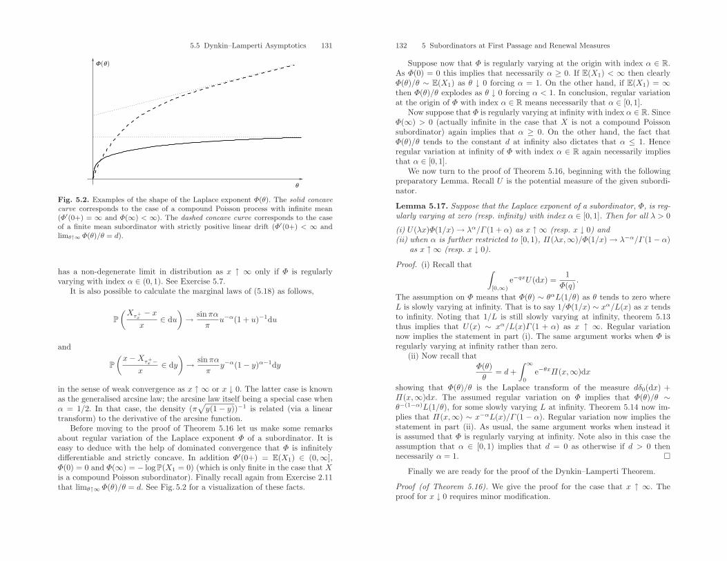
5.5 Dynkin–Lamperti Asymptotics 131
F(q)
q
Fig. 5.2. Examples of the shape of the Laplace exponent Φ(θ). The solid concavecurve corresponds to the case of a compound Poisson process with infinite mean(Φ′(0+) = ∞ and Φ(∞) < ∞). The dashed concave curve corresponds to the caseof a finite mean subordinator with strictly positive linear drift (Φ′(0+) < ∞ andlimθ↑∞ Φ(θ)/θ = d).
has a non-degenerate limit in distribution as x ↑ ∞ only if Φ is regularlyvarying with index α ∈ (0, 1). See Exercise 5.7.
It is also possible to calculate the marginal laws of (5.18) as follows,
P(Xτ+
x− x
x∈ du
)→ sinπα
πu−α(1 + u)−1du
and
P(x−Xτ+
x −x
∈ dy)→ sinπα
πy−α(1− y)α−1dy
in the sense of weak convergence as x ↑ ∞ or x ↓ 0. The latter case is knownas the generalised arcsine law; the arcsine law itself being a special case whenα = 1/2. In that case, the density (π
√y(1− y))−1 is related (via a linear
transform) to the derivative of the arcsine function.Before moving to the proof of Theorem 5.16 let us make some remarks
about regular variation of the Laplace exponent Φ of a subordinator. It iseasy to deduce with the help of dominated convergence that Φ is infinitelydifferentiable and strictly concave. In addition Φ′(0+) = E(X1) ∈ (0,∞],Φ(0) = 0 and Φ(∞) = − log P(X1 = 0) (which is only finite in the case that Xis a compound Poisson subordinator). Finally recall again from Exercise 2.11that limθ↑∞ Φ(θ)/θ = d. See Fig. 5.2 for a visualization of these facts.
132 5 Subordinators at First Passage and Renewal Measures
Suppose now that Φ is regularly varying at the origin with index α ∈ R.As Φ(0) = 0 this implies that necessarily α ≥ 0. If E(X1) < ∞ then clearlyΦ(θ)/θ ∼ E(X1) as θ ↓ 0 forcing α = 1. On the other hand, if E(X1) = ∞then Φ(θ)/θ explodes as θ ↓ 0 forcing α < 1. In conclusion, regular variationat the origin of Φ with index α ∈ R means necessarily that α ∈ [0, 1].
Now suppose that Φ is regularly varying at infinity with index α ∈ R. SinceΦ(∞) > 0 (actually infinite in the case that X is not a compound Poissonsubordinator) again implies that α ≥ 0. On the other hand, the fact thatΦ(θ)/θ tends to the constant d at infinity also dictates that α ≤ 1. Henceregular variation at infinity of Φ with index α ∈ R again necessarily impliesthat α ∈ [0, 1].
We now turn to the proof of Theorem 5.16, beginning with the followingpreparatory Lemma. Recall U is the potential measure of the given subordi-nator.
Lemma 5.17. Suppose that the Laplace exponent of a subordinator, Φ, is reg-ularly varying at zero (resp. infinity) with index α ∈ [0, 1]. Then for all λ > 0
(i) U(λx)Φ(1/x) → λα/Γ (1 + α) as x ↑ ∞ (resp. x ↓ 0) and(ii) when α is further restricted to [0, 1), Π(λx,∞)/Φ(1/x) → λ−α/Γ (1− α)
as x ↑ ∞ (resp. x ↓ 0).
Proof. (i) Recall that ∫[0,∞)
e−qxU(dx) =1
Φ(q).
The assumption on Φ means that Φ(θ) ∼ θαL(1/θ) as θ tends to zero whereL is slowly varying at infinity. That is to say 1/Φ(1/x) ∼ xα/L(x) as x tendsto infinity. Noting that 1/L is still slowly varying at infinity, theorem 5.13thus implies that U(x) ∼ xα/L(x)Γ (1 + α) as x ↑ ∞. Regular variationnow implies the statement in part (i). The same argument works when Φ isregularly varying at infinity rather than zero.
(ii) Now recall thatΦ(θ)θ
= d+∫ ∞
0
e−θxΠ(x,∞)dx
showing that Φ(θ)/θ is the Laplace transform of the measure dδ0(dx) +Π(x,∞)dx. The assumed regular variation on Φ implies that Φ(θ)/θ ∼θ−(1−α)L(1/θ), for some slowly varying L at infinity. Theorem 5.14 now im-plies that Π(x,∞) ∼ x−αL(x)/Γ (1 − α). Regular variation now implies thestatement in part (ii). As usual, the same argument works when instead itis assumed that Φ is regularly varying at infinity. Note also in this case theassumption that α ∈ [0, 1) implies that d = 0 as otherwise if d > 0 thennecessarily α = 1.
Finally we are ready for the proof of the Dynkin–Lamperti Theorem.
Proof (of Theorem 5.16). We give the proof for the case that x ↑ ∞. Theproof for x ↓ 0 requires minor modification.
5.5 Exercises 133
Starting from the conclusion of Theorem 5.6 we have for θ ∈ (0, 1] andφ > 0,
P(Xτ+
x− x
x∈ dφ,
x−Xτ+x −
x∈ dθ
)= U(x(1− dθ))Π(x(θ + dφ))
and hence for 0 < a < b < 1 and c > 0,
P(Xτ+
x− x
x> c,
x−Xτ+x −
x∈ (a, b)
)=∫
(a,b)
Π(x(θ + c),∞)U(x(1dθ))
=∫
(1−b,1−a)
Π(x(1− η + c),∞)Φ(1/x)
U(xdη)Φ(1/x), (5.19)
where in the last equality we have changed variables. From Lemma 5.17 (i) wesee on the one hand that U(xdη)Φ(1/x) converges weakly to ηα−1dη/Γ (α)(we have used that Γ (1+α) = αΓ (α)). On the other hand we have seen frompart (ii) of the same lemma that
limx↓0
Π(x(1− η + c),∞)Φ(1/x)
=(1− η + c)−α
Γ (1− α).
Since Π(x(1 − η + φ),∞) is monotone in η, it follows that the convergenceabove is uniform on (1 − b, 1 − a); recall Exercise 2.4. It follows that theright-hand side of (5.19) converges to∫
(1−b,1−a)
(1− η + c)−α
Γ (1− α)ηα−1
Γ (α)dη
=1
Γ (α)Γ (1− α)
∫(a,b)
(θ + c)−α(1− θ)α−1dθ
as x ↑ ∞ which is tantamount to
limx↑∞
P(x−Xτ+
x −x
∈ dy,Xτ+
x −xx
∈ du)
=α
Γ (α)Γ (1− α)(y + u)−α−1(1− y)α−1dy du
in the sense of weak convergence. Finally, a special property of gammafunctions gives 1/(Γ (α)Γ (1 − α)) = (sinπα)/π and hence the proof iscomplete.
Exercises
5.1. Prove Theorem 5.7.
134 5 Subordinators at First Passage and Renewal Measures
5.2. Suppose that Y is a spectrally positive Levy process of bounded variationdrifting to −∞ with Laplace exponent written in the usual form
log E(e−θY1) = ψ(θ) = dθ −∫
(0,∞)
(1− e−θx)ν(dx),
where necessarily d > 0,∫(0,∞)
(1 ∧ x)ν(dx) < ∞ and ψ′(0+) > 0. Defineσ+x = inft > 0 : Yt > x and Y t = sups≤t Ys.
(i) Suppose that X = Xt : t ≥ 0 is a compound Poisson subordinator withjump distribution (d−ψ′(0+))−1ν(x,∞)dx. By following similar reasoningto the explanation of the Pollaczeck–Khintchin formula in Chap. 4 showthat
P(Yσ+x−x ∈ du, x−Y σ+
x − ∈ dy|σ+x <∞) = P(Xτ+
x−x ∈ du, x−Xτ+
x − ∈ dy).
(ii) Hence deduce that if∫∞0
xν(x,∞)dx < ∞ then for u, y > 0, in the senseof weak convergence
limx↑∞
P(Yσ+x− x ∈ du, x− Y σ+
x − ∈ dy|σ+x <∞)
=1∫∞
0xν(x,∞)dx
ν(u+ y,∞)du dy
(iii) Give an interpretation of the result in (ii) in the context of modellinginsurance claims.
5.3. Suppose that X is a finite mean subordinator and that its associatedpotential measure U does not have lattice support. Suppose that Z is a randomvariable whose distribution is equal to that of the limiting distribution ofXτ+
x− Xτ+
x − as x ↑ ∞. Suppose further that (V,W ) is a bivariate randomvariable whose distribution is equal to the limiting distribution of (Xτ+
x−x, x−
Xτ+x −) as x ↑ ∞ and U is independent of V,W,Z and uniformly distributed
on [0, 1]. Show that (V,W ) is equal in distribution to ((1− U)Z,UZ).
5.4. Let X and Y be two (possibly correlated) subordinators killed indepen-dently at the rate η ≥ 0. Denote their bivariate jump measure by Π(·, ·).Define their bivariate renewal function
U(dx,dy) =∫ ∞
0
dt · P(Xt ∈ dx, Yt ∈ dy),
and suppose that as usual
τ+x = inft > 0 : Xt > x.
5.5 Exercises 135
Use a generalised version of the compensation formula to establish the follow-ing quadruple law
P (∆Xτ+x∈ dt,Xτ+
x − ∈ ds, x− Yτ+x − ∈ dy, Yτ+
x− x ∈ du)
= U(ds, x− dy)Π(dt,du+ y)
for u > 0, y ∈ [0, x] and s, t ≥ 0. This formula will be of use later on whileconsidering the first passage of a general Levy process over a fixed level.
5.5. Let X be any subordinator with Laplace exponent Φ and recall thatτ+x = inft > 0 : Xt > x. Let eα be an exponentially distributed random
variable which is independent of X.
(i) By applying the Strong Markov Property at time τ+x in the expectation
E(e−βXeα 1(Xeα>x)) show that for all α, β, x ≥ 0 we have
E(
e−ατ+
x −βXτ+x
)= (α+ Φ(β))
∫(x,∞)
e−βzU (α)(dz) (5.20)
for all x > 0.(ii) Show further with the help of the identity in (i) that when q > β,∫ ∞
0
e−qxE(
e−ατ+
x −β(Xτ+x−x))
dx =1
q − β
(1− α+ Φ (β)
α+ Φ (q)
).
(iii) Deduce with the help of Theorem 5.9 that
E(e−ατ+x 1(X
τ+x
=x)) = du(α)(x)
where, if d = 0 the term u(α)(x) may be taken as equal to zero and oth-erwise the potential measure U (α) has a density and u(α) is a continuousand strictly positive version thereof.
(iv) Show that for this version of the density, u(α)(0+) = 1/d where d is thedrift of X.
5.6. Suppose that X is a stable subordinator with parameter α ∈ (0, 1) thushaving Laplace exponent Φ(θ) = cθα for θ ≥ 0 and some c > 0 which in thisexercise we will take equal to unity.
(i) Show from Exercise 1.4 that the precise expression for the jump measureis
Π(dx) =x−(1+α)
−Γ (−α)dx.
(ii) By considering the Laplace transform of the potential measure U , showthat
U(dx) =xα−1
Γ (α)dx.
136 5 Subordinators at First Passage and Renewal Measures
(iii) Hence deduce that
P(Xτ+x− x ∈ du, x−Xτ+
x − ∈ dy)
=α sinαπ
π(x− y)α−1(y + u)−(α+1)du dy
for u > 0 and y ∈ [0, x]. Note further that the distribution of the pair(x−Xτ+
x −x
,Xτ+
x− x
x
)(5.21)
is independent of x.(iv) Show that stable subordinators do not creep.
5.7. Suppose that X is any subordinator.
(i) Use the joint law of the overshoot and undershoot of a subordinator todeduce that for β, γ ≥ 0,∫ ∞
0
dx · e−qxE(e−βX
τ+x −
−γ(Xτ+x−x)
1(Xτ+x>x))
=1
q − γ
(Φ(q)− Φ(γ)Φ(q + β)
)− d
Φ(q + β).
(ii) Taking account of creeping, use part (i) to deduce that∫ ∞
0
dx · e−qxE(e−β(X
τ+tx−/t)−γ(X
τ+tx
−tx)/t) =
1(q − γ)
Φ(q/t)− Φ(γ/t)Φ((q + β)/t)
.
(iii) Show that if Φ is regularly varying at zero (resp. infinity) with index αequal to 0 or 1, then the limiting distribution of the pair in (5.21) is trivialas x tends to infinity (resp. zero).
(iv) It is possible to show that if a function f : [0,∞) → (0,∞) satisfies
limf(λt)f(t)
= g(λ)
for all λ > 0 as t tends to zero (resp. infinity) then in fact f must beregularly varying. Roughly speaking, the reason for this is that for λ, µ >0,
g(λµ) = limf(λµt)f(λt)
f(λt)f(t)
= g(µ)g(λ)
showing that g is a multiplicative function. With a little measure theory,one can show that necessarily, it must follow that g(λ) = λρ for someρ ∈ R. See Theorem 1.4.1 of Bingham et al. (1987) for the full details.Use the above remarks to deduce that if (5.21) has a limiting distributionas x tends to infinity (resp. zero), then necessarily Φ is regularly varyingat zero (resp. infinity) with index α ∈ [0, 1]. Hence conclude that (5.21)has a non-trivial limiting distribution if and only if α ∈ (0, 1).
5.5 Exercises 137
5.8. An important class of distributions, denoted L(α) where α is a parameterin [0,∞), are defined as follows. Suppose that F is a probability distributionfunction. Write F (x) = 1−F (x). Then F belongs to L(α) if the support of Fis in [0,∞) and non-lattice, F (x) > 0 for all x ≥ 0 and for all y > 0,
limx↑∞
F (x+ y)F (x)
= e−αy.
Note that the requirement that F is a probability measure can be weakenedto a finite measure as one may always normalise by total mass to fulfill theconditions given earlier.
We are interested in establishing an asymptotic conditional distributionfor the overshoot of a killed subordinator. To this end we assume that X is akilled subordinator with killing rate η > 0, Laplace exponent Φ, jump measureΠ, drift d ≥ 0 and potential measure U which is assumed to belong to classL(α) for some α ≥ 0 such that Φ(−α) <∞.
(i) Show thatP(τ+
x <∞) = ηU(x,∞)
where τ+x = inft > 0 : Xt > x.
(ii) Show that for all β ≥ 0,
E(e−β(X
τ+x−x)|τ+
x <∞) =Φ(β)
ηU(x,∞)
∫(x,∞)
e−β(y−x)U(dy).
(iii) Applying integration by parts, deduce that
limx↑∞
E(e−β(X
τ+x−x)|τ+
x <∞) =Φ(β)η
(α
α+ β
).
(iv) Now take the distribution G defined by its tail
G(x,∞) =e−αx
η
Φ(−α) +
∫(x,∞)
(eαy − eαx)Π(dy)
.
Show that G has an atom at zero and∫(0,∞)
e−βyG(dy) =Φ(β)η
(α
α+ β
)− dα
η,
where d is the drift coefficient of X.(v) Deduce that
limx↑∞
P(Xτ+x− x > u|τ+
x <∞) = G(u)
138 5 Subordinators at First Passage and Renewal Measures
andlimx↑∞
P(Xτ+x
= x|τ+x <∞) =
dα
η.
5.9. Suppose that X is any Levy process of bounded variation with zero driftwhich is not a compound Poisson process. By writing it as the difference oftwo independent subordinators prove that for any x ∈ R,
P(inft > 0 : Xt = x <∞) = 0.
6
The Wiener–Hopf Factorisation
This chapter gives an account of the theory of excursions of a Levy processfrom its maximum and the Wiener–Hopf factorisation that follows as a con-sequence from it.
In Sect. 4.6 the analytical form of the Pollaczek–Khintchine formula wasexplained in terms of the decomposition of the path of the underlying Levyprocess into independent and identically distributed sections of path calledexcursions from the supremum. The decomposition made heavy use of the factthat for the particular class of Levy processes considered, namely spectrallypositive processes of bounded variation, the times of new maxima form adiscrete set.
For a general Levy process, it is still possible to decompose its path into“excursions from the running maximum”. However conceptually this decom-position is a priori somewhat more tricky as, in principle, a general Levyprocess may exhibit an infinite number of excursions from its maximum overany finite period of time. Nonetheless, when considered in the right mathe-matical framework, excursions from the maximum can be given a sensible de-finition and can be shown to form the support of a Poisson random measure.The theory of excursions presents one of the more mathematically challengingaspects of the theory of Levy processes. This means that in order to keep tothe level outlined in the preface of this text, there will be a number of proofs inthe forthcoming sections which are excluded or only discussed at an intuitivelevel.
Amongst a very broad spectrum of probabilistic literature, the Wiener–Hopf factorisation may be thought of as a common reference to a multitude ofstatements concerning the distributional decomposition of the excursions ofany Levy process when sampled at an independent and exponentially distrib-uted time. (We devote a little time later in this text to explain the origin ofthe name “Wiener–Hopf factorisation”.) In the light of the excursion theorygiven in this chapter we explain in detail the Wiener–Hopf factorisation. Thecollection of conclusions which fall under the umbrella of the Wiener–Hopffactorisation turn out to provide a robust tool from which one may analyse a
140 6 The Wiener–Hopf Factorisation
number of problems concerning the fluctuations of Levy processes; in particu-lar problems which have relevance to the applications we shall consider in laterchapters. The chapter concludes with some special classes of Levy processesfor which the Wiener–Hopf factorisation may be exemplified in more detail.
6.1 Local Time at the Maximum
Unlike the Levy processes presented in Sect. 4.6, a general Levy process mayhave an infinite number of new maxima over any given finite period of time. Asour ultimate goal is to show how to decompose events concerning the path of aLevy process according to the behaviour of the path in individual excursions,we need a way of indexing them. To this end we introduce the notion of localtime at the maximum.
To avoid trivialities we shall assume throughout this section that neitherX nor −X is a subordinator. Recall also the definition Xt = sups≤tXs. Inthe sequel we shall repeatedly refer to the process X−X = Xt−Xt : t ≥ 0,which we also recall from Exercise 3.2, which can be shown to be StrongMarkov.
Definition 6.1 (Local time at the maximum). A continuous, non-decreasing, [0,∞)-valued, F-adapted process L = Lt : t ≥ 0 is called alocal time at the maximum (or just local time for short) if the following hold.
(i) The support of the Stieltjes measure dLt is the closure of the (random) setof times t ≥ 0 : Xt = Xt and is finite for each t ≥ 0.
(ii) For every F-stopping time T such that XT = XT on T < ∞ almostsurely, the shifted trivariate process
(XT+t −XT ,XT+t −XT+t, LT+t − LT ) : t ≥ 0
is independent of FT on T <∞ and has the same law as(X,X −X,L
)under P.
(The process which is identically zero is excluded).
Let us make some remarks about the above definition. Firstly if L is alocal time then so is kL for any constant k > 0. Hence local times can at bestbe defined uniquely up to a multiplicative constant. On occasion we shall needto talk about both local time and the time scale on which the Levy processitself is defined. In such cases we shall refer to the latter as real time. Finally,by applying this definition of local time to −X it is clear that one may talkof a local time at the minimum. The latter shall always be referred to as L.
Local times as defined above do not always exist on account of the re-quirement of continuity. Nonetheless, in such cases, it turns out that one mayconstruct right continuous processes which satisfy conditions (i) and (ii) of
6.1 Local Time at the Maximum 141
Definition 6.1 and which serve their purpose equally well in the forthcominganalysis of the Wiener–Hopf factorisation. We provide more details shortly.We give next, however, some examples for which a continuous local time canbe identified explicitly.
Example 6.2 (Spectrally negative processes). Recall that the formal definitionof a spectrally negative Levy process is simply one for which the Levy measuresatisfies Π(0,∞) = 0 and whose paths are not monotone. As there are nopositive jumps the process X must therefore be continuous. It is easy to checkthat L = X fulfils Definition 6.1.
Example 6.3 (Compound Poisson processes with drift d ≥ 0). Just by consid-ering the piece-wise linearity of the paths of these processes, one has obviouslythat over any finite time horizon, the time spent at the maximum has strictlypositive Lebesgue measure with probability one. Hence the quantity
Lt :=∫ t
0
1(Xs=Xs)ds, t ≥ 0 (6.1)
is almost surely positive and may be taken as a candidate for local time.Indeed it increases on t : Xt = Xt, is continuous, non-decreasing and is anF-adapted process. Taking T as in part (ii) of Definition 6.1 we also see thaton T <∞,
LT+t − LT =∫ T+t
T
1(Xs=Xs)ds (6.2)
which is independent of FT because XT+t − XT+t : t ≥ 0 is and has thesame law as L by the Strong Markov Property applied to the process X −Xand the fact that XT − XT = 0. The distributional requirement in part (ii)for the trivariate process (X,X −X,L) follows by similar reasoning.
If we only allow negative jumps and d > 0, then according to the previousexample X also fulfils the definition of local time. However, as we have seenin the proof of Theorem 4.1,
Xt = d
∫ t
0
1(Xs=Xs)ds
for all t ≥ 0.
Next we would like to identify the class of Levy processes for which con-tinuous local time cannot be constructed and for which a right continuousalternative is introduced instead. In a nutshell, the aforementioned class arethose Levy processes whose moments of new maxima form a discrete set. Thequalifying criterion for this turns out to be related to the behaviour of theLevy process at arbitrarily small times; a sense of this has already been givenin the discussion of Sect. 4.6. We spend a little time developing the relevantnotions, namely path regularity, in order to complete the discussion on localtime.
142 6 The Wiener–Hopf Factorisation
Definition 6.4. For a Levy process X, the point x ∈ R is said to be regular(resp. irregular) for an open or closed set B if
Px(τB = 0
)= 1 (resp. 0),
where the stopping time τB = inft > 0 : Xt ∈ B. Intuitively speaking, x isregular for B if, when starting from x, the Levy process hits B immediately.
Note that as τB is a stopping time, it follows that
1(τB=0) = Px(τB = 0|F0).
On the other hand, since F0 contains only null sets, Kolmogorov’s definitionof conditional expectation implies
Px(τB = 0|F0) = Px(τB = 0)
and hence Px(τB = 0) is either zero or one. In fact one may replace τB = 0by any event A ∈ F0 and reach the same conclusion about P(A). This isnothing but Blumenthal’s zero–one law.
We know from the Levy–Ito decomposition that the range of a Levy processover any finite time horizon is almost surely bounded and thanks to rightcontinuity, limt↓0 max−Xt,Xt = 0. Hence for any given open or closed B,the points x ∈ R for which Px(τB = 0) = 1 are necessarily those belonging toB ∪∂B. However, x ∈ ∂B is not a sufficient condition for Px(τB = 0) = 1. Tosee why, consider the case that B = (0,∞) and X is any compound Poissonprocess.
Finally note that the notion of regularity can be established for any Markovprocess with analogous definition to the one given earlier. However, for thespecial case of a Levy process, stationary independent increments allow usreduce the discussion of regularity of x for open and closed sets to simply theregularity of 0 for open and closed sets. Indeed, for any Levy process, x isregular for B if and only if 0 is regular for B − x.
As we shall see shortly, it is regularity of 0 for [0,∞) which dictates whetherone may find a continuous local time. The following result, due in parts toRogozin (1968), Shtatland (1965) and Bertoin (1997), gives precise conditionsfor the slightly different issue of regularity of 0 for (0,∞).
Theorem 6.5. For any Levy process, X, other than a compound Poissonprocess, the point 0 is regular for (0,∞) if and only if∫ 1
0
1tP (Xt > 0) dt = ∞ (6.3)
and the latter holds if and only if one of the following three conditions hold,
(i) X is a process of unbounded variation,(ii) X is a process of bounded variation and d > 0 ,
6.1 Local Time at the Maximum 143
(iii) X is a process of bounded variation, d = 0 and∫(0,1)
xΠ (dx)∫ x0Π (−∞,−y) dy
= ∞.
Here d is the drift coefficient in the representation (2.21) of a Levy process ofbounded variation.
Recall that if N is the Poisson random measure associated with the jumpsof X, then the time of arrival of a jump of size ε > 0 or greater, say, T (ε), isexponentially distributed since
P(T (ε) > t) = P(N([0, t]× R\(−ε, ε)) = 0) = exp−tΠ(R\(−ε, ε)).This tells us that, if Π(R) = ∞, then jumps of size greater than ε become lessand less probable as t ↓ 0. Hence that the jumps that have any influence overthe initial behaviour of the path of X, if at all, will necessarily be arbitrarilysmall. With this in mind, one may intuitively see the conditions (i)–(iii) inTheorem 6.5 in the following way.
In case (i) when σ > 0 regularity follows as a consequence of the presence ofBrownian motion whose behaviour on the small time scale always dominatesthe path of the Levy process. If on the other hand σ = 0, the high intensityof small jumps causes behaviour on the small time scale close to that ofBrownian motion even though the paths are not continuous. (We use thewords “high intensity” here in the sense that
∫(−1,1)
|x|Π(dx) = ∞). Case(ii) says that when the Poisson point process of jumps fulfils the condition∫(−1,1)
|x|Π(dx) <∞, over small time scales, the sum of the jumps grows sub-linearly in time almost surely. Therefore if a drift is present, this dominatesthe initial motion of the path. In case (iii) when there is no dominant drift,the integral test may be thought of as a statement about what the “relativeweight” of the small positive jumps compared to the small negative jumpsneeds to be in order for regularity to occur.
In the case of bounded variation, the integral∫ x0Π (−∞,−y) dy is finite for
all x > 0. This can be deduced by noting that for any Levy process of boundedvariation
∫(−1,0)
|x|Π(dx) <∞ and then integrating by parts. Note also thatTheorem 6.5 implies that processes of unbounded variation are such that 0 isregular for both (0,∞) and (−∞, 0) and that processes of bounded variationwith d > 0 are irregular for (−∞, 0]. For processes of bounded variation withd = 0 it is possible to find examples where 0 is regular for both (0,∞) and(−∞, 0). See Exercise 6.1.
We offer no proof of Theorem 6.5 here. However it is worth recalling thatfrom Lemma 4.11 and the follow up Exercise 4.9 (i) we know that for anyLevy process, X, of bounded variation,
limt↓0
Xt
t= d
almost surely where d is the drift coefficient. This shows that if d > 0 (resp.d < 0) then for all t > 0 sufficiently small, Xt must be strictly positive
144 6 The Wiener–Hopf Factorisation
(resp. negative). That is to say, 0 is regular for (0,∞) and irregular for (−∞, 0]if d > 0 (resp. regular for (−∞, 0) and irregular for [0,∞) if d < 0). For thecase of a spectrally negative Levy process of unbounded variation, Exercise6.2 deduces regularity properties in agreement with Theorem 6.5. In addition,Exercise 6.8 shows how to establish the criterion (6.3).
There is a slight difference between regularity of 0 for (0,∞) and regu-larity of 0 for [0,∞). Consider for example the case of a compound PoissonProcess. The latter is regular for [0,∞) but not for (0,∞) due to the initialexponentially distributed period of time during which the process remains atthe origin. On the other hand, we also have the following conclusion.
Corollary 6.6. The only Levy process for which 0 is regular for [0,∞) butnot for (0,∞) is a compound Poisson process.
Proof. If a process is regular for [0,∞) but not for (0,∞) then, according tothe cases given in Theorem 6.5 it must be a process of bounded variation withzero drift. If the underlying Levy process is not a compound Poisson processthen this would require that the process jumps into (−∞, 0) and back onto 0 infinitely often for arbitrarily small times. This is impossible when onetakes into account Exercise 5.9 which shows that a Levy process of boundedvariation with no drift which is not a compound Poisson process cannot hit apre-specified point.
By definition, when 0 is irregular for [0,∞) the Levy process takes a strictlypositive period of time to return to reach a new maximum above the origin.Hence, applying the Strong Markov Property at the time of first entry into[0,∞) we see that in a finite interval of time there are almost surely a finitenumber of new maxima, in other words, 0 < s ≤ t : Xs = Xs is a discreteset. (Recall that this type of behaviour has been observed for spectrally posi-tive Levy process of bounded variation in Chap. 4). In this case we may thendefine the counting process n = nt : t ≥ 0 by
nt = #0 < s ≤ t : Xs = Xs. (6.4)
We are now ready to make the distinction between those processes whichadmit continuous local times in Definition 6.1 and those that do not.
Theorem 6.7. Let X be any Levy process.
(i) There exists a continuous version of L which is unique up to a multiplica-tive constant if and only if 0 is regular for [0,∞).
6.1 Local Time at the Maximum 145
(ii) If 0 is irregular for [0,∞) then we can take as our definition of local time
Lt =nt∑i=0
e(i)λ , (6.5)
satisfying (i) and (ii) of Definition 6.1, where e(i)λ : i ≥ 0 are indepen-
dent and exponentially distributed random variables with parameter λ > 0(chosen arbitrarily) and nt : t ≥ 0 is the counting process defined in(6.4).
We offer no proof for case (i) which is a particular example of a classicresult from potential theory of stochastic processes, a general account of whichcan be found in Blumenthal and Getoor (1968). The proof of part (ii) isquite accessible and we leave it as an Exercise. Note that one slight problemoccurring in the definition of L in (6.5) is that it is not adapted to the filtrationof X. However this is easily resolved by simply broadening out the filtrationto include σ(e(i)
λ : i ≥ 0) before completing it with null sets. Also the choiceof exponential distribution used in (6.5) is of no effective consequence. Onecould in principle always work with the definition
L′t =nt∑i=0
e(i)1 .
Scaling properties of exponential distributions would then allow us to con-struct the e(i)
λ s and e(i)1 s on the same probability space so that λe(i)
λ = e(i)1
for each i = 0, 1, 2... and this would imply that L′ = λL where L is localtime constructed using exponential distributions with parameter λ. So in factwithin the specified class of local times in part (ii) of the above theorem, theonly effective difference is a multiplicative constant. The reason why we donot simply define Lt = nt has to do with the fact that we shall require somespecial properties of the inverse L−1. This will be discussed in Sect. 6.2.
In accordance with the conclusion of Theorem 6.7, in the case that 0 isregular for [0,∞) we shall henceforth work with a continuous version of Land in the case that 0 is irregular for [0,∞) we shall work with the definition(6.5) for L.
In Example 6.3 we saw that we may use a multiple of the Lebesgue measureof the real time spent at the maximum to give a version of local time which iscontinuous. The fact that the latter is non-zero is a clear consequence of piece-wise linearity of the process. Although compound Poisson processes (withdrift) are the only Levy processes which are piecewise linear, it is nonethelessnatural to investigate to what extent one may work with the Lebesgue measureof the time spent at the maximum for local time in the case that 0 is regularfor [0,∞). Rubinovitch (1971) supplies us with the following charactarisationof such processes.
146 6 The Wiener–Hopf Factorisation
Theorem 6.8. Suppose that X is a Levy process for which 0 is regular for[0,∞). Let L be some continuous version of local time. The constant a ≥ 0satisfying the relation ∫ t
0
1(Xs=Xs)ds = aLt
is strictly positive if and only if X is a Levy process of bounded variation and0 is irregular for (−∞, 0).
Proof. Note that∫∞0
1(Xt=Xt)dt > 0 with positive probability if and only if
E(∫ ∞
0
1(Xt−Xt=0)dt)> 0.
By Fubini’s Theorem and the Duality Lemma the latter occurs if and onlyif∫∞0
P(Xt = 0)dt = E(∫∞0
1(Xt=0)dt) > 0 (recall that Xt := infs≤tXs).Due to the fact that X has paths that are right continuous and monotonedecreasing, the positivity of the last integral happens if and only if it takes analmost surely strictly positive time for X to visit (−∞, 0). In short we havethat
∫∞0
1(Xt=Xt)dt > 0 with positive probabiltiy if and only if 0 is irregular
for (−∞, 0). By Theorem 6.5 the latter can only happen when X has boundedvariation.
Following the same reasoning as used in Example 6.3 it is straightforwardto deduce that ∫ t
0
1(Xs=Xs)ds, t ≥ 0
may be used as a local time. Theorem 6.7 (i) now gives us the existence of aconstant a > 0 so that for a given local time L,
aLt =∫ t
0
1(Xs=Xs)ds.
When 0 is regular for (−∞, 0) the reasoning above also shows that∫ t01(Xs=Xs)ds = 0 almost surely for all t ≥ 0 and hence it is clear that
the constant a = 0. We can now summarise the discussion on local times as follows. There are
three types of Levy processes which are associated with three types of localtimes.
1. Processes of bounded variation for which 0 is irregular for [0,∞). The setof maxima forms a discrete set and we take a right continuous version oflocal time in the form
Lt =nt∑i=0
e(i)1 ,
where nt is the count of the number of maxima up to time t and e(i)1 : i =
0, 1, ... are independent and exponentially distributed random variableswith parameter 1.
6.2 The Ladder Process 147
2. Processes of bounded variation for which 0 is irregular for (−∞, 0). Thereexists a continuous version of local time given by,
Lt = a
∫ t
0
1(Xs=Xs)ds
for some arbitrary a > 0. In the case that X is spectrally negative, wehave that L is equal to a multiplicative constant times X.
3. Processes of unbounded variation, in which case 0 is implicitly regular for[0,∞). We take a continuous version of local time exists but cannot beidentified explicitly as a functional of the path of X in general. However,if X is a spectrally negative Levy process, then this local time may betaken as X.
6.2 The Ladder Process
Define the inverse local time process L−1 = L−1t : t ≥ 0 where
L−1t :=
infs > 0 : Ls > t if t < L∞
∞ otherwise.
Next define the process H = Ht : t ≥ 0 where
Ht :=XL−1
tif t < L∞
∞ otherwise.
The range of inverse local time, L−1, corresponds to the set of real times atwhich new maxima occur, called the ascending ladder times. The range ofprocess H corresponds to the set of new maxima called the ascending ladderheights. The bivariate process (L−1,H) := (L−1
t ,Ht) : t ≥ 0, called theascending ladder process, is the main object of study of this section. Notethat it is implicit from their definition that L−1 and H are processes withpaths that are right continuous with left limits.
The word “ascending” distinguishes the process (L−1,H) from the anal-ogous object (L−1, H), constructed from −X, which is called the descendingladder process (note that local time at the maximum of −X is the local time atthe minimum of X which was previously referred to as L). When the contextis obvious we shall drop the use of the words ascending or descending.
The ladder processes we have defined here are the continuous time ana-logue of the processes with the same name for random walks1. In the case ofrandom walks, one defines Ln to be the number of times a maxima is reachedafter n steps, Tn = infk ≥ 1 : Lk = n as the number of steps required toachieve n new maxima and Hn as the n-th new maxima.
1Recall that Sn : n = 0, 1, 2, ... is a random walk if S0 = 0 and Sn =∑n
i=1ξi
where ξi : i = 1, 2, ... are independent and identically distributed.
148 6 The Wiener–Hopf Factorisation
An additional subtlety for random walks is that the count Ln may be takento include visits to previous maxima (consider for example a simple randomwalk which may visit an existing maximum several times before generatinga strictly greater maximum). In that case the associated ascending ladderprocess is called weak. When Ln : n ≥ 0 only counts the number of newmaxima which exceed all previous maxima, the associated ascending ladderprocess is called strict.
The same subtlety appears in the definition of L for Levy processes when0 is irregular for [0,∞) and our definition of the process nt : t ≥ 0 isanalogous to a count of weak ascending ladder heights. However, this is of noconsequence in the forthcoming discussion as we shall see that, it turns outthat in this setting with probability one no two maxima can be equal anyway.When 0 is regular for [0,∞) but X is not a compound Poisson process weshall again see in due course that ladder heights at different ladder times aredistinct. Finally when X is a compound Poisson process, although one cannotcount the times spent at the maximum, the distinction between weak andstrict maxima will become an issue at some point in later discussion. Indeedthe choice of local time
Lt = a
∫ t
0
1(Xs=Xs)ds, t ≥ 0
is analogous to the count of weak ascending ladder heights in a random walk.Consider for example the continuous time version of a simple random walk;that is a compound Poisson process with jumps in −1, 1.
Our interest in this section will be to characterise the ladder process. Westart with the following lemma which will be used at several places later on.
Lemma 6.9. For each t ≥ 0, both L−1t and L−1
t− are F-stopping times.
Proof. Recall from Sect. 3.1 that thanks to the assumed right continuity of Fit suffices to prove that for each s > 0, L−1
t < s ∈ Fs and a similar notionfor L−1
t− . For all s, t ≥ 0, L−1t < s = Ls− > t which belongs to Fs as the
process L is F-adapted. To prove that L−1t− is a stopping time note that
L−1t− < s =
⋂n≥1
L−1t−1/n < s ∈ Fs.
In the next theorem we shall link the process (L−1,H) to a bivariatesubordinator. Let us remind ourselves what the latter object is. With Exer-cise 2.10 in mind, recall that a bivariate subordinator is a two-dimensional(0,∞)2-valued stochastic processes X = Xt : t ≥ 0 with paths that are
6.2 The Ladder Process 149
right continuous with left limits as well as having stationary independent in-crements2 and further, each component is non-decreasing. It is important tonote that in general it is not correct to think of a bivariate subordinator simplyas a vector process composed of two independent subordinators. Correlationbetween the subordinators in each of the co-ordinates may be represented asfollows. Write X in the form
Xt = dt+∫
[0,t]
∫(0,∞)2
xN(ds× dx), t ≥ 0,
where d ∈ [0,∞)2 and N is the Poisson random measure describing the jumpsdefined on [0,∞)× (0,∞)2 with intensity measure given by dt×Λ(dx,dy) fora bivariate measure Λ on (0,∞)2 satisfying∫
(0,∞)2(1 ∧
√x2 + y2)Λ(dx,dy) <∞.
Independence of the two individual co-ordinate processes of X corresponds tothe case that Λ is a product measure; say Λ(dx,dy) = Λ1(dx)Λ2(dy).
For a general bivariate subordinator, positivity allows us to talk abouttheir Laplace exponent φ (α, β) given by
E(
exp−(α
β
)·Xt
)= exp−φ (α, β) t.
Referring back to Chap. 2, it is a straightforward exercise to deduce that that
φ (α, β) = d ·(α
β
)+∫
(0,∞)2(1− e−(α
β)·(xy))Λ(dx,dy).
Theorem 6.10. Let X be a Levy process and eq an independent and expo-nentially distributed random variable with parameter q ≥ 0. Then
P
(lim supt↑∞
Xt <∞)
= 0 or 1
and the ladder process (L−1,H) satisfies the following properties.
(i) If P(lim supt↑∞Xt = ∞) = 1 then (L−1,H) has the law of a bivariate
subordinator.(ii) If P
(lim supt↑∞Xt <∞) = 1 then for some q > 0 L∞
d= eq, the exponen-tial distribution with parameter q, and (L−1
t ,Ht) : t < L∞ has the samelaw as (L−1,H) := (L−1
t ,Ht) : t < eq where (L−1,H) is a bivariatesubordinator independent of eq.
2Recall that right continuous with left limits and stationary independent incre-ments for a multi-dimensional process means that the same properties holdcomponent-wise. However, it does not necessarily mean that the individual com-ponent processes are independent.
150 6 The Wiener–Hopf Factorisation
Proof. Sincelim sup
t↑∞Xt <∞ = lim sup
Q∋t↑∞Xt <∞
and the latter event is in the tail sigma algebra⋂t∈Q∩[0,∞) σ (Xs : s ≥ t) , then
Kolmogorov’s zero–one law for tail events tells us that P(lim supt↑∞Xt <∞)
= 0 or 1.To deal with (i) and (ii) in the case that 0 is irregular for [0,∞), the analysis
proceeds in the sprit of the discussion around the Pollaczek–Khintchine for-mula in Chap. 4. We give a brief outline of the arguments again. If we agreethat a geometric distribution with parameter 1 is infinite with probabilityone then, the total number of excursions from the maximum n∞ defined in(6.4) is geometrically distributed with parameter 1 − ρ = P(τ+
0 = ∞) whereτ+0 = inft > 0 : Xt > 0. Now define the sequence of times T0 = 0,
Tn+1 = inft > Tn : Xt > XTn
= inft > Tn : ∆Lt > 0= inft > Tn : ∆nt = 1
for n = 0, 1, ..., n∞ where ∆Lt = Lt −Lt−, ∆nt = nt − nt− and inf ∅ = ∞. Itis easy to verify that the latter times form a sequence of stopping times withTn <∞ for all n ≥ 0 and otherwise Tn∞ <∞ and Tn∞+1 = ∞ when n∞ <∞.Further, by the Strong Markov Property for Levy processes, if n∞ <∞ thenthe successive excursions of X from its maximum,
ǫn := Xt : t ∈ (Tn−1, Tn]
for n = 1, ..., n∞ are equal in law to an independent sample of n∞ − 1 copiesof the first excursion from the maximum conditioned to be finite followed bya final independent copy conditioned to be infinite in length. If n∞ = ∞ thenthe sequence ǫn : n = 1, 2, ... is equal in law to an independent sample ofthe first excursion from the maximum.
By considering Fig. 6.1 we see that L−1 (the reflection of L about the di-agonal) is a step function and its successive jumps (the flat sections of L)correspond precisely to the sequence Tn+1 − Tn : n = 0, ..., n∞. From theprevious paragraph, it follows that L−1 has independent and identically dis-tributed jumps and is sent independently to infinity (which we may consideras a “graveyard” state) on the n∞-th jump accordingly with the arrival of thefirst infinite excursion. As the jumps of L are independent and exponentiallydistributed it also follows that the periods between jumps of L−1 are indepen-dent and exponentially distributed. According to Exercise 6.3 the process L−1
is now equal in law to a compound Poisson subordinator killed independentlyafter an exponentially distributed time with parameter λ(1 − ρ). (Again wework with the notation that an exponential distribution with parameter 0is infinite with probability one). It follows by construction that H is also acompound Poisson subordinator killed at the same rate.
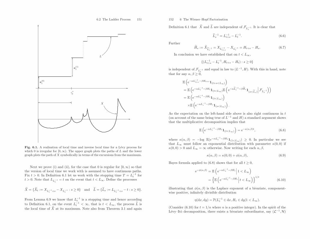
6.2 The Ladder Process 151
L
X
e1(0)
e1(1)
τ0+
Fig. 6.1. A realisation of local time and inverse local time for a Levy process forwhich 0 is irregular for [0,∞). The upper graph plots the paths of L and the lowergraph plots the path of X symbolically in terms of the excursions from the maximum.
Next we prove (i) and (ii), for the case that 0 is regular for [0,∞) so thatthe version of local time we work with is assumed to have continuous paths.Fix t > 0. In Definition 6.1 let us work with the stopping time T = L−1
t fort > 0. Note that LL−1
t= t on the event that t < L∞. Define the processes
X = Xt := XL−1t +s −XL−1
t: s ≥ 0 and L = Ls := LL−1
t +s − t : s ≥ 0.
From Lemma 6.9 we know that L−1t is a stopping time and hence according
to Definition 6.1, on the event L−1t < ∞, that is t < L∞, the process L is
the local time of X at its maximum. Note also from Theorem 3.1 and again
152 6 The Wiener–Hopf Factorisation
Definition 6.1 that X and L are independent of FL−1t. It is clear that
L−1s = L−1
t+s − L−1t . (6.6)
FurtherHs := X
L−1s
= XL−1t+s
−XL−1t
= Ht+s −Hs. (6.7)
In conclusion we have established that on t < L∞,
(L−1t+s − L−1
t ,Ht+s −Ht) : s ≥ 0is independent of FL−1
tand equal in law to (L−1,H). With this in hand, note
that for any α, β ≥ 0,
E(e−αL
−1t+s
−βHt+s1(t+s<L∞)
)= E
(e−αL
−1t −βHt1(t<L∞)E
(e−αL
−1s −βHs1
(s<Ls)
∣∣∣FL−1t
))= E
(e−αL
−1t −βHt1(t<L∞)
)×E(e−αL
−1s −βHs1(s<L∞)
).
As the expectation on the left-hand side above is also right continuous in t(on account of the same being true of L−1 and H) a standard argument showsthat the multiplicative decomposition implies that
E(e−αL
−1t −βHt1(t<L∞)
)= e−κ(α,β)t, (6.8)
where κ(α, β) = −log E(e−αL−11 −βH11(1<L∞)) ≥ 0. In particular we see
that L∞ must follow an exponential distribution with parameter κ(0, 0) ifκ(0, 0) > 0 and L∞ = ∞ otherwise. Now writing for each α, β,
κ(α, β) = κ(0, 0) + φ(α, β), (6.9)
Bayes formula applied to (6.8) shows that for all t ≥ 0,
e−φ(α,β) = E(
e−αL−11 −βH1
∣∣∣ 1 < L∞)
=
E(
e−αL−1t −βHt
∣∣∣ t < L∞)1/t
(6.10)
illustrating that φ(α, β) is the Laplace exponent of a bivariate, component-wise positive, infinitely divisible distribution
η(dx,dy) = P(L−11 ∈ dx,H1 ∈ dy|1 < L∞).
(Consider (6.10) for t = 1/n where n is a positive integer). In the spirit of theLevy–Ito decomposition, there exists a bivariate subordinator, say (L−1,H)
6.2 The Ladder Process 153
whose Laplace exponent is φ(α, β). We now see from (6.8) and (6.9) that(L−1,H) is equal in law to (L−1,H) killed independently (with “graveyard”state ∞) after an exponentially distributed time with parameter q = κ(0, 0).In particular X∞ = ∞ almost surely if and only if q = 0 and otherwiseX∞ = Heq
<∞ almost surely.
Corollary 6.11. In the previous Theorem, the subordinator associated withL−1 has drift a where a is the constant appearing in Theorem 6.8.
Proof. Note that ∆L−1t := L−1
t − L−1t− is greater than ε > 0 follows as a
consequence of the path of X moving away from its maximum for a periodof real time exceeding ε. That is to say, individual jumps of L−1 correspondto individual excursions of X from X. Let us denote by NL−1 the Poissonrandom measure associated with the jumps of L−1. Then the time it takesto accumulate t < L∞ units of local time is the sum of the periods of timethat X has spent away from its maximum plus the real time that X hasspent at its maximum (if at all). The latter qualification is only of significancewhen X is of bounded variation with 0 irregular for (−∞, 0) in which casethe constant a in Theorem 6.8 is strictly positive and then the local time istaken as the Lebesgue measure of the time spent at the maximum. We haveon t < L∞,
L−1t =
∫ L−1t
0
1(Xs=Xs)ds+∫
[0,t]
∫(0,∞)
xNL−1(ds× dx).
From Theorem 6.8 we know that the integral is equal to aLL−1t
= at andhence a is the drift of the subordinator L−1.
Finally note in the case of compound Poisson process for which, with pos-itive probability, the same maxima may be visited over two intervals of timeseparated by at least one excursion, we have that ∆Ht = 0 when ∆L−1
t > 0.In other words, the jump measure of H may have an atom at zero. This wouldbe the case for the earlier given example of a compound Poisson process withjumps in −1, 1. Strictly speaking this violates our definition of a subordina-tor. However, this does not present a serious problem since H is necessarily acompound Poisson subordinator and hence its paths are well defined with thepresence of this atom. Further, this does not affect the forthcoming analysisunless otherwise mentioned.
Example 6.12 (Spectrally negative processes). Suppose that X is a spectrallynegative Levy process with Laplace exponent ψ having right inverse Φ; re-call the latter part of Sect. 3.3 for a reminder of what this means. As notedearlier, we may work with local time given by L = X. It follows that L−1
x
is nothing more than the first passage time above x > 0. (Note that in gen-eral it is not true that L−1
x is the first passage above x). As X is spectrallynegative we have in particular that Hx = XL−1
x= x on x < L∞. Recalling
154 6 The Wiener–Hopf Factorisation
Corollary 3.14 we already know that L−1 is a subordinator killed at rate Φ(0).Hence we may easily identify for α, β ≥ 0, κ(α, β) = Φ(0) + φ(α, β) where
φ(α, β) = [Φ(α)− Φ(0)] + β
is the Laplace exponent of a bivariate subordinator. Note in particular thatL∞ <∞ if and only if Φ(0) > 0 if and only if ψ′(0+) = E(X1) ∈ [−∞, 0) and,on account of the fact that L−1 is the first passage process, the latter occursif and only if P(lim supt↑∞Xt <∞) = 1.
In the special case that X is a Brownian motion with drift ρ, we knowexplicitly that ψ(θ) = ρθ + 1
2θ2 and hence Φ(α) = −ρ +
√ρ2 + 2α. Inverse
local time can then be identified precisely as an inverse Gaussian process(killed at rate 2|ρ| if ρ < 0).
We close this section by making the important remark that the brief intro-duction to excursion theory offered here has not paid fair dues to their generalsetting. Excursion theory formally begins with Ito (1970) with further founda-tional contributions coming from Maisonneuve (1975) and can be applied to amuch more general class of Markov processes than just Levy processes. Recallthat X −X is a Markov process and hence one may consider L as the localtime at 0 of the latter process. In general it is possible to identify excursionsof well defined Markov processes from individual points in their state spacewith the help of local time. The reader interested in a comprehensive accountshould refer to the detailed but nonetheless approachable account given inChap. IV of Bertoin (1996) or Blumenthal (1992).
6.3 Excursions
Recall that in Sect. 4.6 we gave an explanation of the Pollaczek–Khintchineformula by decomposing the path of the Levy processes considered there interms of excursions from the maximum. Clearly this decomposition reliedheavily on the fact that the number of new maxima over any finite timehorizon is finite. That is to say, that 0 is irregular for [0,∞) and the local timeat the maximum is a step function as in case 1 listed at the end of Sect. 6.1.Now that we have established the concept of local time at the maximum forany Levy process we can give the general decomposition of the path of a Levyprocess in terms of its excursions from the maximum.
Definition 6.13. For each moment of local time t > 0 we define
ǫt =
XL−1
t−+s −XL−1t−
: 0 < s ≤ L−1t − L−1
t− if L−1t− < L−1
t
∂ if L−1t− = L−1
t
where we take L−10− = 0 and ∂ is some “dummy” state. Note that when
L−1t− < L−1
t the object ǫt is a process and hence is double indexed with
6.3 Excursions 155
ǫt(s) = XL−1t−+s − XL−1
t−for 0 < s ≤ L−1
t − L−1t− . When ǫt = ∂ we refer
to it as the excursion (from the maximum) associated with local time t.
Note also that excursion paths are right continuous with left limits and, withthe exception of its terminal value (if L−1
t <∞), is valued in (−∞, 0).
Definition 6.14. Let E be the space of excursions of X from its runningsupremum. That is the space of mappings which are right continuous with leftlimits satisfying
ǫ : (0, ζ) → (−∞, 0) for some ζ ∈ (0,∞]ǫ : ζ → [0,∞) if ζ <∞
where ζ = ζ(ǫ) is the excursion length. Write also h = h(ǫ) for the terminalvalue of the excursion so that h(ǫ) = ǫ(ζ). Finally let ǫ = − infs∈(0,ζ) ǫ(s) forthe excursion height.
We will shortly state the fundamental result of excursion theory whichrelates the process (t, ǫt) : t < L∞ and ǫt = ∂ to a Poisson point processon [0,∞) × E . The latter process has not yet been discussed in this texthowever and so we devote a little time to its definition first. Recall that inChap. 2 the existence of a Poisson random measure on an arbitrary sigmafinite measure space (S,S, η) was proved in Theorem 2.4. If we reconsider theproof of Theorem 2.4 then in fact what was proved was the existence of arandom set of points in S, each of which is assigned a unit mass thus definingthe Poisson random measure N . Instead of referring to the Poisson randommeasure on (S,S, η) we can instead refer to its support. The latter is calleda Poisson point process on (S,S, η) (or sometimes the Poisson point processon S with intensity η). In the case that S = [0,∞) × E we may think of theassociated Poisson point process as a process of E-valued points appearing intime.
Theorem 6.15. There exists a σ-algebra Σ and σ-finite measure n such that(E , Σ, n) is a measure space and Σ is rich enough to contain sets of the form
ǫ ∈ E : ζ (ǫ) ∈ A, ǫ ∈ B, h(ǫ) ∈ C
where, for a given ǫ ∈ E, ζ (ǫ), ǫ and h(ǫ) were all given in Definition 6.14.Further, A,B and C are Borel sets of [0,∞].
(i) If P(lim supt↑∞Xt = ∞) = 1 then (t, ǫt) : t ≥ 0 and ǫt = ∂ is a Poissonpoint process on ([0,∞)× E ,B[0,∞)×Σ,dt× dn).
(ii) If P(lim supt↑∞Xt < ∞) = 1 then (t, ǫt) : t < L∞ and ǫt = ∂ is aPoisson point process on ([0,∞)×E ,B[0,∞)×Σ,dt× dn) stopped at thefirst arrival of an excursion which has infinite length.
156 6 The Wiener–Hopf Factorisation
We offer no proof for this result as it goes beyond the scope of this book. Werefer instead to Bertoin (1996) who gives a rigorous treatment. However, theintuition behind this theorem lies with the observation that for each t > 0, byLemma 6.9, L−1
t− is a stopping time and hence by Theorem 3.1 the progressionof XL−1
t−+s−XL−1
t−in the time interval (L−1
t− , L−1t ] is independent of FL−1
t−. As
alluded to earlier, this means that the paths of X may be decomposed into thejuxtaposition of independent excursions from the maximum. The case that thedrift coefficient a of L−1 is strictly positive is the case of a bounded variationLevy process with 0 irregular for (−∞, 0) and hence local time which maybe taken as proportional to the Lebesgue measure of the time that X = X.In this case excursions from the maximum are interlaced by moments of realtime where X can be described as drifting at its maximum. That is to say,moments of real time which contribute to a strict increase in the Lebesguemeasure of the real time the process spends at its maximum. If there is alast maximum, then the process of excursions is stopped at the first arrival inE∞ := ǫ ∈ E : ζ (ǫ) = ∞.
Theorem 6.15 generalises the statement of Theorem 6.10. To see why,suppose that we write
Λ(dx,dy) = n(ζ (ǫ) ∈ dx, h(ǫ) ∈ dy). (6.11)
On t < L∞ the jumps of the ladder process (L−1,H) form a Poisson processon [0,∞)× (0,∞)2 with intensity measure dt×Λ(dx,dy). We can write L−1
t
as the sum of the Lebesgue measure of the time X spends drifting at themaximum (if at all) plus the jumps L−1 makes due to excursions from themaximum. Hence, if N is the counting measure associated with the Poissonpoint process of excursions, then on L∞ > t,
L−1t =
∫ L−1t
0
1(ǫs=∂)ds+∫
[0,t]
∫Eζ (ǫ)N(ds× dǫ)
=∫ L−1
t
0
1(Xs=Xs)ds+∫
[0,t]
∫Eζ (ǫ)N(ds× dǫ)
= at+∫
[0,t]
∫(0,∞)
xNL−1(ds× dx). (6.12)
We can also write the ladder height process H in terms of a drift, say b ≥ 0,and its jumps which are given by the terminal values of excursions. Hence, ont < L∞,
Ht = bt+∫
[0,t]
∫Eh(ǫ)N(ds× dǫ). (6.13)
Also we can see that P(L∞ > t) is the probability that in the process ofexcursions the first arrival in E∞ is after time t. Written in terms of the Poisson
6.4 The Wiener–Hopf Factorisation 157
point process of excursions we see that
P(L∞ > t) = P(N([0, t]× E∞) = 0) = e−n(E∞)t.
This reinforces the earlier conclusion that L∞ is exponentially distributed andwe equate the parameters
κ(0, 0) = n(E∞). (6.14)
6.4 The Wiener–Hopf Factorisation
A fundamental aspect of the theory of Levy processes is a set of conclusionswhich in modern times are loosely referred to as the Wiener–Hopf factorisa-tion. Historically the identities around which the Wiener–Hopf factorisationis centred are the culmination of a number of works initiated from withinthe theory of random walks. These include Spitzer, (1956, 1957, 1964), Feller(1971), Borovkov (1976), Pecherskii and Rogozin (1969), Gusak and Korolyuk(1969), Greenwood and Pitman (1980), Fristedt (1974) and many others; al-though the analytical roots of the so-called Wiener–Hopf method go much fur-ther back than these probabilistic references (see Sect. 6.6). The importance ofthe Wiener–Hopf factorisation is that it gives us information concerning thecharacteristics of the ascending and descending ladder processes. As indicatedearlier, we shall use this knowledge in later chapters to consider a number ofapplications as well as to extract some generic results concerning course andfine path properties of Levy process.
In this section we treat the Wiener–Hopf factorisation following closelythe presentation of Greenwood and Pitman (1980) which relies heavily onthe decomposition of the path of a Levy process in terms of excursions fromthe maximum. Examples of the Wiener–Hopf factorisation will be treated inSect. 6.5.
We begin by recalling that for α, β ≥ 0 the Laplace exponents κ(α, β) andκ(α, β) of the ascending ladder process (L−1,H) and the descending ladderprocess (L−1, H) are defined, respectively, by,
E(e−αL
−11 −βH11(1<L∞)
)= e−κ(α,β) and E
(e−αL
−11 −βH11
(1<L∞)
)= e−κ(α,β).
Further, on account of Theorems 6.10 and 6.15,
κ(α, β) = q + φ (α, β) (6.15)
where φ is the Laplace exponent of a bivariate subordinator and L∞ is expo-nentially distributed with parameter q = n(E∞) ≥ 0. The exponent φ can bewritten in the form
φ (α, β) = αa + βb +∫
(0 ,∞)2(1 − e−αx−βy)Λ (dx ,dy) , (6.16)
158 6 The Wiener–Hopf Factorisation
where the constant a was identified in Corollary 6.8, b is some non-negativeconstant representing the drift of H and Λ(dx,dy) is given in terms of theexcursion measure n in (6.11). It is also important to remark that both κ(α, β)and κ(α, β) can be analytically extended in β to C+ = z ∈ C : ℜz ≥ 0.
The next theorem gives the collection of statements which are known asthe Wiener–Hopf factorisation. We need to introduce some additional notationfirst. As in earlier chapters, we shall understand ep to be an independentrandom variable which is exponentially distributed with mean 1/p. Further,we define
Gt = sups < t : Xs = Xsand
Gt = sups < t : Xs = Xs.An important fact concerning the definition of Gt which is responsible for
the first sentence in the statement of the Wiener–Hopf factorisation (Theorem6.16 below) is that, if X is not a compound Poisson process, then its maximaare obtained at unique times. To see this first suppose that 0 is regular for[0,∞). Since we have excluded Poisson processes, then by Corollary 6.6 thisimplies that 0 is regular for (0,∞). In this case, for any stopping time Tsuch that XT = XT it follows by the Strong Markov Property and regularitythat XT+u > XT for all u > 0; in particular, we may consider the stoppingtimes L−1
t which run through all the times at which X visits its maximum.If the aforementioned regularity fails, then since X is assumed not to be acompound Poisson process, then 0 must be regular for (−∞, 0). In that case,the conclusions of the previous case apply to −X. However, −X has the samelaw as X time reversed. Hence the path of X over any finite time horizonwhen time reversed has new maxima which are obtained at unique times.This implies that X itself cannot touch the same maxima at two differenttimes when sampled over any finite time horizon.
As mentioned earlier however, if X is a compound Poisson process with anappropriate jump distribution, it is possible that X visits the same maximaat distinct ladder times.
Theorem 6.16 (The Wiener–Hopf factorisation). Suppose that X isany Levy process other than a compound Poisson process. As usual, denote byep an independent and exponentially distributed random variable.
(i) The pairs(Gep
,Xep) and (ep −Gep
,Xep−Xep
)
are independent and infinitely divisible, yielding the factorisationp
p− iϑ+ Ψ (θ)= Ψ+
p (ϑ, θ) · Ψ−p (ϑ, θ) (6.17)
where θ, ϑ ∈ R,
Ψ+p (ϑ, θ) = E
(eiϑGep+iθXep
)and Ψ−p (ϑ, θ) = E
(eiϑGep
+iθXep
).
The pair Ψ+p (ϑ, θ) and Ψ−p (ϑ, θ) are called the Wiener–Hopf factors.
6.4 The Wiener–Hopf Factorisation 159
(ii) The Wiener–Hopf factors may themselves be identified in terms of the an-alytically extended Laplace exponents κ(α, β) and κ(α, β) via the Laplacetransforms,
E(e−αGep−βXep
)=
κ(p, 0)κ(p+ α, β)
and E(e−αGep
+βXep
)=
κ(p, 0)κ(p+ α, β)
(6.18)for α, β ∈ C+.
(iii) The Laplace exponents κ(α, β) and κ(α, β) may also be identified in termsof the law of X in the following way,
κ(α, β) = k exp
(∫ ∞
0
∫(0,∞)
(e−t − e−αt−βx
) 1tP(Xt ∈ dx)dt
)(6.19)
and
κ(α, β) = k exp
(∫ ∞
0
∫(−∞,0)
(e−t − e−αt+βx
) 1tP(Xt ∈ dx)dt
)(6.20)
where α, β ∈ R and k and k are strictly positive constants.(iv) By setting ϑ = 0 and taking limits as p tends to zero in (6.17) one obtains
for some constant k′ > 0 (which may be taken equal to unity by a suitablenormalisation of local time),
k′Ψ (θ) = κ(0,−iθ)κ(0, iθ). (6.21)
Let us now make some notes concerning the statement of the Wiener–Hopffactorisation.
Firstly, there are a number of unidentified constants in the expressionsconcerning the Wiener–Hopf factorisation. To some extent, these constantsare meaningless since, as a little reflection reveals, they are dependent onthe normalisation chosen in the definition of local time (cf. Definition 6.1).In this context local time is nothing other than an artificial clock to measureintrinsic time spent at the maximum. Naturally a different choice of local timewill induce a different inverse local time and hence ladder height process.Nonetheless the range of the bivariate ladder process will be invariant tothis choice as this will always correspond to the range of the real times andpositions of the new maxima of the underlying Levy process.
Secondly, the exclusion of the compound Poisson processes from the state-ment of the theorem is not to say that a Wiener–Hopf factorisation for thisclass of Levy processes does not exist. The case of the compound Poissonprocess is essentially the case of the random walk and has some subtle differ-ences which we shall come back to later on.
The proof of Theorem 6.16 we shall give makes use of a simple fact aboutinfinitely divisible distributions as well as the fundamental properties of thePoisson point processes describing the excursions of X. We give these facts
160 6 The Wiener–Hopf Factorisation
in the following two preparatory Lemmas. For the first, it may be useful torecall Exercise 2.10
Lemma 6.17. Suppose that X = Xt : t ≥ 0 is any d-dimensional Levyprocess with characteristic exponent Ψ(θ) = −log E(eiθ·Xt) for θ ∈ Rd. Thenthe pair (ep,Xep
) has a bivariate infinitely divisible distribution with Levy–Khintchine exponent given by
E(eiϑep+iθXep
)= exp
−∫ ∞
0
∫Rd
(1− eiϑt+iθ·x)1te−ptP (Xt ∈ dx) dt
=
p
p− iϑ+ Ψ(θ).
Proof. Noting from the Levy–Khintchine formula (cf. Exercise 2.10) thatℜΨ (θ) = θ ·Aθ/2 +
∫Rd(1− cos θ · x)Π(dx) where A is a d× d matrix which
has non-negative eigenvalues, Π is the Levy measure on Rd and θ ∈ Rd, itfollows that ℜΨ (θ) ≥ 0. Hence we have
E(eiϑep+iθXep
)=∫ ∞
0
pe−pt+iϑt−Ψ(θ)tdt =p
p− iϑ+ Ψ (θ).
On the other hand using the Frullani integral in Lemma 1.7 we see that
exp−∫ ∞
0
∫R(1− eiϑt+iθ·x)
1te−ptP (Xt ∈ dx) dt
= exp
−∫ ∞
0
(1− e−(Ψ(θ)−iϑ)t)1te−ptdt
=
p
p− iϑ+ Ψ (θ).
The result now follows.
The next result concerns the Poisson point process of excursions (t, ǫt) :t ≥ 0 and ǫt = ∂. However, the conclusion depends only on the fact thatpoints of the latter process belong to a product measure space ([0,∞) ×E ,B([0,∞))×Σ,dt× dn) and not that E is the space of excursions.
Lemma 6.18. Suppose that (t, ǫt) : t ≥ 0 is a Poisson point process on([0,∞) × E ,B[0,∞) × Σ,dt × dn). Choose A ∈ Σ such that n(A) < ∞ anddefine
σA = inft > 0 : ǫt ∈ A.(i) The random time σA is exponentially distributed with parameter n(A).(ii) The process (t, ǫt) : t < σA is equal in law to a Poisson point process on
[0,∞)×E\A with intensity dt× dn′ where n′(dǫ) = n(dǫ∩E\A) which isstopped at an independent exponential time with parameter n(A).
(iii) The process (t, ǫt) : t < σA is independent of ǫσA .
6.4 The Wiener–Hopf Factorisation 161
Proof. Let S1 = [0,∞)× A and S2 = [0,∞)× (E\A). Suppose that N is thePoisson random measure associated with the given Poisson point process. Allthree conclusions follow from Corollary 2.5 applied to the restriction of N tothe disjoint sets S1 and S2, say N (1) and N (2), respectively.
Specifically, for (i) note that P(σA > t) = P(N (1)([0, t]×A) = 0) = e−n(A)t
as N (1) has intensity dt× n(dǫ ∩ A). For (ii) and (iii) it suffices to note thatN (2) has intensity dt× n(dǫ ∩ E\A), that
(t, ǫt) ∈ [0,∞)× E : t < σA = (t, ǫt) ∈ [0,∞)× (E\A) : t < σA
and that the first arrival in A is a point belonging to the process N (1) whichis independent of N (2).
Note in fact that, since σA ≤ t = N([0, t] × A) ≥ 1, it is easily seenthat σA is a stopping time with respect to the filtration G = Gt : t ≥ 0where
Gt = σ(N(U × V ) : U ∈ B[0, t] and V ∈ Σ).
In the case that E is taken as the space of excursions, one may take G = F.Now we are ready to give the proof of the Wiener–Hopf factorisation.
Proof (of Theorem 6.16 (i)). The crux of the first part of the Wiener–Hopffactorisation lies with the following important observation. Consider the Pois-son point process of marked excursions on
([0,∞)× E × [0,∞),B[0,∞)×Σ × B[0,∞),dt× dn× dη)
where η(dx) = pe−pxdx for x ≥ 0. That is to say, a Poisson point processwhose points are described by (t, ǫt, e(t)
p ) : t ≥ 0 and ǫt = ∂ where e(t)p is an
independent copy of an exponentially distributed random variable if t is suchthat ǫt = ∂ and otherwise e(t)
p := ∂. The Poisson point process of excursionsis then just a projection of the latter on to [0,∞) × E . Sampling the Levyprocess X up to an independent exponentially distributed random time epcorresponds to sampling the Poisson process of excursions up to time Lep
;that is (t, ǫt) : t < Lep
and t = ∂. In turn, we claim that the latter is equalin law to the projection on to [0,∞)× E of
(t, ǫt, e(t)p ) : t < σ1 ∧ σ2 and ǫt = ∂ (6.22)
where
σ1 := inft > 0 :∫ L−1
t
0
1(Xs=Xs)ds > ep
andσ2 := inft > 0 : ζ(ǫt) > e(t)
p where we recall that ζ(ǫt) is the duration of the excursion indexed by localtime t. Note that in the case that the constant a in Theorem 6.8 is zero,
162 6 The Wiener–Hopf Factorisation
in other words∫ ·01(Xs=Xs)ds = 0, we have simply that σ1 = ∞. A formal
proof of this claim would require the use of some additional mathematicaltools. However, for the sake of brevity, we shall lean instead on an intuitiveexplanation as follows.
We recall that the path of the Levy process up to time ep is the independentjuxtaposition of excursions and further, in the case that the constant a inTheorem 6.8 is strictly positive, excursions are interlaced with moments ofreal time when X = X and which accumulate positive Lebesgue measure. Bythe lack of memory property the event t < Lep
, that is the event that thereare at least t units of local time for a given stretch of ep units of real time,is equivalent to the event that the total amount of real time accumulated atthe maximum by local time t has survived independent exponential killing atrate p as well as each of the excursion lengths up to local time t have survivedindependent exponential killing at rate p. This idea is easier to visualise whenone considers the case that X is a compound Poisson process with strictlypositive or strictly negative drift; see Figs. 6.2 and 6.3.
The times σ1 and σ2 are independent and further σ2 is of the type ofstopping time considered in Lemma 6.18 with A = ζ(ǫ) > ep when appliedto the Poisson point process (6.22). From each of the three statements givenin Lemma 6.18 we deduce three facts concerning the Poisson point process(6.22).
(1) Since∫ L−1
t
01(Xs=Xs)ds = at we have
P(σ1 > t) = P
(∫ L−1t
0
1(Xs=Xs)ds < ep
)= e−apt.
As mentioned earlier, if the constant a = 0 then we have that σ1 = ∞.Further, with the help of Lemma 6.18 (i) we also have that
P(σ2 > t)
= exp−t∫ ∞
0
pe−pxdx · n(ζ(ǫ) > x)
= exp−t∫ ∞
0
pe−pxdx · [n(∞ > ζ(ǫ) > x) + n(ζ(ǫ) = ∞)]
= exp
−n(E∞)t− t
∫(0,∞)
(1− e−px)n(ζ(ǫ) ∈ dx)
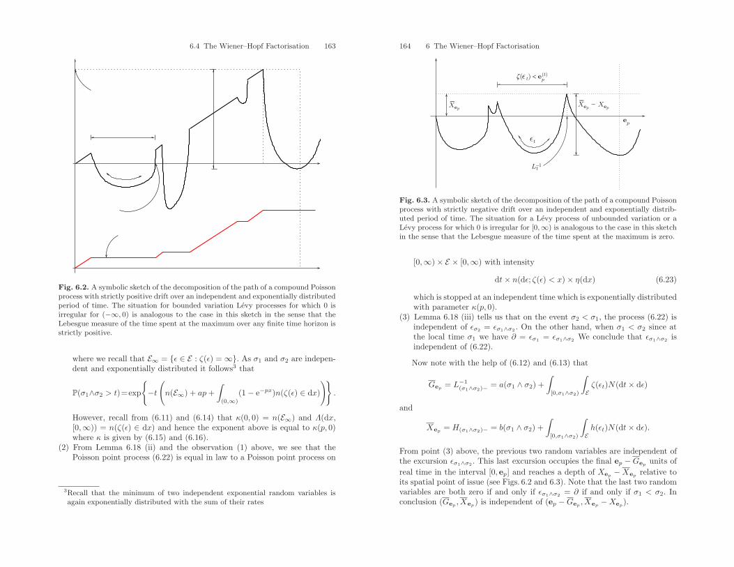
6.4 The Wiener–Hopf Factorisation 163
Fig. 6.2. A symbolic sketch of the decomposition of the path of a compound Poissonprocess with strictly positive drift over an independent and exponentially distributedperiod of time. The situation for bounded variation Levy processes for which 0 isirregular for (−∞, 0) is analogous to the case in this sketch in the sense that theLebesgue measure of the time spent at the maximum over any finite time horizon isstrictly positive.
where we recall that E∞ = ǫ ∈ E : ζ(ǫ) = ∞. As σ1 and σ2 are indepen-dent and exponentially distributed it follows3 that
P(σ1∧σ2 > t)=exp
−t(n(E∞) + ap+
∫(0,∞)
(1− e−px)n(ζ(ǫ) ∈ dx)
).
However, recall from (6.11) and (6.14) that κ(0, 0) = n(E∞) and Λ(dx,[0,∞)) = n(ζ(ǫ) ∈ dx) and hence the exponent above is equal to κ(p, 0)where κ is given by (6.15) and (6.16).
(2) From Lemma 6.18 (ii) and the observation (1) above, we see that thePoisson point process (6.22) is equal in law to a Poisson point process on
3Recall that the minimum of two independent exponential random variables isagain exponentially distributed with the sum of their rates
164 6 The Wiener–Hopf Factorisation
Xep
− Xep
−Xep
z( t) < ep(t)
−
Lt−1
ep
t
Fig. 6.3. A symbolic sketch of the decomposition of the path of a compound Poissonprocess with strictly negative drift over an independent and exponentially distrib-uted period of time. The situation for a Levy process of unbounded variation or aLevy process for which 0 is irregular for [0,∞) is analogous to the case in this sketchin the sense that the Lebesgue measure of the time spent at the maximum is zero.
[0,∞)× E × [0,∞) with intensity
dt× n(dǫ; ζ(ǫ) < x)× η(dx) (6.23)
which is stopped at an independent time which is exponentially distributedwith parameter κ(p, 0).
(3) Lemma 6.18 (iii) tells us that on the event σ2 < σ1, the process (6.22) isindependent of ǫσ2 = ǫσ1∧σ2 . On the other hand, when σ1 < σ2 since atthe local time σ1 we have ∂ = ǫσ1 = ǫσ1∧σ2 We conclude that ǫσ1∧σ2 isindependent of (6.22).
Now note with the help of (6.12) and (6.13) that
Gep= L−1
(σ1∧σ2)− = a(σ1 ∧ σ2) +∫
[0,σ1∧σ2)
∫Eζ(ǫt)N(dt× dǫ)
and
Xep= H(σ1∧σ2)− = b(σ1 ∧ σ2) +
∫[0,σ1∧σ2)
∫Eh(ǫt)N(dt× dǫ).
From point (3) above, the previous two random variables are independent ofthe excursion ǫσ1∧σ2 . This last excursion occupies the final ep −Gep
units ofreal time in the interval [0, ep] and reaches a depth of Xep
−Xeprelative to
its spatial point of issue (see Figs. 6.2 and 6.3). Note that the last two randomvariables are both zero if and only if ǫσ1∧σ2 = ∂ if and only if σ1 < σ2. Inconclusion (Gep
,Xep) is independent of (ep −Gep
,Xep−Xep
).
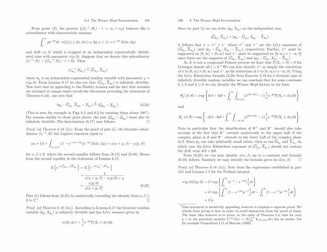
6.4 The Wiener–Hopf Factorisation 165
From point (2), the process (L−1t ,Ht) : t < σ1 ∧ σ2 behaves like a
subordinator with characteristic measure∫ ∞
0
pe−ptdt · n(ζ(ǫ) ∈ dx, h(ǫ) ∈ dy, x < t) = e−pxΛ(dx,dy)
and drift (a, b) which is stopped at an independent exponentially distrib-uted time with parameter κ(p, 0). Suppose that we denote this subordinator(L−1,H) = (L−1
t ,Ht) : t ≥ 0. Then
(L−1eχ,Heχ
) d= (Gep,Xep
)
where eχ is an independent exponential random variable with parameter χ =κ(p, 0). From Lemma 6.17 we also see that (Gep
,Xep) is infinitely divisible.
Now note that by appealing to the Duality Lemma and the fact that maximaare attained at unique times (recall the discussion preceding the statement ofTheorem 6.16), one sees that
(ep −Gep,Xep
−Xep) d= (Gep
,−Xep). (6.24)
(This is seen for example in Figs. 6.2 and 6.3 by rotating them about 180).For reasons similar to those given above, the pair (Gep
,−Xep) must also be
infinitely divisible. The factorisation (6.17) now follows.
Proof (of Theorem 6.16 (ii)). From the proof of part (i), the bivariate subor-dinator (L−1,H) has Laplace exponent equal to
aα+ bβ +∫
(0 ,∞)2(1 − e−αx−βy)e−pxΛ(dx ,dy) = κ(α+ p, β)− κ(p, 0 )
for α, β ≥ 0, where the second equality follows from (6.15) and (6.16). Hencefrom the second equality in the statement of Lemma 6.17,
E(e−αGep−βXep
)= E
(e−αL−1
eχ−βHeχ
)=
χ
κ(α+ p, β)− κ(p, 0) + χ
=κ(p, 0)
κ(α+ p, β). (6.25)
Part (ii) follows from (6.25) by analytically extending the identity from α, β ≥0 to C+.
Proof (of Theorem 6.16 (iii)). According to Lemma 6.17 the bivariate randomvariable (ep, Xep
) is infinitely divisible and has Levy measure given by
π(dt,dx) =1te−ptP(Xt ∈ dx)dt.
166 6 The Wiener–Hopf Factorisation
Since by part (i) we can write (ep, Xep) as the independent sum
(Gep,Xep
) + (ep −Gep, Xep
−Xep)
it follows that π = π+ + π− where π+ and π− are the Levy measures of(Gep
,Xep), and (ep − Gep
, Xep− Xep
), respectively. Further, π+ must besupported on [0,∞)× [0,∞) and π− must be supported on [0,∞)× (−∞, 0]since these are the supports of (Gep
,Xep) and (ep −Gep
, Xep−Xep
).As X is not a compound Poisson process we have that P(Xt = 0) = 0 for
Lebesgue almost all t > 0.4 We can now identify π+ as simply the restrictionof π to [0,∞)×(0,∞) and π− as the restriction of π to [0,∞)×(−∞, 0). Usingthe Levy–Khintchine formula (2.28) from Exercise 2.10 for a bivariate pair ofinfinitely divisible random variables we can conclude that for some constantsk ≥ 0 and k ≥ 0 we can identify the Wiener–Hopf factors in the form
Ψ+p (ϑ, θ) = exp
ikϑ+ ikθ +
∫ ∞
0
∫(0,∞)
(eiϑt+iθx − 1)1te−ptP(Xt ∈ dx)dt
and
Ψ−p (ϑ, θ)=exp
−ikϑ−ikθ+
∫ ∞
0
∫(−∞,0)
(eiϑt+iθx − 1)1te−ptP(Xt ∈ dx)dt
.
Note in particular that the identification of Ψ+ and Ψ− should also takeaccount of the fact that Ψ+ extends analytically to the upper half of thecomplex plane in θ and Ψ− extends to the lower half of the complex planein θ. Since ep can take arbitrarily small values, then so can Gep
and Xep. In
which case the Levy–Khintchine exponent of (Gep,Xep
) should not containthe drift term ikϑ+ ikθ.
From (6.25) we can now identify κ(α, β) up to a constant and formula(6.19) follows. Similarly we may identify the formula given for κ(α, β).
Proof (of Theorem 6.16 (iv)). Note from the expressions established in part(iii) and Lemma 1.7 for the Frullani integral,
κ(p, 0)κ(p, 0) = k′ exp∫ ∞
0
(e−t − e−pt)1tdt
= k′ exp∫ ∞
0
(1− e−pt)e−t1tdt−
∫ ∞
0
(1− e−t)e−pt1tdt
= k′p4This statement is intuitively appealing; however it requires a rigorous proof. Werefrain from giving it here in order to avoid distraction from the proof at hand.The basic idea however is to prove, in the spirit of Theorem 5.4, that for eachq > 0, the potential measure U (q)(dx) := E(
∫∞0
1(Xt∈dx)dt) has no atoms. Seefor example Proposition I.15 of Bertoin (1996).
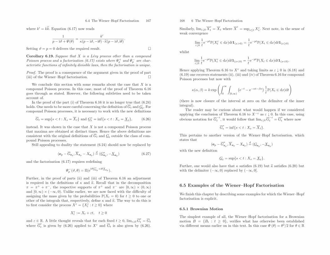
6.4 The Wiener–Hopf Factorisation 167
where k′ = kk. Equation (6.17) now reads
1p− iϑ+ Ψ(θ)
=k′
κ(p− iϑ,−iθ) · κ(p− iϑ, iθ).
Setting ϑ = p = 0 delivers the required result.
Corollary 6.19. Suppose that X is a Levy process other than a compoundPoisson process and a factorisation (6.17) exists where Ψ+
p and Ψ−p are char-acteristic functions of infinitely divisible laws, then the factorisation is unique.
Proof. The proof is a consequence of the argument given in the proof of part(iii) of the Wiener–Hopf factorisation.
We conclude this section with some remarks about the case that X is acompound Poisson process. In this case, most of the proof of Theorem 6.16goes through as stated. However, the following subtleties need to be takenaccount of.
In the proof of the part (i) of Theorem 6.16 it is no longer true that (6.24)holds. One needs to be more careful concerning the definition ofGt and Gt. Forcompound Poisson processes, it is necessary to work with the new definitions
Gt = sups < t : Xs = Xt and G∗t = infs < t : Xs = Xt, (6.26)
instead. It was shown in the case that X is not a compound Poisson processthat maxima are obtained at distinct times. Hence the above definitions areconsistent with the original definitions of Gt and Gt outside the class of com-pound Poisson processes.
Still appealing to duality the statement (6.24) should now be replaced by
(ep −Gep,Xep
−Xep) d= (G∗
ep,−Xep
) (6.27)
and the factorisation (6.17) requires redefining
Ψ−p (ϑ, θ) = E(eiϑG∗ep+iθXep ).
Further, in the proof of parts (ii) and (iii) of Theorem 6.16 an adjustmentis required in the definitions of κ and κ. Recall that in the decompositionπ = π+ + π−, the respective supports of π+ and π− are [0,∞) × (0,∞)and [0,∞) × (−∞, 0). Unlike earlier, we are now faced with the difficulty ofassigning the mass given by the probabilities P(Xt = 0) for t ≥ 0 to one orother of the integrals that, respectively, define κ and κ. The way to do this isto first consider the process Xε = Xε
t : t ≥ 0 where
Xεt := Xt + εt, t ≥ 0
and ε ∈ R. A little thought reveals that for each fixed t ≥ 0, limε↓0 Gε
t = Gt
where Gε
t is given by (6.26) applied to Xε and Gt is also given by (6.26).
168 6 The Wiener–Hopf Factorisation
Similarly, limε↓0 Xε
t = Xt where Xε
= sups≤tXεs . Next note, in the sense of
weak convergence
limε↓0
1te−ptP(Xε
t ∈ dx)dt1(x>0) =1te−ptP(Xt ∈ dx)dt1(x≥0)
whilst
limε↓0
1te−ptP(Xε
t ∈ dx)dt1(x<0) =1te−ptP(Xt ∈ dx)dt1(x<0).
Hence applying Theorem 6.16 to Xε and taking limits as ε ↓ 0 in (6.18) and(6.19) one recovers statements (ii), (iii) and (iv) of Theorem 6.16 for compoundPoisson processes but now with
κ(α, β) = k exp
(∫ ∞
0
∫[0,∞)
(e−t − e−αt−βx
) 1tP(Xt ∈ dx)dt
)
(there is now closure of the interval at zero on the delimiter of the innerintegral).
The reader may be curious about what would happen if we consideredapplying the conclusion of Theorem 6.16 to X−ε as ε ↓ 0. In this case, usingobvious notation for G
−εt , it would follow that limε↓0 G
−εt = G
∗t where now
G∗t = infs < t : Xs = Xt.
This pertains to another version of the Wiener–Hopf factorisation. whichstates that
(ep −G∗ep,Xep
−Xep) d= (Gep
,−Xep)
with the new definition
Gt = sups < t : Xs = Xt.Further, one would also have that κ satisfies (6.19) but κ satisfies (6.20) butwith the delimiter (−∞, 0) replaced by (−∞, 0].
6.5 Examples of the Wiener–Hopf Factorisation
We finish this chapter by describing some examples for which the Wiener–Hopffactorisation is explicit.
6.5.1 Brownian Motion
The simplest example of all, the Wiener–Hopf factorisation for a Brownianmotion B = Bt : t ≥ 0, verifies what has otherwise been establishedvia different means earlier on in this text. In this case Ψ (θ) = θ2/2 for θ ∈ R
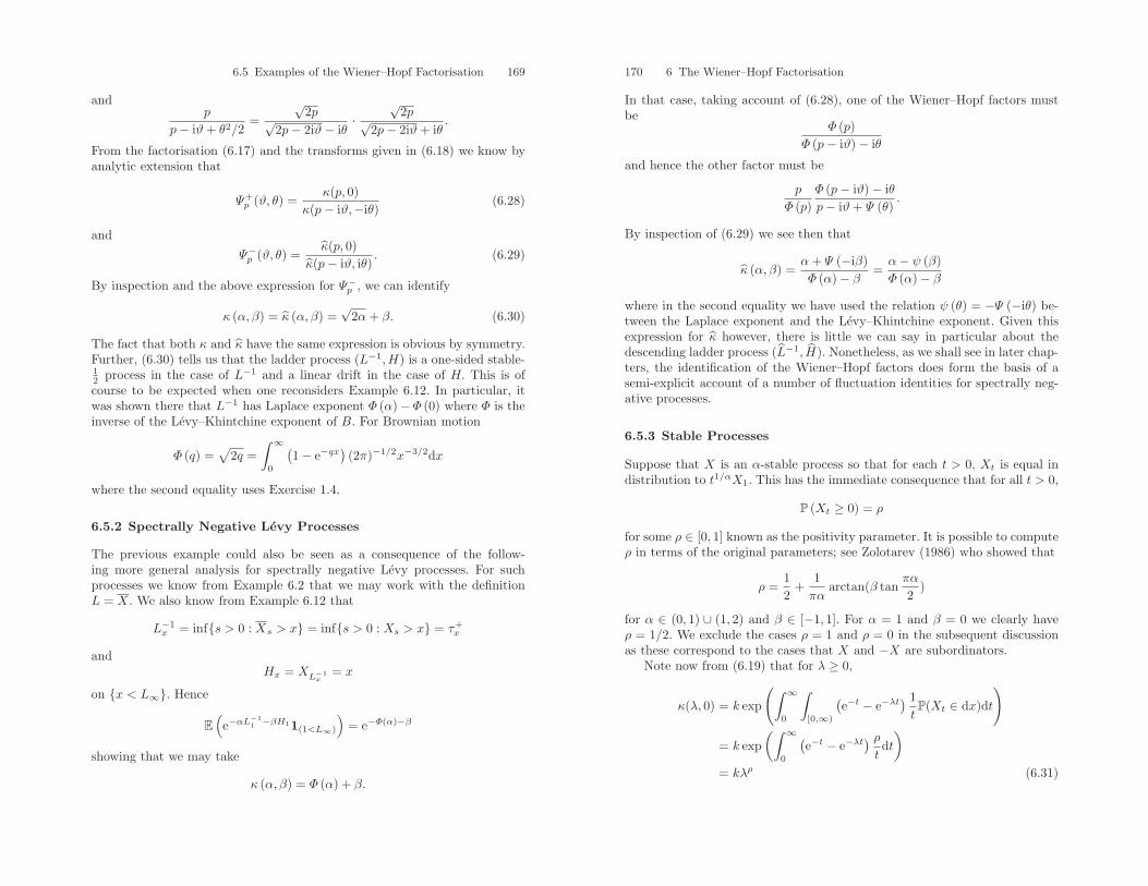
6.5 Examples of the Wiener–Hopf Factorisation 169
andp
p− iϑ+ θ2/2=
√2p√
2p− 2iϑ− iθ·
√2p√
2p− 2iϑ+ iθ.
From the factorisation (6.17) and the transforms given in (6.18) we know byanalytic extension that
Ψ+p (ϑ, θ) =
κ(p, 0)κ(p− iϑ,−iθ)
(6.28)
and
Ψ−p (ϑ, θ) =κ(p, 0)
κ(p− iϑ, iθ). (6.29)
By inspection and the above expression for Ψ−p , we can identify
κ (α, β) = κ (α, β) =√
2α+ β. (6.30)
The fact that both κ and κ have the same expression is obvious by symmetry.Further, (6.30) tells us that the ladder process (L−1,H) is a one-sided stable-12 process in the case of L−1 and a linear drift in the case of H. This is ofcourse to be expected when one reconsiders Example 6.12. In particular, itwas shown there that L−1 has Laplace exponent Φ (α)− Φ (0) where Φ is theinverse of the Levy–Khintchine exponent of B. For Brownian motion
Φ (q) =√
2q =∫ ∞
0
(1− e−qx
)(2π)−1/2x−3/2dx
where the second equality uses Exercise 1.4.
6.5.2 Spectrally Negative Levy Processes
The previous example could also be seen as a consequence of the follow-ing more general analysis for spectrally negative Levy processes. For suchprocesses we know from Example 6.2 that we may work with the definitionL = X. We also know from Example 6.12 that
L−1x = infs > 0 : Xs > x = infs > 0 : Xs > x = τ+
x
andHx = XL−1
x= x
on x < L∞. Hence
E(e−αL
−11 −βH11(1<L∞)
)= e−Φ(α)−β
showing that we may take
κ (α, β) = Φ (α) + β.
170 6 The Wiener–Hopf Factorisation
In that case, taking account of (6.28), one of the Wiener–Hopf factors mustbe
Φ (p)Φ (p− iϑ)− iθ
and hence the other factor must be
p
Φ (p)Φ (p− iϑ)− iθp− iϑ+ Ψ (θ)
.
By inspection of (6.29) we see then that
κ (α, β) =α+ Ψ (−iβ)Φ (α)− β
=α− ψ (β)Φ (α)− β
where in the second equality we have used the relation ψ (θ) = −Ψ (−iθ) be-tween the Laplace exponent and the Levy–Khintchine exponent. Given thisexpression for κ however, there is little we can say in particular about thedescending ladder process (L−1, H). Nonetheless, as we shall see in later chap-ters, the identification of the Wiener–Hopf factors does form the basis of asemi-explicit account of a number of fluctuation identities for spectrally neg-ative processes.
6.5.3 Stable Processes
Suppose that X is an α-stable process so that for each t > 0, Xt is equal indistribution to t1/αX1. This has the immediate consequence that for all t > 0,
P (Xt ≥ 0) = ρ
for some ρ ∈ [0, 1] known as the positivity parameter. It is possible to computeρ in terms of the original parameters; see Zolotarev (1986) who showed that
ρ =12
+1πα
arctan(β tanπα
2)
for α ∈ (0, 1) ∪ (1, 2) and β ∈ [−1, 1]. For α = 1 and β = 0 we clearly haveρ = 1/2. We exclude the cases ρ = 1 and ρ = 0 in the subsequent discussionas these correspond to the cases that X and −X are subordinators.
Note now from (6.19) that for λ ≥ 0,
κ(λ, 0) = k exp
(∫ ∞
0
∫[0,∞)
(e−t − e−λt
) 1tP(Xt ∈ dx)dt
)
= k exp(∫ ∞
0
(e−t − e−λt
) ρtdt)
= kλρ (6.31)
6.5 Examples of the Wiener–Hopf Factorisation 171
where in the final equality we have used the Frullani integral. This tells usdirectly that the process L−1 is itself stable. We can proceed further andcalculate for λ ≥ 0,
κ(0, λ) = k exp
(∫ ∞
0
∫[0,∞)
(e−t − e−λx
) 1tP(Xt ∈ dx)dt
)
= k exp(∫ ∞
0
1tE((
e−t − e−λXt)1(Xt≥0)
)dt)
= k exp(∫ ∞
0
1tE((
e−t − e−λt1/αX1
)1(X1≥0)
)dt)
= k exp(∫ ∞
0
1s
E((
e−sλ−α − e−s
1/αX1
)1(X1≥0)
)ds)
= k exp(∫ ∞
0
1s
E((
e−s − e−Xs)1(Xs≥0)
)ds)
× exp(−∫ ∞
0
ρ
s
(e−s − e−sλ
−α)
ds)
= κ(0, 1)× exp(−∫ ∞
0
1s
(e−s − e−sλ
−α)
ds)
= κ(0, 1)λαρ,
where in the third and fifth equality we have used the fact that s1/αX1 isequal in distribution to Xs. The term κ(0, 1) is nothing more than a constantand hence we deduce that the ascending ladder height process is also a stableprocess of index αρ. It is now immediate from (6.21) that the descendingladder height process is a stable process of index α(1− ρ) which is consistentwith the fact that P (Xt ≤ 0) = 1− ρ. Note that this necessarily implies that0 < αρ ≤ 1 and 0 ≤ α(1− ρ) ≤ 1 when ρ ∈ (0, 1). The extreme cases αρ = 1and α(1 − ρ) = 1 correspond to spectrally negative and spectrally positiveprocesses, respectively. For example, when β = −1 and α ∈ (1, 2) we have aspectrally negative process of unbounded variation. It is easily checked thatρ = 1/α and hence from the calculation above κ(0, λ) = const.×λ consistentlywith earlier established facts for spectrally negative Levy processes. Note thatκ(0, 0) = κ(0, 0) = 0 showing that the killing rates in the ascending anddescending ladder height processes are equal to zero and hence
lim supt↑∞
Xt = − lim inft↑∞
Xt = ∞.
Unfortunately it is not as easy to establish a closed expression for thebivariate exponent κ. The only known results in this direction are those ofDoney (1987) who only deals with a set of parameter values of α and β whichare dense in the full parameter range (0, 2) and [−1, 1]. The expressions ob-tained by Doney are quite complicated however and we refrain from includingthem here.
172 6 The Wiener–Hopf Factorisation
6.5.4 Other Examples
Other than the stable processes, there are very few examples where one knowsof explicit details of the Wiener–Hopf factorisation for processes which haveboth positive and negative jumps. One example, found in Feller (1971), is thecase that X is the difference of a compound Poisson process with exponentiallydistributed jumps and another independent subordinator. The reason why thelatter example is, up to a certain point, analytically tractable boils down tothe fact that the ascending ladder height process must again be a (possiblykilled) compound Poisson subordinator with exponential jumps. This is obvi-ous when one considers that if a new maxima is incurred then it is achievedby an exponentially distributed jump and hence by the lack of memory prop-erty, the overshoot over the previous maximum must again be exponentiallydistributed. Knowing the nature of the ascending ladder height process allowsone to compute the factor Ψ+
p (0, θ) and hence establish the function κ(α, β)as well as the κ(α, β) from the factorisation (6.17).
There is another class of distributions which observe a property similar innature to the lack of memory property and these are phase-type distributions.A distribution F on (0,∞) is phase-type if it is the distribution of the absorp-tion time in a finite state continuous time Markov process J = Jt : t ≥ 0with one state ∆ absorbing and the remaining ones 1, ...,m transient. The pa-rameters of this system are m, the restriction T of the full intensity matrix tothe m transient states and the initial probability (row) vector a = (a1, ..., am)where ai = P(J0 = i). For any i = 1, ...,m, let ti be the intensity of thetransition i → ∆ and write t for the column vector of intensities into ∆. Itfollows that
1− F (x) = aexTu
where u is the m × 1 vector with unit entries. An easy differentiation showsthat the density is given by f(x) = aeTxt.
The “lack of memory”-type property which phase-type distributions en-joy can be expressed as follows. Suppose that Pj : j = 1, ...,m are therespective probabilities of J when started from state j = 1, ...,m and writePa =
∑mj=1 ajPj for the probability of J with randomised initial state having
distribution a. Let τ∆ be the absorption time into state ∆ of J . Then fort, s ≥ 0,
Pa(τ∆ > t+ s|τ∆ > t) = PJt(τ∆ > s)
which is again a phase-type distribution but with the vector a replaced by thevector which has a 1 in position Jt and otherwise zeros for the other entries.
Recently, Mordecki (2002) and Asmussen et al. (2004) have used this prop-erty to establish another example of a Levy process for which elements of theWiener–Hopf factorisation can be expressed in more mathematical detail. Seealso Pistorius (2006) and Mordecki (2005). The process they consider takes
6.5 Examples of the Wiener–Hopf Factorisation 173
the form
Xt = X(+)t −
N(t)∑j=1
Uj , t ≥ 0
where X(+)t : t ≥ 0 is a Levy process which has no negative jumps,
Nt : t ≥ 0 is an independent Poisson process with rate λ and Uj : j ≥ 1are i.i.d. random variables with a common phase-type distribution F . Theidea exploited by the aforementioned authors is that when X obtains a newmaximum, it either does so continuously on account of the process X(+) orwith a jump which is phase-type distributed. Suppose this jump is of lengths + t where t is the undershoot and s is the overshoot. If one thinks of thisjump as the time it takes for absorption of an auxiliary Markov chain, J , froma randomised initial position with distribution a, then s corresponds to thetime it takes to absorption from a randomised initial position Jt. In conclu-sion, the overshoot must be again phase-type distributed but with a differentparameter set. The above phase-type processes thus offer sufficient mathe-matical structure for the Laplace exponent κ(α, β) to be computed in moredetail. We give a brief indication of the structure of κ(α, β) below withoutgoing into details however for the sake of brevity.
The characteristic exponent thus takes the form
Ψ(θ) = aiθ +12σ2θ2 +
∫(0,∞)
(1− eiθx − iθx1(x<1))Π(dx) + λ(E(eiθU1)− 1)
for θ ∈ R. Since E(eiθU1) = −a(iθI + T)−1t, where I is the identity matrix,and the latter expression is effectively the ratio of two complex polynomials,it can be shown that Ψ , can be analytically extended to z ∈ C : ℜz ≤ 0with the exception of a finite number of poles (the eigenvalues of T). Definefor each α > 0, the finite set of roots with negative real part
Iα = ρi : Ψ(ρi) + α = 0 and ℜρi < 0,where multiple roots are counted individually. Next, define for each α > 0, asecond set of roots with negative real part
Jα =ηi :
1α+ Ψ(ηi)
= 0 and ℜηi < 0
again taking multiplicity into account. Asmussen et al. (2004) show that
κ(α, β) =
∏i∈Iα
(β − ρi)∏i∈Jα
(β − ηi)
thus giving a semi-explicit expression for the Wiener–Hopf factor,
Ψ−p (ϑ, θ) =
∏i∈Ip
(−ρi)∏i∈Jp
(−ηi)
∏i∈Ip−iϑ
(−iθ − ρi)∏i∈Jp−iϑ
(−iθ − ηi)
for ℜs ≥ 0.
174 6 The Wiener–Hopf Factorisation
Earlier examples of Wiener–Hopf factorisations for which both factors takea rational form as above were investigated by Borovkov (1976) and Feller(1971).
6.6 Brief Remarks on the Term “Wiener–Hopf”
Having now completed our exposition of the Wiener–Hopf factorisation, thereader may feel somewhat confused as to the association of the name “Wiener–Hopf” with Theorem 6.16. Indeed, in our presentation we have made no refer-ence to works of Wiener nor Hopf. The connection between Theorem 6.16 andthese two scientists lies with their analytic study of the solutions to integralequations of the form
Q(x) =∫ ∞
0
Q(y)f(x− y)dy, x > 0 (6.32)
where f : R → [0,∞) is a pre-specified kernel; see Payley and Wiener (1934)and Hopf (1934). If one considers a compound Poisson processX which has theproperty that lim supt↑∞Xt < ∞ then the Strong Markov Property impliesthat X∞ is equal in distribution to (ξ + X∞) ∨ 0 where ξ is independentof X∞ and has the same distribution as the jumps of X. If the latter jumpdistribution has density f then one shows easily that H(x) = P(X∞ ≤ x)satisfies
H(x) =∫ x
−∞H(x− y)f(y)dy =
∫ ∞
0
f(x− y)H(y)dy
and hence one obtains immediately the existence of a solution to (6.32) forthe given f . This observation dates back to the work of Spitzer (1957).
Embedded in the complex analytic techniques used to analyse (6.32) andgeneralisations thereof by Wiener, Hopf and many others that followed, arefactorisations of operators (which can take the form of Fourier transforms).In the probabilistic setting here, this is manifested in the form of the inde-pendence seen in Theorem 6.16 (i) and how this is used to identify the factorsΨ+ and Ψ− in conjunction with analytic extension in the proof of part (iii)of the same theorem. The full extent of the analytic Wiener–Hopf factorisa-tion techniques go far beyond the current setting and we make no attempt toexpose them here. The name “Wiener–Hopf” factorisation thus appears as arather obscure feature of what may otherwise be considered as a sophisticatedpath decomposition of a Levy process.
Exercises
6.1. Give an example of a Levy process which has bounded variation with zerodrift for which 0 is regular for both (0,∞) and (−∞, 0). Give an example of
6.6 Exercises 175
a Levy process of bounded variation and zero drift for which 0 is only regularfor (0,∞).
6.2. Suppose that X is a spectrally negative Levy process of unbounded vari-ation with Laplace exponent ψ and recall the definition τ+
x = inft > 0 :Xt > x . Recall also that the process τ+ := τ+
x : x ≥ 0 is a (possiblykilled) subordinator (see Corollary 3.14) with Laplace exponent Φ, the rightinverse of ψ.
(i) Suppose that d is the drift of the process τ+. Show that necessarily d = 0.(ii) Deduce that
limx↓0
τ+x
x= 0
and hence thatlim supt↓0
Xt
t= ∞.
Conclude from the latter that 0 is regular for (0,∞) and hence that thejump measure of τ+ cannot be finite.
(iii) From the Wiener–Hopf factorisation of X show that
limθ↑∞
E(eθXeq ) = 0
and hence use this to give an alternative proof that 0 is regular for (0,∞).
6.3. Fix ρ ∈ (0, 1]. Show that a compound Poisson subordinator with jumprate λρ killed at an independent and exponentially distributed time with pa-rameter λ(1 − ρ) is equal in law to a compound Poisson subordinator killedafter an independent number of jumps which is distributed geometrically withparameter 1− ρ.
6.4. Show that the only processes for which∫ ∞
0
1(Xt=Xt)dt > 0 and
∫ ∞
0
1(Xt=Xt)dt > 0
almost surely are compound Poisson processes.
6.5. Suppose that X is spectrally negative with Levy measure Π and Gaussiancoefficient σ and suppose that E(Xt) > 0. (Recall that in general E(Xt) ∈[−∞,∞).)
(i) Show that ∫ −1
−∞Π(−∞, x)dx <∞.
176 6 The Wiener–Hopf Factorisation
(ii) Using Theorem 6.16 (iv) deduce that, up to a constant,
κ(0, iθ) =
(−a+
∫(−∞,−1)
xΠ(dx)
)
−12iθσ2 +
∫(−∞,0)
(1− eiθx)Π(−∞, x)dx.
Hence deduce that there exists a choice of local time at the maximum forwhich the descending ladder height process has jump measure given byΠ(−∞,−x)dx on (0,∞), drift σ2/2 and is killed at rate E(X1).
6.6. Suppose that X is a spectrally negative stable process of index 1 < α < 2.
(i) Deduce with the help of Theorem 3.12 that up to a multiplicative constant
κ(θ, 0) = θ1/α
and hence that P(Xt ≥ 0) = 1/α for all t ≥ 0.(ii) By reconsidering the Wiener–Hopf factorisation, show that for each t ≥ 0
and θ ≥ 0,
E(e−θXt) =∞∑n=0
(−θt1/α)n
Γ (1 + n/α).
This identity is taken from Bingham (1971, 1972).
6.7 (The second factorisation identity). In this exercise we derive whatis commonly called the second factorisation identity which is due to Perch-eskii and Rogozin (1969). It uses the Laplace exponents κ and κ to give anidentity concerning the problem of first passage above a fixed level x ∈ R.The derivation we use here makes use of calculations in Darling et al. (1972)and Alili and Kyprianou (2004). We shall use the derivation of this identitylater to solve some optimal stopping problems.
Define as usualτ+x = inft > 0 : Xt > x
where X is any Levy process.
(i) Using the same technique as in Exercise 5.5, prove that for all α > 0, β ≥ 0and x ∈ R we have
E(
e−ατ+
x −βXτ+x 1(τ+
x <∞)
)=
E(e−βXeα 1(Xeα>x)
)E(e−βXeα
) . (6.33)
(ii) Establish the second factorisation identity as follows. If X is not a subor-dinator then∫ ∞
0
e−qxE(
e−ατ+
x −β(Xτ+x−x)
1(τ+x <∞)
)dx =
κ (α, q)− κ (α, β)(q − β)κ (α, q)
.
6.6 Exercises 177
6.8. Suppose that X is any Levy process which is not a subordinator andep is an independent random variable which is exponentially distributed withparameter p > 0. Note that 0 is regular for (0,∞) if and only if P (Xep
= 0) =0 where ep is an independent exponential random variable with parameter p.Use the Wiener–Hopf factorisation to show that 0 is regular for (0,∞) if andonly if ∫ 1
0
1tP(Xt > 0)dt = ∞.
Now noting that 0 is irregular for [0,∞) if and only if P(Gep= 0) > 0. Show
that 0 is regular for [0,∞) if and only if∫ 1
0
1tP(Xt ≥ 0)dt = ∞.
6.9. This exercise gives the random walk analogue of the Wiener–Hopf factori-sation. In fact this is the original setting of the Wiener–Hopf factorisation. Wegive the formulation in Greenwood and Pitman (1980a). However, one mayalso consult Feller (1971) and Borovkov (1976) for other accounts.
Suppose that under P , S = Sn : n ≥ 0 is a random walk with S0 = 0and increment distribution F . We assume that S can jump both upwards anddownwards, in other words minF (−∞, 0), F (0,∞) > 0 and that F has noatoms. Denote by Γp an independent random variable which has a geometricdistribution with parameter p ∈ (0, 1) and let
G = mink = 0, 1, ...,Γp : Sk = maxj=1,...,Γp
Sj.
Note that SG is the last maximum over times 0, 1, ...,Γp. Define N =infn > 0 : Sn > 0 the first passage time into (0,∞) or equivalently thefirst strict ladder time. Our aim is to characterise the joint laws (G,SG) and(N,SN ) in terms of F , the basic data of the random walk.
(i) Show that (even without the restriction that minF (0,∞), F (−∞, 0) >0),
E(sΓpeiθSΓp ) = exp
−∫
R
∞∑n=1
(1− sneiθx)qn1nF ∗n(dx)
where 0 < s ≤ 1, θ ∈ R, q = 1− p and E is expectation under P . Deducethat the pair (Γp, SΓp
) is infinitely divisible.(ii) Let ν be an independent random variable which is geometrically distrib-
uted on 0, 1, 2, ... with parameter P (N > Γp). Using a path decom-position in terms of excursions from the maximum, show that the pair(G,SG) is equal in distribution to the component-wise sum of ν indepen-dent copies of (N,SN ) conditioned on the event N ≤ Γp and henceform an infinitely divisible 2D distribution.
178 6 The Wiener–Hopf Factorisation
(iii) Show that (G,SG) and (Γp−G,SΓp−SG) are independent. Further, that
the latter pair is equal in distribution to (D,SD) where
D = maxk = 0, 1, ...,Γp : Sk = minj=1,...,Γp
Sj.
(iv) Deduce that
E(sGeiθSG) = exp
−∫
(0,∞)
∞∑n=1
(1− sneiθx)qn1nF ∗n(dx)
for 0 < s ≤ 1 and θ ∈ R. Note when s = 1, this identity was establishedby Spitzer (1956).
(v) Show that
E(sGeiθSG) =P (Γp < N)
1− E((qs)NeiθSN )
and hence deduce that
11− E(sNeiθSN )
= exp
∫(0,∞)
∞∑n=1
sneiθx 1nF ∗n(dx)
.
According to Feller (1971), this is known as Baxter’s identity.
7
Levy Processes at First Passageand Insurance Risk
This chapter is devoted to studying how the Wiener–Hopf factorisation can beused to characterise the behaviour of any Levy process at first passage over afixed level. The case of a subordinator will be excluded throughout this chapteras this has been dealt with in Chap. 5. Nonetheless, the understanding of howsubordinators make first passage will play a crucial role in understanding thecase of a general Levy process.
Recall from Sects. 1.3.1 and 2.7.1 that a natural extension of the classicalCramer–Lundberg model for risk insurance is that of a spectrally negativeLevy process. In that case, if we take X to model the negative of the capitalof an insurance firm, then due to spatial homogeneity a characterisation offirst passage of X at x > 0 corresponds precisely to a characterisation of ruinwhen there is an initial capital at time zero of x units.
To some extent, the results we present on the first passage problem suf-fer from a lack of analytical explicitness which is due to the same symptomsbeing present in the Wiener–Hopf factorisation. None the less there is suffi-cient mathematical structure to establish qualitative statements concerningthe characterisation of first passage, or equivalently ruinous behaviour of in-surance risk processes. This becomes more apparent when looking at asymp-totic properties of the established characterisations.
We start by looking at the general Levy risk insurance model, when theprobability of ruin is strictly less than one and further we consider a versionof Cramer’s estimate of ruin for a reasonably general class of Levy processes.Then we move to a full characterisation of the ruin problem and concludewith some results concerning the asymptotic behaviour of ruin for a specialclass of insurance risk models.
7.1 Drifting and Oscillating
Suppose that X is any Levy process, then define as usual
τ+x = inft > 0 : Xt > x
180 7 Levy Processes at First Passage and Insurance Risk
for x ∈ R. If we now define −X as the capital of an insurance firm, then theprobability of ruin when starting from an initial capital of x > 0 is given byP(τ+
x <∞). In this section we shall establish precisely when the probability ofruin is strictly less than one. Further, in the latter case, we shall give sufficientconditions under which the ruin probability decays exponentially as x ↑ ∞;that is to say we handle the case of Cramer’s estimate of ruin.
Suppose now that H = Ht : t ≥ 0 is the ascending ladder height processof X. If
T+x = inft > 0 : Ht > x,
then quite clearlyP(τ+
x <∞) = P(T+x <∞). (7.1)
Recall from Theorem 6.10 that the process H behaves like a subordinator,possibly killed at an independent and exponentially distributed time. Thecriterion for killing is that P(limsupt↑∞Xt <∞) = 1. Suppose the latter fails.Then the probability on the right-hand side of (7.1) is equal to 1. If on theother hand there is killing, then since killing can occur at arbitrarily smalltimes with positive probability, then P(T+
x <∞) < 1. In conclusion we knowthat for any x > 0,
P(ruin from initial reserve x) < 1 ⇔ P(limt↑∞
supXt <∞) = 1. (7.2)
We devote the remainder of this section then to establishing conditions underwhich P(lim supt↑∞Xt <∞) = 1.
Theorem 7.1. Suppose that X is a Levy process.
(i) If∫∞1
t−1P(Xt ≥ 0)dt <∞ then
limt↑∞
Xt = −∞
almost surely and X is said to drift to −∞.(ii) If
∫∞1
t−1P(Xt ≤ 0)dt <∞ then
limt↑∞
Xt = ∞
almost surely and X is said to drift to ∞.(iii) If both the integral tests in (i) and (ii) fail, 1 then
limt↑∞
supXt = − limt↑∞
inf Xt = ∞
almost surely and X is said to oscillate.1Note that
∫∞1
t−1P(Xt ≥ 0)dt +∫∞1
t−1P(Xt ≤ 0)dt ≥ ∫∞1
t−1dt = ∞ and henceat least one of the integral tests in (i) or (ii) fails.
7.1 Drifting and Oscillating 181
Proof. We follow a similar proof to the one given in Bertoin (1996).(i) From Theorem 6.16 (see also the discussion at the end of Sect. 6.4
concerning the adjusted definitions of G∞ and G∞ for the case of compoundPoisson processes) we have for all α ≥ 0,
E(e−αGep
)= exp
−∫ ∞
0
(1− e−αt)1te−ptP(Xt ≥ 0)dt
. (7.3)
Letting p tend to zero in (7.3) and applying the Dominated ConvergenceTheorem on the left-hand side and the Monotone Convergence Theorem onthe right-hand side we see that
E(e−αG∞
)= exp
−∫ ∞
0
(1− e−αt)1tP(Xt ≥ 0)dt
. (7.4)
If∫∞1
t−1P(Xt ≥ 0)dt <∞ then since 0 ≤ (1−e−αt) ≤ 1∧ t for all sufficientlysmall α, we see that∫ ∞
0
(1− e−αt)1tP(Xt ≥ 0)dt ≤
∫ ∞
0
(1 ∧ t)1tP(Xt ≥ 0)dt
≤∫ ∞
1
1tP(Xt ≥ 0)dt+
∫ 1
0
P(Xt ≥ 0)dt <∞.
Hence once again appealing to the Dominated Convergence Theorem, takingα to zero in (7.4), it follows that
limα↓0
∫ ∞
0
(1− e−αt)1tP(Xt ≥ 0)dt = 0
and therefore P(G∞ <∞) = 1. This implies that P
(X∞ <∞) = 1.
Now noting that∫∞1
t−1P(Xt ≥ 0)dt =∫∞1
t−1(1 − P(Xt < 0))dt < ∞,since
∫∞1
t−1dt = ∞, we are forced to conclude that∫ ∞
1
1tP(Xt < 0)dt = ∞.
The Wiener–Hopf factorisation also gives us
E(e−αGep
)= exp
−∫ ∞
0
(1− e−αt)1te−ptP(Xt ≤ 0)dt
.
Taking limits as p ↓ 0 and noting that∫ ∞
0
(1− e−αt)1tP(Xt ≤ 0)dt ≥ k
∫ ∞
1
1tP(Xt ≤ 0)dt = ∞
for some appropriate constant k > 0, we get P (G∞ = ∞) = 1. EquivalentlyP (X∞ = −∞) = 1.
182 7 Levy Processes at First Passage and Insurance Risk
We have proved that lim supt↑∞Xt <∞ and lim inft↑∞Xt = −∞ almostsurely. This means that
τ−−x := inft > 0 : Xt < −xis almost surely finite for each x > 0. Note that
Xt > x/2 for some t > 0 = X∞ > x/2and hence, since P
(X∞ <∞) = 1, for each 1 > ε > 0, there exists an xε > 0
such that for all x > xε,
P (Xt > x/2 for some t > 0) < ε.
Since τ−−x is a stopping time which is almost surely finite, we can use theprevious estimate together with the Strong Markov Property and concludethat for all x > xε,
P(Xt > −x/2 for some t > τ−−x
)≤ P (Xt > x/2 for some t > 0) < ε.
This gives us the uniform estimate for x > xε,
P
(lim supt↑∞
Xt ≤ −x/2)≥ P
(Xt ≤ −x/2 for all t > τ−−x
)≥ 1− ε.
Since both x may be taken arbitrarily large and ε may be taken arbitrarilyclose to 0 the proof of part (i) is complete.
(ii) The second part follows from the first part applied to −X.(iii) The argument in (i) shows that in fact when
∫∞1
t−1P(Xt ≤ 0)dt =∫∞1
t−1P(Xt ≥ 0)dt = ∞, then −X∞ = X∞ = ∞ almost surely and theassertion follows.
Whilst the last theorem shows that there are only three types of asymp-totic behaviour, the integral tests which help to distinguish between the threecases are not particularly user friendly. What would be more appropriate is acriterion in terms of the triple (a, σ,Π). The latter is provided by Chung andFuchs (1951) and Erickson (1973) for random walks; see also Bertoin (1997).To state their criteria, recall from Theorem 3.8 and Exericse 3.3 that the meanof X1 is well defined if and only if∫ ∞
1
xΠ(dx) <∞ or∫ −1
−∞|x|Π(dx) <∞
in which case E(X1) ∈ [−∞,∞]. When both the above integrals are infinitethe mean E(X1) is undefined.
7.1 Drifting and Oscillating 183
Theorem 7.2. Suppose that X is a Levy process with characteristic measureΠ.
(i) If E(X1) is defined and valued in [−∞, 0) or if E(X1) is undefined and∫ ∞
1
xΠ(dx)∫ x0Π(−∞,−y)dy <∞,
thenlimt↑∞
Xt = −∞.
(ii) If E(X1) is defined and valued in (0,∞] or if E(X1) is undefined and∫ −1
−∞
|x|Π(dx)∫ |x|0
Π(y,∞)dy<∞,
thenlimt↑∞
Xt = ∞.
(iii) If E(X1) is defined and equal to zero or if E(X1) is undefined and bothof the integral tests in part (i) and (ii) fail, then
lim supt↑∞
Xt = − lim inft↑∞
Xt = ∞.
We give no proof here of this important result, although one may consultExercise 7.2 for related results which lean on the classical Strong Law of LargeNumbers.
It is interesting to compare the integral tests in the above theorem withthose of Theorem 6.5. It would seem that the issue of regularity 0 for thehalf line may be seen as the “small time” analogue of drifting or oscillating,however there is no known formal path-wise connection.
In the case that X is spectrally negative, thanks to the finiteness andconvexity of its Laplace exponent ψ(θ) = log E(eθX1) on θ ≥ 0 (see Exercise3.5), one always has that E(X1) ∈ [−∞,∞). That is to say, the asymptoticbehaviour of a spectrally negative Levy process can always be determinedfrom its mean or equivalently ψ′(0+). See Exercise 7.3 which shows how toderive this conclusion from Theorem 7.1 and the Wiener–Hopf factorisation.
On account of the trichotomy of drifting and oscillating, we may now revisethe statement (7.2) as
P(ruin from initial capital x) < 1 ⇔ P(limt↑∞
Xt = −∞) = 1.
We close this section by making some brief remarks on the link betweendrifting and oscillating and another closely related dichotomy known as tran-sience and recurrence which is often discussed within the more general contextof Markov Processes.
184 7 Levy Processes at First Passage and Insurance Risk
Definition 7.3. A Levy process X is said to be transient if for all a > 0,
P(∫ ∞
0
1(|Xt|<a)dt <∞)
= 1
and recurrent if for all a > 0,
P(∫ ∞
0
1(|Xt|<a)dt = ∞)
= 1
In the previous definition, the requirements for transience and recurrencemay appear quite strong as in principle, the given probabilities could be lessthan one. The events in the definition however belong to the tail sigma algebra⋂t∈Q∩[0,∞) σ(Xs : s ≥ t) and hence according to Kolmogorov’s zero-one can
only have probabilities equal to zero or one. Nonetheless, one could arguethat it could be the case for example that for small a it is the case thatP(∫∞0
1(|Xt|<a)dt = ∞) = 0 and for large values of a the same probabilityis 1. It turns out that Levy processes always adhere to one of the two casesgiven in the definition as the following classic analytic dichotomy due to Portand Stone (1971)2 confirms.
Theorem 7.4. Suppose that X is a Levy process with characteristic exponentΨ , then it is transient if and only if for some sufficiently small ε > 0,∫
(−ε,ε)ℜ(
1Ψ(θ)
)dθ <∞
and otherwise it is recurrent.
Probabilistic reasoning also leads to the following interpretation of the di-chotomy.
Theorem 7.5. Suppose that X is any Levy process.
(i) Then, X is transient if and only if
limt↑∞
|Xt| = ∞
almost surely.(ii) Suppose that X is not a compound Poisson process, then X is recurrent
if and only if for all x ∈ R,
lim inft↑∞
|Xt − x| = 0 (7.5)
almost surely.2Theorem 7.4 is built on the strength of the original, but weaker result of Chungand Fuchs (1951). See also Kingman (1964).

7.2 Cramer’s Estimate of Ruin 185
The reason for the exclusion of compound Poisson processes in part (ii) canbe seen when one considers the case of a compound Poisson process where thejump distribution is supported on a lattice, say δZ for some δ > 0. In thatcase it is clear that the set of points visited will be a subset of δZ and (7.5) nolonger makes sense. Otherwise part (ii) says that recurrence is equivalent tothe path of X approaching any given point arbitrarily closely over an infinitetime horizon. Note that this behaviour does not imply that for a given x ∈ R,P(τx <∞) > 0 where τx = inft > 0 : Xt = x. Precisely when the latterhappens will be discussed later in Sect. 7.5.
By definition a process which is recurrent cannot drift to ∞ or −∞ andtherefore must oscillate. Whilst it is clear that a process drifting to ∞ or −∞is transient, an oscillating process may not necessarily be recurrent. Indeedit is possible to construct an example of a transient process which oscillates.Inspired by similar remarks for random walks in Feller (1971) one finds such anexample in the form of a symmetric stable process (β = 0) of index 0 < α < 1.Up to a multiplicative constant, the characteristic exponent for this processis simply Ψ(θ) = |θ|α. According to the integral test in Theorem 7.4, thelatter class of processes are transient. Nonetheless, since by symmetry P(Xt ≥0) = 1/2 = P(Xt ≤ 0), it is clear from the Theorem 7.1 that X oscillates.In contrast, note however that for a linear Brownian motion, the definitionsoscillation and recurrence coincide as do the definitions of transience anddrifting to ±∞.
7.2 Cramer’s Estimate of Ruin
In this section we extend the classical result of Cramer presented in Theorem1.10 to the case of a general Levy process; in particular, a Levy process whichis not necessarily spectrally negative (which was noted to be the natural gener-alisation of the Cramer–Lundberg model). We follow the treatment of Bertoinand Doney (1994). Recall from the previous section that the probability ofruin may be written in the form P(τ+
x <∞). Roughly speaking, our aim is toshow that under suitable circumstances, there exists a constant ν > 0 so thateνxP(τ+
x < ∞) has a precise asymptotic behaviour as x ↑ ∞. That is to say,the probability of ruin decays exponentially when the initial capital becomeslarger. The precise result is formulated as follows.
Theorem 7.6. Assume that X is a Levy process which does not have monotonepaths, for which
(i) limt↑∞Xt = −∞,(ii) there exists a ν ∈ (0,∞) such that ψ(ν) = 0 where ψ(θ) = log E (expθX1)
is the Laplace exponent of X,(iii) the support of Π is not lattice if Π (R) <∞.
186 7 Levy Processes at First Passage and Insurance Risk
Then
limx↑∞
eνxP(τ+x <∞) = κ(0, 0)
(ν∂κ(0, β)∂β
∣∣∣∣β=−ν
)−1
, (7.6)
where the limit is interpreted to be zero if the derivative on the right-hand sideis infinite.
Note that condition (ii) implies the existence of E(X1) and because ofthe conclusion in Theorem 7.2, condition (i) implies further that E(X1) < 0.We know that if the moment generating function of X1 exists to the rightof the origin, then it must be convex (this may be shown using argumentssimilar to those in Exercise 3.5 or alternatively note the remarks in the proofof Theorem 3.9). Conditions (i) and (ii) therefore also imply that for θ ∈(0, ν), the function ψ(θ) is below the origin, eventually climbing above it atθ = ν. Condition (ii) is known as the Cramer condition. Essentially Cramer’sestimate of ruin says that the existence of exponential moments of a Levyprocess which drifts to−∞ implies an exponentially decaying tail of its all timemaximum. Indeed note that P(τ+
x <∞) = P(X∞ > x). Since renewal theorywill play a predominant role in the proof, the third condition of Theorem 7.6is simply for convenience allowing the use of the Renewal Theorem withoutrunning into the special case of lattice supports. Nonetheless, it is possible toremove condition (iii). See Bertoin and Doney (1994) for further details.
Proof (of Theorem 7.6). The proof is long and we break it into steps.
Step 1. Define the potential measure for the ascending ladder heightprocess,
U(A) = E(∫ ∞
0
1(Ht∈A)dt)
for Borel sets A in [0,∞) where L and H are the local time at the supremumand the ascending ladder height process, respectively. Let T+
x = inft > 0 :Ht > x. Applying the Strong Markov Property at this stopping time for Hwe get
U(x,∞) = E(∫ ∞
0
1(Ht>x)dt;T+x < L∞
)= P
(T+x < L∞
)E
(∫ L∞
T+x
1(Ht>x)dt
∣∣∣∣∣Hs : s ≤ T+x
)
= P(T+x < L∞
)E
(∫ L∞
0
1(Ht≥0)dt
)= P
(T+x < L∞
)E (L∞) . (7.7)
Since limt↑∞Xt = −∞ we know that L∞ is exponentially distributed withsome parameter which is recovered from the joint Laplace exponent κ(α, β) by
7.2 Cramer’s Estimate of Ruin 187
setting α = β = 0. Note also that P (T+x < L∞) = P(X∞ > x) = P(τ+
x <∞).Hence (7.7) now takes the form
κ(0, 0)U(x,∞) = P(τ+x <∞). (7.8)
Step 2. In order to complete the proof, we henceforth need to establish aprecise asymptotic for eνxU(x,∞). To this end, we shall show via a change ofmeasure that in fact Uν(dx) := eνxU(dx) on (0,∞) is a renewal measure inwhich case the Key Renewal Theorem 5.1 (ii) will help us clarify the requiredasymptotic.
Since ψ(ν) = 0, we know (cf. Chap. 3) that expνXt : t ≥ 0 is amartingale with unit mean and hence it can be used to define a change ofmeasure via
dPν
dP
∣∣∣∣Ft
= eνXt
which by Theorem 3.9 keeps the process X within the class of Levy processes.From Theorem 6.9 we know that L−1
t is a stopping time and hence we havewith the help of the Strong Markov Property,
Pν(Ht ∈ dx, L−1
t < s)
= E(eνXs ;Ht ∈ dx, L−1
t < s)
= E(eνX
L−1t ;Ht ∈ dx, L−1
t < s)
= eνxP(Ht ∈ dx, L−1
t < s).
Appealing to monotone convergence and taking s ↑ ∞,
Pν (Ht ∈ dx) = eνxP (Ht ∈ dx) . (7.9)
Now note that on (0,∞),
Uν(dx) = eνxU(dx) =∫ ∞
0
Pν(Ht ∈ dx)dt.
The final equality shows that Uν(dx) is equal to the potential measure of theascending ladder height process H under Pν on (0,∞). According to Lemma5.2, the latter is equal to a renewal measure providing that H is a subordinatorunder Pν (as opposed to a killed subordinator). This is proved in the next step.
Step 3. A similar argument to the one above yields
Pν(Ht ∈ dx) = e−νxP(Ht ∈ dx),
where now H is the descending ladder height process. From the last two equal-ities we can easily deduce that the Laplace exponents κν of the descendingladder processes under the measure Pν satisfy
κν(0, β) = κ(0, β + ν)
188 7 Levy Processes at First Passage and Insurance Risk
showing in particular κν(0, 0) = κ(0, ν) > 0. The latter is the rate at whichthe local time L is stopped under Pν and hence Pν(lim inft↑∞Xt > −∞)almost surely. By the trichotomy given in Theorem 7.1 this is equivalent toPν(limt↑∞Xt = ∞). We now have, as required in the previous step, that His a subordinator without killing.
Step 4. We should like to use the Renewal Theorem in conjunction withUν(dx). Note from Lemma 5.2 that the underlying distribution of the latterrenewal measure is given by F (dx) = U
(1)ν (dx) on [0,∞). In order to calculate
its mean, we need to reconsider briefly some properties of κν .From (7.9) one deduces that κ(0, β) < ∞ for β ≥ −ν. Convexity of ψ
on [0, ν] (see the proof of Theorem 3.9) implies that it is also finite alongthis interval. We may now appeal to analytic extension to deduce from theTheorem 6.16 (iv) that
Ψ(θ − iβ) = −ψ(β + iθ) = k′κ(0,−β − iθ)κ(0, β + iθ)
for some k′ > 0, β ∈ [0, ν] and θ ∈ R. Now setting β = ν and θ = 0 we furtherdeduce that
−ψ(ν) = 0 = k′κ(0,−ν)κ(0, ν).
Since k′κ(0, ν) > 0, we conclude that κ(0,−ν) = 0.We may now compute the mean of the distribution F ,
µ =∫
[0,∞)
xU (1)ν (dx)
=∫ ∞
0
dt · e−t∫
[0,∞)
xPν(Ht ∈ dx)
=∫ ∞
0
dt · e−tE(HteνHt)
=∫ ∞
0
dt · e−t−κ(0,−ν)t ∂κ(0, β)∂β
∣∣∣∣β=−ν
=∂κ(0, β)∂β
∣∣∣∣β=−ν
which is possibly infinite in value.Finally, appealing to the Key Renewal Theorem 5.1 (ii) we have that
Uν(dx) converges weakly as a measure to µ−1dx. Hence it now follows from(7.8) that
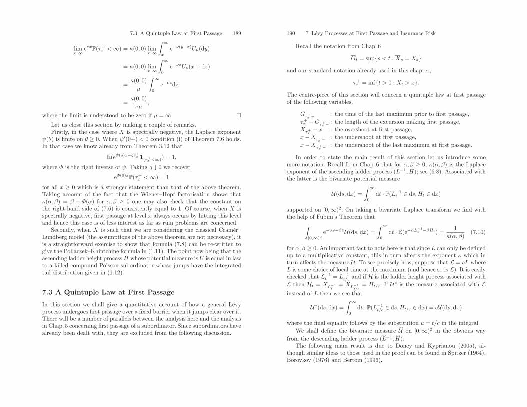
7.3 A Quintuple Law at First Passage 189
limx↑∞
eνxP(τ+x <∞) = κ(0, 0) lim
x↑∞
∫ ∞
x
e−ν(y−x)Uν(dy)
= κ(0, 0) limx↑∞
∫ ∞
0
e−νzUν(x+ dz)
=κ(0, 0)µ
∫ ∞
0
e−νzdz
=κ(0, 0)νµ
,
where the limit is understood to be zero if µ = ∞. Let us close this section by making a couple of remarks.Firstly, in the case where X is spectrally negative, the Laplace exponent
ψ(θ) is finite on θ ≥ 0. When ψ′(0+) < 0 condition (i) of Theorem 7.6 holds.In that case we know already from Theorem 3.12 that
E(eΦ(q)x−qτ+x 1(τ+
x <∞)) = 1,
where Φ is the right inverse of ψ. Taking q ↓ 0 we recover
eΦ(0)xP(τ+x <∞) = 1
for all x ≥ 0 which is a stronger statement than that of the above theorem.Taking account of the fact that the Wiener–Hopf factorisation shows thatκ(α, β) = β + Φ(α) for α, β ≥ 0 one may also check that the constant onthe right-hand side of (7.6) is consistently equal to 1. Of course, when X isspectrally negative, first passage at level x always occurs by hitting this leveland hence this case is of less interest as far as ruin problems are concerned.
Secondly, when X is such that we are considering the classical Cramer–Lundberg model (the assumptions of the above theorem are not necessary), itis a straightforward exercise to show that formula (7.8) can be re-written togive the Pollaczek–Khintchine formula in (1.11). The point now being that theascending ladder height process H whose potential measure is U is equal in lawto a killed compound Poisson subordinator whose jumps have the integratedtail distribution given in (1.12).
7.3 A Quintuple Law at First Passage
In this section we shall give a quantitative account of how a general Levyprocess undergoes first passage over a fixed barrier when it jumps clear over it.There will be a number of parallels between the analysis here and the analysisin Chap. 5 concerning first passage of a subordinator. Since subordinators havealready been dealt with, they are excluded from the following discussion.
190 7 Levy Processes at First Passage and Insurance Risk
Recall the notation from Chap. 6
Gt = sups < t : Xs = Xsand our standard notation already used in this chapter,
τ+x = inft > 0 : Xt > x.
The centre-piece of this section will concern a quintuple law at first passageof the following variables,
Gτ+x − : the time of the last maximum prior to first passage,
τ+x −Gτ+
x − : the length of the excursion making first passage,Xτ+
x− x : the overshoot at first passage,
x−Xτ+x − : the undershoot at first passage,
x−Xτ+x − : the undershoot of the last maximum at first passage.
In order to state the main result of this section let us introduce somemore notation. Recall from Chap. 6 that for α, β ≥ 0, κ(α, β) is the Laplaceexponent of the ascending ladder process (L−1,H); see (6.8). Associated withthe latter is the bivariate potential measure
U(ds,dx) =∫ ∞
0
dt · P(L−1t ∈ ds,Ht ∈ dx)
supported on [0,∞)2. On taking a bivariate Laplace transform we find withthe help of Fubini’s Theorem that∫
[0,∞)2e−αs−βxU(ds,dx) =
∫ ∞
0
dt · E(e−αL−1t −βHt) =
1κ(α, β)
(7.10)
for α, β ≥ 0. An important fact to note here is that since L can only be definedup to a multiplicative constant, this in turn affects the exponent κ which inturn affects the measure U . To see precisely how, suppose that L = cL whereL is some choice of local time at the maximum (and hence so is L). It is easilychecked that L−1
t = L−1t/c and if H is the ladder height process associated with
L then Ht = XL−1t
= XL−1t/c
= Ht/c. If U∗ is the measure associated with Linstead of L then we see that
U∗(ds,dx) =∫ ∞
0
dt · P(L−1t/c ∈ ds,Ht/c ∈ dx) = cU(ds,dx)
where the final equality follows by the substitution u = t/c in the integral.We shall define the bivariate measure U on [0,∞)2 in the obvious way
from the descending ladder process (L−1, H).The following main result is due to Doney and Kyprianou (2005), al-
though similar ideas to those used in the proof can be found in Spitzer (1964),Borovkov (1976) and Bertoin (1996).
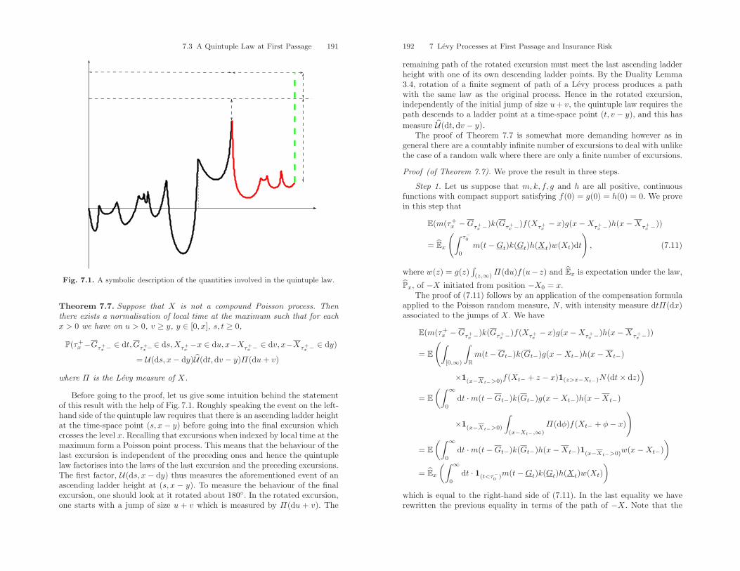
7.3 A Quintuple Law at First Passage 191
Fig. 7.1. A symbolic description of the quantities involved in the quintuple law.
Theorem 7.7. Suppose that X is not a compound Poisson process. Thenthere exists a normalisation of local time at the maximum such that for eachx > 0 we have on u > 0, v ≥ y, y ∈ [0, x], s, t ≥ 0,
P(τ+x −Gτ+
x − ∈ dt, Gτ+x−∈ ds,Xτ+
x−x ∈ du, x−Xτ+
x − ∈ dv, x−Xτ+x − ∈ dy)
= U(ds, x− dy)U(dt,dv − y)Π(du+ v)
where Π is the Levy measure of X.
Before going to the proof, let us give some intuition behind the statementof this result with the help of Fig. 7.1. Roughly speaking the event on the left-hand side of the quintuple law requires that there is an ascending ladder heightat the time-space point (s, x− y) before going into the final excursion whichcrosses the level x. Recalling that excursions when indexed by local time at themaximum form a Poisson point process. This means that the behaviour of thelast excursion is independent of the preceding ones and hence the quintuplelaw factorises into the laws of the last excursion and the preceding excursions.The first factor, U(ds, x− dy) thus measures the aforementioned event of anascending ladder height at (s, x − y). To measure the behaviour of the finalexcursion, one should look at it rotated about 180. In the rotated excursion,one starts with a jump of size u + v which is measured by Π(du + v). The
192 7 Levy Processes at First Passage and Insurance Risk
remaining path of the rotated excursion must meet the last ascending ladderheight with one of its own descending ladder points. By the Duality Lemma3.4, rotation of a finite segment of path of a Levy process produces a pathwith the same law as the original process. Hence in the rotated excursion,independently of the initial jump of size u+ v, the quintuple law requires thepath descends to a ladder point at a time-space point (t, v − y), and this hasmeasure U(dt,dv − y).
The proof of Theorem 7.7 is somewhat more demanding however as ingeneral there are a countably infinite number of excursions to deal with unlikethe case of a random walk where there are only a finite number of excursions.
Proof (of Theorem 7.7). We prove the result in three steps.
Step 1. Let us suppose that m, k, f, g and h are all positive, continuousfunctions with compact support satisfying f(0) = g(0) = h(0) = 0. We provein this step that
E(m(τ+x −Gτ+
x −)k(Gτ+x −)f(Xτ+
x− x)g(x−Xτ+
x −)h(x−Xτ+x −))
= Ex
(∫ τ−0
0
m(t−Gt)k(Gt)h(Xt)w(Xt)dt
), (7.11)
where w(z) = g(z)∫(z,∞)
Π(du)f(u− z) and Ex is expectation under the law,
Px, of −X initiated from position −X0 = x.The proof of (7.11) follows by an application of the compensation formula
applied to the Poisson random measure, N , with intensity measure dtΠ(dx)associated to the jumps of X. We have
E(m(τ+x −Gτ+
x −)k(Gτ+x −)f(Xτ+
x− x)g(x−Xτ+
x −)h(x−Xτ+x −))
= E
(∫[0,∞)
∫Rm(t−Gt−)k(Gt−)g(x−Xt−)h(x−Xt−)
×1(x−Xt−>0)f(Xt− + z − x)1(z>x−Xt−)N(dt× dz))
= E(∫ ∞
0
dt ·m(t−Gt−)k(Gt−)g(x−Xt−)h(x−Xt−)
×1(x−Xt−>0)
∫(x−Xt−,∞)
Π(dφ)f(Xt− + φ− x)
)
= E(∫ ∞
0
dt ·m(t−Gt−)k(Gt−)h(x−Xt−)1(x−Xt−>0)w(x−Xt−))
= Ex(∫ ∞
0
dt · 1(t<τ−0 )m(t−Gt)k(Gt)h(Xt)w(Xt))
which is equal to the right-hand side of (7.11). In the last equality we haverewritten the previous equality in terms of the path of −X. Note that the
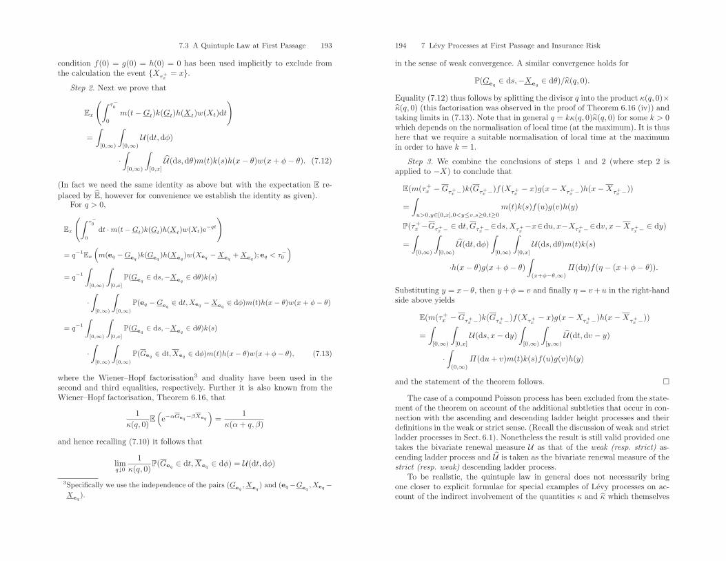
7.3 A Quintuple Law at First Passage 193
condition f(0) = g(0) = h(0) = 0 has been used implicitly to exclude fromthe calculation the event Xτ+
x= x.
Step 2. Next we prove that
Ex
(∫ τ−0
0
m(t−Gt)k(Gt)h(Xt)w(Xt)dt
)
=∫
[0,∞)
∫[0,∞)
U(dt,dφ)
·∫
[0,∞)
∫[0,x]
U(ds,dθ)m(t)k(s)h(x− θ)w(x+ φ− θ). (7.12)
(In fact we need the same identity as above but with the expectation E re-placed by E, however for convenience we establish the identity as given).
For q > 0,
Ex
(∫ τ−0
0
dt ·m(t−Gt)k(Gt)h(Xt)w(Xt)e−qt
)
= q−1Ex
(m(eq −Geq
)k(Geq)h(Xeq
)w(Xeq −Xeq+ Xeq
); eq < τ−0)
= q−1
∫[0,∞)
∫[0,x]
P(Geq∈ ds,−Xeq
∈ dθ)k(s)
·∫
[0,∞)
∫[0,∞)
P(eq −Geq∈ dt, Xeq −Xeq
∈ dφ)m(t)h(x− θ)w(x + φ− θ)
= q−1
∫[0,∞)
∫[0,x]
P(Geq∈ ds,−Xeq
∈ dθ)k(s)
·∫
[0,∞)
∫[0,∞)
P(Geq ∈ dt, Xeq ∈ dφ)m(t)h(x− θ)w(x + φ− θ), (7.13)
where the Wiener–Hopf factorisation3 and duality have been used in thesecond and third equalities, respectively. Further it is also known from theWiener–Hopf factorisation, Theorem 6.16, that
1κ(q, 0)
E(e−αGeq−βXeq
)=
1κ(α+ q, β)
and hence recalling (7.10) it follows that
limq↓0
1κ(q, 0)
P(Geq∈ dt,Xeq
∈ dφ) = U(dt,dφ)
3Specifically we use the independence of the pairs (Geq, Xeq
) and (eq−Geq, Xeq −
Xeq).
194 7 Levy Processes at First Passage and Insurance Risk
in the sense of weak convergence. A similar convergence holds for
P(Geq∈ ds,−Xeq
∈ dθ)/κ(q, 0).
Equality (7.12) thus follows by splitting the divisor q into the product κ(q, 0)×κ(q, 0) (this factorisation was observed in the proof of Theorem 6.16 (iv)) andtaking limits in (7.13). Note that in general q = kκ(q, 0)κ(q, 0) for some k > 0which depends on the normalisation of local time (at the maximum). It is thushere that we require a suitable normalisation of local time at the maximumin order to have k = 1.
Step 3. We combine the conclusions of steps 1 and 2 (where step 2 isapplied to −X) to conclude that
E(m(τ+x −Gτ+
x −)k(Gτ+x −)f(Xτ+
x− x)g(x−Xτ+
x −)h(x−Xτ+x −))
=∫u>0,y∈[0,x],0<y≤v,s≥0,t≥0
m(t)k(s)f(u)g(v)h(y)
P(τ+x −Gτ+
x − ∈ dt,Gτ+x −∈ds,Xτ+
x−x∈du, x−Xτ+
x −∈dv, x−Xτ+x − ∈ dy)
=∫
[0,∞)
∫[0,∞)
U(dt,dφ)∫
[0,∞)
∫[0,x]
U(ds,dθ)m(t)k(s)
·h(x− θ)g(x+ φ− θ)∫
(x+φ−θ,∞)
Π(dη)f(η − (x+ φ− θ)).
Substituting y = x− θ, then y+φ = v and finally η = v+u in the right-handside above yields
E(m(τ+x −Gτ+
x −)k(Gτ+x −)f(Xτ+
x− x)g(x−Xτ+
x −)h(x−Xτ+x −))
=∫
[0,∞)
∫[0,x]
U(ds, x− dy)∫
[0,∞)
∫[y,∞)
U(dt,dv − y)
·∫
(0,∞)
Π(du+ v)m(t)k(s)f(u)g(v)h(y)
and the statement of the theorem follows.
The case of a compound Poisson process has been excluded from the state-ment of the theorem on account of the additional subtleties that occur in con-nection with the ascending and descending ladder height processes and theirdefinitions in the weak or strict sense. (Recall the discussion of weak and strictladder processes in Sect. 6.1). Nonetheless the result is still valid provided onetakes the bivariate renewal measure U as that of the weak (resp. strict) as-cending ladder process and U is taken as the bivariate renewal measure of thestrict (resp. weak) descending ladder process.
To be realistic, the quintuple law in general does not necessarily bringone closer to explicit formulae for special examples of Levy processes on ac-count of the indirect involvement of the quantities κ and κ which themselves
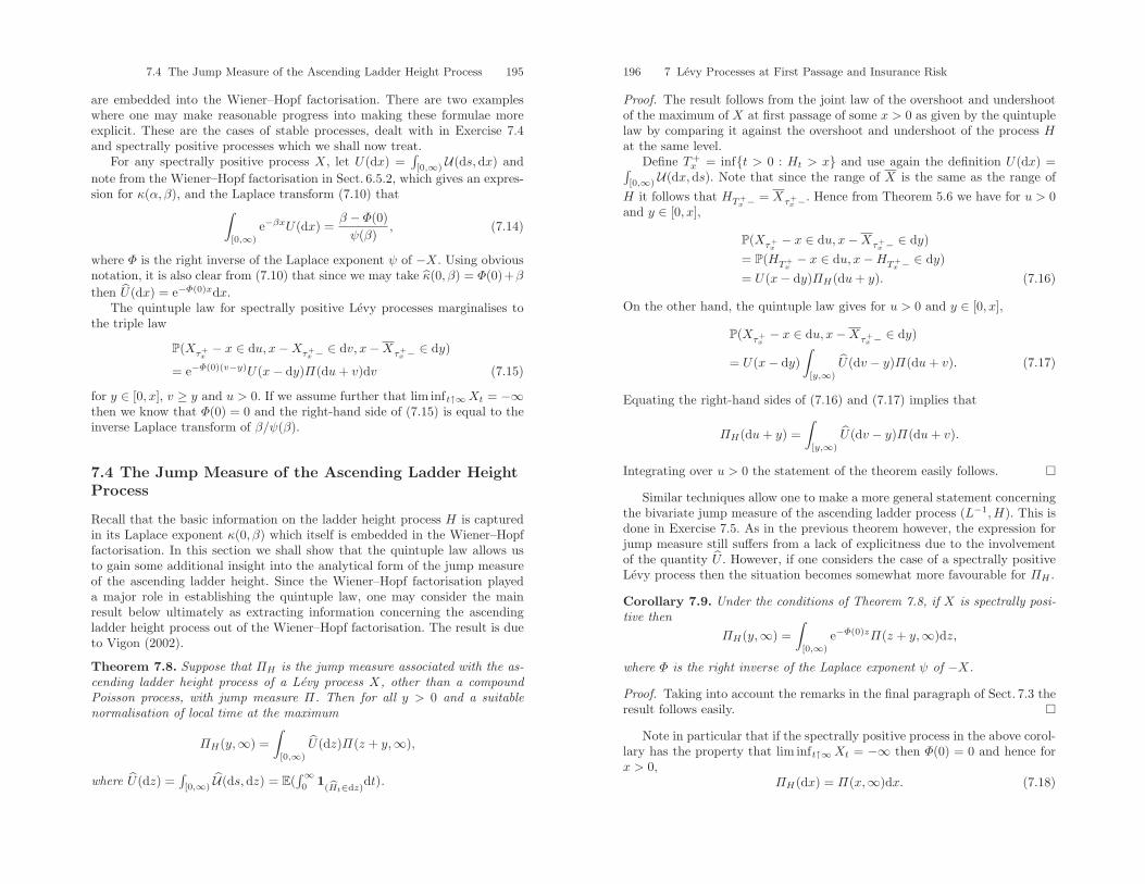
7.4 The Jump Measure of the Ascending Ladder Height Process 195
are embedded into the Wiener–Hopf factorisation. There are two exampleswhere one may make reasonable progress into making these formulae moreexplicit. These are the cases of stable processes, dealt with in Exercise 7.4and spectrally positive processes which we shall now treat.
For any spectrally positive process X, let U(dx) =∫[0,∞)
U(ds,dx) andnote from the Wiener–Hopf factorisation in Sect. 6.5.2, which gives an expres-sion for κ(α, β), and the Laplace transform (7.10) that∫
[0,∞)
e−βxU(dx) =β − Φ(0)ψ(β)
, (7.14)
where Φ is the right inverse of the Laplace exponent ψ of −X. Using obviousnotation, it is also clear from (7.10) that since we may take κ(0, β) = Φ(0)+β
then U(dx) = e−Φ(0)xdx.The quintuple law for spectrally positive Levy processes marginalises to
the triple law
P(Xτ+x− x ∈ du, x−Xτ+
x − ∈ dv, x−Xτ+x − ∈ dy)
= e−Φ(0)(v−y)U(x− dy)Π(du+ v)dv (7.15)
for y ∈ [0, x], v ≥ y and u > 0. If we assume further that lim inft↑∞Xt = −∞then we know that Φ(0) = 0 and the right-hand side of (7.15) is equal to theinverse Laplace transform of β/ψ(β).
7.4 The Jump Measure of the Ascending Ladder HeightProcess
Recall that the basic information on the ladder height process H is capturedin its Laplace exponent κ(0, β) which itself is embedded in the Wiener–Hopffactorisation. In this section we shall show that the quintuple law allows usto gain some additional insight into the analytical form of the jump measureof the ascending ladder height. Since the Wiener–Hopf factorisation playeda major role in establishing the quintuple law, one may consider the mainresult below ultimately as extracting information concerning the ascendingladder height process out of the Wiener–Hopf factorisation. The result is dueto Vigon (2002).
Theorem 7.8. Suppose that ΠH is the jump measure associated with the as-cending ladder height process of a Levy process X, other than a compoundPoisson process, with jump measure Π. Then for all y > 0 and a suitablenormalisation of local time at the maximum
ΠH(y,∞) =∫
[0,∞)
U(dz)Π(z + y,∞),
where U(dz) =∫[0,∞)
U(ds,dz) = E(∫∞0
1(Ht∈dz)
dt).
196 7 Levy Processes at First Passage and Insurance Risk
Proof. The result follows from the joint law of the overshoot and undershootof the maximum of X at first passage of some x > 0 as given by the quintuplelaw by comparing it against the overshoot and undershoot of the process Hat the same level.
Define T+x = inft > 0 : Ht > x and use again the definition U(dx) =∫
[0,∞)U(dx,ds). Note that since the range of X is the same as the range of
H it follows that HT+x − = Xτ+
x −. Hence from Theorem 5.6 we have for u > 0and y ∈ [0, x],
P(Xτ+x− x ∈ du, x−Xτ+
x − ∈ dy)= P(HT+
x− x ∈ du, x−HT+
x − ∈ dy)= U(x− dy)ΠH(du+ y). (7.16)
On the other hand, the quintuple law gives for u > 0 and y ∈ [0, x],
P(Xτ+x− x ∈ du, x−Xτ+
x − ∈ dy)
= U(x− dy)∫
[y,∞)
U(dv − y)Π(du+ v). (7.17)
Equating the right-hand sides of (7.16) and (7.17) implies that
ΠH(du+ y) =∫
[y,∞)
U(dv − y)Π(du+ v).
Integrating over u > 0 the statement of the theorem easily follows.
Similar techniques allow one to make a more general statement concerningthe bivariate jump measure of the ascending ladder process (L−1,H). This isdone in Exercise 7.5. As in the previous theorem however, the expression forjump measure still suffers from a lack of explicitness due to the involvementof the quantity U . However, if one considers the case of a spectrally positiveLevy process then the situation becomes somewhat more favourable for ΠH .
Corollary 7.9. Under the conditions of Theorem 7.8, if X is spectrally posi-tive then
ΠH(y,∞) =∫
[0,∞)
e−Φ(0)zΠ(z + y,∞)dz,
where Φ is the right inverse of the Laplace exponent ψ of −X.
Proof. Taking into account the remarks in the final paragraph of Sect. 7.3 theresult follows easily.
Note in particular that if the spectrally positive process in the above corol-lary has the property that lim inft↑∞Xt = −∞ then Φ(0) = 0 and hence forx > 0,
ΠH(dx) = Π(x,∞)dx. (7.18)
7.5 Creeping 197
The same conclusion was drawn in Exercise 6.5 using the Wiener–Hopffactorisation. If we take further the case that −X is a Cramer–Lundbergprocess then the previous statement is consistent with Theorem 1.9. In thenotation of the latter theorem, on account of irregularity of 0 for (−∞, 0) forthe process−X, the ascending ladder height process of X must be a compoundPoisson subordinator and therefore the jump measure ΠH is proportional to ηwhich is the jump distribution of the descending ladder process of the Cramer–Lundberg process. The constant of proportionality is the arrival rate of thecompound Poisson subordinator. (The latter depends on the normalization oflocal time).
7.5 Creeping
As with the case of a subordinator, one may talk of a Levy process creepingover a fixed level x > 0. To be precise, a Levy process creeps over the level xwhen
P(Xτ+x
= x) > 0. (7.19)
The class of Levy processes which creep upwards atleast one point can easilybe seen to be non-empty by simply considering any spectrally negative Levyprocess. By definition, any spectrally negative Levy process has the propertythat for all x ≥ 0
P(Xτ+x
= x|τ+x <∞) = 1.
From the latter, (7.19) easily follows when we recall from Theorem 3.12 thatP(τ+
x <∞) = e−Φ(0)x > 0 where Φ is the right inverse of the Laplace exponentof X.
Lemma 7.10. Suppose that X is not a compound Poisson process. Then Xcreeps upwards at some (and then all) x > 0 if and only if
limβ↑∞
κ (0, β)β
> 0. (7.20)
Proof. The key to understanding when an arbitrary Levy process creeps up-wards is embedded within the problem of whether a subordinator creeps up-wards. Indeed we know that X creeps across x > 0 if and only if with positiveprobability the point x lies in the range of Xt : t ≥ 0. The latter range is al-most surely identical to the range of the ascending ladder process Ht : t ≥ 0.Hence we see that X creeps across x > 0 if and only if H creeps across x. Forthis reason it follows that if a Levy process creeps over some x > 0, then itwill creep over all x > 0 provided H has the same behaviour. We know fromSect. 5.3 that the only subordinators which may creep over some levels butnot others are compound Poisson subordinators whose jumps are distributedwith lattice support and hence we need to rule this case out. Let us now splitthe discussion into two cases, according to the regularity of 0 for (0,∞).
198 7 Levy Processes at First Passage and Insurance Risk
Suppose that 0 is regular for (0,∞). Recall from Theorem 6.10 that Hhas the law of a (possibly killed) subordinator. This subordinator cannot bea compound Poisson process by the assumption of regularity. We are thenwithin the scope of Theorem 5.9 which tells us that there is creeping if andonly if the underlying subordinator has a strictly positive drift. By definition,however, the Laplace exponent κ(0, β) of H, up to an additive constant (thekilling rate), is the Laplace exponent of the underlying subordinator. Hencethe presence of a strictly positive drift coefficient is exposed by taking the limitgiven in the statement of the lemma (recall Exercise 2.11). In other words,there is creeping if and only if (7.20) holds.
Suppose now that 0 is irregular for (0,∞) which has the consequence thatthe ascending ladder height must be a compound Poisson process subordina-tor. We may not appeal to Theorem 5.9 as in the previous paragraph. Sinceit has been assumed that X is not a compound Poisson process, it also meansthat 0 must be regular for (−∞, 0) and hence the descending ladder heightprocess cannot be a compound Poisson subordinator. According to Corollary7.8 we know that ΠH(dx) =
∫[0,∞)
U(dv)Π(dx + v). Theorem 5.4 (i) shows
that U has no atoms on (0,∞) as H is not a compound Poisson process. HenceΠH has no atoms. In conclusion, whilst H is a compound Poisson process, itsLevy measure, which is proportional to the jump distribution of H, has noatoms and therefore the compound Poisson subordinator H cannot hit speci-fied points. As X will creep over x > 0 if and only if H can hit x with positiveprobability, then we conclude that X cannot creep over x and hence (7.20)fails.
Note that, as in the case of subordinators, the exclusion of compound Pois-son processes from the previous theorem is due to the possibility of examplesin which the jump measure has atoms allowing the process X to jump on tospecific points with positive probability.
The criterion given in the above corollary is not particularly useful ingeneral for determining whether a process can creep upwards or not. Ideallyone would like to establish a criterion in terms of the components of the Levy–Khintchine exponent which is equivalent to upward creeping. The followingresult does precisely this.
Theorem 7.11. Suppose that X is a Levy process which is not a compoundPoisson process. Then X creeps upwards if and only if one of the followingthree situations occur,
(i) X has bounded variation with Levy–Khintchine exponent
Ψ (θ) = −iθd+∫
R\0(1− eiθx)Π(dx)
and d > 0,(ii) X has a Gaussian component,
7.5 Creeping 199
(iii) X has unbounded variation, has no Gaussian component and its charac-teristic measure Π satisfies∫ 1
0
xΠ(x,∞)∫ x0Π(−1,−u)du
dx <∞.
The proof of parts (i) and (ii) appear in Exercise 7.6. The precise formula-tion and proof of part (iii) remained a challenging open problem until recentlywhen it was resolved by Vigon (2002). We do not give details of the proof whichrequires a deep analytical understanding of the Wiener–Hopf factorisation andgoes far beyond the scope of this text. A recent, more probabilistic proof isgiven in Doney (2006).
We close this section by making some remarks on the difference betweena Levy process X creeping over x and hitting the point x. Formally speaking,we say that X hits the point x if P(τx <∞) > 0 where
τx = inft > 0 : Xt = x
with the usual convention that inf ∅ = ∞. Clearly if X creeps over x (eitherupwards or downwards) then it must hit x. When X is a subordinator, theconverse is also obviously true. However, if X is not a subordinator, then itcan be shown that the converse is not necessarily true. The following resultdue to Kesten (1969) and Bretagnolle (1971) gives a complete characterisationof the range of a Levy process.
Theorem 7.12. Suppose that X is not a compound Poisson process. Let
C := x ∈ R : P(τx <∞) > 0
be the set of points that a Levy process can hit. Then C = ∅ if and only if∫Rℜ(
11 + Ψ(u)
)du <∞. (7.21)
Moreover,
(i) If σ > 0, then (7.21) is satisfied and C = R.(ii) If σ = 0 and X is of unbounded variation and (7.21) is satisfied then
C = R.(iii) If X is of bounded variation, then (7.21) is satisfied if and only if d = 0
where d is the drift in the representation (2.22) of its Levy–Khintchineexponent Ψ . In that case C = R unless X or −X is a subordinator andthen C = (0,∞) or C = (−∞, 0), respectively.
From this characterisation one may deduce that, for example, a symmetricα-stable process where α ∈ (1, 2) cannot creep and yet C = R. See Exercise7.6 for details.
200 7 Levy Processes at First Passage and Insurance Risk
7.6 Regular Variation and Infinite Divisibility
It has been pointed out at several points earlier in this chapter that the quin-tuple law lacks to some extent a degree of explicitness which would otherwisegive it far greater practical value for the study of ruin problems. In Sect. 7.7we shall give some indication of how the quintuple law gives some analyt-ical advantage however when studying the asymptotic of ruin problems asthe ruinous barrier tends to infinity. We need to make a short digression firsthowever into the behaviour of infinitely divisible random variables whose Levymeasures have regularly varying tails.
Recall from Definition 5.12 that a function f : [0,∞) → (0,∞) is regularlyvarying at infinity with index ρ ∈ R if for all λ > 0,
limx↑∞
f(λx)f(x)
= λρ.
Let us suppose that H is a random variable valued on [0,∞) which is infinitelydivisible with Levy measure ΠH . Throughout this section we shall supposethat ΠH(·,∞) is regularly varying with index −α for some α > 0. Our interesthere is to understand how this assumed tail behaviour of ΠH reflects on thetail behaviour of the distribution of the random variable H. We do this witha sequence of lemmas. The reader may skip their proofs at no cost to theunderstanding of their application in Sect. 7.7. The first of these lemmas istaken from Feller (1971).
Lemma 7.13. Define the probability measure
ν(dx) =ΠH(dx)ΠH(1,∞)
1(x>1).
Then using the usual notation νn for the n-fold convolution of ν with itself,we have that
ν∗n(x,∞) ∼ nν(x,∞) (7.22)
as x ↑ ∞ for each n = 2, 3, ....
Proof. The result follows by proving a slightly more general result. Supposethat F1 and F2 are distribution functions on [0,∞) such that Fi(x,∞) ∼x−αLi(x) for i = 1, 2 as x ↑ ∞ where L1 and L2 are slowly varying at infinity.Then
(F1 ∗ F2)(x,∞) ∼ x−α(L1(x) + L2(x)) (7.23)
as x ↑ ∞. Indeed from the latter one may argue that (7.22) clearly holds forn = 2 and hence by induction it holds for all integers n ≥ 2.
To prove (7.23), let Y1 and Y2 be independent random variables with distri-butions F1 and F2. Fix δ > 0 and write x′ = x(1+δ). The event Y1+Y2 > x
7.6 Regular Variation and Infinite Divisibility 201
contains the event Y1 > x′ ∪ Y2 > x′ and hence
F1 ∗ F2(x,∞) ≥ F1(x′,∞) + F2(x′,∞).
On the other hand set 1/2 > δ > 0, suppose x′′ = (1 − δ)x then the eventY1 +Y2 > x is a subset of the event Y1 > x′′∪Y2 > x′′∪min(Y1, Y2) >δx. On account of the assumptions made on F1 and F2, it is clear that asx ↑ ∞ P(min(Y1, Y2) > δx) = P(Y1 > δx)2 is of considerably smaller orderthan P(Yi > x′′) for each i = 1, 2. It follows that as x ↑ ∞
F1 ∗ F2(x,∞) ≤ (1 + ε)(F1(x′′,∞) + F2(x′′,∞))
for all small ε > 0. The two inequalities for F1 ∗F2 together with the assumedregular variation imply that
(1 + δ)−α ≤ lim infx↑∞
F1 ∗ F2(x,∞)x−α(L1(x) + L2(x))
≤ lim supx↑∞
F1 ∗ F2(x,∞)x−α(L1(x) + L2(x))
≤ (1 + ε)(1− δ)−α.
Since δ and ε may be made arbitrarily small, the required result follows.
Note that any distribution on [0,∞) which fulfils the condition (7.22)in fact belongs to a larger class of distributions known as subexponential.4
The latter class was introduced by Christyakov (1964) within the context ofbranching processes. The following Lemma, due to Kesten, thus gives a generalproperty of all subexponential distributions.
Lemma 7.14. Suppose that Y is any random variable whose distribution G,satisfying G(x) > 0 for all x > 0, has the same asymptotic convolution prop-erties as (7.22). Then given any ε > 0 there exists a constant C = C(ε) > 0such that
G∗n(x,∞)G(x,∞)
≤ C(1 + ε)n
for all n ∈ 1, 2, ... and x > 0.
Proof. The proof is inductive. Suppose that for each n = 1, 2, ...,
ξn := supx≥0
G∗n(x,∞)G(x,∞)
.
It is clear that ξ1 ≤ 1. Next note that 1−G∗(n+1) = 1−G ∗ (1−G∗n). Thenfor any 0 < T <∞,
4Any distribution F is thus subexponential if, when X1, ..., Xn are independentrandom variables with distribution F , P(X1 + · · · + Xn > x) ∼ nP(X1 > x) asx ↑ ∞.
202 7 Levy Processes at First Passage and Insurance Risk
ξn+1 ≤ 1 + sup0≤x≤T
∫ x
0
1−G∗n(x− y)1−G(x)
G(dx)
+ supx>T
∫ x
0
1−G∗n(x− y)1−G(y)
1−G(x− y)1−G(x)
G(dx)
≤ 1 +1
1−G(T )+ ξn sup
t>T
G(x)−G∗2(x)1−G(x)
.
Since G satisfies (7.22), given any ε > 0, we can choose T > 0 such that
ξn+1 ≤ 1 +1
1−G(T )+ ξn(1 + ε).
Hence, iterating we find
ξn+1 ≤(
2−G(T )1−G(T )
)1ε(1 + ε)n+1
which establishes the claim with the obvious choice of C.
In the next lemma, we use the asymptotic behaviour in Lemma 7.13 andthe uniform bounds in Lemma 7.14 to show that the distribution of H mustalso have regularly varying tails. The result is due to Embrechts et al. (1979).Recall that we are assuming throughout that ΠH(·,∞) is slowly varying withindex −α for some α > 0.
Lemma 7.15. As x ↑ ∞,
P(H > x) ∼ ΠH(x,∞)
implying that the distribution of H has a regularly varying tail at infinity withindex −α.
Proof. The relationship between H and ΠH is expressed via the Levy–Khintchine formula. In this case, since H is [0,∞)-valued, we may considerinstead its Laplace exponent Φ(θ) := − log E(e−θH) which from the Levy–Khintchine formula satisfies
Φ(θ) = dθ +∫
(0,∞)
(1− e−θx)ΠH(dx)
= dθ +∫
(0,1]
(1− e−θx)ΠH(dx) (7.24)
+∫
(1,∞)
(1− e−θx)ΠH(dx). (7.25)
The second equality above allows the random variable H to be seen as equalin distribution to the independent sum of two infinitely divisible randomvariables, say H1 and H2, where H1 has Laplace exponent given by (7.24)
7.7 Asymptotic Ruinous Behaviour with Regular Variation 203
and H2 has Laplace exponent given by (7.25). According to Theorem 3.6,E(eλH1) < ∞ for any λ > 0 because trivially
∫x≥1
eλxΠH1(dx) < ∞ whereΠH1(dx) = ΠH(dx)1(x∈(0,1]). It follows that one may upper estimate the tailof H1 by any exponentially decaying function. Specifically, with the help ofthe Markov inequality, P(H1 > x) ≤ E(eλH1)e−λx for any λ > 0.
On the other hand, by assumption, the tail of the measure ΠH2(dx) =ΠH(dx)1(x≥1) is regularly varying with index −α. Since ΠH2 necessarily hasfinite total mass, we may consider H2 as the distribution at time 1 of a com-pound Poisson process with rate η := ΠH(1,∞) and jump distribution ν(defined in Lemma 7.13). We know then that
P(H2 > x) = e−η∑k≥0
ηk
k!ν∗k(x,∞),
where as usual we interpret ν∗0(dx) = δ0(dx) (so in fact the first term ofthe above sum is equal to zero). Next use the conclusion of Lemma 7.14 withdominated convergence to establish that
limx↑∞
P(H2 > x)ΠH(x,∞)/η
= limx↑∞
e−η∑k≥1
ηk
k!ν∗k(x,∞)ν(x,∞)
.
The conclusion of Lemma 7.13 allows the computation of the limiting sumexplicitly. That is to say
∑k≥1 eηηk/(k − 1)! = η. In conclusion, we have
limx↑∞
P(H2 > x)ΠH(x,∞)
= 1.
The proof of this lemma is thus completed once we show that
limx↑∞
P(H1 +H2 > x)P(H2 > x)
= 1. (7.26)
However, this fact follows by reconsidering the proof of Lemma 7.13. If in thisproof one takes Fi as the distribution of Hi for i = 1, 2, then with the slightdifference that F1 has exponentially decaying tails, one may follow the proofstep by step to deduce that the above limit holds. Intuitively speaking, thetails of H1 are considerably lighter than those of H2 and hence for large x, theevent in the nominator of (7.26) essentially occurs due to a large observationof H2. The details are left as an exercise to the reader.
7.7 Asymptotic Ruinous Behaviour with RegularVariation
In this section, we give the promised example of how to use the quintuple lawto obtain precise analytic statements concerning asymptotic ruinous behav-iour under assumptions of regular variation. The following theorem, due to
204 7 Levy Processes at First Passage and Insurance Risk
Asmussen and Kluppelberg (1996) and Kluppelberg and Kyprianou (2005),is our main objective.
Theorem 7.16. Suppose that X is any spectrally positive Levy process withmean E(X1) < 0. Suppose that Π(·,∞) is regularly varying at infinity withindex −(α + 1) for some α ∈ (0,∞). Then we have the following ruinousbehaviour:
(i) As x ↑ ∞ we have
P(τ+x <∞) ∼ 1
|E(X1)|∫ ∞
x
Π(y,∞)dy
and consequently, the ruin probability is regularly varying at infinity withindex −α. (Note that convexity of the Laplace exponent of −X dictatesthat |E(X1)| <∞ when E(X1) < 0).
(ii) For all u, v >0,
limx↑∞
P(Xτ+
x− x
x/α> u,
−Xτ+x −
x/α> v
∣∣∣∣ τ+x <∞
)=(
1 +v + u
α
)−α.
(7.27)Part (i) of the above theorem shows that when the so called Cramer condi-
tion appearing in Theorem 7.6 fails, conditions may exist where one may stillgain information about the asymptotic behaviour of the ruin probability. Part(ii) shows that with re-scaling, the overshoot and undershoot converges to anon-trivial distribution. In fact the limiting distribution takes the form of abivariate generalised Pareto distribution (cf. Definition 3.4.9 in Embrechts etal. (1997)). The result in part (ii) is also reminiscent of the following extrac-tion from extreme value theory. It is known that a distribution, F , is in thedomain of attraction of a generalised Pareto distribution if F (·,∞) is regularlyvarying at infinity with index −α for some α > 0; in which case
limx↑∞
F (x+ xu/α,∞)F (x)
=(1 +
u
α
)−αfor α > 0 and u > 0.
Generalised Pareto distributions have heavy tails in the sense that theirmoment generating functions do not exist on the positive half of the real axis.Roughly speaking this means that there is a good chance to observe relativelylarge values when sampling from this distribution. This fact is important inthe conclusion of the theorem as it confirms the folk-law that when modellinginsurance risk where claims occur with heavy tails, when ruin occurs, it canoccur when the insurance company has quite healthy reserves and the deficitat ruin will be quite devastating.
Proof (of Theorem 7.16). (i) Following the logic that leads to (7.8) we havethat
P(τ+x <∞) = qU(x,∞) = q
∫ ∞
0
P(Ht > x)dx,
7.7 Asymptotic Ruinous Behaviour with Regular Variation 205
where q = κ(0, 0) is the killing rate of the ascending ladder process. Writing[t] for the integer part of t and note with the help of Lemma 7.14 that forx > 0,
P(Ht > x)P(H1 > x)
≤ P(H[t]+1 > x)P(H1 > x)
≤ C(1 + ε)[t]+1e−q[t].
(To see where the exponential term on the right-hand side comes from, recallthat H is equal in law to a subordinator killed independently at rate q). Nowappealing to the Dominated Convergence Theorem, we have
limx↑∞
P(τ+x <∞)
P(H1 > x)= q
∫ ∞
0
dt · limx↑∞
P(Ht > x)P(H1 > x)
. (7.28)
In order to deal with the limit on the right-hand side above, we shall usethe fact that P(Ht > x) = e−qtP(Ht > x) where Ht is an infinitely divisiblerandom variable. To be more specific, one may think of Ht : t ≥ 0 as asubordinator which when killed at an independent and exponentially distrib-uted time with parameter q, has the same law as Ht : t ≥ 0. Associated tothe random variable Ht is its Levy measure, which necessarily takes the formtΠH . By Lemma 7.15 it follows that
limx↑∞
P(Ht > x)P(H1 > x)
= te−q(t−1).
Hence referring back to (7.28) we have that
limx↑∞
P(τ+x <∞)
ΠH(x,∞)= q
∫ ∞
0
te−qtdt =1q.
On the other hand, taking account of exponential killing, one easily computes
U(∞) =∫ ∞
0
P(Ht <∞)dt =∫ ∞
0
e−qtdt =1q.
The conclusion of the first part now follows once we note from (7.14) thatU(∞) = limβ↓0 β/ψ(β) = 1/ψ′(0+) where ψ(β) = log E(e−βX1) and which inparticular implies q = |E(X1)|.
(ii) Applying the quintuple law in marginalised form, we have
P(Xτ+
x− x > u∗, x−Xτ+
x − > v∗)
=∫ x
0
U(x− dy)∫
[v∗∨y,∞)
dzΠ(u∗ + z,∞)
for u∗, v∗ > 0. For any spectrally positive Levy process which drifts to −∞,Vigon’s identity in Theorem 7.8 reads
ΠH(u,∞) =∫ ∞
u
Π(z,∞)dz.
206 7 Levy Processes at First Passage and Insurance Risk
Choosing u∗ = ux/α and v∗ = x+ vx/α we find that
P(Xτ+
x− x
x/α> u,
−Xτ+x −
x/α> v
)= U(x)Π(x+ x(v + u)/α,∞). (7.29)
From part (i), if the limit exists then it holds that
limx↑∞
P(Xτ+
x− x
x/α> u,
−Xτ+x −
x/α> v
∣∣∣∣ τx <∞)
= limx↑∞
U(x)U(∞)
Π(x+ x(v + u)/α,∞)ΠH(x,∞)
. (7.30)
Since Π(·,∞) is regularly varying with index −(α + 1) by assumption, theMonotone Density Theorem 5.14 implies that ΠH(·,∞) is regularly varyingwith index −α. Hence the limit in (7.30) exists and in particular (7.27) holdsthus concluding the proof.
Exercises
7.1 (Moments of the supremum). Fix n = 1, 2, ... and suppose that∫(1,∞)
xnΠ(dx) <∞ (7.31)
(or equivalently E((maxX1, 0)n) <∞ by Exercise 3.3).
(i) Suppose that XK is the Levy process with the same characteristics as Xexcept that the measure Π is replaced by ΠK where
ΠK(dx) = Π(dx)1(x>−K) + δ−K(dx)Π(−∞,−K).
In other words, the paths of XK are an adjustment of the paths of Xin that all negative jumps of magnitude K or greater are replaced by anegative jump of precisely magnitude K.Deduce that E(|XK
t |n) < ∞ for all t ≥ 0 and that the descending ladderheight process of XK has moments of all orders.
(ii) Use the Wiener–Hopf factorisation together with Maclaurin expansionsup to order n of the terms therein to deduce that
E(Xn
eq) <∞
holds for any q > 0.(iii) Now suppose that q = 0 and lim supt↑∞Xt < ∞ and that (7.31) holds
for n = 2, 3, .... By adapting the arguments above, show that
E(Xn−1
∞ ) <∞.
7.7 Asymptotic Ruinous Behaviour with Regular Variation 207
7.2 (The Strong Law of Large Numbers for Levy Processes). Sup-pose that X is a Levy process such that E|X1| < ∞. For n ≥ 0 letYn = supt∈[n,n+1] |Xt − Xn|. Clearly this is a sequence of independent andidentically distributed random variables.
(i) Use the previous exercise to show that E(Yn) <∞.(ii) Use the classical Strong Law of Large Numbers to deduce that limn↑∞ n−1
Yn = 0.(iii) Now deduce that
limt↑∞
Xt
t= E(X1).
(iv) Now suppose that E(X1) = ∞. Show that
limt↑∞
Xt
t= ∞.
(Hint: consider truncating the Levy measure on (0,∞)).
7.3. The idea of this exercise is to recover the conclusion of Theorem 7.2 forspectrally negative Levy processes, X, using Theorem 7.1 and the Wiener–Hopf factorisation. As usual the Laplace exponent of X is denoted ψ and itsright inverse is Φ.
(i) Using one of the Wiener–Hopf factors show that
E(eβX∞1(−X∞<∞)
)=
0 if ψ′(0) < 0ψ′(0)β/ψ (β) if ψ′(0) ≥ 0.
(ii) Using the other Wiener–Hopf factor show that
E(e−βX∞1(X∞<∞)
)=Φ (0) /(β + Φ (0)) if ψ′(0) < 00 if ψ′(0) ≥ 0.
(iii) Deduce from Theorem 7.1 that limt↑∞Xt = ∞ when E(X1) > 0,limt↑∞Xt = −∞ when E(X1) < 0, and lim supt↑∞Xt = − lim inft↑∞Xt =∞ when E(X1) = 0.
(iv) Deduce that a spectrally negative stable process of index α ∈ (1, 2) nec-essarily oscillates.
7.4. Let X be a stable process with index α ∈ (0, 2) which is not (the negativeof) a subordinator and has positive jumps. Let ρ = P(Xt ≥ 0).
(i) Explain why such processes cannot creep upwards. If further it experiencesnegative jumps, explain why it cannot creep downwards either.
(ii) Suppose that U(dx) =∫[0,∞)
U(dx,ds) for x ≥ 0. Show that (up to amultiplicative constant)
U(dx) =xαρ−1
Γ (αρ)dx
for x ≥ 0. [Hint: reconsider Exercise 5.6].
208 7 Levy Processes at First Passage and Insurance Risk
(iii) Show that for y ∈ [0, x], v ≥ y and u > 0,
P(Xτ+x− x ∈ du, x−Xτ+
x − ∈ dv, x−Xτ+x − ∈ dy)
= c · (x− y)αρ−1(v − y)α(1−ρ)−1
(v + u)1+αdydvdu
where c is a strictly positive constant.(iv) Explain why the constant c must normalise the above triple law to a
probability distribution. Show that
c =sinαρπ
π
Γ (α+ 1)Γ (αρ)Γ (α(1− ρ))
.
7.5. Suppose that X is a Levy process but not a compound Poisson processwith jump measure Π and ascending ladder process (L−1,H) having jumpmeasure Π(dt,dh). Using the conclusion of Exercise 5.4 show that
Π(dt,dh) =∫
[0,∞)
U(dt,dθ)Π(dh+ θ).
Show further that if X is spectrally positive then
Π(dt,dh) =∫ ∞
0
dθ · P(L−1θ ∈ dt)Π(dh+ θ).
7.6. Here we deduce some statements about creeping and hitting points.
(i) Show that
lim|θ|↑∞
Ψ (θ)θ2
=σ2
2
where σ is the Gaussian coefficient of Ψ . Show with the help of the Wiener–Hopf factorisation, k′Ψ (θ) = κ(0,−iθ)κ(0, iθ), that a Levy process creepsboth upwards and downwards if and only if it has a Gaussian component(that is if and only if σ > 0).
(ii) Show that a Levy process of bounded variation with Levy–Khintchineexponent
Ψ (θ) = −iθd+∫
R\0(1− eiθx)Π(dx)
creeps upwards if and only if d > 0.(iii) Show that any Levy process for which 0 is irregular for (0,∞) cannot
creep upwards.(iv) Show that a spectrally negative Levy process with no Gaussian compo-
nent cannot creep downwards.(v) Use part (i) to show that a symmetric α-stable process with α ∈ (1, 2)
cannot creep. Use the integral test (7.21) to deduce that the latter Levyprocess can hit all points.
7.7 Asymptotic Ruinous Behaviour with Regular Variation 209
7.7. Characterising the first passage over a fixed level for a general Levyprocess is clearly non-trivial. Characterizing the first passage outside of a fixedinterval for a general Levy process (the so-called two-sided exit problem) hasmany more difficulties. This exercise concerns one of the few examples of Levyprocesses for which an explicit characterisation can be obtained. The result isdue to Rogozin (1972).
Suppose that X is a stable process with both positive and negative jumpsand index α ∈ (0, 2) with symmetry parameter β ∈ (−1, 1). The case that Xor −X is a subordinator or spectrally negative is thus excluded.5 From thediscussion in Sect. 6.5.3 we know that the positivity parameter ρ ∈ (0, 1) andthat αρ ∈ (0, 1) and α(1− ρ) ∈ (0, 1).
(i) With the help of the conclusion of Exercise 5.6 (ii) show that
Px(Xτ+1≤ 1 + y) = Φαρ
(y
1− x
)for x ≤ 1 and
Px(−Xτ−0≤ y) = Φα(1−ρ)
(yx
)for x ≥ 0 where
Φq(u) =
sinπqπ
∫ u0t−q(1 + t)−1dt for u ≥ 0
0 for u < 0.
[Hint: it will be helpful to prove that∫ 1/(1+θ)
0
uα−1(1− u)−(α+1)dv =θ−α
α
for any θ > 0].(ii) Define
r(x, y)=Px(Xτ+1≤ 1+y; τ+
1 < τ−0 ) and l(x, y)=Px(Xτ−0≥ −y; τ+
1 >τ−0 ).
Show that the following system of equations hold
r(x, y) = Φαρ
(y
1− x
)−∫
(0,∞)
Φαρ
(y
1 + z
)l(x,dz)
and
l(x, y) = Φα(1−ρ)(yx
)−∫
(0,∞)
Φα(1−ρ)
(y
1 + z
)r(x,dz).
(iii) Assuming the above system of equations has a unique solution show that
r(x, y) =sinπαρ
π(1− x)αρxα(1−ρ)
∫ y
0
t−αρ(t+ 1)−α(1−ρ)(t+ 1− x)−1dt
and write down a similar expression for l(x, y).
5The case that X or −X is spectrally negative is dealt with later in Exercise 8.12.
8
Exit Problems for Spectrally NegativeProcesses
In this chapter we consider in more detail the special case of spectrally negativeLevy processes. As we have already seen in a number of examples in previouschapters, Levy processes which have jumps in only one direction turn out tooffer a significant advantage for many calculations. We devote our time in thischapter, initially, to gathering facts about spectrally negative processes fromearlier chapters, and then to an ensemble of fluctuation identities which aresemi-explicit in terms of a class of functions known as scale functions whoseproperties we shall also explore.
8.1 Basic Properties Reviewed
Let us gather what we have already established in previous chapters togetherwith other easily derived facts.
The Laplace exponent. Rather than working with the Levy–Khintchine ex-ponent, it is preferable to work with the Laplace exponent
ψ (λ) :=1t
log E(eλXt
)= −Ψ (−iλ) ,
which is finite at least for all λ ≥ 0. The function ψ : [0,∞) → R is zero atzero and tends to infinity at infinity. Further, it is infinitely differentiableand strictly convex. In particular ψ′(0+) = E (X1) ∈ [−∞,∞). Define theright inverse
Φ (q) = supλ ≥ 0 : ψ (λ) = qfor each q ≥ 0. If ψ′(0+) ≥ 0 then λ = 0 is the unique solution to ψ (λ) = 0and otherwise there are two solutions to the latter with λ = Φ (0) > 0being the larger of the two, the other is λ = 0 (see Fig. 3.3).
212 8 Exit Problems for Spectrally Negative Processes
First passage upwards. The first passage time above a level x > 0 has beendefined by τ+
x = inft > 0 : Xt > x. From Theorem 3.12 we know thatfor each q ≥ 0,
E(e−qτ+x 1(τ+
x <∞)) = e−Φ(q)x.
Further, the process τ+x : x ≥ 0 is a subordinator with Laplace exponent
Φ(q)− Φ(0) killed at rate Φ(0).
Path variation. A spectrally negative Levy process has paths of bounded orunbounded variation. Given the triple (a, σ,Π) as in Theorem 1.6 wherenecessarily suppΠ ⊆ (−∞, 0) we may always write
ψ (λ) = −aλ+12σ2λ2 +
∫(−∞,0)
(eλx − 1− λx1(x>−1))Π (dx) ,
where (a, σ,Π) are the same as those given in the Levy–Khintchine for-mula. When X has bounded variation we may always write
ψ (λ) = dλ−∫
(−∞,0)
(1− eλx
)Π (dx) , (8.1)
where necessarily
d = −a−∫ 0
−1
xΠ(dx)
is strictly positive. Hence a spectrally negative Levy process of boundedvariation must always take the form of a positive drift minus a pure jumpsubordinator. Note that if d ≤ 0 then we would see the Laplace exponentof a decreasing subordinator which is excluded from the definition of aspectrally negative process.
Regularity. From Theorem 6.5 (i) and (ii) one sees immediately then that0 is regular for (0,∞) for X irrespective of path variation. Further, byconsidering the process −X, we can see from the same theorem that 0is regular for (−∞, 0) if and only if X has unbounded variation. Saidanother way, 0 is regular for both (0,∞) and (−∞, 0) if and only if it hasunbounded variation.
Creeping. We know from Corollary 3.13 and the fact that there are no positivejumps that
P(Xτ+x
= x|τ+x <∞) = 1.
Hence spectrally negative Levy processes necessarily creep upwards. Itwas shown however in Exercise 7.6 that they creep downward if and onlyif σ > 0.
Wiener–Hopf factorisation. In Chap. 6 we identified up to a multiplicativeconstant
κ(α, β) = Φ (α) + β and κ(α, β) =α− ψ (β)Φ (α)− β
8.1 Basic Properties Reviewed 213
for α, β ≥ 0. Appropriate choices of local time at the maximum andminimum allow the multiplicative constants to be taken as equal to unity.From Theorem 6.16 (ii) this leads to
E(e−βXep
)=
Φ (p)Φ (p) + β
and E(eβXep
)=
p
Φ (p)Φ (p)− β
p− ψ (β), (8.2)
where ep is an independent and exponentially distributed random variablewith parameter p ≥ 0. The first of these two expressions shows that Xep
is exponentially distributed with parameter Φ (p). Note that when p = 0in the last statement, we employ our usual notation that an exponentialvariable with parameter zero is infinite with probability one.
Drifting and oscillating. From Theorem 7.2 or Exercise 7.3 we have the fol-lowing asymptotic behaviour for X. The process drifts to infinity if andonly if ψ′(0+) > 0, oscillates if and only if ψ′(0+) = 0 and drifts to minusinfinity if and only if ψ′(0+) < 0.
Exponential change of measure. From Exercise 1.5 we know that
ecXt−ψ(c)t : t ≥ 0is a martingale for each c ≥ 0. Define for each c ≥ 0 the change of measure
dPc
dP
∣∣∣∣Ft
= ecXt−ψ(c)t. (8.3)
(Recall that F = Ft : t ≥ 0 is the filtration generated by X which hasbeen completed by null sets of P, which in the case of a Levy processmeans that it is right continuous). When X is a Brownian motion this isthe same change of measure that appears in the most elementary form ofthe Cameron–Martin–Girsanov Theorem. In that case we know that theeffect of the change of measure is that the process X under Pc has thesame law as a Brownian motion with drift c. In Sect. 3.3 we showed thatwhen (X,P) is a spectrally negative Levy process then (X,Pc) is also aspectrally negative Levy process and a straightforward calculation showsthat its Laplace exponent ψc (λ) is given by
ψc (λ) = ψ (λ+ c)− ψ (c)
=
(σ2c− a+
∫(−∞,0)
x(ecx − 1)1(x>−1)Π(dx)
)λ
+12σ2λ2 +
∫(−∞,0)
(eλx − 1− λx1(x>−1))ecxΠ(dx), (8.4)
for λ ≥ −c.When we set c=Φ (p) for p ≥ 0 we discover that ψΦ(p) (λ)=ψ (λ+ Φ (p))−p and hence ψ′Φ(p) (0) = ψ′ (Φ (p)) ≥ 0 on account of the strict convexity
214 8 Exit Problems for Spectrally Negative Processes
of ψ. In particular, (X,PΦ(p)) always drifts to infinity for p > 0. Roughlyspeaking, the effect of the change of measure has been to change the char-acteristics of X to those of a spectrally negative Levy process with expo-nentially tilted Levy measure. Note also that (X,P) is of bounded variationif and only if (X,Pc) is of bounded variation. This statement is clear whenσ > 0. When σ = 0 it is justified by noting that
∫(−1,0)
|x|Π(dx) < ∞if and only if
∫(−1,0)
|x|ecxΠ(dx) < ∞. In the case that X is of boundedvariation and we write the Laplace exponent in the form (8.1) we also seefrom the second equality of (8.4) that
ψc(θ) = dθ −∫
(−∞,0)
(1− eθx)ecxΠ(dx).
Thus under Pc the process retains the same drift and only the Levy mea-sure is exponentially tilted.
8.2 The One-Sided and Two-Sided Exit Problems
In this section we shall develop semi-explicit identities concerning exiting froma half line and a strip. Recall that Px and Ex are shorthand for P(·|X0 = x)and E(·|X0 = x) and for the special case that x = 0 we keep with our oldnotation, so that P0 = P and E0 = E, unless we wish to emphasise the factthat X0 = 0. Recall also
τ+x = inft > 0 : Xt > x and τ−x = inft > 0 : Xt < x
for all x ∈ R. The main results of this section are the following.
Theorem 8.1 (One- and two-sided exit formulae). There exist a familyof functions W (q) : R → [0,∞) and
Z(q)(x) = 1 + q
∫ x
0
W (q)(y)dy, for x ∈ R
defined for each q ≥ 0 such that the following hold (for short we shall writeW (0) = W ).
(i) For any q ≥ 0, we have W (q)(x) = 0 for x < 0 and W (q) is characterisedon [0,∞) as a strictly increasing and continuous function whose Laplacetransform satisfies∫ ∞
0
e−βxW (q)(x)dx =1
ψ (β)− qfor β > Φ (q) . (8.5)
(ii) For any x ∈ R and q ≥ 0,
Ex(e−qτ
−0 1(τ−0 <∞)
)= Z(q)(x)− q
Φ (q)W (q)(x) , (8.6)
8.2 The One-Sided and Two-Sided Exit Problems 215
where we understand q/Φ (q) in the limiting sense for q = 0, so that
Px(τ−0 <∞) =
1− ψ′(0+)W (x) if ψ′(0+) > 01 if ψ′(0+) ≤ 0
. (8.7)
(iii) For any x ≤ a and q ≥ 0,
Ex(e−qτ
+a 1(τ−0 >τ+
a ))
=W (q)(x)W (q)(a)
, (8.8)
and
Ex(e−qτ
−0 1(τ−0 <τ+
a ))
= Z(q)(x)− Z(q)(a)W (q)(x)W (q)(a)
. (8.9)
The function W has been called the scale function because of the analogousrole it plays in (8.8) to scale functions for diffusions in the sense of equation(8.8). In keeping with existing literature we will refer to the functions W (q)
and Z(q) as the q-scale functions.1
Note also that (8.7) should give the Pollaczek–Khintchine formula (1.11)when X is taken as the Cramer–Lundberg risk process. Exercise 8.3 showshow.
Let us make some remarks on the historical appearance of these formulae.Identity (8.6) appears in the form of its Fourier transform in Emery (1973)and for the case that Π is finite and σ = 0 in Korolyuk (1975a). Identity(8.8) first appeared for the case q = 0 in Zolotarev (1964) followed by Takacs(1966) and then with a short proof in Rogers (1990). The case q > 0 is foundin Korolyuk (1975a) for the case that Π is finite and σ = 0, in Bertoin (1996a)for the case of a purely asymmetric stable process and then again for a generalspectrally negative Levy process in Bertoin (1997a) (who refered to a methodused for the case q = 0 in Bertoin (1996a)). See also Doney (2006) for furtherremarks on this identity. Finally (8.9) was proved for the case that Π is finiteand σ = 0 by Korolyuk (1974, 1975a); see Bertoin (1997a) for the generalcase.
Proof (of Theorem 8.1 (8.8)). We prove (8.8) for the case that ψ′(0+) > 0and q = 0, then for the case that q > 0 (no restriction on ψ′(0+)). Finally thecase that ψ′(0+) ≤ 0 and q = 0 is achieved by passing to the limit as q tendsto zero.
Assume that ψ′(0+) > 0 so that −X∞ is P-almost surely finite. Now definethe non-decreasing function
W (x) = Px(X∞ ≥ 0).
1One may also argue that the terminology “scale function” is also inappropriateas the mentioned analogy breaks down in a number of other respects.
216 8 Exit Problems for Spectrally Negative Processes
A simple argument using the law of total probability and the Strong MarkovProperty now yields for x ∈ [0, a)
Px(X∞ ≥ 0) = Ex(Px(X∞ ≥ 0|Fτ+
a))
= Ex(1(τ+
a <τ−0 )Pa(X∞ ≥ 0)
)+ Ex
(1(τ+
a >τ−0 )PXτ
−0
(X∞ ≥ 0))
= Pa(X∞ ≥ 0)Px(τ+a < τ−0 ).
To justify that the second term in the second equality disappears note thefollowing. If X has no Gaussian component then it cannot creep downwardsimplying that Xτ−0
< 0 and then we use that Px(X∞ ≥ 0) = 0 for x < 0.If X has a Gaussian component then Xτ−0
≤ 0 and we need to know thatW (0) = 0. However since 0 is regular for (−∞, 0) and (0,∞) it follows thatX∞ < 0 P-almost surely which is the same as W (0) = 0.
We now have
Px(τ+a < τ−0 ) =
W (x)W (a)
. (8.10)
It is trivial, but nonetheless useful for later use, to note that the same equalityholds even when x < 0 since both sides are equal to zero.
Now assume that q > 0 or q = 0 and ψ′(0+) < 0. In this case, by theconvexity of ψ, we know that Φ (q) > 0 and hence ψ′Φ(q) (0) = ψ′ (Φ (q)) > 0(again by convexity) which implies that under PΦ(q), the process X drifts toinfinity. For (X,PΦ(q)) we have already established the existence of a 0-scalefunction WΦ(q)(x) = PΦ(q)
x (X∞ ≥ 0) which fulfils the relation
PΦ(q)x (τ+
a < τ−0 ) =WΦ(q)(x)WΦ(q)(a)
. (8.11)
However by definition of PΦ(q), we also have that
PΦ(q)x (τ+
a < τ−0 ) = Ex(eΦ(q)(X
τ+a−x)−qτ+
a 1(τ+a <τ
−0 ))
= eΦ(q)(a−x)Ex(e−qτ+a 1(τ+
a <τ−0 )). (8.12)
Combining (8.11) and (8.12) gives
Ex(e−qτ
+a 1(τ+
a <τ−0 )
)= e−Φ(q)(a−x)WΦ(q)(x)
WΦ(q)(a)=
W (q)(x)W (q)(a)
, (8.13)
where W (q)(x) = eΦ(q)xWΦ(q)(x). Clearly W (q) is identically zero on (−∞, 0)and non-decreasing.
Suppose now the final case that ψ′(0+) = 0 and q = 0. Since the limitas q ↓ 0 on the left-hand side of (8.13) exists then the same is true of the
8.2 The One-Sided and Two-Sided Exit Problems 217
right-hand side-By choosing an arbitrary b > a we can thus define, W (x) =limq↓0 W (q)(x)/W (q)(b) for each x ≤ a. Consequently,
W (x) = limq↓0
W (q)(x)W (q)(b)
= limq↓0
Ex(e−qτ
+a 1(τ+
a <τ−0 )
) W (q)(a)W (q)(b)
= Px(τ+a < τ−0 )W (a). (8.14)
Again it is clear that W is identically zero on (−∞, 0) and non-decreasing.It is important to note for the remaining parts of the proof that the de-
finition of W (q) we have given above may be taken up to any multiplicativeconstant without affecting the validity of the arguments.
Proof (of Theorem 8.1 (i)). Suppose again that X is assumed to drift toinfinity so that ψ′(0+) > 0. First consider the case that q = 0. Recalling thatthe definition of W in (8.8) may be taken up to a multiplicative constant, letus work with
W (x) =1
ψ′(0+)Px(X∞ ≥ 0). (8.15)
We may take limits in the second Wiener–Hopf factor given in (8.2) to deducethat
E(eβX∞
)= ψ′(0+)
β
ψ (β)
for β > 0. Integrating by parts, we also see that
E(eβX∞
)=∫
[0,∞)
e−βxP (−X∞ ∈ dx)
= P (−X∞ = 0) +∫
(0,∞)
e−βx dP (−X∞ ∈ (0, x])
=∫ ∞
0
P (−X∞ = 0)β e−βx dx+ β
∫ ∞
0
e−βxP (−X∞ ∈ (0, x]) dx
= β
∫ ∞
0
e−βxP (−X∞ ≤ x) dx
= β
∫ ∞
0
e−βxPx (X∞ ≥ 0) dx,
and hence ∫ ∞
0
e−βxW (x) dx =1
ψ (β)(8.16)
for all β > 0 = Φ(0).Now for the case that q > 0 or q = 0 and ψ′(0+) < 0 take as before
W (q)(x) = eΦ(q)xWΦ(q)(x). As remarked earlier, X under PΦ(q) drifts to infin-ity and hence using the conclusion from the previous paragraph together with
218 8 Exit Problems for Spectrally Negative Processes
(8.4) we have∫ ∞
0
e−βxW (q)(x)dx =∫ ∞
0
e−(β−Φ(q))xWΦ(q)(x)dx
=1
ψΦ(q) (β − Φ (q))
=1
ψ (β)− q
provided β−Φ (q) > 0. Since W (q) is an increasing function we can also talk ofthe measure W (q)(dx) associated with the distribution W (q)(0, x]. Integrationby parts gives a characterisation of the measure W (q),∫
[0,∞)
e−βx W (q)(dx) = W (q)(0) +∫
(0,∞)
e−βx dW (q)(0, x]
=∫ ∞
0
β e−βxW (q)(0)dx+∫ ∞
0
β e−βx W (q)(0, x]dx
=β
ψ (β)− q(8.17)
for β > Φ (q).For the case that q = 0 and ψ′(0+) = 0 one may appeal to the Ex-
tended Continuity Theorem for Laplace Transforms (see Feller (1971), Theo-rem XIII.1.2a) to deduce that since
limq↓0
∫[0,∞)
e−βx W (q)(dx) = limq↓0
β
ψ (β)− q=
β
ψ (β),
then there exists a measure W ∗ such that W ∗ (dx) = limq↓0 W (q) (dx)∫[0,∞)
e−βxW ∗(dx) =β
ψ (β).
Clearly W ∗(x) := W ∗[0, x] is a multiple of W given in (8.14) so we may takeas definition W = W ∗. Hence integration by parts shows that (8.16) holdsagain.
Next we turn to continuity and strict monotonicity of W (q). The argumentis taken from Bertoin (1996a,b). Recall that (t, ǫt) : t ≥ 0 and ǫt = ∂ isthe Poisson point process of excursions on [0,∞) × E with intensity dt × dndecomposing the path of X. Write ǫ for the height of each excursion ǫ ∈ E ; seeDefinition 6.14. Choose a > x ≥ 0 . For spectrally negative Levy processes wework with the definition of local time L = X and hence Lτ+
a−x= Xτ+
a−x= a−x.
Therefore it holds that
Xτ+a−x
> −x = ∀t ≤ a− x and ǫt = ∂, ǫt < t+ x.
8.2 The One-Sided and Two-Sided Exit Problems 219
It follows with the help of (8.10) that
W (x)W (a)
= Px(Xτ+
a> 0)
= P(Xτ+
a−x> −x
)= P(∀t ≤ a− x and ǫt = ∂, ǫt < t+ x)= P(N(A) = 0),
where N is the Poisson random measure associated with the process of excur-sions and A = (t, ǫt) : t ≤ a−x and ǫt ≥ t+x. Since N(A) is Poisson distrib-uted with parameter
∫1A dt n(dǫ) =
∫ a−x0
n (ǫ ≥ t+ x) dt =∫ axn (ǫ ≥ t) dt
we have thatW (x)W (a)
= exp−∫ a
x
n (ǫ ≥ t) dt. (8.18)
Since a may be chosen arbitrarily large, continuity and strict monotonicityfollow from (8.18). Continuity of W also guarantees that it is uniquely definedvia its Laplace transform on [0,∞). From the definition
W (q)(x) = eΦ(q)xWΦ(q) (x) , (8.19)
the properties of continuity, uniqueness and strict monotonicity carry over tothe case q > 0.
Proof (of Theorem 8.1 (ii)). Using the Laplace transform of W (q)(x) (givenin (8.5)) as well as the Laplace–Stieltjes transform (8.17), we can interpretthe second Wiener–Hopf factor in (8.2) as saying that for x ≥ 0,
P(−Xeq∈ dx) =
q
Φ (q)W (q)(dx)− qW (q)(x)dx, (8.20)
and hence for x ≥ 0,
Ex(e−qτ
−0 1(τ−0 <∞)
)= Px(eq > τ−0 )
= Px(Xeq< 0)
= P(−Xeq> x)
= 1− P(−Xeq≤ x)
= 1 + q
∫ x
0
W (q)(y)dy − q
Φ (q)W (q)(x)
= Z(q)(x)− q
Φ (q)W (q)(x). (8.21)
Note that since Z(q)(x) = 1 and W (q)(x) = 0 for all x ∈ (−∞, 0), the state-ment is valid for all x ∈ R. The proof is now complete for the case thatq > 0.
220 8 Exit Problems for Spectrally Negative Processes
Finally we have that limq↓0 q/Φ (q) = limq↓∞ ψ(Φ(q))/Φ(q) which is eitherψ′(0+) if the process drifts to infinity or oscillates so that Φ(0) = 0, or zerootherwise when Φ(0) > 0. The proof is thus completed by taking the limit inq in (8.6).
Proof (of Theorem 8.1 (8.9)). Fix q > 0. We have for x ≥ 0,
Ex(e−qτ−0 1(τ−0 <τ
+a )) = Ex(e−qτ
−0 1(τ−0 <∞))− Ex(e−qτ
−0 1(τ+
a <τ−0 )).
Applying the Strong Markov Property at τ+a and using the fact that X creeps
upwards, we also have that
Ex(e−qτ−0 1(τ+
a <τ−0 )) = Ex(e−qτ
+a 1(τ+
a <τ−0 ))Ea(e
−qτ−0 1(τ−0 <∞)).
Appealing to (8.6) and (8.8) we now have that
Ex(e−qτ−0 1(τ−0 <τ
+a )) = Z(q)(x)− q
Φ(q)W (q)(x)
−W (q)(x)W (q)(a)
(Z(q)(a)− q
Φ(q)W (q)(a)
)and the required result follows.
8.3 The Scale Functions W (q) and Z(q)
Let us explore a little further the analytical properties of the functions W (q)
and Z(q).
Lemma 8.2. For all q ≥ 0, the function W (q) has left and right derivativeson (0,∞) which agree if and only if the measure n(ǫ ∈ dx) has no atoms. Inthat case, W (q) ∈ C1(0,∞).
Proof. First suppose that q > 0. Since W (q)(x) := eΦ(q)xWΦ(q)(x), it sufficesto prove the result for q = 0. However, in this case, we identified
W (x) = W (a) exp−∫ a
x
n(ǫ ≥ t)dt
for any arbitrary a > x. It follows then that the left and right first derivativesexist and are given by
W ′−(x) = n(ǫ ≥ x)W (x) and W ′
+(x) = n(ǫ > x)W (x).
Since W is continuous, W ′ exists if and only if n(ǫ ∈ dx) has no atoms asclaimed. In that case it is clear that it also belongs to the class C1(0,∞).
8.3 The Scale Functions W (q) and Z(q) 221
Although the proof is a little technical, it can be shown that n(ǫ ∈ dx) hasno atoms if X is a process of unbounded variation. If X has bounded variationthen it is very easy to construct an example where n(ǫ ∈ dx) has at leastone atom. Consider for example the case of a compound Poisson process withpositive drift and negative jumps whose distribution has an atom at unity. Anexcursion may therefore begin with a jump of size one. Since thereafter theprocess may fail to jump again before reaching its previous maximum, we seethe excursion measure of heights must have at least an atom at 1; n(ǫ = 1) > 0.In Exercise 8.3 however, for each k = 1, 2, ..., conditions are established underwhich W belongs to the class of Ck(0,∞) when the underlying process hasbounded variation.
Next we look at how W (q) and Z(q) extend analytically in the parameterq. This will turn out to be important in some of the exercises at the end ofthis chapter.
Lemma 8.3. For each x ≥ 0, the function q → W (q)(x) may be analyticallyextended to q ∈ C.
Proof. For a fixed choice of q > 0,∫ ∞
0
e−βxW (q)(x)dx =1
ψ (β)− q
=1
ψ (β)1
1− q/ψ (β)
=1
ψ (β)
∑k≥0
qk1
ψ (β)k(8.22)
for β > Φ(q). The latter inequality implies that 0 < q/ψ(β) < 1. Next notethat ∑
k≥0
qkW ∗(k+1) (x)
converges for each x ≥ 0 where W ∗k is the k th convolution of W with itself.This is easily deduced once one has the estimates
W ∗(k+1) (x) ≤ xk
k!W (x)(k+1)
, (8.23)
which itself can easily be proved by induction. Indeed note that if (8.23) holdsfor k ≥ 1 then by monotonicity of W ,
W ∗(k+1) (x) ≤∫ x
0
yk−1
(k − 1)!W (y)kW (x− y) dy
≤ 1(k − 1)!
W (x)k+1∫ x
0
yk−1 dy
=xk
k!W (x)k+1
.
222 8 Exit Problems for Spectrally Negative Processes
Returning to (8.22) we may now apply Fubini’s Theorem (justified by theassumption that β > Φ(q)) and deduce that∫ ∞
0
e−βxW (q)(x)dx =∑k≥0
qk1
ψ (β)k+1
=∑k≥0
qk∫ ∞
0
e−βxW ∗(k+1) (x) dx
=∫ ∞
0
e−βx∑k≥0
qkW ∗(k+1) (x) dx.
Thanks to continuity of W and W (q) we have that
W (q)(x) =∑k≥0
qkW ∗(k+1) (x) . (8.24)
Now noting that∑
k≥0 qkW ∗(k+1) (x) converges for all q ∈ C we may extend
the definition of W (q) for each fixed x ≥ 0 by the equality given in (8.24).
Suppose that for each c ≥ 0 we call W (q)c the function fulfilling the defini-
tions given in Theorem 8.1 but with respect to the measure Pc. The previousLemma allows us to establish the following relationship for W (q)
c with differentvalues of q and c.
Lemma 8.4. For any q ∈ C and c ∈ R such that ψ(c) <∞ we have
W (q)(x) = ecxW (q−ψ(c))c (x) (8.25)
for all x ≥ 0.
Proof. For a given c ∈ R such that ψ(c) < ∞ the identity (8.25) holds forq − ψ(c) ≥ 0 on account of both left and right-hand side being continuousfunctions with the same Laplace transform. By Lemma 8.3 both left- andright-hand side of (8.25) are analytic in q for each fixed x ≥ 0. The IdentityTheorem for analytic functions thus implies that they are equal for all q ∈ C.
Unfortunately a convenient relation such as (8.25) cannot be given forZ(q). Nonetheless we do have the following obvious corollary.
Corollary 8.5. For each x > 0 the function q → Z(q)(x) may be analyticallyextended to q ∈ C.
The final Lemma of this section shows that a discontinuity of W (q) at zeromay occur even when W (q) belongs to C1(0,∞).
Lemma 8.6. For all q ≥ 0, W (q)(0) = 0 if and only if X has unboundedvariation. Otherwise, when X has bounded variation, it is equal to 1/d whered > 0 is the drift.
8.4 Potential Measures 223
Proof. Note that for all q > 0,
W (q)(0) = limβ↑∞
∫ ∞
0
β e−βxW (q)(x)dx
= limβ↑∞
β
ψ (β)− q
= limβ↑∞
β − Φ (q)ψ (β)− q
=Φ (q)q
limβ↑∞
E(eβXeq
)=
Φ (q)q
P(Xeq= 0).
Now recall that P(Xeq= 0) > 0 if and only if 0 is irregular for (−∞, 0) which
was shown earlier to be for the case of processes having bounded variation.The above calculation also shows that
W (q)(0) = limβ↑∞
β
ψ(β)− q= lim
β↑∞β
ψ(β)
which in turn is equal to 1/d by Exercise 2.11.To deal with the case that q = 0 note from (8.24) that for any p > 0,
W (p)(0) = W (0).
Returning to (8.8) we see that the conclusion of the previous lemma indi-cates that, precisely when X has bounded variation,
P0(τ+a < τ−0 ) =
W (0)W (a)
> 0. (8.26)
Note that the stopping time τ−0 is defined by strict first passage. Hence whenX has the property that 0 is irregular for (−∞, 0), it takes an almost surelypositive amount of time to exit the half line [0,∞). Since the aforementionedirregularity is equivalent to bounded variation for this class of Levy processes,we see that (8.26) makes sense.
8.4 Potential Measures
In this section we give an example of how scale functions may be used todescribe potential measures associated with the one- and two-sided exit prob-lems. This gives the opportunity to study the overshoot distributions at firstpassage below a level. Many of the calculations in this section concerningpotential measures are reproduced from Bertoin (1997a).
224 8 Exit Problems for Spectrally Negative Processes
To introduce the idea of potential measures and their relevance in thiscontext, fix a > 0 and suppose that
τ = τ+a ∧ τ−0 .
A computation in the spirit of Theorem 5.6 and Lemma 5.8 with the help ofthe Compensation Formula (Theorem 4.4) gives for x ∈ [0, a], A any Borel setin [0, a) and B any Borel set in (−∞, 0),
Px(Xτ ∈ B,Xτ− ∈ A)
= Ex
(∫[0,∞)
∫(−∞,0)
1(Xt−≤a,Xt−≥0,Xt−∈A)1(y∈B−Xt−)N(dt× dy)
)
= Ex(∫ ∞
0
1(t<τ)Π(B −Xt)1(Xt∈A)dt)
=∫A
Π(B − y)U(x,dy), (8.27)
where N is the Poisson random measure associated with the jumps of X and
U(x,dy) :=∫ ∞
0
Px(Xt ∈ dy, τ > t)dt.
The latter is called the potential measure of X killed on exiting [0, a] wheninitiated from x. It is also known as the resolvent measure. More generally wecan work with the q-potential measure where
U (q)(x,dy) :=∫ ∞
0
e−qt Px(Xt ∈ dy, τ > t)dt
for q ≥ 0 with the agreement that U (0) = U . If a density of U (q)(x,dy)exists with respect to Lebesgue measure for each x ∈ [0, a] then we call it thepotential density and label it u(q)(x, y) (with u(0) = u). It turns out that fora spectrally negative process, not only does a potential density exist, but wecan write it in semi-explicit terms. This is given in the next theorem due toSuprun (1976) and later Bertoin (1997a). Note, in the statement of the result,it is implicitly understood that W (q)(z) is identically zero for z < 0.
Theorem 8.7. Suppose, for q ≥ 0, that U (q)(x,dy) is the q-potential measureof a spectrally negative Levy process killed on exiting [0, a] where x, y ∈ [0, a].Then it has a density u(q)(x, y) given by
u(q)(x, y) =W (q)(x)W (q)(a− y)
W (q)(a)−W (q)(x− y). (8.28)
Proof. We start by noting that for all x, y ≥ 0 and q > 0,
R(q)(x,dy) :=∫ ∞
0
e−qt Px(Xt ∈ dy, τ−0 > t)dt =1q
Px(Xeq∈ dy,Xeq
≥ 0),
8.4 Potential Measures 225
where eq is an independent, exponentially distributed random variable withparameter q > 0. Note that one may think of R(q) as the q-potential measureof the process X when killed on exiting [0,∞).
Appealing to the Wiener–Hopf factorisation, specifically that Xeq− Xeq
is independent of Xeq, we have that
R(q)(x,dy) =1q
P((Xeq−Xeq
) +Xeq∈ dy − x,−Xeq
≤ x)
=1q
∫[x−y,x]
P(−Xeq∈ dz)
∫[0,∞)
P(Xeq−Xeq
∈ dy − x+ z).
Recall however, that by duality Xeq− Xeq
is equal in distribution to Xeq
which itself is exponentially distributed with parameter Φ(q). In addition,the law of −Xeq
has been identified in (8.20). We may therefore develop theexpression for R(q)(x,dy) as follows:
R(q)(x,dy) =
∫[x−y,x]
(1
Φ(q)W (q)(dz)−W (q)(z)dz
)Φ(q)e−Φ(q)(y−x+z)
dy.
This shows that there exists a density, r(q)(x, y), for the measure R(q)(x,dy).Now applying integration by parts to the integral in the last equality, we havethat
r(q)(x, y) = e−Φ(q)yW (q)(x)−W (q)(x− y).
Finally we may use the above established facts to compute the potentialdensity u(q) as follows. First note that with the help of the Strong MarkovProperty,
qU (q)(x,dy) = Px(Xeq∈ dy,Xeq
≥ 0,Xeq≤ a)
= Px(Xeq∈ dy,Xeq
≥ 0)
−Px(Xeq∈ dy,Xeq
≥ 0,Xeq> a)
= Px(Xeq∈ dy,Xeq
≥ 0)−Px(Xτ = a, τ < eq)Pa(Xeq
∈ dy,Xeq≥ 0).
The first and third of the three probabilities on the right-hand side abovehave been computed in the previous paragraph, the second probability maybe written
Px(e−qτ+a ; τ+
a < τ−0 ) =W (q)(x)W (q)(a)
.
In conclusion, we have then that U (q)(x,dy) has a density
r(q)(x, y)− W (q)(x)W (q)(a)
r(q)(a, y),
which after a short amount of algebra is equal to the right-hand side of (8.28).
226 8 Exit Problems for Spectrally Negative Processes
To complete the proof when q = 0, one may take limits in (8.28) notingthat the right-hand side is analytic and hence continuous in q for fixed valuesx, a, y. The right-hand side of (8.28) tends to u(x, y) by monotone convergenceof U (q) as q ↓ 0.
Note that in fact the above proof contains the following corollary.
Corollary 8.8. For q ≥ 0, the q-potential measure of a spectrally negativeLevy process killed on exiting [0,∞) has density given by
r(q)(x, y) = e−Φ(q)yW (q)(x)−W (q)(x− y)
for x, y ≥ 0.
Define further the q-potential measure of X without killing by
Θ(q)(x,dy) =∫ ∞
0
e−qtPx(Xt ∈ dy)dt
for x, y ∈ R. Note by spatial homogeneity Θ(q)(x,dy) = Θ(q)(0,dy − x). IfΘ(q)(x,dy) has a density, then we may always write it in the form θ(q)(x− y)for some function θ(q). The following corollary was established in Bingham(1975).
Corollary 8.9. For q > 0, the q-potential density of a spectrally negative Levyprocess is given by
θ(q)(z) = Φ′(q)e−Φ(q)z −W (q)(−z)
for all z ∈ R.
Proof. The result is obtained from Corollary 8.8 by considering the effect ofmoving the killing barrier to an arbitrary large distance from the initial point.Formally
θ(q)(z) = limx↑∞
r(q)(x, x+ z) = limx↑∞
e−Φ(q)(x+z)W (q)(x+ z)−W (q)(−z).
Note however that from the proof of Theorem 8.1 (iii) we identified W (q)(x) =eΦ(q)xWΦ(q)(x) where ∫ ∞
0
e−θxWΦ(q)(x)dx =1
ψΦ(q)(θ).
It follows then that
θ(q)(z) = e−Φ(q)zWΦ(q)(∞)−W (q)(−z).
8.5 Identities for Reflected Processes 227
Note that (X,PΦ(q)) drifts to infinity and hence WΦ(q)(∞) <∞. Since WΦ(q)
is a continuous function, we have that
WΦ(q)(∞) = limθ↓0
∫ ∞
0
θ e−θxWΦ(q)(x)dx = limθ↓0
θ
ψΦ(q)(θ)=
1ψ′Φ(q)(0+)
.
As ψ(Φ(q)) = q, differentiation of the latter equality implies that the left-handside above is equal to Φ′(q) and the proof is complete.
To conclude this section, let us now return to (8.27). The above resultsnow show that for z ∈ (−∞, 0) and y ∈ (0, a],
Px(Xτ ∈ dz,Xτ− ∈ dy)
= Π(dz − y)W (x)W (a− y)−W (a)W (x− y)
W (a)
dy. (8.29)
(recall that τ = τ+a ∧ τ−0 ). Similarly, in the limiting case when a tends to
infinity,
Px(Xτ−0∈ dz,Xτ−0 − ∈ dy) = Π(dz − y)
e−Φ(0)yW (x)−W (x− y)
dy.
8.5 Identities for Reflected Processes
In this final section we give further support to the idea that the functionsW (q) and Z(q) play a central role in many fluctuation identities concerningspectrally negative Levy processes. We give a brief account of their appearancein a number of identities for spectrally negative Levy processes reflected eitherat their supremum or their infimum.
We begin by reiterating what we mean by a Levy process reflected in itssupremum or reflected in its infimum. Fix x ≥ 0. Then the process
Y xt := (x ∨Xt)−Xt t ≥ 0
is called the process reflected at its supremum (with initial value x) and theprocess
Zxt := Xt − (Xt ∧ (−x))
is called the process reflected at its infimum (with inital value x).For such processes we may consider the exit times
σxa = inft > 0 : Y xt > a and σxa = inft > 0 : Zxt > a
for levels a > 0. In the spirit of Theorem 8.1 we have the following result.
Theorem 8.10. Let X be a spectrally negative Levy process with Levy mea-sure Π. Fix a > 0. We have
228 8 Exit Problems for Spectrally Negative Processes
(i) for x ∈ [0, a] and θ ∈ R such that ψ(θ) <∞,
E(e−qσxa−θY x
σxa )=e−θx
(Z
(p)θ (a− x)−W (p)
θ (a− x)pW (p)(a) + θZ
(p)θ (a)
W(p)′θ (a) + θW
(p)θ (a)
),
where p = q − ψ(θ) and W(q)′θ (a) is the right derivative at a. Further,
(ii) for x ∈ [0, a],
E(e−qσxa) =
Z(q)(x)Z(q)(a)
.
Part (i) was proved2 in Avram et al. (2004) and part (ii) in Pistorius (2004).The proofs for a general spectrally negative Levy process however turn outto be quite complicated requiring the need for a theory which is beyond thescope of this text; that is to say Ito’s excursion theory. Doney (2005, 2006)gives another proof of the above theorem, again based on excursion theory. Ifit is assumed that the underlying Levy process has bounded variation, then aproof can be given using notions that have been presented earlier in this text.Part (ii) for processes of bounded variation is proved in Exercise 8.11. Belowwe give the proof of part (i) for bounded variation processes and θ = 0. Theproof, based on Korolyuk (1974), requires the slightly stronger assumptionthat W (q) is a C1(0,∞) function, or equivalently from Exercise 8.3 that Πhas no atoms.
Proof (of Theorem 8.10 (i) with bounded variation, θ = 0 and Π has noatoms). Fix a > 0. First note that it suffices to prove the result for x = 0since by the Strong Markov Property
E(e−qσxa) = Ea−x(e−qτ
+a 1(τ+
a <τ−0 ))E(e−qσ
0a) + Ea−x(e−qτ
−0 1(τ−0 <τ
+a )).
The required expression for x = 0 is
E(e−qσ0a) = Z(q)(a)− qW (q)(a)2
W (q)′(a). (8.30)
Using Theorem 8.1 (8.8) we have from the Strong Markov Property thatfor all x ∈ R and t ≥ 0
Ex(e−qτ+a 1(τ−0 >τ
+a )|Ft∧τ−0 ∧τ+
a) = e−q(t∧τ
−0 ∧τ+
a )W (q)(Xt∧τ−0 ∧τ+
a)
W (q)(a).
It is important to note in this calculation that we have used the fact thatW (q)(Xτ+
a)/W (q)(a) = 1 and W (q)(Xτ−0
)/W (q)(a) = 0. Note in particular in
the last equality it is important to note that P(W (q)(Xτ−0) = W (q)(0+)) = 0
2See also the note at the end of this chapter.
8.5 Identities for Reflected Processes 229
as X cannot creep downwards. With similar reasoning one also deduces thatfor all t ≥ 0,
Ex(e−qτ−0 1(τ−0 <∞)|Ft∧τ−0 ∧τ+
a)
= e−q(t∧τ−0 ∧τ+
a )
(Z(q)(Xt∧τ−0 ∧τ+
a)− q
Φ(q)W (q)(Xt∧τ−0 ∧τ+
a)).
The last two computations together with linearity imply that
e−q(t∧τ−0 ∧τ+a )W (q)(Xt∧τ−0 ∧τ+
a) : t ≥ 0
ande−q(t∧τ−0 ∧τ+
a )Z(q)(Xt∧τ−0 ∧τ+a
) : t ≥ 0are martingales.
Since the functions W (q) and Z(q) belong to the class C1(0,∞) we mayapply (a slighly adapted version of) the result in Exercise 4.3 (iii) to deducethat (L − q)W (q)(x) = (L − q)Z(q)(x) = 0 for x ∈ (0, a) where L is thenon-local operator satisfying
Lg(x) = dg′(x) +∫
(−∞,0)
(g(x+ y)− g(x))Π(dy)
for g ∈ C1(R) and d > 0 is the drift of X.Next define
f(x) = Z(q)(x)−W (q)(x)qW (q)(a)W (q)′(a)
and note that an easy calculation leads to f ′(a) = 0. Note also that by linearity(L − q)f(x) = 0 for x ∈ (0, a).
Applying the version of the change of variable formula in Exericse 4.2 tothe stochastic process we have on t < σ0
a,e−qtf(a−Xt +Xt)
= f(a)− q
∫ t
0
e−qsf(a−Xs +Xs)ds+ d
∫ t
0
e−qsf ′(a−Xs +Xs)ds
+∫
[0,t]
∫(−∞,0)
e−qs(f(a−Xs−+Xs− + x))−f(a−Xs−+Xs−)N(ds× dx)
+∫ ∞
0
f ′(a−)dXs, (8.31)
where N is the Poisson random measure associated with the jumps of X. Nowconsider the process
Mt =∫[0,t]
∫(−∞,0)
e−qs(f(a−Xs− +Xs− + x)− f(a−Xs− +Xs−)N(ds× dx)
−∫ t
0
e−qs∫
(−∞,0)
(f(a−Xs− +Xs− + x)− f(a−Xs− +Xs−)dsΠ(dx)
230 8 Exit Problems for Spectrally Negative Processes
for t ≥ 0. As the function f is continuous and bounded on (0, a] and Xt− −Xt− : t ≥ 0 is left continuous, we may use the compensation formula to provethat Mt : t ≥ 0 is a martingale. The proof of this fact is similar in nature tocalculations that appeared in the proof of Theorem 4.7 and we leave it as anexercise for the reader. Returning then to (8.31), we have that on t < σ0
a,
e−qtf(a−Xt +Xt)
= f(a) +∫ t
0
e−qs(L − q)f(a−Xs− +Xs−)ds
+Mt +∫ t
0
f ′(a−)dXs.
Since (L − q)f(x) = 0 for x ∈ (0, a) and f ′(a−) = 0 it follows that
e−qtf(a−Xt +Xt) : t < σ0a,
is a martingale. In particular using the fact that f is bounded, taking itsexpectation and letting t ↑ ∞ we discover that
f(a) = E(e−qσ0af(a− Y 0
σ0a)) = E(e−qσ
0a),
where in the final equality we have used the fact that Z(q)(a − Y 0σ0
a)) = 1
and W (q)(a − Y 0σ0
a) = 0. Note again that in the last equality we have used
the fact that X cannot creep downwards and hence Y 0 cannot hit a at firstpassage above a so that P(W (q)(a−Y 0
σ0a) = W (q)(0+)) = 0. Reconsidering the
expression for f(a) we see that the equality (8.30) and hence the theorem hasbeen proved.
It turns out that it is also possible to say something about the q-potentialfunctions of Y x and Zx with killing at first passage over a specified level a > 0.The latter two are defined, respectively, by
U(q)
(x,dy) =∫ ∞
0
e−qtP(Y xt ∈ dy, σxa > t)dt
for x, y ∈ [0, a) and
U (q)(x,dy) =∫ ∞
0
e−qtP(Zxt ∈ dy, σxa > t)dt
for x, y ∈ [0, a). The following results are due to Pistorius (2004). Alternativeproofs are also given in Doney (2005, 2006). Once again, we offer no proofshere on account of their difficulty.
8.6 Brief Remarks on Spectrally Negative GOUs 231
Theorem 8.11. Fix a > 0. For each q ≥ 0,
(i) for x, y ∈ [0, a)
U(q)
(x,dy) =(W (q)(a− x)
W (q)(0)W (q)′(a)
)δ0(dx)
+(W (q)(a− x)
W (q)′(y)W (q)′(a)
−W (q)(y − x))
dy.
(ii) for x, y ∈ [0, a) the measure U (q)(x,dy) has a density given by
u(q)(x, y) = W (q)(a− y)Z(q)(x)Z(q)(a)
−W (q)(x− y).
As in Theorem 8.10 we take W (q)′ to mean the right derivative. Note inparticular that when the underlying Levy process is of unbounded variation,the q-potential for Zx killed on first passage above a is absolutely continuouswith respect to Lebesgue measure which otherwise has an atom at zero.
On a final note, we emphasise that there exists an additional body ofliterature written in Russian by members of the Kiev school of probabilitywhich considers the type of boundary problems described above for spectrallyone-sided Levy processes using a so-called “potential method” developed inKorolyuk (1974). For example Theorem 8.10 (i) can be found for the casethat Π has finite total mass and σ = 0 in Korolyuk (1975a,b) and Bratiychukand Gusak (1991). The reader is also referred to Korolyuk et al. (1976) andKorolyuk and Borovskich (1981) and references therein.3
8.6 Brief Remarks on Spectrally Negative GOUs
Very closely related to Brownian motion is the Ornstein–Uhlenbeck process.The latter processes are defined as the almost sure path-wise solution Y =Yt : t ≥ 0 to the equation
Yt = Y0 − λ
∫ t
0
Ys ds+Bt, t ≥ 0, (8.32)
where λ > 0 is called the mean reverting drift and Bt : t ≥ 0 is a standardBrownian motion. It turns out that Y may be uniquely identified by
Yt = e−λt(Y0 +
∫ t
0
eλs dBs
), t ≥ 0, (8.33)
3I am greatful to Professors V.S. Korolyuk and M.S. Bratiychuk for bringing thisliterature to my attention.
232 8 Exit Problems for Spectrally Negative Processes
where the integral on the right-hand side is understood as a classical stochasticIto-integral (see the discussion around (4.5)).
Suppose now that in (8.32) we replace the Brownian motion B by a spec-trally negative Levy processes, say X = Xt : t ≥ 0. The resulting object,known as a generalised Ornstein–Uhlenbeck process (GOU for short), also sat-isfies (8.33) where B is replaced by X. Such processes were studied by Had-jiev (1985). In particular Hadjiev gave an expression for the first passage timeabove a specified level of the process which exhibits some similarities to theanalogous expression for spectrally negative Levy processes as follows.
Theorem 8.12. Suppose that Y = Yt : t ≥ 0 is a GOU with mean revertingdrift λ > 0 driven by a spectrally negative Levy process, X = Xt : t ≥ 0 withLaplace exponent ψ, Levy measure Π, and Gaussian coefficient σ. Assume that∫x<−1
log |x|Π(dx) <∞. Fix a > 0 and assume that either X has unboundedvariation or that is has bounded variation and d > λa where d is the drift inthe decomposition (8.1).
Then for y ≤ a, the Laplace transform of τ+a := inft > 0 : Yt > a is
given by
Ey(e−θτ+a ) =
H(θ/λ)(y)H(θ/λ)(a)
for all θ ≥ 0 where for ν > 0 and x ∈ R
H(ν)(x) =∫ ∞
0
exp(xu− 1
λ
∫ u
0
ψ(v)dvv
)uν−1du.
Further work in this area is found in Novikov (2004) and Patie (2004, 2005).In general, compared to the case of Levy processes, there is relatively littleknown about the fluctuations of generalised Ornstein–Uhlenbeck processes.
Other work on generalised Ornstein–Uhlenbeck processes concern theirlong term behaviour. Specifically in the classical case that X is a Brownianmotion, it is well known that Y converges in distribution. In the case thatthe underlying source of randomness is a spectrally negative Levy process,the stationary distribution is known to exist with Laplace transform given inexplicit form provided the Levy measure associated with X satisfies a certainintegrability condition; see for example the discussion in Patie (2005).
Lindner and Maller (2005) also consider stationary distributions of gener-alised Ornstein–Uhlenbeck processes to yet a further degree of abstraction. Intheir case, they define
Yt = e−ξt
(Y0 +
∫ t
0
eξs−dηs
),
where (ξt, ηt) : t ≥ 0 is an arbitrary bivarate Levy process. This in turnmotivates the study of distribution of the complete integral∫ ∞
0
eξs− dηs.
8.6 Exercises 233
It turns out that such integrals also appear in the characterisation of so-calledself-simliar Markov processes, risk theory, the theory of Brownian diffusionsin random environments, mathematical finance and the theory of self-similarfragmentation; see the review paper of Bertoin and Yor (2005) and referencestherein. Particular issues of concern are the almost sure convergence of theabove integral as well as its moments and the tail behaviour of its distribution.See Erickson and Maller (2004), Bertoin and Yor (2005) and Maulik and Zwart(2006).
Exercises
8.1. Suppose that X is a spectrally negative Levy process with Laplace ex-ponent ψ such that ψ′(0+) < 0. Show that for t ≥ 0 and any A in Ft,
limx↑∞
P(A|τ+x <∞) = PΦ(0)(A),
where, as usual, Φ is the right inverse of ψ.
8.2. Suppose that X is a spectrally negative stable process with index α ∈(1, 2) and assume without loss of generality that its Laplace exponent is givenby ψ(θ) = θα for θ ≥ 0 (cf. Exercise 3.7).
(i) Show that for q > 0 and β > q1/α,∫ ∞
0
e−βxW(q)
(x)dx =1
β(βα − q)=∑n≥1
qn−1β−αn−1,
where W(q)
(x) =∫ x0W (q)(y)dy.
(ii) Deduce that for x ≥ 0
Z(q)(x) =∑n≥0
qnxαn
Γ (1 + αn).
Note that the right-hand side above is also equal to Eα(qxα) where Eα(·)is the Mittag–Leffler function of parameter α (a generalisation of the ex-ponential function with parameter α).
(iii) Deduce that for q ≥ 0,
W (q)(x) = αxα−1E′α(qxα)
for x ≥ 0.(iv) Show that for standard Brownian motion that
W (q)(x) =√
2q
sinh(√
2qx) and Z(q)(x) = cosh(√
2qx)
for x ≥ 0 and q ≥ 0.
234 8 Exit Problems for Spectrally Negative Processes
8.3. Suppose thatX is a spectrally negative Levy process of bounded variationsuch that limt↑∞Xt = ∞. For convenience, write Xt = dt − St where S =St : t ≥ 0 is a subordinator with jump measure Π.
(i) Show that necessarily d−1∫∞0
Π(y,∞)dy < 1.(ii) Show that the scale function W satisfies∫
[0,∞)
e−βxW (dx) =1
d− ∫∞0
e−βyΠ(y,∞)dy
and deduce that
W (dx) =1d
∑n≥0
ν∗n(dx),
where ν(dx) = d−1Π(x,∞)dx and as usual we understand ν∗0(dx) =δ0(dx).
(iii) Suppose that S is a compound Poisson process with rate λ > 0 and jumpdistribution which is exponential with parameter µ > 0. Show that
W (x) =1d
(1 +
λ
dµ− λ(1− e−(µ−d−1λ)x)
).
8.4. This exercise is based on Chan and Kyprianou (2005). Suppose that Xis a spectrally negative Levy process of bounded variation and adopt thenotation of the previous question.
(i) Suppose that limt↑∞Xt = ∞. By considering the term for n = 1 in the sumin part (ii) of Exercise 8.3, conclude that W has a continuous derivativeif and only if Π has no atoms.
(ii) Deduce further that for each n ≥ 2, W is n times differentiable (withcontinuous derivatives) if and only if Π(x,∞) is n− 1 times differentiable(with continuous derivatives).
(iii) Now remove the restriction that limt↑Xt = ∞. Show using change ofmeasure that for q > 0 or q = 0 and limt↑∞Xt = −∞, W (q) has thesame smoothness criteria as above. That is to say W (q) has a continuousderivative if and only if Π has no atoms and for n ≥ 2, W (q) is n timesdifferentiable with continuous derivatives if and only if Π(x,∞) is n − 1times differentiable with continuous derivatives.
(iv) For the final case that q = 0 and X oscillates, use (8.24) to deduce thatthe same smoothness criteria apply as in the previous part of the question.
8.5. Let X be any spectrally negative Levy process with Laplace exponent ψ.
(i) Use (8.9) and (8.6) to establish that for each q ≥ 0,
limx↑∞
Z(q)(x)W (q)(x)
=q
Φ(q),
8.6 Exercises 235
where the right-hand side is understood in the limiting sense when q = 0.In addition, show that
lima↑∞
W (q)(a− x)W (q)(a)
= e−Φ(q)x.
(ii) Taking account of a possible atom at the origin, write down the Laplacetransform of W (q)(dx) on [0,∞) and show that if X has unbounded vari-ation then W (q)′(0) = 2/σ2 where σ is the Gaussian coefficient in theLevy–Ito decomposition and it is understood that 1/0 = ∞. If however,X has bounded variation then
W (q)′(0) =Π(−∞, 0) + q
d2.
where it is understood that the right hand side is infinite if Π(−∞, 0)=∞.
8.6. Suppose that X is a spectrally negative Levy process. Using the resultsof Chap. 5, show with the help of the Wiener–Hopf factorisation and scalefunctions that
P(Xτ−x= x) =
σ2
2[W ′(−x)− Φ(0)W (−x)]
for all x ≤ 0. As usual W is the scale function, Φ is the inverse of the Laplaceexponent ψ of X and σ is the Gaussian coefficient.
8.7. This exercise deals with first hitting of points below zero of spectrallynegative Levy processes following the work of Doney (1991). For each x > 0define
T (−x) = inft > 0 : Xt = −x,where X is a spectrally negative Levy process with Laplace exponent ψ andright inverse Φ.
(i) Show that for all c ≥ 0 and q ≥ 0,
Φc(q) = Φ(q + ψ(c))− c.
(ii) Show for x > 0, c ≥ 0 and p ≥ ψ(c) ∨ 0,
E(e−pτ−−x
+c(Xτ−−x
+x)1(τ−−x
<∞)) = ecx(Z(q)c (x)− q
Φc(q)W (q)c (x)
),
where q = p − ψ(c). Use analytic extension to justify that the aboveidentity is in fact valid for all x > 0, c ≥ 0 and p ≥ 0.
(iii) By noting that T (−x) ≥ τ−−x, condition on Fτ−−xto deduce that for p,
u ≥ 0,
E(e−pT (−x)−u(T (−x)−τ−−x)1(T (−x)<∞)) = E(e
−pτ−−x+Φ(p+u)(X
τ−−x
+x)1(τ−−x
<∞)).
236 8 Exit Problems for Spectrally Negative Processes
(iv) By taking a limit as u ↓ 0 in part (iii) and making use of the identity inpart (ii) deduce that
E(e−pT (−x)1(T (−x)<∞)) = eΦ(p)x − ψ′(Φ(p))W (p)(x)
and hence by taking limits again as x ↓ 0,
E(e−pT (0)1(T (0)<∞)
)=
1− ψ′(Φ(p)) 1d ifXhas bounded variation
1 if X has unbounded variation,
where d is the drift term in the Laplace exponent if X has bounded vari-ation.
8.8. Again relying on Doney (1991) we shall make the following applicationof part (iii) of the previous exercise. Suppose that B = Bt : t ≥ 0 is aBrownian motion. Denote
σ = inft > 0 : Bt = Bt = t.(i) Suppose that X is a descending stable- 1
2 subordinator with upward unitdrift. Show that
P(σ <∞) = P(T (0) <∞),
where T (0) is defined in Exercise 8.7.(ii) Deduce from part (i) that P(σ <∞) = 1
2 .
8.9. The following exercise is based on results found in Huzak et al. (2004a).Suppose that we consider a generalisation of the Cramer–Lundberg process,X, in the form of a spectrally negative Levy process which drifts to ∞. Inparticular, it will be the case that X =
∑ni=1 X
(i) where each of the X(i)sare independent spectrally negative Levy processes with Levy measures Π(i)
concentrated on (−∞, 0). One may think of them as competing risk processes.
(i) With the help of the compensation formula, show that for x, y ≥ 0, z < 0and i = 1, ..., n,
Px(Xτ−0 − ∈ dy,Xτ−0∈ dz,∆Xτ−0
= ∆X(i)
τ−0)
= r(x, y)Π(i)(−y + dz)dy,
where r(x, y) is the potential density of the process killed on first passageinto (−∞, 0).
(ii) Suppose now that x = 0 and each of the processes X(i) are of boundedvariation. Recall that any such spectrally negative Levy process is thedifference of a linear drift and a subordinator. Let d be the drift of X.Show that for y > 0,
P(Xτ−0 − ∈ dy,Xτ−0∈ dz,∆Xτ−0
= ∆X(i)
τ−0)
=1dΠ(i)(−y + dz)dy.
8.6 Exercises 237
(iii) For each i = 1, ..., n let di be the drift of X(i). Note that necessarily d =∑ni=1 di. Suppose further that for each i = 1..., n, µi := E(X(i)
1 )−di <∞.Show that the probability that ruin4 occurs as a result of a claim fromthe ith process when x = 0 is equal to µi/d.
8.10. This exercise is based on the results of Chiu and Yin (2005). Supposethat X is any spectrally negative Levy process with Laplace exponent ψ,satisfying limt↑∞Xt = ∞. Recall that this necessarily implies that ψ′(0+) >0. Define for each x ∈ R,
Λ0 = supt > 0 : Xt < 0.
Here we work with the definition sup ∅ = 0 so that the event Λ0 = 0corresponds to the event that X never enters (−∞, 0).
(i) Using the equivalent events Λ0 < t = Xt ≥ 0, infs≥tXs ≥ 0 and theMarkov Property, show that for each q > 0 and y ∈ R
Ey(e−qΛ0) = q
∫ ∞
0
θ(q)(x− y)Px(X∞ ≥ 0)dx,
where θ(q) is the q-potential density of X.(ii) Hence show that for y ≤ 0,
Ey(e−qΛ0) = ψ′(0+)Φ′(q)eΦ(q)y,
where Φ is the right inverse of ψ and in particular
P(Λ0 = 0) =ψ′(0+)/d if X has bounded variation with drift d0 if X has unbounded variation.
(iii) Suppose now that y > 0. Use again the Strong Markov Property to deducethat for q > 0,
Ey(e−qΛ01(Λ0>0)) = ψ′(0+)Φ′(q)Ey(e−qτ−0 +Φ(q)X
τ−0 1(τ−0 <∞)).
(iv) Deduce that for y > 0 and q > 0,
Ey(e−qΛ01(Λ0>0)) = ψ′(0+)Φ′(q)eΦ(q)y − ψ′(0+)W (q)(y).
8.11 (Proof of Theorem 8.10 (ii) with Bounded Variation). Adoptthe setting of Theorem 8.10 (ii). It may be assumed that σxa is a stoppingtime with respect to the filtration F (recall in our standard notation this isthe filtration generated by the underlying Levy process X which satisfies theusual conditions of completion and right continuity).
4Recall that the event “ruin” means τ−0 < ∞.
238 8 Exit Problems for Spectrally Negative Processes
(i) Show that for any x ∈ (0, a],
E(e−qσxa) = Ex(e−qτ
−0 1(τ−0 <τ
+a ))E(e−qσ
0a) + Ex(e−qτ
+a 1(τ+
a <τ−0 )).
(ii) By taking limits as x tends to zero in part (i) deduce that
E(e−qσxa) =
Z(q)(x)Z(q)(a)
for all x ∈ [0, a]. [Hint: recall that W (q)(0) > 0 if X has paths of boundedvariation].
(iii) The following application comes from Dube et al. (2004). Let W be ageneral storage process as described at the beginning of Chap. 4. Nowsuppose that this storage process has a limited capacity say c > 0. Thismeans that when the work load exceeds c units, the excess of work isremoved and dumped. Prove that the Laplace transform (with parameterq > 0) of the first time for the workload of this storage process to becomezero when started from 0 < x < c is given by Z(q)(c − x)/Z(q)(c) whereZ(q) is the scale function associated with the underlying Levy processdriving W .
8.12. Suppose that X is a spectrally negative α-stable process for α ∈ (1, 2).We are interested in establishing the distribution of the overshoot below theorigin when the process, starting from x ∈ (1, 2) first exists in the latterinterval below. In principle one could attempt to invert the formula given inExercise 8.7 (ii). However, the following technique from Rogozin (1972) offersa more straightforward method. It will be helpful to first review Exercise 7.7.
(i) Show that
Px(−Xτ−0≤ y; τ−0 < τ+
1 ) = Φα−1
(yx
)− Px(τ+
1 < τ−0 )Φα−1(y),
where Φα−1 was defined in Exercise 7.7.(ii) Hence deduce that
Px(−Xτ−0≤ y; τ−0 < τ+
1 )
=sinπ(α− 1)
πxα−1(1− x)
∫ y
0
t−(α−1)(t+ 1)−1(t+ x)−1dt.
9
Applications to Optimal Stopping Problems
The aim of this chapter is to show how some of the established fluctuationidentities for Levy processes and reflected Levy processes can be used to solvequite specific, but nonetheless exemplary optimal stopping problems. To someextent this will be done in an unsatisfactory way as we shall do so withoutfirst giving a thorough account of the general theory of optimal stopping.However we shall give rigorous proofs relying on the method of “guess andverify.” That is to say, our proofs will simply start with a candidate solution,the choice of which being inspired by intuition and then we shall prove thatthis candidate verifies sufficient conditions in order to confirm its status asthe actual solution. For a more complete overview of the theory of optimalstopping the reader is referred to the main three texts Chow et al. (1971),Shiryaev (1978) and Peskir and Shiryaev (2006); see also Chap. 10 of Øksendal(2003) and Chap. 2 of Øksendal and Sulem (2004). See also the foundationalwork of Snell (1952) and Dynkin (1963).
The optimal stopping problems we consider in this chapter will be of theform
v(x) = supτ∈T
Ex(e−qτG(Xτ )) (9.1)
(or variants thereof), where X = Xt : t ≥ 0 a Levy process. Further, G is anon-negative measurable function, q ≥ 0 and T is a family of stopping timeswith respect to the filtration1 F. Note that when talking of a solution to (9.1)it is meant that the function v is finite for all x ∈ R.
In the final section, we give an example of a stochastic game driven by aLevy process. Stochastic games are generalised versions of optimal stoppingproblems in which there are two players whose objectives are to maximise andminimise, respectively, an expected value based on the path of an underlyingLevy process.
1Recall that F = Ft : t ≥ 0 where Ft = σ(F0t ,O) such that F0
t = σ(Xs : s ≤ t)and O is the set of P-null sets.
240 9 Applications to Optimal Stopping Problems
9.1 Sufficient Conditions for Optimality
Here we give sufficient conditions with which one may verify that a candidatesolution solves the optimal stopping problem (9.1).
Lemma 9.1. Consider the optimal stopping problem (9.1) for q ≥ 0 underthe assumption that for all x ∈ R,
Px(there exists limt↑∞
e−qtG(Xt) <∞) = 1. (9.2)
Suppose that τ∗ ∈ T is a candidate optimal strategy for the optimal stoppingproblem (9.1) and let v∗(x) = Ex(e−qτ
∗G(Xτ∗)). Then the pair (v∗, τ∗) is a
solution if
(i) v∗(x) ≥ G(x) for all x ∈ R,(ii) the process e−qtv∗(Xt) : t ≥ 0 is a right continuous supermartingale.
Proof. The definition of v∗ implies that
supτ∈T
Ex(e−qτG(Xτ )) ≥ v∗(x)
for all x ∈ R. On the other hand, property (ii) together with Doob’s OptionalStopping Theorem2 imply that for all t ≥ 0, x ∈ R and σ ∈ T ,
v∗(x) ≥ Ex(e−q(t∧σ)v∗(Xt∧σ))
and hence by property (i), Fatou’s Lemma, the non-negativity of G and as-sumption (9.2)
v∗(x) ≥ liminft↑∞Ex(e−q(t∧σ)G(Xt∧σ))
≥ Ex(liminft↑∞e−q(t∧σ)G(Xt∧σ))= Ex(e−qσG(Xσ)).
As σ ∈ T is arbitrary, it follows that for all x ∈ R
v∗(x) ≥ supτ∈T
Ex(e−qτG(Xτ )).
In conclusion it must hold that
v∗(x) = supτ∈T
Ex(e−qτG(Xτ ))
for all x ∈ R. 2Right continuity of paths is used implicitly here.
9.2 The McKean Optimal Stopping Problem 241
When G is a monotone function and q > 0, a reasonable class of candidatesolutions that one may consider in conjunction with the previous lemma arethose based on first passage times over a specified threshold. That is, eitherfirst passage above a given constant in the case that G is monotone increas-ing or first passage below a given constant in the case that G is monotonedecreasing. An intuitive justification may be given as follows.
Suppose that G is monotone increasing. In order to optimise the valueG(Xτ ) one should stop at some time τ for which Xτ is large. On the otherhand, this should not happen after too much time on account of the exponen-tial discounting. This suggests that there is a threshold, which may dependon time, over which one should stop X in order to maximise the expecteddiscounted gain. Suppose however, that by time t > 0 one has not reachedthis threshold. Then, by the Markov property, given Xt = x, any stoppingtime τ which depends only on the continuation of the path of X from thespace-time point (x, t) would yield an expected gain e−qtEx(e−qτG(Xτ )). Theoptimisation of this expression over the latter class of stopping times is es-sentially the same procedure as in the original problem (9.1). Note that sinceX is a Markov process, there is nothing to be gained by considering stop-ping times which take account of the history of the process Xs : s < t.These arguments suggest that threshold should not vary with time and hencea candidate for the optimal strategy takes the form
τ+y = inft > 0 : Xt ∈ A,
where A = [y,∞) or (y,∞) for some y ∈ R. Similar reasoning applies whenG is monotone decreasing.
When q = 0 and G is monotone increasing then it may be optimal neverto stop. To avoid this case, one may impose the added assumption thatlim supt↑∞Xt < ∞ almost surely. One may then again expect to describethe optimal stopping strategy as first passage above a threshold. The reasonbeing that one may not predict when the Levy process is close to its all timemaximum. Again the threshold should be time invariant due to the Markovproperty. If q = 0 and G is monotone decreasing then in light of the afore-mentioned, one may impose the condition that lim inft↑∞Xt > −∞ almostsurely and expect to see an optimal strategy consisting of first passage belowa time invariant threshold.
9.2 The McKean Optimal Stopping Problem
This optimal stopping problem is given by
v(x) = supτ∈T
Ex(e−qτ (K − eXτ )+), (9.3)
242 9 Applications to Optimal Stopping Problems
where T is all F-stopping times and in the current context we consider thecases that either
q > 0 or q = 0 and limt↑∞
Xt = ∞ a.s.
The solution to this optimal stopping problem was first considered byMcKean (1965) for the case that X is linear Brownian motion in the contextof the optimal time to sell a risky asset for a fixed price K and in the presenceof discounting, where the value of the risky asset follows the dynamics of anexponential Brownian motion.
In Darling et al. (1972) a solution to a discrete-time analogue of (9.3) wasobtained. In that case, the process X is replaced by a random walk. Someyears later and again within the context of the the optimal time to sell a riskyasset (the pricing of an American put), a number of authors dealt with thesolution to (9.3) for a variety of special classes of Levy processes.3 Below wegive the solution to (9.3) as presented in Mordecki (2002). The proof we shallgive here comes however from Alili and Kyprianou (2005) and remains closein nature to the random walk proofs of Darling et al. (1972).
Theorem 9.2. The solution to (9.3) under the stated assumption is given by
v(x) =E((
KE(eXeq
)− ex+Xeq
)+)
E(eXeq
)and the optimal stopping time is given by
τ∗ = inft > 0 : Xt < x∗
wherex∗ = logKE
(eXeq
).
Here, as usual, eq denotes an independent random variable which is inde-pendent of X and exponentially distributed with the understanding thatwhen q = 0 this variable is infinite valued with probability one. Further,Xt = infs≤tXs. Note then in the case that q = 0, as we have assumed thatlimt↑∞Xt = ∞, by Theorem 7.1 we know that |X∞| <∞ almost surely.
3Gerber and Shiu (1994) dealt with the case of bounded variation spectrally pos-itive Levy processes; Boyarchenko and Levendorskii (2002) handled a class oftempered stable processes; Chan (2004) covers the case of spectrally negativeprocesses; Avram et al. (2002, 2002a) deal with spectrally negative Levy processesagain; Asmussen et al. (2004) look at Levy processes which have phase-type jumpsand Chesney and Jeanblanc (2004) again for the spectrally negative case.

9.2 The McKean Optimal Stopping Problem 243
Proof (of Theorem 9.2). First note that the assumption (9.2) is trivially sat-isfied. In view of the remarks following Lemma 9.1 let us define the boundedfunctions
vy(x) = Ex(e−qτ
−y (K − e
Xτ−y )+
). (9.4)
We shall show that the solution to (9.3) is of the form (9.4) for a suitablechoice of y ≤ logK by using Lemma 9.1.
According to the conclusion of Exercise 6.7 (i) we have that
Ex(
e−ατ−y +βX
τ−y 1(τ−y <∞)
)= eβx
E(eβXeα 1(−Xeα>x−y))
E(eβXeα )(9.5)
for α, β ≥ 0 and x− y ≥ 0 and hence it follows that
vy(x) =E((KE(eXeq )− ex+Xeq )1(−Xeq
>x−y))
E(eXeq ). (9.6)
Lower bound (i). The lower bound vy(x) ≥ (K − ex)+ is respected if andonly if vy(x) ≥ 0 and vy(x) ≥ (K − ex). From (9.4) we see that vy(x) ≥ 0always holds. On the other hand, a straightforward manipulation shows that
vy(x) = (K − ex) +E((ex+Xeq −KE(eXeq ))1(−Xeq
≤x−y))
E(eXeq ). (9.7)
From (9.7) we see that a sufficient condition that vy(x) ≥ (K − ex) is that
ey ≥ KE(eXeq ). (9.8)
Supermartingale property (ii). On the event t < eq the identity Xeq=
Xt ∧ (Xt + I) holds where conditionally on Ft, I has the same distribution asXeq
. In particular it follows that on t < eq, Xeq≤ Xt + I. If
ey ≤ KE(eXeq ) (9.9)
then for x ∈ R
vy(x) ≥E(1(t<eq)E
((KE(eXeq )− ex+Xt+I)1(−(Xt+I)>x−y)
∣∣∣Ft))E(eXeq )
≥ E(e−qtvy(x+Xt)
)= Ex
(e−qtvy(Xt)
).
Stationary independent increments now imply that for 0 ≤ s ≤ t <∞,
E(e−rtvy(Xt)|Fs) = e−rsEXs(e−r(t−s)vy(Xt−s)) ≤ e−rsvy(Xs) (9.10)
244 9 Applications to Optimal Stopping Problems
showing that e−qtvy(Xt) : t ≥ 0 is a Px-supermartingale. Right continuityof its paths follow from the right continuity of the paths of X and rightcontinuity of vy which can be seen from (9.7).
To conclude, we see then that it would be sufficient to take y=logKE(eXeq )in order to satisfy conditions (i) and (ii) of Lemma 9.1 and establish a solutionto (9.3).
In the case that X is spectrally negative, the solution may be expressedin terms of the scale functions. This was shown by Avram et al. (2002a) andChan (2004).
Corollary 9.3. Suppose that X is spectrally negative. Then
v(x) = KZ(q)(x− x∗)− exZ(p)1 (x− x∗),
where p = q − ψ(1) and
x∗ = log(K
q
Φ(q)Φ(q)− 1q − ψ(1)
).
Recall that Φ1 is the right inverse of ψ1 which in turn is the Laplace exponentof X under the measure P1. Note that we have
ψ1(λ) = ψ(λ+ 1)− ψ(1)
for all λ ≥ −1. Hence as Φ(q)− 1 >−1,
ψ1(Φ(q)− 1) = q − ψ(1) = p
and this implies Φ1(p) = Φ(q)−1, where for negative values of p we understand
Φ1(p) = supλ ≥ −1 : ψ1(λ) = p.The subscript on the functions W (p)
1 and Z(p)1 indicate that they are the scale
functions associated with the measure P1.
Proof (of Corollary 9.3). We know from Theorem 9.2 that v = vy for y = x∗.Hence from (9.4) and the conclusion of Exercise 8.7 (ii) we may write downthe given expression for v immediately as
v(x) = K
(Z(q)(x− x∗)−W (q)(x− x∗)
q
Φ(q)
)−ex
(Z
(p)1 (x− x∗)−W
(p)1 (x− x∗)
p
Φ1(p)
).
Next note that the general form of x∗ given in Theorem 9.2 together with theexpression for one of the Wiener–Hopf factors in (8.2) shows directly that
ex∗
= Kq
Φ(q)Φ(q)− 1q − ψ(1)
.
From (8.25) we have that exW (p)1 (x) = W (q)(x). Hence taking into account
the definition of Φ1(p), two of the terms in the expression for v given abovecancel to give the identity in the statement of the corollary.
9.3 Smooth Fit versus Continuous Fit 245
9.3 Smooth Fit versus Continuous Fit
It is clear that the solution to (9.3) is lower bounded by the gain function Gand further is equal to the gain function on the domain on which the distribu-tion of Xτ∗ is concentrated. It turns out that there are different ways in whichthe function v “fits” on to the gain function G according to certain path prop-erties of the underlying Levy process. The McKean optimal stopping problemprovides a good example of where a dichotomy appears in this respect. Wesay that there is continuous fit at x∗ if the left and right limit points of v at x∗
exist and are equal. In addition, if the left and right derivatives of v exist atthe boundary x∗ and are equal then we say that there is smooth fit at x∗. Theremainder of this section is devoted to explaining the dichotomy of smoothand continuous fit in (9.3).
Consider again the McKean optimal stopping problem. The following The-orem is again taken from Alili and Kyprianou (2005).
Theorem 9.4. The function v(log y) is convex in y > 0 and in particularthere is continuous fit of v at x∗. The right derivative at x∗ is given byv′(x∗+) = −ex
∗+ KP(Xeq
= 0). Thus, the optimal stopping problem (9.3)exhibits smooth fit at x∗ if and only if 0 is regular for (−∞, 0).
Proof. Note that for a fixed stopping time τ ∈ T the expression E(e−qτ (K −ex+Xτ )+) is convex in ex as the same is true of the function (K− cex)+ wherec > 0 is a constant. Further, since taking the supremum is a subadditiveoperation, it can easily be deduced that v(log y) is a convex function in y. Inparticular v is continuous.
Next we establish necessary and sufficient conditions for smooth fit. Sincev(x) = K − ex for all x < x∗, and hence v′(x∗−) = −ex
∗, we are required to
show that v′(x∗+) = −ex∗
for smooth fit. Starting from (9.6) and recallingthat ex
∗= KE(eXeq ), we have
v(x) = −KE((ex−x
∗+Xeq − 1)1(−Xeq>x−x∗)
)= −K(ex−x
∗ − 1)E(eXeq 1(−Xeq
>x−x∗))
−KE((eXeq − 1)1(−Xeq
>x−x∗)).
From the last equality we may then write
v(x)− (K − ex∗)
x− x∗=
v(x) +K(E(eXeq )− 1)x− x∗
= −K (ex−x∗ − 1)
x− x∗E(eXeq 1(−Xeq
>x−x∗))
+KE((eXeq − 1)1(−Xeq
≤x−x∗))
x− x∗.
246 9 Applications to Optimal Stopping Problems
To simplify notations let us call Ax and Bx the last two terms, respectively.It is clear that
limx↓x∗
Ax = −KE(eXeq 1(−Xeq
>0)
). (9.11)
On the other hand, we have that
Bx = KE((eXeq − 1)1(0<−Xeq
≤x−x∗))
x− x∗
= K
∫ x−x∗
0+
e−z − 1x− x∗
P(−Xeq∈ dz)
= Kex∗−x − 1x− x∗
P(0 < −Xeq≤ x− x∗)
+K
x− x∗
∫ x−x∗
0
e−zP(0 < −Xeq≤ z)dz,
where in the first equality we have removed the possible atom at zero fromthe expectation by noting that expXeq
− 1 = 0 on Xeq= 0. This leads
to limx↓x∗ Bx = 0. Using the expression for ex∗
we see that v′(x∗+) = −ex∗+
KP(−Xeq= 0) which equals −ex
∗if and only if P(−Xeq
= 0) = 0; in otherwords, if and only if 0 is regular for (−∞, 0).
Let us now discuss intuitively the dichotomy of continuous and smoothfit as a mathematical principle. In order to make the arguments more visible,we will specialise to the case that X is a spectrally negative Levy process; inwhich case v and x∗ are given in Corollary 9.3. We start by looking in closerdetail at the analytic properties of the candidate solution vy at its boundarypoint y.
Returning to the candidate solutions (vy, τ−y ) for y ≤ logK we have againfrom Exercise 8.7 that
vy(x) = K
(Z(q)(x− y)−W (q)(x− y)
q
Φ(q)
)−ex
(Z
(p)1 (x− y)−W
(p)1 (x− y)
p
Φ1(p)
)= KZ(q)(x− y)− exZ(p)
1 (x− y) +W (q)(x− y)p
Φ1(p)
(ey −K
qΦ1(p)Φ(q)p
),
where p = q−ψ(1) and the second equality follows from (8.25) and specificallythe fact that exW (p)
1 (x) = W (q)(x). Thanks to the analytical properties ofthe scale functions, we may observe that vy is continuous everywhere exceptpossibly at y. Indeed at the point y we find
vy(y−) = (K − ey)
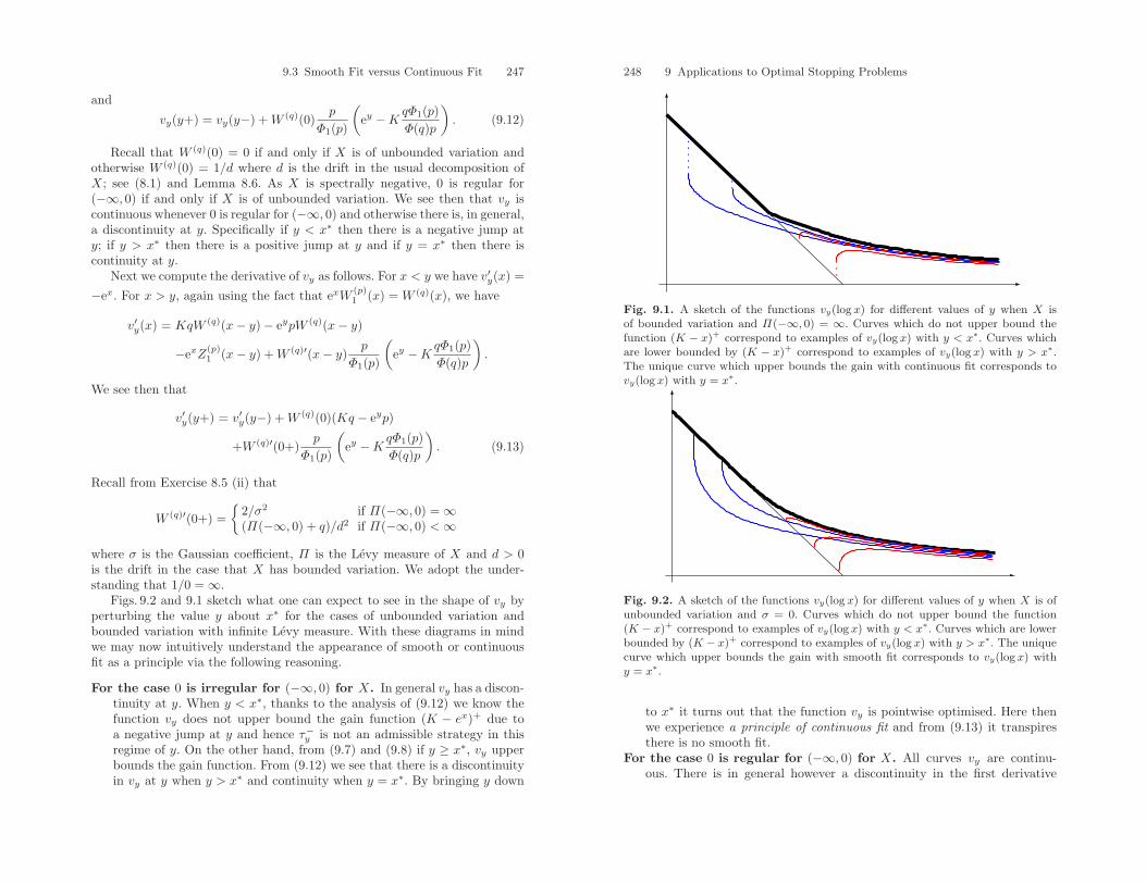
9.3 Smooth Fit versus Continuous Fit 247
and
vy(y+) = vy(y−) +W (q)(0)p
Φ1(p)
(ey −K
qΦ1(p)Φ(q)p
). (9.12)
Recall that W (q)(0) = 0 if and only if X is of unbounded variation andotherwise W (q)(0) = 1/d where d is the drift in the usual decomposition ofX; see (8.1) and Lemma 8.6. As X is spectrally negative, 0 is regular for(−∞, 0) if and only if X is of unbounded variation. We see then that vy iscontinuous whenever 0 is regular for (−∞, 0) and otherwise there is, in general,a discontinuity at y. Specifically if y < x∗ then there is a negative jump aty; if y > x∗ then there is a positive jump at y and if y = x∗ then there iscontinuity at y.
Next we compute the derivative of vy as follows. For x < y we have v′y(x) =
−ex. For x > y, again using the fact that exW (p)1 (x) = W (q)(x), we have
v′y(x) = KqW (q)(x− y)− eypW (q)(x− y)
−exZ(p)1 (x− y) +W (q)′(x− y)
p
Φ1(p)
(ey −K
qΦ1(p)Φ(q)p
).
We see then that
v′y(y+) = v′y(y−) +W (q)(0)(Kq − eyp)
+W (q)′(0+)p
Φ1(p)
(ey −K
qΦ1(p)Φ(q)p
). (9.13)
Recall from Exercise 8.5 (ii) that
W (q)′(0+) =
2/σ2 if Π(−∞, 0) = ∞(Π(−∞, 0) + q)/d2 if Π(−∞, 0) <∞
where σ is the Gaussian coefficient, Π is the Levy measure of X and d > 0is the drift in the case that X has bounded variation. We adopt the under-standing that 1/0 = ∞.
Figs. 9.2 and 9.1 sketch what one can expect to see in the shape of vy byperturbing the value y about x∗ for the cases of unbounded variation andbounded variation with infinite Levy measure. With these diagrams in mindwe may now intuitively understand the appearance of smooth or continuousfit as a principle via the following reasoning.
For the case 0 is irregular for (−∞, 0) for X. In general vy has a discon-tinuity at y. When y < x∗, thanks to the analysis of (9.12) we know thefunction vy does not upper bound the gain function (K − ex)+ due toa negative jump at y and hence τ−y is not an admissible strategy in thisregime of y. On the other hand, from (9.7) and (9.8) if y ≥ x∗, vy upperbounds the gain function. From (9.12) we see that there is a discontinuityin vy at y when y > x∗ and continuity when y = x∗. By bringing y down
248 9 Applications to Optimal Stopping Problems
Fig. 9.1. A sketch of the functions vy(log x) for different values of y when X isof bounded variation and Π(−∞, 0) = ∞. Curves which do not upper bound thefunction (K − x)+ correspond to examples of vy(log x) with y < x∗. Curves whichare lower bounded by (K − x)+ correspond to examples of vy(log x) with y > x∗.The unique curve which upper bounds the gain with continuous fit corresponds tovy(log x) with y = x∗.
Fig. 9.2. A sketch of the functions vy(log x) for different values of y when X is ofunbounded variation and σ = 0. Curves which do not upper bound the function(K − x)+ correspond to examples of vy(log x) with y < x∗. Curves which are lowerbounded by (K − x)+ correspond to examples of vy(log x) with y > x∗. The uniquecurve which upper bounds the gain with smooth fit corresponds to vy(log x) withy = x∗.
to x∗ it turns out that the function vy is pointwise optimised. Here thenwe experience a principle of continuous fit and from (9.13) it transpiresthere is no smooth fit.
For the case 0 is regular for (−∞, 0) for X. All curves vy are continu-ous. There is in general however a discontinuity in the first derivative
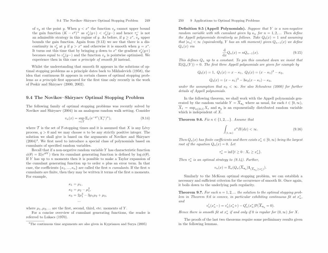
9.4 The Novikov–Shiryaev Optimal Stopping Problem 249
of vy at the point y. When y < x∗ the function vy cannot upper boundthe gain function (K − ey)+ as v′y(y+) < v′y(y−) and hence τ−y is notan admissible strategy in this regime of y. As before, if y ≥ x∗, vy upperbounds the gain function. Again from (9.13) we see that there is a dis-continuity in v′y at y if y > x∗ and otherwise it is smooth when y = x∗.It turns out this time that by bringing y down to x∗ the gradient v′y(y+)becomes equal to v′y(y−) and the function vy is pointwise optimised. Weexperience then in this case a principle of smooth fit instead.
Whilst the understanding that smooth fit appears in the solutions of op-timal stopping problems as a principle dates back to Mikhalevich (1958), theidea that continuous fit appears in certain classes of optimal stopping prob-lems as a principle first appeared for the first time only recently in the workof Peskir and Shiryaev (2000, 2002).
9.4 The Novikov–Shiryaev Optimal Stopping Problem
The following family of optimal stopping problems was recently solved byNovikov and Shiryaev (2004) in an analogous random walk setting. Consider
vn(x) = supτ∈T
Ex(e−qτ (X+τ )n), (9.14)
where T is the set of F-stopping times and it is assumed that X is any Levyprocess, q > 0 and we may choose n to be any strictly positive integer. Thesolution we shall give is based on the arguments of Novikov and Shiryaev(2004)4. We first need to introduce a special class of polynomials based oncumulants of specified random variables.
Recall that if a non-negative random variable Y has characteristic functionφ(θ) = E(eiθY ) then its cumulant generating function is defined by logφ(θ).If Y has up to n moments then it is possible to make a Taylor expansion ofthe cumulant generating function up to order n plus an error term. In thatcase, the coefficients κ1, ..., κn are called the first n cumulants. If the first ncumulants are finite, then they may be written it terms of the first n moments.For example,
κ1 = µ1,
κ2 = µ2 − µ21,
κ3 = 2µ31 − 3µ1µ2 + µ3,
...
where µ1, µ2, ... are the first, second, third, etc. moments of Y .For a concise overview of cumulant generating functions, the reader is
referred to Lukacs (1970).4The continuous time arguments are also given in Kyprianou and Surya (2005)
250 9 Applications to Optimal Stopping Problems
Definition 9.5 (Appell Polynomials). Suppose that Y is a non-negativerandom variable with nth cumulant given by κn for n = 1, 2, ... Then definethe Appell polynomials iteratively as follows. Take Q0(x) = 1 and assumingthat |κn| <∞ (equivalently, Y has an nth moment) given Qn−1(x) we defineQn(x) via
ddx
Qn(x) = nQn−1(x). (9.15)
This defines Qn up to a constant. To pin this constant down we insist thatE(Qn(Y )) = 0. The first three Appell polynomials are given for example by
Q0(x) = 1, Q1(x) = x− κ1, Q2(x) = (x− κ1)2 − κ2,
Q3(x) = (x− κ1)3 − 3κ2(x− κ1)− κ3,
under the assumption that κ3 < ∞. See also Schoutens (2000) for furtherdetails of Appell polynomials.
In the following theorem, we shall work with the Appell polynomials gen-erated by the random variable Y = Xeq
where as usual, for each t ∈ [0,∞),Xt = sups∈[0,t] Xs and eq is an exponentially distributed random variablewhich is independent of X.
Theorem 9.6. Fix n ∈ 1, 2, .... Assume that∫(1,∞)
xnΠ(dx) <∞. (9.16)
Then Qn(x) has finite coefficients and there exists x∗n ∈ [0,∞) being the largestroot of the equation Qn(x) = 0. Let
τ∗n = inft ≥ 0 : Xt ≥ x∗n.Then τ∗n is an optimal strategy to (9.14). Further,
vn(x) = Ex(Qn(Xeq)1(Xeq≥x∗n)).
Similarly to the McKean optimal stopping problem, we can establish anecessary and sufficient criterion for the occurrence of smooth fit. Once again,it boils down to the underlying path regularity.
Theorem 9.7. For each n = 1, 2, ... the solution to the optimal stopping prob-lem in Theorem 9.6 is convex, in particular exhibiting continuous fit at x∗n,and
v′n(x∗n−) = v′n(x∗n+)−Q′n(x∗n)P(Xeq
= 0).
Hence there is smooth fit at x∗n if and only if 0 is regular for (0,∞) for X.
The proofs of the last two theorems require some preliminary results givenin the following lemmas.
9.4 The Novikov–Shiryaev Optimal Stopping Problem 251
Lemma 9.8 (Mean value property). Fix n ∈ 1, 2, ... Suppose that Y isa non-negative random variable satisfying E(Y n) <∞. Then if Qn is the nthAppell polynomial generated by Y , we have that
E(Qn(x+ Y )) = xn
for all x ∈ R.
Proof. Note the result is trivially true for n = 1. Next suppose the result istrue for Qn−1. Then using dominated convergence we have from (9.15) that
ddx
E(Qn(x+ Y )) = E(
ddx
Qn(x+ Y ))
= nE(Qn−1(x+ Y )) = nxn−1.
Solving together with the requirement that E(Qn(Y )) = 0 we have the re-quired result.
Lemma 9.9 (Fluctuation identity). Fix n ∈ 1, 2, ... and suppose that∫(1,∞)
xnΠ(dx) <∞.
Then for all a > 0 and x ∈ R,
Ex(e−qT+a Xn
T+a1(T+
a <∞)) = Ex(Qn(Xeq)1(Xeq≥a)),
where T+a = inft ≥ 0 : Xt ≥ a.
Proof. On the event T+a < eq we have that Xeq
= XT+a
+ S where S isindependent of FT+
aand has the same distribution as Xeq
. It follows that
Ex(Qn(Xeq)1(Xeq≥a)|FT+
a) = 1(T+
a <eq)h(XT+a
),
where h(x) = Ex(Qn(Xeq)) = xn and the last equality follows from Lemma
9.8 with Y = Xeq. Note also that by Exercise 7.1 the integral condition on Π
implies that E(Xn
eq) <∞ which has been used in order to apply Lemma 9.8.
We see, by taking expectations again in the previous calculation, that
Ex(Qn(Xeq)1(Xeq≥a)) = Ex(e−qT
+a Xn
T+a1(T+
a <∞))
as required.
Lemma 9.10 (Largest positive root). Fix n ∈ 1, 2, ... and suppose that∫(1,∞)
xnΠ(dx) <∞.
Suppose that Qn is generated by Xeq. Then Qn has a unique strictly positive
root x∗n such that Qn(x) is negative on [0, x∗n) and positive and increasing on[x∗n,∞).
252 9 Applications to Optimal Stopping Problems
Proof. First note that the statement of the lemma is clearly true for Q1(x) =x− κ1. We proceed then by induction and assume that the result is true forQn−1.
The first step is to prove that Qn(0) ≤ 0. Let
η(a, n) = E(e−qT+a Xn
T+a1(T+
a <∞)),
where T+a = inft ≥ 0 : Xt ≥ a and note that η(a, n) ≥ 0 for all a ≥ 0 and
n = 1, 2, .... On the other hand
η(a, n) = E(Qn(Xeq)1(Xeq≥a))
= −E(Qn(Xeq)1(Xeq<a)
)
= −P(Xeq< a)Qn(0)
+E((Qn(0)−Qn(Xeq))1(Xeq<a)
),
where the first equality follows from Lemma 9.9 and the second by Lemma9.8. Since by definition
Qn(x) = Qn(0) + n
∫ x
0
Qn−1(u)dy (9.17)
for all x ≥ 0 we have the estimate∣∣∣Ex((Qn(0)−Qn(Xeq))1(Xeq<a)
)∣∣∣ ≤ na sup
y∈[0,a]
|Qn−1(y)|P(Xeq< a)
which tends to zero as a ↓ 0. We have in conclusion that
0 ≤ lima↓0
η(a, n) ≤ − lima↓0
P(Xeq< a)Qn(0) + o(a)
and hence necessarily Qn(0) ≤ 0.Under the induction hypothesis for Qn−1, we see from (9.17), together
with the fact that Qn(0) ≤ 0, that Qn is negative and decreasing on [0, x∗n−1).The point x∗n−1 corresponds to the minimum of Qn thanks to the positivityand monotonicity of Qn−1(u) for x > x∗n−1. In particular, Qn(x) tends toinfinity from its minimum point and hence there must be a unique strictlypositive root of the equation Qn(x) = 0.
We are now ready to move to the proofs of the main theorems of thissection.
Proof (of Theorem 9.6). Fix n ∈ 1, 2, .... Thanks to (9.16), E(X1) ∈[−∞,∞) and hence the Strong Law of Large Numbers given in Exercise 7.2implies that (9.2) is automatically satisfied. Indeed, if q > 0 then (X+
t )n growsno faster than Ctn for some constant C > 0.
9.4 The Novikov–Shiryaev Optimal Stopping Problem 253
Definevan(x) = Ex(e−qT
+a (X+
T+a
)n1(T+a <∞)), (9.18)
where as usual T+a = inft ≥ 0 : Xt ≥ a. From Lemma 9.9 we know that
van(x) = Ex(Qn(Xeq)1(Xeq≥a)).
Again referring to the discussion following Lemma 9.1 we consider pairs(van, T
+a ) for a > 0 to be a class of candidate solutions to (9.14). Our goal then
is to verify with the help of Lemma 9.1 that the candidate pair (van, T+a ) solve
(9.14) for some a > 0.
Lower bound (i). We need to prove that van(x) ≥ (x+)n for all x ∈ R. Notethat this statement is obvious for x ∈ (−∞, 0)∪(a,∞) just from the definitionof van. Otherwise when x ∈ (0, a) we have, using the mean value property inLemma 9.8, that for all x ∈ R,
van(x) = Ex(Qn(Xeq)1(Xeq≥a))
= xn − E(Qn(x+Xeq)1(x+Xeq<a)
). (9.19)
From Lemma 9.10 and specifically the fact that Qn(x) ≤ 0 on (0, x∗n] itfollows that, provided
a ≤ x∗n,
we have in (9.19) that van(x) ≥ (x+)n.
Supermartingale property (ii). Provided
a ≥ x∗n
we have almost surely that
Qn(Xeq)1(Xeq≥a) ≥ 0.
On the event that eq > t we have Xeqis equal in distribution to (Xt +
S) ∨ Xt where S is independent of Ft and equal in distribution to Xeq. In
particular Xeq≥ Xt + S. It now follows that
van(x) ≥ Ex(1(eq>t)Qn(Xeq)1(Xeq≥a))
≥ Ex(1(eq>t)Ex(Qn(Xt + S)1(Xt+S≥a)|Ft))= Ex(e−qtvan(Xt)).
From this inequality together with the Markov property, it is easily shownas in the McKean optimal stopping problem that e−qtvan(Xt) : t ≥ 0 is asupermartingale. Right continuity follows again from the right continuity ofthe paths of X together with the right continuity of van which is evident from(9.19).
We now see that the unique choice a = x∗n allows all the conditions ofLemma 9.1 to be satisfied thus giving the solution to (9.14).
254 9 Applications to Optimal Stopping Problems
Note that the case q = 0 can be dealt with in essentially the same manner.In that case it is necessary to assume that lim supt↑∞Xt <∞ and if workingwith the gain function (x+)n for n = 1, 2, ..., then one needs to assume that∫
(1,∞)
xn+1Π(dx) <∞.
Note the power in the above integral is n+ 1 and not n as one must now dealwith the nth moments of X∞; see Exercise 7.1.
Proof (of Theorem 9.7). In a similar manner to the proof of Theorem 9.4 itis straighforward to prove that v is convex and hence continuous.
To establish when there is a smooth fit at x∗n we compute as follows. Forx < x∗n,
vn(x∗n)− vn(xn)x∗n − x
=(x∗n)n − xn
x∗n − x+
Ex(Qn(Xeq)1(Xeq<x
∗n))
x∗n − x
=(x∗n)n − xn
x∗n − x+
Ex((Qn(Xeq)−Qn(x∗n))1(Xeq<x
∗n))
x∗n − x,
where the final equality follows because Qn(x∗n) = 0. Clearly
limx↑x∗n
(x∗n)n − xn
x∗n − x= v′n(x∗n+).
However,
Ex((Qn(Xeq)−Qn(x∗n))1(Xeq<x
∗n))
x∗n − x
=Ex((Qn(Xeq
)−Qn(x))1(x<Xeq<x∗n))
x∗n − x
−Ex((Qn(x∗n)−Qn(x))1(Xeq<x
∗n))
x∗n − x(9.20)
where in the first term on the right-hand side we may restrict the expectationto x < Xeq
< x∗n as, under Px, the possible atom of Xeqat x gives zero
mass to the expectation. Denote by Ax and Bx the two expressions on theright hand side of (9.20). We have that
limx↑x∗n
Bx = −Q′n(x∗n)P(Xeq
= 0).
9.5 The Shepp–Shiryaev Optimal Stopping Problem 255
Integration by parts also gives
Ax =∫
(0,x∗n−x)
Qn(x+ y)−Qn(x)x∗n − x
P(Xeq∈ dy)
=Qn(x∗n)−Qn(x)
x∗n − xP(Xeq
∈ (0, x∗n − x))
− 1x∗n − x
∫ x∗n−x
0
P(Xeq∈ (0, y])Q′
n(x+ y)dy.
Hence it follows thatlimx↑x∗n
Ax = 0.
In conclusion we have that
limx↑x∗n
vn(x∗n)− vn(x)x∗n − x
= v′n(x∗n+)−Q′n(x∗n)P(Xeq
= 0)
which concludes the proof.
9.5 The Shepp–Shiryaev Optimal Stopping Problem
Suppose thatX is a Levy process. Then consider the optimal stopping problem
v(x) = supτ∈T
E(e−qτ+(Xτ∨x)) (9.21)
where q > 0, T is the set of F-stopping times which are almost surely finiteand x ≥ 0. This optimal stopping problem was proposed and solved by Sheppand Shiryaev (1993) for the case that X is a linear Brownian motion and q issufficiently large. Like the McKean optimal stopping problem, (9.21) appearsin the context of an option pricing problem. Specifically, it addresses theproblem of the optimal time to sell a risky asset for the minimum of eitherex or its running maximum when the risky asset follows the dynamics of anexponential linear Brownian motion and in the presence of discounting. InAvram et al. (2004) a solution was given to (9.21) in the case that X is ageneral spectrally negative Levy process (and again q is sufficiently large). Inorder to keep to the mathematics that has been covered earlier on in this text,we give an account of a special case of that solution here. Specifically we dealwith the case that X has bounded variation which we shall write in the usualform
Xt = dt− St, (9.22)
where d > 0 and S is a driftless subordinator with Levy measure Π (concen-trated on (0,∞)). We shall further assume that Π has no atoms. As we shalluse scale functions in our solution, the latter condition will ensure that theyare at least continuously differentiable; see Exercise 8.4. Our objective is thetheorem below. Note that we use standard notation from Chap. 8.
256 9 Applications to Optimal Stopping Problems
Theorem 9.11. Suppose that X is as stated in the the above paragraph, hav-ing Laplace exponent ψ. Suppose that q > ψ(1). Define
x∗ = infx ≥ 0 : Z(q)(x) ≤ qW (q)(x).Then for each x ≥ 0, the solution to (9.21) is given by the pair
v(x) = exZ(q)(x∗ − x)
andτ∗ = inft > 0 : Y x
t > x∗,where Y x = Y x
t : t ≥ 0 is the process X reflected in its supremum wheninitiated from x ≥ 0 so that Y x
t = (x ∨Xt)−Xt.
Before moving to the proof of Theorem 9.11, let us consider the nature of(9.21) and its solution in a little more detail.
Firstly it needs to be pointed out that due to the involvement of the run-ning supremum in the formulation of the problem, one may consider (9.21)as an optimal stopping problem which potentially concerns the three dimen-sional Markov process (t,Xt,Xt) : t ≥ 0. Nonetheless, as with the previoustwo examples of optimal stopping problems it is possible to reduce the dimen-sion of the problem to just one. As indeed one notes from the statement ofTheorem 9.11, the solution is formulated in terms of the process Y x.
The way to do this was noted by Shepp and Shiryaev (1994) in a follow-up article to their original contribution. Recalling the method of change ofmeasure described in Sects. 3.3 and 8.1 (see specifically Corollary 3.11), foreach τ ∈ T we may write
E(e−qτ+(Xτ∨x)) = E1(e−ατ+Yx
τ ),
whereα = q − ψ(1)
and Y x = (x ∨ X) − X is the process reflected in its supremum and issuedfrom x. Hence our objective is now to solve the optimal stopping problem
supτ∈T
E1(e−ατ+Yx
τ ) (9.23)
which is now based on the two dimensional Markov process (t, Y xt ) : t ≥ 0.
Again, arguments along the lines of those in the paragraphs following Lemma9.1 suggest that a suitable class of candidate solutions to (9.23) are of theform (va(x), σxa) with a ≥ 0 where for each x ≥ 0
va(x) = E1(e−ασxa+Y x
σxa ) (9.24)
andσxa = inft > 0 : Y x
t ≥ a.
9.5 The Shepp–Shiryaev Optimal Stopping Problem 257
(Note that the latter is P1-almost surely finite). In addition, one may alsointuitively understand how a threshold strategy for Y x is optimal for (9.21)as follows. The times at which Y x is zero correspond to times at which X,and hence the gain, is increasing. The times at which Y x takes large valuescorrespond to the times at which X is far from its running supremum. Atsuch moments, one must wait for the process to return to its maximum beforethere is an increase in the gain. Exponential discounting puts a time penaltyon waiting too long suggesting that one should look for a threshold strategyin which one should stop if X moves too far from its maximum.
Secondly let us consider the optimal threshold x∗. Define the functionf(x) = Z(q)(x)− qW (q)(x). Differentiating we have
f ′(x) = q(W (q)(x)−W (q)′(x))= qeΦ(q)x((1− Φ(q))WΦ(q)(x))−W ′
Φ(q)(x) (9.25)
where, in the second equality we have used (8.25). Since
ψ′Φ(q)(0+) = ψ′(Φ(q)) > 0,
we know that under PΦ(q) the process X drifts to infinity and hence recall from(8.7) that this implies that WΦ(q)(x) is monotone increasing. In particularW ′Φ(q)(x) > 0 for all x > 0. On the other hand, the assumption that q > ψ(1)
implies that Φ(q) > 1. Hence the right-hand side of (9.25) is strictly negativefor all x > 0. Further we may check with the help of Exercise 8.5 (i) that
limx↑∞
f(x)qW (q)(x)
=1
Φ(q)− 1 < 0.
From (8.25) again, it is clear that the denominator on the left-hand side abovetends to infinity.
Note that f(0+) = 1− qW (q)(0). Since X has bounded variation we knowthat W (q)(0) = d−1. Hence if q ≥ d then f(0+) < 0 so that necessarily x∗ = 0.When q < d, we have that f(0+) > 0, f ′(x) < 0 for all x > 0 and f(∞) = −∞.It follows then that there is a unique solution in [0,∞) to f(x) = 0, namelyx∗, which is necessarily strictly positive.
Note also that as the solution can be expressed in terms of functions whoseanalytic properties are understood sufficiently well that, we may establisheasily the situation with regard to smooth or continuous fit. For each x > 0,the process Y x has the same small-time path behaviour as −X and henceP(σxx = 0) = 0 as P(τ−0 = 0) = 0. This property is independent of x > 0 (thepoint x = 0 needs to be considered as a special case on account of reflection).
Corollary 9.12. When q < d, the solution to (9.21) is convex and henceexhibits continuous fit at x∗. Further it satisfies
v′(x∗−) = v′(x∗+)− q
dex∗
showing that there is no smooth fit at x∗.
258 9 Applications to Optimal Stopping Problems
Proof. The first part follows in a similar manner to the proof of convexity inthe previous two optimal stopping problem. After a straightforward differen-tiation of the solution to (9.21), recalling that W (0+) = 1/d, the last part ofthe corollary follows.
Proof (of Theorem 9.11). As indicated above, we consider candidate solutionsof the form (va, σxa). We can develop the right-hand side of va in terms ofscale functions with the help of Theorem 8.10 (i). However, before doing so,again taking into account the conclusion of Lemma 8.4, let us note that theanalogue of the scale function W
(q)−1 when working under the measure P1 can
be calculated as equal to
[W (q)1 ]−1(x) = exW (q+ψ1(−1))
1 .
However, we also know that ψ1(−1) = ψ(1 − 1) − ψ(1) = −ψ(1) and henceapplying Lemma 8.4 again we have further that
[W (q)1 ]−1(x) = exe−xW (q)(x) = W (q)(x).
This means that we may read out of Theorem 8.10 (i) the identity
va(x) = ex(Z(q)(a− x)−W (q)(a− x)
qW (q)(a)− Z(q)(a)W (q)′(a)−W (q)(a)
). (9.26)
Revisiting the proof of Lemma 9.1 one sees that in fact that requirementthat X is a Levy process is not necessary and one may replace X by Y x
without affecting any of the arguments or conclusions. (Here we mean thatT is still the family of stopping times with respect to the underlying Levyprocess). Let us continue then to check the conditions of the aforementionedmodified version of Lemma 9.1.
Lower bound (i). We need to show that va(s) ≥ ex. The assumption q >ψ(1) implies that Φ(q) > 1 and hence
W (q)′(a)−W (q)(a) > W (q)′(a)− Φ(q)W (q)(a).
On the other hand, from (8.25) we may compute
W (q)′(a)− Φ(q)W (q)(a) = eΦ(q)aW ′Φ(q)(a) > 0,
where the inequality is, for example, due to (8.18). Together with the proper-ties of Z(q)(a)− qW (q)(a) as a function of a, we see that the coefficient
qW (q)(a)− Z(q)(a)W (q)′(a)−W (q)(a)
is strictly positive when a > x∗ and non-positive when a ∈ [0, x∗].
9.5 The Shepp–Shiryaev Optimal Stopping Problem 259
Recalling that Z(q)(x) ≥ 1, we conclude that va(x) ≥ ex when a ∈ [0, x∗].On the other hand, suppose that a > x∗, then
va(a−) = ea −W (q)(0)qW (q)(a)− Z(q)(a)W (q)′(a)−W (q)(a)
< ea, (9.27)
showing that in order to respect the lower bound we necessarily must takea ≤ x∗.
Supermartingale property (ii). We know that the function va(x) is differ-entiable with continuous first derivative on (0, a). Further, the right derivativeat zero exists and is equal to zero. To see this, simply compute
v′a(0+) = ea(Z(q)(a)−W (q)(a)
qW (q)(a)− Z(q)(a)W (q)′(a)−W (q)(a)
−qW (q)(a) +W (q)′(a)qW (q)(a)− Z(q)(a)W (q)′(a)−W (q)(a)
)= 0.
Next recall from Sect. 8.1 that under P1, X remains a Levy process of boundedvariation with the same drift but now with exponentially tilted Levy measureso that in the form (9.22), Π(dy) becomes e−yΠ(dy). Applying the change ofvariable formula in the spirit of Exercise 4.2 and 4.1 we see that, despite thefact that the first derivative of va is not well defined at a,
e−αtva(Y xt ) = va(x)− α
∫ t
0
e−αsva(Y xs )ds
+∫ t
0
e−αs(va(a−)− va(a+))dLat
−d∫ t
0
e−αsv′a(Yxs )ds+
∫ t
0
e−αsv′a(Yxs )d(x ∨Xs)
+∫
[0,t]
∫(0,∞)
e−αs(va(Y xs− + y)− va(Y x
s−))e−yΠ(dy)ds
+Mt. (9.28)
P-almost surely, where Lat : t ≥ 0 counts the number of crossings of theprocess Y x over the level a. Further, for t ≥ 0,
Mt =∫
[0,t]
∫(0,∞)
e−αs(va(Y xs− + y)− va(Y x
s−))N1(ds× dx)
−∫
[0,t]
∫(0,∞)
e−αs(va(Y xs− + y)− va(Y x
s−))e−yΠ(dy)ds,
where N1 is the counting measure associated with the Poisson point processof jumps of the subordinator given in the representation (9.22) of X under P1.
260 9 Applications to Optimal Stopping Problems
In the third integral of (9.28), the process x∨Xs increases only when Y xs = 0.
Since v′a(0+) = 0, then the third integral is equal to zero. Note also that itcan be proved in a straightforward way with the help of the compensationformula in Theorem 4.4 that the process M := Mt : t ≥ 0 is a martingale.
The Markov property together with (9.24) imply that
E1(e−ασxa+Y x
σxa |Ft) = e−α(σx
a∧t)+Y x(σx
a∧t) .
Hence considering the left-hand side of (9.28) on t < σxa, we deduce withthe help of Exercise 4.3 that
L1va(x) :=∫
(0,∞)
(va(x+ y)− va(x))e−yΠ(dy)−dv′a(x)−αva(x) = 0 (9.29)
for all x ∈ (0, a). We also see by inspection va(x) = ex for all x > a. Inthat case, from the definition of the Laplace exponent ψ we know that theexpression on the left-hand side of (9.29) satisfies
L1va(x) = ex∫
(0,∞)
(1− e−y)Π(dy)− dex − αex
= −ex(ψ(1) + α)= −qex < 0
for x > a. In conclusion we have shown that L1va(x) ≤ 0 on x ∈ (0,∞)\a.If a ≥ x∗, then from (9.27) va(a−) − va(a+) ≤ 0. Reconsidering (9.28)
in this light, we see that when a ≥ x∗, the process e−αtva(Xt) : t ≥ 0 isthe difference of a martingale M and a non-decreasing adapted process thusmaking it a supermartingale. Right continuity can be seen from (9.28).
In conclusion, all properties of Lemma 9.1 are satisfied uniquely whena = x∗, thus concluding the proof.
The semi-explicit nature of the functions va : a ≥ 0 again gives theopportunity to show graphically how continuous fit occurs by perturbing thefunction va about the value a = x∗. See Fig. 9.3.
9.6 Stochastic Games
Suppose that H,G are two continuous functions mapping R to [0,∞) satisfy-ing H(x) > G(x) for all x ∈ R and let T be a family of F-stopping times. Forq ≥ 0, σ, τ ∈ T define
Θqτ,σ = e−qτG(Xτ )1(τ≤σ) + e−qσH(Xσ)1(σ<τ).
Consider the existence of a function v : R → [0,∞) and stopping timesτ∗, σ∗ ∈ T which satisfy the relation
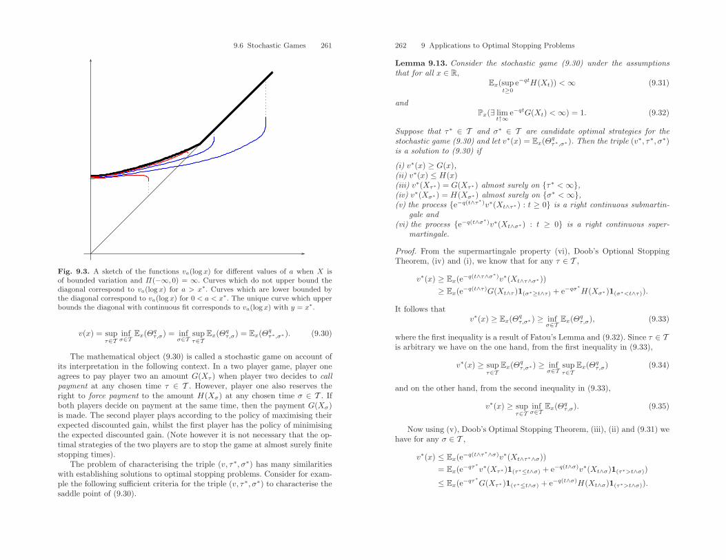
9.6 Stochastic Games 261
Fig. 9.3. A sketch of the functions va(log x) for different values of a when X isof bounded variation and Π(−∞, 0) = ∞. Curves which do not upper bound thediagonal correspond to va(log x) for a > x∗. Curves which are lower bounded bythe diagonal correspond to va(log x) for 0 < a < x∗. The unique curve which upperbounds the diagonal with continuous fit corresponds to va(log x) with y = x∗.
v(x) = supτ∈T
infσ∈T
Ex(Θqτ,σ) = inf
σ∈Tsupτ∈T
Ex(Θqτ,σ) = Ex(Θq
τ∗,σ∗). (9.30)
The mathematical object (9.30) is called a stochastic game on account ofits interpretation in the following context. In a two player game, player oneagrees to pay player two an amount G(Xτ ) when player two decides to callpayment at any chosen time τ ∈ T . However, player one also reserves theright to force payment to the amount H(Xσ) at any chosen time σ ∈ T . Ifboth players decide on payment at the same time, then the payment G(Xσ)is made. The second player plays according to the policy of maximising theirexpected discounted gain, whilst the first player has the policy of minimisingthe expected discounted gain. (Note however it is not necessary that the op-timal strategies of the two players are to stop the game at almost surely finitestopping times).
The problem of characterising the triple (v, τ∗, σ∗) has many similaritieswith establishing solutions to optimal stopping problems. Consider for exam-ple the following sufficient criteria for the triple (v, τ∗, σ∗) to characterise thesaddle point of (9.30).
262 9 Applications to Optimal Stopping Problems
Lemma 9.13. Consider the stochastic game (9.30) under the assumptionsthat for all x ∈ R,
Ex(supt≥0
e−qtH(Xt)) <∞ (9.31)
andPx(∃ lim
t↑∞e−qtG(Xt) <∞) = 1. (9.32)
Suppose that τ∗ ∈ T and σ∗ ∈ T are candidate optimal strategies for thestochastic game (9.30) and let v∗(x) = Ex(Θq
τ∗,σ∗). Then the triple (v∗, τ∗, σ∗)is a solution to (9.30) if
(i) v∗(x) ≥ G(x),(ii) v∗(x) ≤ H(x)(iii) v∗(Xτ∗) = G(Xτ∗) almost surely on τ∗ <∞,(iv) v∗(Xσ∗) = H(Xσ∗) almost surely on σ∗ <∞,(v) the process e−q(t∧τ∗)v∗(Xt∧τ∗) : t ≥ 0 is a right continuous submartin-
gale and(vi) the process e−q(t∧σ∗)v∗(Xt∧σ∗) : t ≥ 0 is a right continuous super-
martingale.
Proof. From the supermartingale property (vi), Doob’s Optional StoppingTheorem, (iv) and (i), we know that for any τ ∈ T ,
v∗(x) ≥ Ex(e−q(t∧τ∧σ∗)v∗(Xt∧τ∧σ∗))
≥ Ex(e−q(t∧τ)G(Xt∧τ )1(σ∗≥t∧τ) + e−qσ∗H(Xσ∗)1(σ∗<t∧τ)).
It follows thatv∗(x) ≥ Ex(Θq
τ,σ∗) ≥ infσ∈T
Ex(Θqτ,σ), (9.33)
where the first inequality is a result of Fatou’s Lemma and (9.32). Since τ ∈ Tis arbitrary we have on the one hand, from the first inequality in (9.33),
v∗(x) ≥ supτ∈T
Ex(Θqτ,σ∗) ≥ inf
σ∈Tsupτ∈T
Ex(Θqτ,σ) (9.34)
and on the other hand, from the second inequality in (9.33),
v∗(x) ≥ supτ∈T
infσ∈T
Ex(Θqτ,σ). (9.35)
Now using (v), Doob’s Optimal Stopping Theorem, (iii), (ii) and (9.31) wehave for any σ ∈ T ,
v∗(x) ≤ Ex(e−q(t∧τ∗∧σ)v∗(Xt∧τ∗∧σ))
= Ex(e−qτ∗v∗(Xτ∗)1(τ∗≤t∧σ) + e−q(t∧σ)v∗(Xt∧σ)1(τ∗>t∧σ))
≤ Ex(e−qτ∗G(Xτ∗)1(τ∗≤t∧σ) + e−q(t∧σ)H(Xt∧σ)1(τ∗>t∧σ)).
9.6 Stochastic Games 263
Taking limits as t ↑ ∞ and applying the Dominated Convergence Theoremwith the help of (9.31), (9.32) and the non-negativity of G, we have
v∗(x) ≤ Ex(Θqτ∗,σ) ≤ sup
τ∈TEx(Θq
τ,σ). (9.36)
Since σ ∈ T is arbitrary, we have on the one hand, from the first inequalityin (9.36),
v∗(x) ≤ infσ∈T
Ex(Θqτ∗,σ) ≤ sup
τ∈Tinfσ∈T
Ex(Θqτ,σ) (9.37)
and on the other hand, from the second inequality in (9.36),
v∗(x) ≤ infσ∈T
supτ∈T
Ex(Θqτ,σ). (9.38)
From (9.34), (9.35), (9.37) and (9.38), we see that
v∗(x) = infσ∈T
supτ∈T
Ex(Θqτ,σ) = sup
τ∈Tinfσ∈T
Ex(Θqτ,σ).
Finally from its definition
v∗(x) = Ex(Θqτ∗,σ∗)
and hence the saddle point is achieved with the strategies (τ∗, σ∗).
To the author’s knowledge there is an extremely limited base of pub-lished literature giving concrete examples of stochastic games driven by Levyprocesses.5 We give an example here which is an excerpt from Baurdoux andKyprianou (2005). Aspects of the general theory can be found in one of theoriginal papers on the topic, Dynkin (1969).
Suppose that X is a spectrally negative Levy process of bounded variationwhich drifts to infinity and denote as usual its Laplace exponent by ψ. Thatis to say, it has the same structure as in (9.22) with d > E(S1) > 0. Considerthe stochastic game (9.30) when G(x) = (K−ex)+, H(x) = G(x)+δ for fixedδ > 0 and T consists of all F-stopping times.
This stochastic game is very closely related to the McKean optimal stop-ping problem. We may think of it as modeling the optimal time to sell toan agent a risky asset for a fixed price K whose dynamics follow those of anexponential Levy process. However, we have in addition now that the pur-chasing agent may also demand a forced purchase; in which case the agentmust pay a supplementary penalty δ for forcing the purchase. Note, however,if the constant δ is too large (for example greater than K) then it will neverbe optimal for the agent to force a purchase in which case the stochastic gamewill have the same solution as the analogous optimal stopping problem. Thatis to say the optimal stopping problem (9.3) with q = 0.
5See for example Gapeev and Kuhn (2005) in print
264 9 Applications to Optimal Stopping Problems
Suppose however that δ is a very small number. In this case, based on theexperience of the above optimal stopping problems, it is reasonable to assumethat one may optimise the expected gain by opting to sell the risky asset oncethe value of X drops below a critical threshold where the gain function G islarge. The level of the threshold is determined by the fact that X drifts toinfinity (and hence may never reach the threshold) as well as the behaviourof the purchasing agent. The latter individual can minimise the expected gainby stopping X in a region of R where the gain function H is small. Thisis clearly the half line (logK,∞). As the gain G is identically zero on thisinterval, it turns out to be worthwhile to stop in the aforementioned interval,paying the penalty δ, rather than waiting for the other player to request apurchase requiring a potentially greater pay out by the agent.
These ideas are captured in the following theorem.
Theorem 9.14. Under the assumptions above, the stochastic game (9.30) hasthe following two regimes of solutions.
(a) Define x∗ by
ex∗
= Kψ′(0+)ψ(1)
(9.39)
and note by strict convexity of ψ that x∗ < logK. Suppose that
δ ≥ Kψ(1)∫ log(ψ(1)/ψ′(0+))
0
e−yW (y)dy,
then
v(x) = K − ex + ψ(1)ex∫ x−x∗
0
e−yW (y)dy, (9.40)
where the saddle point strategies are given by
τ∗ = inft > 0 : Xt < x∗ and σ∗ = ∞.
That is to say, (v, τ∗) is also the solution to the optimal stopping problem
v(x) = supτ∈T
Ex((K − eXτ )+).
(b) Suppose that
δ < Kψ(1)∫ log(ψ(1))/ψ′(0+)
0
e−yW (y)dy
then
v(x) =K − ex + ψ(1)ex
∫ x−z∗0
e−yW (y)dy for x < logKδ for x ≥ logK,
(9.41)
9.6 Stochastic Games 265
where z∗ ∈ (0,K) is the unique solution of the equation
Kψ(1)∫ logK−z
0
e−yW (y)dy = δ (9.42)
and the saddle point strategies are given by
τ∗ = inft > 0 : Xt < z∗ and σ∗ = inft > 0 : Xt > logK.
Proof. For both parts (a) and (b) we shall resort to checking conditions givenin Lemma 9.13. Note that for the stochastic game at hand, conditions (9.31)and (9.32) are both satisfied. The first condition is trivially satisfied and thesecond follows from the fact that limt↑∞Xt = ∞ and H(x) = δ for all x >logK.
(a) As indicated in the statement of the Theorem, the proposed solutionnecessarily solves the McKean optimal stopping problem. Under the presentcircumstances of spectral negativity and bounded variation, the solution tothis optimal stopping problem is given in Corollary 9.3. It is left to the readerto check that this solution corresponds to the function given on the right-handside of (9.40).
Let v∗ be the expression given on the right-hand side of (9.40). We nowproceed to show that v∗, τ∗ and σ∗ fulfill the conditions (i) – (vi) of Lemma9.13.
Bounds (i) and (ii). Since by definition of W ,∫∞0
e−yW (y)dy = 1/ψ(1)we may apply l’Hopital’s rule and compute
limx↑∞
v∗(x) = K − limx↑∞
1− ψ(1)∫ x−x∗0
e−yW (y)dye−x
= K − limx↑∞
ψ(1)ex∗W (x− x∗)
= K − ψ(1)ψ′(0+)
ex∗
= 0,
where the final equality follows from (8.15) and (9.39). Hence, with the as-sumption on δ, which reworded says δ ≥ v∗(logK), and the convexity of v∗
(cf. Theorem 9.4) we have
(K − ex)+ ≤ v∗(x) ≤ (K − ex)+ + δ.
Hence conditions (i) and (ii) of Lemma 9.13 are fulfilled.
Equality with the gain properties (iii) and (iv). Property (iii) is triviallysatisfied by virtue of the fact that v∗ solves (9.3) with q = 0. As σ∗ = ∞ thestatement (iv) is empty.
266 9 Applications to Optimal Stopping Problems
Supermartingale and subartingale properties (v) and (vi). From the proofof Theorem 9.2 we have seen that v∗(Xt) : t ≥ 0 is a supermartingale withright continuous paths. For the submartingale property, we actually need toshow that v∗(Xt∧τ∗) : t ≥ 0 is a martingale. However this follows by theStrong Markov Property since for all t ≥ 0,
Ex((K − eXτ∗ )|Ft∧τ∗) = Ex′(K − eXτ∗ ) where x′ = Xt∧τ∗
= v∗(Xt∧τ∗).
(b) Technically speaking, one reason why we may not appeal to the solutionto (9.3) with q = 0 as the solution to the problem at hand is because thecondition on δ now implies that the solution to part (a) is no longer boundedabove by (K − ex)+ + δ, at least at the point x = logK.
The right-hand side of (9.41) can easily be checked using the fluctuationidentities in Chap. 8 to be equal to
v∗(x) = Ex((K − expXτ−z∗)1(τ−
z∗<τ+log K
)) + δEx(1(τ−z∗>τ
+log K
)) (9.43)
and we check now whether the triple (v∗, τ∗, σ∗) fulfill the conditions (i) – (vi)of Lemma 9.13.
Bounds (i) and (ii). The lower bound is easily established since by (9.43)we have that v∗(x) ≥ 0 and from (9.41) v∗(x) ≥ K − ex. Hence v∗(x) ≥(K − ex)+. For the upper bound, note that v∗(x) = H(x) for x ≥ logK. Onx < logK we also have from (9.41) that
v∗(x)− (K − ex) =ex
KKψ(1)
∫ x−z∗
0
e−yW (y)dy
≤ Kψ(1)∫ logK−z∗
0
e−yW (y)dy
= δ
thus confirming that v∗(x) ≤ H(x).
Equality with the gain properties (iii) and (iv). This is clear by inspection.
Supermartingale properties (v). By considering the representation (9.43)the martingale property is confirmed by a similar technique to the one usedin part (a) and applying the Strong Markov Property to deduce that
v∗(Xt∧τ∗∧σ∗) = Ex((K − eX
τ−z∗ )1(τ−
z∗<τ+log K
) + δ1(τ−z∗>τ
+log K
)|Ft).
Note that in establishing the above equality, it has been used that v∗(Xτ−z∗
) =
(K − eX
τ−z∗ ) and v∗(Xτ+
log K) = δ. Noting that v∗ is a continuous function
9.6 Stochastic Games 267
which is also C1 function on R\logK we may apply the change of variableformula in the spirit of Exercise 4.1 and obtain
v∗(Xt) = v∗(x) +∫ t
0
Hv∗(Xs−)ds+Mt, t ≥ 0 (9.44)
Px almost surely where Mt : t ≥ 0 is a right continuous martingale,
Hv∗(x) = ddv∗
dx(x) +
∫(−∞,0)
(v∗(x+ y)− v∗(x))Π(dy)
andΠ is the Levy measure of X and d is its drift. The details of this calculationare very similar in nature to those of a related calculation appearing in theproof of Theorem 9.11 and hence are left to the reader.
Since v∗(Xt) : t < τ∗ ∧ σ∗ is a martingale we deduce from Exercise 4.3that Hv∗(x) = 0 for all x ∈ (z∗, logK). A straightforward calculation alsoshows that for x < z∗, where v∗(x) = K − ex,
Hv∗(x) = −ex(d+
∫(−∞,0)
(ey − 1)Π(dy)
)= −exψ(1) < 0.
Reconsidering (9.44) we see then that on t < σ∗ the Lebesgue integralis a non-increasing adapted process and hence v∗(Xt) : t < σ∗ is a rightcontinuous supermaringale.
Submartingale property (vi). For x > logK, where v∗(x) = δ, our aim isto show that
Hv∗(x) =∫
(−∞,0)
(v∗(x+ y)− δ)Π(dy) ≥ 0
as a consequence of the fact that
v∗(x) ≥ δ on (0, logK). (9.45)
If this is the case then in (9.44) we have on t < τ∗ that the Lebesgue integralis a non-decreasing adapted process and hence v∗(Xt) : t < τ∗ is a rightcontinuous submartingale. Showing that (9.45) holds turns out to be quitedifficult and we prove this in the lemma immediately below.
In conclusion, the conditions of Lemma 9.13 are satisfied by the triple(v∗, τ∗, σ∗) thus establishing part (b) of the theorem.
Lemma 9.15. The function v∗ in the proof of part (b) of the above theoremis strictly greater than δ for all x < logK.
268 9 Applications to Optimal Stopping Problems
Proof. We assume the notation from the proof of part (b) of the above theo-rem. As a first step we show that v∗ together with the stopping time τ∗ solvesthe optimal stopping problem
f(x) = supτ∈T
Ex(G(X∗τ )), (9.46)
where X∗t : t ≥ 0 is the process X stopped on first entry to (logK,∞), so
that X∗t = Xt∧σ∗ , and
G(x) = (K − ex)+1(x≤logK) + δ1(x>logK).
Recalling the remark at the end of Sect. 9.1, we note from the lower bound (i),equality with the gain property (iii), martingale property and supermartingaleproperty (vi) established in the proof of part (b) of the above theorem that(v, τ∗) solves the optimal stopping problem (9.46).
Next define for each q ≥ 0 the solutions to the McKean optimal stoppingproblem
g(q)(x) = supτ∈T
Ex(e−qτ (K − eXτ )+)
for x ∈ R. The associated optimal stopping time for each q ≥ 0 is given byτ∗q = inft > 0 : Xt < x∗p. From Theorem 9.2 and Corollary 9.3 we knowthat
ex∗q = KE(eXeq ) = K
q
Φ(q)Φ(q)− 1q − ψ(1)
.
Hence the constant x∗q is continuous and strictly increasing to logK as q tendsto infinity. It may also be verified from Corollary 9.3 that
g(q)(logK) = Kq
∫ logK−x∗q
0
(1− e−y)W (q)(y)dy
+Kψ(1)∫ logK−x∗q
0
e−yW (q)(y)dy.
We see then that g(q)(logK) is continuous in q. From Theorem 9.2 we alsoknow that for each fixed x ∈ R, g(q)(x) ↓ 0 as q ↑ ∞. Thanks to these factswe may deduce that there exists a solution to the equation g(q)(logK) = δ.Henceforth we shall assume that q solves the latter equation.
The Strong Markov Property implies that
g(q)(x) = Ex(e−qτ∗q (K − eXτ∗q ))
= Ex(e−qτ∗q (K − eXτ∗q )1(τ∗q <τ
+log K
) + e−qτ+log Kg(q)(logK)1(τ∗q >τ
+log K
))
= Ex(e−qτ∗q (K − eXτ∗q )1(τ∗q <τ
+log K
) + e−qτ+log K δ1(τ∗q >τ
+log K
)).
Hence as v∗ solves (9.46) we have
v∗(x) = supτ∈T
Ex((K − eXτ )+1(τ<σ∗) + δ1(τ≥σ∗))
≥ Ex((K − eXτ∗q )1(τ∗q <σ∗) + δ1(τ∗q ≥σ∗))
≥ g(q)(x).
9.6 Exercises 269
We know from Theorem 9.4 that g(q) is convex and hence the last inequalityensures that v∗(x) ≥ δ for all x < logK as required.
Exercises
9.1. The following exercise is based on Novikov and Shiryaev (2004). Supposethat X is any Levy process and either
q > 0 or q = 0 and limt↑∞
Xt = −∞.
Consider the optimal stopping problem
v(x) = supτ∈T
Ex(e−qτ (1− e−(Xτ )+)) (9.47)
where T is the set of F-stopping times.
(i) For a > 0, prove the identity
Ex(e−qT
+a
(1− e
−XT
+a
)1(T+
a <∞)
)= Ex
((1− e−Xeq
E(e−Xeq )
)1(Xeq≥a)
),
where T+a = inft ≥ 0 : Xt ≥ a.
(ii) Show that the solution to (9.47) is given by the pair (vx∗ , T+x∗) where
vx∗(x) is equal to the left-hand side of the identity in part (i) with a = x∗
wheree−x
∗= E(e−Xeq ).
(iii) Show that there is smooth fit at x∗ if and only if 0 is regular for (0,∞)for X and otherwise continuous fit.
9.2. This exercise is based on Baurdoux and Kyprianou (2005). Suppose thatX is a bounded variation spectrally negative Levy process with characteristicexponent ψ(θ) = dθ−∫
(0,∞)(1−e−θx)Π(dx) for θ ≥ 0 where d is the drift and
Π is the Levy measure of the pure jump subordinator in the decompositionof X. Consider the stochastic game which requires one to find v(x) satisfying
v(x) = supτ∈T
infσ∈T
E(e−qτ+(x∨Xτ )1(τ≤σ) + e−qσ(e(x∨Xσ) + δeXσ )1(τ>σ)), (9.48)
where δ > 0, x ≥ 0, d > q > ψ(1) > 0 and the supremum and infimum areinterchangeable.
(i) Let x∗ be the constant defined in Theorem 9.11. Show that if 1 + δ ≥Z(q)(x∗) the solution to (9.48) is the same as the solution given in Theorem9.11.
270 9 Applications to Optimal Stopping Problems
(ii) Henceforth assume that 1+ δ < Z(q)(x∗). Show that there exists a uniquesolution to equation Z(q)(z∗) = 1 + δ and further that z∗ < x∗. Considerthe function f(x) = Z(q)(x)−qW (q)(x) defined in the discussion precedingTheorem 9.11. Using the analytic properties of f discussed there showthat function exZ(q)(z∗ − x) is convex satisfying v′(0+) > 0 and v′(z∗) =ez∗(1− q/d).
(iii) Show that the solution to (9.48) is given by
v(x) = exZ(q)(z∗ − x),
where z∗ is given in the previous part. Further the saddle point is achievedwith the stopping times
σ∗ = inft > 0 : Y xt = 0 and τ∗ = inft > 0 : Y x
t > z∗,
where Y x = (x ∨X) −X is the process reflected in its supremum issuedfrom x. Note that there is continuous fit at z∗ but not smooth fit.
10
Continuous-State Branching Processes
Our interest in continuous-state branching processes will be in exposing theirintimate relationship with spectrally positive Levy processes. A flavour forthis has already been given in Sect. 1.3.4 where it was shown that compoundPoisson process killed on exiting (0,∞) can be time changed to obtain acontinuous-time Bienayme-Galton-Watson process. The analogue of this pathtransformation in fuller generality consists of time changing the path of aspectrally positive Levy process killed on exiting (0,∞) to obtain a processequal in law to the path of a Markov process which observes the so-calledbranching property (defined in more detail later) and vice versa. The latterprocess is what we refer to as the continuous-state branching process. The timechange binding the two processes together is called the Lamperti transform,named after the foundational work of Lamperti (1967a,b).1
Having looked closely at the Lamperti transform we shall give an accountof a number of observations concerning the long term behaviour as well asconditioning on survival of continuous-state branching processes. Thanks tosome of the results in Chap. 8 semi-explicit results can be obtained.
10.1 The Lamperti Transform
A [0,∞)-valued strong Markov process Y = Yt : t ≥ 0 with probabilitiesPx : x ≥ 0 is called a continuous-state branching process if it has paths thatare right continuous with left limits and its law observes the branching processgiven in Definition 1.14. Another way of phrasing the branching property isthat for all θ ≥ 0 and x, y ≥ 0,
Ex+y(e−θYt) = Ex(e−θYt)Ey(e−θYt). (10.1)
Note from the above equality that after an iteration we may always write foreach x > 0,
1See also Silverstein (1968).
272 10 Continuous-State Branching Processes
Ex(e−θYt) = Ex/n(e−θYt)n (10.2)
showing that Yt is infinitely divisible for each t > 0. If we define for θ, t ≥ 0,
g(t, θ, x) = − logEx(e−θYt),
then (10.2) implies that for any positive integer m,
g(t, θ,m) = ng(t, θ,m/n) and g(t, θ,m) = mg(t, θ, 1)
showing that for x ∈ Q ∩ [0,∞),
g(t, θ, x) = xut(θ), (10.3)
where ut(θ) = g(t, θ, 1) ≥ 0. From (10.1) we also see that for 0 ≤ z < y,g(t, θ, z) ≤ g(t, θ, y) which implies that g(t, θ, x−) exists as a left limit and isless than or equal to g(t, θ, x+) which exists as a right limit. Thanks to (10.3),both left and right limits are the same so that for all x > 0
Ex(e−θYt) = e−xut(θ). (10.4)
The Markov property in conjunction with (10.4) implies that for all x > 0and t, s, θ ≥ 0,
e−xut+s(θ) = Ex(E(e−θYt+s |Yt)
)= Ex
(e−Ytus(θ)
)= e−xut(us(θ)).
In other words the Laplace exponent of Y obeys the semi-group property
ut+s(θ) = ut(us(θ)).
The first significant glimpse one gets of Levy processes in relation to theabove definition of a continuous-state branching process comes with the fol-lowing result for which we offer no proof on account of technicalities (seehowever Exercise 1.11 for intuitive motivation and Chap. II of Le Gall (1999)or Silverstein (1968) for a proof).
Theorem 10.1. For t, θ ≥ 0, suppose that ut(θ) is the Laplace functionalgiven by (10.4) of some continuous-state branching process. Then it is differ-entiable in t and satisfies
∂ut∂t
(θ) + ψ(ut(θ)) = 0 (10.5)
with initial condition u0(θ) = θ where for λ ≥ 0,
ψ(λ) = −q − aλ+12σ2λ2 +
∫(0,∞)
(e−λx − 1 + λx1(x<1))Π(dx) (10.6)
and in the above expression, q ≥ 0, a ∈ R, σ ≥ 0 and Π is a measure supportedin (0,∞) satisfying
∫(0,∞)
(1 ∧ x2)Π(dx) <∞.
10.1 The Lamperti Transform 273
Note that for λ ≥ 0, ψ(λ) = log E(e−λX1) where X is either a spectrallypositive Levy process2 or a subordinator, killed independently at rate q ≥ 0.3
Otherwise said, ψ is the Laplace exponent of a killed spectrally negative Levyprocess or the negative of the Laplace exponent of a killed subordinator. FromSects. 8.1 and 5.5, respectively, we know for example that ψ is convex, infinitelydifferentiable on (0,∞), ψ(0) = q and ψ′(0+) ∈ [−∞,∞). Further, if X is a(killed) subordinator, then ψ(∞) < 0 and otherwise we have that ψ(∞) = ∞.
For each θ > 0 the solution to (10.5) can be uniquely identified by therelation
−∫ ut(θ)
θ
1ψ(ξ)
dξ = t. (10.7)
(This is easily confirmed by elementary differentiation, note also that the lowerdelimiter implies that u0(θ) = θ by letting t ↓ 0.)
From the discussion earlier we may deduce that if a continuous-statebranching process exists, then it is associated with a particular functionψ : [0,∞) → R given by (10.6). Formally speaking, we shall refer to allsuch ψ as branching mechanisms. We will now state without proof the Lam-perti transform which, amongst other things, shows that for every branchingmechanism ψ there exists an associated continuous-state branching process.
Theorem 10.2. Let ψ be any given branching mechanism.
(i) Suppose that X = Xt : t ≥ 0 is a Levy process with no negative jumps,initial position X0 = x, killed at an independent exponentially distributedtime with parameter q ≥ 0. Further, ψ(λ) = log Ex(e−λ(X1−x)). Define fort ≥ 0,
Yt = Xθt∧τ−0 ,
where τ−0 = inft > 0 : Xt < 0 and
θt = infs > 0 :∫ s
0
duXu
> t
then Y = Yt : t ≥ 0 is a continuous-state branching process with branch-ing mechanism ψ and initial value Y0 = x.
(ii) Conversely suppose that Y = Yt : t ≥ 0 is a continuous-state branchingprocess with branching mechanism ψ, such that Y0 = x > 0. Define fort ≥ 0,
Xt = Yϕt,
2Recall that our definition of spectrally positive processes excludes subordinators.See the discussion following Lemma 2.14.
3As usual, we understand the process X killed at rate q to mean that it is killed af-ter an independent and exponentially distributed time with parameter q. Furtherq = 0 means there is no killing.
274 10 Continuous-State Branching Processes
whereϕt = infs > 0 :
∫ s
0
Yudu > t.
Then X = Xt : t ≥ 0 is a Levy process with no negative jumps, killed atthe minimum of the time of the first entry into (−∞, 0) and an indepen-dent and exponentially distributed time with parameter q ≥ 0, with initialposition X0 = x and satisfying ψ(λ) = log E(e−λX1).
It can be shown that a general continuous-state branching process appearsas the result of an asymptotic re-scaling (in time and space) of the contin-uous time Bienayme–Galton–Watson process discussed in Sect. 1.3.4; see Ji-rina (1958). Roughly speaking the Lamperti transform for continuous-statebranching processes then follows as a consequence of the analogous construc-tion being valid for the continuous time Bienayme–Galton–Watson process;recall the discussion in Sect. 1.3.4.
10.2 Long-term Behaviour
For the forthcoming discussion it will be useful to recall the definition ofa Bienayme–Galton–Watson process; the process for which continuous-statebranching processes are a natural analogue in continuous time and space.The latter is a discrete time Markov chain Z = Zn : n = 0, 1, 2, ... withstate space 0, 1, 2, .... The quantity Zn is to be thought of as the size of then-th generation of some asexually reproducing population. The process Z hasprobabilities Px : x = 0, 1, 2, ... such that, under Px, Z0 = x and
Zn =Zn−1∑i=1
ξ(n)i (10.8)
for n = 1, 2, ... where for each n ≥ 1, ξ(n)i : i = 1, 2, ... are independent and
identically distributed on 0, 1, 2, ....Without specifying anything further about the common distribution of the
offspring there are two events which are of immediate concern for the Markovchain Z; explosion and absorption. In the first case it is not clear whether ornot the event Zn = ∞ has positive probability for some n ≥ 1 (the lattercould happen if, for example, the offspring distribution has no moments).When Px(Zn < ∞) = 1 for all n ≥ 1 we say the process is conservative(in other words there is no explosion). In the second case, we note from thedefinition of Z that if Zn = 0 for some n ≥ 1 then Zn+m = 0 for all m ≥ 0which makes 0 an absorbing state. As Zn is to be thought of as the sizeof the nth generation of some asexually reproducing population, the eventZn = 0 for some n > 0 is referred to as extinction.
10.2 Long-term Behaviour 275
In this section we consider the analogues of conservative behaviour andextinction within the setting of continuous-state branching processes. In ad-dition we shall examine the laws of the supremum and total progeny processof continuous-state branching processes. These are the analogues of
supn≥0
Zn and ∑
0≤k≤nZk : n ≥ 0
for the Bienayme–Galton–Watson process. Note in the latter case, totalprogeny is interpreted as the total number of offspring to date.
10.2.1 Conservative Processes
A continuous-state branching process Y = Yt : t ≥ 0 is said to be conserv-ative if for all t > 0, P (Yt <∞) = 1. The following result is taken from Grey(1974).
Theorem 10.3. A continuous-state branching process with branching mech-anism ψ is conservative if and only if∫
0+
1|ψ(ξ)|dξ = ∞.
A necessary condition is, therefore, ψ(0) = 0 and a sufficient condition isψ(0) = 0 and |ψ′(0+)| <∞ (equivalently q = 0 and
∫[1,∞)
xΠ(dx) <∞).
Proof. From the definition of ut(θ), a continuous-state branching process isconservative if and only if limθ↓0 ut(θ) = 0 since, for each x > 0,
Px(Yt <∞) = limθ↓0
Ex(e−θYt) = exp−x limθ↓0
ut(θ),
where the limits are justified by monotonicity. However, note from (10.7) thatas θ ↓ 0,
t = −∫ δ
θ
1ψ(ξ)
dξ +∫ δ
ut(θ)
1ψ(ξ)
dξ,
where δ > 0 is sufficiently small. However, as the left-hand side is independentof θ we are forced to conclude that limθ↓0 ut(θ) = 0 if and only if∫
0+
1|ψ(ξ)|dξ = ∞.
Note that ψ(θ) may be negative in the neighbourhood of the origin and hencethe absolute value is taken in the integral.
From this condition and the fact that ψ is a smooth function, one sees im-mediately that a necessary condition for a continuous-state branching process
276 10 Continuous-State Branching Processes
to be conservative is that ψ(0) = 0; in other words the “killing rate” q = 0. Itis also apparent that a sufficient condition is that q = 0 and that |ψ′(0+)| <∞(so that ψ is locally linear passing through the origin). Due to the fact thatψ(λ) = log E(e−λX1) where X is a Levy process with no negative jumps, itfollows that the latter condition is equivalent to E|X1| < ∞ where X is theLevy processes with no negative jumps associated with ψ. Hence by Theorem3.8 it is also equivalent to
∫[1,∞)
xΠ(dx) <∞.
Henceforth we shall assume for all branching mechanisms that q = 0.
10.2.2 Extinction Probabilities
Thanks to the representation of continuous-state branching processes given inTheorem 10.2 (i), it is clear that the latter processes observe the fundamentalproperty that if Yt = 0 for some t > 0, then Yt+s = 0 for s ≥ 0. Let ζ = inft >0 : Yt = 0. The event ζ <∞ = Yt = 0 for some t > 0 is thus referred toas extinction in line with terminology used for the Bienayme–Galton–Watsonprocess.
This can also be seen from the branching property (10.1). By taking y = 0there we see that P0 must be the measure that assigns probability one to theprocesses which is identically zero. Hence by the Markov property, once instate zero, the process remains in state zero.
Note from (10.4) that ut(θ) is continuously differentiable in θ > 0 (sinceby dominated convergence, the same is true of the left-hand side of the afore-mentioned equality). Differentiating (10.4) in θ > 0 we find that for eachx, t > 0,
Ex(Yte−θYt) = x∂ut∂θ
(θ)e−xut(θ) (10.9)
and hence taking limits as θ ↓ 0 we obtain
Ex(Yt) = x∂ut∂θ
(0+) (10.10)
so that both sides of the equality are infinite at the same time. Differentiating(10.5) in θ > 0 we also find that
∂
∂t
∂ut∂θ
(θ) + ψ′(ut(θ))∂ut∂θ
(θ) = 0.
Standard techniques for first-order differential equations then imply that
∂ut∂θ
(θ) = ce−∫ t
0ψ′(us(θ))ds (10.11)
where c > 0 is a constant. Inspecting (10.9) as t ↓ 0 we see that c = 1. Nowtaking limits as θ ↓ 0 and recalling that for each fixed s > 0, us(θ) ↓ 0 it is
10.2 Long-term Behaviour 277
straightforward to deduce from (10.10) and (10.11) that
Ex(Yt) = xe−ψ′(0+)t, (10.12)
where we understand the left-hand side to be infinite whenever ψ′(0+) = −∞.Note that from the definition ψ(θ) = log E(e−θX1) where X is a Levy processwith no negative jumps, we know that ψ is convex and ψ(0+) ∈ [−∞,∞)(cf. Sects. 5.5 and 8.1). Hence in particular to obtain (10.12), we have useddominated convergence in the integral in (10.11) when |ψ′(0+)| < ∞ andmonotone convergence when ψ′(0+) = −∞.
This leads to the following classification of continuous-state branchingprocesses.
Definition 10.4. A continuous-state branching process with branching mech-anism ψ is called
(i) subcritical, if ψ′(0+) > 0,(ii) critical, if ψ′(0+) = 0 and(iii) supercritical, if ψ′(0+) < 0.
The use of the terminology “criticality” refers then to whether the process will,on average, decrease, remain constant or increase. The same terminology isemployed for Bienayme–Galton–Watson processes where now the three casesin Definition 10.4 correspond to the mean of the offspring distribution beingstrictly less than, equal to and strictly greater than unity, respectively. Theclassic result due to the scientists after which the latter process is namedstates that there is extinction with probability 1 if and only if the meanoffspring size is less than or equal to unity (see Chap. I of Athreya andNey (1972) for example). The analogous result for continuous-state branchingprocesses might therefore read that there is extinction with probability oneif and only if ψ′(0+) ≥ 0. However, here we encounter a subtle difference forcontinuous-state branching processes as the following simple example shows:In the representation given by Theorem 10.2, take Xt = 1 − t correspondingto Yt = e−t. Clearly ψ(λ) = λ so that ψ′(0+) = 1 > 0 and yet Yt > 0 for allt > 0.
Extinction is characterised by the following result due to Grey (1974); seealso Bingham (1976).
Theorem 10.5. Suppose that Y is a continuous-state branching process withbranching mechanism ψ. Let p(x) = Px(ζ <∞).
(i) If ψ(∞) < 0, then for all x > 0, p(x) = 0(ii) Otherwise, when ψ(∞) = ∞, p(x) > 0 for some (and then for all) x > 0
if and only if ∫ ∞ 1ψ(ξ)
dξ <∞
in which case p(x) = e−Φ(0)x where Φ(0) = supλ ≥ 0 : ψ(λ) = 0.
278 10 Continuous-State Branching Processes
Proof. (i) If ψ(λ) = log E(e−λX1) where X is a subordinator, then clearlyfrom the path representation given in Theorem 10.2 (i), extinction occurswith probability zero. From the discussion following Theorem 10.1, the casethat X is a subordinator is equivalent to ψ(λ) < 0 for all λ > 0.
(ii) Since for s, t > 0, Yt = 0 ⊆ Yt+s = 0 we have by monotonicitythat for each x > 0,
Px(Yt = 0) ↑ p(x) (10.13)
as t ↑ ∞. Hence p(x) > 0 if and only if Px(Yt = 0) > 0 for some t > 0. SincePx(Yt = 0) = e−xut(∞), we see that p(x) > 0 for some (and then all) x > 0 ifand only if ut(∞) <∞ for some t > 0.
Fix t > 0. Taking limits in (10.7) as θ ↑ ∞ we see that if ut(∞) <∞, thenit follows that ∫ ∞ 1
ψ(ξ)dξ <∞. (10.14)
Conversely, if the above integral holds, then again taking limits in (10.7) asθ ↑ ∞ it must necessarily hold that ut(∞) <∞.
Finally, assuming (10.14), we have learnt that∫ ∞
ut(∞)
1ψ(ξ)
dξ = t. (10.15)
From (10.13) and the fact that ut(∞) = −x−1 logPx(Yt = 0) we see thatut(∞) decreases as t ↑ ∞ to the largest constant c ≥ 0 such that
∫∞c
1/ψ(ξ)dξbecomes infinite. Appealing to the convexity and smoothness of ψ, the con-stant c must necessarily correspond to a root of ψ in [0,∞), at which pointit will behave linearly and thus cause
∫∞c
1/ψ(ξ)dξ to blow up. There areat most two such points, and the largest of these is described precisely byc = Φ(0) ∈ [0,∞) (see Sect. 8.1). In conclusion,
p(x) = limt↑∞
e−xut(∞) = e−Φ(0)x
as required.
On account of the convexity of ψ we also recover the following corollaryto part (ii) of the above theorem.
Corollary 10.6. For a continuous-state branching process with branchingmechanism ψ satisfying ψ(∞) = ∞ and∫ ∞ 1
ψ(ξ)dξ <∞,
we have p(x) < 1 for some (and then for all) x > 0 if and only if ψ′(0+) < 0.
To summarise the conclusions of Theorem 10.5 and Corollary 10.6, we havethe following cases for the extinction probability p(x):
10.2 Long-term Behaviour 279
Condition p(x)
ψ(∞) < 0 0ψ(∞) = ∞,
∫∞ψ(ξ)−1dξ = ∞ 0
ψ(∞) = ∞, ψ′(0+) < 0,∫∞
ψ(ξ)−1dξ <∞ e−Φ(0)x ∈ (0, 1)ψ(∞) = ∞, ψ′(0+) ≥ 0,
∫∞ψ(ξ)−1dξ <∞ 1
10.2.3 Total Progeny and the Supremum
Thinking of a continuous-state branching process, Yt : t ≥ 0 as the continu-ous time, continuous-state analogue of the Bienayme–Galton–Watson process,it is reasonable to refer to
Jt :=∫ t
0
Yudu
as the total progeny until time t ≥ 0.In this section our main goal, given in the theorem below, is to provide
distributional identities for JT+a
where
T+a = inft > 0 : Yt > a
and sups≤ζ Ys. To ease the statement of the main result, let us first recall thefollowing notation. As noted above, for any branching mechanism ψ, whenψ(∞) = ∞ (in other words when the Levy process associated with ψ is not asubordinator) we have that ψ is the Laplace exponent of a spectrally negativeLevy process. Let Φ(q) = supθ ≥ 0 : ψ(θ) = q (cf. Sect. 8.1). Associated withthe latter are the scale functions W (q) and Z(q); see Sect. 8.2. In particular,∫ ∞
0
e−βxW (q)(x)dx =1
ψ(β)− qfor β > Φ(q)
and Z(q)(x) = 1+q∫ x0W (q)(y)dy. Following the notational protocol of Chap. 8
we denote W (0) by W .
Theorem 10.7. Let Y = Yt : t ≥ 0 be a continuous-state branching processwith branching mechanism ψ satisfying ψ(∞) = ∞.
(i) For each a ≥ x > 0 and q ≥ 0,
Ex(e−q∫ T
+a
0Ysds1(T+
a <ζ)) = Z(q)(a− x)−W (q)(a− x)Z(q)(a)W (q)(a)
.
(ii) For each a ≥ x > 0 and q ≥ 0,
Ex(e−q∫ ζ
0Ysds1(ζ<T+
a )) =W (q)(a− x)W (q)(a)
.
280 10 Continuous-State Branching Processes
Proof. Suppose now that X is the Levy process mentioned in Theorem 10.2(ii). Write in the usual way τ+
a = inft > 0 : Xt > a and τ−0 = inft > 0 :Xt < 0. Then a little thought shows that
τ+a =
∫ T+a
0
Ysds and τ−0 =∫ ζ
0
Ysds.
The proof is now completed by invoking Theorem 8.1 (iii) for the process X.Note that X is a spectrally positive Levy process and hence to implementthe aforementioned result, which applies to spectrally negative processes, onemust consider the problem of two-sided exit from [0, a] of−X when X0 = a−x.
We conclude this section by noting the following two corollaries of Theorem10.7 which, in their original form, are due to Bingham (1976).
Corollary 10.8. Under the assumptions of Theorem 10.7 we have for eacha ≥ x > 0,
Px( sups≤∞
Ys ≤ a) =W (a− x)W (a)
.
In particularPx( sup
s≤∞Ys <∞) = e−Φ(0)x
and the right-hand side is equal to unity if and only if Y is not supercritical.
Proof. The first part is obvious by taking limits as q ↓ 0 in Theorem 10.7 (i).The second part follows by taking limits as a ↑ ∞ and making use of Exercise8.5 (i). Recall that Φ(0) > 0 if and only if ψ′(0+) < 0.
Corollary 10.9. Under the assumptions of Theorem 10.7 we have for eachx > 0 and q ≥ 0,
Ex(e−q∫ ζ
0Ysds) = e−Φ(q)x.
Proof. The proof is again a simple consequence of Theorem 10.7 (i) by takinglimits as a ↑ ∞ and then applying the conclusion of Exercise 8.5 (i).
10.3 Conditioned Processes and Immigration
In the classical theory of Bienayme–Galton–Watson processes where the off-spring distribution is assumed to have finite mean, it is well understood thatby taking a critical or subcritical process (for which extinction occurs withprobability one) and conditioning it in the long term to remain positive un-covers a beautiful relationship between a martingale change of measure andprocesses with immigration; cf. Athreya and Ney (1972) and Lyons et al.(1995). Let us be a little more specific.
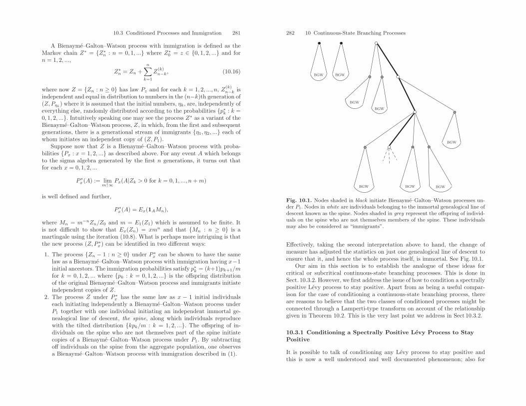
10.3 Conditioned Processes and Immigration 281
A Bienayme–Galton–Watson process with immigration is defined as theMarkov chain Z∗ = Z∗n : n = 0, 1, ... where Z∗0 = z ∈ 0, 1, 2, ... and forn = 1, 2, ...,
Z∗n = Zn +n∑k=1
Z(k)n−k, (10.16)
where now Z = Zn : n ≥ 0 has law Pz and for each k = 1, 2, ..., n, Z(k)n−k is
independent and equal in distribution to numbers in the (n−k)th generation of(Z,Pηk
) where it is assumed that the initial numbers, ηk, are, independently ofeverything else, randomly distributed according to the probabilities p∗k : k =0, 1, 2, .... Intuitively speaking one may see the process Z∗ as a variant of theBienayme–Galton–Watson process, Z, in which, from the first and subsequentgenerations, there is a generational stream of immigrants η1, η2, ... each ofwhom initiates an independent copy of (Z,P1).
Suppose now that Z is a Bienayme–Galton–Watson process with proba-bilities Px : x = 1, 2, ... as described above. For any event A which belongsto the sigma algebra generated by the first n generations, it turns out thatfor each x = 0, 1, 2, ...
P ∗x (A) := lim
m↑∞Px(A|Zk > 0 for k = 0, 1, ..., n+m)
is well defined and further,
P ∗x (A) = Ex(1AMn),
where Mn = m−nZn/Z0 and m = E1(Z1) which is assumed to be finite. Itis not difficult to show that Ex(Zn) = xmn and that Mn : n ≥ 0 is amartingale using the iteration (10.8). What is perhaps more intriguing is thatthe new process (Z,P ∗
x ) can be identified in two different ways:
1. The process Zn − 1 : n ≥ 0 under P ∗x can be shown to have the same
law as a Bienayme–Galton–Watson process with immigration having x−1initial ancestors. The immigration probabilities satisfy p∗k = (k+1)pk+1/mfor k = 0, 1, 2, ... where pk : k = 0, 1, 2, ... is the offspring distributionof the original Bienayme–Galton–Watson process and immigrants initiateindependent copies of Z.
2. The process Z under P ∗x has the same law as x − 1 initial individuals
each initiating independently a Bienayme–Galton–Watson process underP1 together with one individual initiating an independent immortal ge-nealogical line of descent, the spine, along which individuals reproducewith the tilted distribution kpk/m : k = 1, 2, .... The offspring of in-dividuals on the spine who are not themselves part of the spine initiatecopies of a Bienayme–Galton–Watson process under P1. By subtractingoff individuals on the spine from the aggregate population, one observesa Bienayme–Galton–Watson process with immigration described in (1).
282 10 Continuous-State Branching Processes
BGW BGW
BGW
BGW
BGW BGW BGW
BGW
Fig. 10.1. Nodes shaded in black initiate Bienayme–Galton–Watson processes un-der P1. Nodes in white are individuals belonging to the immortal genealogical line ofdescent known as the spine. Nodes shaded in grey represent the offspring of individ-uals on the spine who are not themselves members of the spine. These individualsmay also be considered as “immigrants”.
Effectively, taking the second interpretation above to hand, the change ofmeasure has adjusted the statistics on just one genealogical line of descent toensure that it, and hence the whole process itself, is immortal. See Fig. 10.1.
Our aim in this section is to establish the analogue of these ideas forcritical or subcritical continuous-state branching processes. This is done inSect. 10.3.2. However, we first address the issue of how to condition a spectrallypositive Levy process to stay positive. Apart from as being a useful compar-ison for the case of conditioning a continuous-state branching process, thereare reasons to believe that the two classes of conditioned processes might beconnected through a Lamperti-type transform on account of the relationshipgiven in Theorem 10.2. This is the very last point we address in Sect 10.3.2.
10.3.1 Conditioning a Spectrally Positive Levy Process to StayPositive
It is possible to talk of conditioning any Levy process to stay positive andthis is now a well understood and well documented phenomenon; also for
10.3 Conditioned Processes and Immigration 283
the case of random walks. See Bertoin (1993), Bertoin and Doney (1994b),Chaumont (1994, 1996), Konstantopoulos and Richardson (2002), Duquesne(2003) and Chaumont and Doney (2005) to name but some of the most recentadditions to the literature; see also Lambert (2000) who considers conditioninga spectrally negative Levy process to stay in a strip. We restrict our attentionto the case of spectrally positive Levy processes; in part because this is whatis required for the forthcoming discussion and in part because this facilitatesthe mathematics.
Suppose that X = Xt : t ≥ 0 is a spectrally positive Levy process withψ(λ) = log E(e−λX1) for all λ ≥ 0. (So as before, ψ is the Laplace exponentof the spectrally negative process −X). First recall from Theorem 3.12 thatfor all x > 0,
Ex(e−qτ−0 1(τ−0 <∞)) = e−Φ(q)x, (10.17)
where, as usual, τ−0 = inft > 0 : Xt < 0 and Φ is the right inverse of ψ. Inparticular when ψ′(0+) < 0, so that limt↑∞Xt = ∞, we have that Φ(0) > 0and P(τ−0 = ∞) = 1 − e−Φ(0)x. In that case, for any A ∈ Ft, we may simplyapply Bayes’ formula and the Markov property, respectively, to deduce thatfor all x > 0,
P↑x(A) := Px(A|τ−0 = ∞)
=Ex(1(A,t<τ−0 )P(τ−0 = ∞|Ft)
)Px(τ−0 = ∞)
= Ex(1(A,t<τ−0 )
1− e−Φ(0)Xt
1− e−Φ(0)x
)thus giving sense to “conditioning X to stay positive”. If however ψ′(0+) ≥ 0,in other words, lim inft↑∞Xt = −∞, then the above calculation is not possibleas Φ(0) = 0 and it is less clear what it means to condition the process to staypositive. The sense in which this may be understood is given in Chaumont(1994).
Theorem 10.10. Suppose that eq is an exponentially distributed randomvariable with parameter q independent of X. Suppose that ψ′(0+) ≥ 0. For allx, t > 0 and A ∈ Ft,
P↑x(A) := limq↓0
Px(Λ, t < eq|τ−0 > eq)
exists and satisfies
P↑x(A) = Ex(1(A,t<τ−0 )
Xt
x).
284 10 Continuous-State Branching Processes
Proof. Again appealing to Bayes’ formula followed by the Markov propertyin conjunction with the lack of memory property and (10.17), we have
Ex(Λ, t < eq|τ−0 > eq) =Px(Λ, t < eq, τ−0 > eq)
Px(τ−0 > eq)
=Ex(1(Λ,t<eq∧τ−0 )E(τ−0 > eq|Ft))
Ex(1− e−qτ−0 )
= Ex(1(Λ,t<τ−0 )e
−qt 1− e−Φ(q)Xt
1− e−Φ(q)x
). (10.18)
Under the assumption ψ′(0+) ≥ 0, we know that Φ(0) = 0 and hence byl’Hopital’s rule
limq↓0
1− e−Φ(q)Xt
1− e−Φ(q)x=
Xt
x. (10.19)
Noting also that for all q sufficiently small,
1− e−Φ(q)Xt
1− e−Φ(q)x≤ Φ(q)Xt
1− e−Φ(q)x≤ C
Xt
x,
where C > 1 is a constant. The condition ψ′(0+) ≥ 0 also implies that for allt > 0, E(|Xt|) < ∞ (see Sect. 8.1) and hence by dominated convergence wemay take limits in (10.18) as q ↓ 0 and apply (10.19) to deduce the result.
It is interesting to note that, whilst P↑x is a probability measure for eachx > 0, when ψ′(0+) < 0, this is not necessarily the case when ψ′(0+) ≥ 0.The following lemma gives a precise account.
Lemma 10.11. Fix x > 0. When ψ′(0+) = 0, P↑x is a probability measureand when ψ′(0+) > 0, P↑x is a sub-probability measure.
Proof. All that is required to be shown is that for each t > 0, Ex(1(t<τ−0 )Xt) =x for P↑x to be a probability measure and Ex(1(t<τ−0 )Xt) < x for a sub-probability measure. To this end, recall from the proof of Theorem 10.10that
Ex(1(t<τ−0 )
Xt
x) = lim
q↓0Px( t < eq|τ−0 > eq)
= 1− limq↓0
Px(eq ≤ t|τ−0 > eq)
= 1− limq↓0
∫ t
0
qe−qu
1− e−Φ(q)xPx(τ−0 > u)du
= 1− limq↓0
q
Φ(q)x
∫ t
0
e−quPx(τ−0 > u)du
= 1− limq↓0
ψ′(0+)x
∫ t
0
e−quPx(τ−0 > u)du.
10.3 Conditioned Processes and Immigration 285
It is now clear that when ψ′(0+) = 0 the right-hand side above is equal tounity and otherwise is strictly less than unity thus distinguishing the case ofa probability measure from a sub-probability measure.
Note that when Ex(1(t<τ−0 )Xt) = x, an easy application of the Markovproperty implies that 1(t<τ−0 )Xt/x : t ≥ 0 is a unit mean Px-martingaleso that P↑x is obtained by a martingale change of measure. Similarly whenEx(1(t<τ−0 )Xt) ≤ x, the latter process is a supermartingale.
On a final note, the reader may be curious as to how one characterisesspectrally positive Levy processes, and indeed a general Levy process, to staypositive when the initial value x = 0. In general, this is a non-trivial issue,but possible by considering the weak limit of the measure P↑x as measure onthe space of paths that are right continuous with left limits. The interestedreader should consult Chaumont and Doney (2005) for the most recent andup to date account.
10.3.2 Conditioning a (sub)Critical Continuous-State BranchingProcess to Stay Positive
Let us now progress to conditioning of continuous-state branching processesto stay positive, following closely Chap. 3 of Lambert (2001). We continue toadopt the notation of Sect. 10.1. Our interest is restricted to the case thatthere is extinction with probability one for all initial values x > 0. Accordingto Corollary 10.6 this corresponds to ψ(∞) = ∞, ψ′(0+) ≥ 0 and∫ ∞ 1
ψ(ξ)dξ <∞
and henceforth we assume that these conditions are in force. For notationalconvenience we also set
ρ = ψ′(0+).
Theorem 10.12. Suppose that Y = Yt : t ≥ 0 is a continuous-state branch-ing process with branching mechanism ψ satisfying the above conditions. Foreach event A ∈ σ(Ys : s ≤ t), and x > 0,
P ↑x (A) := lim
s↑∞Px(A|ζ > t+ s)
is well defined as a probability measure and satisfies
P ↑x (A) = Ex(1Aeρt
Ytx
).
In particular, P ↑x (ζ <∞) = 0 and eρtYt : t ≥ 0 is a martingale.
286 10 Continuous-State Branching Processes
Proof. From the proof of Theorem 10.5 we have seen that for x > 0,
Px(ζ ≤ t) = Px(Yt = 0) = e−xut(∞),
where ut(θ) satisfies (10.15). Crucial to the proof will be the convergence
lims↑∞
us(∞)ut+s(∞)
= eρt (10.20)
for each t > 0 and hence we first show that this result holds.To this end note from (10.15) that∫ us(∞)
ut+s(∞)
ρ
ψ(ξ)dξ = ρt.
On the other hand, recall from the proof of Theorem 10.5 that ut(θ) is de-creasing to Φ(0) = 0 as t ↓ 0. Hence, since limξ↓0 ψ(ξ)/ξ = ψ′(0+) = ρ, itfollows that
logus(∞)ut+s(∞)
=∫ us(∞)
ut+s(∞)
1ξdξ =
∫ us(∞)
ut+s(∞)
ψ(ξ)ξρ
ρ
ψ(ξ)dξ → ρt,
as s ↑ ∞ thus proving the claim.With (10.20) in hand we may now proceed to note that
lims↑∞
1− e−Ytus(∞)
1− e−xut+s(∞)=
Ytx
eρt.
In addition,1− e−Ytus(∞)
1− e−xut+s(∞)≤ Ytus(∞)
1− e−xut+s(∞)≤ C
Ytx
eρt
for some C > 1. Hence we may now apply the Markov property and then theDominated Convergence Theorem to deduce that
lims↑∞
Px(A|ζ > t+ s) = lims↑∞
Ex
(1(A,ζ>t)
PYt(ζ > s)
Px(ζ > t+ s)
)= lim
s↑∞Ex
(1(A,ζ>t)
1− e−Ytus(∞)
1− e−xut+s(∞)
)= lim
s↑∞Ex(1(A,ζ>t)
Ytx
eρt).
Note that we may remove the qualification t < ζ from the indicator on theright-hand side above as Yt = 0 on t ≥ ζ. To show that P ↑
x is a probabilitymeasure it suffices to show that for each x, t > 0, Ex(Yt) = e−ρtx. However,the latter was already proved in (10.12). A direct consequence of this is thatP ↑x (ζ > t) = 1 for all t ≥ 0 which implies that P ↑
x (ζ <∞) = 0.
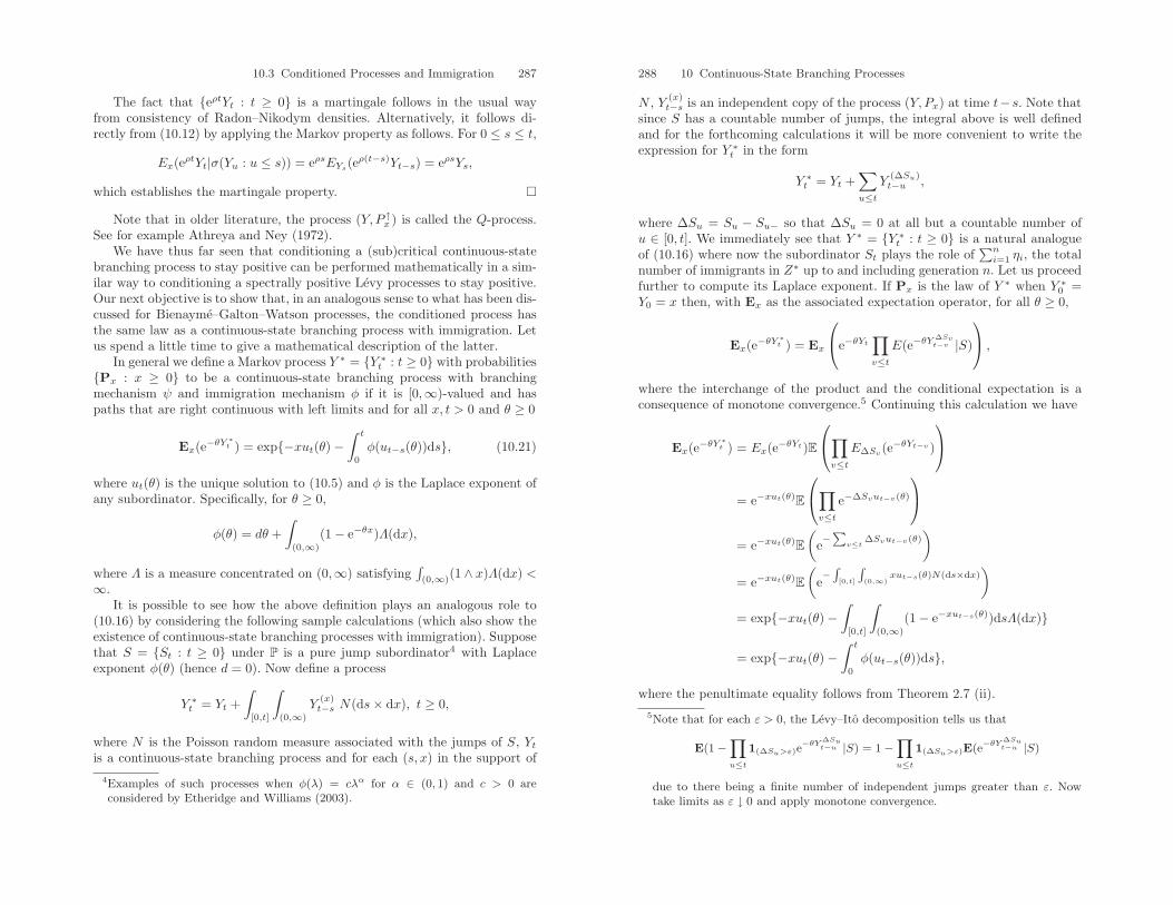
10.3 Conditioned Processes and Immigration 287
The fact that eρtYt : t ≥ 0 is a martingale follows in the usual wayfrom consistency of Radon–Nikodym densities. Alternatively, it follows di-rectly from (10.12) by applying the Markov property as follows. For 0 ≤ s ≤ t,
Ex(eρtYt|σ(Yu : u ≤ s)) = eρsEYs(eρ(t−s)Yt−s) = eρsYs,
which establishes the martingale property.
Note that in older literature, the process (Y, P ↑x ) is called the Q-process.
See for example Athreya and Ney (1972).We have thus far seen that conditioning a (sub)critical continuous-state
branching process to stay positive can be performed mathematically in a sim-ilar way to conditioning a spectrally positive Levy processes to stay positive.Our next objective is to show that, in an analogous sense to what has been dis-cussed for Bienayme–Galton–Watson processes, the conditioned process hasthe same law as a continuous-state branching process with immigration. Letus spend a little time to give a mathematical description of the latter.
In general we define a Markov process Y ∗ = Y ∗t : t ≥ 0 with probabilities
Px : x ≥ 0 to be a continuous-state branching process with branchingmechanism ψ and immigration mechanism φ if it is [0,∞)-valued and haspaths that are right continuous with left limits and for all x, t > 0 and θ ≥ 0
Ex(e−θY∗
t ) = exp−xut(θ)−∫ t
0
φ(ut−s(θ))ds, (10.21)
where ut(θ) is the unique solution to (10.5) and φ is the Laplace exponent ofany subordinator. Specifically, for θ ≥ 0,
φ(θ) = dθ +∫
(0,∞)
(1− e−θx)Λ(dx),
where Λ is a measure concentrated on (0,∞) satisfying∫(0,∞)
(1 ∧ x)Λ(dx) <∞.
It is possible to see how the above definition plays an analogous role to(10.16) by considering the following sample calculations (which also show theexistence of continuous-state branching processes with immigration). Supposethat S = St : t ≥ 0 under P is a pure jump subordinator4 with Laplaceexponent φ(θ) (hence d = 0). Now define a process
Y ∗t = Yt +
∫[0,t]
∫(0,∞)
Y(x)t−s N(ds× dx), t ≥ 0,
where N is the Poisson random measure associated with the jumps of S, Ytis a continuous-state branching process and for each (s, x) in the support of
4Examples of such processes when φ(λ) = cλα for α ∈ (0, 1) and c > 0 areconsidered by Etheridge and Williams (2003).
288 10 Continuous-State Branching Processes
N , Y (x)t−s is an independent copy of the process (Y, Px) at time t− s. Note that
since S has a countable number of jumps, the integral above is well definedand for the forthcoming calculations it will be more convenient to write theexpression for Y ∗
t in the form
Y ∗t = Yt +
∑u≤t
Y(∆Su)t−u ,
where ∆Su = Su − Su− so that ∆Su = 0 at all but a countable number ofu ∈ [0, t]. We immediately see that Y ∗ = Y ∗
t : t ≥ 0 is a natural analogueof (10.16) where now the subordinator St plays the role of
∑ni=1 ηi, the total
number of immigrants in Z∗ up to and including generation n. Let us proceedfurther to compute its Laplace exponent. If Px is the law of Y ∗ when Y ∗
0 =Y0 = x then, with Ex as the associated expectation operator, for all θ ≥ 0,
Ex(e−θY∗
t ) = Ex
⎛⎝e−θYt
∏v≤t
E(e−θY∆Sv
t−v |S)
⎞⎠ ,
where the interchange of the product and the conditional expectation is aconsequence of monotone convergence.5 Continuing this calculation we have
Ex(e−θY∗
t ) = Ex(e−θYt)E
⎛⎝∏v≤t
E∆Sv(e−θYt−v )
⎞⎠= e−xut(θ)E
⎛⎝∏v≤t
e−∆Svut−v(θ)
⎞⎠= e−xut(θ)E
(e−∑
v≤t∆Svut−v(θ)
)= e−xut(θ)E
(e−∫
[0,t]
∫(0,∞)
xut−s(θ)N(ds×dx))
= exp−xut(θ)−∫
[0,t]
∫(0,∞)
(1− e−xut−s(θ))dsΛ(dx)
= exp−xut(θ)−∫ t
0
φ(ut−s(θ))ds,
where the penultimate equality follows from Theorem 2.7 (ii).5Note that for each ε > 0, the Levy–Ito decomposition tells us that
E(1−∏u≤t
1(∆Su>ε)e−θY
∆Sut−u |S) = 1−
∏u≤t
1(∆Su>ε)E(e−θY
∆Sut−u |S)
due to there being a finite number of independent jumps greater than ε. Nowtake limits as ε ↓ 0 and apply monotone convergence.
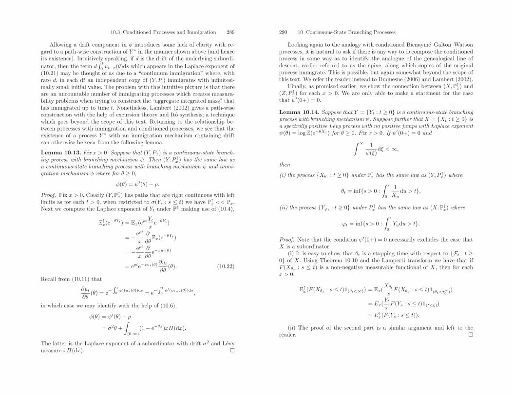
10.3 Conditioned Processes and Immigration 289
Allowing a drift component in φ introduces some lack of clarity with re-gard to a path-wise construction of Y ∗ in the manner shown above (and henceits existence). Intuitively speaking, if d is the drift of the underlying subordi-nator, then the term d
∫ t0ut−s(θ)ds which appears in the Laplace exponent of
(10.21) may be thought of as due to a “continuum immigration” where, withrate d, in each dt an independent copy of (Y, P·) immigrates with infinitesi-mally small initial value. The problem with this intuitive picture is that thereare an uncountable number of immigrating processes which creates measura-bility problems when trying to construct the “aggregate integrated mass” thathas immigrated up to time t. Nonetheless, Lambert (2002) gives a path-wiseconstruction with the help of excursion theory and Ito synthesis; a techniquewhich goes beyond the scope of this text. Returning to the relationship be-tween processes with immigration and conditioned processes, we see that theexistence of a process Y ∗ with an immigration mechanism containing driftcan otherwise be seen from the following lemma.
Lemma 10.13. Fix x > 0. Suppose that (Y, Px) is a continuous-state branch-ing process with branching mechanism ψ. Then (Y, P ↑
x ) has the same law asa continuous-state branching process with branching mechanism ψ and immi-gration mechanism φ where for θ ≥ 0,
φ(θ) = ψ′(θ)− ρ.
Proof. Fix x > 0. Clearly (Y,P↑x) has paths that are right continuous with leftlimits as for each t > 0, when restricted to σ(Ys : s ≤ t) we have P↑x << Px.Next we compute the Laplace exponent of Yt under P↑ making use of (10.4),
E↑x(e−θYt) = Ex(eρtYtx
e−θYt)
= −eρt
x
∂
∂θEx(e−θYt)
= −eρt
x
∂
∂θe−xut(θ)
= eρte−xut(θ)∂ut∂θ
(θ). (10.22)
Recall from (10.11) that
∂ut∂θ
(θ) = e−∫ t
0ψ′(us(θ))ds = e−
∫ t
0ψ′(ut−s(θ))ds
,
in which case we may identify with the help of (10.6),
φ(θ) = ψ′(θ)− ρ
= σ2θ +∫
(0,∞)
(1− e−θx)xΠ(dx).
The latter is the Laplace exponent of a subordinator with drift σ2 and Levymeasure xΠ(dx).
290 10 Continuous-State Branching Processes
Looking again to the analogy with conditioned Bienayme–Galton–Watsonprocesses, it is natural to ask if there is any way to decompose the conditionedprocess in some way as to identify the analogue of the genealogical line ofdescent, earlier referred to as the spine, along which copies of the originalprocess immigrate. This is possible, but again somewhat beyond the scope ofthis text. We refer the reader instead to Duquesne (2006) and Lambert (2002).
Finally, as promised earlier, we show the connection between (X,P↑x) and(Z,P ↑
x ) for each x > 0. We are only able to make a statement for the casethat ψ′(0+) = 0.
Lemma 10.14. Suppose that Y = Yt : t ≥ 0 is a continuous-state branchingprocess with branching mechanism ψ. Suppose further that X = Xt : t ≥ 0 isa spectrally positive Levy process with no positive jumps with Laplace exponentψ(θ) = log E(e−θX1) for θ ≥ 0. Fix x > 0. If ψ′(0+) = 0 and∫ ∞ 1
ψ(ξ)dξ <∞,
then
(i) the process Xθt: t ≥ 0 under P↑x has the same law as (Y, P ↑
x ) where
θt = infs > 0 :∫ s
0
1Xu
du > t,
(ii) the process Yϕt: t ≥ 0 under P ↑
x has the same law as (X,P↑x) where
ϕt = infs > 0 :∫ s
0
Yudu > t.
Proof. Note that the condition ψ′(0+) = 0 necessarily excludes the case thatX is a subordinator.
(i) It is easy to show that θt is a stopping time with respect to Ft : t ≥0 of X. Using Theorem 10.10 and the Lamperti transform we have that ifF (Xθs
: s ≤ t) is a non-negative measurable functional of X, then for eachx > 0,
E↑x(F (Xθs: s ≤ t)1(θt<∞)) = Ex(
Xθt
xF (Xθs
: s ≤ t)1(θt<τ−0 ))
= Ex(YtxF (Ys : s ≤ t)1(t<ζ))
= E↑x(F (Ys : s ≤ t)).
(ii) The proof of the second part is a similar argument and left to thereader.
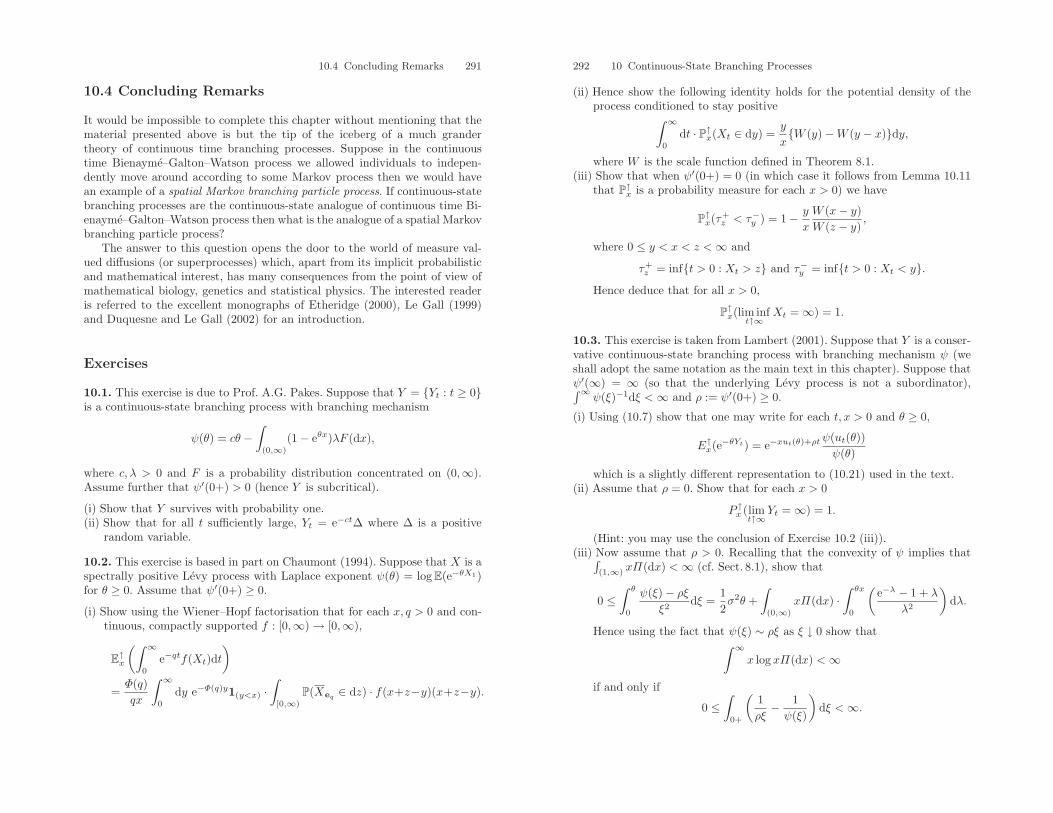
10.4 Concluding Remarks 291
10.4 Concluding Remarks
It would be impossible to complete this chapter without mentioning that thematerial presented above is but the tip of the iceberg of a much grandertheory of continuous time branching processes. Suppose in the continuoustime Bienayme–Galton–Watson process we allowed individuals to indepen-dently move around according to some Markov process then we would havean example of a spatial Markov branching particle process. If continuous-statebranching processes are the continuous-state analogue of continuous time Bi-enayme–Galton–Watson process then what is the analogue of a spatial Markovbranching particle process?
The answer to this question opens the door to the world of measure val-ued diffusions (or superprocesses) which, apart from its implicit probabilisticand mathematical interest, has many consequences from the point of view ofmathematical biology, genetics and statistical physics. The interested readeris referred to the excellent monographs of Etheridge (2000), Le Gall (1999)and Duquesne and Le Gall (2002) for an introduction.
Exercises
10.1. This exercise is due to Prof. A.G. Pakes. Suppose that Y = Yt : t ≥ 0is a continuous-state branching process with branching mechanism
ψ(θ) = cθ −∫
(0,∞)
(1− eθx)λF (dx),
where c, λ > 0 and F is a probability distribution concentrated on (0,∞).Assume further that ψ′(0+) > 0 (hence Y is subcritical).
(i) Show that Y survives with probability one.(ii) Show that for all t sufficiently large, Yt = e−ct∆ where ∆ is a positive
random variable.
10.2. This exercise is based in part on Chaumont (1994). Suppose that X is aspectrally positive Levy process with Laplace exponent ψ(θ) = log E(e−θX1)for θ ≥ 0. Assume that ψ′(0+) ≥ 0.
(i) Show using the Wiener–Hopf factorisation that for each x, q > 0 and con-tinuous, compactly supported f : [0,∞) → [0,∞),
E↑x(∫ ∞
0
e−qtf(Xt)dt)
=Φ(q)qx
∫ ∞
0
dy e−Φ(q)y1(y<x) ·∫
[0,∞)
P(Xeq∈ dz) · f(x+z−y)(x+z−y).
292 10 Continuous-State Branching Processes
(ii) Hence show the following identity holds for the potential density of theprocess conditioned to stay positive∫ ∞
0
dt · P↑x(Xt ∈ dy) =y
xW (y)−W (y − x)dy,
where W is the scale function defined in Theorem 8.1.(iii) Show that when ψ′(0+) = 0 (in which case it follows from Lemma 10.11
that P↑x is a probability measure for each x > 0) we have
P↑x(τ+z < τ−y ) = 1− y
x
W (x− y)W (z − y)
,
where 0 ≤ y < x < z <∞ and
τ+z = inft > 0 : Xt > z and τ−y = inft > 0 : Xt < y.
Hence deduce that for all x > 0,
P↑x(lim inft↑∞
Xt = ∞) = 1.
10.3. This exercise is taken from Lambert (2001). Suppose that Y is a conser-vative continuous-state branching process with branching mechanism ψ (weshall adopt the same notation as the main text in this chapter). Suppose thatψ′(∞) = ∞ (so that the underlying Levy process is not a subordinator),∫∞
ψ(ξ)−1dξ <∞ and ρ := ψ′(0+) ≥ 0.
(i) Using (10.7) show that one may write for each t, x > 0 and θ ≥ 0,
E↑x(e
−θYt) = e−xut(θ)+ρtψ(ut(θ))ψ(θ)
which is a slightly different representation to (10.21) used in the text.(ii) Assume that ρ = 0. Show that for each x > 0
P ↑x (limt↑∞
Yt = ∞) = 1.
(Hint: you may use the conclusion of Exercise 10.2 (iii)).(iii) Now assume that ρ > 0. Recalling that the convexity of ψ implies that∫
(1,∞)xΠ(dx) <∞ (cf. Sect. 8.1), show that
0 ≤∫ θ
0
ψ(ξ)− ρξ
ξ2dξ =
12σ2θ +
∫(0,∞)
xΠ(dx) ·∫ θx
0
(e−λ − 1 + λ
λ2
)dλ.
Hence using the fact that ψ(ξ) ∼ ρξ as ξ ↓ 0 show that∫ ∞x log xΠ(dx) <∞
if and only if
0 ≤∫
0+
(1ρξ
− 1ψ(ξ)
)dξ <∞.
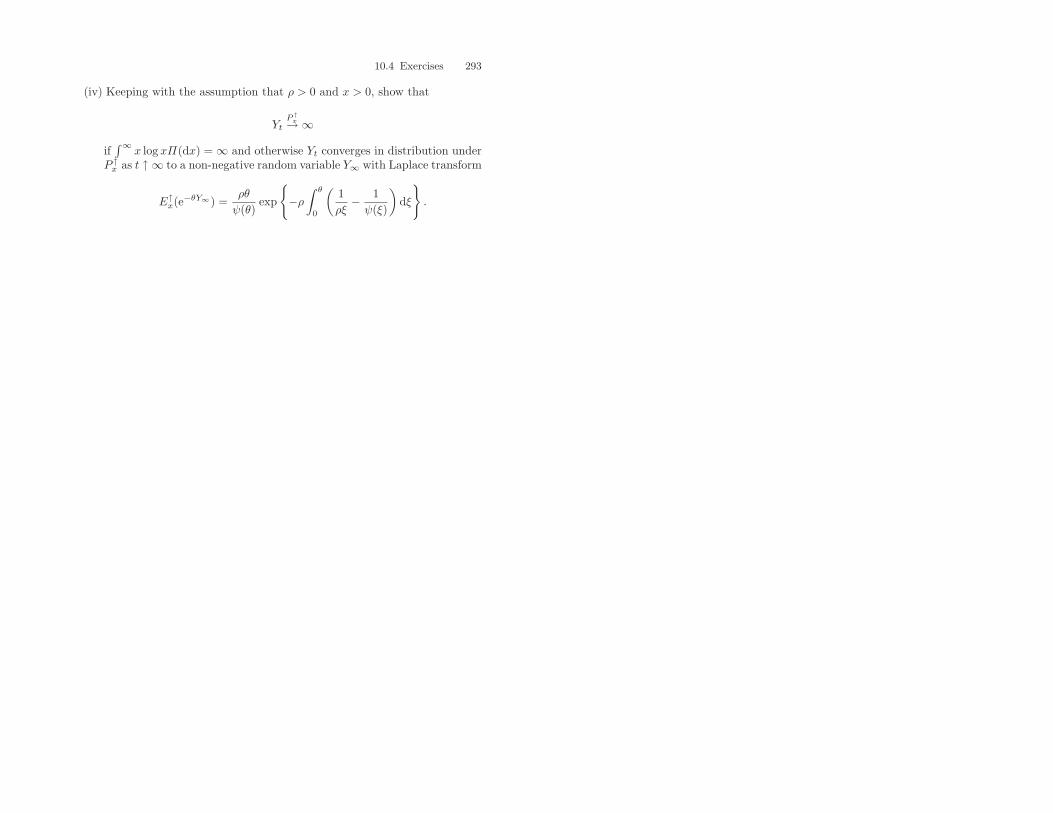
10.4 Exercises 293
(iv) Keeping with the assumption that ρ > 0 and x > 0, show that
YtP↑x→∞
if∫∞
x log xΠ(dx) = ∞ and otherwise Yt converges in distribution underP ↑x as t ↑ ∞ to a non-negative random variable Y∞ with Laplace transform
E↑x(e
−θY∞) =ρθ
ψ(θ)exp
−ρ∫ θ
0
(1ρξ
− 1ψ(ξ)
)dξ
.
Epilogue
The applications featured in this book have been chosen specifically becausethey exemplify, utilise and have stimulated many different aspects of the math-ematical subtleties which together are commonly referred to as the fluctuationtheory of Levy processes. There are of course many other applications of Levyprocesses which we have not touched upon. The literature in this respect isvast.
None the less, let us mention a few topics with a few key references for theinterested reader. The list is by no means exhaustive but merely a selectionof current research activities at the time of writing.
Stable and stable-like processes. Stable processes and variants thereof area core class of Levy processes which offer the luxury of a higher degree ofmathematical tractability in a wide variety of problems. This is in part due totheir inherent scaling properties. Samorodnitsky and Taqqu (1994) providesan excellent starting point for further reading.
Stochastic control. The step from optimal stopping problems driven bydiffusions to optimal stopping problems driven by processes with jumps comeshand in hand with the movement to stochastic control problems driven byjump processes. Recent progress is summarised in Øksendal and Sulem (2004).
Financial mathematics. In Sect. 2.7.3 we made some brief remarks concern-ing how properties of Levy processes may be used to one’s advantage whilemodelling risky assets. This picture is far from complete as, at the very least,we have made no reference to the more substantial and effective stochasticvolatility models. The use of such models increases the mathematical demandson subtle financial issues such as hedging, completeness, exact analytic pricing,measures of risk and so on. Whilst solving some problems in mathematicalfinance, the use of Levy processes also creates many problems. The degreeof complexity of the latter now supports a large and vibrant community of
296 Epilogue
researchers engaged in many new and interesting forms of mathematical the-ories. The reader is again referred to Boyarchenko and Levendorskii (2002a),Schoutens (2003), Cont and Tankov (2004) and Barndorff–Nielsen and Shep-hard (2005). See also Kyprianou et al. (2005).
Regenerative sets and combinatorics. By sampling points independentlyfrom an exponential distribution and grouping them in a way that is deter-mined by a pre-specified regenerative set on [0,∞), such as is given by therange of a subordinator, one may describe certain combinatorial samplingformulae. See Chap. 9 of Kingman (1993) or Gnedin and Pitman (2005).
Stochastic differential equations driven by Levy processes. There is a wellestablished theory for existence, uniqueness and characterisation of the so-lution to stochastic differential equations driven by Brownian motion whichcrop up in countless scenarios within the physical and engineering sciences(cf. Øksendal (2003)). It is natural to consider analogues of these equationswhere now the driving source of randomness is a Levy process. Applebaum(2004) offers a recent treatment.
Continuous-time time series models. Levy processes are the continuous-time analogue of random walks. What then are the continuous time analoguesof time series models, particularly those that are popular in mathematicalfinance such as GARCH processes? The answer to this question has beenaddressed in very recent literature such as Kluppelberg et al. (2004, 2006)and Brockwell et al. (2005). Levy processes play an important role here.
Levy Copulas. The method of using copulas to build in certain paramet-ric dependencies in multivariate distributions from their marginals is a wellestablished theory. See for example the up-to-date account in Nelson (2006).Inspired by this methodology, a limited volume of recent literature has pro-posed to address the modelling of multi-dimensional Levy processes by work-ing with copulas on the Levy measure. The foundational ideas are to be foundin Tankov (2003) and Kallsen and Tankov (2004).
Levy-type processes and pseudodifferential operators. Jacob (2001, 2002,2005) summarises the analysis of Markov processes through certain pseudodif-ferential operators. The latter are intimately related to the infinitesimal gen-erator of the underlying process via complex analysis.
Fractional Levy processes. The concept of fractional Brownian motion alsohas its counterpart for Levy processes; see Samorodnitsky and Taqqu (1994).Interestingly, whilst fractional Brownian motion has at least two consistentdefinitions in the form of stochastic integrals with respect to Brownian motion
Epilogue 297
(the harmonisable representation and the moving-average representation), theanalogues of these two definitions for fractional Levy processes throw outsubtle differences. See for example Benassi, Cohen and Istas (2002, 2004).
Quantum Independent Increment Processes. Levy processes have also beenintroduced in quantum probability, where they can be thought of as an ab-straction of a “noise” perturbing a quantum system. The first examples arosein models of quantum systems coupled to a heat bath and in von Walden-fels’ investigations of light emission and absorption. The algebraic structureunderlying the notions of increment and independence in this setting was de-veloped by Accardi, Schurmann and von Waldenfels. For an introduction tothe subject and a description of the latest research in this area, see Applebaumet al. (2005) and Barndorff-Nielsen et al. (2006).
Levy networks. These systems can be thought of multi-dimensional Levyprocesses reflected on the boundary of the positive orthant of Rd which ap-pear as limiting models of communication networks with traffic process ofunconventional (i.e., long-range dependent) type. See, for example, Harrisonand Williams (1987), Kella (1993) and Konstantopoulos et al. (2004). Thejustification of these as limits can be found, for example, in Konstantopou-los and Lin (1998) and Mikosch et al. (2002). Although Brownian stochasticnetworks have, in some cases, stationary distributions which can be simplydescribed, this is not the case with more general Levy networks. The area ofmultidimensional Levy processes is a challenging field of research.
Fragmentation theory. The theory of fragmentation has recently undergonea surge of interest thanks to its close relation to other probability modelswhich have also enjoyed an equal amount of attention. Closely related toclassical spatial branching processes, a core class of fragmentation processesmodel the way in which an object of unit total mass fragments in continuoustime so that at any moment there are always a countably infinite numberof pieces and further, up to an infinite number of fragmentations may occurover any finite time horizon. In a way that is familiar to Levy processes,the construction of fragmentation processes is done with the help of Poissonpoint processes. In addition there are many embedded probabilistic structureswhich are closely related to special classes of Levy processes. We refer to theforthcoming monograph of Bertoin (2006) for an indication of the state of theart.
Solutions
Chapter 1
1.1 For each i = 1, . . . , n let X(i) = X(i)t : t ≥ 0 be independent Levy processes
and define the process X = Xt : t ≥ 0 by
Xt =
n∑i=1
X(i)t .
Note that the first two conditions in Definition 1.1 are automatically satisfied. For0 ≤ s ≤ t < ∞ it is clear that Xt − Xs is independent of X(i)
u : u ≤ s foreach i = 1, . . . , n and hence is independent of Xu : u ≤ s. Finally Xt − Xs =∑n
i=1X
(i)t −X
(i)s
d=∑n
i=1X
(i)t−s
d= Xt−s.
1.2 (i) Recall the negative Binomial distribution with parameter c ∈ 1, 2, .... andp ∈ (0, 1) is considered to be the distribution one obtains by summing c independentgeometric distributions. Let q = 1 − p. An easy calculation shows that E(eiθΓp) =p/(1− qeiθ) for θ ∈ R and hence if Λc,p is a negative Binomial with parameters c, pas above, then E(eiθΛc,p) = pc/(1− qeiθ)c and the probabilities of Λx,p are given by
P(Λc,p = k) =
(−c
k
)pc(−q)k = (k!)−1(−c)(−c− 1)...(−c− k + 1)pc(−q)k,
where k runs through the non-negative integers. One may easily confirm that therestriction on c can be relaxed to c > 0 in the given analytical description of thenegative Binomial distribution. It is now clear that Γp is infinitely divisible since
E(eiθΓp) = E(eiθΛ1/n,p)n =
(p
1− qeiθ
).
(ii) This follows by showing that E(expiθSΓp) = E(expiθSΛ1/n,p)n which is
a straightforward exercise.
300 Solutions
1.3 (i) Using Fubini’s theorem we have for ∞ > b > a > 0,∫ ∞
0
f(ax)− f(bx)
xdx = −
∫ ∞
0
∫ b
a
f ′(yx)dydx
= −∫ b
a
1
y(f(∞)− f(0))dy
= (f(0)− f(∞)) log(b/a).
(ii) Choosing f(x) = e−x, a = α > 0, and b = α− z, where z < 0,∫ ∞
0
(1− ezx)β
xe−αxdx = log
((1− z/α)β
)(S.1)
from which the first claim follows.One should use the convention that 1/(1−z/α)β = exp−β log(1−z/α) where
an appropriate branch of the logarithm function is taken thus showing that theright-hand side of (S.1) is analytic. Further, to show that
∫∞0
(1 − ezx)βxe−αxdx is
analytic on ℜz < 0, one may estimate∣∣∣∣∫ ∞
0
(1− ezx)β
xe−αxdx
∣∣∣∣ ≤ 2β
∫ ∞
1
e−αxdx + β
∫ 1
0
∑k≥1
|z|kk!
xk−1e−αxdx
from which one may easily show with the help of Fubini’s Theorem that the left-hand side is finite. The fact that
∫∞0
(1− ezx)βxe−αxdx is analytic now follows again
from an expansion of ezx together with Fubini’s Theorem; specifically∫ ∞
0
(1− ezx)β
xe−αxdx = β
∑k≥1
(−z)k
k!
∫ ∞
0
xk−1e−αxdx.
The Identity Theorem tells us that if two functions are analytic on the same domainand they agree on a set which has a limit point in that domain then the two functionsare identical. Since both sides of (S.1) are analytic on w ∈ C : ℜw < 0 and agreeon real z < 0, there is equality on w ∈ C : ℜw < 0. Equality on ℜw = 0 followssince the limit as ℜw ↑ 0 exists on the left-hand side of (S.1) and hence the limit onthe right-hand side exists and both limits are equal.
1.4 (i) Integration by parts shows that∫ ∞
0
(e−ur − 1)r−α−1dr = −u
α
∫ ∞
0
e−urr−αdr = − 1
αuαΓ (1− α), (S.2)
where the second equality follows from substitution t = ur in the integral appearingin the first equality. Now using the fact that Γ (1−α) = −αΓ (−α) the claim follows.Analytic extension may be performed in a similar manner to the calculations in thesolution to Exercise 1.3.
To establish (1.7) from (1.9) with α ∈ (0, 1) first choose σ = 0 and a = η −∫R x1(|x|<1)Π(dx), where Π is given by (1.9). Our task is to prove that∫
R(1− eiθx)Π(dx) = c|θ|α(1− iβ tan(πα/2)sgn θ).
Solutions 301
We have ∫R(1− eiθx)Π(dx)
= −c1Γ (−α)|θ|αe−iπαsgnθ/2 − c2Γ (−α)|θ|αeiπαsgnθ/2 (S.3)
= −Γ (−α) cos(πα/2)|θ|α×(c1 + c2 − ic1 tan(πα/2)sgnθ + ic2 tan(πα/2)sgnθ)
= −(c1 + c2)Γ (−α) cos(πα/2)(1− iβ tan(πα/2)sgnθ).
The required representation follows by replacing −Γ (−α) cos(πα/2)ci by anotherconstant (also called ci) for i = 1, 2 and then setting β = (c1 − c2)/(c1 + c2) andc = (c1 + c2).
(ii) The first part is a straightforward computation. Fourier inversion allows oneto write
1
2π
∫R
2(
1− cos θ
θ2
)eiθxdθ = 1− |x|.
Choosing x = 0 and using symmetry to note that∫
R(1 − cos θ)/θ2dθ = 2∫∞0
(1 −cos θ)/θ2dθ the second claim follows. Now note that∫ ∞
0
(1− eirz + irz1(r<1))1
r2dr
=
∫ ∞
0
(1− cos zr)1
r2− i
∫ 1/z
0
1
r2(sin zr − zr)dr
−i
∫ ∞
1/z
1
r2sin rzdr + i
∫ 1
1/z
1
r2zrdr
=π
2z − iz
(∫ 1
0
1
r2(sin r − r)dr +
∫ ∞
1
r−2 sin rdr − log z
)=
π
2z + iz log z − ikz
for an obvious choice of the constant k. The complex conjugate of this equality isthe identity ∫ ∞
0
(1− e−irz − irz1(r<1))1
r2dr =
π
2z − iz log z + ikz.
To obtain (1.8), let Π be given as in (1.9) and set α = 1, σ = 0, and a = η+(c1−c2)ikand note that for that∫
R(1− eixθ + ixθ1(|x|<1))Π(dx)
= c1
∫ ∞
0
(1− eirθ + irθ1(r<1))1
r2dr
+c2
∫ 0
−∞(1− eirθ + irθ1(r<1))
1
r2dr
= (c1 + c2)π
2|θ|+ sgnθ(c1 − c2)i|θ| log |θ|
302 Solutions
−sgnθ(c1 − c2)ik|θ|= c|θ|
(1 +
2
πβsgnθ log |θ|
)− (c1 − c2)ikθ,
where c = (c1 + c2)π/2 and β = (c1 − c2)/(c1 + c2).(iii) The suggested integration by parts is straightforward. Following similar
reasoning to the previous two parts of the question we can establish (1.7) for α ∈(1, 2) by taking σ = 0, a = η +
∫R x1|x|>1Π(dx), where Π is given by (1.9). Note
that one easily confirms that the last integral converges as α > 1. Further, note that∫R(1− eiθx + iθx)Π(dx)
= c1
∫ ∞
0
(1− eiθx + iθx)1
x1+αdx + c2
∫ ∞
0
(1− e−iθx − iθx)1
x1+αdx
= c1
∫ ∞
0
(1− eisgnθz + isgnθz)|θ|α 1
z1+αdz
+c2
∫ ∞
0
(1− e−isgnθz − isgnθz)|θ|α 1
z1+αdz
−c1Γ (−α)|θ|αe−iπαsgnθ/2 − c2Γ (−α)|θ|αeiπαsgnθ/2.
The right-hand side above is the same as (S.3) and the calculation thus proceeds inthe same way as it does there.
1.5 Let Mt = expiθXt + Ψ(θ)t. Clearly Mt : t ≥ 0 is adapted to the filtrationFt = σ(Xs : s ≤ t) and
E(|Mt|) ≤ eℜΨ(θ) = exp
∫R(1− cos θx)Π(dx)
≤ exp
c
∫R(1 ∧ x2)Π(dx)
for some sufficiently large c > 0. Stationary independent increments also impliesthat for 0 ≤ s ≤ t < ∞,
E(Mt|Fs) = MsE(eiθ(Xt−Xs)|Fs)e−Ψ(θ)(t−s) = MsE(eiθXt−s)eΨ(θ)(t−s) = Ms.
1.6 (i) Similar arguments to those given in the solution to Exercise 1.5 show thatexpλBt−λ2t/2 : t ≥ 0 is a martingale. We have from Doob’s Optimal StoppingTheorem that
1 = E(eλBt∧τs− 12 λ2(t∧τs)) = E(eλ(Bt∧τs+b(t∧τs))−( 1
2 λ2+bλ)(t∧τs)).
Since Bt∧τs +b(t∧τs) ≤ s for all t ≥ 0 and b > 0, which implies that limt↑∞ Bt = ∞and hence that τs < ∞, it follows with the help of the Dominated ConvergenceTheorem and the continuity of the paths of Brownian motion with drift that
1 = limt↑∞
E(eλBt∧τs− 12 λ2(t∧τs)) = E(eλs−( 1
2 λ2+bλ)τs)
as required. By setting q = λ2/2 + bλ we deduce that
E(e−qτs) = e−s(√
b2+2q−b).
Solutions 303
Both right-hand side and left-hand side can be shown to be analytical functions whenwe replace q by a− iθ for a > 0 and θ ∈ R and hence they agree on this parameterrange. Taking limits as a tends to zero confirms that both functions agree when wereplace q by iθ with θ as above.
(ii) When Π(dx) = (2πx3)−1/2e−xb2/2 on x > 0, using Exercise 1.4 (i)∫ ∞
0
(1− eiθx)Π(dx)
=
∫ ∞
0
1√2πx3
(1− eiθ−b2x/2)dx−∫ ∞
0
1√2πx3
(1− e−b2x/2)dx
= −Γ(− 1
2
)2π
(b2
2− iθ
)1/2
+Γ(− 1
2
)2π
(b2
2
)1/2
= (b2 − 2iθ)1/2 − b.
From the Levy–Khintchine formula we clearly require σ = 0 and the above calcula-tion indicates that a =
∫(0,1)
xΠ(dx).
(iii) With µs(dx) = s(2πx3)−1/2 expsb− (s2x−1 + b2x)/2dx,∫ ∞
0
e−λxµs(dx) = ebs−s√
b2+2λ
∫ ∞
0
s√2πx3
e− 1
2
(s√x−√
(b2+2λ)x)2
dx
= ebs−s√
b2+2λ
∫ ∞
0
√2λ + b2
2πue− 1
2
(s√u−√
(b2+2λ)u)2
du,
where the second equality follows from the substitution sx−1/2 = ((2λ + b2)u)1/2.Adding the last two integrals together and dividing by two gives∫ ∞
0
e−λxµs(dx) =1
2
∫ ∞
0
(s√
2πx3+
√2λ + b2
2πx
)e− 1
2 ( s√x−√
(b2+2λ)x)2
dx.
making the substitution η = sx−1/2 −√
(b2 + 2λ)x yields∫ ∞
0
e−λxµs(dx) = ebs−s√
b2+2λ
∫R
1√2π
e−12 η2
dη = ebs−s√
b2+2λ.
1.7 Note by definition τ = τs : s ≥ 0 is also the inverse of the process Bt : t ≥ 0,where Bt = sups≤t Bs. The latter is continuous and Bt > 0 for all t > 0 hence τsatisfies the first two conditions of Definition 1.1. The Strong Markov Property,the fact that Bτs = s and spatial homogeneity of Brownian motion implies thatBτs+t − s : t ≥ 0 is independent of Bu : u ≤ τs. Further, this implies that foreach q ≥ 0, τs+q − τs is equal in distribution to τq and independent of τu : u ≤ s.Similar analysis to the solution of Exercise 1.6 centred around an application ofDoob’s Optimal Stopping Theorem with the stopping time τs to the exponentialmartingale shows that
E(e−qτs) = e−√
2qs.
Note however from the first part of the solution to part (i) of Exercise 1.4 we seethat the above equality implies that τ is a stable process with index α = 1/2 whoseLevy measure is supported on (0,∞), in other words, β = 1.
304 Solutions
1.8 (i) Is self-explanatory.(ii) Let T0 = 0 and define recursively for n = 1, 2 . . ., Tn = infk > Tn−1 : Sk >
STn−1 and let Hn = STn if Tn < ∞. The indexes Tn are called the strong ascendingladder times and Hn are the ladder heights. It is straightforward to prove that Tn
are stopping times. Note that for each n ≥ 1, from the Strong Markov Property,Hn −Hn−1 has the same distribution as S
T+0
.
P (ST−0
∈ dx)
= P (S1 ∈ dx) +∑n≥1
P (S1 > 0, ..., Sn > 0, Sn+1 ∈ dx)
= P (S1 ∈ dx) +∑n≥1
∫(0,∞)
P (S1 > 0, ..., Sn > 0, Sn ∈ dy)µ(dx− y)
= P (S1 ∈ dx)
+
∫(0,∞)
∑n≥1
P (Sn ∈ dy, Sn > Sj for all j = 0, ..., n− 1)µ(dx− y).
The sum in the final equality sums over all indexes of the random walk whichcorrespond to a ladder time. Hence
P (ST−0
∈ dx) = P (S1 ∈ dx) +
∫(0,∞)
∑n≥1
P (Hn ∈ dy)µ(dx− y)
=
∫(0,∞)
V (dy)µ(dx− y),
where V is given in the question.(iii) Note that
µ(z,∞) = P (eβ > z + ξ1) = E(e−β(z+ξ)
)= e−βz
∫ ∞
0
e−βuF (du)
and
µ(−∞, z) = P (ξ ≥ eβ + z) = E(F (z + eβ)).
(iv) Recall that the net profit condition implies that limn↑∞ Sn = ∞ which inturn implies that P (T+
0 < ∞) = 1. The lack of memory condition together withthe fact that upward jumps in S are exponentially distributed implies that S
T+0
is exponentially distributed with parameter β (in particular the latter is a properdistribution because first passage above the origin is guaranteed with probabilityone). From this it follows that for each n = 1, 2, ...,
P (Hn ∈ dx) =1
(n− 1)!βnxn−1e−βxdx
(in other words a gamma distribution with parameters n and β). Returning to thedefinition of V , we see that V (dy) = δ0(dy) + βdy and hence
Solutions 305
P (−ST−0
> x)
= E
(F (eβ + x) +
∫ ∞
0
βF (eβ + x + y)dy
)= E
(F (eβ + x) +
∫ ∞
x
βF (eβ + z)dz
).
Continuing we have
P (−ST−0
> x)
= E
(F (eβ + x) +
∫ ∞
x+eβ
βF (z)dy
)
=
∫ ∞
0
du · βe−βuE
(F (u + x) +
∫ ∞
x+u
βF (z)dy
)=
∫ ∞
x
βe−β(u−x)F (u)du +
∫ ∞
x
βdz · F (z)
∫ z−x
0
βe−βudu
= β
∫ ∞
x
F (z)dz.
1.9 (i) The Laplace exponent may be computed directly using the Poisson distrib-ution of N1 in a similar manner to the calculations in Sect. 1.2.2. One may computedirectly the second derivative ψ′′(θ) = λ
∫(0,∞)
x2e−θxF (dx) > 0 showing that ψ is
strictly convex and in particular continuous on (0,∞). It is clear that ψ(0) = 0 bytaking limits as θ ↓ 0 on both sides of the equality E(eθX1) = eψ(θ) (note X1 ≤ 1).Further it is also clear that ψ(∞) = ∞ since eψ(θ) ≥ E(eθX1 ; X1 > 0). On accountof convexity, there is one root to the equation ψ(θ) = 0 (that is θ = 0) in [0,∞),when ψ′(0+) ≥ 0 and otherwise there are two distinct roots in [0,∞) (the smallestof these two being θ = 0).
(ii) The martingle properties follow from similar arguments to those given in thesolution to Exercise 1.5 (with the help of Doob’s Optimal Stopping Theorem). Inparticular, when sampling at the stopping time t ∧ τ+
x and taking limits as t tendsto infinity,
1 = E(eθ∗X
τ+x−ψ(θ∗)τ+
x1
(τ+x <∞)
) = eθ∗xP(τ+x < ∞) = eθ∗xP(X∞ > x).
Note this shows that X∞ is exponentially distributed with parameter θ∗. In the casethat θ∗ = 0 we interpret this to mean that P(X∞ = ∞) = 1.
(iii) Note thatWs = 0 = Xs = Xs and Xs > w.
Note also that on the latter event ds = dXs = dXs. Hence∫ t
0
1(Ws=0)ds =
∫ t
0
1(Xs=Xs,Xs>w)dXs =
∫ t
0
1(Xs>w)dXs = (Xt − w) ∨ 0.
(iv) A direct computation shows that ψ′(0+) = 1 − λµ. Hence if λµ ≤ 1 thenθ∗ = 0 and X∞ = ∞ almost surely and hence from the previous part, I = ∞ almostsurely.
306 Solutions
(v) When λµ > 1 we have that P(τ+w = ∞) = P(X∞ ≤ w) = 1 − e−θ∗w. Since
I = 0 on τ+w = ∞, it follows that
P(I ∈ dx, τ+w = ∞|W0 = w) = (1− e−θ∗w)δ0(dx).
On the other hand, on the event τ+w < ∞, since τ+
w is a stopping time, and X∞is exponentially distributed, the Strong Markov Property and the Lack of MemoryProperty imply that
P(I ∈ dx, τ+w < ∞|W0 = w) = P
(X∞ − w ∈ dx, X∞ > w|W0 = w
)= θ∗e−θ∗(x+w)dx.
1.10 (i) This is a straightforward exercise in view of Exercise 1.5.(ii) Using Doob’s Optimal Stopping Theorem we have for the bounded stopping
time t ∧ τ+x that
E(eθX
t∧τ+x−(σ2θ2/2+γθ)(t∧τ+
x )) = 1.
Setting θ = (√
γ2 + 2σ2q − γ)/σ2 and letting t ↑ ∞, it follows from the fact thatX
t∧τ+x≤ x for all t ≥ 0 and Dominated Convergence that,
E(e−τ+x ) = e−x(
√γ2+2σ2q−γ)/σ2
.
Now note that by considering the process −X, we may simply write down an
expression for E(e−qτ−−a) by considering the expression above for E(e−qτ+
a ) but withγ replaced by −γ.
(iii) This is a straightforward exercise.
1.11 (i) From the branching property one easily deduces that, Yt under Py is equal
in law to the independent sum∑y
i=1Y
(i)t , where Y
(i)t has the same distribution as
Yt under P1. From this it follows immediately that Ey(e−φYt) = e−yut(φ), whereut(φ) = − log E1(e
−φYt). Note in particular that since at least one of the y individ-uals initiating the branching process may survive until time t with probability e−λt,it follows that ut(φ) ≥ e−φy+λt > 0.
(ii) Applying the Markov property we have for all y = 1, 2, ..., φ > 0 and t, s ≥ 0,
Ey(e−φYt+s) = Ey(EYs(e−φYt)) = Ey(e−ut(φ)Ys)
and hence ut+s(φ) = us(ut(φ)).(iii) Under the assumption π0 = 0, we have as h ↓ 0,
P1(Yh = 1 + i) = λπih + o(h) for i = −1, 1, 2, ...
From this it follows that
limh↓0
E1(e−φYh)− e−φ
h=
∑i=−1,1,2,...
e−φ(i+1)λπi − e−φ = −e−φψ(φ).
Hence reconsidering the left-hand side above, it follows that
∂ut(φ)
∂t
∣∣∣∣t=0
= ψ(φ).
Now use part (ii) and write
∂ut(φ)
∂t= lim
h↓0uh(ut(φ))− ut(φ)
h= ψ(ut(φ)).
Solutions 307
Chapter 2
2.1 We prove (i) and (ii) together. Similar calculations to those in 1.2.1 give
E(sθNi) = e−λi(1−s)
for 0 < s < 1. Independence and Dominated Convergence thus implies that
E(s
∑i≥1
Ni) = lim
n↑∞E(s
∑n
i=1Ni) = e
− limn↑∞∑n
i=1λi(1−s)
.
It now follows that E(s
∑i≥1
Ni) = 0 if and only if P (
∑i≥1
Ni = ∞) = 1 if
and only if∑n
i=1λi = ∞. Further, when
∑n
i=1λi < ∞ P(
∑i≥1
Ni < ∞) =
lims↑1 exp−∑∞i=1
λi(1− s) = 1.
2.2 (i) Suppose that Si : i = 1, 2, ..., n are independent and exponentially dis-tributed. The joint density of (S1, ...., Sn) is given by λne−λ(s1+···+sn) for s1 >0, ..., sn > 0. Using the classical density transform, the density of the partialsums (T1 = S1, T2 = S1 + S2, ..., Tn = S1 + · · · + Sn) is given by λne−λtn fort1 ≤ t2 ≤ · · · ≤ tn. If these partial sums are the arrival times of a Poisson process,then for A ∈ B([0,∞)n),
P ((T1, ..., Tn) ∈ A and Nt = n)
=
∫(t1,...,tn)∈A
1(t1≤t2≤···≤tn≤t)λne−λtndt1 · · · dtn. (S.4)
Dividing by P (Nt = n) = e−λt(λt)n/n! gives the conclusion of part (i)(ii) The right-hand side of (S.4) is the density of the distribution of an ordered
independent sample from a uniform distribution on [0, t] Specifically, n indepen-dent samples from the latter distribution has density 1/tn and there are n! ways ofordering them.
2.3 Note that on [0,∞), 1− e−φy ≤ 1 ∧ φy ≤ (1 ∨ φ)(1 ∧ y). Hence for all φ > 0,∫S
(1− e−φf(x))η(dx) ≤ (1 ∨ φ)
∫S
(1 ∧ f(x))η(dx)
and the claim is now obvious.
2.4 (i) Let us suppose that there exists a function f : [0, 1] → R such thatlimn↑∞ supx∈[0,1] |fn(x) − f(x)|, where fn : n = 1, 2, .... is a sequence in D[0, 1].To show right continuity note that for all x ∈ [0, 1) and ε ∈ (0, 1− x),
|f(x + ε)− f(x)| ≤ |f(x + ε)− fn(x + ε)|+|fn(x + ε)− fn(x)|+|fn(x)− f(x)|.
Each of the three terms on the right-hand side can be made arbitrarily small onaccount of the fact that fn ∈ D[0, 1] or by the convergence of fn to f by choosing εsufficiently small or n sufficiently large, respectively.
308 Solutions
For the existence of a left limit, note that it suffices to prove that for eachx ∈ (0, 1], f(x− ε) is a Cauchy sequence with respect to the distance metric | · | asε ↓ 0. To this end note that for x ∈ (0, 1] and ε, η ∈ (0, x),
|f(x− ε)− f(x− η)| ≤ |f(x− ε)− fn(x− ε)|+|fn(x− ε)− fn(x− η)|+|fn(x− η)− f(x− η)|.
Once again, each of the three terms on the right-hand side can be made arbitrarilysmall by choosing either n sufficiently large or η, ε sufficiently small.
(ii) Suppose that ∆c is a countable set for each c > 0, then since
∆ =⋃n≥1
∆1/n
it follows that ∆ is also a countable set.Suppose then for contradiction that, for a given c > 0, the set ∆c has an accu-
mulation point, say x. This means there exists a sequence yn → x such that for eachn ≥ 1, yn ∈ ∆c. From this sequence we may assume without loss of generality thatthere exists as subsequence xn ↑ x (otherwise if this fails the forthcoming argumentmay be performed for a subsequence xn ↓ x to the function g(x) = f(x−) whichis left continuous with right limits but has the same set of discontinuities). Nowsuppose that N is sufficiently large so that for a given δ > 0, |xm − xn| < δ for allm, n > N . We have
f(xn)− f(xm) = [f(xn)− f(xn−)] + [f(xn−)− f(xm)]
and so it cannot happen that |f(xn)−f(xm)| → 0 as n, m ↑ ∞ as |f(xn)−f(xn−)| >c and yet by left continuity at each xn we may make |f(xn−) − f(xm)| arbitrarilysmall. This means that f(xn) : n ≥ 1 is not a Cauchy sequence which is acontradiction as the limit f(x−) exists.
In conclusion, for each c > 0 there can be no accumulation points in ∆c andthus the latter is at most countable with the implication that ∆ is countable.
2.5 (i) The function f−1 jumps precisely when f is piece-wise constant and thisclearly happens on the dyadic rationals in [0, 1] (that is to say Q2 ∩ [0, 1]). This iseasily seen by simply reflecting the graph of f about the diagonal. This also showsthat jumps of f−1 and g are necessarily positive. Since the set Q ∩ [0, 1] is densein [0, 1] then so are the jumps of g. The function g has bounded variation since itis the difference of two monotone functions. Finally g is right continuous with leftlimits because the same is true of f−1 as an inverse function.
(ii) Note that for any y > 0, for each k = 1, 2, 3, ..., there are either aneven or odd number of jumps of magnitude 2−k in [0, y]. In the case that thereare an even number of jumps, they make net contribution of zero to the valuef(y) =
∑s∈[0,y]∩Q2
J(x). When there are an odd number of jumps they make a
net contribution of magnitude 2−k to f(y). Hence we can upper estimate |f(y)| by∑k≥1
2−k < ∞. Since f only changes value at dyadic rationals, it follows that f is
bounded [0, 1].
Solutions 309
Using similar reasoning to the above, by fixing x ∈ [0, 1] which is not a dyadicrational, one may show that for all integers n > 0, there exists a sufficiently largeinteger N > 0 such that |f(x)−f(y)| ≤∑
k≥N2−k whenever |x−y| < 2−n. Further,
N ↑ ∞ as n ↑ ∞. In other words, when there is no jump, there is a continuity pointin f .
If on the other hand, there is a jump at x ∈ [0, 1] (in other words, x is a dyadicrational), then a similar argument to the above shows that there is right continuity(consider in that case x < y < x+2−n). Further, the existence of a left limit can beestablished by showing in a similar way that |f(x)− J(x)− f(y)| ≤∑
k≥N2−k for
x− 2−n < y < x, where N ↑ ∞ as n ↑ ∞.To show that f has unbounded variation, note that the total variation over [0, 1]
is given by ∑s∈[0,1]∩Q2
|J(s)| = 1
2
∞∑n=1
2n · 2−n = ∞.
Right continuity and left limits, follows from the definition of f and the fact thatthere are a countable number of jumps.
2.6 (i) Apply Theorem 2.7 to the case that S = [0,∞)×R and the intensity measureis dt×Π(dx). According to the latter, by taking f(s, x) = xn we have that for eacht > 0,
∫[0,t]
∫R f(s, x)N(ds×dx) < ∞ if and only if
∫[0,t]
∫R(1∧|x|n)ds×Π(dx) < ∞;
in other words, if and only if∫
R(1∧ |x|n)Π(dx) < ∞. Note however that necessarily∫(−1,1)
x2Π(dx) < ∞ and this implies that∫(−1,1)
|x|nΠ(dx) < ∞. In conclusion, a
necessary and sufficient condition is∫|x|≥1
|x|nΠ(dx) < ∞.
(ii) The proof follows very closely the proof of Lemma 2.9.
2.7 (i) The probability that sup0≤s≤t |Xs − Xs−| is greater than a is one mi-nus the probability that there is no jump of magnitude a or greater. In otherwords 1 − P(N([0, t] × R\(−a, a)) = 0). The latter probability is equal toexp− ∫
[0,t]
∫R\(−a,a)
ds × Π(dx) = exp−tΠ(R\(−a, a)). (Note that this also
shows that Ta := inft > 0 : |Xt −Xt−| > a is exponentially distributed).(ii) The paths of X are continuous if and only if for all a > 0, P(sup0≤s≤t |Xs −
Xs−| > a) = 0 if and only if Π(R\(−a, a)) = 0 (from the previous part) if and onlyif Π = 0.
(iii) and (iv) Obviously a compound Poisson process with drift is piece-wise lin-ear. Clearly, if σ > 0 then paths cannot be piece-wise linear. Suppose now thatΠ(R) = ∞. In that case, lima↓0 P(Ta > t) = 0 showing that lima↓0 Ta = 0 almostsurely. Hence 0 is a limiting point of jump times. Stationary and independent in-crements and the latter imply that any s ∈ Q ∩ (0,∞) (or indeed any s > 0) is alimit point of jump times from the right. In conclusion, paths are piece-wise linearif and only if Π(R) < ∞ and σ = 0 and when Π(R) = ∞ then the jumps are densein [0,∞).
2.8 We have seen that any Levy process of bounded variation may be written inthe form
Xt = dt +
∫[0,t]
∫R
xN(ds× dx), t ≥ 0,
310 Solutions
where N is the Poisson random measure associated with the jumps. However, wemay also decompose the right-hand side so that
Xt =
(d ∨ 0) +
∫[0,t]
∫(0,∞)
xN(ds× dx)
−|d ∧ 0|+
∫[0,t]
∫(−∞,0)
|x|N(ds× dx)
.
Note that both integrals converge on account of Theorem 2.7 (i) as the assumptionthat X is of bounded variation implies that both
∫(0,∞)
(1∧x)Π(dx) and∫(−∞,0)
(1∧|x|)Π(dx) are finite. As N has independent counts on disjoint domains, it followsthat the two integrals on the right-hand side above are independent. The processesin curly brackets above clearly have monotone paths and hence the claim follows.
2.9 (i) The given process is a Levy process by Lemma 2.15. Also by the same Lemmaits characteristic exponent is computable as Ξ Λ, where Λ(θ) = σ2θ2/2 + cθ andΞ(θ) = β log(1 − iθ/α). Hence the given expression for Ψ follows with a minimalamount of algebra.
(ii) It is not clear apriori that the Variance Gamma process as defined in part (i)of the question is a process of bounded variation. However, one notes the factorisation(
1− iθc
α+
σ2θ2
2α
)=(1− iθ
α(1)
)×(1− iθ
α(2)
)and hence Ψ decomposes into the sum of terms of the form β log(1 − iθ/α(i)) fori = 1, 2. This shows that X has the same law as the difference of two independentgamma subordinators with the given parameters.
2.10 Increasing the dimension of the space on which the Poisson random measure ofjumps is defined has little effect to the given calculations for the one dimensional casepresented. Using almost identical proofs to the one dimensional case one may showthat
∫R(1− eiθ·x + iθ ·x1(|x|<1))Π(dx) is the characteristic exponent of a pure jump
Levy process consisting of a compound Poisson process whose jumps are greaterthan or equal to unity in magnitude plus an independent process of compensatedjumps of magnitude less than unity. Add to this a linear drift in the direction a andan independent d-dimensional Brownian motion and one recovers the characteristicexponent given in (2.28).
2.11 As a subordinator is non-negative valued, the Lapalce exponent Φ(q) existsfor all q ≥ 0. This means that the characteristic exponent Ψ(θ) = − log E(eiθX1),initially defined for θ ∈ R, can now be analytically extended to allow for the casethat ℑθ > 0. In that case, plugging θ = iq with q ≥ 0 into the Levy–Khinchineformula for subordinators (2.23), one obtains
Φ(q) = dq +
∫(0,∞)
(1− e−qx)Π(dx).
Suppose temporarily that we truncate the mass of Π within an ǫ-neighbourhoodof the origin and replace Π(dx) by Πǫ(dx) = 1(x>ǫ)Π(dx). In particular, by doingthis, note that Πǫ(0,∞) < ∞. Integration by parts yields
Solutions 311∫(a,A)
(1− e−qx)Πǫ(dx) = −(1− e−qA)Πǫ(A,∞) + (1− e−qa)Πǫ(a,∞)
+q
∫ A
a
e−qxΠǫ(x,∞)dx.
Note however the fact that Πǫ(0,∞) < ∞ implies both that (1−e−qA)Πǫ(A,∞) → 0as A ↑ ∞ and that (1− e−qa)Πǫ(a,∞) → 0 as a ↓ 0. We have then,∫
(ǫ,∞)
(1− e−qx)Πǫ(dx) =
∫(0,∞)
(1− e−qx)Πǫ(dx) = q
∫ ∞
0
e−qxΠǫ(x,∞)dx.
Now talking limits as ǫ ↓ 0 and appealing to the Monotone Convergence Theoremon the right-hand side above we finally conclude that
Φ(q) = dq + q
∫(0,∞)
e−qxΠ(x,∞)dx.
The final part of the question is now a simple application of the DominatedConvergence Theorem.
2.12 In all parts of this exercise, one ultimately appeals to Lemma 2.15.(i) Let B = Bt : t ≥ 0 be a standard Brownian motion and τ = τt : t ≥ 0
be an independent stable subordinator with index α/2, where α ∈ (0, 2). Then forθ ∈ R,
E(eiθBτt ) = E(e−12 θ2τt) = e−C|θ|α
showing that Bτt : t ≥ 0 has the law of a symmetric stable process of index α.
(ii) The subordinator τ has Laplace exponent
− log E(e−qτ1) =2
a
(q
q + a2
)for q ≥ 0; this computation follows with the help of (1.3). To see this, note that X1
has the same distribution as an independent Poisson sum of independent exponen-tially distributed random variables where the Poisson distribution has parameter2/a2 and the exponential distributions have parameter a2. Similarly to the first partof the question we have
− log E(eiθ√
2Bτ1 ) = − log E(e−θ2τ1) =2
a
(θ2
θ2 + a2
).
To show that the right-hand side is the characteristic exponent of the given com-pound Poisson process note that∫
(0,∞)
(1− eiθx)e−axdx =1
a− 1
a− iθ= −1
a
(iθ
a− iθ
)and hence
− log E(eiθX1) = −1
a
(iθ
a− iθ
)+
1
a
(iθ
a + iθ
)=
2
a
(θ2
θ2 + a2
).
(iii) We note that
E(eiθσBN1 ) = E(e−12 σ2θ2N1) = exp2λ(e−σ2θ2/2 − 1).
It is straightforward to show that the latter is equal to E(eiθX1) using (1.3).
312 Solutions
Chapter 3
3.1 (i) We handle the case that t2 > t > t1 ≥ 0, the remaining cases t ≥ t2 > t1 ≥ 0and t2 > t1 ≥ t ≥ 0 are handled similarly. Note that when t2 > u ≥ t > t1, usingExercise 1.5 we have
E(eiθ1Xt1+iθ2Xt2 |Fu) = eiθ1Xt1 E(eiθ2Xt2+Ψ(θ2)t2 |Fu)e−Ψ(θ2)t2
= eiθ1Xt1 eiθ2Xu+Ψ(θ2)ue−Ψ(θ2)t2 .
In particular, considering the right-hand side above for u = t and using right conti-nuity, the limit as u ↓ t satisfies the right expression. Note that this method can beused to prove the same statement when θ1Xt1 + θ2Xt2 is replaced by
∑n
i=1θiXti
for θi ∈ R and ti ≥ 0 for i = 1, ..., n.(ii) This is a consequence of standard measure theory (see for example Theo-
rem 4.6.3 of Durrett (2004)) and part (i).(iii) The conclusion of (ii) implies in particular that for all cylinder sets A =
Xt1 ∈ A1, ..., Xtn ∈ An with ti ≥ 0 and Ai ∈ B(R) for i = 1, ..., n,
P(A|Ft+) = P(A|Ft) (S.5)
almost surely where Ft+ =⋂
s>tFs. Using the fact that the above cylinder set
together with null sets of P generate members of the filtration F we deduce that(S.5) holds for any A ∈ Ft+. As the left-hand side of (S.5) in that case is also equalto 1A almost surely and F is completed by the null sets of P it follows that Ft+ ⊆ Ft.The inclusion Ft ⊆ Ft+ is obvious and hence the filtration F is right continuous.
3.2 It suffices to prove the result for the first process as the second process is thesame as the first process when one replaces X by −X. To this end, define for eachy ≥ 0, Y y
t = (y ∨Xt) −Xt and let Xu = Xt+u −Xt for any u ≥ 0. Note that fort, s ≥ 0,
(y ∨Xt+s)−Xt+s =
(y ∨Xt ∨ sup
u∈[t,t+s]
Xu
)−Xt − Xs
=
[(y ∨Xt −Xt) ∨
(sup
u∈[t,t+s]
Xu −Xt
)]− Xs
=
[Y y
t ∨ supu∈[0,s]
Xu
]− Xs.
From the right-hand side above, it is clear that the law of Y yt+s depends only on Y y
t
and Xu : u ∈ [0, s], the latter being independent of Ft. Hence Y yt : t ≥ 0 is a
Markov process.To upgrade to a strong Markov process, one uses a standard technique that
takes account of the right continuity of the paths of Y yt : t ≥ 0. This involves
approximating a given stopping time τ by a discretised version τ (n) ≥ τ defined in(3.2) and then proving with the help of the Markov property that for each H ∈ Fτ
and 0 ≤ t1 ≤ t2 ≤ · · · ≤ tn < ∞,
P
(H ∩
n⋂i=1
Y y
τ(n)+ti∈ Ai
)=
∫[0,∞)
P
(n⋂
i=1
Y zti∈ Ai
)p(y, H, dz),
Solutions 313
where p(y, H, dz) = P(H ∩ Y y
τ(n) ∈ dz). Then since τ (n) ↓ τ as n ↑ ∞ and Y y isright continuous, by taking limits as n ↑ ∞ the same equality above is valid whenτ (n) is replaced by τ thus exhibiting the Strong Markov Property.
3.3 The solution to this exercise is taken from Sect. 25 of Sato (1999).(i) To prove that g(x) ≤ agebg |x| for ag, bg > 0 use submultiplicativity to show
that for integer n chosen so that |x| ∈ (n− 1, n],
g(x) = g
(n∑
i=1
x/n
)≤ cn−1g(x/n)n.
Since g is bounded on compacts, we may define ag = maxc−1, sup|x|∈[0,1] g(x) ∈(0,∞) and further set bg = agc. We now have from the previous inequality that
g(x) ≤ ag(cag)n−1 ≤ ag(cag)|x| = agebg|x|.
Now suppose that E(g(Xt)) < ∞ for all t > 0. Decomposing as in the proof ofTheorem 3.6, submultiplicativity and independence in the Levy–Ito decompositionimply that
E(g(Xt)) =
∫R
∫R
g(x + y)dF2(y)dF1,3(x),
where F2 is the distribution of X(2)t and F1,3 is the distribution of X
(1)t + X
(3)t . The
last equality implies that for at least one x ∈ R,∫
R g(x + y)dF2(y) < ∞. Next note
from the submulitplicative property that g(y) ≤ cg(−x)g(x + y) ≤ cagebg|x|g(x + y)
and hence E(g(X(2)t )) ≤ cagebg|x| ∫
R g(x + y)dF2(y) < ∞. Recalling that X(2) isa compound Poisson process, a similar calculation to the one in (3.7) shows that∫|y|≥1
g(y)Π(dy) < ∞.
Now suppose that∫|y|≥1
g(y)Π(dy) < ∞. We can write
E(g(Xt)) ≤ cE(g(X(2)t ))E(g(X
(1)t + X
(3)t )).
Note however that since X(2) is a compound Poisson process then one may computeusing submultiplicativity
E(g(X(2)t )) =
∑k≥0
e−λt (λt)k
k!E
(g
(k∑
i=1
ξi
))
≤∑k≥0
e−λt ck−1tk
k!
(∫|x|>1
g(x)Π(dx)
)k
< ∞,
where ξi : i = 1, 2, ... are independent with common distribution given byΠ(R\(−1, 1))−1Π|R\(−1,1). Note also that
E(g(X(1)t + X
(3)t )) ≤ agE
(ebg|X(1)
t+X
(3)t
|)
and the right-hand side can be shown to be finite in a similar way to (3.8) in theproof of Theorem 3.6. In conclusion it follows that E(g(Xt)) < ∞.
314 Solutions
(ii) Suppose that h(x) is a positive increasing function on R such that for x ≤ bit is constant and for x > b, log h(x) is concave. Then writing f(x) = log h(x) itfollows for u, v ≥ b that
f(u + b)− f(u) ≤ f(2b)− f(b)
f(u + v)− f(v) ≤ f(u + b)− f(b)
and hencef(u + v) ≤ f(2b)− 2f(b) + f(u) + f(v).
This implies that h is submultiplicative. As h is an increasing function, it also followsthat
h(|x + y|) ≤ h(|x|+ |y|) ≤ ch(|x|)h(|y|),where c > 0 is a constant.
Note that the function x ∨ 1 fits the description of h and hence, together with|x| ∨ 1 is submultiplicative. The discussion preceding Theorem 3.8 shows then that(xα ∨ 1) and |x|α ∨ 1 are also submultiplicative. One may handle the remainingfunctions similarly.
(iii) Apply the conclusion of Theorem 3.8 to the Levy measure of a stable process.
3.4 First note that any Levy process, X, with no Gaussian component may alwaysbe written up to a linear drift as the difference to two spectrally positive processes.Indeed if X has characteristic exponent given in Theorem 1.6 then one may alwayswrite X = Xup −Xdown, where Xup and Xdown have characteristic exponents
Ψup(θ) = iaθ +
∫(0,∞)
(1− eiθx + iθx1(x<1))Π(dx)
and
Ψdown(θ) =
∫(0,∞)
(1− eiθx + iθx1(x<1))ν(dx),
respectively, where Π is the Levy measure of X and ν(x,∞) = Π(−∞, x). Then (i)is easily verified by showing that the total mass of the Levy measure is finite, (ii)and (iii) are a matter of definition and (iv) follows from Theorem 3.9.
3.5 Note that for β > 0,
ψ(β) = −aβ +1
2σ2β2 +
∫x<−1
(eβx − 1)Π(dx) +
∫0>x>−1
(eβx − 1− βx)Π(dx)
and since for all x < −1, |eβx − 1| < 1 and for 0 > x > −1 we have that
|eβx − 1− βx| ≤∑k≥2
βk
k!|x|k ≤ eβx2
then recalling the restriction∫(−∞,0)
(1 ∧ x2)Π(dx) < ∞ one may appeal to a stan-
dard argument of dominated convergence to differentiate under the integral andobtain
ψ′(β) = −a + σ2β +
∫(−∞,0)
x(eβx − 1(x>−1))Π(dx).
Solutions 315
Using similar arguments one may use dominated convergence and the integrabilitycondition on Π to deduce that for n ≥ 2,
dnψ
dβn(β) = σ21(n=2) +
∫(−∞,0)
xneβxΠ(dx).
Note in particular that ψ′′(β) > 0 showing strict convexity. The fact that ψ(0) = 0is trivial from the definition of ψ and since eψ(β) ≥ E(eβX11(X1>0)) it follows thatψ(∞) = ∞.
3.6 (i) Recall the notation Px(·) = P(·|X0 = x) for any x ∈ R. Now using spectralnegativity, stationary independent increments of the subordinator τ+
x : x ≥ 0 andthe lack of memory property we have
P(Xeq > x + y) = P(τ+x+y < eq)
= E(1(τ+
x <eq)PX
τ+x
(τ+x+y < eq))
= E(1(τ+
x <eq)Px(τ+
x+y < eq))
= P(τ+x < eq)P(τ+
y < eq)
= P(Xeq > x)P(Xeq > y).
(ii) Write f(x) = P(Xeq > x) for all x ≥ 0. Note that as the tail of a distributionfunction, f is right continuous. Further, it fulfils the relation f(x + y) = f(x)f(y)for x, y ≥ 0. The last relation iterates so that for integer n > 0, f(nx) = f(x)n.In the usual way one shows that this implies that for positive integers p, q we havethat f(p/q) = f(1/q)p and f(1) = f(1/q)q and hence for rational x > 0, f(x) =f(1)x = exp −θx, where θ = − log f(1) ≥ 0. Right continuity of f implies that f isidentically equal to the aforementioned exponential function on [0,∞). In conclusion,Xeq is exponentially distributed and in particular, by choosing q sufficiently large,for any β ≥ 0,
E(eβXeq ) =
∫ ∞
0
qe−qtE(eβXt)dt < ∞ (S.6)
showing in particular that E(eβXt) ≤ E(eβXt) < ∞. Note the last inequality followson account of (S.6) and the continuity of βXt : t ≥ 0.
(iii) From Theorem 3.12 we also have that
P(Xeq > x) = P(τ+x < eq)
= E(∫ ∞
0
1(t>τ+
x )qe−qtdt
)= E(e−qτ+
x ) = e−Φ(q)x.
Hence we deduce that Xeq is exponentially distributed with parameter Φ(q). Letting
q ↓ 0 we know that Xeq converges in distribution to X∞ and hence the latter is
infinite if and only if Φ(0) = 0. If Φ(0) > 0 then it is clear that X∞ is exponentiallydistributed with parameter Φ(0). From Exercise 3.5 we know that ψ is convex andhence there are at most two non-negative roots of the equation ψ(β) = 0. There is a
316 Solutions
unique root at zero if and only if ψ′(0) = E(X1) ≥ 0 and otherwise the largest rootis strictly positive.
3.7 We prove (i) and (ii) together. Consider the characteristic exponent developedfor θ ∈ R as follows,
Ψ(θ) = cθα(1− i tan
πα
2
)= c(cos(πα/2))−1θα(cos(πα/2)− i sin(πα/2))
= c(cos(πα/2))−1(θ/i)α
= c(cos(πα/2))−1(−θi)α.
According to Theorem 3.6 E(e−γX1) < ∞ (this is obvious in the case that α ∈ (0, 1)as then P(X1 ≥ 0) = 1 since X is a subordinator) and hence one may analyticallyextend Ψ(θ) to the complex plane where ℑθ ≥ 0. By taking θ = iγ we have fromabove the required result.
Chapter 4
4.1 (i) Recall that necessarily X must be the difference of a linear drift withrate, say, d > 0 and a pure jump subordinator. It follows from Lemma 4.11 thatP(Xt > 0 for all sufficiently small t > 0) = 1 and hence P(τ0 > 0) = 1 whereτ0 = inft > 0 : Xt = 0. The latter is a stopping time and hence applying theStrong Markov Property at this time it follows from the strict positivity of τ0 thatthere can be at most a finite number of visits to the origin in any finite time horizonwith probability one. The claim concerning L0
t : t ≥ 0 is now obvious.(ii) It requires a straightforward review of the proof of change of variable formula
to see that the time horizon [0, t] may be replaced by any finite time horizon ofrandom length. Hence if Tn is the time of the n-th visit of X to 0 for n = 0, 1, 2, ...with T0 = 0, we easily deduce that on t ≥ Tn−1, taking account of the possiblediscontinuity in f at 0,
f(Xt∧Tn) = f(XTn−1) + d
∫ t∧Tn
Tn−1
f ′(Xs)ds
+
∫(Tn−1,t∧Tn)
∫(−∞,0)
(f(Xs− + x)− f(Xs−))N(ds× dx)
+(f(XTn)− f(XTn−))1(t>Tn).
The claim follows by supposing that Tn−1 ≤ t < Tn and then using the aboveidentity and the simple telescopic sum
f(Xt) = f(X0) +
n−1∑i=1
f(XTi)− f(XTi−1)+ f(Xt)− f(XTn−1)
and noting that∫ t
0
(f(Xs)− f(Xs−))dL0t =
n−1∑i=1
(f(XTi)− f(XTi−)).
Solutions 317
4.2 Construct the process X(ε) and define N as in the proof of Theorem 4.2 andconsider the telescopic sum
f(t, Xεt ) = f(0, Xε
0) +
N∑i=1
(f(XTi , XεTi
)− f(XTi−1 , XεTi−1))
+(f(Xt, Xεt )− f(XTN , Xε
TN)).
One may now proceed as in the proof of Theorem 4.2 to apply regular Lebesgue–Steiltjes calculus between the jumps of the process X(ε) (note in particular thatXt : t ≥ 0 has non-decreasing paths and is continuous) taking care to add inthe increments f(XTi , X
εTi− + ξi) − f(XTi , X
εTi−), where ξi : i = 1, 2, .. are the
successive jumps of X(ε) before taking the limit as ε ↓ 0.
4.3 (i) It is a straightforward exercise to prove that y → ∫R(f(x + y)− f(y))Π(dx)is a continuous function. It follows that Tn = inft ≥ 0 : Xt ∈ Bn, where Bn is anopen set and hence by Theorem 3.3 it is also true that Tn is a stopping time.
(ii) This is an application of Corollary 4.6 when one takes φ(s, x) = e−λs(f(Xs−+x)−f(Xs−))1(t≤Tn) (note in particular one uses the fact that
∫R |φ(s, x)|Π(dx) ≤ n).
(iii) The Change of Variable Formula allows us to write on t < Tn,
e−λtf(Xt)=
∫ t
0
e−λs
d
∂f
∂y(Xs)+
∫R(f(Xs + x)− f(Xs))Π(dx)− λf(Xs)
ds+Mt.
It is known that a non-zero Lebesgue integral cannot be a martingale (cf. Exercise3.16 of Lamberton and Lapeyre (1996)) and hence, since Tn ↑ ∞ almost surely, weare forced to deduce that
d∂f
∂y(Xs) +
∫R(f(Xs + x)− f(Xs))Π(dx) = λf(Xs)
for Lebesgue almost every 0 ≤ s ≤ t with probability one. As the support of thedistribution of Xs is R for all s > 0, we may conclude with the help of continuity of
y → d∂f
∂y(y) +
∫R(f(y + x)− f(y))Π(dx)− λf(y)
that the latter is identically equal to zero on R.(iv) This is clear from the conclusion of the previous part.
4.4 Starting with an approximation to φ via (4.8) one may establish this identity ina similar way to the proof of Theorem 4.4, although the calculations are somewhatmore technically voluminous.
4.5 (i) The Levy–Ito decomposition tells us that we may write for each t ≥ 0,
X(ε)t =−at+
∫[0,t]
∫|x|≥1
xN(ds×dx)+
∫[0,t]
∫ε<|x|<1
xN(ds×dx)−t
∫ε<|x|<1
xΠ(dx),
where N is the Poisson random measure associated with the jumps of X. The givenexpression follows by the change of variable formula which now says
318 Solutions
f(t, X(ε)t ) = f(0, X
(ε)0 ) +
∫ t
0
∂f
∂s(s, X(ε)
s )ds
+
(−a−
∫ε<|x|<1
xΠ(dx)
)∫ t
0
∂f
∂x(s, X(ε)
s )ds
+
∫[0,t]
∫|x|>ε
(f(s, X(ε)s− + x)− f(s, X
(ε)s− )− x
∂f
∂x(s, X
(ε)s− ))N(ds× dx)
+
∫[0,t]
∫|x|>ε
x∂f
∂x(s, X
(ε)s− )N(ds× dx).
Hence we may reasonably interpret∫[0,t]
∫|x|≥1
x∂f
∂x(s, X
(ε)s− )N(ds× dx)− a
∫ t
0
∂f
∂x(s, X(ε)
s )ds =
∫ t
0
∂f
∂x(s, X
(ε)s− )dX(2)
s
as the process X(2) has a discrete set of jump times. Further, we identify
M(ε)t =
∫[0,t]
∫1>|x|>ε
x∂f
∂x(s, X
(ε)s− )N(ds×dx)−
(∫ε<|x|<1
xΠ(dx)
)∫ t
0
∂f
∂x(s, X(ε)
s )ds
which is a martingale with respect to Ft : t ≥ 0 by Corollary 4.6. Its pathsare clearly right continuous by definition (note that there are a discrete set of jumptimes for M (ε)) and further, by Exercise 4.4 it is also a square integrable martingale.(Note, it has implicitly been used so far that the first derivative of f in x is uniformlybounded). Note that on account of there being a discrete set of jumps in M (ε) wemay also write it
M(ε)t =
∫ t
0
∂f
∂x(s, X
(ε)s− )dX(3,ε)
s ,
where X(3,ε) is a Levy process with characteristic exponent
Ψ (3,ε)(θ) =
∫ε<|x|<1
(1− eiθx + iθx)Π(dx).
(ii) Using the notation of Chap. 2, for fixed T > 0, considering M (ε)t : t ∈ [0, T ]
as an element of MT , we may appeal again to Exercise 4.4 to deduce that for any0 < ε < η < 1,
||M (ε) −M (η)|| =
E(∫
[0,T ]
∫|x|<1
x2
∂f
∂x(s, X(ε)
s )1(|x|>ε) − ∂f
∂x(s, X(η)
s )1(|x|>η)
2
dsΠ(dx)
)which tends to zero as ε, η ↓ 0 on account of the boundedness of the first derivative off in x and the necessary condition for X to be a Levy process,
∫(−1,1)
x2Π(dx) < ∞.
(iii) We know from the Levy–Ito decomposition that X(ε) converges uniformlyon [0, T ] with probability one along some deterministic subsequence, say εn : n =1, 2, ..., to X. Similar reasoning also shows that thanks to the result in part (ii)there exists a subsubsequence, say ǫ = ǫn : n = 1, 2, ..., of the latter subsequencealong which M (ε) converges uniformly along [0, T ] with probability one to its limit,say M . Hence from part (i) we may say that uniformly on [0, T ],∫ ·
0
∂f
∂x(s, X
(ε)s− )dX(2)
s +
∫ ·
0
∂f
∂x(s, X
(ε)s− )dX(3,ε)
s
Solutions 319
has an almost sure limit as ε ↓ 0 which is equal to∫ ·
0
∂f
∂x(s, Xs−)dX(2)
s + M
and since X is the sum of X(2) and the limit of X(3,ε) we may reasonably denotethe above limit by ∫ ·
0
∂f
∂x(s, Xs−)dXs.
For the other terms in (4.20), note that continuity of f ensures that f(t, X(ε)t ) →
f(t, Xt) as ε ↓ 0 (along ǫ). Further, it can be shown using the assumptions ofboundedness that for all 0 ≤ s ≤ t and y ∈ R,∣∣∣f(s, y + x)− f(s, y)− x
∂f
∂x(s, y)
∣∣∣ ≤ Cx2
for some constant C > 0. Hence by almost sure dominated convergence it followsthat the limit of∫
[0,t]
∫|x|>ε
(f(s, X(ε)s− + x)− f(s, X
(ε)s− )− x
∂f
∂x(s, X
(ε)s− ))N(ds× dx)
is equal to∫[0,t]
∫R(f(s, Xs− + x)− f(s, Xs−)− x
∂f
∂x(s, Xs−))N(ds× dx)
as ε ↓ 0. Note in particular that we use Theorem 2.7 and the integrability condition∫R(1 ∧ x2)Π(dx) < ∞.
(iv) See the technique used in Exercise 4.3.
4.6 (i) The queue remains empty for a period of time that is exponentially distrib-uted. Starting with the initial workload from the first arriving customer, which isindependent of the subsequent evolution of the workload and has distribution F , theperiod B is equal to the time it takes for the workload to become zero again. The lat-ter has the same distribution as τ+
x = inft > 0 : Xt > x when x is independentlyrandomised using the distribution F . Note that X denotes the underlying spectrallypositive Levy process which drives W and whose Laplace exponent is given by
log E(eθX1) = ψ(θ) = θ −∫
(0,∞)
(1− e−θx)λF (dx)
for θ ≥ 0. With the help of Theorem 3.12 we can thus deduce that for β ≥ 0,
E(e−βB) =
∫(0,∞)
E(e−βτ+x )F (dx) =
∫(0,∞)
e−Φ(β)xF (dx) = F (Φ(β)),
where Φ(β) is the largest root of the equation ψ(θ) = β.(ii) The case that ρ = λ
∫(0,∞)
xF (dx) > 1 corresponds to the case that
E(X1) < 0 which implies also that Φ(0) > 0, in other words, following similararguments to those given in Sect. 1.3.1 (involving the Strong Law of Large Num-bers), limt↑∞ Xt = −∞. In turn this implies that the last moment at which X is
320 Solutions
at its supremum is finite almost surely. The process X undergoes a finite number ofexcursions from the maximum before entering an excursion which never returns tothe previous maximum. Note that by the Strong Markov Property, excursions fromthe maximum are independent and between them the process X spends independentand exponentially distributed lengths of time drifting upwards during which time,X = X. If we set p = P(B = ∞) then the above description of excursions impliesthat the number of finite excursions is distributed according to a geometric randomvariable with parameter p.
Note now that p = 1 − limβ↓0 E(e−βB) = 1 − F (Φ(0)). According to the abovediscussion ∫ ∞
0
1(Wt=0)dt =
Γp+1∑k=1
e(k)λ ,
where Γp is a geometric random variable with parameter p and e(k)λ : k = 1, 2, ... is
a sequence of independent random variables (also independent of Γp) each of which isexponentially distributed with parameter λp. One may compute the moment gener-ating function of the random variable on the right-hand side above to find that it hasthe same law as an exponentially distributed random variable with parameter λp.Note however that by definition we have that 0 = Φ(0)−∫
(0,∞)(1−e−Φ(0)x)λF (dx) =
Φ(0)− λp. Hence as required∫∞0
1(Wt=0)dt is exponentially distributed with para-meter Φ(0).
(iii) From its definition we have ρ = 1−ψ′(0) = λ/µ. Recalling that the convolu-tion of an exponential distribution is a gamma distribution, we have from Theorem4.10, the stationary distribution is given by(
1− λ
µ
)(δ0(dx) + 1(x>0)
∞∑k=1
λkxk−1 e−µx
(k − 1)!dx
)
=
(1− λ
µ
)(δ0(dx) + 1(x>0)λe−µx+λxdx
).
4.7 (i) Recall that Et(α) = expαXt − ψ(α)t and note that
dEt(α) = Et−(α)(α dXt − ψ(α) dt
)+
1
2α2Et−(α) d[X, X]ct
+ Et(α)− αEt−(α)Xt.Note also that
dMt = ψ(α)e−αZt− dt + αe−αZt− dZt − 1
2α2e−αZt− d[X, X]ct
− e−αZt + αZt − α dXt
= e−αXt+ψ(α)t[ψ(α)Et−(α) dt + αEt−(α)
(dXt − dXt
)− 1
2α2Et−(α) d[X, X]ct
− Et−(α)eαXt − 1− αXt− αeαXt−ψ(α)t dXt
]= e−αXt+ψ(α)t
−dEt(α) + α
(Et(α)− eαXt−ψ(α)t
)dXt
,
Solutions 321
where Zt = Xt = Xt and we have used that Xt− = Xt. Since Xt = Xt if and onlyif Xt increases, we may write
dMt = e−αXt+ψ(α)t−dEt(α) + α
(Et(α)− eαXt−ψ(α)t
)1(Xt=Xt)
dXt
= −e−αXt+ψ(α)t dEt(α)
showing that Mt is a local martingale since Et(α) is a martingale.(ii) For q > 0, we know from Exercise 3.6 (iii) that Xeq is exponentially distrib-
uted with parameter Φ(q). Hence
E(Xeq
)=
∫ ∞
0
qe−qt E(Xt
)dt =
1
Φ(q)< ∞
and hence, since Xt is a continuous increasing process, we have E(Xt
)< ∞ for all
t.(iii) Now note by the positivity of the process Z and again since X increases,
E
(sups≤t
|Ms|)≤ ψ(α)t + 2 + α E
(Xt
)< ∞
for each finite t > 0.
4.8 (i) The Change of Variable Formula has been given for real valued functions.Nonetheless, one may apply the change of variable formula to both real and imag-inary parts. Similarly one may derive a version of the compensation formula (4.8)for complex valued functions.
The proof that the given process M is a martingale follows a similar line to theproof of Theorem 4.7 by applying the appropriate version of the change of variableformula to expiα(Xt −Xt) + iβXt.
(ii) Similar techniques to those used in the proof of Theorem 4.8 show that
E(∫ eq
0
eiα(Xs−Xs)+iβXsds
)=
1
qE(eiα(Xeq−Xeq )+iβXs
).
Further,
E(∫ eq
0
eiα(Xs−Xs)+iβXsdXs
)= E
(∫ eq
0
eiβXsdXs
)= E
(∫ ∞
0
qe−uqdu ·∫ ∞
0
1(s<u)eiβXsdXs
)= E
(∫ ∞
0
e−qseiβXsdXs
)= E
(∫ ∞
0
e−qτ+x +iβx1
(τ+x <∞)
dx
)=
∫ ∞
0
eiβxe−Φ(q)xdx
=1
Φ(q)− iβ,
322 Solutions
where the first equality uses the fact that Xs−Xs = 0 on the times that X increases,the third equality is a result of an application of Fubini’s Theorem, the fourthequality is the result of a change of variable s → τ+
x , (noting in particular that dueto spectral negativity, X
τ+x
= x) and finally the fifth equality uses Fubini’s Theorem
and Theorem 3.12.Using the equality E(Meq ) = 0 which follows from the fact that M is a martingale
and rearranging terms on the left-hand side of the latter equality with the help ofthe above two observations gives the required result.
(iii) Note that (4.21) factors as follows
Φ(q)
Φ(q)− iβ× q
Φ(q)
Φ(q)− iα
q + Ψ(α).
From Exercise 3.6 (iii) we know that Xeq is exponentially distributed with parameter
Φ(q) and so E(eiβXeq ) is equal to the first factor above. Standard theory of Fouriertransforms lead us to the conclusion that Xeq and (Xeq −Xeq ) are independent.
4.9 (i) By writing X as the difference of two subordinators (which is possible as itis a process of bounded variation, see Exercise 2.8) the limit follows.
(ii) As with the case of a spectrally negative Levy process of bounded variation,as d > 0, part (i) implies that, almost surely, for all sufficiently small t > 0 it is thecase that Xt > 0; in which case P(τ+
0 > 0) = 1.(iii) By inspection one sees that the proof of the Pollaczek–Khintchine formula
in Sect. 4.6 is still valid under the current circumstances in light of the conclusionof part (ii).
Chatper 5
5.1 The proof follows verbatim the proof of Lemma 5.5 (ii) by substituting U for Vand Π for F and further, using Corollary 5.3 in place of Theorem 5.1. It should alsobe noted that E(τ+
x ) = U(x) and hence as before U(x + y) ≤ U(x) + U(y). Finallynote, that from the first part of the theorem we have that
1− limx↑∞
P(Xτ+
x= x) = lim
x↑∞P(X
τ+x− x > 0, x−X
τ+x − ≥ 0)
=1
µ
∫ ∞
0
Π(y,∞)dy. (S.7)
If Φ(θ) is the Laplace exponent of X then from (5.1) it is straightforward to de-duce that Φ′(0) = µ = d +
∫∞0
Π(y,∞)dy. Hence from (S.7) we conclude thatlimx↑∞ P(X
τ+x
= x) = d/µ.
5.2 (i) From Sect. 4.6 we know that for the process Y , P(σ+0 > 0) = 1 and hence
the times of new maxima form a discrete set. Note that Yσ+
x − corresponds to the
undershoot of the last maximum of Y prior to first passage over x and Yσ+
xcor-
responds to the next maximum thereafter. If we define an auxilliary process, sayX = Xt : t ≥ 0, which has positive and independent jumps which are equal indistribution to Y
σ+0
, then according to the decomposition of the path of Y into its
excursions from the maximum, the pair (Yσ+
x− x, x − Y
σ+x −) conditional on the
Solutions 323
event σ+0 < ∞ is equal in law to the overshoot and undershoot of X when first
passing x. It suffices then to take X as a compound Poisson subordinator with theaforementioned jump distribution and thanks to Corollary 4.12 the latter is givenby (d− ψ′(0))−1ν(x,∞)dx.
(ii) An application of Theorem 5.5 (ii) shows that provided E(Yσ+0
) < ∞,
limx↑∞
P(Yσ+
x− x ∈ du, x− Y
σ+x − ∈ dy|σ+
x < ∞)
=1
E(Yσ+0
)P(Y
σ+0∈ du + y)dy
which gives the required result once one notes that E(Yσ+0
) is finite if and only if∫∞0
xν(x,∞)dx < ∞.(iii) When modelling a risk process by −Y , the previous limit is the asymptotic
joint distribution of the deficit at ruin and the wealth prior to ruin conditional onruin occurring when starting from an arbitrary large capital.
5.3 Note from Theorem 5.6 that
limx↑∞
P(Xτ+
x−X
τ+x − ∈ dz)
= limx↑∞
∫[0,z]
P(Xτ+
x− x ∈ dz − y, x−X
τ+x −) ∈ dy
= limx↑∞
∫[0,z]
U(x− dy)Π(dz)
= limx↑∞
(U(x)− U(x− z))Π(dz)
= limx↑∞
1
µzΠ(dz),
where in the final equality we have appealed to Corollary 5.3 (i) (and hence usedthe assumption on U). The last part is an observation due to Winter (1989). Wehave with the help of Fubini’s Theorem,
P((1− U)Z > u, UZ > y) = P(Z > y + u,
y
Z< U < 1− z
Z
)=
∫∫1(z>y+u)1(θ∈(y/z,1−u/z))1(θ∈(0,1))dθ · 1
µzΠ(dz)
=
∫1(z>y+u)
z − u− y
z
z
µΠ(dz)
=1
µ
∫1(z>y+u)
∫1(y+u<s<z)ds
Π(dz)
=1
µ
∫∫1(z>s)1(s>y+u)Π(dz)ds
=1
µ
∫ ∞
y+u
Π(s,∞)ds
= P(V > u, W > y).
324 Solutions
5.4 An analogue of Theorem 4.4 is required for the case of a Poisson random measureN which is defined on ([0,∞) × Rd,B[0,∞) × B(R), dt × Π), where d ∈ 1, 2, ...(although our attention will be restricted to the case that d = 2). Following theproof of Theorem 4.4 one deduces that if φ : [0,∞)× Rd ×Ω → [0,∞) is a randomtime-space function such that:
(i) As a trivariate function φ = φ(t, x)[ω] is measurable.(ii) For each t ≥ 0 φ(t, x)[ω] is Ft × B(Rd)-measurable.(iii) For each x ∈ Rd, with probability one, φ(t, x)[ω] : t ≥ 0 is a left continuous
process.
Then for all t ≥ 0,
E(∫
[0,t]
∫Rd
φ(s, x)N(ds× dx)
)= E
(∫ t
0
∫Rd
φ(s, x)dsΠ(dx)
)(S.8)
with the understanding that the right-hand side is infinite if and only if the left-handside is.
From this the required result follows from calculations similar in nature to thosefound in the proof of Theorem 5.6.
5.5 (i) First suppose that α, β, x > 0. Use the Strong Markov property and notethat
E(e−βXeα 1(Xeα >x)
)= E
(e−βXeα 1
(τ+x <eα)
)= E
(1
(τ+x <eα)
e−βX
τ+x E(
e−β(Xeα−X
τ+x
)∣∣∣Fτ+
x
)).
Now, conditionally on Fτ+
xand on the event τ+
x < eα the random variables
Xeα − Xτ+
xand Xeα have the same distribution thanks to the lack of memory
property of eα and the stationary and independent increments of X. Hence
E(e−βXeα 1(Xeα >x)
)= E
(e−ατ+
x −βXτ+x
)E(e−βXeα
).
Noting that P(Xeα ∈ dx) = αU (α)(dx) we have
E(e−βXeα 1(Xeα >x)
)=
∫(x,∞)
αe−βzU (α)(dz) and E(e−βXeα
)=
α
α + Φ(β)
and hence (5.20) follows. For the case that at least one of α, β or x is zero, simplytake limits on both sides of (5.20).
(ii) Since for q > 0, ∫[0,∞)
e−qyU (α)(dy) =1
α + Φ(q), (S.9)
we have by taking Laplace transforms in (5.20) and applying Fubini’s Theorem thatwhen q > β,
Solutions 325∫ ∞
0
e−qxE(
e−ατ+
x −β(Xτ+x−x))
dx
= (α + Φ(β))
∫[0,∞)
∫ ∞
0
1(z>x)e−βze−(q−β)xdxU (α)(dz)
=(α + Φ(β))
q − β
∫[0,∞)
(e−βz − e−qz)U (α)(dz)
=1
q − β
(1− α + Φ (β)
α + Φ (q)
). (S.10)
(iii) Recall from Exercise 2.11 that
limβ↑∞
Φ(β)
β= d.
By taking β ↑ ∞ and then α ↓ 0 in (S.10) we see with the help of the above limitand dominated convergence that∫ ∞
0
e−qxE(e−ατ+x 1(X
τ+x
=x))dx =d
α + Φ(q).
It is now immediate that if d = 0 then E(e−ατ+x 1(X
τ+x
=x)) = 0 Lebesgue almost
everywhere and hence by Theorem 5.9, this can be upgraded to everywhere. Also,from the above Laplace transform and (S.9) it follows that if d > 0 then U (α)(dx) =
u(α)(x)dx, where Lebesgue almost everywhere u(α)(x) := d−1E(e−ατ+x 1(X
τ+x
=x)).
Since we may think of the latter expectation as the probability that X visits thepoint x when killed independently at rate α, Theorem 5.9 tells us that it is continuousstrictly positive on (0,∞) and hence we take u(α) to be this version.
(iv) From Lemma 5.11 we know that E(e−ατ+x 1(X
τ+x
=x)) → 1 as x ↓ 0. This
implies that u(α)(0+) exists and is equal to 1/d.
5.6 (i) From Exercise 1.4 (i) we see that the Levy measure necessarily takes theform
Π(dx) =x−(1+α)
−Γ (−α)dx.
(ii) From (S.9) we know that for q > 0,∫[0,∞)
e−qxU(dx) =1
qα.
On the other hand, by definition of the Gamma function∫ ∞
0
e−t tα−1
Γ (α)dt = 1
and hence with the change of variable t = qx one sees the agreement of the measuresU(dx) and Γ (α)−1xα−1dx on (0,∞) via their Laplace transforms.
(iii) The identity is obtained by filling in (5.7) with the explicit expressions forU and Π.
326 Solutions
(iv) Recall from Exercise 2.11 that the drift component is obtained by takingthe limit limθ↑∞ θα/θ and hence is equal to zero. Creeping occurs if and only if adrift is present and hence stable subordinators do not creep.
5.7 (i) Using the conclusion of Theorem 5.6 we compute for β, γ ≥ 0,
E(e−βX
τ+x −
−γXτ+x 1(X
τ+x
>x))
=
∫∫1(0≤y<x)1(v>x−y)e
−βy−γ(y+v)U(dy)Π(dv)
=
∫[0,x)
e−(β+γ)yU(dy)
∫(x−y,∞)
e−γvΠ(dv)
.
Noting that the latter is a convolution, it follows for q > γ,∫ ∞
0
dx · e−qxE(e−βX
τ+x −
−γ(Xτ+x−x)
1(Xτ+x
>x))
=
∫ ∞
0
e−(q−γ)xe−(β+γ)xU(dx)
×∫ ∞
0
dx · e−(q−γ)x
∫(x,∞]
e−γvΠ(dv)
=1
Φ(q + β)
∫ ∞
0
dx · e−(q−γ)x
∫(x,∞]
e−γvΠ(dv),
where the final equality uses (S.9). Fubini’s theorem shows that the integral on theright-hand side is equal to∫
(0,∞)
∫ ∞
0
1(v>x)e−(q−γ)xe−γvdxΠ(dv)
=1
q − γ
∫(0,∞)
Π(dv)1− e−qv − (1− e−γv)
=1
q − γΦ(q)− Φ(γ)− d(q − γ).
In conclusion we have that∫ ∞
0
dx · e−qxE(e−βX
τ+x −
−γ(Xτ+x−x)
1(Xτ+x
>x))
=1
q − γ
Φ(q)− Φ(γ)
Φ(q + β)− d
Φ(q + β).
(ii) Theorem 5.9 (ii) and Lemma 5.8 also tell us that∫ ∞
0
dx · e−qxE(e−βX
τ+x −
−γ(Xτ+x−x)
1(Xτ+x
=x)) =d
Φ(q + β)
Solutions 327
and hence ∫ ∞
0
dx · e−qxE(e−βX
τ+x −
−γ(Xτ+x−x)
) =1
q − γ
Φ(q)− Φ(γ)
Φ(q + β).
The required expression follows by making the change of variables x → tx, q → q/t,β → β/t, γ → γ/t.
(iii) Suppose that Φ is slowly varying at zero with index 0. Note with the helpof the Dominated Convergence Theorem,∫ ∞
0
dx · e−qx limt↑∞
E(e−β(X
τ+tx−/t)−γ(X
τ+tx
−tx)/t
) =1
q1(γ=0).
By considering the cases that q = 0 and q > 0 separately we see then that for somex > 0 (in fact almost every x > 0), X
τ+tx−/t tends in distribution to zero as t ↑ ∞
and Xτ+
tx/t tends in distribution to infinity as t ↑ ∞. In particular this implies the
same limiting apply when x = 1 (by dividing both expressions by x and then makingthe change of variable tx → x). The other cases are handled similarly.
(iv) Note that (Xτ+
t−/t, (X
τ+t− t)/t) has a limiting distribution as t tends to
infinity (resp. zero) if and only if (Xτ+
tx−/t, (X
τ+tx− tx)/t) has a limiting distribution
as t tends to infinity (resp. zero) for all x > 0. Note however from the identity inpart (ii) and the information provided on regularly varying functions in the question,one sees by first considering the case that γ = 0 and then the case that β = 0as t tends to infinity (resp. zero) that a limiting distribution exists if and onlyif Φ is regularly varying at zero (infinity resp.). As discussed earlier in Sect. 5.5,if Φ is regularly varying with index α then necessarily α ∈ [0, 1]. Appealing tothe conclusion of part (iii) one thus concludes that there is a non-trivial limitingdistribution of (X
τ+t−/t, (X
τ+t− t)/t) as t tends to infinity (resp. zero) if and only
if α ∈ (0, 1).
5.8 (i) Introduce the auxilliary process X = Xt : t ≥ 0 which is the subordinator
whose Laplace exponent is given by Φ(q)− η. Define also τ+x = inft > 0 : Xt > x.
We have
U(x,∞) = E(∫ ∞
0
1(Xt>x)dt
)= E
(∫ ∞
0
e−ηt1(Xt>x)
dt
)= E
(∫ ∞
τ+x
e−ηt1(Xt>x)
dt
)= E
(e−ητ+
x
∫ ∞
0
e−ηtdt
)=
1
ηP(τ+
x < ∞).
328 Solutions
(ii) Now note with the help of (5.20) that
E(e−β(X
τ+x−x)|τ+
x < ∞) =E(e
−β(Xτ+x−x)
1(τ+
x <∞))
P(τ+x < ∞)
=E(e
−β(Xτ+x−x)
e−ητ+x )
E(e−ητ+x )
=[η + (Φ(β)− η)]
∫(x,∞)
e−β(y−x)U (η)(dy)
ηU (η)(x,∞),
where U (η) is the η-potential of X. However, it is straightforward to prove fromits definition that U (η) = U , the potential measure of X, from which the requiredexpression follows.
(iii) Integration by parts yields
E(e−β(X
τ+x−x)|τ+
x < ∞) =Φ(β)
η
(1−∫ ∞
0
βe−βy U(y + x,∞)
U(x,∞)dy
).
As it has been assumed that U belongs to class L(α) it follows by dominated con-vergence that
limx↑∞
E(e−β(X
τ+x−x)|τ+
x < ∞) =Φ(β)
η
(α
α + β
).
(iv) Note that
G(0,∞) =1
η
(Φ(−α) +
∫(0,∞)
(eαy − 1)Π(dy)
)=
1
η(Φ(−α) + η − αd− Φ(−α))
= 1− dα
η.
We also have using integration by parts∫(0,∞)
e−βxG(dx) = 1− αd
η− β
∫ ∞
0
e−βxG(x,∞)dx
= 1− αd
η− β
η
∫ ∞
0
dx · e−(β+α)x
∫(0,∞)
1(y>x)(eαy − eαx)Π(dy).
Further, starting with an application of Fubini’s Theorem, the last integral can bedeveloped as follows∫ ∞
0
dx · e−(β+α)x
∫(0,∞)
1(y>x)(eαy − eαx)Π(dy)
=
∫(0,∞)
Π(dy) ·
eαy (1− e−(α+β)y)
(α + β)− (1− e−βy)
β
=
1
(α + β)
∫(0,∞)
(eαy − 1)Π(dy)− α
β(α + β)
∫(0,∞)
(1− e−βy)Π(dy)
=1
(α + β)[−Φ(−α) + η − αd]− α
β(α + β)[Φ(β)− η − dβ].
Solutions 329
Putting the pieces together we find∫(0,∞)
e−βxG(dx) =αΦ(β)
η(β + α)− αd
η
as required.(v) Taking account of the atom at the origin, we now have that∫
[0,∞)
e−βxG(dx) =αΦ(β)
η(β + α)
which agrees with the Laplace transform of the limiting conditional distribution ofthe overshoot from part (iii) and hence G represents the overshoot distribution. Inparticular, dα/η is the asymptotic conditional probability of creeping across thebarrier.
5.9 Recall from the Levy–Ito decomposition and specifically Exercise 2.8, theprocess X can be written as the difference of two pure jump subordinators, sayX = Xu−Xd. As they are independent we may condition on the path of one of thesubordinators and note that for x ≥ 0,
P(inft > 0 : Xt = x < ∞) = E[P(inft > 0 : Xut = x + Xd
t < ∞|Xd)].
Now consider any non-decreasing right continuous path g : [0,∞) → [0,∞) whoserange is a countable set. From Theorem 5.9 we know that Xu hits a given non-negative level at any time in [0,∞) with probability zero. Therefore, it hits a givennon-negative level at any given countable subset of time in [0,∞) also with proba-bility zero. That is to say
P(inft > 0 : Xut = g(t) < ∞) = 0.
Referring back to (S.11) we now see that P(inft > 0 : Xut = x + Xd
t < ∞|Xd) andhence P(inft > 0 : Xt = x < ∞) is equal to zero.
Chapter 6
6.1 Irrespective of path variation, any symmetric Levy process which is not acompound Poisson process has the property that 0 is regular for both (0,∞) and(−∞, 0). To see why, it suffices to note that if this were not true then by symmetryit would be the case that 0 is irregular for both (0,∞) and (−∞, 0).
Here are two examples of a Levy process of bounded variation for which 0 isirregular for (0,∞). Firstly consider a spectrally positive Levy process of boundedvariation. The claim follows from Lemma 4.11. For the second example considerthe difference of two stable subordinators with indices 0 < α < α′ < 1, where thesubtracted subordinator is of index α′. Now check using the second integral test inTheorem 6.5 that∫
(0,1)
xΠ(dx)∫ x
0Π(−∞,−y)dy
= O
(∫ 1
0
x · x−(1+α)dx∫ x
0y−α′dy
)= O
(∫ 1
0
1
x1+α′−αdx
)
330 Solutions
and apply the conclusion of the same theorem to deduce there is irregularity of(0,∞). Clearly there must be regularity of 0 for (−∞, 0) as otherwise we wouldhave a compound Poisson process which is not the case.
6.2 (i) By assumption, limq↑∞ Φ(q) = ∞, and we have with the help of Exercise2.11,
d = limq↑∞
Φ(q)
q= lim
q↑∞Φ(q)
ψ(Φ(q))= lim
θ↑∞θ
ψ(θ)= lim
θ↑∞1
ψ′(θ),
where the last equality follows by L’Hopital’s rule. However, we know from Exercise3.5 that ψ, which necessarily takes the form
ψ(θ) = −aθ +1
2σ2θ2 +
∫(−∞,0)
(eθx − 1− θx1(x>−1))Π(dx),
is infinitely differentiable. Hence
d = limθ↑∞
[−a + σ2θ +
∫(−∞,0)
x(eθx − 1(x>−1))Π(dx)]−1 = 0,
where in the last equality we have used the fact that either σ > 0 or∫(−1,0)
|x|Π(dx) =∞.
(ii) As τ+ is a pure jump subordinator, we have from the proof of Theorem 4.11that
limx↓0
τ+x
x= 0
and hence as Xτ+
x= x it follows that
lim supt↓0
Xt
t≥ lim sup
x↓0
Xτ+
x
τ+x
= ∞.
The latter implies that there exists a sequence of random times tn : n ≥ 0 withtn ↓ 0 as n ↑ ∞ such that almost surely Xtn > 0. This in turn implies regularity of 0for (0,∞). If τ+ has finite jump measure then P(τ+
0 > 0) = 1 which implies that Xis irregular for (0,∞). Hence necessarily τ+ has a jump measure with infinite mass.
(iii) From the Wiener–Hopf factorisation given in Sect. 6.5.2 we have that
E(e
θXeq
)=
q
Φ(q)
Φ(q)− θ
q − ψ(θ).
Taking limits as θ ↑ ∞ and recalling from part (i) that limθ↑∞ θψ(θ)−1 = 0 gives us
P(Xeq= 0) = 0.
Finally note that P(Xeq= 0) > 0 if and only if P(τ+
0 > 0) > 0 and hence it must
be the case that P(τ+0 = 0) = 1, in other words, 0 is regular for (0,∞).
6.3 Suppose that N = Nt : t ≥ 0 is a Poisson process with rate λρ and ξn : n =1, 2, ... are independent (also of N) and identically distributed and further, eλ(1−ρ)
Solutions 331
is an independent exponentially distributed random variable with parameter λ(1−ρ),then
− log E(
e−θ∑N1
i=1ξi1(1<eλ(1−ρ))
)= − log E
(e−θ∑N1
i=1ξie−λ(1−ρ)
)= λ(1− ρ) + λρ(1− E(e−θξ1)).
On the other hand, suppose that N = Nt : t ≥ 0 is an independent Poissonprocess with rate λ and Γ1−ρ is a geometric distribution with parameter 1−ρ, then
− log E
(e−θ∑Nt
i=1ξi1
(Nt≤Γ1−ρ)
)= − log E
(e−θ∑Nt
i=1ξiρNt
)= λ− λρE(e−θξ1)
and hence the required result follows.
6.4 Note that∫∞0
1(Xt−Xt=0)dt > 0 if and only if∫∞0
P(Xt −Xt = 0)dt > 0 if and
only if∫∞0
P(Xt = 0)dt > 0 (by duality) if and only if 0 is irregular for (−∞, 0).
Similarly∫∞0
1(Xt−Xt=0)dt > 0 if and only if 0 is irregular for (0,∞). This excludesall Levy processes except for compound Poisson processes.
6.5 (i) We know that the Laplace exponent of a spectrally negative Levy processsatisfies
ψ(θ) = − log E(eθX1) = −aθ +1
2σ2θ2 +
∫(−∞,0)
(eθx − 1− θx1(x>−1))Π(dx).
Taking account of Exercise 3.5 we may compute E(X1) = ψ′(0+) and hence
E(X1) = −a + limθ↓0
∫(−∞,0)
x(eθx − 1(x>−1))Π(dx) = −a +
∫(−∞,−1)
xΠ(dx).
Integration by parts now implies that∫ −1
−∞ Π(−∞, x)dx < ∞.
(ii) As it is assumed that E(X1) > 0, we know from Corollary 3.14 that theinverse local time is a subordinator and hence the ascending ladder height processis a subordinator. In fact, taking L = X, we have already seen that L−1
t = τ+t =
infs > 0 : Xs > t and hence with this choice of local time, Ht = t. It followsthat κ(0,−iθ) = iθ and so from Theorem 6.16 (iv) we have up to a multiplicativeconstant that
κ(0, iθ) =−ψ(iθ)
iθ
= a− 1
2iσ2θ − 1
iθ
∫(−∞,0)
(eiθx − 1− iθx1(x>−1))Π(dx)
=
(−a +
∫(−∞,−1)
xΠ(dx)
)− 1
2iσ2θ +
∫(−∞,0)
(1− eiθx)Π(−∞, x)dx,
where the final equality follows by integration by parts. Note that for β ∈ R,κ(0,−iβ) is the characteristic exponent of the ascending ladder height process. Hence
332 Solutions
from the right-hand side above we see that κ(0,−iβ) is the characteristic exponentof a killed subordinator where the killing rate is E(X1), the drift is σ2/2 and theLevy measure is given by Π(−∞,−x)dx on (0,∞).
6.6 (i) A spectrally negative stable process of index α ∈ (1, 2) has Laplace exponentdefined, up to a multiplicative constant, by ψ(θ) = θα (see Exercise 3.7). FromTheorem 3.12 and Corollary 3.14 we have that the first passage time process τ+
x :x ≥ 0 is a subordinator with Laplace exponent θ1/α. However the latter process isalso the inverse local time at the maximum and hence up to a multiplicative constantκ(θ, 0) = θ1/α. According to the calculations in Sect. 6.5.3 the inverse local time atthe maximum is a stable subordinator with index ρ. It follows then that ρ = 1/α.
(ii) With the help of Fubini’s theorem we have for p sufficiently large that∫ ∞
0
pe−pt
∞∑n=0
(−θt1/α)n
Γ (1 + n/α)dt =
∞∑n=0
(−θ)n
∫ ∞
0
e−pttn/α
Γ (1 + n/α)
p1+n/α
pn/αdt
=
∞∑n=0
(−θ)n
pn/α
=p1/α
p1/α + θ.
We know from Sect. 6.5.2 that κ(p, θ) = p1/α + θ and from the Wiener–Hopf fac-
torisation E(e−θXep ) = κ(p, 0)/κ(p, θ). It follows that
E(e−θXt) =
∞∑n=0
(−θt1/α)n
Γ (1 + n/α)
for Lebesgue almost every t ≥ 0. As t → Xt and hence, by dominated convergence
t → E(e−θXt) are continuous, the last equality is in fact valid for all t ≥ 0.
6.7 (i) For α, x > 0, β ≥ 0,
E(e−βXeα 1(Xeα >x)
)= E
(e−βXeα 1
(τ+x <eα)
)= E
(1
(τ+x <eα)
e−βX
τ+x E(
e−β(Xeα−X
τ+x
)∣∣∣∣Fτ+
x
)).
Now, conditionally on Fτ+
xand on the event τ+
x < eα the random variables Xeα −X
τ+x
and Xeα have the same distribution thanks to the lack of memory property of
eα and the strong Markov property. Hence, we have the factorisation
E(e−βXeα 1(Xeα >x)
)= E
(e−ατ+
x −βXτ+x
)E(e−βXeα
).
(ii) By taking Laplace transforms of both sides of (6.33) and using Fubini’sTheorem, we can write for q > 0,
Solutions 333∫ ∞
0
e−qxE(
e−ατ+
x −β(Xτ+x−x)
1(τ+
x <∞)
)dx
=1
E(e−βXeα
) ∫ ∞
0
e−qxE(e−β(Xeα−x)1(Xeα >x)
)dx
=1
E(e−βXeα
) ∫ ∞
0
e−qx
∫ ∞
0
1(y>x)e−β(y−x)P
(Xeα ∈ dy
)dx
=1
E(e−βXeα
) ∫ ∞
0
e−βy
∫ ∞
0
1(y>x)e−qx+βxdxP
(Xeα ∈ dy
)=
1
(q − β)E(e−βXeα
) ∫ ∞
0
(e−βy − e−qy
)P(Xeα ∈ dy
)
=E(e−βXeα
)− E
(e−qXeα
)(q − β)E
(e−βXeα
) .
The required statement follows by recalling from the Wiener–Hopf factorisation that
E(e−θXeα ) = κ(α, 0)/κ(α, θ).
6.8 (i) Suppose first that 0 is regular for (0,∞). This implies that for p > 0,
P(Xep = 0) = limβ↑∞ E(e−βXep ) = 0. However, from the Wiener–Hopf factorisationwe know that
E(e−βXep ) = exp
−∫ ∞
0
∫[0,∞)
(1− e−βx)e−pt 1
tP(Xt ∈ dx)dt
.
Note that the second integral can be taken over (0,∞) as the integrand is zero whenx = 0. Hence regularity implies that limβ↑∞
∫∞0
∫(0,∞)
(1 − e−βx)e−ptt−1P(Xt ∈dx)dt = ∞. Monotone convergence implies that the latter limit is equal to∫ ∞
0
e−ptt−1P(Xt > 0)dt.
As∫∞1
e−ptt−1dt < ∞ we have that∫ 1
0e−ptt−1P(Xt > 0)dt = ∞. As e−pt ≤ 1 it
follows that∫ 1
0t−1P(Xt > 0)dt = ∞.
Now suppose that∫ 1
0t−1P(Xt > 0)dt = ∞. Using the estimate e−pt ≥ e−p for
t ∈ (0, 1) we have that∫∞0
e−ptt−1P(Xt > 0)dt = ∞. Reversing the arguments
above, we see that P(Xep = 0) = limβ↑∞ E(e−βXep ) = 0 and hence 0 is regular for(0,∞).
(ii) We show equivalently that 0 is irregular for [0,∞) if and only if∫ 1
0t−1P(Xt ≥
0)dt < ∞. To this end, suppose that 0 is irregular for [0,∞) so that limλ↑∞ E(e−λGep )= P(Gep = 0) > 0. From the Wiener–Hopf factorisation we have that
E(e−λGep ) = exp
−∫ ∞
0
(1− e−λt)e−pt 1
tP(Xt ≥ 0)dt
334 Solutions
and hence again appealing to monotone convergence∫∞0
t−1e−ptP(Xt ≥ 0)dt <
∞. Using the bound e−pt ≥ e−p on (0, 1) thus produces the conclusion that∫ 1
0t−1P(Xt ≥ 0)dt < ∞.
Conversely suppose that∫ 1
0t−1P(Xt ≥ 0)dt < ∞. Using the estimate e−pt ≤ 1
one may deduce that∫∞0
t−1e−ptP(Xt ≥ 0)dt < ∞. Reversing the arguments above,
we have that limλ↑∞ E(e−λGep ) = P(Gep = 0) > 0 and thus irregularity of 0 for[0,∞).
6.9 (i) For s ∈ (0, 1) and θ ∈ R, let q = 1− p and note that on the one hand,
E(sΓpeiθSΓp ) = E(E(seiθS1)Γp)
=∑k≥0
p(qsE(eiθS1))k
=p
1− qsE(eiθS1).
On the other hand, with the help of Fubini’s Theorem,
exp
−∫
R
∞∑n=1
(1− sneiθx)qn 1
nF ∗n(dx)
= exp
−
∞∑n=1
(1− snE(eiθSn))qn 1
n
= exp
−
∞∑n=1
(1− snE(eiθS1)n)qn 1
n
= exp
log(1− q)− log(1− sqE(eiθS1))
=
p
1− qsE(eiθS1),
where in the last equality we have appealed to the Mercator–Newton series expan-sion of the logarithm. Comparing the conclusions of the last two series of equal-ities, the required expression for E(sΓpeiθSΓp ) follows. Infinite divisibility followsfrom Exercise 2.10 (which implies the existence of infinitely divisible distributionsin higher dimensions whose characteristic exponent is the natural analogue of theLevy–Khintchine formula in one dimension) noting that the Levy measure is givenby
Π(dy, dx) =
∞∑n=1
δn(dy)F ∗n(dx)1
nqn.
(ii) The path of the random walk may be broken into ν ∈ 0, 1, 2, .... finiteexcursions from the maximum followed by an additional excursion which straddlesthe random time Γp. By the Strong Markov Property for random walks6 and the lack
6The Strong Markov Property for random walks is the direct analogue of the sameproperty for Levy processes. In other words, for any 0, 1, 2, ...-valued randomtime τ satisfying τ < n ∈ σ(S0, S1, ..., Sn), the process Sτ+k−Sτ : k = 1, 2, ...conditional on τ < ∞ is independent of σ(S0, S1, ..., Sn) and has the same law asS.
Solutions 335
of memory property for the geometric distribution the finite excursions must have thesame law, namely that of a random walk sampled on the time points 1, 2, ..., Nconditioned on the event that N ≤ Γp and ν is geometrically distributed withparameter 1− P (N ≤ Γp). Hence we may write
(G, SG) =
ν∑i=1
(N (i), H(i)),
where the pairs (N (i), H(i)) : i = 1, 2, ... are independent having the same dis-tribution as (N, SN ) conditioned on N ≤ Γp. Infinite divisibility follows as aconsequence of part (i).
(iii) The independence of (G, SG) and (Γp − G, SΓp − SG) is immediate fromthe decomposition described in part (ii). Duality7 for random walks implies that thelatter pair is equal in distribution to (D, SD).
(iv) We know that (Γp, SΓp) may be written as the independent sum of (G, SG)and (Γp−G, SG−SΓp) where the latter is equal in distribution to (D, SD). Reviewingthe proof of part (ii) when the strong ladder height is replaced by a weak ladderheight, we see that (Γp−G, SΓp−SG), like (G, SG) is infinitely divisible (in that caseone works with the stopping time N ′ = infn > 0 : Sn ≤ 0; note the relationshipbetween the inequality in the definition of N ′ and the max in the definition ofD). Further, (G, SG) is supported on 1, 2, ... × [0,∞) and (Γp − G, SΓp − SG) issupported on 1, 2, ... × (−∞, 0]. This means that E(sGeiθSG) can be analyticallyextended to the upper half of the complex plane and E(sΓ
p − GeiθSΓp−SG) to thelower half of the complex plane. Taking account of the Levy-Khinchine formula inhigher dimensions (see the remarks in part (iii) in the light of Exercise 2.10), thisforces the factorisation8 of the expression for E(sΓpeiθSΓp ) in such a way that
E(sGeiθSG) = exp
−∫
(0,∞)
∞∑n=1
(1− sneiθx)qn 1
nF ∗n(dx)
(S.11)
and
E(s(Γp−G)eiθ(SΓp−SG)) =E(sΓpeiθSΓp )
E(sGeiθSG).
(v) Note that the path decomposition given in part (i) shows that
E(sGeiθSG) = E(sΣνi=1N(i)
eiθΣνi=1H(i)
),
where the pairs (N (i), H(i)) : i = 1, 2, ... are independent having the same distri-bution as (N, SN ) conditioned on N ≤ Γp. Hence we have
7Duality for random walks is the same concept as for Levy processes. In otherwords, for any n = 0, 1, 2... (which may later be randomised with any independentdistribution) note that the independence and common distribution of incrementsimplies that Sn−k − Sn : k = 0, 1, ..., n has the same law as −Sk : k =0, 1, ..., n.
8Here we catch a glimpse again of the technique which has the taste of the analyti-cal factorisation methods of Wiener and Hopf. It is from this point in the reasoningthat the name “Wiener–Hopf factorisation for random walks” has emerged.
336 Solutions
E(sGeiθSG) =∑k≥0
P (Γp ≤ N)P (Γp > N)kE(sΣki=1N(i)
eiθΣki=1H(i)
)
=∑k≥0
P (N > Γp)P (N ≤ Γp)kE(sNeiθSN |N ≤ Γp)k
=∑k≥0
P (N > Γp)E(sNeiθSN 1(N≤Γp))k
=∑k≥0
P (N > Γp)E((qs)NeiθSN )k
=P (N > Γp)
1− E((qs)NeiθSN ).
Note in the fourth equality we use the fact that P (Γp ≥ n) = qn.The second equality to be proved follows by setting s = 0 in (S.11) to recover
P (N > Γp) = exp
−∫
(0,∞)
∞∑n=1
qn
nF ∗n(dx)
.
Chapter 7
7.1 (i) As it is assumed that E((maxX1, 0)n) < ∞ we have that E(|XKt |n) < ∞
if and only if E((max−XK1 , 0)n) < ∞ and by Exercise 3.3 the latter is automatic
since∫(−∞,−1)
|x|nΠ(dx) < ∞.
(ii) First suppose that q > 0. The Wiener–Hopf factorisation gives us
E(e−iθX
Keq ) = E(e
iθXKeq )
κK(q, iθ)
κK(q, 0), (S.12)
where κK is the Laplace–Fourier exponent of the bivariate descending ladder processand eq is an independent and exponentially distributed random variable with mean
1/q. Note that the descending ladder height process of H cannot have jumps of sizegreater than K as XK cannot jump downwards by more than K. Hence the Levymeasure of the descending ladder height process of XK has bounded support whichwith the help of Exercise 3.3 implies that all moments of the aforementioned processexist. Together with the fact that E(|XK
t |n) < ∞ for all t > 0 this implies that theright-hand side of (S.12) has a Maclaurin expansion up to order n. Specifically this
means that E((XKeq
)n) < ∞. Finally note that due to the truncation, Xeq ≤ XKeq
and hence E(Xneq
) < ∞.(iii) Now suppose that lim supt↑∞ Xt < ∞. In this case we may use the Wiener–
Hopf factorisation for XK in the form (up to a multiplicative constant)
κK(0,−iθ) =ΨK(θ)
κK(0, iθ),
where κK and ΨK are obviously defined. The same reasoning in the previous para-graph shows that the Maclaurin expansion on the right-hand side above exists up
Solutions 337
to order n and hence the same is true of the left-hand side. We make the truncationlevel K large enough so that it is still the case that limt↑∞ XK
∞ = −∞. This ispossible by choosing K sufficiently large so that E(XK
1 ) < 0.We now have that κK(0, 0) = 0 and that κ(0, iθ) has an infinite Maclaurin
expansion. The integral assumption implies that ΨK(θ) has Maclaurin expansionup to order n and as a matter of fact ΨK(0) = 0. It now follows that the ratioΨK(θ)/κK(0, iθ) has a Maclaurin expansion up to order n − 1. Since κK(0,−iθ) isthe cumulative generating function of the ascending ladder height process of XK it
follows that the aforementioned process has finite (n− 1)th moments. Since XK∞ is
equal in law to the ascending ladder height process of XK stopped at an independent
and exponentially distributed time, we have that E((XK∞)n) < ∞. Finally we have
E(Xn∞) < ∞ similar to above X∞ ≤ X
K∞.
7.2 (i) From the stationary and independent increments of X we have that
E(Yn) = E(Y1) ≤ E(maxX1,−X1) ≤ E(X1)− E(X1).
According to Exercise 7.1 the right-hand side above is finite when we assume thatE(maxX1, 0) < ∞ and E(max−X1, 0) < ∞, in other words E(|X1|) < ∞.
(ii) The Strong Law of Large Numbers now applies to the sequence of partialsums of Y1, Y2, .... so that limn↑∞
∑n
i=1Yi/n = E(Y1). This shows in particular
that limn↑∞ Yn/n = 0 almost surely.(iii) Let [t] be the integer part of t. Write
Xt
t=
∑[t]
i=1(Xi −Xi−1)
[t]
[t]
t+
Xt −X[t]
[t]
[t]
t.
Note that the first term on the right-hand side converges almost surely to E(X1) bystationary independent increments and the classical Strong Law of Large Numbers.The second term can be dominated in absolute value by Y[t]/[t] which from part (ii)tends almost surely to zero.
(iv) Now suppose that E(X1) = ∞. This implies that E(max−X1, 0) < ∞and E(maxX1, 0) = ∞. From Exercise 3.3 we know that this is equivalent to∫(−∞,−1)
|x|Π(dx) < ∞ and∫(1,∞)
xΠ(dx) = ∞ where Π is the Levy measure of
X. For K > 1 define the adjusted Levy process XK from X so that all jumps whichare greater than or equal to K are replaced by a jump of size precisely K. Note thelatter process has Levy measure given by
ΠK(dx) = Π(dx)1(x<K) + Π(K,∞)δK(dx).
Since Π(1,∞) < ∞ we have that∫(1,∞)
xΠK(dx) < ∞ for all K > 1. Hence as we
also have that∫(−∞,−1)
|x|ΠK(dx) =∫(−∞,−1)
|x|Π(dx) < ∞, we have that E(|XK1 |)
exists and is finite. Clearly XKt ≤ Xt for all t ≥ 0 and E(XK
1 ) ↑ E(X1) as K ↑ ∞.Hence by choosing K sufficiently large, it can be arranged that E(XK
1 ) > 0. Nowapplying the result from part (iii) we have that lim inft↑∞ Xt/t ≥ lim inft↑∞ XK
t /t =E(XK
1 ). Since K may be taken arbitrarily large the result follows.
7.3 (i) Recall from the strict convexity ψ it follows that Φ (0) > 0 if and only ifψ′(0+) < 0 and hence
338 Solutions
limq↓0
q
Φ (q)=
0 if ψ′(0+) < 0
ψ′(0+) if ψ′(0+) ≥ 0.
The Wiener–Hopf factorisation for spectrally negative Levy processes (see Sect.6.5.2) gives us for β ≥ 0,
E(eβXeq ) =
q
Φ(q)
Φ(q)− β
q − ψ(β).
By taking q to zero in the identity above we now have that
E(eαX∞
)=
0 if ψ′(0+) < 0
ψ′(0+)α/ψ (α) if ψ′(0+) ≥ 0.
(ii) From the other Wiener–Hopf factor we have for β > 0
E(e−βXeq
)=
Φ (q)
Φ (q) + β
and hence by taking the limit of both sides as q tends to zero,
E(e−αX∞
)=
Φ(0)/(β + Φ(0)) if ψ′(0+) < 0
0 if ψ′(0+) ≥ 0.
(iii) The trichotomy in Theorem 7.1 together with the conclusions of parts (i)and (ii) give the required asymptotic behaviour. For example, when ψ′(0+) < 0we have X∞ < ∞ and X∞ = −∞ and when compared against the trichotomy ofasymptotic behaviour, this can only happen in the case of drifting to −∞.
(iv) The given process has Laplace exponent given by ψ(θ) = cθα for some c > 0(see Exercise 3.7). Clearly ψ′(0+) = 0 and hence spectrally negative stable processesof index α ∈ (1, 2) necessarily oscillate according to the conclusion of part (iii).
7.4 (i) According to the Wiener–Hopf factorisation the ascending ladder heightprocess is a stable subordinator with parameter αρ (see Sect. 6.5.3). The latterprocess has no drift and hence X cannot creep upwards (see Exercise 3.7 and Lemma7.10).
(ii) The measure U(dx) is the potential measure of the ascending ladder heightprocess. As mentioned above this process is a stable subordinator with index αρ andhence for θ > 0 (and up to a constant),∫
[0,∞)
e−θxU(dx) =1
θαρ.
It is straightforward to check that the right-hand side agrees with the Laplace trans-form of the measure Γ (αρ)−1xαρ−11(x>0)dx. (Note one will need to make use of thedefinition Γ (z) =
∫∞0
tz−1e−tdt for z > 0, or just revisit Exercise 5.6).
(iii) By simple considerations of symmetry, we deduce easily that U(dx) :=∫[0,∞)
U(dx, ds) is identifiable up to a constant as Γ (α(1− ρ))−1xα(1−ρ)−11(x>0)dx.
The required expression now follows from the quintuple law when marginalised to atriple law with the help of the expressions for U(dx), U(dx) and Π(dx) = x−(α+1)dx(all up to a constant).
Solutions 339
(iv) Since there is no creeping, there is no atom at zero in the overshoot distribu-tion. The constant c must therefore be such that the given triple law is a probabilitydistribution. We show that∫ x
0
∫ ∞
y
∫ ∞
0
(x− y)αρ−1(v − y)α(1−ρ)−1
(v + u)1+αdu dv dy =
π
sin αρπ
Γ (αρ)Γ (α(1− ρ))
Γ (1 + α)
(S.13)to complete the exercise. We do this with the help of the Beta function,∫ 1
0
up−1(1− u)q−1du =Γ (p)Γ (q)
Γ (p + q)
for p, q > 0.First note that ∫ ∞
0
1
(v + u)1+αdu =
1
αv−α.
Next, changing variables with s = y/v we have∫ ∞
y
(v − y)α(1−ρ)−1v−αdv = y−αρ
∫ 1
0
(1− s)α(1−ρ)−1sαρ−1ds
=Γ (α(1− ρ))Γ (αρ)
Γ (α).
Finally using the change of variables t = y/x we have∫ x
0
(x− y)αρ−1y−αρdy =
∫ 1
0
(1− t)αρ−1t1−αρ−1dt
=Γ (αρ)Γ (1− αρ)
Γ (1)
=π
sin αρπ.
Gathering the constants from the above three integrals and recalling that Γ (1+α) =αΓ (α) completes the proof of (S.13)
7.5 For a given Levy process, X, with the usual notation, by marginalising thequintuple law in Theorem 7.7 we have
P(τ+x −G
τ+x − ∈ dt, G
τ+x − ∈ ds, X
τ+x− x ∈ du, x−X
τ+x − ∈ dy)
= U(ds, x− dy)
∫[y,∞)
U(dt, dv − y)Π(du + v)
= U(ds, x− dy)
∫[0,∞)
U(dt, dθ)Π(du + θ + y)
for u > 0, y ∈ [0, x] and s, t ≥ 0. In terms of the bivariate ascending ladderheight process (L−1, H), this quadruple is also equal in distribution to the quadruple(∆L−1
Tx, L−1
Tx−, x−HTx−, HTx − x) where
T+x = inft > 0 : Ht > x.
340 Solutions
According to the conclusion of Exercise 5.4 we also have
P(∆L−1Tx
∈ dt, L−1Tx− ∈ ds, x−HTx− ∈ dy, HTx − x ∈ du)
= U(ds, x− dy)Π(dt, du + y)
for u > 0, y ∈ [0, x] and s, t ≥ 0. Comparing these two quadruple laws it followsthat
Π(dt, du) =
∫[0,∞)
U(dt, dθ)Π(du + θ).
When X is spectrally positive we have Ht = t on t < L∞ and hence
U(dt, dθ) =
∫ ∞
0
P(L−1s ∈ dt, Hs ∈ dθ)ds = P(L−1
θ ∈ dt)dθ
and the second claim follows.
7.6 Recall the Levy–Khintchine formula for Ψ , the characteristic exponent of ageneral Levy process X
Ψ(θ) = iaθ +1
2σ2θ2 +
∫R(1− eiθx + iθx1(|x|<1))Π(dx)
for θ ∈ R where a ∈ R, σ ≥ 0 and Π is a measure supported in R\0 such that∫R(1 ∧ x2)Π(dx) < ∞. It is clear that
lim|θ|↑∞
iaθ + σ2θ2/2
θ2=
σ2
2
and we are therefore required to prove that
lim|θ|↑∞
1
θ2
∫R(1− eiθx + iθx1(|x|<1))Π(dx) = 0. (S.14)
Making use of the inequalities |1 − cos a| ≤ 2(1 ∧ a2) and |a − sin a| ≤ 2(|a| ∧ |a|3)one deduces that for all |θ| sufficiently large,∣∣∣∣ (1− eiθx + iθx1(|x|<1))
θ2
∣∣∣∣ ≤ 4(1 ∧ x2).
Hence dominated convergence implies that the limit in (S.14) passes through theintegral thus justifying the right-hand side.
According to Lemma 7.10, there is creeping upwards if and only if limβ↑∞ κ(0, β)/β > 0. An analogous statement also holds for downward creeping. However, from theabove and the Wiener–Hopf factorisation we have (up to a multiplicative constant)
σ2
2= lim
|θ|↑∞κ(0,−iθ)
θ
κ(0, iθ)
θ.
Creeping both upwards and downwards happens if and only if the right-hand sideis non-zero and hence if and only if a Gaussian component is present.
(ii) Suppose that d < 0. By Theorem 6.5 we know that 0 is irregular for [0,∞) andhence the ascending ladder height process must be driftless with finite jump measure
Solutions 341
in which case creeping upwards is excluded. If d = 0 then by Exercise 5.9 X cannothit points and therefore cannot creep. If d > 0 then from Sect. 6.1 we know that thelocal time at the maximum may be constructed in the form Lt =
∫ t
01(Xs=Xs)ds,
t ≥ 0. In that case, Corollary 6.11 implies that the inverse local time process, L−1,has a drift. Recalling that the ladder height process H = XL−1 , since X has positivedrift d it follows that one may identify a non-singular contribution (with respect toLebesgue measure) to the expression for H equal to d × ct where c is the drift ofL−1. In other words, H has a drift and X creeps.
(iii) The proof of this part is contained in the proof of part (ii).(iv) A spectrally negative Levy process always creeps upwards by definition. If it
has no Gaussian component then by part (i), since it is guaranteed to creep upwards,it cannot creep downwards.
(v) Any symmetric process must either creep in both directions or not at all (bysymmetry). Since stable processes have no Gaussian component then any symmetricstable process cannot creep in either direction. A symmetric α-stable process hascharacteristic exponent Ψ(θ) = c|θ|α. Hence when α ∈ (1, 2) it is clear that∫
R
(1
1 + c|θ|α)
dθ < ∞.
As the latter process has unbounded variation it follows from Theorem 7.12 thatsymmetric α-stable processes with index α ∈ (1, 2) can hit all points but cannotcreep.
7.7 (i) From Exercise 5.6 we know that when X is a stable subordinator with indexα ∈ (0, 1) and τ+
x = inft > 0 : Yt > x we have for u ≥ 0
d
duP(X
τ+x− x ≤ u) =
α sin απ
π
∫ x
0
(x− y)α−1(y + u)−(α+1)dy
=α sin απ
xπ
∫ 1
0
(1− φ)α−1(φ +
u
x
)−(α+1)
dφ,
where in the second equality we have changed variables by y = xφ. If we want toestablish the required identity then, remembering that the ascending ladder heightprocess is a stable subordinator with index αρ, we need to prove that the right-handside above is equal to
d
duΦα
(u
x
)=
sin απ
π
(u
x
)−α (1 +
u
x
)−1 1
x.
Equivalently we need to prove that for all θ > 0
θ−α(1 + θ)−1 = α
∫ 1
0
(1− φ)α−1(φ + θ)−(α+1)dφ.
On the right-hand side above we can change variables via (1 + θ)(1− u) = φ + θ toshow that in fact our goal is to show that for all θ > 0
θ−α
α=
∫ 1/(1+θ)
0
uα−1(1− u)−(α+1)du.
342 Solutions
The quickest way to establish the above identity is to note that both sides are smoothand have the same derivatives as well as tending to 0 as θ ↑ ∞.
(ii) Note that
r(x, y) = Px(Xτ+1≤ 1 + y)− Px(X
τ+1≤ 1 + y, τ−0 < τ+
1 )
= Φαρ
(y
1− x
)−∫
(0,∞)
Px(−Xτ−0
∈ dz, τ−0 < τ+1 )P−z(Xτ+
1≤ 1 + y)
= Φαρ
(y
1− x
)−∫
(0,∞)
l(x, dz)Φαρ
(y
1 + z
).
To obtain the second identity, one notes by considering −X that one may replace rby l, ρ by 1− ρ and x by 1− x.
(iii) It turns out to be easier to differentiate the equations in (ii) in the variabley and to check that the density of the given expression fits this equation. Onetransforms the solution for r into the solution for l by applying the same method atthe end of part (ii) above.
Chapter 8
8.1 We know that for x, q > 0, E(e−qτ+x ) = e−Φ(q)x. As it has been assumed
that ψ′(0+) < 0, it follows that Φ(0) > 0 and hence taking limits as q ↑ ∞ wehave P(τ+
x < ∞) = e−Φ(0)x. Now appealing to Bayes formula and then the MarkovProperty we have
P(A|τ+x < ∞) = eΦ(0)x[P(A,∞ > τ+
x < t) + P(A, τ+x ≥ t)]
= eΦ(0)x[P(A, τ+x < t) + E(1
(A,τ+x ≥t)
PXt(τ+x < ∞))]
= eΦ(0)x[P(A, τ+x < t) + E(1
(A,τ+x ≥t)
eΦ(0)(Xt−x))]
= eΦ(0)xP(A, τ+x < t) + PΦ(0)(A, τ+
x ≥ t).
The second term on the right-hand side tends to PΦ(0)(A) as x ↑ ∞. We thus needto show that
limx↑∞
eΦ(0)xP(A, τ+x < t) = 0 (S.15)
for all t > 0.To this end, note that for q > 0
eΦ(0)xP(τ+x < eq) = eΦ(0)xE(e−qτ+
x ) = e−(Φ(q)−Φ(0))x,
where, as usual, eq is a random variable independent of X which is exponentiallydistributed with parameter q. We know that Φ is strictly increasing (as ψ is strictlyincreasing) and hence limx↑∞ eΦ(0)xP(A, τ+
x < eq) = 0. Since we can choose q arbi-trarily small making P(eq > t) = e−qt arbitrarily close to 1 and since
P(A, τ+x < eq) ≥ P(A, τ+
x < t, t < eq)
the limit (S.15) follows.
Solutions 343
8.2 (i) Note that for any spectrally negative process X, with the usual notation,integration by parts gives for β > Φ(q)∫ ∞
0
e−βxW(q)
(x)dx = − 1
βlimx↑∞
e−βx
∫ x
0
W (q)(y)dy +1
β
∫ ∞
0
e−βxW (q)(x)dx.
The second term on the right-hand side is equal to 1/β(ψ(β)− q) and the first termis equal to zero since W (q)(x) = eΦ(q)xWΦ(q)(x) and hence, writing β = Φ(q) + 2εfor some ε > 0,
limx↑∞
e−βx
∫ x
0
W (q)(y)dy ≤ limx↑∞
e−εx
∫ x
0
e−εyWΦ(q)(y)dy.
We have used here that X under PΦ(q) drifts to infinity and hence∫∞0
e−εyWΦ(q)(y)dy< ∞. In particular using a standard geometric series expansion we have∫ ∞
0
e−βxW(q)
(x)dx =1
β
1
βα − q=
1
β1+α
∑k≥0
(q
βα
)k
=∑n≥1
qn−1β−nα−1.
(ii) For q > 0 and β > Φ(q),∫ ∞
0
e−βxZ(q)(x)dx =1
β+
∫ ∞
0
e−βxW(q)
(x)dx =∑n≥0
qnβ−αn−1.
On the other hand, with the help of Fubini’s Theorem,∫ ∞
0
e−βx∑n≥0
qn xαn
Γ (1 + nα)dx =
∑n≥0
qn
Γ (1 + nα)
1
βαn+1
∫ ∞
0
e−zzαndz
=∑n≥0
qnβ−αn−1
= Eα(qxα).
Continuity of Z(q) means that we can identify it as the given series. The case q = 0has Z(q) = 1 by definition.
(iii) We have for q > 0,
W (q)(x) =1
q
d
dxZ(q)(x) = αxα−1E′
α(qxα).
Since we know from Lemma 8.3 that W (q)(x) is continuous in q for each fixed x, itfollows that W (x) = αxα−1.
(iv) The function W (q) is obtained by a standard exercise in Laplace inversionof (β2/2− q)−1 and Z(q) follows easily thereafter by its definition in terms of W (q).
8.3 (i) The assumption limt↑∞ Xt implies that ψ′(0+) > 0 where ψ is the Laplaceexponent of X. The latter can be written in the form
ψ(θ) = dθ − θ
∫(0,∞)
e−θxΠ(x,∞)dx
for θ ≥ 0 (see (8.1) and Exercise 2.11). Taking derivatives we have

344 Solutions
ψ′(0+) = d−∫ ∞
0
Π(x,∞)dx
thus showing that d−1∫∞0
Π(x,∞)dx < ∞.(ii) From (8.17) and the representation of ψ given above we now have for β > 0,∫
[0,∞)
e−βxW (dx) =1
d− ∫∞0
e−βxΠ(x,∞)dx
=1
d
∑k≥0
(1
d
∫ ∞
0
e−βxΠ(x,∞)dx
)k
=1
d
∑k≥0
∫ ∞
0
e−βxν∗k(dx)
=1
d
∫ ∞
0
e−βx∑k≥0
ν∗k(dx),
where the final equality follows by Fubini’s Theorem and we understand ν∗0(dx) =δ0(dx). It follows that
W (dx) = d−1∑n≥0
ν∗n(dx) (S.16)
on [0,∞).(iii) In the case that S is a compound Poisson subordinator with jump rate
λ > 0 and jumps which are exponentially distributed with parameter µ we have thatΠ(x,∞) = λe−µx and the condition d−1
∫∞0
Π(x,∞)dx < 1 implies that λ < dµ.
In addition for n ≥ 1, ν∗n(dx) = ((n− 1)!)−1(λ/d)nxn−1e−µxdx. Now note that
W (x) =1
d
(1 +∑n≥1
ν∗n[0, x]
)
=1
d
(1 +∑n≥1
(λ
d
)n 1
(n− 1)!
∫ x
0
yn−1e−µydy
)
=1
d
(1 +
∫ x
0
e−µy λ
d
∑k≥0
1
k!
(λy
d
)k
dy
)
=1
d
(1 +
λ
d
∫ x
0
e−(µ−d−1λ)ydy
)=
1
d
(1 +
λ
dµ− λ(1− e−(µ−d−1λ)x)
).
8.4 (i) From (S.16) Exercise 8.3 (ii) it is clear that for x > 0 (so that the termδ0(dx) = 0) the measure W (dx) is absolutely continuous with respect to Lebesguemeasure as the same is true of ν. The smoothness of the density is dictated by theterm indexed n = 1 in (S.16) as all higher convolutions of ν have a density whichcan be expressed in terms of Lebesgue integrals of the form
∫ x
0· · · dy. Indeed we
see that W has a continuous density if and only if Π(x,∞) has no jumps, in otherwords, Π has no atoms.
Solutions 345
(ii) To obtain a continuous kth derivative of W we need to impose conditions onthe convolutions indexed n = 1, ..., k−1 in (S.16). Specifically the minimum required(which pertains to the term indexed n = 1) is that Π(x,∞) has a continuous (n−1)thderivative.
(iii) We may write W (q)(x) = eΦ(q)xWΦ(q)(x) where WΦ(q) plays the role of W
for (X, PΦ(q)) (note in the case that q = 0 and limt↑∞ Xt = −∞ we have thatΦ(0) > 0). Recall in particular that under PΦ(q) the process X remains withinthe class of spectrally negative Levy processes but now it drifts to ∞. Also, whendecomposed into the difference of a positive drift and a pure jump subordinator, theassociated Levy measure of the subordinator is ΠΦ(q)(dx) = eΦ(q)xΠ(dx). Hence the
result of part (ii) applies to ΠΦ(q). In turn this implies W (q) is n times differentiablewith continuous derivatives if and only if Π(x,∞) is n− 1 times differentiable withcontinuous derivatives.
(iv) Finally, when q = 0 and X oscillates, from (8.24) we have that W (q)(x) =∑k≥0
qkW ∗(k+1)(x) and hence considering the term indexed k = 0 we see that W
is continuously differentiable if and only if W (q) is, which establishes the claim onaccount of the conclusion of part (ii).
8.5 (i) First fix q > 0. Taking limits in (8.9) as a ↑ ∞ we must obtain agreement with(8.6) by dominated convergence. The first result follows immediately. The secondresult follows by taking limits as a ↑ ∞ in (8.8) when x is replaced by a−x, applyingdominated convergence again and comparing with the conclusion of Theorem 3.12.For both cases when q = 0, one may take limits as q ↓ in the preceding conclusions.
(ii) Integrating by parts we have for q > 0 and β > Φ(q),∫[0,∞)
e−βxW (q)(dx) = W (q)(0) +
∫(0,∞)
e−βxW (q)(dx)
=
∫ ∞
0
βe−βxW (q)(0)dx +
∫ ∞
0
βe−βxW (q)(0, x]dx
= β
∫ ∞
0
e−βxW (q)(x)dx
=β
ψ(β)− q.
Noting further that W (q) is always differentiable we have∫ ∞
0
e−βxW (q)′(x)dx + W (q)(0) =β
ψ(β)− q.
Next suppose that X has unbounded variation. In that case we know thatW (q)(0) = 0 and further that W (q) is differentiable. Hence
W (q)′(0) = limβ↑∞
∫ ∞
0
βe−βxW (q)′(x)dx = limβ↑∞
β2
ψ(β)− q=
2
σ2,
where the last equality follows from Exercise 7.6 (i).Now suppose that X has bounded variation. In this case we have from Lemma
8.6 that W (q)(0) = d−1 where d is the drift and hence

346 Solutions
W (q)′(0) = limβ↑∞
∫ ∞
0
βe−βxW (q)′(x)dx
= limβ↑∞
β2
dβ − β∫∞0
e−βxΠ(−∞,−x)dx− q− βW (q)(0)
= limβ↑∞
β2(1−W (q)(0)d + W (q)(0)∫∞0
e−βxΠ(−∞,−x)dx) + qβW (q)(0)
dβ − ∫∞0
βe−βxΠ(−∞,−x)dx− q
= limβ↑∞
1
d
∫∞0
βe−βxΠ(−∞,−x)dx + q
d− ∫∞0
e−βxΠ(−∞,−x)dx
=Π(−∞, 0) + q
d2.
In particular, if Π(−∞, 0) = ∞ then the right-hand side above is equal to ∞ andotherwise if Π(−∞, 0) < ∞ then W (q)′(0) is finite.
In conclusion W (q)′(0) is finite if and only if X has a Gaussian component orΠ(−∞, 0) < ∞.
8.6 It has been established that a spectrally negative Levy process creeps downwardsif and only if it has a Gaussian component (σ > 0). Hence if σ = 0 then P(X
τ+x
=
x) = 0. Without loss of generality we are thus left to deal with the case that σ > 0.
We know that for all x ≤ 0, P(Xτ+
x= x) = P(H
T+−x
= −x) where H is the
descending ladder height process and T+−x = inft > 0 : Ht > −x. According
to Theorem 5.9 P(HT+−x
= −x) = cu(−x) where c is the drift of H and u is the
continuous version of the density of U(y) = E(∫∞0
1(Ht≤y)
dt) when c > 0 and
otherwise equal to zero. Recalling from the Wiener–Hopf factorisation for spectrallynegative processes that∫ ∞
0
e−βyu(y)dy =
∫[0,∞)
e−βyU(dy)
=1
κ(0, β)
=β − Φ(0)
ψ(β)
for some appropriate normalisation of local time. (Recall that κ(0,∞) is the Laplace
exponent of H). Since∫∞0
e−βxW (x)dx = ψ(β)−1 and∫∞0
e−βxW ′(x)dx = βψ(β)−1
for β > Φ(0) (see Exercise 8.5) it follows by continuity and Laplace inversion that
u(y) = W ′(y)− Φ(0)W (y).
With the particular normalisation of local time we have chosen, we can identify thedrift c by
c = limβ↑∞
κ(0, β)
β= lim
β↑∞ψ(β)
β2=
σ2
2.
(Here we have used Exercise 7.6 (i)).
Solutions 347
8.7 (i) By definition
Φc(q) = supλ ∈ R : ψc(λ) = q= supλ ∈ R : ψ(λ + c) = ψ(c) + q= Φ(ψ(c) + q)− c.
(ii) Appealing to an exponential change of measure we have for x > 0, c ≥ 0 andp > ψ(c) ∨ 0,
E(
e−pτ−−x
+cXτ−−x 1
(τ−−x<∞)
)= E
(e−qτ−−x
+cXτ−−x
−ψ(c)τ−−x1
(τ−−x<∞)
)= Ec
(e−qτ−−x1
(τ−−x<∞)
)= Ec
x
(e−qτ−0 1
(τ−0 <∞)
)= Z(q)
c (x)− q
Φc(q)W (q)
c (x), (S.17)
where q = p − ψ(c). The case that p = ψ(c) is dealt with by taking limits asp ↓ ψ(c). For each fixed c ≥ 0 the left-hand side is finite for all p ≥ 0 and hencecan be extended analytically to C+ = z ∈ C : ℜz ≥ 0. We also know that the
functions Z(q)c (x) and W
(q)c (x) can be extended analytically to C for fixed x. With
regard to the factor q/Φc(q), note that it is a constant if q = 0 and otherwise
q
Φc(q)=
p− ψ(c)
Φ(p)− c.
The term Φ(p) is the Laplace exponent of a (possibly killed) subordinator and upto the addition of a constant takes the form
Φ(p) = dp +
∫(0,∞)
(1− e−px)ν(dx) ≥ 0
for some measure ν. The term q/Φc(q) is thus also analytically extendable to C+.Since both left- and right-hand side of (S.17) are equal on a set of accumulationpoints on the interior of C+, the Identity Theorem of complex analysis allows us toconclude that they agree for p ∈ z ∈ C : ℜz > 0. By taking limits as p ↓ 0 in(S.17) we see that they also agree on C+.
(iii) Conditioning on Fτ−−x
we have
E(
E(
e−pT (−x)−u(T (−x)−τ−−x
)1(T (−x)<∞)
∣∣∣Fτ−−x
))= E
(e−pτ−−x1
(τ−−x<∞)
E(
e−(p+u)(T (−x)−τ−−x
)1
(T (−x)−τ−−x<∞)
∣∣∣Fτ−−x
))= E
(e−pτ−−x1
(τ−−x<∞)
EXτ−−x
(e−(p+u)τ+
−x1(τ+−x
<∞)
))= E
(e−pτ−−x1
(τ−−x<∞)
e−Φ(p+u)(−x−X
τ−−x
))
,
348 Solutions
which is the required identity. Note that we have used that conditional on Fτ−−x
the
time difference T (−x)− τ−−x is equal in law of first passage from Xτ−−x
to −x.
(iv) Set c = Φ(p + u) and q = p− ψ (Φ(p + u)) = −u. Note then that since
ΦΦ(p+u)(q) = Φ(q + ψ(Φ(p + u)))− Φ(p + u)
= Φ(p)− Φ(p + u)
we have
E(e−pT (−x)−u(T (−x)−τ−−x
)1(T (−x)<∞)
)= eΦ(p+u)x
(Z
(−u)
Φ(p+u)(x)− −u
Φ(p)− Φ(p + u)W
(−u)
Φ(p+u)(x)
).
Hence taking limits as u ↓ 0 we see that
E(e−pT (−x)1(T (−x)<∞)
)= eΦ(p)x − 1
Φ′(p)eΦ(p)xWΦ(p)(x)
= eΦ(p)x − 1
Φ′(p)W (p)(x).
Notice that since ψ(Φ(p)) = p then by differentiating both sides with respect to p itfollows that ψ′(Φ(p)) = 1/Φ′(p).
Now taking limits as x ↓ 0 and recalling that W (p)(0) = 1/d if X has boundedvariation with drift d and otherwise is equal to zero the stated result follows.
8.8 9 (i) The event ∃t > 0 : Bt = Bt = t is equivalent to ∃s > 0 : L−1s = Hs
where (L−1, H) is the ascending ladder height process. However, for a Brownianmotion Hs = s and L−1
s is a Stable- 12
subordinator with Laplace exponent√
2θ forθ ≥ 0. Let X be the difference of the latter process and a positive unit drift, then ifT (0) = inft > 0 : Xt = 0, we have
P(σ < ∞) = P(∃t > 0 : Bt = Bt = t) = P(∃s > 0 : Xs = 0) = P(T (0) < ∞).
(ii) Now note that the Laplace exponent of X is given by ψ(θ) = θ − √2θ for
θ ≥ 0. The latter is a process of bounded variation and ψ′(0) = −∞ showing that(in the usual notation) Φ(0) > 0. In fact Φ(0) is the largest solution of θ =
√2θ. In
other words Φ(0) = 2. According to Exercise 8.7 (iv) we have
P(T (0) < ∞) = 1− ψ′(Φ(0)) = 1−(1− 1
2·√
2 · 2− 12
)=
1
2.
8.9 (i) Let N be Poisson random measure associated with the jumps of X. Note thatN =
∑n
i=1N (i) where for i = 1, ..., n, N (i) is the Poisson random measure associated
with the jumps of X(i). As N (1), ..., N (n) are independent, a little consideration ofhow such independent Poisson random measures are constructions reveals that theyhave disjoint supports with probability one. The compensation formula gives us forBorel A
9It is worth pointing out that the solution to this exercise can be adapted to coverthe case when we replace B by any spectrally negative Levy process in the originalquestion.
Solutions 349
Px(Xτ−0 − ∈ dy, X
τ−0∈ A, ∆X
τ−0= ∆X
(i)
τ−0)
= Ex
(∫[0,∞)
∫(−∞,0)
1(Xt−>0)1(Xt−∈dy)1(y+a∈A)N
(i)(dt× da)
)= Ex
(∫ ∞
0
dt · 1(Xt>0)1(Xt∈dy)
)∫A−y
Π(i)(da)
=
∫ ∞
0
dt · Px(Xt ∈ dy, τ−0 > t)
∫A
Π(i)(dz − y)
= r(x, y)
∫A
Π(i)(dz − y)dy.
Note in particular, as X is spectrally negative there is no downward creeping and 0is irregular for (−∞, 0] hence the above calculations remain valid even when x or yare equal to zero.
(ii) From Corollary 8.8 we have that
r(0, y) = e−Φ(0)W (0)−W (−y),
where Φ is the right inverse of the Laplace exponent of X. Since y > 0 we haveW (−y) = 0 and as X is of bounded variation then W (0) = 1/d. Also, since X driftsto ∞ we have that Φ(0) = 0. The required expression now follows.
(iii) Noting that X cannot creep below the origin, we have
P(τ−0 < ∞, ∆Xτ−0
= ∆X(i)
τ−0) =
1
d
∫(−∞,0)
∫ ∞
0
Π(i)(dz − y)dy
=1
d
∫ ∞
0
Π(i)(−∞,−y)dy
=E(X
(i)1 )− d1
d
=µi
d.
8.10 (i) Starting with an integration by parts, we have
Ey(e−qΛ0) = q
∫ ∞
0
e−qtPy(0 ≤ Λ0 < t)dt
= q
∫ ∞
0
dt · e−qt
∫[0,∞)
Py(Xt ∈ dx)Px(X∞ ≥ 0)
= q
∫ ∞
0
θ(q)(x− y)Px(X∞ ≥ 0)dx.
(ii) Next recall from (8.15) that since limt↑∞ Xt = ∞Px(X∞ ≥ 0) = ψ′(0+)W (x).
Recall also from Corollary 8.9 that for z ∈ R
θ(q)(z) = Φ′(q)e−Φ(q)z −W (q)(−z).
350 Solutions
We shall also need that W (q) is zero on (−∞, 0) and that∫∞0
e−βxW (x)dx = 1/ψ(β)for β > 0. From part (i) we thus have for y ≤ 0
Ey(e−qΛ0) = qψ′(0+)Φ′(q)
∫ ∞
0
e−Φ(q)(x−y)W (x)dx
−qψ′(0+)
∫ ∞
0
W (q)(y − x)W (x)dx
= qψ′(0+)Φ′(q)eΦ(q)y 1
ψ(Φ(q))
= ψ′(0+)Φ′(q)eΦ(q)y.
Setting y = 0 we thus have
P(Λ0 = 0) = limq↑∞
ψ′(0+)Φ′(q).
Note however that 1 = ψ(Φ(q))′ = ψ′(Φ(q))Φ′(q), that Φ(q) →∞ as q ↑ ∞ and hencethe above limit is equal to ψ′(0+)/ψ′(∞). When X has paths of bounded variationwith drift d, L’Hopital’s rule implies that limθ↑∞ ψ′(θ) = limθ↑∞ ψ(θ)/θ = d wherethe last equality follows from Exercise 2.11. If on the other hand X has paths ofunbounded variation, then necessarily P(Λ0 = 0) = 0 because 0 is regular for (−∞, 0)(and hence we deduce that necessarily that for the case at hand ψ′(∞) = ∞ andΦ′(∞) = 0).
(iii) Note that on Λ0 > 0 we have Λ0 > τ−0 and hence conditioning on Fτ−0
and applying the Strong Markov Property
Ey(e−qΛ01(Λ0>0)) = Ey(e−qτ−0 EXτ−0
(e−qΛ0)1(τ−0 <∞)
)
= ψ′(0+)Φ′(q)Ey(e−qτ−0 +Φ(q)X
τ−0 1
(τ−0 <∞)),
where in the penultimate equality we have used the fact that Py(Λ0 > 0) = 1 wheny < 0 (by virtue of the fact that X creeps upwards) and in the final equality wehave used the conclusion of part (ii).
(iv) Changing measure to PΦ(q) now gives
Ey(e−qΛ01(Λ0>0)) = ψ′(0+)Φ′(q)eΦ(q)yPΦ(q)y (τ−0 < ∞)
= ψ′(0+)Φ′(q)eΦ(q)y(1− ψ′Φ(q)(0+)WΦ(q)(y))
= ψ′(0+)Φ′(q)eΦ(q)y − ψ′(0+)W (q)(y),
where in the second equality we have used Theorem 8.1 (ii) and in the final equaltiywe have used Lemma 8.4 and (8.4) and the fact that q = ψ(Φ(q)) implies that1 = ψ′(Φ(q))Φ′(q).
8.11 (i) The process Zx will either exit from [0, a) by first hitting zero or by directlypassing above a before hitting zero. The process Zx up to first hitting of zero behaveslike X up to first passage below zero. These facts together with the Strong MarkovProperty explain the identity.
Solutions 351
(ii) Taking the limit as x tends to zero we have
E(e−qσ0
a
)=
(1− W (q)(0)
W (q)(a)Z(q)(a)
)E(e−qσ0
a
)+
W (q)(0)
W (q)(a)
showing that
E(e−qσ0
a
)=
1
Z(q)(a).
Replacing this last equality into the identity in (i) we have
E(e−qσx
a
)=
(Z(q)(z)− W (q)(z)
W (q)(a)Z(q)(a)
)1
Z(q)(a)+
W (q)(z)
W (q)(a)
=Z(q)(z)
Z(q)(a).
(iii) The path of the workload, taking account of the buffer, up to the first timethe workload becomes zero is precisely that of a spectrally negative Levy processof bounded variation reflected in its infimum run until first passage over the level cand initiated from c − x units of workload. (This is best seen by drawing a sketchof the paths of the workload and rotating them by 180). Hence, in the terminologyof the previous parts of the question, the required Laplace transform is thus equal
to E(e−σc−xc ) = Z(q)(x− c)/Z(q)(c).
8.12 (i) This is a repetition of Exercise 7.7 (ii) with some simplifications. One cantake advantage of the fact that r(x, y) = r(x, 0) = P(τ+
1 < τ−0 ) which follows fromspectral negativity. Recall also from Exercise 6.6 (i) that ρ = 1/α. Reconsideringthe expression for l(x, y) we see that it simplifies to the given expression.
(ii) From Exercise 8.2 we know that W (x) = αxα−1 and hence from Theorem8.1 (iii), Px(τ+
1 < τ−0 ) = xα−1. Plugging this into the expression derived in part (i)we have
Px(−Xτ−0
≤ y; τ−0 < τ+1 )
=sin π(α− 1)
π
(∫ y/x
0
t−(α−1)(t + 1)−1dt− xα−1
∫ y
0
t−(α−1)(1 + t)−1dt
)=
sin π(α− 1)
πxα−1
(∫ y
0
t−(α−1)(x + t)−1dt−∫ y
0
t−(α−1)(1 + t)−1dt
)=
sin π(α− 1)
πxα−1(1− x)
∫ y
0
t−(α−1)(x + t)−1(1 + t)−1dt.
Chapter 9
9.1 (i) Fix a > 0. Note that on the event T+a ≤ eq = Xeq ≥ a we have that
Xeq = XT+
a+ S where stationary independent increments and the lack of memory
property imply that S is independent of FT+
aand equal in distribution to Xeq . We
thus have
352 Solutions
Ex
(1(Xeq≥a)
(1− e−Xeq
E(e−Xeq )
))
= Ex
(1
(T+a ≤eq)
E
(1− e
−XT
+a
+S
E(e−Xeq )
∣∣∣∣∣FT+a
))
= Ex(e−qT+a (1− e
−XT
+a )1
(T+a <∞)
)
as required.(ii) We shall check the conditions of Lemma 9.1. It is clear from part (i) that
since x∗ > 0, vx∗(x) ≥ 0 for all x ∈ R. On the other hand, for x > 0
vx∗(x) = (1− e−x)− E
(1(Xeq<x∗−x)
(1− e−x−Xeq
E(e−Xeq )
))from which one sees that the expectation on the right hand side is negative since
the indicator forces e−x−Xeq > E(e−Xeq ). Hence vx∗(x) ≥ (1− e−x) on x > 0. This
establishes the required lower bound v(x) ≥ (1− e−x+) for all x ∈ R.
Finally we need to show that e−qtvx∗(Xt) : t ≥ 0 is a supermartingale. Weagain employ familiar techniques. Recall that on the event eq > t we have thatXeq = (Xt +S)∨Xt ≥ Xt +S where by stationary and independent increments andthe lack of memory property, S is independent of Ft and has the same distributionas Xeq . We now have that
vx∗(x) ≥ Ex
(1(t<eq)1(Xt+S≥a)
(1− e−Xt−S
E(e−Xeq )
))
= Ex
(e−qtEXt
(1(S≥a)
(1− e−S
E(e−Xeq )
)∣∣∣∣∣Ft
))
= Ex(e−qtvx∗(Xt)).
Using the usual arguments involving stationary and independent increments onemay deduce the required supermartingale property from the above inequality.
In conclusion, Lemma 9.1 now shows that the pair (vx∗ , T+x∗) solves the given
optimal stopping problem.(iii) Note that vx∗(x
∗+) = 1 − e−x∗ and v′x∗(x∗+) = e−x∗ . On the other hand,
from the expression for vx∗(x) given above we have in particular that
vx∗(x∗−) = (1− e−x∗)− E
(1(Xeq =0)
(1− e−x∗−Xeq
E(e−Xeq )
))= (1− e−x∗)
and thus that there is continuity at x∗.
Solutions 353
We also have for x < x∗,
v(x∗)− v(x)
x∗ − x=
(1− e−x∗)− (1− e−x)
x∗ − x
+1
x∗ − xE
(1(Xeq <x∗−x)
(e−x − e−x−Xeq
E(e−Xeq )
))
+e−x∗ − e−x
x∗ − x
1
E(e−Xeq )P(Xeq < x∗ − x), (S.18)
where we have used the fact that e−x∗ = E(e−Xeq ). The first term on the right-hand
side of (S.18) converges to e−x∗ . The third term converges to−E(e−Xeq )−1e−x∗P(Xeq =
0) = P(Xeq = 0). For the third term, with integration by parts, we have
limx↑x∗
1
x∗ − xE
(1(Xeq <x∗−x)
(e−x − e−x−Xeq
E(e−Xeq )
))
= limx↑x∗
1
x∗ − xE
(1(0<Xeq <x∗−x)
(e−x − e−x−Xeq
E(e−Xeq )
))
= limx↑x∗
e−x − e−x∗
x∗ − xP(0 < Xeq < x∗ − x)
− limx↑x∗
1
x∗ − x
∫ x∗−x
0
e−x−yP(0 < Xeq < y)dy
= 0,
where in the first equality we have removed the possible atom at zero of Xeq as itcontributes nothing to the expectation. In conclusion, returning to (S.18) we see thatas x ↑ x∗ we find that v′x∗(x
∗−) = v′x∗(x∗+) − P(Xeq = 0). Hence there is smooth
fit if and only if 0 is irregular for (0,∞) in which case there is only continuous fit.
9.2 (i) Changing measure we may reformulate the given stochastic game in theform
v(x) = supτ∈T
infσ∈T
E1(e−ατ+Y xτ 1(τ≤σ) + e−ασ(eY x
σ + δ)1(τ>σ)), (S.19)
where α = q − ψ(1), Y x = (x ∨ X) − X and the supremum and infimum areinterchangeable.
Considering the solution to the Shepp–Shiryaev optimal stopping problem wemay argue as in the other optimal stopping problems of this chapter to see that
v(x) = supτ∈T E(e−qτ+(Xτ∨x)) is a convex function on account of the gain function
being convex. This implies that when 1 + δ ≥ v(0+) = Z(q)(x∗) we have thatv(x) ≤ ex + δ. Now taking the candidate solution to the given stochastic game asthe triple consisting of v, the associated optimal stopping time τ∗ from the Shepp–Shiryaev optimal stopping problem and σ∗ = ∞ one easily checks that all theconditions of Lemma 9.13 are all satisfied. Hence this candidate solution is in factthe solution according to Lemma 9.13.
354 Solutions
(ii) From the definition of Z(q) one sees that the latter is strictly increasing withZ(q)(0) = 1 and Z(q)(∞) = ∞. It follows that Z(q)(z∗) = 1+δ has a unique solutionand that z∗ < x∗ as Z(q)(x∗) > 1 + δ. According to the discussion in the proof ofTheorem 9.11 f is a strictly decreasing function with f(0) > 0 (here we use theassumption that d > q), f(∞) = −∞ and there is a unique crossing point of theorigin. Consequently it follows that
d
dx(exZ(q)(z∗ − x)) = ex(Z(q)(z∗ − x)− qW (q)(z∗ − x)) = exf(z∗ − x)
is strictly increasing on [0, z∗] and hence v(x) := exZ(q)(z∗−x) is convex on (0, z∗).Further, v′(0+) > 0 and v′(z∗−) = ez∗(1 − qW (q)(0)) = ez∗(1 − q/d) < v′(z∗+) =ez∗ . Since v(x) = ex on (z∗,∞) (which is clearly convex) the fact that v′(z∗−) <v′(z∗+) also shows that v is convex on (0,∞).
(iii) First note that
E(exp−qτ−−(z∗−x) + (x ∨Xτ−−(z∗−x)
)1(τ−−(z∗−x)
<τ+x )
+e−qτ+x (e
(x∨Xτ+x
)+ δe
Xτ+x )1
(τ−−(z∗−x)>τ+
x ))
= exEz∗−x(e−τ−0 1(τ−0 <τ+
z∗ )) + ex(1 + δ)Ez∗−x(e−qτ+
z∗1(τ+
z∗<τ−0 ))
= ex
(Z(q)(z∗ − x)−W (q)(z∗ − x)
Z(q)(z∗)W (q)(z∗)
)+ ex(1 + δ)
W (q)(z∗ − x)
W (q)(z∗)
= v(x),
where in the last equality we have used the fact that Z(q)(z∗) = 1 + δ. Let
τ∗ = inft > 0 : Y xt > z∗ and σ∗ = inft > 0 : Y x
t = 0and note that τ−−(z∗−x) = τ∗ on the event that τ∗ ≤ σ∗ and τ+
x = σ∗ on the event
that τ∗ > σ∗. Changing measure as in (S.19) we thus identify the candidate triple(v, τ∗, σ∗) in terms of the reflected process Y x once we write
v(x) = E1(e−ατ∗+Y xτ∗1(τ∗≤σ∗) + e−ασ∗(eY x
σ∗ + δ)1(τ∗>σ∗)),
where α = q − ψ(1). Our objective is now to verify the conditions of Lemma 9.13.We begin with the bounds. We are required to show that ex ≤ v(x) ≤ ex + δ.
The lower bound is trivial since Z(q)(z∗−x) ≥ 1. For the upper bound, write v(x) =
ex + qg(x) where g(x) = ex∫ z∗−x
0W (q)(y)dy. Using Lemma 8.4 and integration by
parts we see that
g′(x) = ex
(∫ z∗−x
0
W (q)(y)dy −W (q)(z∗ − x)
)
= ex
(1
Φ(q)(W (q)(z∗ − x)−WΦ(q)(0))
− 1
Φ(q)
∫ z∗−x
0
eΦ(q)yW (q)′(y)dy −W (q)(z∗ − x)
)
Solutions 355
which is negative since Φ(q) > 1 (which itself follows from the assumption thatq > ψ(1)). Hence
v(x) ≤ ex + qg(0) = ex + (Z(q)(z∗)− 1) = ex + δ
thus confirming the upper bound.Next we look at when the proposed value function equals the gain functions.
The distribution of Y xτ∗ is concentrated on (z∗,∞). Note that X does not creep
downwards and hence Y x cannot pass above z∗ from below by hitting z∗. Further,the support of the distribution of Y x
σ∗ is the single point 0. We see that v(x) = ex
on the support of Y xτ∗ and v(x) = e0 + δ = 1 + δ on the support of Y x
σ∗ .Now we consider the martingale requirement of Theorem 9.13. First note by the
Strong Markov property that
e−α(t∧τ∗∧σ∗)v(Xt∧τ∗∧σ∗) = E1(e−ατ∗+Y xτ∗1(τ∗≤σ∗) + e−ασ∗(eY x
σ∗ + δ)1(τ∗>σ∗)|Ft)
giving the required martingale property (note that v is continuous and hence theabove process is right continuous). An argument using the Change of Variable For-mula in the spirit of the calculation given in (9.28) shows that L1v(x) = 0 where forany f ∈ C1(R),
L1f(x) =
∫(0,∞)
(f(x + y)− f(x))e−yΠ(dy)− ddf
dx(x)− αf(x).
To show that e−α(t∧σ∗)v(Xt∧σ∗) : t ≥ 0 is a right continuous supermartingaleand that e−α(t∧τ∗)v(Xt∧τ∗) : t ≥ 0 is a right continuous submartinagale we argueagain along the lines of (9.28). We have
e−αtv(Y xt ) = v(x) +
∫ t
0
e−αsL1v(Y xt )ds
+
∫ t
0
e−αs(v(z∗−)− v(z∗+))dLz∗t
+
∫ t
0
e−αsv′(Y xs )d(x ∨Xs)
+Mt, (S.20)
where Lz∗ counts the number of visits to z∗ (which are almost finite in number overfinite periods of time) and M is a martingale. Note that the second integral is zerosince v is continuous and that Y x
s = 0 if s is in the support of d(x ∨Xs). Further afamiliar calculation shows that for x > z∗ where v(x) = ex,
L1v(x) = −qex < 0.
Hence on t < τ∗ we see that the first integral in (S.20) is zero whilst the thirdintegral is non-decreasing since v′(0+) > 0 and so e−α(t∧τ∗)v(Xt∧τ∗) : t ≥ 0is a submartingale (right continuity follows from the continuity of v and the rightcontinuity of Y x). On t < σ∗ the first integral in (S.20) is non-increasing and thethird integral is zero showing that e−α(t∧σ∗)v(Xt∧σ∗) : t ≥ 0 is a supermartingale(right continuity follows as before).
Finally revisiting the calculations in part (ii), the presence of continuous fit andabsence of smooth fit is apparent.
356 Solutions
Chapter 10
10.1 (i) Note that as θ ↑ ∞, ψ(θ) ∼ cθ − λ. Hence it is easy to see that∫ ∞1
ψ(ξ)dξ = ∞
so that from Theorem 10.5 (ii) extinction occurs with probability zero.(ii) The assumption that ψ′(0+) > 0 implies that Px(τ−0 < ∞) = 1 where, as
usual, τ−0 = inft > 0 : Xt < 0 and X is the Levy process with Laplace exponentlog E(e−θX1) = ψ(θ). This means that X has an almost surely finite number ofjumps on the time interval [0, τ−0 ].
Now according to the Lamperti transform in Theorem 10.2 (i), the continuous-state branching process with branching mechanism ψ can be represented by
Yt = Xθt∧τ−0
, t ≥ 0
where
θt = inf
s > 0 :
∫ s
0
du
Xu> t
.
Suppose that n∗ is the number of jumps that X has undergone at time τ−0 . Thejump times on (0, τ−0 ) are then denoted T1, T2, ..., Tn∗ , with T0 := 0 for convenience.
Then for all t >∫ Tn∗0
X−1u du it follows that under Px for x > 0,
t =
∫ θt
0
du
Xu=
n∗∑k=1
∫ Tk
Tk−1
1
x− cu +∑k−1
j=1ξj
du +
∫ θt
Tn∗
1
x− cu +∑n∗
j=1ξj
du,
where ξi : i = 1, 2, 3, ... are the independent and identically distributed sequence
of jumps. For each k = 1, 2, 3, ..., let Sk =∑k
j=1ξj . Simple calculus then shows that
t = −1
clog
(x + Sn∗ − cθt
x + Sn∗ − cTn∗
n∗∏k=1
x + Sk−1 − cTk
x + Sk−1 − cTk−1
).
Since from the Lamperti transform and non-extinction, Yt = Xθt = x + Sn∗ − cθt,it follows that
Yt = e−ct∆
where
∆ = (x + Sn∗ − cTn∗)
n∗∏k=1
x + Sk−1 − cTk−1
x + Sk−1 − cTk.
10.2 (i) Let eq be an independent and exponentially distributed random variablewith parameter q > 0 and set g(x) = xf(x). We have
E↑x
(∫ ∞
0
e−qtf(Xt)dt
)=
1
qE↑x(f(Xeq ))
=1
qxEx(g(Xeq )1
(eq<τ−0 ))
=1
qxE(g(x + Xeq −Xeq
+ Xeq)1(−Xeq
<x)),
Solutions 357
where Xeq= infs≤eq Xs. Next recall from the Wiener–Hopf factorisation (cf. Sect.
8.1) that Xeq − Xeqand Xeq
are independent and the former is equal in distrib-
ution to Xeq . Further, spectral positivity also implies that −Xeqis exponentially
distributed with parameter Φ(q) where Φ is the right inverse of ψ. It now followsthat
E↑x
(∫ ∞
0
e−qtf(Xt)dt
)=
Φ(q)
qx
∫ ∞
0
dy · e−Φ(q)y1(y<x)
∫[0,∞)
P(Xeq ∈ dz) · g(x + z − y) (S.21)
as required.(ii) Changing variables in (S.21) with u = x + z − y we obtain
E↑x
(∫ ∞
0
e−qtf(Xt)dt
)=
Φ(q)
qxe−Φ(q)x
∫ ∞
0
du · eΦ(q)ug(u)
∫[(u−x)∨0,u)
P(Xeq ∈ dz) · e−Φ(q)z.
Recall also from Chap. 8 (specifically (8.20)),
P(Xeq ∈ dz) =q
Φ(q)W (q)(dz)− qW (q)(z)dz,
where W (q) is the scale function defined in Theorem 8.1. Recall that limq↓0 q/Φ(q) =limq↓0 ψ(Φ(q))/Φ(q) = ψ′(0+) since Φ(0+) = 0. Hence taking limits as q ↓ 0 fromthe conclusion of the previous part, and recalling that W (q)(x) = 0 for all x < 0, wesee that
E↑x
(∫ ∞
0
f(Xt)dt
)=
∫ ∞
0
du · g(u)
x
∫[(u−x)∨0,u)
W (dz)
=
∫ ∞
0
du · g(u)
x(W (u)−W (u− x))
and the result follows once we recall that g(u) = uf(u) and that f is an arbitrarycontinuous and compactly supported function.
(iii) From Theorem 10.10 we easily deduce that
P↑x(τ−y < τ+z ∧ t) = Ex
(1
(τ−y <τ+z ∧t)
Xτ−yx
)=
y
xPx(τ−y < τ+
z ∧ t).
Hence taking limits as t ↑ ∞ gives and using Theorem 8.1 (iii) gives us
P↑x(τ−y < τ+z ) =
y
x
W (z − x)
W (z − y). (S.22)
Taking limits in (S.22) as y ↓ 0 we see that P↑x(τ+z < ∞) = 1 for all 0 < x < z < ∞.
Now note from (8.8) that it can be deduced that W (z)/W (z + x) → 1 as z ↑ ∞.
358 Solutions
Taking limits in (S.22) as z ↑ ∞ and then as x ↑ ∞ we thus obtain for each y > 0,
limx↑∞
P↑x(τ−y < ∞) = limx↑∞
y
x= 0.
In conclusion, since for any z > 0, P↑x-almost surely
lim inft↑∞
Xt = lim inft↑∞
Xτ+
z +t=: Iz
and for all y > 0, lim infz↑∞ Iz ≥ y, P↑x-almost surely, it follows that
lim inft↑∞
Xt = ∞
P↑x-almost surely.
10.3 (i) In light of (10.22) the question is effectively asking to prove that for eacht > 0,
∂ut
∂θ(θ) =
ψ(ut(θ))
ψ(θ).
However, this follows from (10.7) and in particular that
∂
∂θ
∫ ut(θ)
θ
1
ψ(ξ)dξ =
1
ψ(ut(θ))− 1
ψ(θ)
∂ut
∂θ(θ) = 0.
(ii) When ρ = 0 we know that Y under Px becomes extinct with probability onefor each x > 0. Hence ut(θ) → 0 as t ↑ ∞ for each θ > 0. It follows directly frompart (i) that for each x > 0, Yt →∞ in P ↑
x -distribution and hence in P ↑x -probability.
However, this implies in Lemma 10.14 (ii) that P ↑x -almost surely, ϕt →∞ as t →∞.
Since from Exercise 10.2 (iii) we know that limt↑∞ Xt = ∞ under P↑x, it follows fromLemma 10.14 that P ↑
x (limt↑∞ Yt = ∞) = 1.(iii) The first part is a straightforward manipulation. Note that the positivity of
the integral follows thanks to the convexity of ψ and the fact that ψ(0) = 0 whichtogether imply that ψ(ξ) ≥ ρξ. Next note that∫ θx
0
(e−λ − 1 + λ
λ2
)dλ
behaves like 12θx as x ↓ 0 and like log x as x ↑ ∞. Hence we have that∫ θ
0
ψ(ξ)− ρξ
ξ2dξ < ∞ ⇐⇒
∫ ∞x log xΠ(dx) < ∞.
On the other hand, as ψ(ξ) ∼ ρξ as θ ↓ 0, the left-hand integral above is finite ifand only ∫
0+
(1
ρξ− 1
ψ(ξ)
)dξ < ∞.
Note that the above integral is positive also because convexity of ψ implies thatψ(ξ) ≥ ρξ.
(iv) Appealing to the expression established in part (i) for ρ > 0, since Y becomesextinct under Px and hence ut(θ) → 0 as t ↑ ∞, we have
Solutions 359
limt↑∞
E↑x(e−θYt) = lim
t↑∞ρut(θ)
ψ(θ)eρt.
Recalling however from (10.7) that∫ θ
ut(θ)
1
ψ(ξ)dξ = t
we see that for t sufficiently large
0 ≤∫ θ
ut(θ)
(1
ρξ− 1
ψ(ξ)
)dξ =
1
ρlog
(θ
ut(θ)eρt
).
Hence
limt↑∞
e↑x(e−θYt) = limt↑∞
ρθ
ψ(θ)exp
−ρ
∫ θ
ut(θ)
(1
ρξ− 1
ψ(ξ)
)dξ
=
ρθ
ψ(θ)exp
−ρ
∫ θ
0
(1
ρξ− 1
ψ(ξ)
)dξ
from which the remaining claims follow easily.
References
Alili, L. and Kyprianou, A.E. (2004) Some remarks on first passage of Levy processes,the American put and smooth pasting. Ann. Appl. Probab. 15, 2062–2080.
Andrew, P. (2005) Proof from first principles of Kesten’s result for the probabilitieswith which a subordinator hits points. Preprint.
Applebaum, D. (2004) Levy Processes and Stochastic Calculus. Cambridge Univer-sity Press, Cambridge.
Applebaum, D., Bhat, B.V.R., Kustermans, J. and Lindsay, J.M. (2005) QuantumIndependent Increment Processes I. From Classical Probability to Quantum Sto-chastic Calculus. Lecture Notes in Mathematics, Springer, Berlin Heidelberg NewYork.
Ash, R. and Doleans-Dade, C.A. (2000) Probability and Measure Theory. SecondEdition. Harcourt, New York.
Asmussen, S., Avram, F. and Pistorius, M. (2004) Russian and American put optionsunder exponential phase-type Levy models. Stochast. Process. Appl. 109, 79–111.
Asmussen, S. and Kluppelberg, C. (1996) Large deviations results for subexponentialtails, with applications to insurance risk. Stochast. Process. Appl. 64, 103–125.
Athreya, S. and Ney, P. (1972) Branching Processes. Springer, Berlin HeidelbergNew York.
Avram, F., Chan, T. and Usabel, M. (2002a) On the valuation of constant barrieroptions under spectrally one-sided exponential Levy models and Carr’s approxi-mation for American puts. Stochast. Process. Appl. 100, 75–107.
Avram, F., Kyprianou, A.E. and Pistorius, M.R. (2002b) Exit problems for spec-trally negative Levy processes and applications to Russian, American andCanadized options. (Unabridged version of [11]). Utrecht University Preprint.
Avram, F., Kyprianou, A.E. and Pistorius, M.R. (2004) Exit problems for spectrallynegative Levy processes and applications to (Canadized) Russian options. Ann.Appl. Probab. 14, 215–235.
Bachelier, L. (1900) Theorie de la speculation. Ann. Sci. Ecole Norm. Sup. 17,21–86.
Bachelier, L. (1901) Theorie mathematique du jeu. Ann. Sci. Ecole Norm. Sup. 18,143–210.
Barndorff–Nielsen, O.E. and Shephard, N. (2005) Continuous-time approach to fi-nancial volatility. Cambridge Unversity Press, Cambridge.
362 References
Barndorff-Nielsen, O.E., Franz, U., Gohm, R., Kummerer, B. and Thorbjørnsen,S. (2006) Quantum Independent Increment Processes II Structure of QuantumLevy Processes, Classical Probability, and Physics. Lecture Notes in Mathematics,Springer, Berlin Heidelberg New York.
Baurdoux, E. and Kyprianou, A.E. (2005) Examples of stochastic games driven byLevy processes. working notes.
Benassi, A., Cohen, S. and Istas, J. (2002) Identification and properties of realharmonizable fractional Levy motions. Bernoulli 8, 97–15.
Benassi, A., Cohen, S. and Istas, J. (2004) On roughness indexes for fractional fields.Bernoulli 10, 357–373.
Bertoin, J. (1993) Splitting at the infimum and excursions in half-lines for randomwalks and Levy processes. Stochast. Process. Appl. 47, 17–35.
Bertoin, J. (1996a) Levy Processes. Cambridge University Press, Cambridge.Bertoin, J. (1996b) On the first exit time of a completely asymmetric stable process
from a finite interval, Bull. London Math. Soc. 28, 514–520.Bertoin, J. (1997a) Regularity of the half-line for Levy processes. Bull. Sci. Math.
121, 345–354.Bertoin, J. (1997b) Exponential decay and ergodicity of completely asymmetric Levy
processes in a finite interval, Ann. Appl. Probab. 7, 156–169.Bertoin, J. (2006) Fragmentation processes. Cambridge University Press, Cambridge.Bertoin, J. and Doney, R.A. (1994a) Cramer’s estimate for Levy processes. Stat.
Probab. Lett. 21, 363–365.Bertoin, J. and Doney, R.A. (1994b) On conditioning a random walk to stay non-
negative. Ann. Probab. 22, 2152–2167.Bertoin, J., van Harn, K. and Steutel, F.W. (1999) Renewal theory and level passage
by subordinators. Stat. Probab. Lett. 45, 65–69.Bertoin, J. and Yor, M. (2005) Exponential functionals of Levy processes. Probab.
Surv. 2, 191–212.Bingham, N.H. (1971) Limit theorems for occupation-times of Markov processes.
Zeit. Wahrsch. Verw. Gebiete 17, 1–22.Bingham, N.H. (1972) Limit theorems for regenerative phenomena, recurrent events
and renewal theory. Zeit. Wahrsch. Verw. Gebiete 21, 20–44.Bingham, N.H. (1975) Fluctuation theory in continuous time, Adv. Appl. Probab. 7,
705–766.Bingham, N.H. (1976) Continuous branching processes and spectral positivity. Sto-
chast. Process. Appl. 4, 217–242.Bingham, N.H., Goldie, C.M. and Teugels, J.L. (1987) Regular Variation. Cambridge
University Press, Cambridge.Bingham, N.H. and Kiesel, R. (1998) Risk-Neutral Valuation. Pricing and Hedging
of Financial Derivatives. Springer, Berlin Heidelberg New York.Black, F. and Scholes, M. (1973) The pricing of options and corporate liabilities. J.
Polit. Econ. 81, 637–659.Blumenthal, R.M. (1992) Excursions of Markov Processes. Birkhauser, Basel.Blumenthal, R.M. and Getoor, R.K. (1968) Markov Processes and Potential Theory.
Academic, New York.Borovkov, A.A. (1976) Stochastic Processes in Queueing Theory. Springer, Berlin
Heidelberg New York.Boyarchenko, S.I and Levendorskii, S.Z. (2002a) Perpetual American options under
Levy processes. SIAM J. Control Optim. 40, 1663–1696.
References 363
Boyarchenko, S.I. and Levendorskii, S.Z. (2002b). Non-Gaussian Merton– Black–Scholes theory. World Scientific, Singapore.
Bratiychuk, N.S. and Gusak, D.V. (1991) Boundary Problem for Processes withIndependent Increments. Naukova Dumka, Kiev (in Russian).
Bretagnolle, J. (1971) Resultats de Kesten sur les processus a accroissementsindependants. Seminaire de Probabilites V, 21–36. Lecture Notes in Mathematics,Springer, Berlin Heidelberg New York.
Brockwell, P.J., Chadraa, E. and Lindner, A. (2005) Continuous-time GARCHprocesses. To appear in the Ann. Appl. Probab.
Campbell, N.R. (1909) The study of discontinuous phenomena. Proc. Camb. Philos.Soc. 15, 117–136.
Campbell, N.R. (1910) Discontinuities in light emission. Proc. Camb. Philos. Soc.15, 310–328.
Carr, P., Geman, H., Madan, D. and Yor, M. (2003) Stochastic volatility for Levyprocesses. Math. Finance 13, 345–382.
Chan, T. (2004) Some applications of Levy processes in insurance and finance. Fi-nance 25, 71–94.
Chan, T. and Kyprianou, A. E. (2005) Smoothness of scale functions for spectarllynegative Levy processes. Preprint.
Chaumont, L. (1994) Sur certains processus de Levy conditionnes a rester positifs.Stoch. Stoch. Rep. 47, 1–20.
Chaumont, L. (1996) Conditionings and path decomposition for Levy processes.Stochast. Process. Appl. 64, 39–54.
Chaumont, L. and Doney, R.A. (2005) On Levy processes conditioned to stay posi-tive. Electron. J. Probab. 10, 948–961.
Chesney, M. and Jeanblanc, M. (2004) Pricing American currency options in anexponential Levy model. Appl. Math. Finance 11, 207–225.
Chiu, S.K. and Yin, C. (2005) Passage times for a spectrally negative Levy processwith applications to risk theory. Bernoulli 11, 511–522.
Chow, Y.S., Robbins, H. and Siegmund, D. (1971) Great Expectations: The Theoryof Optimal Stopping. Boston, Houghton Mifflin.
Christyakov, V.P. (1964) A theorem of sums of independent positive random vari-ables and its applications to branching random processes. Theory Probab. Appl.9, 640–648.
Chung, K.L. and Fuchs, W.H.J. (1951) On the distribution of values of sums ofrandom variables. Mem. Am. Math. Soc. 6, 1–12.
Cramer, H. (1994a) Collected Works. Vol. I. Edited and with a preface by AndersMartin–Lof. Springer, Berlin Heidelberg New York.
Cramer, H. (1994b) Collected Works. Vol. II. Edited and with a preface by AndersMartin–Lof. Springer, Berlin Heidelberg New York.
Cont, R. and Tankov, P. (2004) Financial Modeling with Jump Processes. Chapmanand Hall/CRC, Boca Raton, FL.
Darling, D.A., Liggett, T. and Taylor, H.M. (1972) Optimal stopping for partialsums. Ann. Math. Stat. 43, 1363–1368.
De Finetti, B. (1929) Sulle funzioni ad incremento aleatorio. Rend. Acc. Naz. Lincei.10, 163–168.
Dellacherie, C. and Meyer. P.A. (1975–1993) Probabilites et Potentiel. Chaps. I–VI,1975; Chaps. V–VIII, 1980; Chaps. IX–XI, 1983; Chaps. XII–XVI, 1987; ChapsXVII–XXIV, 1993. Hermann, Paris.
364 References
Doney, R.A. (1987) On Wiener–Hopf factorisation and the distribution of extremafor certain stable processes. Ann. Probab. 15, 1352–1362.
Doney, R.A. (1991) Hitting probabilities for spectrally positive Levy processes. J.London Math. Soc. 44, 566–576.
Doney, R.A. (2005) Some excursion calculations for spectrally one-sided Levyprocesses. Seminaire de Probabilites XXXVIII. 5–15. Lecture Notes in Mathe-matics, Springer, Berlin Heidelberg New York.
Doney, R.A. (2006) Ecole d’ete de Saint-Flour. Lecture notes in Mathematics,Springer, Berlin Heidelberg New York, forthcoming.
Doney, R.A. and Kyprianou, A.E. (2005) Overshoots and undershoots of Levyprocesses. Ann. Appl. Probab. 16, 91–106.
Dube, P., Guillemin, F. and Mazumdar, R. (2004) Scale functions of Levy processesand busy periods of finite capacity. J. Appl. Probab. 41, 1145–1156.
Duquesne, T. (2003) Path decompositions for real Levy processes. Ann. I. H.Poincare 39, 339–370.
Duquesne, T. (2006) Continuum random trees and branching processes with immi-gration. To appear in Stoch. Processes and Appl.
Duquesne, T. and Le Gall, J-F. (2002) Random Trees, Levy Processes and SpatialBranching Processes Asterisque nr. 281.
Durrett, R. (2004) Probability: Theory and Examples, 3rd Edition. Duxbury.Dynkin, E. (1961) Some limit theorems for sums of independent random variables
with infinite mathematical expectations. In Selected Translations Math. Stat.Prob. 1, 171–189. Inst. Math. Satistics Amer. Math. Soc.
Dynkin, E. (1963) The optimum choice of the instant for stopping a Markov process.Soviet Math. Dokl. 4, 627–629.
Dynkin, E.B. (1969) A game-theoretic version of an optimal stopping problem. Dokl.Akad. Nauk SSSR 185, 16–19.
Embrechts, P., Goldie, C. M. and Veraverbeke, N. (1979) Subexponentiality andinfinite divisibility. Zeit. Wahrsch. Verw. Gebiete. 49, 335–347.
Embrechts, P., Kluppelberg, C. and Mikosch, T. (1997) Modelling Extremal Eventsfor Insurance and Finance. Springer, Berlin Heidelberg New York.
Emery, D.J. (1973) Exit problems for a spectrally positive process, Adv. Appl.Probab. 5, 498–520.
Erickson, K.B. (1973) The strong law of large numbers when the mean is undefined.Trans. Am. Math. Soc. 185, 371–381.
Erickson, K.B. and Maller, R.A. (2004) Generalised Ornstein–Uhlenbeck processesand the convergence of Levy processes. Seminaire de Probabilites XXXVIII, 70–94. Lecture Notes in Mathematics, Springer, Berlin Heidelberg New York.
Etheridge, A.M. (2000) An Introduction to Superprocesses. American MathematicalSociety, Providence, RI.
Etheridge, A.M. and Williams, D.R.E. (2003) A decomposition of the (1 + β)-superprocess conditioned on survival. Proc. R. Soc. Edinburgh 133A, 829–847.
Feller, W. (1971) An Introduction to Probability Theory and its Applications. Vol II,2nd edition. Wiley, New York.
Fristedt, B.E. (1974) Sample functions of stochastic processes with stationary inde-pendent increments. Adv. Probab. 3, 241–396. Dekker, New York.
Gapeev, P. and Kuhn, C. (2005) Perpetual convertible bonds in jump–diffusionmodels. Stat. Decisions 23, 15–31.
References 365
Gerber, H.U. and Shiu, E.S.W. (1994) Martingale approach to pricing perpetualAmerican options. Astin Bull. 24, 195–220.
Geman, H., Madan, D. and Yor, M. (2001) Asset prices are Brownian motion: onlyin business time. Quantitative Analysis in Financial Markets. pp. 103–146, WorldScientific, Singapore.
Gikhman, I.I. and Skorokhod, A.V. (1975) The Theory of Stochastic Processes II.Springer, Berlin Heidelberg New York.
Gnedin, A. and Pitman, J. (2005) Regenerative composition structures. Ann.Probab. 33, 445–479.
Good, I.J. (1953) The population frequencies of species and the estimation of pop-ulations parameters. Biometrika 40, 273–260.
Greenwood, P.E. and Pitman, J.W. (1980a) Fluctuation identities for Levy processesand splitting at the maximum. Adv. Appl. Probab. 12, 839–902.
Greenwood, P.E. and Pitman, J. W. (1980b) Fluctuation identities for randomwalk by path decomposition at the maximum. Abstracts of the Ninth Conferenceon Stochastic Processes and Their Applications, Evanston, Illinois, 6–10 August1979, Adv. Appl. Prob. 12, 291–293.
Grey, D.R. (1974) Asymptotic behaviour of continuous time, continuous state-spacebranching processes. J. Appl. Probab. 11, 669–667.
Grosswald, E. (1976) The student t-distribution of any degree of freedom is infinitelydivisible. Zeit. Wahrsch. Verw. Gebiete 36, 103–109.
Gusak, D.V. and Korolyuk, V.S. (1969) On the joint distribution of a process withstationary independent increments and its maximum. Theory Probab. Appl. 14,400–409.
Hadjiev, D.I. (1985) The first passage problem for generalized Ornstein–Uhlenbeckprocesses with nonpositive jumps. Seminaire de probabilites, XIX 80–90. LectureNotes in Mathematics, Springer, Berlin Heidelberg New York.
Halgreen, C. (1979) Self-decomposability of the generalized inverse Gaussian andhyperbolic distributions. Zeit. Wahrsch. Verw. Gebiete 47, 13–18.
Harrison, J. and Kreps, D. (1979) Martingales and arbitrage in multiperiod securitymarkets. J. Econ. Theory 2, 381–408.
Harrison, J. and Pliska, S. (1981) Martingales and stochastic integrals in the theoryof continuous trading. Stochastic Process. Appl. 11, 215–316.
Harrison, J.M. and Williams, R.J. (1987) Brownian models of open queueing net-works with homogeneous customer populations. Stoch. Stoch. Rep. 22, 77–115.
Heyde, C.C. and Seneta, E. (1977) I. J. Bienayme: Statistical theory anticipated.In Studies in the History of Mathematics and Physical Sciences. No. 3. Springer,Berlin Heidelberg New York.
Hopf, E. (1934) Mathematical Problems of Radiative Equilibrium. Cambridge tracts,No. 31. Cambridge University Press, Cambridge.
Horowitz, J. (1972) Semilinear Markov processes, subordinators and renewal theory.Zeit. Wahrsch. Verw. Gebiete 24, 167–193.
Hougaard, P. (1986) Survival models for heterogeneous populations derived fromstable distributions. Biometrika 73, 386–396.
Huzak, M., Perman, M., Sikic, H. and Vondracek, Z. (2004a) Ruin probabilitiesand decompositions for general perturbed risk processes. Ann. Appl. Probab. 14,1378–397.
Huzak, M., Perman, M., Sikic, H. and Vondracek, Z. (2004b) Ruin probabilities forcompeting claim processes. J. Appl. Probab. 41, 679–90.
366 References
Ismail, M.E.H. (1977) Bessel functions and the infinite divisibility of the Studentt-distribution. Ann. Probab. 5, 582–585.
Ismail, M.E.H. and Kelker, D.H. (1979) Special functions, Stieltjes transforms andinfinite divisibility. SIAM J. Math. Anal. 10, 884–901.
Ito, K. (1942) On stochastic processes. I. (Infinitely divisible laws of probability).Jpn. J. Math. 18, 261–301.
Ito, K. (1970) Poisson point processes attached to Markov processes. Prof. 6th Berke-ley Symp. Math. Stat. Probab. III, 225–239.
Ito, K. (2004) Stochastic processes. Springer, Berlin Heidelberg New York.Jacod, J. and Shiryaev, A.N. (1987) Limit Theorems for Stochastic Processes.
Springer, Berlin Heidelberg New York.Jirina, M. (1958) Stochastic branching processes with continuous state space. Czech.
Math. J. 8, 292–312.Johnson, N.L. and Kotz, S. (1970) Distributions in Statistics. Continuous Univariate
Distributions. Vol 1. Wiley, New York.Jørgensen, B. (1982) Statistical Properties of the Generalized Inverse Gaussian Dis-
tribution. Lecture Notes in Statistics vol. 9. Springer, Berlin Heidelberg New York.Kallsen, J. and Tankov, P. Characterization of dependence of multidimensional Levy
processes using Levy copulas. To appear in the J. Multivariate Analy.Kella, O. (1993) Parallel and tandem fluid networks with dependent Levy inputs.
Ann. Appl. Prob. 3, 682–695.Kella, O. and Whitt, W. (1992) Useful martingales for stochastic storage processes
with Levy input. J. Appl. Probab. 29, 396–403.Kella, O. and Whitt, W. (1996) Stability and structural properties of stochastic
storage networks. J. Appl. Prob. 33, 1169–1180.Kennedy, D. (1976) Some martingales related to cumulative sum tests and single
server queues. Stochast. Process. Appl. 4, 261–269.Kesten, H. (1969) Hitting probabilities of single points for processes with stationary
independent increments. Mem. Am. Math. Soc. 93.Khintchine A. (1937) A new derivation of one formula by Levy P., Bull. Moscow
State Univ., I, No 1, 1–5.Kingman, J.F.C. (1964) Recurrence properties of processes with stationary indepen-
dent increments. J. Aust. Math. Soc. 4, 223–228.Kingman, J.F.C. (1967) Completely random measures. Pacific J. Math. 21, 59–78.Kingman, J.F.C. (1993) Poisson Processes. Oxford University Press, Oxford.Kluppelberg, C., Kyprianou, A.E. and Maller, R.A. (2004) Ruin probabilities for
general Levy insurance risk processes. Ann. Appl. Probab. 14, 1766–1801.Kluppelberg, C., and Kyprianou, A.E. (2005) On extreme ruinous behaviour of Levy
insurance risk processes. Preprint.Kluppelberg, C., Lindner, A. and Maller, R. (2004) A continuous-time GARCH
process driven by a Levy process: stationarity and second order behaviour. J.Appl. Prob. 41, 601–622.
Kluppelberg, C., Lindner, A. and Maller, R. (2006) Continuous-time volatility mod-elling: COGARCH versus Ornstein-Uhlenbeck models. In: Kabanov, Y., Lipster,R. and Stoyanov, J. (Eds.), From Stochastic Calculus to Mathematical Finance.The Shiryaev Festschrift. Springer, Berlin Heidelberg New York, to appear.
Kolmogorov, N.A. (1932) Sulla forma generale di un processo stocastico omogeneo(un problema di B. de Finetti). Atti Acad. Naz. Lincei Rend. 15, 805–808.
References 367
Konstantopoulos, T., Last, G. and Lin, S.J. (2004) Non-product form and tail as-ymptotics for a class of Levy stochastic networks. Queueing Syst. 46, 409–437.
Konstantopoulos, T. and Lin, S.J. (1998). Macroscopic models for long-range de-pendent network traffic. Queueing Syst. 28, 215–243.
Konstantopoulos, T. and Richardson, G. (2002) Conditional limit theorems for spec-trally positive Levy processes. Adv. Appl. Probab. 34, 158–178.
Korolyuk, V.S. (1974) Boundary problems for a compound Poisson process. TheoryProbab. Appl. 19, 1–14.
Korolyuk V.S. (1975a) Boundary Problems for Compound Poisson Processes.Naukova Dumka, Kiev (in Russian).
Korolyuk, V.S. (1975b) On ruin problem for compound Poisson process. TheoryProbab. Appl. 20, 374–376.
Korolyuk, V.S. and Borovskich, Ju. V. (1981) Analytic Problems of the AsymptoticBehaviour of Probability Distributions. Naukova Dumka, Kiev (in Russian).
Korolyuk, V.S., Suprun, V.N. and Shurenkov, V.M. (1976) Method of potential inboundary problems for processes with independent increments and jumps of thesame sign. Theory Probab. Appl. 21, 243–249.
Koponen, I. (1995) Analytic approach to the problem of convergence of truncatedLevy flights towards the Gaussian stochastic process. Phys. Rev. E 52, 1197–1199.
Kyprianou, A.E. and Palmowski, Z. (2005) A martingale review of some fluctuationtheory for spectrally negative Levy processes. Seminaire de Probabilites XXXVIII.16–29. Lecture Notes in Mathematics, Springer, Berlin Heidelberg New York.
Kyprianou, A.E. and Surya, B. (2005) On the Novikov–Shiryaev optimal stoppingproblem in continuous time. Electron. Commun. Probab. 10, 146–154.
Kyprianou, A.E., Schoutens, W. and Wilmott, P. (2005) Exotic Option Pricing andAdvanced Levy Models. Wiley, New York.
Jacob, N. (2001) Pseudo-Differential Operators and Markov Processes. Vol. 1:Fourier Analysis and Semigroups. Imperial College Press, London.
Jacob, N. (2002) Pseudo-Differential Operators and Markov Processes. Vol. 2: Gen-erators and Their Potential Theory. Imperial College Press, London.
Jacob, N. (2005) Pseudo-Differential Operators and Markov Processes. Vol. 3:Markov Processes and Applications. Imperial College Press, London.
Lambert, A. (2000) Completely asymmetric Levy processes confined in a finite in-terval. Ann. Inst. H. Poincare 36, 251–274.
Lambert, A. (2001) Arbres, excursions, et processus de Levy completementasymetriques. These, doctorat de l’Universite Pierre et Marie Curie, Paris.
Lambert, A. (2002) The genealogy of continuous-state branching processes withimmigration. Probab. Theory Relat. Fields 122, 42–70.
Lamberton, D. and Lapeyre, B. (1996) Introduction to Stochastic Calculus Appliedto Finance. Chapman and Hall, Boca Raton, FL.
Lamperti, J. (1962) An invariance principle in renewal theory. Ann. Math. Stat. 33,685–696.
Lamperti, J. (1967a) Continuous-state branching processes. Bull. Am. Math. Soc.73, 382–386.
Lamperti, J. (1976b) The limit of a sequence of branching processes. Zeit. Wahrsch.Verw. Gebiete 7, 271–288.
Lebedev, N.N. (1972) Special Functions and Their Applications. Dover Publications,Inc., New York.
368 References
Le Gall, J.-F. (1999) Spatial Branching Processes, Random Snakes and Partial Dif-ferential Equations. Lectures in Mathematics, ETH Zurich, Birkhauser.
Levy, P. (1924) Theorie des erreurs. La loi de Gauss et les lois exceptionelles. Bull.Soc. Math. France. 52, 49–85.
Levy, P. (1925) Calcul des Probabilites. Gauthier–Villars, Paris.Levy, P. (1934) Sur les integrales dont les elements sont des variables aleatoires
independantes. Ann. Scuola Norm. Pisa 3, 337–366; and 4, 217–218.Levy, P. (1954) Theorie de l’addition des variables aleatoires, 2nd edition. Gaulthier–
Villars, Paris.Lindner, A. and Maller, R.A. (2005) Levy integrals and the stationarity of gener-
alised Ornstein–Uhlenbeck processes. Stoch. Proc. Appl. 115, 1701–1722.Lukacs, E. (1970) Characteristic Functions. Second edition, revised and enlarged.
Hafner Publishing Co., New York.Lundberg, F. (1903) Approximerad framstallning av sannolikhetsfunktionen.
Aterforsakring av kollektivrisker. Akad. Afhandling. Almqvist. och Wiksell, Upp-sala.
Lyons, R., Pemantle, R. and Peres, Y. (1995) Conceptual proofs of L log L criteriafor mean behaviour of branching processes. Ann. Probab. 23, 1125–1138.
Madan, D.P. and Seneta, E. (1990) The VG for share market returns J. Business63, 511–524.
Maisonneuve, B. (1975) Exit systems. Ann. Probab. 3, 399–411.Maulik, K. and Zwart, B. (2006) Tail asymptotics for exponential functionals of
Levy processes. Stochast. Process. Appl. 116, 156–177.McKean, H. (1965) Appendix: A free boundary problem for the heat equation arising
from a problem of mathematical economics. Ind. Manag.Rev. 6, 32–39.Merton, R.C. (1973) Theory of rational option pricing. Bell J. Econ. Manage. Sci.
4, 141–183.Mikhalevich, V.S. (1958) Baysian choice between two hypotheses for the mean value
of a normal process. Visnik Kiiv. Univ. 1, 101–104.Mikosch, T., Resnick, S.I., Rootzen, H. and Stegeman, A. (2002). Is network traffic
approximated by stable Levy motion or fractional Brownian motion? Ann. Appl.Probab. 12, 23–68.
Mordecki, E. (2002) Optimal stopping and perpetual options for Levy processes.Finance Stoch. 6, 473–493.
Mordecki, E. (2005) Wiener–Hopf factorization for Levy processes having negativejumps with rational transforms. Submitted.
Nelson, R.B. (2006) An Introduction to Copulas. Springer, Berlin Heidelberg NewYork.
Nguyen-Ngoc, L. and Yor, M. (2005) Some martingales associated to reflected Levyprocesses. Seminaire de Probabilites XXXVII. 42–69. Lecture Notes in Mathe-matics, Springer, Berlin Heidelberg New York.
Novikov, A.A. (2004) Martingales and first-exit times for the Ornstein–Uhlenbeckprocess with jumps. Theory Probab. Appl. 48, 288–303.
Novikov, A.A. and Shiryaev, A.N. (2004) On an effective solution to theoptimal stopping problem for random walks. Theory Probab. Appl. 49,344–354.
Øksendal, B. (2003) Stochastic Differential Equations. An Introduction with Appli-cations. Springer, Berlin Heidelberg New York.
References 369
Øksendal, B. and Sulem, A. (2004) Applied Stochastic Control of Jump Diffusions.Springer, Berlin Heidelberg New York.
Patie, P. (2004) On some first passage time problems motivated by financial appli-cations. Ph.D. Thesis, ETH Lecture Series Zurich.
Patie, P. (2005) On a martingale associated to generalized Ornstein–Uhlenbeckprocesses and an application to finance. Stochast. Process. Appl. 115, 593–607.
Payley, R. and Wiener, N. (1934) Fourier transforms in the complex domain. Am.Math. Soc. Colloq. Pub. 19.
Percheskii, E.A. and Rogozin, B.A. (1969) On the joint distribution of randomvariables associated with fluctuations of a process with independent increments.Theory Probab. Appl. 14, 410–423.
Peskir, G. and Shiryaev, A.N. (2000), Sequential testing problems for Poissonprocesses. Ann. Statist. 28, 837–859.
Peskir, G. and Shiryaev, A.N. (2002) Solving the Poisson disorder problem. Advancesin Finance and Stochastics. pp. 295–312, Springer, Berlin Heidelberg New York.
Peskir, G. and Shiryaev, A. N. (2006) Optimal Stopping and Free-Boundary ValueProblems. Lecture Notes in Mathematics, ETH Zurich, Birkhauser.
Pistorius, M.R. (2004) On exit and ergodicity of the completely asymmetric Levyprocess reflected at its infimum. J. Theor. Probab. 17, 183–220.
Pistorius, M.R. (2006) On maxima and ladder processes for a dense class of Levyprocesses. J. Appl. Probab. 43 no. 1, 208-220.
Port, S.C. and Stone, C.J. (1971) Infinitely divisible processes and their potentialtheory I, II. Annales de l’Institut Fourier. 21, 157–275 and 21, 179–265.
Prabhu, N.U. (1998) Stochastic Storage Processes. Queues, Insurance Risk, Damsand Data Communication. 2nd Edition. Springer, Berlin Heidelberg New York.
Protter, P. (2004) Stochastic Integration and Differential Equations. 2nd Edition.Springer, Berlin Heidelberg New York.
Rogers, L.C.G. (1990) The two-sided exit problem for spectrally positive Levyprocesses, Adv. Appl. Probab. 22, 486–487.
Rogozin, B.A. (1968) The local behavior of processes with independent increments.(Russian) Theory Probab. Appl. 13, 507–512.
Rogozin, B.A. (1972) The distribution of the first hit for stable and asymptoticallystable random walks on an interval. Theory Probab. Appl. 17, 332–338.
Rubinovitch, M. (1971) Ladder phenomena in stochastic processes with stationaryindependent increments. Zeit. Wahrsch. Verw. Gebiete 20, 58–74.
Samorodnitsky, G. and Taqqu, M.S. (1994) Stable Non-Gaussian Random Processes.Chapman and Hall/CRC, Boca Raton, FL.
Samuleson, P. (1965) Rational theory of warrant pricing. Ind. Manage. Rev. 6, 13–32.
Sato, K. (1999) Levy Processes and Infinitely Divisible Distributions. CambridgeUniversity Press, Cambridge.
Schmidli, H. (2001) Distribution of the first ladder height of a stationary risk processperturbed by α-stable Levy motion. Insurance Math. Econom. 28, 13–20.
Schoutens, W. (2003) Levy Processes in Finance. Pricing Finance Derivatives. Wi-ley, New York.
Schoutens, W. and Teugels, J.L. (1998) Levy processes, polynomials and martin-gales. Commun. Stat.–Stochast. Models. 14, 335–349.
Shepp, L. and Shiryaev, A.N. (1993) The Russian option: reduced regret, Ann. Appl.Prob. 3, 603–631.
370 References
Shepp, L. and Shiryaev, A.N. (1994) A new look at the pricing of the Russian option,Theory Probab. Appl. 39, 103–120.
Shiryaev, A.N. (1978) Optimal Stopping Rules. Springer, Berlin Heidelberg NewYork.
Shtatland, E.S. (1965) On local properties of processes with independent incere-ments. Theory Probab. Appl. 10, 317–322.
Silverstein, M.L. (1968) A new approach to local time. J. Math. Mech. 17, 1023–1054.
Snell, J.L. (1952) Applications of martingale system theorems. Trans. Am. Math.Soc. 73, 293–312.
Spitzer, E. (1956) A combinatorical lemma and its application to probability theory.Trans. Am. Math. Soc. 82, 323–339.
Spitzer, E. (1957) The Wiener–Hopf equation whose kernel is a probability density.Duke Math. J. 24, 327–343.
Spitzer, E. (1964) Principles of Random Walk. Van Nostrand, New York.Steutel, F.W. (1970) Preservation of Infinite Divisibility under Mixing and Related
Topics. Math. Centre Tracts, No 33, Math. Centrum, Amsterdam.Steutel, F.W. (1973) Some recent results in infinite divisibility. Stochast. Process.
Appl. 1, 125–143.Suprun, V.N. (1976) Problem of ruin and resolvent of terminating processes with
independent increments, Ukrainian Math. J. 28, 39–45.Takacs, L. (1966) Combinatorial Methods in the Theory of Stochastic Processes.
Wiley, New York.Tankov, P. (2003) Dependence structure positive multidimensional Levy processes.
http://www.math.jussieu.fr/∼tankov/Thorin, O. (1977a) On the infinite divisibility of the Pareto distribution. Scand.
Actuarial J. 31–40.Thorin, O. (1977b) On the infinite divisibility of the lognormal distribution. Scand.
Actuarial J. 121–148.Tweedie, M.C.K. (1984) An index which distinguishes between some important ex-
ponential families. Statistics: Applications and New Directions (Calcutta, 1981),579–604, Indian Statist. Inst., Calcutta.
Vigon, V. (2002) Votre Levy rampe-t-il ? J. London Math. Soc. 65, 243–256.Watson, H.W. and Galton, F. (1874) On the probability of the extinction of families.
J. Anthropol. Inst. Great Britain Ireland 4, 138–144.Winter, B.B. (1989) Joint simulation of backward and forward recurrence times in
a renewal process. J. Appl. Probab. 26, 404–407.Zolotarev, V.M. (1964) The first passage time of a level and the behaviour at infinity
for a class of processes with independent increments, Theory Prob. Appl. 9, 653–661.
Zolotarev, V.M. (1986) One Dimensional Stable Distributions. American Mathemat-ical Society Providence, RI.

Index
Appell polynomials, 250
Bienayme–Galton–Watson process, 24with immigration, 281
bounded variation paths, 54branching property, 24, 271Brownian motion, 1
Cauchy process, 11change of measure, 78
spectrally negative processes, 213change of variable formula, 90characteristic exponent, 4compensation formula, 94completion by null sets, 67compound Poisson process, 5
with drift, 35, 55conditioned to stay positive, 282
continuous-state branching process,285
spectrally positive Levy process, 283continuous fit, 245continuous-state branching process, 23,
271conservative, 275extinction, 278supremum, 280total progeny, 279with immigration, 287
Cramer’s estimate of ruin, 17, 185Cramer–Lundberg risk process, 16creeping, 119, 121, 197, 208current life time, 116
drifting and oscillating, 180, 183duality lemma, 73Dynkin–Lamperti Theorem, 130
Esscher transform, 78excess lifetime, 116excursion, 155excursion process, 155exponential martingale, 28exponential moments, 76
financial mathematics, 58Frullani integral, 8, 27
gamma function, 27gamma process, 7general storage model, 21, 57, 87generalised tempered stable process, 84
hitting points, 199
idle period, 20, 88infinitely divisible distribution, 3, 12integrated tail, 17, 195, 196inverse Gaussian process, 8, 28Ito’s formula, 94, 107
jump measure, 3
Kella–Whitt martingale, 97, 109killed subordinator, 82, 111
Levy measure, 3Levy process, 2
372 Index
Levy process (Continued)Brownian motion, 1Cauchy process, 11compound Poisson process, 5definition, 2gamma process, 7generalised tempered stable process,
84in higher dimensions, 65inverse Gaussian process, 8, 28linear Brownian motion, 7normal inverse Gaussian process, 12Poisson process, 1, 5stable process, 10stable- 1
2process, 11
strictly stable process, 11subordinator, 8variance gamma process, 12, 64
Levy, Paul, 2Levy–Ito decomposition, 33, 35, 51
interpretations of, 56Levy–Khintchine formula, 3, 4ladder process, 147Lamperti transform, 25, 273, 290last passage time, 237linear Brownian motion, 7local time at maximum, 140
Markov process, 67moments, 77
of the supremum, 206monotone density theorem, 127
normal inverse Gaussian process, 12
one sided exit problem, 81, 191, 207,214, 238
for a reflected process, 227optimal stopping problem, 22, 239
McKean, 22, 241Novikov–Shiryaev, 249Shepp–Shiryaev, 255
overshoot and undershoot, 119, 191asymptotics, 121, 130, 134, 137, 204for a general Levy process, 191for killed subordinators, 119stable process, 207
Poisson process, 1, 5Poisson random measure, 35, 38
functionals of, 41Pollaczek-Khintchine formula, 17, 100,
102, 109potential measure, 223
for a killed subordinator, 112for a reflected one sided spectrally
negative Levy process killed onexiting a strip, 231
for a spectrally negative Levy process,226
for a spectrally negative Levy processkilled on exiting [0,∞), 226
for spectrally negative process killedon exiting an interval, 224
for the ladder process, 190support properties, 114
quasi-left-continuity, 70queue, 18, 108quintuple law at first passage, 191
random walk, 6, 29recurrent and transient, 184reflected process, 19, 83, 88regenerative sets, 296regularity, 142regularly varying function, 126renewal measure, 112renewal theorem, 112
scale functions, 214, 220for a Brownian motion, 233for a stable process, 233for processes of bounded variation,
234second factorisation identity, 176smooth fit, 245spectrally one sided, 56spine, 281square integrable martingales, 44, 47stable process, 10
no negative jumps, 85stable- 1
2process, 11
strictly stable process, 11stationary distribution, 21, 100stochastic game, 260stopping time, 68
first entrance time, 70first hitting time, 70
Index 373
first passage time, 80, 116strong law of large numbers, 16, 207strong Markov property, 67subexponential distribution, 201submultiplicative function, 77subordination of a Levy process, 61subordinator, 8, 55, 111
Tauberian theorem, 127transient and recurrent, 184two sided exit problem, 209, 214
unbounded variation paths, 54
variance gamma process, 12, 64
Wiener–Hopf factorisation, 139, 158
Brownian motion, 168
exponentially distributed jumps, 172
historical remarks, 174
phase-type distributed jumps, 172
random walks, 177
spectrally negative Levy process, 169
stable process, 170
workload, 18, 19, 87
Universitext
Aguilar, M.; Gitler, S.; Prieto, C.: Alge-braic Topology from a Homotopical View-point
Aksoy, A.; Khamsi, M.A.: Methods inFixed Point Theory
Alevras, D.; Padberg M.W.: Linear Opti-mization and Extensions
Andersson, M.: Topics in Complex Analysis
Aoki, M.: State Space Modeling of Time Se-ries
Arnold, V. I.: Lectures on Partial Differen-tial Equations
Audin, M.: Geometry
Aupetit, B.: A Primer on Spectral Theory
Bachem, A.; Kern, W.: Linear Program-ming Duality
Bachmann, G.; Narici, L.; Beckenstein, E.:Fourier and Wavelet Analysis
Badescu, L.: Algebraic Surfaces
Balakrishnan, R.; Ranganathan, K.: ATextbook of Graph Theory
Balser, W.: Formal Power Series and LinearSystems of Meromorphic Ordinary Differen-tial Equations
Bapat, R.B.: Linear Algebra and LinearModels
Benedetti, R.; Petronio, C.: Lectures onHyperbolic Geometry
Benth, F. E.: Option Theory with Stochas-tic Analysis
Berberian, S.K.: Fundamentals of RealAnalysis
Berger, M.: Geometry I, and II
Bliedtner, J.; Hansen, W.: Potential The-ory
Blowey, J. F.; Coleman, J. P.; Craig, A.W.(Eds.): Theory and Numerics of DifferentialEquations
Blowey, J.; Craig, A. : Frontiers inNumerical Analysis. Durham 2004
Blyth, T. S.: Lattices and Ordered AlgebraicStructures
Borger, E.; Gradel, E.; Gurevich, Y.: TheClassical Decision Problem
Bottcher, A; Silbermann, B.: Introductionto Large Truncated Toeplitz Matrices
Boltyanski, V.; Martini, H.; Soltan, P. S.:Excursions into Combinatorial Geometry
Boltyanskii, V.G.; Efremovich, V.A.: Intu-itive Combinatorial Topology
Bonnans, J. F.; Gilbert, J. C.; Lemarechal,C.; Sagastizabal, C.A.: Numerical Opti-mization
Booss, B.; Bleecker, D.D.: Topology andAnalysis
Borkar, V. S.: Probability Theory
Brunt B. van: The Calculus of Variations
Buhlmann, H.; Gisler, A.: A Course inCredibility Theory and Its Applications
Carleson, L.; Gamelin, T.W.: ComplexDynamics
Cecil, T. E.: Lie Sphere Geometry: WithApplications of Submanifolds
Chae, S. B.: Lebesgue Integration
Chandrasekharan, K.: Classical FourierTransform
Charlap, L. S.: Bieberbach Groups and FlatManifolds
Chern, S.: Complex Manifolds without Po-tential Theory
Chorin, A. J.; Marsden, J. E.: Mathemati-cal Introduction to Fluid Mechanics
Cohn, H.: A Classical Invitation to Alge-braic Numbers and Class Fields
Curtis, M. L.: Abstract Linear Algebra
Curtis, M. L.: Matrix Groups
Cyganowski, S.; Kloeden, P.; Ombach, J.:From Elementary Probability to StochasticDifferential Equations with MAPLE
Dalen, D. van: Logic and Structure
Das, A.: The Special Theory of Relativity:A Mathematical Exposition
Deitmar, A.: A First Course in HarmonicAnalysis
Arnold, V. I.: Ordinary DifferentialEquations
An Introduction to Infinite-Dimensional AnalysisDa Prato, G.:
Debarre, O.: Higher-Dimensional AlgebraicGeometry
(Eds.)

Devlin, K. J.: Fundamentals of Contempo-rary Set Theory
DiBenedetto, E.: Degenerate ParabolicEquations
Diener, F.; Diener, M.(Eds.): NonstandardAnalysis in Practice
Dimca, A.: Sheaves in Topology
Dimca, A.: Singularities and Topology ofHypersurfaces
DoCarmo, M.P.: Differential Forms andApplications
Duistermaat, J. J.; Kolk, J. A.C.: LieGroups
Edwards, R. E.: A Formal Background toHigher Mathematics Ia, and Ib
Edwards, R. E.: A Formal Background toHigher Mathematics IIa, and IIb
Emery, M.: Stochastic Calculus in Mani-folds
Emmanouil, I.: Idempotent Matrices overComplex Group Algebras
Endler, O.: Valuation Theory
Erez, B.: Galois Modules in Arithmetic
Everest, G.; Ward, T.: Heights of Polyno-mials and Entropy in Algebraic Dynamics
Farenick, D.R.: Algebras of Linear Trans-formations
Foulds, L. R.: Graph Theory Applications
Franke, J.; Hardle, W.; Hafner, C.M.: Sta-tistics of Financial Markets: An Introduc-tion
Frauenthal, J. C.: Mathematical Modelingin Epidemiology
Freitag, E.; Busam, R.: Complex Analysis
Friedman, R.: Algebraic Surfaces and Holo-morphic Vector Bundles
Fuks, D.B.; Rokhlin, V.A.: Beginner’sCourse in Topology
Fuhrmann, P.A.: A Polynomial Approachto Linear Algebra
Gallot, S.; Hulin, D.; Lafontaine, J.: Rie-mannian Geometry
Gardiner, C. F.: A First Course in GroupTheory
Garding, L.; Tambour, T.: Algebra forComputer Science
Godbillon, C.: Dynamical Systems on Sur-faces
Godement, R.: Analysis I, and II
Goldblatt, R.: Orthogonality and SpacetimeGeometry
Gouvea, F.Q.: p-Adic Numbers
Gross, M. et al.: Calabi-Yau Manifolds andRelated Geometries
Gustafson, K. E.; Rao, D.K.M.: NumericalRange. The Field of Values of Linear Oper-ators and Matrices
Gustafson, S. J.; Sigal, I.M.: MathematicalConcepts of Quantum Mechanics
Hahn, A. J.: Quadratic Algebras, CliffordAlgebras, and Arithmetic Witt Groups
Hajek, P.; Havranek, T.: Mechanizing Hy-pothesis Formation
Heinonen, J.: Lectures on Analysis on Met-ric Spaces
Hlawka, E.; Schoißengeier, J.; Taschner,R.: Geometric and Analytic Number The-ory
Holmgren, R.A.: A First Course in DiscreteDynamical Systems
Howe, R., Tan, E.Ch.: Non-Abelian Har-monic Analysis
Howes, N.R.: Modern Analysis and Topol-ogy
Hsieh, P.-F.; Sibuya, Y. (Eds.): Basic The-ory of Ordinary Differential Equations
Humi, M., Miller, W.: Second Course in Or-dinary Differential Equations for Scientistsand Engineers
Hurwitz, A.; Kritikos, N.: Lectures onNumber Theory
Huybrechts, D.: Complex Geometry: An In-troduction
Isaev, A.: Introduction to MathematicalMethods in Bioinformatics
Istas, J.: Mathematical Modeling for theLife Sciences
Iversen, B.: Cohomology of Sheaves
Jacod, J.; Protter, P.: Probability Essen-tials
Jennings, G.A.: Modern Geometry withApplications
Jones, A.; Morris, S. A.; Pearson, K.R.:
Demazure, M.: Bifurcations and Catastro-phes
Abstract Algebra and Famous Inpossibilities
Differential SystemsDumortier.: Qualitative Theory of Planar
Jost, J.: Dynamical Systems. Examples ofComplex Behaviour
Jost, J.: Postmodern Analysis
Jost, J.: Riemannian Geometry and Geo-metric Analysis
Kac, V.; Cheung, P.: Quantum Calculus
Kannan, R.; Krueger, C.K.: AdvancedAnalysis on the Real Line
Kelly, P.; Matthews, G.: The Non-Euclidean Hyperbolic Plane
Kempf, G.: Complex Abelian Varieties andTheta Functions
Kitchens, B. P.: Symbolic Dynamics
Kloeden, P.; Ombach, J.; Cyganowski, S.:From Elementary Probability to StochasticDifferential Equations with MAPLE
Kloeden, P. E.; Platen; E.; Schurz, H.: Nu-merical Solution of SDE Through ComputerExperiments
Kostrikin, A. I.: Introduction to Algebra
Krasnoselskii, M.A.; Pokrovskii, A.V.:Systems with Hysteresis
Kurzweil, H.; Stellmacher, B.: The Theoryof Finite Groups. An Introduction
Lang, S.: Introduction to DifferentiableManifolds
Luecking, D.H., Rubel, L.A.: ComplexAnalysis. A Functional Analysis Approach
Ma, Zhi-Ming; Roeckner, M.: Introductionto the Theory of (non-symmetric) DirichletForms
Mac Lane, S.; Moerdijk, I.: Sheaves inGeometry and Logic
Marcus, D.A.: Number Fields
Martinez, A.: An Introduction to Semiclas-sical and Microlocal Analysis
Matousek, J.: Using the Borsuk-Ulam The-orem
Matsuki, K.: Introduction to the Mori Pro-gram
Mazzola, G.; Milmeister G.; Weissman J.:Comprehensive Mathematics for ComputerScientists 1
Mazzola, G.; Milmeister G.; Weissman J.:Comprehensive Mathematics for ComputerScientists 2
Mc Carthy, P. J.: Introduction to Arith-metical Functions
McCrimmon, K.: A Taste of Jordan Alge-bras
Meyer, R.M.: Essential Mathematics forApplied Field
Meyer-Nieberg, P.: Banach Lattices
Mikosch, T.: Non-Life Insurance Mathe-matics
Mines, R.; Richman, F.; Ruitenburg, W.: ACourse in Constructive Algebra
Moise, E. E.: Introductory ProblemCourses in Analysis and Topology
Montesinos-Amilibia, J.M.: Classical Tes-sellations and Three Manifolds
Morris, P.: Introduction to Game Theory
Nikulin, V.V.; Shafarevich, I. R.: Geome-tries and Groups
Oden, J. J.; Reddy, J. N.: Variational Meth-ods in Theoretical Mechanics
Øksendal, B.: Stochastic Differential Equa-tions
Øksendal, B.; Sulem, A.: Applied Stochas-tic Control of Jump Diffusions
Poizat, B.: A Course in Model Theory
Polster, B.: A Geometrical Picture Book
Porter, J. R.; Woods, R.G.: Extensions andAbsolutes of Hausdorff Spaces
Radjavi, H.; Rosenthal, P.: SimultaneousTriangularization
Ramsay, A.; Richtmeyer, R.D.: Introduc-tion to Hyperbolic Geometry
Rees, E.G.: Notes on Geometry
Reisel, R. B.: Elementary Theory of MetricSpaces
Rey, W. J. J.: Introduction to Robust andQuasi-Robust Statistical Methods
Ribenboim, P.: Classical Theory of Alge-braic Numbers
Rickart, C. E.: Natural Function Algebras
Roger G.: Analysis II
Rotman, J. J.: Galois Theory
Jost, J.: Compact Riemann Surfaces
Applications
´Introductory Lectures
on Fluctuations of Levy Processes with
Kyprianou, A. :
Rautenberg, W.; A Concise Introduction toMathematical Logic
Samelson, H.: Notes on Lie Algebras
Schiff, J. L.: Normal Families
Sengupta, J.K.: Optimal Decisions underUncertainty
Seroul, R.: Programming for Mathemati-cians
Seydel, R.: Tools for Computational Fi-nance
Shafarevich, I. R.: Discourses on Algebra
Shapiro, J. H.: Composition Operators andClassical Function Theory
Simonnet, M.: Measures and Probabilities
Smith, K. E.; Kahanpaa, L.; Kekalainen,P.; Traves, W.: An Invitation to AlgebraicGeometry
Smith, K.T.: Power Series from a Compu-tational Point of View
Smorynski, C.: Logical Number Theory I.An Introduction
Stichtenoth, H.: Algebraic Function Fieldsand Codes
Stillwell, J.: Geometry of Surfaces
Stroock, D.W.: An Introduction to the The-ory of Large Deviations
Sunder, V. S.: An Invitation to von Neu-mann Algebras
Tamme, G.: Introduction to Etale Coho-mology
Tondeur, P.: Foliations on RiemannianManifolds
Toth, G.: Finite Mobius Groups, MinimalImmersions of Spheres, and Moduli
Verhulst, F.: Nonlinear Differential Equa-tions and Dynamical Systems
Wong, M.W.: Weyl Transforms
Xambo-Descamps, S.: Block Error-Cor-recting Codes
Zaanen, A.C.: Continuity, Integration andFourier Theory
Zhang, F.: Matrix Theory
Zong, C.: Sphere Packings
Zong, C.: Strange Phenomena in Convexand Discrete Geometry
Zorich, V.A.: Mathematical Analysis I
Zorich, V.A.: Mathematical Analysis II
Rybakowski, K. P.: The Homotopy Indexand Partial Differential Equations
Sagan, H.: Space-Filling Curves
Ruiz-Tolosa, J. R.; Castillo E.: From Vec-tors to Tensors
Runde, V.: A Taste of Topology
Rubel, L.A.: Entire and Meromorphic Func-tions
Weintraub, S.H.: Galois Theory


![Mark — Introductory - shopeshop.org Riches!/Authors/Kelly... · Web viewMark — Introductory. Introductory Lectures on the Gospels [For more works by William Kelly go here.] Mark](https://img.pdfslide.net/doc/110x75/5ab657a57f8b9a86428d9297/mark-introductory-richesauthorskellyweb-viewmark-introductory-introductory.jpg)