Embed Size (px)
Citation preview

Introductory OpenFOAM® Course
Joel Guerrero University of Genoa, DICAT
Dipartimento di Ingegneria delle Costruzioni, dell'Ambiente e del Territorio
From 2nd to 6th July, 2012
Acknowledgements
These slides are mainly based upon personal experience, OpenFOAM® user guide, OpenFOAM® programmer’s guide, and presentations from previous OpenFOAM® training sessions and OpenFOAM® workshops. We gratefully acknowledge the following OpenFOAM® users for their consent to use their training material: • Hrvoje Jasak. Wikki Ltd. • Hakan Nilsson. Department of Applied Mechanics, Chalmers
University of Technology. • Eric Paterson. Applied Research Laboratory Professor of Mechanical
Engineering, Pennsylvania State University. • Tommaso Lucchini. Department of Energy, Politecnico di Milano.
Today’s lecture
1. Running in parallel 2. Running in a cluster using a job scheduler 3. Running with a GPU

Today’s lecture
1. Running in parallel 2. Running in a cluster using a job scheduler 3. Running with a GPU
Running in parallel
The method of parallel computing used by OpenFOAM is known as domain decomposition, in which the geometry and associated fields are broken into pieces and distributed among different processors. • To decompose the domain we use the decomposePar utility. You also
will need a dictionary named decomposeParDict which is located in the system directory of the case.
• OpenFOAM uses the public domain OpenMPI implementation of the standard message passing interface (MPI). Each processor runs a copy of the solver on a separate part of the domain mesh.
• Finally the solution is reconstructed to obtain the final result. This is done by using the reconstrucPar utility.
Running in parallel
Domain Decomposition • The mesh and fields are decomposed using the decomposePar utility. • The main goal is to break up the domain with minimal effort but in
such a way to guarantee a fairly economic solution. • The geometry and fields are broken up according to a set of
parameters specified in a dictionary named decomposeParDict that must be located in the system directory of the case.
• In the decomposeParDict file the user must set the number of domains which the case should be decomposed into: usually it corresponds to the number of cores available for the calculation.
• numberOfSubdomains 2; • The user has a choice of six methods of decomposition, specified by
the method keyword. • On completion, a set of subdirectories will have been created, one for
each processor. The directories are named processorN where N = 0, 1, 2, … Each directory contains the decomposed fields.

Running in parallel
Domain Decomposition • simple: simple geometric decomposition in which the domain is split
into pieces by direction. • hierarchical: Hierarchical geometric decomposition which is the
same as simple except the user specifies the order in which the directional split is done.
• scotch: requires no geometric input from the user and attempts to minimize the number of processor boundaries (similar to metis).
• manual: Manual decomposition, where the user directly specifies the allocation of each cell to a particular processor.
• metis: requires no geometric input from the user and attempts to minimize the number of processor boundaries.
• parMetis: MPI-based version of METIS with extended functionality.
Not supported anymore

Running in parallel We will now run a case in parallel. From now on follow me. • Go to the $path_to_openfoamcourse/parallel_tut/rayleigh_taylor
folder. In the terminal type: • cd $path_to_openfoamcourse/parallel_tut/rayleigh_taylor • blockMesh • checkMesh • cp 0/alpha1.org 0/alpha1 • funkySetFields -time 0
(if you do not have this tool, copy the files located in the directory 0.init to the directory 0)
• decomposePar • mpirun -np 8 interFoam -parallel
(Here I am using 8 processors. In your case, use the maximum number of processor available in your laptop, for this you will need to modify the decomposeParDict dictionary located in the system folder)

Running in parallel We will now run a case in parallel. From now on follow me. • Go to the $path_to_openfoamcourse/parallel_tut/rayleigh_taylor
folder. In the terminal type: • paraFoam -builtin
To directly post-process the decomposed case or • reconstructPar • paraFoam
To post-process the reconstructed case. More about post-processing in parallel in the next slides. • Notice the syntax used to run OpenFOAM in parallel:
• mpirun -np 8 solver_name -parallel where mpirun is a shell script to use the mpi library, -np is the number of processors you want to use, solver_name is the OpenFOAM solver you want to use, and -parallel is a flag you shall always use if you want to run in parallel.

Running in parallel
• Almost all OpenFOAM utilities for post-processing can be run in parallel. The syntax is as follows:
• mpirun -np 2 utility -parallel (notice that here I am using 2 processors)
• When post-processing cases that have been run in parallel the user has three options: • Reconstruction of the mesh and field data to recreate the
complete domain and fields. • reconstructPar • paraFoam
Running in parallel
• Post-processing each decomposed domain individually • paraFoam -case processor0
To load all processor folders, the user will need to manually create the file processorN.OpenFOAM (where N is the processor number) in each processor folder and then load each file into paraFoam.
• Reading the decomposed case without reconstructing them. For this you will need to: • paraFoam -builtin (this will use a paraFoam version that
will let you read a decomposed case or read reconstructed case)
Today’s lecture
1. Running in parallel 2. Running in a cluster using a job scheduler 3. Running with a GPU

Running in a cluster using a job scheduler
• Running OpenFOAM in a cluster is similar to running in a normal workstation with shared memory.
• The only difference is that you will need to launch your job using a job scheduler.
• Common job schedulers are: • Terascale Open-Source Resource and Queue Manager
(TORQUE). • Simple Linux Utility for Resource Management (SLURM). • Portable Batch System (PBS). • Sun Grid Engine (SGE). • Maui Cluster Scheduler.
• Ask your system administrator the job scheduler installed in your system. Hereafter I will assume that you will run using PBS.
Running in a cluster using a job scheduler
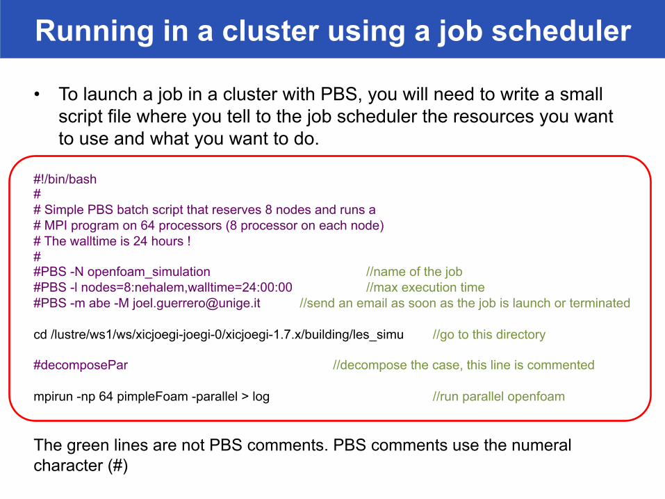
• To launch a job in a cluster with PBS, you will need to write a small script file where you tell to the job scheduler the resources you want to use and what you want to do.
#!/bin/bash # # Simple PBS batch script that reserves 8 nodes and runs a # MPI program on 64 processors (8 processor on each node) # The walltime is 24 hours ! # #PBS -N openfoam_simulation //name of the job #PBS -l nodes=8:nehalem,walltime=24:00:00 //max execution time #PBS -m abe -M [email protected] //send an email as soon as the job is launch or terminated cd /lustre/ws1/ws/xicjoegi-joegi-0/xicjoegi-1.7.x/building/les_simu //go to this directory #decomposePar //decompose the case, this line is commented mpirun -np 64 pimpleFoam -parallel > log //run parallel openfoam The green lines are not PBS comments. PBS comments use the numeral character (#)

Running in a cluster using a job scheduler
• To launch your job you need to use the qsub command (part of the PBS job scheduler). The command will send your job to queue. • qsub script_name
• Remember, running in a cluster is no different from running in your
workstation. The only difference is that you need to schedule your jobs.
• Depending on the system current demand of resources, the resources you request and your job priority, sometimes you can be in queue for hours, even days, so be patient and wait for your turn.

Today’s lecture
1. Running in parallel 2. Running in a cluster using a job scheduler 3. Running with a GPU

Running with a GPU
• The official release of OpenFOAM (version 2.1.x), does not support GPU computing.
• To test OpenFOAM’s GPU capabilities, you will need to install the latest extend version (OpenFOAM-1.6-ext).
• To use your GPU with OpenFOAM, you will need to install the cufflink library. There are a few more options available, but I do like this one.
• You can download cufflink from the following link (as for 1/Jul/2012) : http://code.google.com/p/cufflink-library/
• Additionally, you will need to install the following libraries: • Cusp: which is a library for sparse linear algebra and graph
computations on CUDA. http://code.google.com/p/cusp-library/
• Thrust: which is a parallel algorithms library which resembles the C++ Standard Template Library (STL).http://code.google.com/p/thrust/

Running with a GPU
What is cufflink? cufflink stands for Cuda For FOAM Link. cufflink is an open source library for linking numerical methods based on Nvidia's Compute Unified Device Architecture (CUDA™) C/C++ programming language and OpenFOAM®. Currently, the library utilizes the sparse linear solvers of Cusp and methods from Thrust to solve the linear Ax = b system derived from OpenFOAM's lduMatrix class and return the solution vector. cufflink is designed to utilize the course-grained parallelism of OpenFOAM® (via domain decomposition) to allow multi-GPU parallelism at the level of the linear system solver. Cufflink Features • Currently only supports the OpenFOAM-extend fork of the
OpenFOAM code. • Single GPU support. • Multi-GPU support via OpenFOAM's course grained parallelism
achieved through domain decomposition (experimental).
Running with a GPU
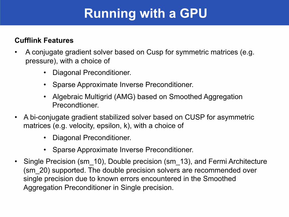
Cufflink Features • A conjugate gradient solver based on Cusp for symmetric matrices (e.g.
pressure), with a choice of • Diagonal Preconditioner.
• Sparse Approximate Inverse Preconditioner.
• Algebraic Multigrid (AMG) based on Smoothed Aggregation Precondtioner.
• A bi-conjugate gradient stabilized solver based on CUSP for asymmetric matrices (e.g. velocity, epsilon, k), with a choice of
• Diagonal Preconditioner.
• Sparse Approximate Inverse Preconditioner. • Single Precision (sm_10), Double precision (sm_13), and Fermi Architecture
(sm_20) supported. The double precision solvers are recommended over single precision due to known errors encountered in the Smoothed Aggregation Preconditioner in Single precision.
Running with a GPU
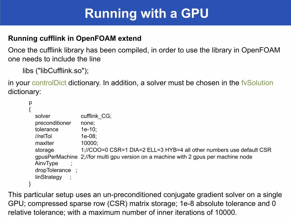
Running cufflink in OpenFOAM extend Once the cufflink library has been compiled, in order to use the library in OpenFOAM one needs to include the line
libs ("libCufflink.so");
in your controlDict dictionary. In addition, a solver must be chosen in the fvSolution dictionary:
p { solver cufflink_CG; preconditioner none; tolerance 1e-10; //relTol 1e-08; maxIter 10000; storage 1;//COO=0 CSR=1 DIA=2 ELL=3 HYB=4 all other numbers use default CSR gpusPerMachine 2;//for multi gpu version on a machine with 2 gpus per machine node AinvType ; dropTolerance ; linStrategy ; }
This particular setup uses an un-preconditioned conjugate gradient solver on a single GPU; compressed sparse row (CSR) matrix storage; 1e-8 absolute tolerance and 0 relative tolerance; with a maximum number of inner iterations of 10000.
Mesh generation using open source tools
Additional tutorials In the folder $path_to_openfoamcourse/parallel_tut you will find many tutorials, try to go through each one to understand how to setup a parallel case in OpenFOAM.
Thank you for your attention
Hands-on session
In the course’s directory ($path_to_openfoamcourse) you will find many tutorials (which are different from those that come with the OpenFOAM installation), let us try to go through each one to understand and get functional using OpenFOAM.
If you have a case of your own, let me know and I will try to do my best to help you to setup your case. But remember, the physics is yours.