Inﬂuence of Local Dynamical Air–Sea Feedback Process on

Influence of Local Dynamical Air–Sea Feedback Process on the Hawaiian LeeCountercurrent

HIDEHARU SASAKI, BUNMEI TAGUCHI, AND NOBUMASA KOMORI

Earth Simulator Center, JAMSTEC, Yokohama, Kanagawa, Japan

YUKIO MASUMOTO

Research Institute for Global Change, JAMSTEC, Yokohama, Kanagawa, Japan

(Manuscript received 7 August 2012, in final form 11 March 2013)

ABSTRACT

Local air–sea interactions over the high sea surface temperature (SST) band along the Hawaiian Lee

Countercurrent (HLCC) are examined with a focus on dynamical feedback of SST-induced wind stress to the

ocean using the atmosphere–ocean coupled general circulation model (CGCM). A pair of ensemble CGCM

simulations are compared to extract the air–sea interactions associated with HLCC: the control simulations

and other simulations, the latter purposely eliminating influences of the high SST band on the sea surface flux

computations in the CGCM. The comparison reveals that oceanic response to surface wind convergence and

positive wind stress curl induced by the high SST band increases (decreases) the HLCC speed in the southern

(northern) flank of the HLCC. The HLCC speed changes are driven by the Ekman suction associated with

positive wind stress curl over the warm HLCC via the thermal wind balance. The HLCC speed increase is

more significant than its decrease. This dynamical feedback is likely to be important to sustain the extension of

the HLCC far to the west. The heat budget analysis confirms that advection of warm water from the west

associatedwith this significant current speed increase plays a role in the southward shift of theHLCCaxis. The

dynamical feedback with the HLCC speed increase can potentially amplify the seasonal and interannual

variations of HLCC.

1. Introduction

Local air–sea interactions associated with the oceanic

fronts andmesoscale phenomena, which have significant

potential impacts to regional and larger-scale climate

systems, are observed in the World Ocean (see reviews

of Small et al. 2008; Chelton andXie 2010).Minobe et al.

(2008) and Tokinaga et al. (2009) revealed that the Gulf

Stream and Kuroshio Extension, respectively, affect not

only the near-surface atmosphere but also the entire

troposphere, suggesting an active role of the mid-

latitude ocean in the weather and climate. Kobashi et al.

(2008) also found a deep atmospheric response to the

subtropical front, associated with the narrow eastward

subtropical countercurrent in the North Pacific in spring.

Furthermore, such atmospheric responses are shown to

influence the oceanic condition in turn. Seo et al.

(2007) revealed a negative feedback to the tropical in-

stability wave (TIW) in the Atlantic that could dampen

the growth rate of the TIW via influence of sea sur-

face temperature (SST) on wind stress. Taguchi et al.

(2012a), on the other hand, suggested that a positive air–

sea feedback plays a role in sustaining the oceanic deep

zonal jets through SST-induced finescale wind stress

curls.

The Hawaiian Lee Countercurrent (HLCC; Qiu et al.

1997; Flament et al. 1998) provides another excellent

opportunity to study local air–sea interactions associ-

ated with oceanic fronts in the extratropics. The HLCC

is a narrow eastward countercurrent extending west-

ward from Hawaii beyond the international date line,

which is originally driven by orographic wind wake be-

hind the Hawaiian Islands (Xie et al. 2001). Recent

satellite observations revealed a zonal band of SST

maximum along the HLCC and associated atmospheric

responses with the surface wind convergence and dis-

tinct clouds over the warm current (Xie et al. 2001).

Corresponding author address: Hideharu Sasaki, Earth Simu-

lator Center, JAMSTEC, 3173-25 Showa-machi, Kanazawa-ku,

Yokohama, Kanagawa, 236-0001, Japan.

E-mail: [email protected]

15 SEPTEMBER 2013 SA SAK I ET AL . 7267

DOI: 10.1175/JCLI-D-12-00586.1

� 2013 American Meteorological Society

Following these atmospheric responses, thermal forcing

onto the ocean, the wind-induced evaporation and

shielding of downward shortwave radiation via clouds,

have been suggested based on analyses of satellite ob-

servations (Xie et al. 2001). The atmospheric response

and its thermal forcing onto the ocean have been con-

firmed to be operative in regional atmospheric model

simulations (Hafner and Xie 2003).

In addition to the thermal forcing, dynamical feed-

backs onto the ocean are expected to occur and are

discussed in the following studies. The positive surface

wind stress curl anomaly over the warm HLCC is

inferred to drive ocean circulation by Sverdrup theory

(Hafner and Xie 2003). Using a high-resolution ocean

general circulation model (GCM), Sasaki and Nonaka

(2006) suggested the importance of local wind conver-

gence over the warm HLCC and associated dynamical

feedback processes in the far-extending HLCC system.

Using an atmospheric–ocean coupled GCM (CGCM),

Sakamoto et al. (2004) succeeded in reproducing the

far-extending HLCC and confirmed that the Hawaiian

Islands are key to trigger the simulated HLCC accom-

panied by the air–sea interactions. While all these stud-

ies conjectured the importance of air–sea interaction in

maintaining the HLCC, detailed mechanisms, partic-

ularly the dynamical feedbacks on to the ocean and

their influences on the HLCC are yet to be explicitly

demonstrated.

This study, therefore, examines how the local atmo-

spheric responses over the warm HLCC in turn in-

fluence the oceanic field using a CGCM. In addition to

ensemble control simulations with atmospheric pertur-

bations, we have conducted another set of ensemble

simulations, in which influence of the warm SST band on

surface heat and momentum flux computations in the

CGCM is purposely excluded. A comparison of results

from the two sets of ensemble simulations is expected to

reveal the air–sea interactions associated with the high

SST band. Influence of the air–sea interactions on oce-

anic temperature field is also examined. The rest of the

paper is organized as follows. In section 2, the CGCM

used in the present study and ensemble simulations is

described. Section 3 shows the local air–sea interactions

induced by the warm HLCC in the CGCM. In section 4,

influences of the dynamical feedback on the HLCC

system are discussed and conclusions are offered.

2. CGCM simulations

a. Model and observation data

The model used in this study is the CGCM for the

Earth Simulator (CFES, Komori et al. 2008), which

consists of the Atmospheric GCM for the Earth Simu-

lator (AFES; Ohfuchi et al. 2004; Enomoto et al. 2008;

Kuwano-Yoshida et al. 2010) and the Oceanic GCM for

the Earth Simulator (OFES; Masumoto et al. 2004;

Komori et al. 2005). The AFES is based on the Center

for Climate System Research (CCSR)/National In-

stitute for Environmental Studies (NIES) atmospheric

GCM 5.4.02 (Numaguti et al. 1997), and the OFES is

based on the Modular Ocean Model version 3 (MOM3;

Pacanowski and Griffies 1999).

The wind stress product at a resolution of 0.58 basedon Quick Scatterometer (QuikSCAT) satellite obser-

vations was obtained from the Japanese Ocean Flux

Datasets with the Use of Remote Sensing Observations

product (J-OFURO; Kutsuwada 1998; Kubota et al.

2002). SST from the Tropical Rainfall Measuring Mis-

sion (TRMM) satellite (Wentz et al. 2000) and sea sur-

face height (SSH) of Maps of the Absolute Dynamic

Topography (MADT) from Archiving, Validation, and

Interpretation of SatelliteOceanographic data (AVISO;

http://www.aviso.oceanobs.com) at a horizontal resolu-

tion of 0.258 were also used.

b. Control and no warm SST band ensemblesimulations

The CFES integration analyzed in this study is a sim-

ulation at a horizontal resolution of T119 (;18) and 48

vertical levels in the atmosphere, and 0.58 horizontal

resolution and 54 vertical levels in the ocean (Richter

et al. 2010; Taguchi et al. 2012b). The reference simula-

tion has been carried out for 150 years starting 1 January

of the climatological atmospheric conditions of the 40-yr

European Centre for Medium-RangeWeather Forecasts

(ECMWF) Re-Analysis (ERA-40; Uppala et al. 2005)

and the oceanic conditions of the temperature and sa-

linity fields from the World Ocean Atlas 1998 (WOA98;

Antonov et al. 1998a,b,c; Boyer et al. 1998a,b,c) without

motion.

The simulated HLCC in the reference simulation ex-

hibits seasonal variations, strong from summer to winter

andweak in spring as observed (Kobashi andKawamura

2002; Sasaki et al. 2010), and interannual variations

(Sasaki et al. 2012) (not shown). We focus on the sim-

ulated HLCC and the associated air–sea interactions in

the summer (from July to September) of the 115th year.

In this period, the HLCC with distinct high SST band

extends farther to the west than in other years, and

the wind stress convergence over the warm HLCC is

prominent (Fig. 1a). Compared with the satellite ob-

servations when the HLCC extended far to the west in

the summer of 2003 (Fig. 1b), the simulated HLCC does

not extend farther west and the wind stress conver-

gence is weak. The HLCC speed away from Hawaii

7268 JOURNAL OF CL IMATE VOLUME 26

is low in the model (.5 cm s21) than in the observa-

tions (.15 cm s21), although the HLCC speed is high

(.20 cm s21) near Hawaii (Fig. 1).

We conducted control ensemble simulations [hereafter

referred to as the control (CNTL) simulations] in the sum-

mer of the 115th year. The ensemble consists of 5members:

one performed with the 1 July initial condition taken

from the reference simulation, and the other four with the

same oceanic initial condition whereas atmospheric fields

replaced with the outputs of the reference simulation on

29 and 30 June and 2 and 3 July, respectively.

In the summer of the 115th year, the SST in the refer-

ence simulation becomes higher along the HLCC than

that of surrounding water (Fig. 2). Other ensemble sim-

ulations removing the influence of the warm SST band

on heat and momentum fluxes in the CGCM have been

conducted from July to September in the 115th year

[hereafter referred to as the no warm SST band (NWSB)

simulations]. In the NWSB simulations, the heat and mo-

mentum fluxes in the rectangular region around theHLCC

(158–238N, 1808–1658W) are estimated at each time step

using the SST smoothed by 88-wide meridional running

means. Differences in ensemblemeans between the CNTL

andNWSB simulations are expected to show contributions

of the high SST peak to local air–sea interactions away

from Hawaii. Considering the influence of atmospheric

natural variability, the statistical significance of the differ-

ences is estimated using two-sided Student’s t test.

3. Results

a. Atmospheric response to high SST band

Atmospheric responses induced by the high SST peak

along the HLCC are examined by comparing ensemble-

mean atmospheric fields between the CNTL and NWSB

FIG. 1. Meridional high-pass filter via removing an 88moving mean is applied to SST and wind

stress; geostrophic eastward current speed (contour, cm s21), SST (color, 8C), and wind stress

vectors (1021Nm22). (a) Mean in the summer of the 115th year in the reference simulation and

(b) mean in the summer of 2003 in the satellite observations of geostrophic current based on the

SSH from AVISO, SST from TRMM satellite, and wind stress from QuikSCAT satellite obser-

vations. Contour intervals are 5 cms21. Wind stress vectors are shown to the west of 1658W.


simulations (hereafter, the ensemble mean fields of

each respective simulations are referred to as simply the

CNTL and NWSB simulations). The ensemble mean

difference in wind stress fields exhibits a zonal band

of convergence toward the high SST peak between

1758 and 1608W and its strong positive curl (.2 31028 Nm23) west of 1658W along approximately 198N(Fig. 3). The positive wind stress curl is produced by

the southwestward wind stress to the north and north-

eastward wind stress to the south with the Coriolis and

pressure gradient forces roughly balanced each other.

This wind stress curl difference is statistically significant

at the 90% confidence level. Cumulus clouds are also

more prominent over the warm HLCC in the CNTL

simulations than in the NWSB simulations (not shown).

These atmospheric responses to the high SST have been

detected in the satellite observations (Xie et al. 2001).

We next look into what mechanisms are responsible

for the near-surface wind response to the underlying

high SST band. It is found that the difference of wind

convergence (.4 3 1027 s21) between the CNTL and

NWSB simulations is spatially best correlated with that

of the positive SLP Laplacian (.0.6 3 10210 Pam21)

along 198N to the west of 1658W (Fig. 4). This relation-

ship is consistent with the pressure adjustment mecha-

nism in the atmospheric boundary layer (ABL) (e.g.,

Lindzen and Nigam 1987), whereby the pressure anom-

alies produce wind convergence over the warm SST (e.g.,

FIG. 2. SST (contour, 8C) in the summer of the 115th year in the reference simulation. Color is

the difference between SST in the reference simulation and that smoothed in the rectangular

region (158–238N, 1808–1658W) by replacing with the meridional running means (SST in the

reference simulation 2 smoothed SST).

FIG. 3. Ensemble mean difference of wind stress vectors (1021Nm22) and curl (color,

1028Nm23) in the summer of the 115th year between the CNTL and NWSB simulations

(CNTL2NWSB). Black contours indicate SST in the CNTL simulation. The hatched region is

where the t-test significance is higher than 0.9.


Minobe et al. 2008; Shimada and Minobe 2011). The

strength of this ABL response can be measured with the

linear slope between the SST Laplacian and wind con-

vergence (Shimada and Minobe 2011). In the reference

simulation in the summer of the 115th year, the slope

is estimated as 4.7 3 104m2 8C21 s21 in the HLCC re-

gion. Interestingly, the air–sea coupling is larger than

that in the western boundary current (WBC) regions

(e.g., 9.8 3 103m2 8C21 s21 in the Agulhas Return Cur-

rent region), although the SST Laplacian in the HLCC

region (;10211 8Cm22) ismuch smaller than in theWBC

region (;10210 8Cm22). This strong air–sea coupling in

the HLCC region is presumably due to the enhanced

surface wind convergence induced by active convection

and its associated latent heat release over the warm

subtropical ocean. The comparison between the cou-

pling magnitudes in the CGCM and observations is

discussed in detail in the appendix.

For the dynamical effect of the perturbation wind

stress on the ocean, the Ekman divergence and thus the

difference of wind stress curl over the high SST band

along the HLCC (Fig. 3) is important, which also seems

to be induced by the pressure adjustment mechanism of

theABL in theCGCM.Based on the simpleABLmodel

(Lindzen and Nigam 1987; Minobe et al. 2008), Taguchi

et al. (2012a) showed that the wind curl is associated

with the wind convergence under the effect of Coriolis

force and the surface friction, leading to the in-phase

relationship between SST Laplacian and wind curl [see

their Eq. (3)]. The linear slope between the latter two in

the summer of the 115th year in the reference simulation

(4.6 3 104m2 8C21 s21) is comparable to that between

the SST Laplacian and wind convergence. Although

the SST along theHLCC is higher by only 0.28C than the

surrounding water (Fig. 2), the ABL response over the

warm ocean around the HLCC induces not only wind

convergence but also the distinct wind curl over the

current.

Besides the pressure adjustment mechanism, the ver-

tical mixing mechanism is another well-known ABL

response to SST anomalies (e.g., Wallace et al. 1989).

However, the relationships between the downwind SST

gradient and wind stress convergence and between the

crosswind SST gradient and wind stress curl are unclear

in the reference simulation (not shown). This is presum-

ably because these relationships suggesting the vertical

mixing mechanism are masked in the HLCC region by

the alternative effect of the pressure adjustment mech-

anism, which can be enhanced by the active convection

over the warm subtropical ocean and the associated la-

tent heat release. What determines the mode of ABL

response to finescale SST anomalies in the HLCC and

other regions should be explored in further studies.

b. Dynamical feedback to the ocean and its influenceon the HLCC

To examine dynamical feedback of the SST-induced

wind stress to the ocean and its influence on the HLCC,

oceanic fields in the CNTL and NWSB simulations are

compared. To the west of 1658W, the eastward surface

current speed of the CNTL simulations is higher (lower)

to the south (north) of HLCC axis than that of the

NWSB simulations (Fig. 5), which suggests the HLCC

speed changes as a result of the dynamical feedback

to the ocean. In the southwest of HLCC around 1758Wwhere themaximum speed is about 8 cms21 in the CNTL

simulations, the current speed increases by more than

1.5 cms21, which is statistically significant at more than

90% confidence level. On the other hand, the current

speed decrease to the north of HLCC is less significant.

FIG. 4. Ensemble mean difference of SLP Laplacian (color, 10210 Pam23) and 10-m wind

convergence (contour, 1027 s21) in the summer of the 115th year between the CNTL and

NWSB simulations (CNTL 2 NWSB).


The zonal mean profile of eastward surface current

speed averaged between 1808 and 1708W also confirms

the HLCC speed increase (decrease) to the south (north)

of HLCC axis: 1.7 cms21 (0.3 cms21) in the CNTL sim-

ulations and 0.8 cm s21 (0.7 cm s21) in the NWSB sim-

ulations along 18.58N (208N) (Fig. 6a). Near Hawaii

(1658–1608W), however, the surface current profiles

in both the simulations are almost the same (Fig. 6b).

These changes in the HLCC speed represent the slight

southward shift away from Hawaii in the CNTL simula-

tions relative to the NWSB simulations. The HLCC

speed change with significant increase in the south could

influence on the current path, which is discussed in detail

in section 4.

Figure 7 shows latitude–depth sections of potential

density and eastward current speed averaged between

1808 and 1708W. In the CNTL simulations, the depth of

the mixed layer is approximately 35m (Fig. 7a), and the

isopycnals in the density range around 23.2su slope up

northward between 188 and 208N and sharply stratified

around 208N at a depth of approximately 50m. The

eastward current, corresponding to the HLCC, is lo-

cated at around 198N in the upper ocean from the sea

surface to 90-m depth, with a core speed higher than

6 cm s21 at a depth of approximately 30m (Fig. 7b).

The eastward current speed in the upper layer above

90m depth is higher (lower) in the southern (northern)

part of the HLCC in the CNTL simulations than in the

NWSB simulations (Fig. 7b). The current speed in-

crease south of HLCC axis between 17.58 and 18.58N is

large (.0.8 cm s21) and statistically significant at more

than 90% confidence level. On the other hand, the

current decrease north of the HLCC axis is relatively

small (,20.6 cm s21) and less significant at the depth

shallower than 20m. The significant HLCC speed in-

crease should help the HLCC extend farther to the west

and be sustained. This result supports the hypothesis

proposed by an OGCM study (Sasaki and Nonaka 2006)

that the local wind convergence over the warm SST

band further drives the HLCC.

The isopycnals centered around 23.2su are shallower

at 198N, and their slopes are steeper (more gradual) to

the south (north) in CNTL simulations than in the

NWSB simulations (Fig. 7a). The positive difference in

potential density around 198N at the depth deeper than

60m is largely significant. In the mixed layer, a pair of

positive and negative differences appears to the north

and south, respectively, of the core of the HLCC in the

CNTL simulations (;198N). Warm (cold) water ad-

vection from the west (east) by the current speed dif-

ference (Fig. 7b) seems to contribute to these density

differences.

c. Mechanism of the HLCC speed change bydynamical feedback

To see the mechanism of dynamical feedback with the

HLCC speed change, the response of pycnocline depth

to the wind convergence over the warm HLCC is ex-

amined. The depth difference of isopycnal surface of

23.2su, corresponding to the typical pycnocline (Fig. 7a)

between the CNTL and NWSB simulations is large

(.1.2 cm) and statistically significant at 90% confidence

level between 1768 and 1728W along 198N (Fig. 8). This

large difference of pycnocline displacement roughly

corresponds to the displacement induced by Ekman

suction via wind stress difference between the CNTL

and NWSB simulations (Fig. 8). This correspondence

shows that the positive wind stress curl of atmospheric

FIG. 5. Ensemble mean difference of eastward surface current speed (cm s21) in the summer

of the 115th year between the CNTL and NWSB simulations (CNTL 2 NWSB). Black con-

tours indicate eastward current speed in the CNTL simulation. Contour intervals are 5 cm s21.

The hatched region is where the t-test significance is higher than 0.9.


FIG. 6. Ensemble mean eastward current speeds (cm s21) at sea

surface averaged (a) between 1808 and 1708Wand (b) between 1658and 1608W in the CNTL (black curves) and NWSB (red curves)

simulations in the summer of the 115th year. Green dashed curve in

(a) indicates the ensemble mean difference of eastward current

speeds between the CNTL and NWSB simulations (CNTL 2NWSB).

FIG. 7. Latitude–depth sections averaged between 1808 and

1708W in the summer of the 115th year. (a) Ensemble mean po-

tential density (su) in the CNTL (solid curve) and NWSB (dashed

curve) simulations. Color indicates the difference of ensemble

mean potential density (CNTL 2 NWSB). (b) Ensemble mean

difference of eastward current speed (color, cm s21) (CNTL 2NWSB). Contours indicate the ensemble mean eastward current

speed (.0 cm s21) in the CNTL simulations with intervals of

1 cm s21. The hatched region is where the t-test significance is

higher than 0.9.


response (Fig. 3) lifts the pycnocline via Ekman suction.

Maximum meridional gradient of the pycnocline dis-

placement between 1808 and 1708W is about 21.0 31027 (0.8 3 1027) to the south (north) of the HLCC,

which could induce the current speed increase of

1.0 cm s21 (decrease of 0.8 cm s21) based on the thermal

wind balance. Therefore, the HLCC speed increase

(.0.8 cm s21) around 188N and decrease (,0.6 cm s21)

around 20.58N (Fig. 7b) are consistent with the thermal

wind balance of the pycnocline slope change (Fig. 7a).

The large differences in both the pycnocline depth and

displacement via Ekman suction can also be found

outside of the region with the smoothed SST in the

NWSB simulations. These signals, however, are not

statistically significant.

d. Influence of local feedbacks on ocean temperature

In this section, how both the local thermal and dy-

namical feedbacks influence the ocean temperature field

around the HLCC is examined. In the region from 1808to 1658Wwhere the air–sea coupling is partially disabled

in the NWSB simulations, the SST is broadly higher to

the south and lower to the north of HLCC in the CNTL

simulations than in the NWSB simulations (Fig. 9).

Around the HLCC, there are a pair of statistically sig-

nificant differences in SST peaks, with the positive peak

FIG. 8. As in Fig. 5, but the color is the ensemble mean difference (CNTL 2 NWSB) of the

23.2su isopycnal surface depth (m) and contours indicate vertical displacements (m) via Ekman

pumping forced by wind stress difference. Based on the finite difference method, the mean

displacement corresponds to that for 1.5 month via Ekman pumping velocity averaged in the

summer. The Ekman pumping velocity is defined as curl(Dt/f )/r, where Dt is the ensemble

mean difference of the wind stress vector, f is the Coriolis parameter, and r is the water density.

The hatched region is where the t-test significance is higher than 0.9.

FIG. 9. As in Fig. 5, but the color is the ensemblemean SST (8C) difference (CNTL2NWSB)

between the CNTL and NWSB simulations, and contours indicate SST in the CNTL simu-

lation with intervals of 0.28C. The hatched region is where the t-test significance is higher

than 0.9.


between 1758E and 1708W along 17.58N (.0.18C) and

the negative peak between 1738 and 1658W along 208N(,0.158C).The surface heat flux difference between the CNTL

and NWSB simulations averaged in the summer of the

115th year is examined. The easterly trade winds are

strengthened to the north and weakened to the south

of HLCC by the southwestward and northeastward

wind stress differences, respectively (Fig. 3), which are

induced by the high SST band. As a result, surface

cooling via evaporation becomes correspondingly large

(,22Wm22) to the north and small (.6Wm22) to the

south (Fig. 10), which are consistent with those in Xie

et al. (2001) and Hafner and Xie (2003). The small

(large) surface cooling to the south along 178N (north

along 19.58N) is significant (nonsignificant). The reason

why the significance of the north is degraded is still un-

clear, which should be examined in the future.

The shielding of downward shortwave radiation by

clouds also appears to influence the SST locally along

the HLCC. Downward shortwave radiation over the

HLCC is lower (,24Wm22) approximately along

19.58N to the west of 1708W in the CNTL simulations

than in the NWSB simulations (Fig. 11) due to more

prominent cumulus clouds over the HLCC in the CNTL

simulations (not shown). These two thermal feedbacks

to the ocean have not been explicitly demonstrated until

the present study, while their influences on the SSTwere

suggested in previous studies (Xie et al. 2001; Hafner

and Xie 2003).

FIG. 10. Ensemble mean difference of latent heat flux (color, Wm22) in the summer of

the 115th year between the CNTL and NWSB simulations (CNTR 2 NWSB). Contours in-

dicate SST in the CNTL simulation. The hatched region is where the t-test significance is higher

than 0.9.

FIG. 11. As in Fig. 5, but the color is the ensemble mean difference (CNTL 2 NWSB) of

downward shortwave radiation (Wm22) at the sea surface between the CNTL and NWSB

simulations, and contours indicate the eastward current speed at sea surface in the CNTL

simulation with the contour interval of 5 cm s21. The hatched region is where the t-test sig-

nificance is higher than 0.9.


In addition to these thermal feedbacks, the HLCC

speed increase of dynamical feedback could influence

the SST via warm (cold) water advection from the west

(east) in the south (north) of HLCC. The significant

positive (negative) zonal current speed difference (Fig.

5) and positive (negative) SST difference (Fig. 9) are to

some degree collocated each other in the south (north)

of HLCC.

To examine what mechanism is important to tem-

perature field around the HLCC, we have monitored

heat budget terms in the mixed layer both in the CNTL

and NWSB simulations. The change rate of the mixed

layer temperature is defined as

›Tmix

›t5

Q

rCpHmix

21

Hmix

ð02H

mix

(U � $T) dz1 residual ,

(1)

where T and Tmix are the potential temperature and its

mean value throughout the mixed layer, respectively;Q

is the surface heat flux minus penetrating shortwave

radiation flux through the bottom of mixed layer; r is the

water density; Cp is the heat capacity; Hmix is the mixed

layer thickness; andU is the current velocity vector. The

depth of mixed layer bottom is defined as the depth

at which potential density differs from the sea surface

density by 0.125su. The left side of this equation repre-

sents the change rate of the mixed layer temperature.

The first term on the right side is the resultant heating

from vertical convergence of heat fluxes, the second

term is the heat advection term in the mixed layer, and

the third term is the residual.

Figure 12 shows the meridional profile of each term

difference of 1808–1708W between the CNTL and

NWSB simulations averaged for the summer of the

115th year. Tendency of the mixed layer temperature

agrees well with the SST difference at the end of the

summer. The residual term, which mostly represents

vertical diffusion, does not have much influence on the

temperature change. The large positive heat advection

difference at around 188–198N (.0.058C month21) is

located slightly to the south of the negative surface heating

difference (,0.058Cmonth21) at around 198N. This heat

advection and the surface heating (.0.058Cmonth21) to

the south of 188N contribute to the positive difference of

mixed layer temperature to the south of 188N. To the

north of 208N, the negative difference of heat advection

also causes the negative difference of mixed layer tem-

perature, although its contribution is relatively small

compared to that in the south. These results show that

not only the surface heating via thermal feedbacks,

but also the heat advection via dynamical feedback,

contribute to the change rate of temperature locally

around the HLCC. Significances of the current speed

difference (Fig. 5) and latent heat flux difference (Fig. 10)

in the south of HLCC support that both of the warm

water advection and surface heating contribute themixed

layer warming in the south of the HLCC. These results

suggest that the both thermal and dynamical feedbacks

play roles in the southward shift of the warm SST band

associated with the HLCC.

4. Conclusions and discussion

The present study examines local air–sea interactions

induced by the high SST band along the HLCC in the

CGCM simulations, with a focus on dynamical feedback

to the ocean. A comparison of ensemble mean results

from the CNTL simulations and NWSB simulations

in which influence of the high SST peak is eliminated

FIG. 12. Change rates differences (8C month21) in the mixed

layer averaged from 1808 to 1708W in the summer of the 115th year

between ensemble means of the CNTL and NWSB simulations

(CNTL2 NWSB). Mixed layer potential temperature (thick solid

curve), term of surface heating minus permeation flux at bottom of

the mixed layer (dashed curve), heat advection term in the mixed

layer (thin solid curve), and residual (dotted curve). Dashed–dotted

line indicates the SST difference at the end of the summer.


reveals that atmospheric response to the SST peak in

turn increases (decreases) the current speed in the

southern (northern) part of HLCC. Ekman suction by

positive wind stress curl over the warm HLCC is re-

sponsible for these HLCC speed changes based on the

thermal wind balance. In addition, the warm and cold

water advections by this HLCC speed changes influence

the temperature around the HLCC. The significant

HLCC speed increase with warm water advection

through the dynamical feedback is likely to be important

to sustain the extension far to the west and the south-

ward shift of the HLCC.

This study suggests that the dynamical feedback of

significant HLCC speed increase with warm water ad-

vection plays a role in the meridional shift of the HLCC.

On the other hand, the previous studies implied that the

high SST band along the HLCC tends to move south-

ward via thermal feedback into the ocean (Xie et al.

2001; Halner and Xie 2003). In addition, other mecha-

nisms such as the influence from background flow

(Maximenko et al. 2008) may contribute the meridional

position of zonal current. Future studies are necessary to

examine what mechanism is important in the HLCC

tilting.

Moreover, it is also possible that the HLCC speed

increase due to the dynamical feedback plays a role in

the seasonal (Kobashi and Kawamura 2002; Sasaki

et al. 2010) and interannual (Sasaki et al. 2012) varia-

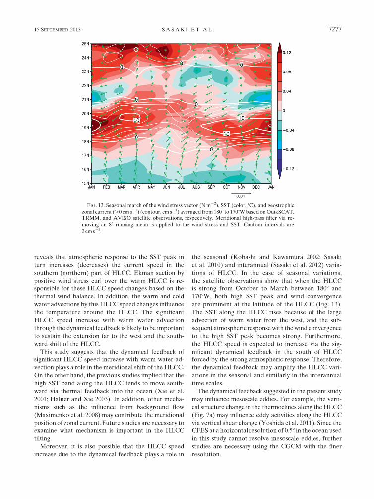
tions of HLCC. In the case of seasonal variations,

the satellite observations show that when the HLCC

is strong from October to March between 1808 and

1708W, both high SST peak and wind convergence

are prominent at the latitude of the HLCC (Fig. 13).

The SST along the HLCC rises because of the large

advection of warm water from the west, and the sub-

sequent atmospheric response with the wind convergence

to the high SST peak becomes strong. Furthermore,

the HLCC speed is expected to increase via the sig-

nificant dynamical feedback in the south of HLCC

forced by the strong atmospheric response. Therefore,

the dynamical feedback may amplify the HLCC vari-

ations in the seasonal and similarly in the interannual

time scales.

The dynamical feedback suggested in the present study

may influence mesoscale eddies. For example, the verti-

cal structure change in the thermoclines along the HLCC

(Fig. 7a) may influence eddy activities along the HLCC

via vertical shear change (Yoshida et al. 2011). Since the

CFES at a horizontal resolution of 0.58 in the ocean usedin this study cannot resolve mesoscale eddies, further

studies are necessary using the CGCM with the finer

resolution.

FIG. 13. Seasonal march of the wind stress vector (Nm22), SST (color, 8C), and geostrophic

zonal current (.0 cm s21) (contour, cm s21) averaged from 1808 to 1708Wbased onQuikSCAT,

TRMM, and AVISO satellite observations, respectively. Meridional high-pass filter via re-

moving an 88 running mean is applied to the wind stress and SST. Contour intervals are

2 cm s21.


We evaluated the statistical significance of our results

only for the summer of the 115th year. However, in-

trinsic variability in other years could be different from

that in this specific summer. In addition, we have not

examined how the local air–sea interactions influence

remotely the wider areas. To address these issues, en-

semble simulations with larger members should be

conducted. These further studies are necessary steps for

better understanding of the role of local air–sea in-

teractions revealed in the present study. It is of great

interest to investigate whether the dynamical feedback

onto the current speed elucidated in this study is oper-

ative not only for the HLCC but also for other currents

with SST front such as the western boundary currents.

The comparison of CGCM simulations demonstrated in

this study to extract the dynamical feedback provides

a useful method to conduct this future work.

Acknowledgments. The CFES simulations were con-

ducted on the Earth Simulator under support from

JAMSTEC. We thank Profs. T. Yamagata, T. Hibiya,

H. Nakamura, M. Watanabe, and H. Hasumi for valuable

discussions. QuikSCAT wind stress data in the J-OFURO

dataset were provided by Prof. K.Kutsuwada. This work is

partially supported by MEXT/JST KAKENHI (HS and

BT: 22106006 and 23340139, BT: 24540476, NK: 22106008

and 22244057).

APPENDIX

Air–Sea Coupling Strength in CGCM andObservation

We have examined the air–sea coupling magnitude in

the reference simulation compared with that in Shimada

and Minobe (2011), who quantified the strength of the

ABL response to SST anomalies via the pressure ad-

justment mechanism with the linear relation between

Laplacians of SST and lower tropospheric air thickness

corresponding to SLP [s(DSST, DH)] and that between

the thickness Laplacian and wind convergence [s(DH,

convU)] using the satellite sounding and scatterometer.

Since the simulated SLP field in the CFES is contami-

nated by the spectral noise by Gibbs phenomena, we

estimate the linear slope between SST Laplacian and

wind convergence [s(DSST, convU)]. Although Shimada

and Minobe (2011) did not directly examine this quan-

tity, it can be inferred by multiplying the two directly

estimated quantities together [i.e., s(DSST, convU) 5s(DSST, DH)3 s(DH, convU)]. In the WBC region, the

annual mean slope (about 1 3 104m2 8C21 s21) in the

reference simulation for 6 years from the 115th to 120th

year is comparable to the estimation from the clima-

tological annual mean based on observations for 6

years (Shimada and Minobe 2011).

REFERENCES

Antonov, J. I., S. Levitus, T. P. Boyer,M. E. Conkright, T. O’Brien,

and C. Stephens, 1998a: Temperature of the Atlantic Ocean.

Vol. 1, World Ocean Atlas 1998, NOAA Atlas NESDIS 27,

166 pp.

——, ——, ——, ——, ——, and ——, 1998b: Temperature of the

Pacific Ocean. Vol. 2, World Ocean Atlas 1998, NOAA Atlas

NESDIS 28, 166 pp.

——, ——, ——, ——, ——, ——, and B. Trotsenko, 1998c:

Temperature of the Indian Ocean. Vol. 3, World Ocean Atlas

1998, NOAA Atlas NESDIS 29, 166 pp.

Boyer, T. P., S. Levitus, J. I. Antonov,M. E. Conkright, T. O’Brien,

and C. Stephens, 1998a: Salinity of the Atlantic Ocean. Vol. 4,

World Ocean Atlas 1998, NOAA Atlas NESDIS 30, 166 pp.

——,——,——,——,——, and——, 1998b: Salinity of the Pacific

Ocean. Vol. 5, World Ocean Atlas 1998, NOAA Atlas

NESDIS 31, 166 pp.

——,——,——,——,——,——, andB. Trotsenko, 1998c: Salinity

of the Indian Ocean. Vol. 6, World Ocean Atlas 1998, NOAA

Atlas NESDIS 32, 166 pp.

Chelton, D. B., and S.-P. Xie, 2010: Coupled ocean-atmosphere

interaction at oceanic mesoscales. Oceanography, 23 (4),

52–69.

Enomoto, T.,A.Kuwano-Yoshida,N.Komori, andW.Ohfuchi, 2008:

Description of AFES 2: Improvements for high-resolution and

coupled simulations. High Resolution Numerical Modelling of

the Atmosphere and Ocean, K. Hamilton and W. Ohfuchi, Eds.,

Springer, 77–97.

Flament, P., S. Kennan, R. Lumpkin, M. Sawyer, and E. Stroup,

1998: The ocean. Atlas of Hawaii, S. P. Juvik and J. O. Juvik,

Eds., University of Hawaii Press, 82–86.

Hafner, J., and S.-P. Xie, 2003: Far-field simulation of theHawaiian

wake: Sea surface temperature and orographic effects. J. Atmos.

Sci., 60, 3021–3032.

Kobashi, F., and H. Kawamura, 2002: Seasonal variation and in-

stability nature of the North Pacific Subtropical Countercur-

rent and the Hawaiian Lee Countercurrent. J. Geophys. Res.,

107, 3185, doi:10.1029/2001JC001225.

——, S.-P. Xie, N. Iwasaka, and T. T. Sakamoto, 2008: Deep at-

mospheric response to the North Pacific oceanic subtropical

front in spring. J. Climate, 21, 5960–5975.

Komori, N., K. Takahashi, K. Komine, T. Motoi, X. Zhang, and

G. Sagawa, 2005: Description of sea-ice component of coupled

ocean-sea ice model for the earth simulator (OIFES). J. Earth

Simul., 4, 31–45.

——, A. Kuwano-Yoshida, T. Enomoto, H. Sasaki, and W. Ohfuchi,

2008: High resolution simulation of the global coupled

atmospheric-ocean system: Description and preliminary out-

comes of CFES (CGCM for the Earth Simulator). High Reso-

lution Numerical Modelling of the Atmosphere and Ocean,

K. Hamilton and W. Ohfuchi, Eds., Springer, 241–260.

Kubota, M., N. Iwasaka, S. Kizu, M. Konda, and K. Kutsuwada,

2002: Japanese ocean flux data sets with use of remote sensing

observations (J-OFURO). J. Oceanogr., 58, 213–225.Kutsuwada, K., 1998: Impact of wind/wind-stress field in the North

Pacific constructed by ADEOS/NSCAT data. J. Oceanogr.,

54, 443–456.


Kuwano-Yoshida, A., T. Enomoto, and W. Ohfuchi, 2010: An

improved cloud scheme for climate simulations.Quart. J. Roy.

Meteor. Soc., 136, 1583–1597.

Lindzen, R. S., and S. Nigam, 1987: On the role of sea surface

temperature gradients in forcing low-level winds and conver-

gence in the tropics. J. Atmos. Sci., 44, 2418–2436.

Masumoto, Y., and Coauthors, 2004: A fifty-year eddy-resolving

simulation of the world ocean: Preliminary outcomes of OFES

(OGCM for the Earth Simulator). J. Earth Simul., 1, 35–56.

Maximenko, N. A., O. V. Melnichenko, P. P. Niiler, and H. Sasaki,

2008: Stationary mesoscale jet-like features in the ocean. Geo-

phys. Res. Lett., 35, L08603, doi:10.1029/2008GL033267.

Minobe, S., A. Kuwano-Yoshida, N. Komori, S.-P. Xie, and R. J.

Small, 2008: Influence of the Gulf Stream on the troposphere.

Nature, 452, 206–209.Numaguti, A., M. Takahashi, T. Nakajima, and A. Sumi, 1997:

Description of CCSR/NIES atmospheric general circulation

model. Study on the Climate System and Mass Transport by

a Climate Model, A. Numaguti, Ed., Center for Global Envi-

ronmental Research, National Institute for Environmental

Studies, 1–48.

Ohfuchi, W., and Coauthors, 2004: 10-km mesh meso-scale re-

solving simulations of the global atmosphere on the Earth

Simulator—Preliminary outcomes of AFES (AGCM for the

Earth Simulator). J. Earth Simul., 1, 8–34.

Pacanowski, R. C., and S. M. Griffies, 1999: The MOM 3 manual.

GFDLOceanGroup Tech. Rep. 4, NOAA/Geophysical Fluid

Dynamics Laboratory, Princeton, NJ, 680 pp.

Qiu, B., D. A. Koh, C. Lumpkin, and P. Flament, 1997: Existence

and formation mechanism of the North Hawaiian Ridge

Current. J. Phys. Oceanogr., 27, 431–444.

Richter, I., S. K. Behera, Y.Masumoto, B. Taguchi, N. Komori, and

T. Yamagata, 2010: On the triggering of Benguela Ni~nos:

Remote equatorial versus local influences. Geophys. Res.

Lett., 37, L20604, doi:10.1029/2010GL044461.

Sakamoto, T. T., A. Sumi, S. Emori, T. Nishimura, H. Hasumi,

T. Suzuki, and M. Kimoto, 2004: Far-reaching effects of the

Hawaiian Islands in the CCSR/NIES/FRCGC high-resolution

climate model. Geophys. Res. Lett., 31, L17212, doi:10.1029/

2004GL020907.

Sasaki, H., and M. Nonaka, 2006: Far-reaching Hawaiian Lee

Countercurrent driven by wind-stress curl induced by warm

SST band along the current. Geophys. Res. Lett., 33, L13602,

doi:10.1029/2006GL026540.

——, S.-P. Xie, B. Taguchi, M. Nonaka, and Y. Masumoto, 2010:

Seasonal variations of the Hawaiian Lee Countercurrent

induced by the meridional migration of the Trade Winds.

Ocean Dyn., 60 (3), 705–715.

——, ——, ——, ——, S. Hosoda, and Y. Masumoto, 2012: In-

terannual variations of the Hawaiian Lee Countercurrent in-

duced by low potential vorticity water ventilation in the

subsurface. J. Oceanogr., 68, 93–111.

Seo, H., M. Jochum, R. Murtugudde, A. J. Miller, and J. O.

Roads, 2007: Feedback of tropical instability-wave-induced

atmospheric variability onto the ocean. J. Climate, 20, 5842–

5855.

Shimada, T., and S. Minobe, 2011: Global analysis of the pressure

adjustment mechanism over sea surface temperature fronts

using AIRS/Aqua data. Geophys. Res. Lett., 38, L06704,

doi:10.1029/2010GL046625.

Small, R. J., and Coauthors, 2008: Air–sea interaction over ocean

fronts and eddies. Dyn. Atmos. Oceans, 45, 274–319.

Taguchi, B., R. Furue, N. Komori, A. Kuwano-Yoshida,

M. Nonaka, H. Sasaki, and W. Ohfuchi, 2012a: Deep oceanic

zonal jets constrained by fine-scale wind stress curls in the South

Pacific Ocean: A high-resolution coupled GCM study.Geophys.

Res. Lett., 39, L08602, doi:10.1029/2012GL051248.

——, H. Nakamura, M. Nonaka, N. Komori, A. Kuwano-Yoshida,

K. Takaya, and A. Goto, 2012b: Seasonal evolutions of at-

mospheric response to decadal SST anomalies in the North

Pacific subarctic frontal zone: Observations and a coupled

model simulation. J. Climate, 25, 111–139.Tokinaga, H., Y. Tanimoto, S.-P. Xie, T. Sampe, H. Tomita, and

H. Ichikawa, 2009: Ocean frontal effects on the vertical de-

velopment of clouds over thewesternNorth Pacific: In situ and

satellite observations. J. Climate, 22, 4241–4260.Uppala, S. M., and Coauthors, 2005: The ERA-40 Re-Analysis.

Quart. J. Roy. Meteor. Soc., 131, 2961–3012.

Wallace, J. M., T. P. Mitchell, and C. Deser, 1989: The influence of

sea surface temperature on surface wind in the eastern equa-

torial Pacific: Seasonal and interannual variability. J. Climate,

2, 1492–1499.

Wentz, F. F., C. Gentemann, D. Smith, and D. Chelton, 2000:

Satellite measurements of sea surface temperature through

clouds. Science, 288, 847–850.

Xie, S.-P., W. T. Liu, Q. Liu, and M. Nonaka, 2001: Far-reaching ef-

fects of the Hawaiian Islands on the Pacific ocean-atmosphere

system. Science, 292, 2057–2060.

Yoshida, S., B. Qiu, and P. Hacker, 2011: Low-frequency eddy

modulations in the Hawaiian Lee Countercurrent: Obser-

vations and connection to the Pacific Decadal Oscillation.

J. Geophys. Res., 116, C12009, doi:10.1029/2011JC007286.


Documents

Inﬂuence of Local Dynamical Air–Sea Feedback Process on