Embed Size (px)
Citation preview
Invariant Manifolds and dispersive HamiltonianEvolution Equations
W. Schlag, http://www.math.uchicago.edu/˜schlag
Boston, January 5, 2012
W. Schlag, http://www.math.uchicago.edu/˜schlag Dispersive Hamiltonian PDEs
Old-fashioned string theoryHow does a guitar string evolve in time?
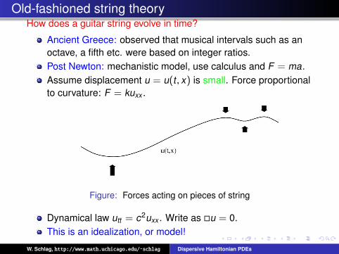
Ancient Greece: observed that musical intervals such as anoctave, a fifth etc. were based on integer ratios.Post Newton: mechanistic model, use calculus and F = ma.Assume displacement u = u(t , x) is small. Force proportionalto curvature: F = kuxx .
Figure: Forces acting on pieces of string
Dynamical law utt = c2uxx . Write as u = 0.This is an idealization, or model!
W. Schlag, http://www.math.uchicago.edu/˜schlag Dispersive Hamiltonian PDEs
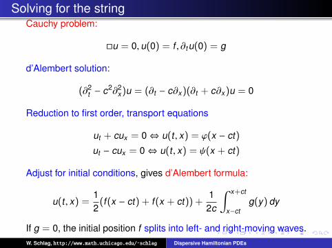
Solving for the stringCauchy problem:
u = 0, u(0) = f , ∂tu(0) = g
d’Alembert solution:
(∂2t − c2∂2
x)u = (∂t − c∂x)(∂t + c∂x)u = 0
Reduction to first order, transport equations
ut + cux = 0⇔ u(t , x) = ϕ(x − ct)
ut − cux = 0⇔ u(t , x) = ψ(x + ct)
Adjust for initial conditions, gives d’Alembert formula:
u(t , x) =12
(f(x − ct) + f(x + ct)) +1
2c
∫ x+ct
x−ctg(y) dy
If g = 0, the initial position f splits into left- and right-moving waves.W. Schlag, http://www.math.uchicago.edu/˜schlag Dispersive Hamiltonian PDEs
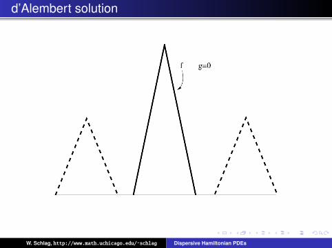
d’Alembert solution
W. Schlag, http://www.math.uchicago.edu/˜schlag Dispersive Hamiltonian PDEs
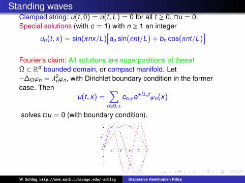
Standing wavesClamped string: u(t , 0) = u(t , L) = 0 for all t ≥ 0, u = 0.Special solutions (with c = 1) with n ≥ 1 an integer
un(t , x) = sin(πnx/L)[an sin(πnt/L) + bn cos(πnt/L)
]Fourier’s claim: All solutions are superpositions of these!Ω ⊂ Rd bounded domain, or compact manifold. Let−∆Ωϕn = λ2
nϕn, with Dirichlet boundary condition in the formercase. Then
u(t , x) =∑
n≥0,±
cn,±e±iλn tϕn(x)
solves u = 0 (with boundary condition).
W. Schlag, http://www.math.uchicago.edu/˜schlag Dispersive Hamiltonian PDEs
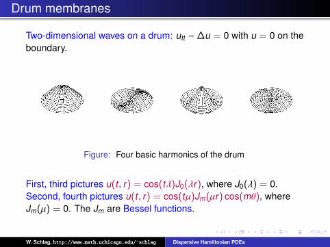
Drum membranes
Two-dimensional waves on a drum: utt −∆u = 0 with u = 0 on theboundary.
Figure: Four basic harmonics of the drum
First, third pictures u(t , r) = cos(tλ)J0(λr), where J0(λ) = 0.Second, fourth pictures u(t , r) = cos(tµ)Jm(µr) cos(mθ), whereJm(µ) = 0. The Jm are Bessel functions.
W. Schlag, http://www.math.uchicago.edu/˜schlag Dispersive Hamiltonian PDEs
Electrification of waves
Maxwell’s equations: E(t , x) and B(t , x) vector fields
div E = ε−10 ρ, div B = 0
curl E + ∂tB = 0, curl B − µ0ε0∂tE = µ0J
ε0 electric constant, µ0 magnetic constant, ρ charge density, Jcurrent density.In vaccum ρ = 0, J = 0. Differentiate fourth equation in time:
curl Bt − µ0ε0Ett = 0⇒ curl (curl E) + µ0ε0Ett = 0
∇(div E) −∆E + µ0ε0Ett = 0⇒ Ett − c2∆E = 0
Similarly Btt − c2∆B = 0.In 1861 Maxwell noted that c is the speed of light, and concludedthat light should be an electromagnetic wave! Wave equationappears as a fundamental equation! Loss of Galilei invariance!
W. Schlag, http://www.math.uchicago.edu/˜schlag Dispersive Hamiltonian PDEs
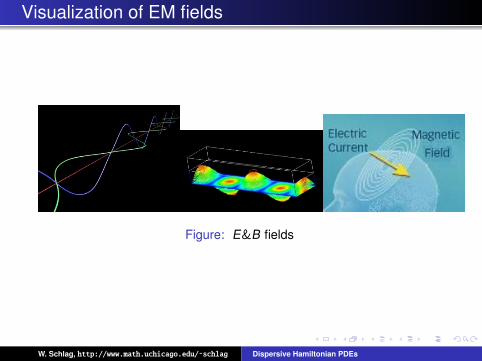
Visualization of EM fields
Figure: E&B fields
W. Schlag, http://www.math.uchicago.edu/˜schlag Dispersive Hamiltonian PDEs
Least action
Principle of Least Action: Paths (x(t), x(t)), for t0 ≤ t ≤ t1 withendpoints x(t0) = x0, and x(t1) = x1 fixed. The physical pathdetermined by kinetic energy K(x, x) and potential energy P(x, x)minimizes the action:
S :=
∫ t1
t0(K − P)(x(t), x(t)) dt =
∫ t1
t0L(x(t), x(t)) dt
with L the Lagrangian.In fact: equations of motion equal Euler-Lagrange equation
−ddt∂L∂x
+∂L∂x
= 0
and the physical trajectories are the critical points of S.For L = 1
2mx2 − U(x), we obtain mx(t) = −U′(x(t)), which isNewton’s F = ma.
W. Schlag, http://www.math.uchicago.edu/˜schlag Dispersive Hamiltonian PDEs
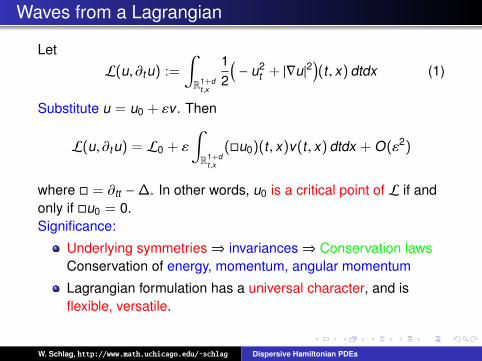
Waves from a Lagrangian
LetL(u, ∂tu) :=
∫R1+d
t ,x
12
(− u2
t + |∇u|2)(t , x) dtdx (1)
Substitute u = u0 + εv. Then
L(u, ∂tu) = L0 + ε
∫R1+d
t ,x
(u0)(t , x)v(t , x) dtdx + O(ε2)
where = ∂tt −∆. In other words, u0 is a critical point of L if andonly if u0 = 0.Significance:
Underlying symmetries⇒ invariances⇒ Conservation lawsConservation of energy, momentum, angular momentum
Lagrangian formulation has a universal character, and isflexible, versatile.
W. Schlag, http://www.math.uchicago.edu/˜schlag Dispersive Hamiltonian PDEs
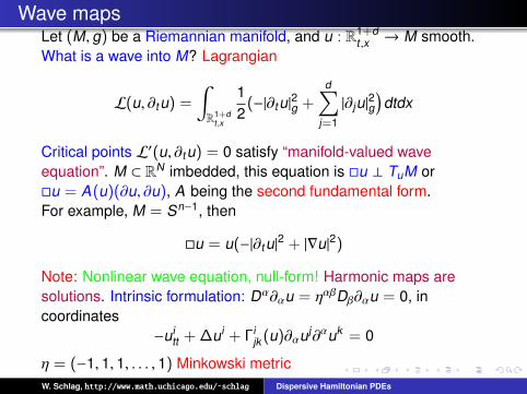
Wave mapsLet (M, g) be a Riemannian manifold, and u : R1+d
t ,x → M smooth.What is a wave into M? Lagrangian
L(u, ∂tu) =
∫R1+d
t ,x
12
(−|∂tu|2g +d∑
j=1
|∂ju|2g)dtdx
Critical points L′(u, ∂tu) = 0 satisfy “manifold-valued waveequation”. M ⊂ RN imbedded, this equation is u ⊥ TuM oru = A(u)(∂u, ∂u), A being the second fundamental form.For example, M = Sn−1, then
u = u(−|∂tu|2 + |∇u|2)
Note: Nonlinear wave equation, null-form! Harmonic maps aresolutions. Intrinsic formulation: Dα∂αu = ηαβDβ∂αu = 0, incoordinates
−uitt + ∆ui + Γi
jk (u)∂αuj∂αuk = 0
η = (−1, 1, 1, . . . , 1) Minkowski metricW. Schlag, http://www.math.uchicago.edu/˜schlag Dispersive Hamiltonian PDEs
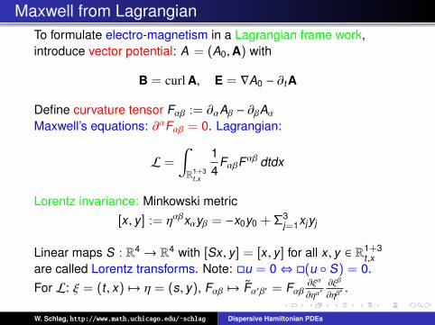
Maxwell from LagrangianTo formulate electro-magnetism in a Lagrangian frame work,introduce vector potential: A = (A0,A) with
B = curl A, E = ∇A0 − ∂tA
Define curvature tensor Fαβ := ∂αAβ − ∂βAα
Maxwell’s equations: ∂αFαβ = 0. Lagrangian:
L =
∫R1+3
t ,x
14
FαβFαβ dtdx
Lorentz invariance: Minkowski metric[x, y] := ηαβxαyβ = −x0y0 + Σ3
j=1xjyj
Linear maps S : R4 → R4 with [Sx, y] = [x, y] for all x, y ∈ R1+3t ,x
are called Lorentz transforms. Note: u = 0⇔ (u S) = 0.For L: ξ = (t , x) 7→ η = (s, y), Fαβ 7→ Fα′β′ = Fαβ
∂ξα
∂ηα′
∂ξβ
∂ηβ′ .
W. Schlag, http://www.math.uchicago.edu/˜schlag Dispersive Hamiltonian PDEs
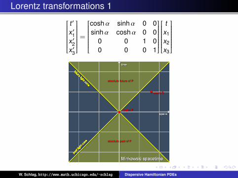
Lorentz transformations 1t ′
x′1x′2x′3
=
coshα sinhα 0 0sinhα coshα 0 0
0 0 1 00 0 0 1
tx1
x2
x3
Figure: Causal structure of space-timeW. Schlag, http://www.math.uchicago.edu/˜schlag Dispersive Hamiltonian PDEs
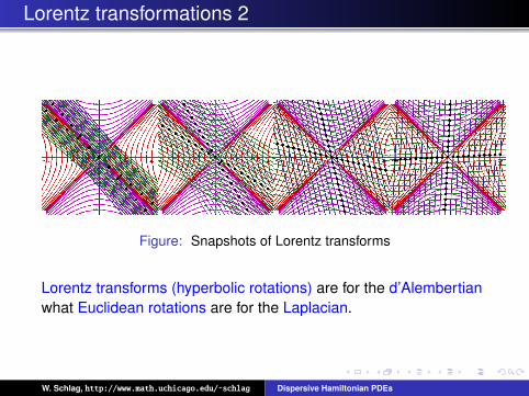
Lorentz transformations 2
Figure: Snapshots of Lorentz transforms
Lorentz transforms (hyperbolic rotations) are for the d’Alembertianwhat Euclidean rotations are for the Laplacian.
W. Schlag, http://www.math.uchicago.edu/˜schlag Dispersive Hamiltonian PDEs
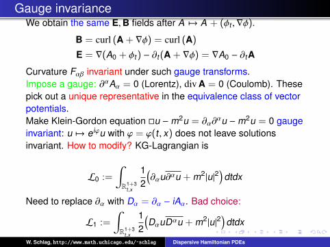
Gauge invarianceWe obtain the same E,B fields after A 7→ A + (φt ,∇φ).
B = curl (A + ∇φ) = curl (A)
E = ∇(A0 + φt ) − ∂t (A + ∇φ) = ∇A0 − ∂tA
Curvature Fαβ invariant under such gauge transforms.Impose a gauge: ∂αAα = 0 (Lorentz), div A = 0 (Coulomb). Thesepick out a unique representative in the equivalence class of vectorpotentials.Make Klein-Gordon equation u −m2u = ∂α∂
αu −m2u = 0 gaugeinvariant: u 7→ e iϕu with ϕ = ϕ(t , x) does not leave solutionsinvariant. How to modify? KG-Lagrangian is
L0 :=
∫R1+3
t ,x
12
(∂αu∂αu + m2|u|2
)dtdx
Need to replace ∂α with Dα = ∂α − iAα. Bad choice:
L1 :=
∫R1+3
t ,x
12
(DαuDαu + m2|u|2
)dtdx
W. Schlag, http://www.math.uchicago.edu/˜schlag Dispersive Hamiltonian PDEs
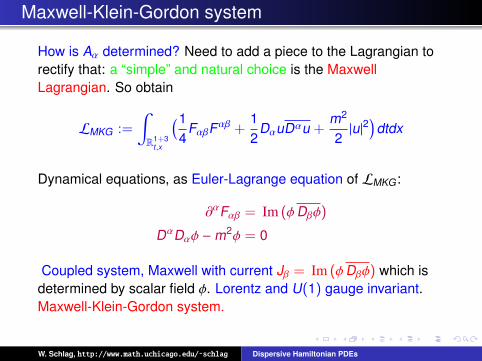
Maxwell-Klein-Gordon system
How is Aα determined? Need to add a piece to the Lagrangian torectify that: a “simple” and natural choice is the MaxwellLagrangian. So obtain
LMKG :=
∫R1+3
t ,x
(14
FαβFαβ +12
DαuDαu +m2
2|u|2
)dtdx
Dynamical equations, as Euler-Lagrange equation of LMKG :
∂αFαβ = Im (φDβφ)
DαDαφ −m2φ = 0
Coupled system, Maxwell with current Jβ = Im (φDβφ) which isdetermined by scalar field φ. Lorentz and U(1) gauge invariant.Maxwell-Klein-Gordon system.
W. Schlag, http://www.math.uchicago.edu/˜schlag Dispersive Hamiltonian PDEs
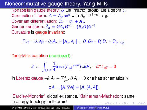
Noncommutative gauge theory, Yang-MillsNonabelian gauge theory: G Lie (matrix) group, Lie algebra g.Connection 1-form: A = Aα dxα with Aα : R1+d → g.Covariant differentiation: Dα = ∂α + Aα.Gauge transform: Aα = GAαG−1 − (∂αG)G−1.Curvature is gauge invariant:
Fαβ = ∂αAβ − ∂βAα + [Aα,Aβ] = DαDβ − DβDα − D[∂α,∂β]
Yang-Mills equation (nonlinear!):
L :=
∫R1+d
14
trace(FαβFαβ) dtdx, DαFαβ = 0
In Lorentz gauge −∂tA0 +∑3
j=1 ∂jAj = 0 one has schematically
A = [A ,∇A ] + [A , [A ,A ]]
Eardley-Moncrief: global existence, Klainerman-Machedon: samein energy topology, null-forms!W. Schlag, http://www.math.uchicago.edu/˜schlag Dispersive Hamiltonian PDEs
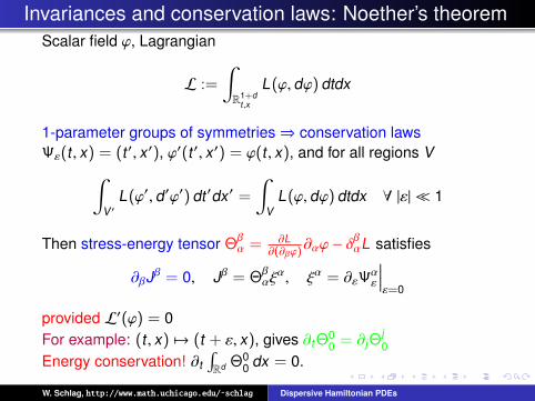
Invariances and conservation laws: Noether’s theoremScalar field ϕ, Lagrangian
L :=
∫R1+d
t ,x
L(ϕ, dϕ) dtdx
1-parameter groups of symmetries⇒ conservation lawsΨε(t , x) = (t ′, x′), ϕ′(t ′, x′) = ϕ(t , x), and for all regions V∫
V ′L(ϕ′, d′ϕ′) dt ′dx′ =
∫V
L(ϕ, dϕ) dtdx ∀ |ε| 1
Then stress-energy tensor Θβα = ∂L
∂(∂βϕ)∂αϕ − δ
βαL satisfies
∂βJβ = 0, Jβ = Θβαξ
α, ξα = ∂εΨαε
∣∣∣∣ε=0
provided L′(ϕ) = 0For example: (t , x) 7→ (t + ε, x), gives ∂t Θ
00 = ∂jΘ
j0
Energy conservation! ∂t∫Rd Θ0
0 dx = 0.
W. Schlag, http://www.math.uchicago.edu/˜schlag Dispersive Hamiltonian PDEs
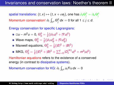
Invariances and conservation laws: Noether’s theorem II
spatial translations: (t , x) 7→ (t , x + εej), one has ∂t Θ0j = ∂k Θk
j
Momentum conservation! ∂t∫Rd Θ0
j dx = 0 for all 1 ≤ j ≤ d.
Energy conservation for specific Lagrangians:
u −m2u = 0, Θ00 = 1
2 (|∂tu|2 + |∇u|2)
Wave maps, Θ00 = 1
2 (|∂tu|2g + |∇u|2g)
Maxwell equations, Θ00 = 1
2 (|E |2 + |B |2)
MKG, Θ00 = 1
2 (|E |2 + |B |2 +∑dα=0 |D
(A)α u|2 + m2|u|2)
Hamiltonian equations refers to the existence of a conservedenergy (in contrast to dissipative systems).
Momentum conservation for KG: ∂t∫Rd ut∇u dx = 0
W. Schlag, http://www.math.uchicago.edu/˜schlag Dispersive Hamiltonian PDEs
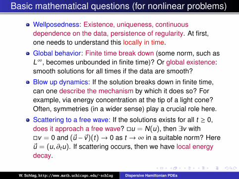
Basic mathematical questions (for nonlinear problems)
Wellposedness: Existence, uniqueness, continuousdependence on the data, persistence of regularity. At first,one needs to understand this locally in time.
Global behavior: Finite time break down (some norm, such asL∞, becomes unbounded in finite time)? Or global existence:smooth solutions for all times if the data are smooth?
Blow up dynamics: If the solution breaks down in finite time,can one describe the mechanism by which it does so? Forexample, via energy concentration at the tip of a light cone?Often, symmetries (in a wider sense) play a crucial role here.
Scattering to a free wave: If the solutions exists for all t ≥ 0,does it approach a free wave? u = N(u), then ∃v withv = 0 and (~u − ~v)(t)→ 0 as t → ∞ in a suitable norm? Here~u = (u, ∂tu). If scattering occurs, then we have local energydecay.
W. Schlag, http://www.math.uchicago.edu/˜schlag Dispersive Hamiltonian PDEs
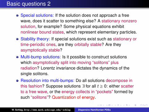
Basic questions 2
Special solutions: If the solution does not approach a freewave, does it scatter to something else? A stationary nonzerosolution, for example? Some physical equations exhibitnonlinear bound states, which represent elementary particles.
Stability theory: If special solutions exist such as stationary ortime-periodic ones, are they orbitally stable? Are theyasymptotically stable?
Multi-bump solutions: Is it possible to construct solutionswhich asymptotically split into moving “solitons” plusradiation? Lorentz invariance dictates the dynamics of thesingle solitons.
Resolution into multi-bumps: Do all solutions decompose inthis fashion? Suppose solutions ∃ for all t ≥ 0: either scatterto a free wave, or the energy collects in “pockets” formed bysuch “solitons”? Quantization of energy.
W. Schlag, http://www.math.uchicago.edu/˜schlag Dispersive Hamiltonian PDEs
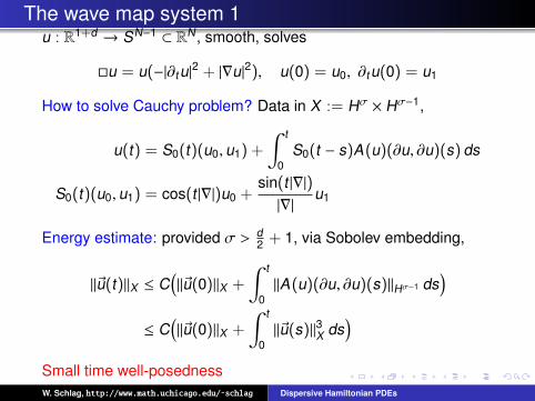
The wave map system 1u : R1+d → SN−1 ⊂ RN, smooth, solves
u = u(−|∂tu|2 + |∇u|2), u(0) = u0, ∂tu(0) = u1
How to solve Cauchy problem? Data in X := Hσ × Hσ−1,
u(t) = S0(t)(u0, u1) +
∫ t
0S0(t − s)A(u)(∂u, ∂u)(s) ds
S0(t)(u0, u1) = cos(t |∇|)u0 +sin(t |∇|)|∇|
u1
Energy estimate: provided σ > d2 + 1, via Sobolev embedding,
‖~u(t)‖X ≤ C(‖~u(0)‖X +
∫ t
0‖A(u)(∂u, ∂u)(s)‖Hσ−1 ds
)≤ C
(‖~u(0)‖X +
∫ t
0‖~u(s)‖3X ds
)Small time well-posednessW. Schlag, http://www.math.uchicago.edu/˜schlag Dispersive Hamiltonian PDEs
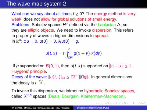
The wave map system 2
What can we say about all times t ≥ 0? The energy method is veryweak, does not allow for global solutions of small energy.Problems: Sobolev spaces Hσ defined via the Laplacian ∆, sothey are elliptic objects. We need to invoke dispersion. This refersto property of waves in higher dimensions to spread.In R3: u = 0, u(0) = 0, ∂tu(0) = g,
u(t , x) = t?
tS2g(x + y)σ(dy)
If g supported on B(0, 1), then u(t , x) supported on∣∣∣|t | − |x |∣∣∣ ≤ 1.
Huygens’ principle.Decay of the wave: ‖u(t , ·)‖∞ ≤ Ct−1‖Dg‖1 In general dimensionsthe decay is t−
d−12 .
To invoke this dispersion, we introduce hyperbolic Sobolev spaces,called Xσ,b spaces (Beals, Bourgain, Klainerman-Machedon).
W. Schlag, http://www.math.uchicago.edu/˜schlag Dispersive Hamiltonian PDEs
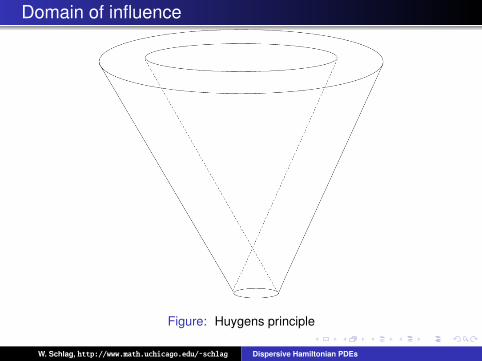
Domain of influence
Figure: Huygens principle
W. Schlag, http://www.math.uchicago.edu/˜schlag Dispersive Hamiltonian PDEs
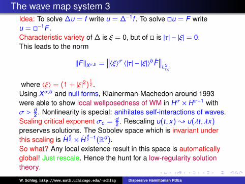
The wave map system 3Idea: To solve ∆u = f write u = ∆−1f . To solve u = F writeu = −1F .Characteristic variety of ∆ is ξ = 0, but of is |τ| − |ξ| = 0.This leads to the norm
‖F‖Xσ,b =∥∥∥〈ξ〉σ 〈|τ| − |ξ|〉b F
∥∥∥L2τ,ξ
where 〈ξ〉 = (1 + |ξ|2)12 .
Using Xσ,b and null forms, Klainerman-Machedon around 1993were able to show local wellposedness of WM in Hσ × Hσ−1 withσ > d
2 . Nonlinearity is special: anihilates self-interactions of waves.Scaling critical exponent σc = d
2 . Rescaling u(t , x) u(λt , λx)preserves solutions. The Sobolev space which is invariant underthis scaling is H
d2 × H
d2−1(Rd).
So what? Any local existence result in this space is automaticallyglobal! Just rescale. Hence the hunt for a low-regularity solutiontheory.
W. Schlag, http://www.math.uchicago.edu/˜schlag Dispersive Hamiltonian PDEs
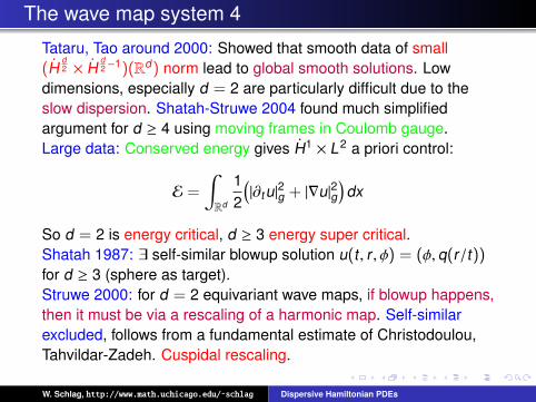
The wave map system 4
Tataru, Tao around 2000: Showed that smooth data of small(H
d2 × H
d2−1)(Rd) norm lead to global smooth solutions. Low
dimensions, especially d = 2 are particularly difficult due to theslow dispersion. Shatah-Struwe 2004 found much simplifiedargument for d ≥ 4 using moving frames in Coulomb gauge.Large data: Conserved energy gives H1 × L2 a priori control:
E =
∫Rd
12
(|∂tu|2g + |∇u|2g
)dx
So d = 2 is energy critical, d ≥ 3 energy super critical.Shatah 1987: ∃ self-similar blowup solution u(t , r , φ) = (φ, q(r/t))for d ≥ 3 (sphere as target).Struwe 2000: for d = 2 equivariant wave maps, if blowup happens,then it must be via a rescaling of a harmonic map. Self-similarexcluded, follows from a fundamental estimate of Christodoulou,Tahvildar-Zadeh. Cuspidal rescaling.
W. Schlag, http://www.math.uchicago.edu/˜schlag Dispersive Hamiltonian PDEs
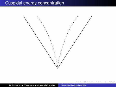
Cuspidal energy concentration
W. Schlag, http://www.math.uchicago.edu/˜schlag Dispersive Hamiltonian PDEs
The wave map system 5
Krieger-S-Tataru 2006: There exist equivariant blowup solutionsQ(rt−ν) + o(1) as t → 0+ for ν > 3
2 and Q(r) = 2 arctan r .Rodnianski-Sterbenz, Raphael-Rodnianski also constructedblowup, but of a completely different nature, closer to the t−1 rate.
For negatively curved targets one has something completelydifferent: Cauchy problem for wave maps R1+2
t ,x → H2, has globalsmooth solutions for smooth data, and energy disperses to infinity(“scattering”). Krieger-S 2009, based on Kenig-Merle approach toglobal regularity problem for energy critical equations, to appear asa book with EMS. Tao 2009, similar result, arxiv.
Sterbenz-Tataru theorem, Comm. Math. Physics: Cauchy problemfor wave maps R1+2
t ,x → M with data of energy E < E0 which is thesmallest energy attained by a non-constant harmonic mapR2 → M. Then global smooth solutions exist.
W. Schlag, http://www.math.uchicago.edu/˜schlag Dispersive Hamiltonian PDEs
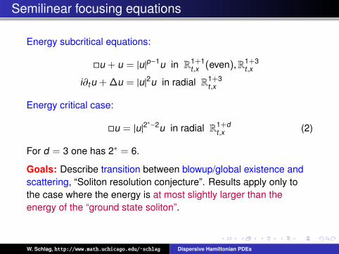
Semilinear focusing equations
Energy subcritical equations:
u + u = |u|p−1u in R1+1t ,x (even),R1+3
t ,x
i∂tu + ∆u = |u|2u in radial R1+3t ,x
Energy critical case:
u = |u|2∗−2u in radial R1+d
t ,x (2)
For d = 3 one has 2∗ = 6.
Goals: Describe transition between blowup/global existence andscattering, “Soliton resolution conjecture”. Results apply only tothe case where the energy is at most slightly larger than theenergy of the “ground state soliton”.
W. Schlag, http://www.math.uchicago.edu/˜schlag Dispersive Hamiltonian PDEs
Basic well-posedness, focusing cubic NLKG in R3
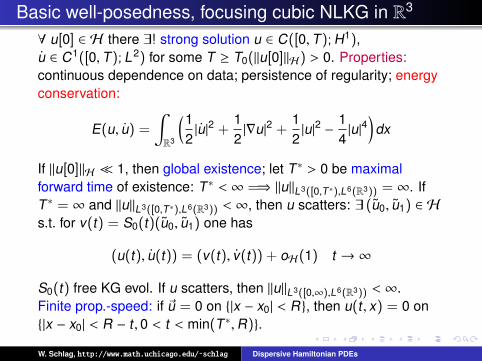
∀ u[0] ∈ H there ∃! strong solution u ∈ C([0,T); H1),u ∈ C1([0,T); L2) for some T ≥ T0(‖u[0]‖H) > 0. Properties:continuous dependence on data; persistence of regularity; energyconservation:
E(u, u) =
∫R3
(12|u|2 +
12|∇u|2 +
12|u|2 −
14|u|4
)dx
If ‖u[0]‖H 1, then global existence; let T∗ > 0 be maximalforward time of existence: T∗ < ∞ =⇒ ‖u‖L3([0,T∗),L6(R3)) = ∞. IfT∗ = ∞ and ‖u‖L3([0,T∗),L6(R3)) < ∞, then u scatters: ∃ (u0, u1) ∈ Hs.t. for v(t) = S0(t)(u0, u1) one has
(u(t), u(t)) = (v(t), v(t)) + oH(1) t → ∞
S0(t) free KG evol. If u scatters, then ‖u‖L3([0,∞),L6(R3)) < ∞.Finite prop.-speed: if ~u = 0 on |x − x0| < R, then u(t , x) = 0 on|x − x0| < R − t , 0 < t < min(T∗,R).
W. Schlag, http://www.math.uchicago.edu/˜schlag Dispersive Hamiltonian PDEs
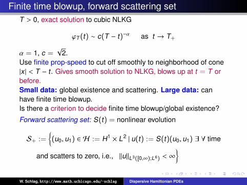
Finite time blowup, forward scattering setT > 0, exact solution to cubic NLKG
ϕT (t) ∼ c(T − t)−α as t → T+
α = 1, c =√
2.Use finite prop-speed to cut off smoothly to neighborhood of cone|x | < T − t . Gives smooth solution to NLKG, blows up at t = T orbefore.Small data: global existence and scattering. Large data: canhave finite time blowup.Is there a criterion to decide finite time blowup/global existence?
Forward scattering set: S(t) = nonlinear evolution
S+ :=(u0, u1) ∈ H := H1 × L2 | u(t) := S(t)(u0, u1) ∃ ∀ time
and scatters to zero, i.e., ‖u‖L3([0,∞);L6) < ∞
W. Schlag, http://www.math.uchicago.edu/˜schlag Dispersive Hamiltonian PDEs
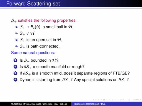
Forward Scattering set
S+ satisfies the following properties:
S+ ⊃ Bδ(0), a small ball in H ,
S+ , H ,
S+ is an open set in H ,
S+ is path-connected.
Some natural questions:
1 Is S+ bounded in H?2 Is ∂S+ a smooth manifold or rough?3 If ∂S+ is a smooth mfld, does it separate regions of FTB/GE?4 Dynamics starting from ∂S+? Any special solutions on ∂S+?
W. Schlag, http://www.math.uchicago.edu/˜schlag Dispersive Hamiltonian PDEs
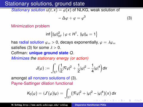
Stationary solutions, ground stateStationary solution u(t , x) = ϕ(x) of NLKG, weak solution of
−∆ϕ + ϕ = ϕ3 (3)
Minimization problem
inf‖ϕ‖2H1 | ϕ ∈ H1, ‖ϕ‖4 = 1
has radial solution ϕ∞ > 0, decays exponentially, ϕ = λϕ∞satisfies (3) for some λ > 0.Coffman: unique ground state Q .Minimizes the stationary energy (or action)
J(ϕ) :=
∫R3
(12|∇ϕ|2 +
12|ϕ|2 −
14|ϕ|4
)dx
amongst all nonzero solutions of (3).Payne-Sattinger dilation functional
K0(ϕ) = 〈J′(ϕ)|ϕ〉 =
∫R3
(|∇ϕ|2 + |ϕ|2 − |ϕ|4)(x) dx
W. Schlag, http://www.math.uchicago.edu/˜schlag Dispersive Hamiltonian PDEs
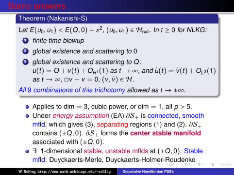
Some answersTheorem (Nakanishi-S)
Let E(u0, u1) < E(Q , 0) + ε2, (u0, u1) ∈ Hrad. In t ≥ 0 for NLKG:1 finite time blowup2 global existence and scattering to 03 global existence and scattering to Q:
u(t) = Q + v(t) + OH1(1) as t → ∞, and u(t) = v(t) + OL2(1)as t → ∞, v + v = 0, (v , v) ∈ H .
All 9 combinations of this trichotomy allowed as t → ±∞.
Applies to dim = 3, cubic power, or dim = 1, all p > 5.Under energy assumption (EA) ∂S+ is connected, smoothmfld, which gives (3), separating regions (1) and (2). ∂S+
contains (±Q , 0). ∂S+ forms the center stable manifoldassociated with (±Q , 0).∃ 1-dimensional stable, unstable mflds at (±Q , 0). Stablemfld: Duyckaerts-Merle, Duyckaerts-Holmer-Roudenko
W. Schlag, http://www.math.uchicago.edu/˜schlag Dispersive Hamiltonian PDEs
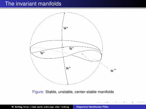
The invariant manifolds
Figure: Stable, unstable, center-stable manifolds
W. Schlag, http://www.math.uchicago.edu/˜schlag Dispersive Hamiltonian PDEs
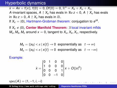
Hyperbolic dynamicsx = Ax + f(x), f(0) = 0,Df(0) = 0, Rn = Xs + Xu + Xc ,A -invariant spaces, A Xs has evals in Re z < 0, A Xu has evalsin Re z > 0, A Xc has evals in iR.If Xc = 0, Hartmann-Grobman theorem: conjugation to etA .
If Xc , 0, Center Manifold Theorem: ∃ local invariant mfldsMu,Ms ,Mc around x = 0, tangent to Xu,Xs ,Xc , respectively.
Ms = |x0| < ε | x(t)→ 0 exponentially as t → ∞
Mu = |x0| < ε | x(t)→ 0 exponentially as t → −∞
Example:
x =
0 1 0 01 0 0 00 0 0 10 0 −1 0
x + O(|x |2)
spec(A) = 1,−1, i,−iW. Schlag, http://www.math.uchicago.edu/˜schlag Dispersive Hamiltonian PDEs
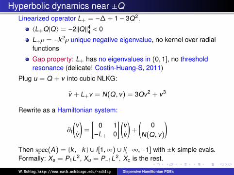
Hyperbolic dynamics near ±QLinearized operator L+ = −∆ + 1 − 3Q2.
〈L+Q |Q〉 = −2‖Q‖44 < 0
L+ρ = −k 2ρ unique negative eigenvalue, no kernel over radialfunctions
Gap property: L+ has no eigenvalues in (0, 1], no thresholdresonance (delicate! Costin-Huang-S, 2011)
Plug u = Q + v into cubic NLKG:
v + L+v = N(Q , v) = 3Qv2 + v3
Rewrite as a Hamiltonian system:
∂t
(vv
)=
[0 1−L+ 0
] (vv
)+
(0
N(Q , v)
)Then spec(A) = k ,−k ∪ i[1,∞) ∪ i(−∞,−1] with ±k simple evals.Formally: Xs = P1L2, Xu = P−1L2. Xc is the rest.
W. Schlag, http://www.math.uchicago.edu/˜schlag Dispersive Hamiltonian PDEs
Schematic depiction of J, K0
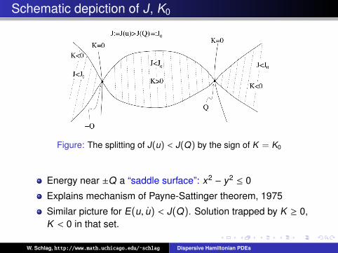
Figure: The splitting of J(u) < J(Q) by the sign of K = K0
Energy near ±Q a “saddle surface”: x2 − y2 ≤ 0
Explains mechanism of Payne-Sattinger theorem, 1975
Similar picture for E(u, u) < J(Q). Solution trapped by K ≥ 0,K < 0 in that set.
W. Schlag, http://www.math.uchicago.edu/˜schlag Dispersive Hamiltonian PDEs
Variational structure above J(Q) (Noneffective!)
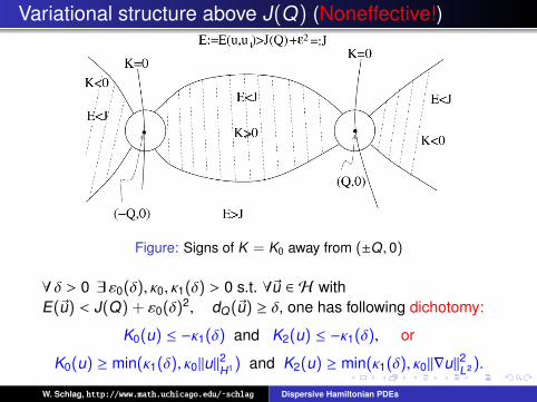
Figure: Signs of K = K0 away from (±Q , 0)
∀ δ > 0 ∃ ε0(δ), κ0, κ1(δ) > 0 s.t. ∀~u ∈ H withE(~u) < J(Q) + ε0(δ)2, dQ(~u) ≥ δ, one has following dichotomy:
K0(u) ≤ −κ1(δ) and K2(u) ≤ −κ1(δ), or
K0(u) ≥ min(κ1(δ), κ0‖u‖2H1) and K2(u) ≥ min(κ1(δ), κ0‖∇u‖2L2).
W. Schlag, http://www.math.uchicago.edu/˜schlag Dispersive Hamiltonian PDEs
Numerical 2-dim section through ∂S+ (with R. Donninger)
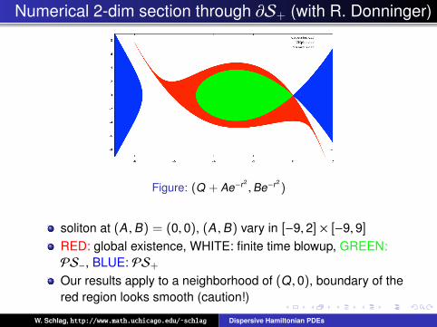
Figure: (Q + Ae−r2,Be−r2
)
soliton at (A ,B) = (0, 0), (A ,B) vary in [−9, 2] × [−9, 9]
RED: global existence, WHITE: finite time blowup, GREEN:PS−, BLUE: PS+
Our results apply to a neighborhood of (Q , 0), boundary of thered region looks smooth (caution!)
W. Schlag, http://www.math.uchicago.edu/˜schlag Dispersive Hamiltonian PDEs
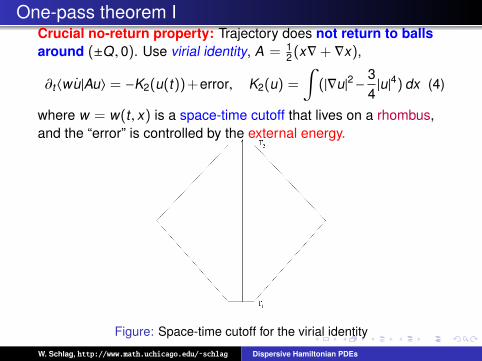
One-pass theorem ICrucial no-return property: Trajectory does not return to ballsaround (±Q , 0). Use virial identity, A = 1
2 (x∇+ ∇x),
∂t〈wu|Au〉 = −K2(u(t))+error, K2(u) =
∫(|∇u|2−
34|u|4) dx (4)
where w = w(t , x) is a space-time cutoff that lives on a rhombus,and the “error” is controlled by the external energy.
Figure: Space-time cutoff for the virial identity
W. Schlag, http://www.math.uchicago.edu/˜schlag Dispersive Hamiltonian PDEs
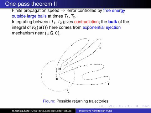
One-pass theorem IIFinite propagation speed⇒ error controlled by free energyoutside large balls at times T1,T2.Integrating between T1,T2 gives contradiction; the bulk of theintegral of K2(u(t)) here comes from exponential ejectionmechanism near (±Q , 0).
Figure: Possible returning trajectories
W. Schlag, http://www.math.uchicago.edu/˜schlag Dispersive Hamiltonian PDEs
EMS/AMS book
W. Schlag, http://www.math.uchicago.edu/˜schlag Dispersive Hamiltonian PDEs