An International Journal

computers & mathematics with applicaticno

PERGAMON Computers and Mathematics with Applications 45 (2003) 1385-1398 www.elsevier.nl/locate/camwa

Invariant Manifolds with Asymptotic Phase for Nonautonomous Difference Equations

B. AULBACH AND C. P~TZSCHE Department of Mathematics, University of Augsburg

D-86135 Augsburg, Germany

Abstract-For autonomous difference equations with an invariant manifold, conditions are known which guarantee that a solution approaching this manifold eventually behaves like a solution on this manifold. In this paper, we extend the fundamental result in this context to difference equations which are nonautonomous and whose solutions are guaranteed only in forward time. @ 2003 Else- vier Science Ltd. All rights reserved.

Keywords-Invariant manifold, Asymptotic phase, Nonautonomous difference equation, Nonin- vertible difference equation, Exponential trichotomy, Reducibility.

1. INTRODUCTION

The concept of asymptotic phase originally occurred in connection with the approach of a solution of an autonomous ordinary differential equation to an orbitally asymptotically stable periodic solution. The well-known Andronov-Witt theorem says that if all but one of the characteristic multiples of a periodic solution p(t) h ave modulus smaller than 1 then any nearby solution behaves asymptotically like a member of the family of periodic solutions ~(t + ‘p) where the phase shift ‘p is the parameter. For ordinary differential equations this result has been extended to manifolds of stationary or periodic solutions and to more general invariant manifolds in [l-4], and for difference equations in [3,5]. In the present paper, we generalize the main result of [3] to the case of a nonautonomous equation whose right-hand side is allowed to be noninvertible and whose invariant manifold does not necessarily consist of stationary solutions. This result may also be considered as a discrete analog of the main result in [2].

The organization of this paper is as follows. In Section 2, we introduce the notation underlying this paper and in Section 3, we prove an auxiliary theorem on the reducibility of linear systems with a certain kind of exponential trichotomy. Section 4 contains another auxiliary result which describes a coordinate change by means of which the main result of this paper can be proved in Section 5.

2. PRELIMINARIES We first fix the notation and introduce the basic concepts underlying this paper. N denotes

the positive integers. A discrete interval I is defined to be the intersection of a real interval with the integers Z = (0, fl, . . . }. For any K E Z we use the abbreviations Zz := [IC, oo) n Z and

0898-1221/03/$ - see front matter @ 2003 Elsevier Science Ltd. All rights reserved. Typeset by .A&-m PII: SO898-1221(03)00093-2

1386 B. AULBACH AND C. PGTZSCHE

Z, := (-03, K.]IXZ. The space of real N x N-matrices is denoted by RN’ N with the zero matrix ON, and GLN(W) is the multiplicative group of invertible matrices in RNX N with the identity IN. N(B) := B-l({O}) denotes the nullspace of a matrix B E RNxN and R(B) := B(RN) its range. For any x E RN, the ball in RN with center Z-C and radius E > 0 is denoted by BE(z). Double bars ]] . ]] stand for an arbitrary norm on RN and our matrix-norms are always induced by vector- norms. In particular, the norm ]]B]]s := ma+llz,r ]]B z z is induced by the Euclidean norm ]I ]]Ic]]~ := (Cr=‘=, ~$)l/~. We write

2’ = f(k, x), (1)

for the difference equation x(k+l) = f(k, x(k)) with the right-hand side f : IxRN + RN where I is a discrete interval. The expression X(k; IC, [) denotes the general solution of equation (1); i.e., X(. ; a, [) solves equation (1) and satisfies the initial condition X( IC; IE, [) = [ for IC E 1 and t E RN. The general solution may be represented recursively as

X(k; K, 6) := E, for k = K,

f(k - 1, X(k - 1; K, E)), for k > K.

Given a matrix sequence A : I -+ RN x N we define the transition matrix G(k, K) E WNxN of the linear equation x’ = A(k)x as the mapping given by

for k = K,

. A(n), for k > K,

and if A(k) is invertible (in RNxN) for k E Z; then we set

9(k, K) := A(k)-1 . . . . . A(/c - 1)-l, for k < K.

Finally, a point [ E RN is called an w-limit point of a mapping p : Zi + RN if there exists a sequence (kn)nEN in Z,$ with limn+oo k, = co and lim,,, ,u(k,) = I.

3. EXPONENTIAL TRICHOTOMIES AND REDUCIBILITY We consider a linear difference equation

x’ = A(k)x, (2)

where the mapping A : Z& --+ RN x N, ICO E Z, is not assumed to have invertible values. Further- more, we consider two sequences of projections P- , P+ : Z$ + RN’ N, K E Z& , with

P-fk + l)A(k) E A(k)P-(k), P+(k + l)A(k) E A(k)P+(k), on Z,+, (3)

and we assume that the relation P- (k) P+ (k) = P+ (k) P- (k) holds on Zz . Hence, IN - P- (k) - P+(k) is a projection on Zz as well. Equation (2) is said to satisfy the regularity condition if the two mappings

4OqP+(q) : R (P+(k)) + R (p+@ + 1,) , 4av(P+(k)+P-(k)) : N (P+(k) + P-(k)) + N (P+(k + 1) + P-(k + 1)))

are invertible for all k E Z$; they are well defined because of the identities (3). If this is the case, we can define the extended transition matrix

. [A(1 - l)l,(,+(,-,))I -l ? for k < L for k = 1,

. . . A(h!(P+(,))~ for k > 1,

Nonautonomous Difference Equations 1387

for (k,l) E (ZZ)2. The complementary expression @pIN-p+-p- (k, 1) is defined analogously. Finally, equation (2) is said to possess an exponential ttichotomy if there exist real numbers 0 < CL < ,8 and K1, K2, KS 2 1 such that the following estimates hold true:

Il@(k,l)P-(l)I1 < K1cxk-‘, for k 2 2 2 K,

\I@~+(~,z)P+(z)(~ 2 K&-“, for 12 k > IC, - (4

I(%,a,-P--P+(W) [IN - P-V) - P+(O] 1) I K3r for k, 1 E Zi.

REMARK 3.1.

(1) If the coefficient matrices appearing in equation (2) are invertible, then the above notion of exponential trichotomy reduces to the corresponding notion used in [5, Definition 1.11. For the differential equations case, see [2].

(2) If the coefficient matrices in equation (2) are independent of k, A(k) = A, then this equa- tion has an exponential trichotomy if all eigenvalues of A with modulus 1 are semisimple.

Equation (2) is called reducible to an equation x’ = B(k)z with B : Zi -t RNxN, if there exists a function A : Z$ -+ BCN(R) with the following properties:

(i) A and A(.)-l are bounded as functions from Z$ to lRNxN; (ii) the identity A(k + l)B(k) = A( holds on Zi.

Later on we need the following reducibility result.

THEOREM 3.2. We suppose system (2) satisfies the following conditions: (i) it has an exponential trichotomy with constants CY, p, K1, K2, K3, and projections P-, Pf

on IQ, K E Z&; (ii) the ranges of the projections are constant on Z$, N- :S rkP-(k), N+ := rkP+(k).

Then system (2) is reducible to a decoupled system

u’ = B-(k)u,

w’ = B+(k)q (5) w’ = B*(k)w,

with B- : Zz -+ RN- xN-, B+ : Z$ + BCN+(W), and B* : Zz + GCN-N--N+ (R). Moreover, the transition matrices V, V, and Q* of the subsystems u’ = B-(k)u, w’ = B+(k)v, and w’ = B*(k)w, respectively, satisfy the estimates

IlV(k, Z)112 5 (2 + K1)6(2 + K2)2Klak-z, for k 1 1 2 IC,

Il@(k,l)112 i (2 + K#(2 + Kz)~Kz@~-‘, for I L k L IS., (6)

Il’J’*W)II, i. (2 + W6(2 + Kz)~&, for k,l E Zi. (7)

(a) Because of the exponential trichotomy of system (2), we have

IIp-(k)l12 I KI, IIp+(k)II, I Kz, for k E zz. (f-9 Using the methods in [6, Lemma 2.21 (for details see [7]) there exists a sequence A : iZ$ --) GLN(l[$) such that on zz we have

(

IN-

A(k)-‘P-(k)A(k) f ON+

) =: D-,

ON-N- -N+

A(k)-‘P+(k)A(k) = (

ON-

IN+

)

-. -. D+, ON-N- -N+

ON-

A(k)-’ [IN - P-(k) -P+(k)] A(k) 3 ON+ -. -. D*,

IN-N- -N+

1388 B. AULBACH AND C. P~TZSCHE

and furthermore, we get

for k E Z;. (9)

Using A as a transformation, system (2) turns into the decoupled system (5), which moreover satisfies the regularity condition with respect to the constant projections D+ and D*. This implies the invertibility of the matrices B+(k) and B*(k) for all k E Z$.

(b) For the transition matrix a’- we obtain

Il’VJ)II, = IlW,W-II, = (IA(k)-‘~(k,l)A(l)D-Il, = IIAW1@(k V-(W)II,

2 (2 + K&2 + IQ2 Il@(kJ)P-(l)lI,

(2 Kl(2 + K#(2 + K2)W-~, for k 2 1 2 tc,

and using arguments as before, one can see that KJ? and 3* satisfy estimates (6) and (7). This completes the proof of Theorem 3.2. I

4. TRANSFORMATION TO QUASILINEAR FORM

For the remainder of this paper, we consider a difference equation

whose right-hand side f : Z&, x JR”’ --+ RN, KO E Z, has the property that f(k, .) is of class C3 for any k E Zz, K E Z& . We suppose that this system has an M-dimensional bounded invariant C3-manifold M c RN. This particularly means that for any initial point (IC,~) in Z& x M, the corresponding solution A( k; IC, E) remains in M for all k E izi. We, furthermore, suppose that any solution ~0 : Z$ + RN of (10) with initial value PO(K) E M satisfies the following hypotheses.

(Hl) The variational equation

Y' = 2 6, clo(k))y

admits an exponential trichotomy with constants 0 < o < 1 < ,B, K1, Kz, K3, and projections P-, P+ whose ranks N- :G rk P-(k) and N+ :E rk P+(k) are constant on Z,$ and satisfy N- + N+ = N - M.

(H2) The limit

~(k,y+~o(k))-~(k,~o(k)) 1 =ON

exists uniformly with respect to k E Zz. (H3) There exists a neighborhood V C_ M of PO(K) such that the derivatives

are bounded.

The following theorem describes a change of coordinates which allows us to transform sys- tem (10) into a particular “quasilinear” form which is suitable for further investigations in the next section.

Nonautonomous Difference Equations 1389

THEOREM 4.1. For any solution p. : Zz + RN of (10) with PO(K) E M and satisfying Hypothe- ses (Hl)-(H3) there exists a local transformation IP, : A,, C Zi x RN -+ RN which transforms system (10) into a system of the form

ii’ = B-(k)?? + & (k , c, 6, ti) iI + B, (k, ii, 6, ti?)C, 5’ = B+(k)??+@ (k,ii,G,ti)G, 8’ = 8 + B; (k,G, 6, ti) fi + B,*(k, ii, 6, tiTJ)i&

(11)

whereGERN-,fiERN+, and 2ir E WM. Furthermore, the following is true.

(a) The domain A,, of the transformation TPO is a neighborhood of the “solution curve” {(k, PO(~)) : k E Zi} with the property that there exists some p1 > 0 with

In addition, for any k E i?$, the mapping 7P, (k, e) is of class C1 and satisfies the identity Tp,(k,po(k)) E 0 on 25:.

(b) The mappings B- and B+ are of type B- : 7&z -+ RN- xN- and B+ : 7,; ---f BLN+ (W), respectively.

(c) The transition matrices Q-, P+ of C’ = B-(k) Q and 6’ = B+(k);, respectively, satisfy the estimates

with real constants l?l, l?z 2 1. (d) The matrix-valued mappings B,, B,, &, &, & are continuous as functions of (fi, 2, &)

and they converge to the respective zero matrix uniformly with respect to k E Zz as (T&i?,&) --+ (O,O,O).

(e) There exist real constants c, C > 0 with the following property: if CL, ,ii : ;Zi + RN are any two solutions of equation (10) which satisfy (k, p(k)), (k, p(k)) E A,, for all k in some subset J C Zi, then the estimates

c II/G) - iG)II 5 ILk cL(k)) - I,o(k, P(k))ll 5 C IIP@) - iG>ll

are valid for all k E J.

PROOF. We subdivide the proof into four steps.

STEP I. In order to decouple the linear part of system (lo), we first use the transformation y = z - po( k) to get from (10) the system

Y' = g (k, po(k))y + r(k, y), (12)

where the remainder term r : Z: x RN + RN turns out to have two continuous partial derivatives with respect to y E RN. Furthermore, we have

r(k,O) E 0, on Z,+, (13)

as well as (cf. (H2))

lim 2 (k, y) = 0, Y+o ay (14)

1390 B. AVLBACH AND C. P~TZSCHE

uniformly with respect to k E Zi. Because of Assumption (Hl), we may apply the reducibil- ity Theorem 3.2 to the linear part of system (12). This provides a transformation matrix A : zi --) 8/c&R), which allows us to decouple this system by means of the transformation Tl:Z~xIWN4UN with Tl(k, y) := A(k)-ly. In fact, the transformed system has the form

u’ = B-(k)u+r-(k,u,v,w),

w’= B+(k)v+r+(k,u,v,w), (15) w’ = B*(k)w + r*(k, u, 21, w),

where B- : Z$ --+ RNmxN-, BS : Zz ---) BLN+ (R), and B* : ;Zz + GLM(R). The phase space RN is split into three parts according to y = (u, V, w) E RN- x RN+ x lR”. Furthermore, the transition matrices W, Qk+, and @* of the linear systems u’ = B-(k)u, v’ = B+(k)w, and w’ = B*(k)w, respectively, obey the estimates

where the constants xi, J?z, Es > 1 only depend on K1, K2, KS and the used norms (see Theorem 3.2(b)). The nonlinearities T-, T+, and T* are twice continuously differentiable with respect to u, V, and w. In addition, because of (13) we get

r-(k,O,O,O)rO, r+(k,O,O,O)rO, r*(k,O,O,O)~O, on Z,+,

as well as (cf. (14))

lim by?--, ?-+, T*)

(~,~,~E4vA0) qu, 21, w) 6, u, v, w) = 0, (17)

uniformly with respect to k E ;Zi. It is worth noting here that both A : Z$ -+ BCN(W) and A(.)-l are bounded.

STEP II. We now determine a local coordinate change which makes the nonlinear terms of system (15) disappear on a set of the form Z$ x (0) x (0) x B where B c RM is an open neighborhood of 0. To this end let X : B -+ M be a local C3-coordinate system of the manifold M with X(0) = PO(K) and X(B) C V. Then, for any v E B the function X(.; ~,x(r])) is a solution of (10) which because of the invariance of M remains in M for all k E Z$. Furthermore, X(.; n, X(v)) - ,ue is a solution of system (12), and therefore, the function

w- (k 71) 4k; rl) =

( ) v+(k; rl) := W$-‘(W; K, X(v)) - PO(k)) (18) v*(k; v)

is a solution of (15) for any r] E B which, moreover, vanishes identically for r] = 0,

v(k;O) = 0, on Z,+. (19)

In addition, the function w(.; 77) is bounded for any fixed r] E B since its values are in M. Differentiating the corresponding solution identity with respect to vi E R, we get

$(k+l;v)= B-(k)

B+(k) + B*(k)

Nonautonomous Difference Equations

oniZ~xBfori=l,..., M. According to (17) and (19) we get for q = 0

$k+l;O)= B- (k)

B+ (k) on z;. (20) z

Thus,theMfunEtions~(~;O),...,~(.;O):Z,t+IRN are solutions of the linear system

u’ = B-(k)u,

w’.= B+(k)v,

w’ = B*(k)w. (21)

Since X : B -+ X(B) is a diffeomorphism, the vectors $$ (0), . . . , $$ (0) E RN are linearly independent, and because of the invertibility of the matrix A(K) E RNxN also the vectors

e (K; 0) (2 A(/c)-lg (O), for i = 1,. . . , M, t 2

are linearly independent. Now we can choose the local coordinate system X of M such that the vectors Z(n;O),..., E (IC; 0) E WM are linearly independent and, since B*(k) E RMxM is reg- ular, we get the linear independence of the solutions $$(.; 0), . . . , $& (.; 0) of the M-dimensional linear system w’ = B*(k) w. Altogether, we thus have

T (k;O) E W,w(~)r for k E Zz. (22)

Furthermore, we get the relation

Finally, the function $$ (s; 0) is bounded by Assumption (H3) because we have

$(k; 0) (it’ A(k)-1 $ (k; n, po(tc)) g(O), for kEiZ,$. (24

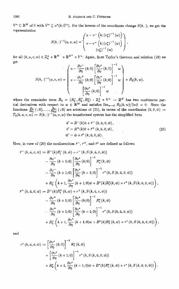
Next, we want to transform system (15) in such a way that the solutions corresponding to v(.;q), 77 E B, get the form (O,O,q). To this end, we consider the mapping S(k,u,v,w) := (U,ZI, 0) + v(k;w) and notice that by Taylor’s theorem this mapping may be represented in the

21 S(k, u, w, w) (g9, 0 w

0 + $ (k; O)w + Rl(kw),

where the remainder term RI = (Rr , Rt , R;) : 25: x B ---f lWN ’ 1s twice continuously differentiable with respect tow E RM and satisfies limW+s Rl(k, w)/11w11 = 0. The mapping w* : Z$ x B -t BM satisfies, because of (19), (22), (23), and

$ (k; 7) (if’ A(k)-’ [ $ 6% K, X(dPX(d + $ (k; Kc, WdP2X(d] ,

together with (H3), the assumptions of Lemma A.1 (see the Appendix). This provides a neigh- borhood U* c B of 0, independent of k, where each vz := w*(k; .) is injective. Lemma A.l, furthermore, implies that (vi)-’ is defined for all k E Zz on a k-independent neighborhood

1392 B. AULBACH AND C. PGTZSCHE

V* 5 IRM of 0 with V* C u*(k; V”). For th e inverse of the coordinate change S(k, .), we get the representation

S(k, .)-yu, w, w) = - (:::;!;;;;::I;] 7

for all (k, U, 21, w) E iZ,+ X RN- X RN+ x V*. Again, from Taylor’s theorem and relation (19) we get

-1

u - g (k; 0) [ F(k;O) 1 w

S(k, .)-l(u, 21, w) = 1: I 21 - g (k; 0) [T (k; O)]

-1

w + R2(k, w),

[ I

-1

T(k;O) w

where the remainder term R2 = (&, Rif , R$) : Z$ x V* + RN has two continuous par- tial derivatives with respect to w E WM and satisfies limW+c R2(k,w)/llwll = 0. Since the functions &(.;O),...,&(.;O) - - are solutions of (21), in terms of the coordinates (u, V, W) := Tz(k, u, w, w) := S(k, .)-I( U, w, w) the transformed system has the simplified form

e’=B-(k)ti+F-(k,ii,~,2TI), i

fi’ = B+(k)a + f+ (k, 4, v, 73) ) (25) w’ = @ + f* (k, ii, ~,.a).

Here, in view of (20) the nonlinearities ?-, v+, and F* are defined as follows:

F- (k,ii, a,@) := B-(k)R, (k,.uT) + T- (k, S (k,e,fl,w))

- f$ (k + l;O) [z (k;O)] -1

R; 6% a)

-F(k+l;O) [$k+l;O)] -1

r*(k,S(k,qqti))

+R, k+l,~(k+l;O)w+B*(k)R;(k,w)+r*(k,S(k,ti,z’,w))), (

r+ (k, U, i?, a) := B+(k)R; (k,a) + r+ (k, S (k,ii, v, a))

-$$k+l;O) [g(k;O)] -1

R; (k 3

- $$ (k + 1;O) [$$ (k + l;O)] -1

r*(k,S(k,ti,&w))

and

-1

r”(k,ii,qa) := 1 $$(k;O) 1 R; (k, 4 1 -1

T* (k, S (k, ii, u, a))

+R; k+l,~(k+l;O)u+B*(k)R;(k,w)+r*(k,S(k,fi,~,~))). (

Nonautonomous Difference Equations 1393

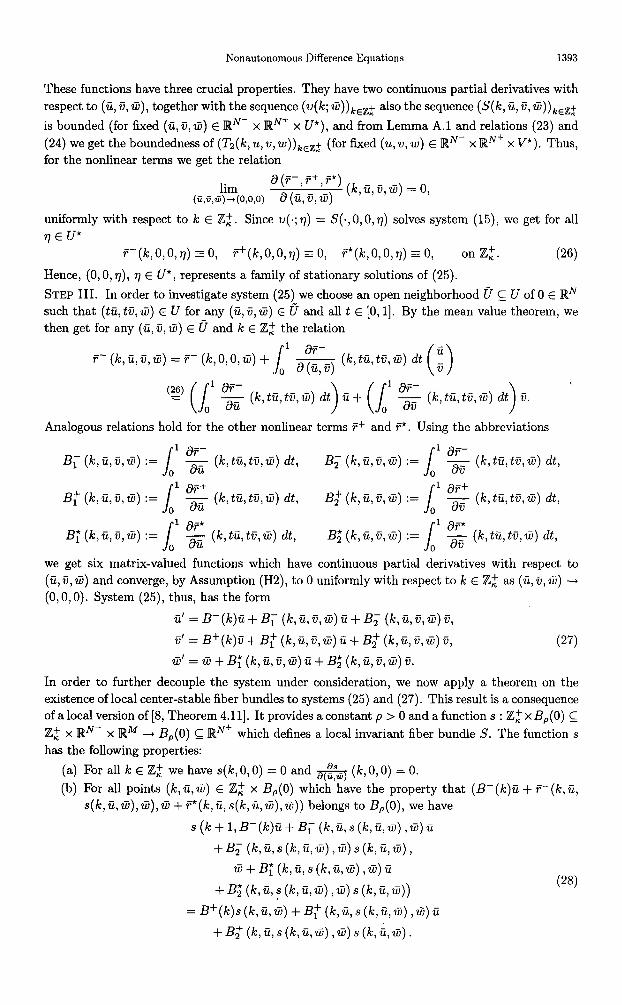
These functions have three crucial properties. They have two continuous partial derivatives with respect to (c, B, c), together with the sequence (v(k; 2~)) kezf also the sequence (S(k, C, V, 3)),eZt is bounded (for fixed (c,G,~TI) E RN- x RN+ x V”), and from Lemma A.1 and relations (23) and (24) we get the boundedness of (Ts(k, u, V, ~))~e~f (for fixed (u, V, W) E RN- x RN+ x V”). Thus, for the nonlinear terms we get the relation

lim (a,o,?i+o,o,o)

y;;+;*’ (k,‘ZL,G,,G) = 0, 7 ,

uniformly with respect to k E iZ$. Since v(.;v) = S(.,O,O,q) solves system (15), we get for all r] E u*

F(k,O,O,q)=O, f+(k,O,o,?+o, F*(k,o,o,7j)‘o, on Z,+. (26) Hence, (0, 0, v), q E U*, represents a family of stationary solutions of (25). STEP III. In order to investigate system (25) we choose an open neighborhood 0 C U of 0 E RN such that (ta, TV, 2~) E U for any (~,‘~,ti) E U and all t E [0, 11. By the mean value theorem, we then get for any (c,v,G) E fi and 5 E Zz the relation

s 1

T=- (k, E, 0, IiT) = P- (k, 0, 0,271) + x (k,tf-i,M,a) dt 0 a(%fl)

(2) (J

l aF- o au. (k,tfi,tqtn) dt

> (s

l ar- ai+ o x (k,t~,t.ij,~) dt ti.

Analogous relations hold for the other nonlinear terms f+ and P. Using the abbreviations

B,+ (k,ii,o,a) := J ’ “+ o aii (k, tii, tfi,a) dt,

(k, tfi, tv, ?ii) dt,

(k, tti, tv, 8) dt,

B; (k,c,o,ci) := I

’ &=+ o ac (k,tG,ti?,a) dt, B; (k, e, a, ti) := J

o1 g (k,t?i,tfi,w) dt,

we get six matrix-valued functions which have continuous partial derivatives with respect to (a, 6, ti) and converge, by Assumption (H2), to 0 uniformly with respect to k E Z$ as (u, 8, W) --) (O,O,O). System (25), thus, has the form

ii’ = B-(k)~ + B, (k, ii, 5, m) ‘1~ + B, (k, fi, zi, a) v,

d = B+(k)u + B,+ (k, a, 9, s) fi + B,+ (k, c, c, w) a, (27) ~‘=8+B;(k,~,~,~)~+Bz*(k,e,a,s)v.

In order to further decouple the system under consideration, we now apply a theorem on the

existence of local center-stable fiber bundles to systems (25) and (27). This result is a consequence of a local version of [8, Theorem 4.111. It provides a constant p > 0 and a function s : Zz x BP(O) C 25; x RN- x BM + BP(O) c RN+ which defines a local invariant fiber bundle S. The function s has the following properties:

(a) For all k E ZL we have .s(k,O,O) = 0 and & (k,O,O) = 0. (b) For all points (k,G,ti) E Z$ x BP(O) which have the property that (B-(k)ti + F(k,fi,

s(k,ii,ti),Q),ti + F*(k,fi, s(k,ii,GJ),G)) belongs to BP(O), we have

s (k + 1, B-(k)fi + B, (k, u, s (k, 4, w) , s) u

+B,(k,a,s(k,c,ti),S)s(k,G,a),

~+B;(k,C,s(k,~,8),w)~

+ B; (k,“,~ (k,ii,a) ,w) s (k,qw))

= B+(k)s(k,ii,s)+B,+(k,ii,s(k,a,a),s)e

+B,+(k,iz,s(k,ti,w),?lr)s(k,i,ti).

(28)

1394 B. AULBACH AND C. P~TZSCHE

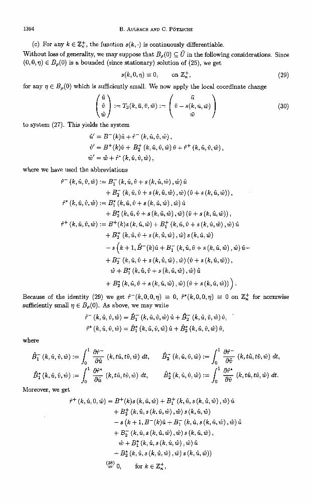
(c) For any k E Z $, the function s(k, .) is continuously differentiable.

Without loss of generality, we may suppose that B,,(O) c 0 in the following considerations. Since (O>O, d E Bp(O) is a bounded (since stationary) solution of (25), we get

s(h 0777) = 0, on Z,+, (2%

for any v E BP(O) w rc is sufficiently small. we now apply the local coordinate change h’ h

?2

0

6 :=T3(k,ii,@,tiJ):= o-&&q 2ir ( - )

(30) 8

to system (27). This yields the system

ii’= B-(k)ti+?- (k,ii,fi,~2~),

6’ = B+(k)5 + B,+ (k, G,~,~)~+~+(IE,&,Qq,

2ir’ = ti + i* (k, i&c, 6))

where we have used the abbreviations

i-(Ic,G,~,~):=B1(k,~,~+s(k,C,~),~)~

+Bz(Ic,~,~+s(Ic,~,zit),~)(~+s(k,5,~)),

+*(k,ii,G,ti) := B;(k,~,~+s(k,Q,2it),2ir)~

+B;(k,ii,fi+s(k,G,ti),~)(~+s(k,O,~)),

P+ (k, G, 6,2i)) := B+(k)s (k ,0,~)+B1+(k,G,~+s(iE,~,2ir),~)~

+Bz+(k,C,~+s(k,G,8),8)s(Ic,G,8)

-s k+l,&-(k)~+B;(k$$+s(k,O,&),zL)Gt (

+B~(k,ii,~+s(k,O,~),ti)(~+~(k,C,2ir)),

2ir+B;(Ic,G,~+s(Ic,~,~),2ir)Q

+ B; (k, ii, 5 + s (k, ii, 61) ,8) (fi + s (k, W))) *

Because of the identity (29) we get P-(k,O,O,q) 2 0, f*(k, O,O, r]) 2 0 on Zz for normwise sufficiently small r] E B,,(O). As above, we may write

P- (k, c, 8, ti) = B, (k ,~,~,~)~++Bz(k,C,~,3)~,

P* (k, 6, G,ti) = I?; (k,ii,G, 6) ii + B; (k, ii, 6, ti) 5,

B, (k, ii, 5, ‘Lir) := s l OP- D x (k,tC,tG,d) dt, s, (k, ii, i3, 6) :=

s

l a+- o x (k, tii, t6, S) dt,

B; (k, G, G,7i) := s

l a+* o x (k,tfi,tii,ti) dt, &(lc,ti,G,&) :=

s

l a+* o x (k,tG,tG,G) dt.

Moreover, we get

i+ (k, ii, O,C) = B+(k)s (k, 0,8)+B1+(k,ii,s(k$,ti),2ir)G

+Bz+(k,iI,s(k,C,ti),zir)s(k,Q,&)

-s(k+l,B-(k)O+B&k,G,s(k,C,~),ti)ii

+B,(k,4,s(k,O,~),~)s(IE,~,2ir),

2i)+B;(Ic,C,s(Ic,~,~),~)~

+ B,* (k, 6, s (k, iiL,2ir) ,3) s (k, ii, G))

(?J) 0 9 for Ic E Z,+,

Nonautonomous Difference Equations 1395

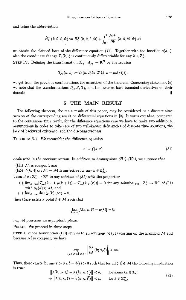
and using the abbreviation

B$ (k, 6, G, 2ir) := I?$ (k, ii, s, &) + J o1 g- (k,ii,ti&ti) dt

we obtain the claimed form of the difference equation (11). Together with the function s(k, .), also the coordinate change Ta(k, =) is continuously differentiable for any k E Z$.

STEP IV. Defining the transformation TP,, : A,, -+ RN by the relation

‘L,(k,~) := TdkT2(k,Tl(k,a: - pa(k)))),

we get from the previous considerations the assertions of the theorem. Concerning statement (e) we note that the transformations Tl, S, T3, and the inverses have bounded derivatives on their domain. I

5. THE MAIN RESULT

The following theorem, the main result of this paper, may be considered as a discrete time version of the corresponding result on differential equations in [2]. It turns out that, compared to the continuous time result, for the difference equations case we have to make two additional assumptions in order to take care of two well-known deficiencies of discrete time solutions, the lack of backward existence, and the disconnectedness.

THEOREM 5.1. We reconsider the difference equation

cc’ = f( k, x) (31)

dealt with in the previous section. In addition to Assumptions (H1)-(H3), we suppose that

(H4) M is compact, and (H5) f(k ‘)lM : M + M is surjective for any k E iZ&.

Thenifp:Zz-+R N is any solution of (31) with the properties

(i) limk-,oo[?;Po (k + 1, p(k + 1)) - TP,,(k, p(k))] = 0 for any solution ~0 : Z$ + RN of (3 with PO(K) E M, and

(ii) limk,, dist (p(k), M) = 0,

then there exists a point [ E M such that

‘1)

&mJ(k; K, E) - dk)I = 0;

i.e., M possesses an asymptotic phase.

PROOF. We proceed in three steps.

STEP I. Since Assumption (H3) applies’to all solutions of (31) starting on the manifold M and because M is compact, we have

Thus, there exists for any E > 0 a S = 6(~) > 0 such that for all t, f E M the following implication is true:

IjX(ko; IS,<) - X (ko; n,f)\I < 6, for some ko E Zz,

~IIX(~;I~,E)-X(~;IC,F)II<E, forkEZ&. (3‘4

1396 B. AULBACH AND C. P~~TZSCHE

STEP II. The compactness of M implies that, because of Property (ii), the function p-has an w-limit point 7 E M. Thus, there exists a sequence (k,),e~ in Zt with

Assumption (H5) then guarantees that the solutions of (31) on M have (not necessarily unique) backward continuations. Therefore, there exists a sequence (~~17n)~e~ in M with

rl = qlc,; 4 %), for n E N. (34)

Since M (and thus, (v~)~~N) is bounded, there exists a converging subsequence (T~_)~~N whose limit 6 := lim,,, nn, belongs to the closed set M. We, therefore, get the estimate

and using (32) and (33) we get

linJp(k,) - X(k,; 4 01 = 0. (35)

Consequently, the solution X(.; K, E) lies in M and the function p - X(.; 6, [) has 0 as w-limit point. In order to simplify our notation, from now on we write (/c~)~~N instead of (&JrnE~.

STEP III. In order to show that the difference p(k) - X(k; K,[) converges to 0 as k -+ 00, we notice that for the function v(k) = (v-,v+,v*)(k) := IJc.;n,~)(k,p(k)) we have, because of Theorem 4.1 (a),

Ix(.;,,&, X(k; &E,E)) = 0, on Z,+. (36)

Because of (35) and the construction of ?JJ(.;n,E), the point 0 E RN is an w-limit point of the function u and it remains to be shown that v(k) converges to 0 as k -+ 00. Assuming the contrary, there exists a real number p E (0, pi) (pi > 0 is defined in Theorem 4.1(a)) and because of Assumption (i) there exists a sequence of nonempty Z-intervals J, := [k,, k$]z, n E M, with k,, kz E Z$, k, < kz < k,+l, such that

lim v(kn) = 0, R-+00

v(k) E BP(O),

v (kn+) E h(O) \ 4/2(O),

forkE U Jo, ?lEPi

for 72 E IV.

(37)

(38)

(39)

On any discrete interval J, the function u is a solution of the linear homogeneous system

u’ = B-(k)u + d,(k, v(k))u + &(k, v(k))w,

w’ = B+(k)v + &(k, v(k))v,

w’ = w + &(k, v(k))u + &(k, v(k))v,

(40)

where the transition matrices \k- and 9+ of u’ = B-(k) u and 21’ = B+(k)w, respectively, satisfy the estimates

Without loss of generality, we may suppose that p > 0 is so small that apart from the estimate

(41)

Nonautonomous Difference Equations 1397

(the positive constants c and C are those of Theorem 4.1(e)), the following estimates are true for all k E UnEPJ J,:

I(B;(k,v(k))l( i min { $, $$} , IIB;(k, v(k))11 5 min { $$, $$},

\l&(k,v(k))/ 5 min { 2, $$} ,

Il&(k,v(k))/ <min{g,$$}, (I&(k,v(k))/ <min{$$,s}.

Using Theorem 4.1(e) we get

ll~(kn’) -+,+;~t)\) (2) i Illx(.;tc,~) (kh+,f))l(

(38) p (41) 1 (42) < ; 5 &)7 for 12 E IV,

and since the sequence (p(kk))nEN is bounded, because of estimate (42), there exists an w-limit point v. := lirnrnhm p(krr+,) E M where (k,+,)mEN is a subsequence of (kz),,,.

As in the second step of this proof we get a point 60 E M such that

)$[/+:,,,1) -+fmi;Go)] =O, (43)

where (k$,,l )m is a further subsequence of ( k$JmEN. Using (42) th is implies that for sufficiently large lo E N we get

\(A (k~m,P~E) - Jf (Cl ;460)(( I ((A (k;t,.pE) -&,)I(

. +llp(k,,,l) -~(k&,~;~,~o)/ ‘?d($$, forlEZi.

Consequently, because of (32) we get from Theorem 4.1(e)

Il~(.;~,~)(k, WC; K,Eo))\[ (? CIlX(k; K,b) - WC; ~,C)ll I PI, for k E “imI,.

Now we are in a position to apply [3, Lemma 8.11 to system (40) and its bounded solution

vo(k) = (6, &G) (k) := Ix(.;n,& W; ~,b)).

This provides a relation of the form

Ema (G, q?, 4) (k) = (O,O,w*) , (44 +

for some w* E RP. From (43) and Theorem 4.1(e) we conclude that the relation

1’i~~ [(W’P’) (k&) - (~,-,d,~;) (k:,,,,)] = (O,O,O)

holds true which, in turn, with (44) yields

/in& (v- , v+ , y*) ( kZml) = (0, 0, w*) . (45)

Then using [3, Lemma B.61 we see that there exist constants Cr, C’s > 0 (which depend only on the growth rates CY, ,0 and I?r, I?s) with the property

IIv* (k,+_,) 11 5 llu* (k) II+ Cl IIv- (4 II + c2 IIv+ (kL> 11 .

Because of (37) and (45), the sequence (v*(k,+,,))lEN and consequently also the sequence

wn+,, )hEW converges to 0 as 1 ---t 00. This, however, contradicts relation (39). I

1398 B. AULBACH AND C. PGTZSCHE

APPENDIX

PARAMETER-DEPENDENT INVERSE FUNCTIONS For the reader’s convenience, we state here a qualitative inverse function theorem which can

be shown using [9, Proposition 2.5.61.

LEMMA A.l. Let R be an open neighborhood of the zero vector of some Banach space X and let T : P x R -+ X be a mapping such that T(p, .) is of class Cm (m 1 2) for any p in some nonempty set P. Furthermore, assume the following:

(i) T(p, 0) = 0 on P; (ii) the partial derivatives $$ (p, 0) : X + X are invertible’ for p E P;

(iii) M := suppEp 11 [g (p, O)]-‘11 < co;

(iv) K := SU~~~,,~~~~BR(O) 11 g (p, x)/I < 00 for some R > 0 with BE(O) G 0.

Then, using the abbreviation P := min{R, 1/2KM}, there exists a uniquely determined mapping

s : 7’ X BP/IM (0) + X with the following properties:

(a) S is bounded; more explicitly,

IMP, Y)II I p, for (P, Y) E p .x BPIZM@).

(b) S(p, 9) is the inverse function of T(p, .); more explicitly,

T(P, 0, Y)) = Y> for (P, Y) E p x BP/zM($

cc) ‘%‘T ‘)bp,&J) is of class C” for each p E P.

REFERENCES 1. B. Aulbach, Behavior of solutions near manifolds of periodic solutions, Journal of Differential Equations 39,

345-377, (1981). 2. B. Aulbach, Invariant manifolds with asymptotic phase, Nonlinear Analysis, Theory, Methods d Applications

6, 817-827, (1982). 3. B. Aulbach, Continuous and discrete dynamics near manifolds of equilibria, In Lecture Notes in Mathematics,

Volume 1058, Springer-Verlag, Berlin, (1984). 4. J. Mpez-Fenner and M. Pinto, On (h, k) manifolds with asymptotic phase, Journal of Mathematical Analysis

and Applications 216, 549-568, (1997). 5. .I. L6pez-Fenner and M. Pinto, (h, k)-Trichotomies and asymptotics of nonautonomous difference systems,

Computers Math. Applic. 33 (lo), 105-124, (1997). 6. I. Gohberg, M.A. Kaashoek and J. Kos, Classification of linear time-varying difference equations under

kinematic similarity, Integral Equations and Operator Theory 25 (4), 445-480, (1996). 7. C. PGtzsche, Nichtautonome Differenzengleichungen mit station&en and invarianten Mannigfaltigkeiten,

Diploma Thesis, University of Augsburg, (1998). 8. B. Aulbach, C. PGtzsche and S. Siegmund, A smoothness theorem for invariant fiber bundles, Journal of

Dynamics and Diflerence Equations 14 (3), 519-547, (2002). 9. R.H. Abraham, J.E. Marsden and T. Ratiu, Manifolds, Tensor Analysis, and Applications, Applied Mathe-

matical Sciences, 75, Springer-Verlag, Berlin, (1988).