INVARIANT TORI IN THE LUNAR PROBLEM

Publ. Mat. (2014), 353–394

Proceedings of New Trends in Dynamical Systems. Salou, 2012.DOI: 10.5565/PUBLMAT Extra14 19

INVARIANT TORI IN THE LUNAR PROBLEM

Kenneth R. Meyer, Jesus F. Palacian, and Patricia Yanguas

Dedicated to Jaume Llibre on his 60th birthday

Abstract: Theorems on the existence of invariant KAM tori are established for

perturbations of Hamiltonian systems which are circle bundle flows. By averagingthe perturbation over the bundle flow one obtains a Hamiltonian system on the orbit

(quotient) space by a classical theorem of Reeb. A non-degenerate critical point of the

system on the orbit space gives rise to a family of periodic solutions of the perturbedsystem. Conditions on the critical points are given which insure KAM tori for the

perturbed flow.These general theorems are used to show that the near circular periodic solutions

of the planar lunar problem are orbitally stable and are surrounded by KAM 2-tori.

For the spatial case it is shown that there are periodic solutions of two types, eithernear circular equatorial, that is, the infinitesimal particle moves close to the plane

of the primaries following near circular trajectories and the other family where the

infinitesimal particle moves along the axis perpendicular to the plane of the primariesfollowing near rectilinear trajectories. We prove that the two solutions are elliptic

and are surrounded by invariant 3-tori applying a recent theorem of Han, Li, and Yi.

In the spatial case a second averaging is performed, and the corresponding or-bit space (called the twice-reduced space) is constructed. The flow of the averaged

Hamiltonian on it is given and several families of invariant 3-tori are determined using

Han, Li, and Yi Theorem.

2010 Mathematics Subject Classification: 34C20, 34C25, 37J15, 37J40, 53D20,70F10, 70K50, 70K65.

Key words: Averaging, normalization, symmetry reduction, orbit space, restrictedthree-body problem, planar and spatial lunar problems, invariant theory, periodicsolutions, action-angle coordinates, invariant KAM tori.

1. Introduction

In an earlier paper [36] the authors investigated the existence, char-acteristic multipliers and stability of periodic solutions of a Hamiltonianvector field which is a small perturbation of a vector field tangent to thefibers of a circle bundle. Our primary examples are the planar and spa-tial lunar problems of celestial mechanics, i.e., the restricted three-bodyproblem where the infinitesimal particle is close to one of the primaries.

354 K. R. Meyer, J. F. Palacian, P. Yanguas

By averaging the perturbation over the fibers of the circle bundleone obtains a Hamiltonian system on the orbit (quotient) space of thecircle bundle. We stated and proved results which have hypotheses onthe reduced system and draw conclusions about the full system. Thenwe applied the general results to the planar and spatial lunar problems.After scaling, the lunar problem is a perturbation of the Kepler problem,which after regularization is a circle bundle flow. We found the classicalnear circular periodic solutions in the planar case and the near circularequatorial and certain near rectilinear periodic solutions in the spatialcase. Then we computed their approximate multipliers and showed thatthere is a “twist”. However, the twist was too degenerate to apply theclassical KAM Theorem on invariant tori as stated in [2].

In this paper we prove sharper general stability theorems that showwhen a degenerate twist is adequate to establish invariant tori near a pe-riodic solution. For two-degrees-of-freedom problems it is enough to ap-peal to the classical invariant curve theorem [28], but higher-dimensionalproblems require the more delicate recent result of Han, Li, and Yi [16].

Then we apply these general theorems to show that the circular pe-riodic solutions of the planar lunar problem are enclosed by invariant2-tori, hence orbitally stable and in the spatial case that there are in-variant 3-tori enclosing the periodic solutions that are near circular equa-torial or near rectilinear in the vertical axis.

We also deal with the axial symmetry reduction in the spatial lunarproblem. This is achieved by performing a second averaging, specifically,normalizing the argument of the node. After truncating higher-orderterms the third component of the angular momentum becomes an inte-gral of the normalized Hamiltonian and we build the corresponding orbitspace called the twice-reduced space. This leads to the appearance ofelliptic relative equilibria of the normalized Hamiltonian for some combi-nations of the parameters. This allows us to obtain invariant KAM torirelated to these equilibria. Because of the degeneracy of the averagedHamiltonian we cannot apply the usual KAM Theorems to conclude theexistence of invariant tori. Again we resort to the theorem by Han, Li,and Yi [16] to overcome this difficulty. Using some local action-anglecoordinates that we construct specifically for the different types of ellip-tic relative equilibria, we establish the existence of KAM 3-tori for theHamiltonian of the spatial restricted three-body problem in the lunarcase.

The paper has five sections. In Section 2 we give the general resultsthat will be used in subsequent sections. Some of the results of Sec-tion 2 are classic, some others are recent. Some of the results collected

Invariant Tori in the Lunar Problem 355

in this section appeared in [36] but Subsections 2.2, 2.3, and 2.4 are new(leaving apart Theorem 2.4). Section 3 contains the application to theplanar lunar problem, leading to the existence of families of KAM 2-toriaround the near circular orbits. In Section 4 we deal with the spatialcase by constructing the orbit space which is a symplectic manifold ofdimension four. We analyze the relative equilibria and their stability,concluding with the existence of two families of KAM 3-tori, one relatedto motions that are near circular equatorial and the other related withmotions near rectilinear. Section 5 is devoted to a further reduction forthe spatial problem. After averaging with respect to the node we trun-cate higher-order terms and obtain a Hamiltonian which has the thirdcomponent of the angular momentum as an integral. Thus we can carryout a second reduction process, the so-called axial symmetry reduction,passing from the four-dimensional orbit space to an orbit space of di-mension two, the twice-reduced space. The analysis of the flow on thisspace is made in detail and we can reconstruct some families of KAM 3-tori using Theorem 2.4. This is achieved after constructing appropriatesets of action-angle pairs in the three types of relative equilibria that areelliptic.

The analysis performed in Sections 3 and 4 is a continuation of thework initiated in [36] but the conclusions on the existence of the invariant2- and 3-tori that we present in this paper are new. On the other handpart of the study in Section 5 has appeared in [9, 21, 22, 32] but theanalysis of these papers is incomplete. A rather complete analysis wasprovided by Sommer [35] but, in our opinion, it is very involved so wehave tried to simplify it in our presentation. Nevertheless Sommer buildsa specific theorem for dealing with Hamiltonians where the perturbationappears at three different scales, making it very degenerate, and it isto her credit that she obtained a KAM-type result that applies to thespatial lunar problem which establishes the existence of new families ofinvariant 3-tori. Han, Li, and Yi [16] have a more general result whichincludes that of Sommer and it is precisely this result, Theorem 2.4, thatwe apply to obtain our KAM tori. Moreover we connect the results ofSection 5 with those of Section 4 to clarify some points that are a bitobscure in Sommer’s presentation.

2. Perturbation theorems

2.1. The orbit space. In this subsection we summarize some generalresults from our earlier paper [36]. Let (M,Ω) be a symplectic manifoldof dimension 2n, H0 : M → R a smooth Hamiltonian which defines a


Hamiltonian vector field Y0 = (dH0)# with symplectic flow φt0. LetI ⊂ R be an interval such that each h ∈ I is a regular value of H0

and N0(h) = H−10 (h) is a compact connected circle bundle over the

orbit space B(h) with projection π : N0(h) → B(h). Assume that thevector field Y0 is everywhere tangent to the fibers of N0(h), i.e., thatall the solutions of Y0 in N0(h) are periodic. We assume that all theseperiodic solutions have periods smoothly depending only on the valueof the Hamiltonian, i.e., the period is a smooth function T = T (h)(sometimes the dependence on h will be omitted in the notation).

Now we state two of Reeb’s classic Theorems [33] in more modernterminology referring to our earlier paper for proofs. Our proofs gavemore insight on the Hamiltonian structure and therefore lead to furtherapplications. The original reduction theorem is the following

Theorem 2.1. The orbit space B inherits a symplectic structure ωfrom (M,Ω), i.e., (B,ω) is a symplectic manifold.

Now look at a perturbation of this situation. Let ε be a small pa-rameter, H1 : M → R smooth, Hε = H0 + εH1, Yε = Y0 + ε Y1 = dH#

ε ,Nε(h) = H−1

ε (h), and φtε the flow defined by Yε. We shall refer to thisas the full system.

Let the average of H1 be

H =1

T

∫ T

0

H1(φt0) dt,

which is a smooth function on B(h), and let φt be the flow on B(h)

defined by Y = dH#. We refer to this as the reduced system.

A critical point of H is non-degenerate if the Hessian at the criticalpoint is non-singular.

Theorem 2.2. If H has a non-degenerate critical point at π(p) = p ∈ Bwith p ∈ N0, then there are smooth functions p(ε) and T (ε) for ε smallwith p(0) = p, T (0) = T , p(ε) ∈ Nε, and the solution of Yε through p(ε)is T (ε)-periodic.

Let the characteristic exponents of the critical point Y (p) be λ1, λ2, . . . ,λ2n−2.Then the characteristic multipliers of the periodic solution throughp(ε) are

1, 1, 1 + ε λ1 T +O(ε2), 1 + ε λ2 T +O(ε2), . . . , 1 + ε λ2n−2 T +O(ε2).

That is to say, a non-degenerate critical point of the reduced systemgives rise to a periodic solution of the full system. The essence of theproof of Theorem 2.2 is the existence of symplectic coordinates for atubular neighborhood of the orbit through p.


Lemma 2.1. Let p ∈ N0(h), with h ∈ I fixed. Then there are symplec-tic coordinates (I, θ, y), valid in a tubular neighborhood of the periodicsolution φt0(p) of Y0(h), where (I, θ) are action-angle coordinates, andy ∈ N , where N is an open neighborhood of the origin in R2n−2. Thepoint p corresponds to (I, θ, y) = (0, 0, 0).

In these coordinates H0 is only a function of I, i.e., H0 = H0(I). Alocal cross section is θ = α, and a local cross section in an energy levelis θ = α, I = β, where α, β are constants. In addition to that, y ∈ Nare coordinates in the cross section in the energy level.

The Hamiltonian is

(1) Hε(I, θ, y) = H0(I) + εH1(I, θ, y) = H0(I) + εH(I, y) +O(ε2).

2.2. Invariant 2-tori. Sometimes one can detect invariant tori usingKAM Theory and at times even stability. First let us consider a simpletwo-degree-of-freedom system where the orbit space is two-dimensional.

Theorem 2.3. Let n = 2 and let p be as in Theorem 2.2 and Lemma 2.1.Suppose there are symplectic action-angle variables (I1, θ1) at p in B suchthat

(2) H = ω1 I1 + ε k(I, I1) +O(ε2),

where ω1 is non-zero and

(3)∂2k(I, I1)

∂I21

6= 0.

Then for sufficiently small ε > 0 encircling the periodic solutions given inTheorem 2.2 there are invariant KAM tori of dimension 2. In particularthe periodic solutions are orbitally stable.

Proof: Take the cross section at p given by Lemma 2.1 with θ = 0 andI = 0. The first return time is Tε = T +O(ε2).

On B the equations are

I1 = O(ε2), θ1 = −ω1 − ε∂k

∂I1(0, I1) +O(ε2).

Integrate these equations by a time Tε to find the period map P : (I1,θ1)→(I ′1, θ

′1) where

I ′1 = I1 +O(ε2), θ′1 = θ1 − ω1 T − ε T∂k

∂I1(0, I1) +O(ε2).

By (3) the twist assumption of Moser’s invariant curve Theorem [28]holds which implies the existence of arbitrarily small invariant curvesencircling p in the cross section. These invariant curves produce invariant


tori in the phase space of the full system defined by (1) and so theperiodic solutions are orbitally stable.

2.3. Higher-order tori. First we state the result of Han, Li, andYi [16], because it gives invariant tori in systems with a degeneratetwist of the type we encounter in the lunar problem and other similarproblems [26]. Refer to those papers for comments about other resultsthat yield KAM tori in degenerate situations.

Starting with a Hamiltonian system of the form

(4) H(I, ϕ, ε)=h0(In0)+εm1h1(In1)+· · ·+εmaha(Ina)+εma+1p(I, ϕ, ε),

where (I, ϕ) ∈ Rn × Tn are action-angle variables with the standardsymplectic structure dI ∧dϕ, and ε > 0 is a sufficiently small parameter.The Hamiltonian H is real analytic in (I, φ, ε) and in particular p issmooth in ε. The parameters a, m, ni (i = 0, 1, . . . , a) and mj (j =1, 2, . . . , a), are positive integers satisfying n0 ≤ n1 ≤ · · · ≤ na = n,m1 ≤ m2 ≤ · · · ≤ ma = m, Ini = (I1, . . . , Ini

), for i = 1, 2, . . . , a.The Hamiltonian H(I, ϕ, ε) is considered in a bounded closed region

Z × Tn × [0, ε∗] ⊂ Rn × Tn × [0, ε∗] for some fixed ε∗ with 0 < ε∗ < 1.For each ε the integrable part of H,

Xε(I) = h0(In0) + εm1 h1(In1) + · · ·+ εma ha(Ina),

admits a family of invariant n-tori T εζ = ζ × Tn with linear flows

x0 + ωε(ζ)t, where, for each ζ ∈ Z, ωε(ζ) = ∇Xε(ζ) is the frequencyvector of the n-torus T εζ and ∇ is the gradient operator. When ωε(ζ)is non-resonant, the flow on the n-torus T εζ becomes quasi-periodic withslow and fast frequencies of different scales. We refer the integrablepart Xε and its associated tori T εζ as the intermediate Hamiltonianand tori, respectively.

Let Ini = (Ini−1+1, . . . , Ini), i = 0, 1, . . . , a (where n−1 = 0, hence

In0 = In0), and define

Ω =(∇In0h0(In0), . . . ,∇Inahna

(Ina))

such that for each i = 0, 1, . . . , a, ∇Ini denotes the gradient with respectto Ini .

The following theorem gives the right setting in which one can ensurethe persistence of KAM tori for Hamiltonians like (4).


Theorem 2.4 (Han, Li, and Yi [16]). Let δ be given with 0 < δ < 1/5.Assume there is a positive integer s such that

(5) Rank∂αI Ω(I) | 0 ≤ |α| ≤ s

= n, ∀ I ∈ Z.

Then there exists an ε0 > 0 and a family of Cantor sets Zε ⊂ Z, 0 < ε <ε0, such that each ζ ∈ Zε corresponds to a real analytic, invariant, quasi-periodic n-torus T

ε

ζ of the Hamiltonian (4) which is slightly deformed

from the intermediate n-torus T εζ . The measure of Z \Zε is O(εδ/s) and

the family T εζ : ζ ∈ Zε, 0 < ε < ε0 varies Whitney smoothly.

The beauty of this level of generalization is that if the conditions ofTheorem 2.4 apply to the Hamiltonian on the orbit space then conditionsof Theorem 2.4 apply to the full system. This follows by using Lemma 2.1in conjunction with Han, Li, and Yi’s Theorem.

However for one of our applications we require something less, namely

Theorem 2.5. Let p be as in Theorem 2.2 and suppose there are sym-plectic action-angle variables (I1, . . . , In−1, θ1, . . . , θn−1) at p in B suchthat

(6) H =

n−1∑k=1

ωk Ik +εj

2

n−1∑k=1

n−1∑l=1

Ckl Ik Il +O(εj+1),

where j ≥ 0, the ωk’s are non-zero, the coefficients Ckl’s are independentof ε and satisfy Ckl = Clk, and all the cubic and higher-order terms inI1, . . . , In−1 are included in O(εj+1).

Assume that detCkl 6= 0. That is, assume the system has been put intoBirkhoff normal form and a “twist” condition is satisfied. Furthermore,assume dT/dh 6= 0, i.e., assume the period varies with H0 in a non-trivial way.

Then for sufficiently small ε > 0 near the periodic solution given inTheorem 2.2 there are invariant KAM tori of dimension n.

Proof: The numbering system of our notation and that of Han, Li,and Yi as stated in Theorem 2.4 are slightly different. Let the Ij ’sbe I, I1, . . . , In−1 where I is as in Lemma 2.1 and I1, . . . , In−1 are asabove. If you think of I as I0 then we have shifted the indexes down by1.

Combining (1) with (2) gives

(7) Hε(I, θ, y) = H0(I) + ε

n−1∑k=1

ωk Ik +εj+1

2

n−1∑k=1

n−1∑l=1

Ckl Ik Il+O(εj+2).


The assumption that dT/dh 6= 0 is equivalent to ∂2H0/∂I2 6= 0. Now

condition (5) is satisfied since it is clear that the rank of

∂αI Ω(I) =

[∂2H0/∂I

2 0

0 C

]

is n where C is the matrix [Ckl] and s = 1.

2.4. Regularization. In our subsequent applications of Theorems 2.4and 2.5, the term H0 will be the Hamiltonian of the Kepler problem.For the consideration of circular solutions (in the planar and the spatialcases) or equatorial solutions (in the spatial case) of the restricted three-body problem, classical Poincare-like coordinates assure that dT/dh 6= 0,but for the rectilinear ones which pass close to collisions we will need touse regularized coordinates. The Kepler problem has a removable singu-larity due to collisions of the infinitesimal with the primary. Removingthe singularity is called regularization. It is important in our study ofcollision and near-collision periodic solutions and their related invarianttori.

Moser [29] shows that the n-dimensional Kepler problem can be reg-ularized in the sense that there is a symplectomorphism that takes theKepler flow for a fixed negative energy level to the geodesic flow ontothe unit tangent bundle of the punctured n-sphere, Sn, punctured atthe north pole. The geodesic flow of the unit sphere over the north polecorresponds to the collision orbits and by adding it back in effect addsthe collisions in a regular flow.

Let E be the whole negative energy region of the Kepler problem,the elliptic region, and let T+Sn be the tangent bundle of the punc-tured sphere minus the zero section. Ligon and Schaaf [24] show how to

transform canonically the whole elliptic region E to the bundle T+Sn.This transformation takes the usual Hamiltonian of the Kepler prob-lem to a Hamiltonian D on T+Sn. Hamiltonian D extends naturallyto T+Sn thus making effective the regularization of the Kepler problemfor all negative energies. Also see [10] and the simpler approach givenby Heckman and de Laat in [18].

For the Kepler problem or the flow defined by D the period is constanton energy levels and dT/dh 6= 0 even at the regularized collision orbits.This is precisely what we need to assure the existence of families ofinvariant 2-tori in Section 3 and invariant 3-tori in Sections 3 and 4,even around the near rectilinear periodic solutions in Subsection 4.3.


3. The planar lunar problem

3.1. The averaged Hamiltonian for the planar problem. Herewe briefly summarize the normalization and reduction as given in [36].For us the lunar problem is the restricted three-body problem wherethe infinitesimal is close to one of the primaries. We start with theHamiltonian of the planar restricted three-body problem given by:

(8) H =1

2(y2

1 + y22)− (x1 y2 − x2 y1)

− µ√(x1 − 1 + µ)2 + x2

2

− 1− µ√(x1 + µ)2 + x2

2

.

First we perform the linear change from y2 and x1 to y2 − µ and x1 − µrespectively to bring one primary to the origin. Then, we introducea small parameter ε by replacing y = (y1, y2) by ε−1(1 − µ)1/3 y andx = (x1, x2) by ε2(1 − µ)1/3 x. By doing so we restrict H to the casewhere the infinitesimal is moving around one of the primaries. Thischange is symplectic with multiplier ε−1(1 − µ)−2/3, thus H must bereplaced by ε−1(1− µ)−2/3H.

Next we scale time by dividing t by ε3 and multiplying H by ε3. Thenwe expand the resulting Hamiltonian in powers of ε to get

(9) Hε =1

2(y2

1 + y22)− 1√

x21 + x2

2

− ε3(x1 y2 − x2 y1) +1

2ε6 µ(−2x2

1 + x22) +O(ε8).

The zeroth-order term is the Hamiltonian of the Kepler problem andthe O(ε3) term is due to the rotating coordinates. It is not until O(ε6)that the other primary influences the motion. This applies for the wholetreatment of the lunar planar and spatial restricted three-body problemsin this section and in Sections 4 and 5.

To construct this flow on the orbit space of (9) we used in [36] a blendof polar and Delaunay coordinates so that the Hamiltonian is ready forthe elimination of the mean anomaly ` to high order by means of thenormalization of Delaunay [12, 13]. This normalization is effectivelythe average of the perturbation over the periodic motions of the Keplerproblem.

The orbit space for the regularized planar Kepler problem is a 2-sphere S2 [29]. A coordinate system for the reduced space is a = G +LA, where G is the angular momentum vector, L is the square root


of the semimajor axis, and A is the perigee vector1. One has A =e(cos g, sin g, 0) and then a1 = e cos g, a2 = e sin g and a3 = G, with G

the third component of G, and e =√

1−G2/L2 the eccentricity. Onecan check that |a| = L and the vector a uniquely determines an orbitof the Kepler problem on the energy level h = −1/(2L2). Each pointon the sphere a2

1 + a22 + a2

3 = L2 corresponds to a bounded orbit of theKepler problem. The points (0, 0,±L) correspond to circular motions,the circle a3 = 0 corresponds to collision motions, and the other points onthe sphere correspond to elliptic motions. The complement of (0, 0,±L)∪a3 = 0 is the orbit space of the elliptic domain E .

We now have

(10) H = −a3 −3

4ε3 µL2(3 a2

1 − 2 a22) +O(ε5).

We note that this Hamiltonian is well defined and smooth on the excep-tional set (0, 0,±L) ∪ a3 = 0 so (10) is the Hamiltonian on the fullorbit space S2.

The Hamiltonian (10) has two non-degenerate critical points, a maxi-mum at a = (0, 0,−L) and a minimum at a = (0, 0, L), which correspondto near circular periodic solutions of the planar restricted three-bodyproblem of period T (ε) = T + O(ε3). These are the classical Hill’s or-bits of the restricted problem, which are the continuation of the circularsolutions of the Kepler problem (see [7, 25] and the references therein).The maximum gives the prograde orbit and the minimum the retrogradeone.

Since H = −a3 + · · · the linearized equations about (0, 0,±L) area1 = a2, a2 = −a1, and so the characteristic exponents at these criticalpoints are ±i.

Thus, these near circular periodic solutions are elliptic with charac-teristic multipliers 1, 1, 1 + ε3 T i+O(ε6) and 1− ε3 T i+O(ε6).

To see if Theorem 2.3 applies at (0, 0,±L) we need several changes ofvariables. We start by moving the equilibria (0, 0,±L) to the origin of acoordinate system. Therefore, we define

a1 = a1, a2 = a2, a3 = a3 ∓ L,

1The vector A points to the perigee which is often attributed to Laplace, Runge, Lenzand others. But since Newton and Kepler knew that perigee was fixed we choose thisneutral name.


and then we introduce (local) symplectic coordinates Q and P as:

Q =√

2La1√

2L± a3

=√

2(L∓G) cos g,

P = ±√

2La2√

2L± a3

= ±√

2(L∓G) sin g.

By recalling that (`, g, L,G) are symplectic variables, it is straightfor-ward to check that (Q,P ) are symplectic. These coordinates are validin the hemispheres ±a3 > 0 (i.e., ±G < L).

Now, to write H in these coordinates first note that

1

2(Q2 + P 2) = L∓G = L∓ a3,

and also

a21 =

Q2

2L2(L± a3), a2

2 =P 2

2L2(L± a3).

Making this change of variables and omitting additive constants gives

H = ±1

2(Q2 + P 2)− 3

16ε3 µ(2P 2 − 3Q2)(Q2 + P 2 − 4L) +O(ε5).

Change to action-angle variables by

Q =√

2 I1 cos θ1, P =√

2 I1 sin θ1

to get

H = ±I1 −3

4ε3 µ I1(2L− I1)(−2 + 5 cos2 θ1) +O(ε5),

then average over θ1 to get

H = ±I1 −3

8ε3 µ I1(2L− I1) +O(ε5).

To apply Theorem 2.3 make the identification k = − 38µ I1(2L − I1).

Now

(11)∂2k

∂I21

=3

4µ,

and it does not vanish. So the hypotheses of Theorem 2.3 hold (afterreplacing ε3 by δ and considering δ the small parameter of Section 2).Moreover, the measure of the frequencies of the invariant curves appear-ing in the proof of Theorem 2.3 is positive. Also, we can be assured thatthere are invariant 2-tori surrounding the periodic solutions arbitrarilyclose to it. Thus we have proved the following


Proposition 3.1. The near circular periodic solutions of the planarlunar problem are orbitally stable and enclosed by invariant KAM 2-torifor small enough ε.

4. The spatial lunar problem

4.1. The averaged Hamiltonian for the spatial problem. Againwe summarize results from [36]. As in the planar case we start with theHamiltonian of the spatial problem given in the rotating frame by

(12) H =1

2(y2

1 + y22 + y2

3)− (x1 y2 − x2 y1)

− µ√(x1 − 1 + µ)2 + x2

2 + x23

− 1− µ√(x1 + µ)2 + x2

2 + x23

.

Then we move one primary to the origin, introduce a small parameter εthat ensures that the infinitesimal is close to a primary, scale the Hamil-tonian as in the planar case, and expand the Hamiltonian in powers of ε.Then, we obtain:

(13) Hε =1

2(y2

1 + y22 + y2

3)− 1√x2

1 + x22 + x2

3

− ε3(x1 y2 − x2 y1) +1

2ε6 µ(−2x2

1 + x22 + x2

3) +O(ε8).

Next we express the Hamiltonian in mixed polar-nodal and Delaunaycoordinates and eliminate the mean anomaly to a fixed order using Lietransformations [11, 25]. The normalized Hamiltonian reads

Hε=− 1

2L2− ε3N

+1

16ε6 µL4

((2+3 e2)

(1−3 c2−3(1−c2) cos(2 ν)

)+30 c e2 sin(2 g) sin(2 ν)

−15 e2 cos(2 g)(1−c2+(1+c2) cos(2 ν)

))+O(ε8),

(14)

where G = |G|, N is the projection of G onto the axis x3 (note thatN coincides with G in the planar version of the Delaunay coordinates)and ν is the argument of the node, e.g. the angular coordinate conjugateto N ; finally c = N/G represents the cosine of the inclination angle, I,of the orbital plane with respect to the equatorial plane and it is enoughto consider I ∈ [0, π]. The transformed Hamiltonian, after truncatinghigher-order terms, depends on the two angles g and ν and their associ-ated momenta G and N respectively, whereas L is an integral of motion.


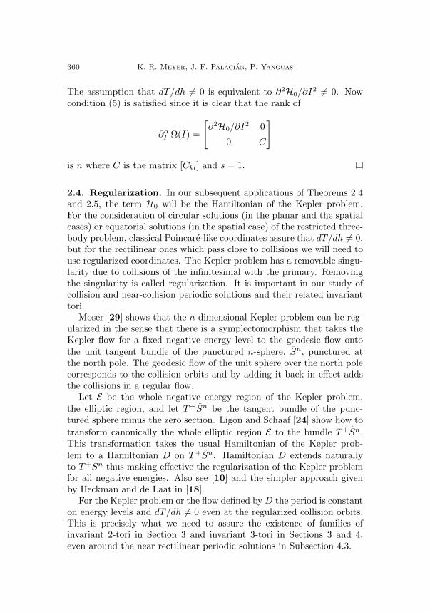
Applying reduction theory, once higher-order terms have been dropp-ed, the Hamiltonian H is defined on the orbit space which is the four-di-mensional manifold S2 × S2 [29]. A similar argument to that given forthe planar Kepler problem in Subsection 3.1 shows that S2×S2 is indeedthe orbit space of the regularized spatial Kepler problem since collisionorbits can be studied in this space as we show below.

We can use the set of variables given by a = (a1, a2, a3) and b =(b1, b2, b3) with the constraints a2

1 + a22 + a2

3 = b21 + b22 + b23 = L2 to pa-rameterize S2×S2, where a = G+LA and b = G−LA. The vector Arepresents the three-dimensional perigee vector. Note that the expres-sions of the components of A and a in terms of the Delaunay coordinatesare not the same as in the planar case, see [8, 31]. A representation ofthe space S2 × S2 is given in Figure 1: on the left, the red point repre-sents the vector a on the sphere |a| = L whereas on the right one, thegreen point accounts for the vector b on the sphere |b| = L.

a3 b3

a1 a2 b1 b2

×

Figure 1. A single motion in the orbit space S2 × S2

is given through the two points on their correspondingspheres.

As 2G = ((a1+b1)2+(a2+b2)2+(a3+b3)2)1/2, then G = 0 if and onlyif a1+b1 = a2+b2 = a3+b3 = 0, a2

1+a22+a2

3 = L2 and b21+b22+b23 = L2. Sothe subset of S2×S2 defined byR = (a,−a) ∈ R6 | a2

1+a22+a2

3 = L2 isa two-dimensional set consisting of collision trajectories. As in Delaunayvariables the circular orbits satisfy G = L this implies that a1 = b1,a2 = b2 and a3 = b3. Thus the circular orbits define the two-dimensionalset given by C = (a,a) ∈ R6 | a2

1 + a22 + a2

3 = L2. On the otherhand equatorial motions satisfy G = |N | and are given by the two-dimensional set Eq = (a,b) ∈ R6 | a2

1 + a22 + a2

3 = L2, b1 = −a1, b2 =−a2, b3 = a3. The use of the variables a and b extends the use of


the Delaunay variables, as we can include equatorial, circular and lineartrajectories [31, 36]. Finally, the other points on S2×S2 correspond toelliptic motions of the spatial Kepler problem.

After several simplifications and manipulations over Hε, the normalform Hamiltonian expressed in the invariants a and b is

H = −1

2(a3 + b3)

− 3

8ε3 µL2

(a2

1 − a22 − a2

3 + b21 − b22 − b23 − 4 a1 b1

+ 2 a2 b2 + 2 a3 b3)

+O(ε5).

(15)

Now, as the Hamiltonian starts as H = − 12 (a3 + b3) + · · · it has

a non-degenerate maximum at (a,b) = (0, 0,−L, 0, 0,−L) and a non-degenerate minimum at (a,b) = (0, 0, L, 0, 0, L), which by Reeb’s Theo-rem 2.2 correspond to elliptic periodic solutions of the spatial restrictedthree-body problem (12) of period T (ε) = T + O(ε3). These are thenear circular equatorial solutions (also called near circular coplanar so-lutions as the small particle moves on the plane determined by the mo-tion of the two primaries) already encountered in the planar case. TheHamiltonian H also has two non-degenerate critical points of index 2 at(a,b) = (0, 0,±L, 0, 0,∓L) which correspond to the near rectilinear mo-tions whose projection in the coordinate space leads to periodic orbitsin the vertical axis x3. They are indeed the near rectilinear trajectoriesfound by Belbruno [3] for small µ.

One sees that the characteristic exponents of all critical points of Yare ±i (double).

Thus, the characteristic multipliers of the four families of periodicsolutions of the system defined by the Hamiltonian (12) are 1, 1, 1 +ε3 T i, 1 + ε3 T i, 1− ε3 T i, 1− ε3 T i plus terms of order O(ε6).

4.2. The circular equatorial points (0, 0,±L, 0, 0,±L). We firstmove the Hamiltonian to the origin by

a1 = a1, a2 = a2, a3 = a3 ± L, b1 = b1, b2 = b2, b3 = b3 ± L,

then we change variables by

Q1 =a2√

2L± a3

, Q2 =b2√

2L± b3,

P1 = ∓ a1√2L± a3

, P2 = ∓ b1√2L± b3

,


with inverse

a1 =∓P1

√2L− P 2

1 −Q21, a2 =Q1

√2L− P 2

1 −Q21, a3 =∓(P 2

1 +Q21),

b1 =∓P2

√2L− P 2

2 −Q22, b2 =Q2

√2L− P 2

2 −Q22, b3 =∓(P 2

2 +Q22).

The change is canonical, with Q1 and Q2 as coordinates and P1 and P2

as their associated momenta.The resulting Hamiltonian is obtained after writing H in terms of

the Qi’s and Pi’s and dropping constant terms, so

H=±1

2(P 2

1 +Q21)± 1

2(P 2

2 +Q22)

− 3

4ε3µL2

(L(P 2

1 + P 22 )− L(Q2

1 +Q22)

−(2P1 P2−Q1Q2)√

2L− P 21 −Q2

1

√2L− P 2

2 −Q22

−(P 22 −Q2

1)(P 22 +Q2

2)−P 21 (P 2

1 −P 22 +Q2

1−Q22))

+O(ε5).

The Hamiltonian H is valid in a neighborhood of (0, 0,±L, 0, 0,±L).Now we scale by Qj = ε−3/2Qj and P j = ε−3/2 Pj for j ∈ 1, 2. The

canonical structure is preserved by dividing H by ε3. After expansion ofthis Hamiltonian in powers of ε we obtain

H=±1

2(P

2

1 +Q2

1)± 1

2(P

2

2 +Q2

2)

− 3

4ε3µL3

(P

2

1 + P2

2 − 4P 1 P 2 −Q2

1 −Q2

2 + 2Q1Q2

)+

3

8ε6µL2

(2(P

4

1−P3

1 P 2−P2

1 P2

2−P 1 P3

2+P4

2)+(P2

1+P2

2)Q1Q2

+2(P2

1−P 1 P 2+P2

2)(Q2

1−Q2

2)+Q1Q2(Q1−Q2)2)

+O(ε8).

For (0, 0, L, 0, 0, L) the eigenvalues associated with the linear differentialequation given through the quadratic part of H are

(16) ±√

1 + 2 ε i = ±ω1 i, ±√

1− 2 ε− 24 ε2 i = ±ω2 i


with ε = 34ε

3 µL3 and ω1 > 1 > ω2 > 0. For the point (0, 0,−L, 0, 0,−L)the eigenvalues are

(17) ±√

1− 2 ε i = ±ω1 i, ±√

1 + 2 ε− 24 ε2 i = ±ω2 i.

In this case ω2 > 1 > ω1 > 0. We remark that if ε = 0, then ω1 = ω2 = 1,thus the quadratic part of H is in 1 : −1 resonance. So we keep ε smallbut positive so that we can apply KAM Theory. As a consequence ω1

and ω2 are close to 1 but different from it.The eigenvectors related to ω1 and ω2 form a basis of R4, thus the

quadratic part of H is brought into normal form through a canonicalchange of variables. This linear change must be applied to H. Thecolumns of the matrix are the eigenvectors scaled so that the matrixis symplectic. After defining the new variables by (q1, q2, p1, p2) thequadratic part of H becomes

±ω1 i q1 p1 ± ω2 i q2 p2.

The values of the frequencies ω1 and ω2 are given in (16) if the quadraticpart is ω1 i q1 p1 +ω2 i q2 p2, whereas if the quadratic part is −ω1 i q1 p1−ω2 i q2 p2 we take the frequencies from (17). From now on when referringto (0, 0, L, 0, 0, L) we assume that ω1 and ω2 are as in (16), and when westudy the point (0, 0,−L, 0, 0,−L) we take the frequencies from (17).

We introduce

q1 =√I1(cosϕ1 − i sinϕ1), q2 =

√I2(cosϕ2 − i sinϕ2),

p1 =√I1(sinϕ1 − i cosϕ1), p2 =

√I2(sinϕ2 − i cosϕ2),

and the change satisfies dq1 ∧ dp1 + dq2 ∧ dp2 = dI1 ∧ dϕ1 + dI2 ∧ dϕ2.This transforms the quadratic terms of H into ±ω1 I1 ± ω2 I2, while thequartic terms are converted into a finite Fourier series in ϕ1 and ϕ2

whose coefficients are homogeneous quadratic polynomials in I1 and I2.Now we average H over ϕ1 and ϕ2, obtaining

H = ±ω1 I1 ± ω2 I2 −(ω2

1 − 1)2(ω21 + 3)

24µL4 ω21

I21

+(ω2

1 − 1)2(21ω21 − 13)

6µL4 ω1 ω2I1 I2

− (ω21 − 1)2(24ω4

1 − 119ω21 + 91)

24µL4 ω22

I22 + · · · .

The coefficients of I1, I2, I21 , I2

2 , and I1 I2 may be expressed in termsof ε, and expanding them in powers of ε around 0 yields expressions suchthat the leading terms of the coefficients of I1 and I2 are independent


of ε while the coefficients of I21 , I2

2 , and I1 I2 are factorized by ε2. Thegenerating functions computed in the averaging process in the two casesare enormous, but they are finite Fourier series in the angles ϕ1 and ϕ2.

At this point we can compute the determinant of the Hessian asso-ciated with H. First we calculate the constraint relating ω1 with ω2

through ε using (16) or (17), obtaining

ω2 =√

(2ω21 − 1)(4− 3ω2

1).

We end up with the same expression for the points (0, 0, L, 0, 0, L) and(0, 0,−L, 0, 0,−L), which is

det

∂2H∂I2

1

∂2H∂I1∂I2

∂2H∂I2∂I1

∂2H∂I2

2

=(ω2

1−1)4(24ω61−1811ω4

1 +1918ω21−403)

144µ2 L8 ω21 ω

22

+· · · .

The determinant vanishes when ω1∈0.53692 . . . , 0.88488 . . . , 1, 8.62479

. . . , however ω1 is near 1 (either above or below, but it never reachesthis value as ε cannot be zero). Next we express the coefficients of H interms of ε, divide the result by ε6 as the quadratic terms of H start atthat order, compute the Hessian, and we obtain:

det

∂2H∂I2

1

∂2H∂I1∂I2

∂2H∂I2∂I1

∂2H∂I2

2

= −153

16µ2 L4 +O(ε3).

Thus Theorem 2.5 applies after setting δ = ε6, using δ as the smallparameter of (6), then j = 1.

According to [16] one has that the measure of the set omitted fromthe established invariant tori related to Theorem 2.4 is of order O(εb)with b =

∑ai=1mi(ni − ni−1). In this case, we need to write down the

Hamiltonian normal form Hε arranged in powers of ε. This is achievedafter putting the frequencies ωi’s in terms of ε, undoing the scalings (ex-cepting the stretching of coordinates passing from Qj ’s and Pj ’s to Qj ’s

and P j ’s as we want that the normal form will be valid in a neighborhoodof the points (0, 0,±L, 0, 0,±L)), expanding the resulting expression in


powers of ε and incorporating the dropped terms to get H. We get

Hε = − 1

2L2∓ ε3L± ε6(I1 + I2) +

3

4ε9µL3(I1 − I2)

− 3

32ε12µL2

(4(I2

1−8I1 I2−I22 )±3µL4(I1+25 I2)

)+O(ε15).

(18)

From (18) we infer that a = 4, m1 = 3, m2 = 6, m3 = 9, m4 = 12,n0 = n1 = 1, n2 = n3 = n4 = 3, therefore b = 12, besides s = 1. Thus,we conclude

Proposition 4.1. There are families of invariant KAM 3-tori aroundthe near circular coplanar periodic solutions of the full system intro-duced by the Hamiltonian (12). These invariant tori form a majorityin the sense that the measure of the complement of their union is oforder O(ε12).

Although we do not know about the non-linear stability of the familiesof periodic solutions, we can say something more about the stability ofthe equilibria (0, 0,±L, 0, 0,±L) of the reduced system on the base space.Since the Hamiltonian H is positive or negative definite at these points,the classical theorem already known to Dirichlet [14, 25] applies.

Proposition 4.2. The relative equilibrium points (0, 0,±L, 0, 0,±L) arestable on the reduced space S2 × S2.

4.3. The rectilinear points (0, 0,±L, 0, 0,∓L). After moving theorigin to the point of interest through

a1 = a1, a2 = a2, a3 = a3 ± L, b1 = b1, b2 = b2, b3 = b3 ∓ L,

we introduce the local symplectic coordinates

Q1 =a2√

2L± a3

, Q2 =b2√

2L∓ b3,

P1 = ∓ a1√2L± a3

, P2 = ± b1√2L∓ b3

,

with inverse

a1 =∓P1

√2L− P 2

1 −Q21, a2 =Q1

√2L− P 2

1 −Q21, a3 =∓(P 2

1 +Q21),

b1 =±P2

√2L− P 2

2 −Q22, b2 =Q2

√2L− P 2

2 −Q22, b3 =±(P 2

2 +Q22).


The resulting Hamiltonian is obtained after putting H in terms ofthe Qi’s and Pi’s and omitting constant terms. We get

H=±1

2(P 2

1 +Q21)∓ 1

2(P 2

2 +Q22)

− 3

4ε3 µL2

(3L(P 2

1 + P 22 ) + L(Q2

1 +Q22)

+(2P1 P2+Q1Q2)√

2L− P 21 −Q2

1

√2L− P 2

2 −Q22

−(P 22 +Q2

1)(P 22 +Q2

2)−P 21 (P 2

1 +P 22 +Q2

1+Q22))

+O(ε5).

The Hamiltonian H is valid in a neighborhood of the points (0, 0,±L,0, 0,∓L).

Next we scale variables through the change Qj = ε−3/2Qj and P j =

ε−3/2 Pj for j ∈ 1, 2. To make the change canonical we must divide Hby ε3. Expanding this Hamiltonian in powers of ε (and keeping the samename for it) we obtain the Hamiltonian:

H = ±1

2(P

2

1 +Q2

1)∓ 1

2(P

2

2 +Q2

2)

− 3

4ε3µL3

(3(P

2

1 + P2

2) + 4P 1 P 2 +Q2

1 +Q2

2 + 2Q1Q2

)+

3

8ε6µL2

(2(P

4

1 + P3

1 P 2 + P2

1 P2

2 + P 1 P3

2 + P4

2)

+ 2P 2(P 1 + P 2)Q2

1 + (P2

1 + P2

2)Q1Q2

+ 2(P2

1 + P 1 P 2 + P2

2)Q2

2 +Q1Q2(Q1 +Q2)2)

+O(ε8).

The eigenvalues associated with the linear vector field given throughthe quadratic part of H are the expressions

±√

1 + 20 ε2 + 2√

5 ε√

3 + 20 ε2 i = ±ω1 i,

±√

1 + 20 ε2 − 2√

5 ε√

3 + 20 ε2 i = ±ω2 i,

(19)

where ε stands for 34ε

3 µL3 and ω1 > 1 > ω2 > 0. Note that ω1 = ω2 = 1

when ε = 0, and the quadratic part of H is in 1 : −1 resonance. Howeverwhen ε 6= 0 the eigenvalues are distinct.


Thus, the relative equilibria of the reduced system are parametricallystable and therefore the corresponding periodic solutions of the full sys-tem (12) dealing with the near rectilinear motions are elliptic.

We keep ε small but positive so that we may perform further nor-malization. By doing so, both ω1 and ω2 remain close to 1 but differentfrom it. As the corresponding set of eigenvectors forms a basis of R4,the quadratic part of H may be brought into normal form through acanonical change of variables. This linear change has to be appliedto H. The columns of the transformation matrix are the eigenvectorsrelated to ±ω1 i and ±ω2 i multiplied by scale constants chosen to makethe change symplectic. We do not give the explicit expression for thischange because it is lengthy and the procedure is standard; see for in-stance [5, 23]. Denoting the new variables by (q1, q2, p1, p2) and usingthe same name for the Hamiltonian, its quadratic part becomes in bothcases

−ω1 i q1 p1 + ω2 i q2 p2.

Next we introduce action-angle variables (I1, I2, ϕ1, ϕ2) by means of

q1 =√I1(cosϕ1 − i sinϕ1), q2 =

√I2(cosϕ2 − i sinϕ2),

p1 =√I1(sinϕ1 − i cosϕ1), p2 =

√I2(sinϕ2 − i cosϕ2).

It is easy to check that dq1 ∧ dp1 + dq2 ∧ dp2 = dI1 ∧ dϕ1 + dI2 ∧ dϕ2.This transformation brings the quadratic terms of H to −ω1 I1 + ω2 I2,while its quartic terms are converted into a finite Fourier series in ϕ1

and ϕ2 whose coefficients are homogeneous quadratic polynomials in I1and I2. We do not give the Hamiltonian because it is enormous.

Now we average H over ϕ1 and ϕ2, and we obtain:

H = −ω1 I1 + ω2 I2 +(7ω6

1 + 13ω41 + 13ω2

1 + 3)(ω21 − 1)2

30µL4 ω21(ω2

1 + 2)2(2ω21 + 1)

I21

− 2(ω21 − 1)2(ω4

1 − 14ω21 − 5)(2ω2

2 + 1)

135µL4 ω1(ω21 + 2)2 ω2

I1 I2

+(7ω6

2 + 13ω42 + 13ω2

2 + 3)(ω22 − 1)2

30µL4 ω22(ω2

2 + 2)2(2ω22 + 1)

I22 + · · · .

The coefficients of I21 , I2

2 , and I1 I2 may be expressed in terms of ε,and after expanding them in powers of ε, one obtains a formula startingin ε2, while the leading terms of the coefficients of I1 and I2 do notdepend on ε. The generating function responsible for this averaging step


is too big to be reproduced here, but it is a finite Fourier series in theangles ϕ1 and ϕ2.

Now we can compute the determinant of the Hessian associatedwith H. Using the constraint which relates ω1 and ω2 through (19)given by

ω2 =

√4− ω2

1

2ω21 + 1

,

we get

det

∂2H∂I2

1

∂2H∂I1∂I2

∂2H∂I2∂I1

∂2H∂I2

2

=(ω2

1−1)6(7ω81−28ω6

1−534ω41−604ω2

1−137)

225µ2 L8 ω21(ω2

1 − 4)(ω21 + 2)4(2ω2

1 + 1)2+· · ·

which does not vanish since the (positive) real roots of the determinantoccur for ω1 = 1 or ω1 = 3.37369 . . . , but as ε does not vanish ω1 remainsgreater than 1.

Now we need to express the coefficients of H in terms of ε. First ofall we use (19) to put ω1 and ω2 in terms of ε and divide the result by ε6

as the quadratic terms of H start at that order. Then we compute theHessian, getting

det

∂2H∂I2

1

∂2H∂I1∂I2

∂2H∂I2∂I1

∂2H∂I2

2

=405

4ε6 µ4 L10 +O(ε12).

Thus Theorem 2.5 cannot be applied directly as the determinant aboveis factorized by ε6. Nevertheless we can still apply Theorem 2.4. Un-doing the scalings introduced to obtain H as function of the actions I1and I2 (excepting the stretching of variables that define Qi’s and P i’s interms of Qi’s and Pi’s), incorporating the terms dropped in the process,expressing the ωi’s in terms of ε, expanding the whole Hamiltonian interms of ε we end up with

Hε = − 1

2L2+ ε6(−I1 + I2)− 3

√15

4ε9 µL3(I1 + I2)

+3

32ε12 µL2

(16(I1 + I2)2 + 15µL4(−I1 + I2)

)+O(ε15).

(20)


The Hamiltonian (20) is valid near the points (0, 0,±L, 0, 0,∓L). ThenTheorem 2.4 can be applied taking a = 3, m1 = 6, m2 = 9, m3 =12, n0 = 1, n1 = n2 = n3 = 3, In0 = (L), In1 = In2 = In3 =(L, I1, I2), In0 = (L), In1 = In2 = In3 = (I1, I2). If h0 is the KeplerianHamiltonian in Delaunay variables and h1, h2, and h3 denote respectivelythe terms of (20) factorized by ε6, ε9, and ε12, the vector of frequencieshas dimension six and is given explicitly by

Ω(I) =

(∂h0

∂L,∂h1

∂I1,∂h1

∂I2,∂h2

∂I1,∂h2

∂I2,∂h3

∂I1,∂h3

∂I2

)

=

(1

L3, −1, 1, −3

√15

4µL3, −3

√15

4µL3,

3(I1 + I2)µL2 − 45

32µ2 L6, 3(I1 + I2)µL2 +

45

32µ2 L6

)and the 4×6-matrix with rows Ω(I), ∂Ω(I)/∂L, ∂Ω(I)/∂I1 and ∂Ω(I)/∂I2has rank three, leading to the existence of the invariant tori of dimensionthree.

We apply Remark 2 of [16, p. 1422] to estimate the measure of thesurviving invariant tori (in the sense of the persistence of the KAM torithat remain when higher-order terms are added). According to [16] onehas that the measure of the set omitted from the established invarianttori is of order O(εb) with b =

∑ai=1mi(ni − ni−1) = 12. As we only

needed the first-order partial derivatives in (5) we have s = 1. Thus, weconclude

Proposition 4.3. There are families of invariant KAM 3-tori aroundthe near rectilinear periodic solutions of the full system defined throughthe Hamiltonian (12). These invariant tori form a majority in the sensethat the measure of the complement of their union is of order O(ε12).

These invariant tori are the generalization of the punctured 2-tori inthe lunar case of the planar restricted three-body problem studied byChenciner and Llibre [4].

Contrarily to the planar case we do not know the non-linear stabilityof the periodic solutions. However, we can say something about thestability of the equilibria (0, 0,±L, 0, 0,∓L) of the reduced system onthe base space.

For the analysis of the stability of these equilibria we use Arnold’sTheorem [27, 34]. We fix ε small and positive. We need to find H4, i.e.,the quartic terms of H as functions of the qi’s, pi’s, in other words, the


quadratic terms of H as functions of I1 and I2, and then compute

H4(ω2, ω1)=(ω2

1−1)2(ω121 −16ω10

1 +66ω81−268ω6

1−275ω41−132ω2

1−24)

15µL4 ω21 (ω2

1 − 4)(2ω41 + 5ω2

1 + 2)2

=6 ε6 µL2 +O(ε9).

Since this term does not vanish for ω1 close to (but larger than) 1,Arnold’s Theorem applies, and thus

Proposition 4.4. The linear equilibria points (0, 0,±L, 0, 0,∓L) arestable on the orbit space S2 × S2.

Even when H4(ω2, ω1) has ε6 as a factor, Arnold’s Theorem in theform given in [30] applies (see also [25, 27]). Indeed in theorems pre-sented in [25, 27, 30], although ε does not appear in the statements,it is introduced in the proofs by scaling. The proofs rely on the finaltheorem in Moser’s classic paper [28] where the invariant curve theoremallows small twists, i.e., terms multiplied by εa with a > 0. This ideawas already used in the proof of Theorem 2.3.

In Subsection 4.2 we could have used the symplectic coordinates in-troduced in [20], which are defined to deal with near circular equatorialmotions in S2 × S2. The computations carried out with this set of vari-ables are a bit shorter than the ones we have applied in Subsection 4.2but we have wanted to maintain a similar set to the one used for thelinear motions here.

5. The second reduction in the spatial lunar problem

5.1. Elimination of the node and the twice-reduced space. Nextwe eliminate the argument of the node by averaging the Hamiltonian (14)with respect to the angle ν. Our aim is to get more insight in the dy-namics of the spatial lunar restricted three-body problem, obtaining newinvariant 3-tori of the Hamiltonian (12). The normalized Hamiltonianhas been studied by several authors, see the references [9, 32, 35], andwe summarize the main results here.

After applying the Lie transformation method [11, 25] with the aimof averaging the angle ν, we end up with the following Hamiltonian

Hε = − 1

2L2− ε3N

+1

16ε6µL4

((1− 3 c2)(5− 3 η2)

− 15(1− c2)(1− η2) cos(2 g))

+O(ε8),

(21)

where η =√

1− e2 = G/L.


After truncating higher-order terms (21) defines a one-degree-of-free-dom system which is invariant with respect to the Keplerian symmetryand the axial symmetry, or equivalently, the actions L and N become ap-proximate integrals of motion. Thus we can reduce the Hamiltonian Hεafter constructing the corresponding orbit space.

The algebra of polynomials on S2 × S2 invariant under the actionassociated with this reduction is generated by the πi’s where

(22)π1 = a2

1 + a22, π2 = a1 b2 − a2 b1, π3 = a3,

π4 = b21 + b22, π5 = a1 b1 + a2 b2, π6 = b3,

together with the constraints

(23) π1 + π23 = L2, π4 + π2

6 = L2, π22 + π2

5 = π1 π4.

Taking the map

πN : S2 × S2 −→ N × R3 : (a,b) 7→ (N, τ1, τ2, τ3) ≡ (N, τ),

where

τ1 =1

2(π3 − π6), τ2 = π2, τ3 = π5

we define the invariants τ1, τ2, and τ3 in terms of a and b as

(24) τ1 =1

2(a3 − b3), τ2 = a1 b2 − a2 b1, τ3 = a1 b1 + a2 b2.

The constraints (23) are used to define the corresponding orbit space.The space TL,N , called twice-reduced space, is defined as the imageof S2 × S2 by πN , that is,

TL,N = πN (S2 × S2)

=τ ∈ R3 | τ2

2 + τ23 =

(L2 − (τ1 +N)2

)(L2 − (τ1 −N)2

),

(25)

for 0 ≤ |N | ≤ L and L > 0. The invariants τ2 and τ3 lie in the interval[N2 − L2, L2 −N2], whereas τ1 belongs to [|N | − L,L− |N |].

It is proved in [8, 9] that when 0 < |N | < L, TL,N is diffeomorphic tothe 2-sphere S2 and therefore the reduction is regular in that region ofthe phase space. However, when N = 0 the space TL,0 is a topological2-sphere with two singular points, namely, the vertices of the surface TL,0at (±L, 0, 0). Thus, the reduction by the axial symmetry is singular [1].When |N | = L the space TL,±L is just a point. This case correspondsto motions that are circular and equatorial at the same time, and needsto be analyzed on S2 × S2, concretely in neighborhoods of the points(0, 0,±L, 0, 0,±L).


The singular points (also called peaks) (±L, 0, 0) of TL,0 and the ex-ceptional case of TL,±L are the images of the points (0, 0,±L, 0, 0,∓L)and (0, 0,±L, 0, 0,±L), whereas the rest of the points of TL,N with0 ≤ |N | < L are images of circles on S2 × S2 by means of πN .

It is instructive to stress that as (±L, 0, 0) are singular points on theorbit space TL,0, they must be relative equilibria of a reduced system re-

lated to a Hamiltonian function, say H, that is properly defined on thesepoints. Thus, when reconstructing the flow of a certain system whosereduced Hamiltonian is H (keeping in mind that H has been obtainedafter reducing the full system by the Keplerian and the axial symme-tries), the points (±L, 0, 0) correspond to families of rectilinear periodicsolutions of the full Hamiltonian, that is, they are the same periodicsolutions reconstructed from the point (0, 0,±L, 0, 0,∓L) on S2 × S2.

This singular reduction was made for the first time by Cushman inthe setting of the artificial satellite theory [8]; see also [6] and the surveypaper [9].

It is possible to express the quantities sin g, cos g and G in terms of τ ,L, and N . Indeed one gets

2G2 = L2 +N2 − τ21 + τ3,

cos g = − τ2√(L2 −N2)2 − (τ2

1 − τ3)2,

sin g = τ1

√2(L2 +N2 − τ2

1 + τ3)

(L2 −N2)2 − (τ21 − τ3)2

,

(26)

and this applies when the argument of the perigee g is well defined.Rectilinear solutions must satisfy G=N=0. Taking also into account

the constraint appearing in (25), we know that they are defined on theone-dimensional set RL,0 = τ ∈R3 | τ2 =0, τ3 =τ2

1−L2. Thus, we mayanalyze linear trajectories as the reduction process regularizes this typeof solutions. In particular, the points (±L, 0, 0) correspond with rectilin-ear motions such that their projection in the coordinate space leads torectilinear orbits in the vertical axis x3 as the points (±L, 0, 0) are theprojections by πN of the points (0, 0,±L, 0, 0,∓L) on S2×S2. Circularmotions are concentrated on a unique point on TL,N whose coordinatesare (0, 0, L2−N2), i.e., on the top point of the orbit space, whereasequatorial (i.e., coplanar with the primaries) trajectories in the twice-reduced space are represented on the bottom point of the surface TL,Nwith coordinates (0, 0, N2−L2).


A picture of the twice-reduced space is depicted in Figure 2: thespace TL,N with N 6=0 appears on the top left, the space TL,0 on the topright, and sections τ2 =0 on the lower part. The green points stand forcircular solutions, the red points refer to equatorial solutions, and theyellow points denote rectilinear vertical solutions. The lower arc drawnin blue comprise the set of all rectilinear solutions.

L2 −N2

N2 − L2

|N |−L L−|N |τ1

|N | > 0

τ3 τ3

L2

|N | = 0

−L L

−L2

τ1

τ3 τ3τ2 τ2

τ1 τ1

Figure 2. Twice-reduced space.

5.2. Dynamics of the spatial lunar problem on TL,N . The nor-malized Hamiltonian (21) is expressed as a function of the τi’s oncehigher-order terms are omitted. Hence we can remove the zeroth andthe O(ε3) terms from Hε. After dropping some constant terms and scal-ing conveniently, the normal form Hamiltonian H in terms of τ reads

(27) H = 4 τ21 + τ3 +O(ε2).

The Poisson brackets of the τi’s are:

(28) τ1, τ2=2 τ3, τ1, τ3=−2 τ2, τ2, τ3=−4 τ1(τ21 −L2−N2).


We can determine the equations of motion related to H by means ofthe following relations

τi =∑

1≤j≤3

τi, τj∂H∂τj

, for i ∈ 1, 2, 3.

Using the Poisson brackets given in (28) we get

τ1 = −2 τ2,

τ2 = −4 τ1(τ21 + 4 τ3 − L2 −N2),

τ3 = 16 τ1 τ2.

(29)

The relative equilibria are the roots of system (29) that satisfy theconstraint of (25) and such that the τi’s lie in their appropriate intervals.Their coordinates (τ1, τ2, τ3) are obtained explicitly, yielding

(i) (0, 0, L2 −N2),

(ii) (0, 0, N2 − L2),

(iii)(±√L2 +N2 − 8L |N |√

15, 0, 2L |N |√

15

)with |N |/L ∈

[0,√

3/5].

The occurrence of the relative equilibria (i)–(iii) is as follows. Wediscard the cases |N | = L, e.g., the prograde and retrograde circularequatorial solutions, since no dynamics can be analyzed as the orbitspace is a point. Moreover, these cases have been already tackled inSubsection 4.2. Thus we will concentrate on the set with |N | < L whereN/L ∈ (−1, 1).

We start by noting that the equilibria (i) and (ii) are present for allvalues of N with 0 ≤ |N | ≤ L. The appearance and disappearance ofthe relative equilibria, when N/L varies, is as follows:

• For |N |/L ∈ (√

3/5, 1) the points (i) and (ii) are the only equilibriaon the surface TL,N .

• If |N |/L=√

3/5 there are also two equilibria, more concretely thepoints (ii) and (i) that collides with the points (iii) at (0, 0, 2

5L2).

• When 0 < |N |/L <√

3/5, there are four equilibria, namely thepoints (i), (ii) and the two points (iii).• For N = 0 the coordinates of (iii) become (±L, 0, 0), that is, they

are the singular points of TL,0. On the other hand the points (i)and (ii) remain as relative equilibria. In particular the point (ii) hascoordinates (0, 0,−L2) and it refers to rectilinear solutions. Morespecifically, they are the solutions whose projections on the coor-dinate space are straight lines on the x1x2-plane passing throughthe origin with an arbitrary slope.


Next we summarize the stability character of the relative equilibria al-though we shall turn to this issue in Subsubsections 5.3.2, 5.3.3 and 5.3.4when dealing with the KAM 3-tori.

• The point (i) represents motions of circular type with an inclination

given by cos(I) = N/L. When√

3/5 < |N |/L < 1 it is a stable

elliptic point (center). If |N |/L =√

3/5 it is a degenerate centerwith normal form P 2 + Q4, therefore stable. It is a hyperbolicpoint (saddle) if 0 ≤ |N |/L <

√3/5.

• The point (ii) corresponds to equatorial trajectories and is ellipticfor all N/L ∈ (−1, 1). The eccentricity is given by (1−N2/L2)1/2.• The two relative equilibria corresponding to (iii) represent mo-

tions with an inclination given by cos(I) = ±( 35 )1/4

√|N |/L (the

plus sign is for N ≥ 0 whereas the minus is for N < 0) and aneccentricity e = (1− ( 5

3 )1/2|N |/L)1/2. In fact the two equilibriumpoints (iii) correspond to the same trajectories, but reckoned in aprograde sense for positive N and in a retrograde one for nega-tive N . They are elliptic for all |N |/L ∈ [0,

√3/5].

In view of the above description a Hamiltonian (supercritical) pitch-fork bifurcation of relative equilibria occurs when N/L crosses either the

value −√

3/5 or√

3/5 as the two elliptic points (iii) and the hyperbolicone (i) collide. See further details in [9, 32, 35].

We present in Figure 3 the flow of the Hamiltonian (27) when |N |/Lcrosses the value

√3/5. In particular, when |N |/L .

√3/5, the two

equilibria (iii) still exist but are located very close to (i).

τ3 τ3 τ3

τ2 τ2 τ2

τ1 τ1 τ1

|N |/L <√

3/5 |N |/L .√

3/5 |N |/L >√

3/5

Figure 3. Sequence of the Hamiltonian pitchfork bi-furcations that take place when |N |/L passes through√

3/5.


In Figure 4 we depict the flow of (27) on the twice-reduced space whenN is near zero. The space TL,0 has two singularities at the points (±L,0,0).When |N | tends to zero the points (iii) move on the surface TL,N awayfrom the point (0, 0, L2 −N2) reaching the peaks of TL,N when N = 0.The stability of the point (ii) remains the same regardless of the valueof N in (−1, 1), thus it does not change when N passes through zero.

τ3 τ3 τ3

τ2 τ2 τ2

τ1 τ1 τ1

N . 0 N = 0 N & 0

Figure 4. The flow of (27) on the twice-reduced spacewhen N is near zero.

We point out that the non-linear stability of the equilibria remains thesame as the linear stability excepting for the degenerate cases at thepitchfork bifurcation. The reason is that saddles remain as saddles underperturbation by the Hartman–Grobman Theorem [17] and the linearcenters become also non-linear centers since system (29) is of one degreeof freedom and the classical Dirichlet stability Theorem applies.

5.3. Invariant KAM 3-tori from the second reduction.

5.3.1. Quasi-periodic solutions of the truncated normal formHamiltonian. We have made two processes of normalization, trunca-tion, and reduction (first averaging the mean anomaly and second aver-aging the argument of the node). So the existence and stability characterof the relative equilibria on the orbit space TL,N are in correspondencewith the existence and stability of invariant 2-tori and quasi-periodic so-lutions of the Hamiltonian (13) in the full phase space once terms of orderhigher than O(ε6) are truncated. Besides, the pitchfork bifurcations oc-

curring at |N |/L =√

3/5 are reconstructed as pitchfork bifurcations ofinvariant 2-tori of the truncated system (13). However we cannot assurethat this dynamics is reflected in the Hamiltonian (12), although we canuse the information of some relative equilibria to obtain KAM tori andquasi-periodic solutions for the full system.


Our goal now is to reconstruct partially the dynamics of the system de-fined through the Hamiltonian (12) obtaining some new invariant 3-toriand quasi-periodic solutions of the spatial problem using Theorem 2.4.This will be the purpose of Subsubsections 5.3.2, 5.3.3, and 5.3.4. Weshall make use of the normal form Hamiltonian (27) and the twice-reduced space (25). Besides we shall discuss the existence of the 3-toriwhose quasi-periodic solutions are of rectilinear type, a situation alreadystudied in Subsection 4.3. This particular case is associated to the sin-gular points (±L, 0, 0) and the closed orbits around them. Indeed, thesepoints are reconstructed to the families of periodic solutions studied inSubsection 4.3. We shall see that excepting for the 3-tori related to thepeak points we shall need to define local symplectic coordinates in orderto be able to construct a pair of action-angle coordinates, say (J, ϕ), soas to apply Han, Li, and Yi’s Theorem.

Similar results were obtained by Kummer [21, 22] and by Som-mer [35]. Kummer performs a second normalization (the one dealingwith the axial symmetry) and computes the twice-reduced space but hedoes not apply singular reduction theory and therefore has to excludethe two singular points that are present when the third component ofthe angular momentum vanishes. He builds action-angle variables fromthe twice-reduced space in order to apply KAM Theory and concludeswith the existence of some invariant 3-tori but his results are only partialand his procedure is very intricate.

Sommer also computes the averaged Hamiltonian with respect to thenode and uses singular reduction theory. In particular she follows Cush-man [9]. Besides she constructs a KAM Theorem to deal with the ap-pearance of the Hamiltonian function at three different time scales andapplies her theorem to conclude the persistence of invariant 3-tori aroundthe relative equilibria of (29) that are of elliptic type. Han, Li, and Yi’sTheorem generalizes Sommer’s Theorem and we use the former togetherwith different sets of symplectic variables, simplifying considerably theamount of computations made by Sommer. Moreover we clarify the ex-istence of the KAM tori that correspond with solutions that are nearrectilinear.

In the following we shall focus on the non-degenerate relative equi-libria of elliptic type dealt within Subsection 5.2 that are representedby regular or singular points on TL,N . Thus, we concentrate on the

point (i) for |N |/L ∈ (√

3/5, 1), the point (ii) for |N |/L ∈ [0, 1) and the

points (iii) for |N |/L ∈ [0,√

3/5).


5.3.2. Invariant 3-tori reconstructed from the point (i). We in-troduce coordinates

(30) Q = ε−1/2√

2(L−G) cos g, P = ε−1/2√

2(L−G) sin g.

This change is symplectic with multiplier ε−1 and extends analytically tothe origin of the QP -plane, provided that Q and P are written in termsof g and G and the computations that carry out satisfy the d’Alembertcharacteristic; see [19, 25] and the examples in [26]. After calculatingthe inverse of (30) putting g and G in terms of Q and P in the Hamilton-ian (21), multiplying this Hamiltonian by ε−1, scaling time to adjust itszeroth term so that it becomes the Kepler Hamiltonian and expandingthe result in power series of ε, we end up with

Hε = − 1

2L2− ε3N +

1

8ε6 µL2(L2 − 3N2)

− 3

8ε7 µL

(2L2Q2 + (5N2 − 3L2)P 2

)+O(ε8).

(31)

As |N |/L ∈ (√

3/5, 1) it is apparent that the point (i) is elliptic.The argument of the perigee is undefined for circular motions, however

it is straightforward to see that the value of the angle g for points near(0, 0, L2 −N2) is close to 0 (for N > 0) or to π (for N < 0).

Now we introduce the action-angle pair (J, ϕ) through:

Q = 21/4

√√5N2 − 3L2 J

Lcosϕ, P = 23/4

√LJ√

5N2 − 3L2sinϕ.

The change satisfies dQ ∧ dP = dJ ∧ dϕ and transforms (31) into

(32) Hε = − 1

2L2− ε3N +

1

8ε6 µL4(L2 − 3N2)

− 3√

2

4ε7 µL2

√5N2 − 3L2 J +O(ε8).

Now we apply Theorem 2.4 with a = 3, m1 = 3, m2 = 6, m3 = 7, n0 = 1,n1 = n2 = 2, n3 = 3, In0 = (L), In1 = In2 = (L,N), In3 = (L,N, J),In0 = (L), In1 = In2 = (N) and In3 = (J). One gets

Ω(I) =

(1

L3,−1,−3

4µL4N,−3

√2

4µL2

√5N2 − 3L2

)and the matrix of order 4 whose rows are Ω(I), ∂Ω(I)/∂L, ∂Ω(I)/∂N ,and ∂Ω(I)/∂J has rank three. Furthermore, as b =

∑ai=1mi(ni − ni−1)

and the integer s of Theorem 2.4 is 1, according to [16], the measure


of excluded tori is of order O(εb), that in this case is O(ε10). So weconclude

Proposition 5.1. For |N |/L ∈ (√

3/5, 1) there are families of invariantKAM 3-tori filled up by the near circular quasi-periodic solutions of thefull system introduced by the Hamiltonian (12). These quasi-periodicsolutions have an inclination given approximately by cos(I) = N/L anda perigee near 0 when N is positive or near π when N is negative. Themeasure of the excluded set of tori is of order O(ε10).

5.3.3. Invariant 3-tori reconstructed from the point (ii). Wecould introduce coordinates based on Delaunay elements, similarly towhat is done in Subsubsection 5.3.2, but then the subsequent analysis isnot valid for N = 0. Thus we proceed differently in order to include inthe analysis any value of N in (−1, 1).

Our aim is to find canonical coordinates Q, P such that the normalform Hamiltonian (21) is written in terms of the new variables (and interms of L and N) and we can apply Theorem 2.4. We also require thatour approach will be valid for N = 0 in order to analyze the invariant torirelated to motions that are at the same time equatorial and rectilinear.See also the picture (c) of Figure 5 with the circles around the point (ii).

We have represented the flow for the case N = 0 in Figure 5 from dif-ferent points of view, showing the appearance of four relative equilibria,namely, three elliptic points and one hyperbolic. The circles surroundingthe elliptic points are reconstructed into invariant 3-tori for the spatiallunar problem.

τ2 τ3 τ2 τ3

τ1 τ2 τ1 τ1

(a) (b) (c) (d)

Figure 5. The flow of (27) for N = 0: (a) viewpointfrom top, (b) viewpoint from right, (c) viewpoint frombottom and (d) viewpoint from front.

Although the argument of the perigee is not well defined in the case ofequatorial motions the value of g for points near (0, 0, N2−L2) is near 0


(for N > 0) or near π (for N < 0). This fact is taken into account whenwe consider the geometry of the quasi-periodic solutions we will obtainin the next paragraphs.

As we are working in a neighborhood of the point (0, 0, N2 − L2) weintroduce functions f1(Q,P ;L,N) and f2(Q,P ;L,N), or f1 and f2 forshort, that have to be determined, and are expected to be small. Thuswe make the transformation

(33) τ1 =f1, τ2 =f2, τ3 =−√f4

1−2(L2+N2) f21 − f2

2 + (L2−N2)2,

where we have used the constraint of (25) to put τ3 in terms of f1 and f2.Replacing the Poisson brackets between the τi’s given in (28) in terms

of Q and P and taking into account that Q,P = 1 we build three par-tial differential equations (one for each Poisson bracket) whose unknownsare f1 and f2. Out of the three equations there is an essential expressionthat has to be zero, the other equations being redundant. The relevantequation is

2√f4

1 − 2(L2 +N2) f21 − f2

2 + (L2 −N2)2 +∂f1

∂Q

∂f2

∂P− ∂f1

∂P

∂f2

∂Q= 0.

As we can choose either f1 or f2 we select a convenient value for f1 = Pand solve for f2, getting

f1(Q,P ;L,N) = P,

f2(Q,P ;L,N) =√(

(L+N)2 − P 2)(

(L−N)2 − P 2)

sin(2Q).(34)

We note that Q = P = 0 implies f1 = f2 = 0 and τ1 = τ2 = 0 whileτ3 = N2 − L2; besides when Q and P are small, f1 and f2 are smallquantities.

Once f1 and f2 are calculated the final change is

τ1 = P,

τ2 =√(

(L+N)2 − P 2)(

(L−N)2 − P 2)

sin(2Q),

τ3 = −√(

(L+N)2 − P 2)(

(L−N)2 − P 2)

cos(2Q).

(35)

The equation τ1 = P represents the local surface around the equilib-rium Q = P = 0 in the space QPτ1, which means that (0, 0, N2 − L2)is a regular point in this chart. In fact we are projecting the Hamil-tonian function in the QP -plane as the change (33) is valid only in aneighborhood of the point (0, 0, N2 − L2) on TL,N .

In particular when N = 0 the above transformation reduces to

τ1 = P, τ2 = (L2 − P 2) sin(2Q), τ3 = −(L2 − P 2) cos(2Q).


Next we put g, sin g and cos g in terms of Q and P by means of (26),yielding the expression

2G2=L2 +N2 − P 2 −√(

(L+N)2 − P 2)((L−N)2 − P 2

)cos(2Q),

cos g=−

√((L+N)2 − P 2

)((L−N)2 − P 2

)sin(2Q)√

(L2−N2)2−(P 2+

√((L+N)2−P 2

)((L−N)2−P 2

)cos(2Q)

)2 ,

sin g=√2P

√L2+N2−P 2−

√((L+N)2−P 2

)((L−N)2−P 2

)cos(2Q)√

(L2−N2)2−(P 2+

√((L+N)2−P 2

)((L−N)2−P 2

)cos(2Q)

)2 ,

(36)

which is a valid expression except for the case of equatorial motions, i.e.,when Q = P = 0 as then G = |N | and g is undefined. The Hamilton-ian (21) is put in terms of Q and P using (36). Next we scale Q and Pby doing (Q,P ) = ε1/2(Q,P ), multiply Hε by the multiplier ε−1 andscale time conveniently. After expanding the Hamiltonian in powers of εand dropping constant terms we obtain:

Hε = − 1

2L2− ε3N − 1

8ε6 µL2(5L2 − 3N2)

+3

8ε7 µL2

(2 (L2 −N2)Q

2+

5L2 − 3N2

L2 −N2P

2)

+O(ε8).

(37)

The development is valid for 0 ≤ |N | < L, and looking at the termfactorized by ε7, the point (ii) is elliptic even for N = 0 as was alreadystated in Subsection 5.2.

The next step is the introduction of an action-angle pair (J, ϕ):

Q = 21/4

√√5L2 − 3N2 J

L2 −N2cosϕ, P = 23/4

√(L2 −N2) J√5L2 − 3N2

sinϕ,

transforming (37) into

(38) Hε = − 1

2L2− ε3N − 1

8ε6 µL2(5L2 − 3N2)

+3√

2

4ε7 µL2

√5L2 − 3N2 J +O(ε8).


Note that dQ ∧ dP = dJ ∧ dϕ. Next one can apply Theorem 2.4 wherethe values of a, mj ’s, nj ’s, I

nj ’s, Inj ’s are as in Subsubsection 5.3.2. Weobtain

Ω(I) =

(1

L3,−1,

3

4µL2N,

3√

2

4µL2

√5L2 − 3N2

),

and the corresponding matrix of order 4 whose rows are given by Ω(I),∂Ω(I)/∂L, ∂Ω(I)/∂N , and ∂Ω(I)/∂J has rank three. We get

Proposition 5.2. There are families of invariant KAM 3-tori filled upby the near equatorial quasi-periodic solutions of the full system intro-duced by the Hamiltonian (12). These quasi-periodic solutions have aneccentricity given approximately by (1−N2/L2)1/2 where |N |/L ∈ [0, 1)and a perigee close to 0 (for positive N) or π (for negative N). WhenN ≈ 0 these quasi-periodic motions are near rectilinear equatorial solu-tions. The measure of the excluded tori is of order O(ε10).

The computations carried out are valid for all N , thus we can concludethat the KAM 3-tori also exist for N near zero. This fact is not easilydeductible from the exposition made by Sommer [35] in Chapter 5 ofher thesis.

5.3.4. Invariant 3-tori reconstructed from the points (iii). We

consider the points (iii) with |N |/L∈ [0,√

3/5).The corresponding Delau-

nay coordinates for these equilibria are (g0, G0)=(±π/2, (5/3)1/4√L|N |).

In particular, when N = 0 it implies that the Delaunay coordinates forthe points (±L, 0, 0) on the surface TL,0 are (g0, G0) = (±π/2, 0). Notethat even when the argument of the perigee is not properly defined forrectilinear motions and so we cannot say that g0 takes any value whenG = 0, it is of interest to note that the corresponding quasi-periodicsolutions that will be reconstructed from these points will have perigeesnear ±π/2 (specifically π/2 when N > 0 and −π/2 if N < 0).

We start by considering the case N 6= 0 as the subsequent analysis isnot valid when N vanishes.

When |N | > 0 Delaunay elements may be used as they are a welldefined set of coordinates. In fact an adequate transformation is definedby

(39) Q = ε−1/2(g − g0), P = ε−1/2(G−G0).

This change is canonical with multiplier ε−1. We put g and G in termsof Q, P , g0, and G0, then we multiply Hε by ε−1 and scale time. Finally


we expand the Hamiltonian in power series of ε around zero, getting

Hε = − 1

2L2− ε3N +

5

4ε6 µL2

(L−

√3/5 |N |

)(L− 2

√3/5 |N |

)− 1

8ε7µL2

(15(L−

√3/5 |N |

)(L−

√5/3|N |

)Q2 + 36P 2

)+O(ε15/2).

(40)

Moreover higher-order terms are unbounded for N = 0, what preventsthe discussion of these paragraphs to be extended to N = 0 or small.Thus for the moment we assume that |N | ≥ N∗ for some N∗ > 0 suchthat the ordering established through the small parameter ε remains thesame. We shall deal with the case N ≈ 0 later on.

As |N |/L∈ [N∗/L,√

3/5) the points (iii) are elliptic in agreement withSubsection 5.2. Indeed, the points (iii) are also elliptic when |N |/L =√

3/5 but then G0 = L and the coordinates (39) are not adequate to han-dle the stability analysis and to obtain the related invariant 3-tori. How-ever it is not a problem because, when |N |/L =

√3/5, the points (iii)

and the point (ii) coincide and we have analyzed its stability character,obtaining as well the KAM 3-tori in Proposition 5.2.

We introduce the action-angle variables (J, ϕ) by means of

Q = 2√

3

√√√√ J√15(L−

√3/5 |N |

)(L−

√5/3 |N |

) cosϕ,

P =1√3

√√15(L−

√3/5 |N |

)(L−

√5/3 |N |

)J sinϕ,

satisfying dQ ∧ dP = dJ ∧ dϕ. This allows us to transform (40) into

Hε = − 1

2L2− ε3N +

5

4ε6 µL2

(L−

√3/5 |N |

)(L− 2

√3/5 |N |

)− 3

2ε7µL2

√15(L−

√3/5 |N |

)(L−

√5/3 |N |

)J+O(ε15/2).

(41)

In order to apply Theorem 2.4 we note that the values of the constantsneeded in the hypotheses of the theorem are as in the previous cases.


This time the frequency vector is

Ω(I) =

(1

L3,−1,

3

4µL2(∓

√15L+ 4N),

−3

2µL2

√15(L−

√3/5 |N |

)(L−

√5/3 |N |

)),

the minus sign in the formula applies for N > 0 while the plus signapplies forN < 0. The matrix of order 4 whose rows are Ω(I), ∂Ω(I)/∂L,∂Ω(I)/∂N , and ∂Ω(I)/∂J has rank three.

Now we focus on the case N ≈ 0 (i.e. the case 0 ≤ |N | < N∗), that is,we analyze the stability of the points (iii) for N small and on the singularpoints (±L, 0, 0) for N = 0 and the existence of the related KAM 3-tori.We scale the normalized Hamiltonian (21) using N = ε4N . Then Hε istransformed into

(42) Hε = − 1

2L2+

1

16ε6µL2

(5L2−3G2−15(L2−G2) cos(2g)

)+O(ε7),

where the higher order tems contain the scaled action N .Omitting higher-order terms we find that the Hamiltonian (42) is the

same as (27) when we take N = 0, i.e., the Hamiltonian defined on TL,0.Note that the procedure applies for non-null but small N as the abovescaling makes that the case N ≈ 0 is the same as the case N = 0 up toterms of order seven in ε.

See the four pictures of Figure 5 and the picture in the middle ofFigure 4 with the closed orbits encircling the points (±L, 0, 0).

Inspired in the way it was done in [15, Subsection 4.4] we introducea transformation to desingularize the points (±L, 0, 0) as follows:

(43) τ1 =1

2w, τ2 =

1

4(u2 − v2), τ3 =

1

2u v.

This change is a 2:1-covering and transforms the constraint (25) definingthe space TL,0 into the 2-sphere

QL,0 = u2 + v2 + w2 − 4L2 = 0.

Thus the points (±L, 0, 0) are converted into the points (u, v, w) =(0, 0,±2L) and these points become regular points of QL,0. The trans-formation (43) is a change of variables that applies in the neighborhoodof the points (iii) for |N | smaller than N∗ or null.

After removing constant terms and projecting the Hamiltonian intothe uv-plane, the normal form Hamiltonian (27) is

(44) H =1

2u v − (u2 + v2) + · · · .


The pair (u, v) does not form a symplectic chart, indeed the Poissonbracket between the two is computed as the vector triple product u, v =(∇u×∇v) · ∇QL,0 where ∇ denotes the gradient of a scalar function inthe chart (u, v, w). We get

u, v = ±1

2

√4L2 − u2 − v2,

where the plus sign applies for (L, 0, 0) while the minus is used for(−L, 0, 0).

The equations of motion associated to (44) are

(45)

u = u, v∂H∂v

= ±1

4(u− 4 v)

√4L2 − u2 − v2,

v = −u, v∂H∂u

= ±1

4(4u− v)

√4L2 − u2 − v2.

The point (u0, v0) = (0, 0) is a critical point of (45) that correspondsto (±L, 0, 0) on TL,0.

The eigenvalues associated with the linearized equations around(u0, v0) are ±

√15L i. Thus the points (0, 0,±2L) are stable, hence

(±L, 0, 0) are stable points on TL,0, which is equivalent to the fact thatthe points (0, 0,±L, 0, 0,∓L) are stable points on S2 × S2. The exis-tence of the relative equilibria (±L, 0, 0) leads to the existence of twofamilies of elliptic periodic solutions for the full system (12) that areof rectilinear type, these solutions already analyzed in Subsection 4.3.We can say more, e.g., that the points (iii) are also stable for N small,which is in agreement with the stability character of (iii) for N such that

N∗/L ≤ |N |/L <√

3/5.Finally in order to establish the existence of KAM 3-tori when N ≈ 0

for the full system we can use the result of Proposition 4.3 after undoingthe scaling N = ε4N and the transformation to normal form that ledto (21), we go back to the Hamiltonian in normal form given by (15).Thus repeating the steps of Subsection 4.3 and using Proposition 4.3, weend up with the existence of KAM 3-tori surrounding the periodic solu-tions that are near rectilinear and whose projections in the coordinatespace indicate that they move close to the axis x3 up and down. Thisimplies that there are KAM 3-tori around the points (iii) for small N(i.e., |N | < N∗) and around the points (±L, 0, 0) for N = 0. In con-clusion there are invariant 3-tori related to the points (iii) for all N

with 0 < |N |/L <√

3/5 and there are invariant 3-tori related to thepoints (±L, 0, 0) for N = 0. In summary:


Proposition 5.3. There are families of invariant KAM 3-tori filled withquasi-periodic solutions of the full system introduced by the Hamilton-ian (12). These quasi-periodic solutions have approximate inclination

and eccentricity given respectively by cos(I) = ±( 35 )1/4

√|N |/L (the plus

sign applies for N ≥ 0 while the minus sign applies for N < 0) and

(1 − ( 53 )1/2|N |/L)1/2 where |N |/L ∈ [0,

√3/5). The perigee of these

quasi-periodic solutions is near π/2 for positive N and near −π/2 fornegative N . The measure of the excluded tori is of order O(ε10).

In the estimate of the measure of the excluded tori in Proposition 5.3we have chosen the exponent ten as it is the minimum of the exponentsof Proposition 4.3 and the one corresponding to the Hamiltonian (41),which is twelve.

Acknowledgments

The authors are partially supported by the Spanish MINECO grantMTM 2011-28227-C02-01 and by the Charles Phelps Taft Foundation.

References

[1] J. M. Arms, R. H. Cushman, and M. J. Gotay, A universalreduction procedure for Hamiltonian group actions, in: “The ge-ometry of Hamiltonian systems” (Berkeley, CA, 1989), Math. Sci.Res. Inst. Publ. 22, Springer, New York, 1991, pp. 33–51. DOI:

10.1007/978-1-4613-9725-0−4.[2] V. I. Arnold, V. V. Kozlov, and A. I. Neıshtadt, “Math-

ematical aspects of classical and celestial mechanics”, [Dynamicalsystems. III], Translated from the Russian original by E. Khukhro,Third edition, Encyclopaedia of Mathematical Sciences 3, Springer-Verlag, Berlin, 2006.

[3] E. A. Belbruno, A new family of periodic orbits for the re-stricted problem, Celestial Mech. 25(2) (1981), 195–217. DOI:

10.1007/BF01230520.[4] A. Chenciner and J. Llibre, A note on the existence of invariant

punctured tori in the planar circular restricted three-body problem,Ergodic Theory Dynam. Systems 8∗ (1988), Charles Conley Memo-rial Issue, 63–72. DOI: 10.1017/S0143385700009330.

[5] R. C. Churchill and M. Kummer, A unified approach to linearand nonlinear normal forms for Hamiltonian systems, J. SymbolicComput. 27(1) (1999), 49–131. DOI: 10.1006/jsco.1998.0244.

http://dx.doi.org/10.1007/978-1-4613-9725-0_4

http://dx.doi.org/10.1007/978-1-4613-9725-0_4

http://dx.doi.org/10.1007/BF01230520

http://dx.doi.org/10.1007/BF01230520

http://dx.doi.org/10.1017/S0143385700009330

http://dx.doi.org/10.1006/jsco.1998.0244


[6] S. L. Coffey, A. Deprit, and B. R. Miller, The critical in-clination in artificial satellite theory, Celestial Mech. 39(4) (1986),365–406. DOI: 10.1007/BF01230483.

[7] C. Conley, On some new long periodic solutions of the plane re-stricted three body problem, Comm. Pure Appl. Math. 16 (1963),449–467. DOI: 10.1002/cpa.3160160405.

[8] R. Cushman, Reduction, Brouwer’s Hamiltonian, and the crit-ical inclination, Celestial Mech. 31(4) (1983), 401–429. DOI:

10.1007/BF01230294.[9] R. H. Cushman, A survey of normalization techniques applied to

perturbed Keplerian systems, in: “Dynamics reported: expositionsin dynamical systems”, Dynam. Report. Expositions Dynam. Sys-tems (N.S.) 1, Springer, Berlin, 1992, pp. 54–112.

[10] R. H. Cushman and J. J. Duistermaat, A characterizationof the Ligon–Schaaf regularization map, Comm. Pure Appl. Math.50(8) (1997), 773–787. DOI: 10.1002/(SICI)1097-0312(199708)50:

8<773::AID-CPA3>3.0.CO;2-3.[11] A. Deprit, Canonical transformations depending on a small

parameter, Celestial Mech. 1 (1969/1970), 12–30. DOI: 10.1007/

BF01230629.[12] A. Deprit, The elimination of the parallax in satellite theory, Ce-

lestial Mech. 24(2) (1981), 111–153. DOI: 10.1007/BF01229192.[13] A. Deprit, Delaunay normalisations, Celestial Mech. 26(1) (1982),

9–21. DOI: 10.1007/ BF01233178.[14] G. L. Dirichlet, Uber die Stabilitat des Gleichgewichts, J. Reine

Angew. Math. 32 (1846), 85–88. DOI: 10.1515/crll.1846.32.85.[15] S. Ferrer, H. Hanßmann, J. Palacian, and P. Yanguas, On

perturbed oscillators in 1-1-1 resonance: the case of axially symmet-ric cubic potentials, J. Geom. Phys. 40(3–4) (2002), 320–369. DOI:10.1016/S0393-0440(01)00041-9.

[16] Y. Han, Y. Li, and Y. Yi, Invariant tori in Hamiltonian systemswith high order proper degeneracy, Ann. Henri Poincare 10(8)(2010), 1419–1436. DOI: 10.1007/s00023-010-0026-7.

[17] P. Hartman, “Ordinary differential equations”, John Wiley &Sons, Inc., New York-London-Sydney, 1964.

[18] G. Heckman and T. de Laat, On the regularization of the Keplerproblem, J. Symplectic Geom. 10(3) (2012), 463–473.

[19] J. Henrard, Virtual singularities in the artificial satellite theory,Celestial Mech. 10 (1974), 437–449. DOI: 10.1007/BF01229120.

[20] M. Inarrea, V. Lanchares, J. F. Palacian, A. Pascual,J. P. Salas, and P. Yanguas, Symplectic coordinates on S2×S2

http://dx.doi.org/10.1007/BF01230483

http://dx.doi.org/10.1002/cpa.3160160405

http://dx.doi.org/10.1007/BF01230294

http://dx.doi.org/10.1007/BF01230294

http://dx.doi.org/10.1002/(SICI)1097-0312(199708)50:8<773::AID-CPA3>3.0.CO;2-3

http://dx.doi.org/10.1002/(SICI)1097-0312(199708)50:8<773::AID-CPA3>3.0.CO;2-3

http://dx.doi.org/10.1007/BF01230629

http://dx.doi.org/10.1007/BF01230629

http://dx.doi.org/10.1007/BF01229192

http://dx.doi.org/10.1007/BF01233178

http://dx.doi.org/10.1515/crll.1846.32.85

http://dx.doi.org/10.1016/S0393-0440(01)00041-9

http://dx.doi.org/10.1016/S0393-0440(01)00041-9

http://dx.doi.org/10.1007/s00023-010-0026-7

http://dx.doi.org/10.1007/BF01229120


for perturbed Keplerian problems: application to the dynamics ofa generalised Størmer problem, J. Differential Equations 250(3)(2011), 1386–1407. DOI: 10.1016/j.jde.2010.09.027.

[21] M. Kummer, On the three-dimensional lunar problem and otherperturbation problems of the Kepler problem, J. Math. Anal. Appl.93(1) (1983), 142–194. DOI: 10.1016/0022-247X(83)90224-X.

[22] M. Kummer, Reduction in the rotating Kepler problem and re-lated topics, in: “Hamiltonian dynamics and celestial mechanics”(Seattle, WA, 1995), Contemp. Math. 198, Amer. Math. Soc., Prov-idence, RI, 1996, pp. 155–179. DOI: 10.1090/conm/198/02488.

[23] A. J. Laub and K. Meyer, Canonical forms for symplecticand Hamiltonian matrices, Celestial Mech. 9 (1974), 213–238. DOI:10.1007/BF01260514.

[24] T. Ligon and M. Schaaf, On the global symmetry of the classicalKepler problem, Rep. Mathematical Phys. 9(3) (1976), 281–300.

[25] K. R. Meyer, G. R. Hall, and D. Offin, “Introduction toHamiltonian dynamical systems and the N -body problem”, Secondedition, Applied Mathematical Sciences 90, Springer, New York,2009.

[26] K. R. Meyer, J. F. Palacian, and P. Yanguas, Geometricaveraging of Hamiltonian systems: periodic solutions, stability, andKAM tori, SIAM J. Appl. Dyn. Syst. 10(3) (2011), 817–856. DOI:10.1137/100807673.

[27] K. R. Meyer and D. S. Schmidt, The stability of the Lagrangetriangular point and a theorem of Arnol’d, J. Differential Equations62(2) (1986), 222–236. DOI: 10.1016/0022-0396(86)90098-7.

[28] J. Moser, On invariant curves of area-preserving mappings of anannulus, Nachr. Akad. Wiss. Gottingen Math.-Phys. Kl. II 1962(1962), 1–20.

[29] J. Moser, Regularization of Kepler’s problem and the averagingmethod on a manifold, Comm. Pure Appl. Math. 23(4) (1970),609–636. DOI: 10.1002/cpa.3160230406.

[30] J. Moser, “Stable and random motions in dynamical systems”,With special emphasis on celestial mechanics, Hermann Weyl Lec-tures, the Institute for Advanced Study, Princeton, N. J. Annalsof Mathematics Studies 77, Princeton University Press, Princeton,N. J.; University of Tokyo Press, Tokyo, 1973.

[31] J. Palacian, Normal forms for perturbed Keplerian systems, J.Differential Equations 180(2) (2002), 471–519. DOI: 10.1006/jdeq.

2001.4068.

http://dx.doi.org/10.1016/j.jde.2010.09.027

http://dx.doi.org/10.1016/0022-247X(83)90224-X

http://dx.doi.org/10.1090/conm/198/02488

http://dx.doi.org/10.1007/BF01260514

http://dx.doi.org/10.1007/BF01260514

http://dx.doi.org/10.1137/100807673

http://dx.doi.org/10.1137/100807673

http://dx.doi.org/10.1016/0022-0396(86)90098-7

http://dx.doi.org/10.1002/cpa.3160230406

http://dx.doi.org/10.1006/jdeq.2001.4068

http://dx.doi.org/10.1006/jdeq.2001.4068


[32] J. Palacian and P. Yanguas, Invariant manifolds of spatial re-stricted three-body problems: the lunar case, in: “New advancesin celestial mechanics and Hamiltonian systems”, Kluwer/Plenum,New York, 2004, pp. 199–224.

[33] G. Reeb, Sur certaines proprietes topologiques des trajectoires dessystemes dynamiques, Acad. Roy. Belgique. Cl. Sci. Mem. Coll.in 8 27(9) (1952), 64 pp.

[34] C. L. Siegel and J. K. Moser, “Lectures on celestial mechanics”,Translation by Charles I. Kalme, Die Grundlehren der mathematis-chen Wissenschaften 187, Springer-Verlag, New York-Heidelberg,1971.

[35] B. Sommer, A KAM Theorem for the spatial lunar problem, Ph.D.Thesis, University of Aachen, Germany (2003).

[36] P. Yanguas, J. F. Palacian, K. R. Meyer, and H. S. Dumas,Periodic solutions in Hamiltonian systems, averaging, and the lu-nar problem, SIAM J. Appl. Dyn. Syst. 7(2) (2008), 311–340. DOI:10.1137/070696453.

Kenneth R. Meyer:

Department of Mathematical Sciences

University of CincinnatiCincinnati, Ohio 45221-0025

USA

E-mail address: [email protected]

Jesus F. Palacian and Patricia Yanguas:

Departamento de Ingenierıa Matematica e InformaticaUniversidad Publica de Navarra31006 Pamplona

SpainE-mail address: [email protected]

E-mail address: [email protected]

http://dx.doi.org/10.1137/070696453

http://dx.doi.org/10.1137/070696453

Documents

INVARIANT TORI IN THE LUNAR PROBLEM