Embed Size (px)
Citation preview
Inventory management with orders without usage
ASML University of Twente Final report
H.E. van der Horst March 6, 2015
Public (except for marked appendices)

Inventory management with orders without usage
Executed commissioned by: ASML
Date: March 6, 2015
Version: Final Concept
By H.E. van der Horst
Supervision University of Twente
Department Industrial Engineering and Business Information Systems Dr. M.C. van der Heijden
Dr. A. Al Hanbali
Supervision ASML
Department Customer Logistics – Inventory Control
Dr. K. Oner
Ir. R. van Sommeren
Faculty & Educational program
Faculty of Behavioural, Management and Social Sciences Master: Industrial Engineering and Management
Track: Production and Logistics Management
Inventory management with orders without usage - H.E. van der Horst ii ii
iii Inventory management with orders without usage - H.E. van der Horst
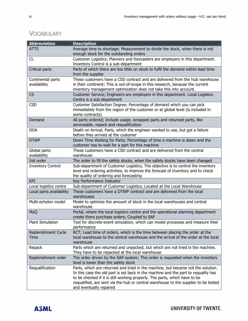
VOCABULARY
Abbreviation Description
ATTS Average time to shortage; Measurement to divide the stock, when there is not
enough stock for the outstanding orders
CL Customer Logistics; Planners and forecasters are employers in this department. Inventory Control is a sub-department
Critical parts Parts of which there are too little on stock to fulfil the demand within lead time
from the supplier
Continental parts availability
These customers have a CSD contract and are delivered from the hub warehouse in their continent; This is out-of-scope in this research, because the current
inventory management optimization does not take this into account.
CS Customer Service; Engineers are employers in this department. Local Logistics
Centre is a sub-department
CSD Customer Satisfaction Degree; Percentage of demand which you can pick
immediately from the region of the customer or at global level (is included in
some contracts)
Demand All parts ordered; Include usage, scrapped parts and returned parts, like serviceable, repack and requalification
DOA Death on Arrival; Parts, which the engineer wanted to use, but got a failure
before they arrived at the customer
DTWP Down Time Waiting for Parts; Percentage of time a machine is down and the customer has to wait for a part for this machine
Global parts
availability
These customers have a CSD contract and are delivered from the central
warehouse
Init order The order to fill the safety stocks, when the safety stocks have been changed
Inventory Control Sub-department of Customer Logistics; The objective is to control the inventory
level and ordering activities, to improve the forecast of inventory and to check
the quality of ordering and forecasting
KPI Key Performance Indicator
Local logistics centre Sub-department of Customer Logistics; Located at the Local Warehouse
Local parts availability These customers have a DTWP contract and are delivered from the local
warehouses
Multi-echelon model Model to optimize the amount of stock in the local warehouses and central warehouse
MyQ Portal, where the local logistics centre and the operational planning department
create there purchase orders; Coupled to SAP
Plant Simulation Tool for discrete-event simulation, which can model processes and measure their
performance
Replenishment Cycle
Time
RCT; Lead time of orders, which is the time between placing the order at the
local warehouse to the central warehouse and the arrival of the order at the local
warehouse
Repack Parts which are returned and unpacked, but which are not tried in the machine. They have to be repacked at the local warehouse
Replenishment order The order driven by the SAP-system; This order is requested when the inventory
level is lower than the safety stock
Requalification Parts, which are returned and tried in the machine, but became not the solution. In this case the old part is set back in the machine and the part to requalify has
to be checked if it is still working properly. The parts, which have to be requalified, are sent via the hub or central warehouse to the supplier to be tested
and eventually repaired
Inventory management with orders without usage - H.E. van der Horst iv iv
ROP Reorder Point
Rush order The order, driven by a manual order of parts
Sales Order The order, what is on beforehand sold to the customer
SAP ERP-system of ASML
Scrap Parts, which are returned and to inexpensive that it is more cost-effective to
scrap these parts and order new parts
Serviceable Parts, which are returned and not even unpacked, but only taken to the customer
SKU Stock Keeping Unit, which has at ASML a personal SKU-code
SLA Service Logistic Agreements; Maintenance contracts with customers of the
machines ASML delivers with targets DTWP and CSD
SPOC Single Person of Contact; Contact person from central to local warehouse
Usage Parts, which are used and will not return at the local warehouse
v Inventory management with orders without usage - H.E. van der Horst
MANAGEMENT SUMMARY
Currently ASML determines the safety stock levels by having the usage as main input in the model,
Spartan, to determine the safety stock levels. However at ASML the orders of parts are not all used parts,
but returned: ??% of the orders from the local warehouse to the customer are not used and will be
returned. Next to that, ??% of the emergency transportation costs are due to orders without usage. Also
the replenishment cycle time is higher for orders without usage.
Thereby the problem in this research is: “ASML is facing higher emergency transportation costs, longer
replenishment cycle time and higher risk of not satisfying the customer contracts due to not incorporating
orders without usage in the inventory level determination.”. Hereby the core question becomes:
“How should ASML respond to orders without usage into the inventory level calculations?
What would be the impact of this incorporation in terms of:
- Emergency transportation costs;
- Inventory holding costs;
- Replenishment cycle time;
- Risk of not satisfying the customer contracts?”
In this research first the current process and forecast is explained. A new part only will be send to the
local warehouse of a customer, when a part is needed and not on stock, or when the inventory level is
lower than the safety stock, which is a result of a usage of a part. The inventory level only changes when
a part is used and not when a part is sent to the customer. This is the policy at ASML. Then the part is
allocated. When returning a part, it can be used (??%), serviceable (??%), requalified (??%), repacked
(??%) and other returns (??%). The other returns are out-of-scope in this research. This means that ??%
of the orders from the local warehouse to the customer is not taken into account in the forecast, because
they are not used. This has the consequence of lower safety stocks than needed, which result in higher
emergency transportation costs.
The forecast at ASML is determined by the exponential smoothing of usage. In the optimization the
local safety stock levels are determined by Spartan, whereby the down time waiting for parts is the
constraint and the holding and emergency transportation costs are minimized. The forecast of the central
demand is the usage during lead time. In the optimization of the central inventory the reorder points are
set by minimizing the holding costs with the constraint of the customer satisfaction degree. The limitation
in this research is that the current inventory model and current measurement of the usage may not be
changed. Only a change in the input of the inventory model may be the result of this research. The
optimizations of the central and local inventory systems are not coupled, whereby a higher inventory
value for the local inventory system does not result in a lower inventory value for the central inventory
system to keep the same targets.
The impact of not including the orders without usage is measured. The impact of orders without
usage on the emergency transportation costs is €?? million in 2013, which is ??% of the total cost.
The impact on the replenishment cycle time is that the cycle time for a SKU with a high number of orders
without usage is higher than a SKU with a low number of orders without usage.
Next the forecast methods following literature are presented and the best method is chosen. The
suitable forecast methods in literature including return demand are developed by the authors Kelle and
Inventory management with orders without usage - H.E. van der Horst vi vi
Silver. They present four forecast methods. Method 2 of Kelle and Silver is found to be the most
appropriate method, because of his high robustness and low number of calculations in the method. Next
to that, the method performs almost as good as the best method. The forecast of method 2 decreases
the demand (usage and returns) with the parts which return during lead time.
Method 2 of Kelle and Silver has the drawback that negative demand may arise for SKUs having many
subsequent periods with zero demand, which have a high number of requalification orders returning in
the coming period. Also this method has still extra calculations than the current forecast. Thereby a new
method is developed. This method is simpler than method 2 of Kelle and Silver and the forecast is the
demand (usage and returns) minus the average number of orders returned.
These methods are applied to the inventory optimization methods of ASML and the most appropriate
method is chosen. The best method is chosen based on the smallest difference in outcome of the
simulation of the reality at ASML and the optimization per method. In the simulation of the local inventory
the developed method has the closest results to the optimization of the local inventory.
Implementing the developed method results in the annual savings of €?? million worldwide, which
includes the annual holding and emergency transportation costs. Next to that, implementing the
developed method results in the reduction in out-of-stocks of ?? parts annually, which is 33% of the
planned out-of-stocks. The costs of these out-of-stocks are not taken into account in the annual savings
and thereby there can be more costs reduction. The method needs an investment in inventory value of
€?? million. The risk and annual costs of the extra inventory value is taken into account in the annual
savings.
In reality the current method results in an underperformance in DTWP, RCT and CSD, because not all
demand is taken into account. The DTWP and CSD are in reality 1% lower than in the current method
(with not taking the returns into account). There is no significant difference in the RCT.
A qualitative result of adding the returns to the forecast, is a better planning, which results in more
satisfied suppliers and a better reaction of the suppliers on the demand of ASML. A better reaction on the
demand, results in less critical parts. Next to that, the emergency transportations will be reduced, which
results in more efficiency and a better consolidation of orders.
The recommendations, based on this research, are as follows:
- Include the return flow in the optimization of the local safety stock levels and the central ROP by
determining the forecast with developed method.
- In the next years ASML will implement a new multi-echelon inventory model, whereby the
optimizations of the central and local inventory costs are combined. The advice is to implement
this multi-echelon inventory model including the developed method. The current prototype is not
yet fully developed, whereby the results are not yet comparable to the current situation. The
recommendation is to calculate the methods with the correct CSDs, when the software is
available and check if the expectation is correct.
Further research is required for the following topics:
- A reverse logistics multi-echelon multi-item inventory model, whereby the multi-echelon model is
combined with the full return flow.
- The reduction of orders without usage, to reduce to core problem of having orders without
usage.

vii Inventory management with orders without usage - H.E. van der Horst
PREFACE
After a fantastic time in Enschede and at the University of Twente, I hereby present my master thesis.
This thesis is the last delivery of the master program Industrial Engineering and Management with the
specialization Production & Logistics Management. The research for this thesis was executed at ASML in
Veldhoven.
First of all I want to thank all people with whom I worked together, lived together, had nice evenings and
nights and who motivates me in my whole student life. I really liked my time with my study colleagues,
my roommates of the Borstelweg and Bentinckstraat, at Rowing Club Euros, at Study association Stress,
with my sorority Nefertiti, in my Student Union board and with my company PIP Advice.
With a lot of energy I worked on this research. It was fun to learn how to implement a theoretical model
in a real, dynamic environment. Besides that it was a good learning experience making all stakeholders of
this research clear what the goal was, methods were and results were.
I would like to thank my supervisors within ASML, K. Oner and R. van Sommeren, for their insights in the
problem and methods at ASML. I appreciated the time they spent in my research and their trust in me to
give me the full freedom and responsibility in my research. I also would like to thank my colleagues for
their critical input and their help for gathering information and getting contacts within the company.
Next to that, I also would like to thank my first supervisor of the University of Twente, M.C. van der
Heijden, for his contribution, critical reviews and enthusiasm for this research. Also thanks to my second
supervisor, A. Al Hanbali, for his support and also critical review. It is really motivating when both
supervisors really read your thesis report and give clear feedback.
I would like to thank all readers for their time to review my thesis report: Sophie, Jelco, Elieke, Tabea,
Tim and Irene. Next to that, I would like to thank my boyfriend Jelco for his positive support during my
study and master thesis. At last I would like to thank my parents, Gerard and Carla, for their support
during my entire study.
Veldhoven, March 6, 2015
H.E. van der Horst

Inventory management with orders without usage - H.E. van der Horst viii viii
ix Inventory management with orders without usage - H.E. van der Horst
TABLE OF CONTENTS
Vocabulary ........................................................................................................................................ iii
Management summary ........................................................................................................................ v
Preface ............................................................................................................................................. vii
1. Assignment description ................................................................................................................. 2
1.1. Company description ASML ................................................................................................... 2
1.2. Motivation of the research .................................................................................................... 2
1.3. Objective & research questions ............................................................................................. 4
1.4. Scope .................................................................................................................................. 7
1.5. Planning .............................................................................................................................. 8
2. Current way of working .............................................................................................................. 10
2.1. Ordering process at the local warehouse.............................................................................. 10
2.2. Process of returning parts ................................................................................................... 13
2.3. Current forecast method ..................................................................................................... 16
2.4. Current determination of reorder points at the local warehouse ............................................ 18
2.5. Current determination of ROPs at the central warehouse ...................................................... 19
2.6. Conclusion ......................................................................................................................... 20
3. Current performance on orders without usage ............................................................................. 22
3.1. The segments with high number of orders without usage ..................................................... 22
3.2. Impact of orders without usage........................................................................................... 25
3.3. Returning time of orders without usage ............................................................................... 26
3.4. Conclusion ......................................................................................................................... 28
4. Literature review forecast method ............................................................................................... 30
4.1. Forecast methods from literature......................................................................................... 30
4.2. Criteria forecast method ..................................................................................................... 31
4.3. Choice of method ............................................................................................................... 31
4.4. Conclusion ......................................................................................................................... 35
5. Applied method .......................................................................................................................... 37
5.1. Applied forecast method to ASML ........................................................................................ 37
5.2. Disadvantages of method 2................................................................................................. 39
5.3. Conclusion ......................................................................................................................... 40
6. Impact methods ......................................................................................................................... 42
6.1. Test methods on correctness .............................................................................................. 42
6.2. Impact on costs ................................................................................................................. 46
Inventory management with orders without usage - H.E. van der Horst x x
6.3. Impact on DTWP ................................................................................................................ 48
6.4. Impact on CSD ................................................................................................................... 48
6.5. Impact on replenishment cycle time in central warehouse..................................................... 49
6.6. Other effects of developed method...................................................................................... 49
6.7. Conclusion ......................................................................................................................... 50
7. Implementation Plan .................................................................................................................. 52
7.1. Implementation plan of developed method .......................................................................... 52
7.2. Drawbacks & risks of implementation plan ........................................................................... 55
7.3. Conclusion ......................................................................................................................... 56
8. Conclusions & Discussion ............................................................................................................ 58
8.1. Conclusion ......................................................................................................................... 58
8.2. Recommendations .............................................................................................................. 59
8.3. Discussion.......................................................................................................................... 59
8.4. Further research................................................................................................................. 60
References ....................................................................................................................................... 62
Appendix .......................................................................................................................................... 64
Appendix A: Forecasting................................................................................................................. 64
Appendix B: Confidential: Reference of confidential names of regions ............................................... 68
Appendix C: Inventory models ........................................................................................................ 69
Appendix D: Confidential: Figures in chapters 1, 2 and 3 .................................................................. 71
Appendix E: Simulation model in Plant Simulation ............................................................................ 72
Appendix F: Confidential: Figures in chapter 6 ................................................................................. 76
xi Inventory management with orders without usage - H.E. van der Horst
LIST OF TABLES
Table 1.1: Planning of master thesis. ................................................................................................... 8
Table 2.1: Overview of differences in order and transportation types. .................................................. 13
Table 2.2: Return of parts. ................................................................................................................ 14
Table 2.3: Reasons for ordering without usage from interviews. .......................................................... 15
Table 3.1: Replenishment cycle time per usage and percentage orders without usage per SKU. ............. 26
Table 4.1: Notation in method 2 of Kelle and Silver and their descriptions. ........................................... 32
Table 4.2: Input parameters in example of method 2 of Kelle and Silver. ............................................. 34
Table 5.1: Example of the negative values of Method 2 of Kelle and Silver. .......................................... 39
Table 6.1: Source of data in results. ................................................................................................... 42
Table 6.2: Results in costs of simulation model of region 2 per method. ............................................... 44
Table 6.3: Optimization of Region 2. .................................................................................................. 45
Table 6.4: Optimization of Region 2 in Chapter 6. ............................................................................... 45
Table 6.5: Results in costs of simulation model of region 2 per method. ............................................... 46
Table 6.6: Optimization and evaluation, normalized with holding costs of developed method. ................ 47
Table 6.7: Difference in DTWP per region. .......................................................................................... 48
Table 7.1: Tasks, actors and costs of informing decision makers. ......................................................... 52
Table 7.2: Tasks, actors and costs of pilot of method in one region. .................................................... 53
Table 7.3: Tasks, actors and costs of implement method for all regions. .............................................. 54
Table 7.4: Tasks, actors and costs of measuring process. .................................................................... 54
Table 7.5: Tasks, actors and costs of evaluation implementation and method. ...................................... 55
Table 7.6: Timeline of implementation. .............................................................................................. 55
Inventory management with orders without usage - H.E. van der Horst xii xii
LIST OF FIGURES
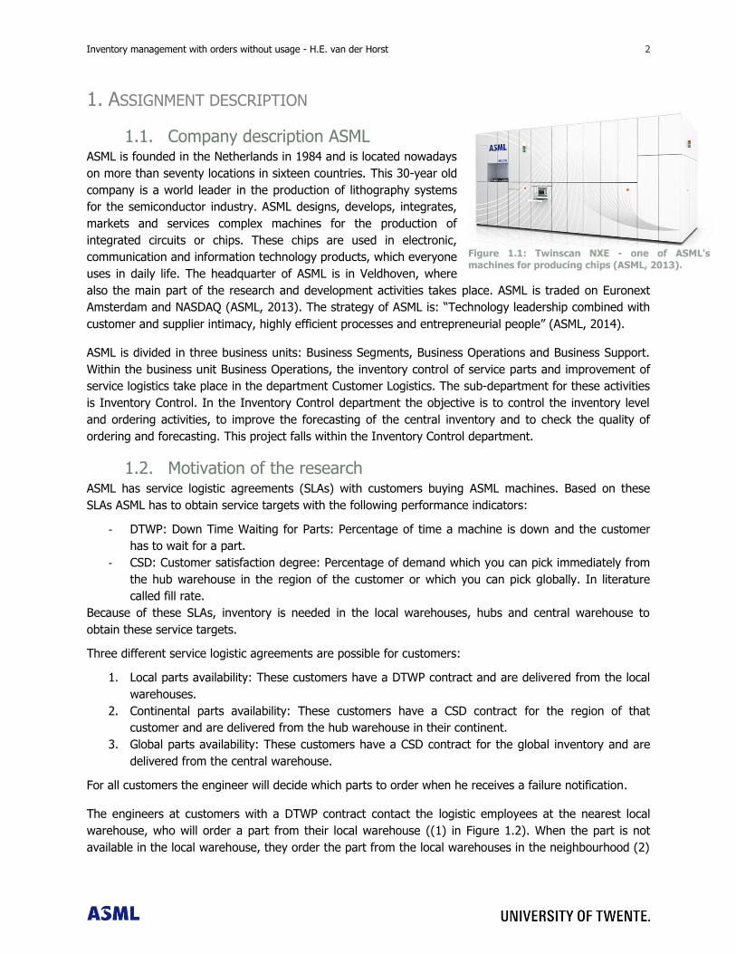
Figure 1.1: Twinscan NXE - one of ASML's machines for producing chips (ASML, 2013). .......................... 2
Figure 1.2: Current Service Process. ..................................................................................................... 3
Figure 1.3: Replenishment cycle time per percentage used. ................................................................... 4
Figure 1.4: Problem cluster of the unavailable parts at the local warehouse. ........................................... 5
Figure 2.1: Process of replenishment order. ........................................................................................ 11
Figure 2.2: Process of rush order. ...................................................................................................... 12
Figure 2.3: Process of return order..................................................................................................... 14
Figure 2.4: Monthly forecasting of failure rates. .................................................................................. 16
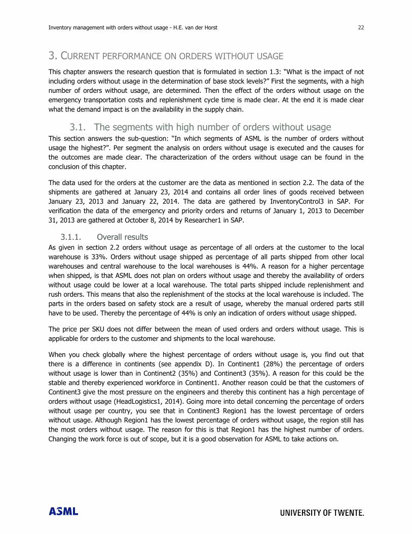
Figure 3.1: A select number of SKUs causes most shipments without usage to the local warehouse ....... 23
Figure 3.2: A select number of SKUs causes most orders without usage at the customer. ...................... 23
Figure 3.3: Number of parts returned per month. ............................................................................... 23
Figure 3.4: Orders without usage per machine type. ........................................................................... 24
Figure 3.5: Transportation type per usage bucket. .............................................................................. 24
Figure 3.6: Emergency transportation costs per usage and (no) ROP/SSL ............................................. 25
Figure 3.7: Emergency transportation costs per usage and machine down............................................ 26
Figure 3.8: Parts to repack are repacked, scrapped or replenished. Data from 2013; ............................. 27
Figure 3.9: Parts to requalify are requalified, scrapped or replenished. ................................................. 27
Figure 5.1: Applied inventory model of the reverse logistics at ASML. ................................................... 37
Figure 6.1: Inventory model in simulation. .......................................................................................... 43
Figure 6.2: Optimization of local inventory for each test. ..................................................................... 44
Figure 6.3: Reality of using the SSLs of the current method and the real demand. ................................ 46
Figure 6.4: Optimization of central inventory for each test. .................................................................. 47
Figure 6.5: Reality of using the ROPs of the current method and the real demand. ............................... 48
Figure 7.1: Implementation of developed method at ASML. ................................................................. 52
Figure A.0.1: Greedy method of SPARTAN following A.A. Kranenburg (2006). ....................................... 65
Figure A.0.2: Approximate evaluation method ..................................................................................... 66
Figure A.0.3: Review of Spartan output .............................................................................................. 67
Figure C.0.4: Different inventory figures of the recovery process ......................................................... 70
Figure E.0.12: Four processes in simulation. ....................................................................................... 72
Figure E.0.13: Welch's method for selecting the length of warming up period. ...................................... 75

1 Inventory management with orders without usage - H.E. van der Horst
Inventory management with orders without usage - H.E. van der Horst 2 2
1. ASSIGNMENT DESCRIPTION
1.1. Company description ASML ASML is founded in the Netherlands in 1984 and is located nowadays
on more than seventy locations in sixteen countries. This 30-year old
company is a world leader in the production of lithography systems
for the semiconductor industry. ASML designs, develops, integrates,
markets and services complex machines for the production of
integrated circuits or chips. These chips are used in electronic,
communication and information technology products, which everyone
uses in daily life. The headquarter of ASML is in Veldhoven, where
also the main part of the research and development activities takes place. ASML is traded on Euronext
Amsterdam and NASDAQ (ASML, 2013). The strategy of ASML is: “Technology leadership combined with
customer and supplier intimacy, highly efficient processes and entrepreneurial people” (ASML, 2014).
ASML is divided in three business units: Business Segments, Business Operations and Business Support.
Within the business unit Business Operations, the inventory control of service parts and improvement of
service logistics take place in the department Customer Logistics. The sub-department for these activities
is Inventory Control. In the Inventory Control department the objective is to control the inventory level
and ordering activities, to improve the forecasting of the central inventory and to check the quality of
ordering and forecasting. This project falls within the Inventory Control department.
1.2. Motivation of the research ASML has service logistic agreements (SLAs) with customers buying ASML machines. Based on these
SLAs ASML has to obtain service targets with the following performance indicators:
- DTWP: Down Time Waiting for Parts: Percentage of time a machine is down and the customer
has to wait for a part.
- CSD: Customer satisfaction degree: Percentage of demand which you can pick immediately from
the hub warehouse in the region of the customer or which you can pick globally. In literature
called fill rate.
Because of these SLAs, inventory is needed in the local warehouses, hubs and central warehouse to
obtain these service targets.
Three different service logistic agreements are possible for customers:
1. Local parts availability: These customers have a DTWP contract and are delivered from the local
warehouses.
2. Continental parts availability: These customers have a CSD contract for the region of that
customer and are delivered from the hub warehouse in their continent.
3. Global parts availability: These customers have a CSD contract for the global inventory and are
delivered from the central warehouse.
For all customers the engineer will decide which parts to order when he receives a failure notification.
The engineers at customers with a DTWP contract contact the logistic employees at the nearest local
warehouse, who will order a part from their local warehouse ((1) in Figure 1.2). When the part is not
available in the local warehouse, they order the part from the local warehouses in the neighbourhood (2)
Figure 1.1: Twinscan NXE - one of ASML's machines for producing chips (ASML, 2013).
3 Inventory management with orders without usage - H.E. van der Horst
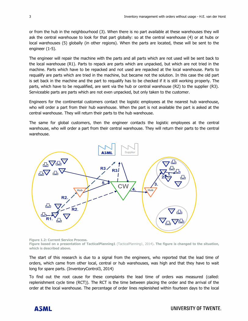
or from the hub in the neighbourhood (3). When there is no part available at these warehouses they will
ask the central warehouse to look for that part globally: so at the central warehouse (4) or at hubs or
local warehouses (5) globally (in other regions). When the parts are located, these will be sent to the
engineer (1-5).
The engineer will repair the machine with the parts and all parts which are not used will be sent back to
the local warehouse (R1). Parts to repack are parts which are unpacked, but which are not tried in the
machine. Parts which have to be repacked and not used are repacked at the local warehouse. Parts to
requalify are parts which are tried in the machine, but became not the solution. In this case the old part
is set back in the machine and the part to requalify has to be checked if it is still working properly. The
parts, which have to be requalified, are sent via the hub or central warehouse (R2) to the supplier (R3).
Serviceable parts are parts which are not even unpacked, but only taken to the customer.
Engineers for the continental customers contact the logistic employees at the nearest hub warehouse,
who will order a part from their hub warehouse. When the part is not available the part is asked at the
central warehouse. They will return their parts to the hub warehouse.
The same for global customers, then the engineer contacts the logistic employees at the central
warehouse, who will order a part from their central warehouse. They will return their parts to the central
warehouse.
Figure 1.2: Current Service Process. Figure based on a presentation of TacticalPlanning1 (TacticalPlanning1, 2014). The figure is changed to the situation,
which is described above.
The start of this research is due to a signal from the engineers, who reported that the lead time of
orders, which came from other local, central or hub warehouses, was high and that they have to wait
long for spare parts. (InventoryControl3, 2014)
To find out the root cause for these complaints the lead time of orders was measured (called:
replenishment cycle time (RCT)). The RCT is the time between placing the order and the arrival of the
order at the local warehouse. The percentage of order lines replenished within fourteen days to the local
Inventory management with orders without usage - H.E. van der Horst 4 4
warehouse was lower than the targeted 86%. To figure out the gap between the actual RCT and the
planned RCT the department Customer Logistics wrote down twenty-three possible causes
(InventoryControl3, 2014). One of these possible causes, namely orders without usage are not taken into
account in planning, is the start of this research. In the remainder of this section, further information
about this research is given. In the next section the problem statement is given.
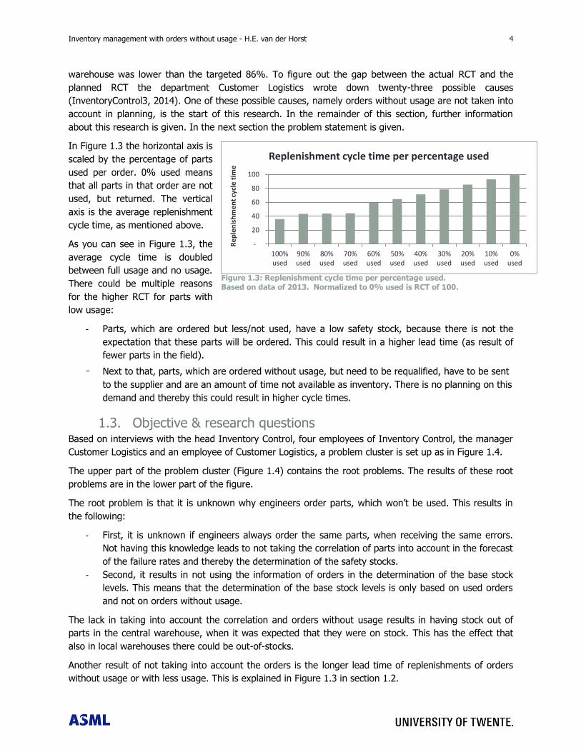
In Figure 1.3 the horizontal axis is
scaled by the percentage of parts
used per order. 0% used means
that all parts in that order are not
used, but returned. The vertical
axis is the average replenishment
cycle time, as mentioned above.
As you can see in Figure 1.3, the
average cycle time is doubled
between full usage and no usage.
There could be multiple reasons
for the higher RCT for parts with
low usage:
- Parts, which are ordered but less/not used, have a low safety stock, because there is not the
expectation that these parts will be ordered. This could result in a higher lead time (as result of
fewer parts in the field).
- Next to that, parts, which are ordered without usage, but need to be requalified, have to be sent
to the supplier and are an amount of time not available as inventory. There is no planning on this
demand and thereby this could result in higher cycle times.
1.3. Objective & research questions Based on interviews with the head Inventory Control, four employees of Inventory Control, the manager
Customer Logistics and an employee of Customer Logistics, a problem cluster is set up as in Figure 1.4.
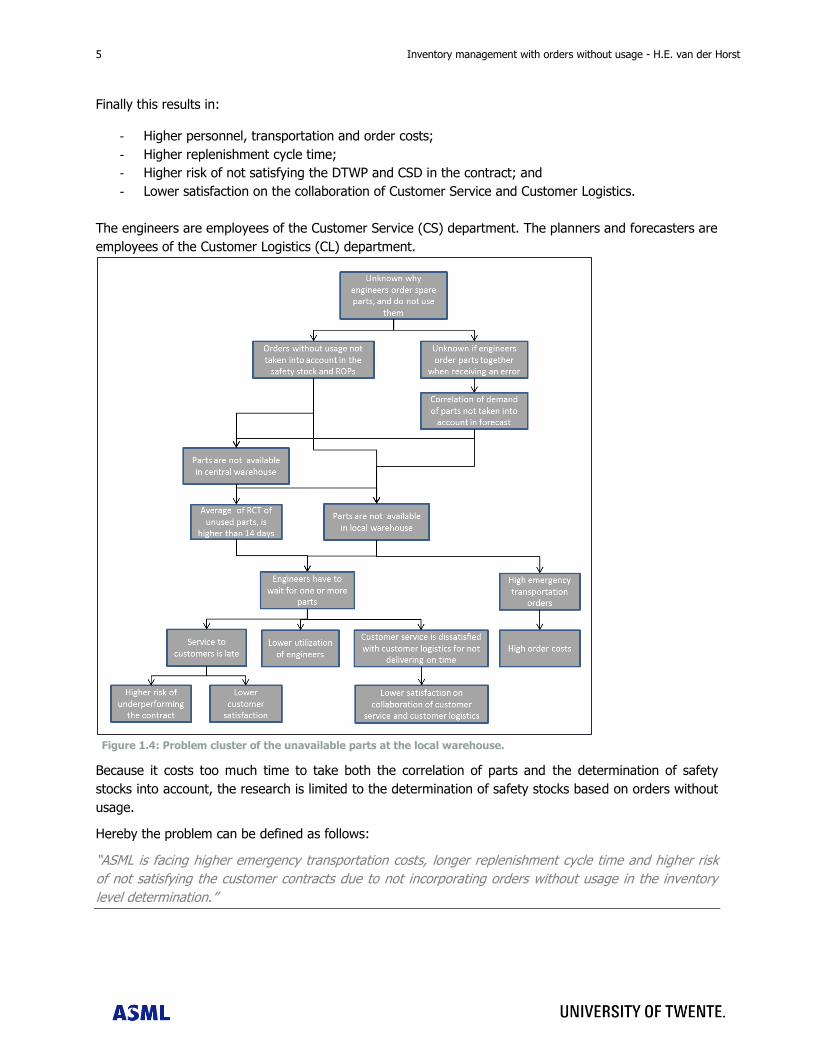
The upper part of the problem cluster (Figure 1.4) contains the root problems. The results of these root
problems are in the lower part of the figure.
The root problem is that it is unknown why engineers order parts, which won‟t be used. This results in
the following:
- First, it is unknown if engineers always order the same parts, when receiving the same errors.
Not having this knowledge leads to not taking the correlation of parts into account in the forecast
of the failure rates and thereby the determination of the safety stocks.
- Second, it results in not using the information of orders in the determination of the base stock
levels. This means that the determination of the base stock levels is only based on used orders
and not on orders without usage.
The lack in taking into account the correlation and orders without usage results in having stock out of
parts in the central warehouse, when it was expected that they were on stock. This has the effect that
also in local warehouses there could be out-of-stocks.
Another result of not taking into account the orders is the longer lead time of replenishments of orders
without usage or with less usage. This is explained in Figure 1.3 in section 1.2.
Figure 1.3: Replenishment cycle time per percentage used. Based on data of 2013. Normalized to 0% used is RCT of 100.
-
20
40
60
80
100
100%used
90%used
80%used
70%used
60%used
50%used
40%used
30%used
20%used
10%used
0%used
Re
ple
nis
hm
en
t cy
cle
tim
e
Replenishment cycle time per percentage used
5 Inventory management with orders without usage - H.E. van der Horst
Finally this results in:
- Higher personnel, transportation and order costs;
- Higher replenishment cycle time;
- Higher risk of not satisfying the DTWP and CSD in the contract; and
- Lower satisfaction on the collaboration of Customer Service and Customer Logistics.
The engineers are employees of the Customer Service (CS) department. The planners and forecasters are
employees of the Customer Logistics (CL) department.
Because it costs too much time to take both the correlation of parts and the determination of safety
stocks into account, the research is limited to the determination of safety stocks based on orders without
usage.
Hereby the problem can be defined as follows:
“ASML is facing higher emergency transportation costs, longer replenishment cycle time and higher risk
of not satisfying the customer contracts due to not incorporating orders without usage in the inventory
level determination.”
Figure 1.4: Problem cluster of the unavailable parts at the local warehouse.
Inventory management with orders without usage - H.E. van der Horst 6 6
The purpose of the research is to give advice to ASML about determining the base stock level based on
the orders and the return flow, by:
- Analysing the process of ordering and returning;
- Analysing the current forecasting method and current method of determination of the safety
stocks and reorder points;
- Analysing the impact of orders without usage;
- Reviewing literature to find forecast methods;
- Developing the forecast which incorporates the order and return flow of orders without usage;
- Comparing the results of the current method and the new method;
- Giving an implementation plan of the new method.
Hereby the core question becomes:
“How should ASML respond to orders without usage into the inventory level calculations?
What would be the impact of this incorporation in terms of:
- Emergency transportation costs;
- Inventory holding costs;
- Replenishment cycle time;
- Risk of not satisfying the customer contracts?”
The current model for determining the safety stocks and reorder points is the basis in this research. The
new forecast will be the input in this model.
This core question can be divided in different research questions; the so called knowledge questions
(Heerkens, 2005). These questions can be answered by reviewing the related literature, interviews at
ASML and data from ASML. The research questions are as follows.
1. What is the current way of working in the order and return process and how does ASML forecast
and determine the base stock levels?
a. How does the ordering process perform at the local warehouse?
b. How does the process of returning parts perform?
c. How does the current forecast method of the used parts perform?
d. How does the current determination of reorder points perform at the local warehouse?
e. How does the current determination of reorder points perform at the central warehouse?
2. What is the impact of not including orders without usage in the determination of base stock
levels?
a. In which segments of ASML is the number of orders without usage the highest?
b. What is the impact of orders without usage on the emergency transportation costs and
replenishment cycle time?
c. How long is the return lead time of orders without usage?
3. Following the literature, what forecast method can be used to determine the demand and return
flow?
a. Which methods are possible to forecast the demand and return orders?
b. What are the criteria to select the forecast method?
c. Which method is following the criteria the best to be added to the forecast of ASML?
7 Inventory management with orders without usage - H.E. van der Horst
4. How can the chosen method be added to the current determination of the base stock level?
a. How can the method be applied to ASML to forecast the order and return flow?
b. What are the disadvantages of the method and how can these disadvantages be
covered?
5. What is the impact of the new methods compared to the current method?
a. Which forecast of the methods is the most correct in the optimization compared to the
reality?
b. What is the cost impact by adding the forecast of the new method to the current
inventory model?
c. What is the impact on DTWP by adding the forecast of the new method to the current
inventory model?
d. What is the impact on CSD by adding the forecast of the new method to the current
inventory model?
e. What is the impact on replenishment cycle time by adding the forecast of the new
method to the current inventory model?
f. What are other effects at ASML by adding the forecast of the new method to the current
inventory model?
6. How can the new forecast method be implemented at ASML?
a. What is the plan to implement the forecast method?
b. What are the risks and drawbacks of the implementation and how can ASML handle
these?
1.4. Scope The scope in this research is the following:
- The description of the process in this research starts when the error in the machine has occurred.
- The description of the process in this research ends when the parts are used or returned to the
local or central warehouse and added to the inventory level.
- The current forecast method and translation to the safety stock model will not be changed,
because this is not reasonable to obtain in six months. The forecast will be added to this model.
- The customers with continental parts availability are not taken into account in this research,
because they are currently also not taken into account in the inventory management
optimization.
- The research is done for service parts.
o The tools are out of scope.
o Service parts for planned service are out of scope, because these will not have orders
without usage.
Inventory management with orders without usage - H.E. van der Horst 8 8
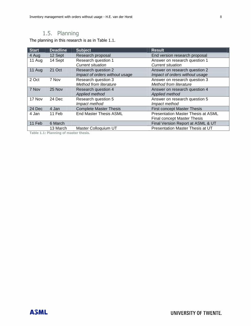
1.5. Planning The planning in this research is as in Table 1.1.
Start Deadline Subject Result
4 Aug 12 Sept Research proposal End version research proposal
11 Aug 14 Sept
Research question 1 Current situation
Answer on research question 1 Current situation
11 Aug 21 Oct
Research question 2 Impact of orders without usage
Answer on research question 2 Impact of orders without usage
2 Oct 7 Nov
Research question 3 Method from literature
Answer on research question 3 Method from literature
7 Nov 25 Nov
Research question 4 Applied method
Answer on research question 4 Applied method
17 Nov 24 Dec Research question 5 Impact method
Answer on research question 5 Impact method
24 Dec 4 Jan Complete Master Thesis First concept Master Thesis
4 Jan 11 Feb End Master Thesis ASML Presentation Master Thesis at ASML Final concept Master Thesis
11 Feb 6 March Final Version Report at ASML & UT
13 March Master Colloquium UT Presentation Master Thesis at UT Table 1.1: Planning of master thesis.
9 Inventory management with orders without usage - H.E. van der Horst
Inventory management with orders without usage - H.E. van der Horst 10 10
2. CURRENT WAY OF WORKING
This chapter answers the research question that is formulated in section 1.3: “What is the current way of
working in the order and return process and how does ASML forecast and determine the base stock
levels?”. First the changes in inventory level are described. Then the current forecast methods and
inventory models for determining safety stocks and ROPs are declared.
2.1. Ordering process at the local warehouse This section answers the sub-question: “How does the ordering process perform at the local
warehouse?”. This section is divided in order types and transportation types.
2.1.1. Order types
The orders can be divided in different types: Init, sales, replenishment and rush (HeadInterfaceTeam1,
2014).
The init orders are the orders to fill the safety stocks, when the safety stocks have been changed. This
order type is out of scope, because it is not possible to forecast these orders. These orders are one-time
changes. Next to that, the delivery lead time of init orders is the length of the lead time of delivering new
parts from the supplier to the central warehouse.
The sales orders are orders which are sold to the customer beforehand, when the customer maintains the
machine by himself. The sales orders are out of scope of this research, because these orders also cannot
be forecasted and have also the lead time of the supplier (HeadInterfaceTeam1, 2014).
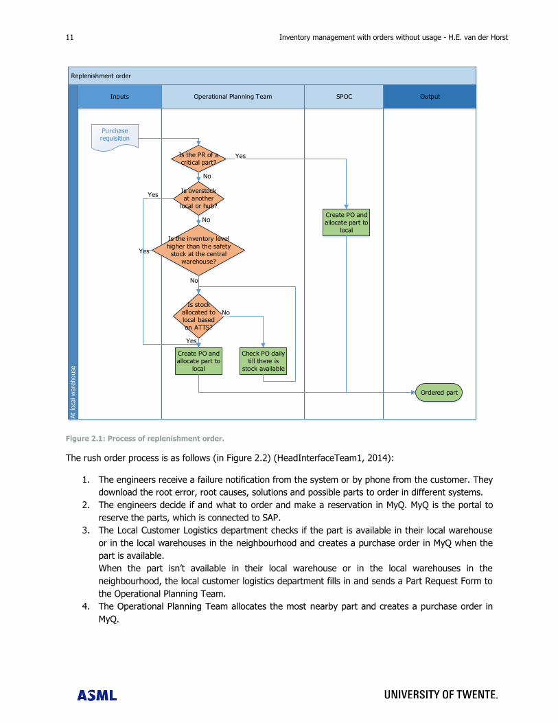
Replenishment orders, as typology at ASML, are orders driven by the SAP-system. These orders are
requested when the inventory level is lower than the safety stock. The parts of the replenishment orders
can be shipped from another local warehouse, when there is overstock at that local warehouse. When
there is no overstock at the local warehouse the parts will be shipped from the central warehouse. The
process is visualised in Figure 2.1 (HeadInterfaceTeam1, 2014).
Rush orders, as typology at ASML, are orders which are driven by manual orders of parts in SAP. Rush
orders are requested by the local logistic centre within the local warehouse. The rush orders are needed
for the parts, which don‟t have a safety stock or where the inventory level is too low for the number of
parts needed. Rush orders are in most cases orders which have to be delivered very fast. It is also
possible to have a rush order which is planned on a specific time in the future, while it is still manual set
(HeadInterfaceTeam1, 2014).
11 Inventory management with orders without usage - H.E. van der Horst
Replenishment order
Inputs Operational Planning Team OutputSPOC
At
loca
l w
are
house
Ordered part
Purchase
requisition
Is the PR of a
critical part?
No
Is overstock
at another
local or hub?
Is the inventory level
higher than the safety
stock at the central
warehouse?
No
Is stock
allocated to
local based
on ATTS?
No
No
Create PO and
allocate part to
local
Yes
Yes
Yes
Create PO and
allocate part to
local
Yes
Check PO daily
ti ll there is
stock available
Figure 2.1: Process of replenishment order.
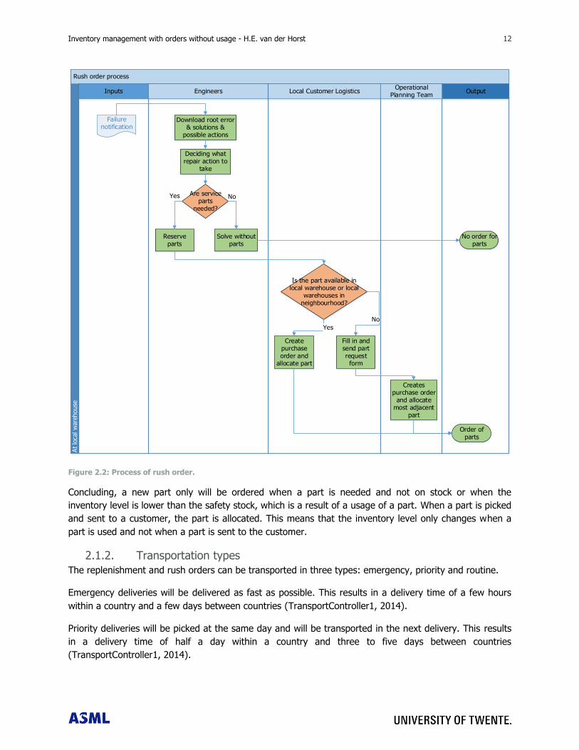
The rush order process is as follows (in Figure 2.2) (HeadInterfaceTeam1, 2014):
1. The engineers receive a failure notification from the system or by phone from the customer. They
download the root error, root causes, solutions and possible parts to order in different systems.
2. The engineers decide if and what to order and make a reservation in MyQ. MyQ is the portal to
reserve the parts, which is connected to SAP.
3. The Local Customer Logistics department checks if the part is available in their local warehouse
or in the local warehouses in the neighbourhood and creates a purchase order in MyQ when the
part is available.
When the part isn‟t available in their local warehouse or in the local warehouses in the
neighbourhood, the local customer logistics department fills in and sends a Part Request Form to
the Operational Planning Team.
4. The Operational Planning Team allocates the most nearby part and creates a purchase order in
MyQ.
Inventory management with orders without usage - H.E. van der Horst 12 12
Rush order process
Inputs Engineers Local Customer Logistics OutputOperational
Planning Team
At
loca
l w
areh
ouse
Failure notification
Are service parts
needed?
Solve without parts
No
Reserve parts
Yes
No order for parts
Is the part available in local warehouse or local
warehouses in neighbourhood?
Create purchase order and
allocate part
Fill in and send part request form
Yes
No
Creates purchase order
and allocate most adjacent
part
Order of parts
Download root error & solutions &
possible actions
Deciding what repair action to
take
Figure 2.2: Process of rush order.
Concluding, a new part only will be ordered when a part is needed and not on stock or when the
inventory level is lower than the safety stock, which is a result of a usage of a part. When a part is picked
and sent to a customer, the part is allocated. This means that the inventory level only changes when a
part is used and not when a part is sent to the customer.
2.1.2. Transportation types
The replenishment and rush orders can be transported in three types: emergency, priority and routine.
Emergency deliveries will be delivered as fast as possible. This results in a delivery time of a few hours
within a country and a few days between countries (TransportController1, 2014).
Priority deliveries will be picked at the same day and will be transported in the next delivery. This results
in a delivery time of half a day within a country and three to five days between countries
(TransportController1, 2014).
13 Inventory management with orders without usage - H.E. van der Horst
Routine deliveries will be picked on the next day and will be transported when possible. This results in a
delivery time of one day within a country and six to nine days between countries (TransportController1,
2014).
Per order type and per transportation type an overview of the differences is given in Table 2.1. The
choice of priority and emergency of a replenishment order is how fast a planner wants to have the critical
part on stock (TransportController1, 2014).
Order type Replenishment Rush
Transportation type Routine Priority Emergency Routine Priority Emergency
Is the order manual made in SAP?
Yes Yes Yes
Is the order requested
automatically by SAP?
Yes Yes Yes
Is the machine down? Yes
Are the parts needed for a planned action within 14 days?
Yes
Is the part a critical part? Yes Yes Table 2.1: Overview of differences in order and transportation types.
2.2. Process of returning parts This section answers the sub-question: “How does the process of returning parts perform?”.
When a part is used, the inventory level decreases. When a part is not used and is returned, the local
customer logistics department fills in the material notification and adds the reason of returning in the
material notification. In table 2.2 the different reasons of returning parts are given following the material
notification.
The data of the return flow are gathered in two phases: the used parts and the returned parts. The data
of the used parts are gathered at August 15, 2014 and contains all order lines of goods received between
January 1, 2013 and December 31, 2013. The data are gathered by Analyst3, responsible for forecasting,
in SAP. The data of the returned parts are gathered at August 20, 2014 and contains all order lines of
goods receipt between January 1, 2013 and December 31, 2013. The data are gathered by
TacticalPlanning2, responsible to determine safety stocks, in SAP. All incomplete order lines are out of
scope, because incomplete order lines cannot be analysed. For verification the data of returned parts are
gathered at August 27, 2014 by CriticalParts1, member of the critical parts team. The data for verification
of used parts are gathered by OperationalPlanner2, member of the critical parts team, at August 21,
2014.
In Table 2.2 you can see that 21% of all parts ordered at the local warehouse are returned and are still
serviceable. Another 12% of all parts ordered are also sent back, but need a handling to add the parts on
stock again. The detailed table can be found in appendix D, because of confidentiality.

Inventory management with orders without usage - H.E. van der Horst 14 14
Reasons for sending back Percentage of total ordered
parts
Percentage of returning
parts
Death on arrival 2% 5%
Repacked 3% 10%
Requalified 7% 21%
Serviceable 21% 64%
Used 67% -
The process of returning the parts is given in Figure 2.3. The parts labelled as “DOA” are out of scope of
this project. The reason for this is that when these parts would not have a failure when they arrived or
when they were installed, they would be used.
Return process
Inputs Engineers OutputSupplier
At
loca
l w
areh
ouse
Is the part defect at arrival?
Book the part as
serviceable
Is the part unpacked?
Yes
Part is delivered at
local warehouse
No
Is the part used?
Yes
No
Used part
Serviceable part
No
DOA process
Add part by local
customer logistics to
local inventory
Is the part tried in the machine?
Yes
No
Repack part by local
customer logistics & add part to
local inventory
Test and requalify
part
Is the part > €400,-?
Is the part > €100,-?
Is the part
critical?
Is the part
critical?
No
Scrap the part
YesYes
No
No
Yes
Scrap part
Book the part as
requalified & send part
by local customer
logistics via the hub, by central MRP planning to
supplier
No
Book the part as
repacked
Yes
Yes
Figure 2.3: Process of return order.
Table 2.2: Return of parts.
15 Inventory management with orders without usage - H.E. van der Horst
The parts, which returned with the label “Requalification”, were sent back by the local logistics centre to
the hub. The hub sent them back to the supplier, who tested the parts and sent them back to the hub. In
the hub the parts are added to the stock of the hub. When the part to be requalified has a price lower
than €400,- and is not a critical part, the part is scrapped before going to the supplier. Critical parts are
parts, of which there are too little on stock to fulfil the demand within lead time from the supplier. If a
part to be requalified cannot be repaired, the part is scrapped. In total 15% of the parts to requalify is
scrapped. The lead times are given in section 3.3 (Criticalparts1, 2014).
The parts to be repacked are sent to the local warehouse, then repacked and added to the stock at the
local warehouse. When the parts to be repacked have a price lower than €100,- and they are not critical
parts, then the part is scrapped, before repacking. In total 16% of the parts to repack is scrapped. The
lead times are given in section 3.3 (Criticalparts1, 2014).
The serviceable are added to the stock in the local warehouse immediately. The lead times are given in
section 3.3 (Criticalparts1, 2014).
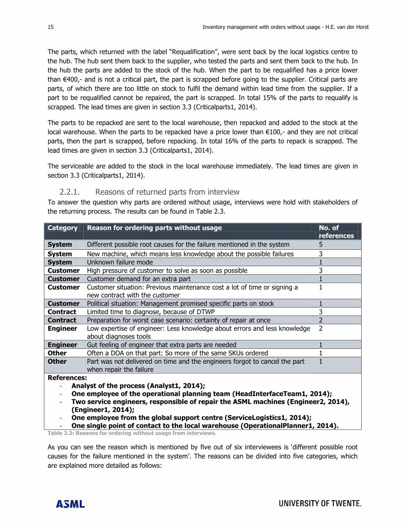
2.2.1. Reasons of returned parts from interview
To answer the question why parts are ordered without usage, interviews were hold with stakeholders of
the returning process. The results can be found in Table 2.3.
Category Reason for ordering parts without usage No. of references
System Different possible root causes for the failure mentioned in the system 5
System New machine, which means less knowledge about the possible failures 3
System Unknown failure mode 1
Customer High pressure of customer to solve as soon as possible 3
Customer Customer demand for an extra part 1
Customer Customer situation: Previous maintenance cost a lot of time or signing a new contract with the customer
1
Customer Political situation: Management promised specific parts on stock 1
Contract Limited time to diagnose, because of DTWP 3
Contract Preparation for worst case scenario: certainty of repair at once 2
Engineer Low expertise of engineer: Less knowledge about errors and less knowledge
about diagnoses tools
2
Engineer Gut feeling of engineer that extra parts are needed 1
Other Often a DOA on that part: So more of the same SKUs ordered 1
Other Part was not delivered on time and the engineers forgot to cancel the part
when repair the failure
1
References:
- Analyst of the process (Analyst1, 2014);
- One employee of the operational planning team (HeadInterfaceTeam1, 2014); - Two service engineers, responsible of repair the ASML machines (Engineer2, 2014),
(Engineer1, 2014); - One employee from the global support centre (ServiceLogistics1, 2014);
- One single point of contact to the local warehouse (OperationalPlanner1, 2014). Table 2.3: Reasons for ordering without usage from interviews.
As you can see the reason which is mentioned by five out of six interviewees is „different possible root
causes for the failure mentioned in the system‟. The reasons can be divided into five categories, which
are explained more detailed as follows:
Inventory management with orders without usage - H.E. van der Horst 16 16
- System: When an engineer looks in the system for the problem, he finds a possible problem.
Subsequently, this possible problem is the input for getting the solution out of another system.
The output of that system is a list of ten different solutions, which were mentioned by an
engineer at least once. Based on that information the decision of what part to order is made
(CompetencyEngineer1, 2014).
- Customer: The machines of ASML are the bottleneck machines in the production process at the
customer, because these are the most expensive machines and thereby the bottlenecks
(ToolPlanning1, 2014). So when a machine is down, the whole flow is down. This results in high
costs, which could lead to more than $500.000,- per hour for the newest machine of ASML
(InventoryControl1, 2014). This situation at the customer results in high pressure of the
customer and high dependency on each other.
- Contract: In the contract with the customer the down time has to be limited. Thereby there is
limited time to diagnose and the repair has to be all at once to avoid losing time.
- Engineer: Because of the difficulties in the system, the engineer has to make decisions based on
his experience and knowledge. Thereby it depends on the engineer, how much parts he will
order.
The next sections present: Current forecast method, current determination of safety stocks at the local
warehouse and current determination of reorder points at the central warehouse.
2.3. Current forecast method This section answers the sub-question: “How does the current forecast method of the used parts
perform?”. This question is used to understand the current forecast method, which can be used later in
determining the new forecast method. First the forecast method of the failure rates at local warehouses
is described. Then the translation of this forecast is made to the central forecast.
2.3.1. Local forecast method
The current forecast of the failure rates is determined monthly. In the local warehouse all SKUs are
stocked according safety stock levels, with as input the expected failure rates.
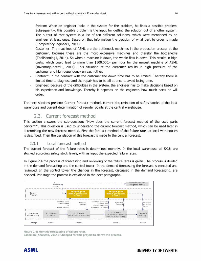
In Figure 2.4 the process of forecasting and reviewing of the failure rates is given. The process is divided
in the demand forecasting and the control tower. In the demand forecasting the forecast is executed and
reviewed. In the control tower the changes in the forecast, discussed in the demand forecasting, are
decided. Per stage the process is explained in the next paragraphs.
Figure 2.4: Monthly forecasting of failure rates. Based on (Analyst3, 2014); Changed for this project to clarify the process.
17 Inventory management with orders without usage - H.E. van der Horst
In S0 the forecast is created. The input is as follows:
1. Usage per SKU per machine per quarter;
2. The number of SKUs per machine;
3. The number of machines per local warehouse.
The failure rate per quarter t is calculated by formula (2.1), as specified by ASML. is the install
base life. This is the number of installed machines times the number of parts of that SKU in that machine
in quarter t. is the average usage per day of SKU i in quarter t. The usage contains the
preventive and corrective replacement of parts (Analyst3, 2014).
The forecast is determined at ASML by formula (2.2). Hereby is the weight percentage. The weight
percentage is measured by formula (2.3). The forecast is the average usage per day of SKU i during the
last three years.
∑
∑
is the decrease of exponentially weight and is 1.4 at ASML. is determined by checking different
weights and thereby 1.4 became a good mix of stiffness and flexibility (Analyst3, 2014). From my own
calculations there is no difference in forecast with different weights. Changing this is out of scope of this
research.
The time taken in the creation of the expected failure rate is three years and every time step is one
quarter of a year. Thereby there are twelve periods. ASML choose for twelve periods because in the
simulation study this amount of time resulted in the best performance of the forecast in terms of forecast
errors (Analyst3, 2014). A t of 12 is the most recent period of the data sample.
The forecasts are reviewed on central and local level for specific SKUs. The criteria are stated in Appendix
A.1. The results of S0 are the forecast of the failure rates per SKU and a list of SKUs to be discussed. The
selected SKUs are discussed in S1 and S2.
In S1 the worldwide forecast of failure rates of the selected SKUs is discussed by the Inventory Control
team and tactical planners per SKU. In this meeting the adjustments can be made per SKU per machine.
In S2 the regional review will take place with the SPOCs: contact persons to the local warehouse. Here
the focus is on regional trends. Adjustments are made per local warehouse.
In the demand meeting (week 4 in Figure 2.4) the decision is made what changes are necessary to
make. The forecast is the input for the determination of the reorder points as explained in section 2.4.
(2.1)
(2.2)
(2.3)
Inventory management with orders without usage - H.E. van der Horst 18 18
2.3.2. Central forecast method
In the central warehouse, SKUs are forecasted if they have a usage of more than six parts in half a year.
A usage less than six parts in six months results in having a reorder point. The reason for this is that the
forecast is reviewed monthly and thereby it is more cost efficient to only forecast SKUs which are used at
least once per month.
The central planners check every month the forecast and they order per month the forecasted amount.
There is no safety stock level or reorder point for the forecasted parts. The forecast is monthly reviewed.
In calculating the ROP the forecast, which is based on the formula (2.4), is needed (InventoryControl2,
2014). Hereby is the forecast worldwide per day for SKU i. is the forecast per day of local
warehouse j for SKU i. J is the number of local warehouses.
∑
2.4. Current determination of reorder points at the local warehouse This section answers the sub-question: “How does the current determination of reorder points perform at
the local warehouse?”. In the half-yearly forecast of the local reorder points Spartan is used to determine
the reorder points with a greedy algorithm (Kranenburg, 2006). A greedy algorithm is an algorithm that
goes through all stages in a problem solving heuristic, whereby at each stage the local optimum is
chosen. It is possible to find the global optimum, but the result could also be a local optimum
(Hazewinkel, 2011).
The inputs for Spartan are as follows (TacticalPlanning2, 2014) (Kranenburg, 2006):
Failure rates occurring following a Poisson process with constant rate ; whereby is the SKU
and is a machine. These failures are determined following section 2.3.1;
Number of machines of type per customer linked to local warehouse j;
Average time for an emergency transportation from the central warehouse to the local
warehouse per SKU ;
Average cost for an emergency transportation from the central warehouse to the local warehouse
;
Average time for a lateral shipment from another local warehouse to the local warehouse per
SKU ;
Average cost for a lateral shipment from another local warehouse to the local warehouse per SKU
;
Holding costs per time unit per SKU .
The objective in Spartan is to minimize the total costs by determining the base stock level of SKU i at
local warehouse j .
The constraints are defined as follows (Kranenburg, 2006):
Maximum average waiting time per local warehouse
: DTWP as specified in section 1.2;
Lead time to deliver the parts with a routine transportation to the local warehouse (from the
central warehouse) is fixed on 14 days.
(2.4)
19 Inventory management with orders without usage - H.E. van der Horst
In this method inventory pooling is applicable, which implies using the same inventory at one local
warehouse of a SKU for several machines. Next to that, pooling is applicable to the lateral transhipment
between local warehouses. In this case when a part is needed, the part also can be ordered from another
local warehouse (and central warehouse). In this case all local warehouses can have lateral
transhipments and thereby this method is full pooling. The greedy method contains three steps
(Kranenburg, 2006).
Step 1: In step one the parameters are initiated, which includes setting zero stock levels: .
Step 2: In step two the base stock levels increase as long as the costs do not increase. Thereby
, the cost difference of SKU i at local warehouse j, is measured to determine if the cost difference
is equal or positive.
Step 3: In step three the stock level increases of the SKU that provides the largest decrease in
waiting time ( ) per unit costs increase , as long as the current solution is not feasible. The
current solution is feasible when the constraints as set above are achieved.
The written out formulas and procedure in detail can be found in Appendix A.2. Some SKUs need an
extra review following the list in Appendix A.3. The review of the output of Spartan is also described in
Appendix A.3.
When the failure rates are changed a lot in a month, the reorder points are changed based on the
approach in section 2.3.1. The safety stock is one month of usage on top of the forecast. For SKUs with a
high fluctuation, this amount can be higher. This amount is based on gut feeling (InventoryControl1,
2014).
2.5. Current determination of ROPs at the central warehouse This section answers the sub-question: “How does the current determination of reorder points perform at
the central warehouse?” When the usage is less than six in the last six months, the SKU has a reorder
point and is ordered based on the reorder point. The reorder points are monthly reviewed and are
reviewed when an SKU is ordered at the supplier (InventoryControl2, 2014).
The expected usage during lead time (DDLT) is calculated by including the expected demand (as in
formula (2.4)) during lead time, including the scrapped parts of the returns in the demand and including
the parts to repair (of the failed parts) of the returns. Please notice that the returns in formula (2.5) are
the result of the usage. So because of a usage the failed parts in the machine are sent back. This is
another flow than the orders without usage. The demand during lead time for SKU i is as follows formula
(2.5) (InventoryControl2, 2014).
( )
The ROP is calculated to fulfil the CSD, Customer Satisfaction Degree. The assumption is made that the
demand during lead time is Poisson distributed. This is measured in August by checking the data with the
distributions (InventoryControl1, 2014). In a Macro in Excel the calculation is made that the ROP will
increase as long as the service level is not yet fulfilled, as in the cumulative function in formula (2.6)
(InventoryControl2, 2014). In formula (2.6) the ROP has to be high enough to fulfil the change of not
going out-of-stock ( ), which has to be higher than the CSD.
(2.5)
Inventory management with orders without usage - H.E. van der Horst 20 20
When the demand is zero during lead time or when the demand is one in the last two months, the
reorder point is two.
These SKUs have a safety stock. The safety stock is the difference between the ROP and the demand
during lead time. So when the ROP is 3 and the demand during lead time is 0.71, then the SSL is 2 (3-
0.71 rounded). For SKUs with a high fluctuation, this amount can be higher. This amount is based on gut
feeling (InventoryControl1, 2014).
2.6. Conclusion This chapter answers the question “What is the current way of working in the order and return process
and how does ASML forecast and determine the base stock levels?”. The conclusions are as follows:
A new part only will be ordered when a part is needed and not on stock or when the inventory
level is lower than the safety stock, which is a result of a usage of a part. The inventory level
only changes when a part is used and not when a part is sent to the customer. Then the part is
allocated.
When returning a part, it can be used (67%), serviceable (21%) or labelled as requalified (7%)
and repacked (3%). This means 33% of the orders from the local warehouse to the customer is
not taken into account in the forecast. The orders without usage are handled different per order
type. The serviceable parts and parts to repack are added to the inventory of the local
warehouse. The parts to requalify are sent to the supplier and added to the inventory of the hub
warehouse.
The forecasted failure rate per local warehouse depends on the usage of a SKU per quarter, the
installed base of machines for that SKU per quarter and the weight factor. The forecast of the
usage per month for the central warehouse is dependent on the usage, the amount to repair and
the lead times from the supplier. Thereby, in the local and central warehouse forecast the orders
without usage are not taken into account.
The reorder points at the local warehouse are constrained by the replenishment lead time and
the constraints in the contract with the customer: the down time waiting for parts and the fill rate
of a SKU. The reorder point at the central warehouse is impacted by the lead time of receiving
new parts and repair parts from the supplier.
(2.6)

21 Inventory management with orders without usage - H.E. van der Horst
Inventory management with orders without usage - H.E. van der Horst 22 22
3. CURRENT PERFORMANCE ON ORDERS WITHOUT USAGE
This chapter answers the research question that is formulated in section 1.3: “What is the impact of not
including orders without usage in the determination of base stock levels?” First the segments, with a high
number of orders without usage, are determined. Then the effect of the orders without usage on the
emergency transportation costs and replenishment cycle time is made clear. At the end it is made clear
what the demand impact is on the availability in the supply chain.
3.1. The segments with high number of orders without usage This section answers the sub-question: “In which segments of ASML is the number of orders without
usage the highest?”. Per segment the analysis on orders without usage is executed and the causes for
the outcomes are made clear. The characterization of the orders without usage can be found in the
conclusion of this chapter.
The data used for the orders at the customer are the data as mentioned in section 2.2. The data of the
shipments are gathered at January 23, 2014 and contains all order lines of goods received between
January 23, 2013 and January 22, 2014. The data are gathered by InventoryControl3 in SAP. For
verification the data of the emergency and priority orders and returns of January 1, 2013 to December
31, 2013 are gathered at October 8, 2014 by Researcher1 in SAP.
3.1.1. Overall results
As given in section 2.2 orders without usage as percentage of all orders at the customer to the local
warehouse is 33%. Orders without usage shipped as percentage of all parts shipped from other local
warehouses and central warehouse to the local warehouses is 44%. A reason for a higher percentage
when shipped, is that ASML does not plan on orders without usage and thereby the availability of orders
without usage could be lower at a local warehouse. The total parts shipped include replenishment and
rush orders. This means that also the replenishment of the stocks at the local warehouse is included. The
parts in the orders based on safety stock are a result of usage, whereby the manual ordered parts still
have to be used. Thereby the percentage of 44% is only an indication of orders without usage shipped.
The price per SKU does not differ between the mean of used orders and orders without usage. This is
applicable for orders to the customer and shipments to the local warehouse.
When you check globally where the highest percentage of orders without usage is, you find out that
there is a difference in continents (see appendix D). In Continent1 (28%) the percentage of orders
without usage is lower than in Continent2 (35%) and Continent3 (35%). A reason for this could be the
stable and thereby experienced workforce in Continent1. Another reason could be that the customers of
Continent3 give the most pressure on the engineers and thereby this continent has a high percentage of
orders without usage (HeadLogistics1, 2014). Going more into detail concerning the percentage of orders
without usage per country, you see that in Continent3 Region1 has the lowest percentage of orders
without usage. Although Region1 has the lowest percentage of orders without usage, the region still has
the most orders without usage. The reason for this is that Region1 has the highest number of orders.
Changing the work force is out of scope, but it is a good observation for ASML to take actions on.
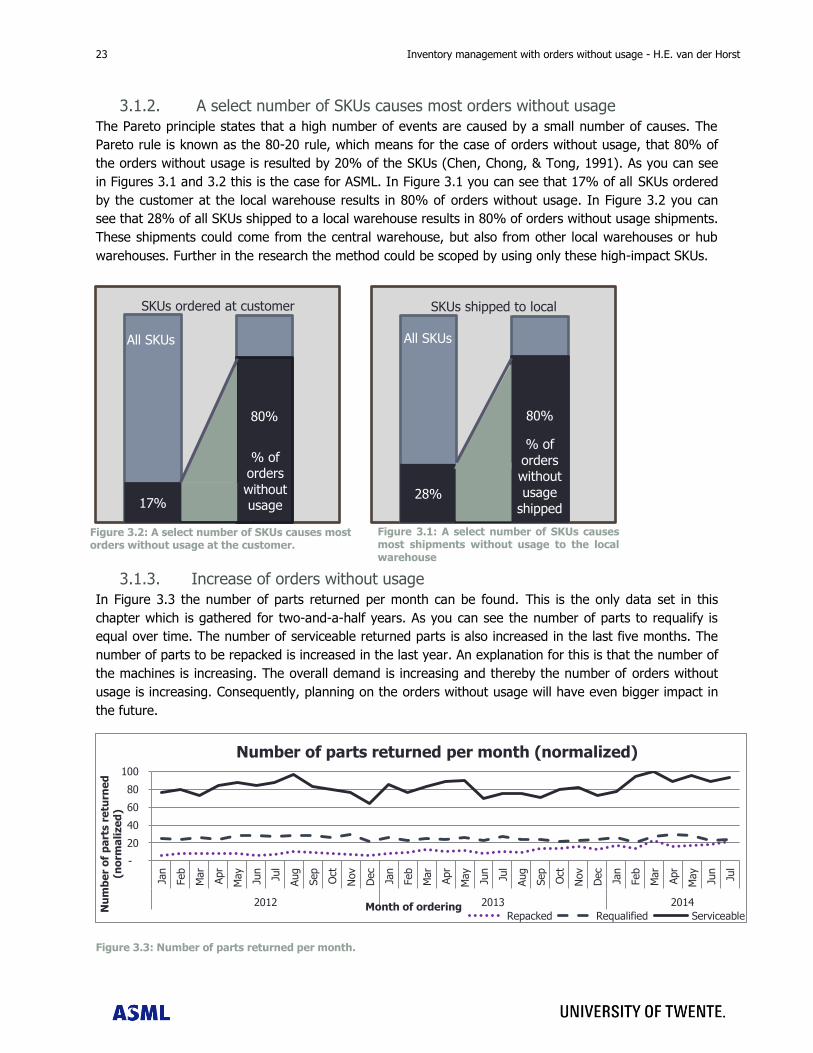
23 Inventory management with orders without usage - H.E. van der Horst
3.1.2. A select number of SKUs causes most orders without usage
The Pareto principle states that a high number of events are caused by a small number of causes. The
Pareto rule is known as the 80-20 rule, which means for the case of orders without usage, that 80% of
the orders without usage is resulted by 20% of the SKUs (Chen, Chong, & Tong, 1991). As you can see
in Figures 3.1 and 3.2 this is the case for ASML. In Figure 3.1 you can see that 17% of all SKUs ordered
by the customer at the local warehouse results in 80% of orders without usage. In Figure 3.2 you can
see that 28% of all SKUs shipped to a local warehouse results in 80% of orders without usage shipments.
These shipments could come from the central warehouse, but also from other local warehouses or hub
warehouses. Further in the research the method could be scoped by using only these high-impact SKUs.
3.1.3. Increase of orders without usage
In Figure 3.3 the number of parts returned per month can be found. This is the only data set in this
chapter which is gathered for two-and-a-half years. As you can see the number of parts to requalify is
equal over time. The number of serviceable returned parts is also increased in the last five months. The
number of parts to be repacked is increased in the last year. An explanation for this is that the number of
the machines is increasing. The overall demand is increasing and thereby the number of orders without
usage is increasing. Consequently, planning on the orders without usage will have even bigger impact in
the future.
Figure 3.3: Number of parts returned per month.
-
20
40
60
80
100
Jan
Feb
Mar
Apr
May
Jun
Jul
Aug
Sep
Oct
Nov
Dec
Jan
Feb
Mar
Apr
May
Jun
Jul
Aug
Sep
Oct
Nov
Dec
Jan
Feb
Mar
Apr
May
Jun
Jul
2012 2013 2014
Nu
mb
er
of
pa
rts r
etu
rne
d
(no
rma
lize
d)
Month of ordering
Number of parts returned per month (normalized)
Repacked Requalified Serviceable
17%
80%
28%
80%
SKUs shipped to local
All SKUs
% of
orders without
usage
shipped
All SKUs
% of orders
without usage
SKUs ordered at customer
Figure 3.1: A select number of SKUs causes most shipments without usage to the local warehouse
Figure 3.2: A select number of SKUs causes most orders without usage at the customer.
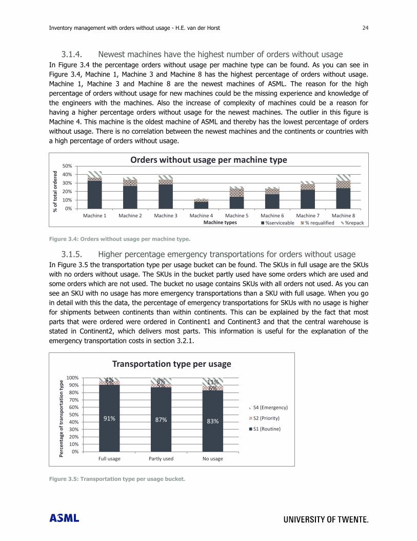
Inventory management with orders without usage - H.E. van der Horst 24 24
3.1.4. Newest machines have the highest number of orders without usage
In Figure 3.4 the percentage orders without usage per machine type can be found. As you can see in
Figure 3.4, Machine 1, Machine 3 and Machine 8 has the highest percentage of orders without usage.
Machine 1, Machine 3 and Machine 8 are the newest machines of ASML. The reason for the high
percentage of orders without usage for new machines could be the missing experience and knowledge of
the engineers with the machines. Also the increase of complexity of machines could be a reason for
having a higher percentage orders without usage for the newest machines. The outlier in this figure is
Machine 4. This machine is the oldest machine of ASML and thereby has the lowest percentage of orders
without usage. There is no correlation between the newest machines and the continents or countries with
a high percentage of orders without usage.
Figure 3.4: Orders without usage per machine type.
3.1.5. Higher percentage emergency transportations for orders without usage
In Figure 3.5 the transportation type per usage bucket can be found. The SKUs in full usage are the SKUs
with no orders without usage. The SKUs in the bucket partly used have some orders which are used and
some orders which are not used. The bucket no usage contains SKUs with all orders not used. As you can
see an SKU with no usage has more emergency transportations than a SKU with full usage. When you go
in detail with this the data, the percentage of emergency transportations for SKUs with no usage is higher
for shipments between continents than within continents. This can be explained by the fact that most
parts that were ordered were ordered in Continent1 and Continent3 and that the central warehouse is
stated in Continent2, which delivers most parts. This information is useful for the explanation of the
emergency transportation costs in section 3.2.1.
Figure 3.5: Transportation type per usage bucket.
0%
10%
20%
30%
40%
50%
Machine 1 Machine 2 Machine 3 Machine 4 Machine 5 Machine 6 Machine 7 Machine 8
% o
f to
tal o
rde
red
Machine types
Orders without usage per machine type
%serviceable % requalified %repack
91% 87% 83%
5% 5% 6%
4% 8% 11%
0%
10%
20%
30%
40%
50%
60%
70%
80%
90%
100%
Full usage Partly used No usage
Pe
rce
nta
ge o
f tr
ansp
ort
atio
n t
ype
Transportation type per usage
S4 (Emergency)
S2 (Priority)
S1 (Routine)
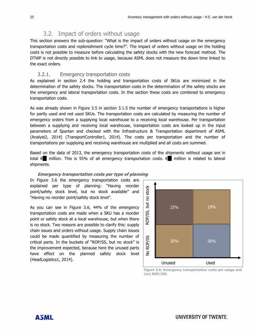
25 Inventory management with orders without usage - H.E. van der Horst
3.2. Impact of orders without usage This section answers the sub-question: “What is the impact of orders without usage on the emergency
transportation costs and replenishment cycle time?”. The impact of orders without usage on the holding
costs is not possible to measure before calculating the safety stocks with the new forecast method. The
DTWP is not directly possible to link to usage, because ASML does not measure the down time linked to
the exact orders.
3.2.1. Emergency transportation costs
As explained in section 2.4 the holding and transportation costs of SKUs are minimized in the
determination of the safety stocks. The transportation costs in the determination of the safety stocks are
the emergency and lateral transportation costs. In this section these costs are combined to emergency
transportation costs.
As was already shown in Figure 3.5 in section 3.1.5 the number of emergency transportations is higher
for partly used and not used SKUs. The transportation costs are calculated by measuring the number of
emergency orders from a supplying local warehouse to a receiving local warehouse. Per transportation
between a supplying and receiving local warehouse, transportation costs are looked up in the input
parameters of Spartan and checked with the Infrastructure & Transportation department of ASML
(Analyst2, 2014) (TransportController1, 2014). The costs per transportation and the number of
transportations per supplying and receiving warehouse are multiplied and all costs are summed.
Based on the data of 2013, the emergency transportation costs of the shipments without usage are in
total €?? million. This is 55% of all emergency transportation costs. €?? million is related to lateral
shipments.
Emergency transportation costs per type of planning
In Figure 3.6 the emergency transportation costs are
explained per type of planning: “Having reorder
point/safety stock level, but no stock available” and
“Having no reorder point/safety stock level”.
As you can see in Figure 3.6, 44% of the emergency
transportation costs are made when a SKU has a reorder
point or safety stock at a local warehouse, but when there
is no stock. Two reasons are possible to clarify this: supply
chain issues and orders without usage. Supply chain issues
could be made quantified by measuring the number of
critical parts. In the buckets of “ROP/SS, but no stock” is
the improvement expected, because here the unused parts
have effect on the planned safety stock level
(HeadLogistics1, 2014).
Used Unused
No R
OP/S
S
RO
P/S
S, but
no s
tock
30%
25%
26%
19%
Figure 3.6: Emergency transportation costs per usage and (no) ROP/SSL
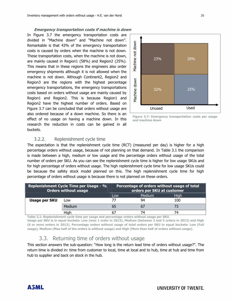
Inventory management with orders without usage - H.E. van der Horst 26 26
Emergency transportation costs if machine is down
In Figure 3.7 the emergency transportation costs are
divided in “Machine down” and “Machine not down”.
Remarkable is that 43% of the emergency transportation
costs is caused by orders when the machine is not down.
These transportation costs, when the machine is not down,
are mainly caused in Region1 (58%) and Region2 (25%).
This means that in these regions the engineers also order
emergency shipments although it is not allowed when the
machine is not down. Although Continent2, Region2 and
Region3 are the regions with the highest percentage
emergency transportations, the emergency transportations
costs based on orders without usage are mainly caused by
Region1 and Region2. This is because Region1 and
Region2 have the highest number of orders. Based on
Figure 3.7 can be concluded that orders without usage are
also ordered because of a down machine. So there is an
effect of no usage on having a machine down. In this
research the reduction in costs can be gained in all
buckets.
3.2.2. Replenishment cycle time
The expectation is that the replenishment cycle time (RCT) (measured per day) is higher for a high
percentage orders without usage, because of not planning on that demand. In Table 3.1 the comparison
is made between a high, medium or low usage and the percentage orders without usage of the total
number of orders per SKU. As you can see the replenishment cycle time is higher for low usage SKUs and
for high percentage of orders without usage. The high replenishment cycle time for low usage SKUs could
be because the safety stock model planned on this. The high replenishment cycle time for high
percentage of orders without usage is because there is not planned on these orders.
Replenishment Cycle Time per Usage - %
Orders without usage
Percentage of orders without usage of total
orders per SKU at customer
Low Medium High
Usage per SKU Low 77 94 100
Medium 65 67 73
High 67 74 74 Table 3.1: Replenishment cycle time per usage and percentage orders without usage per SKU. Usage per SKU is in equal buckets: Low (max 1 order in 2013), Medium (between 2 and 5 orders in 2013) and High
(6 or more orders in 2013). Percentage orders without usage of total orders per SKU in equal buckets: Low (Full
usage), Medium (Max half of the orders is without usage) and High (More than half of orders without usage).
3.3. Returning time of orders without usage This section answers the sub-question: “How long is the return lead time of orders without usage?”. The
return time is divided in: time from customer to local, time at local and to hub, time at hub and time from
hub to supplier and back on stock in the hub.
Figure 3.7: Emergency transportation costs per usage and machine down
Mach
ine d
ow
n
Mach
ine n
ot
dow
n
Used Unused
32%
23%
25%
20%
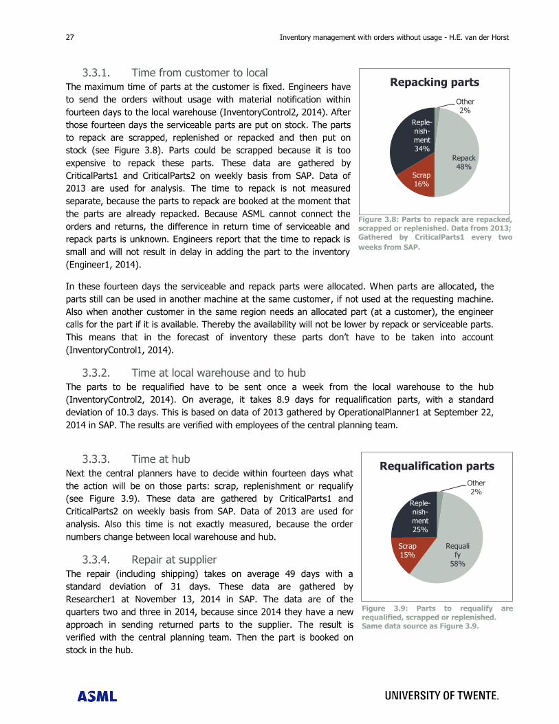
27 Inventory management with orders without usage - H.E. van der Horst
Figure 3.8: Parts to repack are repacked, scrapped or replenished. Data from 2013; Gathered by CriticalParts1 every two
weeks from SAP.
3.3.1. Time from customer to local
The maximum time of parts at the customer is fixed. Engineers have
to send the orders without usage with material notification within
fourteen days to the local warehouse (InventoryControl2, 2014). After
those fourteen days the serviceable parts are put on stock. The parts
to repack are scrapped, replenished or repacked and then put on
stock (see Figure 3.8). Parts could be scrapped because it is too
expensive to repack these parts. These data are gathered by
CriticalParts1 and CriticalParts2 on weekly basis from SAP. Data of
2013 are used for analysis. The time to repack is not measured
separate, because the parts to repack are booked at the moment that
the parts are already repacked. Because ASML cannot connect the
orders and returns, the difference in return time of serviceable and
repack parts is unknown. Engineers report that the time to repack is
small and will not result in delay in adding the part to the inventory
(Engineer1, 2014).
In these fourteen days the serviceable and repack parts were allocated. When parts are allocated, the
parts still can be used in another machine at the same customer, if not used at the requesting machine.
Also when another customer in the same region needs an allocated part (at a customer), the engineer
calls for the part if it is available. Thereby the availability will not be lower by repack or serviceable parts.
This means that in the forecast of inventory these parts don‟t have to be taken into account
(InventoryControl1, 2014).
3.3.2. Time at local warehouse and to hub
The parts to be requalified have to be sent once a week from the local warehouse to the hub
(InventoryControl2, 2014). On average, it takes 8.9 days for requalification parts, with a standard
deviation of 10.3 days. This is based on data of 2013 gathered by OperationalPlanner1 at September 22,
2014 in SAP. The results are verified with employees of the central planning team.
3.3.3. Time at hub
Next the central planners have to decide within fourteen days what
the action will be on those parts: scrap, replenishment or requalify
(see Figure 3.9). These data are gathered by CriticalParts1 and
CriticalParts2 on weekly basis from SAP. Data of 2013 are used for
analysis. Also this time is not exactly measured, because the order
numbers change between local warehouse and hub.
3.3.4. Repair at supplier
The repair (including shipping) takes on average 49 days with a
standard deviation of 31 days. These data are gathered by
Researcher1 at November 13, 2014 in SAP. The data are of the
quarters two and three in 2014, because since 2014 they have a new
approach in sending returned parts to the supplier. The result is
verified with the central planning team. Then the part is booked on
stock in the hub.
Other 2%
Repack 48%
Scrap 16%
Reple-nish-ment 34%
Repacking parts
Other 2%
Requalify
58%
Scrap 15%
Reple-nish-ment 25%
Requalification parts
Figure 3.9: Parts to requalify are requalified, scrapped or replenished. Same data source as Figure 3.9.
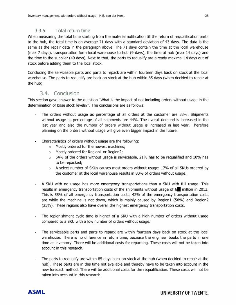
Inventory management with orders without usage - H.E. van der Horst 28 28
3.3.5. Total return time
When measuring the total time starting from the material notification till the return of requalification parts
to the hub, the total time is on average 71 days with a standard deviation of 43 days. The data is the
same as the repair data in the paragraph above. The 71 days contain the time at the local warehouse
(max 7 days), transportation form local warehouse to hub (9 days), the time at hub (max 14 days) and
the time to the supplier (49 days). Next to that, the parts to requalify are already maximal 14 days out of
stock before adding them to the local stock.
Concluding the serviceable parts and parts to repack are within fourteen days back on stock at the local
warehouse. The parts to requalify are back on stock at the hub within 85 days (when decided to repair at
the hub).
3.4. Conclusion This section gave answer to the question “What is the impact of not including orders without usage in the
determination of base stock levels?”. The conclusions are as follows:
- The orders without usage as percentage of all orders at the customer are 33%. Shipments
without usage as percentage of all shipments are 44%. The overall demand is increased in the
last year and also the number of orders without usage is increased in last year. Therefore
planning on the orders without usage will give even bigger impact in the future.
- Characteristics of orders without usage are the following:
o Mostly ordered for the newest machines;
o Mostly ordered for Region1 or Region2;
o 64% of the orders without usage is serviceable, 21% has to be requalified and 10% has
to be repacked;
o A select number of SKUs causes most orders without usage: 17% of all SKUs ordered by
the customer at the local warehouse results in 80% of orders without usage.
- A SKU with no usage has more emergency transportations than a SKU with full usage. This
results in emergency transportation costs of the shipments without usage of €?? million in 2013.
This is 55% of all emergency transportation costs. 42% of the emergency transportation costs
are while the machine is not down, which is mainly caused by Region1 (58%) and Region2
(25%). These regions also have overall the highest emergency transportation costs.
- The replenishment cycle time is higher of a SKU with a high number of orders without usage
compared to a SKU with a low number of orders without usage.
- The serviceable parts and parts to repack are within fourteen days back on stock at the local
warehouse. There is no difference in return time, because the engineer books the parts in one
time as inventory. There will be additional costs for repacking. These costs will not be taken into
account in this research.
- The parts to requalify are within 85 days back on stock at the hub (when decided to repair at the
hub). These parts are in this time not available and thereby have to be taken into account in the
new forecast method. There will be additional costs for the requalification. These costs will not be
taken into account in this research.

29 Inventory management with orders without usage - H.E. van der Horst
Inventory management with orders without usage - H.E. van der Horst 30 30
4. LITERATURE REVIEW FORECAST METHOD
This chapter answers the research question that is formulated in section 1.3: “Following the literature,
what forecast method can be used to determine the demand and return flow?”. First the forecast
methods from literature are given. Then the criteria are made clear and next the method is chosen.
4.1. Forecast methods from literature This section answers the sub-question: “Which methods are possible to forecast the demand and return
orders?”.
Web of Science, Scopus and the University Library catalogue were used to find all articles and books.
Keywords, like „reverse logistics‟, „forecast‟, „stock‟, „inventory control‟, „internet sales‟, „lost sales‟, „sales
with rejection‟, „return parts‟, „reverse logistics‟, „remanufacturing‟, „reuse‟, „recovery‟ and „demand
forecasting‟, were used to find literature. Also forward and backward search is used to check related
articles to already found articles.
Kelle and Silver (1989) developed four different methods of forecasting demand, which include different
amounts of return information. These authors are the most suitable authors who take the returns into
account in the forecast of demand. Most authors take the returns in to account in the inventory
optimization model. Because of the restriction of no changes in the inventory model at ASML, these
articles are not adaptable to ASML.
Method 1 only takes the failure rates of the SKUs into account. Hereby the forecast is the demand
during lead time multiplied with a fixed probability that a part is never returned. The demand
is all orders transported to the customer, so including usage and all return types.
Method 2 is more exact than method 1 and includes all returns (expected) during replenishment lead
time. Hereby the total returns are combining the expected returns during lead time of demand before the
current period and the expected returns during lead time of demand during lead time. The forecast is
the demand during lead time minus the total returns during lead time.
Method 3 includes even more information than method 2, by including the return information per order
per period. This means that each order is separately tracked and information have to be saved of the
demand and returns per period. Hereby the total returns per order are combining the expected returns
per order during lead time. The returns are of demand before the current period and of demand during
lead time. The forecast is the demand during lead time minus the sum of the total returns
during lead time per order. This method requires the most information of all methods.
To reduce the time needed to track the orders separately like in method 3, method 4 is developed. In
method 4 the information of method 2 is used including the correlation of the returns. Hereby the
correlation is taken into account of the returns before current period with the returns during lead time of
demand before current period. The correlation of returns is based on the total amount of returns per
period without identification which order is issued. This means that if there are a high number of returns
before the current period, there will be a lower number of returns during lead time of the demand in the
same period. The total number of returns cannot be higher than the demand of that period. This results
then in a negative correlation and in a higher forecast. The forecast is the demand during lead time
minus the returns during lead time (method 2) plus the correlation of returns (Kelle & Silver,
1989).
31 Inventory management with orders without usage - H.E. van der Horst
4.2. Criteria forecast method This section answers the sub-question: “What are the criteria for the forecast method?”. The methods of
Kelle and Silver (1989) are measured on three criteria in literature:
- Relative error of the forecast of the method compared to the most-informed method:
Kelle and Silver (1989) and De Brito and van der Laan (2009) reason that the method with the
most information is the most realistic method. Thereby method 3 is the most appropriate
method. The second and third best method, relatively method 4 and 2, don‟t differ more than
1% from method 3. Method 1 performs very poorly overall and it is not recommended by de Brito
and van der Laan to use this method in practice (Kelle & Silver, 1989) (De Brito & Van der Laan,
2009).
- Robustness of the method when the return rate is over- or underestimated:
The robustness is measured by De Brito and van der Laan (2009) to find the effect of imperfect
information. The most robust method is method 2. Method 3 is less robust than method 2, but
the gap is at maximum 2% cost difference with relation to method 2 in case of over- and
underestimation. Method 4 is of these three the least robust, with a maximum of 26% difference
in costs compared to method 2. Method 1 is not measured on robustness, because De Brito and
Van der Laan rejected this method based on the forecast errors (De Brito & Van der Laan, 2009).
- Amount of data required as input for the method:
Method 2 needs the individual tracked returns and demand per period. This information is
available at ASML, but not yet sorted. Method 3 needs individual tracked returns and demand per
period. ASML has this information not yet available. Method 4 needs the demand, return rate per
period and the returns of the demand from one period linked to each other. ASML has this
information not yet available. (De Brito & Van der Laan, 2009)
4.3. Choice of method This section answers the sub-question: “Which method is following the criteria the best to be added to
the forecast of ASML?”
The result of the research of Kelle and Silver is that the relative errors of the forecast of method 1 are
considerable, whereby this method is rejected. The improvements of method 2 and 4 are obtainable and
are quite big improvements compared to method 1. Method 3 got the biggest improvement, but it is
difficult and time expensive to obtain all data (Kelle & Silver, 1989). They conclude to implement method
2 or 4.
De Brito and van der Laan advise to use method 2, because this method is the most robust, the
performance difference with the best method is rather small and the investments in recording the data
are not high.
From the overview of the results from literature and the amount of data available at ASML, the conclusion
can be made that method 2 is the best method to implement at ASML. The reason for this is that ASML
already has this information available, this method is the most robust and the performance on forecast
error is rather small compared to method 3 and 4.
In the next section Method 2 of Kelle and Silver is explained in detail. In this section first an example is
given to calculate the forecast with the method of Kelle and Silver. Then the method is explained in the
form of formulas.
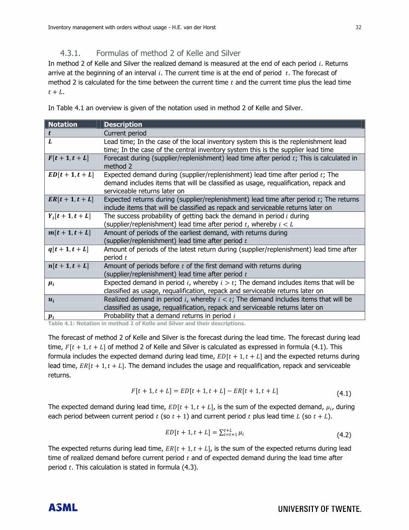
Inventory management with orders without usage - H.E. van der Horst 32 32
4.3.1. Formulas of method 2 of Kelle and Silver
In method 2 of Kelle and Silver the realized demand is measured at the end of each period . Returns
arrive at the beginning of an interval . The current time is at the end of period . The forecast of
method 2 is calculated for the time between the current time and the current time plus the lead time
.
In Table 4.1 an overview is given of the notation used in method 2 of Kelle and Silver.
Notation Description
Current period Lead time; In the case of the local inventory system this is the replenishment lead
time; In the case of the central inventory system this is the supplier lead time Forecast during (supplier/replenishment) lead time after period ; This is calculated in
method 2 Expected demand during (supplier/replenishment) lead time after period ; The
demand includes items that will be classified as usage, requalification, repack and
serviceable returns later on Expected returns during (supplier/replenishment) lead time after period ; The returns
include items that will be classified as repack and serviceable returns later on The success probability of getting back the demand in period during
(supplier/replenishment) lead time after period , whereby
Amount of periods of the earliest demand, with returns during (supplier/replenishment) lead time after period
Amount of periods of the latest return during (supplier/replenishment) lead time after period
Amount of periods before of the first demand with returns during
(supplier/replenishment) lead time after period Expected demand in period , whereby ; The demand includes items that will be
classified as usage, requalification, repack and serviceable returns later on Realized demand in period , whereby ; The demand includes items that will be
classified as usage, requalification, repack and serviceable returns later on Probability that a demand returns in period Table 4.1: Notation in method 2 of Kelle and Silver and their descriptions.
The forecast of method 2 of Kelle and Silver is the forecast during the lead time. The forecast during lead
time, of method 2 of Kelle and Silver is calculated as expressed in formula (4.1). This
formula includes the expected demand during lead time, and the expected returns during
lead time, . The demand includes the usage and requalification, repack and serviceable
returns.
The expected demand during lead time, , is the sum of the expected demand, , during
each period between current period (so ) and current period plus lead time (so ).
∑
The expected returns during lead time, , is the sum of the expected returns during lead
time of realized demand before current period and of expected demand during the lead time after
period . This calculation is stated in formula (4.3).
(4.1)
(4.2)
33 Inventory management with orders without usage - H.E. van der Horst
The first side of formula (4.3), ∑ , is the expected returns during lead time
of realized demand before current period : sum of the realized demand in period , , times the success
probability of getting the demand back during lead time, . The realized demand is the
measured demand in the periods before current period . Here per demand in period the amount of
returns is calculated. The earliest period, , is the earliest period of demand that has
returns during lead time.
The second side of formula (4.3), ∑ , is the expected returns during lead time of
demand during lead time after period : sum of the expected demand, , times the success probability of
getting the demand of period back during lead time, . The time is taken from next period
(first period of returns; ) till the last period of possible returns before lead time . This is
because at the ordered parts will be delivered.
∑ ∑
The last question is how to calculate the success probability, . The success probability is the
sum of the chances that the parts of demand return over different periods during the lead time.
The success probability is calculated differently for each time period:
1. The periods before the earliest demand, with returns during lead time, are the time periods
without returns during lead times. This means that the success probability is zero.
2. The period between the earliest demand, with returns during lead time, and the current period is
the second time bucket. In this time bucket the success probability of returns during lead time of
demand in time is the sum of the chances the parts will be returned during lead time, .
The chance that a demand of period will return during lead time after period is the sum of the
chances the returns from to . When is 1 in , this is the chance of returns in period
. The will increase to the minimum of the lead time, , and the last chance of return of
that demand, . This results in the following formula:
.
3. The period between the current period and the current period plus the lead time is the third time
bucket. In this time bucket the success probability of returns during lead time of demand in time
is the sum of the chances the parts will be returned during lead time, . These returns are
from the first chance of return of that demand, j is 1, and till the minimum of the first return
before t and the lead time. This results in the following formula:
.
The success probability can thereby be given as formula (4.4). The timing of the returns is between
current period and the lead time . The chance that demand returns in that time frame is measured
as the sum of the chances per period .
{
∑
∑
In the next section an example is given to illustrate the method.
(4.4)
(4.3)
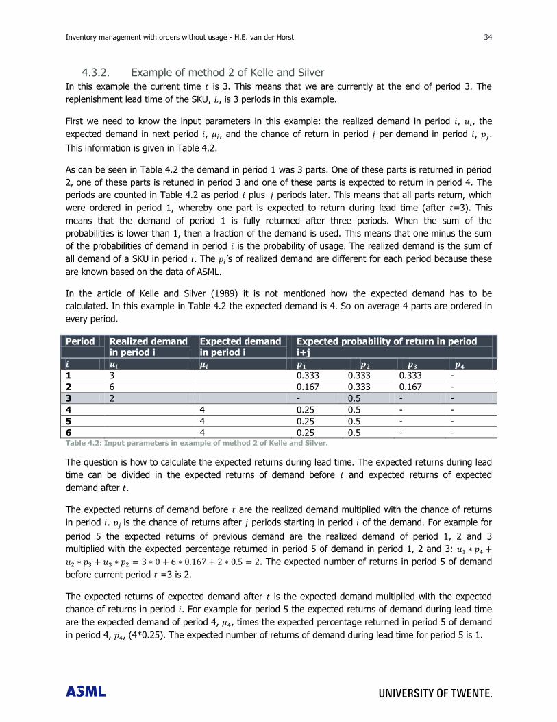
Inventory management with orders without usage - H.E. van der Horst 34 34
4.3.2. Example of method 2 of Kelle and Silver
In this example the current time is 3. This means that we are currently at the end of period 3. The
replenishment lead time of the SKU, , is 3 periods in this example.
First we need to know the input parameters in this example: the realized demand in period , , the
expected demand in next period , , and the chance of return in period per demand in period , .
This information is given in Table 4.2.
As can be seen in Table 4.2 the demand in period 1 was 3 parts. One of these parts is returned in period
2, one of these parts is retuned in period 3 and one of these parts is expected to return in period 4. The
periods are counted in Table 4.2 as period plus periods later. This means that all parts return, which
were ordered in period 1, whereby one part is expected to return during lead time (after =3). This
means that the demand of period 1 is fully returned after three periods. When the sum of the
probabilities is lower than 1, then a fraction of the demand is used. This means that one minus the sum
of the probabilities of demand in period is the probability of usage. The realized demand is the sum of
all demand of a SKU in period . The ‟s of realized demand are different for each period because these
are known based on the data of ASML.
In the article of Kelle and Silver (1989) it is not mentioned how the expected demand has to be
calculated. In this example in Table 4.2 the expected demand is 4. So on average 4 parts are ordered in
every period.
Period Realized demand
in period i
Expected demand
in period i
Expected probability of return in period
i+j
1 3 0.333 0.333 0.333 -
2 6 0.167 0.333 0.167 -
3 2 - 0.5 - -
4 4 0.25 0.5 - -
5 4 0.25 0.5 - -
6 4 0.25 0.5 - - Table 4.2: Input parameters in example of method 2 of Kelle and Silver.
The question is how to calculate the expected returns during lead time. The expected returns during lead
time can be divided in the expected returns of demand before and expected returns of expected
demand after .
The expected returns of demand before are the realized demand multiplied with the chance of returns
in period . is the chance of returns after periods starting in period of the demand. For example for
period 5 the expected returns of previous demand are the realized demand of period 1, 2 and 3
multiplied with the expected percentage returned in period 5 of demand in period 1, 2 and 3:
. The expected number of returns in period 5 of demand
before current period =3 is 2.
The expected returns of expected demand after is the expected demand multiplied with the expected
chance of returns in period . For example for period 5 the expected returns of demand during lead time
are the expected demand of period 4, , times the expected percentage returned in period 5 of demand
in period 4, , (4*0.25). The expected number of returns of demand during lead time for period 5 is 1.
35 Inventory management with orders without usage - H.E. van der Horst
This means that in this example, based on Method 2, the demand minus the returns in period 5: 4 – 2 –
1 = 1. The forecast is thereby 1 for period 5. The forecast in this example is an integer. This doesn‟t have
to be the case.
4.4. Conclusion This section gave answer to the question: “Following the literature, what forecast method can be used to
determine the demand and return flow?”. The conclusions are as follows:
- The suitable literature of forecast methods with returns is the article of Kelle and Silver (1989).
They present four forecast methods, which are compared to each other and measured based on
the articles of Kelle and Silver (1989) and De Brito and Van der Laan (2009). In these articles the
criteria are relative forecast error, robustness and amount of data.
- Based on these criteria method 2 of Kelle and Silver is chosen. This method is the most robust,
can be calculated with available data of ASML and has a rather small forecast error compared to
the two methods of Kelle and Silver with less forecast errors.
- Method 2 includes all returns (expected) during replenishment lead time. Hereby the total returns
are combining the expected returns during lead time of demand before the current period and
the expected returns during lead time of demand during lead time. The forecast is the demand
minus the total returns during lead time.

Inventory management with orders without usage - H.E. van der Horst 36 36
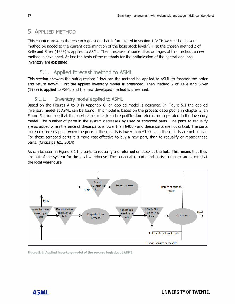
37 Inventory management with orders without usage - H.E. van der Horst
5. APPLIED METHOD
This chapter answers the research question that is formulated in section 1.3: “How can the chosen
method be added to the current determination of the base stock level?”. First the chosen method 2 of
Kelle and Silver (1989) is applied to ASML. Then, because of some disadvantages of this method, a new
method is developed. At last the tests of the methods for the optimization of the central and local
inventory are explained.
5.1. Applied forecast method to ASML This section answers the sub-question: “How can the method be applied to ASML to forecast the order
and return flow?”. First the applied inventory model is presented. Then Method 2 of Kelle and Silver
(1989) is applied to ASML and the new developed method is presented.
5.1.1. Inventory model applied to ASML
Based on the Figures A to D in Appendix C, an applied model is designed. In Figure 5.1 the applied
inventory model at ASML can be found. This model is based on the process descriptions in chapter 2. In
Figure 5.1 you see that the serviceable, repack and requalification returns are separated in the inventory
model. The number of parts in the system decreases by used or scrapped parts. The parts to requalify
are scrapped when the price of these parts is lower than €400,- and these parts are not critical. The parts
to repack are scrapped when the price of these parts is lower than €100,- and these parts are not critical.
For these scrapped parts it is more cost-effective to buy a new part, than to requalify or repack these
parts. (Criticalparts1, 2014)
As can be seen in Figure 5.1 the parts to requalify are returned on stock at the hub. This means that they
are out of the system for the local warehouse. The serviceable parts and parts to repack are stocked at
the local warehouse.
Figure 5.1: Applied inventory model of the reverse logistics at ASML.
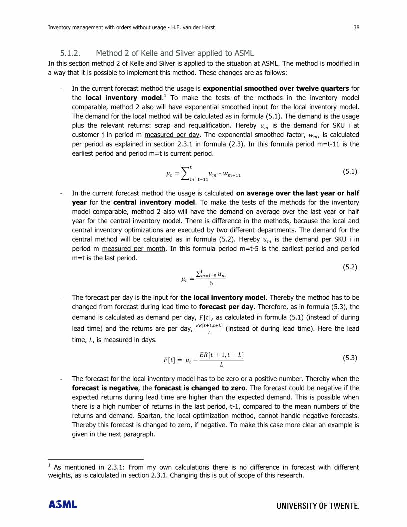
Inventory management with orders without usage - H.E. van der Horst 38 38
5.1.2. Method 2 of Kelle and Silver applied to ASML
In this section method 2 of Kelle and Silver is applied to the situation at ASML. The method is modified in
a way that it is possible to implement this method. These changes are as follows:
- In the current forecast method the usage is exponential smoothed over twelve quarters for
the local inventory model.1 To make the tests of the methods in the inventory model
comparable, method 2 also will have exponential smoothed input for the local inventory model.
The demand for the local method will be calculated as in formula (5.1). The demand is the usage
plus the relevant returns: scrap and requalification. Hereby is the demand for SKU i at
customer j in period m measured per day. The exponential smoothed factor, , is calculated
per period as explained in section 2.3.1 in formula (2.3). In this formula period m=t-11 is the
earliest period and period m=t is current period.
∑
- In the current forecast method the usage is calculated on average over the last year or half
year for the central inventory model. To make the tests of the methods for the inventory
model comparable, method 2 also will have the demand on average over the last year or half
year for the central inventory model. There is difference in the methods, because the local and
central inventory optimizations are executed by two different departments. The demand for the
central method will be calculated as in formula (5.2). Hereby is the demand per SKU i in
period m measured per month. In this formula period m=t-5 is the earliest period and period
m=t is the last period.
∑
- The forecast per day is the input for the local inventory model. Thereby the method has to be
changed from forecast during lead time to forecast per day. Therefore, as in formula (5.3), the
demand is calculated as demand per day, , as calculated in formula (5.1) (instead of during
lead time) and the returns are per day,
(instead of during lead time). Here the lead
time, , is measured in days.
- The forecast for the local inventory model has to be zero or a positive number. Thereby when the
forecast is negative, the forecast is changed to zero. The forecast could be negative if the
expected returns during lead time are higher than the expected demand. This is possible when
there is a high number of returns in the last period, t-1, compared to the mean numbers of the
returns and demand. Spartan, the local optimization method, cannot handle negative forecasts.
Thereby this forecast is changed to zero, if negative. To make this case more clear an example is
given in the next paragraph.
1 As mentioned in 2.3.1: From my own calculations there is no difference in forecast with different weights, as is calculated in section 2.3.1. Changing this is out of scope of this research.
(5.1)
(5.2)
(5.3)
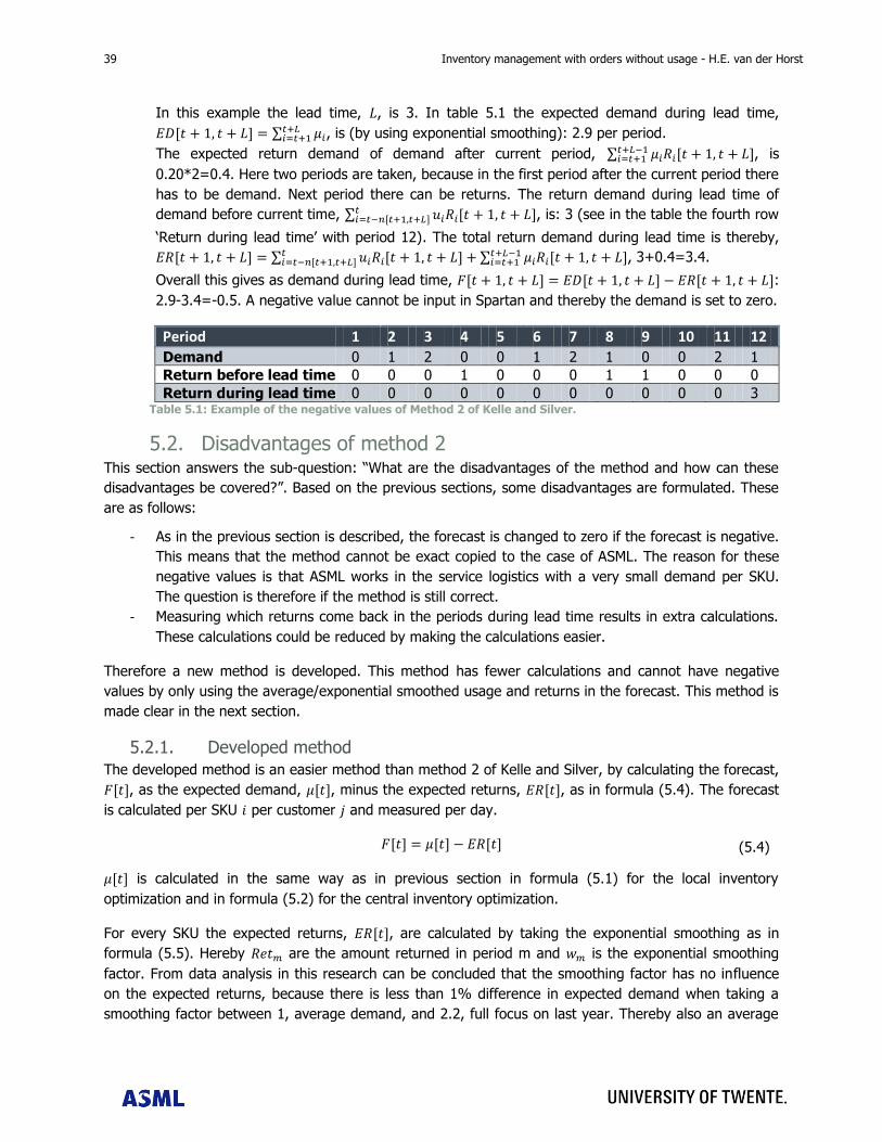
39 Inventory management with orders without usage - H.E. van der Horst
In this example the lead time, , is 3. In table 5.1 the expected demand during lead time,
∑ , is (by using exponential smoothing): 2.9 per period.
The expected return demand of demand after current period, ∑ , is
0.20*2=0.4. Here two periods are taken, because in the first period after the current period there
has to be demand. Next period there can be returns. The return demand during lead time of
demand before current time, ∑ , is: 3 (see in the table the fourth row
„Return during lead time‟ with period 12). The total return demand during lead time is thereby,
∑ ∑
, 3+0.4=3.4.
Overall this gives as demand during lead time, :
2.9-3.4=-0.5. A negative value cannot be input in Spartan and thereby the demand is set to zero.
Period 1 2 3 4 5 6 7 8 9 10 11 12
Demand 0 1 2 0 0 1 2 1 0 0 2 1
Return before lead time 0 0 0 1 0 0 0 1 1 0 0 0
Return during lead time 0 0 0 0 0 0 0 0 0 0 0 3 Table 5.1: Example of the negative values of Method 2 of Kelle and Silver.
5.2. Disadvantages of method 2 This section answers the sub-question: “What are the disadvantages of the method and how can these
disadvantages be covered?”. Based on the previous sections, some disadvantages are formulated. These
are as follows:
- As in the previous section is described, the forecast is changed to zero if the forecast is negative.
This means that the method cannot be exact copied to the case of ASML. The reason for these
negative values is that ASML works in the service logistics with a very small demand per SKU.
The question is therefore if the method is still correct.
- Measuring which returns come back in the periods during lead time results in extra calculations.
These calculations could be reduced by making the calculations easier.
Therefore a new method is developed. This method has fewer calculations and cannot have negative
values by only using the average/exponential smoothed usage and returns in the forecast. This method is
made clear in the next section.
5.2.1. Developed method
The developed method is an easier method than method 2 of Kelle and Silver, by calculating the forecast,
, as the expected demand, , minus the expected returns, , as in formula (5.4). The forecast
is calculated per SKU per customer and measured per day.
is calculated in the same way as in previous section in formula (5.1) for the local inventory
optimization and in formula (5.2) for the central inventory optimization.
For every SKU the expected returns, , are calculated by taking the exponential smoothing as in
formula (5.5). Hereby are the amount returned in period m and is the exponential smoothing
factor. From data analysis in this research can be concluded that the smoothing factor has no influence
on the expected returns, because there is less than 1% difference in expected demand when taking a
smoothing factor between 1, average demand, and 2.2, full focus on last year. Thereby also an average
(5.4)
Inventory management with orders without usage - H.E. van der Horst 40 40
could be taken. Although the smoothing factor will be chosen as 1.4, even as the demand. The reason for
this is that the results are then comparable. Twelve periods is chosen because this is also taken in the
current forecast determination. Thereby the methods are comparable.
∑
The difference with Method 2 of Kelle and Silver is that only the expected demand and returns are taken
into account and not the extra returns of demand before current period. This results in less calculations
and always positive numbers. The difference between the developed method and Method 1 of Kelle and
Silver is that in the developed method the amount of return is not fixed, but depends on the previous
data per SKU.
To give an example of the calculations of the developed method, the data of Table 5.1 in section 5.1.2 is
used. The forecast is thereby the expected demand (exponential smoothed) minus the expected returns
(exponential smoothed). This is 0.97 minus 0.2 per period: 0.77 per period. As can be seen, the
expectation is that the forecast of the developed method is higher than the forecast of Method 2.
5.3. Conclusion This section gave answer to the question “How can the chosen method be added to the current
determination of the base stock level?”. The conclusions are as follows:
- The parts to requalify and the scrapped parts go out of the system in the local inventory system,
next to the used parts. The reason for this is that they will be scrapped or will be tested at the
supplier and will return back at the hub warehouse. These parts are taken into account in the
tests of the methods as demand but will not return. The serviceable and repack demand, which is
not scrapped, will be taken into account in the methods as return demand.
- Method 2 of Kelle and Silver is modified for four elements when applying the method to the case
of ASML. Hereby disadvantages came across: changing the output of the method when having a
negative demand and extra calculations compared to the current method. Therefore a new
method is developed. The developed method is simpler and only includes the expected returns
instead of the expected returns and the returns of previous demand.
(5.5)

41 Inventory management with orders without usage - H.E. van der Horst
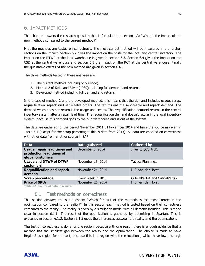
Inventory management with orders without usage - H.E. van der Horst 42 42
6. IMPACT METHODS
This chapter answers the research question that is formulated in section 1.3: “What is the impact of the
new methods compared to the current method?”.
First the methods are tested on correctness. The most correct method will be measured in the further
sections on the impact. Section 6.2 gives the impact on the costs for the local and central inventory. The
impact on the DTWP at the local warehouse is given in section 6.3. Section 6.4 gives the impact on the
CSD at the central warehouse and section 6.5 the impact on the RCT at the central warehouse. Finally
the qualitative effects of the new method are given in section 6.6.
The three methods tested in these analyses are:
1. The current method including only usage;
2. Method 2 of Kelle and Silver (1989) including full demand and returns.
3. Developed method including full demand and returns.
In the case of method 2 and the developed method, this means that the demand includes usage, scrap,
requalification, repack and serviceable orders. The returns are the serviceable and repack demand. The
demand which does not return is the usage and scraps. The requalification demand returns in the central
inventory system after a repair lead time. The requalification demand doesn‟t return in the local inventory
system, because this demand goes to the hub warehouse and is out of the system.
The data are gathered for the period November 2011 till November 2014 and have the source as given in
Table 6.1 (except for the scrap percentage: this is data from 2013). All data are checked on correctness
with other data from another source in SAP.
Data Date gathered Gathered by
Usage, repair lead times and
production lead times of global customers
December 8, 2014 InventoryControl1
Usage and DTWP of DTWP
customers
November 13, 2014 TacticalPlanning1
Requalification and repack
demand
November 24, 2014 H.E. van der Horst
Scrap percentage Every week in 2013 CriticalParts1 and CriticalParts2
Price of SKUs November 26, 2014 H.E. van der Horst Table 6.1: Source of data in results.
6.1. Test methods on correctness This section answers the sub-question: “Which forecast of the methods is the most correct in the
optimization compared to the reality?”. In this section each method is tested based on their correctness
compared to the reality. The reality is given by a simulation model with all demand included. This is made
clear in section 6.1.1. The result of the optimization is gathered by optimizing in Spartan. This is
explained in section 6.1.2. Section 6.1.3 gives the differences between the reality and the optimization.
The test on correctness is done for one region, because with one region there is enough evidence that a
method has the smallest gap between the reality and the optimization. The choice is made to have
Region2 as region for the test, because this is a region with three locations, which have low and high
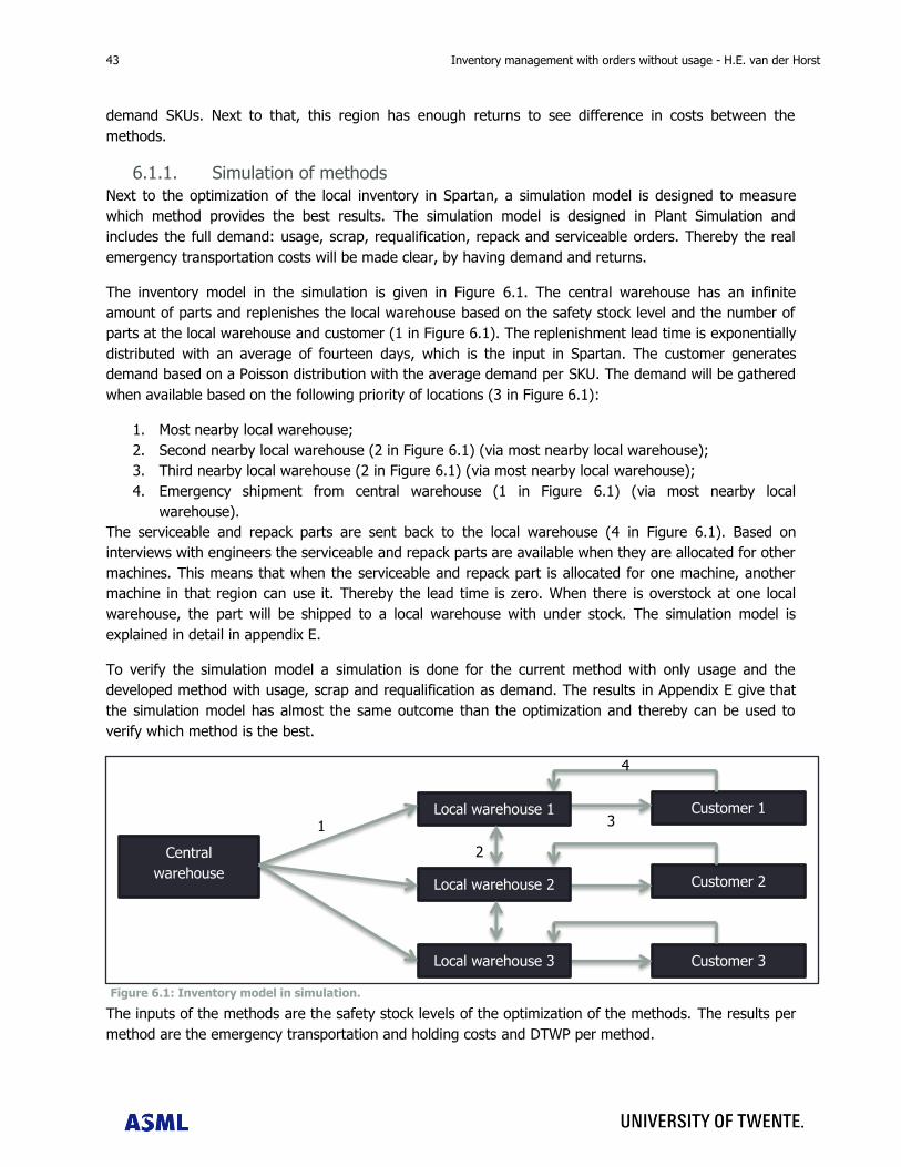
43 Inventory management with orders without usage - H.E. van der Horst
demand SKUs. Next to that, this region has enough returns to see difference in costs between the
methods.
6.1.1. Simulation of methods
Next to the optimization of the local inventory in Spartan, a simulation model is designed to measure
which method provides the best results. The simulation model is designed in Plant Simulation and
includes the full demand: usage, scrap, requalification, repack and serviceable orders. Thereby the real
emergency transportation costs will be made clear, by having demand and returns.
The inventory model in the simulation is given in Figure 6.1. The central warehouse has an infinite
amount of parts and replenishes the local warehouse based on the safety stock level and the number of
parts at the local warehouse and customer (1 in Figure 6.1). The replenishment lead time is exponentially
distributed with an average of fourteen days, which is the input in Spartan. The customer generates
demand based on a Poisson distribution with the average demand per SKU. The demand will be gathered
when available based on the following priority of locations (3 in Figure 6.1):
1. Most nearby local warehouse;
2. Second nearby local warehouse (2 in Figure 6.1) (via most nearby local warehouse);
3. Third nearby local warehouse (2 in Figure 6.1) (via most nearby local warehouse);
4. Emergency shipment from central warehouse (1 in Figure 6.1) (via most nearby local
warehouse).
The serviceable and repack parts are sent back to the local warehouse (4 in Figure 6.1). Based on
interviews with engineers the serviceable and repack parts are available when they are allocated for other
machines. This means that when the serviceable and repack part is allocated for one machine, another
machine in that region can use it. Thereby the lead time is zero. When there is overstock at one local
warehouse, the part will be shipped to a local warehouse with under stock. The simulation model is
explained in detail in appendix E.
To verify the simulation model a simulation is done for the current method with only usage and the
developed method with usage, scrap and requalification as demand. The results in Appendix E give that
the simulation model has almost the same outcome than the optimization and thereby can be used to
verify which method is the best.
The inputs of the methods are the safety stock levels of the optimization of the methods. The results per
method are the emergency transportation and holding costs and DTWP per method.
Figure 6.1: Inventory model in simulation.
Customer 3
Customer 2
Customer 1
Central
warehouse
Local warehouse 1
Local warehouse 2
Local warehouse 3
1
2
3
4
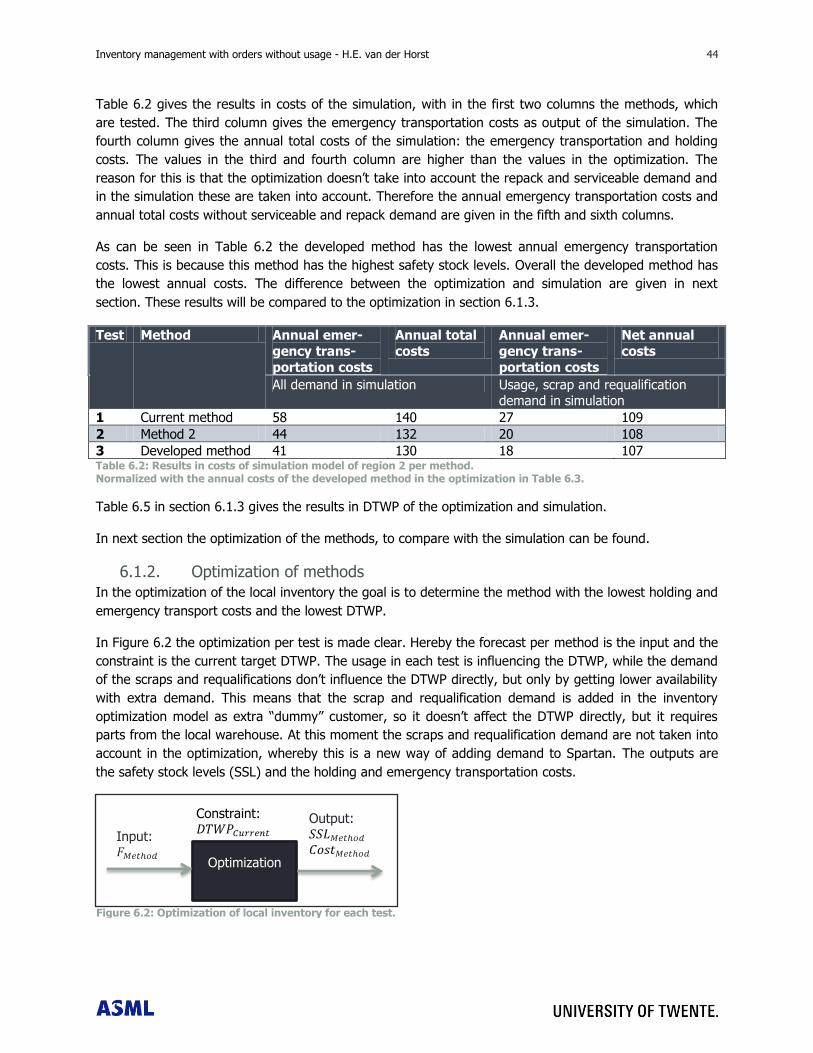
Inventory management with orders without usage - H.E. van der Horst 44 44
Table 6.2 gives the results in costs of the simulation, with in the first two columns the methods, which
are tested. The third column gives the emergency transportation costs as output of the simulation. The
fourth column gives the annual total costs of the simulation: the emergency transportation and holding
costs. The values in the third and fourth column are higher than the values in the optimization. The
reason for this is that the optimization doesn‟t take into account the repack and serviceable demand and
in the simulation these are taken into account. Therefore the annual emergency transportation costs and
annual total costs without serviceable and repack demand are given in the fifth and sixth columns.
As can be seen in Table 6.2 the developed method has the lowest annual emergency transportation
costs. This is because this method has the highest safety stock levels. Overall the developed method has
the lowest annual costs. The difference between the optimization and simulation are given in next
section. These results will be compared to the optimization in section 6.1.3.
Test Method Annual emer-
gency trans-
portation costs
Annual total
costs
Annual emer-
gency trans-
portation costs
Net annual
costs
All demand in simulation Usage, scrap and requalification demand in simulation
1 Current method 58 140 27 109
2 Method 2 44 132 20 108
3 Developed method 41 130 18 107 Table 6.2: Results in costs of simulation model of region 2 per method. Normalized with the annual costs of the developed method in the optimization in Table 6.3.
Table 6.5 in section 6.1.3 gives the results in DTWP of the optimization and simulation.
In next section the optimization of the methods, to compare with the simulation can be found.
6.1.2. Optimization of methods
In the optimization of the local inventory the goal is to determine the method with the lowest holding and
emergency transport costs and the lowest DTWP.
In Figure 6.2 the optimization per test is made clear. Hereby the forecast per method is the input and the
constraint is the current target DTWP. The usage in each test is influencing the DTWP, while the demand
of the scraps and requalifications don‟t influence the DTWP directly, but only by getting lower availability
with extra demand. This means that the scrap and requalification demand is added in the inventory
optimization model as extra “dummy” customer, so it doesn‟t affect the DTWP directly, but it requires
parts from the local warehouse. At this moment the scraps and requalification demand are not taken into
account in the optimization, whereby this is a new way of adding demand to Spartan. The outputs are
the safety stock levels (SSL) and the holding and emergency transportation costs.
Constraint: 𝐷𝑇𝑊𝑃𝐶𝑢𝑟𝑟𝑒𝑛𝑡
Optimization
Input: 𝐹𝑀𝑒𝑡 𝑜𝑑 𝐶𝑜𝑠𝑡𝑀𝑒𝑡 𝑜𝑑
Output: 𝑆𝑆𝐿𝑀𝑒𝑡 𝑜𝑑
Figure 6.2: Optimization of local inventory for each test.
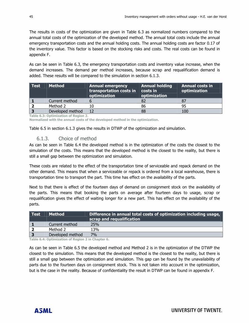
45 Inventory management with orders without usage - H.E. van der Horst
The results in costs of the optimization are given in Table 6.3 as normalized numbers compared to the
annual total costs of the optimization of the developed method. The annual total costs include the annual
emergency transportation costs and the annual holding costs. The annual holding costs are factor 0.17 of
the inventory value. This factor is based on the stocking risks and costs. The real costs can be found in
appendix F.
As can be seen in Table 6.3, the emergency transportation costs and inventory value increase, when the
demand increases. The demand per method increases, because scrap and requalification demand is
added. These results will be compared to the simulation in section 6.1.3.
Test Method Annual emergency
transportation costs in
optimization
Annual holding
costs in
optimization
Annual costs in
optimization
1 Current method 6 82 87
2 Method 2 10 86 95
3 Developed method 12 88 100 Table 6.3: Optimization of Region 2. Normalized with the annual costs of the developed method in the optimization.
Table 6.5 in section 6.1.3 gives the results in DTWP of the optimization and simulation.
6.1.3. Choice of method
As can be seen in Table 6.4 the developed method is in the optimization of the costs the closest to the
simulation of the costs. This means that the developed method is the closest to the reality, but there is
still a small gap between the optimization and simulation.
These costs are related to the effect of the transportation time of serviceable and repack demand on the
other demand. This means that when a serviceable or repack is ordered from a local warehouse, there is
transportation time to transport the part. This time has effect on the availability of the parts.
Next to that there is effect of the fourteen days of demand on consignment stock on the availability of
the parts. This means that booking the parts on average after fourteen days to usage, scrap or
requalification gives the effect of waiting longer for a new part. This has effect on the availability of the
parts.
Test Method Difference in annual total costs of optimization including usage, scrap and requalification
1 Current method 25%
2 Method 2 13%
3 Developed method 7% Table 6.4: Optimization of Region 2 in Chapter 6.
As can be seen in Table 6.5 the developed method and Method 2 is in the optimization of the DTWP the
closest to the simulation. This means that the developed method is the closest to the reality, but there is
still a small gap between the optimization and simulation. This gap can be found by the unavailability of
parts due to the fourteen days on consignment stock. This is not taken into account in the optimization,
but is the case in the reality. Because of confidentiality the result in DTWP can be found in appendix F.
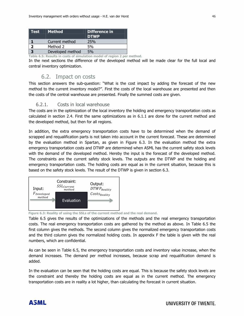
Inventory management with orders without usage - H.E. van der Horst 46 46
Constraint: 𝑆𝑆𝐿𝐶𝑢𝑟𝑟𝑒𝑛𝑡
𝑚𝑒𝑡 𝑜𝑑
Evaluation
Input: 𝐹𝐷𝑒𝑣𝑒𝑙𝑜𝑝𝑒𝑑
𝑚𝑒𝑡 𝑜𝑑
Output: 𝐷𝑇𝑊𝑃𝑅𝑒𝑎𝑙𝑖𝑡𝑦
𝐶𝑜𝑠𝑡𝑠𝑅𝑒𝑎𝑙𝑖𝑡𝑦
Test Method Difference in
DTWP
1 Current method 25%
2 Method 2 5%
3 Developed method 5% Table 6.5: Results in costs of simulation model of region 2 per method.
In the next sections the difference of the developed method will be made clear for the full local and
central inventory optimization.
6.2. Impact on costs This section answers the sub-question: “What is the cost impact by adding the forecast of the new
method to the current inventory model?”. First the costs of the local warehouse are presented and then
the costs of the central warehouse are presented. Finally the summed costs are given.
6.2.1. Costs in local warehouse
The costs are in the optimization of the local inventory the holding and emergency transportation costs as
calculated in section 2.4. First the same optimizations as in 6.1.1 are done for the current method and
the developed method, but then for all regions.
In addition, the extra emergency transportation costs have to be determined when the demand of
scrapped and requalification parts is not taken into account in the current forecast. These are determined
by the evaluation method in Spartan, as given in Figure 6.3. In the evaluation method the extra
emergency transportation costs and DTWP are determined when ASML has the current safety stock levels
with the demand of the developed method. Hereby the input is the forecast of the developed method.
The constraints are the current safety stock levels. The outputs are the DTWP and the holding and
emergency transportation costs. The holding costs are equal as in the current situation, because this is
based on the safety stock levels. The result of the DTWP is given in section 6.3.
Table 6.5 gives the results of the optimizations of the methods and the real emergency transportation
costs. The real emergency transportation costs are gathered by the method as above. In Table 6.5 the
first column gives the methods. The second column gives the normalized emergency transportation costs
and the third column gives the normalized holding costs. In appendix F the table is given with the real
numbers, which are confidential.
As can be seen in Table 6.5, the emergency transportation costs and inventory value increase, when the
demand increases. The demand per method increases, because scrap and requalification demand is
added.
In the evaluation can be seen that the holding costs are equal. This is because the safety stock levels are
the constraint and thereby the holding costs are equal as in the current method. The emergency
transportation costs are in reality a lot higher, than calculating the forecast in current situation.
Figure 6.3: Reality of using the SSLs of the current method and the real demand.
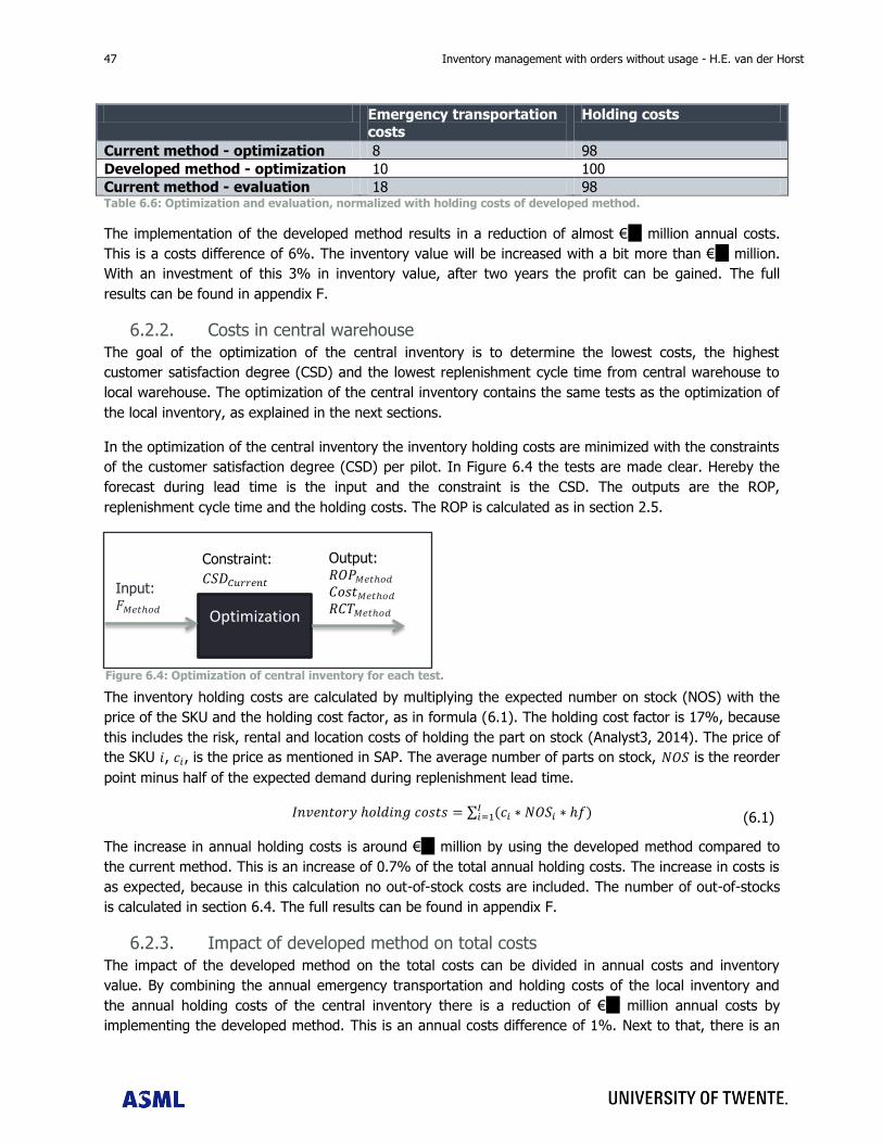
47 Inventory management with orders without usage - H.E. van der Horst
Emergency transportation
costs
Holding costs
Current method - optimization 8 98
Developed method - optimization 10 100
Current method - evaluation 18 98 Table 6.6: Optimization and evaluation, normalized with holding costs of developed method.
The implementation of the developed method results in a reduction of almost €?? million annual costs.
This is a costs difference of 6%. The inventory value will be increased with a bit more than €?? million.
With an investment of this 3% in inventory value, after two years the profit can be gained. The full
results can be found in appendix F.
6.2.2. Costs in central warehouse
The goal of the optimization of the central inventory is to determine the lowest costs, the highest
customer satisfaction degree (CSD) and the lowest replenishment cycle time from central warehouse to
local warehouse. The optimization of the central inventory contains the same tests as the optimization of
the local inventory, as explained in the next sections.
In the optimization of the central inventory the inventory holding costs are minimized with the constraints
of the customer satisfaction degree (CSD) per pilot. In Figure 6.4 the tests are made clear. Hereby the
forecast during lead time is the input and the constraint is the CSD. The outputs are the ROP,
replenishment cycle time and the holding costs. The ROP is calculated as in section 2.5.
The inventory holding costs are calculated by multiplying the expected number on stock (NOS) with the
price of the SKU and the holding cost factor, as in formula (6.1). The holding cost factor is 17%, because
this includes the risk, rental and location costs of holding the part on stock (Analyst3, 2014). The price of
the SKU , , is the price as mentioned in SAP. The average number of parts on stock, is the reorder
point minus half of the expected demand during replenishment lead time.
∑
The increase in annual holding costs is around €?? million by using the developed method compared to
the current method. This is an increase of 0.7% of the total annual holding costs. The increase in costs is
as expected, because in this calculation no out-of-stock costs are included. The number of out-of-stocks
is calculated in section 6.4. The full results can be found in appendix F.
6.2.3. Impact of developed method on total costs
The impact of the developed method on the total costs can be divided in annual costs and inventory
value. By combining the annual emergency transportation and holding costs of the local inventory and
the annual holding costs of the central inventory there is a reduction of €?? million annual costs by
implementing the developed method. This is an annual costs difference of 1%. Next to that, there is an
Figure 6.4: Optimization of central inventory for each test.
Constraint:
𝐶𝑆𝐷𝐶𝑢𝑟𝑟𝑒𝑛𝑡
Optimization
Input: 𝐹𝑀𝑒𝑡 𝑜𝑑
𝐶𝑜𝑠𝑡𝑀𝑒𝑡 𝑜𝑑 𝑅𝐶𝑇𝑀𝑒𝑡 𝑜𝑑
Output: 𝑅𝑂𝑃𝑀𝑒𝑡 𝑜𝑑
(6.1)
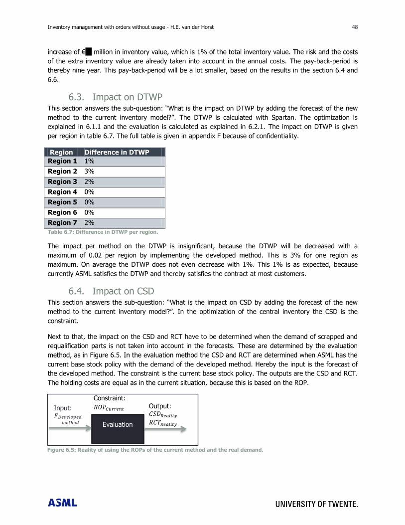
Inventory management with orders without usage - H.E. van der Horst 48 48
increase of €?? million in inventory value, which is 1% of the total inventory value. The risk and the costs
of the extra inventory value are already taken into account in the annual costs. The pay-back-period is
thereby nine year. This pay-back-period will be a lot smaller, based on the results in the section 6.4 and
6.6.
6.3. Impact on DTWP This section answers the sub-question: “What is the impact on DTWP by adding the forecast of the new
method to the current inventory model?”. The DTWP is calculated with Spartan. The optimization is
explained in 6.1.1 and the evaluation is calculated as explained in 6.2.1. The impact on DTWP is given
per region in table 6.7. The full table is given in appendix F because of confidentiality.
Region Difference in DTWP
Region 1 1%
Region 2 3%
Region 3 2%
Region 4 0%
Region 5 0%
Region 6 0%
Region 7 2%
Table 6.7: Difference in DTWP per region.
The impact per method on the DTWP is insignificant, because the DTWP will be decreased with a
maximum of 0.02 per region by implementing the developed method. This is 3% for one region as
maximum. On average the DTWP does not even decrease with 1%. This 1% is as expected, because
currently ASML satisfies the DTWP and thereby satisfies the contract at most customers.
6.4. Impact on CSD This section answers the sub-question: “What is the impact on CSD by adding the forecast of the new
method to the current inventory model?”. In the optimization of the central inventory the CSD is the
constraint.
Next to that, the impact on the CSD and RCT have to be determined when the demand of scrapped and
requalification parts is not taken into account in the forecasts. These are determined by the evaluation
method, as in Figure 6.5. In the evaluation method the CSD and RCT are determined when ASML has the
current base stock policy with the demand of the developed method. Hereby the input is the forecast of
the developed method. The constraint is the current base stock policy. The outputs are the CSD and RCT.
The holding costs are equal as in the current situation, because this is based on the ROP.
Constraint:
𝑅𝑂𝑃𝐶𝑢𝑟𝑟𝑒𝑛𝑡
Evaluation
Input: 𝐹𝐷𝑒𝑣𝑒𝑙𝑜𝑝𝑒𝑑
𝑚𝑒𝑡 𝑜𝑑
𝐶𝑆𝐷𝑅𝑒𝑎𝑙𝑖𝑡𝑦
𝑅𝐶𝑇𝑅𝑒𝑎𝑙𝑖𝑡𝑦
Output:
Figure 6.5: Reality of using the ROPs of the current method and the real demand.
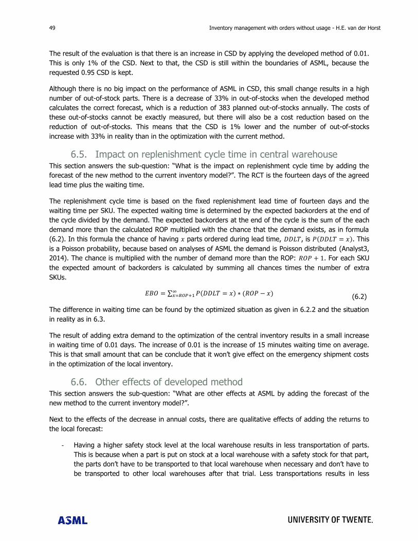
49 Inventory management with orders without usage - H.E. van der Horst
The result of the evaluation is that there is an increase in CSD by applying the developed method of 0.01.
This is only 1% of the CSD. Next to that, the CSD is still within the boundaries of ASML, because the
requested 0.95 CSD is kept.
Although there is no big impact on the performance of ASML in CSD, this small change results in a high
number of out-of-stock parts. There is a decrease of 33% in out-of-stocks when the developed method
calculates the correct forecast, which is a reduction of 383 planned out-of-stocks annually. The costs of
these out-of-stocks cannot be exactly measured, but there will also be a cost reduction based on the
reduction of out-of-stocks. This means that the CSD is 1% lower and the number of out-of-stocks
increase with 33% in reality than in the optimization with the current method.
6.5. Impact on replenishment cycle time in central warehouse This section answers the sub-question: “What is the impact on replenishment cycle time by adding the
forecast of the new method to the current inventory model?”. The RCT is the fourteen days of the agreed
lead time plus the waiting time.
The replenishment cycle time is based on the fixed replenishment lead time of fourteen days and the
waiting time per SKU. The expected waiting time is determined by the expected backorders at the end of
the cycle divided by the demand. The expected backorders at the end of the cycle is the sum of the each
demand more than the calculated ROP multiplied with the chance that the demand exists, as in formula
(6.2). In this formula the chance of having parts ordered during lead time, , is . This
is a Poisson probability, because based on analyses of ASML the demand is Poisson distributed (Analyst3,
2014). The chance is multiplied with the number of demand more than the ROP: . For each SKU
the expected amount of backorders is calculated by summing all chances times the number of extra
SKUs.
∑
The difference in waiting time can be found by the optimized situation as given in 6.2.2 and the situation
in reality as in 6.3.
The result of adding extra demand to the optimization of the central inventory results in a small increase
in waiting time of 0.01 days. The increase of 0.01 is the increase of 15 minutes waiting time on average.
This is that small amount that can be conclude that it won‟t give effect on the emergency shipment costs
in the optimization of the local inventory.
6.6. Other effects of developed method This section answers the sub-question: “What are other effects at ASML by adding the forecast of the
new method to the current inventory model?”.
Next to the effects of the decrease in annual costs, there are qualitative effects of adding the returns to
the local forecast:
- Having a higher safety stock level at the local warehouse results in less transportation of parts.
This is because when a part is put on stock at a local warehouse with a safety stock for that part,
the parts don‟t have to be transported to that local warehouse when necessary and don‟t have to
be transported to other local warehouses after that trial. Less transportations results in less
(6.2)
Inventory management with orders without usage - H.E. van der Horst 50 50
logistic death on arrivals, because every transport gives a risk of a defect by transporting parts.
Also less transportations results in a more sustainable environment.
- Another advantage in the reduction of emergency transportations is a more efficient
consolidation. When an order is transported with emergency this part cannot be consolidated
with other orders, because of the high priority of that order. When the order is transported as
routine, the order can be consolidated with other orders, whereby extra cost reductions can be
gained.
Next to the effects of the decrease in annual costs there are qualitative effects of adding the returns to
the central forecast:
- Less workload is gained when having a realistic planning. When a SKU has a high number of
returned requalification orders, a lot of extra demand is not taken into account in the current
planning. This means that this part has a higher risk to become critical. When a part becomes
critical extra time has to be invested to get extra parts from the supplier. In the worst situation
the part becomes out-of-stock (383 orders more) and extra pressure to the supplier has to be
given.
- A more realistic planning results in a better forecast to the supplier, which increase the
satisfaction of the supplier.
6.7. Conclusion This section gave answer to the question “What is the impact of the new methods compared to the
current method”. The conclusion is as follows:
- The recommendation is to implement the developed method, because this method is the closest
to the reality. Thereby the developed method is most suitable for forecasting the demand at
ASML.
- Implementing the developed method results in an annual cost reduction of ?? million (1%),
combining local and central inventory optimization. The investment is around €?? million (1%).
Next to that the costs will be even more reduced through the following reasons:
o A reduction in out-of-stocks of 33%;
o Less emergency transportations, this results in less extra handling costs and more
efficient consolidation of orders.
- The impact of the developed method on the DTWP is maximum 1% improvement worldwide. For
one region this is 3%. In this region the developed method will improve the DTWP significant.
The impact on the CSD gives a performance improvement of 1%. This doesn‟t give a high impact
on the overall performance of ASML.
The impact on the RCP is limited.

51 Inventory management with orders without usage - H.E. van der Horst
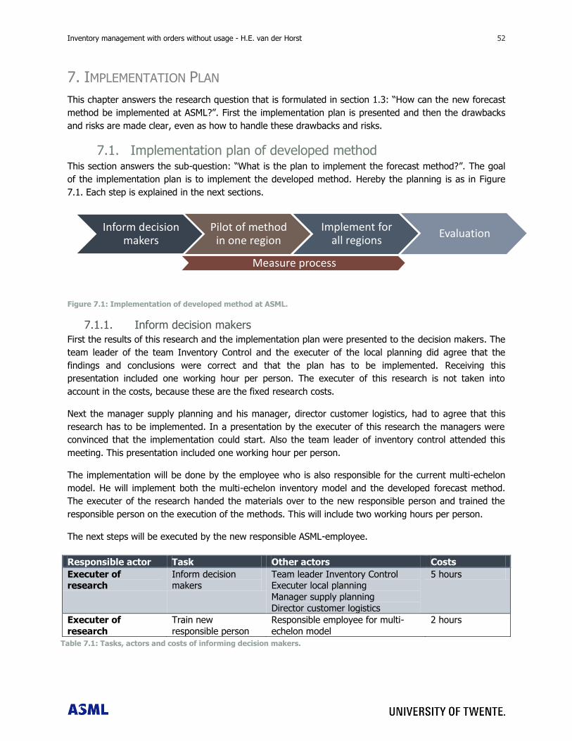
Inventory management with orders without usage - H.E. van der Horst 52 52
7. IMPLEMENTATION PLAN
This chapter answers the research question that is formulated in section 1.3: “How can the new forecast
method be implemented at ASML?”. First the implementation plan is presented and then the drawbacks
and risks are made clear, even as how to handle these drawbacks and risks.
7.1. Implementation plan of developed method This section answers the sub-question: “What is the plan to implement the forecast method?”. The goal
of the implementation plan is to implement the developed method. Hereby the planning is as in Figure
7.1. Each step is explained in the next sections.
Figure 7.1: Implementation of developed method at ASML.
7.1.1. Inform decision makers
First the results of this research and the implementation plan were presented to the decision makers. The
team leader of the team Inventory Control and the executer of the local planning did agree that the
findings and conclusions were correct and that the plan has to be implemented. Receiving this
presentation included one working hour per person. The executer of this research is not taken into
account in the costs, because these are the fixed research costs.
Next the manager supply planning and his manager, director customer logistics, had to agree that this
research has to be implemented. In a presentation by the executer of this research the managers were
convinced that the implementation could start. Also the team leader of inventory control attended this
meeting. This presentation included one working hour per person.
The implementation will be done by the employee who is also responsible for the current multi-echelon
model. He will implement both the multi-echelon inventory model and the developed forecast method.
The executer of the research handed the materials over to the new responsible person and trained the
responsible person on the execution of the methods. This will include two working hours per person.
The next steps will be executed by the new responsible ASML-employee.
Inform decision makers
Pilot of method in one region
Implement for all regions
Evaluation
Measure process
Responsible actor Task Other actors Costs
Executer of research
Inform decision makers
Team leader Inventory Control Executer local planning
Manager supply planning
Director customer logistics
5 hours
Executer of
research
Train new
responsible person
Responsible employee for multi-
echelon model
2 hours
Table 7.1: Tasks, actors and costs of informing decision makers.
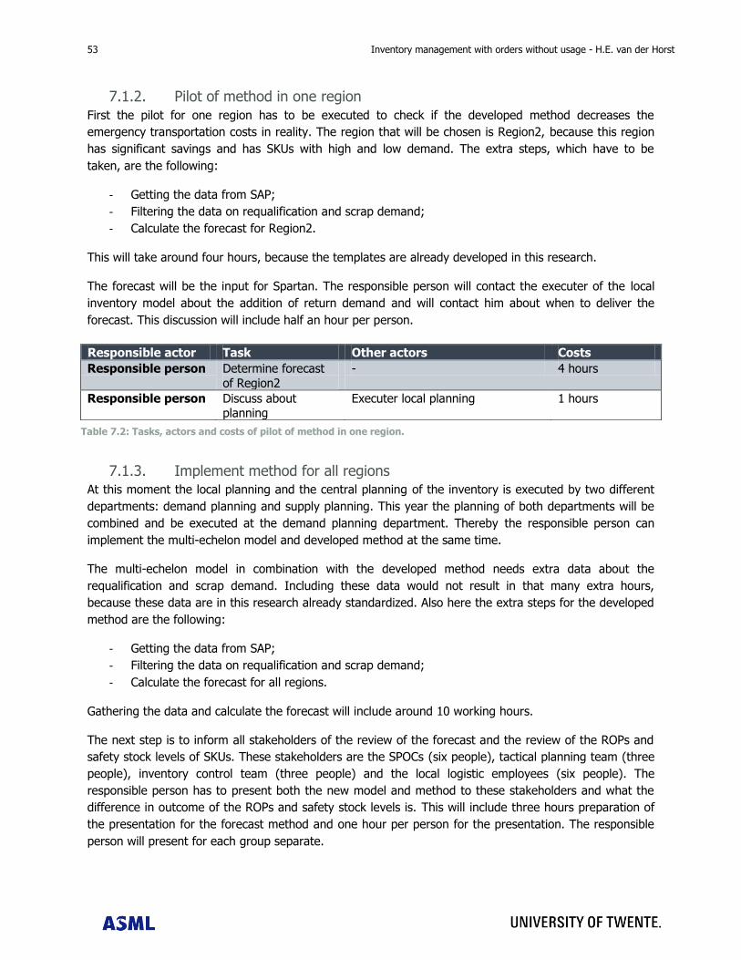
53 Inventory management with orders without usage - H.E. van der Horst
7.1.2. Pilot of method in one region
First the pilot for one region has to be executed to check if the developed method decreases the
emergency transportation costs in reality. The region that will be chosen is Region2, because this region
has significant savings and has SKUs with high and low demand. The extra steps, which have to be
taken, are the following:
- Getting the data from SAP;
- Filtering the data on requalification and scrap demand;
- Calculate the forecast for Region2.
This will take around four hours, because the templates are already developed in this research.
The forecast will be the input for Spartan. The responsible person will contact the executer of the local
inventory model about the addition of return demand and will contact him about when to deliver the
forecast. This discussion will include half an hour per person.
7.1.3. Implement method for all regions
At this moment the local planning and the central planning of the inventory is executed by two different
departments: demand planning and supply planning. This year the planning of both departments will be
combined and be executed at the demand planning department. Thereby the responsible person can
implement the multi-echelon model and developed method at the same time.
The multi-echelon model in combination with the developed method needs extra data about the
requalification and scrap demand. Including these data would not result in that many extra hours,
because these data are in this research already standardized. Also here the extra steps for the developed
method are the following:
- Getting the data from SAP;
- Filtering the data on requalification and scrap demand;
- Calculate the forecast for all regions.
Gathering the data and calculate the forecast will include around 10 working hours.
The next step is to inform all stakeholders of the review of the forecast and the review of the ROPs and
safety stock levels of SKUs. These stakeholders are the SPOCs (six people), tactical planning team (three
people), inventory control team (three people) and the local logistic employees (six people). The
responsible person has to present both the new model and method to these stakeholders and what the
difference in outcome of the ROPs and safety stock levels is. This will include three hours preparation of
the presentation for the forecast method and one hour per person for the presentation. The responsible
person will present for each group separate.
Responsible actor Task Other actors Costs
Responsible person Determine forecast
of Region2
- 4 hours
Responsible person Discuss about planning
Executer local planning
1 hours
Table 7.2: Tasks, actors and costs of pilot of method in one region.
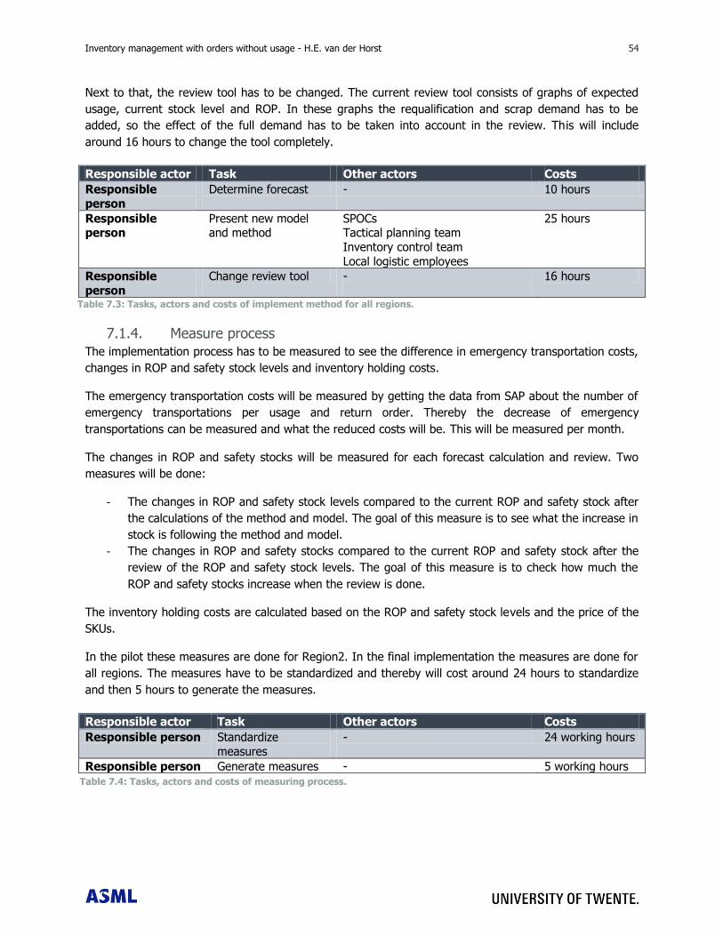
Inventory management with orders without usage - H.E. van der Horst 54 54
Next to that, the review tool has to be changed. The current review tool consists of graphs of expected
usage, current stock level and ROP. In these graphs the requalification and scrap demand has to be
added, so the effect of the full demand has to be taken into account in the review. This will include
around 16 hours to change the tool completely.
7.1.4. Measure process
The implementation process has to be measured to see the difference in emergency transportation costs,
changes in ROP and safety stock levels and inventory holding costs.
The emergency transportation costs will be measured by getting the data from SAP about the number of
emergency transportations per usage and return order. Thereby the decrease of emergency
transportations can be measured and what the reduced costs will be. This will be measured per month.
The changes in ROP and safety stocks will be measured for each forecast calculation and review. Two
measures will be done:
- The changes in ROP and safety stock levels compared to the current ROP and safety stock after
the calculations of the method and model. The goal of this measure is to see what the increase in
stock is following the method and model.
- The changes in ROP and safety stocks compared to the current ROP and safety stock after the
review of the ROP and safety stock levels. The goal of this measure is to check how much the
ROP and safety stocks increase when the review is done.
The inventory holding costs are calculated based on the ROP and safety stock levels and the price of the
SKUs.
In the pilot these measures are done for Region2. In the final implementation the measures are done for
all regions. The measures have to be standardized and thereby will cost around 24 hours to standardize
and then 5 hours to generate the measures.
Table 7.3: Tasks, actors and costs of implement method for all regions.
Responsible actor Task Other actors Costs
Responsible
person
Determine forecast - 10 hours
Responsible person
Present new model and method
SPOCs Tactical planning team
Inventory control team
Local logistic employees
25 hours
Responsible
person
Change review tool -
16 hours
Table 7.4: Tasks, actors and costs of measuring process.
Responsible actor Task Other actors Costs
Responsible person Standardize
measures
- 24 working hours
Responsible person Generate measures - 5 working hours
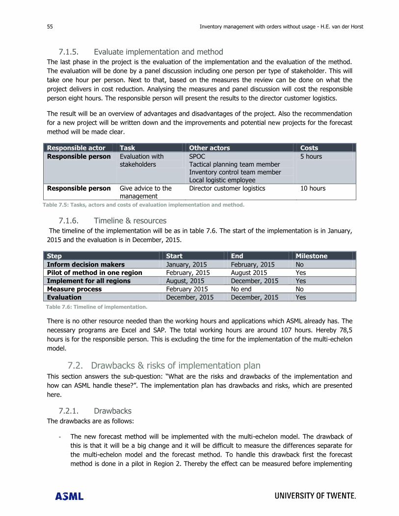
55 Inventory management with orders without usage - H.E. van der Horst
7.1.5. Evaluate implementation and method
The last phase in the project is the evaluation of the implementation and the evaluation of the method.
The evaluation will be done by a panel discussion including one person per type of stakeholder. This will
take one hour per person. Next to that, based on the measures the review can be done on what the
project delivers in cost reduction. Analysing the measures and panel discussion will cost the responsible
person eight hours. The responsible person will present the results to the director customer logistics.
The result will be an overview of advantages and disadvantages of the project. Also the recommendation
for a new project will be written down and the improvements and potential new projects for the forecast
method will be made clear.
Responsible actor Task Other actors Costs
Responsible person Evaluation with
stakeholders
SPOC
Tactical planning team member Inventory control team member
Local logistic employee
5 hours
Responsible person Give advice to the management
Director customer logistics 10 hours
7.1.6. Timeline & resources
The timeline of the implementation will be as in table 7.6. The start of the implementation is in January,
2015 and the evaluation is in December, 2015.
Step Start End Milestone
Inform decision makers January, 2015 February, 2015 No
Pilot of method in one region February, 2015 August 2015 Yes
Implement for all regions August, 2015 December, 2015 Yes
Measure process February 2015 No end No
Evaluation December, 2015 December, 2015 Yes
There is no other resource needed than the working hours and applications which ASML already has. The
necessary programs are Excel and SAP. The total working hours are around 107 hours. Hereby 78,5
hours is for the responsible person. This is excluding the time for the implementation of the multi-echelon
model.
7.2. Drawbacks & risks of implementation plan This section answers the sub-question: “What are the risks and drawbacks of the implementation and
how can ASML handle these?”. The implementation plan has drawbacks and risks, which are presented
here.
7.2.1. Drawbacks
The drawbacks are as follows:
- The new forecast method will be implemented with the multi-echelon model. The drawback of
this is that it will be a big change and it will be difficult to measure the differences separate for
the multi-echelon model and the forecast method. To handle this drawback first the forecast
method is done in a pilot in Region 2. Thereby the effect can be measured before implementing
Table 7.5: Tasks, actors and costs of evaluation implementation and method.
Table 7.6: Timeline of implementation.
Inventory management with orders without usage - H.E. van der Horst 56 56
the model and method. The multi-echelon model can be measured after implementation for
region 2, what the difference is with the current situation and the situation with the developed
forecast method.
- The implementation of the plan will cost a full year. This is a drawback, because the project has
thereby a long term result and it is difficult to keep all stakeholders on one line in a longer
period. To handle this drawback the measurement has to be done monthly to keep everyone at
the same focus.
- A drawback is that the results of implementing the new forecast method will be difficult to
measure on long term. This is because the service demand increases due to having more
customers and more machines. Thereby the costs will be increasing with the extra machines.
This drawback will be reduced by monthly measuring, but is a drawback which ASML cannot
really tackle.
- The last drawback in this implementation is that another person than the executer of this
research will implement the research. This drawback is minimized by having clear documentation
of the full research and having a hand-over moment.
7.2.2. Risks
The risks are as follows:
- The risk of this project is that there will be too many parts on stock. In this research it is made
clear that mostly parts are extra stocked for medium or high usage SKUs. This risk is thereby not
really high, but to lower this risk the measurements has to be done correctly and monthly.
- The risk of reacting on return demand in the inventory levels could result in more returns. This is
because the solution to get all parts in a short time period to the customer does not depend
anymore on having unavailability due to requalification and scrap. This risk can be reduced to
make first good arrangements about the targets on reducing the return demand in combination
with the implementation of this plan.
- Another risk is that only one person is trained on the new forecast method. When this person
forgets some parts or leaves the company there is a risk of a failed implementation. The risk is
not that high, because also the executer of the local planning and the team leader of inventory
control know the approach and expected results of the forecast method and implementation
plan.
7.3. Conclusion This section gave answer to the question: “How can the new forecast method be implemented at
ASML?”. The conclusions are as follows:
- The new forecast method will be implemented by first having a pilot at one region and next
implement the forecast method together with the multi-echelon model for all regions.
- The costs will include around 107 working hours and the timespan of the implementation is one
year. Taking the risks and drawbacks into account it is realistic to stay with the amount of
working hours and the timespan.

57 Inventory management with orders without usage - H.E. van der Horst
Inventory management with orders without usage - H.E. van der Horst 58 58
8. CONCLUSIONS & DISCUSSION
Each chapter finished with the answer on the sub-questions of this research. The conclusion in section
8.1 gives the answer on the research question, which is as follows:
“How should ASML respond to orders without usage into the inventory level calculations?
What would be the impact of this incorporation in terms of:
- Emergency transportation costs;
- Inventory holding costs;
- Replenishment cycle time;
- Risk of not satisfying the customer contracts?”
Section 8.2 gives the recommendations based on this research. Section 8.3 contains the limitations of this
research in the discussion. The last section gives some points for further research.
8.1. Conclusion This section gives the answer on the research question as mentioned above.
ASML should respond to orders without usage by implementing the developed method for determining
the forecast of the local demand and the central demand.
The result of the optimization of local inventory is to choose the developed method based on the annual
inventory holding and emergency transportation cost savings. This method results in a saving of around
?? million per year, with a pay-back period of two years. Adding extra demand in the optimization of local
inventory does not give impact on the DTWP.
The result of the optimization of the central inventory is to add also the developed method. By adding
extra demand to the forecast of the central warehouse the inventory holding costs increase with €??
million, whereby the out-of-stocks will be reduced with ?? orders. The change in CSD and RCT is low and
will not impact the performance of ASML.
The current emergency transportation cost is €?? million annually, whereby the orders without usage
cause ??% of these costs. The impact of adding the developed method to the optimization of the local
and central inventory optimization results in a decrease of about €?? million in emergency transportation
costs. The impact of adding these returns to the optimization of the local inventory is an increase of €??
million of inventory value.
The replenishment cycle time is currently higher of a SKU with a high number of orders without usage
compared to a SKU with a low number of orders without usage, as explained in Chapter 3. Although this
fact, there is no impact on the replenishment cycle time with the developed method, based in the
calculations in Chapter 6. The reason for this is that the return demand is not incorporated in the
optimization of the central inventory. When including the return demand in the optimization of the central
inventory, the replenishment cycle time was changed with a very small amount, which would have too
less impact for investing in inventory value.
The risk of not satisfying the customer contract doesn‟t differ significant, because the new methods don‟t
affect the DTWP a lot.
59 Inventory management with orders without usage - H.E. van der Horst
Other impacts of adding the return value to the optimization of the local and central inventory are:
- Decreased workload and more efficient consolidation of parts, due to a reduction in emergency
transportations. This can result in extra cost reduction;
- Decreased transportations of parts, increased sustainable environment and decreased logistic
death on arrivals, by having more parts on stock;
- Decreased workload and more satisfied suppliers, due to a realistic planning;
- Decreased out-of-stocks and critical parts, due to a realistic planning.
8.2. Recommendations Based on this research the following recommendations are formulated:
- Include the return flow in the optimization of the local and central inventory by determining the
forecast with the developed method. This results in the outcomes as described in the previous
section “Conclusion”.
- In the next years a new multi-echelon inventory model will be implemented at ASML, whereby
the optimizations of the local and central inventory are combined. In appendix G the full
description and results are presented. Based on the optimizations of the multi-echelon model, the
costs of the developed method for the local and central inventory are €?? million annual. The
remark has to be made that the CSD is not correct following the customer contracts, because
that is not possible in the current prototype software. The expectation is that with the real CSD
the annual costs will be around zero. The recommendation is to calculate the methods with the
correct CSDs, when the software is available and check if the expectation is correct. After that
the developed method can be implemented together with the multi-echelon model.
- It would be worthwhile to do research to find a reverse logistics multi-echelon multi-item
inventory model. At this moment there is no model available in the literature, which combines all
these three characteristics. The expectation is by adding the return flow fully to the inventory
model the costs will be more reduced. Because ASML will implement a new multi-echelon model,
it would be a good addition to first discover the possibilities of a reverse logistics multi-echelon
model.
- The final recommendation is to reduce the orders without usage. From data analysis came that in
some regions there are in amount and in percentage of all orders more orders without usage in
one region than another. This means that some regions could learn from other regions in
reducing the orders without usage. Thereby from cost reduction perspective the recommendation
is to reduce orders without usage in the high %/amount regions.
8.3. Discussion Section 8.1 presents the conclusions and section 8.2 contains the recommendations for ASML. This
section discusses the limitations in this research.
Designing the processes and evaluating the results of the data analysis is done by interviewing
employees at ASML. In the timeline it was not possible to interview all stakeholders within ASML. In total
19 employees are interviewed and with these interviews the processes are designed as good as possible.
Maybe when other employees were interviewed the result could be slightly different.
Inventory management with orders without usage - H.E. van der Horst 60 60
The data analysis in chapter 3 is based on data of 2013. This could give a bias, because the demands at
ASML for spare parts are low. So when in one year a part has a demand of zero, another year this could
be three. Because of limited time, the assumption is made that 2013 would be representative for the last
years. In the evaluation of the methods in chapter 6 the demand of the last three years is used, so the
bias would be smaller in measuring the impact when changing the demand.
The return types per order are labelled by the engineers. In this research the correctness of the labelling
is not analysed. Only the way of labelling is checked with three engineers to evaluate if they label the
returns as expected. Based on this check the assumption is taken that all engineers label the returns
correct or within boundaries.
As already mentioned in section 8.2 the most optimized safety stock levels would be reached when the
inventory model would change to a reverse logistics model. In this research ASML didn‟t want to change
the model, but only the input to not change the inventory model every few years. Next to that, there was
not enough time to develop a completely new inventory model.
8.4. Further research Based on the conclusion, recommendation and discussion, the subjects for further research are as
follows:
- As already mentioned in the recommendation and the discussion, research have to be done on a
new reverse logistics multi-echelon multi-item inventory model to include the return demand not
only in the forecast, but in the full inventory model. The expectation is by adding the return flow
fully to the inventory model the costs will be more reduced.
- At the moment the return lead time of requalification parts, which have to be tested at the
supplier, is almost equal to the return lead time of failed parts, which have to be repaired at the
supplier. The reason for this is that this return flow at the supplier has not its own flow, but has
to be added to the normal production of the parts to ASML. In further research possibilities to
decrease the return lead time could be found out. Then the inventory holding costs could be
lowered, because the lead time is reduced.
- The end conclusion, which is also mentioned at the recommendations, it that the best cost
decrease would be the decrease of orders without usage. To decrease this further research could
be done on how to decrease the orders without usage and why one region has more orders
without usage than another region. Possibilities to do research in are to improve the amount of
solutions in the system, which the engineers use, to train the engineers more on the ordering
and to make a policy on ordering that many parts.

61 Inventory management with orders without usage - H.E. van der Horst
Inventory management with orders without usage - H.E. van der Horst 62 62
REFERENCES
Analyst1. (2014, August 5). Used-unused parts. (H. van der Horst, Interviewer)
Analyst2. (2014, April 28). Spartan Costs Data. Veldhoven.
Analyst3. (2014, October 13). Forecast Methodology. (H. van der Horst, Interviewer)
ASML. (2013, July 31). Profile. Retrieved August 5, 2014, from ASML:
http://www.asml.com/asml/show.do?lang=EN&ctx=272&rid=362
ASML. (2014, February 20). Questions & Answers. Retrieved August 7, 2014, from ASML:
http://www.asml.com/asml/show.do?lang=EN&ctx=32894
Aspert, M. v. (2014). Design of an Integrated Global Warehouse and Field Stock Planning Concept for
Spare Parts. Eindhoven: Eindverslagen Stan Ackermans Instituut.
Chen, Y., Chong, P., & Tong, M. (1991). Mathematical and Computer Modelling of Pareto Principle.
Elsevier Science Ltd, 19, 61-80.
Choi, D.-W., Hwang, H., & Koh, S.-G. (2007). A generalized ordering and recovery policy for reusable
items. European Journal of Operational Research, 182, 764–774.
CompetencyEngineer1. (2014, September 4). Coach & PCS. (H. van der Horst, Interviewer)
Criticalparts1. (2014, September 4). Unused parts. (H. van der Horst, Interviewer)
De Brito, M., & Van der Laan, E. (2009). Inventory control with product returns: The impact of imperfect
information. European Journal of Operational Research, 85-101.
Engineer1. (2014, August 20). Order Engineer. (H. van der horst, Interviewer)
Engineer2. (2014, August 19). Order Engineer. (H. E. Van der horst, Interviewer)
Fleischmann, M. (2003). Reverse logistics network structures and design. In L. Wassenhove, Business
aspects of closed-loop supply chains (pp. 117-148). Pittsburgh: Carnegie Mellon University Press.
Hazewinkel, M. (2011, February 7). Greedy algorithm. Retrieved October 28, 2014, from Encyclopedia of
Mathematics:
http://www.encyclopediaofmath.org/index.php?title=Greedy_algorithm&oldid=11679
HeadInterfaceTeam1. (2014, August 12). Different type of orders. (H. van der Horst, Interviewer)
HeadLogistics1. (2014, November 10). Update graduation assignment Hanneke van der Horst. (H. van
der Horst, Interviewer)
Heerkens, J. (2005). Algemene Bedrijfskundige Aanpak. Enschede: TSM Business School.
Inderfurth, K., & van der Laan, E. (2001). Leadtime effects and policy improvement for stochastic
inventory control with remanufacturing. International Journal of Production Economics, 71, 381-
390.
63 Inventory management with orders without usage - H.E. van der Horst
InventoryControl1. (2014). Forecast. Veldhoven: ASML.
InventoryControl2. (2014, September 3). Data and forecasting. (H. van der Horst, Interviewer)
InventoryControl3. (2014, August 6). Introduction project Forecast unused parts. (H. van der Horst,
Interviewer)
Kelle, P., & Silver, E. (1989). Purchasing policy of new containers considering the random returns of
previously issued containers. liE Transactions, 21, 349-354.
Kranenburg, A. (2006). Spare Parts Inventory Control under System Availability Constraints. Eindhoven:
Technische Universiteit Eindhoven.
Mahadevan, B., Pyke, D. F., & Fleischmann, M. (2002). Periodic review, push inventory policies for
remanufacturing. Rotterdam: ERIM Report Series ERS-2002-35-LIS.
Mes, M. (2013, October 3). L5 - Data analysis, warm-up period & comparing models. (H. v. Horst,
Interviewer)
OperationalPlanner1. (2014, August 11). Engineers Orders. (H. E. van der Horst, Interviewer)
ServiceLogistics1. (2014, August 7). Introduction project. (H. van der Horst, Interviewer)
TacticalPlanning1. (2014, September 3). LMS Project. (H. van der horst, Interviewer)
TacticalPlanning2. (2014, August 28). Forecasting. (H. van der Horst, Interviewer)
Teunter, R. (2004). Lot-sizing for inventory systems with product recovery. Computers & Industrial
Engineering, 431-441.
Thierry, M., Salomon, M., Van Nunen, J., & Van Wassenhove, L. (1995). Strategic Issues in Product
Recovery Manufacturing. California Management Review, 37(2), 114-135.
ToolPlanning1. (2014, September 9). Costs Machine Down. (H. van der Horst, Interviewer)
TransportController1. (2014, August 8). Transport. (H. van der Horst, Interviewer)
Van der Laan, E. A. (1997). The effects of remanufacturing on inventory control. Rotterdam: Erasmus
University Rotterdam.
Van der Laan, E. A. (2003). An NPV and AC analysis ofa stochastic inventory system with joint
manufacturing and remanufacturing. International Journal of Production Economics, 81-82, 317-
331.
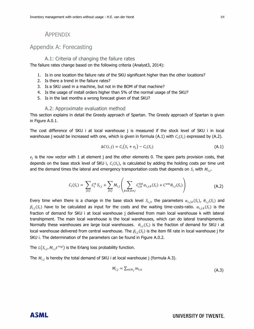
Inventory management with orders without usage - H.E. van der Horst 64 64
APPENDIX
Appendix A: Forecasting
A.1: Criteria of changing the failure rates
The failure rates change based on the following criteria (Analyst3, 2014):
1. Is in one location the failure rate of the SKU significant higher than the other locations?
2. Is there a trend in the failure rates?
3. Is a SKU used in a machine, but not in the BOM of that machine?
4. Is the usage of install orders higher than 5% of the normal usage of the SKU?
5. Is in the last months a wrong forecast given of that SKU?
A.2: Approximate evaluation method
This section explains in detail the Greedy approach of Spartan. The Greedy approach of Spartan is given
in Figure A.0.1.
The cost difference of SKU i at local warehouse j is measured if the stock level of SKU i in local
warehouse j would be increased with one, which is given in formula (A.1) with expressed by (A.2).
( )
is the row vector with 1 at element j and the other elements 0. The spare parts provision costs, that
depends on the base stock level of SKU i, , is calculated by adding the holding costs per time unit
and the demand times the lateral and emergency transportation costs that depends on with .
∑
∑
( ∑
)
Every time when there is a change in the base stock level , the parameters , and
have to be calculated as input for the costs and the waiting time-costs-ratio. is the
fraction of demand for SKU i at local warehouse j delivered from main local warehouse k with lateral
transhipment. The main local warehouse is the local warehouses, which can do lateral transhipments.
Normally these warehouses are large local warehouses. is the fraction of demand for SKU i at
local warehouse delivered from central warehouse. The is the item fill rate in local warehouse j for
SKU i. The determination of the parameters can be found in Figure A.0.2.
The ( ) is the Erlang loss probability function.
The is hereby the total demand of SKU i at local warehouse j (formula A.3).
∑
(A.1)
(A.2)
(A.3)
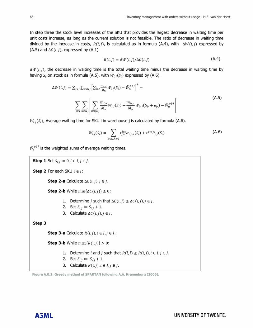
65 Inventory management with orders without usage - H.E. van der Horst
In step three the stock level increases of the SKU that provides the largest decrease in waiting time per
unit costs increase, as long as the current solution is not feasible. The ratio of decrease in waiting time
divided by the increase in costs, , is calculated as in formula (A.4), with expressed by
(A.5) and , expressed by (A.1).
, the decrease in waiting time is the total waiting time minus the decrease in waiting time by
having on stock as in formula (A.5), with expressed by (A.6).
∑ ∑ [∑
]
∑ ∑ * ∑
( )
+
, Average waiting time for SKU i in warehouse j is calculated by formula (A.6).
∑
is the weighted sums of average waiting times.
Step 1 Set 𝑆𝑖 𝑗 ≔ 𝑖 𝐼 𝑗 𝐽
Step 2 For each SKU 𝑖 𝐼:
Step 2-a Calculate 𝐶 𝑖 𝑗 𝑗 𝐽.
Step 2-b While 𝑚𝑖𝑛 𝐶 𝑖 𝑗 ;
1. Determine 𝑗 such that 𝐶 𝑖 𝑗 𝐶 𝑖 𝑗 𝑗 𝐽.
2. Set 𝑆𝑖 𝑗 ≔ 𝑆𝑖 𝑗 .
3. Calculate 𝐶 𝑖 𝑗 𝑗 𝐽.
Step 3
Step 3-a Calculate 𝑅 𝑖 𝑗 𝑖 𝐼 𝑗 𝐽.
Step 3-b While 𝑚𝑎𝑥 𝑅 𝑖 𝑗 :
1. Determine 𝑖 and 𝑗 such that 𝑅 𝑖 𝑗 𝑅 𝑖 𝑗 𝑖 𝐼 𝑗 𝐽.
2. Set 𝑆𝑖 𝑗 ≔ 𝑆𝑖 𝑗 .
3. Calculate 𝑅 𝑖 𝑗 𝑖 𝐼 𝑗 𝐽.
Figure A.0.1: Greedy method of SPARTAN following A.A. Kranenburg (2006).
(A.4)
(A.5)
(A.6)
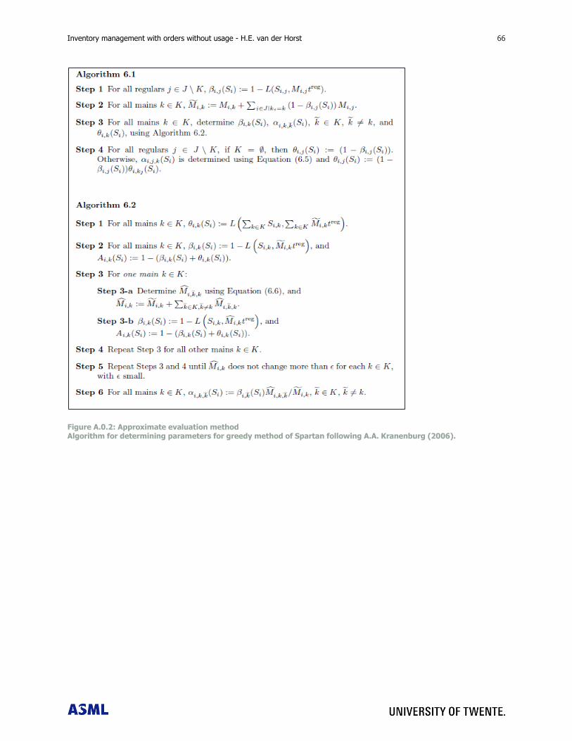
Inventory management with orders without usage - H.E. van der Horst 66 66
Figure A.0.2: Approximate evaluation method Algorithm for determining parameters for greedy method of Spartan following A.A. Kranenburg (2006).
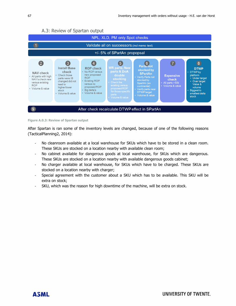
67 Inventory management with orders without usage - H.E. van der Horst
A.3: Review of Spartan output
Figure A.0.3: Review of Spartan output
After Spartan is ran some of the inventory levels are changed, because of one of the following reasons
(TacticalPlanning2, 2014):
- No cleanroom available at a local warehouse for SKUs which have to be stored in a clean room.
These SKUs are stocked on a location nearby with available clean room;
- No cabinet available for dangerous goods at local warehouse, for SKUs which are dangerous.
These SKUs are stocked on a location nearby with available dangerous goods cabinet;
- No charger available at local warehouse, for SKUs which have to be charged. These SKUs are
stocked on a location nearby with charger;
- Special agreement with the customer about a SKU which has to be available. This SKU will be
extra on stock;
- SKU, which was the reason for high downtime of the machine, will be extra on stock.

Inventory management with orders without usage - H.E. van der Horst 68 68
Appendix B: Confidential: Reference of confidential names of regions
69 Inventory management with orders without usage - H.E. van der Horst
Appendix C: Inventory models In this paragraph different inventory models are made clear to give an overview of the possible inventory
models to use. In chapter 5 the models are applied for the research. In Figure C.0.4 four figures of the
inventory system in reverse logistics are given.
Figure C.0.4.A is a closed-loop return system of Teunter (2004). In that system, there is a stock of
recoverable and serviceable parts. The recoverable stock is filled with parts to repair. The serviceable
stock is filled with the repaired parts and the new produced parts.
Figure C.0.4.B is the recovery system of Choi et al (2007). In this system there are also two inventory
points: recoverable and serviceable stock. Next to that, used parts could be scrapped and returned. In
this research this could be seen as “used” and “ordered without usage”/”returned”.
Figure C.0.4.C also has two inventory points, whereby there is no scrap at the customer. On the other
hand there is disposal from the recoverable inventory, which this research also includes. This model is
designed by Van der Laan (1997) and referred in different other papers.
In Figure C.0.4.D different forms of reuse and repair are given. Here it can be seen that in every stage in
the supply chain parts can be returned. In this research this is applicable for the difference in the return
of serviceable, repack and requalification parts. This is designed by Thierry et al (1995) and referred by
Mahadevan et al (2002).
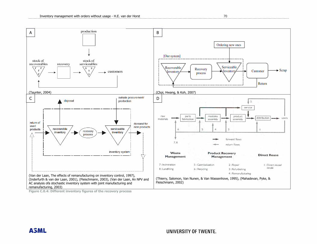
Inventory management with orders without usage - H.E. van der Horst 70 70
(Teunter, 2004)
(Choi, Hwang, & Koh, 2007)
(Van der Laan, The effects of remanufacturing on inventory control, 1997), (Inderfurth & van der Laan, 2001), (Fleischmann, 2003), (Van der Laan, An NPV and AC analysis ofa stochastic inventory system with joint manufacturing and remanufacturing, 2003)
(Thierry, Salomon, Van Nunen, & Van Wassenhove, 1995), (Mahadevan, Pyke, & Fleischmann, 2002)
Figure C.0.4: Different inventory figures of the recovery process
A B
C D

71 Inventory management with orders without usage - H.E. van der Horst
Appendix D: Confidential: Figures in chapters 1, 2 and 3
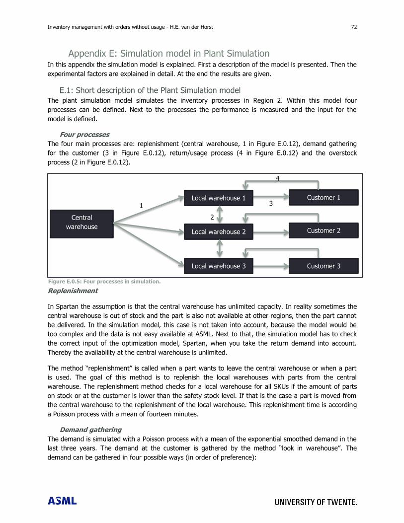
Inventory management with orders without usage - H.E. van der Horst 72 72
Appendix E: Simulation model in Plant Simulation In this appendix the simulation model is explained. First a description of the model is presented. Then the
experimental factors are explained in detail. At the end the results are given.
E.1: Short description of the Plant Simulation model
The plant simulation model simulates the inventory processes in Region 2. Within this model four
processes can be defined. Next to the processes the performance is measured and the input for the
model is defined.
Four processes
The four main processes are: replenishment (central warehouse, 1 in Figure E.0.12), demand gathering
for the customer (3 in Figure E.0.12), return/usage process (4 in Figure E.0.12) and the overstock
process (2 in Figure E.0.12).
Replenishment
In Spartan the assumption is that the central warehouse has unlimited capacity. In reality sometimes the
central warehouse is out of stock and the part is also not available at other regions, then the part cannot
be delivered. In the simulation model, this case is not taken into account, because the model would be
too complex and the data is not easy available at ASML. Next to that, the simulation model has to check
the correct input of the optimization model, Spartan, when you take the return demand into account.
Thereby the availability at the central warehouse is unlimited.
The method “replenishment” is called when a part wants to leave the central warehouse or when a part
is used. The goal of this method is to replenish the local warehouses with parts from the central
warehouse. The replenishment method checks for a local warehouse for all SKUs if the amount of parts
on stock or at the customer is lower than the safety stock level. If that is the case a part is moved from
the central warehouse to the replenishment of the local warehouse. This replenishment time is according
a Poisson process with a mean of fourteen minutes.
Demand gathering
The demand is simulated with a Poisson process with a mean of the exponential smoothed demand in the
last three years. The demand at the customer is gathered by the method “look in warehouse”. The
demand can be gathered in four possible ways (in order of preference):
Figure E.0.5: Four processes in simulation.
Customer 3
Customer 2
Customer 1
Central
warehouse
Local warehouse 1
Local warehouse 2
Local warehouse 3
1
2
3
4
73 Inventory management with orders without usage - H.E. van der Horst
1. Part from the stock of the local warehouse of the customer. Hereby no extra costs are needed
and the delivery time is zero. This is simulated by sending these parts directly to the customer.
2. Part from the stock of the most nearby other local warehouse in the region of the customer.
Hereby some costs are needed and there is a low delivery time.
3. Part from the stock of the second nearby other local warehouse in the region of the customer.
Hereby some more costs are needed and there is a bit more delivery time.
4. Part as emergency from the central warehouse. Hereby high costs are involved and high delivery
time.
The goal of the method “look in warehouse” is to fulfil the demand with the lowest costs and delivery
time.
Return/Usage
After on average fourteen days in a Poisson process the decision is made if a part will return or is used.
This decision is made in the method “return_usage_Region2A”. With a chance of return per SKU per
location the SKU will return or be used. If the part is in the bucket used in this simulation model, the part
could be in reality requalified, scrapped or used. This because all these return/used types will leave the
local inventory system. The returned parts are the serviceable and repack parts, which will be stocked
back in the local warehouse, if they have a safety stock level higher than zero. If there is no safety stock
level of that SKU the part is send back to the central warehouse.
The goal of the method “return_usage_Region2A” is having a realistic amount of returns and usage in the
simulation model. After usage the check is done if replenishment is needed. After a return the check is
done if there is overstock.
Overstock
The overstock is checked when a part returns. There is overstock when the amount of parts of that SKU
at the local warehouse and the customer is higher than the safety stock level. In the method “overstock”
per SKU per local warehouse is measured if there is overstock and if at another local warehouse has too
less parts of this SKU to fulfil the safety stock level. If that is the case the part of that SKU is relocated to
the other local warehouse.
The goal of the method “overstock” is to fulfil the safety stock levels and to reduce overstock.
Input
The input in this simulation model is information per SKU. This information is as follows:
- The total demand per day per customer;
- The chance of return per customer;
- The safety stock level per local warehouse;
- The price.
Other input in the simulation model is the following:
- Lateral transportation costs between all local warehouses;
- Emergency transportation costs to a local warehouse;
- Replenishment time to replenish a local warehouse;
- Delivery times between all local warehouses;
- Delivery time of an emergency to a local warehouse;
Inventory management with orders without usage - H.E. van der Horst 74 74
- Inter arrival time of the demand per local warehouse.
This information is gathered from SAP at ASML and is the same data as in the optimization model. The
information is added to the tables.
Performance measurement
The performance measurement contains the methods “calculateperlocation” and “collectmonthlystatistics”
and the tables “costperlocation” and “totalcost”. The goal of “calculateperlocation” is to calculate the
costs of one month per location. The number of emergency and lateral transportations is measured per
transportation in the method “lookinwarehouse”. The table “costperlocation” lists per location the amount
and costs of emergency and lateral transportations. The method “collectmonthlystatistics” has the goal of
calculating the emergency and lateral transportation and holding costs per month per local warehouse.
The table “total costs” lists this information. The method “collectmonthlystatistics” is called by a
generator every month.
Experiments
Four experiments are defined for this simulation, which have results from the optimization. There are as
follows:
1. The safety stock levels of the current forecast method, which includes only the usage;
2. The safety stock levels of the forecast, which includes usage and scrapped demand;
3. The safety stock levels of the forecast of method 2 of Kelle and Silver, including usage, scrapped
and requalification demand.
4. The safety stock levels of the forecast of the developed method, including usage, scrapped and
requalification demand.
Also a fifth simulation is done for checking the simulation model. This simulation contains the safety stock
levels of the current forecast method, which includes only the usage and contains only usage as output.
This is not the real situation, but it is currently the situation in the optimization model, Spartan.
The experimental settings can be found in next section.
E.2: Experimental settings
The simulation is non-terminating. There is no natural event which stops the simulation, because there is
no opening or closing time of the inventory system. This means that there will be steady state behaviour.
(Mes, 2013)
Non-terminating simulations use a warm-up period, whereby the observations from the beginning of a
simulation depend on the initial conditions, which have to be deleted. After that the steady state average
has to be determined. In this research there is chosen for a batch means method, because this will
contain one run with N batches and one warm-up period. The reason for this is a reduction in simulation
time. (Mes, 2013)
The length of the warm-up period can be found by the graphical method of Welch. Hereby the moving
average is used to see visual the length of the warm-up period. The warm-up period is in this case
eighteen months. This is because the steady state is then reached for all experiments as mentioned
above in the section experiments. For example Figure E.0.13 is given for the warm-up period
determination of the current forecasting method. Because of confidentiality the measure of the y-axis is
not given.
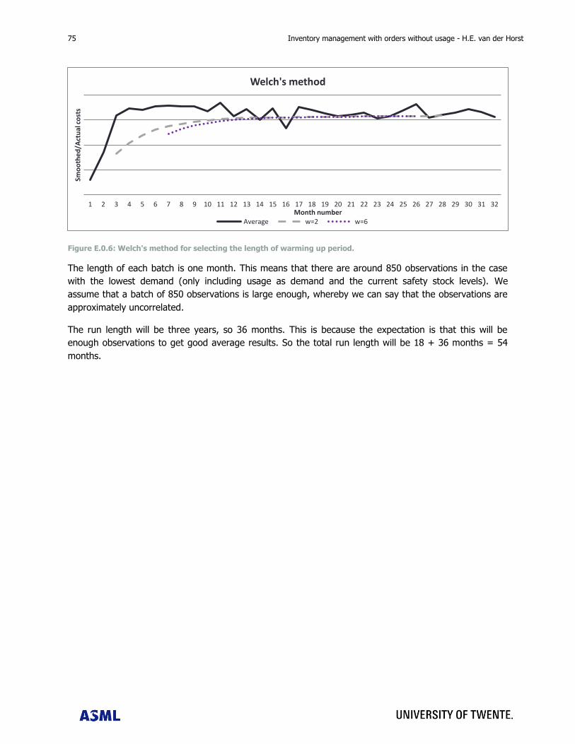
75 Inventory management with orders without usage - H.E. van der Horst
Figure E.0.6: Welch's method for selecting the length of warming up period.
The length of each batch is one month. This means that there are around 850 observations in the case
with the lowest demand (only including usage as demand and the current safety stock levels). We
assume that a batch of 850 observations is large enough, whereby we can say that the observations are
approximately uncorrelated.
The run length will be three years, so 36 months. This is because the expectation is that this will be
enough observations to get good average results. So the total run length will be 18 + 36 months = 54
months.
1 2 3 4 5 6 7 8 9 10 11 12 13 14 15 16 17 18 19 20 21 22 23 24 25 26 27 28 29 30 31 32
Smo
oth
ed
/Act
ual
co
sts
Month number
Welch's method
Average w=2 w=6

Inventory management with orders without usage - H.E. van der Horst 76 76
Appendix F: Confidential: Figures in chapter 6