Embed Size (px)
Citation preview

Inventory Rebalancing and Vehicle Routingin Bike Sharing Systems
Jasper SchuijbroekSchool of Industrial Engineering, Eindhoven University of Technology, The Netherlands, [email protected]
Robert Hampshire*H John Heinz III College, Carnegie Mellon University, Pittsburgh, PA 15213, [email protected]
Willem-Jan van HoeveTepper School of Business, Carnegie Mellon University, Pittsburgh, PA 15213, [email protected]
Bike sharing systems have been installed in many cities around the world and are increasing in popularity. A
major operational cost driver in these systems is rebalancing the bikes over time such that the appropriate
number of bikes and open docks are available to users. We combine two aspects that have previously been
handled separately in the literature: determining service level requirements at each bike sharing station, and
designing (near-)optimal vehicle routes to rebalance the inventory. Since finding provably optimal solutions
is practically intractable, we propose a new cluster-first route-second heuristic, in which the polynomial-
size Clustering Problem simultaneously considers the service level feasibility constraints and approximate
routing costs. Extensive computational results on real-world data from Hubway (Boston, MA) and Capital
Bikeshare (Washington, DC) are provided, which show that our heuristic outperforms a pure mixed integer
programming formulation and a constraint programming approach.
Key words : vehicle routing and scheduling, inventory, queues: applications, programming: integer,
programming: constraints, heuristics
1. Introduction
Bike sharing systems are experiencing wide-spread adoption in major cities around the world,
with over 300 active systems and more than 200 in planning (Meddin and DeMaio 2012). In these
systems, users can pickup and return bikes at designated bike sharing stations with a finite number
of docks. Unfortunately, user behavior results in spatial imbalance of the bike inventory over time.
The system equilibrium is often characterized by unacceptably low availability of bikes or open
docks, for pickups or returns respectively (Fricker et al. 2012, p. 375).
Therefore, operators deploy a fleet of trucks to rebalance the bike inventory. We focus on the
efficiency of these rebalancing operations, a major cost driver for operators (DeMaio 2009, p. 50).
This problem consists of two main components. First, determining the desired inventory level at
each bike station, which is typically done by an analysis of historic user data. Second, designing
truck routes that will perform the necessary pickups and deliveries in order to reach the target
* This material is based upon work partially supported by the National Science Foundation under Grant No. CMMI
#1055832.
1

Schuijbroek, Hampshire, and Van Hoeve: Inventory Rebalancing and Vehicle Routing2
inventory levels. In the literature, these two aspects have been mainly considered separately (see
Section 2 for a literature review). However, in practice operators often face a tradeoff between
user satisfaction and the cost of rebalancing. Moreover, as will be shown in this paper, it may be
advantageous to include stations in a route even though their inventory is already satisfactory, in
order to satisfy the service level requirements at a nearby location. For these reasons, we propose
to consider the inventory balancing problem and the routing problem simultaneously.
We model the stochastic demand by viewing the inventory at each station as a queuing system
with finite capacity and derive closed-form service level requirements on the transient distribution
of the availability of bikes and docks (Section 3). We recognize that service level requirements can
be met when the inventory is between a lower and upper bound. We then introduce the notion of
self-sufficient stations. Self-sufficient stations meet the service level requirements with their starting
inventory and hence should not necessarily be visited by a vehicle.
Next, we consider the routing of vehicles to achieve the service level requirements. Observe that
the pickup and delivery of bikes is unpaired, i.e., our situation corresponds to an extended One-
Commodity Pickup-and-Delivery Vehicle Routing Problem (1-PDVRP, see Hernandez-Perez and
Salazar-Gonzalez 2003). However, while preventing unnecessary vehicle visits, the inventory flexi-
bility at each station adds another layer of complexity to the classical Routing Problem (Section 4).
Since exact mixed integer programs (MIPs) for vehicle routing problems become intractable for
realistic instances, we present a new cluster-first route-second heuristic in Section 5. We incorpo-
rate the service level feasibility constraints in a polynomial-size Clustering Problem (modeled as
a MIP). The routing costs are incorporated into the clustering problem via a new approximation
based on maximum spanning stars. Lastly, we present an improvement scheme based on elimination
cuts to mitigate the approximation error.
In addition, we present a Constraint Programming (CP) formulation in Section 6, acting both
as an effective (exact) solution method for smaller instances and a benchmark for our dedicated
clustered routing heuristics.
Computational experiments (Section 7) using data from Hubway (Boston, MA) and Capital
Bikeshare (Washington, DC) show that our heuristics strongly outperform the classical MIP model.
Within seconds, we identify a feasible solution with a reasonable optimality gap. In a minute, we
find better solutions for almost all instances than the best MIP solution after 2 hours. Moreover,
our dedicated Clustered MIP heuristic outperforms Constraint Programming on larger instances.
We summarize the main contributions of this paper as follows. First, we present a novel formula-
tion of the rebalancing problem using dual-bounded service level constraints. Second, we present a
new polynomial-size Clustering Problem with service level feasibility constraints. Third, we develop
heuristics that are fast and accurate for large instances, and outperform state-of-the-art existing
methods.

Schuijbroek, Hampshire, and Van Hoeve: Inventory Rebalancing and Vehicle Routing3
2. Related Work
The study of bike sharing systems is increasing in popularity. DeMaio (2009) and Shaheen et al.
(2010) provide a history of bicycle sharing, starting with the first generation ‘white bikes’ in Ams-
terdam as early as 1965. From 1995 onwards, the third generation IT-based systems incorporate
‘advanced technologies for bicycle reservations, pickup, drop-off, and information tracking’ (Sha-
heen et al. 2010, p. 7). We identify four research substreams in bike sharing literature: strategic
design, demand analysis, service level analysis, and rebalancing operations.
Strategic design. Since most major cities have planned or considered implementation of
bike sharing systems, and existing systems are often expanded, several studies present models
dedicated to strategic design. Dell’Olio et al. (2011) develop a comprehensive methodology for
implementation, from estimating potential demand to optimizing locations. Martinez et al. (2012)
and Prem Kumar and Bierlaire (2012) present MIP models for the location problem. Lin and Yang
(2011) create a model trading off the interests of both users and investors. We note that none of
the studies include a notion of expected inventory imbalance costs.
Demand analysis. The purpose of demand analysis is twofold: forecasting future demand (e.g.
for service level requirements) and understanding the explaining factors for managerial decision
making. Kaltenbrunner et al. (2010) predict the system inventory state and suggest making such
information available to users. Froehlich and Oliver (2008), Borgnat and Abry (2009), Borgnat
et al. (2011), and Lathia et al. (2012) identify a temporal demand pattern and forecast the number
of rentals. Hampshire and Marla (2012) seek land use and socio-economic factors that explain
the use of bike sharing systems. Vogel et al. (2011) construct clusters of stations with similar
demand patterns. These studies could provide insights that are helpful in improving the service
level requirements developed in this paper.
Service level analysis. Several studies focus on service levels in bike sharing systems. We
recall that service level requirements are typically two-sided: for available bikes and docks. Most
notably, Nair and Miller-Hooks (2011) and Nair et al. (2013) decompose system-wide reliability
into a set of dual-bounded chance constraints for each station. We adapt their dual-bounded service
level constraints, but use a more realistic Markov chain to model the station inventory over time, as
opposed to observing the total net demand (see Section 3). Raviv et al. (2011a) present a queuing
system with finite capacity to model expected user dissatisfaction at each station, similar to our
approach. However, we assume time-independent user arrival rates to derive closed-form solutions.
Leurent (2012) models bike sharing stations as a dual Markovian waiting system, but contrary to
their assumption of waiting customers, we assume immediate lost sales.

Schuijbroek, Hampshire, and Van Hoeve: Inventory Rebalancing and Vehicle Routing4
Rebalancing operations. Using mean field analysis, Fricker et al. (2012) conclude that the
equilibrium system performance collapses under heterogeneity of user behavior and that a pressing
need for rebalancing operations exists. Vogel and Mattfeld (2010) motivate rebalancing activities
using a system dynamics model. Shu et al. (2010) estimate rebalancing operations can lead to an
additional 15-20% of trips supported system-wide.
We identify two modes of rebalancing: providing user incentives and deploying a truck fleet.
While Fricker and Gast (2012) and Waserhole and Jost (2012) develop a pricing strategy, and
some active systems have already implemented incentive schemes (e.g. V+ for Velib’, see Fricker
and Gast 2012, p. 20), we observe that every bike sharing system still operates a vehicle fleet for
rebalancing. Therefore, the underlying vehicle routing problem has received most attention.
Most studies use an exact target inventory for each station, which implies their routing problem
is more closely related to the 1-PDVRP than ours, which adds inventory flexibility. Routing costs
to attain exact target inventories will always be higher than strictly necessary to maintain appro-
priate service levels (see Section 3). We note that our models can be parameterized to solve the
target inventory problem. Caggiani and Ottomanelli (2012) construct a decision support system for
routing. Chemla et al. (2012) present a branch-and-cut algorithm for the single-vehicle problem,
with results on instances of up to 100 stations. Approximation algorithms for the same problem are
given by Benchimol et al. (2011). The work of Contardo et al. (2012) can be considered state of the
art for the multi-vehicle target inventory problem, using Dantzig-Wolfe and Benders decomposition
to derive lower bounds and feasible solutions with low computing times (approximately 5 minutes)
for instances of 5 vehicles and up to 100 stations.
Raviv et al. (2011a) present an alternative approach: the expected system-wide user dissatisfac-
tion is minimized subject to a time limit. Their arc-, time-, and sequence-indexed MIP models are
intractable for systems of reasonable size, however we rely strongly on these models in Section 4
to present the Bike Sharing Rebalancing Problem in its pure MIP form. As mentioned, the dual-
bounded chance constraints from Nair et al. (2013) inspire our service level requirements, but their
paper presents a swapping-based rebalancing model and no explicit vehicle routing.
Lin and Chou (2012) propose an optimization method taking road conditions, traffic regulations,
and geographical factors into account, rather than simply using Euclidian distance. Their actual
distance path calculation is used to implement a heuristic for the VRP. Naturally, using actual
distances would lead to decreased costs in practice.
3. Service Level Requirements
In general, inventory rebalancing efforts are made in order to improve customer service. Contrary
to traditional inventory theory, where the service level increases as inventory increases, bike sharing

Schuijbroek, Hampshire, and Van Hoeve: Inventory Rebalancing and Vehicle Routing5
systems are subject to a net demand process, with an empty station preventing users from picking
up bikes and a full station preventing returns. For the remainder of the paper, we let S represent
the set of bike sharing stations. Let Ci denote the capacity (i.e. number of docks) of station i∈ S.
Net demand implies that after a pickup and a return occur, the inventory is unchanged. Previous
studies (Nair et al. 2013) observe the total net demand (pickups minus returns during observation
period) at each station i ∈ S. However, we note that while observing a net demand of zero, we
often still need bikes and docks. We view the net demand as a stochastic process which needs to
be satisfied during the entire observation period, not only at the end. In Appendix A we motivate
why observing the total net demand is insufficient.
3.1. Service Level Definition
Operators can benefit greatly from measuring their service level (Gunasekaran et al. 2001). But
due to censoring, it is nontrivial to observe lost sales in bike sharing systems. Therefore, operators
commonly measure the (fraction of) time that their stations are full or empty. Some operators are
even penalized by the local government in proportion to such a time measure (e.g. Velib’ in Paris).
In the next section, we show that the number of dissatisfied customers is proportional to this
time measure under the assumption of Poisson demand. Therefore, we can implement a measurable
type 2 service level: the fraction of demands satisfied directly should be larger than β−i for pickups
and larger than β+i for returns. We assume no backorders, i.e., the effect of waiting customers
is negligible. Customers often choose alternative stations in case of stock outs, we assume this
behavior is implicit in the (independent) demand processes.
Definition 1. The service level requirements at station i∈ S are
E[Satisfied bike pickup demands]
E[Total bike pickup demands]≥ β−i
E[Satisfied bike return demands]
E[Total bike return demands]≥ β+
i
for given β−i , β+i ∈ [0,1].
3.2. Markov Chain Formulation
The inventory at station i ∈ S can be modeled as an M/M/1/K queuing system (Kendall 1953),
with the number of customers in the queue representing the inventory. This implies that the
customer inter-arrival times (for bike returns) and service times (i.e. inter-arrival times for bike
pickups) are exponentially distributed with rates λi and µi, respectively, at each station i ∈ S.
We implicitly assume that user behavior during the observation period is stationary. While some
users (e.g. tourists) arrive simultaneously (compound Poisson process), we assume this effect is

Schuijbroek, Hampshire, and Van Hoeve: Inventory Rebalancing and Vehicle Routing6
negligible. There is 1 server and there are K = Ci waiting spaces in the system for station i ∈ S.
The M/M/1/K queue is well-studied (Morse 1958) and closed-form expressions for the transient
probabilities given a starting state are available.
Figure 1 Markov chain for the inventory Si(t) at station i∈ S.
0 1 · · · Ci − 1 Ci
λi λi λi λi
µi µi µi µi
Note. Users arrive with rate λi to return bikes and with rate µi to pickup bikes.
Denote by {Si(t) : t≥ 0} the stochastic process on state space {0, . . . ,Ci} representing the inven-
tory of station i∈ S at time t≥ 0. Define pi(s,σ, t)≡Pr(Si(t) = σ | Si(0) = s), the transient proba-
bility that the inventory at station i∈ S equals σ ∈ {0, . . . ,Ci} at time t≥ 0 given starting inventory
s∈ {0, . . . ,Ci}. Define gi(s,σ)≡ 1T
∫ T0pi(s,σ, t)dt as the expected fraction of the observation period
[0, T ] for which the inventory at station i∈ S equals σ given starting inventory s.
Then, in order to meet both the pickup and return service level from Definition 1 during the
observation period [0, T ], we calculate the expected values:
E[Satisfied bike pickup demands]
E[Total bike pickup demands]=
∫ T0µi (1− pi(s,0, t)) dt
µiT
= 1−∫ T
0pi(s,0, t)dt
T
= 1− gi(s,0)
and similarly
E[Satisfied bike return demands]
E[Total bike return demands]= 1− gi(s,Ci).
Thus, inventory level s satisfies the service level requirements at station i∈ S when 1−gi(s,0)≥ β−iand 1− gi(s,Ci)≥ β+
i .
Lemma 1. A closed-form expression for gi(s,σ) exists.
Proof of Lemma 1. Morse (1958, p. 64) presents a transient solution for the M/M/1/N queue
(note that N =Ci):
pi(s,σ, t) = πi(σ) +2ρ
12 (σ−s)i
Ci + 1
Ci∑m=1
Ki,me−ki,mt

Schuijbroek, Hampshire, and Van Hoeve: Inventory Rebalancing and Vehicle Routing7
with
ρi =λiµi
πi(σ) =
{1
Ci+1if ρi = 1
1−ρi1−ρCi+1
i
ρσi otherwise
Ki,m =
(µiki,m
)(sin
msπ
Ci + 1−√ρi sin
m(s+ 1)π
Ci + 1
)(sin
mσπ
Ci + 1−√ρi sin
m(σ+ 1)π
Ci + 1
)ki,m = λi +µi− 2
√λiµi cos
(mπ
Ci + 1
)The antiderivative Ps,σ(t) follows naturally:
Pi(s,σ, t) =
∫pi(s,σ, t)dt
= πi(σ)t− 2ρ12 (σ−s)i
Ci + 1
Ci∑m=1
Ki,m
e−ki,mt
ki,m.
Thus, gi(s,σ) = 1T
∫ T0pi(s,σ, t)dt= 1
T(Pi(s,σ,T )−Pi(s,σ,0)). �
Intuitively, as the starting inventory increases, the bike pickup service level increases and the
bike return service level decreases. We note that indeed
gi(s+ 1,0)− gi(s,0)≤ 0 and
gi(s+ 1,Ci)− gi(s,Ci)≥ 0
for s∈ {0, . . . ,Ci− 1}, which gives us Lemma 2.
Lemma 2. To meet the service level requirements from Definition 1 at station i ∈ S, it must hold
that si ≥ smini and si ≤ smax
i with
smini = min
{s∈ {0, . . . ,Ci} : 1− gi(s,0)≥ β−i
}smaxi = max
{s∈ {0, . . . ,Ci} : 1− gi(s,Ci)≥ β+
i
}and gi(s,σ) = 1
T
∫ T0pi(s,σ, t)dt.
Hence, vehicles should rebalance the starting inventory s0i such that smin
i ≤ si ≤ smaxi for each
station i ∈ S, in order to meet the service levels β−i , β+i . Denote by S0 = {i ∈ S : smin
i ≤ s0i ≤ smax
i }the set of self-sufficient stations which satisfy the service level requirements with their starting
inventory.
Note that the service level requirements could theoretically be infeasible, e.g. during peak hours.
We identify three types of infeasibility:

Schuijbroek, Hampshire, and Van Hoeve: Inventory Rebalancing and Vehicle Routing8
Figure 2 Example of Service Level Requirements for Hubway (Boston, MA).
− − − −− −
− −
−
−
−
− − −−− − −
− −− − −
−
−−
− −−
−
−− − −
−
−
− −
−
−−
− − − −− − − −
−
− −−
−
−− − − −
−
−
−
−−
−
−−
−
−
− −
− −−
−−
−
−− − −
−
−
−−
−
−−
− −− − −
−
−
−− −
−
−
−−
−
−
−−− −
−
−− −
−
−
− −
−−
−
−
−
−
− −
−
− −
−
−
−
−
− − − −−
−−
−
−
−
−
−
−
−
− − − −
−
− − −
−
−
− − −
−
− − −
−
−
−−
− − −
− −
−
−
−
− −
− −
−
−
●
●
●● ●
● ●
●
●
●
●
●●
●●
●
●
●
●
●
●●
●
●●
●
●
●
●
●
● ●
●
●●
●
●
●●
●●
●●
●
●●
●
●
0
10
20
30
40
50
Stations
Inve
ntor
y bo
unds
(bi
kes)
Starting inventory ●Insufficient Self−sufficient
Note. Observation period 8–9AM on weekdays with β−i = β+
i = 95%. The range [smini , smax
i ] is displayed solid with
[0,Ci] displayed dotted. For reference, we show the starting inventory s0i for each station as a solid marker, based on
a snapshot of the system taken at 8AM on Friday June 1st 2012.
• smaxi < smin
i requires the operator to prioritize the service level requirement for either pickups
or returns at station i∈ S, or choose a weighted average. We observe that most operators prioritize
returns, to prevent users incurring unintended late-return fees.
• 1−gi(Ci,0)<β−i or 1−gi(0,Ci)<β+i implies the inventory always violates (one of) the service
level requirements. This requires the operator to choose the best possible inventory bounds.
• ∑i∈S s0i <∑
i∈S smini or
∑i∈S s
0i >∑
i∈S smaxi implies a system-wide shortage or excess (ignoring
vehicle inventory and capacity for the sake of simplicity).
All types of infeasibility would require the operator to take alternative measures in case service
level problems persist, e.g., increase station capacity, influence user behavior, or introduce or remove
bikes from the system. However, we encountered no infeasibilities in processing any of our data.
Using Lemma’s 1 and 2, we are able to efficiently calculate the service level requirements at each
station using closed-form expressions.
Example 1. For this example, we use trip data provided by Hubway (Boston, MA) for the 60
stations that were active between November 1st 2011 and May 31st 2012. In Appendix B, we give
a detailed overview of the data sources used for our examples and computational results. The
observation period is 8–9AM (T = 1) on weekdays, for which we have 82 observations. We estimate
λ and µ by the mean (Maximum Likelihood Estimator for Poisson variables) number of returns
and pickups, respectively, per observation period.
By requiring a β−i = β+i = 95% service level at each station i∈ S, we calculate smin
i and smaxi using
Lemma 2. The service level requirements for each station are depicted as bounds in Figure 2. We

Schuijbroek, Hampshire, and Van Hoeve: Inventory Rebalancing and Vehicle Routing9
observe that there is a lot of flexibility in the target inventory, with most stations having relatively
wide service level bounds. For one of the stations, smini is relatively high, but this is paired with a
higher than average smaxi , in anticipation of bike pickups clearing sufficient docks.
4. Routing Problem
Recall that vehicles should rebalance the starting inventory s0i such that smin
i ≤ si ≤ smaxi for each
station i ∈ S, in order to meet the service level requirements. We define the Routing Problem, a
pure MIP approach to the Bike Sharing Rebalancing Problem, inspired by Raviv et al. (2011a). The
bike sharing system is represented as a complete directed graph with vertex set S and distances
di,j for all i, j ∈ S. We observe that using a model that is both arc- and sequence-indexed increases
the size, but yields much stronger relaxations than the sequence-indexed model.
Several objectives could be applied to this routing problem, e.g. minimizing the total distance.
However, to maximize user satisfaction it is usually desired to finish the rebalancing operations
as soon as possible. For this reason, we minimize the maximum tour length of the vehicles, i.e.
the makespan of the schedule. Denote by hv the routing costs (distance traveled) of vehicle v ∈ V.
Then, our objective is to minimize the makespan H = maxv∈V hv of rebalancing the bike inventory
such that service level requirements at each station are met. We assume user activity during the
rebalancing operations is negligible. We allow arbitrary route start and end points (no closed tour)
to implement the model on a rolling horizon.
We use a set T = {1, . . . , T} for sequence indexing. We introduce binary decision variables xi,j,t,v
to indicate whether vehicle v ∈ V traverses arc (i, j) in time step t∈ T . Decision variables y−i,t,v, y+i,t,v
indicate bike pickup or delivery, respectively, by vehicle v ∈ V. We use q0v and Qv for the initial
inventory and capacity of vehicle v ∈ V, respectively. The formulation then becomes:
minimize H (P1)
s.t.
s0i +∑t∈T
∑v∈V
(y+i,t,v − y−i,t,v)≥ smin
i ∀i∈ S (1)
s0i +∑t∈T
∑v∈V
(y+i,t,v − y−i,t,v)≤ smax
i ∀i∈ S (2)∑i∈S
∑j∈N
xi,j,1,v ≤ 1 ∀v ∈ V (3)∑j∈N
xi,j,t,v ≤∑j∈S
xj,i,t−1,v ∀i∈ S, t∈ T \ {1}, v ∈ V (4)∑i∈S
∑t∈T
∑v∈V
xi,i,t,v = 0 (5)

Schuijbroek, Hampshire, and Van Hoeve: Inventory Rebalancing and Vehicle Routing10
y−i,t,v ≤Qv
∑j∈N
xi,j,t,v ∀i∈ S, t∈ T , v ∈ V (6)
y+i,t,v ≤Qv
∑j∈S
xj,i,t,v ∀i∈ S, t∈ T , v ∈ V (7)∑t∈T
∑v∈V
y−i,t,v ≤ s0i ∀i∈ S (8)∑
t∈T
∑v∈V
y+i,t,v ≤Ci− s0
i ∀i∈ S (9)
q0v +∑i∈S
∑t∈T :t≤t
(y−i,t,v − y+i,t,v)≥ 0 ∀t∈ T , v ∈ V (10)
q0v +∑i∈S
∑t∈T :t≤t
(y−i,t,v − y+i,t,v)≤Qv ∀t∈ T , v ∈ V (11)
hv =∑i,j∈S
∑t∈T
di,jxi,j,t,v ∀v ∈ V (12)
H ≥ hv ∀v ∈ V (13)
xi,j,t,v ∈ {0,1} ∀i∈ S, j ∈N , t∈ T , v ∈ V
y−i,t,v, y+i,t,v ∈N0 ∀i∈ S, t∈ T , v ∈ V
H,hv ≥ 0 ∀v ∈ V
Constraints (1)-(2) impose the service level requirements from Lemma 2. Constraints (3)-(7) take
care of vehicle routing. Constraints (3) imply that each vehicle starts at most one route. Constraints
(4) take care of flow conservation. Constraints (5) prevent dwelling. Constraints (6)-(7) ensure
pickup or delivery can only take place when leaving from or arriving at a station, respectively. Note
that N ≡S ∪{0} extends the station set with an artificial vertex 0 to allow picking up bikes at the
final stop without incurring routing costs. Constraints (8)-(9) limit the amount of transshipments,
because of the model’s inability to track station inventory over time (cf. Raviv et al. 2011a, p. 10).
Constraints (10)-(11) ensure that the vehicle inventory remains non-negative and within vehicle
capacity at all times. Constraints (12) define the routing costs for each vehicle. Finally, constraints
(13) linearize the objective H = maxv∈V hv. Note that the integrality constraints on y−i,t,v, y+i,t,v can
be relaxed without implications.
Denote by H∗(S,V) the optimal solution obtained by solving (P1) for station set S and vehicle
set V. Solving (P1) gives an optimal solution for the Bike Sharing Rebalancing Problem (apart from
the limited transshipments). However, we observe that(P1) is practically intractable for realistic
station sets with |S| ≥ 50 and vehicle fleets with |V| ≥ 3. Therefore, we introduce Clustered Routing
heuristics in Section 5 and a Constraint Programming heuristic in Section 6 as alternatives to find
high quality solutions in a short amount of time.

Schuijbroek, Hampshire, and Van Hoeve: Inventory Rebalancing and Vehicle Routing11
5. Clustered Routing
We formulate a Clustering Problem to decompose the Routing Problem (P1) into separate single-
vehicle Routing Problems, thereby reducing combinatorial complexity.
A feasible clustering solution assigns disjoint clusters of stations Sv ⊆ S to vehicles v ∈ V such
that the service level requirements can be satisfied using only within-cluster vehicle routing. Imple-
menting these feasibility constraints in existing clustering algorithms, e.g. the Fisher-Jaikumar
algorithm (Fisher and Jaikumar 1981), is non-trivial (see Section 5.3). Therefore, we propose to
formulate the Clustering Problem as an extended Set Partitioning Problem. The core of the model
is a set of binary decision variables:
zi,v =
{1 if station i∈ S is assigned to vehicle v ∈ V,
0 otherwise.
These variables assign a cluster of stations Sv = {i∈ S : zi,v = 1} to each vehicle v ∈ V.
The objective of the Clustering Problem is to find a feasible solution while minimizing makespan
H = maxv∈V hv, i.e., rebalance the system as soon as possible and divide the workload between
vehicles. Optimally, stations are clustered with known exact routing costs for any (feasible) com-
bination of stations Sv. However, the computational complexity (see Section 4) requires us to use
approximations to estimate the routing costs. Therefore, we are interested in non-algorithmic rout-
ing costs approximations that correlate highly with the exact vehicle routing costs within a cluster,
with a consistent over- or underestimation.
5.1. Routing Costs Approximation
It is not straightforward to approximate the optimal routing costs for a cluster, because feasibility
constraints on the vehicle route may require (many) revisits. However, assuming that all stations
in Sv need to be visited, the within-cluster routing costs H∗(Sv,{v}) are bounded from below by
the optimal solution of a Traveling Salesman Problem with an added artificial zero-distance depot
(to model the open tour for rolling horizon implementation). If we impose the triangle inequality,
then this lower bound equals the length of the shortest Hamiltonian path over Sv.TSP approximations are widely studied, see e.g. Laporte (1992). However, exponential approxi-
mations do not scale well in MIPs and, as mentioned, we refrain from algorithmic approximations
because of the feasibility constraints. For example, the MIP formulation of the Held-Karp relaxation
(Held and Karp 1970, Charikar et al. 2004) would require constraints for each non-empty subset
of S. Furthermore, the polynomial-size Assignment Problem relaxation (Dantzig et al. 1954) has
limited applicability, because it does not satisfy monotonicity, i.e., adding stations to a cluster may

Schuijbroek, Hampshire, and Van Hoeve: Inventory Rebalancing and Vehicle Routing12
actually decrease the routing costs approximation. Since sub-tours are not eliminated, our experi-
mentation with the Assignment Problem resulted in the undesirable assignment of geographically
separated groups of stations to the same cluster.
Instead, we introduce the Maximum Spanning Star approximation (we note that Wu et al.
(1998, p. 2) introduce the algorithmic minimum k-star approximation). Denote by SPSi(Sv) =∑j∈Sv di,j the cost of the spanning star (spanning tree with depth one) of Sv rooted at station
i∈ Sv. The routing costs are approximated by the maximum-cost spanning star maxi∈Sv SPSi(Sv).In Section 5.3 we show that the Maximum Spanning Star can be implemented using a polynomial
number of binary assignment variables and constraints. Moreover, the Maximum Spanning Star is
an upper bound on the shortest Hamiltonian path over the cluster. Most importantly, the Maximum
Spanning Star satisfies monotonicity, such that stations are only assigned to a cluster if this is
necessary for feasibility of the service level requirements.
5.2. Properties Maximum Spanning Star
Next, we prove the monotonicity and upper bound of the Maximum Spanning Star approximation,
to motivate our intuition that MAXSPS(Sv) and H∗(Sv,{v}) correlate. Namely, both H∗(Sv,{v})and MAXSPS(Sv) are bounded from below by the shortest Hamiltonian path over Sv, given that
the Maximum Spanning Star satisfies monotonicity (which ensures all stations are visited).
Lemma 3. The Maximum Spanning Star approximation satisfies monotonicity:
MAXSPS(Sv ∪{i})≥MAXSPS(Sv).
Proof of Lemma 3. Assume without loss of generality that MAXSPS(Sv) is rooted at station
j ∈ Sv. Then, MAXSPS(Sv) = SPSj(Sv)≤ SPSj(Sv) + dj,i ≤MAXSPS(Sv ∪{i}). �
Denote by TSP∗0(Sv) the length of the shortest Hamiltonian path over Sv, which, under the
triangle inequality, equals the optimal solution of a Traveling Salesman Problem with an artificial
zero-distance depot.
Lemma 4. The Maximum Spanning Star approximation is an upper bound on the length of the
shortest Hamiltonian path:
MAXSPS(Sv)≥TSP∗0(Sv).
Proof of Lemma 4. Denote by C(Sv) =∑
i,j∈Sv di,j the cost of the directed clique on Sv. Denote
by n= |Sv| the number of stations in a candidate cluster. Then:∑i∈Sv
SPSi(Sv) =C(Sv), which yields
MAXSPS(Sv)≥C(Sv)n
.

Schuijbroek, Hampshire, and Van Hoeve: Inventory Rebalancing and Vehicle Routing13
Akiyama et al. (2004, p. 40) present the Walecki decomposition of a complete undirected graph
Kn with odd n≥ 3 into (n− 1)/2 Hamiltonian cycles. It follows that Kn with even n≥ 2 can be
decomposed into n/2 Hamiltonian paths. This result gives us:
Case 1: n≥ 2 is even. The complete directed graph on Sv can be decomposed into n directed
Hamiltonian paths. Hence,
TSP∗0(Sv)≤C(Sv)n
.
Case 2: n≥ 3 is odd. The complete directed graph on Sv can be decomposed into n− 1 directed
Hamiltonian cycles. We can remove one of the n edges in any of these n− 1 Hamiltonian cycles to
obtain a Hamiltonian path. Thereby,
TSP∗0(Sv)≤n− 1
n
C(Sv)n− 1
=C(Sv)n
.
Thus, for both even and odd n≥ 2 we have
TSP∗0(Sv)≤C(Sv)n≤MAXSPS(Sv). �
We report on the approximation performance of the Maximum Spanning Star in Section 7.1. In
particular, we show that the Maximum Spanning Star approximation is highly correlated with the
actual routing distance for our data sets (correlation of more than 85%).
5.3. Clustering Problem
Next, we implement the Maximum Spanning Star approximation in our Clustering Problem. The
objective is to minimize the estimated makespan H such that service level requirements can be
satisfied using only within-cluster vehicle routing.
minimize H (P2)
s.t. ∑v∈V
zi,v = 1 ∀i∈ S \S0 (14)∑v∈V
zi,v ≤ 1 ∀i∈ S0 (15)
q0v +∑i∈S
s0i zi,v ≥
∑i∈S
smini zi,v ∀v ∈ V (16)
−(Qv − q0v) +
∑i∈S
s0i zi,v ≤
∑i∈S
smaxi zi,v ∀v ∈ V (17)
hv ≥∑j∈S
di,j(zi,v + zj,v − 1) ∀i∈ S, v ∈ V (18)
H ≥ hv ∀v ∈ V (19)
zi,v ∈ {0,1} ∀i∈ S, v ∈ V
H, hv ≥ 0 ∀v ∈ V

Schuijbroek, Hampshire, and Van Hoeve: Inventory Rebalancing and Vehicle Routing14
Figure 3 Example of a solution of the Clustering Problem (P2) for Hubway (Boston, MA).
●
●
●
●
●●
●
●
●
●
●
●
●
●
●
●
●
●
●
●
●
●
●
●
●
●
●
●
●
●
●
● ●
●
●
●
●
●
●
●
●
●
●
●
●
●
●
●
Starting inventory ●Insufficient Self−sufficient
Constraints (14)-(17) ensure feasibility of the clustering solution. Insufficient stations must be
visited by a vehicle (14) and self-sufficient stations can be visited (15). A vehicle cluster must contain
enough bikes, possibly using the vehicle starting inventory q0v, such that service level requirements
can be met through within-cluster repositioning (16). Constraints (17) are similar but then for the
maximum inventory in the cluster, possibly using vehicle surplus capacity Qv − q0v.
Constraints (18) impose SPSi(Sv) as a lower bound on the estimated routing costs hv if station i∈S is assigned to vehicle v ∈ V. Since hv is indirectly minimized, hv ≥MAXSPS(Sv). The estimated
makespan H = maxv∈V hv is linearized through constraints (19).
Note that we have formulated a compact clustering model with routing costs approximation,
which guarantees that the service level requirements can be satisfied at each station while using
only within-cluster vehicle routing.
Example 2. Figure 3 shows the assignment of stations to the two Hubway vehicles obtained by
solving the Clustering Problem (P2) for the service level requirements from Example 1. We use
real inventory data, based on a snapshot of the system taken at 8AM on Friday June 1st 2012.
5.4. Heuristics
Having presented MIP formulations for the Clustering Problem and the Routing Problem, we now
formally introduce our Clustered Routing heuristics.
Heuristic 1 (Clustered MIP). Subsequently:
1. Solve the Clustering Problem (P2).
Schuijbroek, Hampshire, and Van Hoeve: Inventory Rebalancing and Vehicle Routing15
2. For each v ∈ V solve the Routing Problem (P1) with S = Sv and V = {v} to obtain H∗(Sv,{v}).3. H∗ = maxv∈VH
∗(Sv,{v}).
Since the routing costs approximation is imperfect and may therefore lead to sub-optimal clusters,
the Clustered MIP heuristic has an optimality loss. However, we can use the information obtained
from routing the individual clusters to add cuts to the Clustering Problem.
Assume that an unknown optimal solution exists with makespan HOPT strictly less than our best
found solution H∗. This implies that all clusters Sv with known optimal routing costs H∗(Sv,{v})≥H∗ are not part of the optimal solution. Thereby, these clusters can be eliminated from the solution
space of the Clustering Problem. Note that, contrary to problems in which total routing costs are
minimized, these cuts do not need to be removed later.
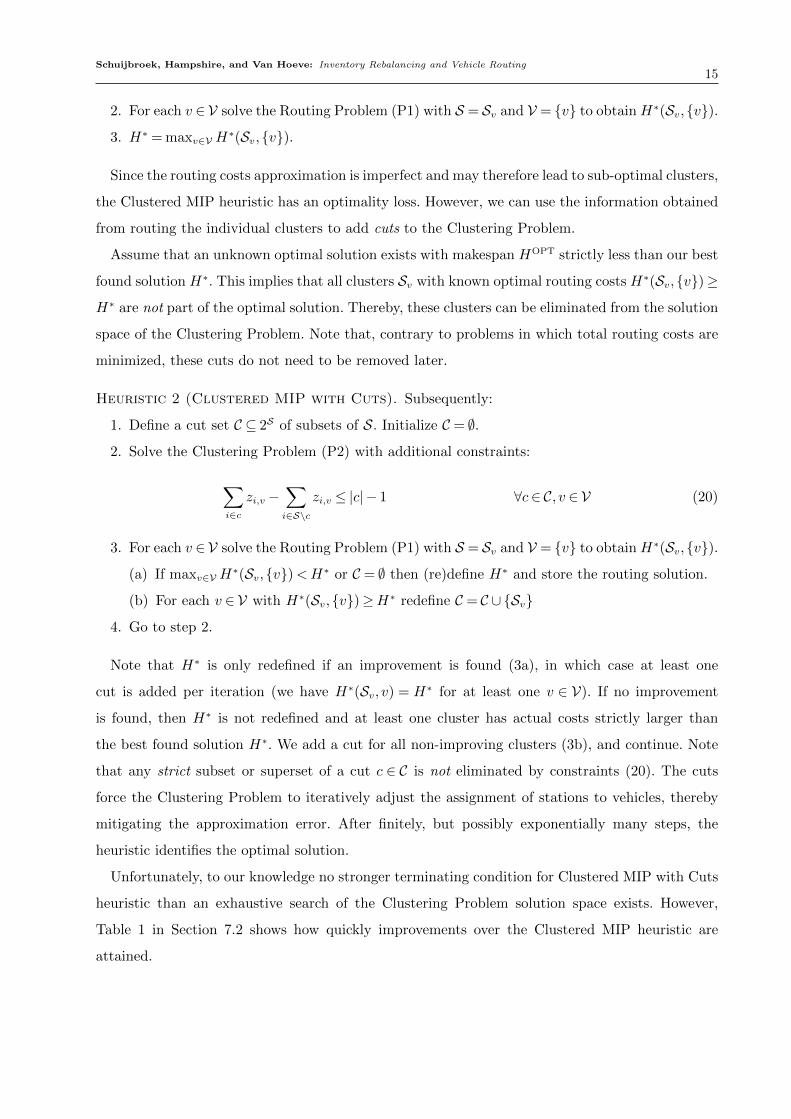
Heuristic 2 (Clustered MIP with Cuts). Subsequently:
1. Define a cut set C ⊆ 2S of subsets of S. Initialize C = ∅.2. Solve the Clustering Problem (P2) with additional constraints:
∑i∈c
zi,v −∑i∈S\c
zi,v ≤ |c| − 1 ∀c∈ C, v ∈ V (20)
3. For each v ∈ V solve the Routing Problem (P1) with S = Sv and V = {v} to obtain H∗(Sv,{v}).(a) If maxv∈VH
∗(Sv,{v})<H∗ or C = ∅ then (re)define H∗ and store the routing solution.
(b) For each v ∈ V with H∗(Sv,{v})≥H∗ redefine C = C ∪ {Sv}4. Go to step 2.
Note that H∗ is only redefined if an improvement is found (3a), in which case at least one
cut is added per iteration (we have H∗(Sv, v) = H∗ for at least one v ∈ V). If no improvement
is found, then H∗ is not redefined and at least one cluster has actual costs strictly larger than
the best found solution H∗. We add a cut for all non-improving clusters (3b), and continue. Note
that any strict subset or superset of a cut c ∈ C is not eliminated by constraints (20). The cuts
force the Clustering Problem to iteratively adjust the assignment of stations to vehicles, thereby
mitigating the approximation error. After finitely, but possibly exponentially many steps, the
heuristic identifies the optimal solution.
Unfortunately, to our knowledge no stronger terminating condition for Clustered MIP with Cuts
heuristic than an exhaustive search of the Clustering Problem solution space exists. However,
Table 1 in Section 7.2 shows how quickly improvements over the Clustered MIP heuristic are
attained.

Schuijbroek, Hampshire, and Van Hoeve: Inventory Rebalancing and Vehicle Routing16
6. Constraint Programming
In this section we present our Constraint Programming (CP) model for the Bike Sharing Rebalanc-
ing Problem. Constraint Programming is among the state of the art for solving complex routing
and scheduling problems, even though it applies a generic modeling and solving approach. In par-
ticular, CP has been applied before to constrained routing problems (Kilby and Shaw 2006). Most
industrial CP solvers combine constraint propagation with large neighborhood search for solving
routing problems (Shaw 1998).
In order to take advantage of the strengths of CP, it is common to represent routing problems as
scheduling problems, by representing the visit of a location as an activity. An activity is a high-level
CP modeling structure that implicitly defines integer variables for its start time, duration, and
end time, and a Boolean variable for its presence. Activities for which the presence is not fixed to
true are called optional activities. Traveling the distance between two locations is represented by
sequence-dependent setup times between the respective activities (for each pair of locations), i.e.,
if station j is visited directly after station i, we need to respect the distance di,j as ‘setup’ time.
In CP, activities impact resources which, in case of routing problems, correspond to the vehicles.
For example, for each vehicle, we must ensure that no two activities overlap.
We next specify the details of our CP model, following the AIMMS notation for activities and
resources (Roelofs and Bisschop 2012). In particular, each activity A induces the variables A.Start,
end time A.End, and presence A.Present, as explained above. For each station i ∈ S and vehicle
v ∈ V, we define optional activities Pickup[i,v] and Delivery[i,v] with duration 0. That is,
each station may be visited by any of the vehicles. Variables y+i,v and y−i,v represent the pickup,
respectively delivery, amount for vehicle v at station i, as in our models above. Our CP model then
becomes:
minimize max
{maxi∈Sv∈V
{Pickup[i,v].End} ,maxi∈Sv∈V
{Delivery[i,v].End}}
(P3)
s.t.
s0i +∑v∈V
y+i,v − y−i,v ≥ smin
i ∀i∈ S (21)
s0i +∑v∈V
y+i,v − y−i,v ≤ smax
i ∀i∈ S (22)∑v∈V
Pickup[i,v].Present+ Delivery[i,v].Present≤ 1 ∀i∈ S (23)
Pickup[i,v].Present= 1⇔ y−i,v ≥ 1 ∀i∈ S, v ∈ V (24)
Pickup[i,v].Present= 0⇔ y−i,v = 0 ∀i∈ S, v ∈ V (25)
Delivery[i,v].Present= 1⇔ y+i,v ≥ 1 ∀i∈ S, v ∈ V (26)

Schuijbroek, Hampshire, and Van Hoeve: Inventory Rebalancing and Vehicle Routing17
Delivery[i,v].Present= 0⇔ y+i,v = 0 ∀i∈ S, v ∈ V (27)
y−i,v, y+i,v ∈ {0, . . . ,Qv} ∀i∈ S, v ∈ V
with resources
Sequential resource VehicleTime[v](
Schedule domain: {0, ...,MaxTime}Activities: Pickup[i,v], Delivery[i,v]
Transition: di,j
)
Parallel resource VehicleInventory[v](
Activities: Pickup[i,v], Delivery[i,v]
Level range: {0, . . . ,Qv}Initial value: q0
v
Begin change: Delivery[i,v]: −y+i,v
End change: Pickup[i,v]: y−i,v
)
Parallel resource StationInventory[i](
Activities: Pickup[i,v], Delivery[i,v]
Level range: {0, . . . ,Ci}Initial value: s0
i
Begin change: Delivery[i,v]: y+i,v
End change: Pickup[i,v]: −y−i,v)
As before, constraints (21)-(22) impose the service level requirements from Lemma 2. Constraints
(23) are so-called alternative resource constraints, which limit the number of visits to one per sta-
tion. Adding these constraints can greatly improve the performance of the constraint propagation,
but the optimal solution may be eliminated. Note that it may not always be possible to impose
the alternative resource constraints, for example due to limited vehicle capacity. In such cases,
the model can trivially be extended to allow multiple visits by increasing the right-hand side. We
can index the activities and variables y−i,v, y+i,v correspondingly. However, our preliminary exper-
imentation showed strongly decreasing computational performance if we allowed multiple visits
per location. Therefore, we imposed the alternative resource constraints in our experiments. Con-
straints (24)-(27) link the vehicle presence constraints with performing a pickup or delivery. Note
that the if and only if constraints enhance propagation.

Schuijbroek, Hampshire, and Van Hoeve: Inventory Rebalancing and Vehicle Routing18
For each vehicle we introduce two types of resources. The first represent the no-overlap conditions
with respect to the vehicle time, using a Sequential resource named VehicleTime[v]. For each
such resource, we identify the discrete time horizon as its Schedule domain, while the keyword
Activities specifies which activities impact the resource. The arc-dependent transition times
model the travel distances via Transition.
The second resource associated with a vehicle is its inventory, modeled as a Parallel resource
named VehicleInventory[v]. In addition to specifying the set of activities in its scope, we define
its Level range to be {0, . . . ,Qv}, which is initialized at q0v. Furthermore, we specify for each
activity in its scope how it impacts the level. For Delivery[i,v], the level is changed at the start
of the activity, with amount −y+i,v. Likewise, for Pickup[i,v], the level is changed at the end of
the activity with amount y−i,v.
Lastly, for each station we define a Parallel resource representing the station inventory, named
StationInventory[i]. The range of this inventory is {0, . . . ,Ci} with initial value s0i . Level changes
for pickups and deliveries are exactly opposite to the vehicle inventory changes.
7. Computational Results
In this section we report on the performance of our routing costs approximation and heuristics.
Recall that we give a detailed overview of our data sources in Appendix B.
7.1. Approximation performance
In Section 5.2 we proved the monotonicity and upper bound MAXSPS(Sv) ≥ TSP∗0(Sv) of the
Maximum Spanning Star to motivate our intuition that MAXSPS(Sv) approximates H∗(Sv,{v})≥TSP∗0(Sv). Figure 4 visualizes this relationship with a scatterplot, in which the line H∗(Sv,{v}) =
MAXSPS(Sv) is shown for reference.
While we established that H∗(Sv,{v})≥TSP∗0(Sv), we note that the additional feasibility con-
straints on the vehicle route imposed in (P1) do not lead to routing costs higher than the MAXSPS
approximation for any instance. Rather, the Maximum Spanning Star consistently overestimates
the routing costs, which is reflected in the high correlation of 87.99%. A linear regression on
H∗(Sv,{v}) with an imposed zero intercept estimates a .4238 coefficient for MAXSPS(Sv) yielding
R2 = 94.28%. Nonetheless, a small approximation error is present. Next, we show how the improve-
ment scheme with elimination cuts overcomes this limitation of the Clustered MIP heuristic.
7.2. Heuristics performance
We report computational results comparing the exact MIP (P1), Clustered MIP (Heuristic 1),
Clustered MIP with Cuts (Heuristic 2), and CP (P3) approaches to the Bike Sharing Rebalancing

Schuijbroek, Hampshire, and Van Hoeve: Inventory Rebalancing and Vehicle Routing19
Figure 4 Computational results for the Maximum Spanning Star routing costs approximation.
●●
●
●
●
●
●●
●●
●●
● ●
●●
●
●●
●
● ●●●
●
●●●
●●
●
●
●
●
●
●●
●
●●
●
●
●●
●
●
●●
●
●
●
● ●●
●
●
●●
●●
●
●
●●
●
●
●● ●●
●●
●● ●
●
●
●
●●
●
●
●
●
●
●●
●
●
●●
●●●
●
●●
●
● ●
●
●
●●
●
●
●
●
●
●
●
●
●
●●
●
●
●
●
●
●●
●
●
●
●
●
●
●●
●
●
●●●●
●
●
● ●
●●
● ●
●●
●
●
●●
● ●●
●
●●
●
●
●
●●
●●
●
0
2500
5000
7500
0 2500 5000 7500 10000 12500 15000 17500 20000 22500 25000Approximation (m)
Rou
ting
cost
s (m
) Number of stations●
●
●
●
●
0
3
6
9
12
Note. Routing costs H∗(S,{v}) are plotted against the approximation MAXSPS(Sv) for all 82 two-vehicle instances
of Hubway (Boston, MA). Each data point corresponds to a cluster. The correlation equals 87.99%.
Problem. We consider multiple families of instances based on real trip and inventory data provided
by Hubway (Boston, MA) and Capital Bikeshare (Washington, DC).
All experiments were performed on an Intel Xeon X3323 @ 2.50GHz with 4GB of memory, using
AIMMS 3.13 FR1 modeling software with MIP solver GUROBI 5.0 (which outperformed CPLEX
12.4 on test instances) and CP solver IBM ILOG CP Optimizer 12.4.
Parameters. A family of instances is defined by a market (Hubway or Capital Bikeshare),
observation period (8–9AM or 4–5PM), service level (consistently 95%) and number of vehicles.
We observe that the morning and afternoon commute are the most challenging rebalancing prob-
lems. Furthermore, different service levels (90%, 99%) did not substantially impact our findings.
Subsequently, for each family we generate multiple instances by using different inventory snapshots
containing the starting inventory s0i for each station i ∈ S at the beginning of the observation
period.
We calculate Euclidian distances di,j = dj,i in meters based on the latitude and longitude of
stations. We assume qv = 0 to refrain from random data generation. For MIP we set |T |= |S \ S0|(this ensures feasibility for our instances) and for the Clustered MIP heuristics we set |T |= |Sv|+1
(this allows a revisit).
Hubway (Boston, MA). We restrict to |S|= 60 stations to obtain sufficient trip observations
to calibrate the service level requirements on 82 weekdays between November 1st 2011 and May
31st 2012. We use 41 inventory snapshots on weekdays between June 1st and July 29th 2012.
Hubway currently operates |V|= 3 vehicles with capacity Qv = 22 since opening an additional 40
stations in Summer 2012. However, during our observations Hubway only operated two vehicles.
We investigate both truck fleet sizes to reveal the possible implications for performance.

Schuijbroek, Hampshire, and Van Hoeve: Inventory Rebalancing and Vehicle Routing20
Table 1 Computational results for Hubway (Boston, MA).
MIP Clustered MIP Clustered MIP with Cuts CP
Family |V| LP bound Best found Time Solution Time Solution Iterations Time Solution Time
8–9AM 2 3228.18 4625 5220.51 4495 0.66 4229 82 60.05 4310 58.568–9AM 3 1660.29 3758 6139.66 3097 0.55 2669 57 60.09 2727 60.084–5PM 2 3347.55 4674 5787.08 4656 0.88 4429 76 60.03 4393 55.694–5PM 3 1674.90 3399 6558.48 3285 0.53 2699 51 60.14 2673 60.07
These results are averaged over the 41 instances of each instance family. The mean number of insufficient stations was equal to |S \ S0|= 10.The MIP solver was unable to find a solution of the full model for three instances. These are excluded from this summary and shown in Appendix C.
Figure 5 Computational results for Hubway (Boston, MA).
8−9AM 4−5PM
0%
25%
50%
75%
100%
125%
0%
25%
50%
75%
100%
125%
2 vehicles3 vehicles
Complexity
Sol
utio
n / M
IP b
est f
ound
Solution
Clustered MIP with Cuts
CP
MIP LP bound
Note. Instances are sorted with decreasing MIP LP bound to MIP best found solution ratio, to approximate com-
plexity. Here, the MIP best found solution is shown as 100%. If the LP bound equals the best found solution (100%),
then the solver was able to solve the exact MIP to optimality.
After extensive experiments we set the computational cut-offs (if unsolved): MIP after 7200
seconds; Clustered MIP after 20 seconds for both (P2) and (P1); Clustered MIP with Cuts after
60 seconds in total with 20 seconds for (P2) and (P1); CP after 60 seconds. For CP we set the
schedule domain with MaxTime= 50000, which proved necessary to quickly identify a feasible (but
low-quality) solution.
Table 1 summarizes our computational results for Hubway. We show the average solutions and
computation times per instance family for the exact MIP and our heuristics. For our improvement
scheme (Clustered MIP with Cuts), we show the number of iterations.
We observe that in 1 minute, our Clustered MIP with Cuts and CP heuristic outperform the best
found solution of the MIP after 2 hours with 5–10% on average for the two-vehicle families. For
the three-vehicle families, the improvement is 15–25%. Note that our Clustered MIP heuristic can,
on average, even generate better solutions than the MIP model within 1 second. This allows more

Schuijbroek, Hampshire, and Van Hoeve: Inventory Rebalancing and Vehicle Routing21
Table 2 Computational results for Capital (Washington, DC).
Clustered MIP Clustered MIP with Cuts CP
Family |V| |S \ S0| Solution Time Solution Iterations Time Solution Time
8–9AM 5 25 7573 32.61 6594 3 120.20 12123 120.394–5PM 5 11 2970 11.64 2548 13 120.18 2736 120.36
The |S \ S0| column shows the mean number of insufficient stations per instance family.
than 60 iterations of the Clustered MIP with Cuts heuristic in 1 minute, yielding an improvement
of approximately 10% over the Clustered MIP heuristic.
In Figure 5 we present a more detailed comparison of our dedicated Clustered MIP with Cuts
heuristic with the CP heuristic for the Hubway instance families. We show how they perform in
comparison to the best found MIP solution after two hours (depicted as 100%). We note that the
performance of the full MIP model decreases strongly for the three vehicle families, with our 1
minute heuristic solutions up to 75% better than the best found solutions after two hours.
CP performs very well for the Hubway instances. We believe that due to the low number of
insufficient stations, on average 10 out of 60, CP is able to quickly identify a feasible solution
which is subsequently improved. We observe that the Routing Problem (P1), when applied to the
individual clusters, becomes intractable when there are more than 15 stations in a cluster. For
instances on which CP outperformed the Clustered MIP heuristics, indeed one vehicle was assigned
more than 15 stations. In these situations, we suggest a hybrid cluster-first, CP-second approach
would leverage both strengths, because CP performed well on single-vehicle test instances.
Capital Bikeshare (Washington, DC). We restrict to |S|= 135 stations to obtain 130 trip
observations on weekdays between January 1st and June 30th 2012. We use 27 8AM and 25 4PM
inventory snapshots of weekdays obtained between December 17th 2012 and January 25th 2013.
Capital Bikeshare currently operates |V|= 5 vehicles with Qv = 25.
We increase the computational cut-offs of Clustered MIP with Cuts and CP to 120 seconds to
accommodate the increased complexity. For CP we increase MaxTime to 75000. Other cut-offs are
identical to those used for Hubway.
With 135 stations and 5 vehicles, the Capital Bikeshare instances were too complex to derive
feasible solutions or even useful LP bounds from the full MIP (P1) within a reasonable amount of
time. Therefore, we report only on the performance of our heuristics.
Table 2 summarizes our computational results for Capital. The 8–9AM instances are more com-
plex than the 4–5PM instances, with on average 25 insufficient stations per instance instead of
11 (see column |S \ S0|. The Clustered MIP with Cuts heuristic is 45% better than CP for the
8–9AM family of instances. This highlights exactly where we believe our cluster-first route-second

Schuijbroek, Hampshire, and Van Hoeve: Inventory Rebalancing and Vehicle Routing22
Figure 6 Computational results for Capital Bikeshare (Washington, DC).
8−9AM 4−5PM
0%
50%
100%
150%
200%
250%
300%
5 vehicles
Complexity
Sol
utio
n / C
lust
ered
MIP
sol
utio
n
Solution
Clustered MIP with Cuts
CP
Note. Instances are sorted with increasing CP solution to Clustered MIP solution ratio, to approximate complexity.
The Clustered MIP solution is shown as 100%.
heuristic excels. The polynomial-size Clustering Problem (P2) allows rapid decomposition of the
multi-vehicle problem into reasonably good single-vehicle clusters. Then, the Routing Problem
(P1) can be solved to optimality for individual clusters in under a second. The improvement cuts
mitigate both the approximation error and (possibly) sub-optimality incurred from cutting off the
Clustering Problem before the solver is finished.
In Figure 6 we present a comparison of the heuristics, with the Clustered MIP heuristic shown
as 100%. For some instances, even the simple Clustered MIP heuristic is up to 65% better than
CP. Figure 6 also shows clearly how adding cuts in the Clustered MIP with Cuts heuristic can
yield improvements of up to 40% over the simple Clustered MIP heuristic.
The results for Capital Bikeshare show that our dedicated Clustered MIP (with Cuts) heuristic
performs better than CP, especially for instances with a large vehicle fleet and a low number of
stations per vehicle. This implies the polynomial-size Clustering Problem can handle large sets
of insufficient stations, given that enough vehicles are available to divide the workload. When an
instance is more similar to a scheduling problem (i.e., a lower number of vehicles and longer routes,
like for some Hubway instances), the techniques embedded in CP show their strength.
8. Conclusions
This paper is the first to unify dual-bounded service level constraints, which add inventory flexi-
bility, and vehicle routing in bike sharing systems. We represent the inventory at each station as
a finite-buffer single-server queuing system and use closed-form analysis of the transient proba-
bilities to calculate service level requirements. We introduce the notion of self-sufficient stations,
which fulfill these requirements with their starting inventory. Hence, self-sufficient stations do not
necessarily need to be visited by a vehicle, but may act as source or sink nodes.

Schuijbroek, Hampshire, and Van Hoeve: Inventory Rebalancing and Vehicle Routing23
We present a mixed integer programming based Clustering Problem that decomposes the multi-
vehicle rebalancing problem into separate single-vehicle problems, while taking into account ser-
vice level feasibility constraints (a cluster-first route-second approach). We introduce a novel
polynomial-size Maximum Spanning Star routing costs approximation for the Clustering Prob-
lem to achieve high computational performance. We develop an improvement scheme based on
elimination cuts to mitigate the approximation error. Furthermore, we provide the first constraint
programming formulation of the bike sharing rebalancing problem.
Using empirical data from two bike sharing systems, we extensively test the Clustered MIP
heuristics against the classical full MIP model and the constraint programming approach. Our
Clustered MIP with Cuts heuristic outperforms the constraint programming formulation as the
number of vehicles (and correspondingly, the number of stations) grows. Constraint programming
performs well when the number of vehicles is low and the number of stations per vehicle is high.
Both the Clustered MIP and constraint programming approaches identify better solutions within
one or two minutes, than the often-used full MIP after two hours. We thus believe that our approach
is suitable for practical implementation in bike sharing systems.
The novel heuristics and our approximation may be applicable to other constrained routing
problems, specifically to (extended) One-Commodity Pickup-and-Delivery VRPs like the empty
freight container rebalancing problem, as well as to other sharing systems.
Appendix A: Net demand process
Figure 7 motivates why we adapt a process view to net demand for bikes, instead of observing total
net demand.
Appendix B: Data sources
In order to produce the examples and computational results, we processed two data sets
from Hubway (Boston, MA) and Capital Bikeshare (Washington, DC), which have identical
formatting. These data sets were made available through their websites thehubway.com and
capitalbikeshare.com. Each data set consists of three tables: Stations, Trips and Snapshots.
The Stations table contains the following fields for each station: id, name, lat, lng, installed,
locked and temporary. We use the id field to create the relationship with the Trips and Inventory
tables. We use the lat and lng fields to calculate the Euclidean distance matrix d in meters with
the spDists function of the sp package in R.
The Trips table contains the following fields for each trip: id, start date, end date,
start station, end station, bike name, bike and member type. We calculate the number of
pickups at a station during the observation period using start date and start station, and the
number of returns using end date and end station, to synchronize these events. As mentioned
Schuijbroek, Hampshire, and Van Hoeve: Inventory Rebalancing and Vehicle Routing24
Figure 7 Net demand during observation period 8–9AM for two popular stations of Hubway (Boston, MA).
South Station - 700 Atlantic Ave. TD Garden - Legends Way
Maximum
Minimum
Net demand
-20 0 20 40 -20 0 20 40Observation
Note. We show both the total net demand at the end of the observation period [0, T ] and the minimum and maximum
value of the net demand process. For the TD Garden station, we observe that the total net demand and the process
extremes are almost identical, in accordance with previous studies (Nair et al. 2013). However, for South Station, the
negative total net demand might suggest that we do not need bikes (i.e. positive net demand). Yet, the maximum
implies that at some moment during most observation periods, the net demand is positive, which requires a positive
starting inventory.
in Section 7.2, we select a subset of the stations for calculating the service level requirements, to
ensure that sufficient trip observations are available.
The Snapshots table contains the following fields for each station/date combination: id, bikes,
docks and date. We calculate capacity= bikes+ docks for each snapshot, since reparations or
extensions may lead to changes in the station capacity over time. We set Ci equal to the maximum
capacity of station i∈ S to prevent infeasibilities. We web scraped the Snapshots table for Capital
Bikeshare from http://capitalbikeshare.com/data/stations/bikeStations.xml.
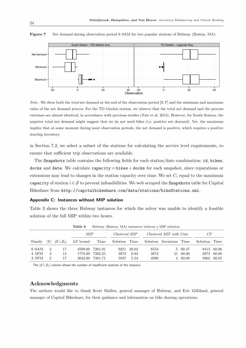
Appendix C: Instances without MIP solution
Table 3 shows the three Hubway instances for which the solver was unable to identify a feasible
solution of the full MIP within two hours.
Table 3 Hubway (Boston, MA) instances without a MIP solution.
MIP Clustered MIP Clustered MIP with Cuts CP
Family |V| |S \ S0| LP bound Time Solution Time Solution Iterations Time Solution Time
8–9AM 2 17 4599.00 7201.91 9251 20.62 8553 5 60.47 8413 60.064–5PM 3 14 1778.00 7202.25 3873 0.94 3873 41 60.00 3873 60.084–5PM 2 17 3632.00 7201.71 5937 5.54 4980 4 60.00 5862 60.05
The |S \ S0| column shows the number of insufficient stations of the instance.
Acknowledgments
The authors would like to thank Scott Mullen, general manager of Hubway, and Eric Gilliland, general
manager of Capital Bikeshare, for their guidance and information on bike sharing operations.

Schuijbroek, Hampshire, and Van Hoeve: Inventory Rebalancing and Vehicle Routing25
References
Akiyama, Jin, Midori Kobayashi, Gisaku Nakamura. 2004. Symmetric Hamilton cycle decompositions of the
complete graph. Journal of Combinatorial Designs 12(1) 39–45. doi:10.1002/jcd.10066.
Benchimol, Mike, Pascal Benchimol, Benoıt Chappert, Arnaud de la Taille, Fabien Laroche, Frederic Meunier,
Ludovic Robinet. 2011. Balancing the stations of a self service “bike hire” system. RAIRO - Operations
Research 45(1) 37–61. doi:10.1051/ro/2011102.
Borgnat, Pierre, Patrice Abry. 2009. Studying Lyon’s Velo’V: A Statistical Cyclic Model. European Confer-
ence on Complex Systems. 1–6.
Borgnat, Pierre, Patrice Abry, Patrick Flandrin, Celine Robardet, Jean-Baptiste Rouquier, Eric Fleury. 2011.
Shared Bicycles in a City: a Signal Processing and Data Analysis Perspective. Advances in Complex
Systems 14(03) 415–438. doi:10.1142/S0219525911002950.
Caggiani, Leonardo, Michele Ottomanelli. 2012. A Modular Soft Computing based Method for Vehicles
Repositioning in Bike-sharing Systems. Procedia - Social and Behavioral Sciences 54 675–684. doi:
10.1016/j.sbspro.2012.09.785.
Charikar, M., M. X. Goemans, H. Karloff. 2004. On the Integrality Ratio for Asymmetric TSP. 45th Annual
IEEE Symposium on Foundations of Computer Science. IEEE, 101–107. doi:10.1109/FOCS.2004.45.
Chemla, Daniel, Frederic Meunier, R. W. Calvo. 2012. Bike sharing system: solving the static rebalancing
problem. Working paper.
Contardo, Claudio, Catherine Morency, Louis-martin Rousseau. 2012. Balancing a Dynamic Public Bike-
Sharing System Balancing a Dynamic Public Bike-Sharing System. Technical report.
Dantzig, G., R. Fulkerson, S. Johnson. 1954. Solution of a Large-Scale Traveling-Salesman Problem. Oper-
ations Research 2(4) 393–410. doi:10.1287/opre.2.4.393.
Dell’Olio, Luigi, Angel Ibeas, Jose Luis Moura. 2011. Implementing bike-sharing systems. Proceedings of the
ICE - Municipal Engineer 164(2) 89–101. doi:10.1680/muen.2011.164.2.89.
DeMaio, Paul. 2009. Bike-sharing: History, Impacts, Models of Provision, and Future. Journal of Public
Transportation 12(4) 41–56.
Fisher, Marshall L., Ramchandran Jaikumar. 1981. A generalized assignment heuristic for vehicle routing.
Networks 11(2) 109–124. doi:10.1002/net.3230110205.
Fricker, Christine, Nicolas Gast. 2012. Incentives and regulations in bike-sharing systems with stations of
finite capacity. Submitted.
Fricker, Christine, Nicolas Gast, Hanene Mohamed. 2012. Mean field analysis for inhomogeneous bike sharing
systems. DMTCS Proceedings. 365–376.
Froehlich, Jon, Nuria Oliver. 2008. Measuring the pulse of the city through shared bicycle programs. Proceed-
ings of International Workshop on Urban, Community, and Social Applications of Networked Sensing
Systems. 16–20.

Schuijbroek, Hampshire, and Van Hoeve: Inventory Rebalancing and Vehicle Routing26
Gunasekaran, A., C. Patel, E. Tirtiroglu. 2001. Performance measures and metrics in a supply chain
environment. International Journal of Operations & Production Management 21(1/2) 71–87. doi:
10.1108/01443570110358468.
Hampshire, Robert C., Lavanya Marla. 2012. An Empirical Analysis of Bike Sharing Usage and Rebalancing:
Explaining Trip Generation and Attraction from Revealed Preference Data. Under review.
Held, Michael, Richard M. Karp. 1970. The Traveling-Salesman Problem and Minimum Spanning Trees.
Oper. Res. 18(6) 1138–1162. doi:10.1287/opre.18.6.1138.
Hernandez-Perez, Hipolito, Juan-Jose Salazar-Gonzalez. 2003. The One-Commodity Pickup-and-Delivery
Travelling Salesman Problem. Michael Junger, Gerhard Reinelt, Giovanni Rinaldi, eds., Combinatorial
Optimization – Eureka, You Shrink! , Lecture Notes in Computer Science, vol. 2570. Springer Berlin
Heidelberg, 89–104. doi:10.1007/3-540-36478-1\ 10.
Kaltenbrunner, Andreas, Rodrigo Meza, Jens Grivolla, Joan Codina, Rafael Banchs. 2010. Urban cycles
and mobility patterns: Exploring and predicting trends in a bicycle-based public transport system.
Pervasive and Mobile Computing 6(4) 455–466. doi:10.1016/j.pmcj.2010.07.002.
Kendall, David G. 1953. Stochastic Processes Occurring in the Theory of Queues and their Analysis by
the Method of the Imbedded Markov Chain. The Annals of Mathematical Statistics 24(3) 338–354.
doi:10.1214/aoms/1177728975.
Kilby, Philip, Paul Shaw. 2006. Vehicle Routing. Francesca Rossi, Peter Van Beek, Toby Walsh, eds.,
Handbook of Constraint Programming , chap. 23. Elsevier, 801–836.
Laporte, Gilbert. 1992. The traveling salesman problem: An overview of exact and approximate algorithms.
European Journal of Operational Research 59(2) 231–247. doi:10.1016/0377-2217(92)90138-Y.
Lathia, Neal, Saniul Ahmed, Licia Capra. 2012. Measuring the impact of opening the London shared bicycle
scheme to casual users. Transportation Res. C 22 88–102. doi:10.1016/j.trc.2011.12.004.
Leurent, Fabien. 2012. Modelling a vehicle-sharing station as a dual waiting system: stochastic framework
and stationary analysis. Under review.
Lin, J. H., T. C. Chou. 2012. A Geo-Aware and VRP-Based Public Bicycle Redistribution System. Inter-
national Journal of Vehicular Technology 2012 1–14. doi:10.1155/2012/963427.
Lin, Jenn-Rong, Ta-Hui Yang. 2011. Strategic design of public bicycle sharing systems with service level
constraints. Transportation Research Part E: Logistics and Transportation Review 47(2) 284–294.
doi:10.1016/j.tre.2010.09.004.
Martinez, Luis M., Luıs Caetano, Tomas Eiro, Francisco Cruz. 2012. An Optimisation Algorithm to Establish
the Location of Stations of a Mixed Fleet Biking System: An Application to the City of Lisbon. Procedia
- Social and Behavioral Sciences 54 513–524. doi:10.1016/j.sbspro.2012.09.769.
Meddin, Russell, Paul DeMaio. 2012. The Bike Sharing World Map. URL http://www.metrobike.net/.
Schuijbroek, Hampshire, and Van Hoeve: Inventory Rebalancing and Vehicle Routing27
Morse, Philip McCord. 1958. Queues, Inventories, And Maintenance: The Analysis Of Operational Systems
With Variable Demand And Supply . Dover ed. Wiley, New York.
Nair, Rahul, Elise Miller-Hooks. 2011. Fleet Management for Vehicle Sharing Operations. Transportation
Sci. 45(4) 524–540. doi:10.1287/trsc.1100.0347.
Nair, Rahul, Elise Miller-Hooks, Robert C. Hampshire, Ana Busic. 2013. Large-Scale Vehicle Sharing
Systems: Analysis of Velib’. International Journal of Sustainable Transportation 7(1) 85–106. doi:
10.1080/15568318.2012.660115.
Prem Kumar, V., Michel Bierlaire. 2012. Optimizing Locations for a Vehicle Sharing System. Swiss Transport
Research Conference. 1–30.
Raviv, Tal, Michal Tzur, Iris A. Forma. 2011a. Static Repositioning in a Bike-Sharing System: Models and
Solution Approaches. ODYSSEUS IV, Izmir .
Roelofs, Marcel, Johannes Bisschop. 2012. AIMMS 3.13 – The Language Reference. Paragon Decision
Technology.
Shaheen, Susan A., Stacey Guzman, Hua Zhang. 2010. Bikesharing in Europe, the Americas, and Asia: Past,
Present, and Future. Tech. rep., Institute of Transportation Studies (UCD), UC Davis, Davis.
Shaw, Paul. 1998. Using constraint programming and local search methods to solve vehicle routing problems.
M. Maher, J.-F. Puget, eds., Proceedings of the Fourth International Conference on Principles and
Practice of Constraint Programming . Springer-Verlag, 417–431.
Shu, Jia, Mabel Chou, Q Liu. 2010. Bicycle-sharing system: deployment, utilization and the value of re-
distribution. Technical report.
Vogel, Patrick, Torsten Greiser, Dirk C. Mattfeld. 2011. Understanding Bike-Sharing Systems using Data
Mining: Exploring Activity Patterns. Procedia - Social and Behavioral Sciences 20 514–523. doi:
10.1016/j.sbspro.2011.08.058.
Vogel, Patrick, Dirk C. Mattfeld. 2010. Modeling of repositioning activities in bike-sharing systems. World
Conference on Transport Research 1–13.
Waserhole, Ariel, Vincent Jost. 2012. Vehicle Sharing System Pricing Regulation: Transit Optimization of
Intractable Queuing Network. Working paper.
Wu, Bang Ye, Giuseppe Lancia, Vineet Bafna, Kun-Mao Chao, R. Ravi, Chuan Yi Tang. 1998. A polyno-
mial time approximation scheme for minimum routing cost spanning trees. Proceedings of the ninth
annual ACM-SIAM symposium on Discrete algorithms. Society for Industrial and Applied Mathemat-
ics, Philadelphia, PA, USA, 21–32.