Embed Size (px)
Citation preview
INVENTORY VALUATION DECISIONS
AND STRATEGY ANALYSIS
A Thesis Submitted to the Graduate Faculty
of the North Dakota State University
of Agriculture and Applied Science
By
Nicholas Ryan Osowski
In Partial Fulfillment of the Requirements for the Degree of
MASTER OF SCIENCE
Major Department: Agribusiness and Applied Economics
July 2004
Fargo, North Dakota
ii
Signature Page
iii
ABSTRACT
Osowski, Nicholas Ryan; M.S.; Department of Agribusiness and Applied Economics; College of Agriculture, Food Systems, and Natural Resources; North Dakota State University; July 2004. Inventory Valuation Decisions and Strategy Analysis. Major Professor: Dr. William W. Wilson.
In this study, a contingent claims model was developed to determine optimal
inventory storing strategy. The model chooses the optimal inventory strategy that
maximizes net present value (NPV) using the Black-Scholes option pricing model.
The contingent claims approach maps the demand for an item carried in inventory
onto an underlying state variable. In this case, price for wheat storage was mapped
onto the underlying commodity that is being milled.
The primary objective of this research is to develop a real options inventory
management tool to determine the optimal inventory level along with determining the
option value while addressing risk in an economically feasible way. A secondary
objective was to compare the contingent claims model results to the economic order
quantity (EOQ) model results.
Separate models were conducted for three different grain commodities with
high volatility. High-protein spring wheat, amber durum, and milling quality oats are
the three commodities used in this study, each of which have their own unique market
characteristics.
Results revealed that in the model most closely related to actual industry
characteristics, the contingent claims model resulted in greater inventories. However,
those results were highly sensitive to market price, volatility, flour price, salvage
value, and marginal increases in sales related to an increase in the underlying asset
price.
iv
ACKNOWLEDGMENTS
I would like to extend my appreciation to Dr. William W. Wilson for his
guidance and assistance. His teaching and advising have had a substantial impact on
my graduate education. Recognition is also given to my committee members, Dr.
William Nganje, Dr. Cheryl Wachenheim, and Dr. John Bitzan. Also, I would like to
thank Mr. Bruce Dahl for his patience, assistance, and daily discussions involving my
research.
A special thanks goes to my family and friends who have been very
supportive and helpful in my collegiate years. This goal was made easier by the
support of these important people, and I am grateful to them.
I want to thank my fellow students with whom I have had many experiences
and learned a great deal from at North Dakota State University and also the
University of Minnesota, Crookston. I have many good friendships that I will
remember forever.
Finally, without the support from both universities and agriculture
departments, I never would have made it this far. I am forever grateful. Thank you.
v
TABLE OF CONTENTS
ABSTRACT....................................................................................................................... iii
ACKNOWLEDGMENTS ................................................................................................. iv
LIST OF TABLES............................................................................................................. ix
LIST OF FIGURES ............................................................................................................ x
CHAPTER 1. STATEMENT OF PROBLEM................................................................... 1
Introduction......................................................................................................................1
Research Problem and Justification .................................................................................3
Problem Elements ............................................................................................................4
Objective ..........................................................................................................................5
Research Method .............................................................................................................6
Thesis Organization .........................................................................................................7 CHAPTER 2. REVIEW OF LITERATURE..................................................................... 8
Introduction......................................................................................................................8
Stockholding of Agricultural Commodities.....................................................................9
Convenience Yield.........................................................................................................15
Logistics Models of Storage ..........................................................................................19
Economic Order Quantity Model...................................................................................22
Relevant Costs of Inventory...........................................................................................24
Real Options...................................................................................................................26
Real Options and Uncertainty........................................................................................28
Contingent Claims .........................................................................................................29
Limits of Real Options...................................................................................................30
vi
Summary ........................................................................................................................31 CHAPTER 3. THEORETICAL MODEL........................................................................ 33
Introduction....................................................................................................................33
Logistical Models...........................................................................................................33
Total Relevant Costs ......................................................................................................42
Contingent Claims .........................................................................................................44
Real Options...................................................................................................................51
Contingent Claims and Inventory ..................................................................................52
Real Options and Inventories.........................................................................................55
Contingent Claims and Discrete Demand......................................................................58
Contingent Claims and Continuous Demand.................................................................60
Conceptual Relationship ................................................................................................64
Summary of Variables ...................................................................................................65
Summary ........................................................................................................................67 CHAPTER 4. EMPIRICAL MODEL.............................................................................. 69
Introduction....................................................................................................................69
Model Overview ............................................................................................................70
Mathematical Model Description ..................................................................................71
Case 1: Base Case .........................................................................................................74 Case 2: Salvage Value for Excess Inventories..............................................................77
Case 3: Salvage Value and Stock-Out Penalty .............................................................80
Number of Calls Calculations........................................................................................82
Detailed Description of Model.......................................................................................85
vii
Base Case Model Values ...............................................................................................89
Parameters and Assumptions .........................................................................................89
Milling Margins and Increases.......................................................................................89
Effect of Quality and Quantity Shortfalls on Inventory Value ......................................90
EOQ Model....................................................................................................................95
Data ................................................................................................................................96
Summary ......................................................................................................................966 CHAPTER 5. RESULTS AND SENSITIVITIES........................................................... 99
Introduction....................................................................................................................99
Base Case Model Definition and Results ......................................................................99
Wheat Base Case..........................................................................................................100
Durum Base Case.........................................................................................................104
Oats Base Case.............................................................................................................107
Base Case Comparison ................................................................................................109
Economic Order Quantity Model.................................................................................110
Sensitivities ..................................................................................................................113
Summary ......................................................................................................................126 CHAPTER 6. SUMMARY............................................................................................ 129
Review of Problem ......................................................................................................129
Review of Objectives...................................................................................................130
Review of Procedures ..................................................................................................131
Review of Results ........................................................................................................134
Implications of Results ................................................................................................139
viii
Limitations of Study ....................................................................................................142
Need for Further Research ...........................................................................................142
Summary ......................................................................................................................143 REFERENCES ............................................................................................................... 145
ix
LIST OF TABLES
Table Page
4.1 Contingent Claims Equation Variable Definitions ................................................74 4.2 Call Calculation Variables .....................................................................................83 4.3 Milling Model Variables........................................................................................89 4.4 Contingent Claims Variables Using Inverse SUR.................................................94 4.5 Economic Order Quantity Mill Variables..............................................................95 4.6 Data Sources ..........................................................................................................97 4.7 Case Variables and Distributions...........................................................................98 5.1 Base Case Wheat Model Results .........................................................................101 5.2 Base Case Durum Model Results ........................................................................105 5.3 Base Case Oat Model Results ..............................................................................107 5.4 Contingent Claims Results...................................................................................110 5.5 Wheat Model EOQ and Contingent Claims.........................................................111 5.6 Durum Model EOQ and Contingent Claims........................................................112 5.7 Oats Model EOQ and Contingent Claims............................................................113 5.8 Salvage Value Simulation....................................................................................122 6.1 Contingent Claims Results...................................................................................135 6.2 EOQ Results.........................................................................................................137
x
LIST OF FIGURES
Figure Page 2.1 Price of storage ......................................................................................................15 2.2 Price of storage with convenience yield ................................................................16 3.1 Inventory supply and usage over time ...................................................................36 3.2 Stock and option prices modeled in a two-step tree ..............................................50 3.3 Value-to-cost ratio .................................................................................................57 3.4 Payoffs with a positive salvage value and penalty for stock outs..........................63 4.1 Wheat payoff base case..........................................................................................76 4.2 Wheat payoff with salvage value ..........................................................................79 4.3 Wheat payoff with salvage value and shortage penalty.........................................81 4.4 Combined wheat payoffs of all cases.....................................................................82 4.5 Wheat supply and usage plotted against price .......................................................93 5.1 NPV and wheat stored as a percentage of milling capacity.................................103 5.2 Combined wheat payoffs all cases.......................................................................104 5.3 NPV and durum stored as a percentage of milling capacity................................106 5.4 NPV and oats stored as a percentage of milling capacity....................................108 5.5 The effect of increasing and decreasing current wheat prices on optimal
storage and NPV ..................................................................................................115 5.6 The effect of increasing and decreasing current durum prices on optimal
storage and NPV ..................................................................................................116 5.7 The effect of increasing and decreasing current oat prices on optimal storage
and NPV...............................................................................................................117 5.8 Effect of increasing and decreasing volatility on optimal storage.......................119 5.9 Effect of increasing and decreasing the salvage value on optimal storage..........120
xi
5.10 The effect of flour prices on optimal storage quantity.........................................123 5.11 The effect of marginal sales on optimal storage quantity ....................................125
1
CHAPTER 1 STATEMENT OF PROBLEM
Introduction
Inventory management is very important to agribusiness firms, with inventory
typically comprising between ten to forty-five percent of the total assets. Historically
inventory has been looked at as a major cost and source of uncertainty due to the
volatility within the commodity market and demand for the value-added product.
The economic order quantity model (EOQ) is one of the fundamental models
used in logistics management to determine the optimal order pattern. It seeks to
maximize expected profits based on a given distribution of the item under varying
types of demand. This conventional approach does not place any asset or option
value on inventory carried within the firm.
Standard tools used for strategic investments are limited and might not have
managers asking the right questions for investments to succeed and allow future
growth. A firm must have a strategic vision that is integrated into a framework of
market analysis so they know when their strategic value is increasing.
Also, uncertainty within the marketplace has forced many agribusinesses to
find other means of managing inventory. One of these tools is the contingent claims
approach using real options. A contingent claims approach investment decision is
one that depends on an uncertain outcome. Many managers of strategic investment
decisions think of uncertainty as costly, but using the real options approach, this
uncertainty creates opportunities for profit.
Agribusiness firms carrying inventory have options. They can either process
the inventory or sell the inventory at the market price; therefore, this option creates a
2
value of the inventory. Using the contingent claims approach, an option is the
opportunity to make a decision after the payoffs are known. The real options
approach uses financial market values in order to place an accurate value on the real
asset. There are three steps to designing and managing strategic investments using
real options. First, identify value options in a strategic investment. Second, redesign
the investment to better use options. Third, manage the investment proactively
through the options created (Amram and Kulatilaka, 1999).
According to Amram and Kulatilaka (1999), the real options approach creates
a valuable connection between project level analyses of strategic investments and the
corporate strategic vision. First, from the corporate level down to the project level,
the real options approach consistently asks the following questions: What value-
creating opportunities are unique to this firm? What amount and type of risk must be
borne to create this value? What risk can be cast aside? Second, from the project
level up, the real options approach creates a framework in which to aggregate project
value, risk, and the structure to manage a company’s net exposure to risk. This
bottom-up approach is where uncertainty plays a key role in creating a vision for
corporate managers.
This contingent claims approach maps the demand and payoffs from inventory
policy into the price of the underlying asset. It builds a portfolio of options that
replicate the payoffs and then derives the value of an inventory policy using option
pricing models in which the value of the policy is contingent on the financial
characteristics of the underlying asset.
3
The contingent claim analysis along with a prototypical agribusiness company
with a supply function that contains uncertainty will be simulated in this study. The
commodities researched in this study all have high uncertainty in price, quality, and
quantity in the marketplace to exploit the value of carrying an inventory.
Commodities will not have direct hedge alternatives but they could be cross-hedged.
14+ percent protein spring wheat, durum, and oats will be researched. These
commodities have variability in quantity and quality and thus are very problematic.
Research Problem and Justification
Historically the EOQ model has been very valuable to agribusinesses in
determining the minimum cost of inventory. The EOQ model uses economies of
scale to exploit fixed costs. This model seeks to minimize total cost subject to the
fixed costs within the supply chain, with the objective of the EOQ model being to
optimize lot sizing in order to reduce the cost of satisfying demand. There are many
trade offs between fixed costs that need to be looked at when implementing this
model.
Minimizing costs is very beneficial to agribusinesses in order to maximize
profits, but these businesses also have to realize the potential for profit from
uncertainty. This is where the contingent claim approach of managing inventory
using real options will have a strategic advantage over the EOQ model.
This contingent claims approach with options gives the agribusiness that is
holding a readily marketable commodity the option to process or sell the commodity
on the marketplace after the value is realized. This option creates a value to the
4
agribusiness in which they can maximize their profit with respect to the uncertainty in
the market and their demand.
Currently most agribusiness firms use the economic order quantity model to
determine the optimal level of inventories held by the firm under varying types of
demand uncertainty. Implementing a recent alternative model using the contingent
claims approach of real options is going to help solve the problem of placing an
option or strategic value on the inventory rather than treating inventories strictly as a
cost. Once the inventories have an option value, the optimal inventory size of a
prototypical agribusiness firm will be obtained using the real options model.
Contingent claims strategy is important for several reasons. Commodity
inventories have a value. They are valuable to an agribusiness whether they are
storing with intent to process or to sell on the open market. The strategic value of this
option will depend strongly on the uncertainty of the commodity market. This
uncertainty will create value in part because the agribusiness will see a greater
investment return. Real options provide the agribusinesses with a strategic
opportunity that can affect how inventory is managed.
Problem Elements
A potential problem element of the theory is that most of the agribusiness
firms potentially will not want to change their inventory management ways in part
because they cannot see the value of the contingent claims approach using real
options. Using real options requires managers to strategically think in a different way
than traditional theory. Real options are a way of thinking in that the commodity has
two or more options within the firm. These two options in this case could be to
5
process or sell the product. This decision depends on the strategic management of the
firm. The firms might be in a commodity market that has a low level of uncertainty.
Thus, implementing this model will have a smaller effect on the optimal inventory
level.
The higher uncertainty within the commodity market creates a higher value
using the real options.
Objective
The objective of this research is to determine the optimal level of inventory
held by a prototypical agribusiness firm under varying types of demand uncertainty
and procurement using the contingent claims approach. The contingent claims
approach uses the options on future sales. The objective would state the level of
inventory which is most valuable to the firm and place an option value on the
inventory. To accomplish this objective, the specific sub-objectives of this study are
as follows:
1. Determine the relationships between price and quality attributes of the
given commodities.
2. Using the information gathered, find the optimal level of inventory using
both contingent claims and the EOQ model.
3. Specifically consider which model is most effective in predicting the
profitability of inventory decisions, thus providing information for
which the inventory model should be used.
This study provides a mechanism for developing a better understanding of the
information requirements necessary for agribusinesses to evaluate inventory
6
management strategies. These information requirements form the basis for
implementing the contingent claims approach using real options into the
agribusinesses corporate management idea. This information would also help the
firm to make more precise decisions when working with commodities that have great
volatility in the marketplace.
Research Method
Several methods will be used to develop a better understanding of the
information requirements for a continent claims approach to inventory management.
These methods include a literature review, development of a theoretical model,
development of a spreadsheet model, and the sensitivity analysis of the model results
for selected scenarios.
The inventory management literature has evolved from several subject areas.
The purpose of the literature review is to provide an overview of stockholding
agricultural commodities, logistical models of storage, and real options. In addition,
insight into firm decision-making will be gained by a review of industrial literature.
These literatures, as well as those specifically related to inventory industries in the
commodity market, will be integrated into this study.
Based on the literature review, a theoretical model will be developed using
real options to find the optimal level of inventory within a firm. The model will
reflect logistical costs, procurement costs, and operations within the firm. Once the
theoretical model is developed, a spreadsheet-based empirical model will be
developed. The model will have areas of uncertainty that will be addressed using a
simulation program.
7
A prototypical agribusiness firm is going to be used in this study. The firm
will have an uncertain supply function with a normal distribution. A salvage value
will be given to any excess inventory the firm carries. A shortage cost will also be an
added cost if the firm does not carry enough products in inventory to meet demand.
The prototypical firm will have all the same logistical costs as the majority of
agribusiness firms.
Commodity price data will have to be gathered in order to address the
problems of volatility in the market. Market information gathered from the exchange
is then entered into the model to show how different commodities affect the
outcomes. A higher volatility in the marketplace should create a higher option value,
thus creating more opportunity for profit within the firm.
A journal article titled “A Contingent Claims Approach to the Inventory
Stocking Decisions” by John D. Stowe and Tie Su (1997) is going to be the base
article for this model. Research into optimizing this model given a prototypical firm
will be added into their current model.
Thesis Organization
The remainder of this study is divided into five parts. Chapter 2, titled
Review of Literature, examines the previous studies in stockholding agricultural
commodities, logistics models of storage, and real options. Chapter 3, titled
Theoretical Model, discusses how the model is set up and the reasons behind the
model. Chapter 4, titled Empirical Model, places the model into a prototypical
agribusiness firm. Chapter 5 explains the results of the empirical model. Finally,
Chapter 6 will sum up the study and offer a conclusion.
8
CHAPTER 2 REVIEW OF LITERATURE
Introduction
Decreased quality and quantity of specific commodities can have a large
impact on the overall cost of the grain inventories. An increased amount of research
has been conducted on how to properly hedge an inventory. Hedging inventories
using the futures markets plays a vital roll in the operating costs of agribusinesses.
The basic inventory decisions show how much inventory to purchase and or
carry when facing uncertain demand. Conventional inventory management
techniques suggest stocking an inventory level that maximizes expected profits. This
approach does not handle risk or the time value of money in a theoretically acceptable
manor.
An appropriate way to incorporate risk and the time value of money is the real
options approach. Real options are seen as a way to properly manage an inventory
that cannot be hedged directly. Real options place an option value on the inventory
instead of the traditional inventory management techniques which link inventory
directly to cost. The financial approach using real options relies on the relationships
between demand and the price of underlying marketable securities.
This chapter focuses on the problematic risks of hedging, inventory, and real
options. Hedging strategies are presented along with inventory strategies used to
discover the optimal inventory policy. Real options are then introduced with some
basic knowledge.
9
Stockholding of Agricultural Commodities
Theory of Price of Storage
Inter-temporal price relations are defined by Working as a relationship at a
given time between prices at different times (1949). An example is the relation at a
given time between a spot price and a forward price for the same commodity or the
relation between two forward prices. The relationship between the prices for
delivery at two different dates is commonly regarded as the cost of carrying the stocks
according to Working (1949).
The basic economic theory of commodity markets and price relationships are
explained in the law of one price (LOP). The law of one price states that there is only
one price for commodities, that being the cash price of the commodity (Blank et al.,
1991). All of the other prices are related to the cash price through storage,
transportation, and processing costs. This theory holds in domestic market analysis,
but it does have some flaws when trying to empirically support it in the international
markets (Blank et al., 1991).
Prices of commodities are also partially dependent on whether the commodity
is storable or non-storable. Blank (1985) classifies a commodity as being storable
when flexible production and a marketing alternative exist. The differences between
storable and non-storable commodities are very significant, and they should be
understood in order to fully comprehend the price relationships.
If a commodity is storable, there might be storage costs that have to be
implemented. If the storage cost is positive, the price when received would have to
be higher than the current price. Positive storage costs exist because of handling,
10
interest, and other expenses (Blank et al., 1991). This positive storage cost must be
paid to the producers that are willing to hold inventory from one time period to
another. Price changes in one period may not be directly reflected in another time
period.
The domestic grain market is a very good example of temporal prices within a
single production period (Blank et al., 1991). Domestic grain markets have a very
seasonal pattern. This seasonal pattern is called systematic fluctuation within the
marketing year (Blank et al., 1991). The quantity supplied is available in periods
after the grain harvest only through storage of the commodity. Commodities are
stored in inventories until the time in which they are used. Because of this, the lowest
price for the commodity appears during harvest. Usually increasing cash prices can
be observed until the next year’s crop is nearing harvest.
A positive carrying charge market can be seen when the futures contracts with
later maturity dates are steadily increasing. The price of storage is the difference
between the prices of alternative contracts indicating what the futures market is
willing to pay inventory holders for storing the commodity (Blank et al., 1991).
An inverted market can be seen when the price for contracts with the later
delivery dates have a lower price than the contracts that are expiring earlier (Blank et
al., 1991). This market is said to have a discount for storing commodities. If a
market experiences inverted prices, there is an economic incentive to deliver the
commodity immediately. “A normally inverted market arises when there is a
relatively low carryover of stocks (and a normal production year coming up) or,
11
alternatively, when there is a temporary storage of stocks in a position to be delivered
against a futures contract” (Blank et al., 1991, p70).
Normal backwardation occurs when the positive carrying charge is
insufficient to cover all the storage costs (Blank et al., 1991). The storage cost has to
be greater than the interest required to cover the cost of carrying the inventory, along
with insurance and warehousing costs (Blank et al., 1991). This is where arbitrage
opportunities exist for grain merchants if the carrying charge between futures
contracts exceeds the storage costs. Hence, storage costs represent the maximum
difference which will be observed in an efficient market. The Keynes’s theory that
hedgers must compensate speculators for assuming the price risk associated with
futures contracts can be one explanation for backwardation (Blank et al., 1991).
Holbrook Working gave an alternative explanation which was the concept of the
supply of storage (Blank et al., 1991).
Keynes’s Theory of Normal Backwardation
Keynes’s theory of backwardation emphasized the financial burden posed by
the necessity for carrying inventories and suggested that futures markets exist to
facilitate hedging (Blank et al., 1991). Working promoted the idea that the function
of futures markets was the provision of returns for storage services (Blank et al.,
1991).
The futures price was an unreliable estimate of the cash price at the expiration
date of the futures contract according to Keynes. Keynes believed the futures price to
be a downward biased of the upcoming cash price. “This theory argues that fact that
speculators sell insurance to hedgers and that the market is normally inefficient
12
because the futures price is a biased estimate of the subsequent cash price” (Blank et
al., 1991, p72).
“Three critical assumptions of the theory of normal backwardation are: that
speculators are net long, they are risk averse (i.e. they require positive profits) and
they are unable to forecast prices (i.e. all their profits can be viewed as a reward for
risk bearing). Given these assumptions, two major implications are associated with
the theory. The first is that over time speculators will earn profits by merely holding
long positions in futures markets. The second implication is that there is an upward
trend in futures prices, relative to spot prices, as the contract approached maturity”
(Blank et al., 1991, p72).
Hedgers generally sell to speculators, and then speculators will generally later
sell the contracts to offset their futures position. Futures contract prices must increase
in order for speculators to profit, and in order for speculators to achieve this
compensation constantly, there must be a risk premium. The risk premium results in
a reduction in price of what the speculators pay to purchase the futures from the
hedgers (Blank et al., 1991)
Several researchers have gathered empirical data to try and prove the theory of
backwardation but found little support for the theory. The empirical data which were
gathered from profit and loss data show that large commercial agriculture hedgers
earn substantial profits from futures trading.
Working’s Theory of the Price of Storage
Holbrook Working’s theoretical extension to backwardation has also proved
to be very important. “Workings theory was critical to the view that futures markets
13
existed solely for the purposes of transferring risk from the hedger to the speculator
and critical of the view that cash and futures markets are autonomous” (Blank et al.,
1991, p73). The price of storage developed by Working said that intertemporal price
relationships are determined by the net costs of carrying stocks.
Commodities are frequently demanded by consumers throughout the year
even though production is seasonal, so this product is placed in storage until
demanded. The term storage refers to the level of inventories; thus, the theory of
storage refers to the demand and supply of commodities as inventories (Blank et al.,
1991). The term does not relate to how much storage is available or the price charged
for the storage. As inventories increase, this lowers the price for storage, which
implies that the price of storage is a downward-sloping curve (Blank et al., 1991).
In Working’s (1949) paper “The Theory of Price of Storage,” inter-temporal
price relations are clearly defined. Working defines inter-temporal price relations as
“relations at a given time between prices applicable to different times, for example
the relation at a given time between a spot price and a forward price for the same
commodity or the relation between two forward prices” (Working, 1949, p1).
Inter-temporal prices examine the present compared to the future changes
between the present and the past or two time periods in the past that are classified as
price changes (Working, 1949). The relation between two future periods usually
remains a constant percentage. An example of this is that April futures are lower than
the May futures by a fairly constant percentage when comparing various years over
time (Working, 1949).
14
Using inter-temporal price relations, the difference between the December
futures and the May futures is commonly called the cost of carrying stocks (Working,
1949). If the supplies of stocks are fairly large, the return for carrying stocks may
exceed the cost of storage. With that theory in mind, when supplies of stocks are
smaller, the return for carrying stocks is usually higher than the cost of storage
(Working, 1949).
A competitive industry will determine the necessary return for storage using
the inter-temporal price relations in the futures market. The competitors competing
for the storage of the commodity have different costs, so they will hedge at different
levels, therefore exposing the necessary return for storage. Each competitor will have
different hedging strategies and will adjust the strategies if they do not like their
current strategy. For example, the returns for storage would equal the amount by
which the futures price exceeds the current price. The expected return for storage is
equal to the expected futures price in May minus the expected futures price in April,
for example (Working, 1949).
There are two limitations to Working’s (1949) theory of price of storage. The
first one is that a lot of the storage is supplied by people who do not hedge and who
decide to store or not regardless of the price of storage. The second is that people
who hedge earn returns which are not exactly equal to the market price of storage.
People are going to store regardless of the quoted price because they are expecting a
higher return.
15
Convenience Yield
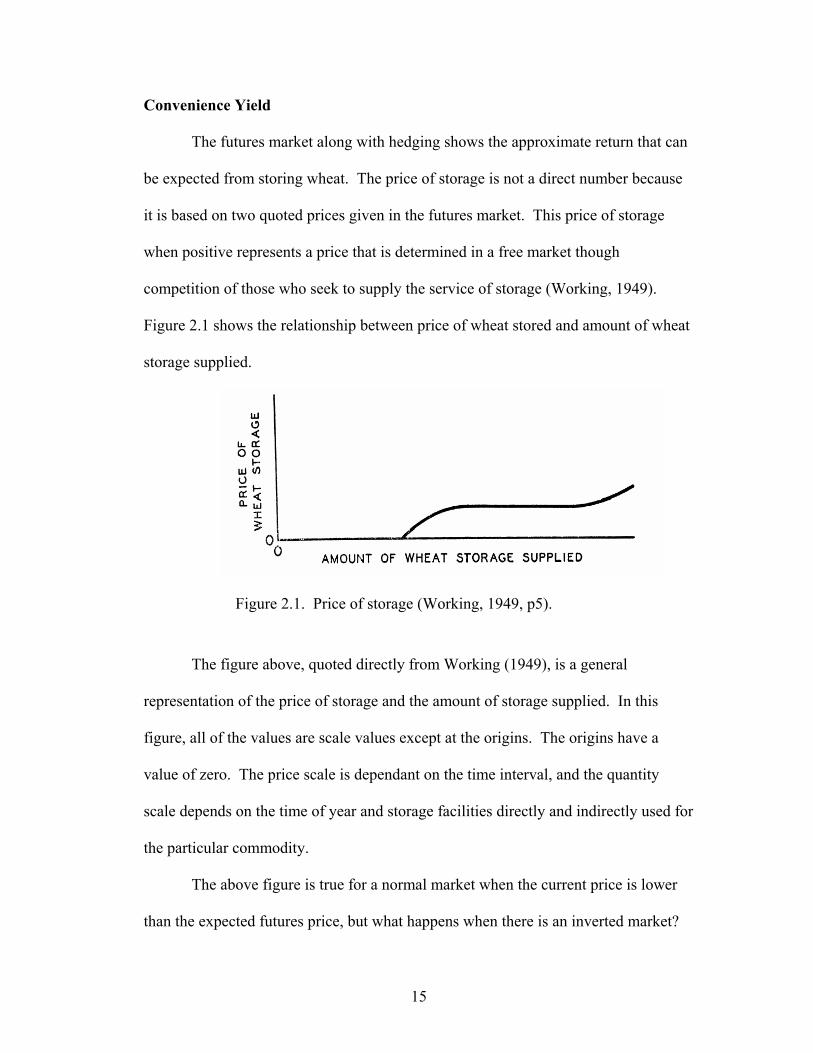
The futures market along with hedging shows the approximate return that can
be expected from storing wheat. The price of storage is not a direct number because
it is based on two quoted prices given in the futures market. This price of storage
when positive represents a price that is determined in a free market though
competition of those who seek to supply the service of storage (Working, 1949).
Figure 2.1 shows the relationship between price of wheat stored and amount of wheat
storage supplied.
Figure 2.1. Price of storage (Working, 1949, p5).
The figure above, quoted directly from Working (1949), is a general
representation of the price of storage and the amount of storage supplied. In this
figure, all of the values are scale values except at the origins. The origins have a
value of zero. The price scale is dependant on the time interval, and the quantity
scale depends on the time of year and storage facilities directly and indirectly used for
the particular commodity.
The above figure is true for a normal market when the current price is lower
than the expected futures price, but what happens when there is an inverted market?
16
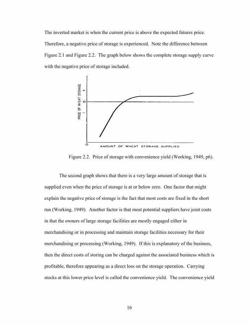
The inverted market is when the current price is above the expected futures price.
Therefore, a negative price of storage is experienced. Note the difference between
Figure 2.1 and Figure 2.2. The graph below shows the complete storage supply curve
with the negative price of storage included.
Figure 2.2. Price of storage with convenience yield (Working, 1949, p6).
The second graph shows that there is a very large amount of storage that is
supplied even when the price of storage is at or below zero. One factor that might
explain the negative price of storage is the fact that most costs are fixed in the short
run (Working, 1949). Another factor is that most potential suppliers have joint costs
in that the owners of large storage facilities are mostly engaged either in
merchandising or in processing and maintain storage facilities necessary for their
merchandising or processing (Working, 1949). If this is explanatory of the business,
then the direct costs of storing can be charged against the associated business which is
profitable, therefore appearing as a direct loss on the storage operation. Carrying
stocks at this lower price level is called the convenience yield. The convenience yield
17
may off set what appears to be a loss from the storage function itself (Working,
1949).
Storage is an adjunct business for most suppliers as they have production,
processing, and/or merchandising facilities. Thus, the suppliers of storage gain a
convenience yield from holding stocks because of the uncertainties in receiving raw
materials and uncertainties in consumer demand for products (Cordier et al., 1989,
p47). Loss to businesses can be substantial if fixed costs are high and the production
process gets interrupted from the lack of raw commodities. Holding inventories can
also give wholesalers a convenience, as it increases the chance for additional
business.
Expectations of the futures availability of a commodity is reflected in the
convenience yield. The greater the possibility that shortages will occur during the life
of the futures contract, the higher the convenience yield (Hull, 2000). Thus, once
again, Hull (2000) states the point that when inventories are high with little chance of
shortages, the convenience yield is low, but on the other hand, when inventories are
low and shortages exist, convenience yields tend to be high. A more substantial
convenience yield per unit can be seen when stocks are lower. Thus, Cordier et al.
(1989, p47) state that the total convenience yield of stocks increases with quantities
held until marginal convenience becomes zero at some large level of stocks. This
means there is a much higher convenience yield at lower stock levels that is
negatively sloped as it approaches zero at some large level of stocks.
Producers may be encouraged to hold inventories because of government
pricing and storage programs, causing current grain users to bid up cash prices above
18
the futures price; thus, an inverted market results. Quality and transportation also
have the same effects of government pricing and storage programs according to
Cordier et al. (1989).
Stulz (2003, p125) states that the convenience yield is the benefit one derives
from holding the commodity physically. The convenience yield reduces the forward
price relative to the spot price, but the storage costs increase the forward price relative
to the spot price. Stulz (2003) uses the example of having some gold which you
could melt down to create a gold chain to wear. If the cash buyer has no use for the
gold, they could lend it, and whoever borrows it would pay the convenience yield to
the lender.
Firms also hold inventories of commodities much the same way they hold
money, according to Williams (1986). The difficulty of moving inventory quickly to
where it is needed explains some of the reasoning behind why firms hold inventory
when cash price is above futures price.
The convenience yield may fluctuate over time in the agricultural futures
market. With fluctuating convenience yields, the positions nearby are subject to basis
risk, which is why investors will generally hedge the nearby positions using the
distant futures (Hong, 2001). With that in mind, the distant contract is less sensitive
to underlying shocks than nearby contracts, so the nearby contracts have higher
volatility. Markets with more volatile convenience yield shocks are more likely to
have a larger futures risk premium, and the futures risk premium increases with the
persistence of convenience yield shocks (Hong, 2001). Hong (2001) states that
because convenience yield fluctuations generate basis risk to trading futures,
19
investors continuously facing spot risk over time have to simultaneously trade futures
of different maturities to optimally hedge their spot positions.
Logistics Models of Storage
Appraisals of Inventory
Reasons for Inventory
Ballou (1999) states that there are two main reasons for carrying inventory,
and they are to improve customer service and reduce costs. Inventories provide a
level of product or service availability which, when located in proximity of the
customer, can meet a high customer service requirement.
There are five main reasons that inventories can reduce overall cost (Ballou,
1999). The first is economies of size in the production runs because carrying an
inventory will allow longer, larger, and more level production runs. Second, firms
may purchase in larger quantities seeing an economy in purchasing and
transportation. Third, firms may purchase greater quantities at the current price if the
product price is anticipated to rise. Fourth, inventories can be used to buffer the
variability and shocks in the marketplace. The fifth reason is that inventories can
help hold a buffer stock to help against natural disasters.
Ballou (1999) lists three reasons inventories draw skepticism. The first is that
inventories are considered wasteful because they absorb capital that might otherwise
be put towards a different use. The second is inventories can mask quality problems.
The last reason is that using inventories promotes insular attitudes about the
20
management of the logistics channel as a whole. This may encourage individual
firms in the supply chain to act inefficiently.
Types of Inventories
Ballou (1999, p. 311) lists inventories in five different forms. The first is
pipeline. These are inventories that are in transit between stocking or production
points because movement is not instantaneous. Speculation is the second type. These
are inventories purchased for price speculation. Regular or cyclical is the third type.
These are inventories necessary to meet the average demand during the time between
successive replenishments. Safety stock is the fourth type, and these inventories are
created as a hedge against variability in demand for the inventory. Obsolete, dead, or
shrinkage stock is the fifth type, and this inventory is out of date, stolen, or
deteriorated.
Push and Pull Approaches
There are two approaches in logistical strategies, labeled as the push and pull
approaches. The pull approach according to Ballou (1999) is a philosophy which
views each stocking point as independent of all others in the channel. Forecasting
demand and determining replenishment quantities are done on an individual level,
thus not taking into consideration the economies of the supply.
Ballou (1999) describes the push approach as an inventory management
strategy when decisions about each inventory are made independently. Inventory
levels are set collectively across the whole system. The push system works well
when there are purchasing or production economies that outweigh the benefits of
minimum collective inventory levels as achieved by the pull method. Using this
21
method, inventories can be managed centrally, taking full advantage of economies
that can be used to lower costs.
Materials Requirements Planning
Materials requirements planning (MRP) methods try to avoid as much as
possible carrying items in inventory through precise timing of material flows to meet
requirements (Ballou, 1999). MRP manages inventory in supply chains with the help
of time-phased inventory levels. It is a preferred method when demand is reasonably
known due to uncertainty of the forecasting component. If demand is forecasted to
change, MRP planning is able to adapt to this new level.
MRP is defined as a mechanical accounting method of supply scheduling
whereby the timing of purchases or of production output is synchronized to meet
period by period operations requirements by offsetting the request for supply from the
requirements by the length of the lead time (Ballou, 1999). The trade off in costs
associated with MRP concepts is between having the materials arrive before they are
needed, in which case they are subject to a holding charge, and the expected cost of
the materials arriving after they are needed so the materials are subject to a late
charge. The challenge of scheduling models (MRP) is to determine the optimal time
to request materials ahead of requirements (Ballou, 1999).
A major problem with the MRP modeling is that not all uncertainties are taken
into account. Ballou (1999) mentions that the challenge of MRP is to find the optimal
release time of materials to meet requirements. There is uncertainty associated with
that release time and the required time for the transportation of that product between
points in the supply chain.
22
Economic Order Quantity Model
The economic order quantity model (EOQ) was developed to find the optimal
order quantity. Alstrom (2001) found that 84 percent of the firms surveyed used the
EOQ model for inventory control. Annual holding cost will increase with an increase
in lot size, but in contrast, the annual order cost decreases with an increase in lot size.
Material cost is independent of lot size because it is assumed to have a fixed price.
The concept of the EOQ is that there is a trade off between the fixed order cost and
the holding cost.
The EOQ assumes the four following inputs: annual demand of the product,
fixed cost incurred per order, cost per unit, and holding cost per year as a fraction of
product cost. Using those inputs, there are three costs that must be considered when
deciding on lot size. The first is annual material cost which is annual cost of material
purchased. Annual order cost is the annual order cost for the lot ordered. The last is
the annual holding cost which is the annual cost of holding inventory.
Lot or batch size is the quantity that a stage of the supply chain either
produces or purchases at a given time. Ballou (1999) defines cycle inventory as the
average inventory that builds up in the supply chain because a stage of the supply
chain either produces or purchases in lots greater that those demanded by consumers.
The key to reducing cycle inventory according to Ballou (1999) is the reduction of lot
size. The key to reducing lot size without increasing costs is to reduce the fixed cost
associated with each lot as stated by Chopra and Meindl (2001). Aggregation across
multiple products, customers, or suppliers works best in trying to help reduce overall
fixed cost.
23
There are several problems associated with the EOQ model. Ballou (1999)
mentions that between the time that the replenishment order is placed at the reorder
point and when it arrives in stock, there is a risk that demand will exceed the
remaining amount of inventory. The probability of this occurring can be controlled
by raising or lowering the reorder point and by adjusting your optimal order quantity.
Ballou (1999) also states that it is not unusual for the reorder point quantity to exceed
the order quantity. This frequently happens when lead times are long and/or demand
rates are high.
Demand Uncertainty
Safety inventory is inventory carried for the purpose of satisfying demand that
exceeds the amount forecasted for a given period. Chopra and Meindl (2001) state
that the appropriate level of safety inventory is determined by two factors; these are
uncertainty of demand or supply and the desired level of product availability. As the
uncertainty of demand or supply increases, the level of safety inventory also
increases. If the desired level of product availability increases, the safety inventory
must also increase. Thus, these two factors must be understood and minimized to
lower the overall amount of safety inventory carried.
Minimizing the amount of safety inventory is a matter of minimizing the total
of two different costs, the first one being the cost of holding safety stocks, and the
second is the cost of being out of stock. The two costs have an inverse relationship:
as one decreases, it increases the other. The risk of being out of stock depends on the
chance of consumption in a delivery period being unusually large.
24
Maia and Qassim (1999) came to the conclusion that the optimal strategy for
safety inventories is to eliminate stock-outs or not to hold safety stocks at all. In this
article, opportunity costs are seen as stock-out costs. They stated that intermediate
inventory levels are uneconomical. Also noted is that the products that should be
stocked are those in which the opportunity costs are higher than inventory costs.
The firms’ operating risk associated with inventory policy can be decomposed
into two components according to Kim and Chung (1989). The first is pure output
market risk which is risk inherent in the demand uncertainty. The second is risk
resulting from the need to determine the order quantity before the actual demand is
revealed.
Kim and Chung (1989) concluded that the optimal inventory level of the risk-
adjusted value-maximizing firm is lower than that of the expected profit-maximizing
one, and the higher a firms output market uncertainty, the lower its optimal inventory
level, where output market uncertainty is defined as the relative volatility of the
demand for the firm’s output.
Relevant Costs of Inventory
Ballou (1999) suggests that there are three general classes of costs that are
important to determining inventory policy. They are procurement costs, carrying
costs, and stock-out costs. Procurement costs are those associated with the
acquisition of goods for the replenishment of inventories. Carrying costs result from
storing or holding goods for a period of time. Carrying costs may be space costs,
capital costs, inventory service costs, and/or inventory risk costs. Stock-out costs are
25
incurred when an order is placed but cannot be filled from the inventory to which the
order is normally assigned.
Heijden (2000) notes that customer service is usually included in conventional
inventory models by imposing a penalty cost on shortages when minimizing
inventories. This creates implementation problems in the application of the model
because you now have penalty costs that have been distorted and are difficult to
establish.
Unlike a fixed asset, stocks held for normal trading or manufacturing purposes
can usually be realized in a matter of months without appreciable loss so that only a
small premium over the marginal cost of borrowing would be required.
Reliability of Delivery
If a supplier is very unreliable, it will cause the purchaser to have higher costs,
whether incurred though stock-outs, buying emergency lots from competitors, or
expediting or carrying larger buffer stocks than would otherwise be necessary. Most
of the reasons for unreliability, such as inefficient dispatch arrangements, insufficient
buffer stocks of finished goods, and factories closing for holidays without warning
being given to customers, are within the control of the supplier.
According to McClelland (1960), it is less usual for the cost of a stock-out to
be estimated and used than for management to make a policy decision about the level
of protection they want. Different levels of protection may be specified according to
the type of commodity–high-profit goods, highly competitive goods, and goods with
no close substitute or whose absence will disrupt production.
26
Real Options
Introduction
Options are the right, not the obligation, to acquire an asset by paying a
certain amount of money on or before a certain time. Options are then opportunities
to take some action in the future, so in that fashion, a capital investment is now an
option. According to Dixit and Pindyck (1995), a company with an opportunity to
invest is holding something much like a financial call option. If the option is not
exercised, the lost value is the opportunity cost that must be included as part of the
cost of the investment. The opportunity is highly sensitive to uncertainty over the
future value of the project.
Real options or contingent claims occur when the underlying assets are real
assets. Real options are held by companies to manage their business and allow for
financial flexibility. Real options are not easy to deal with and often hard to identify.
Managers need to have knowledge about real options as they may sometimes be
tangled together.
Conventional net present value (NPV) is a tool that many mangers rely on but
might not always be the most accurate tool to use when dealing with uncertainty. An
example of this is that the NPV of an investment might be negative. Going ahead
with the investment may give rise to opportunities that will not otherwise occur, while
foregoing the investment means giving up on the option to grow the business. In
using NPV, a mistake has been made according to Turvey (2001) in that conventional
NPV fails to take into consideration the value of growth options, even if the growth
opportunities are uncertain. Real options are based on flexibility, irreversibility, and
27
uncertainty in investments. Irreversibility refers to the making of fixed investments
in capital in which some of the investment costs are sunk, flexibility refers to the right
that managers have to postpone making an irreversible decision until markets
improve, and uncertainty causes irreversibility which creates value using real options.
Types of Real Options
Real options create flexibility for managers in their ability to respond to
various investments and developments over time. Schwartz and Trigeorgis (2001)
classify real options into seven general categories which are option to defer, time to
build option (staged investment), option to alter operating scale, option to abandon,
option to switch, growth options, and multiple interacting options. The options for
reducing upside risk would be options to defer or expand, while options for reducing
downside risk would be options to abandon for salvage value or switch use.
There is a large number of other combinations of these real options that
managers can use in order to correctly asses opportunities. Many of the decisions
managers make take into consideration various types of real options. The option used
in this study is the option on future sales. This option on future sales is similar to a
timing option to expand capacity. The option to expand inventory by assuming sales
of inventory is related to the asset price of the inventory. The expansion option uses
surplus and shortage variables to determine the option value. The surplus variable
determines the value of the option through its net present value.
Asset in Place vs. Options
Assets in place are cash-producing assets that can be evaluated with
discounted cash flow methodologies, while growth options or opportunities to make
28
future investments require option-pricing methodologies. Growth options and a few
other decision opportunities are known as real options to distinguish them from
financial options such as exchange traded puts and calls. According to Luehrman
(1995), projects with high option content are likely to be misevaluated by discounted
cash flow techniques: either the options will be ignored or they will be poorly
approximated.
Real Options and Uncertainty
Real options exist because of uncertainty. Like financial options, if there is no
risk, there is no option value or need for options. The real option is a contingent
claim, which means that its values derived from positive value only. Dixit and
Pindyck (1995) state that the opportunity cost is highly sensitive to uncertainty over
the future value of that project; as a result, new economic conditions that may affect
the perceived riskiness of future cash flows can have a large impact on investment
spending, much larger than, say, a change in interest rates. Thus, viewing
investments as options puts greater emphasis on the role of risk and less emphasis on
interest rates and other financial variables.
The greater the uncertainty over the potential profitability of the investment,
the greater the value of the option and the greater the incentive to wait and keep the
opportunity alive rather than exercise it by investing at once.
Real Options Payoff
Real options have a nonlinear payoff structure. According to Turvey (2001),
the reason for the nonlinear payoff structure is that waiting will only have a value if
the expected value of waiting exceeds the expected value of not waiting. If this is
29
true, then postponing the investment means that the option to wait is being exercised.
If it is false, then postponing the investment is not expected to increase value; the
option to wait will be killed, and the project will be undertaken currently.
Contingent Claims
A contingent claim is an asset whose payoff depends upon the value of
another underlying asset, the value of which is exogenously determined. “A
valuation relationship is a formula relating the value of a contingent claim, or its
derivates, to the value of the underlying assets and other exogenous parameters”
(Brennan, 1979, p53).
Cox and Ross (1976) found that whenever a portfolio can be constructed
which includes the contingent claim and the underlying assets in such proportions that
the instantaneous return on the portfolio is non-stochastic, the resulting valuation
relationship is risk neutral.
Discrete Time Approach
Brennan (1979, p54) claims one of the major advantages of using a discrete
time approach to the pricing of contingent claims is that the restriction of investor
preferences eliminates the requirement of the continuous time approach that an
instantaneously riskless portfolio may be constructed which includes both the
contingent claim and the underling asset. To construct such a portfolio, several key
assumptions have to be made, the first one being that the underlying asset and
contingent claim are traded assets which can be purchased and sold continuously in
any proportions, and the second is restrictions on the stochastic process for the value
30
of the underlying asset (Brennan, 1979). The discrete time approach does not require
these restrictions, thus extending the scope of the option model.
The following are a few examples of contingent claims explained by Brennan
(1979). Different types of tax liability can be thought of as contingent claims in
which the value depends on the accounting income of the firm. In this example of a
contingent claim, neither the contingent claim nor the underlying asset can be traded.
Costs that are only paid in the event of a bankruptcy are also thought of as non-traded
contingent claims.
Limits of Real Options
There are several key limitations to real options as noted by Amram and
Kulatilaka (1999). Amram and Kulatilaka (1999) state the limits to the powerful tool
of real options to be model risk, imperfect proxies, lack of observable prices, lack of
liquidity, and private risk. These limitations are not surprising due to the fact that the
concept of real options is fairly new and the deriving of real options is not an exact
science, but these limits need to be considered when modeling real options.
Once the real option is identified, a valuation model must be created, but the
lack of information about the financial market may cause some bias in the models
mathematics. The model risk is defined by Amram and Kulatilaka (1999) as the
difference between the model answers and the theoretically correct answers. The
short-term models usually represent less model risk, but the risk increases with time
as there is more uncertainty in the future. Managers can counteract the model risk by
being aware of it and taking it into account when looking at the model outputs.
31
Imperfect proxies also limit the manageability of real options. An example of
an imperfect proxy is when a manager writes a contract based on the price of wheat in
Fargo in December, but the only wheat future currently traded is based on delivery in
Minneapolis. If wheat prices in December are different in Fargo than they are in
Minneapolis, you have an imperfect proxy. This risk can be tailored to the business,
thus lowering the risk of imperfect proxies.
A lack of observable prices is also a limit to real options. Price data may not
be available as fast as needed in order to make a decision, or the relevant securities
may not be traded frequently enough, so trades are delayed. If managers are forced to
guess, this will increase the possibility that the options’ full value will not be realized.
The fast access to information using electronics is helping to solve this problem, but it
is still worth noting.
Lack of liquidity can be seen in real assets and thinly traded stocks. They are
characterized by a low trade volume, and any sizable trade can move the market
price. Traders have developed various techniques to minimize the distortions caused
by the lack of liquidity, and some of them can be adopted by users of real options.
Private risk greatly affects the value of real options. Private risk is defined by
Amram and Kulatilaka (1999) as risk that is peculiar to one company. Business
managers are used to looking at private risk, so they tend to give it too much
emphasis when making strategic decisions.
Summary
Factors discussed in this chapter are important in the inventory analysis of
commodity marketing. Most relevant to this research is the defining of a convenience
32
yield. Suppliers of storage that also have adjoining businesses such as milling will
carry inventory even when the price of storage is negative for the simple reason of
convenience. Conventional inventory models are still used in many businesses today
and are still very important in the agribusiness sector, but there is becoming an
increasing awareness of the management tool called real options. The knowledge and
concept of real options expressed in this chapter are very important to understand as
the next chapter builds upon it.
Most of the conventional approaches to inventory in the past look at
minimizing cost with no economical way of looking into the effects of convenience
yields on the optimal inventory level. Past research in the business sector has shown
that there is an increasing awareness of the downfalls of conventional inventory
management tools. Real options are becoming a valuable tool as managers are
seeking out a way to properly account for the optimal profit-maximizing level of
inventory for their particular agribusiness.
The research reported in this thesis differs from past studies in several ways.
Many of the past contingent claims studies have not included real data from
agricultural commodities and have focused more on the theoretical and financial part.
The following chapter will develop a theoretical model in which the optimal
inventory level is defined.
33
CHAPTER 3 THEORETICAL MODEL
Introduction
Inventory strategies are increasing in importance in the commodity marketing
system, and managing inventory uncertainties is becoming a topic of increasing
significance. Two tools for inventory management are the EOQ and contingent
claims. Inventory decisions and techniques affect the logistical flow of commodities
and also the profit of agribusinesses. Inventory management tools are vital to the
marketing system. The increasing variability of quality and demand of agribusiness
adds to the problem of finding the optimal inventory level. Several studies have
shown the relationship between contingent claims and inventory management. This
variability has mangers looking for flexibility when managing inventories under
uncertainty.
This chapter develops the theoretical background on how to define an
inventory model that balances risk and profit. Logistical models are analyzed first.
Second, the effects of the increased volatility in the marketplace are presented. Next,
the contingent claims approach is discussed in the context of inventory decision.
Logistical Models
A variety of logistical techniques can be used to find inventory requirements.
The overall goals of logistics are to get the right product in the right place; at the right
time; and, in the process, at the lowest possible cost. The effect is to reduce cost and
capital and improve customer service.
Conventional approaches use the economic order quantity (EOQ) model. The
EOQ model minimizes the total annual costs for purchase order and holding costs.
34
The EOQ is used to find an optimal order quantity by evaluating the trade off
between order costs and holding costs. The optimal order quantity under the EOQ
model is represented by the following equation:
Q = (2DS/IC)1/2, 3.1 where Q = Optimal order quantity (or lot size), D = Annual demand for the item, S = Procurement cost or order cost, I = Carrying cost as a percentage of the items value, and C = Value of the item carried in inventory.
Results from EOQ models provide the order quantity that minimizes cost.
The equation is the first derivative for a specific cost function, which includes
procurement cost and inventory carrying costs. The optimal order quantity exists
when the summation of the two costs is minimized (Ballou, 1999). The number of
times per year a replenishment order is placed is represented by the term D/Q. The
average amount of inventory on hand is represented by the term Q/2.
The optimal order time between orders is therefore
T = Q/D, 3.2
and the number of times per year to place an order is
N = D/Q. 3.3
Costs and demand cannot always be known exactly; however, the economic
order quantity model is not very sensitive to over- or underestimating data. An
example of this from Ballou (1999) is if demand is in fact 10 percent higher than
anticipated, Q should only be increased by (1.10)1/2 = 4.88 percent. If the carrying
cost is 20 percent lower than assumed, Q should be increased by only (1/(1-0.20))1/2 =
35
11.8 percent. This percentage change is inserted into the EOQ formula without
changing the remaining cost and/or demand factors since they remain constant.
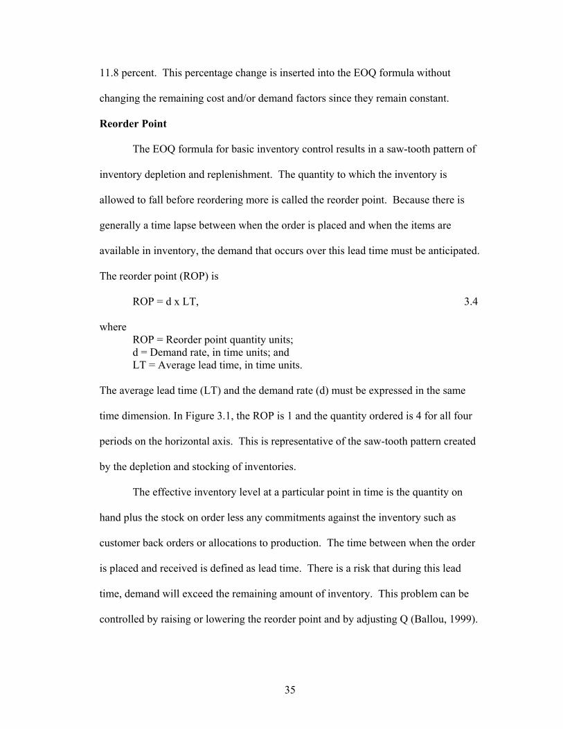
Reorder Point
The EOQ formula for basic inventory control results in a saw-tooth pattern of
inventory depletion and replenishment. The quantity to which the inventory is
allowed to fall before reordering more is called the reorder point. Because there is
generally a time lapse between when the order is placed and when the items are
available in inventory, the demand that occurs over this lead time must be anticipated.
The reorder point (ROP) is
ROP = d x LT, 3.4 where
ROP = Reorder point quantity units; d = Demand rate, in time units; and LT = Average lead time, in time units.
The average lead time (LT) and the demand rate (d) must be expressed in the same
time dimension. In Figure 3.1, the ROP is 1 and the quantity ordered is 4 for all four
periods on the horizontal axis. This is representative of the saw-tooth pattern created
by the depletion and stocking of inventories.
The effective inventory level at a particular point in time is the quantity on
hand plus the stock on order less any commitments against the inventory such as
customer back orders or allocations to production. The time between when the order
is placed and received is defined as lead time. There is a risk that during this lead
time, demand will exceed the remaining amount of inventory. This problem can be
controlled by raising or lowering the reorder point and by adjusting Q (Ballou, 1999).
36
0
1
2
3
4
5
6
0 1 2 3 4
Time
Qua
ntity
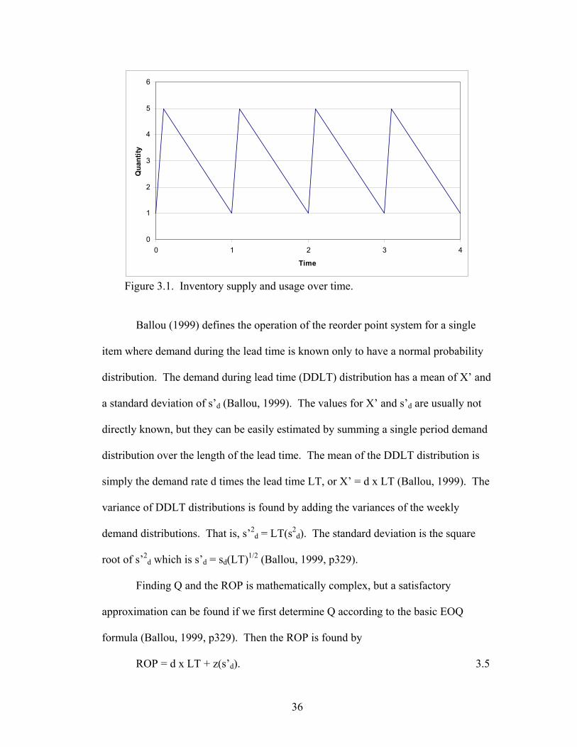
Figure 3.1. Inventory supply and usage over time.
Ballou (1999) defines the operation of the reorder point system for a single
item where demand during the lead time is known only to have a normal probability
distribution. The demand during lead time (DDLT) distribution has a mean of X’ and
a standard deviation of s’d (Ballou, 1999). The values for X’ and s’d are usually not
directly known, but they can be easily estimated by summing a single period demand
distribution over the length of the lead time. The mean of the DDLT distribution is
simply the demand rate d times the lead time LT, or X’ = d x LT (Ballou, 1999). The
variance of DDLT distributions is found by adding the variances of the weekly
demand distributions. That is, s’2d = LT(s2
d). The standard deviation is the square
root of s’2d which is s’d = sd(LT)1/2 (Ballou, 1999, p329).
Finding Q and the ROP is mathematically complex, but a satisfactory
approximation can be found if we first determine Q according to the basic EOQ
formula (Ballou, 1999, p329). Then the ROP is found by
ROP = d x LT + z(s’d). 3.5
37
The number of standard deviations from the mean of DDLT distribution is defined as
the variable z to give us the desired probability of being in stock during the lead time
period (P). The value of z is found in a normal distribution table for the fraction of
the area P under the DDLT distribution.
Extending the ROP model to account for lead time uncertainties adds to the
realism of the model. To do this, the standard deviation (s’d) of the DDLT
distribution based on uncertainty in both demand and lead time has to be found
(Ballou, 1998). This can be found by adding the variance of demand to the variance
of lead time, giving us a the following revised formula for s’d of
s’d = (LT s2d + d2sLT
2)1/2, 3.6
where sLT is the standard deviation of the lead time.
Combining demand and lead time variability in this way can greatly increase
s’d and the resulting safety stock. In that manner, the equation may lead to an
overstatement of s’d and the resulting amount of safety stock. Ballou (1999) suggests
the following precise procedure for determining the standard deviation of demand
during lead time: a lead time starts when the replenishment order is triggered. The
end of lead time by definition is when the order is received. The year-to-date demand
is then examined. The difference between the current demand year-to-date and the
value when the order was released is precisely, by definition, the demand during the
lead time (Ballou, 1999). The values of this variable can be forecast (usually with
very simple forecast models), and the mean square error is the variance of demand
during lead time, precisely the value being sought. Alternately and less precisely, the
38
longest lead time may be used as the average lead time with SLT set at zero (0). The
standard deviations are then computed as s’d = sd(LT)1/2.
The following is an example of the EOQ and ROP out of Ballou (1999).
Buyers Products Company distributes an item known as Tie Bar, which is a U-bolt
used on truck equipment. The following data have been collected for this item.
Monthly demand forecast, d 11,107 units Std. error of forecast, sd 3,099 units Replenishment lead time, LT 1.5 months Item value, C $0.11/unit Cost for processing vendor order, S $10/order Carrying cost, I 20%/year In-stock probability during lead time, P 75% The reorder quantity is
Q = (2DS/IC)1/2 = [(2x11,107x10)/(0.20/12x0.11)]1/2 = 11,008 units. 3.7
The reorder point is
ROP = d x LT + z(s’d), 3.8
where s’d = sd(LT)1/2 = 3,099(1.5)1.2 = 3795 units. The area of the normal distribution
being examined is 0.75; thus, using s statistical z table, the z value is equal to 0.67.
Thus,
ROP = 11,107 x 1.5 + 0.67 x 3795 = 19,203 units, 3.9
so when the effective inventory level drops to 19,203 units, place a reorder for 11,008
units.
Ernest and Pyke (1992) develop a component part stocking model that
minimizes the total inventory holding and ordering costs for all parts, subject to a fill
rate constraint. They introduce (Zi) a random variable representing the undershoot of
the reorder point for part i. This is the amount below the reorder point when an order
39
is placed. The distribution of Z is based on the excess random variable of a renewal
process, and its expected value E(Z) is approximately ((σ2 + µ2)/µ – 1)/2, where σ is
the standard deviation of demand for the product per period and µ is the mean
demand for the product period.
Supply Uncertainty
Most of the traditional economic order quantity research focuses on demand
variability. In contrast, the problem in this thesis is one of supply uncertainty. The
variability’s of uncertainty in supply = f(quality, quantity, and price). Inventories are
often used to protect the supply chain from the uncertainty, but these inventories at
various points have different levels of responsiveness. Despite the sparse research on
supply uncertainty, there are several useful articles that focus on the issue.
One of the most well-known simulation studies is that of Whybark and
Williams (1976). They identify four types of uncertainty in a production system: in
supply timing, in demand timing, in supply quantity, and in demand quantity. Supply
timing is the uncertainty that can arise from variations in vendor lead times or flow
rates. Supply quantity uncertainty arises when there are shortages. A shortage is
when supplies are not able to meet demand. To simulate supply quantity uncertainty,
Whybark and Williams (1976) assumed the actual quantity received was uniformly
distributed around the quantity scheduled to be received for each order. “Lumpiness”
is defined by Whybark and Williams (1976) as the change from period to period of
the gross requirements. It is an important factor in material requirements planning
(MRP) research and can be measured by the coefficient of variation (Cv). As the
requirements become “lumpy,” the coefficient of variation increases. They then
40
show, using a simulation study of a single-item, single-stage system, that safety
stocks are the best mechanism for protecting against uncertainty in the supply or
demand quantity, while safety times are preferred for timing uncertainties in either
the supply or demand process.
Lee and Billington (1993) use a stock keeping units (SKU) model to support
the systems necessary to anticipate variability and optimize it. At a downstream site,
the demand for SKU i generates demand for input parts that are needed to
manufacture the SKU. This, in turn, becomes the demand for parts at upstream sites
that supply the current site. The demand transition process develops the first two
moments of the demand on the SKUs at an upstream sight. Lee and Billington (1997)
consider an upstream sight g and multiple downstream sites that receive the part j
from this upstream site. Then,
),()()(),(
kgpbkuvgu jijii
ijjgKk
j ∑∑∈
= and 3.10
),()()( 222
),(
2 kgpbksvgs jijii
ijjgKk
j ∑∑∈
= , 3.11
where k = the index of downstream sites; K(g, j) = the set of downstream sites that are supplied by this upstream site for part j; ui(k) = the mean demand per week for SKU I at downstream site k; si(k) = the standard deviation of demand per week for SKU i at site k; pj(g, k) = the proportion of the requirement of part j at downstream site k that is to be sourced from the current upstream site g; uj(g) = the mean demand per week for part j at the upstream site g (known as SKU there); sj(g) = the standard deviation of demand per week for part j at upstream site g (known as SKU there); vij = the indicator variable: equals 1 if part j is needed for SKU i, 0 otherwise; and bij = the number of units of part j needed in one unit of SKU i.
41
Using the model, suppose that input material at a site k is sourced from
upstream site g. Then, the immediate availability level of the material at site k is the
fill rate of the material at site g, where the material is known as an SKU. Delays due
to material shortage at site g are the response time of the materials at site g given that
the SKU is out of stock there.
Anupindi and Akella (1993) assume that demand is stochastic and
continuously distributed with a known distribution, but they have uncertainties in
supply that arise from delivery contracts, suppliers, quantity, higher priced suppliers,
etc. They state the optimal policy with the following structure: there exist two order
points, ūn and ōn, and the on-hand inventory is denoted with x, such that when on-
hand inventory x< ōn, then both suppliers may be used; when ōn≤x< ūn, only the
cheaper supplier will be used. Finally, no order will be placed when x≥ ūn. They
assume in the model that the supply process is such that from facility i with
probability βi, all of the order quantity is supplied, and with probability 1- βi, nothing
is supplied. The expected cost of ordering from two facilities can be written as
follows:
,)()(
)()()()(
)()()()(
)()()()(
)()(),,(12.3
12
212121
2121012
0 2120 121
20 12122211121
21
21
21
21
ix
xwxw
xww
x
xwxw
xww
dfx
dfxwdfxw
dfxwwdfxh
dfxwhdfxwh
dfxwwhwcwcxwwM
βξξξββπ
ξξξβπβξξξβπβ
ξξξβπβξξξββ
ξξξββξξξββ
ξξξββββ
∫
∫∫
∫∫∫∫
∫
∞
∞
+
∞
+
∞
++
++
++
−+
−−+−−+
−−−•+−+
−++−++
−++•++=
where
wi = order quantity from facility i,
42
x = inventory on hand, ci = per unit ordering cost from facility i, h = holding cost per unit per period, π = penalty cost per unit per period, βi = probability that all of the orders from facility i will be delivered,
iβ = 1 - βi,
ξ = total requirement (random variable), f(•) = density of total requirement, F(•) = distribution of total requirement, F (•) = complementary distribution function, M(x,w1,w2) = single-period cost function, J1(x) = optimal cost function, and E(•) = the expectation operator.
The first two terms represent the expected ordering cost on the amount
delivered, the next three terms represent the expected holding costs, and finally, we
have the expected penalty costs. Thus, the problem can be formulated as
),,(min)( 210,121
xwwMxJww ≥
= . 3.13
This is the single-period cost function for the inventory policy. It is evident from the
nature of the optimal policy that the ordering depends upon the on-hand inventory.
There could be a modification to the model which assumes a fixed minimum order
quantity that is always ordered from both suppliers. The suppliers in return promise
delivery of the fixed quantity every period; the uncertainty in the supply process does
not affect the delivery of the fixed quantity.
Total Relevant Costs
The total relevant cost is useful for comparing alternative inventory policies or
determining the impact of deviations from optimal policies. The total relevant cost
function can be expressed as Total cost = order cost + carrying cost (regular cost) +
carrying cost (safety stock) + stock-out cost:
TC = D/Q x S + IC x Q/2 + ICzs’d + D/Qks’d E(z), 3.14
43
where k is the out-of-stock cost per unit. Stock-out costs consist of two elements.
First, the combined term of s’d E(z) represents the expected number of units out of
stock during an order cycle. E(z) is called the unit normal loss integral whose values
are tabled as a function of the normal deviate z. Second, the term D/Q is the number
of order cycles per period of time, usually a year. Hence, the number of order cycles
times the expected number of units out of stock during each order cycle gives the
total expected number of units of stock for the entire period. Multiplying the total
expected number of units of stock by the out-of-stock costs yields the total period
cost.
McClelland (1960) also notes that it is helpful to divide up stockholding costs
into two separate components. McClelland (1960) divides up the stockholding costs
into value of the stockholding and physical storage cost. Value stockholding costs
include costs such as interest, insurance, and risk; the total cost of each varies with
the purchase price of the goods. Guerrero et al. (1986) note that inventory cost can be
lowered by shifting safety stock to lower (less costly) levels of the product structure.
Risk Assessment
Most of the classical EOQ inventory models do not account for economic and
financial risks associated with carrying inventory. Inflation and time value are
modeled into the EOQ by Ray and Chaubhuri (1997). In their model, they use an
item having an inventory-level-dependent demand rate at any instant. Shortages are
allowed, and deterioration of the inventory over time is not taken into account, nor is
the time value of money and different inflation rates for various costs associated with
the inventory system.
44
Two distinctly different price discovery mechanisms are used in the
agribusiness market. The first is spot price, and the second is forward prices;
differences in these two pricing mechanisms must be understood as pricing with
forward prices will have varying degrees of uncertainty depending on the basis,
liquidity, and other arbitrage opportunities. Spot prices are prices set for immediate
delivery that day, whereas forward prices are contracts to buy or sell an asset at a
certain time in the future for a certain price (Hull, 2000). Most of the forward
contracts are done over the counter, whereas futures contracts are traded on
exchanges.
In years of shortages in supply and lack of quality, prices may be relatively
high and heterogeneous, whereas years with a surplus in supply and good quality, the
price may be relatively low and homogenous. Forward prices can provide a way to
help eliminate the risk because of uncertain forward prices of commodities. Once a
forward contract is agreed upon, it has to be stored from the time it was harvested
until the contract delivery date. This is a role of either the supplier or the buyer. The
risks associated with the future commodity prices are a clear role of the forward
contracts.
Contingent Claims
Introduction
The EOQ model and capital asset pricing (CAPM) models have been used in
the past, but there currently is a much more sophisticated way to model inventory
payoffs using contingent claims and real options.
45
Contingent claims analysis is well suited to evaluate inventory decisions under
uncertainty because the payoff from the firm’s inventory decisions is contingent with
its value dependent upon uncertain supply or demand in the future. Payoffs can then
be replicated to build a portfolio of options deriving the value of an inventory policy.
Cox et al. (1979) showed that the value of a financial call option can be
computed by the construction of a portfolio that replicates the return of the option
under any state of nature. An option on a stock can be replicated by borrowing funds
and buying some of the stock (for a call option) or by lending funds and selling some
of the stock (for a put options). Using arbitrage, risk-neutral probabilities can be
derived. This approach is called contingent claims because the valuation of the
option is contingent upon the value of the underlying asset.
To apply contingent claims evaluation to real investment analysis, it is
necessary to find an asset or groups of assets that are correlated with the net return of
the investment to be analyzed. This correlated asset is called a “twin asset” by Tauer
(2000). Tauer (2000) states that the value of the twin asset is known at the beginning
of the investment period, but the value of the investment is not known at the
beginning since that is the value being estimated. Information about changes in the
value of the twin asset is used to determine the value of the investment. This process
of determining the value of the investment is much easier when the financial options
are used as derivatives of an underlying asset, but it is much harder to find a “twin
asset” to model the net returns of an investment. In the case of agriculture, however,
there are strong correlations between the price of an underlying commodity and the
net returns.
46
A major advantage of the discrete time option pricing model is the absence of
the assumption of the ability to form a riskless portfolio with both the contingent
claim and the underlying asset (Chung, 1990). Such a portfolio can only be formed
under strong assumptions that the underlying assets and the contingent claim be not
only traded as assets but may also be purchased and sold continuously in any
proportions. The discrete time model does not impose such requirements and thus
extends the applicability of the option pricing model.
Financial Options
There are two basic types of financial options. A call option is defined by
Hull (2002) as an option to buy an asset at a certain price by a certain date. A put
option is defined by Hull (2002) as an option to sell an asset for a certain price by a
certain date. In the case of this study, the call option will be used as the agribusiness
is demanding commodities to be supplied.
There is one major difference between financial traded assets and real assets,
and that is that in financial traded assets, the settlement is always in cash rather than
delivering the portfolio underlying the index, but in the case of real options, the
underlying assets are real assets in that they have an underlying value.
The Black-Scholes model for valuing stock options has one major underlying
assumption, and that is that stock prices are normally distributed in the short period.
They have a normally distributed mean and standard deviation. Several other
assumptions of the Black-Scholes model as noted by Hull (2002) are that there are not
transactions costs or taxes; there are not dividends on the stock during the life of the
option; there are no riskless arbitrage opportunities; security trading is continuous;

47
investors can borrow or lend at the same risk-free rate of interest; and the short-term,
risk-free rate of interest is constant. Some of the assumptions have been relaxed by
other researchers, but these were the initial assumptions when the model was
developed.
Forward contract prices can be derived using the Black-Scholes model. From
Hull (2002), the long forward contract that matures at time T with delivery price K
has a value at maturity equal to
ST - K 3.15
because it enables an asset worth ST to be purchased for K. In a risk-neutral world,
the expected value of ST = S0euT. In the variable S0euT, S0 is the price of the asset
underlying the forward or futures contract (in years), u is the storage costs per annum
as a proportion of the spot price, and T is time until delivery date in a forward or
futures contract (in years). The expected payoff from the contract at maturity in a
risk-neutral world is therefore
S0euT- K. 3.16
Discounting at the risk-free rate r for time T gives the value f of the forward
contract today as
F = e-rT-( S0erT- K) = ST - K e-rT. 3.17
The expected return on the stock is not in the Black-Scholes equation. There
is a general principal known as risk-neutral valuation which states that a security
dependent on other traded securities can be valued on the assumption that the world is
risk neutral (Hull, 2002). In the risk-neutral world, the expected return from all
48
securities is the risk-free interest rate, and the correct discount rate for expected cash
flows is also the risk-free interest rate.
An implied volatility substituted into the Black-Scholes equation gives the
market price of the option. Empirical results show that the volatility of a stock is
much higher when the exchange is open than when it is closed (Hull 2002). The
Black-Scholes equation is well suited for simple real options, those with a single
source of uncertainty and a single decision date (Amram and Kulatilaka, 1999), but
this is not always the case when making inventory management decisions, so a more
complex model that handles multiple sources of uncertainty and differing decision
dates is necessary.
The Black-Scholes equation cannot be used to value options when there is a
seasonal or time-varying pattern to the convenience yield (Amram and Kulatilaka,
1999). A time-varying pattern can be accommodated in the binomial options
valuation model by calculating separate values of p for each node based on the
changing values of δ. The lattice of the binomial tree will remain intact because the
rate of return to the underlying asset is independent of its value.
With a constant δ, the expected capital gains return to a futures contract is (r-
δ), where δ is the net of storage costs (Amram and Kulatilaka, 1999). The
relationship between the futures price and the spot price is
Futures price = Spot Price*e(r-δ)T, 3.18
where T is the time to maturity of the futures contract. Because the futures price, the
spot price, and the risk-free rate of return are observable, the convenience yield (net
of storage costs) can be calculated using this equation.
49
Pricing options in a risk-free environment is relatively simple using a one step
binomial model. This is possible because the option values are independent of risk
preferences, and the same valuations will be obtained even when it is assumed that
everyone is indifferent to risk or risk neutral (Amram and Kulatilaka, 1999). It is
argued that with the assumption that no arbitrage opportunities exist, the return on the
portfolio of options must be equal to the risk-free interest rate. This enables the
determination of the cost of setting up the portfolio and therefore the options price.
The probability of an upward movement in a risk-neutral world is not the same as the
probability of an upward movement in the real world. The probability of an up
movement in the real world is q (Hull, 2002).
A one-step binomial model can be extended to a two-step binomial model to
show the option price at the initial node of the tree. The option prices at the final
nodes of the tree are calculated. The stock price is initially S0. During each time
step, it either moves up to u times its initial value or down to d times it initial value.
The notation of the value of the option is shown on the tree. The risk-free interest
rate is r, and the length of the time step is δt years. Thus,
],)1([ uduutr
u fppfef −== − δ 3.19
])1([ ddudtr
d fppfef −== − δ , and 3.20
].)1([ dutr fppfef −== − δ 3.21
Then substituting the above equations, the below equation is derived:
].)1()1(2[ 222dduduu
tr fpfppfpef −+−+= − δ 3.22
Figure 3.2 is a stock and option prices model in the general two-step tree.
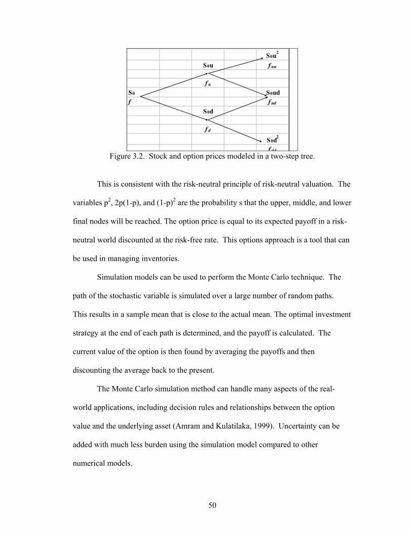
50
S0u2
S0u f uu
f uS0 S0udf f ud
S0d
f dS0d
2
f dd
S0u2
S0u f uu
f uS0 S0udf f ud
S0d
f dS0d2
f dd Figure 3.2. Stock and option prices modeled in a two-step tree.
This is consistent with the risk-neutral principle of risk-neutral valuation. The
variables p2, 2p(1-p), and (1-p)2 are the probability s that the upper, middle, and lower
final nodes will be reached. The option price is equal to its expected payoff in a risk-
neutral world discounted at the risk-free rate. This options approach is a tool that can
be used in managing inventories.
Simulation models can be used to perform the Monte Carlo technique. The
path of the stochastic variable is simulated over a large number of random paths.
This results in a sample mean that is close to the actual mean. The optimal investment
strategy at the end of each path is determined, and the payoff is calculated. The
current value of the option is then found by averaging the payoffs and then
discounting the average back to the present.
The Monte Carlo simulation method can handle many aspects of the real-
world applications, including decision rules and relationships between the option
value and the underlying asset (Amram and Kulatilaka, 1999). Uncertainty can be
added with much less burden using the simulation model compared to other
numerical models.

51
Simulation models also can solve path-dependent options in which the value
of the option depends not only on the value of the underlying asset but also on the
particular path of value followed by the underlying asset. This approach has the
additional benefit of providing an estimate of the error by giving the standard error of
the sample mean (Benninga et al. 1996).
Real Options
An option is the right, but not the obligation, to take an action in the future.
Options are valuable where there is uncertainty. For example, one option contract
traded on the financial exchanges gives the buyer the opportunity to buy stock at a
specified price on a specified date and will be exercised only if the price of the stock
on the date exceeds the specified price. Many strategic investments create subsequent
opportunities that may be taken, so the investment opportunity can be viewed as a
stream of cash flow plus a set of options.
The real options approach is the extension of financial option theory to
options on real (non-financial) assets (Amarm and Kulatilaka, 1999). While financial
options are detailed in the contract, real options embedded in strategic investments
must be identified and specified. Moving from financial options to real options
requires a change in the way of thinking, one that brings the discipline of the financial
markets to internal strategic investment decisions.
Real options have three components that are useful to managers. The first is
that options are contingent decisions, meaning an option is the opportunity to make a
decision after you see how events unfold. On the decision date, if events have turned
out well, a different decision will be made rather than if the events turned out poorly.
52
This implies that the payoff to an option is nonlinear, meaning it changes with the
decision made. Second, option valuations are aligned with financial market
valuations. The real options approach uses financial market inputs and concepts to
value complex payoffs across all types of real assets. The result is a comparison of
managerial options, financial market alternatives, and internal investment
opportunities and transaction opportunities. The last component is that options can be
used to design and manage strategic investments proactively. The nonlinear payoffs
can also be a design tool. Managers must identify and value the options in a strategic
investment, then redesign the investment to better use the options, and manage the
investment proactively though the options created.
The real options approach gives managers a decision-making and valuation
tool that reflects good project management, ensuring that these decisions lead to the
highest market valuation of corporate strategy.
Contingent Claims and Inventory
Traditional valuation tools use forecasts of outcomes (sales, profits, and so on)
of future investments and of terminal values to arrive at seemingly precise numbers,
but that imposes a fixed path on a business’s future developments. It is well known
that a fixed path view is artificial, and in reality, pursuing a new business opportunity
may result in a variety of outcomes that call for a wide range of strategic responses.
This wide range of responses is called the cone of uncertainty (Amram and
Kulatilaka, 1999). The real options approach recognizes this uncertainty, and it sees
what managers see: an investment today creates opportunities or options to change
operating and investment decisions later depending on the actual outcome.
53
The real options model must be adjusted for leakage in values arising from
cash flows or a convenience yield1 that accrues between decision points. Leakage
arises because only the holder of the underlying asset obtains the cash flow and or
convenience yield from the underlying asset. Amram and Kulatilaka (1999) state that
sources of leakage include positive cash flows (dividend, rental, interest, license,
royalty income), explicit negative cash flows (storage costs, taxes, licensing/royalty
fees, insurance costs, loss from perishable damage), and implicit benefits
(convenience yields). Convenience value arises from the ability to store a commodity
and to sell it at will in the spot market. Owners of commodities obtain benefits that
are not obtained by owing a contract on a commodity. Most agricultural commodities
will have a convenience yield just prior to harvest, when it is most likely that
shortages will occur.
Inventories can be thought of as insurance investments in that they reduce
exposure to uncertainty. Investing in excess capacity ensures against running out of
product if demand surges, but with a cost which is the incremental costs of
construction and carrying capacity built beyond immediate needs. This insurance
pays off only in a few outcomes. This is where managers use real options to value
investment and also check to see whether the value exceeds the cost.
Real options have recently applied to inventory analysis. As managers are
searching for a more quantitative tool that can be used to guide decisions about
inventories and assess the impacts of inventories on these decisions, they are looking
to real options. Real options help solve this problem of correctly handling all risks
1 The smaller the level of stocks, the greater is the convenience yield for holding an additional unit (Leuthold et al., 1989). There is long standing literature on convenience yields in agricultural commodities due to the cyclical pattern of harvest.
54
associated with carrying inventory that the net present value analysis overlooks. The
objective of the real options approach is to maximize the value of an investment using
a portfolio of assets which are highly correlated with the investment. If both upside
and downside risk are not properly addressed, managers have difficulty properly
identifying the correct inventory investments. The real options analysis to invest
under uncertainty and in the determination of optimal investment rules depends on the
stochastic process for the underlying asset.
An inventory can be viewed as a call option by mapping between the
characteristics of the inventory and the determinants of the call option value. A call
option is the right to buy an asset at a set price. Inventory is similar to a call option
in that if it is bought at a lower price and stored until processed with the market price
increasing, the processor has the ability to use inventories that were purchased at a
lower price. Given this ability, processors with inventory have the potential to sell or
use inventory, depending on market conditions. The decision makes the payoff of the
inventory nonlinear. An inventory decision involves making expenditures to buy the
commodity asset. This is similar to exercising an option: the amount expended is the
exercise price (X), and the value of the asset acquired is the stock price (S). The
length of time the company can wait without losing the opportunity is the time to
expiration (t), and the risk of the project is reflected in the standard deviation of
returns on the asset (σ). The time value is given by the risk-free rate (r) (Luehrman,
1995).
A call option should be exercised if the stock price exceeds the exercise price
at expiration. In this case, the stock price (S) corresponds to present value (expected
55
net cash flows), and the exercise price (X) corresponds to present value (capital
expenditure). Thus, for a call option, NPVq = S/PV(X) (Luehrman, 1995). If NPVq
exceeds 1, the options should be exercised, but if NPVq is less than 1, the option is
“out of the money” and should not be exercised.
The variability per unit of time of returns on the project is measured by the
variance of the returns, σ2. Multiplying the variance per unit time by the amount of
time remaining gives cumulative variance, σ2t (Luehrman, 1995). Cumulative
variance is a measure of how much things could change before time runs out and a
decision must be made. The more cumulative variance an option has, the more
valuable the option. Thus, if the option value is ignored and the variance
“uncertainty” is not taken into account, there is a tendency to undervalue inventories.
If there is greater uncertainty in the market place in that stock-outs might occur, the
option value will increase and the managers will see the full potential of the shortages
on firm.
Real Options and Inventories
There are three good examples of how option pricing approaches can be
applied to the inventory problem. Stowe and Gehr (1991) provide two financial
approaches to handling inventory. The first is a replicating portfolio approach
comparing the value of a portfolio of securities, and the second is the option pricing
solution to the discrete sales problem. Stowe and Gehr’s (1991) payoffs replicate
those of the inventory policy compared to the value of a portfolio of securities.
Chung (1990) shows another option pricing model. In Chung’s model, the inventory
payoffs are a linear function of demand with demand and the investors’ discount rate
56
jointly, log-normally distributed. The inventory reorder point is solved using a
binomial option pricing approach by Becker (1994).
These studies did not take into account that managers can make decisions after
certain payoffs are known; thus the payoffs become nonlinear or contingent claims.
The real options approach utilizes contingent claims in trying to find the profit-
maximizing inventory level given the circumstances that are developed. Real options
can be used to value inventories as an insurance policy in that they are an option on
future sales.2 If the inventory is depleted, the sales are lost. If the inventory is in
excess, the profit declines because of excess inventory carrying costs.
Real options also take into consideration uncertainty in a more “respectful
way,” thus allowing for more flexibility and giving more value to uncertainty.
Convenience yields are also a large part of agricultural commodity markets, and the
real options approach accounts for this and maximizes the profit from and inventory
with convenience yields.
Inventory can be defined in the rectangle defined by Luehrman (1998) as
option space. Option space is defined by two-option value metrics, each of which
captures a different part of the value associated with being able to defer an
investment. Option space can help address the issue of whether to invest in an
inventory or not and what to do in the meantime. The first metric contains all of the
usual data captured in NPV but adds the time value of being able to defer the
investment. Luehrman (1998, p91) defines the metric NPVq as the value of the
2 The option on future sales is the excess capacity real option. This option is also a contingent claim in that the future sales depend upon the underlying asset investments value. This real option is the decision to build excess capacity and value the shortages. In this study, net present value (NPV) was used to place a value on the option.
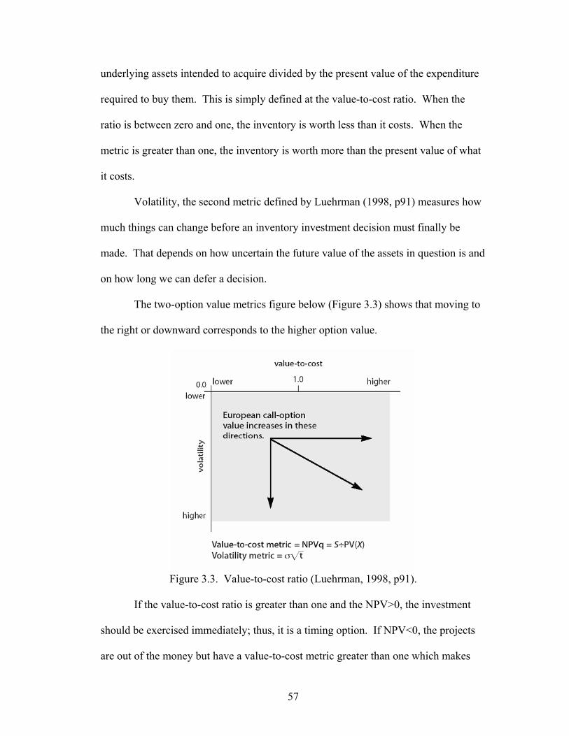
57
underlying assets intended to acquire divided by the present value of the expenditure
required to buy them. This is simply defined at the value-to-cost ratio. When the
ratio is between zero and one, the inventory is worth less than it costs. When the
metric is greater than one, the inventory is worth more than the present value of what
it costs.
Volatility, the second metric defined by Luehrman (1998, p91) measures how
much things can change before an inventory investment decision must finally be
made. That depends on how uncertain the future value of the assets in question is and
on how long we can defer a decision.
The two-option value metrics figure below (Figure 3.3) shows that moving to
the right or downward corresponds to the higher option value.
Figure 3.3. Value-to-cost ratio (Luehrman, 1998, p91).
If the value-to-cost ratio is greater than one and the NPV>0, the investment
should be exercised immediately; thus, it is a timing option. If NPV<0, the projects
are out of the money but have a value-to-cost metric greater than one which makes
58
them promising in the future. If the volatility is in the lower region and the value-to-
cost ratio is greater than one, the investment should be exercised.
Contingent Claims and Discrete Demand
The conventional approach to inventory stocking decisions relies on a criteria
that maximizes expected profits given a distribution of demand for the inventory
item. The contingent claims approach presented maps the demand and payoffs from
an inventory policy onto the price of an underlying state variable, builds a portfolio of
options that replicates payoffs, and then derives the value of an inventory policy using
option pricing models in which the value of the policy is contingent on the financial
characteristics of the underlying asset.
The basic distribution of discrete demand does not have probabilities attached
to each demand level. Demand in the conventional approach is assigned a
probability, thus limiting the results. The discrete demand with contingent claims has
various demand levels that are associated with price ranges of the underlying state
variables. The underlying asset can be the value of a foreign currency, fixed income
indexes, individual securities, and or commodities.
The payoffs according to Stowe and Su (1997) depend on the level of demand
in the state (Di) and the choice of inventory stocking level (Qk). The investment is
CQk:
),0,max(),min( ikikik DQEDQPPayoff −+= 3.23
where P = Selling price per unit, Qk = Choice of inventory stocking level in that state, Di = Level of demand in that state, E = Excess quantity selling price per unit, and C = Cost per unit.
59
Stowe and Su (1997) state that the net present value (NPV) of a particular
inventory policy is equal to the present value of the payoffs minus the outlay:
.1
, ki
n
ikik OutlaypPayoffNPV −= ∑
=
3.24
The net present value of the futures payoffs is the sum of the products of the cash
flow in each state (Payoffi,k) and its respective state price (pi) (Stowe and Su, 1997).
The state price according to Stowe and Su (1997) is the value of a claim that pays off
$1.00 in that state of nature and zero otherwise. These above state prices are the basic
element to the contingent claims approach to inventory analysis. The state prices in
this contingent claim model are similar to the element of probabilities in conventional
inventory models.
The state price using the Black-Scholes option pricing model is as follows:
)]},[)]([{),( 221221 YXdNYXdNeYYp rt =−== − 3.25
where P(Y1,Y2) = state price for a claim that pays $1.00 if Y1<St<Y2, e-rt = present value factor for risk-free rate r and time period t, N(d) = value of cumulative normal for d, d2 = [ln(So/X)+(r+σ2/2)t]/σ√t-σ√t, So = current price of underlying state variable, X = exercise price of the option, t = time until maturity of the option, r = riskless rate of return, and σ = volatility of the underlying state variable. These calculated state prices account for the likelihood that each state of
nature will occur. This method of determining state prices is obtained through
intuition rather than reasoning, as variable N(d2) represents the risk-neutral probably
of an option expiring in the money (Stowe and Su, 1997). The state price is then
found by multiplying the discount factor for a riskless rate by the difference between
60
two risk-neutral probabilities. Time value of money and risk are both reflected upon
in these probable state prices.
The optimal inventory policy using contingent claims and this discrete
demand case depend on the shape of the payoff function, market conditions, and the
characteristics of the underlying assets. Changing one or all of these will result in a
change in the NPV of an inventory policy in somewhat predictable ways.
Contingent Claims and Continuous Demand
Inventory policies having continuous demand can also be analyzed using
contingent claims in a similar fashion as discrete demand. There are three steps in
finding the optimal inventory level. First, the payoffs have to be mapped from an
inventory policy onto the price of the underlying asset. Second, a portfolio of options
has to be constructed that replicates the payoffs, and last, the NPV has to be obtained
from determining the value of the portfolio and then subtracting the investment costs.
A base case as shown in Stowe and Su (1997) has no salvage value for excess
inventory and no penalties for shortages. It is assumed that sales are tied to an
underlying asset with a current price of $50, standard deviation of 0.35, an interest
rate of 0.10 percent, and a payoff maturity of 0.5 years. Sales will be zero if the asset
price is below $30 but will increase by ten units per $1 above this price. The
investment per unit is $6, the price per unit sold is $10, and the salvage value is zero.
An inventory stocking policy with 300 units was mapped out. The payoff is zero if
the asset price is below $30, increases with a slope of 100 for S>$30, and reaches its
maximum of $3,000 when the asset price is $60. The option strategy is thus a vertical
spread with a portfolio of options that replicates a payoff of a long position of 100
61
call options with an exercise price of $30 and a short position of 100 call options with
an exercise price of $60. The NPV of the inventory policy under which the firm
stocks 300 units can be calculated by subtracting the initial outlay from the value of
the call options. NPV = 100C(X=30) – 100C(X=60) – 6(300). Inventory carrying
costs can also be built into the option pricing model by treating them as a dividend
yield, which is used to adjust the stock price before it is input into the Black-Scholes
option pricing model (Stowe and Su, 1997):
),()( 21 dNXedNSeC rtt −− −= δ 3.26
where
),/(])2/()/[ln( 21 ttrXSd σσδ +−+=
tdd σ−=2 , and =2δ annualized dividend yield.
The NPV is not the optimal inventory policy because at the margin, adding an
additional unit to the inventory stock increases the investment by $6 and raises the
potential payoff by $10; the additional $10 payoff is achieved by increasing the
exercise price of the short position in 100 call options by $0.10. The NPV is
NPV = 100C(X=30) – 100C(X=30+0.10Q) – 6Q. 3.27
This option strategy above is representative of a vertical spread in which the optimal
inventory policy can be found by taking the derivative of the NPV equation with
respect to Q, which results in
06)10.030(100 =−∂
+=∂−=
∂∂
QQXC
QNPV and 3.28
06)10.030(100 =−∂∂
∂+=∂
−=∂
∂QX
XQXC
QNPV . 3.29
Since ∂X/∂Q = 0.10 in this problem, the optimal state price occurs where
62
6.0)10.030(=
∂+=∂
−X
QXC . 3.30
Since ∂C/∂X = -e-rtN(d2), Q and X are found by iterating until ∂C/∂X has the desired
level, and in this case, it happens when Q = 169.35 units and X = $46.94.
In most cases, the above inventory situation will not exist, in part because
most firms will encounter penalties for shortages and have salvage values for excess
inventories. If demand exceeds quantity stocked, the company will incur stock-out
costs on the inventory they are short. These stock-out costs are conventionally looked
at as a loss of profit on the sales. Penalties are also considered as part of the stock-out
costs. The profit lost on the sale due to a stock-out is captured. Stock-outs can also
have additional costs to the extent that it injures the customer, thus causing the
customer switching costs or losing the customer. The customer could also impose a
stock-out cost on the supplier by paying a lower price for the good.
Using the above example to imply a salvage value and stock-out penalties, the
problem becomes more realistic. The salvage value limits the risk of carrying excess
inventory so that the stocks have a positive value. Stock-out penalties will cause the
payoff to decline when the inventory is depleted. Figure 3.4 shows the payoff with a
positive salvage value and a penalty for stock-outs.
This nonlinear payoff function in the figure above is due to the contingent
claim that managers have the decision to invest or not, and that decision will affect
the payoff function.
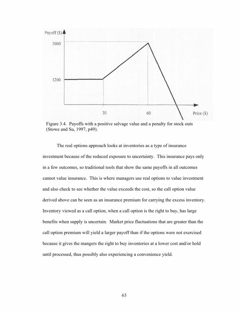
63
Figure 3.4. Payoffs with a positive salvage value and a penalty for stock outs (Stowe and Su, 1997, p49).
The real options approach looks at inventories as a type of insurance
investment because of the reduced exposure to uncertainty. This insurance pays only
in a few outcomes, so traditional tools that show the same payoffs in all outcomes
cannot value insurance. This is where managers use real options to value investment
and also check to see whether the value exceeds the cost, so the call option value
derived above can be seen as an insurance premium for carrying the excess inventory.
Inventory viewed as a call option, when a call option is the right to buy, has large
benefits when supply is uncertain. Market price fluctuations that are greater than the
call option premium will yield a larger payoff than if the options were not exercised
because it gives the mangers the right to buy inventories at a lower cost and/or hold
until processed, thus possibly also experiencing a convenience yield.
64
Conceptual Relationship
The conventional approach of inventory analyzes the optimal stock-out
probability by deriving the expected benefit of stocking an additional unit with the
expected cost of stocking that additional unit (Stowe and Su, 1997). The following
equation shows expected revenue from selling the unit of pπ; the expected salvage
value is (1-π)s, and the expected stock-out penalty avoided is nπ (Stowe and Su,
1997):
cnsp =+−+ πππ )1( and 3.31
nsp
sc+−
−=π , 3.32
where π = the stock-out probability, p = the selling unit price per unit, c = the cost per unit, and n = penalty for a stock-out. Stowe and Su (1997) alter the conventional equations above to be consistent
with the contingent claims approach by replacing objective probabilities with risk-
neutral probabilities. The expected benefits also have to be discounted by the riskless
rate. With N(d2) as the risk-neutral probability of a stock-out, the new equation is as
follows. This equation sets the present value of the expected benefit of stocking an
additional unit of inventory equal to the investment in one unit of inventory (Stowe
and Su, 1997):
cdnNdNsdpNe rt =+−+− )]())(1()([ 222 . 3.33
Using the above equation and rewriting it to get the equation in terms of the
state price of the contingent claim yields the following equation (Stowe and Su,
1997):
65
nsp
secdNeXC rt
rt
+−−
==∂∂
−−
− )( 2 . 3.34
The equation ∂C/∂X is the state price of the contingent claim. The state price of the
contingent claims is the value of a $1.00 payoff if the underlying asset price is above
the exercise price. The state price is a calculation of two factors, the first factor being
the present value and the second being N(d2), which is the risk-neutral probability of
a stock-out. According to Stowe and Su (1997), N(d2) is the risk-neutral probability
of the underlying asset price exceeding the exercise price, thus meaning the option is
in the money. Using this state price is more economically sound because it includes
the time value of money and the effects of risk. This advantage is the fundamental
difference between the conventional approach and contingent claims and is why the
latter is a more appropriate way to manage inventory.
Conventional and contingent claims forecast sales in two different ways.
Conventional inventory management tools rely on an estimation of the distribution of
future demand. Contingent claims use the underlying variables to forecast sales.
These same variables are then used to value a portfolio of options. The payoff
functions calculated with the contingent claims are based on the underlying assets
value in the marketplace; once the payoffs are calculated, the optimal inventory
policy is determined using the payoffs.
Summary of Variables
This section defines the important variables that must be considered when
analyzing inventory strategies. All of the variables will have an effect on the
inventory policy both negatively and positively, but they have to be understood in
order to find the optimal level.
66
Procurement costs that are associated with the ordering cost, shortage cost,
and temporal prices are among some of the factors that force agribusiness managers
to carry inventory (Polataglu and Sahin, 2000). These costs will all go down with
increased lot size and less reordering. Holding costs have an opposite effect; hence, as
the lot size increases, holding costs will also increase (Polataglu and Sahin, 2000). In
order to determine the optimal inventory level, a balance has to be found between the
two types of cost. This balance will depend on demand forecasts, cost structures, and
the operating conditions of the business.
Uncertainty of supply is an important factor when determining the optimal
inventory policy. Uncertainty in quantity, price, quality, and other variables will have
a large effect on how much inventory will be carried. Uncertainty of supply
forecasting will have an impact on the supply prices, thus the need for accurate
forecasting methods. The amount of a forecasting error will determine if a business is
penalized with shortage costs or with excess inventory carrying costs. The amount of
safety inventory carried by a business is also reflective of the accuracy of their
forecasting. Thus, if the forecasting methods are not accurate, higher safety
inventories must be carried. Hoshino (1996), states that the level of safety stock can
be lowered by adopting the fixed interval ordering policy when the forecasting error
is small.
Shortage costs and service levels are also related to supply forecasting in that
if supply forecast is accurate, there would be no need to take these variables into
consideration. Since there is always some sector of supply that is uncertain, shortage
costs and service levels have to be incorporated into inventory management. In order
67
to meet a required service level in most cases, some level of safety inventory is
required to prevent stock-outs which lower the service level of the firm. Shortage
costs can be very costly to the firm if the buyer encounters switching costs and or
decides to buy from another firm.
The salvage value of the inventory plays a vital role in the overall expected
profit function of a firm. If the inventory can be sold at a reduced price other than
zero, there is a greater chance the firm will hold inventories to reduce procurement
costs as well as shortage costs and to increase the service levels.
The traditional purchasing approach (Goffin et al., 1997) shows that there are
several key factors that influence purchasing decisions for the buyers. They are unit
price, quality conformance, and speed of delivery. Goffin et al. (1997) found the unit
price to be the main emphasis of purchasing, but the others were also taken into
consideration when buying.
Summary
There is an apparent increasing awareness of real options and contingent
claims in the management sector of business. Two factors to consider when
managing inventory include the time value of money and the risk level associated
with the particular industry. These two factors are not accounted for in the
conventional inventory management approach. The ability of managers to
conceptually see how inventory levels affect their profit will greatly influence how
inventory is managed.
The EOQ model was an acceptable way of managing inventory in the past and
still is used by many businesses today, but its value is limited in situations with higher
68
risk. It does not take into account the market value of the product which in today’s
agribusiness is a very large part of risk, as commodity quality and quantity are
sometimes limited.
The contingent claims approach is not new, but it is just starting be researched
and adapted to more and more managerial tools. Its adds flexibility to the business as
well as increases the NPV by finding the optimal inventory level that maximizes
profits. Using contingent claims for inventory analysis can greatly increase profits
once recognized and portfolios are built. There are a few basic limitations to
contingent claims as listed in Chapter 2, but the benefits far outweigh the limitations
when compared to conventional methods of inventory management.
69
CHAPTER 4 EMPIRICAL MODEL
Introduction
Wheat, durum, and oats are three commodities that pose unique problems in
the marketplace. Fundamental characteristics in these markets create uncertainties
that result in large volatility in the prices, quantity, and quality. It is difficult to
correctly address uncertainty in conventional inventory models such as the economic
order quantity model (EOQ). Until the recent introduction of contingent claims in
inventory strategy analysis, there was not a financially sound method to address the
issue of uncertainty.
Inventories can be interpreted as a real option. Specifically, they are similar
to a call option. A bull spread is the type of call spread used in this study. It is
created by buying a call option on a stock with a certain strike price and then selling a
call option on the same stock with a higher strike price. This option created by call
requires an initial investment which is the inventory. Inventories are a form of real
options called the option on future sales; as such, there are two critical issues. One is
to determine the optimal level of stocks, given the option value. The second is to
determine the option value of inventories held in stocks.
This chapter describes the development of a contingent claims model that
maps the payoffs of the inventory strategy onto the price of the underlying asset. The
second step of the real options analysis is to develop a portfolio of options that
replicates those payoffs. Then the final step is to place a value on the portfolio by
subtracting the investment to obtain the net present value.
70
The purpose of this chapter is to describe the analytical model of the
contingent claims approach. It starts with a brief model overview before proceeding
into the mathematical models. The contingent claims models are then defined for
three cases. The first case does not have a salvage value or shortage penalty, the
second case has a salvage value but no shortage penalty, and the third case has a
salvage value and shortage penalty. The model variables are then described and
defined for all three cases and commodities. The economic order quantity (EOQ)
model follows with explanations of the variables. A data section follows indicating
where the information was gathered. It is followed by a chapter summary.
Model Overview
The contingent claims methodology is used to model commodity inventories.
Sales of the finished product, in this case flour, are mapped onto the underlying
commodity that is carried in inventory. Northern spring wheat 14+ percent protein,
hard amber durum, and milling quality oats were used as the underlying commodities
to be milled into flour or various other products. There are several differences among
the wheat, durum, and oat commodities in this study. Wheat can be hedged, but the
basis risk for higher protein may induce stockholding. Hard amber durum and
milling oats cannot be easily directly hedged and thus have to be cross-hedged, which
introduces additional risk. Overall quality of the commodities cannot be hedged, thus
introducing a shortage risk for meeting requirements for end-use.
Demand for the finished product follows a continuous distribution. In this
model, demand and inventory policy are determined annually. Using a continuous
71
distribution of demand focuses on supply risk and the effects it has on overall
inventory implication of the raw commodity.
Three specific cases are modeled in this study. The first, the base case, does
not have a salvage value or a shortage penalty, the second case encompasses a
salvage value but has no shortage penalty, and the third case considers the salvage
value along with a shortage penalty. The first model should result in the least amount
of inventory due to less risk associated with running short, and also, it does not have a
floor in place to which the company can liquidate storage and still at least gain the
salvage value of the asset. The NPV of the inventory policies should also decline
from Case 1 to Case 3 due to the increased costs of carrying higher inventory at a
greater risk.
The EOQ is compared to the contingent claims inventory analysis in this
study. The EOQ model is from Ballou (1999, p325). The EOQ model at its basic
formulation is a close approximation to the base case of the contingent claims model.
The more complex EOQ model takes into consideration lead times, probability of
product being in stock, and standard error of forecast and is closely related to the
complex contingent claims Case 3. The EOQ determines the optimal order quantity
subject to assumptions where the contingent claim determines the value of an
inventory carrying strategy.
Mathematical Model Description
The mathematical model accounts for the primary inventory costs and
revenues. Costs include interest, storage, shipping, commodity, and a shortage
penalty. Revenues include the price per unit sold and the salvage value. The
72
mathematical models in this study are adopted from Stowe and Su (1997).
Derivations of the optimal stock-out probability calculations given the three cases are
partially related to their work.
Determining the Optimal Stock-Out Probability
The optimal stock-out probability is an important parameter to determine and
is one of the major differences between the conventional and contingent claims
inventory approaches. The optimal stock-out probability is the probability of demand
exceeding quantity (Stowe and Su, 1997). Conventional approaches that use the EOQ
choose the optimal stock-out probability by equating the expected benefit of stocking
an additional unit with the expected cost of stocking that additional unit; thus, payoff
can be defined as
cnsp =+−+ πππ )1( , 4.1
where π = the stock-out probability, p = the selling price per unit, c = the cost per unit, s = the salvage value per unit, and n = the penalty for a stock-out. Optimizing 4.1 can determine the conventional optimal stock-out probability which is
nsp
sc+−
−=π . 4.2
Selling price per unit is the value of what the good can be sold for. It is
revenue that is flowing into the business from a sale of the finished product. The
selling price is the flour price in this study. Cost per unit is the cost to buy the assets
required to produce one unit of output. In this study, the cost per unit is the
underlying commodity price. Salvage value is what the asset can be liquidated for; it
73
is the minimum value which the firm would see from holding or producing an asset.
The salvage value used in this study is the price paid for the commodity plus ten
cents, which implies normal market returns to storage with storage and shipping
subtracted out. This is because the storage fee is lost, and the business has to pay to
ship out the commodity. The stock-out penalty is a cost to the business if demand
requirements are not met. Stock-out penalties in this study are calculated to be the
margin on flour production. Finally, the stock-out probability is defined as the point
at which demand exceeds quantity; this point is calculated in Equation 4.2.
The conventional approach to choosing stocking levels can be used in all three
cases of this study. The numerator in Equation 4.2 is considered to be the carrying
cost of an additional unit of inventory. The benefit of selling an additional unit of
inventory is the denominator.
The contingent claims solution of the optimal stock-out probability replaces
objective probabilities with risk-neural probabilities by discounting the expected
benefits by the riskless rate which generates the optimal state price. The optimal state
price replaces the objective probabilities in the conventional approach with risk-
neutral probabilities. The salvage value is an expected benefit that, if used, has to be
discounted by the riskless rate. Using Equations 4.1 and 4.2 and transforming them
into contingent claims formulation yields the optimal state price used in this study.
The optimal state price is the probability of demand exceeding quantity that will
maximize the NPV of the firm. The NPV calculations for Cases 1 through 3 can be
seen in Equations 4.4, 4.8, and 4.12, respectively. The optimal state price is
nsp
secdNeXC rt
rt
+−−
==∂∂
−−
− )( 2 , 4.3
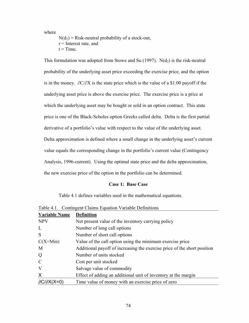
74
where N(d2) = Risk-neutral probability of a stock-out, r = Interest rate, and t = Time. This formulation was adopted from Stowe and Su (1997). N(d2) is the risk-neutral
probability of the underlying asset price exceeding the exercise price, and the option
is in the money. ∂C/∂X is the state price which is the value of a $1.00 payoff if the
underlying asset price is above the exercise price. The exercise price is a price at
which the underlying asset may be bought or sold in an option contract. This state
price is one of the Black-Scholes option Greeks called delta. Delta is the first partial
derivative of a portfolio’s value with respect to the value of the underlying asset.
Delta approximation is defined where a small change in the underlying asset’s current
value equals the corresponding change in the portfolio’s current value (Contingency
Analysis, 1996-current). Using the optimal state price and the delta approximation,
the new exercise price of the option in the portfolio can be determined.
Case 1: Base Case
Table 4.1 defines variables used in the mathematical equations.
Table 4.1. Contingent Claims Equation Variable Definitions Variable Name Definition NPV Net present value of the inventory carrying policy L Number of long call options S Number of short call options C(X=Min) Value of the call option using the minimum exercise price M Additional payoff of increasing the exercise price of the short position Q Number of units stocked C Cost per unit stocked V Salvage value of commodity X Effect of adding an additional unit of inventory at the margin ∂C/∂X(X=0) Time value of money with an exercise price of zero
75
The inventory strategy defined in the base case has no salvage value for
excess inventories or no penalties for shortages. Sales are tied to the underlying
commodity with a current price and standard deviation. The mathematical
formulation of the NPV of the base case is
CQMQMINXSCMINXLCNPV −+=−== )()( . 4.4
The optimal inventory is the derivative of the NPV with respect to Q, and then
setting the derivative equal to zero. Equation 4.5 is the derivative of Equation 4.4
with respect to Q and setting it equal to zero.
0)(=−
∂+=∂
−=∂
∂ CQ
MQMINXCSQ
NPV . 4.5
Equation 4.5 can be reduced to add in the marginal effect of adding another unit of
inventory on the payoff, thus yielding
(4.6) 0)(=−
∂∂
∂+=∂
−=∂
∂ CQX
XMQMINXCS
QNPV .
∂X/∂Q is defined at the margin as the effect of adding an additional unit to inventory
NPV. The additional unit of inventory increases the payoff by X at the margin, and
the Q is the number of short call options. This number is calculated for the base case
and is the same for all cases. The optimal state price is a risk-neutral probability level
that is a balance between the costs and revenues of inventory that maximizes the total
expected profits. The optimal state price occurs where
)*/()(QXSC
XMQMINXC
∂∂
=∂
+=∂ . 4.7
Using the ∂C/∂X in Equation 4.3, the optimal quantity and price can be found.
The quantity found is the amount that should be held in inventory, and the price is the
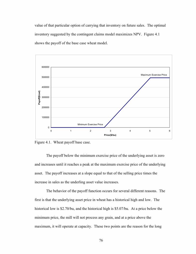
76
value of that particular option of carrying that inventory on future sales. The optimal
inventory suggested by the contingent claims model maximizes NPV. Figure 4.1
shows the payoff of the base case wheat model.
Minimum Exercise Price
Maximum Exercise Price
0
100000
200000
300000
400000
500000
600000
0 1 2 3 4 5 6
Price($/bu)
Payo
ff($/
cwt)
Figure 4.1. Wheat payoff base case.
The payoff below the minimum exercise price of the underlying asset is zero
and increases until it reaches a peak at the maximum exercise price of the underlying
asset. The payoff increases at a slope equal to that of the selling price times the
increase in sales as the underling asset value increases.
The behavior of the payoff function occurs for several different reasons. The
first is that the underlying asset price in wheat has a historical high and low. The
historical low is $2.70/bu, and the historical high is $5.07/bu. At a price below the
minimum price, the mill will not process any grain, and at a price above the
maximum, it will operate at capacity. These two points are the reason for the long
77
and short calls. The long call replicates the minimum payoff of the inventory
carrying policy, while the short calls replicate the maximum payoff of the inventory
carrying policy. A linear line drawn between the two suggests the payoff may fall
anywhere between the two points.
A call option is the right to buy an asset at a certain price by a certain date.
The long call option means the business is purchasing the right to own an asset at a
certain price by a certain date. The short call option means the business is selling the
right to own an asset at a certain price by a certain date. Thus, the long call option
replicates buying the inventory, and the short call options replicate selling in the
inventory.
This base case is representative of an agribusiness that does not have a salvage
value on excess inventory items stocked and also will not incur a shortage penalty if
demand exceeds quantity stocked.
Case 2: Salvage Value for Excess Inventories
This second case assumes excess inventory can be liquidated for a
predetermined salvage value. In the base case, salvage value is equal to the price paid
per bushel plus ten cents to imply a normal market, minus storage and shipping costs.
The salvage value in the grain market varies. If the market is inverted, the salvage
value is less than the price paid for the commodity when it was bought. If the market
is normal, the salvage value is greater than the price at which the asset was bought.
This has a direct link on the optimal inventory level as it creates a floor in which to
limit potential losses from the inventory carrying policy. Thus, the NPV is
CQMQMINXSCMINXLCXXCVQNPV −+=−=+=∂∂= )()()0(/* . 4.8
78
The derivative of the above NPV with respect to Q and setting it equal to zero yields
0)()0( =−∂
+=∂−=
∂∂
=∂
∂ CQ
MQMINXCLXXCV
QNPV . 4.9
Simplifying Equation 4.9 by adding in the marginal effects of adding an additional
unit of inventory yields the following:
0)()(=−−
∂∂
∂+=∂
−=∂
∂ −rtVeCQX
XMQMINXCL
QNPV . 4.10
Equation 4.10 can then be broken down to the optimal state price where
QXS
VeCX
MQMINXC rt
∂∂−
=∂
+=∂−
−
/*)()( . 4.11
Using the ∂C/∂X as defined above, the optimal quantity and price can be
found by deriving the optimum. The numerator in Equation 4.11 is the cost per unit
stocked minus the salvage value per unit with the time value of money. This is a
major difference between the conventional approach, and this contingent claims
approach is the time value of money associated with the salvage value. The time
value of money adds depth to the model because it takes into consideration the cost of
having money tied up in inventory. The denominator of Equation 4.11 is the number
of short call options times the marginal effect to the NPV of adding an additional unit
of inventory. The quantity is optimal stock level and is the amount that should be
held in inventory, and the price is the value of that particular option of carrying that
inventory on future sales.
Figure 4.2 shows the payoff associated with the base case in wheat.
The payoff now has a different slope than the previous figure (Figure 4.1).
The payoff changes because the inventory can now be sold at a salvage value, thus
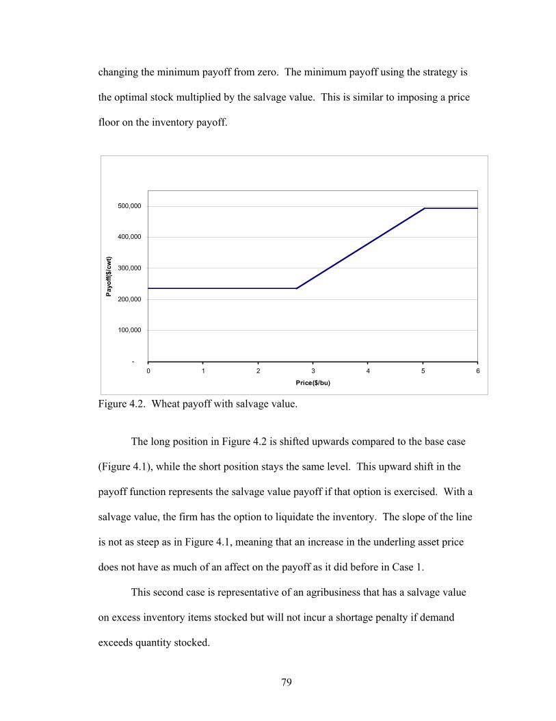
79
changing the minimum payoff from zero. The minimum payoff using the strategy is
the optimal stock multiplied by the salvage value. This is similar to imposing a price
floor on the inventory payoff.
-
100,000
200,000
300,000
400,000
500,000
0 1 2 3 4 5 6
Price($/bu)
Payo
ff($/
cwt)
Figure 4.2. Wheat payoff with salvage value.
The long position in Figure 4.2 is shifted upwards compared to the base case
(Figure 4.1), while the short position stays the same level. This upward shift in the
payoff function represents the salvage value payoff if that option is exercised. With a
salvage value, the firm has the option to liquidate the inventory. The slope of the line
is not as steep as in Figure 4.1, meaning that an increase in the underling asset price
does not have as much of an affect on the payoff as it did before in Case 1.
This second case is representative of an agribusiness that has a salvage value
on excess inventory items stocked but will not incur a shortage penalty if demand
exceeds quantity stocked.
80
Case 3: Salvage Value and Stock-Out Penalty
Case 3 deals with a common inventory problem of demand exceeding the
quantity carried on inventory. When this happens, the business generates a stock-out
penalty. If the business has a shortage, it implies a shortage penalty. A salvage value
is also allowed in this third case. With both the salvage value and the shortage
penalty, the case replicates what a typical agribusiness would face. The NPV for the
inventory carrying policy is
CQMQMINXSCMINXLCXXCVQNPV −+=−=+=∂∂= )()()0(/ . 4.12
Taking the derivative of the NPV with respect to Q and setting it equal to zero yields
the following:
0)()0( =−∂
+=∂−=
∂∂
=∂
∂ CQ
MQMINXCLXXCV
QNPV . 4.13
Simplifying the above equation by adding in the marginal effects of adding an
additional unit of inventory along with the shortage penalty if demand exceeds
quantity stocked yields the equation below:
.0)()(
=−−∂∂
∂+=∂
=∂
∂ −rtVeCQX
XMQMINXCL
QNPV
4.14
Equation 4.14 can be broken down to derive the optimal state price. The optimal
state price is equal to the equation below:
QXS
VeCX
MQMINXC rt
∂∂−
=∂
+=∂ −
/*)()( . 4.15
Using the ∂C/∂X formula, Equation 4.3, the optimal quantity and price can be
found by iterating until it has the desired value. Equation 4.15 is similar to Equation
4.11 but has a different number of short call options. This is because the short call
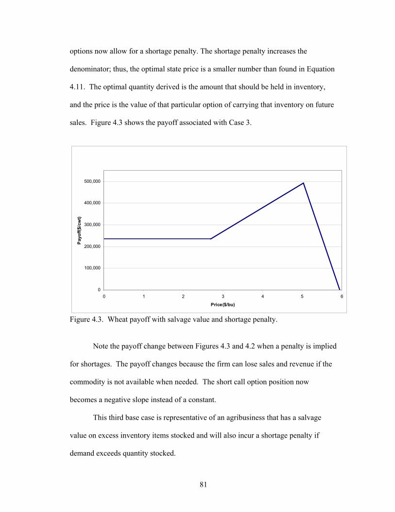
81
options now allow for a shortage penalty. The shortage penalty increases the
denominator; thus, the optimal state price is a smaller number than found in Equation
4.11. The optimal quantity derived is the amount that should be held in inventory,
and the price is the value of that particular option of carrying that inventory on future
sales. Figure 4.3 shows the payoff associated with Case 3.
0
100,000
200,000
300,000
400,000
500,000
0 1 2 3 4 5 6
Price($/bu)
Pay
off($
/cw
t)
Figure 4.3. Wheat payoff with salvage value and shortage penalty.
Note the payoff change between Figures 4.3 and 4.2 when a penalty is implied
for shortages. The payoff changes because the firm can lose sales and revenue if the
commodity is not available when needed. The short call option position now
becomes a negative slope instead of a constant.
This third base case is representative of an agribusiness that has a salvage
value on excess inventory items stocked and will also incur a shortage penalty if
demand exceeds quantity stocked.
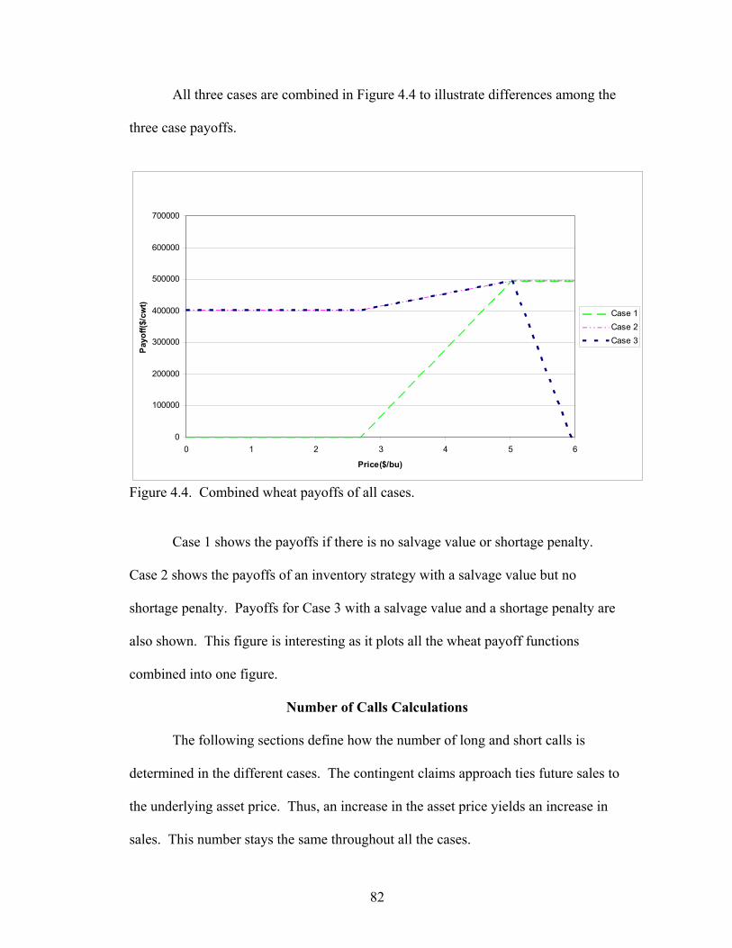
82
All three cases are combined in Figure 4.4 to illustrate differences among the
three case payoffs.
0
100000
200000
300000
400000
500000
600000
700000
0 1 2 3 4 5 6
Price($/bu)
Pay
off($
/cw
t)
Case 1Case 2Case 3
Figure 4.4. Combined wheat payoffs of all cases.
Case 1 shows the payoffs if there is no salvage value or shortage penalty.
Case 2 shows the payoffs of an inventory strategy with a salvage value but no
shortage penalty. Payoffs for Case 3 with a salvage value and a shortage penalty are
also shown. This figure is interesting as it plots all the wheat payoff functions
combined into one figure.
Number of Calls Calculations
The following sections define how the number of long and short calls is
determined in the different cases. The contingent claims approach ties future sales to
the underlying asset price. Thus, an increase in the asset price yields an increase in
sales. This number stays the same throughout all the cases.
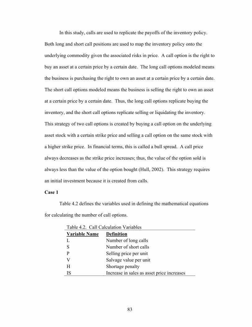
83
In this study, calls are used to replicate the payoffs of the inventory policy.
Both long and short call positions are used to map the inventory policy onto the
underlying commodity given the associated risks in price. A call option is the right to
buy an asset at a certain price by a certain date. The long call options modeled means
the business is purchasing the right to own an asset at a certain price by a certain date.
The short call options modeled means the business is selling the right to own an asset
at a certain price by a certain date. Thus, the long call options replicate buying the
inventory, and the short call options replicate selling or liquidating the inventory.
This strategy of two call options is created by buying a call option on the underlying
asset stock with a certain strike price and selling a call option on the same stock with
a higher strike price. In financial terms, this is called a bull spread. A call price
always decreases as the strike price increases; thus, the value of the option sold is
always less than the value of the option bought (Hull, 2002). This strategy requires
an initial investment because it is created from calls.
Case 1
Table 4.2 defines the variables used in defining the mathematical equations
for calculating the number of call options.
Table 4.2. Call Calculation Variables Variable Name Definition L Number of long calls S Number of short calls P Selling price per unit V Salvage value per unit H Shortage penalty IS Increase in sales as asset price increases
84
The number of long and short call options in the base case is equal. The
number of long call options is derived by multiplying the increase in sales contingent
on the underlying asset price by the price per unit sold:
ISPL *= . 4.16
An example from Stowe and Su (1997, p47) states “Sales will be zero if asset price is
below $30, but will increase by ten units per $1 increase above this price.” That
describes the increase in sales contingent on the underlying asset price. Once the
numbers of long call options are calculated, the same number can be used for the
number of short call options in this case because these are offsetting options. The
long call option is the value of the underlying asset or product, and the short position
is the value of future sales of that asset.
Case 2
The numbers of long and short call options for Case 2 are also equal. The
difference between the calculations in Case 1 is the number of call options and Case 2
is the sales price or net revenue changes due to the fact of having a salvage value.
The number of long call options in Case 2 is derived by subtracting the salvage value
from the price per unit sold and then multiplying it by the increase in sales contingent
on the underlying asset price:
ISVPL *)( −= . 4.17
This yields the number of long call options which is equal to the number of short call
options.
85
Case 3
The numbers of long and short call options in Case 3 with a salvage value and
shortage penalty are not equal. The numbers of long call options are the same as
Case 2, but the number or short call options changes to reflect the shortage penalty.
The number or short call options now becomes the shortage penalty multiplied by the
increase in sales contingent on the underlying asset price, then adding it to the
number of long call options:
LISHS += * . 4.18
The number of short call options is increased due to the shortage penalty if the
business is not able to meet demand in the specified time period. This is the
downward slope to the payoff function in Case 3 that can be seen in Figure 4.4.
Detailed Description of Model
This section provides a more detailed description of the model. The flow of
the inventory and how various costs are calculated are included in the following
sections. A table at the end of the section shows the values used in the following
calculations. The following section describes data sources.
Calculations
Conversions
With the inventory payoff being modeled to the underlying asset, it is
necessary to convert underlying asset input prices into output prices (e.g., flour
equivalents). These numbers were obtained from contacts within each of the
industries.
86
Underlying Asset Details
The model reacts to changes in the price of the underlying asset and its
variability. The mill draws grain from the local market. In this case, Minneapolis
prices were used for NO. 1 dark northern spring (14%+Protein), NO. 1 hard amber
durum, and milling quality oats. The standard deviation for the prices was obtained
from the years 1990-02. Yearly prices were used because annual stock-use ratio was
also used in this study.
Investment per Unit
Investment per unit is a calculated value based on the price of the commodity
bought and placed in storage and storage costs. Actual price of the commodity in a
given time period was used. The implied storage cost was four cents per bushel,
close to commercial storage costs typically paid by agribusiness. Investment per unit
is
MSCPBI *)( += , 4.19
where I = Investment per unit $/cwt, PB = Price paid per bushel $/bu, SC = Storage cost per bushel $/bu, and M = Multiplier for converting bushels to hundredweight.
Adding the price of the commodity per bushel and the storage costs yields the
investment per unit.
Price per Unit Sold
Price per unit sold is calculated by adding the revenues from the finished
product, to mill feed values. The product price was used for the finished product, and
that price was obtained from the same time period as the commodity price. Mill feed
87
values were obtained from the same time period and also added into the price per unit
sold as they are a valuable byproduct of milling:
MFPPPS += , 4.20
where PS = Price per unit sold $/cwt, PP = Product price $/cwt, and MF = Mill feed price $/cwt.
Adding the product price to the mill feed price calculates the product price that was
used in this study. The prices are in hundredweights.
Salvage Value
The salvage value is an important calculation in Cases 2 and 3. It is calculated
by subtracting the storage cost and shipping cost on a per-bushel basis from the
commodity price used in the investment per unit and then adding ten cents to account
for a normal market with positive carry. This salvage value is then converted into
cwt:
MBSPSTCPSV *)( +−−= , 4.21
where SV = Salvage value $/cwt, CP = Commodity price $/bu, ST = Storage cost $/bu, SP = Shipping cost $/bu, B = Normal market carry $/bu, and M = Multiplier for converting bushels to hundredweight.
A normal market is used in this study on all the grains. The variable B in
Equation 4.21 is ten cents in this study. That implies that the market price for the
grain went up ten cents from the time the grain is bought to the time the salvage value
is calculated. This is a normal assumption as the market is normal and will see an
increase in the salvage price due to normal market conditions.
88
Inverted markets can be added into this model using the salvage value. The
value of the underlying asset can be adjusted to show inverted or normal market
trends. For example, if the base price is $4.00/bu, an inverted market would be when
the commodity value twelve months from now is $3.80/bu, which provides a
disincentive to carry stocks, but the reverse is true if the market price in twelve
months is $4.20/bu; this provides an incentive to carry greater stocks. This is an
added benefit of using the contingent claims model.
Using the salvage value creates revenue in the option that has to be discounted
by the time value of money which, in this case, is the annual interest rate. This
creates a floor for the option given that a particular inventory position is at least
guaranteed the salvage value per unit.
Shortage Penalty
A shortage penalty is used in the third case and has an impact on how much
inventory to carry and the option value. The shortage penalty in Case 3 is the lost
milling margin from not running the raw commodities through the mill. This is much
like a lost sale because it has a negative effect on the revenue flows of a business. If
demand exceeds the quantity available in storage, the mill loses revenue because of
the lost sales. This does not take into consideration lost or disgruntled customers due
to the fact that in the industry, there are many substitutes. Milling margin values used
for the shortage penalty were obtained from industry contacts.
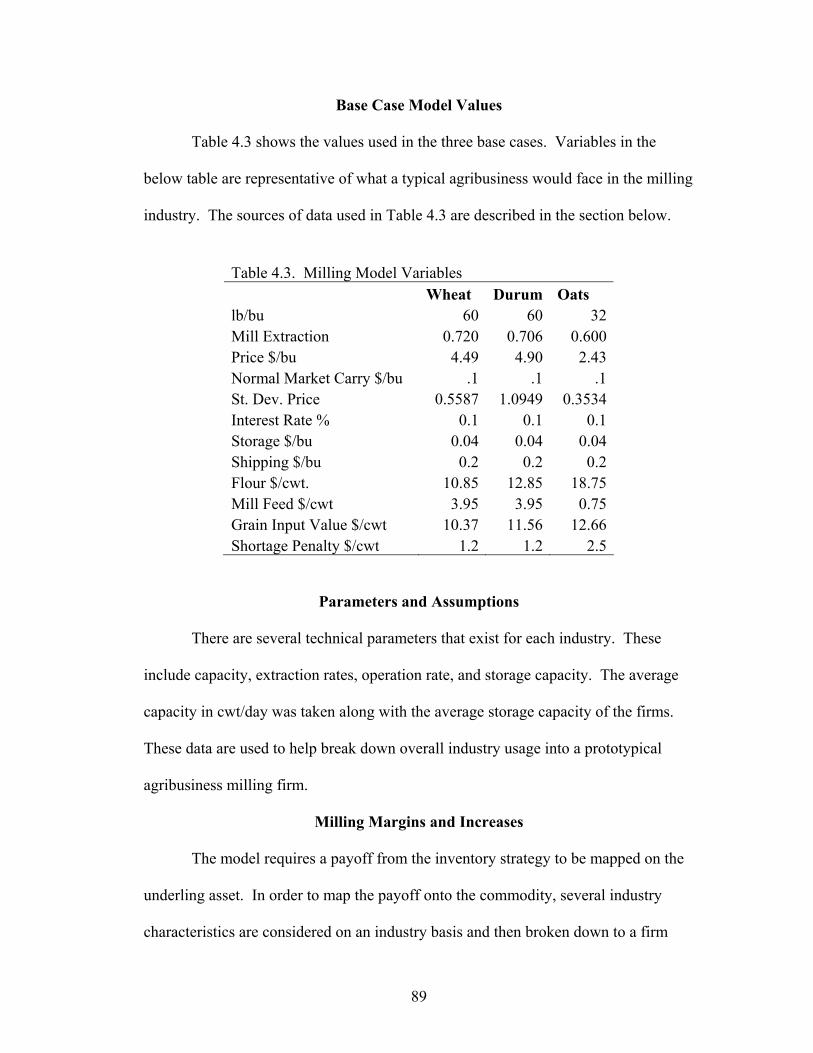
89
Base Case Model Values
Table 4.3 shows the values used in the three base cases. Variables in the
below table are representative of what a typical agribusiness would face in the milling
industry. The sources of data used in Table 4.3 are described in the section below.
Table 4.3. Milling Model Variables Wheat Durum Oats lb/bu 60 60 32 Mill Extraction 0.720 0.706 0.600 Price $/bu 4.49 4.90 2.43 Normal Market Carry $/bu .1 .1 .1 St. Dev. Price 0.5587 1.0949 0.3534 Interest Rate % 0.1 0.1 0.1 Storage $/bu 0.04 0.04 0.04 Shipping $/bu 0.2 0.2 0.2 Flour $/cwt. 10.85 12.85 18.75 Mill Feed $/cwt 3.95 3.95 0.75 Grain Input Value $/cwt 10.37 11.56 12.66 Shortage Penalty $/cwt 1.2 1.2 2.5
Parameters and Assumptions
There are several technical parameters that exist for each industry. These
include capacity, extraction rates, operation rate, and storage capacity. The average
capacity in cwt/day was taken along with the average storage capacity of the firms.
These data are used to help break down overall industry usage into a prototypical
agribusiness milling firm.
Milling Margins and Increases
The model requires a payoff from the inventory strategy to be mapped on the
underling asset. In order to map the payoff onto the commodity, several industry
characteristics are considered on an industry basis and then broken down to a firm
90
level. The industry characteristics were flour grind, commodity production, and
percentage of acceptable quality.
Effect of Quality and Quantity Shortfalls on Inventory Value
An important variable motivating the contingent claims theory in modeling
commodity inventory carrying is the effect on the underlying asset price on the future
sales of a product. This has a large impact on stability and reliability of the model.
To pinpoint this number along with adding quality and quantity variables into the
model, the following steps were used.
Stowe and Su (1997, p47) use the following as their contingent claim: “Sales
will be zero if the asset price is below $30, but will increase by ten units per $1.00
increase above this price.” This is a large assumption in the contingent claims model
as it is one of the main numbers behind mapping the payoff of the future sales on the
underlying commodity. Similar data and relationships do not exist in the grain
processing sector, though if they could be derived for individual firms, they would be
highly autonomous. Thus, in order to represent how much storage would be used in
the grain industry, the following steps were taken to simulate typical industry storage
demands.
First the following annual data were collected: flour grind, commodity
production, beginning stocks, imports, domestic use, exports, price, and quality. The
data were all converted into similar units. A representative annual usage was
calculated using historical industry data:
)/( XDUESSUR
ESXDUIPDBS+=
=−−++, 4.22
91
where BS = Beginning stocks, PD = Production, I = Imports, DU = Domestic use, X = Exports, ES = Ending stocks, and SUR = Stocks to use ratio.
Beginning stock is the average of the years 1998-2002 beginning stock. Production
was assumed to be the average of the years 1998-2002. Imports were the average of
the past five years. Total supply is found by summing up beginning stocks,
production, and imports. Domestic use was assumed to be the average of the past
five years with dependence on the correlation between total domestic use and
commodity grind. Exports are the average of the past five years. Ending stocks are
then total supply minus domestic use minus exports. The stocks-to-use ratio was
calculated by adding the domestic use and exports and then dividing the ending
stocks by that total usage.
A projected price is estimated using historical annual stock to use ratio and
commodity prices. The regression was run using the years 1990-2002. A shorter
time period was used to maintain a more accurate forecast due in part to changes in
the industries. Price is a function of the stocks-to-use ratio of that given year. A
regression was also run using the inverse stocks-to-use ratio, thus taking away the
linear assumption. The two regressions were used to forecast a price of the above
forecasted year using the above stocks-to-use ratio for the forecasted year:
tESURP ++= 10 βα , 4.23
92
where P = Price, α = Intercept, β1 = Estimated parameter, and Et = Error term from regression.
The effect of the stocks-to-use ratio on the price of the commodity was then
estimated. The more accurate forecast using the inverse stocks-to-use ratio was used
in this study.
Quality of the commodity has an important effect on how much inventory
agribusiness firms carry. The following equation was used to determine if an
agribusiness would be able to process and sell the commodity stored:
LSDPAPMPD =−** , 4.24
where PD = Production, PM = Average percent milled, PA = Percent acceptable, D = Demand, and LS = Long/short.
Production was represented as a risk-normal function with dependency on the
correlation between commodity grind and commodity production. Average
percentage of milled commodity is a calculated value that takes the acceptable
production divided by the commodity grind. The acceptable production is found by
taking production and multiplying it by percent acceptable. Percent acceptable is
estimated using quality data. Yearly percent acceptable was best fit using the past ten
years’ quality data. Quantity acceptable is found by multiplying production by
average percent milled by percent acceptable. Demand is the risk normal of the past
five years and is the independent variable. The quantity of storage used is found by
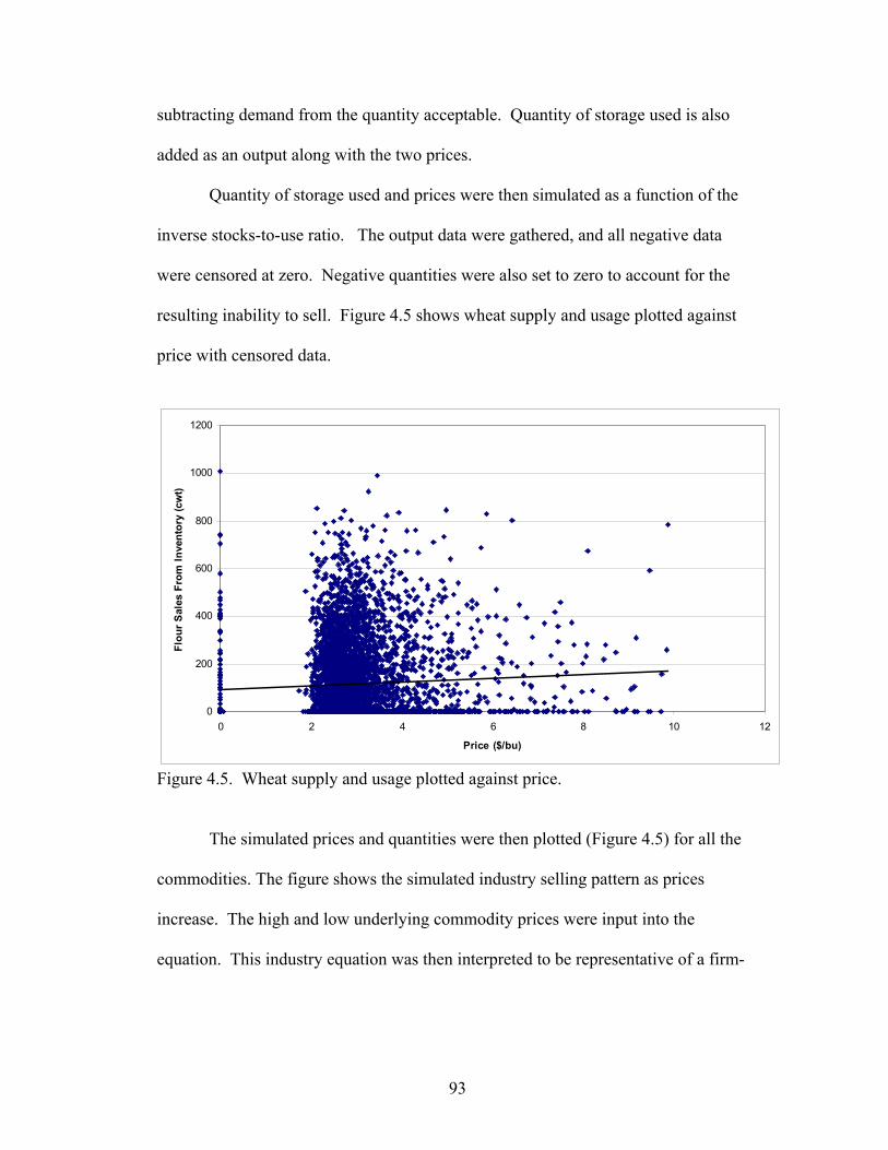
93
subtracting demand from the quantity acceptable. Quantity of storage used is also
added as an output along with the two prices.
Quantity of storage used and prices were then simulated as a function of the
inverse stocks-to-use ratio. The output data were gathered, and all negative data
were censored at zero. Negative quantities were also set to zero to account for the
resulting inability to sell. Figure 4.5 shows wheat supply and usage plotted against
price with censored data.
0
200
400
600
800
1000
1200
0 2 4 6 8 10 12
Price ($/bu)
Flou
r Sal
es F
rom
Inve
ntor
y (c
wt)
Figure 4.5. Wheat supply and usage plotted against price.
The simulated prices and quantities were then plotted (Figure 4.5) for all the
commodities. The figure shows the simulated industry selling pattern as prices
increase. The high and low underlying commodity prices were input into the
equation. This industry equation was then interpreted to be representative of a firm-
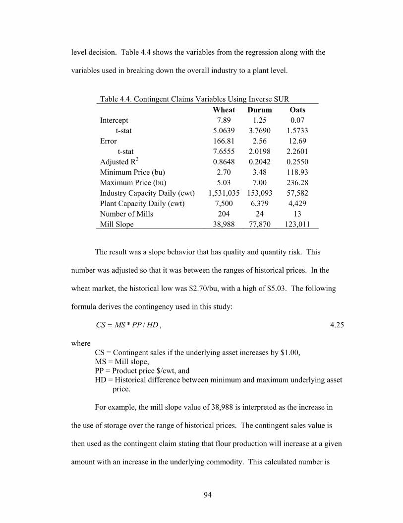
94
level decision. Table 4.4 shows the variables from the regression along with the
variables used in breaking down the overall industry to a plant level.
Table 4.4. Contingent Claims Variables Using Inverse SUR Wheat Durum Oats Intercept 7.89 1.25 0.07 t-stat 5.0639 3.7690 1.5733 Error 166.81 2.56 12.69 t-stat 7.6555 2.0198 2.2601 Adjusted R2 0.8648 0.2042 0.2550 Minimum Price (bu) 2.70 3.48 118.93 Maximum Price (bu) 5.03 7.00 236.28 Industry Capacity Daily (cwt) 1,531,035 153,093 57,582 Plant Capacity Daily (cwt) 7,500 6,379 4,429 Number of Mills 204 24 13 Mill Slope 38,988 77,870 123,011
The result was a slope behavior that has quality and quantity risk. This
number was adjusted so that it was between the ranges of historical prices. In the
wheat market, the historical low was $2.70/bu, with a high of $5.03. The following
formula derives the contingency used in this study:
HDPPMSCS /*= , 4.25
where CS = Contingent sales if the underlying asset increases by $1.00, MS = Mill slope, PP = Product price $/cwt, and
HD = Historical difference between minimum and maximum underlying asset price.
For example, the mill slope value of 38,988 is interpreted as the increase in
the use of storage over the range of historical prices. The contingent sales value is
then used as the contingent claim stating that flour production will increase at a given
amount with an increase in the underlying commodity. This calculated number is
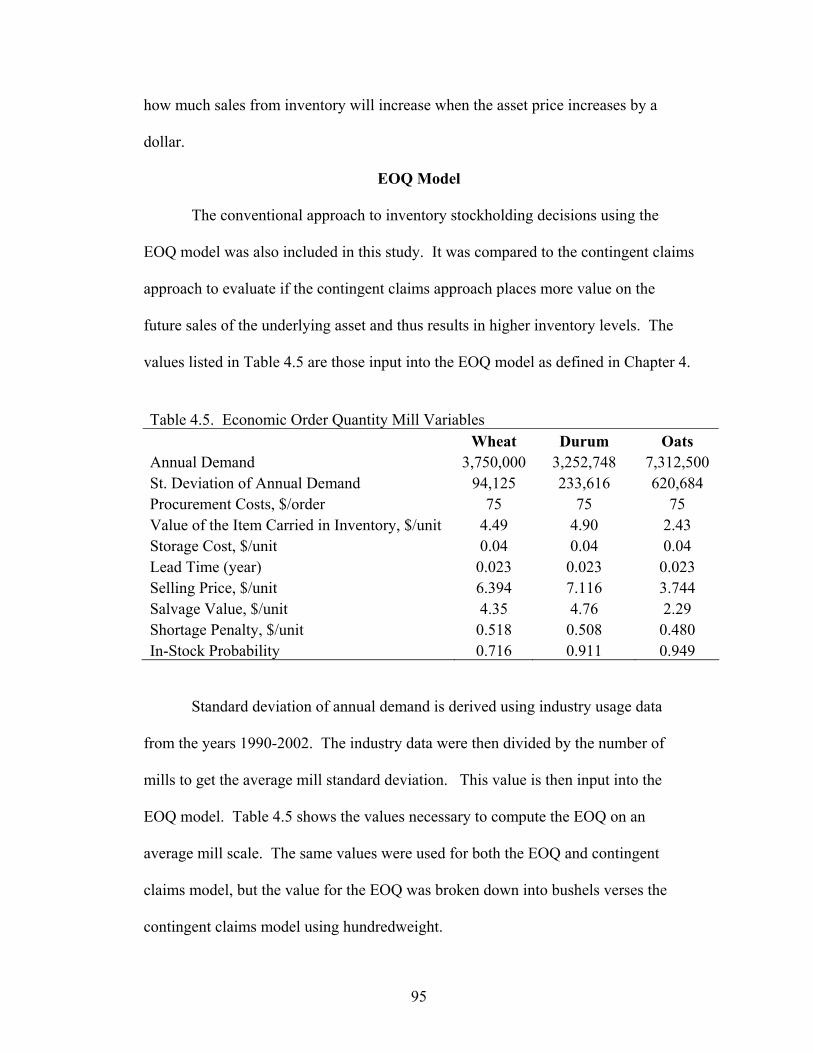
95
how much sales from inventory will increase when the asset price increases by a
dollar.
EOQ Model
The conventional approach to inventory stockholding decisions using the
EOQ model was also included in this study. It was compared to the contingent claims
approach to evaluate if the contingent claims approach places more value on the
future sales of the underlying asset and thus results in higher inventory levels. The
values listed in Table 4.5 are those input into the EOQ model as defined in Chapter 4.
Table 4.5. Economic Order Quantity Mill Variables Wheat Durum Oats Annual Demand 3,750,000 3,252,748 7,312,500 St. Deviation of Annual Demand 94,125 233,616 620,684 Procurement Costs, $/order 75 75 75 Value of the Item Carried in Inventory, $/unit 4.49 4.90 2.43 Storage Cost, $/unit 0.04 0.04 0.04 Lead Time (year) 0.023 0.023 0.023 Selling Price, $/unit 6.394 7.116 3.744 Salvage Value, $/unit 4.35 4.76 2.29 Shortage Penalty, $/unit 0.518 0.508 0.480 In-Stock Probability 0.716 0.911 0.949
Standard deviation of annual demand is derived using industry usage data
from the years 1990-2002. The industry data were then divided by the number of
mills to get the average mill standard deviation. This value is then input into the
EOQ model. Table 4.5 shows the values necessary to compute the EOQ on an
average mill scale. The same values were used for both the EOQ and contingent
claims model, but the value for the EOQ was broken down into bushels verses the
contingent claims model using hundredweight.
96
Data
Data Sources
Data used in this research was obtained from the following sources (Table
4.6).
Data Behavior
Stochastic and strategy variables are identified and included in the model.
The stochastic variables in the model introduce quality and quantity risk in addition to
the option valuation model to determine the optimal inventory carrying level.
The strategy variables in projecting the production and usage in a year include
production, domestic use, percent acceptable, and demand. These variables are
stochastic with the commands for @Risk shown in Table 4.7 for the base case.
Variations were made for the different commodities as needed.
Summary
Contingent claims models can be used where the optimal level of inventory
using options and the option value of carrying inventory are desired. When using
contingent claims as an inventory management tool, managers have to carefully
address the input values. The contingent claims inventory model has many different
variables that have a significant impact on the model. The values determine the
optimal state price which is more robust as it impounds the effects of risk and the
time value of money. The conventional stock-out probability uses an objective
function that is not risk neutral, and it also does not take into consideration the time
value of money. Values that are used for the variables in this study were all
explained earlier in this chapter.
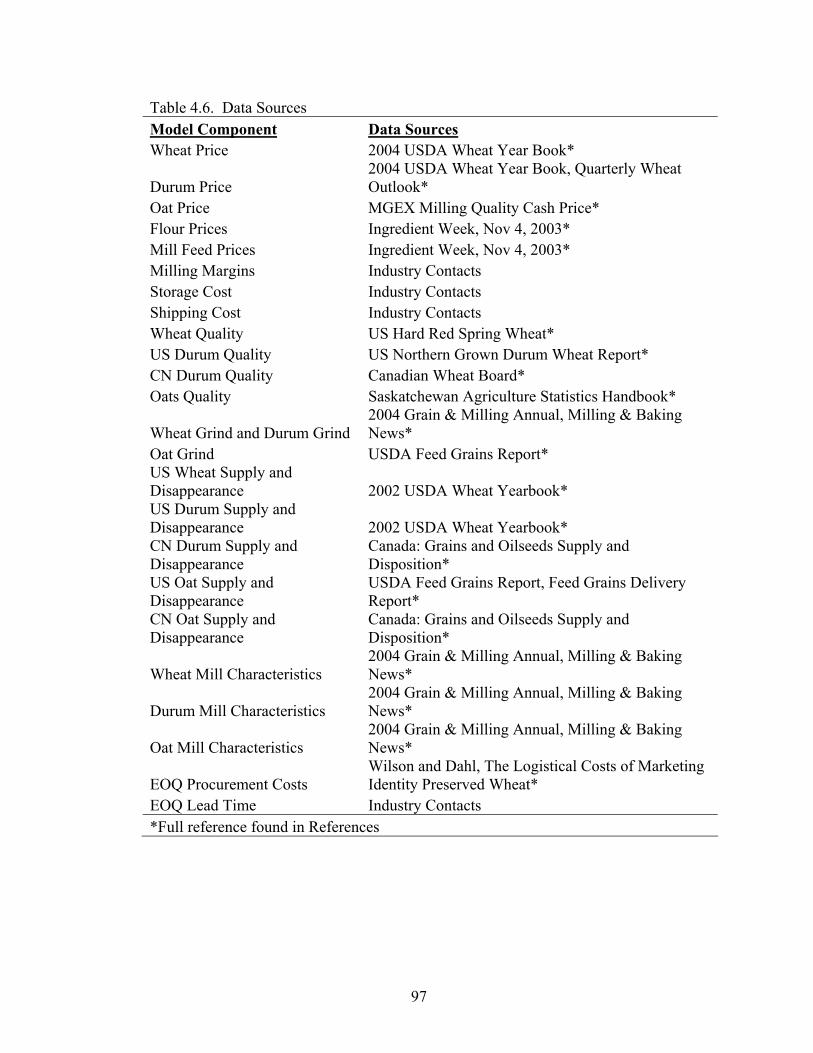
97
Table 4.6. Data Sources Model Component Data Sources Wheat Price 2004 USDA Wheat Year Book*
Durum Price 2004 USDA Wheat Year Book, Quarterly Wheat Outlook*
Oat Price MGEX Milling Quality Cash Price* Flour Prices Ingredient Week, Nov 4, 2003* Mill Feed Prices Ingredient Week, Nov 4, 2003* Milling Margins Industry Contacts Storage Cost Industry Contacts Shipping Cost Industry Contacts Wheat Quality US Hard Red Spring Wheat* US Durum Quality US Northern Grown Durum Wheat Report* CN Durum Quality Canadian Wheat Board* Oats Quality Saskatchewan Agriculture Statistics Handbook*
Wheat Grind and Durum Grind 2004 Grain & Milling Annual, Milling & Baking News*
Oat Grind USDA Feed Grains Report* US Wheat Supply and Disappearance 2002 USDA Wheat Yearbook* US Durum Supply and Disappearance 2002 USDA Wheat Yearbook* CN Durum Supply and Disappearance
Canada: Grains and Oilseeds Supply and Disposition*
US Oat Supply and Disappearance
USDA Feed Grains Report, Feed Grains Delivery Report*
CN Oat Supply and Disappearance
Canada: Grains and Oilseeds Supply and Disposition*
Wheat Mill Characteristics 2004 Grain & Milling Annual, Milling & Baking News*
Durum Mill Characteristics 2004 Grain & Milling Annual, Milling & Baking News*
Oat Mill Characteristics 2004 Grain & Milling Annual, Milling & Baking News*
EOQ Procurement Costs Wilson and Dahl, The Logistical Costs of Marketing Identity Preserved Wheat*
EOQ Lead Time Industry Contacts *Full reference found in References
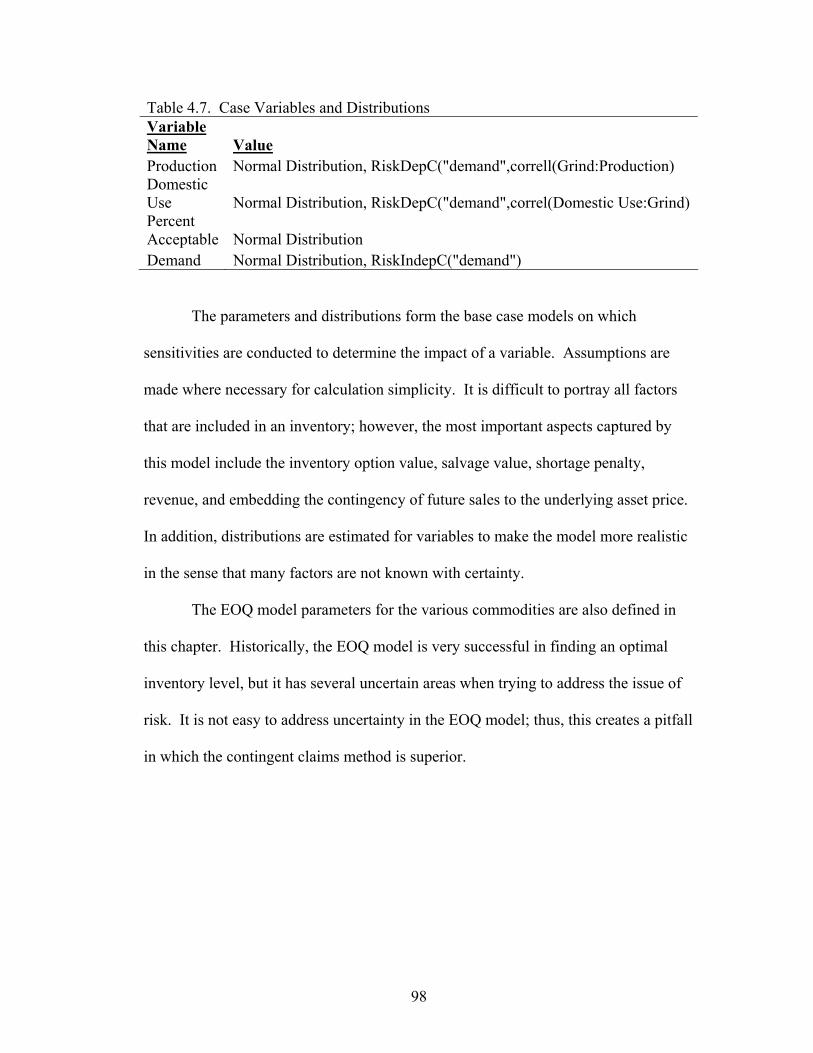
98
Table 4.7. Case Variables and Distributions Variable Name Value Production Normal Distribution, RiskDepC("demand",correll(Grind:Production) Domestic Use Normal Distribution, RiskDepC("demand",correl(Domestic Use:Grind) Percent Acceptable Normal Distribution Demand Normal Distribution, RiskIndepC("demand") The parameters and distributions form the base case models on which
sensitivities are conducted to determine the impact of a variable. Assumptions are
made where necessary for calculation simplicity. It is difficult to portray all factors
that are included in an inventory; however, the most important aspects captured by
this model include the inventory option value, salvage value, shortage penalty,
revenue, and embedding the contingency of future sales to the underlying asset price.
In addition, distributions are estimated for variables to make the model more realistic
in the sense that many factors are not known with certainty.
The EOQ model parameters for the various commodities are also defined in
this chapter. Historically, the EOQ model is very successful in finding an optimal
inventory level, but it has several uncertain areas when trying to address the issue of
risk. It is not easy to address uncertainty in the EOQ model; thus, this creates a pitfall
in which the contingent claims method is superior.
99
CHAPTER 5 RESULTS AND SENSITIVITIES
Introduction
Inventory can be viewed as a real option, specifically an option on future
sales. Real options create value in uncertain conditions and, using contingent claims
payoffs from inventory positions, can be mapped onto the underlying asset.
Contingent claims determine the optimal quantity using the state price and also create
an option on the inventory. Contingent claims are a valuable inventory management
tool. As there becomes more uncertainty in the commodity markets, it is creating
higher volatility, and to address this, it is necessary to use financial instruments that
account for the increased risk. Chapter 4 builds up the contingent claims model used
in this study, and this chapter will explain the results of the model.
This chapter includes the results from the base case models and a presentation
of the impacts that various strategy variables have on the optimal state price that has a
direct effect on inventory holding. Section one is a definition of the three different
commodity models for wheat, durum, and oats. The second section defines the
results of the economic order quantity (EOQ) model on each of the three commodity
models. The third section consists of sensitivities to the Case 3 model. A summary
of the results is presented in the last section. The base case models are designed to
represent a typical inventory situation in the various commodity milling industries
analyzed.
Base Case Model Definition and Results
Each of the models contains three separate cases. The first case does not
contain a salvage value or shortage penalty. The second contains a salvage value but
100
does not have a shortage penalty. Salvage value and shortage penalties are both
included in the third case.
Wheat Base Case
The grain in the wheat model is a northern spring wheat with 14+ percentage
protein. Since wheat can be directly hedged, the relevant risk is that of the basis risk.
Basis is defined as the difference between the current cash price and the futures price
of the same commodity (Chicago Board of Trade, 1989). The basis in the northern
spring wheat with 14+ percent protein market fluctuates, thus imposing uniqueness in
this grade of wheat.
In presenting the results, there are a number of important values that are
derived and interpreted. They were derived in the previous chapters and are defined
here prior to presenting the results. The optimal state price is the risk-neutral
probability of the underlying asset price exceeding the exercise price and the option
in the money. This optimal state price replaces the objective probability in the
conventional optimal stock-out probability and is more economically feasible because
it discounts for the time value of money. In option valuation, the optimal state price
is similar to the Greek delta in the Black-Scholes option pricing model. The exercise
price for the short call options is determined using the optimal state price representing
the exercise price for the short call option that maximizes the NPV of the inventory
storage function. When the short exercise price derived by the contingent claims
model is greater than the exercise price of the long position, a positive inventory is
suggested, else a short position is suggested to maximize the NPV. In some cases, the
optimal inventory level is positive; in others it is negative, but by definition, it is the
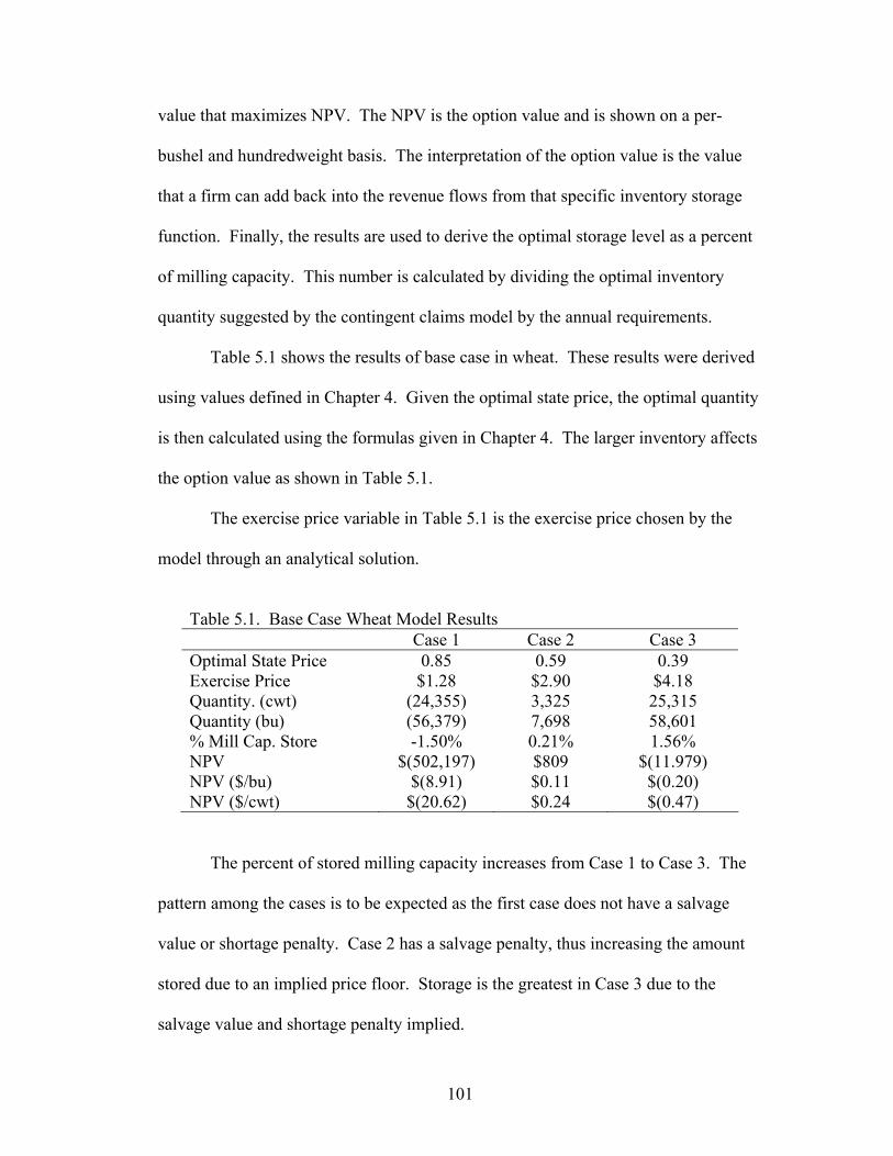
101
value that maximizes NPV. The NPV is the option value and is shown on a per-
bushel and hundredweight basis. The interpretation of the option value is the value
that a firm can add back into the revenue flows from that specific inventory storage
function. Finally, the results are used to derive the optimal storage level as a percent
of milling capacity. This number is calculated by dividing the optimal inventory
quantity suggested by the contingent claims model by the annual requirements.
Table 5.1 shows the results of base case in wheat. These results were derived
using values defined in Chapter 4. Given the optimal state price, the optimal quantity
is then calculated using the formulas given in Chapter 4. The larger inventory affects
the option value as shown in Table 5.1.
The exercise price variable in Table 5.1 is the exercise price chosen by the
model through an analytical solution.
Table 5.1. Base Case Wheat Model Results Case 1 Case 2 Case 3 Optimal State Price 0.85 0.59 0.39 Exercise Price $1.28 $2.90 $4.18 Quantity. (cwt) (24,355) 3,325 25,315 Quantity (bu) (56,379) 7,698 58,601 % Mill Cap. Store -1.50% 0.21% 1.56% NPV $(502,197) $809 $(11.979) NPV ($/bu) $(8.91) $0.11 $(0.20) NPV ($/cwt) $(20.62) $0.24 $(0.47)
The percent of stored milling capacity increases from Case 1 to Case 3. The
pattern among the cases is to be expected as the first case does not have a salvage
value or shortage penalty. Case 2 has a salvage penalty, thus increasing the amount
stored due to an implied price floor. Storage is the greatest in Case 3 due to the
salvage value and shortage penalty implied.
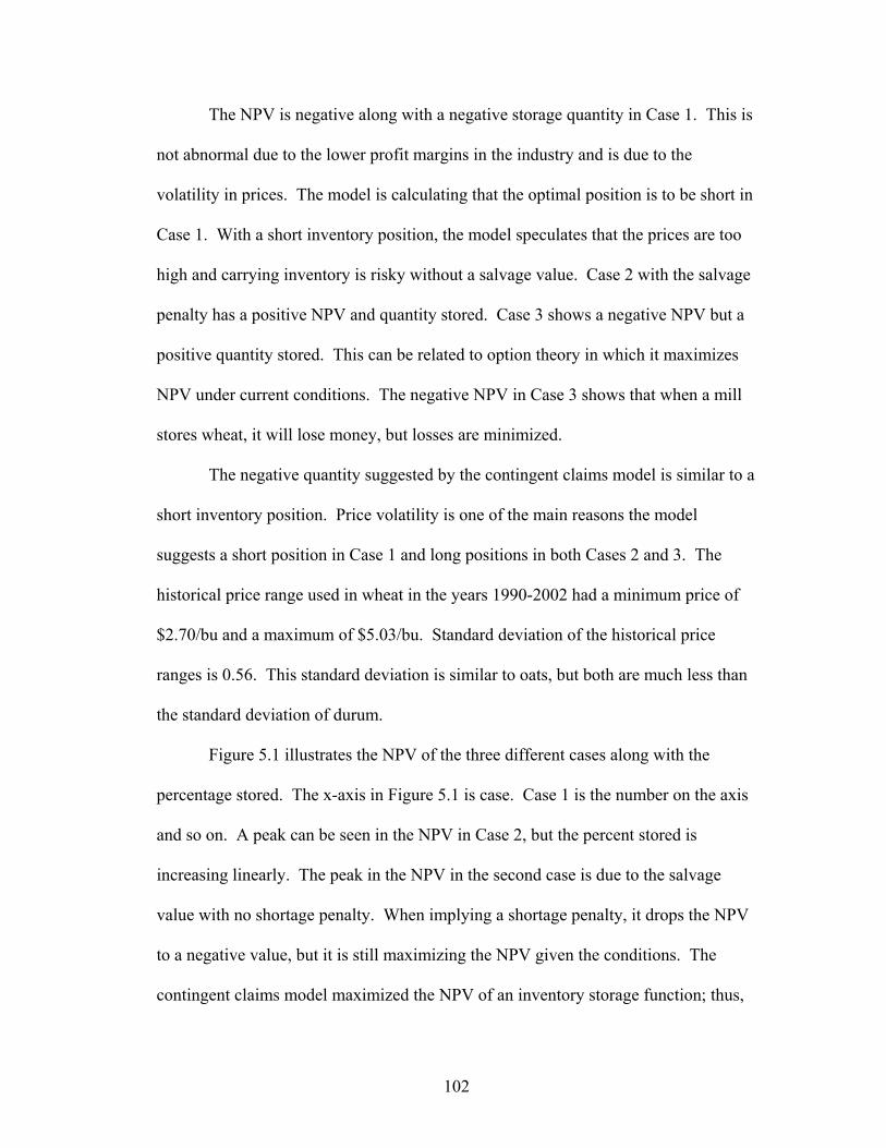
102
The NPV is negative along with a negative storage quantity in Case 1. This is
not abnormal due to the lower profit margins in the industry and is due to the
volatility in prices. The model is calculating that the optimal position is to be short in
Case 1. With a short inventory position, the model speculates that the prices are too
high and carrying inventory is risky without a salvage value. Case 2 with the salvage
penalty has a positive NPV and quantity stored. Case 3 shows a negative NPV but a
positive quantity stored. This can be related to option theory in which it maximizes
NPV under current conditions. The negative NPV in Case 3 shows that when a mill
stores wheat, it will lose money, but losses are minimized.
The negative quantity suggested by the contingent claims model is similar to a
short inventory position. Price volatility is one of the main reasons the model
suggests a short position in Case 1 and long positions in both Cases 2 and 3. The
historical price range used in wheat in the years 1990-2002 had a minimum price of
$2.70/bu and a maximum of $5.03/bu. Standard deviation of the historical price
ranges is 0.56. This standard deviation is similar to oats, but both are much less than
the standard deviation of durum.
Figure 5.1 illustrates the NPV of the three different cases along with the
percentage stored. The x-axis in Figure 5.1 is case. Case 1 is the number on the axis
and so on. A peak can be seen in the NPV in Case 2, but the percent stored is
increasing linearly. The peak in the NPV in the second case is due to the salvage
value with no shortage penalty. When implying a shortage penalty, it drops the NPV
to a negative value, but it is still maximizing the NPV given the conditions. The
contingent claims model maximized the NPV of an inventory storage function; thus,
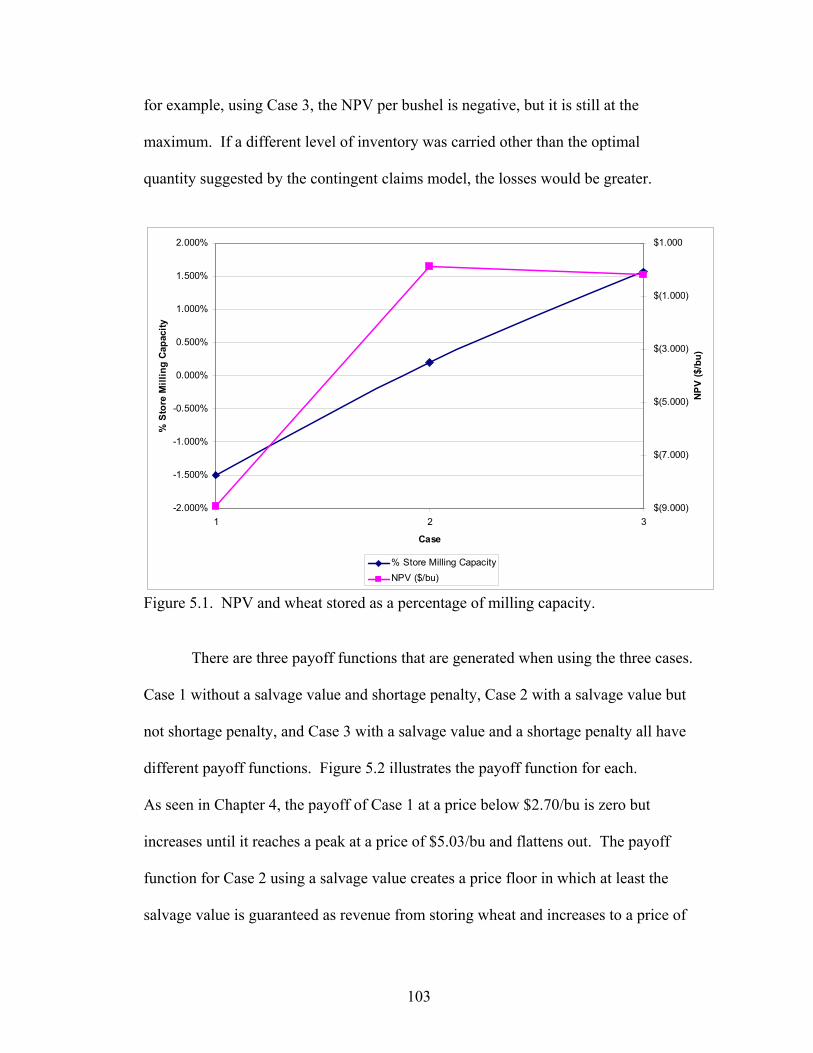
103
for example, using Case 3, the NPV per bushel is negative, but it is still at the
maximum. If a different level of inventory was carried other than the optimal
quantity suggested by the contingent claims model, the losses would be greater.
-2.000%
-1.500%
-1.000%
-0.500%
0.000%
0.500%
1.000%
1.500%
2.000%
1 2 3
Case
% S
tore
Mill
ing
Capa
city
$(9.000)
$(7.000)
$(5.000)
$(3.000)
$(1.000)
$1.000
NPV
($/b
u)
% Store Milling CapacityNPV ($/bu)
Figure 5.1. NPV and wheat stored as a percentage of milling capacity.
There are three payoff functions that are generated when using the three cases.
Case 1 without a salvage value and shortage penalty, Case 2 with a salvage value but
not shortage penalty, and Case 3 with a salvage value and a shortage penalty all have
different payoff functions. Figure 5.2 illustrates the payoff function for each.
As seen in Chapter 4, the payoff of Case 1 at a price below $2.70/bu is zero but
increases until it reaches a peak at a price of $5.03/bu and flattens out. The payoff
function for Case 2 using a salvage value creates a price floor in which at least the
salvage value is guaranteed as revenue from storing wheat and increases to a price of
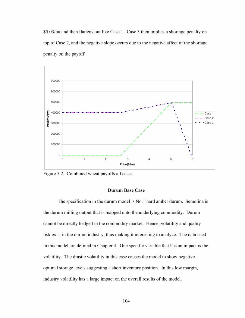
104
$5.03/bu and then flattens out like Case 1. Case 3 then implies a shortage penalty on
top of Case 2, and the negative slope occurs due to the negative affect of the shortage
penalty on the payoff.
Figure 5.2. Combined wheat payoffs all cases.
Durum Base Case
The specification in the durum model is No.1 hard amber durum. Semolina is
the durum milling output that is mapped onto the underlying commodity. Durum
cannot be directly hedged in the commodity market. Hence, volatility and quality
risk exist in the durum industry, thus making it interesting to analyze. The data used
in this model are defined in Chapter 4. One specific variable that has an impact is the
volatility. The drastic volatility in this case causes the model to show negative
optimal storage levels suggesting a short inventory position. In this low margin,
industry volatility has a large impact on the overall results of the model.
0
100000
200000
300000
400000
500000
600000
700000
0 1 2 3 4 5 6
Price($/bu)
Payo
ff($/
cwt)
Case 1Case 2Case 3
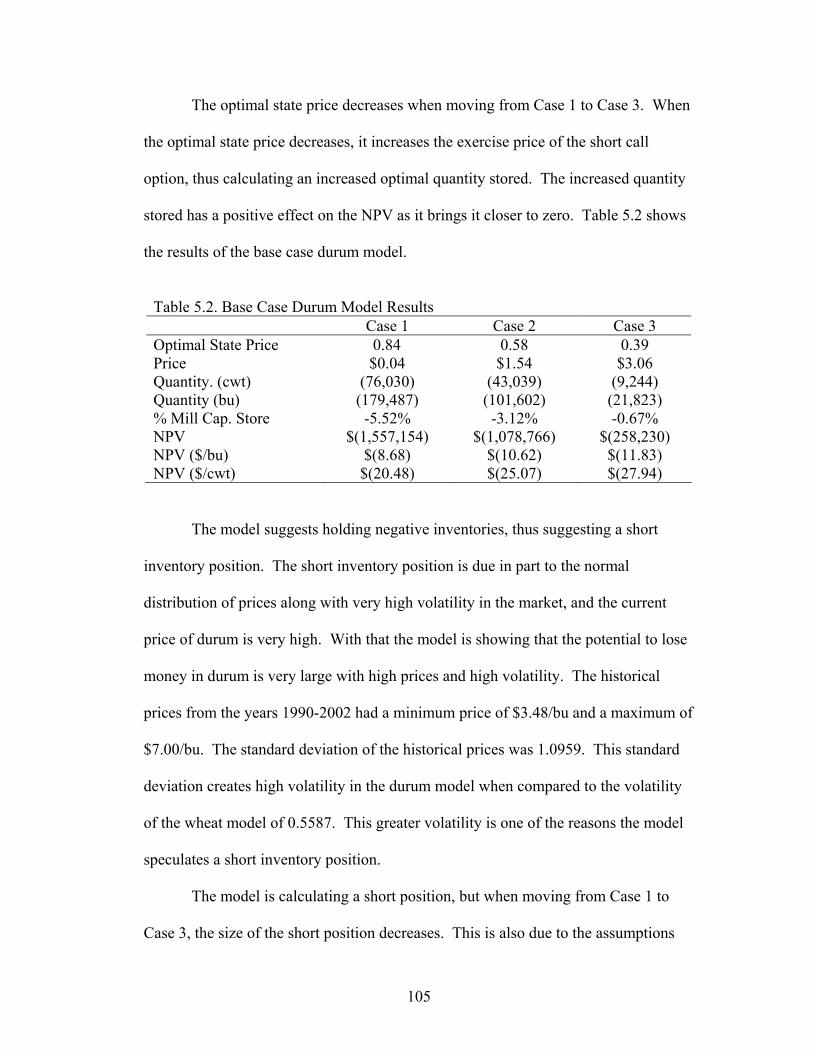
105
The optimal state price decreases when moving from Case 1 to Case 3. When
the optimal state price decreases, it increases the exercise price of the short call
option, thus calculating an increased optimal quantity stored. The increased quantity
stored has a positive effect on the NPV as it brings it closer to zero. Table 5.2 shows
the results of the base case durum model.
Table 5.2. Base Case Durum Model Results Case 1 Case 2 Case 3 Optimal State Price 0.84 0.58 0.39 Price $0.04 $1.54 $3.06 Quantity. (cwt) (76,030) (43,039) (9,244) Quantity (bu) (179,487) (101,602) (21,823) % Mill Cap. Store -5.52% -3.12% -0.67% NPV $(1,557,154) $(1,078,766) $(258,230) NPV ($/bu) $(8.68) $(10.62) $(11.83) NPV ($/cwt) $(20.48) $(25.07) $(27.94)
The model suggests holding negative inventories, thus suggesting a short
inventory position. The short inventory position is due in part to the normal
distribution of prices along with very high volatility in the market, and the current
price of durum is very high. With that the model is showing that the potential to lose
money in durum is very large with high prices and high volatility. The historical
prices from the years 1990-2002 had a minimum price of $3.48/bu and a maximum of
$7.00/bu. The standard deviation of the historical prices was 1.0959. This standard
deviation creates high volatility in the durum model when compared to the volatility
of the wheat model of 0.5587. This greater volatility is one of the reasons the model
speculates a short inventory position.
The model is calculating a short position, but when moving from Case 1 to
Case 3, the size of the short position decreases. This is also due to the assumptions
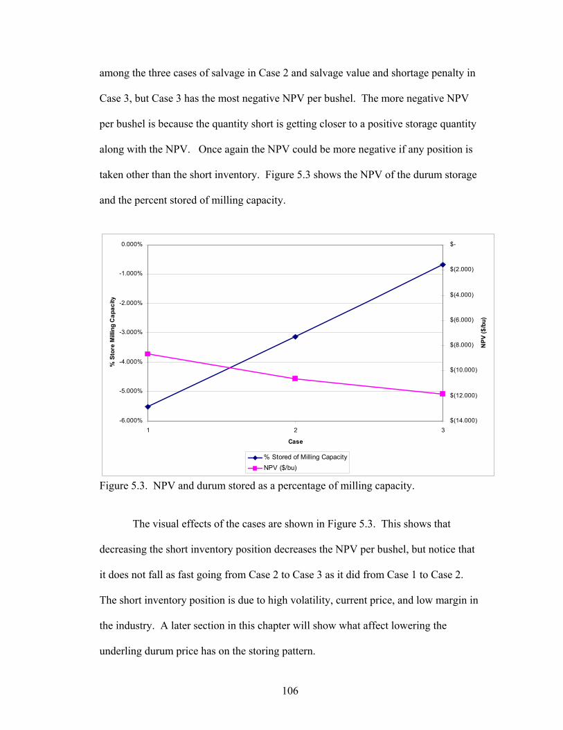
106
among the three cases of salvage in Case 2 and salvage value and shortage penalty in
Case 3, but Case 3 has the most negative NPV per bushel. The more negative NPV
per bushel is because the quantity short is getting closer to a positive storage quantity
along with the NPV. Once again the NPV could be more negative if any position is
taken other than the short inventory. Figure 5.3 shows the NPV of the durum storage
and the percent stored of milling capacity.
-6.000%
-5.000%
-4.000%
-3.000%
-2.000%
-1.000%
0.000%
1 2 3
Case
% S
tore
Mill
ing
Cap
acity
$(14.000)
$(12.000)
$(10.000)
$(8.000)
$(6.000)
$(4.000)
$(2.000)
$-
NPV
($/b
u)
% Stored of Milling CapacityNPV ($/bu)
Figure 5.3. NPV and durum stored as a percentage of milling capacity.
The visual effects of the cases are shown in Figure 5.3. This shows that
decreasing the short inventory position decreases the NPV per bushel, but notice that
it does not fall as fast going from Case 2 to Case 3 as it did from Case 1 to Case 2.
The short inventory position is due to high volatility, current price, and low margin in
the industry. A later section in this chapter will show what affect lowering the
underling durum price has on the storing pattern.
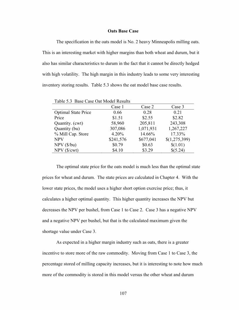
107
Oats Base Case
The specification in the oats model is No. 2 heavy Minneapolis milling oats.
This is an interesting market with higher margins than both wheat and durum, but it
also has similar characteristics to durum in the fact that it cannot be directly hedged
with high volatility. The high margin in this industry leads to some very interesting
inventory storing results. Table 5.3 shows the oat model base case results.
Table 5.3 Base Case Oat Model Results Case 1 Case 2 Case 3 Optimal State Price 0.66 0.28 0.21 Price $1.51 $2.55 $2.82 Quantity. (cwt) 58,960 205,811 243,308 Quantity (bu) 307,086 1,071,931 1,267,227 % Mill Cap. Store 4.20% 14.66% 17.33% NPV $241,576 $677,041 $(1,275,399) NPV ($/bu) $0.79 $0.63 $(1.01) NPV ($/cwt) $4.10 $3.29 $(5.24)
The optimal state price for the oats model is much less than the optimal state
prices for wheat and durum. The state prices are calculated in Chapter 4. With the
lower state prices, the model uses a higher short option exercise price; thus, it
calculates a higher optimal quantity. This higher quantity increases the NPV but
decreases the NPV per bushel, from Case 1 to Case 2. Case 3 has a negative NPV
and a negative NPV per bushel, but that is the calculated maximum given the
shortage value under Case 3.
As expected in a higher margin industry such as oats, there is a greater
incentive to store more of the raw commodity. Moving from Case 1 to Case 3, the
percentage stored of milling capacity increases, but it is interesting to note how much
more of the commodity is stored in this model versus the other wheat and durum
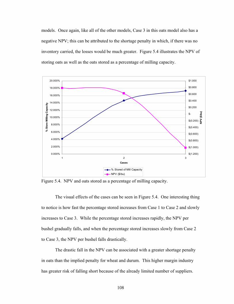
108
models. Once again, like all of the other models, Case 3 in this oats model also has a
negative NPV; this can be attributed to the shortage penalty in which, if there was no
inventory carried, the losses would be much greater. Figure 5.4 illustrates the NPV of
storing oats as well as the oats stored as a percentage of milling capacity.
0.000%
2.000%
4.000%
6.000%
8.000%
10.000%
12.000%
14.000%
16.000%
18.000%
20.000%
1 2 3
Cases
% S
tore
Mill
ing
Cap
acity
$(1.200)
$(1.000)
$(0.800)
$(0.600)
$(0.400)
$(0.200)
$-
$0.200
$0.400
$0.600
$0.800
$1.000
NPV
($/b
u)
% Stored of Mill CapacityNPV ($/bu)
Figure 5.4. NPV and oats stored as a percentage of milling capacity.
The visual effects of the cases can be seen in Figure 5.4. One interesting thing
to notice is how fast the percentage stored increases from Case 1 to Case 2 and slowly
increases to Case 3. While the percentage stored increases rapidly, the NPV per
bushel gradually falls, and when the percentage stored increases slowly from Case 2
to Case 3, the NPV per bushel falls drastically.
The drastic fall in the NPV can be associated with a greater shortage penalty
in oats than the implied penalty for wheat and durum. This higher margin industry
has greater risk of falling short because of the already limited number of suppliers.
109
The oats industry has different characteristics than the wheat and durum markets,
such as many suppliers and highly concentrated industry.
Base Case Comparison
The base cases are all different, and all three grains have characteristics that
created the differing inventory strategies. Wheat can be hedged but has high basis
risk, durum cannot be hedged but has high volatility, and oats cannot be hedged and
is a high margin industry. Table 5.4 shows the optimal state price, NPV per bushel,
and the percent store of milling capacity. The percent store of milling capacity is
found by dividing the optimal quantity by the annual requirements of the mill.
The optimal state price decreases when moving from Case 1 to Case 3 in all
three grains. In wheat and durum, the optimal state prices are similar in all three
cases, but when looking at oats, the optimal state prices are much less in all three
cases. The decrease in optimal state price is because of the value used for the
variables as shown in Chapter 4. The lower the optimal state price, the higher the
percent stored of milling capacity, or in durum, it is a smaller short inventory
position. The NPV per bushel in Case 3 is less than Case 2. This is due to the
shortage penalty in the model in which if the firm runs out of the grain, it loses
revenue, in which case the model is speculating to store more inventory to
compensate. The NPV per bushel shows the maximum option value that a firm can
gain using the contingent claim model. If the option value is negative, it simply
implies that storing is costing the firm money, but at a minimized amount when
compared to a non-optimal quantity.
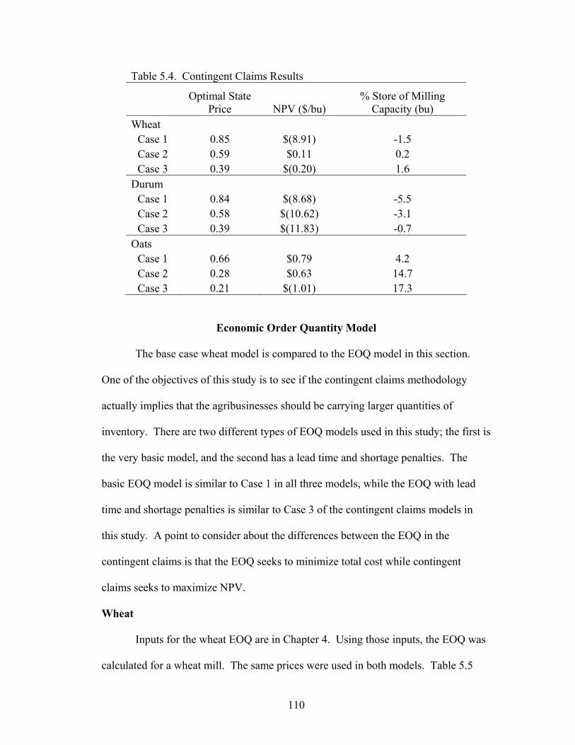
110
Table 5.4. Contingent Claims Results
Optimal State
Price NPV ($/bu) % Store of Milling
Capacity (bu) Wheat
Case 1 0.85 $(8.91) -1.5 Case 2 0.59 $0.11 0.2 Case 3 0.39 $(0.20) 1.6
Durum Case 1 0.84 $(8.68) -5.5 Case 2 0.58 $(10.62) -3.1 Case 3 0.39 $(11.83) -0.7
Oats Case 1 0.66 $0.79 4.2 Case 2 0.28 $0.63 14.7 Case 3 0.21 $(1.01) 17.3
Economic Order Quantity Model
The base case wheat model is compared to the EOQ model in this section.
One of the objectives of this study is to see if the contingent claims methodology
actually implies that the agribusinesses should be carrying larger quantities of
inventory. There are two different types of EOQ models used in this study; the first is
the very basic model, and the second has a lead time and shortage penalties. The
basic EOQ model is similar to Case 1 in all three models, while the EOQ with lead
time and shortage penalties is similar to Case 3 of the contingent claims models in
this study. A point to consider about the differences between the EOQ in the
contingent claims is that the EOQ seeks to minimize total cost while contingent
claims seeks to maximize NPV.
Wheat
Inputs for the wheat EOQ are in Chapter 4. Using those inputs, the EOQ was
calculated for a wheat mill. The same prices were used in both models. Table 5.5
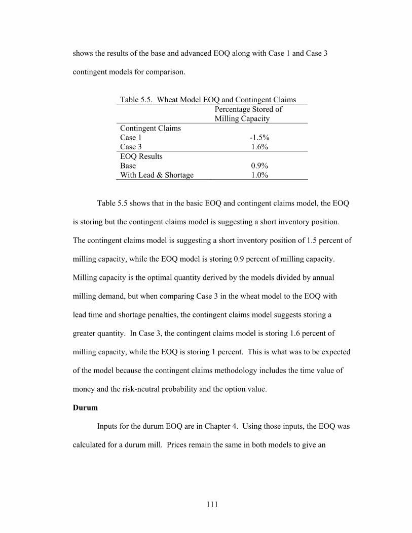
111
shows the results of the base and advanced EOQ along with Case 1 and Case 3
contingent models for comparison.
Table 5.5. Wheat Model EOQ and Contingent Claims
Percentage Stored of Milling Capacity
Contingent Claims Case 1 -1.5% Case 3 1.6% EOQ Results Base 0.9% With Lead & Shortage 1.0%
Table 5.5 shows that in the basic EOQ and contingent claims model, the EOQ
is storing but the contingent claims model is suggesting a short inventory position.
The contingent claims model is suggesting a short inventory position of 1.5 percent of
milling capacity, while the EOQ model is storing 0.9 percent of milling capacity.
Milling capacity is the optimal quantity derived by the models divided by annual
milling demand, but when comparing Case 3 in the wheat model to the EOQ with
lead time and shortage penalties, the contingent claims model suggests storing a
greater quantity. In Case 3, the contingent claims model is storing 1.6 percent of
milling capacity, while the EOQ is storing 1 percent. This is what was to be expected
of the model because the contingent claims methodology includes the time value of
money and the risk-neutral probability and the option value.
Durum
Inputs for the durum EOQ are in Chapter 4. Using those inputs, the EOQ was
calculated for a durum mill. Prices remain the same in both models to give an
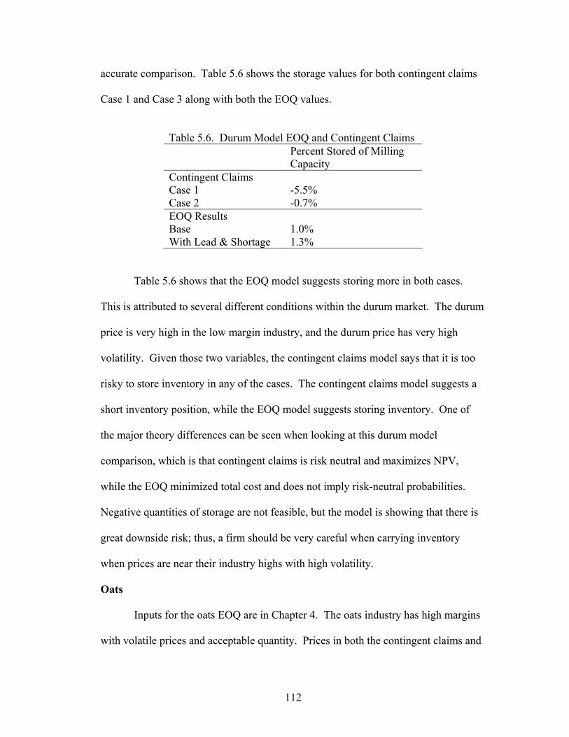
112
accurate comparison. Table 5.6 shows the storage values for both contingent claims
Case 1 and Case 3 along with both the EOQ values.
Table 5.6. Durum Model EOQ and Contingent Claims
Percent Stored of Milling Capacity
Contingent Claims Case 1 -5.5% Case 2 -0.7% EOQ Results Base 1.0% With Lead & Shortage 1.3%
Table 5.6 shows that the EOQ model suggests storing more in both cases.
This is attributed to several different conditions within the durum market. The durum
price is very high in the low margin industry, and the durum price has very high
volatility. Given those two variables, the contingent claims model says that it is too
risky to store inventory in any of the cases. The contingent claims model suggests a
short inventory position, while the EOQ model suggests storing inventory. One of
the major theory differences can be seen when looking at this durum model
comparison, which is that contingent claims is risk neutral and maximizes NPV,
while the EOQ minimized total cost and does not imply risk-neutral probabilities.
Negative quantities of storage are not feasible, but the model is showing that there is
great downside risk; thus, a firm should be very careful when carrying inventory
when prices are near their industry highs with high volatility.
Oats
Inputs for the oats EOQ are in Chapter 4. The oats industry has high margins
with volatile prices and acceptable quantity. Prices in both the contingent claims and
113
EOQ are the same to make an accurate comparison among the two models. The data
Table 5.7 show the results of the EOQ along with Case 1 and Case 3 of the contingent
claims.
Table 5.7. Oats Model EOQ and Contingent Claims
Percent Stored of Milling
Capacity Contingent Claims Case 1 4.2% Case 2 15.9% EOQ Basic 0.7% Lead Time 1.0%
Table 5.7 shows that the EOQ model suggests storing much less than the
contingent claims approach in both cases. This is much different than is seen in both
the wheat and durum. In this higher margin industry, it is more valuable to store.
With higher margins in the industry, there is much greater potential for losses and
foregone earnings if a shortage occurs. The contingent claims model suggests storing
more quantity due to a few different reasons. The first is that it is a high-profit
industry with volatility, and if a shortage occurs, it has a great effect on profits; thus,
storing may return a negative NPV, but it is more profitable than the next best option
which is not to store. The second thing is that the shortage penalty in this market is
much greater due to the fact the industry does not have as much excess production as
can be seen in the wheat and durum industry.
Sensitivities
Stochastic variables are used to demonstrate risks that are present in carrying
inventory. The main uncertainty is in the commodity markets. Sensitivities are
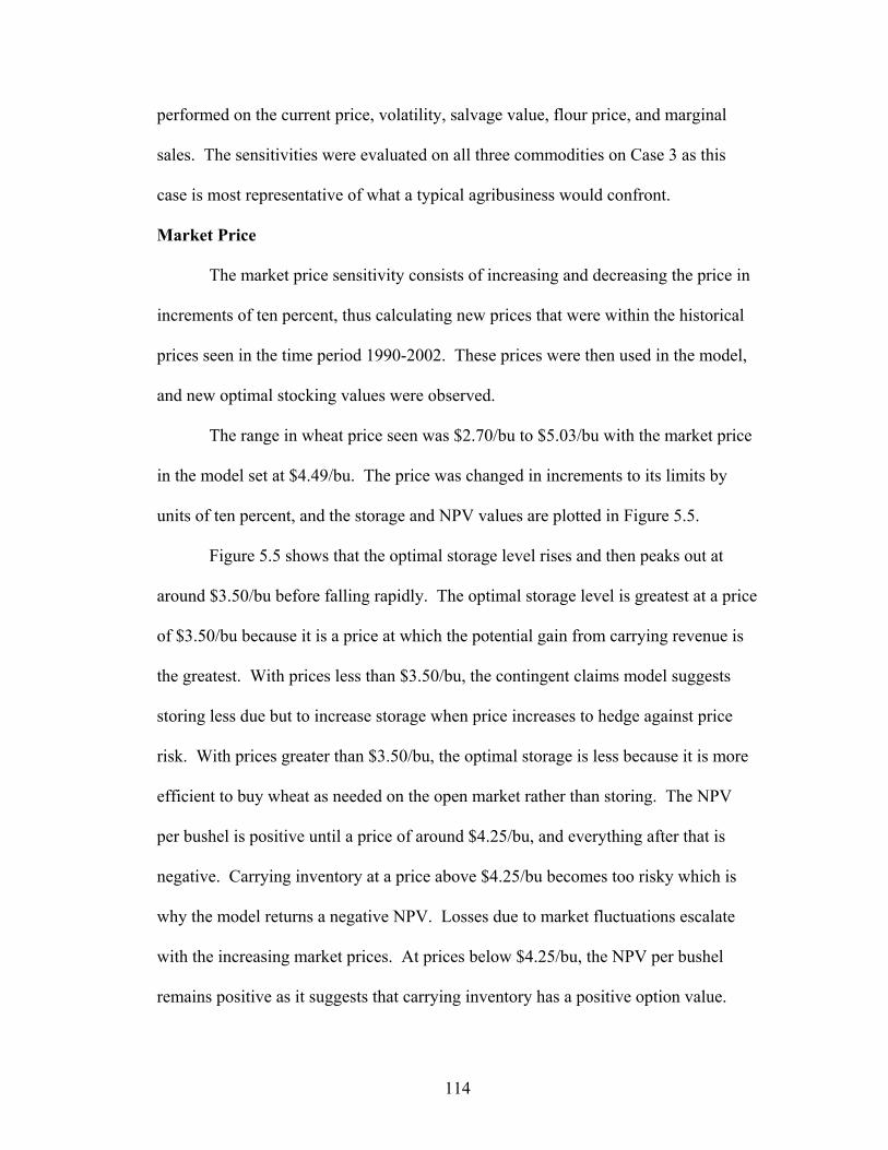
114
performed on the current price, volatility, salvage value, flour price, and marginal
sales. The sensitivities were evaluated on all three commodities on Case 3 as this
case is most representative of what a typical agribusiness would confront.
Market Price
The market price sensitivity consists of increasing and decreasing the price in
increments of ten percent, thus calculating new prices that were within the historical
prices seen in the time period 1990-2002. These prices were then used in the model,
and new optimal stocking values were observed.
The range in wheat price seen was $2.70/bu to $5.03/bu with the market price
in the model set at $4.49/bu. The price was changed in increments to its limits by
units of ten percent, and the storage and NPV values are plotted in Figure 5.5.
Figure 5.5 shows that the optimal storage level rises and then peaks out at
around $3.50/bu before falling rapidly. The optimal storage level is greatest at a price
of $3.50/bu because it is a price at which the potential gain from carrying revenue is
the greatest. With prices less than $3.50/bu, the contingent claims model suggests
storing less due but to increase storage when price increases to hedge against price
risk. With prices greater than $3.50/bu, the optimal storage is less because it is more
efficient to buy wheat as needed on the open market rather than storing. The NPV
per bushel is positive until a price of around $4.25/bu, and everything after that is
negative. Carrying inventory at a price above $4.25/bu becomes too risky which is
why the model returns a negative NPV. Losses due to market fluctuations escalate
with the increasing market prices. At prices below $4.25/bu, the NPV per bushel
remains positive as it suggests that carrying inventory has a positive option value.
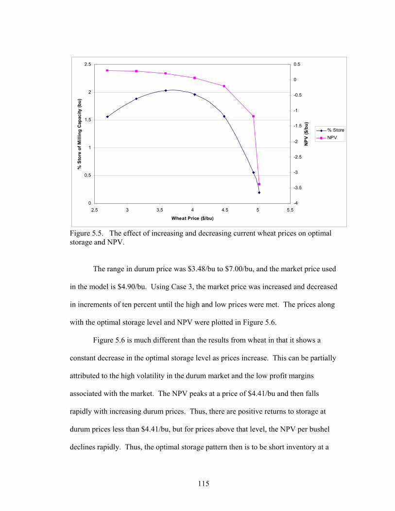
115
Figure 5.5. The effect of increasing and decreasing current wheat prices on optimal storage and NPV. The range in durum price was $3.48/bu to $7.00/bu, and the market price used
in the model is $4.90/bu. Using Case 3, the market price was increased and decreased
in increments of ten percent until the high and low prices were met. The prices along
with the optimal storage level and NPV were plotted in Figure 5.6.
Figure 5.6 is much different than the results from wheat in that it shows a
constant decrease in the optimal storage level as prices increase. This can be partially
attributed to the high volatility in the durum market and the low profit margins
associated with the market. The NPV peaks at a price of $4.41/bu and then falls
rapidly with increasing durum prices. Thus, there are positive returns to storage at
durum prices less than $4.41/bu, but for prices above that level, the NPV per bushel
declines rapidly. Thus, the optimal storage pattern then is to be short inventory at a
0
0.5
1
1.5
2
2.5
2.5 3 3.5 4 4.5 5 5.5
Wheat Price ($/bu)
% S
tore
of M
illin
g Ca
paci
ty (b
u)
-4
-3.5
-3
-2.5
-2
-1.5
-1
-0.5
0
0.5
NPV
($/b
u)
% StoreNPV
116
durum price above $4.41/bu. Furthermore, the optimal storage level is positive so
long as the prices are less than $4.41/bu, and then they decline. The reason for this is
that at a price above $4.41/bu, the contingent claims model suggests it is too risky to
store given the high volatility in the market and the low margins.
-4
-3
-2
-1
0
1
2
3
4
3.3 3.8 4.3 4.8 5.3 5.8
Durum Price ($/bu)
% S
tore
of M
illin
g Ca
paci
ty (b
u)
-14
-12
-10
-8
-6
-4
-2
0
2
NPV
($/b
u)
% StoreNPV
Figure 5.6. The effect of increasing and decreasing current durum prices on optimal storage and NPV. The observed range in oat price was $1.09/bu to $2.77/bu, and the market
price in the base case was $2.43/bu. The optimal storage level and NPV are plotted in
Figure 5.7 below.
The results show that optimal storage levels increase with increased oat prices.
At a price below $1.90/bu, the contingent claims model suggests positive storage
even though the returns on that storage are negative. This is because it is still
beneficial to store oats because the risk of a shortage is too overwhelming, thus the
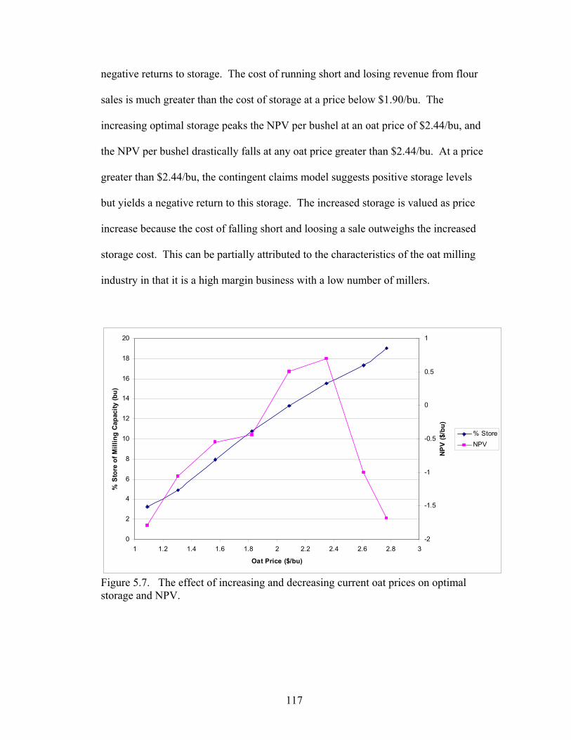
117
negative returns to storage. The cost of running short and losing revenue from flour
sales is much greater than the cost of storage at a price below $1.90/bu. The
increasing optimal storage peaks the NPV per bushel at an oat price of $2.44/bu, and
the NPV per bushel drastically falls at any oat price greater than $2.44/bu. At a price
greater than $2.44/bu, the contingent claims model suggests positive storage levels
but yields a negative return to this storage. The increased storage is valued as price
increase because the cost of falling short and loosing a sale outweighs the increased
storage cost. This can be partially attributed to the characteristics of the oat milling
industry in that it is a high margin business with a low number of millers.
0
2
4
6
8
10
12
14
16
18
20
1 1.2 1.4 1.6 1.8 2 2.2 2.4 2.6 2.8 3
Oat Price ($/bu)
% S
tore
of M
illin
g Ca
paci
ty (b
u)
-2
-1.5
-1
-0.5
0
0.5
1
NPV
($/b
u)% StoreNPV
Figure 5.7. The effect of increasing and decreasing current oat prices on optimal storage and NPV.
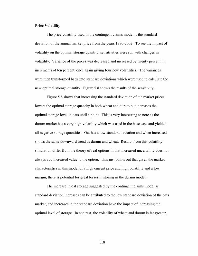
118
Price Volatility
The price volatility used in the contingent claims model is the standard
deviation of the annual market price from the years 1990-2002. To see the impact of
volatility on the optimal storage quantity, sensitivities were run with changes in
volatility. Variance of the prices was decreased and increased by twenty percent in
increments of ten percent, once again giving four new volatilities. The variances
were then transformed back into standard deviations which were used to calculate the
new optimal storage quantity. Figure 5.8 shows the results of the sensitivity.
Figure 5.8 shows that increasing the standard deviation of the market prices
lowers the optimal storage quantity in both wheat and durum but increases the
optimal storage level in oats until a point. This is very interesting to note as the
durum market has a very high volatility which was used in the base case and yielded
all negative storage quantities. Oat has a low standard deviation and when increased
shows the same downward trend as durum and wheat. Results from this volatility
simulation differ from the theory of real options in that increased uncertainty does not
always add increased value to the option. This just points out that given the market
characteristics in this model of a high current price and high volatility and a low
margin, there is potential for great losses in storing in the durum model.
The increase in oat storage suggested by the contingent claims model as
standard deviation increases can be attributed to the low standard deviation of the oats
market, and increases in the standard deviation have the impact of increasing the
optimal level of storage. In contrast, the volatility of wheat and durum is far greater,
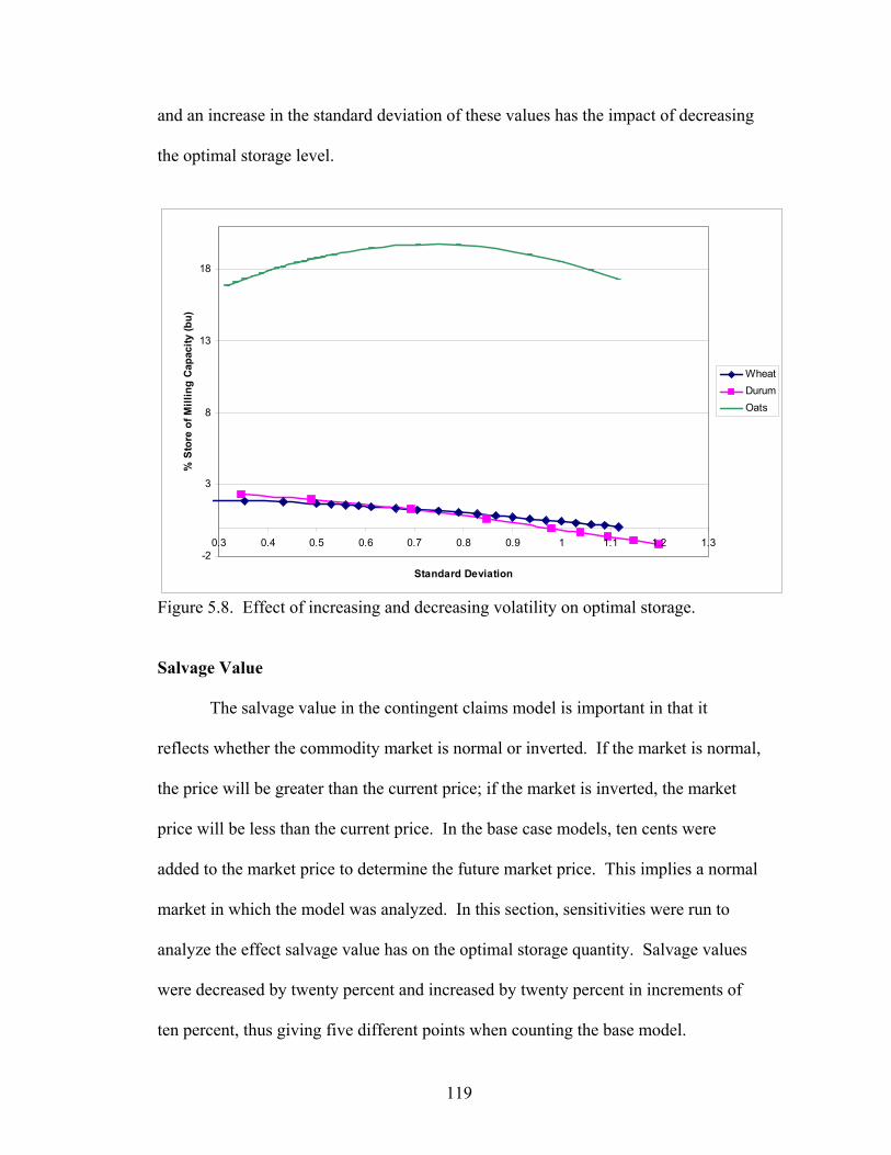
119
and an increase in the standard deviation of these values has the impact of decreasing
the optimal storage level.
-2
3
8
13
18
0.3 0.4 0.5 0.6 0.7 0.8 0.9 1 1.1 1.2 1.3
Standard Deviation
% S
tore
of M
illin
g Ca
paci
ty (b
u)
WheatDurumOats
Figure 5.8. Effect of increasing and decreasing volatility on optimal storage. Salvage Value
The salvage value in the contingent claims model is important in that it
reflects whether the commodity market is normal or inverted. If the market is normal,
the price will be greater than the current price; if the market is inverted, the market
price will be less than the current price. In the base case models, ten cents were
added to the market price to determine the future market price. This implies a normal
market in which the model was analyzed. In this section, sensitivities were run to
analyze the effect salvage value has on the optimal storage quantity. Salvage values
were decreased by twenty percent and increased by twenty percent in increments of
ten percent, thus giving five different points when counting the base model.
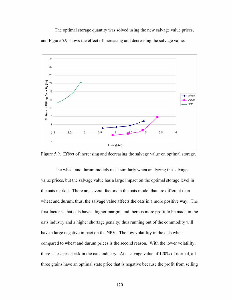
120
The optimal storage quantity was solved using the new salvage value prices,
and Figure 5.9 shows the effect of increasing and decreasing the salvage value.
-6
-2
2
6
10
14
18
22
26
30
34
2 2.5 3 3.5 4 4.5 5 5.5 6
Price ($/bu)
% S
tore
of M
illin
g Ca
paci
ty (b
u)
WheatDurumOats
Figure 5.9. Effect of increasing and decreasing the salvage value on optimal storage. The wheat and durum models react similarly when analyzing the salvage
value prices, but the salvage value has a large impact on the optimal storage level in
the oats market. There are several factors in the oats model that are different than
wheat and durum; thus, the salvage value affects the oats in a more positive way. The
first factor is that oats have a higher margin, and there is more profit to be made in the
oats industry and a higher shortage penalty; thus running out of the commodity will
have a large negative impact on the NPV. The low volatility in the oats when
compared to wheat and durum prices is the second reason. With the lower volatility,
there is less price risk in the oats industry. At a salvage value of 120% of normal, all
three grains have an optimal state price that is negative because the profit from selling
121
the grain is greater than the profit of selling the flour. Wheat has all positive optimal
storage levels; when the salvage value is at 80% of normal, the optimal storage level
almost reaches zero. When the salvage value of durum is 110% of normal, the
contingent claims model suggests storing, but at any level less than that, the model
suggests having a short inventory position. This short inventory position when the
salvage value is decreased is because it becomes more risky to store durum due to the
high volatility in prices. There would be potential to lose a lot of money in the durum
market without the price floor imposed by the salvage value. Oats has a very positive
and highly sloped line when the salvage value is analyzed. This is partially attributed
to the oats market with its greater margins.
The optimal state price decreases as the salvage value increases. The optimal
state price decreases because the salvage value is in the denominator of the optimal
state price formula; thus, as the salvage value increases, the optimal state price
declines, and the contingent claims model suggests storing a greater optimal quantity.
Percent stored of milling capacity increases as the optimal state price decreases.
Smaller optimal state prices in the Black-Scholes model suggest an exercise price of
the short call option to increase. When the exercise price of the short call option
increases relative to the exercise price of the long call option, a higher optimal
quantity is suggested; this is part of the contingent claims formulation. As the
salvage value increases, there is an increase in the option value or NPV per bushel.
This increase in NPV is associated with the ability to liquidate the asset at a higher
price due to the increase in salvage value. Thus, as the salvage value increases, the
option value of carrying inventory increases. Increasing the salvage value decreases
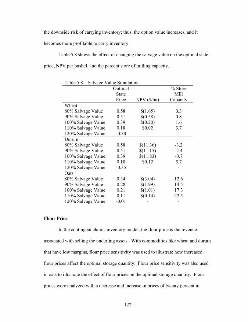
122
the downside risk of carrying inventory; thus, the option value increases, and it
becomes more profitable to carry inventory.
Table 5.8 shows the effect of changing the salvage value on the optimal state
price, NPV per bushel, and the percent store of milling capacity.
Table 5.8. Salvage Value Simulation
Optimal State Price NPV ($/bu)
% Store Mill
Capacity Wheat 80% Salvage Value 0.58 $(1.65) 0.3 90% Salvage Value 0.51 $(0.58) 0.8 100% Salvage Value 0.39 $(0.20) 1.6 110% Salvage Value 0.18 $0.02 3.7 120% Salvage Value -0.30 - - Durum 80% Salvage Value 0.58 $(11.36) -3.2 90% Salvage Value 0.51 $(11.15) -2.4 100% Salvage Value 0.39 $(11.83) -0.7 110% Salvage Value 0.18 $0.12 5.7 120% Salvage Value -0.35 - - Oats 80% Salvage Value 0.34 $(3.04) 12.6 90% Salvage Value 0.28 $(1.99) 14.5 100% Salvage Value 0.21 $(1.01) 17.3 110% Salvage Value 0.11 $(0.14) 22.5 120% Salvage Value -0.01 - -
Flour Price
In the contingent claims inventory model, the flour price is the revenue
associated with selling the underling assets. With commodities like wheat and durum
that have low margins, flour price sensitivity was used to illustrate how increased
flour prices affect the optimal storage quantity. Flour price sensitivity was also used
in oats to illustrate the effect of flour prices on the optimal storage quantity. Flour
prices were analyzed with a decrease and increase in prices of twenty percent in
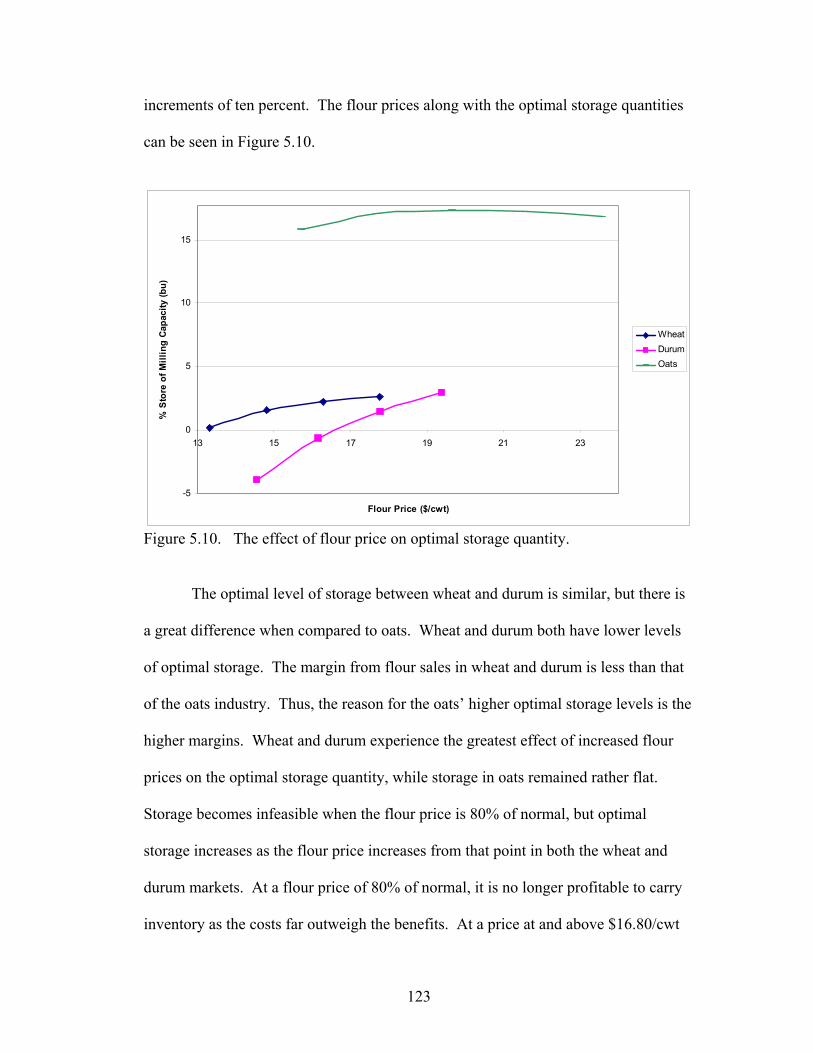
123
increments of ten percent. The flour prices along with the optimal storage quantities
can be seen in Figure 5.10.
-5
0
5
10
15
13 15 17 19 21 23
Flour Price ($/cwt)
% S
tore
of M
illin
g Ca
paci
ty (b
u)
WheatDurumOats
Figure 5.10. The effect of flour price on optimal storage quantity. The optimal level of storage between wheat and durum is similar, but there is
a great difference when compared to oats. Wheat and durum both have lower levels
of optimal storage. The margin from flour sales in wheat and durum is less than that
of the oats industry. Thus, the reason for the oats’ higher optimal storage levels is the
higher margins. Wheat and durum experience the greatest effect of increased flour
prices on the optimal storage quantity, while storage in oats remained rather flat.
Storage becomes infeasible when the flour price is 80% of normal, but optimal
storage increases as the flour price increases from that point in both the wheat and
durum markets. At a flour price of 80% of normal, it is no longer profitable to carry
inventory as the costs far outweigh the benefits. At a price at and above $16.80/cwt
124
of flour, the contingent claims model suggests a positive storage. Oat flour price
increased the optimal storage level to a point and then caused the optimal storage
level to decrease at a point of greater than normal flour price. The high flour price in
relation to the underlying grain reaches a saturation point where there is no more
added benefit to storing more oats even if the flour price is increasing. This is to be
expected as oats already have a large implied margin; thus, increasing the flour price
will not have the same effect as it would on durum and wheat. Wheat and durum
optimal storage quantities increase fairly rapidly with durum seeing the greatest
increase of the two.
Marginal Sales
Using contingent claims methodology to model the optimal inventory quantity
requires a link between sales and the underlying asset. In this study, the output of
flour was linked to the underlying input which is the raw commodity. This variable is
the contingent claim as it shows how much sales would increase with an increase in
the underlying asset price. This is the parameter that does not have an effect on the
optimal state price, but it does have an effect on the optimal order quantity. In this
case, this relationship was estimated, and the result is a variable that shows how
storage needs increase as the underlying grain price increases, which is in contrast
with Stowe and Su (1997) who simply assumed that sales will increase 10 units for
every $1 increase in the underlying asset. Regression results were used to derive
prototypical relationships. Wheat regression calculated an added increase in sales
from inventory at 38,988 cwt, durum had an increase of 77,870 cwt, and oats had an
increase in sales from inventory of 123,011 cwt. These values were then divided by
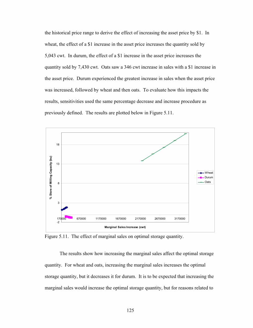
125
the historical price range to derive the effect of increasing the asset price by $1. In
wheat, the effect of a $1 increase in the asset price increases the quantity sold by
5,043 cwt. In durum, the effect of a $1 increase in the asset price increases the
quantity sold by 7,430 cwt. Oats saw a 346 cwt increase in sales with a $1 increase in
the asset price. Durum experienced the greatest increase in sales when the asset price
was increased, followed by wheat and then oats. To evaluate how this impacts the
results, sensitivities used the same percentage decrease and increase procedure as
previously defined. The results are plotted below in Figure 5.11.
-2
3
8
13
18
170000 670000 1170000 1670000 2170000 2670000 3170000
Marginal Sales Increase (cwt)
% S
tore
of M
illin
g Ca
paci
ty (b
u)
WheatDurumOats
Figure 5.11. The effect of marginal sales on optimal storage quantity.
The results show how increasing the marginal sales affect the optimal storage
quantity. For wheat and oats, increasing the marginal sales increases the optimal
storage quantity, but it decreases it for durum. It is to be expected that increasing the
marginal sales would increase the optimal storage quantity, but for reasons related to
126
the parameters in the durum model, it returns the opposite results. The durum model
has several unique features to it. It has a very high volatility and high market prices
that are near the upper limits of the distribution of historical prices. This has an effect
on why the durum has a negative slope.
Summary
Market trends that have increased volatility along with quality shortfalls have
pressed the issue of storage as of late. There are several ways to address this issue of
quality shortfalls, and one of the ways is through storage and carrying increased
stocks. Conventional models have a hard time capturing the increased volatility and
quality shortfalls that are seen in the market. This chapter gives the results of the
contingent claims model outlined in Chapter 4. The contingent claims model places
value on the uncertainty in the marketplace and seeks to maximize the NPV of the
storage function.
There are several highly sensitive variables in the contingent claims model
that have different effects on the various grains in this study. Wheat with its high
basis risk, along with durum and oat which are commodities that cannot be directly
hedged, were analyzed in this chapter. Sensitivities were performed on the variables
to illustrate the effect they have on the optimal storage level and also the NPV per
bushel.
There are many results and sensitivities in this chapter that are useful to
understand and have varying impacts on the optimal storage strategy. The major
results are
127
1. Wheat has positive storage values in all three cases, and Case 3 of the wheat
contingent claims model suggests storing a greater amount than the EOQ model.
2. Durum with its high volatility in the market returns a short inventory position
using the contingent claims but a positive position using the EOQ model.
3. Oats with is high margin and fairly low price volatility maintains a highly positive
optimal storage level that is far greater in the contingent claims model than the
EOQ model.
4. When market price is adjusted using a sensitivity, it shows that there is increasing
returns to a point and then there are decreasing returns.
5. Price volatility has an overall negative effect on the optimal storage level except
in the oats model where there is already low market volatility. Thus, increasing
the volatility in the wheat and durum model decreases the optimal storage level
suggested by the contingent claims model.
6. Increasing the salvage value has a positive effect on the optimal storage quantity.
When the salvage value is increased, it suggests a positive return to storage; thus,
the contingent claims model suggests storing a greater quantity.
7. Flour price has a positive effect on the overall optimal storage quantity. In both
the wheat and durum markets, the optimal storage quantity can see a rapid
increase with an increase in the flour price, but oats, on the other hand, shows a
peak in the optimal order quantity.
The contingent claims model provides another tool in which mangers can analyze
their inventory strategy, but there are several key variables that have a substantial
impact on the overall optimal inventory level suggested by the contingent claims
128
model. Sensitivities were used on these variables to see their effect on the optimal
inventory level.
129
CHAPTER 6 SUMMARY
Review of Problem
An increase in the complexity of the grain marketing system is occurring and
may become further complicated with more frequent quantity and quality shortfalls.
The complexity is due to several developments. First, there is increased pressure on
farmers to grow crops that are more economically feasible, thus shifting the
production of some grains to other countries and then having to import the
commodities. In addition, slight changes in the overall weather conditions affect the
quality of the commodity drastically, and millers seek the highest quality for food
grade. Furthermore, commodities considered in this study are high risk. High-
protein spring wheat can be hedged, but it has very high basis risk, and hard amber
durum and milling oats cannot be directly hedged.
Commodity prices in the agricultural industry are very important due to their
effect on not only producers but also processors. This research examined how the
underlying commodity price and risk affect their optimal storage level along with the
profitability of storage. Inventories can be regarded as real options and can be
viewed as call options because they require an initial investment. This initial
investment is an option on future sales. Using the contingent claims methodology,
the optimal inventory level along with the net present value (NPV) or option value
can be derived. The option value is the added benefit of carrying inventories that is
added back into the revenue flows.
Contingent claims models were used in this study to value inventories and
evaluate storage decisions. Contingent claims place value on uncertainty and map the
130
payoff from the futures sales onto the underlying asset. One of the main features that
the continent claims models uses is the risk-neutral probability. It accounts for the
time value of money using the optimal state price, where the traditional approach uses
the optimal stock-out probability. The conventional economic order quantity (EOQ)
model uses just an objective probability without the risk-neutral assumption.
Review of Objectives
An option pricing model was used in this study to determine optimal
inventories and the option value. Option pricing models are useful when addressing
problems for which conventional models are less appropriate. This study uses the
real option called “option on future sales.” The objective is to determine the optimal
level of inventory held by a prototypical agribusiness firm under varying types of
demand uncertainty and procurement using the contingent claims approach. The
objective states the level of inventory which is most valuable to the firm and places
an option value on the inventory in net present value (NPV) per bushel.
There are several specific objectives of the study. The relationship between
price, quality, and quantity and how it affects the overall demand for storage was
determined. The optimal inventory level was found using both the contingent claims
model and the EOQ model in wheat, durum, and oats. Specifically considered is
which model is most effective in predicting the profitability of inventory decisions,
thus providing information on which inventory model should be used. The models
were also compared and analyzed. The method used in this study was contingent
claims along with the EOQ for comparison of the optimal inventory levels. The
contingent claims model used in this study was extracted from Stowe and Su (1997).
131
Ballou (1999) was used for the EOQ model and its formulations. Both of the models
used the same market data so that comparisons across the two models were not
biased.
There is a specific relationship between price and quality of the attributes that
millers seek in the different commodities. Usually what millers seek for food grade is
higher quality that also comes at a price premium. The optimal state price was
derived from the contingent claims model in all three grains. The optimal state price
is the time-discounted risk-neutral optimal level. The input data were representative
of a prototypical agribusiness firm that is in processing or marketing. The optimal
inventory level determined using the EOQ was also evaluated to examine if the EOQ
model carried more inventory than the contingent claims model.
The study provides a model for developing a better understanding of the
information requirements necessary for agribusinesses to evaluate inventory
management strategies. This information forms the basis for implementing the
contingent claims approach using real options into the agribusinesses corporate
management idea. This information would also help the firm to make more precise
decisions when working with commodities that have great volatility in the
marketplace.
Review of Procedures
Model Description
Contingent claims methodology was used to determine the optimal inventory
level that a prototypical agribusiness would carry under given circumstances. In this
fashion, the inventory output which is flour sales is directly linked to the underlying
132
asset which is the commodity. A forecasted demand for inventory using quality and
quantity variables that are affected by the overall production is represented by a
normal distribution. The model has both long and short calls that are used to offset
risks associated with carrying inventory. In this study, calls are used to replicate the
payoffs of the inventory policy. Both long and short call positions are used to map
the inventory policy onto the underlying commodity given the associated risks in
price. A call option is the right to buy an asset at a certain price by a certain date.
The long call options modeled mean the business is purchasing the right to own an
asset at a certain price by a certain date. The short call options modeled mean the
business is selling the right to own an asset at a certain price by a certain date. Thus,
the long call options replicate buying the inventory, and the short call options
replicate selling or liquidating the inventory. Use of this strategy is created by buying
a call option on the underlying asset stock with a certain strike price and selling a call
option on the same stock with a higher strike price. In financial terms, this is called a
bull spread. A call price always decreases as the strike price increases; thus, the value
of the option sold is always less than the value of the option bought (Hull, 2002).
This strategy requires an initial investment.
There are a number of important values that are derived and interpreted. They
are defined here in the summary. The optimal state price is the risk-neutral
probability of the underlying asset price exceeding the exercise price and the option
in the money. This optimal state price replaces the objective probability in the
conventional optimal stock-out probability. Risk-neutral probability is defined as the
value of the option increasing at the risk-free interest rate. In option valuation, the

133
optimal state price is similar to the Greek delta in the Black-Scholes option pricing
model. The exercise price for the short call options determined using the optimal
state price represents the exercise price that maximizes the NPV of the inventory
storage function. When the short exercise price derived by the contingent claims
model is greater than the exercise price of the long position, a positive inventory is
suggested. Otherwise, a short position is suggested to maximize the NPV. In some
cases, the optimal inventory level is positive; in others, it is negative, but by
definition, it is the value that maximizes NPV. The NPV is the option value and is
shown on a per-bushel and hundredweight basis. The interpretation of the option
value is the value that a firm can add back into the revenue flows from that specific
inventory storage function. Finally, the results are used to derive the optimal storage
level as a percent of milling capacity. This number is calculated by dividing the
optimal inventory quantity suggested by the contingent claims model by the annual
requirements.
From an economic standpoint, the contingent claims model addresses the
areas of uncertainty in a more meaning full way than the EOQ. Supply is not known
for certain; it is forecasted, and this forecasted supply has an effect on how much to
store and also the net present value (NPV) of the storage function. The forecasted
supply distribution is introduced to show that there will be years with high and low
quality and supplies of commodities. The supply distribution looks at quality,
production, percentage milled, exports, and imports, each contributing to annual
usage.
134
Review of Results
The contingent claims model calculates the optimal state price which is
interpreted as the value of a $1 payoff if the underlying asset price is above the
exercise price. The optimal state price is derived from the current price of the
underlying asset, flour price, salvage value, shortage penalty, interest, and time. This
optimal state price is important to agribusiness firms because the optimal inventory
quantity is calculated from it. Precise numbers are necessary as inputs to determine
the optimal state price because they have a significant impact on the results of the
contingent claims model. Once the optimal state price is determined, the optimal
storing quantity is then determined. The calculated NPV per bushel is interpreted as
the value of having a unit in inventory. In some cases, it is negative, reflecting that
the option value of the inventory is not positive.
Various sensitivities were performed to determine how different variables
react to changes in the model and how they affect the optimal storing quantity.
Sensitivities were performed to determine their effect on optimal storage using the
Case 3 situation in each of the commodities. The third case model takes into account
both salvage value and a shortage penalty which is more representative of the
industry. Current price of the underling asset, price volatility of the underlying asset,
salvage value, flour price, and the marginal increase in sales were the sensitivities.
Base Case Model Results
The base case models use prices based in a specific period. The prices of the
underlying commodity are fairly high and on the top end of the distributions of prices
over the historical period examined.
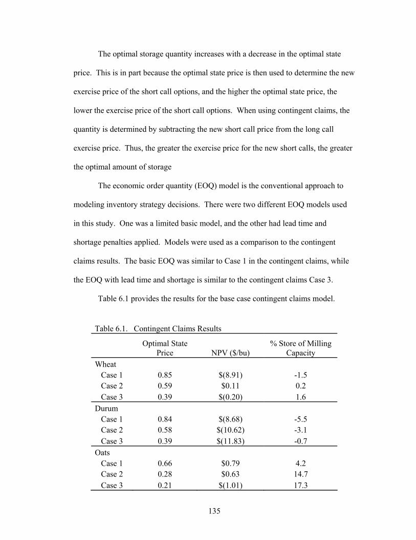
135
The optimal storage quantity increases with a decrease in the optimal state
price. This is in part because the optimal state price is then used to determine the new
exercise price of the short call options, and the higher the optimal state price, the
lower the exercise price of the short call options. When using contingent claims, the
quantity is determined by subtracting the new short call price from the long call
exercise price. Thus, the greater the exercise price for the new short calls, the greater
the optimal amount of storage
The economic order quantity (EOQ) model is the conventional approach to
modeling inventory strategy decisions. There were two different EOQ models used
in this study. One was a limited basic model, and the other had lead time and
shortage penalties applied. Models were used as a comparison to the contingent
claims results. The basic EOQ was similar to Case 1 in the contingent claims, while
the EOQ with lead time and shortage is similar to the contingent claims Case 3.
Table 6.1 provides the results for the base case contingent claims model.
Table 6.1. Contingent Claims Results
Optimal State
Price NPV ($/bu) % Store of Milling
Capacity Wheat
Case 1 0.85 $(8.91) -1.5 Case 2 0.59 $0.11 0.2 Case 3 0.39 $(0.20) 1.6
Durum Case 1 0.84 $(8.68) -5.5 Case 2 0.58 $(10.62) -3.1 Case 3 0.39 $(11.83) -0.7
Oats Case 1 0.66 $0.79 4.2 Case 2 0.28 $0.63 14.7 Case 3 0.21 $(1.01) 17.3
136
The optimal state price is the risk-neutral probability of the value of a $1.00
payoff if the underlying asset price is above the exercise price. This optimal state
price replaces the optimal stock-out quantity in the conventional models. This
optimal state price is more feasible as it adds the time value of money and it is a risk-
neutral function instead of an objective function. Agribusinesses have to be aware of
the time value of money and account for the option value of carrying inventories.
This option value can either be positive or negative.
As the optimal state price decreases, there is an increase in the optimal
inventory level. This increase in inventory level is associated with the increase in the
exercise price of the short call option. The short call exercise price increases with a
decrease in the optimal state price deriving an increase in the optimal quantity. The
NPV per bushel is the value added by using the storage strategy. It is maximized in
the contingent claims analysis. The percentage stored of milling capacity is the
optimal quantity suggested by the contingent claims model divided by the annual
milling usage. The three cases are all different. In Case 1, there is no salvage value
or shortage penalty. Case 2 has a salvage value but no shortage penalty. Case 3 has a
salvage value and a shortage penalty. Moving from Case 1 to Case 3, optimal state
prices decrease and optimal inventory levels increase.
The contingent claims model shows a very high optimal storage quantity for
the oats industry. This is due partially to the higher profit margins associated with the
industry, which produce lower state prices.
The negative option values calculated by the contingent claims model along
with carrying a positive inventory can be associated with the model’s formulation.
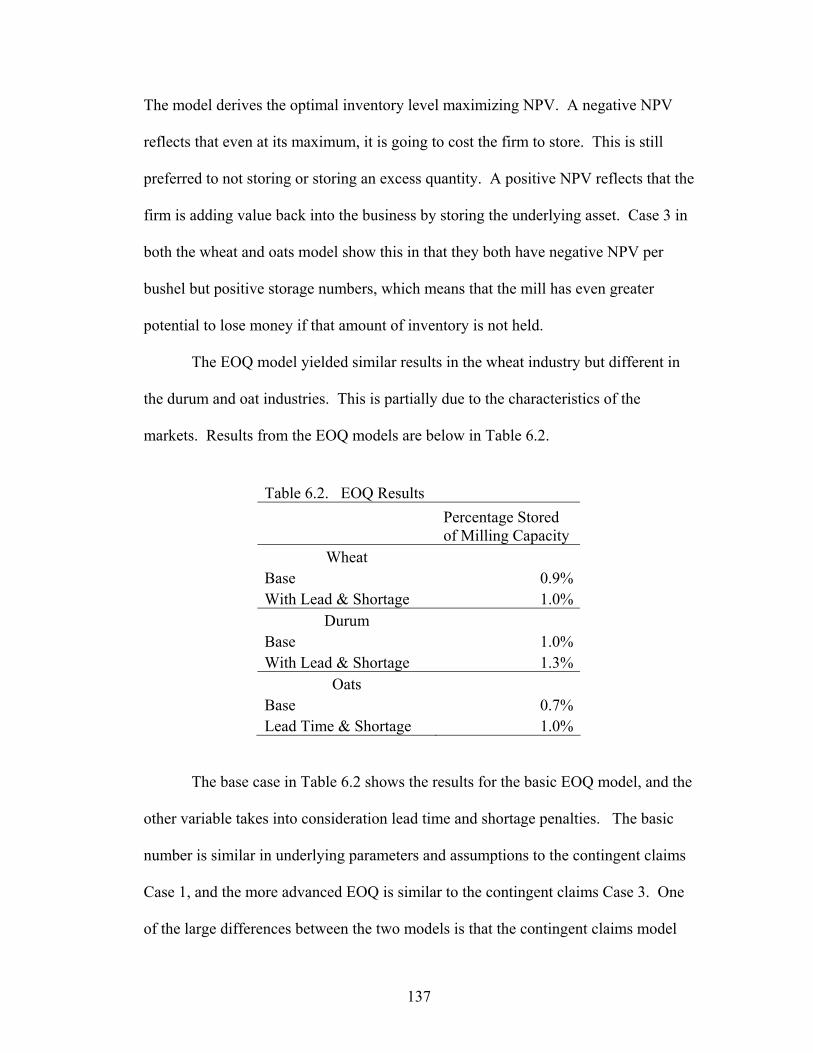
137
The model derives the optimal inventory level maximizing NPV. A negative NPV
reflects that even at its maximum, it is going to cost the firm to store. This is still
preferred to not storing or storing an excess quantity. A positive NPV reflects that the
firm is adding value back into the business by storing the underlying asset. Case 3 in
both the wheat and oats model show this in that they both have negative NPV per
bushel but positive storage numbers, which means that the mill has even greater
potential to lose money if that amount of inventory is not held.
The EOQ model yielded similar results in the wheat industry but different in
the durum and oat industries. This is partially due to the characteristics of the
markets. Results from the EOQ models are below in Table 6.2.
Table 6.2. EOQ Results
Percentage Stored of Milling Capacity
Wheat Base 0.9% With Lead & Shortage 1.0%
Durum Base 1.0% With Lead & Shortage 1.3%
Oats Base 0.7% Lead Time & Shortage 1.0%
The base case in Table 6.2 shows the results for the basic EOQ model, and the
other variable takes into consideration lead time and shortage penalties. The basic
number is similar in underlying parameters and assumptions to the contingent claims
Case 1, and the more advanced EOQ is similar to the contingent claims Case 3. One
of the large differences between the two models is that the contingent claims model
138
maximizes NPV while the EOQ model minimizes total cost. The risk-neutral
approach to the contingent claims approach makes more sense.
Sensitivities
Sensitivities were performed to see how the model reacts to changes in the
parameter variables. These variables have a direct effect on the optimal inventory
level. All of the sensitivities discounted the present value by twenty percent in
increments of ten percent and also increased the present value by twenty percent in
increments of ten percent. This resulted in four new values plus the present value.
These values were then examined to see the relationship they had on the optimal
storage level. The major results are
1. Wheat has positive storage values in all three cases, and Case 3 of the wheat
contingent claims model suggests storing a greater amount than the EOQ model.
2. Durum with its high volatility in the market returns a short inventory position
using the contingent claims but a positive position using the EOQ model.
3. Oats with its high margin and fairly low price volatility maintain a highly positive
optimal storage level that is far greater in the contingent claims model than the
EOQ model.
4. When market price is adjusted using sensitivity, it shows that there are increasing
returns to a point and thereafter decreasing returns.
5. Price volatility has an overall negative effect on the optimal storage level except
in the oats model where there already is low market volatility, but once the oats
model volatility is increased, it also showed that it has a negative affect on
139
optimal storage. Thus, increasing the volatility in the wheat and durum model
decreases the optimal storage level suggested by the contingent claims model.
6. Increasing the salvage value has a positive effect on the optimal storage quantity.
When the salvage value is increased, it suggests a positive return to storage; thus,
the contingent claims model suggests storing a greater quantity.
7. Flour price has a positive effect on the overall optimal storage quantity. In both
the wheat and durum markets, the optimal storage quantity can see a rapid
increase with an increase in the flour price, but oats, on the other hand, see a peak
in the optimal order quantity.
Implications of Results
Stocks are important in agricultural marketing/processing. Traditional
inventory models are useful, but they are limited in their ability to properly address
the issue of price volatility and risk in the marketplace. These marketing and
processing industries could be interpreted as real options, more precisely the option
on future sales. The underlying asset is the grain, while the future sale is the flour.
Market price, commodity price volatility, flour price, salvage value, and shortage
penalties all are important variables to consider when analyzing the optimal inventory
level.
Commodity shortfalls leading to increased volatility and prices are adding to
the complexity of the commodity markets. Divergent results obtained along with the
sensitivities suggest that decisions regarding inventories are highly sensitive and
impacted by many variables. Thus, in order to adopt the real options framework,
firms and managers have to pay careful attention to the values of the input variables.
140
An increase in the overall price volatility adds to the risks of carrying
inventory and results in a loss of NPV. This loss, however, is diminished as the
volatility in the marketplace is decreased when the quality and quantity variables are
stabilized. This can be seen when comparing the wheat results to the durum results,
as they both have about the same profit margins, but durum has an increased amount
of volatility.
Price volatility has a large impact on optimal storage level. With high
volatility, firms are at great risk if they store excess quantities. The high volatility
examined in the durum industry illustrated the risks of storing. The lower volatility in
the wheat and oats markets suggested positive storage numbers using contingent
claims. As a firm in a highly volatile industry, strategic inventory decisions must be
carefully analyzed.
Flour price is the revenue gained from sales. If the flour price has a high
built-in margin, the firm has more to lose if it incurs a shortage. Thus, flour price has
a direct affect on inventory levels. An industry such as oats has a relatively high
margin when compared to wheat and durum, suggesting an increased optimal storage
level for oats.
The salvage value implies either a normal or inverted commodity market. If a
firm is seeing downward prices in the future, the optimal inventory will be less than if
the market was normal with prices in the future above current. Salvage value has a
direct affect on the optimal inventory level; thus, sensitivities on the salvage value
illustrate that as it increases, the optimal inventory level also increases. A firm is
going to store a greater quantity in a market where there are positive returns to
141
storage. When markets are inverted and future salvage value is less than the market
price, the firm still stores but at a decreased level. This phenomenon was illustrated
in all three grains.
The shortage value also implies what a firm has to lose if demand is not met
by inventory. This is a cost to the firm; thus, it has a direct affect on the optimal
inventory level. All of these variables are linked together in the contingent claims
model to provide the option value of carry inventory in a NPV per bushel. This
calculation shows what revenue a storage function is adding or taking away from the
firm. Although the storage function may not always return a positive NPV per
bushel, it is still the maximum at which the firm can achieve and it limits the
downside risk.
The introduction of contingent claims into strategic inventory planning
impacts the overall optimal storage quantity, especially in high-margin industries
such as oats. These higher margin industries show that carrying a greater amount of
inventory may not yield a positive NPV, but it does limit the losses to do price
volatility and other market changes that cannot be directly hedged.
The study also points out something that is very interesting in the theory of
storage and that is the convenience yield. This is when a commodity is held in
storage in an inverted market. As seen in the wheat and oat models, even as prices of
the salvage value drop, positive inventory numbers are suggested. The positive
optimal storage quantity shows that millers and businesses yield some benefits from
having inventory readily available for access. This option value created by the
142
contingent claims model is similar to an insurance policy. The policy is written and
held by the firm; by doing this, the firm has the right to the added value of the policy.
Limitations of Study
A major limitation of this study is the lack of knowledge about how the
underlying asset price affects the future flour sales. This contingent claims value was
simulated in @Risk to get an approximation. In addition, this model shows that as
the asset price increases, so does the quantity milled. While this is true in most cases,
it might not always be the correct assumption. Stowe and Su (1997) have a
contingent claim in their model that illustrates that sales will increase by ten units
with a $1 increase in the underlying asset price; this assumption, while valid for the
specific case, is not always an easy number to calculate.
A critical variable in this study is the market price. The market prices used in
this study were from November 2004 and were on the high end of the historical
distribution of prices from the years 1990-2002. They have an impact on the results
as shown the in the market price simulations of the grains.
In most cases, the flour and commodity prices change together in the
marketplace unless there is a contract to be fulfilled at a specific price, but in this
study, the corresponding numbers do not change together as they do in the
marketplace, thus partially limiting the results of the model.
Need for Further Research
Further research on how flour sales are affected by the increase and decrease
of the underlying asset price is needed. This contingent claim is one of the reasons
this methodology has not been adopted more readily within the agribusiness industry.
143
The issue of how flour price increases with an increase in the underlying asset price is
also another area that could be explored in more depth.
Further research on how future sales are affected by the increase in the
underlying asset price would greatly enhance this work. It is shown in the results that
different contingent claims values produced different optimal storage quantities with
differing NPV. Determining an equation that incorporates a variable for the unit of
sales increase as an increase in asset prices would be a noteworthy accomplishment.
This study uses data for prices and revenues at one point in time. Adding
variability to this to see its effect over time would add depth to the model. The model
then would have a distribution of prices with a relationship to revenue in which to
calculate the optimal inventory level.
Obtaining data on actual mill configurations including storage, milling
capacity, and efficiency would greatly enhance this study. The values used in this
study of are a representative firm. The firm data are calculated using the industry
data divided by the firms. Currently, industry averages are used to determine the
optimal storage level.
Summary
As agribusiness firms see increased volatility in the marketplace, there is a
need for a more sophisticated inventory management tool. The conventional
approach will always play a vital role in solving inventory decisions. There comes a
need for a more efficient way to deal with volatility. Many different variables are
combined in the optimal inventory strategy, some of which have a large impact on the
overall optimal storage quantity. This study points out how using contingent claims
144
can benefit agribusinesses and explains some of the variables that have a large impact
on the overall feasibility of the option model.
This study makes three major contributions to inventory management. First,
the optimal inventory storage function is derived from the optimal state prices. This
results in an inventory position that maximizes NPV while accounting for uncertainty
in an economically feasible way and discounting for the time value of money.
Second, the study shows the option value of the inventory storage function. The
option value is the value that a company would expect to pay to insure their payoffs
from inventory. This value, whether positive or negative, is maximized. Finally, this
study shows that there are several key variables that have a significant impact on the
optimal state price that derives the optimal inventory level. Managers no longer can
estimate what values are input into inventory strategies; these variables need to be
precise and accurate for the particular firm.
145
REFERENCES
Akella, Ram, and Anupindi, Ravi, “Diversification under Supply Uncertainty.” Management Science. v39, n8 (August 1993) 944-63.
Alstrom, Paul. “Numerical Computation of Inventory Policies, Based on the EOQ/σx
Value for Order-Point Systems.” International Journal of Production Economics. v71, n1-3 (May 2001) 235-45.
Amram, Martha, and Kulatilaka, Nalin. “Disciplined Decisions: Aligning Strategy
with the Financial Markts.” Harvard Business Review. January-February 1999.
Baker, K.H., Guerrero, H.H., and Southard, M.H., “The Dynamics of Hedging the
Master Schedule.” International Journal of Production Research. v24, n6 (1986) 1475-83.
Ballou, R.H. Business Logistics Management (4th Edition). Englewood Cliffs, NJ:
Prentice Hall. 1999. Becker, M., 1994. “The Reorder Point as an Option on Future Sales.” Paper Presented
at the International Symposium on Cash, Treasury, and Working Capital Management (October). St. Louis, MO.
Benninga, Simon, Steinmetz, Raz, and Stroughair, John. “Implementing Numerical
Option Pricing Model.” Conceptual Economics and Finance: Modeling and Analysis with Mathematica. Editor Hal Varian. New York, NY: Springer-Verlag, Incorporated. 1996, 251-68.
Billington, Corey, and Lee, Hau L., “Material Management in Decentralized Supply
Chains.” Operations Research. v41, n5 (September-October 1993) 835-47. Blank, Steven C. “Price Dependence and Futures Price Theory.” Northeastern
Journal of Agricultural and Resource Economics, v14 (1985) 169-76. Blank, Steven C., Carter, Colin A., and Schmiesing, Brian H., Futures and Options
Markets Trading in Financials and Commodities. Englewood Cliffs, NJ: Prentice Hall. 1991.
Brennan, M.J., “The Pricing of Contingent Claims in Discrete Time Models.” The
Journal of Finance. v34, n1 (March 1979) 53-68. Canadian Wheat Board. “Data on Distribution of Amber Durum Grades.” Canadian
Wheat Board. 2004-05.
146
Chaudhuri, K.S., and Ray, J., “An EOQ Model with Stock-Dependant Demand, Shortage, Inflation and Time Discounting.” International Journal of Production Economics. v53 (1997) 171-80.
Chicago Board of Trade. “Commodity Trading Manual.” Education and Marketing
Services, Department of the Chicago Board of Trade. Board of Trade of the City of Chicago. 1989.
Chopra, Sunil, and Meindl, Peter. “Supply Chain Management.” Upper Saddle
River, NJ: Prentice Hall. 2001. Choprar, Sunil, and Meindl, Peter, Supply Chain Management Strategy, Planning,
and Operation. Upper Saddle River, NJ: Prentice Hall. 2001. Chung, Kee H., “Inventory Decision under Demand Uncertainty: A Contingent
Claims Approach.” The Financial Review, v25, n4 (November 1990) 623-30. Chung, Kee Ho, and Kim, Young H., “Inventory Management under Uncertainty: A
Financial Theory of the Transactions Motive.” Managerial and Decision Economics. v10, n4 (December 1989) 291-98.
Contingency Analysis, http://www.contingencyanalysis.com, 1996. January 2004. Cordier, Jean E., Junkus, Joan C., and Leuthold, Raymond M., The Theory and
Practice of Futures Markets. Lexington, MA: Lexington Books. 1989. Cox, J.C., and Ross, S.A., “The Valuation of Options for Alternative Stochastic
Processes.” Journal of Financial Economics. v3 (1976). Cox, John, Ross, Stephen, and Rubinstein, Mark. “Option Pricing: A Simplified
Approach.” Journal of Financial Economics, v7 (1979) 229-63. Dixit, Avinash K., and Pindyck, Robert S., “The Options Approach to Capital
Investment.” Harvard Business Review. (May-June 1995). Ernst, Richardo, and Pyke, David F., “Component Part Stocking Policies.” Naval
Research Logistics. v39 (1992) 509-29. Goffin, Keith, New, Colin, and Szwejczewski, Marek, “Managing Suppliers: When
Fewer Can Mean More.” International Journal of Physical Distribution & Logistics, v27, n7, (1997) 422-36.
Grain & Milling Annual 2004. Kansas City, MO: Sosland Publishing Co. 2003.
147
Hong, Harrison, “Stochastic Convenience Yield, Optimal Hedging and the Term Structure Open Interest and Futures Prices.” Graduate School of Business, Stanford University, Stanford, CA. July 23, 2001.
Hoshino, Kyoji, “Criterion for Choosing Ordering Policies Between Fixed-Size and
Fixed-Interval, Pull-Type and Push Type.” International Journal of Production Economics. v44 (1996) 91-95.
Hull, John C., Options, Futures, & Other Derivatives (4th Edition). Upper Saddle
River, NJ: Prentice Hall. 2000. Hull, John C., Fundamentals of Futures and Options Markets (4th Edition). Upper
Saddle River, NJ: Prentice Hall. 2002. Luehrman, Timothy A., “Capital Projects as Real Options: An Introduction.”
Harvard Business Review. March 1995. Luehrman, Timothy A., “Strategy as a Portfolio of Real Options.” Harvard Business
Review. July-August 1998. Maia, Luis Otavio Aleotti, and Qassim, Raad Yahya, “Minimum Cost Safety Stocks
for Frequent Delivery Manufacturing.” International Journal of Production Economics. v62 (1999) 233-36.
McClelland, W.G., “The Least-Cost Level of Stocks and Rate of Interest” Journal of
Industrial Economics. v8, n2 (March 1960) 151-71. Milling and Baking News. “Ingredient Week.” Milling and Baking News. v2, n36
(2003) 33-40. Minneapolis Grain Exchange, “Historical Cash Oats No. 2 Heavy.” Minneapolis,
MN: Minneapolis Grain Exchange. 1990-2002. North Dakota Agriculture Experiment Station (Fargo). Department of Cereal
Chemistry and Technology. “The quality of regional (Montana, North and South Dakota, Minnesota) hard red spring wheat crop.” Various.
Palisade Corporation. 2000. @Risk4.0 – Professional Edition. Software New York. Polataglu, Hakan, and Sahin, Izzet, “Optimal Procurement Policies under Price-
Dependant Demand.” International Journal of Production Economics. v65, n2 (April 2000) 141-71.
Saskatchewan Agriculture, Food and Rural Revitalization. “Agricultural Statistics
Handbook.” Saskatchewan, Canada: Saskatchewan Agriculture, Food and Rural Revitalization. 1996-2002.
148
Schwartz, Eduardo S., and Trigeorgis, Lenos, Real Options and Investment under Uncertainty: Classical Readings and Recent Contributions. Cambridge, MA: MIT Press. 2001.
Statistics Canada, Cereals and Oilseeds Review Series. “Canada: Grains and
Oilseeds Supply and Disposition.” Agriculture and Agri-Food Canada. June 4, 2004. http://www.agr.gc.ca/policy/winn/biweekly/e/sd1e/2004e/jun2004_e.htm.
Stowe, John D., and Su, Tie, “A Contingent Claims Approach to the Inventory-
Stocking Decision.” Financial Management. v26, n4, (Winter 1997) 42-55. Stulz, Rene. Risk Management and Derivatives. Mason, OH: South-Western. 2003. Tauer, Loren W., “Investment Analysis in Agriculture.” Staff paper, Department of
Agricultural, Resource and Managerial Economics, Cornell University, Cornell, NY. April 2000.
Tierney, William I. Jr. “Quarterly Wheat Outlook.” Marketing Kansas State
University, Manhattan, KS. September 4, 2003. Tigeirgis, Lenos. “Real Options and Interactions with Financial Flexibility.”
Financial Management. Tampa, FL. v22, n2 (Autum 1993) 202-35. Turvey, Calum G., “Mycogen as a Case Study in Real Options.” Review of
Agricultural Economics. v23, n1 (Spring/Summer 2001) 243-64. USDA Economic Research Service. “Feed Situation and Outlook Yearbook, Feed
Grains Delivery System.” March 2004. http://www.ers.usda.gov/db/feedgrains/default.asp?ERSTab=3.
USDA Economic Research Service. “Wheat Situation and Outlook Yearbook”
March 2004. http://www.ers.usda.gov/data/sdp/view.asp?f=crops/88008/&arc=C.
van der Heijden, Matthieu, “Near Cost-Optimal Inventory Control Policies for
Divergent Networks under Fill Rage Constraints.” International Journal of Production Economics. v63, n2 (January 2000) 161-79.
Whybark, D. Clay, and Williams, J. Gregg, “Material Requirements Planning under
Uncertainty.” Decision Sciences. v45 (1976) 595-606. Williams, Jeffrey. The Economic Function of Futures Markets. New York:
Cambridge University Press. 1986.
149
Wilson, William W., and Dahl, Bruce L. “The Logistical Costs of Marketing Identity Preserved Wheat.” Agribusiness and Applied Economics Report No. 495. Department of Agribusiness and Applied Economics, North Dakota State University, Fargo. 2002.
Working, Holbrook. “The Theory of Price of Storage.” American Economic Review.
(December 1949) 1254-62.