INVERSE, a FORTRAN Program to Solve for Two-Dimensional Slip

UNITED STATES DEPARTMENT OF THE INTERIOR GEOLOGICAL SURVEY

INVERSE, a FORTRAN Program to Solve for Two-Dimensional Slip On a Vertical Strike Slip Fault by Inversion of Line-Length Data

by

R.A. Harris and P. Segalll

Open-File Report 86-451

This report is preliminary and has not been edited or reviewed for conformity with Geological Survey standards and nomenclature. Any use of trade names and trademarks in this publication is for descriptive purposes only and does not constitute endorsement by the U.S. Geological Survey. Although this program has been tested extensively, the U.S. Geological Survey makes no guarantee of correct results.

Htenlo Park, California

1986

TABLE OF CONTENTS

PAGE

INTRODUCTION .......................................................... 3

MATHEMATICAL METHOD .................................................... 5

PROGRAM OVERVIEW ....................................................... 10

INPUT DESCRIPTION ...................................................... 11

OUTPUT DESCRIPTION ..................................................... 17

PROGRAM OPERATION ...................................................... 18

REFERENCES ............................................................. 19

APPENDIX A: SAMPLE INPUT FILE ......................................... 20

APPENDIX B: SAMPLE OUTPUT FILE ........................................ 22

APPENDIX C: FORTRAN PROGRAM CODE ...................................... 30

ILLUSTRATIONS

FIGURE 1 ............................................................... 16

INTRODUCTION

INVERSE.FOR is a FORTRAN 77 program which runs on the VAX/VMS 785 computer. Its creation was motivated by the desire to use line-length measurements made at the earth's surface for information about two-dimensional slip at depth on the San Andreas fault near Parkfield, California. In the Parkfield area, a transition occurs as the surface expression of the San Andreas fault progresses from a creeping zone in the northwest to a locked zone in the southeast. We have used the inverse program to invert line-length measurements made in the Parkfield area for slip on the San Andreas fault. The results have included the imaging of a locked patch at depth, located beneath the transition zone. (Harris and Segall, 1985, Segall and Harris, 1986).

The program is designed to perform a two-dimensional inversion of trilateration line-length data or strain data to solve for strike-slip motion on a vertical strike-slip fault. It also solves for a component of strain perpendicular to the fault plane. A few parts of the program, such as the subroutine CHINSSL, have been borrowed from Will Prescott's program MAIN29.FOR. Interactive input routines and the subroutine which sends the slip model to a file where it can be plotted were provided by Bob Simpson.

There are five subroutines in the program. They are:

1) CHINSSL, which calculates the Green's functions using Chinnery's equations (Chinnery, 1961) for surface displacement caused by a vertical rectangular dislocation in an elastic half-space.

2) CRD, which translates and rotates coordinates to a fault-centered system.

3) FMODEL, which reads the fault geometry information and sets up a fault grid representing the fault plane.

4) MODELWT, which calculates a weighting matrix for the model.

5) SENSIT, which does a singular-value-decomposition of the data kernel matrix and computes a number of paramenters for each run. Included among these are the model and data resolution and covariance, the estimated model, data misfits, and the geodetically determined seismic moment. One may loop through SENSIT using a varying number of singular values from the decomposition. This permits the user to choose the optimal variance and resolution of the model.

Operation of the program requires the input of station coordinates, line-length or strain data with standard deviations, and geometry of the fault grid. One may also input constraints on the slip to be allowed in the model. Output consists of all input values, the calculated model, data misfits, and moment.

This report begins with a mathematical explanation of the program. Because the data are treated as a linear function of the model, the matrix equations are relatively simple. The math section shows how the model constraints are entered into the data kernel matrix and the data vector. It

also explains the model and data-weighting, in addition to computations for the fit of the model.

The portion of the report entitled INPUT consists of a line-by-line description of a sample input file, 22KSCC.DAT. Each element required by the program is defined. The section entitled OUTPUT, gives a list of the information shown in the sample output file, 22KSCC.OUT. Brief instructions are also provided to show the user how to run this FORTRAN program on the VAX/VMS 785. The last section contains a printout of the FORTRAN program INVERSE.FOR, the sample input file, 22KSCC.DAT, and the sample output file, 22KSCC.OUT.

MATHEMATICAL METHOD

The object of the FORTRAN program INVERSE.FOR is to solve the discretized linear matrix problem

Y = [A] x X (1)

for the unknown (mxl) model vector X, given the (nxl) data vector, Y, and the (nxm) Green's function matrix [A]. Treatment of this basic problem is found in many linear algebra texts (e.g. Strang, 1976, Lanczos, 1961). We assume that measurements at the earth's surface, Y, may be explained by some distribution of strike-slip motion on the fault plus a component of normal strain, which together form elements of the model vector, X. The "formal" inverse solution, in the discrete form, is

*est = [A]' 1 x Y (2)

where [A]-l is the inverse of [A], and Xest is an estimate of the solution.

In order to solve the inverse problem, (2), we need to specify the data kernel, [A], which relates behaviour on the fault to behaviour on the earth's surface. We begin by treating the fault as a 2-dimensional fault plane consisting of discrete dislocations in a homogeneous, isotropic, elastic, half-space. (Chinnery, 1961). The centers of the discrete dislocations are arranged in a rectangular grid pattern which we call the fault grid. Individual rectangular elements in this grid are referred to as blocks. Slip is constant in each block. The bottom of the fault grid is referred to as the transition depth. Below this depth the slip rate is assumed to be constant, both in space and time. To the left of the fault grid, down to the transition depth, the slip rate is also assumed constant. This simulates a freely creeping zone. To the right, the slip is assumed to be zero, simulating a completely locked portion of the fault. (See Figure 1.) Only strike-slip motion on the fault plane and a component of normal strain are modelled.

If there is auxiliary information available, such as near fault surface slip data, which we desire to strongly influence the model in certain blocks, we may accomplish this by adding elements to the data vector Y and to the data kernel, [A]. For each of the nff (number of constrained) model blocks, one row with an appropriate distribution of 1's and O's is added to the data kernel matrix, after the first n rows of Chinnery functions. The corresponding slip value for each constrained block is added as an element to the data vector. Y then becomes an (n+nff x 1) vector of displacement measurements and [A] becomes an (n+nff x m) dimensioned data kernel.

In order to solve equation (2), we use the generalized or, Lanczos inverse, [A]L to operate on the data vector, y (Lanczos, 1961). For our case, which is a mixed-determined problem, the Lanczos inverse simultaneously minimizes the length of the model vector, X 2 an d the length of the residual vector |e |2 where

e 2 = (Y - [A] x X) 2 (3)

The mixed-determined problem assumes that for some model elements there is more than one data element resolving that area while for other model elements there are no data elements which are capable of resolving the slip distribution. In the overdetermined regions of the model, a least-squares fit to the data is used. Simultaneously, the underdetermined regions of the model are solved for with the help of some a-priori assumption, such as minimum model length, or smoothness, or closeness of fit to a prior model.

An efficient way of obtaining the Lanczos inverse of the data kernel, and at the same time neatly splitting the data kernel into underdetermined and overdetermined parts is to use the singular value decomposition approach (s.v.d.). Any (n x m) matrix, [A] may be decomposed into 3 matrices [U], an (nxn) square matrix of eigenvectors which span the data space of [A], an (nxm) matrix, [A], consisting of the singular values of [A] on the diagonal with zeroes elsewhere, and an (mxm) square matrix V-transpose, [V]t containing the eigenvectors spanning the model space.

CA] = [U] x [A] x [V]t (4)

This is referred to as the singular value decomposition (s.v.d.) of the matrix [A].

The singular value matrix, [A], may be split into two parts, a (pxp) part with non-zero singular values on the diagonal, [A]p and an (n-p x m-p) part with zero singular values, CA]Q. Correspondingly, the data eigenvector matrix splits into [U]p and [UJ0 and the model eigenvector matrix [V]p and [V]0 . This split is important because it tells us what we can and cannot determine about the model from the data. All of the information to be derived from the matrix [A] is contained in the three matrices [U]p , [A!P and [V] p . The other three matrices, [U]0 , [A]0 and [V]0 are orthogonal to the p-space, and lie in the null space of the data kernel.

An inverse, so-called the Lanczos or generalized inverse, [A]L may be formed

[A]L = [V] x [A]-l x [U]t (5)

where [A]-l is the inverse matrix of [A] and [U]t is the transpose matrixof [U]. One can solve the inverse problem for the estimated model parameters,xest»

xest = CA]-L x Y (6)

= [V] x [A]-l x [U]t x [Y] (7)

As discussed above, [A] can also be constructed as

[A] = [U]p x [A]p x [V]j5, (8)

so we can also form

xest = [V]p x [A]pl x [U]f x Y (9)

As mentioned previously, the Lanczos inverse simultaneously minimizes the data residual and the length of the model vector. Such solutions are called "minimum-length" solutions. Another assumption may be made about the nature of the "underdetermined" regions of the model; one can require that the solution across such regions is as smooth as possible. This is a desired characteristic, as it ties some of the more poorly determined fault-grid blocks to the better known boundary constraints, such as the shallow slip-rates and the long term deep slip-rate.

In the smooth case what we minimize is the length of the second derivative of model parameters, rather than the model parameters themselves. This leads us to minimize

[Tm ] x X 2 (10)

where Tm is an m x m matrix of Laplacian operators. (Menke, 1984). By using this model weighting matrix, Tm , the model estimate resulting from the Lanczos inverse becomes a smooth model. The "overdetermined parts of the model are still best fits to the data while the "underdetermined" parts now smoothly blend into the better determined regions.

The new equations for X 1 which is the new weighted version of the model vector, X and for Y 1 which is the new weighted version of the data vector, Y are:

X 1 = [Tm ] x X (11)

Y 1 = [Td ] x Y. (12)

Tm is the smoothing matrix for the model and Td is a data weighting matrix in which each data element is weighted by the inverse of the standard deviation of that element.

Equation 1 can now be written as

Y 1 = [A 1 ] x [X 1 ] (13)

with

[A] 1 = [Td ] x [A] x [Tm]-l (14)

We may perform an s.v.d. on A 1 to get U 1 , [A] 1 , and [Y]t § . A smoothed model estimate is then obtained by using a Tm consisting of Laplacian operators in 2-d:

Xest ' [V-1 x [A]lL x [V x Y

= [TJ- 1 x [Y]^ x [A]' 1 ' x [U]^ x [Td ] x Y (15)

In addition to the model estimate, by using the matrices from the singular value decomposition of the data kernel, it is easy to write equations

8

for the model resolution, [R], the model covariance, [C], and the data resolution, [D]. The model resolution, which maps a true model into the model estimate, is given by

CR] = [TJ- x [V]^ x [V] x [TJ (16)

The data resolution, which maps the observed data into the calculated data is

[D] = [T^- 1 x [U]^ x [U]* x [Td ] (17)

and the model covariance, which provides error bars on the model is

EC] = [T- 1 x [V] x [A]' 2 ' x [Y] x [T- 11 (18)

The model covariance may be used to obtain a root-mean-square standard deviation of the model elements.

In order to choose the correct number of singular values to use in the inversion, we also calculate a parameter called chekmod. This parameter, which is a rotated form of the model,

chekmod = [A]-! 1 x [U]'t x Y 1 (19)

= [A]-!' x Y" (20)

where Y" = [U]'t x Y 1 (21)

can be compared with its expected variance, a(Y") x [\]'- 2 , for each singular value, to determine which elements exceed their expected uncertainties. Because the matrix [cov Y"] is just the identity matrix, we end up comparing chekmod with the inverse of the smallest singular value. When chekmod is greater than this value, it has exceeded its expected uncertainty.

The geodetically determined seismic moment is the most robust quantity determined from the inversion of line-length data. It can be calculated after the model vector has been obtained, by summing the slip over all of the fault grid blocks, multiplied by the area of a block, and the shear modulus, n

MQ = u x area x 2-i xest (l) (22) i=2,m-2

The elements which are not included in the sum are the deep slip, the slip in the left-hand block, and the normal strain component.

Two statistical parameters which are useful to calculate are the misfit of the data to the model, *2, and the root mean square standard deviation of the model elements. The misfit, or *2 is given by

((o(i)-c(i))/C(i)) 2 (23)over all lines

where o(i) is the observed data measurement, c(i) is the calculated data measurement, and C(i) is the standard deviation of that line. The root mean square standard deviation of the model parameters, rmsstdev is defined as

rmsstdev «/ C(i,i))/nvf (24)i

where nvf is the number of variable faults.

10

PROGRAM OVERVIEW

A step-by-step summary of the program flow is presented below.

1) Read (interactively) the number of singular values to use in the inversion, the number of additional singular values to use, the type of model weighting, and whether or not to include a normal strain component.

2) Read file containing line-length or strain data.

3) Read fault model using SUBROUTINE FMODEL and set up geometry.

4) Rotate stations to fault-centered coordinate system using SUBROUTINE CRD.

5) Compute station displacements due to each fault, in fault-centered coordinates.

6) Calculate Chinnery functions with SUBROUTINE CHINSSL.

7) Obtain station displacements in NS-EW coordinate system (rotate again, using SUBROUTINE CRD).

8) Calculate green's functions, including normal component of strain, if desired.

9) Add extra lines to green's functions for the constrained grid blocks.

10) Read the fixed block slip constraints and their standard deviations.

11) Form data-weighting matrix, and its calculate its inverse.

12) Form model-weighting matrix, with call to SUBROUTINE MODELWT.

13) Form inverse of model-weighting matrix.

14) Call SUBROUTINE SENSIT to determine the singular value decomposition of the data kernel [A], and to obtain the model estimate, the data-fit to the model, the root-mean-square standard deviation of the model elements, the moment, etc. Loop through SENSIT for each requested additional singular value, and recalculate the above parameters.

11INPUT DESCRIPTION

Interactively, the program INVERSE.FOR will ask for information about the number of singular values to use in the inversion and the type of model weighting desired by the user. The input file for the FORTRAN program requires (x,y) station coordinates in meters, line-length or strain data for the corresponding lines, (described in detail in King et. al., unpub. data, 1984), and a fault model. A sample input file, given in Appendix A, is 22KSCC.DAT. Following is a line-by-line description of the input parameters. The words between asterisks are the names of variables used in the program. Below each term is an explanation of what is to be input.

Interactively, the program asks for:

*NSTART*The number of singular values to start with

*NUMRUN*The number of times to perform the singular value loop after NSTART. An iterative loop in the Subroutine SENSIT starts with NSTART singular values in the singular value decomposition and runs NUMRUN additional times through the process.

*NWT*The type of model-weighting desired. NWT=1 implies that no model-weighting is to be used, and the solution will be the minimum-length solution. NWT=2 implies that a model-weighting matrix which results in a smooth model will be used.

*NSTRAIN*The model parameter involving a component of strain normal to the fault plane. NSTRAIN=1 leads to no normal strain and a resulting model of 2-d slip on the fault. NSTRAIN=2 leads to a model of 2-d slip on the fault plane plus a component of strain perpendicular to the fault plane.

The input file requires the following lines of information: Line 1 ~7ormat(il,i4,3i5,5x,10a4)

*IOPT*A single digit which indicates whether strain data or line-lengthdata is to be used'O 1 for strain cards'I 1 for pairs of line-length cards

*NF*The number of grid blocks (constrained and variable), including large block to left of fault grid and block beneath transition depth

*NLINES*The number of trilateration lines to be used in the inversion

12

*NSTNS*The number of stations (endpoints of the trilateration lines)

*NFF*The number of grid blocks with constrained slip

*DESCRI*A short (word) description of the program run

Line 2 to Line 2+NSTNS format(a8,6x,fl6.0,6x,fl6.0)

Each line has the following station information

*STA*Station name

*XX*X-coordinate in meters

*YY*Y-coordinate in meters

Next NLINES lines (for strain cards)Each line has the following line-length information:format(a5,8x,a8,lx,a8,t44,fl0.3,t54,f7.4)

*NET*Network name

*SN1*Station 1 endpoint name

*SN2*Station 2 endpoint name

*DATE*Decimal years - 1900(Note that this is not a required input parameter and is not used in theprogram.)

*NMEAS*Number of measurements made for this line (Note this is not a required input parameter)

*DISTAN*Line-length (meters)

*STR*Rate of line-length change (meters/year)

*SD*Standard deviation of the rate (meters/year)

13

*AZI*Line azimuth measured clockwise from North in degrees, SN1 to SM2.

or, for pairs of line-length cards, Next 2*NLINES

First card in the pair

*NET*

*SN1*

*SN2*

*DATE*

*AZ*

*DISMARK1*Mark-to-mark distance (meters)Note this is not used in the program.

*DISTAN*Arc-distance (meters)

*SD*Standard deviation of the line-length change (meters)

Second card in the pair

*NET*

*SN1*

*SN2*

*DATE*

*AZ*

*DISMARK2*Mark-to-mark distance of the second distance measurement (meters)

*DIST2*Arc-distance of the second distance measurement (meters)

*SD*

14

The following cards in the input file are used to set up the fault grid model Fault blocks can be specified in 3 ways by defining "kode"

1 = one endpoint, azimuth, length

2 = two endpoints

3 = midpoint, azimuth, half-length

4 = grid of blocks

Each line in the input is for a different fault block or fault-grid block geometry. The fault information to be input in each line is: format(3i4,4x,8f8.0)

*KODE*A number (1,2,3,4) as defined above

*NHE*The number of horizontal elements in the grid (NHE = 0 if kode is not 4)

*NVE*The number of vertical elements in the grid (NVE = 0 if kode is not 4)

*DU*The depth to the top of the fault block (or grid) in kilometers

*DL*The depth to the bottom of the fault partition in kilometers

*AZ*Azimuth from north, in degrees

*LENGTH*Total fault length in kilometers If kode = 3 then fault half-length

*X1*Endpoint coordinate (meters)If kode = 3 then midpoint coordinate

*Y1*Endpoint coordinate (midpoint if kode = 3)

*X2*

*Y2*

15

After reading in the fault model parameters, the next NFF lines are the modelslip constraints.Each line consists of:Ki4,2el2.4)

*INDEX*The block number which is assigned fixed slip

*CONSRATThe constrained slip value in meters/year

*CONSWT*The standard deviation of the constraint (meters/year)

The final line signals that the input is complete:

*0*

A comment on the system for numbering the fault blocks:The model weighting routine is presently arranged so that blocks are numbered in the manner depicted in Figure 1. The left hand block is number 1, the top left block in the grid is 2, and so on to the last block, which is below the transition depth.

1BH

Su

rfa

ce t

race

of

fau

lt

Cre

epin

g

zon

e

[consta

nt

slip

)

Blo

ck

1

Blo

ck

2

3 4 5

6 7 8 9

10

11 12

13

14

15

16

17

Lock

ed

zon

e

(no

sl

ip)

Tra

nsitio

n depth

Incr

easi

ng

depth

Dee

p sl

ip

zon

e

(co

nsta

nt

slip

)

Blo

ck

18

1'*

/ C

r°SS

se

ctio

n o

f tn

e

fau1

t.

To

the le

ft o

f th

e fa

ult g

rid

, In

i

*Je

-5 ^ co

nst

ant,

equa

l to

th

e

cree

p in

th

at

regio

n.

To

the

betw

n th

^fS

n?

' ?

e f?

UU

!S

10

Cke

d an

d th

ere

is

n°

S1

1'P-

The

11ne

ru

nni"

9

betw

een

the fa

ult p

lane

(c

on

sis

tin

g o

f B

lock

s 1

to

17

and

the lo

cke

d z

one)

an

d "*

17

OUTPUT DESCRIPTION

The output file (see Appendix B for an example) reproduces the input file, then shows the calculated block coordinates and lists the assigned constraints. In detail, this includes:

Information about the singular value decomposition of the rotated data kernel matrix, [A] 1 . The IMSL warning error may be ignored, since this program does not use all of the singular values.

For each run of the singular loop,. The number of singular values used. The smallest singular value used. Chekmod and l/(smallest singular value used). The r.m.s. model standard deviation (m/yr). The fit of the data to the model (dimensionless). The moment rate of the solution (dyne-cm/yr). The normal strain component of the solution (micro-strain/yr)

For each line. The observed data. The calculated data. The misfit of the predicted line-length to the observed. The station displacements

For each fault block. The estimated slip rate (m/yr) . The standard deviation (m/yr)

18

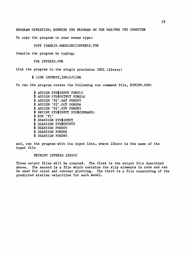
PROGRAM OPERATION; RUNNING THE PROGRAM ON THE VAX/VMS 785 COMPUTER

To copy the program to your areas type:

COPY [HARRIS.PARKLONG]INVERS E.FOR

Compile the program by typing:

FOR INVERSE.FOR

Link the program to the single precision IMSL library:

$ LINK INVERSE,IMSLS/LIBR

To run the program create the following run command file, RUNINV.COM:

$ ASSIGN SYSfclNPUT FOR015i ASSIGN SYS$OUTPUT FOR016$ ASSIGN 'P2'.DAT FOR005$ ASSIGN 'P2'.OUT FOR006$ ASSIGN 'P2'.STV FOR085$ DEFINE SYSfclNPUT SYS$COMMAND:$ RUN 'PI'$ DEASSIGN SYSfclNPUT$ DEASSIGN SYS$OUTPUTi DEASSIGN FOR005$ DEASSIGN FOR006$ DEASSIGN FOR085

and, run the program with the input line, where 22kscc is the name of the input file

@RUNINV INVERSE 22KSCC

Three output files will be created. The first is the output file described above. The second is a file which contains the slip elements in code and can be used for color and contour plotting. The third is a file consisting of the predicted station velocities for each model.

19

REFERENCES

Chinnery, M.A. (1961), "The deformation of the ground around surface faults." Bull. Seism. Soc. Am. 51, 355-372.

Harris, R., and P. Segall (1985), "Determination of the slip deficit along the Parkfield CA section of the San Andreas fault from the inversion of trilateration data." EOS Trans. AGU (abstract), 46, 985.

King, N.E., Prescott, W.H., and K.J. Wendt, Unpublished line-length record information. August 1983, revised January 1984.

Lanczos, C. (1961), Linear Differential Operators. Van Nostrand-Reinhold, Princeton, New Jersey.

Menke, W. (1984), Geophysical Data Analysis! Discrete Inverse Theory. Academic Press, Orlando, Florida.

Segall, P., and R. Harris (1986), "Slip deficit on the Parkfield, California section of the San Andreas fault as revealed by inversion of geodetic data." Science, in press.

Strang, G. (1976), Linear Algebra and its Applications. Academic Press, New York, New York.

20

APPENDIX A

Sample input file22KSCC.DAT

0 134 45airwayalmondbarrenbenchblhllresbonniecastlechiches2cottondavisgoldhatchhopperkengermasonmid fmine mtmine rm2parkred hillshadetesswildsanlu +sanlu +sanlu +sanlu +sanlu +sanlu +sanlu +sanlu +sanlu +sanlu +sanlu +sanlu +

23 14 Parkfieldx = 372863.34x - 387280.44x - 376124.53x = 397009.41x = 352361.27x = 405248.78x - 398499.18x - 396029.12x = 408764.94x = 356267.64x - 397333.49x = 412537.33x = 394082.18x = 397814.27x = 388953.45x = 382038.42x - 390064.12x - 390064.39x - 401440.70x = 404862.12x = 367312.91x = 364621.55x = 386399.82airway barrenairway blhllresairway chiches2airway davisairway tessalmond barrenalmond benchalmond chiches2almond red hillbarren chiches2barren tessbench bonnie

y - 205517.50 metersy = 230311.04 metersy - 219925.67 metersy - 251596.36 metersy = 209785.62 metersy = 266058.53 metersy = 273018.53 metersy = 212436.47 metersy = 256002.59 metersy « 195729.09 metersy = 261032.85 metersy = 244618.21 metersy = 243719.35 metersy - 270235.58 metersy = 261439.02 metersy - 271317.48 metersy - 276596.15 metersy = 276599.84 metersy = 268212.82 metersy - 235801.52 metersy = 284025.23 metersy - 212466.02 metersy = 253809.22 meters79.487 6 14772.850 0.000680.613 5 20942.138-0.000779.495 6 24165.589 0.000580.543 5 19268.005-0.003180.603 5 10780.267-0.000879.500 6 15242.453-0.001379.128 7 23402.636-0.003779.499 6 19901.080-0.000981.929 23 18418.864 0.001279.489 6 21268.287 0.001279.820 5 13710.150-0.001477.421 8 16643.001-0.0052

cal zone cal zone cal zone cal zone cal zone cal zone cal zone cal zone cal zone cal zone cal zone cal zone cal zone cal zone cal zone cal zone cal zone cal zone cal zone cal zone cal zone cal zone cal zone

0.0018 11.3 0.0013 280.3 0.0013 72.1 0.0026 237.9 0.0009 308.7 0.0009 225.7 0.0011 23.2 0.0011 152.5 0.0016 71.3 0.0011 109.3 0.0009 235.5 0.0006 28.3

21

sanlusanlusanlusanlusanlusanlusanlusanlusanlusanlusanlusanlusanlusanlusanlusanlusanlusanlusanlusanlusanlusanlusanlusanlusanlusanlusanlusanlusanlusanlusanlusanlusanlu

1 04 123 012

1324354657687990

101112123134

0

+ bench cotton-1- bench gold-I- bench hatch+red bench hopper+ bench kenger+ bench mason-I- bench red hill+ bench wild-I- blhllres davis-1- blhllres tess+ bonnie cotton+ bonnie gold+ bonnie kenger+ bonnie mason+ castle shade-1- chiches2 red hill+ cotton gold+ cotton kenger+ cotton mason+ cotton red hill-1- davis tess+ gold kenger-I- hatch red hill+red hopper mason-l-red hopper red hill+red hopper wild+ kenger mason-1- kenger mid f+ mason mine rm2+ mason wild+ mid f mine mt+ mine mt shade+ park red hill

0 0. 22.11 0. 22.0 22. 1000.

2.51e-02 l.Oe-052.4e-02 l.Oe-052.2e-02 l.Oe-052.2e-02 l.Oe-051.8e-02 l.Oe-051.6e-02 l.Oe-051.4e-02 l.Oe-051.2e-02 l.Oe-05l.le-02 l.Oe-050.9e-02 l.Oe-050.8e-02 l.Oe-050.6e-02 l.Oe-050.4e-02 l.Oe-053.3e-02 l.Oe-05

76.52182.36478.85777.75376.52276.74478.64178.44680.37180.61478.13478.46278.13477.41877.54979.48978.70378.30176.04080.38483.31578.70376.20678.47580.94078.46676.57380.47477.27478.47179.12777.81178.153319.3139.3139.3

174

106

1714105457578

10669

172736

18545

178

155

102127

11

17 12553.207 0. 9441.189-0.

10 17023.263 0. 8402.882-0.

17 18654.694-0. 14 12718.058 0. 10 17638.621-0.

10837.091 0. 14589.692-0. 12550.087-0. 10651.863-0. 9374.990-0. 8526.553-0.

8 16935.680 0. 10 32455.025 0.

24979.096-0. 12488.113 0. 17956.211-0.

17 20541.974 0. 27 20573.730-0.

18706.194 0. 9214.194-0.

18 11688.836-0. 18445.590 0. 13375.042-0. 12680.805 0.

17 12484.315-0. 8 15682.504 0.

15 15196.422-0. 8045.069-0. 9482.293 0.

21 23304.541 0. 27 32504.094-0.

100. 379999. 36. 379999.

1000. 379999.

0031 0.0004 68.20058 0.0027 0.60059 0.0008 113.00021 0.0009 199.00076 0.0011 1.10017 0.0006 319.30006 0.0008 152.30014 0.0006 280.40011 0.0013 162.90016 0.0016 76.10031 0.0010 159.50007 0.0005 236.30007 0.0005 298.00053 0.0006 252.90172 0.0013 288.10036 0.0013 19.40004 0.0011 292.40021 0.0013 321.10108 0.0009 284.00073 0.0010 189.70031 0.0035 24.90026 0.0014 1.70024 0.0004 219.80024 0.0008 342.50004 0.0024 124.90022 0.0008 321.30022 0.0005 223.90076 0.0010 272.60099 0.0007 2.80023 0.0006 197.10023 0.0011 55.30186 0.0007 286.60086 0.0007 172.7280068. 000000. 000000,280068. 000000. 000000,280068. 000000. 000000,

22

APPENDIX B

Sample output file 22KSCC.OUT

nwt (l^no-modelwting, 2=smooth) = 2 iopt (O-strcards, l^llcards)... " 0 number of faults............... = 134number of lines................ 45number of stations............. *= 23number of fixed faults......... = 14Parkfield

stationairwayalmondbarrenbenchblhllresbonniecastlechiches2cottondavisgoldhatchhopperkengermasonmid fmine mtmine rm2parkred hillshadetesswild

xcoord(m) 372863.344 387280.438 376124.531 397009.406 352361.281 405248.781 398499.188 396029.125 408764.938 356267.625 397333.500 412537.344 394082.188 397814.281 388953.438 382038.406 390064.125 390064.375 401440.688 404862.125 367312.906 364621.563 386399.813

ycoord(m) 205517.500 230311.047 219925.672 251596.359 209785.625 266058.531 273018.531 212436.469 256002.594 195729.094 261032.844 244618.203 243719.344 270235.594 261439.016 271317.469 276596.156 276599.844 268212.813 235801.516 284025.219 212466.016 253809.219

23

netsanlusanlusanlusanlusanlusanlusanlusanlusanlusanlusanlusanlusanlusanlusanlusanlusanlusanlusanlusanlusanlusanlusanlusanlusanlusanlusanlusanlusanlusanlusanlusanlusanlusanlusanlusanlusanlusanlusanlusanlusanlusanlusanlusanlusanlu

stnlairwayairwayairwayairwayairwayalmondalmondalmondalmondbarrenbarrenbenchbenchbenchbenchbenchbenchbenchbenchbenchblhllresblhllresbonniebonniebonniebonniecastlechiches2cottoncottoncottoncottonda visgoldhatchhopperhopperhopperkengerkengermasonmasonmid fmine mtpark

stn2barrenblhllreschiches2da vistessbarrenbenchchiches2red hillchiches2tessbonniecottongoldhatchhopperkengermasonred hillwildda vistesscottongoldkengermasonshadered hillgoldkengermasonred hilltesskengerred hillmasonred hillwildmasonmid fmine rm2wildmine mtshadered hill

length(m)14772.85020942.13824165.58919268.00510780.26715242.45323402.63619901.08018418.86421268.28713710.15016643.00112553.2079441.189

17023.2638402.882

18654.69412718.05817638.62110837.09114589.69212550.08710651.8639374.9908526.553

16935.68032455.02524979.09612488.11317956.21120541.97420573.73018706.1949214.194

11688.83618445.59013375.04212680.80512484.31515682.50415196.4228045.0699482.293

23304.54132504.094

dl/dt(m/yr) stdev0.0006

-0.00070.0005

-0.0031-0.0008-0.0013-0.0037-0.00090.00120.0012

-0.0014-0.00520.0031

-0.00580.0059

-0.0021-0.00760.0017

-0.00060.0014

-0.0011-0.0016-0.0031-0.0007-0.00070.00530.0172

-0.00360.0004

-0.00210.0108

-0.00730.0031

-0.0026-0.00240.0024

-0.00040.0022

-0.00220.0076

-0.0099-0.00230.00230.0186

-0.0086

0.00180.00130.00130.00260.00090.00090.00110.00110.00160.00110.00090.00060.00040.00270.00080.00090.00110.00060.00080.00060.00130.00160.00100.00050.00050.00060.00130.00130.00110.00130.00090.00100.00350.00140.00040.00080.00240.00080.00050.00100.00070.00060.00110.00070.0007

az11.3280.372.1

237.9308.7225.723.2

152.571.3

109.3235.528.368.20.6

113.0199.0

1.1319.3152.3280.4162.976.1

159.5236.3298.0252.9288.119.4292.4321.1284.0189.724.91.7

219.8342.5124.9321.3223.9272.6

2.8197.155.3

286.6172.7

INPUT MODEL GRIDDING 100 0. 22 319 100. 379999. 280068, 0. 0,

INPUT MODEL GRIDDING 4 12 11 0. 22 139 36. 379999. 280068, 0. 0,

24

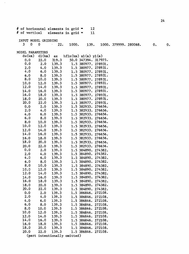
# of horizontal elements in grid = 12 # of vertical elements in grid = 11

INPUT MODEL GRIDDING 300 22. 1000. 139. 1000. 379999. 280068.

MODEL PARAMETERSdu(km)002468

10121416182002468

10121416182002468

10121416182002468

101214161820

000000000000000000000000000000000000000000000

dl(km) az222468

101214161820222468

101214161820222468

101214161820222468

10121416182022

000000000000000000000000000000000000000000000

319139139139139139139139139139139139139139139139139139139139139139139139139139139139139139139139139139139139139139139139139139139139139

hfln(km) xl(m).3.3.3.3.3.3.3.3.3.3.3.3.3.3.3.3.3.3.3.3.3.3.3.3.3.3.3.3.3.3.3.3.3.3.3.3.3.3.3.3.3.3.3.3.3

5011111111111111111111111111111111111111111111

.0

.5

.5

.5

.5

.5

.5

.5

.5

.5

.5

.5

.5

.5

.5

.5

.5

.5

.5

.5

.5

.5

.5

.5

.5

.5

.5

.5

.5

.5

.5

.5

.5

.5

.5

.5

.5

.5

.5

.5

.5

.5

.5

.5

.5

347394.380977.380977.380977.380977.380977.380977.380977.380977.380977.380977.380977.382933.382933.382933.382933.382933.382933.382933.382933.382933.382933.382933.384890.384890.384890.384890.384890.384890.384890.384890.384890.384890.384890.386846.386846.386846.386846.386846.386846.386846.386846.386846.386846.386846.

yl(m)317975.278931.278931.278931.278931.278931.278931.278931.278931.278931.278931.278931.276656.276656.276656.276656.276656.276656.276656.276656.276656.276656.276656.274382.274382.274382.274382.274382.274382.274382.274382.274382.274382.274382.272108.272108.272108.272108.272108.272108.272108.272108.272108.272108.272108.

0.

(part intentionally omitted)

25

0.2.4.6.8.

10.12.14.16.18.20.0.2.4.6.8.

10.12.14.16.18.20.0.2.4.6.8.

10.12.14.16.18.20.22.

0000000000000000000000000000000000

2468

101214161820222468

101214161820222468

10121416182022

1000

.0

.0

.0

.0

.0

.0

.0

.0

.0

.0

.0

.0

.0

.0

.0

.0

.0

.0

.0

.0

.0

.0

.0

.0

.0

.0

.0

.0

.0

.0

.0

.0

.0

.0

139139139139139139139139139139139139139139139139139139139139139139139139139139139139139139139139139139

.3

.3

.3

.3

.3

.3

.3

.3

.3

.3

.3

.3

.3

.3

.3

.3

.3

.3

.3

.3

.3

.3

.3

.3

.3

.3

.3

.3

.3

.3

.3

.3

.3

.3

1.1.1.1.1.1.1.1.1.1.1.1.1.1.1.1.1.1.1.1.1.1.1.1.1.1.1.1.1.1.1.1.1.

1000.

5555555555555555555555555555555550

398584.398584.398584.398584.398584.398584.398584.398584.398584.398584.398584.400540.400540.400540.400540.400540.400540.400540.400540.400540.400540.400540.402496.402496.402496.402496.402496.402496.402496.402496.402496.402496.402496.379999.

258461258461258461258461258461258461258461258461258461258461258461256187256187256187256187256187256187256187256187256187256187256187253912253912253912253912253912253912253912253912253912253912253912280068

CONSTRAINTS: for block for block for block for block for block for block for block for block for block for block for block 101 for block 112 for block 123 for block 134

'S: RATE AND STANDARD DEVIATION (M/YR1 rate =2 rate -

13 rate =24 rate -35 rate -46 rate =57 rate =68 rate =79 rate -90 rate -.01 rate =.12 rate =23 rate =34 rate =

0.2510E-01+/-0.2400E-01+/-0.2200E-01+/-0.2200E-01+/-0.1800E-01+/-0.1600E-01+/-0.1400E-01+/-0.1200E-01+/-0.1100E-01+/-0.9000E-02+/-0.8000E-02+/-0.6000E-02+/-0.4000E-02+/-0.3300E-01+/-

0.1000E-040.1000E-040.1000E-040.1000E-040.1000E-040.1000E-040.1000E-040.1000E-040.1000E-040.1000E-040.1000E-040.1000E-040.1000E-040.1000E-04

26

SINGULAR VALUES OF THE ROTATED GREENS FUNCS

singvals of aprime

0.456486E+06 0.196466E+06 0.120834E+06 0.973487E+05 0.815308E+05 0.580905E+05 0.439687E-K)5 0.351016E+05

0.292690E+05 0.253086E+05 0.225827E+05 0.207249E+05 0.195190E+05 0.18839 3E+05 0.237243E+03 0.105676E+03

0.792925E-I-02 0.505534E+02 0.364254E-K)2 0.287318E+02 0.154786E+02 0.127340E+02 0.114169E+02 0.732972E+01

0.418895E-K)! 0.309239E+01 0.291581E+01 0.201120E+01 0.121997E+01 0.995859E+00 0.640766E+00 0.506019E+00

0.455233E+00 0.303286E-I-00 0.227816E+00 0.176209E+00 0.677878E-01 0.544228E-01 0.498610E-01 0.274274E-01

0.257065E-01 0.135312E-01 0.959325E-02 0.386022E-02 0.183881E-02 0.140398E-02 0.799351E-03 0.794726E-03

0.712292E-03 0.493906E-03 0.352511E-03 0.299378E-03 0.916494E-04 0.714557E-04 0.456862E-04 0.913640E-05

0.835066E-05 0.632742E-05 0.329123E-05 0.OOOOOOE-KK) O.OOOOOOE-l-00 O.OOOOOOE-l-00 O.OOOOOOE-K)0 O.OOOOOOE-K)0

O.OOOOOOE+00 O.OOOOOOE+00 O.OOOOOOE+00 O.OOOOOOE+00 O.OOOOOOE+00 O.OOOOOOE+00 O.OOOOOOE+00 O.OOOOOOE+00

O.OOOOOOE+00 O.OOOOOOE+00 O.OOOOOOE+00 O.OOOOOOE+00 0.OOOOOOE+00 0.OOOOOOE+00 0.OOOOOOE+00 0.OOOOOOE+00







O.OOOOOOE+00 O.OOOOOOE+00 O.OOOOOOE+00 O.OOOOOOE+00 O.OOOOOOE+00 O.OOOOOOE+00 O.OOOOOOE+00

using 17singvals, smallest= 0.7929E+02for 17 singvals

rms model st.dev= 0.2281E-02 the strain component is -0.6309E-07

sum of, the misfits squared = 0.7561E+02 moment rate = 0.2640E+25 +/- 0.2251E+24

chekmod = 0.5630E-01 I/smallest sinval = 0.1261E-01

27

airwayairwayairwayairwayairwayalmondalmondalmondalmondbarrenbarrenbenchbenchbenchbenchbenchbenchbenchbenchbenchblhllresblhllresbonniebonniebonniebonniecastlechiches2cottoncottoncottoncottondavisgoldhatchhopperhopperhopperkengerkengermasonmasonmid fmine mtpark

barrenblhllreschiches2davistessbarrenbenchchiches2red hillchiches2tessbonniecottongoldhatchhopperkengermasonred hillwilddavistesscottongoldkengermasonshadered hillgoldkengermasonred hilltesskengerred hillmasonred hillwildmasonmid fmine rm2wildmine mtshadered hill

obs data0.6000E-03

-0.7000E-030.5000E-03

-0.3100E-02-0.8000E-03-0.1300E-02-0.3700E-02-0.9000E-030.1200E-020.1200E-02-0.1400E-02-0.5200E-020.3100E-02

-0.5800E-020.5900E-02

-0.2100E-02-0.7600E-020.1700E-02-0.6000E-030.1400E-02

-0.1100E-02-0.1600E-02-0.3100E-02-0.7000E-03-0.7000E-030.5300E-020.1720E-01

-0.3600E-020.4000E-03

-0.2100E-020.1080E-01

-0.7300E-020.3100E-02

-0.2600E-02-0.2400E-020.2400E-02-0.4000E-030.2200E-02

-0.2200E-020.7600E-02-0.9900E-02-0.2300E-020.2300E-020.1860E-01-0.8600E-02

calc data-0.6430E-03-0.1526E-03-0.5774E-03-0.9558E-030.1319E-03

-0.7585E-03-0.2967E-02-0.1235E-030.6226E-030.7165E-03-0.5906E-03-0.5150E-020.2359E-02

-0.7432E-020.4369E-02

-0.1472E-02-0.9433E-020.1806E-02

-0.4729E-030.2612E-02

-0.9132E-04-0.3971E-03-0.2369E-02-0.6091E-04-0.3613E-030.4806E-020.1704E-01

-0.3455E-020.5177E-05

-0.2675E-020.8904E-02

-0.6172E-02-0.8577E-03-0.2036E-02-0.1795E-02-0.9927E-030.1599E-020.7240E-03

-0.1672E-020.9875E-02-0.1029E-01-0.1194E-020.1657E-020.1779E-01-0.1047E-01

(obs-calc)/sigma 0.6906E+00

-0.4211E+00 0.8288E+00

-0.8247E+00-0.1035E+01-0.6016E+00-0.6663E+00-0.7059E+00 0.3609E+00 0.4395E+00-0.8993E+00-0.8288E-01 0.1853E+01 0.6044E+00 0.1914E+01

-0.6974E+00 0.1666E+01

-0.1760E+00-0.1588E+00-0.2020E+01-0.7759E+00-0.7518E+00-0.7312E+00-0.1278E+01-0.6775E+00 0.8235E+00 0.1238E+00

-0.1118E+00 0.3589E+00 0.4424E+00 0.2107E+01

-0.1128E+01 0.1131E+01

-0.4027E+00-0.1513E+01 0.4241E+01

-0.8330E+00 0.1845E+01

-0.1057E+01-0.2275E+01 0.5587E+00

-0.1844E+01 0.5844E+00 0.1161E+01 0.2677E+01

28

ESTIMATED MODEL (M/YR)block

123456789

101112131415161718192021222324252627282930313233343536373839 40 414243444546474849 50

slip(m/yr) 0.2510E-01 0.2400E-01- 0.2161E-01 0.1894E-01 0.1688E-01 0.1575E-01 0.1560E-01 0.1634E-01 0.1790E-01 0.2020E-01 0.2326E-01 0.2730E-01 0.2200E-01 0.1835E-01 0.1387E-01 0.1021E-01 0.8101E-02 0.7716E-02 0.8971E-02 0.1167E-01 0.1561E-01 0.2061E-01 0.2648E-01 0.2200E-01 0.1653E-01 0.1030E-01 0.5350E-02 0.2504E-02 0.1945E-02 0.3540E-02 0.7013E-02 0.1204E-01 0.1828E-01 0.2540E-01 0.1800E-01 0.1286E-01 0.6648E-02 0.1591E-02 0.1297E-02 0.1727E-02 0.1976E-03 0.4184E-02 0.9861E-02 0.1683E-01 0.2469E-01 0.1600E-01 0.1077E-01 0.4618E-02 0.2652E-03 0.2931E-02

st.dev.(m/yr) O.OOOOE+00 O.OOOOE+00 0.3757E-03 0.8041E-03 0.1138E-02 0.1329E-02 0.1375E-02 0.1300E-02 0.1133E-02 0.8993E-03 0.6219E-03 0.3176E-03 O.OOOOE-KX) 0.6512E-03 0.1419E-02 0.2029E-02 0.2382E-02 0.2473E-02 0.2342E-02 0.2041E-02 0.1621E-02 0.1120E-02 0.5718E-03 O.OOOOE-KX) 0.8688E-03 0.1877E-02 0.2662E-02 0.3100E-02 0.3197E-02 0.3011E-02 0.2615E-02 0.2070E-02 0.1428E-02 0.7281E-03 O.OOOOE-KX) 0.1068E-02 0.2205E-02 0.3024E-02 0.3437E-02 0.3485E-02 0.3247E-02 0.2800E-02 0.2208E-02 0.1520E-02 0.7738E-03 O.OOOOE+00 0.1113E-02 0.2206E-02 0.2929E-02 0.3256E-02

51 -0.3120E-0252 -0.9439E-0353 0.3298E-0254 0.9225E-0255 0.1643E-0156 0.2449E-0157 0.1400E-0158 0.9525E-0259 0.4141E-0260 -0.1262E-0361 -0.2345E-0262 -0.2255E-0263 0.4144E-0464 0.4265E-0265 0.1006E-0166 0.1704E-0167 0.2482E-0168 0.1200E-0169 0.8734E-0270 0.4673E-0271 0.1482E-0272 -0.2283E-0473 0.4136E-0374 0.2729E-0275 0.6706E-0276 0.1205E-0177 0.1844E-0178 0.2554E-0179 0.1100E-0180 0.8591E-0281 0.5905E-0282 0.3998E-0283 0.3354E-0284 0.4150E-0285 0.6384E-0286 0.9939E-0287 0.1463E-0188 0.2022E-0189 0.2645E-0190 0.9000E-0291 0.8318E-0292 0.7440E-0293 0.6873E-0294 0.6976E-0295 0.7971E-0296 0.9965E-0297 0.1297E-0198 0.1694E-0199 0.2175E-01

100 0.2720E-01101 0.8000E-02102 0.8388E-02103 0.8682E-02104 0.8945E-02

0.3257E-020.3015E-020.2594E-020.2047E-020.1411E-020.7196E-03O.OOOOE-KX)0.8731E-030.1708E-020.2267E-020.2545E-020.2590E-020.2444E-020.2145E-020.1722E-020.1203E-020.6185E-03O.OOOOE+000.4658E-030.1033E-020.1532E-020.1885E-020.2061E-020.2055E-020.1878E-020.1551E-020.1105E-020.5745E-03O.OOOOE+000.5744E-030.1249E-020.1823E-020.2211E-020.2387E-020.2353E-020.2130E-020.1748E-020.1239E-020.6430E-03O.OOOOE+000.8429E-030.1774E-020.2485E-020.2891E-020.3006E-020.2871E-020.2535E-020.2041E-020.1429E-020.7360E-03O.OOOOE+000.9571E-030.1995E-020.2754E-02

29

9437E-02 1041E-01 1205E-01 1450E-01 1785E-01 2213E-01 2727E-01 .6000E-02 6766E-02 7572E-02 8293E-02 9016E-02 9919E-02 .1122E-01 1317E-01 1603E-01 2011E-01 2576E-01 4000E-02 3847E-02 4233E-02 4840E-02 5458E-02 .6101E-02 6924E-02 8169E-02 1021E-01 1374E-01 2020E-01 3300E-01

135 -0.6309E-01 THE EXTENSION-RATE

105106107108109110111112113114115116117118119120121122123124125126127128129130131132133134

0.0000000000,0000000000000000000

0.3151E-02 0.3220E-02 0.3027E-02 0.2636E-02 0.2099E-02 0.1458E-02 0.7472E-03 O.OOOOE+00 0.8724E-03 0.1781E-02 0.2419E-02 0.2733E-02 0.2763E-02 0.2575E-02 0.2225E-02 0.1762E-02 0.1219E-02 0.6232E-03 O.OOOOE+00 0.5625E-03 0.1095E-02 0.1450E-02 0.1615E-02 0.1619E-02 0.1500E-02 0.1291E-02 0.1019E-02 0.7036E-03 0.3597E-03 O.OOOOE+00 0.1236E-01 PERPENDICULAR TO THE F.P. IS -0.6309E-01 MICRO-STRAIN/YR

stn displacement x-direcairwayalmondbarrenbenchblhllresbonniecastlechiches2cottondavisgoldhatchhopperkengermasonmid fmine mtmine rm2parkred hillshadetesswild

-0.4670E-02-0.4256E-02-0.4740E-02-0.1173E-02-0.4375E-020.5248E-020.6248E-02

-0.4561E-020.4156E-02

-0.4162E-020.4062E-020.1262E-02-0.2620E-020.5565E-02

-0.2778E-02-0.3447E-020.7417E-020.7418E-020.5257E-02

-0.2135E-02-0.6458E-02-0.4638E-02-0.3341E-02

y-direc0.1212E-010.9817E-020.1145E-010.5115E-020.1295E-01-0.4489E-02-0.5359E-020.9821E-02-0.2351E-020.1312E-01-0.2515E-02-0.1650E-030.7235E-02

-0.4645E-020.6135E-020.8556E-02-0.4954E-02-0.4954E-02-0.4618E-020.5178E-020.9936E-020.1237E-010.7594E-02

30

APPENDIX C

The FORTRAN program INVERSE.FOR

C NEW VERSION OF THE INVERSE PROGRAM BY RAH JUNE 1986C THIS VERSION GIVES OPTION OF INCLUDING COMPONENT OF EXTENSIONC PERPENDICULAR TO THE FAULT PLANE, IN ADDITION TO THE 2-D FAULT MODELC IT ALSO GIVES A CHOICE OF SMOOTH MODEL-WEIGHTING ORC MODEL-WEIGHTING BY THE IDENTITY (WHICH GIVES A MINIMUM-LENGTH SOLN)Cc This Fortran program is used to invert geodetic line-length or strainc data for slip on a gridded 2-dimensional vertical strike-slip fault.c We use 2-d Chinnery functions for the dislocation model, andc incorporate data weighting and model weighting.c Subroutine Sensit does a singular value decomposition on the Chinneryc function matrix. The resulting model estimates, covariance, resolution,c etc. are determined for a varying number of singular values.c Misfits and resolution are calculated for the data.c Fixed faults (constrained rates with standard deviations)c and variable faults are permitted.ccc Compile with single precision IMSL routinescc input at terminalc nstart - number of singular values to start withc numrum - number of times to loop through the singularc value loopc nwt - type of model-weighting desiredc nwt=l no weighting, results in minimum-length modelc nwt=2 smoothing, results in smooth modelc nstrain - normal strain component in modelc nstrain * 1 noc nstrain = 2 yescc input in data filec iopt - 0 for strain cards, 1 for *pairs* of llcardsc nf - total number of faults in single fit (fixed + variable)c nvf - number of variable faultsc nlines - number of linesc nstns - number of stationsc nff - number of fixed faults (nf includes nff and nvf)cc station coordinate cards in metersc line length change cards (sta l,sta 2,length,length change, stdc dev)c all in metersc

31

c modelc nhe - number of horizontal elts in gridc nve - number of vertical elts in gridc al - half length of fault (km)c du - depth to top of fault (km)c dl - depth to bottom of fault (km)c az - az of fault (clockwise from north,in degrees)c fx,fy - midpt coordinates of center of faultc consrat- constrained slip(m) on specified block #c see subroutine FMODEL for more detailsc outputc all inputc program converts all coordinates of fault blocks and datac to a fault centered systemc with xl parallel to fault, x2perpendicular to fault and x3 downc (xl = x, x2 = y)c Right lateral slip is positive.cc calls CHINSSL, CRD, FMODEL, GETINT, MODELWT, SENSIT, OUTSGc GETINT, WRHEADER, LENTRUE, LJUST, LEFTENDcc this program uses IMSL routines:c EBALAF, EBBCKF, EGRH3F, EHBCKF, EHESSF, EIGRF, LSVDB,c LSVDF, LSVG1, LSVG2, UERTST, UGETIO, USWFM, USWFV, VHS12,c VMULFB, VMULFF, VMULFPc

real*8 sn(2,500), sta(200), distan(500), dist2, distreal*4 x(200), y(200), dx(2), dy(2), xx(200), yy(200)dimension tmstore(500,500),s(500)dimension green(500,500), deltal(500,500), descri(lO)dimension azi(500), sdx(200), sdy(200), str(500)dimension sd(500),stamovx(500,500),stamovy(500,500)dimension stndispx(200), stndispy(200), stndisp(200)dimension xpos(500),ypos(500),proje(500),projn(500)character*5 net(500)character*! icross(500,500), eff, spaceinteger keep(2)

cdimension aprime(500,500),v(500,500),ut(500,500) dimension u(500,500),sinval(500),wk(1000) dimension workar(500,500),td(500,500),tdinv(500,500) dimension tminv(500,500),tm(500,500),resolv(500,500) dimension datares(500,500),prodl(500,500),prod2(500,500) dimension prod3(500,500),sinvalm2(500),sinvalml(500) dimension covm(500,500),utnew(500,500),c(500,500) dimension estmodl(500),datacalc(500),dmisfit(500) dimension sdmod(500),tmt(500,500),vnew(500,500) dimension als(500),dus(500),dls(500),us(500) dimension azs(500),fxs(500),fys(500) dimension chekmod(500),slipco(500),OMEGA(500)

ccc

32

data blankMh /, nldim/500/, nfdim/500/, eff/'F'/, space/' '/data dtr/0.01745329/

c c cc input at terminal number of singular values to start with c and the number of times to loop through the singular value decomposition c in subroutine SENSIT c Also input if smooth model-weighting is wanted (l=no)

call getint('# of svals to start with',17,nstart)call getint('# of additional times to loop thru the

+s.v.d.',0,numrun)call getintCmodelwting l=no,2=yes' ,2,nwt)call getint('normal strain l=no,2=yes',2,nstrain)write(16,503) nstart,numrun,nwt,nstrain

c c

105 continuejf=0

cc read header card (data file) c stop when nf (first 5 columns) 0 c

read (5,603) iopt,nf,nlines,nstns,nff,descriif(nf.eq.O) go to 100write (6,505) nwt,iopt,nf,nlines,nstns,nff,descri

cC

c read station coordinates. cc

read(5,605)(sta(i),xx(i),yy(i),i=l,nstns)write(6,507)write(6,509)(sta(i),xx(i),yy(i),i=l,nstns)

c cc read data, stop when nlines=0 and jump to model generating section c read strain cards if iopt=0c read *pairs* of llcards if iopt=lc **************************************************************c

if (nlines.eq.O) go to 107 if(iopt.eq.l) go to 200read (5,607) (net(j),(sn(i,j),i=l,2),distan(j),

+ str(j),sd(j),azi(j),j=l,nlines) write(6,511)write(6,513) (net(j),(sn(i,j),i=l,2),distan(j),

+ str(j),sd(j),azi(j),j=l,nlines) go to 202

33

200 do 201 i«l,nlinesread(5,609) net(i),(sn(k,i),k=l,2),azi(i),distan(i) read(5,611) dist2,sd(i) str(i)=dist2-distan(i)write(6,515) net(i),(sn(k,i),k=l,2),distan(i),

+ str(i),sd(i),azi(i)201 continue202 continue c

c At this point the data has been read.c Subroutine fmodel generates the fault model.c *************************************c

call fmodel(nf,nff,nfdim,als,dus,dls,azs,fxs,fys, + nve,nhe,elarea,ratio)nvet = nvenhet = nhe

c cc generate the data kernel G. c cc for right lateral motion positive, slip = -1.0 c loop on fault segments, jf= # of segment c107 continue

Jf-Jf+1 c

al-als(jf)du=dus(jf)dl-dls(Jf)slip=-1.0az=azs(jf)fx=fxs(jf)fy-fys(jf)

cc convert to fault-centered coordinate system, c first save xpos and ypos c

do 108 i=l,nstnsxpos(i)=xx(i)ypos(i)=yy(i)x(i)=xx(i)y(l)-yyCi)

108 continue c

call crd (jf,x,y,nstns,nf,az,fx,fy,proje,projn) cc compute station displacements due to current fault, c where x(i), y(i) are now in fault centered coords

34

sll=0.s22=0.s!2=0.do 106 i=linstnsx(i)=x(i)/1000.

x3=0 kk=i

c cc al,a2,a3,a4 are displacement components in the ul-direction c bl,b2,b3,b4 u2-direction c cl,c2,c3,c4 u3-direction c dl,d2,d3,d4 are the strain components in the 1-direction c fl,f2,f3,f4 2-direction c hl,h2,h3,h4 12-direction c sdx is the total displacement in the x-direction (parallel fault) c sdy y-direction (perpendicular) c sdz z-direction (vertical) c

call chinssl (slip,-fx(kk),y(kk),x3,+al,+dl,al,bl,cl,dl,fl,hl) call chinssl (slip,+x(kk) ,y(kk),x3,+al,+du,a2,b2,c2,d2,f2,h2) call chinssl (slip,+x(kk),y(kk) ,x3,-al,-Kll,a3,b3,c3,d3,f3,h3) call chinssl (slip,+x(kk) ,y(kk),x3,-al,+du,a4,b4,c4,d4,f4,h4) sll=(dl-d2-d34d4)*1000. s22=(fl-f2-f3+f4)*1000. Sl2=(hl-h2-h3+h4)*1000.

csdx(i)=al-a2-a3+a4 sdy(i)=bl-b2-b3+b4 sdz=cl-c2-c3+c4

c106 continue cc compute line length changes due to current fault. c

if (nlines.eq.O) go to 112 do 104 j=l,nlines

cdo 103 1-1,2 keep(i) = 0 do 102 k=l,nstnsif (sn(i,j).ne.sta(k)) go to 102 keep(i)~k kk=keep(i) go to 101

102 continue 101 continue

dx(i)=sdx(kk) dy(i)=sdy(kk)

103 continue c

35

if ( keep(l)*keep(2) .eq. 0 ) thenwrite (6,517) (keep(i),sn(i,j),i=l,2)dist = 0.0deltal(j,jf) = 999.azim = 999.

else11 = keep(2)mm = keep(l)sx=x(ll)-x(mm)sy=y(11)-y(mm)dist = sqrt(sx*sx+sy*sy)rx=dx(2)-dx(l)ry=dy(2)-dy(l)deltal(j,jf) - (rx*sx + ry*sy) / distif ( y(ll)*y(mm) .ge. 0. ) then

icross(j,jf) = spaceelse

icross(j,jf) = effendifazim = atan2(-sx,sy) * 180.73.14158 + 90,if (azim .le. 0.) azim = azim + 360.dist = dist * 1000.

endif

cdist = dist + deltal(j,jf)

c c104 continue 112 continuec c********************************************************cc express station displacements in ns-ew coord system.c save station displacements due to current fault beforec obtaining next one.c

call crd(jf,sdx,sdy,nstns,nf,az,0.,0.,proje,projn)do 114 it=l,nstnsstamovx(it,jf)=sdx(it)stamovy(it,jf)=sdy(it)

114 continuec c************************************************c ..........................

if(jf.lt.nf) go to 107 cc end of loopc *********************************************************

36

c calculate coefficient for normal strain component if(nstrain.ne.2) go to 458 fx=fxs(nf) fy=fys(nf) az=azs(nf) call crd(jf,xpos,ypos,nstns,nf,az,fx,fy,proje,projn)

cc ************************************************************458 nvf=nf-nff

lindex=nlines-Hnffnfplusl - nf+1if(nstrain.ne.2) nfplusl=nf

cc set Green's function matrix to the nf columns of deltal c

do 302 i=l,nlinesdo 303 j=l,nfgreen(i,j)=deltal(i,j)


37

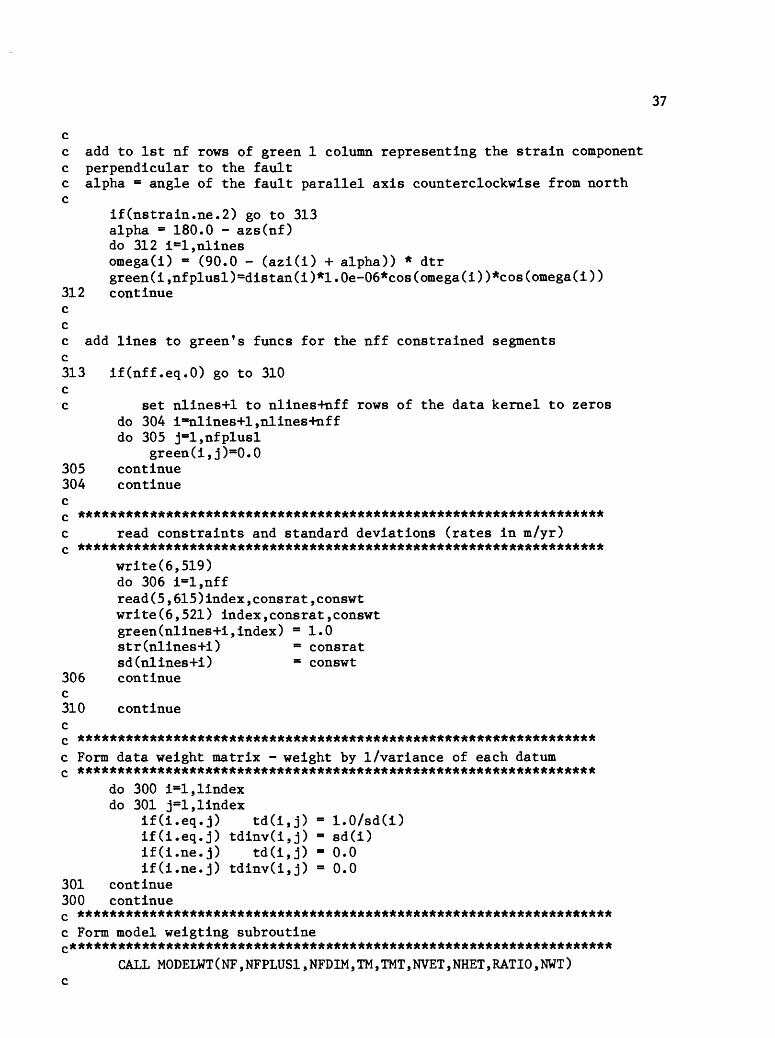
cc add to 1st nf rows of green 1 column representing the strain componentc perpendicular to the faultc alpha = angle of the fault parallel axis counterclockwise from northc

if(nstrain.ne.2) go to 313alpha = 180.0 - azs(nf)do 312 i=l,nlinesomega(i) - (90.0 - (azi(i) + alpha)) * dtrgreen(i,nfplusl)=distan(i)*1.0e-06*cos(omega(i))*cos(omega(i))

312 continueccc add lines to green's funcs for the nff constrained segmentsc313 if(nff.eq.O) go to 310cc set nlines+1 to nlines+nff rows of the data kernel to zeros

do 304 i=nlines+l,nlines+nffdo 305 j=l,nfplusl

green(i,j)=0.0 305 continue 304 continue c cc read constraints and standard deviations (rates in m/yr) c

write(6,519)do 306 1-1,nffread(5,615)index,consrat,conswtwrite(6,521) index,consrat,conswtgreen(nlines+i,index) -1.0str(nlines+i) « consratsd(nlines+i) = conswt

306 continue c310 continue c cc Form data weight matrix - weight by 1/variance of each datumc *****************************************************************

do 300 i=l,lindex do 301 j-l,llndex

if(i.eq.j) td(i,j) - 1.0/sd(i)if(i.eq.j) tdinv(i,j) - sd(i)if(i.ne.j) td(i,j) - 0.0if(i.ne.j) tdinv(i,j) - 0.0

301 continue 300 continue c c Form model weigting subroutine

(*************************;

CALL MODELWT(NF,NFPLUSl,NFDIM,TM,TMT,NVET,NHET,RATIO,NWT)

38

C FORM TMINV USING IMSL ROUTINE LGINF TO CALCULATE GENERALIZED INVERSE OF TM C

DO 111 1=1,NFPLUSl DO 111 J=l,NFPLUSl

TMSTORE(I,J)=TM(I,J) 111 CONTINUE

TOL=0.0CALL LGINF(TMSTORE,500,NFPLUSl,NFPLUSl,TOL,TMINV,

+ 500,S,WK,IERO) C

c Calculate model, resolution, misfits, covariance, c chi-squared for weighted-model and data problem

call sensit (v,green,aprime,ut,sinval,wk,workar, + u,td,tdinv,tm,tminv,prodl,prod2,prod 3, + resolv,datares,sinvalm2,sinvalml,covm, + utnew,c,estmodl,str,nldim,nfdim,NFPLUSl, + nlines,nf,nvf,nff,datacalc,sd,dmisfit,sdmod, + lstsig,sn,nstart,numrun,lindex,vnew, + chekmod,nhe,nve,elarea,slipco,sta, + stamovx,stamovy,nstns,stndispx,stndispy, + stndisp,proje,projn)

ccccw call uswfmCgreens funcs',12,green,500,lindex,nf,3)c

go to 105100 continuecc main program read and write statement formatscc

503 format (Ix,'start with',i4,' singular values'/+ ' loop through the s.v.d.',i2,' more times'/ + ' model-weighting option 1 ,i2,' l=none,2=smooth'/ + ' normal strain component*,i2,' 1=110,2=yes')

505 format (llx,'nwt (l=no-modelwting, 2=smooth) = ',i3/ + llx,'iopt (0=strcards, l=llcards)... = ',i3/ + llx,'number of faults............... = ',i3/+ llx,'number of lines................ = ',i3/+ llx,'number of stations............. = ',i3/+ llx,'number of fixed faults......... = ',i3/+ Ilx,10a4)

507 format (//10x,'station',9x,'xcoord(m)',6x,'ycoord(m)') 509 format (10x,a8,2x,2fl5.3)511 format (//Ix,'net',4x,'stnl',5x,'stn2',7x,'length(m)',

+ ' dl/dt(m/yr)',lx,'stdev',2x,'az')

39

513 format 515 format 517 format 519 format

+521 format 603 format 605 format 607 format

+609 format 611 format 615 format

stop end

(Ix,a5,2x,a8,lx,a8,2x,fl0.3,2x,f7.4,2x,f6.4,2x,f5.1) (Ix,a5,lx,a8,lx,a8,2x,fl0.3,2x,f7.4,2x,f6.4,2x,f5.1) (Ix,2(i3,'/',a8,2x),' 0 station not on X-Y list 1 ) (//lx,' CONSTRAINTS: RATE AND STANDARD DEVIATION ','(M/YR)')

(lx,'for block',i4,' rate (il,i4,3i5,5x,10a4)(a8,6x,fl6.0,6x,f!6.0) Ca5,8x,a8,lx,a8,t44,fl0.3,t54,f7.4,

Ix,f6.4,t69,f5.1)(a5,lx,a8,lx,a8,t37,f5.1,t56,fll.4) (t56,fll.4,fl0.4) (14,el2.4,el2.4)

f ,el2.4,'+/-',el2.4)

40

cc SUBROUTINES CALLED BY INVERSEc ***********************************************c ***********************************************c GETINTcc converts a string answer to an integer provided the stringc is not blank....c ques = question to be askedc intdefault = default answerc int » integer answerc

subroutine getint(ques,intdefault,int) c

integer int, intdefaultcharacter*(*) quescharacter*10 default, ans, fmtcharacter bel*lparameter (bel-char(7))

cwrite(default,'(ilO) f ) intdefaultcall 1just(default)lengdef = lentrue(default)

clengq = lentrue(ques)

10 print f (/,lh$,a) f& ques(1:lengq)//': ['//default(Itlengdef)//'] 'read (*,'(a)') ansleng = lentrue(ans)if(leng.eq.O) then

int = intdefaultelse

write(fmt,'(a,i3,a) f ) '(i f leng, ')' read(ans(1:leng),fmt,err=90) int

endif c

return cc.....error message 90 print f (/,lx,a) f ,

&'*** error, expecting an integer answer... try again...'print *, belgoto 10end

c c

41

c ***********************************************c MODELWTcc subroutine to calculate model-weight matrixc for second differences (laplacian) in two dimensional inversec

SUBROUTINE MODELWT(NF,NFPLUS1,NFDIM,D,DT,NVE,NHE,RATIO,NWT) c

DIMENSION d(nfdim,l),dt(nfdim,l) dimension xpartd(500,500), ypartd(500,500)

c cc nf=number of faultsc nhe^number of horizontal elements in grid c nve=number of vertical elements in grid c ngrid=number of elements in grid c nuprhsûpper r.h. block in grid c nlrhs=lower r.h. block in grid c ratioKLength/height of blocks in grid=dx/dy c nwt=l if no model-weighting is desired, c nvt-2 if smoothing is desired c

RATIOSQ - RATIO * RATIO NGRID - NHE * NVE NUPRHS - NGRID - NVE -I- 2 NLRHS - NGRID + 1

CC IF NO MODEL-WEIGHTING IS DESIRED, ASSIGN MODEL-WEIGHTING C MATRIX, [D], TO BE THE IDENTITY MATRIX C

IF(NWT.EQ.1)GO TO 500 C C INITIALIZE ARRAY ELEMENTS

DO 5 I=l,NLRHS+2DO 5 J=l,NLRHS+2XPARTD(I,J) =0.0YPARTD(I,J) - 0.0D(I,J) - 0.0

5 CONTINUE C C TO LEFT EDGE OF GRID ASSIGN XPART OF LAPLACIAN

DO 10 I - 2,NVE+1XPARTDU,!) - + 1.0XPARTD(I,I) - - 2.0XPARTD(I,I+NVE) - + 1.0

10 CONTINUE C C TO RIGHT EDGE OF GRID ASSIGN XPART OF LAPLACIAN

DO 20 I - NUPRHS,NLRHSXPARTDU,I-NVE) - + 1.0XPARTD(I,I) - - 2.0

20 CONTINUE C

42

C TO TOP ASSIGN YPART OF LAPLACIANDO 30 I = 2,NUPRHS,NVEYPARTD(I,I) = - 1.0YPARTD(I,I-H) - + 1.0

30 CONTINUE C C TO BOTTOM ASSIGN YPART OF LAPLACIAN

DO 40 I = NVE+1,NLRHS,NVEYPARTD(I,I-1) = + 1.0YPARTD(I,I) = - 2.0YPARTD(I,NGRID+2) = + 1.0

40 CONTINUE CC ASSIGN XPARTS TO ALL PREVIOUSLY UNASSIGNED C (EXCLUDE LEFT & RIGHT EDGES)

DO 100 I - NVE+2, NLRHS-NVEXPARTD(I,I-NVE) = + 1.0XPARTD(I,I) = - 2.0XPARTD(I,I+NVE) = + 1.0

100 CONTINUE CC ASSIGN YPARTS TO ALL PREVIOUSLY UNASSIGNED C (EXCLUDE TOP & BOTTOM EDGES)

K - 3 150 L = K + NVE - 3

DO 200 I - K,LIF(I.GT.NLRHS) GO TO 250YPARTD(I,I-1) = + 1.0YPARTD(I,I) = - 2.0YPARTD(I,I+1) = + 1.0

200 CONTINUEK = K + NVEGO TO 150

CC ADD XPART & YPART OF LAPLACIAN TO FORM D(I,J) C WEIGHT SMOOTHING FOR NON-SQUARE BLOCKS 250 DO 300 I = 1,NLRHS+1

DO 300 J = 1,NLRHS+1D(I,J) - XPARTD(I,J) + RATIOSQ*YPARTD(I,J)

300 CONTINUE c C ASSIGN D(I,J) TO 2 SIDE CONSTRAINTS AND TO THE STRAIN COMPONENT

D(l,l) = 1-0D(NLRHS+1,NLRHS+1) =1.0 D(NFPLUS1,NFPLUS1) =1.0 GO TO 700

C500 DO 600 I=1,NFPLUS1

DO 600 J=1,NFPLUS1 IF(I.EQ.J) D(I,J)=1.0 IF(I.NE.J) D(I,J)=0.0

600 CONTINUE C C

43

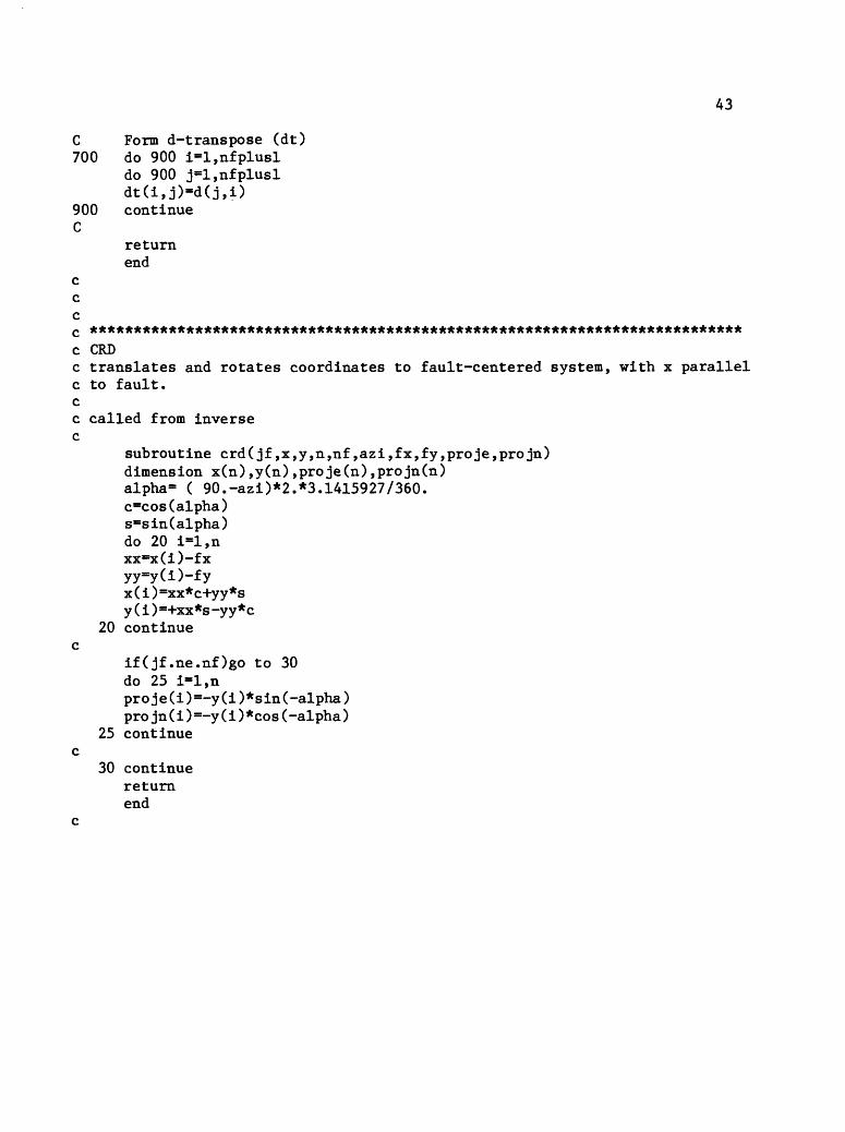
C Form d-transpose (dt) 700 do 900 i=l,nfplusl

do 900 j=l,nfplusl

900 continue C

returnend

c c cC

c CRDc translates and rotates coordinates to fault-centered system, with x parallelc to fault.cc called from inversec

subroutine crd(jf ,x,y,n,nf ,azi,fx,fy,proje,projn)dimension x(n),y(n) ,proje(n) ,projn(n)alpha- ( 90. -azi)*2.*3. 1415927/360.c-cos( alpha)s=s in (alpha)do 20 i=l,nxx=x(i)-fxyy=y(i)-fyx(i)=xx*c+yy*sy(i)=+xx*s-yy*c

20 continue c

if(jf.ne.nf)go to 30do 25 i-l,nproje(i)=-y(i)*sin (-alpha)pro jn(i)=-y(i)*cos (-alpha)

25 continue c

30 continuereturnend

44

c ************************************************c FMODEL

subroutine fmodel(nf,nff,nfdim,als,dus,dls,azs,fxs,fys, + . nve,nhe,elarea,ratio)

cc this subroutine reads fault cards and calculates c elements required by inverse, c faults can be specified in 3 ways: c one endpoint, azimuth, length c two endpoints c midpoint, azimuth, half-lengthc subroutine returns midpoint, azimuth, and half-length to inverse. c .........................cc variables:cc kode = l=one endpoint, azimuth, lengthc 2=both endpointsc 3=midpoint, azimuth, half-lengthc 4=grid; one endpoint azimuth lengthc nhe - number of horizontal elements, used for kode=4c nve = number of vertical elements, used for kode=4c du = depth to top (km)c dl = depth to bottom (km)c az = azimuth (from 1 to 2)c length = total fault length (km), or half-length if kode=3c xl,yl,x2,y2 = end pt coordinates (m), or (xl,yl) asmidpt if kode=3c al = half length (km)c fx,fy = mid pt coordinates (m)c

real lengthdata dtr/0.01745329/dimension als(nfdim),dus(nfdim),dls(nfdim)dimension azs(nfdim),fxs(nfdim),fys(nfdim)

ck=0

cc read model parameters c

700 read(5,617) kode,nhe,nve,du,dl,az,length,xl,yl,x2,y2write(6,523)write(6,525) kode,nhe,nve,du,dl,az,length,xl,yl,x2,y2

cgo to (1,2,3,4) kode

cc **************************************c one endpoint, azimuth, lengthc **************************************1 angle = az * dtr

al - length/2.fx = xl -l- al * sin(angle) * 1000. fy = yl + al * cos(angle) * 1000.go to 5

c **************************************

45

c two endpointsc **************************************2 continue

fx = 0.5 * (xl + x2)fy - 0.5 * (yl + y2)dx = x2 - xldy = y2 - ylal = sqrt(dx*dx + dy*dy) / 2000.az = atan2(dx,dy)/dtrif ( az .It. 0.0 ) az - az + 360.go to 5

c *************************************c midpoint, azimuth, half-lengthc *************************************3 fx=xl

fy-yial=lengthgo to 5

c *************************************5 k=k+l

als(k)=aldus(k)=dudls(k)=dlazs(k)=azfxs(k)=fxfys(k)=fy

cif(k.eq.nf) go to 1000if(k.lt.nf) go to 700

c *************************************c gridded fault elementsc *************************************4 continue c

write(6,527) nhewrite(6,529) nve

nhesave=nhenvesave=nvengf=nhe*nvedeltalen=length/float(nhe)deltaht=(dl-du)/float(nve)ratio=deltalen/deltahtelarea=deltalen*deltaht*l.Oe+10azrads=(180-az)*3.14159/180.0deltax=1000*deltalen*sin(azrads)deltay=1000*deltalen*cos(azrads)xstart=xl-0.5*deltaxystart=y1+0.5*deltaygdu=du

46

do 600fxaBxstart+j*deltaxfyssystart-j*deltaydo 500 i=l,nvek=k+ldu=gdu + (i-l)*deltahtdl=gdu + i*deltahtals (k) !BdeltaIen/2.0dus(k)=dudls(k)=dlazs(k)~azfxs(k)=fxfys(k)=fy


cif(k.lt.nf) go to 700

cc *************************************c print computed elements 1000 continue

write(6,531) write(6,533) do 1100 1-1,nfwrite(6,535) dus(i),dls(i),azs(i),als(i),fxs(i),fys(i)

1100 continue c c

nve - nvesave nhe - nhesave

cc read and write format statements c

523 format(//lx, f INPUT MODEL GRIDDING')525 format(lX,3i4,4x,8f8.0)527 format(/lx,*# of horizontal elements in grid - f ,i4)529 format(lx,*# of vertical elements in grid - f ,i4)531 format(/lx, f MODEL PARAMETERS 1 )533 format(4x, f du(km) f ,2x, f dl(km) f ,2x, f az f ,3x,

+ f hfIn(km) f ,lx, f xl(m) f ,lx, f yl(m) f ) 535 format(4f8.1,2f8.0) 617 format(314,4x,8f8.0)

creturn end

c c

47

c SENSITsubroutine sensit (v,a,aprime,ut,sinval,wk,workar,

+ u,td,tdinv,tm,tminv,prodl,prod2, + prod3,resolv,datares,sinvalm2,sinvalml, + covm,utnew,c,estmodl,str,nldim,nfdim, + NFPLUSl,nlines,nf,nvf,nff, + datacalc,sd,dmisfit,sdmod,Istsig,sn, + nstart,numrun,lindex,vnew,chekmod, + nhe,nve,elarea,slipco,sta, + stamovx,stamovy,nstns,stndispx,stndispy, + stndisp,proje,projn)

cc Computes the u,v and s matrices of a singular value decomposition, c Prints out singular values.c Also calculates model-resolution, covariance, and c estimated model, and data resolutionc Does calculations which keep a varying number of singular values, c Can compare chekmod and 1/smallest singval to decide how many c singular values to keep- want chekmod | I/smallest singular value, cc Notes: nlines - number of baselinesc nf total number of faults (fixed + variable) c nff - number of fixed faults c nvf - number of variable faultsc a Greens func array in main program (unrotated) c aprime " Greens func array in Sensit (rotated space) c

dimension a(nldim,l),aprime(nldim,!),v(nldim,l) dimens ion ut(nldim,1),sinval(1),wk(1) dimens ion u(nldim,1),workar(nldim,1),resolv(nfdim,1) dimension td(nldim,1),tdinv(nldim,1),tm(nfdim,1) dimension tminv(nfdim,l),prodl(nfdim,!) dimension prod2(nfdim,l),prod3(nfdim,l) dimension sinvalml(nfdim),sinvalm2(nfdim) dimension c(nfdim,1),covm(nfdim,1),utnew(nldim,1) dimension estmodl(nfdim),str(nldim),npar(4) dimension datares(nldim,!),datacalc(nldim),sd(nldim) dimension dmisfit(nldim),sdmod(nfdim),slipco(nfdim) dimension vnew(nldim,l),chekmod(nfdim),product(500) dimension stamovx(nfdim,!),stamovy(nfdim,!) dimension stndispx(nldim),stndispy(nldim) dimension stndisp(2*nldim),proje(nldim),projn(nldim) real*8 sn(2,nldim), sta(2*nldim)

c cc Weight (or 'transform') the data kernel A; A'=Td*A*Tm**-l c

call vmulff(td,a,lindex,lindex,nfPLUSl,nldim,nldim, + prodl,nldim,ier)call vmulff(prodl,tminv,lindex,nfPLUS1,nfPLUS1,

+ nldim,nfdim,aprime,nldim,ier) cw call uswfm ('Rotated Greens func',19,aprime,nldim, cw + lindex,nfPLUSl,3) c

48

c Form singular value decomposition of aprime where A f =U*S*Vt c note that U,S,and V are in transformed (primed) system c Create a space to store V

do 1 i = l,lindex do 1 j = l,nfPLUSl

v(i,j) = aprime(i,j) 1 continue c c create a space to put U, where Ut = U-transpose

do 45 i=l,lindexdo 42 j=l,lindexif(i.eq.j) ut(i,j) = 1.0if(i.ne.j) ut(i,j) = 0.0

42 continue 45 continue cc ** Call IMSL SVD routine to find aprime = u*s*vt ** c

call Isvdf (v,nldim,lindex,nfPLUSl,ut,nldim, + lindex,sinval,wk,ier)

write (6, 537)537 format(// f SINGULAR VALUES OF THE ROTATED GREENS FUNCS 1 /) c

call ugetio(3,5,6)call uswfv( 'singvals of aprime 1 ,18, sinval,nfPLUSl, 1,3)

cc set a do loop to cycle through a # of singvals c if there are zero constrained blocks, then start c the loop with one singular value c

if(nff.eq.O) nstart=l do 884 ind=nstart ,nstart-fnumrun if(ind.gt.nf) go to 999 Istsig = indwrite(6,539)lstsig,sinval(lstsig)

539 formatC/// 1 using 1 ,i5, 'singvals, smallest= f ,e!2.4) c c c cc** Calculate resolution matrix Tm**(-l)*V*Vt*Tm ** c

call vmulfp (v,v,nfPLUSl, Istsig, nfPLUSl,nldim,nldim,prod2, + nfdim,ier)

call vmulff (tminv,prod2,nfPLUSl,nfPLUSl,nfPLUSl,nfdim,nfdim, + prod3,nfdim,ier)

call vmulff (prod3,tm,nfPLUSl,nfPLUSl,nfPLUSl,nfdim, + nfdim,resolv,nfdim,ier)

cw call uswf m( f resolution ' ,10, resolv,nf dim, nfPLUSl,nfPLUSl, 3) c c

49

c** calculate data resolution (datares) where N"Td**(-l)*U*Ut*Td **c form U from Utc

do 150 i=l,lindexdo 150 j«l,lindex

150 continuecc

call vmulff (u,ut,lindex,lstsig,lindex,nldim,nldim, + prod2,nfdim,ier)

call vmulff (tdinv,prod2,lindex,lindex,lindex,nldim,nfdim, + prod3,nfdim,ier)

call vmulff (prod3,td,lindex,lindex,lindex,nfdim,nldim, + datares, nldim,ier)

cw call uswfmCdata resolution* ,15, datares, nldim,lindex,lindex, 3) c c cc** Compute model covariance matrix ** c covm - Tm**(-l)*V*sinvalm2*Vt*(Tm**(-l))t c

do 5 i - l,lstsigsinvalm2(i) = 1.0 / (sinval(i)*sinval(i))

5 continue c

npar(l) - nfPLUSlnpar(2) = Istsignpar(3) = 0npar(4) = 0call vmulfb (v,nldim,sinvalm2,nfdim,npar,prodl,nfdim)call vmulfp (prodl,v,nfPLUSl, Istsig, nfPLUSl,nfdim,nldim,

+ prod2,nfdim,ier)call vmulff (tminv,prod2,nfPLUSl,nfPLUSl,nfPLUSl,nfdim,

+ nfdim,prod3,nfdim,ier)call vmulfp (prod3,tminv,nfPLUSl,nfPLUSl,nfPLUSl,nfdim,

+ nf dim, covm, nf dim, ier)cw call uswfm( f modelcov f ,8,covm,nfdim,nfPLUSl,nfPLUSl,3) c cc ** calculate sqrt(covm(i,i))= st.dev. model parameter i - sdmod(i) ** c ** and the r.m.s. model standard deviation rmsstdev ** c ** To avoid problems w/ roundoff set #'s with absolute values ** c ** less than l.Oe-08 equal to O.Oe-08 ** c c

rmsstdev = 0.0do 617 i=l,nfpluslif(abs(covm(i,i)).lt.l.0e-08) covm(i,i)=0.0e-08sdmod(i)=sqrt(covm(i,i))rmsstdev = rmsstdev + covm(i,i)

617 continueif(nvf.eq.O) go to 619rmsstdev = sqrt(rmsstdev/float(nvf ))

50

write(6,541) lstsig,rmsstdev 541 formatClx/for'jiS,' singvals'/

+ 10x, f rms model st.dev=t ,e!2.4) c c cc ** calculate mest = Tm**(-l)*V * 1/sinval * Ut * Td *data ** c 619 do 16 i=l,lstsig

sinvalml(i) = sqrt(sinvalm2(i)) 16 continuecw call uswfm ('v-matrix',8,v,nldim,nfPLUSl,nfPLUSl,3) cw call uswfm ( f u-matrixt f ,9,ut,nldim,lindex,lindex,3) c c only use first Istsig columns of v

do 442 i=l,nfPLUSldo 446 j-1,Istsigvnew(i,j) - v(i,j)

446 continue 442 continue c c only use first Istsig rows of ut

do 335 i = 1,Istsigdo 333 j = 1,lindexutnew(i,j) = ut(i,j)

333 continue 335 continue cc form chekmod = sinvalml * utnew * td * data c prodl = utnew * td c product = prodl * data c

call vmulff(utnew,td,Istsig,lindex,lindex, + nldim,nldim,prodl,nfdim,ier)

c c

do 222 i-1,Istsigproduct(i) =0.0do 220 j=l,lindexproduct(i) = product(i) + prodl(i,j)*str(j)

220 continue 222 continue c

do 217 1-1,Istsigchekmod(i) product(i) * sinvalml(i)

217 continue c

51

c form estmodl m tminv * vnew * chekmod c prod3 tminv * vnew c estmodl = prod3 * chekmod c

call vmulff(tminv,vnew,nfPLUSl,nfPLUSl,lstsig,nfdim, + nldim,prod3,nfdim,ier)

cdo 224 i=l,nfPLUSlestmodl(i)=0.0do 223 j=l,lstsigestmodl(i) - estmodl(i) + prod3(i,j)*chekmod(j)

223 continue224 continuecc form stndispx stamovx * estmodlc stndispy = stamovy * estmodlc

do 209 l=l,nstnsstndispx(l)=0.0stndispy(1)=0.0do 209 k-l,nfstndispx(l) asstndispx(l)+stamovx(l,k)*estmodl(k)stndispy (l) ssstndispy(l)+stamovy(l,k)*estmodl(k)

209 continue c

if(nfplusl.eq.nf) go to 211 cc add component for normal strain c first change units of normal micro-strain to normal strain

estmodls - l.Oe-06 * estmodl(nfplusl)write(6,3!9)estmodls

319 format(12x,'the strain component is',e!2.4)do 210 i-l,nstnsstndispx(i) stndispx(i)+(proje(i)*estmodls)stndispy(i)=stndispy(i)+(projn(i)*estmodls)

210 continue c c c

52

c ******************************************************c reformat model to plot on color graphics terminalscc add 2 extra columns of blocks to grid on l.h.s toc replace large blockc add 3 extra rows of blocks to grid on bottom211 nec=2

ner=3 c

index=l c

do 300 i=l,necdo 310 j=l,nveslipco(index)=estmodl(l)index=index+l

310 continuedo 320 k=l,nerslipco(index)=estmodl(nf)index=index+l


c c

icount=2do AGO i=l,nhedo 410 j=icount,icount+nve-1slipco(index)=estmodl(j)index=index+l

410 continuedo 420 k=l,nerslipco(index)=estmodl(nf)index=index+l

420 continueicount=j

400 continue c cc CONVERT TO MILLIMETERS c

ncol=nhe+necnrow=nve+nerncolel=ncol*nrowdo 900 i=l,ncolelslipco(i)=1000*slipco(i)

900 continue c

xo=0.0yo=0.0dx=3.0dy=2.0call outsg(lstsig,ncol,nrow,xo,dx,yo,dy,slipco)

53

c*****************************ccc determine the calculated data using the modelcc do 334 i=l,lindex

do 334 i»l,nlinesdatacalcCiÔ.Odo 334 j-l,nfPLUSldatacalc(i) asdatacalc(i)+a(i,j)*estmodl(j)

334 continue cc ** determine the data misfits **c ** « (obs. data - calc. data)i / st. dev. data point i ** c

do 339 i=l,nlinesdmisfit(i)= (str(i)-datacalc(i))/sd(i)

339 continue c c cc ** determine sum (misfits)sq. ** c ** « sum (dmisfit(i))sq. **

chisqÔ.Odo 356 i=l,nlineschisq » chisq + dmisfit(i)*dmisfit(i)

356 continuewrite(6,543)chisq

543 format(lx,llx,'sum of, the misfits squared * *,el2.4) c c cc calculate moment rate and standard deviation c do not include slip rates in first or last model elements c shearmod =* shear modulus of medium (c.g.s)c elarea *" area of grid elements (cm**2); returned from fmodel c c

shearmod ** 3.0e+llsmoment =0.0covmoment =0.0do 448 l-2,nf-lsmoment = smoment + estmodl(i)do 448 j-2,nf-lcovmoment = covmoment + covm(i,j)

448 continuesmoment = shearmod*elarea*smoment*100sdmoment ** shearmod*elarea*sqrt(covmoment)*100write(6,545) smoment, sdmoment

545 format(12x,'moment rate - f ,el2.4,2x,' +/- f ,2x,e!2.4) c c

54

c more writing routines c

write(6,547) chekmod(lstsig),sinvalml(lstsig) 547 format(lx, f chekmod = ',e!2.4, f I/smallest sinval = f ,e!2.4)

write(6,549) 549 format(//24x,'obs data*,7x, f calc data*,5x,'(obs-calc)/sigma f )

do 444 i=l,nlineswrite(6,551)(sn(j,i),j=l,2),str(i),datacalc(i),dmisfit(i)

551 format(lx,a8,lx,a8,4x,el2.4,4x,el2.4,4x,el2.4) 444 continue c

write(6,553) 553 format(/// f ESTIMATED MODEL (M/YR) f )

write(6,555) 555 format(lx,'block slip(m/yr) st.dev.(m/yr)*)

do 447 i=l,nfpluslwrite(6,557) i,estmodl(i),sdmod(i)

557 format(lx,i4,el2.4,3x,e!2.4) 447 continue c

if(nfplusl.eq.nf) go to 560WRITE(6,559) ESTMODL(NFPLUSl)

559 FORMATCIX,' THE EXTENSION-RATE PERPENDICULAR TO THE F.P. IS 1 ,-I- E12.4,' MICRO-STRAIN/YR')

C560 write(6,561)561 formatC// 1 stn displacement (m)V

-I- 17x, f x-direc y-direc f )do 458 i=l,nstnswrite(6,563) sta(i),stndispx(i),stndispy(i)

563 format(lx,a8,4x,el2.4,4x,el2.4) 458 continue cc reformat stndisp to be 1 long vector w/ alternating x and y components c for input to main!2 c

do 882 i=l,nstnsstndisp(2*i-l) = stndispx(i)stndisp(2*i) = stndispy(i)

882 continue c

do 881 i=l,2*nstnswrite(85,565) stndisp(i),sta((i-KL)/2)

881 continue 565 format(e!2.4,a8) c c884 continue 999 return

end

55

cc CHINSSLc fault displacements for chinnery strike slip fault modelc called from inversecc ul,u2,u3 are the components of the displacement vector u(k)c

subroutine chinssl (u,xl,x2,x3,pl,p3,ul,u2,u3,el,e2,el2) r - sqrt((xl-pl)**2+x2**2+(x3-p3)**2) rp - r + p3 f - 0.0if(r.lt.l.e9) f K3.*r*rp-(3.*r+A.*p3)*(3.*r+p3))/(rp*r**3) el=(u/25.1328)*(x2/rp**2)*(l.-(xl-pl)**2*f) e2-(u/25.1328)*(x2/rp**2)*(l. -2.*(3.*r+A.*p3)/r-x2**2*f)

c e!2= (u/50.2656)^((xl-pl)/r)*(A.*p3/(x2**2+p3**2)-(7.*r+8.*p3) c 1 /rp**2-x2**2*r*f/rp**2) +((xl-pl)/rp**2)*(l.-x2**2*f))

ud - u/50.2656 xlmpl = xl - pi xlpldr = xlmpl/r x2sq » x2**2 p3sq » p3**2 x2p3 « x2sq + p3sq r78p3 = 7. *r + 8. *p3 p3xp - p3/x2p3 p3xpt4 - A. * p3xp rpsq = rp**2 r78pdr = r78p3/rpsq fdrpsq = f/rpsq x2sqr = x2sq * r xrfrp " x2sqr * fdrpsq xlplrp = xlmpl / rpsq x2sqf * x2sq * f x2sql ~ 1. - x2sqf yl = p3xptA - r78pdr y2 yl - xrfrp y3 - xlplrp * x2sql yA « xlpldr * y2 y5 - yA 4- y3 e!2 - ud * y5

u2 - (u/25.1328)*(alog(rp) +p3/rp -x2**2*(3.*r+A.*p3)/(r*rp**2)) u3=(u/12.566A)*x2*(rp+p3)/(r*(r4-p3)) if (pS.eq.O.) p3-.00001ul - (u/25.1328)*(-x2*(xl-pl)*(3.*r4-A.*p3)/(r*rp**2)

1 +A.*atan(x2*r/(p3*(xl-pl)))) return end

56

cc OUTSGcc Converts a grid file to Standard Grid Format for color plotting.c

subroutine outsg(iter,ncol,nrow,xo,dx,yo,dy,array) c

character*10 line, quesparameter (line = '(/,lx,a)', ques = '(/,lh$,a)')

ccharacter filename*50, fileroot*50, idroot*50, id*56, pgm*8 character numb*4 real array(*), grid(500,500)

cparameter (iout=22) common/outsgntimes/ ntimes ntimes « ntimes + 1

c c..... Get info

if(ntimes.eq.l) thenprint ques, ' Give root for SG filename: ' read '(a)', filerootprint ques, ' Give title (45 chars): ' read '(a)', idroot pgm - 'greform ' dummy = 0.0 nz = 1 iprj - 0 cm = 0.0 bl - 0.0

endif c c.....Open files.

write(numb,'(i4)') iter call 1just(numb)filename = fileroot(l:lentrue(fileroot))//numb(l:lentrue(numb))

& //'.sg'open(iout,file=filename,form= l unformatted',status='new')

cc..... Convert array to Standard Grid form

index=0do 30 i = l,ncol do 30 j - l,nrow index=index + 1

30 grid(i,nrow-j+l) = array(index) c c.....Write out Standard Grid

id = idroot(l:lentrue(idroot))//'; iter = '//numb(1:lentrue(numb)) call wrheader(iout,id,pgm,ncol,nrow,nz,xo,dx,yo,dy,iprj,cm,bl) do 50 j=l,nrow

50 write(iout) dummy,(grid(i,j), i=l,ncol) close(iout) return end

57

c *********************************************************************c LENTRUEc called by GETINT, OUTSGc

integer function lentrue(string)c Gives position of last non-blank, non-tab, non-null c character in string, c Returns 0 if no such beast in string c Programmed by R.Simpson - U.S.G.S. c

character*(*) stringcharacter*! blank, tab, nullparameter (blank88 * f , tab=schar(9), null=char(0))

clentrueÔ

cdo 100 i=len(string),l,-lif(string(i:i).ne.blank.and.

& string(i:i).ne.tab.and. & string(i:i).ne.null) then

lentrueî return

endif100 continue

creturnend

cC

c LJUSTc called by GETINT, OUTSGc

subroutine 1just(string)c Left justifies a string by eliminating blanks, tabs, nulls c at left end of string, c Programmed by R.Simpson - U.S.G.S. c

character*(*) string c

ifirst-leftend(string) c

if(ifirst.le.l) thenreturn

celse12=len(string)-(ifirst-l) string(l:12)=string(ifirst:ifirst+12-l) string(12+l:len(string))= f f

endif c

returnend

58

c **************************************************************c WRHEADERc called by OUTSGc

subroutine wrheader (unit , id ,pgm,ncol ,nrow,nz , & xo,dx,yo,dy,iproj,cm,bl)

ccharacter id*56, pgm*8integer unit

cwrite (uni t ) id , pgm , ncol ,nrow ,nz , xo , dx , yo , dy , ipro j , cm , bl

creturnend

c LEFTENDc called by LJUSTc

integer function leftend(string)c Gives position of first non-blank, non-tab, non-null c character in string. c Returns 0 if no such beast in string. c Programmed by R.Simpson - U.S.G.S. c

character* (*) stringcharacter*! blank, tab, nullparameter (blank58 ' ', tab=char(9), null=char(0))

cleftend=0

cdo 100 i=l,len(string)if (string(i :i) .ne. blank. and.

& string(iri) .ne. tab. and. & string (iri).ne.null) then

leftend=i return

endif100 continue

creturnend

c

Documents

INVERSE, a FORTRAN Program to Solve for Two-Dimensional Slip