Inverse geometry heat transfer problem based on a radial basis

INTERNATIONAL JOURNAL FOR NUMERICAL METHODS IN ENGINEERINGInt. J. Numer. Meth. Engng 2004; 00:122 Prepared using nmeauth.cls [Version: 2002/09/18 v2.02]

Inverse geometry heat transfer problem based on a radial basisfunctions geometry representation

Marcial Gonzalez and Marcela B. Goldschmit∗

Center for Industrial Research, FUDETECDr. Jorge A. Simini 250, B2804MHA, Campana, Buenos Aires, Argentina

SUMMARY

We present a methodology for solving a nonlinear inverse geometry heat transfer problem wherethe observations are temperature measurements at points inside the object and the unknown is thegeometry of the volume where the problem is deÞned. The representation of the geometry is basedon radial basis functions (RBFs) and the nonlinear inverse problem is solved using the iterativelyregularized Gauss-Newton method. In our work, we consider not only the problem with no geometryrestrictions but also the bound-constrained problem.The methodology is used for the industrial application of estimating the location of the 1150C

isotherm in a blast furnace hearth, based on measurements of the thermocouples located inside it. Wevalidate the solution of the algorithm against simulated measurements with different levels of noiseand study its behavior on different regularization matrices. Finally, we study the error behavior of thesolution. Copyright c° 2004 John Wiley & Sons, Ltd.

key words: heat conduction; inverse geometry problem; radial basis functions; iterativelyregularized Gauss-Newton method; blast furnace hearth

1. INTRODUCTION

Inverse heat transfer problems are important for various industrial applications. The purposeof inverse heat transfer problems is to recover causal characteristics from information aboutthe temperature Þeld. Causal characteristics of heat transfer are boundary conditions and theirparameters, initial conditions, thermophysical properties, volumetric heat sources as well asgeometric characteristics of the studied object.In this paper, we present a methodology for solving a nonlinear inverse geometry heat transfer

problem where the observations are temperature measurements at points inside the object andthe unknown is the geometry of the volume where the problem is deÞned. In Section 2, we

∗Correspondence to: Center for Industrial Research, FUDETEC. Dr. Jorge A. Simini 250, B2804MHA,Campana, Buenos Aires, Argentina.E-mail: [email protected]

Contract/grant sponsor: SIDERAR (Argentina)

Copyright c° 2004 John Wiley & Sons, Ltd.

2 M.GONZALEZ AND M. B. GOLDSCHMIT

formally deÞne the general inverse heat transfer problem and describe the Þnite element modeldeveloped to solve the direct heat transfer problem.There are a number of publications dealing with industrial applications of inverse geometry

problems (IGPs). Wawrzynek et al.[1] have combined IGPs with infrared tomography in orderto study non-destructive evaluation of surface damages in concrete structural elements. Parket al.[2] have developed a model to identify the boundary shape of a domain dominated bynatural convection, which can be potentially applied in the determination of a phase changeisotherm in the Bridgman crystal growth of semiconductor materials. Kwag et al.[3] haveestimated the phase front motion of ice by applying an IGP; this model was used by theauthors for controlling and monitoring a latent heat energy storage system. Huang et al.[4]have proposed to use an IGP to estimate the shape of frost growth on an evaporating tubeby using temperature readings. Ganapathysubramanian et al.[5] have presented a frameworkto evaluate the shape sensitivity of Þnite thermo-inelastic deformations and have applied themethod to the design of open- and closed-die forging processes.It is well-known that inverse problems are typically ill-posed in the sense that small

observation perturbations can lead to big errors in the solution. Such problems do not fulÞllHadamards postulates of well-posedness [6, 7], where one of the following properties does nothold: a solution exists for all admissible data, the solution is unique, the solution dependscontinuously on the data. Therefore, regularization methods have to be applied in order toguarantee a stable solution.Several regularization methods have been used in the literature to handle nonlinear ill-posed

problems [6, 7] by replacing the original ill-posed problem with a well-posed approximatedproblem. Iterative regularization appears to be one of the most efficient approaches for theconstruction of stable algorithms for solving nonlinear inverse problems [7]. Among this classof methods, we use the iteratively regularized Gauss Newton method [8, 9, 10, 11]. In Section3, we formulate the inverse geometry problem considering the case of a linear combination ofseveral regularization matrices and a bound constrained problem with geometry restrictions.The estimated geometry of the object is described by polyharmonic radial basis functions

(RBFs) from a set of interpolation points deÞned by a set of parameters which are actually theinverse geometry problem unknowns. RBFs are used both because they impose few restrictionson the geometry of the interpolation points which do not need to lie on a regular grid, andbecause they provide a smooth interpolation [12, 13, 14, 15, 16, 17].Radial basis functions are a recent tool for interpolating data and have been used in many

areas. Perrin et al. [14] and Carr et al. [13] have used RBFs in medical imaging; Turk et al.[18] and Carr et al. [12] have modeled surfaces implicitly with RBFs in computer graphics;Kansa [16, 17] has introduced the RBFs method for solving partial differential equations; andBelytschko et al. [19] have developed a structured Þnite element method for solids which usesRBFs to implicitly deÞne surfaces. Frankle [15] has found that the RBFs are the best 2Dscheme among 29 different methods for scattered data interpolation.In Section 4, we present the parametrization of the geometry, an introduction to RBFs

interpolation and a description of a simple bidimensional remeshing algorithm developed byus.The industrial problem to be solved in this paper is the estimation of the blast furnace

hearth wear. One of the most critical parts of the blast furnace is its hearth, which cannotbe repaired or relined without interrupting its production for a long time. Therefore, theblast furnace campaign is mainly limited by the hearth refractory wear which is produced

Copyright c° 2004 John Wiley & Sons, Ltd. Int. J. Numer. Meth. Engng 2004; 00:122Prepared using nmeauth.cls

INVERSE GEOMETRY HEAT TRANSFER PROBLEM 3

by thermo-chemical solution and thermo-mechanical damage [20]. Since direct measurementsof the remaining lining thickness are impossible to be obtained, we use information aboutthe thermal state of the blast furnace hearth to estimate the erosion proÞle. Moreover, thelocation of the 1150C isotherm is particularly useful because it represents a potential limit onthe penetration of liquid iron into the hearth wall porosity (1150C is the eutectic temperatureof carbon saturated iron [20]).In Section 5, we develop the industrial application of estimating the location of the 1150C

isotherm in a blast furnace hearth, based on measurements of thermocouples located insideit [21, 22, 23, 24]. Further, we validate the solution of the algorithm against simulatedmeasurements with different levels of noise and study its behavior on different regularizationmatrices. We analyze the problem with no geometry restrictions but also the bound-constrainedproblem. Finally, we study the error behavior of the solution.The last Section deals with the work conclusions.

2. DEFINITION OF THE GENERAL PROBLEM

Consider a general steady-state heat transfer problem deÞned on an arbitrary volume (Ω)which has a Þxed boundary (∂Ωn) where natural boundary conditions are applied, and anunknown boundary (∂ΩT ) where a known temperature is applied. The shape and number ofmaterials that the volume Ω contains will depend on the location of the boundary ∂ΩT . Asshown in Figures 1.a and 1.b, since the materials are on Þxed positions, different locations ofthe boundary ∂ΩT cause different shapes of materials M3 and M4.

!

M1

M2

M3

M4

!!n

!!T

!

M1

M2

M3

M4

!!n

!!T

(a) (b)

Figure 1. Schematic of the general problem.

Our purpose is to determine the location of the boundary ∂ΩT , and so the geometry ofthe volume Ω, matching a set of temperatures measured at certain points located inside thevolume. Therefore, our general problem is an inverse geometry heat transfer problem wherethe observations are temperature measurements at points inside the volume and the unknownis the geometry of the volume where the problem is deÞned.



2.1. The direct heat transfer problem

The direct problem solution is a prerequisite for the solution of the inverse problem. Our directproblem is a steady-state heat transfer problem governed by

∇ · (k∇T ) = 0 ∀x ∈ Ω, (1)

where k is the temperature-dependent thermal conductivity, Ω ⊂ Rndim is a bounded domainwith 1 ≤ ndim ≤ 3, and ∂Ω is the smooth boundary of Ω.Equation (1) is subjected to the following boundary conditions on ∂ΩT , ∂Ωq and ∂Ωc,

complementary parts of ∂Ω ( ∂Ωn = ∂Ωq ∪ ∂Ωc, ∂Ωq ∩ ∂Ωc = ∅ and ∂Ω = ∂ΩT ∪ ∂Ωn,∂ΩT ∩ ∂Ωn = ∅):

Dirichlet boundary condition on ∂ΩT :T = Tw ∀x ∈ ∂ΩT , (2)

where Tw is a given imposed temperature. Neumann boundary condition on ∂Ωq:

−k ∇T · n = qw ∀x ∈ ∂Ωq , (3)

where qw is a given normal heat ßux and n is the outward normal to the surface ∂Ω. Robin boundary condition on ∂Ωc:

−k ∇T · n = h (T − T∞) ∀x ∈ ∂Ωc , (4)

where h is the convective heat transfer coefficient and T∞ is the ambient temperature.

The Galerkin Þnite element method [25, 26] is used to solve the direct heat transfer problem.Thus, we obtain the following system of equations¡

Kk +Kc¢TFEM − F = 0, (5)

where TFEM is the vector of nodal temperatures, Kk is the conductivity matrix, Kc is thethermal convection matrix and F is the thermal load vector, given byeT = N TFEM , (6)

Kk =

ZΩ

BT k B dV , (7)

Kc =

Z∂Ωc

h NT N dS , (8)

F =

Z∂Ωc

h NT T∞ dS −Z∂Ωq

NT qw dS , (9)

where eT is the approximated temperature Þeld, N is the Þnite element interpolation matrix,

and B is the temperature-gradient interpolation matrix whose components are Bij =∂Nj∂xi

.

The equations are nonlinear because the thermal conductivity is temperature-dependent;therefore, it is necessary to solve them using an iterative technique.



3. FORMULATION OF THE INVERSE GEOMETRY PROBLEM

We consider our problem in Þnite-dimensional subspaces because we aim at obtaining practicalapplications. This means that not only the number of measurements is Þnite, but also thelocation of the unknown boundary ∂ΩT is parametrized in order to obtain the approximatesolution numerically.Therefore, we parametrize the location of the unknown boundary ∂ΩT by a set of np

parameters p = (p1, . . . , pnp), and we formulate the inverse problem as Þnding the geometryparameters p∗ such that

p∗ = arg minp∈Rnp

F(p) (10)

where F(p) is a function deÞned by the least-square error between the calculated and measuredtemperatures. Thus, F(p) is given by

F(p) = 1

2

°° T(p) − TObs°°2 = 1

2

nobsXi=1

h eT(xObsi ,p) − TObsi

i2, (11)

where TObsi is the temperature measured at point xObsi , eT(xObsi ,p) is the temperature calculated

by the Þnite element model using the geometry parameters p, and nobs is the number ofobservations.It is well-known that inverse problems are typically ill-posed in the sense that small

observation perturbations can lead to big errors in the solution [6, 7]. Therefore, it is necessaryto apply regularization methods in order to guarantee a stable solution. Several regularizationmethods have been used in the literature, and iterative regularization appears to be one of themost efficient approaches for the construction of stable algorithms for solving nonlinear inverseproblems [7]. Among this class of methods, we use the iteratively regularized Gauss Newtonmethod.

3.1. Iteratively regularized Gauss-Newton method

We use a discrete scheme of the interatively regularized Gauss-Newton method [8, 9, 10, 11],whose iterative solution is deÞned by:

GNpIter+1 = pIter +hDTT(pIter) DT(pIter) + αIter L

T Li−1

·hDTT(pIter) ∆T

Obs(pIter) + αIter L

T L¡p4 − pIter¢i (12)

where Iter denotes the iteration number; DT(p) is the sensitivity matrix; L is some

regularization matrix; ∆TObs(p) is a vector whose components arehTObsi − eT(xObsi , p)

iwith

i = 1, nobs; p4 is an a priori suitable approximation of the unknown set of parameters; andαIter > 0 is the regularization parameter.Further, the solution calculated with the iteratively regularized Gauss-Newton method,

GNpIter+1, is used to update pIter as follows

pIter+1 = pIter + βIter¡GNpIter+1 − pIter¢ (13)



where βIter > 0 is a step length such that

F∗(pIter+1) < F∗(pIter) , (14)

with

F∗(p) =1

2

°° T(p) − TObs°°2 + 1

2α°° L ¡

p− p4¢°°2 . (15)

The selection of a step length makes sense due to the highly non-linear nature of the functionF∗(p), in which case βIter is typically less than 1.00.

3.1.1. Evaluation of the sensitivity matrix. The sensitivity matrix components are the partialderivatives of the temperature with respect to the set of geometry parameters. We evaluatethem using a discretize-then-differenciate approach [27], which means that we Þrst discretizethe temperature Þeld and then we differentiate it by a Þnite difference approximation

∂T

∂pj

¯(x,p)

≈eT(x,p1,...,pj+∆pj ,...,pnp) − eT(x,p1,...,pj ,...,pnp)

∆pj. (16)

Therefore, the sensitivity matrix can be written as

DT(p)=

N(xObs1 )

∂T

∂p1

¯FEM(p)

· · · N(xObs1 )

∂T

∂pnp

¯FEM(p)

.... . .

...

N(xObsnobs)∂T

∂p1

¯FEM(p)

· · · N(xObsnobs)∂T

∂pnp

¯FEM(p)

∈ Rnobs×np , (17)

where∂T

∂pj

¯FEM(p)

are vectors of nodal sensitivities with respect to the parameter pj , such that

∂T

∂pj

¯(x,p)

≈ N(x)∂T

∂pj

¯FEM(p)

. (18)

The components of these nodal sensitivity vectors can be easily obtained from deÞnition(16) because the Þnite element discretization support is the same as the one we use for thetemperature Þeld.

3.1.2. Evaluation of the regularization matrix. The regularization matrix L is the discreteform of some differential operators [28, 11]. We choose a combination of the identity matrix Iand discrete approximations of derivative operators given by

LT L =2Xk=0

wk LTk Lk , (19)



where

L0 = I ∈ Rnp×np (20)

L1 =

1 −1. . .

. . .1 −1

∈ R(np−1)×np (21)

L2 =

1 2 −1. . .

. . .. . .

1 2 −1

∈ R(np−2)×np (22)

and wk ≥ 0 are weighting factors such that2Xk=0

wk = 1. In Section 5, we study the solution

behavior on different regularization matrices.

3.1.3. Determination of the regularization parameter. The regularization parameter αIter >0 is a priori chosen such that

1 ≥ αIter+1αIter

≥ r, limIter→∞

αIter = 0 (23)

with r < 1. This monotically decreasing sequence has as its Þrst term the optimal regularizationparameter for the Tikhonov regularization method [6]

α0 ∼ δ 22ν+1 , ν ∈ [1/2; 1] (24)

where δ is called the noise level.

3.1.4. Convergence criterion. Due to the instability of ill-posed problems, the iteration mustnot be arbitrarily continued when iterative regularization methods are used. Instead, theiterative process must be stopped at the right iteration because only for an appropriatestopping iteration, a stable solution is yielded. As shown in Figure 2, while the observationfunction (Equation (11)) decreases as the number of iterations increases, the error in theparameters (assuming the real solution known) starts to increase after certain number ofiterations. Therefore, a stopping rule must be properly chosen.We use the discrepancy principle as a stopping rule [6], that is, the iterative process is

repeated until the iteration Iterδ, such that°°° T(pIterδ ) − TObs°°° ≤ τ δ < °° T(pIter) − TObs

°° 0 ≤ Iter < Iterδ , (25)

for some τ > 1.The discrepancy principle is based on stopping as soon as the observation function is in the

order of the noise level, which means that the best approximation one should expect is in theorder of the data error.

3.2. The bound-constrained problem

We stated our inverse geometry problem as Þnding the location of the boundary ∂ΩT , which isparametrized by a set of parameters p, such that a set of temperature measurements at points



T!pIter" " TObs " pIter " pReal"

Iter Iter

Figure 2. Typical error behaviour.

inside the volume is matched. But the location of the boundary ∂ΩT may be subjected to somegeometry restrictions, typically the thermally unloaded geometry bounds. These geometryrestrictions can be expressed as geometry parameters bounds depending on the parametrizationadopted.Consequently, as Equation (12) has the following variational form

FIter(p) =1

2

°°°DT(pIter) ¡ p− pIter¢−∆TObs(pIter)

°°°2 + 12α°°L ¡

p− p∆¢°°2 , (26)

we reduce the original problem to a bound-constrained problem

minp∈Rnp

FIter(p)

subject to gk(p) ≤ 0 k = 1, np(27)

where gk(p) = pk − pmaxk are the geometry parameters inequality constraint conditions.The Lagrange multiplier method [29] is used to convert the constraint minimization problem

into a simpler problem, such that

pIter+1 = arg minp∈Rnp

³FIter(p) + λk g

k(p)

´(28)

where λk are the Lagrange multipliers.Therefore, Equation (12) is rewritten as·DTT(pIter) DT(pIter)+α L

T L DGT(rp)

DG(rp) 0

¸··δpδλ

¸=

·DTT(pIter) ∆T

Obs(pIter)+α L

TL¡p∆ − pIter¢−DGT

(rp)rλ

−G(rp)

¸(29)

where

DG(p) =∂gk

∂pj

¯(p)

∈ Rnac×np ; ∀ gk(p) > 0 , (30)



r indicates the iteration of the optimization subproblem, and nac is the number of activeconstraints. Note that the dimension of the equation system to be solved changes as thenumber of active constraints changes.The solution is iteratively updated as follows

r+1p = pIter + βIter δp (31)r+1λ = rλ+βIter δλ (32)

until a convergence criterion is satisÞed. As a result, we obtain an acceptable feasible solutionof pIter+1 from this optimization subproblem.

3.3. The algorithm

Direct problem

TiOBS i # 1,nobs

Iter # 0

#T x i

OBS, pIter i # 1,nobs

DT!pIter"#

N!x1OBS "

!T!p1 !pIter "

FEM$ N!x1

OBS "!T!pnp !pIter"

FEM

% & %

N!xn obsOBS "

!T!p1 !pIter "

FEM$ N!xnobs

OBS "!T!pnp !pIter"

FEM

Evaluation of the sensitivity

matrix

LT L # #k#0

2

wk LkT Lk

!Iter # !0 ' rIter"1

!0 # "2

2#$1

Iteratively regularized Gauss-Newton method solution

DT!pIter "T DT!pIter "$! LT L DG! r p"

T

DG! rp" 0'

"p"!

#DT!pIter "

T "T!pIter "OBS $! LTL! p% " pIter " " DG! rp"

T r!

"G! rp"

r$1p # pIter $ $ Iter "p r$1!#r! $$ Iter "!

Convergence

Determination of the step length $ Iter

pIter$1 # r$1p

Observations

Convergence

Determination of the active constraints

;

No

EndYes

Iter # Iter $ 1

Figure 3. Iterative algorithm of the nonlinear inverse problem.

In Figure 3, we show the iterative algorithm of the nonlinear inverse problem. There arethree different steps involved in the iterative process:



the solution of the direct problem, the evaluation of the sensitivity matrix, which requires to solve the direct problem severaltimes, and

the determination of the iteratively regularized Gauss-Newton method solution of thebound-constrained problem, which also requires to solve the direct problem several timeswhen the optimal step length is determined.

4. PARAMETRIZATION OF THE GEOMETRY

As stated in Section 3, the location of the unknown boundary ∂ΩT is parametrized byp = (p1, . . . , pnp), a set of np parameters. In addition, each parameter pi has a base pointwith coordinates BPpi and a direction vector DVpi ; therefore, the deÞnition of the unknownboundary is given by

SPpi = BPpi + pi DVpi . (33)

Figure 4 shows an example of a set of base points and direction vectors which are used todescribe the location of the unknown boundary ∂ΩT . Note that the selection of their locationand orientation clearly depends on the geometry of each problem.

!

M1

M2

M3

M4

!!n

!!T

Surface points

Base points

Direction vectors

Figure 4. Schematic of the geometry parametrization.

Hence, given a set of surface points, the location of the unknown boundary ∂ΩT isinterpolated with a smooth function. We consider radial basis functions (RBFs) because theyimpose few restrictions on the geometry of the interpolation points which do not need to lieon a regular grid, and because they provide a smooth interpolation [12, 13, 14, 15, 16, 17].Therefore, the direct heat transfer problem domain is perfectly deÞned.Finally, since the direct problem must be solved several times for each inverse problem

iteration, we use remeshing techniques in order to discretize each different geometry.



4.1. Radial Basis Functions

The problem consists in Þnding an interpolation function Φ (x) given a set of nsp points onthe unknown boundary ∂ΩT (where Φ = 0) and a set of nip points inside the volume Ω (whereΦ < 0). For this purpose, we choose RBFs deÞned by

Φ(x) = q (x) +nX

i = 1

αi R(kx−xik) (34)

where n = nsp + nip; q(x) is a low degree polynomial; αi are real numbers; and R is the basisfunction [12, 13, 14, 19] of which some examples are given below

1. Biharmonic spline, R(r) = r .2. Thin plate spline, R(r) = r2 log(r) .

3. Gaussian, R(r) = e−cr2

.4. Triharmonic spline, R(r) = r3 .5. Triharmonic thin plate spline, R(r) = r4 log(r) .6. Multiquadratic, R(r) =

√r2 + c2 .

7. Exponential, R(r) = er .

Among them, we use thin plate spline functions on R2 deÞned by

R(r) = r2 log(r) (35)

q(x) = q(x1,x2) = d0 + d1 x1 + d2 x2 . (36)

As Φ(x) is chosen from the Beppo-Levi space of distributions on R2 with square integrablesecond derivative, some conditions must be imposed on αi

nXi = 1

αi =nX

i = 1

αi xi1 =

nXi = 1

αi xi2 = 0 . (37)

Therefore, the coefficients αi and dj are obtained from the following system of equations·A QQT 0

¸µαd

¶=

µΦ0

¶(38)

where

Aij =°°xi − xj°°2 log(°°xi − xj°°) , A ∈ Rn×n; (39)

Q =

1 x11 x12...

......

1 xn1 xn2

∈ Rn×3; (40)

αT =¡α1 · · · αn

¢ ∈ Rn; (41)

dT =¡d0 d1 d2

¢ ∈ R3; (42)

ΦT =¡Φ(x1) · · · Φ(xn)

¢ ∈ Rn . (43)

Note that Φ(xi) will be equal to zero except for the nip interior points.



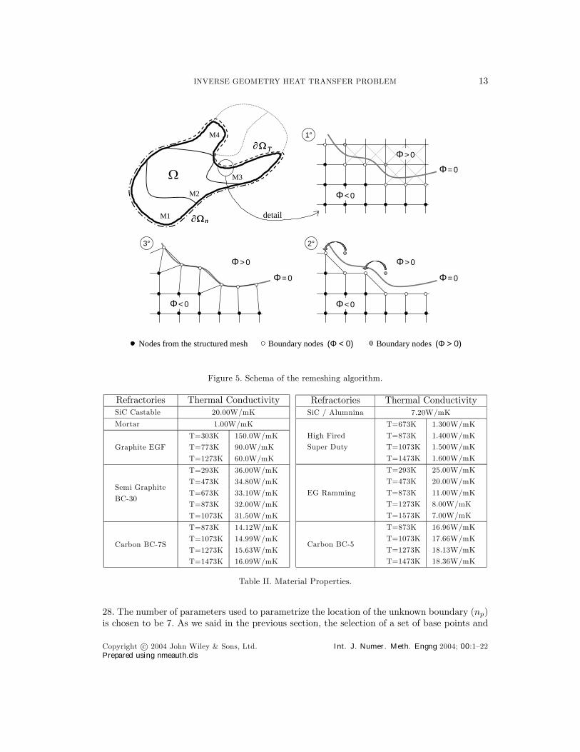
4.2. Remeshing algorithm

As we focus on bidimensional problems, we implemented the following simple but effectiveremeshing algorithm:

1. The starting point is a structured mesh of quadrilateral elements, where differentmaterials may be deÞned. According to the deÞnition of the interpolation function Φ (x),there will be some nodes located inside the volume Ω, where Φ < 0, and some locatedoutside, where Φ > 0. Remember that the unknown boundary ∂ΩT is deÞned as Φ = 0.

2. All the elements with three or four nodes inside the volume Ω (Φ < 0) remain in themesh (Step 1 of Figure 5).

3. A set of boundary nodes is deÞned. These nodes are the white (Φ < 0) and grey(Φ > 0) nodes of Figure 5.

4. The nodes that belong to the set of boundary nodes and that are located outside thevolume Ω (Φ > 0) are collapsed generating triangular elements (Step 2 of Figure 5).

5. Each node that belongs to the set of boundary nodes is moved to the nearest point ofthe unknown boundary ∂ΩT (Step 3 of Figure 5). The nearest point is calculated solvingthe following non-linear optimization problem:

minxf(x) =

1

2

°°x− xNode°°2 (44)

subject to Φ(x) = 0 (45)

where xNode are the coordinates of the node that is being moved.

5. INDUSTRIAL APPLICATION

In this section, we develop the industrial application of estimating the location of the 1150Cisotherm in a blast furnace hearth, based on measurements of thermocouples located inside it.Regarding the direct problem, we model a vertical section of the lining (Figure 6) with

axisymmetric Þnite elements because the geometry of the blast furnace hearth is rotationallysymmetric about an axis and is subjected to axisymmetric cooling conditions (Table I). TheÞnite element mesh has around 5000 isoparametric elements depending on the geometry solvedfor each inverse problem iteration. Table II shows the temperature dependence of the hearthrefractories thermal properties considered in the direct model.

Cooling zone Convective cooling parametersLower hearth

sprayhwater= 150

Wm2C Twater= 20

C

Bottom cooling hair=

µ152.5− 169.9 r

rmax+45.3

hr

rmax

i2¶W

m2C Tair=³26 + 22 r

rmax

´C

Table I. Cooling conditions.

Regarding the inverse geometry problem, there are 28 thermocouples located inside the blastfurnace hearth section (as shown in Figure 6) so the number of observations (nobs) is equal to



1°

2°3°

Φ< 0

!

M1

M2

M3

M4

detail

Φ< 0

Φ< 0

Φ= 0

Φ= 0

Φ= 0

Φ> 0

Φ> 0Φ> 0

!! n!! n

!! T!! T

Boundary nodes (Φ < 0) Boundary nodes (Φ > 0)Nodes from the structured mesh

Figure 5. Schema of the remeshing algorithm.

Refractories Thermal ConductivitySiC Castable 20.00W/mK

Mortar 1.00W/mK

Graphite EGF

T=303K 150.0W/mK

T=773K 90.0W/mK

T=1273K 60.0W/mK

Semi Graphite

BC-30

T=293K 36.00W/mK

T=473K 34.80W/mK

T=673K 33.10W/mK

T=873K 32.00W/mK

T=1073K 31.50W/mK

Carbon BC-7S

T=873K 14.12W/mK

T=1073K 14.99W/mK

T=1273K 15.63W/mK

T=1473K 16.09W/mK

Refractories Thermal ConductivitySiC / Alumnina 7.20W/mK

High Fired

Super Duty

T=673K 1.300W/mK

T=873K 1.400W/mK

T=1073K 1.500W/mK

T=1473K 1.600W/mK

EG Ramming

T=293K 25.00W/mK

T=473K 20.00W/mK

T=873K 11.00W/mK

T=1273K 8.00W/mK

T=1573K 7.00W/mK

Carbon BC-5

T=873K 16.96W/mK

T=1073K 17.66W/mK

T=1273K 18.13W/mK

T=1473K 18.36W/mK

Table II. Material Properties.

28. The number of parameters used to parametrize the location of the unknown boundary (np)is chosen to be 7. As we said in the previous section, the selection of a set of base points and



Steel shellSiC CastableMortarGraphite EGFSemi Graphite BC30Carbon BC-7SHigh Fired Super DutySiC / AluminaEG RammingCarbon BC-5

Air (Bottom cooling)

Lowerhearthspray

Lowerhearthspray

Lowerhearthspray

Lowerhearthspray

Thermocouple

Figure 6. Vertical section of the blast furnace hearth.

direction vectors depends on the geometry of each problem. In our problem, we select themdepending also on the position of the thermocouples.Figure 7 shows the set of base points and direction vectors which are used to describe the

location of the 1150C isotherm, where the set of surface points is interpolated using thin platespline RBFs (see Section 4.1).In order to validate the solution of the algorithm against measurement uncertainties, we

simulate measurements with different levels of noise following these steps:

1. We deÞne a real geometry described by a set of geometry parameters pReal.2. We calculate the temperature observations that correspond to the real geometry,TReal, assuming error free measurements.

3. We simulate measurements with different levels of noise (noise = 5%, 10%, 15%) asfollows

TObsi = TReali (1+ ξ · noise) (46)

where ξ ∈ [−1; +1] is a uniformly distributed random disturbance.

Then, we solve the inverse geometry heat transfer problem for each set of observations, usingas initial guess the regularization geometry p0 = p∆, and we evaluate the following relativeerrors

εobs =

°° T(pIter) − TObs°°

kTObsk (47)



Base Point and

Direction Vector

Thermocouples

Surface points

!!x" # 0

!!x" & 0

!!x" ' 0

Base points

Figure 7. Parametrization of the unknown boundary location.

εgeom =

°° pIter − pReal°°

kpRealk . (48)

Finally, we focus on three aspects of the problem:

The determination of the optimal regularization matrix for a problem with no geometryrestrictions.

The algorithm behavior when the problem is subjected to some geometry restrictions. The error behavior of the solution.

5.1. Determination of the optimal regularization matrix

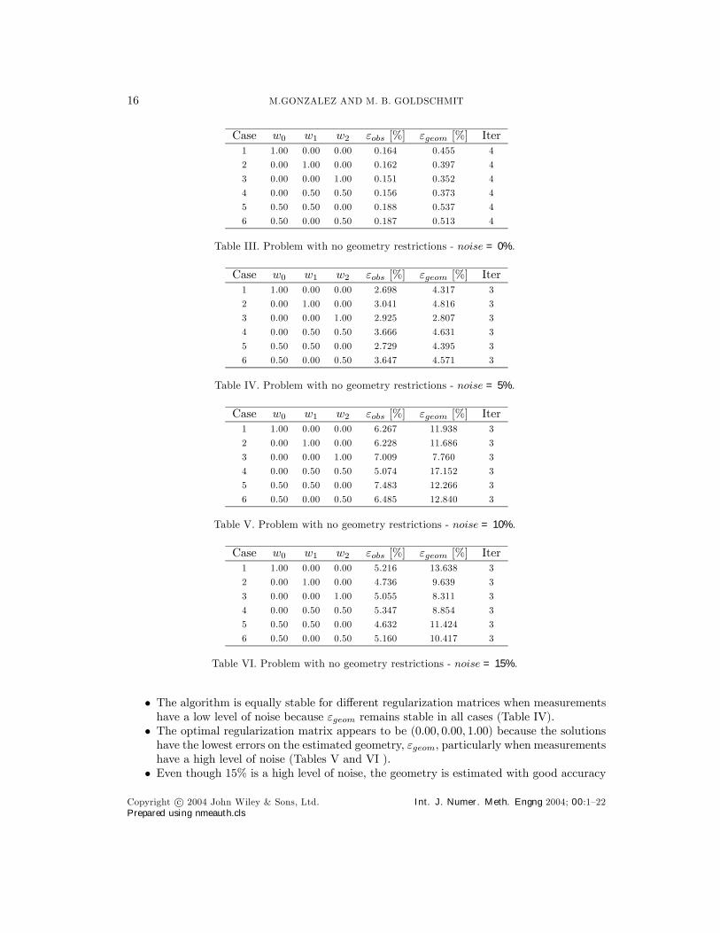
We study the behavior of the algorithm on different regularization matrices. For this purpose,we propose Þve regularization matrices as linear combinations of L0, L1, L2 (Equation 19) andsolve the inverse geometry heat transfer problem for each case, assuming a problem with nogeometry restrictions.Tables III, IV, V and VI show the relative errors (εobs and εgeom) and the number of

iterations required to solve the problem for each set of weighting factors (w0, w1, w2) and foreach noise level.Analyzing these results, we conclude that:

As is expected, the error on the estimated geometry, εgeom, increases as the noiseincreases.



Case w0 w1 w2 εobs [%] εgeom [%] Iter1 1.00 0.00 0.00 0.164 0.455 4

2 0.00 1.00 0.00 0.162 0.397 4

3 0.00 0.00 1.00 0.151 0.352 4

4 0.00 0.50 0.50 0.156 0.373 4

5 0.50 0.50 0.00 0.188 0.537 4

6 0.50 0.00 0.50 0.187 0.513 4

Table III. Problem with no geometry restrictions - noise = 0%.


2 0.00 1.00 0.00 3.041 4.816 3

3 0.00 0.00 1.00 2.925 2.807 3

4 0.00 0.50 0.50 3.666 4.631 3

5 0.50 0.50 0.00 2.729 4.395 3

6 0.50 0.00 0.50 3.647 4.571 3

Table IV. Problem with no geometry restrictions - noise = 5%.


2 0.00 1.00 0.00 6.228 11.686 3

3 0.00 0.00 1.00 7.009 7.760 3

4 0.00 0.50 0.50 5.074 17.152 3

5 0.50 0.50 0.00 7.483 12.266 3

6 0.50 0.00 0.50 6.485 12.840 3

Table V. Problem with no geometry restrictions - noise = 10%.


2 0.00 1.00 0.00 4.736 9.639 3

3 0.00 0.00 1.00 5.055 8.311 3

4 0.00 0.50 0.50 5.347 8.854 3

5 0.50 0.50 0.00 4.632 11.424 3

6 0.50 0.00 0.50 5.160 10.417 3

Table VI. Problem with no geometry restrictions - noise = 15%.

The algorithm is equally stable for different regularization matrices when measurementshave a low level of noise because εgeom remains stable in all cases (Table IV).

The optimal regularization matrix appears to be (0.00, 0.00, 1.00) because the solutionshave the lowest errors on the estimated geometry, εgeom, particularly when measurementshave a high level of noise (Tables V and VI ).

Even though 15% is a high level of noise, the geometry is estimated with good accuracy



Exact geometryRegularization geometryError = 5%Error = 10%Error = 15%

Figure 8. Estimated geometry for different levels of noise, using the optimal regularization matrix.

in the context of the industrial application (Figure 8).

5.2. The bound-constrained problem

We also study the behavior of the algorithm on different regularization matrices but, as ouraim is to consider the bound-constrained problem, we only analyze the noise level for whichthe iterative solution process yields unfeasible solutions due to its instability. This is the caseof noise = 10%.Table VII shows the relative errors (εobs and εgeom) and the number of iterations required

to solve the bound-constrained problem for each set of weighting factors (w0, w1, w2).


2 0.00 1.00 0.00 7.353 7.198 4

3 0.00 0.00 1.00 6.630 5.798 3

4 0.00 0.50 0.50 7.161 5.094 5

5 0.50 0.50 0.00 7.914 8.063 4

6 0.50 0.00 0.50 7.236 5.759 5

Table VII. Problem with geometry restrictions - noise = 10%.

Analyzing these results, we conclude that:



The solution is clearly improved and stabilized for all the regularization matrices whenthe bound-constrained algorithm is used (Tables V and VII).

The optimal regularization matrix appears to be (0.00, 0.00, 1.00), as in the problem withno geometry restrictions.

More iterations are needed to reach convergence, which is an expected conclusion becausethe constraints are iteratively imposed.

The geometry is estimated with good accuracy in the context of the industrial application(Figure 9).

Exact geometryRegularization geometryError = 10%

Figure 9. Geometry estimated by the bound-constrained algorithm, using the optimal regularizationmatrix..

5.3. Error behavior of the solution

We study the error behavior of the solution considering the optimal regularization matrix(0.00, 0.00, 1.00) and the case of noise = 10%, noise level for which the iterative solutionprocess yields unfeasible solutions. Moreover, as this behavior depends on multiple factors, wedivide the study in three parts.In the Þrst part of the study, we analyze the error behavior of the solution calculating an

appropriate step length (Section 3.1) and considering no geometry restrictions. In the secondpart of the study, we also calculate an appropriate step length but we consider some geometryrestrictions. Finally, in the third part of the study, we use a constant step length equal to 1.00in order to evaluate the importance of calculating an appropriate step length.



Figures 10, 11 and 12 show the evolution of the relative errors (εobs and εgeom) during theiterative process.Analyzing these results, we conclude that:

The typical instability of ill-posed problems, which cases εgeom to increase after someiterations while εobs always decreases, clearly occurs in the Þrst case (Figure 10). ThisconÞrms the use of the discrepancy principle as a stopping rule for the iterative process,as we explained in Section 3.1.4.

The solution is strongly stabilized when the bound-constrained algorithm is used (Figure11). Even in this case, the discrepancy principle is an efficient stopping rule for theiterative process.

The behavior of the solution is not good when a constant step length equal to 1.00 isused (Figure 12). Therefore, as is expected, the selection of an appropriate step lengthmakes sense due to the highly non-linear nature of the problem.

0%

10%

20%

30%

40%

50%

60%

70%

80%

90%

100%

110%

0 1 2 3 4 5 6 7 8 9 10 11

(obs

0%

10%

20%

30%

40%

50%

60%

0 1 2 3 4 5 6 7 8 9 10 11

(geom

Iterations Iterations

Figure 10. Error behavior of the solution, calculating an appropiate step length and considering nogeometry restrictions.

6. CONCLUSIONS

We have developed an inverse geometry heat transfer model for estimating the location ofthe 1150C isotherm in a blast furnace hearth. The observations of the inverse problem aretemperature measurements at points inside the object and the unknown is the geometry of thevolume where the problem is deÞned. We considered not only the problem with no geometryrestrictions but also the bound-constrained problem. Due to the typical instability of ill-posedproblems and the nonlineality of our inverse problem, we have used the iteratively regularizedGauss-Newton method.The inverse geometry problem is based on a radial basis functions geometry representation.

For this purpose, the location of the unknown boundary has been parametrized by a setof parameters and described with radial basis functions. We considered RBFs because theyimpose few restrictions on the geometry and because they provide a smooth interpolation.



0%

10%

20%

30%

40%

50%

60%

0 1 2 3 4 5 6 7 8 9 10 110%

10%

20%

30%

40%

50%

60%

70%

80%

90%

100%

110%

0 1 2 3 4 5 6 7 8 9 10 11

(obs (geom


Figure 11. Error behavior of the solution, calculating an appropiate step length and considering somegeometry restrictions.

0%

10%

20%

30%

40%

50%

60%

0 1 2 3 4 5 6 7 8 9 10 110%

10%

20%

30%

40%

50%

60%

70%

80%

90%

100%

110%

0 1 2 3 4 5 6 7 8 9 10 11

(obs (geom


Figure 12. Error behavior of the solution, using a step length equal to 1.00 and considering no geometryrestrictions.

The behavior of the algorithm on different regularization matrices has been studied analyzingits stability against simulated measurements with different levels of noise.We can conclude, from the results of the analyzed cases, that the optimal regularization

matrix appears to be L2 (the discrete approximation of the second derivative operator) forboth the problem with no geometry restrictions and the bound-constrained problem. We alsoconclude that the solution is clearly improved and stabilized if the bound-constrained algorithmis used when the iterative solution process yields unfeasible solutions due to the instability ofthe problem.On the basis of our numerical experimentation, we conÞrmed that a stopping rule for the

iterative process must be used, and that the selection of an appropriate step length makessense due to the highly non-linear nature of the problem.Finally, as the geometry is estimated with good accuracy in the context of the industrial

application, we conclude that the algorithm developed is a reliable tool for estimating thelocation of the 1150C isotherm in a blast furnace hearth.



ACKNOWLEDGEMENT

We thankfully acknowledge the Þnancial support and the information provided by SIDERAR (SanNicolás, Argentina).

REFERENCES

1. Wawrzynek A, Kogut M, Nowak A, Delpak R, Hu C-W. Regularization method in geometrical inverseheat conduction problems-Preliminary report. ECCOMAS 2000. Barcelona, 2000.

2. Park HM, Shin HJ. Shape identiÞcation for natural convection problems using the adjoint variablemethod. Journal of Computational Physics 2003; 186:198-211.

3. Kwag D-S, Park I-S, Kim W-S. Inverse geometry problem of estimating the phase front motion of ice ina thermal storage system. Inverse Problems in Science and Engineering 2004; 12(1):1-15.

4. Huang C-H. An inverse geometry problem in estimating frost growth on an evaporating tube. Heat andMass Transfer 2002; 38:615-623.

5. Ganapathysubramanian S, Zabaras N. A continuum sensitivity method for Þnite thermo-inelasticdeformations with applications to the design of hot forming processes. Int. J. Numer. Meth. Engng2002; 55:1391-1437.

6. Engl HW, Hanke M, Neubauer A. Regularization of inverse problems. Kluwer Academic Publishers, 1996.7. Alifanov OM. Inverse heat transfer problems. Springer-Verlag, 1994.8. Kaltenbacher B. On convergence rates of some iterative regularization methods for an inverse problemfor nonlinear parabolic equation connected with continuous casting of steel. J. Inv. Ill-Posed Problems1999; 7(2):145-164.

9. Jin QN. The analysis of a discrete scheme of the iteratively regularized Gauss-Newton method. InverseProblems 2000; 16:1457-1476.

10. Kaltenbacher B, Neubauer A, Ramm AG. Convergence rates of the continuous regularized Gauss-Newtonmethod. J. Inv. Ill-Posed Problems 2002; 10(3):261-280.

11. Doicu A, Schreier F, Hess M. Iteratively regularized Gauss-Newton method for atmospheric remotesensing. Computer Physics Communications 2002; 148:214-226.

12. Carr JC, Beatson RK, Cherrie JB, Mitchell TJ, Fright WR, McCallum BC. Reconstruction andrepresentation of 3D objects with radial basis functions. ACM SIGGRAPH 2001. Los Angeles, CA,2001; 67-76.

13. Carr JC, Fright TJ, Batson RK. Surface interpolation with radial basis functions for medical imaging.IEEE Transactions on Medical Imaging 1997; 20(Y):1-18.

14. Perrin F, Bertrand O, Pernier J. Scalp current density mapping: value and estimation from potentialdata. IEEE Transactions on Biomedical Engineering 1987; BME-34(4):283-288.

15. Franke R. Scattered data interpolation tests of some methods. Mathematics of Computation 1982;38(157):181-200.

16. Kansa EJ. Multiquadrics - A scattered data approximation scheme with applications to computationalßuid-dynamics - II. Surface approximations and partial derivative estimates. Computers Math. Applic.1990; 19(8/9):147-161.

17. Kansa EJ. Multiquadrics - A scattered data approximation scheme with applications to computationalßuid-dynamics - I. Solutions to parabolic, hyperbolic and elliptic partial differential equations. ComputersMath. Applic. 1990; 19(8/9):127-145.

18. Turk G and OBrien JF. Variational implicit surfaces. Technical Report GIT-GVU-99-15, GeorgiaInstitute of Technology, 1999.

19. Belytschko T, Parimi C, Moes N, Sukumar N, Usui S. Structured extended Þnite element method forsolids deÞned by implicit surfaces. Int. J. Numer. Meth. Engng 2003; 56:609-635.

20. Torrkulla J and Saxén H, Model of the state of the blast furnace hearth, ISIJ International 2000;40(5):438-447.

21. Sorli K and Skaar IM, Monitoring the wear-line of a melting furnace. 3rd Int. Conference on InverseProblems in Engineering 1999, Port Ludlow, WA, 1999.

22. Schulte M, Klima R, Ringel D, Voss M. Improved wear-control at the blast furnace hearth by directheat-ßux measurements. Ironmaking Conference Proceedings 1998; 607-614.

23. Kurpisz K, A method for determining steady state temperature distribution within blast furnace hearthlining by measuring temperature at selected points. Transactions ISIJ 1988; 28:926-929.

24. Gonzalez M, Goldschmit MB, Zubimendi JL, Gonzalez N, Ametrano R, Giandomenico F. Inversegeometry problem of estimating the location of the 1150C isotherm in a blast furnace hearth. Proceedingsof the 4th IAS Ironmaking Conference 2003. San Nicolás, Argentina, 2003; 381-386.



25. Bathe KJ. Finite element procedures. Prentice-Hall, 1996.26. Zienkiewicz OC, Taylor RL. The Finite Element Method (5th edn). Butterworth-Heinemann, 2000.27. Appel JR and Gunzburger MD. Sensitivity calculation in ßows with discontinuities. Proc. 14th AIAA

Applied Aerodynamics Conference New Orleans, USA 1996.28. Brezinski C, Redivo-Zaglia M, Rodriguez G, Seatzu S. Multi-parameter regularization techniques for

ill-conditioned linear systems. Numer. Math. 2003; 94:203-228.29. Luenberger DG. Linear and nonlinear programming. Addison Wesley, 1984.


Documents

Inverse geometry heat transfer problem based on a radial basis