Inverse Problem for a Parabolic System - pvamu.edu Inverse Problem for a Parabolic System Reza Pourgholi*, Amin Esfahani and Hassan Dana Mazraeh School of Mathematics and Computer

521

Inverse Problem for a Parabolic System

Reza Pourgholi

*, Amin Esfahani and Hassan Dana Mazraeh

School of Mathematics and Computer Sciences

Damghan University

P.O.Box 36715-364

Damghan, Iran

[email protected]; [email protected]; [email protected]

*Corresponsing author

Abstract

In this paper a numerical approach combining the least squares method and a genetic algorithm

is proposed for the determination of the source term in an inverse parabolic system (IPS). A

numerical experiment confirm the utility of this algorithm as the results are in good agreement

with the exact data. Results show that a reasonable estimation can be obtained by the genetic

algorithm within a CPU with clock speed 2.7 GHz.

Keywords: Inverse parabolic system; Least squares method; Genetic algorithm

MSC 2010 No.: 65M32, 35K05

1. Introduction

Inverse problems are encountered in many branches of engineering and science. In one particular

branch, heat transfer, the inverse problem can be used to such conditions as temperature or

surface heat flux, or can be used to determine important thermal properties such as the thermal

conductivity or heat capacity of solids.

Several functions and parameters can be estimated from the inverse parabolic problem: static and

moving heating sources, material properties, initial conditions, boundary conditions, optimal

shape etc. Fortunately, many methods have been reported to solve inverse parabolic problems

(Alifanov, 1994; Beck et al., 1985; Beck et al., 1996; Beck, et al., 1986; Dowding and Beck,

1999; Cabeza et al., 2005; Liu, 2008; Molhem and Pourgholi, 2008; Murio, 1993; Murio and

Available at

http://pvamu.edu/aam

Appl. Appl. Math.

ISSN: 1932-9466

Vol. 12, Issue 1 (June 2017), pp. 521 -539

Applications and Applied

Mathematics:

An International Journal

(AAM)

mailto:[email protected]

mailto:[email protected];%[email protected]



Pourgholi et al. 255

Paloschi, 1988; Pourgholi et al., 2009; Pourgholi and Rostamian, 2010; Shidfar et al., 2006; Zhou

et al., 2010).

In this paper, for we consider the following IPS in the

dimensionless form

{

( ) ( ) ( ) ( ) ( ) ( ) ( ) ( ) ( ) ( ) ( ) ( ) ( ) ( )

( 1 )

{

( ) ( ) ( ) ( )

( ) ( ) ( ) ( ) ( ) ( ) ( ) ( )

( 2 )

and the over specified condition

( ) ( ) ( 3 )

where ( ) ( ) and ( ) are continuous known real-valued functions,

( ) ( ) ( ) ( ) ( ) and ( ) are infinitely differentiable known real-valued

functions and represents the final existence time for the time evolution of the problem, while

the function f (x,t) is unknown which remains to be determined from some interior temperature

measurements.

System (1) - (3) arises, for example, in the study of chemical reactions (see e.g. (Bothe, 2003;

Chipot et al. 2009; E´rdi and To´th, 1989 )), and in a wide variety of mathematical biology and

physical situations (see e.g. (Hillen, and Painter, 2009; Lauffenburger et al. 1982; Shigesada et

al. 1979)). The controllability properties of system (1)-(3) has been studied, for example, in

[Ammar-Khodja et al. 2006; Ammar-Khodja et al. 2011; L. de Teresa, 2000; Gonza´lez-Burgos

and Pérez-Garc´ıa, 2006; Leáutaud,2010; Russell, 1973 ]. See also [Ammar-Khodja et al. 2011]

for a nice survey on this issue. The recent work [Fernańdez-Cara et al. 2010] studies system (1)-

(3) in one space dimension and with constant coupling coefficients. The cases of higher space

dimensions and varying coupling coefficients (and in particular when the coefficients vanish in a

neighborhood of the boundary) are, to our knowledge, completely open.

We should note that, for a given function ( ), we can prove the existence of a unique solution

( ( ) ( )) of (1)-(3). More precisely, one can easily observe that system (1) with the

conditions (2) can be reduced to

{

( ) ( ) ( ) ( ) ( ) ( ) ( )

( ) ( ) ( ) ( ) ( ) ( ) ( )

( ) ( ) ( ) ( )

( ) ( ) ( ) ( )

( 4 )

where

( ) ( ) ( ) ( ) ( ) ( ) ( ) ( ) ( ) ( )

255 AAM: Intern. J., Vol. 12, Issue 1 (June 2017)

– – (

–

),

and

′

( ′

)

We notice for ( ) that, on the space ( ( )) endowed with the natural inner product

⟨ ⃗ ⟩ ( ) ( ) ⟨ ⟩

( ) ( ) ⟨ ⟩ ( ) ( )

with ⃗ ( ) and ( ) the operator

(

)

with domain ( ( ) ( )) , is self-adjoint, where ( ) and

are the usual Sobolev

spaces. As a consequence, for ( ( )), ( ) and ( ) with ( ) the Cauchy problem (4) is well-posed in ( ( )) , in the sense of semigroup theory

[Lions, 1988]. Moreover, for the general case ( ) ( ) ( ( )), if we suppose

that (( ) ( )) and ( ) ( ( )) , then there exists a unique solution

( ) of (4) satisfying

(( )

( )) ( ( ))

and

(( )

( ))

More precisely, this result can be obtained by defining the bilinear form

A: ( ( ))

(

( ))

by

( ⃗ ) ∫ ( ⃗ ( ) ( ) )

verifying that A satisfies

)i) for every ⃗ ( ( )) the function ( ⃗ ) is measurable,

(ii) ( ⃗ ) ( ( ))

– ( ( )) ,

(iii) ( ⃗ ) (

( ))

( ( )) , for almost every and for

all ( ( )) ,


where and are constants, and applying a similar argument to (Lions and Magenes,

1961 Theorem 7.1), see also (Lions and Magenes,1961; Baiocchi, 1964; Lions and Magenes,

1960; Lions and Magenes, 1968).

We should remark that if the assumptions given above hold and is known, one can obtain a

unique solution ( ) of (1)-(2). But in the case when ( ) depends only on or , by using

the overspecified condition (16), one can find a unique solution ( ) of the inverse problem

(1) - (3).

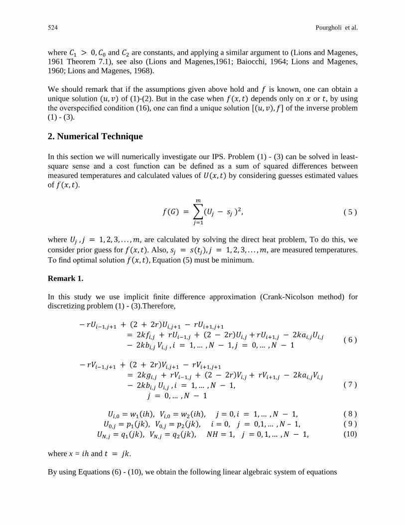
2. Numerical Technique

In this section we will numerically investigate our IPS. Problem (1) - (3) can be solved in least-

square sense and a cost function can be defined as a sum of squared differences between

measured temperatures and calculated values of ( ) by considering guesses estimated values

of ( ).

( ) ∑( )

( 5 )

where , are calculated by solving the direct heat problem, To do this, we

consider prior guess for ( ). Also, ( ) , are measured temperatures.

To find optimal solution ( ) Equation (5) must be minimum.

Remark 1.

In this study we use implicit finite difference approximation (Crank-Nicolson method) for

discretizing problem (1) - (3).Therefore,

( )

( )

( 6 )

( )

( )

( 7 )

( ) ( ) ( 8 )

( ) ( ) – ( 9 )

( ) ( ) (10)

where x = and .

By using Equations (6) - (10), we obtain the following linear algebraic system of equations


(

)

(

)

(

)

+

(

)

(

)

(

)

(

)

(

)

(

)

(

)

(

)

(

)

(

)


(

)

(

)

(

)

3. Genetic algorithm

Genetic algorithms, primarily developed by Holland (Holland, 1975), have been successfully

applied to various optimization problems. It is essentially a searching method based on the

Darwinian principles of biological evolution. Genetic algorithm is a stochastic optimization

algorithm which employs a population of chromosomes, each of which represents a possible

solution. By applying genetic operators, each successive incremental improvement in a

chromosome becomes the basis for the next generation. The process continues until the desired

number of generations has been completed or the predefined fitness value has been reached.

Typically binary coding is used in classic genetic algorithm, where each solution is encoded as a

chromosome of binary digits. Each member of the population represents an encoded solution in

the classic genetic algorithm. For many problems, this kind of coding is not natural. The genetic

algorithm used in this work is not a classic genetic algorithm. Instead, the application of genetic

algorithm to this discrete-time optimal control problem is called a real-valued genetic algorithm

(RVGA). The continuous function is discrete for numerical computation and simulated by a

chromosome. The value of each gene is a real number and indicates the heat generation at each

time step (Liu, 2008).

The procedure of an RVGA is as follows:

Step 1. Generate at random an initial population of chromosomes.

Step 2. Evaluate the fitness of each chromosome in the population.

Step 3. Select chromosomes, based on the fitness function, for recombination.

Step 4. Recombine pairs of parents to generate new chromosomes.

Step 5. Mutate the resulting new chromosomes.

Step 6. Evaluate the fitness of new chromosomes.

Step 7. Update population.

Step 8. Repeat Step 3 to Step 7, until the fitness function is convergent or less than a predefined

value.

4. A modified real-valued genetic algorithm (RVGA) to

determine ( )

In this paper we use a modified RVGA for determining ( ) In this algorithm, chromosomes

are encoded as real-valued matrices. The column of each chromosome illustrates


. We consider each column of chromosomes as a gene. That illustrates

gene of chromosome of . For finding optimal solution of ( ), Equation (5) must be

minimum. For this purpose, we consider Equation (5) as fitness function and calculate simulated

s by solving direct system for each chromosome. At the end of algorithm, the chromosome by

lowest fitness is the best solution of ( ). To determine the ( ) we interpolate the best

solution. To improve performance of RVGA, we added new step to algorithm after “mutation”

operation, for modifying new chromosomes at each iteration. Figure 15 shows the flowchart of

modified RVGA.

The procedure of a modified RVGA is as follows:

Step 1. Generate at random an initial population of chromosomes.

Step 2. Evaluate the fitness of each chromosome in the population.

Step 3. Select some chromosomes as parents by tournament selection.

Step 4. For generating pair of new chromosomes, pair of parents crossover together as follow:

( – )

( ) ,

where illustrates first parent, illustrates second parent, illustrates first new

chromosome, illustrates second new chromosome, and are random numbers in

.

Step 5. For applying ”Mutation” operation on new chromosomes, selecting a gene of each new

chromosome randomly and each element of genes adding by random number.

Step 6. Finding the first best gene between new chromosomes and copy that gene to first gene

of all chromosomes. Then finding the second best gene between new chromosomes and

copy that gene to second gene of all chromosomes. Continue this procedure for all

genes. Now all new chromosomes are the same. For generating new hopeful

chromosomes, genes of second to end chromosomes replace by genes of first

chromosome adding by random small values.

Step 7. Evaluate the fitness of new chromosomes.

Step 8. Update the population.

Step 9. Repeat Step 3 to Step 8, until the fitness function is convergent or less than a predefined

value.

The flowchart of the proposed algorithm for determining ( ) has been presented in Figure 15.


5. Numerical Results and Discussion

The aim of this section is to see the applicability of the present numerical method described in

Section 4 for solving our IPS. As expected IPS (1) is ill-posed and therefore it is necessary to

investigate the stability of the present method by giving a test problem. Now, we give the

following examples in .

Our first example is

{ ( ) ( ) ( ) ( ) ( )

( ) ( ) ( ) ( )

(11)

{

( ) (√ ) (√ )

( ) ⁄ (√ ) (√ )

( )

( ) ( ⁄ )

( ) ( ⁄ )

( ) ( ⁄ )

(12)

by the over specified condition

( ) ( ) (13)

Here, the exact values of ( ), ( ) and ( ) are (

(√ ) (√ )) and ( (√ ) (√ )),

respectively.

The second example is

{ ( ) ( ) ( ( )) ( ) ( ( )) ( ) ( )

( ) ( ) ( ( )) ( ) ( ( )) ( )

(14)

{

( ) ( )

( ) ( )

( )

( )

( ) ( ⁄

( ) ( ⁄ )

(15)

by the over specified condition

( ) ( ) (16)


where the exact values of ( ), ( ) and ( ) are ( ), ( ) and

( ), respectively.

The experimental data ( ) (measured temperatures at ) are obtained from the exact

solution of the direct problem by adding a random perturbation error to the exact solution of the

direct problem in order to generate noisy data, where and is random value in ( ).

Remark 2.

In an IS there are two sources of error in the estimation. The first source is the unavoidable bias

deviation (or deterministic error). The second source of error is the variance due to the

amplification of measurement errors (stochastic error). The global effect of deterministic and

stochastic errors is considered in the mean squared error or total error, (Dowding and Beck,

1999).

[

( )( )∑ ∑ ( ̂ )

]

,

(17)

where ( )( ) is the total number of estimated values, ̂ is calculated values from

interpolated equation and is exact values of ( ).

In our examples here, a population of 20 chromosomes of 100 genes ( ) is used as the initial guess to obtain for numerical results of modified RVGA. Also each

gene has 9 elements ( ). Table 1 presents the results for 1 to 1000

generations for the first example and also Table 2 presents the results for 1 to 10000 generations

for the second example. Note that calculated by 900 total number of points.

Table 1. The results of modified RVGA for a population of 20 chromosomes of 100 genes for

1 to 1000 generations

Gen. Best fitness Time(s) S

1 3.3079e − 003 1.4602 0.3800

100 3.1073e − 004 99.7811 0.0756

200 1.8876e − 004 199.5500 0.0727

300 9.6134e – 005 298.7181 0.0420

400 7.7658e − 005 397.6857 0.0479

500 1.1534e − 005 491.71616 0.0343

600 1.7591e − 005 601.0169 0.0415

700 5.1188e − 006 701.3476 0.0286

800 3.2938e − 006 791.4607 0.0168

900 8.5618e − 007 0.0068 0.0112

1000 4.7571e − 007 996.1871 0.0072


Table 2. The results of modified RVGA for a population of 20 chromosomes of 100 genes for

1 to 10000 generations.

Gen. Best fitness Time(s) S

1 3.1719e − 001 2.9304 1.7655

100 3.2618e − 002 3068.7060 0.5948

200 7.1283e − 002 6091.6555 0.1425

300 7.4315e − 002 9049.7577 0.0973

400 8.4910e − 003 11930.9340 0.0867

500 4.9218e − 003 15032.7922 0.0965

600 9.5096e − 004 18152.1576 0.0733

700 9.7175e − 004 21188.5469 0.0764

800 6.3248e − 005 24124.0975 0.0178

900 9.0588e − 006 26981.9134 0.0134

1000 4.1515e − 006 29998.4709 0.0068

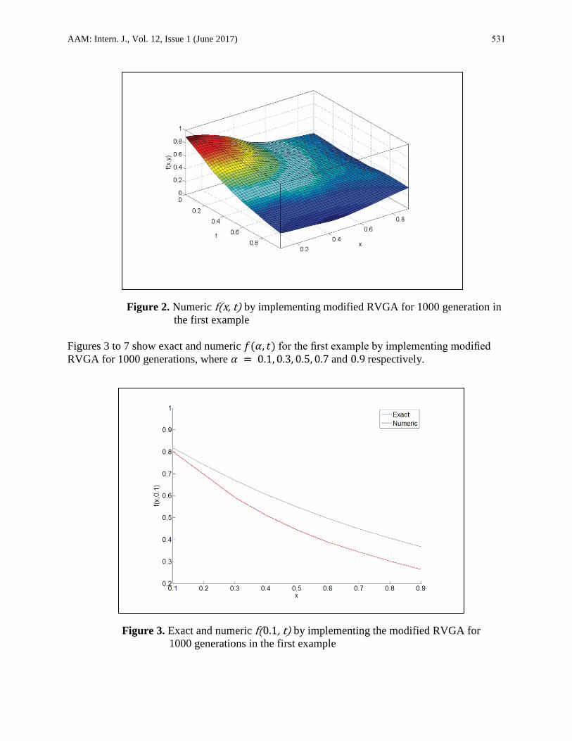
Figures 1 and 2 show the exact and numeric ( ) for the first example by implementing the

modified RVGA for 1000 generations.

Figure 1. Exact f(x, t) of the first example


Figure 2. Numeric f(x, t) by implementing modified RVGA for 1000 generation in

the first example

Figures 3 to 7 show exact and numeric ( ) for the first example by implementing modified

RVGA for 1000 generations, where and respectively.

.

Figure 3. Exact and numeric f(0.1, t) by implementing the modified RVGA for

1000 generations in the first example


.


1000 generations in the first example

Figure 5. Exact and numeric f(0.5, t) by implementing the modified RVGA for 1000

generations in the first example







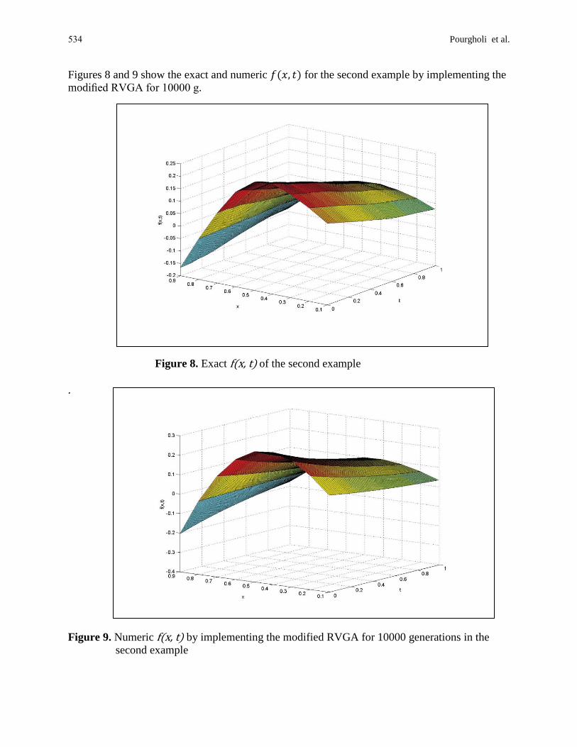
Figures 8 and 9 show the exact and numeric ( ) for the second example by implementing the

modified RVGA for 10000 g.

Figure 8. Exact f(x, t) of the second example

.

Figure 9. Numeric f(x, t) by implementing the modified RVGA for 10000 generations in the

second example


Figures 10 to 14 show exact and numeric ( ) for the second example by implementing the

modified RVGA for 10000 generations, where and respectively.


10000 generations in the second example











Figure 15. Flowchart of the modified RVGA

6. Conclusion

i. The present study successfully applied a numerical method to IPS (1) - (3).

ii. To solve the IPS by using our genetic algorithm, the unknown function will be guessed and

we do not need the regularization. This will improve the execution time.

iii. Results show that a reasonable estimation can be obtained by a genetic algorithm within a

CPU with clock speed 2.7 GHz.

iv. The present method has been found stable with respect to small perturbation in the input

data.


REFERENCES

Alifanov, O. M. (1994). Inverse Heat Transfer Problems, Springer, New York.

Ammar-Khodja, F. Benabdallah, A. Dupaix, C. 320 (2006). Null-controllability of some

reaction- diffusion systems with one control force, J. Math. Anal. Appl. 928–943.

Ammar-Khodja, F. Benabdallah, A. Gonza´lez-Burgos, M. de Teresa, L. (2011). Recent results

on the controllability of linear coupled parabolic problems: A survey, Math. Control Related

Fields 1 267–306.

Baiocchi, C. (1964). Sui problemi ai limiti per le equazioni paraboliche del tipo del calore,

Bollettino dell’Unione Matematica Italiana (serie 3) 4 407–422.

Beck, J. Blackwell, V. B. and St, C.R. (1985).Clair, Inverse Heat Conduction:

IllPosedcProblems, Wiley-Interscience, New York.

Beck, J. Blackwell, V. B. and Haji-sheikh, (1996). A. Comparison of some inverse heat

conduction methods using experimental data, Internat. J. Heat Mass Transfer 3 3649–3657.

Beck, J.V. and Murio, D.C. (1986). Combined function specification-regularization procedure

for solution of inverse heat condition problem, AIAA J. 24 180–185.

Bothe, D. Hilhorst, D. (2003). A reaction-diffusion system with fast reversible reaction, J. Math.

Anal. Appl. 286 125–13.

Cabeza, J.M.G. Garcia, J.A.M. . Rodriguez, A.C (2005). A Sequential Algorithm of Inverse Heat

Conduction Problems Using Singular Value Decomposition, International Journal of

Thermal Sciences, 44 235–2.

Chipot, M. Hilhorst, D. Kinderlehrer, D. Olech, M. (2009). Contraction in L1 and large time

behavior for a system arising in chemical reactions and molecular motors, Differ. Equ. Appl.

1 139-151.

de Teresa, L. (2000). Insensitizing controls for a semilinear heat equation, Comm. Partial Dif-

ferential Equations 25 39–72.

Dowding, K. J. and Beck, J. V. (1999). A Sequential Gradient Method for the Inverse Heat

Conduction Problems, J. Heat Transfer, 121 300–306.

E´rdi P. To´th, J. (1989). Mathematical Models of Chemical Reactions. Theory and Applications

of Deterministic and Stochastic Models, Nonlinear Science: Theory and Applications,

Princeton University Press, Princeton, NJ.

Fernańdez-Cara, E. Gonza´lez-Burgos, de Teresa, M. L. (2010). Boundary controllability of

parabolic coupled equations, J. Funct. Anal. 259 1720–1758.

González-Burgos, M. Pe´rez-Garcıá, R. (2006). Controllability results for some nonlinear

coupled parabolic systems by one control force, Asymptotic Analysis 46 123–162.

Hillen, T. Painter, K.J.(1989). A user’s guide to PDE models for chemotaxis, J. Math. Biol. 183–

217.

Holland, J.H. (1975).Adaptation in Natural and Artificial System, University of Michigan Press,

Ann Arbor.

Lauffenburger, D. Aris, R. Keller, K. (1982). Effects of cell motility and chemotaxis on

microbial population growth, Biophysical Journal 40 209–219.

Leáutaud, M. (2010). Spectral inequalities for non-self adjoint elliptic operators and application

to the null controllability of parabolic systems, J. Funct. Anal. 258 2739–2778.

Lions, J.-L. (1988).Controlabilite´ exacte, perturbations et stabilisation de syste´mes distribue´s,

Tome 1, volume 8 of Recherches en Mathe´matiques Appliqueès, Masson, Paris.


Lions, J.-L. (1988).Controlabilite´ exacte, perturbations et stabilisation de syste´mes distribue´s,

Tome 1, volume 8 of Recherches en Mathe´matiques Appliqueès, Masson, Paris.

Lions, J.-C. Magenes, E. (1961). Proble`mes aux limites non homoge`nes. II, Annales de

l’institut Fourier 11 137–178.

Lions, J.-C. Magenes, E. (1961). Proble`mes aux limites non homoge`nes. IV, Annali della

Scuola Normale Superiore di Pisa 15 311–326.

Lions,J.-C. Magenes, E. (1960). Remarques sur les proble`mes aux limites pour ope´rateurs

paraboliques, Compt. Rend. Acad. Sci. (Paris) 251 2118-2120.

Lions, J.-C. Magenes, E. (1968). Proble`mes aux limites non homoge`nes el applications, Dunod.

Liu, F.-B. (2008). A modified genetic algorithm for solving the inverse heat transfer problem of

estimating plan heat source, International Journal of Heat and Mass Transfer, 51 3745–3752.

Molhem, H. and Pourgholi, R. (2008). A numerical algorithm for solving a one-dimensional

inverse heat conduction problem, Journal of Mathematics and Statistics 4 (1) 60–63.

Murio, D.A. (1993). The Mollification Method and the Numerical Solution of Ill-Posed Prob-

lems, Wiley-Interscience, New York.

Murio, D.C. and Paloschi]]], J.R. (1988). Combined mollification-future temperature procedure

for solution of inverse heat conduction problem, J. comput. Appl. Math., 23 235–244.

Pourgholi, R. Azizi, N. Gasimov, Y.S. Aliev, F. Khalafi, H.K. (2009). Removal of Numerical

Instability in the Solution of an Inverse Heat Conduction Problem, Communications in

Nonlinear Science and Numerical Simulation 14 (6) 2664–2669.

Pourgholi, R. and Rostamian, M. (2010). A numerical technique for solving IHCPs using

Tikhonov regularization method, Applied Mathematical Modelling 34 (8) 2102-2110.

Russell, D.L. (1973). A unified boundary controllability theory for hyperbolic and parabolic

partial differential equations, Studies in Appl. Math. 52 189–221.

Shidfar, A. Pourgholi, R. and Ebrahimi, (2006). M. A Numerical Method for Solving of a Non-

linear Inverse Diffusion Problem, Computers and Mathematics with Applications 52 1021–

1030.

Shigesada, N. Kawasaki, K. Teramoto, E. (1979). Spatial segregation of interacting species, J.

Theoret. Biol. 79 83-99.

Zhou, J. Zhang, Y. Chen, J. K. Feng, Z. C. (2010). Inverse Heat Conduction in a Composite Slab

With Pyrolysis Effect and Temperature-Dependent Thermophysical Properties, J. Heat

Transfer, 132 (3) 034502 (3 pages).

Documents

Inverse Problem for a Parabolic System - pvamu.edu Inverse Problem for a Parabolic System Reza Pourgholi*, Amin Esfahani and Hassan Dana Mazraeh School of Mathematics and Computer