Inverse Transport Problems (Generalized) Stability ... · Inverse Transport Problems (Generalized) Stability Estimates ... In summary: We haveuniqueness ... accurately is actually

Radon 100 March 30, 2017Radon 100 March 30, 2017Radon 100 March 30, 2017

Inverse Transport Problems

(Generalized) Stability Estimates

Guillaume Bal

Department of Applied Physics & Applied Mathematics

Columbia University

Joint with Alexandre Jollivet


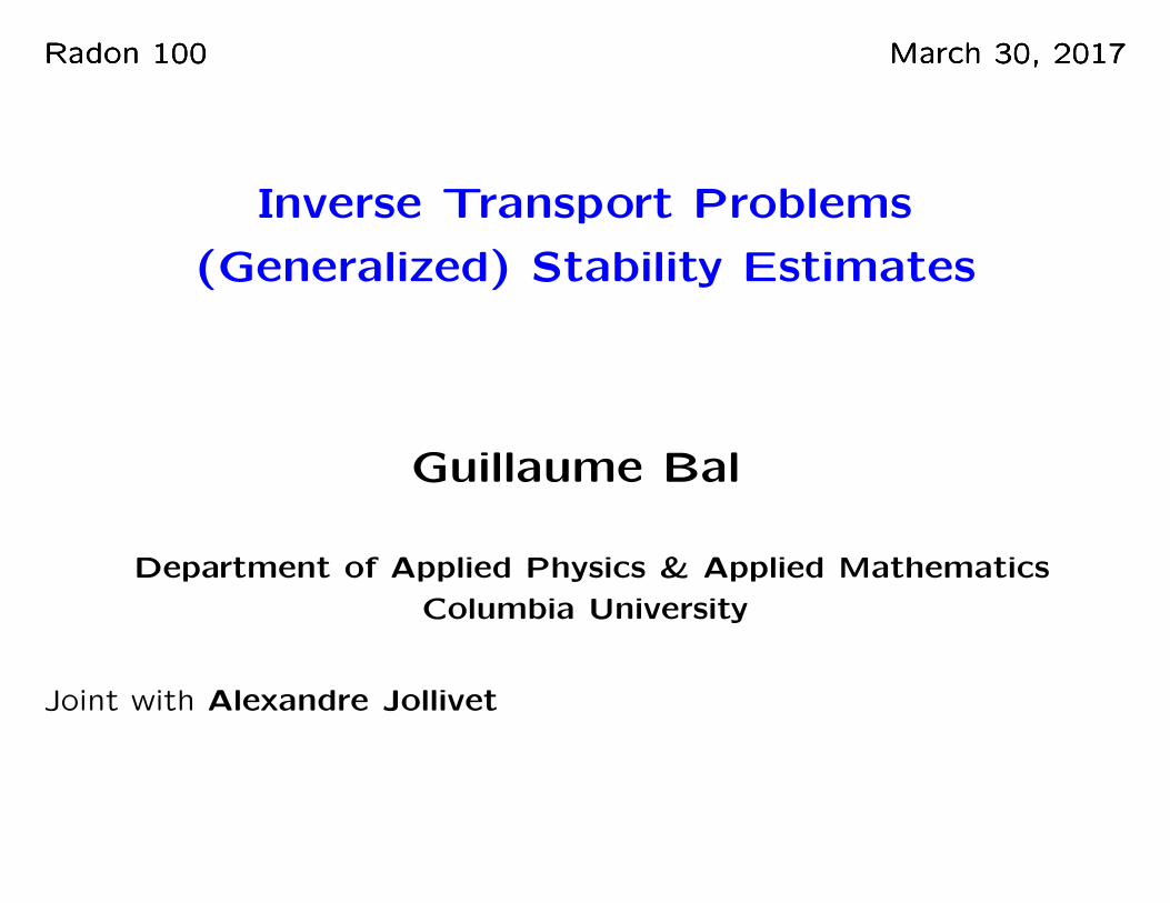
Data Acquisition in CT-scan

a(x) is unknown absorption coeffi-

cient. For each line in the plane ,

the measured ratio uout(s, θ)/uin(s, θ)

is equal to:

exp(−∫

line(s,θ)a(x)dl

). s =line-offset.

The X-ray density u(x, θ) solves the

transport equation

θ · ∇u(x, θ) + a(x)u(x, θ) = 0.

Here, x is position and θ =

(cos θ, sin θ) direction.


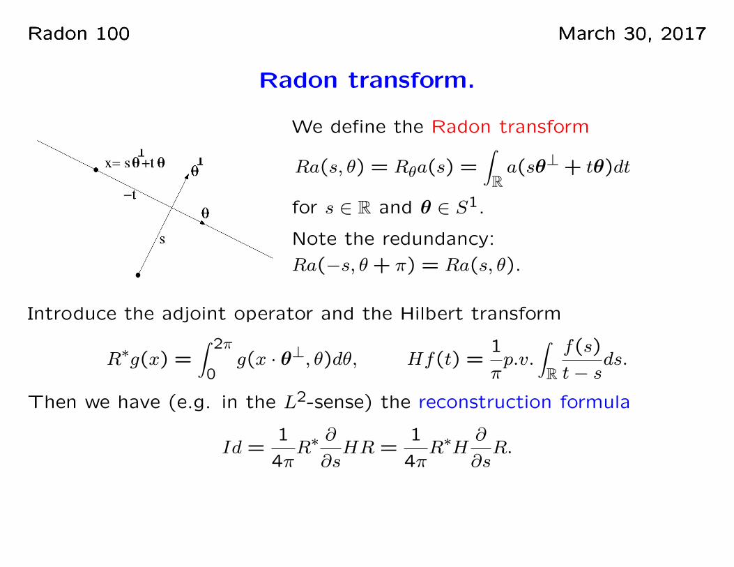
Radon transform.

We define the Radon transform

Ra(s, θ) = Rθa(s) =∫Ra(sθ⊥+ tθ)dt

for s ∈ R and θ ∈ S1.

Note the redundancy:

Ra(−s, θ + π) = Ra(s, θ).

Introduce the adjoint operator and the Hilbert transform

R∗g(x) =∫ 2π

0g(x · θ⊥, θ)dθ, Hf(t) =

1

πp.v.

∫R

f(s)

t− sds.

Then we have (e.g. in the L2-sense) the reconstruction formula

Id =1

4πR∗

∂

∂sHR =

1

4πR∗H

∂

∂sR.


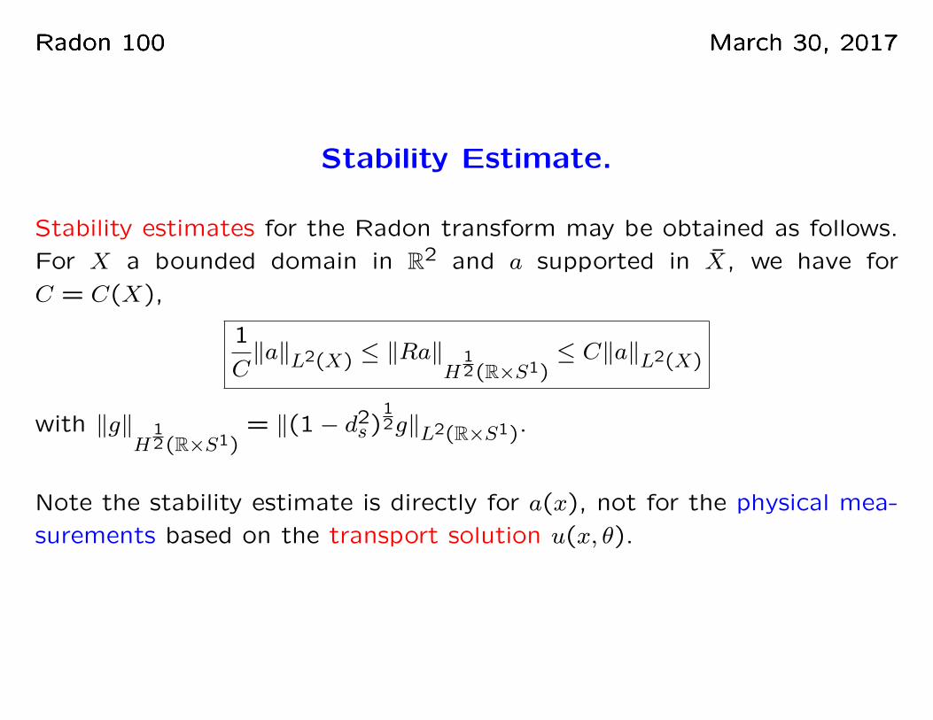
Stability Estimate.

Stability estimates for the Radon transform may be obtained as follows.

For X a bounded domain in R2 and a supported in X, we have for

C = C(X),

1

C‖a‖L2(X) ≤ ‖Ra‖

H12(R×S1)

≤ C‖a‖L2(X)

with ‖g‖H

12(R×S1)

= ‖(1− d2s)

12g‖L2(R×S1).

Note the stability estimate is directly for a(x), not for the physical mea-

surements based on the transport solution u(x, θ).


Scattering Scattering

As we heard in previous talks, several applications have at their core an

inverse Radon transform: CT, SPECT, PET.

Neglected so far: scattering. Scattering is typically not very informative

(no contrast) but it is there. Its reconstruction helps with that of other

coefficients.

[Courdurier, Monard, Osses, Romero. Simultaneous source and attenu-

ation reconstruction in SPECT using ballistic and single scattering data

2015;

Phys Med Biol. 2011; Review and current status of SPECT scatter cor-

rection. Hutton B.F., Buvat I, Beekman F.J.

Talk here in, e.g., MS17 by Herbert Egger, Vadim Markel]

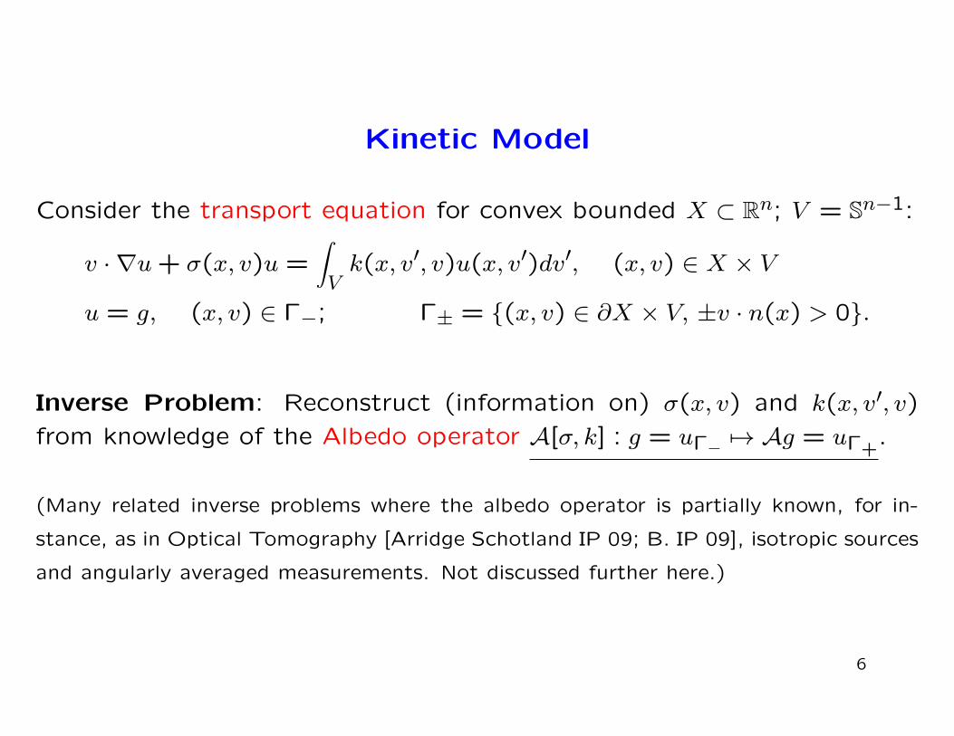
Kinetic Model

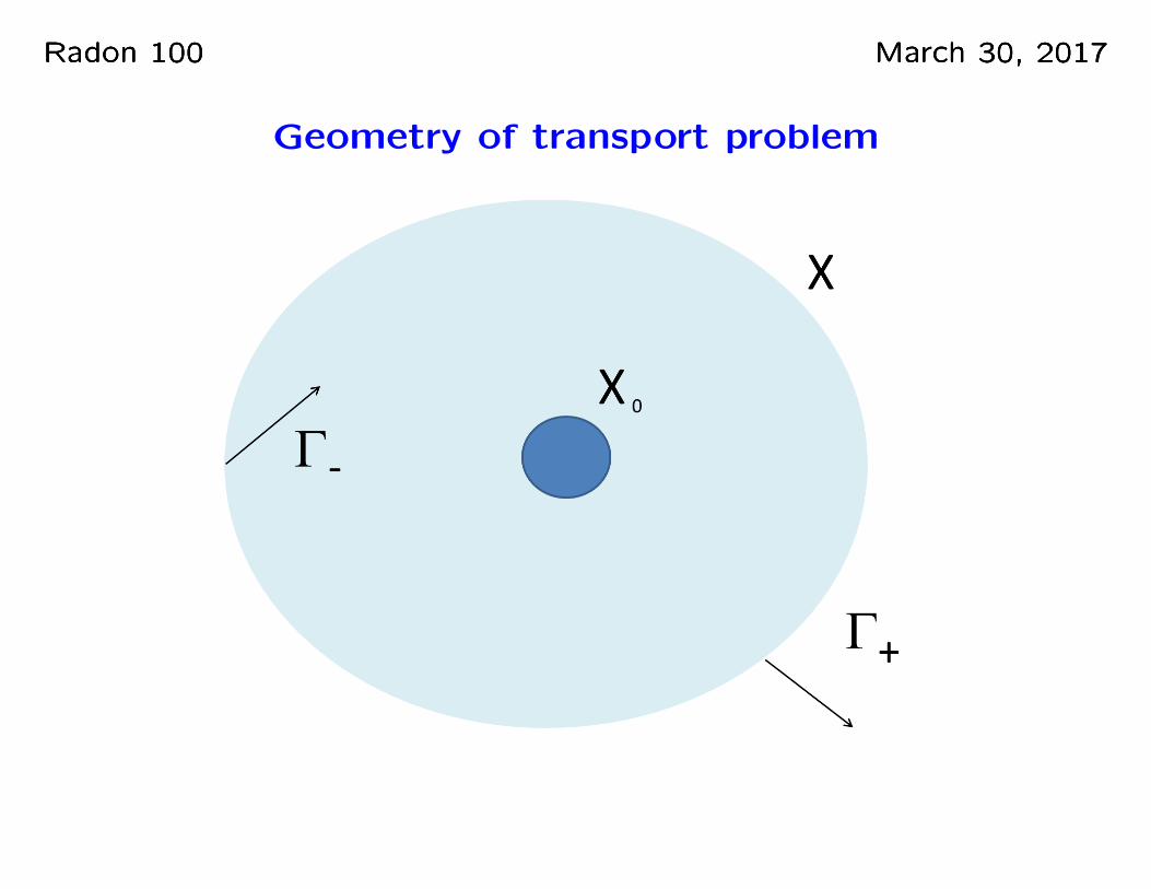
Consider the transport equation for convex bounded X ⊂ Rn; V = Sn−1:

v · ∇u+ σ(x, v)u =∫Vk(x, v′, v)u(x, v′)dv′, (x, v) ∈ X × V

u = g, (x, v) ∈ Γ−; Γ± = {(x, v) ∈ ∂X × V, ±v · n(x) > 0}.

Inverse Problem: Reconstruct (information on) σ(x, v) and k(x, v′, v)

from knowledge of the Albedo operator A[σ, k] : g = uΓ− 7→ Ag = uΓ+.

(Many related inverse problems where the albedo operator is partially known, for in-

stance, as in Optical Tomography [Arridge Schotland IP 09; B. IP 09], isotropic sources

and angularly averaged measurements. Not discussed further here.)

6


Geometry of transport problem

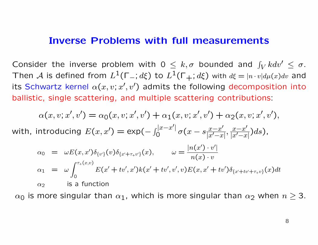
Inverse Problems with full measurements

Consider the inverse problem with 0 ≤ k, σ bounded and∫V kdv

′ ≤ σ.

Then A is defined from L1(Γ−; dξ) to L1(Γ+; dξ) with dξ = |n · v|dµ(x)dv and

its Schwartz kernel α(x, v;x′, v′) admits the following decomposition into

ballistic, single scattering, and multiple scattering contributions:

α(x, v;x′, v′) = α0(x, v;x′, v′) + α1(x, v;x′, v′) + α2(x, v;x′, v′),

with, introducing E(x, x′) = exp(−∫ |x−x′|0 σ(x− s x−x

′|x′−x|,

x−x′|x′−x|)ds),

α0 = ωE(x, x′)δ{v′}(v)δ{x′+τ+v′}(x), ω =|n(x′) · v′|n(x) · v

α1 = ω

∫ τ+(x,v)

0E(x′ + tv′, x′)k(x′ + tv′, v′, v)E(x, x′ + tv′)δ{x′+tv′+τ+v}(x)dt

α2 is a function

α0 is more singular than α1, which is more singular than α2 when n ≥ 3.

8

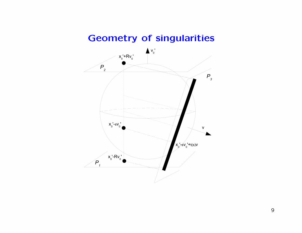
Geometry of singularitiesv

0'

vx

0'-sv

0'

x0'+Rv

0'

x0'-Rv

0'

P2

P3

P1

x0'-sv

0'+t(s)v

9

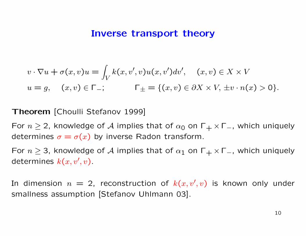
Inverse transport theory


u = g, (x, v) ∈ Γ−; Γ± = {(x, v) ∈ ∂X × V, ±v · n(x) > 0}.

Theorem [Choulli Stefanov 1999]

For n ≥ 2, knowledge of A implies that of α0 on Γ+×Γ−, which uniquely

determines σ = σ(x) by inverse Radon transform.

For n ≥ 3, knowledge of A implies that of α1 on Γ+×Γ−, which uniquely

determines k(x, v′, v).

In dimension n = 2, reconstruction of k(x, v′, v) is known only under

smallness assumption [Stefanov Uhlmann 03].

10

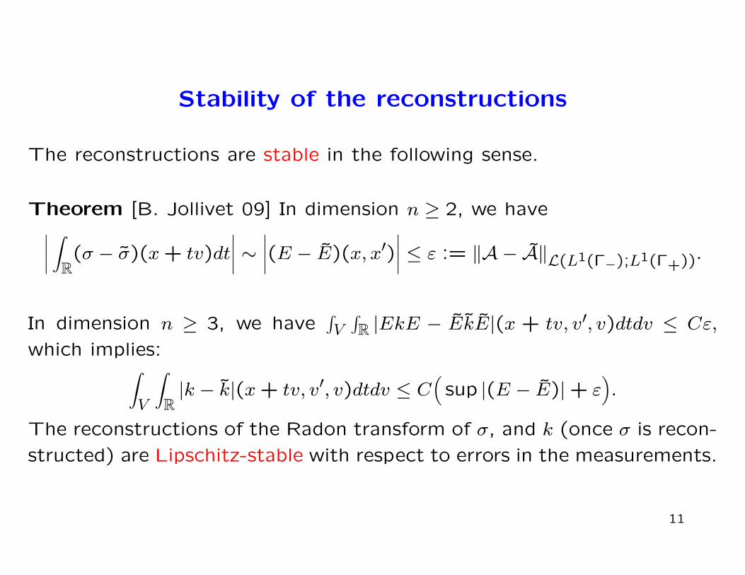
Stability of the reconstructions

The reconstructions are stable in the following sense.

Theorem [B. Jollivet 09] In dimension n ≥ 2, we have∣∣∣∣ ∫R(σ − σ)(x+ tv)dt∣∣∣∣ ∼ ∣∣∣∣(E − E)(x, x′)

∣∣∣∣ ≤ ε := ‖A − A‖L(L1(Γ−);L1(Γ+)).

In dimension n ≥ 3, we have∫V∫R |EkE − EkE|(x + tv, v′, v)dtdv ≤ Cε,

which implies:∫V

∫R|k − k|(x+ tv, v′, v)dtdv ≤ C

(sup |(E − E)|+ ε

).

The reconstructions of the Radon transform of σ, and k (once σ is recon-

structed) are Lipschitz-stable with respect to errors in the measurements.

11

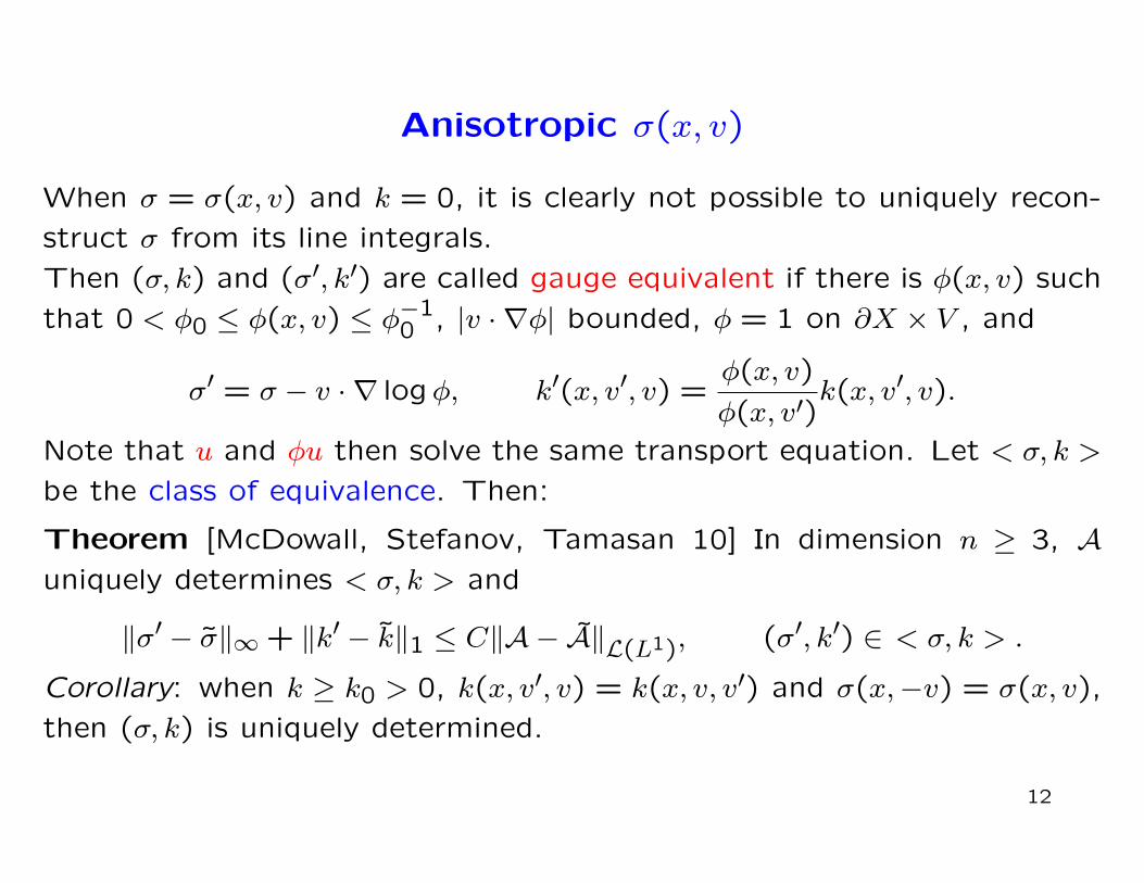
Anisotropic σ(x, v)

When σ = σ(x, v) and k = 0, it is clearly not possible to uniquely recon-

struct σ from its line integrals.

Then (σ, k) and (σ′, k′) are called gauge equivalent if there is φ(x, v) such

that 0 < φ0 ≤ φ(x, v) ≤ φ−10 , |v · ∇φ| bounded, φ = 1 on ∂X × V , and

σ′ = σ − v · ∇ logφ, k′(x, v′, v) =φ(x, v)

φ(x, v′)k(x, v′, v).

Note that u and φu then solve the same transport equation. Let < σ, k >

be the class of equivalence. Then:

Theorem [McDowall, Stefanov, Tamasan 10] In dimension n ≥ 3, Auniquely determines < σ, k > and

‖σ′ − σ‖∞+ ‖k′ − k‖1 ≤ C‖A − A‖L(L1), (σ′, k′) ∈ < σ, k > .

Corollary: when k ≥ k0 > 0, k(x, v′, v) = k(x, v, v′) and σ(x,−v) = σ(x, v),

then (σ, k) is uniquely determined.

12


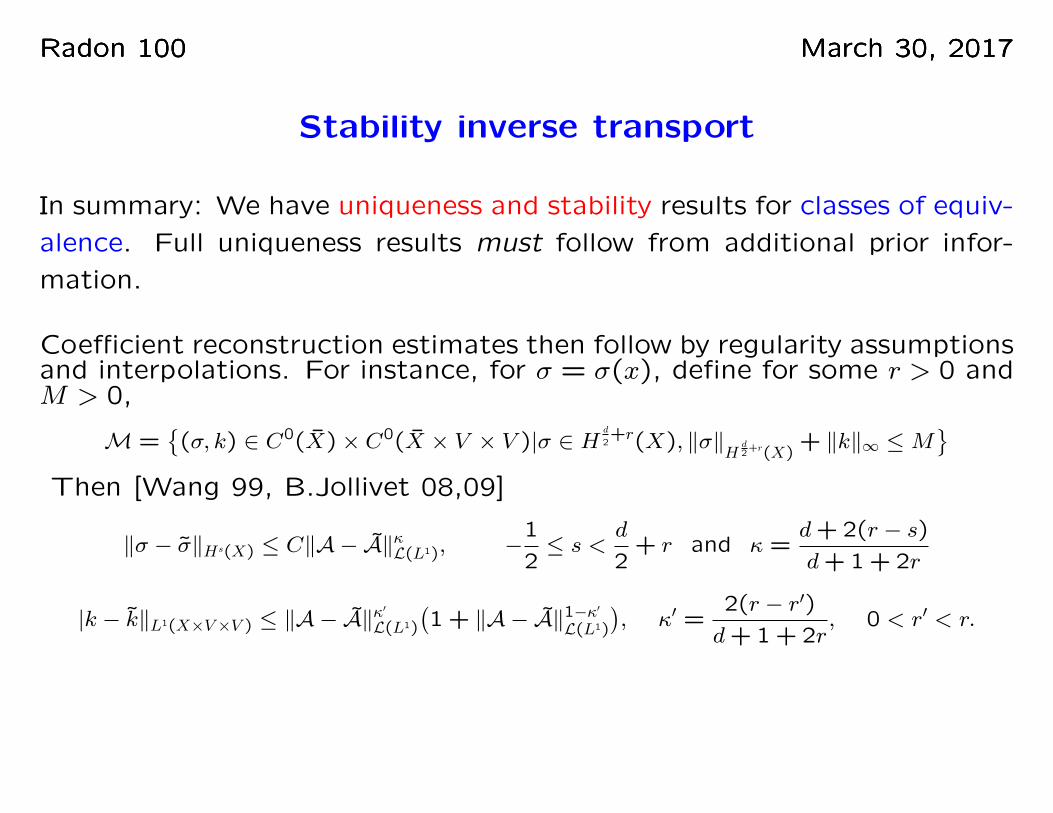
Stability inverse transport

In summary: We have uniqueness and stability results for classes of equiv-

alence. Full uniqueness results must follow from additional prior infor-

mation.

Coefficient reconstruction estimates then follow by regularity assumptionsand interpolations. For instance, for σ = σ(x), define for some r > 0 andM > 0,

M ={

(σ, k) ∈ C0(X)× C0(X × V × V )|σ ∈ Hd

2+r(X), ‖σ‖

Hd2

+r(X)+ ‖k‖∞ ≤M

}Then [Wang 99, B.Jollivet 08,09]

‖σ − σ‖Hs(X) ≤ C‖A − A‖κL(L1), −1

2≤ s <

d

2+ r and κ =

d+ 2(r − s)d+ 1 + 2r

|k − k‖L1(X×V×V ) ≤ ‖A− A‖κ′

L(L1)

(1 + ‖A − A‖1−κ′

L(L1)

), κ′ =

2(r − r′)d+ 1 + 2r

, 0 < r′ < r.


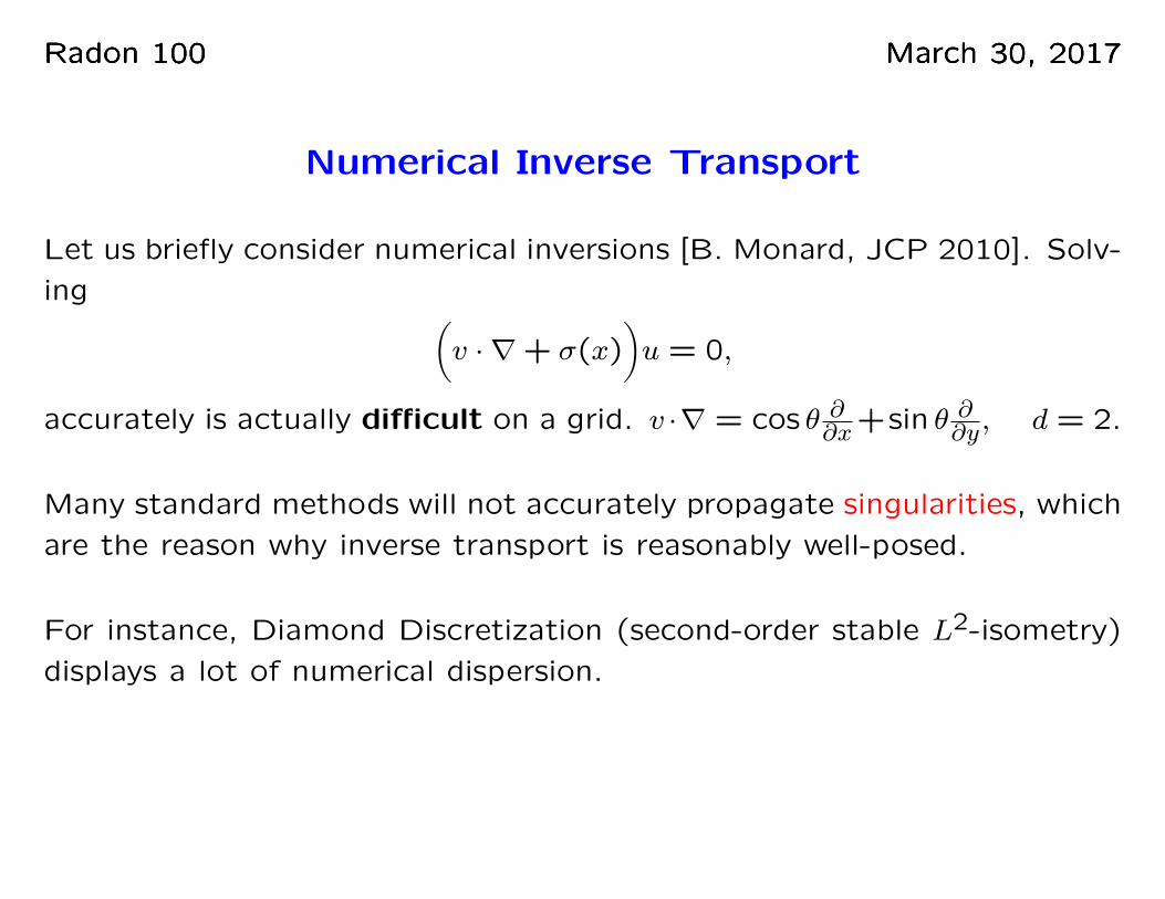
Numerical Inverse Transport

Let us briefly consider numerical inversions [B. Monard, JCP 2010]. Solv-

ing (v · ∇+ σ(x)

)u = 0,

accurately is actually difficult on a grid. v ·∇ = cos θ ∂∂x+sin θ ∂∂y , d = 2.

Many standard methods will not accurately propagate singularities, which

are the reason why inverse transport is reasonably well-posed.

For instance, Diamond Discretization (second-order stable L2-isometry)

displays a lot of numerical dispersion.

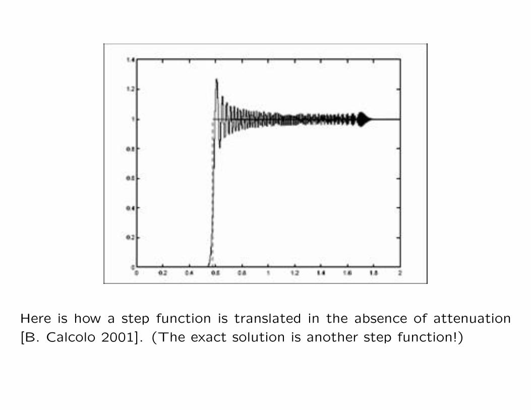
Here is how a step function is translated in the absence of attenuation

[B. Calcolo 2001]. (The exact solution is another step function!)

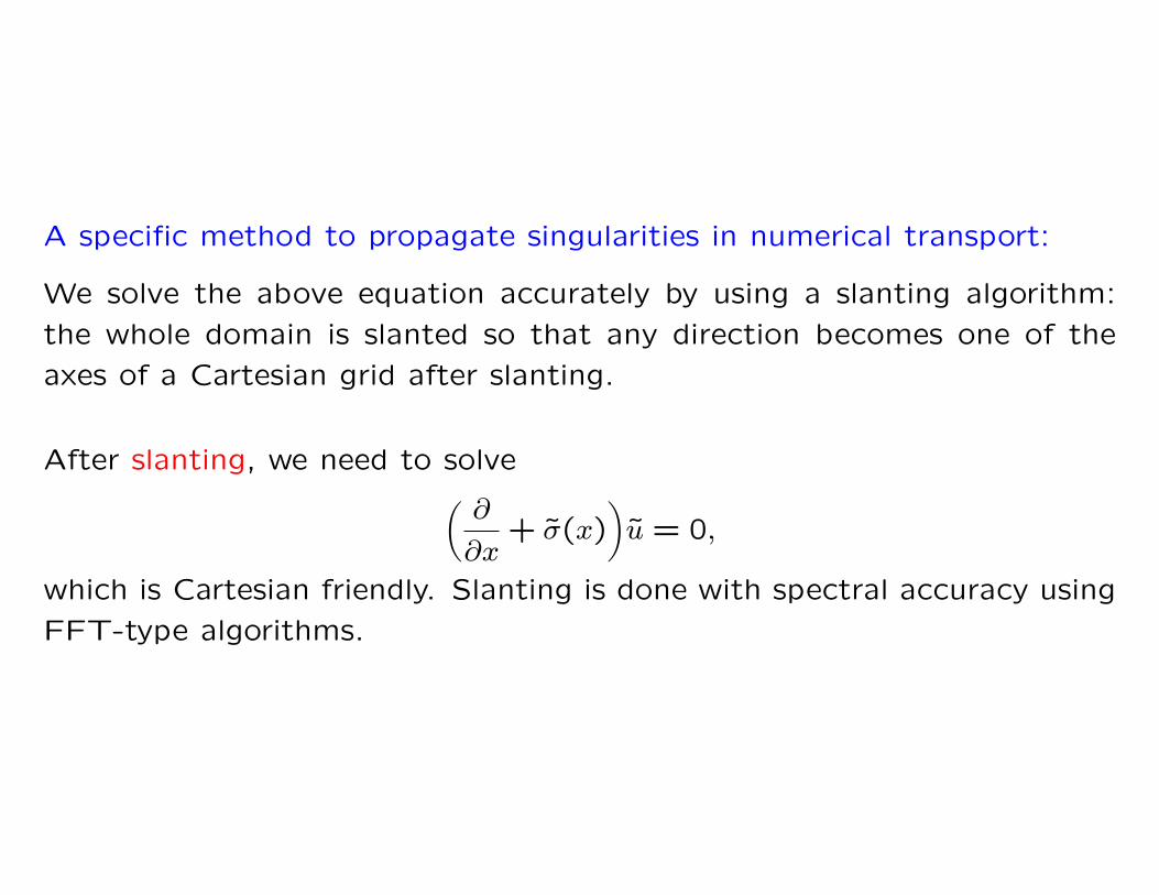
A specific method to propagate singularities in numerical transport:

We solve the above equation accurately by using a slanting algorithm:

the whole domain is slanted so that any direction becomes one of the

axes of a Cartesian grid after slanting.

After slanting, we need to solve(∂

∂x+ σ(x)

)u = 0,

which is Cartesian friendly. Slanting is done with spectral accuracy using

FFT-type algorithms.


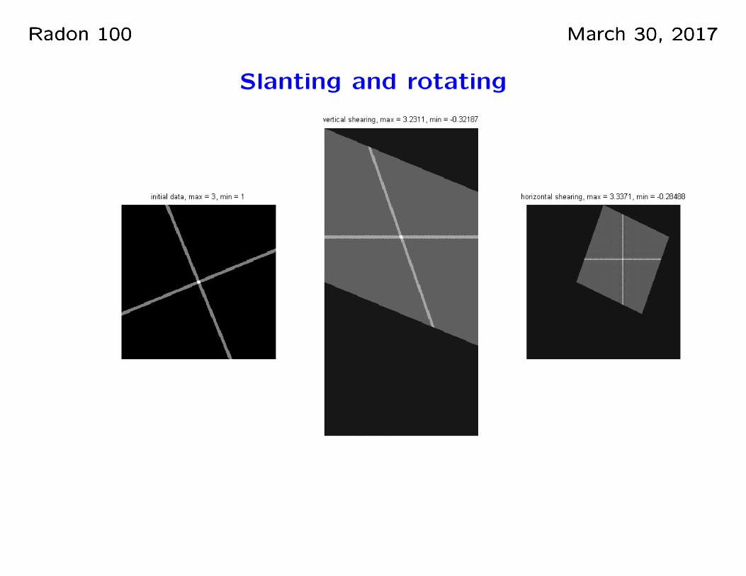
Slanting and rotating


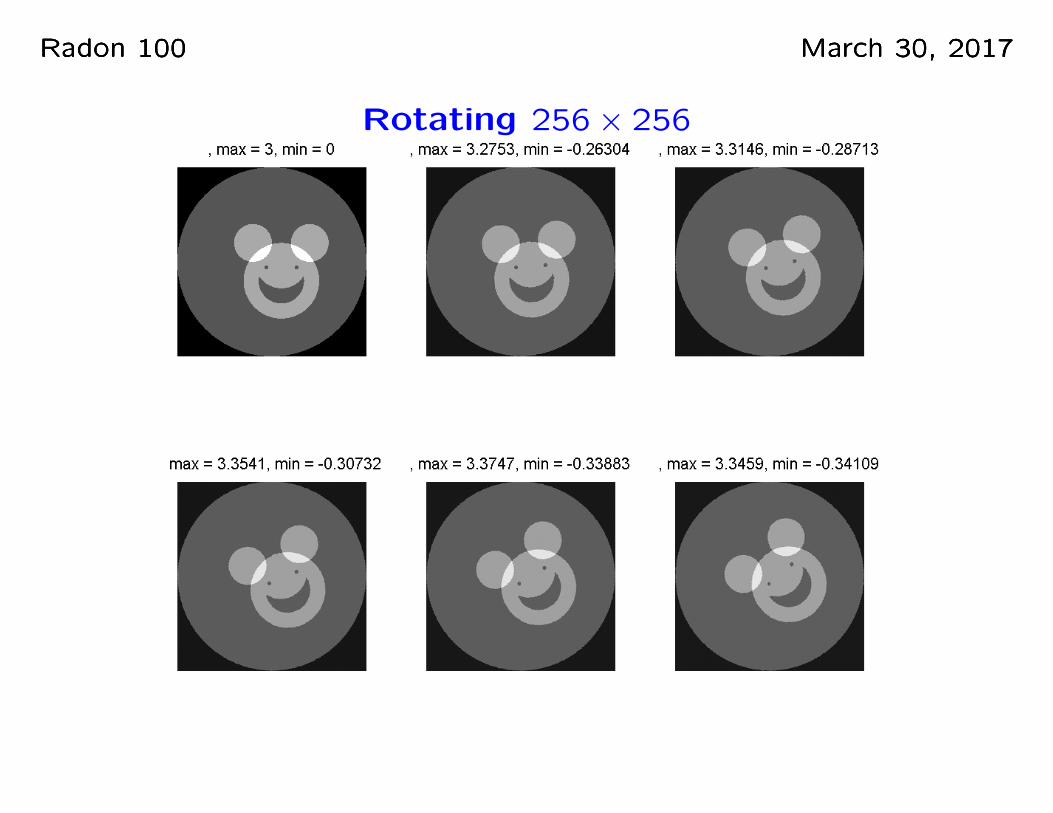
Rotating 256× 256


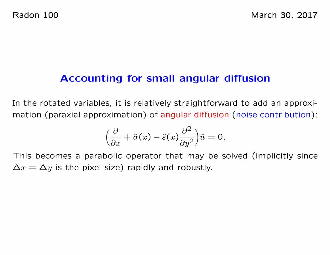
Accounting for small angular diffusion

In the rotated variables, it is relatively straightforward to add an approxi-

mation (paraxial approximation) of angular diffusion (noise contribution):(∂

∂x+ σ(x)− ε(x)

∂2

∂y2

)u = 0,

This becomes a parabolic operator that may be solved (implicitly since

∆x = ∆y is the pixel size) rapidly and robustly.

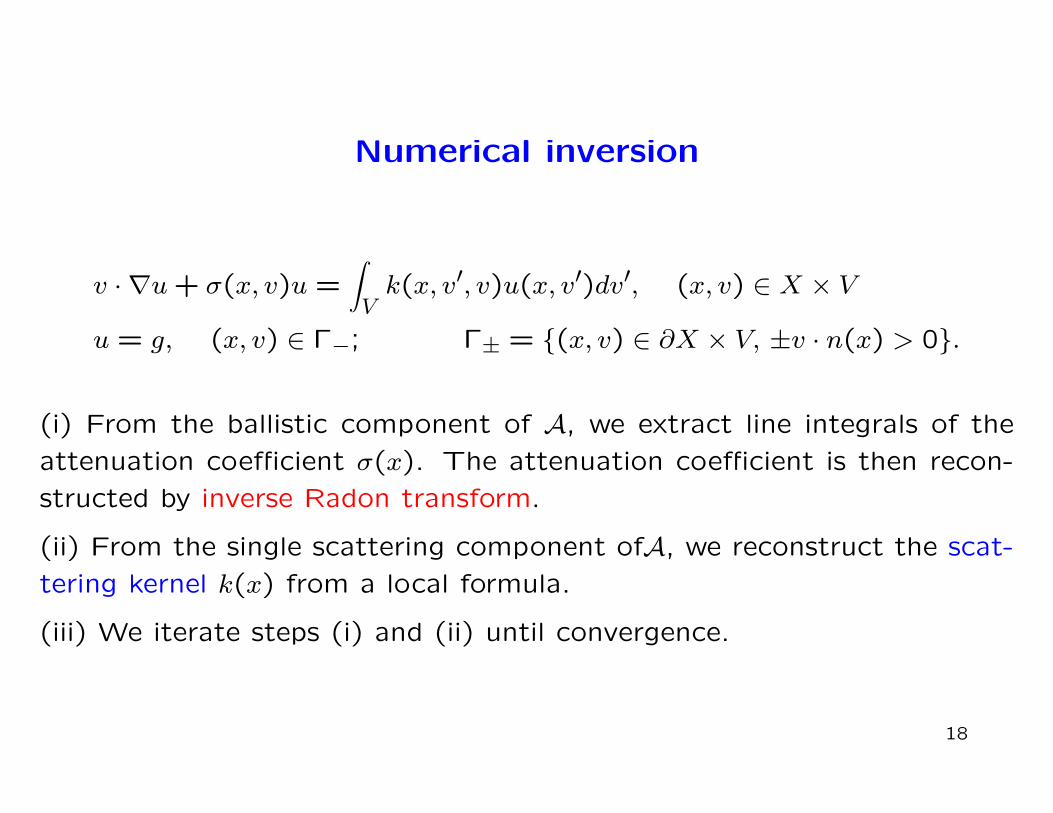
Numerical inversion


u = g, (x, v) ∈ Γ−; Γ± = {(x, v) ∈ ∂X × V, ±v · n(x) > 0}.

(i) From the ballistic component of A, we extract line integrals of the

attenuation coefficient σ(x). The attenuation coefficient is then recon-

structed by inverse Radon transform.

(ii) From the single scattering component ofA, we reconstruct the scat-

tering kernel k(x) from a local formula.

(iii) We iterate steps (i) and (ii) until convergence.

18


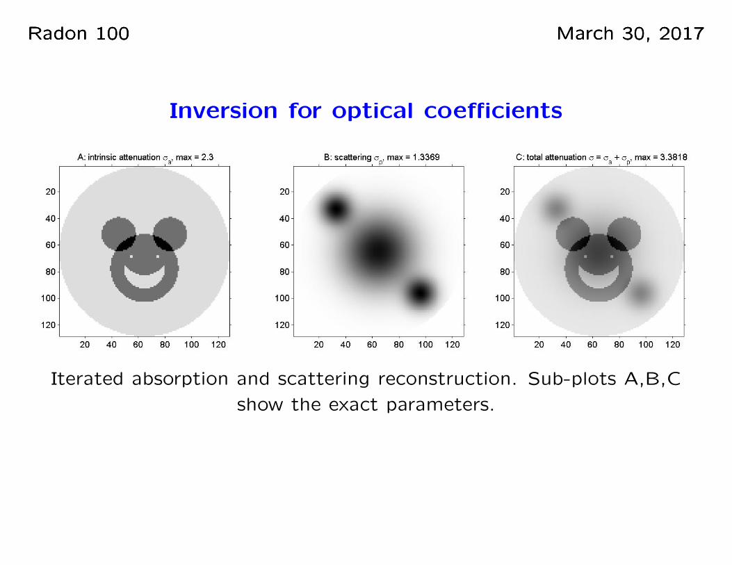
Inversion for optical coefficients

Iterated absorption and scattering reconstruction. Sub-plots A,B,C

show the exact parameters.

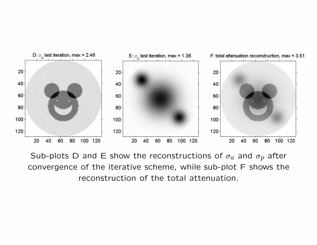
Sub-plots D and E show the reconstructions of σa and σp after

convergence of the iterative scheme, while sub-plot F shows the

reconstruction of the total attenuation.


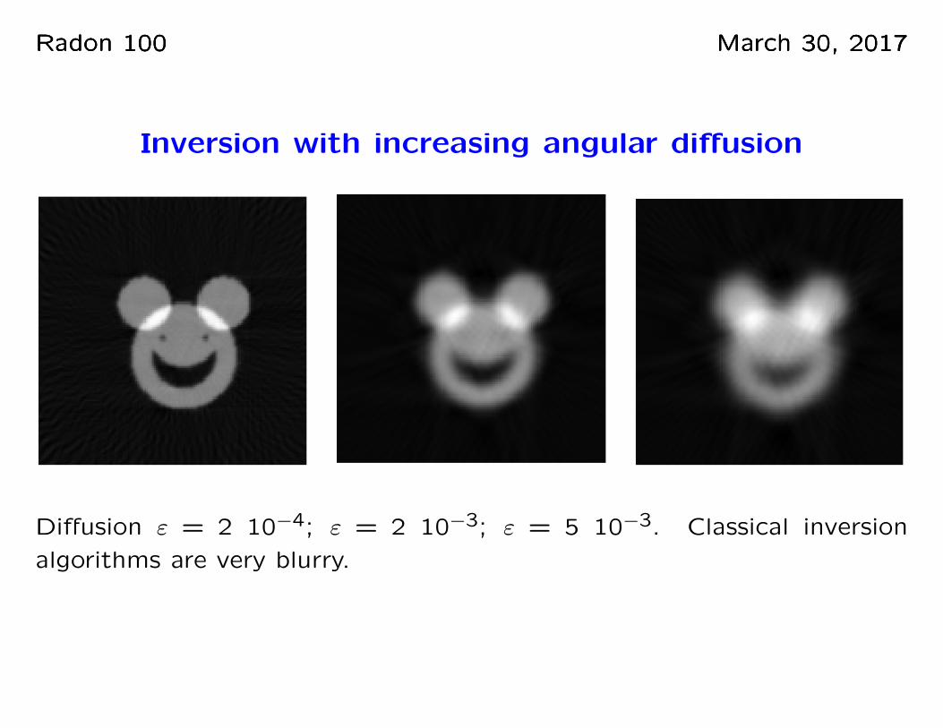
Inversion with increasing angular diffusion

Diffusion ε = 2 10−4; ε = 2 10−3; ε = 5 10−3. Classical inversion

algorithms are very blurry.


What did we do right?

Uniqueness:

Stability:

Numerical validation:


What are we missing?

Stability estimates of the form

‖σ′ − σ‖∞+ ‖k′ − k‖1 ≤ C‖A − A‖L(L1),

are useful if the right-hand side is small when noise is small. This is a

problem in many practical settings, where noise may not be modeled by

a variation of albedo operators or where ‖A − A‖L(L1) is not small.

There is nothing wrong (mathematically) with the stability estimates.

But they may not be the right tool to assess data errors and, hence,

reconstruction errors.




Detector noise models

The preceding example is a good application of the above stability es-

timates: small errors in the measurements translate into small errors in

the reconstructions.

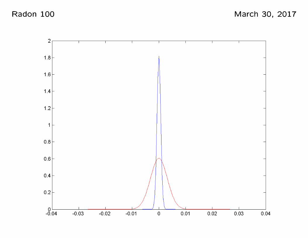
Now consider blurring at the detector level.




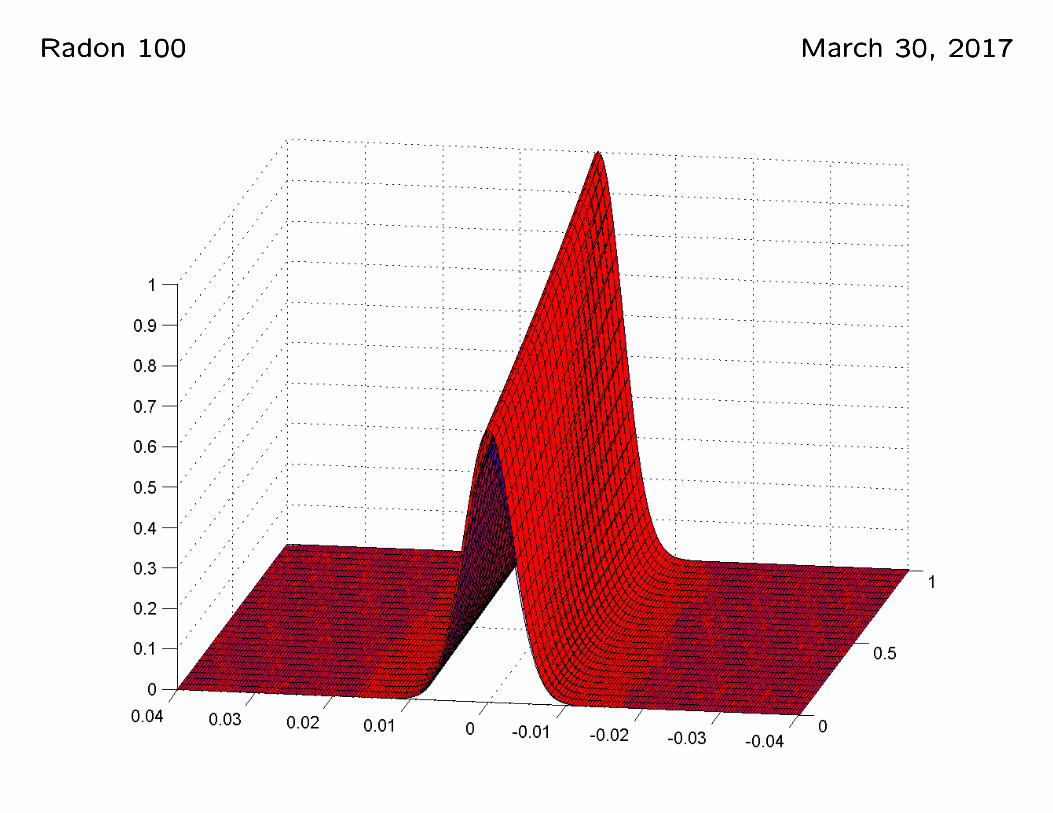
Detector and source noise models

In the preceding example, detector noise moves available data away from

the range of the albedo operator. Any “projection” onto that range

would result in potentially catastrophic errors levels.

Now consider errors at the source level. Sources are never perfectly in

the predicted shape and location.




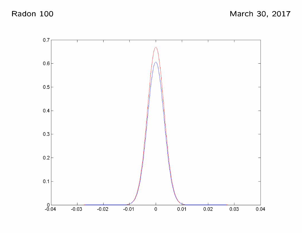
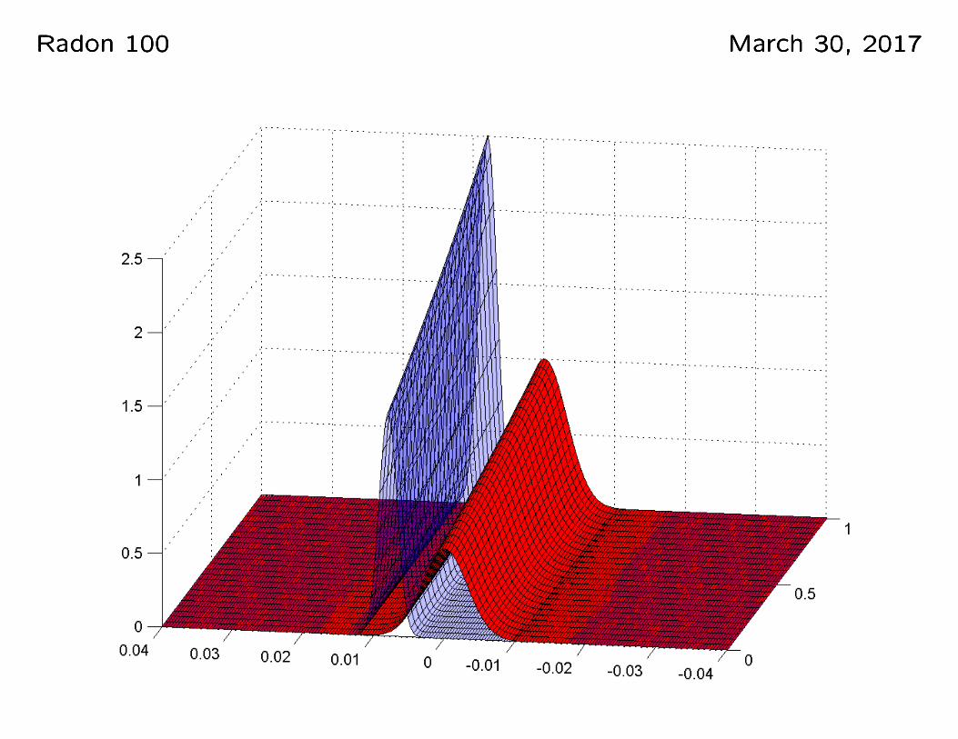
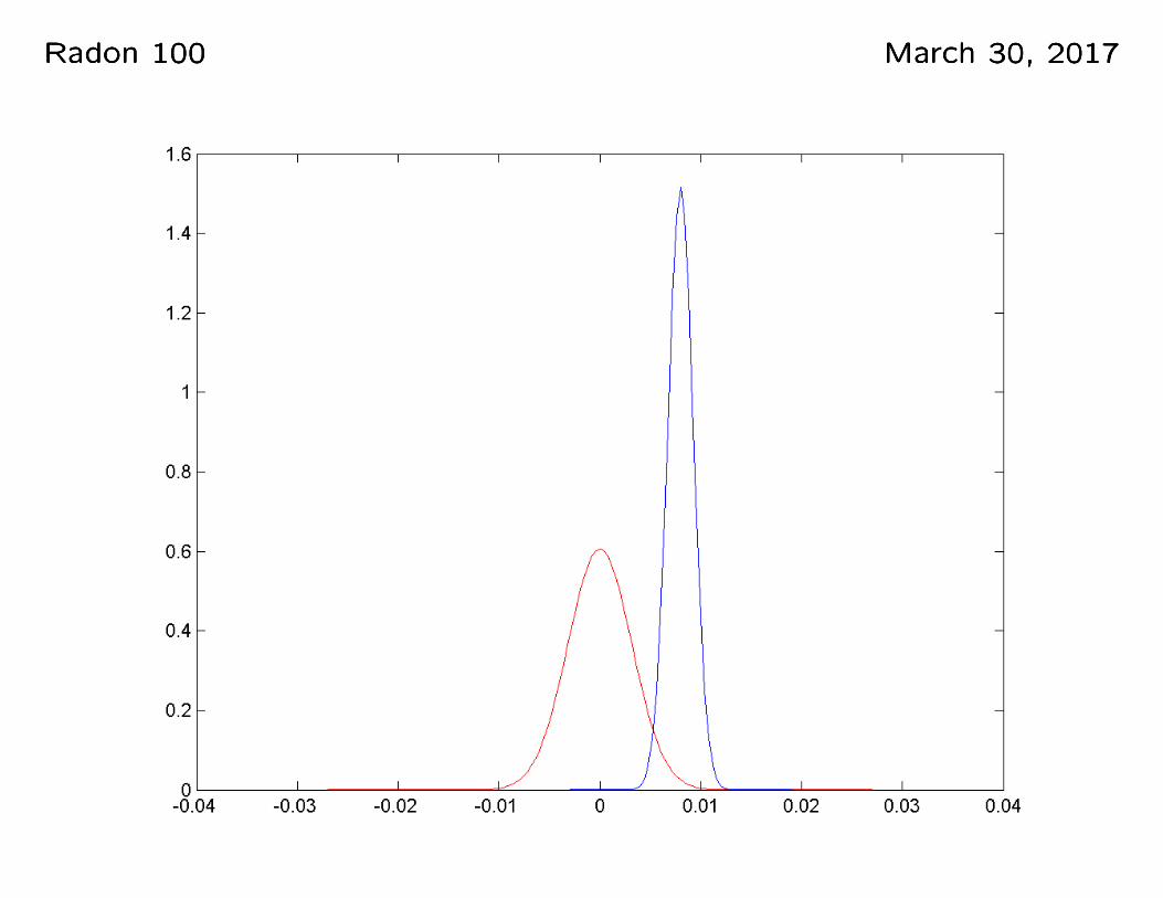
Source noise models

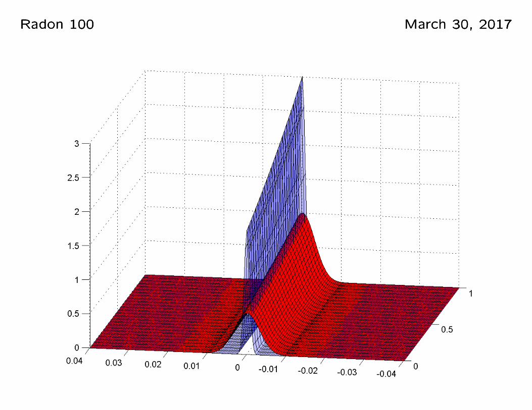
Here again, the errors move available data away from the range of the

albedo operator. Again, ‘projection” onto that range would result in

catastrophic errors levels as the L1 norm between the “blue” and “red”

graphs is large.

Yet, small blurring at the detector level or small mis-alignment of the

source term typically do not result is catastrophic reconstructions for

an inverse transport / inverse Radon problem that is not irremediably

ill-posed. How should one model this?


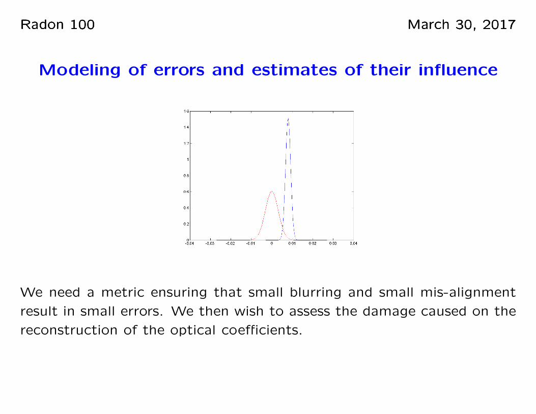
Modeling of errors and estimates of their influence

We need a metric ensuring that small blurring and small mis-alignment

result in small errors. We then wish to assess the damage caused on the

reconstruction of the optical coefficients.

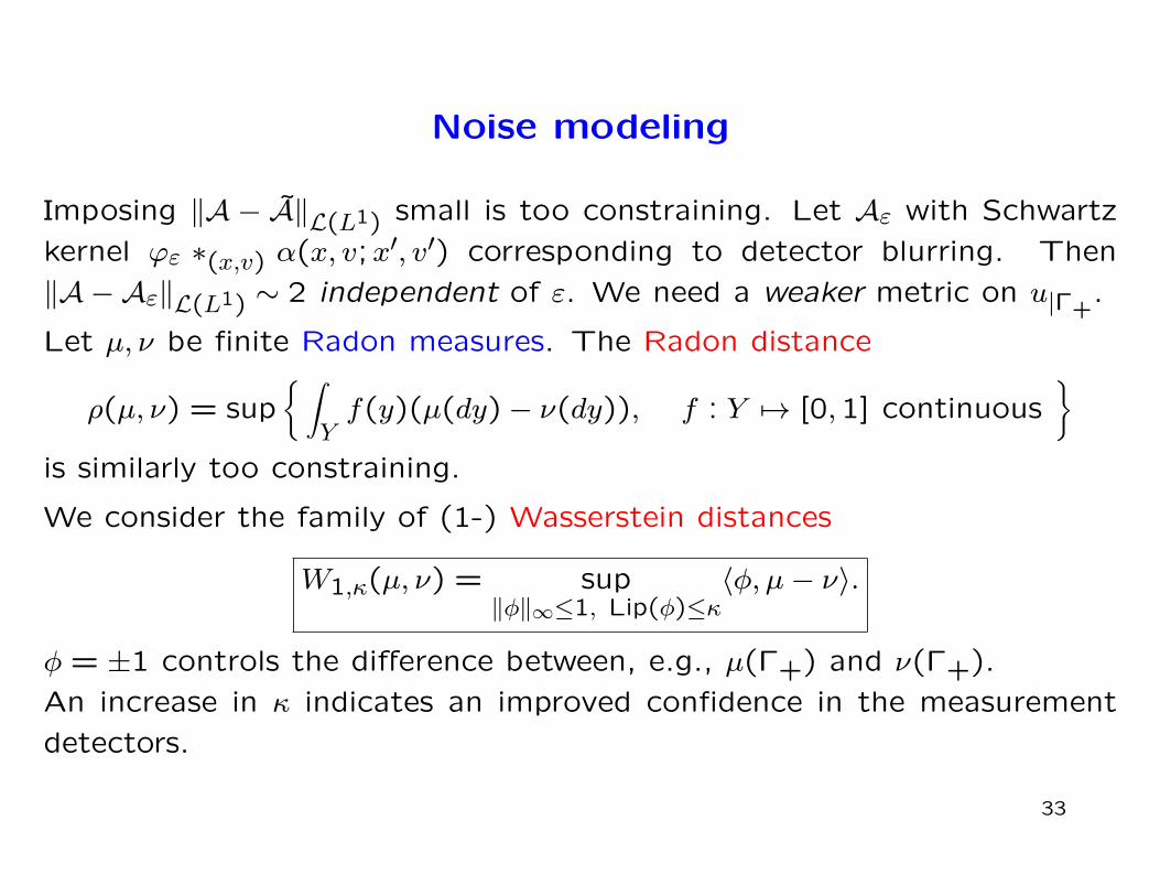
Noise modeling

Imposing ‖A − A‖L(L1) small is too constraining. Let Aε with Schwartz

kernel ϕε ∗(x,v) α(x, v;x′, v′) corresponding to detector blurring. Then

‖A −Aε‖L(L1) ∼ 2 independent of ε. We need a weaker metric on u|Γ+.

Let µ, ν be finite Radon measures. The Radon distance

ρ(µ, ν) = sup{ ∫

Yf(y)(µ(dy)− ν(dy)), f : Y 7→ [0,1] continuous

}is similarly too constraining.

We consider the family of (1-) Wasserstein distances

W1,κ(µ, ν) = sup‖φ‖∞≤1, Lip(φ)≤κ

〈φ, µ− ν〉.

φ = ±1 controls the difference between, e.g., µ(Γ+) and ν(Γ+).

An increase in κ indicates an improved confidence in the measurement

detectors.

33


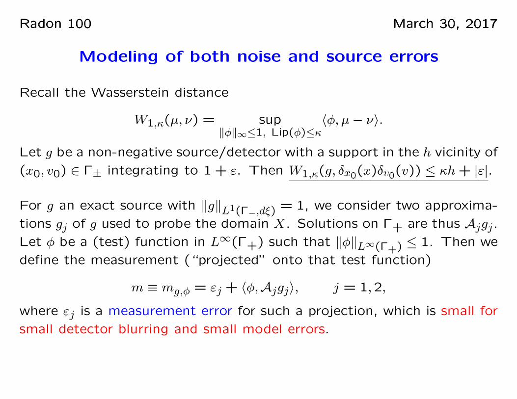
Modeling of both noise and source errors

Recall the Wasserstein distance

W1,κ(µ, ν) = sup‖φ‖∞≤1, Lip(φ)≤κ

〈φ, µ− ν〉.

Let g be a non-negative source/detector with a support in the h vicinity of

(x0, v0) ∈ Γ± integrating to 1 + ε. Then W1,κ(g, δx0(x)δv0(v)) ≤ κh+ |ε|.

For g an exact source with ‖g‖L1(Γ−,dξ)= 1, we consider two approxima-

tions gj of g used to probe the domain X. Solutions on Γ+ are thus Ajgj.Let φ be a (test) function in L∞(Γ+) such that ‖φ‖L∞(Γ+) ≤ 1. Then we

define the measurement (“projected” onto that test function)

m ≡ mg,φ = εj + 〈φ,Ajgj〉, j = 1,2,

where εj is a measurement error for such a projection, which is small for

small detector blurring and small model errors.

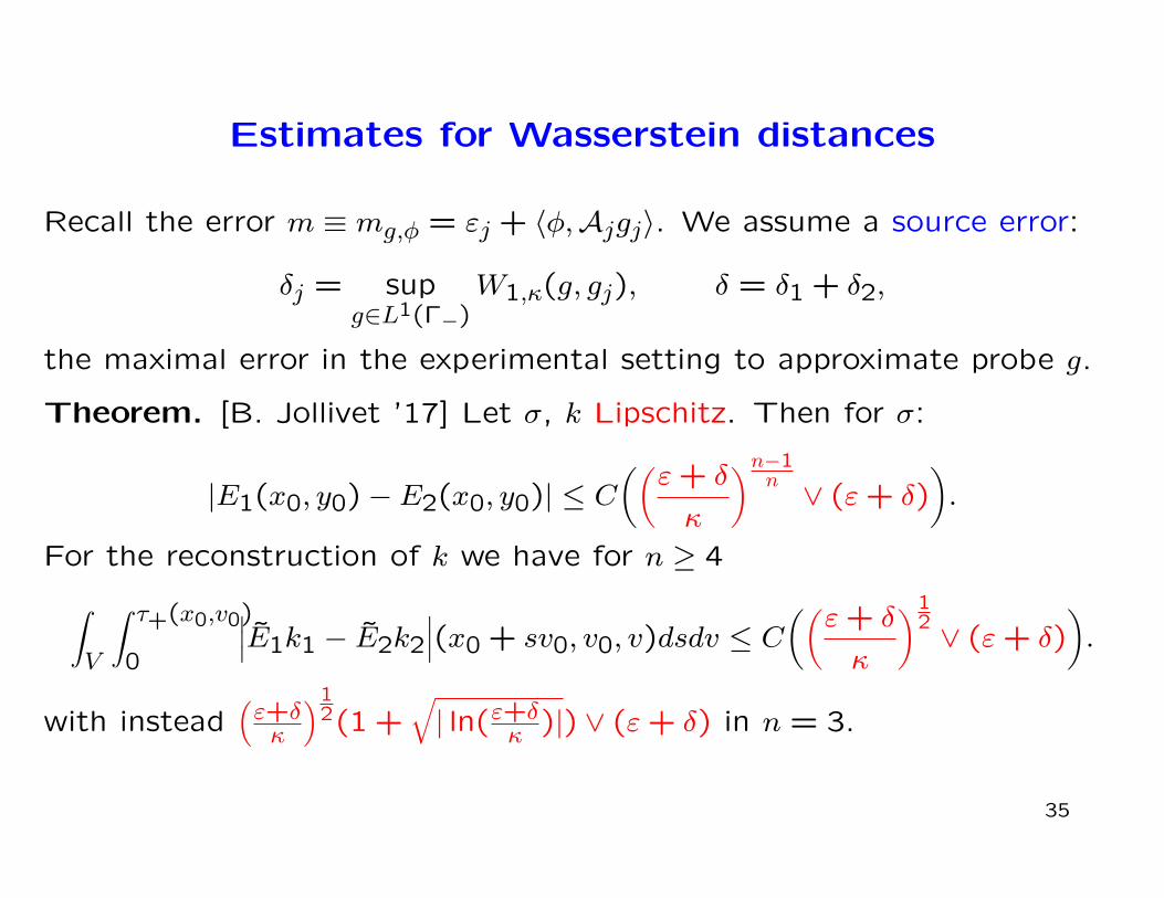
Estimates for Wasserstein distances

Recall the error m ≡ mg,φ = εj + 〈φ,Ajgj〉. We assume a source error:

δj = supg∈L1(Γ−)

W1,κ(g, gj), δ = δ1 + δ2,

the maximal error in the experimental setting to approximate probe g.

Theorem. [B. Jollivet ’17] Let σ, k Lipschitz. Then for σ:

|E1(x0, y0)− E2(x0, y0)| ≤ C((ε+ δ

κ

)n−1n ∨ (ε+ δ)

).

For the reconstruction of k we have for n ≥ 4∫V

∫ τ+(x0,v0)

0

∣∣∣E1k1 − E2k2

∣∣∣(x0 + sv0, v0, v)dsdv ≤ C((ε+ δ

κ

)12 ∨ (ε+ δ)

).

with instead(ε+δκ

)12(1 +

√| ln(ε+δ

κ )|) ∨ (ε+ δ) in n = 3.

35


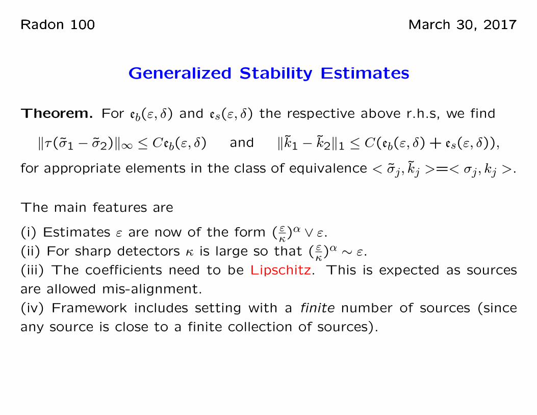
Generalized Stability Estimates

Theorem. For eb(ε, δ) and es(ε, δ) the respective above r.h.s, we find

‖τ(σ1 − σ2)‖∞ ≤ Ceb(ε, δ) and ‖k1 − k2‖1 ≤ C(eb(ε, δ) + es(ε, δ)),

for appropriate elements in the class of equivalence < σj, kj >=< σj, kj >.

The main features are

(i) Estimates ε are now of the form (εκ)α ∨ ε.(ii) For sharp detectors κ is large so that (εκ)α ∼ ε.(iii) The coefficients need to be Lipschitz. This is expected as sources

are allowed mis-alignment.

(iv) Framework includes setting with a finite number of sources (since

any source is close to a finite collection of sources).


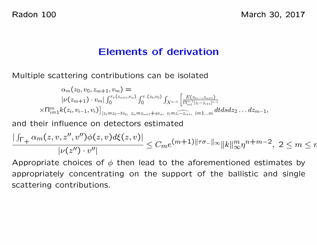
Elements of derivation

Multiple scattering contributions can be isolated

αm(z0, v0, zm+1, vm) =

|ν(zm+1) · vm|∫ τ+(zm+1,vm)

0

∫ τ−(z0,v0)0

∫Xm−2

[E(z0,...,zm+1)

Πm−1i=1 |zi−zi+1|n−1

×Πmi=1k(zi, vi−1, vi)

]|z1=z0−tv0, zm=zm+1+svm, vi= zi−zi+1, i=1...m

dtdsdz2 . . . dzm−1,

and their influence on detectors estimated

|∫Γ+

αm(z, v, z′′, v′′)φ(z, v)dξ(z, v)||ν(z′′) · v′′|

≤ Cme(m+1)‖τσ−‖∞‖k‖m∞ηn+m−2, 2 ≤ m ≤ n− 1,

Appropriate choices of φ then lead to the aforementioned estimates by

appropriately concentrating on the support of the ballistic and single

scattering contributions.


What did we do right?

Uniqueness:

Stability:

Numerical validation:

Physics based stability:

Documents

Inverse Transport Problems (Generalized) Stability ... · Inverse Transport Problems (Generalized) Stability Estimates ... In summary: We haveuniqueness ... accurately is actually