Investigating continental rifting in the Western US

with seismic methodsScott Burdick, Tolulope Olugboji, & Vedran Lekic

GSA Fall MeetingNovember 2, 2015

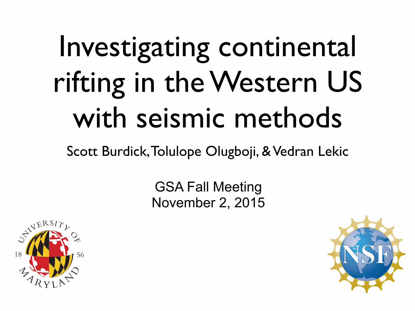
What can seismology tell us about rifting processes?

Pure shear - symmetric

Simple shear - asymmetric

Buck

198

8

(Huismans)et)al.,)2001)))

Localized strain due to upwelling

• Geometry of boundaries (Moho, LAB) constrains distribution of strain throughout lithosphere, informing on rheology and modes of deformation

• 3D/along-strike variation relates rifting to preexisting structure

• Vp/Vs ratio helps understand distribution and role of melt

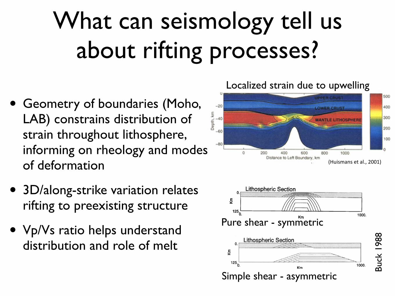
Ability to map complex, steeply dipping structure

3D formulation/ability to incorporate 3D velocities

Handle tradeoff between boundary depth and

smooth velocity

NEEDS

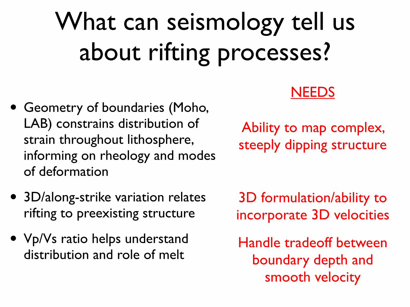
What can seismology tell us about rifting processes?

• Geometry of boundaries (Moho, LAB) constrains distribution of strain throughout lithosphere, informing on rheology and modes of deformation

• 3D/along-strike variation relates rifting to preexisting structure

• Vp/Vs ratio helps understand distribution and role of melt

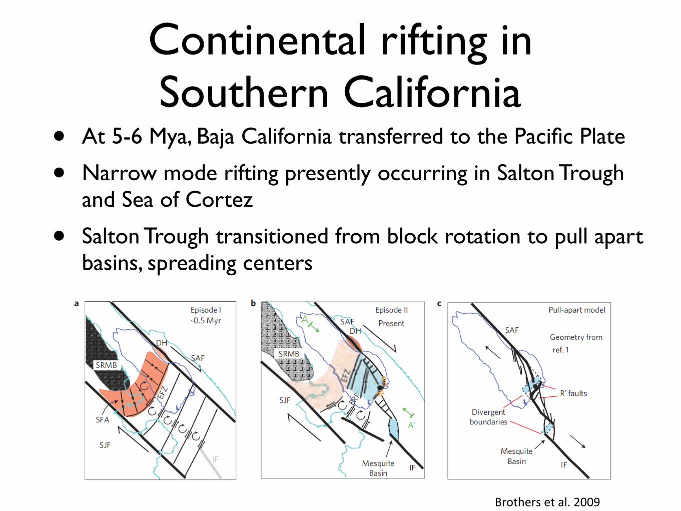
Continental rifting in Southern California

• At 5-6 Mya, Baja California transferred to the Pacific Plate

• Narrow mode rifting presently occurring in Salton Trough and Sea of Cortez

• Salton Trough transitioned from block rotation to pull apart basins, spreading centers

Brothers(et(al.(2009((

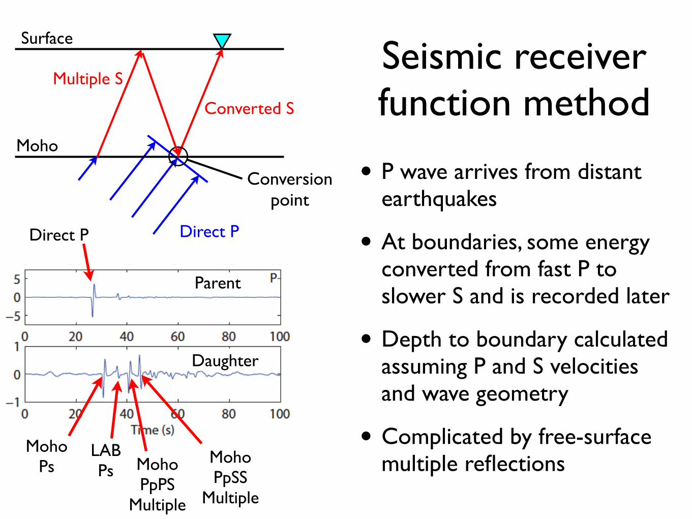
Seismic receiver function method

• P wave arrives from distant earthquakes

• At boundaries, some energy converted from fast P to slower S and is recorded later

• Depth to boundary calculated assuming P and S velocities and wave geometry

• Complicated by free-surface multiple reflections

Moho

Surface

Direct P

Converted S

Direct P

Moho Ps

LAB Ps Moho

PpPSMultiple

Moho PpSS

Multiple

Parent

Daughter

Conversion point

Multiple S

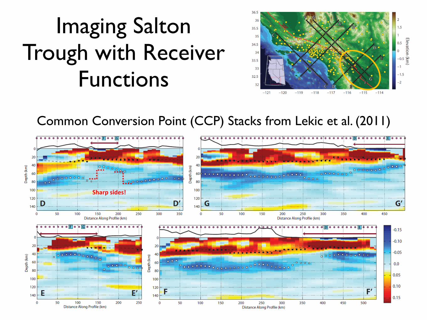
Imaging Salton Trough with Receiver

Functions

Common Conversion Point (CCP) Stacks from Lekic et al. (2011)

Sharp&sides!&

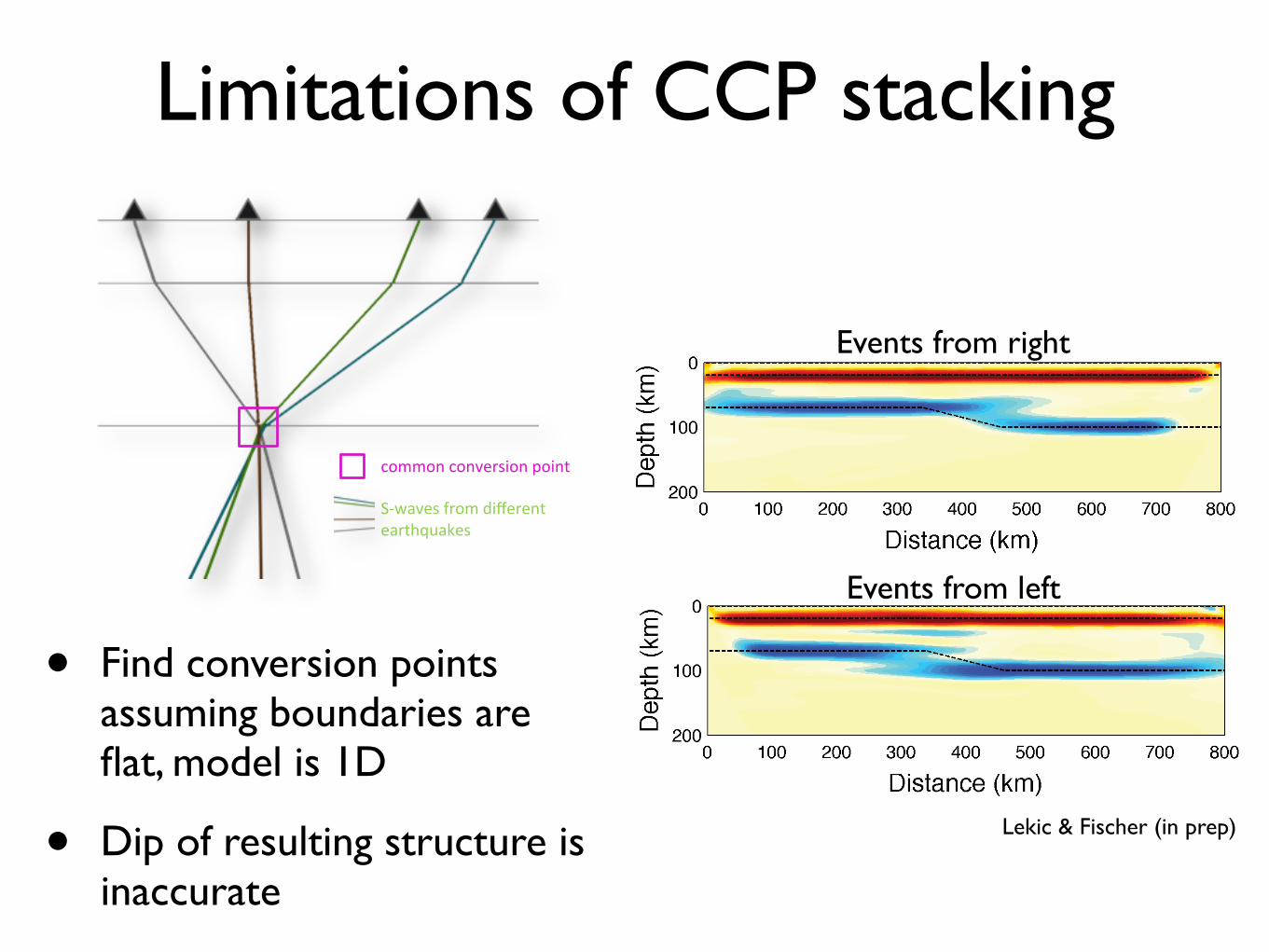
Limitations of CCP stacking

• Find conversion points assuming boundaries are flat, model is 1D

• Dip of resulting structure is inaccurate

common%conversion%point%%S.waves%from%different%earthquakes%

Events from right

Events from left

Lekic & Fischer (in prep)

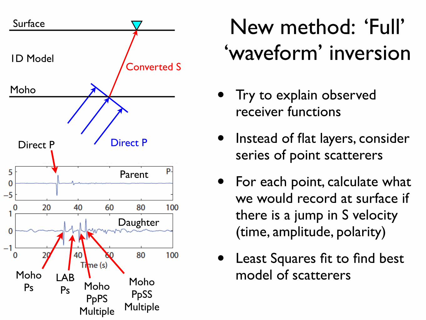
New method: ‘Full’ ‘waveform’ inversion

Direct P

Moho

Surface

Direct P

Converted S

Direct P

Moho Ps

LAB Ps Moho

PpPSMultiple

Moho PpSS

Multiple

Parent

Daughter

• Try to explain observed receiver functions

• Instead of flat layers, consider series of point scatterers

• For each point, calculate what we would record at surface if there is a jump in S velocity (time, amplitude, polarity)

• Least Squares fit to find best model of scatterers

1D Model

Direct P

Surface

Direct P

Converted S

Point Scatterer

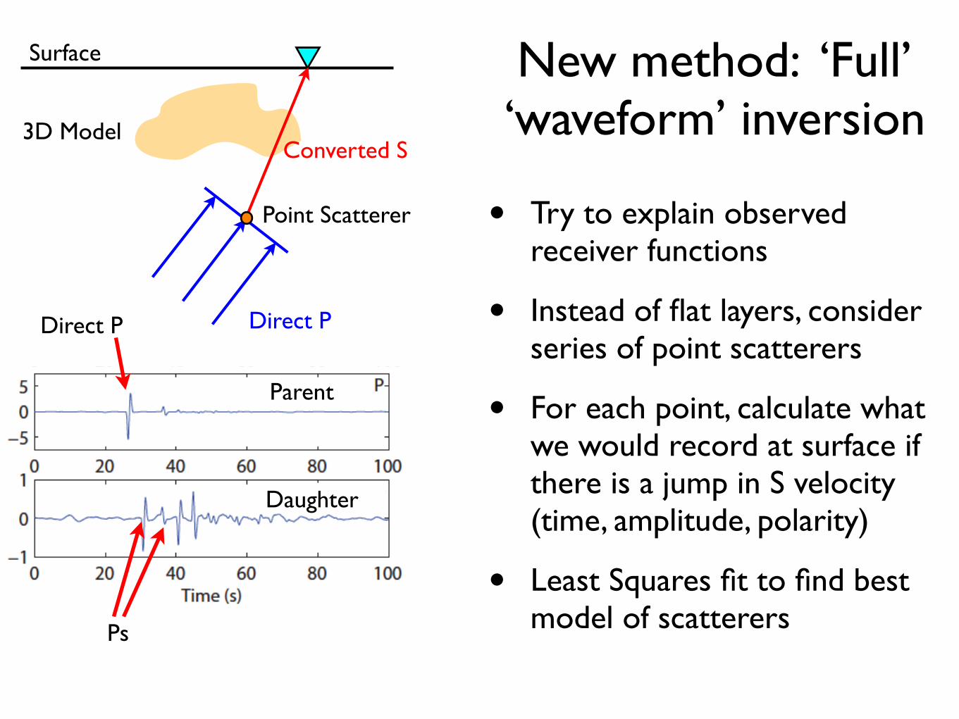
New method: ‘Full’ ‘waveform’ inversion

Direct P

Ps

Parent

Daughter

• Try to explain observed receiver functions

• Instead of flat layers, consider series of point scatterers

• For each point, calculate what we would record at surface if there is a jump in S velocity (time, amplitude, polarity)

• Least Squares fit to find best model of scatterers

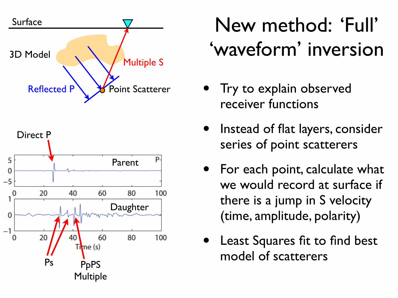
3D Model

3D Model

Direct P

Surface

Reflected P

Multiple S

Point Scatterer

New method: ‘Full’ ‘waveform’ inversion

Direct P

PpPSMultiple

Parent

Daughter

Ps

• Try to explain observed receiver functions

• Instead of flat layers, consider series of point scatterers

• For each point, calculate what we would record at surface if there is a jump in S velocity (time, amplitude, polarity)

• Least Squares fit to find best model of scatterers

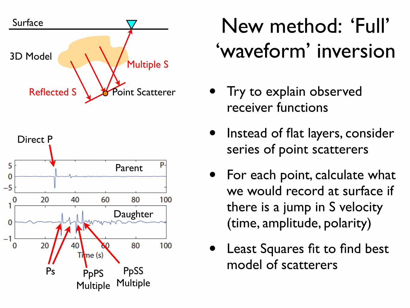
3D Model

Direct P

Surface

Reflected S

Multiple S

Point Scatterer

New method: ‘Full’ ‘waveform’ inversion

Direct P

PpSSMultiple

Parent

Daughter

Ps PpPSMultiple

• Try to explain observed receiver functions

• Instead of flat layers, consider series of point scatterers

• For each point, calculate what we would record at surface if there is a jump in S velocity (time, amplitude, polarity)

• Least Squares fit to find best model of scatterers

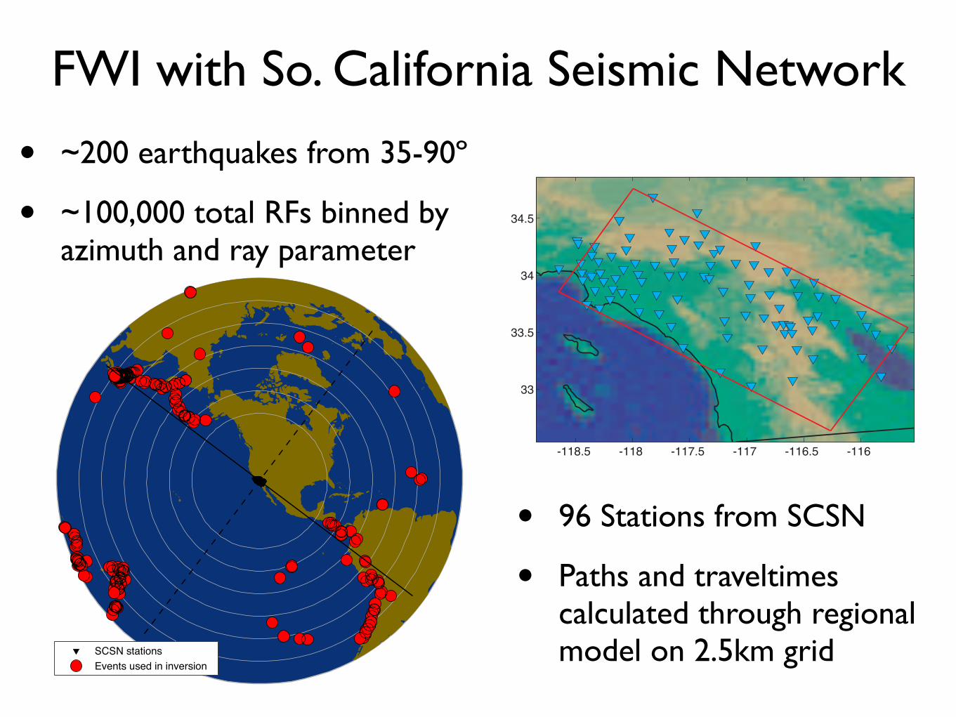
FWI with So. California Seismic Network

SCSN stationsEvents used in inversion

• ~200 earthquakes from 35-90º

• ~100,000 total RFs binned by azimuth and ray parameter

-118.5 -118 -117.5 -117 -116.5 -116

33

33.5

34

34.5

• 96 Stations from SCSN

• Paths and traveltimes calculated through regional model on 2.5km grid

NW−SE Offset (km)

Dept

h (k

m)

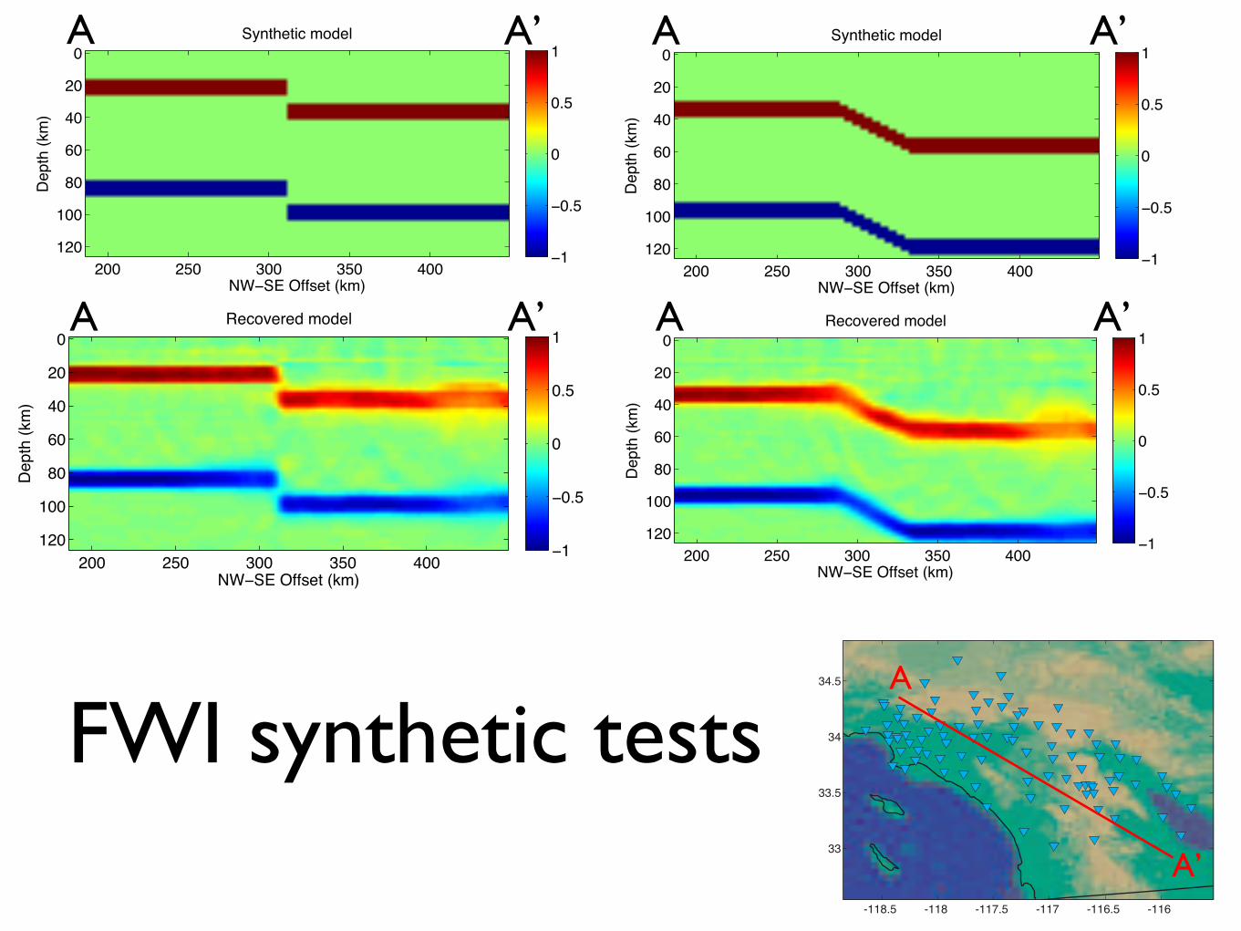
Synthetic model

200 250 300 350 400

0

20

40

60

80

100

120 −1

−0.5

0

0.5

1

NW−SE Offset (km)

Dept

h (k

m)

Recovered model

200 250 300 350 400

0

20

40

60

80

100

120 −1

−0.5

0

0.5

1

NW−SE Offset (km)

Dept

h (k

m)

Recovered model

200 250 300 350 400

0

20

40

60

80

100

120 −1

−0.5

0

0.5

1

NW−SE Offset (km)

Dept

h (k

m)

Synthetic model

200 250 300 350 400

0

20

40

60

80

100

120 −1

−0.5

0

0.5

1

FWI synthetic tests

-118.5 -118 -117.5 -117 -116.5 -116

33

33.5

34

34.5 A

A’

A A’

A A’

A A’

A A’

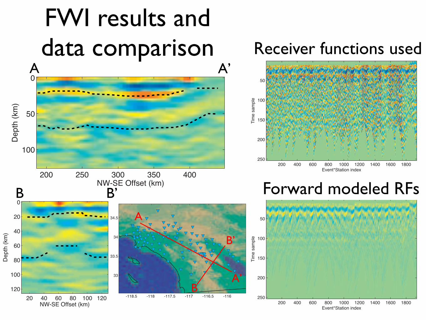
FWI results and data comparison Data used in inversion

Event*Station index

Tim

e sa

mpl

e

200 400 600 800 1000 1200 1400 1600 1800

50

100

150

200

250

Modeled data

Event*Station index

Tim

e sa

mpl

e

200 400 600 800 1000 1200 1400 1600 1800

50

100

150

200

250

Receiver functions used

Forward modeled RFs

-118.5 -118 -117.5 -117 -116.5 -116

33

33.5

34

34.5 A

A’

B’

B

A A’

B B’

-118.5 -118 -117.5 -117 -116.5 -116

33

33.5

34

34.5

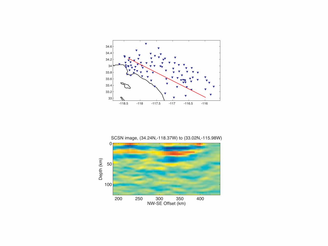
SCSN image, (34.24N,-118.37W) to (33.02N,-115.98W)

NW-SE Offset (km)

Dep

th (k

m)

200 250 300 350 400

0

50

100-118.5 -118 -117.5 -117 -116.5 -116

33

33.2

33.4

33.6

33.8

34

34.2

34.4

34.6

SCSN image, (32.88N,-116.72W) to (33.78N,-116.04W)

NW-SE Offset (km)

Dep

th (k

m)

20 40 60 80 100 120

0

20

40

60

80

100

120

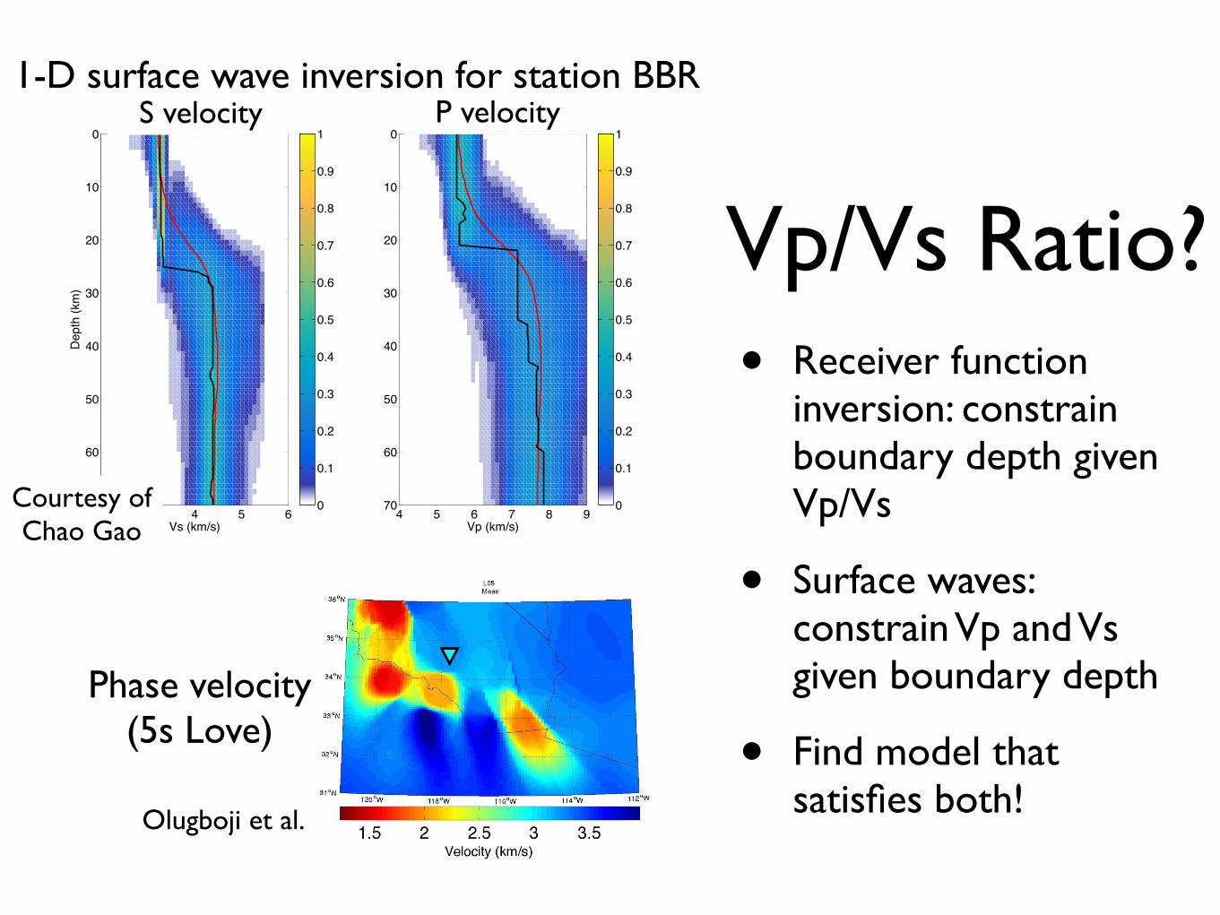
• Receiver function inversion: constrain boundary depth given Vp/Vs

• Surface waves: constrain Vp and Vs given boundary depth

• Find model that satisfies both!

Vp/Vs Ratio?

Phase velocity (5s Love)

2 3 4 5 6

0

10

20

30

40

50

60

70Vs (km/s)

Dep

th (k

m)

S−Velocities

0

0.1

0.2

0.3

0.4

0.5

0.6

0.7

0.8

0.9

1

4 5 6 7 8 9

0

10

20

30

40

50

60

70Vp (km/s)

P−Velocities

0

0.1

0.2

0.3

0.4

0.5

0.6

0.7

0.8

0.9

1 0

10

20

30

40

50

60

700 0.02 0.04 0.06 0.08 0.1

Discontinuity−BBR−CI

Transition Probability

S velocity P velocity1-D surface wave inversion for station BBR

Courtesy of Chao Gao

Olugboji et al.

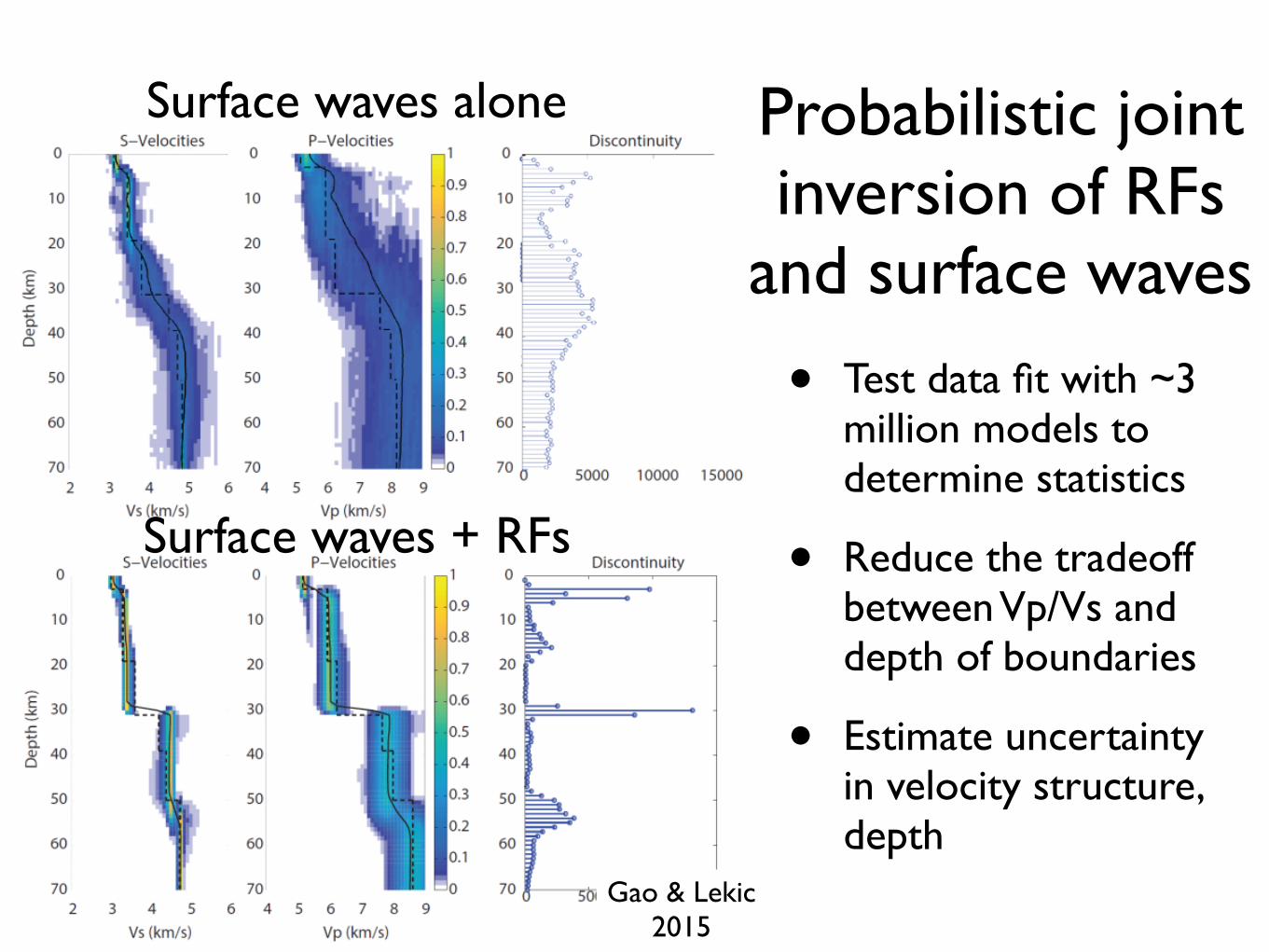
• Test data fit with ~3 million models to determine statistics

• Reduce the tradeoff between Vp/Vs and depth of boundaries

• Estimate uncertainty in velocity structure, depth

Gao & Lekic 2015

Probabilistic joint inversion of RFs

and surface waves

Surface waves alone

Surface waves + RFs

Conclusions• Desire for greater understanding of rifting processes

—dominant rheology, mode of deformation—drives advances in seismic methods

• Full Waveform Inversion of receiver functions accounts for 3D structure and can image steep dips

• Probabilistic inversion of surface waves and receiver functions reduces (and estimates!) uncertainty in boundaries and Vp/Vs

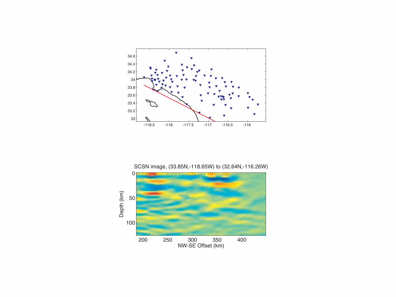
-118.5 -118 -117.5 -117 -116.5 -11633

33.2

33.4

33.6

33.8

34

34.2

34.4

34.6

SCSN image, (33.85N,-118.65W) to (32.64N,-116.26W)

NW-SE Offset (km)

Dep

th (k

m)

200 250 300 350 400

0

50

100

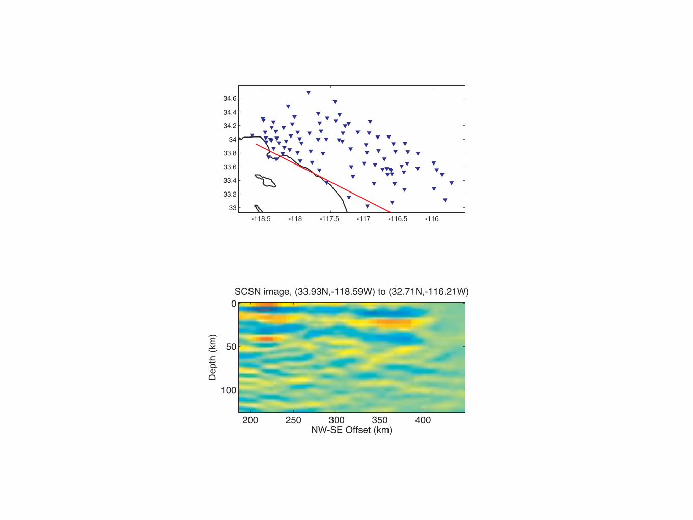
-118.5 -118 -117.5 -117 -116.5 -11633

33.2

33.4

33.6

33.8

34

34.2

34.4

34.6

SCSN image, (33.93N,-118.59W) to (32.71N,-116.21W)

NW-SE Offset (km)

Dep

th (k

m)

200 250 300 350 400

0

50

100

-118.5 -118 -117.5 -117 -116.5 -11633

33.2

33.4

33.6

33.8

34

34.2

34.4

34.6

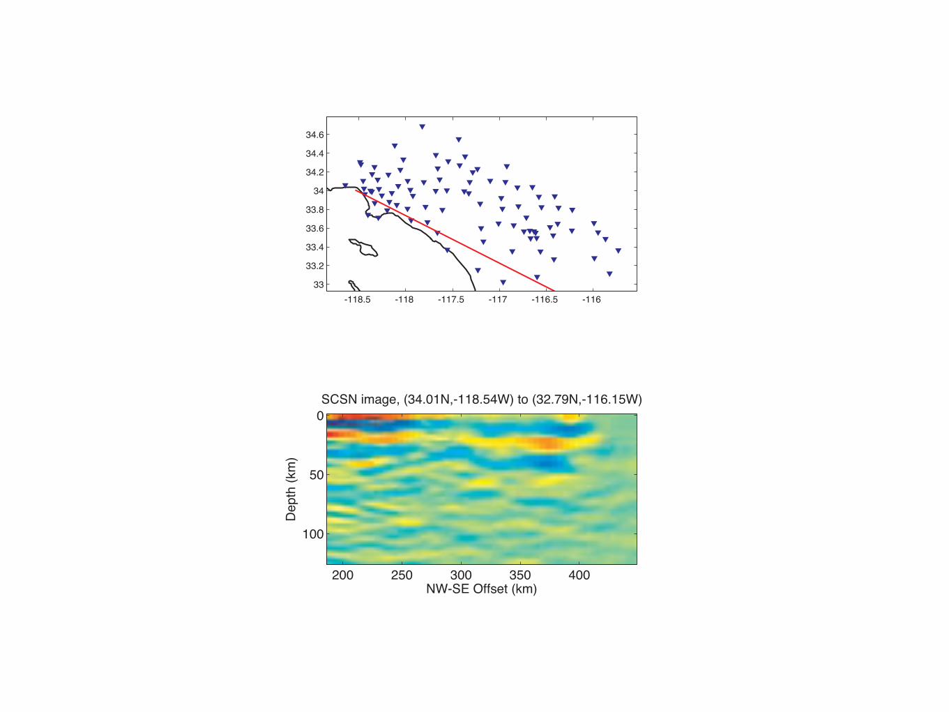
SCSN image, (34.01N,-118.54W) to (32.79N,-116.15W)

NW-SE Offset (km)

Dep

th (k

m)

200 250 300 350 400

0

50

100

-118.5 -118 -117.5 -117 -116.5 -11633

33.2

33.4

33.6

33.8

34

34.2

34.4

34.6

SCSN image, (34.09N,-118.48W) to (32.87N,-116.09W)

NW-SE Offset (km)

Dep

th (k

m)

200 250 300 350 400

0

50

100

-118.5 -118 -117.5 -117 -116.5 -11633

33.2

33.4

33.6

33.8

34

34.2

34.4

34.6

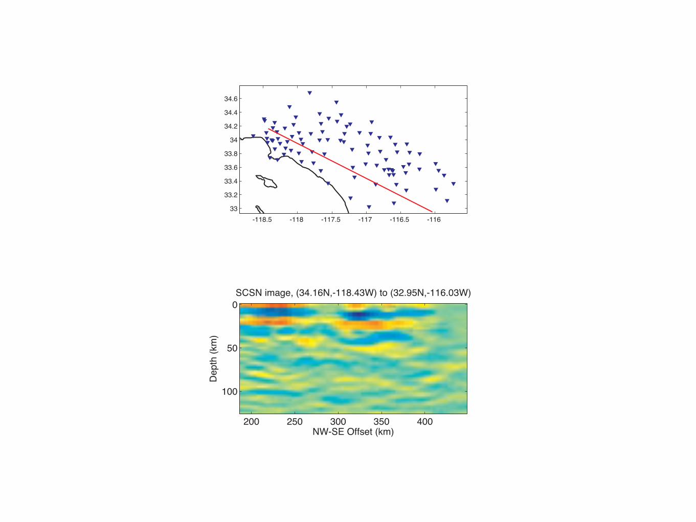
SCSN image, (34.16N,-118.43W) to (32.95N,-116.03W)

NW-SE Offset (km)

Dep

th (k

m)

200 250 300 350 400

0

50

100

-118.5 -118 -117.5 -117 -116.5 -11633

33.2

33.4

33.6

33.8

34

34.2

34.4

34.6

SCSN image, (34.24N,-118.37W) to (33.02N,-115.98W)

NW-SE Offset (km)

Dep

th (k

m)

200 250 300 350 400

0

50

100

-118.5 -118 -117.5 -117 -116.5 -11633

33.2

33.4

33.6

33.8

34

34.2

34.4

34.6

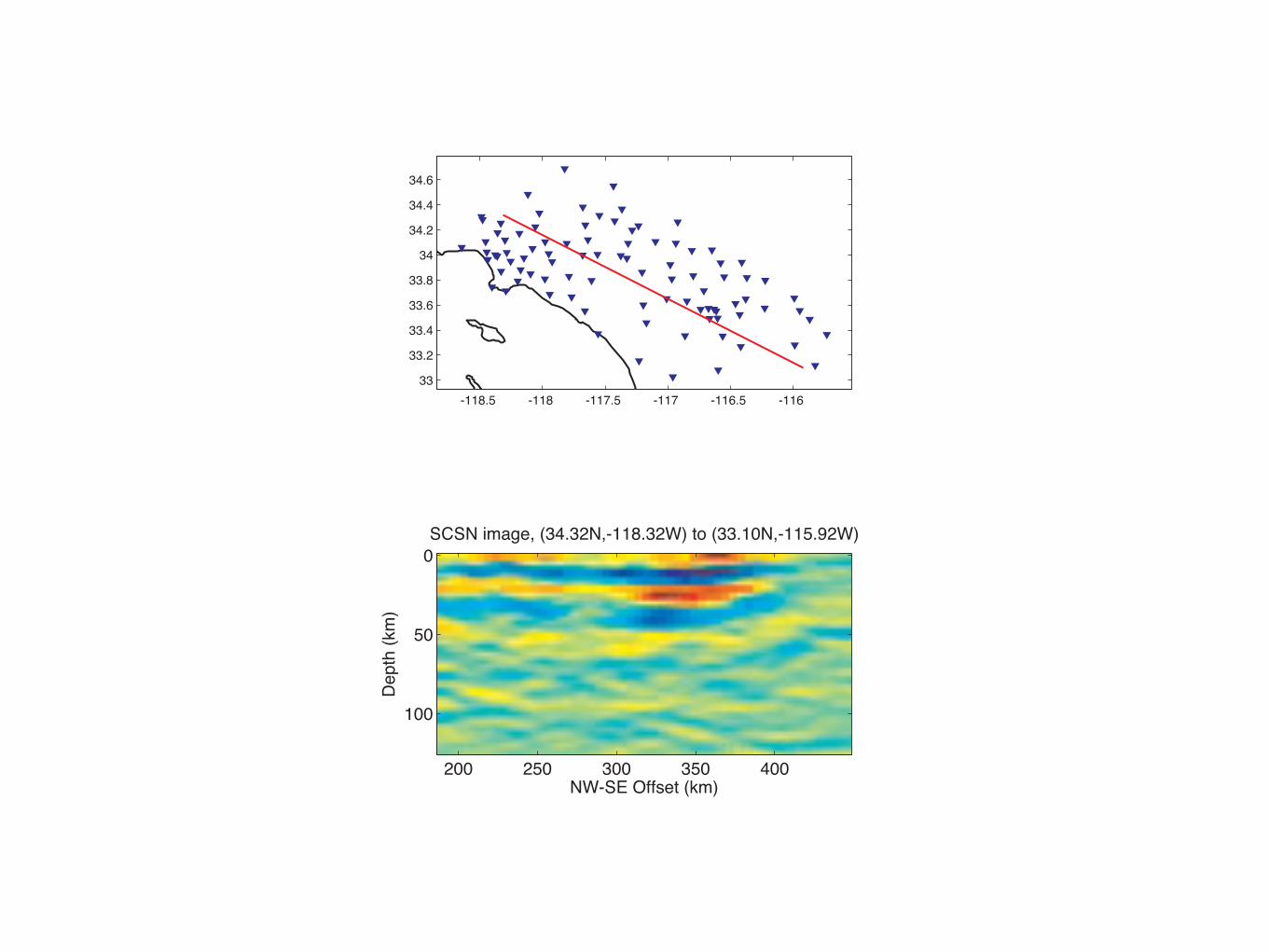
SCSN image, (34.32N,-118.32W) to (33.10N,-115.92W)

NW-SE Offset (km)

Dep

th (k

m)

200 250 300 350 400

0

50

100

-118.5 -118 -117.5 -117 -116.5 -11633

33.2

33.4

33.6

33.8

34

34.2

34.4

34.6

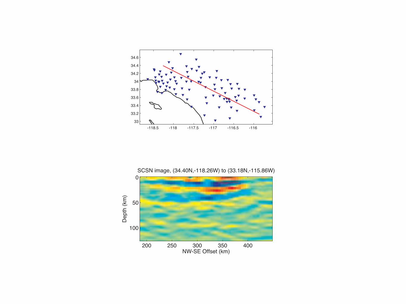
SCSN image, (34.40N,-118.26W) to (33.18N,-115.86W)

NW-SE Offset (km)

Dep

th (k

m)

200 250 300 350 400

0

50

100

-118.5 -118 -117.5 -117 -116.5 -11633

33.2

33.4

33.6

33.8

34

34.2

34.4

34.6

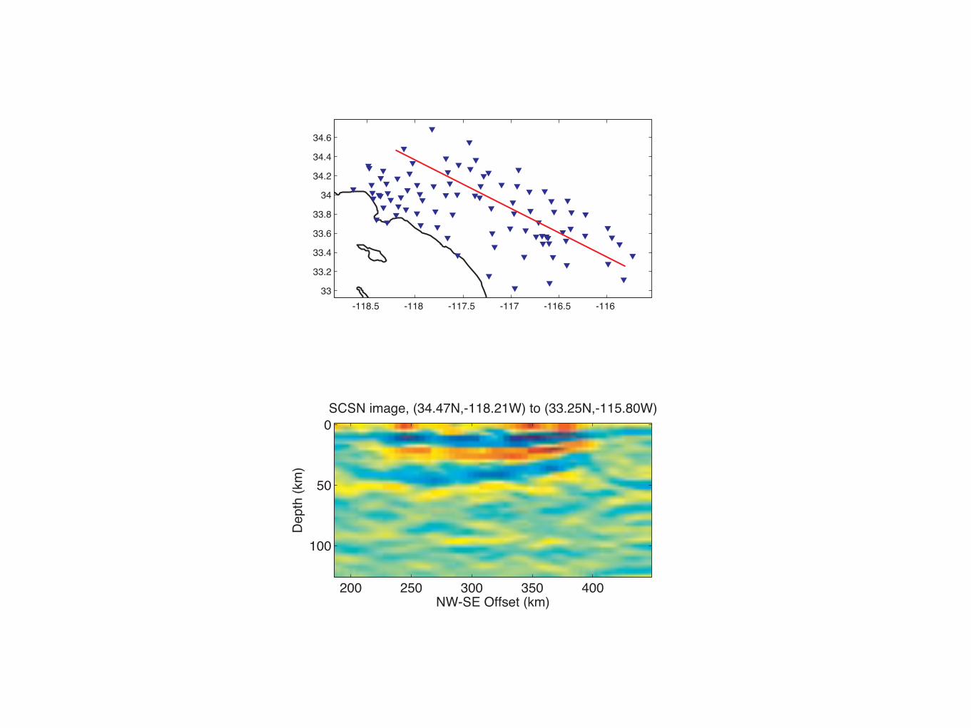
SCSN image, (34.47N,-118.21W) to (33.25N,-115.80W)

NW-SE Offset (km)

Dep

th (k

m)

200 250 300 350 400

0

50

100

-118.5 -118 -117.5 -117 -116.5 -11633

33.2

33.4

33.6

33.8

34

34.2

34.4

34.6

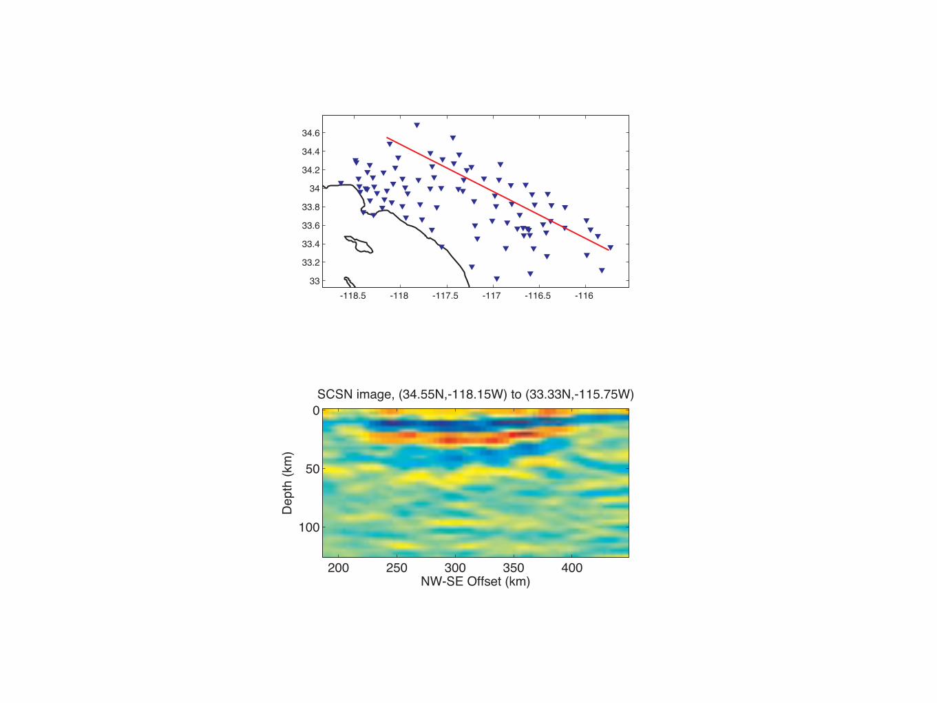
SCSN image, (34.55N,-118.15W) to (33.33N,-115.75W)

NW-SE Offset (km)

Dep

th (k

m)

200 250 300 350 400

0

50

100

-118.5 -118 -117.5 -117 -116.5 -11633

33.2

33.4

33.6

33.8

34

34.2

34.4

34.6

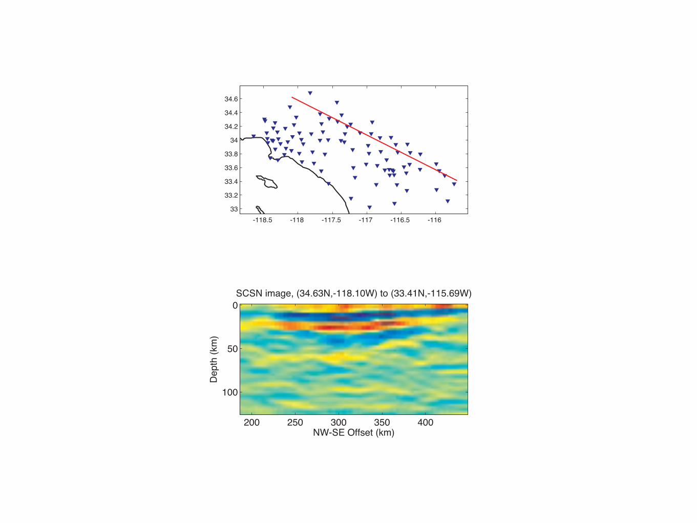
SCSN image, (34.63N,-118.10W) to (33.41N,-115.69W)

NW-SE Offset (km)

Dep

th (k

m)

200 250 300 350 400

0

50

100

-118.5 -118 -117.5 -117 -116.5 -11633

33.2

33.4

33.6

33.8

34

34.2

34.4

34.6

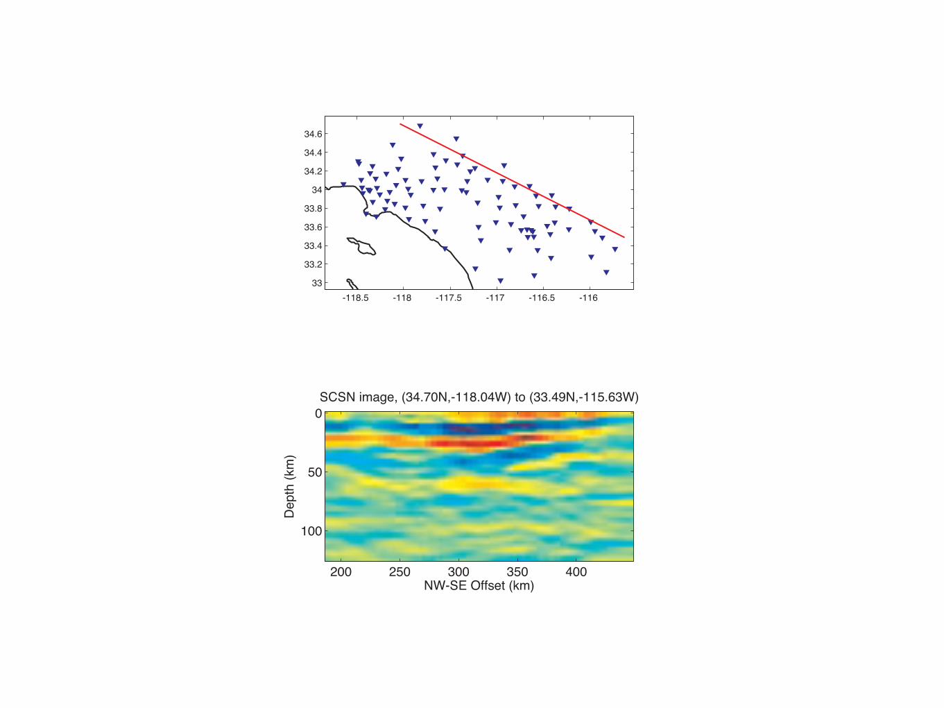
SCSN image, (34.70N,-118.04W) to (33.49N,-115.63W)

NW-SE Offset (km)

Dep

th (k

m)

200 250 300 350 400

0

50

100