Investigating the Feasibility of · EVs - Electric Vehicles ... Composition of organic waste disposed in Santa Barbara County from 2015 to 2040. 27 ... Air pollution emissions factors

Investigating the Feasibility of

Greenhouse Gas Mitigation in

Santa Barbara County A Group Project submitted in partial satisfaction of the requirements for the degree of Master

of Environmental Science and Management

Prepared By: Alex Brotman, Lily Brown, and Cassandra Squiers

Advisor: Sangwon Suh

April 2015

As authors of this Group Project report, we are proud to archive this report on the Bren School’s

website such that the results of our research are available for all to read. Our signatures on the

document signify our joint responsibility to fulfill the archiving standards set by the Bren School

of Environmental Science & Management.

_______________________________

Alex Brotman

_______________________________

Lily Brown

_______________________________

Cassandra Squiers

The mission of the Bren School of Environmental Science & Management is to produce

professionals with unrivaled training in environmental science and management who will devote

their unique skills to the diagnosis, assessment, mitigation, prevention, and remedy of the

environmental problems of today and the future. A guiding principal of the School is that the

analysis of environmental problems requires quantitative training in more than one discipline

and an awareness of the physical, biological, social, political, and economic consequences that

arise from scientific or technological decisions.

The Group Project is required of all students in the Master of Environmental Science and

Management (MESM) Program. The project is a three-quarter activity in which small groups of

students conduct focused, interdisciplinary research on the scientific, management, and policy

dimensions of a specific environmental issue. This Group Project Final Report is authored by

MESM students and has been reviewed and approved by:

_______________________________

Sangwon Suh

Acknowledgments

We would like to thank everyone who assisted and supported us during this project. We would

especially like to thank our faculty advisor, Sangwon Suh, our external advisors, Andrew

Plantinga and David Raney, and our client, the Santa Barbara County Air Pollution Control

District, specifically Molly Pearson, Brian Shafritz, and Carly Wilburton.

We would also like to the faculty and staff at the Bren School of Environmental Science &

Management at the University of California, Santa Barbara for all their insight and guidance.

Acronyms

AB 32 - Assembly Bill 32, the California Global Warming Solutions Act of 2006

ARB - California Air and Resources Board

CAPCOA - California Air Pollution Control Officers Association

CEC - California Energy Commission

CEQA - California Environmental Quality Act

CFCs - Chlorofluorocarbons

CH4 - Methane

CPUC - California Public Utilities Commission

CO - Carbon Monoxide

CO2 - Carbon Dioxide

CO2e - Carbon Dioxide Equivalent

DOE - United States Department of Energy

E3 - Energy and Environmental Economics, Inc.

EIA - Energy Information Administration

EMFAC - Emissions Factor Model

EPA - United States Environmental Protection Agency

EVs - Electric Vehicles

GHG - Greenhouse Gases

HFCs - Hydrofluorocarbons

HVAC - Heating, Ventilation, and Air Conditioning

kWh - Kilowatt Hours

NCTR - National Center for Transit Research

NOx - Nitrogen Oxides

N2O - Nitrous Oxide

NREL - National Renewable Energy Laboratory

O3 - Ozone

PFCs - Perfluorocarbons

PG&E - Pacific Gas & Electric

PV - Photovoltaic

RPS - Renewable Portfolio Standard

RTPA - Regional Transportation Planning Agency

SBCAG - Santa Barbara County Association of Governments

SCE - Southern California Edison

SF6 - Sulfur Hexafluoride

VMT - Vehicle Miles Traveled

VOCs - Volatile Organic Compounds

Table of Contents

1 Executive Summary ............................................................................................................... 1

2 Project Objectives .................................................................................................................. 3

3 Project Significance ............................................................................................................... 3

4 Background ............................................................................................................................ 3

4.1 Climate Change and GHG Emissions ..................................................................................................... 3

4.2 California’s GHG Policies ............................................................................................................................ 4

4.3 Mitigating GHG Emissions ......................................................................................................................... 6

4.4 GHG Abatement Cost Curves ................................................................................................................... 7

4.4.1 Existing GHG Abatement Cost Curves ......................................................................................... 9

4.4.2 Limitations of GHG Abatement Cost Curves .......................................................................... 10

4.5 GHG Mitigation Assessments ................................................................................................................ 11

4.6 GHG Emissions in Santa Barbara County .......................................................................................... 12

4.7 GHG Mitigation Strategies for Santa Barbara County ................................................................. 12

4.7.1 Energy Efficiency Retrofits ............................................................................................................. 13

4.7.2 Solar Power ......................................................................................................................................... 14

4.7.3 Electric Vehicles ................................................................................................................................. 16

4.7.4 Commuter Benefit Programs and Alternative Work Schedules ...................................... 16

4.7.5 Agricultural Engine Electrification .............................................................................................. 18

4.7.6 Flare Gas Recapture ......................................................................................................................... 18

4.7.7 Rangeland Composting.................................................................................................................. 19

5 Santa Barbara County GHG Emissions Forecast ................................................................ 20

5.1 Methods ........................................................................................................................................................ 20

5.1.1 Household and Employment Projections ................................................................................ 21

5.1.2 Utility Emissions Factors ................................................................................................................. 21

5.1.3 Residential Energy Use and Emissions ..................................................................................... 22

5.1.4 Commercial Energy Use and Emissions ................................................................................... 23

5.1.5 On-Road Transportation ................................................................................................................ 24

5.1.6 Oil and Gas Industry Flares ........................................................................................................... 25

5.1.7 Organic Waste ................................................................................................................................... 26

5.1.8 Agriculture Engines .......................................................................................................................... 27

5.2 Results ............................................................................................................................................................ 27

6 Santa Barbara County GHG Abatement Cost Curve ......................................................... 29

6.1 Methods ........................................................................................................................................................ 29

6.1.1 Selection of GHG Mitigation Strategies ................................................................................... 29

6.1.2 GHG Abatement Cost Curve ......................................................................................................... 30

6.1.3 Electricity Price Assumptions ........................................................................................................ 30

6.1.4 Gas Price Assumptions ................................................................................................................... 31


6.1.6 Residential and Commercial Solar PV ....................................................................................... 33


6.1.8 Commuter Benefits and Alternative Work Schedules ......................................................... 35

6.2 Results ............................................................................................................................................................ 39

6.2.1 Santa Barbara County GHG Abatement Cost Curve ............................................................ 39


6.2.3 Solar PV ................................................................................................................................................ 42



7 Opportunities and Barriers to Implementation ................................................................ 47

7.1 Energy Efficient Retrofits ......................................................................................................................... 47

7.1.1 Relevant Zoning Codes .................................................................................................................. 47

7.1.2 Available Incentives and Rebates ............................................................................................... 47

7.1.3 Relevant Programs and Legislation ........................................................................................... 48

7.2 Solar PV ......................................................................................................................................................... 50

7.2.1 Relevant Zoning Codes .................................................................................................................. 50


7.2.3 Relevant Programs ........................................................................................................................... 53

7.3 Electric Vehicles .......................................................................................................................................... 53


7.3.2 Relevant Programs and Legislation ........................................................................................... 55

7.4 Commuter Benefits and Alternative Work Schedules .................................................................. 57

7.4.1 Relevant United States Code ........................................................................................................ 57

7.4.2 Relevant Programs ........................................................................................................................... 57

7.5 Success Stories ............................................................................................................................................ 59

7.5.1 Solar Energy and Energy Efficiency ............................................................................................ 59



8 Recommendations ............................................................................................................... 64

8.1 Energy Efficiency Retrofits ...................................................................................................................... 64

8.2 Solar PV ......................................................................................................................................................... 65

8.3 Electric Vehicles .......................................................................................................................................... 65

8.4 Commuter Benefits ................................................................................................................................... 65

9 Conclusion ............................................................................................................................ 67

10 Works Cited .......................................................................................................................... 68

11 Appendix............................................................................................................................... 76

11.1 Appendix A. Residential and Commercial Energy Use Data ...................................................... 76

11.2 Appendix B. Energy Star Data ............................................................................................................... 77

11.3 Appendix C. Solar PV Prices from 2015-2040 ................................................................................. 78

11.4 Appendix D. EMFAC Data ....................................................................................................................... 79

11.5 Appendix E. Vehicle Purchase Cost ..................................................................................................... 80

11.6 Appendix F. Air Pollution Emissions Factors .................................................................................... 81

11.7 Appendix G. Flare Gas Emissions in Santa Barbara County ....................................................... 81

11.8 Appendix H. GHG Mitigation Strategies ........................................................................................... 82

List of Figures

Figure 1. Breakdown of 2012 GHG emissions in California by gas. ............................................................. 4

Figure 2. California’s GHG emissions by sector in 2012. .................................................................................. 5

Figure 3. How to read a GHG abatement cost curve. ........................................................................................ 8

Figure 4. McKinsey & Company’s GHG abatement cost curve for North America.

Source: McKinsey & Company (2007) ..................................................................................................................... 9

Figure 5. Household electricity consumption by end-use in California. ................................................. 14

Figure 6. Solar photovoltaics (PV) resource potential of the United States in kWh/m2/day. .......... 15

Figure 7. Outline of the method applied in EMFAC2011-SG to calculate emissions reductions due

to the Low Carbon Fuel Standard (LCFS) and the Pavley Bill. ..................................................................... 25

Figure 8. Composition of organic waste disposed in Santa Barbara County from 2015 to 2040. 27

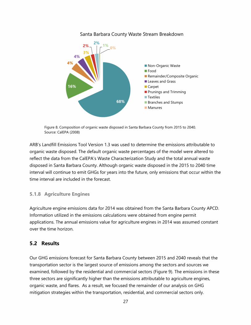
Figure 9. Santa Barbara County's GHG emissions inventory for select sectors for 2015 to 2040 in

kilotons CO2e. ................................................................................................................................................................ 28

Figure 10. GHG abatement cost curve for Santa Barbara County from 2015 to 2040. Abatement

costs are in real $2014 per ton of CO2e. Abatement potential per year is in kilotons of CO2e. ... 39

Figure 11. Sensitivity analyses of the lifetime cost per ton of GHG abated for refrigerator, HVAC,

and LEDs, for residential and commercial office buildings. Data labels indicate the range of the

input parameter. ........................................................................................................................................................... 41

Figure 12. Sensitivity analysis of the discount rate, annual growth in electricity prices, and the

availability of tax rebates for calculating the lifetime cost per ton of GHG abated for commercial

and residential solar PV. ............................................................................................................................................ 43

Figure 13. Sensitivity analyses for the GHG abatement cost of electric passenger cars, light duty

vehicles, and transit buses. ....................................................................................................................................... 45

List of Tables

Table 1. Monthly commuter benefits incentive caps for 2015. .................................................................. 17

Table 2. Electricity emissions factors for electricity for PG&E and SCE projected by E3 ................... 21

Table 3. Natural Gas Emissions Factor ................................................................................................................. 22

Table 4. Average Price of Electricity in Santa Barbara County. ................................................................... 31

Table 5. California retail price for diesel and gasoline fuel in March, 2015 ........................................... 31

Table 6. Fuel price projections for diesel and gasoline to 2040 ................................................................. 31

Table 7. Commuter benefit program tax savings............................................................................................. 38

Table 8. Abatement cost and GHG reduction potential of residential energy efficiency retrofits in

Santa Barbara County from 2015-2040. .............................................................................................................. 40

Table 9. Abatement cost and GHG reduction potential of commercial office building energy

efficiency retrofits in Santa Barbara County from 2015-2040. .................................................................... 40

Table 10. GHG abatement cost and potential for commercial and residential solar PV in Santa

Barbara County from 2015-2040. .......................................................................................................................... 42

Table 11. GHG abatement cost and potential for EVs in Santa Barbara County from 2015-2040. 43

Table 12. Air pollution reduction (tons) from 2015-2040 associated with converting new

passenger cars, light duty truck, and all transit buses in the county to EVs. ......................................... 45

Table 13. GHG abatement cost and potential for commuter benefits and alternative work

schedules in Santa Barbara County from 2015-2040. .................................................................................... 46

Table 14. Residential energy retrofit rebates offered by SCE and PG&E ................................................ 48

Table 15. Summary of available incentives for EVs. ........................................................................................ 55

Appendix

Appendix 13.1.1. Average annual residential energy use in Santa Barbara County (2015). ............ 76

Appendix 13.1.2. Santa Barbara County commercial building employee and energy use statistics

per square foot (2015)................................................................................................................................................ 76

Appendix 13.1.3. Total commercial natural gas and electricity use in Santa Barbara County by

building type (2015). ................................................................................................................................................... 76

Appendix 13.2.1. The mean, maximum, and minimum energy efficiency of Energy Star

geothermal heat pumps, air source heat pumps, and room air conditioning ...................................... 77

Appendix 13.2.2. The mean, maximum, and minimum energy efficiency of Energy Star certified

commercial HVAC units ............................................................................................................................................. 77

Appendix 13.2.3. The mean, maximum, and minimum Natural gas (therms/year) and electricity

use (kWh/yr) use of Energy Star certified water heaters by type............................................................... 77

Appendix 13.2.4. The mean, maximum, and minimum electricity use of Energy Star certified

refrigerators. ................................................................................................................................................................... 77

Appendix 13.2.5. The wattage and price of commercial and residential LED light bulbs from 2015

to 2040 ............................................................................................................................................................................. 78

Appendix 13.3.1. Cost per watt of Solar PV for 2015 – 2040 ....................................................................... 78

Appendix 13.4.1. Reduction factors applied in EMFAC2011-SG to emissions estimates to

generate carbon dioxide reductions expected from the Pavley Bill and the Low Carbon Fuel

Standard (EMFAC2011 technical documentation) ........................................................................................... 79

Appendix 13.4.2. EMFAC2011 output for Santa Barbara County (2011-2040). .................................... 80

Appendix 13.5.1. Purchase cost for passenger cars and light duty vehicles by fuel type for 2015-

2040 in real 2014 dollars. .......................................................................................................................................... 80

Appendix 13.6.1. Air pollution emissions factors (g/mile) for passenger cars, light duty trucks as

given by the GREET model for 2015 and 2020. ................................................................................................ 81

Appendix 13.7.1. Flare gas emission volumes and sources ......................................................................... 81

1

1 Executive Summary

In California, there are a number of policies in place that require governments, businesses, and

agencies to mitigate GHG emissions. Two of the state-level initiatives are the California Global

Warming Solutions Act of 2006 (AB 32) and the 2010 California Environmental Quality Act

(CEQA) Guideline Amendments. AB 32 requires California to reduce GHG emissions to 1990

levels by 2020, while CEQA directs state and local agencies to avoid or mitigate any significant

GHG emissions associated with public projects.

Over the next several years, Santa Barbara County’s annual GHG emissions are projected to

increase and, in order to comply with California’s regulations, these emissions must be mitigated

or offset. Although GHG mitigation targets can be met by purchasing carbon offset credits from

a national or international exchange, county residents and decision-makers alike would prefer to

reduce GHG emissions through local mitigation projects. Local GHG reduction projects are

preferred because they can generate co-benefits for the county, such as economic growth and

reduced air pollution.

The objective of this project was to determine which mitigation strategies would be the most

cost-effective and easily implemented in Santa Barbara County given the county’s unique

characteristics. The first step of the project was the construction a GHG emissions forecast. The

forecast revealed the relative contribution of different sectors to the county’s economy to GHG

output allowing us to prioritize analysis of mitigation options in the highest emitting, and

therefore highest reduction potential, sectors. In addition, the forecast served as a baseline from

which the impact of GHG mitigation efforts could be calculated. The GHG emissions forecast

included select sources from the transportation, residential, commercial, agricultural, oil and gas,

and waste sectors and revealed that the transportation, residential, and commercial sectors emit

significantly more GHGs than the other examined sectors. Consequently, the GHG mitigation

strategies that we chose to analyze were within these high emitting sectors.

The GHG mitigation strategies that we selected for analysis were energy efficiency retrofits, solar

photovoltaics, electric vehicles, commuter benefits programs, and alternative work schedules. In

order to determine the cost-effectiveness of these strategies, we calculated the net present

value of the cost and the total GHG reduction potential over our selected time horizon from

2015 to 2040. We then summarized the results in a GHG abatement cost curve, which is a visual

tool commonly used to display the cost-effectiveness of GHG mitigation strategies. Our results

indicate that Santa Barbara County can mitigate nearly 18,000 kilotons of GHGs over the next 25

years and nearly 10,000 kilotons of reduction can be achieved at a negative cost.

2

In addition to determining the cost-effectiveness of each mitigation option, it was necessary to

investigate the feasibility of implementing these GHG mitigation strategies in Santa Barbara

County. For each strategy, we explored current incentive programs and policies that could

facilitate or hinder GHG mitigation project implementation. We found that there are a number

of local, state, and federal programs in place that minimize barriers to strategy implementation.

Most of these programs offer financial incentives, educate the public, assist customers with

paperwork, connect customers with providers, or provide some combination of these services.

The results of our GHG abatement cost curve for the county, combined with our review of

existing opportunities and barriers to implementing the GHG mitigation strategies, indicate that

Santa Barbara County should prioritize lighting retrofits, heating, ventilation, and cooling (HVAC)

retrofits, solar photovoltaics (PV), electric vehicles (EVs), commuter benefits programs, and

alternative work schedules to mitigate GHGs locally.

3

2 Project Objectives

1. Create a GHG emissions forecast for select sources in sectors of interest in Santa Barbara

County.

2. Determine the cost-effectiveness of GHG mitigation strategies and visualize results in a

GHG abatement cost curve.

3. Analyze the opportunities and barriers to implementing GHG mitigation strategies

4. Provide recommendations to the county regarding which GHG mitigation strategies

should be pursued based on cost-effectiveness and ease of implementation.

3 Project Significance

While climate change is a global issue, many of the factors that influence GHG emissions, such

as transportation infrastructure, land use, and waste disposal, are controlled by local

governments. Consequently, local action to mitigate GHGs is critical to combating climate

change and will be essential to California’s success in meeting state-wide reduction targets. By

identifying the most cost-effective and easily implemented GHG mitigation strategies, this

project will help Santa Barbara County choose the best strategies to reduce GHG emissions and

meet state reduction goals.

4 Background

4.1 Climate Change and GHG Emissions

Climate change is caused by the amplification of the greenhouse effect, which describes how

greenhouse gases (GHGs) trap heat in Earth’s atmosphere by absorbing and emitting infrared

radiation. Since the industrial revolution, human activity, mainly the combustion of fossil fuels,

has significantly increased the concentration of GHGs in the atmosphere. As a result, global

mean temperatures have been rising over the past century with the ten warmest years on record

occurring within the past sixteen year (Kahn, 2015). The effects of a warming planet include sea

level rise, changes in precipitation, a decline in biodiversity, and an increase in extreme weather

events (IPCC, 2013).

4

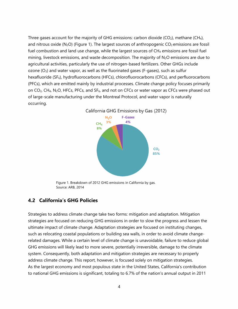
Three gases account for the majority of GHG emissions: carbon dioxide (CO2), methane (CH4),

and nitrous oxide (N2O) (Figure 1). The largest sources of anthropogenic CO2 emissions are fossil

fuel combustion and land use change, while the largest sources of CH4 emissions are fossil fuel

mining, livestock emissions, and waste decomposition. The majority of N2O emissions are due to

agricultural activities, particularly the use of nitrogen-based fertilizers. Other GHGs include

ozone (O3) and water vapor, as well as the fluorinated gases (F-gases), such as sulfur

hexafluoride (SF6), hydrofluorocarbons (HFCs), chlorofluorocarbons (CFCs), and perfluorocarbons

(PFCs), which are emitted mainly by industrial processes. Climate change policy focuses primarily

on CO2, CH4, N2O, HFCs, PFCs, and SF6, and not on CFCs or water vapor as CFCs were phased out

of large-scale manufacturing under the Montreal Protocol, and water vapor is naturally

occurring.

Figure 1. Breakdown of 2012 GHG emissions in California by gas.

Source: ARB, 2014

4.2 California’s GHG Policies

Strategies to address climate change take two forms: mitigation and adaptation. Mitigation

strategies are focused on reducing GHG emissions in order to slow the progress and lessen the

ultimate impact of climate change. Adaptation strategies are focused on instituting changes,

such as relocating coastal populations or building sea walls, in order to avoid climate change-

related damages. While a certain level of climate change is unavoidable, failure to reduce global

GHG emissions will likely lead to more severe, potentially irreversible, damage to the climate

system. Consequently, both adaptation and mitigation strategies are necessary to properly

address climate change. This report, however, is focused solely on mitigation strategies.

As the largest economy and most populous state in the United States, California's contribution

to national GHG emissions is significant, totaling to 6.7% of the nation’s annual output in 2011

5

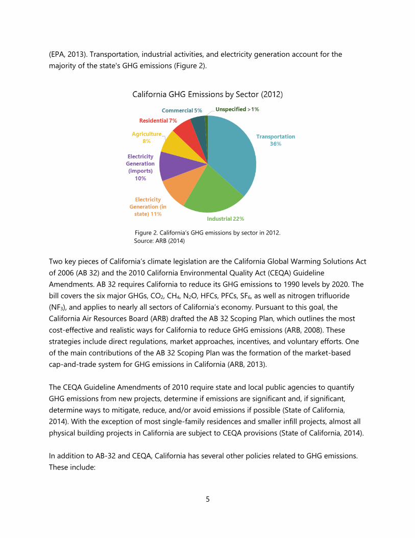
(EPA, 2013). Transportation, industrial activities, and electricity generation account for the

majority of the state's GHG emissions (Figure 2).

Figure 2. California’s GHG emissions by sector in 2012.

Source: ARB (2014)

Two key pieces of California’s climate legislation are the California Global Warming Solutions Act

of 2006 (AB 32) and the 2010 California Environmental Quality Act (CEQA) Guideline

Amendments. AB 32 requires California to reduce its GHG emissions to 1990 levels by 2020. The

bill covers the six major GHGs, CO2, CH4, N2O, HFCs, PFCs, SF6, as well as nitrogen trifluoride

(NF3), and applies to nearly all sectors of California’s economy. Pursuant to this goal, the

California Air Resources Board (ARB) drafted the AB 32 Scoping Plan, which outlines the most

cost-effective and realistic ways for California to reduce GHG emissions (ARB, 2008). These

strategies include direct regulations, market approaches, incentives, and voluntary efforts. One

of the main contributions of the AB 32 Scoping Plan was the formation of the market-based

cap-and-trade system for GHG emissions in California (ARB, 2013).

The CEQA Guideline Amendments of 2010 require state and local public agencies to quantify

GHG emissions from new projects, determine if emissions are significant and, if significant,

determine ways to mitigate, reduce, and/or avoid emissions if possible (State of California,

2014). With the exception of most single-family residences and smaller infill projects, almost all

physical building projects in California are subject to CEQA provisions (State of California, 2014).

In addition to AB-32 and CEQA, California has several other policies related to GHG emissions.

These include:

6

Assembly Bill 1493 (Pavley Bill) – Passed in 2009, the Pavley Bill requires California to develop

and adopt regulations that achieve the maximum feasible reduction of GHGs emitted by

passenger vehicles and light-duty trucks.

Sustainable Communities Sustainable Communities & Climate Protection Act (SB 375) – SB

372 requires ARB to develop regional GHG emission reduction targets for passenger vehicles for

2020 and 2035.

Renewables Portfolio Standard (Senate Bill X1-2) – The Renewable Portfolio Standard (RPS)

requires investor owned utilities, electric service providers, and community choice aggregators

to procure 33% of their electricity from renewable energy by 2020. The RPS is jointly

administered by the California Public Utilities Commission (CPUC) and the California Energy

Commission (CEC).

4.3 Mitigating GHG Emissions

As a result of AB 32, CEQA, and other existing policies, governments, businesses, and agencies

are often encouraged or required to mitigate their GHG emissions. The Intergovernmental Panel

on Climate Change defines a GHG mitigation option as "a technology, practice, or policy that

reduces or limits the emissions of GHGs or increases their sequestration" (Adler et al., 1995).

GHG mitigation can be achieved by:

Avoiding the operation or activity;

Changing the operation or activity;

Adding emissions control technologies; and

Sequestering emissions that have been released (CAPCOA, 2010).

Instead of mitigating, an entity that is required to reduce GHG emissions can purchase offsets

on an exchange from a party that generates GHG emission credits through voluntarily

mitigation. In order for voluntary mitigation offset credits to be accepted onto the exchange, the

mitigation project must be:

Additional - The reduction in GHG emissions must exceed, i.e. be in addition to, GHG

emission reductions or removals that would have otherwise occurred;

Real and Quantifiable - The reduction in GHG emissions must represent actual

emissions reductions. This requires the amount of GHG emissions reduced to be

accurately quantified;

7

Verifiable - The reduction in GHG emissions should be monitored and confirmed by an

independent third party; and

Permanent - The reduction in GHG emissions must endure for the foreseeable future,

e.g. at least 100 years (Offset Quality Initiative, 2008).

These requirements are in place to ensure that businesses, organization, and agencies do not

receive GHG mitigation credit for efforts they would have pursued under a business-as-usual

scenario or that do not truly reduce GHG emissions.

4.4 GHG Abatement Cost Curves

A GHG abatement cost curve is a commonly used economic tool that outlines the cost-

effectiveness of a selection of GHG mitigation measures over a specified time period. The

purpose of a GHG abatement cost curve is to provide policy-makers with the information

required to implement cost-effective GHG reduction measures. Since a number of states have

passed legislation setting emissions reduction targets, GHG abatement cost curves can also be

used to help policy-makers meet statewide emissions goals.

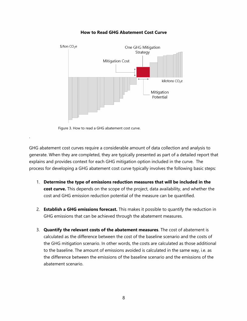
In a GHG abatement cost curve, mitigation measures are arranged along the horizontal axis

from left to right in order of increasing cost. Each measure is displayed as a bar, with the width

of the bar indicating the magnitude of GHG abatement achievable over the timeframe and the

height of the bar indicating the cost of abatement per ton of CO2 equivalence (CO2e). An

abatement option is displayed as having a negative cost when its long-term savings (due to

lower operating costs, lower energy use, etc.) outweigh its upfront costs (Figure 3).

8

How to Read GHG Abatement Cost Curve

Figure 3. How to read a GHG abatement cost curve.

.

GHG abatement cost curves require a considerable amount of data collection and analysis to

generate. When they are completed, they are typically presented as part of a detailed report that

explains and provides context for each GHG mitigation option included in the curve. The

process for developing a GHG abatement cost curve typically involves the following basic steps:

1. Determine the type of emissions reduction measures that will be included in the

cost curve. This depends on the scope of the project, data availability, and whether the

cost and GHG emission reduction potential of the measure can be quantified.

2. Establish a GHG emissions forecast. This makes it possible to quantify the reduction in

GHG emissions that can be achieved through the abatement measures.

3. Quantify the relevant costs of the abatement measures. The cost of abatement is

calculated as the difference between the cost of the baseline scenario and the costs of

the GHG mitigation scenario. In other words, the costs are calculated as those additional

to the baseline. The amount of emissions avoided is calculated in the same way, i.e. as

the difference between the emissions of the baseline scenario and the emissions of the

abatement scenario.

9

Beyond these key steps, the methodology for generating cost curves can vary considerably

depending on the application; cost curves can be developed for singular industries, like

agriculture, entire economies, or on state, national, and global geographic scales.

4.4.1 Existing GHG Abatement Cost Curves

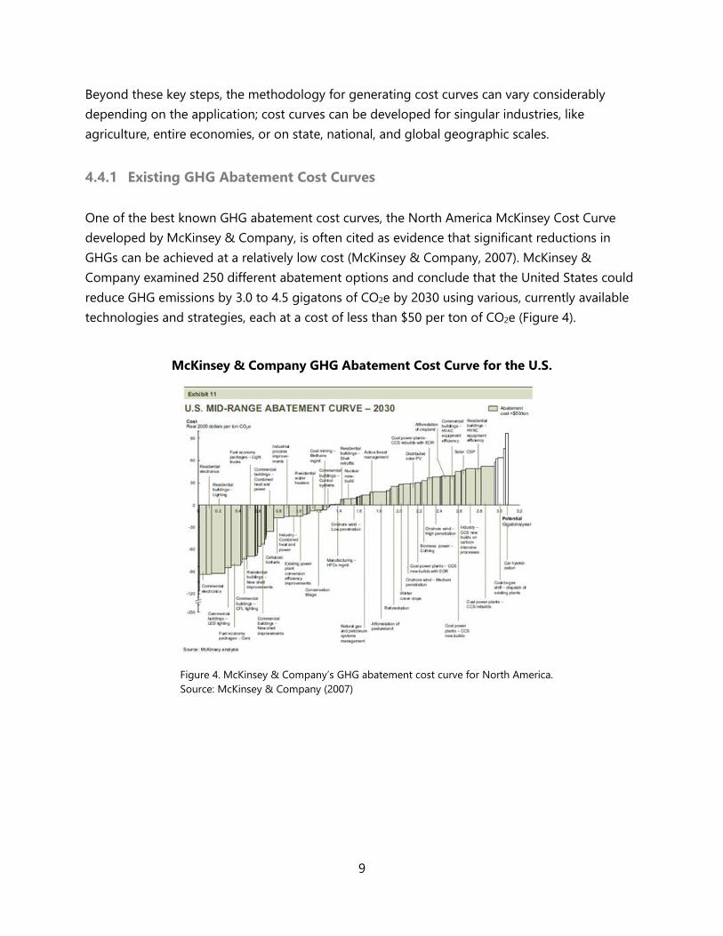
One of the best known GHG abatement cost curves, the North America McKinsey Cost Curve

developed by McKinsey & Company, is often cited as evidence that significant reductions in

GHGs can be achieved at a relatively low cost (McKinsey & Company, 2007). McKinsey &

Company examined 250 different abatement options and conclude that the United States could

reduce GHG emissions by 3.0 to 4.5 gigatons of CO2e by 2030 using various, currently available

technologies and strategies, each at a cost of less than $50 per ton of CO2e (Figure 4).

McKinsey & Company GHG Abatement Cost Curve for the U.S.

Figure 4. McKinsey & Company’s GHG abatement cost curve for North America.

Source: McKinsey & Company (2007)

10

Other GHG abatement cost curves relevant to the U.S. include those generated by Sweeney &

Weyant (2008) and Lutsey and Sperling (2009). Sweeney & Weyant (2008) examine over 40 GHG

abatement options for their California-specific GHG abatement cost curve, which they created as

a tool to guide policy makers implementing AB 32. Like, McKinsey & Company (2007), Sweeney

& Weyant (2008) analyze GHG mitigation options across several sectors, including commercial

and residential energy use, transportation, electricity generation, industrial processes, and land-

use. The GHG abatement cost curve created by Lutsey and Sperling (2009) focuses on the

transportation sector. Specifically, they examine mitigation strategies related to improving the

efficiency of light-duty vehicles and commercial trucks, increasing the use of hybrid gas-electric

vehicles, using alternative refrigerant for vehicle air conditioning, and replacing traditional fuels

with low carbon alternatives. Similarly to McKinsey & Company (2007), Sweeney & Weyant

(2008) and Lutsey and Sperling (2009) conclude that many abatement options will have a

negative cost. Sweeney & Weyant (2008), however, find many abatement measures with positive

costs that exceed $50 per ton of CO2e, concluding that the cost of implementing AB 32 may

exceed $100 per ton CO2e.

In constructing their GHG abatement cost curves, McKinsey & Company (2007), Sweeney &

Weyant (2008), and Lutsey and Sperling (2009) all use a bottom-up approach. They rely primarily

on government sources, such as the U.S. Environmental Protection Agency (EPA), the U.S. Energy

Information Association (EIA), and the U.S. Department of Energy (DOE) for national and state

data on GHG sources and sinks. Thus, they accept many of the assumptions made by these

sources, which they outline briefly in their reports. As is typically included in the quantification of

GHG emissions, both McKinsey & Company (2007) and Sweeney & Weyant (2008) included CO2,

CH4, N2O, SF6, HFCs, and PFCs in their analysis, and standardized all GHG sources and sinks by

converting them into units of CO2e.

4.4.2 Limitations of GHG Abatement Cost Curves

GHG abatement cost curves forecast into the future, which requires cost curve developers to

make a number of assumptions. As a result, GHG abatement cost curves are inherently

uncertain. In addition, GHG abatement cost curves are limited by the fact that there are many

factors that can affect the viability of a given GHG mitigation measure that cannot easily be

accounted for, such as equity implications and administrative efforts (Sweeney & Weyant, 2008).

GHG abatement cost curves are also often sensitive to baseline assumptions and therefore are

limited where these assumptions lack precision. Other shortcomings of GHG abatement cost

curves include their inability to account for:

11

Interactions between GHG abatement options;

Future development of new technologies and improvements to existing technologies;

Future regulations or policies that may influence some of the measures; and

Co-benefits of GHG mitigation, such as improved human health.

GHG abatement cost curves are also limited to GHG mitigation strategies with quantifiable costs

and impacts. This often results in a focus on technological strategies to reduce GHGs, such as

cleaner energy sources and increased energy efficiency, as behavioral interventions can be

difficult to quantify. For example, the abatement options covered by McKinsey & Company and

Sweeney & Weyant (2008) included:

Building and appliance energy efficiency;

Improvements in vehicle fuel economy;

Greater reliance on low-carbon fuels and renewable energy

Improvements in industrial processes; and

Land-use and forestry and expanding and enhancing carbon sinks.

4.5 GHG Mitigation Assessments

Quantifications of GHG mitigation cost and potential begin by establishing a GHG emissions

inventory. A GHG emissions inventory helps (1) identify the sectors and activities that emit

GHGs; (2) understand GHG emission trends; and (3) create goals and strategies for reducing

GHG emissions (EPA, 2014). For local and community GHG inventories, transportation and

energy use in the residential and commercial sectors are likely to be among the biggest

contributors to GHG emissions (EPA, 2014).

Once an inventory has been established, a GHG emissions baseline scenario is created so that

the impacts of GHG mitigation projects can be calculated. ARB defines a baseline as “the

scenario that reflects a conservative estimate of the business-as-usual performance or activities

for the relevant type of activity or practice” (ARB, 2009). Simply put, the baseline is meant to

capture the GHG emissions that would occur in the absence of the mitigation or offset project(s)

under consideration.

To enable the evaluation of specific mitigation projects, the baseline must include sufficient

detail about the relevant GHG emitting factors and activities, such as future energy use patterns,

fuel production systems, and technology choices (Lazarus et al., 1995). Selecting a base year and

time horizon are also crucial to establishing a baseline. Since the projection of economic

variables and the characterization of technologies can become quite uncertain when looking 50-

12

100 years into the future (Lazarus et al., 1995), the time horizon for mitigation assessments is

usually around 20-40 years (Adler et al., 1995). Because establishing a baseline is not an exact

science, a baseline should be conservatively defined (Goodward & Kelly, 2010).

To quantify GHG emissions, data on the GHG emissions of the activity in question are collected

and summarized. Then, individual GHGs are converted to CO2e by multiplying the emissions

values (generally expressed in terms of metric tons per year) by their global warming potential

(GWP). The general equation for emissions quantifications is:

GHG Emissions = [source metric] x [emissions factor] x [GWP]

The “source metric” is the quantity of the source of the GHG emissions (for example, gallons of

diesel fuel) and the “emissions factor” is the rate at which emissions are generated per unit of

source metric (for example, kilograms of CO2 per gallon of diesel fuel) (CAPCOA, 2010). The total

GHGs emitted from an individual source is the sum of emissions from each GHG.

4.6 GHG Emissions in Santa Barbara County

As part of the Energy and Climate Action Plan, the County of Santa Barbara completed a GHG

emissions inventory for unincorporated Santa Barbara County for 2007. The inventory does not

include incorporated cities, UC Santa Barbara, state and federal lands, or offshore oil and gas

facilities. This inventory found that transportation was the largest source of GHG emissions in

unincorporated Santa Barbara County, accounting for roughly 521,160 metric tons (MT) of CO2e.

Residential and commercial energy use were the second and third highest sources of GHG

emissions, accounting for 195,490 MT CO2e and 121,580 MT CO2e, respectively. Other sources of

GHG emissions include off-road equipment, solid waste disposal, agriculture, water and

wastewater, industrial energy, and aircraft operations. The county’s Energy and Climate Action

Plan excludes sources of emissions that could not be quantified as well as those over which the

county lacks jurisdictional control. In terms of forecasting GHG emissions, the county estimates

that, under a business-as-usual scenario, community-wide emissions will grow by approximately

14% by 2020 and by approximately 29% by 2035 (County of Santa Barbara, 2013).

4.7 GHG Mitigation Strategies for Santa Barbara County

While the GHG emissions inventory created for Santa Barbara County’s Energy and Climate

Action Plan is restricted to unincorporated Santa Barbara County, it, along with existing GHG

emissions inventories for California, suggests that transportation and energy use in the

commercial and residential sectors have significant potential for GHG reduction. In the following

13

section, we will review various strategies used to mitigate GHG emissions in these sectors, as

well as other strategies that are particularly relevant to Santa Barbara County.

4.7.1 Energy Efficiency Retrofits

Energy efficiency retrofits (also referred to as energy retrofits) describe a variety of strategies,

such as installing better insulating windows or replacing old light bulbs with more efficient ones,

that are aimed at decreasing the overall energy use of a building. Energy efficiency retrofits to

residential and commercial buildings have the potential to save a significant amount of energy,

usually at a negative cost as the initial investment in new appliances is paid off by utility bill

savings over the lifetime of the retrofit. For example, residential retrofits have been found to

reduce total household energy use anywhere from 10% to 33% (Brook et al. 2012; Jackson et al.,

2012; Cohen et al., 1991). Given that over 80% of the homes in Santa Barbara County were built

over 25 years ago, energy efficiency retrofits are likely an appropriate and effective method for

reducing energy use in the county (emPower Santa Barbara County, 2013).

Types of energy efficiency retrofits include:

Improving roof, ceiling, attic, secondary wall, and floor insulation;

Replacing inefficient appliances with new, efficient models;

Installing smart or programmable thermostats;

Installing better insulation windows; and

Switching to compact fluorescent or LED light bulbs.

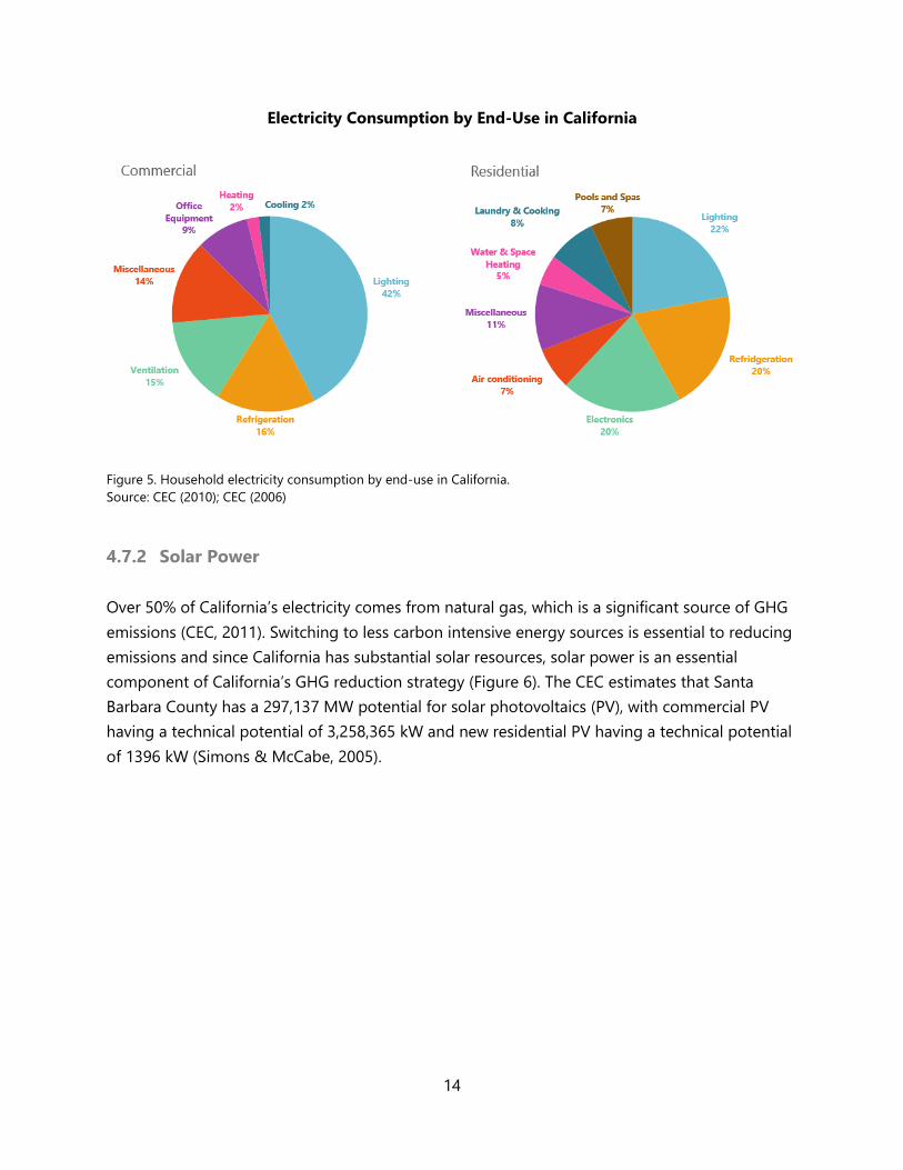
In California, lighting is the largest end-use of electricity in the commercial and residential

sectors, while other significant end-uses include refrigerators, heating and cooling, TVs, PCs, and

Office Equipment (Figure 5).

14

Electricity Consumption by End-Use in California

Figure 5. Household electricity consumption by end-use in California.

Source: CEC (2010); CEC (2006)

4.7.2 Solar Power

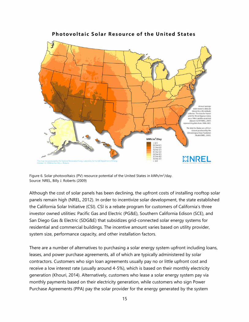
Over 50% of California’s electricity comes from natural gas, which is a significant source of GHG

emissions (CEC, 2011). Switching to less carbon intensive energy sources is essential to reducing

emissions and since California has substantial solar resources, solar power is an essential

component of California’s GHG reduction strategy (Figure 6). The CEC estimates that Santa

Barbara County has a 297,137 MW potential for solar photovoltaics (PV), with commercial PV

having a technical potential of 3,258,365 kW and new residential PV having a technical potential

of 1396 kW (Simons & McCabe, 2005).

15

Figure 6. Solar photovoltaics (PV) resource potential of the United States in kWh/m2/day.

Source: NREL, Billy J. Roberts (2009)

Although the cost of solar panels has been declining, the upfront costs of installing rooftop solar

panels remain high (NREL, 2012). In order to incentivize solar development, the state established

the California Solar Initiative (CSI). CSI is a rebate program for customers of California’s three

investor owned utilities: Pacific Gas and Electric (PG&E), Southern California Edison (SCE), and

San Diego Gas & Electric (SDG&E) that subsidizes grid-connected solar energy systems for

residential and commercial buildings. The incentive amount varies based on utility provider,

system size, performance capacity, and other installation factors.

There are a number of alternatives to purchasing a solar energy system upfront including loans,

leases, and power purchase agreements, all of which are typically administered by solar

contractors. Customers who sign loan agreements usually pay no or little upfront cost and

receive a low interest rate (usually around 4-5%), which is based on their monthly electricity

generation (Khouri, 2014). Alternatively, customers who lease a solar energy system pay via

monthly payments based on their electricity generation, while customers who sign Power

Purchase Agreements (PPA) pay the solar provider for the energy generated by the system

16

rather than paying for the system itself (Gordon, 2013). Homeowners interested in purchasing

rooftop solar can also take out a home equity loan. Home equity loans vary case by case, but

typically charge a low interest rate because they use the home as collateral.

4.7.3 Electric Vehicles

Electric vehicles have significant GHG reduction potential in California. All-electric vehicles (EVs),

are powered solely by an electric battery and thus have no tailpipe emissions. Any emissions

from EVs are indirect emissions due to electricity generation. Because they are more efficient at

converting energy, EVs also have a higher fuel economy than conventional fuel vehicles. Given

that roughly 37% of GHG emissions in California come from transportation, EVs are a significant

component of the state’s strategy to reduce GHG emissions. In 2012, California Governor

Edmund G. Brown Jr. issued an Executive Order calling for over 1.5 million EVs on California

roads by 2025 (Governor’s Interagency Working Group on Zero-emission Vehicles, 2013).

Pursuant to this goal, the California’s Zero-Emission Vehicle (ZEV) Action Plan identifies specific

strategies and actions that agencies can take to promote the adoption of EVs and plug-in hybrid

electric vehicles (PHEVs) in a variety of sectors. Strategies recommended by the plan include

continuing consumer rebates for the purchase or lease of ZEVs, development of interoperability

standards for electric vehicle charging stations, raising consumer awareness of ZEVs, and

expanding ZEVs within public and private bus fleets (Governor’s Interagency Working Group on

Zero-emission Vehicles, 2013).

Although they have higher upfront costs than conventional fuel vehicles, some studies suggest

that EVs may be cheaper over their lifetime due to lower maintenance and fuel costs (Atkins, et

al. 2013; Griffith, 1995). In their analysis of electrifying Florida’s transit buses, Atkins, et al. (2013)

find that the total lifetime cost for an electric bus is lower than that of a diesel bus. Aguirre et al.

(2012), however, find that the lifetime cost of an EV is slightly higher than that of a conventional

vehicle. In addition to reduced emissions, Atkins, et al. (2013) find that electrifying public transit

may result in co-benefits such as increased economic activity due to an increased demand for

electricity. Griffith (1995) likewise found that Santa Barbara’s Metropolitan Transit District’s

electric buses reduce aggregate emissions of nitrous oxides (NOx), particulate matter, and

carbon monoxide (CO) by roughly 95% in comparison to diesel buses.

4.7.4 Commuter Benefit Programs and Alternative Work Schedules

Commuter benefit programs are employer-administered tax-based incentive programs built into

the federal tax code (IRS code 132(f)). The code provides for a commuter benefit account that

17

employees can place earned wages into a commuter benefit account that can be used to pay for

alternative modes of transportation is not subject to payroll or income taxes.

There are two possible structures for a commuter benefits program:

1. An employee-paid, pre-tax benefit; or

2. An employer-paid subsidy program.

The pre-tax benefit program requires employees to divert money from their paycheck into in an

untaxed account that is then re-administered to employees in the form of travel vouchers or

transportation-limited debit cards (Commute Smart, 2014). For an employer-paid subsidy

program, the employer administers subsidies in the form of untaxed vouchers or transit debit

cards. Employers can administer their own commuter benefits program or hire a benefit vendor.

Benefit vendors usually charge approximately $3 to $5 per month per participant (Commute

Smart, 2014).

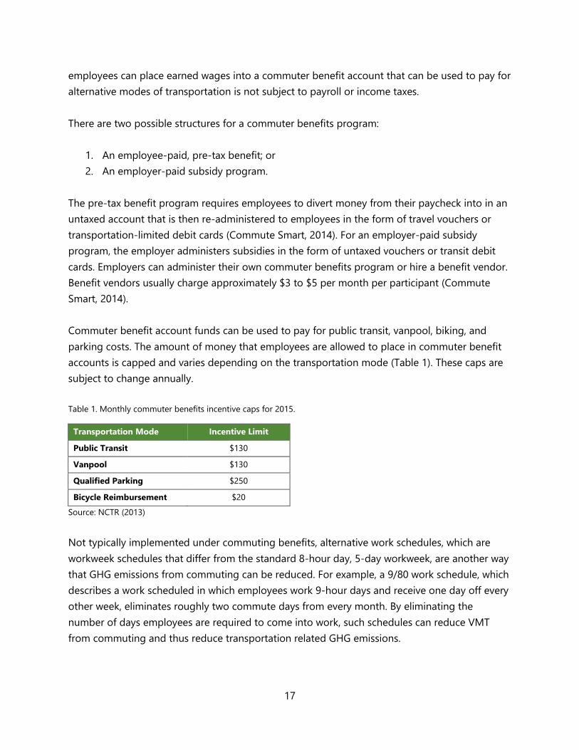
Commuter benefit account funds can be used to pay for public transit, vanpool, biking, and

parking costs. The amount of money that employees are allowed to place in commuter benefit

accounts is capped and varies depending on the transportation mode (Table 1). These caps are

subject to change annually.

Table 1. Monthly commuter benefits incentive caps for 2015.

Transportation Mode Incentive Limit

Public Transit $130

Vanpool $130

Qualified Parking $250

Bicycle Reimbursement $20

Source: NCTR (2013)

Not typically implemented under commuting benefits, alternative work schedules, which are

workweek schedules that differ from the standard 8-hour day, 5-day workweek, are another way

that GHG emissions from commuting can be reduced. For example, a 9/80 work schedule, which

describes a work scheduled in which employees work 9-hour days and receive one day off every

other week, eliminates roughly two commute days from every month. By eliminating the

number of days employees are required to come into work, such schedules can reduce VMT

from commuting and thus reduce transportation related GHG emissions.

18

4.7.5 Agricultural Engine Electrification

Agriculture engines, which are frequently diesel-powered, impact local air pollution and GHG

emissions. Currently, California regulations require agricultural diesel engines exceeding a rating

of 50 brake horsepower to be registered with the local Air Pollution Control District. Agriculture

engines are also regulated under ARB’s Airborne Toxic Control Measure for Stationary Diesel

Engines, which requires engines to meet certain emission standards. To incentivize the adoption

of low emissions agriculture engines, state and local programs provide funding for engine

electrification. The Santa Barbara County APCD, for example, offers funding of up to 80% of the

cost of the new equipment for cleaner off-road equipment, including large spark ignition

engines, agricultural tractors, and construction equipment (APCD, 2013).

4.7.6 Flare Gas Recapture

Flaring is the process by which untreated natural gas, primarily composed of CH4, is converted

into CO2 via open-air combustion and released into the atmosphere (Bott, 2007). Although

flaring is wasteful and contributes to GHG emissions, it is preferable to venting untreated natural

gas directly into the atmosphere since CH4 is a more potent GHG than CO2. According to a 2007

study conducted by the ARB, flares from California’s oil and gas industry emit approximately 260

kilotons of CO2 equivalent annually (Lee, 2011).

Gas flaring is standard in the oil and gas industry for safety, economic, and practical reasons.

Emergency flares are necessary to alleviate dangerous pressure build-ups that occur in wells

during the extraction process. Flares are also used to dispose of gas when the volume generated

is too small or the gas is too impure to make sale viable. (Bott, 2007).

Alternatives to flaring include selling the gas or using it to generate electricity on-site. Before

sale, natural gas must be processed in order to remove impurities and proper gas transportation

infrastructure must be in place. The cost, however, is often prohibitive and outweighs the

financial benefits of selling small volumes of gas at a low market price. The use of on-site

electricity generation technologies, such as microturbines, can be a more financially viable

option for waste gas. Microturbines typically are between 30kW to 250kW with a combined

capital and installation cost of approximately $2,500/kW, which is recuperated within a few years

through electricity bill savings (McAvoy, 2011; Energy and Environmental Analysis, 2008).

Although microturbines can operate on variety of fuel types, including unprocessed natural gas,

there is concern that impurities, like sulfur, which is typically present in high amounts in

untreated gas, have the potential to generate acidic byproducts that could corrode system

components (Energy and Environmental Analysis, 2008). Other potential problems with

19

microturbines include reduced efficiencies at low gas loads and suboptimal ambient

temperatures as well as part degradation (Energy and Environmental Analysis, 2008).

4.7.7 Rangeland Composting

Rangeland, which is defined here as “land on which plant cover is composed principally of

grasses, grass-like plants, forbs, or shrubs suitable for grazing,” stores approximately 20-30% of

the world’s soil organic carbon (SOC) (DeLonge, 2014; Haden et al., 2014). SOC storage in

rangelands occurs when plants assimilate atmospheric carbon or carbon from manure

deposition (DeLonge, 2014). The capacity of rangelands to serve as a carbon sink depends on

climatic variables, disturbance frequency, and management practices. Phenomena such as

drought, overgrazing, and soil degradation can lead to plant death and increases in microbial

decomposition which, depending on the magnitude, can turn a rangeland from a carbon sink

into a carbon source (DeLonge, 2014).

California, which is approximately 40-50% rangeland, could achieve significant GHG reduction

through rangeland management practices that maximize carbon sequestration. To this end,

scientists in the state have been researching a number of land management practices, including

rangeland composting. Rangeland composting directly increases SOC because the applied

organic matter integrates with the rangeland soil, is sequestered in plants, and enhances plant

growth by adding nutrients. Additionally, rangeland composting prevents CH4 emissions that

would have otherwise occurred had the compost decomposed in anaerobic conditions in a

landfill (Haden et al., 2014). In January of 2015, rangeland composting was accepted as GHG

offset method that can be used to generate credits for sale on voluntary carbon markets

(CAPCOA, 2015).

20

5 Santa Barbara County GHG Emissions Forecast

5.1 Methods

Developing a baseline GHG emissions forecast was the first phase of our project. The sectors

and sources of GHG emissions included in the forecast include:

Residential Energy Use;

Commercial Energy Use;

On-Road Transportation;

Oil & Gas Flares;

Organic Waste; and

Agriculture Engines.

These sectors were chosen either because they are known to be high emitting sectors or were of

interest to our client and team. The GHG emissions forecast we created for Santa Barbara

County projects GHG emissions from these sectors and sources from 2015 to 2040 given that:

Economic and demographic trends continue;

No new legislation is passed; and

No new projects are undertaken.

Our GHG emissions forecast accounts for relevant measures and projects that have been

approved, but not yet implemented or completed, including the RPS, the Pavley Bill, and the

Low Carbon Fuel Standard (LCFS). The GHG emissions forecast serves as an emissions baseline

scenario for Santa Barbara County, and any reduction in GHG emissions below this baseline is

considered GHG mitigation.

The first step required to generate our GHG emissions forecast was to determine the GHG

emissions of the selected sectors in 2015. This was accomplished by obtaining the most current

GHG emissions data available and adjusting the values to reflect the changes expected to occur

between the date the data were collected and 2015. Once the GHG emissions inventory for 2015

was completed, it was grown annually to 2040 according to assumptions about the annual

growth and development of each sector. The specific calculations and assumptions used to

create our GHG emissions forecast for Santa Barbara County are outlined in the following

sections.

21

5.1.1 Household and Employment Projections

The Santa Barbara County Association of Government’s (SBCAG) Regional Growth Forecast

provided household and sector-specific employment data that were used to calculate the GHG

emissions associated with residential and commercial energy use. In the SBCAG report, the

figures are projected from 2010 and estimated for 2020, 2035, and 2040 by region. To obtain

annual values, linear growth was assumed between the time points.

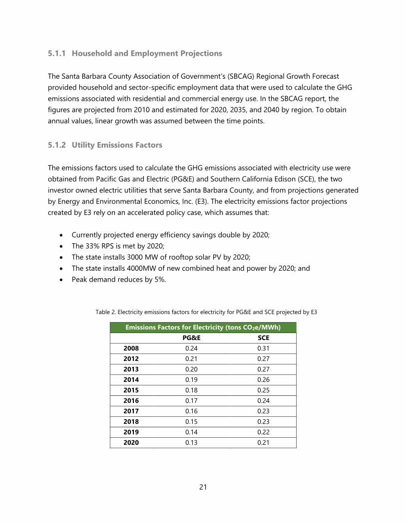
5.1.2 Utility Emissions Factors

The emissions factors used to calculate the GHG emissions associated with electricity use were

obtained from Pacific Gas and Electric (PG&E) and Southern California Edison (SCE), the two

investor owned electric utilities that serve Santa Barbara County, and from projections generated

by Energy and Environmental Economics, Inc. (E3). The electricity emissions factor projections

created by E3 rely on an accelerated policy case, which assumes that:

Currently projected energy efficiency savings double by 2020;

The 33% RPS is met by 2020;

The state installs 3000 MW of rooftop solar PV by 2020;

The state installs 4000MW of new combined heat and power by 2020; and

Peak demand reduces by 5%.

Table 2. Electricity emissions factors for electricity for PG&E and SCE projected by E3

Emissions Factors for Electricity (tons CO2e/MWh)

PG&E SCE

2008 0.24 0.31

2012 0.21 0.27

2013 0.20 0.27

2014 0.19 0.26

2015 0.18 0.25

2016 0.17 0.24

2017 0.16 0.23

2018 0.15 0.23

2019 0.14 0.22

2020 0.13 0.21

22

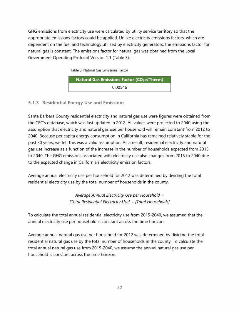
GHG emissions from electricity use were calculated by utility service territory so that the

appropriate emissions factors could be applied. Unlike electricity emissions factors, which are

dependent on the fuel and technology utilized by electricity generators, the emissions factor for

natural gas is constant. The emissions factor for natural gas was obtained from the Local

Government Operating Protocol Version 1.1 (Table 3).

Table 3. Natural Gas Emissions Factor

Natural Gas Emissions Factor (CO2e/Therm)

0.00546

5.1.3 Residential Energy Use and Emissions

Santa Barbara County residential electricity and natural gas use were figures were obtained from

the CEC’s database, which was last updated in 2012. All values were projected to 2040 using the

assumption that electricity and natural gas use per household will remain constant from 2012 to

2040. Because per capita energy consumption in California has remained relatively stable for the

past 30 years, we felt this was a valid assumption. As a result, residential electricity and natural

gas use increase as a function of the increase in the number of households expected from 2015

to 2040. The GHG emissions associated with electricity use also changes from 2015 to 2040 due

to the expected change in California’s electricity emission factors.

Average annual electricity use per household for 2012 was determined by dividing the total

residential electricity use by the total number of households in the county.

Average Annual Electricity Use per Household =

[Total Residential Electricity Use] ÷ [Total Households]

To calculate the total annual residential electricity use from 2015-2040, we assumed that the

annual electricity use per household is constant across the time horizon.

Average annual natural gas use per household for 2012 was determined by dividing the total

residential natural gas use by the total number of households in the county. To calculate the

total annual natural gas use from 2015-2040, we assume the annual natural gas use per

household is constant across the time horizon.

23

5.1.4 Commercial Energy Use and Emissions

Commercial electricity and natural gas data were also obtained from the CEC’s database, which

was last updated in 2012. Our commercial GHG emissions forecast included office buildings,

government buildings, and hotels and motels. Other commercial building types were omitted

because recommendations for energy use reductions for specialized buildings, like industrial

plants and hospitals, are complicated and site-specific. Unlike residential energy use, we could

not assume that all commercial buildings have the same basic energy use profile and thus could

not calculate average energy use by dividing total commercial energy use by the number of

commercial buildings. Additionally, there is no data available on the total number of commercial

buildings in Santa Barbara County. Instead, a bottom-up approach was utilized to estimate the

energy use emissions from the commercial sector.

Employment and employee density data were used to estimate the square footage of each type

of commercial building which was then used to determine the total energy use by employment

sector. The general methodology utilized was as follows:

Total Energy Use by Building Type/Employment Sector =

[Number of Employees in Sector] x [SQF per Employee] x [Annual Energy Use per SQF]

The SBCAG Regional Growth Forecast provided employment by sector data. Estimates for the

number of square feet per employee typical for office buildings, government buildings, and

hotels and motels were obtained from a Southern California Association of Governments (SCAG)

employee density study. Finally, Energy IQ, an interactive database that utilizes data from the

California Commercial End-Use Survey, was used to estimate the average annual energy use per

square foot of each building type.

Commercial sector GHG emissions for 2015 were calculated by applying the appropriate

emissions factors to the total commercial energy use. To accomplish this, we assumed that the

commercial sector is homogenous throughout the county.

The total GHG emissions by building type were grown annually holding the employee density

and energy use values constant across the time horizon. Therefore, changes in annual GHG

emissions are a function of the expected change in the number of employees per industry

between 2015 and 2040.

24

5.1.5 On-Road Transportation

On-road vehicle population, vehicle miles traveled (VMT), and emissions data for Santa Barbara

County were obtained from SBCAG. SBCAG utilized ARB’s Emissions Factor (EMFAC) emissions

estimator model to generate the data. EMFAC2011, the latest in a series of EMFAC models, is

utilized by SBCAG, and other Regional Transportation Planning Agencies (RTPAs) in California, to

generate the transportation forecasts required for government-mandated planning reports.

EMFAC2011

EMFAC2011 is composed of two different modules, EMFAC2011-LDV and EMFAC2011-HD,

which address different vehicle types and rely on two different methods. EMFAC2011-LDV

addresses light duty (less than 14,000 pounds gross vehicle weight rating) gasoline and diesel

passenger vehicles and urban transit buses. In this module, vehicle population data is estimated

using a combination of 2009 vehicle registration data from the Department of Motor Vehicles,

Smog Check data, and Vehicle Identification Number (VIN) decoders. VMT estimates come from

RTPA estimates, when supplied, or are based on default speed distributions and mileage accrual

rates. SBCAG did not supply VMT data for the EMFAC2011-LDV model. The methodology for the

emissions calculations can be found in the EMFAC2011 technical documentation and other

supporting documents.

EMFAC2011-HD addresses commercial heavy-duty (exceeding 14,000 pounds gross vehicle

weight rating) gasoline and diesel trucks and buses. The vehicle population, VMT estimates, and

emissions factors utilized are from the 2010 Statewide Truck and Bus Rule amendments (EMFAC

Technical Documentation).

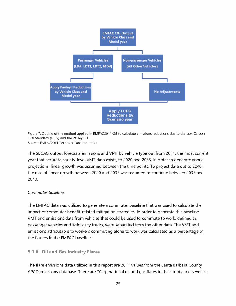
The EMFAC output utilized in this report is from EMFAC2011-SG, which is a synthesis of the

EMFAC2011-LDV and EMFAC2011-HD modules. The GHG emissions estimates from this model

incorporate the emissions reductions expected from the Low Carbon Fuel Standard (LCFS) and

Pavley Bill (Figure 7). The effects of the LCSF and Pavley Bill are applied to the emissions

predictions in the form of “correction factors” that reduce the carbon dioxide emissions from the

baseline expectations (Appendix D). Assumptions about the penetration of zero-emissions

vehicles are also integrated into EMFAC2011.

25

Figure 7. Outline of the method applied in EMFAC2011-SG to calculate emissions reductions due to the Low Carbon

Fuel Standard (LCFS) and the Pavley Bill.

Source: EMFAC2011 Technical Documentation.

The SBCAG output forecasts emissions and VMT by vehicle type out from 2011, the most current

year that accurate county-level VMT data exists, to 2020 and 2035. In order to generate annual

projections, linear growth was assumed between the time points. To project data out to 2040,

the rate of linear growth between 2020 and 2035 was assumed to continue between 2035 and

2040.

Commuter Baseline

The EMFAC data was utilized to generate a commuter baseline that was used to calculate the

impact of commuter benefit-related mitigation strategies. In order to generate this baseline,

VMT and emissions data from vehicles that could be used to commute to work, defined as

passenger vehicles and light-duty trucks, were separated from the other data. The VMT and

emissions attributable to workers commuting alone to work was calculated as a percentage of

the figures in the EMFAC baseline.

5.1.6 Oil and Gas Industry Flares

The flare emissions data utilized in this report are 2011 values from the Santa Barbara County

APCD emissions database. There are 70 operational oil and gas flares in the county and seven of

26

these flares were included in the forecast. The flares included operate continuously and emit at

least 500 metric tons of CO2e annually. These characteristics indicate that there could be a

sufficient volume and flow rate of gas for distributed generation technology to be viable

(Appendix G).

The GHG emissions from existing flares were held constant across the time horizon. It was

assumed that no new flares would come online and no existing flares would be decommissioned

over the time horizon.

5.1.7 Organic Waste

The annual GHG emissions attributable to organic waste disposed in Santa Barbara County was

estimated through the use of the California Department of Resources Recycling and Recovery’s

(CalRecycle) waste disposal data and the California ARB’s emissions calculator model. CalRecycle

maintains a database that contains annual waste disposal data from 1990 to 2013 for all active

landfills in Santa Barbara County. These data show that waste disposal trends are not dependent

on fluctuations in household or population numbers, but rather are more strongly correlated to

other economic trends.

Since prediction of economic trends is out of the scope of this project, and because the annual

fluctuations in the amount of waste disposed from year to year are small, the average amount of

waste disposed from 1990 to 2013 was assumed constant over the time horizon.

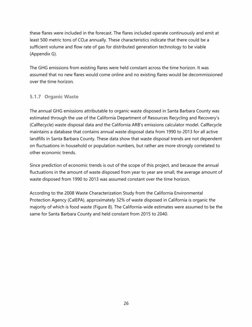
According to the 2008 Waste Characterization Study from the California Environmental

Protection Agency (CalEPA), approximately 32% of waste disposed in California is organic the

majority of which is food waste (Figure 8). The California-wide estimates were assumed to be the

same for Santa Barbara County and held constant from 2015 to 2040.

27

Figure 8. Composition of organic waste disposed in Santa Barbara County from 2015 to 2040.

Source: CalEPA (2008)

ARB’s Landfill Emissions Tool Version 1.3 was used to determine the emissions attributable to

organic waste disposed. The default organic waste percentages of the model were altered to

reflect the data from the CalEPA’s Waste Characterization Study and the total annual waste

disposed in Santa Barbara County. Although organic waste disposed in the 2015 to 2040 time

interval will continue to emit GHGs for years into the future, only emissions that occur within the

time interval are included in the forecast.

5.1.8 Agriculture Engines

Agriculture engine emissions data for 2014 was obtained from the Santa Barbara County APCD.

Information utilized in the emissions calculations were obtained from engine permit

applications. The annual emissions value for agriculture engines in 2014 was assumed constant

over the time horizon.

5.2 Results

Our GHG emissions forecast for Santa Barbara County between 2015 and 2040 reveals that the

transportation sector is the largest source of emissions among the sectors and sources we

examined, followed by the residential and commercial sectors (Figure 9). The emissions in these

three sectors are significantly higher than the emissions attributable to agriculture engines,

organic waste, and flares. As a result, we focused the remainder of our analysis on GHG

mitigation strategies within the transportation, residential, and commercial sectors only.

68%

16%

4%

4%3%

2%2%

1%0%

Santa Barbara County Waste Stream Breakdown

Non-Organic Waste

Food

Remainder/Composite Organic

Leaves and Grass

Carpet

Prunings and Trimming

Textiles

Branches and Stumps

Manures

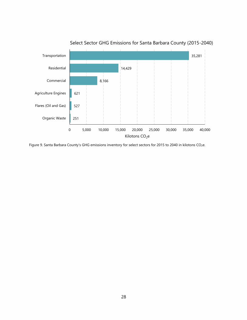
28

Figure 9. Santa Barbara County's GHG emissions inventory for select sectors for 2015 to 2040 in kilotons CO2e.

251

527

621

8,166

14,429

35,281

0 5,000 10,000 15,000 20,000 25,000 30,000 35,000 40,000

Organic Waste

Flares (Oil and Gas)

Agriculture Engines

Commercial

Residential

Transportation

Kilotons CO2e

Select Sector GHG Emissions for Santa Barbara County (2015-2040)

29

6 Santa Barbara County GHG Abatement Cost Curve

6.1 Methods

6.1.1 Selection of GHG Mitigation Strategies

We focused on mitigation strategies within the transportation, residential, and commercial

sectors because they are the highest emitting sectors in our forecast. In order to get select the

best strategies in these sectors, we conducted an extensive literature review and generated a list

of potential GHG mitigation strategies (Appendix H). We excluded strategies that:

1. Were infeasible given the characteristics of Santa Barbara County;

2. Lacked sufficient data to credibly establish a baseline, cost, and/or effectiveness; or

3. Were already in place at the state or county level.

From this list, we chose strategies that had high GHG reduction potential, were of interest to our

client and team, and were feasible to investigate given the timeframe and scope of this project.

The strategies included in this analysis are:

Energy Efficiency Retrofits

o Upgrades to lighting, heating, ventilation, and air conditioning (HVAC), water

heating, and refrigerating

Solar PV

o Installation of solar PV systems to residential buildings

o Installation of solar PV systems to commercial buildings

Electric Vehicles

o Electric Passenger Cars

o Electric Light Duty Trucks

o Electric Transit Buses

Commuter Benefits Programs and Alternative Work Schedules

o Vanpooling

o 9/80 Work Schedules

In the following section, we will review the methodology used to calculate the cost and GHG

reduction potential of each of these strategies over the 2015-2040 time period.

30

6.1.2 GHG Abatement Cost Curve

McKinsey & Company and Lutsey and Sperling (2009) use a discount rate of 7% in their GHG

mitigation supply curve for the U.S., which is consistent with federal policy making guidelines.

Sweeney & Weyant (2008), however, use a 5% discount rate for their California-specific GHG

abatement cost curve. Lower discount rates of 3-5% are typical for government or low risk

projects (Libecap, 2014). Therefore, we use a 5% discount rate to calculate the net present value

(NPV) of all costs associated with each GHG reduction strategy.

The GHG mitigation potential of each mitigation strategy was calculated as if all mitigation

strategies were implemented simultaneously. Therefore, the final GHG abatement cost curve

represents the collective GHG mitigation potential of all strategies together, rather than if only

one measure was implemented at a time.

For each GHG mitigation option, annual total costs were discounted and then summed over the

time horizon to get the NPV of the total cost. NPV was calculated as follows:

Where:

Ct = Net cash inflow during the time period

Co= initial investment

r = discount rate

t = number of time periods

All cost data were converted into 2014 real dollars using the U.S. Bureau of Labor Statistics’

Consumer Price Index inflation calculator.

Total GHG emissions mitigated were also calculated annually and summed over the time horizon

to get the total GHG mitigation potential of each strategy. Annual values for GHG mitigation

potential, however, were not discounted.

6.1.3 Electricity Price Assumptions

All cost calculations that depend on the price of electricity use the average price of electricity

paid by residential and commercial customers (Table 3). These averages were calculated using

data from Electricity Local, which provides the average electricity price paid by residential and

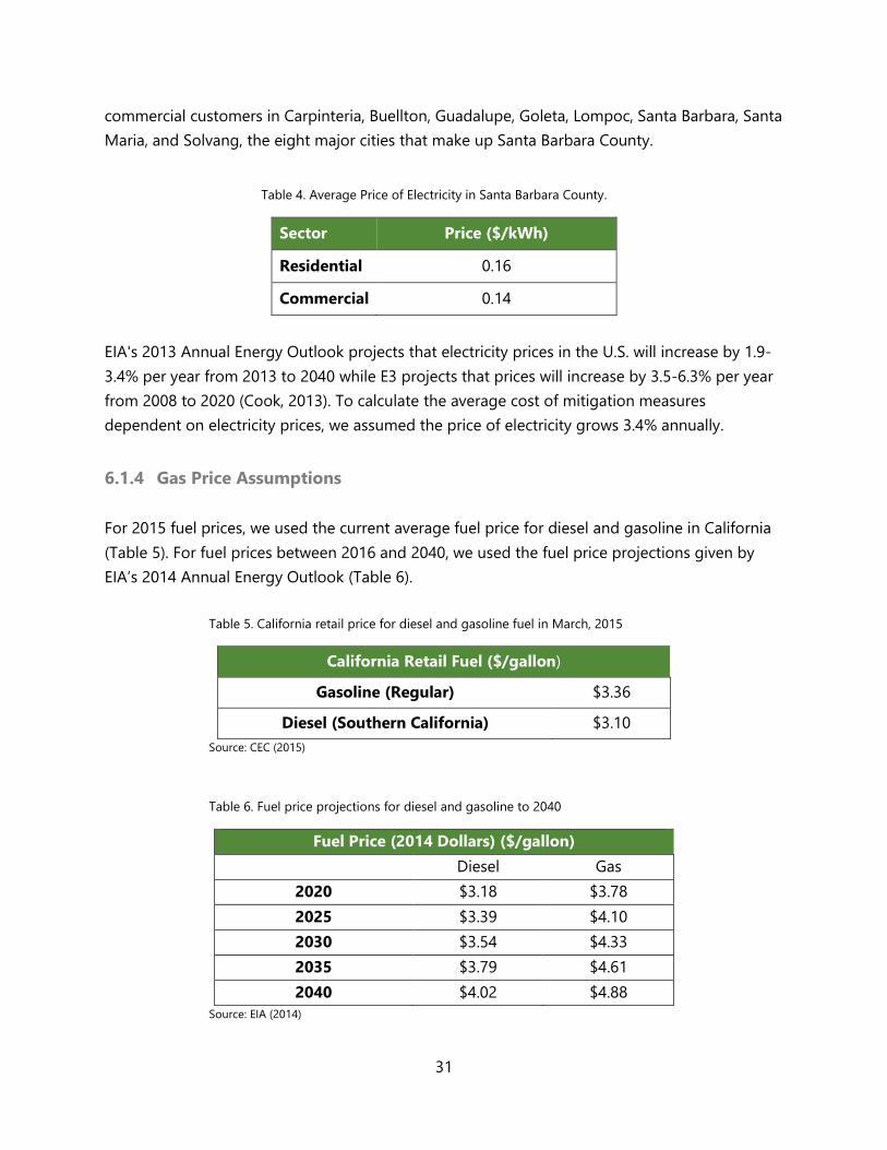
31

commercial customers in Carpinteria, Buellton, Guadalupe, Goleta, Lompoc, Santa Barbara, Santa

Maria, and Solvang, the eight major cities that make up Santa Barbara County.

Table 4. Average Price of Electricity in Santa Barbara County.

Sector Price ($/kWh)

Residential 0.16

Commercial 0.14

EIA's 2013 Annual Energy Outlook projects that electricity prices in the U.S. will increase by 1.9-

3.4% per year from 2013 to 2040 while E3 projects that prices will increase by 3.5-6.3% per year

from 2008 to 2020 (Cook, 2013). To calculate the average cost of mitigation measures

dependent on electricity prices, we assumed the price of electricity grows 3.4% annually.

6.1.4 Gas Price Assumptions

For 2015 fuel prices, we used the current average fuel price for diesel and gasoline in California

(Table 5). For fuel prices between 2016 and 2040, we used the fuel price projections given by

EIA’s 2014 Annual Energy Outlook (Table 6).

Table 5. California retail price for diesel and gasoline fuel in March, 2015

California Retail Fuel ($/gallon)

Gasoline (Regular) $3.36

Diesel (Southern California) $3.10

Source: CEC (2015)

Table 6. Fuel price projections for diesel and gasoline to 2040

Fuel Price (2014 Dollars) ($/gallon)

Diesel Gas

2020 $3.18 $3.78

2025 $3.39 $4.10

2030 $3.54 $4.33

2035 $3.79 $4.61

2040 $4.02 $4.88

Source: EIA (2014)

32


For the residential and commercial energy efficiency retrofits calculations, we assumed that all

households and all government and office buildings in the county in 2015 are retrofitted and

that all households and all government and office buildings added to the county in subsequent

years are outfitted with the same retrofits immediately. Data on the average cost and average

energy savings associated with each type of retrofit were taken from the National Renewable

Energy Laboratory (NREL), Energy Star, and the Santa Barbara County Better Buildings Program.

Data on the lifetime of each retrofit and the number of each retrofit needed per household

came from the Santa Barbara County Better Buildings Program. Data for the number of

households and the expected growth in households in the county came from SBCAG. We used

E3’s emissions factor projections for electricity in California to calculate GHG emissions avoided

per kWh of electricity saved.

In the residential sector, we calculated the cost and GHG mitigation potential of replacing all

light bulbs in all homes in the county with LED light bulbs, and of installing more efficient HVAC

units, water heaters, and refrigerators. For the commercial sector, we examined the same

retrofits, with the exception of water heaters. Our baseline scenario for measuring GHG

mitigation potential of LEDs assumes that all households and all office buildings currently use

incandescent light bulbs, but that once the price of LED light bulbs becomes competitive with

incandescent light bulbs, households switch over to LEDs. For upgrading HVAC units, water

heaters, and refrigerators, which range in cost and energy use based on type and model, we

calculated the average cost and average energy use for each type of retrofit based on Energy

Star data and used those averages to calculate the cost and mitigation potential of each.

Annual cost for each type of retrofit was calculated as follows:

Annual Cost =

[Purchase Cost x Units per Home - Energy Bill Savings per Home] x [Retrofitted Homes]

Our calculation of annual cost took into account replacement cost based on the lifetime of each

retrofit. We also assumed that incentives and rebates that are currently available for lighting,

HVAC, water heater, and refrigerator upgrades are utilized.

Annual GHG emission reductions were calculated using the average annual electricity savings

per household for the given retrofit along with the emissions factor for electricity generated in

California as follows.

33

Annual GHG Reductions =

[Emissions Factor] x [Average Annual Energy Savings] x [Retrofitted Homes]

6.1.6 Residential and Commercial Solar PV

For the residential and commercial solar PV calculations, we assume that all households and

government, office, and hotel and motel buildings in the county install solar PV systems. It is

also assumed that all additional households and included commercial buildings constructed in

subsequent years install solar PV systems immediately. To account for the baseline growth in

solar PV installations amongst commercial and residential buildings, we assumed that solar

installations grew by 7.5% per year, as this is the baseline growth in solar PV predicted by EIA

(U.S. Energy Information Administration, 2014).

Solar costs were calculated using cost per watt. Annual data on the cost per watt for solar PV

was obtained from NREL (Appendix C). Data on the average number of sun-hours in a day and

the average number of sun-days in a year were obtained from the National Climatic Data

Center. We used the average sun-days per year (286) and average sun-hours per day (5.94) for

Santa Maria as the county averages.

We calculated average system size by dividing the average annual electricity use per building by

the number of sun-hours in a year as follows:

Average System Size = [kWh per Year] ÷ [Sun-hours per Day x Sun-days per Year]

To get the average purchase price of the system, average system size was then converted to

watts and then multiplied by the cost per watt:

Purchase Price = [System Size] x [Cost per Watt]

To calculate the amount of electricity offset by the solar energy system, we subtracted efficiency

losses from the system size then multiplied by the number of sun-hours in a year as follows:

kWh Delivered by System Annually =

[System Size - Efficiency Losses] x [Sun-hours per Day] x [Sun-days per Year]

Annual costs were calculated as the sum of purchase cost, annual maintenance cost, and

electricity bill savings:

34

Annual Cost = [Capital Cost per Home - Energy Bill Savings per Home] x [Number of Homes]

Annual GHG emissions were calculated using the average annual electricity use per household in

Santa Barbara County along with the emissions factors for electricity generated in California as

supplied by E3:

Annual GHG Savings = [Emissions Factor] x [Average Annual Energy Use] x [Number of Buildings]


The calculations pertaining to electrifying the county’s transit bus fleet and electrifying all new

passenger cars and light duty trucks in the county used the emissions outputs, number of

vehicles, and VMT per year as given by the EMFAC model. EMFAC divides light duty trucks into

two categories: light duty trucks with a gross vehicle weight rating (GVWR) of less than 3750 lbs.

(LDT-1), and light duty trucks with a GVWR of 3751 to 5750 pounds (LDT-2). All vehicle

categories included in the EMFAC model output are divided into diesel-fueled and gas-fueled

vehicle sub categories. To account for differences in purchase cost, vehicle population, GHG

emissions, VMT, etc., separate calculations were completed for each vehicle category and each

vehicle type.

Our estimate of the cost of electrifying the county’s transit bus fleet assumes that all buses have

a lifespan of 12 years, as this assumption is common in the literature (Clark et al., 2007; Griffith

1995; Lajunen 2014). We assume that electric transit buses have an average fuel economy of

1.92 kWh/mile, as stated by electric bus manufacturers, and that this fuel economy improves by

0.5% per year, as estimated by Li et al. (2013).

We assume passenger cars and light duty trucks have a lifespan of 11 years as this is the average

lifespan of modern vehicles (Seng, 2013). We also assume that electric light duty vehicles have

an average fuel economy of 0.33 kWh/mile in 2015. This average was calculated using data from

fueleconomy.gov on the fuel economy of all commercially available EVs in the U.S. We assumed

that the fuel economy for light duty EVs also improves by 0.5% annually.

Annual costs for the baseline scenario and for the electric bus scenario were calculated using the

following equation:

Total Annual Cost = [Annual Fuel Costs] + [Annual Purchase Cost] + [Annual Maintenance Costs]

35

Annual fuel costs were calculated using the following equation:

Annual Fuel Cost = [Fuel Economy] x [Annual VMT] x [Price of Fuel]

The fuel economy for the baseline scenario was derived from EMFAC emissions and VMT data

using the relevant emissions factor for fuel as follows:

Miles per gallon = [Tons CO2e] ÷ [Tons CO2e/gallon Fuel] x [VMT]

Annual purchase cost data for 2015 to 2040 for light duty vehicles was taken from national

averages as given by EIA.

Annual GHG emissions for the electric bus scenario and electric light duty vehicles scenarios

were calculated using the following equation:

Annual GHG Emissions = [Fuel Economy] x [Annual VMT] x [Electricity Emissions Factor]

To calculate the total GHG mitigation for each scenario, annual GHG emissions were summed

over the time horizon and then subtracted from the total GHG emissions of the relevant

baseline.

In addition to calculating the cost and GHG mitigation potential of EVs, we also calculated the

air pollution reduction potential. Air pollution reductions were calculated by multiplying the

annual VMT of the relevant baseline scenario by the emissions factor for the given air pollutant

and then summing annual values over the time horizon. Air pollution emissions factors for each

type of vehicle were obtained from Argonne National Laboratory’s GHG, Regulated Emissions,

and Energy use in Transportation (GREET) Model (Cai et al., 2013). The air pollutants included

were volatile organic compounds (VOCs), carbon monoxide (CO), nitrous oxides (NOx), sulfur

dioxide (SO2), particulate matter with a diameter of 10 micrometers or less (PM10) and of 2.5

micrometers or less (PM2.5), CH4, and N2O.

6.1.8 Commuter Benefits and Alternative Work Schedules

In order to calculate the GHG reduction potential of alternative 9/80 work schedules and of

vanpooling, it was necessary to generate a commuting emissions baseline. The baseline was

limited to emissions attributable to people commuting alone to work by gas or diesel-powered

vehicles. It was assumed that passenger cars and light-duty trucks were the only vehicle types

used to commute to work.

36

According to the SBCAG 2007 Commute Profile, the average daily commute in Santa Barbara

County is 28 miles. We multiplied this value by the average number of workdays in a year to get

the annual commute VMT per commuter:

VMT Annually per Commuter= [28 VMT Daily] x [250 Workdays]

Approximately 71% of people commute alone via passenger vehicle as their primary mode of

transportation to work (SBCAG, 2007). We assumed there was no secondary mode of

transportation and used this percentage to determine the total number of people commuting

alone to work in the county:

Number Solitary Commuters=

[Annual Employment Projection] x [0.71 Percent Solitary Commuters]

In order to determine the annual VMT attributable to solitary commuters, the number of solitary

commuters was multiplied by the annual VMT attributable to solitary commuting to work. Then,

the value was adjusted to reflect the gas and diesel-powered reduction in VMT due to the EV

replacement mitigation strategy outlined in the prior section:

Annual Solitary Commute VMT=

[Number Solitary Commuters] x [7000 VMT per Worker Annually] - [VMT Reduced by EVs]

The annual solitary commute VMT number was calculated as a percentage of total VMT

expended in the county by vehicles in the commuter vehicle categories (passenger cars and

light-duty trucks). Then, this value was multiplied by the annual emissions of those vehicle

categories to get the total annual emissions due to solitary commuting:

Percentage Annual VMT Attributable to Solitary Commuting =

[VMT Solitary Commuters] ÷ [Annual VMT in Passenger and Light - Duty Truck Categories]

Annual Emissions Attributable Solitary Commuting =

[Percentage Annual VMT Attributable to Solitary Commuting]

x [Annual Emissions in Passenger and Light-Duty Truck Categories]

Emissions reductions due to vanpooling and 9/80 work schedules were calculated as a reduction

from this emissions baseline. The GHG reduction due to 9/80 schedules was calculated first as a

reduction in the number of VMT traveled due to people commuting to work fewer days

annually. The 9/80 work schedules calculation followed the same structure outlined above,

37

except the number of annual workdays spent commuting is 224 days instead of 250, which

results in an annual VMT attributable to each solitary commuter of 6,272 instead of 7,000 VMT.

It was assumed that all employed people in Santa Barbara County work 9/80 schedules.

Subtracting the 9/80 commuting emissions from the solitary commuting baseline gives the total

amount of emissions reductions due to 9/80 schedules.

Emissions Reductions from 9/80 Schedules=

[Annual Emissions from Solitary Commuting] –

[Annual Emissions 9/80 Schedule Solitary Commuting]

Emission reductions due to vanpooling were calculated assuming every employed person in the

county uses a vanpool to commute to work with two people per vanpool. This emissions

calculation was completed by dividing the emissions from the total 9/80 schedule emissions by

two:

Emissions Reductions from Vanpooling=

[Annual Emissions 9/80 Schedule Solitary Commuting] ÷ [2]

There are no positive costs associated with switching to 9/80 schedules, but there are negative

costs in the form of fuel savings. There are also negative costs associated with fuel savings for

vanpooling. In order to calculate fuel savings, it was necessary to calculate the amount of money

spent on gasoline by solitary commuters annually. This was achieved by multiplying the annual

VMT expended by solitary commuters by the average fuel economy and the price of fuel in that

year.

Annual $ Spent on Fuel for Solitary Commuting =

[Annual Solitary Commute VMT] x [Average Fuel Economy (Gal/Mile)] x [Fuel Price ($/Gal]

The total fuel savings for 9/80 schedules and vanpooling were calculated as a function of the

number of gallons of fuel reduced due to reduced VMT.

Vanpooling has the additional positive cost of vanpool fees and negative cost of commuter

account tax savings. The typical cost to belong to a vanpool is approximately $2,000 per year.

This value multiplied by the total number of people participating in the program, which is the

total number of people commuting to work solitarily, gives the total annual costs due to

vanpooling:

Annual Costs Vanpooling=

[Annual Costs Vanpooling] x [Number Solitary Commuters]

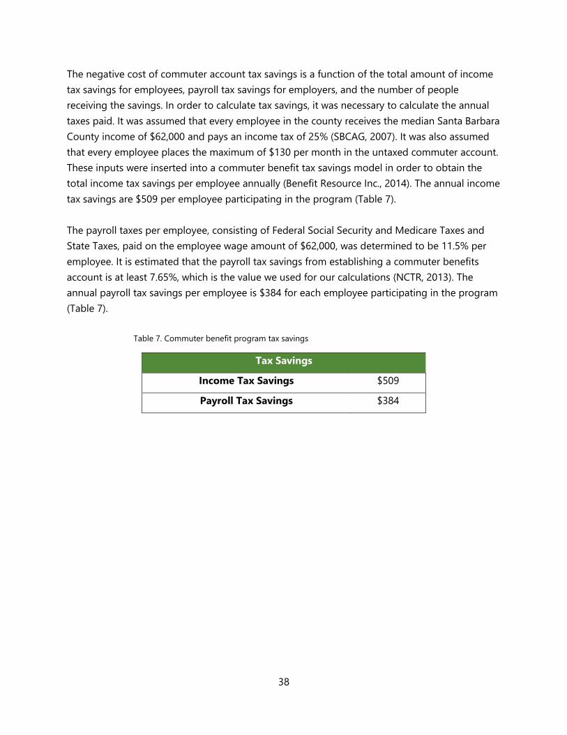
38

The negative cost of commuter account tax savings is a function of the total amount of income

tax savings for employees, payroll tax savings for employers, and the number of people

receiving the savings. In order to calculate tax savings, it was necessary to calculate the annual

taxes paid. It was assumed that every employee in the county receives the median Santa Barbara

County income of $62,000 and pays an income tax of 25% (SBCAG, 2007). It was also assumed

that every employee places the maximum of $130 per month in the untaxed commuter account.

These inputs were inserted into a commuter benefit tax savings model in order to obtain the

total income tax savings per employee annually (Benefit Resource Inc., 2014). The annual income

tax savings are $509 per employee participating in the program (Table 7).

The payroll taxes per employee, consisting of Federal Social Security and Medicare Taxes and

State Taxes, paid on the employee wage amount of $62,000, was determined to be 11.5% per

employee. It is estimated that the payroll tax savings from establishing a commuter benefits

account is at least 7.65%, which is the value we used for our calculations (NCTR, 2013). The

annual payroll tax savings per employee is $384 for each employee participating in the program

(Table 7).

Table 7. Commuter benefit program tax savings

Tax Savings

Income Tax Savings $509

Payroll Tax Savings $384

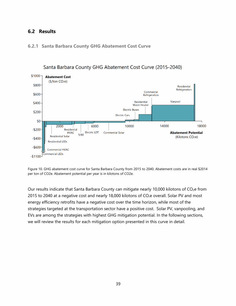
39

6.2 Results

6.2.1 Santa Barbara County GHG Abatement Cost Curve

Figure 10. GHG abatement cost curve for Santa Barbara County from 2015 to 2040. Abatement costs are in real $2014

per ton of CO2e. Abatement potential per year is in kilotons of CO2e.

Our results indicate that Santa Barbara County can mitigate nearly 10,000 kilotons of CO2e from

2015 to 2040 at a negative cost and nearly 18,000 kilotons of CO2e overall. Solar PV and most

energy efficiency retrofits have a negative cost over the time horizon, while most of the

strategies targeted at the transportation sector have a positive cost. Solar PV, vanpooling, and

EVs are among the strategies with highest GHG mitigation potential. In the following sections,

we will review the results for each mitigation option presented in this curve in detail.

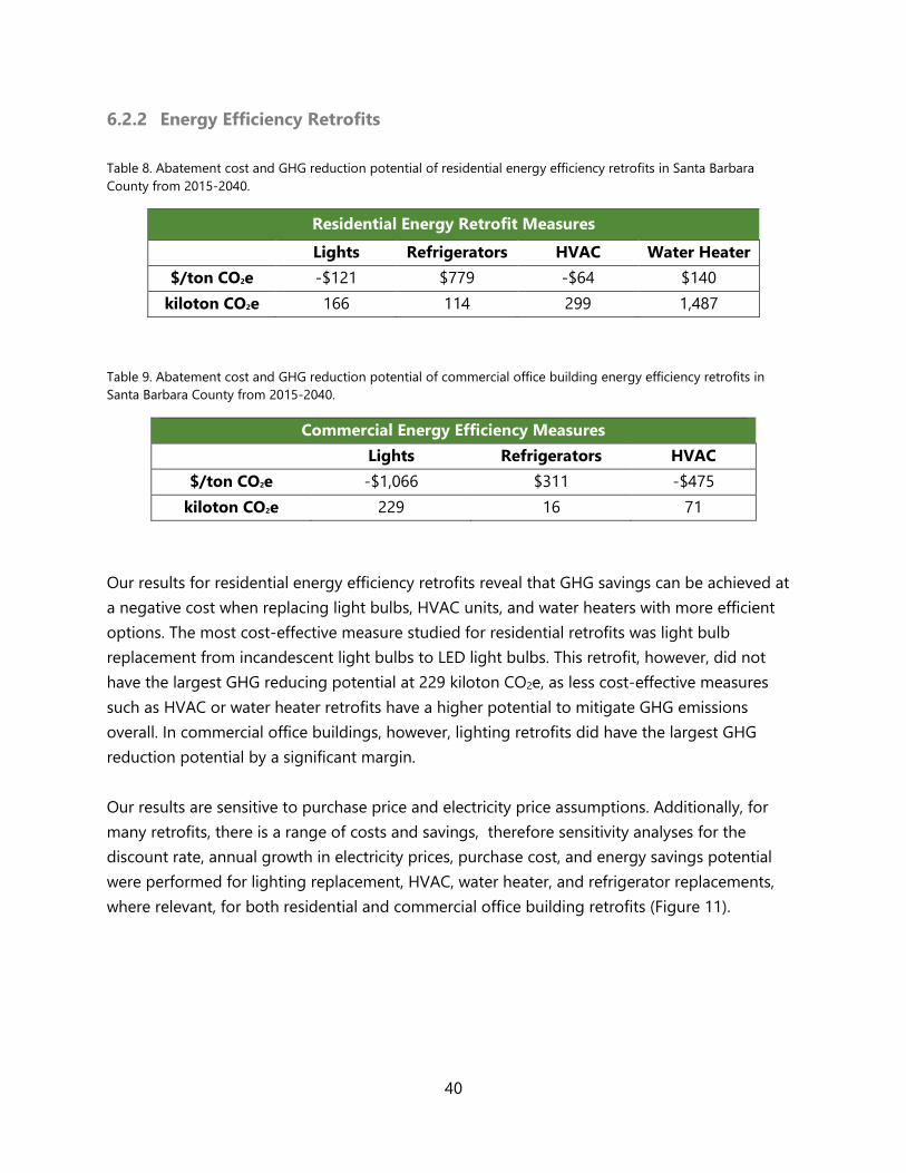
40


Table 8. Abatement cost and GHG reduction potential of residential energy efficiency retrofits in Santa Barbara

County from 2015-2040.

Residential Energy Retrofit Measures

Lights Refrigerators HVAC Water Heater

$/ton CO2e -$121 $779 -$64 $140

kiloton CO2e 166 114 299 1,487

Table 9. Abatement cost and GHG reduction potential of commercial office building energy efficiency retrofits in

Santa Barbara County from 2015-2040.

Commercial Energy Efficiency Measures

Lights Refrigerators HVAC

$/ton CO2e -$1,066 $311 -$475

kiloton CO2e 229 16 71

Our results for residential energy efficiency retrofits reveal that GHG savings can be achieved at

a negative cost when replacing light bulbs, HVAC units, and water heaters with more efficient

options. The most cost-effective measure studied for residential retrofits was light bulb

replacement from incandescent light bulbs to LED light bulbs. This retrofit, however, did not

have the largest GHG reducing potential at 229 kiloton CO2e, as less cost-effective measures

such as HVAC or water heater retrofits have a higher potential to mitigate GHG emissions

overall. In commercial office buildings, however, lighting retrofits did have the largest GHG

reduction potential by a significant margin.

Our results are sensitive to purchase price and electricity price assumptions. Additionally, for

many retrofits, there is a range of costs and savings, therefore sensitivity analyses for the

discount rate, annual growth in electricity prices, purchase cost, and energy savings potential

were performed for lighting replacement, HVAC, water heater, and refrigerator replacements,

where relevant, for both residential and commercial office building retrofits (Figure 11).

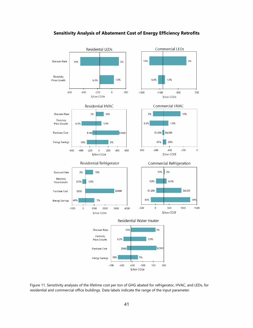
41

Sensitivity Analysis of Abatement Cost of Energy Efficiency Retrofits

Figure 11. Sensitivity analyses of the lifetime cost per ton of GHG abated for refrigerator, HVAC, and LEDs, for

residential and commercial office buildings. Data labels indicate the range of the input parameter.

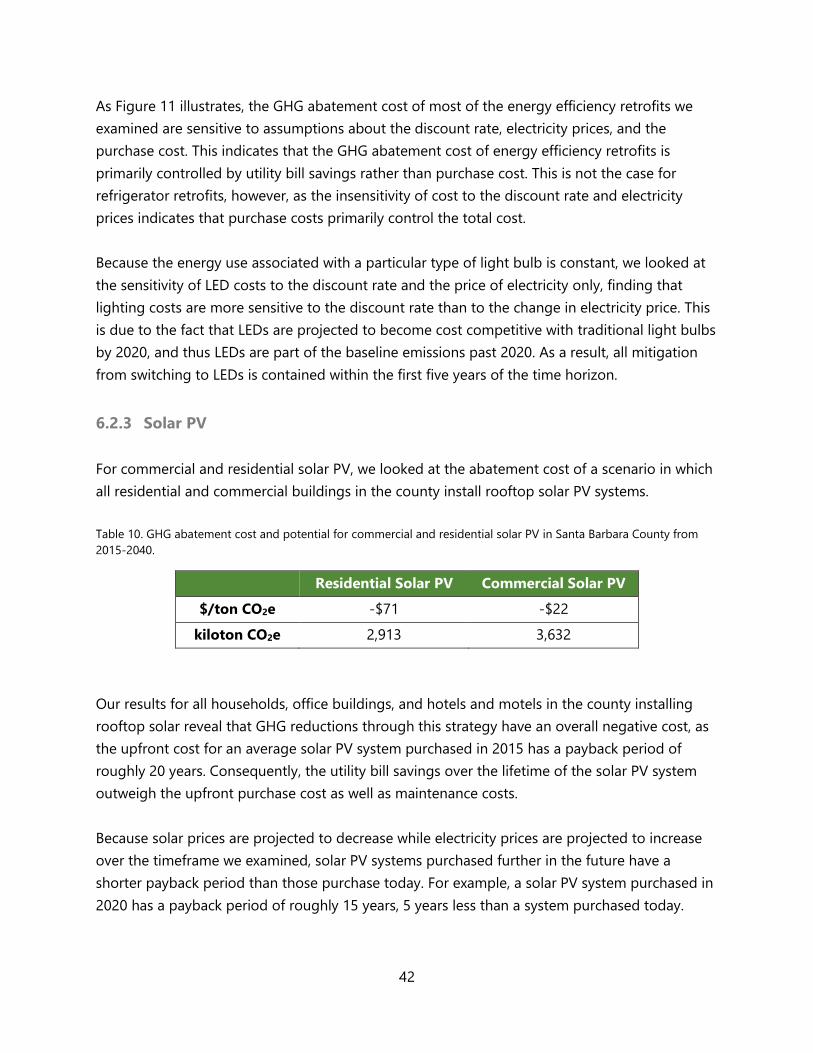
42

As Figure 11 illustrates, the GHG abatement cost of most of the energy efficiency retrofits we

examined are sensitive to assumptions about the discount rate, electricity prices, and the

purchase cost. This indicates that the GHG abatement cost of energy efficiency retrofits is

primarily controlled by utility bill savings rather than purchase cost. This is not the case for

refrigerator retrofits, however, as the insensitivity of cost to the discount rate and electricity

prices indicates that purchase costs primarily control the total cost.

Because the energy use associated with a particular type of light bulb is constant, we looked at

the sensitivity of LED costs to the discount rate and the price of electricity only, finding that

lighting costs are more sensitive to the discount rate than to the change in electricity price. This

is due to the fact that LEDs are projected to become cost competitive with traditional light bulbs

by 2020, and thus LEDs are part of the baseline emissions past 2020. As a result, all mitigation

from switching to LEDs is contained within the first five years of the time horizon.

6.2.3 Solar PV

For commercial and residential solar PV, we looked at the abatement cost of a scenario in which

all residential and commercial buildings in the county install rooftop solar PV systems.

Table 10. GHG abatement cost and potential for commercial and residential solar PV in Santa Barbara County from

2015-2040.

Residential Solar PV Commercial Solar PV

$/ton CO2e -$71 -$22

kiloton CO2e 2,913 3,632

Our results for all households, office buildings, and hotels and motels in the county installing

rooftop solar reveal that GHG reductions through this strategy have an overall negative cost, as

the upfront cost for an average solar PV system purchased in 2015 has a payback period of

roughly 20 years. Consequently, the utility bill savings over the lifetime of the solar PV system

outweigh the upfront purchase cost as well as maintenance costs.

Because solar prices are projected to decrease while electricity prices are projected to increase

over the timeframe we examined, solar PV systems purchased further in the future have a

shorter payback period than those purchase today. For example, a solar PV system purchased in

2020 has a payback period of roughly 15 years, 5 years less than a system purchased today.

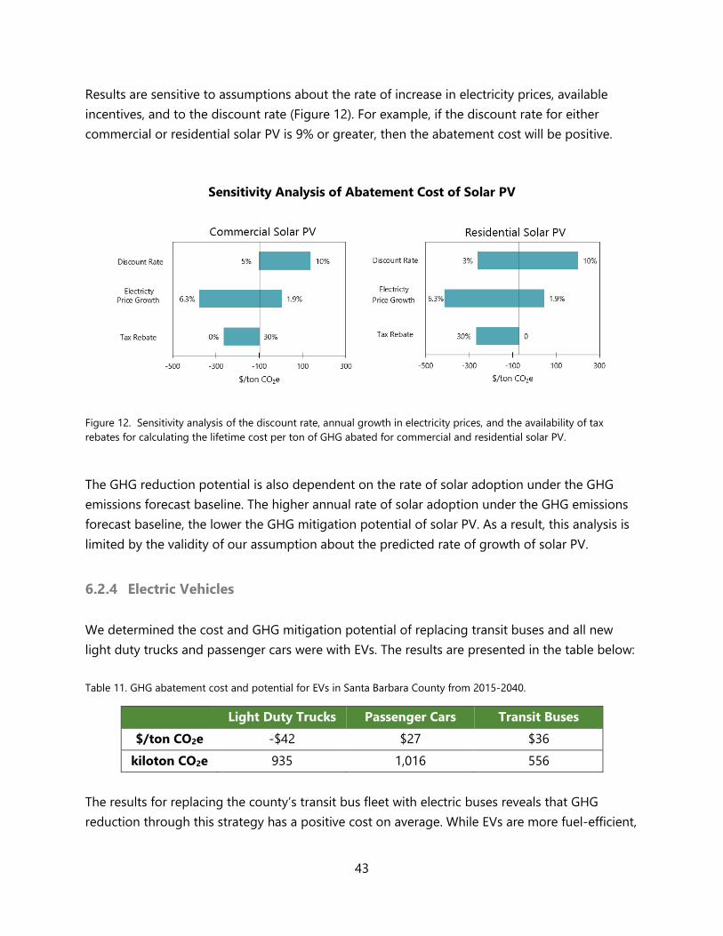
43

Results are sensitive to assumptions about the rate of increase in electricity prices, available

incentives, and to the discount rate (Figure 12). For example, if the discount rate for either

commercial or residential solar PV is 9% or greater, then the abatement cost will be positive.

Sensitivity Analysis of Abatement Cost of Solar PV

Figure 12. Sensitivity analysis of the discount rate, annual growth in electricity prices, and the availability of tax

rebates for calculating the lifetime cost per ton of GHG abated for commercial and residential solar PV.

The GHG reduction potential is also dependent on the rate of solar adoption under the GHG

emissions forecast baseline. The higher annual rate of solar adoption under the GHG emissions

forecast baseline, the lower the GHG mitigation potential of solar PV. As a result, this analysis is

limited by the validity of our assumption about the predicted rate of growth of solar PV.


We determined the cost and GHG mitigation potential of replacing transit buses and all new

light duty trucks and passenger cars were with EVs. The results are presented in the table below:

Table 11. GHG abatement cost and potential for EVs in Santa Barbara County from 2015-2040.

Light Duty Trucks Passenger Cars Transit Buses

$/ton CO2e -$42 $27 $36

kiloton CO2e 935 1,016 556

The results for replacing the county’s transit bus fleet with electric buses reveals that GHG

reduction through this strategy has a positive cost on average. While EVs are more fuel-efficient,

44

lower maintenance, and are declining in purchase cost, fuel and maintenance savings over the

lifetime of the vehicle are lower than the purchase price of the vehicle.

The cost of electrifying the entire transit bus fleet in Santa Barbara County is higher than

electrifying all new passenger cars and light duty trucks. This is due to the fact that the cost

difference between a conventional diesel or gasoline bus and an electric bus is greater than that

for smaller vehicles. Unlike transit buses or passenger cars, the abatement cost for light duty

trucks is negative. This is due to the greater fuel economy difference between an electric vehicle

and a light duty truck, as conventional fuel light duty trucks are large and less fuel efficient than

passenger cars. Consequently, the fuel cost savings of switching from a truck to an electric

vehicle is greater than from switching from a passenger car, and thus the option is more cost-

effective.

Cost calculations for electric cars are sensitive to assumptions in electricity prices and

assumptions about available incentives (Figure 13). While the GHG abatement cost for electric

passenger cars is unaffected by changes to the discount rate, the cost for light duty vehicles is

affected. This disparity is due to the fact that the cost of electric light duty vehicles is more

influenced by fuelling cost savings because light duty vehicles are less efficient than passenger

cars. In the case of passenger cars, the total GHG abatement cost is negative if customers

receive the maximum incentives currently available, take advantage of special EV rates offered

by the electric utility, or if the annual growth in electricity prices is low.

The GHG abatement cost of electric buses is sensitive to assumptions about purchase and

maintenance cost, but not to assumptions about electricity prices, which had almost no impact

on cost (Figure 13). The abatement cost of electric buses is also somewhat sensitive to

assumptions about the discount rate, indicating that purchase and maintenance cost have a

greater influence than fuel savings on total cost.

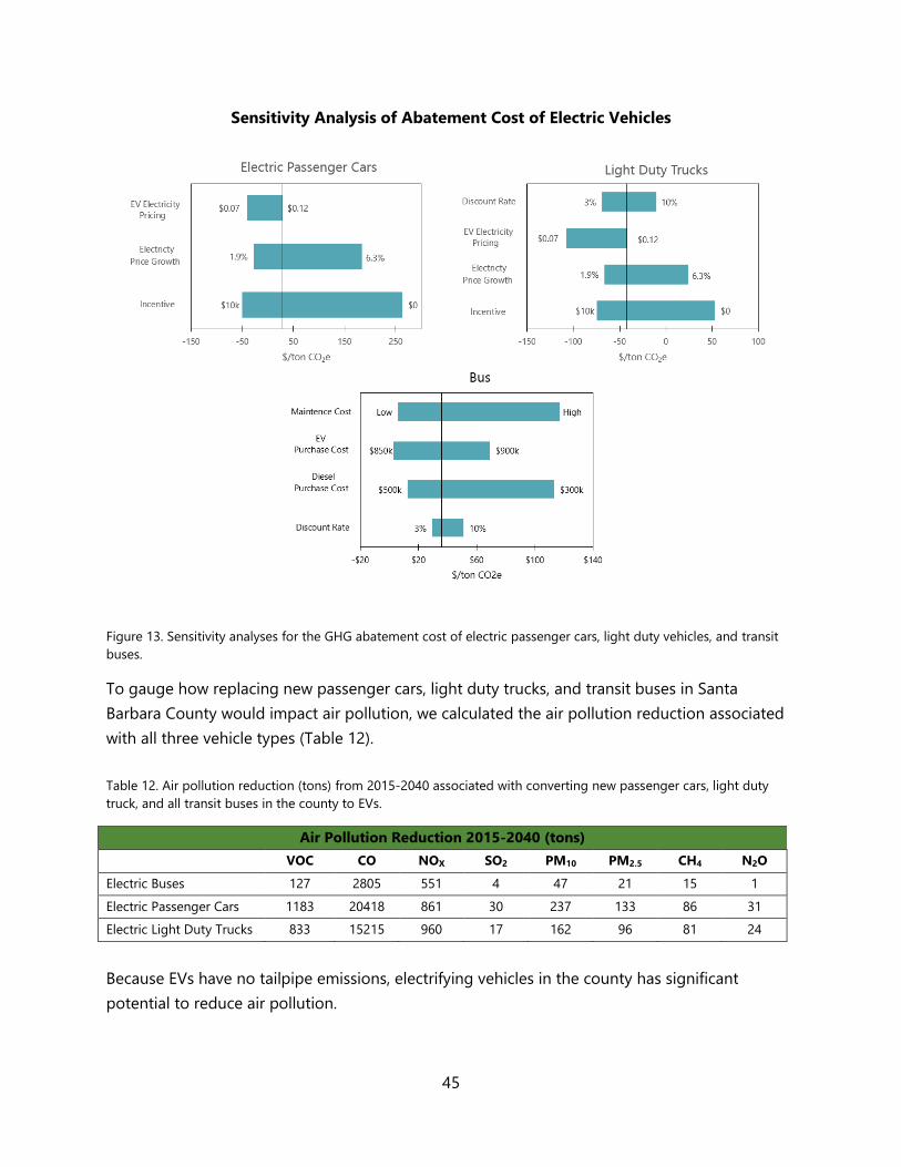
45

Sensitivity Analysis of Abatement Cost of Electric Vehicles

Figure 13. Sensitivity analyses for the GHG abatement cost of electric passenger cars, light duty vehicles, and transit

buses.

To gauge how replacing new passenger cars, light duty trucks, and transit buses in Santa

Barbara County would impact air pollution, we calculated the air pollution reduction associated

with all three vehicle types (Table 12).

Table 12. Air pollution reduction (tons) from 2015-2040 associated with converting new passenger cars, light duty

truck, and all transit buses in the county to EVs.

Air Pollution Reduction 2015-2040 (tons)

VOC CO NOX SO2 PM10 PM2.5 CH4 N2O

Electric Buses 127 2805 551 4 47 21 15 1

Electric Passenger Cars 1183 20418 861 30 237 133 86 31

Electric Light Duty Trucks 833 15215 960 17 162 96 81 24

Because EVs have no tailpipe emissions, electrifying vehicles in the county has significant

potential to reduce air pollution.

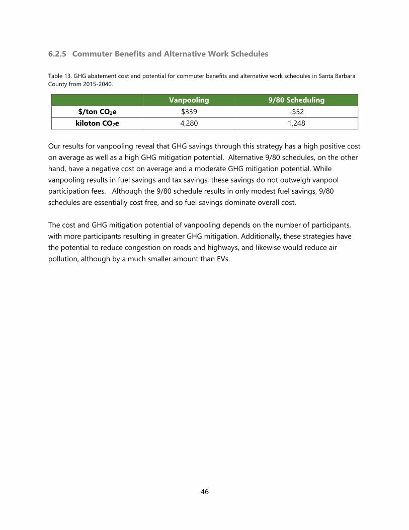
46


Table 13. GHG abatement cost and potential for commuter benefits and alternative work schedules in Santa Barbara

County from 2015-2040.

Vanpooling 9/80 Scheduling

$/ton CO2e $339 -$52

kiloton CO2e 4,280 1,248

Our results for vanpooling reveal that GHG savings through this strategy has a high positive cost

on average as well as a high GHG mitigation potential. Alternative 9/80 schedules, on the other

hand, have a negative cost on average and a moderate GHG mitigation potential. While

vanpooling results in fuel savings and tax savings, these savings do not outweigh vanpool

participation fees. Although the 9/80 schedule results in only modest fuel savings, 9/80

schedules are essentially cost free, and so fuel savings dominate overall cost.

The cost and GHG mitigation potential of vanpooling depends on the number of participants,

with more participants resulting in greater GHG mitigation. Additionally, these strategies have

the potential to reduce congestion on roads and highways, and likewise would reduce air

pollution, although by a much smaller amount than EVs.

47

7 Opportunities and Barriers to Implementation

While cost-effectiveness is an important criterion for local governments when considering

investment in GHG mitigation, cost alone does not determine the feasibility of a given GHG

mitigation strategy. Existing legislation, zoning codes, and other policies have the potential to

either facilitate or impede the implementation of new programs targeted at reducing GHG

emissions. In the following section, we will review the current barriers and opportunities at the

federal, state, and local levels for the GHG mitigation strategies examined in this analysis.

7.1 Energy Efficient Retrofits

7.1.1 Relevant Zoning Codes

Retrofitting an existing building with energy efficient upgrades does not constitute land use

development and is therefore not subject to permitting and review by the Planning and

Development department in Santa Barbara County. The only exception to this rule is water tanks

greater than 5,000 gallons in size and/or with a diameter to height ratio of 2:1 or greater (Santa

Barbara County Ordinance No. 5639).

According to the Orcutt Community Plan, buildings that produce noise greater than 45 decibels

are required to have double-paned windows. The plan, though not aimed to increase energy

efficiency, does encourage higher than average adoption of double-paned windows. The plan

also states that “rooftop mechanical structures,” like some air conditioning units, should be

avoided when possible for aesthetic reasons, requiring those that cannot be avoided to be

“shielded from view from surrounding roadways and residences through architectural design,

camouflage housing, or other appropriate methods” (Santa Barbara County Planning &

Development Comprehensive Planning Division, 2004).

7.1.2 Available Incentives and Rebates

High upfront cost is often the largest barrier to energy-saving retrofits to residential and

commercial buildings. To combat this problem, the federal, state, and county governments,

along with utility companies, offer financing options for energy efficient appliances.

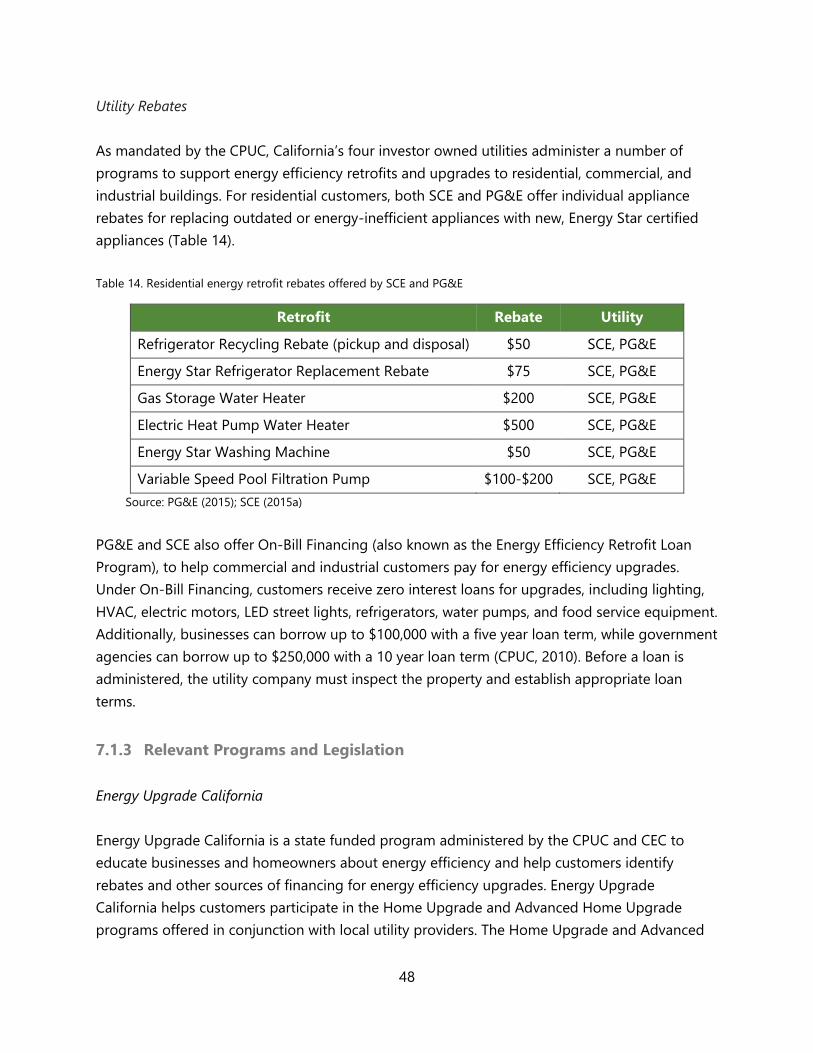
48

Utility Rebates

As mandated by the CPUC, California’s four investor owned utilities administer a number of

programs to support energy efficiency retrofits and upgrades to residential, commercial, and

industrial buildings. For residential customers, both SCE and PG&E offer individual appliance

rebates for replacing outdated or energy-inefficient appliances with new, Energy Star certified

appliances (Table 14).

Table 14. Residential energy retrofit rebates offered by SCE and PG&E

Retrofit Rebate Utility

Refrigerator Recycling Rebate (pickup and disposal) $50 SCE, PG&E

Energy Star Refrigerator Replacement Rebate $75 SCE, PG&E

Gas Storage Water Heater $200 SCE, PG&E

Electric Heat Pump Water Heater $500 SCE, PG&E

Energy Star Washing Machine $50 SCE, PG&E

Variable Speed Pool Filtration Pump $100-$200 SCE, PG&E

Source: PG&E (2015); SCE (2015a)

PG&E and SCE also offer On-Bill Financing (also known as the Energy Efficiency Retrofit Loan

Program), to help commercial and industrial customers pay for energy efficiency upgrades.

Under On-Bill Financing, customers receive zero interest loans for upgrades, including lighting,

HVAC, electric motors, LED street lights, refrigerators, water pumps, and food service equipment.

Additionally, businesses can borrow up to $100,000 with a five year loan term, while government

agencies can borrow up to $250,000 with a 10 year loan term (CPUC, 2010). Before a loan is

administered, the utility company must inspect the property and establish appropriate loan

terms.

7.1.3 Relevant Programs and Legislation

Energy Upgrade California

Energy Upgrade California is a state funded program administered by the CPUC and CEC to

educate businesses and homeowners about energy efficiency and help customers identify

rebates and other sources of financing for energy efficiency upgrades. Energy Upgrade

California helps customers participate in the Home Upgrade and Advanced Home Upgrade

programs offered in conjunction with local utility providers. The Home Upgrade and Advanced

49

Home Upgrade programs are both whole home approaches to energy efficiency that allow

customers to bundle several energy efficiency measures by connecting them with qualified

energy efficiency contractors, who identify suitable energy efficiency retrofits, help customers fill

out necessary paperwork (including rebate forms), and perform safety compliance checks

(Energy Upgrade California, 2015).

A Home Upgrade aims to reduce a home’s energy use by 10% or more while an Advanced

Home Upgrade aims to reduce a home’s energy use by at least 45% (Energy Upgrade California,

2015). A Home Upgrade may include simple efficiency measures such as better insulation,

whole-house air sealing, duct sealing, and furnace and AC replacements, while an Advanced

Home Upgrade includes deeper improvements such as a cool roof, hardwire lighting, a tankless

water heater system, and energy-efficient windows (Energy Upgrade California, 2015).

Customers pursuing a Home Upgrade or Advanced Home Upgrade can receive up to $2,500 and

$6,500 in rebates and incentives, respectively (PG&E, 2014).

Empower Central Coast

At the county level, emPower Central Coast (formerly emPower Santa Barbara County) provides

unsecured loans with low interest rates for energy efficiency retrofits from CoastHills Federal

Credit Union and Ventura County Credit Union. The emPower Central Coast program partners

with Energy Upgrade California to provide customized, flexible loans for the Home Upgrades

package and for solar energy systems. Loans from emPower Central Coast range from $1,000 to

$30,000, require no equity or collateral, have terms of up to 15 years, and have no prepayment

penalties (emPower Central Coast, 2015). With their loan application, customers must submit

their contractor’s bid proposal, a list of the upgrades they intend to install, and a letter verifying

their enrollment in the selected incentive program. Contractors fill out and submit the rebate

and incentive forms, and projects must be completed within 60 days of being approved by the

rebate program and emPower Central Coast (emPower Central Coast, 2015).

Santa Barbara Green Business Program

The Santa Barbara Green Business Program is a voluntary program that offers a certification for

green business practices such as the use of solar energy systems or energy efficiency retrofits in

their facilities. The program both credits businesses for existing practices and rewards newly

adopted technology and practices. Although the program offers no cash incentives of their own,

it offers Small Business Awards and certification as a means of incentivizing businesses to join

the program.

50

7.2 Solar PV

7.2.1 Relevant Zoning Codes

Santa Barbara County’s land use and development code exempts roof-mounted solar energy

systems from design review and permit approval. Roof-mounted solar energy systems, however,

may require building, electrical, and plumbing permits where applicable. Such permits are issued

through the Santa Barbara County Planning and Development Board (Santa Barbara County

Land Use & Development Code, section 35.20.160). If the solar energy system could possibly

have an adverse impact on public health or safety, for example, shining a glare onto oncoming

traffic on a busy street, a solar use permit is also required. A proposed rooftop solar energy

system that is within a “Special Problem Area,” i.e. an area that is particularly sensitive to

construction and land use development, will also require additional permitting along with

approval from the Special Problems Area Review Committee (SPARC) (Santa Barbara County

Ordinance Code § 10-1.5). Unlike roof-mounted systems, freestanding solar energy systems do

require a coastal development permit or land use permit (Santa Barbara County Land Use &

Development Code, section 35.20.160).

For those who wish to go through the permitting process as quickly as possible, Santa Barbara

County has developed an “Expedited Residential PV Permit Process” that promises 48 hour

permit turnaround for new solar PV energy systems that:

Are composed of four or fewer series strings per inverter;

Have an inverter capacity with a continuous AC power output of 13.44 kW or less;

Use an engineered mounting system;

Have a rooftop distributed weight of less than 5lbs./ft2 and less than 40 lbs. per

attachment;

Have a list PV modules, utility-interactive inverters, and combiner boxes as components;

and

Have an AC interconnection point on the load side of service disconnecting means

(County of Santa Barbara Planning and Development, 2011).

In cases in which all these requirements are not met, processing may take up to 10 working

days. All permit applicants must also submit the following documents along with their permit

application:

The Santa Barbara County permit application;

The site plan showing the location of the solar PV system;

51

The seal and signature of the architect, engineer, or electrical contractor;

The Photovoltaic Manufacturer’s Module & Inverter Specification Data Sheets;

The electrical wiring drawings;

The completed Questionnaire Page for the Expedited Plan Review; and

The Signage Requirements for PV Interactive System (County of Santa Barbara Planning

and Development, 2011).


Federal Tax Credit

Pursuant to the Federal Energy Improvement and Extension Act of 2008, homeowners and

businesses that decide to invest in solar energy systems or solar-powered water heating can

claim a tax credit of 30% of the installation cost of the system. This credit runs through

December 31, 2016, but may be extended (IRS, 2014). In cases in which construction and costs

span more than one tax year, or in which there is excess credit, the credit can be carried forward

to the next tax year (IRS, 2014). Currently, there is no maximum credit that can be granted for an

installed solar energy system. The solar energy system must serve a residence that is located

within the United States and that is owned by the taxpayer. Eligible solar-powered water heaters

must be certified by the Solar Rating Certification Corporation (SRCC) and produce at least half

of the energy used to heat the residence’s water.

PACE Financing

Property Assessed Clean Energy (PACE) is a voluntary program in which local governments can

offer financing to residential, commercial, and industrial building owners for energy efficiency,

renewable energy, and water conservation upgrades. Qualified service providers help building

owners select a PACE qualified project, while the PACE program itself is responsible for

processing applications, approving projects, and providing or arranging financing. Additional

rebates may also be used in conjunction with PACE financing.

As an example, PACE financing may have the following requirements:

Mortgage-related debt must not exceed 90% of property value;

Mortgage payments must be current;

Owners must have no more than one 30-day mortgage late payment over the past year;

Property taxes must be current, one late payment in last three years allowed;

No outstanding involuntary liens (tax or mechanic liens);

52

No active bankruptcies within last seven years;

For condominiums, written authorization from management is required; and

The senior mortgage debt lender must acknowledge placement of assessment (Renovate

America, 2015).

In order for property owners in Santa Barbara County to secure a PACE loan, they must find a

participating regional program, such as the HERO Program in Lompoc, California. The borrower

can then submit a project proposal, a project plan, and a letter of acknowledgement from the

principal lender in order to negotiate the terms of the loan. Once the financials are agreed upon,

the loan is paid back yearly as part of a special line item on the property’s tax statement. The

interest rate on each loan is determined by the term period of the loan itself, be it five, 10, or 20

years. This property tax is transferable if the property is subsequently sold, making the new

owner responsible for paying back the remainder of the loan.

Advantages of offering PACE financing include increased economic activity and job creation and

increased energy and water conservation. For example, a 2011 study of four cities, which

included the City of Santa Barbara, found that every $1 million in PACE spending generated $10

million in gross economic output, 60 jobs, and $1 million in combined federal, state, and local

tax revenue on average (Pozdena and Josephson, 2011). In Santa Barbara specifically, they found

that for every $1 million in project purchases, solar PV generated 6 new jobs and had a state and

local fiscal impact of $34,686, while energy efficiency programs also generated 6 new jobs and

had a state and local fiscal impact of $34,973 (Pozdena and Josephson, 2011).

Although PACE saw initial success, the seniority of the PACE lien to a property’s principal

mortgage caused the Federal Housing Finance Agency to advise lending firms Fannie Mae and

Freddie Mac to deny backing mortgages on properties with senior PACE liens (Hsu, 2010). Since

that time, residential enrollment has fallen, but certain measures have been taken to make

borrowing under PACE more secure, including loan loss reserve funds and appropriate

disclosure agreements. California Governor Jerry Brown has also proposed a state-run reserve

fund of $10 million to back PACE financing (Baker, 2013).

Utility Company Incentives

SCE and PG&E both offer incentives to customers for installing solar energy systems. Time of

Use billing plans can make electricity less expensive for solar energy-generating customers who

primarily only need to rely on utility generated electricity during off-peak hours (i.e. at night)

when electricity is cheapest, as their solar energy system can provide their electricity during peak

daytime hours.

53

In addition to Time of Use billing, Net Energy Metering is available to solar energy system users.

Net Energy Metering rewards customers for surplus energy provided back into the electricity

grid. When the solar energy system produces more electricity than is used by the customer, the

excess can be used to relieve peak demand, and the customer is rewarded at a rate equal to that

of the cost of the electricity provided. Under a Net Energy Metering agreement, residential

customers are billed yearly while commercial customers are billed monthly. For multi-tenant

homes, Virtual Net Energy Metering accomplishes the same goals as Net Energy Metering, but

breaks up the energy bill of the entire building into manageable accounts for individual tenants.

(SCE, 2015b). Finally, SCE’s Multi-Family Affordable Solar Housing (MASH) Virtual NEM

subsidizes solar energy systems at a lower rate for low income, multi-family housing units.

7.2.3 Relevant Programs

The Santa Barbara County Million Solar Roofs program aims to popularize renewable energy

through the installation and use of personal solar power with an auxiliary purpose of job

creation in the clean energy sector. Through a partnership with Santa Barbara County, the

Million Solar Roofs initiative helps to lighten the design review process for solar energy systems.

Consequently, design review for solar energy systems has been relegated to project proposals

with “significant visual or historical impacts” (City of Santa Barbara, 2006). In place of restrictive

legislation, guidelines for solar development have been passed to prevent traditional community

aesthetic standards from obstructing solar installation. Additionally, the City of Santa Barbara

established the Solar Energy System Guidelines and Recognition Program to further incentivize

the installation of aesthetically pleasing solar energy systems (Community Development

Department City of Santa Barbara, 2006). The guide describes strategies for installing systems

that maintain aesthetic quality while maximizing efficiency. The program also established the

Solar Recognition Awards, which are presented to citizens that install high quality solar energy

systems that are hidden from public view, were a challenge to design, and are maximally

efficient.

7.3 Electric Vehicles

Despite their environmental benefits and greater fuel economy, there are many barriers to

greater adoption of EVs, including:

Lack of infrastructure - EV charging infrastructure is not widespread in comparison to

infrastructure for conventional fuel vehicles. Part of California’s ZEV Action Plan called for

the expansion of charging stations, with the goal of developing sufficient EV

infrastructure to support one million EVs in California by 2020. Local governments can

54

address this barrier by investing in EV charging stations in their communities and

streamlining the permitting processes for EV infrastructure.

High upfront cost - While federal and state incentives are available, they are not always

able to cover the entire cost difference between an EV and a conventional vehicle, and

applying for incentives, which are not received until after the purchase/leasing of the

vehicle, might be prohibitive for some customers.

Limited range - While EVs can cover the majority of household trips, they are less

practical for long distance driving than conventional fuel vehicles. EVs typically have a

range of 50 to 100 miles on a single charge. Electric buses, because of their larger

battery, can go up to 150 miles on a single charge. Although a 50-100 mile range is

enough to cover the majority of all household vehicle trips in the United States, EVs can

take several hours to recharge and so are inconvenient for longer trips (NREL, 2011). The

time required to recharge an EV depends on the size and type of the batteries as well as

the type of charging equipment used.

Fewer vehicle options - Currently, an EV option is not available for all vehicle types.

Most commercially available EVs are small passenger cars.

Low consumer awareness - Many customers are not aware of the benefits or incentives

available for EVs. Detail about incentives and rebates currently available for EVs at the

state and federal level is provided in the section below.


To address cost differential between EVs and conventional vehicles, there are a number of

incentives at the federal, state, and even local level designed to make EVs affordable. A summary

of all available incentives and sources of funding for EVs is provided in Table 15.

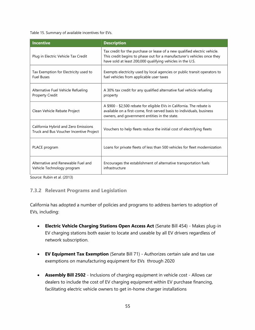
55

Table 15. Summary of available incentives for EVs.

Incentive Description

Plug in Electric Vehicle Tax Credit

Tax credit for the purchase or lease of a new qualified electric vehicle.

This credit begins to phase out for a manufacturer’s vehicles once they

have sold at least 200,000 qualifying vehicles in the U.S.

Tax Exemption for Electricity used to

Fuel Buses

Exempts electricity used by local agencies or public transit operators to

fuel vehicles from applicable user taxes

Alternative Fuel Vehicle Refueling

Property Credit

A 30% tax credit for any qualified alternative fuel vehicle refueling

property

Clean Vehicle Rebate Project

A $900 - $2,500 rebate for eligible EVs in California. The rebate is

available on a first-come, first-served basis to individuals, business

owners, and government entities in the state.

California Hybrid and Zero Emissions

Truck and Bus Voucher Incentive Project Vouchers to help fleets reduce the initial cost of electrifying fleets

PLACE program Loans for private fleets of less than 500 vehicles for fleet modernization

Alternative and Renewable Fuel and

Vehicle Technology program

Encourages the establishment of alternative transportation fuels

infrastructure

Source: Rubin et al. (2013)

7.3.2 Relevant Programs and Legislation

California has adopted a number of policies and programs to address barriers to adoption of

EVs, including:

Electric Vehicle Charging Stations Open Access Act (Senate Bill 454) - Makes plug-in

EV charging stations both easier to locate and useable by all EV drivers regardless of

network subscription.

EV Equipment Tax Exemption (Senate Bill 71) - Authorizes certain sale and tax use

exemptions on manufacturing equipment for EVs through 2020

Assembly Bill 2502 - Inclusions of charging equipment in vehicle cost - Allows car

dealers to include the cost of EV charging equipment within EV purchase financing,

facilitating electric vehicle owners to get in-home charger installations

56

Homeowners associations and charging stations (Senate Bill 880) - Outlines the rights

and responsibilities of homeowner associations and EV owners for charging in common-

interest developments to ensure that electric vehicle owners are not unreasonably

prohibited from installing charging equipment

Assembly Bill 1092 - Requires the California Building Standards Commission and the

Department of Housing and Community Development to develop standards for PEV

charging infrastructure in multi-unit dwellings and non-residential developments

Renewable Fuel Standard - The federal Renewable Fuel Standard requires that 36

billion gallons of totally renewable fuel be used as transportation fuel by 2022 in the U.S.

Electric Vehicle Everywhere Workplace Charging Challenge - The Department of

Energy initiated a program in early 2013 that encourages employers to place EV chargers

in their workplaces. Many businesses, including national and international companies,

have already signed on to this program.

Utility Incentives for Electric Vehicles

In addition to high upfront cost, recently declining gasoline prices and increasing electricity

prices in California may disincentivize EV adoption. However, investor owned utilities, including

PG&E and SCE, offer alternate rate options that can reduce the cost of vehicle charging, namely

Time of Use plans and Electric Vehicle plans.

Time of Use plans are opt-in rate structures that reward customers for using electricity during

off-peak hours (usually between 9:00pm and 12:00pm) by charging a low rate (around

$0.12/kWh) for electricity used during off-peak hours and a higher rate (around $0.20/kWh to

$0.30/kWh) for electricity used during peak hours. Because many EV owners charge their

vehicles overnight during off-peak hours, this plan facilitates low cost vehicle charging.

Electric Vehicle Plans use a separate meter to bill the electricity used to charge an EV at a lower

rate. This plan also utilizes Time of Use pricing; lower rates apply during off-peak hours. This

type of plan requires a separate meter or in-home charging station to be installed.

Although no formal policies have been proposed or put in place, the CPUC has been

considering other alternative-fueled vehicle programs and policies to encourage the adoption of

cleaner vehicles, and has been asked by the CA ZEV Action Plan to explore how electric rates can

be used to support the adoption of EVs in public transit (Gallo et al., 2014).

57

Finally, the federal Transit Investments for Greenhouse Gas and Energy Reduction (TIGGER)

program provides capital grants to public transit agencies for the purpose of reducing energy

use or GHG emissions associated with public transit. TIGGER selects projects based on:

Total projected GHG/energy savings;

Project innovation;

National applicability;

Project readiness;

Project management; and

Return on investment.

7.4 Commuter Benefits and Alternative Work Schedules

7.4.1 Relevant United States Code

In order for a business or organization to establish an alternate work schedule, such as a 9/80

work schedule, certain steps must be taken. If the business or organization’s workforce is part of

a union, the provisions of the work schedule must be in the initial employment contract, and

negotiated with a representative agent of that union. For non-union workforces, an agency may

unilaterally install an alternative work schedule. In both cases, the head of the employing agency

must approve the schedules, and has the power to veto such a schedule if the schedule might

have adverse impacts on the agency, such as:

A reduction in agent productivity;

A diminished level of service; or

An increase in operating costs, excluding administrative cost of establishing such a

program (U.S. Office of Personnel Management, 1996).

7.4.2 Relevant Programs

Established by the U.S. EPA and the U.S. Department of Transportation, the Best Workplaces for

Commuters program recognizes employers that provide their employees with outstanding

commuter benefits programs. The program also offers toolkits and information on benefits to

employers who are interested in commuter benefit programs for their business. In 2007,

management responsibilities shifted to the National Center for Transit Research within the

Center for Urban Transportation Research.

58

In order to become a member of the Best Workplaces for Commuters program, employers must

abide by the Best Workplaces for Commuters program’s stated National Standards of

Excellence. Under the National Standards of Excellence, employers must offer their employees

one “primary benefit,” such as employer-paid vanpooling or bus passes, in addition to three

“secondary benefits” such as ridesharing or carpool matching (which are often free), preferred

parking, or compressed work schedules. Employers must also offer Emergency Ride Home

services, which provide low or no cost transport in the case of an emergency.

If these Standards of Excellence are met, employers must then prove that they have a central

point of contact for commuter benefits within their organization, keep their information on

commuter benefits in a centralized location, actively promote commuter benefits to their

employees, agree to use the Best Workplaces for Commuters name and logo to promote

themselves, and ensure that within 18 months of acceptance into the program, at least 14% of

employees use the commuter benefit services. Lastly, employers must pay a $230 annual

membership fee to the Best Workplaces for Commuters (Bond, 2013).

Some of the benefits of membership into the Best Workplaces for Commuters include national

branding and recognition, technical assistance in implementing improvements to their

commuter benefit programs, staff training for managing commuter benefit programs, web-

based tools for tracking program analytics, and forums for information exchange between

members. These benefits are all in addition to the conventional benefits of commuter benefit

programs, including employee attraction and retention, tax and cost savings, reputation

benefits, and reduction in GHG emissions as well as other environmental benefits.

Best Workplaces for Commuters Commuter Benefit Program Implementation Guidelines

For employers to establish a pre-tax commuter benefits program, the following steps should be

taken:

1. Determine whether administration of the program will take place in-house or via a third

party administrator. Small employers may find in-house staffing to be favorable, and may

reach out to local transit agencies for specifics on acquiring and distributing transit

passes and other benefits. Larger employers, on the other hand, may find third party

administrators favorable because of their larger range of options and economies of scale.

2. Identify key departments and managers in which to nest their commuter benefits

program. The most likely choices are human resources, payroll/accounting, tax/legal, or

departments created specifically for this duty.

59

3. Determine the specific commuter benefits to be offered. Some options include

subsidized parking or transit fares, a subsidized highway transit vehicle, or bicycle travel

reimbursements. Any combination of these benefits may be offered up to the federally

established tax free limit.

4. Consult with its accounting department to establish a specific deduction code for the

benefit.

5. Create and distribute program information on how to sign up, how to choose benefits,

and how to claim them.

6. Market their program to employees with orientations, benefit fairs, and special events,

etc. (Baker, 2012).

7.5 Success Stories

7.5.1 Solar Energy and Energy Efficiency

Local governments can promote solar energy by providing local lending and tax incentives,

passing solar friendly legislation, setting clean energy goals, and installing solar energy systems

on government buildings (Burr et al., 2014). Partnerships with local utility companies can also

facilitate adoption of solar energy, as utility companies can offer incentives and set goals for

clean energy grid mixes. For example, Seattle City Light, the public electricity utility that serves

the City of Seattle, allows customers to invest in community run, large-scale solar projects that,

although not directly on customer property, generate savings that are reflected in their

electricity bills.

Berkeley FIRST

The City of Berkeley Financing Initiative for Renewable and Solar Technology (FIRST) was the

pilot program for what now has become PACE financing. Founded in 2008, FIRST aimed to

“catalyze the transition to a more sustainable use of energy and also deliver benefits beyond

emission reductions, including a new source of job growth, reduced strain on the electric power

system, and more comfortable and well-maintained buildings” (Fuller et al., 2009). Like PACE

financing, FIRST provided funds for the installation of electric and thermal solar energy systems,

repaid through an additional property tax line item on the property, with tax-deductible interest.

The finances for the program were originally borrowed from the city’s newly formed Sustainable

Energy Financing District, which itself was funded by the issuance of a special tax bond to be

60

paid back semi-annually over 20 years with money accrued from the new property taxes (Fuller

et al., 2009).

Once a plan was approved, the city would issue the property owner a reimbursement check

following project completion. Like PACE financing, the new property tax line item was

transferable to any new owner of the property. The program proved to be popular as all $1.5

million in available funds were applied for within 10 minutes of the program applications

becoming available. While not all applicants followed through to project installation, FIRST still

managed to directly finance 13 solar energy systems and inspire an additional 40 projects to be

developed by other means (City of Berkeley, 2010). According to the project’s Final Evaluation

report, 50% of survey respondents said that a lack of financing options was a major reason why

they did not install a personal solar energy system sooner. Additionally, 90% of respondents that

did participate in the FIRST program were satisfied with the program, and another 70% said that

the application process was easy. There were, however, certain areas that needed improvement,

including more flexible payment options, better upfront communication of additional property

tax costs, and a lower loan interest rate.

Energy Independence Program

The Energy Independence Program in Palm Springs, California was successful enough to warrant

three separate rounds of fully distributed funding. In this example of PACE-like funding, the

city’s general fund provided $7.5 million to fund 200 projects, each averaging $36,000 in cost. Of

these funded projects, 70% were for energy efficiency retrofits and the other 30% were for solar

energy system installation. The program boasted a first year consumer savings of $20 million,

and seven new clean energy startups have credited their inception to the opportunities

presented by the program (Mattson et al., 2009)

Green Finance SF

Green Finance SF, a PACE financing program in San Francisco, uses the free market to set terms

in which property owners identify their own project lenders and negotiate financing terms with

them. The city then collects the increased property tax and reimburses the principal project

lender. This structure is designed to provide security to the lenders to enable them to provide

competitive financing terms to the borrower. To be eligible, property owners must own property

within the San Francisco city limits and must have a professional water and energy audit done to

their property prior to beginning the project (CEC, 2013). This project is particularly successful

because it secures financing by requiring written consent from all lenders with outstanding liens

61

on the proposed property stating that they allow a senior PACE loan to supersede their own

(Burr et al., 2014).

Solar America Cities Program

Portland, Oregon was initially chosen by the Federal government to participate in its Solar

America Cities program, providing funding and support for solar energy system initiatives. This,

combined with efforts to collaborate with local nonprofits to educate the public, led to the

establishment of a collective purchasing model for solar energy systems that spread throughout

the city. Educating the public about where they could find incentives to install solar energy

systems led to a lowering of costs for suppliers that subsequently obtained a large volume of

business. As a result of these programs, Portland installed 7.1 MW of solar power on 560 homes.

The success of this program inspired multiple “solarize” campaigns throughout the country,

including one in California. Since then, Portland has begun to streamline its permitting process

with an online permitting system, which further decreases soft costs to consumers and solar

installation firms alike. All efforts have been supplemented with state-enacted policies granting

tax credits for residential and commercial solar energy systems (Burr et al., 2014).


Many local governments in California have already adopted policies and programs aimed at

increasing adoption of EVs. For example, the City of Berkeley offers a simple permitting process

to approve EV chargers in homes, only requiring an inexpensive over-the-counter electrical

permit, while the City of Thousand Oaks partnered with a third party company and the Ventura

County Air Pollution Control District to fund and install a DC Fast Charging station at the

Thousand Oaks Transportation Center.

Los Angeles Department of Water and Power’s Charge Up L.A.!, program offers rebates to

residential and commercial customers who purchase charging equipment for EVs. Residential

customers can receive a rebate of up to $750 towards the purchase of an EV charger as well as a

discount on their electricity bill if they install a Time of Use meter, while commercial customers

can receive up to $750 for hardwired wall-mounted EV chargers and up to $1,000 for stand-

alone pedestal chargers (LADWP, 2013).

The City of Riverside’s Alternative Fuel Vehicle Rebate Program offers a rebate of up $500 for

the purchase of new EVs to residents of Riverside. Similarly, the City of Corona’s Alternative Fuel

Vehicle REBATE Program offers a rebate to Corona residents of up to $2,000 for the purchase of

a new qualified Alternative Fuel Vehicle or $1,000 for a qualified used vehicle (City of Corona,

62

2015). Due to the popularity of the program, however, funds have been exhausted for the 2014-

2015 fiscal year. Rather than offering rebates, the cities of Hermosa Beach and Santa Monica

incentive EVs by offering free metered parking for EVs.


BART Citywide Pre-Tax Commuter Benefits

In 2009, the Bay Area Rapid Transit (BART) conducted a survey on their citywide pre-tax

commuter benefits program and found that nearly half (46%) of San Francisco daily riders take

advantage of pre-tax commuter benefits offered by their employer, and that a total of 68% of all

BART fares were pre-tax (BART, 2009). Of all the survey respondents, 96% found it easy to sign

up for the program and 90% reported that claiming their benefits was also easy. This success is

derived from the relatively high number of employers (58%) in the Bay Area that offer transit

benefits as well as the high rate of employee interest (78%). High rates of employee interest are

also expressed by the amount of employees whose employer does not offer benefits but that

would be interested in such a program (90%). Employers largely utilized third party benefit

organizers such as Commuter Check and Wageworks to administer and manage their transit

benefits programs, as only 6% administered their own benefits to employees. There were,

however, several critical comments directed at the program, such as long lines, limited hours of

regional office operation, and that the program sometimes runs out of tickets. BART replied that

an entirely online system could be the answer to these problems, and it is moving forward with

implementation of such a program (BART, 2009).

Denver Federal Workers Compressed Workweek Experiment

In an experiment involving federal employees in Denver, Colorado, a compressed workweek of

four days and 10 hours per day found that this workweek had no adverse effects on the use of

commuter benefit measures, such as ride-sharing, and reduced employee VMT by 15% (FTA,

1992). The study also found that compressed work schedules are most applicable to employees

with office and administrative work functions, particularly government agencies, as well as

assembly line manufacturing workers.

Finally, the study found that in order to ensure that compressed work schedules would have no

extra cost to the employer, state policies and legislation may need to be revised to allow certain

compressed work schedules without the requirement of overtime pay (FTA, 1992).

63

Texas Instruments Ad-Hoc Flexibility Policy

Texas Instruments (TI) experimented with what it called an “ad-hoc flexibility” work schedule in

which most, but not all, employees were allowed to make changes to their work schedules. This

included occasional telecommuting and compressed work schedules for the purpose of allowing

time for employees’ personal business, such as doctors’ appointments, child care, or late-night

work commitments. As a result of the ad-hoc flexibility program, TI noted higher employee

retention rates, lower stress levels, and higher efficiency as well as increased development of

employee skills due to “job sharing” (Giglio, 2005).

Aflac Insurance Compressed Work Schedules

The insurance company Aflac experimented with, and has since adopted, a variety of

compressed work schedules. Aflac offers both a four by 10 workweek as well as a three by 12

workweek, offering three and four days off per week, respectively. Requests for scheduling

changes must be met with supervisor approval, and are employee chosen and employee driven.

Feedback on these scheduling options are facilitated through employee focus group sessions,

allowing employees the chance to comment on the system directly to management, as well as

to allow management to gather data on program effectiveness and participation. Since the

change, Aflac employees report being happier and more effective, and have an enhanced sense

of pride and value of their professional lives. Aflac also reports that higher worker productivity

has helped their bottom line, and has reduced costly employee turnover, stating that retention

rates have risen from 87% pre-program to 94% post-program, making their decision to

implement flex work good for both business and the environment (Giglio, 2005).

64

8 Recommendations

The results of our GHG abatement cost curve for Santa Barbara County, combined with our

review of existing opportunities and barriers to implementing the GHG mitigation strategies

included in this analysis, reveal that Santa Barbara County can make meaningful reductions in

GHG emissions by facilitating adoption of energy efficiency, solar PV, EVs, commuter benefits

programs, and alternative work schedules. In the following sections, we provide detailed

recommendations regarding which GHG mitigation strategies are most worthwhile and what

county decision makers can do to promote and adopt these strategies.

8.1 Energy Efficiency Retrofits

The numerous utility company rebates and facilitator programs like Energy Upgrade California

and emPower Central Coast make energy efficiency retrofits to residential and commercial

buildings a financially beneficial means to reduce GHG emissions. By combining high value

rebates with low and zero interest loans procured through emPower Central Coast, property

owners can reduce investment costs in energy efficiency measures and realize monetary savings

quickly. Our analysis of GHG mitigation cost suggest that lighting and HVAC retrofits are

particularly favorable as they can save property owners money and are eligible for existing

rebates. These measures are also relatively easy to implement and do not require governmental

approval or permitting. In particular, the use of fluorescent lighting in office buildings is

expensive and widespread, so energy efficiency improvements in this particular niche can result

in substantial monetary savings and as well as significant GHG reductions.

Upgrading to more efficient water heaters is also a favorable retrofit in terms of GHG mitigation

potential as most standard water heaters run on natural gas. Efficient water heaters, however,

have a positive cost over their lifetime, even when utility bill savings are accounted for. Because

this measure has both high cost and high GHG mitigation potential, investing in higher rebates

and incentives for efficient or solar powered water heaters could be worthwhile. If increasing

rebates for efficient water heaters is not feasible, however, this strategy should not be pursued if

cost-effectiveness takes priority over GHG mitigation.

Based on our analysis, upgrading refrigerators to more efficient models is the least favorable

energy efficiency strategy as it is not only high cost, but also low in GHG reduction potential. For

this measure to be cost-effective, existing rebates would need to be higher such that property

owners are incentivized to choose the more expensive, more efficient models. However, even

65

the most efficient models are unlikely to result in substantial GHG reductions, and so upgrading

refrigerators in residential and commercial buildings is a low priority mitigation strategy.

8.2 Solar PV

Because of its overall negative cost, supportive state and local policies, and significant GHG

reduction potential, solar energy is a highly recommendable GHG mitigation strategy for Santa

Barbara County. Currently, most cities in the county do not have a PACE program, and so

instituting more PACE programs could be one way to increase the adoption of solar energy in

the county. Solar education programs and streamlining the permitting process can also facilitate

solar adoption. Santa Barbara County has already made strides in solar permitting, as the county

has already expedited the permitting process. As of 2009, however, the cities of Santa Maria,

Santa Barbara, Lompoc, Solvang, and Guadalupe, have a high permitting fee for solar energy

systems relative to the rest of the county, which may disincentivize solar energy in these cities

(Mills et al., 2009). Lowering this permit fee could increase adoption of solar and therefore

should be considered.

8.3 Electric Vehicles

While our analysis reveals that reducing GHG emissions through EVs, on average, has a positive

cost, the large mitigation potential, legislative support and co-benefits of EVs make them a

worthwhile means to mitigating GHG emissions. Given the right combination of incentives and

fuel pricing, EVs can be cost competitive, or even cheaper, than conventional fuel vehicles over

the time horizon we examined. Therefore, we suggest that local governments take action to

make EV ownership more affordable in order to increase adoption rates. There is already

significant state support for EVs because they are a major component of California’s strategy to

meet the GHG reduction goals outlined by AB 32. As a result, there are many resources already

available to local governments, agencies, and businesses including information on how to grow

EV infrastructure, increase customer awareness, and incentivize EV ownership. Additionally, EVs

have the added benefit of reducing air pollution, making them particularly relevant for local

governments for whom air pollution is a major concern.

8.4 Commuter Benefits

Because commuter benefit accounts are low cost, are financial beneficial to both employees and

employers, and have significant GHG mitigation potential, we recommend that Santa Barbara

County businesses establish commuter benefit accounts. Vanpooling, however, is not a cost-

effective means to reduce GHG emissions because the high costs of being in a vanpool

66

outweigh the total tax and fuel savings. Commuter benefit accounts could be utilized at a total

negative cost if employees chose a cheaper mode of transportation to get to work, such as

public transportation. However, the cheaper the transit mode utilized, the less money is placed

into the tax-free account, which results in lower tax savings.

Alternative 9/80 work schedules can be established at no cost, reduce GHGs attributable to

commuting, and provide savings to employees via reduced gasoline costs. While these

schedules cannot be adopted by all businesses, we recommend that businesses that can switch

to 9/80 schedules or some alternative longer workday and shorter workweek make the change.

67

9 Conclusion

The analysis provided in this report is a first step to implementing additional GHG mitigation

strategies in Santa Barbara County. Because our findings and recommendations are limited to

the 12 GHG mitigations strategies we examined, a potential next step would be to extend this

analysis to include other strategies. Additionally, because this report does not provide an

exhaustive GHG emissions inventory for the county, it may be useful to create a GHG emissions

inventory for other sectors, such as the industrial sector, that are potentially high-emitting

sectors, but were excluded from this analysis.

Furthermore, this type of analysis is limited to GHG mitigation strategies for which cost and GHG

mitigation potential estimates can be quantified via existing data. This excludes strategies, such

as behavioral interventions, which are critical to GHG mitigation as behavior plays a significant

role in energy use, adoption of cleaner technologies, and purchasing decisions. Investigating

such strategies would likely require pilot programs in order to generate data on cost, GHG

mitigation potential, and ease of implementation.

Finally, an analysis of the co-benefits of the mitigation strategies examined in this report is

advised in order to garner additional support for local mitigation by creating greater justification

for investment in these strategies.

68

10 Works Cited

Adler, M., D. Bleviss, J. Christensen, O. Davidson, D. Phantumvanit, J. Rabinovitch, J. Sathaye,C.

Smyser, 1995: Methods for Assessment of Mitigation Options, In Climate Chang 1995: Impacts,

Adaptations and Mitigation of Climate Change: Scientific-Technical Analyses. Contribution of

Working Group II to the Second Assessment Report of the Intergovernmental Panel on Climate

Change [Robert T. Watson, M.C. Zinyowera, and Richard H. Moss, (eds)], Cambridge University

Press, Cambridge

Almihoub, A. A. A., Mula, J. M., & Rahman, M. M. (2013). Marginal abatement cost curves

(MACCs): important approaches to obtain (firm and sector) greenhouse gases (GHGs) reduction.

International Journal of Economics and Finance, 5(3), 35–54.

BART Marketing & Research Department. (2009). Pre‐tax Commuter Benefits BART Rider Survey.

BART. Retrieved from http://www.bart.gov/sites/default/files/docs/prextaxsurvey.pdf

Baker, D. R. (2013, November 25). S.F. plans to revive solar finance program. Retrieved March 16,

2015, from http://www.sfgate.com/business/article/S-F-plans-to-revive-solar-finance-program-

5011312.php

Baker, S. (2012, August 13). Setting up a pre-tax commuter benefits program. Retrieved from

http://usf-cutr.custhelp.com/app/answers/detail/a_id/3163/~/setting-up-a-pre-tax-commute-

benefits-program

Benefit Resource Inc. (2014). Calculate Your Commuter Tax Savings. Retrieved from

http://www.benefitresource.com/employee-participant/resource-center/calculate-your-

savings/calculate-your-commuter-tax-savings/

Brook, M., C. Collopy, D. Eden, T. Ferris, C. Graillat, H. Lam, S. Lerman, R. Menten, B.

Pennington, J. Regnier, K. Roberts, and J. Wu. 2012. Comprehensive Energy Efficiency Program

for Existing Buildings Scoping Report. California Energy Commission.

http://www.energy.ca.gov/ab758/documents/

Burr, J., Dutzik, T., Schneider, J., & Sargent, R. (2014). Shining Cities: at the Forefront of America’s

Solar Energy Revolution. Environment America. Retrieved from

http://www.environmentamerica.org/sites/environment/files/reports/EA_shining_cities_scrn_0.pd

f

State of California (2014). Frequently Ask Questions About CEQA. California Natural Resources

Agency. Retrieved January 24, 2014, from http://resources.ca.gov/ceqa/more/faq.html

http://www.sfgate.com/business/article/S-F-plans-to-revive-solar-finance-program-5011312.php

http://www.sfgate.com/business/article/S-F-plans-to-revive-solar-finance-program-5011312.php

http://usf-cutr.custhelp.com/app/answers/detail/a_id/3163/~/setting-up-a-pre-tax-commute-benefits-program

http://usf-cutr.custhelp.com/app/answers/detail/a_id/3163/~/setting-up-a-pre-tax-commute-benefits-program

http://www.energy.ca.gov/ab758/documents/

http://resources.ca.gov/ceqa/more/faq.html

69

California Air Pollution Control Officers Association (CAPCOA). (2010). Quantifying Greenhouse

Gas Mitigation Measures: A Resource for Local Government to Assess Emission Reductions from

Greenhouse Gas Mitigation Measures. California Air Pollution Control Officers Association.

California Air Pollution Control Officers Association. (2015, January 6). New GHG protocol

recruits ranchers in fight against climate change. Retrieved from http://www.capcoa.org/wp-

content/uploads/2015/01/CAPCOA%20Press%20Release%202014%20GHG%20Protocol%201-6-

2015.pdf

The California Air Resources Board (ARB). (2008). Climate Change Scoping Plan. Retrieved from

http://www.arb.ca.gov/cc/scopingplan/document/adopted_scoping_plan.pdf

The California Air Resources Board (ARB). (2013). California Cap on Greenhouse Gas

Emissions and Market-Based Compliance Mechanisms to Allow for the Use of Compliance

Instruments Issued by Linked Jurisdictions. Retrieved from

http://www.arb.ca.gov/cc/capandtrade/ctlinkqc.pdf

The California Air Resources Board (ARB). (2011). Compliance Offset Protocol Urban Forest

Projects (pp. 1–44). Retrieved from

http://www.arb.ca.gov/regact/2010/capandtrade10/copurbanforestfin.pdf

The California Air Resources Board (ARB). (2014, December 22). California Greenhouse Gas

Emission Inventory. Retrieved January 17, 2015, from

http://www.arb.ca.gov/cc/inventory/inventory_current.htm

California Energy Commission. (2006). California Commercial End-Use Survey (No. CEC-400-

2006-005). Retrieved from http://www.energy.ca.gov/2006publications/CEC-400-2006-005/CEC-

400-2006-005.PDF

California Energy Commission. (2010). 2009 California Residential Appliance Saturation Study

(No. CEC‐ 200‐ 2010‐004‐ES). California Energy Commission. Retrieved from

http://www.energy.ca.gov/2010publications/CEC-200-2010-004/CEC-200-2010-004-ES.PDF

California Energy Commission (CEC). (2013). How PACE Benefits Property Owners. Retrieved

March 17, 2015, from https://commercial-

pace.energyupgradeca.org/county/san_francisco/commercial_property_owners

California Energy Commission (CEC). (2015). California Gasoline Statistics & Data. Retrieved

March 16, 2015, from http://energyalmanac.ca.gov/gasoline/

California Environmental Protection Agency (CalEPA). (2009). California 2008 Statewide Waste

Characterization Study. California Environmental Protection Agency.

http://www.capcoa.org/wp-content/uploads/2015/01/CAPCOA%20Press%20Release%202014%20GHG%20Protocol%201-6-2015.pdf









http://www.arb.ca.gov/cc/inventory/inventory_current.htm

http://www.energy.ca.gov/2006publications/CEC-400-2006-005/CEC-400-2006-005.PDF

http://www.energy.ca.gov/2006publications/CEC-400-2006-005/CEC-400-2006-005.PDF

http://energyalmanac.ca.gov/gasoline/

70

California Public Utilities Commission (CPUC). (2010). Energy Efficiency On-Bill Financing

Program (2010-2012). Retrieved February 15, 2015, from

http://www.cpuc.ca.gov/NR/rdonlyres/2CC4EAB4-2D17-4074-9D25-

ECFD428B9AF3/0/EE11OnBillFinancing0710.pdf

City of Berkeley Planning and Development Department Office of Energy and Sustainable

Development. (2010, November). Berkeley FIRST Final Evaluation. Retrieved from

http://www.ci.berkeley.ca.us/uploadedFiles/Planning_and_Development/Level_3_-

_Energy_and_Sustainable_Development/Berkeley%20FIRST%20Final%20Evaluation%20current.pd

f

City of Corona. (2015). Alternative Fuel Vehicle Rebate Program. Retrieved from

http://www.discovercorona.com/City-Departments/Public-Works/Public-Services-and-

Information/Alternative-Fuel-Vehicle-Rebate-Program.aspx

City of Santa Barbara. (2006, November 14). The City of Santa Barbara Council Agenda Report.

Retrieved from

http://services.santabarbaraca.gov/CAP/MG52564/AS52568/AS52576/AS52577/AI52637/DO526

38/1.PDF

Clark, N., Zhen, F., Wayne, S., & Lyons, D. (2007). Transit Bus Life Cycle Cost and Year 2007

Emissions Estimation. U.S. Department of Transportation Federal Transit Administration.

Retrieved from http://www.fta.dot.gov/documents/WVU_FTA_LCC_Final_Report_07-23-2007.pdf

Cook, J. (2013). The Future of Electricity Prices in California: Understanding Market Drivers and

Forecasting to 2040 (pp. 1–37). UC Davis Energy Efficiency Center. Retrieved from

http://eec.ucdavis.edu/files/02-06-2014-The-Future-of-Electricity-Prices-in-California-Final-

Draft-1.pdf

Community Development Department City of Santa Barbara. (2006). Solar Energy System Design

Guidelines & Solar Recognition Program. Retrieved from

http://www.santabarbaraca.gov/civicax/filebank/blobdload.aspx?BlobID=17301

County of Santa Barbara Planning and Development. (2011). Expedited Electrical Permit Process

(48 Hour) for Residential Roof Mount Photovoltaic Systems. Retrieved from

http://sbcountyplanning.org/building/Documents/Policies_Bulletins/BC-2011-

004%20Expedited%20Residential%20PV%20Permit%20Process%202-21-12.pdf

DeLonge, M. S., Owen, J. J., & Silver, W. L. (2014). Greenhouse Gas Mitigation Opportunities in

California Agriculture: Review of California Rangeland Emissions and Mitigation Potential (No. NI

GGMOCA R 4) (pp. 1–47). Nicholas Institute. Retrieved from

http://nicholasinstitute.duke.edu/sites/default/files/ni_ggmoca_r_4.pdf

http://www.fta.dot.gov/documents/WVU_FTA_LCC_Final_Report_07-23-2007.pdf

http://eec.ucdavis.edu/files/02-06-2014-The-Future-of-Electricity-Prices-in-California-Final-Draft-1.pdf



http://www.santabarbaraca.gov/civicax/filebank/blobdload.aspx?BlobID=17301

71

Ekins, P., & Kesicki, F. (2012). Marginal abatement cost curves: a call for caution. Climate Policy,

12, 219–236. doi:10.1080/14693062.2011.582347

emPower Central Coast. (2015). Apply for a Loan. Retrieved March 15, 2015, from

http://www.empowersbc.org/its-easy-get-started/apply-loan

emPower Santa Barbara County. (2013). Local Residential Energy Efficiency Financing. Retrieved

from

http://www1.eere.energy.gov/wip/solutioncenter/pdfs/bbs2013_hacker_local_residential_energy_

financing.pdf

Energy and Environmental Analysis. (2008). Technology Characterization: Microturbines (pp. 1–

21). Retrieved from http://epa.gov/chp/documents/catalog_chptech_microturbines.pdf

Energy Upgrade California. (2015). Get a Home Upgrade and Increase Comfort. Retrieved

February 2, 2015, from http://www.energyupgradeca.org/en/save-energy/home/take-control-

for-savings-and-comfort/get-a-home-upgrade-and-increase-comfort

Fuller, M. C., Portis, S. C., & Kammen, D. M. (2009). Toward a Low Carbon Economy: Municipal

Financing for Energy Efficiency and Solar Power. Environment, 51(1), 24–32.

Gallo, J.-B., Bloch-Rubin, T., & Tomić, J. (2014). Peak Demand Charges and Electric Transit

Buses. White Paper. U.S. Department of Transportation Federal Transit Administration.

Giglio, K. (2005). Workplace Flexibility Case Study Texas Instruments and Flexibility. Retrived

from

https://workfamily.sas.upenn.edu/sites/workfamily.sas.upenn.edu/files/imported/pdfs/texas_instr

uments.pdf

Goodward, J., & Kelly, A. (2010). The Bottom Line on Offsets. World Resources Institute.

Gordon, S. (2013, August 23). Solar Leases vs Power Purchase Agreements (PPAs). Retrieved

October 20, 2014, from http://heliopower.com/residential-solar/solar-leases-vs-power-

purchase-agreements-whats-the-difference/

Governor’s Interagency Working Group on Zero-emission Vehicles. (2013). 2013 ZEV Action Plan:

A roadmap toward 1.5 million zero-emission vehicles on California roadways by 2025. Office of

Governor Edmund G. Brown Jr.

The Greenhouse Gas Protocol. (2012). GHG Protocol FAQ. Retrieved from

http://www.ghgprotocol.org/calculation-tools/faq

Gross, D. (2014, September 5). Further. Slate. Retrieved from

http://www.slate.com/articles/technology/the_juice/2014/09/electric_buses_proterra_wants_to_ri

d_america_of_emission_spewing_buses.html

http://www1.eere.energy.gov/wip/solutioncenter/pdfs/bbs2013_hacker_local_residential_energy_financing.pdf

http://www1.eere.energy.gov/wip/solutioncenter/pdfs/bbs2013_hacker_local_residential_energy_financing.pdf

http://www.energyupgradeca.org/en/save-energy/home/take-control-for-savings-and-comfort/get-a-home-upgrade-and-increase-comfort

http://www.energyupgradeca.org/en/save-energy/home/take-control-for-savings-and-comfort/get-a-home-upgrade-and-increase-comfort

https://workfamily.sas.upenn.edu/sites/workfamily.sas.upenn.edu/files/imported/pdfs/texas_instruments.pdf

https://workfamily.sas.upenn.edu/sites/workfamily.sas.upenn.edu/files/imported/pdfs/texas_instruments.pdf

http://www.slate.com/articles/technology/the_juice/2014/09/electric_buses_proterra_wants_to_rid_america_of_emission_spewing_buses.html

http://www.slate.com/articles/technology/the_juice/2014/09/electric_buses_proterra_wants_to_rid_america_of_emission_spewing_buses.html

72

Haden, V. R., Gryze, S. D., Nelson, N., Parkhurst, R., & Rood, A. (2014). CAPCOA GHG Rx Protocol:

Methodology for Compost Additions to Grazed Grassland. California Air Pollution Control Officers

Association.

Hsu, T. (2010, July 7). Fannie, Freddie freeze PACE energy-efficiency retrofit financing programs.

Retrieved from http://latimesblogs.latimes.com/money_co/2010/07/fannie-freddie-freeze-pace-

energyefficiency-retrofit-financing-programs.html

IPCC, 2013: Summary for Policymakers. In: Climate Change 2013: The Physical Science Basis.

Contribution of Working Group I to the Fifth Assessment Report of the Intergovernmental Panel

on Climate Change [Stocker, T.F., D. Qin, G.-K. Plattner, M. Tignor, S.K. Allen, J. Boschung, A.

Nauels, Y. Xia, V. Bex and P.M. Midgley (eds.)]. Cambridge University Press, Cambridge, United

Kingdom and New York, NY, USA

Internal Revenue Service (IRS). (2014, April 28). Energy Incentives for Individuals in the American

Recovery and Reinvestment Act. Retrieved November 6, 2014, from

http://www.irs.gov/uac/Energy-Incentives-for-Individuals-in-the-American-Recovery-and-

Reinvestment-Act

Jackson, R., Boudreaux, P., Kim, E.-J., & Roberts, S. (2012). Advancing Residential Energy Retrofits

(pp. 127–140). ACEEE. Retrieved from

http://www.aceee.org/files/proceedings/2012/data/papers/0193-000032.pdf

Kahn, B. (2015, January 5). 2014 Officially Hottest Year on Record. Scientific American. Retrieved

from http://www.scientificamerican.com/article/2014-officially-hottest-year-on-record/

KEMA, Inc. 2010. (2009). California Residential Appliance Saturation Study. California Energy

Commission. Publication number: CEC‐ 200‐2010‐004‐ES.

Khouri, A. (2014, October 8). SolarCity now offering loans to buy solar systems. Los Angeles

Times. Retrieved October 19, 2014, from http://www.latimes.com/business/la-fi-solarcity-loans-

20141008-story.html

Lajunen, A. (2014). Energy consumption and cost-benefit analysis of hybrid and electric city

buses. Transportation Research Part C: Emerging Technologies, 38, 1–15.

doi:10.1016/j.trc.2013.10.008

Lazarus, M., Heaps, C., & von Hippel, D. (1995). Methods for Assessment of Mitigation Options

Appendix IV: Mitigation Assessment Handbook (pp. 1–47). IPCC. Retrieved from http://sei-

us.org/Publications_PDF/SEI-MethodsAssessmentMitigationOption-94.pdf

Li, S., Kahn, M. E., & Nickelsburg, J. (2013). The Political Economy of Public Bus Procurement: The

Role of Regulation, Energy Prices and Federal Subsidies.



http://www.scientificamerican.com/article/2014-officially-hottest-year-on-record/

http://www.latimes.com/business/la-fi-solarcity-loans-20141008-story.html

http://www.latimes.com/business/la-fi-solarcity-loans-20141008-story.html

http://sei-us.org/Publications_PDF/SEI-MethodsAssessmentMitigationOption-94.pdf

http://sei-us.org/Publications_PDF/SEI-MethodsAssessmentMitigationOption-94.pdf

73

Libecap, G. (2014, October). Introduction to Conceptual Issues. University of California, Santa

Barbara.

Los Angeles Department of Water and Power (LADWP). (2013). EV Incentives. Retrieved March 1,

2015, from https://ladwp.com/ladwp/faces/ladwp/commercial/c-gogreen/c-gg-driveelectric/c-

gg-de-evincentives?_adf.ctrl-state=122vyvxkkx_25&_afrLoop=611106503348773

Lutsey, N., & Sperling, D. (2009). Greenhouse gas mitigation supply curve for the United States

for transport versus other sectors. Transportation Research Part D: Transport and Environment,

14(3), 222–229. doi:10.1016/j.trd.2008.12.002

McWhinney, J. (2014). Home-Equity Loans: What You Need To Know. Retrieved October 20,

2014, from http://www.investopedia.com/articles/pf/05/041305.asp

Mills, C., Newick, K., Stewart, J., & Compeán, T. W. (2009). Solar Electric Permit Fees In Southern

California: A Comparative Report. Sierra Club. Retrieved from

http://www.ventura.org/rma/planning/pdf/info/socalpvfeereport-v1.pdf

Matson, D., Hacker, A., Paul, M., Rierson, A., & Nisbet, B. (2009). Santa Barbara County Municipal

Energy Financing District Feasibility Study. County of Santa Barbara. Retrieved from

http://cosb.countyofsb.org/uploadedFiles/housing/CCEIP/SBCO_FeasibilityStudyFinal.pdf

McAvoy, T. (2011, October). 10 Things You Didn’t Know About Microturbines. Retrieved from

http://www.cogeneration.org/111011Conf/Presentations/McAvoy.pdf

McKinsey & Company (2007). Reducing U.S. Greenhouse Gas Emissions: How Much and at What

Cost? US Greenhouse Gas Abatement Mapping Initiative Executive Report.

National Center for Transit Research (NCTR). (2013, January 2). Qualified Transportation Fringe

Benefits Summary Table. Retrieved February 21, 2015, from

http://www.nctr.usf.edu/programs/clearinghouse/commutebenefits/

National Renewable Energy Laboratory (NREL). (2012). Cost and Performance Data of Power

Generation Technologies. Retrieved from http://bv.com/docs/reports-studies/nrel-cost-

report.pdf%E2%80%8E

National Renewable Energy Laboratory (NREL). (2011). Plug-In Electric Vehicle Handbook for

Consumers. U.S. Department of Energy | Energy Efficiency and Renewable Energy. Retrieved

from http://www.nrel.gov/docs/fy15osti/63599.pdf

Offset Quality Initiative. (2008). Ensuring Offset Quality: Integrating High Quality Greenhouse

Gas Offsets Into North America. Retrieved from

http://www.offsetqualityinitiative.org/pdfs/OQI_Ensuring_Offset_Quality_7_08.pdf

http://www.investopedia.com/articles/pf/05/041305.asp

http://cosb.countyofsb.org/uploadedFiles/housing/CCEIP/SBCO_FeasibilityStudyFinal.pdf

http://www.nctr.usf.edu/programs/clearinghouse/commutebenefits/

http://bv.com/docs/reports-studies/nrel-cost-report.pdf%E2%80%8E

http://bv.com/docs/reports-studies/nrel-cost-report.pdf%E2%80%8E

http://www.nrel.gov/docs/fy15osti/63599.pdf



74

Pacific Gas & Electric Company (PG&E). (2014). Energy Upgrade California Home Upgrade

Frequently Asked Questions. Retrieved from

http://www.pge.com/en/myhome/saveenergymoney/energysavingprograms/euca/faq/index.pa

ge#advanced

Pacific Gas and Electric Company (PG&E). (2015, January). Home Money Saver: 2015 Residential

Rebates Catalog. Retrieved from

http://www.pge.com/includes/docs/pdfs/shared/saveenergymoney/rebates/ee_residential_rebat

e_catalog.pdf

Pozdena, R., & Josephson, A. (2011). Economic Impact Analysis of Property Assessed Clean Energy

Programs (PACE). ECONorthwest. Retrieved from

http://www.figtreefinancing.com/pdf/ECONorthwest%20Report%20Apr%202011.pdf

Renovate America. (2015). HERO FAQ. Retrieved March 10, 2015, from

https://www.heroprogram.com/FAQ

Rubin, B., Chester, M., & Mankey, J. (2013). Zero-Emission Vehicles in California: Community

Readiness Guidebook. State of California. Retrieved from

http://opr.ca.gov/docs/ZEV_Guidebook.pdf

Santa Barbara County Air Pollution Control District (APCD). (2013). Off-Road Equipment

Replacement Program: Frequently Asked Questions (Faqs). Retrieved March 20, 2015, from

http://www.ourair.org/wp-content/uploads/ORERP-2013-FAQs.pdf

Santa Barbara County Association of Governments. (2007). 2007 Commute Profile - For Santa

Barbara, San Luis Obispo and Ventura Counties. Retrieved from

http://www.sbcag.org/uploads/2/4/5/4/24540302/2007_commuter_profile_report.pdf

Santa Barbara County Ordinance Code, Article XV, § 10-1.5

Santa Barbara County, California. Ordinance No. 5639

Santa Barbara County Land Use & Development Code. (2014). § 35.20.040

Santa Barbara County Land Use & Development Code. (2014). § 35.30.160

Santa Barbara County Planning & Development Comprehensive Planning Division. (2004). Orcutt

Community Plan. Retrieved from

http://longrange.sbcountyplanning.org/planareas/orcutt/documents/Orcutt%20Community%20

Plan%20Final%20web%20version.pdf

http://www.pge.com/includes/docs/pdfs/shared/saveenergymoney/rebates/ee_residential_rebate_catalog.pdf

http://www.pge.com/includes/docs/pdfs/shared/saveenergymoney/rebates/ee_residential_rebate_catalog.pdf

http://www.figtreefinancing.com/pdf/ECONorthwest%20Report%20Apr%202011.pdf

http://www.ourair.org/wp-content/uploads/ORERP-2013-FAQs.pdf

75

Seng, Mark. (2013, August 6). Polk Finds Average Age Of Light Vehicles Continues To Rise.

Retrieved January 7, 2015, from http://www.prnewswire.com/news-releases/polk-finds-average-

age-of-light-vehicles-continues-to-rise-aging-fleet-creates-new-challenges-for-aftermarket-

218494301.html

Simons, G., & McCabe, J. (2005). California Solar Resources in Support of the 2005 Integrated

Energy Policy Report. California Energy Commission. Retrieved from

http://www.energy.ca.gov/2005publications/CEC-500-2005-072/CEC-500-2005-072-D.PDF

Southern California Edison (SCE). (2015a). Rebates & Incentives: Efficiency Has Its Perks.

Retrieved March 15, 2015, from https://www.sce.com/wps/portal/home/residential/rebates-

savings/rebates

Southern California Edison (SCE). (2015b). Net Energy Metering. Retrieved March 16, 2015, from

https://www.sce.com/wps/portal/home/residential/generating-your-own-power/net-energy-

metering

Sweeney, J., & Weyant, J. (2008). Analysis of Measures to Meet the Requirements of California’s

Assembly Bill 32. Discussion Draft. Precourt Institute for Energy Efficiency, Stanford University.

U.S. Department of Energy (DOE). (2015). Energy Efficiency and Conservation Block Grant

Program. Retrieved February 22, 2015, from http://energy.gov/eere/wipo/energy-efficiency-and-

conservation-block-grant-program

U.S. Environmental Protection Agency (EPA). (2013). Inventory of U.S. Greenhouse Gas Emissions

and Sinks: 1990-2011.(No. EPA 430-R-13-001) Retrieved from

http://www.epa.gov/climatechange/Downloads/ghgemissions/US-GHG-Inventory-2013-Main-

Text.pdf

U.S. Environmental Protection Agency (EPA). (2014, September 17). Developing a Greenhouse

Gas Inventory. Retrieved February 10, 2015, from

http://www.epa.gov/statelocalclimate/local/activities/ghg-inventory.html

U.S. Energy Information Administration (EIA). (2014). Annual Energy Outlook 2014 with

Projections to 2040 (No. DOE/EIA-0383). Retrieved from

http://www.eia.gov/forecasts/aeo/pdf/0383(2014).pdf

U.S. Department of Transportation Federal Transit Administration (FTA). (1992, August). TDM

Status Report Variable Work Hours. Retrieved from

http://ntl.bts.gov/lib/5000/5600/5647/tdmvwh.pdf

U.S. Office of Personnel Management. (1996, December). Handbook on Alternate Work

Schedules. Retrieved March 17, 2015, from http://www.opm.gov/policy-data-oversight/pay-

leave/reference-materials/handbooks/alternative-work-schedules/



https://www.sce.com/wps/portal/home/residential/rebates-savings/rebates

https://www.sce.com/wps/portal/home/residential/rebates-savings/rebates

https://www.sce.com/wps/portal/home/residential/generating-your-own-power/net-energy-metering

https://www.sce.com/wps/portal/home/residential/generating-your-own-power/net-energy-metering

http://www.epa.gov/climatechange/Downloads/ghgemissions/US-GHG-Inventory-2013-Main-Text.pdf



http://www.eia.gov/forecasts/aeo/pdf/0383(2014).pdf

http://ntl.bts.gov/lib/5000/5600/5647/tdmvwh.pdf

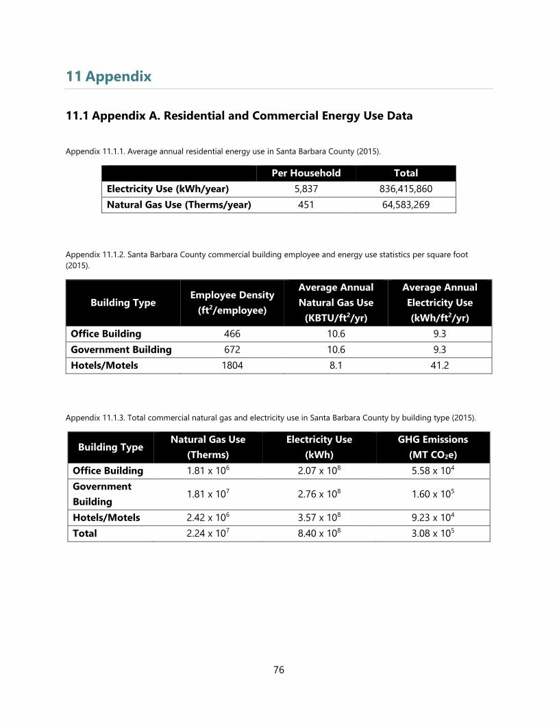
76

11 Appendix

11.1 Appendix A. Residential and Commercial Energy Use Data

Appendix 11.1.1. Average annual residential energy use in Santa Barbara County (2015).

Per Household Total

Electricity Use (kWh/year) 5,837 836,415,860

Natural Gas Use (Therms/year) 451 64,583,269

Appendix 11.1.2. Santa Barbara County commercial building employee and energy use statistics per square foot

(2015).

Building Type Employee Density

(ft2/employee)

Average Annual

Natural Gas Use

(KBTU/ft2/yr)

Average Annual

Electricity Use

(kWh/ft2/yr)

Office Building 466 10.6 9.3

Government Building 672 10.6 9.3

Hotels/Motels 1804 8.1 41.2

Appendix 11.1.3. Total commercial natural gas and electricity use in Santa Barbara County by building type (2015).

Building Type Natural Gas Use

(Therms)

Electricity Use

(kWh)

GHG Emissions

(MT CO2e)

Office Building 1.81 x 106 2.07 x 108 5.58 x 104

Government

Building 1.81 x 107 2.76 x 108 1.60 x 105

Hotels/Motels 2.42 x 106 3.57 x 108 9.23 x 104

Total 2.24 x 107 8.40 x 108 3.08 x 105

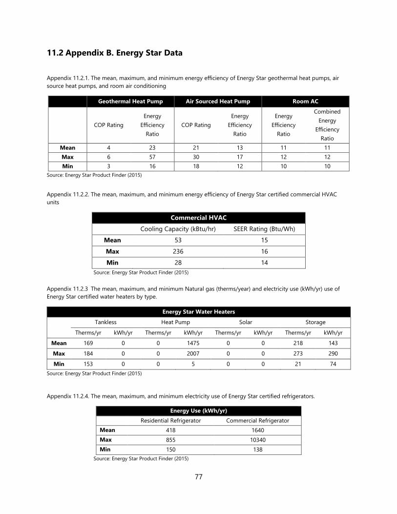
77

11.2 Appendix B. Energy Star Data

Appendix 11.2.1. The mean, maximum, and minimum energy efficiency of Energy Star geothermal heat pumps, air

source heat pumps, and room air conditioning

Geothermal Heat Pump Air Sourced Heat Pump Room AC

COP Rating

Energy

Efficiency

Ratio

COP Rating

Energy

Efficiency

Ratio

Energy

Efficiency

Ratio

Combined

Energy

Efficiency

Ratio

Mean 4 23 21 13 11 11

Max 6 57 30 17 12 12

Min 3 16 18 12 10 10

Source: Energy Star Product Finder (2015)

Appendix 11.2.2. The mean, maximum, and minimum energy efficiency of Energy Star certified commercial HVAC

units

Commercial HVAC

Cooling Capacity (kBtu/hr) SEER Rating (Btu/Wh)

Mean 53 15

Max 236 16

Min 28 14


Appendix 11.2.3. The mean, maximum, and minimum Natural gas (therms/year) and electricity use (kWh/yr) use of

Energy Star certified water heaters by type.

Energy Star Water Heaters

Tankless Heat Pump Solar Storage

Therms/yr kWh/yr Therms/yr kWh/yr Therms/yr kWh/yr Therms/yr kWh/yr

Mean 169 0 0 1475 0 0 218 143

Max 184 0 0 2007 0 0 273 290

Min 153 0 0 5 0 0 21 74


Appendix 11.2.4. The mean, maximum, and minimum electricity use of Energy Star certified refrigerators.

Energy Use (kWh/yr)

Residential Refrigerator Commercial Refrigerator

Mean 418 1640

Max 855 10340

Min 150 138


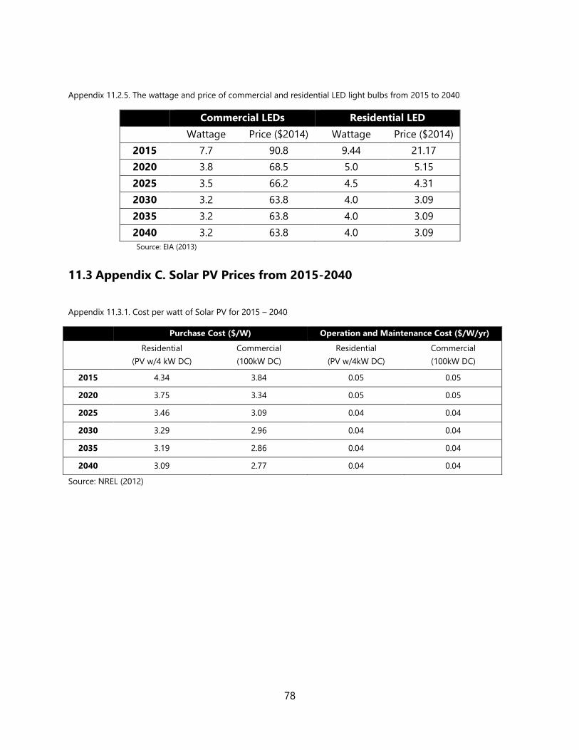
78

Appendix 11.2.5. The wattage and price of commercial and residential LED light bulbs from 2015 to 2040

Commercial LEDs Residential LED

Wattage Price ($2014) Wattage Price ($2014)

2015 7.7 90.8 9.44 21.17

2020 3.8 68.5 5.0 5.15

2025 3.5 66.2 4.5 4.31

2030 3.2 63.8 4.0 3.09

2035 3.2 63.8 4.0 3.09

2040 3.2 63.8 4.0 3.09

Source: EIA (2013)

11.3 Appendix C. Solar PV Prices from 2015-2040

Appendix 11.3.1. Cost per watt of Solar PV for 2015 – 2040

Purchase Cost ($/W) Operation and Maintenance Cost ($/W/yr)

Residential

(PV w/4 kW DC)

Commercial

(100kW DC)

Residential

(PV w/4kW DC)

Commercial

(100kW DC)

2015 4.34 3.84 0.05 0.05

2020 3.75 3.34 0.05 0.05

2025 3.46 3.09 0.04 0.04

2030 3.29 2.96 0.04 0.04

2035 3.19 2.86 0.04 0.04

2040 3.09 2.77 0.04 0.04

Source: NREL (2012)

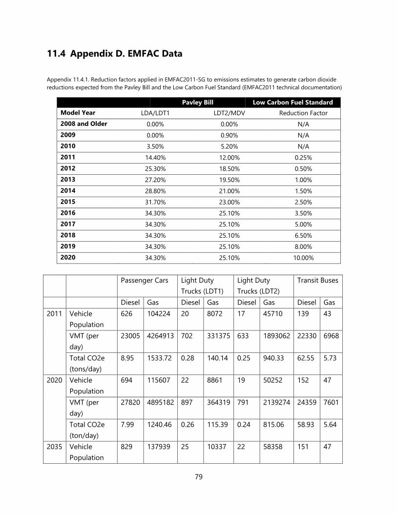
79

11.4 Appendix D. EMFAC Data

Appendix 11.4.1. Reduction factors applied in EMFAC2011-SG to emissions estimates to generate carbon dioxide

reductions expected from the Pavley Bill and the Low Carbon Fuel Standard (EMFAC2011 technical documentation)

Pavley Bill Low Carbon Fuel Standard

Model Year LDA/LDT1 LDT2/MDV Reduction Factor

2008 and Older 0.00% 0.00% N/A

2009 0.00% 0.90% N/A

2010 3.50% 5.20% N/A

2011 14.40% 12.00% 0.25%

2012 25.30% 18.50% 0.50%

2013 27.20% 19.50% 1.00%

2014 28.80% 21.00% 1.50%

2015 31.70% 23.00% 2.50%

2016 34.30% 25.10% 3.50%

2017 34.30% 25.10% 5.00%

2018 34.30% 25.10% 6.50%

2019 34.30% 25.10% 8.00%

2020 34.30% 25.10% 10.00%

Passenger Cars Light Duty

Trucks (LDT1)

Light Duty

Trucks (LDT2)

Transit Buses

Diesel Gas Diesel Gas Diesel Gas Diesel Gas

2011 Vehicle

Population

626 104224 20 8072 17 45710 139 43

VMT (per

day)

23005 4264913 702 331375 633 1893062 22330 6968

Total CO2e

(tons/day)

8.95 1533.72 0.28 140.14 0.25 940.33 62.55 5.73

2020 Vehicle

Population

694 115607 22 8861 19 50252 152 47

VMT (per

day)

27820 4895182 897 364319 791 2139274 24359 7601

Total CO2e

(ton/day)

7.99 1240.46 0.26 115.39 0.24 815.06 58.93 5.64

2035 Vehicle

Population

829 137939 25 10337 22 58358 151 47

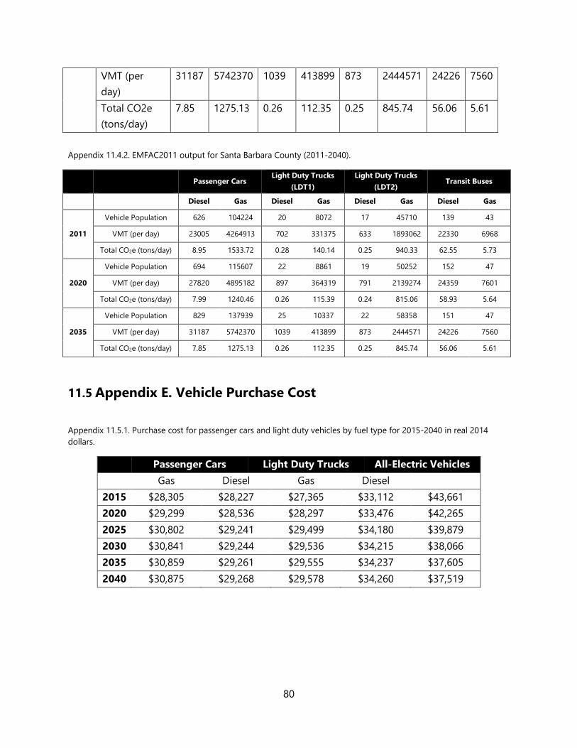
80

VMT (per

day)

31187 5742370 1039 413899 873 2444571 24226 7560

Total CO2e

(tons/day)

7.85 1275.13 0.26 112.35 0.25 845.74 56.06 5.61

Appendix 11.4.2. EMFAC2011 output for Santa Barbara County (2011-2040).

Passenger Cars

Light Duty Trucks

(LDT1)

Light Duty Trucks

(LDT2) Transit Buses

Diesel Gas Diesel Gas Diesel Gas Diesel Gas

2011

Vehicle Population 626 104224 20 8072 17 45710 139 43

VMT (per day) 23005 4264913 702 331375 633 1893062 22330 6968

Total CO2e (tons/day) 8.95 1533.72 0.28 140.14 0.25 940.33 62.55 5.73

2020


VMT (per day) 27820 4895182 897 364319 791 2139274 24359 7601


2035


VMT (per day) 31187 5742370 1039 413899 873 2444571 24226 7560


11.5 Appendix E. Vehicle Purchase Cost

Appendix 11.5.1. Purchase cost for passenger cars and light duty vehicles by fuel type for 2015-2040 in real 2014

dollars.

Passenger Cars Light Duty Trucks All-Electric Vehicles

Gas Diesel Gas Diesel

2015 $28,305 $28,227 $27,365 $33,112 $43,661

2020 $29,299 $28,536 $28,297 $33,476 $42,265

2025 $30,802 $29,241 $29,499 $34,180 $39,879

2030 $30,841 $29,244 $29,536 $34,215 $38,066

2035 $30,859 $29,261 $29,555 $34,237 $37,605

2040 $30,875 $29,268 $29,578 $34,260 $37,519

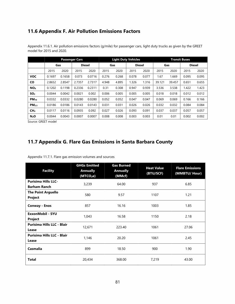
81

11.6 Appendix F. Air Pollution Emissions Factors

Appendix 11.6.1. Air pollution emissions factors (g/mile) for passenger cars, light duty trucks as given by the GREET

model for 2015 and 2020.

Passenger Cars Light Duty Vehicles Transit Buses

Gas Diesel Gas Diesel Gas Diesel

2015 2020 2015 2020 2015 2020 2015 2020 2015 2020 2015 2020

VOC 0.1697 0.1658 0.073 0.0716 0.276 0.268 0.078 0.077 1.67 1.669 0.095 0.095

CO 2.8652 2.8547 2.7357 2.7317 4.948 4.895 1.326 1.316 39.121 39.457 0.651 0.655

NOX 0.1202 0.1198 0.2336 0.2311 0.31 0.308 0.947 0.939 3.536 3.538 1.422 1.423

SO2 0.0044 0.0042 0.0021 0.002 0.006 0.005 0.005 0.005 0.018 0.018 0.012 0.012

PM10 0.0332 0.0332 0.0280 0.0280 0.052 0.052 0.047 0.047 0.069 0.069 0.166 0.166

PM2.5 0.0186 0.0186 0.0143 0.0143 0.031 0.031 0.026 0.026 0.032 0.032 0.084 0.084

CH4 0.0117 0.0116 0.0935 0.092 0.027 0.026 0.093 0.091 0.037 0.037 0.057 0.057

N2O 0.0044 0.0043 0.0007 0.0007 0.008 0.008 0.003 0.003 0.01 0.01 0.002 0.002

Source: GREET model

11.7 Appendix G. Flare Gas Emissions in Santa Barbara County

Appendix 11.7.1. Flare gas emission volumes and sources

Facility

GHGs Emitted

Annually

(MTCO2e)

Gas Burned

Annually

(MMcf)

Heat Value

(BTU/SCF)

Flare Emissions

(MMBTU/ Hour)

Purisima Hills LLC-

Barham Ranch 3,239 64.00 937 6.85

The Point Arguello

Project 580 9.57 1107 1.21

Conway - Enos 857 16.16 1003 1.85

ExxonMobil - SYU

Project 1,043 16.58 1150 2.18

Purisima Hills LLC - Blair

Lease 12,671 223.40 1061 27.06

Purisima Hills LLC - Blair

Lease 1,146 20.20 1061 2.45

Casmalia 899 18.50 900 1.90

Total 20,434 368.00 7,219 43.00

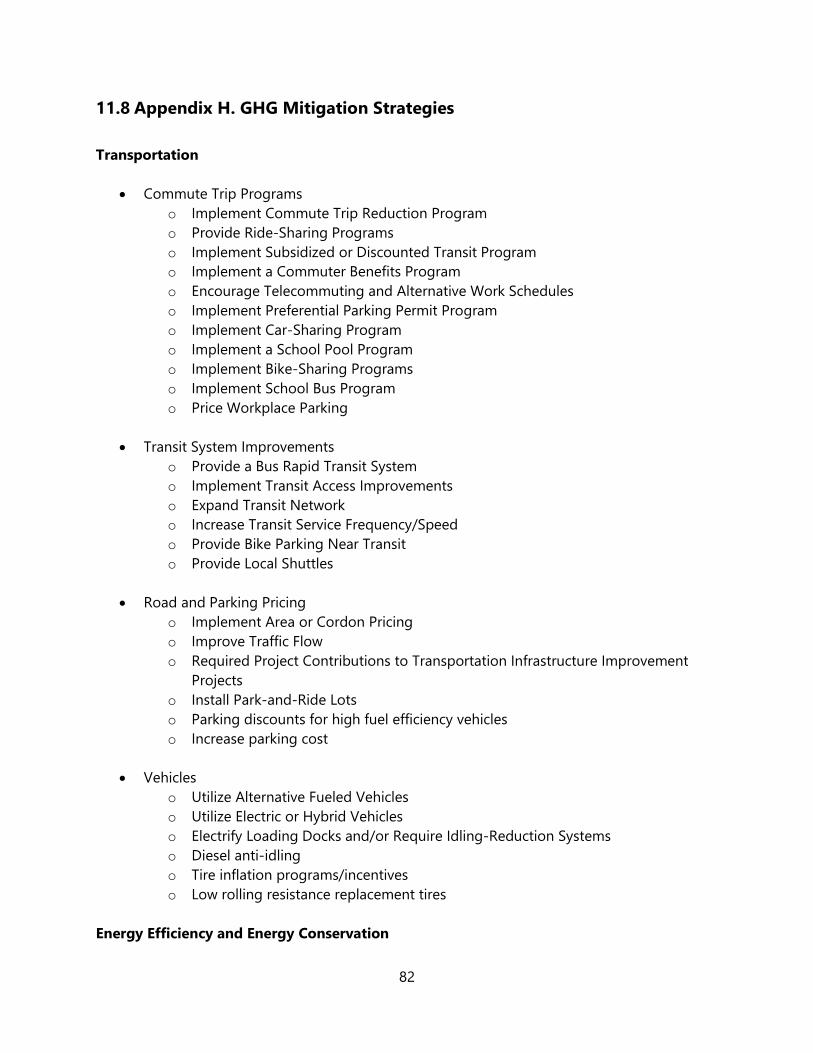
82

11.8 Appendix H. GHG Mitigation Strategies

Transportation

Commute Trip Programs

o Implement Commute Trip Reduction Program

o Provide Ride-Sharing Programs

o Implement Subsidized or Discounted Transit Program

o Implement a Commuter Benefits Program

o Encourage Telecommuting and Alternative Work Schedules

o Implement Preferential Parking Permit Program

o Implement Car-Sharing Program

o Implement a School Pool Program

o Implement Bike-Sharing Programs

o Implement School Bus Program

o Price Workplace Parking

Transit System Improvements

o Provide a Bus Rapid Transit System

o Implement Transit Access Improvements

o Expand Transit Network

o Increase Transit Service Frequency/Speed

o Provide Bike Parking Near Transit

o Provide Local Shuttles

Road and Parking Pricing

o Implement Area or Cordon Pricing

o Improve Traffic Flow

o Required Project Contributions to Transportation Infrastructure Improvement

Projects

o Install Park-and-Ride Lots

o Parking discounts for high fuel efficiency vehicles

o Increase parking cost

Vehicles

o Utilize Alternative Fueled Vehicles

o Utilize Electric or Hybrid Vehicles

o Electrify Loading Docks and/or Require Idling-Reduction Systems

o Diesel anti-idling

o Tire inflation programs/incentives

o Low rolling resistance replacement tires

Energy Efficiency and Energy Conservation

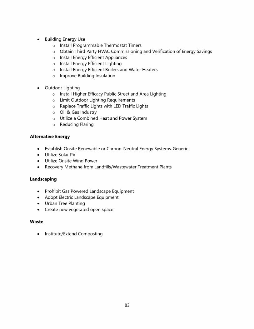
83

Building Energy Use

o Install Programmable Thermostat Timers

o Obtain Third Party HVAC Commissioning and Verification of Energy Savings

o Install Energy Efficient Appliances

o Install Energy Efficient Lighting

o Install Energy Efficient Boilers and Water Heaters

o Improve Building Insulation

Outdoor Lighting

o Install Higher Efficacy Public Street and Area Lighting

o Limit Outdoor Lighting Requirements

o Replace Traffic Lights with LED Traffic Lights

o Oil & Gas Industry

o Utilize a Combined Heat and Power System

o Reducing Flaring

Alternative Energy

Establish Onsite Renewable or Carbon-Neutral Energy Systems-Generic

Utilize Solar PV

Utilize Onsite Wind Power

Recovery Methane from Landfills/Wastewater Treatment Plants

Landscaping

Prohibit Gas Powered Landscape Equipment

Adopt Electric Landscape Equipment

Urban Tree Planting

Create new vegetated open space

Waste

Institute/Extend Composting