Investigating the impact of flow rate ramp-up on Carbon

1 | P a g e

Investigating the impact of flow rate ramp-up on Carbon Dioxide start-up injection Revelation J Samuel1 and Haroun Mahgerefteh

Department of Chemical Engineering, University College London, WC1E 7JE, UK

Received / Accepted / Published

Abstract: Carbon Capture and Storage (CCS) represents the technology for capturing carbon dioxide

(CO2) produced from large emission sources, such as fossil-fuel power plants, transporting and

depositing it in underground geological formations, such as depleted oil and gas fields. CO2 injection

flow rate ramp-up time is essential for the development of optimal injection strategies and best-

practice guidelines for the minimisation of the risks associated with the process. The rate of rapid

quasi-adiabatic Joule-Thomson expansion when high pressure CO2 is injected into a low pressure

injection well if not monitored carefully may lead to significant temperature drops posing several

risks, including: blockage due to hydrate and ice formation with interstitial water. The paper employ

a Homogeneous Equilibrium Mixture (HEM) model, where the mass, momentum, and energy

conservation equations are considered for a mixture of liquid and gaseous phases assumed to be at

thermal and mechanical equilibrium with one another. In particular, this study considers linearly

ramped-up injection mass flow rate from 0 to 38.5 kg/s over 5 minutes (fast), 30 minutes (medium)

and 2 hours (slow). The reliability and applicability of the HEM model is tested against real-life CO2

injection experiment wellbore temperature data obtained from the Ketzin pilot site Brandenburg,

Germany. The ramping up injection mass flow rate simulation results predicted the fast (5 mins)

injection ramp-up as best option for the minimisation of the associated process risks.

Keywords: boundary conditions; carbon capture and storage; CO2 injection; ramp-up; transient

model

1 This work was supported in part by the Petroleum Technology Development Fund (PTDF) under Grant PTDF/E/OSS/PHD/SRJ/717/14 and the Department of Chemical Engineering, University College London. Corresponding author: Revelation Samuel specialises in multi-phase flow modelling, pipeline safety and risk management and CCS. Email: [email protected]; Tel.: +44 2076793809

2 | P a g e

1. Introduction

Carbon Capture and Storage (CCS)

represents the technology for capturing carbon

dioxide (CO2) produced from large point

sources, such as fossil-fuel power plants,

transporting it, e.g. by pipelines, ships or

trucks, and depositing it in underground

geological formations, such as depleted oil and

gas fields or saline aquifers. CCS is widely

recognised as a key technology to meet the

ambitious 2 ºC agreement reached at the Paris

COP 21 meeting (COP 21, 2015; UNFCCC,

2016). While CCS technology is promising, it

is also very expensive, particularly due to the

high costs of capture and compression, which

have been the main focus of recent studies

(Dennis Gammer, 2016). In addition, it has

been pointed out that in order to reduce the

costs of CCS, the integration between the

various elements of its chain should be

considered (IEAGHG, 2015). While this has

been done mainly for CO2 capture/purification

and transport processes, less attention has been

paid to interfacing between the transportation

and storage elements of CCS, which has

become particularly important for the safe and

optimal injection of CO2 into depleted gas

fields (De Koeijer et al, 2014).

Depleted gas fields represent prime potential

targets for the large-scale storage of captured

CO2 emitted from industrial sources and fossil-

fuel power plants (Oldenburg et el, 2001). For

instance, in the case of the UK, the Southern

North Sea and the East Irish Sea depleted gas

reservoirs provide 3.8 of the total 4-billion-

tonne storage capacity required to meet UK’s

CO2 reduction commitments for the period

2020-2050 (Hughes, 2009). Depleted gas

reservoirs are often considered as preferential

for CO2 storage, given their proven capacity to

retain buoyant fluids and the availability of

geological data, such as pressure, porosity and

permeability, derived from years of gas

production (Sanchez Fernandez et al., 2016).

The UK has completed three large FEED study

projects for offshore CO2 storage at Hewett,

Goldeneye and Endurance sites (Cotton, Gray,

& Maas, 2017). In order to further the

development of CCS and boost the confidence

of both private investors and the public in the

deployment of full-chain industrial CCS

systems, it is of paramount importance to

guarantee that the third element of the chain,

i.e. the storage site, will be of high-quality and

operate in safe conditions. A recent study has

investigated the key factors having the highest

impact on the safe storage of CO2 into depleted

oil and gas fields (Hannis et al, 2017). In

particular, key geological storage properties,

such as pressure, temperature, depth and

permeability, can affect injectivity and lead to

variations in the CO2 flow. Therefore, changes

in the operation of the storage sites will require

flow and pressure management within the CO2

transportation network (Sanchez Fernandez et

al., 2016).

The most effective way of transporting the

captured CO2 for subsequent sequestration

using high-pressure pipelines is in the dense

phase (Böser & Belfroid, 2013). The

CO2 arriving at the injection well will typically

be at pressure greater than 70 bar and at

temperature between 4 and 8 ºC. Given the

substantially lower pressure at the wellhead,

the uncontrolled injection of CO2 will result in

its rapid, quasi-adiabatic Joule-Thomson

expansion leading to significant temperature

drops (Curtis M. Oldenburg, 2007). This

process could pose several risks, including:

blockage due to hydrate and ice

formation following contact of the cold

sub-zero CO2 with the interstitial water

around the wellbore and the formation

water in the perforations at the near

well zone;

possible freezing of annular fluids (see

Fig. 2) resulting in potential wellbore

damage.

thermal stress shocking of the wellbore

casing steel as it cools beyond its

specified lowest temperature leading to

its fracture and escape of CO2;

CO2 backflow into the injection system

due to the violent evapouration of the

expanding liquid CO2 upon entry into

the low pressure wellbore.

Samuel and Mahgerefeth / International Journal of Greenhouse Gas Control

3 | P a g e

In order to minimise all these risks, accurate

mathematical models are necessary to simulate

the time-dependent behaviour of the CO2

injected into the well and subsequently released

into the depleted reservoir, and thereby develop

appropriate injection strategies to reduce the

subsequent risks.

A significant amount of research has already

been devoted to the analysis of the injection of

CO2 from wells into underground reservoirs

(André et al, 2007; Goodarzi et al, 2010;

Nordbotten et al, 2005). However, as noted in

Linga & Lund, (2016) and Munkejord et al,

(2016), the analysis of the transient behaviour

of the CO2 flowing inside the injection wells

has received limited attention in the literature,

and more experimental data are needed (De

Koeijer et al., 2014). Lu & Connell, (2008)

discussed a steady-state model to evaluate the

flow of CO2 and its mixtures in non-isothermal

wells. Paterson et al, 2008) simulated the

temperature and pressure profile considering

CO2 liquid-gas phase change in static wells,

assuming a quasi-steady state and neglecting

changes in kinetic energy. Lindeberg, (2011)

proposed a model combining Bernoulli’s

equation for the pressure drop along the well

and a simple heat transfer mechanism between

the fluid and the surrounding rock. The model

was applied to the Sleipner CO2 injection well.

Pan et al, (2011) presented analytical solutions

for steady-state, compressible two-phase flow

through a wellbore under isothermal conditions

using a drift flux model. Lu & Connell, (2014)

investigated a non-isothermal and unsteady

wellbore flow model for multispecies mixtures.

Ruan et al., (2013) and (Jiang et al., 2014)

developed a two-dimensional radial numerical

model to study CO2 temperature increase

mechanisms in the tubing, and the impact of

CO2 injection on the rock temperature in both

axial and radial directions. Xiaolu Li, Xu, Wei,

& Jiang, (2015) developed a model to account

for the dynamics of CO2 into injection wells

subject to highly-transient operations, such as

start-up and shut-in. Linga & Lund, (2016)

discussed a two-fluid model for vertical flow

applied to CO2 injection wells, predicting flow

regimes along the well and computing friction

and heat transfer accordingly. Xiaojiang Li et

al., (2017) presented a unified model for

wellbore flow and heat transfer in pure CO2

injection for geological sequestration, EOR and

fracturing operations. Also recently, Samuel &

Mahgerefteh, (2017) published a paper on

transient flow modelling of the start-up

injection process without ramp-up. The study

shows the consequent effect of quasi-adiabatic

Joule-Thomson expansion when high pressure

CO2 is injected into a low pressure injection

well. Acevedo & Chopra, (2017) conducted a

prior work on transients and start up injection

for the Goldeneye injection well. They studied

the influence of phase behaviour in the well

design of CO2 injectors. The study shows that

during transient operations (closing-in and re-

starting injection operations), a temperature

drop is observed at the top of the well for a

short period of time. This is due to the

reduction of friction caused by a lower

injection rate. The duration of these operations

dictates the extent to which the various well

elements are affected. The sequence of steady

state injection, closing-in operation (30

minutes), closed-in time (10minutes), and

starting-up operation (30minutes) was

simulated for the low reservoir pressure case

using OLGA. However, no publication

critically considered the flowrate ramping up

times studied in this paper.

In this study, we investigate the CO2

injection flow rate ramp-up times which is

driven by the need for the development of

optimal injection strategies and best-practice

guidelines for the minimisation of the risks

associated with the process. Investigating

injection flow rate ramp-up is essential in

understanding the rate of rapid, quasi-adiabatic

Joule-Thomson expansion when high pressure

CO2 is injected into a low pressure injection

well. A Homogeneous Equilibrium Model

(HEM), where the mass, momentum, and

energy conservation equations are considered

for a mixture of liquid and gaseous phases

assumed to be at thermal and mechanical

equilibrium with one another is employed.

Fluid/wall friction, gravitational force, and heat


4 | P a g e

transfer between the fluid and the outer well

layers are also taken into account.

2. Development of mathematical model

Fig. 1 shows a schematic flow diagram of a

typical injection well. A control volume

consisting of a section of the tube is considered

for the analysis and derivation of model

governing equations.

Fig. 1: Schematic representation of a control

volume within a vertical pipe and the forces

acting on it

Where 𝐹𝑃, 𝐹𝑓, 𝐹𝑔, 𝜌 and 𝑢 are pressure

force, frictional force, gravitational force, fluid

density and velocity respectively. L, Dp and ∆𝑥

are well depth, diameter and differential

control volume.

This study considers a purely vertical

injection tube only hence, pipe inclination is

unaccounted for. The following simplified

assumptions are applied:

One-dimensional flow in the pipe

Homogeneous equilibrium fluid flow

Negligible fluid structure interaction

through vibrations

Constant cross section area of pipe

The assumption of homogeneous

equilibrium flow means that all phases are at

mechanical and thermal equilibrium (i.e.

phases are flowing with same velocity and

temperature) hence the three conservation

equations should be applied for the fluid

mixture. Although, in practice usually the

vapour phase travels faster than the liquid

phase, the HEM model has been investigated

proven to have an acceptable accuracy in many

practical applications.

The following gives a detailed account of

the HEM model employed for the simulation of

the time-dependent flow of CO2 in injection

wells. The system of four partial differential

equations for the CO2 liquid/gas mixture, to be

solved in the well tubing, can be written in the

well-known conservative form as follows:

𝜕

𝜕𝑡𝑸 +

𝜕

𝜕𝑥𝑭(𝑸) = 𝑺𝟏 + 𝑺𝟐 (1)

where

𝑸 = (

𝜌𝐴𝜌𝑢𝐴𝜌𝐸𝐴𝐴

) , 𝑭(𝑸)

= (

𝜌𝑢𝐴

𝜌𝑢2𝐴 + 𝐴𝑃𝜌𝑢𝐻𝐴0

), 𝑺𝟏

=

(

0

𝑃𝜕𝐴

𝜕𝑥00 )

, 𝑺𝟐

= (

0𝐴(𝐹 + 𝜌𝛽𝑔)

𝐴(𝐹𝑢 + 𝜌𝑢𝛽𝑔 + 𝑞)0

)

(2)

In the above, the first three equations

correspond to mass, momentum, and energy

conservation, respectively. The fourth equation

describes the fact that the cross-sectional area


5 | P a g e

𝐴 is, at any location along the well, constant in

time, but might vary along the depth of the

well. Moreover, 𝑢 and 𝜌 are the mixture

velocity and density, respectively. 𝑃 is the

mixture pressure, while 𝐸 and 𝐻 represent the

specific total energy and total enthalpy of the

mixture, respectively. They are defined as:

𝐸 = 𝑒 + 1

2 𝑢2 (3)

𝐻 = 𝐸 + 𝑃

𝜌 (4)

where 𝑒 is the specific internal energy. In

addition, 𝑥 denotes the space coordinate, 𝑡 the

time, 𝐹 the viscous friction force, 𝑞 the heat

flux, and 𝑔 the gravitational acceleration. In the

case of the HEM, the assumption of

mechanical equilibrium, i.e. no phase slip, is

retained.

The system of partial differential Eq. (2) is

an extension of the work previously done in

(Curtis M. Oldenburg, 2007), (Celia &

Nordbotten, 2009), by accounting for both a

variable cross-sectional area and additional

source terms. By analysing in more detail the

various source terms appearing on the right-

hand side of Eq. (2).

The frictional loss 𝐹 in Eq. (2) can be

expressed as

𝐹 = −𝑓𝑤𝜌𝑢2

𝐷𝑝 (5)

where 𝑓𝑤 is the Fanning friction factor,

calculated using Chen’s correlation (Chen,

1979), and 𝐷𝑝 is the internal diameter of the

pipe.

The gravitational term includes

𝛽 = 𝜌𝑔 sin 𝜃 (6)

which accounts for the possible well

deviation.

In Eq. (2) the source term 𝑄 accounts for the

heat exchange between the fluid and the well

wall. The corresponding heat transfer

coefficient 𝜂 is calculated using the well-

known Dittus-Boelter correlation (Dittus &

Boelter, 1930):

𝜂 = 0.023 𝑅𝑒0.8𝑃𝑟0.4𝑘

𝐷𝑝 (7)

where 𝑘, 𝑅𝑒 and 𝑃𝑟 are the thermal

conductivity, Reynold’s number and Prandtl’s

number for the fluid. The heat exchanged

between the fluid and the wall is calculated

using the following formula:

𝑞 = 4

𝐷𝑝𝜂(𝑇𝑤 − 𝑇) (8)

𝑇𝑤 and 𝑇 are the temperatures of the fluid

and of the wall, respectively. Note that 𝑇𝑤 =𝑇𝑤(𝑥, 𝑡), i.e. 𝑇𝑤 is not assumed constant, but

variable with time and space.

2.1. Boundary conditions

In order to close the conservation Eq. (2),

suitable boundary conditions must be specified.

In this study, the boundary conditions are

implemented by introducing ’ghost cells’ on

both ends of the computational domain,

representing the wellhead and bottom-hole.

2.1.1. Top of the well

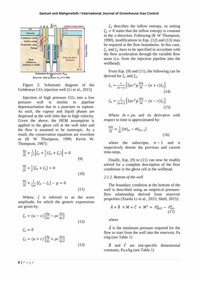
At the wellhead, Fig. 2 is a schematic

representation of the flow through the

wellbore. As can be seen in Fig. 2, CO2 is

injected into the well at the top and exit at the

bottom into the reservoir. The injection strings

are tapered and narrower going down the well.

This allows the rapid injection of CO2 and

minimises the pressure drop along the

wellbore. The development of the required

inlet boundary condition for simulating CO2

injection is detailed below.


6 | P a g e

Figure 2: Schematic diagram of the

Goldeneye CO2 injection well (Li et al., 2015)

Injection of high pressure CO2 into a low

pressure well is similar to pipeline

depressurisation due to a puncture or rupture.

As such, the vapour and liquid phases are

dispersed at the well inlet due to high velocity.

Given the above, the HEM assumption is

applied in the ghost cell at the well inlet and

the flow is assumed to be isentropic. As a

result, the conservation equations are rewritten

as (K W Thompson, 1990; Kevin W.

Thompson, 1987):

𝜕𝜌

𝜕𝑡+

1

𝑐2[𝜁2 +

1

2(𝜁3 + 𝜁1)] = 0

(9)

𝜕𝑝

𝜕𝑡+1

2[𝜁3 + 𝜁1] = 0

(10)

𝜕𝑢

𝜕𝑡+

1

2𝜌𝑐[𝜁3 − 𝜁1] − 𝑔 = 0

(11)

Where, 𝜁 is referred to as the wave

amplitude, for which the generic expressions

are given by:

𝜁1 = (𝑢 − 𝑐) {𝜕𝑝

𝜕𝑥− 𝜌𝑐

𝜕𝑢

𝜕𝑥}

(12)

𝜁2 = 0

𝜁3 = (𝑢 + 𝑐) {𝜕𝑝

𝜕𝑥+ 𝜌𝑐

𝜕𝑢

𝜕𝑥}

(13)

𝜁2 describes the inflow entropy, so setting

𝜁2 = 0 states that the inflow entropy is constant

in the 𝑥-direction. Following (K W Thompson,

1990), modifications to Eqs. (12) and (13) may

be required at the flow boundaries. In this case,

𝜁1 and 𝜁3 have to be specified in accordant with

the flow acceleration through the variable flow

areas (i.e. from the injection pipeline into the

wellhead).

From Eqs. (9) and (11), the following can be

derived for 𝜁1 and 𝜁3:

𝜁1 =1

(𝑢−𝑐){2𝜌𝑐2𝑔

𝜕�̇�

𝜕𝑡− (𝑢 + 𝑐)𝜁3}

(14)

𝜁3 =1

(𝑢+𝑐){2𝜌𝑐2𝑔

𝜕�̇�

𝜕𝑡− (𝑢 − 𝑐)𝜁1}

(15)

Where �̇� = 𝜌𝑢 and its derivative with

respect to time is approximated by:

𝜕�̇�

𝜕𝑡=

1

∆𝑡[�̇�|𝑛 − �̇�|𝑛−1]

(16)

where the subscripts, 𝑛 − 1 and 𝑛

respectively denote the previous and current

time-steps.

Finally, Eqs. (9) to (11) can now be readily

solved for a complete description of the flow

conditions in the ghost cell at the wellhead.

2.1.2. Bottom of the well

The boundary condition at the bottom of the

well is described using an empirical pressure-

flow relationship derived from reservoir

properties (Xiaolu Li et al., 2015; Shell, 2015):

�̃� + �̃� × 𝑀 + �̃� × 𝑀2 = 𝑃𝐵𝐻𝑃2 − 𝑃𝑟𝑒𝑠

2 (17)

where

�̃� is the minimum pressure required for the

flow to start from the well into the reservoir, Pa

s/kg (see Table 1)

�̃� and �̃� are site-specific dimensional

constants, Pa.s/kg (see Table 1)


7 | P a g e

𝑀 is the instantaneous mass flow rate at the

bottom-hole, kg/s

𝑃𝐵𝐻𝑃 is the instantaneous bottom-hole

pressure, bar and

𝑃𝑟𝑒𝑠 is the reservoir static pressure, bar.

The right hand side of Eq. (17) represent the

pressure differential between the bottom of the

well and the reservoir. Significantly, when

𝑃𝐵𝐻𝑃2 > 𝑃𝑟𝑒𝑠

2 there is injection into the

reservoir whereas when 𝑃𝐵𝐻𝑃2 < 𝑃𝑟𝑒𝑠

2 there is a

backflow or blowout. In other words, the

boundary condition at the bottom of the well

can be discretely utilised to satisfy both

injection and blowout cases. In describing the

relationship between the reservoir and the

bottom of the well, Eq. (17) represents a more

sophisticated condition than a standard, linear

correlation between the bottom-hole pressure

and the flow rate.

3. Numerical method and injection well CO2

inlet conditions

In this study, an effective model based on

the Finite Volume Method (FVM),

incorporating a conservative Godunov type

finite-difference scheme (Godunov 1959,

Radvogin et al. 2011, Cumber et al. 1994) is

used. The FVM is well-established and

thoroughly validated CFD technique. In

essence, the methodology involves the

integration of the fluid flow equations over the

entire control volumes of the solution domain

and then accurate calculation of the fluxes

through the boundaries of the computed cells.

For the purpose of numerical solution of the

governing equations they are written in a

vector form (Toro 2010):

𝜕�⃗�

𝜕𝑡+𝜕𝑓

𝜕𝑧= 𝑆 ,

(18)

where

�⃗� = (𝜌 , 𝜌𝑢 , 𝜌𝑒)𝑇,

𝐹 = (𝜌𝑢 , (𝜌𝑢2 + 𝑃) ,

𝑢( 𝜌𝑢𝑒 + 𝜌𝑢2 + 𝑃))𝑇

𝑆 = (𝑆𝑚, 𝑆𝑚𝑜𝑚, 𝑆𝑒)𝑇

(19)

�⃗� , 𝐹 and 𝑆 are the vectors of conserved

variables, fluxes and source terms respectively.

The source terms 𝑆𝑚, 𝑆𝑚𝑜𝑚and 𝑆𝑒 describe the

effects of mass, momentum and energy

exchange between the fluid and its surrounding

respectively, as well as friction and heat

exchange at the pipe wall.

3.1 Model Validation

The model relevance and applicability to

real-world injection project is validated using

Ketzin pilot site experimental data. The model

predictions are closely in agreement with the

real-life CO2 injection scenario.

CO2 injection well initial and boundary

conditions for Ketzin pilot site Brandenburg,

Germany obtained from Möller et al, (2014)

employed for the model validation are:

CO2 inlet pressure 57 bar, temperatures

10 oC and 20 oC, and injection mass

flow rate 0.41 kg/s

Initial wellhead pressure 48 bar and

temperature 10 oC,

Total well depth 550m; 0.0889m

internal diameter

Initial bottom-hole pressure 68 bar and

temperature 33 oC,

As can be seen in Figs. 3 and 4, the

simulation results for 10oC and 20oC injection

inlet temperature condition all showed good

agreement with the experimental data. The

performance of our model in relation to the

Ketzin pilot real-world experimental injection

project shows it reliability and applicability.


8 | P a g e

Figure 3: Well temperature profile for 10oC

inlet CO2 injection temperature

Figure 4: Well temperature profile for 20oC

inlet CO2 injection temperature

4. Injection well and CO2 inlet conditions

The data used in this study obtained from

the Peterhead CCS project include the well

depth and pressure and temperature profiles,

along with the surrounding formation

characteristics as presented in (Xiaolu Li et al.,

2015; Shell UK, 2015) and reproduced in Table

1. The Peterhead CCS project was proposed to

capture one million tonnes of CO2 per annum

for 15 years from an existing combined cycle

gas turbine located at Peterhead Power Station

in Aberdeenshire, Scotland. In the project, the

CO2 captured from the Peterhead Power

Station would have been transported by

pipeline and then injected into the depleted

Goldeneye reservoirs. Despite the cancellation

of the project funding, useful information was

already available, given that the Goldeneye

reservoir had been used for extraction of

natural gas for many years.

Table 1: Goldeneye injection well and CO2

inlet conditions (Shell UK, 2015)

Input parameter Value

Wellhead pressure,

bar 36

Wellhead

temperature, K 277

Bottom-hole

temperature, K 353

Well

diameter/depth, m

0 – 800m depth:

0.125m

800 – 2000m depth:

0.0765m

2000–2582m depth:

0.0625m

CO2 injection mass

flow rate, kg/s

3 different cases:

linearly ramped-up

to 38.5 kg/s in 5

minutes, 30 minutes

and 2 hours

Injection tube

diameter, m 0.125m

CO2 inlet pressure,

bar 115

CO2 inlet

temperature, K 280

Outflow

�̃� = 0

�̃� = 1.3478 × 1012 Pa2s/kg

�̃� = 2.1592 × 1010 Pa2s2/kg2

𝑃𝑟𝑒𝑠 = 172 bar


9 | P a g e

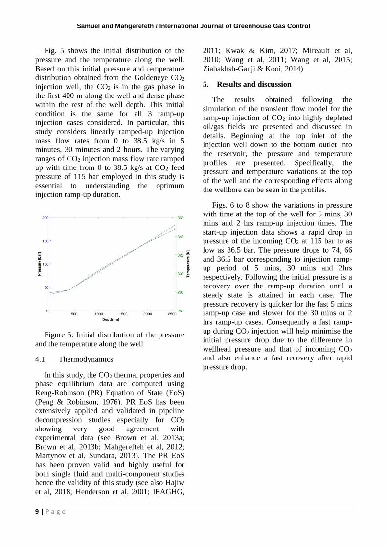
Fig. 5 shows the initial distribution of the

pressure and the temperature along the well.

Based on this initial pressure and temperature

distribution obtained from the Goldeneye CO2

injection well, the CO2 is in the gas phase in

the first 400 m along the well and dense phase

within the rest of the well depth. This initial

condition is the same for all 3 ramp-up

injection cases considered. In particular, this

study considers linearly ramped-up injection

mass flow rates from 0 to 38.5 kg/s in 5

minutes, 30 minutes and 2 hours. The varying

ranges of CO2 injection mass flow rate ramped

up with time from 0 to 38.5 kg/s at CO2 feed

pressure of 115 bar employed in this study is

essential to understanding the optimum

injection ramp-up duration.

Figure 5: Initial distribution of the pressure

and the temperature along the well

4.1 Thermodynamics

In this study, the CO2 thermal properties and

phase equilibrium data are computed using

Reng-Robinson (PR) Equation of State (EoS)

(Peng & Robinson, 1976). PR EoS has been

extensively applied and validated in pipeline

decompression studies especially for CO2

showing very good agreement with

experimental data (see Brown et al, 2013a;

Brown et al, 2013b; Mahgerefteh et al, 2012;

Martynov et al, Sundara, 2013). The PR EoS

has been proven valid and highly useful for

both single fluid and multi-component studies

hence the validity of this study (see also Hajiw

et al, 2018; Henderson et al, 2001; IEAGHG,

2011; Kwak & Kim, 2017; Mireault et al,

2010; Wang et al, 2011; Wang et al, 2015;

Ziabakhsh-Ganji & Kooi, 2014).

5. Results and discussion

The results obtained following the

simulation of the transient flow model for the

ramp-up injection of CO2 into highly depleted

oil/gas fields are presented and discussed in

details. Beginning at the top inlet of the

injection well down to the bottom outlet into

the reservoir, the pressure and temperature

profiles are presented. Specifically, the

pressure and temperature variations at the top

of the well and the corresponding effects along

the wellbore can be seen in the profiles.

Figs. 6 to 8 show the variations in pressure

with time at the top of the well for 5 mins, 30

mins and 2 hrs ramp-up injection times. The

start-up injection data shows a rapid drop in

pressure of the incoming CO2 at 115 bar to as

low as 36.5 bar. The pressure drops to 74, 66

and 36.5 bar corresponding to injection ramp-

up period of 5 mins, 30 mins and 2hrs

respectively. Following the initial pressure is a

recovery over the ramp-up duration until a

steady state is attained in each case. The

pressure recovery is quicker for the fast 5 mins

ramp-up case and slower for the 30 mins or 2

hrs ramp-up cases. Consequently a fast ramp-

up during CO2 injection will help minimise the

initial pressure drop due to the difference in

wellhead pressure and that of incoming CO2

and also enhance a fast recovery after rapid

pressure drop.


10 | P a g e

Figure 6: CO2 wellhead pressure variation with

time for 5 mins ramp-up injection case

Figure 7: CO2 wellhead pressure variation with

time for 30 mins ramp-up injection case

Figure 8: CO2 wellhead pressure variation

with time for 2 hrs ramp-up injection case

As can be seen in Fig. 9 where all three

ramp-up cases are shown together. The 5 mins

ramp-up case predicts a lesser pressure drop

and high recovery compared with the other

cases of 30 mins and 2 hrs ramp-up. This

implies that for best practice a fast ramp-up is

recommended to minimise the risk of large

pressure drop and a corresponding low

temperature. This shows that the injected CO2

undergoes a refrigeration effect caused by the

Joule-Thomson expansion.

Figure 9: CO2 wellhead pressure profiles for 5

mins, 30 mins and 2 hrs ramp-up injection

cases

Figs. 10 to 12 show the variations in

temperature with time at the top of the well for

5 mins, 30 mins and 2 hrs ramp-up injection

times. The start-up injection data shows a rapid

drop in temperature of the incoming CO2 from


11 | P a g e

277 K to as low 226 K. The temperature drops

to 252, 238 and 226 K corresponding to

injection ramp-up period of 5 mins, 30 mins

and 2hrs respectively. Following the initial

temperature drop is a recovery over the ramp-

up duration until a steady state is attained in

each case. The temperature recovery however

gets better with increasing ramp-up duration.

The predicted steady-state temperatures after

recovery for the fast 5 mins ramp-up case and

slower for the 30 mins or 2 hrs ramp-up cases

are respectively 277, 280 and 303 K.

Consequently a fast ramp-up during CO2 start-

up injection will help minimise this initial

temperature drop due to the difference in the

pressure at top of the injection well and that of

the incoming CO2. Also, in order to enhance a

fast recovery after the initial rapid pressure and

temperature drop.

Figure 10: CO2 wellhead temperature variation

with time for 5 mins ramp-up injection case


with time for 30 mins ramp-up injection case


with time for 2 hrs ramp-up injection case

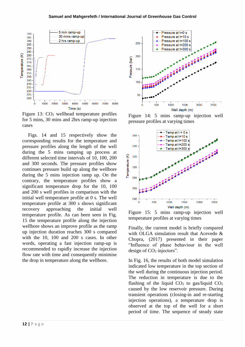
As can be seen in Fig. 13 where all three

ramp-up cases of CO2 wellhead temperature

profiles are shown together. The 5 mins ramp-

up case predicts a lesser temperature drop

compared with the other cases of 30 mins and 2

hrs ramp-up. This implies that for best practice

a fast (5 mins) ramp-up is recommended to

minimise the risk of large temperature drop. In

simply terms, the fast ramp-up is exposed to a

short time refrigeration effect caused by the

Joule-Thomson expansion.


12 | P a g e

Figure 13: CO2 wellhead temperature profiles

for 5 mins, 30 mins and 2hrs ramp-up injection

cases

Figs. 14 and 15 respectively show the

corresponding results for the temperature and

pressure profiles along the length of the well

during the 5 mins ramping up process at

different selected time intervals of 10, 100, 200

and 300 seconds. The pressure profiles show

continues pressure build up along the wellbore

during the 5 mins injection ramp up. On the

contrary, the temperature profiles show a

significant temperature drop for the 10, 100

and 200 s well profiles in comparison with the

initial well temperature profile at 0 s. The well

temperature profile at 300 s shows significant

recovery approaching the initial well

temperature profile. As can been seen in Fig.

15 the temperature profile along the injection

wellbore shows an improve profile as the ramp

up injection duration reaches 300 s compared

with the 10, 100 and 200 s cases. In other

words, operating a fast injection ramp-up is

recommended to rapidly increase the injection

flow rate with time and consequently minimise

the drop in temperature along the wellbore.

Figure 14: 5 mins ramp-up injection well

pressure profiles at varying times

Figure 15: 5 mins ramp-up injection well

temperature profiles at varying times

Finally, the current model is briefly compared

with OLGA simulation result that Acevedo &

Chopra, (2017) presented in their paper

“Influence of phase behaviour in the well

design of CO2 injectors”.

In Fig. 16, the results of both model simulation

indicated low temperature in the top section of

the well during the continuous injection period.

The reduction in temperature is due to the

flashing of the liquid CO2 to gas/liquid CO2

caused by the low reservoir pressure. During

transient operations (closing-in and re-starting

injection operations), a temperature drop is

observed at the top of the well for a short

period of time. The sequence of steady state


13 | P a g e

injection, closing-in operation (30 minutes),

closed-in time (10minutes), and starting-up

operation (30minutes) for the low reservoir

pressure case was simulated using OLGA

(Acevedo & Chopra, 2017) and our model, see

Figure 16. As can be seen the current model

predicted slightly lower CO2 temperatures than

OLGA. This is likely due to the inconsistency

of the Peng-Robinson Equation of State

employed in the current study for the

prediction of CO2 thermodynamics properties.

Figure 16: Comparison of temperature profiles

at the top of the well sequence of closing and

opening a CO2 injector well

6. Conclusions and recommendations

This study has led to the development and

testing of a rigorous model for the simulation

of the highly-transient multi-phase flow

phenomena taking place in wellbores during

the start-up injection of high pressure CO2 into

depleted gas fields. In practice, the model

developed can serve as a valuable tool for the

development of optimal injection strategies and

best-practice guidelines for the minimisation of

the risks associated with the start-up injection

of CO2 into depleted gas fields. In order to

assess key parameters having the greatest

impact on the transient flow of CO2 in the

injection well, sensitivity analysis has been

performed over several parameters by different

authors. However, varying injection ramping

up times considered in this study has never

been studied in previous publications. As such,

this study introduces a new area of

consideration and gives a clearer insight on the

effects of CO2 injection ramp-up times on the

wellbore pressure and temperature profiles.

The importance of investigating the injection

flow rates ramp-up times is driven by the need

for the development of optimal injection

strategies and best-practice guidelines for the

minimisation of the risks associated with the

process.

Based on the application of the model

developed in this work to realistic test cases

involving the ramping up of CO2 injection flow

rates from 0 to 38.5 kg/s into the Goldeneye

depleted reservoir in the North Sea following

fast (5 mins), medium (30 mins) and slow (2

hrs) injection ramp-up times, the main findings

and recommendations of this work can be

summarised as follows:

The degree of cooling along the

injection well becomes less severe with

a decrease in the injection ramp-up

duration. In other words, operating a

fast start-up injection ramp-up is

recommended (i.e. between 5 and 30

mins) rather than a slower one (over 2

hrs). This is due the limited exposure

time to the refrigeration effect caused

by the JT expansion on the injected

CO2.

The formation of ice during the ramp

up injection process is likely, given that

in all cases considered the minimum

fluid temperature falls well below 0 oC

at the top of the well. This poses the

risk of ice formation and ultimately

well blockage should a sufficient

quantity of water be present. Thus, for

this case study injecting CO2 at

temperatures well above 290 K at flow

rate ramp-up duration of 5 mins will be

best practice to minimise this risk.

The minimum simulated CO2

temperature and the corresponding

pressure predicted at the top of well

during the start-up injection flow rate


14 | P a g e

ramp-up process are close to the ranges

where CO2 hydrates formation would

be expected. The ideal hydrate

formation conditions are pressures and

temperatures below 273.15 K and 12.56

bar however, tiny molecules of CO2

hydrates begin formation at pressures

and temperatures just below 283 K and

49.99 bar (Circone et al., 2003; Yang et

al., 2012).

Given the observed relatively large

drop in temperature at the top of the

well especially for the 2 hrs injection

flow ramp-up case, well failure due to

thermal stress shocking (i.e. as a result

of the temperature gradient between

inner and outer layers of the steel

casing) during the injection process

could be a real risk. This could lead to a

brittle fracture situation should the

temperature drops below –30 oC. The

design temperature at which steel

becomes highly brittle according the

Stainless Steel Information Centre of

North America. Hence, the risk of

injection system failure due to thermal

stress shocking of the steel casing can

be avoided by keeping to a fast or

medium injection flow ramp-up.

Finally, it is critically important to bear in mind

that the above conclusions are not universal.

On the contrary, they are only based on the

case study investigated. Each injection scenario

must be individually examined in order to

determine the likely risks. In this paper, the

necessary computational tool is developed to

make such risks assessment.

7. References

Acevedo, L., & Chopra, A. (2017). Influence

of Phase Behaviour in the Well Design of

CO2Injectors. Energy Procedia,

114(November 2016), 5083–5099.

http://doi.org/10.1016/j.egypro.2017.03.16

63

André, L., Audigane, P., Azaroual, M., &

Menjoz, A. (2007). Numerical modeling

of fluid-rock chemical interactions at the

supercritical CO2-liquid interface during

CO2 injection into a carbonate reservoir,

the Dogger aquifer (Paris Basin, France).

Energy Conversion and Management,

48(6), 1782–1797.

http://doi.org/10.1016/j.enconman.2007.0

1.006

Böser, W., & Belfroid, S. (2013). Flow

Assurance Study. Energy Procedia, 37,

3018–3030.


8

Brown, S., Beck, J., Mahgerefteh, H., & Fraga,

E. S. (2013). Global sensitivity analysis of

the impact of impurities on CO2 pipeline

failure. Reliability Engineering and

System Safety, 115, 43–54.

http://doi.org/10.1016/j.ress.2013.02.006

Brown, S., Martynov, S., Mahgerefteh, H., &

Proust, C. (2013). A homogeneous

relaxation flow model for the full bore

rupture of dense phase CO2 pipelines.

International Journal of Greenhouse Gas

Control, 17, 349–356.

http://doi.org/10.1016/j.ijggc.2013.05.020

Celia, M. a., & Nordbotten, J. M. (2009).

Practical modeling approaches for

geological storage of carbon dioxide.

Ground Water, 47(5), 627–638.

http://doi.org/10.1111/j.1745-

6584.2009.00590.x

Chen, N. H. (1979). An Explicit Equation for

Friction Factor in Pipe. Industrial &

Engineering Chemistry Fundamentals,

18(3), 296–297.

http://doi.org/10.1021/i160071a019

Circone, S., Stern, L. a., Kirby, S. H., Durham,

W. B., Chakoumakos, B. C., Rawn, C. J.,

… Ishii, Y. (2003). CO 2

Hydrate: Synthesis, Composition,

Structure, Dissociation Behavior, and a

Comparison to Structure I CH 4 Hydrate.

The Journal of Physical Chemistry B,


15 | P a g e

107(23), 5529–5539.

http://doi.org/10.1021/jp027391j

COP 21. (2015). COP 21 Paris France

Sustainable Innovation Forum 2015

working with UNEP.

Cotton, A., Gray, L., & Maas, W. (2017).

Learnings from the Shell Peterhead CCS

Project Front End Engineering Design.

Energy Procedia, 114, 5663–5670.

http://doi.org/10.1016/J.EGYPRO.2017.0

3.1705

De Koeijer, G., Hammer, M., Drescher, M., &

Held, R. (2014). Need for experiments on

shut-ins and depressurizations in

CO2injection wells. In Energy Procedia

(Vol. 63, pp. 3022–3029). Elsevier B.V.


5

Dennis Gammer. (2016). Reducing the cost of

CCS - Developments in Capture Plant… |

The ETI. Retrieved from

http://www.eti.co.uk/insights/reducing-

the-cost-of-ccs-developments-in-capture-

plant-technology/

Dittus, F. W., & Boelter, L. M. K. (1930). Heat

Transfer in Automobile Radiators, 2, 443.

Goodarzi, S., Settari, A., Zoback, M. D., &

Keith, D. (2010). Thermal Aspects of

Geomechanics and Induced Fracturing in

CO2 Injection With Application to CO2

Sequestration in Ohio River Valley. SPE

International Conference on CO2

Capture, Storage, and Utilization. Society

of Petroleum Engineers.

http://doi.org/10.2118/139706-MS

Hajiw, M., Corvisier, J., Ahmar, E. El, &

Coquelet, C. (2018). Impact of impurities

on CO2 storage in saline aquifers:

Modelling of gases solubility in water.


Control, 68, 247–255.

http://doi.org/10.1016/J.IJGGC.2017.11.0

17

Hannis, S., Pearce, J., Chadwick, A., & Kirk,

K. (2017). IEAGHG Technical Report

January 2017 Case Studies of CO 2

Storage in Depleted Oil and Gas Fields,

(January).

Henderson, N., de Oliveira, J. R., Souto, H. P.

A., & Marques, R. P. (2001). Modeling

and Analysis of the Isothermal Flash

Problem and Its Calculation with the

Simulated Annealing Algorithm.

Industrial & Engineering Chemistry

Research, 40(25), 6028–6038.

http://doi.org/10.1021/ie001151d

Hughes, D. S. (2009). Carbon storage in

depleted gas fields: Key challenges.

Energy Procedia, 1(1), 3007–3014.


8

IEAGHG. (2015). Carbon Capture and Storage

Cluster Projects: Review and Future

Opportunities, (April).

IEAGHG (International Energy Agency

greenhouse gas emissions). (2011).

Effects of Impurities on Geological

Storage of CO2, (June), Report: 2011/04.

Jiang, P., Li, X., Xu, R., Wang, Y., Chen, M.,

Wang, H., & Ruan, B. (2014). Thermal

modeling of CO2 in the injection well and

reservoir at the Ordos CCS demonstration

project, China. International Journal of

Greenhouse Gas Control, 23, 135–146.


Kwak, D.-H., & Kim, J.-K. (2017). Techno-

economic evaluation of CO2 enhanced oil

recovery (EOR) with the optimization of

CO2 supply. International Journal of



Li, X., Li, G., Wang, H., Tian, S., Song, X., Lu,

P., & Wang, M. (2017). International

Journal of Greenhouse Gas Control A

unified model for wellbore flow and heat

transfer in pure CO 2 injection for


16 | P a g e

geological sequestration , EOR and

fracturing operations. International

Journal of Greenhouse Gas Control, 57,

102–115.


Li, X., Xu, R., Wei, L., & Jiang, P. (2015).

Modeling of wellbore dynamics of a CO2

injector during transient well shut-in and

start-up operations. International Journal

of Greenhouse Gas Control, 42, 602–614.


Lindeberg, E. (2011). Modelling pressure and

temperature profile in a CO2 injection

well. Energy Procedia, 4, 3935–3941.


2

Linga, G., & Lund, H. (2016). A two-fluid

model for vertical flow applied to CO2

injection wells. International Journal of



Lu, M., & Connell, L. D. (2008). Non-

isothermal flow of carbon dioxide in

injection wells during geological storage.


Control, 2(2), 248–258.

http://doi.org/10.1016/S1750-

5836(07)00114-4

Lu, M., & Connell, L. D. (2014). The transient

behaviour of CO2 flow with phase

transition in injection wells during

geological storage – Application to a case

study. Journal of Petroleum Science and

Engineering, 124, 7–18.

http://doi.org/10.1016/j.petrol.2014.09.02

4

Mahgerefteh, H., Brown, S., & Denton, G.

(2012). Modelling the impact of stream

impurities on ductile fractures in CO2

pipelines. Chemical Engineering Science,

74, 200–210.

http://doi.org/10.1016/j.ces.2012.02.037

Martynov, S., Brown, S., Mahgerefteh, H., &

Sundara, V. (2013). Modelling choked

flow for CO2 from the dense phase to

below the triple point. International


552–558.


Mireault, R. A., Stocker, R., Dunn, D. W., &

Pooladi-Darvish, M. (2010). Wellbore

Dynamics of Acid Gas Injection Well

Operation. Society of Petroleum

Engineers. http://doi.org/10.2118/135455-

MS

Möller, F., Liebscher, A., Martens, S.,

Schmidt-Hattenberger, C., & Streibel, M.

(2014). Injection of CO2 at ambient

temperature conditions - Pressure and

temperature results of the “cold injection”

experiment at the Ketzin pilot site. In

Energy Procedia (Vol. 63, pp. 6289–

6297).


0

Munkejord, S. T., Hammer, M., & L??vseth, S.

W. (2016). CO2 transport: Data and

models - A review. Applied Energy, 169,

499–523.

http://doi.org/10.1016/j.apenergy.2016.01.

100

Nordbotten, J. M., Celia, M. A., & Bachu, S.

(2005). Injection and storage of CO2 in

deep saline aquifers: Analytical solution

for CO2 plume evolution during injection.

Transport in Porous Media, 58(3), 339–

360. http://doi.org/10.1007/s11242-004-

0670-9

Oldenburg, C. M. (2007). Joule-Thomson

cooling due to CO2 injection into natural

gas reservoirs. Energy Conversion and

Management, 48(6), 1808–1815.

http://doi.org/10.1016/j.enconman.2007.0

1.010

Oldenburg, C. M., Pruess, K., & Benson, S. M.

(2001). Process modeling of CO2


17 | P a g e

injection into natural gas reservoirs for

carbon sequestration and enhanced gas

recovery. Energy & Fuels, 15(2), 293–

298. http://doi.org/Doi

10.1021/Ef000247h

Pan, L., Webb, S. W., & Oldenburg, C. M.

(2011). Analytical solution for two-phase

flow in a wellbore using the drift-flux

model. Advances in Water Resources,

34(12), 1656–1665.

http://doi.org/10.1016/j.advwatres.2011.0

8.009

Paterson, L., Lu, M., Connell, L., & Ennis-

King, J. (2008). Numerical Modeling of

Pressure and Temperature Profiles

Including Phase Transitions in Carbon

Dioxide Wells. SPE Annual Technical

Conference and Exhibition, Denver,

Colorado USA, Sept 21-24. Society of

Petroleum Engineers.

http://doi.org/10.2118/115946-MS

Peng, D.-Y., & Robinson, D. B. (1976). A New

Two-Constant Equation of State.

Industrial & Engineering Chemistry

Fundamentals, 15(1), 59–64.

http://doi.org/10.1021/i160057a011

Ruan, B., Xu, R., Wei, L., Ouyang, X., Luo, F.,

& Jiang, P. (2013). Flow and thermal

modeling of CO2 in injection well during

geological sequestration. International


271–280.


Samuel, R. J., & Mahgerefteh, H. (2017).

Transient Flow Modelling of Start-up

CO2 Injection into Highly-Depleted

Oil/Gas Fields. International Journal of

Chemical Engineering and Applications,

8(5), 319–326.

http://doi.org/10.18178/ijcea.2017.8.5.677

Sanchez Fernandez, E., Naylor, M., Lucquiaud,

M., Wetenhall, B., Aghajani, H., Race, J.,

& Chalmers, H. (2016). Impacts of

geological store uncertainties on the

design and operation of flexible CCS

offshore pipeline infrastructure.


Control, 52, 139–154.


Shell. (2015). Peterhead CCS Project.

Shell UK, T. R. (2015). Peterhead CCS Project.

Thompson, K. W. (1987). Time dependent

boundary conditions for hyperbolic

systems. Journal of Computational

Physics, 68(1), 1–24.

http://doi.org/10.1016/0021-

9991(87)90041-6

Thompson, K. W. (1990). Time-dependent

boundary conditions for hyperbolic

systems, {II}. Journal of Computational

Physics, 89, 439–461.

http://doi.org/10.1016/0021-

9991(90)90152-Q

UNFCCC. (2016). The Paris Agreement - main

page.

Wang, J., Ryan, D., Anthony, E. J., Wildgust,

N., & Aiken, T. (2011). Effects of

impurities on CO2transport, injection and

storage. Energy Procedia, 4, 3071–3078.


9

Wang, J., Wang, Z., Ryan, D., & Lan, C.

(2015). A study of the effect of impurities

on CO2 storage capacity in geological

formations. International Journal of


http://doi.org/10.1016/J.IJGGC.2015.08.0

02

Yang, M., Song, Y., Ruan, X., Liu, Y., Zhao,

J., & Li, Q. (2012). Characteristics of CO2

hydrate formation and dissociation in

glass beads and silica gel. Energies, 5(4),

925–937.

http://doi.org/10.3390/en5040925


18 | P a g e

Ziabakhsh-Ganji, Z., & Kooi, H. (2014).

Sensitivity of Joule-Thomson cooling to

impure CO2 injection in depleted gas

reservoirs. Applied Energy, 113, 434–451.

http://doi.org/10.1016/j.apenergy.2013.07.

059

Documents

Investigating the impact of flow rate ramp-up on Carbon