UNCLASSIFIED: Distribution Statement A. Approved for public release.

2012 NDIA GROUND VEHICLE SYSTEMS ENGINEERING and TECHNOLOGY SYMPOSIUMModeling & Simulation, Testing and Validation (MSTV) Mini-Symposium

August 14-16, Michigan

INVESTIGATING THE MOBILITY OF LIGHT AUTONOMOUS TRACKED VEHICLESUSING A HIGH PERFORMANCE COMPUTING SIMULATION CAPABILITY

Dan NegrutHammad Mazhar

Daniel MelanzDept. of Mech. EngineeringUniv. of Wisconsin–Madison

Madison, WI 53706

David LambParamsothy Jayakumar

Michael LetherwoodU.S. Army TARDECWarren, MI 48397

Abhinandan JainMarco Quadrelli

Jet Propulsion LaboratoryCalifornia Institute of Technology

Pasadena, CA 91109

ABSTRACT

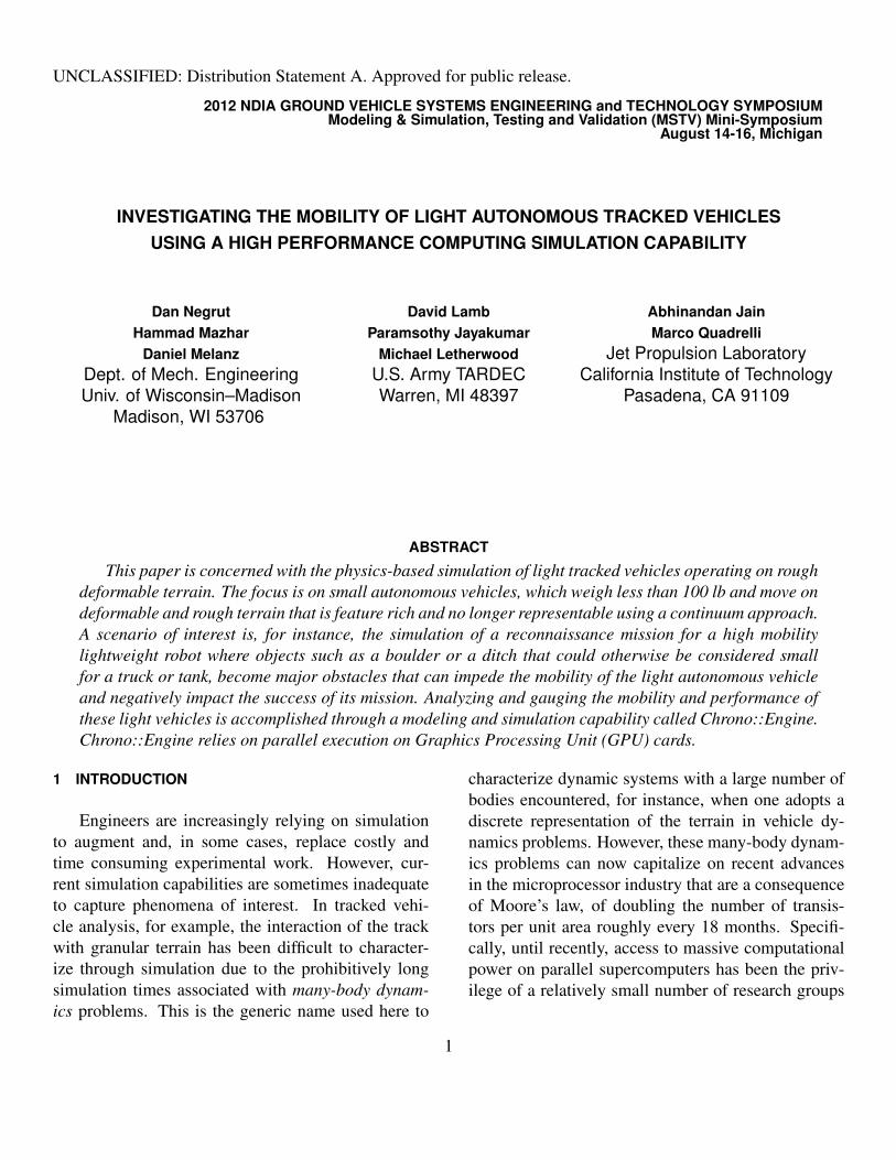
This paper is concerned with the physics-based simulation of light tracked vehicles operating on roughdeformable terrain. The focus is on small autonomous vehicles, which weigh less than 100 lb and move ondeformable and rough terrain that is feature rich and no longer representable using a continuum approach.A scenario of interest is, for instance, the simulation of a reconnaissance mission for a high mobilitylightweight robot where objects such as a boulder or a ditch that could otherwise be considered smallfor a truck or tank, become major obstacles that can impede the mobility of the light autonomous vehicleand negatively impact the success of its mission. Analyzing and gauging the mobility and performance ofthese light vehicles is accomplished through a modeling and simulation capability called Chrono::Engine.Chrono::Engine relies on parallel execution on Graphics Processing Unit (GPU) cards.

1 INTRODUCTION

Engineers are increasingly relying on simulationto augment and, in some cases, replace costly andtime consuming experimental work. However, cur-rent simulation capabilities are sometimes inadequateto capture phenomena of interest. In tracked vehi-cle analysis, for example, the interaction of the trackwith granular terrain has been difficult to character-ize through simulation due to the prohibitively longsimulation times associated with many-body dynam-ics problems. This is the generic name used here to

characterize dynamic systems with a large number ofbodies encountered, for instance, when one adopts adiscrete representation of the terrain in vehicle dy-namics problems. However, these many-body dynam-ics problems can now capitalize on recent advancesin the microprocessor industry that are a consequenceof Moore’s law, of doubling the number of transis-tors per unit area roughly every 18 months. Specifi-cally, until recently, access to massive computationalpower on parallel supercomputers has been the priv-ilege of a relatively small number of research groups

1

UNCLASSIFIED

in a select number of research facilities, thus limitingthe scope and impact of high performance comput-ing (HPC). This scenario is rapidly changing due toa trend set by general-purpose computing on graph-ics processing unit (GPU) cards. NVIDIA’s CUDAlibrary [21] allows one to use the streaming multipro-cessors available in high-end graphics cards. In thissetup, a latest generation NVIDIA GPU Kepler cardwill reach 1.5 Teraflops by the end of 2012 owing to aset of 1536 scalar processors working in parallel, eachfollowing a Single Instruction Multiple Data (SIMD)execution paradigm. Despite having only 1536 scalarprocessors, such a card is capable of managing tens ofthousands of parallel threads at any given time. Thisovercommitting of the GPU hardware resources is atthe cornerstone of a computing paradigm that aggres-sively attempts to hide costly memory transactionswith useful computation, a strategy that has lead, infrictional contact dynamics simulation, to a one orderof magnitude reduction in simulation time for many-body systems [20, 34].

The challenge of using parallel computing to re-duce simulation time and/or increase system sizestems, for the most part, from the task of design-ing and implementing many-body dynamics specificparallel numerical methods. Designing parallel algo-rithms suitable for frictional contact many-body dy-namics simulation remains an area of active research.Results reported in [16] indicate that the most widelyused commercial software package for multibody dy-namics simulation, which draws on a so called penaltyor regularization approach, runs into significant diffi-culties when handling simple problems involving hun-dreds of contact events, and thus cases with thousandsof contacts become intractable. Unlike these penaltyor regularization approaches where the frictional in-teraction is represented by a collection of stiff springscombined with damping elements that act at the inter-face of the two bodies [11, 22, 28, 29], the approachembraced herein draws on a different mathematicalframework. Specifically, the parallel algorithms relyon time-stepping procedures producing weak solu-tions of the differential variational inequality (DVI)

problem that describes the time evolution of rigid bod-ies with impact, contact, friction, and bilateral con-straints. When compared to penalty-methods, the DVIapproach has a greater algorithmic complexity, butavoids the small time steps that plague the former ap-proach.

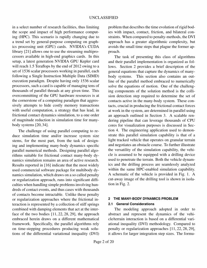
The task of presenting this class of algorithmsand their parallel implementation is organized as fol-lows. Section 2 provides a brief description of thegeneral equations that capture the dynamics of many-body systems. This section also contains an out-line of the parallel method embraced to numericallysolve the equations of motion. One of the challeng-ing components of the solution method is the colli-sion detection step required to determine the set ofcontacts active in the many-body system. These con-tacts, crucial in producing the frictional contact forcesat work in the system, are determined in parallel usingan approach outlined in Section 3. A scalable ren-dering pipeline that can leverage thousands of CPUcores for visualization purposes is discussed in Sec-tion 4. The engineering application used to demon-strate this parallel simulation capability is that of alight tracked vehicle that operates on granular terrainand negotiates an obstacle course. To further illustratethe versatility of the simulation capability, the vehi-cle is assumed to be equipped with a drilling deviceused to penetrate the terrain. Both the vehicle dynam-ics and the drilling process are seamlessly analyzedwithin the same HPC-enabled simulation capability.A schematic of the vehicle is provided in Fig. 1. Acut-away image of the drilling tool is shown in isola-tion in Fig. 2.

2 THE MANY-BODY DYNAMICS PROBLEM

2.1 General Considerations

The modeling approach adopted in order toabstract and represent the dynamics of the vehi-cle/terrain interaction is based on a differential vari-ational inequality (DVI) methodology. Compared topenalty or regularization approaches [11, 22, 28, 29],it allows for larger integration step sizes. The formu-

Page 2 of 20

UNCLASSIFIED

FIGURE 1: Light autonomous vehicle negotiating a pile of rubble.

FIGURE 2: Cutaway view: Anchor penetrating granular material [18].

lation of the equations of motion, that is, the equa-tions that govern the time evolution of a multibodysystem, is based on the so-called absolute, or Carte-sian, representation of the position and attitude of eachrigid body in the system. The state of the systemis denoted by the generalized positions q =

[rT

1 ,εT1 ,

. . . ,rTnb,εT

nb

]T ∈ R7nb and their time derivatives q =[rT

1 , εT1 , . . . , r

Tnb, εT

nb

]T ∈ R7nb , where nb is the numberof bodies, r j is the absolute position of the center ofmass of the jth body, and the quaternions (Euler pa-rameters) ε j are used to represent rotation and to avoidsingularities. Instead of using quaternion derivatives

in q, it is more advantageous to work with angu-lar velocities expressed in the local (body-attached)reference frames; in other words, the method de-scribed will use the vector of generalized velocitiesv =

[rT

1 , ωT1 , . . . , r

Tnb, ωT

nb

]T ∈ R6nb . Note that the gen-eralized velocity can be easily obtained as q = L(q)v,where L is a linear mapping that transforms eachωi into the corresponding quaternion derivative εi bymeans of the linear algebra formula εi =

12GT (q)ωi,

with 3x4 matrix G(q) as defined in [12].

Page 3 of 20

UNCLASSIFIED

2.1.1 Bilateral Constraints Bilateral constraintsrepresent kinematic relationships between two rigidbodies in the system. For example, spherical joints,prismatic joints, or revolute joints can be expressed asholonomic algebraic equations constraining the rela-tive positions of two bodies. A set B of constraintsleads to a collection of scalar equations

Ψi(q, t) = 0, i ∈B , (1)

the number of which depends on the type of con-straints in set B. Bilateral constraints must also be sat-isfied at the velocity level,

dΨi(q, t)dt

= 0 ⇒

∂Ψi

∂qq+

∂Ψi

∂ t= ∇qΨ

Ti q+

∂Ψi

∂ t

= ∇qΨTi L(q)v+

∂Ψi

∂ t= 0,

which is obtained by taking one time derivative ofEquation 1.

2.1.2 Unilateral Constraints and Friction Uni-lateral constraints enforce contact constraints betweenrigid bodies in the system. It is assumed that a gapfunction, Φ(q), can be defined for each pair of near-enough bodies. This gap function describes the dis-tance between the closest points on the two bodies ofinterest.

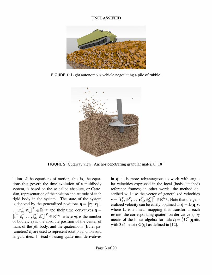
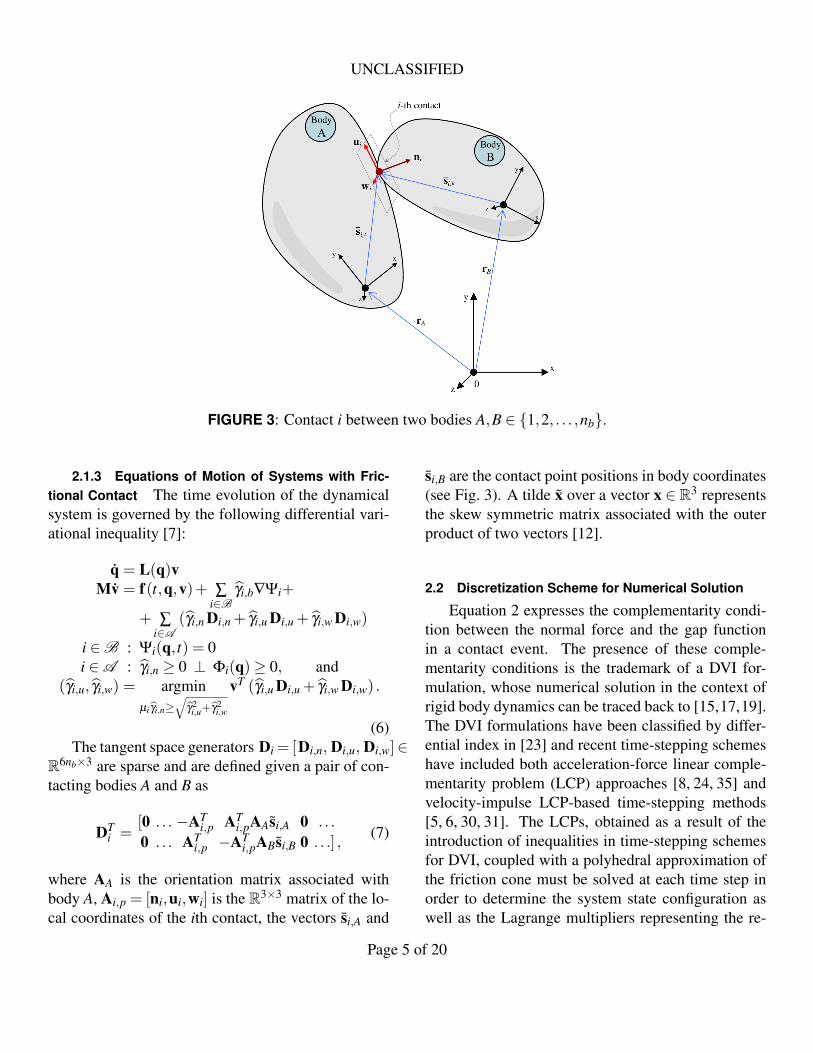
Unilateral contact constraints also introduce fric-tion forces into the system. When a contact is active,or Φi(q) = 0, a normal force acts on each of the twobodies at the contact point. When a contact is inac-tive, or Φi(q) > 0 , no normal force exists. This rep-resents a complementarity condition. Consider twobodies A and B in contact as shown in Fig. 3. Let nibe the normal at the contact pointing toward the exte-rior of the body of lower index, which by conventionis considered to be body A. Let ui and wi be two vec-tors in the contact plane such that ni,ui,wi ∈ R3 are

mutually orthonormal vectors. The frictional contactforces are defined by the multipliers γi,n ≥ 0, γi,u, andγi,w, which lead to the normal component of the fric-tion force, Fi,N = γi,nni and the tangential componentof the force Fi,T = γi,uui + γi,wwi.

The Coulomb friction model, which draws forcontact i on the friction coefficient µi, is used to writethe following constraints:

γi,n ≥ 0, Φi(q)≥ 0, Φi(q)γi,n = 0, (2)

µiγi,n ≥√

γ2i,u + γ2

i,w , ||vi,T ||(

µiγi,n−√

γ2i,u + γ2

i,w

)= 0,

〈Fi,T ,vi,T 〉=−||Fi,T || ||vi,T || (3)

Equation 2 captures the complementarity conditionpreviously described. The subsequent two equationsrelate the magnitude and direction of the friction forceto the multipliers and tangential velocity of the con-tact. These remaining equations can be expressed inan equivalent manner using the maximum dissipationprinciple. This frames the Coulomb friction model asa minimization problem, which can be seen in Equa-tion 4.

(γi,u, γi,w) = argmin√γ2

i,u+γ2i,w≤µiγi,n

vTi,T (γi,uui + γi,wwi) . (4)

The nature of the friction cone can be seen if yet an-other form of the friction force equations is consid-ered. The friction force of the i-th contact can be ex-pressed as follows, where ϒ is a cone in three dimen-sions whose slope is tan−1 µi.

Fi = Fi,N +Fi,T = γi,nni + γi,uui + γi,wwi ∈ ϒ, (5)

Page 4 of 20

UNCLASSIFIED

FIGURE 3: Contact i between two bodies A,B ∈ {1,2, . . . ,nb}.

2.1.3 Equations of Motion of Systems with Fric-tional Contact The time evolution of the dynamicalsystem is governed by the following differential vari-ational inequality [7]:

q = L(q)vMv = f(t,q,v)+ ∑

i∈Bγi,b∇Ψi+

+ ∑i∈A

(γi,n Di,n + γi,u Di,u + γi,w Di,w)

i ∈B : Ψi(q, t) = 0i ∈A : γi,n ≥ 0 ⊥ Φi(q)≥ 0, and

(γi,u, γi,w) = argminµiγi,n≥

√γ2

i,u+γ2i,w

vT (γi,u Di,u + γi,w Di,w) .

(6)The tangent space generators Di = [Di,n, Di,u, Di,w]∈

R6nb×3 are sparse and are defined given a pair of con-tacting bodies A and B as

DTi =

[0 . . . −ATi,p AT

i,pAAsi,A 0 . . .

0 . . . ATi,p −AT

i,pABsi,B 0 . . .] ,(7)

where AA is the orientation matrix associated withbody A, Ai,p = [ni,ui,wi] is the R3×3 matrix of the lo-cal coordinates of the ith contact, the vectors si,A and

si,B are the contact point positions in body coordinates(see Fig. 3). A tilde x over a vector x ∈ R3 representsthe skew symmetric matrix associated with the outerproduct of two vectors [12].

2.2 Discretization Scheme for Numerical Solution

Equation 2 expresses the complementarity condi-tion between the normal force and the gap functionin a contact event. The presence of these comple-mentarity conditions is the trademark of a DVI for-mulation, whose numerical solution in the context ofrigid body dynamics can be traced back to [15,17,19].The DVI formulations have been classified by differ-ential index in [23] and recent time-stepping schemeshave included both acceleration-force linear comple-mentarity problem (LCP) approaches [8, 24, 35] andvelocity-impulse LCP-based time-stepping methods[5, 6, 30, 31]. The LCPs, obtained as a result of theintroduction of inequalities in time-stepping schemesfor DVI, coupled with a polyhedral approximation ofthe friction cone must be solved at each time step inorder to determine the system state configuration aswell as the Lagrange multipliers representing the re-

Page 5 of 20

UNCLASSIFIED

action forces [15, 31]. If the simulation entails a largenumber of contacts and rigid bodies, as in the case ofpart feeders, packaging machines, and granular flows,the computational burden of classical LCP solvers canbecome significant. Indeed, a well-known class of nu-merical methods for LCPs based on simplex methods,also known as direct or pivoting methods [10], mayexhibit exponential worst-case complexity [9]. Theymay be impractical even for problems involving asfew as several hundred bodies when friction is present[4, 33]. Moreover, the three-dimensional Coulombfriction case leads to a nonlinear complementarityproblem (NCP): the use of a polyhedral approxima-tion to transform the NCP into an LCP introduces ar-tificial anisotropy in friction cones [5, 31, 35]. Thisdiscrete and finite approximation of friction cones isone of the reasons for the large dimension of the prob-lem that needs to be solved in multibody dynamicswith frictional contact.

In order to circumvent the limitations imposed bythe use of classical LCP solvers and the limited accu-racy associated with polyhedral approximations of thefriction cone, a parallel fixed-point iteration methodwith projection on a convex set has been proposed,developed, and tested in [7]. The method is based ona time-stepping formulation that solves at every step acone constrained optimization problem [2]. The time-stepping scheme, proved to converge in a measure dif-ferential inclusion sense to the solution of the originalcontinuous-time DVI, sets off at time tl by assumingthat a set of contacts, A , exists between bodies in thesystem, and a set of bilateral constraints, B, is alsoactive. The governing differential equations then as-sume the form of a DVI problem. The equation of mo-tion is discretized so that an approximation to the so-lution can be found at discrete instants in time. Givena position q(l) and velocity v(l) at the time step t(l),the numerical solution is found at the new time stept(l+1) = t(l)+h by solving the following optimization

problem with equilibrium constraints [32]:

M(v(l+1) −v(l)) = hf(t(l),q(l),v(l))+ ∑i∈B

γi,b∇Ψi +

+∑i∈A (γi,n Di,n + γi,u Di,u + γi,w Di,w) ,(8)

i ∈B : 1hΨi(q(l), t)+∇ΨT

i v(l+1)+ ∂Ψi∂ t = 0 (9)

i ∈A : 0≤ 1hΦi(q(l))+ DT

i,nv(l+1) ⊥ γ in ≥ 0, (10)

(γi,u,γi,w) = argminµiγi,n≥

√γ2

i,u+γ2i,w

v(l+1),T (γi,u Di,u + γi,w Di,w)

(11)

q(l+1) = q(l)+hL(q(l))v(l+1). (12)

Here, γs represents the constraint impulse of a con-tact constraint; that is, γs = hγs, for s = n,u,w. The1hΦi(q(l)) term achieves constraint stabilization; its ef-fect is discussed in [3]. Similarly, the term 1

hΨi(q(l))achieves stabilization for bilateral constraints. Thescheme converges to the solution of a measure differ-ential inclusion [2] when the step size h→ 0.

The proposed approach casts the problem asa monotone optimization problem through a relax-ation over the complementarity constraints, replacingEq. (10) with

i ∈A :0≤ 1

hΦi(q(l))+ DTi,nv(l+1)

−µi√

(vT Di,u)2 +(vT Di,w)2 ⊥ γ in ≥ 0.

The solution of the modified time-steppingscheme will approach the solution of the same mea-sure differential inclusion for h → 0 as the originalscheme [2], yet, in some situations, for large h, µ , orrelative velocity v(l+1), i.e., when not in an asymptoticregime, this relaxation can introduce motion oscilla-tions. It was shown in [7] that the modified scheme

Page 6 of 20

UNCLASSIFIED

is a cone complementarity problem (CCP), which canbe solved efficiently by an iterative numerical methodthat relies on projected contractive maps. Omittingfor brevity some of the details discussed in [7, 34],we note that the algorithm makes use of the followingvectors:

k ≡Mv(l)+hf(t(l),q(l),v(l)) (13)

bi ≡{

1hΦi(q(l)),0,0

}Ti ∈A , (14)

bi ≡ 1hΨi(q(l), t)+ ∂Ψi

∂ t , i ∈B. (15)

The solution, in terms of dual variables of the CCP(the multipliers), is obtained by iterating the followingcontraction maps until convergence, where Πϒi repre-sents the orthogonal projection on the friction coneassociated with contact i [32]:

∀i∈A : γr+1i = Πϒi

[γr

i −ωηi(DT

i vr +bi)]

(16)

∀i∈B : γr+1i = Πϒi

[γr

i −ωηi(∇ΨT

i vr +bi)].(17)

At each iteration r, before repeating (16) and (17),also the primal variables (the velocities) are updatedas

vr+1 = M−1

(∑

z∈ADzγ

r+1z + ∑

z∈B∇Ψzγ

r+1z + k

).(18)

2.3 Parallel ImplementationThe dynamics of a large multibody system whose

bodies interact through contact, friction, and bilateralconstraints can be simulated in time via the CCP algo-rithm previously described. A sequential implemen-tation of this algorithm is described by the followingpseudo-code:

Algorithm 1: Inner Iteration Loop

1. For i∈A (q,δ ), evaluate ηi = 3/Trace(DTi M−1 Di).

2. For i ∈B, evaluate ηi = 1/(∇ΨTi M−1∇Ψi).

3. Warm start: if some initial guess γ∗ is available formultipliers, then set γ0 = γ∗, otherwise γ0 = 0.

4. Initialize velocities: v0 = ∑i∈A M−1 Diγ0i +

∑i∈B M−1∇Ψiγi,b0 +M−1k .

5. For i ∈ A (q(l),δ ), compute changes in multipli-ers for contact constraints:

γr+1i = λ Πϒi

(γr

i −ωηi(

DTi vr +bi

))+

(1−λ )γri ;

∆γr+1i = γ

r+1i − γr

i ;∆vi = M−1 Di∆γ

r+1i .

6. For i ∈B, compute changes in multipliers for bi-lateral constraints:

γr+1i = λ

(γr

i −ωηi(∇ΨT

i vr +bi))

+(1−λ )γr

i ;∆ γ

r+1i = γ

r+1i − γr

i ;∆vi = M−1∇Ψi∆γ

r+1i .

7. Apply updates to the velocity vector:vr+1 = vr +∑i∈A ∆vi +∑i∈B ∆vi

8. r := r + 1. Repeat from 5 until convergence, oruntil r > rmax.

The stopping criterion is based on the value of thevelocity update. The overall algorithm that providesan approximation to the solution of Eqs. 8 through 12relies on Algorithm 1 and requires the following steps:

Algorithm 2: Outer, Time-Stepping, Loop

1. Set t = 0, step counter l = 0, provide initial valuesfor q(l) and v(l).

2. Perform collision detection between bodies, ob-taining nA possible contact points within a dis-tance δ . For each contact i, compute Di,n, Di,u,Di,w; for each bilateral constraint compute theresidual Φi(q), which also provides bi.

3. For each body, compute forces f(t(l),q(l),v(l)).4. Use Algorithm 1 to solve the cone complemen-

tarity problem and obtain unknown impulse γ andvelocity v(l+1).

5. Update positions using q(l+1) = q(l) +hL(q(l))v(l+1).

6. Increment t := t + h, l := l + 1, and repeat from

Page 7 of 20

UNCLASSIFIED

step 2 until t > tend

A parallel implementation that leveraged the par-allel computing power of commodity GPUs was con-sidered based on the two algorithms outlined above.Solution of the CCP problem proceeds as a collec-tion of functions, or kernels, which are executed onthe GPU. First, some pre-processing steps are exe-cuted. Applied forces are calculated in a body-parallelfashion, and contacts are preprocessed in a contact-parallel fashion to compute the normal direction andfriction plane directions. Next, the inner iteration loopis entered and a series of four kernels is executed untilconvergence. In a contact-parallel manner, the unilat-eral constraints are processed. In a constraint-parallelmanner, the bilateral constraints are processed. Ina reduction-slot-parallel manner, speed updates aresummed to a single resultant per body. Finally, ina body-parallel manner, speed updates are applied toeach body. Once a certain number of iterations hasbeen performed or convergence has been achieved, thegeneralized velocities are integrated forward in timein a body-parallel fashion to get the set of generalizedpositions. Details of the parallel reduction of speed-updates can be found in [20]. Pseudo-code for theparallel implementation can be seen below. Details re-garding data structures and computational flow of theparallel implementation can also be found in [20, 34].The details regarding the parallel collision detectionare provided in Section 3.

Parallel Kernels for Solution of DynamicsProblem

1. Parallel Collision Detection2. (Body parallel) Force kernel3. (Contact parallel) Contact preprocessing kernel4. Inner Iteration Loop:

(a) (Contact parallel) CCP contact kernel(b) (Bilateral-Constraint parallel) CCP constraint

kernel(c) (Reduction-slot parallel) Velocity change re-

duction kernel(d) (Body parallel) Body velocity update kernel

5. (Body parallel) Time integration kernel

3 PARALLEL COLLISION DETECTIONThe implemented 3D collision detection algorithm

performs a two-level spatial subdivision using axis-aligned bounding boxes. The first partitioning occursat the CPU level and yields a relatively small num-ber of large boxes. The second partitioning of each ofthese boxes occurs at the GPU level yielding a largenumber of small bins. The GPU 3D collision detec-tion, which handles spheres, ellipsoids, and planes,occurs in parallel at the bin level. Any other geome-tries are represented as a collection of these primitivesusing a padding (decomposition) process detailed in[13]. Several kernel calls build on each other to even-tually enable, in a one-thread-per-bin GPU parallelfashion, an exhaustive collision detection process inwhich thread i checks for collisions between all thebodies that happen to intersect the associated bin i.This requires O(b2

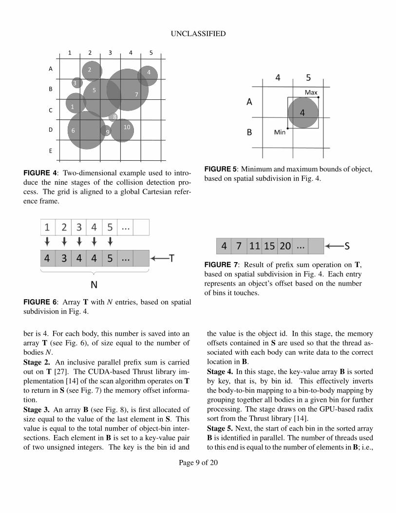
i ) computational effort, where birepresents the number of bodies touching bin i. Thevalue of bi is controlled by an appropriate selectionof the bin size. Figure 4 illustrates a typical collisiondetection scenario and is used in what follows to out-line the nine stages of the proposed approach. Notethat the actual implementation is for 3D collision de-tection and does not require the bodies to be spheres.Stage 1. The process begins by counting for each ob-ject the number of bins it intersects. As Fig. 5 shows,an object (body) can intersect, or touch, more than onebin. The minimum and maximum bounding points ofeach object are determined and placed in their respec-tive bins. For example, Fig. 5 shows that object 4’sminimum point lies in B4 and its maximum point inA5. The entire object must fit between the minimumand maximum points; therefore the number of binsthat the object intersects can be determined quickly bycounting the number of bins between the two points ineach axis and multiplying them. In this case the num-

Page 8 of 20

UNCLASSIFIED

FIGURE 4: Two-dimensional example used to intro-duce the nine stages of the collision detection pro-cess. The grid is aligned to a global Cartesian refer-ence frame.

FIGURE 5: Minimum and maximum bounds of object,based on spatial subdivision in Fig. 4.

FIGURE 6: Array T with N entries, based on spatialsubdivision in Fig. 4.

FIGURE 7: Result of prefix sum operation on T,based on spatial subdivision in Fig. 4. Each entryrepresents an object’s offset based on the numberof bins it touches.

ber is 4. For each body, this number is saved into anarray T (see Fig. 6), of size equal to the number ofbodies N.Stage 2. An inclusive parallel prefix sum is carriedout on T [27]. The CUDA-based Thrust library im-plementation [14] of the scan algorithm operates on Tto return in S (see Fig. 7) the memory offset informa-tion.Stage 3. An array B (see Fig. 8), is first allocated ofsize equal to the value of the last element in S. Thisvalue is equal to the total number of object-bin inter-sections. Each element in B is set to a key-value pairof two unsigned integers. The key is the bin id and

the value is the object id. In this stage, the memoryoffsets contained in S are used so that the thread as-sociated with each body can write data to the correctlocation in B.Stage 4. In this stage, the key-value array B is sortedby key, that is, by bin id. This effectively invertsthe body-to-bin mapping to a bin-to-body mapping bygrouping together all bodies in a given bin for furtherprocessing. The stage draws on the GPU-based radixsort from the Thrust library [14].Stage 5. Next, the start of each bin in the sorted arrayB is identified in parallel. The number of threads usedto this end is equal to the number of elements in B; i.e.,

Page 9 of 20

UNCLASSIFIED

FIGURE 8: Array B, based on spatial subdivision in Fig. 4.

FIGURE 9: Sorted array B, based on spatial subdivision in Fig. 4.

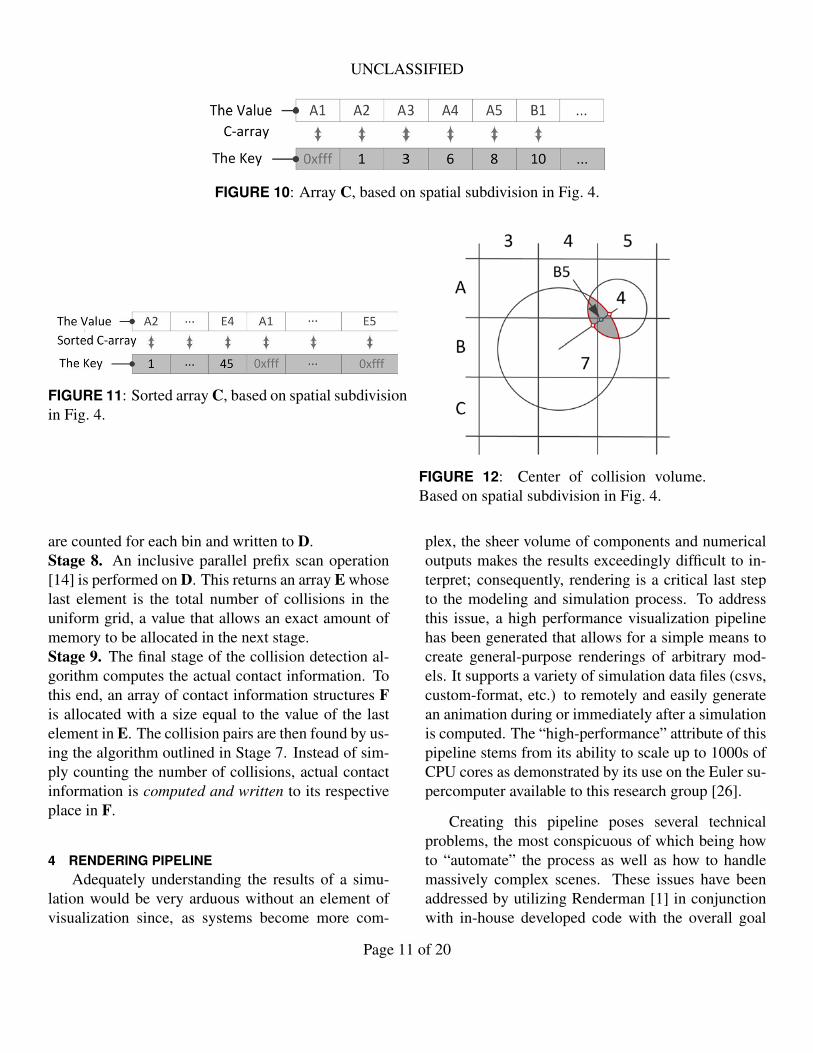
the number of object-bin interactions. Each threadreads the current and previous bin value; if these val-ues differ, then the start of a bin has been detected.The starting positions for each bin are written into anarray C of key-value pairs of size equal to the numberof bins in the 3D grid. When the start of a bin is foundin array B, the thread and bin id are saved as the keyand value, respectively. This pair is written to the ele-ment in C indexed by the bin id. Note that not all binsare active. Inactive bins; i.e., bins touched by zeroor one bodies, are set to 0xffffffff, the largest possiblevalue for an unsigned integer on a 32-bit, X86 archi-tecture. Figure 10 shows the outcome of this stage.

Stage 6. The array C is next radix-sorted [14] by key.Consequently, inactive bins (identified by the 0xffffffffentries, represented for brevity as 0xfff in Fig. 11)“migrate” to the end of the array.

Stage 7. The total number of active bins is determinednext by finding the index in the sorted array C of thefirst occurrence of 0xffffffff. Determining this indexallows memory and thread usage to be allocated accu-rately thus having no threads wasted on inactive bins.One GPU thread is assigned in this stage to each activebin to perform an exhaustive, brute-force, bin-parallelcollision detection for the purpose of only countingthe collision events. By carefully selecting the binsize, the number of objects being tested for collisions

is expected to be small; i.e., on average, bi is in therange of 3 to 4 objects per bin. After counting thetotal number of collisions in its bin, the thread writesthat tally into an unsigned integer array D of size equalto the number of active bins.

More involved, the algorithm for counting andsubsequently computing ellipsoid collision informa-tion is described in detail in [25]. For spheres, thealgorithm checks for collisions by calculating the dis-tance between the centers of the objects. Contacts canoccur only when the distance between the spheres’centers is less than or equal to the sum of their radii.Because one object could be contained within morethan one bin, checks were implemented to preventdouble counting. Since the midpoint of a collisionvolume can be contained only within one bin, only onethread (associated with that bin) will register/count acollision event. For example, in order to determinethe midpoint of the collision volume the algorithm re-lies on the vector from the centroid of object 4 to thecentroid of object 7; see Fig. 12. The points where thisvector intersects each object defines a segment; the lo-cation of the middle of this segment is used to decidethe unique bin that claims ownership of the contact. Ifone object is completely inside the other, the midpointof the collision volume is the centroid of the smallerobject. Using this process, the number of collisions

Page 10 of 20

UNCLASSIFIED

FIGURE 10: Array C, based on spatial subdivision in Fig. 4.

FIGURE 11: Sorted array C, based on spatial subdivisionin Fig. 4.

FIGURE 12: Center of collision volume.Based on spatial subdivision in Fig. 4.

are counted for each bin and written to D.Stage 8. An inclusive parallel prefix scan operation[14] is performed on D. This returns an array E whoselast element is the total number of collisions in theuniform grid, a value that allows an exact amount ofmemory to be allocated in the next stage.Stage 9. The final stage of the collision detection al-gorithm computes the actual contact information. Tothis end, an array of contact information structures Fis allocated with a size equal to the value of the lastelement in E. The collision pairs are then found by us-ing the algorithm outlined in Stage 7. Instead of sim-ply counting the number of collisions, actual contactinformation is computed and written to its respectiveplace in F.

4 RENDERING PIPELINEAdequately understanding the results of a simu-

lation would be very arduous without an element ofvisualization since, as systems become more com-

plex, the sheer volume of components and numericaloutputs makes the results exceedingly difficult to in-terpret; consequently, rendering is a critical last stepto the modeling and simulation process. To addressthis issue, a high performance visualization pipelinehas been generated that allows for a simple means tocreate general-purpose renderings of arbitrary mod-els. It supports a variety of simulation data files (csvs,custom-format, etc.) to remotely and easily generatean animation during or immediately after a simulationis computed. The “high-performance” attribute of thispipeline stems from its ability to scale up to 1000s ofCPU cores as demonstrated by its use on the Euler su-percomputer available to this research group [26].

Creating this pipeline poses several technicalproblems, the most conspicuous of which being howto “automate” the process as well as how to handlemassively complex scenes. These issues have beenaddressed by utilizing Renderman [1] in conjunctionwith in-house developed code with the overall goal

Page 11 of 20

UNCLASSIFIED

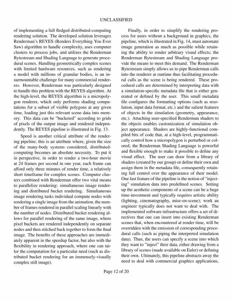
of implementing a full fledged distributed-computingrendering solution. The developed solution leveragesRenderman’s REYES (Renders Everything You EverSaw) algorithm to handle complexity, uses computerclusters to process jobs, and utilizes the RendermanBytestream and Shading Language to generate proce-dural scenes. Handling geometrically complex sceneswith limited hardware resources, such as renderinga model with millions of granular bodies, is an in-surmountable challenge for many commercial render-ers. However, Renderman was particularly designedto handle this problem with the REYES algorithm. Atthe high-level, the REYES algorithm is a micropoly-gon renderer, which only performs shading compu-tations for a subset of visible polygons at any giventime, loading just this relevant scene data into mem-ory. This data can be ”bucketed” according to gridsof pixels of the output image and rendered indepen-dently. The REYES pipeline is illustrated in Fig. 13.

Speed is another critical attribute of the render-ing pipeline; this is an attribute where, given the sizeof the many-body systems considered, distributed-computing becomes an absolute necessity. To put itin perspective, in order to render a two-hour movieat 24 frames per second in one year, each frame canafford only three minutes of render time, a relativelyshort timeframe for complex scenes. Computer clus-ters combined with Renderman offer two vital meansto parallelize rendering: simultaneous image render-ing and distributed bucket rendering. Simultaneousimage rendering tasks individual compute nodes withrendering a single image from the animation, the num-ber of frames rendered in parallel scaling linearly withthe number of nodes. Distributed bucket rendering al-lows for parallel rendering of the same image, wherepixel buckets are rendered independently on separatenodes and then stitched back together to form the finalimage. The benefits of these approaches are immedi-ately apparent in the speedup factor, but also with theflexibility in rendering approach, where one can tai-lor the computation for a particular need (such as dis-tributed bucket rendering for an immensely-visuallycomplex still image).

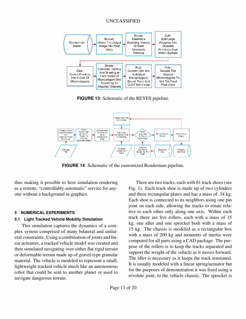
Finally, in order to simplify the rendering pro-cess for users without a background in graphics, thepipeline, which is illustrated in Fig. 14, must automateimage generation as much as possible while retain-ing the ability to render arbitrary visual effects; theRenderman Bytestream and Shading Language pro-vide the means to meet this demand. The RendermanBytestream simply allows us to pipe Renderman callsinto the renderer at runtime thus facilitating procedu-ral calls as the scene is being rendered. These pro-cedural calls are determined by interpreting data witha simulation-specific metadata file that is either gen-erated or defined by the user. This small metadatafile configures the formatting options (such as reso-lution, input data format, etc.) and the salient featuresof objects in the simulation (geometry, appearance,etc.). Attaching user-specified Renderman shaders tothe objects enables customization of simulation ob-ject appearance. Shaders are highly-functional com-piled bits of code that, at a high-level, programmati-cally control how a micropolygon is perturbed or col-ored; the Renderman Shading Language is powerfuland flexible enough to make it possible to define anyvisual effect. The user can draw from a library ofshaders (created by our group) or define their own andassign them in the metadata file, consequently retain-ing full control over the appearance of their model.One last feature of the pipeline is the notion of “inject-ing” simulation data into predefined scenes. Settingup the aesthetic components of a scene can be a hugetime-investment and typically requires artistic ability(lighting, cinematography, mise-en-scene); work anengineer typically does not want to deal with. Theimplemented software infrastructure offers a set of di-rectives that one can insert into existing Rendermanscenes that, when encountered at render time, will beoverridden with the emission of corresponding proce-dural calls (such as piping the interpreted simulationdata). Thus, the users can specify a scene into whichthey want to ”inject” their data, either drawing from alibrary of scenes (made available on Euler) or definingtheir own. Ultimately, this pipeline abstracts away theneed to deal with commercial graphics applications,

Page 12 of 20

UNCLASSIFIED

FIGURE 13: Schematic of the REYES pipeline.

FIGURE 14: Schematic of the customized Renderman pipeline.

thus making it possible to host simulation renderingas a remote, “controllably-automatic” service for any-one without a background in graphics.

5 NUMERICAL EXPERIMENTS

5.1 Light Tracked Vehicle Mobility Simulation

This simulation captures the dynamics of a com-plex system comprised of many bilateral and unilat-eral constraints. Using a combination of joints and lin-ear actuators, a tracked vehicle model was created andthen simulated navigating over either flat rigid terrainor deformable terrain made up of gravel-type granularmaterial. The vehicle is modeled to represent a small,lightweight tracked vehicle much like an autonomousrobot that could be sent to another planet or used tonavigate dangerous terrain.

There are two tracks, each with 61 track shoes (seeFig. 1). Each track shoe is made up of two cylindersand three rectangular plates and has a mass of .34 kg.Each shoe is connected to its neighbors using one pinjoint on each side, allowing the tracks to rotate rela-tive to each other only along one axis. Within eachtrack there are five rollers, each with a mass of 15kg, one idler and one sprocket both with a mass of15 kg. The chassis is modeled as a rectangular boxwith a mass of 200 kg and moments of inertia werecomputed for all parts using a CAD package. The pur-pose of the rollers is to keep the tracks separated andsupport the weight of the vehicle as it moves forward.The idler is necessary as it keeps the track tensioned.It is usually modeled with a linear spring/actuator butfor the purposes of demonstration it was fixed using arevolute joint, to the vehicle chassis. The sprocket is

Page 13 of 20

UNCLASSIFIED

used to drive the vehicle and is attached using a rev-olute joint to the chassis. Torque is applied to drivethe track, with each track driven independently of theother. When the sprocket rotates, it comes into con-tact with the cylinders on the track shoe and turns thetrack with a gear like motion.

The track for the vehicle was created by first gen-erating a ring of connected track shoes. This ringwas dropped onto a sprocket, five rollers, and an idlerwhich was connected to the chassis using a linearspring. The idler was pushed with 2000 N of forceuntil the track was tensioned and the idler had stoppedmoving. This pre-tensioned track was then saved to adata file and loaded for the simulation of the completevehicle.

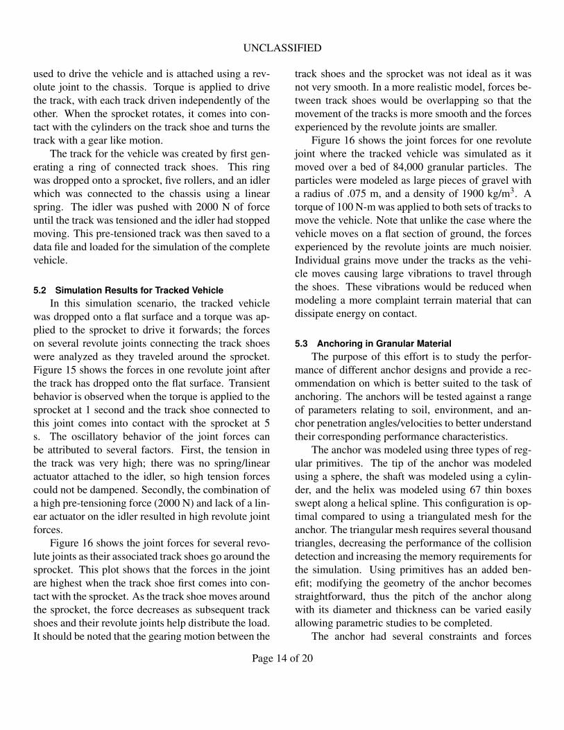
5.2 Simulation Results for Tracked VehicleIn this simulation scenario, the tracked vehicle

was dropped onto a flat surface and a torque was ap-plied to the sprocket to drive it forwards; the forceson several revolute joints connecting the track shoeswere analyzed as they traveled around the sprocket.Figure 15 shows the forces in one revolute joint afterthe track has dropped onto the flat surface. Transientbehavior is observed when the torque is applied to thesprocket at 1 second and the track shoe connected tothis joint comes into contact with the sprocket at 5s. The oscillatory behavior of the joint forces canbe attributed to several factors. First, the tension inthe track was very high; there was no spring/linearactuator attached to the idler, so high tension forcescould not be dampened. Secondly, the combination ofa high pre-tensioning force (2000 N) and lack of a lin-ear actuator on the idler resulted in high revolute jointforces.

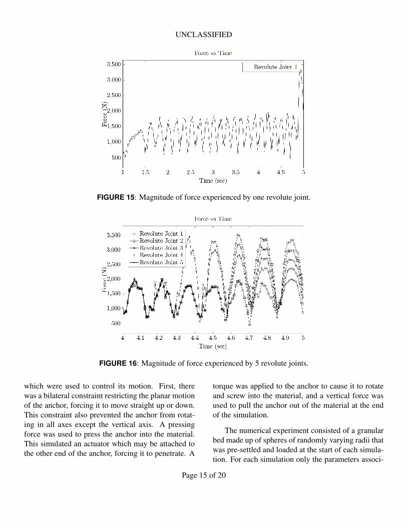
Figure 16 shows the joint forces for several revo-lute joints as their associated track shoes go around thesprocket. This plot shows that the forces in the jointare highest when the track shoe first comes into con-tact with the sprocket. As the track shoe moves aroundthe sprocket, the force decreases as subsequent trackshoes and their revolute joints help distribute the load.It should be noted that the gearing motion between the

track shoes and the sprocket was not ideal as it wasnot very smooth. In a more realistic model, forces be-tween track shoes would be overlapping so that themovement of the tracks is more smooth and the forcesexperienced by the revolute joints are smaller.

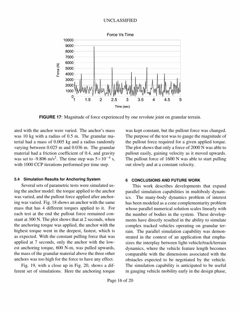
Figure 16 shows the joint forces for one revolutejoint where the tracked vehicle was simulated as itmoved over a bed of 84,000 granular particles. Theparticles were modeled as large pieces of gravel witha radius of .075 m, and a density of 1900 kg/m3. Atorque of 100 N-m was applied to both sets of tracks tomove the vehicle. Note that unlike the case where thevehicle moves on a flat section of ground, the forcesexperienced by the revolute joints are much noisier.Individual grains move under the tracks as the vehi-cle moves causing large vibrations to travel throughthe shoes. These vibrations would be reduced whenmodeling a more complaint terrain material that candissipate energy on contact.

5.3 Anchoring in Granular MaterialThe purpose of this effort is to study the perfor-

mance of different anchor designs and provide a rec-ommendation on which is better suited to the task ofanchoring. The anchors will be tested against a rangeof parameters relating to soil, environment, and an-chor penetration angles/velocities to better understandtheir corresponding performance characteristics.

The anchor was modeled using three types of reg-ular primitives. The tip of the anchor was modeledusing a sphere, the shaft was modeled using a cylin-der, and the helix was modeled using 67 thin boxesswept along a helical spline. This configuration is op-timal compared to using a triangulated mesh for theanchor. The triangular mesh requires several thousandtriangles, decreasing the performance of the collisiondetection and increasing the memory requirements forthe simulation. Using primitives has an added ben-efit; modifying the geometry of the anchor becomesstraightforward, thus the pitch of the anchor alongwith its diameter and thickness can be varied easilyallowing parametric studies to be completed.

The anchor had several constraints and forces

Page 14 of 20

UNCLASSIFIED

FIGURE 15: Magnitude of force experienced by one revolute joint.

FIGURE 16: Magnitude of force experienced by 5 revolute joints.

which were used to control its motion. First, therewas a bilateral constraint restricting the planar motionof the anchor, forcing it to move straight up or down.This constraint also prevented the anchor from rotat-ing in all axes except the vertical axis. A pressingforce was used to press the anchor into the material.This simulated an actuator which may be attached tothe other end of the anchor, forcing it to penetrate. A

torque was applied to the anchor to cause it to rotateand screw into the material, and a vertical force wasused to pull the anchor out of the material at the endof the simulation.

The numerical experiment consisted of a granularbed made up of spheres of randomly varying radii thatwas pre-settled and loaded at the start of each simula-tion. For each simulation only the parameters associ-

Page 15 of 20

UNCLASSIFIED

FIGURE 17: Magnitude of force experienced by one revolute joint on granular terrain.

ated with the anchor were varied. The anchor’s masswas 10 kg with a radius of 0.5 m. The granular ma-terial had a mass of 0.005 kg and a radius randomlyvarying between 0.025 m and 0.036 m. The granularmaterial had a friction coefficient of 0.4, and gravitywas set to -9.806 m/s2. The time step was 5×10−4 s,with 1000 CCP iterations performed per time step.

5.4 Simulation Results for Anchoring System

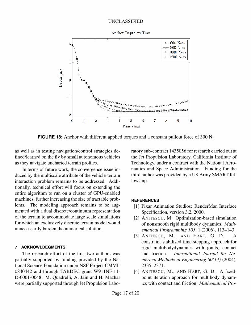
Several sets of parametric tests were simulated us-ing the anchor model: the torque applied to the anchorwas varied, and the pullout force applied after anchor-ing was varied. Fig. 18 shows an anchor with the samemass that has 4 different torques applied to it. Foreach test at the end the pullout force remained con-stant at 300 N. The plot shows that at 2 seconds, whenthe anchoring torque was applied, the anchor with thehighest torque went in the deepest, fastest, which isas expected. With the constant pulling force that wasapplied at 7 seconds, only the anchor with the low-est anchoring torque, 600 N-m, was pulled upwards,the mass of the granular material above the three otheranchors was too high for the force to have any effect.

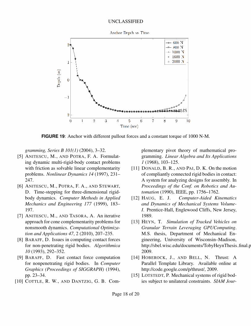
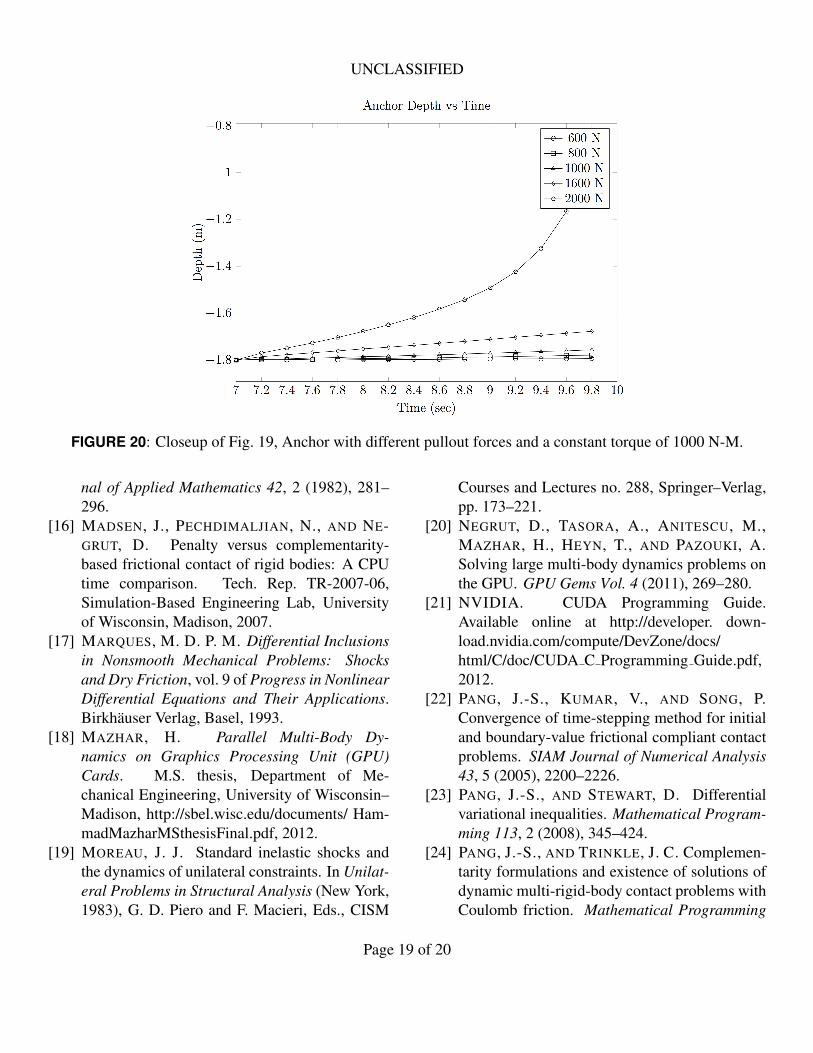
Fig. 19, with a close up in Fig. 20, shows a dif-ferent set of simulations. Here the anchoring torque

was kept constant, but the pullout force was changed.The purpose of the test was to gauge the magnitude ofthe pullout force required for a given applied torque.The plot shows that only a force of 2000 N was able topullout easily, gaining velocity as it moved upwards.The pullout force of 1600 N was able to start pullingout slowly and at a constant velocity.

6 CONCLUSIONS AND FUTURE WORKThis work describes developments that expand

parallel simulation capabilities in multibody dynam-ics. The many-body dynamics problem of interesthas been modeled as a cone complementarity problemwhose parallel numerical solution scales linearly withthe number of bodies in the system. These develop-ments have directly resulted in the ability to simulatecomplex tracked vehicles operating on granular ter-rain. The parallel simulation capability was demon-strated in the context of an application that empha-sizes the interplay between light-vehicle/track/terraindynamics, where the vehicle feature length becomescomparable with the dimensions associated with theobstacles expected to be negotiated by the vehicle.The simulation capability is anticipated to be usefulin gauging vehicle mobility early in the design phase,

Page 16 of 20

UNCLASSIFIED

FIGURE 18: Anchor with different applied torques and a constant pullout force of 300 N.

as well as in testing navigation/control strategies de-fined/learned on the fly by small autonomous vehiclesas they navigate uncharted terrain profiles.

In terms of future work, the convergence issue in-duced by the multiscale attribute of the vehicle-terraininteraction problem remains to be addressed. Addi-tionally, technical effort will focus on extending theentire algorithm to run on a cluster of GPU-enabledmachines, further increasing the size of tractable prob-lems. The modeling approach remains to be aug-mented with a dual discrete/continuum representationof the terrain to accommodate large scale simulationsfor which an exclusively discrete terrain model wouldunnecessarily burden the numerical solution.

7 ACKNOWLDEGMENTS

The research effort of the first two authors waspartially supported by funding provided by the Na-tional Science Foundation under NSF Project CMMI-0840442 and through TARDEC grant W911NF-11-D-0001-0048. M. Quadrelli, A. Jain and H. Mazharwere partially supported through Jet Propulsion Labo-

ratory sub-contract 1435056 for research carried out atthe Jet Propulsion Laboratory, California Institute ofTechnology, under a contract with the National Aero-nautics and Space Administration. Funding for thethird author was provided by a US Army SMART fel-lowship.

REFERENCES[1] Pixar Animation Studios: RenderMan Interface

Specification, version 3.2, 2000.[2] ANITESCU, M. Optimization-based simulation

of nonsmooth rigid multibody dynamics. Math-ematical Programming 105, 1 (2006), 113–143.

[3] ANITESCU, M., AND HART, G. D. Aconstraint-stabilized time-stepping approach forrigid multibodydynamics with joints, contactand friction. International Journal for Nu-merical Methods in Engineering 60(14) (2004),2335–2371.

[4] ANITESCU, M., AND HART, G. D. A fixed-point iteration approach for multibody dynam-ics with contact and friction. Mathematical Pro-

Page 17 of 20

UNCLASSIFIED

FIGURE 19: Anchor with different pullout forces and a constant torque of 1000 N-M.

gramming, Series B 101(1) (2004), 3–32.[5] ANITESCU, M., AND POTRA, F. A. Formulat-

ing dynamic multi-rigid-body contact problemswith friction as solvable linear complementarityproblems. Nonlinear Dynamics 14 (1997), 231–247.

[6] ANITESCU, M., POTRA, F. A., AND STEWART,D. Time-stepping for three-dimensional rigid-body dynamics. Computer Methods in AppliedMechanics and Engineering 177 (1999), 183–197.

[7] ANITESCU, M., AND TASORA, A. An iterativeapproach for cone complementarity problems fornonsmooth dynamics. Computational Optimiza-tion and Applications 47, 2 (2010), 207–235.

[8] BARAFF, D. Issues in computing contact forcesfor non-penetrating rigid bodies. Algorithmica10 (1993), 292–352.

[9] BARAFF, D. Fast contact force computationfor nonpenetrating rigid bodies. In ComputerGraphics (Proceedings of SIGGRAPH) (1994),pp. 23–34.

[10] COTTLE, R. W., AND DANTZIG, G. B. Com-

plementary pivot theory of mathematical pro-gramming. Linear Algebra and Its Applications1 (1968), 103–125.

[11] DONALD, B. R., AND PAI, D. K. On the motionof compliantly connected rigid bodies in contact:A system for analyzing designs for assembly. InProceedings of the Conf. on Robotics and Au-tomation (1990), IEEE, pp. 1756–1762.

[12] HAUG, E. J. Computer-Aided Kinematicsand Dynamics of Mechanical Systems Volume-I. Prentice-Hall, Englewood Cliffs, New Jersey,1989.

[13] HEYN, T. Simulation of Tracked Vehicles onGranular Terrain Leveraging GPUComputing.M.S. thesis, Department of Mechanical En-gineering, University of Wisconsin–Madison,http://sbel.wisc.edu/documents/TobyHeynThesis final.pdf,2009.

[14] HOBEROCK, J., AND BELL, N. Thrust: AParallel Template Library. Available online athttp://code.google.com/p/thrust/, 2009.

[15] LOTSTEDT, P. Mechanical systems of rigid bod-ies subject to unilateral constraints. SIAM Jour-

Page 18 of 20

UNCLASSIFIED

FIGURE 20: Closeup of Fig. 19, Anchor with different pullout forces and a constant torque of 1000 N-M.

nal of Applied Mathematics 42, 2 (1982), 281–296.

[16] MADSEN, J., PECHDIMALJIAN, N., AND NE-GRUT, D. Penalty versus complementarity-based frictional contact of rigid bodies: A CPUtime comparison. Tech. Rep. TR-2007-06,Simulation-Based Engineering Lab, Universityof Wisconsin, Madison, 2007.

[17] MARQUES, M. D. P. M. Differential Inclusionsin Nonsmooth Mechanical Problems: Shocksand Dry Friction, vol. 9 of Progress in NonlinearDifferential Equations and Their Applications.Birkhauser Verlag, Basel, 1993.

[18] MAZHAR, H. Parallel Multi-Body Dy-namics on Graphics Processing Unit (GPU)Cards. M.S. thesis, Department of Me-chanical Engineering, University of Wisconsin–Madison, http://sbel.wisc.edu/documents/ Ham-madMazharMSthesisFinal.pdf, 2012.

[19] MOREAU, J. J. Standard inelastic shocks andthe dynamics of unilateral constraints. In Unilat-eral Problems in Structural Analysis (New York,1983), G. D. Piero and F. Macieri, Eds., CISM

Courses and Lectures no. 288, Springer–Verlag,pp. 173–221.

[20] NEGRUT, D., TASORA, A., ANITESCU, M.,MAZHAR, H., HEYN, T., AND PAZOUKI, A.Solving large multi-body dynamics problems onthe GPU. GPU Gems Vol. 4 (2011), 269–280.

[21] NVIDIA. CUDA Programming Guide.Available online at http://developer. down-load.nvidia.com/compute/DevZone/docs/html/C/doc/CUDA C Programming Guide.pdf,2012.

[22] PANG, J.-S., KUMAR, V., AND SONG, P.Convergence of time-stepping method for initialand boundary-value frictional compliant contactproblems. SIAM Journal of Numerical Analysis43, 5 (2005), 2200–2226.

[23] PANG, J.-S., AND STEWART, D. Differentialvariational inequalities. Mathematical Program-ming 113, 2 (2008), 345–424.

[24] PANG, J.-S., AND TRINKLE, J. C. Complemen-tarity formulations and existence of solutions ofdynamic multi-rigid-body contact problems withCoulomb friction. Mathematical Programming

Page 19 of 20

UNCLASSIFIED

73, 2 (1996), 199–226.[25] PAZOUKI, A., MAZHAR, H., AND NEGRUT,

D. Parallel ellipsoid collision detection withapplication in contact dynamics-DETC2010-29073. In Proceedings to the 30th Comput-ers and Information in Engineering Conference(2010), S. Fukuda and J. G. Michopoulos, Eds.,ASME International Design Engineering Tech-nical Conferences (IDETC) and Computers andInformation in Engineering Conference (CIE).

[26] SBEL. Euler: A CPU/GPU–HeterogeneousCluster at the Simulation-Based EngineeringLaboratory, University of Wisconsin-Madison.http://sbel.wisc.edu/Hardware, 2012.

[27] SENGUPTA, S., HARRIS, M., ZHANG, Y.,AND OWENS, J. Scan primitives for GPUcomputing. In Proceedings of the 22nd ACMSIGGRAPH/EUROGRAPHICS symposium onGraphics hardware (2007), Eurographics Asso-ciation, p. 106.

[28] SONG, P., KRAUS, P., KUMAR, V., AND

DUPONT, P. Analysis of rigid-body dynamicmodels for simulation of systems with frictionalcontacts. Journal of Applied Mechanics 68(1)(2001), 118–128.

[29] SONG, P., PANG, J.-S., AND KUMAR, V. Asemi-implicit time-stepping model for frictionalcompliant contact problems. International Jour-nal of Numerical Methods in Engineering 60, 13

(2004), 267–279.[30] STEWART, D. E. Rigid-body dynamics with

friction and impact. SIAM Review 42(1) (2000),3–39.

[31] STEWART, D. E., AND TRINKLE, J. C. An im-plicit time-stepping scheme for rigid-body dy-namics with inelastic collisions and Coulombfriction. International Journal for NumericalMethods in Engineering 39 (1996), 2673–2691.

[32] TASORA, A. A Fast NCP Solver for LargeRigid-Body Problems with Contacts. In Multi-body Dynamics: Computational Methods andApplications, C. Bottasso, Ed. Springer, 2008,pp. 45–55.

[33] TASORA, A., MANCONI, E., AND SILVESTRI,M. Un nuovo metodo del simplesso per il prob-lema di complementarit lineare mista in sistemimultibody con vincoli unilateri. In Proceedingsof AIMETA 05 (Firenze, Italy, 2005).

[34] TASORA, A., NEGRUT, D., AND ANITESCU,M. Large-scale parallel multi-body dynamicswith frictional contact on the Graphical Process-ing Unit. Journal of Multi-body Dynamics 222,4 (2008), 315–326.

[35] TRINKLE, J., PANG, J.-S., SUDARSKY, S.,AND LO, G. On dynamic multi-rigid-body con-tact problems with Coulomb friction. Zeitschriftfur angewandte Mathematik und Mechanik 77(1997), 267–279.

Page 20 of 20