1

Investigating the Puzzling conditional

Market Risk-Return Relationship

Omrane Guedhami ∗

Finance et AssuranceFaculty of Administrative Science

Laval UniversityPavillon Palasis Prince

Quebec (Quebec), G1K 2A7Guedhami@ipo.umass.edu

and

Oumar SyDepartment of Finance

HEC School of Business3000 Chemin de la Côte-Sainte-Catherine

Montreal (Quebec), H3T 2A7Oumar.Sy@hec.ca

∗ We have benefited from comments by Narjess Boubakri, Van Son Lai, To Minh-Chau, Marie-Claude

Beaulieu, Sean Cleary, Glenn Baigent, John Rumsey, Shen Fuxi, and Taewon Yang. Special thanks to

Barbara Hoffman and Rebecca Dauer. All errors remain ours.

Comments, proofs and reprint requests should be addressed to Omrane Guedhami, Departement Finance et

Assurance, Faculty of Administrative Science, Laval University, Pavillon Palasis-Prince, Quebec (Quebec),

G1K 7P4.

2

Abstract

This paper investigates the conflicting results documented by the existing empirical literature on

the relationship between the expected market risk premium and conditional market variance. We

show that the previous tests are biased because they use the realized market risk premium as a

proxy for the expected market risk premium without accounting for the negative portion of the

market risk premium distribution. The empirical evidence based on a new test, allowing up and

down-market volatility to have different impacts on the market risk premium, indicates a

consistent and significant risk-return relationship.

KEY WORDS : Market Risk Premium, Market Volatility, EGARCH.

Investigating the Puzzling conditional

Market Risk-Return Relationship

Abstract: This paper investigates the conflicting results documented by the existing empirical

literature on the relationship between the expected market risk premium and conditional market

variance. We show that the previous tests are biased because they use the realized market risk

premium as a proxy for the expected market risk premium without accounting for the negative

portion of the market risk premium distribution. The empirical evidence based on a new test,

allowing up and down-market volatility to have different impacts on the market risk premium,

indicates a consistent and significant risk-return relationship.

Many papers have examined the intertemporal relationship between expected returns

and conditional volatility of the market. Theoretically, if investors are risk-averse, the capital

asset pricing model (CAPM) developed by Sharpe (1964) and Lintner (1965) implies a

positive, linear relationship between the expected market risk premium and conditional

market variance. However, the empirical findings on this relationship are controversial.

Bollerslev, Engle and Wooldridge (1988) and Harvey (1989) find a significant positive

relationship between the expected market risk premium and conditional volatility of the

market. French, Schwert and Stambaugh (1987) show that this relationship is positive, but

insignificant. Baillie and DeGennaro (1990) find no evidence for a statistically significant

relationship between the market risk premium and conditional variance or standard deviation

4

and conclude that others measures of risk are more important than the variance of returns;

Whereas, Campbell (1987) and Glosten, Jagannathan and Runkle (1993) find a significantly

negative relationship. Other papers have also examined the relationship between expected

returns and conditional volatility of the market, but most of them reject the cross-sectional

and the intertemporal implications of the CAPM.1 Recently, Scruggs (1998) investigates

these conflicting results and shows that the negative relationship between the expected

market risk premium and conditional market variance reported in previous studies is due to

the omission of an interest rate-state variable in the conditional market risk premium

equation. By estimating an ad hoc model, which incorporates the interest rate in both

conditional mean and variance equations, Scruggs (1998) restores the positive and significant

relationship between the market risk premium and conditional market variance.

However, we can argue that including the interest rate in both conditional mean and

variance in Scruggs’ equations is not theoretically justified. This is because no theoretical

argument to this time justifies the incorporation of an interest rate variable into the

conditional market risk premium equation. Furthermore, the presence of the interest rate in

both the conditional market risk premium and the conditional market variance equations

results in multicolinearity problems with the result that the estimates of both equations do not

have a valid interpretation. Moreover, when the interest rate is not included in the conditional

mean and variance equations, the relationship remains weak or negative (model 2a, p. 587).

We think that the puzzle related to the single-factor market risk-return relationship remains

unresolved at this time.

The theoretical positive relationship between the market risk premium and

conditional market variance supported by asset pricing models requires the positivity of the

market risk in all states. Since all previous studies use realized returns to test the relationship

5

between the expected market risk premium and conditional market variance, the implicit

assumption being made is that the realized market risk premium is an unbiased estimate of

the expected market risk premium. However, since the realized market risk premium may be

negative in some states, we believe that previous studies don’t explicitly test the relationship

between the market risk premium and conditional market variance.

The purpose of this paper is to reexamine the puzzling single-factor relationship

between the expected market risk premium and conditional market variance found in

previous studies. Unlike these studies, this paper presents a new test which recognizes the

impact of using realized market risk premium as a proxy for expected market risk premium.

This test allows up and down-market volatility to have distinct impacts on the market risk

premium. We show that the estimates of the single factor market risk-return relationship may

be biased downwards due to the use of the realized market risk premium as a proxy for the

expected market risk premium. Therefore, not accounting for states where the realized market

risk premium is negative leads to an aggregation bias resulting from the compensation effects

of the positive and the negative market risk premium. We find evidence of a positive

(negative) and significant relationship between the market risk premium and conditional

market variance in bull (bear) market context. This result is important since it (i) explains the

negative or the weak relationship between volatility and expected return reported in some

studies and (ii) restores the pertinence of the variance as a measure of risk .

The remainder of this paper is organized as follows. The next Section presents

theoretical models and empirical procedures used for tests. Section II discusses methodology.

Section III describes the data and presents empirical results and finally Section IV concludes

the paper.

6

I. Models and Procedures

This section describes the theoretical models and empirical procedures that we use to

test the different specifications of the single-factor relationship between the market risk

premium and conditional market variance. Previous tests on this issue made the implicit

assumption that the realized market risk premium is an unbiased estimate of the expected

market risk premium. The major contribution of this paper is to show the impact of this

assumption on testing the risk-return relationship since the positive risk-return relationship

postulated by most asset pricing models is based on the expected returns.

A. The Theoretical Model

Following the majority of previous studies on the intertemporal relationship between

the market risk premium and conditional market variance, we consider a conditional version

of the Sharpe-Lintner CAPM in which expected market risk premium is related to the

conditional volatility of the market according to the following equation:

2t,mmt,m1t ]r[E σλ=− (1)

where Et-1[.] denotes the expectation operator conditional on information available at

time t-1; rm,t is the market risk premium; σ²m,t is the conditional market variance; and λm is

the price of risk. Since λm is also the coefficient of relative risk aversion, and therefore should

be positive, equation (1) implies a positive and linear relation between the expected market

risk premium and conditional market variance.

7

B. The Empirical Procedures

First, we present traditional tests of the conditional single-factor relationship between

the market risk premium and conditional market variance. Second, we conduct our empirical

tests using up and down market information decomposition which recognize the impact of

using realized market risk premium to proxy for expected market risk premium.

B.1. Traditional Tests

In order to test the relationship between the market risk premium (rm,t) and

conditional market variance (σ2m,t), we use the following model as derived from the previous

studies 2:

Model 1:t,m

2t,mm0t,m ˆr ε+σλ+λ= (2)

The investors’ risk-aversion hypothesis implies that the λm coefficient (the price of

risk) is positive. Equation (2) is tested, among others, by Campbell (1987), French, Schwert

and Stambaugh (1987), Glosten, Jagannathan and Runkle (1993) and Scruggs (1998).

B.2. Tests with Up and Down-Market Information Decomposition

Equation (1) indicates that the conditional expected market risk premium is a positive

and linear function of the conditional market variance. When the expected market risk

increases, the anticipated returns should adjust accordingly in order to compensate the

investors for the additional risk. This relationship has crucial implications for the empirical

tests because an increase of the conditional market variance must be associated with an

8

increase in the risk premium anticipated by investors. This theoretical association led

researchers to directly test for a positive relationship. However, as these tests use the realized

market risk premium as a proxy for the expected market risk premium, we argue that they do

not explicitly test the conditional single-factor market risk-return relationship. In fact, the

positivity of the expected market risk premium in all states is a necessary condition for

equation (1), however, there are states where the realized market risk premium is negative

(Table 1 shows that the market risk premium is negative in 44% of the cases). Therefore, the

traditional tests of the conditional single-factor market risk-return relationship should account

for the negative portion of the market risk premium distribution.

Below, we present the methodology that we are using to obtain the empirical model

that recognizes the impact of using realized market risk premium as a proxy for the expected

market risk premium and allows up and down-market periods volatility to have different

effects on the market risk premium. Our approach is inspired by the study of Pettengill,

Sundaram and Mathur (1995) on the CAPM. According to these authors (p. 103) “since these

tests use realized returns instead of expected returns, we argue that the validity of the SLB

(Sharpe-Lintner-Black) model is not directly examined. Indeed, recognition of a second

critical relationship between the predicted market returns and the risk-free return suggests

that previous tests of the relationship between beta and the returns must be modified. The

need to modify previous tests results from the model's requirement that a portion of the

market return distribution be below the risk-free rate”.

A reasonable inference about this critical relationship is that returns associated to

high volatility are less than returns associated to low volatility when the market risk premium

is negative (down market period). To infer this, assume that the economy is represented by

9

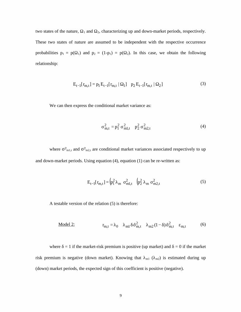
two states of the nature, Ω1 and Ω2, characterizing up and down-market periods, respectively.

These two states of nature are assumed to be independent with the respective occurrence

probabilities p1 = p(Ω1) and p2 = (1-p1) = p(Ω2). In this case, we obtain the following

relationship:

]r[Ep]r[Ep]r[E 2t,m1t21t,m1t1t,m1t Ω|+Ω|= −−− (3)

We can then express the conditional market variance as:

2t,2m

22

2t,1m

21

2t,m pp σ+σ=σ (4)

where σ²m1,t and σ²m2,t are conditional market variances associated respectively to up

and down-market periods. Using equation (4), equation (1) can be re-written as:

( ) ( ) 2t,2mm

22

2t,1mm

21t,m1t pp]r[E σλ+σλ=− (5)

A testable version of the relation (5) is therefore:

Model 2: t,m2

t,m2m2

t,m1m0t,m ˆ)1(ˆr ε+σδ−λ+σδλ+λ= (6)

where δ = 1 if the market-risk premium is positive (up market) and δ = 0 if the market

risk premium is negative (down market). Knowing that λm1 (λm2) is estimated during up

(down) market periods, the expected sign of this coefficient is positive (negative).

10

II. Methodology

A. The Empirical Model of the Conditional Variance

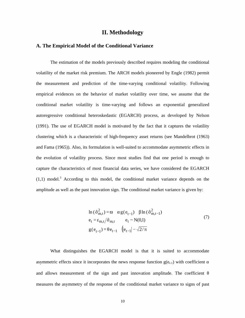
The estimation of the models previously described requires modeling the conditional

volatility of the market risk premium. The ARCH models pioneered by Engle (1982) permit

the measurement and prediction of the time-varying conditional volatility. Following

empirical evidences on the behavior of market volatility over time, we assume that the

conditional market volatility is time-varying and follows an exponential generalized

autoregressive conditional heteroskedastic (EGARCH) process, as developed by Nelson

(1991). The use of EGARCH model is motivated by the fact that it captures the volatility

clustering which is a characteristic of high-frequency asset returns (see Mandelbrot (1963)

and Fama (1965)). Also, its formulation is well-suited to accommodate asymmetric effects in

the evolution of volatility process. Since most studies find that one period is enough to

capture the characteristics of most financial data series, we have considered the EGARCH

(1,1) model.3 According to this model, the conditional market variance depends on the

amplitude as well as the past innovation sign. The conditional market variance is given by:

( )π−+θ=

σε=

σβ+α+ω=σ

−−−

−−

/2ee)e(g

)1,0(N~eˆe

)ˆ(ln)e(g)ˆ(ln

1t1t1t

tt,mt,mt

21t,m1t

2t,m

(7)

What distinguishes the EGARCH model is that it is suited to accommodate

asymmetric effects since it incorporates the news response function g(et-1) with coefficient α

and allows measurement of the sign and past innovation amplitude. The coefficient θ

measures the asymmetry of the response of the conditional market variance to signs of past

11

return shocks. A negative (positive) coefficient θ implies that negative (positive) return

shocks have more impact on the conditional volatility than positive (negative) return shocks

of the same magnitude. When θ = 0, the news response function g(et-1) is then symmetric and

depends only on lagged return shocks. According to Engle and Ng (1993, p. 1753) “The

EGARCH model differs from the standard GARCH model in two main respects: (1) the

EGARCH model allows good news and bad news to have different impacts on volatility,

while the standard GARCH model does not, and (2) the EGARCH model allows big news to

have a greater impact on volatility than the standard GARCH model”.

B. Maximum Likelihood Methodology

The models are estimated using the maximum likelihood method, whose estimates

are obtained by searching for values of parameters that maximize the likelihood function (L),

calculated from the products of all conditional densities of the prediction errors.

∑=

σ

ε−σ−π−=

N

1t2

t,m

t,m2t,m

ˆ)ˆ(ln)2ln(

2

1lnL (8)

The likelihood function is maximized by using the dual Quasi-Newton algorithm. The

starting values for the regression parameters are obtained by using the ordinary least squares

estimates.

12

III. Empirical Results

A. Data Description

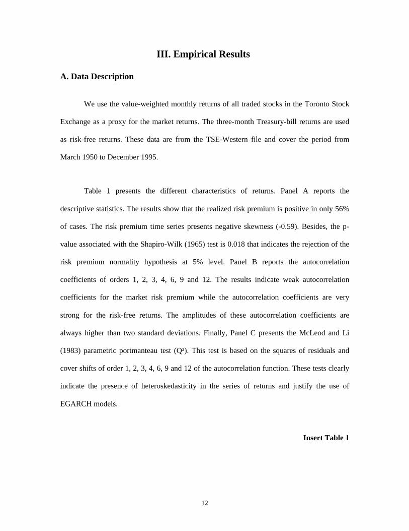
We use the value-weighted monthly returns of all traded stocks in the Toronto Stock

Exchange as a proxy for the market returns. The three-month Treasury-bill returns are used

as risk-free returns. These data are from the TSE-Western file and cover the period from

March 1950 to December 1995.

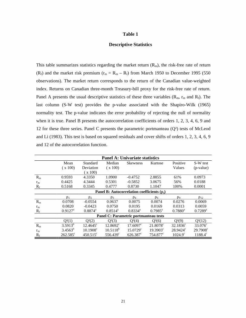
Table 1 presents the different characteristics of returns. Panel A reports the

descriptive statistics. The results show that the realized risk premium is positive in only 56%

of cases. The risk premium time series presents negative skewness (-0.59). Besides, the p-

value associated with the Shapiro-Wilk (1965) test is 0.018 that indicates the rejection of the

risk premium normality hypothesis at 5% level. Panel B reports the autocorrelation

coefficients of orders 1, 2, 3, 4, 6, 9 and 12. The results indicate weak autocorrelation

coefficients for the market risk premium while the autocorrelation coefficients are very

strong for the risk-free returns. The amplitudes of these autocorrelation coefficients are

always higher than two standard deviations. Finally, Panel C presents the McLeod and Li

(1983) parametric portmanteau test (Q²). This test is based on the squares of residuals and

cover shifts of order 1, 2, 3, 4, 6, 9 and 12 of the autocorrelation function. These tests clearly

indicate the presence of heteroskedasticity in the series of returns and justify the use of

EGARCH models.

Insert Table 1

13

B. The Results

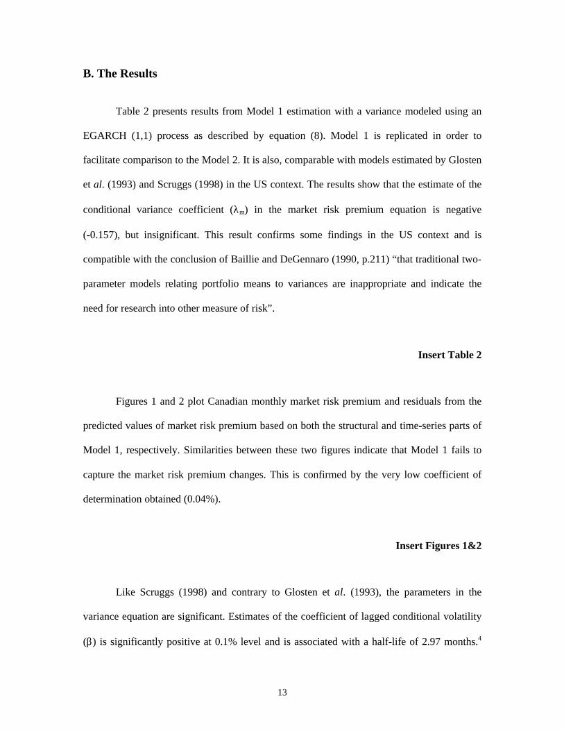
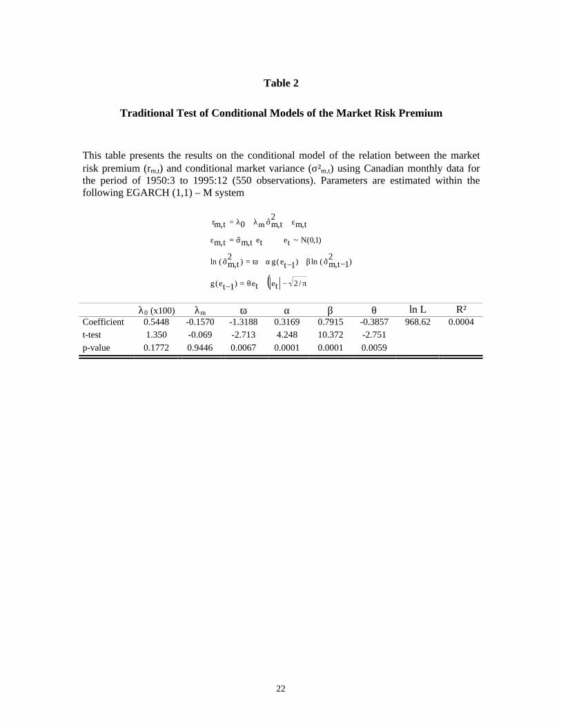
Table 2 presents results from Model 1 estimation with a variance modeled using an

EGARCH (1,1) process as described by equation (8). Model 1 is replicated in order to

facilitate comparison to the Model 2. It is also, comparable with models estimated by Glosten

et al. (1993) and Scruggs (1998) in the US context. The results show that the estimate of the

conditional variance coefficient (λm) in the market risk premium equation is negative

(-0.157), but insignificant. This result confirms some findings in the US context and is

compatible with the conclusion of Baillie and DeGennaro (1990, p.211) “that traditional two-

parameter models relating portfolio means to variances are inappropriate and indicate the

need for research into other measure of risk”.

Insert Table 2

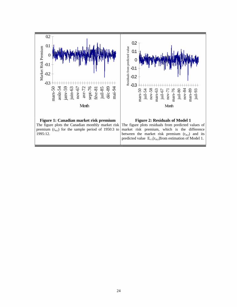
Figures 1 and 2 plot Canadian monthly market risk premium and residuals from the

predicted values of market risk premium based on both the structural and time-series parts of

Model 1, respectively. Similarities between these two figures indicate that Model 1 fails to

capture the market risk premium changes. This is confirmed by the very low coefficient of

determination obtained (0.04%).

Insert Figures 1&2

Like Scruggs (1998) and contrary to Glosten et al. (1993), the parameters in the

variance equation are significant. Estimates of the coefficient of lagged conditional volatility

(β) is significantly positive at 0.1% level and is associated with a half-life of 2.97 months.4

14

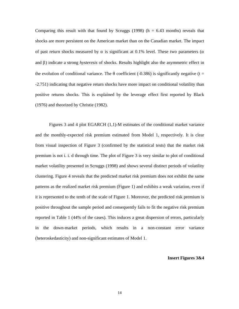
Comparing this result with that found by Scruggs (1998) (h = 6.43 months) reveals that

shocks are more persistent on the American market than on the Canadian market. The impact

of past return shocks measured by α is significant at 0.1% level. These two parameters (α

and β) indicate a strong hysteresis of shocks. Results highlight also the asymmetric effect in

the evolution of conditional variance. The θ coefficient (-0.386) is significantly negative (t =

-2.751) indicating that negative return shocks have more impact on conditional volatility than

positive returns shocks. This is explained by the leverage effect first reported by Black

(1976) and theorized by Christie (1982).

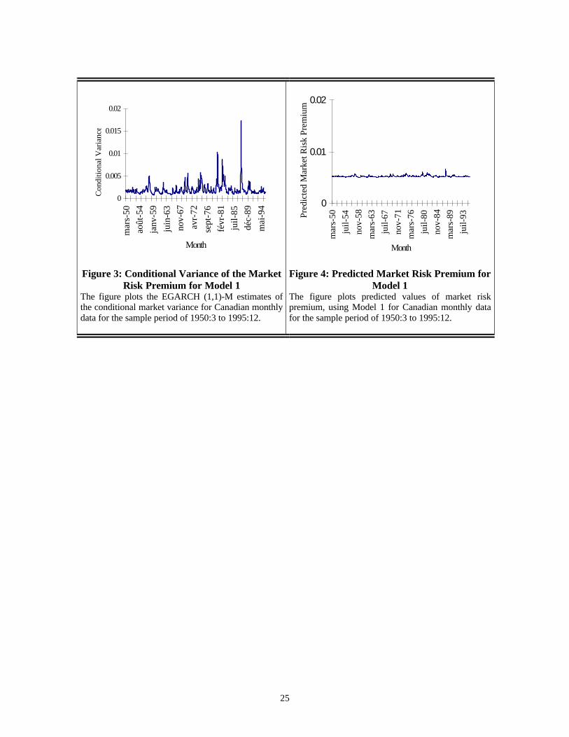
Figures 3 and 4 plot EGARCH (1,1)-M estimates of the conditional market variance

and the monthly-expected risk premium estimated from Model 1, respectively. It is clear

from visual inspection of Figure 3 (confirmed by the statistical tests) that the market risk

premium is not i. i. d through time. The plot of Figure 3 is very similar to plot of conditional

market volatility presented in Scruggs (1998) and shows several distinct periods of volatility

clustering. Figure 4 reveals that the predicted market risk premium does not exhibit the same

patterns as the realized market risk premium (Figure 1) and exhibits a weak variation, even if

it is represented to the tenth of the scale of Figure 1. Moreover, the predicted risk premium is

positive throughout the sample period and consequently fails to fit the negative risk premium

reported in Table 1 (44% of the cases). This induces a great dispersion of errors, particularly

in the down-market periods, which results in a non-constant error variance

(heteroskedasticity) and non-significant estimates of Model 1.

Insert Figures 3&4

15

In summary, our results confirm those obtained for the American market. This is not

surprising knowing the findings of Eun and Shim (1989) that shocks in the American market

are quickly disseminated to the rest of the world. Moreover, Theodossiou and Lee (1993)

show that the conditional volatility in the Canadian market is imported from outside,

particularly from the US market. Using EGARH process to model market volatility, we find a

negative and insignificant relationship between the Canadian market risk premium and

conditional market variance.

Table 3 presents the results of estimating Model 2. As we discussed previously, we

transformed Model 1 in order to allow for different reactions (in sign and amplitude)

depending on up and down-market periods. We modelled the volatility using an EGARCH

(1,1) process. As expected, the coefficient λm1 (16.64) is significantly positive at the 0.1%

level (t = 11.04). Thus, during up-market periods, increases in volatility results in a rise of the

market risk premium. The coefficient λm2 (-16.01) is significantly negative at the 0.1% level

(t = -10.95). This implies a negative relationship between the market risk premium and

conditional variance during the down-market periods. Thus, an increase of the market

conditional variance results in an increase of losses during the down market periods. These

results go against those of traditional tests. Indeed, the amplitudes of the price of risk for up

and down-market periods are very close in absolute value but in opposite sign. Consequently,

we argue that aggregating these two-segmented conditional relations results in a

mispecification which may explain the weakness and the absence of consistency (both

economically and statistically) of traditional tests of the conditional market risk-return

relationship.

Insert Table 3

16

The estimation of the conditional variance equation shows the presence of

heteroskedasticity. The coefficient for past volatility shocks (α) and past conditional variance

(β) are statistically significant, indicating that the volatility of the Canadian market risk

premium is predictable using past information. The asymmetry of response parameter (θ) is

statistically insignificant. This shows that unexpected change of the market risk premium has

a symmetric impact on volatility when the asymmetrical effect is taken into account in the

mean equation (Model 2).

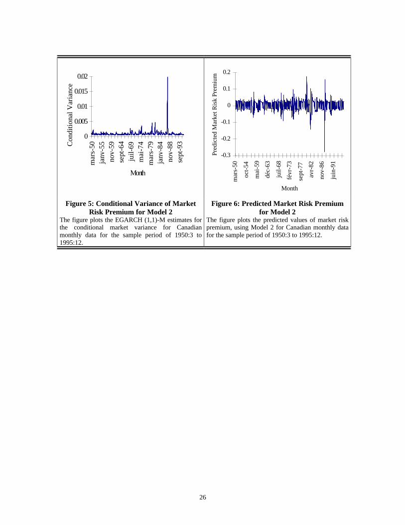
Figures 5 and 6 plot EGARCH (1,1)-M estimates of conditional market variance and

monthly-expected risk premium estimated from Model 2, respectively. The conditional

volatility plot exhibits extreme volatility as shown in Figure 5. Figure 6 reveals that Model 2

also predicts down market patterns and gives a plot that exhibits a better fit of realized market

risk premium. This is confirmed by the appreciable increase of the likelihood function and

the coefficient of determination of Model 2 compared to Model 1 (49.41% versus 0.04%).

Insert Figures 5&6

IV. Conclusion

This paper investigates the relation between the market risk premium and conditional

market variance and attempts to resolve the conflicting results reported by previous studies.

Results from the traditional test reveal a negative and insignificant relation between the

market risk premium and conditional market variance and confirm weak relations reported in

the US market. However, we show that these traditional tests employed by previous studies

17

are biased because they aggregate the risk premium associated with up and down-market

periods when they use of realized market risk premium as a proxy for expected market risk

premium.

We also conduct a new test which recognizes the impact of using realized market risk

premium to proxy for expected market risk premium and allows up and down market

volatility to have different effects on the market risk premium. The empirical results indicate

a strong relationship between the market risk premium and conditional market variance

whatever the sign of the market risk premium is. We obtain a positive (negative) and

significant relationship between the market risk premium and conditional market variance in

bull (bear) market context. These results restore not only the importance of the variance as a

measure of risk, but also the cross-sectional and the intertemporal implications of the market-

based CAPM.

18

ENDNOTES

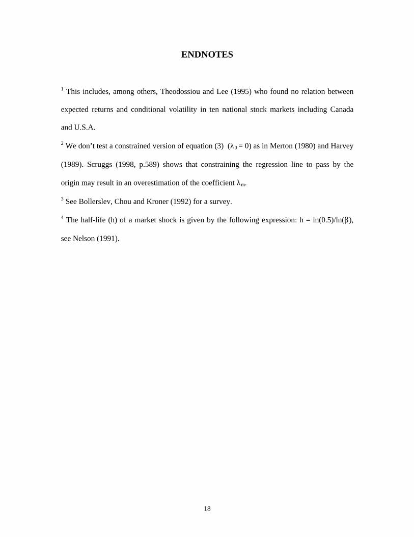
1 This includes, among others, Theodossiou and Lee (1995) who found no relation between

expected returns and conditional volatility in ten national stock markets including Canada

and U.S.A.

2 We don’t test a constrained version of equation (3) (λ0 = 0) as in Merton (1980) and Harvey

(1989). Scruggs (1998, p.589) shows that constraining the regression line to pass by the

origin may result in an overestimation of the coefficient λm.

3 See Bollerslev, Chou and Kroner (1992) for a survey.

4 The half-life (h) of a market shock is given by the following expression: h = ln(0.5)/ln(β),

see Nelson (1991).

19

References

Baillie, R. T. and DeGennaro R. P., “ Stock Returns and Volatility”, Journal of Financial andQuantitative Analysis, 25 (1990), 203-214.

Black, F., “Studies of Stock Price Volatility Changes”, Proceedings of the 1976 Meetings ofthe American Statistical Association, Business and Economics Statistics Section, 1976,177-181.

Bollerslev, T., Chou R. Y. and Kroner K. F., “Arch Modeling in Finance: A Review of TheTheory and Empirical Evidence ”, Journal of Econometrics, 52 (1992), 5-59.

Bollerslev, T., Engle R. F. and Wooldridge J. M., “A Capital Asset Pricing Model with TimeVarying Covariances ”, Journal of Political Economy, 96 (1988), 116-131.

Campbell, J. Y., “ Stock Returns and The Term Structure ”, Journal of Financial Economics,18 (1987), 873-399.

Christie, A. A., “The Stochastic Behaviour of Common Stock Variances: Value, Leverage,and Interest Rate effects”, Journal of Financial Economics, 10 (1982), 407-432.

Engle, R. F., “ Autoregressive Conditional Heteroskedasticity with Estimates of TheVariance of United Kingdom Inflation”, Econometrica, 55 (1982), 391-407.

Engle, R. F. and Ng V. K., “Measuring and Testing The Impact of News on Variance”,Journal of Finance, 48 (1993), 1749-1778.

Eun, C. S. and Shim S., “International Transmission of Stock Market Movements”, Journalof Financial and Quantitative Analysis, 24 (1989), 241-256.

Fama, E. F., “The Behaviour of Stock Market Prices”, Journal of Business, 38 (1965), 34-105.

French, K. R., Schwert W. G. and Stambaugh R. F., “Expected Stock Returns andVariance ”, Journal of Financial Economics, 19 (1987), 3-29.

Glosten, L. R., Jagannathan R. and Runkle D. E., “On The Relation Between The ExpectedValue and The Variance of The Nominal Excess Return on Stocks ”, Journal ofFinance, 48 (1993), 1779-1801.

Harvey, C. R., “Time-Varying Conditional Covariances in Tests of Asset Pricing Models ”,Journal of Financial Economics, 24 (1989), 289-317.

Lintner, J., “The Valuation of Risk Assets and The Selection of Risky Investments in StocksPortfolios and Capital Budgets ”, Review of Economics and Statistics, 47 (1965), 13-37.

20

Mandelbrot, B., “The Variation of Certain Speculative Prices”, The Journal of Business, 36(1963), 394-419.

McLeod, A. I. and Li W. K., “ Diagnostic Checking ARMA Time Series Models UsingSquared Residual Autocorrelation ”, Journal of Time Series Analysis, 4 (1983), 269-273.

Merton, R. C., “ On Estimating The Expected Return On The Market: An ExploratoryInvestigation ”, Journal of Financial Economics, 8 (1980), 323-361.

Nelson, D. B., “ Conditional Heteroskedasticity in Asset Returns : A New Approach ”,Econometrica, 59 (1991), 347-370.

Pettengill, G. N., Sundaram S. and Mathur I., “ The Conditional Relation between Beta andReturns ”, Journal of Financial and Quantitative Analysis, 30 (1995), 101-116.

Scruggs, J. T., “ Resolving The Puzzling Intertemporal Relation Between The Market RiskPremium and Conditional Market Variance: A Two-Factor Approach”, Journal ofFinance, 53 (1998), 575-603.

Shapiro, S. S. and Wilk, M. B., “An Analysis of Variance Test for Normality (completesamples),” Biometrika, 52 (1965), 591-611.

Sharpe, W. F., “Capital Asset Prices: A Theory of Market Equilibrium under Conditions ofRisk”, Journal of Finance, 19 (1964), 425-442.

Theodossiou, P. and Lee U., “ Mean and Volatility Spillovers Across Major National StockMarkets: Further Empirical Evidence”, Journal of Financial Research, 16 (1993), 337-350.

Theodossiou, P. and Lee U., “ Relationship Between Volatility and Expected Returns AcrossInternational Stock Markets”, Journal of Business Finance and Accounting, 22 (1995),289-300.

21

Table 1

Descriptive Statistics

This table summarizes statistics regarding the market return (Rm), the risk-free rate of return

(Rf) and the market risk premium (rm = Rm – Rf) from March 1950 to December 1995 (550

observations). The market return corresponds to the return of the Canadian value-weighted

index. Returns on Canadian three-month Treasury-bill proxy for the risk-free rate of return.

Panel A presents the usual descriptive statistics of these three variables (Rm, rm and Rf). The

last column (S-W test) provides the p-value associated with the Shapiro-Wilk (1965)

normality test. The p-value indicates the error probability of rejecting the null of normality

when it is true. Panel B presents the autocorrelation coefficients of orders 1, 2, 3, 4, 6, 9 and

12 for these three series. Panel C presents the parametric portmanteau (Q²) tests of McLeod

and Li (1983). This test is based on squared residuals and cover shifts of orders 1, 2, 3, 4, 6, 9

and 12 of the autocorrelation function.

Panel A: Univariate statisticsMean

( x 100)Standard

Deviation( x 100)

Median( x 100)

Skewness Kurtose PositiveValues

S-W test(p-value)

Rm 0.9593 4.3350 1.0900 -0.4752 2.8855 61% 0.0973rm 0.4425 4.3444 0.5301 -0.5852 3.0675 56% 0.0188Rf 0.5168 0.3345 0.4777 0.8730 1.1047 100% 0.0001

Panel B: Autocorrelation coefficients (ρρj)ρ1 ρ2 ρ3 ρ4 ρ6 ρ9 ρ12

Rm 0.0708 -0.0554 0.0637 0.0075 0.0074 0.0276 0.0069rm 0.0820 -0.0423 0.0750 0.0195 0.0169 0.0313 0.0059Rf 0.9127a 0.8874a 0.8514a 0.8334a 0.7985a 0.7880a 0.7289a

Panel C: Parametric portmanteau testsQ²(1) Q²(2) Q²(3) Q²(4) Q²(6) Q²(9) Q²(12)

Rm 3.5913b 12.4645c 12.8692c 17.6097c 21.8078c 32.1836c 33.076c

rm 3.4563b 10.1908c 10.5118b 15.0729c 19.3903c 28.9424c 29.7908c

Rf 262.585c 450.515c 556.439c 626.387c 754.877c 1024.9c 1188.4c

22

Table 2

Traditional Test of Conditional Models of the Market Risk Premium

This table presents the results on the conditional model of the relation between the marketrisk premium (rm,t) and conditional market variance (σ²m,t) using Canadian monthly data forthe period of 1950:3 to 1995:12 (550 observations). Parameters are estimated within thefollowing EGARCH (1,1) – M system

( )π−+θ=

σβ+α+ω=σ

σ=ε

ε+σλ+λ=

−

−−

/2ee)e(g

)ˆ(ln)e(g)ˆ(ln

)1,0(N~teeˆ

ˆmr

tt1t

21t,m1t

2t,m

tt,mt,m

t,m2

t,m0t,m

λ0 (x100) λm ω α β θ ln L R²Coefficient 0.5448 -0.1570 -1.3188 0.3169 0.7915 -0.3857 968.62 0.0004t-test 1.350 -0.069 -2.713 4.248 10.372 -2.751

p-value 0.1772 0.9446 0.0067 0.0001 0.0001 0.0059

23

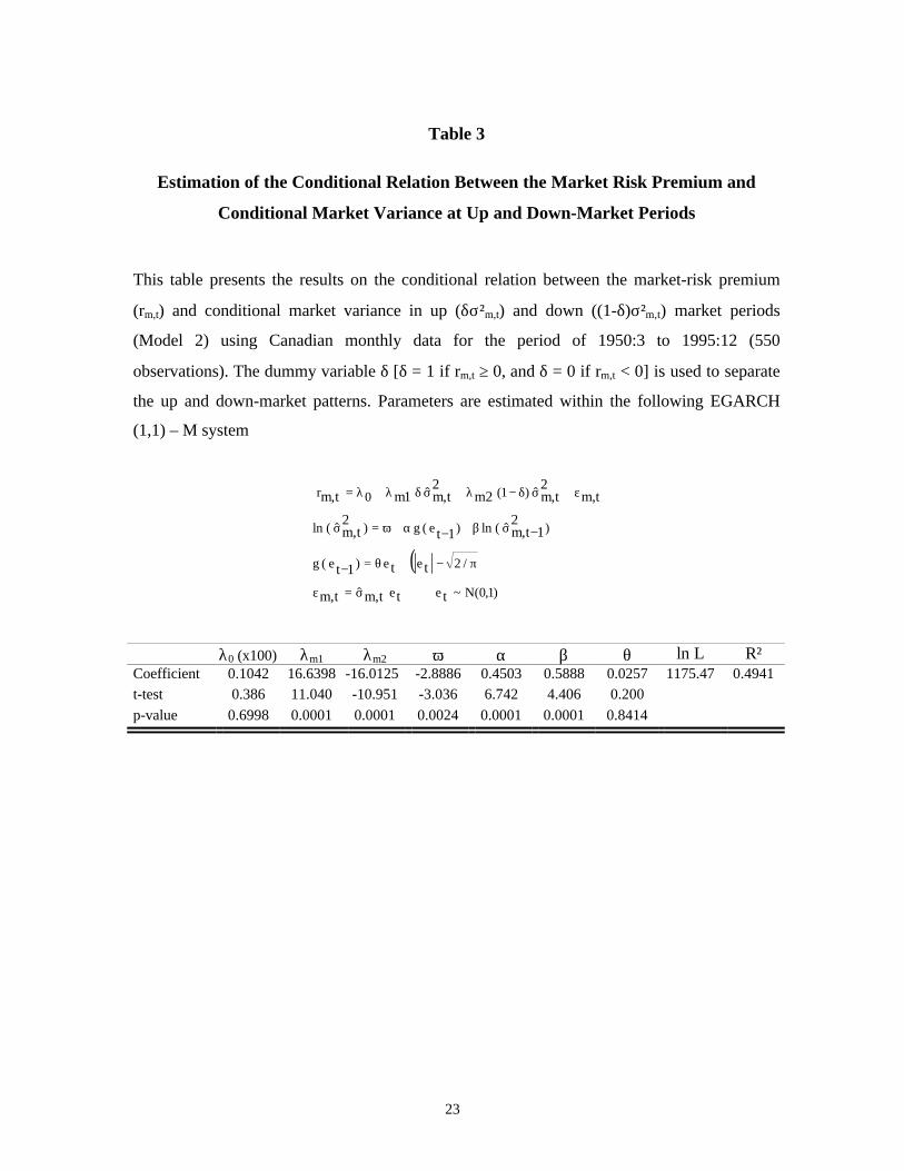
Table 3

Estimation of the Conditional Relation Between the Market Risk Premium and

Conditional Market Variance at Up and Down-Market Periods

This table presents the results on the conditional relation between the market-risk premium

(rm,t) and conditional market variance in up (δσ²m,t) and down ((1-δ)σ²m,t) market periods

(Model 2) using Canadian monthly data for the period of 1950:3 to 1995:12 (550

observations). The dummy variable δ [δ = 1 if rm,t ≥ 0, and δ = 0 if rm,t < 0] is used to separate

the up and down-market patterns. Parameters are estimated within the following EGARCH

(1,1) – M system

( ))1,0(N~eeˆ

/2ee)e(g

)ˆ(ln)e(g)ˆ(ln

ˆ)1(ˆ0r

ttt,mt,m

tt1t

21t,m1t

2t,m

t,m2

t,m2m2

t,m1mt,m

σ=ε

π−+θ=

σβ+α+ω=σ

ε+σδ−λ+σδλ+λ=

−

−−

λ0 (x100) λm1 λm2 ω α β θ ln L R²Coefficient 0.1042 16.6398 -16.0125 -2.8886 0.4503 0.5888 0.0257 1175.47 0.4941t-test 0.386 11.040 -10.951 -3.036 6.742 4.406 0.200

p-value 0.6998 0.0001 0.0001 0.0024 0.0001 0.0001 0.8414

24

-0.3

-0.2

-0.1

0

0.1

0.2

mar

s-50

août

-54

janv

-59

juin

-63

nov-

67av

r-72

sept

-76

févr

-81

juil-

85dé

c-89

mai

-94

Month

Mar

ket R

isk

Prem

ium

-0.3

-0.2

-0.1

0

0.1

0.2

mar

s-50

juil-

54no

v-58

mar

s-63

juil-

67no

v-71

mar

s-76

juil-

80no

v-84

mar

s-89

juil-

93

Month

Res

idua

ls f

rom

pre

dict

ed v

alue

s

Figure 1: Canadian market risk premiumThe figure plots the Canadian monthly market riskpremium (rm,t) for the sample period of 1950:3 to1995:12.

Figure 2: Residuals of Model 1The figure plots residuals from predicted values ofmarket risk premium, which is the differencebetween the market risk premium (rm,t) and itspredicted value Et-1[rm,t]from estimation of Model 1.

25

0

0.005

0.01

0.015

0.02

mar

s-50

août

-54

janv

-59

juin

-63

nov-

67

avr-

72

sept

-76

févr

-81

juil-

85

déc-

89

mai

-94

Month

Con

ditio

nal V

aria

nce

0

0.01

0.02

mar

s-50

juil-

54

nov-

58

mar

s-63

juil-

67

nov-

71

mar

s-76

juil-

80

nov-

84

mar

s-89

juil-

93

Month

Pred

icte

d M

arke

t Ris

k Pr

emiu

m

Figure 3: Conditional Variance of the MarketRisk Premium for Model 1

The figure plots the EGARCH (1,1)-M estimates ofthe conditional market variance for Canadian monthlydata for the sample period of 1950:3 to 1995:12.

Figure 4: Predicted Market Risk Premium forModel 1

The figure plots predicted values of market riskpremium, using Model 1 for Canadian monthly datafor the sample period of 1950:3 to 1995:12.

26

0

0.005

0.01

0.015

0.02

mar

s-50

janv

-55

nov-

59se

pt-6

4ju

il-69

mai

-74

mar

s-79

janv

-84

nov-

88se

pt-9

3Month

Con

ditio

nal V

aria

nce

-0.3

-0.2

-0.1

0

0.1

0.2

mar

s-50

oct-

54

mai

-59

déc-

63

juil-

68

févr

-73

sept

-77

avr-

82

nov-

86

juin

-91

Month

Pred

icte

d M

arke

t Ris

k Pr

emiu

m

Figure 5: Conditional Variance of MarketRisk Premium for Model 2

The figure plots the EGARCH (1,1)-M estimates forthe conditional market variance for Canadianmonthly data for the sample period of 1950:3 to1995:12.

Figure 6: Predicted Market Risk Premiumfor Model 2

The figure plots the predicted values of market riskpremium, using Model 2 for Canadian monthly datafor the sample period of 1950:3 to 1995:12.