Investigating user behavior by analysis of gaze data

IN DEGREE PROJECT COMPUTER SCIENCE AND ENGINEERING,SECOND CYCLE, 30 CREDITS

, STOCKHOLM SWEDEN 2016

Investigating user behavior by analysis of gaze dataEvaluation of machine learning methods for user behavior analysis in web applications

FREDRIK DAHLIN

KTH ROYAL INSTITUTE OF TECHNOLOGYSCHOOL OF COMPUTER SCIENCE AND COMMUNICATION

Investigating user behavior by analysis of gazedata

Evaluation of machine learning methods for user behavior analysis in web applications

FREDRIK [email protected]

Degree of Master of Science in Industrial Engineering and ManagementDegree of Master in Computer Science and Engineering

Supervisor: Jens LagergrenExaminer: Johan Håstad

Employer: TobiiAugust 2016

AbstractUser behavior analysis in web applications is currently mainlyperformed by analysis of statistical measurements based onuser interactions or by creation of personas to better un-derstand users. Both of these methods give great insightsin how the users utilize a web site, but do not give anyadditional information about what they are actually doing.

This thesis attempts to use eye tracking data for analy-sis of user activities in web applications. Eye tracking datahas been recorded, labeled and analyzed for 25 test partic-ipants. No data source except eye tracking data has beenused and two different approaches are attempted where thefirst relies on a gaze map representation of the data and thesecond relies on sequences of features.

The results indicate that it is possible to distinguishuser activities in web applications, but only at a high error-rate. Improvement are possible by implementing a less sub-jective labeling process and by including features from otherdata sources.

ReferatUndersöka användarbeteende via analys av

blickdataI nuläget utförs analys av användarbeteende i webbapplika-tioner primärt med hjälp av statistiska mått över använda-res beteenden på hemsidor tillsammans med personas förö-kad förståelse av olika typer av användare. Dessa metoderger stor insikt i hur användare använder hemsidor men geringen information om vilka typer av aktiviteter användarehar utfört på hemsidan.

Denna rapport försöker skapa metoder för analys avanvändaraktiviter på hemsidor endast baserat på blickda-ta fångade med eye trackers. Blick data från 25 personerhar samlats in under tiden de utför olika uppgifter på oli-ka hemsidor. Två olika tekniker har utvärderats där denena analyserar blick kartor som fångat ögonens rörelser un-der 10 sekunder och den andra tekniken använder sig avsekvenser av händelser för att klassificera aktiviteter.

Resultaten indikerar att det går att urskilja olika ty-per av vanligt förekommande användaraktiviteter genomanalys av blick data. Resultatet visar också att det är storosäkerhet i prediktionerna och ytterligare arbete är nöd-vändigt för att finna användbara modeller.

Contents

1 Introduction 1

2 Background 32.1 Introduction to eye tracking . . . . . . . . . . . . . . . . . . . . . . . 3

2.1.1 Methods . . . . . . . . . . . . . . . . . . . . . . . . . . . . . . 32.1.2 Applications . . . . . . . . . . . . . . . . . . . . . . . . . . . 42.1.3 Eye movements during activities . . . . . . . . . . . . . . . . 4

2.2 Introduction to machine learning . . . . . . . . . . . . . . . . . . . . 42.2.1 Evaluation of machine learning models . . . . . . . . . . . . . 5

2.3 Eye tracking and machine learning . . . . . . . . . . . . . . . . . . . 6

3 Method 93.1 Data set . . . . . . . . . . . . . . . . . . . . . . . . . . . . . . . . . . 93.2 Unsupervised feature-learning approach . . . . . . . . . . . . . . . . 10

3.2.1 Data representation - Gaze maps . . . . . . . . . . . . . . . . 103.2.2 Feature learning - Restricted Boltzmann machine . . . . . . . 113.2.3 Classification - K-means clustering . . . . . . . . . . . . . . . 14

3.3 Sequence approach . . . . . . . . . . . . . . . . . . . . . . . . . . . . 153.3.1 Data representation . . . . . . . . . . . . . . . . . . . . . . . 153.3.2 Classification - Hidden Markov Model . . . . . . . . . . . . . 16

4 Results 214.1 Labelled activity sequences . . . . . . . . . . . . . . . . . . . . . . . 214.2 Unsupervised feature learning approach . . . . . . . . . . . . . . . . 21

4.2.1 Classification - K-means clustering . . . . . . . . . . . . . . . 214.3 Sequence approach . . . . . . . . . . . . . . . . . . . . . . . . . . . . 25

4.3.1 Classification - Hidden Markov Model . . . . . . . . . . . . . 27

5 Discussion 375.1 Unsupervised feature learning approach . . . . . . . . . . . . . . . . 375.2 Sequence approach . . . . . . . . . . . . . . . . . . . . . . . . . . . . 385.3 Segment sizes . . . . . . . . . . . . . . . . . . . . . . . . . . . . . . . 395.4 Definitions of the user activities . . . . . . . . . . . . . . . . . . . . . 395.5 Critique . . . . . . . . . . . . . . . . . . . . . . . . . . . . . . . . . . 39

5.6 Ethical aspects . . . . . . . . . . . . . . . . . . . . . . . . . . . . . . 405.7 Future work . . . . . . . . . . . . . . . . . . . . . . . . . . . . . . . . 405.8 Conclusion . . . . . . . . . . . . . . . . . . . . . . . . . . . . . . . . 41

Bibliography 43

Appendices 45

A Appendix 47A.1 RBM - Grid search results . . . . . . . . . . . . . . . . . . . . . . . . 47A.2 K-means - Cluster statistics . . . . . . . . . . . . . . . . . . . . . . . 50

Chapter 1

Introduction

Understanding how users interact with web applications is a growing research area.Internet has become a natural part of people’s everyday life as they rely on it bothin their professional and personal lives. Internet has also removed barriers for inter-national companies to reach new customer groups in other countries. Competitionfor users and customers is high as competitors is only a few clicks away. It is there-fore important for companies to get an understanding of how their users interactswith their web application and also why the users behave the way they do.

Analysis of user behavior in web applications are currently performed by creat-ing personas and analysis of statistical measurements of user activities. Personasare imaginary but probable users that are likely to use a specific web application.Personas are given background stories and are then used to evaluate web applica-tions by trying to understand specific user type’s needs and desires by trying tosimulate how that user type would interact with the web application.

Statistical tools make use of information transferred between the web browserand the web applications server to analyze user behavior. Measurements includetime spent on the web application, number of mouse clicks and navigational flowof an user. Statistical tools provides companies with user statistics, but can onlyidentify user activities implicitly. For example, statistical tools can capture that auser has spent 16 seconds on a product page, but cannot determine if the user waslooking at products or trying to navigate to another page. It can only record whatthe user clicked on next and therefore implicitly identify the most probable useractivity.

One way to identify user activities in web applications is analysis of eye-trackingdata. Eye-trackers records where a user is looking on the screen at a specific time.Gaze data consists of three different kinds of eye movements, fixations, saccades andblinks. Fixations occur when a user is fixated on a point on the screen, and saccadeswhen the user is moving between fixations. Eye movement differs depending on theactivity. For example, a user that is reading is moving from left to right with smallchanges in height. A user that is watching a video is fixated in the center of thevideo clip and then moves to areas of interest. These two eye movement patterns

1

2 CHAPTER 1. INTRODUCTION

differs significantly and can be identified from eye tracking data by data analysismethods.

The goal of this master thesis is to develop methods for analysis of user behav-ior in web applications based on gaze data. The analysis should return a list ofrecognized user activities and could be used as a compliment to other user behavioranalytic methods that are unable to identify what kind of activity a user has beenperforming.

Two different approaches for identification of user activities have been tested.The first approach relies on a analysis of gaze maps containing information on eyemovements under a short period of time. The second approach relies on sequencesof gaze data features to predict activities.

The results shows that some of the activities defined in Section 3 are recognizableby both approaches tested in this thesis. However, further specification of eachactivity and data from other sources would probably enhance the performance ofthe models.

Chapter 2

Background

This section covers theoretical background for eye tracking and related machinelearning methodology. Eye tracking is introduced in Section 2.1 together with ex-planations of eye tracking methods and its applications. It also includes theoreticalbackground on eye movements associated with various activities. Basic machinelearning are presented in Section 2.2. Finally, research combining machine learningand eye tracking is presented in Section 2.3.

2.1 Introduction to eye tracking

Eye tracking can refer to either tracking the point of gaze or tracking the motionof the eye relative to the head. In this thesis eye tracking refers to tracking thepoint of gaze, which is also referred to as gaze tracking. Eye tracking research hasuncovered several types of eye movements. In this thesis, two eye movements are ofspecific interest; so-called saccades and fixations [22].

2.1.1 Methods

There are currently four different methods for tracking the motions of the eye.Three of the systems are intrusive systems that requires attachment of devices onthe person whose eyes should be tracked. The fourth system is a remote approachthat does not require any attached devices. The first intrusive system depends oncontact lenses with magnetic search coils. The person wearing the lenses is putinside an magnetic field, and by measuring the voltage in the coils, the movementof the eye can be traced [26, 14]. The second intrusive system is electro-oculogram(EOG) based eye trackers that relies on using electrodes to measure skin potentialsaround the eye. Eye movements creates shifts in the skin potentials which can beused to calculate the point of gaze [13]. The third intrusive system makes use ofmeasurements of reflected infra-red light for tracking the eyes movement. A pair ofglasses with infra-red lights and sensors are used to illuminate the eye and measurehow the light is reflected. This method is called binocular infrared oculography [16].

3

4 CHAPTER 2. BACKGROUND

The non-intrusive method for tracking the movement of the eyes is using camerasand near infra-red light. Near infra-red lights are used to create reflections on theeye ball that are captured by the cameras. Measurements of the distance betweenthe pupil and these reflections are then used to calculate the point of gaze [19].

2.1.2 Applications

Traditionally, eye tracking have been used in several types of diagnostic studiesbut has recently become a part of interactive systems. Examples of research fieldswith applications of eye tracking are neuroscience, psychology, computer science,industrial engineering and marketing [5]. Examples of applications of eye trackingare drowsiness detection, diagnosis of various clinical conditions, iris recognition,eye typing for physically disabled, cognitive and behavioral therapy, visual search,marketing/advertising and user interface evaluation [2].

2.1.3 Eye movements during activities

Diagnostic studies with eye tracking has discovered that there is a connection be-tween the eyes movement and different types of activities such as reading or search-ing [5]. There are numerous studies of eye movement during reading. Researchindicates that there exist typical eye movements connected to reading. However,the eye movements differ between different texts and even depending on how aperson reads. Different texts have different fonts, line lengths and other visual vari-ations at the same time as they differ in difficulty. Difficult texts result in longerfixation times and shorter saccades as more focus points are required to understandthe text. How a person reads also influences the movements of the eyes. The meanfixation length is for example longer when reading aloud or while listening to a voicereading the same text compared to reading silently [24].

Studies of visual search have also concluded that eye movements differs depend-ing on in which context the search is being performed. Research on visual searchhas been performed by studying subjects searching in text or text-like material, im-ages, within complex arrays such as X-ray and within random arrays of charactersor objects. There are considerable variations in fixation time and saccade lengthdepending on what content is being searched [24].

2.2 Introduction to machine learningMachine learning is a sub-field within computer science that focuses on patternrecognition in large data sets [1]. Patterns are learned by supplying a model withtraining data that is used to tune the parameters of a model so that it fits thetraining data as close as possible. Given new data the model should then be ableto perform predictions of probable outputs. Predicting a discrete output is calledclassification problems and problems where a machine learning model predicts realvalued outputs are called regression problems [1].

2.2. INTRODUCTION TO MACHINE LEARNING 5

Machine learning models can roughly be categorized in two major categoriescalled supervised and unsupervised machine learning models. Supervised machinelearning models relies on knowing the correct answer for each input in the trainingdata. Unsupervised machine learning models does not rely on knowing the correctanswer, but identifies similarities in the data to learn patterns [1].

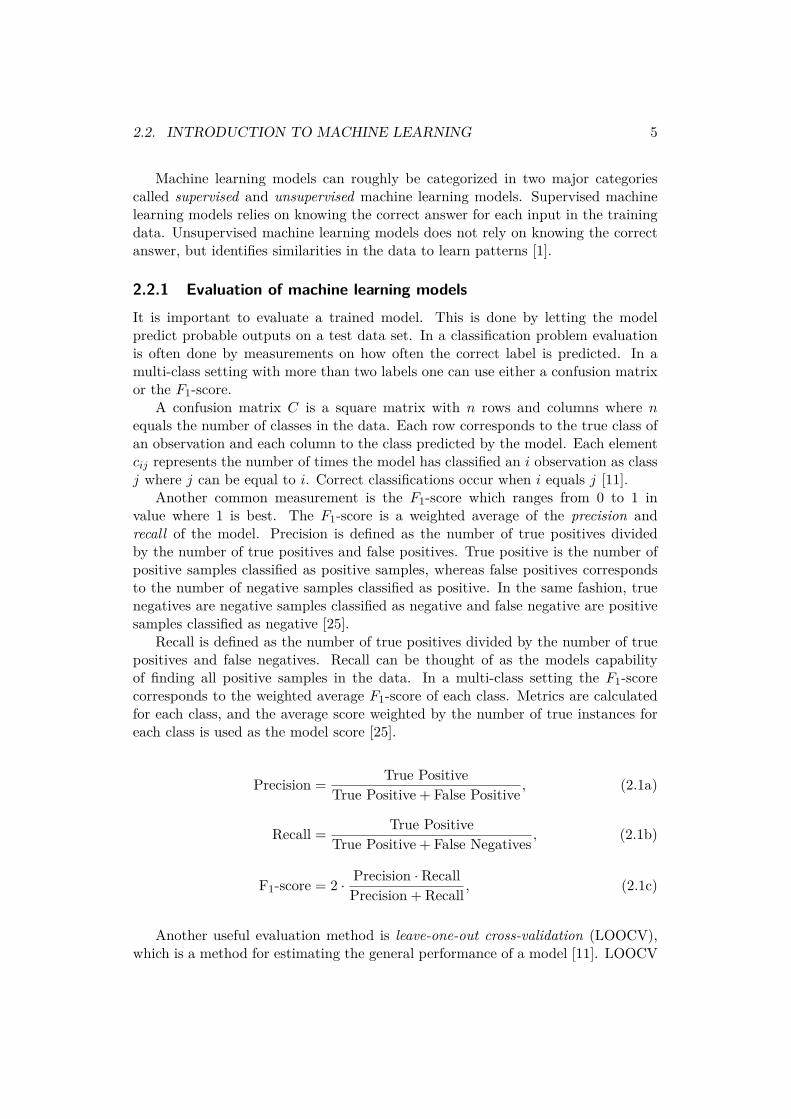
2.2.1 Evaluation of machine learning modelsIt is important to evaluate a trained model. This is done by letting the modelpredict probable outputs on a test data set. In a classification problem evaluationis often done by measurements on how often the correct label is predicted. In amulti-class setting with more than two labels one can use either a confusion matrixor the F1-score.

A confusion matrix C is a square matrix with n rows and columns where nequals the number of classes in the data. Each row corresponds to the true class ofan observation and each column to the class predicted by the model. Each elementcij represents the number of times the model has classified an i observation as classj where j can be equal to i. Correct classifications occur when i equals j [11].

Another common measurement is the F1-score which ranges from 0 to 1 invalue where 1 is best. The F1-score is a weighted average of the precision andrecall of the model. Precision is defined as the number of true positives dividedby the number of true positives and false positives. True positive is the number ofpositive samples classified as positive samples, whereas false positives correspondsto the number of negative samples classified as positive. In the same fashion, truenegatives are negative samples classified as negative and false negative are positivesamples classified as negative [25].

Recall is defined as the number of true positives divided by the number of truepositives and false negatives. Recall can be thought of as the models capabilityof finding all positive samples in the data. In a multi-class setting the F1-scorecorresponds to the weighted average F1-score of each class. Metrics are calculatedfor each class, and the average score weighted by the number of true instances foreach class is used as the model score [25].

Precision = True PositiveTrue Positive + False Positive , (2.1a)

Recall = True PositiveTrue Positive + False Negatives , (2.1b)

F1-score = 2 · Precision · RecallPrecision + Recall , (2.1c)

Another useful evaluation method is leave-one-out cross-validation (LOOCV),which is a method for estimating the general performance of a model [11]. LOOCV

6 CHAPTER 2. BACKGROUND

uses one observation in the data as test data and remaining observations as trainingdata. This is repeated for every observation in the data set so that each observationwill be used as test data once. The mean F1-score and the standard deviation overall iterations is used as a measurement of the general performance of the model.

2.3 Eye tracking and machine learning

Recent eye tracking research often includes machine learning models for analysisof collected data. Modern high frequency eye trackers are accurate and able torecord the gaze point at a rate of at least 300 Hz. High frequency recordings ofeye movements provide gaze point information at a millisecond scale, which makesit possible to distinguish rapid eye movements that previously were undetectable.The high sample rate generates large amounts of data that enables the usage ofmachine learning for data analysis [5].

Studies involving machine learning and eye tracking often rely on various eyemovement features. These features often builds upon knowledge from eye trackingstudies and features such as mean fixation time and saccade length are common.Choosing relevant features is key for a machine learning model to be able to properlylearn relevant patterns in the data. Features are selected either manually or byutilizing feature learning methods. Manual selection of features can either be basedon expert knowledge of the data or by trial-and-error [1, 11].

Section 2.1 highlighted that eye movements differ between various activities.This was tested in an eye tracking study [7] where participants performed four dif-ferent tasks corresponding to scene search, scene memorization, reading and pseudo-reading. Twelve participants were observed performing each task one at a time. Thedata was pre-processed to remove fixations longer than 1,500 ms and saccades pre-ceding blinks was also removed. Various types of features were extracted from therecordings. These features were selected on basis of previous knowledge within theeye tracking community; mean and standard deviation of fixation durations, meanand standard deviation of saccade amplitude and number of fixations per trial. Theparameters µ, σ, τ were used to define the shape of an Gaussian distribution rep-resenting the fixation duration. They finally used a Naïve Bayes classifier togetherwith leave-one-out cross-validation and achieved an accuracy of 68 to 80 % whichcan be compared to the 25 % baseline [7].

Correct manual selection of features requires a deep understanding of the data.However, there has recently been promising results within unsupervised featurelearning where features are learned from the data by various machine learning algo-rithms. These algorithms does not require any previous knowledge about the databut instead infer it directly from the data [3].

Unsupervised feature learning algorithms are provided with training data thatis used for finding key features in the data, which can be used to transform the datainto a new representation that can be feed to a machine learning algorithm. Featurelearning methods have generated promising results within fields such as speech

2.3. EYE TRACKING AND MACHINE LEARNING 7

recognition, computer vision and gesture recognition with higher performance thancomplex state-of-the-art methods based on manual feature selection. One study[3] presents a comparison of different unsupervised feature learning methods on twobenchmark data sets. It shows that simple unsupervised feature learning algorithmsare able to find new data representations. This in combination with a classificationalgorithm is then able to achieve state-of-the-art performance, indicating that expertknowledge of the data set is not always necessary to successfully develop machinelearning algorithms.

Unsupervised feature learning models have also been applied within eye trackingresearch. One study applied unsupervised feature learning models on recordings ofeight participants using a web application. Eye tracking data was transformedinto so called heat maps that represented how fixations moved over the screenduring a period of thirty seconds. Each fixation was marked with a circle andthe color of the circle varied depending on when the fixation occurred during thethirty second segment. Early fixations was colored white and later ones was coloredblack [27]. The heat maps was feed into a restricted Boltzmann machine (RBM)that learned a new representation of the data. The data was transformed intothe new representation and feed to a K-means clustering algorithm [27]. Manualinspection of each cluster showed that similar behaviors were clustered together.The twelve biggest clusters were labeled and could then be used to label a recordingto find similar user behavior. Comparisons of the labeled recordings gave insightson common and outlier user behavior.

Another way to classify eye movements is to represent the data as time-data.Models for sequential classification take into account the temporal factor in the dataand assumes that the value of an observation depends on the previous observations.One of the most prevalent models for sequential learning are hidden Markov models(HMM). These models are the core component in many state-of-the-art solutions forclassification of sequential data within research fields such as speech recognition[4],handwriting recognition[21] and gesture recognition[18].

Each of these fields uses various feature representations that capture key factorsof the sequential data. A common feature used in handwriting recognition is theslope and curvature of a pen stroke instead of actual coordinates of the movementof the pen. These kinds of pre-processing of the data often yield good results as theHMM model can focus on finding patterns within key features of the data.

HMMs has also been applied within eye tracking research. One study [6] aimedto classify eye movements as belonging to either reading or something else. Record-ings of eye movement during reading were converted into observation sequencesof saccades where each observation was represented as incremental changes. TheHMM was compared to an artificial neural network (ANN) with a F1-score of 95%and 90%, respectively.

Chapter 3

Method

This chapter presents the details of the two approaches implemented in this thesis.Details of the data set are presented in Section 3.1. The first approach for classifica-tion of user activities in web applications is based on unsupervised feature learningand is presented in Section 3.2. A second supervised approach which relies on asequential representation of the data is presented in Section 3.3.

Both approaches for user activity classification were selected based on the find-ings of the literature study presented in Section 2.3. The unsupervised featurelearning approach was selected for various reasons. The main reason was to in-vestigate what kind of user activities an unsupervised approach would find in thedata and if those user activities would correspond to activities of interest, such asreading or information search. The supervised approach was selected as a moretraditional method for classifying sequential data that could be used in comparisonto the unsupervised approach.

3.1 Data set

A single data set was used that consisted of video recordings of a browser windowthat captured the behavior along with their eye movement. The temporal eyetracking data contains information of gaze position along with a classification ofwhich type of eye movement the observation corresponds to.

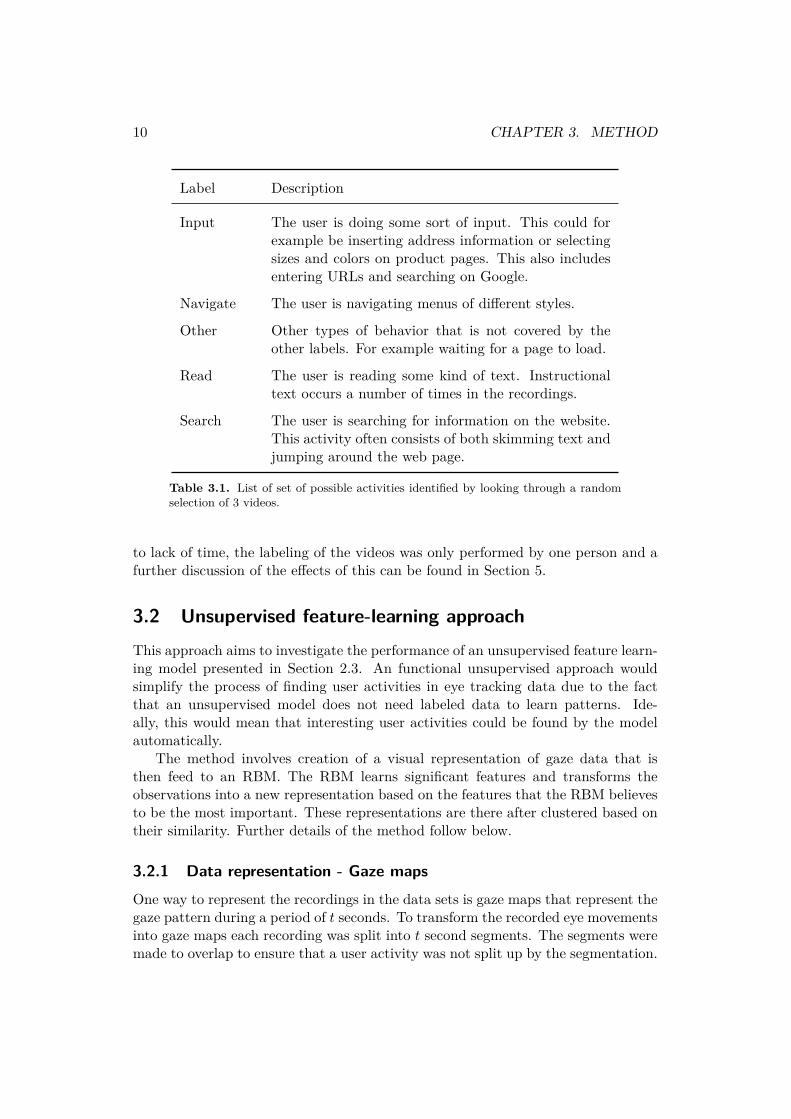
The data set contains video recordings of 36 participants reading instructionaltext and searching for information at bank websites. The average recording time is 8minutes. Recordings with weighted sampling rates below 70% are removed from thedata sets as correct labeling became infeasible, resulting in 25 remaining recordings.Videos from the data set are inspected and a set of user activities defined and usedfor labeling of the data set. A list of defined user activities and a description oftheir meaning is presented in table 3.1.

The labeling of the data set is based on subjective opinions of what the partic-ipants are doing in the videos. To decrease the level of subjectivity in the labelingprocess one could let several persons label the data and evaluate the results. Due

9

10 CHAPTER 3. METHOD

Label Description

Input The user is doing some sort of input. This could forexample be inserting address information or selectingsizes and colors on product pages. This also includesentering URLs and searching on Google.

Navigate The user is navigating menus of different styles.

Other Other types of behavior that is not covered by theother labels. For example waiting for a page to load.

Read The user is reading some kind of text. Instructionaltext occurs a number of times in the recordings.

Search The user is searching for information on the website.This activity often consists of both skimming text andjumping around the web page.

Table 3.1. List of set of possible activities identified by looking through a randomselection of 3 videos.

to lack of time, the labeling of the videos was only performed by one person and afurther discussion of the effects of this can be found in Section 5.

3.2 Unsupervised feature-learning approachThis approach aims to investigate the performance of an unsupervised feature learn-ing model presented in Section 2.3. An functional unsupervised approach wouldsimplify the process of finding user activities in eye tracking data due to the factthat an unsupervised model does not need labeled data to learn patterns. Ide-ally, this would mean that interesting user activities could be found by the modelautomatically.

The method involves creation of a visual representation of gaze data that isthen feed to an RBM. The RBM learns significant features and transforms theobservations into a new representation based on the features that the RBM believesto be the most important. These representations are there after clustered based ontheir similarity. Further details of the method follow below.

3.2.1 Data representation - Gaze maps

One way to represent the recordings in the data sets is gaze maps that represent thegaze pattern during a period of t seconds. To transform the recorded eye movementsinto gaze maps each recording was split into t second segments. The segments weremade to overlap to ensure that a user activity was not split up by the segmentation.

3.2. UNSUPERVISED FEATURE-LEARNING APPROACH 11

Starting position

t1 t2 t3 t4 t5 t6 t7 t8 t9 t10 t11 t12 ...

Window slides

t1 t2 t3 t4 t5 t6 t7 t8 t9 t10 t11 t12 ...

Final position

... tn−10tn−11 tn−1tn−2tn−3tn−4tn−5tn−6tn−7tn−8tn−9 tn

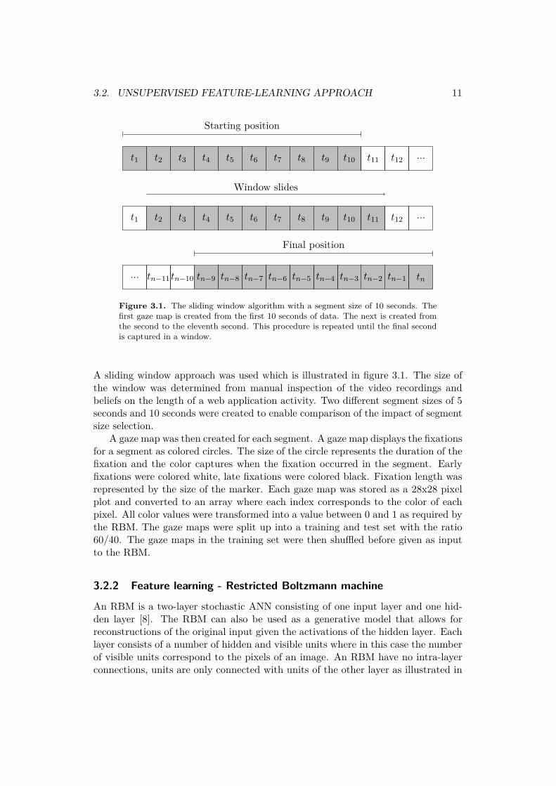
Figure 3.1. The sliding window algorithm with a segment size of 10 seconds. Thefirst gaze map is created from the first 10 seconds of data. The next is created fromthe second to the eleventh second. This procedure is repeated until the final secondis captured in a window.

A sliding window approach was used which is illustrated in figure 3.1. The size ofthe window was determined from manual inspection of the video recordings andbeliefs on the length of a web application activity. Two different segment sizes of 5seconds and 10 seconds were created to enable comparison of the impact of segmentsize selection.

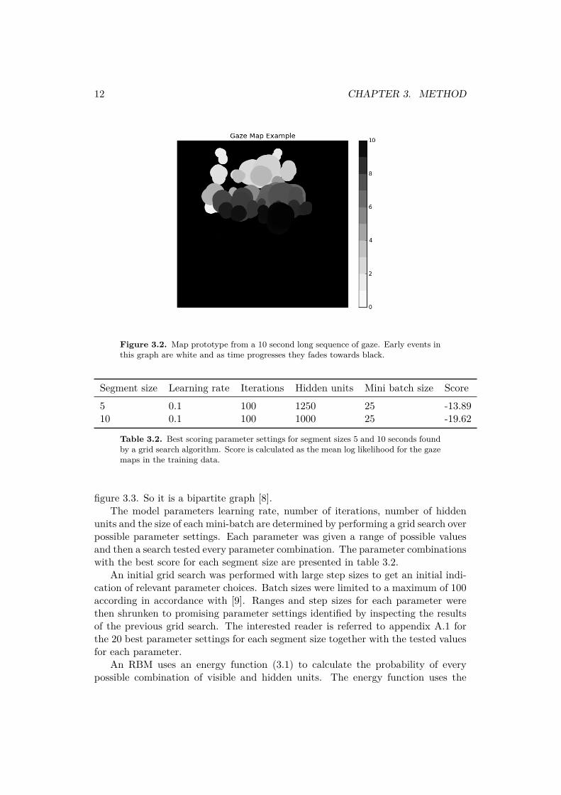
A gaze map was then created for each segment. A gaze map displays the fixationsfor a segment as colored circles. The size of the circle represents the duration of thefixation and the color captures when the fixation occurred in the segment. Earlyfixations were colored white, late fixations were colored black. Fixation length wasrepresented by the size of the marker. Each gaze map was stored as a 28x28 pixelplot and converted to an array where each index corresponds to the color of eachpixel. All color values were transformed into a value between 0 and 1 as required bythe RBM. The gaze maps were split up into a training and test set with the ratio60/40. The gaze maps in the training set were then shuffled before given as inputto the RBM.

3.2.2 Feature learning - Restricted Boltzmann machine

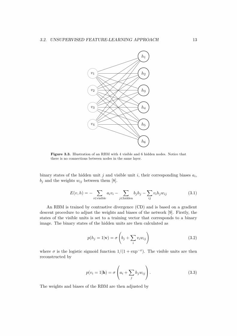
An RBM is a two-layer stochastic ANN consisting of one input layer and one hid-den layer [8]. The RBM can also be used as a generative model that allows forreconstructions of the original input given the activations of the hidden layer. Eachlayer consists of a number of hidden and visible units where in this case the numberof visible units correspond to the pixels of an image. An RBM have no intra-layerconnections, units are only connected with units of the other layer as illustrated in


Figure 3.2. Map prototype from a 10 second long sequence of gaze. Early events inthis graph are white and as time progresses they fades towards black.

Segment size Learning rate Iterations Hidden units Mini batch size Score

5 0.1 100 1250 25 -13.8910 0.1 100 1000 25 -19.62

Table 3.2. Best scoring parameter settings for segment sizes 5 and 10 seconds foundby a grid search algorithm. Score is calculated as the mean log likelihood for the gazemaps in the training data.

figure 3.3. So it is a bipartite graph [8].The model parameters learning rate, number of iterations, number of hidden

units and the size of each mini-batch are determined by performing a grid search overpossible parameter settings. Each parameter was given a range of possible valuesand then a search tested every parameter combination. The parameter combinationswith the best score for each segment size are presented in table 3.2.

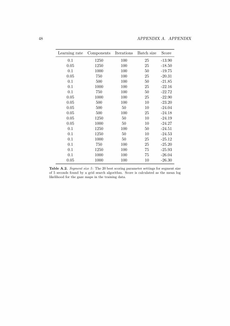
An initial grid search was performed with large step sizes to get an initial indi-cation of relevant parameter choices. Batch sizes were limited to a maximum of 100according in accordance with [9]. Ranges and step sizes for each parameter werethen shrunken to promising parameter settings identified by inspecting the resultsof the previous grid search. The interested reader is referred to appendix A.1 forthe 20 best parameter settings for each segment size together with the tested valuesfor each parameter.

An RBM uses an energy function (3.1) to calculate the probability of everypossible combination of visible and hidden units. The energy function uses the

3.2. UNSUPERVISED FEATURE-LEARNING APPROACH 13

v1

v2

v3

v4

h1

h2

h3

h4

h5

h6

Figure 3.3. Illustration of an RBM with 4 visible and 6 hidden nodes. Notice thatthere is no connections between nodes in the same layer.

binary states of the hidden unit j and visible unit i, their corresponding biases ai,bj and the weights wij between them [8].

E(v, h) = −∑

i∈visibleaivi −

∑j∈hidden

bjhj −∑ij

vihjwij (3.1)

An RBM is trained by contrastive divergence (CD) and is based on a gradientdescent procedure to adjust the weights and biases of the network [9]. Firstly, thestates of the visible units is set to a training vector that corresponds to a binaryimage. The binary states of the hidden units are then calculated as

p(hj = 1|v) = σ

(bj +

∑i

viwij

)(3.2)

where σ is the logistic sigmoid function 1/(1 + exp−x). The visible units are thenreconstructed by

p(vi = 1|h) = σ

ai +∑

j

hjwij

. (3.3)

The weights and biases of the RBM are then adjusted by


4wij = ε ((vihj)data − (vihj)reconstruction) (3.4a)

4ai = ε ((vi)data − (vi)reconstruction) (3.4b)

4bj = ε ((hj)data − (hj)reconstruction) (3.4c)

where ε represents the learning rate of the RBM [8].RBM models for each segment size were created with 784 visible units cor-

responding to each pixel in the gaze maps. Each RBM was initialized with thecorresponding hyper parameter settings presented in table 3.2 and trained with 60% of the training data. The remaining 40 % were used as test data sets that weretransformed by the trained RBM models and given as input to K-means clusteringmodels created for each segment size.

3.2.3 Classification - K-means clusteringOne way of identifying user activities in web applications is to cluster gaze patternsbased on their similarity. If the clustering is successful, there should be clustersthat correspond to specific user activities.

K-means [11] is a clustering algorithm that creates k distinct non-overlappingclusters. The algorithm clusters observations to each cluster by calculating the dis-tance between the observation and the centroid of a cluster. The observation is thenassigned to the cluster to which it is closest. The K-means algorithm implementedin this thesis strives to partition the observations into k clusters such that the to-tal within-cluster-variation, summed over all k clusters is as small as possible [11].Hence, the objective is given by

minimizec1,...,ck

{K∑

k=1

1|Ck|

∑i,i′∈Ck

Hamming(xi, xi′)}

(3.5)

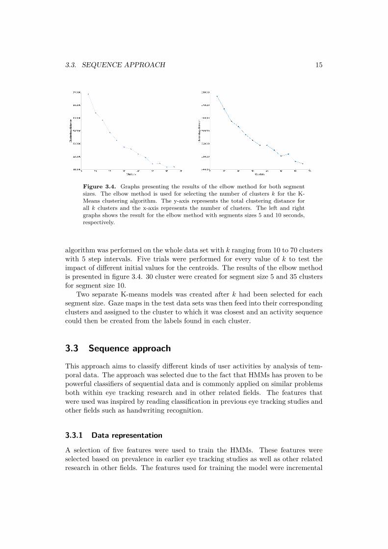
The k centroids can either be predefined manually or initialized randomly byselecting k observations as centroids. K-means cannot infer the number of clustersfrom the data, and k must therefore be selected manually. In this case, the correctnumber of user activities is unknown. Selection of k will therefore be based onbeliefs of the number of user activities in the data and an analysis of the totalclustering distance. The total clustering distance is the sum of distances betweenobservations and the centroid within each cluster [11].

Analysis of the total clustering distance was performed by visually inspectinga scree plot for an elbow point. The total clustering distance was calculated for arange of possible values of k and then plotted. As k increases, the total clusteringdistance will diminish rapidly and then taper off. We then select the last k forwhich a significant improvement can be identified. Selecting that specific k ensuresthat most gaze patterns can be explained by k clusters [11]. The K-means clustering

3.3. SEQUENCE APPROACH 15

Figure 3.4. Graphs presenting the results of the elbow method for both segmentsizes. The elbow method is used for selecting the number of clusters k for the K-Means clustering algorithm. The y-axis represents the total clustering distance forall k clusters and the x-axis represents the number of clusters. The left and rightgraphs shows the result for the elbow method with segments sizes 5 and 10 seconds,respectively.

algorithm was performed on the whole data set with k ranging from 10 to 70 clusterswith 5 step intervals. Five trials were performed for every value of k to test theimpact of different initial values for the centroids. The results of the elbow methodis presented in figure 3.4. 30 cluster were created for segment size 5 and 35 clustersfor segment size 10.

Two separate K-means models was created after k had been selected for eachsegment size. Gaze maps in the test data sets was then feed into their correspondingclusters and assigned to the cluster to which it was closest and an activity sequencecould then be created from the labels found in each cluster.

3.3 Sequence approach

This approach aims to classify different kinds of user activities by analysis of tem-poral data. The approach was selected due to the fact that HMMs has proven to bepowerful classifiers of sequential data and is commonly applied on similar problemsboth within eye tracking research and in other related fields. The features thatwere used was inspired by reading classification in previous eye tracking studies andother fields such as handwriting recognition.

3.3.1 Data representation

A selection of five features were used to train the HMMs. These features wereselected based on prevalence in earlier eye tracking studies as well as other relatedresearch in other fields. The features used for training the model were incremental


changes in x and y coordinates between sequences of fixations, the fixation time,and the direction of the saccade represented as the sine and cosine [10] defined as

cosα(t) = 4x(t)4s(t) sinα(t) = 4y(t)

4s(t) , (3.6a)

4s(t) =√4x2(t) +4y2(t). (3.6b)

Each recording was split up into 5 and 10 second segments using the slidingwindow approach illustrated in figure 3.1. Segments that consisted of one useractivity were stored and used as training data in the classification step.

3.3.2 Classification - Hidden Markov ModelThe HMM is a sequence classifier that can map a sequence of observations to asequence of labels. A first-order HMM relies on the first-order Markov assumptionwhich states that the probability of a particular state only depends on the previ-ous state [23]. HMMs have been the model of choice for classification of temporalsequential data for some time, prevalent within research fields such as speech recog-nition [12], natural language modeling [17], on-line handwriting recognition [20] andfor analysis of biological sequences such as proteins and DNA [15].

A HMM model denoted λ = (A,B, π) consists of three major components; atransition matrix A, an emission matrix B and an initial state distribution π. AHMM maps a sequence of observations O = {O1, O2, ..., Ot} to a sequence of hiddenstates S = {S1, S2, ..., St}. Observations in this case refer to features that canbe observed in the recorded eye movement data such as the mean fixation timeor saccade length. The hidden states cannot be observed themselves, hence theirname, but instead generates a visible observation sequence which can be used toestimate the underlying hidden state sequence [23].

A trained model can be used to quantify how probable an observation sequenceis given the model P (O|λ), or present the most probable hidden state sequence givenan observation sequence. HMMs are therefore useful in classification problems asvarious models can be trained to recognize various behavior. One can then use amaximum likelihood approach to classify a new observation sequence by feeding thesequence to each model and then select the one with the highest probability.

Constructing a HMM involves solving three different problems. Rabiner [23]defines these three problems as follows.

Problem 1 Given the observation sequence O = {O1, O2, ..., Ot} and a modelλ = (A,B, π), how do we efficiently compute P (O|λ), the probability of theobservation sequence given the model?

Problem 2 Given the observation sequence O = {O1, O2, ..., Ot} and the model λ,how do we choose a corresponding state sequence S = {s1, s2, ..., st} which is


optimal. Given the model λ = (A,B, π) and an observation sequence O, findan optimal S in some meaningful sense?

Problem 3 How do we adjust the model parameters λ = (A,B, π) to maximizeP (O|λ)?

These three problems are solved using the forward backward procedure, theViterbi algorithm and the Baum-Welch algorithm, respectively. However, thereexists other implementation issues when practically implementing HMMs. Firstly,long observation sequences often results in calculations involving small probabilitieswhich cause underflows. One solution to mitigate this problem is using a scalingfactor denoted c [23]. Small probabilities can also create problems when calculatingthe probability of a sequence or when re-estimating the A and B matrices in theBaum-Welch algorithm. The probability of a sequence is therefore represented as alog-probability which mitigates underflow problems.

Another problem is the initialization of the model parameters A, B and π. Themost problematic is B which greatly contributes to the successful training of aHMM. It was therefore estimated by utilizing the Viterbi algorithm and recursion.This procedure is presented in [23] and interested readers are referred to this tutorialfor further details [23].

The forward backward procedure

The forward backward procedure solves Problem 1. This enables evaluation of thelikelihood of an observation sequences given a model. The measurement that oftenis represented as a log-likelihood can be seen as a score that enables comparison ofthe likelihood of a observation sequence given some models.

The procedure introduces a new variable called the forward variable αt(i) whichcan be interpreted as the likelihood for a sequence of observations up to time t. Wedefine this variable as

αt(i) = P (O = {O1, . . . , Ot}, qt = Si|λ). (3.7)

Here, α is initialized by calculating the cross-product of the initial state distributionand the column in the observation matrix that corresponds to the first observationsymbol given by

α1(i) = πibi(O1), 1 ≤ i ≤ N. (3.8)

Then, αt(i) is calculated by multiplying αt−1(i) with the transition matrix A andthen multiplying it with the column of the observation matrix that corresponds tothe observation symbol at time t+ 1., i.e.,

αt(i) =[

N∑i=1

αt(i)aij

]bj(Ot+1), 1 ≤ t ≤ T − 1, 1 ≤ j ≤ N (3.9)


Every calculation of αt(i) is scaled with the scaling factor ct defined as 1 over αt.The scaling factor is used to calculate αt(i) which is the scaled equivalent to αt(i),i.e.,

ct =[

N∑i=1

αt(i)]−1

, αt(i) = ct · αt(i). (3.10)

After the computation of all α-values up until time T one can calculate the proba-bility for observing the observation sequence given the model, i.e.,

P (O|λ) =[

T∏t=1

ct

]−1

, log [P (O|λ)] = −T∑

t=1log ct. (3.11)

Calculations of the forward variable αt(i) are often combined with calculations of thebackward variable βt(i) which is defined as the probability of the partial observationsequence from t+ 1 to the end, given the states Si at time t and the model λ,

βt(i) = P (O = {Ot+1, . . . , OT }|qt = Si, λ). (3.12)

βT (i) is initialised with the value 1 for each state. Previous time steps are thencomputed by multiplying the transition matrix A with the column in the observationmatrix B that corresponds to the observation symbol Ot+1 and then multiplyingthe values with βt+1(j), i.e.,

βt(i) =N∑

j=1aijbj(Ot+1)βt+1(j), t = {T − 1, T − 2, . . . , 1}, 1 ≤ i ≤ N. (3.13)

Scaling of βt(i) is performed in the same fashion as for the forward variable. Boththe forward and backward variables are necessary for solving both problems 2 and3.

Viterbi algorithm

The Viterbi algorithm solves Problem 2. The algorithm uncovers the hidden part ofthe model by finding a optimal state sequence S = {s1, s2, . . . , sT } that could haveproduced the observation sequence O = {O1, O2, . . . , OT }. The best score along asingle path at time t denoted δy(i) accounts for the first t observations and ends instate Si, i.e.,

δt(i) = maxq1,q2,...,qt−1

P (Q = i, O|λ) (3.14)

Note that δt(i) is calculated in a similar fashion as the forward variable and it isinitialized exactly as the forward variable (3.8). The main difference is that insteadof summing over all states only the most probable state is saved. The value of the


most probable state is stored in δt(i) and the actual state is stored in ψt(i) whichis initialized as 0. Those two quantities are computed by

δt(j) = max1≤i≤N

[δt−1(i)aij

], 2 ≤ t ≤ T, 1 ≤ j ≤ N, (3.15)

ψt(j) = argmax1≤i≤N

[δt−1(i)aij

]bj(Ot), 2 ≤ t ≤ T, 1 ≤ j ≤ N. (3.16)

The optimal state sequence is then created by storing the most probable endstate q∗T and then backtracking to the beginning.

q∗t = ψt+1(q∗t+1), t = {T − 1, T − 2, . . . , 1}. (3.17)

Baum-Welch algorithm

The Baum-Welch algorithm can be used to solve Problem 3. This step is often re-ferred to as a training algorithm as the model learns how to best capture observationsequences.

The Baum-Welch algorithm is generally trained by using one observation se-quence. As all recordings have been labeled and segmented into observation se-quences with their corresponding label, the Baum-Welch algorithm needs to bealtered so that it can train the model with several observation sequences.

Given k observation sequences the Baum-Welch algorithm calculates the prob-ability for that sequence given the current model and uses PK to cancel out thescaling factor for each observation sequence where Pk is defined as

P (O|λ) =K∏

k=1P (Ok|λ) =

K∏k=1

Pk, log [P (O|λ)] = −K∑

k=1logPk. (3.18)

The Baum-Welch algorithm adjusts the transition matrix A and the observationmatrix B with the help of the forward and backward variables created by the proce-dure in section 3.3.2. The re-estimation formula for A is presented in (3.19). Eachelement of A is calculated by counting the expected number of transitions betweenstate Si to state Sj and then dividing the sum with the total number of expectedtransitions from state Si, i.e,

aij =

K∑k=1

1Pk

Tk−1∑t=1

αkt (i)aijbj(Ok

t+1)βkt+1(j)

K∑k=1

1Pk

Tk−1∑t=1

αkt (i)βk

t+1(j). (3.19)

The observation matrix B is re-estimated by calculating the expected numberof times in state j and observing the observation symbol vk divided by the expectednumber of times in state j i.e,.


bj(k) =

K∑k=1

1Pk

Tk−1∑t=1

s.t.Ot=vk

αkt (i)βk

t+1(j)

K∑k=1

1Pk

Tk−1∑t=1

αkt (i).βk

t+1(j)(3.20)

Finally the third parameter of the model π is re-estimated with the value 1 foreach state.

Implementation

Five HMMs corresponding to the user activities reading, information search, nav-igating menus, inputting information and other were created. All created HMMswere ergodic, meaning that the transition matrix allowed transitions between everystate in the model, and had for hidden units. Each hidden unit can be thought ofas representing one of the saccade directions up, down, left and right. All emissionmatrices was constructed with one multivariate Gaussian distribution for each state.

An LOOCV approach was used for evaluating the general performance of themodel. One recording at the time was used as the test data set and the rest were usedfor training the models. Each recording is split up into observation sequences whereeach observation consists of the features defined in Section 3.3.1. The number ofobservations per observation sequence differed depending on the segment length, 5 or10 seconds, and the gaze pattern of each participant. Recordings in the training dataset with observation sequences consisting solely of observations corresponding to oneuser activity were used to train the models. For example, an observation sequencewith observations labeled as reading was used to train the HMM corresponding tothe user activity reading.

The recording in the test data set was then split up into observation sequences.Each observation sequence was feed to each one of the five HMMs. Each HMM thencalculated the probability of the observation sequence with the forward backwardprocedure. The user activity of the HMM with the highest score is then used as aprediction for the observation sequence.

Chapter 4

Results

This chapter presents the results of the two approaches presented in the previouschapter 3, methodology. Firstly, the labeled activity sequences for all recordingsare presented in Section 4.1. Next, the results of the unsupervised feature learningapproach is presented in Section 4.2. Finally the results of the supervised featuresequence approach is presented in Section 4.3.

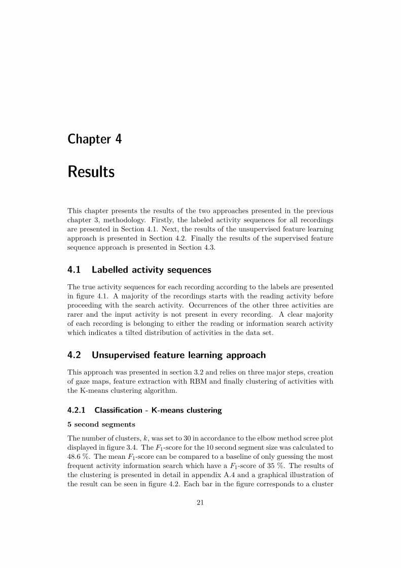
4.1 Labelled activity sequencesThe true activity sequences for each recording according to the labels are presentedin figure 4.1. A majority of the recordings starts with the reading activity beforeproceeding with the search activity. Occurrences of the other three activities arerarer and the input activity is not present in every recording. A clear majorityof each recording is belonging to either the reading or information search activitywhich indicates a tilted distribution of activities in the data set.

4.2 Unsupervised feature learning approachThis approach was presented in section 3.2 and relies on three major steps, creationof gaze maps, feature extraction with RBM and finally clustering of activities withthe K-means clustering algorithm.

4.2.1 Classification - K-means clustering5 second segments

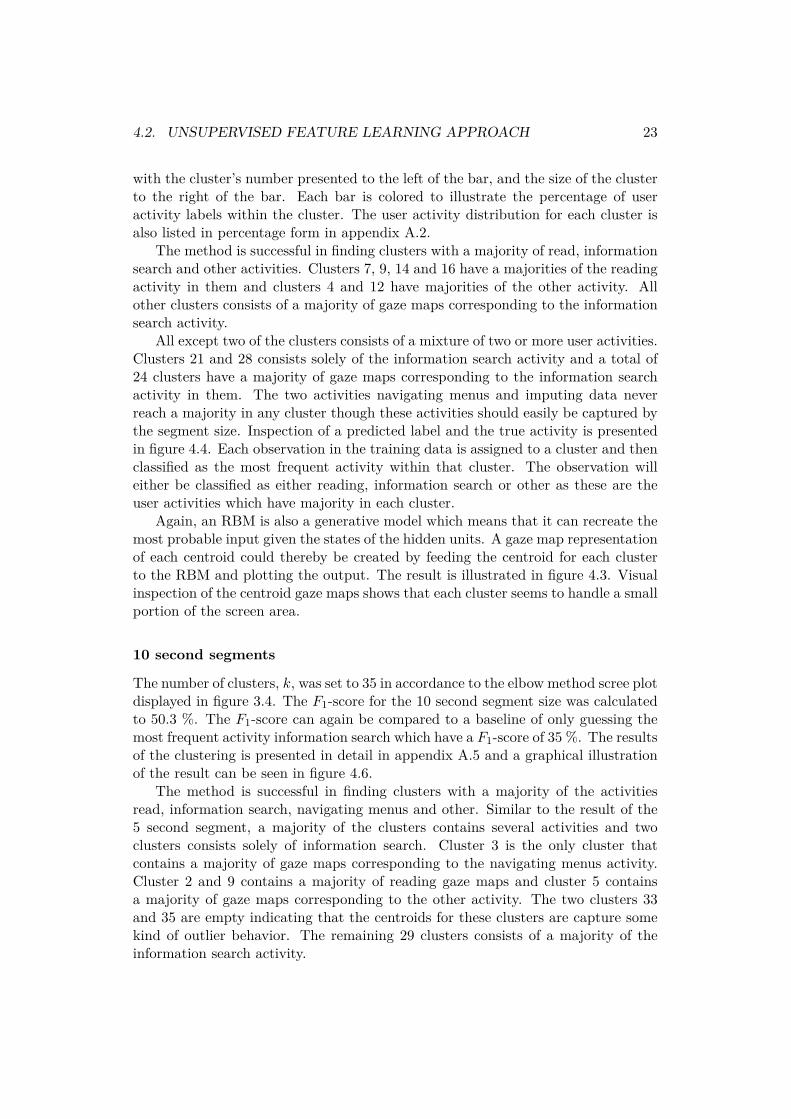
The number of clusters, k, was set to 30 in accordance to the elbow method scree plotdisplayed in figure 3.4. The F1-score for the 10 second segment size was calculated to48.6 %. The mean F1-score can be compared to a baseline of only guessing the mostfrequent activity information search which have a F1-score of 35 %. The results ofthe clustering is presented in detail in appendix A.4 and a graphical illustration ofthe result can be seen in figure 4.2. Each bar in the figure corresponds to a cluster

21

22 CHAPTER 4. RESULTS

Figure 4.1. Graphical illustration of the sequences of activities for all recordings inthe bank data set. Each line corresponds to one recording and each color correspondsto a user activity. Dark blue fields corresponds to reading, light blue fields correspondsto information search, orange fields corresponds to navigation, sand fields correspondsto input activities and finally green fields corresponds to other types of activities. Forexample, all recordings start with the reading activity before switching to eitherinformation search or the other activity.

4.2. UNSUPERVISED FEATURE LEARNING APPROACH 23

with the cluster’s number presented to the left of the bar, and the size of the clusterto the right of the bar. Each bar is colored to illustrate the percentage of useractivity labels within the cluster. The user activity distribution for each cluster isalso listed in percentage form in appendix A.2.

The method is successful in finding clusters with a majority of read, informationsearch and other activities. Clusters 7, 9, 14 and 16 have a majorities of the readingactivity in them and clusters 4 and 12 have majorities of the other activity. Allother clusters consists of a majority of gaze maps corresponding to the informationsearch activity.

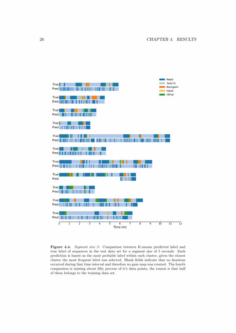
All except two of the clusters consists of a mixture of two or more user activities.Clusters 21 and 28 consists solely of the information search activity and a total of24 clusters have a majority of gaze maps corresponding to the information searchactivity in them. The two activities navigating menus and imputing data neverreach a majority in any cluster though these activities should easily be captured bythe segment size. Inspection of a predicted label and the true activity is presentedin figure 4.4. Each observation in the training data is assigned to a cluster and thenclassified as the most frequent activity within that cluster. The observation willeither be classified as either reading, information search or other as these are theuser activities which have majority in each cluster.

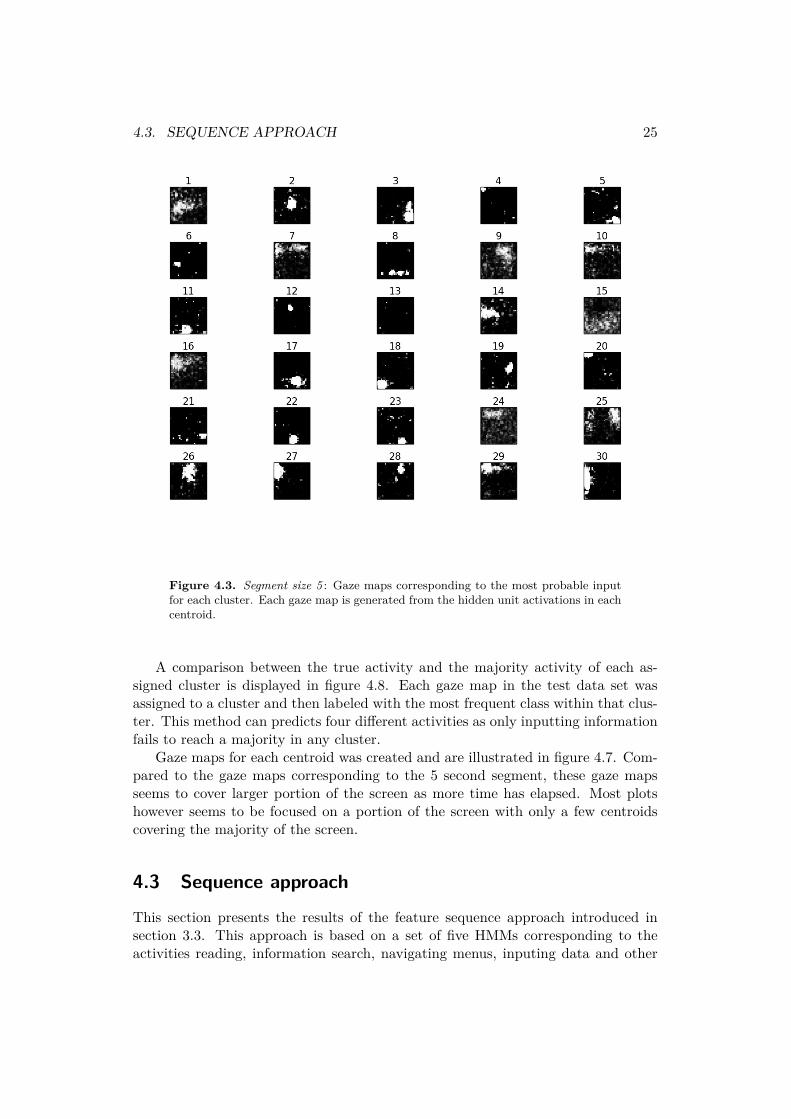
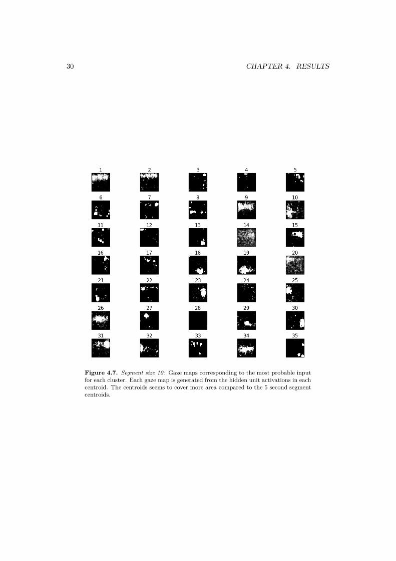
Again, an RBM is also a generative model which means that it can recreate themost probable input given the states of the hidden units. A gaze map representationof each centroid could thereby be created by feeding the centroid for each clusterto the RBM and plotting the output. The result is illustrated in figure 4.3. Visualinspection of the centroid gaze maps shows that each cluster seems to handle a smallportion of the screen area.

10 second segments

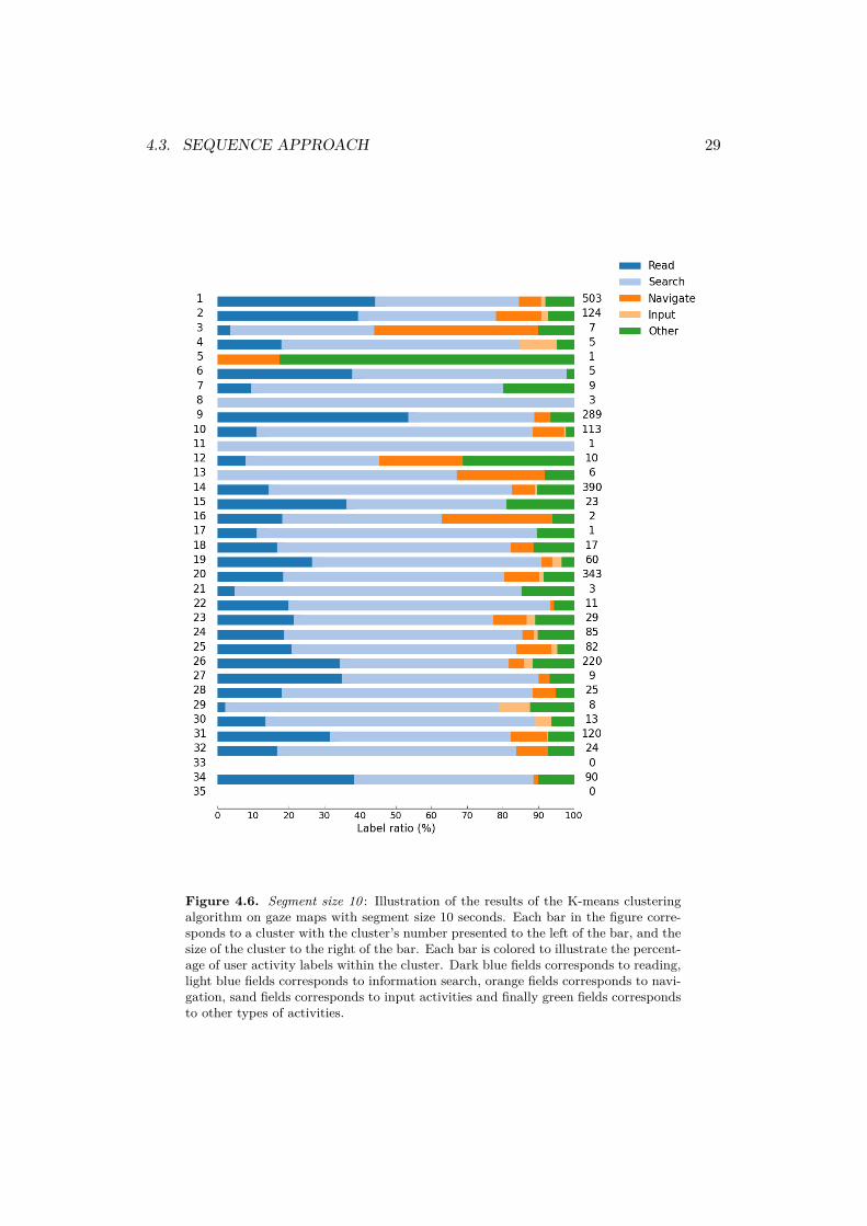
The number of clusters, k, was set to 35 in accordance to the elbow method scree plotdisplayed in figure 3.4. The F1-score for the 10 second segment size was calculatedto 50.3 %. The F1-score can again be compared to a baseline of only guessing themost frequent activity information search which have a F1-score of 35 %. The resultsof the clustering is presented in detail in appendix A.5 and a graphical illustrationof the result can be seen in figure 4.6.

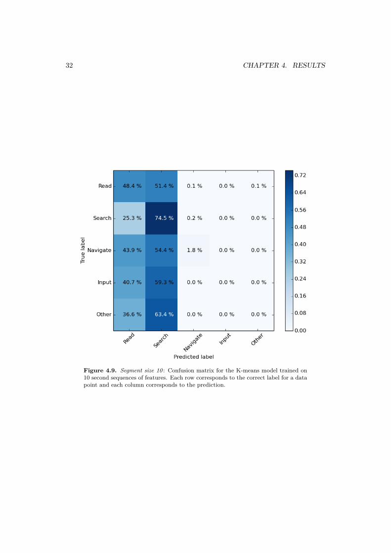
The method is successful in finding clusters with a majority of the activitiesread, information search, navigating menus and other. Similar to the result of the5 second segment, a majority of the clusters contains several activities and twoclusters consists solely of information search. Cluster 3 is the only cluster thatcontains a majority of gaze maps corresponding to the navigating menus activity.Cluster 2 and 9 contains a majority of reading gaze maps and cluster 5 containsa majority of gaze maps corresponding to the other activity. The two clusters 33and 35 are empty indicating that the centroids for these clusters are capture somekind of outlier behavior. The remaining 29 clusters consists of a majority of theinformation search activity.


Figure 4.2. Segment size 5 : Illustration of the results of the K-means clusteringalgorithm on gaze maps with segment size 5 seconds. Each bar in the figure corre-sponds to a cluster with the cluster’s number presented to the left of the bar, and thesize of the cluster to the right of the bar. Each bar is colored to illustrate the per-centage of user activity labels within the cluster. The ratio of labels for each clusteris represented with a color for each activity. Dark blue fields corresponds to reading,light blue fields corresponds to information search, orange fields corresponds to navi-gation, sand fields corresponds to input activities and finally green fields correspondsto other types of activities.


Figure 4.3. Segment size 5 : Gaze maps corresponding to the most probable inputfor each cluster. Each gaze map is generated from the hidden unit activations in eachcentroid.

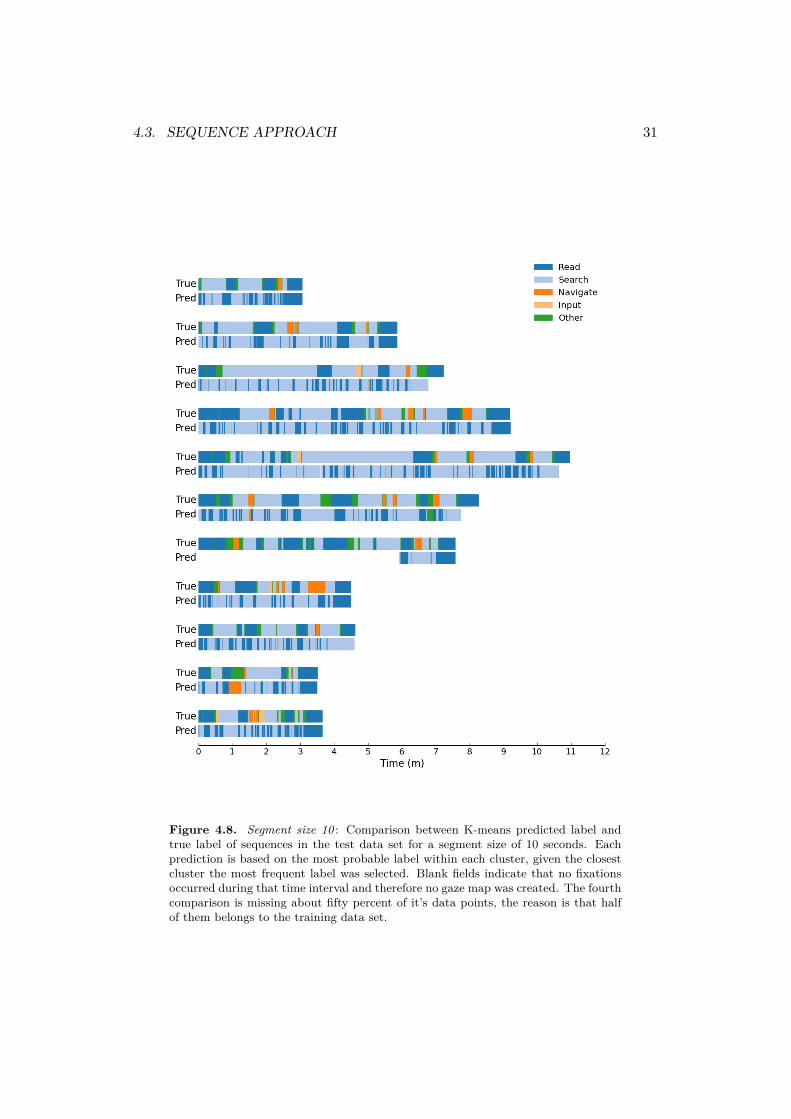
A comparison between the true activity and the majority activity of each as-signed cluster is displayed in figure 4.8. Each gaze map in the test data set wasassigned to a cluster and then labeled with the most frequent class within that clus-ter. This method can predicts four different activities as only inputting informationfails to reach a majority in any cluster.

Gaze maps for each centroid was created and are illustrated in figure 4.7. Com-pared to the gaze maps corresponding to the 5 second segment, these gaze mapsseems to cover larger portion of the screen as more time has elapsed. Most plotshowever seems to be focused on a portion of the screen with only a few centroidscovering the majority of the screen.


This section presents the results of the feature sequence approach introduced insection 3.3. This approach is based on a set of five HMMs corresponding to theactivities reading, information search, navigating menus, inputing data and other


Figure 4.4. Segment size 5 : Comparison between K-means predicted label andtrue label of sequences in the test data set for a segment size of 5 seconds. Eachprediction is based on the most probable label within each cluster, given the closestcluster the most frequent label was selected. Blank fields indicate that no fixationsoccurred during that time interval and therefore no gaze map was created. The fourthcomparison is missing about fifty percent of it’s data points, the reason is that halfof them belongs to the training data set.


kinds of activity. Each model is trained with sequences of features correspondingto their activity.

4.3.1 Classification - Hidden Markov Model5 second segments

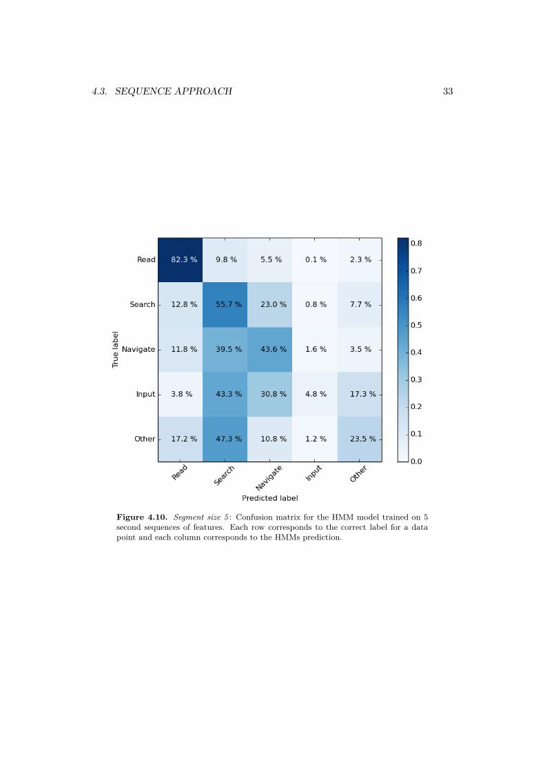
The general performance of the HMM model was evaluated by LOOCV and themean F1-score and its standard deviation is 66 % and 0.16 %, respectively. Themean F1-score can be compared to a baseline of only guessing the most frequentactivity information search which have a F1-score of 35 %. The models confusionmatrix (4.10) contains the predictions made by the model. Each row correspondsto the true activity in a segment and each column represents the prediction of themodel.

The read, information search and navigating menu activities all have a majorityof correct predictions. The input and other activity are correctly predicted in aminority of the cases. The navigation and information search activity seems to beclosely related as information often is incorrect predicted as navigating menus andvice versa.

The LOOCV tested each recordings labels against the predictions of the HMMand the result is illustrated in figure 4.11. Some sequences does not consist ofone label and the true label for that segment has therefore been set to the mostcommon activity label in that 5 second segment. Predictions for the reading activityare performing well. The model often incorrectly predicts information search as anavigation activity which also can be seen in the confusion matrix.

10 second segments

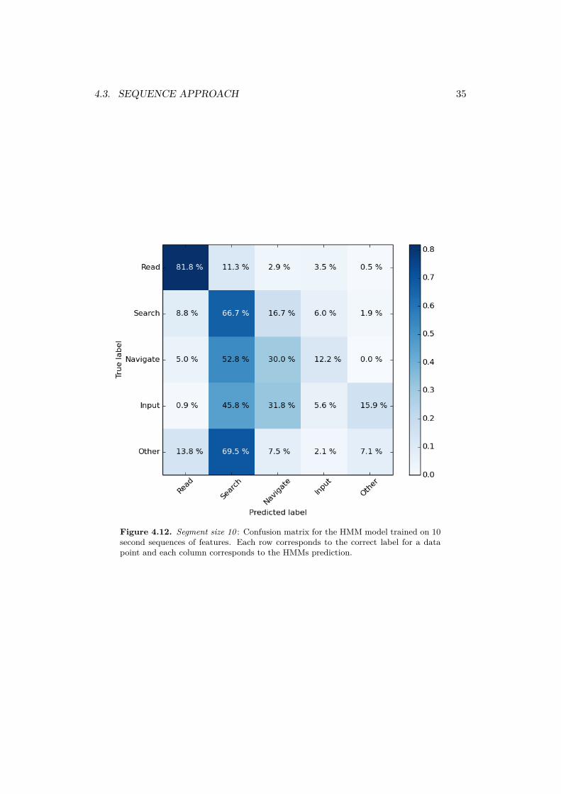
The mean F1-score and its standard deviation for 10 second segments is 70 % and0.10 %, respectively. The baseline F1-score for this segment size is 36 %. Both theread and information search activities have a majority of correct predictions. Thenavigating menus, input and other activity are correctly predicted in a minorityof the cases. The confusion matrix 4.12 also indicates that the navigation andinformation search activity seems to be closely related as they often are missclassifiedas each other. The other activity is often classified as information search.

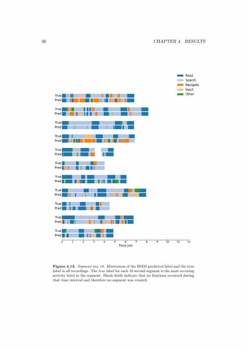
The LOOCV tested each recordings labels against the predictions of the HMMand the result is illustrated in figure 4.13. Some sequences does not consist of onelabel and the true label for that segment has therefore been set to the most com-mon activity label in that 10 second segment. Predictions for the reading activityis performing well. The model often incorrectly predicts information search as anavigation activity which also can be seen in the confusion matrix.


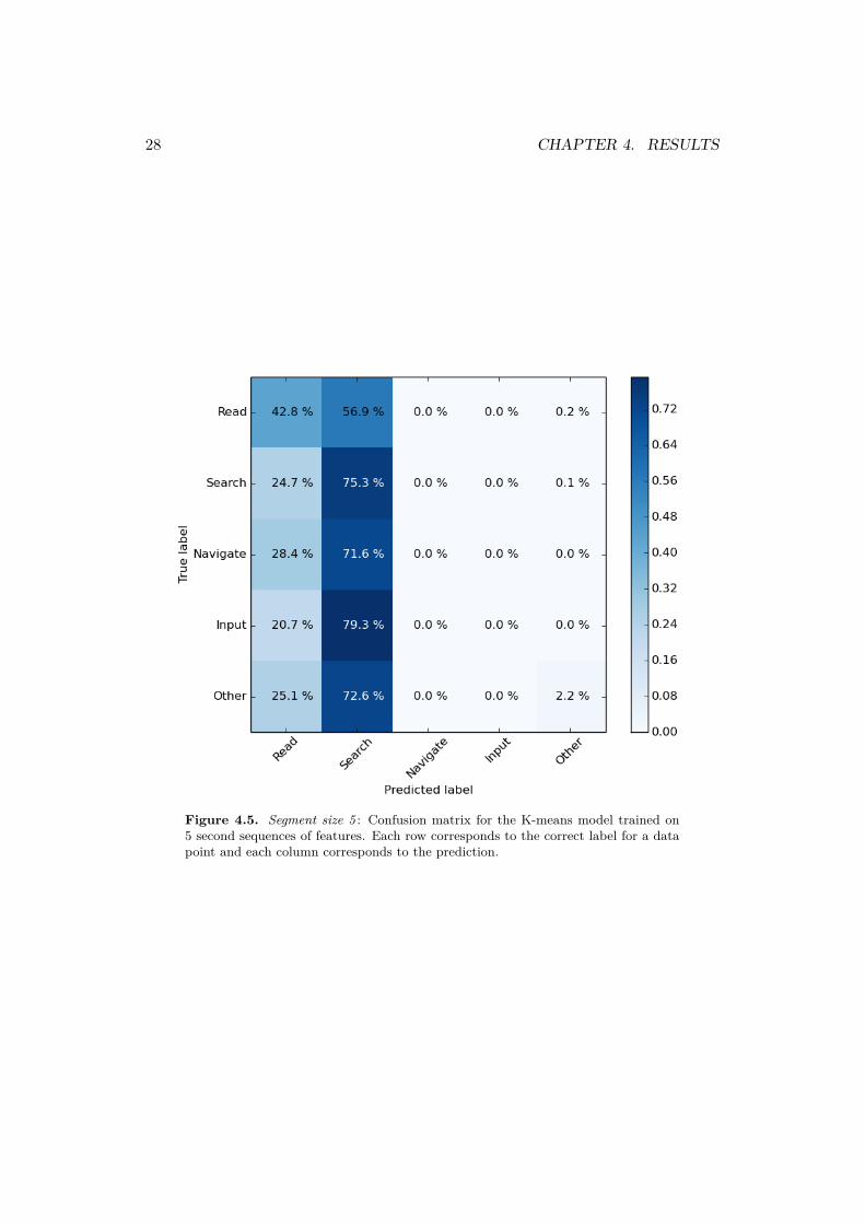
Figure 4.5. Segment size 5 : Confusion matrix for the K-means model trained on5 second sequences of features. Each row corresponds to the correct label for a datapoint and each column corresponds to the prediction.


Figure 4.6. Segment size 10 : Illustration of the results of the K-means clusteringalgorithm on gaze maps with segment size 10 seconds. Each bar in the figure corre-sponds to a cluster with the cluster’s number presented to the left of the bar, and thesize of the cluster to the right of the bar. Each bar is colored to illustrate the percent-age of user activity labels within the cluster. Dark blue fields corresponds to reading,light blue fields corresponds to information search, orange fields corresponds to navi-gation, sand fields corresponds to input activities and finally green fields correspondsto other types of activities.


Figure 4.7. Segment size 10 : Gaze maps corresponding to the most probable inputfor each cluster. Each gaze map is generated from the hidden unit activations in eachcentroid. The centroids seems to cover more area compared to the 5 second segmentcentroids.


Figure 4.8. Segment size 10 : Comparison between K-means predicted label andtrue label of sequences in the test data set for a segment size of 10 seconds. Eachprediction is based on the most probable label within each cluster, given the closestcluster the most frequent label was selected. Blank fields indicate that no fixationsoccurred during that time interval and therefore no gaze map was created. The fourthcomparison is missing about fifty percent of it’s data points, the reason is that halfof them belongs to the training data set.


Figure 4.9. Segment size 10 : Confusion matrix for the K-means model trained on10 second sequences of features. Each row corresponds to the correct label for a datapoint and each column corresponds to the prediction.


Figure 4.10. Segment size 5 : Confusion matrix for the HMM model trained on 5second sequences of features. Each row corresponds to the correct label for a datapoint and each column corresponds to the HMMs prediction.


Figure 4.11. Segment size 5 : Illustration of the HMM predicted label and the truelabel in all recordings. The true label for each 5 second segment is the most occuringactivity label in the segment. Blank fields indicate that no fixations occurred duringthat time interval and therefore no segment was created.


Figure 4.12. Segment size 10 : Confusion matrix for the HMM model trained on 10second sequences of features. Each row corresponds to the correct label for a datapoint and each column corresponds to the HMMs prediction.


Figure 4.13. Segment size 10 : Illustration of the HMM predicted label and the truelabel in all recordings. The true label for each 10 second segment is the most occuringactivity label in the segment. Blank fields indicate that no fixations occurred duringthat time interval and therefore no segment was created.

Chapter 5

Discussion

This thesis aimed to introduce methods for identifying user activities in web appli-cations based solely on eye tracking data. The two methods that were implementedin were both evaluated with a labeled data set. As mentioned in Section 3, the dataset are labeled by only one person and is therefore highly subjective. The resultsof this paper should therefore not be seen as absolute truths, but as indications ofthe implemented methods strengths and weaknesses.

5.1 Unsupervised feature learning approach

The unsupervised feature-learning approach used in this paper gave some interestingresults. After applying it with labeled data one could see that the RBM did findclusters with a clear majority of the reading, information search, navigating menusand other activities. The larger segment size of 10 seconds performed best with anF1-score of 50.3 %. However, no cluster had a majority of the inputting informationactivity. Evaluation of the clustering is also problematic as most of the largerclusters contains a combination of different activities for both segment sizes.

Inspection of the gaze map representations of the cluster centroids shows thatthe clusters corresponds to different areas of the screen. So the clusters seems tocorrespond more to areas of the screen than to specific kinds of activities. Oneexample is cluster 9 in the 10 second segment implementation that consists of 54.8% reading activity and corresponds to a horizontal scan on the top half of the screenas illustrated in figure 4.7. All recordings contained instructional text as previouslymentioned in Section 3.1 and cluster 9 consists of segments of reading these instruc-tions, this has also been confirmed by manual inspection of the recordings. Theseresults indicates that the method is sensitive to particular types of layouts and willprobably not perform well as a generic classifier of user activities.

The confusion matrices corresponding to each segment size reveals that themethod predicts the information search activity correctly about 75 % of the times.The remaining four user activities are constantly incorrectly predicted as informa-tion search a majority of the times.

37

38 CHAPTER 5. DISCUSSION

With this in mind, using this method for classifying user activity will not providegood results. Using the majority label of each cluster as a prediction will limitthe possibility of the model to make predictions of all activities. The 5 secondsegment size yielded clusters with a majority of the reading, information searchand other activity while the 10 second segment size also had a cluster containing amajority of the navigating menu activity. The gaze map representation shows thatthe navigating menu activity corresponds to scanning the right hand side of thescreen in this case. Inputting information into forms is not recognized by either ofthe segment sizes.

RBMs is also sensitive to unbalanced training data. Visual inspection of figure4.1 shows that each recording contains a majority of read and search activitieswhich skews the RBM towards recognizing these two activities. If one is interestedin finding less frequent activities one would need to balance the training data setbefore training the RBM. This approach was not tested as the aim was to evaluatethe feasibility of a totally unsupervised training process.


The feature sequence approach was able to classify the information search andreading patterns in the data. However, this approach also struggles to find theless occurring activities in the data such as navigating menus, input and other.The confusion matrices show that the search and navigation activities are hard toseparate which indicates that they are similar in regards to the selected features.The same is true for the activity other and information search where a majority ofsegments labeled as other is incorrectly classified as search for both segment sizes.

The performance of the sequence approach can be compared to previous studiesclassifying activities in controlled environments. Previous studies that classifiedactivities based on gaze data have accuracies between 68 % and 95 % dependingon the implementation. In comparison, the sequence approach implemented inthis thesis had a F1-score of 70 % for the 10 second segment size. This resultseems reasonable in this setting as not all segments that the HMM has classified dobelong to a single activity, but instead consists of various activities. As there are notransition or combination activities defined in this thesis, the correct label for eachsegment was determined by a majority vote instead of being specified as a transitionor combination activity. This will surely lead to faulty predictions which will lowerthe score of the method. One way to handle this issue would be to implement aprobability limit for allowing predictions. Probabilities lower than the limit wouldresult in an unknown activity classification and predictions higher then the limitwould be predicted according to the highest scoring HMM. Another approach wouldbe to create combination activities that hopefully would catch segments with morethan one activity.

The sequence approach performed better than the unsupervised feature learningapproach. The drawback of the sequence approach is however the need for labeled

5.3. SEGMENT SIZES 39

data for training. Currently, labeled data is a necessity for proper evaluation ofboth approaches as looking through the clusters is time consuming and probablynot applicable in a real world situation.

5.3 Segment sizesBoth the unsupervised feature learning approach and the feature sequence approachwere tested with two different segment sizes of 5 and 10 seconds. Inspection of theresults shows that a segment size of 10 seconds seems to provide better stability toboth approaches. Further optimization of segment size could possibly improve theaccuracy of both models and should be investigated further.

5.4 Definitions of the user activitiesThe results of both methods indicate that the activity definitions used in this thesisneeds to be reworked. It seems that there is a need for either more training examplesfor each activity, or possibly more precise labeling, such as vertical and horizontalnavigation. The activity other is used in recordings where the browser are loadinga page or the users gaze constantly leaves the screen. This pattern is hard torecognize according to both models and could perhaps benefit from a narrowerdefinition as well. The input activity is for similar reasons barely recognizable.There are great differences between individuals inputting information into formsregarding gaze focus. Some of the participants focused on the input field and someswitched between looking down, probably on the keyboard, and looking at the form.These differences seems too be to much to handle for both approaches.

5.5 CritiqueThe unsupervised feature learning approach implemented in this thesis proved tobe unsuitable for classifying user activities in web applications. The gaze map datarepresentation combined with the RBM are not able to find sequential informationin the gaze maps. Inspection of the gaze maps corresponding to the cluster centroidsshows that there are only fields of white fixations indicating that the RBM focuseson early fixations. Therefore, the RBM is not able to correctly learn the sequenceof the fixations which is important for distinguishing different activities but insteadfocuses on areas of the screen. Variations of gaze maps were created where differentmarker sizes were tested but without any improvement. The data representationclearly needs to be reworked to better capture the sequential information.

Prediction of user activities is also problematic for the unsupervised featureapproach. By choosing to predict the classification label based on the majorityactivity for each cluster, the model was limited to predicting either the reading,information searching, navigating menu or other activity. This means that themodel can never achieve high prediction rates as one of the five activities will never

40 CHAPTER 5. DISCUSSION

be predicted by the model. The purpose of this approach was however to investigateif the approach would be able to cluster together activities by itself which it sadlydid not do correctly. The few clusters that consisted of a majority of the other ornavigating menu activity were small and seems to be to specific.

The data set itself is also subject to critique. Besides the manual labeling of thedata the recordings also contained instruction screens that covered the whole display.These screens were displayed before and between tasks. The texts were centeredand had a fixed width. Reading these instructional screens is most likely easier toidentify compared to short reading periods in a continuous web flow. Another dataset should therefore be used to evaluate how certain these methods can predict thereading activity in the recordings.

5.6 Ethical aspects

This thesis has shown that it is possible to predict user activities with high accuracybased solely on gaze data. The two approaches created in this thesis are aimed foranalysis of user behavior and are in their current state a bit unreliable and in needof further development. However, future methods might be able to predict useractivities with high accuracy and could then be used for other purposes such assurveillance. Methods that also incorporates the mind set or feelings of a usercould possibly be developed as some recordings showed clear signs of frustrated orconfused users.

Therefore there are concerns of personal integrity connected to the technologydeveloped in this thesis. Using gaze data in surveillance methods can possiblygive plenty of insight into a persons mindset. This kind of information is privateand regulations on how eye tracking data is distributed should therefore be definedto hinder the information from spreading. Eye trackers for commercial use arecurrently being produced and will surely increase in popularity as web designersand game developers are incorporating eye tracking into their systems. The sideeffect is that eye tracking data will become abundant.

Hopefully this technology will only be applied on gaze data recorded with theformal consent of the person being monitored.

5.7 Future work

The results from this thesis show that there seems to exist eye movements corre-sponding to some of the key activities of interest. The first approach with unsuper-vised feature learning could possibly benefit from deeper neural networks such asthe deep belief network (DBN) which is basically a number of nested RBMs. DBNsare able to learn more complex pattern and might provide features that better mod-els the data. The gaze map could also be further optimized regarding the sizes offixation markings and possibly capture saccades.

5.8. CONCLUSION 41

The HMM method could possibly be replaced by a recurrent neural network(RNN) which is sequence classifier based on neural networks. RNNs have recentlyprovided promising results within speech recognition and could be applied to thisproblem. Another extension would be to create a real-time classifier based on eitheran HMM or RNN.

As this thesis aimed to test the accuracy user behavior classification solely basedon gaze data, a natural extension would be to introduce information from the webbrowser. One possible extension would be to include the position of the mouseand what element it is hovering over. This would greatly benefit the navigationand input activities as the patterns seems to be hard to separate by themselves.Incorporating browser information with eye tracking analysis would therefore be anatural next step to improve the accuracy of the predictions.

5.8 ConclusionThis paper has evaluated two different approaches for classifying user activities inweb applications. The first approach was based on unsupervised feature learning ofgaze maps containing sequences of fixations. The method was successful in findingfrequent activities such as reading and information searching, but was unable toidentify less frequent activities such as inputting data into forms or navigatingmenus. The second approach which used sequences of features performs well inclassifying the activities information search and reading, but struggles with theactivities navigating menus, inputting data and other. Comparison of differentsegment sizes shows that a segment size of 10 seconds produces better results andseems to be more stable than the shorter segment size of 5 seconds. Though thereare clear indications that some activities can be classified with gaze data, combininginformation from web browsers would be a promising extension that would mostdefinitely help with predictions of less frequent activities in a web session.

Bibliography

[1] Christopher M. Bishop. Pattern Recognition and Machine Learning. Springer-Verlag, 2006.

[2] HR Chennamma and Xiaohui Yuan. A survey on eye-gaze tracking techniques.arXiv-preprint arXiv:1312.6410, 2013.

[3] Adam Coates, Andrew Y. Ng, and Honglak Lee. An analysis of single-layernetworks in unsupervised feature learning. In International Conference onArtificial Intelligence and Statistics (AISTATS), pages 215–223, Ft. Laverdale,FL, USA, April 2011.

[4] L. Deng and X. Li. Machine learning paradigms for speech recognition: Anoverview. IEEE Transactions on Audio, Speech, and Language Processing,21(5):1060–1089, 2013.

[5] Andrew T. Duchowski. A breadth-first survey of eye-tracking applications.Behavior Research Methods, Instruments, & Computers, 34(4):455–470, 2002.

[6] Carl Johan Gustavsson. Real-time classification of reading in gaze data. Masterthesis, Kungliga Tekniska Högskolan, 2010.

[7] John M. Henderson, Svetlana V. Shinkareva, Jing Wang, Steven G. Luke, andJenn Olejarczyk. Predicting Cognitive State from Eye Movements. PLoS ONE,8, 2013.

[8] Geoffrey Hinton. A practical guide to training restricted Boltzmann machines.Technical report, Department of Computer Science, University of Toronto,2010.

[9] Geoffrey E Hinton. Training products of experts by minimizing contrastivedivergence. Neural computation, 14(8):1771–1800, 2002.

[10] Stefan Jaeger, Stefan Manke, Juergen Reichert, and Alex Waibel. Online hand-writing recognition: the npen++ recognizer. International Journal on Docu-ment Analysis and Recognition, 3(3):169–180, 2001.

43

44 BIBLIOGRAPHY

[11] Gareth James, Daniela Witten, Trevor Hastie, and Robert Tibshirani. Anintroduction to statistical learning: with applications in R. Springer-Verlag,2014.

[12] Frederick Jelinek. Statistical methods for speech recognition. MIT press, 1997.

[13] Arie E. Kaufman, Amit Bandopadhay, and Bernard D. Shaviv. An eye track-ing computer user interface. In Proceedings of the IEEE 1993 Symposium onResearch Frontiers in Virtual Reality, pages 120–121, San Jose, CA, USA, Oc-tober 1993.

[14] Robert V. Kenyon. A soft contact lens search coil for measuring eye movements.Vision Research, 25(11):1629 – 1633, 1985.

[15] Anders Krogh, Michael Brown, I Saira Mian, Kimmen Sjölander, and DavidHaussler. Hidden Markov models in computational biology: Applications toprotein modeling. Journal of Molecular Biology, 235(5):1501–1531, 1994.

[16] Arvind Kumar and Glenn Krol. Binocular infrared oculography. The Laryn-goscope, 102(4):367–378, 1992.

[17] Christopher D Manning and Hinrich Schütze. Foundations of statistical naturallanguage processing. MIT Press, 1999.

[18] S. Mitra and T. Acharya. Gesture recognition: A survey. IEEE Transactions onSystems, Man, and Cybernetics, Part C (Applications and Reviews), 37(3):311–324, May 2007.

[19] Carlos H. Morimoto and Marcio R.M. Mimica. Eye gaze tracking techniques forinteractive applications. Computer Vision and Image Understanding, 98(1):4– 24, 2005. Special Issue on Eye Detection and Tracking.

[20] R Nag, Kin Hong Wong, and Frank Fallside. Script recognition using hiddenMarkov models. In Proceedings of the 1986 IEEE International Conference onAcoustics, Speech, and Signal Processing (ICASSP), volume 11, pages 2071–2074, Tokyo, Japan, April 1986.

[21] Thomas Plötz and Gernot A. Fink. Markov Models for handwriting ecognition.Springer-Verlag, 2011.

[22] Tobii Pro. Types of eye movement. http://www.tobiipro.com/learn-and-support/learn/whatdowestudywhenwe-use-eye-tracking-data/types-of-eye-movements/, 2016. [Online; accessed 2016-04-07].

[23] Lawrence R. Rabiner. A tutorial on hidden Markov models and selected appli-cations in speech recognition. Proceedings of the IEEE, 77(2):257–286, 1989.

[24] Keith Rayner. Eye movements in reading and information processing: 20 yearsof research. Psychological bulletin, 124(3):372, 1998.

BIBLIOGRAPHY 45

[25] Cornelis van Rijsbergen. Information Retrieval. Butterworth, 1979.

[26] Alfred L. Yarbus. Eye Movements and Vision. Plenum Press, 1967.

[27] Miroslav Šimek. Processing and comparing of eye-tracking data using machinelearning. Technical report, Slovak University of Technology in Bratislava, Fac-ulty of Informatics and Information Technologies, 2015.

Appendix A

Appendix

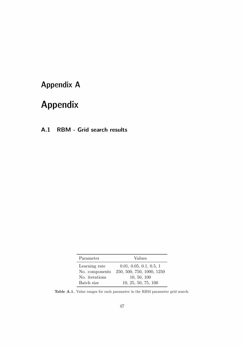
A.1 RBM - Grid search results

Parameter Values

Learning rate 0.01, 0.05, 0.1, 0.5, 1No. components 250, 500, 750, 1000, 1250No. iterations 10, 50, 100Batch size 10, 25, 50, 75, 100

Table A.1. Value ranges for each parameter in the RBM parameter grid search.

47

48 APPENDIX A. APPENDIX

Learning rate Components Iterations Batch size Score

0.1 1250 100 25 -13.900.05 1250 100 25 -18.500.1 1000 100 50 -19.750.05 750 100 25 -20.310.1 500 100 50 -21.850.1 1000 100 25 -22.160.1 750 100 50 -22.720.05 1000 100 25 -22.900.05 500 100 10 -23.200.05 500 50 10 -24.040.05 500 100 25 -24.180.05 1250 50 10 -24.190.05 1000 50 10 -24.270.1 1250 100 50 -24.510.1 1250 50 10 -24.530.1 1000 50 25 -25.120.1 750 100 25 -25.200.1 1250 100 75 -25.930.1 1000 100 75 -26.040.05 1000 100 10 -26.30

Table A.2. Segment size 5 : The 20 best scoring parameter settings for segment sizeof 5 seconds found by a grid search algorithm. Score is calculated as the mean loglikelihood for the gaze maps in the training data.

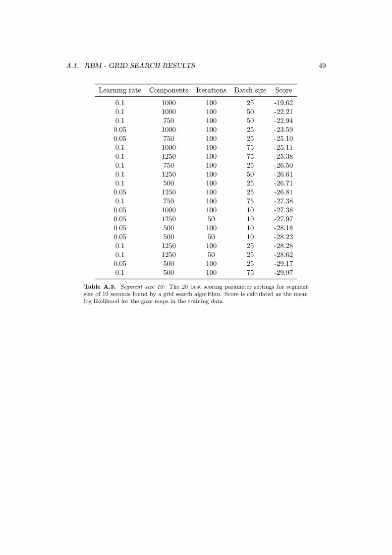
A.1. RBM - GRID SEARCH RESULTS 49

Learning rate Components Iterations Batch size Score

0.1 1000 100 25 -19.620.1 1000 100 50 -22.210.1 750 100 50 -22.940.05 1000 100 25 -23.590.05 750 100 25 -25.100.1 1000 100 75 -25.110.1 1250 100 75 -25.380.1 750 100 25 -26.500.1 1250 100 50 -26.610.1 500 100 25 -26.710.05 1250 100 25 -26.810.1 750 100 75 -27.380.05 1000 100 10 -27.380.05 1250 50 10 -27.970.05 500 100 10 -28.180.05 500 50 10 -28.230.1 1250 100 25 -28.280.1 1250 50 25 -28.620.05 500 100 25 -29.170.1 500 100 75 -29.97

Table A.3. Segment size 10 : The 20 best scoring parameter settings for segmentsize of 10 seconds found by a grid search algorithm. Score is calculated as the meanlog likelihood for the gaze maps in the training data.

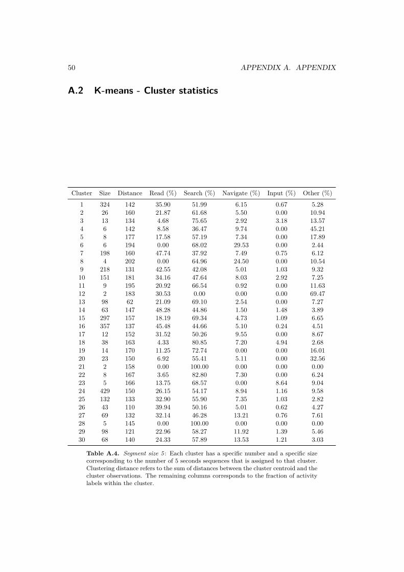
50 APPENDIX A. APPENDIX

A.2 K-means - Cluster statistics

Cluster Size Distance Read (%) Search (%) Navigate (%) Input (%) Other (%)

1 324 142 35.90 51.99 6.15 0.67 5.282 26 160 21.87 61.68 5.50 0.00 10.943 13 134 4.68 75.65 2.92 3.18 13.574 6 142 8.58 36.47 9.74 0.00 45.215 8 177 17.58 57.19 7.34 0.00 17.896 6 194 0.00 68.02 29.53 0.00 2.447 198 160 47.74 37.92 7.49 0.75 6.128 4 202 0.00 64.96 24.50 0.00 10.549 218 131 42.55 42.08 5.01 1.03 9.3210 151 181 34.16 47.64 8.03 2.92 7.2511 9 195 20.92 66.54 0.92 0.00 11.6312 2 183 30.53 0.00 0.00 0.00 69.4713 98 62 21.09 69.10 2.54 0.00 7.2714 63 147 48.28 44.86 1.50 1.48 3.8915 297 157 18.19 69.34 4.73 1.09 6.6516 357 137 45.48 44.66 5.10 0.24 4.5117 12 152 31.52 50.26 9.55 0.00 8.6718 38 163 4.33 80.85 7.20 4.94 2.6819 14 170 11.25 72.74 0.00 0.00 16.0120 23 150 6.92 55.41 5.11 0.00 32.5621 2 158 0.00 100.00 0.00 0.00 0.0022 8 167 3.65 82.80 7.30 0.00 6.2423 5 166 13.75 68.57 0.00 8.64 9.0424 429 150 26.15 54.17 8.94 1.16 9.5825 132 133 32.90 55.90 7.35 1.03 2.8226 43 110 39.94 50.16 5.01 0.62 4.2727 69 132 32.14 46.28 13.21 0.76 7.6128 5 145 0.00 100.00 0.00 0.00 0.0029 98 121 22.96 58.27 11.92 1.39 5.4630 68 140 24.33 57.89 13.53 1.21 3.03

Table A.4. Segment size 5 : Each cluster has a specific number and a specific sizecorresponding to the number of 5 seconds sequences that is assigned to that cluster.Clustering distance refers to the sum of distances between the cluster centroid and thecluster observations. The remaining columns corresponds to the fraction of activitylabels within the cluster.

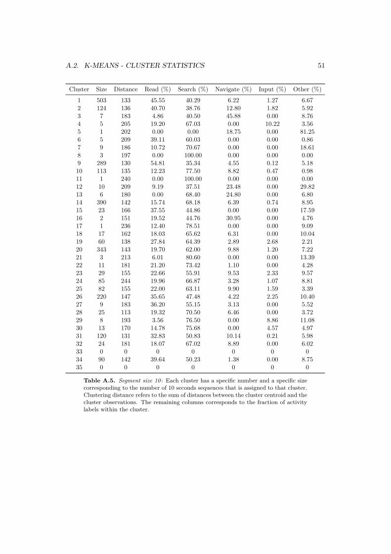
A.2. K-MEANS - CLUSTER STATISTICS 51

Cluster Size Distance Read (%) Search (%) Navigate (%) Input (%) Other (%)

1 503 133 45.55 40.29 6.22 1.27 6.672 124 136 40.70 38.76 12.80 1.82 5.923 7 183 4.86 40.50 45.88 0.00 8.764 5 205 19.20 67.03 0.00 10.22 3.565 1 202 0.00 0.00 18.75 0.00 81.256 5 209 39.11 60.03 0.00 0.00 0.867 9 186 10.72 70.67 0.00 0.00 18.618 3 197 0.00 100.00 0.00 0.00 0.009 289 130 54.81 35.34 4.55 0.12 5.1810 113 135 12.23 77.50 8.82 0.47 0.9811 1 240 0.00 100.00 0.00 0.00 0.0012 10 209 9.19 37.51 23.48 0.00 29.8213 6 180 0.00 68.40 24.80 0.00 6.8014 390 142 15.74 68.18 6.39 0.74 8.9515 23 166 37.55 44.86 0.00 0.00 17.5916 2 151 19.52 44.76 30.95 0.00 4.7617 1 236 12.40 78.51 0.00 0.00 9.0918 17 162 18.03 65.62 6.31 0.00 10.0419 60 138 27.84 64.39 2.89 2.68 2.2120 343 143 19.70 62.00 9.88 1.20 7.2221 3 213 6.01 80.60 0.00 0.00 13.3922 11 181 21.20 73.42 1.10 0.00 4.2823 29 155 22.66 55.91 9.53 2.33 9.5724 85 244 19.96 66.87 3.28 1.07 8.8125 82 155 22.00 63.11 9.90 1.59 3.3926 220 147 35.65 47.48 4.22 2.25 10.4027 9 183 36.20 55.15 3.13 0.00 5.5228 25 113 19.32 70.50 6.46 0.00 3.7229 8 193 3.56 76.50 0.00 8.86 11.0830 13 170 14.78 75.68 0.00 4.57 4.9731 120 131 32.83 50.83 10.14 0.21 5.9832 24 181 18.07 67.02 8.89 0.00 6.0233 0 0 0 0 0 0 034 90 142 39.64 50.23 1.38 0.00 8.7535 0 0 0 0 0 0 0

Table A.5. Segment size 10 : Each cluster has a specific number and a specific sizecorresponding to the number of 10 seconds sequences that is assigned to that cluster.Clustering distance refers to the sum of distances between the cluster centroid and thecluster observations. The remaining columns corresponds to the fraction of activitylabels within the cluster.

www.kth.se

Documents

Investigating user behavior by analysis of gaze data