Embed Size (px)
Citation preview

University of Arkansas, Fayetteville University of Arkansas, Fayetteville
ScholarWorks@UARK ScholarWorks@UARK
Graduate Theses and Dissertations
12-2015
Investigation Of A Numerical Algorithm For A Discretized Rubber-Investigation Of A Numerical Algorithm For A Discretized Rubber-
Belt Continuously Variable Transmission Dynamic Model And Belt Continuously Variable Transmission Dynamic Model And
Techniques For The Measurement Of Belt Material Properties. Techniques For The Measurement Of Belt Material Properties.
Brian Gene Ballew University of Arkansas, Fayetteville
Follow this and additional works at: https://scholarworks.uark.edu/etd
Part of the Applied Mechanics Commons, and the Engineering Mechanics Commons
Citation Citation Ballew, B. G. (2015). Investigation Of A Numerical Algorithm For A Discretized Rubber-Belt Continuously Variable Transmission Dynamic Model And Techniques For The Measurement Of Belt Material Properties.. Graduate Theses and Dissertations Retrieved from https://scholarworks.uark.edu/etd/1375
This Thesis is brought to you for free and open access by ScholarWorks@UARK. It has been accepted for inclusion in Graduate Theses and Dissertations by an authorized administrator of ScholarWorks@UARK. For more information, please contact [email protected].
Investigation Of A Numerical Algorithm For A Discretized
Rubber-Belt Continuously Variable Transmission Dynamic Model
And Techniques For The Measurement Of Belt Material Properties.
A thesis submitted in partial fulfillment
of the requirements for the degree of
Master of Science in Mechanical Engineering.
by
Brian Gene Ballew
University of Arkansas
Bachelor of Science in Mechanical Engineering, 2012
December 2015
University of Arkansas
This thesis is approved for recommendation to the Graduate Council.
_______________________________
Dr. Uche Wejinya
Thesis Director
_______________________________
Dr. Larry Roe
Committee Member
_______________________________
Dr. Roy McCann
Committee Member
ABSTRACT
A numerical algorithm for modeling the dynamic response of a rubber-belt Continuously
Variable Transmission (CVT) belt is recreated. The numerical attributes applied to the algorithm
and difficulties with numerical stability are discussed in detail. The degrees of freedom of the
system have been expanded to include the dynamics of the engine torque output and vehicle loads
such as rolling resistance and aerodynamic drag. This was done to emphasize the use of the model
as an analysis tool for simulating CVT/engine/vehicle response. The increased degrees of freedom
require the addition of a linear dampening element between belt nodes to dampen resonance
between the input and output pulley. This value of damping was computed based on node mass
and node natural frequency.
The material properties of the belt greatly influence the model dynamics, but few methods
for measuring these properties has ever been outlined in previous works. Different techniques for
measuring axial stiffness, longitudinal stiffness, and bending stiffness are described in detail. The
range of forces applied during testing were deduced from previous experimental tests to ensure
material properties were measured under ideal conditions seen in CVT application. The methods
for applying the forces are also designed around re-creating loading conditions seen in application.
The material properties are then compared to values used by other researchers. The values for
stiffness tend to agree, within an order of magnitude, while material damping was not compared
due to testing equipment limitations.
The results of the simulations with a linear PI-controller with a feed-forward gain
generating the axial force on the primary are analyzed. The axial force on the secondary is fixed
to simplify the simulation. These results may aid in future work and study of electronically
controlled CVT simulation.

ACKNOWLEDGEMENTS
I would first of all like to thank Dr. Uche Wejinya for taking on the responsibility of
Committee Chair and for supporting me throughout my academic career. I would also like to thank
Dr. Larry Roe and Dr. Roy McCann for being a part of my advisor committee. I would also like
to thank the faculty of the Department of Mechanical Engineering at the University of Arkansas
and in particular Monty Roberts for his advice during my thesis work.

DEDICATIONS
I would like to dedicate this work to my family for their support and in particular my loving
wife, Kimberly for supporting me through the late nights of working away from home.
TABLE OF CONTENTS
1. INTRODUCTION...................................................................................................................1
1.1 Applications Of Rubber Belt Continuously Variable Transmission......................1
1.2 Definition Of Research...............................................................................................2
1.3 Objective Of Research................................................................................................3
1.4 Original Contributions...............................................................................................4
1.5 Outline Of Chapters...................................................................................................5
2 PREVIOUS WORKS AND CONTRIBUTIONS.................................................................6
2.1 Basic CVT Operation.................................................................................................6
2.2 CVT Efficiency............................................................................................................9
2.3 Closed Form Solutions..............................................................................................12
2.4 Discretized Belt Models............................................................................................14
3 NUMERICAL ALGORITHM.............................................................................................15
3.1 Setting Up The Initial Conditions............................................................................15
3.2 Defining The Internal Forces...................................................................................17
3.3 Defining The External Forces..................................................................................22
3.4 Centripetal Acceleration..........................................................................................24
3.5 Friction Model...........................................................................................................25
3.6 Torque Transfer And Angular Acceleration..........................................................26
3.7 Numerical Search Routine.......................................................................................27
3.8 Numerical Integration..............................................................................................30
3.9 Torque And Axial Force Input To The Simulation...............................................32
4 MATERIAL STIFFNESS PROPERTIES AND MEASUREMENTS.............................34
4.1 Design Of The Experimental Test Range...............................................................34
4.2 Longitudinal Stiffness...............................................................................................37
4.3 Axial Stiffness............................................................................................................40
4.3.1 Axial Stiffness With Rectangular Cross-Section.......................................41
4.3.2 Axial Stiffness With Machined Test Block...............................................44
4.3.3 Axial Stiffness With Machined Adaptors..................................................47
4.4 Bending Stiffness.......................................................................................................49
4.4.1 Bending Stiffness Measured......................................................................50
4.4.2 Bending Stiffness Computed.....................................................................53
5 SIMULATION/ALGORITHM RESULTS........................................................................55
6 CONCLUSION.....................................................................................................................63
7 RECOMMENDED FUTURE WORK................................................................................65
REFERENCES......................................................................................................................66
APPENDICES.......................................................................................................................69
LIST OF FIGURES
Figure 1. CVT pulley system components.......................................................................................6
Figure 2. Speed sensing input pulley and torque sensing output pulley..........................................7
Figure 3. Efficiency test results.....................................................................................................10
Figure 4. Normalized tension distribution on the output pulley....................................................12
Figure 5. Non-dimensional radial penetration...............................................................................12
Figure 6. Tables used for approximating axial force.....................................................................13
Figure 7. Discretized rubber belt...................................................................................................14
Figure 8. Ratio range and radii......................................................................................................15
Figure 9. The initial node placement.............................................................................................16
Figure 10. Defining the system properties.....................................................................................17
Figure 11. Velocity vector diagram...............................................................................................19
Figure 12. Bending moment and equivalent force diagram...........................................................21
Figure 13. Radial penetration and axial compression....................................................................22
Figure 14. Search routine code for un-deflected radius.................................................................28
Figure 15. Search routine for un-deflected radius diagram...........................................................28
Figure 16. Free-body diagram for the vehicle...............................................................................33
Figure 17. Inputs into the CVT algorithm.....................................................................................33
Figure 18. Tinius Olsen H50KS tensile tester...............................................................................35
Figure 19. Experimental data for 1800 RPM input speed with a CVT ratio of 2..........................36
Figure 20. Tensile test-fixture and setup........................................................................................37
Figure 21. Raw tensile test data.....................................................................................................38
Figure 22. Corrected tensile test data.............................................................................................39
Figure 23. Axial compression........................................................................................................40
Figure 24. Prepared sample for compression test with rectangular geometry...............................41
Figure 25. Compression test setup with rectangular geometry......................................................42
Figure 26. Raw data from rectangular geometry compression test...............................................42
Figure 27. Prepared sample for machined aluminum block test....................................................44
Figure 28. Force diagram for machined aluminum block compression test..................................44
Figure 29. Experimental setup for machined aluminum block compression test..........................45
Figure 30. Computed data for machined aluminum block compression test.................................45
Figure 31. Prepared sample for v-block adaptor compression test................................................47
Figure 32. Test setup for v-block adaptor compression test..........................................................47
Figure 33. Raw v-block adaptor compression test data.................................................................48
Figure 34. Beam bending moment and angle of deflection...........................................................49
Figure 35. Force diagram and dimensions of 3-point bend test.....................................................50
Figure 36. Experimental test setup for 3-point bend test...............................................................51
Figure 37. Raw data for 3-point bend test......................................................................................52
Figure 38. Assumed area contributing to the area moment of inertia............................................53
Figure 39. Cross-section of belt contributing to area moment of inertia.......................................54
Figure 40. Response of the CVT with linear damping..................................................................57
Figure 41. Response of the CVT without linear damping.............................................................58
Figure 42. Damped tension distribution at 5 seconds....................................................................59
Figure 43. Un-damped tension distribution at 5 seconds...............................................................60
Figure 44. PI controller axial force for damped belt......................................................................61
Figure 45. PI controller axial force for un-damped belt................................................................62
LIST OF TABLES
Table 1. Modulus from tensile tests...............................................................................................39
Table 2. Modulus and Young’s Modulus for rectangular sample compression test......................43
Table 3. Computed modulus for the machined aluminum block compression test.......................46
Table 4. Modulus for V-block adaptor compression test...............................................................48
Table 5. Bending stiffness modulus...............................................................................................52
Table 6. Bending stiffness calculations.........................................................................................54
Table A1. System constant............................................................................................................66
Table B1. Simulation initial conditions and inputs........................................................................67
Table B2. Values of material properties used in reference [15]....................................................67
1
CHAPTER 1: INTRODUCTION
1.1 Applications of Rubber Belt Continuously Variable Transmission
The rubber belt continuously variable transmission or CVT is used in power transmission
applications ranging from industrial belt drives to automotive and ATV/UTV applications. The
advantage of using a CVT over a fixed ratio belt drive or geared transmission is its variable ratio
capability. This offers the advantage of varying the ratio from the input to the output, within the
CVT’s range. This is particularly useful in power sports applications when the engine has a narrow
power band; the variable ratio allows the engine to operate at a fixed speed for maximum power
output while the CVT transmission shifts to increases the output speed of the vehicle. This is done
to maximize raw power output for maximum acceleration.
In automotive applications, this variable ratio is also taken advantage of to maximize fuel
economy and to reduce noise, vibration and harshness (NVH) characteristics associate with manual
or automatic transmissions. Since manual or automatic transmissions require shifting between
fixed gears, torque output to the wheels of the vehicle is momentarily interrupted causing harsh
acceleration or deceleration to the vehicle that may be unpleasant to the vehicle occupants. The
variable ratio also allows the engine to maintain an optimal operating condition while the ratio or
vehicle speed is varied.
Though there are a lot of advantages to CVT’s, they tend to suffer from one major
disadvantage and that’s maximum power transmission capacity. This limitation tends to be around
the 200-250 hp range for metal belt or chain CVT’s and around 100-150 hp for rubber belt CVT’s.
Power transmission is dependent on the friction capacity of the CVT, so for high torque
2
applications the normal forces on the belt must be large enough to create the required friction.
These high loads leads to decreased efficiency and increase component wear.
1.2 Definition of Research
A numerical model for rubber belt CVT’s already exists, but limits the degrees of freedom
by fixing the input speed of the input pulley as a function of time. The current models also don’t
implement engine torque output models and lacks the vehicle model to predict load generated on
the CVT by the vehicle during driving conditions. The research work describing the mathematical
model also does not explain the numerical techniques used in detail, this leaves the algorithm open
for interpretation. The effects of certain parameter and solving techniques on numerical stability
are also not discussed to any great length.
The measurement of belt material properties in existing literature is also lacking, often
listing numerical values with out justification or explanation of measurement techniques. These
material properties are inputs to the numerical model and dictate much of the CVT system
dynamics. These material properties heavily influence the solutions generated by the algorithm
and must be accurately representative of what is actually seen in application in order to generate
accurate solutions.
3
1.3 Objective of Research
The objectives of this research work are to recreate the numerical algorithm outlined in
previous work and discuss in detail the numerical strategy and solving techniques used at each step
of the algorithm. This also includes expanding the degrees of freedom of the system so that more
inputs can be used to drive the simulation. This includes creating a vehicle model with rolling
resistance and aerodynamic loads and engine model to drive inputs to the CVT system. Lastly,
material property measurements of axial stiffness, longitudinal stiffness and bending stiffness are
outlined. This will include test setup and justification for test range of the forces applied to the
sample during measurement.
4
1.4 Original Contributions
First, the implementation of a high level numerical model that includes inputs from engine
and vehicle sub-models has yet to be presented as a whole. This expanded model would aid in the
validation of the vehicle/engine/CVT system as a whole to give insight into system response.
Previous numerical models used a time-dependent input pulley speed to run simulations. This
reduced the degrees of freedom of the system and fundamentally alters the dynamic response of
the system. By using torque as the input to the system, the angular speeds of the pulleys are
governed purely by the forces generated at the belt and pulley interface and torque inputs. With
the addition of engine and vehicle models, a linear damping element was added between the belt
nodes to reduce oscillations in both the belt nodes and pulleys angular velocities. Second, the
techniques for measuring material properties will be outlined and justified based on existing
experimental data. And lastly, simulation results will be discussed using a PI controller with a
feed-forward gain to actuate the primary clutch’s axial force. The will also be used to simulate the
difference in the solutions generated when a linear damper is include between the discretized belt
nodes.
5
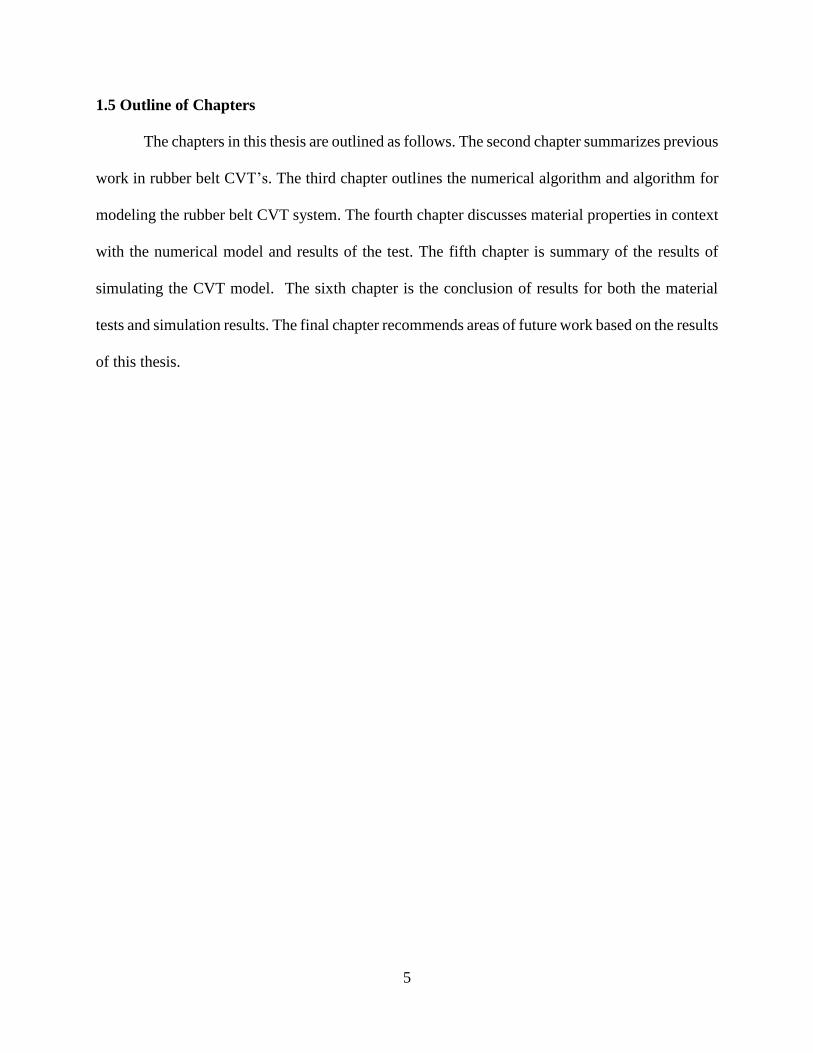
1.5 Outline of Chapters
The chapters in this thesis are outlined as follows. The second chapter summarizes previous
work in rubber belt CVT’s. The third chapter outlines the numerical algorithm and algorithm for
modeling the rubber belt CVT system. The fourth chapter discusses material properties in context
with the numerical model and results of the test. The fifth chapter is summary of the results of
simulating the CVT model. The sixth chapter is the conclusion of results for both the material
tests and simulation results. The final chapter recommends areas of future work based on the results
of this thesis.
6
CHAPTER 2: PREVIOUS WORKS AND CONTRIBUTIONS
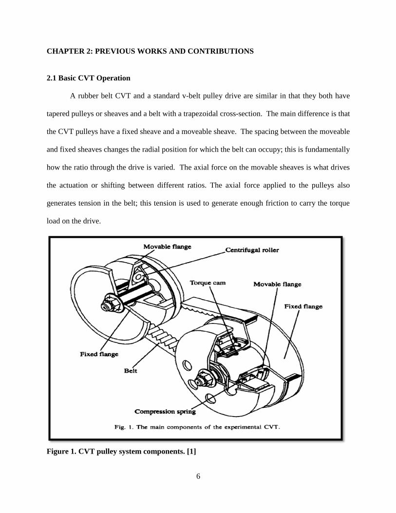
2.1 Basic CVT Operation
A rubber belt CVT and a standard v-belt pulley drive are similar in that they both have
tapered pulleys or sheaves and a belt with a trapezoidal cross-section. The main difference is that
the CVT pulleys have a fixed sheave and a moveable sheave. The spacing between the moveable
and fixed sheaves changes the radial position for which the belt can occupy; this is fundamentally
how the ratio through the drive is varied. The axial force on the movable sheaves is what drives
the actuation or shifting between different ratios. The axial force applied to the pulleys also
generates tension in the belt; this tension is used to generate enough friction to carry the torque
load on the drive.
Figure 1. CVT pulley system components. [1]
7
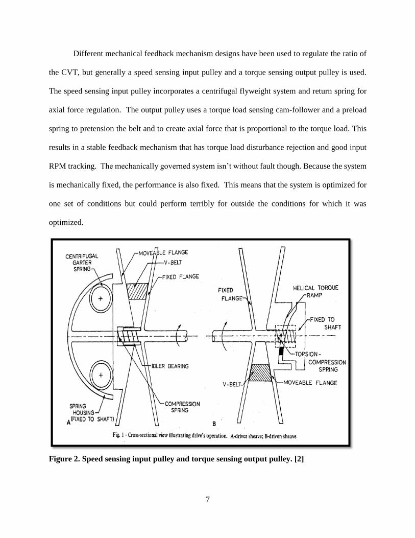
Different mechanical feedback mechanism designs have been used to regulate the ratio of
the CVT, but generally a speed sensing input pulley and a torque sensing output pulley is used.
The speed sensing input pulley incorporates a centrifugal flyweight system and return spring for
axial force regulation. The output pulley uses a torque load sensing cam-follower and a preload
spring to pretension the belt and to create axial force that is proportional to the torque load. This
results in a stable feedback mechanism that has torque load disturbance rejection and good input
RPM tracking. The mechanically governed system isn’t without fault though. Because the system
is mechanically fixed, the performance is also fixed. This means that the system is optimized for
one set of conditions but could perform terribly for outside the conditions for which it was
optimized.
Figure 2. Speed sensing input pulley and torque sensing output pulley. [2]

8
The various design parameters of the mechanical feedback mechanism dictate the response
and efficiency of the CVT drive. These parameters are interconnected which makes tuning the
CVT very difficult. Usually these parameters are set to meet a steady state performance goal while
also having to meet a desirable transient response. This interconnection of the mechanical
components often leads to trade-offs in performance that depend on the design goals of the system.
9
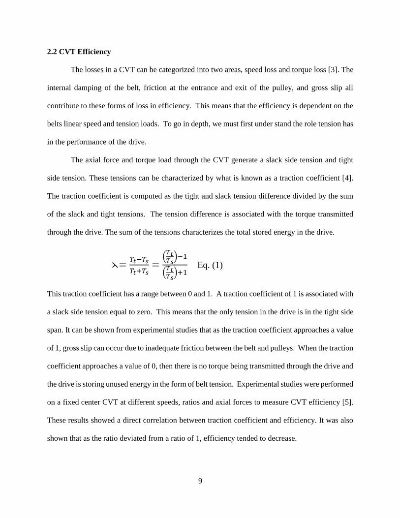
2.2 CVT Efficiency
The losses in a CVT can be categorized into two areas, speed loss and torque loss [3]. The
internal damping of the belt, friction at the entrance and exit of the pulley, and gross slip all
contribute to these forms of loss in efficiency. This means that the efficiency is dependent on the
belts linear speed and tension loads. To go in depth, we must first under stand the role tension has
in the performance of the drive.
The axial force and torque load through the CVT generate a slack side tension and tight
side tension. These tensions can be characterized by what is known as a traction coefficient [4].
The traction coefficient is computed as the tight and slack tension difference divided by the sum
of the slack and tight tensions. The tension difference is associated with the torque transmitted
through the drive. The sum of the tensions characterizes the total stored energy in the drive.
This traction coefficient has a range between 0 and 1. A traction coefficient of 1 is associated with
a slack side tension equal to zero. This means that the only tension in the drive is in the tight side
span. It can be shown from experimental studies that as the traction coefficient approaches a value
of 1, gross slip can occur due to inadequate friction between the belt and pulleys. When the traction
coefficient approaches a value of 0, then there is no torque being transmitted through the drive and
the drive is storing unused energy in the form of belt tension. Experimental studies were performed
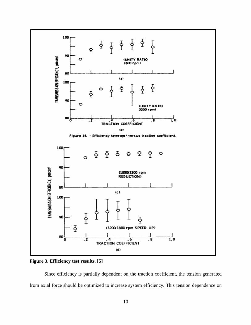
on a fixed center CVT at different speeds, ratios and axial forces to measure CVT efficiency [5].
These results showed a direct correlation between traction coefficient and efficiency. It was also
shown that as the ratio deviated from a ratio of 1, efficiency tended to decrease.
⋋=𝑇𝑡−𝑇𝑠
𝑇𝑡+𝑇𝑠=
(𝑇𝑡𝑇𝑠
)−1
(𝑇𝑡𝑇𝑠
)+1 Eq. (1)
10
.
Figure 3. Efficiency test results. [5]
Since efficiency is partially dependent on the traction coefficient, the tension generated
from axial force should be optimized to increase system efficiency. This tension dependence on
11
efficiency lead to the investigation of optimal tension for CVT drives by [4]. Using experimental
results and theoretical models, equations were create to help preliminary predications of optimal
axial force to maximize efficiency of the CVT at steady state operating conditions.
12
2.3 Closed Form Solutions
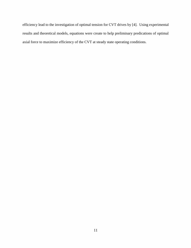
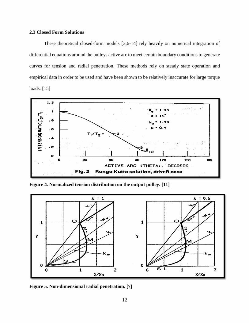
These theoretical closed-form models [3,6-14] rely heavily on numerical integration of
differential equations around the pulleys active arc to meet certain boundary conditions to generate
curves for tension and radial penetration. These methods rely on steady state operation and
empirical data in order to be used and have been shown to be relatively inaccurate for large torque
loads. [15]
Figure 4. Normalized tension distribution on the output pulley. [11]
Figure 5. Non-dimensional radial penetration. [7]
13
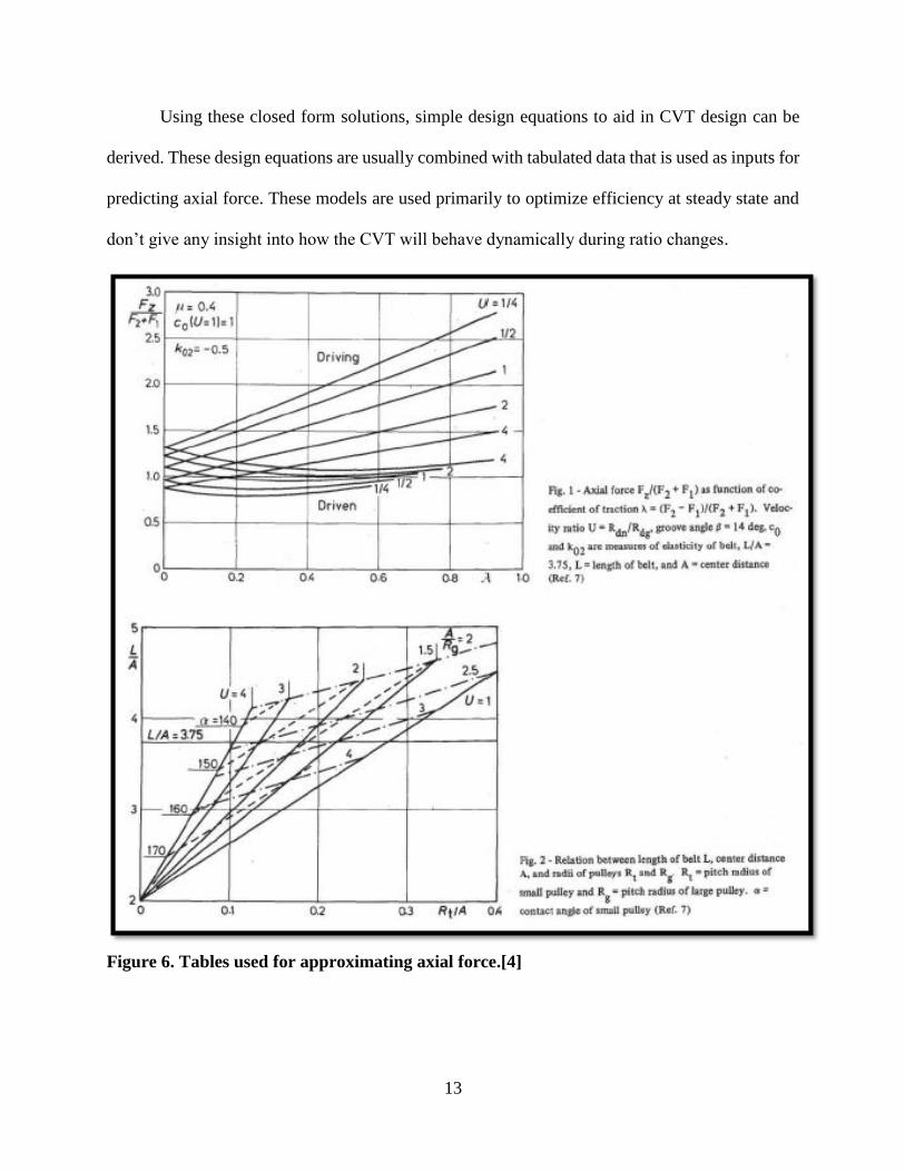
Using these closed form solutions, simple design equations to aid in CVT design can be
derived. These design equations are usually combined with tabulated data that is used as inputs for
predicting axial force. These models are used primarily to optimize efficiency at steady state and
don’t give any insight into how the CVT will behave dynamically during ratio changes.
Figure 6. Tables used for approximating axial force.[4]
14
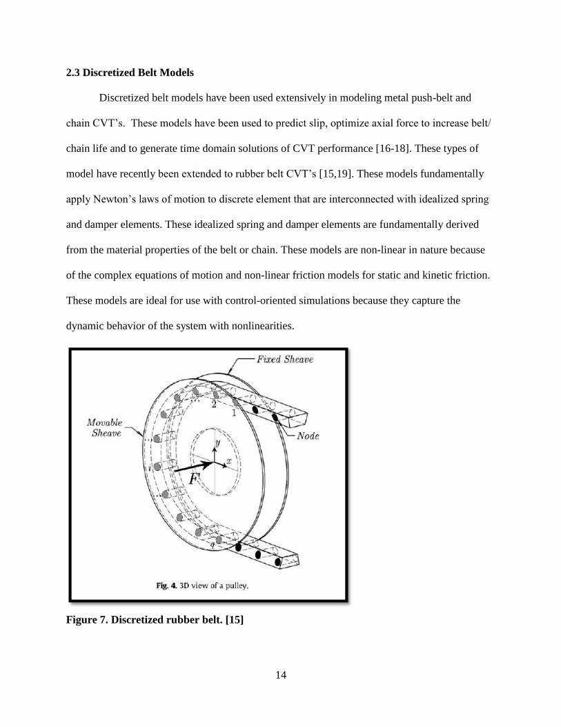
2.3 Discretized Belt Models
Discretized belt models have been used extensively in modeling metal push-belt and
chain CVT’s. These models have been used to predict slip, optimize axial force to increase belt/
chain life and to generate time domain solutions of CVT performance [16-18]. These types of
model have recently been extended to rubber belt CVT’s [15,19]. These models fundamentally
apply Newton’s laws of motion to discrete element that are interconnected with idealized spring
and damper elements. These idealized spring and damper elements are fundamentally derived
from the material properties of the belt or chain. These models are non-linear in nature because
of the complex equations of motion and non-linear friction models for static and kinetic friction.
These models are ideal for use with control-oriented simulations because they capture the
dynamic behavior of the system with nonlinearities.
Figure 7. Discretized rubber belt. [15]
15
CHAPTER 3. NUMERICAL ALGORITHM.
3.1 Setting up the Initial Conditions.
To begin, the belt is discretized into n-nodes. The initial node spacing (𝑙𝑜) and mass of
each node (𝑚) can be calculated as follows.
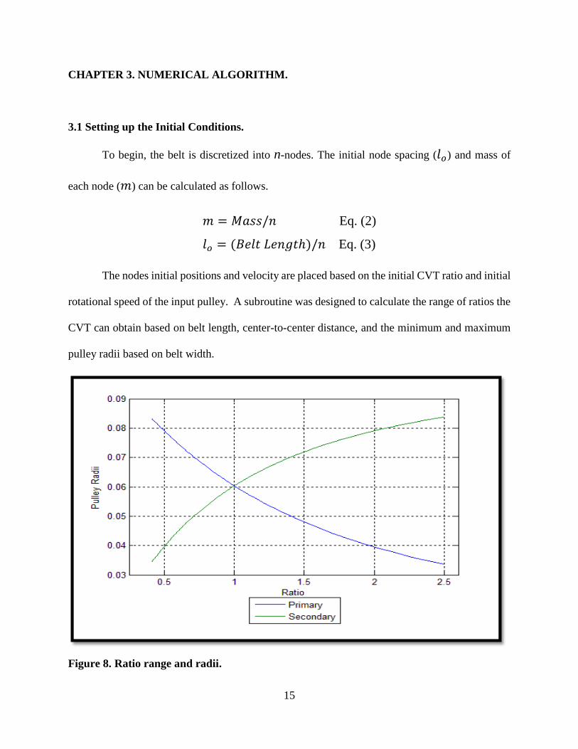
The nodes initial positions and velocity are placed based on the initial CVT ratio and initial
rotational speed of the input pulley. A subroutine was designed to calculate the range of ratios the
CVT can obtain based on belt length, center-to-center distance, and the minimum and maximum
pulley radii based on belt width.
Figure 8. Ratio range and radii.
𝑚 = 𝑀𝑎𝑠𝑠/𝑛 Eq. (2)
𝑙𝑜 = (𝐵𝑒𝑙𝑡 𝐿𝑒𝑛𝑔𝑡ℎ)/𝑛 Eq. (3)
16
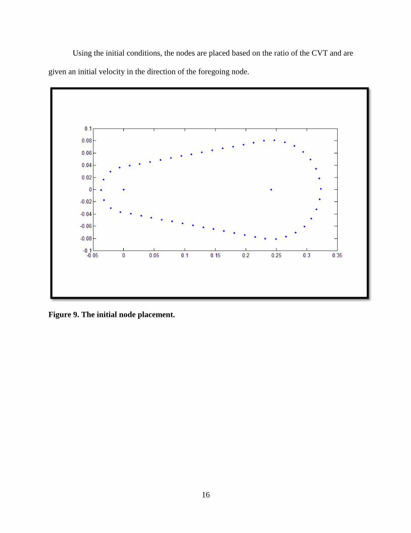
Using the initial conditions, the nodes are placed based on the ratio of the CVT and are
given an initial velocity in the direction of the foregoing node.
Figure 9. The initial node placement.
17
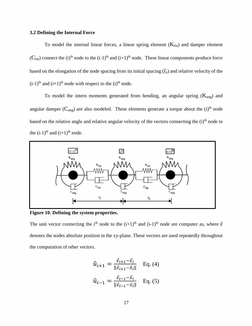
3.2 Defining the Internal Force
To model the internal linear forces, a linear spring element (Klin) and damper element
(Clin) connect the (i)th node to the (i-1)th and (i+1)th node. These linear components produce force
based on the elongation of the node spacing from its initial spacing (lo) and relative velocity of the
(i-1)th and (i+1)th node with respect to the (i)th node.
To model the intern moments generated from bending, an angular spring (Kang) and
angular damper (Cang) are also modeled. These elements generate a torque about the (i)th node
based on the relative angle and relative angular velocity of the vectors connecting the (i)th node to
the (i-1)th and (i+1)th node.
Figure 10. Defining the system properties.
The unit vector connecting the ith node to the (i+1)th and (i-1)th node are computer as, where �⃗�
denotes the nodes absolute position in the xy-plane. These vectors are used repeatedly throughout
the computation of other vectors.
�̂�𝑖+1 =�⃗�𝑖+1−�⃗�𝑖
‖�⃗�𝑖+1−�⃗�𝑖‖ Eq. (4)
�̂�𝑖−1 =�⃗�𝑖−1−�⃗�𝑖
‖�⃗�𝑖−1−�⃗�𝑖‖ Eq. (5)
18
The magnitude of the internal force from elongation on the ith node is computed based on the
increase in relative node spacing. The force then acts in the direction of the corresponding unit
vector.
The relative velocity of (i-1)th and (i+1)th node with respect to the ith node can be broken
up into components parallel and perpendicular to the unit vectors �̂�𝒊+𝟏 and �̂�𝒊−𝟏. The relative
velocity that is parallel to the unit vector contributes to the linear damping while the
perpendicular component contributes to the angular damping.
, where �⃗� is the absolute velocity of the corresponding node.
The force from the linear damping term can be computed as follows.
The moment about the ith node produced from angular damping and angular stiffness also
depend on the (i+1)th and (i-1)th nodes relative velocity and relative position. There are several
alternative methods for computing the vectors and vector valued functions, the methods
presented in this paper were chosen based on intuition and for simplicity of defining the system.
�⃗�𝑘𝑙𝑖𝑛,(𝑖+1)= 𝐾𝑙𝑖𝑛 ∗ (‖�⃗�𝑖+1 − �⃗�𝑖‖ − 𝑙0) ∙ �̂�𝑖+1 Eq. (6)
�⃗�𝑘𝑙𝑖𝑛,(𝑖−1)= 𝐾𝑙𝑖𝑛 ∗ (‖�⃗�𝑖−1 − �⃗�𝑖‖ − 𝑙0) ∙ �̂�𝑖−1 Eq. (7)
�⃗⃗�∥,(𝑖+1) = ‖�⃗�𝑖+1 − �⃗�𝑖‖ ∙ �̂�𝑖+1 Eq. (8)
�⃗⃗�⊥,(𝑖+1) = (�⃗�𝑖+1 − �⃗�𝑖) − �⃗⃗�∥,(𝑖+1) Eq. (9)
�⃗⃗�∥,(𝑖−1) = ‖�⃗�𝑖−1 − �⃗�𝑖‖ ∙ �̂�𝑖−1 Eq. (10)
�⃗⃗�⊥,(𝑖−1) = (�⃗�𝑖−1 − �⃗�𝑖) − �⃗⃗�∥,(𝑖−1) Eq. (11)
�⃗�𝐶𝑙𝑖𝑛,(𝑖+1)= 𝐶𝑙𝑖𝑛 ∗ �⃗⃗�∥,(𝑖+1) Eq. (12)
�⃗�𝐶𝑙𝑖𝑛,(𝑖−1)= 𝐶𝑙𝑖𝑛 ∗ �⃗⃗�∥,(𝑖−1) Eq. (13)
19
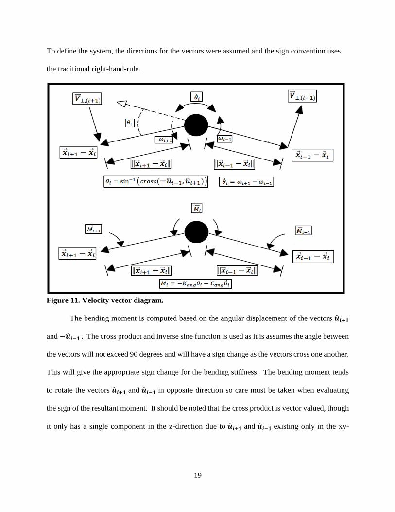
To define the system, the directions for the vectors were assumed and the sign convention uses
the traditional right-hand-rule.
Figure 11. Velocity vector diagram.
The bending moment is computed based on the angular displacement of the vectors �̂�𝒊+𝟏
and −�̂�𝒊−𝟏 . The cross product and inverse sine function is used as it is assumes the angle between
the vectors will not exceed 90 degrees and will have a sign change as the vectors cross one another.
This will give the appropriate sign change for the bending stiffness. The bending moment tends
to rotate the vectors �̂�𝒊+𝟏 and �̂�𝒊−𝟏 in opposite direction so care must be taken when evaluating
the sign of the resultant moment. It should be noted that the cross product is vector valued, though
it only has a single component in the z-direction due to �̂�𝒊+𝟏 and �̂�𝒊−𝟏 existing only in the xy-
20
plane. The magnitude and sign of this z-component are used to evaluate the magnitude and
direction of both bending stiffness and angular damping.
The angular damping is dependent on the relative angular velocity of the vectors �̂�𝒊+𝟏 and
�̂�𝒊−𝟏 as they rotate about the ith node. The angular velocity of each vector (�̂�𝒊+𝟏 and �̂�𝒊−𝟏) can be
computed based on the perpendicular component of relative velocity, length the vector connecting
the nodes and the unit vector connecting the nodes. The difference is these angular velocities are
the time rate of change of the angle between the vectors �̂�𝒊+𝟏 and �̂�𝒊−𝟏.
The resultant moment from both angular stiffness and angular damping are then used to
form an equivalent force to reduce the degrees of freedom of the system. This equivalent force
system must also includes the moment about the ith node as well as the moments about the (i+1)th
and (i-1)th nodes.
𝜃𝑖 = sin−1(𝑐𝑟𝑜𝑠𝑠(−�̂�𝑖−1, �̂�𝑖+1)) Eq. (14)
𝜔𝑖+1 =𝑐𝑟𝑜𝑠𝑠(𝑢𝑖+1,�⃗⃗⃗�⊥,(𝑖+1))
‖�⃗�𝑖+1−�⃗�𝑖‖ Eq. (15)
𝜔𝑖−1 =𝑐𝑟𝑜𝑠𝑠(𝑢𝑖−1,�⃗⃗⃗�⊥,(𝑖−1))
‖�⃗�𝑖−1−�⃗�𝑖‖ Eq. (16)
�̇�𝑖 = 𝜔𝑖+1 − 𝜔𝑖−1 Eq. (17)
21
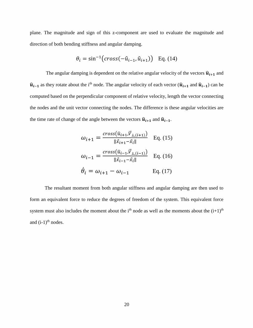
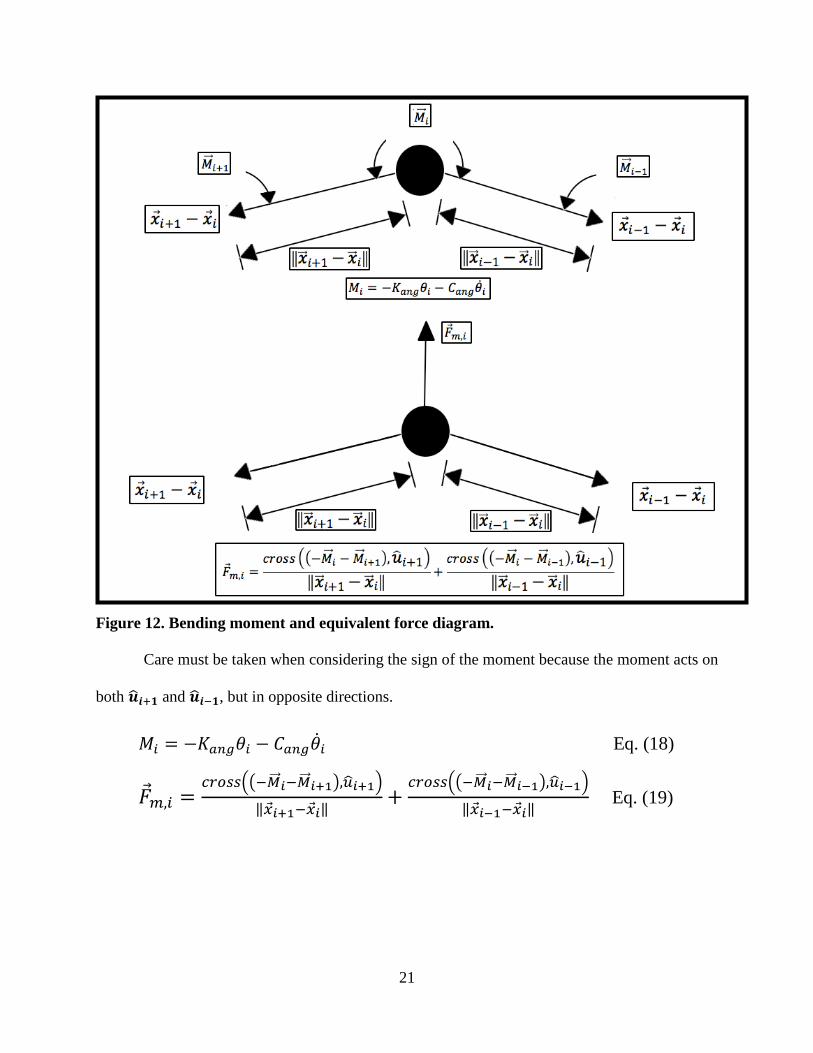
Figure 12. Bending moment and equivalent force diagram.
Care must be taken when considering the sign of the moment because the moment acts on
both �̂�𝒊+𝟏 and �̂�𝒊−𝟏, but in opposite directions.
𝑀𝑖 = −𝐾𝑎𝑛𝑔𝜃𝑖 − 𝐶𝑎𝑛𝑔�̇�𝑖 Eq. (18)
�⃗�𝑚,𝑖 =𝑐𝑟𝑜𝑠𝑠((−�⃗⃗⃗�𝑖−�⃗⃗⃗�𝑖+1),�̂�𝑖+1)
‖�⃗�𝑖+1−�⃗�𝑖‖+
𝑐𝑟𝑜𝑠𝑠((−�⃗⃗⃗�𝑖−�⃗⃗⃗�𝑖−1),𝑢𝑖−1)
‖�⃗�𝑖−1−�⃗�𝑖‖ Eq. (19)
22
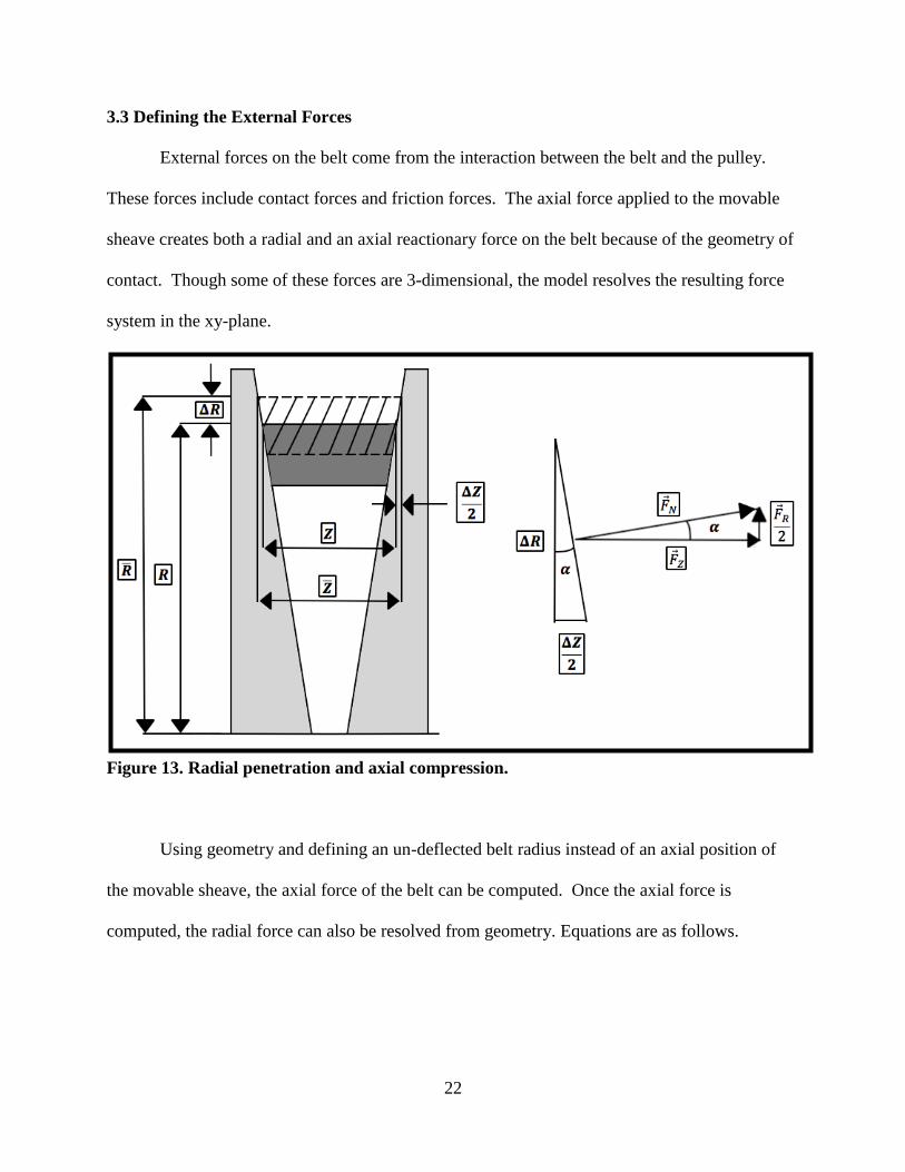
3.3 Defining the External Forces
External forces on the belt come from the interaction between the belt and the pulley.
These forces include contact forces and friction forces. The axial force applied to the movable
sheave creates both a radial and an axial reactionary force on the belt because of the geometry of
contact. Though some of these forces are 3-dimensional, the model resolves the resulting force
system in the xy-plane.
Figure 13. Radial penetration and axial compression.
Using geometry and defining an un-deflected belt radius instead of an axial position of
the movable sheave, the axial force of the belt can be computed. Once the axial force is
computed, the radial force can also be resolved from geometry. Equations are as follows.
23
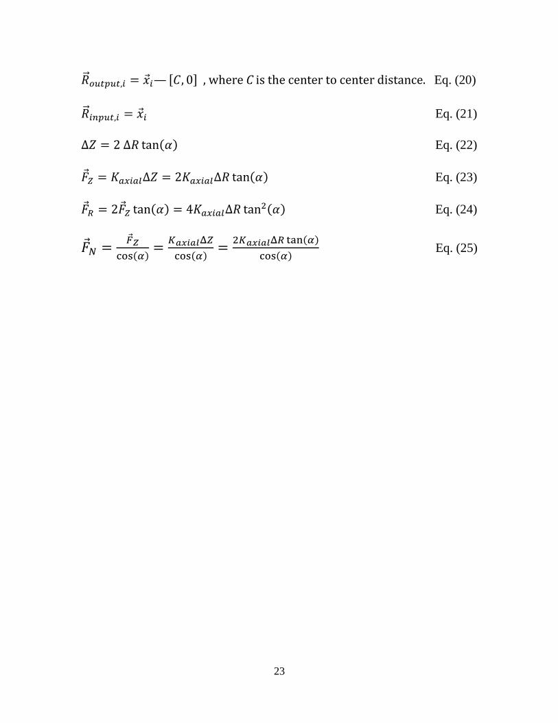
�⃗⃗�𝑜𝑢𝑡𝑝𝑢𝑡,𝑖 = �⃗�𝑖—[𝐶, 0] , where C is the center to center distance. Eq. (20)
�⃗⃗�𝑖𝑛𝑝𝑢𝑡,𝑖 = �⃗�𝑖 Eq. (21)
Δ𝑍 = 2 Δ𝑅 tan(𝛼) Eq. (22)
�⃗�𝑍 = 𝐾𝑎𝑥𝑖𝑎𝑙Δ𝑍 = 2𝐾𝑎𝑥𝑖𝑎𝑙Δ𝑅 tan(𝛼) Eq. (23)
�⃗�𝑅 = 2�⃗�𝑍 tan(𝛼) = 4𝐾𝑎𝑥𝑖𝑎𝑙Δ𝑅 tan2(𝛼) Eq. (24)
�⃗�𝑁 =�⃗�𝑍
cos(𝛼)=
𝐾𝑎𝑥𝑖𝑎𝑙Δ𝑍
cos(𝛼)=
2𝐾𝑎𝑥𝑖𝑎𝑙Δ𝑅 tan(𝛼)
cos(𝛼) Eq. (25)
24
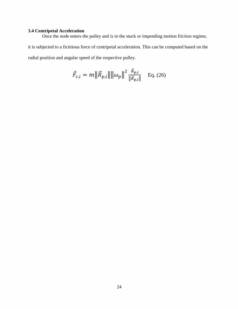
3.4 Centripetal Acceleration
Once the node enters the pulley and is in the stuck or impending motion friction regime,
it is subjected to a fictitious force of centripetal acceleration. This can be computed based on the
radial position and angular speed of the respective pulley.
�⃗�𝑐,𝑖 = 𝑚‖�⃗⃗�𝑝,𝑖‖‖𝜔𝑝‖2 �⃗⃗�𝑝,𝑖
‖�⃗⃗�𝑝,𝑖‖ Eq. (26)

25
3.5 Friction Model
The friction model used in the algorithm is a nonlinear Coulomb friction model. The
modes of friction are stuck/static friction, sliding/kinetic friction, or impending motion. Which
friction regime the node is in depends on the sum of the forces acting on the node (Eq. (28)) and
the relative velocity between the belt node and the CVT pulley (Eq. (27)).
The friction force equations are as follows.
The resultant force acting on the node is as follows.
�⃗�𝑟𝑒𝑙,𝑖 = �⃗�𝑖 − 𝑐𝑟𝑜𝑠𝑠(�⃗⃗�𝑝,𝑖 , �⃗⃗⃗�𝑝) Eq. (27)
�⃗�𝑠𝑢𝑚,𝑖 = �⃗�𝑘𝑙𝑖𝑛,(𝑖+1)+ �⃗�𝑘𝑙𝑖𝑛,(𝑖−1)
+ �⃗�𝐶𝑙𝑖𝑛,(𝑖+1)+ �⃗�𝐶𝑙𝑖𝑛,(𝑖−1)
+ �⃗�𝑚,𝑖 + �⃗�𝑐,𝑖 Eq. (28)
𝑓𝑖 = −𝐹𝑧,𝑖𝜇𝑑�⃗⃗�𝑟𝑒𝑙,𝑖
‖�⃗⃗�𝑟𝑒𝑙,𝑖‖ 𝑖𝑓 (‖�⃗�𝑟𝑒𝑙,𝑖‖ ≥ 𝑣𝑚𝑖𝑛) Eq. (29)
𝑓𝑖 = −�⃗�𝑠𝑢𝑚,𝑖 𝑖𝑓 (‖�⃗�𝑟𝑒𝑙,𝑖‖ < 𝑣𝑚𝑖𝑛 𝑎𝑛𝑑 ‖�⃗�𝑠𝑢𝑚,𝑖‖ < 𝐹𝑧,𝑖𝜇𝑠 ) Eq. (30)
𝑓𝑖 = −𝐹𝑧,𝑖𝜇𝑠�⃗�𝑠𝑢𝑚,𝑖
‖�⃗�𝑠𝑢𝑚,𝑖‖ 𝑖𝑓 (‖�⃗�𝑟𝑒𝑙,𝑖‖ < 𝑣𝑚𝑖𝑛 𝑎𝑛𝑑 ‖�⃗�𝑠𝑢𝑚,𝑖‖ ≥ 𝐹𝑧,𝑖𝜇𝑠 ) Eq. (31)
�⃗�𝑟𝑒𝑠,𝑖 = �⃗�𝑠𝑢𝑚,𝑖 + 𝑓𝑖 Eq. (32)
26
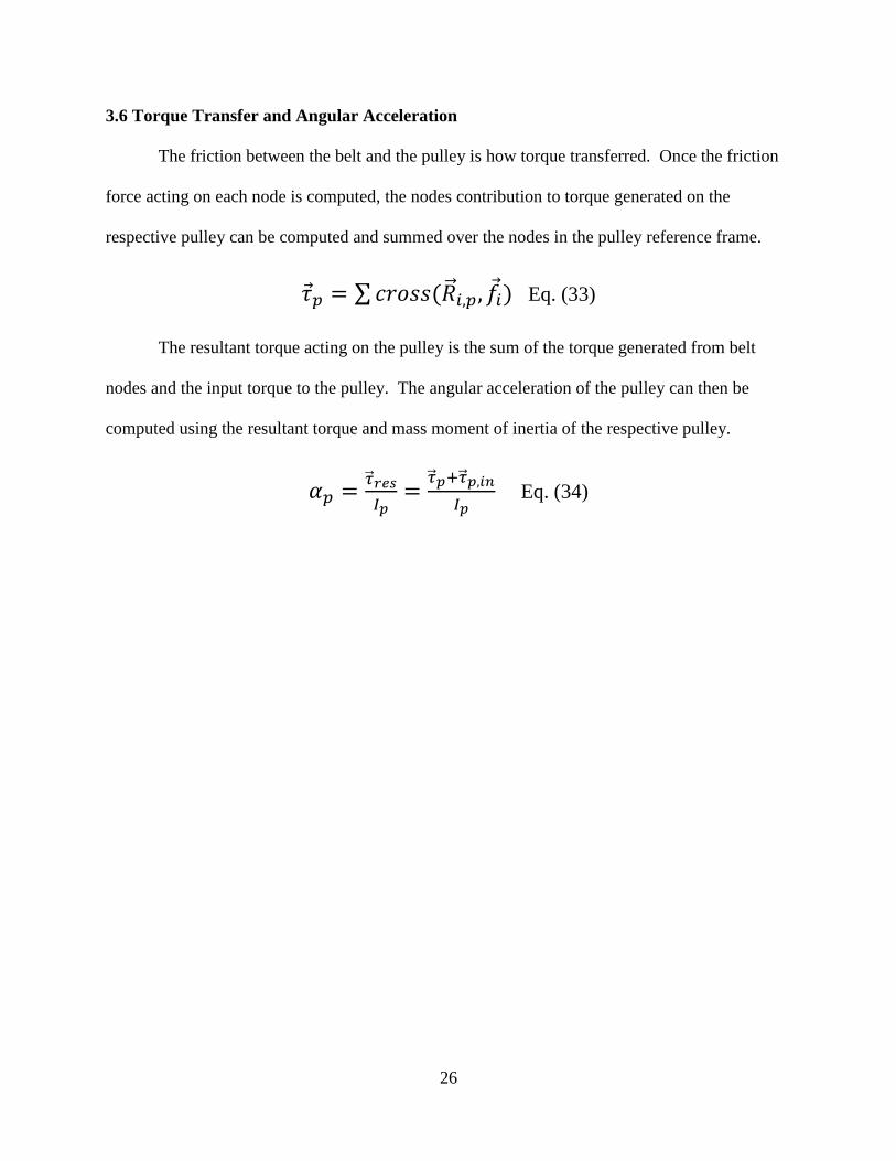
3.6 Torque Transfer and Angular Acceleration
The friction between the belt and the pulley is how torque transferred. Once the friction
force acting on each node is computed, the nodes contribution to torque generated on the
respective pulley can be computed and summed over the nodes in the pulley reference frame.
The resultant torque acting on the pulley is the sum of the torque generated from belt
nodes and the input torque to the pulley. The angular acceleration of the pulley can then be
computed using the resultant torque and mass moment of inertia of the respective pulley.
𝜏𝑝 = ∑𝑐𝑟𝑜𝑠𝑠(�⃗⃗�𝑖,𝑝, 𝑓𝑖) Eq. (33)
𝛼𝑝 =�⃗⃗�𝑟𝑒𝑠
𝐼𝑝=
�⃗⃗�𝑝+�⃗⃗�𝑝,𝑖𝑛
𝐼𝑝 Eq. (34)
27
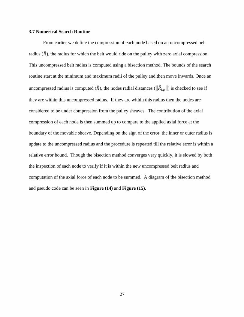
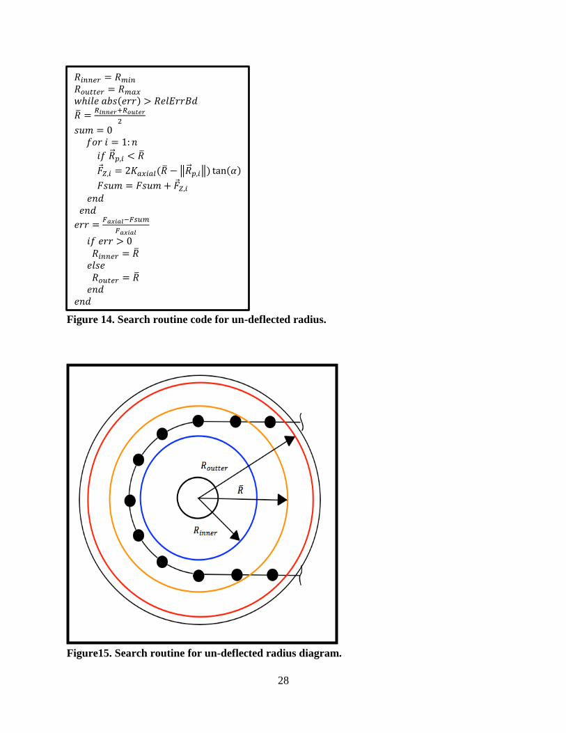
3.7 Numerical Search Routine
From earlier we define the compression of each node based on an uncompressed belt
radius (�̅�), the radius for which the belt would ride on the pulley with zero axial compression.
This uncompressed belt radius is computed using a bisection method. The bounds of the search
routine start at the minimum and maximum radii of the pulley and then move inwards. Once an
uncompressed radius is computed (�̅�), the nodes radial distances (‖�⃗⃗�𝑖,𝑝‖) is checked to see if
they are within this uncompressed radius. If they are within this radius then the nodes are
considered to be under compression from the pulley sheaves. The contribution of the axial
compression of each node is then summed up to compare to the applied axial force at the
boundary of the movable sheave. Depending on the sign of the error, the inner or outer radius is
update to the uncompressed radius and the procedure is repeated till the relative error is within a
relative error bound. Though the bisection method converges very quickly, it is slowed by both
the inspection of each node to verify if it is within the new uncompressed belt radius and
computation of the axial force of each node to be summed. A diagram of the bisection method
and pseudo code can be seen in Figure (14) and Figure (15).
28
Figure 14. Search routine code for un-deflected radius.
Figure15. Search routine for un-deflected radius diagram.
𝑅𝑖𝑛𝑛𝑒𝑟 = 𝑅𝑚𝑖𝑛 𝑅𝑜𝑢𝑡𝑡𝑒𝑟 = 𝑅𝑚𝑎𝑥 𝑤ℎ𝑖𝑙𝑒 𝑎𝑏𝑠(𝑒𝑟𝑟) > 𝑅𝑒𝑙𝐸𝑟𝑟𝐵𝑑
�̅� =𝑅𝑖𝑛𝑛𝑒𝑟+𝑅𝑜𝑢𝑡𝑒𝑟
2
𝑠𝑢𝑚 = 0
𝑓𝑜𝑟 𝑖 = 1: 𝑛
𝑖𝑓 �⃗⃗�𝑝,𝑖 < �̅�
�⃗�𝑍,𝑖 = 2𝐾𝑎𝑥𝑖𝑎𝑙(�̅� − ‖�⃗⃗�𝑝,𝑖‖) tan(𝛼)
𝐹𝑠𝑢𝑚 = 𝐹𝑠𝑢𝑚 + �⃗�𝑍,𝑖
𝑒𝑛𝑑
𝑒𝑛𝑑
𝑒𝑟𝑟 =𝐹𝑎𝑥𝑖𝑎𝑙−𝐹𝑠𝑢𝑚
𝐹𝑎𝑥𝑖𝑎𝑙
𝑖𝑓 𝑒𝑟𝑟 > 0
𝑅𝑖𝑛𝑛𝑒𝑟 = �̅�
𝑒𝑙𝑠𝑒
𝑅𝑜𝑢𝑡𝑒𝑟 = �̅�
𝑒𝑛𝑑
𝑒𝑛𝑑
29
The stability of this algorithm is fairly robust and converges relatively quickly considering
that the bisection method is used four times per time step. Some checks were also added so that
the bisection method considered the physical system limitations as well. There are two scenarios
that must be checked.
The first being when all the nodes are at the maximum radius. This means the bisection
method would iterate infinitely trying to converge to the outer maximum radius slowing down the
algorithm. This cause an infinite loop as the algorithm tries to meet a relative error requirement
that it can never achieve. So a check was added to exit the search routine if the nodes are at the
maximum radius and to set all axial forces to the belt nodes to zero. The axial forces are set to zero
because the axial forces are used in another part of the algorithm for computing the friction force
on the node. This also has a physic interpretation of the pulley sheaves being completely closed,
which mean the sheaves cannot compress the belt node axially. The second issue of stability
comes from if a belt node tries to enter the minimum radius, which it physically cannot do. To
solve this problem, once a node is determined to be within the minimum radius, the radial
components of force acting on the node that tend to cause it to accelerate into the minimum radius
are computed, then they are applied as a reactionary force so that these radial forces cancel. This
also has the physical interpretation of generating a reactionary force as the belt contacts the shaft
passing through the center of the CVT pulley.
30
3.8 Numerical Integration
The numerical integration technique used is a Runge-Kutta 4th order fixed step ODE solver.
Because the system of equations of force acting on the belt nodes are non-linear and computed
explicitly, an implicit ODE solver cannot be used. The system of equations can be represented as
a traditional state space. The only difference is the value of the 𝐴𝑥 portion of the state space is
computed explicitly due to the nonlinearities.
It was also discovered that this system of equations is quite stiff. Since an implicit solver
can’t be used, unusually small time steps were needed when integrating to ensure numerical
stability of the solutions. I suspect that there are two causes for this problem.
First, the magnitude of the forces acting on the belt nodes are very large in comparison to
the very small node mass. This causes large accelerations of the nodes for relatively small changes
in force.
Second is the belts linear velocity at low ratios and high input pulley speeds. Because the
belts velocity is very large at these conditions, to large of a time step could cause very large errors
�̇� = 𝐴𝑥 + 𝐵𝑢 Eq. (35)
�̇� =
[ �⃗�1
⋮�⃗�𝑛
�⃗�1
⋮�⃗�𝑛
�⃗�𝐷𝑟
�⃗�𝐷𝑛]
= 𝐴
[
�⃗�1
⋮�⃗�𝑛
�⃗�1
⋮�⃗�𝑛
�⃗⃗⃗�𝐷𝑟
�⃗⃗⃗�𝐷𝑛]
+ 𝐵 [𝜏𝐷𝑟,𝑖𝑛 0
0 𝜏𝐷𝑛,𝑖𝑛] =
[
�⃗�1
⋮�⃗�𝑛
�⃗�𝑠𝑢𝑚,1
𝑚
⋮�⃗�𝑠𝑢𝑚,𝑛
𝑚
�⃗⃗�𝐷𝑟+�⃗⃗�𝐷𝑟,𝑖𝑛
𝐼𝐷𝑟
�⃗⃗�𝐷𝑛+�⃗⃗�𝐷𝑛,𝑖𝑛
𝐼𝐷𝑛 ]
Eq. (36)
31
in the nodes position. Since most of the forces acting on the belt nodes are mostly dependent on
the node position in the xy-plane, even small errors in position can generate large force fluctuations
on the nodes. This cycle of position, velocity and acceleration dependence can causes the algorithm
to be very unstable for relatively small time steps. The time steps used for this algorithm are on
the order of 10-5 seconds. In future work, I would recommend investigating the stability of the
algorithm when the time step for integration is scaled based on the belts linear velocity. This could
greatly decrease simulation time and also decrease time between iterations of the CVT system
design.
32
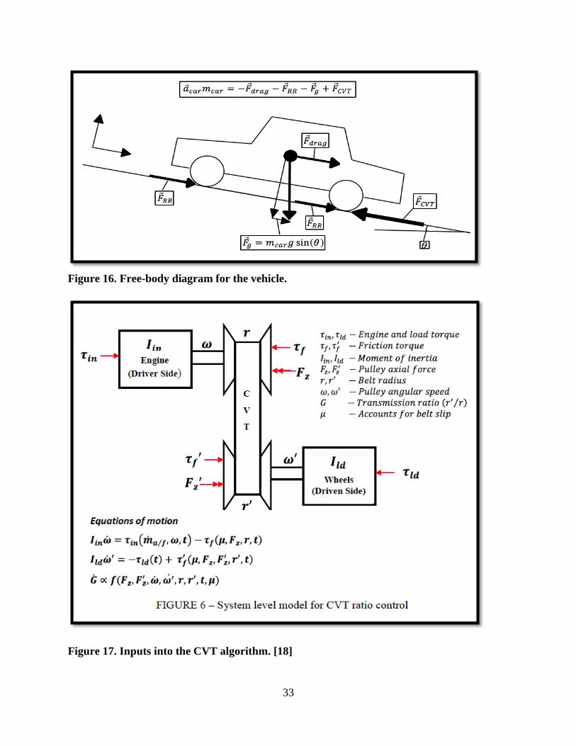
3.9 Torque and Axial Force Inputs to the Simulation
Torque and axial force inputs to the model are similar to those used in [10] for automotive
chain or metal belt CVT’s numerical models. This includes a vehicle and engine sub-model. Since
the CVT model is in the time domain, a disturbance in the form of vehicle braking, road grade
increase or an increase in engine torque output can be created at any point in the simulation. This
allows for simulating the response of either a mechanically governed or electronic controlled CVT
to this disturbance. This allows for flexibility in how the inputs to the system are defined. Previous
rubber belt algorithms made the input speed to the CVT time dependent. This fundamentally fixes
the degree of freedom for the rotational speed of the input pulley of the CVT and negates the
dynamics interaction between the input and output pulley speeds.
The axial force inputs to the system set the boundary condition for the search routine
mentioned in section 3.7. This axial force can be generated either by a control system or from a
model of the mechanically governed system This may require more outputs from the CVT
algorithm to know the axial position of the moveable sheave. This requires only minor changes to
the code of the algorithm. For this paper, electronic control of the axial force input to the system
is considered.
33
Figure 16. Free-body diagram for the vehicle.
Figure 17. Inputs into the CVT algorithm. [18]
34
CHAPTER 4. MATERIAL STIFFNESS PROPERTIES AND MEASUREMENT.
4.1 Designing the Experimental Test Range.
When determining how to measure the material properties of a material, we must consider how
this material property is defined. To model the tension in the belt, an idealized spring connects
each node. A change in node spacing from the initial spacing is seen as a compression or elongation
of this idealized spring. The axial compression of the belt between the pulley sheaves is also
modeled as an idealized spring. The internal bending stiffness of the belt is modeled as an idealized
angular spring. It is assumed that an angular displacement of the unit vector connecting the nodes
from 180 degrees will generate a bending moment. The equipment to adequately measure damping
wasn’t readily available, so stiffness is the only property measured in this paper. It is assumed that
damping is viscous in nature because of the ease of modeling.
Since the CVT belt is primarily composed of rubber, the characteristics of rubber must be
considered when designing the tests. The stress strain curve of rubber tends to be much different
than other materials and so the rubbers modulus must be defined in the range of forces applied.
The material properties of rubber also tend to be much different in compression than in tension.
So to produce a well-defined modulus for compression or tension, the range of forces the belt sees
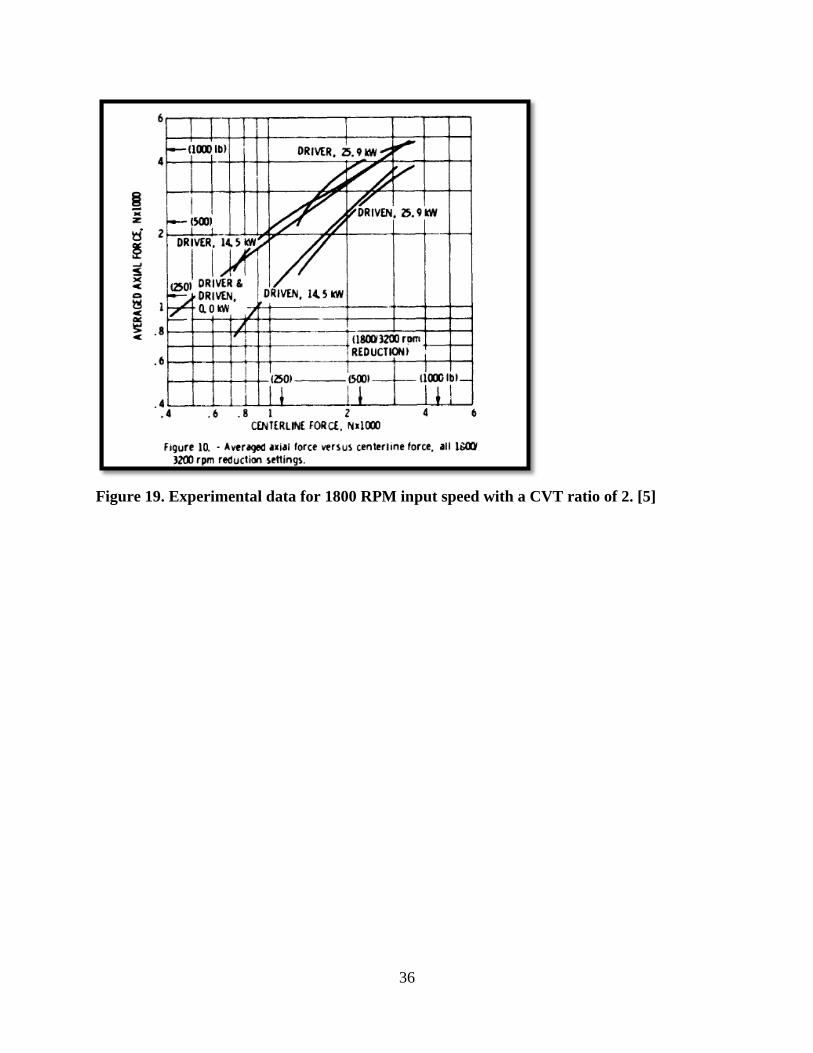
in application must also be considered. Experimental test data presented by [5] is used to form the
maximum range of force used in these test.
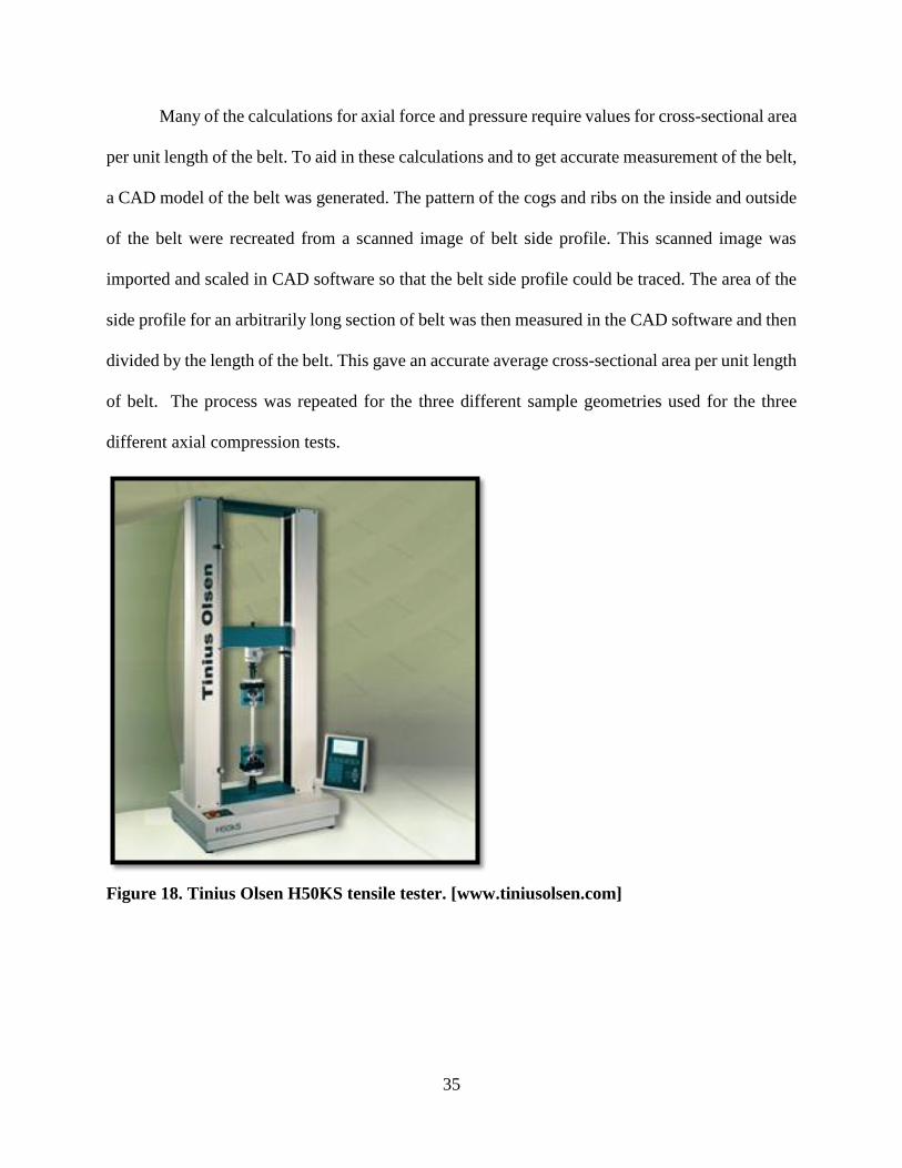
The equipment used was the Tinius Olsen H50KS bench top tester. The force transducer
ranges available were a 1 kN and 50 kN force transducer. The extensometer used was Tinius Olsen,
Model (LS-4%-2A) with a 2-inch gauge length. Any fixtures were fabricated in house and are
detailed in subsequent section. All test were performed on a Gates G-Force 26C3596 CVT belt.
35
Many of the calculations for axial force and pressure require values for cross-sectional area
per unit length of the belt. To aid in these calculations and to get accurate measurement of the belt,
a CAD model of the belt was generated. The pattern of the cogs and ribs on the inside and outside
of the belt were recreated from a scanned image of belt side profile. This scanned image was
imported and scaled in CAD software so that the belt side profile could be traced. The area of the
side profile for an arbitrarily long section of belt was then measured in the CAD software and then
divided by the length of the belt. This gave an accurate average cross-sectional area per unit length
of belt. The process was repeated for the three different sample geometries used for the three
different axial compression tests.
Figure 18. Tinius Olsen H50KS tensile tester. [www.tiniusolsen.com]
36
Figure 19. Experimental data for 1800 RPM input speed with a CVT ratio of 2. [5]
37
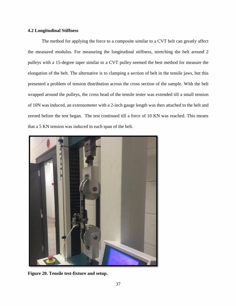
4.2 Longitudinal Stiffness
The method for applying the force to a composite similar to a CVT belt can greatly affect
the measured modulus. For measuring the longitudinal stiffness, stretching the belt around 2
pulleys with a 15-degree taper similar to a CVT pulley seemed the best method for measure the
elongation of the belt. The alternative is to clamping a section of belt in the tensile jaws, but this
presented a problem of tension distribution across the cross section of the sample. With the belt
wrapped around the pulleys, the cross head of the tensile tester was extended till a small tension
of 10N was induced, an extensometer with a 2-inch gauge length was then attached to the belt and
zeroed before the test began. The test continued till a force of 10 KN was reached. This means
that a 5 KN tension was induced in each span of the belt.
Figure 20. Tensile test-fixture and setup.
38
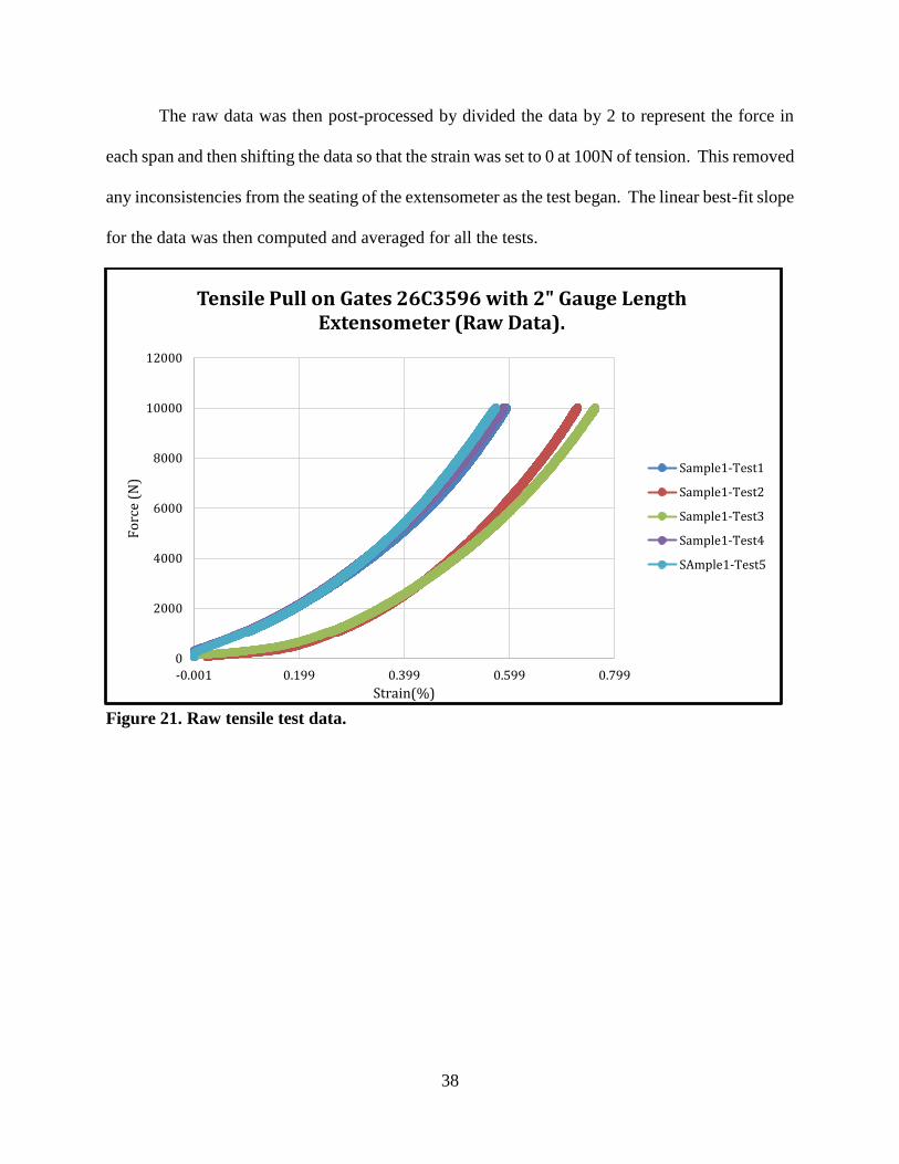
The raw data was then post-processed by divided the data by 2 to represent the force in
each span and then shifting the data so that the strain was set to 0 at 100N of tension. This removed
any inconsistencies from the seating of the extensometer as the test began. The linear best-fit slope
for the data was then computed and averaged for all the tests.
Figure 21. Raw tensile test data.
0
2000
4000
6000
8000
10000
12000
-0.001 0.199 0.399 0.599 0.799
Fo
rce
(N)
Strain(%)
Tensile Pull on Gates 26C3596 with 2" Gauge Length Extensometer (Raw Data).
Sample1-Test1
Sample1-Test2
Sample1-Test3
Sample1-Test4
SAmple1-Test5
39
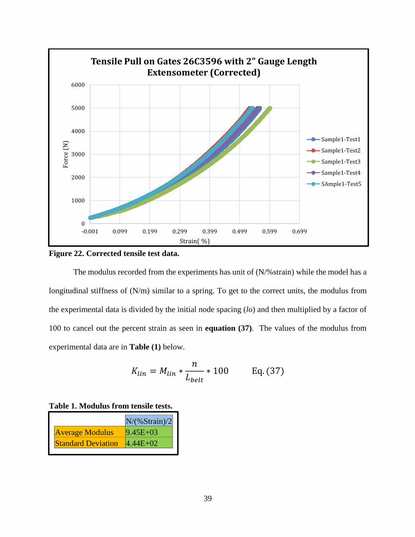
Figure 22. Corrected tensile test data.
The modulus recorded from the experiments has unit of (N/%strain) while the model has a
longitudinal stiffness of (N/m) similar to a spring. To get to the correct units, the modulus from
the experimental data is divided by the initial node spacing (lo) and then multiplied by a factor of
100 to cancel out the percent strain as seen in equation (37). The values of the modulus from
experimental data are in Table (1) below.
𝐾𝑙𝑖𝑛 = 𝑀𝑙𝑖𝑛 ∗𝑛
𝐿𝑏𝑒𝑙𝑡∗ 100 Eq. (37)
Table 1. Modulus from tensile tests.
0
1000
2000
3000
4000
5000
6000
-0.001 0.099 0.199 0.299 0.399 0.499 0.599 0.699
Fo
rce
(N)
Strain( %)
Tensile Pull on Gates 26C3596 with 2" Gauge Length Extensometer (Corrected)
Sample1-Test1
Sample1-Test2
Sample1-Test3
Sample1-Test4
SAmple1-Test5
N/(%Strain)/2
Average Modulus 9.45E+03
Standard Deviation 4.44E+02
40
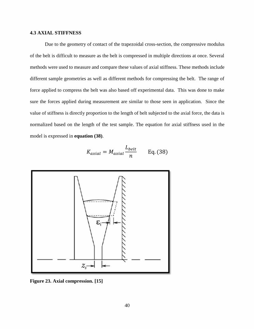
4.3 AXIAL STIFFNESS
Due to the geometry of contact of the trapezoidal cross-section, the compressive modulus
of the belt is difficult to measure as the belt is compressed in multiple directions at once. Several
methods were used to measure and compare these values of axial stiffness. These methods include
different sample geometries as well as different methods for compressing the belt. The range of
force applied to compress the belt was also based off experimental data. This was done to make
sure the forces applied during measurement are similar to those seen in application. Since the
value of stiffness is directly proportion to the length of belt subjected to the axial force, the data is
normalized based on the length of the test sample. The equation for axial stiffness used in the
model is expressed in equation (38).
𝐾𝑎𝑥𝑖𝑎𝑙 = 𝑀𝑎𝑥𝑖𝑎𝑙
𝐿𝑏𝑒𝑙𝑡
𝑛 Eq. (38)
Figure 23. Axial compression. [15]
41
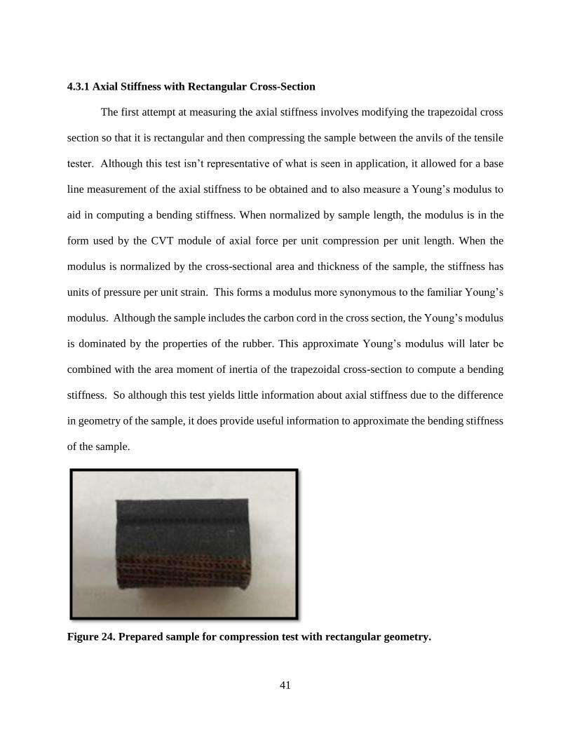
4.3.1 Axial Stiffness with Rectangular Cross-Section
The first attempt at measuring the axial stiffness involves modifying the trapezoidal cross
section so that it is rectangular and then compressing the sample between the anvils of the tensile
tester. Although this test isn’t representative of what is seen in application, it allowed for a base
line measurement of the axial stiffness to be obtained and to also measure a Young’s modulus to
aid in computing a bending stiffness. When normalized by sample length, the modulus is in the
form used by the CVT module of axial force per unit compression per unit length. When the
modulus is normalized by the cross-sectional area and thickness of the sample, the stiffness has
units of pressure per unit strain. This forms a modulus more synonymous to the familiar Young’s
modulus. Although the sample includes the carbon cord in the cross section, the Young’s modulus
is dominated by the properties of the rubber. This approximate Young’s modulus will later be
combined with the area moment of inertia of the trapezoidal cross-section to compute a bending
stiffness. So although this test yields little information about axial stiffness due to the difference
in geometry of the sample, it does provide useful information to approximate the bending stiffness
of the sample.
Figure 24. Prepared sample for compression test with rectangular geometry.
42
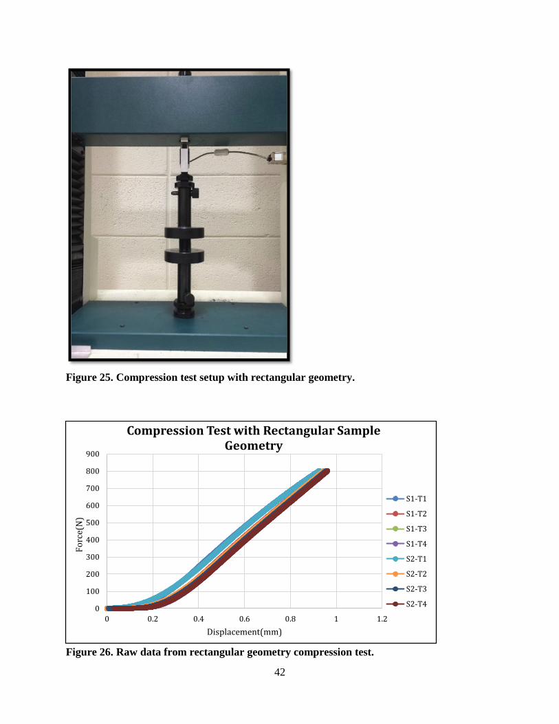
Figure 25. Compression test setup with rectangular geometry.
Figure 26. Raw data from rectangular geometry compression test.
0
100
200
300
400
500
600
700
800
900
0 0.2 0.4 0.6 0.8 1 1.2
Fo
rce(
N)
Displacement(mm)
Compression Test with Rectangular Sample Geometry
S1-T1
S1-T2
S1-T3
S1-T4
S2-T1
S2-T2
S2-T3
S2-T4
43
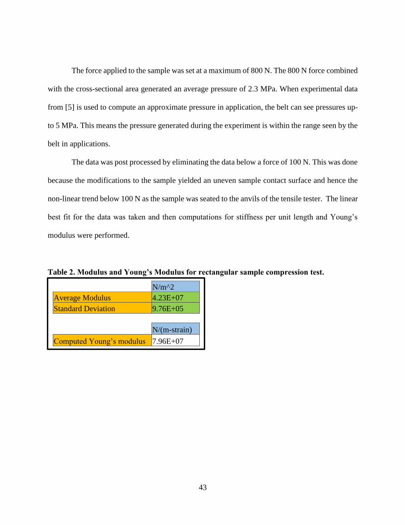
The force applied to the sample was set at a maximum of 800 N. The 800 N force combined
with the cross-sectional area generated an average pressure of 2.3 MPa. When experimental data
from [5] is used to compute an approximate pressure in application, the belt can see pressures up-
to 5 MPa. This means the pressure generated during the experiment is within the range seen by the
belt in applications.
The data was post processed by eliminating the data below a force of 100 N. This was done
because the modifications to the sample yielded an uneven sample contact surface and hence the
non-linear trend below 100 N as the sample was seated to the anvils of the tensile tester. The linear
best fit for the data was taken and then computations for stiffness per unit length and Young’s
modulus were performed.
Table 2. Modulus and Young’s Modulus for rectangular sample compression test.
N/m^2
Average Modulus 4.23E+07
Standard Deviation 9.76E+05
N/(m-strain)
Computed Young’s modulus 7.96E+07
44
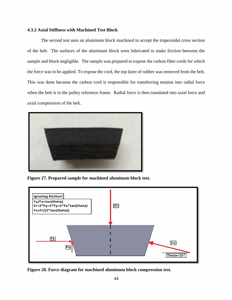
4.3.2 Axial Stiffness with Machined Test Block
The second test uses an aluminum block machined to accept the trapezoidal cross section
of the belt. The surfaces of the aluminum block were lubricated to make friction between the
sample and block negligible. The sample was prepared to expose the carbon fiber cords for which
the force was to be applied. To expose the cord, the top layer of rubber was removed from the belt.
This was done because the carbon cord is responsible for transferring tension into radial force
when the belt is in the pulley reference frame. Radial force is then translated into axial force and
axial compression of the belt.
Figure 27. Prepared sample for machined aluminum block test.
Figure 28. Force diagram for machined aluminum block compression test.
45
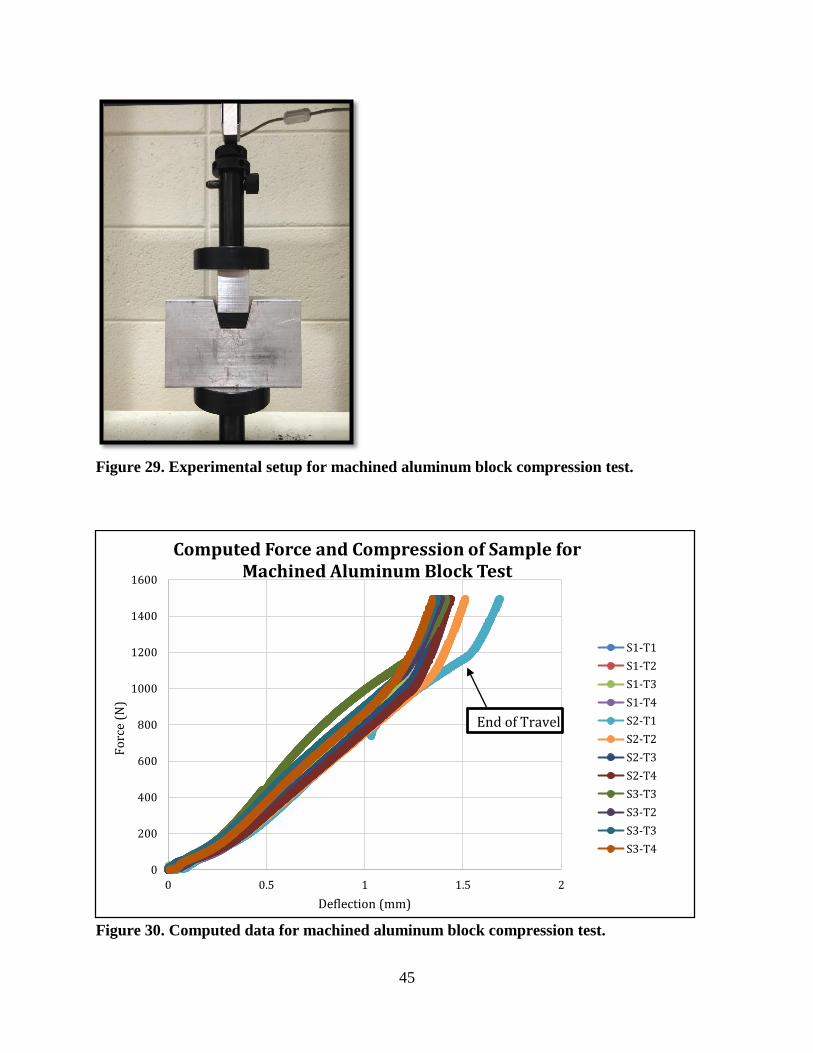
Figure 29. Experimental setup for machined aluminum block compression test.
Figure 30. Computed data for machined aluminum block compression test.
0
200
400
600
800
1000
1200
1400
1600
0 0.5 1 1.5 2
Fo
rce
(N)
Deflection (mm)
Computed Force and Compression of Sample for Machined Aluminum Block Test
S1-T1
S1-T2
S1-T3
S1-T4
S2-T1
S2-T2
S2-T3
S2-T4
S3-T3
S3-T2
S3-T3
S3-T4
End of Travel
46
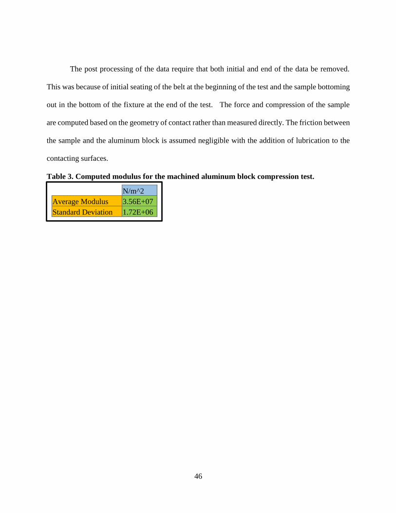
The post processing of the data require that both initial and end of the data be removed.
This was because of initial seating of the belt at the beginning of the test and the sample bottoming
out in the bottom of the fixture at the end of the test. The force and compression of the sample
are computed based on the geometry of contact rather than measured directly. The friction between
the sample and the aluminum block is assumed negligible with the addition of lubrication to the
contacting surfaces.
Table 3. Computed modulus for the machined aluminum block compression test.
N/m^2
Average Modulus 3.56E+07
Standard Deviation 1.72E+06
47
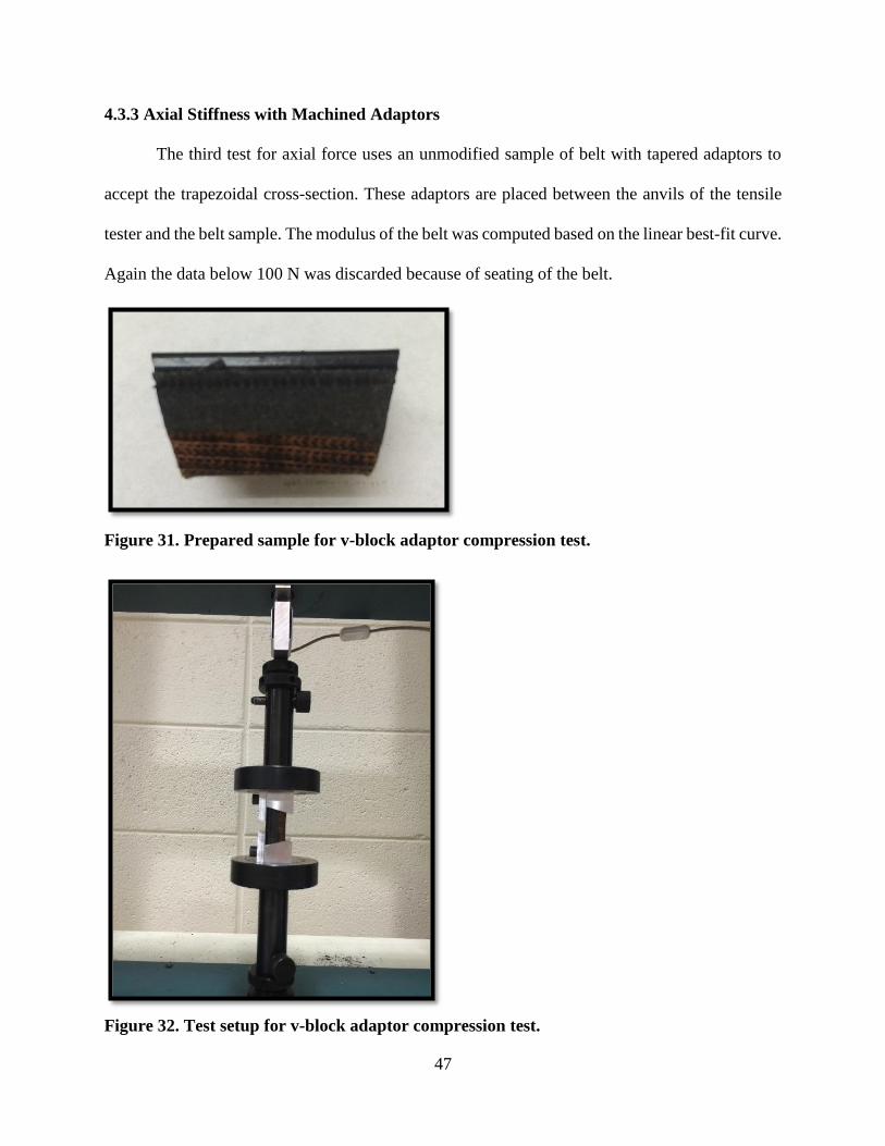
4.3.3 Axial Stiffness with Machined Adaptors
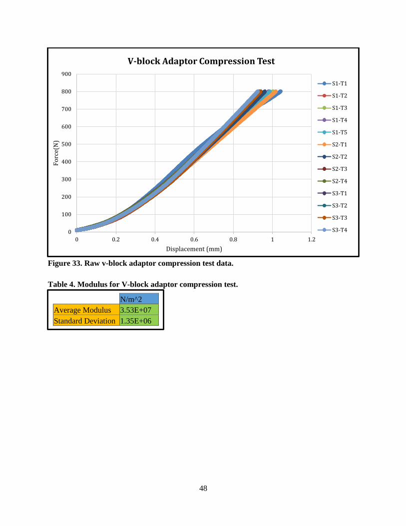
The third test for axial force uses an unmodified sample of belt with tapered adaptors to
accept the trapezoidal cross-section. These adaptors are placed between the anvils of the tensile
tester and the belt sample. The modulus of the belt was computed based on the linear best-fit curve.
Again the data below 100 N was discarded because of seating of the belt.
Figure 31. Prepared sample for v-block adaptor compression test.
Figure 32. Test setup for v-block adaptor compression test.
48
Figure 33. Raw v-block adaptor compression test data.
Table 4. Modulus for V-block adaptor compression test.
0
100
200
300
400
500
600
700
800
900
0 0.2 0.4 0.6 0.8 1 1.2
Fo
rce(
N)
Displacement (mm)
V-block Adaptor Compression Test
S1-T1
S1-T2
S1-T3
S1-T4
S1-T5
S2-T1
S2-T2
S2-T3
S2-T4
S3-T1
S3-T2
S3-T3
S3-T4
N/m^2
Average Modulus 3.53E+07
Standard Deviation 1.35E+06
49
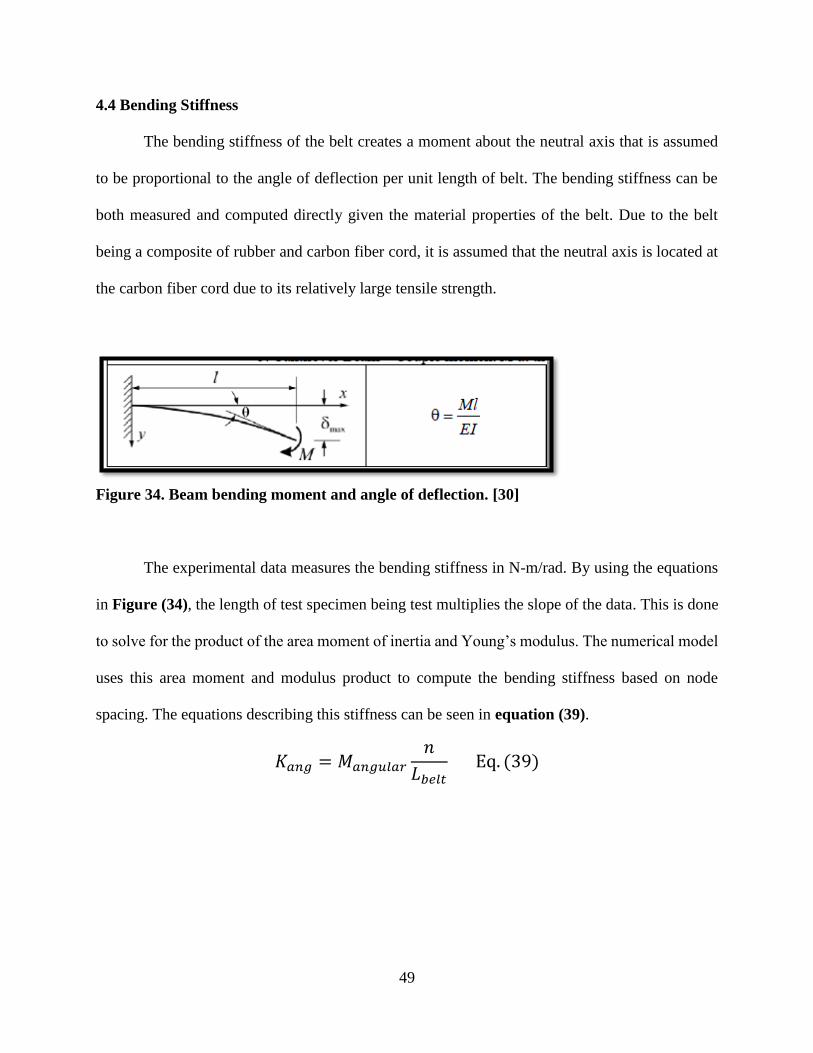
4.4 Bending Stiffness
The bending stiffness of the belt creates a moment about the neutral axis that is assumed
to be proportional to the angle of deflection per unit length of belt. The bending stiffness can be
both measured and computed directly given the material properties of the belt. Due to the belt
being a composite of rubber and carbon fiber cord, it is assumed that the neutral axis is located at
the carbon fiber cord due to its relatively large tensile strength.
Figure 34. Beam bending moment and angle of deflection. [30]
The experimental data measures the bending stiffness in N-m/rad. By using the equations
in Figure (34), the length of test specimen being test multiplies the slope of the data. This is done
to solve for the product of the area moment of inertia and Young’s modulus. The numerical model
uses this area moment and modulus product to compute the bending stiffness based on node
spacing. The equations describing this stiffness can be seen in equation (39).
𝐾𝑎𝑛𝑔 = 𝑀𝑎𝑛𝑔𝑢𝑙𝑎𝑟
𝑛
𝐿𝑏𝑒𝑙𝑡 Eq. (39)
50
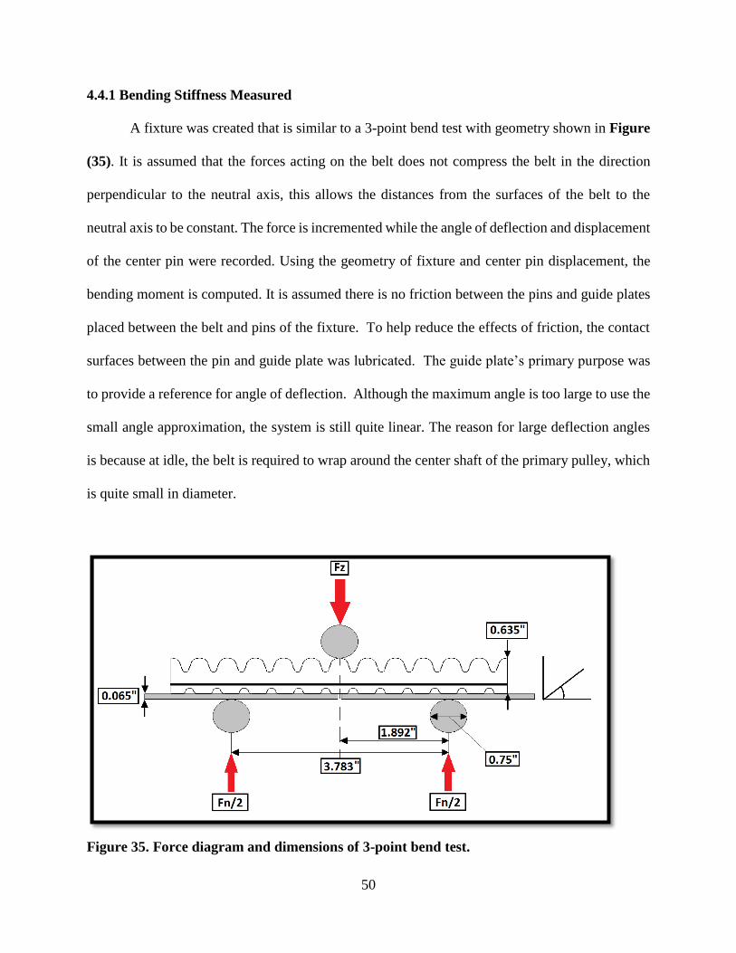
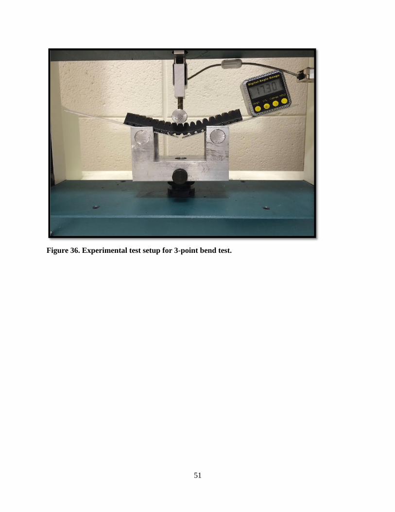
4.4.1 Bending Stiffness Measured
A fixture was created that is similar to a 3-point bend test with geometry shown in Figure
(35). It is assumed that the forces acting on the belt does not compress the belt in the direction
perpendicular to the neutral axis, this allows the distances from the surfaces of the belt to the
neutral axis to be constant. The force is incremented while the angle of deflection and displacement
of the center pin were recorded. Using the geometry of fixture and center pin displacement, the
bending moment is computed. It is assumed there is no friction between the pins and guide plates
placed between the belt and pins of the fixture. To help reduce the effects of friction, the contact
surfaces between the pin and guide plate was lubricated. The guide plate’s primary purpose was
to provide a reference for angle of deflection. Although the maximum angle is too large to use the
small angle approximation, the system is still quite linear. The reason for large deflection angles
is because at idle, the belt is required to wrap around the center shaft of the primary pulley, which
is quite small in diameter.
Figure 35. Force diagram and dimensions of 3-point bend test.
51
Figure 36. Experimental test setup for 3-point bend test.
52
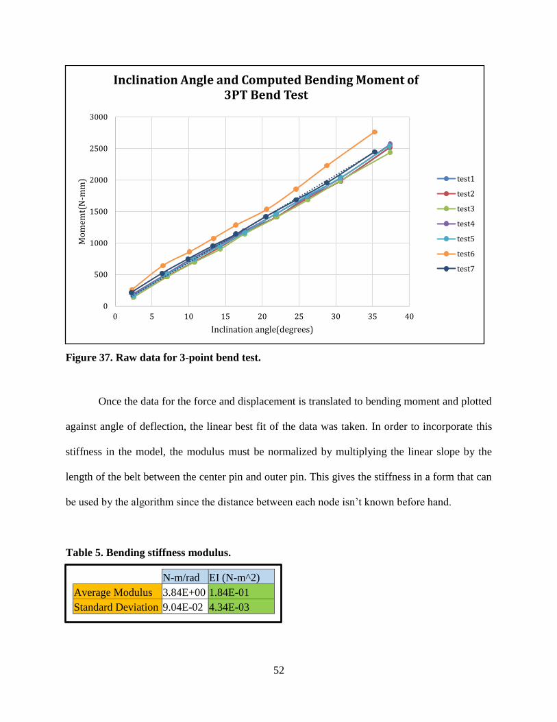
Figure 37. Raw data for 3-point bend test.
Once the data for the force and displacement is translated to bending moment and plotted
against angle of deflection, the linear best fit of the data was taken. In order to incorporate this
stiffness in the model, the modulus must be normalized by multiplying the linear slope by the
length of the belt between the center pin and outer pin. This gives the stiffness in a form that can
be used by the algorithm since the distance between each node isn’t known before hand.
Table 5. Bending stiffness modulus.
0
500
1000
1500
2000
2500
3000
0 5 10 15 20 25 30 35 40
Mo
mem
t(N
-mm
)
Inclination angle(degrees)
Inclination Angle and Computed Bending Moment of 3PT Bend Test
test1
test2
test3
test4
test5
test6
test7
N-m/rad EI (N-m^2)
Average Modulus 3.84E+00 1.84E-01
Standard Deviation 9.04E-02 4.34E-03
53
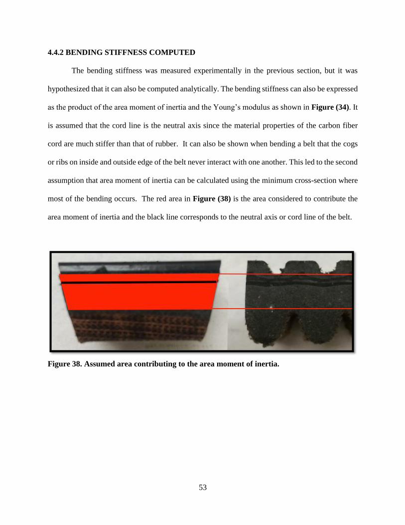
4.4.2 BENDING STIFFNESS COMPUTED
The bending stiffness was measured experimentally in the previous section, but it was
hypothesized that it can also be computed analytically. The bending stiffness can also be expressed
as the product of the area moment of inertia and the Young’s modulus as shown in Figure (34). It
is assumed that the cord line is the neutral axis since the material properties of the carbon fiber
cord are much stiffer than that of rubber. It can also be shown when bending a belt that the cogs
or ribs on inside and outside edge of the belt never interact with one another. This led to the second
assumption that area moment of inertia can be calculated using the minimum cross-section where
most of the bending occurs. The red area in Figure (38) is the area considered to contribute the
area moment of inertia and the black line corresponds to the neutral axis or cord line of the belt.
Figure 38. Assumed area contributing to the area moment of inertia.
54
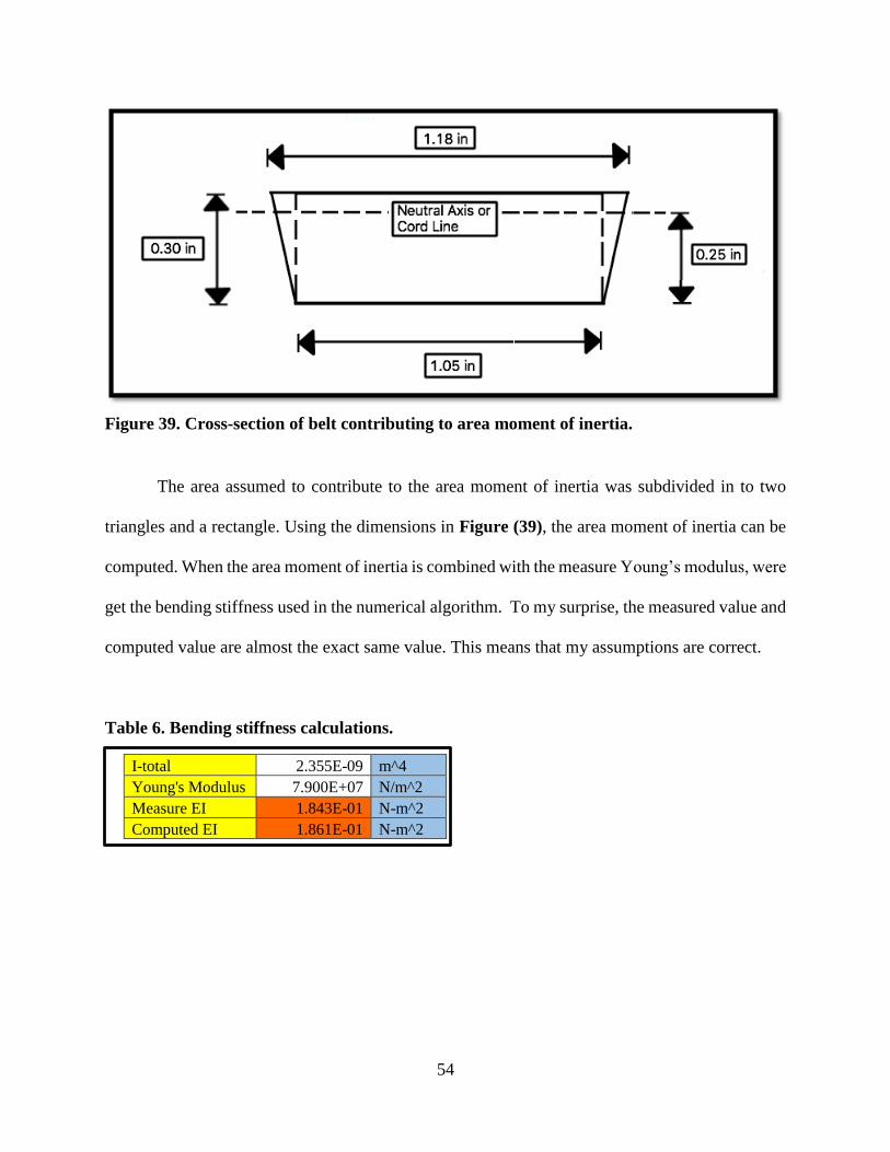
Figure 39. Cross-section of belt contributing to area moment of inertia.
The area assumed to contribute to the area moment of inertia was subdivided in to two
triangles and a rectangle. Using the dimensions in Figure (39), the area moment of inertia can be
computed. When the area moment of inertia is combined with the measure Young’s modulus, were
get the bending stiffness used in the numerical algorithm. To my surprise, the measured value and
computed value are almost the exact same value. This means that my assumptions are correct.
Table 6. Bending stiffness calculations.
I-total 2.355E-09 m^4
Young's Modulus 7.900E+07 N/m^2
Measure EI 1.843E-01 N-m^2
Computed EI 1.861E-01 N-m^2
55
CHAPTER 5: SIMULATION/ALGORITHM RESULTS
The numerical algorithm in this paper has been previously validated experimentally by
[15], though there may be a slight variation in numerical techniques in this adaptation. In this
simulation, a PI controller with feed-forward gain for input speed objective tracking, a linear
damping element between belt nodes and vehicle model have been added. The results of the
simulation with and without the linear damper, will be compared. Initial conditions and all other
inputs besides input pulley axial force and vehicle load are kept constant. Although fixing the input
torque and axial force on the output pulley wasn’t ideal, this was done to eliminate the number of
variables that could affect the response of the system.
Before simulation can begin, constants defining the system need to be defined. These
include geometric and inertial properties of the CVT, material properties of the CVT belt and
assumed inertial and aerodynamic properties of the vehicle. These constant are also used by
various sub-routines for preliminary calculations and setup of the initial conditions for simulation.
These measured and assumed constants are available in Table (A1) in Appendix A.
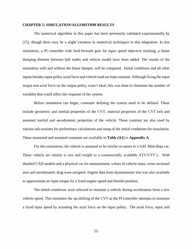
For this simulation, the vehicle is assumed to be similar in nature to a SAE Mini-Baja car.
These vehicle are similar is size and weight to a commercially available ATV/UTV’s. With
detailed CAD models and a physical car for measurement, values of vehicle mass, cross-sectional
area and aerodynamic drag were assigned. Engine data from dynamometer test was also available
to approximate an input torque for a fixed engine speed and throttle position.
The initial conditions were selected to simulate a vehicle during acceleration form a low
vehicle speed. This simulates the up-shifting of the CVT as the PI controller attempts to maintain
a fixed input speed by actuating the axial force on the input pulley. The axial force, input and
56
output speed of the CVT and CVT ratio are recorded for a 5 second simulation. The list of initial
condition, computed constant and controller gains are list in Table (B1) in Appendix B.
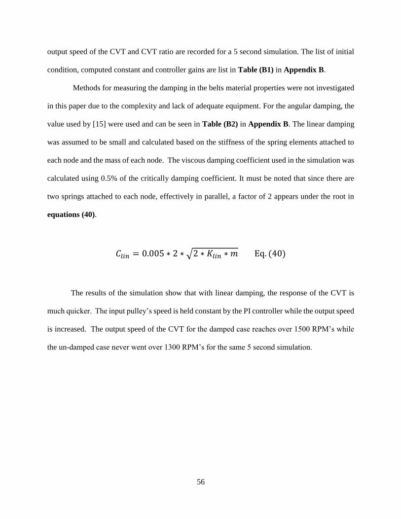
Methods for measuring the damping in the belts material properties were not investigated
in this paper due to the complexity and lack of adequate equipment. For the angular damping, the
value used by [15] were used and can be seen in Table (B2) in Appendix B. The linear damping
was assumed to be small and calculated based on the stiffness of the spring elements attached to
each node and the mass of each node. The viscous damping coefficient used in the simulation was
calculated using 0.5% of the critically damping coefficient. It must be noted that since there are
two springs attached to each node, effectively in parallel, a factor of 2 appears under the root in
equations (40).
𝐶𝑙𝑖𝑛 = 0.005 ∗ 2 ∗ √2 ∗ 𝐾𝑙𝑖𝑛 ∗ 𝑚 Eq. (40)
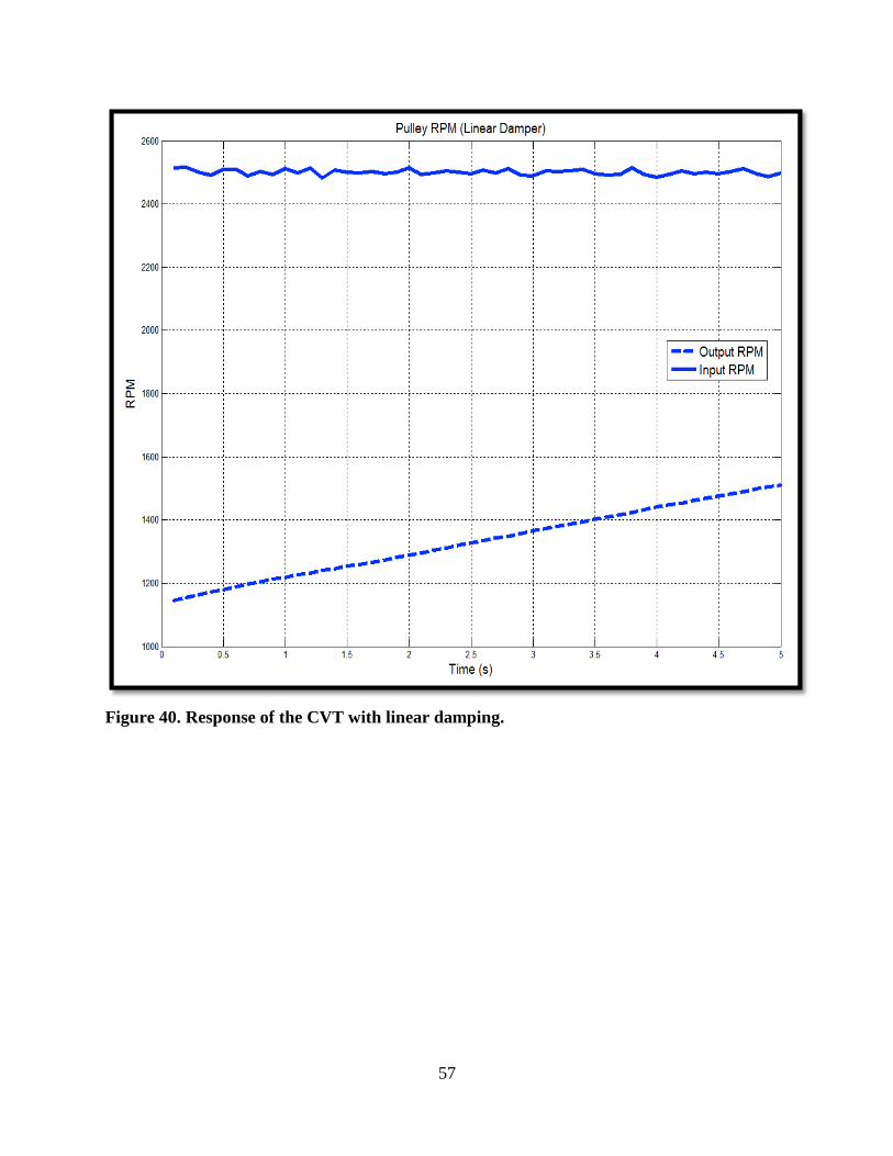
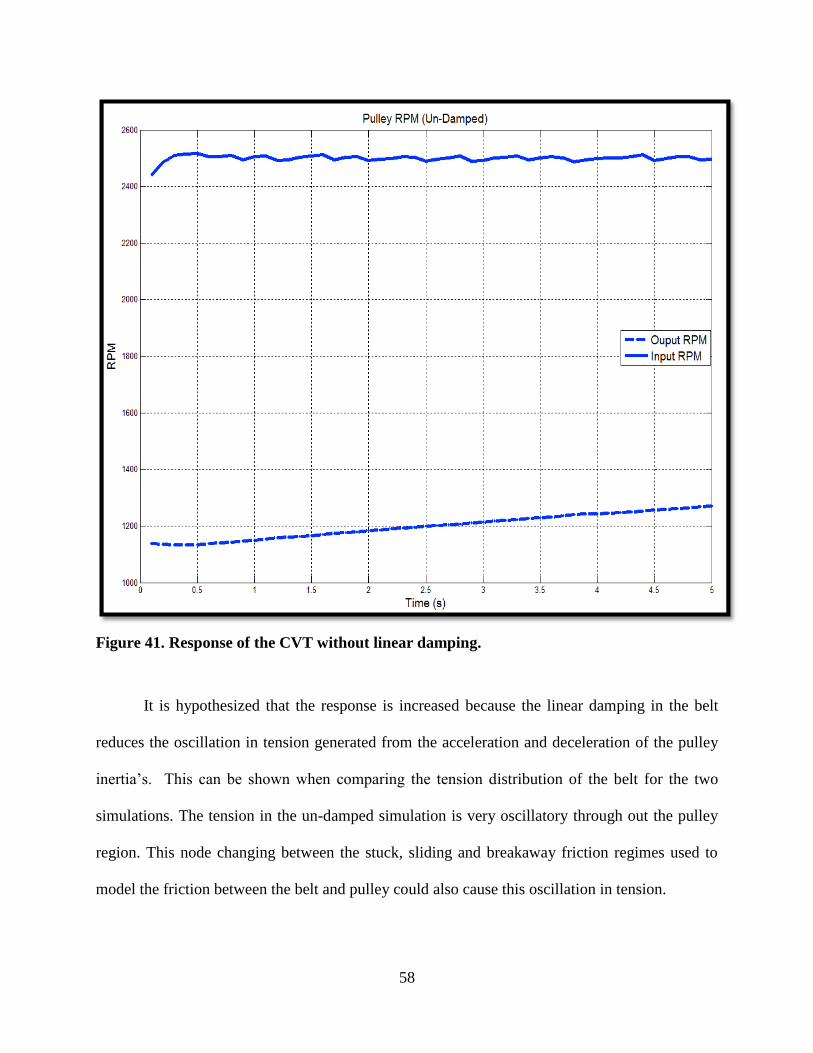
The results of the simulation show that with linear damping, the response of the CVT is
much quicker. The input pulley’s speed is held constant by the PI controller while the output speed
is increased. The output speed of the CVT for the damped case reaches over 1500 RPM’s while
the un-damped case never went over 1300 RPM’s for the same 5 second simulation.
57
Figure 40. Response of the CVT with linear damping.
58
Figure 41. Response of the CVT without linear damping.
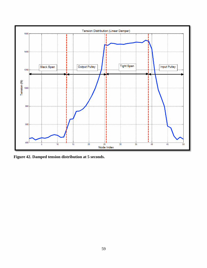
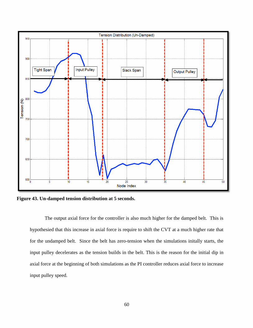
It is hypothesized that the response is increased because the linear damping in the belt
reduces the oscillation in tension generated from the acceleration and deceleration of the pulley
inertia’s. This can be shown when comparing the tension distribution of the belt for the two
simulations. The tension in the un-damped simulation is very oscillatory through out the pulley
region. This node changing between the stuck, sliding and breakaway friction regimes used to
model the friction between the belt and pulley could also cause this oscillation in tension.
59
Figure 42. Damped tension distribution at 5 seconds.
60
Figure 43. Un-damped tension distribution at 5 seconds.
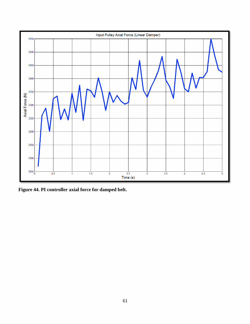
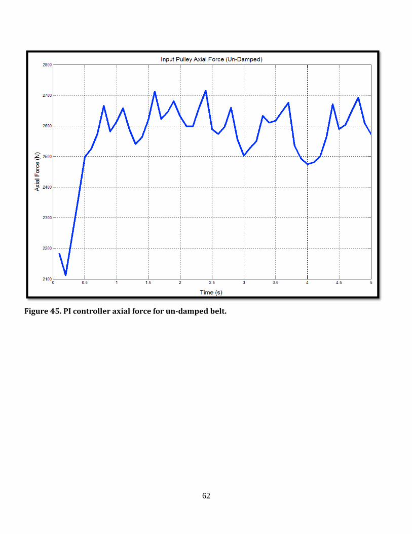
The output axial force for the controller is also much higher for the damped belt. This is
hypothesied that this increase in axial force is require to shift the CVT at a much higher rate that
for the undamped belt. Since the belt has zero-tension when the simulations initally starts, the
input pulley decelerates as the tension builds in the belt. This is the reason for the initial dip in
axial force at the beginning of both simulations as the PI controller reduces axial force to increase
input pulley speed.
61
Figure 44. PI controller axial force for damped belt.
62
Figure 45. PI controller axial force for un-damped belt.
63
CHAPTER 6: CONCLUSIONS
Methods for measuring the stiffness properties of CVT belts have been developed. It has
been shown that the angular stiffness can be computed analytically using the cord line as the neutral
axis and the results agree with experimental measurements. This analytical bending stiffness was
computed using the measured Young’s modulus of the rubber. The Young’s modulus was
measured a modified sample under axial compression. The axial stiffness of the belt was also
measured using different techniques and values compared. The axial stiffness tends to agree when
the cross-section is left in the trapezoidal configuration. When the top layer of the belt was
removed to expose the carbon cord for one of the tests with the trapezoidal cross-section, it was
slightly softer than a similar test with an unmodified sample. This is because the rubber material
above the cord line is much thin in comparison to the rubber below the cord line. This is to be
expected, but the significance is that the two methods of measure tend to agree. The longitudinal
stiffness was measured using an extensometer and pulley system attached to the tensile machine.
All measured stiffness’s agree within an order of magnitude to values reported by the author of the
original numerical algorithm.
A numerical algorithm from previous work has been recreated with detailed insight into
stability and numerical techniques. The search routine for meeting the boundary condition of axial
force applied and node axial compression uses a bi-section method that converges very quickly to
a specified relative error bound. Conditions that cause instability in the search routine have been
addressed in a manor that mimics the physical attributes of the CVT at these conditions. The
stability of the Runge-Kutta 4th order solver used for numerical integration in the time domain was
discussed and found that very small time steps were needed to do to the stiffness of the system.
The explicit non-linear equations of motion make the use of implicit solvers impossible to
64
implement. The addition of a linear damper between belt nodes was added and is computed base
on a scaled critical viscous damping factory. The response of the CVT, for the same initial
conditions and PI controller, were simulated with and without the linear damping present between
nodes. The time response of the CVT increased with the presence of the linear damping element.
The output of the PI controller with feed-forward gain provided adequate input pulley RPM
objective tracking, even as the ratio of the CVT deviated greatly. This means that future electronic
control of CVT’s may be provide adequate tracking and control using this controller design. The
addition of gain scheduling would increase the range of stability
65
CHAPTER 7: RECOMMENDED FUTURE WORK
The damping effects of the belt were not measured in this work due to the lack of adequate
equipment. The use of a viscous damper is the simplest to implement and measure, but structural
damping may characterize the damping of the rubber better. The magnitude and rate of cyclical
loading seen in application would need to be determined to adequately characterize the damping
of the material for use in this model. The method for measuring these damping factors could use
similar fixtures outline in this work to measure material stiffness’s.
A detailed analysis of the frictional properties of CVT belt could also lead to a better
friction model to use in this algorithm. The ideal method would vary the contact pressure and
relative slip speeds between a belt sample and an aluminum counter-face. These pressures and slip
speeds should reflect those seen in application.
The control strategy for actuating the axial force on the pulleys was touched on in this work
but a more in-depth investigation would be needed to develop a complete control strategy.
Different control strategies have been explored for push-belt and metal chain CVT’s that may be
applicable for the rubber belt CVT.
The model used in this work has been validated in previous work, but with the addition of
a linear damper, revalidation would be needed. This may reveal that the new model with linear
damping present will be more stable and accurate for higher speed ratio changes.
66
REFERENCES
[1] Chen, T.f., D.w. Lee, and C.k. Sung. "An Experimental Study on Transmission Efficiency of
a Rubber V-belt CVT." Mechanism and Machine Theory33.4 (1998): 351-63. Web.
[2] Oliver, L. R., K. G. Hornung, J. E. Swenson, and H. N. Shapiro. "Design Equations for a
Speed and Torque Controlled Variable Ratio V-Belt Transmission." SAE Technical Paper Series
(1973): n. pag. Web.
[3] Gerbert, B. G. "Power Loss and Optimum Tensioning of V-Belt Drives." Journal of
Engineering for Industry J. Eng. for Industry 96.3 (1974): 877. Web.
[4] Gerbert, B. G. "Adjustable Speed V-Belt Drives-Mechanical Properties and Design." SAE
Technical Paper Series (1974): n. pag. Web.
[5] Bents, David J. "Axial Force and Efficiency Tests of Fixed Center Variable Speed Belt
Drive." SAE Technical Paper Series (1981): n. pag. Web.
[6] Kong, Lingyuan, and Robert G. Parker. "Steady Mechanics of Belt-Pulley Systems." Journal
of Applied Mechanics J. Appl. Mech. 72.1 (2005): 25. Web.
[7] Sorge, F. "A Simple Model for the Axial Thrust in V-Belt Drives." Journal of Mechanical
Design J. Mech. Des. 118.4 (1996): 589. Web.
[8] Sorge, F. "A Theoretical Approach to the Shift Mechanics of Rubber Belt Variators." Journal
of Mechanical Design J. Mech. Des. 130.12 (2008): 122602. Web.
[9] Cammalleri, Marco, and Francesco Sorge. "Approximate Closed-Form Solutions for the Shift
Mechanics of Rubber Belt Variators." Volume 6: ASME Power Transmission and Gearing
Conference; 3rd International Conference on Micro- and Nanosystems; 11th International
Conference on Advanced Vehicle and Tire Technologies (2009): n. pag. Web.
[10] Gerbert, G. "Belt Slip—A Unified Approach." Journal of Mechanical Design J. Mech. Des.
118.3 (1996): 432. Web.
[11] Dolan, J. P., and W. S. Worley. "Closed-Form Approximations to the Solution of V-Belt
Force and Slip Equations." J. of Mech. Trans. Journal of Mechanisms Transmissions and
Automation in Design 107.2 (1985): 292. Web.
[12] Sorge, Francesco, and Marco Cammalleri. "Helical Shift Mechanics of Rubber V-Belt
Variators." Journal of Mechanical Design J. Mech. Des. 133.4 (2011): 041006. Web.
[13] Oliver, Larry R., and Dewey D. Henderson. "Torque Sensing Variable Speed V-Belt Drive."
SAE Technical Paper Series (1972): n. pag. Web.
67
[14] Oliver, Larry R. “Contemporary Methods in V-Belt Drive Design.” American Society of
Agricultural Engineering (1976): n. pag. Web.
[15] Julió, G., and J.-S. Plante. "An Experimentally-validated Model of Rubber-belt CVT
Mechanics." Mechanism and Machine Theory 46.8 (2011): 1037-053. Web.
[16] Srivastava, Nilabh, and Imtiaz Haque. "A Review on Belt and Chain Continuously Variable
Transmissions (CVT): Dynamics and Control." Mechanism and Machine Theory 44.1 (2009):
19-41. Web.
[17] Carbone, G., L. De Novellis, G. Commissaris, and M. Steinbuch. "An Enhanced CMM
Model for the Accurate Prediction of Steady-State Performance of CVT Chain Drives." Journal
of Mechanical Design J. Mech. Des. 132.2 (2010): 021005. Web.
[18] Bhate, Rohan Vasudev. “Control Oriented Transient-dynamic Modeling and Simulation of
Metal V-belt Cvt”. Thesis. University of North Carolina at Charlotte, 2009. Print.
[19] Bertini, L., L. Carmignani, and F. Frendo. "Analytical Model for the Power Losses in
Rubber V-belt Continuously Variable Transmission (CVT)." Mechanism and Machine Theory 78
(2014): 289-306. Web.
[20] Tseng, Chyuan-Yaw, Li-Wen Chen, Yuan-Ting Lin, and Jhao-Yi Li. "A Hybrid Dynamic
Simulation Model for Urban Scooters with a Mechanical-type CVT." 2008 IEEE International
Conference on Automation and Logistics (2008): n. pag. Web.
[21] Aaen, Olav. Olav Aaen's Clutch Tuning Handbook. Racine, WI: AAEN Performance, 2011.
Print.
[22] Wang, Cheng, and Chang-Song Jiang. "Computer Modeling of CVT Ratio Control System
Based on Matlab." 2011 3rd International Conference on Computer Research and Development
(2011): n. pag. Web.
[23] Kasai, Y., and Y. Morimoto. "Electronically Controlled Continuously Variable
Transmission (ECVT-II)." International Congress on Transportation Electronics, (1988): n. pag.
Web.
[24] Zhu, C-C, H-J Liu, J-J Tian, Q. Xiao, and X-S Du. "Experimental Research on the Effect of
Structural Parameters on the Governing Characteristics of a Pulley-drive, Continuously Variable
Transmission." Proceedings of the Institution of Mechanical Engineers, Part D: Journal of
Automobile Engineering 224.6 (2010): 775-84. Web.
[25] Adyanthaya, Vivek, N. B. Joshi, and A. D. Samant. "Optimization and Evaluation of a Belt
Driven CVT for a 125 Cc, 4 Stroke Scooter." SAE Technical Paper Series (1995): n. pag. Web.
68
[26] Carbone, G., L. Mangialardi, and G. Mantriota. "Theoretical Model of Metal V-Belt Drives
During Rapid Ratio Changing." Journal of Mechanical Design J. Mech. Des. 123.1 (2001): 111.
Web.
[27] Leamy, Michael J., and Tamer M. Wasfy. "Transient and Steady-State Dynamic Finite
Element Modeling of Belt-Drives." J. Dyn. Sys., Meas., Control Journal of Dynamic Systems,
Measurement, and Control 124.4 (2002): 575. Web.
[28] Oliver, Larry R., and Dewey D. Henderson. "Torque Sensing Variable Speed V-Belt Drive."
SAE Technical Paper Series (1972): n. pag. Web.
[29] Childs, T. H C, and D. Cowburn. "Power Transmission Losses in V‐belt Drives Part 2:
Effects of Small Pulley Radii." ARCHIVE: Proceedings of the Institution of Mechanical
Engineers, Part D: Transport Engineering 1984-1988 (vols 198-202) 201.14 (1987): 41-53.
Web.
[30] Ruina, Andy. "BEAM DEFLECTION FORMULA." (n.d.): n. pag. Web.
<http://ruina.mae.cornell.edu/Courses/ME4735-2012/Rand4770Vibrations/BeamFormulas.pdf>.
[31] Burden, Richard L., and J. Douglas. Faires. Numerical Analysis. Boston: PWS-Kent Pub.,
1993. Print.
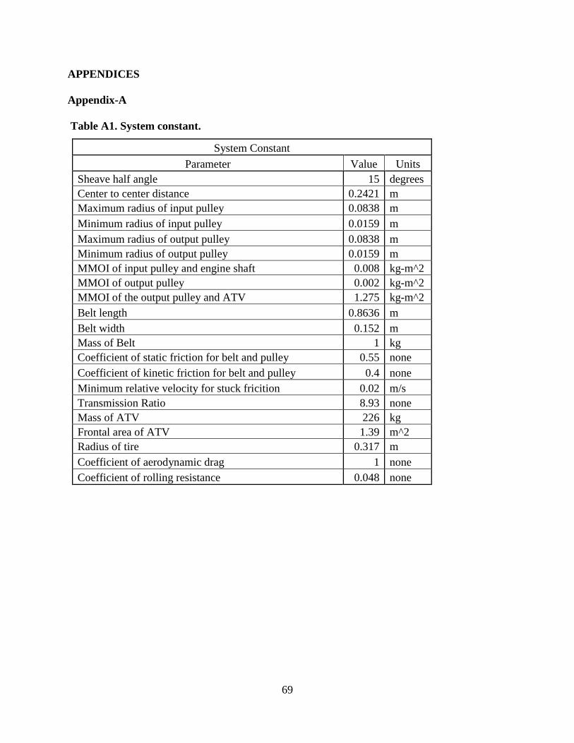
69
APPENDICES
Appendix-A
Table A1. System constant.
System Constant
Parameter Value Units
Sheave half angle 15 degrees
Center to center distance 0.2421 m
Maximum radius of input pulley 0.0838 m
Minimum radius of input pulley 0.0159 m
Maximum radius of output pulley 0.0838 m
Minimum radius of output pulley 0.0159 m
MMOI of input pulley and engine shaft 0.008 kg-m^2
MMOI of output pulley 0.002 kg-m^2
MMOI of the output pulley and ATV 1.275 kg-m^2
Belt length 0.8636 m
Belt width 0.152 m
Mass of Belt 1 kg
Coefficient of static friction for belt and pulley 0.55 none
Coefficient of kinetic friction for belt and pulley 0.4 none
Minimum relative velocity for stuck fricition 0.02 m/s
Transmission Ratio 8.93 none
Mass of ATV 226 kg
Frontal area of ATV 1.39 m^2
Radius of tire 0.317 m
Coefficient of aerodynamic drag 1 none
Coefficient of rolling resistance 0.048 none
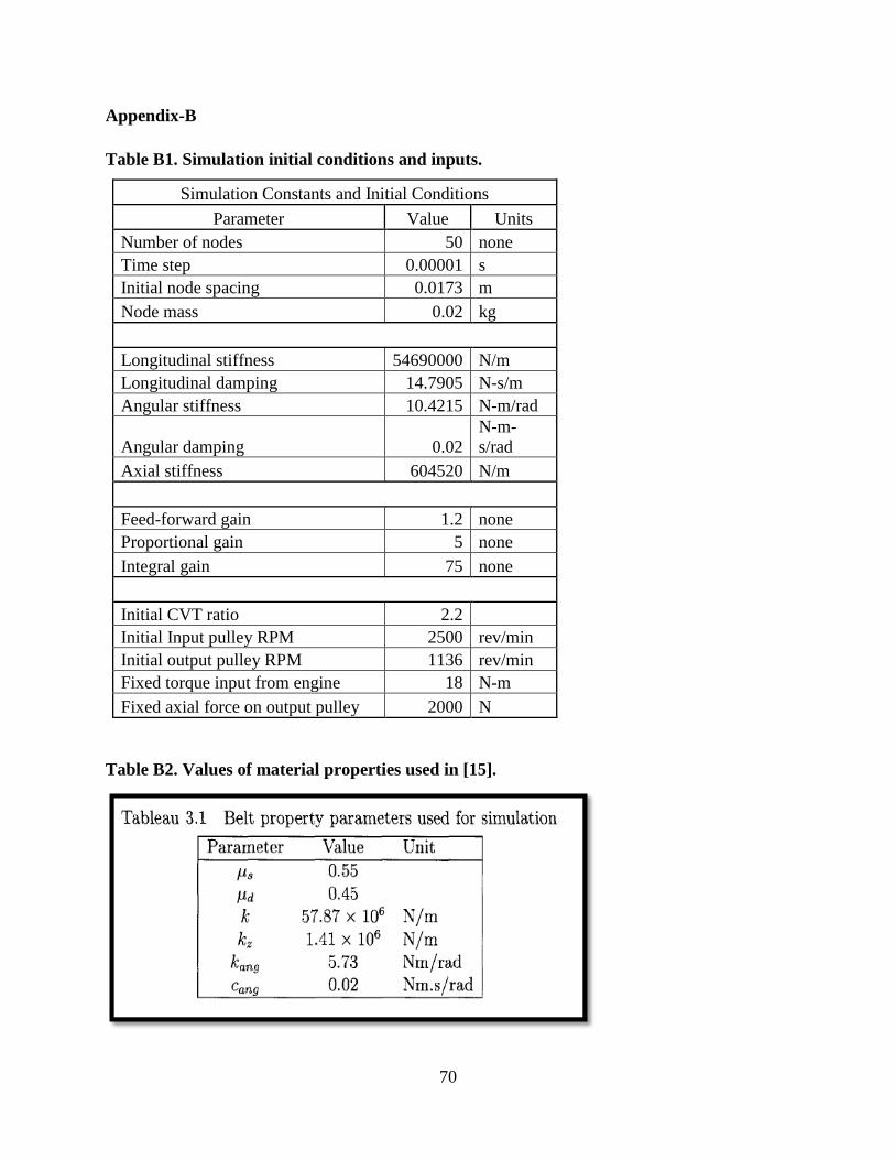
70
Appendix-B
Table B1. Simulation initial conditions and inputs.
Simulation Constants and Initial Conditions
Parameter Value Units
Number of nodes 50 none
Time step 0.00001 s
Initial node spacing 0.0173 m
Node mass 0.02 kg
Longitudinal stiffness 54690000 N/m
Longitudinal damping 14.7905 N-s/m
Angular stiffness 10.4215 N-m/rad
Angular damping 0.02
N-m-
s/rad
Axial stiffness 604520 N/m
Feed-forward gain 1.2 none
Proportional gain 5 none
Integral gain 75 none
Initial CVT ratio 2.2
Initial Input pulley RPM 2500 rev/min
Initial output pulley RPM 1136 rev/min
Fixed torque input from engine 18 N-m
Fixed axial force on output pulley 2000 N
Table B2. Values of material properties used in [15].