Embed Size (px)
Citation preview
INVESTIGATION OF SEPARATION STRATEGIES FOR BIOANALYTICAL
METHODS: CHROMATOGRAPHY, ION MOBILITY AND MASS SPECTROMETRY
By
James N. Dodds
Dissertation
Submitted to the Faculty of the
Graduate School of Vanderbilt University
in partial fulfillment of the requirements
for the degree of
DOCTOR OF PHILOSOPHY
in
Chemistry
May 11, 2018
Nashville, TN
Approved:
John A. McLean, Ph.D.
David E. Cliffel, Ph.D.
Steven D. Townsend, Ph.D.
Erin C. Rericha, Ph.D.

ii
To my friends, family, and coworkers,
who have me helped along the way and have been there always.
iii
ACKNOWLEDGEMENTS
I would like to thank my dissertation advisor Dr. John. A. McLean first and foremost for
providing me with the opportunity to join the McLean research group and pursue my passion of
exploring bioanalytical applications of mass spectrometry. I have been very fortunate in this
opportunity to develop my scientific skills in a setting of cutting edge analytical instrumentation
and mentorship which are hallmarks of our research team. Thank you for your mentorship,
expertise, and patience throughout this process.
I would like to thank my dissertation committee members, Dr. David E. Cliffel, Steven D.
Townsend, and Erin C. Rericha for their time and diligence throughout this process. I have
appreciated your feedback along the way at each of our meetings, and I am especially grateful for
the differences in perspective that each of you have provided, as it is very easy to get stuck in our
own microcosm in our respective research fields.
I would also like to acknowledge Dr. Jody C. May for timeless hours of editing and
mentorship for the past five years. I know that time is precious for everyone, and that makes your
sacrifice all the more meaningful. I am deeply grateful for all of your training and advice and I
know I am a better scientist for it.
I also want to acknowledge my colleagues in the McLean research group for helping me
with presentations, proof reading papers, and enduring countless hours of troubleshooting both
professional and personal problems both inside and outside of the lab. I hope that each of you
know how much you mean to me, and I only wish the best for you all as you finish your time in
the lab and move on to other phases in life.

iv
I would also like to thank my family and my friends who have provided support for me
over these past five years. I know that most of the time my spent rambling on about scientific ideas
might not have been the most interesting discussions, but I appreciate you listening just the same.
Lastly, I would like to acknowledge the funding sources for this research: the Vanderbilt
Institute of Chemical Biology, the College of Arts and Sciences, the Vanderbilt Institute for
Integrative Biosystems Research and Education, the Center for Innovative Technology, the
National Institutes of Health (NIH Grant R01GM099218) and under Assistance Agreement No.
83573601 awarded by the U.S. Environmental Protection Agency. This work has not been
formally reviewed by EPA. The views expressed in this document are solely those of the authors
and do not necessarily reflect those of the Agency. EPA does not endorse any products or
commercial services mentioned in this publication. Furthermore, the content is solely the
responsibility of the authors and does not necessarily represent the official views of the funding
agencies and organizations.

v
TABLE OF CONTENTS
Page
DEDICATION…………………………………………………………………………………….ii
ACKNOWLEDGMENTS..............................................................................................................iii
LIST OF TABLES.......................................................................................................................... .x
LIST OF FIGURES……………………………………………………………………………… xi
LIST OF ABBREVIATIONS………………………………………………………………….. xiii
Chapters
Introduction ......................................................................................................................................1
State of the Field and Personal Contributions......................................................................1
1. Chiral Separation Strategies in Mass Spectrometry: Integration of Chromatography,
Electrophoresis, and Gas-Phase Mobility ............................................................................4
1.1. Introduction ...............................................................................................................4
1.2. Chromatography and Mass Spectrometry .................................................................7
1.2.1. Liquid Chromatography ................................................................................10
1.3. Electrophoresis-Mass Spectrometry .......................................................................13
1.3.1. Isomer Separations by IM-MS ......................................................................18
1.4. Conclusions .............................................................................................................23
1.5. Acknowledgements .................................................................................................24
1.6. References ...............................................................................................................24
vi
2. Isomeric and Conformational Analysis of Small Drug and Drug-Like Molecules by Ion
Mobility-Mass Spectrometry (IM-MS)..............................................................................30
2.1. Introduction .................................................................................................................30
2.1.1. Isomers ..............................................................................................................31
2.2. Instrumentation and Theory ........................................................................................34
2.2.1. Drift Tube Ion Mobility ....................................................................................36
2.2.2. Traveling Wave Ion Mobility ...........................................................................37
2.3. Current Work in Isomer Structural Separations..........................................................38
2.3.1. Separation of Constitutional Isomers ................................................................38
2.3.2. Separation of Conformational Isomers .............................................................41
2.4. Materials .....................................................................................................................44
2.5. Methods.......................................................................................................................46
2.5.1. Preparing the Instrument ...................................................................................47
2.5.2. Data Acquisition ...............................................................................................48
2.5.3. Data Workup .....................................................................................................49
2.6. Acknowledgements .....................................................................................................50
2.7. References ...................................................................................................................51
3. Assessing Ion Mobility Resolving Power Theory for Broadscale Mobility Analysis with a
High Precision Uniform Field Ion Mobility-Mass Spectrometer ......................................56
3.1. Introduction .................................................................................................................56

vii
3.2. Experimental ...............................................................................................................59
3.2.1. Uniform Field IM-MS Instrument ....................................................................60
3.2.2. Analytical Precision ..........................................................................................62
3.3. Data Acquisition and Analysis....................................................................................63
3.3.1. Semi-Empirical Fitting Procedure ....................................................................64
3.4. Results and Discussion ...............................................................................................64
3.4.1. Factors affecting semi-empirical coefficients ...................................................64
3.4.2. Empirical Correlation of Theoretical Resolving Power ....................................68
3.4.3. Broadscale Validity of Semi-Empirical Results ...............................................75
3.5. Conclusions .................................................................................................................77
3.6. Acknowledgments.......................................................................................................79
3.7. References ...................................................................................................................79
4. Investigation of the Complete Suite of the Leucine and Isoleucine Isomers: Towards
Prediction of Ion Mobility Separation Capabilities ...........................................................82
4.1. Introduction .................................................................................................................82
4.2. Experimental Methods ................................................................................................84
4.2.1. Preparation of Standards ...................................................................................84
4.2.2. Experimental Parameters ..................................................................................84
4.2.3. Collision Cross Section Measurements ............................................................87
4.3. Results and Discussion ...............................................................................................87
4.3.1. Isomer Classifications and Separations ............................................................87

viii
4.3.2. Peak Shape Modeling and Ion Mobility ...........................................................89
4.3.3. Resolving Power and Separations .....................................................................92
4.4. Conclusions .................................................................................................................98
4.5. Acknowledgements ...................................................................................................100
4.6. References .................................................................................................................101
5. Correlating Resolving Power, Resolution, and Collision Cross Section: Unifying Cross-
Platform Assessment of Separation Efficiency in Ion Mobility Spectrometry................106
5.1. Introduction ...............................................................................................................106
5.2. Experimental Methods ..............................................................................................110
5.2.1. Chemical Standards ........................................................................................110
5.2.2. Instrumentation and Methods .........................................................................111
5.2.3. Selection of Published Spectra........................................................................111
5.2.4. Evaluation of Separation Efficiency ...............................................................112
5.3. Results and Discussion .............................................................................................113
5.3.1. Gaussian Distributions ....................................................................................113
5.3.2. CCS-Based Resolving Power .........................................................................113
5.3.3. Cross-Platform Assessment ............................................................................115
5.3.4. Traveling Wave Resolving Power ..................................................................117
5.3.5. Cross-Platform Assessment of Separation Capabilities ..................................119
5.3.6. How Much Resolving Power is Necessary .....................................................122
5.3.6.1. Mass Analysis ....................................................................................122

ix
5.3.6.2. Ion Mobility Analysis ........................................................................124
5.3.7. Ion Mobility-Mass Spectrometry ....................................................................124
5.4. Conclusions ...............................................................................................................125
5.5. Acknowledgements ...................................................................................................126
5.6. References .................................................................................................................127
APPENDIX
A. References of Adaption for Chapters ......................................................................................134
B. Supplementary Materials for Chapter II..................................................................................135
C. Supplementary Materials for Chapter III ................................................................................138
D. Supplementary Materials for Chapter IV ................................................................................151
E. Supplementary Materials for Chapter V..................................................................................159

x
LIST OF TABLES
Table Page
3.1. Summary of Results from Semi-Empirical Fitting .................................................................65
4.1. Predicted Resolving Power for Leucine Isomer Separations ..................................................99
5.1. Various Ion Mobility Techniques and Dispersive Dimensions ............................................107
5.2. Separation Parameters for Published Ion Mobility Separations ...........................................116
xi
LIST OF FIGURES
Figure Page
1.1. Increasing Structural Complexity for One Molecular Formula ................................................6
1.2. Three Point Model for Chiral Separations ................................................................................8
1.3. Mechanisms of Chiral Separations .........................................................................................12
1.4. Instrument Schematic for Agilent 6560 ..................................................................................16
1.5. Timescale of Analytical Separations ......................................................................................17
1.6. Skeletal Structure and Separation of Leucine Isomers ...........................................................19
1.7. Desmopressin Structure and Chiral IM-MS Separation .........................................................21
2.1. Structures of Acetaminophen Constitutional Isomers ............................................................32
2.2. Block Diagrams of Drift Tube and Traveling Wave Instrumentation ....................................35
2.3. Skeletal Structure and Separation of Leucine Isomers ...........................................................40
2.4. Complexity of Carbohydrate Isomers .....................................................................................43
2.5. Drift Time Profiles for Thalidomide Chiral Isomers ..............................................................45
3.1. Instrument Schematic for Agilent 6560 ..................................................................................61
3.2. Resolving Power Curves as a Function of Gate Width...........................................................69
3.3. 3D Resolving Power Curves for Experimental and Theoretical Models ................................72
3.4. Resolving Power as a Function of Reduced Mobility ............................................................74

xii
3.5. Resolving Power Curves as a function of Drift Gas Composition .........................................76
4.1. Isomer Classification Hierarchy .............................................................................................86
4.2. Skeletal Structure and Separation of Leucine Isomers ...........................................................88
4.3. Theoretical Resolution as a Function of Resolving Power and Concentration ......................91
4.4. Plot of Increasing Separation as a Function of Resolving Power ...........................................95
4.5. Experimental and Theoretical Separations of Leucine Isomers .............................................97
5.1. Selected Ion Mobility Separations from Literature Publications ..........................................114
5.2. Ion Mobility Separations as a Function of Resolving Power and CCS ................................120
5.3. Biological Separation of Peptides from Ion Mobility and Mass Spectrometry ....................123

xiii
LIST OF ABBREVIATIONS
CCS Collision Cross Section
µs Microsecond
3D Three-Dimensional
ACN Acetonitrile
MeOH Methanol
MS Mass Spectrometry
ms Millisecond
MS/MS Tandem Mass Spectrometry
IM Ion Mobility
eV Electron Volt
GC Gas Chromatography
LC Liquid Chromatography
HILIC Hydrophilic Interaction Liquid Chromatography
CE Capillary Electrophoresis
TLC Thin Layer Chromatography
CID Collision Induced Disassociation
ETD Electron Transfer Disassociation

xiv
DT Drift Time
FWHM Full Width at Half Maximum Height
Rp Resolving Power
Rp-p Two-Peak Resolution
ΔCCS% Percent Difference in Cross Section
ESI Electrospray Ionization
MALDI Matrix-Assisted Laser Desorption Ionization
IM-MS Ion Mobility-Mass Spectrometry
m/z Mass-To-Charge Ratio
ppb Parts Per Billion
ppm Parts Per Million
TOF Time of Flight Mass Spectrometer
QTOF Quadrupole-Time of Flight
TWIMS Traveling Wave Ion Mobility Spectrometry
DTIMS Drift Tube Ion Mobility Spectrometry
UPLC Ultra-Performance Liquid Chromatography
SFC Supercritical Fluid Chromatography

1
INTRODUCTION
STATE OF THE FIELD AND PERSONAL CONTRIBUTIONS
The field of mass spectrometry has been developing rapidly after its initial debut in the
second half of the previous century.1 The separation capacity of instrumentation in MS has
increased by orders of magnitude in comparison to initial devices developed in the previous
century, and new platforms are being developed each year. While mass spectrometry is still
enjoying steady growth in the analytical community, several intrinsic challenges remain in the
analysis of complex samples. Specifically, the analysis and characterization of isomeric species in
complex biological matrices remains a distinct issue of paramount importance for downstream
metabolic pathway analysis. To address the challenge these isomeric species present, many
orthogonal separation techniques have been developed to separate isomeric compounds prior to
mass analysis. These techniques include, but are not limited to, gas and liquid chromatography,
capillary electrophoresis, and ion mobility spectrometry.
As ion mobility spectrometry is a gas phase separation which takes place in the millisecond
timescale, this technique is rapidly growing in popularity in the analytical community, specifically
studies related to mass spectrometry.2 Currently, two of the most popular instrument platforms in
IM-MS are time-dispersive methods, namely drift tube and traveling wave ion mobility
spectrometers, which are currently marketed by Agilent Technologies and Waters Corporation,
respectively. While these two instrument vendors have been very successful in terms of marketing
their new platforms, new instruments are being commercialized each year. As a result of the
rapidly expanding market for ion mobility technology, other instrument manufacturers are
developing additional strategies to improve the separation capacity of ion mobility spectrometry,

2
including high pressure separations and ion trapping devices (Tofwerks and Bruker, respectively).3
The more recent additions to the ion mobility field achieve an increased capacity for separation by
extending the effective path length in which the gas phase analytes are able to interact with the
drift gas, which operates as a pseudo stationary phase in these devices. In this manner, the
emerging ion mobility platforms can be seen in analogous fashion to advances in liquid
chromatography with smaller particle diameter or increased column length. My initial ion mobility
studies illustrated exciting separation potential for constitutional isomers related to amino acids
(see Chapter 4), while stereoisomers proved to be more challenging to separate using ion mobility.
While these results were somewhat expected in that existing chromatography methods illustrate
similar characteristics, these studies did show that ion mobility could provide a comparable level
of separation efficiency in comparison to condensed phase methods with orders of magnitude less
analysis time. More massive chiral compounds did illustrate some propensity for separation based
on macromolecular rearrangement, which is imperative in the production of pharmaceuticals.
These studies are covered in detail in Chapters 1 and 2, and to our knowledge represent one of the
few ion mobility studies which provides chiral recognition (separation of diastereomers) in an
achiral drift gas environment.
With so many new devices launched on the market in the past decade, establishing a
common metric to gauge each platform is imperative in the field to avoid ambiguity with regard
to instrument performance. Using this lens as an objective, my graduate studies have largely been
devoted towards characterizing the fundamental separation performance of both ion mobility
spectrometers in my laboratory as well as those devices just emerging on the market. While an
expanded account of these studies are provided in Chapters 4 and 5 of this work, briefly an
ensemble of literature was collected throughout the ion mobility field and the instrument

3
performance of each platform was characterized in terms of efficiency of instrumentation
(resolving power, Rp) and difficulty of separation (percent difference in CCS, or %CCSΔ). Using
the metrics established throughout my graduate studies, the works compiled in this dissertation
were able to definitively demonstrate that the new devices operate with a level of separation
efficiency increased by almost an order of magnitude over the previous generation of instruments,
even those released only a decade ago. Using these emerging platforms allows researchers to
characterize complex mixtures of isomeric species previously inseparable by the previous
generation of instruments, which provides an additional level of selectivity for identification of
unknown compounds. These advances will push the ion mobility field to the forefront of the mass
spectrometry community, increasing the peak capacity of existing workflows and generating
further confidence in establishing collision cross section libraries for untargeted analysis.
References
1. Griffiths, J. A brief history of mass spectrometry. Anal. Chem. 2008, 80, 5678-5683.
2. May, J. C., and McLean, J. A. Anal. Chem. 2015, 8, 1422-1436.
3. Dodds, J. N.; May, J. C.; and McLean, J. A. Anal. Chem. 2017, 89, 12176-12184.

4
CHAPTER 1
CHIRAL SEPARATION STRATEGIES IN MASS SPECTROMETRY: INTEGRATION OF
CHROMATOGRAPHY, ELECTROPHORESIS, AND GAS-PHASE MOBILITY
1.1. Introduction
As chiral molecules by definition are characterized by rotation of plane polarized light, it
may initially seem odd that many analytical studies have utilized mass spectrometry (MS), a non-
spectroscopic technique, to analyze chiral systems. As the biological function of compounds is
derived from molecular structure, many mass spectrometry studies specifically focus on what
structural forms of the analyte contribute to an observed phenotype.1 Modern mass spectrometers
are highly selective, often able to identify small molecule analytes (< 200 Da) based solely on
accurate mass measurement to a level of better than 2 ppm in mass error (0.0002%) and approach
unambiguous molecular formula determination at 100 ppb.2 However, mass spectrometry is
intrinsically a “chiral blind” experiment, wherein the mass measurement has no inherent
differentiation towards the chirality of the molecule detected. For these reasons chiral recognition
by MS is typically obtained by condensed phase-separation techniques which we focus on in this
chapter.
Mass spectrometers separate and detect analyte ions by means of their mass-to-charge ratio,
which can be subsequently deconvoluted to the corresponding neutral analyte mass. For
identification of unknowns, the molecular mass is typically screened against a compound database
(e.g. PubChem, Metlin, etc.) in order to determine the most probable molecular formula of the
analyte.3 However, as the molecular mass increases, so does the potential structural complexity of
the system and the likelihood of detecting multiple isomeric species possessing a shared molecular

5
formula.4 For example, as shown in Figure 1.1, as molecular mass increases from 150-400 Da the
number of corresponding entries catalogued in the PubChem database for each molecular formula
increases dramatically.
As the number of potential isomers increases for a single molecular formula, separation
and identification of unique structures becomes increasingly challenging. The implementation of
various fragmentation techniques (e.g. CID, ETD) in tandem MS/MS methods has been very
successful in providing an approach toward differentiating constitutional isomers (compounds
with differing molecular scaffolds) either by variations in observed fragment ion masses or bond
disassociation energies.5,6 However, more structurally similar stereoisomers (chiral isomers)
predominantly fragment with similar fragmentation patterns, and hence are difficult to differentiate
through tandem MS/MS approaches. In order to overcome the challenge of differentiating isomers
by MS, other analytical techniques are commonly utilized prior to mass analysis. These methods
include capillary electrophoresis (CE),7 gas chromatography (GC),8 liquid chromatography (LC),9
supercritical fluid chromatography (SFC),10 electrochemical sensing11 and more recently ion
mobility (IM).12 As liquid chromatography is the most frequently used method of chromatographic
separation, we will initially focus on typical LC strategies and mechanics and then devote the
remaining chapter on the emerging role of ion mobility in isomer separations.
Regardless of the chosen analytical approach to chiral selectivity, it is thought that the
general mechanics of chiral separations are related on a molecular level to the so called “three-
point model” known as Pirkle’s Rule (see Figure 1.2 A).13,14 In order to distinguish chiral
molecules in a chromatographic system, both isomers must interact with the chiral selector in such
a manner that one analyte interacts more strongly with the chiral selector than the other and hence
is more retained. Theory advocating for the three-point model suggests that at the heart of chiral

6
Figure 1.1. Illustration of increasing structural isomer complexity within a given molecular
formula which scales as a function of the molecular mass. Example formulae corresponding to a
given mass is provided for relative example.
≈ 400 Da
≈ 300 Da
≈ 150 Da(C8H9NO2)
(C18H21NO3)
(C25H38O5)
2,311 Isomer Structures
15,329 Isomer Structures
4,495 Isomer Structures
e.g. hydrocodone
e.g. methaqualone
e.g. acetaminophen

7
recognition is a three-point interaction between the substituents in a chiral molecule in the analyte
and the structure of chiral selector (e.g. stationary phase) which preferentially retains one
stereochemistry of the analyte (Analyte 1, Figure 1.2 A). This preferred mechanism of retention is
based on the stereochemistry at the chiral center and of the subsequent neighboring atoms which
interact stronger with the chiral selector in one enantiomer form compared to the other (for
example by hydrogen bonding), leading to enantioselectivity in chiral separations. This selective
binding requires multiple interactions, thus chiral separations have been most successfully
implemented in the condensed phase, where the collision frequency is high, such as in LC or SFC
separations.
1.2. Chromatography and Mass Spectrometry
Although the specific origins of chromatography are still debated, several literature sources
attribute the foundation of chromatography to Russian scientist Mikhail Tsvet15-17 who published
his first work detailing the separation of chlorophyll pigments in green plants in the early 1900s.18
Tsvet’s observations relating analyte adsorption (with what is now called the stationary phase) to
the importance of solvent composition (later termed the mobile phase) established the framework
for our current understanding of chromatographic techniques. Later work from Martin and Synge
further developed the study of partition chromatography, and for their efforts they were jointly
awarded the Nobel Prize in 1952.19 Chromatography methods continued to increase in popularity
and with the introduction of analytical mass spectrometry the two techniques were combined in
the 1950s to provide orthogonal separation methods based on polarity discrimination and mass
analysis.20 In the separation of complex analytical mixtures, typically the chromatographic
separation is performed prior to mass analysis, which serves as the detector. In this way, the

8
Figure 1.2. (A) Depiction of the classic three-point model used to describe stereoselection with
the stationary phase in condensed phase chromatography. (B) Description of the three main
approaches towards chiral separations in chromatography.

9
chromatographic separation functions to deconvolute the resulting mass spectra and enhance
sensitivity by reducing ion suppression effects. As modern mass spectrometers are highly
selective, an intrinsic molecular formula can often be determined based solely on high resolution
mass analysis.21 However, as a single molecular formula can be shared by many isomeric species,
a key capability of chromatographic separations is to differentiate isomers through differences in
physio-chemical affinities. Because constitutional isomers have distinct skeletal structures, and
hence differing regions of localized polarity, many constitutional isomers may be differentiated by
various chromatography approaches.22 While efforts to combine chromatography and mass
spectrometry have improved the separation efficiency for many isomeric systems, we primarily
focus on the separation of chiral molecules, as they are currently the most difficult class of isomers
to differentiate.
Historically, there are three general methodologies to distinguish chiral molecules via
chromatographic techniques and these approaches are outlined in Figure 1.2 B. Pre-column
derivatization of enantiomers prior to chromatographic analysis (utilizing both an achiral
stationary and mobile phase) is popular in GC and LC. Briefly, prior to analysis both enantiomers
are chemically modified to produce diastereomer pairs which are subsequently separated based on
physical or chemical differences in an achiral environment. This technique has an advantage
compared to other methods due to simplicity in stationary and mobile phase composition which
can be readily adopted from previous achiral methods. However, as this particular method requires
additional sample preparation steps before (and sometimes after) analysis, this technique is
generally less favored than direct analysis methods. These strategies are described in numerous
articles which provide an in-depth background on derivatization for chiral separations.23-25

10
An alternative approach to stereoisomer separations in chromatography utilizes chiral
mobile phase additives to differentiate chiral molecules in a complex mixture. For example, in
1980 Gil-Av and Hare were able to separate L- and D- amino acids by LC on a conventional C18
column using a chiral mobile phase comprised of a low concentration solution of L-proline and
copper acetate.26 Because the mobile phase must be chiral to facilitate the separation of analytes
in this method, traditional mobile phase compositions and gradient methods are difficult to
implement. For these reasons, this method has decreased in popularity over time despite not
requiring analyte derivatization and being successfully applied to chiral selectivity in several
applications.27,28
For the remainder of our discussion on chromatography we will focus on the third approach
to chiral separations, which utilizes chiral stationary phases (CSPs) combined with traditional
mobile phase compositions (e.g. H2O, ACN, MeOH) to achieve chiral selectivity. An early
example of this technique is the 1960’s study by Gil-Av and coworkers exploring potential
methods to separate enantiomer amino acid derivatives in GC.29 As chiral stationary phases allow
for direct analysis of enantiomer pairs in a complex mixture with no additional derivatization steps
or complex mobile phase additives, this technique quickly gained favor due to experimental
simplicity and is currently the preferred method in modern LC-MS applications with several
reviews covering this topic in depth.13,30
1.2.1. Liquid Chromatography
With the advent of electrospray ionization (ESI)31,32 liquid chromatography is now the
preferred method of separation prior to mass analysis. While chiral mobile phases have illustrated

11
some propensity for LC separations, we will focus here on the current trend of utilizing chiral
stationary phases to introduce stereochemical selectivity to a conventional LC setup. Briefly,
several mechanisms of chiral selectivity are proposed for chiral LC separations, including dipole-
dipole interactions, π-π staking, hydrogen bonding, inclusion complexation, and steric hindrance
(see Figure 1.3 A).33 Many modern CSPs utilize a combination of these strategies to enhance chiral
recognition and selectivity. For example, many macrocyclic selectors such as cyclodextrin based
CSPs possess pockets of hydrogen bonding in addition to larger areas of inclusion complexation
which preferentially select one enantiomer over the other. While uncovering the intricacies of the
partitioning interaction in chiral LC is important from a fundamental standpoint, for an in-depth
explanation of the chemistry behind CSP selectivity the reader is directed to several comprehensive
literature reviews which have been dedicated to this topic.30,34
Broadly speaking, while each specific column can incorporate various methods of
enantiorecognition (Figure 1.3 A), there are three main classes of chiral columns (see Figure 1.3
B) utilized in research and industry.
Although many of these stationary phases provide selectivity, they often target a narrow
scope of isomeric species for chiral recognition. For instance, the Pirkle-type CSP developed by
William H. Pirkle’s lab at Illinois (currently marketed as Whelk-O1 CSP by Regis Technologies)
was initially developed to target the separation of S- and R- naproxen.35 Naproxen is a
commercially available non-steroidal anti-inflammatory drug (NSAID) that alleviates pain and
soreness in the S chirality (the eutomer form), yet the distomer form (R-naproxen) exhibits no
analgesic effect and has been implicated in liver toxicity. Although a controlled chiral synthesis of
naproxen was patented in 1988,36 given the acute toxicity of R-naproxen it is important to test for
and quantify its presence. The Whelk-O1 CSP has been shown to provide baseline resolution of

12
Figure 1.3. (A) Diagram illustrating several mechanisms for intermolecular interactions that
facilitate chiral separation. (B) Description of the three main types of chiral stationary phases
commercially available with corresponding description of the CSP. Included in the lower panel is
a description of a commonly used Pirkle type CSP with reported separation obtained for
enantiomers of Naproxen. Reprinted (adapted) with permission from Pirkle et. al. Copyright
(1992) American Chemical Society.
π-πInteractions
HydrogenBonding
InclusionComplexation
StericHindrance
Dipole-DipoleInteractions
δ+
δ-
δ+
δ+
δ-1. Polymer Based
•Proteins
•Polysaccharides
•Synthetic Polymer
2. Macrocycles
•Cyclodextrins
•Antibotics
•Crown Ethers
3. Low Mass
•Pirkle-type
•Ion Exchange
(S)-Naproxen
(R)-Naproxen
[pain reliever]
[liver poisoning]
Prof. William H. Pirkle (Illinois)Marketed as Whelk-O1 CSP
by Regis Technologies
Example of a Pirkle-type CSP
MethodFlow Rate: 2.0 mL/min
20% IPA in Hexane +0.1 % AA
UV Vis: 254 nm
Whelk-O1 CSP
(A) (B)

13
the two enantiomers.33 When enantioselectivity is achieved it can be described by determining the
enantiomeric excess of the desired product (see Figure 1.3 B).
% Enantiomeric Excess =AreaA−AreaB
AreaA+AreaB x 100 (1)
While these types of separations are highly advantageous in pharmaceutical industries that
focus on synthesizing a few target molecules in large quantities, their high degree of analytical
selectivity may not be particularly beneficial when deployed in broadscale untargeted analysis. As
mentioned previously, while many CSPs available in LC are highly selective, they typically require
more diligent care and maintenance and are only compatible with a narrow range of mobile phase
compositions. Also CSP columns are typically very expensive ($1,000 USD or more from 2017
estimates), which can be a barrier for adoption by modest research institutions or small companies
developing interest towards chiral separations. Finally, many enantiomer separations require very
specific mobile phase compositions, gradients and flow rates to obtain separation, which severely
limits wide range applicability.
1.3. Electrophoresis-Mass Spectrometry
Ion mobility spectrometry (IMS) is an isomer selective gas-phase electrophoretic technique
which is complementary to traditional chromatographic approaches. While GC and LC separate
molecules based on differences in volatility or polarity, ion mobility is selective to differences in
size, shape and charge in the gas-phase. Essentially, under an applied electric field (Eo) the gas-
phase ion formed by the ionization process (e.g. APCI, MALDI, or ESI) migrates through an inert
buffer gas (termed the drift gas) towards the detector, which is commonly a mass spectrometer in

14
modern research applications (see Figure 1.4). As an analogy, the drift gas is similar to the
stationary phase in traditional chromatography, although strictly speaking IMS is not a
chromatographic technique as the drift gas is not stationary and ions do not partition within it. The
time required for an ion to traverse the drift region (termed drift time, td, equation 2) is proportional
to the ion’s mobility in the gas phase (K).
td =L
KEo (2)
Here, L is the length of the drift region. The drift time measured in IMS is similar to retention time
in chromatography applications, and K is analogous to the normalized retention factor. It is
common practice to convert raw ion mobility drift times to a collision cross section (CCS), which
is both a fundamental ion property and a standardized value useful for cross-systems
comparisons.37,38 After accounting for relevant laboratory conditions and other experimental
parameters (e.g. temperature, pressure and drift gas composition) the ion’s collision cross section
can be calculated using the fundamental low field ion mobility equation, which is commonly
referred to as the Mason-Schamp relationship (equation 3), where V is the voltage applied in the
drift tube (of length L), ec is the elementary charge constant, No is the gas number density and
mgas and mion are the masses of the drift gas and analyte, respectively.39,40 An ion’s CCS is a
measure of its rotationally averaged surface area in the gas phase and is a descriptor of molecular
size, typically reported in square angstroms (Å2).
CCS =3∙Zec
16No∙ (
2π
kbT)
1
2∙ (
mion+mgas
mion∙mgas)
1
2∙ (
V∙td
L2 ∙273.15
T∙
P
760) (3)

15
The classic instrument platform used to measure ion mobility (and hence collision cross
section) is the drift tube ion mobility spectrometer (DTIMS), which utilizes a low magnitude and
uniform electric field to conduct ion mobility separations (see Figure 1.4). Ions with sufficiently
different gas phase electrophoretic mobilities (or CCS) are then separated in drift time space, and
subsequent mass analysis determines the molecular formula and ion intensity. In this manner IM
separations are complementary to mass analysis, and provide unique information in the form of
size-mass relationships.41 These two techniques are commonly interfaced to separate (IM) and
detect (MS) isomer species in complex samples similar to LC-MS. Considering a hypothetical
example in Figure 1.4 of folded forms of secondary peptide structure the more compact α-helix
structure may have a reduced cross sectional area in the gas phase compared to the more open β-
sheet form and hence these two theoretical conformers could be separated by ion mobility. If both
molecules share the same molecular formula, the mass spectrometer alone could not differentiate
between the two folded forms based solely on mass. Although there are many other instrumental
designs for which IM separations have been investigated (e.g. Traveling Wave IM, High-Field
Asymmetric Waveform IM, Differential Mobility Spectrometry) all IM techniques are selective to
molecular size and shape. There are many literature reviews available which discuss the subtle
differences in each technique.42-44
The inherent properties of IM offer several distinct advantages that have recently generated
interest in the field both in lieu of and combined with chromatography. First, IM separations occur
on the millisecond timescale, and hence readily interface with detection from mass spectrometry
which operates on a micro to milli second timescale (see Figure 1.5). GC and LC separations occur
on a timescale of minutes and in some cases can exceed one hour, which results in limited sample
throughput in comparison to IM-MS analysis. Also, because the equivalent stationary phase in ion

16
Figure 1.4. Instrument schematic of the Agilent 6560 uniform field ion mobility-mass
spectrometer. Adapted from May et. al. 2015, Ref. 41 with permission from the Royal Society of
Chemistry.

17
Figure 1.5. Timescale of analytical separations in an online LC-IM-QTOF experiment with
corresponding number of spectra. Adapted with permission from May et. al., Ref. 42. Copyright
2017 American Chemical Society.

18
mobility is the buffer gas (typically pure helium or nitrogen), there are no “column choices” or
solvent elution profiles to optimize aside from drift gas composition. While this characteristic
limits the amount of experimental variables which can be altered to enhance selectivity, analytical
reproducibility is high and there exist no memory effects. In effect, once the experimental
parameters of drift tube voltage and pressure are optimized, these variables are then held constant
independent of sample composition, which simplifies experimental design and facilitates inter-
laboratory comparisons. The remainder of this chapter will focus on exploring some recent isomer
separations by this technique.
1.3.1. Isomer Separations by IM-MS
Traditional mass spectrometry analysis is isomerically blind, so a key application of IM
separation prior to mass selection is focused on differentiating isomeric species, including some
stereoisomers, although currently the application space for IM-MS separation of chiral isomers is
limited. IM-MS separations have targeted isomers of many chemical systems including
carbohydrates,45 lipids,46,47 peptides,48 and organometallic complexes.49 For example, recent work
in our lab surveyed the intricacies of IM separation for amino acids related to the classically studied
system of leucine and isoleucine (see Figure 1.6).50 An analysis of 11 leucine/isoleucine isomers
(molecular formula C6H13NO2) illustrated that for small molecule systems (< 200 Da),
constitutional isomers typically possessed larger differences in CCS in comparison to
stereoisomers (diastereomer and enantiomers). Diastereomers did show distinct differences in
CCS (although they were unresolvable in a multi-component mixture with the current
instrumentation, see Figure 1.6 B-III). These findings are in agreement with other studies noting

19
Figure 1.6. (A) Skeletal structures for 11 isomers related to leucine and isoleucine are shown with
modifications of both bond coordination and stereochemistry. Also noted are the measured
collision cross sections and corresponding standard deviations. (B) (I) Ion mobility arrival time
distributions for all corresponding isomers are illustrated by analyzing individual standards. (II
and III) Separations for constitutional isomers examined in this work, along with the
corresponding mixtures (black traces). Stereoisomers (IV and V) have more structural similarities
in cross section space, and hence are more challenging to separate. Adapted with permission from
Dodds et. al., Ref. 50, Copyright 2017 American Chemical Society.

20
that diastereomers have intrinsic differences in chemical and physical properties, which forms the
basis of separation with other techniques (e.g. chiral chromatography). In comparison, the
enantiomers investigated in this study possessed cross sectional differences within experimental
error, suggesting they may not be resolvable by conventional uniform field IM. While these results
were intuitive, they demonstrated that IM approaches exhibit similar tendencies towards separation
of compounds comparable to the selectivity observed in traditional chromatography techniques,
that is, constitutional isomers are more readily separated in contrast to stereoisomers.
Other studies by Hofmann and coworkers have examined IM separations of various
isomeric carbohydrates utilizing traveling wave IM.45 Their investigation of carbohydrate isomers
demonstrated that constitutional rearrangements in monomer connectivity (1→3 vs. 1→4
linkages) and stereochemical variations in α/β bonds were more influential in IM separations in
comparison to alterations in axial/equatorial functional groups. Likely the differences in α/β
connectivity in covalent linkages alter the gas phase packing efficiency of the ion on a
macromolecular level and hence induce larger structural changes in cross sectional area compared
to axial/equatorial substitutions.
While these studies suggest that small chiral molecules are not separable by current IM
instrumentation, larger peptides and proteins with L/D amino acid substitutions have been shown
to produce cross sectional differences within the current level of detection). Also, preliminary
results for larger chiral systems (nonapeptides, ca. 1100 Da) obtained in the author’s laboratory
yielded similar capacity for separating L/D amino acid substitutions by IM-MS. Desmopressin, a
nine amino acid system (see Figure 1.7 A) yielded experimentally distinct cross sections for each

21
Figure 1.7. (A) The skeletal structure of desmopressin is illustrated along with specific regions for
the ring and tail regions. (B) Experimental separation of desmopressin diastereomers with
corresponding collision cross sections.

22
diastereomer studied, both of which are structurally identical except for differences in chirality at
Arg 8. These desmopressin diastereomers possessed significantly different CCS values as to be
nearly half-height resolved. The current hypothesis for this IM separation is that the change in
chirality at Arg 8 produces a large structural shift in conformation between the tail and ring system
of the molecule, and hence facilitates the separation of both isomers in a two-component mixture
(see Figure 1.7 B). While these molecules are an exception to the challenge of separating
stereoisomers by IM approaches, they do indicate a possible future of rapid separation of specific
pharmaceuticals whereby changes in stereochemistry produce macromolecular rearrangements
separable by IM. Such macromolecular stereoselectivity could be exploited through tailored
chemical derivatization. Another approach to achieving chiral separations via ion mobility was
demonstrated using chiral drift gas modifiers to provide selectivity towards enantiospecific
separations. While a majority of ion mobility experiments are conducted in a single component
high purity gas (e.g. helium or nitrogen), these drift gas modifier experiments introduce small
quantities of a chiral dopant (e.g. (S)-2-butanol) to facilitate chiral selectivity.52 Current research
suggests that the chiral modifier interacts with the analyte in a similar fashion to the
chromatographic approaches described above (via the three-point rule). The addition of a chiral
modifier in the drift gas functions to retain one isomer form in preference. The two analyte isomers
will subsequently have distinct drift times, facilitating separation in drift time space. However, as
the addition of a chiral modifier inherently changes the composition of the drift gas (an integral
component of the Mason-Schamp relationship), the collision cross sections measured from these
experiments will be specific to the exact gas composition utilized, and thus the addition of these
modifiers loses both structural context and makes cross-platforms comparisons challenging.
Additionally, chiral separations by doped IM have only been demonstrated in this single study

23
using an ambient pressure IM, and thus this capability may be specific to this type of
instrumentation.
1.4. Conclusions
In order for ion mobility to become a widely adopted separation technique, many
instrument improvements are currently being developed to obtain increased selectivity of analytes
based on differences in gas phase molecular structure. These new instruments utilize an increased
number of interactions between the analyte and drift gas to improve separation efficiency, in
similar manner to longer column length or increased packing efficiency in traditional
chromatographic approaches. Examples of these new high-resolution ion mobility instruments
include the high pressure drift tube IM-MS marketed by TOFWERK,47 the trapped ion mobility
spectrometer (timsTOF) produced by Bruker (Billerica, MA),53 and new cyclic traveling wave
devices currently undergoing simultaneous development by Waters Corporation (Milford, MA)54
and Pacific Northwest National Lab (Richland, WA).55 These new IM instruments are now
demonstrating the capability to resolve some isomers with a level of selectivity approaching
modern LC separations. For example, both LC and IM can provide baseline resolution of leucine
and isoleucine isomers.56
While it is unlikely that IM will replace traditional methods of chromatography such as LC
and GC, the relative speed of IM separations also enable this technique to be used in conjunction
with traditional LC/GC-MS approaches.1 For example, Lareau et. al. were able to analyze non-
derivativized glycans by LC-IM-MS/MS utilizing traveling wave IM following LC separation on
a traditional C18 column.57 However, the lengthy gradients of LC may become a limiting factor
24
for high-throughput and large scale studies, and hence ion mobility approaches may be more
amenable towards applications where rapid measurements are desirable. Therefore, the push for
higher resolution IM instruments with separation capabilities rivaling those of traditional
chromatographic approaches are a principle aim of future instrument design, and these emerging
technologies may be more amendable to chiral separations by IM.
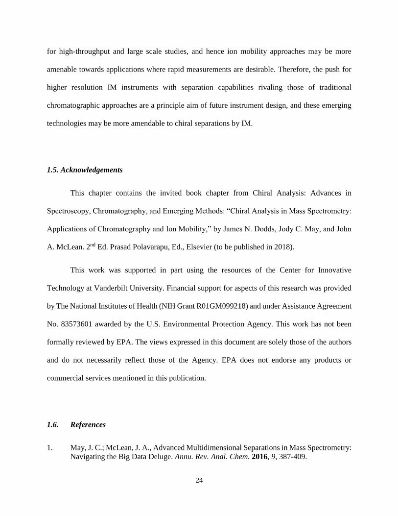
1.5. Acknowledgements
This chapter contains the invited book chapter from Chiral Analysis: Advances in
Spectroscopy, Chromatography, and Emerging Methods: “Chiral Analysis in Mass Spectrometry:
Applications of Chromatography and Ion Mobility,” by James N. Dodds, Jody C. May, and John
A. McLean. 2nd Ed. Prasad Polavarapu, Ed., Elsevier (to be published in 2018).
This work was supported in part using the resources of the Center for Innovative
Technology at Vanderbilt University. Financial support for aspects of this research was provided
by The National Institutes of Health (NIH Grant R01GM099218) and under Assistance Agreement
No. 83573601 awarded by the U.S. Environmental Protection Agency. This work has not been
formally reviewed by EPA. The views expressed in this document are solely those of the authors
and do not necessarily reflect those of the Agency. EPA does not endorse any products or
commercial services mentioned in this publication.
1.6. References
1. May, J. C.; McLean, J. A., Advanced Multidimensional Separations in Mass Spectrometry:
Navigating the Big Data Deluge. Annu. Rev. Anal. Chem. 2016, 9, 387-409.

25
2. Herniman, J. M.; Langley, G. J.; Bristow, T. W.T.; O’Conner, G., The Validation of Exact
Mass Measurements for Small Molecules using FT-ICRMS for Improved Confidence in
the Selection of Elemental Formulas. J. Mass Spectrom. 2005, 16, 1100-1108.
3. Smith, C. A.; Grace, G. O.; Want, E. J.; Qin, C.; Trauger, S. A.; Brandon, T. R.; Custodio,
D. E.; Abagyan, R.; Siuzdak, G., METLIN: A Metabolite Mass Spectral Database.
Proceedings of the 9th International Congress of Therapeutic Drug Monitoring & Clinical
Toxicology, Louisville, Kentucky, April 23-28, 2005, 27, 747-751.
4. May, J. C.; Morris, C. B.; McLean, J. A., Ion Mobility Collision Cross Section
Compendium. Anal. Chem. 2017, 89, 1032-1044.
5. Cooks, R. G., Collision-induced dissociation: Readings and commentary. J. Mass
Spectrom. 1995, 30, 1215-1221.
6. Lebedev, A. T.; Damoc, E.; Makarov, A. A.; Samgina, T. Y., Discrimination of Leucine
and Isoleucine in Peptides Sequencing with Orbitrap Fusion Mass Spectrometer. Anal.
Chem. 2014, 86, 7017-7022.
7. Simpson, D. C.; Smith, R. D., Combining capillary electrophoresis with mass spectrometry
for applications in proteomics. Electrophoresis 2005, 26, 1291-1305.
8. Santos, F. J.; Galceran, M. T., Modern developments in gas chromatography-mass
spectrometry-based environmental analysis. J. Chromatogr. A. 2003, 1000, 125-151.
9. Lee, M. S.; Kerns, E. H., LC/MS applications in drug development. Mass Spectrom. Rev.
1999, 18, 187-279.
10. Schmitz, H. H.; Artz, W. E., High-performance liquid chromatography and capillary
supercritical-fluid chromatography separation of vegetable carotenoids and carotenoid
isomers. J. Chromatogr. A. 1989. 479, 261-268.
11. Boussouar, I.; Chen, Q.; Chen, X.; Zhang, Y.; Zhang, F.; Tian, D.; White, H. S.; Li, H.,
Single Nanochannel Platform for Detecting Chiral Drugs. Anal. Chem. 2017, 89, 1110-
1116.
12. Enders, J. R.; McLean, J. A., Chiral and Structural Analysis of Biomolecules Using Mass
Spectrometry and Ion Mobility-Mass Spectrometry. Chirality. 2009, 21, 253-264.
13. Tang, M.; Zhang, J.; Zhuang, S.; Liu, W., Development of chiral stationary phases for high-
performance liquid chromatographic separation. Trac-Trend Anal. Chem. 2012, 39, 180-
194.
14. Berthod, A., Chiral Recognition in Separation Methods. Mechanisms and Applications.
2010, 1-32.

26
15. Ettre, L. S.; Sakodynskii, K. I.; M. S., Tswett and the Discovery of chromatography I: Early
work (1899-1903). Chromatographia 1993, 35, 223-231.
16. Abraham, M. H., 100 years of chromatography-or is it 171? J. Chromatogr. A 2004, 1061,
113-114.
17. Strain, H. H.; Sherma, J., Michael Tswett’s contributions to sixty years of chromatography.
J. Chem. Educ. 1967, 44, 235-237.
18. Tswett, M., Physical-chemical studies on the chlorophyll. Adsorption. Ber. Dtsch. Bot.
Ges. 1906, 24, 316.
19. Martin, A. J. P.; Synge, R. L. M., A new form of chromatography employing two liquid
phases. Biochem. J. 1941, 35, 91-121.
20. Gohlke, R. S., Time-of-Flight Mass Spectrometry and Gas-Liquid Partition
Chromatography. Anal. Chem. 1959, 31, 535-541.
21. Marshall, A. G.; Hendrickson, C. L.; Shi, S. D., Scaling MS Plateaus with High-Resolution
FT-ICRMS. Anal. Chem. 2002, 74, 252A-259A.
22. Bayer, E.; Grom, E.; Kaltenegger, B.; Uhmann, R., Separation of amino acids by high
performance liquid chromatography. Anal. Chem. 1976, 48, 1106-1109.
23. Schurig, V., Separation of enantiomers by gas chromatography. J. Chromatogr. A, 2001,
906, 275-299.
24. Juvancz, Z.; Petersson, P., Enantioselectivity gas chromatography. J. Microcolumn. Sep.
1996, 8, 99-114.
25. Hashimoto, A.; Nishikawa, T.; Oka, T.; Takahashi, K.; Hayashi, T., Determination of free
amino acid enantiomers in rat brain and serum by high-performance liquid chromatography
after derivatization with N-tert.-butyloxycarbonyl-L-cysteine and o-phthaldialdehyde. J.
Chromatogr. B 1992, 582, 41-48.
26. Gil-Av, E.; Tishbee, A.; Hare, P. E., Resolution of underivatized amino acids by reversed-
phase chromatography. J. Am. Chem. Soc. 1980, 102, 5115-5117.
27. Stalcup, A. M.; Agyei, N. M., Heparin: A Chiral Mobile-Phase Additive for Capillary Zone
Electrophoresis. Anal. Chem. 1994, 66, 3054-3059.

27
28. Guo, Z.; Wang, H.; Zhang, Y., Chiral separation of ketoprofen on an achiral C8 column by
HPLC using norvancomycin as chiral mobile phase additives. J. Pharm. Biomed. Anal.
2006, 41, 310-314.
29. E. Gil-Av, B.; Feibush, R.; Charles-Sigler, R., Separation of enantiomers by gas liquid
chromatography with an optically active stationary phase. Tetrahedron Lett. 1966, 1009.
30. Cavazzini, A.; Pasti, L.; Massi, A.; Marchetti, N.; Dondi, F., Recent applications in chiral
high performance liquid chromatography: A review. Analytica Chimica Acta 2011, 706,
205-222.
31. Yamashita, M.; Fenn, J. B., Electrospray ion source. Another variation on the free-jet
theme. J. Phys. Chem., 1984, 88, 4451-4459.
32. Dole, M.; Mack L. L.; Hines, R. L.; Mobley, R. C.; Ferguson L. D.; Alice, M. B., Molecular
Beams of Macroions. J. Chem. Phys. 1968. 49, 2240-2249.
33. Pirkle, W. H.; Pochapsky, T. C., Considerations of chiral recognition relevant to the liquid
chromatography separation of enantiomers. Chem. Rev. 1989, 89, 347-362.
34. Lämmerhofer, M., Chiral recognition by enantioselective liquid chromatography:
Mechanisms and modern chiral stationary phases. J Chromatogr. A. 2010, 1217, 814-856.
35. Pirkle, W. H.; Welch, C. J.; Lamm, B., Design, Synthesis, and Evaluation of an Improved
Enantioselective Naproxen Selector. J. Org. Chem. 1992, 57, 3854-3860.
36. Piccolo, O.; Valoti, E.; Giuseppina, V., Process for preparing naproxen. U. S. Patent
4,736,061 A, 1988.
37. Paglia, G.; Williams, J. P.; Menikarachchi, L.; Thompson, J. W.; Tyldesley-Worster, R.;
Halldórsson, S.; Rolfsson, O.; Moseley, A.; Grant, D.; Langridge, J.; Palsson, B. O.;
Astarita, G., Ion Mobility Derived Collision Cross Sections to Support Metabolomics
Applications. Anal. Chem. 2014, 86, 3985-3993.
38. Stow, S. M.; Causon, T. J.; Zheng, X.; Kurulugama, R. T.; Mairinger, T.; May, J. C.;
Rennie, E. E.; Baker, E. S.; Smith, R. D.; McLean, J. A.; Hann, S.; Fjeldsted, J. C., An
Interlaboratory Evaluation of Drift Tube Ion Mobility-Mass Spectrometry Collision Cross
Section Measurements. Anal. Chem. 2017, (submitted).
39. Mason, E. A.; McDaniel, E. W., Transport Properties of Ions in Gases; John Wiley & Sons:
New York, 1988; p. 560.
40. Siems, W. F.; Viehland, L. A.; Hill, H. H. Jr., Improved Momentum-Transfer Theory for
Ion Mobility. 1. Derivation of the Fundamental Equation. Anal. Chem. 2012, 84, 9782-
9791.
28
41. May, J. C.; Dodds, J. N.; Kurulugama, R. T.; Stafford, G. C.; Fjeldsted, J. C.; McLean, J.
A., Broadscale resolving power performance of a high precision uniform field ion mobility-
mass spectrometer. Analyst 2015, 140, 6824-6833.
42. May, J. C.; McLean, J. A., Ion Mobility-Mass Spectrometry: Time-Dispersive
Instrumentation. Anal. Chem. 2015, 87, 1422-1436.
43. Fenn, L. S.; Kliman, M.; Mahsut, A.; Zhao, S. R.; McLean, J. A., Characterizing ion
mobility-mass spectrometry conformation space for the analysis of complex biological
samples. Anal. Bioanal. Chem. 2009, 394, 235-244.
44. May, J. C.; Goodwin, C. R.; Lareau, N. M.; Leaptrot, K. L.; Morris, C. B.; Kurulugama,
R. T.; Mordehai, A.; Klein, C.; Barry, W.; Darland, E.; Overney, G.; Imatani, K.; Stafford,
G. C.; Fjeldsted, J. C.; McLean, J. A., Conformational Ordering of Biomolecules in the
Gas Phase: Nitrogen Collision Cross Sections Measured on a Prototype High Resolution
Drift Tube Ion Mobility-Mass Spectrometer. Anal. Chem. 2014, 86, 2107-2116.
45. Hofmann, J.; Hahm, H. S.; Seeberger, P. H.; Pagel, K., Identification of carbohydrate
anomers using ion mobility-mass spectrometry. Nature 2015, 526, 241-244.
46. Lalli, P. M.; Corilo, Y. E.; Fasciotti, M.; Riccio, M. F.; de Sa, G. F.; Daroda, R. J.; Souza,
G. H.; McCullagh, M.; Bartberger, M. D.; Eberlin, M. N.; Campuzano, I. D., Baseline
resolution of isomers by traveling wave ion mobility mass spectrometry: investigating the
effects of polarizable drift gases and ionic charge distribution. J. Mass Spectrom. 2013, 48,
989-997.
47. Groessl, M.; Graf, S.; Knochenmuss, R., High resolution ion mobility-mass spectrometry
for separation and identification of isomeric lipids. Analyst 2015, 140, 6904-6911.
48. Harper, B.; Neumann, E. K.; Stow, S. M.; May, J. C.; McLean, J. A.; Solouki, T.,
Determination of ion mobility collision cross sections for unresolved isomeric mixtures
during tandem mass spectrometry and chemometric deconvolution. Anal. Chim. Acta.
2016, 939, 64-72.
49. Giles, K.; Williams, J. P.; Campuzano, I., Enhancements in travelling wave ion mobility
resolution. Rapid Commun. Mass Spectrom. 2011, 11, 1559-1566.
50. Dodds, J. N.; May, J. C.; McLean, J. A., Investigation of the Complete Suite of the Leucine
and Isoleucine Isomers: Toward Prediction of Ion Mobility Separation Capabilities. Anal.
Chem. 2017, 89, 952-959.
51. Jia, C.; Lietz, C. B.; Yu, Q.; Li, L., Site-Specific Characterization of D-Amino Acid
Containing Peptide Epimers by Ion Mobility Spectrometry. Anal Chem. 2014, 86, 2972-
2981.
52. Dwivedi, P.; Wu, C.; Matz, L. M.; Clowers, B. H.; Siems, W. F.; Hill, H. H., Gas-Phase
Chiral Separations by Ion Mobility Spectrometry. Anal. Chem. 2006, 78, 8200-8206.

29
53. Silveira, J. A.; Ridgeway, M. E.; Park, M. A., High Resolution Trapped Ion Mobility
Spectrometry of Peptides. Anal. Chem. 2014, 86, 5624-5627.
54. Giles, K.; Wildgoose, J. L.; Pringle, S.; Langridge, D.; Nixon, P.; Garside, J.; Carney, P.,
Characterising a T-Wave Enabled Multi-Pass Cyclic Ion Mobility Separator. ASMS 2015.
Poster.
55. Deng, L.; Ibrahim, Y. M.; Baker, E. S.; Aly, N. A.; Hamid A. M.; Zhang, X.; Zheng, X.;
Garimella, S. V. B.; Webb, I. K.; Prost, S. A.; Sandoval, J. A.; Norheim, R. V.; Anderson,
G. A.; Tolmachev, A. V.; Smith, R. D., Ion Mobility Separations of Isomers based upon
Long Path Length Structures for Lossless Ion Manipulations Combined with Mass
Spectrometry. ChemistrySelect. 2016, 1, 2396-2399.
56. Groessl, M.; Graf, S., Separation of isomers in lipidomics and metabolomics experiments
by high resolution ion mobility spectrometry-mass spectrometry (IMS-MS). ASMS 2016.
Poster.
57. Lareau, N. M.; May, J. C.; McLean, J. A., Non-derivatized glycan analysis by reverse phase
liquid chromatography and ion mobility-mass spectrometry. Analyst, 2015, 140, 3335-
3338.
58. Griffiths, J. A brief history of mass spectrometry. Anal. Chem. 2008, 80, 5678-5683.

30
CHAPTER 2
ISOMERIC AND CONFORMATIONAL ANALYSIS OF SMALL DRUG AND DRUG-LIKE
MOLECULES BY ION MOBILITY-MASS SPECTROMETRY (IM-MS)
2.1. Introduction
The process of developing new drug candidates has changed significantly over time, as a
result of the Human Genome Project and other technological advances in computational modeling
and bioformatics.1 For example, high-throughput screening methods provide unparalleled capacity
to screen millions of chemical structures for potential drug efficacy,2,3 as opposed to simply
developing a target candidate and anticipating relevant biochemical action. Regardless of the
desired approach towards production of novel drug candidate molecules by either reverse
pharmacology, the classical approach, or natural product discovery,4,5,6 most drugs take several
years to develop and millions of dollars to become marketable as a requirement of validation
through in-depth clinical trials, evaluation of safety risks and FDA approval.7 As part of this
development process, the analytical need to study the structural characteristics of these small
molecules is imperative.
Structural characterization of potential drug candidates, either derived from natural sources
or synthesized in the laboratory, is a complex and time consuming process, and for rapid analyses,
pharmaceutical companies value the high degree of analytical selectivity and sensitivity afforded
by modern mass spectrometry (MS) methods towards overall quality control of synthesized
products and characterization of new drug targets.8,9 Although mass spectrometers are highly
selective, often able to assign a molecular formula for a target analyte based solely on molecular
mass measurement, isomeric species are difficult to differentiate by traditional MS methods, even

31
with the addition of tandem MS/MS approaches.10,11 Because the biological function of chemical
compounds can change with their structural variation, isomeric species are a highly researched
area of the pharmaceutical field.12 Condensed phase separation techniques such as gas or liquid
chromatography are often utilized to separate complex mixtures prior to mass analysis and provide
the ability to separate isomers by differences in chemical properties, such as polarity or boiling
point. These methods, while effective, are often highly selective to narrow classes of isomers and
are not inherently high-throughput techniques. In this chapter, we describe the application of IM-
MS, an emerging analytical technique for structurally characterizing small molecule isomer
systems, with a particular focus on the role of IM-MS in characterizing biological systems and
relevant pharmaceutical applications.
2.1.1. Isomers
Isomers are defined as compounds having the same molecular formula, but differing in
their overall chemical structure.13 Isomeric species are further sub-divided into categories that
reflect their structural variations, which may include covalent bond rearrangements (constitutional
isomers), stereochemical variations (stereoisomers), or rotational isomers, commonly referred to
as rotamers. As constitutional isomers vary in skeletal structure between constituent atoms, these
isomers possess a broad scope of biological activity based upon their particular structural
arrangements. For example, the molecular formula C8H9NO2 is reported to have 33 isomers by the
PubChem database,14 and many of these isomers have unique chemical behavior and physiological
function (Figure 2.1). In one case, paracetamol (more commonly known as acetaminophen) is a
well-known analgesic, yet its constitutional isomer, methyl anthranilate functions as a bird
repellent and a flavor additive in drinks.15 The structural makeup of constitutional isomers can also

32
Figure 2.1. Structures related to four constitutional isomers of chemical formula C8H9NO2 and
corresponding function or typical use.
Acetaminophen(analgesic)
3-Methyoxybenzamide(polymerase inhibitor)
Methyl Anthranilate(flavoring agent)
4-Ethylnitrobenzene(chemical sensor)

33
vary widely depending on their biological class. For example, lipid isomers typically vary in alkyl
chain position and cis/trans double bond positioning,16 while peptides tend to have sequence order
variation or even amino acid substitutions comprised of the same chemical formula (e.g.
leucine/isoleucine).17
In addition to constitutional isomers, compounds with the same molecular formula can
differ in stereochemistry, (i.e. diastereomers and enantiomers) resulting in varying chemical and
physical properties. For example, ethambutol is a 204 Da molecule (C10H24N2O2) possessing two
stereocenters. In the (+) form (S,S) ethambutol is frequently used to treat tuberculosis.18 However,
with inversion of chirality at its two stereocenters to form (-) or (R,R) ethambutol, the molecule is
known to cause blindness.19 Isomers also exist for two compounds possessing the same chemical
scaffold and chirality. For example, rotamers are small molecule conformers where multiple three-
dimensional molecular structures can arise as a result of rotation around a single bond. In some
cases this bond rotation gives rise to atropisomerism, which is the restriction of rotation around a
single covalent bond which results in distinct optical isomers. A commonly cited rotamer example
which exhibits freedom of rotation around a single bond are the Newman projections of butane.20
In other cases where rotation is not restricted, different stable conformations are still possible,
especially in protein analysis. Small molecules in particular are noted for producing a variety of
conformations as a result of their flexibility.21 Because of the diverse chemical activity that can
exist within constitutional and conformational isomers, finding useful and efficient ways to explore
the structure of these molecules can provide insight into their specific chemical properties.
For the past 15 years IM-MS has made large contributions in the analysis of constitutional
and conformational isomers.22,23,52 As result of the commercialization and rapid adoption of IM-
MS instrumentation,24,33,37 the Web of Science database cites over 3,500 articles in the last decade
34
related to IM-MS studies.25 While ion mobility has been traditionally utilized to study large
biological systems, more recently it has been applied to the study of smaller (< 400 Daltons) drug
and drug-like molecules.26,27 In this chapter, we describe the technique and theory of IM-MS,
provide examples of the use of IM-MS to characterize various small drug and drug-like molecules,
and provide some basic methodology towards collecting and analyzing IM-MS data using a
commercially available IM-MS platform (Agilent 6560) as an example.37
2.2. Instrumentation and Theory
IM-MS is an emerging analytical technique that separates gas phase ions into two
dimensions based upon molecular size and weight. In the mobility dimension, analyte ions are
separated based upon their two-dimensional orientationally-averaged size in the gas phase
(collision cross section, CCS), which provides information regarding their size and shape.28,33 In
the mass spectrometer dimension, separation is based upon the mass to charge ratio (m/z) of the
analyte ion, which is directly correlated to its intrinsic molecular formula. Combined, IM-MS
provides unique and important information regarding the gas-phase density preferences of
different classes of molecules, which can identify unknown compounds which share similar
structural scaffolds.36,47
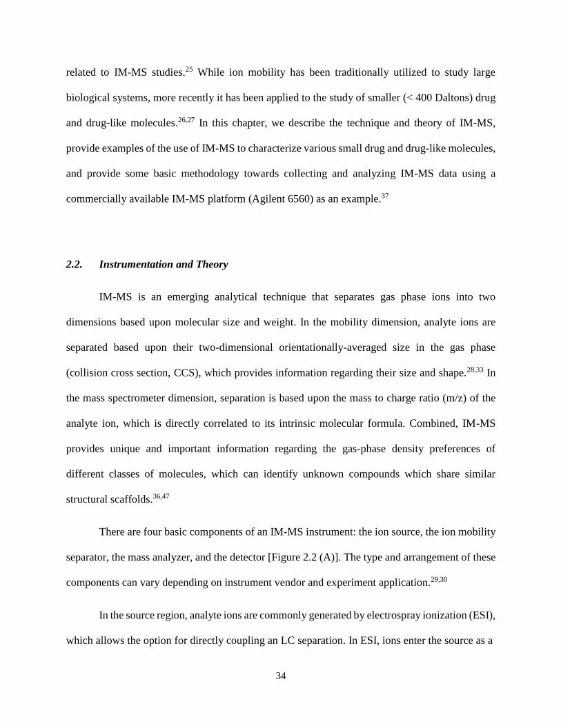
There are four basic components of an IM-MS instrument: the ion source, the ion mobility
separator, the mass analyzer, and the detector [Figure 2.2 (A)]. The type and arrangement of these
components can vary depending on instrument vendor and experiment application.29,30
In the source region, analyte ions are commonly generated by electrospray ionization (ESI),
which allows the option for directly coupling an LC separation. In ESI, ions enter the source as a

35
Figure 2.2. (A) Block diagram of a typical IM-MS instrument. Ions are separated in the presence
of a neutral drift gas by (B) a declining electric field along a series of ring electrodes (DTIMS), or
(C) by a pulse wave generated by applied sequential voltage along a series of ring electrodes
(TWIMS).
(B) (C)V
olt
age
Vo
ltag
e
Distance Distance
Drift Tube IMS Traveling Wave IMS
++ ++
Mass Spectrometer
Ion ActivationRegion
(A)
Ion MobilityIonization
SourceSample
Introduction

36
liquid and are vaporized using a combination of gas flows and electric fields, which ultimately
generate gas-phase ions. While ESI is the most commonly used ion source, other ion source types
include laser and chemical ionization (e.g. MALDI and APCI).31 ESI commonly produces
protonated and deprotonated ions ([M+H]+, [M-H]-), as well as various alkali metal cation species,
such as [M+Na]+ and [M+K]+, where M represents the neutral form of the molecule. Once ions
are generated, they are released into the ion mobility spectrometer where they are separated based
on their gas-phase size and shape (CCS). Following the mobility separation, ions enter the mass
analyzer where they are separated by their mass-to-charge ratio (m/z). For more in-depth
information regarding the experiment, we refer the reader to a recent literature review which covers
the various IM techniques and instrumentation in detail.32,33
Ion mobility techniques can be broadly separated into two method types: time dispersive
methods, which include drift tube and traveling wave ion mobility spectrometry (DTIMS and
TWIMS, respectively), and space dispersive methods, which primarily include high field-
asymmetric waveform IM and differential ion mobility spectrometry (FAIMS and DMS,
respectively) which collectively operate as mobility filtering devices. The examples presented in
this chapter will focus on recent applications of the time dispersive methods of DTIMS and
TWIMS, which collectively represent the majority of IM instrumentation currently utilized.33
2.2.1. Drift Tube Ion Mobility
In drift tube ion mobility (DTIMS), the IM region consists of a series of ring electrodes
contained within a neutral drift gas (typically helium or nitrogen) [Fig. 2.2 (B)].34,35 DTIMS is
operated at one of two pressure regimes: low (1-10 Torr) and elevated (ca. 760 Torr) pressures.

37
Typically, ion transmission is more efficient at reduced pressure, yet typically results in somewhat
reduced IM resolving power from high diffusion. As ions are introduced into the drift tube, they
are drawn through the drift region as a result of an applied electric field along the ring electrodes.
During ion drift, the ions interact with the buffer gas at low energy and molecules with smaller
rotationally averaged surface area (smaller CCS), transverse the region faster as a result of fewer
collisions. Mathematically, the CCS of the analyte ion can be calculated using the Mason-Schamp
equation36,37 where K0 is the measured mobility of the ion, z is the charge of the ion, T is the
temperature of the drift gas, and N0 is the number density of the drift gas at standard temperature
and pressure. The terms e and kB are the elementary charge and Boltzmann’s constant,
respectively.
CCS =3𝑧𝑒
16𝑁𝑜(
2𝜋
𝜇𝑘𝐵𝑇)
12⁄ 1
𝐾0 (1)
2.2.2. Traveling Wave Ion Mobility
Similar to DTIMS, a traveling wave ion mobility drift cell uses an inert buffer gas and a
series of ring electrodes to move ions through the drift region, but typically the electrodes have
smaller inner diameters than what is used in DTIMS to facilitate better axial ion focusing [Figure
2.2 (C)].38,39 In TWIMS, ion pulses are mobility separated by sequentially applying a direct current
voltage to the rings in a series along the drift cell to create a migrating potential along the length
of the cell. These sequential low voltage pulses generate waves of electric potential that push ions
through the drift region. As the wave propels the ions forward through the device, low energy
elastic collisions occur between the analyte ions and the buffer gas. Smaller ions experience fewer
collisions with the buffer gas, and as a result, traverse the drift region faster than larger ions,

38
resulting in shorter drift times. This mechanism is almost identical to what is experienced in
DTIMS, but with the exception that larger ions are slower in TWIMS as a result of “falling over”
the wave pulses during their transit through the cell. The drift times are converted to collision cross
sections through a calibration procedure which takes into account the drift times and CCS of
known internal standards.40,41 The ion mobility spectra obtained from both TWIMS and DTIMS
are qualitatively similar.
2.3. Current Work in Isomer Structural Separations
Historically, there have been several reported studies where DTIMS and TWIMS have
been used to observe both constitutional and conformational structures of large molecules, where
structural differences are significant and readily measured.42,43,44 In this section, we will present
some recent examples of the use of TWIMS and DTIMS to separate constitutional and
conformational isomers in small molecule systems, which have been given less attention in the
literature, but nonetheless are important avenues for developing IM-MS for the separation and
characterization of drug and drug-like small molecule isomer systems.
2.3.1. Separation of Constitutional Isomers
Often chromatography resolution can be difficult to achieve for molecules with similar
polarities, and hence constitutional isomers have been studied in detail by IM-MS. In an effort to
differentiate molecules of interest from complex matrices (e.g. biological samples and natural
product extracts), mobility techniques have investigated the separation of a wide variety of
chemical classes including lipids, carbohydrates,45,46 peptides47,48 and fossil fuels.49 As a specific

39
example, we will consider the highly studied isomer system of leucine and isoleucine, which
represent a classically studied isomer pair from an analytical separation perspective, as both
compounds have the same chemical formula (C6H13NO2) and hence cannot be distinguished by
MS measurements alone. From an ion mobility perspective, leucine and isoleucine have been
shown to be differentiable using several ion mobility techniques, including FAIMS50 and
TWIMS.51 In a recent study by Dodds et al., 11 different leucine/isoleucine isomers were studied
using DTIMS and focused on the positive ion forms of these molecules, [M+H]+.52 The sub-classes
of isomers investigated in this study include enantiomers (two molecules whose stereochemistry
is opposite at every chiral center), diastereomers (two molecules with multiple chiral centers of
which some, but not all, have opposite stereocenters), and constitutional isomers related to leucine
and isoleucine. A plot of the range of diversity in CCS for these compounds appears in Figure 2.3.
As illustrated in the figure, the differences in the CCS vary depending on isomer type. For example,
the enantiomers (e.g. L-leucine and D-leucine) show no statistical difference their measured
collision cross sections, and similarly, diastereomers (e.g. L-isoleucine and L-allo-isoleucine)
exhibit different CCS values, but are still very challenging to differentiate (typically 0.4%
difference in CCS). However, as the molecules become more structurally diverse, the isomers
possess more significant differences in cross section. Specifically, 3 constitutional isomers (N-N-
dimethylglycine ethyl ester, L-tert-leucine, and L-norleucine) are structurally distinct enough to
yield baseline or near-baseline separation and possess 3.6% and 3.1% difference in their respective
empirical cross sections.
In addition to illustrating the separation of various constitutional isomers, the authors
proposed a mathematical relationship correlating the percent difference in cross section of any two
isomers of interest with respect to instrumental resolving power (Rp). Briefly, the efficiency of ion

40
Figure 2.3. (A) Leucine/isoleucine isomers with chemical formula C6H13NO2 examined in this
study. Experimental cross sections with respective standard deviations are shown at the right with
corresponding stereochemistry. (B) (I) Experimental IM spectra overlays for all isomer
compounds (standard error bars omitted for clarity). (II) Overlay of the IM spectra corresponding
to N,N-dimethylglycine ethyl ester, L-tert-leucine, and L-norleucine and the IM spectrum
corresponding to the mixture (black). (III) Overlays of L-isoleucine and L-leucine in addition to
the equal ratio mixture. (IV and V) Overlays of diastereomers and enantiomers, respectively.
Adapted with permission from Ref. 52, Copyright 2017 American Chemical Society.
L-Norleucine
D-Leucine (2R)
L-Leucine (2S)
L-Isoleucine (2S,3S)
L-allo-Isoleucine (2S,3R)
L-tert-Leucine (2S)
D-tert-Leucine (2R)
D-allo-Isoleucine (2R,3S)
6-Aminocaproic acid
N,N-Dimethylglycine ethyl ester
D-Isoleucine (2R,3R)
127.5 0.3 (Å2)
129.3 0.2 (Å2)
132.4 0.3 (Å2)
132.5 0.2 (Å2)
132.9 0.2 (Å2)
133.1 0.3 (Å2)
133.5 0.3 (Å2)
133.3 0.3 (Å2)
135.1 0.3 (Å2)
135.2 0.3 (Å2)
136.6 0.3 (Å2)
0
50
100
120 125 130 135 140 145
Re
lati
ve
Ab
un
da
nc
e (
%) 0
50
100
120 125 130 135 140 145
0
50
100
120 125 130 135 140 145
Collision Cross Section (Å2)
0
50
100
120 125 130 135 140 145
0
50
100
120 125 130 135 140 145
Constitutional
Isomers
L-Isoleucine
L-Leucine
L-allo-Isoleucine
L-Isoleucine
(A) (B)
(I)
(II)
(III)
(IV)
(V)
Constitutional
Isomers
Diastereomers
Enantiomers
(1)
(2)
(3)
(4)
(5)
(6)
(7)
(8)
(9)
(10)
(11)
(1) (2)
(3)(4)
(5)(6)(7) (8) (9) (10)
(11)
(1) (3) (11)
L-Isoleucine
D-Isoleucine
(7) (9)
(5) (7)
(7) (8)
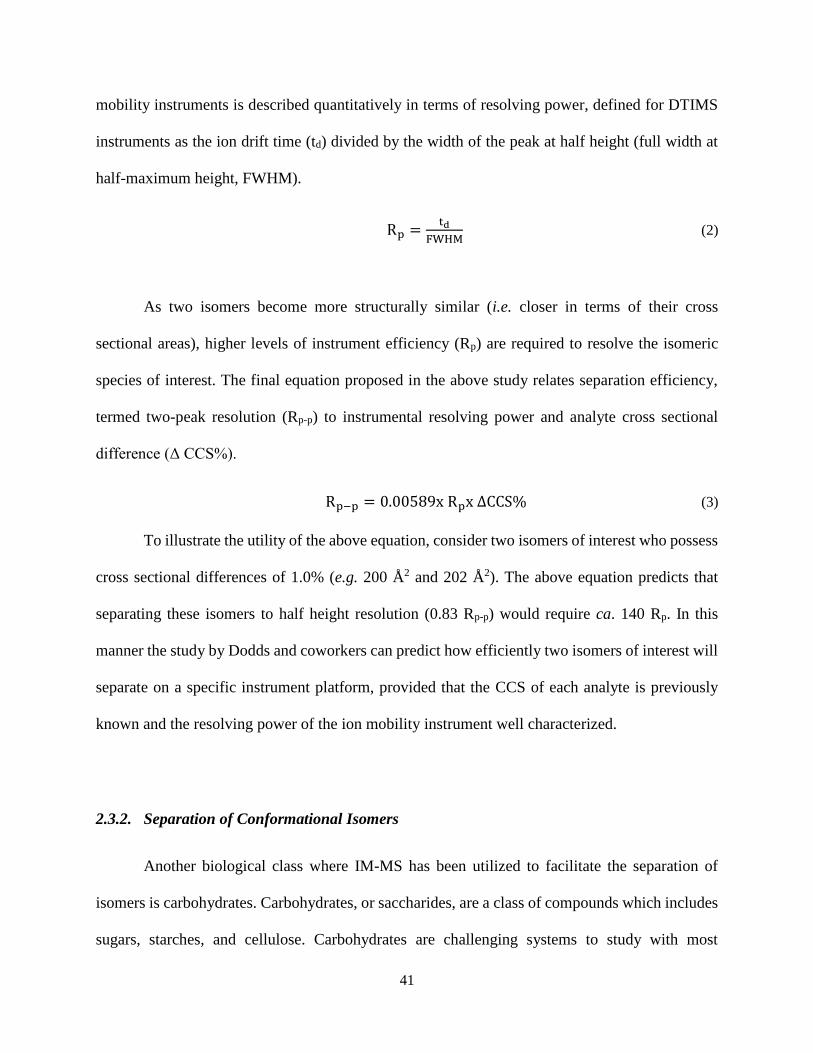
41
mobility instruments is described quantitatively in terms of resolving power, defined for DTIMS
instruments as the ion drift time (td) divided by the width of the peak at half height (full width at
half-maximum height, FWHM).
Rp =td
FWHM (2)
As two isomers become more structurally similar (i.e. closer in terms of their cross
sectional areas), higher levels of instrument efficiency (Rp) are required to resolve the isomeric
species of interest. The final equation proposed in the above study relates separation efficiency,
termed two-peak resolution (Rp-p) to instrumental resolving power and analyte cross sectional
difference (Δ CCS%).
Rp−p = 0.00589x Rpx ΔCCS% (3)
To illustrate the utility of the above equation, consider two isomers of interest who possess
cross sectional differences of 1.0% (e.g. 200 Å2 and 202 Å2). The above equation predicts that
separating these isomers to half height resolution (0.83 Rp-p) would require ca. 140 Rp. In this
manner the study by Dodds and coworkers can predict how efficiently two isomers of interest will
separate on a specific instrument platform, provided that the CCS of each analyte is previously
known and the resolving power of the ion mobility instrument well characterized.
2.3.2. Separation of Conformational Isomers
Another biological class where IM-MS has been utilized to facilitate the separation of
isomers is carbohydrates. Carbohydrates, or saccharides, are a class of compounds which includes
sugars, starches, and cellulose. Carbohydrates are challenging systems to study with most

42
analytical techniques as they commonly exist as complex mixtures in nature with variations in
skeletal structure, bond coordination, and stereochemistry (Figure 2.4). Studies are further
complicated because many of the compounds in these mixtures have the same molecular formula
(isomers) which again prevents them from being fully characterized using traditional mass
spectrometry methods. This makes ion mobility a particularly intriguing tool to explore
carbohydrate systems.
A recent example of the utility of IM to study carbohydrates was carried out by Li and
coworkers.53 In their study of sugars, TWIMS was used to measure drift time profiles for ions of
monosaccharide-glycolaldehydes and disaccharides of various simple sugars. While this work is
another example of the ability of ion mobility to separate constitutional isomers, there were
occasions where the presence of multiple conformations appeared, even for what was believed to
be a single analyte ion. For example, the monosaccharide glycolaldehyde β-D-glucopyranosyl-2-
glycolaldehyde (β-D-glc-GA) was analyzed in negative mode ESI and produced a drift time profile
that generates two distinct peaks for the deprotonated ion. The authors propose that the appearance
of these multiple conformations may be attributed to several cyclic/acyclic forms produced by
hemiacetal formation in the gas phase. While most conformers are typically noted for large
bimolecular species (i.e. proteins), these small molecule analytes produced multiple distributions
(peaks) for one ion form. Thus this work illustrated the possibility to observe conformers even in
a relatively small molecule system.
The appearance of conformational isomers for small drug-like molecules has also become
evident in studies related to thalidomide in the authors’ laboratory. Thalidomide is a small
molecule drug that is currently used primarily for the treatment of specific cancers and for
alleviating various symptoms of leprosy. However, historically thalidomide is recognized as one
43
Figure 2.4. Complexity of carbohydrate isomers represented graphically pertaining to both
constitutional isomers (connectivity isomers) and stereoisomers (axial/equatorial substitutions,
chair/boat conformations, and α/β glycosidic linkage orientation).
Axial / Equatorial –OH groups
Chair / Boat Conformation
Connectivity (e.g. 1-3/1-4)
α / β
β-D-Glucose-GA
Carbohydrate Isomers
Chair Conformation
Boat Conformation

44
of the first drugs whose different enantiomer forms produced drastically different biological
effects. Figure 5 illustrates the structures and drift time profiles for the [M+H]+ and [M+H]- ions
of (S,-)-thalidomide and (R,+)-thalidomide along with corresponding CCS. The drift time profiles
of both positive and negative mode ions for both enantiomers are identical. This result is expected
as stereochemical differences in small molecules are not expected to result in different drift time
distributions. However, multiple peaks were detected for both enantiomers of thalidomide in each
ionization mode. Structurally, this observation is reasoned as being a consequence of the
possibility for multiple molecular conformations arising from rotation around the single N-C bond
that links the two ring moieties.
The development of methods for characterizing small drug and drug-like molecules has
become an important focal point for the pharmaceutical industry. As a result there has been a
concentrated effort towards discovering new technologies to aide in the development of new drugs.
The examples presented in this work provide strong support for the use of IM-MS as an important
analytical technology in exploring the structural diversity of constitutional and conformational
isomers of small drug and drug-like molecules. In the following sections, we provide the materials
and methods necessary to obtain an IM-MS spectra for small molecules (here S-thalidomide, 258
Da) using a commercially available IM-MS platform (Agilent IM-MS 6550).
2.4. Materials
a) The sample preparation described here is for use with direct infusion via a syringe pump
operated at low flow rates (i.e. 5-100 µL/min). As with any analytical study, it is beneficial to have
analyte samples and solvents with optimal purity for analysis. In this study, S-thalidomide was

45
Figure 2.5. Drift time profiles of (R) and (S) thalidomide enantiomers with corresponding CCS
observed in both positive and negative mode (A and B, respectively) for nitrogen drift gas.
Structures are illustrated at the bottom for chiral reference.
(+) Thalidomide (-) Thalidomide
0
20
40
60
80
100
19 20 21 22 23
Re
lati
ve I
nte
nsit
y
Drift Time (ms)Drift Time (ms)
20
(I) 152.5 Å2
(III) 162.3 Å2
(II) 157.8 Å2
(IV) 169.0 Å2
(A)
(S, -) Thalidomide
[birth defects]
(R, +) Thalidomide
[morning sickness]
0
20
40
60
80
100
21 22 23 24 25 26 27
Re
lati
ve I
nte
nsit
y
Drift Time (ms)
(+) Thalidomide (-) Thalidomide
(B)Positive Mode (M+H) Negative Mode (M-H)
23
Drift Time (ms)
(VI) 159.8 Å2
(V) 153.5 Å2

46
purchased from Sigma-Aldrich and the solvent (Optima LC-MS grade Water) was obtained from
Fisher Scientific. A range of analyte concentration can be used and should be selected based upon
instrument sensitivity and limits of detection. Standard protocol for this instrument using direct
infusion recommends an analyte concentration of 1-10 μg/mL. For the experiment described here,
a 10 μg/mL sample of S-thalidomide was prepared using 10 mM ammonium acetate in water.
b) The instrument must be tuned prior to data collection in order to perform at optimal
sensitivity, resolution, and accuracy. Towards this end a commercially-available tune mix solution
containing several standards over a range of masses and mobilities was used (Agilent Tune Mix,
part number G1969-85000). Specifics of the tuning method are described in the methods section.
c) Direct infusion was carried out using a 500 µL glass syringe and a kD Scientific syringe
pump. Flow rates were as described in the methods section to follow.
d) Collection of IM-MS data was obtained using Agilent Mass Hunter Acquisition
Software (v.7.00). Data workup of IM-MS distributions was performed using Agilent IM-MS
Browser Software (v. 7.02)
2.5. Methods
The method described below is for new users to the Agilent 6560 IM-MS instrument who
have general knowledge of traditional mass spectrometry operation. It is intended to provide the
novice user with the basic steps necessary to obtain a routine IM-MS spectra. It is not intended to
provide an exhaustive description of all instrument settings and their uses. The reader should
consult their service manual for extended instructions and a comprehensive description of settings.
47
2.5.1. Preparing the Instrument
a) To ensure drift time and collision cross section reproducibility, check instrument
pressures in each of the following instrument compartments: the high pressure funnel region
should be set to 4.80 Torr (+/- 0.02), trap funnel region pressure at 3.80 Torr (+/- 0.01), and drift
tube pressure should be maintained at 3.95 Torr (+/- 0.01). A pressure regulation manifold
(alternate gas kit, Agilent) is recommended here in order to automatically maintain these pressure
settings. Alternatively, the user may choose to monitor and make manual adjustments to the drift
tube pressure in order to maintain the precision of the IM measurements.
b) Open the Agilent Mass Hunter Workstation Data Acquisition Program. Under the
“Context” menu (Figure 6A), choose the “Tune” setting to perform an autotune. The source
temperatures and voltages will be preset for the Agilent Tune Mixture (Figure B.1), and the ion
polarity and scan mode will be selected as a function of the molecules of interest per individual
experiment (low mass mode (50-250 m/z), normal mode (50-1700 m/z), or high mass range (100-
3200 m/z). In this case we are investigating thalidomide (258 Da), and have selected the normal
instrument tuning mode (50-1700 m/z).
c) Select the “Tune and Calibration” tab [Figure B.1 (C)]. Select desired ionization mode
(positive mode is used here), TOF (time of flight), mass calibration/check, and the corresponding
mass range depending on the analyte to be studied. Once settings have been chosen, click “Apply”
to apply these settings prior to tuning [(Figure B.1 (D)].
d) Ensure that the calibrant line contains adequate calibrant solution and is plumbed into
the primary nebulizer before starting the autotune. It is recommended that at minimum, a quarter
of the calibration bottle volume (ca. 30 mL) be filled with calibration solution prior to tuning. Turn

48
on the tune mix by right clicking in the Q-TOF selection box [Figure B.1 (E)] and selecting
calibrant.
e) When the tune mix ions appear in the spectra window (e.g., m/z 322, 622, and 922 in
positive ion mode), click on the “Start TOF Mass calibration” button [Figure B.1 (F)].
f) Upon tune completion, a calibration report will be generated as a portable document file
(.pdf) file. From this report, ensure that signal intensity is greater than 1 x 10⁵ ion counts and that
the ion mobility resolution is between 40-60. If not, the user may wish to repeat the autotune
procedure. After tuning, click the “Instrument State” tab [Figure B.1 (G)], and then click “Save”
and “Apply”.
g) Once the instrument is tuned in the desired ion mode, switch to the acquisition mode
under the context menu [Figure B.1 (A)] to start collecting data.
2.5.2. Data Acquisition (consult Figure 7)
a) Load the pre-existing low mass method in the drag-down box in method editor and click
“Apply” [(Figure B.2 (A)]. If the user is interested in collecting collision cross sections, the method
should include a voltage gradient in the drift tube region in order subtract out the non-mobility
flight time. This voltage gradient can be accessed under the “Advanced Parameters” tab of the
method editor screen, [Figure B.2 (B)]. For a detailed explanation of the voltage gradient method
we refer the reader to Ref. 36 and its Supporting Information to describe the non-mobility
component of the drift time, and subsequent conversion to CCS.

49
b) Load the sample in the syringe and syringe pump for direct infusion. Ensure that the
syringe pump is set with the correct syringe diameter in order to output the correct flow rates.
Although flow rate will vary based on specific instrument source settings and sensitivity, the flow
rate used here is 1-10 µL/min. Turn on the syringe pump. Once sample reaches the instrument,
analyte ion peaks begin to appear in the mass window.
c) NOTE: If minimizing sample consumption is important, the user may wish to conduct
step 4 prior to turning on the syringe pump.
d) To setup the data acquisition, select the “Sample Run” tab at the bottom of the method
editor screen [Figure B.2 (C)]. In the sample run mode, name the file [Figure B.2 (D)] and select
the path directory [Figure B.2 (E)] for your file.
e) To acquire data, click the forward arrow [Figure B.2 (F)] in the sample run screen.
2.5.3. Data Workup
a) After data acquisition is complete, load the “Agilent Mass Hunter IM-MS Browser”
software and open the desired file. OPTIONAL: Once the file has opened, select “Condense File”
under the “Actions” tab [Figure B.3 (A)]. Condensing files will compress the data from each
experimental sequence into a single frame, which is convenient for viewing multiple segment runs
(e.g., CCS experiments) or long infusion experiments.
b) In IM-MS Browser, you can view the resulting mass spectrum [Figure B.3 (B)], drift
spectra data [Figrue B.3 (C)] and the 2-D plot of mass-to-charge vs drift time [Figure B.3 (D)] for

50
all ions in the sample. In the example spectrum of thalidomide [Figure B.3 (E)], we will focus on
the mass-to-charge ion at 259.0708, [M+H]+.
c) Expand the Counts vs. Mass-To-Charge window by right clicking and holding on the
mass axis and dragging over the desired mass range. (To expand or contract any axis right click
hold any axis and move the mouse right or left.) To move the peak right or left, left click and hold
the axis and drag accordingly [Figure B.3 (B)].
d) To obtain a drift time spectrum for a specific mass-to-charge region, right click and drag
over the desired ion in the drift time vs m/z region. This produces a box around the desired ion
[Figure B.3 (F)]. Command “Ctrl X” copies the selected region and “Ctrl D” pastes the spectra in
the user drift spectra window [Figure B.3 (G)].
e) This work flow was repeated for each thalidomide enantiomer in both positive and
negative ion mode and a processed version is illustrated in the main text as Figure 2.5.
2.6. Acknowledgements
This chapter contains the invited book chapter in Bioinformatics and Drug Delivery:
Methods and Protocols, 3rd Ed. in the Methods in Molecular Biology Series: “Isomeric and
Conformational Analysis of Small Drug and Drug-Like Molecules by Ion Mobility-Mass
Spectrometry (IM-MS),” by Shawn T. Phillips, James N. Dodds, Jody C. May, and John A.
McLean. Richard S. Larson and Tudor Oprea, Eds. Springer (to be published in 2018).
Financial support for aspects of this research was provided by The National Institutes of
Health (NIH Grant R01GM099218) and under Assistance Agreement No. 83573601 awarded by

51
the U. S. Environmental Protection Agency. This work has not been formally reviewed by EPA.
The views expressed in this document are solely those of the authors and do not necessarily reflect
those of the Agency. EPA does not endorse any products or commercial services mentioned in this
publication. Furthermore, the content is solely the responsibility of the authors and does not
necessarily represent the official views of the funding agencies and organizations. The authors also
thank the VU Center for Innovative Technology for support and assistance.
2.7. References
1. Chail, H., DNA sequencing technologies key to the Human Genome Project. Nature
Education 2008, 1, 219.
2. Shekhar, P. C.; Smoczynski, R.; Tretyn, A., Sequencing technologies and genome
sequencing. J. Appl. Genet. 2011, 52, 413-435.
3. Zhang, J. H.; Chung, T. D.; Oldenburg K. R., A simple statistical parameter for use in
evaluation and validation of high throughput screening assays. J. Biomol. Screen 1999, 4,
67-73.
4. Takenaka, T., Classical vs reverse pharmacology in drug discovery. BJU Int. 2001, 88, 7-
10.
5. Harvey, A. L.; Edrada-Ebel, R.; Quinn, R. J., The re-emergence of natural products for
drug discovery in the genomics era. Nat. Rev. Drug Discov. 2015, 14, 111-129.
6. Vaidya, A. D. B., Reverse pharmacology-A paradigm shift for drug discovery and
development. Current Research in Drug Discovery 2014, 1, 39-44.
7. Roses, A. D., Pharmacogenetics in drug discovery and development: a translational
perspective. Nat. Rev. Drug Discov. 2008, 7, 807-817.
8. Nageswara Rao, R.; Talluri, M. V., An overview of recent applications of inductively
coupled plasma-mass spectrometry (ICP-MS) in determination of inorganic impurities in
drugs and pharmaceuticals. J. Pharm. Biomed. Anal. 2007, 43, 1-13.
9. Kauppila, T. J.; Wiseman, J. M.; Ketola, R. A.; Kotiaho, T.; Cooks, R. G.; Kostiainen, R.,
Desorption electrospray ionization mass spectrometry for the analysis of pharmaceuticals
and metabolites. Rapid Commun. Mass Spectrom. 2006, 20, 387-392.
52
10. Cooks, R. G., Special feature: Historical. Collision-induced dissociation: readings and
commentary. J. Mass Spectrom. 1995, 30, 1215-1221.
11. Wells, J. M.; McLuckey, S. A., Collision-induced dissociation (CID) of peptides and
proteins. Methods Enzymol. 2005, 402, 148-185.
12. Nguyen, L. A.; He, H.; Pham-Huy, C. Chiral drugs: An overview. Int. J. Biomed Sci. 2006,
2, 85-100.
13. McMurry, J. Organic Chemistry. 2008 7th ed. Belmont, CA.
14. NCBI.NLM.NIH.Gov. Search terms “C8H9NO2.” Accessed 18 Apr 2017
15. Ferreres, F.; Giner, J. M.; Tomás-Barberán, F. A., A comparative study of hesperetin and
methyl anthranilate as markers of the floral origin of citrus honey. J. Sci. Food Agric. 1994,
65, 371-372.
16. Groessl, M.; Graf, S.; Knochenmuss, R., High resolution ion mobility-mass spectrometry
for separation and identification of isomeric lipids. Analyst 2015, 140, 6904-6911.
17. Xiao, Y.; Vecchi, M. M.; Wen, D., Distinguishing between leucine and isoleucine by
integrated LC-MS analysis using Orbitrap Fusion mass spectrometer. Anal. Chem. 2016,
88, 10757-10766.
18. Takayama, K.; Kilburn, J. O., Inhibition of synthesis of arabinogalactan by ethambutol in
mycobacterium smegmatis. Antimicrob. Agents Chemother. 1989, 33, 1493-1499.
19. Chatterjee, V. K.; Buchanan, D. R.; Friedmann, A. I.; Green, M., Ocular toxicity following
ethambutol in standard dosage. Br. J. Dis. Chest. 1986, 80, 288-291.
20. Carey, R., Organic Chemistry. 1996, 3rd ed. McGraw Hill, New York, 89-92.
21. Kothiwale, S.; Mendenhall, J. L.; Meiler, J., BCL::CONF: small molecule conformational
sampling using a knowledge based rotamer library. J. Cheminform. 2015, 7:47.
22. Paglia, G., Williams, J. P.; Menikarachchi, L.; Thompson, J. W.; Tyldesley-Worster, R.;
Halldórsson, S.; Rolfsson, O.; Moseley, A.; Grant, D.; Langridge, J.; Palsson, B. O.,
Astarita, G., Ion mobility derived collision cross sections to support metabolomics
applications. Anal. Chem. 2014, 86, 3985-3993.
23. Enders, J. R.; McLean, J. A., Chiral and Structural Analysis of Biomolecules Using Mass
Spectrometry and Ion Mobility –Mass Spectrometry. Chirality 2009, 21, 253-264.
24. Pringle, S. D.; Giles, K.; Wildgoose, J. L.; Williams, J. P.; Slade, S. E.; Thalassinos, K.;
Bateman, R. H.; Bowers, M. T.; Scrivens, J. H., An investigation of the mobility separation

53
of some peptide and protein ions using a new hybrid quadrupole/travelling wave IMS/oa-
TOF instrument. Int. J. Mass Spectrom. 2007, 261, 1-12.
25. Web of Science. Thomson Reuters. Search terms “Ion Mobility” AND “Mass
Spectrometry.” Articles from 2002-2017. Accessed 15 May, 2017
26. Paglia, G.; Astarita, G., Metabolomics and lipidomics using traveling-wave ion mobility
mass spectrometry. Nat. Protoc. 2017, 12, 797-813.
27. Stow, S. M.; Lareau, N. M.; Hines, K. M.; McNees, C. R.; Goodwin, C. R.; Bachmann,
B. O.; McLean, J. A., in “Natural Products Analysis: instrumentation, methods, and
applications” (Havlíček, V. and Spížek, J., Eds.) 2014, 397-432, John Wiley & Sons, Inc.,
Hoboken, NJ.
28. Sundarapandian, S.; May, J. C.; McLean, J. A., Dual source ion mobility mass-
spectrometer for direct comparison of ESI and MALDI collision cross section
measurements. Anal. Chem. 2010, 82, 3247-3254.
29. Cumeras, R.; Figueras, E.; Davis, C. E.; Baumbach, J. I.; Grácia, I., Review on ion mobility
spectrometry. Part 1: Current instrumentation. Analyst 2015, 140, 1376-1390.
30. Cumeras, R.; Figueras, E.; Davis, C. E.; Baumbach, J. I.; Grácia, I. Review on ion mobility
. Part 2: Hyphenated methods and effects of experimental parameters. Analyst 2015, 140,
1391-1410.
31. Adamov, A.; Mauriala, T.; Teplov, V.; Laakia, J.; Pedersen, C. S.;Kotiaho, T., Sysoev, A.
A. Characterization of a high resolution drift tube ion mobility spectrometer with a multi-
ion source platform. Int. J. Mass Spectrom. 2010, 298, 24-29.
32. Kanu, A. B.; Dwivedi P.; Tam, M.; Matz, L.; and Hill, H. H. Jr. Ion mobility–mass
spectrometry. J. Mass Spectrom. 2008, 43, 1–22
33. May, J. C.; McLean, J. A., Ion mobility-mass spectrometry: Time-dispersive
instrumentation. Anal. Chem. 2015, 87, 1422-1436.
34. Jurneczko, E.; Kalapothakis, J.; Campuzano, I. D.; Morris, M., Barran, P. E., Effects of
drift gas on collision cross sections of a protein standard in linear drift tube and traveling
wave ion mobility mass spectrometry. Anal. Chem. 2012, 84, 8524-8531.
35. Ujma, J.; Giles, K.; Morris, M.; Barran, P. E. New high resolution ion mobility mass
spectrometer capable of measurements of collision cross sections from 150 to 520 K. Anal.
Chem. 2016, 88, 9469-9478.
36. Mason, E. A.; McDaniel, E. W. Transport Properties of Ions in Gases, 1988, John Wiley
and Sons, Indianapolis, IN.

54
37. May, J. C.; Goodwin, C. R.; Lareau, N. M.; Leaptrot, K. L.; Morris, C. B.; Kurulugama,
R. T.; Mordehai, A.; Klein C., Barry, W.; Darland, E.; Overney, G.; Imatani, K.; Stafford,
G. C.; Fjeldsted, J. C., McLean, J. A. Conformational ordering of biomolecules in the gas
phase: Nitrogen collision cross sections measured on a prototype high resolution drift tube
ion mobility-mass spectrometer. Anal. Chem. 2014, 86, 2107-2116.
38. Giles, K.; Williams, J. P.; Campuzano, I. Enhancements in travelling wave ion mobility
resolution. Rapid Commun. Mass Spectrom. 2011, 25, 1559-1566.
39. Shvartsburg, A. A.; Smith, R. D. Fundamentals of traveling wave ion mobility
spectrometry. Anal. Chem. 2008, 80, 9689-9699.
40. Bush, M. F.; Campuzano, I. D.; Robinson, C. V. Ion mobility mass spectrometry of peptide
ions: effects of drift gas and calibration strategies. Anal. Chem. 2012, 84, 7124-7130.
41. Hines, K. M.; May, J. C.; McLean, J. A.; Xu, L. Evaluation of collision cross section
calibrants for structural analysis of lipids by traveling wave ion mobility-mass
spectrometry. Anal. Chem. 2016, 88, 7329-7336.
42. Lanucara, F.; Holman S. W.; Gray, C. J.; Eyers, C. E. The power of ion mobility-mass
spectrometry for structural characterization and the study of conformational dynamics. Nat.
Chem. 2014, 6, 281-294.
43. May, J. C.; McLean, J. A. A uniform field ion mobility of melittin and implications of low-
field mobility for resolving fine cross-sectional detail in peptide and protein experiments.
Proteomics 2015, 15, 2862-2871.
44. Shvartsburg, A. A.; Tang, K.; Smith, R. D. Two-dimensional ion mobility analyses of
proteins and peptides. Methods Mol. Biol. 2009, 492, 417-445.
45. Kurulugama, R. T.; Darland, E.; Kuhlmann, F.; Stafford, G.; Fjeldsted, J. Evaluation of
drift gas selection in complex sample analyses using a high performance drift tube ion
mobility-QTOF mass spectrometer. Analyst 2015, 140, 6834-6844.
46. Gaye, M. M.; Nagy, G.; Clemmer, D. E.; Pohl, N. L. Multidimensional analysis of 16
glucose isomers by ion mobility spectrometry. Anal. Chem. 2016, 88, 2335-2344.
47. Glaskin, R. S.; Valentine, S. J.; Clemmer, D. E. A scanning frequency mode for ion
cyclotron mobility Spectrometry. Anal. Chem. 2010, 82, 8266-8271.
48. Fenn, L. S.; McLean, J. A. Structural separations by ion mobility-MS for glycomics and
glycoproteomics. Methods Mol. Biol. 2013, 951, 171-194.
49. Lalli, P. M.; Corilo, Y. E.; Rowland, S. M.; Marshall, A. G.; Rodgers, R. P. Isomeric
separation and structural characterization of acids in petroleum by ion mobility mass
spectrometry. Energy Fuels 2015, 29, 3626-3633.

55
50. Barnett, D. A.; Ells, B.; Guevremont, R.; Purves, R. W. Separation of leucine and
isoleucine by electrospray ionization-high field asymmetric waveform ion mobility
spectrometry-mass spectrometry. J. Am. Chem. Soc. 1999, 10, 1279-1284.
51. Knapman, T. W.; Berryman, J. T.; Campuzano, I.; Harris, S. A.; Ashcroft, A. E.
Considerations in experimental and theoretical collision cross-section measurements of
small molecules using travelling wave ion mobility spectrometry-mass spectrometry. Int.
J. Mass Spectrom. 2010, 298, 17-23.
52. Dodds, J. N.; May, J. C.; McLean, J. A. Investigation of the complete suite of the leucine
and isoleucine isomers: Toward prediction of ion mobility separation capabilities. Anal.
Chem. 2017, 89, 952-959.
53. Li, H.; Bendiak, B.; Siems, W. F.; Gang, D. R.; Hill, H. H. Jr. Ion mobility mass
spectrometry analysis of isomeric disaccharide precursor, product and cluster ions. Rapid
Commun. Mass Spectrom. 2013, 27, 2699-2709.

56
CHAPTER 3
ASSESSING ION MOBILITY RESOLVING POWER THEORY FOR BROADSCALE
MOBILITY ANALYSIS WITH A HIGH PRECISION UNIFORM FIELD ION MOBILITY-
MASS SPECTROMETER
3.1. Introduction
In the early ion mobility literature, the term “resolving power” was used to characterize the
precision and accuracy of an ion mobility spectrometer and was based on the sharpness of a single
peak.1,2 In its initial use, resolving power was a qualitative metric used to compare the relative
capabilities of one ion mobility technique or instrument to another. Following the
commercialization and development of ambient pressure, uniform field ion mobility spectrometry
(IMS) in the 1970s,3–5 there were several attempts at quantifying the IMS separation efficiency
including the use of theoretical plate numbers,6 two-peak resolution,8,9 and single-peak resolving
power.7,10,11 Of these, the single peak resolving power was widely adopted and is currently the
conventional means by which the separation efficiency of IMS is quantified.12,13 The
experimentally measured ion mobility resolving power (Rm) is a dimensionless ratio defined as the
mobility drift time (td) divided by the width of the peak (Δtd):
𝑅𝑚 =𝑡𝑑
Δ𝒕𝑚 (1)
Here, the drift time is measured from the centroid of the ion mobility peak and the peak
width is determined using the full width at half maximum (FWHM) definition. The single peak
resolving power can be used to directly compare the achievable resolution of different IMS
instruments utilizing the same ion mobility technique. Thus, a temporal resolving power definition
can directly assess the separation performance between uniform field instruments, but an

57
alternative definition such as a cross-section based resolving power may be more applicable to
compare, for example, a uniform field drift tube to a traveling-wave instrument.14
The theoretical drift time of an ion in a uniform electric field is described by a
rearrangement of the ion mobility proportionality equation:15
td =L
K∙E0 (2)
where L is the drift length (cm), K is the ion mobility constant (cm2 V−1 s−1 ) measured under the
experimental conditions (i.e., not using a standardized temperature and pressure), and E0 is the
electric field (V cm−1) in which the IMS separation is being conducted. Equation 2 can be linked
through the commonly reported “reduced mobility” value (K0) by multiplying the right hand side
by the standardized temperature and pressure conditions:
td =L
K0·E0∙ (
273.15
T∙
P
760) (3)
Here, T and P are the temperature (in K) and pressure (in Torr), respectively, of the drift
tube. Equation 3 provides a direct theoretical prediction of the drift time of an ion with a known
reduced mobility value under conditions in which the electric field and drift length are well-
characterized, such as the case in uniform field IMS. A theoretical expression for peak width,
necessary to predict the denominator in equation (1), is somewhat more complicated. Revercomb
and Mason derived a peak width expression which includes considerations for ion diffusion and
the width of the initial ion packet (gate width, tg):7

58
Δ𝑡 = (𝑡𝑔2 +
16𝑙𝑛2∙𝑘𝐵·𝑇
𝑉∙𝑧∙𝑒∙ 𝑡𝑑
2)
1
2 (4)
Here, three correction terms (α, β, and γ) are introduced and the value of these terms are
found through linear regression analysis of empirical data. The α term replaces the diffusion term
coefficient in equation (4) (16ln2kb/ze) and is related to the ion drift time (residence time in the
instrument). Deviations from the value of the diffusion term are attributed to broadening during
ion drift, such as effects caused by field inhomogeneity, space-charge, and inelastic ion-neutral
interactions. The β term accounts for dependencies on the initial ion gate pulse width, which
include space-charge effects and distortions associated with the initial gating event. The γ term is
a catch-all for additional sources of variance, such as peak broadening occurring outside of the ion
mobility region, detector effects, and post-acquisition distortion of the arrival time distribution.
For ideal correspondence to eqn (4), α = 0.957 × 10³ V K−1, β = 1, and γ =0s2.
Combining eqn (3) and (6) with eqn (1) yields the following theoretical expression,
termed the semi-empirical resolving power (RSE):
𝑅𝑐 =
𝐿
𝐾0∙𝐸0∙(
273.15
𝑇∙
𝑃
760)
(𝑡𝑔2+
16𝑙𝑛2∙𝑘𝐵∙𝑇
𝑉∙𝑒∙𝑧∙𝑡𝑑
2)
12
(5)
Once a semi-empirical linear regression analysis is conducted for a particular instrument
platform, the correction terms can be included in equation (7) to provide a theoretical means of
predicting the resolving power for any analyte with a known gas-phase reduced mobility. The
obvious caveat to this semi-empirical approach is that the solution to the correction terms in
equation (6) and (7) are instrument-specific and will not have predictive capabilities beyond that
of the instrument configuration in which the initial evaluation data was obtained.

59
In this report, we investigate the extent of agreement between ion mobility resolving power
theories and experimental results obtained on a commercially-available ion mobility-mass
spectrometer (IM-MS). The IM-MS used in this work is a recently developed uniform field IMS
coupled to a quadrupole time-of-flight MS.22 This instrument is based on the IM-MS designs by
Smith and coworkers23–26 and incorporates a low-pressure (ca. 4 Torr) drift tube bracketed by
electrodynamic ion funnels for efficient ion trap gating and transmission between spectrometer
components. Because this instrument operates at uniform electric field and under conditions of
constant temperature and pressure, it is expected that a semi-empirical treatment of resolving
power theory should garner further insight into the separation performance of such instruments
under constant conditions of controlled IMS parameters.
3.2. Experimental
A commercially-available MS tuning solution consisting of a range of symmetrically-
branched phosphazines (Agilent tuning mixture, ATM; Agilent Technologies, Santa Clara, CA)
was used to generate the ion mobility data necessary for determining the semi-empirical terms.
This ATM solution is predissolved in an acetonitrile/water solution (95:5, % v : v) at a weight-to-
volume (w/v) concentration of less than 0.01% for each constituent. The ATM solution was diluted
by a factor of ten using a 59:1 (v:v) acetonitrile : water solution prior to use. For generalized
comparisons, SDGRG peptide (Sigma-Aldrich), ten-carbon quaternary ammonium salt (TAA10,
Sigma-Aldrich) and melittin peptide (Sigma-Aldrich) were obtained as dry powders and used at
working concentrations of ca. 1 μg mL−1. SDGRG and melittin were reconstituted in a 1:1
methanol:water solution with ca. 1% trifluoroacetic acid to promote protonation. TAA10 was
dissolved in a 1:1 methanol:chloroform solution.

60
3.2.1. Uniform Field IM-MS Instrument
The instrumentation used in this study is a commercial IM-MS (6560 Ion Mobility-QTOF,
Agilent) and has been described in detail previously.22 A conceptual schematic detailing the major
components of the instrument is contained in Figure 3.1. Briefly, ions are transferred to the ion
mobility region through a heated capillary and a two-stage ion funnel. The first ion funnel stage
operates at elevated pressures and serves to collect and focus ions exiting the capillary.24 The
second ion funnel stage is configured as a dual-gate ion funnel trap,25 which operates in a trap-
and-release scheme to introduce discretely-gated ion pulses into the IMS. An ion storage time of
2000 μs is used for these experiments. The ion release time (gate width) can be defined anywhere
from 0 to upwards of several hundred ms, although for this study the gate widths were surveyed
in the range of 100 to 500 μs. Following their release from the ion trap, ions are introduced directly
into a uniform field drift tube operated at ambient temperature, which was slightly elevated for all
days in which the data was obtained (305.4 ± 0.6 K). The drift tube is constructed from 0.6 mm
thick guard rings of 5 cm inner diameter, has a length of 78.1 cm, and is capable of operating in a
drift field range from 0.7 to 25 V cm−1 (E/N of 0.5 to 19.3 Td at 4 Torr). Nitrogen (UHP), helium
(UHP), and carbon dioxide (Coleman Grade) maintained at ca. 4 Torr are used for ion mobility
separations described in this work. All gases are passed through a gas purifier trap (nitrogen and
helium; RMSN and RMSH, Agilent; for carbon dioxide, and regulated into the IMS through a
precision flow controller (640B 10 Torr range, MKS Instruments) monitoring the read-out from
an absolute pressure capacitance gauge (CDG 500, Agilent) mounted directly on the drift tube
chamber. In a single experiment, this flow controller setup is capable of maintaining a constant
drift tube pressure to ±0.01 Torr, which enables high measurement reproducibility. To ensure
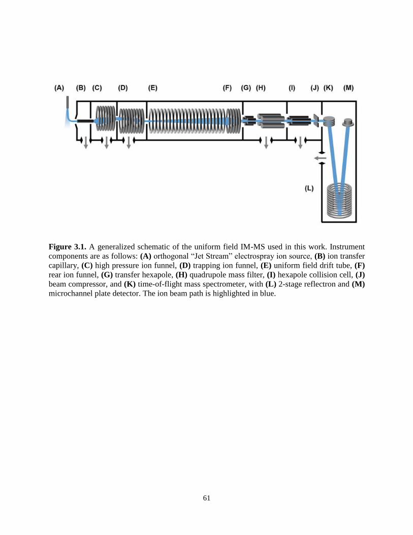
61
Figure 3.1. A generalized schematic of the uniform field IM-MS used in this work. Instrument
components are as follows: (A) orthogonal “Jet Stream” electrospray ion source, (B) ion transfer
capillary, (C) high pressure ion funnel, (D) trapping ion funnel, (E) uniform field drift tube, (F)
rear ion funnel, (G) transfer hexapole, (H) quadrupole mass filter, (I) hexapole collision cell, (J)
beam compressor, and (K) time-of-flight mass spectrometer, with (L) 2-stage reflectron and (M)
microchannel plate detector. The ion beam path is highlighted in blue.

62
purity, the IMS is operated at an elevated pressure with respect to the trapping ion funnel region.
For nitrogen and carbon dioxide, this pressure difference is ca. 150 mTorr. For helium, it was
found that a difference of ca. 230 mTorr or greater is necessary to ensure drift gas purity. Following
IMS separation, radially diffuse ions are recollected by a third ion funnel located at the exit end of
the drift tube. This rear ion funnel is operated at the same pressure (4 Torr) as the drift tube with a
DC field of ca. 18 V cm−1. Following the IMS, ions are transferred through a hexapole into the
high vacuum Q-TOF stage of the instrument, where they are analyzed by their mass-to-charge.
Optional mass selection and ion activation (collision-induced dissociation) can be conducted in
this interfacing region between the IM and MS stages, though these schemes are not utilized in
this present work. Although the time-of-flight mass spectrometer is capable of a resolving power
greater than 40,000 (m/Δm), for purposes of these experiments the instrument was operated with
settings designed to improve sensitivity and mass transmission range (“extended dynamic range”
mode), and this resulted in a mass resolving power of ca. 20,000.
The ATM solution used to evaluate the semi-empirical fits was infused into one of two ion
sources: a dual electrospray ionization source (dual “Jet Stream”, Agilent), or an orthogonally-
configured nano-electrospray ionization source (G1992A Nanospray, Agilent). For the Jet Stream
source, the ATM solution was infused from the “reference B” sample solution reservoir with the
default injection backpressure. For nanoelectrospray, the ATM solution was directly infused using
a syringe pump (Cole-Parmer) at a flow rate of ca. 1 μL min−1.
3.2.2. Analytical Precision

63
The instrumentation used in this work is considered a “high precision” ion mobility
instrument in that it is capable of obtaining reproducible measurements of the mobility drift time
to better than 0.1 ms. For conversion of drift time measurements to ion transport coefficients (K0
and collision cross section), this represents a relative error of better than 0.5%.22 Analytical
precision affects the reproducibility of the ion mobility drift time, but does not directly affect the
FWHM.
3.3. Data Acquisition and Analysis
All ion mobility data was obtained using the MassHunter Data Acquisition software
(Agilent). A software feature which allows individual experimental sequences to be defined was
utilized to obtain consecutive ion mobility spectra at various drift potentials between 350 and 1750
V (4.5 to 22.4 V cm−1) in increments of 100 V. This corresponds to instrument settings from 600
V to 2000 V for the “drift tube entrance” potential and 250 V for the “drift tube exit” potential.
For each sequence, data was signal averaged for 2 minutes. These drift voltage sequence
experiments were acquired for initial ion gate widths ranging from 100 to 500 μs in 100 μs
increments, which corresponds to the ion release time setting in the instrument control software.
Following acquisition, each segmented data file was analyzed using the MassHunter IMS Browser
software (Agilent). Peaks of interest were isolated and their centroid drift time values and FWHM
were extracted as tabulated data using capabilities within the software. In some cases, the FWHM
was determined manually. K0 values necessary to conduct the resolving power analysis were
obtained directly from the software, using procedures previously described.22 Briefly, this involves
conducting drift time measurements for a sequence of fields in order to determine the time

64
component associated with ion transit outside of the mobility region. K0 can then be solved via
equation (3).
3.3.1. Semi-empirical Fitting Procedure
The semi-empirical coefficients (α, β, and γ) for equation (6) and (7) were determined for
each ion system using procedures outlined by Siems et al.12 Details of the procedure as utilized in
this study are included in the ESI. Briefly, this involves a linear regression analysis of equation
(6). The α coefficient is the slope of the best-fit line to data projected as Ttd2/V (the diffusion
parameter) versus Δt2 for a series of ions. The β coefficient is determined from a slope of the best-
fit line to data plotted as tg2 versus Δt2. The γ coefficient is obtained through orthogonal correlation
of results from the linear regression analysis of α and β. Plots corresponding to this analysis are
contained in Figure C.5 and C.7. A strong correlation was observed between the ion species and
the β and γ coefficients, so these terms were replaced with an equation which includes K0 (Figure
C.8). These coefficients and coefficient equations are summarized at the bottom of Table 1.
3.4. Results and Discussion
3.4.1. Factors affecting semi-empirical coefficients
Because each of the semi-empirical coefficients are associated with a specific component
of variance from equation 6, their deviation from the “ideal” values (equation 4) can provide some
insight into the physical source of band broadening within the instrument. For the α coefficient,
previous work has demonstrated this value is consistently larger in stand-alone drift tube

65
Table 3.1. Summary of results from the semi-empirical linear regression analysis. K0 values are
for nitrogen drift gasa

66
instruments than the ideal value of 0.957 × 10⁻³ V K−1, with experimental α values of ca. 1.2 ×
10−3 V K−1 or greater.12 This observation has been previously attributed to inhomogeneity in the
electric field. In this work, we obtain an average α value of 0.910 × 10⁻³ V K−1 (Table 3.1), which
does not depend strongly on the ion species (Figure C3). The α value found in this study is close
to the ideal value. A cursory explanation would be that the drift tube in this work operates with a
high degree of homogeneity, yet ions also pass through an electrodynamic ion funnel prior to being
measured (Figure 1F). Because α is essentially the magnitude of the response of the peak width to
the drift time, we can only say that for the current instrumentation, peaks broaden as expected from
diffusion. This may be a general characteristic of drift tubes coupled to MS via a conductance-
limiting aperture, as the previous work had been carried out on ambient pressure instrumentation
using relatively large diameter Faraday plate detectors which would sample the entire radially-
diffuse ion cloud. The explanation of β and γ is not so straightforward. Previous work had
characterized these coefficients using measurements obtained from a single ion (Cl−, H3O+, or
O2−), and thus the β and γ values were previously reported as a single value for each instrument
geometry evaluated. In this present study, we evaluated these semi-empirical terms using a series
of analytes possessing a wide range of mobility values. Thus, our results for β and γ are different
for each ion investigated (Table 3.1). For β, we obtain a range of values from 0.181 to 0.536, which
is significantly smaller than the ideal situation of β = 1. In the previous study by Siems et. al., β
was consistently greater than 1 (ca. 1.1 to 1.6). Since β is a multiplier for the gate width, this
coefficient represents a correction for peak width variations which are caused during the ion gating
event. Values greater than 1 were explained as originating from additional band broadening due to
space-charge effects (Coulombic repulsion), which would become greater as the pulse width was
increased, i.e., as more ions were introduced per pulse. In contrast, all of the β values measured in

67
this work were well below 1, suggesting that the resulting ion pulse widths are narrower than
would be expected from the time duration that the ions are admitted into the drift tube via the
control software (i.e., the applied temporal gate width). We infer that this is a consequence of
conducting the ion gating using an ion trap, rather than a more traditional electrostatic ion depletion
gate (Tyndall or Bradbury-Nielsen gate). A similar ion compression effect has been observed when
operating the ion gate region using multiple grid stages,27,28 and we suggest a field-focusing
behavior may also be occurring in the present instrumentation which utilizes a similar 2-grid
structure in the region of ion confinement.25 We note that unlike what is observed for most ambient
pressure IMS instruments, this instrument operates closer to the diffusion limit in terms of
resolving power. For γ, the ideal value is 0 s2, that is, no additional sources of variance other than
the initial gate width and normal diffusion.16 For previous drift tubes, the value for γ was found to
vary anywhere from 0.47 × 10⁻⁸ s2 to as high as 2.1 × 10⁻⁸ s2 , 12 which corresponds to an added
variance of between ca. 0.07 to 0.14 ms. In this work, the value of γ determined for the present
instrumentation was found to be ion dependent, with upper values of 4.8 × 10⁻⁷ s2 (Table 3.1),
which corresponds to a variance of ca. 0.69 ms. This value of γ is about 5-fold greater than what
was determined in the previous study, where the source of band broadening was attributed to image
current induction and detector response effects for the Faraday detector used. For the present IM-
MS instrument, the IMS spectra are obtained through temporal correlation of ion signal from the
electron multiplier in the MS stage. Microchannel plate electron multipliers exhibit peak
broadening effects on the order of picoseconds,29 and so detector effects would not be an issue in
this current work. We suggest that the primary source for γ is due to ion transit through the rear
ion funnel, which is not accounted for in the length term used to determine the theoretical drift
time from equation 3. This claim is supported by the observation that γ is mobility-dependent

68
(Table 3.1). The relatively large values for γ suggest that there is a significant contribution to band-
broadening occurring in the rear funnel, yet the measured resolving power values and the analysis
of the α coefficient both suggest that the instrument is operating near the diffusion limit. One
explanation for this is that the band broadening which occurs in the rear funnel is counteracted by
the additional mobility separation which occurs due the rear funnel operating as an extension of
the drift tube. The additional contribution of the rear ion funnel as a mobility separator which
operates with no significant loss in resolving power has been noted in a previous study.23 While
the data in this current work also suggests that the funnel operates as an extension of the drift tube,
no attempt was made to match the field between the drift tube and the rear funnel, which would be
expected to further improve the quantitative agreement between experiment and theory. Finally, it
is worth noting that drift time correction is not utilized in this study due to the difficulty in
determining the peak width contribution of the non-mobility transit time of the ions. While not
investigated further here, the temporal contribution of the rear ion funnel is well characterized and
could be incorporated into the ion mobility peak width theory in the form of an added source of
variance, as the ion funnel length (11.6 cm), pressure (4 Torr), and electric field (17.8 V cm−1)
used in this present study are known.
3.4.2. Empirical Correlation of Theoretical Resolving Power
Once the semi-empirical coefficients are determined for a wide range of gate widths and
ion systems, equation 7 can be expanded in order to generate a generalized resolving power
expression which describes the performance of the current instrumentation. These results are
provided as equation (S10) in the ESI. An evaluation of both the conditional and semi-empirical
theories

69
Figure 3.2. Empirical resolving power curves (data points) compared to theory (solid lines) as a
function of the ion mobility separation field (drift field) for three molecular ions (nominal m/z 322,
622, and 922). Error bars for each point are obtained from four replicate measurements. (A) The
conditional resolving power (Rc) from equation (5) predicts the qualitative trends of the
experimental observations, but quantitative correlation varies based on the ion system and gate
width used. (B) The semi-empirical resolving power (RSE) from equation (7) exhibits a more
quantitative correlation than the conditional resolving power for all gate widths investigated in this
study (100, 200, 300, 400, and 500 μs). For clarity, only the data for 100 and 500 μs gate widths
are shown.
70
is contained in Figure 3.2 for the m/z 322, 622, and 922 ions. Experimental data is projected as
points with error bars obtained from 4 replicate measurements. Of general note is that in many
cases, the error associated with the measured resolving power for a single data point is in excess
of 5%. This reflects the challenges associated with obtaining quantitatively-reproducible
measurements of the peak width, as opposed to the drift time which exhibits close correlation to
equation 3 (Figure B.1). In Fig. 2.1 A, the conditional resolving power theory via equation 5
exhibits only qualitative agreement with experimental results, with significant deviation being
observed at low and high gate widths. Conditional resolving power consistently predicts
significantly better resolving power when using lower gate widths, but the data suggests that this
is only significant when studying low-mass ions (i.e., ions possessing high K0 values above ca. 1
cm2 V−1s−1). Experimental results indicate that higher mass ions do not benefit significantly in
resolving power from smaller gate widths, and so for such studies, increasing the gate width would
be advantageous to improve instrument sensitivity. This gate width dependence on the accuracy
of equation 5 is consistent with previous observations,13 and deviation has also been noted in
experimental measurements at extreme pressures (up to 2280 Torr).30 Note that a gate width of
200 μs is commonly utilized in IMS studies, and under this condition, there is a coincidentally
good correlation between conditional resolving power theory and experimental results (Figure
C.2), which suggests that deviations between theory and experiment are not obvious under routine
investigations. To our knowledge this work represents the first study where the conditional
resolving power was explicitly tested for ions spanning a wide range of reduced mobilities (Table
3.1), and in particular, for larger ions with K0 values below ca. 1 cm2 V−1s−1 as what would be
encountered for biomolecules. This work also represents the first comprehensive study of resolving
power theory for reduced pressure IMS. Because the present instrumentation is configured in a

71
manner that is far from the conditions assumed by conditional resolving power (i.e., ion trap gating,
sub-ambient IMS pressures, and post-mobility focusing via the ion funnel), the observed
deviations between conditional resolving power theory and empirical results is not surprising,
particularly for larger ions which spend more time in the IMS stage of the instrument. Figure B.2
B contains the results from the semi-empirical resolving power theory via eqn (7) utilizing the
methods described in the ESI. A significant improvement in the correlation between experiment
and theory is observed in this case across all initial ion gate widths investigated (100 to 500 μs, cf.
Figure C.3). Some deviation does occur for the lower mobility ion, m/z 922, where the semi-
empirical treatment underpredicts the resolving power by about 15% on the high end, which is a
fairly consistent deviation across all gate widths at this mobility (Figure C.3). Similar results are
also observed for the m/z 2722 ion (Figure C.4). The m/z 922 ion was explicitly used in the initial
evaluation of the semi-empirical theory, and so better correlation was anticipated, but this would
appear to be a more realistic expectation of accuracy when working with a theory generalized
against a wide range of parameters. Because both the conditional and semi-empirical resolving
power expressions account for the ion’s reduced mobility, a 3-dimensional resolving power curve
can be obtained which is ion species dependent. Figure 3.3 contains the resulting 3D analysis for
both the conditional resolving power of eqn (5) (Figure C.3 A), and the semi-empirical resolving
power of equation 7 (Figure C.3 B). Both curves were generated using a drift gas pressure of 4.00
Torr and a temperature of 304.2 K and describe the performance of singly-charged ions only. A
gate width of 200 μs was also chosen for comparison between the two theories, as the best
correlation between conditional resolving power and experimental data was observed at this
setting, meaning any differences observed between the two theories at this gate width is expected

72
Figure 3.3. 3D resolving power curves projecting the predicted resolving power for singly-charged
ions across a range of drift fields and ion mobilities. (A) Conditional resolving power (equation
5), and (B) semi-empirical resolving power via equation (7) using coefficient expressions obtained
in this current work. Both expressions assume 4 Torr drift gas pressure with an initial gate width
of 200 μs. As compared with the conditional resolving power, the semi-empirical resolving power
predicts a relatively narrow drift field range for accessing the optimal resolving power, as well as
a more uniform resolving power response for a wide range of ion species.

73
to be significant. Conditional resolving power predicts that higher resolving powers are accessible
as the mobility of the ion decreases (i.e., large ions), and that accessing these higher resolving
powers requires different drift fields.18 This observation suggests that conditional resolving power
theory underestimates diffusional effects that increase with lower mobilities, which is accounted
for in the semiempirical treatment. Additionally, the semi-empirical treatment pertaining to
observations from the current instrument indicates that the resolving power performance is
relatively linear across a range of ion mobilities. This observation is better illustrated by extracting
the resolving power maxima (highest values) for both 3D surfaces and plotting these as a function
of K0 (Figure C.4 A). This analysis indicates there is good correlation between conditional and
semi-empirical resolving power theory at high mobilities (fast ions) where ions spend a limited
amount of time in the mobility region, but deviation becomes significant in the low mobility (slow
ions) regime. This deviation between the two theories occurs at a K0 of ca. 1 cm2 V−1s−1, which
for a peptide drifting in nitrogen represents an analyte mass of ca. 500 Da.22 Additional molecular
class specific mobility ranges for nitrogen drift gas are projected at the bottom of the plot to help
frame these observations in the context of practical results. The implication of this observation is
that for the current instrumentation, the accuracy of predictions made by the conditional resolving
power theory are limited to small analyte systems (i.e., ions with high K0 values). A second
observation which can be made from Figure C.3 is that the highest resolving power values
predicted by the semi-empirical theory are fairly constant and experimentally-accessible across a
relatively narrow range of drift fields (between 14 and 17 V cm−1). This can be better illustrated
by plotting the drift field corresponding to the highest resolving power values as a function of the
ion’s reduced mobility (Figure C.4 B). Thus, in practice, accessing high resolving power values
should require only minor adjustments to the drift field. Taken collectively, these observations

74
Figure 3.4. Plots of the highest achievable resolving power values predicted by both theories for
singly-charged ions. Trends are extracted from the maxima in Figure 3.3 (i.e., the “crest” of each
surface plot). (A) The highest (optimal) resolving power accessible as a function of the reduced
mobility. Corresponding molecular class-specific mobility ranges are also provided for ion
mobility in nitrogen drift gas (lower bars). (B) The required drift field necessary to access the
optimal resolving power as a function of the reduced mobility. Both projections indicate that the
semi-empirical resolving power theory predicts a narrow range of both optimal resolving powers
(50 to 60) and drift fields (14 to 17 Vcm−1) across a fairly wide range of mobilities.
75
suggest that the present instrumentation performs at optimal resolving power for a wide dynamic
range of ion species under similar operational conditions. This may be a general observation for
all ion mobility instrumentation, as quantitative investigations of the conditional resolving power
to date have focused only on small analytes with reduced mobility values greater than 1.2 cm2
V−1s−1,13,18,31,32 although this study also represents the first test of conditional resolving power
theory for reduced pressure IMS, so these results may also be specific to subambient pressure
operation around 4 Torr.
3.4.3. Broadscale Validity of Semi-Empirical Results
In order to further investigate the extent of correlation between experiment and theory,
three ions systems exhibiting vastly different gas-phase transport properties were compared against
the current theories. The ion systems used in this comparison are: (1) a small peptide in nitrogen
with a K0 close to 1 (SDGRG, K0 = 1.02 cm2V−1s−1),22 (2) a quaternary ammonium cation in carbon
dioxide, which exhibits very low mobility (TAA10, K0 = 0.50 cm2V−1s−1), and (3) a triply-charged
peptide (melittin bee venom) in helium,33 which has a very high gas phase mobility (K0 = 3.03
cm2V−1s−1). Typical operational conditions (200 μs gate width and 4 Torr drift gas) are used in
these comparisons. Note that both theories are drift gas independent, since both theoretical
expressions describe ion transport in terms of the gas-phase reduced mobility, which inherently
accounts for differences in ion motion in various drift gases. Thus, the theories developed in this
work are applicable to a variety of drift gases. Experimental results for the three ion systems are
contained in Figure 3.5. For ions with reduced mobility values around ca. 1 cm2V−1s−1, both
theories correlate well with experimental results (Figure 3.5 A). This is consistent with the
previous observation for m/z 622 (K0 = 1.01 cm2V−1s−1) at this gate width (Figure C.2 and C.3).

76
Figure 3.5. Comparison of experiment and theories generalized to a wide range of reduced
mobility values. (A) Singly-charged SDGRG peptide measured in nitrogen drift gas (K0 = 1.02
cm2V−1s−1) exhibits good correlation to both theories. (B) Singly-charged quaternary ammonium
cation with ten-carbon branches (TAA10) measured in carbon dioxide drift gas possesses a very
low mobility value (K0 = 0.50 cm2V−1s−1), and here the semi-empirical resolving power better
predicts the experimental resolving power of this system. (C) The triply-charged melittin peptide
in helium drift gas exhibits a high mobility (K0 = 3.03 cm2V−1s−1) as well as being multiply-
charged, which despite the unconventionally high mobility still shows good correlation to the
semi-empirical resolving power developed in this work.

77
At low mobilities, which represents large ions or ions drifting in more massive drift gases (such as
carbon dioxide in this case), conditional resolving power theory significantly overestimates the
magnitude of the resolving power, whereas the semiempirical theory correlates closely to
experimental results, albeit with slightly underestimated predictions (Figure 3.5B). This is similar
to the trends observed for the m/z 922 system (Figures 3.2C, S2 and S3). In the third case for very
high mobility ions, both theories show qualitative agreement, with semiempirical theory
correlating better than conditional resolving power (Figure 3.5 B). Note that in this latter system,
a multiplycharged ion is evaluated (z = 3), and thus requires that the integer charge state be
introduced into the denominator of the diffusion term in the semi-empirical theory. Extension of
the semi-empirical theory to higher charge-state systems was not an original intention of this work,
but results are indeed favorable. We caution here, however, that preliminary work with a protein
exhibiting even higher charge states (myoglobin, z = 9 to 24) has not resulted in the good
correlation to semi-empirical theory as seen for the melittin system, so further refinement to the
theory is necessary. While the systems in Figure 3.5 represent extreme cases in terms of the
reduced mobility, the good correlation observed indicates that the semi-empirical theory can be
qualitatively extended beyond the range in which it was initially evaluated (cf., Table 3.1).
3.5. Conclusions
A wide-scale evaluation of two current theories for ion mobility resolving power
(conditional and semi-empirical) was applied to high precision results obtained on a recently
developed IM-MS instrument. The predictive capabilities of conditional resolving power theory
were found to be qualitatively good for high mobility ions (e.g., small molecules), but deviated
significantly for low mobility ion systems and gate widths beyond 200 μs. Better correlation to

78
experimental observations was found for a semi-empirical treatment of resolving power which was
developed using empirical data on the current instrumentation, and initial evaluation of the semi-
empirical theory demonstrated good correlation across a relatively wide range of ion mobilities
(K0 between 0.50 and 3.03 cm2V−1s−1). The semi-empirical theory was used to generalize the
performance of the current instrument and results suggest that the instrumentation is capable of
accessing the optimal resolving power for a wide range of analytes within a relatively narrow range
of drift fields, independent of the drift gas utilized. When taken collectively, these observations
indicate that the linear response of the instrument in terms of ion mobility separation efficiency is
high. The decreased dependency of the gate width on the accessible resolving power for lower
mobility ions (K0 below ca. 1 cm2V−1s−1) indicates that for higher mass studies (greater than m/z
of ca. 500), the gate width may be increased to improve sensitivity without a significant loss in
resolving power. As with any semi-empirical treatment, the results are specific to the
instrumentation and experimental conditions used in this study, namely operating the drift tube at
ca. 4 Torr and ambient temperature, and investigating low charge-state ions. Conditional resolving
power is thus recommended over the current semi-empirical theory for estimating the accessible
resolving power for ion mobility instrumentation that differs significantly from the present study,
such as ambient pressure drift tubes and stand-alone IMS instruments. Finally, it should be noted
that obtaining quantitatively reproducible resolving power values on any drift tube platform is
challenging without careful attention to maintaining drift gas purity and stability of all important
ion mobility conditions, specifically drift fields, gas pressures, temperatures, and robust methods
to extract the quantitative data (drift time centroids and temporal peak widths) from the raw
measurements. The high precision capabilities of the present instrumentation greatly facilitates
these types of quantitative studies.
79
3.6. Acknowledgements
This chapter contains the published research article: James N. Dodds, Jody C. May, and
John A. McLean, “Broadscale Resolving Power Performance of a High Precision Uniform Field
Ion Mobility-Mass Spectrometer,” Analyst, 2015, 140, 6824-6833.
J.C.M, J.N.D, and J.A.M. thank M. Ray Keller for assistance in data analysis and Katrina
L. Leaptrot for reviewing various drafts of the manuscript. Vanderbilt authors gratefully
acknowledge a Thought Leader award from Agilent Technologies. Financial support for this
research was provided by Agilent Technologies, the National Institutes of Health National Center
for Advancing Translational Sciences (NIH-NCATS Grant 4UH3TR000491-3), the National
Science Foundation (MRI CHE-1229341), the Vanderbilt Institute of Chemical Biology, the
Vanderbilt Institute for Integrative Biosystems Research and Education, and Vanderbilt
University.
3.7. References
1. Israel, H.; Schulz, L., The Mobility-Spectrum of Atmospheric Ions-Principles of
Measurements and Results. Terr. Magn. Atmos. Electr. 1933 38, 285-300.
2. Bradbury, N. E.,The Absolute Values of the Mobility of Gaseous Ions in Pure Gases. Phys.
Rev. 1932, 40, 508-523.
3. Cohen, M. J.; Karasek, F. W., Plasma Chromatography-A New Dimension for Gas
Chromatography and Mass Spectrometry. J. Chromatogr. Sci. 1970, 8, 330-337.
4. Cram, S. P.; Chesler, S. N., Coupling of High Speed Plasma Chromatography with Gas
Chromatography. J. Chromatogr. Sci., 1973, 11, 391–401.
5. Karasek, F. W. Plasma Chromatography. Anal. Chem., 1974, 46, 710A-720A.
6. Spangler, G. E.; Collins, C. I., Peak Shape Analysis and Plate Theory for Plasma
Chromatography. Anal. Chem. 1975, 47, 403-407.

80
7. Revercomb, H. E.; Mason, E. A., Theory of Plasma Chromatography/Gaseous
Electrophoresis. Review, Anal. Chem. 1975, 47, 970-983.
8. F. W. Karasek, Study of Technology Relating to Plasma Chromatography Sensing Tubes,
Final Report, Contract #8SU77-00227, University of Waterloo Research Institute,
Waterloo, Ontario, Canada, 1980.
9. Carrico, J. P.; Sickenberger, D. W.; Spangler, G. E.; Vora, K. N.,Simple Electrode Design
for Ion Mobility Spectrometry. J. Phys. E: Sci. Instrum., 1983, 16, 1058-1062.
10. Rokushika, S.; Hatano, H.; Baim, M. A.; Hill, H. H., Resolution Measurement for Ion
Mobility Spectrometry. Anal. Chem. 1985, 57, 1902-1907.
11. Watts, P.; Wilders, A., On the Resolution Obtainable in Practical Ion Mobility Systems.
Int. J. Mass Spectrom. Ion Processes, 1992, 112, 179-190.
12. Siems, W. F.; Wu, C.; Tarver, E. E.; Hill, H. H.; Larsen, P. R.; McMinn, D. G., Measuring
the Resolving Power of Ion Mobility Spectrometers. Anal. Chem., 1994, 66, 4195-4201.
13. Kanu, A. B.; Gribb, M. M.; Hill, H. H., Predicting Optimal Resolving Power for Ambient
Ion Mobility Spectrometry. Anal. Chem. 2008, 80, 6610-6619.
14. May, J. C.; McLean, J. A., Ion Mobility-Mass Spectrometry: Time-Dispersive
Instrumentation. Anal. Chem. 2015, 87, 1422-1436.
15. Mason, E. A.; McDaniel, E. W., Transport Properties of Ions in Gasses, 1998.
16. Spangler, G. E., Expanded Theory for the Resolving Power of a Linear Ion Mobility
Spectrometer. Int. J. Mass Spectrom. 2002, 220, 399-418.
17. Glasser, M. L., Peak Shape Analysis for Ion Mobility Spectroscopy. J. Appl. Phys. 1988,
63, 4823-4831.
18. Davis, E. J.; Williams, M. D.; Siems, W. F.; Hill, H. H., Voltage Sweep Ion Mobility
Spectrometry. Anal. Chem. 2011, 83, 1260-1267.
19. Verbeck, G. F.; Ruotolo, B. T.; Gillig, K. J.; Russel, D. H., Resolution Equations for High-
Field Ion Mobility. J. Am. Soc. Mass Spectrom.. 2004, 15, 1320-1324.
20. Mariano, A. V.; Su, W.; Guharay, S. K., Effect of Space Charge on Resolving Power and
Ion Loss in Ion Mobility Spectrometry. Anal. Chem. 2009, 81, 3385-3391.
21. Tolmachev, A. V.; Clowers, B. H.; Belov, M. E.; Smith, R. D., Coulombic Effects in Ion
Mobility Spectrometry. Anal. Chem. 2009, 81, 4778-4787.
22. May, J. C.; Goodwin, C. R.; Lareau, N. M.; Leaptrot, K. L.; Morris, C. B.; Kurulugama,
R. T.; Mordehai, A.; Klein, C.; Barry, W.; Darland, E.; Overney, K.; Imatani, K.; Stafford,
G. C.; Fjeldsted, J. C.; McLean, J. A., Conformational Ordering of Biomolecules in the

81
Gas Phase: Nitrogen Collision Cross Sections Measured on a Prototype High Resolution
Drift Tube Ion Mobility-Mass Spectrometer. Anal. Chem. 2014, 86, 2107-2116.
23. Tang, K.; Shvartsburg, A. A.; Lee, H.-N.; Prior, D. C.; Buschbach, M. A.; Li, F.;
Tolmachev, A. V.; Anderson, G. A.; Smith, R. D., Anal. Chem. 2005, 77, 3330-3339.
24. Baker, E. S.; Clowers, B. H.; Li, F.; Tang, K.; Tolmachev, A. V.; Prior, D. C.; Belov, M.
E.; Smith, R. D., Ion Mobility Spectrometry-Mass Spectrometry Peformance Using
Electrodynamic Ion Funnels and Elevated Drift Gas Pressures. J. Am. Soc. Mass Spectrom.
2007, 18, 1176-1187.
25. Clowers, B. H.; Ibrahim, Y.; Prior, D. C.; Danielson, W. F.; Belov, M.; Smith, R. D.,
Enhanced Ion Utilization Efficiency Using an Electrodynamic Ion Funnel Trap as an
Injection Mechanism for Ion Mobility Spectrometry. Anal. Chem. 2008, 80, 612-623.
26. Ibrahim, Y. M.; Baker, E. S.; Danielson, W. F.; Norheim, R. V.; Prior, D. C.; Anderson,
G. A.; Belov, M. E.; Smith, R. D., Development of a New Ion Mobility (Quadrupole) Time-
of-Flight Mass Spectrometer. Int. J. Mass Spectrom. 2015, 377, 655-662.
27. Du, Y.; Wang, W.; Li, H., Bradbury-Nielsen-Gate-Grid Structure for Further Enhancing
the Resolution of Ion Mobility Spectrometry. Anal. Chem. 2012, 84, 5700-5707.
28. Du, Y.; Wang, W.; Li, H., Resolution Enhancement of Ion Mobility Spectrometry by
Improving the Three-Zone Properties of the Bradbury-Nielsen Gate. Anal. Chem. 2012,
84, 1725-1731.
29. Wiza, J. L., Microchannel Plate Detectors. Nucl. Instrum.Methods 1979, 162, 587-601.
30. Davis, E. J.; Dwivedi, P.; Maggie, T.; Siems, W. F.; Hill, H. H., High-Pressure Ion Mobility
Spectrometry. Anal. Chem. 2009, 81, 3270-3275.
31. Kaplan, K.; Graf, S.; Tanner, C.; Gonin, M.; Fuhrer, K.; Knochenmuss, R.; Dwivedi, P.;
Hill, H. H., Resistive Glass IM-TOFMS. Anal. Chem. 2010, 82, 9336-9343.
32. Roscioli, K. M.; Davis, E.; Siems, W. F.; Mariano, A.; Su, W. S.; Guharay, S. K.; Hill, H.
H., Modular Ion Mobility Spectrometer for Explosives Detection Using Corona Ionization.
Anal. Chem. 2011, 162, 587-601.
33. May, J. C.; McLean, J. A., A Uniform Field Ion Mobility Study of Melittin and
Implications of Low-Field Mobility for Resolving Fine Cross-Sectional Detail in Peptide
and Protein Experiments. Proteomics 2015, 15, 2862-2871.

82
CHAPTER 4
INVESTIGATION OF THE COMPLETE SUITE OF THE LEUCINE AND ISOLEUCINE
ISOMERS: TOWARDS PREDICTION OF ION MOBILITY SEPARATION CAPABILITIES
4.1. Introduction
The separation of isomers, or compounds that contain the same atomic composition yet
possess different chemical structures, has been an active area of analytical chemistry since the first
isomer separation was documented by Pasteur in 1849.1 The biological activity of compounds
exhibit isomeric specificity which manifests in a broad range of physiological processes including
metabolic pathways,2 reactive oxygen species,3 and cancer research.4 Isomers represent a broad
range of structural heterogeneity which are classified based on differences either in bond
coordination or stereochemistry. Compounds that differ as a result of physical rearrangement of
chemical bonds, (i.e. constitutional isomers) represent the most structurally diverse isomer class.
Stereoisomers are compounds which have identical branching between atoms but differ in chirality
at one or more stereocenters. A specific sub-class of chiral molecules are enantiomers which
exhibit mirrored stereochemistry. Biological compounds tend to exist in only one particular
stereochemistry,5 such as the amino acids, which predominately exist in the L- form. While the
precise origin of stereochemistry preference is still unknown, observations of chirality in meteorite
samples and in deep space suggests L- stereochemistry preferences are primordial.6,7 Due to
identical chemical compositions, chemical isomers are of the same mass and thus are challenging
to separate by traditional mass spectrometry techniques alone. Tandem MS/MS methods such as
collision induced dissociation8,9 and electron transfer dissociation10-12 can alleviate these
challenges in cases where two isomers either differ in bond dissociation energies or possess

83
constitutional arrangements that produce unique fragmentation spectra. However, for structurally
similar isomers, fragment ions are often shared by both precursors and hence tandem MS is not
sufficient to confidently identify these components in a biological mixture (see Figure D.1,
Supporting Information).13,14
Ion mobility-mass spectrometry (IM-MS) has gained recent interest as a rapid separation
technique which can be applied to the separation and characterization of isomers.15-20 Although
condensed phase separation techniques such as gas and liquid chromatography can be tailored for
the separation of specific isomeric classes, IM-MS operates on a timescale that is several orders of
magnitude faster and can be used in conjunction with condensed phase separations and tandem
MS/MS techniques.21,22 IM-MS is a particularly useful analytical combination in that the mass
spectrometry separates molecules based on their intrinsic mass, whereas ion mobility provides a
complimentary separation based on molecular size and shape based on the gas-phase collision
cross section (CCS). While there has been significant progress in correlating the CCS to the
primary molecular structure and composition,23-25 it is challenging to predict CCS particularly for
isomeric systems. Consequently, the ability of IM-MS to separate any given isomeric system is
difficult to predict without referring to empirical studies.
For our study of isomeric separations we chose to investigate the classic amino acid isomer
system leucine and isoleucine, which has been previously studied by both chromatography
approaches26-28 and various ion mobility techniques including field asymmetric waveform ion
mobility spectrometry (FAIMS),29-31 traveling wave ion mobility spectrometry (TWIMS),32 and
uniform field ion mobility operated at ambient pressure.33 This small molecule system (131 Da)
was chosen as it is large enough to possess a diverse family of isomers yet small enough not to
exhibit significant higher-order structural effects (i.e. conformers) that would otherwise

84
complicate the interpretation of results. A total of eleven leucine/isoleucine isomers (C6H13NO2)
were chosen for this study, including four biologically-relevant forms (L-leucine, L-isoleucine, L-
norleucine, and L-tert-leucine) which collectively include examples of different bond coordination
and stereochemistry (Figure 4.1). Although nonlinear field IM-MS techniques (e.g., FAIMS) have
been shown to enhance the separation of these types of isomers, drift tube ion mobility
spectrometry (DTIMS) was specifically chosen for this work, as this uniform field-based technique
facilitates the quantitative comparison of separations through the empirical measurement of the
CCS.
4.2. Experimental Methods
4.2.1. Preparation of Standards
Optima LC-MS grade water and ammonium acetate were purchased from Fisher Scientific
(Fair Lawn, NJ, USA). 6-aminocaproic acid, L-norleucine, D-leucine, L-isoleucine, L-allo-
isoleucine, N,N-dimethylglycine ethyl ester, and L-leucine were purchased from Sigma-Aldrich
(St. Louis, MO, USA). D-tert-leucine, D-allo-isoleucine, L-tert-leucine and D-isoleucine were
purchased from Alfa Aesar (Ward Hill, MA, USA). Samples were prepared at an initial
concentration of 1 mg/mL and were subsequently diluted in water buffered with 10 mM
ammonium acetate (pH 6.5) to a final concentration of 10 µg/mL for analysis. No additional acid
was needed to promote protonation. All isomers investigated in this work are summarized in Figure
4.2.
4.2.2. Experimental Parameters

85
A commercial uniform field ion mobility-mass spectrometer (6560, Agilent Technologies, Santa
Clara, CA, USA) was used to obtain high resolution mass spectrometry and ion mobility data
(nominally 15,000 and 60, respectively). Details of the instrument have been previously
described.34,35 Briefly, the instrument consists of a uniform field 78.1 cm drift tube coupled to a
tandem quadrupole time-of-flight (QTOF) mass spectrometer. The drift tube is bracketed by
electrodynamic ion funnels and ion mobility separations were conducted in nitrogen drift gas (4.00
Torr, ca. 30) for these studies. All samples were directly infused using a syringe pump (Cole-
Palmer, Vernon Hills, IL) operated at 10 µL/min into a thermally-assisted electrospray ionization
source (Agilent Jet Stream). The instrument was operated in positive ion mode with 3.8 kV applied
to the ion transfer capillary and 1.8 kV applied to the ion focusing nozzle. Source temperatures
were kept low (200 ) to aid in ionization of fragile molecules.
Ion mobility parameters were adjusted to obtain maximum resolving power as described
previously.36,37 These prior studies indicate that the resolving power for drift tubes is optimized
when the initial ion pulse width is small, and hence the gate width (referred to as “Trap Release
Time” in this instrument) was set to a short duration (100 µs) relative to the ion drift time which
is on the order of tens of milliseconds. The drift field also strongly affects the instrument resolving
power, and separations were conducted at drift voltages which maximize the resolving power
within the mobility and mass range of the analytes, corresponding to 14.7 V/cm (see Figure D.2,
Supporting Information). The nominal resolving power (58 ± 2) was consistent for all analytes
investigated and represents the optimal values for singly-charged analytes for this particular
instrument (see Table D.1, Supporting Information).37 All mobility spectra correspond to the
protonated species of the C6H13NO2 molecule. Other adducts observed (M+Na and M+K) were
not evaluated further in this study.
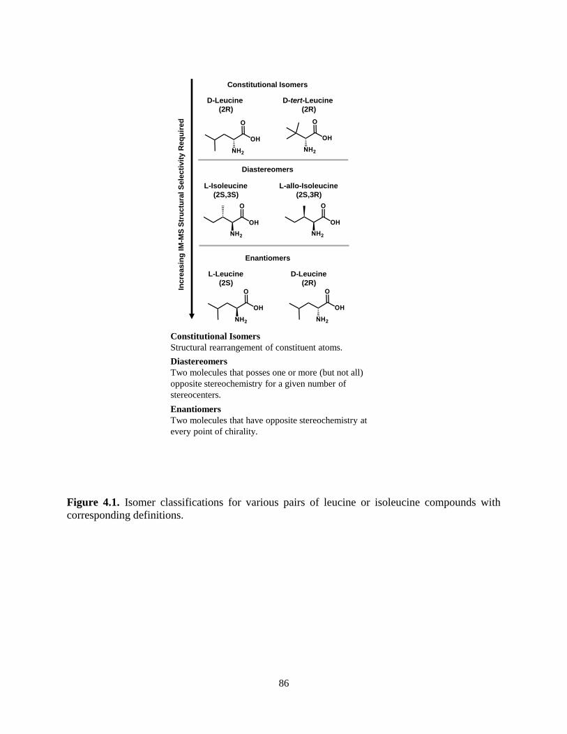
86
Figure 4.1. Isomer classifications for various pairs of leucine or isoleucine compounds with
corresponding definitions.
Constitutional Isomers
Structural rearrangement of constituent atoms.
Diastereomers
Two molecules that posses one or more (but not all)
opposite stereochemistry for a given number of
stereocenters.
Enantiomers
Two molecules that have opposite stereochemistry at
every point of chirality.
D-Leucine
(2R)
L-Leucine
(2S)
D-tert-Leucine
(2R)
L-Isoleucine
(2S,3S)
L-allo-Isoleucine
(2S,3R)
D-Leucine
(2R)
Inc
reasin
g I
M-M
S S
tru
ctu
ral S
ele
cti
vit
y R
eq
uir
ed
Enantiomers
Diastereomers
Constitutional Isomers

87
4.2.3. Collision Cross Section Measurements
Cross sections were determined from a stepped field technique in which the applied voltage
across the drift tube was varied in 7 increments from 550 to 1550V (7.0 to 19.8 V/cm, or 6 to 16
Td at 4 Torr) in order to determine the time ions reside outside the drift cell. The corrected drift
times are then used with relevant laboratory conditions (pressure, temperature) to obtain a collision
cross section value based on the fundamental low field equation, commonly referred to as the
Mason-Schamp relationship (Figure D.3, Supporting Information).38,39
4.3. Results and Discussion
4.3.1. Isomer Classifications and Separations
Figure 4.2 A illustrates the chemical structures of the 11 leucine/isoleucine isomers
(C6H13NO2) with corresponding collision cross sections and standard deviations obtained in this
study. All of the isomers exhibit a nitrogen cross section that spans approximately 10 square
angstroms (from ca. 127 to 137 Å2) with an average CCS of 133 Å2. The percent relative standard
deviation of all CCS values is ca. 0.2% for 7 sequential replicate measurements of each analyte.
Mobility spectra and corresponding ion mobility data are provided in Supporting Information
(Figure D.4 and Table D.1, respectively). Figure 4.2 B-I contains the overlaid IM spectra of all 11
isomers which were individually measured. No secondary peak features are observed for any of
the individual analytes, and mobility peaks are narrow with a resolving power at the limit of the
instrumentation for singly-charged ions (ca. 60).37 Figure 4.2 B-II illustrates the overlaid mobility
profiles for the constitutional isomers N,N-dimethylglycine ethyl ester (1), L-tert-leucine (3), and
L-norleucine (11). These three constitutional isomers possess a percent difference in cross section

88
Figure 4.2. (A) The leucine/isoleucine isomers with chemical formula C6H13NO2 examined in this
study. Experimental cross sections with respective standard deviations are shown at the right with
corresponding stereochemistry. (B) (I) Experimental IM spectra overlays for all isomer
compounds (standard error bars omitted for clarity). (II) Overlay of the IM spectra corresponding
to N,N-dimethylglycine ethyl ester, L-tert-leucine, and L-norleucine and the IM spectrum
corresponding to the mixture (black). (III) Overlays of L-isoleucine and L-leucine in addition to
the equal ratio mixture. (IV and V) Overlays of diastereomers and enantiomers, respectively. IM
spectra corresponding to the mixture of standards in (IV) and (V) can be found in the supporting
information (see Figure D.4).
L-Norleucine
D-Leucine (2R)
L-Leucine (2S)
L-Isoleucine (2S,3S)
L-allo-Isoleucine (2S,3R)
L-tert-Leucine (2S)
D-tert-Leucine (2R)
D-allo-Isoleucine (2R,3S)
6-Aminocaproic acid
N,N-Dimethylglycine ethyl ester
D-Isoleucine (2R,3R)
127.5 0.3 (Å2)
129.3 0.2 (Å2)
132.4 0.3 (Å2)
132.5 0.2 (Å2)
132.9 0.2 (Å2)
133.1 0.3 (Å2)
133.5 0.3 (Å2)
133.3 0.3 (Å2)
135.1 0.3 (Å2)
135.2 0.3 (Å2)
136.6 0.3 (Å2)
0
50
100
120 125 130 135 140 145
Re
lati
ve
Ab
un
da
nc
e (
%) 0
50
100
120 125 130 135 140 145
0
50
100
120 125 130 135 140 145
Collision Cross Section (Å2)
0
50
100
120 125 130 135 140 145
0
50
100
120 125 130 135 140 145
Constitutional
Isomers
L-Isoleucine
L-Leucine
L-allo-Isoleucine
L-Isoleucine
(A) (B)
(I)
(II)
(III)
(IV)
(V)
Constitutional
Isomers
Diastereomers
Enantiomers
(1)
(2)
(3)
(4)
(5)
(6)
(7)
(8)
(9)
(10)
(11)
(1) (2)
(3)(4)
(5)(6)(7) (8) (9) (10)
(11)
(1) (3) (11)
L-Isoleucine
D-Isoleucine
(7) (9)
(5) (7)
(7) (8)

89
of 3.6%and 3.1%, respectively. This CCS difference is sufficient to allow for near baseline
separation of the corresponding three component mixture (black trace). Figure 4.2 B-III depicts an
overlay of L-isoleucine and L-leucine, which have a 1.2% difference in cross section. These two
isomers are also classified as constitutional isomers, but are more structurally similar compared to
the three analytes in panel B-II. While the mobility overlays of these two compounds are distinctly
different, the analysis of the corresponding mixture indicates that they are unresolvable at the
current level of resolving power (ca. 60).
Figure 4.2 B-IV and V contain the overlaid IM spectra of diastereomers and enantiomers
respectively. Although the cross sections for L-allo-isoleucine and L-isoleucine are statistically
different (ca. 0.4%), the mixture of both diastereomers yields a single broad distribution (see
Figure D.5, Supporting Information). For the enantiomers, the centroids of each peak are not
statistically different. Specifically, the difference in their cross sections (0.2 Å2) is within the
standard error of the measurement (± 0.3 Å2, or 0.2%). Collectively, these observations
demonstrate that for relatively simple small molecules, constitutional isomers show the most
disparate cross sectional differences, followed by diastereomers and enantiomers, respectively.
While the correlation between structural and CCS differences is an intuitive result, these
observations underscore that small molecules of this size and class predominately undergo
structurally-selective IM separations under conditions of low E fields in nitrogen drift gas.
4.3.2. Peak Shape Modeling in Ion Mobility

90
Drift profiles collected from uniform field ion mobility represent a composite of individual
ion arrival times and can be described by a normal distribution. Rigorously, peak shape fitting in
DTIMS is accomplished using the ion transport or flux equation,39,40 but it was found that this
higher level of peak fitting did not contribute to the accuracy of the fit and added an unnecessary
level of complexity. Therefore, a simple Gaussian fit was used to describe the ion mobility arrival
time distributions. The mean of the normal distribution represents either the measured drift time
(i.e. the peak centroid) or cross section, and the standard deviation of the peak itself (σ) can be
derived from the measured full width at half the maximum height (FWHM = 2.355 σ). Note that
this standard deviation is not the same as the standard deviation reported for the CCS uncertainty,
the latter of which is associated only with the peak centroid and is determined from replicate
experimental measurements.
Figure 4.3 A illustrates the modeled mobility distributions and experimental data
(dashed and solid lines, respectively) for L-isoleucine and L-norleucine (dashed lines) which are
overlaid with experimental measurements (solid lines). Both peaks are separated in the individual
overlays by ca. 70%, yet when a mixture of the two compounds is analyzed with equal peak
abundance (Figure 4.3 B), the actual valley between the two peaks is about 50% i.e., half-height
separation. The importance of this distinction between the separation of a true mixture versus
individual overlays can also be noted for the mixture of leucine and isoleucine in Figure 2 as well
as the stereoisomer mixtures spectral overlays provided in the Supporting Information (Figure
D.5). For a given separation of two components the optimal resolution will occur when both
species are in equal abundance as defined by equal ion mobility peak areas. This would occur in
an equimolar mixture only if both species exhibit the same ionization efficiency. The normal

91
Figure 4.3. Experimental (solid lines) and modeled distributions (dashed) for isomer standards
and mixtures. (A) Individual overlays for L-isoleucine (light blue) and L-norleucine (orange). (B)
Mixtures of L-isoleucine and L-norleucine in equal relative abundance. (C) Experimental and
modeled distributions of an unequal height mixture for D-leucine (60%) and D-tert-leucine
(100%). Modeled separations for L-isoleucine and L-norleucine at simulated lower (D) and higher
(E) resolving power.
0
50
100
120 125 130 135 140 145
0
50
100
120 125 130 135 140 145
0
50
100
120 125 130 135 140 145
Rela
tive A
bu
nd
an
ce (
%)
Collision Cross Section (Å2)
Peak overlays
Mixtures
(Equal Height)
0
50
100
120 125 130 135 140 145
0
50
100
120 125 130 135 140 145
Rp = 40
Rp = 100
Verification of Mathematical Model
Simulated Resolving Power
Mixtures
(Unequal Height)
(A)
(B)
(C)
(D)
(E)
(11)(7)
(11)(7)
(10)(4)
(11)(7)
(11)(7)

92
distribution model allows for simulation of both equal abundance mixtures (Figure 4.3 B) as well
as practical mixtures that do not have equal abundance for each isomer. Panel C of Figure 4.3
portrays a mixture of D-leucine and D-tert-leucine and illustrates that an unequal ratio of two
isomers can be modeled by scaling the relative abundance of the isomer in lower abundance (60%
for D-leucine) as compared to the base peak. Typically, if two compounds exhibit half-height
separation (50% valley, FWHM) as in panel B, the two peaks are still distinguishable even if the
relative abundance of the two isomers is fairly disparate (secondary peak exhibiting around 25%
of the peak area of the base peak). As the percent difference in cross section between the two peaks
increases, the relative abundance of the two analytes has significantly less of an impact on the
overall separation (see Figure D.6, Supporting Information).
4.3.3. Resolving Power and Separations
Resolving power for drift tube instruments has been extensively studied previously.41-43
Resolving power (Rp) is a single peak measurement defined in DTIMS as in the ion drift time (td)
divided by the peak full width at half maximum height (FWHM).
𝑅𝑝 =𝑡𝑑
𝐹𝑊𝐻𝑀 (1)
Because the relative CCS of analytes is not altered in low-field DTIMS, the peak width has
a significant effect on the resulting separations. In other words, at low field, the relative spacing
of analytes in either the drift time or CCS scale (the dispersion dimension) does not change and so
narrowing the peak width will directly benefit the resulting resolution of two closely-spaced
analyte peaks. Resolving power is thus an important metric for characterizing the resolution in
93
low-field DTIMS instruments. Other ion mobility techniques such as TWIMS or FAIMS do not
exhibit a simple relationship between resolution and their respective dispersion dimensions, and
so the relationship between single-peak resolving power and two-peak resolution are more
complicated and this will be the subject of future work.
A relevant and important question is how much resolving power is actually needed for a
routine separation of chemical isomers. This idea has been approached in mass spectrometry by
Marshall44 who noted that mass resolution precedes in “plateaus” of separating analyte systems
exhibiting similar mass differences (e.g., adducts and isotopes). In order to expand this concept to
uniform field studies, the mathematical modeling developed in this study was used to map the
separation of two hypothetical IM peaks for varying degrees of cross sectional similarity. For a
given percent difference in cross section, there exists a minimum peak width (resolving power)
needed to obtain separation in a drift tube instrument. The results for 10, 50, and 90% separation
are shown in Figure 4.4. Note that for simplicity, the plot in Figure 4.4 was constructed considering
two peaks of equal abundance. The correlation of values depicted in Figure 4.4 was verified
experimentally using data from the current study (circle 3) as well as higher resolving power data
from other uniform field studies (circles 1 and 2). For example, a recent high pressure DTIMS
demonstrated the half-height separation of phosphatidylcholine lipid isomers exhibiting a ca. 0.4%
cross sectional difference by operating at greater than 300 resolving power (circle 1).45 In another
study, ambient pressure DTIMS was able to demonstrate the separation of leucine and isoleucine
to half-height (circle 2).46 To connect these observations to physically meaningful systems, various
isomer classes are portrayed with ranges of percent difference in cross section based on the isomers
in this study (colored regions, Figure 4.4).

94
Classically, the quality of a separation is quantified in terms of two-peak resolution (Rp-p),
which is defined as the distance between peak centers divided by their average peak widths
(Equation 2). A coefficient of 1.18 (2.355 σ / 2) is included in order to define the peak widths in
half-height terms.
𝑅𝑝−𝑝 = 1.18 ∙𝑡𝑑(𝐵)−𝑡𝑑(𝐴)
𝐹𝑊𝐻𝑀(𝐵)−𝐹𝑊𝐻𝑀(𝐴) (2)
The insets in Figure 4.4 contain theoretical distributions corresponding to two overlapping
peaks of equal height, and indicate that the scale for two-peak resolution is between ca. 0.5 and
1.5 for unresolved and completely resolved peaks, respectively. Through substitution of equations
1 and 2, resolving power and resolution have been shown to be directly correlated in ion mobility
by Tabrizchi47 through the selectivity factor (α).
𝑅𝑝−𝑝 = 0.589 ∙ 𝑅𝑝 ∙𝛼−1
𝛼 (3)
For ion mobility, the selectivity factor is the ratio of the separation parameter for the two peaks
which for DTIMS can be described in terms of drift time,47 reduced mobility,46 or CCS. As
collision cross section represents an important physical descriptor of molecular size which is now
routinely obtainable, we have made substitutions for CCS instead of α. By examining the normal
distribution corresponding to the separations obtained for the leucine and isoleucine isomers, we
were able to confirm Tabrizchi’s findings, and the result is Equation 4, which relates resolving
power and the percent difference in CCS (ΔCCS,%) to overall separation efficiency in terms of the
two-peak resolution.
𝑅𝑝−𝑝 = 0.00589 ∙ 𝑅𝑝 ∙ Δ𝐶𝐶𝑆,% (4)

95
Figure 4.4. A plot of the resolving power required to separate two compounds for a given percent
difference in CCS for uniform field ion mobility. The middle trace (solid black) represents a half-
height separation (50%). Theoretical traces for 90, 50, and 10% separation are illustrated in the
top right insets (A, B, and C) with their corresponding values for two-peak resolution. Quantiles
are based on observations from this study. Experimental observations are also noted for previous
uniform field studies (circles 1 and 2) and the current study (3).
cis/trans
isomersste
reo
iso
me
rs
constitutional isomers
0
50
100
125 130 135 140 145
CCS (Å2)
Rp-p = 1.23
90% Separation
0
50
100
125 130 135 140 145
Rp-p = 0.83
50% Separation
0
50
100
125 130 135 140 145
Rp-p = 0.61
10% Separation
CCS (Å2)
R.A
. (%
)R
.A.
(%)
R.A
. (%
)
CCS (Å2)
No
Sep
ara
tio
nB
aseli
ne
Sep
ara
tio
n
10% 50% 90%
% Separation (A) (B)
(C)
0
100
200
300
400
500
0 0.5 1 1.5 2 2.5 3
Reso
lvin
g P
ow
er
Req
uir
ed
fo
r S
ep
ara
tio
n
Percent Difference in Collision Cross Section (%)
1
2
3
96
To verify Equation 4 experimentally, we examined a baseline separation of the isomers D-
leucine and 6-aminocaproic acid. The predicted resolving power of 57 for each of the two isomers
with a cross section difference of 4.5% should provide a peak-to-peak resolution of 1.50 using
equation 4. Comparison of these predictions to experimental data showed ca. 5 % error in the
prediction with an actual two-peak resolution of 1.43, which has 94% separation, or only 6% peak
overlap. The corresponding experimental and theoretical ion mobility distributions for this system
are contained in Figure 5.5 A. To examine the accuracy for equation 4 on a broad scale, the
experimental drift times and peak widths for each of the 11 isomers were matched in a pairwise
comparison and the two-peak resolution (Rp-p) was calculated for all iterations (55 pairs).
Collectively, over 67% of the resolution values determined from overlaying each experimental
distribution deviate by less than 0.1 from values predicted through equation 4. For reference, the
insets in Figure 5 illustrate a two-peak resolution difference of 0.1 for two closely spaced peaks.
Overall, the predicted resolutions for the isomer matches are in agreement to experimental
measurements across a wide range of percent difference in cross section. This agreement illustrates
the general applicability of equation 4 to predict separations for both structurally similar molecules
(small % difference in CCS) as well as two isomers that are readily separated (large % difference
in CCS). For reference, Figure 5 also includes vertical dotted lines (blue) which delineate the
number of corresponding isomer pairs which are resolvable via different degrees of resolving
power. For example, at 50 resolving power, the analysis predicts that 30% of the 55 isomer pairs
can be resolved. A resolving power of 100 is predicted to separate 60% of the pairs, whereas at
200 resolving power, 74% of the isomer pairs are predicted to be resolved. Finally, to resolve all
isomer pairs, theory predicts a required ion mobility resolving power of ca. 2000 (Table 4.1),
which is approximately an order of magnitude higher than current state-of-the-art

97
Figure 4.5. (A) Experimental (top) and theoretical (bottom) separation of 6-aminocaproic acid and
D-leucine. Predicted two peak resolution is within a ca. 5% error from the experimental resolution
of the two component mixture. (B) Comparison of the predicted separation via equation 4 with
experimental data corresponding to the overlay of 55 pairwise matched isomers examined in this
study. More than 67% of the separations result in less than 0.1 error in two-peak resolution. A
difference in Rp-p of 0.1 is illustrated in the top two theoretical traces. For half height separations,
a resolving power of 200 is sufficient to separate 74% of the isomer pairwise matches. Resolving
powers of 100 and 50 would be able to separate 60% and 30% of the isomer matches, respectively.
-0.6
-0.5
-0.4
-0.3
-0.2
-0.1
0
0.1
0.2
0.3
0.4
0.5
0.6
0 1 2 3 4 5 6 7
( >67% of data within
0.1 resolution error)
200 Rp
100 Rp
50 Rp
D-Leucine6-Aminocaproic
Acid
Difference in CCS (%)
0
50
100
125 130 135 140 145
0
50
100
125 130 135 140 145(0.8 Rp-p) (0.9 Rp-p)
Rel. I
nte
nsit
y
Dif
fere
nc
e i
n t
wo
-pe
ak r
eso
luti
on
(Exp
eri
men
tal R
p-p
–P
red
icte
d R
p-p
)
(B)
D-Leucine6-Aminocaproic
Acid Rp = 57
Rp-p = 1.43
(94% Separation)
Rp = 57
Rp-p = 1.50
(97% Separation)
(A)
Rela
tive A
bu
nd
an
ce (
%)
Collision Cross Section (Å2)
Experimental Separation
0
50
100
120 125 130 135 140 145
0
50
100
120 125 130 135 140 145
Theoretical Separation

98
instrumentation.48-50 It should be noted, however, that this determination of separation potential
for closely related isomers in Table 4.1 (within 0.4%) is based solely on percent difference in CCS
and should be taken as such noting the precision of the CCS measurement (± 0.2-0.3%). These
isomers may not be separable despite increases in resolving power due the level of precision in
CCS with the current instrumentation. Another practical approach for isomer separation in ion
mobility utilizes the introduction of chiral drift gas modifiers, such as (S)-2-butanol,51 to facilitate
separation of isomers based on differences in stereochemistry.
4.4. Conclusions
In this current study of small molecule isomers (131 Da), typically enantiomers were on
average 0.1% different in cross section. For diastereomers, the percent difference in cross section
was found to be around 0.4%. Constitutional isomers represented the most resolvable isomer class,
but CCS differences varied significantly, with percent differences in cross section ranging from
0.3 to 6.9%. The predictable performance of uniform field DTIMS and the capability of deriving
molecular information in the form of the CCS allows for the development of a mathematical model
which relates percent differences in CCS to both single peak resolving power (Rp) and two-peak
resolution (Rp-p). It was found that the instrument utilized could resolve at half-height
approximately one-third of the isomers chosen for this study, which represent a significant number
of stereoisomers and enantiomers which are mostly unresolvable. The current state-of-the-art
resolving power is approximately 250 for ambient pressure DTIMS50 and trapped ion mobility
(TIMS),48 which can theoretically resolve about three-quarters (ca. 78%) of the isomer pairs.
Finally, the model developed predicts that a resolving power in excess of 2000 would be necessary
to resolve all combinations of the leucine/isoleucine isomers investigated in this study. Other

99
Table 4.1. Predicted resolving power required to separate each of the isomer pairs at half height.

100
studies from the author’s laboratory show that larger systems (nonapeptides, ca. 1100 Da) exhibit
large differences in cross section (2.0%) for diastereomers due to macromolecular rearrangements
based on stereochemistry. Larger molecular systems, however, will also possess significantly more
possible isomeric forms than the relatively small system investigated in this current work22 and
can exist as conformers which are expected to impose greater demands on the required ion mobility
resolving power. The correlation between CCS and resolution developed in this and ongoing work
are expected to benefit the development of computational approaches which can predict the
separation of any two compounds with known CCS given that the resolving power of the ion
mobility instrument utilized is well-characterized. This in turn will provide the capability for
prediction of ion mobility separation behavior so as long as a high precision experimental
measurement of the CCS (or other transport property) exists. The broadscale applicability of
equation 4 and Figure 4.4 to other ion mobility techniques (e.g., FAIMS/DMS, TWIMS, and
TIMS) is currently under investigation.
4.5. Acknowledgements
This chapter contains the published research article: James N. Dodds, Jody C. May, and
John A. McLean, “Investigation of the Complete Suite of the Leucine and Isoleucine Isomers:
Towards Prediction of Ion Mobility Separation Capabilities,” Analytical Chemistry 2017, 89, 952-
959.
Financial support for aspects of this research was provided by The National Institutes of
Health (NIH R01GM099218) and under Assistance Agreement No. 83573601 awarded by the U.S.
Environmental Protection Agency. It has not been formally reviewed by EPA. The views

101
expressed in this document are solely those of the authors and do not necessarily reflect those of
the Agency. EPA does not endorse any products or commercial services mentioned in this
publication. Furthermore, the content is solely the responsibility of the authors and does not
necessarily represent the official views of the funding agencies and organizations.
4.6. References
1. Flack, H. D. Louis Pasteur’s Discovery of Molecular Chirality and Spontaneous
Resolution in 1848, Together with a Complete Review of His Crystallographic and
Chemical Work. Acta Cryst. 2009. A65, 371-389.
2. Cruz-Hernandez, C.; Deng, Z.; Zhou, J.; Hill, A. R.; Yurawecz, M. P.; Delmonte, P.;
Mossoba, M. M.; Dugan M. E. R.; Kramer, J. K. G. Methods for Analysis of Conjugated
Linoleic Acids and Trans-18:1 Isomers in Dairy Fats by Using a Combination of Gas
Chromatography, Silver-Ion Thin-Layer Chromatography/Gas Chromatography, and
Silver-Ion Liquid Chromatography. Journal of AOAC International 2004, 87, 545-562.
3. Lecoq, S.; Perin, F.; Plessis, M. J.; Strapelias, H.; Duquesne, M. Comparison of the in vitro
Metabolisms and Mutagenicitiesof dibenzo[a,c]anthracene, dibenzo[a,j]anthracene and
dibenzo[a,j]anthracene: Influcene of Norharman. Carcinogenisis 1989, 10, 461-469.
4. Kelly, N. S.; Hubbard, N. E.; Erickson K. L. Conjugated Linoleic Acid Isomers and Cancer.
Journal of Nutrition 2007, 137, 2599-2607.
5. Brewer, A.; Davis, A. P. Chiral Encoding May Provide a Simple Solution to the Origin of
Life. Nature Chemistry 2014, 6, 569-574.
6. Cronin, J. R. and Sandra Pizzarello. Enantiomeric Excesses in Meteoritic Amino Acids.
Science 1997, 275, 951-955.
7. McGuire, B. A.; Carroll, P. B.; Loomis, R. A.; Finneran, I. A.; Jewell, P. R.; Remijan, A.
J.; Blake, G. A. Discovery of the Interstellar Chiral Molecule Propylene Oxide. Science
2016, 352, 1449-1452.
8. Cooks, R. G. Collision-Induced Dissociation: Readings and Commentary. J. Mass
Spectrom. 1995, 30, 1215-1221.
9. Wells, J. M.; McLuckey, S. A. Collision-Induced Dissociation (CID) of Peptides and
Proteins. Methods Enzymol. 2005, 402, 148-185.

102
10. Syka, J. E.; Coon, J. J.; Schroeder, M. J.; Shabanowitz, J.; Hunt, D. F. Peptide and Protein
Sequence Analysis by Electron Transfer Dissociation Mass Spectrometry. Proc. Nat. Acad.
Sci. U.S.A. 2004, 101, 9528-9533.
11. Lebedev, A. T.; Damoc, E.; Makarov, A. A.; Samgina, T. Y., Discrimination of Leucine
and Isoleucine in Peptides Sequencing with Orbitrap Fusion Mass Spectrometer. Anal.
Chem. 2014, 86, 7017-7022.
12. Xiao, Y. Vecchi, M. M.; Wen, D. Distinguishing between Leucine and Isoleucine by
Integrated LC-MS Analysis Using an Orbitrap Fusion Mass Spectrometer. Anal. Chem.
2016, 88, 10757-10766.
13. Zaia, J. Mass Spectrometry of Oligosaccharides. Mass Spectrom. Rev. 2004, 23, 161-227.
14. Blanksby, S. J.; Mitchell, T. W. Advances in Mass Spectrometry for Lipidomics. Ann. Rev.
Anal. Chem. 2010, 3, 433-465.
15. Hagen, D. F. Characterization of Isomeric Compounds by Gas and Plasma
Chromatography. Anal. Chem. 1979, 51, 870-874.
16. Wu, C.; Siems, W. F.; Hill, H. H., Jr. Secondary Electrospray Ionization Ion Mobility
Spectrometry/Mass Spectrometry of Illicit Drugs. Anal. Chem. 2000, 72, 396-403.
17. Srebalus Barnes, C. A.; Hilderbrand, A. E.; Valentine, S. J.; Clemmer, D. E. Resolving
Isomeric Peptide Mixtures: A Combined HPLC/Ion Mobility-TOFMS Analysis of a 4000-
Component Combinatorial Library. Anal. Chem. 2002, 74, 26-36.
18. Fenn, L. S.; McLean, J. A. Structural Resolution of Carbohydrate Positional and Structural
Isomers Based on Gas-Phase Ion Mobility-Mass Spectrometry. Phys. Chem. Chem. Phys.
2011, 13, 2196-2205.
19. Forsythe, J. G.; Stow, S. M.; Nefzger, H.; Kwiecien, N. W.; May, J. C.; McLean, J. A.;
Hercules, D. M. Structural Characterization of Methylenedianiline Regiosomers by Ion
Mobility-Mass Spectrometry, Tandem Mass Spectrometry, and Computational Strategies:
I. Electrospray Spectra of 2-Ring Isomers. Anal. Chem. 2014, 86, 4362-4370.
20. Lalli, P. M.; Corilo, Y. E.; Fasciotti, M.; Riccio, M. F.; de Sa, G. F.; Daroda R. J.; Souza,
G. H.; McCullagh M.; Bartberger, M. D.; Eberlin M. N.; Campuzano I. D. Baseline
Resolution of Isomers by Traveling Wave Ion Mobility Mass Spectrometry: Investigating
the Effects of Polarizable Drift Gasses and Ionic Charge Distribution. J. Mass Spectrom.
2013, 48, 989-997.

103
21. May, J. C.; McLean, J. A. Ion Mobility-Mass Spectrometry: Time-Dispersive
Instrumentation. Anal. Chem. 2015, 87, 1422-1436.
22. May, J. C.; McLean, J. A. Advanced Multidimensional Separations in Mass Spectrometry:
Navigating the Big Data Deluge. Annu. Rev. Anal. Chem. 2016, 9, 387-409.
23. Shah, A. R.; Agarwal, K.; Baker, E. S.; Singhal, M.; Mayampurath, A. M.; Ibrahim, Y. M.;
Kangas, L. J.; Monroe, M. E.; Zhao, R.; Belov, M. E.; Anderson, G. A.; Smith, R. D.
Machine Learning Based Prediction for Peptide Drift Times in Ion Mobility Spectrometry.
Bioinformatics 2010, 26, 1601-1607.
24. Oliferenko, A. A.; Tian, F.; Karelson, M.; Katritzky, A. R. Prediction of Peptide IMS Cross
Sections from Extended Molecular Connectivity. Int. J. Mass Spectrom. 2012, 314, 1-5.
25. Gonzales, G. B.; Smagghe, G.; Coelus, S.; Adriaenssens, D.; De Winter, K.; Desmet, T.;
Raes, K.; Van Camp, J. Collision Cross Section Prediction of Deprotonated Phenolics in a
Travelling-Wave Ion Mobility Spectrometer Using Molecular Descriptors and
Chemometrics. Anal. Chim. Acta. 2016, 924, 68-76.
26. Junge, M.; Huegel H.; Marriott, P. J. Enantiomeric Analysis of Amino Acids by Using
Comprehensive Two-Dimesional Gas Chromatography. Chirality. 2007, 19, 228-234.
27. Lim, G.; Nam H.; Park, C.; Mun, S. Effect of Liquid-Phase Composition on the Henry’s
Constants of Valine, Isoleucine, and Leucine in a Capcell-Pack C18 Chromatography. J.
Liq. Chromatogr. Relat. Technol. 2013, 36, 180-196.
28. Moreno-González, D.; Toraño, J. S.; Gámiz-Gracia, L.; García-Campaña A.M.; de Jong,
G. J.; Somsen, G. W., Micellar Electrokinetic Chromatography-Electrospray Ionization
Mass Spectrometry Employing a Volatile Surfactant for the Analysis of Amino Acids in
Human Urine. Electrophoresis. 2013, 34, 2615-2622.
29. Barnett, D. A.; Ells, B.; Guevremont R. Purves, R.W. Separation of Leucine and Isoleucine
by Electrospray Ionization-High Field Asymmetric Waveform Ion Mobility Spectrometry-
Mass Spectrometry. J. Am. Soc. Mass Spectrom. 1999, 10, 1279-1284.
30. McCooeye, M.; Mester, Z. Comparison of Flow Injection Analysis Electrospray Mass
Spectrometry and Tandem Mass Spectrometry and Electrospray High-Field Asymmetric
Waveform Ion Mobility Mass Spectrometry and Tandem Mass Spectrometry for the
Determination of Underivatized Amino Acids. Rapid Commun. Mass Spectrom. 2006, 20,
1801-1808.
31. Shvartsburg, A. A.; Creese, A. J.; Smith, R. D.; Cooper, H. J. High-Resolution Differential
Ion Mobility Separations Using Helium-Rich Gases. Anal. Chem. 2010, 82, 8327-8334.

104
32. Knapman, T. W.; Berryman, J. T.; Campuzano, I.; Harris, S. A.; Ashcroft, A. E.
Considerations in Experimental and Theoretical Collision Cross-Section Measurements of
Small Molecules using Travelling Wave Ion Mobility Spectrometry-Mass Spectrometry
Int. J. Mass Spectrom. 2010, 298, 17-23.
33. Asbury, G. R.; Hill, H. H., Evaluation of Ultrahigh Resolution Ion Mobility Spectrometry
as an Analytical Separation Device in Chromatographic Terms. J. Microcolumn
Separations. 2000, 12, 172-178.
34. May, J. C.; Goodwin, C. R.; Lareau, N. M.; Leaptrot, K. L.; Morris, C. B.; Kurulugama,
R. T.; Mordehai, A.; Klein, C.; Barry, W.; Darland, E.; Overney, G.; Imatani, K.; Stafford,
G. C.; Fjeldsted, J. C.; McLean, J. A. Conformational Ordering of Biomolecules in the
Gase Phase: Nitrogen Collision Cross Sections Measured on a Prototype High Resolution
Drift Tube Ion Mobility Mass-Spectrometer. Anal. Chem. 2014, 86, 2107-2116.
35. May, J. C.; McLean, J. A. A Uniform Field Ion Mobility Study of Melittin and Implications
of Low-Field Mobility for Resolving Fine Cross-Sectional Detail in Peptide and Protein
Experiments. Proteomics 2015, 15, 2862-2871.
36. Kanu, A. B.; Gribb, M. M.; Hill, H. H. Predicting Optimal Resolving Power for Ambient
Pressure Ion Mobility Spectrometry. Anal. Chem. 2008, 80, 6610-6619.
37. May, J. C.; Dodds, J. N.; Kurulugama, R. T.; Stafford, G. C.; Fjeldsted J. C.; McLean, J.
A. Broadscale Resolving Power Performance of a High Precision Uniform Field Ion
Mobility-Mass Spectrometer. Analyst 2015, 140, 6824-6833.
38. Mason, E. A.; Schamp, H. W. Mobility of Gaseous Ions in Weak Electric Fields. Ann.
Phys. 1958, 4, 233-270.
39. Mason, E. A.; McDaniel, E. W. Transport Properties of Ions in Gases; John Wiley & Sons:
New York, 1988, p 560.
40. Moseley, J. T.; Gatland, I. R.; Martin, D. W.; McDaniel, E. W. Measurements of Transport
Properties of Ions in Gases; Results for K+ Ions in N2. Phys. Rev. 1969, 178, 234-239.
41. Rokushika, S.; Hatano, H.; Baim, M. A.; Hill, H. H. Jr. Resolution Measurement for Ion
Mobility Spectrometry. Anal. Chem. 1985, 57, 1902-1907.
42. Watts, P.; Wilders, A., On the Resolution Obtainable in Practical Ion Mobility Systems.
Int. J. Mass Spectrom. Ion Processes 1992, 112, 179-190.
43. Siems, W. F.; Wu, C.; Tarver, E. E.; Hill, H. H.; Larsen, P. R.; McMinn, D. G. Measuring
the Resolving Power of Ion Mobility Spectrometers. Anal. Chem. 1994, 66, 4195-4201.

105
44. Marshall, A.G.; Hendrickson, C.L.; Shi S.D. Peer Reviewed: Scaling MS Plateaus with
High Resolution FT-ICRMS. A Guide to Increasing Resolution and Higher Masses by MS.
Anal. Chem. 2002, 74, 252-259.
45. Groessl M.; Graf, S.; Lisa, M. Holcapek, M.; Sampaio, J.; Dick, B.; Vogt, B.;
Knochenmuss, R.; 63rd Annual Conference on Mass Spectrometry and Allied Topics 2015.
46. Asbury, G. R.; Hill, H. H., Jr. Evaluation of Ultrahigh Resolution Ion Mobility
Spectrometry as an Analytical Separation Device in Chromatographic Terms. J. Micro.
Sep. 2000, 12, 172-178.
47. Tabrizchi, M.; Rouholahnejad, F. Pressure Effects on Resolution in Ion Mobility
Spectrometery. Talanta 2006, 69, 87-90.
48. Silveira, J. A.; Ridgeway, M. E.; Park, M. A. High Resolution Trapped Ion Mobility
Spectrometry of Peptides. Anal. Chem. 2014, 86, 5624-5627.
49. Deng, L.; Ibrahim, Y. M.; Baker, E. S.; Aly, N. A.; Hamid, A. M.; Zhang, X.; Zheng, X.;
Garimella, S. V. B.; Webb, I. K.; Prost, S. A. Sandoval, J. A.; Norheim, R. V.; Anderson,
G. A.; Tolmachev, A. V.; Smith, R. D. Ion Mobility Separations of Isomers Based Upon
Long Path Length Structures for Lossless Ion Manipulations Combined with Mass
Spectrometry. ChemistrySelect 2016, 1, 2396-2399.
50. Groessl, M.; Graf, S.; Knochenmuss, R. High Resolution Ion Mobility-Mass Spectrometry
for Separation and Identification of Isomeric Lipids. Analyst 2015, 140, 6904-6911.
51. Dwivedi, P.; Wu, C.; Matz, L. M.; Clowers, B. H.; Siems, W. F.; Hill, H. H., Gas-Phase
Chiral Separations by Ion Mobility Spectrometry. Anal. Chem. 2006, 78, 8200-8206.

106
CHAPTER 5
CORRELATING RESOLVING POWER, RESOLUTION, AND COLLISION CROSS
SECTION: UNIFYING CROSS-PLATFORM ASSESSMENT OF SEPARATION
EFFICIENCY IN ION MOBILITY SPECTROMETRY
5.1. Introduction
Ion mobility combined with mass spectrometry (IM-MS) is now an important and
established analytical technique for characterizing chemical compounds simultaneously by
molecular size (collision cross section, CCS) and molecular weight (mass-to-charge ratio, m/z).1-4
In the past decade, a myriad of ion mobility technologies have been developed and interfaced with
MS (Table 5.1), including traveling wave drift cells (TWIMS),5,6 uniform field and confining RF
drift tubes (DTIMS and rf-DTIMS),7,8 mobility separators (FAIMS/DMS),9,10 field-flow dispersive
devices (DMA TIMS, and Transversal Modulation IMS, TMIMS),11-14 and confining 2-
dimensional ion conveyors (SLIM),15,16 among others. While each of these IM technologies utilize
different mobility dispersive fields to generate an ion mobility spectrum, all operate on a common
basis of separating molecules based upon differences in their gas-phase ion mobility behavior.
Thus, it should be possible to relate the separation efficiency of all IM techniques to a common,
normalized parameter such as the reduced ion mobility coefficient (K0), or the gas-specific CCS
value.
In ion mobility and mass spectrometry, the resolving power (Rp) is defined quantitatively
from a single peak as a ratio of the location of the peak divided by its width (eqn. 1).17
Rp = x
Δ x (1)

107
Table 5.1. Various IM techniques and the respective dispersion dimension commonly reported for
each technique.
IM Technique Abbreviation Dispersion Dimension
Drift Tube Ion Mobility Spectrometry DTIMS Time
Confining RF DTIMS rf-DTIMS Time
Ambient Pressure DTIMS ap-DTIMS Time
Traveling Wave Ion Mobility Spectrometry TWIMS Time
Cyclic Traveling Wave Ion Mobility Spectrometry Cyclic TWIMS Time
Trapped Ion Mobility Spectrometry TIMS Time
Structures for Lossless Ion Manipulations SLIM (DTIMS and TWIMS) Time
Asymmetric Field Ion Mobility Spectrometry FAIMS Voltage
Differential Mobility Spectrometry DMS Voltage
Differential Mobility Analyzer DMA Voltage
Overtone Mobility Spectrometry OMS Frequency
Cyclic Ion Mobility Spectrometry Cyclic IMS Frequency

108
Here, x is the dimensional location of the measurement, which is technique-specific, and
Δx is commonly defined as the full width of the peak at half its maximum height (fwhm). In mass
spectrometry, the dimension of x is mass-to-charge (m/z) which is an intrinsic property of the ion.
As all mass spectrometers report separations in m/z space, mass resolving power provides a
convenient and reliable common basis for comparing results from different MS techniques (e.g.,
quadrupole, time-of-flight, and Fourier transform ion trap instruments). For modern mass
spectrometers, mass separation efficiency can range from a few thousand (quadrupoles and
electrodynamic ion traps), to tens of thousands (time-of-flight), to upwards of one million
resolving power (Fourier transform MS). In contrast, IM resolving power is commonly calculated
from the technique-specific mobility dispersion dimension (e.g., drift time or dispersion voltage)
and resolving powers are rarely reported above 100.
While the time-based definition of resolving power (t/Δt) has been utilized for over two
decades to report the separation efficiency of DTIMS instruments, the emergence of other IM
techniques has complicated the interpretation of the time-based IM resolving power. For example,
TWIMS ion mobility dispersion occurs on a timescale that is about an order of magnitude faster
than many DTIMS platforms, resulting in erroneously low resolving power value when the time-
based definition is utilized. The shortcomings of a time-based resolving power definition led Giles
and coworkers to report a CCS-based resolving power (CCS/ΔCCS) when quantifying the
separation efficiency of a second-generation TWIMS device.6 For some IM techniques, mobility
separations do not directly occur in the time domain, such as with TIMS and FAIMS/DMS where
a scanned electric field is utilized to generate a time-dependent IM spectrum. As recently
underscored by Glish and coworkers, FAIMS/DMS is capable of achieving very high resolving
power numbers (e.g., 7903), however, the corresponding 2-peak separation is lower than this high

109
resolving power suggested.18 Hence, a technique-specific resolving power definition cannot give
a comparable description of the analytical selectivity of different IM instruments.
While a single peak resolving power definition is a convenient metric for assessing IM
instrument performance, practical separation efficiency is also often defined in terms of two-peak
resolution (Rpp), which is a definition commonly used in condensed phase chromatography to
quantify separation efficiency. IM shares similarities with chromatography, namely that analyte
separations in both techniques are based on an extrinsic property (retention time and CCS,
respectively) which can be altered to enhance the analytical selectivity of the separation. Two-
peak resolution in IM is defined as separation of two closely-spaced Gaussian peaks (e.g.
compounds A and B) via equation 2.19,20
𝑅pp(experiment) = 1.18 xXB−XA
ΔxB+ΔxA (2)
Conventionally for IM, equation 2 is defined in the time-domain (drift time for x) and the
fwhm of each peak is used. Our previous study indicated a direct relationship between two-peak
resolution (Rpp), single-peak resolving power (Rp) and the ion’s gas-phase collision cross section
(CCS), through equation 3.21
𝑅pp (predicted) = 0.00589 x 𝑅px ΔCCS% (3)
Here the resolution is denoted as “predicted” to indicate that this value can be obtained
theoretically. For a mobility separation of two analytes, Rp should be calculated as the average
resolving power of both peaks, whereas the percent difference in cross section (ΔCCS%) is based
on the average CCS, as defined in equation 4.

110
ΔCCS% =(CCSB−CCSA)
avgerage CCSA,B x 100% (4)
We emphasize here that the ΔCCS% is a measure of how different two compounds are in cross
section space, calculated as a percentage, and in this manner ΔCCS% is size-independent. For
example, two molecules with CCS measurements of 100 and 101 Å2 (Δ 1 Å2) have the same
ΔCCS% (1.0% difference) as a separate pair of compounds measuring 200 and 202 Å2 (Δ 2 Å2).
These two separations should be equally challenging, and hence require the same measure of
resolving power to separate as their percent difference in CCS space is equal. It is also important
to note that when resolving power is measured as CCS/ΔCCS, that ΔCCS is the FWHM of a given
IMS peak, and is not related to the percent difference in cross section of two peaks (ΔCCS%).
The validity of equation 4 was previously established based on a Gaussian fit to uniform
field IM data and provided the basis for predicting the IM separation of two analytes in a
hypothetical mixture given that both their CCS values and the instrument resolving power was
known.21
In this present study, we attempt to ascertain whether the relationship in equation 3 reflects
a general observation of mobility behavior across various instrumentation and techniques. Thus
this work endeavors to unify the various methods of mobility separation under a single descriptor
of analytical efficiency in order to predict analyte separation for cross systems assessment.
5.2. Experimental Methods
5.2.1. Chemical Standards

111
L-leucine (61819) and L-isoleucine (I2752) were obtained from Sigma-Aldrich (St. Louis,
MO, USA). The protein digest standard (MassPrep Mix 1) was obtained from Waters Co. (Milford,
MA, USA) and consists of four tryptically-digested proteins (yeast enolase, rabbit phophorylase
b, yeast alcohol dehydrogenase, and bovine serum albumin). The L-leucine and L-isoleucine
standards were reconstituted to a final concentration of 10 μg/mL in high purity water (18 MΩ,
Milli-Q, EMD Millipore, Billerica, MA, USA) buffered with 10 mM ammonium acetate (Sigma-
Aldrich) to a pH of 6.5 (SevenEasy pH Meter, Mettler-Toledo, Columbus, OH, USA).
5.2.2. Instrumentation and Methods
A commercial DTIMS instrument (6560, Agilent Technologies) was used for all empirical CCS
measurements performed in this study. Details of the instrumentation and CCS method have been
previously described.7,19,22 Briefly, chemical standards were directly infused into the electrospray
ionization source (Jet Stream, Agilent) at a flow rate of 5 μL/min using a syringe pump (KDS 101,
KD Scientific, Inc.). Ion mobility separations were conducted in a uniform field drift tube operated
with high purity nitrogen drift gas at 3.95 Torr and room temperature (ca. 298 K). A seven-frame
stepped electric field method was utilized in the range of 10.9 to 18.5 V/cm, which provided the
necessary data to perform a linear regression analysis used to determine the non-mobility ion
transit times. This DTIMS CCS method was previously optimized based on the results of an
interlaboratory study.23
5.2.3. Selection of Published Spectra

112
Previously published IM spectra were selected for this current study based on the quality
of the published spectra, the inclusion of two well-defined ion mobility distributions (either
partially or fully resolved), and the requirement that measurements were obtained from pure
chemical standards. A diverse set of spectra were selected representing different IM
instrumentation and techniques. The applicability of a Gaussian-based model for separation was
assessed using a protocol described in the Supporting Information (Figure E.1). Briefly, theoretical
Gaussian distributions were generated and overlaid onto IM spectra obtained from the literature
(see Figure 5.1 A-F). The important assumption made here is that the published IM spectra
represent near optimal separations for each IM technique, as these spectra were obtained from
experts in their respective fields. While not comprehensive, the spectra chosen here are
representative of many well-conducted studies across the field. A comprehensive and annotated
list of references to each spectrum used in this assessment is provided in the Supporting
Information (Appendix E.1).
5.2.4. Evaluation of Separation Efficiency
A total of 22 published ion mobility separations were examined from multiple sources
including peer-reviewed literature, conference posters, and instrument vendor white papers, which
represent various IM techniques and platforms (Table E.2) and a broad range of analyte masses
(131 to 8566 Da). For each separation, CCS values were used as reported from the cited source
and the percent difference in CCS was calculated through equation 4. Average resolving power
and resolution were calculated via equations 1 and 2, respectively, using the dimension of the
reported separation. Utilizing the average resolving power and the calculated percent difference in
CCS, the predicted resolution (Rpp) is subsequently calculated via equation 3. In order to compare

113
the theoretical resolution predicted by equation 4 to the observed experimental two-peak
resolution, we calculate the percent error in our prediction through equation 5.
Percent Error =Experimental 𝑅pp−Predicted 𝑅pp
Experimental 𝑅pp x 100% (5)
5.3. Results and Discussion
5.3.1. Gaussian Distributions
While the mechanics of ion diffusion in drift tube instruments are well characterized and
can be described as Gaussian to a good approximation,24-26 the band-broadening mechanisms for
other IM separation methods cannot be easily described by the first principles established in the
kinetic theory of gases. To determine if other mobility techniques exhibit peak shapes that can
modeled with a normal distribution, the IM spectra selected for this study were examined using a
protocol described in the Supporting Information (Figure E.1). Based on the quality of correlation
observed between the published IM spectra and the theoretical Gaussian distributions, it was
concluded here that the spectra from a wide distribution of IM techniques exhibit peak shapes
accurately described by a normal distribution in standard operating conditions (e.g. no secondary
conformers or peak saturation is observed (Figure 5.1 A-F). This observation, in turn, justifies the
use of a Gaussian-based mathematical description of ion mobility separation efficiency.
5.3.2. CCS-Based Resolving Power
Obtaining CCS from different IM experiments can be challenging as the fundamental ion
mobility equation is only applicable for uniform field instruments with well-characterized gas

114
Figure 5.1. Selected IM spectra obtained from the literature representing challenging analyte
separations using various IM techniques and instrumentation. Gaussian distribution overlays are
shown as dotted traces. The corresponding single-peak resolving powers and percent differences
in CCS as determined in the current analysis are provided for each example. (A)
Reproduced/Adapted with permission from Groessl and coworkers, 2016 (see Supporting
Information). (B) Reproduced/Adapted with permission from Ref. 30. American Chemical
Society, 2014. (C) Reproduced/Adapted with permission from Ref. 6. Wiley and Sons, 2011. (D)
Reproduced/Adapted with permission from Ref. 52. Elsevier, 1999. (E) Reproduced/Adapted with
permission from Ref. 32. American Chemical Society, 2010. (F) Reproduced/Adapted with
permission from Ref. 36. American Chemical Society, 2010.
(A) ap-DTIMS
(B) TIMS
(C) TWIMS
(D) FAIMS
(E) OMS
0
50
100
25000 27000 29000 31000 33000 35000
Re
l. In
ten
sity
Drift Time (ms)
Re
l. In
ten
sity
CCS (Å2)
Re
l. In
ten
sity
Drift Time (ms)
0
50
100
2.5 2.7 2.9 3.1 3.3 3.5 3.7 3.9 4.1 4.3
Compensation Voltage (V)
Re
l. In
ten
sity
R
el.
Inte
nsi
ty
Field Application Frequency (Hz)
Re
l. In
ten
sity
0
50
100
5 6 7 8 9 10 11
0
50
100
35.5 36 36.5 37
(F) Cyclic IMS
0
50
100
480 490 500 510 520
Leucine/Isoleucine (+1)
positional isomers
ΔCCS% ≈ 1.0%
Rp ≈ 16 (V/ΔV)
Barnett et al. (1999)
Ref. S
Ubiquitin (+10)
conformers
ΔCCS% ≈ 2.8%
Rp ≈ 67 (Hz/ΔHz)
Lee et al. (2010)
Ref. T
PC 18:1 (E/Z) (+1)
cis / trans isomers
ΔCCS% ≈ 0.8%
Rp ≈ 268 (t/Δt)
Groessl et al. (2016)
Ref. B
Substance P (+3)
conformers
ΔCCS% ≈ 1.0%
Rp ≈ 178 (CCS/ΔCCS)
Silveira et al. (2014)
Ref. P
Ruthenium Complex (+2)
positional (o / p) isomers
ΔCCS% ≈ 5.7%
Rp ≈ 25 (t/Δt)
Giles et al (2011)
Ref. N
Field Application Frequency (Hz)
0
50
100
144 145 146 147 148
Tryptic Peptides (+2)
ΔCCS% ≈ 2.2%
Rp ≈ 417 (Hz/ΔHz)
Glaskin et al. (2010)
Ref. V

115
compositions, e.g., DTIMS and DMA. Other IM techniques, namely TWIMS, OMS27-29 and
TIMS12,30,31 have established protocols for converting the corresponding transmission frequency
of analytes into CCS or Ko,31,32 which is of particular utility in relation to equations 3 and 4.
Defining the FAIMS and DMS separations in terms of CCS is more challenging as the mobility
spectra are reported in terms of the compensation voltage that transmits the ion of interest.
Depending on the particular experiment setup, nominal resolving power in FAIMS (V/ΔV) can be
artificially low (Figure 5.1 D), or uncharacteristically high, as noted by a recent report.18 It is not
currently possible to translate FAIMS or DMS measurements directly into cross section space
using a fundamental relationship. In addition, many FAIMS and DMS experiments are carried out
in a mixture of drift gases in order to enhance selectivity,33,34 making comparisons to published
CCS values (which are gas-specific) challenging.35 For the purposes of this study, chemical
systems with known CCS values are selected, which allows each chosen spectra to be evaluated
in terms of the percent difference in CCS.
5.3.3. Cross-Platform Assessment
For the 22 ion mobility separations surveyed in this study, both the observed experimental
resolution (equation 2) and predicted resolution (equation 3), were calculated and the
corresponding percent error between these calculations was determined via equation 5. The percent
error is a reflection of the ability of equation 3 to predict the level of separation efficiency for two
analytes possessing a characterized difference in cross section at a given level of resolving power.
Results are summarized in Table 5.2. Mobility separations for DTIMS, TIMS, and OMS
instruments32,36-41 (Data Points A to J, and T) show sufficient agreement with equation 3, with
typically less than 10% error between the experimental and predicted resolution. We consider this

116
Table 5.2. Separation parameters reported for various ion mobility platforms. The “Reference
Point” column references the annotations in Figure 4 and in Appendix S1 of the supporting
information.
First Author
Ref. Point
Percent Difference in
CCS (%)1
Reported Resolving
Power
(Rp)2
Calculated Resolving
Power
(Rp)3
Experimental Resolution
(Rpp
)4
Predicted Resolution
(Rpp
)5
Percent Error in Resolution
(%)6
Dispersion Axis
Projected in IM Spectra
DT
IMS
Groessl, M. A 0.4 >250 332 0.84 0.78 7.3 td (ms)
Groessl, M. B 0.8 250 268 1.38 1.26 8.3 td (ms)
Groessl, M. C [1.2] [251] 251 1.77 1.77 -0.3 td (ms)
Asbury, G. R. D [1.2] [130] 131 0.76 0.93 -22.2 td (ms)
Groessl, M. E 1.3 [187] 187 1.31 1.46 -11.8 td (ms)
Pierson, G. U. F 1.7 [66] 66 0.65 0.65 0.1 CCS (Å2)
Tang , G. R. G 1.7 [62] 63 0.58 0.63 -8.0 td (ms)
Dodds, J. N. H 2.3 58 58 0.79 0.79 0.1 CCS (Å2)
Gaye, M. M. I 2.6 [83] 83 1.26 1.26 0.0 CCS (Å2)
Adamov, A. J 3.2 77 72 1.46 1.46 -0.2 K0 (cm2/Vs)
TW
IMS
Deng, L. K 0.4 124 342 0.71 0.26 63.1 td (ms)
Giles, K. L 1.5 -- [208] 4.34 1.90 56.3 td (ms)
Giles, K. M 5.1 18 40 1.21 0.55 55.0 td (ms)
Giles, K. N 5.7 25 41 1.36 0.83 38.7 td (ms)
Hofmann, J. O 5.9 26 43 1.51 0.88 41.4 td (ms)
TIM
S Silveira, J. A. P 1.0 154-183 178 1.05 1.06 -0.3 CCS (Å2)
Bruker Q 1.0 [113] 113 0.68 0.69 -0.6 K0 (cm2/Vs)
Bruker R 1.7 185 177 1.74 1.74 0.1 K0 (cm2/Vs)
OT
HE
R
Barnett, D. A. S [1.0] -- 130 0.83 -- -- Voltage (V)
Lee, S. T 2.8 [66] 67 1.09 1.09 0.1 Frequency (Hz)
Glaskin, R. S. U 2.7 121 85 1.42 1.33 6.3 Frequency (Hz)
Glaskin, R. S. V 2.2 417 145 1.90 5.72 185 Frequency (Hz)
1. Calculated from equation 4. Bracketed values were determined using CCS values obtained in the PI’s laboratory 2. Bracketed values were calculated from equation 1 using the dispersion axis provided. 3. Calculated from equation 1 using the CCS-based definition for R
p.
4. Calculated from equation 2 using the dispersion axis provided. 5. Calculated from equation 3 using the dispersion axis provided. 6. Calculated from equation 5.

117
good agreement as experimental single-peak resolving power can vary by as much as 11% between
consecutive measurements on a DTIMS instrument.22 This good correlation suggests for DTIMS,
TIMS, and OMS, the separation efficiency as determined from each corresponding dispersion
dimension correlate to their respective CCS-based resolving powers. In some cases, for
FAIMS/DMS, the (time and frequency, respectively) correlate closely with the CCS-based Rp
definition developed in this work. However, FAIMS/DMS and cyclic IMS separations are
currently reported based on dispersion voltages or field application frequency, respectively, which
yield Rp values that do not dispersion axis is reported with negative values which cannot be used
to determine resolving power. For cyclic IMS, the frequency based Rp values are higher than the
CCS-based Rp, whereas utilizing the voltage axis in FAIMS yields Rp values that are lower than
their corresponding CCS-based Rp. An erroneously low Rp was also found for TWIMS when using
the time-domain definition of resolving power, and this result is discussed in detail in the following
section.
5.3.4. Traveling Wave Resolving Power
Large deviations from equation 4 in terms of percent error (typically 40% or larger) were
found for traveling wave instruments, which are utilized extensively by the IM-MS community.
This limitation in time-based Rp calculations for TWIMS has been previously reported. For
example, in their well-documented separation of reverse peptides (SDGRG and GRGDS, point M)
Giles and coworkers were able to separate these two sequence isomers with ca. 5.1% difference in
CCS to near baseline resolution using a second generation TWIMS geometry (Synapt G2).6 Using
their experimental time-based resolving power of ca. 18 (td/Δtd) results in ca. 55% error through
the prediction given by equation 4 (Figure D.2 A). The interpretation of this discrepancy is that

118
although both drift tube and traveling wave experiments are time-dispersive separations, traveling
wave devices operate at a higher level of selectivity than would be expected for their corresponding
time based resolving power.6,42,43 Interestingly, using the established protocols for converting
analyte drift time to CCS in TWIMS,44,45 Giles and coworkers also calculated resolving power in
cross section space (CCS/ΔCCS). Their resulting experimental CCS-based Rp are nearly identical
to what is found in this current work (ca. 40 CCS/ΔCCS) and show much more agreement to the
predicted Rp (equation 3) than the time-based Rp, with 1% versus 55% error, respectively, based
on equation 5 (Figure E.2 B). Following this example, we converted TWIMS resolving power
from the time domain (td/Δtd) to CCS space (CCS/ΔCCS) for five different TWIMS separations
reported in the literature, and the results are summarized in Table E.1 (also Figures E.3, E.4, and
Table E.1). The five selected TWIMS separations include 3 studies of isomer separations obtained
on the Synapt G2 (Points M, N, and O) where time based Rp is ca. 20-25,6,46 however once the
CCS-based definition of equation 1 is used, the Rp is approximately doubled (ca. 40 CCS/ΔCCS).
These larger Rp values better-reflect the analytical selectivity of TWIMS, with a corresponding
low percent error predicted by equation 5. Conversion to CCS-based Rp is also necessary for the
recently developed cyclic TWIMS4,47 (Point L) which indicates that this device operates with a
resolving power of ca. 480 for 50 cycles (c.f., Table E.1). Additionally, the SLIM-based TWIMS
instrument currently being developed by Smith and coworkers at Pacific Northwest National
Laboratory (Point K),48 has shown very high analytical separation capabilities, and using the CCS-
based definition, we can quantify for the first time the resolving power of current SLIM-based
TWIMS devices as benchmarking around 340 (Figure E.4). We note that the SLIM technology
was initially developed for DTIMS-based separations.49,50 The discrepancy between CCS and time

119
based Rp in TWIMS is related to the nonlinear relationship between voltage and analyte drift time
in these devices, which has been discussed previously.42,43,51
5.3.5. Cross-Platform Assessment of Separation Capabilities
Unlike the TWIMS instruments, both time and CCS based Rp are nominally very similar
for drift tube instruments. For example, in our previous work the separations related to isomers of
leucine/isoleucine indicate the same level of nominal resolving power in both the time dimension
and CCS space (ca. 60 td/Δtd and CCS/ΔCCS).21 Other DTIMS conversions from time to CCS-
based Rp also indicated negligible differences in resolving power, typically less than 5%. This
correlation of Rp in both the time and CCS dimension is a result of the linear relationship between
drift time and CCS in uniform field instruments. Other IM techniques in Figure 5.1 measure Rp in
terms of reduced mobility (Ko/ΔKo) and also exhibit low percent error. As FAIMS is not able to
empirically measure CCS, the only FAIMS spectrum used in this work (Point S, Table 5.2),52 is
included for comparison using previously measured nitrogen-based CCS values in our laboratory.
Also, it should be noted that Barnett et. al. utilized ambient air (compressed) as the buffer gas
instead of pure nitrogen, which will yield a slightly different CCS than what is used in this
comparison.52
With a common frame of reference, we can compare the separation abilities of various IM
techniques. The plot in Figure 2 depicts boundary regions representing various levels of separation
efficiency calculated through equation 3 covering a wide range of percent difference in CCS and
resolving power. Numerical relationships between Rp and ΔCCS% are tabulated in Tables 5.2 and
E.1. The location of a given data point in Figure 5.2 corresponds to the percent difference in CCS

120
Figure 5.2. Plot depicting the required resolving power to separate two compounds in ion mobility
with a known percent difference in cross section. Various levels of separation efficiency are
indicated along the top panels both in terms of two-peak resolution (Rpp) and visually by means of
percent separation. Previously published ion mobility separations (c.f., Table 2) are referenced in
the plot and represent various ion mobility techniques. The techniques labeled “Other” (green
triangles) include FAIMS, OMS, and cyclic IMS. Resolving powers for traveling wave and cyclic
IMS instruments are reported here in the ion cross section domain (CCS/ΔCCS).
0
100
200
300
400
500
00.511.522.53
Percent Difference in Cross Section, ΔCCS% (%)
0
50
100
125 130 135 140 145
%
CCS (Å2)0
50
100
125 130 135 140 145CCS (Å2)0
50
100
125 130 135 140 145CCS (Å2)0
50
100
125 130 135 140 145CCS (Å2)0
50
100
125 130 135 140 145CCS (Å2)
Rpp = 0.8350% Separation
Rpp = 0.5No Separation
Rpp = 2.0ca. 100% Separation
Rpp = 0.6110% Separation
Rpp = 1.2390% Separation
Reso
lvin
g P
ow
er,
Rp
Trapped Ion
Mobility
Traveling Wave
Ion Mobility
FAIMS
R
L
S
T
E
N
No
Sep
ara
tio
n
No Separation
DTIMS
TIMS
TWIMS
OTHER
Legend
C
P
Low Pressure
Drift Tube
Overtone Mobility
High Pressure
Drift Tube
A
M
Q
UJ
SLIM-based
TWIMS
K
I
D
G FH
B
Cyclic IMS
V
O
Cyclic TWIMS

121
of the specific compounds analyzed, the experimental resolving power (determined as described
previously), and the calculated two-peak resolution of the published separation. The light shaded
region at the top left section of the graph corresponds to all combinations of ΔCCS% and Rp which
will yield baseline or greater separation (Rpp ≥ 1.23). For example, reverse peptides
(SDGRG/GRGDS (+1), ΔCCS = 1.5%) were baseline separated by Giles et. al. using a prototype
cyclic TWIMS instrument with ca. 480 resolving power (CCS/ΔCCS) (Point L, Rpp = 4.34).53 The
darker shaded regions at the bottom right of Figure 2 indicate regions of greater than half-height
separation (Rpp ≥ 1.23), equal to half height separation (Rpp = 0.83) and minimum resolution (Rp-p
≤ 0.61, or 10% separation), respectively. Note the current state-of-the art in IM performs with Rp
over 300, which enables separation of ions differing by as little as ca. 0.5% in CCS (e.g., 1 Å2 at
200 Å2).54,55 In the ap-DTIMS examples chosen for this work, high resolution is achieved by
operating the instrument at greater than atmospheric pressures (ca. 1050 Torr) and utilizing
Hadamard transform multiplexing.56,57
Figure 5.2 reveals several important analytical trends for the field of ion mobility. First,
despite the wide range of CCS values represented here (ca. 100 to 500 Å2), the percent difference
in CCS and the CCS-based Rp represents robust parameters for comparing the relative separation
capabilities of different IM instrumentation. Second, various IM instruments operate across a very
wide range of separation efficiencies, with the majority of commercially-available IM-MS
platforms accessing IM resolving powers of 80 or less. The highest separation efficiencies
represent ap-DTIMS and long path length TWIMS devices (both cyclic and serpentine), which
have demonstrated resolving powers (CCS/ΔCCS) in excess of 300.

122
5.3.6. How Much Resolving Power is Necessary
In order to assess the amount of resolving power required for routine ion mobility
separation in biological applications, a protein digest was evaluated, which yielded a total of 100
CCS measurements for +1 and +2 protonated tryptic peptides. Identifications were made on the
basis of mass measurement accuracy, which was less than 5 ppm for all peptides used in the
subsequent analysis.
5.3.6.1. Mass Analysis
In order to describe the separation of the digested peptides by IM-MS, first we examine the
mass dimension of the separation (Figure 3A). Of the 204 possible peptides (no missed cleavages),
10 peptides (ca. 5%) are constituents of isomeric pairs generated by permuted amino acid
sequences (e.g., LAK and ALK) or isomeric amino acid substitutions (e.g. leucine/isoleucine) and
hence are not resolvable by single-dimensional MS alone. To separate all 204 possible peptides in
the digest (excluding the 5 isomer pairs) from the nearest neighboring peak (i.e. 203 separations)
would require ca. 100,000 mass resolving power (Figure 3A and 3C), which is currently obtainable
by FTMS (Orbitraps and ion cyclotron resonance).58-60 The smallest observable difference in the
mass dimension was 0.062 Δm/z, which requires greater than 10,000 mass Rp to separate at half
height. Interestingly, by noting all of the possible peptides produced in the digest, Figure 3A shows
that a mass resolving power of 10,000 should be able to resolve ca. 95% of the possible peptides
in the mixture at half height. If the mass Rp was increased by an order of magnitude to 100,000
(e.g., an Orbitrap mass analyzer) peptide coverage only increases by 3% (198/203 peptide pairs

123
Figure 5.3. Comparison of mass spectrometry and ion mobility data collected from a tryptic
peptide mixture originating from four proteins. (A) Difference in m/z between nearest neighbors
for all possible peptides in the digest mixture (light blue) and from those peptides observed
experimentally in this study (gray). (B) Bar graph of the percent difference in CCS between
nearest-neighboring peptides for the 99 analyte pairs observed. (C) Separation of two doubly
charged peptides by mass spectrometry and suspected conformers of each peptide noted through
ion mobility.
≥ 2
1
0.1
0.01
0.001
0
85 163
446.9 447.3447.1 447.5
Mass-to-Charge Ratio
IV
314 Å2
II/III
333 Å2
I
341 Å2
Rp = 70
(td/Δtd)
Unresolvable by mass alone
1,000,000
(C) Ion Mobility-Mass Spectrometry Selectivity
4/5
Possible Peptides (204)
Observed Peptides (100)
0.0-0.5
0.5-1.0
1.0-1.5
1.5-2.0
2.0-3.0
3.0+
5
5
4
Number of Compound Pairs
CC
S D
iffe
ren
ce
of
Clo
se
st
Pa
irs
(%
)
(B) Ion Mobility Selectivity
50
Mass Resolving
Power (m/Δm)
12
26
47
I
IV
IIIII
I/II
m/z 447.28
DIPVPKPK (+2)
Rp = 16,106
(m/Δm)
III/IV
m/z 447.21
YGNPWEK (+2)
Rp = 14,805
(m/Δm)
0/0
0/6
2/6
8/23
100,000
10,000
1,000
Mass
Analyzer
Quadrupole
TOF
Orbitrap
FT-ICR
(A) Mass Spectrometry Selectivity
Ion Mobility
Resolving Power
(CCS/ΔCCS)
70
90
140
280
>280
Ma
ss
Dif
fere
nc
e o
f C
los
es
t P
air
s (
m/z
)
Dri
ft T
ime
(m
s)
21
22
23
24
25
26
27
28
29
30

124
separable). Thus, for this proteomics example, high resolution MS is the primary analytical
dimension in which most analytes are resolved.
5.3.6.2. Ion Mobility Analysis
To examine the potential of separating the peptides based on differences in mobility, the
100 observed analytes were sorted in order of increasing CCS and the percent difference in CCS
from the nearest neighbor peak was calculated (Figure 5.3 B). The results of this pair-wise CCS
analysis indicate that more than half of the compound pairs analyzed (ca. 53%) have a percent
difference in CCS of at least 0.5% from their nearest neighbor. Separating these compounds based
purely on mobility alone would require 280 resolving power or less, which is currently obtainable
(Table S2). 30,57,61 To separate ca. 95% (CCS ≥ 0.02%) of the peptides by IM alone would require
about 7,000 mobility resolving power. Interestingly, this level of mobility resolving power is on
the same order of magnitude as a moderate resolution mass analyzer (c.f., Figure 3 A). However,
this magnitude of resolving power is far beyond the capabilities of current IM instrumentation.
Also, if the sample size was increased (i.e. N>100 compounds), the probability of concomitant IM
peaks would be high and thus decreases the likelihood of discrete analytes being resolved. This
indicates that IM selectivity is supplemental to the superior separation capabilities of MS and the
best analytical performance is achieved when both techniques are used in concert (IM-MS).
5.3.7. Ion Mobility-Mass Spectrometry
Clearly, the full analytical utility of ion mobility is accessible only when directly coupled
to a mass spectrometer.4,62,63 Current mass analyzers are highly selective (Rp > 100,000), and, in
125
many cases, accurate mass measurement when combined with tandem MS/MS capabilities can
elucidate an analyte identification. However, when investigating analytical mixtures that possess
isomers or investigating proteins which often express many conformers, ion mobility analysis is
chemically insightful. For example, Figure 5.3 C illustrates a closer examination of two peaks
noted in the IM-MS experiment for the protein digest. Two different peptides (from two different
protein precursors) have an exact mass difference of 0.063 m/z and are resolvable by TOF mass
analysis (features I/II and III/IV). However, the mass spectrometer cannot distinguish that
DIPVPKPK (+2) has two distinct isobaric features (I and II) that are discernible in the ion mobility
dimension at 70 resolving power (td/Δtd) for this +2 ion. Likewise, YGNPWEK (+2) also possesses
secondary features when observed in the IM dimension (III/IV). However, the primary features (II
and III) possess near identical CCS values and are unresolvable by ion mobility alone whereas the
mass spectrometer resolves these features as two distinct peaks. Hence, the utility of IM-MS is
evident in the analysis of complex samples that require identification of both distinct molecules
(MS) and potential isomers, conformers or multimeric species of these compounds (IM),
illustrating the well-known advantages of hyphenated separations.64,65
5.4. Conclusions
Here we develop a straightforward theoretical framework for comparing the separation
efficiency of different IM techniques by defining the instrument resolving power in terms of the
gas-phase CCS. We note that defining resolving power in this manner is particularly critical for
obtaining meaningful metrics of separation capabilities for TWIMS techniques. Based on the
analysis developed in this work, the separation capabilities of various IM instrumentation can, for
the first time, be compared relative to differences in the gas-phase CCS. The results of this study

126
indicate that current ion mobility instruments operate across a broad range of separation
efficiencies between 50 and 300 resolving power (CCS/ΔCCS) and the current state-of-the-art IM
instruments are now demonstrating Rp in excess of 300 and thus are capable of separating
compounds with CCS differences as low as 0.5% (c.f., Table 2). While this high level of structural
selectivity enables IM to resolve constitutional isomers and conformers (typically 0.5% difference
in CCS or greater), we hypothesize to resolve the majority of the components in a biological
mixture using ion mobility alone would require resolving powers on the order of several thousand,
which is far beyond the capabilities of current instrumentation and may not be achievable due to
fundamental peak broadening limits imposed by ion diffusion. Ion mobility experiments therefore
provide the greatest analytical benefits when combined with mass spectrometry, as well as other
analytical dimensions (e.g. LC-IM-MS), which collectively function to broaden the analytical
selectivity of the chemical separation. Nevertheless, routine ion mobility resolving powers in
excess of 300 which are now being demonstrated will be essential to addressing chemical
separations in highly challenging studies, such as in synthetic biology, medicine, and the omics
sciences.
Finally, the guidance as illustrated in this manuscript suggest a potential criterion for
reporting ion mobility resolving power in the future, similar to guidelines also reported in other
scientific contexts, such as standards set forth for microarray (MIAME)”,66 proteomics
(MIAPE)”,67 and glycomics experiments (MIRAGE).68
5.5. Acknowledgements

127
This chapter contains the published research article: James N. Dodds, Jody C. May, and
John A. McLean, “Correlating Resolving Power, Resolution and Collision Cross Section: Unifying
Cross Platform Assessment of Separation Efficiency in Ion Mobility Spectrometry,” Analytical
Chemistry 2017, 89, 12176-12184.
Financial support for aspects of this research was provided by The National Institutes of
Health (NIH Grant R01GM099218) and under Assistance Agreement No. 83573601 awarded by
the U. S. Environmental Protection Agency. This work has not been formally reviewed by EPA.
The views expressed in this document are solely those of the authors and do not necessarily reflect
those of the Agency. EPA does not endorse any products or commercial services mentioned in this
publication. Furthermore, the content is solely the responsibility of the authors and does not neces-
sarily represent the official views of the funding agencies and organizations.
5.6. References
1. Zhong, Y.; Hyung, S.-J.; Ruotolo, B. T., Ion Mobility-Mass Spectrometry for Structural
Proteomics. Expert Rev Proteomic 2012, 9, 47-58.
2. Lapthorn, C.; Pullen, F.; Chowdhry, B. Z., Ion Mobility Spectrometry-Mass Spectrometry
(IM-MS) of Small Molecules: Separating and Assigning Structures to Ions. Mass
Spectrom. Rev. 2012, 32, 43-71.
3. Maurer, M. M.; Donohoe, G. C.; Valentine, S. J., Advances in Ion Mobility-Mass
Spectrometry Instrumentation and Techniques for Characterizing Structural Heterogeneity.
Analyst 2015, 140, 6782-6798.
4. May, J. C.; McLean, J. A., Ion Mobility-Mass Spectrometry: Time-Dispersive
Instrumentation. Anal. Chem. 2015, 87, 1422-1436.
5. Giles, K.; Pringle, S. D.; Worthington, K. R.; Little, D.; L., W. J.; Bateman, R. H.,
Applications of a Travelling Wave-Based Radio-Frequency-Only Stacked Ring Ion Guide.
Rapid Commun. Mass Spectrom. 2004, 18, 2401-2414.
128
6. Giles, K.; Williams, J. P.; Campuzano, I., Enhancements in Travelling Wave Ion Mobility
Resolution. Rapid Commun. Mass Spectrom. 2011, 25, 1559-1566.
7. May, J. C.; Goodwin, C. R.; Lareau, N. M.; Leaptrot, K. L.; Morris, C. B.; Kurulugama,
R. T.; Mordehai, A.; Klein, C.; Barry, W.; Darland, E.; Overney, G.; Imatani, K.; Stafford,
G. C.; Fjeldsted, J. C.; McLean, J. A., Conformational Ordering of Biomolecules in the
Gas Phase: Nitrogen Collision Cross Sections Measured on a Prototype High Resolution
Drift Tube Ion Mobility-Mass Spectrometer. Anal. Chem. 2014, 86, 2107-2116.
8. Allen, S. J.; Giles, K.; Gilbert, T.; Bush, M. F., Ion Mobility Mass Spectrometry of Peptide,
Protein, and Protein Complex Ions Using a Radio-Frequency Confining Drift Cell. Analyst
2016, 141, 884-891.
9. Shvartsburg, A. A., Differential Ion Mobility Spectrometry: Nonlinear Ion Transport and
Fundamentals of FAIMS; CRC Press: Boca Raton, FL, 2009.
10. Purves, R. W., Enhancement of Biological Mass Spectrometry by Using Separations Based
on Changes in Ion Mobility (FAIMS and DMS). Anal. Bioanal. Chem. 2013, 405, 35-42.
11. Amo-Gonzalez, M.; Fernandez de la Mora, J., Mobility Peak Tailing Reduction in a
Differential Mobility Analyzer (DMA) Coupled with a Mass Spectrometer and Several
Ionization Sources. J. Am. Soc. Mass Spectrom. 2017, 8, 1506-1517.
12. Fernandez-Lima, F. A.; Kaplan, D. A.; Suetering, J.; Park, M. A., Trapped Ion Mobility
Spectrometry: Past, Present and Future Trends. Int. J. Ion Mobil. Spectrom. 2011, 14, 93-
98.
13. Michelmann, K.; Silveira, J. A.; Ridgeway, M. E.; Park, M. A., Fundamentals of Trapped
Ion Mobility Spectrometry. J. Am. Soc. Mass Spectrom. 2015, 26, 14-24.
14. Vidal-de-Miguel, G.; Macía, M.; Cuevas, J., Transversal Modulation Ion Mobility
Spectrometry (TM-IMS), A New Mobility Filter Overcoming Turbulence Related
Limitations. Anal. Chem. 2012, 84, 7831-7837.
15. Deng, L.; Ibrahim, Y. M.; Hamid, A. M.; Garimella, S. V.; Webb, I. K.; Zheng, X.; Prost,
S. A.; Sandoval, J. A.; Norheim, R. V.; Anderson, G. A.; Tolmachev, A. V.; Baker, E. S.;
Ibrahim, Y. M.; Smith, R. D., Ultra-High Resolution Ion Mobility Separations Utilizing
Traveling Waves in a 13m Serpentine Path Length Structures for Lossless Ion
Manipulations Module. Anal. Chem. 2016, 88, 8957-8964.
16. Deng, L.; Webb, I. K.; Garimella, S. V.; Hamid, A. M.; Zheng, X.; Norheim, R. V.; Prost,
S. A.; Anderson, G. A.; Sandoval, J. A.; Baker, E. S. Ibrahim, Y. M.; Smith, R. D.,
Serpentine Ultralong Path with Extended Routing (SUPER) High Resolution Traveling

129
Wave Ion Mobility-MS Using Structures for Lossless Ion Manipulations. Anal. Chem.
2017, 89, 4628-4634.
17. Siems, W. F.; Wu, C.; Tarver, E. E.; Hill, H. H., Jr.; Larsen, P. R.; McMinn, D. G.,
Measuring the Resolving Power of Ion Mobility Spectrometers. Anal. Chem. 1994, 66,
4195-4201.
18. Santiago, B. G.; Harris, R. A.; Isenberg, S. L.; Glish, G. L., Resolving Powers of >7900
Using Linked Scans: How Well Does Resolving Power Describe the Separation Capability
of Differential Ion Mobility Spectrometry. Analyst 2015, 140, 6871-6878.
19. Kurulugama, R. T.; Darland, E.; Kuhlmann, F.; Stafford, G.; Fjeldsted, J., Evaluation of
Drift Gas Selection in Complex Sample Analyses Using a High Performance Drift Tube
Ion Mobility-QTOF Mass Spectrometer. Analyst 2015, 14, 6834-6844.
20. Tabrizchi, M.; Rouholahnejad, F., Pressure Effects on Resolution in Ion Mobility
Spectrometry. Talanta 2006, 69, 87-90.
21. Dodds, J. N.; May, J. C.; McLean, J. A., Investigation of the Complete Suite of Leucine
and Isoleucine Isomers: Toward Prediction of Ion Mobility Separation Capabilities. Anal.
Chem. 2016, 89, 952-959.
22. May, J. C.; Dodds, J. N.; Kurulugama, R. T.; Stafford, G. C.; Fjeldsted, J. C.; McLean, J.
A., Broadscale Resolving Power Performance of a High Precision Uniform Field Ion
Mobility-Mass Spectrometer. Analyst 2015, 140, 6824-6833.
23. Stow, S. M.; Causon, T. J.; Zheng, X.; Kurulugama, R. T.; Mairinger, T.; May, J. C.;
Rennie, E. E.; Baker, E. S.; Smith, R. D.; McLean, J. A.; Hann, S.; Fjeldsted, J. C., An
Interlaboratory Evaluation of Drift Tube Ion Mobility-Mass Spectrometry Collision Cross
Section Measurements. Anal. Chem. 2017, 89, 9048-9055.
24. Spangler, G. E.; Collins, C. I., Peak Shape Analysis and Plate Theory for Plasma
Chromatography. Anal. Chem. 1975, 47, 403-407.
25. Edelson, D.; Morrison, J.; McKnight, L.; Sipler, D., Interpretation of Ion-Mobility
Experiments in Reacting Systems. Phys. Rev. 1967, 164, 71-75.
26. Revercomb, H. E.; Mason, E. A., Theory of Plasma Chromatography/Gaseous
Electrophoresis. Review. Anal. Chem. 1975, 47, 970-983.
27. Kurulugama, R. T.; Nachtigall, F. M.; Lee, S.; Valentine, S. J.; Clemmer, D. E., Overtone
Mobility Spectrometry: Part 1. Experimental Observations. J. Am. Soc. Mass Spectrom.
2009, 20, 729-737.

130
28. Valentine, S. J.; Stokes, S. T.; Kurulugama, R. T.; Nachtigall, F. M.; Clemmer, D. E.,
Overtone Mobility Spectrometry: Part 2. Theoretical Considerations of Resolving Power.
J. Am. Soc. Mass Spectrom. 2008, 20, 738-750.
29. Valentine, S. J.; Kurulugama, R. T.; Clemmer, D. E., Overtone Mobility Spectrometry:
Part 3. On the Origin of Peaks. J. Am. Soc. Mass Spectrom. 2011, 22, 804-816.
30. Silveira, J. A.; Ridgeway, M. E.; Park, M. A., High Resolution Trapped Ion Mobility
Spectrometry of Peptides. Anal. Chem. 2014, 86, 5624-5627.
31. Hernandez, D. R.; DeBord, J. D.; Ridgeway, M. E.; Kaplan, D. A.; Park, M. A.; Fernandez-
Lima, F. A., Ion Dynamics in a Trapped Ion Mobility Spectrometer. Analyst 2014, 139,
1913-1921.
32. Lee, S.; Ewing, M. A.; Nachtigall, F. M.; Kurulugama, R. T.; Valentine, S. J.; Clemmer,
D. E., Determination of Cross Sections by Overtone Mobility Spectrometry: Evidence for
Loss of Unstable Structures at Higher Overtones. J Phys. Chem. B 2010, 114, 12406-
12415.
33. Shvartsburg, A. A.; Tang, K.; Smith, R. D., Understanding and Designing Field
Asymmetric Waveform Ion Mobility Spectrometry Separations in Gas Mixtures. Anal.
Chem. 2004, 76, 7366-7374.
34. Santiago, B. G.; Harris, R. A.; Isenberg, S. L.; Ridgeway, M. E.; Pilo, A. L.; Kaplan, D.
A.; Glish, G. L., Improved Differential Ion Mobility Separations Using Linked Scans of
Carrier Gas Composition and Compensation Field. J. Am. Soc. Mass Spectrom. 2015, 26,
1746-1753.
35. May, J. C.; Morris, C. B.; McLean, J. A., Ion Mobility Collision Cross Section
Compendium. Anal. Chem. 2017, 89, 1032-1044.
36. Glaskin, R. S.; Valentine, S. J.; Clemmer, D. E., A Scanning Frequency Mode for Ion
Cyclotron Mobility Spectrometry. Anal. Chem. 2010, 82, 8266-8271.
37. Reid Asbury, G.; Hill, H. H., Jr., Evaluation of Ultrahigh Resolution Ion Mobility
Spectrometry as an Analytical Separation Device in Chromatographic Terms. J.
Microcolumn Sep. 2000, 12, 172-178.
38. Pierson, N. A.; Chen, L.; Valentine, S. J.; Russell, D. H.; Clemmer, D. E., Number of
Solution States of Bradykinin from Ion Mobility Spectrometry Measurements. J. Am.
Chem. Soc. 2011, 133, 13810-13813.

131
39. Tang, X.; Bruce, J. E.; Hill, H. H., Jr., Design and Performance of an Atmospheric Pressure
Ion Mobility Fourier Transform Ion Cyclotron Resonance Mass Spectrometer. Rapid
Commun. Mass Spectrom. 2007, 21, 1115-1122.
40. Gaye, M.; Nagy, G.; Clemmer, D.; Pohl, N., Multidimensional Analysis of 16 Glucose
Isomers by Ion Mobility Spectrometry. Anal. Chem. 2016, 88, 2335-2344.
41. Adamov, A.; Mauriala, T.; Teplov, V.; Laakia, J.; Pedersen, C. S.; Kotiaho, T.; Sysoev, A.
A., Characterization of a High Resolution Drift Tube Ion Mobility Spectrometer With a
Multi-Ion Source Platform. Int. J. Mass Spectrom. 2010, 298, 24-29.
42. Shvartsburg, A. A.; Smith, R. D., Fundamentals of Traveling Wave Ion Mobility
Spectrometry. Anal. Chem. 2008, 80, 9689-9699.
43. May, J. C.; McLean, J. A., The Influence of Drift Gas Composition on the Separation
Mechanism in Traveling Wave Ion Mobility Spectrometry: Insight from Electrodynamic
Simulations. Int. J. Ion Mobil. Spectrom. 2013, 16, 85-94.
44. Ruotolo, B. T.; Giles, K.; Campuzano, I.; Sandercock, A. M.; Bateman, R. H.; Robinson,
C. V., Evidence for Macromolecular Protein Rings in the Absence of Bulk Water. Science
2005, 310, 1658-1661.
45. Bush, M. F.; Hall, Z.; Giles, K.; Hoyes, J.; Robinson, C. V.; Ruotolo, B. T., Collision Cross
Sections of Proteins and Their Complexes: A Calibration Framework and Database for
Gas-Phase Structural Biology. Anal. Chem. 2010, 82, 9557-9565.
46. Hofmann, J.; Hahm, H. S.; Seeberger, P. H.; Pagel, K., Identification of Carbohydrate
Anomers Using Ion Mobility-Mass Spectrometry. Nature 2015, 526, 241-244.
47. Giles, K.; Ujma, J.; Wildgoose, J. L.; Green, M. R.; Richardson, K.; Langridge, D. J.;
Tomczyk, N., A High Performance OA-ToF Mass Spectrometer for Accurate Mass
Measuremnet of Mobility Separated Ions. In 65th Annual American Society for Mass
Spectrometry Conference: Indianapolis, IN, 2017.
48. Deng, L.; Ibrahim, Y. M.; Baker, E. S.; Aly, N. A.; Hamid, A. M.; Zhang, X.; Zheng, X.;
Garimella, S. V.; Webb, I. K.; Prost, S. A., Ion Mobility Separations of Isomers Based
Upon Long Path Length Structures for Lossless Ion Manipulations Combined with Mass
Spectrometry. ChemistrySelect 2016, 1, 2396-2399.
49. Webb, I. K.; Garimella, S. V. B.; Tolmachev, A. V.; Chen, T.-C.; Zhang, X.; Norheim, R.
V.; Prost, S. A.; LaMarche, B.; Anderson, G. A.; Ibrahim, Y. M.; Smith, R. D.,
Experimental Evaluation and Optimization of Structures for Lossless Ion Manipulations

132
for Ion Mobility Spectrometry with Time-of-Flight Mass Spectrometry. Anal. Chem. 2014,
86, 9169-9176.
50. Tolmachev, A. V.; Webb, I. K.; Ibrahim, Y. M.; Garimella, S. V. B.; Zhang, X.; Anderson,
G. A.; Smith, R. D., Characterization of Ion Dynamics in Structures for Lossless Ion
Manipulations. Anal. Chem. 2014, 86, 9162-9168.
51. Zhong, Y.; Hyung, S.-J.; Ruotolo, B. T., Characterizing the Resolution and Accuracy of a
Second-Generation Traveling-Wave Ion Mobility Separator for Biomolecular Ions.
Analyst 2011, 136, 3534-3541.
52. Barnett, D. A.; Ells, B.; Guevremont, R.; Purves, R. W., Separation of Leucine and
Isoleucine by Electrospray Ionization-High Field Asymmetric Waveform Ion Mobility
Spectrometry-Mass Spectrometry. J. Am. Soc. Mass Spectrom. 1999, 10, 1279-1284.
53. Giles, K.; Wildgoose, J. L.; Pringle, S.; Langridge, D. J.; Nixon, P.; Garside, J.; Carney,
P., Characterising a T-Wave Enabled Multi-Pass Cyclic Ion Mobility Separator. In 63rd
Annual American Society for Mass Spectrometry Conference: St. Louis, MO, 2015.
54. Kirk, A. T.; Zimmermann, S., Pushing a Compact 15cm Long Ultra-High Resolution Drift
Tube Ion Mobility Spectrometer with R=250 to R=425 Using Peak Deconvolution. Int. J.
Ion Mobil. Spectrom. 2015, 18, 17-22.
55. Kirk, A. T.; Raddatz, C.-R.; Zimmermann, S., Separation of Isotopologues in Ultra-High-
Resolution Ion Mobility Spectrometry. Anal. Chem. 2017, 89, 1509-1515.
56. Zhang, X.; Knochenmuss, R.; Siems, W. F.; Liu, W.; Graf, S.; Hill, H. H., Jr., Evaluation
of Hadamard Transform Atmospheric Pressure Ion Mobility Time-of-Flight Mass
Spectrometry for Complex Mixture Analysis. Anal. Chem. 2013, 86, 1661-1670.
57. Groessl, M.; Graf, S.; Knochenmuss, R., High Resolution Ion Mobility-Mass Spectrometry
for Separation and Identification of Isomeric Lipids. Analyst 2015, 140, 6904-6911.
58. Scheltema, R. A.; Hauschild, J.-P.; Lange, O.; Hornburg, D.; Denisov, E.; Damoc, E.;
Kuehn, A.; Makarov, A.; Mann, M., The Q Exactive HF, A Benchtop Mass Spectrometer
with a Pre-Filter, High-Performance Quadrupole and an Ultra-High-Field Orbitrap
Analyzer. Mol. Cell. Proteomics 2014, 13, 3698-3708.
59. Nagornov, K. O.; Gorshkov, M. V.; Kozhinov, A. N.; Tsybin, Y. O., High-Resolution
Fourier Transform Ion Cyclotron Resonance Mass Spectrometry with Increased
Throughput for Biomolecular Analysis. Anal. Chem. 2014, 86, 9020-9028.

133
60. Shaw, J. B.; Lin, T.-Y.; Leach, F. E.; Tolmachev, A. V.; Tolić, N.; Robinson, E. W.;
Koppenaal, D. W.; Paša-Tolić, L., 21 Tesla Fourier Transform Ion Cyclotron Resonance
Mass Spectrometer Greatly Expands Mass Spectrometry Toolbox. J. Am. Soc. Mass
Spectrom. 2016, 27, 1929-1936.
61. Hamid, A. M.; Garimella, S. V. B.; Ibrahim, Y. M.; Deng, L.; Zheng, X.; Webb, I. K.;
Anderson, G. A.; Prost, S. A.; Norheim, R. V.; Tolmachev, A. V.; Baker, E. S.; Smith, R.
D., Achieving High Resolution Ion Mobility Separations Using Traveling Waves in
Compact Multiturn Structures for Losslesss Ion Manipulations. Anal. Chem. 2016, 88,
8949-8956.
62. Hoaglund, C. S.; Valentine, S. J.; Sporleder, C. R.; Reilly, J. P.; Clemmer, D. E., Three-
Dimensional Ion Mobility/TOFMS Analysis of Electrosprayed Biomolecules. Anal. Chem.
1998, 70, 2236-2242.
63. McLean, J. A., The Mass-Mobility Correlation Redux: The Conformational Landscape of
Anhydrous Biomolecules. J. Am. Soc. Mass Spectrom. 2009, 20, 1775-1781.
64. Giddings, J. C., Two-Dimensional Separations: Concept and Promise. Anal. Chem. 1984,
56, 1258A-1270A.
65. May, J. C.; McLean, J. A., Advanced Multidimensional Separations in Mass Spectrometry:
Navigating the Big Data Deluge. Ann. Rev. Anal. Chem. 2016, 9, 387-409.
66. Brazma, A.; Hingamp, P.; Quackenbush, J.; Sherlock, G.; Spellman, P.; Stoeckert, C.;
Aach, J.; Ansorge, W.; Ball, C. A.; Causton, H. C.; Gaasterland, T.; Glenisson, P.;
Holstege, F. C. P.; Kim, I. F.; Markowitz, V.; Matese, J. C.; Parkinson, H.; Robinson, A.;
Sarkans, U.; Schulze-Kremer, S.; Stewart, J.; Taylor, R.; Vilo, J.; Vingron, M., Minimum
Information About a Microarry Experiment (MIAME)-Toward Standards for Microarry
Data. Nat Genet 2001, 29, 365-371.
67. Taylor, C. F.; Paton, N. W.; Lilley, K. S.; Binz, P.-A.; Julian, R. K.; Jones, A. R.; Zhu, W.;
Apweiler, R.; Aebersold, R.; Deutsch, E. W.; Dunn, M. J.; Heck, A. J. R.; Leitner, A.;
Macht, M.; Mann, M.; Martens, L.; Neubert, T. A.; Patterson, S. D.; Ping, P.; Seymour, S.
L.; Souda, P.; Tsugita, A.; Vandekerckhove, J.; Vondriska, T. M.; Whitelegge, J. P.;
Wilkins, M. R.; Xenarios, I.; Yates, J. R.; Hermjakob, H., The Minimum Information
About a Proteomics Experiment (MIAPE). Nat Biotech 2007, 25, 887-893.
68. Kolarich, D.; Rapp, E.; Struwe, W. B.; Haslam, S. M.; Zaia, J.; McBride, R.; Agravat, S.;
Campbell, M. P.; Kato, M.; Ranzinger, R., The Minimum Information Required for a
Glycomics Experiment (MIRAGE) Project: Improving the Standards for Resporting Mass-
Spectrometry-Based Glycoanalytic Data. Mol. Cell. Proteomics 2013, 12, 991-995.

134
APPENDIX A
REFERENCES OF ADAPTATION FOR CHAPTERS
Chapter I. James N. Dodds, Jody C. May, John A. McLean, “Chiral Analysis in Mass
Spectrometry: Applications of Chromatography and Ion Mobility,” Invited chapter
for inclusion in “Chiral Analysis: Advances in Spectroscopy, Chromatography, and
Emerging Methods,” 2nd Ed. Prasad Polavarapu, Ed., Elsevier (to be published in
2018).
Chapter II. Shawn T. Phillips, James N. Dodds, Jody C. May, and John A. McLean, “Isomeric
and Conformational Analysis of Small Drug and Drug-Like Molecules by Ion
Mobility-Mass Spectrometry (IM-MS),” Invited Chapter for inclusion in
“Bioinformatics and Drug Delivery: Methods and Protocols,” 3rd Ed. Richard S.
Larson and Tudor Oprea, Eds. Springer (to be published in 2018).
Chapter III. James N. Dodds, Jody C. May, John A. McLean, ““Broadscale Resolving Power
Performance of a High Precision Uniform Field Ion Mobility-Mass Spectrometer,”
Analyst, 2015, 140, 6824-6833.
Chapter IV. James N. Dodds,* Jody C. May,* and John A. McLean, “Investigation of the
Complete Suite of the Leucine and Isoleucine Isomers: Towards Prediction of Ion
Mobility Separation Capabilities,” Analytical Chemistry 2017, 89, 952-959. (*Co-
first authors)
Chapter V. James N. Dodds,* Jody C. May,* and John A. McLean, “Correlating Resolving
Power, Resolution and Collision Cross Section: Unifying Cross Platform
Assessment of Separation Efficiency in Ion Mobility Spectrometry,” Analytical
Chemistry 2017, 89, 12176-12184. (*Co-first authors)
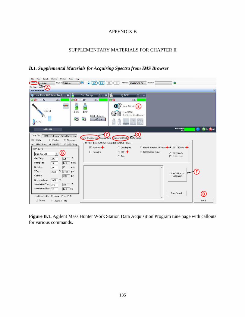
135
APPENDIX B
SUPPLEMENTARY MATERIALS FOR CHAPTER II
B.1. Supplemental Materials for Acquiring Spectra from IMS Browser
Figure B.1. Agilent Mass Hunter Work Station Data Acquisition Program tune page with callouts
for various commands.
GC
E
A
F
D
B
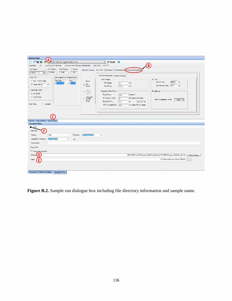
136
Figure B.2. Sample run dialogue box including file directory information and sample name.
f
A
B
C
F
E
D

137
Figure B.3. Agilent Mass Hunter IM-MS Browser interface. (A) Mass spectrum of thalidomide,
(B) drift spectra window with expanded window for thalidomide drift profile, and (C) 2-D IM-MS
window with call out of the thalidomide [M+H]+ ion species.
A
B
DC
E
F
G

138
SUPPLEMENTARY MATERIALS FOR CHAPTER III
C.1. Supplemental Materials for Theoretical and Experimental Resolving Power
Figure C.1. Correlation of theoretical drift time values obtained from equation 3 (in manuscript)
to experimental drift times for the m/z 322 ion. Each point represents 4 replicate measurements.
For drift time, theory accurately predicts the experimental results. The expanded region at low drift
field where error is highest (left inset) illustrates that the gate width contribution is within
experimental error. The right inset demonstrates the difference between experimental and
theoretical drift times, while not zero, is systematically reproducible at the higher drift fields
(beyond 8 V/cm). The higher error at low drift field is reproducible for the other ions and we infer
that this represents error associated with the extrapolation procedure used to correct the drift time
for the non-mobility component. Note here that in order to utilize the IMS drift length (78.1 cm)
in equation 3, the experimental drift times are corrected by subtracting the non-mobility time
component, as obtained by conducting the stepped drift field linear regression analysis used in
determining ion transport data [1]. The low drift field values (below 8 V/cm) are not utilized in
this linear regression analysis.
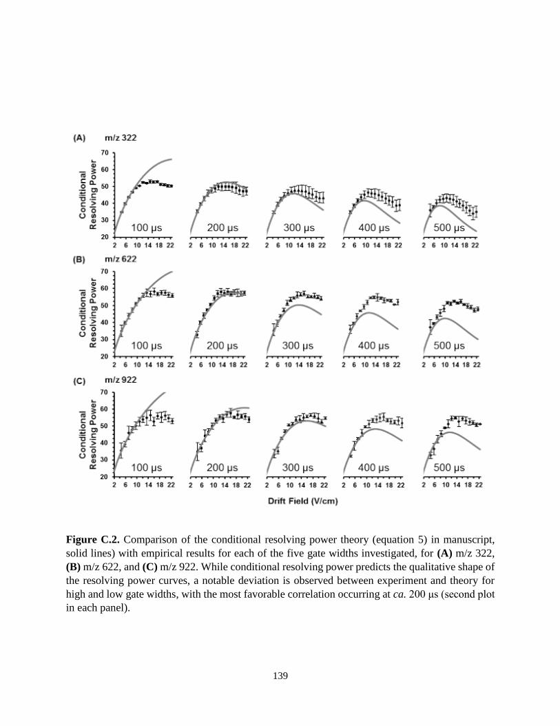
139
Figure C.2. Comparison of the conditional resolving power theory (equation 5) in manuscript,
solid lines) with empirical results for each of the five gate widths investigated, for (A) m/z 322,
(B) m/z 622, and (C) m/z 922. While conditional resolving power predicts the qualitative shape of
the resolving power curves, a notable deviation is observed between experiment and theory for
high and low gate widths, with the most favorable correlation occurring at ca. 200 μs (second plot
in each panel).

140
Figure C.3. Comparison of the semi-empirical resolving power theory (equation 7 in manuscript)
to experimental results using the coefficients determined for the current instrumentation used in
this study. Empirical results are the same as shown in Figure C.2. Good quantitative correlation is
observed for these three ions across all gate widths investigated.

141
Figure C.4. Comparison of the conditional resolving power formula with the derived
semiempirical method for a low mobility ion (ATM m/z 2722) at an applied gate width of 200 μs.
Conditional resolving power theory significantly over-predicts the resolving power at this low
mobility, which is consistent with the trend observed for the other ATM ions (Figure C.2).
Semiempirical resolving power is closer to experimental measurements, with a slight under-
prediction of the resolving power, which is similar to the correlation observed for the m/z 922
system (Figure C.3).
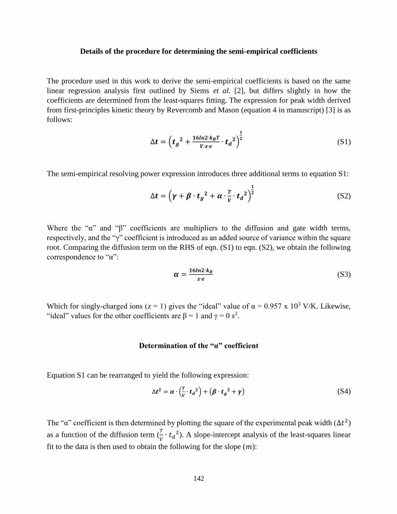
142
Details of the procedure for determining the semi-empirical coefficients
The procedure used in this work to derive the semi-empirical coefficients is based on the same
linear regression analysis first outlined by Siems et al. [2], but differs slightly in how the
coefficients are determined from the least-squares fitting. The expression for peak width derived
from first-principles kinetic theory by Revercomb and Mason (equation 4 in manuscript) [3] is as
follows:
Δ𝒕 = (𝒕𝒈𝟐 +
𝟏𝟔𝒍𝒏𝟐∙𝒌𝑩𝑻
𝑽∙𝒛∙𝒆∙ 𝒕𝒅
𝟐)
𝟏
𝟐 (S1)
The semi-empirical resolving power expression introduces three additional terms to equation S1:
Δ𝒕 = (𝜸 + 𝜷 ∙ 𝒕𝒈𝟐 + 𝜶 ∙
𝑻
𝑽∙ 𝒕𝒅
𝟐)
𝟏
𝟐 (S2)
Where the “α” and “β” coefficients are multipliers to the diffusion and gate width terms,
respectively, and the “γ” coefficient is introduced as an added source of variance within the square
root. Comparing the diffusion term on the RHS of eqn. (S1) to eqn. (S2), we obtain the following
correspondence to “α”:
𝜶 =𝟏𝟔𝒍𝒏𝟐∙𝒌𝑩
𝒛∙𝒆 (S3)
Which for singly-charged ions (z = 1) gives the “ideal” value of α = 0.957 x 10³ V/K. Likewise,
“ideal” values for the other coefficients are β = 1 and γ = 0 s2.
Determination of the “α” coefficient
Equation S1 can be rearranged to yield the following expression:
Δ𝒕𝟐 = 𝜶 ∙ (𝑻
𝑽∙ 𝒕𝒅
𝟐) + (𝜷 ∙ 𝒕𝒈𝟐 + 𝜸) (S4)
The “α” coefficient is then determined by plotting the square of the experimental peak width (Δ𝑡2)
as a function of the diffusion term (𝑇
𝑉∙ 𝑡𝑑
2). A slope-intercept analysis of the least-squares linear
fit to the data is then used to obtain the following for the slope (𝑚):

143
𝑚 = 𝛼 (S5)
and the y-intercept (𝑦0):
𝑦0 = 𝛽 ∙ 𝑡𝑑2 + 𝛾 (S6)

144
Figure C.5. Linear regression analysis used to determine the “α” coefficient, shown here for the
m/z 322 ion. Each line represents a different dataset obtained using one of five different initial ion
gate widths (100, 200, 300, 400, and 500 μs); data within each gate width is measured for eight
separate drift fields (13.4, 14.7, 16.0, 17.3, 18.6, 19.9, 21.1, and 22.4 V/cm). Note that this analysis
was conducted for nine components of the ATM solution (m/z 322, 622, 922, 1222, 1522, 1822,
2122, 2422, and 2722) and the slopes obtained from each linear fit was averaged to obtain the “α”
used in the manuscript.

145
Figure C.6. Variation of all “α” values obtained from eight different ions as a function of the ion’s
reduced mobility value (K0). No strong correlation between “α” and K0 was observed, and so the
average “α” (0.000910 ± 0.00005 V/K) was utilized in all subsequent analysis.

146
Determination of the “β” coefficient
As was done previously, equation (S1) can be rearranged to yield the following expression:
Δ𝒕𝟐 = 𝜷 ∙ (𝒕𝒈𝟐) + (𝜶 ∙
𝑻
𝑽∙ 𝒕𝒅
𝟐 + 𝜸) (S7)
The “β” coefficient is determined here by plotting the square of the experimental peak width (Δ𝒕2)
as a function of the square of the gate width (𝒕𝒈𝟐). A slope-intercept analysis of the least-squares
linear fit to the data is then used to obtain the following for the slope (𝑚):
𝑚 = 𝛽 (S8)
and the y-intercept (𝒚𝟎):
𝑦0 =∙ 𝛼 ∙𝑇
𝑉∙ 𝑡𝑑
2 + 𝛾 (S9)
The slope corresponding to the highest field (22.4 V/cm) is used as the “β” coefficient in
subsequent analyses as this represents the situation in which ions spend the least amount of time
in the drift tube, and thus would exhibit the strongest “memory” of the initial gating event.

147
Figure C.7. Linear regression analysis used to determine the “β” coefficient, shown here for the
m/z 922 ion. A best fit line was plotted for data from each of five field strengths (17.3, 18.6, 19.8,
21.1, and 22.4 V/cm) with each data set representing measurements obtained from the five gate
widths evaluated (100, 200, 300, 400, and 500 μs). While additional data was obtained at lower
drift fields, the higher fields represent conditions in which ions transit the drift region faster and
thus would retain more memory of the influence of the initial gating event. This also introduces
some additional variability in the data, as noted by the inconsistent slope at the highest field
investigated (22.4 V/cm).
148
Determination of the “γ” coefficient
The determination of “γ” described here deviates slightly from the original work by Siems et al.
In the original work, “γ” was determined by performing a linear regression analysis on all y-
intercept values obtained from the “α” and “β” plots to generate new datasets which represent
hypothetical data in the limits of zero gate width, and infinite voltage, respectively. The y-
intercepts obtained from these hypothetical datasets is “γ” [2]
Here, we utilize the values obtained for “α” and “β” directly into the y-intercept expressions
(equation (C.6) and equation (C.9) and solve for “γ” directly for each linear fit. This results in a
tabulated set of “γ” values for each ion investigated. To obtain “γ” from the “α” expression via.
equation (C.6), the “β” obtained at the highest drift field is utilized, which represents the case
where ions spend the least amount of time in the drift region. This also simplifies the analysis since
only a single “α” value is evaluated for each data series. Obtaining “γ” from the “β” expression
via. equation (C.9) is more straightforward and involves solving for “β” by utilizing the average
“α” obtained for each ion. The average is rationalized here since “α” does not exhibit a strong
dependence on the specific ion utilized in the analysis (Figure C.6).

149
Figure C.8. Regression analysis used to determine the function which relates the semi-empirical
coefficients (β and γ) to the ion’s reduced mobility, K0. (A) The curve best fitting the data is a
power fit based on eight high mass ions in the ATM solution (m/z 622, 922, 1222, 1522, 1822,
2122, 2422, and 2722). (B) Fitting parameters for the “β” term as a function of mobility for the
m/z 322, 622, and 922 ions. These equations are reintroduced into the semi-empirical resolving
power expression (equation 7 in the manuscript) in order to introduce the ion-specific contribution
to each of these terms.

150
Using the coefficients and coefficient expressions summarized in Table 1 in the manuscript, the
semi-empirical resolving power equation is expanded to the following functional form:
𝑹𝑺𝑬 =
𝑳
𝑲𝟎∙𝑬𝟎∙(
𝟐𝟕𝟑.𝟏𝟓
𝑻∙
𝑷
𝟕𝟔𝟎)∙𝟏𝟎𝟎𝟎
[(𝟎.𝟎𝟒𝟑𝟒∙𝑲𝟎−𝟐.𝟖𝟏𝟏)+(𝟎.𝟑𝟏𝟒𝟓∙𝑲𝟎
𝟐−𝟎.𝟎𝟑𝟓∙𝑲𝟎)·𝒕𝒈𝟐+(𝟎.𝟎𝟎𝟎𝟗𝟏)·
𝑻
𝑽∙(
𝑳
𝑲𝟎∙𝑬𝟎∙(
𝟐𝟕𝟑.𝟏𝟓
𝑻∙
𝑷
𝟕𝟔𝟎)∙𝟏𝟎𝟎𝟎)
𝟐
]
𝟎.𝟓 (S10)
The 103 multipliers in the numerator and the RHS of the denominator within the square root term
is necessary to convert drift time to milliseconds, which is the unit used in the semi-empirical
expressions. Note also that the gate time (𝑡𝑔) term is in milliseconds (whereas conventionally this
is reported in microseconds).
References
1. May, JC; Goodwin, CR; Lareau, NM; Leaptrot, KL; Morris, CB; Kurulugama, RT;
Mordehai, A; Klein, C; Barry, W; Darland, E; Overney, G; Imatani, K; Stafford, GC; Fjeldsted,
JC; McLean, JA; “Conformational Ordering of Biomolecules in the Gas Phase: Nitrogen Collision
Cross Sections Measured on a Prototype High Resolution Drift Tube Ion Mobility-Mass
Spectrometer”, Analytical Chemistry 86, 2107-2116 (2014).
2. Siems, WF; Wu, C; Tarver, EE; Hill Jr., HH; Larsen, PR; McMinn, DG; “Measuring the
Resolving Power of Ion Mobility Spectrometers” Analytical Chemistry 66, 4195-4201 (1994).
3. Revercomb, HE; Mason, EA; “Theory of Plasma Chromatography/Gaseous
Electrophoresis— A Review” Analytical Chemistry 47(7), 970-983 (1975).

151
SUPPLEMENTARY MATERIALS FOR CHAPTER IV
D.1. Supplemental Materials for Investigation of Leucine and Isoleucine Isomers
D.1.1. Comments on measuring CCS and Ion Mobility Distributions Presented in this Work
All IM-MS measurements in this study were obtained in positive ionization mode utilizing
incremental steps of increasing drift field in the mobility portion of the Agilent 6560 IM-MS with
nitrogen as the drift gas. After the non-mobility flight times (i.e. dead times) were subtracted at
each voltage and the collision cross section for each analyte was calculated, the equation shown
in Figure C.3 was used to convert the time component of the experiment (x axis) to CCS. The
optimal drift field occurs at 14.7 V/cm for the analytes examined in this study (see Figure C.2),
and hence the distributions at this drift field are presented in Figures C.4 and C.5. All theoretical
(modeled) spectra are generated using Equation 4 of the main text.
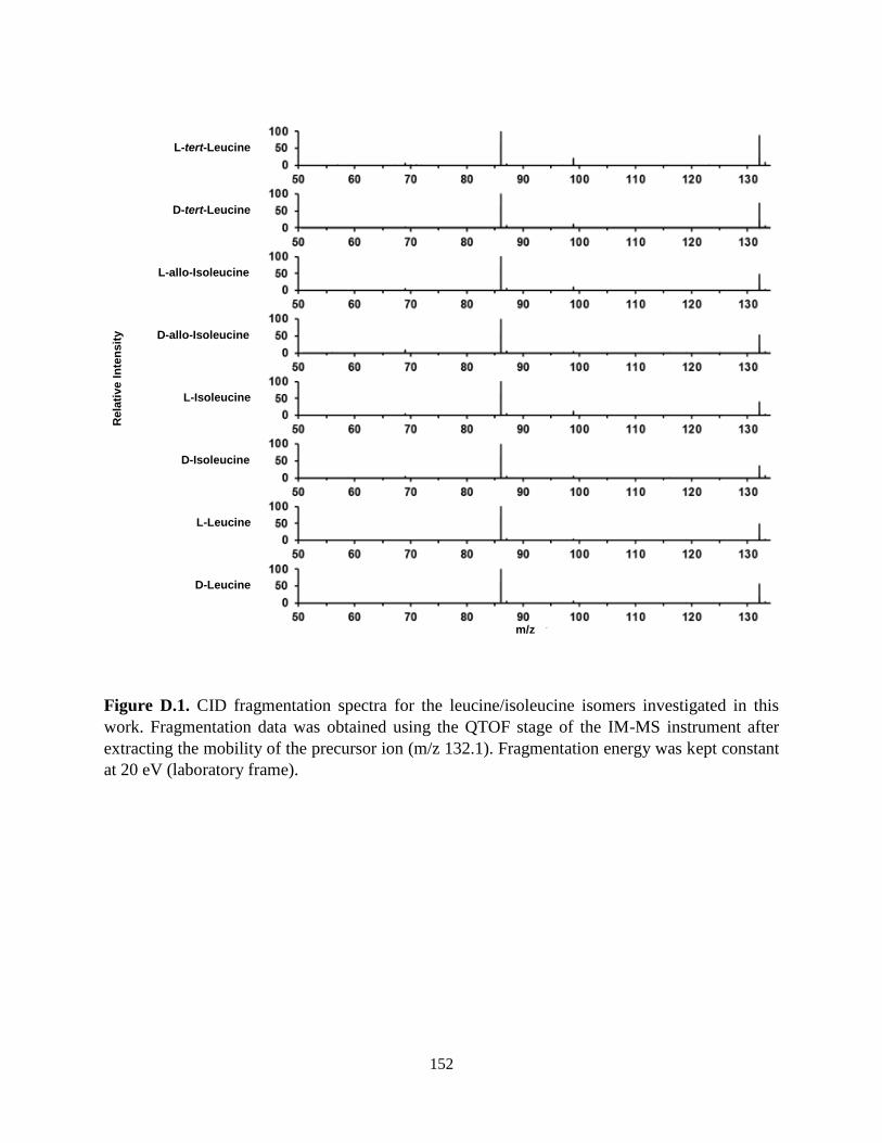
152
Figure D.1. CID fragmentation spectra for the leucine/isoleucine isomers investigated in this
work. Fragmentation data was obtained using the QTOF stage of the IM-MS instrument after
extracting the mobility of the precursor ion (m/z 132.1). Fragmentation energy was kept constant
at 20 eV (laboratory frame).
L-tert-Leucine
D-tert-Leucine
L-allo-Isoleucine
D-allo-Isoleucine
L-Isoleucine
D-Isoleucine
L-Leucine
D-Leucine
m/z
Rela
tive I
nte
nsit
y

153
Figure D.2. An overlaid IM spectrum obtained at different drift fields which demonstrates the
separation of a mixture of L-norleucine and L-isoleucine for various applied drift fields. The
optimal separation occurs at the maximum observed resolving power, here 61 resolving power at
14.7 V/cm, which results in a ca. 50% valley for this isomer pair.
0
25
50
75
100
10 15 20 25 30 35 40
R.A
. (%
)
Ion Mobility Drift Time (ms)
7 V/cm
Rp = 46
8 V/cm
Rp = 4910 V/cm
Rp = 54
12 V/cm
Rp = 59
17 V/cm
Rp = 54
20 V/cm
Rp = 54
14 V/cm
Rp = 61

154
Table D.1. Cross section data for each isomer of C6H13NO2 investigated in this work. The standard
deviation of the CCS for each measurement (RSD ca. 0.2%) is included in addition to the
corresponding reduced mobility (ko), drift time, FWHM, and resolving power.
MoleculeCCS (Å2)
σ CCS (Å2)
td(14.7 V/cm)
FWHM (ms)
Ko(cm2/V s) RP
D-Leucine 135.2 0.3 19.14 0.32 1.634 59.8
L-Leucine 135.1 0.3 19.1 0.34 1.635 56.2
D-Isoleucine 133.3 0.3 18.9 0.33 1.658 57.3
L-Isoleucine 133.5 0.3 18.89 0.32 1.655 59.0
D-allo-Isoleucine 133.1 0.3 18.87 0.30 1.66 62.9
L-allo-Isolecuine 132.9 0.2 18.87 0.32 1.663 59.0
D-tert-Leucine 132.5 0.2 18.76 0.34 1.668 55.2
L-tert-Leucine 132.4 0.3 18.77 0.33 1.669 56.9
L-Norleucine 136.6 0.3 19.35 0.32 1.617 60.5
6-Aminocaproic Acid 129.3 0.2 18.27 0.30 1.709 60.9
N-N-Dimethylglycine 127.5 0.3 18.15 0.32 1.732 56.7

155
Figure D.3. Linear correlation between drift time and collision cross section obtained from the
Mason-Schamp equation (below) for isomers analyzed in this study. Drift times correlate to peak
centroids at 14.7 V/cm in a uniform field instrument. Error bars indicate the uncertainty in the CCS
measurement.
Cross sections were obtained by calculating the corrected drift time and incorporating various
laboratory parameters of the experiment including ion mass (mion), gas mass (mgas), drift voltage
(V), drift tube length (L), temperature (T) and pressure (P).
Ω =𝟑𝒁𝒆𝒄
𝟏𝟔𝑵∗ (
𝟐𝝅
𝒌𝒃𝑻)
𝟏
𝟐∗ (
𝒎𝒊𝒐𝒏+𝒎𝒈𝒂𝒔
𝒎𝒊𝒐𝒏∗𝒎𝒈𝒂𝒔)
𝟏
𝟐∗ (
𝑽∗𝒕𝒅
𝑳𝟐 ∗𝟐𝟕𝟑.𝟏𝟓
𝑻∗
𝑷
𝟕𝟔𝟎 𝒕𝒐𝒓𝒓 )
CCS = 7.32 (tdrift) - 5.00
R² = 0.99
126
128
130
132
134
136
138
18 18.5 19 19.5
Co
llis
ion
Cro
ss S
ecti
on
(Å
2)
Ion Mobility Drift Time (ms)

156
Figure D.4. Individual drift spectra from Figure 4.2 B with dotted lines to indicate the range of
CCS data.
0
50
100
120 125 130 135 140 145
0
50
100
120 125 130 135 140 145
0
50
100
120 125 130 135 140 145
0
50
100
120 125 130 135 140 145
0
50
100
120 125 130 135 140 145
0
50
100
120 125 130 135 140 145
0
50
100
120 125 130 135 140 145
0
50
100
120 125 130 135 140 145
0
50
100
120 125 130 135 140 145
0
50
100
120 125 130 135 140 145
0
50
100
120 125 130 135 140 145
L-Norleucine
D-Leucine (2R)
L-Leucine (2S)
L-Isoleucine (2S,3S)
L-allo-Isoleucine (2S,3R)
L-tert-Leucine (2S)
D-tert-Leucine (2R)
D-allo-Isoleucine (2R,3S)
6-Aminocaproic acid
N,N-Dimethylglycine ethyl ester
D-Isoleucine (2R,3R)
Rela
tive A
bu
nd
an
ce (
%)
Collision Cross Section (Å2)
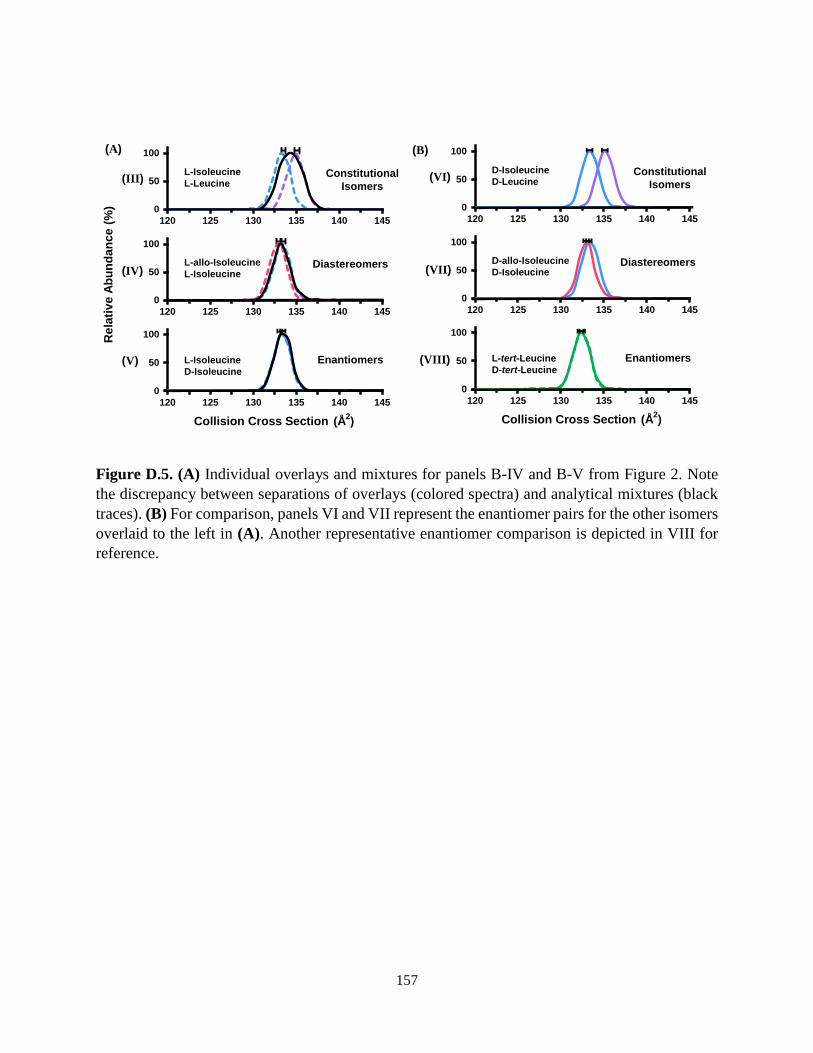
157
Figure D.5. (A) Individual overlays and mixtures for panels B-IV and B-V from Figure 2. Note
the discrepancy between separations of overlays (colored spectra) and analytical mixtures (black
traces). (B) For comparison, panels VI and VII represent the enantiomer pairs for the other isomers
overlaid to the left in (A). Another representative enantiomer comparison is depicted in VIII for
reference.
0
50
100
120 125 130 135 140 145
Rela
tiv
e A
bu
nd
an
ce (
%)
0
50
100
120 125 130 135 140 145
Collision Cross Section (Å2)
0
50
100
120 125 130 135 140 145
L-allo-Isoleucine
L-Isoleucine
L-Isoleucine
D-Isoleucine
(IV)
(V)
Diastereomers
Enantiomers
L-Isoleucine
L-Leucine(III) Constitutional
Isomers
0
50
100
120 125 130 135 140 145
0
50
100
120 125 130 135 140 145
Collision Cross Section (Å2)
0
50
100
120 125 130 135 140 145
D-allo-Isoleucine
D-Isoleucine
L-tert-Leucine
D-tert-Leucine
(VII)
(VIII)
Diastereomers
Enantiomers
D-Isoleucine
D-Leucine(VI) Constitutional
Isomers
(A) (B)

158
Figure D.6. Comparison highlighting the effect of isomer abundance ratios on separation
efficiency. Abundance ratios have significantly more of an impact on separation efficiency for
more difficult separations (i.e. lower percent difference in CCS). For isomers that are 2-1.5%
different in CCS both compounds are distinguishable in a 3:1 ratio at 100 resolving power. As the
molecules become more structurally similar (similar cross sections, and hence lower percent
difference) the isomer ratio becomes increasingly more important in order to observe both species
in a mixture.
0
50
100
120 125 130 135 140 145
0
50
100
120 125 130 135 140 145
0
50
100
120 125 130 135 140 145
0
50
100
120 125 130 135 140 145
0
50
100
120 125 130 135 140 145
0
50
100
120 125 130 135 140 145
2% Diff. in CCS
1.5% Diff. in CCS
1% Diff. in CCS
1:1 Isomer Ratio 3:1 Isomer Ratio
Collision Cross Section (Å2) Collision Cross Section (Å2)
*Both peaks simulated
at 100 resolving power

159
SUPPLEMENTARY MATERIALS FOR CHAPTER V
E.1. Supporting Information for Ion Mobility Cross Section, Resolving Power and Resolution
Comments on Modeling Ion Mobility Distributions Presented in this Work
In this Supporting Information we describe each step in the process to fit Gaussian
distributions to existing publication data (see Figure C.1). We also include additional figures
related to IM separations in TWIMS related to the discrepancy between reporting time based
resolving power versus CCS based Rp (see Figures C.2 and C.3). Lastly we include descriptive
citations for the 22 sources examined in this work and provide links to the non-peer reviewed
sources. Finally, we discuss each previously reported IM separation in detail and any pertinent
information that provides context for the empirical measurements (e.g. cited resolving power,
CCS, and chemical identity of molecules/isomers that are separated).

160
Figure E.1. Workflow for overlaying Gaussian fits to published spectra. This method was applied
for all sources referenced in Figures 2, 3, and 4. Two-peak resolution values (Rpp) were calculated
by using equation 7 in the manuscript along with relevant information noted from the source
publication (i.e. drift time, CCS, and FWHM). Letter abbreviations added to delinate figures in
caption (here A). Reproduced/Adapted with permission from Ref. A with permission from Michael
Groessl, primary author (ASMS 2016, see Ref. A).
1. Examine original source data.(Must include CCS or Reduced mobility data)
2. Overlay Excel template of Gaussian Fit-Match X and Y axis.
0
50
100
35.5 36 36.5 37
3. Extract x axis value (drift time, CCS, etc.) and adjust peak width to match source – Calculate Rp and Resolution
Drift Tube (Uniform Field) Ion Mobility
Re
l. In
ten
sity
Drift Time (ms)
PC 18:1 (E/Z)Rp ≈ 267
0.8% Diff. CCS
Groessl, M. 2016
Ref. X
0
50
100
35.5 36 36.5 37
4. Resize to fit publication template
4. Change color and edit publication notes, labels, etc. as necessary.
5. Overlay Excel Gaussian fit in current publication
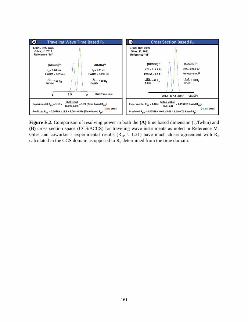
161
Figure E.2. Comparison of resolving power in both the (A) time based dimension (td/fwhm) and
(B) cross section space (CCS/ΔCCS) for traveling wave instruments as noted in Reference M.
Giles and coworker’s experimental results (Rpp ≈ 1.21) have much closer agreement with Rp
calculated in the CCS domain as opposed to Rp determined from the time domain.
(SDGRG)2+
CCS ≈ 222.7 Å2
FWHM ≈ 5.9 Å2
CCS
Δ CCS≈ 38 Rp
Experimental Rpp = 1.18 x = 1.21 (Time Based Rpp) (1.79-1.60)
(0.095-0.09)Experimental Rpp = 1.18 x = 1.19 (CCS Based Rpp)
(222.7-211.7)
(5.0+5.9)
Predicted Rpp = 0.00589 x 18.3 x 5.06 = 0.546 (Time Based Rp) Predicted Rpp = 0.00589 x 40.0 x 5.06 = 1.19 (CCS Based Rp)
5.06% Diff. CCS
Giles, K. 2011
Reference “M”
td ≈ 1.60 ms
(GRGDS)2+
FWHM ≈ 0.09 ms
td
FWHM≈ 18 Rp
CCS ≈ 211.7 Å2
(GRGDS)2+
FWHM ≈ 5.0 Å2
CCS
Δ CCS≈ 42 Rp
Traveling Wave Time Based RpA
(SDGRG)2+
td ≈ 1.79 ms
FWHM ≈ 0.095 ms
td
FWHM≈ 19 Rp
Cross Section Based RpB
Drift Time (ms)
(-0.1% Error)(55% Error)
CCS (Å2)
5.06% Diff. CCS
Giles, K. 2011
Reference “M”
1 1.5 2 203.7 217.2 230.7

162
Figure E.3. Separation of Ruthenium complexes (ortho/para isomers) as described in reference
“N”. (A) Time based resolving power, which does not accurately reflect the separation efficiency
of the device. (B) Cross section based Rp is a more accurate depiction of TWIMS selectivity.
Reproduced/Adapted with permission from Ref. 6. Wiley and Sons, 2011.

163
Figure E.4. Separation of cis/trans lipid isomers in the SLIM traveling wave currently undergoing
development by Smith and coworkers at PNNL. As with the commercial TWIMS devices, time
based resolving power is not an accurate descriptor of separation efficiency (A). Conversion to
CCS based Rp (B) is more reflective of the analytical selectivity of this device.
Reproduced/Adapted with permission from Ref. 48 in main text, Wiley and Sons, 2016.

164
First Author
Reference Point
Percent Difference in
CCS (%)1
Experimental Resolving
Power (Rp)2
Experimental Resolution
(Rpp
)3
Predicted Resolution
(Rpp
)4
Percent Error in Resolution
(%)5
Dispersion Axis Used in the
Calculations
TW
IMS
Deng, L. K 0.4 342 0.72 0.72 -0.7 td CCS
Giles, K. L 1.5 476 4.34 4.34 0.1 td CCS
Giles, K. M 5.1 40 1.19 1.19 -0.1 td CCS
Giles, K. N 5.7 41 1.38 1.38 0.1 td CCS
Hofmann, J. O 5.9 43 1.49 1.49 0.0 td CCS
1. Calculated from equation 4. 2. Calculated from equation 1 using the CCS. 3. Calculated from equation 2 using the CCS as the dispersion axis. 4. Calculated from equation 3 using the CCS-based definition for R
p.
5. Calculated from equation 5.
Table E.1. TWIMS separation parameters calculated by defining the separation equations in terms
of the CCS.

165
Table E.2. Tabulated relationship between CCS-based resolving power and the percent difference
in collision cross section.
Resolving Power
% Difference in CCS resolvable at Half Height
400 0.36 375 0.38 350 0.40 325 0.43 300 0.47 275 0.51 250 0.56 225 0.63 200 0.70 175 0.81 150 0.94 125 1.13 100 1.41 75 1.88 50 2.82 25 5.63
Inc
reasin
g Io
n M
ob
ilit
y S
ele
cti
vit
y
In
cre
asin
g D
iffi
cu
lty o
f Is
om
er
Sep
ara
tio
n

166
Supplemental References for Chapter 5.
(A) Groessl, M.; Graf, S.; Lisa, M.; Holcapek, M.; Sampaio, J.; Dick, B.; Vogt, B.; Knochenmuss,
R. “Analysis of Isomeric Lipids by High Resolution Ion Mobility Mass Spectrometry”. 63rd
Annual ASMS Conference on Mass Spectrometry and Allied Topics, St. Louis, MO (2015) - Poster.
Link: http://www.tofwerk.com/wp-content/uploads/2015/06/Tofwerk_WP262_asms2015.pdf
(accessed March 1, 2017)
(B) Groessl, M.; Graf, S. “Separation of Isomers in Lipidomics and Metabolomics Experiments
by High Resolution Ion Mobility Spectrometry-Mass Spectrometry (IMS-MS)” 64th Annual ASMS
Conference on Mass Spectrometry and Allied Topics, San Antonio, TX (2016) - Poster.
Link: http://www.tofwerk.com/wp-
content/uploads/2016/06/TOFWERK_ASMS2016_TP469.pdf (accessed March 1, 2017)
(C) Groessl, M.; Graf, S. “Separation of Isomers in Lipidomics and Metabolomics Experiments
by High Resolution Ion Mobility Spectrometry-Mass Spectrometry (IMS-MS)” 64th Annual ASMS
Conference on Mass Spectrometry and Allied Topics, San Antonio, TX (2016) - Poster.
Link: http://www.tofwerk.com/wp-
content/uploads/2016/06/TOFWERK_ASMS2016_TP469.pdf (accessed March 1, 2017)
(D) Asbury, G. R.; Hill, H.H.; J. “Evaluation of Ultrahigh Resolution Ion Mobility Spectrometry
as an Analytical Separation Device in Chromatographic Terms” Journal of Microcolumn
Separations 12, 172-178 (2000). Figure 5, middle panel.
(E) Groessl, M.; Klee, S.; Graf, S.; “High Resolution Ion Mobility Spectrometry-Mass
Spectrometry (IMS-MS) for Separation of Isomers in Natural Products and Complex Mixtures”
64th Annual ASMS Conference on Mass Spectrometry and Allied Topics, San Antonio, TX (2016)
- Poster.
(F) Pierson, N.A.; Chen L.; Valentine, S. J.; Russell, D. H.; Clemmer, D. E. “Number of Solution
States of Bradykinin from Ion Mobility And Mass Spectrometry Measurements” Journal of the
American Chemical Society 133, 13810-13813 (2011). Figure 2, 90:10 dioxane:water spectrum.
(G) Tang, X.; Bruce, J. E.; Hill, H. H. “Design and Performance of an Atmospheric Pressure Ion
Mobility Fourier Transform Ion Cyclotron Resonance Mass Spectrometer” Rapid
Communications in Mass Spectrometry 21, 1115-1122 (2007). Figure 6, mixture.
(H) Dodds, J. N.; May, J. C.; McLean, J. A. “Investigation of the Complete Suite of Leucine and
Isoleucine Isomers: Toward Prediction of Ion Mobility Separation Capabilities” Analytical
Chemistry 89, 952-959 (2016). Figure 3B.
(I) Gaye, M. M.; Nagy, G.; Clemmer, D. E.; Pohl, N. L. B. “Multidimensional Analysis of 16
Glucose Isomers by Ion Mobility Spectrometry” Analytical Chemistry 88, 2335-2344 (2016).
Figure 2.
167
(J) Adamov, A.; Mauriala, T.; Teplov, V.; Laakia, J.; Pedersen, C. S.; Kotiaho, T.; Sysoev, A. A.
“Characterization of a High Resolution Drift Tube Ion Mobility Spectrometer with a Multi-Ion
Source Platform” International Journal of Mass Spectrometry 298, 24-29 (2010). Figure 4B.
(K) Deng, L.; Ibrahim, Y. M.; Baker, E. S.; Aly, N. A.; Hamid A. M.; Zhang, X.; Zheng, X.;
Garimella, S. V. B.; Webb, I. K.; Prost, S. A.; Sandoval, J. A.; Norheim, R. V.; Anderson, G. A.;
Tolmachev, A. V.; Smith, R. D. “Ion Mobility Separations of Isomers based upon Long Path
Length Structures for Lossless Ion Manipulations Combined with Mass Spectrometry”
ChemistrySelect 1, 2396-2399 (2016). Figure 2C.
(L) Giles, K.; Ujma, J.; Wildgoose, J.; Green, M. R.; Richardson, K.; Langridge, D.; Tomczyk, N.
“Design and Performance of a Second-Generation Cyclic Ion Mobility Enabled Q-TOF” 65th
Annual ASMS Conference on Mass Spectrometry and Allied Topics, Indianapolis, IN (2017) –
Poster.
Link: http://www.waters.com/webassets/cms/library/docs/2017asms_giles_cyclic.pdf (Accessed
August 29, 2017)
(M) Giles, K.; Williams J. P.; Campuzano, J. “Enhancements in Travelling Wave Ion Mobility
Resolution” Rapid Communications in Mass Spectrometry 25, 1559-1566 (2011). Figure 2, bottom
panel.
(N) Giles, K.; Williams J. P.; Campuzano, J. “Enhancements in Travelling Wave Ion Mobility
Resolution” Rapid Communications in Mass Spectrometry 25, 1559-1566 (2011). Figure 3.
(O) Hofmann, J.; Hahm, H. S.; Seeberger, P. H.; Pagel, K. “Identification of Carbohydrate
Anomers using Ion Mobility-Mass Spectrometry” Nature 526, 241-244 (2015). Figure 2C, third
panel (isomers 6 and 3).
(P) Silveira, J. A.; Ridgeway, M. E.; Park, M. A. “High Resolution Trapped Ion Mobility
Spectrometry of Peptides” Analytical Chemistry 86, 5624-5627 (2014). Figure 2B.
(Q) Commercial vendor (Bruker) brochure for the timsTOFTM instrument, “1844502 –
timsTOF™. Flexibility to Empower Your Ideas” (2016). Figure 4C.
Link: https://www.bruker.com/fileadmin/user_upload/8-PDF-
Docs/Separations_MassSpectrometry/Literature/Brochures/1844502_timsTOF_brochure_05-
2016_ebook.pdf (Accessed March 1, 2017)
(R) Commercial vendor (Bruker) brochure for the timsTOFTM instrument, “1844502 – timsTOF™.
Flexibility to Empower Your Ideas” (2016). Figure 2.
Link: https://www.bruker.com/fileadmin/user_upload/8-PDF-
Docs/Separations_MassSpectrometry/Literature/Brochures/1844502_timsTOF_brochure_05-
2016_ebook.pdf (Accessed March 1, 2017)
(S) Barnett, D. A.; Ells, B.; Guevremont, R.; Purves, R. W. “Separation of Leucine and Isoleucine
by Electrospray Ionization-High Field Asymmetric Waveform Ion Mobility Spectrometry-Mass
168
Spectrometry” Journal of the American Society for Mass Spectrometry 10, 1279-1284 (1999).
Figure 4, lower trace.
(T) Lee, S.; Ewing, M. A.; Nachtingall, F. M.; Kurulgama, R. T.; Valentine, S. J.; Clemmer, D. E.
“Determination of Cross Sections by Overtone Mobility Spectrometry: Evidence for Loss of
Unstable Structures at Higher Overtones” Journal of Physical Chemistry B 114, 12406-12415
(2010). Figure 2, panel 2 (21st harmonic frequency number).
(U) Glaskin, R. S.; Valentine, S. J.; Clemmer, D. E. “A Scanning Frequency Mode for Ion
Cyclotron Mobility Spectrometry” Analytical Chemistry 82, 8266-8271 (2010). Figure 4, third
inset.
(V) Glaskin, R. S.; Valentine, S. J.; Clemmer, D. E. “A Scanning Frequency Mode for Ion
Cyclotron Mobility Spectrometry” Analytical Chemistry 82, 8266-8271 (2010). Figure 4, first
inset.

169
APPENDIX E
CURRICULUM VITAE
James N. Dodds, Ph.D.
Vanderbilt University Department of Chemistry
7330 Stevenson Center, Station B 35-1822
Nashville, TN 37235
Lab: (615)-343-4563
EDUCATION
Vanderbilt University Nashville, TN
Ph.D. in Chemistry Expected May 2018
Dissertation: Investigation Of Separation Strategies for Bioanalytical Methods: Chromatography,
Ion Mobility, and Mass Spectrometry
Advisor: Dr. John A. McLean
University of North Georgia Dahlonega, GA
Advisor: Dr. Dan Thompson May 2013

170
RESEARCH EXPERIENCE
Graduate Research Assistant Aug 2013-May 2018
Vanderbilt University, Nashville, TN
Advisor: Dr. John A. McLean
Development of separation strategies for the characterization of complex biological matrices using
chromatography, ion mobility, and mass spectrometry.
Independent Undergraduate Research Aug 2012-Dec 2012
University of North Georgia, Dahlonega, GA
Advisor: Dr. Dan Thompson
Designed an interface between a thermogravimetric analyzer and a single quadrupole mass
spectrometer to analyzer pyrolysis byproducts of analytical standards.
PUBLICATIONS
1. Dodds, J. N.; May, J. C.; McLean, J. A. “Correlating Resolving Power, Resolution, and
Collision Cross Section: Unifying Cross-Platform Assessment of Separation Efficiency in Ion
Mobility Spectrometry.” Anal. Chem. 2017, 89, 12176-12184.
2. Dodds, J. N.; May, J. C.; McLean, J. A. “Investigation of the Complete Suite of Leucine and
Isoleucine Isomers: Toward Prediction of Ion Mobility Separation Capabilities.” Anal. Chem.
2017, 89, 952-959.
3. May, J. C.; Dodds, J. N.; Kurulugama, R. T.; Stafford, G. C.; Fjeldsted, J. C.; McLean, J. A.
“Broadscale Resolving Power Performance of a High Precision Uniform Field Ion Mobility-
Mass Spectrometer. Analyst 2015, 140, 6824-6833.
4. Dodds, J. N.; May, J. C.; McLean, J. A. “Chiral Strategies in Mass Spectrometry: Integration
of Chromatography, Electrophoresis, and Gas-Phase Mobility.” Book Chapter in Chiral
Analysis: Advances in Spectroscopy, Chromatography, and Emerging Methods. 2017.
5. Phillips, S. T.; Dodds, J. N.; May, J. C.; McLean, J. A. “Isomeric and Conformational Analysis
of Small Drug and Drug-Like Molecules by Ion Mobility-Mass Spectrometry (IM-MS).” Book
Chapter in Methods in Molecular Biology Series. 3rd Ed. 2017

171
PRESENTATIONS
1. Dodds, J. N.; May, J. C.; McLean, J. A. “A Theoretical and Empirical Approach to Separating
Isomer Classes in Uniform Field Ion Mobility.” 65th ASMS, San Antonio, TX (Spring 2016)
ORAL.
2. Dodds, J. N.; May, J. C.; McLean, J. A. “Ion Mobility and the Omics: The Challenge of
Separating Isomeric Systems.” SciX 2017, Reno, NV (Fall 2017) ORAL.
3. Dodds, J. N.; May, J. C.; McLean, J. A. “Correlating Resolving Power, Resolution, and
Collision Cross Section: Broadscale Depiction of Separation Efficiency in Ion Mobility
Spectrometry.” 66th ASMS, Indianapolis, IN (Spring 2017) POSTER.
4. Dodds, J. N.; May, J. C.; McLean, J. A. “Correlating Resolving Power, Resolution, and
Collision Cross Section: Broadscale Depiction of Separation Efficiency in Ion Mobility
Spectrometry.” 66th ASMS, Indianapolis, IN (Spring 2017) POSTER.
5. Dodds, J. N.; May, J. C.; McLean, J. A. “Improving the Separation of Isomers in Ion Mobility-
Mass Spectrometry.” Quantitative Chemical Biology Conference, Nashville, TN (Fall 2016)
POSTER.
6. Dodds, J. N.; Leaptrot, K. L.; May, J. C.; McLean, J. A. “Resolution and Resolving Power
Studies Investigating the Separation Capabilities of Drift Tube and Traveling Wave Ion
Mobility-Mass Spectrometers.” 64th ASMS, St. Louis, MO (Spring 2015) POSTER.
7. Dodds, J. N.; May, J. C.; McLean, J. A. “Investigating the Ion Mobility Resolving Power of a
Commercially Available Uniform Ion Mobility-Mass Spectrometer.” Southeastern Region
Meeting of the American Chemical Society, Nashville, TN (Fall 2014) POSTER.
TEACHING EXPERIENCE
1. Head Teaching Assistant for General Chemistry Laboratory Courses (Spring 2016).
2. Teaching Assistant for General Chemistry Laboratory Course (104 A/B) – Assisted instructor
in laboratory practicals and weekly study sessions (Fall 2013 – Fall 2015).
3. Teaching Assistant for General Chemistry for Non-Science Majors Laboratory Course (101) –
Assisted instructor in laboratory practicals and preparation of chemical reagents (Spring 2016).

172
Perspectives and Outlooks
With the state of the ion mobility community expanding so rapidly, the future directions of the
research provided in this document allow for multiple paths of expansion related to this work.
Using the higher resolution instruments described in Chapter 5 illustrates the bright future of
separation in store for ion mobility. For example, a new professor coming into the field would
have several distinct directions for research topics in the near future. Provided sufficient funding,
a new professor could theoretically use the relationships described in this work to study previously-
inseparable species in complex mixtures. As a concrete example, the diastereomers of L-allo-
isoleucine and L-isoleucine described in Chapter 4 have yet to be separated by ion mobility
analysis alone. In this work we illustrated that these two diastereomers possess collision cross
section values which are about 0.4% different in size. While this difference is not large enough to
separate using the instrumentation currently available in our laboratory (ca. 60 Rp), the new
instruments (e.g. TofWerk HP-Drift Tube and Bruker’s timsTOF) have sufficient resolving power
(ca. 300+ Rp) to separate these compounds. The physical analysis of this specific experiment
would unambiguously demonstrate the predictive ability of the equations described in this work to
model ion mobility separations prior to an empirical experiment. It is also very plausible that the
level of selectivity provided with access to the newest instrumentation in ion mobility spectrometry
would provide further separation across a host of biological classes (e.g. cis/trans lipids and α/β
linkages in carbohydrate chemistry). While often only a sole stereoisomer is responsible for
biological activity (e.g. L- specific amino acids), the additional selectivity of ion mobility could
highlight uncommon instances when the least-preferred chiral variant is included in a sample,
potentially highlighting specific bioanalytical activity that might not have been otherwise
characterized. Furthermore, without limited funding it would be possible to purchase each high

173
resolution ion mobility platform variant (TofWerk HP-Drift Tube, timsTOF, and Water’s Cyclic
TWIMS G2S after commercialization) and this process would provide a unifying experimental
separation group for an established set of ion mobility separations. The principle shortcoming of
Chapter 5 in this work is that most research into ion mobility separations is spread across a wide
host of compounds, and very rarely are two or more identical mixtures ever examined across
platforms. Provided unlimited funding, if each of the above instruments were centralized in one
research facility translational experiments across platforms would highlight the intricacies of
separation specific to each device (i.e. TWIMS, DTIMS, TIMS, etc.).
While these ideas are very achievable in terms of purchasing analytical standards and
subsequent analysis by each instrument type, the monetary investment of each platform is around
$1,000,000 USD. Also, while the studies described would be very exciting, they would probably
only be highlighted in a single publication, which is not an ideal return on investment. Towards
this directive in a realistic setting, a new P.I. in the field who would like to examine this hypothesis
would be better served by forming collaborations with the research groups who currently house
each type of high resolution instrument. Also, it is often imperative to have a long working history
with each specific platform in order to gain the highest separation capability possible for each
device (see Chapter 3). With these practical concerns, it seems having a central scientist travel to
each research group along with the samples of interest could follow the experiment within each
group under the supervision of the local instrument expert, ensuring that each IM-MS separation
is operated at peak capacity.
The other major area of interest in ion mobility spectrometry described in this work is related
to developing CCS libraries as an addition identifier of chemical composition. Towards this end,
without financial restrictions it would be a herculean undertaking to purchase every analytical

174
standard related to primary metabolism and collect CCS information for future compilation in
future repositories. This work would be monumental in paving the way for untargeted analysis by
IM-MS for analytes across a wide range of biological classes, including carbohydrates, lipids,
peptides and amino acids. While this effort would require large sums of time, money, and effort,
the results produced by such an endeavor would be translational across the ion mobility field.
However, the data analysis of such an effort would be incredibly time consuming, all financial
concerns aside. For example, a recent work in our laboratory examined the factors related to CCS
measurement for 700 primary metabolites purchased as analytical standards. While the actual data
acquisition only required a week of instrument time, the data analysis has currently taken several
months. As such, running every analytical standard with biological relevance is probably
unrealistic, even if the standards do exist.
While the current investigation of primary metabolites by IM-MS is rapidly concluding, if a
new researcher was entering the ion mobility field another area in dire need of research would be
the rapid screening of designer drugs by portable ion mobility spectrometers. Commercial
instruments are often utilized in airport security screens, and increased levels of resolving power
for new devices are directly reflected from advancements in larger IM-MS platforms. Roadside
screening of drugs by ion mobility analysis would require analytical standards for comparison to
ensure instrument reproducibility, and small concentrations (ca. 1 mg/mL) of these narcotics are
available from commercial vendors without requiring DEA approval. Studies related to rapid drug
testing would expand the current realm of ion mobility research from academic institutions into
more broadscale forensic analysis. The devices that are currently available also represent a modest
financial acquisition (ca. $20,000-40,000) and are well within the confines of procurement for a
new faculty member at a small state university.


![The Mass Spectrometry Primerhuffman/lectures/figures/... · [ Beginners Guide to Liquid Chromatography ] Who Uses Mass Spectrometry? Before considering mass spectrometry (MS), you](https://img.pdfslide.net/doc/110x75/5f1ffcbf46fafb32e122dc33/the-mass-spectrometry-primer-huffmanlecturesfigures-beginners-guide-to.jpg)