INVESTIGATION OF THE EFFECTS OF PHONONS ON THECHARACTERISTICS OF SEMICONDUCTOR QUANTUM DOT BASED

STRUCTURES

DAVOUD GHODSI NAHRI

FACULTY OF SCIENCEUNIVERSITY OF MALAYA

KUALA LUMPUR

2017

INVESTIGATION OF THE EFFECTS OF PHONONS ONTHE CHARACTERISTICS OF SEMICONDUCTOR

QUANTUM DOT BASED STRUCTURES

DAVOUD GHODSI NAHRI

THESIS SUBMITTED IN FULFILMENTOF THE REQUIREMENTS

FOR THE DEGREE OF DOCTOR OF PHILOSOPHY

FACULTY OF SCIENCEUNIVERSITY OF MALAYA

KUALA LUMPUR

2017

ii

UNIVERSITI MALAYA

ORIGINAL LITERARY WORK DECLARATION

Name of Candidate: Davoud Ghodsi Nahri (I.C No: )

Registration/Matric No: SHC120051

Name of Degree: Doctor of Philosophy

Title of Thesis (“this Work”): INVESTIGATION OF THE EFFECTS OF

PHONONS ON THE CHARACTERISTICS OF SEMICONDUCTOR

QUANTUM DOT BASED STRUCTURES

Field of Study: Quantum nanophotonics

I do solemnly and sincerely declare that:

(1) I am the sole author / write of this Work;

(2) This Work is original;

(3) Any use of any work in which copyright exist was done by way of fair dealing

and for permitted purposes and any excerpt or extract from, or reference to or

reproduction of any copyright work has been disclosed expressly and

sufficiently and the title of the Work and its authorship have been

acknowledged in this Work;

(4) I do not have any actual knowledge nor do I ought reasonably to know that the

making of this work constitutes an infringement of any copyright work;

(5) I hereby assign all and every rights in the copyright to this Work to the

University of Malaya (“UM”), who henceforth shall be owner of all the

copyright in this Work and that any reproduction or use in any form or by any

means whatsoever is prohibited without the written consent of UM having been

first had and obtained;

(6) I am fully aware that if in the course of making this Work I have infringed any

copyright whether intentionally or otherwise, I may be subject to legal action

or any other action as may be determined by UM.

Candidate’s Signature Date

Subscribed and solemnly declared before,

Witness’s signature Date

Name:

Designation:

ABSTRACT

In the first part of this dissertation, a dissipative quantum dot (QD) -cavity system

coupled to a longitudinal acoustic (LA) phonon reservoir is studied using a numerically

exact real-time path-integral approach. Three distinct dynamical regimes of weak (WC),

strong (SC), and coherent coupling (CC) are discussed and more accurate conditions iden-

tifying them are presented. Our results show that to have the CC regime, which is charac-

terized by clear vacuum Rabi oscillation (VRO), vacuum Rabi splitting (VRS) should be

larger than the sum of the widths of the corresponding peaks. In order to distinguish be-

tween contributions of population decay and impure dephasing, induced by LA phonons

and the dissipations, on the quantum dynamics of the QD-cavity system, we propose a

two-part phenomenological expression which fits the QD-cavity decay curves perfectly

and is used to calculate the corresponding spectra. The emission rate increases from the

carrier recombination rate to a maximum value, which is the mean of the QD and cavity

dissipation rates, with QD-cavity coupling strength. We introduce a quantity that can be

applied in determining the distinct coupling regimes; This quantity enables us to iden-

tify the onset of the SC regime as the point where the impure dephasing term begins to

contribute to the central band of the spectrum significantly, as a result of the existence of

VRO with a very small frequency (unclear VRO) at the corresponding decay curve. Its

contribution to the width of the central band increases with the coupling strength up to

the onset of the CC regime, then reduces as a result of the appearance of sidebands in

the spectra. The effective population decay and impure dephasing rate contribute solely

to the width—of the central and sideband peaks of the triplet spectra respectively—only

beyond a very large coupling strength which is the same across the considered tempera-

ture range. In the second part, we demonstrate that all the available experimental data of

temperature (T)-dependent shift of photoluminescence (PL) peak of In(Ga)As QD sam-

iii

ples can be modeled successfully by using a two-oscillator model if and only if the whole

temperature interval (0–300 K) is divided into a few parts (at most four parts), depending

on dispersion degree of the PL peak from a monotonic behavior. Analysis of the numeri-

cal results show that excitons mostly interact (inelastically) with acoustic (AC) or optical

(OP) phonons separately. Increasing QDs uniformity, by using some improved growth

techniques, results in decreasing or removing the sigmoidal behavior, enhancing total AC

phonon contribution to the redshift of the PL peak. Elevation of the zero bandgap (ZBG)

energy up to a critical value about 1.4 eV, for In(Ga)As QDs grown using molecular-

beam epitaxy, results in enhancement of QD symmetry and total OP phonon contribution

and reduction of QDs uniformity and total AC phonon contribution, while a rollover hap-

pens for further increase of the ZBG. Therefore we find that the highest QD symmetry

and the lowest exciton fine structure splitting correspond to this critical value of ZBG, in

accordance with previous experimental results.

iv

ABSTRAK

Dalam bahagian pertama disertasi ini, kuantum dot (QD) sistem -cavity lesap di-

gandingkan kepada akustik membujur (LA) takungan fonon dikaji menggunakan masa

nyata pendekatan jalan-penting yang berangka tepat. Tiga rejim berbeza dinamik lemah

(WC), kuat (SC), dan gandingan koheren (CC) dibincangkan dan keadaan yang lebih tepat

mengenal pasti mereka yang dibentangkan. Keputusan kami menunjukkan bahawa untuk

mempunyai rejim CC, yang mempunyai ciri-ciri vakum jelas Rabi ayunan (Vro), vakum

Rabi membelah (VRS) hendaklah lebih besar daripada jumlah lebar puncak yang sepadan.

Dalam usaha untuk membezakan antara sumbangan pereputan penduduk dan dephasing

suci, disebabkan oleh fonon LA dan dissipations, kepada dinamik kuantum sistem QD-

rongga, kami mencadangkan ungkapan fenomenologi dua bahagian yang sesuai lengkung

pereputan QD-rongga dengan sempurna dan digunakan untuk mengira spektrum yang sa-

ma. Kenaikan kadar pelepasan daripada kadar penggabungan semula pembawa kepada

nilai maksimum, iaitu min QD dan rongga kadar pelesapan, dengan QD-rongga kekuatan

gandingan. Kami memperkenalkan kuantiti yang boleh digunakan dalam menentukan re-

jim gandingan berbeza; Kuantiti ini membolehkan kami mengenal pasti bermulanya rejim

SC sebagai titik di mana jangka dephasing suci mula menyumbang kepada band tengah

spektrum dengan ketara, akibat daripada kewujudan Vro dengan kekerapan yang sangat

kecil (tidak jelas Vro) di lengkung pereputan sepadan. Sumbangannya kepada lebar jalur

bertambah pusat dengan kekuatan gandingan sehingga bermulanya rejim CC, kemudian

mengurangkan akibat daripada kemunculan jalursisi dalam spektrum. Pereputan pen-

duduk berkesan dan kadar dephasing suci menyumbang semata-mata untuk lebar-puncak

pusat dan jalur sisi spektrum triplet yang masing-masing sahaja di luar kekuatan ganding-

an yang sangat besar yang adalah sama di seluruh julat suhu dipertimbangkan. Dalam ba-

hagian kedua, kita menunjukkan bahawa semua data uji kaji suhu (T) anjakan -dependent

v

daripada photoluminescence (PL) puncak In (Ga) Sebagai sampel QD boleh dimodelkan

dengan jayanya dengan menggunakan model dua pengayun jika dan hanya jika selang

suhu keseluruhan (0-300 K) dibahagikan kepada beberapa bahagian (paling empat ba-

hagian), bergantung kepada tahap penyebaran puncak PL dari tingkah laku monotonic.

Analisis keputusan berangka menunjukkan bahawa excitons kebanyakannya berinteraksi

(inelastically) dengan akustik (AC) atau optik (OP) fonon secara berasingan. Mening-

katkan QDs keseragaman, dengan menggunakan beberapa teknik pertumbuhan yang le-

bih baik, keputusan dalam mengurangkan atau menghapuskan tingkah laku sigmoidal,

meningkatkan jumlah AC fonon sumbangan kepada anjakan merah puncak PL. Keting-

gian sifar memberikan nilai jurang (ZBG) tenaga sehingga nilai kritikal kira-kira 1.4 eV,

untuk Dalam (Ga) Sebagai QDs ditanam menggunakan epitaxy, keputusan dalam pening-

katan simetri QD dan jumlah caruman OP fonon dan pengurangan QDs keseragaman

dan jumlah molekul-beam sumbangan fonon AC, manakala peralihan yang berlaku un-

tuk peningkatan selanjutnya ZBG. Oleh itu kita dapati bahawa QD simetri tertinggi dan

yang paling rendah exciton struktur halus membelah sesuai dengan nilai ini kritikal ZBG,

selaras dengan keputusan eksperimen sebelumnya.

vi

ACKNOWLEDGEMENTS

I would like to thank my family especially my wife for their kindness, support, and co-

operation. I thank my supervisor Prof. Dr. C. H. Raymond Ooi and friends who helped

me in preparing and completing this work. Finally, I acknowledge the respectful ref-

erees especially Prof. Dr. Manfred Bayer and Prof. Dr. Mikhail Vasilevskiy for re-

viewing my thesis. This work was supported by High Impact Research MoE grant no.

UM.C/625/1/HIR/MOHE/CHAN/04 from the Ministry of Education of Malaysia.

vii

viii

TABLE OF CONTENTS

ORIGINAL LITERARY WORK DECLARATION ii

ABSTRACT iii

ABSTRAK v

ACKNOWLEDGEMENTS vii

TABLE OF CONTENTS viii

LIST OF FIGURES x

LIST OF TABLES xv

LIST OF ABBREVIATIONS xvi

LIST OF APPENDICES xviii

CHAPTER 1: INTRODUCTION 1

1.1 Introduction 2

1.1.1 Quantum Dots 1

1.1.2 Phonons 4 1.2 Motivations for Research 5

1.3 Accomplished Studies 7

CHAPTER 2: LITERATURE REVIEW 11

2.1 Quantum Confinement Effects, Density of States, and Electronic

Structure 11

2.2 Phonons Dephasing in Quantum Dots 16

2.2.1 Types of Dephasing in Quantum Dots 16

2.2.2 Exact and Perturbative Approaches 18

2.2.3 Dephasing due to Optical-Phonon Interaction 27

2.2.4 Dephasing due to Acoustic-Phonon Interaction 31

2.2.5 Dephasing due to Both Optical- and Acoustic-Phonon Interactions 32

2.2.6 Comparison with the Perturbative Approach 33

2.2.7 Comparison with Experiment 37

2.3 Quantum Dot Cavity-Quantum Electrodynamic Systems 46

2.3.1 Theoretical Approaches to Investigate Quantum Dot-Cavity Quantum

Electrodynamic Systems 50

2.4 General Formulation of Path-Integral Approach 53

2.4.1 Lagrangian Formulation of Quantum Mechanics 55

2.4.2 Definition of Influence Functional 58

2.5 Temperature-Dependent Bandgap Variation 60

2.5.1 Photoluminescence Spectrum 60

2.5.2 Semi-Empirical Models for Projecting Temperature-Dependent

Bandgap Variation 61

2.5.3 Temperature-Dependent Bandgap Variation in Quantum Dot Samples 65

ix

CHAPTER 3: MODELING AND SIMULATION METHODS 77

3.1 Introduction 77 3.2 Dissipative Quantum Dot-Cavity System Coupled to a Superohmic

Environment 67 3.3 Real-Time Path-Integral Approach for the Open Quantum Dot-Cavity

System

3.4 Two-Oscillator Model 88

CHAPTER 4: RESULTS AND DISCUSSIONS 93

4.1 Introduction 93

4.2 Quantum Dot-Cavity Quantum Electrodynamics: Impure Dephasing-

Induced Effects 93

4.3 Temperature-Dependent Shift of Photoluminescence Peak of In(Ga)As

Quantum Dots: Role of Acoustic and Optical Phonons 108

CHAPTER 5: CONCLUSIONS 120

APPENDICES 123

REFERENCES 143

LIST OF FIGURES

Figure 1.1 Characteristic size of a QD relative to a single atom and a photoniccrystal. A single atom, shown in (a), measures a few angstromwhile self-assembled InGaAs QDs, like the one shown in (b),typically have dimensions of tens of nanometer and consist ofapproximately 105 atoms. The micrograph in (b) shows anuncapped QD obtained by scanning tunneling microscopy. SingleQDs can be embedded in photonic nanostructures forquantum-optics experiments, an example of which is (c) thatshows a scanning electron micrograph image of a photonic-crystalwaveguide, where the photonic lattice constant typically is around250 nm (Lodahl, Mahmoodian, Stobbe, 2015). 2

Figure 1.2 Atomic force microscope (AFM) scan of inhomogeneouslybroadened InAs QDs ensemble grown on (a) an unpatterned and(b) a patterned substrate with a period of 200 nm (Sergeev, Mitin,Strasser, 2010; Schramboeck, Andrews, Roch, Schrenk, Strasser,2007). 4

Figure 1.3 Two different mode types: acoustic (AC) and optical (OP)phonons. u is atom displacement. M is the mass of the largeratoms, which is represented by the larger open circles. m is thelower-mass atoms, represented by the small solid circles. 5

Figure 2.1 Schematic representation of bulk and nanostructures and theirdensity of states (DOS). 13

Figure 2.2 Dispersion relations of electrons and holes for differentdimensionalities. For all cases, the dispersions above the thickhorizontal zero energy line are for electrons and the dispersionsbelow are for holes. In the 2-D and 1-D cases, the dispersionshown is for the confined direction(s) only, while the 3-Ddispersion can be used for the unconfined direction(s). 14

Figure 2.3 (a) Discrete energy levels in a InAs QD grown on GaAs substrate.Wave functions are shown for the states shown.The listed InAsbandgap (0.354 eV) is the intrinsic bandgap value at roomtemperature (b) Energy levels in a perfect square well withinfinitely high potential barriers. 16

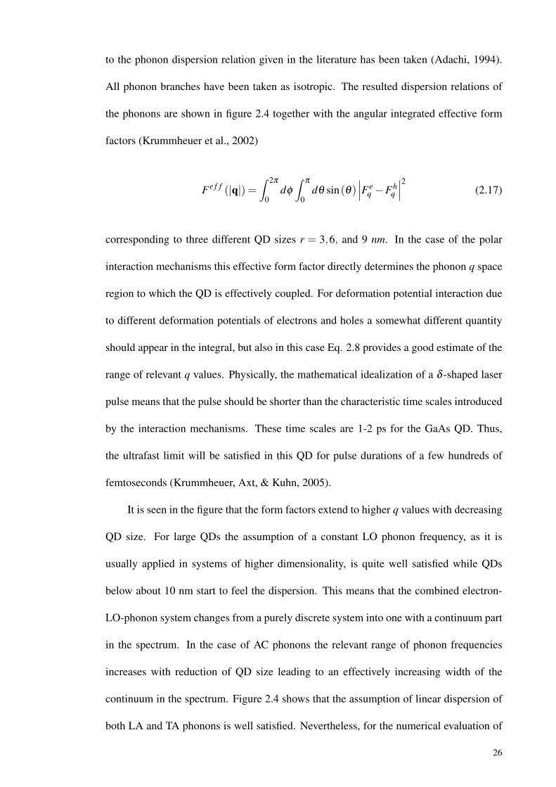
Figure 2.4 Dispersion relations of the LO, LA, and TA phonons taken in thecalculations as well as normalized effective form factors see Eq.2.17] describing the coupling of QDs with three different sizesr = 3,6, and 9 nm to the various phonon modes (Krummheuer etal., 2002). 27

Figure 2.5 The degeneracy has been lifted in acoustic and optical dispersioncurves by an anisotropic lattice. a represents the lattice constant(Klingshirn, 1995). 28

x

Figure 2.6 Optical polarizations induced by a δ -function-shaped optical pulse(left column) and absorption spectra (right column) for a QDinteracting with optical phonons at a temperature of 300 K. Thecalculation results without phonon dispersion have been shown inthe parts (a) and (b), in parts (c) and (d) [(e) and (f)] the resultsincluding dispersion are plotted for a 6-nm (3-nm) QD. Thespectra of the n-phonon sidebands due to phonon emission (n > 0)or phonon absorption (n < 0) are shifted by −nhωLO towards theZPL. In part (d) they are multiplied by the factors 3×103 (|n|= 1)and 2×106 (|n|= 2); the corresponding factors in part (f) are3×104 (|n|= 1) and 4×107 (|n|= 2) (Krummheuer et al., 2002). 30

Figure 2.7 Optical polarizations induced by a δ -function-shaped optical pulse(left column) and absorption spectra (right column) for a 3-nm QDinteracting with AC phonons at three different temperatures. Parts(a) and (b) refer to piezoelectric coupling, parts (c) and (d) todeformation potential coupling (Krummheuer et al., 2002). 32

Figure 2.8 Optical polarizations induced by a δ -function-like optical pulse(left column) and absorption spectra (right column) for a 6-nm QDinteracting with OP and AC phonons at three differenttemperatures T = 4, 77, and 300 K (Krummheuer et al., 2002). 34

Figure 2.9 Same as figure 2.8 but for a 3-nm QD (Krummheuer et al., 2002). 35Figure 2.10 Comparison of the exact absorption spectra (left column) with

those obtained from a correlation expansion up to the second orderin the coupling matrix elements (right column) for (a) and (b) polaroptical, (c) and (d) piezoelectric, and (e) and (f) deformationpotential, as well as for (g) and (h) the combination of allmechanisms at a temperature of 4 K (Krummheuer et al., 2002). 36

Figure 2.11 Semilogarithmic plot of the EL intensity of a single QD. (a) Withincreasing temperature the line broadening increases due tostronger AC phonon interaction. (b) Comparison of the measuredline shape with two calculated spectra, using alternatively a simpleGaussian (red dashed curve) and a realistic eight-band k·p wavefunction (green dotted curve) (Stock et al., 2011). 40

Figure 2.12 Comparison of the spectral phonon density for two different wavefunctions. For AC phonons (energy < 10 meV ) the Gaussian wavefunction (black curves) decreases too quickly, leading to anunderestimation of the phonon scattering (Stock et al., 2011). 42

Figure 2.13 OP phonon replica of a single QD. (a) The black dotted curveshows three ZPL lines, each one having a replica, separated by36.5 meV (red spectra, top energy scale). (b) Comparison of theLO line shape between experimentally measured (black) andcalculated spectra with (red dotted curve) or without (green dashedcurve) taking into account a finite lifetime of the phonon of 10 ps.A finite lifetime of the phonon provides a better description of thebroad line shape of the LO phonon replica (Stock et al., 2011). 43

xi

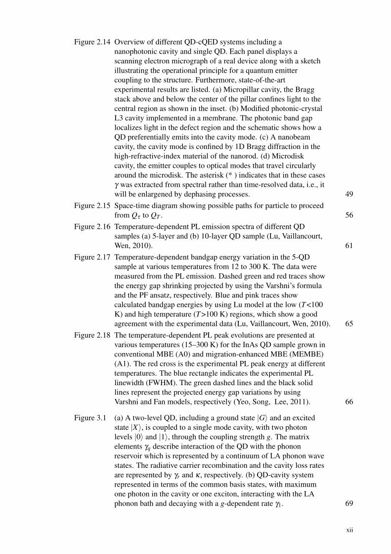
Figure 2.14 Overview of different QD-cQED systems including ananophotonic cavity and single QD. Each panel displays ascanning electron micrograph of a real device along with a sketchillustrating the operational principle for a quantum emittercoupling to the structure. Furthermore, state-of-the-artexperimental results are listed. (a) Micropillar cavity, the Braggstack above and below the center of the pillar confines light to thecentral region as shown in the inset. (b) Modified photonic-crystalL3 cavity implemented in a membrane. The photonic band gaplocalizes light in the defect region and the schematic shows how aQD preferentially emits into the cavity mode. (c) A nanobeamcavity, the cavity mode is confined by 1D Bragg diffraction in thehigh-refractive-index material of the nanorod. (d) Microdiskcavity, the emitter couples to optical modes that travel circularlyaround the microdisk. The asterisk (* ) indicates that in these casesγ was extracted from spectral rather than time-resolved data, i.e., itwill be enlargened by dephasing processes. 49

Figure 2.15 Space-time diagram showing possible paths for particle to proceedfrom Qτ to QT . 56

Figure 2.16 Temperature-dependent PL emission spectra of different QDsamples (a) 5-layer and (b) 10-layer QD sample (Lu, Vaillancourt,Wen, 2010). 61

Figure 2.17 Temperature-dependent bandgap energy variation in the 5-QDsample at various temperatures from 12 to 300 K. The data weremeasured from the PL emission. Dashed green and red traces showthe energy gap shrinking projected by using the Varshni’s formulaand the PF ansatz, respectively. Blue and pink traces showcalculated bandgap energies by using Lu model at the low (T <100K) and high temperature (T >100 K) regions, which show a goodagreement with the experimental data (Lu, Vaillancourt, Wen, 2010). 65

Figure 2.18 The temperature-dependent PL peak evolutions are presented atvarious temperatures (15–300 K) for the InAs QD sample grown inconventional MBE (A0) and migration-enhanced MBE (MEMBE)(A1). The red cross is the experimental PL peak energy at differenttemperatures. The blue rectangle indicates the experimental PLlinewidth (FWHM). The green dashed lines and the black solidlines represent the projected energy gap variations by usingVarshni and Fan models, respectively (Yeo, Song, Lee, 2011). 66

Figure 3.1 (a) A two-level QD, including a ground state |G〉 and an excitedstate |X〉, is coupled to a single mode cavity, with two photonlevels |0〉 and |1〉, through the coupling strength g. The matrixelements γq describe interaction of the QD with the phononreservoir which is represented by a continuum of LA phonon wavestates. The radiative carrier recombination and the cavity loss ratesare represented by γr and κ , respectively. (b) QD-cavity systemrepresented in terms of the common basis states, with maximumone photon in the cavity or one exciton, interacting with the LAphonon bath and decaying with a g-dependent rate γ1. 69

xii

Figure 3.2 Time-dependence of normalized real (left panel) and imaginary(right panel) parts of the memory kernel K (t) at differenttemperatures. It seems that the memory kernel with the length 4ps, as tc = εnc = 4 ps, is appropriate for the spherical QD withradius 5 nm and the deformation potential coupling to LA phonons. 78

Figure 3.3 Schematic representation of the configuration space includingsome trajectories (like the red path), started from an initial state,and the memory truncation. The ovals indicate the time points tn;Solid ovals correspond to the points within the memory lengthwith the memory cutoff number nc = 3 for the time point tq, whilehollow ovals correspond to the time steps p, with q− p > nc,which are not taken into account at the time tq. The solid linesindicate the path segments included in T jcq , while the dashed linesindicate non-included path segments at the time tq. 85

Figure 4.1 The decay dynamics of the QD-cavity system for differentcoupling strengths at T = 0 K with the recombination rate γr (=0.001 ps−1) = 0.0063 rad/ps = 4.135 µeV and the cavity decayrate κ (= 0.0242 ps−1) = 0.1519 rad/ps = 100 µeV . Three distinctdynamical regimes of weak, intermediate (strong), and coherentcoupling can be determined in the figure. 95

Figure 4.2 A comparison between the actual decay (pink), obtained using thenumerical RTPI calculations, an exponential decay (red), obtainedby fitting a single exponential to the actual decay, and a fit of theactual decay by using Eq. 4.1 (green) at g= 15 µeV and T = 0 K. 96

Figure 4.3 Comparison between the decay curves, obtained by RTPIapproach, and a fit of the phenomenological expression 4.1 for twocases. The phenomenological expression fits the numerically exactresults of the QD-cavity decay curves perfectly. 99

Figure 4.4 Two examples of fitting equation 4.1 to the exact state |1〉population of the dissipation-less QD-cavity system, obtained fromour microscopic RTPI calculation. The phenomenologicalexpression projects the exact state population perfectly as well. 99

Figure 4.5 The corresponding normalized spectra, Re(ρ11 (ω)), of the decaycurves shown in figure 4.1, calculated for different values of theQD-cavity coupling g at T = 0 K with γr (= 0.001 ps−1) = 0.0063rad/ps = 4.135 µeV and κ (= 0.0242 ps−1) = 0.1519 rad/ps =100 µeV . The separated sideband peaks appear clearly at about g=60 µeV , indicating the onset of the CC regime. 100

Figure 4.6 The normalized spectrum (black), Lorentzian part (red), andimpure dephasing part (green), plotted for g= 60 µeV and T = 0 K.The spectrum is obtained as a result of combination of theLorentzian and impure dephasing part. 101

Figure 4.7 The central peak FWHM (CPFWHM) extracted from the spectrafor three different temperatures T = 0, 20 and 80 K as a function ofg. γr = 0.0063 rad/ps = 4.135 µeV and κ= 0.1519 rad/ps = 100µeV . The cubic spline data interpolation has been used to connectthe many points (not shown) calculated by numerically exact RTPImethod. 102

xiii

Figure 4.8 Γ1 (FWHM of the effective population decay) and CPFWHMversus g at T = 0 K. The inset shows Γ1 and CPFWHM at a short ginterval. γr = 0.0063 rad/ps = 4.135 µeV and κ= 0.1519 rad/ps =100 µeV . The cubic spline data interpolation has been used toconnect the many points (not shown) calculated by numericallyexact RTPI method. 103

Figure 4.9 The introduced quantity δFWHM, which is difference of CPFWHMand Γ1, for different QD-cavity coupling strengths at three diversetemperatures T = 0, 20 and 80 K. The inset of figure 4.9 shows theintroduced quantity as the main figure at small g. 104

Figure 4.10 (a) The normalized impure dephasing spectra for different g at T =0 K. As g increases within the CC regime, a rollover occurs andthe contribution of (FWHM of) the impure dephasing spectra to(FWHM of) the central peak of the spectra, Re(ρ11 (ω)), decreasesto zero as a result of increasing clear VRO frequency which leadsto growing separated sidebands. (b) The normalized impuredephasing spectra only for different small g at T = 0 K for a betterview. The parameters γr = 0.001 ps−1 = 0.0063 rad/ps and κ=0.0242 ps−1 = 0.1519 rad/ps were used. 105

Figure 4.11 FWHM of the effective population decay, Γ1, versus g at threevarious temperatures T = 0, 20, and 80 K with γr = 0.0063 rad/ps= 4.135 µeV and κ = 0.1519 rad/ps = 100 µeV . The effectivepopulation decay rate is proportional to the inverse of temperaturefor the coupling strengths less than about g= 500 µeV . 107

Figure 4.12 Fitted T-dependent shift of PL peak for SOQDs with differentthicknesses (a) 1.8, (b) 2.4, and (c) 18 MLs. Dividing the wholeT-interval to three shorter parts, shown by different colors, TOMprojects the whole data successfully. 109

Figure 4.13 Fitted T-dependent shift of PL peak for SOQDs with differentthicknesses: (a) 1, (b) 1.5, (c) 2, and (d) 2.5 MLs. 111

Figure 4.14 Fitted T-dependent shrinkage of bandgap peak for SOQDs grownby MBE, HDE, and MBE+MDH techniques with differentthicknesses: (a) and (b) 1.6, (c) and (d) 2.4. 114

Figure 4.15 Fitted PL peak shift of QDs grown using (a) MBE and (b)migration enhanced MBE [abbreviated as MEE] for the samenumber of 3 MLs. 114

Figure 4.16 Fitted T-dependent shrinkage of bandgap energy peak for SOQDswith a different number of layers (a) 5 and (b) 10. 117

xiv

LIST OF TABLES

Table 2.1 Density of states (DOS) for electrons in the conduction band of asemiconductor. D stands for dimension. The 2 in the zerodimension case is just the spin degeneracy, since the volume part ofthe prefactor no longer exists. θ(E−En) =0 for E < En. and 1 forE > En. 12

Table 3.1 Phonon Energy Peaks for GaAs, InAs, and InGaAs Bulk 91

Table 4.1 Parameters Obtained Using Fit, Eqs. 3.53 and 3.54, the FinalColumn Shows the Obtained Transition Temperatures for SOQDswith 1.8, 2.4, and 18 MLs 108

Table 4.2 Parameters Obtained Using Fit, Eqs. 3.53 and 3.54, and theObtained Transition Temperatures for SOQDs with 1, 1.5, 2, and2.5 MLs 111

Table 4.3 Parameters Obtained Using Fit, Eqs. 3.53 and 3.54, and theObtained Transition Temperatures for SOQDs Grown Using MBE,HDE, MBE+MDH, and MEE Methods with 1.6, 2.4, and 3 MLs 115

Table 4.4 Parameters Obtained Using Fit, Eqs. 3.53 and 3.54, and theObtained Transition Temperatures for SOQDs with DifferentNumber of Layers 5 and 10 118

xv

xvi

LIST OF ABBREVIATIONS

1-D One Dimension

2-D Two Dimension

3-D Three Dimension

AC acoustic

AFM Atomic Force Microscope

AlN Aluminum Nitride

CB Conduction Band

CC Coherent Coupling

CPFWHM Central Peak Full Width at Half Maximum

DOS Density of States

EIT Electromagnetically Induced Transparency

EL Electroluminescence

ES Excited State

FSS Fine-Structure Splitting

FWHM Full Width at Half Maximum

GS Ground State

HDE Heterogeneous Droplet Epitaxy

IBM Independent Boson Model

IC Intermediate Coupling

IHB Inhomogeneous Broadening

In(Ga)As Indium Gallium Arsenide

LA Longitudinal Acoustic

LED Light Emitting Diodes

LO Longitudinal Optical

MBE Molecular Beam Epitaxy

MDH Modulation Doped Heterostructure

ME Master Equation

MEE Migration-Enhanced MBE

MLs Monolayers

NZ Nakajima-Zwanzig

OP Optical

OQC Open Quantum Dot-Cavity

PF Power Function

PL Photoluminescence

QD Quantum Dot

QD-cQED Quantum Dot-Cavity Quantum E lectrodynamics

QUAPI Quasi-Adiabatic Propagator Feynman Path Integral

RDM Reduced Density Matrix

RQCDM Reduced Open QD-Cavity Density Matrix

RTPI Real-Time Path-Integral

SC Strong Coupling

SK Stranski–Krastanov

SNR Squared 2-Norm of the Residual

SOQD Self-Organized Quantum Dot

T Temperature

TA Transverse Acoustic

TC Time-Convolutionless

TO Transverse Optical

TOM Two-Oscillator Model

xvii

VB Valence Band

VRO Vacuum Rabi Oscillation

VRS Vacuum Rabi splitting

WC Week Coupling

ZB Zero Bandgap

ZPL Zero Phonon Line

xviii

LIST OF APPENDICES

Appendix A Derivation of Discretized Real-Time Path-Integrals for

Dissipative Quantum Dot-Cavity System Coupled to Longitudinal

Acoustic Phonon Bath 124

CHAPTER 1

INTRODUCTION AND MOTIVATIONS

1.1 Introduction

The existence of a discrete and anharmonic electronic spectrum is the prerequisite

for many quantum-optics experiments since it enables generating single photon when an

electron undergoes a transition between two levels. An obvious choice is a single atom,

which represents a clean quantum system with discrete electronic states. The ability to

create discrete electronic states in a solid-state system enables a range of new opportu-

nities for integrated quantum-optics experiments, this can be achieved in a quantum dot

(QD). As QDs are embedded in a solid (substrate), they are inherently coupled to the envi-

ronment degrees of freedom (phonons). The interactions of the QD carriers with phonons

lead to broadening of the discretized electronic states and play an important role in the

electrical and optical properties of the QD structures. In this study, we focus on four

important types of phonons called: transverse optical (TO), longitudinal optical (LO),

transverse acoustic (TA), and longitudinal acoustic (LA) phonons. In the following, an

introduction about QDs and phonons is presented.

1.1.1 Quantum Dots

QDs are electrically semiconducting nanostructured regions, composed of elements

of groups II to VI the periodic table such as In(Ga)As/GaAs, GaAs/AlGaAs, InP/Zn(S,

Se), GaN//AlN, GaSb/GaAs, Si, Ge/Si, CdSe/ZnS. A relatively new kind of QDs called

perovskite have also been introduced (Park, Guo, Makarov, & Klimov, 2015). Gener-

ally, there are two types of colloidal and epitaxial QDs, our focus in this thesis is on

epitaxial QDs which are grown by epitaxial methods and called self-assembled or self-

1

organized QDs as well. Although QDs consist of tens of thousands of atoms they have

optical properties similar to single atoms due to the quantum confinement of electrons’

and holes’ wave-functions to a nanometer length scale. Therefore, they are also called

"artificial atoms" or "macro atoms". Since QDs are solid-state emitters they can readily

be implemented in photonic nanostructures such as nanowires, plasmonic nanoantennas,

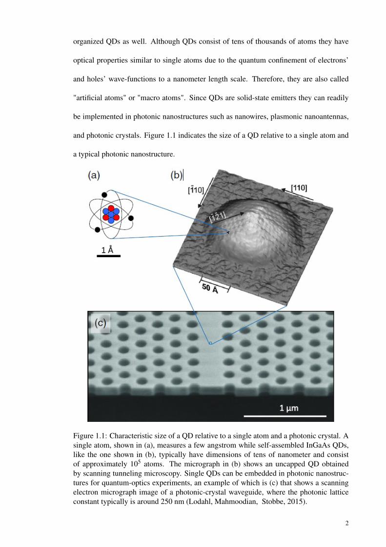
and photonic crystals. Figure 1.1 indicates the size of a QD relative to a single atom and

a typical photonic nanostructure.

Figure 1.1: Characteristic size of a QD relative to a single atom and a photonic crystal. Asingle atom, shown in (a), measures a few angstrom while self-assembled InGaAs QDs,like the one shown in (b), typically have dimensions of tens of nanometer and consistof approximately 105 atoms. The micrograph in (b) shows an uncapped QD obtainedby scanning tunneling microscopy. Single QDs can be embedded in photonic nanostruc-tures for quantum-optics experiments, an example of which is (c) that shows a scanningelectron micrograph image of a photonic-crystal waveguide, where the photonic latticeconstant typically is around 250 nm (Lodahl, Mahmoodian, Stobbe, 2015).

2

As the size of a QD approaches the Bohr radius of the bulk exciton, quantum con-

finement effects become pronounced leading to quantized energy levels for charge carriers

(electrons and holes) inside the QD. This leads to a discrete spectrum of quantum states

like the energy levels of an atom and significant modification of the optical and electronic

properties: Light emission from QDs has a higher quantum efficiency than emission from

bulk materials. In addition, the nonlinear polarizability and transition oscillator strength

are spectrally concentrated and increased in magnitude in the size regime of QDs.

One of the important experimental advantages of QDs is that they are made of semi-

conductor materials for which a wealth of growth and processing technology have been

developed over the past decades. Sophisticated crystal-growth procedures combined with

semiconductor processing methods such as electron-beam lithography, etching, and depo-

sition constitute the generic nanofabrication platform on which the significant experimen-

tal progress within quantum nanophotonics during the past decades has been built. Since

semiconductors are very sensitive to impurities and defects, QDs are fabricated by epi-

taxial methods such as molecular-beam epitaxy, where heterostructures are grown with

monolayer precision under ultrahigh-vacuum conditions (Shchukin & Bimberg, 1999;

Stangl, Holý, & Bauer, 2004; Biasiol & Heun, 2011). The most common approach to

grow In(Ga)As QDs is the Stranski-Krastanov method that relies on the self-assembly of

InAs or InGaAs QDs on a GaAs surface due to the 7% larger lattice constant of InAs

compared to that of GaAs. As a consequence, only a thin wetting layer of InAs can

be deposited on GaAs before the strain is relaxed by the nucleation of QDs in the form

of randomly positioned islands. In order to protect the QDs from oxidation and to pre-

vent interaction with surface states, a GaAs capping layer is grown atop the QDs. While

Stranski-Krastanov QDs have a pyramidal shape before capping, they develop the shape

of a truncated pyramid after capping (Eliseev et al., 2000) due to a significant material

intermixing. This in turn leads to an inhomogeneous indium distribution and a strain that

3

varies throughout the QD. Typically, QDs are grown with heights in the range of 1–10

nm and in-plane sizes in the range of 2–70 nm (Lodahl, Mahmoodian, & Stobbe, 2015;

Cheng, Lowe, Reece, & Gooding, 2014). Controlling the size and therefore the quantum

confinement as well as the material composition enables tailoring the emission wave-

length. Size variations between different ensemble’s QDs within a single growth run are

inevitable, i.e., a QD ensemble will be inhomogeneously broadened, implying that indi-

vidual tuning of single QDs would generally be required in order to couple them mutually.

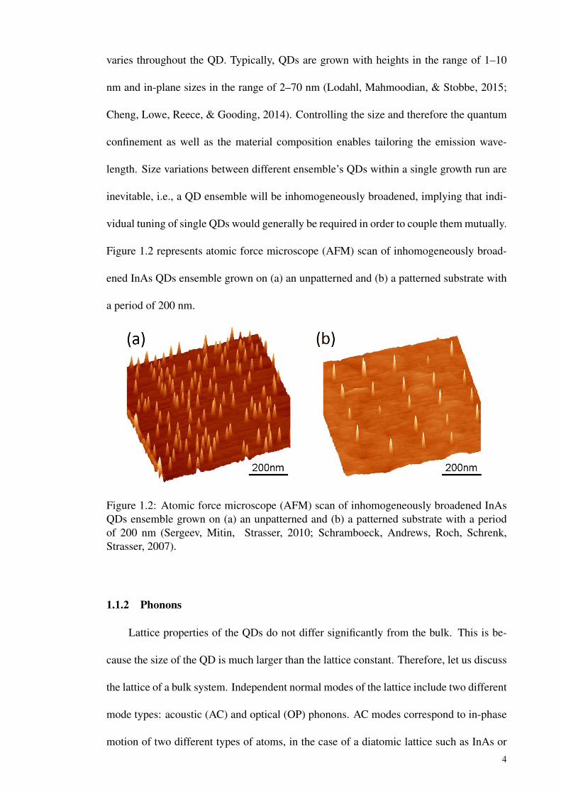
Figure 1.2 represents atomic force microscope (AFM) scan of inhomogeneously broad-

ened InAs QDs ensemble grown on (a) an unpatterned and (b) a patterned substrate with

a period of 200 nm.

Figure 1.2: Atomic force microscope (AFM) scan of inhomogeneously broadened InAsQDs ensemble grown on (a) an unpatterned and (b) a patterned substrate with a periodof 200 nm (Sergeev, Mitin, Strasser, 2010; Schramboeck, Andrews, Roch, Schrenk,Strasser, 2007).

1.1.2 Phonons

Lattice properties of the QDs do not differ significantly from the bulk. This is be-

cause the size of the QD is much larger than the lattice constant. Therefore, let us discuss

the lattice of a bulk system. Independent normal modes of the lattice include two different

mode types: acoustic (AC) and optical (OP) phonons. AC modes correspond to in-phase

motion of two different types of atoms, in the case of a diatomic lattice such as InAs or

4

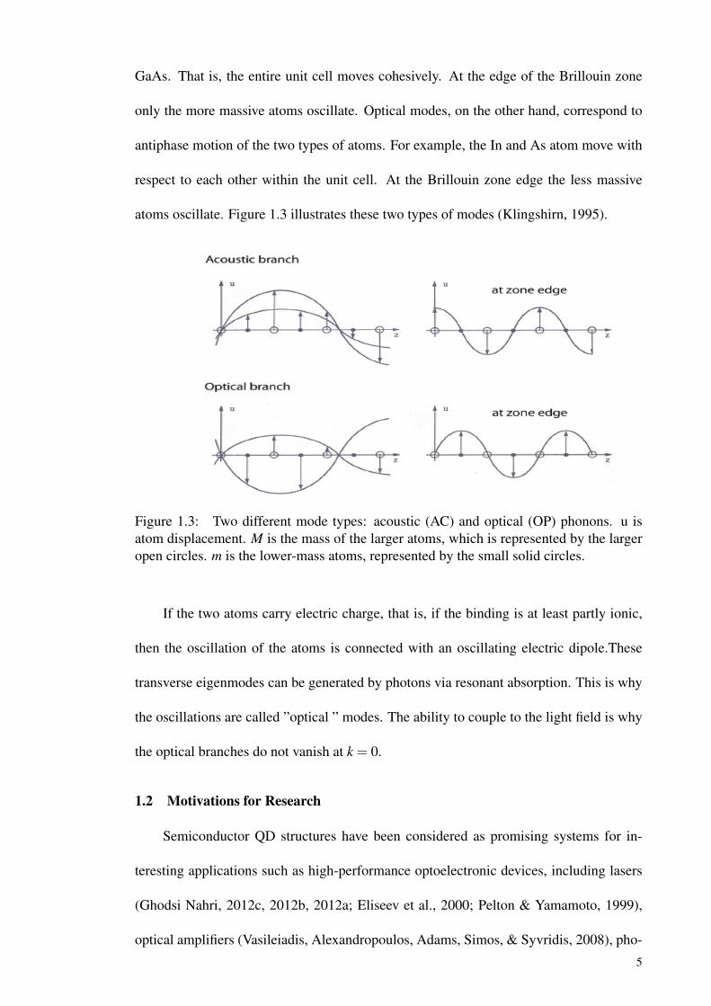
GaAs. That is, the entire unit cell moves cohesively. At the edge of the Brillouin zone

only the more massive atoms oscillate. Optical modes, on the other hand, correspond to

antiphase motion of the two types of atoms. For example, the In and As atom move with

respect to each other within the unit cell. At the Brillouin zone edge the less massive

atoms oscillate. Figure 1.3 illustrates these two types of modes (Klingshirn, 1995).

Figure 1.3: Two different mode types: acoustic (AC) and optical (OP) phonons. u isatom displacement. M is the mass of the larger atoms, which is represented by the largeropen circles. m is the lower-mass atoms, represented by the small solid circles.

If the two atoms carry electric charge, that is, if the binding is at least partly ionic,

then the oscillation of the atoms is connected with an oscillating electric dipole.These

transverse eigenmodes can be generated by photons via resonant absorption. This is why

the oscillations are called ”optical ” modes. The ability to couple to the light field is why

the optical branches do not vanish at k = 0.

1.2 Motivations for Research

Semiconductor QD structures have been considered as promising systems for in-

teresting applications such as high-performance optoelectronic devices, including lasers

(Ghodsi Nahri, 2012c, 2012b, 2012a; Eliseev et al., 2000; Pelton & Yamamoto, 1999),

optical amplifiers (Vasileiadis, Alexandropoulos, Adams, Simos, & Syvridis, 2008), pho-

5

todetectors (Barve et al., 2010; Lu, Vaillancourt, & Meisner, 2007b, 2007a), and light

emitting diodes (LEDs) (Basu, 1997), single and entangled photon sources (Somaschi et

al., 2016; Park et al., 2015; Muller, Bounouar, Jons, Glassl, & Michler, 2014; Stevenson

et al., 2012; Salter et al., 2010; Claudon et al., 2010; Michler et al., 2000; Benson, San-

tori, Pelton, & Yamamoto, 2000), cavity quantum electrodynamic effects (Hennessy et

al., 2007; Reithmaier et al., 2004; Yoshie et al., 2004), quantum information and compu-

tation processing (Nilsson et al., 2013; Ladd et al., 2010; Chen, Piermarocchi, & Sham,

2001; Tanamoto, 2000; Burkard, Loss, & DiVincenzo, 1999), quantum cryptography,

and teleportation (Nilsson et al., 2013). Other investigated applications of semiconductor

nanostructures include photonic network components, such as optical switches and mod-

ulators (Kelly, 1995), among other nonlinear photonic devices. The potential of quantum

information and computation processing has triggered many research since years ago and

QDs have been investigated as integral parts of a variety of quantum information and

computation processing schemes (Schrier & Whaley, 2005; Brown, Lidar, & Whaley,

2001; Brun & Wang, 2000). However, the key properties and suitability of QD structures

to have a proper physical performance for improved applications strongly depend on un-

derstanding their basic characteristics such as phonon-induced effects on the performance

of these structures.

We study the effects induced by LA phonons in a hybrid single QD-cavity system

and by AC and OP phonons in samples of QD ensembles. A scalable QD-cavity platform,

where the interaction between the single photon with the QD can be engineered and con-

trolled to a high degree, can be obtained by understanding and controlling the effects

induced by phonons on the QD-cavity dynamics. Such a scalable QD-cavity platform can

realize a perfect single photon source (Somaschi et al., 2016; He et al., 2013; Gazzano

et al., 2013; Michler et al., 2000) which is a main requirement for quantum computation

and information processing (O’Brien, Furusawa, & Vuckovic, 2009; Knill, Laflamme, &

6

Milburn, 2001). It is also applicable for low-threshold and nano lasers (Strauf & Jahnke,

2011; Noda, 2006; Michler, 2003) as well as tests of fundamental aspects of quantum

mechanics (Haroche & Raimond, 2006). Study of the effects induced by phonons on the

bandgap width of self-organized quantum dots (SOQDs), on the other hand, offers a char-

acteristic “fingerprint” of the material under investigation from which one can find optical

and structural properties such as phonon statistics. It also is of considerable importance

for improving QD-based structures including QDs’ samples applicable in optoelectronic

devices.

1.3 Accomplished Studies

The thesis is organized as follows: In Chap. 2, the quantum confinement and its

effects on the electronic structure and density of states of QDs are reviewed. AC and

OP phonon-induced dephasing effects, separately and in combination, in QDs are dis-

cussed obtaining the relevant absorption spectra and optical polarization. The results of

an exact and a perturbative approach are compared. The exact results of electrolumi-

nescence spectra accounting for AC and OP phonon are also compared with the experi-

mental results. In section 2.3, QD-cavity quantum electrodynamic (QD-cQED) systems

are introduced and the theoretical models to investigate them are briefly reviewed. Gen-

eral formulation of Feynman path-integral approach is presented in the next section. In

section 2.5, temperature-dependent bandgap energy variation and three semi-empirical

models for projecting it is presented. The models applied for performing the simulations

of this work are presented in Chap. 3; Numerically exact real-time path-integral (RTPI)

approach modified for the QD-cQED system and implementation of a suitable numeri-

cal algorithm to evaluate the derived density matrix elements are offered. In section 3.4,

two-oscillator model applied to project temperature-dependent bandgap variation of self-

assembled QD ensembles is given. Chap. 4 and 5 are devoted to simulation results and

7

conclusion. A detailed derivation of the QD-cavity density matrix elements by using the

numerically exact RTPI approach is offered in the appendix.

To investigate the phonon-induced effects on the semiconductor QD structures, in

this thesis, a solid-state cQED system, consisting of a single semiconductor QD (a solid-

state emitter) coupled resonantly to single mode of an optical nanocavity, is investigated

by using the numerically exact RTPI approach. Within this approach, we treat exciton-

photon and exciton-phonon interactions on the same footing, exciton decay and cavity

loss are included phenomenologically by adding the non-Hermitian terms to the Hamilto-

nian. In fact, we have applied the full non-Hermitian Hamiltonian within the path-integral

formalism which is numerically exact. We identify three different regimes of QD-cQED

in the simulated decay dynamics and provide more precise conditions for those regimes.

We study the effects induced by impure dephasing of coherent coupling between the

dressed states, originated from LA phonon bath and the dissipations, on the decay curves

and the corresponding spectra by proposing a two-term phenomenological expression that

perfectly reproduces the decay curves. We extract effective population decay and impure

dephasing rates and obtain a maximum achievable value for the emission rate, which is

the mean of the QD and cavity dissipation rates. Projecting the proposed phenomeno-

logical expression to the state population, obtained from our RTPI calculation for the

dissipation-less QD-cavity system, we find an approximate expression for the effective

impure dephasing rate. The effects of temperature and the QD-cavity coupling strength

on the width of the central peak of the spectra is studied. To investigate the role of the

effective impure dephasing rate on the width of central peak of the spectra we introduce

a quantity which is applicable to determine the distinct regimes of the QD-cavity cou-

pling as well. We demonstrate that the contribution of the impure dephasing part to the

central band of the spectra starts at the onset of the strong coupling (SC) regime, which

originates from the existence of vacuum Rabi Oscillation (VRO) with a very small fre-

8

quency (unclear VRO) at the corresponding decay curve. Its contribution to the central

peak increases with the coupling strength within the SC regime as a result of enhancing

frequency of the unclear VRO. At the onset of the CC regime, the contribution begins to

reduce as a result of the appearance of sidebands in the spectra, which originates from

clear VRO. The reduction continues down to zero as the effective population decay and

impure dephasing rate contribute separately to the central and sideband peaks of the triplet

spectra, respectively, only beyond a very large coupling strength which is the same across

the considered temperature range. It is also shown that to obtain the maximum achievable

emission rate, at a higher temperature, a larger coupling strength is required as a result of

temperature-dependence of the effective population decay rate (Ghodsi Nahri, Mathkoor,

& Ooi, 2016).

In the second part of this work, in order to study the role of AC and OP phonons at

the temperature (T)-dependent shift of photoluminescence (PL) peak of self-assembled

QD ensembles we apply the two-oscillator model (TOM) to 15 available experimental

datasets of In(Ga)As/GaAs QD ensembles, with a different number of monolayers (MLs)

and layers, taken from published papers [36-44]. We correspond the low energy oscil-

lator to AC phonons and the high energy one to OP phonons. We find that the TOM

can project all the samples with a good accuracy if the whole temperature interval 0-300

K is divided into, at most, four parts depending on the degree of the dispersion from

a monotonic decrease of the bandgap energy peak. Our results suggest that, low QDs

uniformity in an ensemble results in the dispersion (anomalous temperature behavior of

PL peak), and the whole AC phonon contribution to the T-dependent shift of PL peak

decreases for higher dispersions. Some growth techniques, which improve the QDs uni-

formity, lead to removal of the dispersion (sigmoidal behavior) and thus increase of AC

phonon contribution to T-dependent shrinkage of the PL peak. We also propose a trade

off between QDs uniformity (inhomogeneous broadening (IHB) of the QDs sample) and

9

QD symmetry. Enhancement of QDs uniformity increases total AC phonon contribution

and enhancement of the symmetry increases total OP phonon contribution (Ghodsi Nahri

& Ooi, 2014).

10

CHAPTER 2

LITERATURE REVIEW

2.1 Quantum Confinement Effects, Density of States, and Electronic Structure

As the structure size is reduced, more confinement leads to an increase in the ef-

fective band gap of the material and causes excited states to move higher in energy just

as energy levels move higher in an infinite potential square well. Reduction of the well

width, with decrease of the QD size, deeply affects the QD energy levels and exciton fine

structure through the strong size dependence of the exchange interaction and confinement

energy. There are variety of advantages inherent in using low-dimensional system for de-

vices compared to using bulk materials, they include, depending on the specifics of the

system, improved efficiency, speed, and gain and noise reduction as well as a reduced

threshold current density and insensitivity to operating temperature. The last item is due

to energy spacing in the strong confinement regime being larger than kBT (Kelly, 1995).

Additionally, oscillator strength becomes more concentrated as dimensions is reduced

just as absorption becomes spectrally discrete. Gain, therefore, is also repartitioned into

discrete states. The transition rate per electron-hole pair stays the same even as dimen-

sions is reduced (Peaker & Grimmeiss, 1991), which leads to very strong lasing capability

(Rafailov et al., 2006).

An appropriate way to approach the subject of low-dimensionality is to explore the

properties of the density of states (DOS), a quantity that dictates the oscillator strength of

certain transitions. The DOS is derived from the number of states per energy per volume.

This calculation is explicitly worked out in many modern solid state physics text books

like Ref. (Grahn, 1999).

11

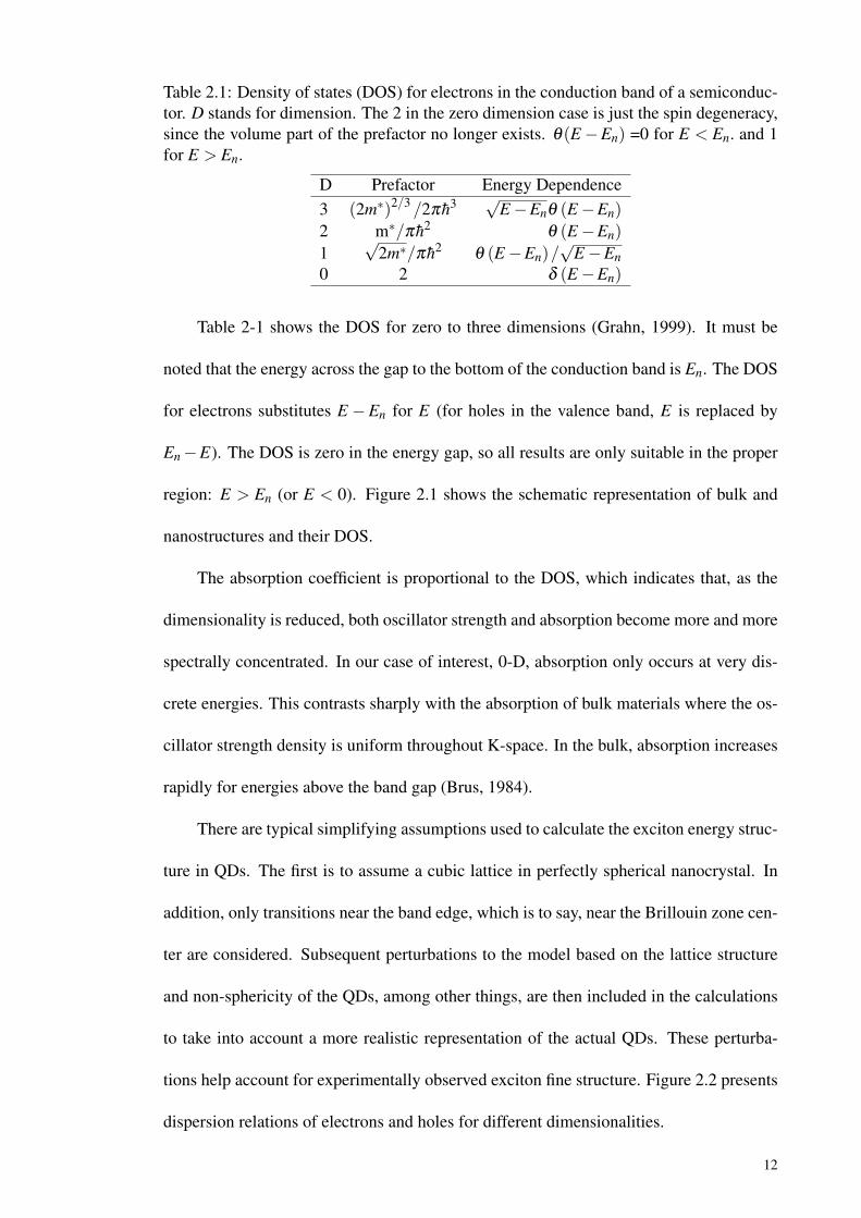
Table 2.1: Density of states (DOS) for electrons in the conduction band of a semiconduc-tor. D stands for dimension. The 2 in the zero dimension case is just the spin degeneracy,since the volume part of the prefactor no longer exists. θ(E−En) =0 for E < En. and 1for E > En.

D Prefactor Energy Dependence3 (2m∗)2/3 /2π h3 √

E−Enθ (E−En)

2 m∗/π h2θ (E−En)

1√

2m∗/π h2θ (E−En)/

√E−En

0 2 δ (E−En)

Table 2-1 shows the DOS for zero to three dimensions (Grahn, 1999). It must be

noted that the energy across the gap to the bottom of the conduction band is En. The DOS

for electrons substitutes E −En for E (for holes in the valence band, E is replaced by

En−E). The DOS is zero in the energy gap, so all results are only suitable in the proper

region: E > En (or E < 0). Figure 2.1 shows the schematic representation of bulk and

nanostructures and their DOS.

The absorption coefficient is proportional to the DOS, which indicates that, as the

dimensionality is reduced, both oscillator strength and absorption become more and more

spectrally concentrated. In our case of interest, 0-D, absorption only occurs at very dis-

crete energies. This contrasts sharply with the absorption of bulk materials where the os-

cillator strength density is uniform throughout K-space. In the bulk, absorption increases

rapidly for energies above the band gap (Brus, 1984).

There are typical simplifying assumptions used to calculate the exciton energy struc-

ture in QDs. The first is to assume a cubic lattice in perfectly spherical nanocrystal. In

addition, only transitions near the band edge, which is to say, near the Brillouin zone cen-

ter are considered. Subsequent perturbations to the model based on the lattice structure

and non-sphericity of the QDs, among other things, are then included in the calculations

to take into account a more realistic representation of the actual QDs. These perturba-

tions help account for experimentally observed exciton fine structure. Figure 2.2 presents

dispersion relations of electrons and holes for different dimensionalities.

12

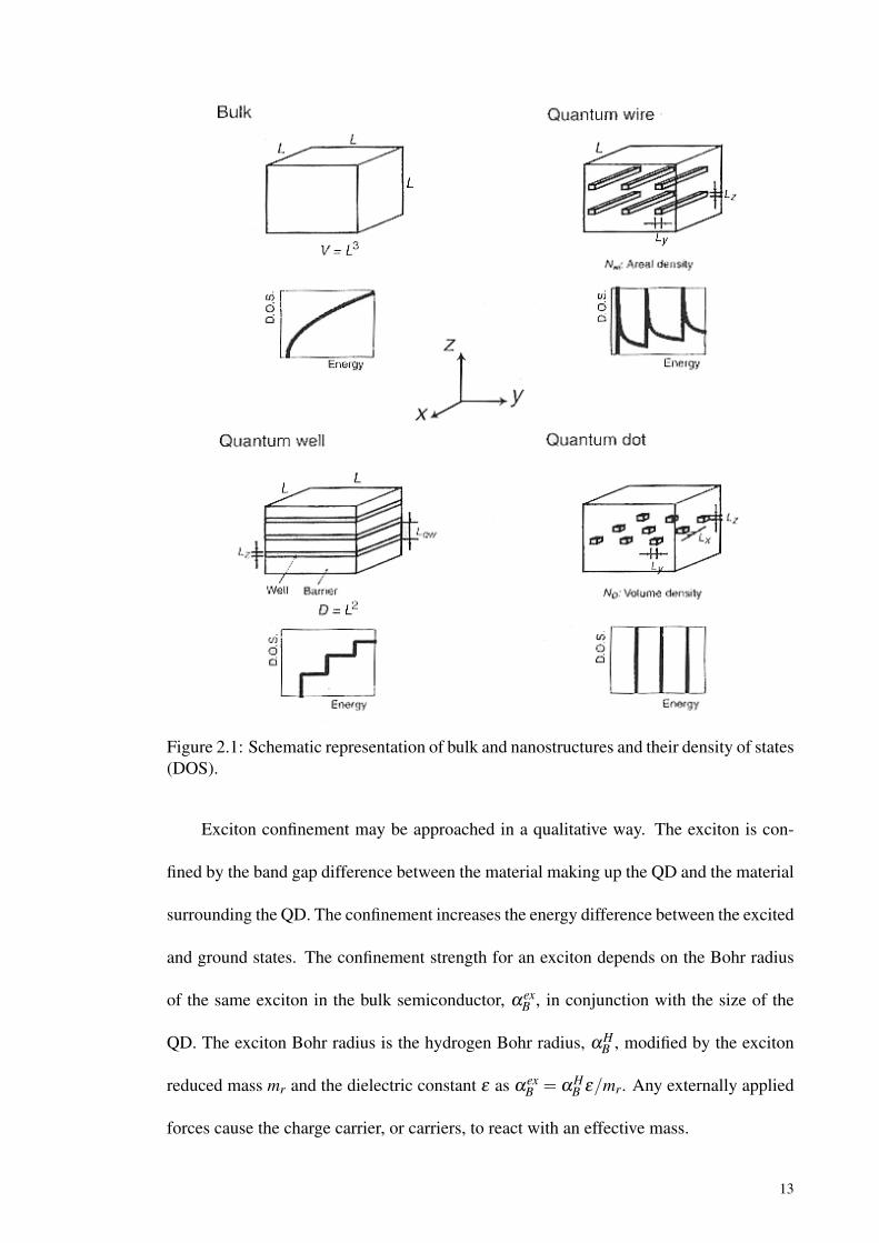
Figure 2.1: Schematic representation of bulk and nanostructures and their density of states(DOS).

Exciton confinement may be approached in a qualitative way. The exciton is con-

fined by the band gap difference between the material making up the QD and the material

surrounding the QD. The confinement increases the energy difference between the excited

and ground states. The confinement strength for an exciton depends on the Bohr radius

of the same exciton in the bulk semiconductor, αexB , in conjunction with the size of the

QD. The exciton Bohr radius is the hydrogen Bohr radius, αHB , modified by the exciton

reduced mass mr and the dielectric constant ε as αexB = αH

B ε/mr. Any externally applied

forces cause the charge carrier, or carriers, to react with an effective mass.

13

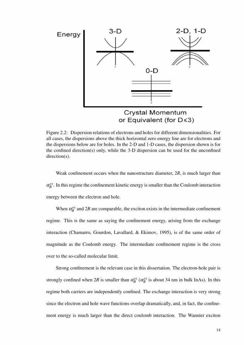
Figure 2.2: Dispersion relations of electrons and holes for different dimensionalities. Forall cases, the dispersions above the thick horizontal zero energy line are for electrons andthe dispersions below are for holes. In the 2-D and 1-D cases, the dispersion shown is forthe confined direction(s) only, while the 3-D dispersion can be used for the unconfineddirection(s).

Weak confinement occurs when the nanostructure diameter, 2R, is much larger than

αexB . In this regime the confinement kinetic energy is smaller than the Coulomb interaction

energy between the electron and hole.

When αexB and 2R are comparable, the exciton exists in the intermediate confinement

regime. This is the same as saying the confinement energy, arising from the exchange

interaction (Chamarro, Gourdon, Lavallard, & Ekimov, 1995), is of the same order of

magnitude as the Coulomb energy. The intermediate confinement regime is the cross

over to the so-called molecular limit.

Strong confinement is the relevant case in this dissertation. The electron-hole pair is

strongly confined when 2R is smaller than αexB (αex

B is about 34 nm in bulk InAs). In this

regime both carriers are independently confined. The exchange interaction is very strong

since the electron and hole wave functions overlap dramatically, and, in fact, the confine-

ment energy is much larger than the direct coulomb interaction. The Wannier exciton

14

(described by hydrogen Hamiltonian) can no longer reasonably be said to exist. Now an

exchange interaction term must be included to the corresponding Hamiltonian and the di-

rect coulomb term my be neglected. Therefore, when we use the term ”excitons” in QDs,

it is a misnomer and really refers to correlated electron-hole pairs in QDs. Confinement

causes a larger band gap and atomic-like discrete states (see figure 2.3).

In QDs, the exciton experiences the potential of a 3-D quantum mechanical square

well. Because QDs are usually overcoated with larger band gap semiconductor the ex-

citons are in a finite potential well and can experience a small amount of wave function

leakage outside the core of the QD, leading to a larger effective QD size. As indicated

in Figure 2.3, energy bands for electrons in the conduction band (CB) and holes in the

valence band (VB) break up into discrete, atomic-like levels.

In the 0-D case, in a 3-D square potential well with infinitely high barriers, the energy

levels are obtained using (Harrison, 2005)

En =n2h2

π2

2m∗e,h(2R)2 , n = 1,2,3..... (2.1)

There are an infinite number of bound states. R is the half-width of the well (or

the radius of the nanocrystal). In a real QD structure, there are finite number of bound

states. As R→ 0, En diverges. In a real structure, the states converge to the Bloch states

of the barrier material; in our case those of GaAs. Since the ground state energy is now

larger than the intrinsic band gap, we can readily see that the confinement increases the

energy of the exciton system. The exciton experiences an enhanced Coulomb (attractive,

in this case) interaction. In particular, the exchange interaction plays a very larger role

in the energy levels of strongly confined excitons. The exciton energy level structure

consists of the transitions between discrete quantum levels of the electrons and holes.

Among the various types of QDs, self-assembled QDs resemble most closely the ideal of

15

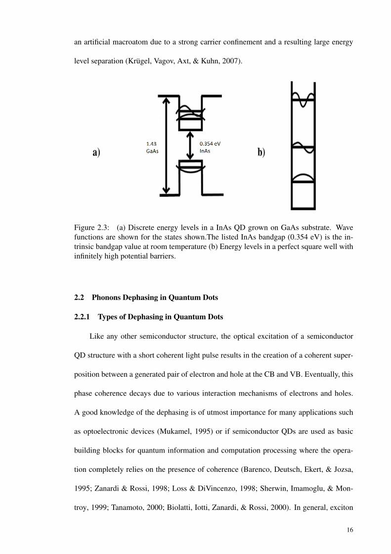
an artificial macroatom due to a strong carrier confinement and a resulting large energy

level separation (Krügel, Vagov, Axt, & Kuhn, 2007).

Figure 2.3: (a) Discrete energy levels in a InAs QD grown on GaAs substrate. Wavefunctions are shown for the states shown.The listed InAs bandgap (0.354 eV) is the in-trinsic bandgap value at room temperature (b) Energy levels in a perfect square well withinfinitely high potential barriers.

2.2 Phonons Dephasing in Quantum Dots

2.2.1 Types of Dephasing in Quantum Dots

Like any other semiconductor structure, the optical excitation of a semiconductor

QD structure with a short coherent light pulse results in the creation of a coherent super-

position between a generated pair of electron and hole at the CB and VB. Eventually, this

phase coherence decays due to various interaction mechanisms of electrons and holes.

A good knowledge of the dephasing is of utmost importance for many applications such

as optoelectronic devices (Mukamel, 1995) or if semiconductor QDs are used as basic

building blocks for quantum information and computation processing where the opera-

tion completely relies on the presence of coherence (Barenco, Deutsch, Ekert, & Jozsa,

1995; Zanardi & Rossi, 1998; Loss & DiVincenzo, 1998; Sherwin, Imamoglu, & Mon-

troy, 1999; Tanamoto, 2000; Biolatti, Iotti, Zanardi, & Rossi, 2000). In general, exciton

16

coherence in QDs is too fragile to be used for these applications, although improvements

in system design and QD fabrication may make QDs as viable components in the fu-

ture. Other potential applications of particular interest include the storage of light, or of

information transmitted by light. A slow exciton dephasing rate is required for these ap-

plication. Slow light has also been demonstrated in GaAs quantum well system using the

coherence of excitons (Ku et al., 2004). Another demonstrated phenomenon using exci-

ton coherence is electromagnetically induced transparency (EIT) which based on exciton

correlations was first observed in GaAs quantum wells (Phillips & Wang, 2002).

In higher dimensional systems, such as bulk semiconductors and quantum wells, the

dephasing is mainly associated with a change of occupations due to transitions between

different states, i.e., with reexcitation (thermalization), carrier relaxation, or recombina-

tion processes. This is called "impure dephasing". Impure dephasing, at least approxi-

mately, requires the conservation of energy between initial and final state which, in these

cases of a continuous electronic spectrum, usually can be easily satisfied. In QDs, how-

ever, the electronic spectrum is discrete and it is much harder that this condition to be

fulfilled. For the case of carrier-phonon interaction lack of this condition has resulted

in the prediction of a so-called "phonon-bottleneck" in the relaxation (Bockelmann &

Bastard, 1990; Benisty, 1995).

The dephasing of optical transitions, on the other hand, is not restricted to such real

transitions; it is well known that virtual transitions which do not lead to a change of oc-

cupations also contribute to the dephasing of optical polarizations (Muljarov & Zimmer-

mann, 2004; Muljarov, Takagahara, & Zimmermann, 2005; Muljarov & Zimmermann,

2007). This contribution leads to elastic scattering of AC phonons and is called "pure de-

phasing". Because of the large separation between the QD energy levels and the resulting

strong reduction of real phonon-mediated transitions between these states, pure dephas-

ing is of particular importance in small QDs at elevated temperatures where it dominates

17

the recombination process (Palinginis & Wang, 2001; Takagahara, 1999).

QDs behave in many aspects similar to atoms with a spectrum which can to a large

extent be designed artificially. This fact together with their capability for integration make

them very attractive for applications in quantum information and computation. However,

the main difference compared to atoms is the coupling of their excitonic degrees of free-

dom to the lattice vibrations which typically results in much faster decoherence times.

Typical dephasing times of single QDs have been found in experiments to be in the range

from several hundreds of femtoseconds (Borri et al., 1999) at room temperature up to a

few tens of picoseconds (Zrenner, 2000; Bonadeo et al., 1998; Gammon, Snow, Shan-

brook, Katzer, & Park, 1996) at low temperatures. Using four-wave-mixing spectroscopy

on an ensemble of QDs even dephasing times of more than 600 ps at 7 K have been

observed (Borri et al., 2001).

2.2.2 Exact and Perturbative Approaches

In this part, we study the pure interactions of electrons and holes with AC and OP

phonons by using exact (analytical) and perturbative approaches. To do so, we consider

a strongly confined QD, i.e. a QD with well separated sublevels. We are interested

in optical transitions from the uppermost level in the VB to the lowest CB state. The

corresponding electronic degrees of freedom shall be represented by Fermi operators c†,

c (d†, d) for the creation and annihilation of an electron (hole) in the lowest (uppermost)

CB (VB) state. In addition to the dipole coupling to an external laser field the electron

and hole interact with AC and OP phonons. The corresponding Hamiltonian is as:

H = hΩc†c−M0 ·E(

c†d† +dc)+ h∑

j,qω j (q)b†

j,qb j,q

+h∑j,q

(γ

ej,qb j,qc†c− γ

hj,qb j,qd†d +H.C.

), (2.2)

18

where b j,q and b†j,q denote Bose operators for the creation and destruction of a phonon

in the phonon branch j with wave vector q and energy hω j (q). The branch index j can

represent either longitudinal-optical (LO) phonons, longitudinal-acoustic (LA) phonons,

or transverse-acoustic (TA) phonons. It could also refer to interface or confined phonons.

γej,q and γh

j,q are the QD-phonon coupling matrix elements for the electron and hole, re-

spectively. Here, we restrict ourselves to the case of bulk phonon modes. hΩ is the energy

of the optical gap including the exciton binding energy but without polaronic renormal-

izations; note that we have taken the energy of the hole as the zero of energy. If the

exciton binding energy is smaller than the separation of the single-particle energies the

mixing of different states by the Coulomb interaction can be neglected and the excitonic

effect reduces to a lowering of the gap by an amount given by the electron-hole Coulomb

matrix element (Schmitt-Rink, Miller, & Chemla, 1987). Finally, M0 describes the dipole

coupling to the laser field E. Without the dipole coupling the above Hamiltonian is known

as the independent boson model (IBM) (G. Mahan, 1990). It has been well known for

a long-time that the IBMs allow for exact results (Duke & Mahan, 1965; Wehner, Ulm,

Chemla, & Wegener, 1998; V. Axt, Herbst, & Kuhn, 1999; Steinbach et al., 1999; Castella

& Zimmermann, 1999).

We aim to analyze the dephasing properties of the optical polarization, induced by

the coupling to phonons defined in Eq. 2.2. It should be noted that the carrier-phonon

interaction in Eq. 2.2 does not lead to a change of the occupations of the electron or the

hole level, because the interaction Hamiltonian commutes with the operators c†c and d†d

for the respective occupations. Therefore, the model does not comprise an energy relax-

ation mechanism. Nevertheless, the phonon coupling may still cause to the pure dephas-

ing (Mukamel, 1995). It has been found that pure dephasing may become the dominant

dephasing mechanism at not too low temperatures for optically excited quantum wells

(X. Fan, Takagahara, Cunningham, & Wang, 1998) and QDs (Palinginis & Wang, 2001).

19

Furthermore, the contribution of higher excited states to pure dephasing under realistic

conditions is considerably smaller than the direct diagonal coupling even in QDs which

are somewhat larger than those studied here. This finding also justifies our restriction to

only two sublevels.

We still have to specify the QD-phonon coupling matrix elements γe(h)j,q for each

interaction mechanism corresponding to the relevant phonon branches. Assuming that

the QD and the surrounding barrier material do not differ significantly in their lattice and

dielectric properties we can approximate the phonon modes with the corresponding three-

dimensional bulk modes. Thus, the coupling matrix elements γe(h)j,q for the electron and

hole can be separated into two factors, where the first depends on the specific coupling

mechanism, whereas the second can be calculated from the wave functions ψe(h) (r) of

the electron and hole within the QD potential:

γe(h)j,q = ϕ

e(h)j,q Fe(h)

q , (2.3)

where ϕe(h)j,q is the bulk coupling matrix element and with the form factors

Fe(h)q =

∫V

d3r∣∣∣ψe(h) (r)

∣∣∣2 eiq.r. (2.4)

We consider the respective influences of three types of carrier-phonon coupling mecha-

nisms: the polar optical coupling to LO phonons, the deformation potential coupling to

LA phonons, and the piezoelectric coupling to LA and TA phonons. The polar optical

interaction is accounted for by the usual Frohlich-coupling (Krummheuer, Axt, & Kuhn,

2002):

ϕe(h)LO,q = i

[e2ωLO (q)

2hε0V

(1

ε∞

− 1εs

)] 12 1

q, (2.5)

where εs and ε∞ are the static and high-frequency dielectric constants, respectively, ε0 de-

20

notes the vacuum susceptibility, e represents the elementary charge, V is a normalization

volume, and q = |q| is the modulus of q. Finally, ωLO (q) is the angular frequency (the

dispersion relation) of the LO phonons.

The coupling to AC phonons may be through the deformation potential or the piezo-

electric coupling. While the deformation potential primarily couples the electronic sys-

tem to LA phonons, the piezoelectric scattering couples it to both LA and TA phonons;

usually the TA piezoelectric scattering is considerably larger due to the smaller sound

velocity (G. D. Mahan, 1972). Accounting for both piezoelectric and deformation po-

tential interactions the coupling ϕe/hAC,q to AC phonons is given by (G. D. Mahan, 1972;

G. Mahan, 1990)

ϕe/hAC, j,q =

1√2V η hω j (q)

[qDe(h)

j + iM j (q)], (2.6)

where η is the density of the semiconductor material, De(h)j denotes the deformation po-

tential constant for electron (hole), and M j is the piezoelectric coupling and q is the unit

vector in the direction of q. The branch index j runs over the longitudinal and transverse

modes and the constants De(h)j are nonzero only for the LA mode. The piezoelectric cou-

pling would in principle result in an anisotropy (G. D. Mahan, 1972; G. Mahan, 1990)

that is, usually neglected. Instead, an effective isotropic model is constructed that is ob-

tained by averaging over the angles. More specifically, it is only the square of M j (q) that

introduces the anisotropy in our final results as will become evident later. Therefore an

angle average over this quantity is required. For a crystal with zinc blende structure the

averaging yields (G. D. Mahan, 1972)

14π

∫ 2π

0dφ

∫π

0dθ sin(θ)M2

j (q) = A j

(2ee14

εsε0

)2

, (2.7)

21

where e14 is the piezoelectric coefficient and A j are mode dependent geometrical factors

that can be found, e.g., in Ref.(G. D. Mahan, 1972).

It should be noted that all three coupling matrix elements are valid only in the long-

wavelength limit because they are derived on the basis of a continuum model for the

phonons. However, even in the case of the smallest QDs the coupling only extends over

a relatively small part of the Brillouin zone where the dispersion relations do not deviate

much from the continuum case so that these matrix elements can still be considered to be

good approximations (Krummheuer et al., 2002).

It is possible to derive closed-form analytical expressions for a number of linear or

nonlinear δ -like signals. In order to do so, in this case we have to determine the complex

polarization vector P to linear order in the laser field. As P is related to the off-diagonal

element Y = 〈dc〉 of the electronic density matrix by

P = M0Y, (2.8)

we have to calculate the linear response of Y . It is convenient to follow the generating

functions approach outlined in Refs. (V. Axt et al., 1999; Steinbach et al., 1999) for a

single mode system and in Ref. (V. M. Axt & Mukamel, 1997) for the multimode case.

Specialized to the present model the generating function method involves the following

steps: First one has to set up the Heisenberg equation of motion for the generating func-

tion (Krummheuer et al., 2002) as

Y(

α j,q,β j,q)

=⟨

dce∑ j,q α j,qb†e∑ j,q β j,qb

⟩. (2.9)

Up to linear order in the laser field the resulting equation is closed. It is a first-order

partial differential equation that can be easily solved (V. Axt et al., 1999; Steinbach et

22

al., 1999; V. M. Axt & Mukamel, 1997). The polarization is obtained from P = M0Y =

M0Y(

α j,q,β j,q = 0)

. As a result of this procedure it is found in agreement with pre-

vious results (Wehner et al., 1998) that the linear polarization induced by a δ -like laser

pulse, i.e., E(t) = E0δ (t), which is polarized parallel to M0 is given by (Krummheuer et

al., 2002)

P(t) = θ (t)i |M0|2 E0

he−iΩt exp

[∑j,q

∣∣g j,q∣∣2(e−iω j(q)t−n j (q)

∣∣∣e−iω j(q)t−1∣∣∣2−1

)]= ε0χ (t)E0, (2.10)

where

n j (q) =1

ehω j(q)/kBT −1(2.11)

stands for the equilibrium phonon occupation at temperature T , g j,q = γXj,q/ω j (q) is a

dimensionless coupling strength where γXj,q = γe

j,q−γhj,q being the exciton coupling matrix

element, the pulse area is θ (t) = 2M0.E0/h and

Ω = Ω−∑j, q

ω j (q) j,q∣∣2 = Ω−∑

j, q

(γX

j,q

)2

ω j (q)(2.12)

represents the polaron shifted transition frequency. For optical phonons the quantity

S = ∑q∣∣gLO,q

∣∣2 is usually called the Huang-Rhys parameter (Schmitt-Rink et al., 1987;

Huang & Rhys, 1950). In the derivation of the linear polarization in Eq. 2.10 it has been

assumed that before the laser excitation the system is in the electronic ground state and

that the initial statistical operator for the phonon system corresponds to an equilibrium

distribution at temperature T and is thus given by

ρph =exp(−H ph

0 /kBT)

Tr(

e−H ph0 /kBT

) , (2.13)

23

where H ph0 = h∑ j,q ω j (q)b†

j,qb j,q. The linear susceptibility χ (t) defined in Eq. 2.10

contains contributions from all possible multiphonon processes. It is valid for arbitrary

coupling strengths and temperatures. Using Eq. 2.10 it is easy to determine the linear

absorption spectrum as the absorption coefficient at frequency ω is directly proportional

to the imaginary part Im [χ (ω)] where χ (ω) is the Fourier transform of χ (t). As en-

ergy relaxation is not included in the model, the corresponding spectrum may contain

unbroadened lines. The numerical results have been obtained by multiplying χ (t) by a

factor e−t/t0 and then performing the Fourier transformation. In order to seeing the ef-

fect of pure dephasing separately from other dephasing mechanisms the rather long time

constant of t0 = 500 ps has been chosen (Krummheuer et al., 2002).

It is usually not possible to obtain exact results for models with more complicated

coupling schemes. In order to approximate the desired spectrum, perturbative approaches

are mostly used in these cases. It is therefore instructive to compare the exact result in Eq.

2.10 with the outcome of commonly used approximations. A widely used approach for

quantum kinetic studies of the carrier-phonon interaction is called the correlation expan-

sion (Schilp, Kuhn, & Mahler, 1994; Kuhn, 1998). Within this approach one starts with

the equation of motion for the off-diagonal element Y of the density matrix which reads

∂

∂ tY =−iΩY +

ih

M0.E− i ∑j, q

[γ

Xj,qY (−)

j,q + γX∗j,qY (+)

j,q

], (2.14)

where the phonon-assisted density matrices Y (−)j,q and Y (+)

j,q are defined as Y (−)j,q =

⟨dcb j,q

⟩and Y (+)

j,q =⟨

dcb†j,q

⟩. Unlike the equation of motion for the generating function

Y(

α j,q,β j,q)

, Eq. 2.14 is not closed; instead it is the starting point for an infinite hi-

erarchy of higher-order phonon-assisted density matrices. The correlation expansion ap-

proach is based on truncation of the phonon-assisted hierarchy by factorizing higher order

phonon-assisted density matrices on a chosen level. Mostly the truncation is invoked after

24

the first step, i.e., one writes down equations of motion for the density matrices Y (−)j,q and

Y (+)j,q and factorizes the density matrices with double phonon assistances, e.g., according

to⟨

dcb†j,qb j,q

⟩≈ 〈dc〉

⟨b†

j,qb j,q

⟩. This procedure results in the following equations for

the phonon-assisted density matrices:

∂

∂ tY (−)

j,q = −i[Ω+ω j (q)

]Y (−)

j,q − iγX∗j,q[1+n j (q)

]Y,

∂

∂ tY (+)

j,q = −i[Ω−ω j (q)

]Y (+)

j,q − iγXj,qn j (q)Y. (2.15)

The correlation expansion truncated at this level yields results that are correct up to second

order in the phonon coupling. The solution of Eqs. 2.14 and 2.15 may be obtained by

taking the Fourier transforms of these equations. From the relation between Y and the

polarization one can then directly read off the linear susceptibility in frequency space:

χ (ω) =|M0|2

hε0

Ω−ω− iγ0 +∑j, q

∣∣∣γXj,q

∣∣∣2 [1+n j (q)]

ω + iγ0−Ω−ω j (q)+∑

j, q

∣∣∣γXj,q

∣∣∣2 n j (q)

ω + iγ0−Ω+ω j (q)

−1

.

(2.16)

Here, a finite minimal spectral width given by γ0 = 1/t0 has been introduced, which

corresponds to the finite decay also used in the Fourier transform of the exact result

(Krummheuer et al., 2002).

A spherical GaAs QD which is confined in the vertical (z) direction by infinite bar-

riers while in the lateral (x,y) plane with a parabolic confinement potential is assumed.

Taking the same potential shape for electrons and holes results in a lateral extension of

the hole wave function which is by a factor of (me/mh)(1/4) ≈ 0.87 smaller than the elec-

tron wave function. The vertical size of the QD is given by the well width while the

lateral size is defined as the radius where the electron density is reduced to half its max-

imum value. In order to include the dispersion of the LO phonon branch, the shape of

the dispersion relation obtained from a standard diatomic linear chain model adjusted

25

to the phonon dispersion relation given in the literature has been taken (Adachi, 1994).

All phonon branches have been taken as isotropic. The resulted dispersion relations of

the phonons are shown in figure 2.4 together with the angular integrated effective form

factors (Krummheuer et al., 2002)

Fe f f (|q|) =∫ 2π

0dφ

∫π

0dθ sin(θ)

∣∣∣Feq −Fh

q

∣∣∣2 (2.17)

corresponding to three different QD sizes r = 3,6, and 9 nm. In the case of the polar

interaction mechanisms this effective form factor directly determines the phonon q space

region to which the QD is effectively coupled. For deformation potential interaction due

to different deformation potentials of electrons and holes a somewhat different quantity

should appear in the integral, but also in this case Eq. 2.8 provides a good estimate of the

range of relevant q values. Physically, the mathematical idealization of a δ -shaped laser

pulse means that the pulse should be shorter than the characteristic time scales introduced

by the interaction mechanisms. These time scales are 1-2 ps for the GaAs QD. Thus,

the ultrafast limit will be satisfied in this QD for pulse durations of a few hundreds of

femtoseconds (Krummheuer, Axt, & Kuhn, 2005).

It is seen in the figure that the form factors extend to higher q values with decreasing

QD size. For large QDs the assumption of a constant LO phonon frequency, as it is

usually applied in systems of higher dimensionality, is quite well satisfied while QDs

below about 10 nm start to feel the dispersion. This means that the combined electron-

LO-phonon system changes from a purely discrete system into one with a continuum part

in the spectrum. In the case of AC phonons the relevant range of phonon frequencies

increases with reduction of QD size leading to an effectively increasing width of the

continuum in the spectrum. Figure 2.4 shows that the assumption of linear dispersion of

both LA and TA phonons is well satisfied. Nevertheless, for the numerical evaluation of

26

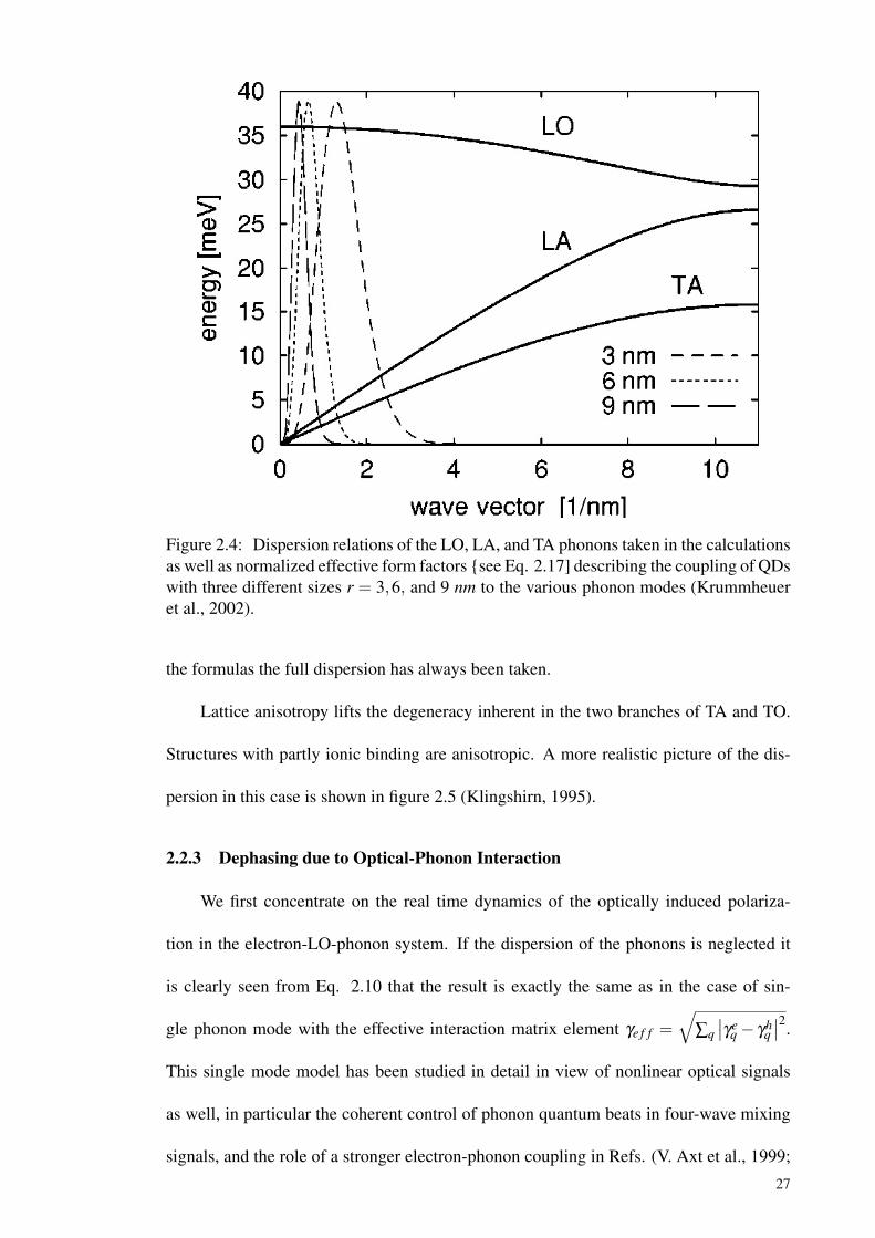
Figure 2.4: Dispersion relations of the LO, LA, and TA phonons taken in the calculationsas well as normalized effective form factors see Eq. 2.17] describing the coupling of QDswith three different sizes r = 3,6, and 9 nm to the various phonon modes (Krummheueret al., 2002).

the formulas the full dispersion has always been taken.

Lattice anisotropy lifts the degeneracy inherent in the two branches of TA and TO.

Structures with partly ionic binding are anisotropic. A more realistic picture of the dis-

persion in this case is shown in figure 2.5 (Klingshirn, 1995).

2.2.3 Dephasing due to Optical-Phonon Interaction

We first concentrate on the real time dynamics of the optically induced polariza-

tion in the electron-LO-phonon system. If the dispersion of the phonons is neglected it

is clearly seen from Eq. 2.10 that the result is exactly the same as in the case of sin-

gle phonon mode with the effective interaction matrix element γe f f =√

∑q∣∣γe

q− γhq∣∣2.

This single mode model has been studied in detail in view of nonlinear optical signals

as well, in particular the coherent control of phonon quantum beats in four-wave mixing

signals, and the role of a stronger electron-phonon coupling in Refs. (V. Axt et al., 1999;

27

Figure 2.5: The degeneracy has been lifted in acoustic and optical dispersion curves byan anisotropic lattice. a represents the lattice constant (Klingshirn, 1995).

Steinbach et al., 1999; Castella & Zimmermann, 1999; Kuhn, Axt, Herbst, & Binder,

1999). The optical polarization resulting from the excitation with an optical pulse with a

δ -function-like shape in time as well as the corresponding absorption spectrum are shown

for the case of a 6-nm QD at temperature 300 K in figure 2.6(a) and (b). The optical polar-

ization exhibits quantum beats with the phonon frequency; no decay is present. The spec-

trum consists of a series of δ -function peaks at the zero-phonon transition and at integer

multiples of the phonon frequency above and, for nonzero temperature, below that tran-

sition. The weights of the various lines depend on temperature and, through the effective

coupling constant (or the Huang-Rhys parameter), on the QD parameters. A closed-form

28

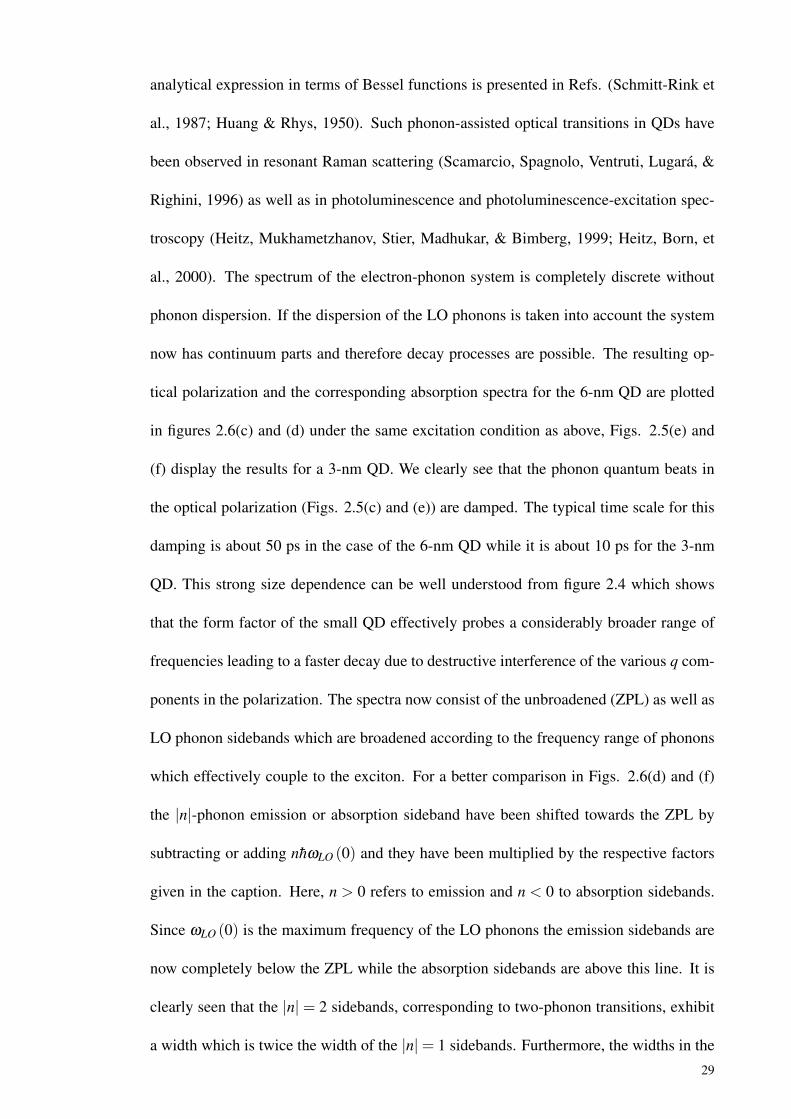
analytical expression in terms of Bessel functions is presented in Refs. (Schmitt-Rink et

al., 1987; Huang & Rhys, 1950). Such phonon-assisted optical transitions in QDs have

been observed in resonant Raman scattering (Scamarcio, Spagnolo, Ventruti, Lugará, &

Righini, 1996) as well as in photoluminescence and photoluminescence-excitation spec-

troscopy (Heitz, Mukhametzhanov, Stier, Madhukar, & Bimberg, 1999; Heitz, Born, et

al., 2000). The spectrum of the electron-phonon system is completely discrete without

phonon dispersion. If the dispersion of the LO phonons is taken into account the system

now has continuum parts and therefore decay processes are possible. The resulting op-

tical polarization and the corresponding absorption spectra for the 6-nm QD are plotted

in figures 2.6(c) and (d) under the same excitation condition as above, Figs. 2.5(e) and

(f) display the results for a 3-nm QD. We clearly see that the phonon quantum beats in

the optical polarization (Figs. 2.5(c) and (e)) are damped. The typical time scale for this

damping is about 50 ps in the case of the 6-nm QD while it is about 10 ps for the 3-nm

QD. This strong size dependence can be well understood from figure 2.4 which shows

that the form factor of the small QD effectively probes a considerably broader range of

frequencies leading to a faster decay due to destructive interference of the various q com-

ponents in the polarization. The spectra now consist of the unbroadened (ZPL) as well as

LO phonon sidebands which are broadened according to the frequency range of phonons

which effectively couple to the exciton. For a better comparison in Figs. 2.6(d) and (f)

the |n|-phonon emission or absorption sideband have been shifted towards the ZPL by

subtracting or adding nhωLO (0) and they have been multiplied by the respective factors

given in the caption. Here, n > 0 refers to emission and n < 0 to absorption sidebands.

Since ωLO (0) is the maximum frequency of the LO phonons the emission sidebands are

now completely below the ZPL while the absorption sidebands are above this line. It is

clearly seen that the |n| = 2 sidebands, corresponding to two-phonon transitions, exhibit

a width which is twice the width of the |n|= 1 sidebands. Furthermore, the widths in the

29

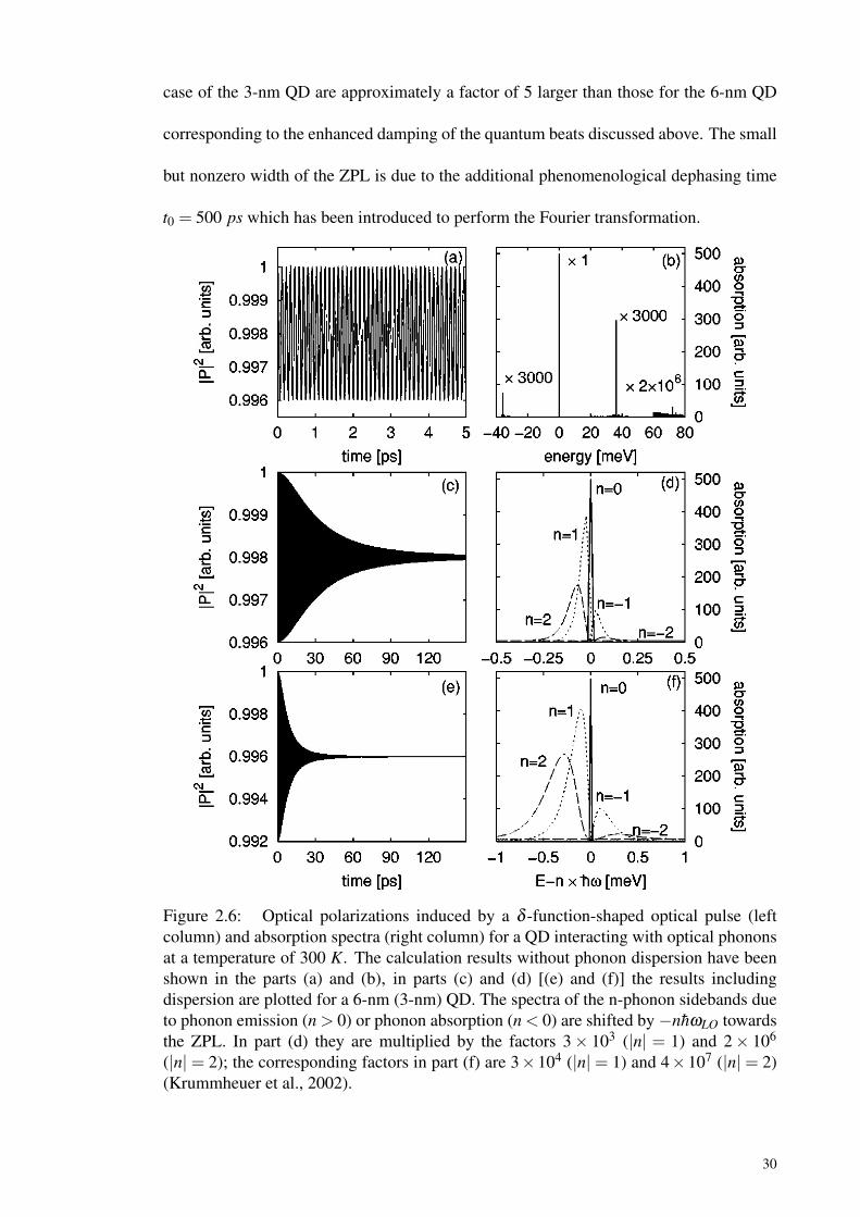
case of the 3-nm QD are approximately a factor of 5 larger than those for the 6-nm QD

corresponding to the enhanced damping of the quantum beats discussed above. The small

but nonzero width of the ZPL is due to the additional phenomenological dephasing time

t0 = 500 ps which has been introduced to perform the Fourier transformation.

Figure 2.6: Optical polarizations induced by a δ -function-shaped optical pulse (leftcolumn) and absorption spectra (right column) for a QD interacting with optical phononsat a temperature of 300 K. The calculation results without phonon dispersion have beenshown in the parts (a) and (b), in parts (c) and (d) [(e) and (f)] the results includingdispersion are plotted for a 6-nm (3-nm) QD. The spectra of the n-phonon sidebands dueto phonon emission (n > 0) or phonon absorption (n < 0) are shifted by −nhωLO towardsthe ZPL. In part (d) they are multiplied by the factors 3× 103 (|n| = 1) and 2× 106

(|n|= 2); the corresponding factors in part (f) are 3×104 (|n|= 1) and 4×107 (|n|= 2)(Krummheuer et al., 2002).

30

2.2.4 Dephasing due to Acoustic-Phonon Interaction

AC phonons are characterized by a continuous spectrum starting at zero frequency.

Therefore the phonon sidebands approach the ZPL and, under suitable conditions, may

result in a broadened ZPL (Duke & Mahan, 1965). In figure 2.7 the optical polarization

and the absorption spectrum are shown for a 3-nm QD at three different temperatures

T = 4, 77, and 300 K, as obtained from calculations including piezoelectric (Figs. 2.7(a)

and (b) and deformation potential (Figs. 2.6(c) and (d) coupling. Interestingly, it is found

that in all cases the polarization remains at a finite value at long times corresponding to an

unbroadened ZPL. This can be understood from the q dependence of the matrix element

in the limit of small q values.

According to figure 2.4 it is found that for small q: ω j (q)→ ωLO for the optical

branch and ω j (q)→ v jq for the acoustic branches, where v j are the respective sound

velocities. Therefore, according to Eq. 2.6 the bulk coupling matrix elements of defor-

mation couplings γXj,q = γe

j,q− γhj,q scale as

√q and the ones of piezoelectric coupling are

proportional to 1/√

q. In general, the deformation potential for electrons and holes are

different and the form factors of both carrier types approach unity for q→ 0, therefore the

total coupling constant is proportional to q2. The bulk piezoelectric coupling constant, on

the other hand, being a polar mechanism, has exactly the same value for electrons and

holes. Then, the form factors of the electron and hole exactly cancel at q = 0. The lowest

order in difference of the form factors is proportional to q2 and thus the total coupling

constant is proportional to q3/2. A vanishing coupling constant for q→ 0 gives rise to an

unbroadened ZPL (Krummheuer et al., 2002).

It can be seen in Figs 2.7(a) and (c) that the dynamics due to interactions with AC

phonons exhibits a pronounced temperature dependence. At low temperatures the line

is strongly asymmetric; there is only a contribution on the high-energy side of the ZPL

31

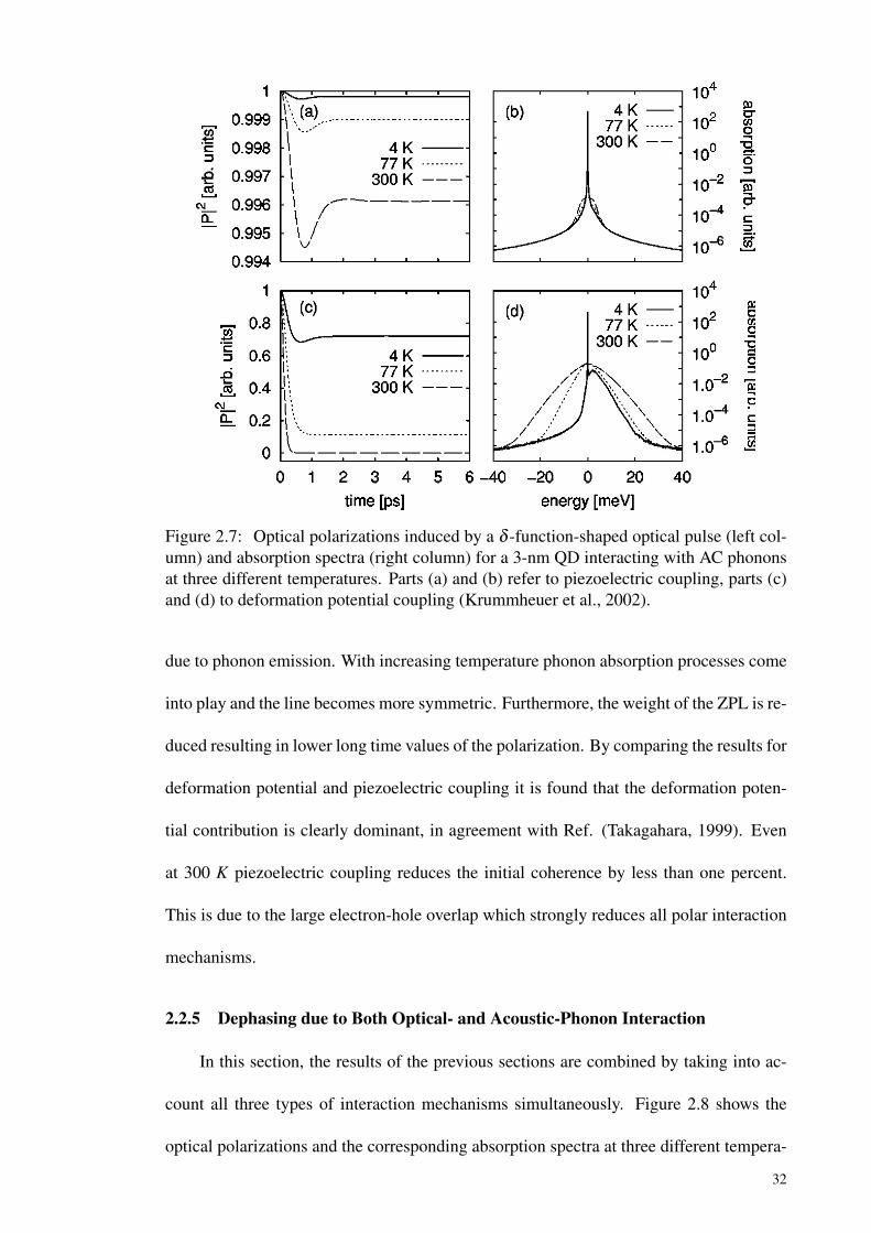
Figure 2.7: Optical polarizations induced by a δ -function-shaped optical pulse (left col-umn) and absorption spectra (right column) for a 3-nm QD interacting with AC phononsat three different temperatures. Parts (a) and (b) refer to piezoelectric coupling, parts (c)and (d) to deformation potential coupling (Krummheuer et al., 2002).

due to phonon emission. With increasing temperature phonon absorption processes come

into play and the line becomes more symmetric. Furthermore, the weight of the ZPL is re-

duced resulting in lower long time values of the polarization. By comparing the results for

deformation potential and piezoelectric coupling it is found that the deformation poten-

tial contribution is clearly dominant, in agreement with Ref. (Takagahara, 1999). Even

at 300 K piezoelectric coupling reduces the initial coherence by less than one percent.

This is due to the large electron-hole overlap which strongly reduces all polar interaction

mechanisms.

2.2.5 Dephasing due to Both Optical- and Acoustic-Phonon Interaction

In this section, the results of the previous sections are combined by taking into ac-

count all three types of interaction mechanisms simultaneously. Figure 2.8 shows the

optical polarizations and the corresponding absorption spectra at three different tempera-

32

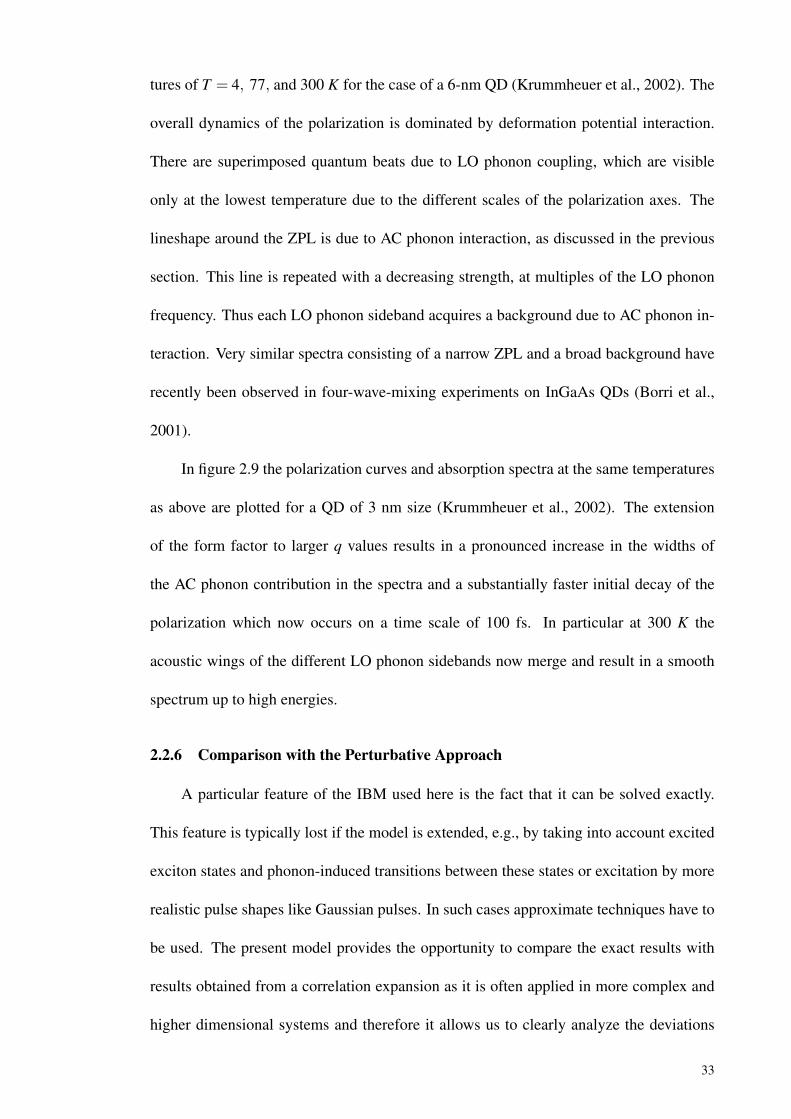
tures of T = 4, 77, and 300 K for the case of a 6-nm QD (Krummheuer et al., 2002). The

overall dynamics of the polarization is dominated by deformation potential interaction.

There are superimposed quantum beats due to LO phonon coupling, which are visible

only at the lowest temperature due to the different scales of the polarization axes. The

lineshape around the ZPL is due to AC phonon interaction, as discussed in the previous

section. This line is repeated with a decreasing strength, at multiples of the LO phonon

frequency. Thus each LO phonon sideband acquires a background due to AC phonon in-

teraction. Very similar spectra consisting of a narrow ZPL and a broad background have

recently been observed in four-wave-mixing experiments on InGaAs QDs (Borri et al.,

2001).

In figure 2.9 the polarization curves and absorption spectra at the same temperatures

as above are plotted for a QD of 3 nm size (Krummheuer et al., 2002). The extension

of the form factor to larger q values results in a pronounced increase in the widths of

the AC phonon contribution in the spectra and a substantially faster initial decay of the

polarization which now occurs on a time scale of 100 fs. In particular at 300 K the

acoustic wings of the different LO phonon sidebands now merge and result in a smooth

spectrum up to high energies.

2.2.6 Comparison with the Perturbative Approach

A particular feature of the IBM used here is the fact that it can be solved exactly.

This feature is typically lost if the model is extended, e.g., by taking into account excited

exciton states and phonon-induced transitions between these states or excitation by more

realistic pulse shapes like Gaussian pulses. In such cases approximate techniques have to

be used. The present model provides the opportunity to compare the exact results with

results obtained from a correlation expansion as it is often applied in more complex and

higher dimensional systems and therefore it allows us to clearly analyze the deviations

33

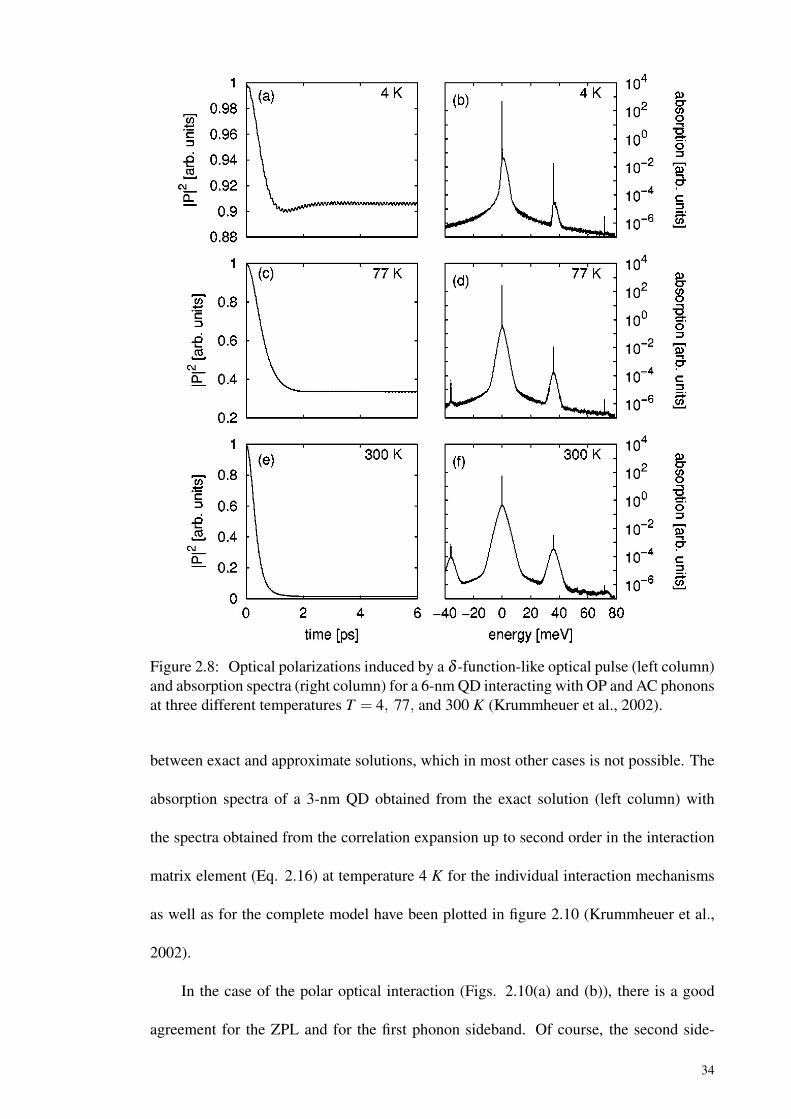
Figure 2.8: Optical polarizations induced by a δ -function-like optical pulse (left column)and absorption spectra (right column) for a 6-nm QD interacting with OP and AC phononsat three different temperatures T = 4, 77, and 300 K (Krummheuer et al., 2002).

between exact and approximate solutions, which in most other cases is not possible. The

absorption spectra of a 3-nm QD obtained from the exact solution (left column) with

the spectra obtained from the correlation expansion up to second order in the interaction

matrix element (Eq. 2.16) at temperature 4 K for the individual interaction mechanisms

as well as for the complete model have been plotted in figure 2.10 (Krummheuer et al.,

2002).

In the case of the polar optical interaction (Figs. 2.10(a) and (b)), there is a good

agreement for the ZPL and for the first phonon sideband. Of course, the second side-

34

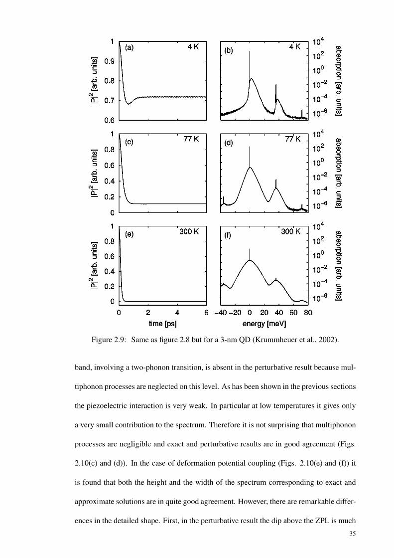
Figure 2.9: Same as figure 2.8 but for a 3-nm QD (Krummheuer et al., 2002).

band, involving a two-phonon transition, is absent in the perturbative result because mul-

tiphonon processes are neglected on this level. As has been shown in the previous sections

the piezoelectric interaction is very weak. In particular at low temperatures it gives only

a very small contribution to the spectrum. Therefore it is not surprising that multiphonon

processes are negligible and exact and perturbative results are in good agreement (Figs.

2.10(c) and (d)). In the case of deformation potential coupling (Figs. 2.10(e) and (f)) it

is found that both the height and the width of the spectrum corresponding to exact and

approximate solutions are in quite good agreement. However, there are remarkable differ-

ences in the detailed shape. First, in the perturbative result the dip above the ZPL is much

35

Figure 2.10: Comparison of the exact absorption spectra (left column) with those ob-tained from a correlation expansion up to the second order in the coupling matrix ele-ments (right column) for (a) and (b) polar optical, (c) and (d) piezoelectric, and (e) and(f) deformation potential, as well as for (g) and (h) the combination of all mechanisms ata temperature of 4 K (Krummheuer et al., 2002).

more pronounced than in the exact result. This is due to the fact that one-phonon tran-

sitions with a small wave vector are strongly suppressed because, as already discussed

above, in this range the matrix element is proportional to√

q. Therefore positions in

the immediate vicinity of the ZPL can only be reached by at least two-phonon processes

which again are absent in the perturbative treatment. Second, the approximate absorp-

tion spectrum exhibits a series of dips above 10 meV which is absent in the exact result.

36

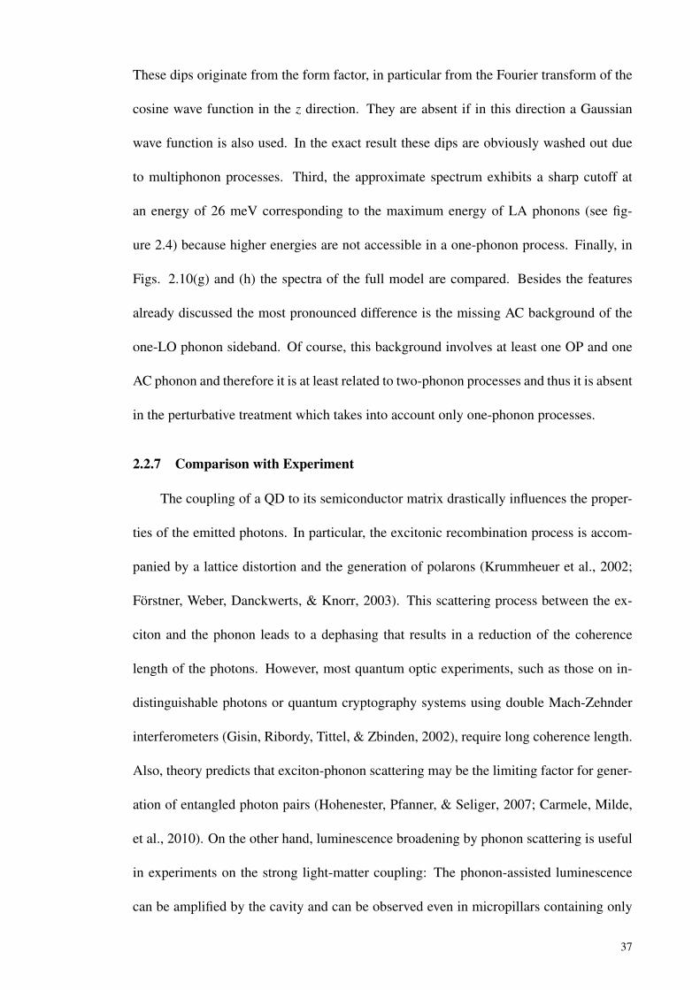
These dips originate from the form factor, in particular from the Fourier transform of the

cosine wave function in the z direction. They are absent if in this direction a Gaussian

wave function is also used. In the exact result these dips are obviously washed out due

to multiphonon processes. Third, the approximate spectrum exhibits a sharp cutoff at

an energy of 26 meV corresponding to the maximum energy of LA phonons (see fig-

ure 2.4) because higher energies are not accessible in a one-phonon process. Finally, in

Figs. 2.10(g) and (h) the spectra of the full model are compared. Besides the features

already discussed the most pronounced difference is the missing AC background of the

one-LO phonon sideband. Of course, this background involves at least one OP and one

AC phonon and therefore it is at least related to two-phonon processes and thus it is absent

in the perturbative treatment which takes into account only one-phonon processes.

2.2.7 Comparison with Experiment

The coupling of a QD to its semiconductor matrix drastically influences the proper-

ties of the emitted photons. In particular, the excitonic recombination process is accom-

panied by a lattice distortion and the generation of polarons (Krummheuer et al., 2002;

Förstner, Weber, Danckwerts, & Knorr, 2003). This scattering process between the ex-

citon and the phonon leads to a dephasing that results in a reduction of the coherence

length of the photons. However, most quantum optic experiments, such as those on in-

distinguishable photons or quantum cryptography systems using double Mach-Zehnder

interferometers (Gisin, Ribordy, Tittel, & Zbinden, 2002), require long coherence length.

Also, theory predicts that exciton-phonon scattering may be the limiting factor for gener-

ation of entangled photon pairs (Hohenester, Pfanner, & Seliger, 2007; Carmele, Milde,

et al., 2010). On the other hand, luminescence broadening by phonon scattering is useful

in experiments on the strong light-matter coupling: The phonon-assisted luminescence

can be amplified by the cavity and can be observed even in micropillars containing only

37

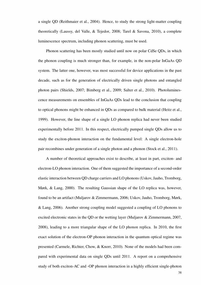
a single QD (Reithmaier et al., 2004). Hence, to study the strong light-matter coupling

theoretically (Laussy, del Valle, & Tejedor, 2008; Tarel & Savona, 2010), a complete

luminescence spectrum, including phonon scattering, must be used.

Phonon scattering has been mostly studied until now on polar CdSe QDs, in which

the phonon coupling is much stronger than, for example, in the non-polar InGaAs QD

system. The latter one, however, was most successful for device applications in the past

decade, such as for the generation of electrically driven single photons and entangled

photon pairs (Shields, 2007; Bimberg et al., 2009; Salter et al., 2010). Photolumines-

cence measurements on ensembles of InGaAs QDs lead to the conclusion that coupling

to optical phonons might be enhanced in QDs as compared to bulk material (Heitz et al.,

1999). However, the line shape of a single LO phonon replica had never been studied

experimentally before 2011. In this respect, electrically pumped single QDs allow us to

study the exciton-phonon interaction on the fundamental level: A single electron-hole

pair recombines under generation of a single photon and a phonon (Stock et al., 2011).

A number of theoretical approaches exist to describe, at least in part, exciton- and

electron-LO phonon interaction. One of them suggested the importance of a second-order

elastic interaction between QD charge carriers and LO phonons (Uskov, Jauho, Tromborg,

Mørk, & Lang, 2000). The resulting Gaussian shape of the LO replica was, however,

found to be an artifact (Muljarov & Zimmermann, 2006; Uskov, Jauho, Tromborg, Mørk,

& Lang, 2006). Another strong coupling model suggested a coupling of LO phonons to

excited electronic states in the QD or the wetting layer (Muljarov & Zimmermann, 2007,

2008), leading to a more triangular shape of the LO phonon replica. In 2010, the first

exact solution of the electron-OP phonon interaction in the quantum optical regime was

presented (Carmele, Richter, Chow, & Knorr, 2010). None of the models had been com-

pared with experimental data on single QDs until 2011. A report on a comprehensive

study of both exciton-AC and -OP phonon interaction in a highly efficient single-photon

38

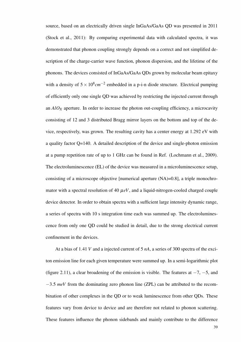
source, based on an electrically driven single InGaAs/GaAs QD was presented in 2011

(Stock et al., 2011): By comparing experimental data with calculated spectra, it was

demonstrated that phonon coupling strongly depends on a correct and not simplified de-

scription of the charge-carrier wave function, phonon dispersion, and the lifetime of the

phonons. The devices consisted of InGaAs/GaAs QDs grown by molecular beam epitaxy

with a density of 5× 108cm−2 embedded in a p-i-n diode structure. Electrical pumping

of efficiently only one single QD was achieved by restricting the injected current through

an AlOX aperture. In order to increase the photon out-coupling efficiency, a microcavity

consisting of 12 and 3 distributed Bragg mirror layers on the bottom and top of the de-

vice, respectively, was grown. The resulting cavity has a center energy at 1.292 eV with

a quality factor Q=140. A detailed description of the device and single-photon emission

at a pump repetition rate of up to 1 GHz can be found in Ref. (Lochmann et al., 2009).

The electroluminescence (EL) of the device was measured in a microluminescence setup,

consisting of a microscope objective [numerical aperture (NA)=0.8], a triple monochro-

mator with a spectral resolution of 40 µeV , and a liquid-nitrogen-cooled charged couple

device detector. In order to obtain spectra with a sufficient large intensity dynamic range,

a series of spectra with 10 s integration time each was summed up. The electrolumines-

cence from only one QD could be studied in detail, due to the strong electrical current

confinement in the devices.

At a bias of 1.41 V and a injected current of 5 nA, a series of 300 spectra of the exci-

ton emission line for each given temperature were summed up. In a semi-logarithmic plot

(figure 2.11), a clear broadening of the emission is visible. The features at −7, −5, and

−3.5 meV from the dominating zero phonon line (ZPL) can be attributed to the recom-

bination of other complexes in the QD or to weak luminescence from other QDs. These

features vary from device to device and are therefore not related to phonon scattering.

These features influence the phonon sidebands and mainly contribute to the difference

39

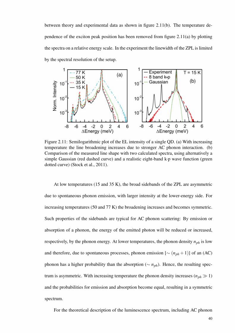
between theory and experimental data as shown in figure 2.11(b). The temperature de-

pendence of the exciton peak position has been removed from figure 2.11(a) by plotting

the spectra on a relative energy scale. In the experiment the linewidth of the ZPL is limited

by the spectral resolution of the setup.

Figure 2.11: Semilogarithmic plot of the EL intensity of a single QD. (a) With increasingtemperature the line broadening increases due to stronger AC phonon interaction. (b)Comparison of the measured line shape with two calculated spectra, using alternatively asimple Gaussian (red dashed curve) and a realistic eight-band k·p wave function (greendotted curve) (Stock et al., 2011).

At low temperatures (15 and 35 K), the broad sidebands of the ZPL are asymmetric

due to spontaneous phonon emission, with larger intensity at the lower-energy side. For

increasing temperatures (50 and 77 K) the broadening increases and becomes symmetric.

Such properties of the sidebands are typical for AC phonon scattering: By emission or

absorption of a phonon, the energy of the emitted photon will be reduced or increased,

respectively, by the phonon energy. At lower temperatures, the phonon density nph is low

and therefore, due to spontaneous processes, phonon emission [∼ (nph + 1)] of an (AC)

phonon has a higher probability than the absorption (∼ nph). Hence, the resulting spec-

trum is asymmetric. With increasing temperature the phonon density increases (nph 1)

and the probabilities for emission and absorption become equal, resulting in a symmetric

spectrum.

For the theoretical description of the luminescence spectrum, including AC phonon

40

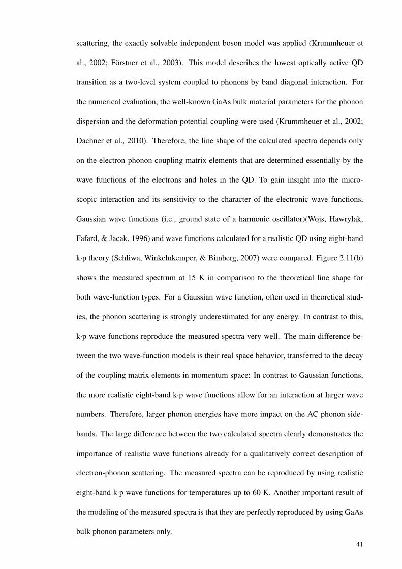
scattering, the exactly solvable independent boson model was applied (Krummheuer et

al., 2002; Förstner et al., 2003). This model describes the lowest optically active QD

transition as a two-level system coupled to phonons by band diagonal interaction. For

the numerical evaluation, the well-known GaAs bulk material parameters for the phonon

dispersion and the deformation potential coupling were used (Krummheuer et al., 2002;

Dachner et al., 2010). Therefore, the line shape of the calculated spectra depends only

on the electron-phonon coupling matrix elements that are determined essentially by the

wave functions of the electrons and holes in the QD. To gain insight into the micro-

scopic interaction and its sensitivity to the character of the electronic wave functions,

Gaussian wave functions (i.e., ground state of a harmonic oscillator)(Wojs, Hawrylak,

Fafard, & Jacak, 1996) and wave functions calculated for a realistic QD using eight-band

k·p theory (Schliwa, Winkelnkemper, & Bimberg, 2007) were compared. Figure 2.11(b)

shows the measured spectrum at 15 K in comparison to the theoretical line shape for

both wave-function types. For a Gaussian wave function, often used in theoretical stud-

ies, the phonon scattering is strongly underestimated for any energy. In contrast to this,

k·p wave functions reproduce the measured spectra very well. The main difference be-

tween the two wave-function models is their real space behavior, transferred to the decay

of the coupling matrix elements in momentum space: In contrast to Gaussian functions,

the more realistic eight-band k·p wave functions allow for an interaction at larger wave

numbers. Therefore, larger phonon energies have more impact on the AC phonon side-

bands. The large difference between the two calculated spectra clearly demonstrates the

importance of realistic wave functions already for a qualitatively correct description of

electron-phonon scattering. The measured spectra can be reproduced by using realistic

eight-band k·p wave functions for temperatures up to 60 K. Another important result of

the modeling of the measured spectra is that they are perfectly reproduced by using GaAs

bulk phonon parameters only.

41

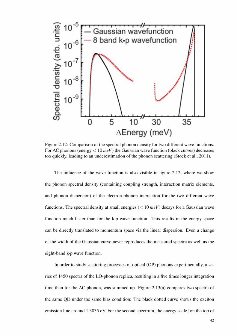
Figure 2.12: Comparison of the spectral phonon density for two different wave functions.For AC phonons (energy < 10 meV ) the Gaussian wave function (black curves) decreasestoo quickly, leading to an underestimation of the phonon scattering (Stock et al., 2011).

The influence of the wave function is also visible in figure 2.12, where we show

the phonon spectral density (containing coupling strength, interaction matrix elements,

and phonon dispersion) of the electron-phonon interaction for the two different wave

functions. The spectral density at small energies (< 10 meV ) decays for a Gaussian wave

function much faster than for the k·p wave function. This results in the energy space

can be directly translated to momentum space via the linear dispersion. Even a change

of the width of the Gaussian curve never reproduces the measured spectra as well as the

eight-band k·p wave function.

In order to study scattering processes of optical (OP) phonons experimentally, a se-

ries of 1450 spectra of the LO-phonon replica, resulting in a five times longer integration

time than for the AC phonon, was summed up. Figure 2.13(a) compares two spectra of

the same QD under the same bias condition: The black dotted curve shows the exciton

emission line around 1.3035 eV. For the second spectrum, the energy scale [on the top of

42

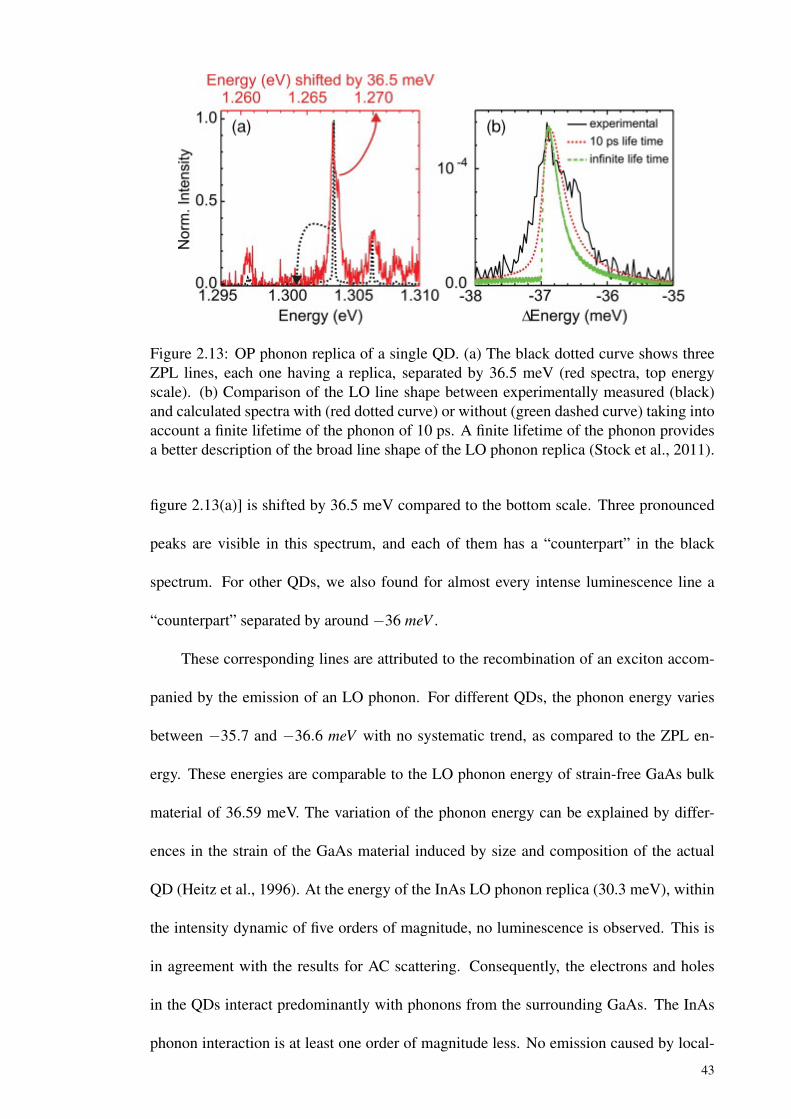
Figure 2.13: OP phonon replica of a single QD. (a) The black dotted curve shows threeZPL lines, each one having a replica, separated by 36.5 meV (red spectra, top energyscale). (b) Comparison of the LO line shape between experimentally measured (black)and calculated spectra with (red dotted curve) or without (green dashed curve) taking intoaccount a finite lifetime of the phonon of 10 ps. A finite lifetime of the phonon providesa better description of the broad line shape of the LO phonon replica (Stock et al., 2011).

figure 2.13(a)] is shifted by 36.5 meV compared to the bottom scale. Three pronounced

peaks are visible in this spectrum, and each of them has a “counterpart” in the black

spectrum. For other QDs, we also found for almost every intense luminescence line a

“counterpart” separated by around −36 meV .

These corresponding lines are attributed to the recombination of an exciton accom-

panied by the emission of an LO phonon. For different QDs, the phonon energy varies

between −35.7 and −36.6 meV with no systematic trend, as compared to the ZPL en-

ergy. These energies are comparable to the LO phonon energy of strain-free GaAs bulk

material of 36.59 meV. The variation of the phonon energy can be explained by differ-

ences in the strain of the GaAs material induced by size and composition of the actual

QD (Heitz et al., 1996). At the energy of the InAs LO phonon replica (30.3 meV), within

the intensity dynamic of five orders of magnitude, no luminescence is observed. This is

in agreement with the results for AC scattering. Consequently, the electrons and holes

in the QDs interact predominantly with phonons from the surrounding GaAs. The InAs

phonon interaction is at least one order of magnitude less. No emission caused by local-

43

ized InAs-type phonons in the QD is observed.

We focus on the coupling strength of the exciton-LO phonon interaction. The cou-

pling strength is usually described by the Huang-Rhys factor, given by the intensity ratio

of the ZPL IZPL and the nth phonon replica In (at zero temperature) by In/IZPL = SneS/n!

(Huang & Rhys, 1950; Landolt-Bórnstein, 1987). In figure 2.13 the intensity is nor-

malized with respect to the ZPL. Both the emission lines are located outside the cavity

resonance in the stop band, so their intensities can be compared. The intensity of the LO

phonon replica is about four orders of magnitude lower than the ZPL intensity, resulting

in a Huang-Rhys factor of S ≈ 10−4. This value is one order of magnitude less than for

GaAs bulk phonons, indicating a reduced phonon coupling in this electrically pumped

single QD. The Huang-Rhys factor from the calculated spectral density (figure 2.12) has

additionally been derived (Stock et al., 2011; May & Kuhn, 2000). The calculations

yields factors of S≈ 10−4, confirming the experimental result.

The line shape of the phonon replicas enables us to access the coupling mechanism

between the exciton and the LO phonon: The recombination of an electron-hole pair in a

QD has a discrete energy and the linewidth of the ZPL is only limited by the lifetime of the

exciton to a few µeV (Borri et al., 2001). Therefore, any broadening of the luminescence

upon generation of an LO phonon is due to the intrinsic phonon properties or coupling

of the phonons to other modes. Figure 2.13(b) shows the LO phonon replica at larger

spectral resolution. The resulting full width at half maximum of 700 µeV is well above

the spectral resolution and about one hundred times larger than for the ZPL. Hence, LO

phonons of varying energies are generated during the recombination processes in the same

single QD. Also, the line shape is again slightly asymmetric, showing a faster decay on

the low-energy side than on the high-energy side. This specific line shape is consistent

with a broadening mechanism that results from a realistic wave-number-dependent LO

phonon dispersion ωLO (q) beyond the Einstein model ωLO = const: In such a dispersion

44

relation, a higher energy corresponds to a smaller momentum. Since the electron-phonon

coupling favors low-momentum phonons, the generation of higher-energy phonons has a

larger probability than that of lower-energy phonons, and thus yields an asymmetry of the

line shape.

For a quantitative understanding of this coupling mechanism, we compare the ex-

perimental results with a model (figure 2.13), where LO phonon assisted luminescence

spectra are calculated using the independent boson model and approximating the real

optical-phonon dispersion by a cosine. This approximation agrees very well with the ex-

perimentally observed dispersion (Landolt-Bórnstein, 1987). For the coupling matrix el-

ements, Gaussian wave functions and eight-band k·p wave functions, respectively, again

are compared. In contrast to the AC phonon coupling, the influence of different wave

functions is less pronounced. In figure 2.12 it can be seen that the LO phonon part of

the spectral density shows a much faster decay than the acoustic phonon part. Hence the

LO phonon replicas for Gaussian and eight-band k·p wave functions differ only slightly.

For a complete description of the LO phonon-scattering process, a finite lifetime of 10

ps ((Rudin, Reinecke, & Bayer, 2006) and (Bhatt, Kim, & Stroscio, 1994)) for the LO

phonons has also been included. The resulting LO replica in figure 2.13(b) reproduces

very well the measured line shape, whereas a line shape with neglected phonon lifetime

is too narrow. A perfect fit to the experimental data results in a phonon lifetime of 5 ps

Additional phonon replica broadening, due to the influence of excited and wetting layer

states, was predicted for the more enhanced electron-phonon coupling in CdSe systems

(Muljarov & Zimmermann, 2007). A significant influence in the GaAs material system

in the calculations could not be observed.

The AC and OP phonon scattering on the most fundamental level, at which a single

photon and a phonon are generated by the recombination of a single exciton in a single

electrically driven InGaAs/GaAs QD, were presented. By comparing experimental and

45

calculated spectra, we conclude that (i) GaAs bulk material phonon modes represent the

dominant broadening mechanism; (ii) localized InAs-type phonons are not observed; (iii)

a large LO replica broadening of ≈ 700 µeV is induced by interaction with large wave-

number phonons, having a finite lifetime; (iv) k·p wave functions are essential for the

description of the excitons; and (v) the independent boson model using these wave func-

tions provides the proper wave-vector dependence for a quantitative understanding of the

experimental results.

2.3 Quantum Dot-Cavity Quantum Electrodynamic Systems

Solid-state cavity quantum electrodynamic (cQED) systems, consist of a solid-state

emitter like single semiconductor quantum dot (QD) coupled either resonantly or non-

resonantly to single mode of an optical nano (micro) cavity, have promising properties

for both fundamental and practical applications; A scalable QD-cQED platform, where

the interaction between the single photon with the QD can be engineered and controlled

to a high degree, can realize a perfect single photon source (Somaschi et al., 2016; He

et al., 2013; Gazzano et al., 2013; Michler et al., 2000) which is a crucial requirement

for quantum computation and information processing (Knill et al., 2001; O’Brien et al.,

2009). It is also applicable for low-threshold and nano-scale lasers (Noda, 2006; Strauf &

Jahnke, 2011; Michler, 2003) as well as tests of fundamental aspects of quantum mechan-

ics (Haroche & Raimond, 2006). Since the QD is a solid structure, QD-cQED systems

are inherently coupled to the environment (phonon bath) and the interactions of the QD

carriers with phonons play an important role in the QD-cavity dynamics (Ates et al.,

2009; Kaer, Gregersen, & Mork, 2013; Nysteen, Kaer, & Mork, 2013; Roy & Hughes,

2012). Resonating light in a cavity provides an efficient way of enhancing light-matter

interaction since the coupling to one localized mode can be strongly enhanced compared

to all other modes. It has been well understood that the light-matter (QD-cavity) coupling

46

efficiency can be improved by structuring the cavity, which is the essence of modern re-

search in solid-state cQED (Lodahl et al., 2015). In photonic nanostructures the cavities

can have very small mode volumes, which enhances the interaction strength. The two

decisive cQED figures of merit are the quality factor Q and the effective mode volume

V of the localized quasimode. In the following, various QD-cQED systems, including a

nanophotonic cavity and single QD, with high-Q and small-V cavities are reviewed.

Micropillar cavities have been widely exploited as high-Q cavities. They can be fab-

ricated by epitaxial growth of alternating layers of refractive indexes n1 and n2 (e.g., GaAs

and AlGaAs) each of thickness λ/4ni, i = 1, 2, and by subsequently etching a micropillar

with a typical diameter of a few microns and a height of around 10 µm (Reithmaier et

al., 2004). The alternating layers form a Bragg mirror with a reflectivity that is controlled

by the number of layers. An extended spacer layer of length, e.g., λ = n1 in between

two such Bragg mirrors forms a highly localized cavity mode where QDs can be posi-

tioned; see figure 2.14(a). The two Bragg mirrors are often grown with different numbers

of layers in order to make a one-sided cavity consisting of a highly reflecting mirror and

an out-coupling mirror with an optimized transmission. The diameter of the micropillar

is chosen to restrict the lateral extension of the guided mode confined in the high-index

material, which leads to a small mode volume. Choosing the diameter below 1− 2 µm,

however, is found to significantly reduce Q due to the sensitivity to sidewall roughness

(Gazzano et al., 2013). Typical mode volumes accessible in micropillar cavities are at the

level of∼ 10(λ/n)3 and tapered cavities have recently been proposed as a way of localiz-

ing light even better (Lermer et al., 2012). Highly localized cavity modes can be obtained

by introducing defects in photonic-crystal membranes and a multitude of different design

possibilities have been explored in the literature. This flexibility of being able to tailor a

cavity mode by controlling the geometry of the photonic crystal and the defect area indeed

provides a very important asset of the photonic crystal platform. One of the most success-

47

ful and important designs so far is the L3 cavity that is obtained from a 2D triangular lat-

tice in a photonic-crystal membrane by leaving out three holes [cf. figure 2.14(b)], leading

to a mode volume of less than ∼ (λ/n)3. It was realized that the Q factor can be signif-

icantly boosted by more than an order of magnitude by displacing the holes at each end

of the cavity by just a fraction of a lattice constant, whereby leakage to radiation modes

can be strongly suppressed (Akahane, Asano, Song, & Noda, 2003). This remarkable

sensitivity to the detailed design reflects the large potential of photonic-crystal cavities.

A cavity Q factor of 2× 106 has been observed experimentally in modified L3 cavities

in silicon at a wavelength of 1.55 µm (Lai et al., 2014). Lower Q factors are generally

observed for GaAs cavities since they are matched to the shorter wavelength of InGaAs

QDs of around 950 nm and therefore more sensitive to fabrication imperfections, residual

scattering, and absorption due to the embedded QDs, as well as bulk and surface absorp-

tion, which is more pronounced at shorter wavelengths (Michael et al., 2007). A cavity Q

factor of 3×104 has been reported in a GaAs L3 cavity containing a single QD (Hennessy

et al., 2007). A number of different photonic-crystal cavity structures have been consid-

ered that potentially have higher Q factors including waveguide heterostructures (Song,

Noda, Asano, & Akahane, 2005) for which a Q factor of 5.5× 104 in a GaAs cavity with

QDs has been reported (Ota, Iwamoto, Kumagai, & Arakawa, 2011), nanobeam cavities

(Ohta et al., 2011), or even random Anderson-localized modes in photonic-crystal waveg-

uides due to naturally occurring fabrication imperfections (Topolancik, Ilic, & Vollmer,

2007; Smolka et al., 2011). The nanobeam cavity displayed in figure 2.14(c) is a 1D

photonic crystal consisting of etched holes in a narrow and thin membrane with a central

defect area defining the cavity region (Ohta et al., 2011). Finally microdisk cavities [see

figure 2.14(d)] constitute another class of resonators where the trapping of light is due

to total internal reflection rather than Bragg scattering. In a microdisk cavity the light is

confined to the rim of the disk in a whispering-gallery mode that can have a very high Q

48

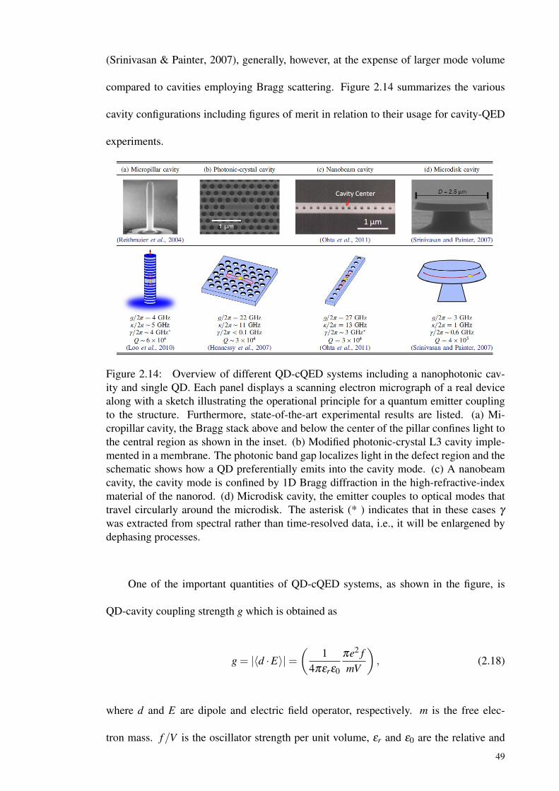
(Srinivasan & Painter, 2007), generally, however, at the expense of larger mode volume

compared to cavities employing Bragg scattering. Figure 2.14 summarizes the various

cavity configurations including figures of merit in relation to their usage for cavity-QED

experiments.

Figure 2.14: Overview of different QD-cQED systems including a nanophotonic cav-ity and single QD. Each panel displays a scanning electron micrograph of a real devicealong with a sketch illustrating the operational principle for a quantum emitter couplingto the structure. Furthermore, state-of-the-art experimental results are listed. (a) Mi-cropillar cavity, the Bragg stack above and below the center of the pillar confines light tothe central region as shown in the inset. (b) Modified photonic-crystal L3 cavity imple-mented in a membrane. The photonic band gap localizes light in the defect region and theschematic shows how a QD preferentially emits into the cavity mode. (c) A nanobeamcavity, the cavity mode is confined by 1D Bragg diffraction in the high-refractive-indexmaterial of the nanorod. (d) Microdisk cavity, the emitter couples to optical modes thattravel circularly around the microdisk. The asterisk (* ) indicates that in these cases γ

was extracted from spectral rather than time-resolved data, i.e., it will be enlargened bydephasing processes.

One of the important quantities of QD-cQED systems, as shown in the figure, is

QD-cavity coupling strength g which is obtained as

g = |〈d ·E〉|=(

14πεrε0

πe2 fmV

), (2.18)

where d and E are dipole and electric field operator, respectively. m is the free elec-

tron mass. f/V is the oscillator strength per unit volume, εr and ε0 are the relative and

49

vacuum permittivity (Gaussian units: 4πε0→ 1), respectively. The oscillator strength is

given as f = 2mω0d2/e2h where ω0 is the cavity mode frequency and e is the electron

charge. Other important parameters of QD-cavity systems include cavity decay rate, κ ,

QD recombination rate, γr, and cavity quality factor, Q, which is defined as Q = ω0κ

.

2.3.1 Theoretical Approaches to Investigate Quantum Dot-Cavity Quantum Elec-trodynamic Systems

Theoretical description of QD-cQED including carrier-phonon interactions has been

discussed in the literature usually based on derivation of quantum master equation (ME)

using the Liouville–von Neumann equation and the second-order Born approximation;

One common approach is to use a standard weak-coupling theory, which only includes

exciton-phonon interactions to second order and is known to break down at higher temper-

atures, strong exciton-phonon couplings (McCutcheon & Nazir, 2010), and in the pres-

ence of cavity coupling (Roy & Hughes, 2011). In another approach, exciton-cavity

coupling is considered as a perturbation and time-convolutionless (TC) technique is ap-

plied (Hohenester et al., 2009). Applying the unitary polaron transformation to the model

Hamiltonian, that encapsulates non-perturbative coupling effects beyond second-order

Born approximation, and utilizing either the Nakajima-Zwanzig (NZ) (Wilson-Rae &

Imamoglu, 2002; Kaer, Nielsen, Lodahl, Jauho, & Mørk, 2012) or TC (Kaer et al., 2012)

projection operator techniques result in a polaron frame ME in NZ or TC form. A varia-

tionally optimized ME, through a combination of a variationally optimized unitary trans-

formation and TC projection operator technique, for a coherently laser-driven QD has

also been proposed (McCutcheon, Dattani, Gauger, Lovett, & Nazir, 2011). The varia-

tional ME gives reliable results over a wide range of parameters even in regimes in which

previous ME approaches fail. However, these quantum MEs are obtained by applying

second-order perturbation expansion and thus can only provide approximate results (Lee,

Moix, & Cao, 2012). There are only a few non-perturbative techniques to attain the nu-

50

merically exact dynamics in all the regimes of parameters including strong coupling, high

temperatures, and long-time dynamics. Those methods include the hierarchy master equa-

tion (Tanimura, 2006; Ishizaki & Tanimura, 2005), the multiconfiguration time-dependent

Hartree approach (Meyer, Manthe, & Cederbaum, 1990; Beck, Jäckle, Worth, & Meyer,

2000; Thoss, Wang, & Miller, 2001), and the quasi-adiabatic propagator Feynman path-

integral (QUAPI) (Makarov & Makri, 1994; Makri & Makarov, 1995b, 1995a) which

usually is used as a "benchmark" to examine validity of standard approaches that utilize

approximations (McCutcheon et al., 2011; Lee et al., 2012; Vagov, Croitoru, Axt, Mach-

nikowski, & Kuhn, 2011). The main disadvantage of QUAPI or real-time path-integral

(RTPI) compared to the approximate approaches is that it is computationally more expen-

sive.

QUAPI or RTPI can be formulated in a closed form for models that the system is lin-

early coupled to harmonic-oscillator degrees of freedom (Sim, 2001) such as QD-cavity

system coupled to environment phonons. An efficient method for calculation of the re-

duced density matrix (RDM) derived in QUAPI approach has been proposed (Makarov

& Makri, 1994; Makri & Makarov, 1995b, 1995a), its subsequent improvement, making

the method easier to implement, has been presented later (Sim, 2001). The main focus

of these studies has been systems with ohmic or subohmic coupling types, for which

physical problems, such as dynamic localization and the crossover between coherent and

incoherent dynamics, have been studied (Vagov, Croitoru, Glässl, Axt, & Kuhn, 2011).

When the effective environment spectral density J (ω) scales as J(ω) ∼ ωα in the low-

frequency limit with 0<α < 1, the system-environment coupling is called "subohmic". If

α = 1 it is called "ohmic" while the case α > 1 is referred to as "superohmic". As we will

show later and have also been discussed in the literature (McCutcheon et al., 2011; Vagov,

Croitoru, Glässl, et al., 2011; Ramsay, Godden, et al., 2010; Ramsay, Gopal, et al., 2010;

Machnikowski & Jacak, 2004; Vagov et al., 2004; Krummheuer et al., 2002; Vagov, Axt,

51

& Kuhn, 2002; Besombes, Kheng, Marsal, & Mariette, 2001; Borri et al., 2001; Stievater

et al., 2001), the pure dephasing type carrier-phonon coupling in strongly confined semi-

conductor QDs represents an example for a system with superohmic coupling. The first

implementation of the numerically accurate RTPI method that is able to deal with the su-

perohmic couplings for a QD with few carrier states coupled to external Gaussian pulses

and longitudinal acoustic (LA) phonons has been presented in Ref. (Vagov, Croitoru,

Glässl, et al., 2011). Later, the authors extended their implementation to the case where

the classical field is replaced by a single quantized cavity mode (Glässl et al., 2012), in

this case, a QD without dissipation is coupled to LA phonon reservoir and a loss-less cav-

ity. The published work does not include mathematical details of the extended method.

To incorporate the losses, in Ref. (Vagov, Glässl, Croitoru, Axt, & Kuhn, 2014), the au-

thors have obtained the evolution of the populations and coherences from a ME derived

from the Liouville–von Neumann equation including the Jaynes-Cummings Hamiltonian

and the standard Lindblad super-operators accounting for exciton-LA phonon interaction

(phonon-induced pure dephasing rate), the QD, and cavity dissipations. This is the sim-

plest way to account for cavity loss, radiative decay, and the QD coupling to LA phonons.

Within this approach, the phonon-exciton interaction is not treated to all orders; In fact, it

is also included phenomenologically like the losses. The Lindblad formalism does not ac-

count for the damping and frequency renormalizations of Rabi oscillations that are known

to result from the dressing of the electronic states with LA phonons due to the pure de-

phasing coupling. As a phenomenological way to describe these renormalizations, the

authors have introduced a modified QD-cavity coupling constant in their model. Then,

they have extracted the values of LA phonon-induced pure dephasing rate and the mod-

ified coupling constant using a match of a phenomenological equation, reproducing the

state population calculated by the RTPI approach, to the solution of the ME in the limited

case of a loss-less QD-cavity system. Thus, their approach is basically an approximate

52

method with a number of phenomenological terms.

2.4 General Formulation of Path-Integral Approach

Many situations occur in quantum mechanics in which several systems are coupled

together but one or more of them are not of primary interest. Problems in the theory of

measurement and in statistical mechanics present good examples of such situations. For

instance, suppose that the quantum behavior of a system is to be investigated when it is

coupled to one or more measuring instruments. The instruments in themselves are not of

primary interest. However, their effects are those of perturbing the characteristics of the

system being observed. A more concrete example is the case of a QD in an excited state

which interacts with the electromagnetic field in a lossy cavity resonator and a phonon

bath. If, however, the QD were not coupled to any external disturbances, it would simply

remain unperturbed in its original excited state. The phonon bath, although not of central

interest to us, influences the behavior of the QD-cavity field system.

To make the discussion more definite, let us suppose there are two non-relativistic

quantum systems whose coordinates are represented in a general way by Q and X coupled

together through some interaction potential which is a function of the parameters of the

two systems. It. is desired to compare the expectation value of an observable which is a

function of the Q variables only. As is well known, the complete problem can be analyzed

by taking the Hamiltonian of the complete system, forming the wave equation, as follows:

H (Q)+H (X)+V (Q,X)Ψ(Q,X) =−(

hi

)∂

∂ tΨ(Q,X) , (2.19)

and then finding its solution. In general, this is an extremely difficult problem. In addition,

when this approach is used, it is not easy to see how to eliminate the coordinates of X and

include its effect in an equivalent way when making computations on Q. A satisfactory

53

method of formulating such problems like this in a general way was made available by

the introduction of the Lagrangian formulation of quantum mechanics by Feynman. He

applied the techniques afforded by this method extensively to studies in quantum elec-

trodynamics. Thus, in a problem where several charged particles interact through the

electromagnetic field, he found that it was possible to eliminate the coordinates of the

field and recast the problem in terms of the coordinates of the particles alone. The effect

of the field was included as a delayed interaction between the particles (R. P. Feynman,

1948, 1950).

The central goal of this section is to develop a general formalism for finding all of

the quantum effects of an environmental system upon a system of interest, to investigate

the properties of this formalism, and to draw conclusions about the quantum effects of

environmental system on the system of interest.

In the next part, after a brief discussion of the Lagrangian formulation of quantum

mechanics, a general formulation of the problem is made and certain functionals, called

influence functionals, will be defined, which contain the effect of the environmental sys-

tem on the system of interest in terms of the coordinates of the system of interest only.

It is to be emphasized that although we shall talk of general environmental system

and system of interest, the Lagrangian formulation is restricted to cases involving mo-

mentum or coordinate operators. Therefore, strictly speaking, systems in which the spin

is of importance are not covered by this analysis. However, this has no bearing on the

results since their nature is such that their extension to the case where spins are important

can be inferred (R. Feynman & Vernon, 1963, 2000).

An equivalent approach can be made to the problem using the Hamiltonian formu-

lation of quantum mechanics by making use of the ordered operator calculus developed

by Feynman (R. P. Feynman, 1951). This approach was used to some extent by Fano

(Fano, 1957) and has been developed further by Makarov and Makri (Makarov & Makri,

54

1994; Makri & Makarov, 1995b, 1995a). Some advantages of this approach include many

results may be obtained more simply than by the Lagrangian method and non-classical

concepts such as spin enter the formalism naturally. However, the physical significance

of the functions being dealt with are often clearer in the Lagrangian method.

2.4.1 Lagrangian Formulation of Quantum Mechanics

We begin the discussion with a brief introduction to the Lagrangian or space-time

approach to quantum mechanics and the formal way in which one may set up problems

of many variables. Let us suppose that we are considering a single system which has

coordinates that are denoted by Q, and that for the time being it is not acted on by any

other quantum system. It can be acted out by outside forces, however. The system may

be very complicated, in which case Q represents all the coordinates in a very general way.

If at a time t the variable Q is denoted by Qt , then the amplitude for the system to go from

position Qτ at t = τ to QT at t = T is given by

K (QT ,T ;Qτ ,τ) =∫

all Q(t)exp [(i/h)S (Q)]DQ(t) , (2.20)

in this integral which represents the sum over all possible paths Q(t) in coordinate space

from Qτ to QT of the functional exp [(i/h)S (Q)] where

S (Q) =∫ T

τ

L(Q,Q, t

)dt (2.21)

is the action calculated classically from the Lagrangian for the trajectory Q(t). For the

case that Q is a single linear coordinate of position, this is represented in the diagram in

figure 2.15. The magnitude of the amplitude for all paths is equal but the phase for each

path is given by the classical action along that path in units of h. Thus, amplitudes for

neighboring paths which have large phases tend to cancel. The paths which contribute the

55

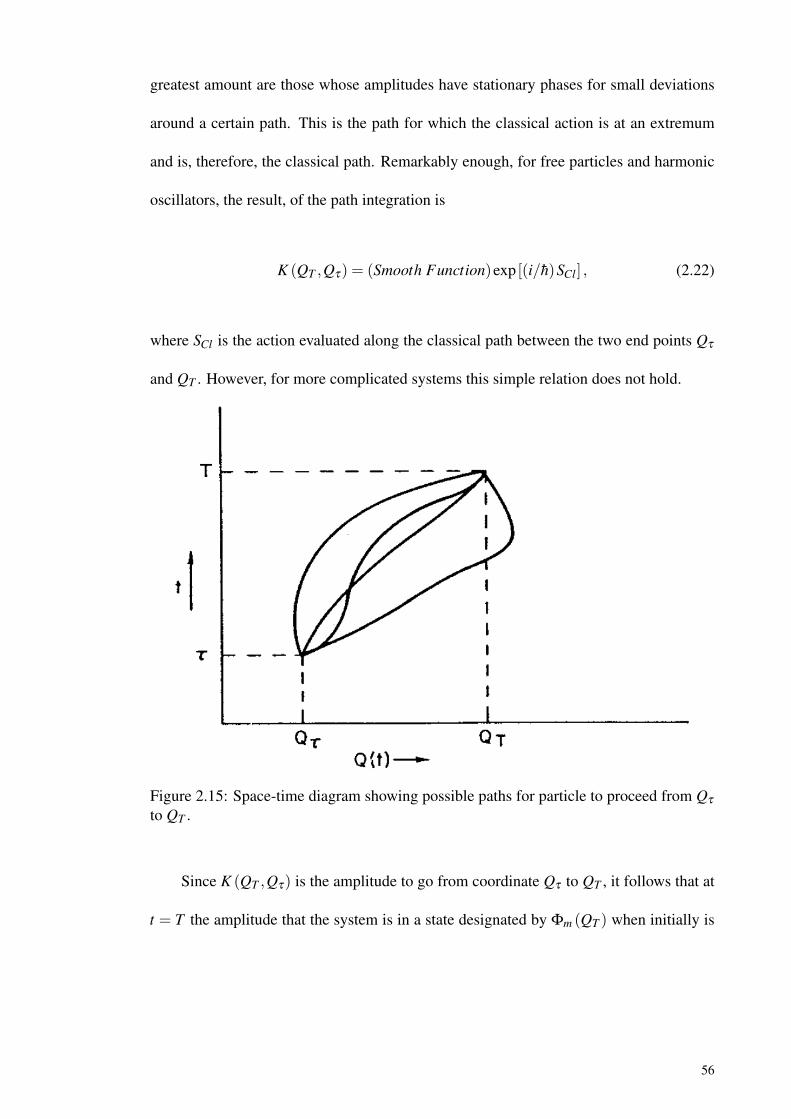
greatest amount are those whose amplitudes have stationary phases for small deviations

around a certain path. This is the path for which the classical action is at an extremum

and is, therefore, the classical path. Remarkably enough, for free particles and harmonic

oscillators, the result, of the path integration is

K (QT ,Qτ) = (Smooth Function)exp [(i/h)SCl] , (2.22)

where SCl is the action evaluated along the classical path between the two end points Qτ

and QT . However, for more complicated systems this simple relation does not hold.

Figure 2.15: Space-time diagram showing possible paths for particle to proceed from Qτ

to QT .

Since K (QT ,Qτ) is the amplitude to go from coordinate Qτ to QT , it follows that at

t = T the amplitude that the system is in a state designated by Φm (QT ) when initially is

56

in a state Φn (Qτ) is given by

Amn =∫

Φ∗m (QT )K (QT ,Qτ)Φn (Qτ)dQT dQτ (2.23)

=∫

Φ∗m (QT )exp [(i/h)S (Q)]Φn (Qτ)DQ(t)dQT dQτ .

The probability of the transition from n→ m is given by |Amn|2 and from Eq. 2.23 it can

be written in the form of multiple integrals as follows:

Pmn =∫

Φ∗m (QT )Φm

(Q′T)

exp(i/h)[S (Q)−S

(Q′)]

(2.24)

×Φn (Qτ)Φ∗n(Q′τ)

DQ(t)DQ′ (t)dQT dQ′T dQτdQ′τ .

As a example of a more complicated case let us consider two systems whose coordinates

are Q and X .. The systems are coupled by a potential which can be designated as V (Q,X)

and incorporated in the total Lagrangian. We assume that when V = 0 the states of Q and

X can be described by sets of wave functions Φk(Q) and χp(X) respectively. If, initially,

Q is in a state Φn(Qτ) and X is in a state χi(Xτ), then the amplitude that Q goes from state

n to m while X goes from state i to f can be formed in a similar way to that of Eq. 2.23 as

Am f , ni =∫

Φ∗m (QT )χ

∗f (QT )exp [(i/h)S (Q,X)]Φn (Qτ)χi(Xτ)

×DQ(t)DX (t)dQT dXT dQτdXτ , (2.25)

where S(Q,X) represents the classical action of the entire system including both Q and

X . The important property of separability afforded by writing the amplitude in this way

is now apparent. For instance, if one wishes to know the effect that X has on Q when X

undergoes a transition from state i to f , then all of the integrals on the X variables may

be done first. What is left is an expression for Amn for Q and in terms of Q variables

57

only but with the effect of X included. The extension of writing transition amplitudes for

large numbers of systems is obvious. In principle the order in which the variables are

eliminated is always arbitrary.

2.4.2 Definition of Influence Functional

A functional can now be defined which can be used to describe mathematically the

effect of external quantum systems upon the behavior of a quantum system of interest.

The fundamental theorem may be stated as follows: For any system, Q, acted on

by external classical forces and quantum mechanical systems as discussed above, the

probability that it makes a transition from state Ψn(Qτ) at t = τ to Ψm(QT ) at t = T can

be written as

Pmn =∫

Ψ∗m (QT )Ψm

(Q′T)

exp(i/h)

[S0 (Q)−S0

(Q′)]

F(Q, Q′

)×Ψ

∗n(Q

′τ)Ψn(Qτ)DQ(t)DQ′ (t)dQτdQ′τdQT dQ′T , (2.26)

where F (Q, Q′) contains all the effects of the external influences on Q and S0 (Q) =∫ Tτ

L(Q,Q, t

)dt is the action of Q without external disturbance. The proof of this is

straightforward. Let us examine two coupled systems characterized by coordinates Q

and X . Q will represent the system of interest and X the quite general environmental

system (excepting only the effects of spin) coupled by a general potential V (Q,X , t) to Q.

Assume Q to be initially (t = τ) in state Ψn(Qτ) and X to be in state χi (Xτ), a product

state. The probability that Q is found in state Ψm(QT ) while X is in state χ f (XT ) at t = T

58

can be written in the manner discussed above and is

Pm f , ni =∣∣Am f , ni

∣∣2=

∫Ψ∗m (QT )Ψm

(Q′T)

χ∗f (XT )χ f

(X ′T)

×exp(i/h)

[S0 (Q)−S0

(Q′)+S0 (X)−S0

(X ′)+SI (Q,X)−SI

(Q′,X ′

)]×Ψ

∗n(Q

′τ)Ψn(Qτ)χ

∗i(X ′τ)

χi (Xτ)DQ(t)DX (t)DQ′ (t)DX ′ (t)dQτdXτ

×dQ′τdX ′τdQT dXT dQ′T dX ′T , (2.27)

The primed variables were introduced when the integrals for each Am f , ni were combined.

Now if all the components of Eq. 2.27 which involves coordinates other than Q or Q’ is

separated out and designated as F (Q, Q′), then the following expression is obtained

F(Q, Q′

)=

∫χ∗f (XT )χ f

(X ′T)

×exp(i/h)

[S0 (X)−S0

(X ′)+SI (Q,X)−SI

(Q′,X ′

)]×χ∗i(X ′τ)

χi (Xτ)DX (t)DX ′ (t)dXτdX ′τdXT dX ′T , (2.28)

Incorporation of this expression into Eq. 2.27 yields the desired form as Eq. 2.26. If the

path-integrals are written in terms of kernels, Eq. 2.28 becomes

F(Q, Q′

)=

∫χ∗f (XT )χ f

(X ′T)

KQ (XT ,Xτ)K∗Q′(X ′T ,X

′τ

)×χ∗i(X ′τ)

χi (Xτ)dXτdX ′τdXT dX ′T (2.29)

where the subscript Q means that the kernel includes the effect of a potential V (Q,X)

acting on X during the interval τ < t < T . As can be seen, F is a functional whose form

depends upon the physical system X , the initial and final states of X , and the coupling

between Q and X .

59

It is to be emphasized that the formulation of F is such that it includes all the effects

of the environmental system in influencing the behavior of the system of interest. Thus,

if there are two systems A and B which can act on Q, and if

FA on Q = FB on Q (2.30)

then the effects of A on Q are the same as those of B on Q. It follows that if simplifying

assumptions are necessary in finding FA on Q and FB on Q (due to the complicated nature

of A and B) and if the resulting functions are equal, then within the approximations the

effects of A and B on the system of interest are the same. In the situation where the

environmental system is composed of a linear system or combinations of linear systems

we shall see that the same form of F is always appropriate. To adapt this general form of

F to a particular linear system it is only necessary to know such quantities as impedance

and temperature which determine its classical behavior. In still other situations, very weak

coupling between systems is involved. The approximate F which can be used in this case

to represent the effect of the environmental systems has a form which is independent

of the nature of the environmental system. This form is the same as for linear systems

(R. Feynman & Vernon, 1963, 2000).

2.5 Temperature-Dependent Bandgap Variation

2.5.1 Photoluminescence Spectrum

In order to obtain photoluminescence (PL) spectrum of energy levels of a QD en-

semble, the QD ensemble is excited at an energy well above those energy levels. This is

so-called nonresonant excitation. The PL is inhomogeneously broadened because there is

a contribution from every QD in the ensemble sample, which typically contains a variety

of QD sizes.

60

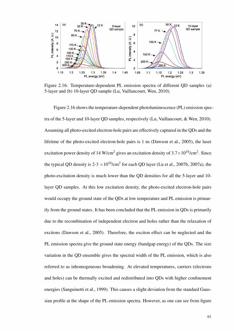
Figure 2.16: Temperature-dependent PL emission spectra of different QD samples (a)5-layer and (b) 10-layer QD sample (Lu, Vaillancourt, Wen, 2010).

Figure 2.16 shows the temperature-dependent photoluminescence (PL) emission spec-

tra of the 5-layer and 10-layer QD samples, respectively (Lu, Vaillancourt, & Wen, 2010).

Assuming all photo-excited electron-hole pairs are effectively captured in the QDs and the

lifetime of the photo-excited electron-hole pairs is 1 ns (Dawson et al., 2005), the laser

excitation power density of 14 W/cm2 gives an excitation density of 3.7×1010/cm2. Since

the typical QD density is 2-3 ×1010/cm2 for each QD layer (Lu et al., 2007b, 2007a), the

photo-excitation density is much lower than the QD densities for all the 5-layer and 10-

layer QD samples. At this low excitation density, the photo-excited electron-hole pairs

would occupy the ground state of the QDs at low temperature and PL emission is primar-

ily from the ground states. It has been concluded that the PL emission in QDs is primarily

due to the recombination of independent electron and holes rather than the relaxation of

excitons (Dawson et al., 2005). Therefore, the exciton effect can be neglected and the

PL emission spectra give the ground state energy (bandgap energy) of the QDs. The size

variation in the QD ensemble gives the spectral width of the PL emission, which is also

referred to as inhomogeneous broadening. At elevated temperatures, carriers (electrons

and holes) can be thermally excited and redistributed into QDs with higher confinement

energies (Sanguinetti et al., 1999). This causes a slight deviation from the standard Gaus-

sian profile at the shape of the PL emission spectra. However, as one can see from figure

61

2.16, the whole PL spectrum shifts to lower energies as temperature increases. This indi-

cates that the QD ensembles experience the same trend of temperature-dependent energy

gap variations. For simplicity, the peak energy of the PL emission is used to represent the

energy gap variations.

2.5.2 Semi-Empirical Models for Projecting Temperature-Dependent Bandgap Vari-ation

Two mechanisms are responsible for temperature-dependent bandgap shift; the electron-

phonon interaction and the thermal lattice expansion. For both mechanisms the contri-

butions of the individual lattice oscillators with energies ε=hω are proportional to the

average phonon occupation number n=[exp(ε/kBT )−1]−1 (O’Donnell & Chen, 1991),

temperature-dependent bandgap E (T ) can therefore be represented as

E (T ) = E (0)− α

kB

∫∞

0dε

εw(ε)

exp(ε/kBT )−1. (2.31)

Here α =−dE (T )/dT |T→∞ is the slope of the linear T dependence in the high temper-

ature limit, E (0) is the band gap energy at 0 K and w(ε)≥ 0 is the normalized weighting

function of the phonon oscillators,∫

dεw(ε) = 1. Different assumptions for w(ε) lead to

the several models such as power-function ansatz which is discussed in the following.

A convenient analytical treatment of E (T ) is obtained by a power-function (PF)

ansatz (Pässler, 2003): w(ε) = v(ε/εc)v−1 /εc, v > 0 for ε up to the cutoff energy εc of

the phonon spectrum, and w(ε) = 0 above. In this model, the T→0 asymptotes are given

by power functions [E (0)−E (T )] ∝ T P, where the fractional exponent p usually ranges

from 2 to 3 (Pässler, 1997, 19999). A detailed analysis shows that for the frequently

observed regime of intermediate to large phonon dispersion E (T ) is given as

E (T ) = E (0)− αθ

2

[

1+3

∑n=1

αn (v)(

2Tθ

)n+v

+

(2Tθ

)5+v]1/(5+v)

−1

, (2.32)

62

where the expansion coefficients αn (v) are

α1 (v) =5+ v

6

(π

2

)2+(v−1)2/2,

α2 (v) =1− v

2,

α3 (v) =(5+ v)(1+ v)2

3v(2+ v).

The average phonon temperature θ=〈ε〉/kB=vεc/ [kB (1+ v)] (Pässler, 2000), leading to

a cutoff energy εc = kBθ (1+ v)/v. The dispersion coefficient ∆ =

√〈ε2〉−〈ε〉2/〈ε〉 is

1/√

v(2+ v) (Pässler, 2003). Besides the zero-temperature energy, this model contains

three parameters for fitting the experimental data.

Another well-known model which originated from bulk semiconductors is the Varshni

model (Y. Varshni, 1967; Y. P. Varshni, 1970), This model is empirically expressed as

E (T ) = E (0)− αT 2

β +T, (2.33)

where α and β are the two Varshni coefficients to be determined by fitting the experi-

mental data with Eq. 2.33. The Varshni equation was devised to fit the seemingly linear

decrease in the high temperature region and the quadratic decrease in the low temperature

region as observed in many semiconductor material systems.

We call the third semi-empirical model as Lu model, it describes as

E (T ) = E (0)+θ1

T −θ2, (2.34)

where θ1 and θ2 has temperature dimension, K, and together with E (0) should be ob-

tained from the fit of the experimental data (Lu et al., 2010). There are two additional

methods called Fan or Vina and two-oscillator model which will be discussed in the next

63

chapter.

2.5.3 Temperature-Dependent Bandgap Variation in Quantum Dot Samples

It is appropriate to check whether models developed for bulk may be used for de-

scribing temperature-dependent bandgap in the QD structures. Figure 2.17 shows the

temperature-dependent energy gap variation in the 5-layer QD sample at various temper-

atures from 12 to 300 K (Lu et al., 2010). A sigmoidal-shape temperature-dependent

bandgap shrinkage was obtained. Similar observations have been reported ((Sanguinetti

et al., 2002; Brusaferri et al., 1996)). Also shown in figure 2.17 are the energy gap shrink-

ing projected by using the Varshni’s formula ( Eq. 2.33) and the power function ansatz

( Eq. 2.32), dashed green and red traces, respectively. The measured QD temperature-

dependent energy gap variation shows significant deviation from the projections of these

models. This indicates that QDs have different temperature-dependent bandgap energy

properties than bulk semiconductors. The blue and pink traces are the calculated energy

gaps by using Lu model ( Eq. 2.34) in the low (T <100 K) and high temperature (T >100

K) regions.

According to figure 2.17, it seems that the Lu model can project the experimental

data perfectly. However, a complete study of several works conducted for modeling of the

temperature dependent shrinkage of In(Ga)As/GaAs SOQD bandgaps, one can infer that

this basic property of QDs still cannot be described properly using the existing models;

in the work performed by Wei et al. (Z. F. Wei et al., 2005) none of the aforementioned

models were used, instead a model similar to the Varshni model could project the InGaAs

QDs PL peak shrinkage data only up to 170 K. In the work done by Ortner et al. (Ortner

et al., 2005), the four abovementioned models were used to project single-QD spectrum

of In(Ga)As/GaAs QDs. The conclusion was that PF and two-oscillator models provide

better fits than the Varshni and Fan (Vina) models. In the next work conducted by Lu et al.

64

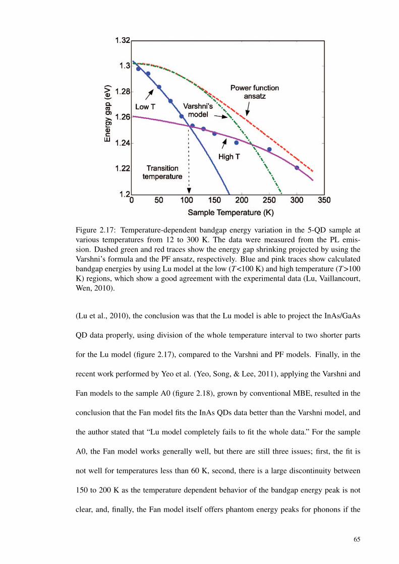
Figure 2.17: Temperature-dependent bandgap energy variation in the 5-QD sample atvarious temperatures from 12 to 300 K. The data were measured from the PL emis-sion. Dashed green and red traces show the energy gap shrinking projected by using theVarshni’s formula and the PF ansatz, respectively. Blue and pink traces show calculatedbandgap energies by using Lu model at the low (T <100 K) and high temperature (T >100K) regions, which show a good agreement with the experimental data (Lu, Vaillancourt,Wen, 2010).

(Lu et al., 2010), the conclusion was that the Lu model is able to project the InAs/GaAs

QD data properly, using division of the whole temperature interval to two shorter parts

for the Lu model (figure 2.17), compared to the Varshni and PF models. Finally, in the

recent work performed by Yeo et al. (Yeo, Song, & Lee, 2011), applying the Varshni and

Fan models to the sample A0 (figure 2.18), grown by conventional MBE, resulted in the

conclusion that the Fan model fits the InAs QDs data better than the Varshni model, and

the author stated that “Lu model completely fails to fit the whole data.” For the sample

A0, the Fan model works generally well, but there are still three issues; first, the fit is

not well for temperatures less than 60 K, second, there is a large discontinuity between

150 to 200 K as the temperature dependent behavior of the bandgap energy peak is not

clear, and, finally, the Fan model itself offers phantom energy peaks for phonons if the

65

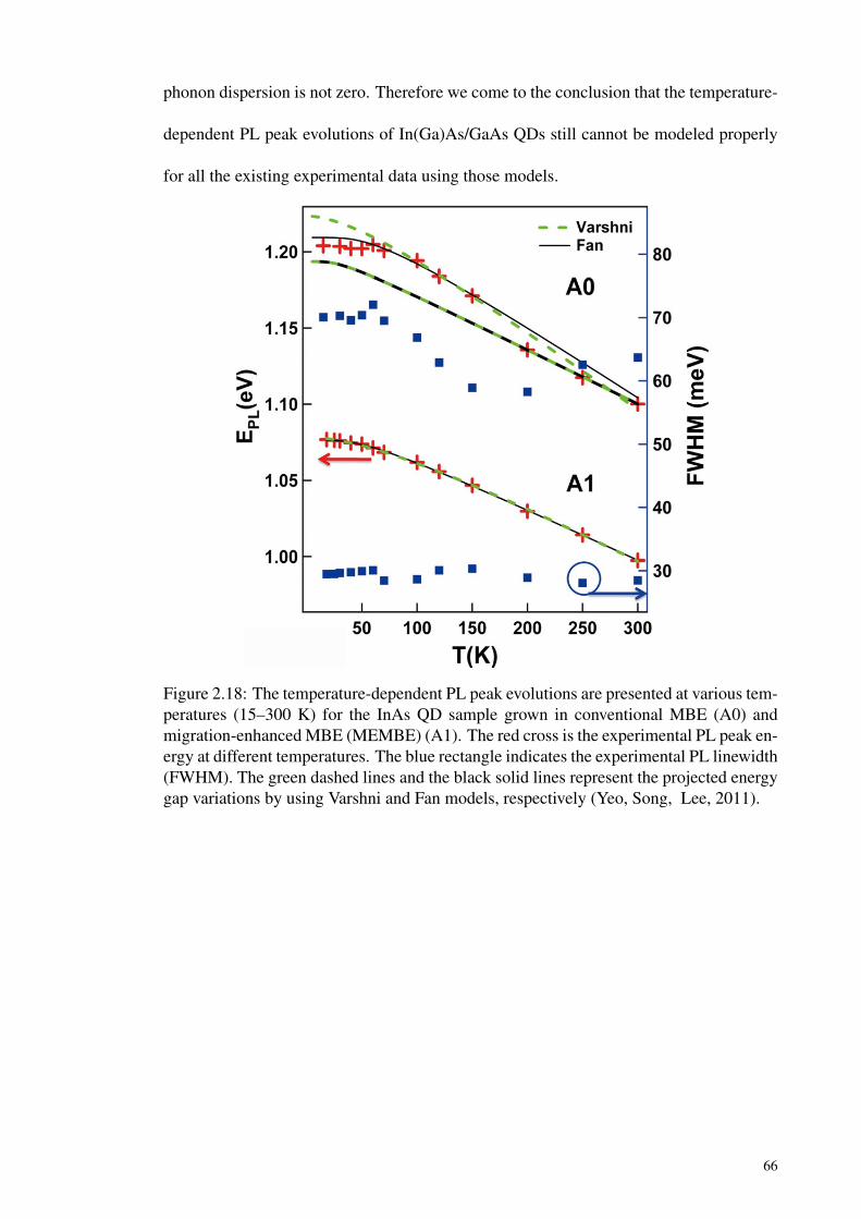
phonon dispersion is not zero. Therefore we come to the conclusion that the temperature-

dependent PL peak evolutions of In(Ga)As/GaAs QDs still cannot be modeled properly

for all the existing experimental data using those models.

Figure 2.18: The temperature-dependent PL peak evolutions are presented at various tem-peratures (15–300 K) for the InAs QD sample grown in conventional MBE (A0) andmigration-enhanced MBE (MEMBE) (A1). The red cross is the experimental PL peak en-ergy at different temperatures. The blue rectangle indicates the experimental PL linewidth(FWHM). The green dashed lines and the black solid lines represent the projected energygap variations by using Varshni and Fan models, respectively (Yeo, Song, Lee, 2011).

66

CHAPTER 3

MODELING AND SIMULATION METHODS

3.1 Introduction

In the first part of this chapter, the model describing a single QD inserted into a lossy

nanophotonic cavity and coupled to a LA phonon bath is presented. To study the quantum

dynamics of the open QD-cavity system modified real-time path-integral (RTPI) approach

is discussed and an efficient algorithm to evaluate the derived density matrix is presented.

Then, in the second part of the chapter, two oscillator model (TOM) is discussed, which

will be used to model phonon-induced temperature-dependent shift of photoluminescence

(PL) peak for experimental datasets of In(Ga)As/GaAs QDs with a different number of

monolayers (MLs) and layers.

3.2 Dissipative Quantum Dot-Cavity System Coupled to a Superohmic Environ-ment

We consider a semiconductor quantum dot (QD) in the strong confinement limit,

i.e., the electronic single particle states are energetically well separated and the Coulomb

interaction provides negligible mixing between them, linearly coupled to lattice vibra-

tions (phonons). The QD is considered to have only two optically active electronic levels

that are resonantly coupled to a single mode cavity. Assuming the lattice and dielectric

properties of the confined QD do not differ notably from the environment, the phonon

modes are approximated with the corresponding three-dimensional bulk modes, like in

the bulk material. It has generally been approved that optical phonons do not contribute

to exciton–phonon interactions at temperatures less than about 100 K (Borri et al., 2001;

Muljarov & Zimmermann, 2004; Uskov et al., 2000; Takagahara, 1999; Ghodsi Nahri &

Ooi, 2014), thus, restricting our simulations to those temperatures, we can safely neglect

67

the polar optical coupling to LO phonons. We also neglect the piezoelectric coupling to

LA and TA phonons, which has been shown to have a small effect for (In,Ga)As QDs,

and only account for the deformation potential coupling to LA phonons, which dominates

the exciton-LA phonon interactions in (In,Ga)As QD (see Chap. 2).

Schematic representation of such a two level QD coupled to a single mode cavity and

the LA phonon bath is illustrated in figure 3.1(a). A two-level QD, including a ground

state (GS) represented by |G〉 and an excited state (ES) expressed by |X〉, is coupled to

a single mode cavity, with two photon levels |0〉 and |1〉, through the coupling strength

g. The phonon bath is represented by a continuum of LA phonon wave states |q1〉 to

|qM〉, the matrix elements describing interaction of the QD with the phonon reservoir is

expressed by γq. The radiative population decay of the excited QD is described by the

rate γr. The cavity loss is represented by the rate κ . The QD-cavity system with these

dissipation is called "dissipative QD-cavity system".

We first introduce the, possibly time dependent, total (model) Hamiltonian that de-

scribes the dissipative QD-cavity (DQC) system coupled to the phonon degrees of free-

dom as:

H (t) = HQD0 +HC

0 +HQD−CI +HQD

γr +HCκ +HPh

0 +HQD−PhI

= HS +HR +HSR, (3.1)

where HQD0 and HC

0 describe the uncoupled QD and cavity Hamiltonian, HQD−CI corre-

sponds to the QD-cavity interaction Hamiltonian through which the QD state and the cav-

ity mode become strongly coupled and new polariton modes, which have partial exciton

and partial cavity character (Reithmaier et al., 2004; Hennessy et al., 2007), are formed.

HQDγr and HC

κ represent QD and cavity dissipation Hamiltonian respectively. HPh0 is the

Hamiltonian of free LA phonon bath and HQD−PhI describes interaction of the QD with the

68

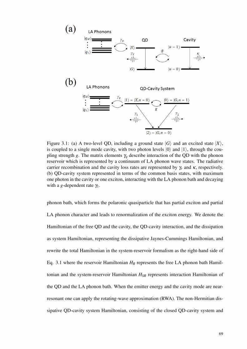
Figure 3.1: (a) A two-level QD, including a ground state |G〉 and an excited state |X〉,is coupled to a single mode cavity, with two photon levels |0〉 and |1〉, through the cou-pling strength g. The matrix elements γq describe interaction of the QD with the phononreservoir which is represented by a continuum of LA phonon wave states. The radiativecarrier recombination and the cavity loss rates are represented by γr and κ , respectively.(b) QD-cavity system represented in terms of the common basis states, with maximumone photon in the cavity or one exciton, interacting with the LA phonon bath and decayingwith a g-dependent rate γ1.

phonon bath, which forms the polaronic quasiparticle that has partial exciton and partial

LA phonon character and leads to renormalization of the exciton energy. We denote the

Hamiltonian of the free QD and the cavity, the QD-cavity interaction, and the dissipation

as system Hamiltonian, representing the dissipative Jaynes-Cummings Hamiltonian, and

rewrite the total Hamiltonian in the system-reservoir formalism as the right-hand side of

Eq. 3.1 where the reservoir Hamiltonian HR represents the free LA phonon bath Hamil-

tonian and the system-reservoir Hamiltonian HSR represents interaction Hamiltonian of

the QD and the LA phonon bath. When the emitter energy and the cavity mode are near-

resonant one can apply the rotating-wave approximation (RWA). The non-Hermitian dis-

sipative QD-cavity system Hamiltonian, consisting of the closed QD-cavity system and

69

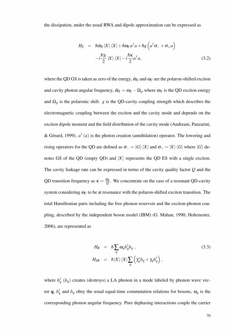
the dissipation, under the usual RWA and dipole approximation can be expressed as

HS = hωX |X〉〈X |+ hωCa†a+ hg(

a†σ−+σ+a

)−i

hγr

2|X〉〈X |− i

hκ

2a†a, (3.2)

where the QD GS is taken as zero of the energy, ωX and ωC are the polaron-shifted exciton

and cavity photon angular frequency, ωX = ωX −Ωp where ωX is the QD exciton energy

and Ωp is the polaronic shift. g is the QD-cavity coupling strength which describes the

electromagnetic coupling between the exciton and the cavity mode and depends on the

exciton dipole moment and the field distribution of the cavity mode (Andreani, Panzarini,

& Gérard, 1999). a† (a) is the photon creation (annihilation) operator. The lowering and

rising operators for the QD are defined as σ− = |G〉〈X | and σ+ = |X〉〈G| where |G〉 de-

notes GS of the QD (empty QD) and |X〉 represents the QD ES with a single exciton.

The cavity leakage rate can be expressed in terms of the cavity quality factor Q and the

QD transition frequency as κ = ωXQ . We concentrate on the case of a resonant QD-cavity

system considering ωC to be at resonance with the polaron-shifted exciton transition. The

total Hamiltonian parts including the free phonon reservoir and the exciton-phonon cou-

pling, described by the independent boson model (IBM) (G. Mahan, 1990; Hohenester,

2006), are represented as

HR = h∑q

ωqb†qbq , (3.3)

HSR = h |X〉〈X |∑q

(γ∗q bq + γqb†

q

),

where b†q (bq) creates (destroys) a LA phonon in a mode labeled by phonon wave vec-

tor q, b†q and bq obey the usual equal-time commutation relations for bosons, ωq is the

corresponding phonon angular frequency. Pure dephasing interactions couple the carrier

70

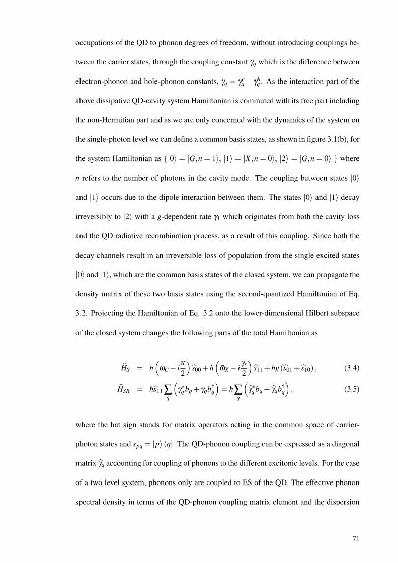
occupations of the QD to phonon degrees of freedom, without introducing couplings be-

tween the carrier states, through the coupling constant γq which is the difference between

electron-phonon and hole-phonon constants, γq = γeq − γh

q . As the interaction part of the

above dissipative QD-cavity system Hamiltonian is commuted with its free part including

the non-Hermitian part and as we are only concerned with the dynamics of the system on

the single-photon level we can define a common basis states, as shown in figure 3.1(b), for

the system Hamiltonian as |0〉 = |G,n = 1〉, |1〉 = |X ,n = 0〉, |2〉 = |G,n = 0〉 where

n refers to the number of photons in the cavity mode. The coupling between states |0〉

and |1〉 occurs due to the dipole interaction between them. The states |0〉 and |1〉 decay

irreversibly to |2〉 with a g-dependent rate γ1 which originates from both the cavity loss

and the QD radiative recombination process, as a result of this coupling. Since both the

decay channels result in an irreversible loss of population from the single excited states

|0〉 and |1〉, which are the common basis states of the closed system, we can propagate the

density matrix of these two basis states using the second-quantized Hamiltonian of Eq.

3.2. Projecting the Hamiltonian of Eq. 3.2 onto the lower-dimensional Hilbert subspace

of the closed system changes the following parts of the total Hamiltonian as

HS = h(

ωC− iκ

2

)s00 + h

(ωX − i

γr

2

)s11 + hg(s01 + s10) , (3.4)

HSR = hs11 ∑q

(γ∗q bq + γqb†

q

)= h∑

q

(γ∗q bq + γqb†

q

), (3.5)

where the hat sign stands for matrix operators acting in the common space of carrier-

photon states and spq = |p〉〈q|. The QD-phonon coupling can be expressed as a diagonal

matrix γq accounting for coupling of phonons to the different excitonic levels. For the case

of a two level system, phonons only are coupled to ES of the QD. The effective phonon

spectral density in terms of the QD-phonon coupling matrix element and the dispersion

71

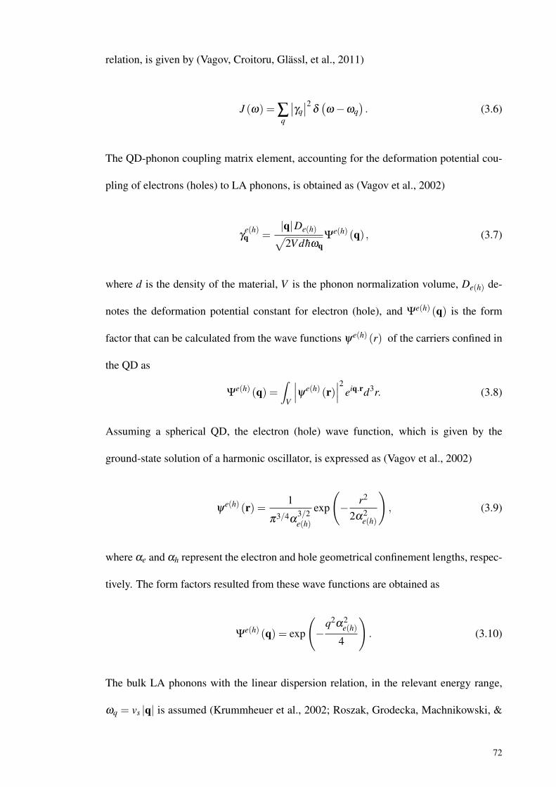
relation, is given by (Vagov, Croitoru, Glässl, et al., 2011)

J (ω) = ∑q

∣∣γq∣∣2 δ

(ω−ωq

). (3.6)

The QD-phonon coupling matrix element, accounting for the deformation potential cou-

pling of electrons (holes) to LA phonons, is obtained as (Vagov et al., 2002)

γe(h)q =

|q|De(h)√2V dhωq

Ψe(h) (q) , (3.7)

where d is the density of the material, V is the phonon normalization volume, De(h) de-

notes the deformation potential constant for electron (hole), and Ψe(h) (q) is the form

factor that can be calculated from the wave functions ψe(h) (r) of the carriers confined in

the QD as

Ψe(h) (q) =

∫V

∣∣∣ψe(h) (r)∣∣∣2 eiq.rd3r. (3.8)

Assuming a spherical QD, the electron (hole) wave function, which is given by the

ground-state solution of a harmonic oscillator, is expressed as (Vagov et al., 2002)

ψe(h) (r) =

1

π3/4α3/2e(h)

exp

(− r2

2α2e(h)

), (3.9)

where αe and αh represent the electron and hole geometrical confinement lengths, respec-

tively. The form factors resulted from these wave functions are obtained as

Ψe(h) (q) = exp

(−

q2α2e(h)

4

). (3.10)

The bulk LA phonons with the linear dispersion relation, in the relevant energy range,

ωq = vs |q| is assumed (Krummheuer et al., 2002; Roszak, Grodecka, Machnikowski, &

72

Kuhn, 2005; Krügel, Axt, Kuhn, Machnikowski, & Vagov, 2005; Grosse & Zimmermann,

2007; Stock et al., 2011) with vs being the sound velocity in the material. Inserting Eqs.

3.7 and 3.10 into Eq. 3.6 and replacing the summation over the wave vector q with an

integral, assuming an isotropic momentum space, the phonon spectral density is obtained

as

J (ω) =ω3

4π2dhv5s

[De exp

(−ω2α2

e4v2

s

)−Dh exp

(−

ω2α2h

4v2s

)]2

, (3.11)

which scales, for small frequencies, as J(ω) ∼ ω3; therefore, it is indeed of the super-

ohmic type. It tends to zero as a Gaussian function, faster than eight-band k.p wave func-

tions (see figure 2.12), in the opposite limit of high frequencies. It is worth to note that

other types of phonon modes, e.g., half-space or slab modes (Krummheuer, Axt, Kuhn,

D’Amico, & Rossi, 2005), can be incorporated into the present approach as long as the

modes form continua which lead to finite memory times. We take typical GaAs parame-

ters: d = 5370 kgm−3, vs = 5110 ms−1, De =−14.6 eV , and Dh =−4.8 eV (Krummheuer

et al., 2002) with αe = 5 nm. We also consider a constant ratio αh = 0.87αe for the elec-

tron and hole confinement lengths (Glässl et al., 2011).

3.3 Real-Time Path-Integral Approach for the Open Quantum Dot-Cavity System

3.3.1 Discretized Real-Time Path-Integral Formulation

Reduced open QD-cavity density matrix (RQCDM) is obtained by taking the partial

trace over the density matrix of the total system, i.e. the open QD-cavity and the phonon

bath, with respect to the phonon reservoir as

ρ(t) = Trph[χ(t)], (3.12)

also referred to as tracing out the degrees of freedom of the reservoir. To derive a dis-

cretized real-time path-integral (RTPI) representation for the RQCDM, we write the total

73

density matrix at time t, in Eq. 3.12, in terms of the initial total density matrix, χ(0), and

the time evolution operator as

ρ(t) = Trph[U(t)χ(0)U†(t)]. (3.13)

We assume that the bath is initially at thermal equilibrium and that the system–bath inter-

action is switched on at t = 0, so that the total statistical operator initially can be factorized

as product of carrier-photon and phonon operators

χ(0) = ρ(0)⊗ 1Z

exp

[− h

kBT ∑q

ωqb†qbq

], (3.14)

where Z is the normalization constant of the phonon distribution at temperature T , and

ρ(0) is the initial statistical operator for the carrier-photon system (initial RQCDM). The

time evolution operator is given by

U(t) = T exp(− i

h

∫ t

0H(t ′)dt ′

), (3.15)

where T is the time ordering operator. As shown in the Appendix, Eq. 3.13 together

with Eqs. 3.14 and 3.15 can be represented in the form of a path-integral, where the

phonon variables are readily traced out. Time t is discretized into N time steps of the

length ε = t/N with the time grid points tn = nε and n = 0, ...,N. Any of the coupled

basis states of the dissipative QD-cavity system, |0〉 or |1〉, at time tn are represented by

|s+n 〉 for forward propagation in time and by |s−n 〉 for backward propagation on a path that

runs in the backward (decreasing) time direction. Here we write the final expression for

74

the RQCDM elements in the interaction picture as

ρs+N s−N(tN) = lim

N→∞

N

∏n=1

∑s±n−1

Hs+n s+n−1S H

s−n s−n−1∗S

n

∏n′=0

e fnn′ρs+0 s−0(0) , (3.16)

where the configuration summations are over all s+n , s−n , which can be interpreted as "sum

over all trajectories" of the open QD-cavity system that connect the RQCDM at time tN

to the initial one at time zero. For the present case of the three-level system with two

coupled levels, involved in the dynamics, the indexes s+n and s−n are assumed to take only

the values 0 and 1. One approximates Eq. 3.16 with a finite N and ε in order to develop a

numerical algorithm for practical calculations. Hs+n s+n−1S and H

s−n s−n−1∗S are one-dimensional

short-time forward and backward bare system propagators which are defined as

Hs+n s+n−1S H

s−n s−n−1∗S =

⟨s+n∣∣e−iHSε/h ∣∣s+n−1

⟩⟨s−n−1

∣∣eiH†S ε/h ∣∣s−n ⟩ , (3.17)

where the dissipative QD-cavity Hamiltonian, in the matrix form, for the present case of

maximum one cavity photon is given by

HS = h

ωC− iκ

2 g

g ωX − i γr2

.

In order to calculate matrix elements of the system short-time propagator and its Her-

mitian conjugate, between time steps n and n− 1, presented in Eq. 3.17 HS should be

diagonalized. The non-local bath functional fnn′ , accounting for effects of the phonon

bath, in Eq. 3.16 is given by

fnn′ =−(s+n − s−n

)(ηn−n′s

+n′−η

∗n−n′s

−n′), (3.19)

75

where the short-time Feynman-Vernon–like influence functional is defined as Inn′ = exp( fnn′),

the influence coefficient ηm, depending only on m = n−n′ time steps, is expressed as

ηm 6=0 =∫ (m+1)ε

mε

dτ

∫ε

0dτ′K(τ− τ

′) (3.20)

= 4∫

∞

0dω

J (ω)

ω2 sin2(

εω

2

)coth

(hω

2kBT

)cos(mεω)− isin(mεω)

,

ηm=0 =∫

ε

0dτ

∫τ

0dτ′K(τ− τ

′) (3.21)

= 2∫

∞

0dω

J (ω)

ω2

sin2

(εω

2

)coth

(hω

2kBT

)− i(εω− sin(εω))

,

here the memory kernel (system-bath correlation function) K (t), accounting for delayed

influences by time t, is given by

K (t) =∫

∞

0dωJ (ω)

[coth

(hω

2kBT

)cos(ωt)− isin(ωt)

]. (3.22)

Note that while the influence functional introduces non-Markovian interactions between

time points separated by several time steps m, the system propagator Eq. 3.17 only con-

nects the nearest time point, which is a Markovian interaction. Eqs. 3.16-3.22 are core

equations describing numerically exact RTPI approach, for the open QD-cavity system

coupled to a continuum of LA phonon modes, enabling us to obtain the RQCDM ele-

ments at an arbitrary time (Ghodsi Nahri et al., 2016).

3.3.2 Memory Length Finiteness and Truncation of the Influence Coefficient

An efficient method for calculation of the reduced density matrix (RDM) in Eq. 3.16

is called “tensor multiplication scheme", in which the RDM is evaluated by using a proper

tensor propagator in each iteration, has been presented in Refs.(Makri & Makarov, 1995b,

1995a; Sim, 2001). It is based on the fact that for harmonic baths, described by smooth

76

spectral density functions, range of the nonlocal interactions in the influence functional is

indeed finite for any temperature, including even zero temperature, such that the nonlocal

kernel extends over only a few time steps if the path-integral is discretized by using ac-

curate quasiadiabatic propagators (Makarov & Makri, 1994; Makri & Makarov, 1995b,

1995a). This is the case when the heat bath is characterized by a broad spectrum that

extends to reasonably high frequencies, which is characteristic of condensed phase envi-

ronments. This feature arises from destructive phase interference between modes located

within the reservoir’s broad spectral density, resulting in disruption of quantum coher-

ence in the macroscopic bath which, in turn, leads to loss of memory of initial conditions

after sufficiently long time periods. Although the evolution of the RDM is not Marko-

vian in such cases the finite length of nonlocal interactions in the influence functional

leads to Markovian dynamics for the tensor propagator, which implies that the long-time

path-integral can be broken into a series of shorter time calculations, permitting iterative

time evolution schemes. In fact, in cases where the memory length is not very long com-

pared to the allowed time step, the tensor multiplication scheme provides a numerically

exact means of calculating the quantum dynamics of (dissipative) systems coupled to de-

phasing (dissipating) reservoirs for arbitrarily long times, as it preserves the trace of the

RDM, provided that the nonlocal interactions are not truncated too soon. The scheme

also surpasses usual Monte Carlo methods as they are not feasible for long times due to

the alternating signs in the discretized RTPIs (Makri & Makarov, 1995b, 1995a; Sim,

2001). We have plotted normalized real and imaginary parts of the memory kernel K (t)

in figure 3.2 in order to find the memory length (depth) at different temperatures. As it

is clearly seen, at T = 0 K, real part of the memory kernel almost becomes zero after 5

ps, while at higher temperatures T = 20 K and T = 80 K the memory becomes shorter,

taking the effective value about 4 ps. There is not noticeable change in the memory depth

and amplitude for temperatures larger than T = 20 K. The memory amplitude is smallest

77

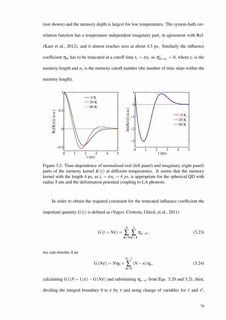
(not shown) and the memory depth is largest for low temperatures. The system-bath cor-

relation function has a temperature independent imaginary part, in agreement with Ref.

(Kaer et al., 2012), and it almost reaches zero at about 4.5 ps. Similarly the influence

coefficient ηm has to be truncated at a cutoff time tc = εnc as ηcm>nc

= 0, where tc is the

memory length and nc is the memory cutoff number (the number of time steps within the

memory length).

0 1 2 3 4 5

−0.5

0

0.5

1

t (ps)

Re[

K(t

)] (

a.u

.)

0 1 2 3 4 5

−3

−2

−1

0

1

t (ps)

Im[K

(t)]

(a.

u.)

0 K

20 K

80 K

0 K

20 K

80 K

Figure 3.2: Time-dependence of normalized real (left panel) and imaginary (right panel)parts of the memory kernel K (t) at different temperatures. It seems that the memorykernel with the length 4 ps, as tc = εnc = 4 ps, is appropriate for the spherical QD withradius 5 nm and the deformation potential coupling to LA phonons.

In order to obtain the required constraint for the truncated influence coefficient the

important quantity G(t) is defined as (Vagov, Croitoru, Glässl, et al., 2011)

G(t = Nε) =N

∑n=1

n

∑n′=1

ηn−n′, (3.23)

we can rewrite it as

G(Nε) = Nη0 +N−1

∑n=1

(N−n)ηn, (3.24)

calculating G((N +1)ε)−G(Nε) and substituting ηn−n′ from Eqs. 3.20 and 3.21, then,

dividing the integral boundary 0 to ε by τ and using change of variables for τ and τ ′,

78

finally, we obtain

G(t) =∫ t

0dτ

∫τ

0dτ′K(τ− τ

′) (3.25)

=∫

∞

0dω

J (ω)

ω2 [1− cos(ωt)]coth(

hω

2kBT

)− i [ωt− sin(ωt)].

The long time asymptotics of Eq. 3.25, taking the coupling Eq. 3.11, evaluates to

G(t→ ∞) → G0− iΩpt (3.26)

G0 =∫

∞

0dω

J (ω)

ω2 coth(

hω

2kBT

)= const.

Ωp =∫

∞

0dω

J (ω)

ω= const.

where limt→∞cos(ωt) = limt→∞

sin(ωt) = 0 is considered. Here Ωp is the standard pola-

ronic shift, which effectively leads to a renormalization of the transition frequency, while

exp[−G0] defines the residual coherence, at temperature T , which remains in the closed

QD-cavity system coupled to the bath in the long time limit. exp[−G0/2] can be inter-

preted as a factor that renormalizes the Rabi frequency (Y.-J. Wei et al., 2014). It is ap-

propriate to add the polaronic shift Ωp to the exciton transition frequency, so that we have

taken into account the renormalized exciton transition frequency ωX = ωX −Ωp in Eq.

3.2 and later on. G0 increases with temperature, thereby reducing the residual coherence.

In the present case of a dissipative QD-cavity system coupled to the phonon bath, the

residual coherence is zero. For the case of the truncation approximation, i.e., ηcm>nc

= 0,

we divide G(t) around the truncation point and obtain nonzero influence coefficients for

79

m = n−n′ ≤ nc as

Gc (t = Nε) =nc

∑n=1

n

∑n′=1

ηcn−n′+

N

∑n=nc+1

n

∑n′=1

ηcn−n′

=nc

∑n=1

n

∑n′=1

ηcn−n′+

t− tcε

nc

∑n=0

ηcn , (3.27)

the long time asymptotics of Gc(t) in Eq. 3.27 is obtained as

Gc (t→ ∞) → Gc0 +Gc

I t (3.28)

Gc0 =

nc

∑n=1

n

∑n′=1

ηcn−n′, Gc

I =1ε

nc

∑n=0

ηcn ,

since in this case of the truncation approximation, the asymptotic relations for the quantity

G(t) in Eq. 3.26 must also hold, therefore, comparing Eq. 3.28 with the exact asymptotic

in Eq. 3.26 one obtains the following constraint for the truncated influence coefficient:

nc

∑n=0

ηcn =−iεΩp (3.29)

which is consistent with the exact identity:

∞

∑n=0

ηn =∫

∞

0εK (τ)dτ =−iε

∫∞

0dω

J (ω)

ω. (3.30)

In the truncation approximation, it is most important to enforce the constraint in Eq. 3.29

for the real part of the kernel, i. e.

nc

∑n=0

Re [ηcn ] = 0. (3.31)

It should be noted that the constraint Eq. 3.29 and the necessity of its enforcement is

specific to the superohmic case (Vagov, Croitoru, Glässl, et al., 2011). To fulfill the

80

constraint in Eq. 3.29, we assume a possible complex nonzero value A for the following

expressionnc

∑n=0

ηcn + iεΩp = A. (3.32)

Modifying the influence coefficient ηcn according to

ηcn = η

cn−

1nc +1

(nc

∑n=0

ηcn + iεΩp

), (3.33)

the constraint in Eq. 3.29 is fulfilled. It is mentioned in (Vagov, Croitoru, Glässl, et al.,

2011) that in the case of superohmic coupling in QD systems, for which the truncation

does not lead to qualitative changes of the system dynamics if Eq. 3.29 holds, possible

quantitative errors due to the truncation can be well controlled by varying the time step

ε and the memory cutoff length tc = εnc . It should be noted, however, that as far as we

have examined, for the present case of the QD-cavity system under investigation, if the

constraint in Eq. 3.29 is not applied, a significant quantitative change occurs only in the

real part of the off-diagonal RDM elements.

3.3.3 Implementation of the Numerical Algorithm

The truncated influence coefficient approximation, which is based on finiteness of

range of the memory length, enormously decreases the numerical load for calculation of

the RQCDM, Eq.3.16, especially when it is combined with the so-called tensor multipli-

cation scheme. The original formulation of this scheme, presented in Refs. (Makarov &

Makri, 1994; Makri & Makarov, 1995b, 1995a), was somewhat cumbersome and required

multiple runs of the algorithm to obtain the complete time evolution. Its subsequent im-

provement allowing an “on-the-fly filtering” and “path re-indexing” has been proposed in

Ref. (Sim, 2001). On-the-fly path selection or on-the-fly filtering process selects more

probable paths in the course of the time propagation in a single run. The path re-indexing

81

process unifies all the similar paths into one with a weight obtained from summing up the

weights of those trajectories for times larger than the memory length in the single run.

Here, we present a brief summary of the method with few modifications, adapted for the

dynamic calculation of the QD-cavity system coupled to the harmonic bath of LA phonon

oscillators. We implement the algorithm through an iterative method containing a set of

recurrence equations which briefly summarize the steps to evaluate Eq. 3.16. We start

with rewriting Eq. 3.16, considering a finite N, at the present time tq as

ρs+q s−q (tq) = ∑s+q−1,...,s

+0

∑s−q−1,...,s

−0

[

q−1

∏n=1

Hs+n s+n−1S H

s−n s−n−1∗S

n

∏n′=0

e fnn′ρs+i s−i(0)

][

Hs+q s+q−1S H

s−q s−q−1∗S

q

∏n′=0

e fqn′

], (3.34)

where we have expressed the system propagator and the influence functional expressions

as a product of the “history” and “memory” terms. For the RDM at the present time tq, the

history term includes only the interactions between the past grid-time points from tn=0 = 0

to tn=q−1 = tn=q − ε while the memory term corresponds to the interactions between

the present grid-time point and the past time points. By identifying the history and the

memory terms, the redundant calculations can be avoided. Following this separation idea

and defining trajectories as sequences of s+n and s−n , the discretized expression of the

RQCDM in Eq. 3.34 can be rewritten as

⟨s+q∣∣ ρ(tq) ∣∣s−q ⟩= Ls±q

∑js±q

T jq−1Ms±jq

, (3.35)

where jq−1 represents the path segment from time t0 = 0 to tq−1 = (q−1)ε of jth config-

uration, i.e., jq−1 =(

s+jq−1, ...,s+j0,s

−jq−1

, ...,s−j0

)where the subscript jl correspond to the

grid point at time lε on the jth configuration. Ls±q

is the total number of possible configu-

82

rations ending at a certain pair(s+q ,s

−q)

at time qε . In the two-level system each path is

represented by a long sequence of 0s and 1s with the length 2(q+1). The history and the

memory terms are then represented by

T jq−1=

q−1

∏n=1

Hs+jn s+jn−1S H

s−jn s−jn−1∗

S

n

∏n′=0

ef j

nn′ ρs+i s−i(0) , (3.36)

Ms±jq= H

s+jq s+jq−1S H

s−jq s−jq−1∗

S

q

∏n′=0

ef jqn′ , (3.37)

where Ms±jqdenotes the interactions of a certain pair

(s+jq,s

−jq

)at the present time tq with

the past time points on the jth configuration. It can be seen that the history and memory

terms can be reused as the next propagation history weight (term) without redundant cal-

culations. However, as RDM propagates the number of configurations and corresponding

weights to be stored increases exponentially as D2q, where D = 2 is the number of system

eigenstates and an initial state has been considered. Thus, we need to apply other mech-

anisms to decrease the storage array size; As the strength of nonlocal interactions drops

off rapidly beyond a certain value of tc = εnc due to coupling to the phonon bath, imply-

ing that only a finite memory length needs to be included, it is sufficient to include only

22(nc+1) configurations for the times t > tc without losing numerical accuracy. Because of

the finite memory length, by the time that RDM propagates up to tnc+p = (nc + p)ε , con-

tributions from the first p time grid points are negligible and can thus be ignored without

affecting the final results. For instance, if p = 2, the contributions of the initial point and

the second grid point are neglected. Furthermore, some of the trajectories become identi-

cal allowing us to combine them as one effective path. This re-indexing of the trajectories

leads to the reduction of the number of paths to be integrated and can be implemented

when the propagator passes the bath memory time. Nevertheless, the number of configu-

rations enhances exponentially to 22nc as RDM propagates up to the bath memory time.

To alleviate this, on-the-fly path filtering of the propagator functional is applied; it re-

83

moves the paths with weights less than a chosen cutoff from the path integration in each

propagation step and may start from the first propagation step. The trajectory re-indexing

technique, on the other hand, is applied for the propagation beyond the bath memory

time. Accordingly, on-the-fly filtering and the trajectory re-indexing technique reduce

the number of configurations to be integrated substantially. Figure 3.3 shows schematic

representation of the configuration space including some trajectories (like the red path),

started from an initial state, and the memory truncation for nc = 3 .

Considering the finite memory length, Eq. 3.34 can be rewritten for two different

areas of time points n as

ρs+n s−n (tn) =

Ls±n

∑js±n

T jn, n≤ nc (3.38)

ρs+n s−n (tn) =

Lcs±n

∑jcs±n

T jcn, nc < n (3.39)

where for n ≤ nc each configuration is represented as jn = (s+jn , ...,s+j0,s−jn, ...,s−j0) and

Ln = ∑s±n

Ls±nis the total number of possible paths ending at time nε . While for nc < n

each trajectory segment is defined as jcn = (s+jn, ...,s

+jn−nc

,s−jn, ...,s−jn−nc

) and Lcn = ∑

s±nLc

s±n.

The history weights are given by recurrence equations as

T j0 = ρs+0 s−0(t0 = 0) = ρs+i s−i

, n = 0 (3.40)

Tkn= Tkn−1

Mkn, 1≤ n≤ nc (3.41)

Tkcn

= Tkcn−1

Mckn, nc < n (3.42)

where T j0 is in fact the initial RQCDM elements and Tknintroduces summing up the

weights of similar paths as a result of the trajectory re-indexing technique. The memory

84

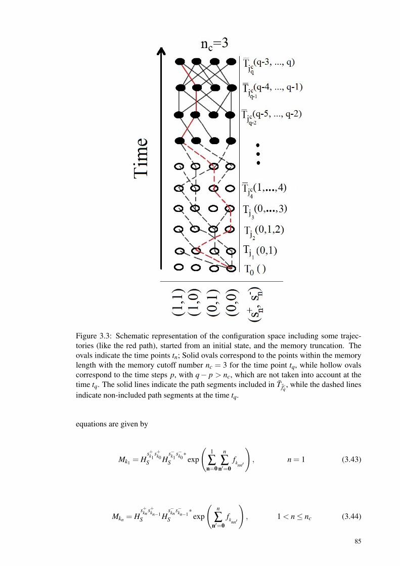
Figure 3.3: Schematic representation of the configuration space including some trajec-tories (like the red path), started from an initial state, and the memory truncation. Theovals indicate the time points tn; Solid ovals correspond to the points within the memorylength with the memory cutoff number nc = 3 for the time point tq, while hollow ovalscorrespond to the time steps p, with q− p > nc, which are not taken into account at thetime tq. The solid lines indicate the path segments included in T jcq , while the dashed linesindicate non-included path segments at the time tq.

equations are given by

Mk1 = Hs+k1

s+k0S H

s−k1s−k0∗

S exp

(1

∑n=0

n

∑n′=0

fknn′

), n = 1 (3.43)

Mkn = Hs+kn

s+kn−1S H

s−kns−kn−1

∗S exp

(n

∑n′=0

fknn′

), 1 < n≤ nc (3.44)

85

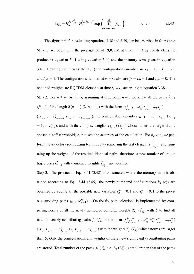
Mckn= H

s+kns+kn−1

S Hs−kn

s−kn−1∗

S exp

(n

∑n′=n−nc

fknn′

), nc < n (3.45)

The algorithm, for evaluating equations 3.38 and 3.39, can be described in four steps:

Step 1. We begin with the propagation of RQCDM at time t1 = ε by constructing the

product in equation 3.41 using equation 3.40 and the memory term given in equation

3.43. Defining the initial state (1, 1) the configurations number are k1 = 1, ...,L1 = 22,

and Ls±1= 1. The configurations number, at t0 = 0, also are j0 = L0 = 1 and fk00 = 0. The

obtained weights are RQCDM elements at time t1 = ε , according to equation 3.38.

Step 2. For n ≤ nc (nc < n), assuming at time point n− 1 we know all the paths jn−1

( jcn−1) of the length 2(n−1) (2(nc +1)) with the form (s+jn−1

, ...,s+j1,s−jn−1

, ...,s−j1)

((s+jn−1, ...,s+jn−nc−1

,s−jn−1, ...,s−jn−nc−1

)), the configurations number jn−1 = 1, ...,Ln−1 ( jcn−1

= 1, ...,Lcn−1

), and with the complex weights T jn−1(T jcn−1

) whose norms are larger than a

chosen cutoff (threshold) δ that sets the accuracy of the calculation. For nc < n, we per-

form the trajectory re-indexing technique by removing the last element s±jn−nc−1and sum-

ming up the weights of the resulted identical paths, therefore, a new number of unique

trajectories k′cn−1 with combined weights Tk′cn−1are obtained.

Step 3. The product in Eq. 3.41 (3.42) is constructed where the memory term is ob-

tained according to Eq. 3.44 (3.45), the newly numbered configurations kn (kcn) are

obtained by adding all the possible new variables s+n = 0,1 and s−n = 0,1 to the previ-

ous surviving paths jn−1 (k′cn−1). “On-the-fly path selection” is implemented by com-

paring norms of all the newly numbered complex weights Tkn(Tkc

n) with δ to find all

new noticeably contributing paths jn ( jcn) of the form (s+jn ,s

+jn−1

, ...,s+j1 ,s−jn,s−jn−1

, ...,s−j1)

((s+jn ,s+jn−1

, ...,s+jn−nc,s−jn,s

−jn−1

, ...,s−jn−nc)) with the weights T jn (T jcn) whose norms are larger

than δ . Only the configurations and weights of these new significantly contributing paths

are stored. Total number of the paths jn ( jcn), i.e. Ln (Lc

n), is smaller than that of the paths

86

kn (kcn) as a result of on the fly path filtering process which can be applied from the first

propagation step.

Step 4. We obtain the augmented RDM (RQCDM) elements at the time step n, sum-

ming up over weights of the noticeably contributing configurations ending at a certain

pair (s+n ,s−n ) as in Eq. 3.38 (3.39).

The procedure defined by steps 2–4 finds the most important contributing paths by

an iterative construction, which is done “on-the-fly” and enables us to obtain the entire

time evolution in a single run. The accuracy of the numerical results depends on three

parameters that should be selected carefully; the time increment ε , the memory cutoff

number nc, and the threshold δ . The choice of εnc is dictated by the effective temporal

extension of the memory kernel (the memory length), which follows from the QD geome-

try and the coupling mechanism. As it is shown in figure 3.2, the choice of 4 ps length for

the memory (εnc = 4 ps) is appropriate for the spherical QD with radius 5 nm and the de-

formation potential coupling to LA phonons. Therefore, we find that the memory length

may also roughly be estimated by 2τph = 4ae/vs, i.e., the time needed for a sound wave

to cross the QD two times (3.91 ps). It turns out that the results converge for a time slice

ε = 0.4 ps and the memory cutoff number nc = 10. The threshold δ increases with the

QD-cavity coupling strength g. The appropriate value for δ , in a given g, is obtained by

comparing the results of few runs with different values δ until the results do not change

notably with further decreasing δ . Parameters nc and δ determine the total number of

paths that need to be stored in the computer memory. The large number of paths that need

to be memorized is the main limitation of the algorithm, especially for models with larger

numbers of system states.

87

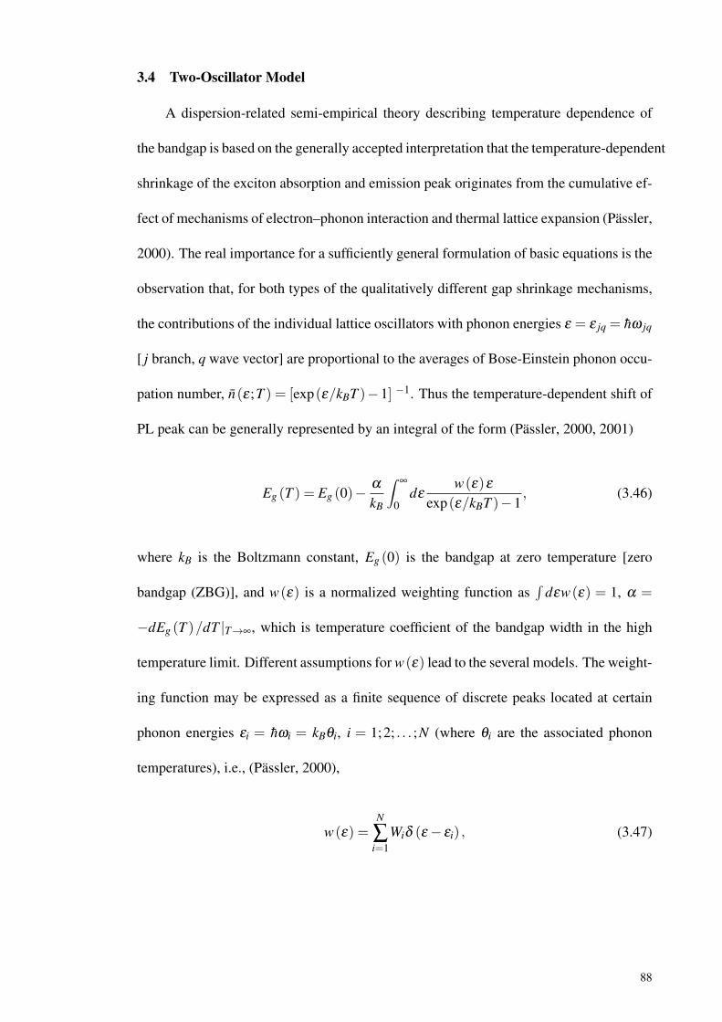
3.4 Two-Oscillator Model

A dispersion-related semi-empirical theory describing temperature dependence of

the bandgap is based on the generally accepted interpretation that the temperature-dependent

shrinkage of the exciton absorption and emission peak originates from the cumulative ef-

fect of mechanisms of electron–phonon interaction and thermal lattice expansion (Pässler,

2000). The real importance for a sufficiently general formulation of basic equations is the

observation that, for both types of the qualitatively different gap shrinkage mechanisms,

the contributions of the individual lattice oscillators with phonon energies ε = ε jq = hω jq

[ j branch, q wave vector] are proportional to the averages of Bose-Einstein phonon occu-

pation number, n(ε;T ) = [exp(ε/kBT )−1] −1. Thus the temperature-dependent shift of

PL peak can be generally represented by an integral of the form (Pässler, 2000, 2001)

Eg (T ) = Eg (0)−α

kB

∫∞

0dε

w(ε)ε

exp(ε/kBT )−1, (3.46)

where kB is the Boltzmann constant, Eg (0) is the bandgap at zero temperature [zero

bandgap (ZBG)], and w(ε) is a normalized weighting function as∫

dεw(ε) = 1, α =

−dEg (T )/dT |T→∞, which is temperature coefficient of the bandgap width in the high

temperature limit. Different assumptions for w(ε) lead to the several models. The weight-

ing function may be expressed as a finite sequence of discrete peaks located at certain

phonon energies εi = hωi = kBθi, i = 1;2; . . . ;N (where θi are the associated phonon

temperatures), i.e., (Pässler, 2000),

w(ε) =N

∑i=1

Wiδ (ε− εi) , (3.47)

88

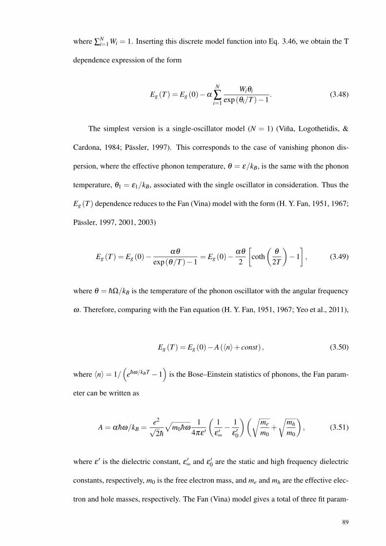
where ∑Ni=1Wi = 1. Inserting this discrete model function into Eq. 3.46, we obtain the T

dependence expression of the form

Eg (T ) = Eg (0)−α

N

∑i=1

Wiθi

exp(θi/T )−1. (3.48)

The simplest version is a single-oscillator model (N = 1) (Viña, Logothetidis, &

Cardona, 1984; Pässler, 1997). This corresponds to the case of vanishing phonon dis-

persion, where the effective phonon temperature, θ = ε/kB, is the same with the phonon

temperature, θ1 = ε1/kB, associated with the single oscillator in consideration. Thus the

Eg (T ) dependence reduces to the Fan (Vina) model with the form (H. Y. Fan, 1951, 1967;

Pässler, 1997, 2001, 2003)

Eg (T ) = Eg (0)−αθ

exp(θ/T )−1= Eg (0)−

αθ

2

[coth

(θ

2T

)−1], (3.49)

where θ = hΩ/kB is the temperature of the phonon oscillator with the angular frequency

ω . Therefore, comparing with the Fan equation (H. Y. Fan, 1951, 1967; Yeo et al., 2011),

Eg (T ) = Eg (0)−A(〈n〉+ const) , (3.50)

where 〈n〉= 1/(

ehω/kBT −1)

is the Bose–Einstein statistics of phonons, the Fan param-

eter can be written as

A = α hω/kB =e2√

2h

√m0hω

14πε ′

(1

ε ′∞− 1

ε ′0

)(√me

m0+

√mh

m0

), (3.51)

where ε ′ is the dielectric constant, ε ′∞ and ε ′0 are the static and high frequency dielectric

constants, respectively, m0 is the free electron mass, and me and mh are the effective elec-

tron and hole masses, respectively. The Fan (Vina) model gives a total of three fit param-

89

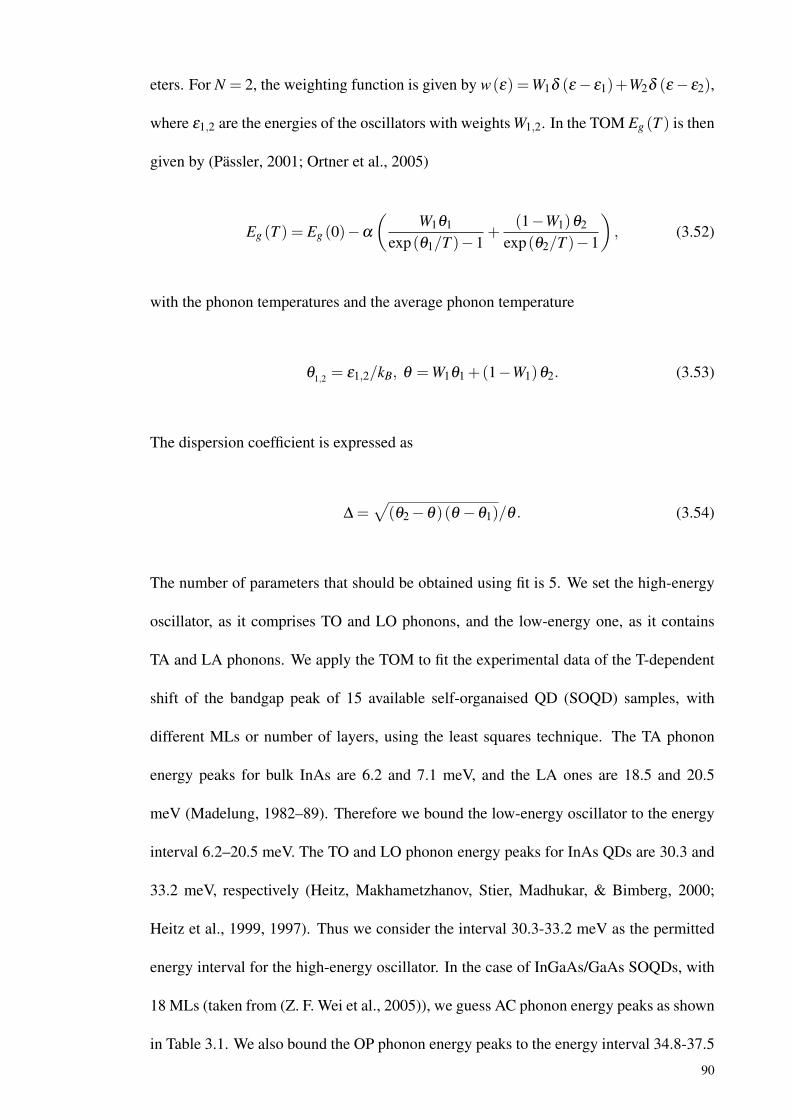
eters. For N = 2, the weighting function is given by w(ε) =W1δ (ε− ε1)+W2δ (ε− ε2),

where ε1,2 are the energies of the oscillators with weights W1,2. In the TOM Eg (T ) is then

given by (Pässler, 2001; Ortner et al., 2005)

Eg (T ) = Eg (0)−α

(W1θ1

exp(θ1/T )−1+

(1−W1)θ2

exp(θ2/T )−1

), (3.52)

with the phonon temperatures and the average phonon temperature

θ1,2 = ε1,2/kB, θ =W1θ1 +(1−W1)θ2. (3.53)

The dispersion coefficient is expressed as

∆ =√

(θ2−θ)(θ −θ1)/θ . (3.54)

The number of parameters that should be obtained using fit is 5. We set the high-energy

oscillator, as it comprises TO and LO phonons, and the low-energy one, as it contains

TA and LA phonons. We apply the TOM to fit the experimental data of the T-dependent

shift of the bandgap peak of 15 available self-organaised QD (SOQD) samples, with

different MLs or number of layers, using the least squares technique. The TA phonon

energy peaks for bulk InAs are 6.2 and 7.1 meV, and the LA ones are 18.5 and 20.5

meV (Madelung, 1982–89). Therefore we bound the low-energy oscillator to the energy

interval 6.2–20.5 meV. The TO and LO phonon energy peaks for InAs QDs are 30.3 and

33.2 meV, respectively (Heitz, Makhametzhanov, Stier, Madhukar, & Bimberg, 2000;

Heitz et al., 1999, 1997). Thus we consider the interval 30.3-33.2 meV as the permitted

energy interval for the high-energy oscillator. In the case of InGaAs/GaAs SOQDs, with

18 MLs (taken from (Z. F. Wei et al., 2005)), we guess AC phonon energy peaks as shown

in Table 3.1. We also bound the OP phonon energy peaks to the energy interval 34.8-37.5

90

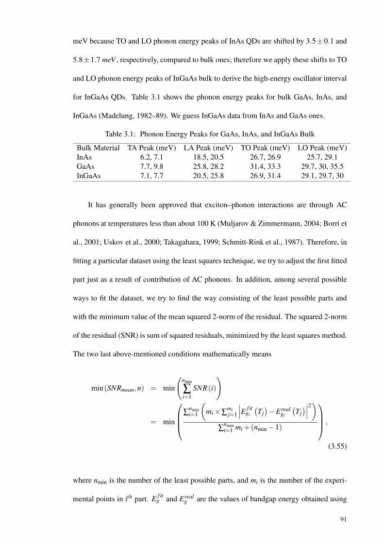
meV because TO and LO phonon energy peaks of InAs QDs are shifted by 3.5±0.1 and

5.8±1.7 meV , respectively, compared to bulk ones; therefore we apply these shifts to TO

and LO phonon energy peaks of InGaAs bulk to derive the high-energy oscillator interval

for InGaAs QDs. Table 3.1 shows the phonon energy peaks for bulk GaAs, InAs, and

InGaAs (Madelung, 1982–89). We guess InGaAs data from InAs and GaAs ones.

Table 3.1: Phonon Energy Peaks for GaAs, InAs, and InGaAs Bulk

Bulk Material TA Peak (meV) LA Peak (meV) TO Peak (meV) LO Peak (meV)InAs 6.2, 7.1 18.5, 20.5 26.7, 26.9 25.7, 29.1GaAs 7.7, 9.8 25.8, 28.2 31.4, 33.3 29.7, 30, 35.5InGaAs 7.1, 7.7 20.5, 25.8 26.9, 31.4 29.1, 29.7, 30

It has generally been approved that exciton–phonon interactions are through AC

phonons at temperatures less than about 100 K (Muljarov & Zimmermann, 2004; Borri et

al., 2001; Uskov et al., 2000; Takagahara, 1999; Schmitt-Rink et al., 1987). Therefore, in

fitting a particular dataset using the least squares technique, we try to adjust the first fitted

part just as a result of contribution of AC phonons. In addition, among several possible

ways to fit the dataset, we try to find the way consisting of the least possible parts and

with the minimum value of the mean squared 2-norm of the residual. The squared 2-norm

of the residual (SNR) is sum of squared residuals, minimized by the least squares method.

The two last above-mentioned conditions mathematically means

min(SNRmean,n) = min

(nmin

∑i=1

SNR(i)

)

= min

∑nmini=1

(mi×∑

mij=1

∣∣∣E f itgi

(Tj)−Ereal

gi

(Tj)∣∣∣2)

∑nmini=1 mi +(nmin−1)

,

(3.55)

where nmin is the number of the least possible parts, and mi is the number of the experi-

mental points in ith part. E f itg and Ereal

g are the values of bandgap energy obtained using

91

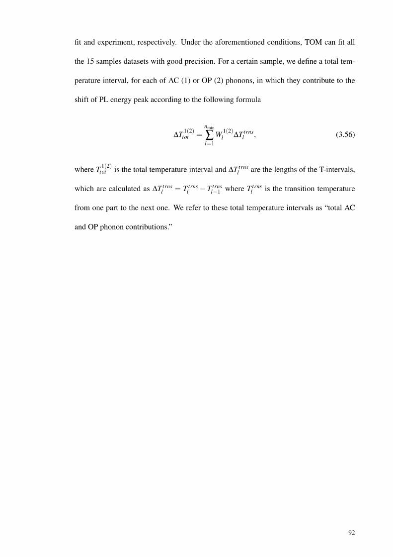
fit and experiment, respectively. Under the aforementioned conditions, TOM can fit all

the 15 samples datasets with good precision. For a certain sample, we define a total tem-

perature interval, for each of AC (1) or OP (2) phonons, in which they contribute to the

shift of PL energy peak according to the following formula

∆T 1(2)tot =

nmin

∑l=1

W 1(2)l ∆T trns

l , (3.56)

where T 1(2)tot is the total temperature interval and ∆T trns

l are the lengths of the T-intervals,

which are calculated as ∆T trnsl = T trns

l −T trnsl−1 where T trns

l is the transition temperature

from one part to the next one. We refer to these total temperature intervals as “total AC

and OP phonon contributions.”

92

CHAPTER 4

RESULTS AND DISCUSSIONS

4.1 Introduction

In the first part of this chapter, we present the results obtained from numerically

accurate RTPI simulation of the QD-cavity system dynamics initially prepared in the

state |1〉, i.e. the QD is at ES with no photon within the cavity, and coupled to a LA

phonon bath through deformation potential. The effects induced by impure dephasing

of the dressed states (VRO damping), originated from exciton coupling to LA phonons

and from dissipations including QD and cavity losses, on the quantum dynamics of the

QD-cavity system are investigated. In the second part of the chapter, we present results

of TOM projection of temperature-dependent shift of PL peak for In(Ga)As QDs with

different number of monolayers and layers. We investigate the role and contributions of

AC and OP phonons at the PL peak shift.

4.2 Quantum Dot-Cavity Quantum Electrodynamics: Impure Dephasing-InducedEffects

In terms of the decay dynamics, the emitter-cavity coupling efficiency can be di-

vided into three different dynamical regimes; weak, intermediate, and coherent (Madsen

et al., 2011). The coupling regimes are also divided into three regimes of weak, strong,

and coherent in terms of appearance and resolution of so-called vacuum Rabi splitting

(VRS) (Auffèves et al., 2010). A high degree controllable QD-cavity platform demands a

comprehensive understanding of these different coupling regimes, especially, the strong

coupling (SC) and coherent coupling (CC) regimes; The most striking feature of SC is the

splitting of the spectral shape when the cavity and the QD are at resonance, in this case,

the cavity and the QD lines do not superimpose but anticross with a splitting related to

93

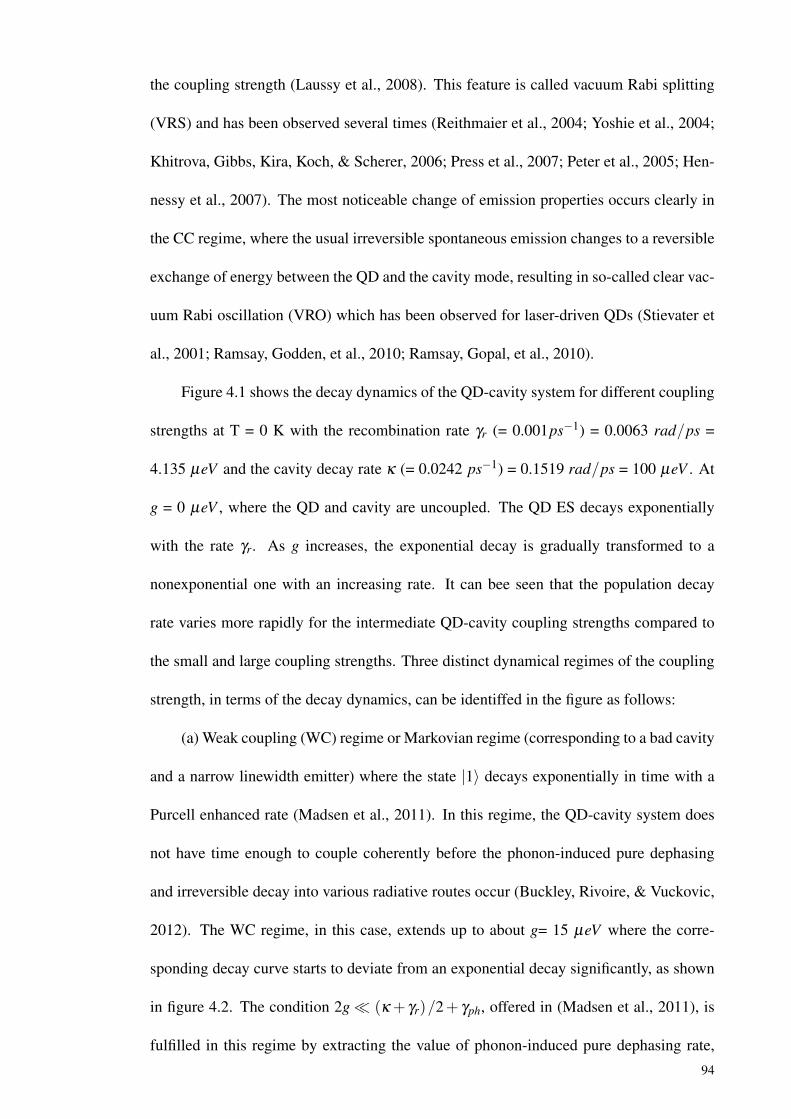
the coupling strength (Laussy et al., 2008). This feature is called vacuum Rabi splitting

(VRS) and has been observed several times (Reithmaier et al., 2004; Yoshie et al., 2004;

Khitrova, Gibbs, Kira, Koch, & Scherer, 2006; Press et al., 2007; Peter et al., 2005; Hen-

nessy et al., 2007). The most noticeable change of emission properties occurs clearly in

the CC regime, where the usual irreversible spontaneous emission changes to a reversible

exchange of energy between the QD and the cavity mode, resulting in so-called clear vac-

uum Rabi oscillation (VRO) which has been observed for laser-driven QDs (Stievater et

al., 2001; Ramsay, Godden, et al., 2010; Ramsay, Gopal, et al., 2010).

Figure 4.1 shows the decay dynamics of the QD-cavity system for different coupling

strengths at T = 0 K with the recombination rate γr (= 0.001ps−1) = 0.0063 rad/ps =

4.135 µeV and the cavity decay rate κ (= 0.0242 ps−1) = 0.1519 rad/ps = 100 µeV . At

g = 0 µeV , where the QD and cavity are uncoupled. The QD ES decays exponentially

with the rate γr. As g increases, the exponential decay is gradually transformed to a

nonexponential one with an increasing rate. It can bee seen that the population decay

rate varies more rapidly for the intermediate QD-cavity coupling strengths compared to

the small and large coupling strengths. Three distinct dynamical regimes of the coupling

strength, in terms of the decay dynamics, can be identiffed in the figure as follows:

(a) Weak coupling (WC) regime or Markovian regime (corresponding to a bad cavity

and a narrow linewidth emitter) where the state |1〉 decays exponentially in time with a

Purcell enhanced rate (Madsen et al., 2011). In this regime, the QD-cavity system does

not have time enough to couple coherently before the phonon-induced pure dephasing

and irreversible decay into various radiative routes occur (Buckley, Rivoire, & Vuckovic,

2012). The WC regime, in this case, extends up to about g= 15 µeV where the corre-

sponding decay curve starts to deviate from an exponential decay significantly, as shown

in figure 4.2. The condition 2g (κ + γr)/2+ γph, offered in (Madsen et al., 2011), is

fulfilled in this regime by extracting the value of phonon-induced pure dephasing rate,

94

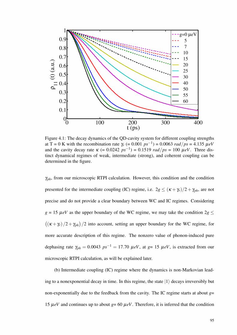
0 100 200 300 4000

0.1

0.2

0.3

0.4

0.5

0.6

0.7

0.8

0.9

1

t (ps)

ρ11 (

t) (

a.u.)

g=0 µeV

5

7

10

15

20

25

30

40

50

55

60

Figure 4.1: The decay dynamics of the QD-cavity system for different coupling strengthsat T = 0 K with the recombination rate γr (= 0.001 ps−1) = 0.0063 rad/ps = 4.135 µeVand the cavity decay rate κ (= 0.0242 ps−1) = 0.1519 rad/ps = 100 µeV . Three dis-tinct dynamical regimes of weak, intermediate (strong), and coherent coupling can bedetermined in the figure.

γph, from our microscopic RTPI calculation. However, this condition and the condition

presented for the intermediate coupling (IC) regime, i.e. 2g ≤ (κ + γr)/2+ γph, are not

precise and do not provide a clear boundary between WC and IC regimes. Considering

g = 15 µeV as the upper boundary of the WC regime, we may take the condition 2g ≤((κ + γr)/2+ γph

)/2 into account, setting an upper boundary for the WC regime, for

more accurate description of this regime. The nonzero value of phonon-induced pure

dephasing rate γph = 0.0043 ps−1 = 17.70 µeV , at g= 15 µeV , is extracted from our

microscopic RTPI calculation, as will be explained later.

(b) Intermediate coupling (IC) regime where the dynamics is non-Markovian lead-

ing to a nonexponential decay in time. In this regime, the state |1〉 decays irreversibly but

non-exponentially due to the feedback from the cavity. The IC regime starts at about g=

15 µeV and continues up to about g= 60 µeV . Therefore, it is inferred that the condition

95

0 100 200 300 4000.4

0.5

0.6

0.7

0.8

0.9

1

t (ps)

ρ11 (

t) (

a.u.)

exp fit

RTPI data

eq. (4.1)

Figure 4.2: A comparison between the actual decay (pink), obtained using the numericalRTPI calculations, an exponential decay (red), obtained by fitting a single exponential tothe actual decay, and a fit of the actual decay by using Eq. 4.1 (green) at g= 15 µeV andT = 0 K.

((κ + γr)/2+ γph

)/2 ≤ 2g ≤ 2

((κ + γr)/2+ γph

)is satisfied for this regime. This condi-

tion modifies the condition given in Ref. (Madsen et al., 2011) setting a lower boundary

and a higher upper boundary for the IC regime. It originates from the fact that our model

is more accurate and elaborated compared to the model applied in Ref. (Madsen et al.,

2011) which is an approximate model for moderate g (Madsen et al., 2011).

(c) The third regime is the coherent and non-Markovian regime where the time scale

of forming coherent coupling between the QD and the cavity field is shorter than that of

the pure dephasing and dissipations, which leads to re-excitation of the state in a reversible

evolution. Consequently, clear vacuum Rabi oscillation (VRO) occurs. As it is seen in

the figure, the coherent coupling (CC) regime starts at about g= 60 µeV , which means

that the condition (κ + γr)/2+ γph ≤ g should be satisfied in this regime. Our condition

for the CC regime modifies the condition given in Ref. (Madsen et al., 2011) as well.

There is another classification of different operating regimes, in the literature, in

96

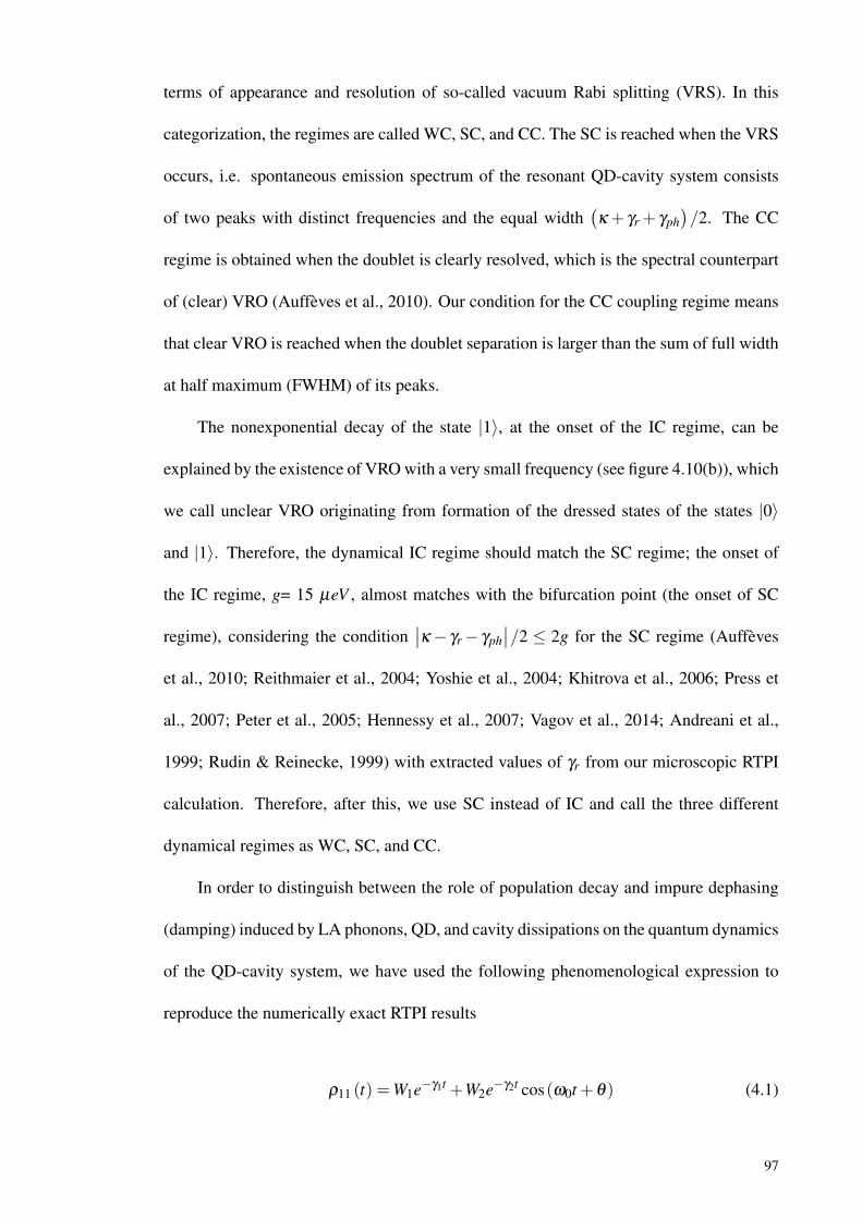
terms of appearance and resolution of so-called vacuum Rabi splitting (VRS). In this

categorization, the regimes are called WC, SC, and CC. The SC is reached when the VRS

occurs, i.e. spontaneous emission spectrum of the resonant QD-cavity system consists

of two peaks with distinct frequencies and the equal width(κ + γr + γph

)/2. The CC

regime is obtained when the doublet is clearly resolved, which is the spectral counterpart

of (clear) VRO (Auffèves et al., 2010). Our condition for the CC coupling regime means

that clear VRO is reached when the doublet separation is larger than the sum of full width

at half maximum (FWHM) of its peaks.

The nonexponential decay of the state |1〉, at the onset of the IC regime, can be

explained by the existence of VRO with a very small frequency (see figure 4.10(b)), which

we call unclear VRO originating from formation of the dressed states of the states |0〉

and |1〉. Therefore, the dynamical IC regime should match the SC regime; the onset of

the IC regime, g= 15 µeV , almost matches with the bifurcation point (the onset of SC

regime), considering the condition∣∣κ− γr− γph

∣∣/2 ≤ 2g for the SC regime (Auffèves

et al., 2010; Reithmaier et al., 2004; Yoshie et al., 2004; Khitrova et al., 2006; Press et

al., 2007; Peter et al., 2005; Hennessy et al., 2007; Vagov et al., 2014; Andreani et al.,

1999; Rudin & Reinecke, 1999) with extracted values of γr from our microscopic RTPI

calculation. Therefore, after this, we use SC instead of IC and call the three different

dynamical regimes as WC, SC, and CC.

In order to distinguish between the role of population decay and impure dephasing

(damping) induced by LA phonons, QD, and cavity dissipations on the quantum dynamics

of the QD-cavity system, we have used the following phenomenological expression to

reproduce the numerically exact RTPI results

ρ11 (t) =W1e−γ1t +W2e−γ2t cos(ω0t +θ) (4.1)

97

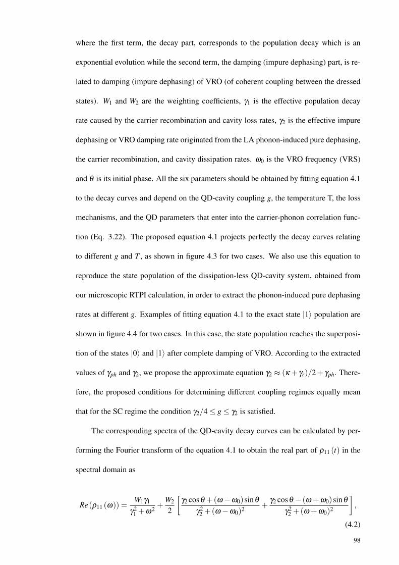
where the first term, the decay part, corresponds to the population decay which is an

exponential evolution while the second term, the damping (impure dephasing) part, is re-

lated to damping (impure dephasing) of VRO (of coherent coupling between the dressed

states). W1 and W2 are the weighting coefficients, γ1 is the effective population decay

rate caused by the carrier recombination and cavity loss rates, γ2 is the effective impure

dephasing or VRO damping rate originated from the LA phonon-induced pure dephasing,

the carrier recombination, and cavity dissipation rates. ω0 is the VRO frequency (VRS)

and θ is its initial phase. All the six parameters should be obtained by fitting equation 4.1

to the decay curves and depend on the QD-cavity coupling g, the temperature T, the loss

mechanisms, and the QD parameters that enter into the carrier-phonon correlation func-

tion (Eq. 3.22). The proposed equation 4.1 projects perfectly the decay curves relating

to different g and T , as shown in figure 4.3 for two cases. We also use this equation to

reproduce the state population of the dissipation-less QD-cavity system, obtained from

our microscopic RTPI calculation, in order to extract the phonon-induced pure dephasing

rates at different g. Examples of fitting equation 4.1 to the exact state |1〉 population are

shown in figure 4.4 for two cases. In this case, the state population reaches the superposi-

tion of the states |0〉 and |1〉 after complete damping of VRO. According to the extracted

values of γph and γ2, we propose the approximate equation γ2 ≈ (κ + γr)/2+ γph. There-

fore, the proposed conditions for determining different coupling regimes equally mean

that for the SC regime the condition γ2/4≤ g≤ γ2 is satisfied.

The corresponding spectra of the QD-cavity decay curves can be calculated by per-

forming the Fourier transform of the equation 4.1 to obtain the real part of ρ11 (t) in the

spectral domain as

Re(ρ11 (ω)) =W1γ1

γ21 +ω2 +

W2

2

[γ2 cosθ +(ω−ω0)sinθ

γ22 +(ω−ω0)2 +

γ2 cosθ − (ω +ω0)sinθ

γ22 +(ω +ω0)2

],

(4.2)

98

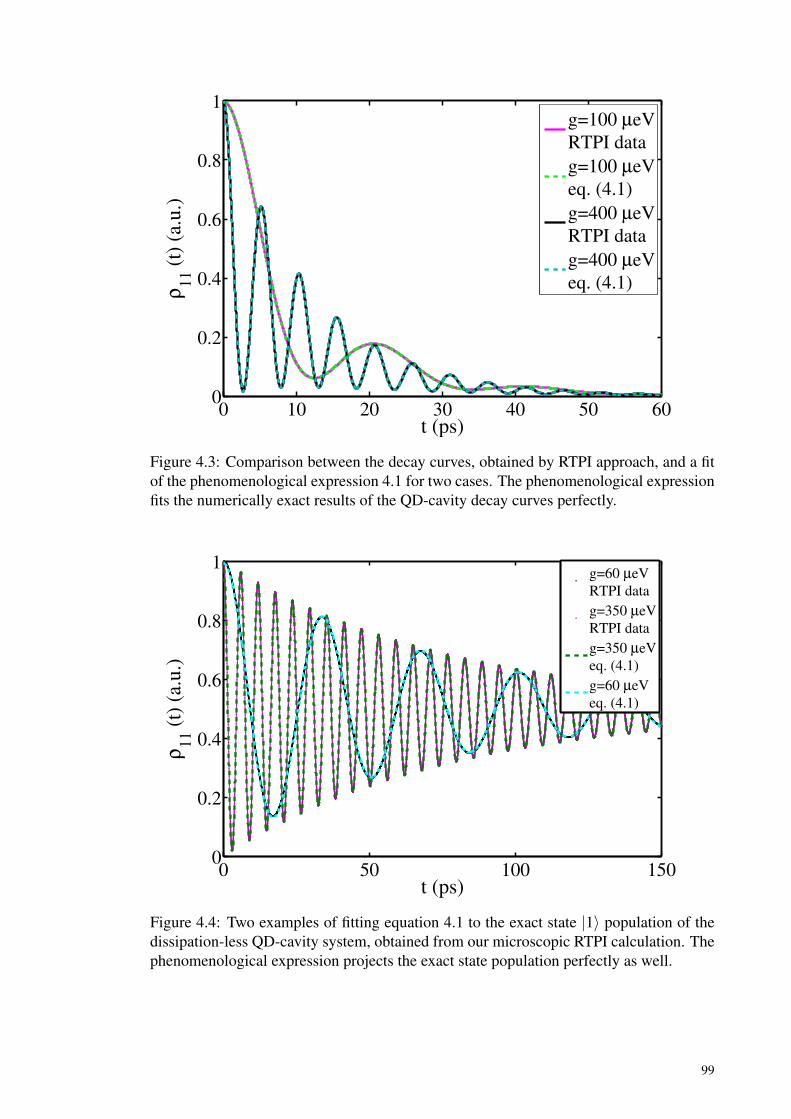
0 10 20 30 40 50 600

0.2

0.4

0.6

0.8

1

t (ps)

ρ11 (

t) (

a.u.)

g=100 µeV

RTPI data

g=100 µeV

eq. (4.1)

g=400 µeV

RTPI data

g=400 µeV

eq. (4.1)

Figure 4.3: Comparison between the decay curves, obtained by RTPI approach, and a fitof the phenomenological expression 4.1 for two cases. The phenomenological expressionfits the numerically exact results of the QD-cavity decay curves perfectly.

0 50 100 1500

0.2

0.4

0.6

0.8

1

t (ps)

ρ11 (

t) (

a.u.)

g=60 µeV

RTPI data

g=350 µeV

RTPI data

g=350 µeV

eq. (4.1)

g=60 µeV

eq. (4.1)

Figure 4.4: Two examples of fitting equation 4.1 to the exact state |1〉 population of thedissipation-less QD-cavity system, obtained from our microscopic RTPI calculation. Thephenomenological expression projects the exact state population perfectly as well.

99

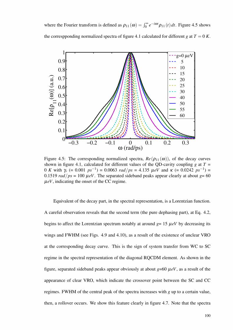
where the Fourier transform is defined as ρ11 (ω) =∫

∞

0 e−iωtρ11 (t)dt. Figure 4.5 shows

the correspponding normalized spectra of figure 4.1 calculated for different g at T = 0 K.

−0.3 −0.2 −0.1 0 0.1 0.2 0.30

0.1

0.2

0.3

0.4

0.5

0.6

0.7

0.8

0.9

1

ω (rad/ps)

Re[

ρ11(ω

)] (

a.u.)

g=0 µeV

5

10

15

20

25

30

40

50

55

60

Figure 4.5: The corresponding normalized spectra, Re(ρ11 (ω)), of the decay curvesshown in figure 4.1, calculated for different values of the QD-cavity coupling g at T =0 K with γr (= 0.001 ps−1) = 0.0063 rad/ps = 4.135 µeV and κ (= 0.0242 ps−1) =0.1519 rad/ps = 100 µeV . The separated sideband peaks appear clearly at about g= 60µeV , indicating the onset of the CC regime.

Equivalent of the decay part, in the spectral representation, is a Lorentzian function.

A careful observation reveals that the second term (the pure dephasing part), at Eq. 4.2,

begins to affect the Lorentzian spectrum notably at around g= 15 µeV by decreasing its

wings and FWHM (see Figs. 4.9 and 4.10), as a result of the existence of unclear VRO

at the corresponding decay curve. This is the sign of system transfer from WC to SC

regime in the spectral representation of the diagonal RQCDM element. As shown in the

figure, separated sideband peaks appear obviously at about g=60 µeV , as a result of the

appearance of clear VRO, which indicate the crossover point between the SC and CC

regimes. FWHM of the central peak of the spectra increases with g up to a certain value,

then, a rollover occurs. We show this feature clearly in figure 4.7. Note that the spectra

100

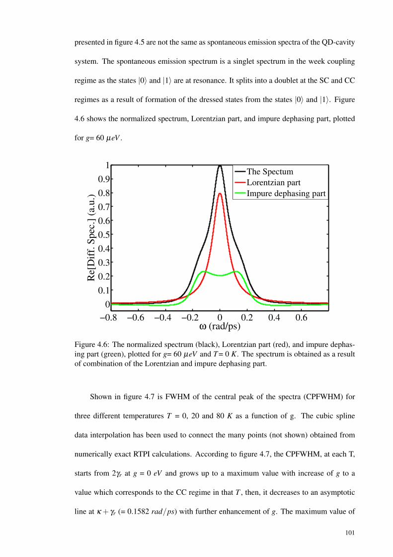
presented in figure 4.5 are not the same as spontaneous emission spectra of the QD-cavity

system. The spontaneous emission spectrum is a singlet spectrum in the week coupling

regime as the states |0〉 and |1〉 are at resonance. It splits into a doublet at the SC and CC

regimes as a result of formation of the dressed states from the states |0〉 and |1〉. Figure

4.6 shows the normalized spectrum, Lorentzian part, and impure dephasing part, plotted

for g= 60 µeV .

−0.8 −0.6 −0.4 −0.2 0 0.2 0.4 0.6

0

0.1

0.2

0.3

0.4

0.5

0.6

0.7

0.8

0.9

1

ω (rad/ps)

Re[

Dif

f. S

pec

.] (

a.u.)

The Spectum

Lorentzian part

Impure dephasing part

Figure 4.6: The normalized spectrum (black), Lorentzian part (red), and impure dephas-ing part (green), plotted for g= 60 µeV and T = 0 K. The spectrum is obtained as a resultof combination of the Lorentzian and impure dephasing part.

Shown in figure 4.7 is FWHM of the central peak of the spectra (CPFWHM) for

three different temperatures T = 0, 20 and 80 K as a function of g. The cubic spline

data interpolation has been used to connect the many points (not shown) obtained from

numerically exact RTPI calculations. According to figure 4.7, the CPFWHM, at each T,

starts from 2γr at g = 0 eV and grows up to a maximum value with increase of g to a

value which corresponds to the CC regime in that T , then, it decreases to an asymptotic

line at κ + γr (= 0.1582 rad/ps) with further enhancement of g. The maximum value of

101

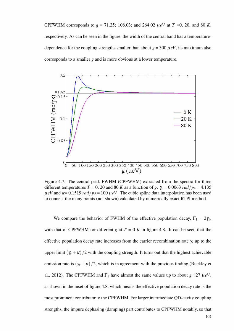
CPFWHM corresponds to g = 71.25; 108.03; and 264.02 µeV at T =0, 20, and 80 K,

respectively. As can be seen in the figure, the width of the central band has a temperature-

dependence for the coupling strengths smaller than about g = 300 µeV , its maximum also

corresponds to a smaller g and is more obvious at a lower temperature.

Figure 4.7: The central peak FWHM (CPFWHM) extracted from the spectra for threedifferent temperatures T = 0, 20 and 80 K as a function of g. γr = 0.0063 rad/ps = 4.135µeV and κ= 0.1519 rad/ps = 100 µeV . The cubic spline data interpolation has been usedto connect the many points (not shown) calculated by numerically exact RTPI method.

We compare the behavior of FWHM of the effective population decay, Γ1 = 2γ1,

with that of CPFWHM for different g at T = 0 K in figure 4.8. It can be seen that the

effective population decay rate increases from the carrier recombination rate γr up to the

upper limit (γr +κ)/2 with the coupling strength. It turns out that the highest achievable

emission rate is (γr +κ)/2, which is in agreement with the previous finding (Buckley et

al., 2012). The CPFWHM and Γ1 have almost the same values up to about g =27 µeV ,

as shown in the inset of figure 4.8, which means the effective population decay rate is the

most prominent contributor to the CPFWHM. For larger intermediate QD-cavity coupling

strengths, the impure dephasing (damping) part contributes to CPFWHM notably, so that

102

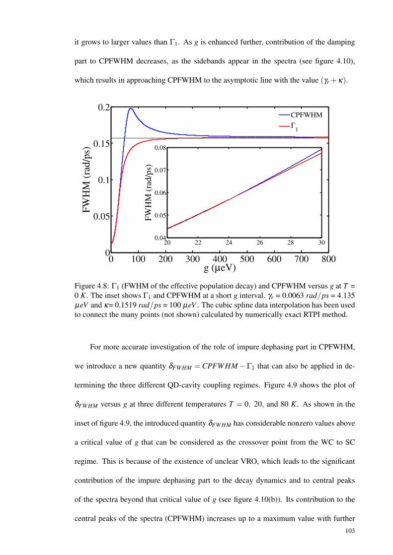
it grows to larger values than Γ1. As g is enhanced further, contribution of the damping

part to CPFWHM decreases, as the sidebands appear in the spectra (see figure 4.10),

which results in approaching CPFWHM to the asymptotic line with the value (γr +κ).

0 100 200 300 400 500 600 700 8000

0.05

0.1

0.15

0.2

g (µeV)

FW

HM

(ra

d/p

s)

20 22 24 26 28 300.04

0.05

0.06

0.07

0.08F

WH

M (

rad

/ps)

CPFWHM

Γ1

Figure 4.8: Γ1 (FWHM of the effective population decay) and CPFWHM versus g at T =0 K. The inset shows Γ1 and CPFWHM at a short g interval. γr = 0.0063 rad/ps = 4.135µeV and κ= 0.1519 rad/ps = 100 µeV . The cubic spline data interpolation has been usedto connect the many points (not shown) calculated by numerically exact RTPI method.

For more accurate investigation of the role of impure dephasing part in CPFWHM,

we introduce a new quantity δFWHM = CPFWHM−Γ1 that can also be applied in de-

termining the three different QD-cavity coupling regimes. Figure 4.9 shows the plot of

δFWHM versus g at three different temperatures T = 0, 20, and 80 K. As shown in the

inset of figure 4.9, the introduced quantity δFWHM has considerable nonzero values above

a critical value of g that can be considered as the crossover point from the WC to SC

regime. This is because of the existence of unclear VRO, which leads to the significant

contribution of the impure dephasing part to the decay dynamics and to central peaks

of the spectra beyond that critical value of g (see figure 4.10(b)). Its contribution to the

central peaks of the spectra (CPFWHM) increases up to a maximum value with further

103

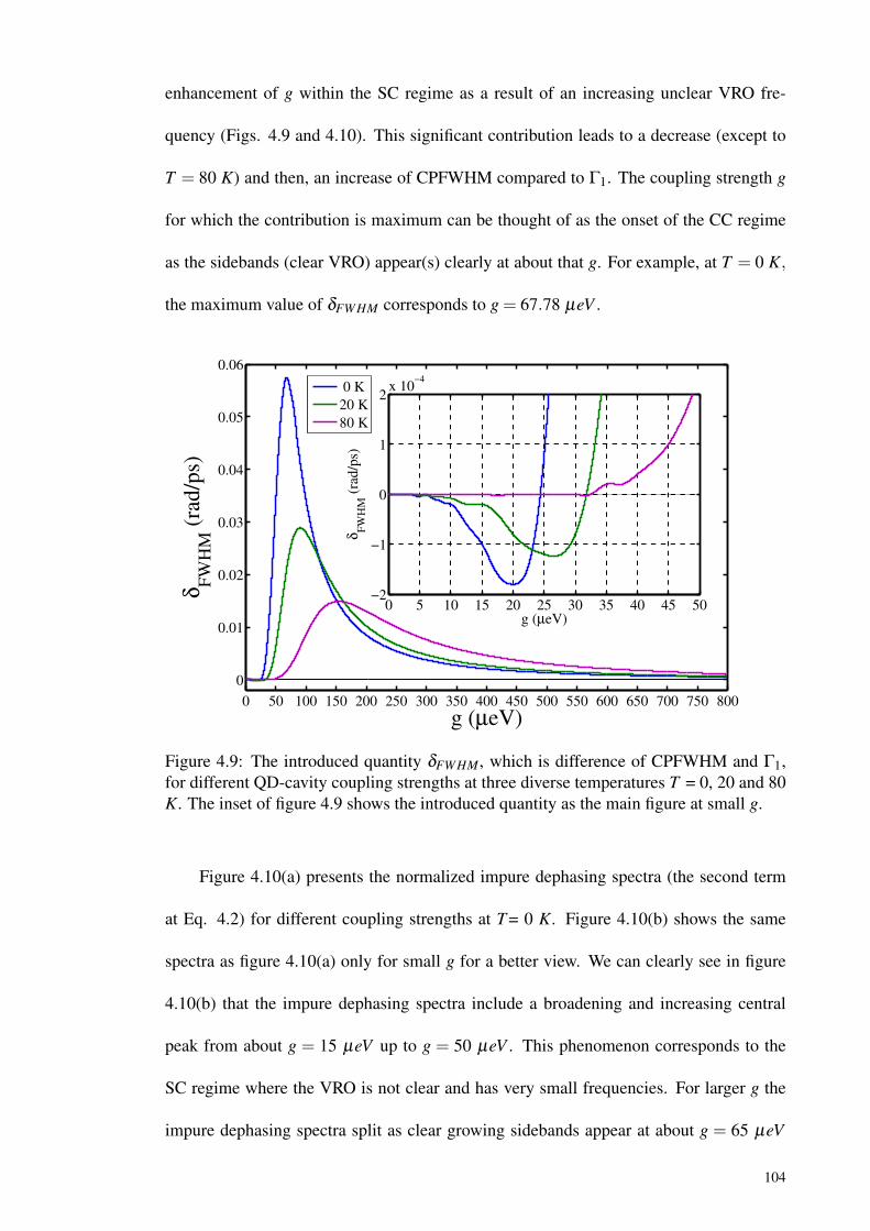
enhancement of g within the SC regime as a result of an increasing unclear VRO fre-

quency (Figs. 4.9 and 4.10). This significant contribution leads to a decrease (except to

T = 80 K) and then, an increase of CPFWHM compared to Γ1. The coupling strength g

for which the contribution is maximum can be thought of as the onset of the CC regime

as the sidebands (clear VRO) appear(s) clearly at about that g. For example, at T = 0 K,

the maximum value of δFWHM corresponds to g = 67.78 µeV .

0 50 100 150 200 250 300 350 400 450 500 550 600 650 700 750 800

0

0.01

0.02

0.03

0.04

0.05

0.06

g (µeV)

δF

WH

M (

rad/p

s)

0 5 10 15 20 25 30 35 40 45 50−2

−1

0

1

2x 10

−4

g (µeV)

δF

WH

M (

rad

/ps)

0 K

20 K

80 K

Figure 4.9: The introduced quantity δFWHM, which is difference of CPFWHM and Γ1,for different QD-cavity coupling strengths at three diverse temperatures T = 0, 20 and 80K. The inset of figure 4.9 shows the introduced quantity as the main figure at small g.

Figure 4.10(a) presents the normalized impure dephasing spectra (the second term

at Eq. 4.2) for different coupling strengths at T = 0 K. Figure 4.10(b) shows the same

spectra as figure 4.10(a) only for small g for a better view. We can clearly see in figure

4.10(b) that the impure dephasing spectra include a broadening and increasing central

peak from about g = 15 µeV up to g = 50 µeV . This phenomenon corresponds to the

SC regime where the VRO is not clear and has very small frequencies. For larger g the

impure dephasing spectra split as clear growing sidebands appear at about g = 65 µeV

104

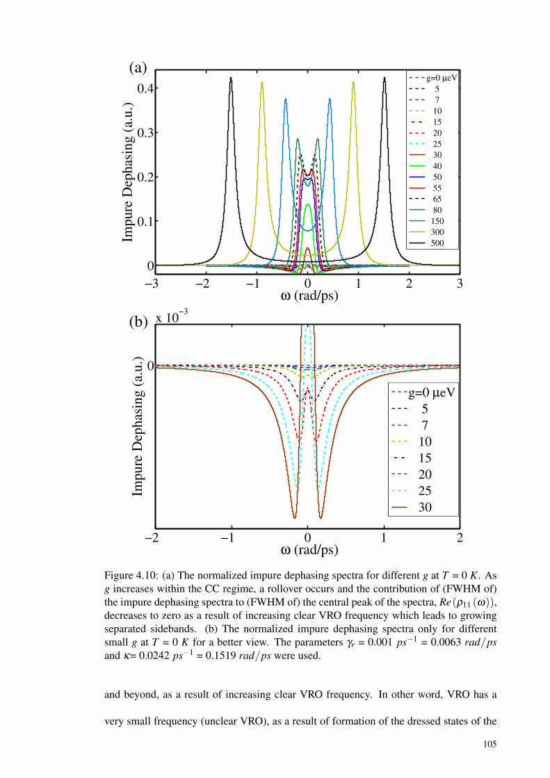
−3 −2 −1 0 1 2 3

0

0.1

0.2

0.3

0.4

ω (rad/ps)

Impure

Dep

has

ing (

a.u.)

g=0 µeV

5

7

10

15

20

25

30

40

50

55

65

80

150

300

500

(a)

−2 −1 0 1 2

0

x 10−3

ω (rad/ps)

Impure

Dep

has

ing (

a.u.)

g=0 µeV

5

7

10

15

20

25

30

(b)

Figure 4.10: (a) The normalized impure dephasing spectra for different g at T = 0 K. Asg increases within the CC regime, a rollover occurs and the contribution of (FWHM of)the impure dephasing spectra to (FWHM of) the central peak of the spectra, Re(ρ11 (ω)),decreases to zero as a result of increasing clear VRO frequency which leads to growingseparated sidebands. (b) The normalized impure dephasing spectra only for differentsmall g at T = 0 K for a better view. The parameters γr = 0.001 ps−1 = 0.0063 rad/psand κ= 0.0242 ps−1 = 0.1519 rad/ps were used.

and beyond, as a result of increasing clear VRO frequency. In other word, VRO has a

very small frequency (unclear VRO), as a result of formation of the dressed states of the

105

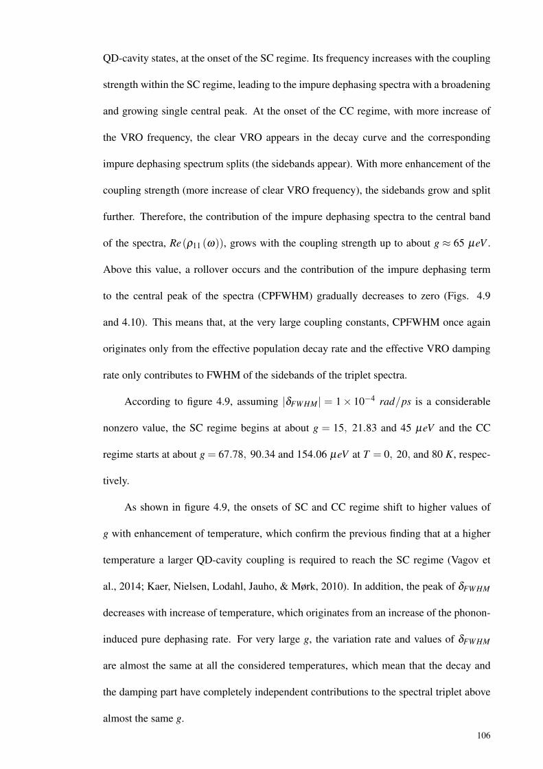
QD-cavity states, at the onset of the SC regime. Its frequency increases with the coupling

strength within the SC regime, leading to the impure dephasing spectra with a broadening

and growing single central peak. At the onset of the CC regime, with more increase of

the VRO frequency, the clear VRO appears in the decay curve and the corresponding

impure dephasing spectrum splits (the sidebands appear). With more enhancement of the

coupling strength (more increase of clear VRO frequency), the sidebands grow and split

further. Therefore, the contribution of the impure dephasing spectra to the central band

of the spectra, Re(ρ11 (ω)), grows with the coupling strength up to about g ≈ 65 µeV .

Above this value, a rollover occurs and the contribution of the impure dephasing term

to the central peak of the spectra (CPFWHM) gradually decreases to zero (Figs. 4.9

and 4.10). This means that, at the very large coupling constants, CPFWHM once again

originates only from the effective population decay rate and the effective VRO damping

rate only contributes to FWHM of the sidebands of the triplet spectra.

According to figure 4.9, assuming |δFWHM| = 1× 10−4 rad/ps is a considerable

nonzero value, the SC regime begins at about g = 15, 21.83 and 45 µeV and the CC

regime starts at about g = 67.78, 90.34 and 154.06 µeV at T = 0, 20, and 80 K, respec-

tively.

As shown in figure 4.9, the onsets of SC and CC regime shift to higher values of

g with enhancement of temperature, which confirm the previous finding that at a higher

temperature a larger QD-cavity coupling is required to reach the SC regime (Vagov et

al., 2014; Kaer, Nielsen, Lodahl, Jauho, & Mørk, 2010). In addition, the peak of δFWHM

decreases with increase of temperature, which originates from an increase of the phonon-

induced pure dephasing rate. For very large g, the variation rate and values of δFWHM

are almost the same at all the considered temperatures, which mean that the decay and

the damping part have completely independent contributions to the spectral triplet above

almost the same g.

106

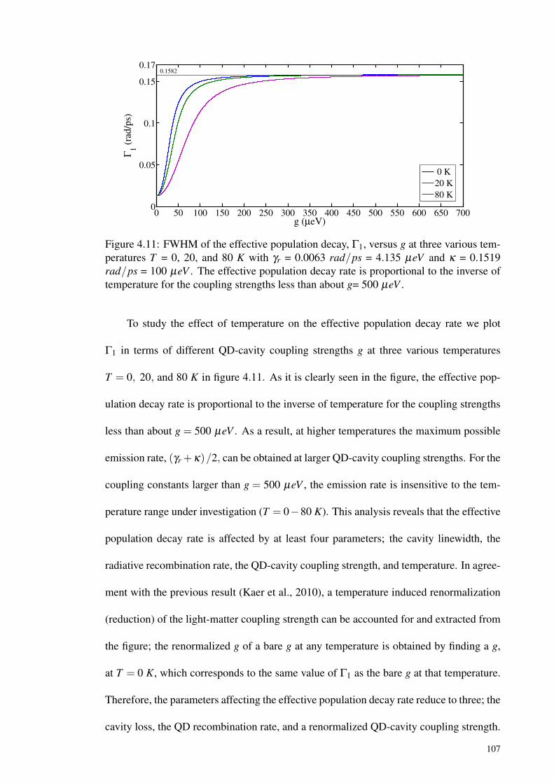
0 50 100 150 200 250 300 350 400 450 500 550 600 650 7000

0.05

0.1

0.15

0.17

g (µeV)

Γ1 (

rad

/ps)

0 K

20 K

80 K

0.1582

Figure 4.11: FWHM of the effective population decay, Γ1, versus g at three various tem-peratures T = 0, 20, and 80 K with γr = 0.0063 rad/ps = 4.135 µeV and κ = 0.1519rad/ps = 100 µeV . The effective population decay rate is proportional to the inverse oftemperature for the coupling strengths less than about g= 500 µeV .

To study the effect of temperature on the effective population decay rate we plot

Γ1 in terms of different QD-cavity coupling strengths g at three various temperatures

T = 0, 20, and 80 K in figure 4.11. As it is clearly seen in the figure, the effective pop-

ulation decay rate is proportional to the inverse of temperature for the coupling strengths

less than about g = 500 µeV . As a result, at higher temperatures the maximum possible

emission rate, (γr +κ)/2, can be obtained at larger QD-cavity coupling strengths. For the

coupling constants larger than g = 500 µeV , the emission rate is insensitive to the tem-

perature range under investigation (T = 0−80 K). This analysis reveals that the effective

population decay rate is affected by at least four parameters; the cavity linewidth, the

radiative recombination rate, the QD-cavity coupling strength, and temperature. In agree-

ment with the previous result (Kaer et al., 2010), a temperature induced renormalization

(reduction) of the light-matter coupling strength can be accounted for and extracted from

the figure; the renormalized g of a bare g at any temperature is obtained by finding a g,

at T = 0 K, which corresponds to the same value of Γ1 as the bare g at that temperature.

Therefore, the parameters affecting the effective population decay rate reduce to three; the

cavity loss, the QD recombination rate, and a renormalized QD-cavity coupling strength.

107

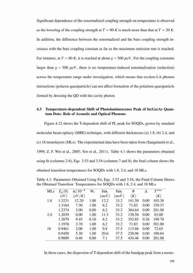
Significant dependence of the renormalized coupling strength on temperature is observed

as the lowering of the coupling strength at T = 80 K is much more than that at T = 20 K.

In addition, the difference between the renormalized and the bare coupling strength in-

creases with the bare coupling constant as far as the maximum emission rate is reached.

For instance, at T = 80 K, it is reached at about g = 500 µeV . For the coupling constants

larger than g = 500 µeV , there is no temperature-induced renormalization (reduction)

across the temperature range under investigation, which means that exciton-LA phonon

interactions (polaron quasiparticle) can not affect formation of the polariton quasiparticle

formed by dressing the QD with the cavity photon.

4.3 Temperature-dependent Shift of Photoluminescence Peak of In(Ga)As Quan-tum Dots: Role of Acoustic and Optical Phonons

Figure 4.12 shows the T-dependent shift of PL peak for SOQDs, grown by standard

molecular beam epitaxy (MBE) technique, with different thicknesses (a) 1.8, (b) 2.4, and

(c) 18 monolayers (MLs). The experimental data have been taken from (Sanguinetti et al.,

1999; Z. F. Wei et al., 2005; Yeo et al., 2011). Table 4.1 shows the parameters obtained

using fit (columns 2-6), Eqs. 3.53 and 3.54 (columns 7 and 8), the final column shows the

obtained transition temperatures for SOQDs with 1.8, 2.4, and 18 MLs.

Table 4.1: Parameters Obtained Using Fit, Eqs. 3.53 and 3.54, the Final Column Showsthe Obtained Transition Temperatures for SOQDs with 1.8, 2.4, and 18 MLs

MLs Eg (0) α/10−4 W1 hω1 hω2 θ ∆ T trns

(eV ) (eV/K) (meV ) (meV ) (K) (K)1.8 1.3231 12.20 1.00 12.2 33.2 141.50 0.00 103.38

1.3164 7.30 1.00 6.2 33.2 71.83 0.00 159.371.2374 3.00 0.00 6.2 33.2 384.64 0.00 201.00

2.4 1.2039 0.00 1.00 11.3 33.2 130.58 0.00 63.001.2079 9.45 0.10 6.2 33.2 352.65 0.26 199.701.1976 3.70 1.00 6.2 33.2 71.83 0.00 301.00

18 0.9461 2.00 1.00 9.8 37.5 113.86 0.00 72.650.9450 5.30 1.00 20.6 37.5 238.96 0.00 180.640.9009 0.46 0.00 7.1 37.5 434.46 0.00 201.00

In these cases, the dispersion of T-dependent shift of the bandgap peak from a mono-

108

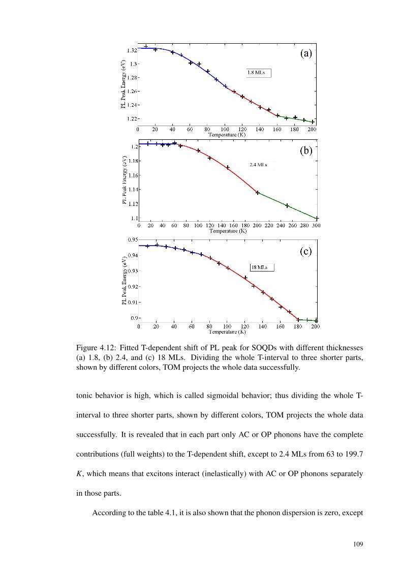
Figure 4.12: Fitted T-dependent shift of PL peak for SOQDs with different thicknesses(a) 1.8, (b) 2.4, and (c) 18 MLs. Dividing the whole T-interval to three shorter parts,shown by different colors, TOM projects the whole data successfully.

tonic behavior is high, which is called sigmoidal behavior; thus dividing the whole T-

interval to three shorter parts, shown by different colors, TOM projects the whole data

successfully. It is revealed that in each part only AC or OP phonons have the complete

contributions (full weights) to the T-dependent shift, except to 2.4 MLs from 63 to 199.7

K, which means that excitons interact (inelastically) with AC or OP phonons separately

in those parts.

According to the table 4.1, it is also shown that the phonon dispersion is zero, except

109

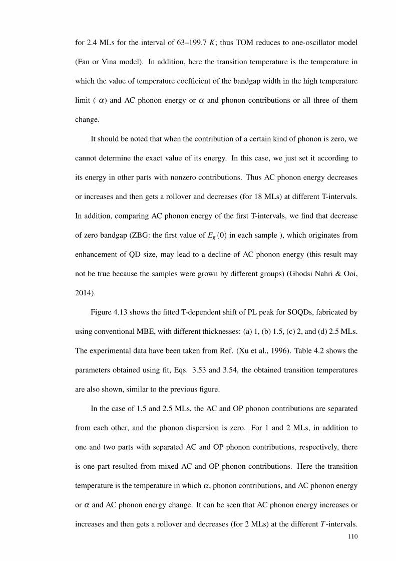
for 2.4 MLs for the interval of 63–199.7 K; thus TOM reduces to one-oscillator model

(Fan or Vina model). In addition, here the transition temperature is the temperature in

which the value of temperature coefficient of the bandgap width in the high temperature

limit ( α) and AC phonon energy or α and phonon contributions or all three of them

change.

It should be noted that when the contribution of a certain kind of phonon is zero, we

cannot determine the exact value of its energy. In this case, we just set it according to

its energy in other parts with nonzero contributions. Thus AC phonon energy decreases

or increases and then gets a rollover and decreases (for 18 MLs) at different T-intervals.

In addition, comparing AC phonon energy of the first T-intervals, we find that decrease

of zero bandgap (ZBG: the first value of Eg (0) in each sample ), which originates from

enhancement of QD size, may lead to a decline of AC phonon energy (this result may

not be true because the samples were grown by different groups) (Ghodsi Nahri & Ooi,

2014).

Figure 4.13 shows the fitted T-dependent shift of PL peak for SOQDs, fabricated by

using conventional MBE, with different thicknesses: (a) 1, (b) 1.5, (c) 2, and (d) 2.5 MLs.

The experimental data have been taken from Ref. (Xu et al., 1996). Table 4.2 shows the

parameters obtained using fit, Eqs. 3.53 and 3.54, the obtained transition temperatures

are also shown, similar to the previous figure.

In the case of 1.5 and 2.5 MLs, the AC and OP phonon contributions are separated

from each other, and the phonon dispersion is zero. For 1 and 2 MLs, in addition to

one and two parts with separated AC and OP phonon contributions, respectively, there

is one part resulted from mixed AC and OP phonon contributions. Here the transition

temperature is the temperature in which α , phonon contributions, and AC phonon energy

or α and AC phonon energy change. It can be seen that AC phonon energy increases or

increases and then gets a rollover and decreases (for 2 MLs) at the different T -intervals.

110

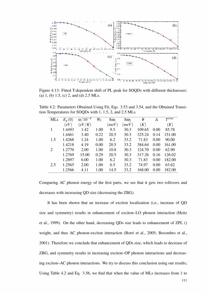
Figure 4.13: Fitted T-dependent shift of PL peak for SOQDs with different thicknesses:(a) 1, (b) 1.5, (c) 2, and (d) 2.5 MLs.

Table 4.2: Parameters Obtained Using Fit, Eqs. 3.53 and 3.54, and the Obtained Transi-tion Temperatures for SOQDs with 1, 1.5, 2, and 2.5 MLs

MLs Eg (0) α/10−4 W1 hω1 hω2 θ ∆ T trns

(eV ) (eV/K) (meV ) (meV ) (K) (K)1 1.4493 1.42 1.00 9.5 30.3 109.65 0.00 85.78

1.4461 3.40 0.22 20.5 30.3 325.24 0.14 151.001.5 1.4268 1.24 1.00 6.2 33.2 71.83 0.00 90.00

1.4218 4.19 0.00 20.5 33.2 384.64 0.00 161.002 1.2770 2.00 1.00 10.8 30.3 124.70 0.00 62.90

1.2769 15.00 0.29 20.5 30.3 317.26 0.16 126.021.2897 6.00 1.00 6.2 30.3 71.83 0.00 182.00

2.5 1.2565 2.00 1.00 6.5 33.2 74.97 0.00 63.621.2566 4.11 1.00 14.5 33.2 168.00 0.00 182.00

Comparing AC phonon energy of the first parts, we see that it gets two rollovers and

decreases with increasing QD size (decreasing the ZBG).

It has been shown that an increase of exciton localization (i.e., increase of QD

size and symmetry) results in enhancement of exciton–LO phonon interaction (Heitz

et al., 1999). On the other hand, decreasing QDs size leads to enhancement of ZPL ()

weight, and thus AC phonon-exciton interaction (Borri et al., 2005; Besombes et al.,

2001). Therefore we conclude that enhancement of QDs size, which leads to decrease of

ZBG, and symmetry results in increasing exciton–OP phonon interactions and decreas-

ing exciton–AC phonon interactions. We try to discuss this conclusion using our results;

Using Table 4.2 and Eq. 3.56, we find that when the value of MLs increases from 1 to

111

1.5 (ZBG decreases to 1.4268 eV), which results in enhancement of QDs size, total OP

phonon contribution increases, while for further increase of QD thickness (size), total

AC phonon contribution increases. Therefore we conclude that elevation of the num-

ber of MLs up to 1.5 (decline of ZBG down to 1.4268 eV) results in increase of QD

symmetry, then a rollover happens and QD symmetry decreases for further increase of

the number of MLs (decline of ZBG). Asymmetry in a QD, which originates from an

elongation of the QD along one crystal axis and inbuilt strain in the crystal, results in

asymmetric electron-hole exchange interaction in the QD and thus exciton fine-structure

splitting (FSS) (Shields, 2007; Gammon, Snow, Shanabrook, Katzer, & Park, 1996). As

shown in (Stevenson et al., 2006) and (Young et al., 2005), FSS decreases with increase

of emission energy up to about 1.4 eV, then it is inverted and enhanced for QDs emitting

at energies more than 1.4 eV. An emission energy, which is very near to 1.4 eV, corre-

sponds to QDs with almost zero exciton FSS (Salter et al., 2010; Stevenson et al., 2006;

Young et al., 2005). As we can see from Table 4.2, this emission energy is near to the PL

peak emission energy of QDs with 1.5 MLs (1.4268 eV). According to our results, with

increase of the ZBG (decrease of QD size) to 1.4268 eV (or more accurately, 1.4 eV), the

QD symmetry increases, then a rollover happens and it decreases for further increase of

the ZBG (decrease of QD size), thus we believe that change of the QD symmetry results

in FSS change as the number of MLs decreases because only the QD symmetry can get a

rollover like FSS with the ZBG variations. We also conclude that, for SOQDs grown us-

ing conventional MBE, the highest symmetry and the lowest FSS correspond to a certain

ZBG about 1.42 eV (a certain number of MLs near to 1.5) or more accurately 1.4 eV (or

more exactly, near to 1.6 ML (Stevenson et al., 2006).

Figures 4.14 and 4.15 show fitted T -dependent shrinkage of bandgap peak for SO-

QDs grown by common MBE and by other epitaxial techniques with different thick-

nesses; for Figs. 4.14(a) and 4.14(b) 1.6, for 4.14(c) and 4.14(d) 2.4, and for 4.15(a) and

112

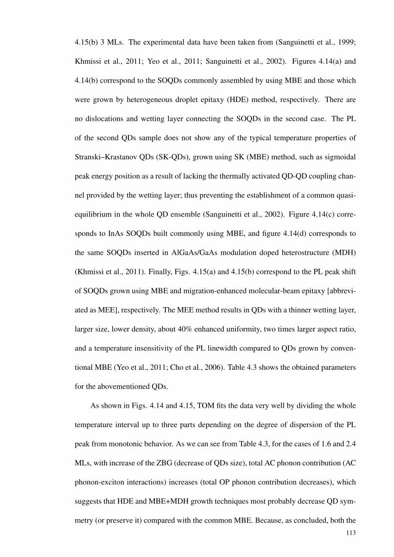
4.15(b) 3 MLs. The experimental data have been taken from (Sanguinetti et al., 1999;

Khmissi et al., 2011; Yeo et al., 2011; Sanguinetti et al., 2002). Figures 4.14(a) and

4.14(b) correspond to the SOQDs commonly assembled by using MBE and those which

were grown by heterogeneous droplet epitaxy (HDE) method, respectively. There are

no dislocations and wetting layer connecting the SOQDs in the second case. The PL

of the second QDs sample does not show any of the typical temperature properties of

Stranski–Krastanov QDs (SK-QDs), grown using SK (MBE) method, such as sigmoidal

peak energy position as a result of lacking the thermally activated QD-QD coupling chan-

nel provided by the wetting layer; thus preventing the establishment of a common quasi-

equilibrium in the whole QD ensemble (Sanguinetti et al., 2002). Figure 4.14(c) corre-

sponds to InAs SOQDs built commonly using MBE, and figure 4.14(d) corresponds to

the same SOQDs inserted in AlGaAs/GaAs modulation doped heterostructure (MDH)

(Khmissi et al., 2011). Finally, Figs. 4.15(a) and 4.15(b) correspond to the PL peak shift

of SOQDs grown using MBE and migration-enhanced molecular-beam epitaxy [abbrevi-

ated as MEE], respectively. The MEE method results in QDs with a thinner wetting layer,

larger size, lower density, about 40% enhanced uniformity, two times larger aspect ratio,

and a temperature insensitivity of the PL linewidth compared to QDs grown by conven-

tional MBE (Yeo et al., 2011; Cho et al., 2006). Table 4.3 shows the obtained parameters

for the abovementioned QDs.

As shown in Figs. 4.14 and 4.15, TOM fits the data very well by dividing the whole

temperature interval up to three parts depending on the degree of dispersion of the PL

peak from monotonic behavior. As we can see from Table 4.3, for the cases of 1.6 and 2.4

MLs, with increase of the ZBG (decrease of QDs size), total AC phonon contribution (AC

phonon-exciton interactions) increases (total OP phonon contribution decreases), which

suggests that HDE and MBE+MDH growth techniques most probably decrease QD sym-

metry (or preserve it) compared with the common MBE. Because, as concluded, both the

113

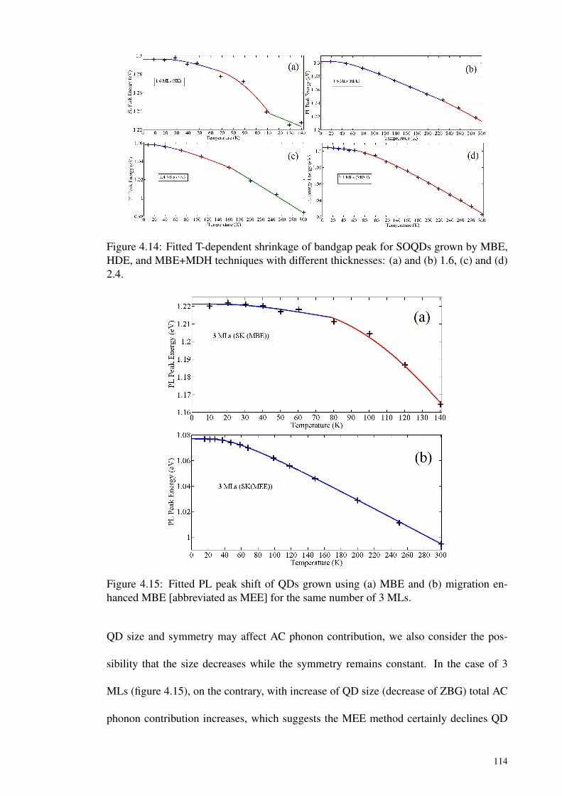
Figure 4.14: Fitted T-dependent shrinkage of bandgap peak for SOQDs grown by MBE,HDE, and MBE+MDH techniques with different thicknesses: (a) and (b) 1.6, (c) and (d)2.4.

Figure 4.15: Fitted PL peak shift of QDs grown using (a) MBE and (b) migration en-hanced MBE [abbreviated as MEE] for the same number of 3 MLs.

QD size and symmetry may affect AC phonon contribution, we also consider the pos-

sibility that the size decreases while the symmetry remains constant. In the case of 3

MLs (figure 4.15), on the contrary, with increase of QD size (decrease of ZBG) total AC

phonon contribution increases, which suggests the MEE method certainly declines QD

114

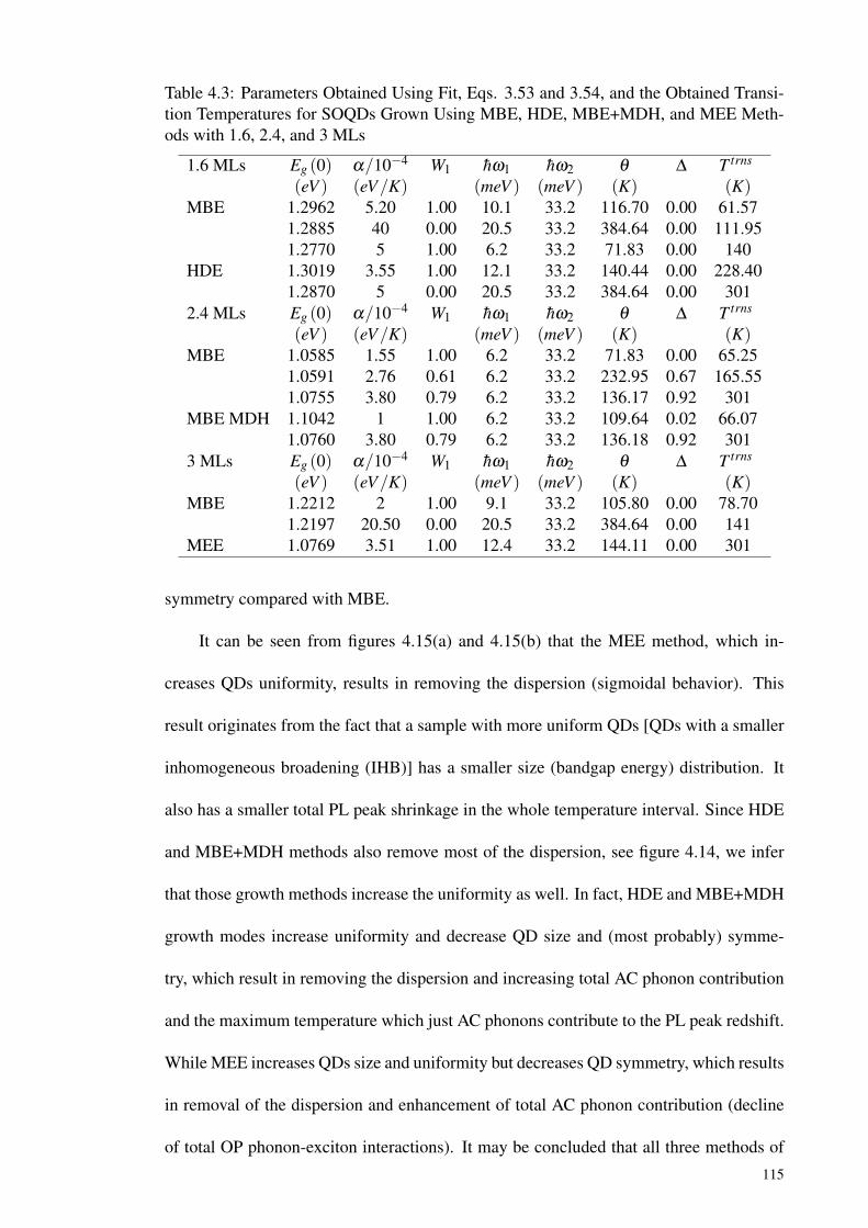
Table 4.3: Parameters Obtained Using Fit, Eqs. 3.53 and 3.54, and the Obtained Transi-tion Temperatures for SOQDs Grown Using MBE, HDE, MBE+MDH, and MEE Meth-ods with 1.6, 2.4, and 3 MLs

1.6 MLs Eg (0) α/10−4 W1 hω1 hω2 θ ∆ T trns

(eV ) (eV/K) (meV ) (meV ) (K) (K)MBE 1.2962 5.20 1.00 10.1 33.2 116.70 0.00 61.57

1.2885 40 0.00 20.5 33.2 384.64 0.00 111.951.2770 5 1.00 6.2 33.2 71.83 0.00 140

HDE 1.3019 3.55 1.00 12.1 33.2 140.44 0.00 228.401.2870 5 0.00 20.5 33.2 384.64 0.00 301

2.4 MLs Eg (0) α/10−4 W1 hω1 hω2 θ ∆ T trns

(eV ) (eV/K) (meV ) (meV ) (K) (K)MBE 1.0585 1.55 1.00 6.2 33.2 71.83 0.00 65.25

1.0591 2.76 0.61 6.2 33.2 232.95 0.67 165.551.0755 3.80 0.79 6.2 33.2 136.17 0.92 301

MBE MDH 1.1042 1 1.00 6.2 33.2 109.64 0.02 66.071.0760 3.80 0.79 6.2 33.2 136.18 0.92 301

3 MLs Eg (0) α/10−4 W1 hω1 hω2 θ ∆ T trns

(eV ) (eV/K) (meV ) (meV ) (K) (K)MBE 1.2212 2 1.00 9.1 33.2 105.80 0.00 78.70

1.2197 20.50 0.00 20.5 33.2 384.64 0.00 141MEE 1.0769 3.51 1.00 12.4 33.2 144.11 0.00 301

symmetry compared with MBE.

It can be seen from figures 4.15(a) and 4.15(b) that the MEE method, which in-

creases QDs uniformity, results in removing the dispersion (sigmoidal behavior). This

result originates from the fact that a sample with more uniform QDs [QDs with a smaller

inhomogeneous broadening (IHB)] has a smaller size (bandgap energy) distribution. It

also has a smaller total PL peak shrinkage in the whole temperature interval. Since HDE

and MBE+MDH methods also remove most of the dispersion, see figure 4.14, we infer

that those growth methods increase the uniformity as well. In fact, HDE and MBE+MDH

growth modes increase uniformity and decrease QD size and (most probably) symme-

try, which result in removing the dispersion and increasing total AC phonon contribution

and the maximum temperature which just AC phonons contribute to the PL peak redshift.

While MEE increases QDs size and uniformity but decreases QD symmetry, which results

in removal of the dispersion and enhancement of total AC phonon contribution (decline

of total OP phonon-exciton interactions). It may be concluded that all three methods of

115

HDE, MBE+MDH, and MEE increase QDs uniformity; as a result of providing a thin (or

no) wetting layer and accordingly, increase total AC phonon contribution and decrease

the symmetry. This suggests a trade-off between QDs uniformity and symmetry as an

enhancement in the uniformity (decrease of IHB) causes a decline in the symmetry and

vice versa. It means that IHB, which is a characteristic of the whole sample, affects QD

symmetry, which is a characteristic of the single QDs. This is similar to a result offered

previously in (Ghodsi Nahri, 2012b), which states different IHBs cause to different ho-

mogeneous broadening (which is again a single QD characteristic) in a given temperature.

Uniformity increases total AC phonon contribution and the symmetry increases total OP

phonon contribution.

Comparing MBE data of Table 4.3 for 1.6 and 2.4 MLs, similarly, we find that de-

crease of ZBG, as a result of QDs size enhancement, results in decrease of QD symmetry,

while comparing 2.4 and 3 MLs (MBE data), we find that increase of ZBG, as a result

of decrease of QDs size, leads to enhancement of QD symmetry. We may attribute this

phenomenon to change of ZBG backward and toward the critical value 1.4 eV which cor-

responds to the highest QD symmetry. Thus we infer that increase of ZBG up to a critical

value about 1.4 eV, for QDs grown using MBE and MEE, results in enhancement of QD

symmetry and total OP phonon contribution and decrease of QDs uniformity and total

AC phonon contribution, while a rollover happens for further increase of ZBG. In order

for this result always to be true, the growth details should still be the same. It is also

nearly inferable from Table 4.1 that decrease of ZBG, as a result of QDs size enhance-

ment, backward 1.4 eV leads to reduction of total OP phonon contribution and increase

of total AC phonon contribution.

We can find the meaning of the transition temperature in Table 4.3 as follows: it

is shown that α , phonon contributions, and AC phonon energy change in the different

temperature parts in the cases of 1.6 and 3 MLs (MBE). While for 2.4 MLs, just α and

116

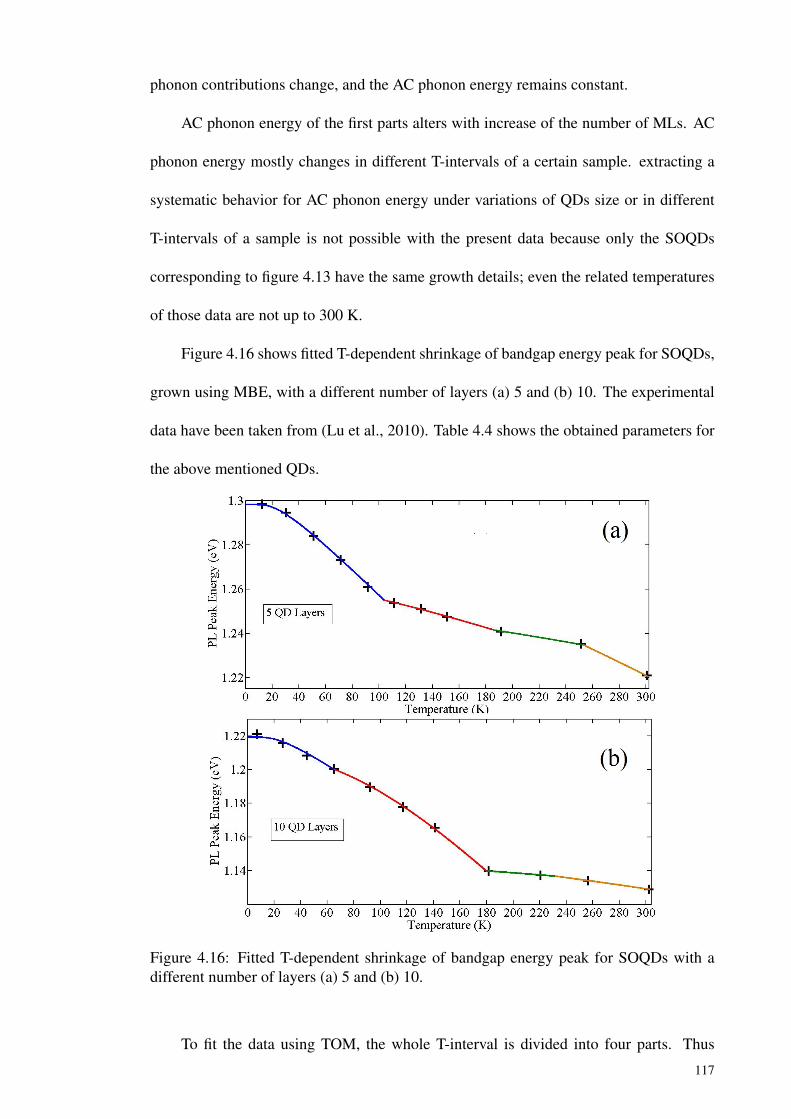
phonon contributions change, and the AC phonon energy remains constant.

AC phonon energy of the first parts alters with increase of the number of MLs. AC

phonon energy mostly changes in different T-intervals of a certain sample. extracting a

systematic behavior for AC phonon energy under variations of QDs size or in different

T-intervals of a sample is not possible with the present data because only the SOQDs

corresponding to figure 4.13 have the same growth details; even the related temperatures

of those data are not up to 300 K.

Figure 4.16 shows fitted T-dependent shrinkage of bandgap energy peak for SOQDs,

grown using MBE, with a different number of layers (a) 5 and (b) 10. The experimental

data have been taken from (Lu et al., 2010). Table 4.4 shows the obtained parameters for

the above mentioned QDs.

Figure 4.16: Fitted T-dependent shrinkage of bandgap energy peak for SOQDs with adifferent number of layers (a) 5 and (b) 10.

To fit the data using TOM, the whole T-interval is divided into four parts. Thus

117

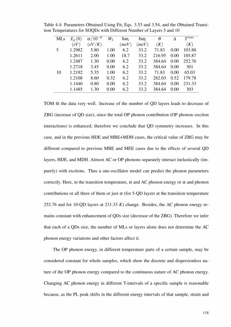
Table 4.4: Parameters Obtained Using Fit, Eqs. 3.53 and 3.54, and the Obtained Transi-tion Temperatures for SOQDs with Different Number of Layers 5 and 10

MLs Eg (0) α/10−4 W1 hω1 hω2 θ ∆ T trns

(eV ) (eV/K) (meV ) (meV ) (K) (K)5 1.2982 5.80 1.00 6.2 33.2 71.83 0.00 103.88

1.2611 2.00 1.00 18.7 33.2 216.95 0.00 185.871.2487 1.30 0.00 6.2 33.2 384.64 0.00 252.761.2718 3.45 0.00 6.2 33.2 384.64 0.00 301

10 1.2192 5.35 1.00 6.2 33.2 71.83 0.00 65.031.2108 8.60 0.32 6.2 33.2 282.03 0.52 179.781.1440 0.80 0.00 6.2 33.2 384.64 0.00 231.331.1485 1.30 0.00 6.2 33.2 384.64 0.00 303

TOM fit the data very well. Increase of the number of QD layers leads to decrease of

ZBG (increase of QD size), since the total OP phonon contribution (OP phonon–exciton

interactions) is enhanced; therefore we conclude that QD symmetry increases. In this

case, and in the previous HDE and MBE+MDH cases, the critical value of ZBG may be

different compared to previous MBE and MEE cases due to the effects of several QD

layers, HDE, and MDH. Almost AC or OP phonons separately interact inelastically (im-

purely) with excitons. Thus a one-oscillator model can predict the phonon parameters

correctly. Here, in the transition temperature, α and AC phonon energy or α and phonon

contributions or all three of them or just α (for 5-QD layers at the transition temperature

252.76 and for 10-QD layers at 231.33 K) change. Besides, the AC phonon energy re-

mains constant with enhancement of QDs size (decrease of the ZBG). Therefore we infer

that each of a QDs size, the number of MLs or layers alone does not determine the AC

phonon energy variations and other factors affect it.

The OP phonon energy, in different temperature parts of a certain sample, may be

considered constant for whole samples, which show the discrete and dispersionless na-

ture of the OP phonon energy compared to the continuous nature of AC phonon energy.

Changing AC phonon energy in different T-intervals of a specific sample is reasonable

because, as the PL peak shifts in the different energy intervals of that sample, strain and

118

quantum confinement (QDs size) alter, and it has been shown that strain and quantum

confinement affect phonon energies (Heitz et al., 1996; Stock et al., 2011). So the AC

phonon energy can be changed. Perhaps variations of strain and quantum confinement

also are the causes of changes in phonon contributions in the different intervals of a QD

sample.

119

CHAPTER 5

CONCLUSIONS

In the first part of this work, an open QD-cQED system including a dissipative QD, ini-

tially prepared at ES, coupled to a LA phonon bath and a lossy cavity, with maximum

one photon, has been studied using numerically accurate RTPI approach. Within this

approach, we treated exciton-photon and exciton-phonon interactions on equal footing,

exciton radiative decay and cavity loss were included phenomenologically through the

non-Hermitian terms. Different coupling regimes of QD-cQED, called weak, interme-

diate, and coherent, defined in terms of the decay dynamics were discussed and stricter

conditions identifying them were provided. It was found that these regimes match the cou-

pling regimes defined in terms of appearance and resolution of VRS. Our results showed

that to have the CC regime, VRS (the doublet separation) should be larger than the sum of

the widths of the corresponding peaks. In order to discern between the role of population

decay and impure dephasing (damping), induced by LA phonons and the dissipations,

on the quantum dynamics of the QD-cavity system, we proposed a phenomenological

expression which projects the QD-cavity decay curves perfectly, enabling us to calculate

the corresponding spectra. The expression fits the decay curves very well. We found

an approximate expression for the effective impure dephasing rate using a match of the

state population for the dissipation-less QD-cavity system, calculated by our microscopic

RTPI approach, to the phenomenological expression. It was found that the increase of

light-matter coupling strength results in enhancing CPFWHM from 2γr up to a maximum

value within the CC regime then, decreasing it to an asymptotic line, the value of which

is the sum of the QD and cavity dissipation rates. The width of the central peak of the

spectra (CPFWHM) is temperature dependent for not very large coupling strengths. The

120

effective population decay (emission) rate increases from the carrier recombination rate to

a maximum value, which is mean of the QD and cavity dissipation rates, with the coupling

strength. In order to study the role of the effective impure dephasing rate on CPFWHM

we introduced a quantity that was used in determining the different coupling regimes as

well. This quantity enabled us to define the onset of the SC regime as the point where the

impure dephasing part begins to contribute to the central band of the spectra significantly,

which originates from the existence of VRO with a very small frequency (unclear VRO),

because the corresponding impure dephasing spectrum only includes a central peak. Its

contribution to CPFWHM increases with the coupling strength up to the onset of the CC

regime, then decreases as a result of the appearance of sidebands (splitting of the impure

dephasing spectra), which originates from the appearance of clear VRO at the correspond-

ing decay curves. CPFWHM arises solely from the effective population decay rate only at

small and at very large coupling strengths. In other words, the effective population decay

and impure dephasing rates contribute separately to the width of, respectively, the cen-

tral and sideband peaks of the triplet spectra only beyond a very large coupling strength

which is the same across the considered temperature range. Temperature-dependence of

the effective population decay rate means that at a higher temperature a larger coupling

strength is required to obtain the maximum achievable emission rate. There is no temper-

ature induced renormalization (reduction) of the light–matter coupling strength at very

large coupling constants.

In the second part, it was found that if whole temperature 0–300 K is divided into

several parts (at most four parts), depending on the degree of dispersion from a monotonic

behavior of T-dependent shift of PL peak and considering the first part as AC phonons

have the total contribution, TOM is able to fit all the available data of In(Ga)As QDs very

well. The meaning of transition temperature is the temperature in which the value of tem-

perature coefficient of the bandgap width in the high temperature limit plus one or both of

121

phonon contributions and AC phonon energy change. Almost AC phonon energy varies in

different T- (or energy) intervals of a certain sample, which may originate from a change

in strain and quantum confinement. The numerical results suggest that excitons mostly

interact (impurely) with AC or OP phonons separately, especially when T-dependent PL

peak shift of a sample has a high dispersion from a monotonic behavior, which originates

from a low QDs uniformity. Thus there is zero-phonon dispersion, and the TOM reduces

to one-oscillator model (Fan or Vina model). Increasing QDs uniformity by using some

growth techniques (HDE, MBE+MDH, and MEE) results in reducing or removing the

dispersion (sigmoidal behavior), enhancing the total AC phonon contribution (exciton–

AC phonon interaction) and the maximum temperature which AC phonons contribute to

the T-dependent red shift of PL emission peak. We also proposed a tradeoff between

QDs uniformity (IHB of the QDs sample) and QD symmetry. QDs uniformity directly

changes (increases) total AC phonon contribution, and the symmetry directly affects (in-

creases) total OP phonon contribution. Increasing ZBG, as a result of decrease of QDs

size, up to a critical value about 1.4 eV, for In(Ga)As QDs grown using MBE and MEE,

results in enhancement of QD symmetry and total OP phonon contribution and decrease

of QDs uniformity and total AC phonon contribution, while a rollover happens for further

enhancement of ZBG. Therefore we find that the highest QD symmetry and the lowest

exciton FSS correspond to this critical value of ZBG. Enhancement of the number of QD

layers (from 5 to 10) leads to increase of total OP phonon contribution and reduction

of total AC phonon contribution. It seems that the critical value of ZBG, corresponding

to QD samples containing several layers and those grown by HDE and MBE+MDH, is

different than about 1.4 eV.

122

Appendices

123

APPENDIX A

DERIVATION OF DISCRETIZED REAL-TIME PATH-INTEGRALS FORDISSIPATIVE QUANTUM DOT-CAVITY SYSTEM COUPLED TO

LONGITUDINAL ACOUSTIC PHONON BATH

In this appendix we present a discretized real-time path-integral representation of the

dynamics for an open QD-cavity system coupled to a continuum of AC phonons, with

smooth spectral density, by pure dephasing type interactions. A linear carrier-phonon

coupling is assumed, which allows to eliminate the phonon degrees of freedom exactly

and to construct a closed form of the influence functional integral for the system under

investigation. Our model Hamiltonian including open QD-cavity (OQC) system coupled

to the LA phonon reservoir, as described in Chap. 3, is

H (t) = HS +HR +HSR = h(

ωC− iκ

2

)s00 + h

(ωX − i

γr

2

)s11

+hg(s01 + s10)+ h∑q

ωqb†qbq + h∑

q

(γ∗q bq + γqb†

q

), (A.1)

where the hat sign stands for matrix operators acting in the subspace of the carrier-photon

states. Here, the OQC system contains three levels denoted by |0〉 = |G,n = 1〉, |1〉 =

|X ,n = 0〉, and |2〉 = |G,n = 0〉 where n refers to the number of photons in the cavity

mode. Only the states |0〉 and |1〉 are coupled due to the dipole interaction between

them. The states |0〉 and |1〉 decay to the state |2〉 irreversibly with the variable rate γ1, as

described in Chap. 3.

In order to derive a discretized RTPI representation for the RQCDM, we start by

taking the partial trace over the total density matrix (total statistical operator), expressed

in terms of the initial total density matrix, χ(0), and the time evolution operator, in the

124

interaction picture as

ρ(t) = Trph[U(t)χ(0)U†(t)]. (A.2)

Identity operators, In, of the system-bath, i.e. the OQC system and its environment,

is constructed as a direct product of identity operators in the space of carrier-photon states,

|s+n 〉, and the space of coherent phonon states, |Zn〉, so that

In = Is+n ⊗ IZ

n = ∑s+n

∣∣s+n ⟩⟨s+n ∣∣⊗∫ ∞

−∞

dµn |Zn〉〈Zn|

dµn = ∏q

e−ZqnZqndZqndZqn

π,

(A.3)

where the coherent phonon states are defined by bq |Zn〉 = Zqn |Zn〉. The integrations are

performed on the complex plane of the conjugate variables Zqn and Zqn = Z∗qn.

Performing the trace in Eq. A.2 over the phonon degrees of freedom, at time t,

which, here, is equivalent to integrations over the phonon variables Zq f we have

ρs+f s−f(t) =

⟨s+f∣∣∣Trph[χ(t)]

∣∣∣s−f ⟩=

∫dµ f

⟨s+f ,Z f

∣∣∣U(t)χ(0)U†(t)∣∣∣s−f ,Z f

⟩, (A.4)

where∣∣∣s+f ⟩ and

∣∣∣s−f ⟩ correspond to the system eigenbasis for forward and backward

propagation in the final time t. Using the completeness relations of the system-bath at the

initial time, with index i, for forward and backward propagation, we obtain

ρs+f s−f(t) =

∫dµ f

∫dµi

∫dµ′i ∑

s+i ,s−i

⟨s+f ,Z f

∣∣∣U(t)∣∣s+i ,Zi

⟩⟨s+i ,Zi

∣∣χ(0) ∣∣s−i ,Z′i⟩⟨s−i ,Z′i∣∣U†(t)∣∣∣s−f ,Z f

⟩. (A.5)

125

The time evolution operator, which correspond to the total Hamiltonian, is given by

U(t,0) = T exp(− i

h

∫ t

0H (τ)dτ

), (A.6)

where T is the time ordering operator. According to the Trotter discretization, we dis-

cretize the time interval [0, t], of the integration over the total Hamiltonian, into N time

steps of the length ε = tn− tn−1 = t/N, yielding support points tn = nε with n = 1, ...,N,

while we consider the limit N→ ∞ (or equivalently, ε → 0), therefore

∫ t

0H(τ)dτ = lim

N→∞

N

∑n=1

∫ tn

tn−1

H(τ)dτ = limN→∞

N

∑n=1

εH (tn) , (A.7)

where we have approximated the time-varying Hamiltonian H(τ) by a piecewise constant

Hamiltonian H (tn) in the small enough time intervals where the Hamiltonian is constant

during each of the small time interval ε .

Factorizing the time-evolution operator with the discretized Hamiltonian, as a con-

sequence of the Baker-Campbell-Hausdorff expansion for a sufficiently small time slice ε

(Kleinert, 2006), and keeping the first-order accuracy of the discretization (O(ε)), omit-

ting the higher orders of ε , we attain

U(t,0)≈ limN→∞

TN

∏n=1

U (tn, tn−1) = limN→∞

TN

∏n=1

e−iεH(tn)/h, (A.8)

where t0 = 0, tN = t and the product is time ordered, with decreasing n from left to

right. By inserting a complete set of states between each pair of the short-time evolution

operators we have

U(t) ≈ limN→∞

(e−iεH(tN)/hIN−1...e−iεH(t2)/hI1e−iεH(t1)/h

). (A.9)

126

Therefore, the first matrix element in Eq. A.5 is represented as

⟨s+N ,ZN

∣∣U(t)∣∣s+0 ,Z0

⟩= lim

N→∞∑

s+N−1

∑s+N−2

...∑s+1

∫dµN−1

∫dµN−2...

∫dµ1

N

∏n=1

An = limN→∞

TN−1

∏n=1

[∑s+n

∫dµn

]N

∏n=1

An, (A.10)

where initial and final states are denoted by indexes n = 1 and n = N and short-time

amplitude An is represented as

An =⟨s+n ,Zn

∣∣e−iεH(tn)/h ∣∣s+n−1,Zn−1⟩. (A.11)

Partitioning the total Hamiltonian into the one-dimensional free system Hamiltonian,

HS(tn), and the influence Hamiltonian, HIn f (tn) = HR(tn) +HSR(tn), and again factor-

izing the short time-evolution operator, keeping the first-order accuracy O(ε), it can be

written as

e−iεH(tn)/h ≈ e−iεHS(tn)/he−iεHIn f (tn)/h. (A.12)

Using a complete set of system states and the fact that HS is diagonal in the phonon

subspace and that HIn f is diagonal in the subspace of carrier-photon states, the matrix

element An is written as

An ≈⟨s+n∣∣e−iεHS(tn)/h ∣∣s+n−1

⟩⟨s+n−1,Zn

∣∣e−iεHIn f (tn)/h ∣∣s+n−1,Zn−1⟩. (A.13)

Using a standard result for matrix elements of a normal ordered phonon operator function

(Vagov, Croitoru, Glässl, et al., 2011),

〈Z|F(b†q,bq)

∣∣Z′⟩= e∑q ZqZ′qF(Zq,Z′q), (A.14)

127

for the second matrix element in Eq. A.13, we obtain

⟨s+n−1,Zn

∣∣e−iεHIn f (tn)/h ∣∣s+n−1,Zn−1⟩=⟨s+n−1

∣∣eS0n∣∣s+n−1

⟩, (A.15)

where

S0n = ∑q

ZqnZqn−1− iε ∑q

(γqnZqn + γ

∗qnZqn−1 +ωqZqnZqn−1

). (A.16)

The index n in the matrix γqn indicates that it acts on the carrier-photon states of the nth

time slice. Inserting Eq. A.15 into Eq. A.13 and substituting the result into A.10, the

short-time amplitude and the matrix elements of the evolution operator are obtained as

An ≈⟨s+n∣∣eS0n−iεHS(tn)/h ∣∣s+n−1

⟩,⟨

s+N ,ZN∣∣U(t)

∣∣s+0 ,Z0⟩

=⟨s+N∣∣ lim

N→∞

TN−1

∏n=1

[∫dµn

]eS0∣∣s+0 ⟩ ,

(A.17)

where T is the time ordering operator for the operators in the carrier-photon state subspace

and

S0 =N

∑n=1

(S0n− iεHS(tn)/h

). (A.18)

Using the following identity:

N

∑n=1

ZqnZqn−1 = ZqNZqN +N−1

∑n=1

ZqnZqn− ε

N

∑n=1

Zqn

(Zqn−Zqn−1

)ε

. (A.19)

keeping the accuracy O(ε) and using the conversion of summation to integral, as defined

128

in Eq. A.7, for the exponent in Eq. A.17 we gain

S0 =N−1

∑n=1

∑q

ZqnZqn +∑q

Zq (t)Zq (t)−ih

∫ t

0dτHS (τ)

−∑q

∫ t

0dτ[Zq(τ)Zq(τ)+ iωqZq(τ)Zq(τ)+ iγq(τ)Zq(τ)+ iγ∗q (τ)Zq(τ)

],

(A.20)

where Zqn =(Zqn−Zqn−1

)/ε and we used the boundary conditions ZqN = Zq(t) and

ZqN = Zq(t).

As a result, the matrix elements of the evolution operator, defined in Eq. A.10 and

A.11, become a path-integral over phonon variables, formally represented as

⟨s+f ,Z f

∣∣∣U(t)∣∣s+i ,Zi

⟩=⟨

s+f∣∣∣∫ DZeS(τ) ∣∣s+i ⟩ , (A.21)

where ∫DZ = lim

N→∞T

N−1

∏n=1

∫∏

q

dZqndZqn

π, (A.22)

and the “action functional” S is given by

S = ∑q

Zq (t)Zq (t)−ih

∫ t

0dτHS (τ)−∑

q

∫ t

0dτ[

Zq(τ)Zq(τ)+ iωqZq(τ)Zq(τ)+ iγqZq(τ)+ iγ∗q Zq(τ)].

(A.23)

Since the action functional is quadratic in the phonon variables the correspond-

ing path-integrals can be calculated exactly. The action is defined as S(Zq, Zq,Zq, t) =

∑q Zq (t)Zq (t)−ih∫ t

0 dτHS (τ)−∑q∫ t

0 L(Zq, Zq,τ)dt where L(Zq, Zq,τ) is the Lagrangian.

We expand the general path around the classical one as Zq (τ) = ZClq (τ)+ηq (τ) where

ηq (τ) denotes fluctuating paths about the classical one with the boundary conditions

129

ηq (0) = ηq (t) = 0. Classical trajectories are determined by the requirement that the

action functional evaluated along them must be stationary, therefore,

∂ SCl (t)∂ZCl

q= 0,

∂ SCl (t)

∂ZClq

= 0, (A.24)

where SCl (t) = S(ZClq , ZCl

q ,ZClq , t) is called extremal action. In order to satisfy Eq. A.24

the Lagrangian must obey the Euler-Lagrange equations (Khandekar, Lawande, & Bhag-

wat, 1998; Kakushadze, 2015), so that

ddt

∂L

∂ ZClq

− ∂L

∂ZClq

= ZClq (τ)+ iωqZCl

q (τ)+ iγq (τ) = 0, (A.25)

and

ddt

∂L∂ ZCl

q− ∂L

∂ZClq

= ZClq (τ)− iωqZCl

q (τ)− iγ∗q (τ) = 0. (A.26)

Using the expansion about the classical path (fluctuation expansion), the equations of

motion A.25 and A.26, and the boundary conditions for the fluctuating paths the action is

obtained as S (t) = SCl + Sη where Sη =−∑q∫ t

0(ηq (τ) ηq (τ)+ iωqηq (τ)ηq (τ)

)dτ . As

the classical path, at each q, is stationary and the fluctuating paths are zero at the initial

and final times, the path-integral for the evolution operator is obtained as

⟨s+f ,Z f

∣∣∣U(t)∣∣s+i ,Zi

⟩=

[∫DηeSη

]⟨s+f∣∣∣eSCl

∣∣s+i ⟩ . (A.27)

The general solutions of Eqs. A.25 and A.26 are obtained using the boundary conditions

ZClq (0) = Zqi, ZCl

q (t) = Z∗q f , (A.28)

130

as

ZClq (τ) = Zqie−iωqτ − i

∫τ

0dτ′e−iωq(τ−τ ′)

γq(τ′) , (A.29)

ZClq (τ) = Z∗q f eiωq(τ−t)− i

∫ t

τ

dτ′eiωq(τ−τ ′)

γ∗q(τ′) . (A.30)

These classical paths are operators in the carrier-photon state subspace. It can be seen

that now they are not complex conjugate which justifies the notation Z.

To obtain the action evaluated along the classical path, we rewrite Eq. A.25 as

Zq (τ) =−iωqZq (τ)− iγq (τ) , (A.31)

using Eq. A.29 the term Zq (t)Zq (t) can be written as

Zq (t)Zq (t) = Z∗q f Zqie−iωqt− iZ∗q f

∫ t

0dτ′e−iωq(t−τ ′)

γq(τ′) , (A.32)

where we used the boundary condition in Eq. A.28. Substituting Eqs. A.29, A.31 and

A.32 into Eq. A.23 we obtain the extremal action SCl for the path-integral of the evolution

operator as

SCl = − ih

∫ t

0dτHS(τ)+∑

qZ∗q f Zqie−iωqt

−∑q

∫ t

0dτ

∫τ

0dτ′eiωq(τ

′−τ)γ∗q (τ)γq

(τ′)

−i∑q

Z∗q f

∫ t

0dτeiωq(τ−t)

γq(τ)− i∑q

Zqi

∫ t

0dτe−iωqτ

γ∗q (τ).

(A.33)

Now, we shall derive the extremal action S′Cl for path-integral of Hermitian conjugate

(H.C.) of the evolution operator (time-reversal evolution operator) through the same steps

131

as for the evolution operator. Here, we mention some parts of the derivation; Discretized

form of the time-reversal evolution operator U† similarly is written as

U†(t)≈ limN→∞

T ′N

∏n=1

U†(tn, tn−1) = lim

N→∞T ′

N

∏n=1

eiεH ′(tn)/h, (A.34)

where T ′ is the time ordering operator increasing n from left to right. Substituting the

completeness relation of the system-bath, I′n = Is−n ⊗ IZ′

n = ∑s−n |s−n 〉〈s−n |⊗

∫dµ ′n |Z′n〉〈Z′n|,

between each pair of the time-reversal evolution operator, the corresponding matrix ele-

ments in Eq. A.5 read as

⟨s−0 ,Z

′0∣∣U†(t)

∣∣s−N ,ZN⟩= lim

N→∞T ′

N−1

∏n=1

[∑s−n

∫dµ′n

]N

∏n=1

A†n, (A.35)

where the short-time amplitude is represented by

A†n =

⟨s−n−1,Z

′n−1∣∣eiεH ′(tn)/h ∣∣s−n ,Z′n⟩ . (A.36)

Partitioning the total Hamiltonian into system and influence parts and factorizing the short

time-reversal evolution operator with keeping O(ε), then, using Eq. A.14 for the influ-

ence Hamiltonian and the identity in Eq. A.19 one finally obtains

⟨s−0 ,Z

′0∣∣U†(t)

∣∣s−N ,ZN⟩=⟨s−0∣∣ lim

N→∞T ′

N−1

∏n=1

[∫dµ′n

]e

S′0 ∣∣s−N⟩ ,with

S′0 =N−1

∑n=1

∑q

Z′qnZ′qn +∑q

Z′q (t)Z′q (t)+ih

∫ t

0dτH ′S (τ)

−∑q

∫ t

0dτ

[Z′q(τ)Z

′q(τ)− iωqZ′q(τ)Z

′q(τ)− iγ ′q(τ)Z

′q(τ)− iγ ′∗q (τ)Z′q(τ)

].

(A.37)

132

Once again the summation to integral conversion and the boundary conditions Z′qN =

Z′q(t) and Z′qN = Z′q(t) were used. The path-integral representation of the matrix elements

of the time-reversal evolution operator is written as

⟨s−0 ,Z

′0∣∣U†(t)

∣∣s−N ,ZN⟩=⟨s−i∣∣∫ DZ′eS′(t)

∣∣∣s−f ⟩ , (A.38)

where ∫DZ′ = lim

N→∞T ′

N−1

∏n=1

∫∏

q

dZ′qn

dZ′qn

π, (A.39)

and the action functional S′ is given by

S′(t) = ∑q

Z′q(t)Z′q(t)+

ih

∫ t

0dτH ′S(τ)−∑

q

∫ t

0dτ[

Z′q(τ)Z′q(τ)− iωqZ′q(τ)Z

′q(τ)− iγ ′q(τ)Z

′q(τ)− iγ ′∗q (τ)Z′q(τ)

].

(A.40)

The classical paths are solutions of the Euler-Lagrange equations for the Lagrangian, so

that

ddt

∂L′

∂ Z′q

Cl− dL′

dZ′qCl= Z′q

Cl (τ)+ iωqZ′qCl (τ)+ iγ ′q (τ) = 0, (A.41)

ddt

∂L′

∂ Z′qCl −∂L′

∂Z′qCl = Z′q

Cl (τ)− iωqZ′qCl (τ)− iγ ′∗q (τ) = 0. (A.42)

Employing the fluctuation expansion, the equations of motion A.41 and A.42, and the

boundary conditions for the fluctuating paths the action is obtained as S′ (t) = S′Cl + S′η

where S′η = −∑q∫ t

0(η ′q (τ) ˙η ′q (τ)− iωqη ′q (τ)η ′q (τ)

)dτ . Then, the path-integral for the

time-reversal evolution operator is derived as

⟨s−i ,Z

′i∣∣U†(t)

∣∣∣s−f ,Z f

⟩=

[∫Dη′eS′η

]⟨s−i∣∣eS′Cl

∣∣∣s−f ⟩ . (A.43)

133

Using the boundary conditions

Z′qCl (t) = Z′q f , Z′q

Cl(0) = Z′∗qi , (A.44)

the classical trajectories are obtained as

Z′qCl (τ) = Z′q f e−iωq(τ−t)+ i

∫ t

τ

dτ′e−iωq(τ−τ ′)

γ′q(τ′) , (A.45)

Z′qCl (τ) = Z′∗qie

iωqτ + i∫

τ

0dτ′eiωq(τ−τ ′)

γ′∗q(τ′) , (A.46)

obtaining Z′qCl(t) using Eq. A.46 and Z

′q

Cl (τ) using Eq. A.42, substituting them together

with Eq. A.46 into Eq. A.40 we derive the extremal action for the path-integral of the

time-reversal evolution operator as

S′Cl =ih

∫ t

0dτH ′S (τ)+∑

qZq f Z′∗qie

iωqt

−∑q

∫ t

0dτ

∫τ

0dτ′e−iωq(τ

′−τ)γ′q(τ)γ

′∗q(τ′)

+i∑q

Zq f

∫ t

0dτe−iωq(τ−t)

γ′∗q (τ)+ i∑

qZ′∗qi

∫ t

0dτeiωqτ

γ′q (τ) ,

(A.47)

where the boundary condition in Eq. A.44 has been used. Both SCl and S′Cl , defined in

Eqs. A.33 and A.47, are operators in the space of carrier-photon states which are denoted

by indexes s+and s− for SCl and S′Cl , respectively. s+ and s− propagate at the forward and

backward time-direction, receptively.

Until now, we have eliminated the phonon degrees of freedom in the matrix elements

of the time evolution operator and its H.C. and determined their path-integral represen-

tations along the classical trajectories by obtaining the corresponding extremal actions.

Now, we should work on the third matrix element (matrix element of the initial total sta-

134

tistical operator) given in Eq. A.5; It is assumed that, in the carrier-photon and phonon

coherent states representation, the initial total statistical operator χ(0), defined in Eq.

3.15, has the form

χ(0) = ρ(0)⊗ 1Z

exp

[− h

kBT ∑q

ωqb†qbq

], (A.48)

where Z is the normalization constant of the phonon distribution at temperature T (bare

bath partition function at temperature T ). Inserting it into the corresponding matrix ele-

ment and using the identity operators, in the space of carrier-photon states, we have

⟨s+i ,Zi

∣∣χ(0) ∣∣s−i ,Z′i⟩= ∑s+i

⟨s+i ,Zi

∣∣ 1Z

e−h

kBT ∑q ωqb†qbq∣∣s+i ,Z′i⟩⟨s+i ∣∣ ρ(0) ∣∣s−i ⟩ , (A.49)

we can replace the phonon operators using Eq. A.14, so that

⟨s+i ,Zi

∣∣χ(0) ∣∣s−i ,Z′i⟩= 1Z

exp

[∑q

e−hωqkBT Z∗qiZ

′qi

]ρ

s+i s−i, (A.50)

where we have used the Taylor expansion and ρs+i s−i

is the initial RQCDM element.

Inserting Eqs.A.27, A.43, and A.50 into Eq. A.5, for RQCDM we obtain

ρs+f s−f(t) =

1π3Z

[∫DηDη

′e(Sη+S′η )]

× ∑s+i ,s

−i

∫∏

q

[e−Z∗q f Zq f−Z∗qiZqi−Z′∗qiZ

′qidZ∗q f dZq f dZ∗qidZqidZ′∗qidZ′qi

]

×⟨

s+f ,s−f

∣∣∣exp(

SCl + S′Cl

)∣∣s+i ,s−i ⟩exp

(∑q

e−hωqkBT Z∗qiZ

′qi

)ρ

s+i s−i,

(A.51)

where the six-dimensional complex integral, over phonon eigenvalues and their complex

conjugates at initial and final times, should be performed. To do so, we have used the

135

change of variables as Z(′)qk = X + jY and Z(′)∗

qk = X − jY with dZ(′)qk dZ(′)∗

qk = dXdY where

k = f , i then, making use of the standard Gaussian integral (Gerry & Knight, 2005)

∫∞

−∞

e−αs2e±β sds =

√π

αe

β24α , (A.52)

and after some calculation, finally, we arrive at

ρs+f s−f(t) =

[∫DηDη

′e(Sη+S′η )]

∑s+i ,s

−i

⟨s+f ,s

−f

∣∣∣eFS+ fB∣∣s+i ,s−i ⟩ρ

s+i s−i,

(A.53)

where Z = Tr(exp[

∑q e−hωqkBT Z∗qiZ

′qi

]) = ∏q

[1− exp(−hωq/kBT )

]−1 and the term[∫DηDη ′e(Sη+S′η )

]is absorbed by a normalization when the final density matrix is cal-

culated numerically. The system functional FS is represented as

FS =ih

∫ t

0dτ

(H ′S(τ)− HS(τ)

), (A.54)

and the bath functional fB, accounting for effects of the environment, is given by

fB = −∑q[nq

∫ t

0dτe−iωqτ

(γ∗q (τ)− γ

′∗q (τ)

)×∫ t

0dτ′eiωqτ ′ (

γq(τ′)− γ

′q(τ′))

−∫ t

0dτ

∫ t

0dτ′eiωq(τ−τ ′)

γq(τ)γ′∗q (τ ′)+

∫ t

0dτ

∫τ

0dτ′e−iωq(τ−τ ′)

γ∗q (τ)γq

(τ′)

+∫ t

0dτ

∫τ

0dτ′eiωq(τ−τ ′)

γ′q(τ)γ

′∗q(τ′)]. (A.55)

where nq =[exp(hωq/kBT )−1

]−1 is the Bose–Einstein distribution of phonons at tem-

perature T . One can simplify fB if the excitonphonon coupling constants satisfy certain

symmetry conditions, for example, they are purely real or imaginary, i.e. γ ′q(τ) = γ ′∗q (τ)

136

and γq(τ) = γ∗q (τ). Under these conditions, knowing that for any function,

∫ t

0dτ

∫ t

0dτ′ f(τ,τ ′

)=

∫ t

0dτ

∫τ

0dτ′ f(τ,τ ′

)+∫ t

0dτ

∫ t

τ

dτ′ f(τ,τ ′

)=

∫ t

0dτ

∫τ

0dτ′ [ f(τ,τ ′

)+ f

(τ′,τ)], (A.56)

and using the quantity

(nq +1

)e−iωq(τ−τ ′)+nqeiωq(τ−τ ′)

= coth(

hωq

2kBT

)cos(ωq(τ− τ

′))− isin(ωq(τ− τ

′))= µq

(τ− τ

′) , (A.57)

after some calculation finally, one obtains

fB (t, t) = −∑q

∫ t

0dτ

∫τ

0dτ′ (

γ∗q (τ)− γ

′∗q (τ)

)×(µq(τ− τ

′)γq(τ

′)−µ∗q(τ− τ

′)γ′q(τ′))

=∫ t

0dτ

∫τ

0dτ′φB(τ,τ ′

). (A.58)

The system functional FS contains nondiagonal operators in the carrier-photon state space

while the bath functional fB includes diagonal phonon coupling matrices.

Equations A.53-A.55 and A.57-A.58 define the evaluated path-integral, over phonon

variables for the forward and backward time propagation, expressed using continuous

time-ordered products of operators in the space of carrier-photon states. Now, we shall

construct a new path-integral over eigenstates of the closed QD-cavity system, propagat-

ing forward and backward at time, by returning to a suitable discretized representation.

Since the main steps are analogous to the previous cases of construction of the path-

integral with phonon variables, we briefly present the derivation steps; We discretize the

137

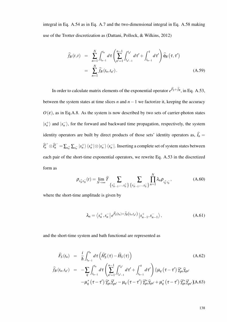
integral in Eq. A.54 as in Eq. A.7 and the two-dimensional integral in Eq. A.58 making

use of the Trotter discretization as (Dattani, Pollock, & Wilkins, 2012)

fB (t, t) =N

∑n=1

∫ tn

tn−1

dτ

(n−1

∑n′=1

∫ tn′

tn′−1

dτ′+∫

τ

tn−1

dτ′

)φB(τ,τ ′

)=

N

∑n=1

fB (tn, tn′) . (A.59)

In order to calculate matrix elements of the exponential operator eFS+ fB , in Eq. A.53,

between the system states at time slices n and n−1 we factorize it, keeping the accuracy

O(ε), as in Eq.A.8. As the system is now described by two sets of carrier-photon states

|s+n 〉 and |s−n 〉, for the forward and backward time propagation, respectively, the system

identity operators are built by direct products of those sets’ identity operators as, In =

Is+n ⊗ Is−

n =∑s+n ∑s−n |s+n 〉〈s+n |⊗|s−n 〉〈s−n |. Inserting a complete set of system states between

each pair of the short-time exponential operators, we rewrite Eq. A.53 in the discretized

form as

ρs+N s−N(t) = lim

N→∞T ∑s+N−1,...,s

+0

∑s−N−1,...,s

−0

N

∏n=1

λnρs+0 s−0

, (A.60)

where the short-time amplitude is given by

λn =⟨s+n ,s

−n∣∣eFS(tn)+ fB(tn,tn′)

∣∣s+n−1,s−n−1⟩, (A.61)

and the short-time system and bath functional are represented as

FS (tn) =ih

∫ tn

tn−1

dτ

(H ′S (τ)− HS (τ)

)(A.62)

fB (tn, tn′) = −∑q

∫ tn

tn−1

dτ

(n−1

∑n′=1

∫ tn′

tn′−1

dτ′+∫

τ

tn−1

dτ′

)µq

(τ− τ

′)γ∗qnγqn′

−µ∗q(τ− τ

′)γ∗qnγ′qn′−µq

(τ− τ

′)γ′∗qnγqn′+µ

∗q(τ− τ

′)γ′∗qnγ′qn′,(A.63)

138

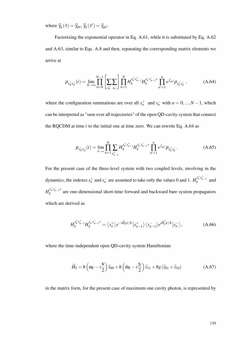
where γq (τ) = γqn, γq (τ′) = γqn′ .

Factorizing the exponential operator in Eq. A.61, while it is substituted by Eq. A.62

and A.63, similar to Eqs. A.8 and then, separating the corresponding matrix elements we

arrive at

ρs+N s−N(t) = lim

N→∞

N−1

∏n=0

[∑s+n

∑s−n

]N

∏n=1

Hs+n s+n−1S H

s−n s−n−1∗S

n

∏n′=1

e fnn′ρs+0 s−0, (A.64)

where the configuration summations are over all s+n and s−n with n = 0, ...,N−1, which

can be interpreted as "sum over all trajectories" of the open QD-cavity system that connect

the RQCDM at time t to the initial one at time zero. We can rewrite Eq. A.64 as

ρs+N s−N(t) = lim

N→∞

N

∏n=1

∑s±n−1

Hs+n s+n−1S H

s−n s−n−1∗S

n

∏n′=1

e fnn′ρs+0 s−0. (A.65)

For the present case of the three-level system with two coupled levels, involving in the

dynamics, the indexes s+n and s−n are assumed to take only the values 0 and 1. Hs+n s+n−1S and

Hs−n s−n−1∗S are one-dimensional short-time forward and backward bare system propagators

which are derived as

Hs+n s+n−1S H

s−n s−n−1∗S =

⟨s+n∣∣e−iHSε/h ∣∣s+n−1

⟩⟨s−n−1

∣∣eiH†S ε/h ∣∣s−n ⟩ , (A.66)

where the time-independent open QD-cavity system Hamiltonian

HS = h(

ωC− iκ

2

)s00 + h

(ωX − i

γr

2

)s11 + hg(s01 + s10) (A.67)

in the matrix form, for the present case of maximum one cavity photon, is represented by

139

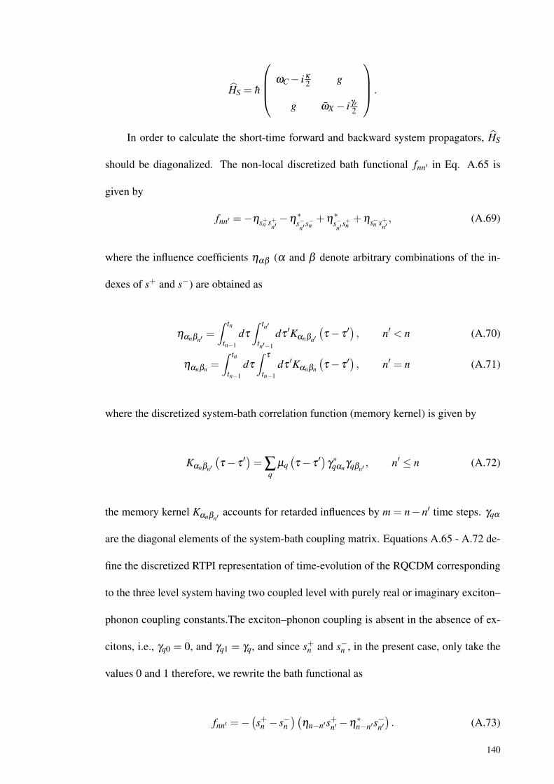
HS = h

ωC− iκ

2 g

g ωX − i γr2

.

In order to calculate the short-time forward and backward system propagators, HS

should be diagonalized. The non-local discretized bath functional fnn′ in Eq. A.65 is

given by

fnn′ =−ηs+n s+n′−η

∗s−n′s−n+η

∗s−

n′s+n+ηs−n s+

n′, (A.69)

where the influence coefficients ηαβ (α and β denote arbitrary combinations of the in-

dexes of s+ and s−) are obtained as

ηαnβn′=∫ tn

tn−1

dτ

∫ tn′

tn′−1

dτ′Kαnβn′

(τ− τ

′) , n′ < n (A.70)

ηαnβn =∫ tn

tn−1

dτ

∫τ

tn−1

dτ′Kαnβn

(τ− τ

′) , n′ = n (A.71)

where the discretized system-bath correlation function (memory kernel) is given by

Kαnβn′

(τ− τ

′)= ∑q

µq(τ− τ

′)γ∗qαn

γqβn′, n′ ≤ n (A.72)

the memory kernel Kαnβn′accounts for retarded influences by m = n−n′ time steps. γqα

are the diagonal elements of the system-bath coupling matrix. Equations A.65 - A.72 de-

fine the discretized RTPI representation of time-evolution of the RQCDM corresponding

to the three level system having two coupled level with purely real or imaginary exciton–

phonon coupling constants.The exciton–phonon coupling is absent in the absence of ex-

citons, i.e., γq0 = 0, and γq1 = γq, and since s+n and s−n , in the present case, only take the

values 0 and 1 therefore, we rewrite the bath functional as

fnn′ =−(s+n − s−n

)(ηn−n′s

+n′−η

∗n−n′s

−n′). (A.73)

140

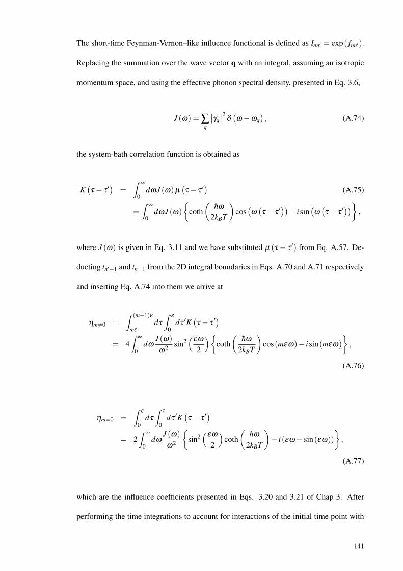
The short-time Feynman-Vernon–like influence functional is defined as Inn′ = exp( fnn′).

Replacing the summation over the wave vector q with an integral, assuming an isotropic

momentum space, and using the effective phonon spectral density, presented in Eq. 3.6,

J (ω) = ∑q

∣∣γq∣∣2 δ

(ω−ωq

), (A.74)

the system-bath correlation function is obtained as

K(τ− τ

′) =∫

∞

0dωJ (ω)µ

(τ− τ

′) (A.75)

=∫

∞

0dωJ (ω)

coth

(hω

2kBT

)cos(ω(τ− τ

′))− isin(ω(τ− τ

′)) ,

where J (ω) is given in Eq. 3.11 and we have substituted µ (τ− τ ′) from Eq. A.57. De-

ducting tn′−1 and tn−1 from the 2D integral boundaries in Eqs. A.70 and A.71 respectively

and inserting Eq. A.74 into them we arrive at

ηm 6=0 =∫ (m+1)ε

mε

dτ

∫ε

0dτ′K(τ− τ

′)= 4

∫∞

0dω

J (ω)

ω2 sin2(

εω

2

)coth

(hω

2kBT

)cos(mεω)− isin(mεω)

,

(A.76)

ηm=0 =∫

ε

0dτ

∫τ

0dτ′K(τ− τ

′)= 2

∫∞

0dω

J (ω)

ω2

sin2

(εω

2

)coth

(hω

2kBT

)− i(εω− sin(εω))

,

(A.77)

which are the influence coefficients presented in Eqs. 3.20 and 3.21 of Chap 3. After

performing the time integrations to account for interactions of the initial time point with

141

other time points we add n, n′ = 0 to the influence functional term and rewrite Eq. A.65

as

ρs+N s−N(t) = lim

N→∞

N

∏n=1

∑s±n−1

Hs+n s+n−1S H

s−n s−n−1∗S

n

∏n′=0

e fnn′ρs+0 s−0, (A.78)

where we have used the fact that according to Eq. A.73, defining the initial state (s+n ,

s−n ) = (0,0) or (1,1), f00 = 0. Equation A.78 is the final expression for the RQCDM

elements in the interaction picture, given in equation 3.16 of Chap. 3. One approximates

Eq. A.78 with a finite N and ε in order to develop a numerical algorithm for practical

calculations.

142

REFERENCES

Adachi, S. (1994). GaAs and related materials. World Scientific.

Akahane, Y., Asano, T., Song, B.-S., & Noda, S. (2003). High-q photonic nanocavity ina two-dimensional photonic crystal. Nature (London), 425, 944.

Andreani, L. C., Panzarini, G., & Gérard, J.-M. (1999, Nov). Strong-coupling regimefor quantum boxes in pillar microcavities: Theory. Physical Review B, 60, 13276-13279.

Ates, S., Ulrich, S. M., Ulhaq, A., Reitzenstein, S., Loffler, A., Hofling, S., & Michler,P. (2009). Non-resonant dot–cavity coupling and its potential for resonant single-quantum-dot spectroscopy. Nature Photonics, 3, 724.

Auffèves, A., Gerace, D., Gérard, J.-M., Santos, M., Andreani, L. C., & Poizat, J.-P.(2010, Jun). Controlling the dynamics of a coupled atom-cavity system by puredephasing. Physical Review B, 81, 245419.

Axt, V., Herbst, M., & Kuhn, T. (1999). Coherent control of phonon quantum beats.Superlattices and Microstructures, 26(2), 117 - 128.

Axt, V. M., & Mukamel, S. (1997). In nonlinear optical materials. IMA volumes inmathematics and its applications (Vol. 101). Springer.

Barenco, A., Deutsch, D., Ekert, A., & Jozsa, R. (1995, May). Conditional quantumdynamics and logic gates. Physical Review Letters, 74, 4083-4086.

Barve, A., Rotter, T., Sharma, Y., Lee, S., Noh, S., & Krishna, S. (2010). Systematicstudy of different transitions in high operating temperature quantum dots in a wellphotodetectors. Applied Physics Letters., 97, 061105.

Basu, P. K. (1997). Theory of optical processes in semiconductors: bulk and microstruc-tures. Clarendon Press, Oxford University Press.

Beck, M., Jäckle, A., Worth, G., & Meyer, H.-D. (2000). The multiconfiguration time-dependent hartree (MCTDH) method: a highly efficient algorithm for propagatingwavepackets. Physics Reports, 324(1), 1 - 105.

Benisty, H. (1995, May). Reduced electron-phonon relaxation rates in quantum-boxsystems: Theoretical analysis. Physical Review B, 51, 13281–13293.

Benson, O., Santori, C., Pelton, M., & Yamamoto, Y. (2000, Mar). Regulated and entan-gled photons from a single quantum dot. Physical Review Letters, 84, 2513–2516.

Besombes, L., Kheng, K., Marsal, L., & Mariette, H. (2001, Mar). Acoustic phononbroadening mechanism in single quantum dot emission. Physical Review B, 63,155307.

143

Bhatt, A. R., Kim, K. W., & Stroscio, M. A. (1994). Theoretical calculation oflongitudinal-optical-phonon lifetime in GaAs. Journal of Applied Physics, 76(6),3905-3907.

Biasiol, G., & Heun, S. (2011). Compositional mapping of semiconductor quantum dotsand rings. Physics Reports, 500(4–5), 117 - 173.

Bimberg, D., Stock, E., Lochmann, A., Schliwa, A., Tofflinger, J. A., Unrau, W., &Kalagin, A. K. (2009). Quantum dots for single- and entangled-photon emitters.IEEE Photonics Journal, 1(1).

Biolatti, E., Iotti, R. C., Zanardi, P., & Rossi, F. (2000, Dec). Quantum informationprocessing with semiconductor macroatoms. Physical Review Letters, 85, 5647–5650.

Bockelmann, U., & Bastard, G. (1990, Nov). Phonon scattering and energy relaxation intwo-, one-, and zero-dimensional electron gases. Physical Review B, 42, 8947–8951.

Bonadeo, N. H., Chen, G., Gammon, D., Katzer, D. S., Park, D., & Steel, D. G. (1998,Sep). Nonlinear nano-optics: Probing one exciton at a time. Physical Review Letters,81, 2759–2762.

Borri, P., Langbein, W., Mørk, J., Hvam, J. M., Heinrichsdorff, F., Mao, M.-H., & Bim-berg, D. (1999, Sep). Dephasing in inas/gaas quantum dots. Physical Review B, 60,7784–7787.

Borri, P., Langbein, W., Schneider, S., Woggon, U., Sellin, R. L., Ouyang, D., & Bimberg,D. (2001, Sep). Ultralong dephasing time in ingaas quantum dots. Physical ReviewLetters, 87, 157401.

Borri, P., Langbein, W., Woggon, U., Stavarache, V., Reuter, D., & Wieck, A. D. (2005,Mar). Exciton dephasing via phonon interactions in inas quantum dots: Dependenceon quantum confinement. Physical Review B, 71, 115328.

Brown, K. R., Lidar, D. A., & Whaley, K. B. (2001, Dec). Quantum computing withquantum dots on quantum linear supports. Physical Review A, 65, 012307.

Brun, T. A., & Wang, H. (2000, Feb). Coupling nanocrystals to a high-q silica micro-sphere: Entanglement in quantum dots via photon exchange. Physical Review A, 61,032307.

Brus, L. E. (1984). Electron–electron and electron-hole interactions in small semiconduc-tor crystallites: The size dependence of the lowest excited electronic state. Journalof Chemical Physics, 80(9), 4403.

Brusaferri, L., Sanguinetti, S., Grilli, E., Guzzi, M., Bignazzi, A., Bogani, F., & Franchi,S. (1996). Thermally activated carrier transfer and luminescence line shape in self-organized inas quantum dots. Applied Physics Letters., 69, 3354.

Buckley, S., Rivoire, K., & Vuckovic, J. (2012). Engineered quantum dot single-photonsources. Reports on Progress in Physics, 75, 126503.

144

Burkard, G., Loss, D., & DiVincenzo, D. P. (1999, Jan). Coupled quantum dots asquantum gates. Physical Review B, 59, 2070–2078.

Carmele, A., Milde, F., Dachner, M.-R., Harouni, M. B., Roknizadeh, R., Richter, M.,& Knorr, A. (2010, May). Formation dynamics of an entangled photon pair: Atemperature-dependent analysis. Physical Review B, 81, 195319.

Carmele, A., Richter, M., Chow, W. W., & Knorr, A. (2010, Apr). Antibunching of ther-mal radiation by a room-temperature phonon bath: A numerically solvable model fora strongly interacting light-matter-reservoir system. Physical Review Letters, 104,156801.

Castella, H., & Zimmermann, R. (1999, Mar). Coherent control for a two-level systemcoupled to phonons. Physical Review B, 59, R7801–R7804.

Chamarro, M., Gourdon, C., Lavallard, P., & Ekimov, A. I. (1995). Enhancement of ex-citon exchange interaction by quantum confinement in cdse nanocrystals. JapaneseJournal of Applied Physics, 34(S1), 12-14.

Chen, P., Piermarocchi, C., & Sham, L. J. (2001, Jul). Control of exciton dynamics innanodots for quantum operations. Physical Review Letters, 87, 067401.

Cheng, X., Lowe, S. B., Reece, P. J., & Gooding, J. J. (2014). Colloidal silicon quantumdots: from preparation to the modification of self-assembled monolayers (sams) forbio-applications. Chemical Society Reviews, 43(2680), 2680–2700.

Cho, N. K., Ryu, S. P., Song, J. D., Choi, W. J., Lee, J. I., & H., J. (2006). Comparison ofstructural and optical properties of InAs quantum dots grown by migration-enhancedmolecular-beam epitaxy and conventional molecular-beam epitaxy. Applied PhysicsLetters., 88, 133104.

Claudon, J., Bleuse, J., Malik, N., Bazin, M., Jaffrennou, P., Gregersen, N., & Gerard, J.(2010). A highly efficient single-photon source based on a quantum dot in a photonicnanowire. Nature Photonics, 4, 174-177.

Dachner, M.-R., Malic, E., Richter, M., Carmele, A., Kabuss, J., Wilms, A., & Knorr,A. (2010). Theory of carrier and photon dynamics in quantum dot light emitters.physica status solidi (b), 247(4), 809–828.

Dattani, N. S., Pollock, F. A., & Wilkins, D. M. (2012). Analytic influence functionalsfor numerical feynman integrals in most open quantum systems. Quant. Phys. Lett.,1(1), 35-45.

Dawson, P., Rubel, O., Baranovskii, S. D., Pierz, K., Thomas, P., & Göbel, E. O. (2005,Dec). Temperature-dependent optical properties of InAs/GaAs quantum dots: Inde-pendent carrier versus exciton relaxation. Physical Review B, 72, 235301.

Duke, C. B., & Mahan, G. D. (1965, Sep). Phonon-broadened impurity spectra. i. densityof states. Physical Review, 139, A1965–A1982.

Eliseev, P. G., Li, H., Stintz, A., Liu, G. T., Newell, T. C., Malloy, K. J., & Lester, L. F.

145

(2000). Transition dipole moment of InAs/InGaAs quantum dots from experimentson ultralow-threshold laser diodes. Applied Physics Letters., 77(2), 262.

Fan, H. Y. (1951, Jun). Temperature dependence of the energy gap in semiconductors.Physical Review, 82, 900–905.

Fan, H. Y. (1967). Photon-electron interaction, crystals without fields (Vol. p. 134).Springer.

Fan, X., Takagahara, T., Cunningham, J., & Wang, H. (1998). Pure dephasing inducedby exciton–phonon interactions in narrow gaas quantum wells. Solid State Commu-nications, 108(11), 857 - 861.

Fano, U. (1957, Jan). Description of states in quantum mechanics by density matrix andoperator techniques. Review of Modern Physics, 29, 74-93.

Feynman, R., & Vernon, F. (1963). The theory of a general quantum system interactingwith a linear dissipative system. Annals of Physics, 24, 118 - 173.

Feynman, R., & Vernon, F. (2000). The theory of a general quantum system interactingwith a linear dissipative system. Annals of Physics, 281(1), 547 - 607.

Feynman, R. P. (1948, Apr). Space-time approach to non-relativistic quantum mechanics.Review of Modern Physics, 20, 367–387.

Feynman, R. P. (1950, Nov). Mathematical formulation of the quantum theory of elec-tromagnetic interaction. Physical Review, 80, 440–457.

Feynman, R. P. (1951, Oct). An operator calculus having applications in quantum elec-trodynamics. Physical Review, 84, 108–128.

Förstner, J., Weber, C., Danckwerts, J., & Knorr, A. (2003, Sep). Phonon-assisted damp-ing of rabi oscillations in semiconductor quantum dots. Physical Review Letters, 91,127401.

Gammon, D., Snow, E. S., Shanabrook, B. V., Katzer, D. S., & Park, D. (1996, Apr).Fine structure splitting in the optical spectra of single GaAs quantum dots. PhysicalReview Letters, 76, 3005–3008.

Gammon, D., Snow, E. S., Shanbrook, B. V., Katzer, D. S., & Park, D. (1996). Homoge-neous linewidths in the optical spectrum of a single gallium arsenide quantum dot.Science, 273, 87.

Gazzano, O., de Vasconcellos, S. M., Arnold, C., Nowak, A., Galophin, E., Sagnes, I., &Senellart, P. (2013). Bright solid-state sources of indistinguishable single photons.Nature Communication, 4, 1425.

Gerry, C., & Knight, P. (2005). Introductory quantum optics. Cambridge UniversityPress.

Ghodsi Nahri, D. (2012a). Analysis of dynamic, modulation, and output power properties

146

of self-assembled quantum dot lasers. Laser Physics Letters,, 9, 682–690.

Ghodsi Nahri, D. (2012b, Jul). Investigation of the effects of nonlinear optical gain andthermal carrier excitation on characteristics of self-assembled quantum-dot lasers.Optics Express, 20(14), 14754–14768.

Ghodsi Nahri, D. (2012c). Simulation of output power and optical gain characteristicsof self-assembled quantum-dot lasers: Effects of homogeneous and inhomogeneousbroadening, quantum dot coverage and phonon bottleneck. Optics Laser Technol-ogy, 44(8), 2436 - 2442.

Ghodsi Nahri, D., Mathkoor, F. H. A., & Ooi, C. H. R. (2016, Dec.). Real-time path-integral approach for dissipative quantum dot-cavity quantum electrodynamics: Im-pure dephasing-induced effects. Journal of Physics: Condensed Matter, 29, 055701.

Ghodsi Nahri, D., & Ooi, C. H. R. (2014, May). Modeling temperature-dependent shiftof photoluminescence peak of In(Ga)As quantum dots with acoustic and opticalphonons as two oscillators. Journal of the Optical Society of America B, 31(5),1182–1191.

Gisin, N., Ribordy, G., Tittel, W., & Zbinden, H. (2002, Mar). Quantum cryptography.Review of Modern Physics, 74, 145–195.

Glässl, M., Sörgel, L., Vagov, A., Croitoru, M. D., Kuhn, T., & Axt, V. M. (2012, Jul).Interaction of a quantum-dot cavity system with acoustic phonons: Stronger light-matter coupling can reduce the visibility of strong coupling effects. Physical ReviewB, 86, 035319.

Glässl, M., Vagov, A., Lüker, S., Reiter, D. E., Croitoru, M. D., Machnikowski, P., &Kuhn, T. (2011, Nov). Long-time dynamics and stationary nonequilibrium of anoptically driven strongly confined quantum dot coupled to phonons. Physical ReviewB, 84, 195311.

Grahn, H. T. (1999). In semiconductor physics. Worldd Scientific.

Grosse, F., & Zimmermann, R. (2007, Jun). Electron-phonon interaction in embeddedsemiconductor nanostructures. Physical Review B, 75, 235320.

Haroche, S., & Raimond, J. (2006). Exploring the quantum. Oxford University Press.

Harrison, P. (2005). Quantum wells, wires and dots: Theoretical and computationalphysics of semiconductor nanostructures. John Wiley Sons Ltd.

He, Y.-M., He, Y., Wei, Y.-J., Wu, D., Atatüre, M., Schneider, C., & Pan, J.-W. (2013).On-demand semiconductor single-photon source with near-unity indistinguishabil-ity. Nature Nanotechnology., 8, 213.

Heitz, R., Born, H., Hoffmann, A., Bimberg, D., Mukhametzhanov, I., & A., M. (2000).Resonant raman scattering in self-organized InAs/GaAs quantum dots. AppliedPhysics Letters., 77, 3746–3748.

147

Heitz, R., Grundmann, M., Ledentsov, N. N., Eckey, L., Veit, M., Bimberg, D., & Alferov,Z. I. (1996). Multiphonon relaxation processes in self-organized InAs/GaAs quan-tum dots. Applied Physics Letters., 68, 361–363.

Heitz, R., Makhametzhanov, I., Stier, O., Madhukar, A., & Bimberg, D. (2000). Phonon-assisted polar exciton–transitions in self-organized InAs/GaAs quantum dots. Phys-ica E, 7, 398.

Heitz, R., Mukhametzhanov, I., Stier, O., Madhukar, A., & Bimberg, D. (1999, Nov).Enhanced polar exciton-LO-phonon interaction in quantum dots. Physical ReviewLetters, 83, 4654–4657.

Heitz, R., Veit, M., Ledentsov, N. N., Hoffmann, A., Bimberg, D., Ustinov, V. M.,& Alferov, Z. I. (1997, Oct). Energy relaxation by multiphonon processes inInAs/GaAs quantum dots. Physical Review B, 56, 10435–10445.

Hennessy, K., Badolato, A., Winger, M., Gerace, D., Atatüre, M., Gulde, S., & Imamoglu,A. (2007). Quantum nature of a strongly coupled single quantum dot–cavity system.Nature (London), 445, 896.

Hohenester, U. (2006). Handbook of theoretical and computational nanotechnologyogy.American Scientific.

Hohenester, U., Laucht, A., Kaniber, M., Hauke, N., Neumann, A., Mohtashami, A., &Finley, J. J. (2009, Nov). Phonon-assisted transitions from quantum dot excitons tocavity photons. Physical Review B, 80, 201311.

Hohenester, U., Pfanner, G., & Seliger, M. (2007, Jul). Phonon-assisted decoherence inthe production of polarization-entangled photons in a single semiconductor quantumdot. Physical Review Letters, 99, 047402.

Huang, K., & Rhys, A. (1950). Theory of light absorption and non-radiative transitionsin f-centres. Proceedings of the Royal Society of London A: Mathematical, Physicaland Engineering Sciences, 204(1078), 406–423.

Ishizaki, A., & Tanimura, Y. (2005). Quantum dynamics of system strongly coupled tolow-temperature colored noise bath: Reduced hierarchy equations approach. Journalof the Physical Society of Japan, 74(12), 3131-3134.

Kaer, P., Gregersen, N., & Mork, J. (2013). The role of phonon scattering in the indis-tinguishability of photons emitted from semiconductor cavity QED systems. NewJournal of Physics, 15(3), 035027.

Kaer, P., Nielsen, T. R., Lodahl, P., Jauho, A.-P., & Mørk, J. (2010, Apr). Non-markovianmodel of photon-assisted dephasing by electron-phonon interactions in a coupledquantum-dot–cavity system. Physical Review Letters, 104, 157401.

Kaer, P., Nielsen, T. R., Lodahl, P., Jauho, A.-P., & Mørk, J. (2012, Aug). Microscopictheory of phonon-induced effects on semiconductor quantum dot decay dynamics incavity QED. Physical Review B, 86, 085302.

148

Kakushadze, Z. (2015). Path integral and asset pricing. Path integral and asset pricing,Quantitative Finance, 15:11, 1759-1771, 15:11, 1759-1771.

Kelly, M. J. (1995). Low-dimensional semiconductors: materials, physics, technology,and devices. Clarendon Press, Oxford University Press.

Khandekar, D., Lawande, S. W., & Bhagwat, K. V. (1998). Path-integral methods andtheir applications,. World Scientific.

Khitrova, G., Gibbs, H. M., Kira, M., Koch, S. W., & Scherer, A. (2006). A. vacuum rabisplitting in semiconductors. Nature Physics, 2, 81-90.

Khmissi, H., Baira, M., Sfaxi, L., Bouzaıene, L., Saidi, F., Bru-Chevallier, C., & Maaref,H. (2011). Optical investigation of InAs quantum dots inserted in AlGaAs/GaAsmodulation doped heterostructure. Journal of Applied Physics, 109, 054316.

Kleinert, H. (2006). Path integrals in quantum mechanics, statistics, polymer physics,and financial markets, 4th ed. World Scientific.

Klingshirn, C. F. (1995). Semiconductor optics. Springer.

Knill, E., Laflamme, R., & Milburn, G. J. (2001). A scheme for efficient quantumcomputation with linear optics. Nature (London), 409, 46.

Krügel, A., Vagov, A., Axt, V. M., & Kuhn, T. (2007, Nov). Monitoring the buildup ofthe quantum dot polaron: Pump-probe and four-wave mixing spectra from excitonsand biexcitons in semiconductor quantum dots. Physical Review B, 76, 195302.

Krummheuer, B., Axt, V. M., & Kuhn, T. (2002, May). Theory of pure dephasing andthe resulting absorption line shape in semiconductor quantum dots. Physical ReviewB, 65, 195313.

Krummheuer, B., Axt, V. M., & Kuhn, T. (2005, Dec). Coupled polarization and acoustic-phonon dynamics after optical excitation of quantum dots near surfaces. PhysicalReview B, 72, 245336.

Krummheuer, B., Axt, V. M., Kuhn, T., D’Amico, I., & Rossi, F. (2005, Jun). Pure de-phasing and phonon dynamics in GaAs- and GaN-based quantum dot structures: In-terplay between material parameters and geometry. Physical Review B, 71, 235329.

Krügel, A., Axt, V. M., Kuhn, T., Machnikowski, P., & Vagov, A. (2005). The roleof acoustic phonons for Rabi oscillations in semiconductor quantum dots. AppliedPhysics B, 81,, 897.

Ku, P., Sedgwick, F., Chang-Hasnain, C. J., Palinginis, P., Li, T., Wang, H., & Chuang,S. (2004, Oct). Slow light in semiconductor quantum wells. Optics Letters, 29(19),2291–2293.

Kuhn, T. (1998). Theory of transport properties of semiconductor nanostructures. In(p. 173). Chapman and Hall.

149

Kuhn, T., Axt, V. M., Herbst, M., & Binder, E. (1999). Coherent control in atoms,molecules, and semiconductors. In (p. 113). Kluwer Academic.

Ladd, T. D., Jelezko, F., Laflamme, R., Nakamura, Y., Monroe, C., & O/’Brien, J. L.(2010). Quantum computers. Nature, 464, 45-53.

Lai, Y., Pirotta, S., Urbinati, G., Gerace, D., Minkov, M., Savona, V., & Galli, M. (2014).Genetically designed L3 photonic crystal nanocavities with measured quality factorexceeding one million. Applied Physics Letters., 104, 241101.

Landolt-Bórnstein. (1987). Semiconductors: Intrinsic properties of group IV elementsand II-V, II-VI and I-VII compounds (Vol. III/22a). Springer, Berlin.

Laussy, F. P., del Valle, E., & Tejedor, C. (2008, Aug). Strong coupling of quantum dotsin microcavities. Physical Review Letters, 101, 083601.

Lee, C. K., Moix, J., & Cao, J. (2012). Accuracy of second order perturbation theoryin the polaron and variational polaron frames. Journal of Chemical Physics, 136,204120.

Lermer, M., Gregersen, N., Dunzer, F., Reitzenstein, S., Höfling, S., Mørk, J., & Forchel,A. (2012, Jan). Bloch-wave engineering of quantum dot micropillars for cavityquantum electrodynamics experiments. Physical Review Letters, 108, 057402.

Lochmann, A., Stock, E., Tofflinger, J. A., Unrau, W., Toropov, A., Bakarov, A., & Bim-berg, D. (2009). Electrically pumped, micro-cavity based single photon sourcedriven at 1 GHz. Electronics Letters, 45(11), 566-567.

Lodahl, P., Mahmoodian, S., & Stobbe, S. (2015, May). Interfacing single photons andsingle quantum dots with photonic nanostructures. Review of Modern Physics, 87,347-400.

Loss, D., & DiVincenzo, D. P. (1998, Jan). Quantum computation with quantum dots.Physical Review A, 57, 120–126.

Lu, X., Vaillancourt, J., & Meisner, M. J. (2007a). A modulation-doped longwave infraredquantum dot photodetector with high photoresponsivity. Semiconductor Science andTechnology, 22, 993.

Lu, X., Vaillancourt, J., & Meisner, M. J. (2007b). Temperature dependent photorespon-sivity and high-temperature (190 k) operation of a quantum dot infrared photodetec-tor. Applied Physics Letters., 91, 051115.

Lu, X., Vaillancourt, J., & Wen, H. (2010). Temperature-dependent energy gap variationin InAs/GaAs quantum dots. Applied Physics Letters., 96, 173105.

Machnikowski, P., & Jacak, L. (2004, May). Resonant nature of phonon-induced dampingof rabi oscillations in quantum dots. Physical Review B, 69, 193302.

Madelung, H. T. O. (1982–89). Landolt-bornstein: Numerical data and functional re-lationships in science and technology (Vol. 17a/b and 22a). New Series, Group III,

150

Springer.

Madsen, K. H., Ates, S., Lund-Hansen, T., Löffler, A., Reitzenstein, S., Forchel, A., &Lodahl, P. (2011, Jun). Observation of non-markovian dynamics of a single quantumdot in a micropillar cavity. Physical Review Letters, 106, 233601.

Mahan, G. (1990). Many-particle physics. Plenum Publishers.

Mahan, G. D. (1972). Polarons in ionic crystals and polar semiconductors. In (p. 533).Amsterdam.

Makarov, D. E., & Makri, N. (1994). Path integrals for dissipative systems by tensor mul-tiplication. Condensed phase quantum dynamics for arbitrarily long time. ChemicalPhysics Letters, 221(5), 482 - 491.

Makri, N., & Makarov, D. (1995a). Tensor propagator for iterative quantum time evo-lution of reduced density matrices. ii. numerical methodology. Journal of ChemicalPhysics, 102, 4611.

Makri, N., & Makarov, D. (1995b). Tensor propagator for iterative quantum time evolu-tion of reduced density matrices. i. theory. Journal of Chemical Physics, 102, 4600.

May, V., & Kuhn, O. (2000). Charge and energy transfer dynamics in molecular systems. Wiley-VCH Verlag, Berlin.

McCutcheon, D. P. S., Dattani, N. S., Gauger, E. M., Lovett, B. W., & Nazir, A. (2011,Aug). A general approach to quantum dynamics using a variational master equation:Application to phonon-damped rabi rotations in quantum dots. Physical Review B,84, 081305.

McCutcheon, D. P. S., & Nazir, A. (2010). Quantum dot rabi rotations beyond the weakexciton–phonon coupling regime. New Journal of Physics., 12, 113042.

Meyer, H.-D., Manthe, U., & Cederbaum, L. (1990). The multi-configurational time-dependent hartree approach. Chemical Physics Letters, 165(1), 73 - 78.

Michael, C. P., Srinivasan, K., Johnson, T. J., Painter, O., Lee, K. H., Hennessy, K., &Hu, E. (2007). Wavelength- and material-dependent absorption in GaAs and AlGaAsmicrocavities. Applied Physics Letters., 90, 051108.

Michler, P. (2003). Single quantum dots, topics of applied physics. Springer-Verlag.

Michler, P., Kiraz, A., Becher, C., Schoenfeld, W. V., Petroff, P. M., Zhang, L., &Imamoglu, A. (2000). A quantum dot single-photon turnstile device. Science,290(5500), 2282–2285.

Mukamel, S. (1995). Principles of nonlinear optical spectroscopy. Oxford UniversityPress.

Muljarov, E. A., Takagahara, T., & Zimmermann, R. (2005, Oct). Phonon-induced exci-ton dephasing in quantum dot molecules. Physical Review Letters, 95, 177405.

151

Muljarov, E. A., & Zimmermann, R. (2004, Nov). Dephasing in quantum dots: Quadraticcoupling to acoustic phonons. Physical Review Letters, 93, 237401.

Muljarov, E. A., & Zimmermann, R. (2006, Jan). Comment on "dephasing times inquantum dots due to elastic LO phonon-carrier collisions". Physical Review Letters,96, 019703.

Muljarov, E. A., & Zimmermann, R. (2007, May). Exciton dephasing in quantum dotsdue to LO-phonon coupling: An exactly solvable model. Physical Review Letters,98, 187401.

Muljarov, E. A., & Zimmermann, R. (2008). Exciton dephasing in quantum dots: Cou-pling to LO phonons via excited states. Physics Status Solidi b, 245, 1106.

Muller, M., Bounouar, S., Jons, K. D., Glassl, M., & Michler, P. (2014, March). On-demand generation of indistinguishable polarization-entangled photon pairs. NaturePhotonics, 8(3), 224–228.

Nilsson, J., Stevenson, R. M., Chan, K. H. A., Skiba-Szymanska, J., Lucamarini, M.,Ward, M. B., & Shields, A. J. (2013). Quantum teleportation using a light-emittingdiode. Nature Photonics, 7, 311–315.

Noda, S. (2006). Seeking the ultimate nanolaser. Science, 314(5797), 260–261.

Nysteen, A., Kaer, P., & Mork, J. (2013, Feb). Proposed quenching of phonon-inducedprocesses in photoexcited quantum dots due to electron-hole asymmetries. PhysicalReview Letters, 110, 087401.

O’Brien, J., Furusawa, A., & Vuckovic, J. (2009). Photonic quantum technologies. NaturePhoton., 3, 687.

O’Donnell, K. P., & Chen, X. (1991). Temperature dependence of semiconductor bandgaps. Applied Physics Letters., 58, 2924.

Ohta, R., Ota, Y., Nomura, M., Kumagai, N., Ishida, S., Iwamoto, S., & Y., A. (2011).Strong coupling between a photonic crystal nanobeam cavity and a single quantumdot. Applied Physics Letters., 98, 173104.

Ortner, G., Schwab, M., Bayer, M., Pässler, R., Fafard, S., Wasilewski, Z., &Forchel, A. (2005, Aug). Temperature dependence of the excitonic band gap inInxGa1−xAs/GaAs self-assembled quantum dots. Physical Review B, 72, 085328.

Ota, Y., Iwamoto, S., Kumagai, N., & Arakawa, Y. (2011, Nov). Spontaneous two-photonemission from a single quantum dot. Physical Review Letters, 107, 233602.

Palinginis, P., & Wang, H. (2001). High-resolution spectral hole burning in CdSe/ZnScore/shell nanocrystals. Applied Physics Letters., 78, 1541.

Park, Y.-S., Guo, S., Makarov, N. S., & Klimov, V. I. (2015, Aug). Room temperaturesingle-photon emission from individual perovskite quantum dots. ACS Nano, 9(10),10386–10393.

152

Peaker, A. R., & Grimmeiss, H. G. (1991). Low-dimensional structures in semiconduc-tors: from basic physics to applications. Plenum Press.

Pelton, M., & Yamamoto, Y. (1999, Mar). Ultralow threshold laser using a single quantumdot and a microsphere cavity. Physical Review A, 59, 2418–2421.

Peter, E., Senellart, P., Martrou, D., Lemaître, A., Hours, J., Gérard, J. M., & Bloch,J. (2005, Aug). Exciton-photon strong-coupling regime for a single quantum dotembedded in a microcavity. Physical Review Letters, 95, 067401.

Phillips, M., & Wang, H. (2002, Oct). Spin coherence and electromagnetically inducedtransparency via exciton correlations. Physical Review Letters, 89, 186401.

Press, D., Götzinger, S., Reitzenstein, S., Hofmann, C., Löffler, A., Kamp, M., &Yamamoto, Y. (2007, Mar). Photon antibunching from a single quantum-dot-microcavity system in the strong coupling regime. Physical Review Letters, 98,117402.

Pässler, R. (1997). Basic model relations for temperature dependencies of fundamentalenergy gaps in semiconductors. Physics Status Solidi B, 200, 155.

Pässler, R. (19999). Parameter sets due to fittings of the temperature dependencies offundamental bandgaps in semiconductors. Physics Status Solidi B, 216, 975.

Pässler, R. (2000). Moderate phonon dispersion shown by the temperature dependenceof fundamental band gaps of various elemental and binary semiconductors includingwide-band gap materials. Journal of Applied Physics, 88, 2570.

Pässler, R. (2001). Temperature dependence of fundamental band gaps in group IV,III−V, and II−VI materials via a two-oscillator model. Journal of Applied Physics,89, 6235–6240.

Pässler, R. (2003). Semi-empirical descriptions of temperature dependences of band gapsin semiconductors. Physics Status Solidi B, 236, 710.

Rafailov, E., McRobbie, A. D., Cataluna, M. A., O’Faolain, L., Sibbett, W., & Livshits,D. A. (2006). Investigation of transition dynamics in a quantum-dot laser opticallypumped by femtosecond pulses. Applied Physics Letters, 88, 041101.

Ramsay, A. J., Godden, T. M., Boyle, S. J., Gauger, E. M., Nazir, A., Lovett, B. W., &Skolnick, M. S. (2010, Oct). Phonon-induced Rabi-frequency renormalization ofoptically driven single InGaAs/GaAs quantum dots. Physical Review Letters, 105,177402.

Ramsay, A. J., Gopal, A. V., Gauger, E. M., Nazir, A., Lovett, B. W., Fox, A. M., &Skolnick, M. S. (2010, Jan). Damping of exciton Rabi rotations by acoustic phononsin optically excited InGaAs/GaAs quantum dots. Physical Review Letters, 104,017402.

Reithmaier, J. P., Sek, G., Löffler, A., Hofmann, C., Kuhn, S., Reitzenstein, S., & Forchel,A. (2004). Strong coupling in a single quantum dot–semiconductor microcavity

153

system. Nature (London), 432, 197-200.

Roszak, K., Grodecka, A., Machnikowski, P., & Kuhn, T. (2005, May). Phonon-induceddecoherence for a quantum-dot spin qubit operated by raman passage. PhysicalReview B, 71, 195333.

Roy, C., & Hughes, S. (2011, Jun). Phonon-dressed mollow triplet in the regime of cavityquantum electrodynamics: Excitation-induced dephasing and nonperturbative cavityfeeding effects. Physical Review Letters, 106, 247403.

Roy, C., & Hughes, S. (2012, Mar). Polaron master equation theory of the quantum-dot mollow triplet in a semiconductor cavity-QED system. Physical Review B, 85,115309.

Rudin, S., & Reinecke, T. L. (1999, Apr). Oscillator model for vacuum Rabi splitting inmicrocavities. Physical Review B, 59, 10227–10233.

Rudin, S., Reinecke, T. L., & Bayer, M. (2006, Oct). Temperature dependence of opticallinewidth in single InAs quantum dots. Physical Review B, 74, 161305.

Salter, C. L., Stevenson, R. M., Farrer, I., Nicoll, C. A., Ritchie, D. A., & Shields, A. J.(2010). An entangled-light-emitting diode. Nature, 465, 594–597.

Sanguinetti, S., Henini, M., Grassi Alessi, M., Capizzi, M., Frigeri, P., & Franchi, S.(1999, Sep). Carrier thermal escape and retrapping in self-assembled quantum dots.Physical Review B, 60, 8276–8283.

Sanguinetti, S., Mano, T., Oshima, M., Tateno, T., Wakaki, M., & Koguchi, N. (2002).Temperature dependence of the photoluminescence of InGaAs/GaAs quantum dotstructures without wetting layer. Applied Physics Letters., 81, 3067.

Scamarcio, G., Spagnolo, V., Ventruti, G., Lugará, M., & Righini, G. C. (1996, Apr).Size dependence of electron—LO-phonon coupling in semiconductor nanocrystals.Physical Review B, 53, R10489–R10492.

Schilp, J., Kuhn, T., & Mahler, G. (1994, Aug). Electron-phonon quantum kineticsin pulse-excited semiconductors: Memory and renormalization effects. PhysicalReview B, 50, 5435–5447.

Schliwa, A., Winkelnkemper, M., & Bimberg, D. (2007, Nov). Impact of size, shape,and composition on piezoelectric effects and electronic properties of In(Ga)AsGaAsquantum dots. Physical Review B, 76, 205324.

Schmitt-Rink, S., Miller, D. A. B., & Chemla, D. S. (1987, May). Theory of the linear andnonlinear optical properties of semiconductor microcrystallites. Physical Review B,35, 8113–8125.

Schrier, J., & Whaley, K. B. (2005, Aug). Atomistic theory of coherent spin transferbetween molecularly bridged quantum dots. Physical Review B, 72, 085320.

Shchukin, V. A., & Bimberg, D. (1999, Jul). Spontaneous ordering of nanostructures on

154

crystal surfaces. Review of Modern Physics, 71, 1125–1171.

Sherwin, M. S., Imamoglu, A., & Montroy, T. (1999, Nov). Quantum computation withquantum dots and terahertz cavity quantum electrodynamics. Physical Review A, 60,3508–3514.

Shields, A. J. (2007). Semiconductor quantum light sources. Nature Photonics, 1, 215–223.

Sim, E. (2001). Quantum dynamics for a system coupled to slow baths: On-the-flyfiltered propagator method. Journal of Chemical Physics, 115, 4450.

Smolka, S., Thyrrestrup, H., Sapienza, L., Lehmann, T. B., Rix, K. R., Froufe-Pérez,L. S., & Lodahl, P. (2011). Probing the statistical properties of anderson localizationwith quantum emitters. New Journal of Physics, 13(6), 063044.

Somaschi, N., Giesz, V., Santis, L. D., Loredo, J. C., Almeida, M. P., Hornecker, G., &Senellart, P. (2016). Near-optimal single-photon sources in the solid state. NaturePhotonics., 10, 340-345.

Song, B.-S., Noda, S., Asano, T., & Akahane, Y. (2005). Ultra-high-Q photonic double-heterostructure nanocavity. Nature Materials., 4, 207.

Srinivasan, K., & Painter, O. (2007). Linear and nonlinear optical spectroscopy of astrongly coupled microdisk–quantum dot system. Nature (London), 450, 862.

Stangl, J., Holý, V., & Bauer, G. (2004, Sep). Structural properties of self-organizedsemiconductor nanostructures. Review of Modern Physics, 76, 725–783.

Steinbach, D., Kocherscheidt, G., Wehner, M. U., Kalt, H., Wegener, M., Ohkawa, K., &Axt, V. M. (1999, Nov). Electron-phonon quantum kinetics in the strong-couplingregime. Physical Review B, 60, 12079–12090.

Stevenson, R. M., Salter, C. L., Nilsson, J., Bennett, A. J., Ward, M. B., Farrer, I., &Shields, A. J. (2012, Jan). Indistinguishable entangled photons generated by a light-emitting diode. Physical Review Letters, 108, 040503.

Stevenson, R. M., Young, R. J., Atkinson, P., Cooper, K., Ritchie, D. A., & Shields,A. (2006). A semiconductor source of triggered entangled photon pairs. Nature(London), 439, 179–182.

Stievater, T. H., Li, X., Steel, D. G., Gammon, D., Katzer, D. S., Park, D., & Sham, L. J.(2001, Sep). Rabi oscillations of excitons in single quantum dots. Physical ReviewLetters, 87, 133603.

Stock, E., Dachner, M.-R., Warming, T., Schliwa, A., Lochmann, A., Hoffmann, A.,& Bimberg, D. (2011, Jan). Acoustic and optical phonon scattering in a singleIn(Ga)As quantum dot. Physical Review B, 83, 041304.

Strauf, S., & Jahnke, F. (2011). Single quantum dot nanolaser. Laser Photonics Reviews,5(5), 607–633.

155

Takagahara, T. (1999, Jul). Theory of exciton dephasing in semiconductor quantum dots.Physical Review B, 60, 2638–2652.

Tanamoto, T. (2000, Jan). Quantum gates by coupled asymmetric quantum dots andcontrolled-NOT-gate operation. Physical Review A, 61, 022305.

Tanimura, Y. (2006). Stochastic Liouville, Langevin, Fokker–Planck, and master equa-tion approaches to quantum dissipative systems. Journal of the Physical Society ofJapan, 75(8), 082001.

Tarel, G., & Savona, V. (2010, Feb). Linear spectrum of a quantum dot coupled to ananocavity. Physical Review B, 81, 075305.

Thoss, M., Wang, H., & Miller, W. H. (2001). Self-consistent hybrid approach forcomplex systems: Application to the spin-boson model with debye spectral density.Journal of Chemical Physics, 115, 2991.

Topolancik, J., Ilic, B., & Vollmer, F. (2007, Dec). Experimental observation of strongphoton localization in disordered photonic crystal waveguides. Physical Review Let-ters, 99, 253901.

Uskov, A. V., Jauho, A.-P., Tromborg, B., Mørk, J., & Lang, R. (2000, Aug). Dephasingtimes in quantum dots due to elastic LO phonon-carrier collisions. Physical ReviewLetters, 85, 1516–1519.

Uskov, A. V., Jauho, A. P., Tromborg, B., Mørk, J., & Lang, R. (2006, Jan). Uskov et al.reply:. Physical Review Letters, 96, 019704.

Vagov, A., Axt, V. M., & Kuhn, T. (2002, Oct). Electron-phonon dynamics in opticallyexcited quantum dots: Exact solution for multiple ultrashort laser pulses. PhysicalReview B, 66, 165312.

Vagov, A., Axt, V. M., Kuhn, T., Langbein, W., Borri, P., & Woggon, U. (2004, Nov).Nonmonotonous temperature dependence of the initial decoherence in quantum dots.Physical Review B, 70, 201305.

Vagov, A., Croitoru, M. D., Axt, V. M., Machnikowski, P., & Kuhn, T. (2011). Dynamicsof quantum dots with strong electron phonon coupling: Correlation expansion vs.path integrals. physica status solidi (b), 248(4).

Vagov, A., Croitoru, M. D., Glässl, M., Axt, V. M., & Kuhn, T. (2011, Mar). Real-timepath integrals for quantum dots: Quantum dissipative dynamics with superohmicenvironment coupling. Physical Review B, 83, 094303.

Vagov, A., Glässl, M., Croitoru, M. D., Axt, V. M., & Kuhn, T. (2014, Aug). Competitionbetween pure dephasing and photon losses in the dynamics of a dot-cavity system.Physical Review B, 90, 075309.

Varshni, Y. (1967). Temperature dependence of the energy gap in semiconductors. Phys-ica, 34(1), 149 - 154.

156

Varshni, Y. P. (1970, Nov). Temperature dependence of the elastic constants. PhysicalReview B, 2, 3952–3958.

Vasileiadis, M., Alexandropoulos, D., Adams, M. J., Simos, H., & Syvridis, D. (2008).Potential of InGaAs/GaAs quantum dots for applications in vertical cavity semicon-ductor optical amplifiers. IEEE Journal of Selected Topics in Quantum Electronics,14(4), 1180-1187.

Viña, L., Logothetidis, S., & Cardona, M. (1984, Aug). Temperature dependence of thedielectric function of germanium. Physical Review B, 30, 1979–1991.

Wehner, M. U., Ulm, M. H., Chemla, D. S., & Wegener, M. (1998, Mar). Coherentcontrol of electron-LO-phonon scattering in bulk GaAs. Physical Review Letters,80, 1992–1995.

Wei, Y.-J., He, Y., He, Y.-M., Lu, C.-Y., Pan, J.-W., Schneider, C., & Nazir, A. (2014,Aug). Temperature-dependent mollow triplet spectra from a single quantum dot:Rabi frequency renormalization and sideband linewidth insensitivity. Physical Re-view Letters, 113, 097401.

Wei, Z. F., Xu, S. J., Duan, R. F., Li, Q., Wang, J., Zeng, Y. P., & Liu, H. C. (2005).Thermal quenching of luminescence from buried and surface InGaAs self-assembledquantum dots with high sheet density. Journal of Applied Physics, 98, 084305.

Wilson-Rae, I., & Imamoglu, A. (2002, May). Quantum dot cavity-QED in the presenceof strong electron-phonon interactions. Physical Review B, 65, 235311.

Wojs, A., Hawrylak, P., Fafard, S., & Jacak, L. (1996, Aug). Electronic structure andmagneto-optics of self-assembled quantum dots. Physical Review B, 54, 5604–5608.

Xu, Z. Y., Lu, Z. D., Yang, X. P., Yuan, Z. L., Zheng, B. Z., Xu, J. Z., & Chang,L. L. (1996, Oct). Carrier relaxation and thermal activation of localized excitonsin self-organized InAs multilayers grown on GaAs substrates. Physical Review B,54, 11528–11531.

Yeo, I., Song, J. D., & Lee, J. (2011). Temperature-dependent energy band gap variationin self-organized InAs quantum dots. Applied Physics Letters., 99, 151909.

Yoshie, T., Scherer, A., Hendrickson, J., Khitrova, G., Gibbs, H. M., Rupper, G., &Deppe, D. G. (2004). Vacuum rabi splitting with a single quantum dot in a photoniccrystal nanocavity. Nature, 432, 200-203.

Young, R. J., Stevenson, R. M., Shields, A. J., Atkinson, P., Cooper, K., Ritchie, D. A.,& Skolnick, M. S. (2005, Sep). Inversion of exciton level splitting in quantum dots.Physical Review B, 72, 113305.

Zanardi, P., & Rossi, F. (1998, Nov). Quantum information in semiconductors: Noiselessencoding in a quantum-dot array. Physical Review Letters, 81, 4752–4755.

Zrenner, A. (2000). A close look on single quantum dots. Journal of Chemical Physics,112, 7790.

157