Investigation on the effects of measurement and temporal

Journal of Theoretical and Applied Vibration and Acoustics 6(1) 1-16 (2020)

I S A V

Journal of Theoretical and Applied

Vibration and Acoustics

journal homepage: http://tava.isav.ir

Investigation on the effects of measurement and temporal

uncertainties on rolling element bearings prognostics

Mehdi Behzad,*a

Amirhossein Mollaali,b Motahareh Mirfarah,

b

Hesam Addin Arghandc

a Professor, Faculty of Mechanical Engineering, Sharif University of Technology, Tehran, Iran b M.Sc., Faculty of Mechanical Engineering, Sharif University of Technology, Tehran, Iran cPhD., Faculty of Mechanical Engineering, Sharif University of Technology, Tehran, Iran

A R T I C L E I N F O

A B S T R A C T

Article history:

Received 2 February 2020

Received in revised form

5 March 2020

Accepted 23 April 2020

Available online 29 April 2020

Estimation of remaining useful life (RUL) of rolling element bearings

(REBs) has a major effect on improving the reliability in the industrial

plants. However, due to the complex nature of the fault propagation in these

components, their prognosis is affected by various uncertainties. This effect

is intensified when the recorded data is offline, which is very common for

many industrial machines due to the lower cost rather than the online

monitoring strategy. In the present paper, in order to overcome the

shortcoming of the feed-forward neural network (FFNN) in REBs

prognostics, a new method for considering two main uncertainties (caused

by the measurement and process noises) is proposed, in the presence of

offline data acquisition. In the proposed method, the primary RUL

probability distribution corresponded to each offline measured data is

predicted, utilizing the outputs of trained FFNNs. Then, the predicted RUL

distribution will become more robust in confronting the temporal changes,

by taking into account the approval of pervious stage predictions to the

present prediction. As a result, the overall probability distribution of REBs

RUL and also its confidence levels (CLs) are obtained. Finally, the

evaluation of the proposed method is performed by utilizing bearing

experimental datasets. The results show that the proposed method has the

capability to express the estimated RUL CLs in the offline data acquisition

method, effectively. By providing a probabilistic perspective, the proposed

method can improve the reliability of the asset and also the decision-making

about the future of the industrial plants.

© 2020 Iranian Society of Acoustics and Vibration, All rights reserved.

Keywords:

Prognostics,

Remaining useful life,

Rolling element bearing,

Feed-forward neural network,

Uncertainty,

Offline data acquisition.

* Corresponding author:

E-mail address: [email protected] (M. Behzad)

http://dx.doi.org/10.22064/tava.2020.121073.1152

M. Behzad et al. /Journal of Theoretical and Applied Vibration and Acoustics 6(1) 1-16 (2020)

2

1. Introduction

Accurate functionality of the rotating machinery plays an important role in improving plant

efficiency. In unexpected breakdowns, expensive costs of downtime are inflicted on the system,

besides the repair costs[1]. To prevent the excessive costs and improve system reliability,

condition-based maintenance (CBM) is applied to the critical industrial plants, as one of the

newest and the most effective maintenance strategies in the last decades [2]. On the other hand,

rolling element bearings (REBs) are widely used in rotating machinery, and their failure may

lead to catastrophic damage in the machine. It should be noticed that almost 50 percent of

failures in the rotating machines are because of REBs fault[3]. Therefore, they are known as

critical components and implementation of the CBM strategy for their fault detection and

remaining useful life prediction is a vital task.

The CBM strategy is generally divided into two main steps: diagnosis and prognosis[4]. The

former detects faults, especially in the early stages of fault propagation. While the latter is

mainly concerned about estimating the remaining useful life (RUL) of the asset. Predominantly,

there are three different approaches for predicting the RUL, as follows[1]:

- Physical model-based methodology

- Knowledge-based methodology

- Data-driven methodology

Physical models are generally based on the defect growth description. Li et al [5] used a defect

propagation model so as to estimate the RUL of REBs. In another work, Li and Lee [6] utilized

Paris’ law to model the crack evolution in gear. Mainly, it is difficult to develop an accurate

physics-based model, due to the system complexity as well as the complicated nature of defect

growth. Consequently, the aforesaid methodology has had limited application in practical cases.

On the other hand, knowledge-based models which are mainly constructed based on expert

knowledge, may not be restricted to the analytical theories. However, their low flexibility leads

to their inability in the analysis of complicated processes[7]. As an effort, Lembessis et al [8]

predicted the fault growth by implementing an online expert system (ES).

Data-driven models utilize the observation data, in order to recognize the underlying pattern

between the input(s) and output(s)[1]. One of the most popular data-driven models in prognostics

is a neural network (NN) model. NN models are the learning-based approaches and have

considerable high flexibility in analyzing complicated dynamic systems, such as the REBs

degradation process. Thus, utilizing the NN models is very common in the literature of REBs

prognostics.

The feed-forward neural network (FFNN) method has been employed by researchers to predict

the RUL of REBs [9, 10]. Gebraeel et al [11] have predicted the RUL of REBs based on

experimental data, using vibration amplitude of defective frequencies and their harmonics as the

input features. In another research, Mahammad et al [12] used kurtosis and RMS features as the

inputs of FFNN. Tian [13] employed the FFNN method on the actual industrial data to estimate

the RUL. Zhao et al[14] predicted RUL of REBs, utilizing linear regression model and time-

frequency features. Vachtsevanos and Wang [15] presented a dynamic wavelet neural network

(DWNN) for prognosis purposes. In another research, Cui et al [16] analyzed the defect growth,


3

using a dynamic recurrent neural network (RNN). Satish and Sarma [17] developed a hybrid

model by combining fuzzy logic with NN to identify conditions and RUL estimation.

The procedure of RUL prediction is full of uncertainties, due to the complex nature of defect

initiation and propagation, especially in REBs. However, the NNs are unable to model different

uncertainties and they cannot represent a probabilistic description for the predicted RUL, in spite

of their merits and capabilities in predicting the complex dynamic behavior of REBs degradation.

This shortcoming leads to a lack of confidence level (CL) for the prediction outputs and

consequently affects the logical decision-making process [2]. On the other hand, the data

acquisition in most industrial plants is performed in the offline method, regarding the imposed

cost reduction strategies in the plant. In this situation, the existence of different uncertainties

becomes even a more serious problem[7]. Therefore, in the presence of offline data acquisition,

consideration of the main sources of uncertainties is essential in the REBs prognostics using NN

models.

The main concern of the present paper is to overcome the NNs shortcoming in providing the CL

in the estimation of REBs remaining useful life. In this way, the proposed algorithm considers

two of the most important uncertainties in the prognostics with the offline data acquisition from

the REBs; first, caused by the measurement and second, caused by process noises. Consequently,

the resultant RUL prediction is represented through a probability distribution function that can

describe the CL of any given RUL, contrary to the output of conventional FFNN models.

The remainder of this paper is organized as follows: The utilized experimental data is introduced

in section 2. In section 3, the existent uncertainties in the NN-based prognostics are briefly

discussed. The proposed method for modeling the measurement and the temporal uncertainties in

the application of REBs prognostics is presented in section 4. In section 5, the model is

evaluated, using run to failure datasets. Finally, conclusions are presented in section 6.

2. Experimental Data

An experimental dataset of REBs run to failure tests, named PRONOSTIA is utilized for

studying the performance of the proposed method in this paper. The PRONOSTIA vibration data

was published in the PHM2012 conference as a data challenge [18]. Many researchers used this

dataset, in order to assess their proposed method [19-22]. This experiment includes seven run-to-

failure tests of REBs in the first constant operating condition (4000 N radial force and 1800 rpm

rotational speed). The vibration time signals have been recorded every 10 seconds with 25.6 kHz

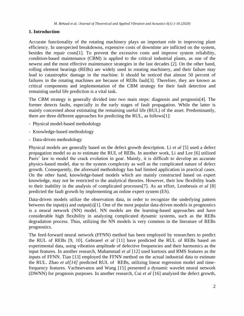
sampling frequency. The PRONOSTIA platform is shown in Fig 1.

As discussed in[23], bearings 2 and 4 of the first operating condition have unnatural behavior.

Therefore, in the remainder of this paper, five datasets of the first operating condition will be

utilized. The RMS of the vibration signal is employed as the REBs health indicator (HI) and the

input of the data-driven model. The trends of RMS for the utilized REBs are shown in Fig 2.


4

Fig 1: Overview of the experimental platform

Fig 2: The trends of RMS for the utilized REBs

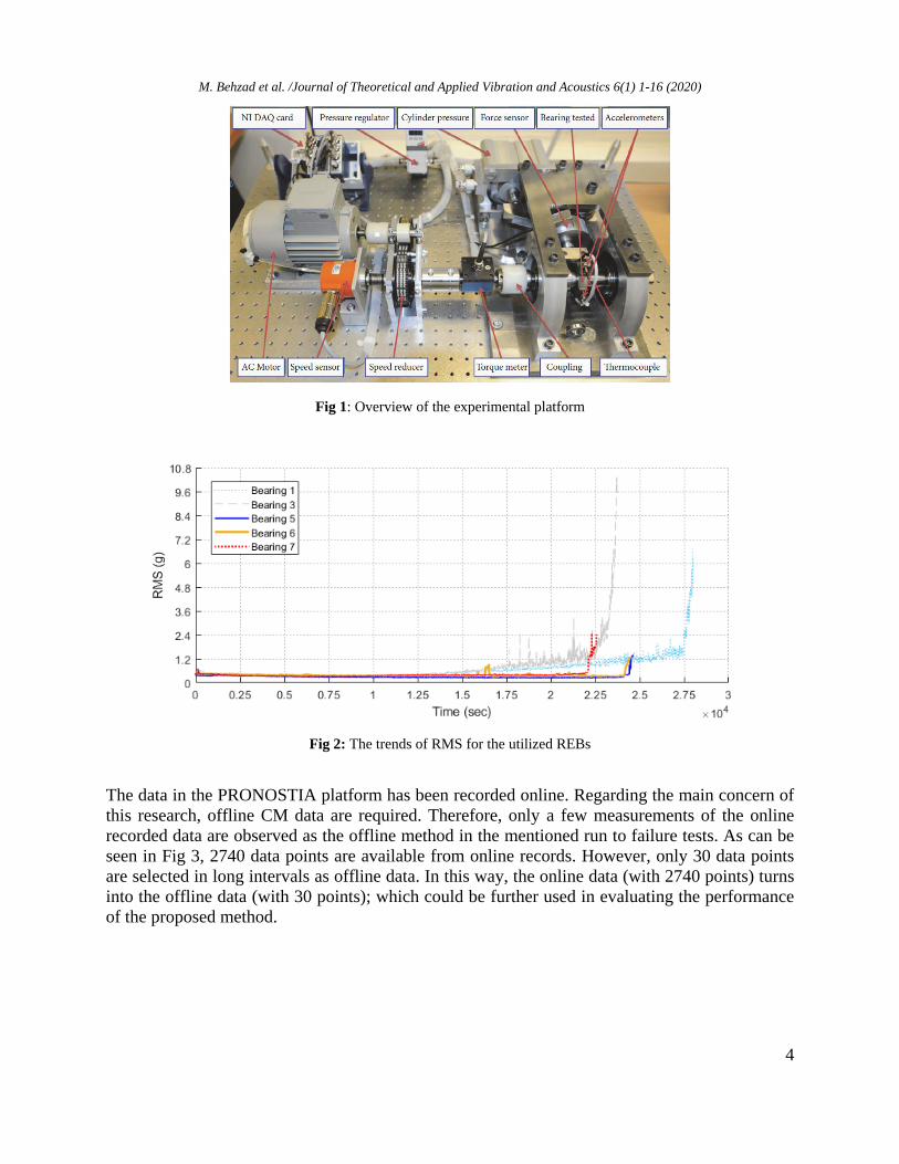
The data in the PRONOSTIA platform has been recorded online. Regarding the main concern of

this research, offline CM data are required. Therefore, only a few measurements of the online

recorded data are observed as the offline method in the mentioned run to failure tests. As can be

seen in Fig 3, 2740 data points are available from online records. However, only 30 data points

are selected in long intervals as offline data. In this way, the online data (with 2740 points) turns

into the offline data (with 30 points); which could be further used in evaluating the performance

of the proposed method.


5

Fig 3: Turning the online data into the offline data

3. Uncertainty in NN-based Prognostics

The remaining useful life of REB is inherently a stochastic variable, due to the presence of

uncertainties. In other words, the accuracy of RUL estimation through the NN-based methods are

affected by different uncertainty sources; which the well-known ones are as follows[24]:

- The lack of an analytical model for the degradation process

- Measurement noises

- Process noises

Generally, it is impossible to derive an exact mathematical model that can explain the

degradation process. So, it is common to consider some assumptions to make a practical model.

However, the corresponded results are less accurate under these assumptions. In NN-based

methods, the desired mathematical pattern is made through a black-box structure. Thus, the

hidden underlying assumptions in this structure may lead to inaccurate results (similar to the

other methods).

Measuring the real values of the HI in the component is costly or practically impossible. This is

due to the presence of noises, disturbances, and imperfection of the data acquisition equipment,

which all are considered as measurement noises in the acquired signal. The measurement noise

affects the prediction result, so it is considered as the second source of uncertainty[25].

The third source of uncertainty is process noise, which can be observed through the temporal

changes in the trend of HI. These changes are not due to the change in the real condition of the

asset and consequently, the HI value will go back to the normal state, after a while. As these

local changes are not expected to influence the prediction result, the utilized prognostics

algorithm has to be capable of comprehending the aforesaid uncertainty[26].

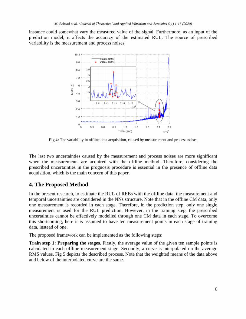
For instance, the online trend of the RMS feature has been illustrated in Fig 4. This trend could

also be acquired through limited offline measured points which can be seen in the figure. In an

arbitrary stage of the offline data acquisition process, it is possible to record any of the existing

points, as the offline measured data (Fig 4). It should be noticed that every data around this point,

had also the chance of being chosen as the current machine condition. Therefore, the measuring


6

instance could somewhat vary the measured value of the signal. Furthermore, as an input of the

prediction model, it affects the accuracy of the estimated RUL. The source of prescribed

variability is the measurement and process noises.

Fig 4: The variability in offline data acquisition, caused by measurement and process noises

The last two uncertainties caused by the measurement and process noises are more significant

when the measurements are acquired with the offline method. Therefore, considering the

prescribed uncertainties in the prognosis procedure is essential in the presence of offline data

acquisition, which is the main concern of this paper.

4. The Proposed Method

In the present research, to estimate the RUL of REBs with the offline data, the measurement and

temporal uncertainties are considered in the NNs structure. Note that in the offline CM data, only

one measurement is recorded in each stage. Therefore, in the prediction step, only one single

measurement is used for the RUL prediction. However, in the training step, the prescribed

uncertainties cannot be effectively modelled through one CM data in each stage. To overcome

this shortcoming, here it is assumed to have ten measurement points in each stage of training

data, instead of one.

The proposed framework can be implemented as the following steps:

Train step 1: Preparing the stages. Firstly, the average value of the given ten sample points is

calculated in each offline measurement stage. Secondly, a curve is interpolated on the average

RMS values. Fig 5 depicts the described process. Note that the weighted means of the data above

and below of the interpolated curve are the same.


7

Fig 5: Data interpolation process

Train step 2: Calculating mean and standard deviation of RULs in each stage. For every ten

available points in each offline measurement stage, the corresponded RUL is calculated by

means of the interpolated curve and Eq 1. In other words, ten different RULs for ten RMS values

are determined in each stage. For instance, Fig 6 shows the variation amount of the calculated

RUL in the existence of two offline RMS data for a short period.

A Aend

B Bend

RUL t t

RUL t t

(1)

where t̅A and t̅B are the elapsed lives corresponded to the projected RMS values of points A and

B onto the interpolation curve, respectively. RUL̅̅ ̅̅ ̅̅A and RUL̅̅ ̅̅ ̅̅

B are the calculated values of RULs

corresponded to points A and B, respectively; and tend represents the REB’s end of life. Then a

normal distribution is fitted to the RULs of ten recorded RMS (which have been obtained

through Eq 1) in each stage of the offline measurements. Further, the mean and standard

deviation of the fitted distributions are calculated.

Fig 6:Procedure of the corresponded RUL calculation, for each record


8

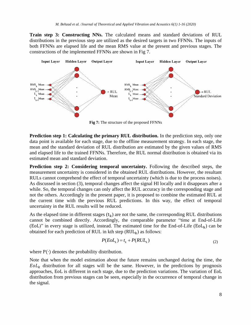
Train step 3: Constructing NNs. The calculated means and standard deviations of RUL

distributions in the previous step are utilized as the desired targets in two FFNNs. The inputs of

both FFNNs are elapsed life and the mean RMS value at the present and previous stages. The

constructions of the implemented FFNNs are shown in Fig 7.

Fig 7: The structure of the proposed FFNNs

Prediction step 1: Calculating the primary RUL distribution. In the prediction step, only one

data point is available for each stage, due to the offline measurement strategy. In each stage, the

mean and the standard deviation of RUL distribution are estimated by the given values of RMS

and elapsed life to the trained FFNNs. Therefore, the RUL normal distribution is obtained via its

estimated mean and standard deviation.

Prediction step 2: Considering temporal uncertainty. Following the described steps, the

measurement uncertainty is considered in the obtained RUL distributions. However, the resultant

RULs cannot comprehend the effect of temporal uncertainty (which is due to the process noises).

As discussed in section (3), temporal changes affect the signal HI locally and it disappears after a

while. So, the temporal changes can only affect the RUL accuracy in the corresponding stage and

not the others. Accordingly in the present paper, it is proposed to combine the estimated RUL at

the current time with the previous RUL predictions. In this way, the effect of temporal

uncertainty in the RUL results will be reduced.

As the elapsed time in different stages (tk) are not the same, the corresponding RUL distributions

cannot be combined directly. Accordingly, the comparable parameter “time at End-of-Life

(EoL)” in every stage is utilized, instead. The estimated time for the End-of-Life (EoLk) can be

obtained for each prediction of RUL in kth step (RULk) as follows:

( ) ( )k k kP EoL t P RUL (2)

where P(∙) denotes the probability distribution.

Note that when the model estimation about the future remains unchanged during the time, the

𝐸𝑜𝐿𝑘 distribution for all stages will be the same. However, in the predictions by prognosis

approaches, EoL is different in each stage, due to the prediction variations. The variation of EoL

distribution from previous stages can be seen, especially in the occurrence of temporal change in

the signal.


9

Thus, in this paper, the effect of temporal changes on the prediction results is reduced, by

combining the estimated EoL distribution at the present stage k (P(EoLk)) with the last two

previous ones (P(EoLk−1), and P(EoLk−2)). Here, the overall probability distribution of EoL at

tk (EoLOverall,k) is assumed to be a linear combination of the estimated P(EoLk), P(EoLk−1) and

P(EoLk−2); which includes both measurement and temporal uncertainties.

2,

2

( )

( )

k

i i

i kOverall k k

i

i k

w P EoL

P EoL

w

(3)

where P(EoLi)s are the last three PDFs of estimated RUL up to present time stage k obtained

from “Prediction step 1”; and wis represent their corresponding weights. The weights define the

relative contribution of each prediction in the linear combination and lie within the interval [0,1].

The denominator term is also utilized to normalize the calculated output so that the total under

area equals to one as in probability distributions.

The calculated EoL probability distribution at the present time ( P(EoLk) ) contains much more

valuable information than the others because it is based on the last observation of the component

condition. Therefore, the weight of corresponded prediction ( P(EoLk) ) is considered to be one

(wk = 1). On the other hand, since the main goal in this step is to resist being affected by the

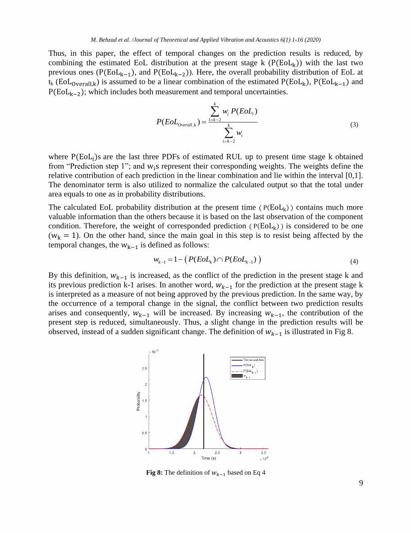
temporal changes, the wk−1 is defined as follows:

1 11 ( ) ( )k k kw P EoL P EoL (4)

By this definition, 𝑤𝑘−1 is increased, as the conflict of the prediction in the present stage k and

its previous prediction k-1 arises. In another word, 𝑤𝑘−1 for the prediction at the present stage k

is interpreted as a measure of not being approved by the previous prediction. In the same way, by

the occurrence of a temporal change in the signal, the conflict between two prediction results

arises and consequently, 𝑤𝑘−1 will be increased. By increasing 𝑤𝑘−1, the contribution of the

present step is reduced, simultaneously. Thus, a slight change in the prediction results will be

observed, instead of a sudden significant change. The definition of 𝑤𝑘−1 is illustrated in Fig 8.

Fig 8: The definition of 𝑤𝑘−1 based on Eq 4


10

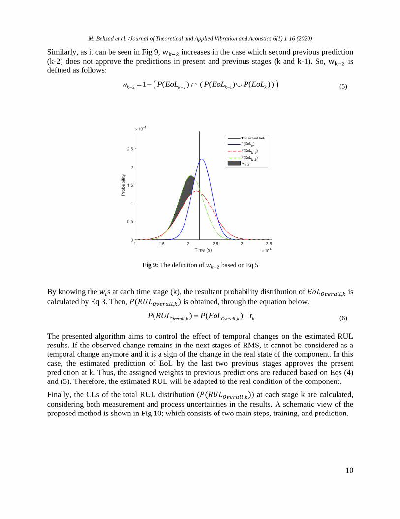
Similarly, as it can be seen in Fig 9, wk−2 increases in the case which second previous prediction

(k-2) does not approve the predictions in present and previous stages (k and k-1). So, wk−2 is

defined as follows:

2 2 11 ( ) ( ( ) ( ))k k k kw P EoL P EoL P EoL (5)

Fig 9: The definition of 𝑤𝑘−2 based on Eq 5

By knowing the 𝑤𝑖s at each time stage (k), the resultant probability distribution of 𝐸𝑜𝐿𝑂𝑣𝑒𝑟𝑎𝑙𝑙,𝑘 is

calculated by Eq 3. Then, 𝑃(𝑅𝑈𝐿𝑂𝑣𝑒𝑟𝑎𝑙𝑙,𝑘) is obtained, through the equation below.

, ,( ) ( )Overall k Overall k kP RUL P EoL t (6)

The presented algorithm aims to control the effect of temporal changes on the estimated RUL

results. If the observed change remains in the next stages of RMS, it cannot be considered as a

temporal change anymore and it is a sign of the change in the real state of the component. In this

case, the estimated prediction of EoL by the last two previous stages approves the present

prediction at k. Thus, the assigned weights to previous predictions are reduced based on Eqs (4)

and (5). Therefore, the estimated RUL will be adapted to the real condition of the component.

Finally, the CLs of the total RUL distribution (𝑃(𝑅𝑈𝐿𝑂𝑣𝑒𝑟𝑎𝑙𝑙,𝑘)) at each stage k are calculated,

considering both measurement and process uncertainties in the results. A schematic view of the

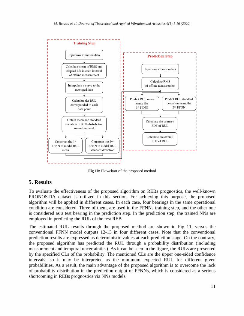
proposed method is shown in Fig 10; which consists of two main steps, training, and prediction.


11

Fig 10: Flowchart of the proposed method

5. Results

To evaluate the effectiveness of the proposed algorithm on REBs prognostics, the well-known

PRONOSTIA dataset is utilized in this section. For achieving this purpose, the proposed

algorithm will be applied in different cases. In each case, four bearings in the same operational

condition are considered. Three of them, are used in the FFNNs training step, and the other one

is considered as a test bearing in the prediction step. In the prediction step, the trained NNs are

employed in predicting the RUL of the test REB.

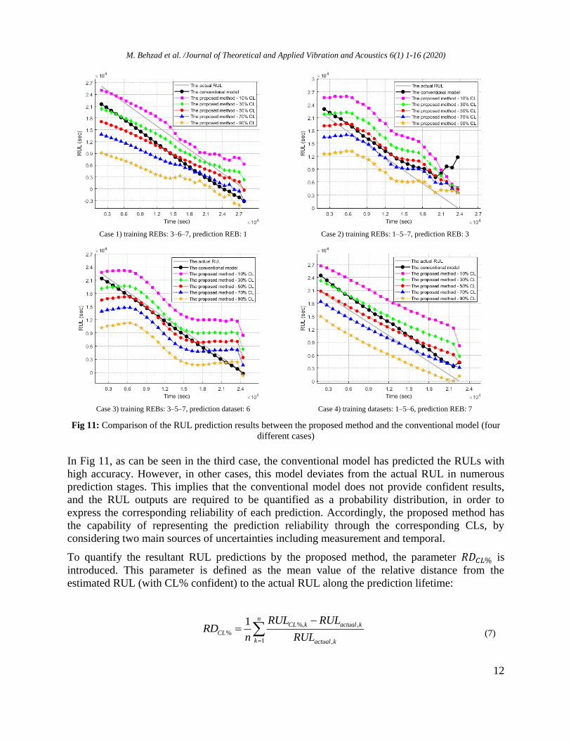
The estimated RUL results through the proposed method are shown in Fig 11, versus the

conventional FFNN model outputs 12-13 in four different cases. Note that the conventional

prediction results are expressed as deterministic values at each prediction stage. On the contrary,

the proposed algorithm has predicted the RUL through a probability distribution (including

measurement and temporal uncertainties). As it can be seen in the figure, the RULs are presented

by the specified CLs of the probability. The mentioned CLs are the upper one-sided confidence

intervals; so it may be interpreted as the minimum expected RUL for different given

probabilities. As a result, the main advantage of the proposed algorithm is to overcome the lack

of probability distribution in the prediction output of FFNNs, which is considered as a serious

shortcoming in REBs prognostics via NNs models.


12

Case 1) training REBs: 3–6–7, prediction REB: 1 Case 2) training REBs: 1–5–7, prediction REB: 3

Case 3) training REBs: 3–5–7, prediction dataset: 6 Case 4) training datasets: 1–5–6, prediction REB: 7

Fig 11: Comparison of the RUL prediction results between the proposed method and the conventional model (four

different cases)

In Fig 11, as can be seen in the third case, the conventional model has predicted the RULs with

high accuracy. However, in other cases, this model deviates from the actual RUL in numerous

prediction stages. This implies that the conventional model does not provide confident results,

and the RUL outputs are required to be quantified as a probability distribution, in order to

express the corresponding reliability of each prediction. Accordingly, the proposed method has

the capability of representing the prediction reliability through the corresponding CLs, by

considering two main sources of uncertainties including measurement and temporal.

To quantify the resultant RUL predictions by the proposed method, the parameter 𝑅𝐷𝐶𝐿% is

introduced. This parameter is defined as the mean value of the relative distance from the

estimated RUL (with CL% confident) to the actual RUL along the prediction lifetime:

%, ,

%

1 ,

1 nCL k actual k

CL

k actual k

RUL RULRD

n RUL

(7)


13

where n indicates the total number of stages. 𝑅𝑈𝐿𝐶𝐿%,𝑘 is the minimum expected RUL for the

given probability (CL%) at stage k, and 𝑅𝑈𝐿𝑎𝑐𝑡𝑢𝑎𝑙,𝑘 is the actual RUL at stage k.

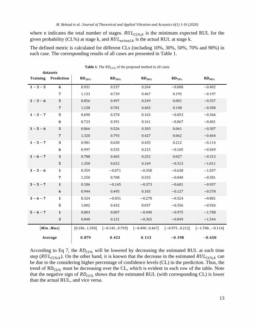
The defined metric is calculated for different CLs (including 10%, 30%, 50%, 70% and 90%) in

each case. The corresponding results of all cases are presented in Table 1.

Table 1. The 𝑅𝐷𝐶𝐿% of the proposed method in all cases

𝐝𝐚𝐭𝐚𝐬𝐞𝐭𝐬

𝐓𝐫𝐚𝐢𝐧𝐢𝐧𝐠 𝐏𝐫𝐞𝐝𝐢𝐜𝐭𝐢𝐨𝐧 𝐑𝐃𝟏𝟎% 𝐑𝐃𝟑𝟎% 𝐑𝐃𝟓𝟎% 𝐑𝐃𝟕𝟎% 𝐑𝐃𝟗𝟎%

𝟏 − 𝟑 − 𝟓 𝟔 0.931 0.537 0.264 −0.008 −0.402

𝟕 1.133 0.739 0.467 0.195 −0.197

𝟏 − 𝟑 − 𝟔 𝟓 0.856 0.497 0.249 0.001 −0.357

𝟕 1.238 0.781 0.465 0.148 −0.308

𝟏 − 𝟑 − 𝟕 𝟓 0.690 0.378 0.162 −0.053 −0.366

𝟔 0.723 0.391 0.161 −0.067 −0.401

𝟏 − 𝟓 − 𝟔 𝟑 0.866 0.526 0.303 0.061 −0.307

𝟕 1.320 0.793 0.427 0.062 −0.464

𝟏 − 𝟓 − 𝟕 𝟑 0.981 0.658 0.435 0.212 −0.114

𝟔 0.997 0.535 0.215 −0.105 −0.569

𝟏 − 𝟔 − 𝟕 𝟑 0.788 0.465 0.252 0.027 −0.313

𝟓 1.350 0.652 0.169 −0.313 −1.011

𝟑 − 𝟓 − 𝟔 𝟏 0.359 −0.071 −0.358 −0.638 −1.037

𝟕 1.250 0.708 0.333 −0.040 −0.581

𝟑 − 𝟓 − 𝟕 𝟏 0.186 −0.145 −0.373 −0.601 −0.937

𝟔 0.944 0.495 0.183 −0.127 −0.578

𝟑 − 𝟔 − 𝟕 𝟏 0.324 −0.031 −0.278 −0.524 −0.881

𝟓 1.002 0.432 0.037 −0.356 −0.926

𝟓 − 𝟔 − 𝟕 𝟏 0.803 0.007 −0.490 −0.975 −1.708

𝟑 0.840 0.121 −0.365 −0.849 −1.544

[𝑴𝒊𝒏 , 𝑴𝒂𝒙] [0.186 , 1.350] [−0.145 , 0.793] [−0.490 , 0.467] [−0.975 , 0.212] [−1.708 , −0.114]

𝐀𝐯𝐞𝐫𝐚𝐠𝐞 𝟎. 𝟖𝟕𝟗 𝟎. 𝟒𝟐𝟑 𝟎. 𝟏𝟏𝟑 −𝟎. 𝟏𝟗𝟖 −𝟎. 𝟔𝟓𝟎

According to Eq 7, the 𝑅𝐷𝐶𝐿% will be lowered by decreasing the estimated RUL at each time

step (𝑅𝑈𝐿𝐶𝐿%,𝑘). On the other hand, it is known that the decrease in the estimated 𝑅𝑈𝐿𝐶𝐿%,𝑘 can

be due to the considering higher percentage of confidence levels (CL) in the prediction. Thus, the

trend of RDCL% must be decreasing over the CL, which is evident in each row of the table. Note

that the negative sign of 𝑅𝐷𝐶𝐿% shows that the estimated RUL (with corresponding CL) is lower

than the actual RUL, and vice versa.


14

The performance of the proposed method is not the same in different cases. As an instance, the

𝑅𝐷50% is positive (50% CL line is above the actual RUL) in most of the cases. On the other

hand, it is negative in some other cases; as in training datasets 5-6-7 on the prediction datasets 1

and 3. As an overall view for each CL, the [𝑀𝑖𝑛 , 𝑀𝑎𝑥] interval and also the average 𝑅𝐷𝐶𝐿% are

represented, correspondingly. It can be seen from the average row that the RD50% is about 0.113.

This value means that the estimated 50% CL is 11.3% upper than the actual RUL, on average. As

another expression, the corresponding estimation is a little optimistic about the RUL of REB. On

the other hand, the average of RD90% is -0.650; which can be interpreted as a pessimistic view

about the RUL of the asset. In this way, the proposed method provides a new perspective in NN-

based prognostics about the future of an asset.

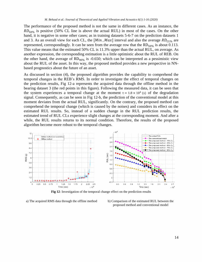
As discussed in section (4), the proposed algorithm provides the capability to comprehend the

temporal changes in the REB’s RMS. In order to investigate the effect of temporal changes on

the prediction results, Fig 12-a represents the acquired data through the offline method in the

bearing dataset 3 (the red points in this figure). Following the measured data, it can be seen that

the system experiences a temporal change at the moment t = 1.8 × 104 (s) of the degradation

signal. Consequently, as can be seen in Fig 12-b, the prediction of the conventional model at this

moment deviates from the actual RUL, significantly. On the contrary, the proposed method can

comprehend the temporal change (which is caused by the noises) and considers its effect on the

estimated RUL results. So, instead of a sudden change in the RUL prediction results, the

estimated trend of RUL CLs experience slight changes at the corresponding moment. And after a

while, the RUL results returns to its normal condition. Therefore, the results of the proposed

algorithm become more robust to the temporal changes.

Fig 12: Investigation of the temporal change effect on the prediction results

a) The acquired RMS data through the offline method b) Comparison of the estimated RUL between the

proposed method and conventional model


15

6. Conclusion

This paper has proposed a probabilistic method so as to improve the NN-based prognostics of

REBs, in the presence of the offline data acquisition. The main concern is to take into account

the measurement and temporal uncertainties. For achieving this purpose, two FFNNs have been

employed in order to estimate the mean and standard deviation of the primary RUL distribution

at each stage. Then, the temporal uncertainty has been considered in the RUL distribution based

on the degree of approval by the previous stage predictions.

The method has been evaluated by using the experimental results of the bearing accelerated run

to failure tests. The superior property of the presented method over the conventional model is

providing a probability distribution and its CLs for the estimated RUL, by considering different

uncertainties. It has also illustrated in the results that the method can comprehend the temporal

changes in the HI signal, and consequently consider its effect on the corresponding predictions.

According to the proposed probabilistic perspective, the NN-based prognostics can be more

practically used in improving the system reliability and also the industrial decision-making about

the future of plants.

There are several important directions for future research, as follows:

- Identifying the real state of the system by other methods may improve the results.

- Other types of the probability distribution for RUL could be utilized in further studies.

- Utilizing other types of NN may affect the results.

References

[1] Y. Peng, M. Dong, M.J. Zuo, Current status of machine prognostics in condition-based maintenance: a review,

Int J Adv Manuf Technol, 50 (2010) 297-313.

[2] Y. Lei, N. Li, L. Guo, N. Li, T. Yan, J. Lin, Machinery health prognostics: A systematic review from data

acquisition to RUL prediction, Mechanical Systems and Signal Processing, 104 (2018) 799-834.

[3] A. Rai, S.H. Upadhyay, A review on signal processing techniques utilized in the fault diagnosis of rolling

element bearings, Tribology International, 96 (2016) 289-306.

[4] G.J. Vachtsevanos, Intelligent fault diagnosis and prognosis for engineering systems, Wiley Hoboken, 2006.

[5] Y. Li, T.R. Kurfess, S.Y. Liang, Stochastic prognostics for rolling element bearings, Mechanical Systems and

Signal Processing, 14 (2000) 747-762.

[6] C.J. Li, H. Lee, Gear fatigue crack prognosis using embedded model, gear dynamic model and fracture

mechanics, Mechanical systems and signal processing, 19 (2005) 836-846.

[7] J.Z. Sikorska, M. Hodkiewicz, L. Ma, Prognostic modelling options for remaining useful life estimation by

industry, Mechanical systems and signal processing, 25 (2011) 1803-1836.

[8] E. Lembessis, G. Antonopoulos, R.E. King, C. Halatsis, J. Torres, CASSANDRA: an on-line expert system for

fault prognosis, in: Proc. the 5th CIM Europe Conference on Computer Integrated Manufacturing, 1989.

[9] Z. Tian, L. Wong, N. Safaei, A neural network approach for remaining useful life prediction utilizing both

failure and suspension histories, Mechanical Systems and Signal Processing, 24 (2010) 1542-1555.

[10] O. Fink, E. Zio, U. Weidmann, Predicting component reliability and level of degradation with complex-valued

neural networks, Reliability Engineering & System Safety, 121 (2014) 198-206.

[11] N. Gebraeel, M. Lawley, R. Liu, V. Parmeshwaran, Residual life predictions from vibration-based degradation

signals: a neural network approach, IEEE Transactions on industrial electronics, 51 (2004) 694-700.

[12] S. Saon, T. Hiyama, Predicting remaining useful life of rotating machinery based artificial neural network,

Computers & Mathematics with Applications, 60 (2010) 1078-1087.

[13] Z. Tian, An artificial neural network method for remaining useful life prediction of equipment subject to

condition monitoring, Journal of Intelligent Manufacturing, 23 (2012) 227-237.


16

[14] M. Zhao, B. Tang, Q. Tan, Bearing remaining useful life estimation based on time–frequency representation

and supervised dimensionality reduction, Measurement, 86 (2016) 41-55.

[15] G. Vachtsevanos, P. Wang, Fault prognosis using dynamic wavelet neural networks, in: 2001 IEEE

Autotestcon Proceedings. IEEE Systems Readiness Technology Conference.(Cat. No. 01CH37237), IEEE, 2001, pp.

857-870.

[16] Q. Cui, Z. Li, J. Yang, B. Liang, Rolling bearing fault prognosis using recurrent neural network, in: 2017 29th

Chinese Control And Decision Conference (CCDC), IEEE, 2017, pp. 1196-1201.

[17] B. Satish, N.D.R. Sarma, A fuzzy BP approach for diagnosis and prognosis of bearing faults in induction

motors, in: IEEE Power Engineering Society General Meeting, 2005, IEEE, 2005, pp. 2291-2294.

[18] P. Nectoux, R. Gouriveau, K. Medjaher, E. Ramasso, B. Chebel-Morello, N. Zerhouni, C. Varnier,

PRONOSTIA: An experimental platform for bearings accelerated degradation tests, in, 2012.

[19] S. Hong, Z. Zhou, E. Zio, K. Hong, Condition assessment for the performance degradation of bearing based on

a combinatorial feature extraction method, Digital Signal Processing, 27 (2014) 159-166.

[20] Z. Liu, M.J. Zuo, Y. Qin, Remaining useful life prediction of rolling element bearings based on health state

assessment, Proceedings of the Institution of Mechanical Engineers, Part C: Journal of Mechanical Engineering

Science, 230 (2016) 314-330.

[21] L. Guo, N. Li, F. Jia, Y. Lei, J. Lin, A recurrent neural network based health indicator for remaining useful life

prediction of bearings, Neurocomputing, 240 (2017) 98-109.

[22] Y. Pan, M.J. Er, X. Li, H. Yu, R. Gouriveau, Machine health condition prediction via online dynamic fuzzy

neural networks, Engineering Applications of Artificial Intelligence, 35 (2014) 105-113.

[23] M. Behzad, H.A. Arghand, A. Rohani Bastami, Remaining useful life prediction of ball-bearings based on high-

frequency vibration features, Proceedings of the Institution of Mechanical Engineers, Part C: Journal of Mechanical

Engineering Science, 232 (2018) 3224-3234.

[24] Y. Lei, Intelligent fault diagnosis and remaining useful life prediction of rotating machinery, Butterworth-

Heinemann, 2016.

[25] X.-S. Si, Z.-X. Zhang, C.-H. Hu, Data-Driven Remaining Useful Life Prognosis Techniques, Beijing, China:

National Defense Industry Press and Springer-Verlag GmbH, (2017).

[26] N. Li, Y. Lei, J. Lin, S.X. Ding, An improved exponential model for predicting remaining useful life of rolling

element bearings, IEEE Transactions on Industrial Electronics, 62 (2015) 7762-7773.

Documents

Investigation on the effects of measurement and temporal