i

INVESTIGATIONS INTO THE ISSUE OF REACTIVE

POWER SHARING AMONGST PHOTOVOLTAIC

BASED DISTRIBUTED GENERATORS OPERATING IN

A MICROGRID

A Thesis submitted to Gujarat Technological University

for the Award of

Doctor of Philosophy

in

Electrical Engineering

By

PATEL URVI NIKUNJ

119997109006

under supervision of

Dr. Hiren H. Patel

GUJARAT TECHNOLOGICAL UNIVERSITY

AHMEDABAD

February– 2019

ii

© PATEL URVI NIKUNJ

iii

DECLARATION

I declare that the thesis entitled Investigations into the issue of reactive power

sharing amongst photovoltaic based distributed generators operating in a

microgrid submitted by me for the degree of Doctor of Philosophy is the record of

research work carried out by me during the period from 2011 to 2019 under the

supervision of Dr. Hiren H. Patel and this has not formed the basis for the award of

any degree, diploma, associateship, fellowship, titles in this or any other University

or other institution of higher learning.

I further declare that the material obtained from other sources has been duly

acknowledged in the thesis. I shall be solely responsible for any plagiarism or

other irregularities, if noticed in the thesis.

Signature of the Research Scholar: …………………………… Date:

…………….

Name of Research Scholar: Patel Urvi Nikunj

Place: …………………………………

iv

CERTIFICATE

I certify that the work incorporated in the thesis Investigations into the issue of

reactive power sharing amongst photovoltaic based distributed generators

operating in a microgrid submitted by Smt. Patel Urvi Nikunj was carried out

by the candidate under my supervision/guidance. To the best of my knowledge:

(i) the candidate has not submitted the same research work to any other institution

for any degree/diploma, Associateship, Fellowship or other similar titles (ii) the

thesis submitted is a record of original research work done by the Research

Scholar during the period of study under my supervision, and (iii) the thesis

represents independent research work on the part of the Research Scholar.

Signature of Supervisor: ……………………….. Date: ………………

Name of Supervisor: Dr. Hiren H. Patel

Place: …………………

v

Course-work Completion Certificate

This is to certify that Mrs. Patel Urvi Nikunj enrolment no. 119997109006 is a PhD

scholar enrolled for PhD program in the branch 2011 of Gujarat Technological University,

Ahmedabad.

(Please tick the relevant option(s))

She has been exempted from the course-work (successfully completed during M. Phil

Course)

She has been exempted from Research Methodology Course only (successfully

completed during M. Phil Course)

She has successfully completed the PhD course work for the partial requirement for the

award of PhD Degree. His/ Her performance in the course work is as follows-

Grade Obtained in Research

Methodology

(PH001)

Grade Obtained in Self Study Course (Core

Subject)

(PH002)

BB

BB

Signature of Supervisor:

Name of Supervisor: Dr. Hiren H. Patel

vi

Originality Report Certificate

It is certified that PhD Thesis titled Investigations into the issue of reactive power

sharing amongst photovoltaic based distributed generators operating in a

microgrid has been examined by us. We undertake the following:

a. Thesis has significant new work / knowledge as compared already published

or are under consideration to be published elsewhere. No sentence, equation,

diagram, table, paragraph or section has been copied verbatim from previous work

unless it is placed under quotation marks and duly referenced.

b. The work presented is original and own work of the author (i.e. there is no

plagiarism). No ideas, processes, results or words of others have been presented

as Author own work.

c. There is no fabrication of data or results which have been compiled /

analysed.

d. There is no falsification by manipulating research materials, equipment or

processes, or changing or omitting data or results such that the research is not

accurately represented in the research record.

e. The thesis has been checked using Turnitin (copy of originality report

attached) and found within limits as per GTU Plagiarism Policy and instructions

issued from time to time (i.e. permitted similarity index <=25%).

Signature of the Research Scholar: …………………………… Date: ….………

Name of Research Scholar: Patel Urvi Nikunj

Place: …………………………………

Signature of Supervisor: ………………………… Date: ……………

Name of Supervisor: Dr. Hiren H. Patel

Place: …………………

vii

viii

ix

PhD THESIS Non-Exclusive License to

GUJARAT TECHNOLOGICAL UNIVERSITY

In consideration of being a PhD Research Scholar at GTU and in the interests of the

facilitation of research at GTU and elsewhere, I, Patel Urvi Nikunj having

(119997109006) hereby grant a non-exclusive, royalty free and perpetual license to

GTU on the following terms:

a) GTU is permitted to archive, reproduce and distribute my thesis, in whole or in

part, and/or my abstract, in whole or in part ( referred to collectively as the “Work”)

anywhere in the world, for non-commercial purposes, in all forms of media;

b) GTU is permitted to authorize, sub-lease, sub-contract or procure any of the acts

mentioned in paragraph (a);

c) GTU is authorized to submit the Work at any National / International Library,

under the authority of their “Thesis Non-Exclusive License”;

d) The Universal Copyright Notice (©) shall appear on all copies made under the

authority of this license;

e) I undertake to submit my thesis, through my University, to any Library and

Archives. Any abstract submitted with the thesis will be considered to form part of the

thesis.

f) I represent that my thesis is my original work, does not infringe any rights of

others, including privacy rights, and that I have the right to make the grant conferred

by this non-exclusive license.

g) If third party copyrighted material was included in my thesis for which, under the

terms of the Copyright Act, written permission from the copyright owners is required,

I have obtained such permission from the copyright owners to do the acts mentioned

in paragraph (a) above for the full term of copyright protection.

x

h) I retain copyright ownership and moral rights in my thesis, and may deal with the

copyright in my thesis, in any way consistent with rights granted by me to my

University in this non-exclusive license.

i) I further promise to inform any person to whom I may hereafter assign or license

my copyright in my thesis of the rights granted by me to my University in this non-

exclusive license.

j) I am aware of and agree to accept the conditions and regulations of PhD

including all policy matters related to authorship and plagiarism.

Signature of the Research Scholar: df

Name of Research Scholar: Patel Urvi Nikunj

Date: Place:

Signature of Supervisor:

Name of Supervisor: Dr. Hiren H. Patel

Date: Place:

Seal:

xi

Thesis Approval Form

The viva-voce of the PhD Thesis submitted by Mrs. Smt. Patel Urvi Nikunj

(Enrollment No. 119997109006) entitled Investigations into the issue of reactive

power sharing amongst photovoltaic based distributed generators operating in a

microgrid was conducted on …………………….…(day and date) at Gujarat

Technological University.

(Please tick any one of the following option)

The performance of the candidate was satisfactory. We recommend that

he/she be awarded the PhD degree.

Any further modifications in research work recommended by the panel after 3

months from the date of first viva-voce upon request of the Supervisor or

request of Independent Research Scholar after which viva-voce can be re-

conducted by the same panel again.

(briefly specify the modifications suggested by the panel)

The performance of the candidate was unsatisfactory. We recommend that

he/she should not be awarded the PhD degree.

(The panel must give justifications for rejecting the research work)

----------------------------------------------------- -----------------------------------------------------

Name and Signature of Supervisor with Seal 1) (External Examiner 1) Name and Signature

------------------------------------------------------- ------------------------------------------------------- 2) (External Examiner 2) Name and Signature 3) (External Examiner 3) Name and Signature

xii

Abstract

A microgrid (MG) provides promising option for future electricity generation by

incorporating electricity generation from non-conventional or renewable energy sources.

The share of electricity generation from renewable sources is increasing rapidly in the grid

or MG. It is mainly due to the depletion of conventional energy sources, increasing cost of

these sources and growing environmental concern. Amongst various renewable energy

sources, photovoltaic (PV) has emerged as one of the most potential energy sources to

provide clean energy. However, increased penetration of PV sources has also given rise to

several challenges. One of these challenges is reactive power management through the PV

inverters.

Usually, the PV inverters are operated to exchange mainly active power with the main

grid. However, the PV inverters do have the capability to exchange the reactive power with

the grid or microgrid. Several studies have focused on the reactive power control through

PV based inverters. However, often the impact of the variable active power from the PV

array on the available reactive power margin is ignored. It may lead to overloading of the

inverters or unequal utilization of the resources.

In this research, reactive power sharing algorithms are proposed which takes into account

the variable nature of the active power available from the PV based DGs and then

distributes the reactive power amongst the various DGs based on the available reactive

power margins. The algorithms proposed as ‘Equal Apparent Power’ assigns the reactive

power amongst the DGs having identical ratings in such a way that the gap amongst the

utilization factors of these inverters decreases. However, it is observed that the order in

which the reactive power is allocated amongst the inverters, affects the standard deviation

of the utilization factors of the inverters. Hence, the algorithm is further modified and

proposed as ‘Equal power sharing with least standard deviation’ (EAPS-LSD) to take into

account the order/sequence in which the reactive power is allocated amongst DGs having

identical ratings. Another algorithm proposed as ‘Proportional apparent power sharing with

least standard deviation’ (PAPS-LSD)’ assigns reactive power amongst the inverters of un-

identical ratings to achieve the equal utilization of the inverters. The algorithms are

evaluated against other approaches like equal reactive power sharing and optimal reactive

xiii

power sharing algorithms in terms of their capabilities to obtain the best solution that gives

the least standard deviation of utilization factors of the inverters. Through the simulation

results it is shown that the standard deviation of utilization factors of the inverters is

significantly lower than other approaches.

In the islanded mode, the inverter based DGs are usually operated as controlled voltage

source where the conventional droop-control scheme is usually employed for sharing of

active and reactive power. The load is shared amongst energy sources in proportion to their

ratings using the fixed droop coefficient. The scheme suffers from the issue of ineffective

utilization of the resources (source, inverters, energy storage etc.) when performance of

some sources are dependent on environmental conditions. A modified droop-control

strategy is proposed for a microgrid comprising of photovoltaic (PV) based distributed

generators (DG) operating in parallel with other DGs in this work. The modified droop sets

the frequency reference such that the PV sources operate at their maximum power point

and the energy demanded from the auxiliary source is restricted to the minimum. Also

proper distribution of reactive power amongst the inverters is obtained through the PAPS

algorithm implemented in the secondary control unit. It ensures equal utilization of

inverters thereby preventing overloading or underutilization of DGs. The control scheme

can work even in case of the failure of the communication channel between the primary

and the secondary control units, when the PAPS is unable to send the reference reactive

power information. In such case, the primary control unit shares the reactive power based

on the information of the local variables through the droop control.

In addition the accuracy of the reactive power sharing through the conventional droop

control is also affected by the mismatch in impedance. Mathematical analysis is included

to reveal the limitations of the conventional droop control in case the impedance mismatch

occurs. It leads to voltage mismatch of the inverters. Further, the conventional droop has

fixed droop coefficient which may lead to larger frequency overshoots during load

changes. A modified droop control scheme based on the principle of virtual impedance and

of arctan function for the droop control is also presented to overcome this limitation. The

error mismatch of the output voltage of the inverters is minimized using virtual impedance

while the improved time response is achieved through the modification of the real-power

frequency droop using arctan function. Simulations results are presented to justify the

effectiveness of the control approach.

xiv

Acknowledgement

I would like to express my gratitude to all who have been provided a very good support

and motivation to me during the course of my PHD work. I would like to express my

gratitude to my supervisor Prof. Hiren H. Patel, who has given opportunity to work under

his guidance. I am really thankful to him for his constant support and guidance in many

technical issues at various stages of research work. His in depth technical knowledge

helped me to define my research path. I am extremely thankful to my DPC members Dr. S.

R. Joshi and Dr. A. K. Panchal for their valuable suggestions and support during my

research work.

I would also like to express my gratitude to my previous institute, C. K. Pithawalla College

of Engineering and Technology (CKPCET), staff members Dr. Naimish Zaveri, Hetal

Patel, Arpita Shah, Divyesh Mistry and friends Dr. Kalpesh Patil, Neha Shah for providing

me very good working environment, all kind of support and help in my research work. I

am also very much thankful to my present institute Dr. S. & S. S. Ghandhy Government

Engineering College, Surat and faculties for all support during my final phase of thesis

writing. I am also thankful to Gujarat Technological University (GTU) Vice Chancellor,

Registrar and PHD section for all support during my research work.

This research is dedicated to my dearest husband Nikunj and my daughter Kesha who have

been source of continuous encouragement and support without any voice of dissent or

discomfort. It is impossible for me to complete my research work without their valuable

moral support. The words are not enough to express my gratitude towards my parents, in-

laws family, my dear sister Rachana for unconditional love and blessings.

There are several others who have played a significant role during my research and whose

name i have failed to mention. I extend my sincere thanks to all who have contributed

directly or indirectly in achieving my ambition

Above all, I am very much thankful to almighty GOD for blessed me with a very happy

and successful life

Urvi Nikunj Patel

xv

Table of Content

Chapter 1 Introduction………………………………………………………… 1

1.1 Introduction…………………………………………………… 1

1.2 Overview of the Thesis……………………………………….. 4

Chapter 2 Literature Survey…………………………………………………... 6

2.1 Microgrid……………………………………………………… 6

2.2 Active and Reactive Power Sharing amongst Conventional

DGs…………………………………………………………… 10

2.3 Introduction to PV based DG…………………………………. 13

2.3.1 PV Cell Characteristic and Model……………………. 13

2.3.2 Grid Interface for PV system…………………………. 15

2.4 Active and Reactive Power Sharing with PV based DGs…….. 18

2.5 Objective and Scope of work…………………………………. 21

Chapter 3 Modeling and Control of DGs in a Microgrid……………………. 23

3.1 System Configuration…………………………………………. 23

3.2 Modeling of a PV source……………………………………… 24

3.3 Control of DG in Grid Connected Mode.................................... 28

3.3.1 Modeling of inverter and its AC side dynamics...……. 29

3.3.2 Phase Locked Loop (PLL)……………………………. 32

3.3.3 Active-Reactive power control (P-Q Control)………... 34

3.3.4 Simulation Results……………………………………. 38

3.4 Control of DG in an Islanded Mode…………………………... 42

3.4.1 Modeling of Dynamics of Inverter Output …………... 43

3.4.2 Inverter Control ……………………………………… 44

3.4.3 Simulation Results ………............................................ 47

3.5 Transitions between Modes…………………………………… 49

3.5.1 Transition from islanded mode to grid-connected

mode………………………………………………...... 49

3.5.2 Transition from grid-connected mode to islanded

mode………………………………………………….. 54

3.6 Summary……………………………………………………… 56

Chapter 4 Reactive Power Sharing Algorithm……………………………….. 57

4.1 System Configuration and Inverter Control ………………….. 57

4.2 Equal Apparent Power Sharing Algorithm with Least

Standard Deviation (EAPS-LSD)………………..................... 58

4.2.1 EAPS-LSD Control Algorithm …………………….… 61

4.2.2 Simulation Results……………………………………. 64

4.2.2.1 Performance of EAPS algorithm without

permutations………………………………... 64

xvi

4.2.2.2 Performance of EAPS algorithm with

permutations………………………………... 74

4.3 Proportional Apparent Power Sharing (PAPS-LSD)…………. 79

4.3.1 Principle of Proportional Apparent Power Sharing

(PAPS-LSD)………………………………………….. 79

4.3.2 Proportional Apparent Power sharing (PAPS-LSD)

Control Algorithm……………………………………. 81

4.3.3 Results and Analysis …………………………………. 84

4.4 Summary……………………………………………………… 91

Chapter 5 Modified Droop Control for Power Sharing……………………… 92

5.1 System Configuration…………………………………………. 93

5.2 Principle of Modified Active Power Droop Control …………. 94

5.3 Inverter Control ………………………...…………………….. 95

5.4 Simulation Results…………………………………………….. 99

5.5 Summary……………………………………………………… 109

Chapter 6 Modified Droop Control with Arctan Function and Virtual

Impedance…………………………………………………………... 110

6.1 Limitation of Conventional Droop Control Method………….. 111

6.1.1 Active Power Sharing………………………………… 112

6.1.2 Reactive Power Sharing………………………………. 113

6.2 Modified droop control with arctan function and virtual

impedance……………………………………………………... 114

6.3 Simulation Results…………………………………………….. 117

6.4 Summary……………………………………………………… 124

Chapter 7 Summary Conclusions and Future Scope………………………… 125

7.1 Summary of the Contributions………………………………... 125

7.2 Conclusions…………………………………………………… 128

7.3 Scope of the future work……………………………………… 129

List of References…………………………………………………... 130

List of Publications…………………………………………………. 138

List of Appendices………………………………………………….. 139

xvii

List of Abbreviation

AC Alternating Current

AM Air Mass

AS Auxiliary Source

CAN Controller Area Network

CSI Current Source Inverter

DC Direct Current

DFIG Doubly Fed Induction Generator

DG Distributed Generation

DIN German Institute for Standardization

DKE

German Commission for Electrical, Electronic and Information

Technologies of DIN and VDE

EAPS Equal Apparent Power Sharing

EAPS-LSD Equal Apparent Power Sharing with Least Standard Deviation

ERPS Equal Reactive Power Sharing

ESS Energy Storage System

FACTS Flexible AC Transmission System

IEEE Institute of Electrical and Electronic Engineers

IEC International Electrotechnical Commission

INC Incremental Conduction

LC Local Controller

LCF Inductance-Capacitance Filter

MC Microsource Controller

MG Microgrid

MGCC Microgrid Central Controller

MPP Maximum Power Point

MPPT Maximum Power Point Tracking

ORPS Optimal Reactive Power Sharing

P & O Perturb and Observe

PAPS-LSD Proportional Apparent Power Sharing with Least Standard Deviation

PCC Point of Common Coupling

PD Phase Detector

PE Power Electronics

PEC Power Electronics Converters

PI Proportional Integrator

PLL Phase-Locked Loop

PMSG Permanent Magnet Synchronous Generator

xviii

P-Q Active-Reactive power

PV Photovoltaic

PWM Pulse Width Modulation

P-ω Active Power Vs. Frequency

Q-V Reactive power and Voltage

RMS Root mean square

R/X Resistance to Reactance ratio

SCIG Squirrel Cage Induction Generator

SD Standard Deviation

SDmin Minimum Standard Deviation

SG Synchronous generators

SOC State-Of-Charge

SRF Synchronous Reference Frame

SS Static Switch

STC Standard Test Conditions

THD Total Harmonic Distortion

UF Utilization Factor

UFmean Mean value of Utilization Factor

VAR Volt Ampere Reactive

VCO Voltage Controlled Oscillator

V-f Voltage and frequency

VFD Voltage based droop controller

VSC Voltage Source Converter

VSI Voltage Source Inverter

WEGS Wind Energy Generation Systems

WRIG Wound Rotor Induction Generator

xix

List of Symbols

a-b-c Three-Phase co-ordinate voltage/current constant

ap Arctan bounding multiplier

α-β Two-phase coordinate voltage/ current signals

𝛼 Diode D ideality factor

C DC link capacitor

CPV Capacitor of PV array

Cfi Filter capacitance of ith DG

epi Errors in active power sharing

eqi Errors in reactive power sharing

fs Switching Frequency

i1abc DG1 output line current

1i→

Space vectors of inverter-1’s output line current

IPH Photo current

ID Current through diode of PV cell model

ISH Current through shunt resistance of PV cell model

I0 Reverse saturation current of the diode of PV cell model

I PV cell output current

i1d ,i1q d-axis and q-axis component of DG1 output line current

i1dref, i1qref d-axis and q-axis component of reference DG1 line current

i ith inverter

Kp PI control proportional gain

Ki PI control integral gain

K Boltzmann constant

Li Line inductance of ith DG

mabc Modulating signal phase-a, phase-b and phase-c

m1d , m1q d-axis and q-axis component of modulating signal

m No of DG unit

mp Active power droop coefficient

n No of possible permutations

nq Reactive power droop coefficient

NP Numbers of parallel connected modules

NS Numbers of series connected modules

Pi Active power delivered by ith DG

Piref Reference Active power for ith DG

xx

PVi ith Photovoltaic Array

PMPP Power at maximum power point

P*-Q* Active and reactive power set point for droop

PL ,QL Load active and reactive power demand

PDC1 Active power delivered to inverter-1 dc side by PV source

PPV1 Active power obtained from PV1 source

P1ac Active power to be transferred by inverter-1

PT Total active power generated by the PV arrays

PT , QT Total active power and reactive power

PTn , QTn New value of total active power and reactive power

Pperm Permutations for active power

PMPPi Maximum Active power of ith PV array

q Electron charge [1.60217646˟10-19C]

Qi Reactive power delivered by ith DG

Q1ref Reference Reactive power for ith DG

Qij Reactive power of ith inverter for permutation j

Rs , Rsh Series and shunt resistance respectively, of PV cell model

Ri Line resistance of ith DG

SiN Nominal power rating of ith DG

Si Apparent power utilized by inverter of ith DG

ST Total apparent power required

STn Total of nominal apparent power ratings

STnew New apparent power to be managed by system

Sinew New value of apparent power ith inverter

STD Total desired apparent power

STDn New total desired apparent power

Siref Reference apparent power of ith inverter

Sperm Permutations for nominal apparent power

SiN Nominal apparent power rating of ith inverter

SD Standard deviation

SDmin Least standard deviation

T Temperature of the p-n junction in Kelvin

[Ts] Clarke transformation matrix

UFi Utilization factor of ith inverter

UFmean Mean value of utilization factor

Vgabc Grid ac voltage

Vgm Grid peak voltage

xxi

V1abc Inverter-1’s output phase voltage

V1m Amplitude of inverter-1’s output phase voltage

1V→

Space vectors of inverter-1’s output voltage

VDC DC link voltage

VDCref Reference DC link voltage

Vt1abc Inverter-1’s terminal voltage

1tV→

Space vectors of terminal voltage of the inverter

VMPP, IMPP Voltage and current at maximum PV power

V PV array output voltage

Voc Open circuit voltage of PV array

ΔV Allowable deviation in voltage

Vgd ,Vgd d-axis and q-axis component of grid voltage

V1d ,V1q d-axis and q-axis component of DG1 output voltage

Vt1d ,Vt1q d-axis and q-axis component of inverter-1’s terminal voltage

Vdroop Voltage obtained from Q-V droop characteristic

Viref Reference voltage amplitude for ith inverter

Vo Voltage set point

x Scaling factor

Z0i Line impedance of ith DG

Zv(s) Virtual output impedance

ω0 Grid frequency

𝜙0 Initial phase angle of grid voltage

𝜙 Phase angle of reference voltage generated using droop equations

δ Estimated phase angle

ω Estimated frequency

ωC Cut off frequency of low pass filter

ωiref Reference frequency for ith inverter

ω* Frequency set point

ωdroop Frequency obtained from P- ω droop characteristic

Δω Additional frequency component

θi Voltage angle of ith inverter

γi The per-unit output impedance of ith inverter

ρ Arctan droop coefficient

Hz Hertz

Ω Ohm

µF Micro Farad

µH Micro Henry

xxii

List of Figures

Fig.

No. Title

Page

No.

2.1 Typical microgrid structure 8

2.2 Hierarchical control levels of a microgrid 11

2.3 PV cell models : (a) Two-diode model (b) One-diode model 14

2.4 I-V characteristic of PV cell 14

3.1 System configuration of a microgrid considered for study 24

3.2 One-diode model of a PV cell. 25

3.3 I-V and P-V characteristics of a PV module 26

3.4 Performance showing MPPT : (a) Voltage (Vm) at MPP (b) Current (Im)

at MPP (c) Maximum power PMPP 27

3.5 Control scheme for DG1 unit in d-q frame when operating in grid-

connected mode 28

3.6 Control block diagram representing VSI and its AC side dynamics 31

3.7 Basic structure of SRF-PLL 32

3.8 PLL response for step change in frequency : (a) Input signal (b)

Estimated frequency 33

3.9 PLL response for step change in phase angle : (a) Input signal (b)

Estimated frequency 34

3.10 P-Q Control block diagram of inverter 36

3.11 Inverter control strategy 37

3.12

Power exchanged by PV based DG with the grid : (a) Maximum active

power generated by PV (b) Reference active power to be trasfered to

inverter ac side (c) Active power delivered by the DG1 (d) Reactive

power delivered by DG1 (e) DC link voltage

39

3.13

Power exchage by DGs operating in parallel (a) Active power delivered

by DGs (b) Reactive power delivered by DG (c) Active and reactive

power injected into grid

40

3.14

Grid-connected operation of DGs : (a) d-axis component of DG1

inverter’s output voltage (b) Grid voltages (c) Currents delivered by DG1

(d) Currents injected into the grid

41

3.15 Microgrid in islanding mode 42

3.16 Single line diagram of DG1 43

3.17 Model representing inverter output side dynamics 44

3.18 Microgrid in islanding mode 45

3.19 Block diagram representing reference voltage generation using droop 46

xxiii

control

3.20 V-f mode control of inverter 47

3.21

Islanded mode operation (a) Active power of DGs,grid and load (b)

Reactive power of DGs,grid and load(c) inverter’s output voltage d-axis

component (d)frequency(e) inverter-1’s current

48

3.22 Inverter control for transitions between modes 50

3.23 Logic Controller block diagram 51

3.24 Resynchronization results : (a) d-axis grid voltage (b) q-axis grid voltage

(c) Frequency of inverter output voltage (d) Inverter and grid voltage 52

3.25

Islanded to grid transitions : (a) Active power shared by DGs (b) Reactive

power shared by DGs (c) Inv-1 output current (d) Grid current (e)

Inverter side d-axis voltage (f) frequency

53

3.26

Grid to islanded transitions (a) Active power shared by DGs (b) Reactive

power shared by DGs (c) Inv-1 output current (d) Grid current (e) d-axis

componet of inverter outputvoltage (f) frequency

55

4.1 System configuration of a Microgrid with four DGs 58

4.2 Sharing of apparent power(a) With equal active power generation (b)

With unequal active power generation 59

4.3 Sharing of apparent power for change in sequence of inverters 60

4.4 Flowchart for the proposed equal apparent power sharing approach (a)

Main program (b) Subroutine 63

4.5

Power sharing using ORPS Algorithm case(i): (a) Active power

delivered by DGs (b) Reactive power delivered by DGs (c) Apparent

power of inverters

65

4.6

Power sharing using ERPS Algorithm case (i): (a) Active power

delivered by DGs (b) Reactive power delivered by DGs (c) Apparent

power of inverters

67

4.7

Power sharing using proposed EAPS Algorithm case (i): (a) Active

power delivered by DGs (b) Reactive power delivered by DGs (c)

Apparent power of inverters

68

4.8

Power sharing using ORPS Algorithm case (ii): (a) Active power

delivered by DGs (b) Reactive power delivered by DGs (c) Apparent

power of inverters

70

4.9

Power sharing using ERPS Algorithm case (ii): (a) Active power

delivered by DGs (b) Reactive power delivered by DGs (c) Apparent

power of inverters

71

4.10

Power sharing using proposed EAPS Algorithm case (ii): (a) Active

power delivered by DGs (b) Reactive power delivered by DGs (c)

Apparent power of inverters

72

4.11 Vector representation showing power sharing for case (I) 74

xxiv

4.12 Vector representation showing power sharing for case (ii) 75

4.13 Vector representation showing power sharing for Case(iii) 77

4.14 Vector representation of PAPS Approach 79

4.15 Flowchart for the proposed PAPS-LSD approach (a) Main program (b)

Subroutine 82

4.16

Power sharing with PAPS and ORPS algorithm for case (i):Active power

delivered by DGs (b) Reactive power shared by inverters (c) Apparent

power of inverter

83

4.17 Power sharing with ORPS and PAPS-LSD algorithm for case (ii) 85

4.18 Vector representation of apparent power rating for duration (t=0-1 sec)

for case (ii) 85

4.19

Power sharing for case (iii): (a) Active power generated by PV array, (b)

Reactive power sharing with ORPS and (c) Reactive power sharing with

PAPS-LSD algorithm

86

4.20

Power sharing for case (iv): (a) Active power generated by PV array, (b)

Reactive power sharing with ORPS and (c) Reactive power sharing with

PAPS-LSD algorithm)

88

5.1 System configuration of a Microgrid with four DGs 91

5.2 Modified active power-frequency droop characteristic 92

5.3 Control block diagram 94

5.4 Control circuit block diagram for the PV inverter 95

5.5 Conventional droop control (a) Active power sharing (b) Reactive power

sharing (c) Frequency 98

5.6

Modified active power droop control and conventional reactive power

control: (a) Active power of DGs (b) Reactive power of DGs (c)

Frequency

98

5.7 Modified active power /ERPS droop control (a) Active power sharing

(b) Reactive power sharing 100

5.8 Simulation results with proposed active-reactive power control approach:

(a) Active power of DGs (b) Reactive power of DGs 101

5.9 Performance with heavy load case (i): (a) Active power sharing (b)

Reactive power sharing (c) Frequency 103

5.10 Performance with low load case (i): (a) Active power sharing (b)

Reactive power sharing (c) Frequency 105

5.11 Results with PAPS and master-slave method (a) Active power sharing (b)

Status of communication and (c) Reactive power sharing 106

6.1 System configurations with two inverters 109

6.2 Droop control scheme with virtual impedance 113

6.3 Effect of arctan function on fixed gradient droop 114

6.4

Power sharing with convention droop control when γ1=γ2.(a)-(b)active

and reactive power shared by inverters;(c) operating frequency of inverter 116

xxv

(d) output voltage of inverter

6.5

Power sharing with convention droop control when γ1 γ2.(a)-(b) active

and reactive power shared by inverters;(c)operating frequency of inverter

(d) output voltage of inverter

117

6.6

Performance with droop control having virtual impedance loop

whenγ1≠γ2:(a) ;(b) active and reactive power shared by the inverters,

respectively; (c) operating frequency of the inverters; (d) amplitude of

output voltage of the inverters

118

6.7

Performance with arctan function based modified droop control and

γ1≠γ2: (a)-(b) active and reactive power shared by the inverters,

respectively; (c) operating frequency of the inverters; (d) amplitude of

output voltage of the inverters

119

6.8

Performance with both arctan function and virtual impedance based

modified droop control for γ1≠γ2: (a)-(b) active and reactive power shared

by the inverters, respectively; (c) operating frequency of the inverters; (d)

amplitude of output voltage of the inverters.

120

6.9 Frequency response for the cases (iii)-(v). 121

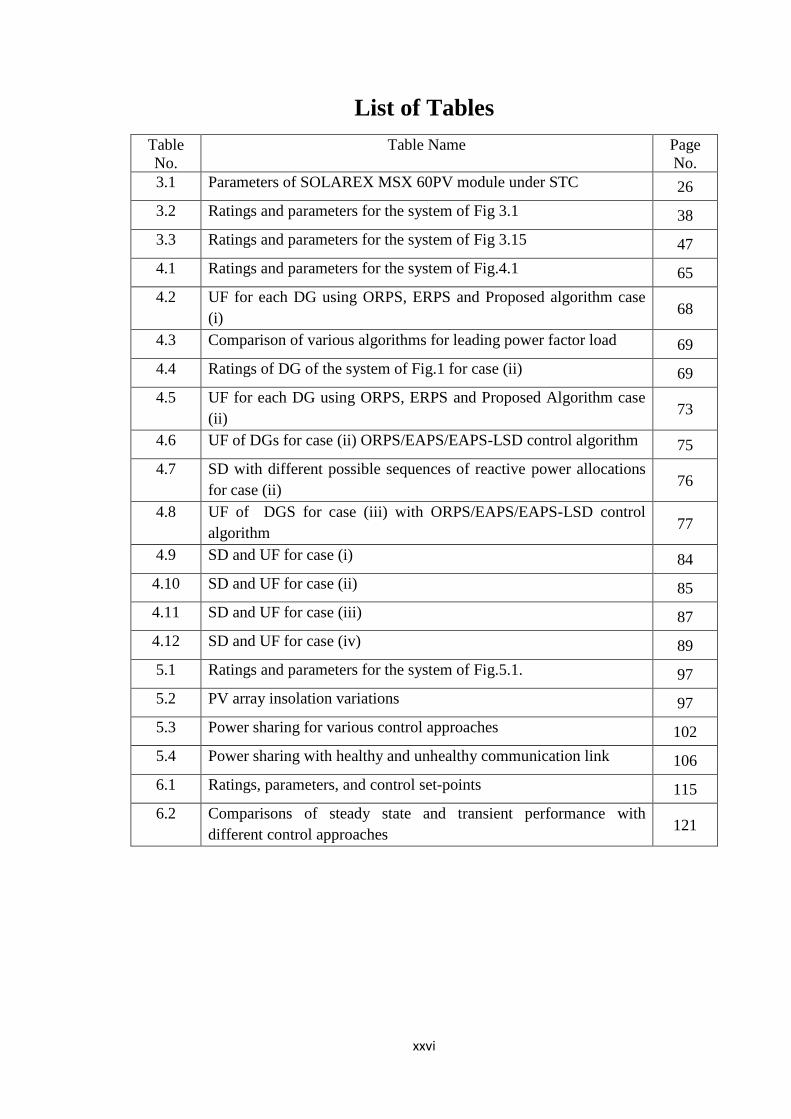
xxvi

List of Tables

Table

No.

Table Name Page

No.

3.1 Parameters of SOLAREX MSX 60PV module under STC 26

3.2 Ratings and parameters for the system of Fig 3.1 38

3.3 Ratings and parameters for the system of Fig 3.15 47

4.1 Ratings and parameters for the system of Fig.4.1 65

4.2 UF for each DG using ORPS, ERPS and Proposed algorithm case

(i) 68

4.3 Comparison of various algorithms for leading power factor load 69

4.4 Ratings of DG of the system of Fig.1 for case (ii) 69

4.5 UF for each DG using ORPS, ERPS and Proposed Algorithm case

(ii) 73

4.6 UF of DGs for case (ii) ORPS/EAPS/EAPS-LSD control algorithm 75

4.7 SD with different possible sequences of reactive power allocations

for case (ii) 76

4.8 UF of DGS for case (iii) with ORPS/EAPS/EAPS-LSD control

algorithm 77

4.9 SD and UF for case (i) 84

4.10 SD and UF for case (ii) 85

4.11 SD and UF for case (iii) 87

4.12 SD and UF for case (iv) 89

5.1 Ratings and parameters for the system of Fig.5.1. 97

5.2 PV array insolation variations 97

5.3 Power sharing for various control approaches 102

5.4 Power sharing with healthy and unhealthy communication link 106

6.1 Ratings, parameters, and control set-points 115

6.2 Comparisons of steady state and transient performance with

different control approaches 121

i

List of Appendices

Appendix A Load Model 137

1

CHAPTER – 1

Introduction

1.1 Introduction

Due to the ever growing demand of the energy, the conventional energy sources like oil

and fossil fuels are depleting at a very fast rate. With the increase in the depletion rate of

these sources, not only the cost of electricity generation has increased but also it is

aggravating issues like pollution, greenhouse gas emission, global warming etc. In this

context, power generation through renewable energy sources is gaining more attention

compared to power generation from conventional fossil fuels.

The power generation from these renewable sources like solar photovoltaic (PV), wind,

bio-mass etc. has brought a paradigm shift in the utility. The power generation earlier was

mainly dominated by few large centralized power plants and distributed to the remotely

located consumers through the transmission and distribution system. Today, in addition to

the centralized power plants, a significant share of power generation is through distributed

generators (DG). These DGs are relatively much smaller in capacity, located near to

consumers and distributed in nature, and often use clean source of energy to generate

electricity. These distributed generators (even referred as dispersed generators) can operate

independently to supply the load locally or can remain connected to the distribution

network to operate in the grid-connected mode to feed the power to the network.

This has led to the concept of Microgrid (MG) [1]. It represents an electrical network,

generally a low voltage distribution system formed of DGs, customers or loads and storage

devices (batteries, energy capacitors, flywheel etc.). MG offers a solution to integrate the

DGs of various technologies (PV, wind, biomass, fuel cell etc.) and different nature

(environmental dependence, response time) to work in a complementing manner to

improve the overall performance of the utility.

Introduction

2

Proper integration and control of the DGs in a microgrid could improve the utility’s

performance by providing several system support benefits like decrease in the power

transmission losses, improvement in the utilization of the resources, improvement in the

voltage profile of the system, congestion management etc. [2]. However, the variability

and the uncertainty in the output power of some of the DGs (e.g. based on PV and wind),

whose operation is characterized by the dependence on environmental factors, presents

certain challenges in attaining these objectives. The variations and the uncertainty in the

output power of the environmental dependent DGs can be matched by adding the reserves

or storage in the system, however at an extra cost. In case of sudden change in the output

power from these DGs, the reserve/storage system ensures the power balance thereby

maintaining the system stability.

The conventional rotating synchronous generators (SG), due to their inertia and capability

of reactive power control besides the active power exchange, are less vulnerable to sudden

transient changes in the load [3]. Hence, the issue of maintaining stability (rotor-angle

stability, voltage stability, frequency stability) is not a major concern with the system

dominated by synchronous generators. Compared to large SGs of the centralized power

plants, the DGs of the microgrid have either small or no inertia. The reason is static power

electronic converters through which most of the DGs are interfaced to the grid. As a result

any sudden change or disturbance in the system, either from the load side or the generation

side, may lead to sudden change in the frequency or the voltage resulting into the

instability. Hence, due to the inertia-less nature of DGs, it is difficult to ensure the dynamic

stability. Further the insufficient reactive power support mechanisms (due to their limited

inverter capacity or due to the restrictions placed by the grid or regulatory bodies) of the

DGs may not be able to contribute to the voltage regulation, which can adversely affect the

systems performance. The inadequate reactive power support may lead to low voltage

profile in a large portion of the network, which ultimately may cause transient instability,

since it may create electro-mechanical power imbalance at the SG [4]. The situation

worsens with the increase in the penetration level of the renewable energy source based

inertia-less DGs. The situation is even more critical when the operation is in an islanded

mode, where number of conventional power plants or rotational generators is less

indicating relatively little overall kinetic energy in the system. Hence, in order to maintain

both the voltage and the transient stability, it is must to ensure adequate reactive power

reserve into the system.

Introduction

3

The voltage support can be attained by deploying various reactive power support devices

like fixed or switched capacitors/reactors, excitation control, on load tap changing

transformers, flexible AC transmission system devices (FACTS) etc. The reactive power

support to a certain extent (if permitted by the utility) is also possible through DGs. The

inverter through which the DGs are interfaced to the grid can help in the reactive power

exchange.

Reactive power control through wind energy generation systems (WEGS) having power

electronic interface have been reported [5]. The reactive power capability of the WEGS

systems depend on the type of the generator (squirrel cage induction generator (SCIG),

wound rotor induction generator (WRIG) or permanent magnet synchronous generator

(PMSG)) and the rating of the converters used (fully rated or partially rated depending on

the configuration of WEGS). The PMSG has relatively better capability to meet the

reactive power support than that of the doubly fed induction generator (DFIG). But the size

of the converter for PMSG is larger as it has to handle full power as compared to that of

DFIG, where the grid side converter usually handles slip power.

Similar to that of the WEGS, the power electronic interface of PV based DGs could be

used to provide reactive power support. In the last couple of decade, the solar photovoltaic

(PV) has emerged as the most potential alternative of electricity generation due to its

modularity, easy and quick commissioning, pollution free nature, no maintenance etc.

Though the solar PV based DGs can contribute to reactive power support, the main focus

with PV based system has been restricted to provide the active power to the load or grid.

Just like WEGS, PV sources also present many challenges due to its environmental

dependency. Further, its non-linear operating characteristic varies with its orientation,

array configuration, shading pattern etc. [6]-[8]. The optimum utilization of the PV array

demands careful design of the PV array, its orientation, appropriate selection of the

converter and its components, appropriate maximum power point tracking algorithm etc.

[9].

Despite of the popularity of the PV based DGs and the fastest growth rate amongst the

various renewable based DGs, PV based DGs are not yet considered as the contributor for

reactive power support. The PV based DGs are mostly operated at unity power factor to

just supply the active power. But the active power delivered by DG depends on available

Introduction

4

PV power, which further is dependent on the irradiation. As a result the PV inverters are

under-utilized for most of the time of the day. Hence, it is possible to provide reactive

power support with the PV inverter to utilize the inverter effectively. However, unlike the

WEGS, reactive power support regulations are yet not that clearly framed or introduced in

form of the grid codes. But the increasing level of penetration PV based DGs demands to

tap the potential of these systems to provide support to the reactive power exchange.

Another important issue when several DGs are operating simultaneously in a given

network or a microgrid is that of sharing the active and reactive power judiciously amongst

the DGs. Improper operation or control of the DGs may not only lead to ineffective

utilization of the DGs, but may also lead to unequal loading of the lines (or DGs) and may

result into circulating currents between the DGs. The circulating current resulting from the

inaccurate reactive power sharing can be excessive in case the DGs share non-linear loads.

If due care is not taken in designing the active and reactive power sharing amongst the

DGs, it may lead to overloading of the inverters, increased losses, under-utilization of the

inverters, overall reduced efficiency etc. Thus, the task of active and reactive power

sharing amongst the PV based inverters is crucial and requires effective power

management system and requires the detailed study of the reactive power management

capabilities of the PV systems and the control strategies reported in the literature for the

MG having PV based renewable.

1.2 Overview of Thesis

The main contributions by the thesis are

Chapter 2 describes a literature review on the various modes of operation DGs in a

microgrid. It also investigates various active and reactive power control algorithms for the

DGs. Based on the literature review some important research gaps have been identified and

the objectives are set for the research work.

Chapter 3 details the mathematical analysis involved in the modeling of power electronic

converter based DGs operating in a microgrid. Model demonstrates operation of DG in

both the islanded and grid-connected mode as well as can have the smooth/seamless

transition between these modes.

Introduction

5

Chapter 4 proposes reactive power sharing algorithms that shares the reactive power based

on the remaining capacity (margin available after supplying the active power) of the

associated inverters of the PV based DGs. It results into better utilization of inverters and

prevent the overloading of the inverters. The effectiveness of the algorithms over other

methods is also illustrated through the simulation results.

Chapter 5 presents the modified droop control technique for active and reactive power

sharing amongst the DGs. It incorporates the proposed reactive power sharing algorithm

for reactive power sharing while the dynamic droop coefficient is introduced in the active

power vs. frequency (P-ω) droop to take care of the variations in the environmental

conditions. The effectiveness of modified droop control method is studied by analyzing its

performance with conventional droop control methods.

Chapter 6: Reactive power sharing is highly affected by miss-match in line impedances.

The effect of line impedance miss-match can be minimized by using virtual impedance and

the bandwidth can be improved by incorporating arctan function. The control method

incorporating these features is presented and the improvement in the performance over the

conventional method is highlighted through the simulation results obtained through

Matlab/Simulink.

Chapter 7 Finally presents the concluding remarks and future scope from the research

investigations.

6

CHAPTER – 2

Literature Survey

Electrical utility network has recently witnessed a major shift from the passive network

characterized by the unidirectional power flow to the active network that is characterized

by the bidirectional power flow capability. The characteristic of bidirectional power flow

in the network is attributed due to the presence of DGs. These DGs can significantly affect

the performance of the electrical network either positively if controlled properly or

adversely if not planned and operated in a coordinated manner. A microgrid can provide a

platform for these DGs to have their coordinated operation so that they can contribute in

improving the overall performance of the system. The chapter presents the review on the

fundamental of microgrids, operating modes, control strategies for power sharing between

these sources and the issues related with them.

2.1 Microgrid

The Microgrid (MG) represents an electrical network formed by the interconnection of

small, modular and dispersed energy generation sources like micro-turbines, fuel cells,

photovoltaic, etc., together with energy storage devices like flywheels, ultra capacitors and

batteries, etc., and usually controllable loads at low voltage distribution systems [10]. It

connects multiple DGs and storage to multiple consumers. Thus, it can be considered as a

small grid (or a zone or area) within the main grid or can also work independently of the

grid (if isolated).

A critical feature of the MG is its appearance to the surrounding distribution grid as a

single controllable system. It comprises of several DGs within it. Often a considerable

amount of generation through these DGs is from renewable sources like PV or wind. These

DGs require power electronic interface to integrate them in a microgrid. These power

electronic converters facilitate not only allows the desired exchange of power with the grid

Literature Survey

7

but also regulates the output signals (magnitude, frequency, harmonics etc.) within limits.

Thus, Power electronics provide the control and flexibility required by the microgrid

concept, ensuring that MG can meet its customers as well as utilities’ needs, e.g. improved

reliability, uninterrupted power supply, reduced feeder losses, support local voltage and

frequency and increased efficiency [11]. It enables high penetration of DGs without

redesigning of the entire system.

MG has three distinctive grid architectures, namely AC, DC and DC/AC distributions [12].

Amongst these architectures AC distribution is the most popular and commonly used

structure for microgrid, where the power is distributed to the AC loads through AC

distribution network. Hence, the sources like PV that generates DC and energy storage

devices like batteries are interfaced to the AC distribution through inverters. Fig.2.1 shows

the typical MG configuration. It consists of conventional and non-conventional DGs along

with the inverters, energy storage devices, hierarchical control system and associated local

loads. MG is connected to utility at a point of common coupling (PCC). The microgrid

central controller (MGCC) is a core of a hierarchical control system. At the lower level,

local controller (LC) and microsource controller (MC) exchange information with the

MGCC and maintains stable MG operations. The MGCC provides power set point to LC

and MC in order to control DGs to satisfy load’s power demand. The entire control system

is supported by communication infrastructure.

MG can operate in grid-connected mode in synchronization with the utility distribution

grid or in isolation in an islanded mode of operation from the utility distribution grid. MG

disconnects from the main grid when fault occurs on the utility grid and continue to

operate independently and serve its customers’ power needs and reconnects to the grid

once the problem is solved if the fault is removed.

In grid-connected mode, MG (or the DGs) is usually controlled as if a controllable power

source to exchange the desired power with the utility grid. The voltage reference needed

for the functioning of the DGs of the MG is provided by the grid. The active and reactive

power references for the DGs of the MG are set by MGCC. The MC usually operates its

associated inverter (or DG) as current source inverter (CSI) using active and reactive

power (P-Q) control [13]. It is ensured that the quality of power injected to the grid

matches the limits set by regulatory bodies or is as per the specified standards [14].

Literature Survey

8

FIGURE 2.1 Typical microgrid structure [10]

MG can island or separate from utility grid and can operate independently using static

switch (SS). Islanding may be intentional due to repair (or maintenance work) or

unintentional due to grid faults. Islanding operation is more critical as it presents several

challenges for the stable and safe operation of the MG as well as of DGs. Some of the

challenges for the MG operating in an islanded mode are ensuring power balance,

maintaining voltage and frequency deviations within limits, avoiding overloading of

inverters, minimizing circulating current, preserving good power quality etc. [15]

especially during the case of transient changes in the system. In the islanded mode of

operation, it is desired to have adequate energy storage in form of batteries, ultra

capacitors, flywheels etc. in the system to ensure initial power balance [16]. However, the

control strategies must ensure the state-of-charge (SOC) of energy storage system (ESS)

within certain range to stabilize frequency and voltage in the islanding mode [17].

In islanded mode, the DGs should also be responsible for frequency and voltage control.

Hence, the inverters of the DGs can be operated as voltage source inverter (VSI) using

voltage and frequency (V-f) control method [18]. Master-slave control and multi-master

control strategies can be employed for the control of these inverters [19]. In master salve

control, only one of the DGs (which is reliable and having relatively higher capacity) is

Literature Survey

9

operated in V-f mode to provide voltage and frequency references, whereas inverters of

other DGs acting as slaves are operated in P-Q mode [20], [21]. The master regulates the

voltage and provides the references for power sharing to the salve inverters. However

failure of master unit affects the system operations. To overcome this limitation, an

improved master/salve control, which incorporates priority window to provide random

selection of master, is proposed in [22]. However the performance of master may get

affected due to the current overshoot as it does not incorporate current control loop. In

multi-master approach, many inverters can operate as VSI in V-f mode with pre-defined

frequency/active-power and voltage/reactive-power characteristics. Simultaneously some

other DGs with P-Q control may also coexist [23]. But these approaches, which falls in the

category of centralized control, require data communication links for communication of

data and hence preferable for small scale system where distance between DGs is smaller.

However, if the DGs are scattered over large area, the decentralized approaches are

preferred as it does not require any communication link.

The islanding detection and reconnection of the island to the utility on the restoration of

the normalcy (i.e. fault removed) also demands attention as plug and play functionality is

the very important feature of the MG. Reconnection with the utility is only possible after

proper synchronization of voltage and frequency of MG with the grid. Resynchronization

techniques must ensure reconnection with the minimum transient in the overall system.

Thus, the reconnection of MG (or the DG sources) is acceptable only when the voltage

error, frequency error and the phase-angle error are within the range specified by the

regulatory standards like IEEE Std. 1547 [24]. Resynchronization techniques must ensure

reconnection with the minimum transient in the overall system.

Besides achieving the stable operation in either the grid-connected mode or the islanded

mode of operation, it is must to have the smooth transition between these two modes to

avoid any undesired frequency or voltage disturbances to the consumers operating in the

microgrid. This demands fast and effective switching between the P-Q and V-f control

strategies to have a seamless transition from grid-connected to islanded mode or vice-versa

[25]-[26]. A control technique using phase locked loop design for transition between the

two modes with minimum transient is reported in [27]. In [28] an admittance compensation

method is presented to reduce the transients during switching from islanded to grid

connected operation by implementation of inner voltage control loop to control the peak

Literature Survey

10

output current. In [29] the objective of smooth transition between the modes for a multi-

inverter (multi-DG) based system is realized using ‘upper-level’ controller whose function

is to identify the mode (i.e. mode attribute) and to provide the transfer commands for the

transition from one mode to another. The algorithm for mode transfer is implemented

using robust CAN communication. The accurate power flow control along with proper

current sharing amongst the DGs is achieved through the dual-loop voltage control. The

control strategies for seamless transfer between modes require fast islanding detection

scheme. Various active and passive islanding detection methods are reported to detect the

grid abnormal conditions [30], [31].

2.2 Active and Reactive Power Sharing amongst Conventional DGs

The microsources (MS) based on their interfacing medium can be either classified as direct

coupled conventional rotating machines, such as generator driven by gas turbine or a diesel

engine generator, or energy sources(such as microturbines, fuel cell, photovoltaic and wind

based generators) interfaced through the static power electronics converters (PEC) [32].

However, energy sources interfaced through PECs present considerable complexity and

challenges due to the diverse nature of the sources and practically no inertia (due to static

PEC). These power electronic converters are fast to respond and hence, can help in

improving the overall performance. But they have low sustained overload capability and

also leads to issues like harmonic generation, interaction amongst sources, resonance etc.

However, if properly managed, coordinated and controlled, they can provide distinct

benefits to the overall system performance [33]. The system performance can be improved

if the issues related to accurate sharing of active–reactive power, voltage–frequency

regulation, optimal power flow control, etc. are properly addressed with appropriate

control strategies. These objectives are of different kind and require different control on

timescales. Each objective requires a control structure at different hierarchy. The

hierarchical control architecture is based on primary, secondary and tertiary control as

shown in Fig. 2.2 [34]-[36]. The objective of the primary control is to maintain voltage and

frequency to nominal values by sharing power in proportion to the DGs ratings. The

secondary control’s role is to compensate voltage and frequency deviations caused by the

primary control, while the tertiary control, which is the slowest on the timescale, manages

power transfer between MG and main grid by operating optimal power sharing algorithms.

Literature Survey

11

FIGURE 2.2 Hierarchical control levels of a microgrid [34]

The primary control of the centralized control approach addressed in [37] consists of

voltage and current control loops to operate inverters either in P-Q mode or V-f control

mode. It consists of outer power control loop, which calculates current references for inner

current control loop. The review of various control strategies for power sharing is reported

in [38]. It mainly discusses some of the primary control methods for power sharing

amongst the inverters. These methods include control strategies like

centralized/concentrated control, mater/slave control, distributed control [39]-[41], which

require communication link for exchanging the information for calculating the references

for sharing power. All these reactive power management methods can achieve excellent

voltage regulation with accurate power sharing. However these control strategies require

communication links for exchange of data, which increases system cost and reduces

system reliability.

Unlike the centralized control, the decentralized control does not require any

communication links and rely mainly on the local measurements for the power sharing.

Literature Survey

12

Decentralized control can be implemented using droop based control, which improves

redundancy and reliability of a system by avoiding use of high cost and complex network

[42]-[43]. In droop control, power sharing is achieved by active power/frequency (P-ω)

and reactive power/voltage (Q-V) droop characteristic. The conventional P-ω and Q-V

droop control is applicable for the case where high inductive equivalent impedance is

present between the grid and VSC [44]. The active and reactive power can be controlled

independently (i.e. decoupled control of P and Q) using P-ω and Q-V relationships,

respectively. This is no longer applicable with medium transmission line representing

complex impedance, which results into coupling effect between active and reactive power

control [45]. As a result, the conventional droop control may lead to error in the power

sharing. The error in reactive power sharing can also result from the mismatch in feeder

impedance, which can cause circulating current to flow amongst the inverters. Thus the

accuracy of reactive power sharing is highly dependent on the value of line impedance,

resistance to reactance ratio of the line (R/X), voltage setting of inverters etc. [46]. Mostly

the researchers have focused on modifications of the conventional droop control technique

to reduce the error in reactive power sharing caused by the impedance mismatch. In [47] a

method to reduce the effect of voltage drop caused by the filter impedance on the Q-V

droop control is addressed. However the accuracy of power sharing is still affected by

unequal line impedances. Another approach of frame transformation is addressed in [48],

where the accurate reactive power sharing is achieved by transformation angle

information. However, it results into slow dynamics due to added current loop. An

adaptive droop controller in which the phase angle is estimated by phase locked loop to

determine the frame transformation angle is proposed in [49].The virtual impedance based

improved droop control is presented in [50]-[52]. The virtual impedance based control is

operated with a view to match the per unit output impedances of the inverters operating in

parallel by creating a voltage drop across a virtual impedance. The virtual impedance

creates a “voltage drop” without resulting into any actual active and/or reactive power

consumption. The virtual impedance based droop control method reported in [53] provides

good transient behavior in accurate reactive power sharing. The transient behavior can

further be improved by the addition of arctan function introduced by [54]. The arctan

droop control removes the constant frequency droop slope and replaces it with an arctan

algorithm. The arctan function ensures the operating frequency of MG within preset

bounds.

Literature Survey

13

Most of these methods thus address improvement in the accuracy of the reactive power

sharing accuracy by reducing errors due to the impedance mismatch. Further, in all these

approaches the load is shared amongst energy sources in proportion to their ratings using

the fixed droop coefficient. These methods do not consider the nature of the energy source,

for example the dependency on the environment of PV or wind based DGs, in the power

sharing. Hence, the power sharing strategies discussed above may not work satisfactorily

for such sources.

2.3 Introduction to PV based DG

Amongst various renewable energy sources, photovoltaic (PV) has emerged as one of the

most potential energy sources to provide clean energy. The reason for its popularity is the

decrease in cost of PV modules and the lucrative feed-in-tariff policies by the

governments. The PV provides promising option for grid-connected systems as well as for

off grid applications as local power supply. The capacity of PV based system has reached

the level of 250 MW and above [55]. Thus, it is appearing as a key component in the future

energy mix which can solve energy dilemma of human community. Hence, the significant

potential of PV based DGs shall be effectively utilized through the concept of MG [56].

However, PV based DGs present certain challenges which must be addressed to realize the

benefits from the PV based DGs [57]. The challenges are due to uncertain and intermittent

nature of PV, which is largely environmental dependence. Further, the size of the PV based

systems varies from few kWs to several MWs. Also PV source is connected to the grid

through the PEC. Thus, it is inertia-less source of energy unlike the conventional rotational

generators. Due to this PV sources are not capable to support dynamic behavior of MG

during transient conditions without any storage support [58]. Thus the presence of PV

source in MG increases challenges to maintain the stability in case of power imbalance

caused due to the variations in solar irradiance, passing clouds, change in load etc. While

ensuring the above objective of the power balance, the control strategy for the PV based

DGs must ensure that the energy drawn from the storage is the minimum and the PV array

is always effectively utilized.

Literature Survey

14

2.3.1 PV Cell Characteristic and Model

The PV cell can be modeled using a single-diode model or a two-diode model shown in

Fig. 2.3. The two-diode model represents PV cell as a DC current source in parallel with

two diodes that represent currents flowing due to diffusion and charge recombination [59],

[60].

(a) Two-diode model (b) One-diode model

FIGURE 2.3 PV cell models

Two resistances Rsh and Rs represent contact resistance and internal PV cell resistances,

respectively. The two-diode model can be converted to single-diode model [61] by

neglecting current flowing through D2 as shown in Fig. 2.3(b). It is widely used for PV

application as it is sufficient to represent PV nature and dynamics. However two-diode

model is more precise compared to one-diode model. The PV cell characteristic is non-

linear in nature as the PV array output power changes with the change in sun direction,

solar irradiations and temperature. For a particular operating condition, there is single

maximum power point (MPP) in a PV characteristic as shown in Fig. 2.4.

FIGURE 2.4 I-V characteristic of a PV cell

Literature Survey

15

It is desirable to operate PV array near to this MPP to get maximum utilization of the PV

array. The technique employed to operate the PV array at this point is known as maximum

power point tracking (MPPT). The performance of PV source can be improved against the

variations of solar irradiations using MPPT techniques. Various MPPT methods have been

reported in the literature since 1960 [62]. The most common algorithm reported are Perturb

and Observe (P&O) and incremental conduction (INC) methods. The INC algorithm offers

higher efficiency than the P&O under rapidly varying irradiation conditions.

2.3.2 Grid Interface for PV system

The grid interface for the PV system varies depending upon the power to be exchanged,

voltage level of the grid (where interfacing is required), environmental conditions, desired

power quality, efficiency, reliability, etc. The PV interface may be broadly classified based

on the number of power conversion stages or based on the popular PV system

configurations centralized PV inverter, string PV inverter, multi-string PV inverter or

module level inverter [63]-[65].

PV source can be termed as a single-stage or two-stage conversion system based on the

number of power conversion involved for interfacing the PV array with the grid. The

single-stage system uses single inverter for PV and grid interfacing. It incorporates both

the MPPT and the current shaping feature through the inverter. Hence, it requires lesser

components and has higher conversion efficiency [63]. But it suffers from drawback of

voltage ripple of double the grid (fundamental) frequency on the dc bus due for a single

phase connection [64]. A two-stage conversion system consists of additional DC-DC

converter as first stage along with the inverter at the second stage [65]. The first stage

boosts the PV array voltage along with maximum power point tracking (MPPT) whereas

second stage employs DC to DC converter and does the current shaping. The additional

stage increases components cost and losses but it decouples the grid and the PV array due

to the presence of the intermediate dc-link capacitor. Also additional stage boosts the

voltage level and allows one to use less numbers of PV modules in series thereby reducing

the effect of partial shading and hence, minimizing the chances of possible power loss due

to the partial shading.

Literature Survey

16

The other way of classification of the PV system, as mentioned above, is based on the

interface required depending on the PV array configuration. The most popular amongst

them is the centralized inverter configuration. Though the centralized inverter being the

simplest and the cheapest, it lacks modularity and suffers from the issue of losses

mismatch as it involves a single maximum power point tracking (MPPT). Unlike it the

string PV inverter configuration has one inverter per string and hence, overcomes the

above limitations, at the higher cost. The multi-sting inverter configuration embraces the

advantages of both these converters. The DC-DC converter used with each string provides

MPPT for each PV string, while the single inverter helps in exchanging the power with the

grid.

The power electronics interface mentioned above, irrespective of its configuration or the

number of stages, must meet certain criteria that are enforced by the utilities. The

regulations are imposed in form of the grid codes for the DGs in most of the countries. It is

also tried to have some consensus in form of a common standard across the countries for

these DGs by some of the international agencies like IEEE (Institute of Electrical and

Electronic Engineers) in the US, IEC (International Electrotechnical Commission) in

Switzerland and DKE (German Commission for Electrical, Electronic and Information

Technologies of DIN and VDE) in Germany, etc.These standards mention about the

allowable power quality, design and operational conditions, safety measures, tripping time

in case of abnormal conditions, reconnection time, test procedures etc. For PV and other

inverter based sources, IEEE 929-2000: ‘Recommended Practice for Utility Interface of

PV Systems’ [66] has the longest history and probably is the most used standard.

However, today IEEE 1547-2003 [24], ‘Standard for Interconnecting Distributed

Resources with Electric Power Systems’ is considered as the most important standard for

interfacing of all types of DGs. It mentions about general requirements, power quality,

response under abnormal conditions, islanding and design and test conditions, installation,

commissioning etc. It is applicable for interfacing DG at medium as well as low-voltage

distribution networks. It mentions that the PV based DGs need to be disconnected from the

utility in case of abnormal grid conditions in terms of frequency and voltage. The PV

inverters must be disconnected in 0.16s if the voltage at PCC (VPCC) <0.5Vnom; in 2s if

0.5Vnom<VPCC<0.88Vnom; in 1.0s if 1.1Vnom < VPCC<1.2Vnom and in 0.16s if VPCC>1.2Vnom

where Vnom is the standard/nominal grid voltage. Likewise the IEC 61727 mentions that

Literature Survey

17

the PV inverters must be disconnected in 0.1s VPCC < 0.5Vnom; in 2s if 0.5Vnom <

VPCC<0.85Vnom; in 2.0s if 1.1Vnom < VPCC<1.35Vnom and in 0.05s if VPCC>1.35Vnom [67].

The VDE 0126-1-1 just mentions a single range for disconnection in case of the voltage

deviations [68]. The DG must be disconnected in 0.2s if 1.1Vnom < VPCC <0.85Vnom.

Similarly the disconnection time for the frequency variations are also mentioned by these

standards. According to IEEE 1547, IEC 61727 and VDE 0125-1.1 the disconnection times

are 0.16s, 0.2 and 0.2s, respectively if the frequency violates the limits 59.3-60.5Hz, 49-

51Hz and 47.5Hz-50.2Hz, respectively.

The quality of the power injected by the PV system into the grid or to the load is also a

major concern and is governed by practices and standards on voltage, flicker, frequency,

harmonics and power factor. The PV system shall disconnect from utility if these standards

are violated. As the DC component may saturate the transformers, the PV systems are not

allowed to inject the DC current component beyond 0.5% of rated RMS current as per

IEEE 1574. The limit set by IEC 61727 and VDE 0126-1-1 are 1% and 1A, respectively.

Regarding the current harmonics injected by the DGs, the limits set by IEEE 1547 and IEC

61727 are same. According to these standards the amplitudes of the odd current harmonics

of the order lower than 11th must be less than 4% (even harmonics 25% of that of odd

harmonics permissible) of the fundamental while the THD must be less than 5%. In IEC

61000-3-2 sets the harmonic limits as IEC 61727 is yet not approved in Europe.

Most PV based grid-connected DGs are designed to operate at the unity power factor or

close to it. However, for PV installations with large capacity local grid requirements apply

as they may participate in the grid control. IEEE 1574 being a generalized standard it

allows the PV based DGs to have reactive power exchange like other DGs. Even the

requirements about power factors are not mentioned in VDE 0126-1-1. It is the only IEC

61727 that states that PV based DG shall have an average lagging powerfactor greater than

0.9 when the output is greater than 50 %.

In general the following parameters are of interest for designing the control of PV inverters

[69]:

• Voltage harmonic levels (5th , 7th and 11th less than 6%, 5% and 3.5% of

fundamental)

• Maximum voltage THD <5 %.

• Current harmonics (as mentioned above) with THD < 5%

Literature Survey

18

• DC component < 1%

• Maximum voltage unbalance for three-phase inverters : 3 %.

• Voltage amplitude variations: maximum ±10 % of standard voltage.

• Frequency variations: maximum ±1 % of standard frequency.

• Voltage dips: duration<1 sec with deep< 60 % of that of fundamental

• Power factor > 0.9

2.4 Active and Reactive Power Sharing with PV based DGs

Often the grid-connected DGs are allowed to just exchange active power with the grid.

Hence, most of the PV inverters are operated as current source inverter (CSI) to deliver

only active power to the grid i.e. controlled to operate at a unity power factor. However, as

the active power delivered by PV based DG depends on active power from PV array,

which is further dependent on the irradiation or time of the day, the PV inverters are under-

utilized for most of the time of the day. Hence, it is possible to provide reactive power

support with the PV inverter to utilize the inverter effectively. Now-a-days the grid

regulations are also relaxed and the DGs are allowed to have the reactive power exchange

as well [70].

As the level of penetration of PV based DGs is increasing, it is prudent to tap the potential

of these systems to provide support to the reactive power exchange. Therefore, it is

essential that the control scheme for the PV based DGs should ensure proper reactive

power sharing amongst inverters besides the extraction of maximum power from the PV

arrays. There is a lot of research invested on the issues related to the reactive power

management amongst the DGs operating in the microgrid. However, the reactive power

management; especially when several PV based DGs are connected in parallel or operating

in a grid is a challenging task [71].When several PV sources are operating simultaneously

in the grid, due care must be taken to distribute the reactive power (besides the active

power) amongst the inverters especially under conditions like unidentical ratings of DGs,

rapidly varying irradiations, miss-match in impedances, load transients etc.

The conventional droop techniques can be used for sharing or allocating reactive power

besides that of active power. However, the active and reactive power sharing using

conventional droop is based on fixed droop coefficient irrespective of available energy

Literature Survey

19

from nonconventional energy sources like PV and wind [72]. The frequency and the

voltage set points are mainly determined by the load and it ignores the variation in active

power. This may affect the effective utilization of the PV sources when working with

conventional droop control. For example, with the conventional droop control, a drop in

generation of one PV based DG causes reduction in output of other DGs operating in

parallel i.e. if the output power of one of the PV based DG decreases, its frequency

increases (operating point on the P-ω shifts left and upwards). As other DGs must operate

at the same frequency, they must reduce their output, thereby forcing the auxiliary source

to supply more power. Thus, an auxiliary source with large capacity, to maintain power

balance and stability, is required.

In [73] dynamic droop load sharing is proposed, wherein the insensitivity of the

conventional droop control is modified by incorporating dynamic droop parameters.

However, PV source is not operated at the MPP and its effectiveness for various load

conditions is not explored. An enhanced droop control, which shares active power amongst

paralleled two-stage PV inverters by varying the dc link voltage within a reasonable range,

is reported in [74]. But the operation of the PV array is not maintained at the MPP and

even nothing has been mentioned about the reactive power sharing amongst the PV

inverters. Also, the absence of storage may result into instability, especially when

operating with low irradiation level or with rapidly varying load. In [75] battery storage is

utilized to ensure power balance and hence, stability. The active power required by the

load is shared based on the available power from PV array and the state-of-charge (SOC)

of the battery unit. The control strategy employing a universal controller that does not

require reconfiguration for different modes of operation is reported in [76]. The controller

embeds the functions of droop control, dc-link voltage regulation and MPPT. The PV

sources operate at the MPP. But the loading range is limited and the system exhibits slow

response. In [77] voltage based droop controller is employed to integrate renewable

sources for power sharing. It employs the P-Vdc control (i.e. relationship between active-

power and dc link voltage) along with constant power band for effective utilization of the

PV arrays. In these researches, the researchers have tried to include the variable and

intermittent nature of the PV based DGs in the control scheme for sharing the active

power. However, they have not focused on the effect of variable nature of PV on the

reactive power sharing.

Literature Survey

20

As the active power that the PV based DG can supply vary, the available margin for the

DG to support the reactive power also varies. Thus, the reactive power injection/absorption

capability is actually constrained by the available margin with the inverter besides that of

the local load requirement and/or the grid regulations [78]. However, fixed Q-V droop

based control ignores it and hence, if the reactive power demand increases, it is shared

amongst the inverters as per the fixed droop set initially. As a result, the inverter of the DG

supplying more active power is likely to operate near its rating or may get overloaded [78].

The accurate reactive power sharing is also desired to reduce the errors introduced due to

voltage unbalance which may cause the circulating current amongst the DGs that may

result into overloading of inverters. The reactive power sharing algorithm addressed in [79]

takes into account the apparent power limit of the inverter and the active power available

from PV source and shares reactive power proportionally amongst the inverters such that

the inverter overloading is avoided. The algorithm is implemented using hierarchical droop

control approach. The primary control is implemented using droop control whereas

reactive power sharing algorithm is divided between primary and secondary control unit.

However, the algorithm is not able to utilize the maximum available apparent power

capacity of inverter. In addition, unlimited storage is considered to achieve the power

balance. In [80], optimal reactive power sharing strategy (ORPS) is proposed for large

scale PV inverters. ORPS control aims to achieve maximum power transfer capability of

the entire system by assigning reactive power to each inverter in proportion to the active

power delivered by the inverter. However, in case of large variations in the active power

supplied by the inverters, the inverter supplying higher active power may get overloaded or

may operate towards its upper limit. On the contrary, the inverter supplying lesser active

power supplies less reactive power, thus resulting into its under-utilization in terms of its

apparent power transfer capability. Sharing of reactive power equally amongst the

inverters is addressed in [81]. Equal reactive power sharing [ERPS] control approach

addressed in [81] divides reactive power demand equally amongst inverters. Thus, as the

reactive power is equally shared by the inverters, irrespective of the active power supplied

by them, it leads to unequal utilization of the inverters. Another approach presented in [82]

is based on proportional reactive power sharing, where the total reactive power is divided

amongst the inverters in proportion to the active power supplied through them. Reactive

power sharing with other approach to minimize the transmission power losses is addressed

using optimization algorithm in [83]-[84]. However the equal utilization of inverter is not

addressed with respect to reactive power sharing.

Literature Survey

21

Thus, it is required to further investigate the issue of active and reactive power sharing

amongst PV based DGs operating in a microgrid with a view to effectively utilize the

resources, to avoid their overloading, to minimize the storage requirement etc.

2.5 Objective and Scope of work

Conventional droop control approach is highly dependent on the value of line impedance,

R/X i.e. resistance to reactance ratio of the line, voltage setting of inverters etc. These

factors lead to issues like voltage control, accurate sharing of active and reactive power,

inverter overloading and synchronization with other inverters as well as circulating current.

Modified droop control methods are reported in the literature to solve the issues related to

reactive power sharing. However issues when operating with sources like PV and other

environmental dependent sources like improper utilization of inverters or PV source,

overheating or reaching the limit of inverter, power loss etc. are not addressed to a great

extent. Most of the studies carried out so far have ignored the real or actual dynamic

characteristics of the dispersed energy sources involved in the micro-grid and also the

interaction among these resources. Hence, it does not allow the realization of true

operation of a microgrid, which is largely influenced by the dynamics of dispersed energy

resource. If inverter capacity is utilized by considering active power delivered by PV, it is

possible to have the maximum utilization of the inverters (and DGs) without overloading

of any inverter. This research focuses on this issue and accordingly the objective of the

research is set as follows:

To investigate the various issues related to reactive power sharing in the microgrid

comprising of PV based distributed sources and hence, to devise a control strategy for

the distributed generators which can share the reactive power based on the available

margin (rather that the nominal capacity).Further the control scheme must ensure

effective utilization of the inverters used for interfacing DGs, effective utilization of

the PV sources and minimum storage requirement besides providing the capability to

operate in grid-connected and islanded mode,

To achieve these objectives, the scope of work includes:

Literature Survey

22

1. To study, model, simulate and evaluate microgrid operation in grid connected mode

and islanded mode.

2. To investigate the issues with the conventional and some other control strategies

reported in the literature in sharing the power amongst the sources in a microgrid

comprising of PV based DGs.

3. To devise reactive power sharing algorithm for the DGs of identical and unidentical

ratings to achieve the objectives mentioned above.

4. To define a parameter for comparison of the new power sharing algorithm with the

control schemes and to evaluate these methods for various loads and/or

environmental conditions.

5. To evaluate the effect of mismatch in the line impedances on reactive power

sharing and to minimize the error.

23

CHAPTER – 3

Modeling and Control of DGs in a Microgrid

As mentioned in the previous chapter, a microgrid is characterized by the presence of

distributed generators (DGs). These DGs can operate in a grid-connected mode or in an

islanded mode of operation. In grid-connected mode the control objective is to exchange

real and reactive power with the grid as voltage is imposed by utility grid. In this mode

inverter is usually operated as a controlled current source using P-Q control technique.

Unlike the grid-connected mode, in islanded mode DG must regulate the voltage and

frequency. Due to faults or some abnormalities the MG may need to be islanded and again

must be connected to the grid when the normal operating conditions are restored. Thus, the

microgrid (or the inverters of the DGs) must be controlled appropriately to provide stable

operations in both the islanded or grid-connected modes and must smoothly i.e. seamlessly

transit between the two modes. This chapter presents the modeling of the PV based DGs

and the control scheme for their operations in islanded and grid-connected mode as well as

the transition between these modes. Transition between the two modes is achieved with

appropriate switching of P-Q and V-f mode control of inverters.

3.1 System Configuration

Fig.3.1 shows a microgrid comprising m numbers of PV based DGs connected in parallel

with the utility grid at the point of common coupling (PCC). PV1 through PVm represents

the PV array along with the DC-DC converter that acts as a MPP tracker and helps in

stepping up the voltage. The DG unit thus consists of a PV array as a primary energy

source, a DC-DC converter, a three phase inverter and an LC filter. The MG is connected

to the main grid through a static switch and a transformer. The static switch, transformer

and the associated control of converters are not shown here in Fig.3.1 for the sake of

simplicity/clarity. The static switch when closed, the MG operates in a grid-connected

mode and functions in an islanded mode when the static switch is open. The impedance

(Z01-Z0m) takes into account impedance of interfacing inductor, line, filter and isolation

Modeling and Control of DGs in a Microgrid

24

transformers. The reference set points of active and reactive power to be delivered is

provided by the MGCC. The grid-connected and islanded modes of operation of MG along

with the detailed control schemes are elaborated in the sections 3.3 and 3.4. Following

section present the modelling of a PV source along with the MPPT control.

FIGURE 3.1 System configuration of a microgrid considered for study

3.2 Modeling of a PV Source

A PV source can be modeled as a current source in parallel with the diode. The commonly

used single-diode model of a PV cell is shown in Fig.3.2. It consists of a current source to

represent the photo current (IPH), which is mainly dependent on the insolation it receives.

A diode parallel to current source is due to the inherent P-N diode nature of the PV cell.

The current through it is represented by ID. Rsh (which carries current ISH) and Rs (which

carries current I) represent internal parasitic resistances to take into account internal power

Modeling and Control of DGs in a Microgrid

25

loss in the PV cell. Rsh originates due to the fabrication defects while Rs is due to the

resistance of the bond between the cells and the semiconductor itself [59]-[60].

FIGURE 3.2 One-diode model of a PV cell.

The I-V characteristic equation of a PV cell can be expressed using (3.1)-(3.3)

SHDPH IIII −−= 3.1

]1)Tk

qV[exp(II 0D −

=

3.2

where, I0 is the reverse saturation current of the diode D in ampere, q is the electron’s

charge [1.60217646˟10-19C], K is the Boltzmann constant [1.3806503˟10-23J/K], T is the

temperature of the p-n junction in Kelvin and 𝛼 is the diode ideality factor.

The elementary PV cell can be represented by (3.3) where ISH is ignored (as Rs and Rsh are

not considered).

]1)Tk

qV[exp(III 0PH −

−=

3.3

But representation of a practical module requires additional parameters, Rs and RSh. With

these parameters the I-V characteristic is represented by (3.4)

sh

ss0PH

R

IRV1

TK

)IRV(qexpIII

+−

−

+−=

3.4

A photovoltaic module consists of multiple PV cells connected in series to provide a

higher output voltage/power. For large commercial and utility scale PV systems large

number of such modules are connected in series and parallel to form a PV array to supply

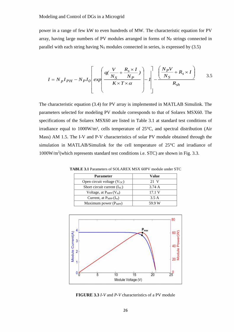
Modeling and Control of DGs in a Microgrid

26

power in a range of few kW to even hundreds of MW. The characteristic equation for PV

array, having large numbers of PV modules arranged in forms of NP strings connected in

parallel with each string having NS modules connected in series, is expressed by (3.5)

sh

sS

P

P

s

S0PPHp

R

IRN

VN

1TK

)N

IR

N

V(q

expININI

+

−

−

+

−=

3.5

The characteristic equation (3.4) for PV array is implemented in MATLAB Simulink. The

parameters selected for modeling PV module corresponds to that of Solarex MSX60. The

specifications of the Solarex MSX60 are listed in Table 3.1 at standard test conditions of

irradiance equal to 1000W/m², cells temperature of 25°C, and spectral distribution (Air

Mass) AM 1.5. The I-V and P-V characteristics of solar PV module obtained through the

simulation in MATLAB/Simulink for the cell temperature of 25°C and irradiance of

1000W/m2(which represents standard test conditions i.e. STC) are shown in Fig. 3.3.

TABLE 3.1 Parameters of SOLAREX MSX 60PV module under STC

Parameter Value

Open circuit voltage (VOC) 21 V

Short circuit current (ISC) 3.74 A

Voltage, at PMPP (Vm) 17.1 V

Current, at PMPP (Im) 3.5 A

Maximum power (PMPP) 59.9 W

FIGURE 3.3 I-V and P-V characteristics of a PV module

Modeling and Control of DGs in a Microgrid

27

The I-V characteristic of the PV module is similar to the characteristic of a voltage source

in the higher voltage range (from 85-90% of Voc to Voc) whereas it exhibits the nature of a

current source in the lower voltage ranges (i.e. from 0 till 60-70% of Voc). In between these

ranges of the PV voltage, the I-V characteristic is non-linear in nature and the power output

of the PV in this range is high and near to its maximum value. It is observed from the P-V

curve shown in Fig. 3.3, that there exists a unique operating point defined as maximum

power point (MPP) where a maximum power (PMPP) is available from the module [62].

The power on either side of the MPP decreases hence, the rate of change of power with

respect to change in voltage at MPP is zero.

The PV and grid interfacing is achieved using two stage conversion system. The MPPT

method used in this research is Perturb & Observe (P & O) technique [63]. In P&O

method, the control parameter (duty-cycle) is periodically perturbed and PV output power

and the voltage are measured. From the comparison of the output power and the voltage

for the two successive duty-cycles (or control parameters), one before perturbation and

another after perturbation, the sign or the direction of the next perturbation is determined.

The MATLAB simulation results for two-stage PV system showing the MPPT tracking are

given in Fig.3.4.

FIGURE 3.4 Performance showing MPPT: (a)Voltage (Vm) at MPP, (b)Current (Im) at MPP and

(c) Maximum power PMPP

Modeling and Control of DGs in a Microgrid

28

The results shown are obtained with a PV array formed from PV modules having

parameters indicated in Table 3.1. The PV array comprises of 266 strings in parallel, each

having 25 modules connected in series (NP= 266 and NS=25). During t=0-1s, irradiance on

the PV array is considered as 1000W/m². The irradiance decreases to 500W/m² at t=1s.

The temperature is considered as 25°C throughout. Fig. 3.4(a)-(c) shows the maximum

current (Im), the maximum voltage (Vm) and the maximum power (PMPP) corresponding to

the MPP obtained with P&O MPPT control algorithm. The voltage (Vm) at which the

maximum power occurs (corresponding to MPP) remains almost constant as shown in Fig.

3.4 (a). It is observed that during t=0-1s, the maximum power extracted (Pmax) from PV

array is 400 kW. At t=1s, the reduction in irradiation to 500 W/ m2 results into reduction in

the current at MPP to almost half the previous value as shown in Fig. 3.4 (b). As a result

output power of the PV system also reduces to half i.e. 200 kW as shown in Fig. 3.4 (c).

3.3. Control of DG in Grid-Connected Mode

Fig. 3.5 shows detailed schematic diagram of one of the DGs of Fig.3.1. It employs the

control using d-q reference frame. R1, L1 and Cf1 represent line and filter parameters. The

PV array and associated dc-dc converter is controlled to extract maximum power from PV

using MPPT algorithm by the MPPT controller. Inverter is controlled in P-Q mode by

regulating inverter output current using current control loop. It also incorporates outer

power control loop and dc link voltage control loop. The synchronizing angle required for

abc-dq frame transformation is provided by phase locked loop (PLL).

FIGURE 3.5 Control scheme for DG1 unit in d-q frame when operating in grid-connected mode

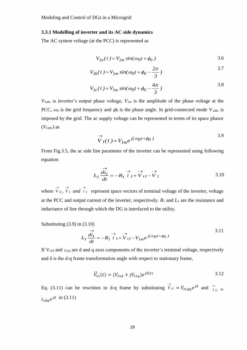
Modeling and Control of DGs in a Microgrid

29

3.3.1 Modelling of inverter and its AC side dynamics

The AC system voltage (at the PCC) is represented as

)tsin(V)t(V 00m1a1 += 3.6

)3

2tsin(V)t(V 00m1b1

−+=

3.7

)3

4tsin(V)t(V 00m1c1

−+=

3.8

V1abc is inverter’s output phase voltage, V1m is the amplitude of the phase voltage at the

PCC, ω0 is the grid frequency and 𝜙0 is the phase angle. In grid-connected mode V1abc is

imposed by the grid. The ac supply voltage can be represented in terms of its space phasor

(V1abc) as

)0t0(jm11 eV)t(V

+→

=

3.9

From Fig.3.5, the ac side line parameter of the inverter can be represented using following

equation

11t111

1 VViRdt

diL

→→→→

−+−=

3.10

where 1tV→

, 1V→

and 1i→

represent space vectors of terminal voltage of the inverter, voltage

at the PCC and output current of the inverter, respectively. R1 and L1 are the resistance and

inductance of line through which the DG is interfaced to the utility.

Substituting (3.9) in (3.10)

)0t0(jm11t11

11 eVViR

dt

diL

+→→

→

−+−=

3.11

If Vt1d and Vt1q are d and q axes components of the inverter’s terminal voltage, respectively

and δ is the d-q frame transformation angle with respect to stationary frame,

𝑡1(𝑡) = (𝑉𝑡1𝑑 + 𝑗𝑉𝑡1𝑞)𝑒𝑗𝛿(𝑡) 3.12

Eq. (3.11) can be rewritten in d-q frame by substituting 1tV→

= 𝑉𝑡1𝑑𝑞𝑒𝑗𝛿 and

1ti→

=

𝑖1𝑑𝑞𝑒𝑗𝛿 in (3.11)

Modeling and Control of DGs in a Microgrid

30

𝐿1

𝑑

𝑑𝑡(𝑖1𝑑𝑞𝑒

𝑗𝛿) = −𝑅1(𝑖1𝑑𝑞𝑒𝑗𝛿) + (𝑉𝑡1𝑑𝑞𝑒

𝑗𝛿) − 𝑉1𝑚𝑒𝑗(𝜔0𝑡+𝜙0)

3.13

Phase locked loop (PLL) can be used to estimate angle (δ) required for abc to d-q

transformation.

Eq. (3.13) can be expressed as

𝐿1

𝑑

𝑑𝑡(𝑖1𝑑𝑞) = −𝑗(𝐿1

𝑑𝛿

𝑑𝑡)𝑖1𝑑𝑞 − 𝑅1(𝑖1𝑑𝑞) + (𝑉𝑡1𝑑𝑞) − 𝑉1𝑚𝑒𝑗(𝜔0𝑡+𝜙0−𝛿)

3.14

Eq. (3.14) is decomposed into its real and imaginary components represented by

(3.15) and (3.16), respectively.

𝐿1

𝑑𝑖1𝑑

𝑑𝑡= (𝐿1

𝑑𝛿

𝑑𝑡)𝑖1𝑞 − 𝑅1(𝑖1𝑑) + (𝑉𝑡1𝑑) − 𝑉1𝑚 cos(𝜔0𝑡 + 𝜙0 − 𝛿)

3.15

𝐿1

𝑑𝑖1𝑞

𝑑𝑡= −(𝐿1

𝑑𝛿

𝑑𝑡)𝑖1𝑑 − 𝑅1(𝑖1𝑞) + (𝑉𝑡1𝑞) − 𝑉1𝑚 sin(𝜔0𝑡 + 𝜙0 − 𝛿)

3.16

Let a new control variable ω be defined as expressed by (3.17).

𝑑𝛿

𝑑𝑡= 𝜔(𝑡)

3.17

Hence, (3.15) and (3.16) can be expressed as

𝐿1

𝑑𝑖1𝑑

𝑑𝑡= 𝐿1𝜔(𝑡)𝑖1𝑞 − 𝑅1(𝑖1𝑑) + (𝑉𝑡1𝑑) − 𝑉1𝑚 cos(𝜔0𝑡 + 𝜙0 − 𝛿)

3.18

𝐿1

𝑑𝑖1𝑞

𝑑𝑡= −𝐿1𝜔(𝑡)𝑖1𝑑 − 𝑅1(𝑖1𝑞) + (𝑉𝑡1𝑞) − 𝑉1𝑚 sin(𝜔0𝑡 + 𝜙0 − 𝛿)

3.19

The system expressed by (3.18)-(3.19) is non-linear as it contains the products of time

varying quantities. If δ is considered to have zero initial condition, 𝜔(𝑡)is nearly equal to

zero. (3.18) and (3.19) with this initial condition can be described as

𝐿1

𝑑𝑖1𝑑

𝑑𝑡= −𝑅1(𝑖1𝑑) + (𝑉𝑡1𝑑) − 𝑉1𝑚 cos(𝜔0𝑡 + 𝜙0 − 𝛿)

3.20

𝐿1

𝑑𝑖1𝑞

𝑑𝑡= −𝑅1(𝑖1𝑞) + (𝑉𝑡1𝑞) − 𝑉1𝑚𝑠𝑖𝑛(𝜔0𝑡 + 𝜙0 − 𝛿)

3.21

Modeling and Control of DGs in a Microgrid

31

Equations (3.20)-(3.21) represent two decoupled, first-order system energized by input

−𝑉1𝑚 cos(𝜔0𝑡 + 𝜙0 − 𝛿) and −𝑉1𝑚𝑠𝑖𝑛(𝜔0𝑡 + 𝜙0 − 𝛿), respectively. The proper

selection of ω and δ is necessary to convert (3.20)-(3.21) in d-q frame. If ω=ω0 and

δ(t)=ω0t +𝜙0 , (3.18)-(3.19) can be represented by (3.22)-(3.23), which describe a linear

system(of second order) as shown in Fig. 3.6.

𝐿1

𝑑𝑖1𝑑

𝑑𝑡= 𝐿1𝜔0𝑖1𝑞 − 𝑅1(𝑖1𝑑) + (𝑉𝑡1𝑑) − 𝑉1𝑑

3.22

𝐿1

𝑑𝑖1𝑞

𝑑𝑡= −𝐿1𝜔0𝑖1𝑑 − 𝑅1(𝑖1𝑞) + (𝑉𝑡1𝑞) − 𝑉1𝑞

3.23

Where Vt1d, and Vt1q, represent DC quantities of inverter terminal voltage while i1d and i1q

represent DC quantities of line current. V1d and V1q represent DC quantities of voltage at

PCC. The phase locked loop (PLL) circuit is used to obtain synchronization angle. The

PLL ensures δ(t)=ω0t +𝜙0. The PLL configuration used for deriving the information of δ

and its design is discussed later in the next section.

The magnitude of the inverter’s terminal voltage is linearly dependent on modulation

index and the DC link voltage. Hence, the output voltage of ideal inverter in d-q frame

is represented as

𝑉𝑡1𝑑 =𝑉𝐷𝐶1

2𝑚1𝑑

3.24

𝑉𝑡1𝑞 =𝑉𝐷𝐶1

2𝑚1𝑞

3.25

where VDC1 is DC side voltage of an inverter-1 and m1d, m1q are d-q axis components of

modulating signal mabc. Thus, equations (3.24) and (3.25) represent a VSI. Block diagram

representing AC side dynamics of VSI expressed by (3.22)-(3.23) and an ideal VSI by

(3.24)-(3.25) is shown in Fig 3.6.

FIGURE 3.6 Control block diagram representing VSI and its AC side dynamics

Modeling and Control of DGs in a Microgrid

32

3.3.2 Phase Locked Loop (PLL)

The PLL plays very important role in grid synchronization with DG. PLL is a circuit which

synchronizes it output signal with a reference or input signal in frequency as well as phase.

It provides synchronizing angle (δ) necessary for abc-dq frame transformation of voltage

and current signals. Synchronous Reference Frame PLL (SRF-PLL) is popularly used for

phase/frequency estimation. The basic structure of SRF-PLL, which is used in this work, is

shown in Fig 3.7. The phase angle δ can be anticipated by synchronizing utility voltage

(Vgabc) with the PLL rotating reference frame through feedback loop. For this, the 3-phase

grid voltage is first transformed to stationary reference frame (αβ0) using Clarke

transformation matrix [T𝛼β].

FIGURE 3.7 Basic structure of SRF-PLL

Thus, the 3-phase balance grid voltage having amplitude Vgm can be expressed as (3.26)

(where 𝑣𝑔𝑎𝑏𝑐 = [𝑣𝑔𝑎𝑣𝑔𝑏𝑣𝑔𝑐 ]T )

𝑣𝑔𝑎𝑏𝑐 = 𝑉𝑔𝑚 ×

(

𝑠𝑖𝑛 𝜔0𝑡

𝑠𝑖𝑛 (𝜔0𝑡 −2𝜋

3)

𝑠𝑖𝑛 (𝜔0𝑡 +2𝜋

3))

3.26

Using Clarke’s transformation, (3.26) is represented in stationary αβ reference frame as

𝑣𝑔𝛼𝛽0 = [𝑇𝛼𝛽] × 𝑣𝑔𝑎𝑏𝑐 3.27

where vgαβ0 = [vgα vgβ vg0] T while the transformation matrix [T𝛼β] is represented as (3.28)

[𝑇𝛼𝛽] =2

3

[ 1 −

1

2−

1

2

0√3

2−

√3

21

√2

1

√2

1

√2 ]

3.28

Modeling and Control of DGs in a Microgrid

33

The Park’s transformation is used to transform αβ components from stationary reference to

rotating reference frame d-q components as expressed by (3.29)

[𝑣𝑔𝑑

𝑣𝑔𝑞] = [𝑇𝑑𝑞] [

𝑣𝑔𝛼

𝑣𝑔𝛽]; where [𝑇𝑑𝑞] = [

𝑐𝑜𝑠(𝛿) 𝑠𝑖𝑛(𝛿)

−𝑠𝑖𝑛(𝛿) 𝑐𝑜𝑠(𝛿)] 3.29

The q axis component (vgq) of vgdq is forced to zero by passing it to PI controller. It forces

vgq to zero by adjusting rotational speed (ω) of d-q frame in steady state. Hence the d-axis

component (vgd) gives the magnitude of the positive sequence component of grid voltage in

steady state condition. The synchronizing angle (δ) is obtained using voltage control

oscillator (VCO) after integrating estimated frequency.

The performance of SRF-PLL is analyzed using MATLAB Simulink for two cases (i) step

change in frequency of input voltage and (ii) Phase angle jump of input voltage signal. Fig

3.8 shows response of PLL for step change in frequency of input voltage. The RMS value

of input voltage is considered equal to 230V at 50 Hz. Fig. 3.8 (a) and (b) show the input

voltage signal and estimated frequency (ω), respectively. Fig. 3.8 (a) shows that during

initial period (t< 2s) frequency of input signal is 50 Hz and it is reduced to 47 Hz at time

t=2s. Fig. 3.8(b) shows that the PLL accurately estimates the frequency by tracking the

input voltage frequency. It takes 3 to 4 cycles to reach to new steady state frequency.

(a)

(b)

FIGURE 3.8 PLL response for step change in frequency: (a) Input signal, and (b) Estimated

frequency

Modeling and Control of DGs in a Microgrid

34

The performance of SRF-PLL is also evaluated for sudden phase jump of input signal. The

sudden phase change may occur because of line to ground fault or switching of loads in

power system. Fig. 3.9 (a) shows input signal when it undergoes a sudden phase jump of

30ᵒ at t= 2sec. The frequency estimated by PLL under this condition is shown in Fig.

3.9(b). The sudden rise in frequency is observed at time t=2 s, but it settles to nominal

value of 50 Hz after 4-5 cycles.

(a)

(b)

FIGURE 3.9 PLL response for step change in phase angle: (a) Input signal and (b) Estimated

frequency

3.3.3 Active-Reactive Power Control (P-Q Control)

Active –Reactive power (P-Q) control method is used to operate inverter as a controlled

current source for desired active and reactive power exchange with the grid. The active and

reactive power delivered by DGs’ inverter to the grid at PCC are given in d-q frame as

𝑃1 =3

2(𝑖1𝑑𝑉1𝑑 + 𝑖1𝑞𝑉1𝑞)

3.30

𝑄1 =3

2(−𝑖1𝑞𝑉1𝑑 + 𝑖1𝑑𝑉1𝑞)

3.31

where P1, Q1 are active and reactive power delivered to the grid, respectively.

Modeling and Control of DGs in a Microgrid

35

In steady state condition PLL forces the q-axis component of voltage V1q to zero as

discussed in section 3.3.2. Hence, (3.30) and (3.31) can be rewritten as

𝑃1 =3

2 (𝑖1𝑑𝑉1𝑑)

3.32

𝑄1 =3

2(−𝑖1𝑞𝑉1𝑑)

3.33

Equations (3.32) and (3.33) indicate that P1 and Q1 can be independently controlled by

regulating i1d and i1q, respectively. Hence, reference current signals for the current control

loop for d and q axis, i1dref and i1qref, respectively can be obtained from active power

reference (P1ref) and reactive power reference (Q1ref).

𝑖1𝑑𝑟𝑒𝑓 =2

3𝑉1𝑑(𝑃1𝑟𝑒𝑓 )

3.34

𝑖1𝑞𝑟𝑒𝑓 =2

3𝑉1𝑞(𝑄1𝑟𝑒𝑓 )

3.35

The power control loop compares actual output powers (P1, Q1) with the reference power

set points (P1ref, Q1ref) to generate required current references (i1dref, i1qref) for the current

control loop. However, i1d and i1q are not decoupled as observed from Fig. 3.6 and

equations (3.22) and (3.23). To remove the decoupling of the dynamics of i1d and i1q, m1d

and m1q shall be set as

𝑚1𝑑 =2

𝑉𝐷𝐶(𝑢1𝑑−𝐿1𝜔0𝑖1𝑞 + 𝑉1𝑑)

3.36

𝑚1𝑞 =2

𝑉𝐷𝐶(𝑢1𝑞+𝐿1𝜔0𝑖1𝑑 + 𝑉1𝑞)

3.37

where u1d and u1q are the two new control variables. The control variable u1d is derived

from the current error of i1dref -i1d, which in turn is derived from the active power error P1ref

- P1. Similarly, the control variable u1q is derived from the current error i1qref - i1q, which is

derived from the reactive power error Q1ref - Q1. Thus, the control block diagram for P-Q

control that finally generates d-q axis components of the modulation index (m1d and m1d) to

generate the desired d-q axis components of the output voltage of the inverter (Vt1d and

Vt1q) is shown in Fig 3.10.

Modeling and Control of DGs in a Microgrid

36

FIGURE 3.10 P-Q Control block diagram of inverter

The reference active power (P1ref) delivered towards inverter ac side is obtained from dc

link voltage control loop. The main function of dc link voltage control is to regulate dc bus

voltage at a desired voltage reference (VDCref). The dc link voltage control ensures stable

operation of PV system. The DC link voltage control is obtained from the principle of

power balance. If PPV1 is active power obtained from PV source, PDC1 is a power delivered

to the dc side of inverter-1, the power balance equation is written as

1DC1PV2

1DC PPCV2

1

dt

d−=

3.38

If inverter power loss is ignored, the inverter dc side power is assumed to be equal to

inverter ac side power (P1ac). P1ac is the real power to be transferred by inverter that

includes real power P1 delivered to the grid, power loss in the resistance and the

instantaneous power consumed by the interfacing inductor. Hence (PDC) can be expressed

as

2

11

2

111ac11DCdt

diL

2

3iR

2

3PPP

+

+==

→→

3.39

By substituting (3.39) in (3.38),

2

11

2

1111PV2

1DCdt

diL

2

3iR

2

3PPCV

2

1

dt

d

−

−−=

→

→

3.40

Eq. (3.40) indicates dynamics of dc link voltage control. DC link voltage (VDC) and hence

PPV can be controlled by inverter ac side current (i1). Substituting P1 from (3.30), (3.40) can

be represented in d-q frame as

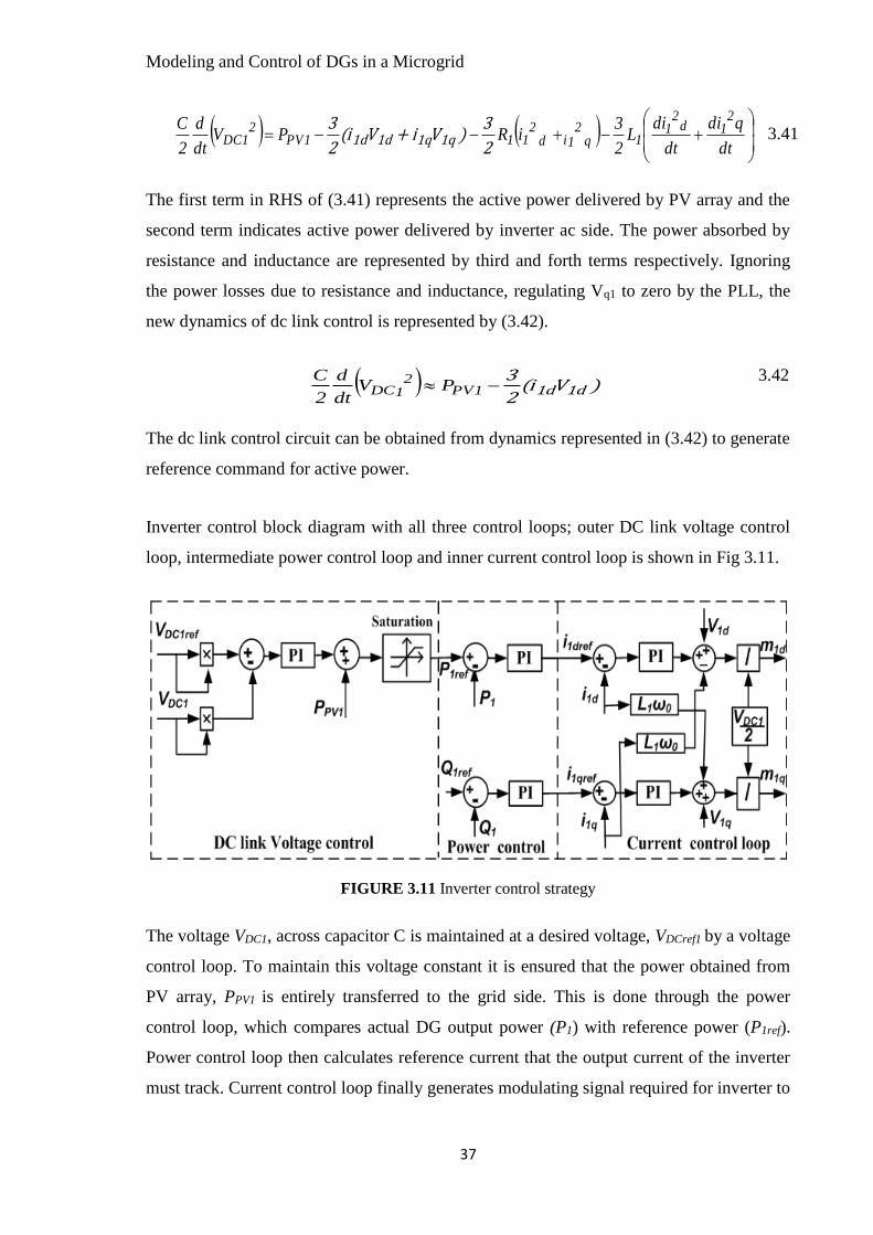
Modeling and Control of DGs in a Microgrid

37

( ) ( )

+−+−−=

dt

qdi

dt

diL

2

3iRPV

dt

d

2

C2

1d2

11q

21id

2111PV

21DC

2

3)Vi+V(i

2

31q1q1d1d

3.41

The first term in RHS of (3.41) represents the active power delivered by PV array and the

second term indicates active power delivered by inverter ac side. The power absorbed by

resistance and inductance are represented by third and forth terms respectively. Ignoring

the power losses due to resistance and inductance, regulating Vq1 to zero by the PLL, the

new dynamics of dc link control is represented by (3.42).

( ) )V(i2

31d1d− 1PV

21DC PV

dt

d

2

C

3.42

The dc link control circuit can be obtained from dynamics represented in (3.42) to generate

reference command for active power.

Inverter control block diagram with all three control loops; outer DC link voltage control

loop, intermediate power control loop and inner current control loop is shown in Fig 3.11.

FIGURE 3.11 Inverter control strategy

The voltage VDC1, across capacitor C is maintained at a desired voltage, VDCref1 by a voltage

control loop. To maintain this voltage constant it is ensured that the power obtained from

PV array, PPV1 is entirely transferred to the grid side. This is done through the power

control loop, which compares actual DG output power (P1) with reference power (P1ref).

Power control loop then calculates reference current that the output current of the inverter

must track. Current control loop finally generates modulating signal required for inverter to

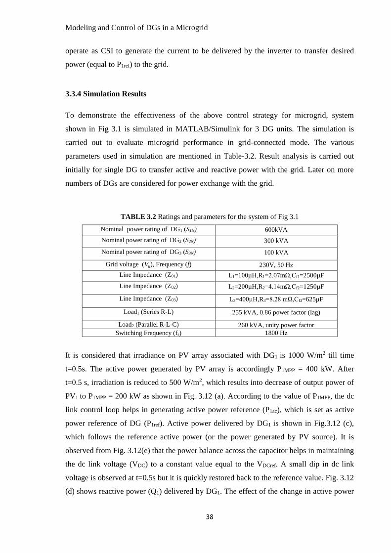
Modeling and Control of DGs in a Microgrid

38

operate as CSI to generate the current to be delivered by the inverter to transfer desired

power (equal to P1ref) to the grid.

3.3.4 Simulation Results

To demonstrate the effectiveness of the above control strategy for microgrid, system

shown in Fig 3.1 is simulated in MATLAB/Simulink for 3 DG units. The simulation is

carried out to evaluate microgrid performance in grid-connected mode. The various

parameters used in simulation are mentioned in Table-3.2. Result analysis is carried out

initially for single DG to transfer active and reactive power with the grid. Later on more

numbers of DGs are considered for power exchange with the grid.

TABLE 3.2 Ratings and parameters for the system of Fig 3.1

Nominal power rating of DG1 (S1N) 600kVA

Nominal power rating of DG2 (S2N) 300 kVA

Nominal power rating of DG3 (S3N) 100 kVA

Grid voltage (Vg), Frequency (f) 230V, 50 Hz

Line Impedance (Z01) L1=100µH,R1=2.07mΩ,Cf1=2500µF

Line Impedance (Z02) L2=200µH,R2=4.14mΩ,Cf2=1250µF

Line Impedance (Z03) L3=400µH,R3=8.28 mΩ,Cf3=625µF

Load1 (Series R-L) 255 kVA, 0.86 power factor (lag)

Load2 (Parallel R-L-C) 260 kVA, unity power factor

Switching Frequency (fs) 1800 Hz

It is considered that irradiance on PV array associated with DG1 is 1000 W/m2 till time

t=0.5s. The active power generated by PV array is accordingly P1MPP = 400 kW. After

t=0.5 s, irradiation is reduced to 500 W/m2, which results into decrease of output power of

PV1 to P1MPP = 200 kW as shown in Fig. 3.12 (a). According to the value of P1MPP, the dc

link control loop helps in generating active power reference (P1ac), which is set as active

power reference of DG (P1ref). Active power delivered by DG1 is shown in Fig.3.12 (c),

which follows the reference active power (or the power generated by PV source). It is

observed from Fig. 3.12(e) that the power balance across the capacitor helps in maintaining

the dc link voltage (VDC) to a constant value equal to the VDCref. A small dip in dc link

voltage is observed at t=0.5s but it is quickly restored back to the reference value. Fig. 3.12

(d) shows reactive power (Q1) delivered by DG1. The effect of the change in active power

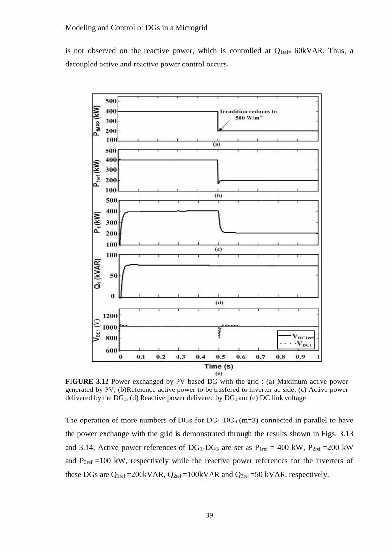
Modeling and Control of DGs in a Microgrid

39

is not observed on the reactive power, which is controlled at Q1ref= 60kVAR. Thus, a

decoupled active and reactive power control occurs.

FIGURE 3.12 Power exchanged by PV based DG with the grid : (a) Maximum active power

generated by PV, (b)Reference active power to be trasfered to inverter ac side, (c) Active power

delivered by the DG1, (d) Reactive power delivered by DG1 and (e) DC link voltage

The operation of more numbers of DGs for DG1-DG3 (m=3) connected in parallel to have

the power exchange with the grid is demonstrated through the results shown in Figs. 3.13

and 3.14. Active power references of DG1-DG3 are set as P1ref = 400 kW, P2ref =200 kW

and P3ref =100 kW, respectively while the reactive power references for the inverters of

these DGs are Q1ref =200kVAR, Q2ref =100kVAR and Q3ref =50 kVAR, respectively.

Modeling and Control of DGs in a Microgrid

40

(a)

(b)

(c)

FIGURE 3.13 Power exchage by DGs operating in parallel: (a)Active power delivered by DGs,

(b) Reactive power delivered by DG and (c) Active and reactive power injected into grid

The local load represented by series R-L and parallel R-L-C network at the PCC are

modeled to evaluate performance of MG. Equations used for modeling of 3- phase series

R-L load and R-L-C load are given in appendix A. The load connected at the PCC is

considered as 255.5 kVA with 0.86 lagging power factor till t=0.5s (220+j130 kVA). After

t=0.5s a unity power factor load of 260 kW at the PCC. Fig 3.13 (a) shows actual active

power delivered by DG1-DG3 along with the power consumed by load. It is observed that

power delivered by DG1 through DG3 follows their respective reference active powers

(P1ref = 400 kW, P2ref =200 kW and P3ref =100 kW). The actual active power supplied

through DGs is P1 = 390 kW, P2 =197 kW and P3 = 96 kW due to the power losses in the

inverter and line. As observed form Fig. 3.13(b), the reactive powers of the DGs are

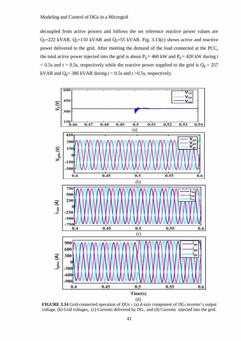
Modeling and Control of DGs in a Microgrid

41

decoupled from active powers and follows the set reference reactive power values are

Q1=222 kVAR, Q2=110 kVAR and Q3=55 kVAR. Fig. 3.13(c) shows active and reactive

power delivered to the grid. After meeting the demand of the load connected at the PCC,

the total active power injected into the grid is about Pg = 460 kW and Pg = 420 kW during t

< 0.5s and t > 0.5s, respectively while the reactive power supplied to the grid is Qg = 257

kVAR and Qg= 386 kVAR during t < 0.5s and t >0.5s, respectively.

(a)

(b)

(c)

(d)

FIGURE 3.14 Grid-connected operation of DGs : (a) d-axis component of DG1 inverter’s output

voltage, (b) Grid voltages, (c) Currents delivered by DG1 and (d) Currents injected into the grid.

Modeling and Control of DGs in a Microgrid

42

Fig. 3.14(a) shows d-axis component of inverter’s output voltage, which is equal to the

amplitude of the fundamental voltage of the inverter’s output phase voltage. Fig. 3.14(b) -

(d) show the 3-phase instantaneous phase voltage at the PCC, current delivered by DG1

and the grid currents, respectively. At t=0.5s, change in load causes deviation in d-axis

component of the inverter’s output voltage from the reference, but the voltage controller

restores it quickly (in about quarter cycle) at the desired reference as shown in Fig. 3.14(a).

Voltage at the PCC is imposed by the grid so, as shown in Fig. 3.14(b), it is not affected by

the change in load. After t=0.5s increase in the amplitude of the grid current is observed as

the apparent power exchanged with the grid has increased as observed from Fig. 3.13 (c).

3.4 Control of DG in an Islanded Mode

Fig. 3.15 shows microgrid configuration when static switch shown in Fig. 3.1 is open and

main utility is disconnected. The islanding may be intentional due to planned maintenance

or unintentional due to faulty condition on the main grid. In this mode the MG elements

are responsible for maintaining reliability of MG without support of main grid.

FIGURE 3.15 Microgrid in islanded mode

Modeling and Control of DGs in a Microgrid

43

3.4.1 Modeling of dynamics of inverter output

The schematic showing the control of one of the DGs of Fig.3.15 is shown in Fig. 3.16.

The equation representing islanded operation in abc frame can be written as

FIGURE 3.16 Single line diagram of DG1

1111t1

1 ViRVdt

diL

→→→→

−−=

3.43

1L11

1f iidt

dVC

→→→

−=

3.44

where Vtabc and V1abc are inverter’s output voltage and load voltage, respectively. Eq.

(3.43)-(3.44) can be written in d-q frame transformation as expressed through (3.45)

through (3.48)

q101d1d11tdd1

1 iLViRVdt

diL +−−=

3.45

d101q1q11tqq1

1 iLViRVdt

diL −−−=

3.46

q101fd1Ld1d1

1f VCiidt

dVC +−=

3.47

d101fq1Lq1q1

1f VCiidt

dVC −−=

3.48

Equations (3.45) through (3.48) are used to model the DG operating in an islanded mode as

shown in Fig. (3.17).

Modeling and Control of DGs in a Microgrid

44

FIGURE 3.17 Model representing inverter output side dynamics

3.4.2 Inverter Control

The main control objectives of islanded MG are to regulate system voltage and frequency

as well as to share load in proportional to DG ratings. The control must be accomplished

by using locally measured variables. In case of multiple DGs the power is shared based on

droop characteristic of DGs. The inverters are operated as controlled voltage source using

V-f mode. Three control loops are employed for control of inverters as shown in Fig. 3.18.

The outer droop control loop, intermediate voltage control and the inner current control

loop. The P versus ω (P-ω) and Q versus V (Q-V) droop characteristics are used for

sharing of active and reactive power amongst DGs. References for voltage control loop are

obtained from voltage reference generator, which generates desired voltage from voltage

amplitude and frequency provided by droop control block. Droop control block uses droop

equations of P-ω and Q-V to generate reference voltage and frequency. The input power

signals to the droop control block are provided by power calculator and low pass filter

circuit.

Power calculator block calculates output active power (p1) and reactive power (q1) using

(3.49)-(3.50).

𝑝1 =3

2(𝑖1𝑑𝑉1𝑑 + 𝑖1𝑞𝑉1𝑞)

3.49

𝑞1 =3

2(𝑖1𝑞𝑉1𝑑 − 𝑖1𝑑𝑉1𝑞)

3.50

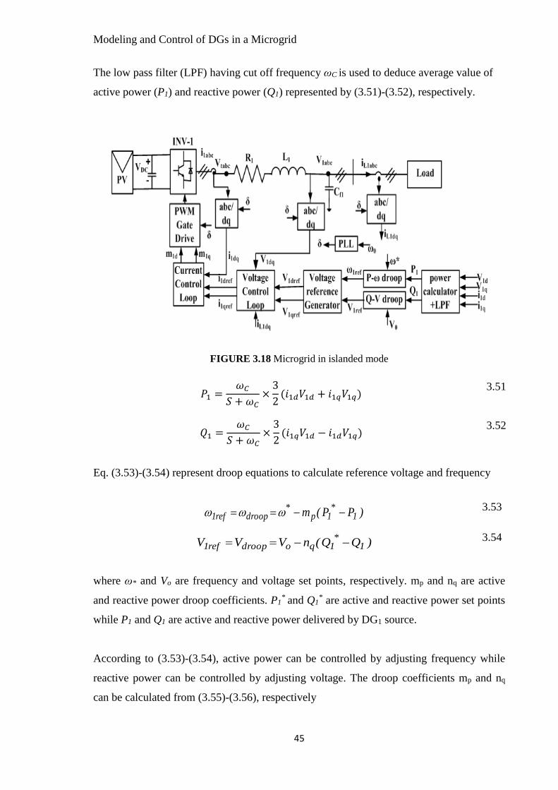
Modeling and Control of DGs in a Microgrid

45

The low pass filter (LPF) having cut off frequency ωC is used to deduce average value of

active power (P1) and reactive power (Q1) represented by (3.51)-(3.52), respectively.

FIGURE 3.18 Microgrid in islanded mode

𝑃1 =𝜔𝐶

𝑆 + 𝜔𝐶×

3

2(𝑖1𝑑𝑉1𝑑 + 𝑖1𝑞𝑉1𝑞)

3.51

𝑄1 =𝜔𝐶

𝑆 + 𝜔𝐶×

3

2(𝑖1𝑞𝑉1𝑑 − 𝑖1𝑑𝑉1𝑞)

3.52

Eq. (3.53)-(3.54) represent droop equations to calculate reference voltage and frequency

)PP(m 1*

1p*

droopref1 −−== 3.53

)QQ(nVVV 1*

1qodroopref1 −−== 3.54

where ω* and Vo are frequency and voltage set points, respectively. mp and nq are active

and reactive power droop coefficients. P1* and Q1

* are active and reactive power set points

while P1 and Q1 are active and reactive power delivered by DG1 source.

According to (3.53)-(3.54), active power can be controlled by adjusting frequency while

reactive power can be controlled by adjusting voltage. The droop coefficients mp and nq

can be calculated from (3.55)-(3.56), respectively

Modeling and Control of DGs in a Microgrid

46

=

1

pP

m

3.55

=

1

pQ

Vn

3.56

where, Δω and ΔV are allowable deviation in frequency and voltage, respectively.

Voltage reference generator generates three phase sinusoidal voltage signal using (3.57)-

(3.60). Reference three phase alternating voltage is transformed into d-q frame to obtain d-

q axis components of voltage V1dref and V1qref , respectively.

= dtref1 3.57

SinVV m1aref1 = 3.58

)120(SinVV m1bref1−=

3.59

)240(SinVV m1cref1−=

3.60

The detailed block diagram representing (3.51)-(3.60) is shown in Fig. 3.19.

FIGURE 3.19 Block diagram representing reference voltage generation using droop control

Voltage control loop generates desired current reference signals (i1dref and i1qref) by acting

on the voltage errors (V1dref –V1d) and (V1qref –V1q). Current control loop generates desired

modulating signal by controlling actual output current that follows the reference current

signals. Fig. 3.20 shows detailed block diagram of voltage control and current control.

Modeling and Control of DGs in a Microgrid

47

FIGURE 3.20 V-f mode control of inverter

3.4.3 Simulation Results

To demonstrate the effectiveness of the above control strategy microgrid system shown in

Fig 3.15 and discussed in previous sections is simulated in MATLAB/Simulink. This

simulation is carried out to evaluate microgrid performance in islanding mode. The various

parameters used in simulation are mentioned in Table-3.3. The nominal ratings and line

parameters are same as Table- 3.2.

TABLE 3.3 Ratings and parameters for the system of Fig 3.15

Active and reactive power set points of DG1 (P1* ,Q1*) 400kW, 200 kVAR

Active and reactive power set points of DG2 (P2* ,Q2*) 200kW, 100 kVAR

Active and reactive power set points of DG3 (P3* ,Q3*) 100kW, 50 kVAR

Active and reactive power droop co-efficient (mp1,nq1) -1.25e-6,-5e-5

Active and reactive power droop co-efficient (mp2,nq2) -2.5e-6,-1e-4

Active and reactive power droop co-efficient (mp3,nq3) -5e-6,-2e-4

Load1 (Series R-L) PL1=220 kW , QL1=130 kVAR

Load2 (Parallel R-L-C) PL2= 260 kW, QL2= 0 kVAR

Fig. 3.21 shows active power and reactive power supplied by DGs to the load in islanding

mode. All three DGs share active and reactive power in proportion to their ratings.

DG1shares more power compared to other two DGs. Fig. 3.21(a) shows active power

shared by all DGs. During time interval t=0-0.5s, active power supplied by DG1-DG3 are

P1=126 kW, P2=63 kW and P3=31 kW for active power PL=220 kW required by the load.

After t=0.5s, the load at the PCC is unity power factor load with active power demand of

PL=260 kW. Thus, it results into increase of active power shared by DGs to P1=150 kW,

P2=75 kW and P3=36 kW.

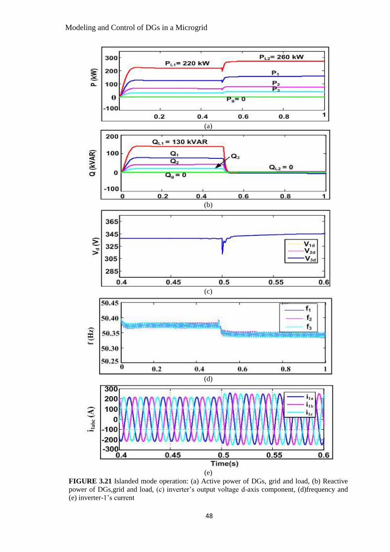
Modeling and Control of DGs in a Microgrid

48

(a)

(b)

(c)

(d)

(e)

FIGURE 3.21 Islanded mode operation: (a) Active power of DGs, grid and load, (b) Reactive

power of DGs,grid and load, (c) inverter’s output voltage d-axis component, (d)frequency and

(e) inverter-1’s current

Modeling and Control of DGs in a Microgrid

49

It is also observed that power delivered by grid is zero as it is disconnected and power

demand is shared by all DGs according to their droop characteristics. Fig. 3.21 (b) shows

reactive power shared by DGs for the reactive power demand of QL=130 kVAR for t<0.5s.

As observed, Q1=74 kVAR, Q2=37 kVAR and Q3=19 kVAR. After t=0.5s, reactive power

demand is decreased to zero and accordingly reactive power shared by all DGs is zero as

shown in Fig. 3.21(b). Fig. 3.21(c) shows the magnitude of d-axis component of inverter’s

terminal voltage. It decreases momentarily when the load change occurs and attains the

desired value due to the operation of the voltage control loop. Fig. 3.21(d) shows operating

frequency of DGs which is 50.38 Hz during first time period (t<0) and decreases to a new

value of 50.33 Hz after the load change. The value of new frequency at which the

operation settles is dependent on the DG’s frequency droop settings Fig. 3.21(e) shows the

current delivered by inverter 1. It is observed that current delivered by DG1 increases after

t=0.5s as the apparent power of the load has increased after t > 0.5s from 255.5kVA to 260

kVA.

3.5 Transition between modes

Microgrid operation during transitions between modes is more critical as it is essential to

maintain voltage and frequency to nominal values to form stable islanded. Also proper

synchronization between grid and inverter output voltage and phase angle is maintained

during islanded to grid transition operation. During transition from islanding mode to grid

connected mode major challenges are to synchronize inverter output voltage and frequency

with grid voltage and frequency with respect to amplitude as well as phase angle.

3.5.1 Transition from islanded mode to grid-connected mode

The smooth transition of microgrid between the two modes can be obtained by switching

between P-Q control (of grid-connected mode) and V-f control (of islanded mode). Fig.

3.22 shows control strategy for transition between the two modes. According to the

command issued by the logic controller, the operation in either of these modes occurs.

The logic controller checks the grid conditions once utility is restored after islanded

operation. It issues mode command for transition from islanded to grid connected

operation after utility parameters are restored to their nominal values. For example during

Modeling and Control of DGs in a Microgrid

50

transition from islanding mode to grid connected mode, it is necessary to check whether

inverter’s output voltage is having equal amplitude and phase with respect to grid voltage

or not. Logic controller detects required condition for grid synchronization and allows the

islanded MG to reconnect with the main grid.

FIGURE 3.22 Inverter control for transitions between modes

The detailed block diagram of the control scheme for transition between modes is shown in

Fig. 3.23. The inverter side voltage (Vabc) must resynchronize to grid voltage (Vgabc) before

closer of main switch. Initially MG is operated in islanding mode with system frequency

regulated at nominal frequency value (ω0). Phase error may exist between Vabc and Vgabc

when ac system is restored. AC system voltage restoration is detected by peak detector by

comparing its value with desired threshold (i.e. within acceptable limits). If Vgabc is greater

than threshold, ac system is considered as restored and voltage controlled oscillator (VCO)

is switched to PLL mode. The PLL is designed to force Vgq to zero to regulate frequency to

nominal value. The logic controller also observes values of Vgq and ω along with the

amplitude of Vgabc. When all these values are above their threshold, the controller

command is changed from 0 (islanding) to 1 (Grid connected) mode. This command is

used for operating main switch as well as to switch the control strategies of Fig.3.22.

Operation of logic control block shown in Fig. 3.23 is simulated in the

MATLAB/Simulink. Parameters for simulation are considered same as mentioned in

Table-3.2 and Table-3.3. Resynchronization of inverter voltage with grid voltage followed

by closer of the main switch is shown in Fig. 3.24.

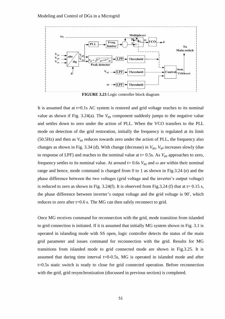
Modeling and Control of DGs in a Microgrid

51

FIGURE 3.23 Logic controller block diagram

It is assumed that at t=0.1s AC system is restored and grid voltage reaches to its nominal

value as shown if Fig. 3.24(a). The Vgq component suddenly jumps to the negative value

and settles down to zero under the action of PLL. When the VCO transfers to the PLL

mode on detection of the grid restoration, initially the frequency is regulated at its limit

(50.5Hz) and then as Vgq reduces towards zero under the action of PLL, the frequency also

changes as shown in Fig. 3.34 (d). With change (decrease) in Vgq, Vgd increases slowly (due

to response of LPF) and reaches to the nominal value at t= 0.5s. As Vgq approaches to zero,

frequency settles to its nominal value. At around t= 0.6s Vgq and ω are within their nominal

range and hence, mode command is changed from 0 to 1 as shown in Fig.3.24 (e) and the

phase difference between the two voltages (grid voltage and the inverter’s output voltage)

is reduced to zero as shown in Fig. 3.24(f). It is observed from Fig.3.24 (f) that at t= 0.15 s,

the phase difference between inverter’s output voltage and the grid voltage is 90ᵒ, which

reduces to zero after t=0.6 s. The MG can then safely reconnect to grid.

Once MG receives command for reconnection with the grid, mode transition from islanded

to grid connection is initiated. If it is assumed that initially MG system shown in Fig. 3.1 is

operated in islanding mode with SS open, logic controller detects the status of the main

grid parameter and issues command for reconnection with the grid. Results for MG

transitions from islanded mode to grid connected mode are shown in Fig.3.25. It is

assumed that during time interval t=0-0.5s, MG is operated in islanded mode and after

t=0.5s static switch is ready to close for grid connected operation. Before reconnection

with the grid, grid resynchronization (discussed in previous section) is completed.

Modeling and Control of DGs in a Microgrid

52

(a)

(f)

FIGURE 3.24 Resynchronization results : (a) d-axis grid voltage, (b) q-axis grid voltage, (c)

Frequency of inverter output voltage and (d) Inverter and grid voltage

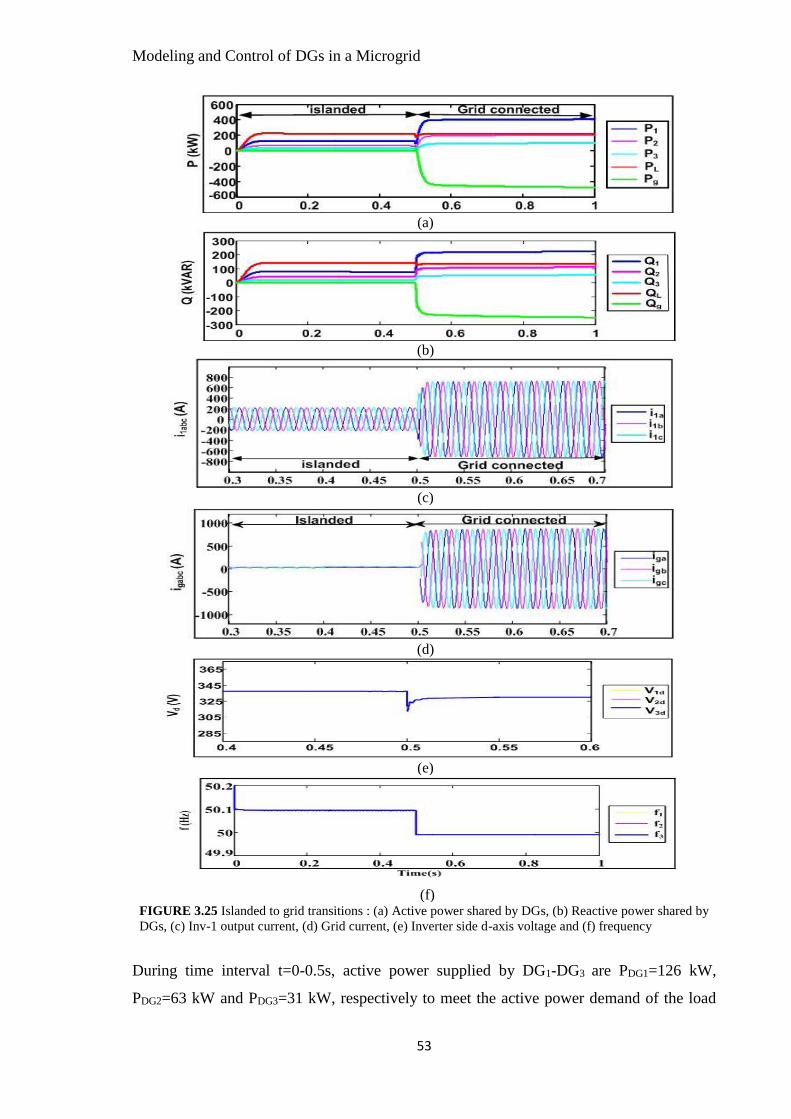
Modeling and Control of DGs in a Microgrid

53

(a)

(b)

(c)

(d)

(e)

(f) FIGURE 3.25 Islanded to grid transitions : (a) Active power shared by DGs, (b) Reactive power shared by

DGs, (c) Inv-1 output current, (d) Grid current, (e) Inverter side d-axis voltage and (f) frequency

During time interval t=0-0.5s, active power supplied by DG1-DG3 are PDG1=126 kW,

PDG2=63 kW and PDG3=31 kW, respectively to meet the active power demand of the load

Modeling and Control of DGs in a Microgrid

54

(PL=220 kW).After t=0.5s power delivered by DG1-DG3 is P1=390 kW, P2=197 kW and

P3=96 kW, respectively whereas power consumed by load is 220 kW and active power

injected by DGs are 460kW as discussed in the grid connected operation and shown in Fig.

3.25(a).Similarly reactive powers delivered by DGs during islanded mode (t=0-0.5s) are

Q1=74 kVAR, Q2=37kVAR and Q3=19 kVAR for load demand of 130 kVAR and during

grid connected mode (t=0.5-1s), Q1= 221kVAR, Q2=110 kVAR and Q3=55 kVAR as

shown in Fig 3.25(b). Line current flowing through inv-1 is shown in Fig.3.25(c) which is

less during first interval corresponding to P1=126 kW and increased during second interval

corresponding to P1=390 kW. Fig. 3.25(d) shows that no current flows into grid during

islanded mode. However, after t=0.5s, in the grid-connected mode, current flows into the

grid due to injection of active and reactive power from DGs. Inverter voltage during both

the modes is shown in Fig. 3.25(e). This voltage is maintained as per droop setting during

islanded mode by voltage control and it is imposed by the utility in grid connected mode.

Frequency during operation in different modes is shown in Fig. 3.25(f), which is set by

droop control method at 50.3 Hz during t<0.5s and becomes equal to grid frequency equal

to 50 Hz after t=0.5s.

3.5.2 Transition from grid-connected mode to islanded mode

The MG transition from grid connected mode to islanded mode occurs intentionally due to

planned maintenance (or repair) or unintentionally due to fault on utility. The transition

from grid connected mode to islanded mode is described in this section. The control circuit

shown in Fig. 3.22 is used in P-Q mode in grid connected operation and V-f mode in

islanded mode. It is considered that during initial time period t< 0-1 sec, MG is connected

to grid to exchange real and reactive power with the grid. A same load with the active and

reactive power demand having 220kW and 130kVAR is considered at the PCC. At t=1s

static switch opens to form islanded MG and the load is shared amongst the DGs using

droop control method. Fig.3.26 (a)-(b) shows that during t<1s, active power and reactive

power delivered by DG1-DG3 are according to their reference set points, as discussed in

grid connected operation of MG. At t=1s, as utility is disconnected, the active power

cannot be delivered to the grid (i.e. Pg=0). Hence, DG1- DG3 must generate active power

just enough to meet the load’s demand. Thus, to meet the load’s demand (PL=220 kW and

QL=130kVAR), DGs’ active power output are P1=126 kW, P2=63 kW and P3=31kW and

the reactive power output are about Q1=74 kVAR, Q2=37 kVAR and Q3=19 kVAR.

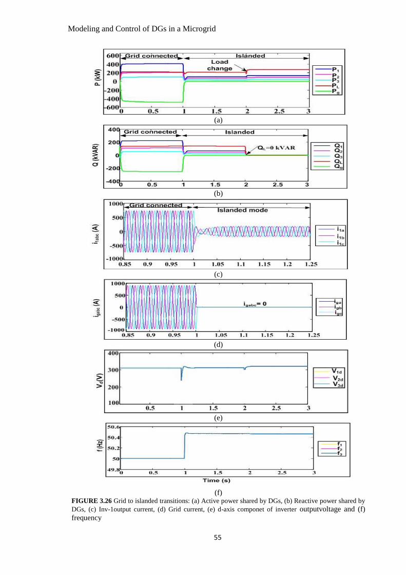
Modeling and Control of DGs in a Microgrid

55

(a)

(b)

(c)

(d)

(e)

(f) FIGURE 3.26 Grid to islanded transitions: (a) Active power shared by DGs, (b) Reactive power shared by

DGs, (c) Inv-1output current, (d) Grid current, (e) d-axis componet of inverter outputvoltage and (f)

frequency

Modeling and Control of DGs in a Microgrid

56

Load changes at t=2s with the active and reactive power demand equal to PL2=260 kW and

QL2=0 kVAR. The new load demand is again shared accurately by all DGs in proportional

to their ratings as per the droop settings. Figures 3.26(c) and (d) show the output current of

inverter-1 and grid current. It is observed that inverter-1’s current is 730A (peak) for t<1s

whereas it reduces to nearly 180A (peak) after t=1s, while the current injected to the grid is

equal to 900A during t<1s and reduces to zero after t=1s. The d-axis components of

inverters output voltage is also shown in Fig. 3.26(e).Inverter’s output voltage is disturbed

from nominal value during the transition from grid connected mode to islanded mode but

is quickly reinstated to nominal value by the voltage control loop. Fig. 3.26 (f) shows the

change in frequency from grid connected operation to islanded operation. It is observed

that during grid connected operation, frequency is imposed by the grid and all DGs are

operated at nominal frequency of 50 Hz. whereas during islanded mode, frequency is

defined from P-ω droop characteristic of DGs and set at a new value corresponding to

50.45 Hz.

3.6 Summary

In this chapter MG modeling and the control scheme for the operation of MG in grid-

connected mode, islanded mode and transition between these modes is presented. The P-Q

and V-f control are employed for the grid-connected mode and the islanded mode,

respectively. In grid connected mode, the active and reactive power are exchanged with the

grid (and the load) as per the references or the set points provided by the MGCC unit. In

islanded mode active and reactive power demand of the load is shared by the DGs. The

power references are set in proportion to the rating of the DGs as per the conventional

droop control principle. It is observed that the control strategy can effectively provide the

stable operation in grid-connected as well as islanded mode of operation and can execute

smooth transition between the two modes. However, conventional droop control principle

does not provide effective solution for power sharing amongst the DGs with respect to

their optimum utilization. It is possible to ensure reactive power sharing amongst DGs

based on the actual active power delivered by PV inverter. By this means, it is possible to

utilize maximum available capacity of inverter. Next chapter focuses on this aspect and

proposes reactive power sharing algorithm to achieve these objectives.

57

CHAPTER – 4

Reactive Power Sharing Algorithm

The reactive power transfer capability of PV based DGs can be utilized to fulfill reactive

power requirement of the load or to provide reactive power support to the grid. However,

as active power delivered by PV sources is uncertain (due to the dependency on

environmental condition) and varies continuously, the available margin of the inverter for

reactive power exchange also varies. Hence, the reactive power sharing must be done

sensibly otherwise there are chances that the inverter may operate at its limit or may get

overloaded. Hence, accurate reactive power allocation of each inverter connected with

DGs is essential for avoiding overloading of any inverter. This chapter proposes reactive

power sharing algorithms to have equal utilization of the inverters to prevent their

overloading or underutilization. These algorithms are

(i) Equal Apparent Power Sharing algorithm with Least Standard Deviation

(EAPS-LSD)

(ii) Proportional Apparent Power Sharing algorithm with Least Standard Deviation

(PAPS-LSD)

4.1 System Configuration and Inverter Control

The proposed algorithm is evaluated for the MG architecture shown in Fig.4.1. The MG

configuration consists of four DGs (m=4) connected with the stiff grid. The system

configuration discussed in chapter 3 is repeated in this section. The inverters are controlled

to extract PMPP from PV source and to deliver active and reactive power to the load and

grid. The power management task is performed by MGCC unit using low bandwidth

communication links. The reactive power sharing algorithms discussed in the following

sections are executed by MGCC to provide reactive power references (Qiref) to all DGs.

Reactive Power Sharing Algorithm

58

The control system described in chapter 3, Fig. 3.2 is used for real and reactive power

transfer with the grid.

FIGURE 4.1 System configuration of a Microgrid with four DGs

4.2 Equal Apparent Power sharing algorithm with Least Standard

Deviation (EAPS-LSD)

The principle of sharing apparent power among inverters with the proposed method is

described using four inverters. Thus, if PT is the total active power generated by the PV

arrays and QL is reactive power demand of the load (or to be supplied to the grid), then the

required apparent power (ST) to be handled by the inverters is

2L

Q2T

PT

S += 4.1

Fig. 4.2(a) shows the case when the PV arrays PV1 through PV4 receive uniform irradiation

and hence, all the DGs generate equal active power. In order to equalize their apparent

powers, the reactive power must also be the same. As a result, the magnitude and phase of

apparent power of inverters 1 through 4 (S1 through S4) are same as shown in Fig. 4.2(a)

Reactive Power Sharing Algorithm

59

and the inverters’ apparent power vectors are aligned with the vector ST. Hence, the

resultant apparent power handled by all the DGs is equal to the algebraic as well as the

arithmetic sum of S1 through S4.

Fig. 4.2(b) represents the case when the PV arrays PV1 through PV4 operate with different

irradiations. As the active powers generated by the arrays are different, the inverters must

supply different reactive powers such that their apparent powers are same. Accordingly,

the inverter-1 must provide one-fourth of the total apparent power (i.e. ST/4). However, the

active power associated with it is P1 which is less than PT/4.

(a) (b)

FIGURE 4.2 Sharing of apparent power (a) With equal active power generation (b) With unequal active

power generation

Hence, the reactive power that inverter-1 must supply is expressed by (4.2)

21

2T

1 P4

SQ −

=

4.2

This results into change in the operating power factor of inverter-1. Further, vector S1 is no

longer aligned with vector ST. Hence, the remaining apparent power that inverters 2

through 4 must handle is represented by vector STnew. As a result if these three inverters are

controlled to share the remaining apparent power equally, each must supply STnew/3. The

reactive power that inverter-2 must supply is accordingly obtained as

Reactive Power Sharing Algorithm

60

22

2

Tnew2 P

3

SQ −

=

4.3

Similarly, the reactive powers Q3 and Q4, that inverters 3 and 4 must supply, and hence

their apparent powers S3 and S4, can be computed. It is evident from the Fig. 4.2(b) that

DGs with higher active power has to handle lower reactive power and vice-versa. Further,

vectors S1 through S4 are not aligned confirming that the inverters operate at different

power factors. Though vectors S1 through S4 are not aligned with ST, their magnitudes tend

to be equal indicating nearly equal apparent power sharing.

In the given vector diagram of Fig.4.2 (b),for the given active powers P1 through P4 for the

inverters 1 through 4, the reactive powers for the inverters are obtained in sequence Q1, Q2,

Q3 and then Q4. However, for the same values of active powers if the sequence for reactive

power calculation is selected differently (say Q2, Q3, Q1 and Q4), the values (and

orientation) of S1, S2, S3 and S4 are different as shown in Fig.4.3. Hence numbers of

permutation is possible in active and apparent power according to the sequences. Also, for

given permutation, a unique solution for sharing reactive power exists. Thus, the order

(sequence) in which the reference reactive powers for the inverters are obtained

significantly affects the apparent power sharing.

FIGURE 4.3 Sharing of apparent power for change in sequence of inverters

Reactive Power Sharing Algorithm

61

4.2.1 EAPS-LSD Control Algorithm

The flowchart for the control algorithm for sharing apparent power equally amongst m

inverters is shown in Fig. 4.4. The control principle presented in earlier section is

embedded in the flowchart. The algorithm of Fig. 4.4 determines the best possible

alternative of distributing the reactive power amongst the inverters to have nearly equal

apparent power sharing. Fig. 4.4(a) shows the process of evaluating various permutations

of scheduling of the inverters while Fig. 4.4(b) shows a subroutine, which calculates

desired reactive power references for the inverters for given permutation.

As shown in Fig. 4.4(a), the algorithm computes the 𝑛 × 𝑚 matrices Pperm and Sperm which

represent the n possible permutations for active power and nominal apparent power of the

m inverters, respectively. Pperm is derived from PMPP, which comprises of elements PMPPi

that represents the active power of ith DG. Similarly Sperm is derived from SiN, where SiN is

the nominal apparent power rating of ith inverter. For each permutation j, the subroutine is

called to determine the reference reactive powers Qij for the inverters (i=1, 2,…,m).

The principle presented in section 4.2 is followed in the sub-routine of Fig. 4.5(b) to

compute the reference reactive powers (Qij) for the inverters. For the given ( jth)

permutation, the sub-routine calculates the available reactive power Qi using (4.4)-(4.6).

For simplicity, Pi and Si are the variables introduced for Pperm(j,i) and Sperm(j,i) respectively

i)(j,PP permi = 4.4

)i,j(SSpermi

=

4.5

2

i

2

iNiPSQ −=

4.6

Therefore, total active power (PT), reactive power (QT) and apparent power (ST) supplied

by the inverter to satisfy desired reactive power demand of the load requirement are

represented by (4.7)-(4.9), respectively.

=

=m

1i

iT PP

4.7

=

=m

1i

iTQQ

4.8

Reactive Power Sharing Algorithm

62

2

T

2

TTQPS +=

4.9

To achieve equal apparent power sharing, each inverter must supply apparent power

represented by

]i)1m[(SS TTnew −+= 4.10

However, STnew may exceed SiN. In such case, the reference apparent and reactive powers

are set as SiN and Qi, respectively for that inverter which does not satisfy (4.11).

iNTnew SS 4.11

The remaining active and reactive powers to be delivered by inverter are modified by

subtracting already assigned values to the inverter. The remaining active power (PTn) to be

supplied and reactive power demand to satisfy (QTn) is derived as shown in (4.12), and

(4.13), respectively.

−

=

−=1i

0i

iTTnPPP

where 0P0=

4.12

−

=

−=1i

0i

irefLTnQQQ where 0Q

ref0=

4.13

Accordingly, the apparent power (Sinew) that ith inverter must supply can be obtained by

(4.14)

( )i)1m(/QPS2

Tn2

Tninew −++=

4.14

Thus, the reactive power reference for the ith inverter (for jth permutation) can be calculated

as

2i

2inewiref PSQ −=

4.15

Equation (4.15) is used to calculate reference reactive power of ith inverter for

jthpermutation (Qij). The apparent power to be handled by the ith inverter (Sinv(i)) and the

utilization factor (UFi) of the inverters are computed. Utilization factor is defined as the

ratio of apparent power delivered by the inverter to the nominal apparent power rating of

inverter and expressed by (4.16).

iNS

)i(invSiUF =

4.16

Reactive Power Sharing Algorithm

63

The process is repeated for all the permutations and the best possible option is identified

based on the least standard deviation (SDmin) of the utilization factors of the inverters.

Standard deviation (SD) for the utilization factors of the inverters is represented as

FIGURE 4.4 Flowchart for the proposed equal apparent power sharing approach : (a) Main program and (b)

Subroutine

Reactive Power Sharing Algorithm

64

( )( )

=

−−

=m

1i

2meanUF)i(UF

1m

1SD

4.17

where, UFmean is the mean value of UF for all inverters. Initially, the SD is set to high

value (SDmin = 1000) and updated continuously in process of search of the best option

having the least standard deviation. The permutation index for the permutation having the

least SD i.e. SDmin is finally used to assign the reference reactive powers Qref to m inverters

in the order 1 through m.

4.2.2 Simulation Results

The EAPS algorithm is evaluated in the MATLAB/Simulink for the MG system shown in

Fig. 4.1. The results of proposed algorithm are compared with the two more control

approached of reactive power sharing: Optimal Reactive Power Sharing [80] and Equal

Reactive Power Sharing [81]. Initially in sub-section 4.2.2.1, EAPS algorithm is employed

that does not consider the permutations for active power and apparent power i.e. the order

of allocation of reactive power amongst inverters is considered as 1-2-3-4.Thus, basically

EAPS algorithm can be represented simply by the sub-routine of Fig. 4.4. Later in sub

section 4.2.2.2, the permutations are also considered to identify the best possible allocation

sequence that results into the least standard deviations of utilization factors.

4.2.2.1 Performance of EAPS algorithm without permutations

The performance of the algorithm is evaluated for two different cases. In case (i), all the

inverters are of equal ratings while in case (ii), all inverters are having unequal ratings.

Here, the performance is evaluated without considering the different permutations possible

for allocating the reactive power amongst the inverters.

Case (i): Equal DG ratings

The ratings and parameters for the MG configuration shown in Fig. 4.1 are tabulated in

Table-4.1. The nominal apparent power rating of 500 kVA is considered for all DGs. The

active power generated at given instant corresponds to (PMPP) by associated PV array of

DGs are set as reference value of active power for the inverters. The active power

Reactive Power Sharing Algorithm

65

extracted from PV sources PV1-PV4 is considered as 400kW, 300kW, 250kW and 450kW,

respectively during t=0.5s. Due to deviation in solar irradiation conditions, the active

power extracted from PV1 is reduced to 200kW at t=0.5s whereas the active power

generated by PV3 is changed to 400 kW at t=1s. Active, reactive and apparent power

sharing results using ORPS control algorithm is shown in Fig. 4.5(a)-(c). The ORPS

algorithm [80] is consider to calculate reactive power references for inverters and given in

Table-4.2.

TABLE 4.1 Ratings and parameters for the system of Fig.4.1

Nominal power rating of DG1 (S1N) 500 kVA

Nominal power rating of DG2 (S2N) 500 kVA

Nominal power rating of DG3 (S3N) 500 kVA

Nominal power rating of DG4 (S4N) 500 kVA

Grid voltage(Vg), Frequency(f) 415V, 50 Hz

Line parameter (Z01=Z02=Z03=Z04) L=100µH,R=2.07mΩ,Cf=2500µF

Load 1.92 MVA, 0.78 power factor (lag)

No of PV inverters (m) 4

(a)

(b)

(c)

FIGURE 4.5 Power sharing using ORPS Algorithm case(i): (a) Active power delivered by DGs, (b) Reactive

power delivered by DGs and (c) Apparent power of inverters

Reactive Power Sharing Algorithm

66

It is observed from Figs. 4.5(a) and (b) that, when P1 is reduced from 400 kW to 200 kW at

t=0.5s, the reactive power delivered by DG1 (Q1) also changes from 300 kVAR to 262

kVAR. The reactive power delivered by DG2-DG4 also changes. Similarly at t=1s, when P3

increases to 400 kW, Q1 through Q3 changes. Thus, if power generated by any one of the

PV array changes, the reactive power references and hence, the reactive power supplied by

all the inverters change (except those which are operating at their limits SiN). Fig. 4.5(c)

shows that inverters 1 and 4 operate at their maximum apparent power limits (S1N and S4N,

respectively) till t=0.5s. At t=0.5s, when P1 reduces, Q1 also reduces simultaneously and

hence, from t=0.5s to t=0.1s only inverter 4 operates at its full capacity. It is observed that

the change in Pi and Qi is such that the ratio Pi/Qi remains equal for all the inverters that do

not reach the rated capacity. An index defined as utilization factor (Si/SiN) is used to

indicate the extent to which the capacity of the inverter is utilized.

Fig.4.6 shows the results obtained with equal reactive power sharing (ERPS) algorithm

[81], for same irradiation pattern on the PV array. To meet the total reactive power demand

of the load 1200kVAR through the inverters 1 through 4, each inverter must output 300

kVAR Hence, the reference reactive power for inverter 1, 2 and 3 are set equal to 300

kVAR while for inverter-4 which hits its apparent power limit, it is restricted to 218

kVAR. It is observed from Figs. 4.6(a)-(c), even if the active power supplied by the PV

array changes, the effect is not observed in the reactive power sharing. It is also evident

from Fig.4.6(c) that inverter-4 continuously operates at its rated capacity of 500 kVA.

Inverters 1 and 3 also operate at their rated capacities for some time. It is also observed

that Si (for i=1, 2 and 4) remains almost constant for t=0.5s to 2s inspite of the change in P3

at t=1s. The reason being no change in Pi and Qi (for i =1, 2 and 4) for this period. Unlike

ORPS the reactive power demand of the load is not met fully inspite of the fact that many

inverters still operate below their rated limits. Thus, the inverters are not utilized optimally

and also the percentage utilization of all the inverters varies greatly.

Fig.4.7 shows performance with proposed algorithm when same pattern of irradiation on

the PV array as that considered for ORPS and ERPS is maintained. At t=0.5s, when the

irradiation of PV1 decreases resulting into the decrease in the output power of inverter 1,

the reactive power of inverter 1 increases. Simultaneously, the reactive powers of all other

inverters decrease in spite of the fact that there is no change in the power output from PV

arrays PV2, PV3 and PV4. This results into minimizing the gap of percentage utilization of

Reactive Power Sharing Algorithm

67

different inverters. Similarly, at t=1s when P3 changes from 250 kW to 400 kW, reactive

power of all the inverters changes to achieve better sharing of the active and reactive

power amongst them

(a)

(b)

(c)

FIGURE 4.6 Power sharing using ERPS Algorithm case (i): (a) Active power delivered by DGs, (b) reactive

power delivered by DGs and (c) Apparent power of inverters

Table-4.2 shows the active, reactive and apparent powers shared by the inverters over the

different periods for ORPS, ERPS and the proposed approach.It is also observed from the

Table-4.2 that using ORPS, all the inverters are operating at different utilization factors.

The utilization factors vary greatly showing that some of the inverters operate much below

their rated capacity when some others have already hit their limits. For example, inverter-1

operates with the lowest utilization factor (0.65 from t=0.5s till 1s and 0.69 from t=1s till

2s) while inverter-4 is operating at its limit. The unequal utilization of the inverters, not

only results into unequal losses, efficiency and heating of different inverters, but may

damage the inverters that continuously operate at their apparent power limits. Using ERPS,

it is observed that for change in active power, the effect is not observed in the reactive

power sharing. Table-4.2 shows the active, reactive and apparent powers shared by

Reactive Power Sharing Algorithm

68

proposed algorithm. Unlike ORPS and ERPS, the utilization factors for the proposed

method, vary a little for all the DGs indicating uniform loading of the inverters.

(a)

(b)

(c)

FIGURE 4.7 Power sharing using proposed EAPS Algorithm case (i): (a) Active power delivered by DGs

(b) Reactive power delivered by DGs and (c) Apparent power of inverters

TABLE 4.2 UF for each DG using ORPS, ERPS and Proposed algorithm case (i)

ORPS ERPS Proposed (EAPS)

t (s) Pi Q

iref S

i UF Q

iref S

i UF Q

iref S

i UF

0-0.5

400 300 500 1.00 300 500 1.00 229 460 0.92

300 373 478 0.95 300 424 0.84 354 464 0.92

250 310 398 0.79 300 390 0.78 393 466 0.93

450 218 500 1.00 218 500 1.00 222 500 1.00

0.5-1

200 262 329 0.65 300 360 0.72 374 424 0.85

300 392 493 0.98 300 424 0.84 311 432 0.86

250 325 410 0.82 300 390 0.78 355 434 0.86

450 218 500 1.00 218 500 1.00 159 477 0.95

1-2

200 282 345 0.69 300 360 0.72 405 452 0.90

300 400 500 1.00 300 424 0.84 356 465 0.93

400 300 500 1.00 300 500 1.00 262 478 0.95

450 218 500 1.00 218 500 1.00 175 482 0.96

Note: Pi, Qiref, Si are mentioned in kW, kVAR and kVA. UF is mentioned in percentage.

Reactive Power Sharing Algorithm

69

The three algorithms are tested even with a different load having a leading power factor

(PF). Table 4.3 shows the results obtained with a load of 1.16 MVA, 0.86 power factor

(lead). It is observed that even with leading power factor, proposed algorithm performance

is superior. Standard deviations of the utilization factors of the various inverters are

calculated, to quantify the effectiveness of the algorithm to distribute the apparent power

equally amongst the inverters. Standard deviations of the utilization factors for ORPS,

ERPS and EAPS, for the case represented by Table 4.3 are 0.204, 0.147 and 0.055,

respectively. Lesser the standard deviation better is the performance.

TABLE 4.3 Comparison of various algorithms for leading power factor load

Algorithms Pi

(kW)

Qiref

(kVAR)

Si

(kVA)

Uti. Fac.

Si/SNi

ORPS

300 -180 350 0.70

200 -120 233 0.46

150 -90 175 0.35

350 -210 408 0.82

ERPS

300 -150 335 0.67

200 -150 250 0.50

150 -150 212 0.42

350 -150 380 0.76

Proposed

300 0 300 0.60

200 -233 307 0.61

150 -271 309 0.61

350 -96 362 0.72

Case (ii): Unequal DG ratings

The proposed algorithm is also evaluated for the case when all DGs of the system shown in

Fig.4.1 have unequal ratings. The nominal ratings for the DGs are mentioned in Table 4.4.

The load, line parameters, capacitance and the grid voltage are considered same as that of

case (i).In this case the active power generated by PV arrays PV1, PV2, PV3 and PV4 are

P1= 200kW, P2 =300 kW, P3 =400 kW and P4 =500 kW, respectively. A step increase in

irradiation on PV array PV1 occurs at t=0.5s, which results in the output of P1 to increase to

300kW. At t=1s, irradiation on PV array P3 decreases suddenly, resulting into the change

in its output power from 400kW to 200kW. The active, reactive and apparent power

sharing by inverters 1 through 4 with ORPS control are displayed in Fig. 4.8 and the

results are quantified in Table 4.4.

TABLE 4.4 Ratings of DG of the system of Fig.1 for case (ii)

Nominal power rating of DG1 (S1N) 400 kVA

Nominal power rating of DG2 (S2N) 500 kVA

Nominal power rating of DG3 (S3N) 600 kVA

Nominal power rating of DG4 (S4N) 700 kVA

Reactive Power Sharing Algorithm

70

Figs 4.8(a) and (b) shows that when P1 is increased from 200 kW to 300 kW at t=0.5s, Q1

also increases from 171 kVAR to 240 kVAR. Hence its apparent power increases, leading

to its utilization factor of 0.96. The reactive powers of inverters 2 through 4 decrease with

their active powers still at the same values. Thus, S2 through S4 decrease lowering the

utilization of inverters 2 through 4. This increases the miss-match in the utilization factors.

The miss-match further increases after t=1s, when the output power of P3 decreases from

400kW to 200kW. The decrease in P3 at t=1s is associated with the simultaneous decrease

in Q3. Hence, to meet the reactive power demand of the load, more reactive power needs to

be supplied by inverters 1, 2 and 4. Hence, while the utilization factor of inverter-3

decreases, utilization factor of other inverter increases. Thus, inverter-3 is the least utilized

inverter with utilization factor of 0.45 while inverter-1 is fully utilized with the utilization

factor of 1.00. Fig. 4.8(c) also highlights that after t=1s, inverter-1 operates at its apparent

power limit (S1N).

(a)

(b)

(c)

FIGURE 4.8 Power sharing using ORPS Algorithm case (ii): (a) Active power delivered by DGs (b)

Reactive power delivered by DGs (c) Apparent power of inverters

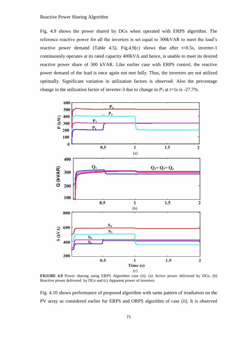
Reactive Power Sharing Algorithm

71

Fig. 4.9 shows the power shared by DGs when operated with ERPS algorithm. The

reference reactive power for all the inverters is set equal to 300kVAR to meet the load’s

reactive power demand (Table 4.5). Fig.4.9(c) shows that after t=0.5s, inverter-1

continuously operates at its rated capacity 400kVA and hence, is unable to meet its desired

reactive power share of 300 kVAR. Like earlier case with ERPS control, the reactive

power demand of the load is once again not met fully. Thus, the inverters are not utilized

optimally. Significant variation in utilization factors is observed. Also the percentage

change in the utilization factor of inverter-3 due to change in P3 at t=1s is -27.7%.

Fig. 4.10 shows performance of proposed algorithm with same pattern of irradiation on the

PV array as considered earlier for ERPS and ORPS algorithm of case (ii). It is observed

(a)

(b)

(c)

FIGURE 4.9 Power sharing using ERPS Algorithm case (ii): (a) Active power delivered by DGs, (b)

Reactive power delivered by DGs and (c) Apparent power of inverters

Reactive Power Sharing Algorithm

72

from Table 4.5 that during t=0-0.5s, the proposed algorithm tries to share the apparent

power equally amongst all the inverters. Hence, as the inverter-1 reaches its limit, it is

operated at 400kVA (100% capacity), while inverters 2, 3 and 4 are operated around

500kVA demonstrating the tendency of equalizing the reactive power sharing. At t=0.5s,

when the irradiation of PV1 increases resulting into the increase in the output power of

inverter 1, the output reactive power of inverter 1 decreases. Simultaneously the reactive

powers of all other inverters increase.

(a)

(b)

(c)

FIGURE 4.10 Power sharing using proposed EAPS Algorithm case (ii): (a) Active power delivered by DGs

(b) Reactive power delivered by DGs and (c) Apparent power of inverters

This results into minimizing the miss-match in the reactive powers of the inverters and

hence, reduces the gap of percentage utilization of different inverters. Thus, the algorithm

inherently has the feature of minimizing the mismatch. But still the mismatch is relatively

large. This is due to the equal apparent power sharing principle of the algorithm, which

inspite of the unequal nominal kVA rating of the inverters, tries to allocate the apparent

Reactive Power Sharing Algorithm

73

power equally amongst the DG inverters. Hence, it results into the unequal utilization

factor of the DGs. At t=1s when P3 changes from 400 kW to 200kW, Q3 increases and Q4

and Q2 decrease to achieve better power sharing amongst the inverters. The least utilization

factor of 0.6 is observed for inverter-3.

TABLE 4.5 UF for each DG using ORPS, ERPS and Proposed Algorithm case (ii)

ORPS ERPS Proposed (EAPS)

t (s) Pi Q

iref S

i UF Q

iref S

i UF Q

iref S

i UF

0-0.5

200 171 263 0.65 300 360 0.90 346 399 0.99

300 257 395 0.79 300 424 0.84 388 500 0.98

400 342 526 0.87 300 500 0.83 310 500 0.83

500 425 656 0.93 300 583 0.83 154 520 0.74

0.5-1

300 240 384 0.96 265 400 1.00 265 399 0.99

300 240 384 0.76 300 424 0.84 400 500 0.99

400 320 512 0.85 300 500 0.83 338 523 0.87

500 400 640 0.91 300 547 0.78 197 537 0.76

1-2

300 276 407 1.00 265 400 1.00 265 399 0.99

300 277 408 0.81 300 424 0.84 344 450 0.90

200 185 272 0.45 300 360 0.60 412 450 0.75

500 462 680 0.97 300 547 0.78 179 500 0.75

Note: Pi, Qiref, Si are mentioned in kW, kVAR and kVA. UF is mentioned in percentage.

Table 4.5 shows the active, reactive and apparent powers shared by proposed algorithm.It

is observed from Table 4.5 that percentage decrease in utilization factor for inverter-3 (due

to change in P3 at t=1s) is -13.8%, which is relatively smaller than that observed with

ORPS (-47%) and ERPS (-27.7%).

4.2.2.2 Performance of EAPS algorithm with permutations

This sub-section presents the cases where the reactive power allocation amongst the

inverters are based on the algorithm shown in Fig. 4.4, which evaluates various possible

sequences of calculation and allocation of reactive power amongst the inverters. The best

possible sequence of allocation that results into the least standard deviation in UFs of the

inverters is identified. The performance of the proposed approach is also evaluated for

different solar irradiation condition against three control approaches: ORPS [19], EAPS

[23] and EAPS-LSD. The actual active, reactive and apparent power delivered by four

DGs can be obtained as shown in Figs. 4.8-4.10. The results are analysed on the basis of

vector diagram drawn from tabulated data. Following three cases are considered.

Case (i): Uniform irradiation on all PV arrays

Reactive Power Sharing Algorithm

74

Case (ii): Unequal power generation by PV arrays

Case (iii): Unequal active power generation with one PV array out of service

Case (i): Uniform irradiation on all PV

In this case all the PV arrays receive similar irradiance and operate under uniform

conditions. As a result all the DGs generate equal active power (400 kW). Due to this the

reference reactive power assigned to all the inverters is same (150 kVAR) and all the

inverters work at same power factor (0.936). The UF for the inverters and SD are 0.854

and 0, respectively. The results are similar irrespective of the control approaches. Fig.4.11

shows the vector diagram representing the power shared by each inverter (all are

overlapping).

FIGURE 4.11 Vector representation showing power sharing for case (i)

Case (ii): Unequal power generation by PV arrays

It is considered that the arrays receive different irradiance level resulting into active power

generation of 400kW, 350kW, 250kW and 400kW by PV arrays PV1, PV2, PV3 and PV4,

respectively. Table 4.6 shows the power sharing for the three control approach OPRS,

EAPS, and EAPS-LSD. With the ORPS control the inverter-3 operates with the least UF

of 0.54 while inverters 1 and 4 have UF of 0.87. Against this the maximum and minimum

UFs for EAPS are 0.84 and 0.77, respectively. The gap further reduces for EAPS-LSD

where the maximum and minimum UFs are recorded as 0.82 and 0.77. As a result the SD

is minimum (=0.019) for EAPS-LSD against 0.029 and 0.154 observed for EAPS and

ORPS, respectively. It is evident that the minimization of the SD for EAPS and EAPS-

LSD is realized by allowing the inverters to operate at different power factors. Some of the

DGs do operate at low power factors (0.64 for inverter-3) with EAPS and EAPS-LSD;

Reactive Power Sharing Algorithm

75

however the system power factor with these control approaches is still the same (0.92) as

that obtained with ORPS control.

TABLE 4.6 UF of DGs for case (ii) ORPS/EAPS/EAPS-LSD control algorithm

ORPS algorithm

Inv.

No. (i)

Pi

(kW)

Qiref

(kVAR)

Si

(kVA)

UF

SD PF

1 400 171 435 0.87

0.15

0.92

2 350 150 381 0.76 0.92

3 250 107 272 0.54 0.92

4 400 172 435 0.87 0.92

EAPS algorithm

1 400 0 400 0.80

0.029

1.00

2 350 169 389 0.77 0.90

3 250 300 390 0.77 0.64

4 400 131 421 0.84 0.95

EAPS –LSD algorithm

1 400 100 412 0.82

0.019

0.97

2 350 202 404 0.80 0.86

3 250 298 389 0.77 0.64

4 400 0 400 0.80 1.00

The graphical representation showing the power shared by the inverters with the three

control approaches is shown in Fig.4.12. It is evident that S1-S4 vectors for ORPS method

are once again aligned with the ST vector. However, for EAPS and EAPS-LSD, they are no

longer aligned with the ST vector. Further, it is observed that the order/sequence in which

the reactive powers are allocated results into different orientations of S1 through S4. If the

allocation of reactive power is done in the order 1-2-3-4 then SD is 0.029 as shown in

Table 4.6 and by the row corresponding to Sr. No. 21 in Table 4.7.

FIGURE 4.12 Vector representation showing power sharing for case (ii)

It shows the SD for all possible sequence in which the reactive power can be allocated

amongst the inverter using the control principle. The least SD equal to 0.019 is obtained for

Reactive Power Sharing Algorithm

76

the combination 4-3-2-1 (Sr. No. 1). Thus, the order of allocation of reactive powers does

affect the value of SD.

TABLE 4.7 SD with different possible sequences of reactive power allocations for case (ii)

Sr. No. Inverter’s

Order

Inverter

SD 1 2 3 4

1 4-3-2-1 Qiref 100 202 298 0 0.019

Si 412 404 389 400

2 4-3-1-2 Qiref 59.0 243 298 0 0.031

Si 404 426 389 400

3 4-2-3-1 Qiref 131 169 300 0 0.029

Si 421 389 390 400

4 4-2-1-3 Qiref 0 169 431 0 0.102

Si 400 389 498 400

5 4-1-2-3 Qiref 0 240 360 0 0.038

Si 400 424 438 400

6 4-1-3-2 Qiref 0 257 343 0 0.034

Si 400 434 424 400

7 3-4-2-1 Qiref 106 206 287 0 0.028

Si 414 406 381 400

8 3-4-1-2 Qiref 71.0 242 287 0 0.036

Si 406 425 381 400

9 3-2-4-1 Qiref 62.5 188 287 62.5 0.022

Si 405 397 381 405

10 3-2-1-4 Qiref 62.5 188 287 62.5 0.022

Si 405 397 381 405

11 3-1-2-4 Qiref 0 206 288 106 0.028

Si 400 406 381 414

12 3-1-4-2 Qiref 0 242 287 71.0 0.036

Si 400 425 381 406

13 2-3-4-1 Qiref 81.5 150 287 81.5 0.031

Si 408 381 381 408

14 2-3-1-4 Qiref 81.5 150 287 81.5 0.031

Si 408 381 381 408

15 2-4-3-1 Qiref 144 150 306 0 0.036

Si 425 381 395 400

16 2-4-1-3 Qiref 0 167 433 0 0.107

Si 400 381 500 400

17 2-1-4-3 Qiref 0 167 433 0 0.107

Si 400 381 500 400

18 2-1-3-4 Qiref 0 150 306 144 0.036

Si 400 381 395 425

19 1-3-2-4 Qiref 0 202 298 100 0.019

Si 400 404 389 412

20 1-3-4-2 Qiref 0 243 298 59.0 0.031

Si 400 426 389 404

21 1-2-3-4 Qiref 0 169 300 131 0.029

Si 400 389 390 421

22 1-2-4-3 Qiref 0 169 431 0 0.102

Si 400 389 498 400

23 1-4-2-3 Qiref 0 240 360 0

0.038 Si 400 424 438 400

24 1-4-3-2 Qiref 0 257 343 0

0.034 Si 400 434 424 400

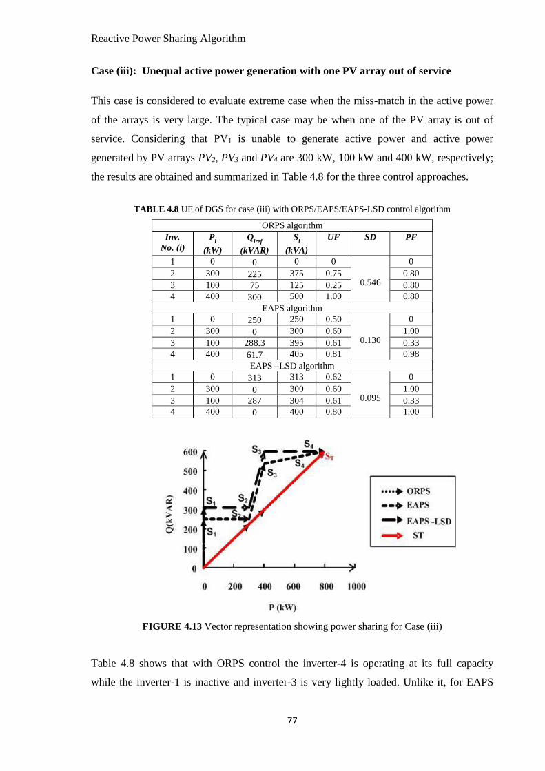
Reactive Power Sharing Algorithm

77

Case (iii): Unequal active power generation with one PV array out of service

This case is considered to evaluate extreme case when the miss-match in the active power

of the arrays is very large. The typical case may be when one of the PV array is out of

service. Considering that PV1 is unable to generate active power and active power

generated by PV arrays PV2, PV3 and PV4 are 300 kW, 100 kW and 400 kW, respectively;

the results are obtained and summarized in Table 4.8 for the three control approaches.

TABLE 4.8 UF of DGS for case (iii) with ORPS/EAPS/EAPS-LSD control algorithm

ORPS algorithm

Inv.

No. (i)

Pi

(kW)

Qiref

(kVAR)

Si

(kVA)

UF

SD PF

1 0 0 0 0

0.546

0

2 300 225 375 0.75 0.80

3 100 75 125 0.25 0.80

4 400 300 500 1.00 0.80

EAPS algorithm

1 0 250 250 0.50

0.130

0

2 300 0 300 0.60 1.00

3 100 288.3 395 0.61 0.33

4 400 61.7 405 0.81 0.98

EAPS –LSD algorithm

1 0 313 313 0.62

0.095

0

2 300 0 300 0.60 1.00

3 100 287 304 0.61 0.33

4 400 0 400 0.80 1.00

FIGURE 4.13 Vector representation showing power sharing for Case (iii)

Table 4.8 shows that with ORPS control the inverter-4 is operating at its full capacity

while the inverter-1 is inactive and inverter-3 is very lightly loaded. Unlike it, for EAPS

Reactive Power Sharing Algorithm

78

and EAPS-LSD the inverters are relatively more uniformly utilized. SD with EAPS-LSD is

0.095, which is higher than in case (ii). However, it is due to the fact that the inverter-4 has

to deliver 400kVA (totally contributed by active power) which is higher than one-fourth of

the ST (i.e. ST/4 = 250kVA). As one should extract maximum possible power generated

from PV array, the apparent power supplied by inverter-4 cannot be reduced below

400kVA.As a result the inverter-4 operates with higher UF than other 3 which operate at

nearly same UF. Fig. 4.13 shows vector representation for ORPS, EAPS and EAPS-LSD

for data of Table 4.8.

4.3 Proportional Apparent Power Sharing (PAPS-LSD)

The algorithm discussed in previous section (4.2) (EAPS-LSD) operates all the inverters to

supply equal apparent power, thereby leading to the equal utilization of the inverters.

However, the algorithm works effectively only for inverters of equal rating and shows

mismatch in utilization when the inverters ratings are not same. To overcome this

limitation a reactive power sharing algorithm is proposed for inverters of unequal rating.

The algorithm assigns reactive power required amongst the inverters in proportion to their

apparent power ratings i.e. named as PAPS-LSD.

4.3.1 Principle of Proportional Apparent Power Sharing (PAPS-LSD)

Proportional apparent power sharing (PAPS-LSD) is based on the principle of operating

the inverters in such a way that they share the power in proportional to their nominal

ratings. The principle of proposed reactive power sharing method (PAPS-LSD) is

described using vector representation shown in Fig.4.14. Four PV connected DGs where

S1N…S4N are the nominal apparent power ratings of DGs are considered. The total desired

apparent power (STD) depends on reactive power demand of the load (QL= QT) and total

active power (PT) generated by the PV sources and is represented as

2L

2TTD QPS +=

4.18

Accordingly, the total apparent power capability of system ST is expressed by (4.19)

22TTT QPS +=

4.19

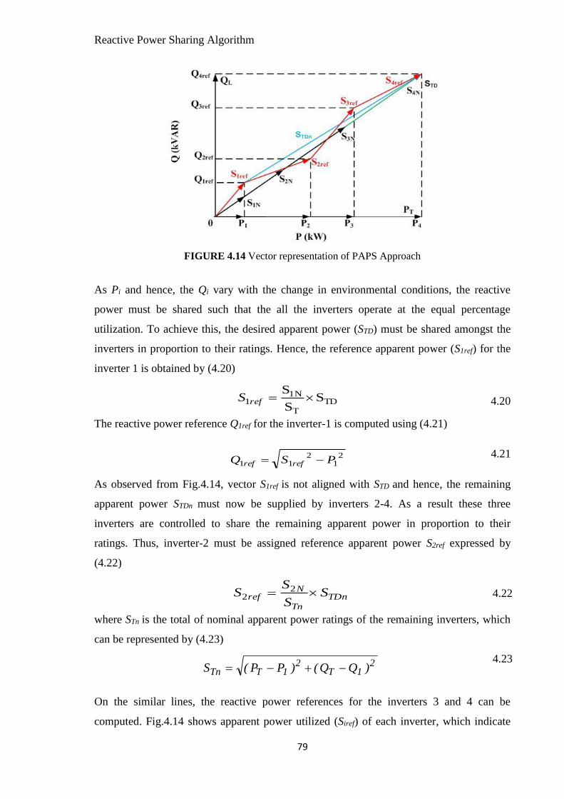
Reactive Power Sharing Algorithm

79

FIGURE 4.14 Vector representation of PAPS Approach

As Pi and hence, the Qi vary with the change in environmental conditions, the reactive

power must be shared such that the all the inverters operate at the equal percentage

utilization. To achieve this, the desired apparent power (STD) must be shared amongst the

inverters in proportion to their ratings. Hence, the reference apparent power (S1ref) for the

inverter 1 is obtained by (4.20)

TDT

1N1 S

S

S=refS

4.20

The reactive power reference Q1ref for the inverter-1 is computed using (4.21)

21

211 PSQ refref −=

4.21

As observed from Fig.4.14, vector S1ref is not aligned with STD and hence, the remaining

apparent power STDn must now be supplied by inverters 2-4. As a result these three

inverters are controlled to share the remaining apparent power in proportion to their

ratings. Thus, inverter-2 must be assigned reference apparent power S2ref expressed by

(4.22)

TDnTn

Nref S

S

SS = 2

2

4.22

where STn is the total of nominal apparent power ratings of the remaining inverters, which

can be represented by (4.23)

21T

21TTn )QQ()PP(S −+−=

4.23

On the similar lines, the reactive power references for the inverters 3 and 4 can be

computed. Fig.4.14 shows apparent power utilized (Siref) of each inverter, which indicate

Reactive Power Sharing Algorithm

80

that their vector length is proportional to their nominal ratings. The detailed algorithm is

presented in the next section.

4.3.2 Proportional Apparent Power sharing (PAPS-LSD) Control Algorithm

The principle mentioned in the previous section computes the reactive power Q1ref -Q4ref

from the active power information PV1-PV4. The algorithm shown in Fig.4.15 not only

follows the principle described in section 6.3.1. Fig. 4.15(a) shows the flow chart of

evaluating various permutations of inverter. Fig. 4.15(b) shows a subroutine which

calculates the reference reactive power for the inverter for the given permutation.

The algorithm, shown in Fig. 4.15(a) computes the n possible permutations for active

power and apparent power corresponding to different sequence in which the reactive

power references can be computed and assigned to the inverters. Permutation matrix of

active powers (PMPPi), apparent power (Sperm), Reactive power of ith inverter can be

represented same as (4.4)-(4.6), respectively. Total active power (PT), reactive power (QT)

and apparent power (ST) can be represented as (4.7)-(4.9), respectively.

For the given ( jth) permutation, and ith inverter the sub-routine calculates the available

reactive power (Qi )

22iiNi PSQ −=

4.24

Once reactive power is assigned to any inverter, the remaining active, reactive, apparent

power to be supplied by the rest of inverters is updated. Thus, the new value of total active

power (PTn), total reactive power available (QTn), total apparent power capacity of the

remaining inverters (STn), remaining reactive power to be met (QDn) and total remaining

apparent power (STDn) to be shared can be represented as (4.25)-(4.29).

−

=

−=

1

0

i

i

iTTn PPPwhere 00 =P

4.25

−

=

−=

1

0

i

i

iTTn QQQ where 00 =Q

4.26

22TnTnTn QPS +=

4.27

Reactive Power Sharing Algorithm

81

−

=

−=

1

0

i

i

irefDDn QQQ where 00 =refQ

4.28

22DnTnTDn QPS +=

4.29

To achieve proportional apparent power sharing, each inverter must supply apparent power

represented by

TDnTn

iNiref S

S

SS =

4.30

The reference apparent power may exceed active power delivered by ith inverter (Pi). In

such case reactive power is set to zero for that particular inverter which does not satisfy

(4.31)

iiref PS 4.31

Hence, the reference reactive power for the ith inverter (for jth permutation) can be obtained

as

22iirefiref PSQ −=

4.32

Reference reactive power assigned to inverter should not exceed its maximum available

rating (Qi) as indicated by (4.33)

iiref QQ 4.33

If condition of (4.33) is violated, the reference reactive power for the ith inverter (for jth

permutation) is set as

iiref QQ = 4.34

Based on Qiref and PMMPi for the given permutation, the apparent power to be handled by

the inverter (Sinv) and the utilization factor (UF) of the inverters are computed. The best

possible option is identified based on the least standard deviation (SDmin) of the utilization

factors of the inverters.

4.3.3 Results and analysis

To evaluate performance of above algorithm, microgrid system configuration shown in

Fig.4.1 is simulated in MATLB/Simulink. Simulation line parameters are considered same

as Table-4.1, whereas nominal ratings of the DG1-DG4 are considered as 350 kVA, 400

kVA, 450 kVA and 500 kVA respectively. Two control algorithms, ORPS [18] and PAPS-

LSD are evaluated for following cases: (i) PV sources with active power (PVi) generation

proportional to the nominal ratings of the inverter (ii) PV sources with equal active power

Reactive Power Sharing Algorithm

82

generation (iii) PV sources with unequal active power generation (iv)One of the PV source

is unable to deliver PV power

FIGURE 4.15 Flowchart for the PAPS-LSD approach: (a) Main program and (b) Subroutine

Reactive Power Sharing Algorithm

83

Case (i) PV sources with active power generation in proportional inverter nominal

ratings

In this case all the PV arrays operate under Standard Test Conditions (STC) i.e. irradiation

of 1 kW/m2 and temperature of 25 C. Hence, they generate active power equal to their

nominal ratings which is considered as 90% of the nominal kVA ratings of the associated

inverters. The additional margin is kept for reactive power compensation as well as for

safety margin. Accordingly the powers generated by arrays PV1 through PV4 are 315 kW,

360 kW, 405 kW and 450 kW, respectively. The reference reactive power assigned with

PAPS-LSD and ORPS methods are same under this case. With all the approaches the

reactive power shared by the inverters are in proportional to their nominal ratings. As the

active powers are also in proportional to the nominal ratings of the inverters, the UF of all

the inverters are same as shown in Table 4.9. Hence, all inverters operate at same power

factor with equal UF (96%) with zero SD. Fig. 4.16 shows active power, reactive power

and apparent power of each inverter for these methods.

(a)

(b)

(c)

FIGURE 4.16 Power sharing with PAPS and ORPS algorithm for case (i): (a) Active power delivered by

DGs, (b) Reactive power shared by inverters and (c) Apparent power of inverter

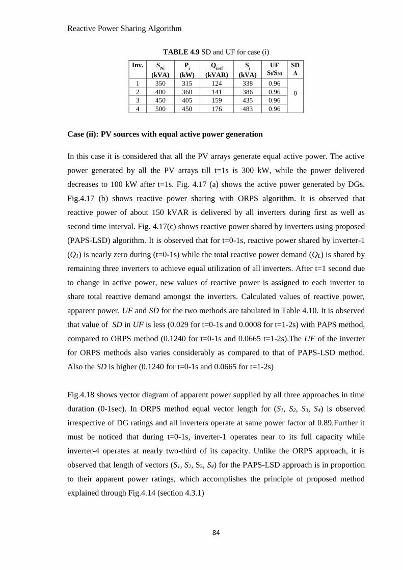
Reactive Power Sharing Algorithm

84

TABLE 4.9 SD and UF for case (i)

Inv.

SNi

(kVA)

Pi

(kW)

Qiref

(kVAR)

Si

(kVA)

UF

Si/SNi

SD

Δ

1 350 315 124 338 0.96

0

2 400 360 141 386 0.96

3 450 405 159 435 0.96

4 500 450 176 483 0.96

Case (ii): PV sources with equal active power generation

In this case it is considered that all the PV arrays generate equal active power. The active

power generated by all the PV arrays till t=1s is 300 kW, while the power delivered

decreases to 100 kW after t=1s. Fig. 4.17 (a) shows the active power generated by DGs.

Fig.4.17 (b) shows reactive power sharing with ORPS algorithm. It is observed that

reactive power of about 150 kVAR is delivered by all inverters during first as well as

second time interval. Fig. 4.17(c) shows reactive power shared by inverters using proposed

(PAPS-LSD) algorithm. It is observed that for t=0-1s, reactive power shared by inverter-1

(Q1) is nearly zero during (t=0-1s) while the total reactive power demand (QL) is shared by

remaining three inverters to achieve equal utilization of all inverters. After t=1 second due

to change in active power, new values of reactive power is assigned to each inverter to

share total reactive demand amongst the inverters. Calculated values of reactive power,

apparent power, UF and SD for the two methods are tabulated in Table 4.10. It is observed

that value of SD in UF is less (0.029 for t=0-1s and 0.0008 for t=1-2s) with PAPS method,

compared to ORPS method (0.1240 for t=0-1s and 0.0665 t=1-2s).The UF of the inverter

for ORPS methods also varies considerably as compared to that of PAPS-LSD method.

Also the SD is higher (0.1240 for t=0-1s and 0.0665 for t=1-2s)

Fig.4.18 shows vector diagram of apparent power supplied by all three approaches in time

duration (0-1sec). In ORPS method equal vector length for (S1, S2, S3, S4) is observed

irrespective of DG ratings and all inverters operate at same power factor of 0.89.Further it

must be noticed that during t=0-1s, inverter-1 operates near to its full capacity while

inverter-4 operates at nearly two-third of its capacity. Unlike the ORPS approach, it is

observed that length of vectors (S1, S2, S3, S4) for the PAPS-LSD approach is in proportion

to their apparent power ratings, which accomplishes the principle of proposed method

explained through Fig.4.14 (section 4.3.1)

Reactive Power Sharing Algorithm

85

(a)

(b)

(c)

FIGURE 4.17 Power sharing with ORPS and PAPS-LSD algorithm for case (ii)

FIGURE 4.18 Vector representation of apparent power rating for duration (t=0-1 sec) for case (ii)

TABLE 4.10 SD and UF for case (ii)

ORPS Proposed PAPS

Inv. Time

(sec)

SNi

(kVA)

Pi

(kW)

Qiref

(kVAR)

Si

(kVA)

UF

Si/SNi

SD

Δ

Qiref

(kVAR)

Si

(kVA)

UF

Si/SNi

SD

Δ

1

t=0-1

350 300 150 335 0.958

0.1240

0 300 0.857

0.0290

2 400 300 150 335 0.839 116 322 0.804

3 450 300 150 335 0.745 209 366 0.812

4 500 300 150 335 0.671 275 407 0.814

1

t=1-2

350 100 150 180 0.515

0.0665

110 149 0.425

0.0008

2 400 100 150 180 0.451 138 170 0.426

3 450 100 150 180 0.401 164 192 0.427

4 500 100 150 180 0.361 188 213 0.426

Reactive Power Sharing Algorithm

86

Case (iii) All PV sources with unequal power generation

In this case all PV arrays PV1-PV4 generate unequal active powers of 200 kW, 300 kW,

350 kW and 400 kW, respectively during time interval t=0 to 1s. Thus, the active power

generation is further not in proportional to the nominal apparent power rating of the

inverters. Active powers delivered by the inverters are shown in Fig. 4.19(a). Reactive

power sharing by ORPS and proposed algorithm is shown in Fig. 4.19(b)-(c), respectively.

(a)

(b)

(c)

FIGURE 4.19 Power sharing for case (iii): (a) Active power generated by PV array, (b) Reactive power

sharing with ORPS and (c) Reactive power sharing with PAPS-LSD algorithm

Fig. 4.19(b) shows that for ORPS approach, reactive power shared by the inverters is such

that their operating power factor remains the same; while Fig. 4.19(c) shows constant

reactive power for the PAPS-LSD approach. It is observed that for PAPS approach,

reactive power delivered by inverter-1, which is having the least rating and supplying the

least active power, is greater compared to other sources. Inverters 2-4 also share the

reactive power such that the UFs remain nearly equal (about 0.83). At t=1s, power

Reactive Power Sharing Algorithm

87

extracted from array PV1 increases from 200 kW to 300 kW and that of PV2 decreases from

300 kW to 100 kW. In response to these the reactive power shared by inverter-1 decreases

whereas that of inverter-2 increases for achieving effective utilization of inverters (Fig.4.19

(c)).The change in reactive power supplied (though not that large as observed for inverter 1

and 2) is also observed for inverter-3

Table-4.11 shows active power, reactive power, apparent, UF and SD for this case. It is

observed that during t=1-2s, when active power P2 decreases, the reactive power (and

hence, apparent power) supplied by inverter-2 also decreases for ORPS approach, which

results into only (28%) utilization of inverter-2. In PAPS-LSD when active power P2

decreases at t=1s, the reactive power supplied by inverter-2 increases. As a result, SD

obtained through ORPS method is 0.1155 during t=0-1s and 0.3191 for t=1-2s, which is

significantly large compared to PAPS method (0.0064 during t=0-1s and 0.0022 for t=1-

2s).

TABLE 4.11 SD and UF for case (iii)

ORPS Proposed PAPS

Inv. Time

(sec)

SNi

(kVA)

Pi

(kW)

Qiref

(kVAR)

Si

(kVA)

UF

Si/SNi

SD

Δ

Qiref

(kVAR)

Si

(kVA)

UF

Si/SNi

SD

Δ

1

t=0-1

350 200 096 222 0.634

0.1155

206 287 0.820

0.0064

2 400 300 144 333 0.832 144 333 0.832

3 450 350 168 388 0.863 133 374 0.832

4 500 400 192 444 0.887 117 417 0.834

1

t=1-2

350 300 157 339 0.967

0.3191

0 300 0.857

0.0022

2 400 100 052 113 0.282 307 323 0.807

3 450 350 183 395 0.878 152 382 0.848

4 500 400 208 451 0.902 141 424 0.848

Case (iv) One of the PV sources is unable to deliver PV power

This case considers extreme condition where one of the PV arrays is unable to generate

active power. The reason may be some fault on the dc-dc converter connecting the PV

array with the inverter or intended cut off of the dc-dc converters or array for maintenance

or repair. Active power generated by inverters 2 to 4 are 300 kW, 350 kW and 400 kW,

respectively. At t=1s active power generated by inverter-3 also reduces to zero as shown in

Fig. 4.20(a). As shown in Fig.20 (c), reactive power shared by inverter-1 is maximum

(nearly 266 kVAR) with proposed method where as zero with ORPS method (Fig.

3=4.20(b)).

Reactive Power Sharing Algorithm

88

Table 4.12 shows active, reactive and apparent power sharing for the case (iv). It is

observed that the inverter-1 is utilized nearly 76% in first duration and 60% in second

duration when operating with PAPS method where as 0 % utilization is observed in both

intervals for ORPS method. For t=0-1s, SD is observed 0.0292 in PAPS, which is much

less in comparison to 0.4476 obtained with ORPS. Even for t=1-2 s, SD with PAPS is

much lesser then that obtained with ORPS approach. It is observed for ORPS approach that

inverter-4 is operating above its maximum limit for t >1s as reactive power is shared by

only two inverters.

(a)

(b)

(c)

FIGURE 4.20 Power sharing for case (iv): (a) Active power generated by PV array, (b) Reactive power

sharing with ORPS and (c) Reactive power sharing with PAPS-LSD algorithm)

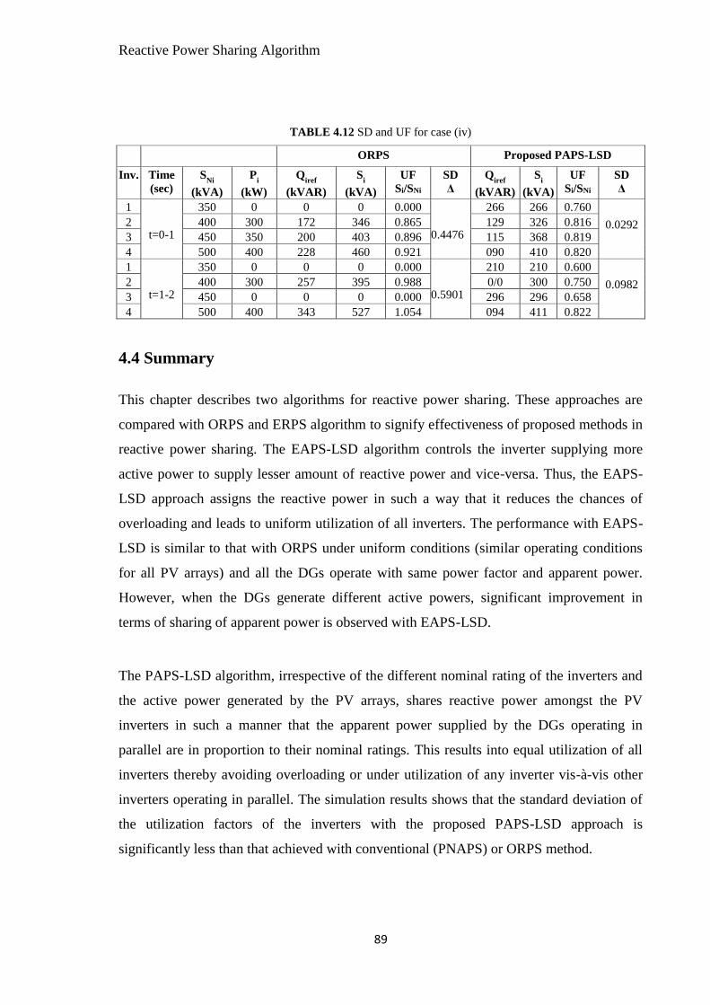
Reactive Power Sharing Algorithm

89

TABLE 4.12 SD and UF for case (iv)

ORPS Proposed PAPS-LSD

Inv. Time

(sec)

SNi

(kVA)

Pi

(kW)

Qiref

(kVAR)

Si

(kVA)

UF

Si/SNi

SD

Δ

Qiref

(kVAR)

Si

(kVA)

UF

Si/SNi

SD

Δ

1

t=0-1

350 0 0 0 0.000

0.4476

266 266 0.760

0.0292

2 400 300 172 346 0.865 129 326 0.816

3 450 350 200 403 0.896 115 368 0.819

4 500 400 228 460 0.921 090 410 0.820

1

t=1-2

350 0 0 0 0.000

0.5901

210 210 0.600

0.0982

2 400 300 257 395 0.988 0/0 300 0.750

3 450 0 0 0 0.000 296 296 0.658

4 500 400 343 527 1.054 094 411 0.822

4.4 Summary

This chapter describes two algorithms for reactive power sharing. These approaches are

compared with ORPS and ERPS algorithm to signify effectiveness of proposed methods in

reactive power sharing. The EAPS-LSD algorithm controls the inverter supplying more

active power to supply lesser amount of reactive power and vice-versa. Thus, the EAPS-

LSD approach assigns the reactive power in such a way that it reduces the chances of

overloading and leads to uniform utilization of all inverters. The performance with EAPS-

LSD is similar to that with ORPS under uniform conditions (similar operating conditions

for all PV arrays) and all the DGs operate with same power factor and apparent power.

However, when the DGs generate different active powers, significant improvement in

terms of sharing of apparent power is observed with EAPS-LSD.

The PAPS-LSD algorithm, irrespective of the different nominal rating of the inverters and

the active power generated by the PV arrays, shares reactive power amongst the PV

inverters in such a manner that the apparent power supplied by the DGs operating in

parallel are in proportion to their nominal ratings. This results into equal utilization of all

inverters thereby avoiding overloading or under utilization of any inverter vis-à-vis other

inverters operating in parallel. The simulation results shows that the standard deviation of

the utilization factors of the inverters with the proposed PAPS-LSD approach is

significantly less than that achieved with conventional (PNAPS) or ORPS method.

90

CHAPTER – 5

Modified droop control for power sharing

The droop control method is widely used for sharing of active and reactive power amongst

the DGs in islanded mode as discussed section 3.2 of chapter 3, However, the conventional

droop control method has several drawbacks when used for sharing power amongst PV

based DGs operating in an island. P-ω droop method, when used for such DGs, shares

active power based on fixed droop coefficient irrespective of available energy from the PV

source under given environmental conditions. Hence, the frequency and the voltage set

points are mainly determined by the load and it ignores the variation in active power (P)

due to the intermittent and uncertain nature of the energy source. With the conventional

droop control, a drop in generation of one PV based DG (which may be due to the decrease

in insolation level or shading on the array of that DG) causes reduction in output of other

DGs operating in parallel. This requires large capacity auxiliary source (AS) to maintain

power balance and stability.

Thus, the droop control strategy suffers from the issue of ineffective utilization of the

sources and instability in case when performance of some of the sources (e.g. PV or wind

based) is dependent on environmental conditions. Hence, a modified droop control strategy

is proposed in this chapter for a microgrid comprising of PV based distributed generators

(DG) operating in parallel with other DGs. Dynamic nature applied to the droop

characteristic sets the frequency reference such that the PV sources operate at their

maximum power point and the energy demanded from the auxiliary source is the

minimum. It ensures optimum active power distribution amongst all DGs. The margin

available after supplying the active power, which varies for the PV based DGs, is used to

allocate the references for reactive power sharing. The reactive power sharing algorithm

ensures that the standard deviation of the percentage utilization of the inverters is kept the

minimum. The effectiveness of the proposed strategy against other approaches is justified

through the simulation results obtained in MATLAB/Simulink.

Modified Droop Control for Power Sharing

91

5.1 System Configuration

The system configuration comprising of four DGs and the auxiliary energy source shown

in Fig. 5.1, is considered to evaluate the performance of the proposed modified droop

control strategy. The first two DGs (DG1 and DG2) are the photovoltaic based DGs while

the remaining two (DG3 and DG4) are fed from reliable energy source like microturbines

or fuel cell. The PV based DGs (DG1 and DG2) are considered to be identical. The PV

based DGs comprises of a PV array along with a dc-dc converter, which is controlled to

output maximum power using MPP tracking (MPPT) method. The DC-DC converters

used for the MPPT are not shown in Fig.5.1 for the sake of brevity. The power electronic

inverters (INV-1 through INV-4) are used to control the energy supplied by these DGs.

Additionally they are also controlled to provide the reactive demand of the load. The

impedances Z0i, where ‘i ’represents ith DG, take into account the impedance of interfacing

inductor, the impedance of cable and isolation transformer.

FIGURE 5.1 System configuration of a Microgrid with four DGs

Modified Droop Control for Power Sharing

92

An auxiliary source represented by AS is required to satisfy power balance. It comes into

action and supplies the power when load demand increases beyond the cumulative active

power generated by all the DGs. It acts as a recipient of active power in case the active

power required by the load is less than that generated by the PV based DGs. The AS also

participates in the active power exchange when a sudden change in the load or input power

occurs. Once the control algorithm regains the new equilibrium position (i.e. power

balance is regained) the power supplied/absorbed by AS becomes zero. Amongst four

DGs, the reliable sources based DGs (DG3 and DG4) are operated with conventional droop

control while environment dependent PV source based DGs (DG1 and DG2) are controlled

with modified droop control method for supplying the active power. As the active power

supplied by the PV based DG vary with the environmental conditions, the maximum

reactive power which can be exchanged through its inverter also varies. The control

scheme employed takes care of variable reactive power margin of the PV based inverters

and distributes the reactive power amongst inverters 1 through 4 in proportion to the

available reactive power capabilities of these inverters.

5.2 Principle of Modified Active Power Droop Control

The principle of modified active power droop control is illustrated through the Fig. 5.2,

which shows P-ω characteristics for DG1- DG4.

FIGURE 5.2 Modified active power-frequency droop characteristic

Modified Droop Control for Power Sharing

93

Let the PV based DGs are initially operating at frequency ω1, corresponding to point A.

The operating points for the DG3 and DG4 at this frequency are B and C. If the output

power of PV based DGs decrease due to the decrease in insolation, the operating point on

its droop characteristic shifts to A1 corresponding to frequency ω2 (ω2 >ω1). This in turn

decreases the output power of DG3 and DG4 as they have to operate at the same frequency

ω2 (corresponding to points B1 and C1, respectively). This will lead to active power

imbalance in the system. To avoid such situation, when the output of PV array decreases

due to the decrease in the insolation, its operating frequency must be lowered (rather than

increasing) so that the DG3 and DG4 can supply the extra power to maintain the

equilibrium/stability. Thus, the modified droop characteristics exhibits the dynamic nature

as the additional frequency component (Δω) is added to the frequency set point derived

through the conventional droop characteristic. As a result, the operation of both DG1 and

DG2 occur corresponding to point A2 (at ωnew), while the DG3 and DG4 operate

corresponding to points B2 and C2, respectively.

5.3 Inverter Control

The modified droop control for sharing active and reactive power is implemented using

hierarchical control structure. The primary control unit (PCU) consists of dynamic droop

characteristic, which ensures that the PV based DGs are always operated at their MPP,

while other DGs share active power in proportion to their ratings. The AS provides the

active power only when all DGs hit their limits. This minimizes the AS requirement. The

reactive power sharing algorithm employed in the secondary control unit (SCU) ensures

that the standard deviation of the percentage utilization of the inverters is kept the

minimum. In case of the communication failure between the primary and the secondary

control units, the DGs fall back on the master-slave control approach employing dynamic

P-ω and Q-V droop control. The block diagram shown in Fig. 5.3 shows the control unit

comprising of PCUs and the SCU. The control scheme employed takes care of variable

reactive power margin of the PV based inverters. The PAPS reactive power algorithm

executed by the SCU assigns reactive power references to PCUs of inverters 1 through 4.

These references finally set the reactive power of the inverters in proportion to the

available reactive power capabilities of these inverters.

The detailed block diagram of PCU of the control scheme for controlling the inverter’s

Modified Droop Control for Power Sharing

94

output voltage to achieve desired active and reactive power exchange is shown in Fig. 5.4.

As observed through the Fig.5.4, the control scheme incorporates the modifications in the

conventional droop characteristics for sharing the active and reactive power of the load.

FIGURE 5.3 Control block diagram

The modified droop characteristics are defined in general for these sources as

P))(Ps

iK

pK(xP)(Ppmoωrefω MPP −++−−= 5.1

= Pm 0p

5.2

where mp is the slope of the characteristic, for PV based sources P* represents the

maximum active power that it provides when working under standard test conditions

(STC) i.e. its nominal power rating. ωo is the frequency corresponding to rated power(P*)

of the DG, ωref is the operating frequency when the DG supplies power (P kW) and PMPP

is maximum power extracted from the PV array under given conditions .

The power calculator block shown in Fig. 5.4 determines the active and reactive power

shared by DGs. The inverter’s output voltage (Vabc) and current (iabc) are transformed into

d-q frame to obtain the active power (p) and reactive power (q) using (5.3) and (5.4)

)ViVi(2

3p qqdd +=

5.3

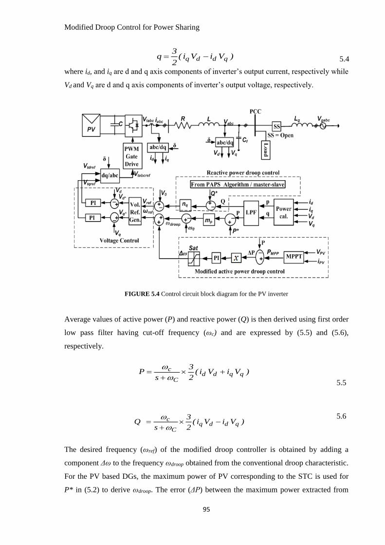
Modified Droop Control for Power Sharing

95

)ViVi(2

3q qddq −=

5.4

where id, and iq are d and q axis components of inverter’s output current, respectively while

Vd and Vq are d and q axis components of inverter’s output voltage, respectively.

FIGURE 5.4 Control circuit block diagram for the PV inverter

Average values of active power (P) and reactive power (Q) is then derived using first order

low pass filter having cut-off frequency (ωc) and are expressed by (5.5) and (5.6),

respectively.

)ViVi(2

3

sP qqdd

C

c ++

=

5.5

)ViVi(2

3

sQ qddq

C

c −+

=

5.6

The desired frequency (ωref) of the modified droop controller is obtained by adding a

component Δω to the frequency ωdroop obtained from the conventional droop characteristic.

For the PV based DGs, the maximum power of PV corresponding to the STC is used for

P* in (5.2) to derive ωdroop. The error (ΔP) between the maximum power extracted from

Modified Droop Control for Power Sharing

96

the PV array under given conditions (PMPP) and the active power supplied through the

inverter (P) is used to derive Δω. The PMPP information is obtained from the perturb and

observe (P&O) MPPT algorithm implemented with the first-stage (dc-dc) converter. ΔP is

then scaled by a factor x before it is processed by the PI controller. ωref required for the

voltage control loop, is then derived as expressed by (5.7) using Δω and ωdroop.

droopref +=

5.7

The reactive power droop control is implemented using reactive power vs. voltage (Q-V)

droop equation represented by (5.8), which provides the reference voltage (Vref) for the

voltage control loop.

)QQ(nVV *qoref −−=

5.8

*q QVn =

5.9

The reference reactive power (Q*) required for (5.8)-(5.9) is obtained through the reactive

power sharing algorithm (described in chapter 4) executed by the SCU. In case the

communication link between the PCUs and the SCU fails, the reactive power references

are set by the master-slave control approach with the adaptive feature for both P-ω and Q-

V droop. In such case the reactive power reference used in (5.8)-(5.9) (for ith inverter) is

calculated from locally available data using (5.10).

22*

iiNi PSQ −=

5.10

The reference reactive power (Q*) required for (5.8)-(5.9) is obtained through the

proportional reactive power sharing algorithm (PAPS) described in chapter 4. Voltage and

frequency references, Vref and ωref, respectively, are then applied to the voltage control

loop. It includes reference sinusoidal generator and voltage regulator loop. Reference

generator generates sinusoidal three-phase ac voltages from the Vref and ωref, and then

further applies abc-dq transformation to derive the reference d-q voltage components Vd*

and Vq*. Voltage regulator loop compares these Vd* and Vq* with actual inverter output d-q

voltage components (Vd and Vq). The error is then processed to derive the three-phase

sinusoidal reference voltage signal for PWM control of the inverter. The control scheme

for DG3 and DG4 are identical except that it does not incorporate MPPT algorithm and the

blocks that derive Δω.

Modified Droop Control for Power Sharing

97

5.4 Simulation Results

To demonstrate the effectiveness of the proposed control strategy to share the active and

reactive power amongst the various sources, the microgrid system shown in Fig. 5.1 is

simulated in MATLAB/Simulink. The performance of the proposed control strategy is also

evaluated against other approaches [47], [81]. The system parameters considered for the

simulation study are mentioned in Table-5.1 while Table-5.2 shows the variation in the

maximum power output of the PV arrays (PVi) due to the variation in the insolation level

(𝛼i).

TABLE 5.1 Ratings and parameters for the system of Fig.5.1.

kVA rating of PV inverter-1 (S1) 250 kVA

kVA rating of PV inverter-2 (S2) 250kVA

kVA rating of inverter-3 ( S3) 375kVA

kVA rating of inverter-4 ( S4) 565 kVA

Nominal power rating of AS 1000kVA

Line impedance (Z1,Z2) R1=0.5Ω, L1=320μH,C1=20 μF

Line impedance (Z3) R3=0.33Ω, L3=213μH,C3=30 μF

Line impedance (Z4) R4=0.22Ω, L4=142μH,C4=45 μF

mp1,mp2,mp3,mp4 (Hz/kW) -2.5e-6,-2.5e-6,-1.66e-6,-1.11e-6

nq1,nq2,nq3,nq4 (V/kVAR) -1e-4,-1e-4,-6.66e-5,-4.44e-5

Line to Line o/p voltage (rms) 230 V

Grid’s nominal frequency f(Hz) 50

Frequency range (fmax-fmin)(Hz) 50.2-49.7

TABLE 5.2 PV array insolation variations

Time (s) Insolation α1

kW/m2

Output Power

(kW)

Insolation α2

kW/m2

Output

Power (kW)

0-1 1.0 200 1.0 200

1-2 0.5 100 1.0 200

2-3 0.5 100 0.3 60

Figure 5.5 shows results obtained with the conventional droop control method. The four

DGs controlled using the droop control operates simultaneously to meet the demand of the

1000 kVA, 0.8pf (lag) load (i.e. 800 kW, 600 kVAR). It is observed from Fig. 5.5(a), that

the active power supplied by the four DGs is in proportion to their ratings (250: 250: 375:

565). Thus, during t=0-1 s, active power supplied by the two PV sources is 140kW while

that of the inverters 3 and 4 are 215 W and 312 kW, respectively. As a result, the power

supplied through the PV based inverters is much less than the maximum power (200 kW as

shown in Table-5.1) that the PV sources can supply, leading to the ineffective utilization of

the PV sources. At t=1s as the insolation on the PV array PV1 decreases to 0.5kW/m2, it

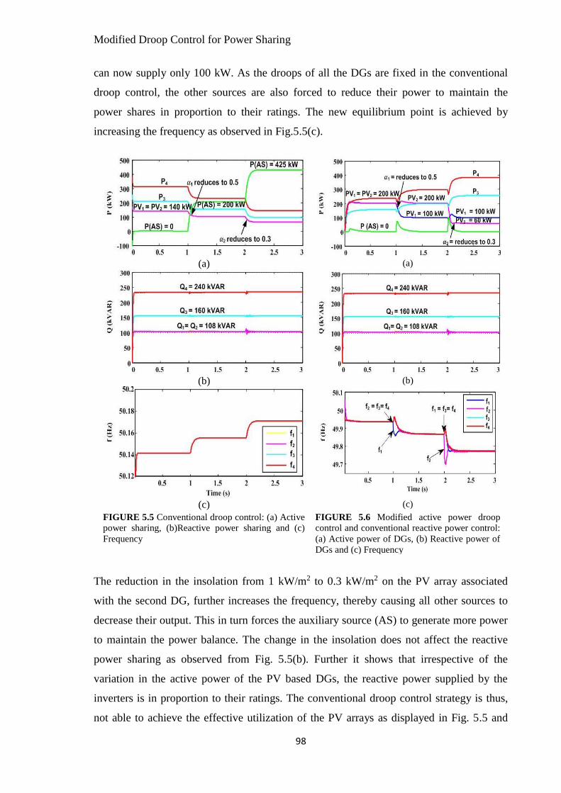
Modified Droop Control for Power Sharing

98

can now supply only 100 kW. As the droops of all the DGs are fixed in the conventional

droop control, the other sources are also forced to reduce their power to maintain the

power shares in proportion to their ratings. The new equilibrium point is achieved by

increasing the frequency as observed in Fig.5.5(c).

(a) (a)

(b) (b)

(c) (c)

FIGURE 5.5 Conventional droop control: (a) Active

power sharing, (b)Reactive power sharing and (c)

Frequency

FIGURE 5.6 Modified active power droop

control and conventional reactive power control:

(a) Active power of DGs, (b) Reactive power of

DGs and (c) Frequency

The reduction in the insolation from 1 kW/m2 to 0.3 kW/m2 on the PV array associated

with the second DG, further increases the frequency, thereby causing all other sources to

decrease their output. This in turn forces the auxiliary source (AS) to generate more power

to maintain the power balance. The change in the insolation does not affect the reactive

power sharing as observed from Fig. 5.5(b). Further it shows that irrespective of the

variation in the active power of the PV based DGs, the reactive power supplied by the

inverters is in proportion to their ratings. The conventional droop control strategy is thus,

not able to achieve the effective utilization of the PV arrays as displayed in Fig. 5.5 and

Modified Droop Control for Power Sharing

99

tabulated in Table-5.3.

Fig. 5.6 shows the simulation results with the modified P-ω control strategy, which always

ensure the operation of the PV arrays at their maximum power points. It is observed from

Fig. 5.6(a) that during t=0-1s, active power delivered by both PV sources is 200 kW, which

is the maximum power that the PV sources generate with insolation of 1 kW/m2. This is

obtained by inserting an additional frequency component Δω to shift the P-ω

characteristics. It is observed from Fig.5.6 (c) that the addition of Δω, changes the

operating frequency to 49.95 Hz. As a result, the operation of inverters 3 and 4 deliver also

shifts to new operating points corresponding to the new frequency. During t=1-2s, when

the output power of PV1 is reduced to half (100 kW), Δω causes the P-ω characteristic of

inverter-1 to change such that the operating frequency decreases (unlike conventional

droop control where the frequency increases as shown in Fig. 5.6(c). This also forces the

inverters 3 and 4 to operate at lower frequency, thereby increasing their output power.

Output power of PV2 still corresponds to its maximum power of 200kW as observed in

Fig. 5.5(a). Similarly when the insolation on the second PV source decreases at t=2s, the

operating frequency is decreased further to obtain the new equilibrium point, where the PV

sources PV1 and PV2 operate at their maximum power of 100 kW and 60 kW, respectively.

The remaining active power (640 kW) is matched by the DG3 and DG4 in proportion to

their rating. Thus, PV based DGs always extract the maximum possible power from PV

arrays and the remaining power is met through the remaining DGs, till they reach their

limit (as set by droop settings).Therefore AS remains off in modified droop control as long

as the DGs (other than PV based) operate below their limits. AS supplies power only for a

short duration (when the step changes in power occur), to minimize the active power

mismatch for ensuring stability. Thus, optimum utilization of the various sources is

ensured. Fig. 5.6(b) shows reactive power sharing by DGs. It is observed that results are

same as that of Fig. 5.5(b) as all inverters are controlled using conventional Q-V droop

control method for reactive power sharing.

The inverters can also be controlled to share the reactive power equally by the inverters as

mentioned in equal reactive power sharing (ERPS) approach [81]. The reactive power

obtained using ERPS algorithm are used as references Q1*, Q2*, Q3* and Q4* (Fig. 5.4) to

determine droop characteristics for reactive power sharing. As the reactive power demand

of load is 600 kVAR, all inverters are assigned reference values of 150 kVAR. Fig. 5.7

Modified Droop Control for Power Sharing

100

shows active power sharing using the modified P-ω control while the reactive power

sharing using ERPS algorithm. Fig. 5.7(b) shows that the reactive power delivered by all

inverters is about 150 kVAR, but not exactly equal to 150 kVAR. The line impedances and

their mismatch is the reason for the inaccuracy in the reactive power sharing. It can be

minimized by introducing the virtual line impedance in line [51]. It is observed that

reactive power assigned to each inverter is nearly independent of the active power

delivered by the inverter.

(a)

(b)

FIGURE 5.7 Modified active power /ERPS droop control : (a) Active power sharing and (b) Reactive

power sharing

The results are also summarized in Table-5.3. It is observed from the Table-5.3 that these

approaches (reactive power sharing with conventional droop control and ERPS) do not

yield the equal percentage utilization of the inverters (referred as utilization factor UF).

The variation in the UF of the inverters is large leading to higher standard deviation of UF.

This can be minimized by assigning higher reactive power to the PV based inverters that

supply relatively lesser active power.

Figure 5.8 shows results of active and reactive power sharing using the proposed modified

active and reactive droop control, which not only extracts the maximum power from the

PV array but also tries to achieve the equal UFs of the inverters. Fig. 5.8(a) shows active

power sharing which is similar to that shown in Fig. 5.6(a). Fig. 5.8(b) shows reactive

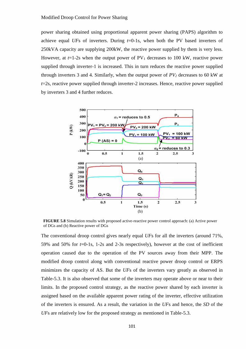
Modified Droop Control for Power Sharing

101

power sharing obtained using proportional apparent power sharing (PAPS) algorithm to

achieve equal UFs of inverters. During t=0-1s, when both the PV based inverters of

250kVA capacity are supplying 200kW, the reactive power supplied by them is very less.

However, at t=1-2s when the output power of PV1 decreases to 100 kW, reactive power

supplied through inverter-1 is increased. This in turn reduces the reactive power supplied

through inverters 3 and 4. Similarly, when the output power of PV2 decreases to 60 kW at

t=2s, reactive power supplied through inverter-2 increases. Hence, reactive power supplied

by inverters 3 and 4 further reduces.

(a)

(b)

FIGURE 5.8 Simulation results with proposed active-reactive power control approach: (a) Active power

of DGs and (b) Reactive power of DGs

The conventional droop control gives nearly equal UFs for all the inverters (around 71%,

59% and 50% for t=0-1s, 1-2s and 2-3s respectively), however at the cost of inefficient

operation caused due to the operation of the PV sources away from their MPP. The

modified droop control along with conventional reactive power droop control or ERPS

minimizes the capacity of AS. But the UFs of the inverters vary greatly as observed in

Table-5.3. It is also observed that some of the inverters may operate above or near to their

limits. In the proposed control strategy, as the reactive power shared by each inverter is

assigned based on the available apparent power rating of the inverter, effective utilization

of the inverters is ensured. As a result, the variation in the UFs and hence, the SD of the

UFs are relatively low for the proposed strategy as mentioned in Table-5.3.

Modified Droop Control for Power Sharing

102

Modified Droop Control for Power Sharing

103

The performance of the proposed control strategy is further explored when operating with

heavy and low load conditions. The performance is even evaluated for the case when the

communication link between the PCUs and the SCU fails. Under such case the SCU is

unable to provide reactive power references derived through the PAPS to the PCUs. Thus,

following three cases are considered to evaluate the performance of the control scheme (i)

Performance with heavy load condition, (ii) Performance with low load condition and (iii)

Performance when the communication link between PSU and SCU fails

Case (i): Performance with heavy load condition

Fig. 5.9(a) shows that both the PV based DGs supply 200 kW (corresponding to 1kW/m2)

till t=1s and then supply 100 kW/m2 (corresponding to 0.5 kW/m2) due to the reduction in

the insolation level. Till t=2s the total load to be supplied is 721 kVA at 0.8pf (600 kW,

400 kVAR). A step change in load is considered at t=1s resulting in the total load of 1220

kVA at 0.8 pf lag (1000 kW, 700 kVAR).

(a)

(b)

(c)

FIGURE 5.9 Performance with heavy load case (i): (a) Active power sharing, (b) Reactive power sharing

and (c) Frequency

Modified Droop Control for Power Sharing

104

At t=1s, the reduction in the active power of PV based DGs is compensated by the increase

in the active power supplied through inverters 3 and 4. They share the active power in

proportion to their ratings. This is achieved by quickly lowering the operating frequency as

observed in Fig. 5.9(c). As the active power demand is well below the total active power

generating capacity of all the DGs put together, the output power of AS is zero. Just like

earlier case, the decrease in the active power of the DG1 and DG2 causes their reactive

power to increase. At t=2s, the active power demand of the load increases to a level at

which the DG3 and DG4 reach to their active power limit. The active power limit for the

DG3 and DG4 are set as 300kW and 450kW, respectively. Thus, DG1 –DG4 can supply

only 950 kW, forcing the AS source to provide the deficit active power (50 kW). When the

total active power of the DG1 – DG4 just matches the active power demand of the load, the

operating frequency reaches to the least value of 49.7 Hz (as set on the droop

characteristic). At this point, it is not possible for DG3 and DG4 to supply more active

power (as already operating on the limits) by further reducing the frequency as per the

droop control principle. Hence, any further increase in active power demand is met by

increasing the output of AS.

Case (ii): Performance with low load condition

Figure 5.10 shows results when operating with light load conditions (400 kW, 300 kVAR).

During t=0-1.5s, PV based DGs are able to match the active power needed by the load and

hence, the DG3 and DG4 do not supply any active power. The operating frequency under

this case corresponds to the highest value of 50.2 Hz (on the droop characteristic). Under

this condition, DG3 and DG4 just provide the reactive power needed by the load. At t=1.5s,

the reduction in the insolation level lowers the active power of DG1 and DG2. The

modified controller quickly lowers the frequency to a new operating point so that the

decrease in the active power of DG1 and DG2 can be matched by the increase in the active

power of DG3 and DG4.

Case (iii): Performance when the communication link between PSU and SCU fails

Figure 5.11 shows the performance when the communication link between PSU and SCU

fails. The communication between PSC and SCU breaks at t=0.5s and the healthy

condition is restored at t=1.5s. Fig. 5.11(a) shows that the active power generated by both

Modified Droop Control for Power Sharing

105

the PV sources is PV1=PV2=200 kW till t=1s and after t=1s the output of PV sources

reduced to PV1=100 kW and PV2=60 kW. As active power to be supplied by the DG is

dependent on the power generated by the array and as it can be determined locally, the

status of the communication link (healthy or faulty) does not affect the active power

sharing. Fig. 5.11(b) shows the status of communication link.

(a)

(b)

(c)

FIGURE 5.10 Performance with low load case (i): (a) Active power sharing, (b) Reactive power sharing

and (c) Frequency

In the normal (or healthy condition of communication link), the reactive power references

for reactive power sharing are received from the SCU. But when the communication

between PSU and SCU gets disturbed, the provisional control by master-slave approach is

activated. Once communication is retrieved, the reactive power references are once again

derived through the PAPS algorithm. The reactive power sharing with healthy and faulty

conditions of the communication link is shown in Fig. 5.11(c). It is observed that when the

communication link is healthy, the reactive power references are derived through the

proposed reactive power sharing algorithm, which is implemented in SCU. Hence, it

results into very less SD as compared to the case when the communication is disturbed and

Modified Droop Control for Power Sharing

106

the reactive power references are derived from master-slave approach. The power sharing

and the utilization of the DGs are summarized through the data presented in Table 5.4

TABLE 5.4 Power sharing with healthy and unhealthy communication link

Time Pi

Qi

Si

SN

UF SD Control

t=0-0.5s

200 9 200

250 80

0.013

PAPS 200 9 200 250 80

167 240 292 375 78

248 357 434 565 77

t=0.5-1s

200 80 215 250 86

0.103 Master- Slave

200 80 215 250 86

167 180 246 375 65

248 275 370 565 66

t=1-1.5s

100 124 159 250 63

0.086 Master- Slave

60 131 143 250 57

260 145 298 375 79

395 215 450 565 79

t=1.5-2s

100 157 186 250 74

0.010

PAPS

60 174 184 250 74

260 117 285 375 76

395 167 428 565 76

Note: Pi, Qi, Si are mentioned in kW, kVAR and kVA. UF is mentioned in

percentage.

(a)

(b)

(c)

FIGURE 5.11 Results with PAPS and master-slave method: (a) Active power sharing, (b)Status of

communication and (c) Reactive power sharing

Modified Droop Control for Power Sharing

107

5.5 Summary

The conventional droop control does not take into account the variation in the output of the

PV based DGs and hence leads to ineffective utilization of PV sources as well as other

DGs. This demands more storage as the AS has to supply the energy inspite of the fact that

other conventional DGs are still capable to meet the load requirement. The proposed

control strategy modifies the P-ω characteristics by quickly adjusting the frequency

reference for the PV based DGs such that the decrease in their output power is quickly

compensated by the increase in the output power of other DGs. It is observed that the

operating frequency is strictly maintained within the predefined limits of 49.7 Hz-50.2 Hz.

The PAPS algorithm used for assigning the reference reactive power to the Q-V droop

forces the inverter carrying more active power to supply lesser reactive power and vice-

versa. It helps in preventing overloading of any inverters. Also, the percentage utilization

factors of the inverters are nearly equal as confirmed through the very low value of

standard deviation of the utilization factors. The auxiliary energy source supplies the

energy only when the conventional DGs are unable to provide any extra active power or in

case of momentary active power imbalance caused by the sudden change in the power

from DGs or change in load. Thus, the AS inherently helps in providing stability against

sudden power mismatch. The algorithm also takes care of the situation where the

communication between PCU and SCU gets disturbed. The reactive power sharing under

such case is achieved by the PCU’s using the local information. The proposed active and

reactive power sharing approach together is observed to offer an effective solution for the

optimal utilization of the DGs and the inverters.

108

CHAPTER – 6

Modified Droop Control with Arctan Function and

Virtual Impedance

The droop control method is traditionally adopted to distribute active and reactive power

amongst the DGs operating in parallel. With the conventional droop control scheme

accurate load sharing amongst the inverters (in proportion to their power ratings), can be

achieved if the inverters (or DGs) have the same output per-unit impedances .However, the

accuracy of distribution of active and reactive power among the DGs controlled by the

conventional droop control approach is highly dependent on the value of line impedance,

R/X i.e. resistance to reactance ratio of the line, voltage setting of inverters etc.

In reactive power sharing methods, discussed in previous chapter-5, line impedances are

considered in proportion to the active and reactive power droop coefficients. However,

mismatch in line impedances results into error in reactive power sharing as it is difficult to

strictly maintain equal per-unit line impedances for the DGs. Mathematical analysis is

included in this chapter to reveal the limitations of the conventional droop control in case

the impedance mis-match occurs. Under such case (of mis-match), it is necessary to

overcome the error introduced due to line impedance mismatch. The error in reactive

power sharing is minimized by inserting virtual impedance in line with the inverters to

remove the mis-match in impedance.

The effect of line impedance variation on reactive power sharing for the conventional

droop control method is evaluated in this chapter. A modified droop control approach to

reduce the effect of impedance mis-match and to improve the time response is proposed.

The error mis-match in the output voltage of the inverter is minimized using virtual

impedance while the improved time response is achieved by modifying the real-power

frequency droop using arctan function. Simulations results are presented to validate the

effectiveness of the control approach.

Modified Droop Control with Arctan Function and Virtual Impedance

109

6.1 Limitation of conventional droop control method

Limitation of conventional droop is explained with a system having two inverters

operating in parallel to supply a common load connected at Point of common Coupling

(PCC) as shown in Fig. 6.1.The nominal power ratings of the inverters are S1N and S2N. It is

assumed that the line is inductive in nature, accordingly the inverter’s output voltage is

mainly dependent on the reactive power (Q−V relationship) and frequency is

predominantly dependent on the active power(P−ω relationship).

FIGURE 6.1 System configurations with two inverters

The conventional P−ω and Q−E droop relations for active and reactive power sharing

amongst DGs are expressed by (6.1) and (6.2), respectively

)PP(m i*

ipioiref −−= 6.1

)(*

iiqioiref QQnVV −−= 6.2

where Pi* , Qi* , o , and oV are active power, reactive power, frequency and output voltage

of the ith DG, respectively under nominal (rated) conditions. nqi and mpi represents

frequency and voltage droop coefficients, respectively for the ith inverter. iref is the

frequency when ith DG is delivering active power Pi while irefV is its output voltage when it

is exchanging reactive power Qi. The droop coefficients nqi and mpi for the ith inverter (or

DG) are usually determined by the desired voltage droop and frequency droop,

respectively.

Modified Droop Control with Arctan Function and Virtual Impedance

110

The frequency is integrated to obtain the phase of the reference voltage for inverter. In

order for the inverters to share the load in proportional to their power ratings, the droop

coefficients of the inverters should be in inverse proportional to their power ratings [13],

i.e. nqi and mpi should satisfy

𝑛𝑞1 𝑆1𝑁 = 𝑛𝑞2 𝑆2𝑁 6.3

𝑚𝑝1 𝑆1𝑁 = 𝑚𝑝2 𝑆2𝑁 6.4

Hence, nqi and mpi must also satisfy

2p

2q

1p

1q

m

n

m

n=

6.5

6.1.1 Active Power Sharing

It is obvious that the inverters operating in a microgrid should have the same frequency

under equilibrium (i.e. under steady state) conditions. Thus, for the two inverters shown in

Fig. 6.1, under steady state ω1= ω2. Hence, for proportional active power sharing amongst

the DGs following condition must be satisfied.

𝑚𝑝1𝑃1 = 𝑚𝑝2𝑃2 6.6

Since the coefficients mpi is chosen to satisfy (6.4), it is always ensured that the active

power sharing is proportional to their power ratings i.e.

𝑃1

𝑆1𝑁=

𝑃2

𝑆2𝑁

6.7

The active power Pi, reactive power Qi and apparent power Si supplied by ith the inverter to

the bus/load of voltage (V) can be expressed as

𝑃𝑖 =𝑉𝑖𝑟𝑒𝑓𝑉

𝑍0𝑖sin 𝜃𝑖

6.8

𝑄𝑖 = −𝑉𝑖𝑟𝑒𝑓𝑉 cos 𝜃𝑖 − 𝑉2

𝑍0𝑖

6.9

𝑆𝑖 = 𝑃𝑖 + 𝑗𝑄𝑖 6.10

where 𝜃𝑖 is the angle between V and Viref, Zoi is the output (line) impedance for the ith

inverter. It is evident that the active power Pi is predominately dependent on the power

angle 𝜃𝑖 (for small value of 𝜃𝑖), while the reactive power Qi mostly depends on the

amplitude of output-voltage Viref.

Modified Droop Control with Arctan Function and Virtual Impedance

111

Alternatively, according to (6.8), the condition of active power sharing represented in

(6.6) can be written as

𝑚𝑝1

𝑉1𝑟𝑒𝑓𝑉

𝑍01𝑠𝑖𝑛𝜃1 = 𝑚𝑝2

𝑉2𝑟𝑒𝑓𝑉

𝑍02𝑠𝑖𝑛𝜃2

6.11

Ifθ1=θ2 and V1ref = V2ref, then

𝑚𝑝1

𝑍01=

𝑚𝑝2

𝑍02

6.12

From (6.8) and (6.12) it is evident that the active power sharing is in the ratio of the

droops which is dependent on the ration of output impedances. In other words, the

change in the ratio of impedances affects the power sharing.

6.1.2 Reactive Power Sharing

The reactive power of the two inverters can be obtained by substituting (6.2) into (6.9)

yielding,

𝑄𝑖 =𝑉0𝑐𝑜𝑠𝜃𝑖 − 𝑉

𝑛𝑞𝑖𝑐𝑜𝑠𝜃𝑖 +𝑍0𝑖

𝑉⁄

6.13

Substituting (6.13) into (6.2) the deviation or error in voltage amplitudes of the two

inverters is

𝑉2𝑟𝑒𝑓 − 𝑉1𝑟𝑒𝑓 =𝑉0𝑐𝑜𝑠𝜃𝑖 − 𝑉

𝑐𝑜𝑠𝜃1 +𝑍0𝑖

𝑛𝑞1𝑉⁄

−𝑉0𝑐𝑜𝑠𝜃𝑖 − 𝑉

𝑐𝑜𝑠𝜃2 +𝑍0𝑖

𝑛𝑞2𝑉⁄

6.14

It is reported in [13] that the voltage deviation ΔV of the two units leads to considerable

errors in load sharing. From (6.14), the error ΔV could be made zero if conditions

expressed by (6.15) is satisfied

𝑛𝑞1𝑄1 = 𝑛𝑞2𝑄2 𝑜𝑟 𝑄1

𝑆1𝑁=

𝑄2

𝑆2𝑁

6.15

However it is a challenging task to obtain this condition because of numerical

computational errors, disturbances, parameter drifts and component mismatches. This

condition is satisfied if

𝑛𝑞1

𝑍01=

𝑛𝑞2

𝑍02 𝑎𝑛𝑑 𝜃1 = 𝜃2

6.16

Modified Droop Control with Arctan Function and Virtual Impedance

112

In other words, nqi should be proportional to its output impedance Zoi. In other words Zoi

should satisfy (6.16). From (6.16) and (6.3), in order to achieve accurate sharing of

reactive power, the (inductive) output impedance should be designed to satisfy

𝑍01𝑆1𝑁 = 𝑍02𝑆2𝑁 6.17

As the per-unit output impedance of ith inverter is expressed by (6.18)

𝛾𝑖 =𝑍0𝑖

𝑉0𝐼𝑖

⁄=

𝑍0𝑖𝑆𝑖𝑁

(𝑉0)2

6.18

Substituting (6.18) into (6.17), the condition is equivalent to

𝛾1 = 𝛾2 6.19

Thus, in order to achieve accurate proportional power sharing for the conventional droop

control scheme,(6.19) proves that the per-unit output impedances of all inverters operated

in parallel should be equal. If this is not met, then the voltage set-points Viref are not the

same and errors appear in the reactive power sharing. However, this is almost impossible

in reality. It is difficult to maintain V1ref = V2ref or θ1=θ2 (as required for (6.12)) because of

the presence of numerical computational errors, disturbances and noises. It is also difficult

to maintain γ1 = γ2 because of different feeder impedances, parameter drifts and component

mismatches. The reality is that none of these conditions would be met. Hence, a

mechanism is needed to achieve an accurate proportional load sharing when such uncertain

factors exist.

6.2 Modified Droop control with arctan function and virtual impedance

Due to the mis-match in the per-unit values of the output impedances of the DGs (or

inverters) operating in a micro-grid, the conventional droop with relationship (P v/s ω

and/or Q v/s V) may not behave as desired as concluded in previous section. Fig. 6.2

advocates the control scheme that overcomes the limitations of the conventional

droop-control scheme. It incorporates two significant features: (i) minimization of the

mismatch in per-unit output impedances of the inverters by inserting virtual

impedance in series with the feeder resistance and (ii) limiting the rate of change of

frequency and its excursion by employing arctan function as shown in Fig. 6.2.

Modified Droop Control with Arctan Function and Virtual Impedance

113

FIGURE 6.2 Droop control scheme with virtual impedance

The principle of insertion of virtual impedance to minimize the effect of mis-match is

mentioned next. With a view to match the per-unit output impedances of the inverters

operating in parallel, the virtual impedance loop adds fictitious or virtual impedance in

series with the real line impedance to fulfill the condition mentioned in (6.12). The virtual

impedance creates a “voltage drop” without generating any actual active power losses

and/or reactive power requirement. In order to increase the stability of the system, to

reduce the impact of circulating currents, and to share linear and nonlinear loads, virtual

impedance is added into the system by an additional control loop [85]-[86], which can be

represented as

𝑉𝑟𝑒𝑓 = 𝑉𝑑𝑟𝑜𝑜𝑝 − 𝑍𝑣(𝑠) ∗ 𝐼𝑖 6.20

where Vdroop is the voltage reference delivered by the droop method and Zv(s) is the virtual

output impedance. The calculation and design of virtual impedances is reported by [85].

Fig. 6.2 shows the block diagram representing the implementation of the virtual impedance

loop. The virtual voltage drop is calculated using the inverters’ output current. Hence, in

this case, the virtual impedance is expected to be added between the inverter and the local

load. This allows the inverter’s output impedance to vary virtually. Insertion of the virtual

impedance, as mentioned above, helps in reducing the mis-match of the impedances and

thus, overcomes one of the limitations of the conventional droop control. Another,

limitation of the conventional droop control approach is that any excursions in power may

cause a rapid change in frequency which causes the DG unit to operate outside the

permissible frequency range. Further, the conventional droop control has the same gradient

Modified Droop Control with Arctan Function and Virtual Impedance

114

for the P− ω and Q−V droop for the entire range. According to [87], higher the value of m

or n gradient, faster is the response. Hence, it can be concluded that changing of gradient

with the load is required to achieve both these objectives: (i) restricting the frequency

within desired range and (ii) faster response.

Arctan based algorithm [54] can be applied to overcome these limitations of constant

frequency droop and to operate the frequency always within pre-set bounds. In this

algorithm dynamic droop adjustments are performed to achieve better control while

implementing frequency and voltage bounding. The algorithm basically limits the gradient

near the frequency bounds. Unlike the conventional power-frequency droop profile, which

is inherently limited to have a fixed concavity of zero, the arctan function based droop

control allows variance in both gradient and concavity of the power profile. This helps in

achieving natural frequency bounding independently from the overall system controller as

shown in Fig.6.3. The reason for the superior performance with arctan based algorithm is

the monotonic increase in the value in the pre-set boundary. In fact, any function (e.g. cube

function) that provides a monotonically increasing function for the pre-set boundary can be

considered for modification of the power frequency droop profile. However, arctan

function is more preferred as it is less complex and involves low computational time.

FIGURE 6.3 Effect of arctan function on fixed gradient droop

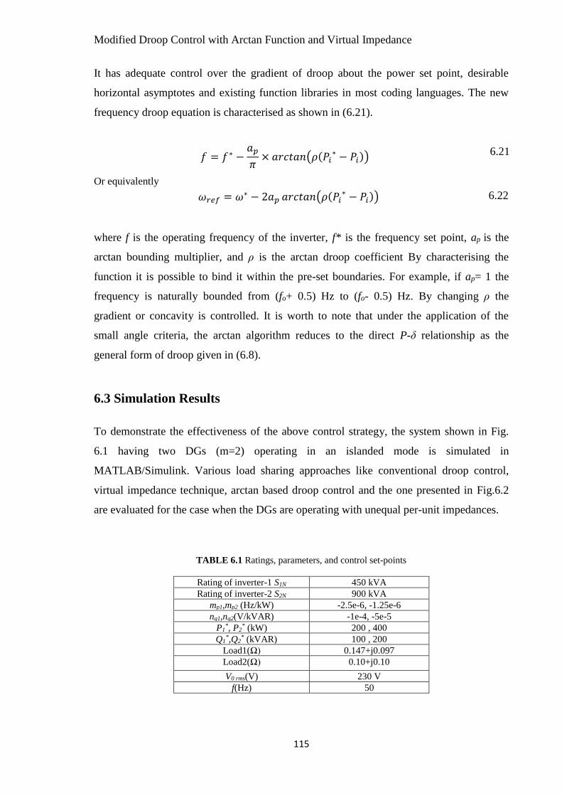
Modified Droop Control with Arctan Function and Virtual Impedance

115

It has adequate control over the gradient of droop about the power set point, desirable

horizontal asymptotes and existing function libraries in most coding languages. The new

frequency droop equation is characterised as shown in (6.21).

𝑓 = 𝑓∗ −𝑎𝑝

𝜋× 𝑎𝑟𝑐𝑡𝑎𝑛(𝜌(𝑃𝑖

∗ − 𝑃𝑖)) 6.21

Or equivalently

𝜔𝑟𝑒𝑓 = 𝜔∗ − 2𝑎𝑝 𝑎𝑟𝑐𝑡𝑎𝑛(𝜌(𝑃𝑖∗ − 𝑃𝑖)) 6.22

where f is the operating frequency of the inverter, f* is the frequency set point, ap is the

arctan bounding multiplier, and ρ is the arctan droop coefficient By characterising the

function it is possible to bind it within the pre-set boundaries. For example, if ap= 1 the

frequency is naturally bounded from (fo+ 0.5) Hz to (fo- 0.5) Hz. By changing ρ the

gradient or concavity is controlled. It is worth to note that under the application of the

small angle criteria, the arctan algorithm reduces to the direct P-δ relationship as the

general form of droop given in (6.8).

6.3 Simulation Results

To demonstrate the effectiveness of the above control strategy, the system shown in Fig.

6.1 having two DGs (m=2) operating in an islanded mode is simulated in

MATLAB/Simulink. Various load sharing approaches like conventional droop control,

virtual impedance technique, arctan based droop control and the one presented in Fig.6.2

are evaluated for the case when the DGs are operating with unequal per-unit impedances.

TABLE 6.1 Ratings, parameters, and control set-points

Rating of inverter-1 S1N 450 kVA

Rating of inverter-2 S2N 900 kVA

mp1,mp2 (Hz/kW) -2.5e-6, -1.25e-6

nq1,nq2(V/kVAR) -1e-4, -5e-5

P1*, P2

* (kW) 200 , 400

Q1*,Q2

* (kVAR) 100 , 200

Load1(Ω) 0.147+j0.097

Load2(Ω) 0.10+j0.10

V0 rms(V) 230 V

f(Hz) 50

Modified Droop Control with Arctan Function and Virtual Impedance

116

As the operation in islanded mode is much more critical than that of grid connected mode,

the comparison is done for islanded mode only. Besides the steady-state performance, the

dynamic performances of the control strategy is also evaluated by applying a sudden i.e.

step change in the load. The ratings of the inverter, droop-coefficients, set-points and

details of load are mentioned in the Table-6.1.

Case (i): Conventional droop control for same per-unit impedances

The feeder impedances are considered purely inductive (Z01= j0.0370 Ω and Z02 =

j0.0185Ω = 0.5Z01). As the inverter-1’s rating is twice the rating of inverter-2, the per-unit

impedances of these inverters as evident from (6.19) are same i.e. (γ1 = γ2 = 0.3147 p.u.).

The performance with conventional droop control scheme is shown through the Figs.

6.4(a)-(d). The active and reactive powers shared by the inverters till t=3s (with only load-

1 connected at PCC) is 250 kW (P1= 83.4 kW, P2=166.6 kW= 2P1) and 165 kVAR (Q1=55

kVAR, Q2=110 kVAR= 2Q1), respectively and after t=3s (when both load-1 and load-2 are

connected) is 423.3 kW (P1=141.1 kW, P2=282.2 kW= 2P1) and 351 kVAR (Q1=117

kVAR, Q2=234 kVAR= 2Q1), respectively. It is observed that the active and reactive

power sharing amongst the inverters are exactly in the ratio of their apparent power (kVA)

ratings i.e. S1/S2. Fig. 6.4(d) also shows that the voltage deviation ΔV=V2d– V1d is zero.

FIGURE 6.4 Power sharing with convention droop control when γ1=γ2: (a)-(b)active and reactive power

shared by inverters, respectively, (c) operating frequency of inverter and (d) output voltage of inverter

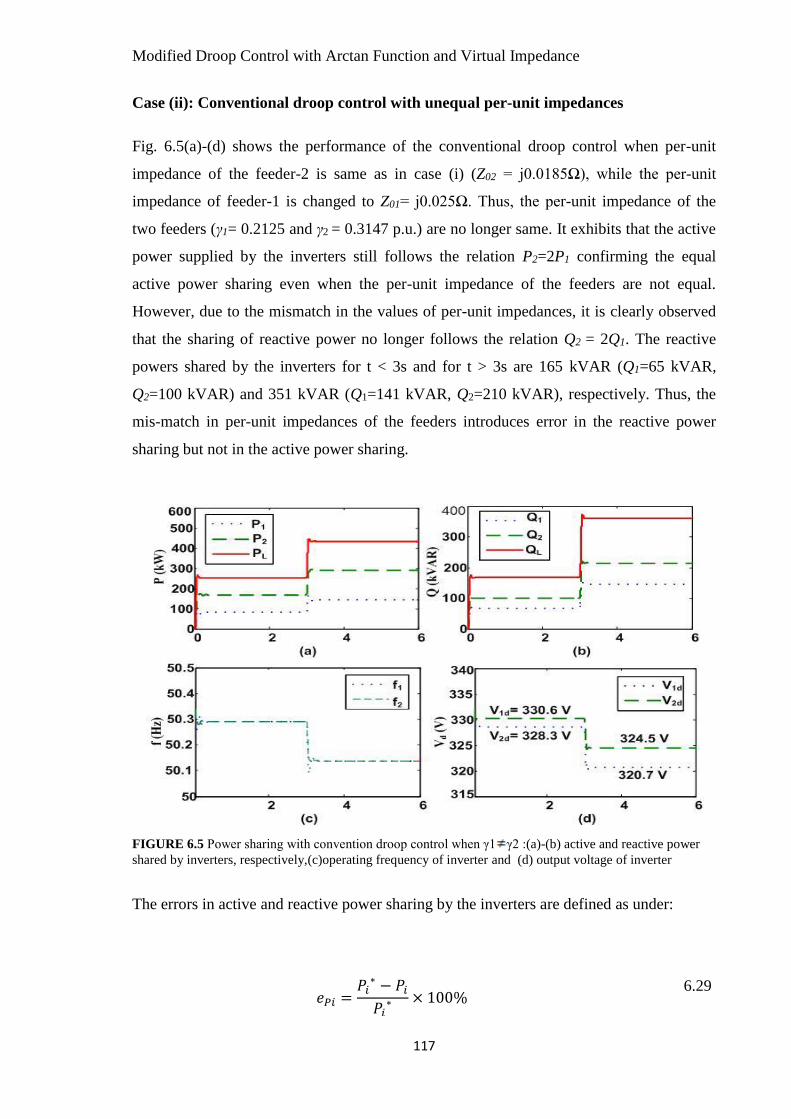
Modified Droop Control with Arctan Function and Virtual Impedance

117

Case (ii): Conventional droop control with unequal per-unit impedances

Fig. 6.5(a)-(d) shows the performance of the conventional droop control when per-unit

impedance of the feeder-2 is same as in case (i) (Z02 = j0.0185Ω), while the per-unit

impedance of feeder-1 is changed to Z01= j0.025Ω. Thus, the per-unit impedance of the

two feeders (γ1= 0.2125 and γ2 = 0.3147 p.u.) are no longer same. It exhibits that the active

power supplied by the inverters still follows the relation P2=2P1 confirming the equal

active power sharing even when the per-unit impedance of the feeders are not equal.

However, due to the mismatch in the values of per-unit impedances, it is clearly observed

that the sharing of reactive power no longer follows the relation Q2 = 2Q1. The reactive

powers shared by the inverters for t < 3s and for t > 3s are 165 kVAR (Q1=65 kVAR,

Q2=100 kVAR) and 351 kVAR (Q1=141 kVAR, Q2=210 kVAR), respectively. Thus, the

mis-match in per-unit impedances of the feeders introduces error in the reactive power

sharing but not in the active power sharing.

FIGURE 6.5 Power sharing with convention droop control when γ1 γ2 :(a)-(b) active and reactive power

shared by inverters, respectively,(c)operating frequency of inverter and (d) output voltage of inverter

The errors in active and reactive power sharing by the inverters are defined as under:

𝑒𝑃𝑖 =𝑃𝑖

∗ − 𝑃𝑖

𝑃𝑖∗ × 100%

6.29

Modified Droop Control with Arctan Function and Virtual Impedance

118

𝑒𝑄𝑖 =𝑄𝑖

∗ − 𝑄𝑖

𝑄𝑖∗ × 100%

6.30

where Pi* is the active power and Qi

* is the reactive power supplied by the ith inverter,

respectively when both the inverters share the active and reactive power exactly in

proportion to their ratings. The reactive power sharing errors, eQ1 and eQ2, for the inverters

1 and 2 are -18.18% and 9.09% till t=3s and -20.51 % and 10.25 % after t=3s. In addition it

can be observed from Fig. 6.5(d) that unlike the case-(i) voltage deviation ΔV=V2d – V1d

=2.3V is also not zero.

Case (iii): Virtual impedance based droop control under the conditionsγ1≠ γ2

The per-unit output impedances of the inverters are maintained at the same values, Z01=

j0.0250Ω and Z02 = j0.0185Ω, as in case (ii) (γ1= 0.2125 and γ2 = 0.3147 p.u.). To

minimize the effect of mis-match in the per-unit impedances, virtual impedance ZV =

j0.012Ω is added in series with Z01. The virtual inductive impedance loop is employed to

achieve the matching of impedances and thereby improve power sharing, especially the

reactive power shared by the inverters.

FIGURE 6.6 Performance with droop control having virtual impedance loop when γ1≠γ2: (a)-(b) active and

reactive power shared by the inverters, respectively, (c) operating frequency of the inverters and (d)

amplitude of output voltage of the inverters

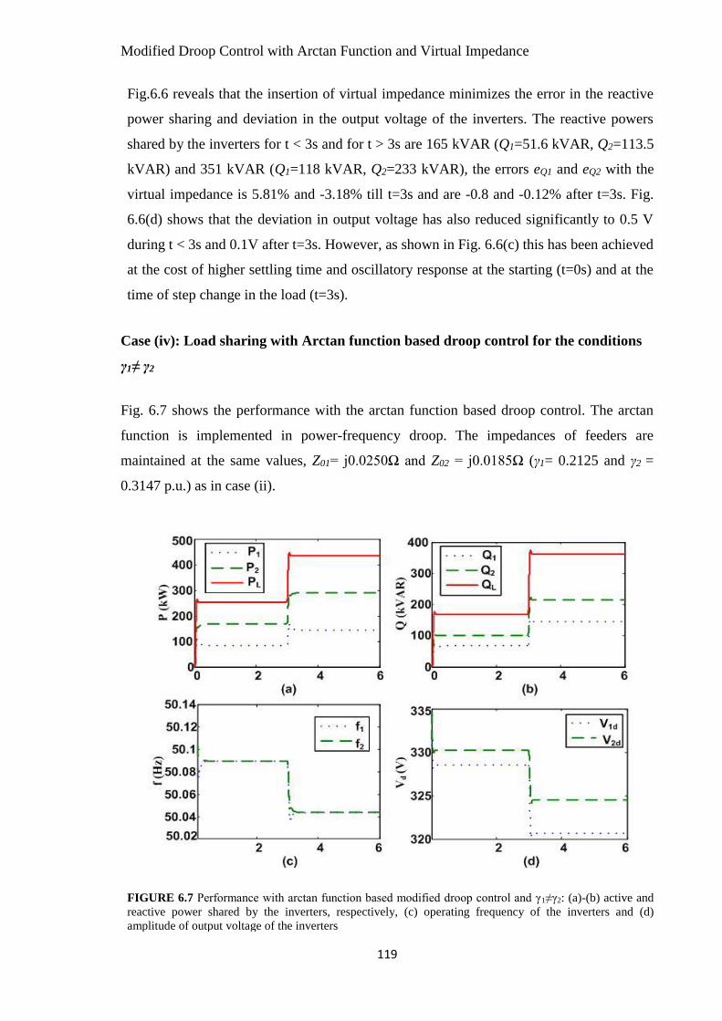
Modified Droop Control with Arctan Function and Virtual Impedance

119

Fig.6.6 reveals that the insertion of virtual impedance minimizes the error in the reactive

power sharing and deviation in the output voltage of the inverters. The reactive powers

shared by the inverters for t < 3s and for t > 3s are 165 kVAR (Q1=51.6 kVAR, Q2=113.5

kVAR) and 351 kVAR (Q1=118 kVAR, Q2=233 kVAR), the errors eQ1 and eQ2 with the

virtual impedance is 5.81% and -3.18% till t=3s and are -0.8 and -0.12% after t=3s. Fig.

6.6(d) shows that the deviation in output voltage has also reduced significantly to 0.5 V

during t < 3s and 0.1V after t=3s. However, as shown in Fig. 6.6(c) this has been achieved

at the cost of higher settling time and oscillatory response at the starting (t=0s) and at the

time of step change in the load (t=3s).

Case (iv): Load sharing with Arctan function based droop control for the conditions

γ1≠ γ2

Fig. 6.7 shows the performance with the arctan function based droop control. The arctan

function is implemented in power-frequency droop. The impedances of feeders are

maintained at the same values, Z01= j0.0250Ω and Z02 = j0.0185Ω (γ1= 0.2125 and γ2 =

0.3147 p.u.) as in case (ii).

FIGURE 6.7 Performance with arctan function based modified droop control and γ1≠γ2: (a)-(b) active and

reactive power shared by the inverters, respectively, (c) operating frequency of the inverters and (d)

amplitude of output voltage of the inverters

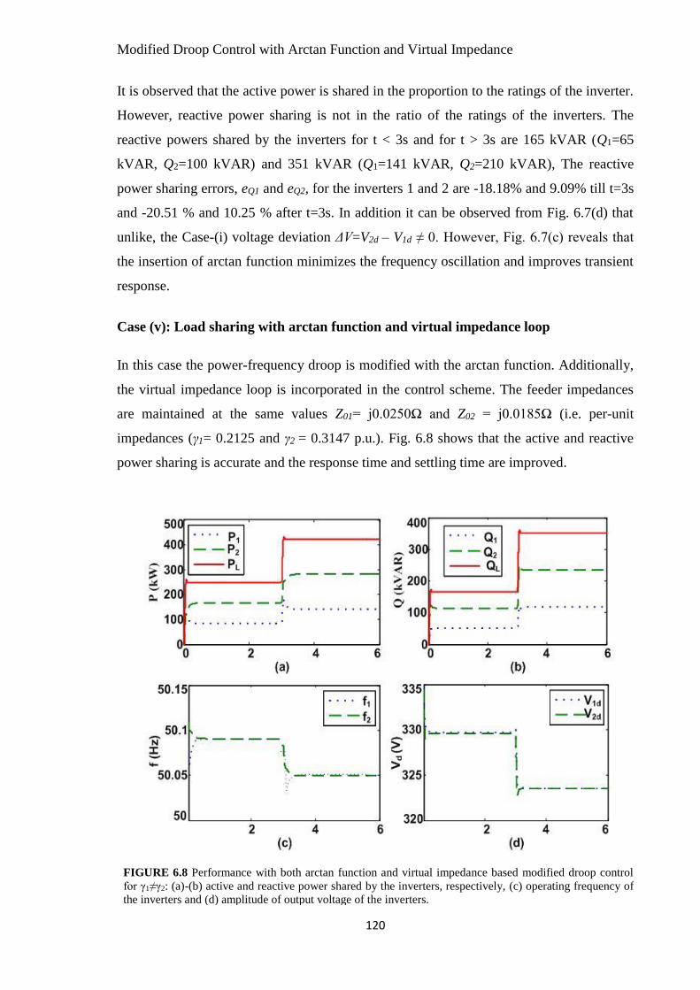
Modified Droop Control with Arctan Function and Virtual Impedance

120

It is observed that the active power is shared in the proportion to the ratings of the inverter.

However, reactive power sharing is not in the ratio of the ratings of the inverters. The

reactive powers shared by the inverters for t < 3s and for t > 3s are 165 kVAR (Q1=65

kVAR, Q2=100 kVAR) and 351 kVAR (Q1=141 kVAR, Q2=210 kVAR), The reactive

power sharing errors, eQ1 and eQ2, for the inverters 1 and 2 are -18.18% and 9.09% till t=3s

and -20.51 % and 10.25 % after t=3s. In addition it can be observed from Fig. 6.7(d) that

unlike, the Case-(i) voltage deviation ΔV=V2d – V1d ≠ 0. However, Fig. 6.7(c) reveals that

the insertion of arctan function minimizes the frequency oscillation and improves transient

response.

Case (v): Load sharing with arctan function and virtual impedance loop

In this case the power-frequency droop is modified with the arctan function. Additionally,

the virtual impedance loop is incorporated in the control scheme. The feeder impedances

are maintained at the same values Z01= j0.0250Ω and Z02 = j0.0185Ω (i.e. per-unit

impedances (γ1= 0.2125 and γ2 = 0.3147 p.u.). Fig. 6.8 shows that the active and reactive

power sharing is accurate and the response time and settling time are improved.

FIGURE 6.8 Performance with both arctan function and virtual impedance based modified droop control

for γ1≠γ2: (a)-(b) active and reactive power shared by the inverters, respectively, (c) operating frequency of

the inverters and (d) amplitude of output voltage of the inverters.

Modified Droop Control with Arctan Function and Virtual Impedance

121

Fig. 6.8(b) reveals that the insertion of virtual impedance minimizes the error in the

reactive power sharing and deviation in the output voltage of the inverters and Fig.6.8 (c)

shows that the frequency response is improved due to the arctan function. The errors eQ1

and eQ2 with the virtual impedance and output voltage deviation is same as case (iii). So,

advantages of both arctan function and virtual impedance can be achieved by combining

the features of these two methods with the conventional droop control concept.

Fig.6.9 compares the response of frequency for the cases (iii)-(v). It can be observed that

the control scheme which incorporates the features of both arctan function based control

and virtual impedance loop based control give better steady state and good transient

response.Table-6.2 summarizes the steady state and transient performance of the system

with different control approaches in response to the load change at t=3s.The response is

quantified in terms of eQ1, eQ2 and settling time ts for (γ1= 0.2125 and γ2 = 0.3147 p.u.)

FIGURE 6.9 Frequency response for the cases (iii)-(v).

TABLE 6.2 Comparisons of steady state and transient performance with different control

approaches

Control Approach eQ1 (%) eQ2 (%) ts (s)

Conventional droop with mismatch impedance -20.51 10.25 0.2

Conventional droop with virtual impedance loop 0.8 -0.12 0.5

Modified droop with Arctan function -20.5 10.3 0.10

Modified droop control with Arctan function and Virtual

impedance loop

0.8 -0.12 0.06

Modified Droop Control with Arctan Function and Virtual Impedance

122

6.4 Summary

With the conventional droop control approach, it is must to maintain the same voltage set-

points and per-unit impedance of the inverters, to ensure active and reactive power sharing

in proportion to the rating of the inverters operating in parallel. In case of the violation of

above, the inverters do share the active power in proportion to their ratings, but not the

reactive power. The modified control scheme that encompasses the feature of both virtual

impedance control and arctan based modified droop control not only overcomes this

limitation but also exhibits superior response under transient conditions. As the gradient of

modified droop (based on arctan function) near the extremes/limit of the range is low, the

rate of change of frequency and its overshoot are less than that in case of conventional

droop control. The results confirm that the proposed approach performs accurately even

when the output per-unit impedances do not match (γ1≠γ2). However, it must be ensured

that 𝑛1

𝑚1=

𝑛2

𝑚2 .

Modified Droop Control with Arctan Function and Virtual Impedance

123

CHAPTER – 7

Summary, Conclusions and Future Scope

This chapter summarizes the work reported in this report, the major contribution and some

important conclusions. The scope for the future work is also presented at the end of the

chapter.

7.1 Summary of the Contributions

Renewable or non-conventional energy sources based microgrids are gaining popularity

compared to the conventional fuel based centralized power plants. The microgrids are

characterized by the presence of DGs, which are connected to the utility through power

electronic interface. These DGs or the microgrid can operate independently to supply the

local loads or can operate in a grid-connected mode to exchange the power with grid. The

active and reactive power exchange/control is not that critical in a grid-connected mode as

is the case with the islanded-mode of operation. The severity of problem is more when

several environmental dependent DGs are operating simultaneously in a microgrid

operating in an islanded mode.

The conventional droop control method, which is very popularly used for load sharing in

an islanded mode, suffers from several limitations like inaccurate sharing of power,

ineffective utilization of the resources, higher storage requirement, circulating current,

heating or overloading of inverters etc.The accuracy of the droop-control in sharing the

reactive power is influenced by the mismatch of the impedance of the DG feeders,

imbalance in the load, non-linear loads etc. Further, in case of the DGs based on the source

like PV (or wind), the actual reactive power margin with the inverter varies with the

irradiations. Improper reactive power control under such case may lead to overloading of

the inverters. Hence it is desired to have an effective load sharing control strategy for the

DGs operating in a microgrid, which can address the issues mentioned above.

Modified Droop Control with Arctan Function and Virtual Impedance

124

The research work has focussed mainly on the control strategy for the PV based distributed

generators which can target following

• Effective utilization of the PV sources

• Effective utilization of the inverters used for interfacing DGs

• Minimum storage requirement

• Capability to operate in grid-connected and islanded mode

• Seamless transition between the two modes

In this context, reactive algorithms are presented in this work. The algorithm judiciously

distributes the reactive power amongst the inverters to achieve the equal utilization of the

inverters. Further, the control scheme ensures that the PV sources operate at their

maximum power points and distributes remaining active power demanded by the load

amongst the rest of the sources (in proportion to their ratings) till they reach their limits.

This minimizes the storage requirement. The control scheme can further facilitate the

smooth transition from the islanded mode to grid-connected mode or vice-versa.

The various contributions made through the work are summarized below.

Modeling of MG comprising of PV based DGs is carried out to investigate issues

related to active and reactive power transfer from the DGs in various operating

modes. The detailed analysis for modeling of the DG along with its control

schemes is provided. Active-reactive power (P-Q) control strategy is employed in

grid connected mode to transfer desired active and reactive power. Voltage and

frequency control (V-f) strategy is applied in islanded mode to achieve stable

islanded operation. A conventional droop-control (P-ω and Q-V) strategy is also

implemented for sharing the load amongst the DGs operating in an islanded mode.

The control strategy not only takes care of stable operation of MG in either of grid-

connected or islanded mode of operation, but also ensures smooth or seamless

transition between these two modes.

The available reactive power capacity (or margin) of the PV based DG inverters

vary with the change the irradiance. Hence, reactive power sharing algorithms are

proposed that takes care of the active power variations in the output of the PV

based DG sources. These algorithms helps to share the reactive power based on the

Modified Droop Control with Arctan Function and Virtual Impedance

125

remaining capacity (margin available) of the associated inverters and hence, ensure

better utilization of inverters thereby preventing the overloading of any inverter.

Equal apparent power sharing algorithm (EAPS) is developed for sharing reactive

power amongst PV based DGs/inverters of equal rating and analyzed with

MATLAB/Simulink. It tries to attain nearly equal utilization of the inverter

capacities. However, it does not consider the order in which the reactive power to

be assigned amongst the inverters is calculated. The modified EAPS algorithm

referred as EAPS-LSD, where LSD stands for least standard deviation, is presented

to even consider the order of allocation of reactive power amongst inverters. It

incorporates the loop to identify the best possible order of assigning the reactive

power to the inverters. It reduces the standard deviation of utilization factor of the

inverters.

Though the EAPS and EAPS-LSD algorithms try to minimize the gap amongst the

utilization of the inverters of identical ratings, they do not work well with DGs of

unidentical ratings. Hence, proportional apparent power sharing algorithm (PAPS-

LSD) is proposed which shares reactive power in proportion to the available

apparent power rating of the inverters of unidentical ratings. The effectiveness of

the algorithm over other methods is also demonstrated.

The above algorithm (PAPS-LSD) is combined with the droop-control principle to

offer a modified droop control method. The proposed control scheme introduces a

dynamic droop coefficient in active power vs. frequency (P-ω) droop and reactive

power vs. voltage (Q-V) droop. The effectiveness of modified droop control

method is studied by analyzing its performance with conventional droop control

methods. The modified droop control adjusts the frequency through a dynamic

droop component in such a way that the PV sources always operate at their MPPs

and the energy drawn from the auxiliary source is kept to the minimum. Further,

the PAPS-LSD, which is implemented in the SCU, ensures that the reactive power

distribution amongst the inverters is such that the standard deviation of the

utilization factors of the inverters is the least. Thus, the proposed approach helps in

achieving the effective utilization of PV arrays, inverters of the various DGs and

the auxiliary source.

Modified Droop Control with Arctan Function and Virtual Impedance

126

Mis-match in the line impedances greatly affects the performance of the

conventional droop-control based reactive power sharing amongst the inverters

operating in the microgrid. Due to the mis-match in the line impedance the reactive

power shared is no longer in proportion to the rating of the DGs. It may result into

the deviation of the reference voltages of the inverters causing the circulating

current and/or overloading of the inverters. The modified control scheme that

encompasses the feature of both virtual impedance control and arctan based

modified droop control is proposed. The virtual impedance minimized the effect of

impedance mis-match while the arctan based droop control helps in exhibiting

superior response under transient conditions. As the gradient of modified droop

(based on arctan function) near the extremes of the range is low, the rate of change

of frequency and its overshoot reduces. The improvement in the performance with

this approach over the conventional method is highlighted through the simulation

results obtained through Matlab/Simulink.

7.2 Conclusions

This research presents reactive power sharing algorithms working on principles of equal

(EAPS-LSD) and proportional (PAPS-LSD) apparent power sharing to achieve equal

utilization of the inverters. The PAPS algorithm, irrespective of the different nominal

rating of the inverters and the active power generated by the PV arrays, shares reactive

power amongst the PV inverters in such a manner that it results into equal utilization of all

inverters thereby avoiding overloading or under-utilization of any inverter. The algorithm

when combined with droop control principle yields superior performance in terms of both

the active and reactive power sharing. The conventional droop control does not take into

account the variation in the output of the PV based DGs and hence leads to ineffective

utilization of PV sources as well as other DGs. The modified droop control strategy

employing PAPS provides adaptive nature to the Q-V while the adaptive nature to P-ω

characteristics is realized by adding frequency error that is related to variations in

irradiance. As a result the frequency reference for the PV based DGs is adjusted such that

the decrease in their output power is quickly compensated by the increase in the output

power of other DGs. The proposed PAPS algorithm along with the modified droop control

ensures better reactive power sharing leading to effective utilization of inverters, minimum

energy storage requirement and good response. The insertion of virtual impedance and the

Modified Droop Control with Arctan Function and Virtual Impedance

127

arctan function in the droop control further improves the performance by minimizing the

error in reactive power sharing caused due to impedance mis-match. Through the

simulation results obtained in MATLAB/Simulink, the effectiveness of the various reactive

power sharing algorithms and the modified droop controls to enhance the performance of

system (in terms of effective utilization of PV array, inverters, sources; good response;

better accuracy of sharing etc.) is justified.

7.3 Scope of the future work

In this thesis reactive power sharing algorithms for PV based MG is proposed in order to

get equal utilization of inverters and to obtain maximum power transfer capacity of the

entire system. Some ideas or suggestions for further investigations in this field are as

follows.

The research work has considered reactive power sharing amongst the PV based

DGs and other reliable DGs operating in a microgrid. However, analysis related to

voltage and/or frequency stability is not considered in depth. The issue of stability

for a microgrid dominated by large number of environmental dependent sources

demands further investigations and could be focused.

The current work has just focused on sharing the reactive power (associated with

the fundamental components) amongst the inverters. However, the microgrid may

consist of large amount of non-linear loads. It may be interesting to explore the

sharing of these harmonics amongst the inverters when operating with the non-

linear loads. The sharing of reactive power (reactive power due to fundamental

component and that associated with harmonics) amongst the inverters of

environmental dependent DGs and other DGs may be very challenging and requires

further investigations.

List of References

108

List of References

[1] R. Lasseter, A. Akhil, C. Marnay, J. Stephens, J. Dagle, R. Guttromson, A.

Meliopoulous, R .Yinger and J. Eto.,“The CERTS microgrid concept,” white paper for

transmissionreliability program, office ofpower technologies U.S. department of

energy,April 2002.

[2] P. T. Cheng, C. A. Chen T. L. Lee and S. Y. Kuo,“A cooperative imbalance

compensation method for distributed-generation interface converter,” in IEEE Trans.

Ind. Appl. vol. 45, no. 2, pp. 805-815, March/April 2009.

[3] A. Keyhani,M. Marwali and Min Dai, “Integration of green and renewable energy in

electric power system,”A text book by Wiley publications, 2009.

[4] N. Eghtedarpour and E. Farjah, “Power control and management in a hybrid AC/DC

microgrid,” IEEE Trans. Smart Grid, vol. 5, no. 3,pp. 1494–1505, May 2014.

[5] M. Sarkar, L. Meegahapola and M. Datta, “Reactive power management in renewable

rich power grids: A review of grid-codes, renewable generators, support devices,

control strategies and optimization algorithms,” IEEE Access, vol. 6, 2018.

[6] L. Meegahapola and T. Littler, “Distributed solar-PV generation: Impacton voltage

control and stability,” in Handbook of Distributed Generation. Cham, Switzerland:

Springer, pp. 317- 342,2017.

[7] Y. Huang, F. Z. Peng, J. Wang and D. Yoo, “Survey of power conditioning system for

PV power generation,” Power Electronics Specialist Conference, PESC 2006, pp.1-6,

June 2006.

[8] A. Marinopoulos, F. Papandrea, M. Reza, S. Norrga, F. Spertino and Napoli, “Grid

integration aspects of large solar PV installations: LVRTcapability and reactive

power/voltage support requirements,” in ProcIEEE PowerTech, Trondheim, Norway,

pp. 1-8. 2011.

[9] W. Libo, Z. Zhengming and L. Jianzheng, “A single-stage three phase grid-

connectedphotovoltaic system with modified MPPT method and reactive power

compensation,” IEEE Trans Energy Convers., vol. 22, no.4,pp. 881–886, December

2007.

List of References

109

[10] B. Lasseter, “Microgrid-Distributed power generation”,IEEE Power engineering

societywinter meeting, vol.1, pp.146-149, 2001.

[11] H. Bevrani and T. Ise, “Microgrid Dynamics and Control,” John Wiley & Sons,

Hoboken,NJ,USA, 2017.

[12] F. Qiang, A. Naisiri, A. Solanki, A. Bani-Ahmed, L. Weber, V. Bhavaraju,

“Microgrids: Architectures, Controls, Protection, and Demonstration”, in journal of

Electrical power components and system, vol. 43, no.12, pp.1453-1465, July 2015.

[13] Y. Li, and C. Kao, “An accurate power control strategy for power Electronics-

interfaced distributedgeneration units operating in a low voltage multibus

microgrid,”IEEE Trans. Power Electron., vol. 24, no. 12, pp.2977-2988, December.

2009.

[14] Electromagnetic compatibility (EMC)-Part 3-2, Limits- Limits for harmonicscurrent

emmisions, IEC Std.61000-3-2, International Electrotechnical Commission,2009.

[15] W. Du, Q. Jiang, M.J. Erickson, and R. Lasseter, “Voltage-source control of PV

inverter in a CERTS microgrid,”IEEE Trans. Power Deliv., vol. 29, no.4, pp.1726–

1734, August. 2014.

[16] O. Y. Kim, J. H. Jeon, S. Kim, C. Cho, J. Park, H. Kim and K. Nam, “Cooperative

Control Strategy of Energy Storage System and Microsources for Stabilizing the

Microgrid during Islanded Operation,” IEEE Trans. on power electron., vol. 25, no. 12,

pp.3037-3048, December 2010.

[17] H. Lee and B. Koo, “The stetegy control of islanded microgrid using battery state of

charge,” 6th int. conf. on intelligent sys. modeling and simulation, pp.164-168,February

2015.

[18] A. Tsikalakis and N. Hatziargyriou, “Centralized control for optimizing microgrids

operation,” IEEE Trans. on Energy Convers., vol. 23, no. 1, pp. 241-248, March 2008.

[19] J. Lopes, C. Moreira, and A. Madureira, “Defining controlstrategies for

microgridsislanded operation,” IEEE Trans. Power Syst.,vol. 21, no. 2, pp. 916–924,

May 2006.

[20] J. Tan, H. Lin, and J. Zhang, “A novel load sharing control technique for

paralleledinverters,” in Proc. 34th Annu. IEEE Power Electron. Spec. Conf., Acapulco,

Mexicopp. 1432–1437, June 2003.

List of References

110

[21] M. Marwali, J. Jung and A. Keyhani, “Control of distributed generation systems—

Part II: Load sharing control,” IEEE Trans.Power Electron., vol. 19, no. 6, pp. 1551–

1561, Nov. 2004.

[22] Y. Pei, G. Jiang, and X. Yang, “Auto-master-slave control technique ofparallel

inverters in distributed AC power systems and UPS,” in Proc.35th Annu. IEEE Power

Electron. Spec. Conf., Aachen, Germany, pp. 2050–2053, June 2004.

[23] Jiefeng HU. “Advanced Control in Smart Microgrids”. University of Technology,

Sydney, Australia. PhD Thesis, June 2013.

[24] IEEE Draft Standard for “Interconnecting Distributed Resourceswith Electric power

systems,” IEEE WGStd. IEEE Std. 1547-2003, July 2001.

[25] J. Vasquez, J. Guerrero and A. Luna, “Adaptive droop controlapplied to voltage-

source inverters operating in grid-connectedand islanded modes,” IEEE Trans.

IndElectron., vol. 56, no. 10,pp. 4088–4096, October. 2009.

[26] X. Sun, Y. Lee and D. Xu, “Modeling, analysis, and implementation ofparallel multi-

inverter systems with instantaneous average-current-sharingscheme,” IEEE Trans.

PowerElectron., vol. 18, no. 3, pp. 844–856, May2003.

[27] R. Teodorescu and F. Blaabjerg, “Flexible control of small wind turbineswith grid

failure detection operating in stand-alone and grid-connectedmode,” IEEE Trans.

Power Electron., vol. 19, no. 5, pp. 1323–1332, September 2004.

[28] S. Park, C. Chen, J. Lai and S. Moon, “Admittance compensationin current loop

control for a grid-tie LCL fuel cell inverter,” IEEE Trans. Power Electron., vol. 23, no.

4, pp. 1716–1723, July 2008.

[29] C. Chen, Y. Wang,J. Lai, Y. Lee and Daniel Martin, “Design of Parallel Inverters for

Smooth Mode Transfer Microgrid Applications,”IEEE Trans. on power electron., vol.

25, no. 1, pp.6-15, january 2010.

[30] G. Gonzalez and R. Iravani, “Current injection for activeislanding detection of

electronically-interfaced distributed resources,”IEEE Trans. Power Del., vol. 21, no. 3,

pp. 1698–1705, Jul.2006.

[31] L. Lopes and Y. Zhang, “Islanding detection assessment of multiinvertersystems with

active frequency drifting methods,” IEEE Trans.Power Del., vol. 23, no. 1, pp. 480–

486, Jan. 2008.

List of References

111

[32] F. Katiraei, M.Iravani and P.W. Lehn, “Small-signal dynamic model of a micro-grid

including conventional and electronically interfaced distributed resources,”IET

Generation, Trans. and Distri., vol. 1, no. 3, pp. 369-378, May 2007.

[33] J. Holtz and K.Werner, “Multi-inverter UPS system with redundant load sharing

control,”IEEE Trans. Ind. Electron., vol. 37, no. 6, pp. 506–513, Dec. 1990.

[34] A. Bidram and A. Davoudi, “Hierarchical structure of microgrids control

system,”IEEE Trans Smart Grid, vol.3,no. 4, pp. 1963–1976, Dec.2012.

[35] K. Brabandere, K. Vanthournout, J. Driesen, G. Deconinck and R. Belmans “Control

of microgrids,” in Proc. IEEE Power & Energy Society General Meeting,pp. 1–7. June

2007.

[36] HU. Jiefeng “Advanced Control in Smart Microgrids”. University of Technology,

Sydney, Australia. PhD Thesis, June 2013.

[37] N. Hatziargyriou, “Microgrids: architectures and control” Wiley-IEEE Press, 2014.

[38] Y. Han, H. Li, P. Shen, E.Coelho and J. Guerrero,“Review of active and reactive

power sharing strategies in hierarchical controlled microgrids,”IEEE trans.power

electron., vol. 32, no. 3, pp.2427-2451,March 2017.

[39] J. Rocabert, A. Luna, F. Blaabjerg and P. Rodriguez, “Control of powerconverters in

AC microgrids,” IEEE Trans. Power Electron., vol. 27,no. 11, pp. 4734–4749, Nov.

2012.

[40] O. Palizban and K. kaohaniemi, “Hierarchical control structure in microgridswith

distributed generation: Island and grid-connected mode,”Renew. Sustain. Energy Rev.,

vol. 44, pp. 797–813, Apr. 2015.

[41] J. M. Guerrero, P. Loh and M. Chandorkar, “Advanced control architecturesfor

intelligent microgrids—Part I: Decentralized and hierarchicalcontrol,” IEEE Trans.

Ind. Electron., vol. 60, no. 4, pp. 1254–1262,April 2013.

[42] M. Chandorkar, D. Divan and R. Adapa, “Control of Parallel Connected Inverters in

Standalone ac Supply Systems,” IEEE Trans. Ind. Applications,vol.29,no.1,pp.136 –

143,January 1993.

[43] J. Guerrero, J. Vasquez and J. Matas, “Hierarchical control of droop-controlled AC

and DC microgrids—A general approach toward standardization,” IEEE Trans. Ind.

Electron., vol. 58, no. 1,pp. 158–172, Jan. 2011.

List of References

112

[44] T. Vandoorn, J. D. M. De Kooning and B. Meersman,“Review of primary control

strategies for islanded microgrids withpower-electronic interfaces,” Renew Sustain.

Energy Rev., vol. 19,pp. 613–628, Mar. 2013.

[45] C. Lee, C. Chu and P. Cheng, “A new droop control method for the autonomous

operation of distributed energy resource s interface converters,” IEEE Trans. Power

Electron., vol. 28, no. 4,pp. 1980–1993, April 2013.

[46] E. Rokrok andM. Golshan, “Adaptive voltage droop method for voltage source

inverters in an islanded multibus microgrid,” IET Gen. Trans. Dist., vol. 4,

no.5,pp.562–578, January 2010.

[47] C. Sao and P. Lehn, “Autonomous load sharing of voltage source converters,” IEEE

Trans. Power Del., vol. 20, no. 2, pp. 1009–1016, April 2005.

[48] C. Lee, C. Chuang, C. Chu and P. Chang, “Control strategiesfor distributed energy

resources interface converters in the low voltagemicrogrid,” in IEEE Energy

Conversion Congress and exposition (ECCE2009), San Jose, CA, Sep. 20-24, 2009.

[49] J. Vasquez, J. Guerrero, A. Luna, P. Rodriguez and R. Teodorescu,“Adaptive droop

control applied to voltage-source inverters operating ingrid-connected and islanded

modes,” IEEE Trans. Ind. Electron., vol. 56,no. 10, pp. 4088–4096, Oct. 2009.

[50] W. Yao, M. Chen, and J. Matas, “Design and analysis of the droop control method for

parallel inverters considering the impact of the complex impedance on the power

sharing,” IEEE Trans. Ind. Electron., vol. 58,no. 2, pp. 576–588, Feb. 2011.

[51] J. He, Y. W. Li and J. M. Guerrero, “An islanding microgrid power sharing approach

using enhanced virtual impedance control scheme,” IEEE Trans. Power Electron., vol.

28, no. 11, pp. 5272–5282,Nov. 2013.

[52] H. Hua, L. Yao, S. Yao, S. Mei, and J. M. Guerrero, “An improved droop control

strategy for reactive power sharing in islanded microgrid,” IEEE Trans. Power

Electron., vol. 30, no. 6, pp. 3133–3141,Jun. 2014.

[53] Y. Zhu, F. Zhuo and F. Wang, “A virtual impedance optimization method for reactive

power sharing in networked microgrid”, IEEE Tran. Power Electron., vol. 31, no.4, pp.

2890-2904,2014.

[54] C. Rowe, T. Summers, R. Betz, D. Cornforth and T. Moore,“Arctan Power–Frequency

Droop for Improved MicrogridStability,”IEEE Trans. on power electronics, vol. 28,

no. 8, pp. 3747-3459,Auguest 2013.

List of References

113

[55] R. Hasan, S. Mekhilef, M. Seyedmahmoudian and B. Horan, “Grid-connected isolated

PVmicro inverters: A review, Renewable and Sustainable Energy”, vol.67, pp.1065-

1080,2017.

[56] B. Azzopardiand J. Mutale, “Smart integration of future grid-connected PV systems,”

In Photovoltaic Specialists Conference (PVSC), 34th IEEE conference, pp. 7-12, June

2009.

[57] M. Eltawil and Z. Zhao,“Grid-connected photovoltaic power systems:Technical

andpotential problems-A review,” Renew. Sustain.Energy Rev., vol. 14, no. 1, pp. 112–

129, January 2010.

[58] S. Teleke, M. Baran, A. Huang, S. Bhattacharya and L. Anderson,“Control strategies

for battery energy storage for wind farm dispatching,”IEEE Trans. Energy Convers.,

vol. 24, no. 3, pp. 725–732, Sep. 2009.

[59] J. Gow and C. Manning, "Development of a photovoltaic array model for use in

power-electronics simulation studies," in proc. IEE Electric power applications, vol

146, issue 2, pp.193-200, March 1999.

[60] A. Cheknane, H. Hilal, F. Djeffal, B. Benyoucef and J. Charles, “An Equivalent

circuit approach to organic solar cell modeling”, Microelectronics Journal vol. 39,pp.

1173-1180, Oct. 2008.

[61] M. Villalva, J. Gazoli E. Filho, “Comprehensive approach to modeling and simulation

of photovoltaic array”, IEEE Trans on Power Electro. vol. 24, no.5, pp. 1198-1208,

May 2009.

[62] T. Esram and P. L. Chapman, “Comparison of photovoltaic array maximum power

pointtracking techniques,” IEEE Trans. Energy Convers.,vol. 22, no. 2, pp. 434–449,

Jun. 2007.

[63] M. Malinowski, K. Gopakumar, J. Rodriguez and M. A. Perez,“A survey on cascaded

multilevel inverters,”IEEE Trans, on Ind. Electron.,vol.57, no.7, pp.2197-2206, July

2010.

[64] H. Abu-Rub, J. Holtz, J. Rodriguez and G. Baoming,“Medium-voltage multilevel

converters –state of the art– state of the art, challenges, and requirements in industrial

applications,”IEEETrans. on Ind. Electron., vol. 57, no. 7, pp. 2581-2596, July 2010.

[65] S.Kjaer, J. Pedersen and F. Blaabjerg, “ A review of single-phase grid connected

invertertopology for photovoltaic modules”, IEEE Trans. on Ind. Appl., vol. 41, no. 5,

pp.1292-1306, September 2006.

List of References

114

[66] IEEE Std 929-2000, IEEE “Recommended Practice for Utility Interface of

Photovoltaic(PV) Systems,” April 2000.

[67] IEC 61727 Ed. 2, “Photovoltaic (PV) Systems – Characteristics of the Utility

Interface”,December 2004.

[68] VDE V 0126-1-1, “Automatic Disconnection Device between a Generator and the

Public Low-Voltage Grid,”Document 0126003, VDE Verlag, 2006.

[69] Standard EN 50160, “Voltage Characteristics of Public Distribution System,”

CENELEC:European Committee for Electrotechnical Standardization, Brussels,

Belgium, November 1999.

[70] A. Ellis, R. Nelson, E. Engeln, R. Walling, J. McDowell, L. Casey, E. Seymour, W.

Peter,C. Barker and B. Kirby, “Reactive power interconnection requirements for PV

andwind plants- recommendations to NERC”, Report of SANDIA, February 2012.

[71] Y. Han, H. Li, P. Shen, E. Antônio A. Coelho and J. Guerrero, ‘‘Review of active

andreactive power sharing strategies in hierarchical controlled microgrids,’’IEEE

TransPower Electron., vol. 32, no. 3, pp. 2427–2451, Mar. 2017.

[72] S. Adhikari and F. Li, “Coordinated V-f and P-Q control of solar photovoltaic

generatorswith MPPT and battery storage in microgrids.”, IEEE Trans. on Smart Grid

, vol. 5,no. 3, pp. 1270-1281, May 2014.

[73] Egwebe, M. Fazeli, P.Ignic and P. Holland,“Implementation and stability study of

dynamic droop in islanded microgrid,” IEEE Trans. on Energy. Conversion, vol. 31,

no. 3, pp. 821-831, September 2016.

[74] H. Liu, Y. Yang, X. Wang, P. Loh, F. Blaabjerg, W. Wang and D. Xu, “An enhanced

droop control scheme for resilient active power sharing in paralleled two-stage PV

invertersystem,” Proc. IEEE, Int. Conf. Applied Power Electro. Conf. and

Exposition(APEC),pp. 1253-1260, 2016.

[75] H. Mahmood, D. Michaelson and J. Jin, “A Power management strategy for

PV/Battery hybrid systems in islanded microgrids,” IEEE Emerg. Select. Topics Power

Electron., vol.2, no. 4, pp. 870–882, Oct. 2014.

[76] Q. Shafiee, J. M. Guerrero and J. C. Vasquez, “Distributed secondary control for

islandedmicrogrids-A novel approach,” IEEE Trans. Power Electron., vol. 29, no. 2,

pp. 1018-1031, Feb. 2014.

[77] J. Yeung, G. Vanalme, J. Myrzik, P. Karaliolios, M. Bongaerts, J. Bozelie and W.

L.Kling, “Development of a voltage and frequency control strategy for an

List of References

115

autonomousLV network with distributed generators,” in 44th International

Universities’ PowerEngineering Conference (UPEC 2009). Glasgow, Scotland, Sep.

2009.

[78] A. Milczarek, M. Apap, C. Staines and J. Guerrero, “Secondary control for reactive

powersharing and voltage amplitude restoration in droop-controlled ıslanded

microgrids”IEEE Inter. Symposium on Power Electronics for Distributed Generation

Systems (PEDG), June 2012.

[79] A. Milczarek, M.Malinowski and J. Guerrero, “Reactive Power Management in

islandedmicrogrid-proportional power sharing in hierarchical droop control”,IEEE

Trans. Smart grid,vol. 6, no.4, pp. 1631-1638, Feb. 2015.

[80] Z. Wang, K. Passino and J.Wang, “Optimal reactive power allocation in large scale

gridconnected photovoltaic system,” Journal of optimization theory and application,

vol.167, no.2, pp.761-779, July 2015.

[81] A. Micallef, M. Apap and J.Guerrero, “Reactive power sharing and voltageharmonic

distortion compensation of droop controlled single phase islandedmicrogrids,” IEEE

Trans. Smart grid, vol. 5, no.3, pp. 1149-1158, 2014.

[82] F. Nejabatkhah and W.L. Yun, “Overview of Power Management Strategies of Hybrid

AC/DC Microgrid,” in Power Electronics, IEEE Transactions on,vol.30, no.12,

pp.7072-7089, Dec. 2015.

[83] G. Chen and J. Yang, “A New Particle Swarm Optimization Solution to Optimal

Reactive Power Flow Problems,” Asia-Pacific Power Energy Eng. Conf., no. 1, pp. 1–

4, Mar. 2009.

[84] P. Smita and B. N. Vaidya, “Particle Swarm Optimization based Optimal PowerFlow

for reactive loss minimization,” 2012 IEEE Students’ Conf. Electr. Electron. Comput.

Sci., pp. 1–4, Mar. 2012.

[85] J. Guerrero, J. Matas , L. Garcia de Vicu˜na, M. Castilla and J. Miret,“Output

impedance design for parallel-connected UPS inverters with wireless load sharing

control,” IEEE Trans. Ind. Electron.,vol.52, no.4, pp. 1126–1135, Auguest 2005.

[86] J. Guerrero, J. Matas , L. Garcia de Vicu˜na, M. Castilla and J. Miret, “Decentralized

control for parallel operation of distributed generation inverters using resistive output

impedance,” IEEE Trans Ind Electron.,vol.54,no. 2, pp. 994–1004, March 2007.

[87] C. Rowe, T. Summers, R. Betz and D. Cornforth and,“ Small signal stability analysis

of arctan power frequency droop,” Proc. Power Electron. Drive Syst. Conf. pp. 787–

792, December 2011.

List of Publications

108

List of Publications

[1] Urvi N. Patel and Hiren H. Patel, “An effective power management strategy for

phtovoltaic based distributed generation,” in Proc. 16thAnnu. Conf. IEEE-EEEIC, June

2016.

[2] Urvi N. Patel and Hiren H. Patel, “Power sharing strategy for photovoltaic based

distributed generators operating in parallel,” in Transactions on Environment and

Electrical Engineering, vol. 1, no. 4, 2016.

[3]Urvi Patel, Neha Shah and Hiren Patel, “Reactive power management stretegy for

photovoltaic based distributed generators operating under non- uniform conditions,” in

IEEE Int. Conf. PEEIC, 13-14 April 2018.

[4] Neha Shah, Urvi Patel and Hiren H. Patel, “Improved Reactive power management

stretegy for photovoltaic based distributed generators”, International Journal of

Renewable Energy Research, vol.8, no.4, pp. 2035-2046, Dec. 2018.

[5] Urvi N. Patel, Deepak Gondliya and Hiren H. Patel, “Modified droop control scheme

for power sharing amongst inverters in microgrid,” in Techno press Journal of Advance

in Energy Research, vol. 3, no.2, pp.81-95, 2015

Communicated for Publications

[1] Urvi N. Patel and Hiren H. Patel, “ New control algorithm for effective sharing of

reactivepower in PV based microgrid to achieve equal utilization of PV inverters,”

submitted to International Journal of Emerging Electric Power Systems (IJEEPS).

[2] Urvi Patel and Hiren Patel, “Modified Droop Control for Islanded Photovoltaic

BasedMicrogrid for Effective Utilization of Distributed Generators”, to be submitted to

International Transaction on Electrical Enegry System, Wiley.

List of Appendices

108

Appendix A

Load Models

Two loads are modeled to evaluate performance of MG system in grid connected load and

islanding mode shown in Fig. 3.1.

(i)Series R-L Load

FIGURE A.1 Series R-L Load

Modeling equations for 3- phase series R-L load are given as

𝐿𝐿1

𝑑𝑖𝐿1𝑎

𝑑𝑡= −𝑅𝐿1𝑖𝐿1𝑎 + 𝑉𝑎

A.1

𝐿𝐿1

𝑑𝑖𝐿1𝑏

𝑑𝑡= −𝑅𝐿1𝑖𝐿1𝑏 + 𝑉𝑏

A.2

𝐿𝐿1

𝑑𝑖𝐿1𝑐

𝑑𝑡= −𝑅𝐿1𝑖𝐿1𝑐 + 𝑉𝑐

A.3

Equations (A.1)-(A.3) are written in d-q frame as

𝑑𝑖𝐿1𝑑

𝑑𝑡= −

𝑅𝐿1

𝐿𝐿1𝑖𝐿1𝑑 + 𝜔0𝑖𝐿1𝑞 +

1

𝐿𝐿1𝑉𝑑

A.4

𝑑𝑖𝐿1𝑞

𝑑𝑡= −

𝑅𝐿1

𝐿𝐿1𝑖𝐿1𝑞 − 𝜔0𝑖𝐿1𝑑 +

1

𝐿𝐿1𝑉𝑞

A.5

List of Appendices

109

Equations (A-1)-(A-5) are modeled in Matlab Simulink and shown in Fig. A.2.

FIGURE A.2Series R-L Load Model

(ii)Parallel R-L-C / Series R-L Load

FIGURE A.3 Parallel R-L-C Load

Modeling equations for 3- phase parallel R-L-C load are given as

𝐿𝐿2

𝑑𝑖𝐿2𝑎

𝑑𝑡= −𝑅𝐿2𝑖𝐿2𝑎 + 𝑉𝑎 − 𝑉1𝑎 − 𝑉𝑛2

A-6

𝐿𝐿2

𝑑𝑖𝐿2𝑏

𝑑𝑡= −𝑅𝐿2𝑖𝐿2𝑏 + 𝑉𝑏 − 𝑉1𝑏 − 𝑉𝑛2

A-7

List of Appendices

110

𝐿𝐿2

𝑑𝑖𝐿2𝑐

𝑑𝑡= −𝑅𝐿2𝑖𝐿2𝑐 + 𝑉𝑐 − 𝑉1𝑐 − 𝑉𝑛2

A-8

Equations (3.32)-(3.34) are written in d-q frame as

𝑑𝑖𝐿2𝑑

𝑑𝑡= −

𝑅𝐿2

𝐿𝐿2𝑖𝐿2𝑑 + 𝜔𝑖𝐿2𝑞 +

1

𝐿𝐿2𝑉𝑑 −

1

𝐿𝐿2𝑉1𝑑

A-9

𝑑𝑖𝐿2𝑞

𝑑𝑡= −

𝑅𝐿2

𝐿𝐿2𝑖𝐿2𝑞 + 𝜔𝑖𝐿2𝑑 +

1

𝐿𝐿2𝑉𝑞 −

1

𝐿𝐿2𝑉1𝑞

A-10

The voltage across capacitor can be represented as

𝐶2

𝑑𝑉1𝑎

𝑑𝑡= 𝑖𝐿2𝑎

A-11

In d-q frame

𝑑𝑉1𝑑

𝑑𝑡= 𝜔𝑉1𝑞+

1

𝐶2𝑖𝐿2𝑑

A-12

𝑑𝑉1𝑞

𝑑𝑡= 𝜔𝑉1𝑑+

1

𝐶2𝑖𝐿2𝑞

A-13

Equations (A-6)-(A-13) are modeled in Matlab Simulink and shown in Fig A.4.

FIGURE A.4 Parallel R-L-C load model