Embed Size (px)
Citation preview
Investigations on Void Formation in Composite Molding Processes and Structural
Damping in Fiber-Reinforced Composites with Nanoscale Reinforcements
Caleb Joshua DeValve
Dissertation submitted to the Faculty of the
Virginia Polytechnic Institute and State University
in partial fulfillment of the requirements for the degree of
Doctor of Philosophy
In
Mechanical Engineering
Ranga Pitchumani, Chair
Scott W Case
Mark R Paul
Shashank Priya
Pablo A Tarazaga
February 27, 2013
Blacksburg, Virginia
Keywords: fiber-reinforced composites, carbon nanotubes, analytical longitudinal permeability,
void formation, material damping
Copyright © 2013 Caleb DeValve
Investigations on Void Formation in Composite Molding Processes and Structural
Damping in Fiber-Reinforced Composites with Nanoscale Reinforcements
Caleb Joshua DeValve
Abstract
Fiber-reinforced composites (FRCs) offer a stronger and lighter weight alternative to
traditional materials used in engineering components such as wind turbine blades and rotorcraft
structures. Composites for these applications are often fabricated using liquid molding
techniques, such as injection molding or resin transfer molding. One significant issue during
these processing methods is void formation due to incomplete wet-out of the resin within the
fiber preform, resulting in discontinuous material properties and localized failure zones in the
material. A fundamental understanding of the resin evolution during processing is essential to
designing processing conditions for void-free filling, which is the first objective of the
dissertation. Secondly, FRCs used in rotorcraft experience severe vibrational loads during
service, and improved damping characteristics of the composite structure are desirable. To this
end, a second goal is to explore the use of matrix-embedded nanoscale reinforcements to
augment the inherent damping capabilities in FRCs.
The first objective is addressed through a computational modeling and simulation of the
infiltrating dual-scale resin flow through the micro-architectures of woven fibrous preforms,
accounting for the capillary effects within the fiber bundles. An analytical model is developed
for the longitudinal permeability of flow through fibrous bundles and applied to simulations
which provide detailed predictions of local air entrapment locations as the resin permeates the
preform. Generalized design plots are presented for predicting the void content and processing
time in terms of the Capillary and Reynolds Numbers governing the molding process.
The second portion of the research investigates the damping enhancement provided to FRCs
in static and rotational configurations by different types and weight fractions of matrix-
embedded carbon nanotubes (CNTs) in high fiber volume fraction composites. The damping is
measured using dynamic mechanical analysis (DMA) and modal analysis techniques, and the
results show that the addition of CNTs can increase the material damping by up to 130%.
Numerical simulations are conducted to explore the CNT vibration damping effects in rotating
composite structures, and demonstrate that the vibration settling times and the maximum
displacement amplitudes of the different structures may be reduced by up to 72% and 50%,
respectively, with the addition of CNTs.

iii
Acknowledgements
I give honor and praise to my lord and savior Jesus Christ, who has blessed me with the
ability and determination that I have applied to complete the research contained in this
dissertation. My advisor, Dr. Pitchumani, was instrumental in encouraging me to pursue my
doctoral degree, and I am extremely thankful for his patient guidance and belief in me as a
student. Helpful discussions and resources lent to me by Drs. Scott Case, Mark Paul, Pablo
Tarazaga, and Shashank Priya were invaluable, and I am appreciative of their assistance and
guidance. I could not have completed this degree without the support and love of my wife Keri,
and I cannot thank her enough for standing behind me and my studies. I am also indebted to my
parents and grandparents, who taught me how to live life to the fullest with a balance of
discipline, hard-work, and fun. My parents-in-law, brothers, lab mates, and friends are a source
of enjoyment and fulfillment, and I love spending time with them. I am indebted to each and
every one of the aforementioned individuals, and I thank God daily for their presence and
influence in my life.
The research in this dissertation is funded in part by the National Science Foundation with
Grant No. CBET-0934008, and the U.S. Department of Education through a GAANN fellowship
to Caleb DeValve through Award No. P200A060289. Their support is gratefully acknowledged.
iv
Table of Contents
Abstract ........................................................................................................................................... ii
Acknowledgements ........................................................................................................................ iii
List of Figures ................................................................................................................................ vi
List of Tables ............................................................................................................................... xiii
Chapter 1: Introduction .................................................................................................................. 1
1.1 Analytical Modeling of the Longitudinal Permeability of Aligned Fibrous Media ............. 1
1.2 Simulation of Void Formation in Liquid Composite Molding Processes ............................ 4
1.3 Experimental Investigation of the Damping Enhancement from CNTs .............................. 7
1.4 Simulation of Rotating Composite Structures with CNT Damping ................................... 10
Chapter 2: Analytical Longitudinal Permeability Prediction of Aligned Rigid Fibers ............... 13
2.1 Modeling ............................................................................................................................ 13
2.2 Results and Error Estimation.............................................................................................. 21
2.3 Nomenclature used in Chapter 2 ........................................................................................ 29
Chapter 3: Numerical Simulation of Void Formation in LCM Processes ................................... 31
3.1 Modeling ............................................................................................................................ 31
3.2 Void Diagrams ................................................................................................................... 38
3.3 Dynamic Void Development .............................................................................................. 45
3.4 Experimental Comparison .................................................................................................. 50
3.5 Processing Metrics ............................................................................................................. 55
3.6 Nomenclature used in Chapter 3 ........................................................................................ 60
Chapter 4: Experimental Investigation of the Damping Enhancement in Fiber-reinforced
Composites with CNTs ................................................................................................................. 62
4.1 Composite Fabrication and Testing Methods..................................................................... 62
4.1.1 Sample Preparation ..................................................................................................... 63
v
4.1.2 Damping Measurement ............................................................................................... 66
4.2 CNT Dispersion.................................................................................................................. 69
4.3 Damping in Cantilevered Beams........................................................................................ 74
4.4 Damping in Rotating Beams .............................................................................................. 79
4.5 Nomenclature used in Chapter 4 ........................................................................................ 88
Chapter 5: Analysis of Vibration Damping in a Rotating Composite Beam with CNTs ............ 89
5.1 Modeling of Simple Rotating Beam .................................................................................. 89
5.2 Validation of Model ........................................................................................................... 94
5.3 Parametric Study ................................................................................................................ 97
5.4 Nomenclature used in Chapter 5 ...................................................................................... 108
Chapter 6: Numerical Simulation of CNT-based Damping in Rotating Composite Structures 110
6.1 Three-Dimensional Rotating Beam Model ...................................................................... 110
6.2 Model Validation.............................................................................................................. 115
6.3 Parametric Study .............................................................................................................. 119
6.4 Nomenclature used in Chapter 6 ...................................................................................... 130
Chapter 7: Conclusions and Future Work .................................................................................. 131
7.1 Numerical Simulation of Void Formation in LCM Processes ......................................... 131
7.2 CNT Damping in Fiber-Reinforced Composite Structures .............................................. 132
7.3 Future Work ..................................................................................................................... 134
Bibliography ............................................................................................................................... 136
vi
List of Figures
Figure 1: Comparison of the active and passive vibration control schemes used in rotor
technology [80–83] and the damping effects of embedded carbon nanotubes [78,79] in fiber-
reinforced composites ..................................................................................................................... 8
Figure 2: Schematic illustration of aligned fibers arranged in a (a) rectangular array and (b)
hexagonal array, with the associated representative unit cell configurations and geometric
parameters. .................................................................................................................................... 14
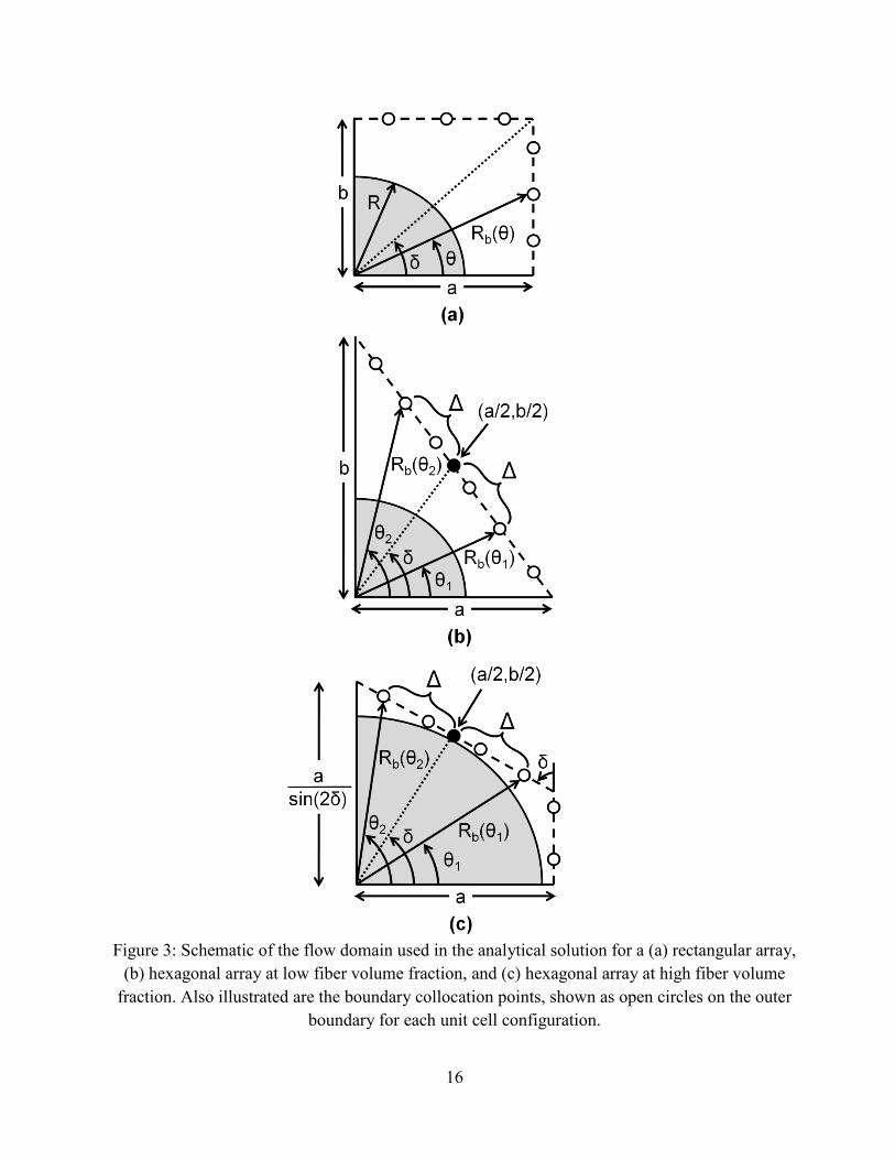
Figure 3: Schematic of the flow domain used in the analytical solution for a (a) rectangular array,
(b) hexagonal array at low fiber volume fraction, and (c) hexagonal array at high fiber volume
fraction. Also illustrated are the boundary collocation points, shown as open circles on the outer
boundary for each unit cell configuration. .................................................................................... 16
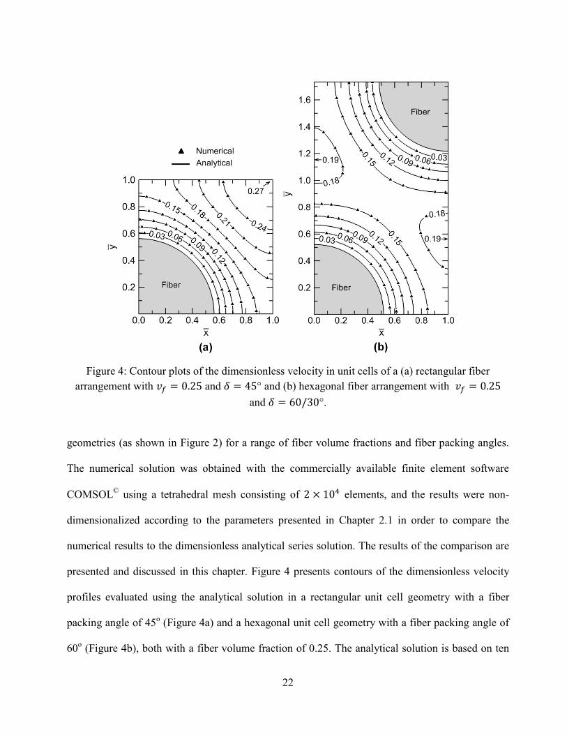
Figure 4: Contour plots of the dimensionless velocity in unit cells of a (a) rectangular fiber
arrangement with and and (b) hexagonal fiber arrangement with
and . ........................................................................................................................... 22
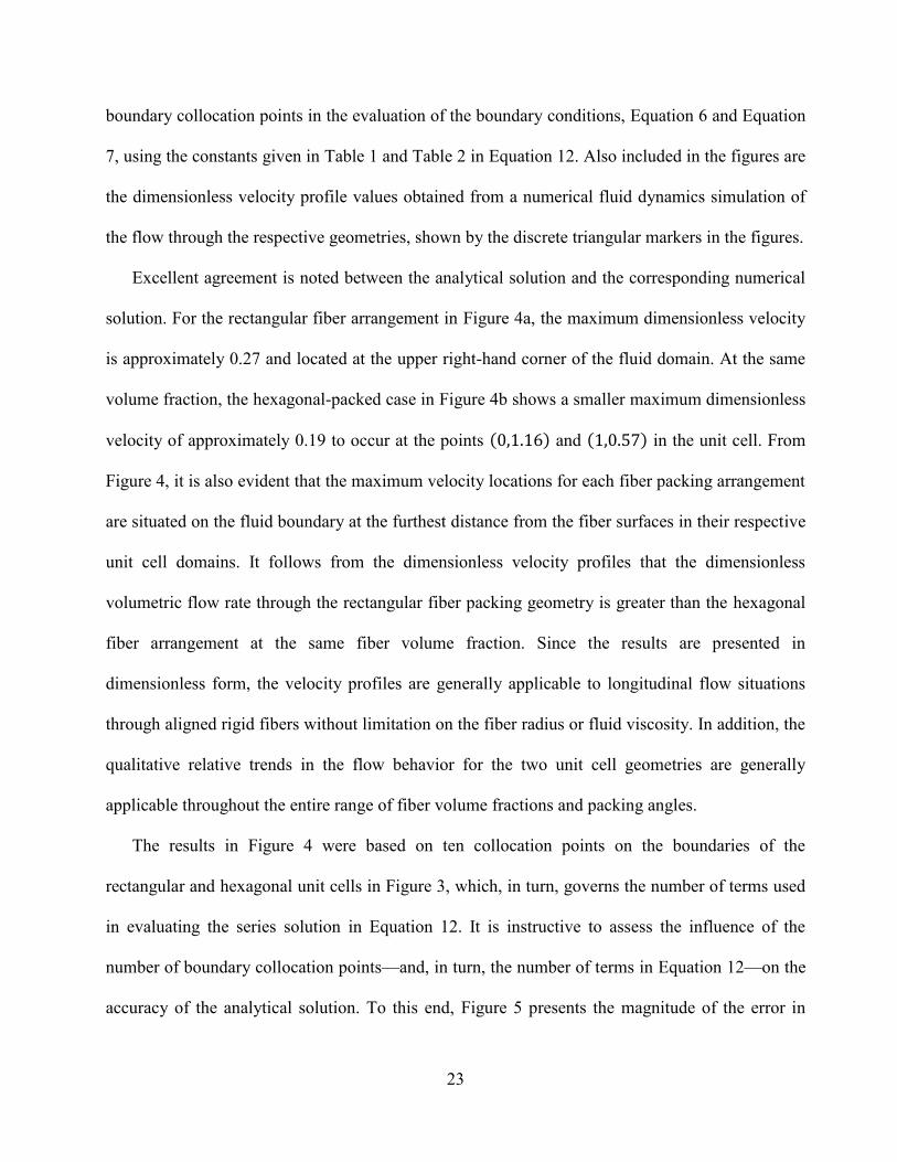
Figure 5: Variation of the error between the numerical and analytical solutions for flow rate
through a rectangular fiber array at different fiber volume fractions as the number of terms in Eq.
12 is varied; for (a) , (b) , (c) , and (d) . .......... 24
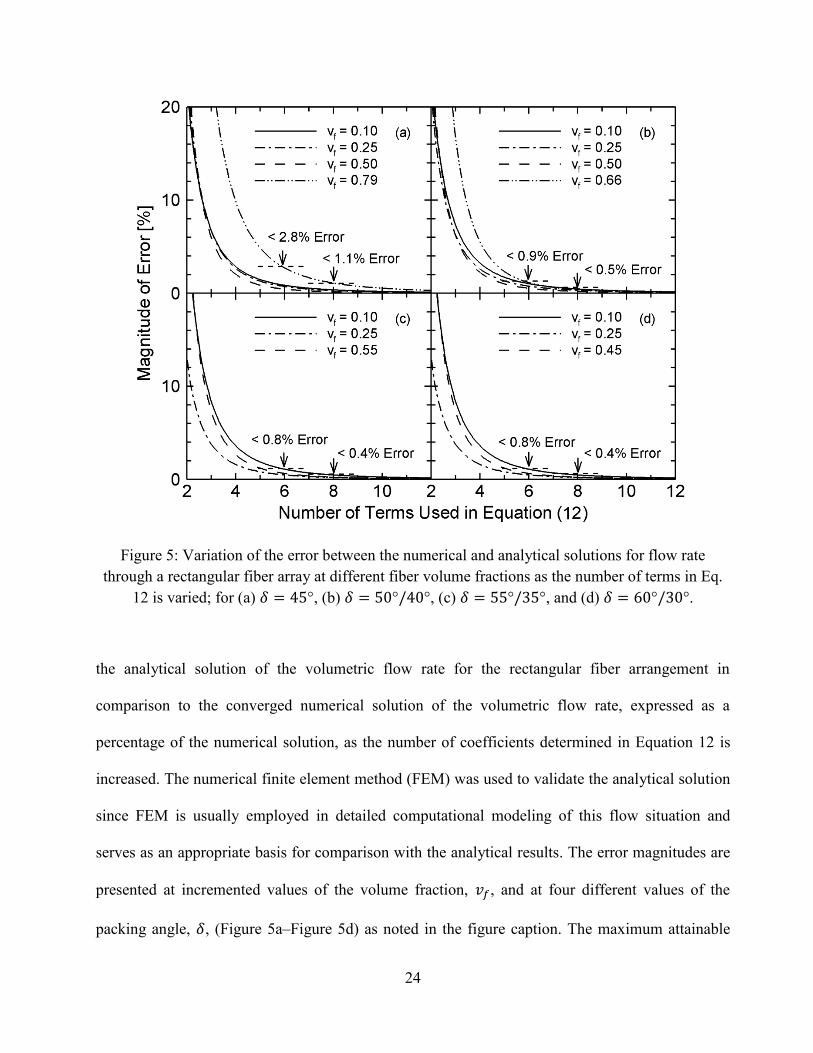
Figure 6: Variation of the dimensionless permeability with the fiber volume fraction and fiber
packing angle for a rectangular arrangement of fibers. ................................................................ 25
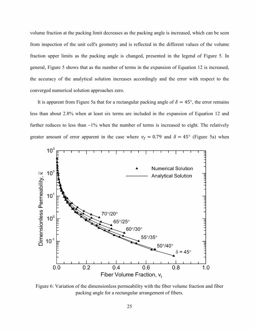
Figure 7: Variation of the dimensionless permeability with the fiber volume fraction and fiber
packing angle for a hexagonal arrangement of fibers. .................................................................. 27
Figure 8: Schematic illustration of the fiber preform architecture with two layers of nested plain
weave preform shown from an (a) isometric and (b) side view, along with the fiber bundle width,
a, thickness, b, and unit cell length, l. ........................................................................................... 31
Figure 9: Schematic of the two-dimensional slices of the fiber preform architecture at
(a) 1/2, (b) 3/8 (c) 1/4, (d) 1/8, and (e) 0. The dark gray area indicates the presence of a fiber
vii
bundle and the initial air surrounding the woven fiber bundles is represented by the light gray
shading. ......................................................................................................................................... 32
Figure 10: Variation of the dimensionless transverse permeability [3] and the longitudinal
permeability developed in Chapter 2 and [27] with the fiber bundle volume fraction for fiber
tows with a hexagonal-packed fiber arrangement.. ...................................................................... 35
Figure 11: Snapshots of the resin infiltration, shown by the gray shading, through the various
two-dimensional cross-sections of the Rovcloth 2454 fiber preform for and
at , , , , and . The void content in each slice, , the volume-averaged
void content, , and the final void content, , are indicated at each time step for each cross-
section. .......................................................................................................................................... 40
Figure 12: Snapshots of the resin infiltration, shown by the gray shading, through the various
two-dimensional cross-sections of the Rovcloth 2454 fiber preform for and
at , , , , and . The void content in each slice, , the volume-averaged
void content, , and the final void content, , are indicated at each time step for each cross-
section. .......................................................................................................................................... 42
Figure 13: Snapshots of the resin infiltration, shown by the gray shading, through the various
two-dimensional cross-sections of the Rovcloth 2454 fiber preform for and
at , , , and . The void content in each slice, , the volume-averaged
void content, , and the final void content, , are indicated at each time step for each cross-
section. .......................................................................................................................................... 43
Figure 14: Void content, , in each of the two-dimensional planes of the Rovcloth 2454 fabric
for the parameter combinations of (a) and , (b)
and , (c) and , and (d) and .
....................................................................................................................................................... 45
Figure 15: Volume-averaged void content, , in the Rovcloth 2454 fabric with (a)
, (b) , (c) , and (d) . Note that several of the plots
are overlapping one another in (a)–(c). ......................................................................................... 47
viii
Figure 16: Comparison of the void content evolution with time for the Rovcloth 2454 and the
Owens Corning WR10/3010 plain weave fabrics, in the two-dimensional plane for the
parameter combinations of (a) and , (b) and
, (c) and , and (d) and .
....................................................................................................................................................... 48
Figure 17: Comparison between experimentally measured [97] and numerically simulated final
average void content values, , for the Rovcloth 2454 fabric, along with a comparison of the
numerical simulation results predicting the void formation in the Owens Corning WR10/3010
fabric. Also presented are the results of a fully three-dimensional simulation of the flow in the
complete unit cell geometry depicted in Figure 8 for a Rovcloth 2454 fabric. ............................ 51
Figure 18: Pressure contours, p [MPa] in the Rovcloth 2454 fabric at steady state in the
plane for (a) , (b) and (c) , where the gray shaded area
represents the resin and the unshaded area represents the entrapped air locations. ...................... 54
Figure 19: Contours of (a) maximum final void content, , found in the two-dimensional
slices of the Rovcloth 2454, (b) volume-averaged final void content, , considering each of
the two-dimensional slices, (c) dimensionless excess flow time, , and (d) combined parameter
on a Capillary number–Reynolds number plane for the Rovcloth 2454. The most
favorable processing window shown by the shaded light gray oval region in (d) is superimposed
by the dashed oval in (a)–(c) to illustrate the corresponding maximum void content, average void
content, and excess flow time, respectively, associated with the most favorable processing
window .......................................................................................................................................... 56
Figure 20: The aluminum mold used for fabricating the composite beams consisting of (a) a top
plate and (b) a middle spacer and a bottom plate. A finished composite sample measuring 318 x
76 x 2 mm is shown in (c). ............................................................................................................ 64
Figure 21: (a) The experimental rotating test stand, consisting of an aluminum frame, a DC
motor, two cantilever beams mounted using a clamp connected to the central rotating shaft, and a
slip ring routing the signals from the accelerometers to the Labview™
control board. (b) The
ix
Labview™
user interface for controlling and monitoring the motor velocity profile, as well as for
displaying and saving the vibration data from the rotating beams. .............................................. 67
Figure 22: Scanning electron microscopy images of the (a) as received SWCNTs depicting large
agglomerates, and fracture surfaces of the epoxy-CNT composite showing the relative nanotube
dispersion after (b) shear mixing (no ultrasonic processing) and with (c) shear mixing and 10
minutes of ultrasonic processing using a 12.5 mm probe. ............................................................ 70
Figure 23: Variation of the material damping loss factor, , with the ultrasonic processing time,
, for a carbon fiber reinforced composite with and one weight percent CNT loading.
....................................................................................................................................................... 72
Figure 24: Variation of the material damping loss factor, , with strain, , using various CNT
weight percentage loadings, , for (a) SWCNTs with dimensions of < 2 nm in diameter and 5–15
in length, and MWCNTs measuring (b) 15 nm in diameter and 5–20 in length, (c) 30 nm
in diameter and 5–20 in length, and (d) 30 nm in diameter and 1–5 in length. ............... 74
Figure 25: Variation of the material damping loss factor, , with strain, , using (a) no CNT and
varying the fiber volume fraction of the composite material, as well as using various weight
percentages of MWCNTs (15 nm in diameter, 5–20 in length) with constant values of (b)
0.00, (c) 0.46, and (d) 0.58. ........................................................................................................... 76
Figure 26: Comparison of the damping measured in the first mode of the composite beam with
and no CNT using various testing conditions as indicated. ........................................ 80
Figure 27: The first transverse natural frequencies of the aluminum and composite beams with
and % SWCNTs as a function of angular speed. The symbols and associated error
bars indicate the experimentally measured values and the lines indicate the predicted natural
frequencies using a finite element model (FEM) for each of the various materials. .................... 81
Figure 28: The measured damping in the first transverse mode of vibration for the aluminum and
composite beams with and % SWCNTs as a function of angular speed for
(a) 0.46 and (b) 0.58. The experimentally measured values are denoted by the symbols and
associated error bars, and the lines represent linear regression fits through the respective data. . 83
x
Figure 29: The measured damping in the first three transverse modes of vibration for the
composite beams with and % SWCNTs for (a) and RPM, (b)
and RPM, (c) and RPM, and (d) and
RPM. ............................................................................................................................................. 86
Figure 30: (a) Schematic of the hub and beam geometry with hub radius, R, beam length, L,
thickness, a, and width, b, and a description of the (b) dimensionless and (c) dimensional angular
speed profile, governed by the dimensionless and dimensional steady-state angular speed, and
, and the dimensionless and dimensional ramp time, and , respectively. ......................... 90
Figure 31: Validation of the dynamic beam response predicted using the numerical model with
results presented by (a) Chung and Yoo [87] and (b) Cai, et al. [120]. ....................................... 94
Figure 32: Comparison of the numerical simulation using the presented model with a three-
dimensional FEM solution for and , where the dimensionless
vibration settling times for the ramp, , and hold, , periods are also indicated. .................. 96
Figure 33: (a) Effect of varying the slenderness ratio, , on the dimensionless tip displacement of
the beam, , for and , where the inset figure presents a larger
view of the simulation results from to . Contour plots of the dimensionless vibration
settling times during the (b) ramp ( and (c) hold ( ) periods are presented for the two
slenderness ratios on the damping parameter plane. ........................................................... 98
Figure 34: (a) Effect of varying the dimensionless hub radius, , on the dimensionless tip
displacement of the beam, , for and , where the inset figure
presents a larger view of the simulation results from to . Contour plots of the
dimensionless vibration settling times during the (b) ramp ( and (c) hold ( ) periods are
presented for the two dimensionless hub radii on the damping parameter plane. ............ 100
Figure 35: (a) Effect of varying the dimensionless steady-state angular speed, , on the
dimensionless tip displacement of the beam, , for and ,
where the inset figure presents a larger view of the simulation results from to .
Contour plots of the dimensionless vibration settling times during the (b) ramp ( and (c) hold
xi
( ) periods are presented for the two dimensionless angular speeds on the damping
parameter plane. .......................................................................................................................... 102
Figure 36: (a) Effect of varying the dimensionless ramp time, , on the dimensionless tip
displacement of the beam, , for and , where the inset figure
presents a larger view of the simulation results from to . Contour plots of the
dimensionless vibration settling times during the (b) ramp ( and (c) hold ( ) periods are
presented for the two dimensionless ramp times on the damping parameter plane. ......... 103
Figure 37: Contours of the dimensionless settling times during (a) ramp ( and (b) hold ( )
periods on the on the damping parameter plane for the conditions mimicking the helicopter
rotor vibration control study in [80]: , , , and . ................... 106
Figure 38: Geometry and mesh of the (a) simple beam, (b) Boeing VR7 helicopter rotor, and (c)
NREL 5 MW wind turbine blade. The thickness, a, width, b, and length, L, of each geometry are
also labeled.................................................................................................................................. 113
Figure 39: Geometry and mesh of the (a) simple beam, (b) Boeing VR7 helicopter rotor, and (c)
NREL 5 MW wind turbine blade. The thickness, a, width, b, and length, L, of each geometry are
also labeled.................................................................................................................................. 116
Figure 40: Comparison of the first and second transverse natural frequency values as a function
of angular speed, , using the current numerical model shown with the dashed line and empty
square markers for the (a) simple beam, (b) helicopter rotor, and (c) wind turbine blade
compared with various results from the literature indicated with a solid line. ........................... 117
Figure 41: The absolute value of the displacement at the tip of the simple beam, , during the
hold period using RPM and s for CNT weight percentage loadings of (a)
and (b) . The decay envelope of the vibrations are noted in each case with an
exponential fit line and the filled circles represent the 95% settling times, , for each
respective simulation during the hold period. The respective maximum tip displacement, ,
in each case is also noted. ........................................................................................................... 119
xii
Figure 42: Normalized maximum tip displacement, , ranging from 0 to for the (a)
simple beam, (b) helicopter rotor, and (c) wind turbine blade during the hold period as a function
of angular speed, , and various levels of CNT weight percentage loading, . ....................... 121
Figure 43: Normalized maximum tip displacement, , of the (a) simple beam, (b) helicopter
rotor, and (c) wind turbine blade during the hold period as a function of ramp time, , for a CNT
weight percentage loading of . ...................................................................................... 123
Figure 44: Normalized 95% settling time, , for the (a) simple beam, (b) helicopter rotor, and (c)
wind turbine blade during the hold period as a function of angular speed, , and various levels
of CNT weight percentage loading, . ....................................................................................... 124
Figure 45: Normalized maximum tip displacement, , for the wind turbine blade with a
geometric thickness ratio, , of (a) and (b) , and normalized 95% settling time, , for the
simple beam with varying thickness values of (c) and (d) as a function of angular
speed, , and various levels of CNT weight percentage loading, . ........................................ 126
Figure 46: Contour plots of the average percentage decrease in maximum tip displacement, ,
and settling time, , shown by the solid and dashed lines, respectively, when incorporating two
weight percent CNTs ( ) in the composite matrix compared to the baseline composite
without nanotubes ( ) for the (a) simple beam, (b) helicopter rotor, and (c) wind turbine
blade as a function of angular speed, , and the geometry thickness ratio, . ........................ 127
xiii
List of Tables
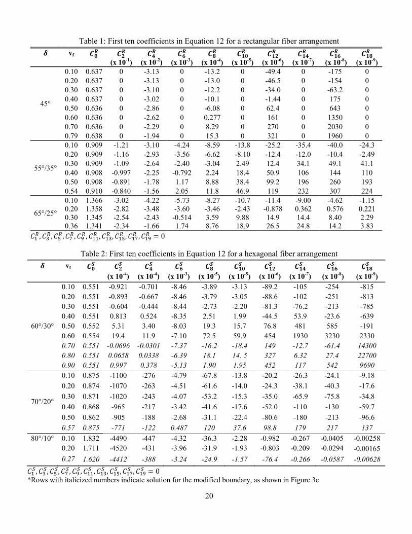
Table 1: First ten coefficients in Equation 12 for a rectangular fiber arrangement ...................... 20
Table 2: First ten coefficients in Equation 12 for a hexagonal fiber arrangement ....................... 20
Table 3: Range of values of carbon nanotube, fiber reinforcement, and ultrasonic processing
parameters used in the experimental study. .................................................................................. 65
Table 4: Values of the variables in Equations 32 and 33 used in the parametric study................ 97
Table 5: Parameter values describing the three composite structures considered in the study. . 114
1
Chapter 1: Introduction
This dissertation addresses several fundamental issues pertaining to composites technology,
specifically void formation in composite molding processes and structural damping in fiber-
reinforced composites with nanoscale reinforcements. First, a review of research involving the
analytical modeling of the permeability of fibrous media is presented, along with a discussion of
past research concerning the simulation of void formation in liquid composite molding (LCM)
processes. An examination of the previous experimental and analytical studies regarding the
damping behavior of fiber-reinforced composites with matrix-embedded CNTs is presented to
complete the introduction in this chapter.
1.1 Analytical Modeling of the Longitudinal Permeability of Aligned Fibrous Media
Longitudinal fluid flow through an arrangement of aligned rigid cylindrical fibers occurs in
most composite processing techniques including liquid molding processes. Resin flow through
fiber tows during the resin infiltration stage of composite fabrication is often described as flow
through a porous medium characterized principally by the fiber volume fraction and a permeability
tensor. The permeability tensor can be constructed based on the transverse and longitudinal
permeability of the aligned fiber bundle and the local orientation of the fiber bundle within the
preform. Therefore, the evaluation of the transverse and longitudinal permeability of aligned rigid
fibers has been the focus of many studies in the literature.
Fundamentally, the permeability of a porous fibrous medium is a geometric parameter and a
measure of the resistance offered by the porous microstructure to the fluid flow as a function of the
relative arrangement of the fibers, the fiber volume fraction, and the individual fiber radii. A
comprehensive review of the previous analytical and experimental work on transverse and
2
longitudinal flow through aligned fibrous media is summarized in [1], from which, a few of the
reviewed analytical longitudinal permeability models are reiterated here. An analytical solution for
the transverse and longitudinal permeability of randomly packed fiber arrangements up to a fiber
volume fraction of 0.7 was developed in [2]. Lubrication theory was used to predict transverse
permeability values close to the fiber packing limit along with a simplified cell model to predict
the transverse permeability at low fiber volume fractions in [3]. The longitudinal fluid flow
problem was solved in [4] by simplifying the fluid boundary of the unit cell domain from a square
to a circle, and an approximate solution for the flow was obtained. A solution for the pressure drop
and the shear stress distribution along the fiber wall for longitudinal flow through aligned rigid
fibers was developed in [5], and the method of distributed singularities was used in [6] to arrive at
an approximate solution in the form of a power series.
In [7,8] the longitudinal permeability was solved for by modifying the fiber geometry based on
the fiber packing arrangement, i.e., approximating the circular fibers as square in cross section for
square packing and hexagonal in cross section for hexagonal packing. Other studies have proposed
the superposition of three fundamental solutions which approximately satisfy the boundary
conditions of the longitudinal flow configuration [9]. Fractal geometry was applied in [10,11] to
characterize the dual-scale nature of flow through porous preforms in order to evaluate
permeability values. In [12] the method of fundamental solutions was applied using a Stokeslet-
based model and low Reynolds number flow to model the flow across an array of cylinders
oriented transverse to the flow, where the results can be combined with Darcy's law to predict
permeability values. A three-dimensional finite element model of a simplified plain weave unit cell
was used to simulate the resin flow through a preform in [13], and an effective permeability based
on the simulation results was reported. The research in [14] developed an analytical algorithm to
3
predict the transverse permeability of fiber tows considering the unsaturated flow length in the
fiber perform.
A common method for experimentally determining the permeability of fibrous reinforcements
is to physically force resin through a preform mat and monitor the pressure and flow rate
throughout the mold, combining these results with Darcy's law or an empirically fit equation to
determine the permeability of the preform as a function of the fiber volume fraction (e.g. [15–21]).
A full review of these experimental methods for determining permeability was presented in [22],
and this review also includes a short summary of the permeability prediction models documented
in the literature. Experiments have demonstrated that the capillary forces within a fiber tow
increase with an increase in fiber volume fraction (e.g. [23]), indicating the relative importance of
including capillary effects in permeability calculations at high fiber volume fractions.
It is evident from the foregoing review that the analytical approaches in the literature are based
on approximations of either the geometry or the governing flow physics, which leads to
permeability values that substantially deviate from the actual values, particularly for arrangements
with high fiber volume fraction. Chapter 2 of this dissertation presents an analytical series solution
for the problem of fluid flow through aligned rigid fibers and, in turn, evaluation of the
longitudinal permeability. The governing equations for the fluid flow in a representative volume
element are solved using the separation of variables technique combined with a boundary
collocation method [24,25], in which the boundary conditions are satisfied along the outside edges
of the fluid domain at discrete points. Using this approach, the analytical results are shown to be in
excellent agreement with a numerical finite element solution for rectangular and hexagonal
packing arrangements of the fibers and for all fiber volume fractions, . Chapter 2 presents the
analytical model development and the permeability results in a dimensionless form as a function of
4
the fiber volume fraction and fiber packing arrangement, demonstrating a general applicability and
easy use of the results for predicting the longitudinal permeability of fiber tows consisting of
aligned rigid fibers
1.2 Simulation of Void Formation in Liquid Composite Molding Processes
It is well known that composite materials fabricated through liquid composite molding (LCM)
processes and similar methods often exhibit defects from air entrapment during the resin
infiltration process, leading to flaws in the resulting cured composite material such as potential
failure locations and discontinuous material properties. These air voids undermine the property and
performance benefits of fiber reinforced composites and are sought to be avoided during
composites manufacturing. Air entrapment occurs during the preform infiltration step of LCM
processes by virtue of the dual scale nature of the resin flow through and around the fiber tows in
the preform. The resin flow is primarily influenced by the fiber preform geometry, mold
complexity, and resin properties. In addition, the processing parameters imposed on the system, for
example the vacuum pressure in vacuum assisted resin transfer molding (VARTM) and the
injection flow rate in resin transfer molding (RTM), have a significant effect on the resin flow and
consequently influence the relative size and location of the entrapped air voids in the resulting
composite material.
The flow through fibrous preforms is effectively modeled as a porous medium and is
fundamentally governed by the preform permeability, which is a measure of the resistance offered
to the flow by the porous structure of the preform. Toward describing the flow in liquid molding
processes, the model developed in Chapter 2 as well as numerous studies in the literature relate the
transverse and longitudinal permeability of the porous structure to the fiber bundle volume fraction
5
and the fiber diameter for idealized rectangular and hexagonal packing arrangements of fibers
within the tow bundles [1,3,6,26,27]. A detailed review of experiments and theoretical studies on
low Reynolds number flow through fibrous porous media and the permeability relationships is
presented in [22]. The infiltration of the resin into the fiber bundles is further affected by the
capillary pressure at the resin flow front, which is fundamentally a function of the fiber bundle
volume fraction, the individual fiber filament radius, and the surface tension and wetting angle of
the infiltrating resin with respect to the fiber surface [28]. These effects are increasingly significant
at the relatively high fiber bundle volume fractions generally found in the preform fabrics used as
reinforcements in advanced composites [29].
A summary of the physics associated with modeling flow through porous media and a review
of the advancements in numerical simulation tools used to model LCM processes in two- and
three-dimensional geometries, including investigations concerned with micro- and macro-void
prediction in fibrous preforms, are given in [30–32]. The formation of entrapped air locations is
primarily the result of the dual-scale nature of the resin infiltration, consisting of flow through the
macro-scale channels around the fiber bundles (the inter-tow regions) combined simultaneously
with flow through the micro-scale pores within the fiber bundles (intra-tow regions) around the
individual fibers [33]. Several techniques have been explored in the literature to model the resin
infiltration and the consequent air entrapment in LCM and similar processes. Darcy's law was used
in [34] to predict air entrapment within a cylindrical fiber bundle by considering resin flow radially
inward in the fiber bundle cross-section and using an ideal gas assumption to determine the
entrapped air volume within the bundle. This model was further developed to study the effect of
varying the individual fiber diameter and number of fibers in each bundle on the resulting size of
the entrapped air void within a single fiber bundle [35]. A similar study utilizing Darcy's law was
6
conducted to predict the void formation over time by using the finite element method to simulate
resin flowing transversely over a fiber tow [36]. Darcy's law was also used in [37] to predict
processing conditions that led to macro-void formation, and the results were presented as a
function of the Capillary number. The model in [37] was extended to include the effects of
injection pressure and distance from the mold inlet and the analytical predictions were validated
experimentally [38]. Simplified cross-sections of various multi-layer woven fabrics were analyzed
in [39] using a control volume to predict void formation. The Lattice Boltzmann Method was used
to model air entrapment location and size considering transverse flow through arrays of square-
packed fiber bundles when compared with similar experimental results [40]. Optimization of
VARTM processing parameters based on dual-scale flow analysis was presented in [41] to
minimize the void formation and mold fill time. In addition, a simulation of LCM processes was
developed which considered the different permeabilities in the warp and weft directions as well as
air bubble formation and migration, where the results were able to predict voids throughout the
local zones of the flow domain as a function of the Capillary number [42].
The studies in the literature have focused primarily on simplified two-dimensional fiber
preform geometries (e.g. [43]) or three-dimensional geometries described by a bulk permeability
(e.g. [31]), whereas the flow in actual processing is both fully three-dimensional and contains
multi-scale flow. Towards a realistic prediction of void entrapment during liquid molding
processes, a numerical model is developed in Chapter 3 to describe resin permeation through a
preform comprised of multiple layers of the plain weave fabric architecture. Considering flow
through a three-dimensional unit cell and representative two-dimensional slices of the plain weave
geometry, the analysis accounts for the capillary forces at the resin-air interface, and additionally,
the effects of nesting between adjacent layers of fabric. Simulations are performed for a wide
7
range of the Capillary and Reynolds numbers in order to explore their individual effects on the
location and relative size of air entrapment within the preform architecture. Based on the numerical
simulation results, the effects of the resin flow conditions and preform parameters on the final void
content and processing time are discussed in Chapter 3 along with the most favorable flow
conditions for void minimization.
1.3 Experimental Investigation of the Damping Enhancement from CNTs
Fiber-reinforced composites offer a strong and lightweight alternative to traditional building
materials and are increasingly being used across a broad spectrum of engineering applications,
including aerospace structures, sports equipment, and wind turbines [44–46]. Composite materials
used in such applications often suffer from vibrations caused by dynamic loads acting on the
system, resulting in reduced efficiency and comfort, undesirable noise, and a shortened lifespan of
the structure. Previous research has shown that various types of nano-scale fillers—such as carbon
nanofibers, ceramic nanoparticles, and carbon nanotubes (CNTs)—can be incorporated into the
composite matrix to enhanced the electrical, thermal, and mechanical properties of the material,
including vibration damping augmentation [47–50]. In particular, the addition of CNTs to
composite matrices has been found in several studies to provide significant damping enhancement
to the material, allowing for the fabrication of composite structures with increased resistance to
vibrations [51,52].
Carbon nanotubes as matrix-reinforcement have been the focus of the majority of composite
nano-filler studies based upon their theoretical upper limit of specific strength, modulus, and
conductivity [53]. Many reports concerning CNTs embedded in composite materials have noted
evidence of a weak bond at the interface of the CNT-matrix, which undermines the mechanical and
8
conductive property benefits provided to the material by the CNTs [54,55]. Consequently, much
work has been dedicated to investigating various surface treatments of CNTs in order to improve
the bond between the CNT and composite matrix and better attain the valuable properties of the
CNTs in the overall material [56–59]. However, this weak interfacial bond may alternatively be
exploited to increase the damping in the composite material as a result of the stick-slip action
which occurs at the CNT-matrix interface as the material is put under strain [60–62]. Numerous
studies in the literature, as reviewed in [63], have focused on embedding CNTs in the matrix of
composite materials for damping augmentation. Experimental measurements utilizing a thin film
of CNTs grown by vapor deposition on a silica substrate have reported a 200% increase in
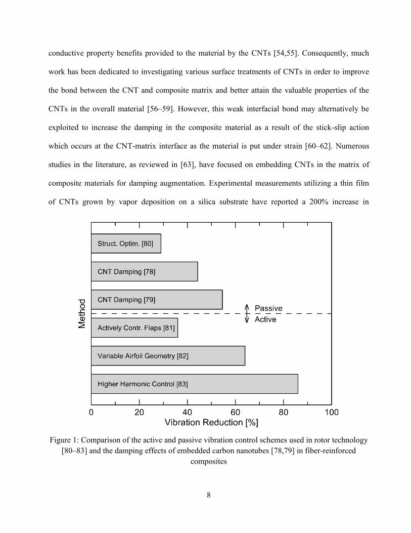
Figure 1: Comparison of the active and passive vibration control schemes used in rotor technology
[80–83] and the damping effects of embedded carbon nanotubes [78,79] in fiber-reinforced
composites
9
damping over the baseline system without nanotubes [64,65]. Active constrained layer damping
(ACLD) treatments utilizing CNTs and sandwich beams with a CNT-epoxy core have
demonstrated a damping increase of 40–1400% compared to the same beam fabricated without
CNTs [66–71]. A 400–1100% augmentation in material damping was measured when CNTs were
incorporated into the matrix of neat resin composites [52,55,60,61,72–75], and fiber reinforced
composites with matrix-embedded CNTs have exhibited a damping increase of 50–130% [76–79].
Several of the aforementioned published studies in the literature have noted that passive CNT
damping would benefit numerous applications which are currently made using composite materials
and experience undesirable vibrations, notably rotating structures such as wind turbine blades and
helicopter rotors. Although vibrations in rotating composite structures may be mitigated by other
passive damping techniques (e.g. structural optimization [80]), these systems are predominantly
controlled by active suppression methods including actively controlled flaps (ACF) [81], variable
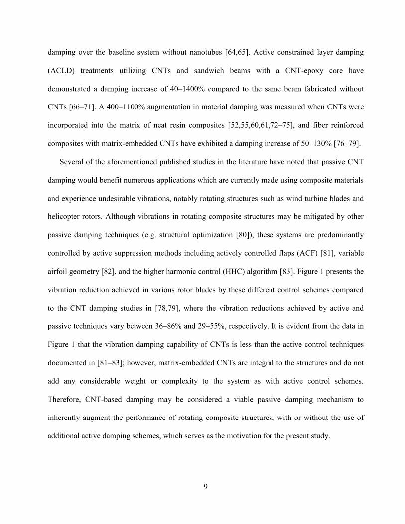
airfoil geometry [82], and the higher harmonic control (HHC) algorithm [83]. Figure 1 presents the
vibration reduction achieved in various rotor blades by these different control schemes compared
to the CNT damping studies in [78,79], where the vibration reductions achieved by active and
passive techniques vary between 36–86% and 29–55%, respectively. It is evident from the data in
Figure 1 that the vibration damping capability of CNTs is less than the active control techniques
documented in [81–83]; however, matrix-embedded CNTs are integral to the structures and do not
add any considerable weight or complexity to the system as with active control schemes.
Therefore, CNT-based damping may be considered a viable passive damping mechanism to
inherently augment the performance of rotating composite structures, with or without the use of
additional active damping schemes, which serves as the motivation for the present study.
10
Although much work in the literature has focused on the damping characteristics of CNTs in
composites, there has been a lack of emphasis on experimental studies of embedded CNTs in high
fiber volume fraction composites, which are essential for achieving the necessary strength and
modulus values for practical engineering structures. In addition, there is a need to experimentally
explore the effects of CNT damping in a physical rotating composite beam in order to better
understand how this CNT damping phenomenon may be exploited in rotating composites. Chapter
4 reports the results of an experimental study measuring the damping in CNT-reinforced
composites as a function of strain, fiber volume fraction, and nanotube type and weight percentage
loading, focusing on functional high fiber volume fraction composites in (1) a stationary frame,
using DMA and modal analysis techniques, and (2) a rotating frame, to provide greater insight into
passive CNT-damping capabilities in structures such as helicopter blades and wind turbine rotors.
1.4 Simulation of Rotating Composite Structures with CNT Damping
In order to characterize this CNT damping phenomena, several models have been proposed in
the literature to describe the damping mechanism of the CNTs within the composite matrix. As
discussed above, the additional damping provided by the CNTs in the composite may be explained
in part by the poor bond that is exhibited between the surface of the CNTs and the surrounding
composite matrix [84], resulting in energy dissipation through an interfacial stick-slip mechanism
as these two surfaces slide over one another under strain [60,61,72,78]. A structural damping
model for polymer composites containing single-walled carbon nanotubes (SWCNTs) was
presented in [73], describing the energy dissipation using the assumption of stick-slip motion
caused by friction between a debonded SWCNT and the surrounding resin. A similar study was
developed in [62], which considered the nanotube-nanotube interactions as well as the interfacial
11
stick-slip action at the nanotube-matrix interface. A distributed CNT friction model which
incorporated the spatial distribution of nanotubes using a statistical approach was established in
[85], and reported a nonlinear relationship between the predicted damping and the applied
excitation amplitude. In [72] a numerical simulation of CNTs embedded in an epoxy matrix was
presented which explored the effects of various CNT orientations within the resin at different
strain levels, applied to predict a material loss factor as a function of strain. Other approaches have
modeled CNT damping using the Kelvin-Voigt model of nonlinear viscoelastic systems, where a
closed form solution using this method is presented in [69]. A study concerning the effect of CNT-
infused material coatings on the damping characteristics of a metal fan blade was developed in
[74] using numerical simulations, where the results demonstrated an overall improvement in the
blades modal characteristics when using the coating infused with CNTs.
In Chapter 5, the stick-slip damping model presented in [78] is applied along with viscous
damping to investigate the effects of CNT-based damping on the dynamic response of a rotating
composite beam. The model is developed using the dimensionless form of the Euler-Bernoulli
equation and solved by means of the finite element method (FEM). The effect of rotation on the
beam is considered by deriving the equations of motion in a rotating frame of reference and
applying dynamic body forces that are dependent on the angular speed and acceleration
experienced by the beam. The geometry is excited by a dimensionless angular speed profile related
to the typical operating conditions of functional rotor blades [80–83,86,87], and the effects of
CNT-based damping expressed in terms of coulomb and viscous damping parameters as well as
the geometry and angular speed on the dynamic response of the rotating composite beam are
explored in the results presented in Chapter 5.
12
Chapter 6 explores the effects of matrix-embedded CNTs in rotating composite structures
using numerical simulations by applying empirical CNT-damping functions and the finite element
method (FEM). Three different cantilevered composite structures of increasing complexity are
studied: (1) a simple rectangular beam, (2) a helicopter rotor based on a Boeing VR7 airfoil [88],
and (3) a wind turbine blade modeled according the theoretical NREL 5 MW wind turbine
specifications [89]. A stick-slip damping mechanism described by the coulomb friction model is
assumed to describe the CNT damping phenomena, and the damping in the composite structure
considering only the fiber-matrix material (i.e. without CNT-reinforcement) is described with a
viscous damping term [78]. The effect of rotation on the structure is modeled using a dynamic
body force which is dependent on the angular speed and acceleration experienced by the structure,
and the three geometries are excited by an angular speed profile specific to the typical operating
conditions of each respective structure. Additionally, the relative geometric dimensions of each
structure are varied to study their effect on each simulation case. The model development along
with the effects of CNT damping, angular speed, and geometric variation on the dynamic response
of different rotating composite structures are presented in Chapter 6.
13
Chapter 2: Analytical Longitudinal Permeability Prediction of Aligned Rigid Fibers
This chapter presents the analytical modeling of the longitudinal permeability of aligned rigid
fiber bundles. Two different fiber bundle packing configurations are considered along with various
fiber volume fractions, and the resulting permeability values are presented in dimensionless form
for general applicability.
2.1 Modeling
The goal of the modeling in this chapter is to develop an analytical relationship between the
longitudinal permeability, , and the governing geometric parameters for a porous medium
comprised of a periodic arrangement of aligned rigid fibers. To this end, the problem of a viscous
fluid flowing longitudinally through a bundle of aligned rigid fibers, presented schematically in
Figure 2, is considered first. Two different fiber packing arrangements are analyzed, described as
rectangular-packed or hexagonal fiber tows, shown, respectively, in Figure 2a and Figure 2b. By
virtue of the symmetry of the fiber packing arrangements, the geometry can be simplified as a
representative unit cell of width, a, height, b, and length, L, for each packing configuration with an
associated fiber radius, R, and packing angle, , as shown in Figure 2a and Figure 2b.
The flow is assumed to be laminar and the inertial forces are considered to be much less than
the viscous forces, or equivalently, that the flow Reynolds number, , such that the fluid
motion is described by Stokes flow [90]. Further, for a fully-developed flow in the representative
volume element, the pressure gradient in the direction of the flow can be expressed as
,
where is the pressure difference between the inlet and the outlet planes of the unit cell, and is
the length of the unit cell in the flow ( -) direction. The governing equation can then be written in

14
Figure 2: Schematic illustration of aligned fibers arranged in a (a) rectangular array and (b)
hexagonal array, with the associated representative unit cell configurations and geometric
parameters.
cylindrical polar coordinates, in a nondimensional form, as
where, referring to Figure 2, all the unit cell parameters are normalized with respect to the fiber
radius, , as is the angular coordinate and the dimensionless
axial flow velocity, , is given by , in which is the axial velocity in the z-
direction along the fibers, and is the fluid viscosity.
Of the four boundary conditions needed to solve Equation 1 uniquely, three are identical for
both the rectangular and the hexagonal fiber packing arrangements shown in Figure 2, namely, (1)
15
the fluid velocity at the fiber-fluid interface ( ) must satisfy the no-slip condition and the
fluid shear stress must be zero (i.e. symmetry lines) along both (2) the bottom edge ( ) and (3)
the left edge ( ) of the unit cell. These conditions are defined mathematically in
dimensionless form as:
The fourth boundary condition is dependent on the fiber packing arrangement. For the rectangular-
packed fiber arrangement shown in Figure 2a, the velocity field is symmetric about the boundary,
, where denotes the dimensionless radial distance to the outer fluid
boundary, , of the rectangular unit cell geometry defined by and , as shown in
Figure 3a, such that
For the hexagonal fiber arrangement presented in Figure 2b, the velocity field is symmetric with
respect to the center of the unit cell along any line drawn through the central point
.
Additionally, the gradient of the velocity field exhibits an anti-symmetry with respect to the central
point
along this same line. For simplicity, this line passing through the unit cell center,
, on which the two aforementioned boundary conditions are satisfied, is taken to be the
diagonal line connecting points and , as shown by the dashed line in Figure 3b. In this
case, the boundary conditions are expressed mathematically in a dimensionless form as:
16
Figure 3: Schematic of the flow domain used in the analytical solution for a (a) rectangular array,
(b) hexagonal array at low fiber volume fraction, and (c) hexagonal array at high fiber volume
fraction. Also illustrated are the boundary collocation points, shown as open circles on the outer
boundary for each unit cell configuration.
17
where
Equivalently, the boundary conditions in Equations 6 and Equations 7 can be expressed by
considering any two points on the boundary line defined through
which are on opposite
sides of the center
and equidistant from this point, denoted by Δ in Figure 3b and Figure 3c,
where, at these two points, the velocities are equal and the velocity gradients are equal in
magnitude but opposite in sign.
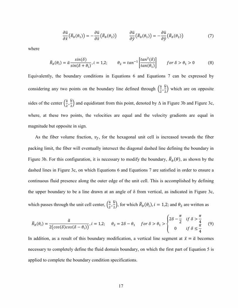
As the fiber volume fraction, , for the hexagonal unit cell is increased towards the fiber
packing limit, the fiber will eventually intersect the diagonal dashed line defining the boundary in
Figure 3b. For this configuration, it is necessary to modify the boundary, , as shown by the
dashed lines in Figure 3c, on which Equations 6 and Equations 7 are satisfied in order to ensure a
continuous fluid presence along the outer edge of the unit cell. This is accomplished by defining
the upper boundary to be a line drawn at an angle of from vertical, as indicated in Figure 3c,
which passes through the unit cell center,
, for which and are written as
In addition, as a result of this boundary modification, a vertical line segment at becomes
necessary to completely define the fluid domain boundary, on which the first part of Equation 5 is
applied to complete the boundary condition specifications.
18
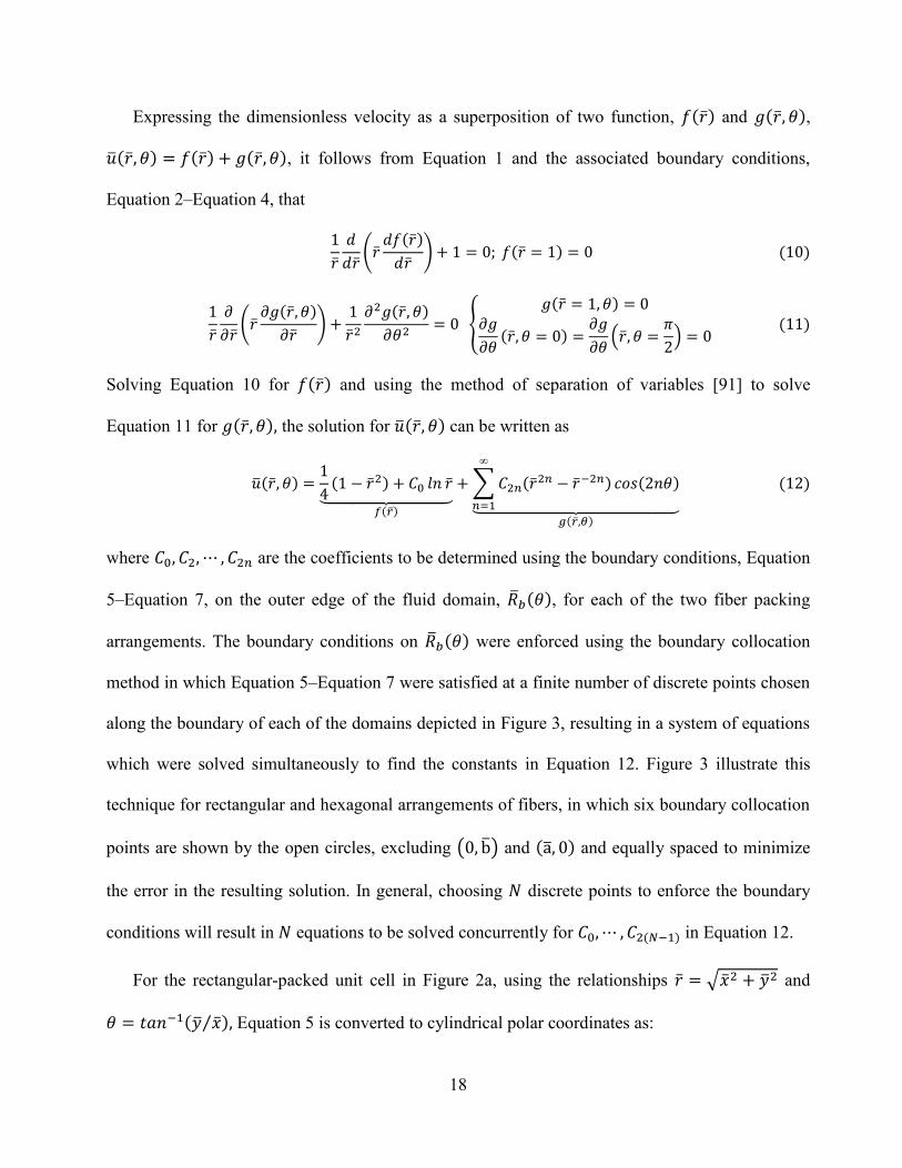
Expressing the dimensionless velocity as a superposition of two function, and ,
, it follows from Equation 1 and the associated boundary conditions,
Equation 2–Equation 4, that
Solving Equation 10 for and using the method of separation of variables [91] to solve
Equation 11 for the solution for can be written as
where are the coefficients to be determined using the boundary conditions, Equation
5–Equation 7, on the outer edge of the fluid domain, , for each of the two fiber packing
arrangements. The boundary conditions on were enforced using the boundary collocation
method in which Equation 5–Equation 7 were satisfied at a finite number of discrete points chosen
along the boundary of each of the domains depicted in Figure 3, resulting in a system of equations
which were solved simultaneously to find the constants in Equation 12. Figure 3 illustrate this
technique for rectangular and hexagonal arrangements of fibers, in which six boundary collocation
points are shown by the open circles, excluding and and equally spaced to minimize
the error in the resulting solution. In general, choosing discrete points to enforce the boundary
conditions will result in equations to be solved concurrently for in Equation 12.
For the rectangular-packed unit cell in Figure 2a, using the relationships and
Equation 5 is converted to cylindrical polar coordinates as:
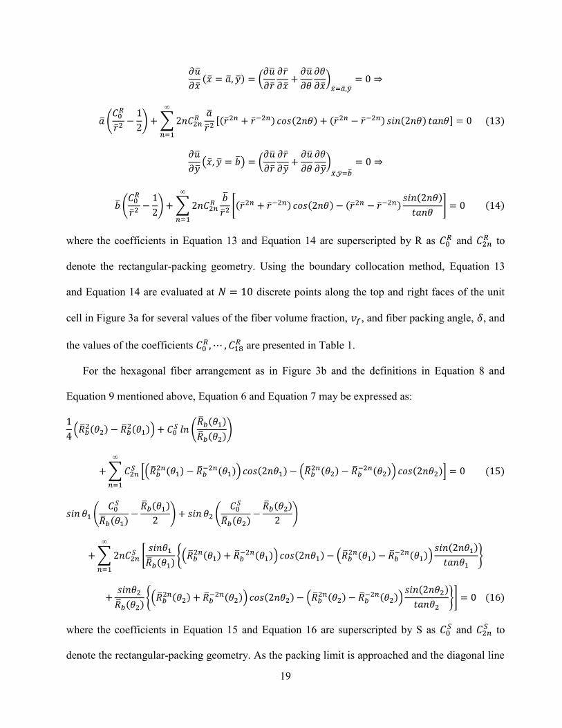
19
where the coefficients in Equation 13 and Equation 14 are superscripted by R as and
to
denote the rectangular-packing geometry. Using the boundary collocation method, Equation 13
and Equation 14 are evaluated at discrete points along the top and right faces of the unit
cell in Figure 3a for several values of the fiber volume fraction, , and fiber packing angle, , and
the values of the coefficients
are presented in Table 1.
For the hexagonal fiber arrangement as in Figure 3b and the definitions in Equation 8 and
Equation 9 mentioned above, Equation 6 and Equation 7 may be expressed as:
where the coefficients in Equation 15 and Equation 16 are superscripted by S as and
to
denote the rectangular-packing geometry. As the packing limit is approached and the diagonal line
20
Table 1: First ten coefficients in Equation 12 for a rectangular fiber arrangement
vf
(x 10
-1)
(x 10-2
)
(x 10-3
)
(x 10-4
)
(x 10-5
)
(x 10-6
)
(x 10-7
)
(x 10-8
)
(x 10-9
)
45°
0.10 0.637 0 -3.13 0 -13.2 0 -49.4 0 -175 0 0.20 0.637 0 -3.13 0 -13.0 0 -46.5 0 -154 0
0.30 0.637 0 -3.10 0 -12.2 0 -34.0 0 -63.2 0
0.40 0.637 0 -3.02 0 -10.1 0 -1.44 0 175 0 0.50 0.636 0 -2.86 0 -6.08 0 62.4 0 643 0
0.60 0.636 0 -2.62 0 0.277 0 161 0 1350 0
0.70 0.636 0 -2.29 0 8.29 0 270 0 2030 0
0.79 0.638 0 -1.94 0 15.3 0 321 0 1960 0
55°/35°
0.10 0.909 -1.21 -3.10 -4.24 -8.59 -13.8 -25.2 -35.4 -40.0 -24.3
0.20 0.909 -1.16 -2.93 -3.56 -6.62 -8.10 -12.4 -12.0 -10.4 -2.49
0.30 0.909 -1.09 -2.64 -2.40 -3.04 2.49 12.4 34.1 49.1 41.1
0.40 0.908 -0.997 -2.25 -0.792 2.24 18.4 50.9 106 144 110 0.50 0.908 -0.891 -1.78 1.17 8.88 38.4 99.2 196 260 193
0.54 0.910 -0.840 -1.56 2.05 11.8 46.9 119 232 307 224
65°/25°
0.10 1.366 -3.02 -4.22 -5.73 -8.27 -10.7 -11.4 -9.00 -4.62 -1.15 0.20 1.358 -2.82 -3.48 -3.60 -3.46 -2.43 -0.878 0.362 0.576 0.221 0.30 1.345 -2.54 -2.43 -0.514 3.59 9.88 14.9 14.4 8.40 2.29 0.36 1.341 -2.34 -1.66 1.74 8.76 18.9 26.5 24.8 14.2 3.83
Table 2: First ten coefficients in Equation 12 for a hexagonal fiber arrangement
vf
(x 10-4
)
(x 10-4
)
(x 10-3
)
(x 10-5
)
(x 10-5
)
(x 10-6
)
(x 10-7
)
(x 10-8
)
(x 10-9
)
60°/30°
0.10 0.551 -0.921 -0.701 -8.46 -3.89 -3.13 -89.2 -105 -254 -815
0.20 0.551 -0.893 -0.667 -8.46 -3.79 -3.05 -88.6 -102 -251 -813
0.30 0.551 -0.604 -0.444 -8.44 -2.73 -2.20 -81.3 -76.2 -213 -785
0.40 0.551 0.813 0.524 -8.35 2.51 1.99 -44.5 53.9 -23.6 -639
0.50 0.552 5.31 3.40 -8.03 19.3 15.7 76.8 481 585 -191
0.60 0.554 19.4 11.9 -7.10 72.5 59.9 454 1930 3230 2330
0.70 0.551 -0.0696 -0.0301 -7.37 -16.2 -18.4 149 -12.7 -61.4 14300
0.80 0.551 0.0658 0.0338 -6.39 18.1 14. 5 327 6.32 27.4 22700
0.90 0.551 0.997 0.378 -5.13 1.90 1.95 452 117 542 9690
70°/20°
0.10 0.875 -1100 -276 -4.79 -67.8 -13.8 -20.2 -26.3 -24.1 -9.18
0.20 0.874 -1070 -263 -4.51 -61.6 -14.0 -24.3 -38.1 -40.3 -17.6
0.30 0.871 -1020 -243 -4.07 -53.2 -15.3 -35.0 -65.9 -75.8 -34.8
0.40 0.868 -965 -217 -3.42 -41.6 -17.6 -52.0 -110 -130 -59.7
0.50 0.862 -905 -188 -2.68 -31.1 -22.4 -80.6 -180 -213 -96.6
0.57 0.875 -771 -122 0.487 120 37.6 98.8 179 217 137
80°/10° 0.10 1.832 -4490 -447 -4.32 -36.3 -2.28 -0.982 -0.267 -0.0405 -0.00258
0.20 1.711 -4520 -431 -3.96 -31.9 -1.93 -0.803 -0.209 -0.0294 -0.00165
0.27 1.620 -4412 -388 -3.24 -24.9 -1.57 -76.4 -0.266 -0.0587 -0.00628
*Rows with italicized numbers indicate solution for the modified boundary, as shown in Figure 3c
21
through the unit cell center is modified as discussed previously and illustrated in Figure 3c, the
additional boundary on the right face of the unit cell where will be satisfied by applying
Equation 13. Table 2 presents the values of the coefficients
calculated using the
boundary collocation method with discrete boundary points for several values of the fiber
volume fraction, , and fiber packing angle, .
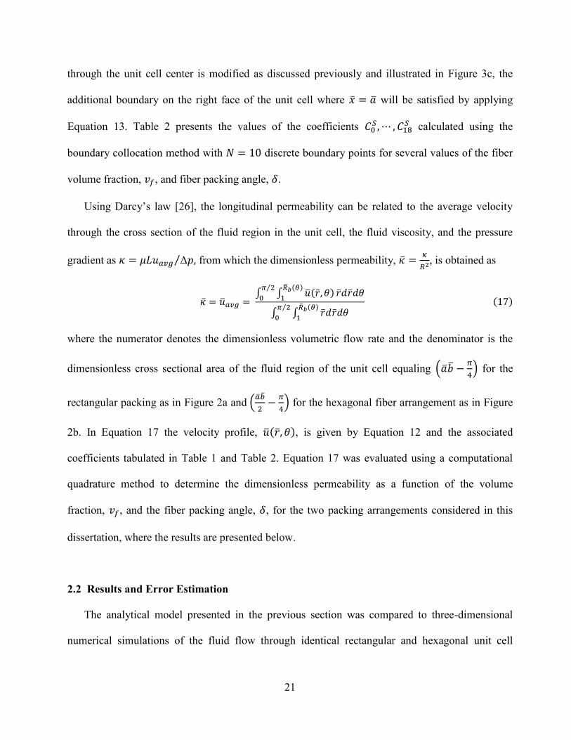
Using Darcy’s law [26], the longitudinal permeability can be related to the average velocity
through the cross section of the fluid region in the unit cell, the fluid viscosity, and the pressure
gradient as Δ from which the dimensionless permeability,
, is obtained as
where the numerator denotes the dimensionless volumetric flow rate and the denominator is the
dimensionless cross sectional area of the fluid region of the unit cell equaling
for the
rectangular packing as in Figure 2a and
for the hexagonal fiber arrangement as in Figure
2b. In Equation 17 the velocity profile, , is given by Equation 12 and the associated
coefficients tabulated in Table 1 and Table 2. Equation 17 was evaluated using a computational
quadrature method to determine the dimensionless permeability as a function of the volume
fraction, , and the fiber packing angle, , for the two packing arrangements considered in this
dissertation, where the results are presented below.
2.2 Results and Error Estimation
The analytical model presented in the previous section was compared to three-dimensional
numerical simulations of the fluid flow through identical rectangular and hexagonal unit cell
22
Figure 4: Contour plots of the dimensionless velocity in unit cells of a (a) rectangular fiber
arrangement with and and (b) hexagonal fiber arrangement with
and .
geometries (as shown in Figure 2) for a range of fiber volume fractions and fiber packing angles.
The numerical solution was obtained with the commercially available finite element software
COMSOL©
using a tetrahedral mesh consisting of elements, and the results were non-
dimensionalized according to the parameters presented in Chapter 2.1 in order to compare the
numerical results to the dimensionless analytical series solution. The results of the comparison are
presented and discussed in this chapter. Figure 4 presents contours of the dimensionless velocity
profiles evaluated using the analytical solution in a rectangular unit cell geometry with a fiber
packing angle of 45o (Figure 4a) and a hexagonal unit cell geometry with a fiber packing angle of
60o (Figure 4b), both with a fiber volume fraction of 0.25. The analytical solution is based on ten
23
boundary collocation points in the evaluation of the boundary conditions, Equation 6 and Equation
7, using the constants given in Table 1 and Table 2 in Equation 12. Also included in the figures are
the dimensionless velocity profile values obtained from a numerical fluid dynamics simulation of
the flow through the respective geometries, shown by the discrete triangular markers in the figures.
Excellent agreement is noted between the analytical solution and the corresponding numerical
solution. For the rectangular fiber arrangement in Figure 4a, the maximum dimensionless velocity
is approximately 0.27 and located at the upper right-hand corner of the fluid domain. At the same
volume fraction, the hexagonal-packed case in Figure 4b shows a smaller maximum dimensionless
velocity of approximately 0.19 to occur at the points and in the unit cell. From
Figure 4, it is also evident that the maximum velocity locations for each fiber packing arrangement
are situated on the fluid boundary at the furthest distance from the fiber surfaces in their respective
unit cell domains. It follows from the dimensionless velocity profiles that the dimensionless
volumetric flow rate through the rectangular fiber packing geometry is greater than the hexagonal
fiber arrangement at the same fiber volume fraction. Since the results are presented in
dimensionless form, the velocity profiles are generally applicable to longitudinal flow situations
through aligned rigid fibers without limitation on the fiber radius or fluid viscosity. In addition, the
qualitative relative trends in the flow behavior for the two unit cell geometries are generally
applicable throughout the entire range of fiber volume fractions and packing angles.
The results in Figure 4 were based on ten collocation points on the boundaries of the
rectangular and hexagonal unit cells in Figure 3, which, in turn, governs the number of terms used
in evaluating the series solution in Equation 12. It is instructive to assess the influence of the
number of boundary collocation points—and, in turn, the number of terms in Equation 12—on the
accuracy of the analytical solution. To this end, Figure 5 presents the magnitude of the error in
24
Figure 5: Variation of the error between the numerical and analytical solutions for flow rate
through a rectangular fiber array at different fiber volume fractions as the number of terms in Eq.
12 is varied; for (a) , (b) , (c) , and (d) .
the analytical solution of the volumetric flow rate for the rectangular fiber arrangement in
comparison to the converged numerical solution of the volumetric flow rate, expressed as a
percentage of the numerical solution, as the number of coefficients determined in Equation 12 is
increased. The numerical finite element method (FEM) was used to validate the analytical solution
since FEM is usually employed in detailed computational modeling of this flow situation and
serves as an appropriate basis for comparison with the analytical results. The error magnitudes are
presented at incremented values of the volume fraction, , and at four different values of the
packing angle, , (Figure 5a–Figure 5d) as noted in the figure caption. The maximum attainable
25
volume fraction at the packing limit decreases as the packing angle is increased, which can be seen
from inspection of the unit cell's geometry and is reflected in the different values of the volume
fraction upper limits as the packing angle is changed, presented in the legend of Figure 5. In
general, Figure 5 shows that as the number of terms in the expansion of Equation 12 is increased,
the accuracy of the analytical solution increases accordingly and the error with respect to the
converged numerical solution approaches zero.
It is apparent from Figure 5a that for a rectangular packing angle of , the error remains
less than about 2.8% when at least six terms are included in the expansion of Equation 12 and
further reduces to less than ~1% when the number of terms is increased to eight. The relatively
greater amount of error apparent in the case where and (Figure 5a) when
Figure 6: Variation of the dimensionless permeability with the fiber volume fraction and fiber
packing angle for a rectangular arrangement of fibers.
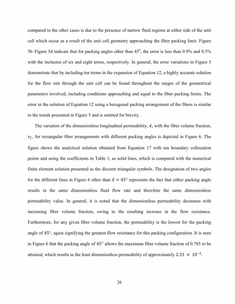
26
compared to the other cases is due to the presence of narrow fluid regions at either side of the unit
cell which occur as a result of the unit cell geometry approaching the fiber packing limit. Figure
5b–Figure 5d indicate that for packing angles other than 45o, the error is less than 0.9% and 0.5%
with the inclusion of six and eight terms, respectively. In general, the error variations in Figure 5
demonstrate that by including ten terms in the expansion of Equation 12, a highly accurate solution
for the flow rate through the unit cell can be found throughout the ranges of the geometrical
parameters involved, including conditions approaching and equal to the fiber packing limits. The
error in the solution of Equation 12 using a hexagonal packing arrangement of the fibers is similar
to the trends presented in Figure 5 and is omitted for brevity.
The variation of the dimensionless longitudinal permeability, , with the fiber volume fraction,
, for rectangular fiber arrangements with different packing angles is depicted in Figure 6. The
figure shows the analytical solution obtained from Equation 17 with ten boundary collocation
points and using the coefficients in Table 1, as solid lines, which is compared with the numerical
finite element solution presented as the discrete triangular symbols. The designation of two angles
for the different lines in Figure 6 other than represents the fact that either packing angle
results in the same dimensionless fluid flow rate and therefore the same dimensionless
permeability value. In general, it is noted that the dimensionless permeability decreases with
increasing fiber volume fraction, owing to the resulting increase in the flow resistance.
Furthermore, for any given fiber volume fraction, the permeability is the lowest for the packing
angle of , again signifying the greatest flow resistance for this packing configuration. It is seen
in Figure 6 that the packing angle of allows the maximum fiber volume fraction of 0.785 to be
attained, which results in the least dimensionless permeability of approximately
27
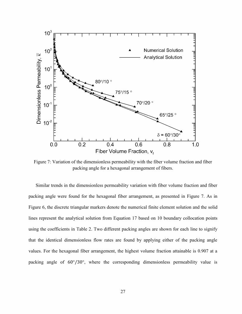
Figure 7: Variation of the dimensionless permeability with the fiber volume fraction and fiber
packing angle for a hexagonal arrangement of fibers.
Similar trends in the dimensionless permeability variation with fiber volume fraction and fiber
packing angle were found for the hexagonal fiber arrangement, as presented in Figure 7. As in
Figure 6, the discrete triangular markers denote the numerical finite element solution and the solid
lines represent the analytical solution from Equation 17 based on 10 boundary collocation points
using the coefficients in Table 2. Two different packing angles are shown for each line to signify
that the identical dimensionless flow rates are found by applying either of the packing angle
values. For the hexagonal fiber arrangement, the highest volume fraction attainable is 0.907 at a
packing angle of , where the corresponding dimensionless permeability value is
28
approximately , which is approximately an order of magnitude lower than the
minimum permeability noted for the rectangular packing in Figure 6.
In both Figure 6 and Figure 7, excellent agreement is seen between the analytical results and
the numerical values. It is evident from a comparison of the permeability values in Figure 6 and
Figure 7 that at any fiber volume fraction, the rectangular fiber packing offers less resistance to the
fluid flow than the hexagonal fiber arrangement, which is reflected in the higher dimensionless
permeability value for the rectangular fiber arrangement. This difference is particularly
pronounced at higher fiber volume fractions and reduces as the fiber volume fraction decreases,
where the smallest tested fiber volume fraction of resulted in the dimensionless
permeability values converging to the same value of approximately 450 for all cases of the
different relative fiber arrangements.
The longitudinal permeability values presented in Figure 6 and Figure 7 can be compared to
experimental results reported in the literature to evaluate the accuracy of the analytical results
compared to physical measurements. An experiment measuring the longitudinal permeability of an
array of aligned cylinders was presented in [20], reporting a dimensionless permeability on the
order of for a hexagonal fiber arrangement with a volume fraction of 0.6. Considering the
results presented in Figure 7 for a hexagonal fiber arrangement, it is evident that at the
analytical solution also predicts a permeability on the order of and therefore exhibits good
agreement with the experimentally measured value in [20]. In addition, the study in [23] examined
a fiber tow made up of glass filaments with a diameter of 12 and experimentally measured the
dimensionless longitudinal permeability to be on the order of for a fiber volume fraction of
0.6, which is on the same order of magnitude as the measurements in [20] and the analytical results
presented in Figure 6 and Figure 7.
29
As the fiber volume fraction of the fiber tow is increased, the effects of capillary pressure
will become increasingly significant in permeability measurements and predictions (e.g. [23,28]).
According to [28], the capillary pressure, , in the longitudinal direction of aligned rigid fibers
can be expressed in terms of the fiber volume fraction, , fiber radius, , surface tension, , and
contact angle, , as:
. In a typical liquid composite molding process the surface
tension will be on the order of N/m, the contact angle will be on the order of 10 degrees, and
the fiber radius will be on the order of 10-5
m. Applying the above expression to a fiber tow with a
volume fraction of 0.8 results in a capillary pressure of approximately 8 kPa. The applied pressure
in a liquid composite molding application is typically on the order of 102 kPa, which is more than
an order of magnitude higher than the capillary pressure calculated in the previous scenario.
Therefore, reasonable accuracy should be expected when using the permeability values presented
in Figure 6 and Figure 7, however these results should be used carefully when applied to situations
involving fiber tows with small filament diameters and high fiber volume fractions where the
capillary effect may become increasingly significant. The model developed in this chapter along
with an established transverse permeability model are applied to describe the local permeability
tensor of a woven preform fabric used in the numerical simulation of void formation in LCM
processes presented in Chapter 3.
2.3 Nomenclature used in Chapter 2
a width of unit cell [m]
b height of unit cell [m]
C Equation 12 constants
L length of unit cell [m]
30
N number of boundary collocation points
P pressure [Pa]
r radial-direction coordinate [m]
R fiber radius [m]
Rb radius to flow boundary [m]
Re Reynolds number
u velocity vector [m/s]
vf fiber volume fraction
x x-direction coordinate [m]
y y-direction coordinate [m]
z z-direction coordinate [m]
Greek symbols
surface tension [N/m]
fiber packing angle [degrees]
angular-direction coordinate [degrees]
permeability [m2]
fluid viscosity [Pa·s]
contact angle [degrees]
Superscripts/subscripts
dimensionless value
rectangular fiber packing
hexagonal fiber packing
index of constants in solution equation
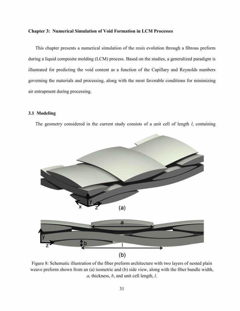
31
Chapter 3: Numerical Simulation of Void Formation in LCM Processes
This chapter presents a numerical simulation of the resin evolution through a fibrous preform
during a liquid composite molding (LCM) process. Based on the studies, a generalized paradigm is
illustrated for predicting the void content as a function of the Capillary and Reynolds numbers
governing the materials and processing, along with the most favorable conditions for minimizing
air entrapment during processing.
3.1 Modeling
The geometry considered in the current study consists of a unit cell of length l, containing
Figure 8: Schematic illustration of the fiber preform architecture with two layers of nested plain
weave preform shown from an (a) isometric and (b) side view, along with the fiber bundle width,
a, thickness, b, and unit cell length, l.
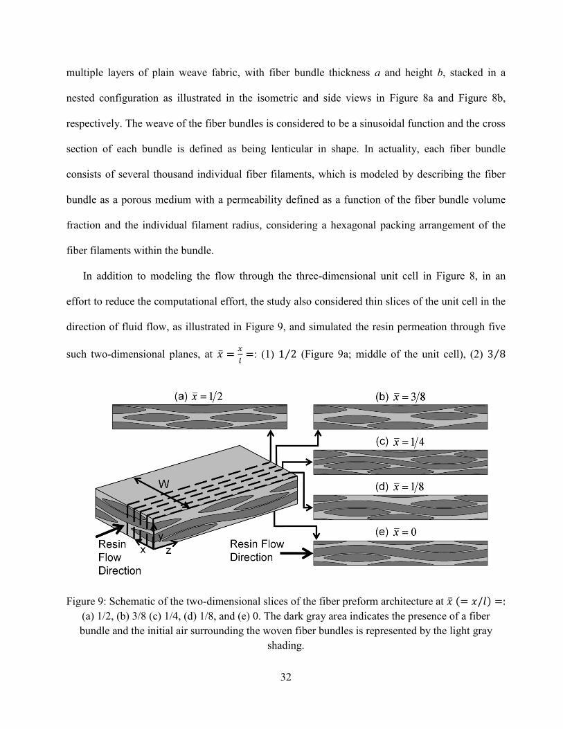
32
multiple layers of plain weave fabric, with fiber bundle thickness a and height b, stacked in a
nested configuration as illustrated in the isometric and side views in Figure 8a and Figure 8b,
respectively. The weave of the fiber bundles is considered to be a sinusoidal function and the cross
section of each bundle is defined as being lenticular in shape. In actuality, each fiber bundle
consists of several thousand individual fiber filaments, which is modeled by describing the fiber
bundle as a porous medium with a permeability defined as a function of the fiber bundle volume
fraction and the individual filament radius, considering a hexagonal packing arrangement of the
fiber filaments within the bundle.
In addition to modeling the flow through the three-dimensional unit cell in Figure 8, in an
effort to reduce the computational effort, the study also considered thin slices of the unit cell in the
direction of fluid flow, as illustrated in Figure 9, and simulated the resin permeation through five
such two-dimensional planes, at
: (1) (Figure 9a; middle of the unit cell), (2)
Figure 9: Schematic of the two-dimensional slices of the fiber preform architecture at
(a) 1/2, (b) 3/8 (c) 1/4, (d) 1/8, and (e) 0. The dark gray area indicates the presence of a fiber
bundle and the initial air surrounding the woven fiber bundles is represented by the light gray
shading.
33
(Figure 9b), (3) (Figure 9c), (4) (Figure 9d), and (5) (Figure 9e; edge of the unit cell).
The void fraction in the three-dimensional geometry was then estimated through a volumetric
summation of the void content in individual slices. It can be observed from the geometry shown in
Figure 8 that the three-dimensional fiber architecture is anti-symmetric about the middle plane
defined in Figure 9a, which implies that the slices in Figure 9b–Figure 9e are inverted at their
respective locations when mirrored on the opposite side of the middle plane (at ).
However, in a two-dimensional modeling the flow is identical through these inverted
configurations and as a result the simulations on one half of the unit cell are representative of the
flow through the entire domain.
For both the three-dimensional unit cell geometry and the two-dimensional slices, the
governing mathematical equations describing the resin flow through the macro-scale inter-bundle
regions and the porous fiber bundles are the conservation of mass and momentum along with the
equation associated with the volume of fluid (VOF) method [92] used to track and advance the
resin/air interface during the filling process. The governing mathematical equations are expressed
in a nondimensional form using the following dimensionless parameters:
where is the dimensionless velocity vector describing the fluid motion and is the inlet resin
velocity, , , and are the three dimensionless Cartesian directions, is dimensionless time, is
dimensionless pressure, and is the density of the resin phase. In addition, the Reynolds number,
Re, and Capillary number, Ca, are defined as:
34
where the resin viscosity is and is the surface tension. In the VOF method, the volume
fraction of the resin in a computational cell, , is governed in dimensionless form by:
where is the dimensionless gradient operator. Assuming incompressible fluid properties,
conservation of mass is described by the dimensionless continuity equation, written as:
Conservation of momentum for flow around the fiber bundles in the macro-pores of the unit cell is
enforced through the dimensionless Navier-Stokes equation. In the case of flow within the micro-
pores of the fiber bundle, two source terms are added to this equation in order to account for the
porous and capillary effects within the fiber bundle. For conciseness of presentation, Equation 20
and Equation 21 include the porous media and capillary source terms (the last two terms in
Equation 20 and Equation 21), however these two source terms are only active within the porous
domains of the unit cell. The presence of the two-phase flow in the model requires two momentum
equation descriptions using the properties of the different fluid phases, written for resin and air,
respectively, as:
where the density and viscosity of the air phase are denoted by and , respectively, is the
dimensionless porous media source term, and the dimensionless capillary source term is denoted
by . The dimensionless source term corresponding to the flow through the porous fiber bundles
was expressed using Darcy's Law as
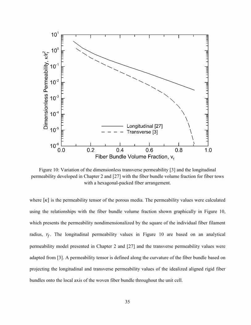
35
Figure 10: Variation of the dimensionless transverse permeability [3] and the longitudinal
permeability developed in Chapter 2 and [27] with the fiber bundle volume fraction for fiber tows
with a hexagonal-packed fiber arrangement.
where is the permeability tensor of the porous media. The permeability values were calculated
using the relationships with the fiber bundle volume fraction shown graphically in Figure 10,
which presents the permeability nondimensionalized by the square of the individual fiber filament
radius, . The longitudinal permeability values in Figure 10 are based on an analytical
permeability model presented in Chapter 2 and [27] and the transverse permeability values were
adapted from [3]. A permeability tensor is defined along the curvature of the fiber bundle based on
projecting the longitudinal and transverse permeability values of the idealized aligned rigid fiber
bundles onto the local axis of the woven fiber bundle throughout the unit cell.
36
By definition, the capillary forces are present only at the resin-air interface within the fiber
bundle flow field of the geometry. However, a continuum method for modeling surface tension
effects across the interface of two adjacent fluids was developed in [93]. By using the divergence
theorem, the capillary effects at the resin-air interface can be converted to a body force and
expressed as a source term in the momentum equation [94], written as
where is the dimensionless capillary pressure in the fiber bundle at the resin-air interface and
is the local volume fraction of the resin. In the VOF model, the volume fraction variable is defined
as 0 for purely resin and 1 for purely air. At the interface of these two phases is a thin region where
the volume fraction varies smoothly between 0 and 1, and a value of 0.5 is chosen to represent the
approximate transition between phases. It is evident that the gradient of the volume fraction term
in Equation 23 will be non-zero only along this thin region where varies between 0 and 1,
satisfying the physical presence of the capillary forces occurring at the resin-air interface. Within
the idealized fiber bundle of straight aligned rigid fibers, the capillary force occurs in two principal
directions: causing the resin to wick (1) radially inward perpendicular to the fibers and (2)
longitudinally through the fibers in the bundle. In the first case, the dimensionless capillary
pressure forces the resin radially into the fiber bundle (perpendicular to the individual fibers) and
can be expressed in dimensionless form according to [35] as
where is the dimensionless capillary pressure acting radially along the fibers, is the wetting
angle of the resin, is the fiber volume fraction of the fiber bundle, and is the angular location
of the resin-air meniscus during flow between neighboring fibers. The integral in Equation 24 is
37
necessary to average the pressure as the capillary width changes according to perpendicular flow
between two adjacent cylindrical fibers. In the case of capillary flow longitudinal to the aligned
rigid fibers, the capillary width is constant as the resin is wicked along the channels and
consequently the dimensionless capillary pressure is constant as well and written in dimensionless
form according to [28] as
where is the capillary pressure acting longitudinal to the fibers. Following the foregoing
approach, the capillary pressure values can be calculated at the resin-air interface in the two
principal resin infiltration directions.
Equation 18–Equation 25 provide a complete description of the resin flow through the preform
and were numerically solved to investigate the resin evolution through the plain weave preform
architecture illustrated in Figure 8 and Figure 9. A constant and uniform resin velocity was
imposed as the boundary condition at the inlet plane of the unit cell geometry and a constant
pressure boundary was enforced at the outlet plane. The top and bottom faces of the unit cell were
defined as periodic boundaries based on the geometry of the two-dimensional fiber arrangements
as seen in Figure 9a–Figure 9e. It must be mentioned that the domain considered for the modeling
consists of a full repeating unit cell and a half unit cell length upstream and a half unit cell
downstream. This extended unit cell geometry allows the initially uniform resin flow front to
migrate naturally through and around the fiber bundles in the first half unit cell before entering the
complete unit cell of study (which is the focus of the results presented below), thereby better
approximating the actual resin flow development through the preform geometry.
The domain geometry and the model formulation were implemented in and solved using the
commercial ANSYS Fluent™ software using numerous supplementary user-defined functions
38
(UDF's) developed to model the permeability and surface tension forces included in the
momentum equation. The two-dimensional models used a mesh of approximately
elements and elements were used in the three-dimensional simulations. The PISO
scheme was used for the pressure-velocity coupling [95], a first-order implicit scheme was applied
for the time discretization, a second-order upwind scheme was implemented for the momentum
discretization, and the CICSAM scheme was used to solve the volume fraction equation [96].
Iterations at each time step were allowed to run until the residuals for each governing equation
dropped below , and various grid densities and time-steps were explored to verify grid and
time-step independence. All computations were performed on a single Dell PowerEdge R610
server with a 2.53 GHz processor and 12 GB of RAM, and the computing times for a fully three-
dimensional solution through a complete unit cell (Figure 8) ranged from 5–8 days depending on
the Ca and Re values, whereas the computing times were correspondingly in the range of 8–20 hrs.
for the simulations through the five two-dimensional slices (Figure 9a–Figure 9e) of the three-
dimensional volume. The simulations yielded the flow front progression through the inter- and
intra-fiber-bundle regions of the unit cell as a function of time. Using the flow progression
information, the void locations in the unit cell as well as the total void content was calculated as a
function of time to determine the steady state void fraction, where the results of the study are
presented and discussed below.
3.2 Void Diagrams
Two commercially available plain weave fabric geometries were chosen for the study,
specifically a Rovcloth 2454 (Fiber Glass Industries Inc., Amsterdam, NY) and an Owens Corning
WR10/3010 (OCV Fabrics US Inc., Toledo, OH) fabric with their associated fiber bundle
39
dimensions, and inter-bundle spacing. For the Rovcloth 2454 fabric, the preform dimensions of a,
b, and l were determined to be 4.1, 0.43, and 5.5 mm, respectively, and the second plain weave
fabric, Owens Corning WR10/3010 (OC WR10/3010), had a similar weave geometry with a, b,
and l equaling 3.5, 0.78, and 4.5 mm, respectively. In both fabrics the fiber bundles were assumed
to have a fiber volume fraction of 0.6 and the individual fiber filaments within the fiber bundle
were considered to be 10 in diameter. The dynamic viscosity of the resin was chosen to be
0.01 Pa·s and the resin-air interface was described with a contact angle of 30 degrees.
A parametric study was conducted to investigate the effects of varying the Reynolds, Re, and
Capillary, Ca, numbers on the resulting void content evolution in each of the five planar slices
identified in Figure 9. Four different Re values of 0.23, 5.75, 40.3, and 479 as well as four Ca
numbers of , , , were studied in each of the five
planes, for a total of 80 parametric runs. These values of Ca and Re were chosen for the parametric
sweep in order to compare the current numerical simulations with similar experimental results
presented in [97]. In each case, the flow progression and corresponding void content were recorded
over time, as discussed in this Section. Further, the results of the flow along the planar unit cell
slices (Figure 9) are also compared with results from simulations of the full three-dimensional flow
through the unit cell geometry shown in Figure 8 to establish the accuracy of the computationally
simpler modeling using the multiple two-dimensional slices.
Figure 11–Figure 13 present snapshots of the resin infiltrating each plane of the fiber preform
architecture at progressive times throughout the mold filling process at various combinations of
Capillary and Reynolds numbers using the two-dimensional planar geometries. The resin is
injected uniformly at the left plane of the unit cell (as shown in Figure 9e) and allowed to permeate
through the entire geometry. The local void content, , at each time step is presented below every
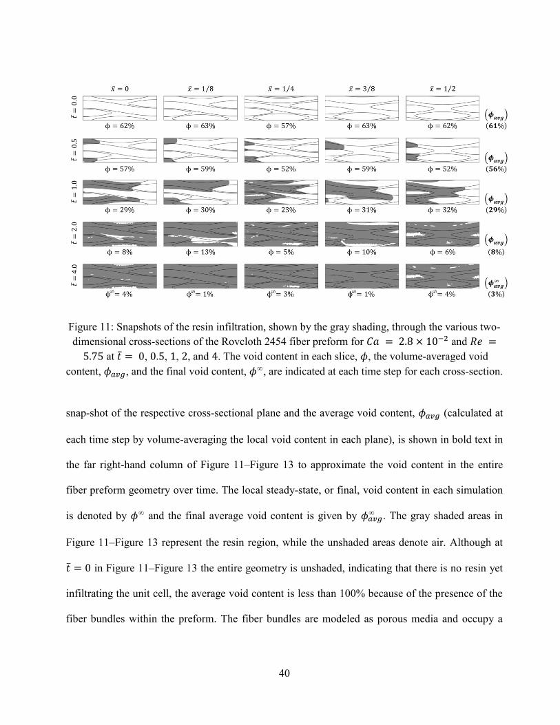
40
Figure 11: Snapshots of the resin infiltration, shown by the gray shading, through the various two-
dimensional cross-sections of the Rovcloth 2454 fiber preform for and
at , , , , and . The void content in each slice, , the volume-averaged void
content, , and the final void content, , are indicated at each time step for each cross-section.
snap-shot of the respective cross-sectional plane and the average void content, (calculated at
each time step by volume-averaging the local void content in each plane), is shown in bold text in
the far right-hand column of Figure 11–Figure 13 to approximate the void content in the entire
fiber preform geometry over time. The local steady-state, or final, void content in each simulation
is denoted by and the final average void content is given by . The gray shaded areas in
Figure 11–Figure 13 represent the resin region, while the unshaded areas denote air. Although at
in Figure 11–Figure 13 the entire geometry is unshaded, indicating that there is no resin yet
infiltrating the unit cell, the average void content is less than 100% because of the presence of the
fiber bundles within the preform. The fiber bundles are modeled as porous media and occupy a
41
fixed volume of approximately 39% of the unit cell and, therefore, the initial average void content
at is 61%.
The resin flow development through the fiber geometry for and
is presented in Figure 11. Initially, at , the resin has not yet infiltrated the unit cell and each
of the five planes is saturated with air, where the edges of the fiber bundles in each of the
respective slices are clearly visible and . At the resin has begun to flow into
the unit cell and primarily follows the path of least resistance through the macro-scale channels in
between the fiber bundles, although some fiber bundle permeation is also evident. As time
advances to the resin has permeated further into the macro-scale channels and has also
begun to fill into the fiber bundles of each plane, entrapping significant pockets of air in the
and planes within the fiber bundles. The resin flow front reaches the outlet in
the macro-scale channels in each of the different plane sections at , and the average void
content is found to be approximately eight percent of the total unit cell volume. At the void
content decreases to approximately three percent and becomes nearly steady over time in each of
the planes, depicting the final size and location of the entrapped air pockets within each of the fiber
bundles. Significant void formation is visible in the , , and planes at this
steady state condition and, conversely, almost complete resin saturation is apparent in the
and planes. Note that the periodic nature of the resin flow enforced at the top and bottom
faces of each of the unit cells is apparent throughout the simulation results presented in Figure 11.
Several observations can be made regarding the void formation in each of the fiber bundles in
the simulation shown in Figure 11: It is evident that at the void in the first cross-running
bundle (seen as one half bundle section at the left edge of the frame in Figure 11 for ) is
larger than the void in the third cross-running bundle (the one half bundle section at the right edge
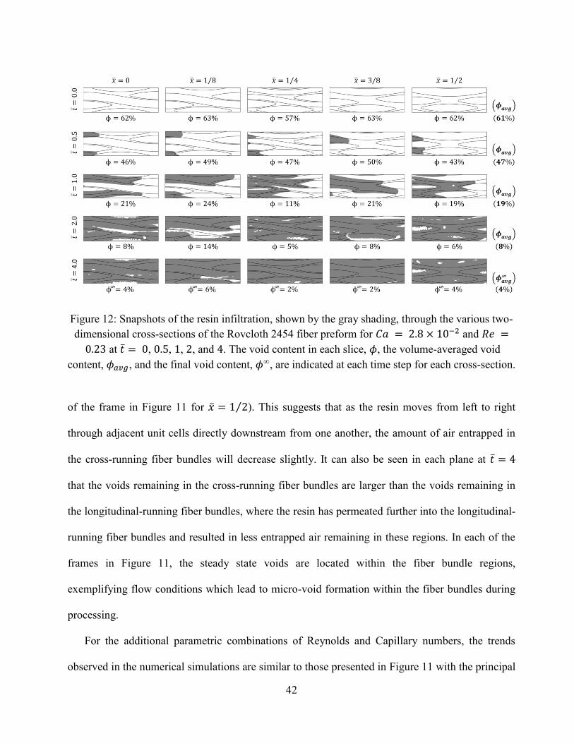
42
Figure 12: Snapshots of the resin infiltration, shown by the gray shading, through the various two-
dimensional cross-sections of the Rovcloth 2454 fiber preform for and
at , , , , and . The void content in each slice, , the volume-averaged void
content, , and the final void content, , are indicated at each time step for each cross-section.
of the frame in Figure 11 for ). This suggests that as the resin moves from left to right
through adjacent unit cells directly downstream from one another, the amount of air entrapped in
the cross-running fiber bundles will decrease slightly. It can also be seen in each plane at
that the voids remaining in the cross-running fiber bundles are larger than the voids remaining in
the longitudinal-running fiber bundles, where the resin has permeated further into the longitudinal-
running fiber bundles and resulted in less entrapped air remaining in these regions. In each of the
frames in Figure 11, the steady state voids are located within the fiber bundle regions,
exemplifying flow conditions which lead to micro-void formation within the fiber bundles during
processing.
For the additional parametric combinations of Reynolds and Capillary numbers, the trends
observed in the numerical simulations are similar to those presented in Figure 11 with the principal
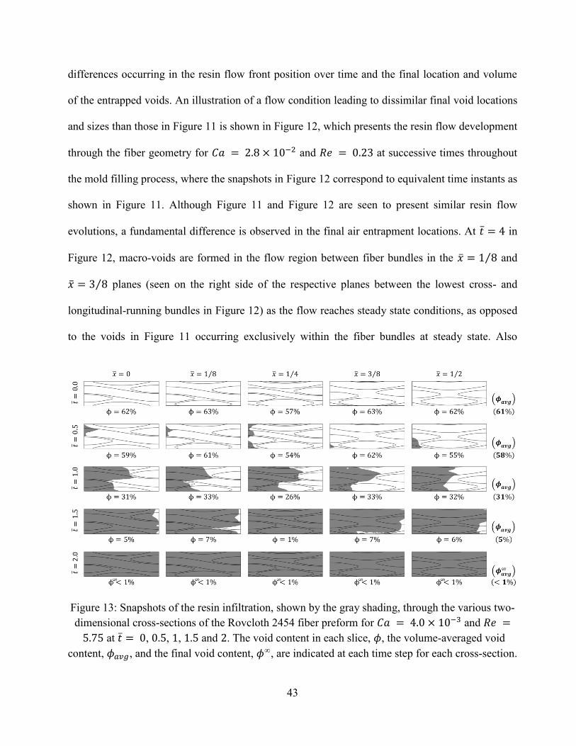
43
differences occurring in the resin flow front position over time and the final location and volume
of the entrapped voids. An illustration of a flow condition leading to dissimilar final void locations
and sizes than those in Figure 11 is shown in Figure 12, which presents the resin flow development
through the fiber geometry for and at successive times throughout
the mold filling process, where the snapshots in Figure 12 correspond to equivalent time instants as
shown in Figure 11. Although Figure 11 and Figure 12 are seen to present similar resin flow
evolutions, a fundamental difference is observed in the final air entrapment locations. At in
Figure 12, macro-voids are formed in the flow region between fiber bundles in the and
planes (seen on the right side of the respective planes between the lowest cross- and
longitudinal-running bundles in Figure 12) as the flow reaches steady state conditions, as opposed
to the voids in Figure 11 occurring exclusively within the fiber bundles at steady state. Also
Figure 13: Snapshots of the resin infiltration, shown by the gray shading, through the various two-
dimensional cross-sections of the Rovcloth 2454 fiber preform for and
at , , , and . The void content in each slice, , the volume-averaged void
content, , and the final void content, , are indicated at each time step for each cross-section.
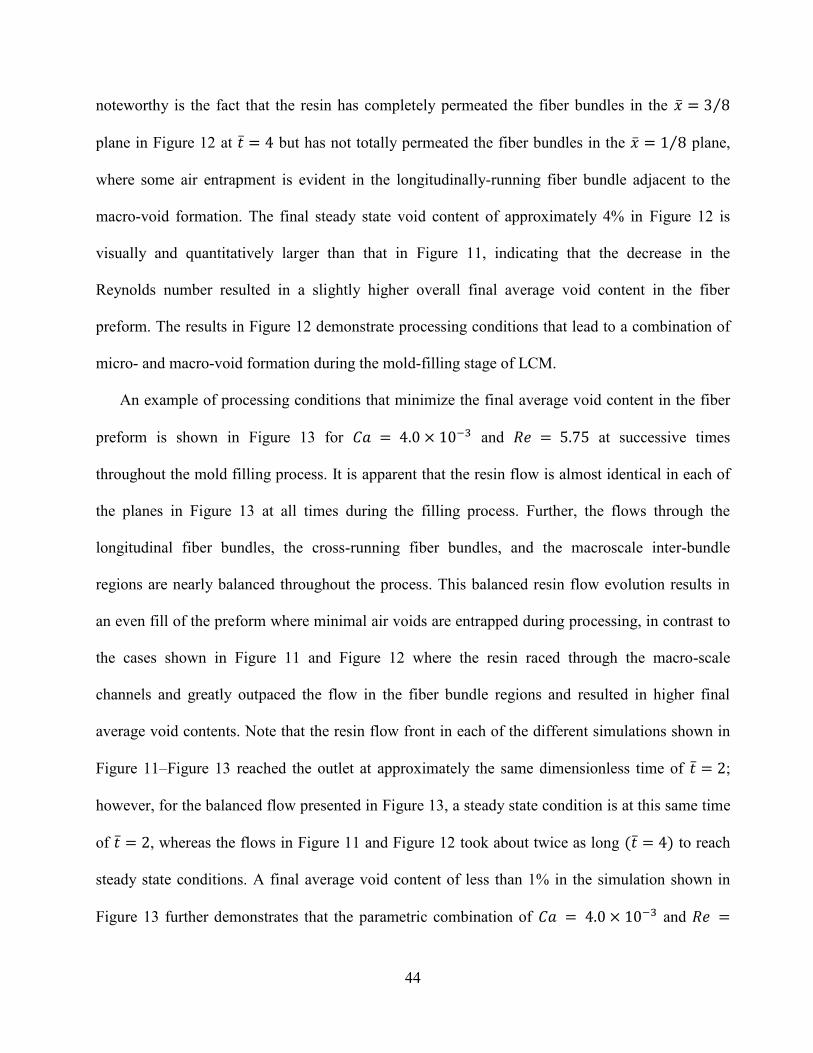
44
noteworthy is the fact that the resin has completely permeated the fiber bundles in the
plane in Figure 12 at but has not totally permeated the fiber bundles in the plane,
where some air entrapment is evident in the longitudinally-running fiber bundle adjacent to the
macro-void formation. The final steady state void content of approximately 4% in Figure 12 is
visually and quantitatively larger than that in Figure 11, indicating that the decrease in the
Reynolds number resulted in a slightly higher overall final average void content in the fiber
preform. The results in Figure 12 demonstrate processing conditions that lead to a combination of
micro- and macro-void formation during the mold-filling stage of LCM.
An example of processing conditions that minimize the final average void content in the fiber
preform is shown in Figure 13 for and at successive times
throughout the mold filling process. It is apparent that the resin flow is almost identical in each of
the planes in Figure 13 at all times during the filling process. Further, the flows through the
longitudinal fiber bundles, the cross-running fiber bundles, and the macroscale inter-bundle
regions are nearly balanced throughout the process. This balanced resin flow evolution results in
an even fill of the preform where minimal air voids are entrapped during processing, in contrast to
the cases shown in Figure 11 and Figure 12 where the resin raced through the macro-scale
channels and greatly outpaced the flow in the fiber bundle regions and resulted in higher final
average void contents. Note that the resin flow front in each of the different simulations shown in
Figure 11–Figure 13 reached the outlet at approximately the same dimensionless time of ;
however, for the balanced flow presented in Figure 13, a steady state condition is at this same time
of , whereas the flows in Figure 11 and Figure 12 took about twice as long to reach
steady state conditions. A final average void content of less than 1% in the simulation shown in
Figure 13 further demonstrates that the parametric combination of and
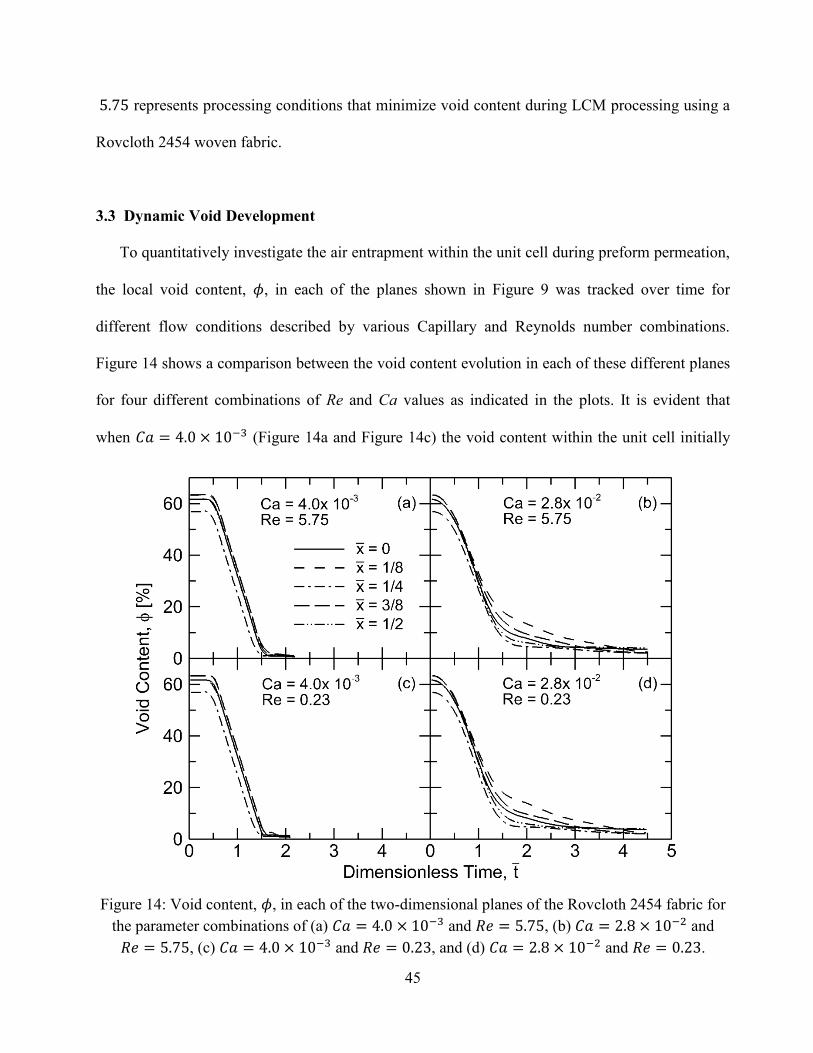
45
represents processing conditions that minimize void content during LCM processing using a
Rovcloth 2454 woven fabric.
3.3 Dynamic Void Development
To quantitatively investigate the air entrapment within the unit cell during preform permeation,
the local void content, , in each of the planes shown in Figure 9 was tracked over time for
different flow conditions described by various Capillary and Reynolds number combinations.
Figure 14 shows a comparison between the void content evolution in each of these different planes
for four different combinations of Re and Ca values as indicated in the plots. It is evident that
when (Figure 14a and Figure 14c) the void content within the unit cell initially
Figure 14: Void content, , in each of the two-dimensional planes of the Rovcloth 2454 fabric for
the parameter combinations of (a) and , (b) and
, (c) and , and (d) and .
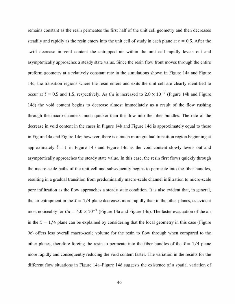
46
remains constant as the resin permeates the first half of the unit cell geometry and then decreases
steadily and rapidly as the resin enters into the unit cell of study in each plane at . After the
swift decrease in void content the entrapped air within the unit cell rapidly levels out and
asymptotically approaches a steady state value. Since the resin flow front moves through the entire
preform geometry at a relatively constant rate in the simulations shown in Figure 14a and Figure
14c, the transition regions where the resin enters and exits the unit cell are clearly identified to
occur at and , respectively. As Ca is increased to (Figure 14b and Figure
14d) the void content begins to decrease almost immediately as a result of the flow rushing
through the macro-channels much quicker than the flow into the fiber bundles. The rate of the
decrease in void content in the cases in Figure 14b and Figure 14d is approximately equal to those
in Figure 14a and Figure 14c; however, there is a much more gradual transition region beginning at
approximately in Figure 14b and Figure 14d as the void content slowly levels out and
asymptotically approaches the steady state value. In this case, the resin first flows quickly through
the macro-scale paths of the unit cell and subsequently begins to permeate into the fiber bundles,
resulting in a gradual transition from predominantly macro-scale channel infiltration to micro-scale
pore infiltration as the flow approaches a steady state condition. It is also evident that, in general,
the air entrapment in the plane decreases more rapidly than in the other planes, as evident
most noticeably for (Figure 14a and Figure 14c). The faster evacuation of the air
in the plane can be explained by considering that the local geometry in this case (Figure
9c) offers less overall macro-scale volume for the resin to flow through when compared to the
other planes, therefore forcing the resin to permeate into the fiber bundles of the plane
more rapidly and consequently reducing the void content faster. The variation in the results for the
different flow situations in Figure 14a–Figure 14d suggests the existence of a spatial variation of
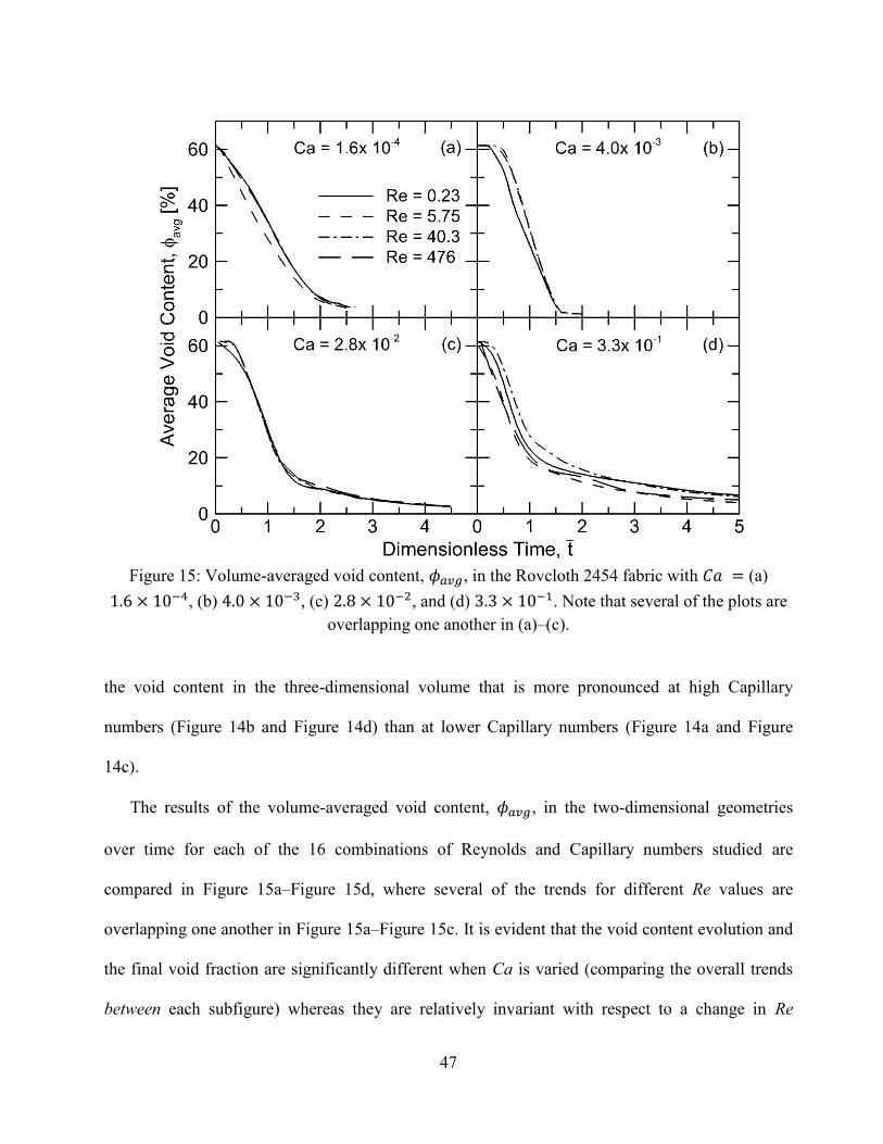
47
Figure 15: Volume-averaged void content, , in the Rovcloth 2454 fabric with (a)
, (b) , (c) , and (d) . Note that several of the plots are
overlapping one another in (a)–(c).
the void content in the three-dimensional volume that is more pronounced at high Capillary
numbers (Figure 14b and Figure 14d) than at lower Capillary numbers (Figure 14a and Figure
14c).
The results of the volume-averaged void content, , in the two-dimensional geometries
over time for each of the 16 combinations of Reynolds and Capillary numbers studied are
compared in Figure 15a–Figure 15d, where several of the trends for different Re values are
overlapping one another in Figure 15a–Figure 15c. It is evident that the void content evolution and
the final void fraction are significantly different when Ca is varied (comparing the overall trends
between each subfigure) whereas they are relatively invariant with respect to a change in Re
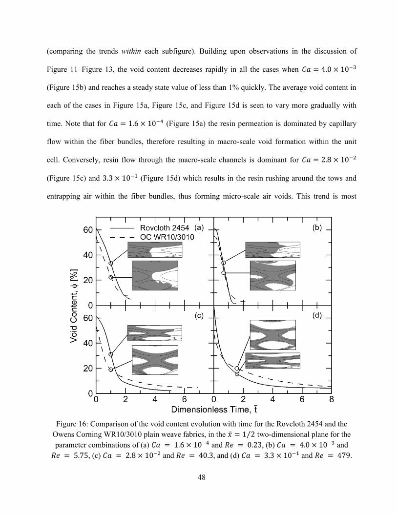
48
(comparing the trends within each subfigure). Building upon observations in the discussion of
Figure 11–Figure 13, the void content decreases rapidly in all the cases when
(Figure 15b) and reaches a steady state value of less than 1% quickly. The average void content in
each of the cases in Figure 15a, Figure 15c, and Figure 15d is seen to vary more gradually with
time. Note that for (Figure 15a) the resin permeation is dominated by capillary
flow within the fiber bundles, therefore resulting in macro-scale void formation within the unit
cell. Conversely, resin flow through the macro-scale channels is dominant for
(Figure 15c) and (Figure 15d) which results in the resin rushing around the tows and
entrapping air within the fiber bundles, thus forming micro-scale air voids. This trend is most
Figure 16: Comparison of the void content evolution with time for the Rovcloth 2454 and the
Owens Corning WR10/3010 plain weave fabrics, in the two-dimensional plane for the
parameter combinations of (a) and , (b) and
, (c) and , and (d) and .
49
apparent in the curves shown in Figure 15c and Figure 15d where the void content initially
decreases rapidly–corresponding to the quick infiltration of the macro-scale flow paths. The void
content evolution then transitions and becomes more gradual over time as the resin infiltration
begins to permeate into the micro-scale pores of the fiber bundles and the flow approaches a steady
state. An examination of the trends in Figure 14 and Figure 15 reveal that the Capillary number has
a relatively greater effect on the spatial void content distribution as well as the final void fraction
and should therefore be carefully chosen in the design of the processing conditions, in agreement
with the results presented in several studies (e.g. [41–43,97,98]).
The effect of the preform fabric geometry was studied by considering a second plain weave
fabric, OC WR10/3010, with a similar weave geometry as the Rovcloth 2454 except for the bundle
dimensions as mentioned in Chapter 3.1. In order to explore the influence of the fiber bundle
geometry on the air entrapment evolution within the preform, Figure 16a–Figure 16d present a
comparison of the void content that is developed in the plane for the two different fabrics,
for four different combinations of the Reynolds and Capillary numbers as indicated in the figure
caption. In each case, snapshots of the numerical simulation results are presented at selected times
during the infiltration process, where the gray shaded areas represent the resin phase. The results
shown in Figure 16 illustrate that the Owens Corning fabric initially begins with a slightly lower
amount of air as a result of the different geometry. As time progresses, at the early stages of resin
permeation, the Owens Corning fabric continues to contain less air than the Rovcloth fabric and
the qualitative resin permeation and the rate of the void content evolution are similar for the two
fabrics. However, in each case, the void content in the Rovcloth fabric eventually decreases to less
than that of the Owens Corning fabric and the steady state void content in the Rovcloth fabric is
consistently lower than that in the Owens Corning material, as seen in Figure 16a–Figure 16d. In
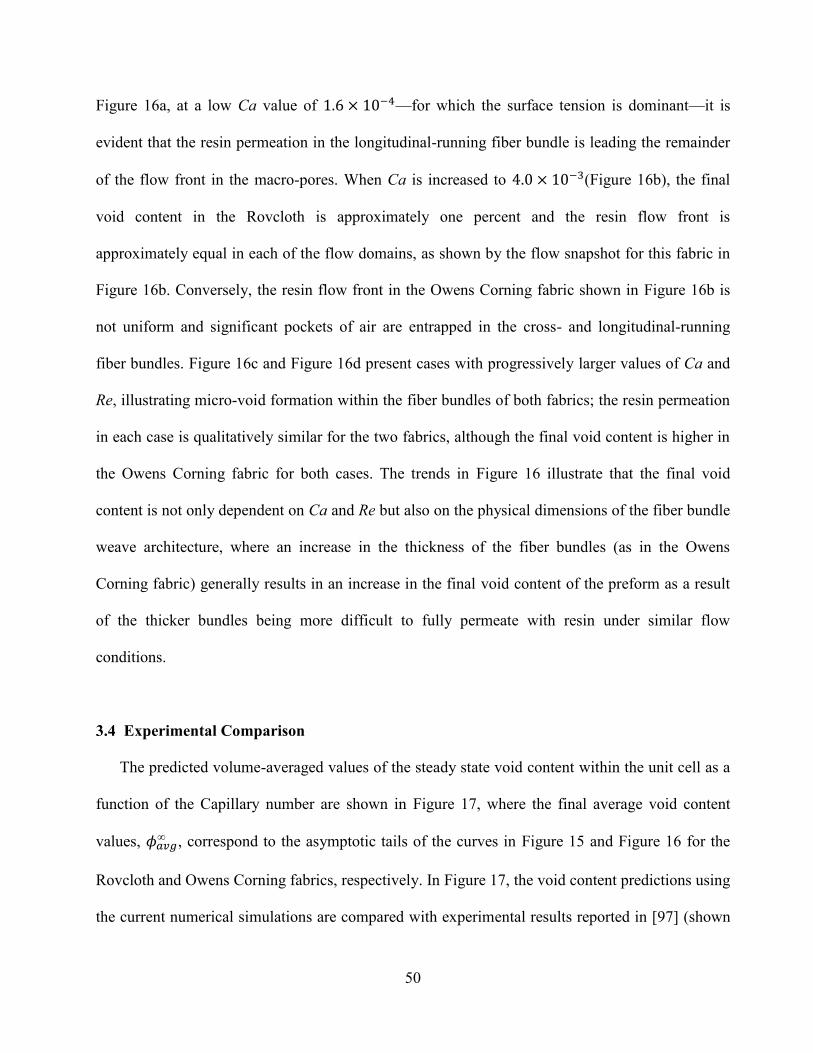
50
Figure 16a, at a low Ca value of —for which the surface tension is dominant—it is
evident that the resin permeation in the longitudinal-running fiber bundle is leading the remainder
of the flow front in the macro-pores. When Ca is increased to (Figure 16b), the final
void content in the Rovcloth is approximately one percent and the resin flow front is
approximately equal in each of the flow domains, as shown by the flow snapshot for this fabric in
Figure 16b. Conversely, the resin flow front in the Owens Corning fabric shown in Figure 16b is
not uniform and significant pockets of air are entrapped in the cross- and longitudinal-running
fiber bundles. Figure 16c and Figure 16d present cases with progressively larger values of Ca and
Re, illustrating micro-void formation within the fiber bundles of both fabrics; the resin permeation
in each case is qualitatively similar for the two fabrics, although the final void content is higher in
the Owens Corning fabric for both cases. The trends in Figure 16 illustrate that the final void
content is not only dependent on Ca and Re but also on the physical dimensions of the fiber bundle
weave architecture, where an increase in the thickness of the fiber bundles (as in the Owens
Corning fabric) generally results in an increase in the final void content of the preform as a result
of the thicker bundles being more difficult to fully permeate with resin under similar flow
conditions.
3.4 Experimental Comparison
The predicted volume-averaged values of the steady state void content within the unit cell as a
function of the Capillary number are shown in Figure 17, where the final average void content
values, , correspond to the asymptotic tails of the curves in Figure 15 and Figure 16 for the
Rovcloth and Owens Corning fabrics, respectively. In Figure 17, the void content predictions using
the current numerical simulations are compared with experimental results reported in [97] (shown
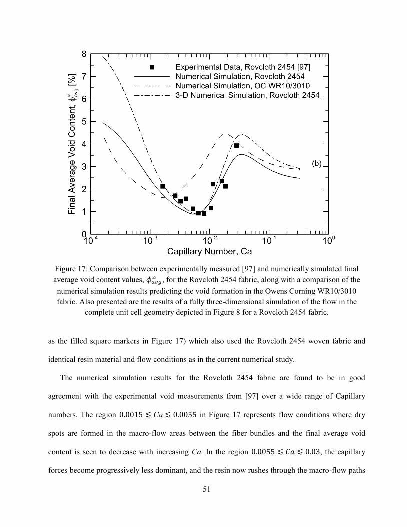
51
Figure 17: Comparison between experimentally measured [97] and numerically simulated final
average void content values, , for the Rovcloth 2454 fabric, along with a comparison of the
numerical simulation results predicting the void formation in the Owens Corning WR10/3010
fabric. Also presented are the results of a fully three-dimensional simulation of the flow in the
complete unit cell geometry depicted in Figure 8 for a Rovcloth 2454 fabric.
as the filled square markers in Figure 17) which also used the Rovcloth 2454 woven fabric and
identical resin material and flow conditions as in the current numerical study.
The numerical simulation results for the Rovcloth 2454 fabric are found to be in good
agreement with the experimental void measurements from [97] over a wide range of Capillary
numbers. The region in Figure 17 represents flow conditions where dry
spots are formed in the macro-flow areas between the fiber bundles and the final average void
content is seen to decrease with increasing Ca. In the region , the capillary
forces become progressively less dominant, and the resin now rushes through the macro-flow paths
52
in the unit cell geometry to entrap air within the fiber bundles forming micro-voids, and the final
average void content is seen to increase with Ca between 0.0055 and 0.03. The increase in macro-
void formation when Ca is decreased below 0.0055 and an increase in micro-void formation when
Ca is increased above 0.0055 up to 0.03 indicate that an ideal balance of the macro- and micro-
scale flow within the unit cell geometry occurs when Ca 0.0055 for the Rovcloth fabric.
Also presented in Figure 17 as the dash-dot line is the variation of the steady state void fraction
with the Capillary number based on a fully three-dimensional solution of the flow through the
complete three-dimensional unit cell (Figure 8) of the Rovcloth fabric, for comparison with the
experimental results in [97] (the filled square markers in Figure 17) and the results based on the
simulations using the five two-dimensional slices (the solid line in Figure 17). The three-
dimensional simulation of the Rovcloth fabric shows excellent agreement with the experimental
results in [97], predicting a similar void content trend as a function of the Capillary number. It is
seen that the void content determined based on the five two-dimensional simulations shows good
agreement with the results of the three-dimensional solution for ; in the region
the simulations through the two-dimensional planes are seen to underpredict the void content
by up to 3% relative to the complete three-dimensional simulation, for . This can be
explained by considering that the capillary forces at the resin-air interface become increasingly
dominant as Ca is decreased, and the wicking flow within the fiber bundles becomes much more
significant. This wicking resin flow in the fiber bundles in the x-direction (Figure 8) of the three-
dimensional unit cell are not accounted for in the two-dimensional slices taken along the y-z
planes. Therefore, the resin is wicked in only two directions in the two-dimensional slices, with the
predominant wicking occurring along the direction of resin infiltration (z-direction in Figure 8)
toward the exit of the unit cell. As a result, the air is pushed out of the unit cell efficiently and
53
results in a lower final average void content. On the other hand, in the three-dimensional unit cell
wicking in the x-direction is equally dominant as that in the z-direction towards the outlet. These
additional flow paths caused by the resin wicking in the x-direction result in less air being pushed
out three-dimensional unit cell, especially at low values of Ca, which leads to a higher overall void
percentage in these cases. Computationally, however, the three-dimensional solution required over
a week of CPU time for the smallest Ca of , whereas the simulation through the five
two-dimensional slices for this case took a maximum of only about 20 hrs. of CPU time,
representing a tremendously faster approach to solving the problem without significant loss of
accuracy.
As a comparison of the effects of the geometric parameters of the plain weave architecture, the
final average void content in the Owens Corning fabric calculated from the numerical simulations
is also presented in Figure 17 as the dashed line, where the trends are very similar to those of the
Rovcloth fabric and the experimental data in [97]. The final average void content for the Owens
Corning fabric are generally higher and the minimum and the maximum void fraction are found at
smaller Capillary numbers at about 0.002 and 0.015, respectively, compared to the corresponding
values of 0.0055 and 0.03 for the Rovcloth fabric. The results suggest that the flow paths offered to
the infiltrating resin differs depending on the geometric parameters of the preforms, resulting in
different values of Ca that describe a balance of the micro- and macro-scale flows in the preform.
This result is significant in the determination of ideal processing conditions as well as a prediction
of the overall final void content for different preform geometries.
Figure 17 shows that the final average void content decreases as the Capillary number is
increased beyond 0.03 for the Rovcloth fabric and beyond 0.02 for the Owens Corning fabric.
This is attributed to the increased pressure gradients within the preform for the higher Capillary
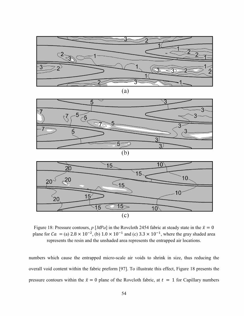
54
Figure 18: Pressure contours, p [MPa] in the Rovcloth 2454 fabric at steady state in the
plane for (a) , (b) and (c) , where the gray shaded area
represents the resin and the unshaded area represents the entrapped air locations.
numbers which cause the entrapped micro-scale air voids to shrink in size, thus reducing the
overall void content within the fabric preform [97]. To illustrate this effect, Figure 18 presents the
pressure contours within the plane of the Rovcloth fabric, at for Capillary numbers
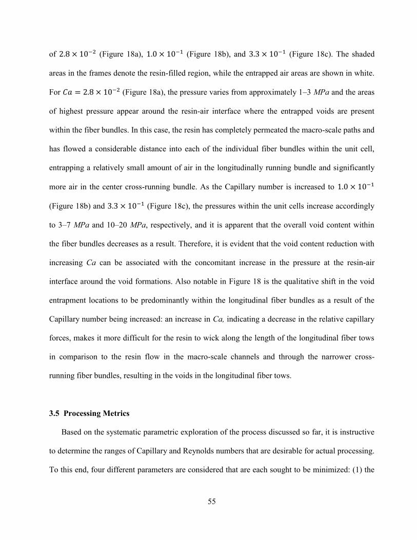
55
of (Figure 18a), (Figure 18b), and (Figure 18c). The shaded
areas in the frames denote the resin-filled region, while the entrapped air areas are shown in white.
For (Figure 18a), the pressure varies from approximately 1–3 MPa and the areas
of highest pressure appear around the resin-air interface where the entrapped voids are present
within the fiber bundles. In this case, the resin has completely permeated the macro-scale paths and
has flowed a considerable distance into each of the individual fiber bundles within the unit cell,
entrapping a relatively small amount of air in the longitudinally running bundle and significantly
more air in the center cross-running bundle. As the Capillary number is increased to
(Figure 18b) and (Figure 18c), the pressures within the unit cells increase accordingly
to 3–7 MPa and 10–20 MPa, respectively, and it is apparent that the overall void content within
the fiber bundles decreases as a result. Therefore, it is evident that the void content reduction with
increasing Ca can be associated with the concomitant increase in the pressure at the resin-air
interface around the void formations. Also notable in Figure 18 is the qualitative shift in the void
entrapment locations to be predominantly within the longitudinal fiber bundles as a result of the
Capillary number being increased: an increase in Ca, indicating a decrease in the relative capillary
forces, makes it more difficult for the resin to wick along the length of the longitudinal fiber tows
in comparison to the resin flow in the macro-scale channels and through the narrower cross-
running fiber bundles, resulting in the voids in the longitudinal fiber tows.
3.5 Processing Metrics
Based on the systematic parametric exploration of the process discussed so far, it is instructive
to determine the ranges of Capillary and Reynolds numbers that are desirable for actual processing.
To this end, four different parameters are considered that are each sought to be minimized: (1) the
56
Figure 19: Contours of (a) maximum final void content, , found in the two-dimensional slices
of the Rovcloth 2454, (b) volume-averaged final void content, , considering each of the two-
dimensional slices, (c) dimensionless excess flow time, , and (d) combined parameter
on a Capillary number–Reynolds number plane for the Rovcloth 2454. The most favorable
processing window shown by the shaded light gray oval region in (d) is superimposed by the
dashed oval in (a)–(c) to illustrate the corresponding maximum void content, average void content,
and excess flow time, respectively, associated with the most favorable processing window
maximum void content from among the five preform planes, , (2) the average void content
over all the five preform planes, , (3) a dimensionless excess flow time needed to reach steady
state, and (4) a combined objective defined as , all calculated from the two-
dimensional geometry results. Figure 19a–Figure 19d presents contour maps of the four parameters
identified above on a Reynolds number—Capillary number space for the Rovcloth 2454 fabric.
57
The predicted maximum and average values of the steady state void content within the unit cell
are shown in Figure 19a and Figure 19b, respectively, and correspond to the tails of the curves in
Figure 14 and Figure 15 for the different values of Re and Ca studied in each of the cross-sections.
The maximum steady state void content for each flow situation was observed to occur
predominantly in either the or plane and therefore represents a worst-case scenario
in terms of air entrapment. A volume average of the void content in the five different planes at
their respective steady state conditions was used to calculate the average steady state void content
values shown in Figure 19b and is representative of the approximate void content measurement
that would be reported experimentally. The maximum steady state void content values (Figure
19a) of the cases studied all fall between the range of approximately two to six percent of the
entire unit cell volume while the average steady state void content values (Figure 19b) all fall
within the range of approximately one to four percent.
It is observed from the data in Figure 19a that the maximum void content occurs at low
Reynolds numbers and high Capillary numbers, and progressively decreases for all Re as Ca is
decreased to approximately 0.001 and then begins to increase again as Ca is further reduced. The
approximately vertical nature of the contour lines in Figure 19a at the low and moderate Ca values
suggest that the maximum void content in these cases has a greater dependency on Ca than on Re.
This trend reflects the fact that the capillary forces at the resin-air interface increase in comparison
with the inertial forces dominating the macro-flow paths as Ca decreases, causing the resin to
permeate more rapidly into the fiber bundles and reducing micro-void formation. In contrast, as Re
varies independent of Ca the ratio of inertia to viscous forces is changed, which appears to have a
lesser effect on the resulting flow and final void content. The final average void content values
shown in Figure 19b are all less than the maximum void content values (Figure 19a) at similar
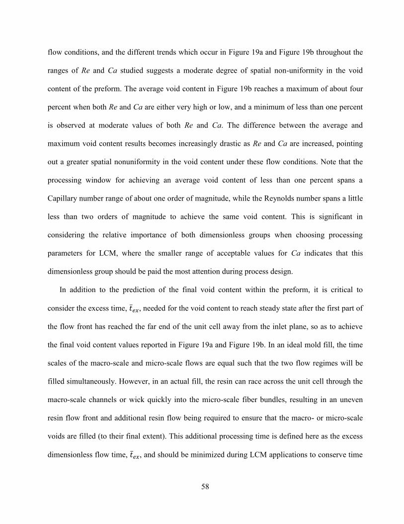
58
flow conditions, and the different trends which occur in Figure 19a and Figure 19b throughout the
ranges of Re and Ca studied suggests a moderate degree of spatial non-uniformity in the void
content of the preform. The average void content in Figure 19b reaches a maximum of about four
percent when both Re and Ca are either very high or low, and a minimum of less than one percent
is observed at moderate values of both Re and Ca. The difference between the average and
maximum void content results becomes increasingly drastic as Re and Ca are increased, pointing
out a greater spatial nonuniformity in the void content under these flow conditions. Note that the
processing window for achieving an average void content of less than one percent spans a
Capillary number range of about one order of magnitude, while the Reynolds number spans a little
less than two orders of magnitude to achieve the same void content. This is significant in
considering the relative importance of both dimensionless groups when choosing processing
parameters for LCM, where the smaller range of acceptable values for Ca indicates that this
dimensionless group should be paid the most attention during process design.
In addition to the prediction of the final void content within the preform, it is critical to
consider the excess time, , needed for the void content to reach steady state after the first part of
the flow front has reached the far end of the unit cell away from the inlet plane, so as to achieve
the final void content values reported in Figure 19a and Figure 19b. In an ideal mold fill, the time
scales of the macro-scale and micro-scale flows are equal such that the two flow regimes will be
filled simultaneously. However, in an actual fill, the resin can race across the unit cell through the
macro-scale channels or wick quickly into the micro-scale fiber bundles, resulting in an uneven
resin flow front and additional resin flow being required to ensure that the macro- or micro-scale
voids are filled (to their final extent). This additional processing time is defined here as the excess
dimensionless flow time, , and should be minimized during LCM applications to conserve time
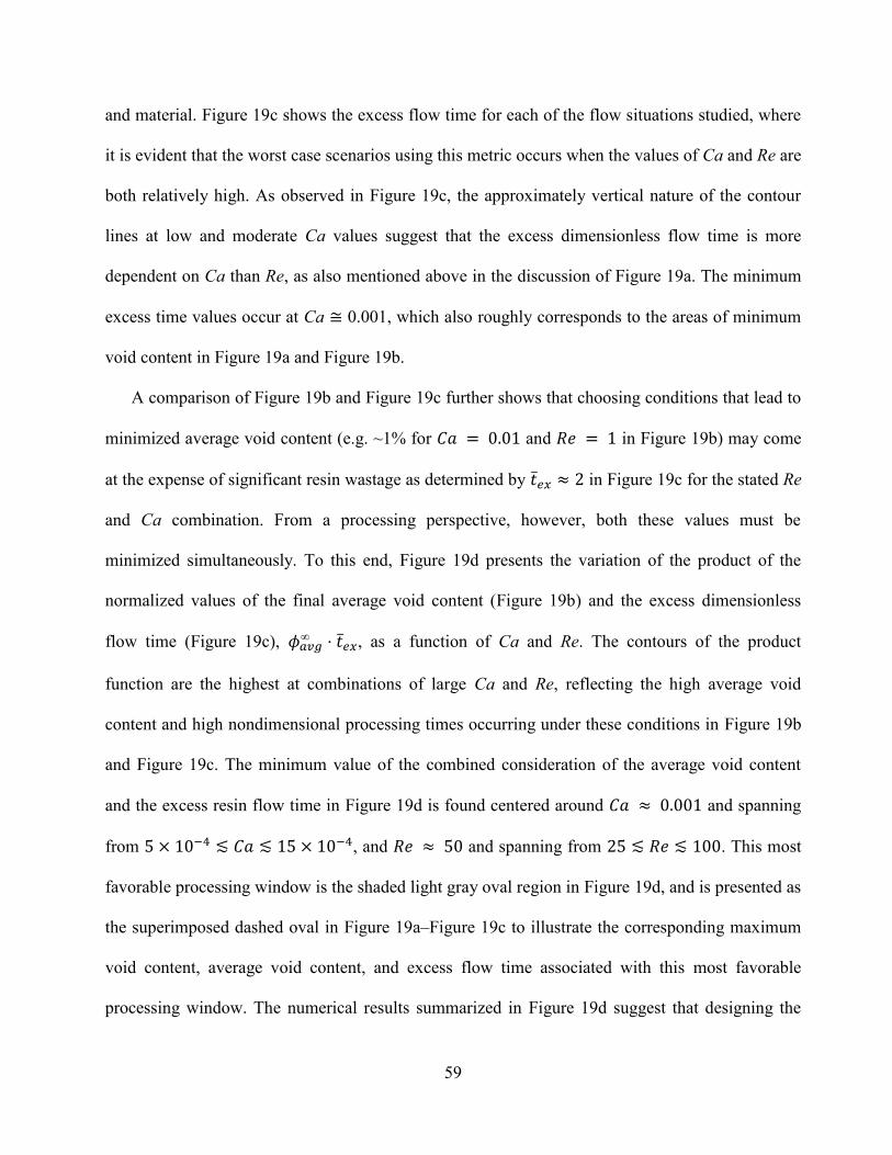
59
and material. Figure 19c shows the excess flow time for each of the flow situations studied, where
it is evident that the worst case scenarios using this metric occurs when the values of Ca and Re are
both relatively high. As observed in Figure 19c, the approximately vertical nature of the contour
lines at low and moderate Ca values suggest that the excess dimensionless flow time is more
dependent on Ca than Re, as also mentioned above in the discussion of Figure 19a. The minimum
excess time values occur at Ca 0.001, which also roughly corresponds to the areas of minimum
void content in Figure 19a and Figure 19b.
A comparison of Figure 19b and Figure 19c further shows that choosing conditions that lead to
minimized average void content (e.g. ~1% for and in Figure 19b) may come
at the expense of significant resin wastage as determined by in Figure 19c for the stated Re
and Ca combination. From a processing perspective, however, both these values must be
minimized simultaneously. To this end, Figure 19d presents the variation of the product of the
normalized values of the final average void content (Figure 19b) and the excess dimensionless
flow time (Figure 19c), , as a function of Ca and Re. The contours of the product
function are the highest at combinations of large Ca and Re, reflecting the high average void
content and high nondimensional processing times occurring under these conditions in Figure 19b
and Figure 19c. The minimum value of the combined consideration of the average void content
and the excess resin flow time in Figure 19d is found centered around and spanning
from , and and spanning from . This most
favorable processing window is the shaded light gray oval region in Figure 19d, and is presented as
the superimposed dashed oval in Figure 19a–Figure 19c to illustrate the corresponding maximum
void content, average void content, and excess flow time associated with this most favorable
processing window. The numerical results summarized in Figure 19d suggest that designing the
60
mold-filling stage of preform permeation such that the Ca and the Re fall within this most
favorable processing window would result in the minimum combination of both final void content
(~1% average or ~2% maximum) and the dimensionless processing time (~0.1) for a Rovcloth
2454 woven fabric. The trends presented in Figure 19 provide an example of using the current
numerical simulations as a decision making tool regarding processing parameters for preform
permeation and the arrival at mold-filling designs that tradeoff between the competing effects
involved in LCM processes. These results fulfill the first objective of this dissertation by
presenting a numerical simulation of resin permeation in LCM processes, addressing the issue of
void formation in composite molding processes. The second goal of this dissertation concerning
the augmentation of the damping characteristics of composite materials through nanoscale
reinforcement is dealt with in Chapter 4–Chapter 6.
3.6 Nomenclature used in Chapter 3
a fiber bundle thickness [m]
b fiber bundle height [m]
Ca Capillary number
cap capillary source term [N/m3]
por porous media source term [N/m3]
l unit cell length [m]
p pressure [Pa]
pc,l longitudinal capillary pressure [Pa]
pc,r radial capillary pressure [Pa]
rf fiber filament radius [m]
Re Reynolds number
61
t time [s]
u velocity vector [m/s]
vf fiber bundle volume fraction
x x-direction coordinate [m]
y y-direction coordinate [m]
z z-direction coordinate [m]
Greek symbols
fluid volume fraction
resin-air meniscus location
contact angle [degrees]
permeability [m2]
viscosity [Pa·s]
density [Kg/m3]
surface tension [N/m]
void content
Superscripts/subscripts
dimensionless value
air phase
average quantity
resin phase
steady-state value
62
Chapter 4: Experimental Investigation of the Damping Enhancement in Fiber-reinforced
Composites with CNTs
This chapter investigates the damping effects of carbon nanotubes (CNTs) embedded in the
matrix of fiber-reinforced composite materials. The composite materials are analyzed using
dynamic mechanical analysis (DMA) and various modal analysis techniques to determine the
damping characteristics of the composite as a function of strain, fiber volume fraction, and
nanotube type and weight percentage loading. In addition, experiments are conducted using
cantilevered beams in both a stationary and rotating frame in order to explore the effects of
rotation on the damping behavior of the composite material.
4.1 Composite Fabrication and Testing Methods
Various lengths, diameters, and concentrations of CNTs are considered in the fabrication of
different composite specimens, and an ultrasonic probe is used to disperse the as-received
agglomerated CNTs throughout the resin. The effect of different ultrasonic processing times on the
CNT dispersion is studied to determine the processing conditions which maximize the damping
characteristics of the final composite. Four types of CNTs are used in the current study: one single-
walled CNT (SWCNT) geometry and three different multi-walled CNT (MWCNT) geometries.
The SWCNTs are purchased from SES Research (Houston, TX) with >90% purity and dimensions
of <2 nm in diameter, D, and 5–15 in length, L, and the multi-walled CNTs are purchased from
Nanolab (Waltham, MA) with >95% purity and dimensions of: (1) nm and
, (2) nm and , and (3) nm and . Each of the
different nanotube types are obtained from the respective companies in large quantities from the
same lot in order to minimize any variation that may occur between different production batches.
63
The composite samples are made via hand layup and compression molding, and the cured
composites are tested using several different techniques to determine their material damping
characteristics.
4.1.1 Sample Preparation
The composite samples are fabricated using a compression molding method in which the resin
flows through the thickness of the part as it is being compressed to ensure uniformity of CNT
dispersion throughout the sample. The CNT-epoxy mixture is prepared as follows: First, EPON
826 resin (Hexion Specialty Chemicals, Columbus OH) is mixed with Heloxy Modifier 68
(Hexion Specialty Chemicals, Columbus OH) using a ratio of 4:1 by weight in order to reduce the
viscosity of the resin. Appropriate amounts of the resin and CNTs are then weighed into a beaker
using an Ohaus Explorer Pro balance to achieve the proper CNT weight percentage, , in the
epoxy. The nanotubes are then carefully mixed into the resin by hand using a medical grade utensil
in order to ensure that the CNTs are integrated with the resin before transport from the balance.
After this brief manual stirring, the resin-CNT combination is blended using an IKA T25 high-
shear mixer for 90 seconds. A Cole-Parmer 500 watt ultrasonic processor with a 12.5 mm probe is
then used to disperse the carbon nanotubes in the sample using a pulsed on-off mode with one
second pulses for an optimum duration so as to maximize the damping in the final composite, as
described in Chapter 4.2. Following sonication, an appropriate amount of Epikure 3274 hardener
(Hexion Specialty Chemicals, Columbus OH) is added to the sample and immediately incorporated
with the CNT-resin sample using manual stirring for two minutes and high-shear mixing for an
additional 90 seconds. The entire resin sample is then transferred to a larger diameter beaker to
increase the exposed surface area of the resin and degassed for 30 minutes.
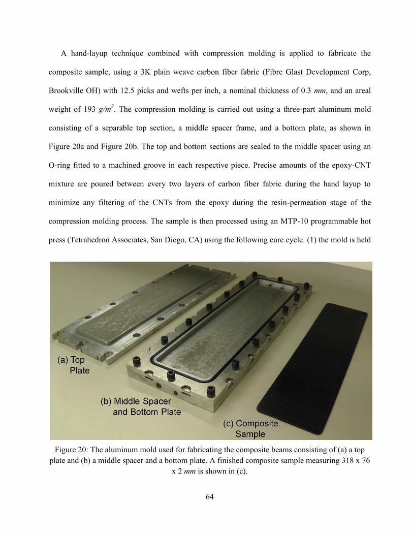
64
A hand-layup technique combined with compression molding is applied to fabricate the
composite sample, using a 3K plain weave carbon fiber fabric (Fibre Glast Development Corp,
Brookville OH) with 12.5 picks and wefts per inch, a nominal thickness of 0.3 mm, and an areal
weight of 193 g/m2. The compression molding is carried out using a three-part aluminum mold
consisting of a separable top section, a middle spacer frame, and a bottom plate, as shown in
Figure 20a and Figure 20b. The top and bottom sections are sealed to the middle spacer using an
O-ring fitted to a machined groove in each respective piece. Precise amounts of the epoxy-CNT
mixture are poured between every two layers of carbon fiber fabric during the hand layup to
minimize any filtering of the CNTs from the epoxy during the resin-permeation stage of the
compression molding process. The sample is then processed using an MTP-10 programmable hot
press (Tetrahedron Associates, San Diego, CA) using the following cure cycle: (1) the mold is held
Figure 20: The aluminum mold used for fabricating the composite beams consisting of (a) a top
plate and (b) a middle spacer and a bottom plate. A finished composite sample measuring 318 x 76
x 2 mm is shown in (c).
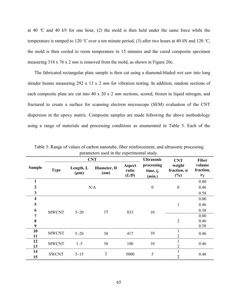
65
at 40 ºC and 40 kN for one hour, (2) the mold is then held under the same force while the
temperature is ramped to 120 ºC over a ten minute period, (3) after two hours at 40 kN and 120 ºC,
the mold is then cooled to room temperature in 15 minutes and the cured composite specimen
measuring 318 x 76 x 2 mm is removed from the mold, as shown in Figure 20c.
The fabricated rectangular plate sample is then cut using a diamond-bladed wet saw into long
slender beams measuring 292 x 13 x 2 mm for vibration testing. In addition, random sections of
each composite plate are cut into 40 x 20 x 2 mm sections, scored, frozen in liquid nitrogen, and
fractured to create a surface for scanning electron microscope (SEM) evaluation of the CNT
dispersion in the epoxy matrix. Composite samples are made following the above methodology
using a range of materials and processing conditions as enumerated in Table 3. Each of the
Table 3: Range of values of carbon nanotube, fiber reinforcement, and ultrasonic processing
parameters used in the experimental study.
Sample
CNT Ultrasonic
processing
time, tp
(min.)
CNT
weight
fraction,
(%)
Fiber
volume
fraction,
Type Length, L
( )
Diameter, D
(nm)
Aspect
ratio
(L/D)
1
N/A 0 0
0.00
2 0.46
3 0.58
4
MWCNT 5–20 15 833 10
1
0.00
5 0.46
6 0.58
7
2
0.00
8 0.46
9 0.58
10 MWCNT 5–20 30 417 10
1 0.46
11 2
12 MWCNT 1–5 30 100 10
1 0.46
13 2
14 SWCNT 5–15 2 5000 5
1 0.46
15 2
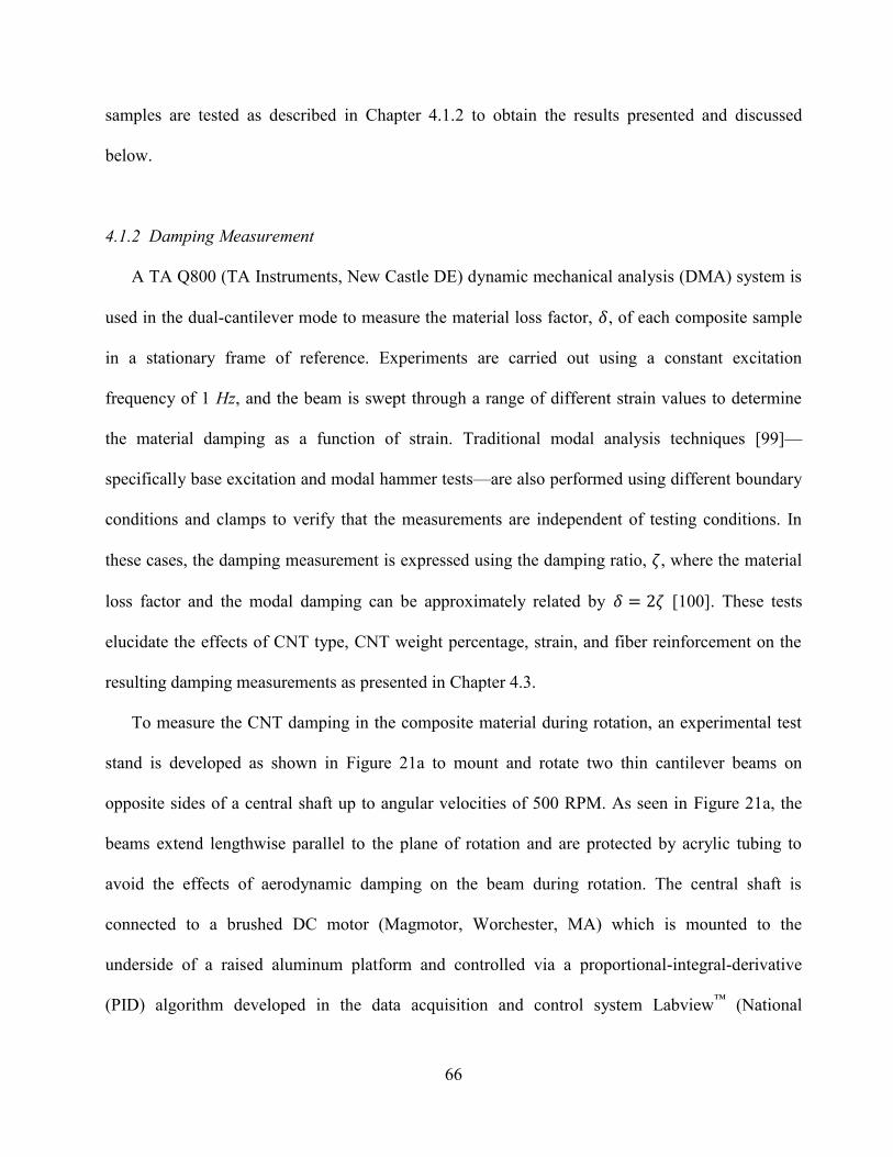
66
samples are tested as described in Chapter 4.1.2 to obtain the results presented and discussed
below.
4.1.2 Damping Measurement
A TA Q800 (TA Instruments, New Castle DE) dynamic mechanical analysis (DMA) system is
used in the dual-cantilever mode to measure the material loss factor, , of each composite sample
in a stationary frame of reference. Experiments are carried out using a constant excitation
frequency of 1 Hz, and the beam is swept through a range of different strain values to determine
the material damping as a function of strain. Traditional modal analysis techniques [99]—
specifically base excitation and modal hammer tests—are also performed using different boundary
conditions and clamps to verify that the measurements are independent of testing conditions. In
these cases, the damping measurement is expressed using the damping ratio, , where the material
loss factor and the modal damping can be approximately related by [100]. These tests
elucidate the effects of CNT type, CNT weight percentage, strain, and fiber reinforcement on the
resulting damping measurements as presented in Chapter 4.3.
To measure the CNT damping in the composite material during rotation, an experimental test
stand is developed as shown in Figure 21a to mount and rotate two thin cantilever beams on
opposite sides of a central shaft up to angular velocities of 500 RPM. As seen in Figure 21a, the
beams extend lengthwise parallel to the plane of rotation and are protected by acrylic tubing to
avoid the effects of aerodynamic damping on the beam during rotation. The central shaft is
connected to a brushed DC motor (Magmotor, Worchester, MA) which is mounted to the
underside of a raised aluminum platform and controlled via a proportional-integral-derivative
(PID) algorithm developed in the data acquisition and control system Labview™
(National
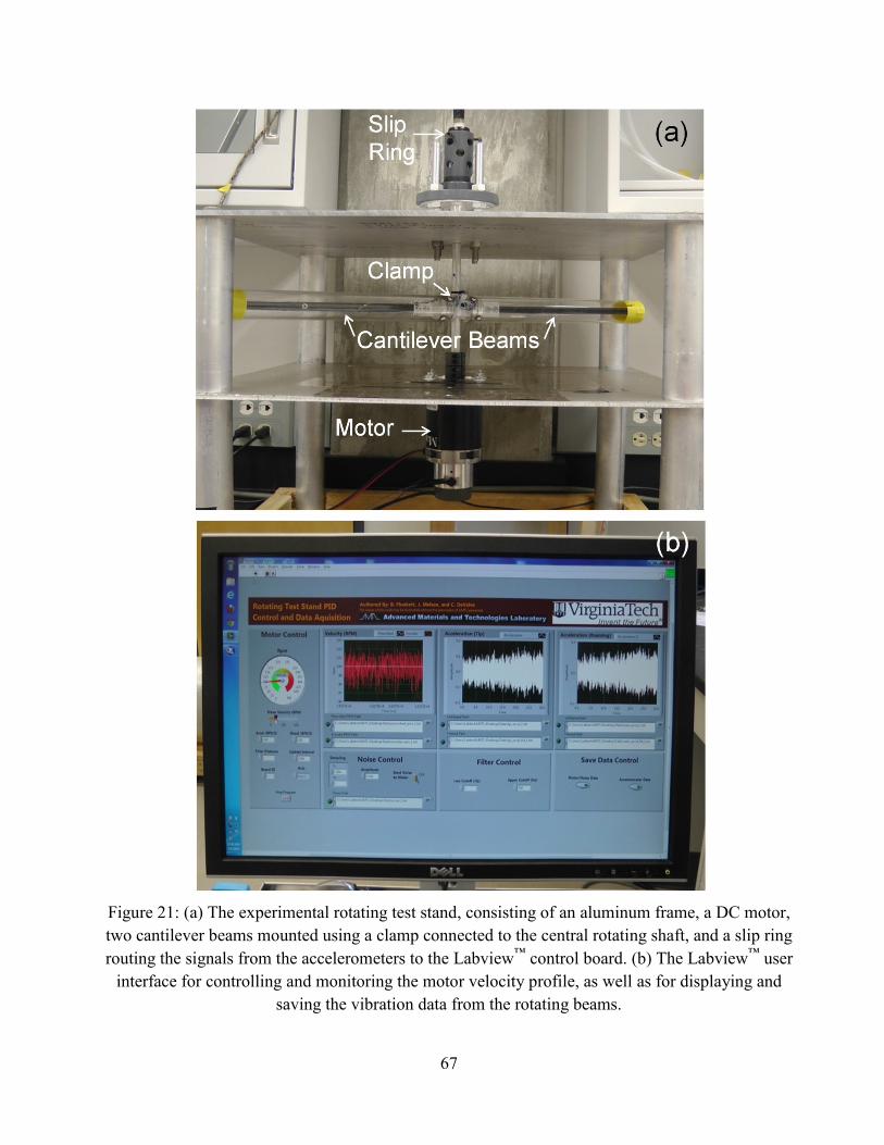
67
Figure 21: (a) The experimental rotating test stand, consisting of an aluminum frame, a DC motor,
two cantilever beams mounted using a clamp connected to the central rotating shaft, and a slip ring
routing the signals from the accelerometers to the Labview™
control board. (b) The Labview™
user
interface for controlling and monitoring the motor velocity profile, as well as for displaying and
saving the vibration data from the rotating beams.
68
Instruments, Austin, TX) with a user interface as shown in Figure 21b. The vibrations of the beams
are measured during rotation using two miniature ICP accelerometers (PCB Piezotronics, Depew,
NY) and 30 seconds of continuous data is recorded using a sampling rate of 1800 samples per
second. The location of the first accelerometer is fixed at the tip of the beam for all the
experiments, where the second "roving" accelerometer is positioned variably along the length of
the beam at precise increments during different experimental measurements to verify the mode
shapes of the beam. The accelerometers are powered by an external current source (Dytran
Instruments Inc., Chatsworth, CA), and the signal from the test rig is passed through a liquid
mercury slip ring (Mercotac, Carlsbad, CA) at the top of the rotating test stand (shown in Figure
21a) and fed through an analog low-pass filter (DL Instruments, Ithaca, NY) before being recorded
by the Labview™
data acquisition system. Uniform white noise of 10 RPM is added to the
constant RPM motor control signal in order to randomly excite the base of the beam during
operation, creating an input condition that maximizes the effectiveness of the operational modal
analysis (OMA) technique [101–103] which assumes that the system is subject to random
excitation. The vibration measurements are taken from the test setup at incremental angular speed
values and the data is compiled and analyzed using the stochastic subspace identification
unweighted principle component (SSI-UPC) algorithm [104,105] in the OMA software package
ARTeMIS™
(Structural Vibration Solutions, Denmark) to extract the modal parameters of the
system. The results of the damping measurements using the various test methods described in this
subsection are presented and discussed in Chapter 4.4.
69
4.2 CNT Dispersion
In order to maximize the benefits of the CNTs in the final composite material, individual
nanotubes should be distributed as evenly as possible throughout the resin by completely
dispersing the as-received CNT agglomerates without breaking the individual CNTs. Various
techniques are available for dispersion as reviewed in [106], of which a mechanical method using
energy generated from an ultrasonic probe is employed in this work to disperse the nanotube
agglomerates. For effective dispersion, it is important to understand the effects of ultrasonic
processing time on the dispersion of the CNTs throughout the resin and, in turn, the effects of the
different dispersion states on the CNT-induced damping in the resulting composite material. As the
resin-CNT mixture is ultrasonically processed for an increasing amount of time, two competing
effects take place within the sample: (1) the agglomerated CNTs are increasingly dispersed and
approach conditions in which the individual CNTs are evenly distributed throughout the resin,
maximizing their effectiveness in improving the material properties of the overall composite, and
(2) the individual CNTs are increasingly broken apart and become shorter, approaching conditions
resembling amorphous carbon if processed for too long and thus nullifying the potential benefits of
the CNTs to the material. Therefore, it follows that a balance of these two effects should occur
using an intermediate processing time of the sample where the CNTs are significantly dispersed
without considerable breakage of the individual nanotubes, maximizing the CNT damping effect in
the final composite.
A systematic investigation is carried out using ultrasonic processing times in 2.5 minute
increments up to 30 minutes on separate resin samples with one weight percent SWCNTs and
MWCNTs (30 nm, 5–20 ). In all the cases, a 12.5 mm probe is employed as the dispersing
instrument and the ultrasonic power is held constant at 500 W. The ultrasonically dispersed CNT-
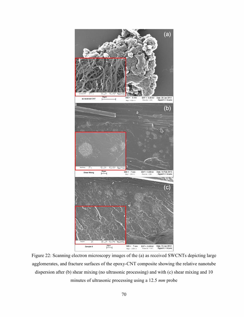
70
Figure 22: Scanning electron microscopy images of the (a) as received SWCNTs depicting large
agglomerates, and fracture surfaces of the epoxy-CNT composite showing the relative nanotube
dispersion after (b) shear mixing (no ultrasonic processing) and with (c) shear mixing and 10
minutes of ultrasonic processing using a 12.5 mm probe
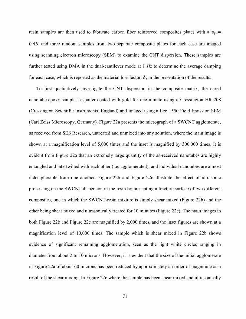
71
resin samples are then used to fabricate carbon fiber reinforced composites plates with a
, and three random samples from two separate composite plates for each case are imaged
using scanning electron microscopy (SEM) to examine the CNT dispersion. These samples are
further tested using DMA in the dual-cantilever mode at 1 Hz to determine the average damping
for each case, which is reported as the material loss factor, , in the presentation of the results.
To first qualitatively investigate the CNT dispersion in the composite matrix, the cured
nanotube-epoxy sample is sputter-coated with gold for one minute using a Cressington HR 208
(Cressington Scientific Instruments, England) and imaged using a Leo 1550 Field Emission SEM
(Carl Zeiss Microscopy, Germany). Figure 22a presents the micrograph of a SWCNT agglomerate,
as received from SES Research, untreated and unmixed into any solution, where the main image is
shown at a magnification level of 5,000 times and the inset is magnified by 300,000 times. It is
evident from Figure 22a that an extremely large quantity of the as-received nanotubes are highly
entangled and intertwined with each other (i.e. agglomerated), and individual nanotubes are almost
indecipherable from one another. Figure 22b and Figure 22c illustrate the effect of ultrasonic
processing on the SWCNT dispersion in the resin by presenting a fracture surface of two different
composites, one in which the SWCNT-resin mixture is simply shear mixed (Figure 22b) and the
other being shear mixed and ultrasonically treated for 10 minutes (Figure 22c). The main images in
both Figure 22b and Figure 22c are magnified by 2,000 times, and the inset figures are shown at a
magnification level of 10,000 times. The sample which is shear mixed in Figure 22b shows
evidence of significant remaining agglomeration, seen as the light white circles ranging in
diameter from about 2 to 10 microns. However, it is evident that the size of the initial agglomerate
in Figure 22a of about 60 microns has been reduced by approximately an order of magnitude as a
result of the shear mixing. In Figure 22c where the sample has been shear mixed and ultrasonically
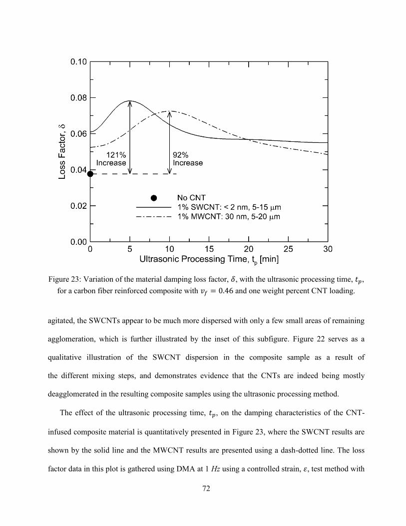
72
Figure 23: Variation of the material damping loss factor, , with the ultrasonic processing time, ,
for a carbon fiber reinforced composite with and one weight percent CNT loading.
agitated, the SWCNTs appear to be much more dispersed with only a few small areas of remaining
agglomeration, which is further illustrated by the inset of this subfigure. Figure 22 serves as a
qualitative illustration of the SWCNT dispersion in the composite sample as a result of
the different mixing steps, and demonstrates evidence that the CNTs are indeed being mostly
deagglomerated in the resulting composite samples using the ultrasonic processing method.
The effect of the ultrasonic processing time, , on the damping characteristics of the CNT-
infused composite material is quantitatively presented in Figure 23, where the SWCNT results are
shown by the solid line and the MWCNT results are presented using a dash-dotted line. The loss
factor data in this plot is gathered using DMA at 1 Hz using a controlled strain, , test method with
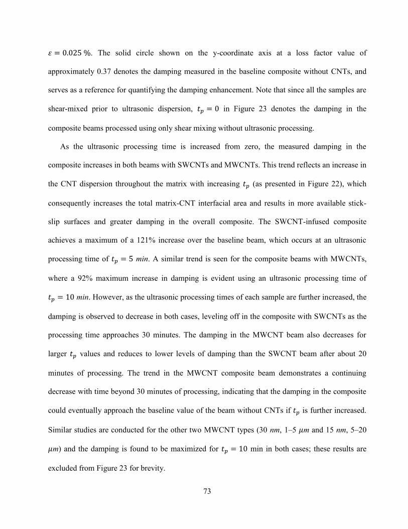
73
. The solid circle shown on the y-coordinate axis at a loss factor value of
approximately 0.37 denotes the damping measured in the baseline composite without CNTs, and
serves as a reference for quantifying the damping enhancement. Note that since all the samples are
shear-mixed prior to ultrasonic dispersion, in Figure 23 denotes the damping in the
composite beams processed using only shear mixing without ultrasonic processing.
As the ultrasonic processing time is increased from zero, the measured damping in the
composite increases in both beams with SWCNTs and MWCNTs. This trend reflects an increase in
the CNT dispersion throughout the matrix with increasing (as presented in Figure 22), which
consequently increases the total matrix-CNT interfacial area and results in more available stick-
slip surfaces and greater damping in the overall composite. The SWCNT-infused composite
achieves a maximum of a 121% increase over the baseline beam, which occurs at an ultrasonic
processing time of min. A similar trend is seen for the composite beams with MWCNTs,
where a 92% maximum increase in damping is evident using an ultrasonic processing time of
min. However, as the ultrasonic processing times of each sample are further increased, the
damping is observed to decrease in both cases, leveling off in the composite with SWCNTs as the
processing time approaches 30 minutes. The damping in the MWCNT beam also decreases for
larger values and reduces to lower levels of damping than the SWCNT beam after about 20
minutes of processing. The trend in the MWCNT composite beam demonstrates a continuing
decrease with time beyond 30 minutes of processing, indicating that the damping in the composite
could eventually approach the baseline value of the beam without CNTs if is further increased.
Similar studies are conducted for the other two MWCNT types (30 nm, 1–5 m and 15 nm, 5–20
m) and the damping is found to be maximized for min in both cases; these results are
excluded from Figure 23 for brevity.
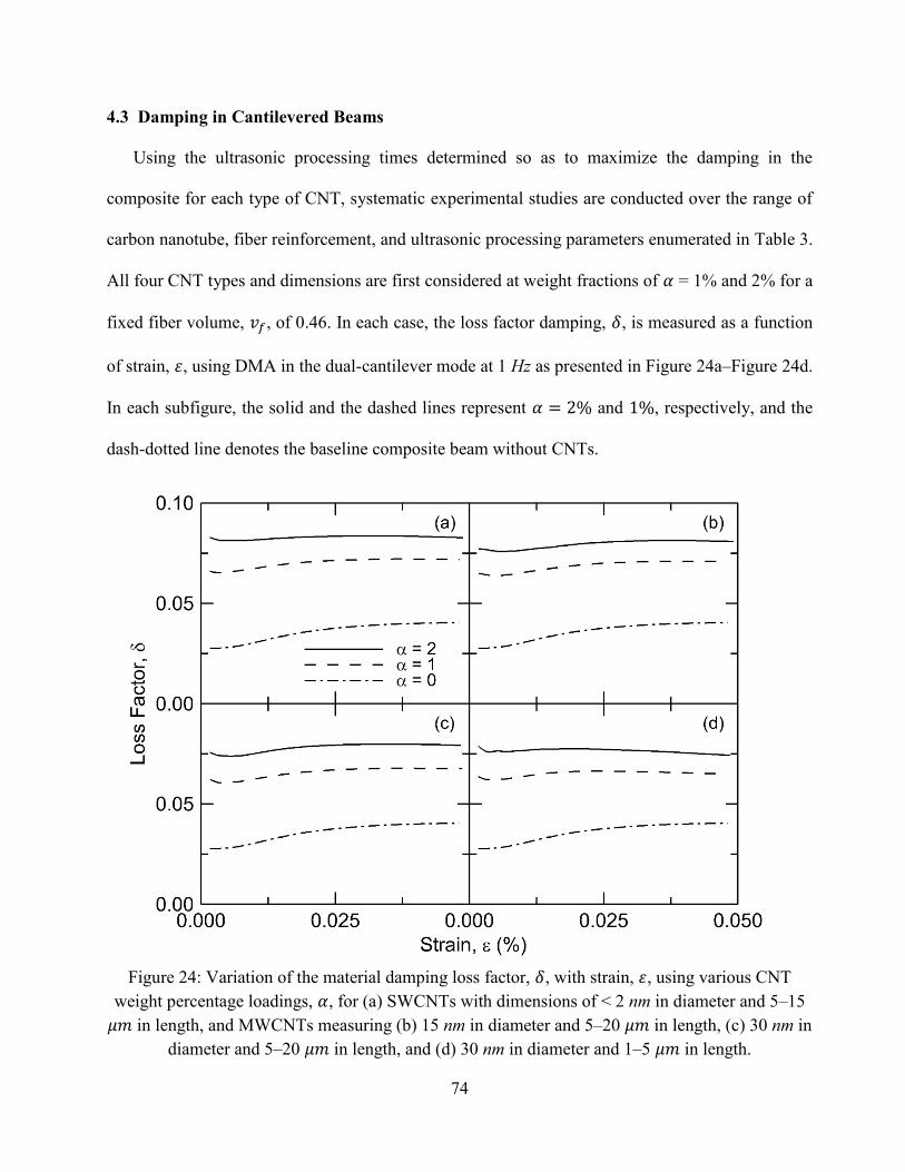
74
4.3 Damping in Cantilevered Beams
Using the ultrasonic processing times determined so as to maximize the damping in the
composite for each type of CNT, systematic experimental studies are conducted over the range of
carbon nanotube, fiber reinforcement, and ultrasonic processing parameters enumerated in Table 3.
All four CNT types and dimensions are first considered at weight fractions of = 1% and 2% for a
fixed fiber volume, , of 0.46. In each case, the loss factor damping, , is measured as a function
of strain, , using DMA in the dual-cantilever mode at 1 Hz as presented in Figure 24a–Figure 24d.
In each subfigure, the solid and the dashed lines represent and , respectively, and the
dash-dotted line denotes the baseline composite beam without CNTs.
Figure 24: Variation of the material damping loss factor, , with strain, , using various CNT
weight percentage loadings, , for (a) SWCNTs with dimensions of < 2 nm in diameter and 5–15
in length, and MWCNTs measuring (b) 15 nm in diameter and 5–20 in length, (c) 30 nm in
diameter and 5–20 in length, and (d) 30 nm in diameter and 1–5 in length.
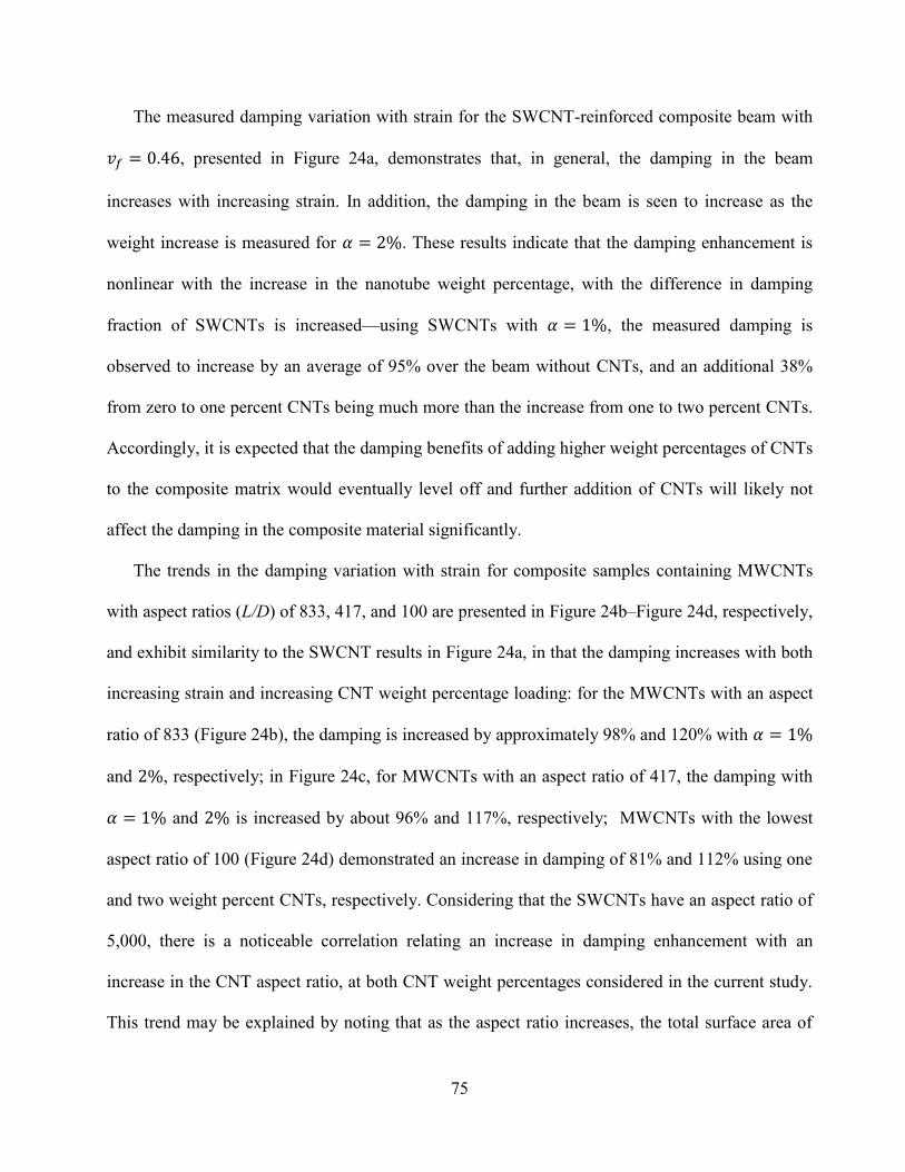
75
The measured damping variation with strain for the SWCNT-reinforced composite beam with
, presented in Figure 24a, demonstrates that, in general, the damping in the beam
increases with increasing strain. In addition, the damping in the beam is seen to increase as the
weight increase is measured for . These results indicate that the damping enhancement is
nonlinear with the increase in the nanotube weight percentage, with the difference in damping
fraction of SWCNTs is increased—using SWCNTs with , the measured damping is
observed to increase by an average of 95% over the beam without CNTs, and an additional 38%
from zero to one percent CNTs being much more than the increase from one to two percent CNTs.
Accordingly, it is expected that the damping benefits of adding higher weight percentages of CNTs
to the composite matrix would eventually level off and further addition of CNTs will likely not
affect the damping in the composite material significantly.
The trends in the damping variation with strain for composite samples containing MWCNTs
with aspect ratios (L/D) of 833, 417, and 100 are presented in Figure 24b–Figure 24d, respectively,
and exhibit similarity to the SWCNT results in Figure 24a, in that the damping increases with both
increasing strain and increasing CNT weight percentage loading: for the MWCNTs with an aspect
ratio of 833 (Figure 24b), the damping is increased by approximately 98% and 120% with
and , respectively; in Figure 24c, for MWCNTs with an aspect ratio of 417, the damping with
and is increased by about 96% and 117%, respectively; MWCNTs with the lowest
aspect ratio of 100 (Figure 24d) demonstrated an increase in damping of 81% and 112% using one
and two weight percent CNTs, respectively. Considering that the SWCNTs have an aspect ratio of
5,000, there is a noticeable correlation relating an increase in damping enhancement with an
increase in the CNT aspect ratio, at both CNT weight percentages considered in the current study.
This trend may be explained by noting that as the aspect ratio increases, the total surface area of
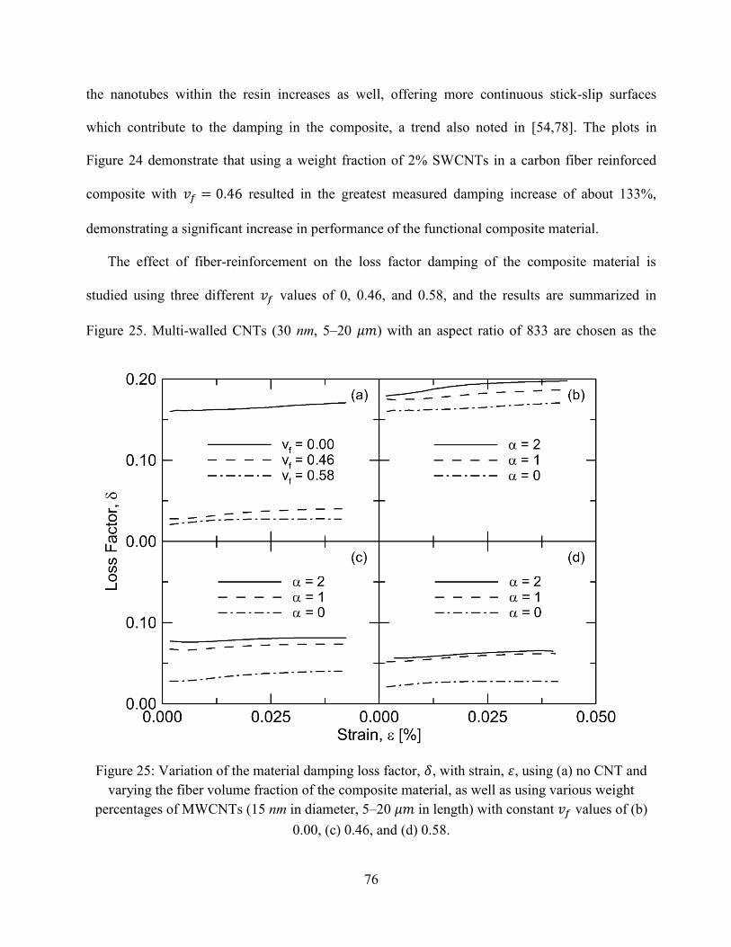
76
the nanotubes within the resin increases as well, offering more continuous stick-slip surfaces
which contribute to the damping in the composite, a trend also noted in [54,78]. The plots in
Figure 24 demonstrate that using a weight fraction of 2% SWCNTs in a carbon fiber reinforced
composite with resulted in the greatest measured damping increase of about 133%,
demonstrating a significant increase in performance of the functional composite material.
The effect of fiber-reinforcement on the loss factor damping of the composite material is
studied using three different values of 0, 0.46, and 0.58, and the results are summarized in
Figure 25. Multi-walled CNTs (30 nm, 5–20 ) with an aspect ratio of 833 are chosen as the
Figure 25: Variation of the material damping loss factor, , with strain, , using (a) no CNT and
varying the fiber volume fraction of the composite material, as well as using various weight
percentages of MWCNTs (15 nm in diameter, 5–20 in length) with constant values of (b)
0.00, (c) 0.46, and (d) 0.58.
77
nanoscale reinforcement based on their similar damping qualities to SWCNTs but at a lower cost
and greater availability in large batch sizes. Figure 25a presents the effect of the carbon fiber
reinforcement without CNTs ( ) on the material damping. The solid line represents the
composite material made out of only epoxy resin with no fiber reinforcement or CNTs, and the
damping in this case is quite high, averaging a loss factor of approximately 0.16. However, when
the fiber reinforcement is added to the resin, the damping is observed to decrease dramatically,
where the dashed and dash-dotted lines signify = 0.46 and 0.58, respectively, and show a
corresponding decrease in damping of 78% and 84% relative to the neat epoxy resin. The damping
in the beam decreases as a result of the fiber addition because of the added rigidity to the sample
from the carbon fiber reinforcement and consequent increase in the specific strength to stiffness
ratio, which is generally noted to result in a material with decreased vibration damping
characteristics and has been observed in similar composite material studies [47,76,78].
The effect of various CNT weight fractions is explored by considering the three different
values of 0, 0.46, and 0.58, as presented in Figure 25b–Figure 25d, respectively. For the composite
without fiber reinforcement shown in Figure 25b, the measured values of the loss factor are quite
high and range from 0.16 to 0.20. The damping is steadily augmented as the CNT weight fraction
is increased, where the CNT-infused resin material with has a loss factor measuring
almost 0.20 at high strain. In Figure 25c and Figure 25d corresponding to = 0.46 and 0.58,
respectively, the overall damping qualities of the composite are reduced as the composite is
reinforced with carbon fiber weave material, similar to the trends in Figure 25a. However, with
increasing weight fraction of CNTs in the matrix of the composite material at these high values,
a damping enhancement is clearly evident over the respective baseline beams in each case. In
Figure 25c, with , the baseline beam without CNTs and only carbon fiber reinforcement
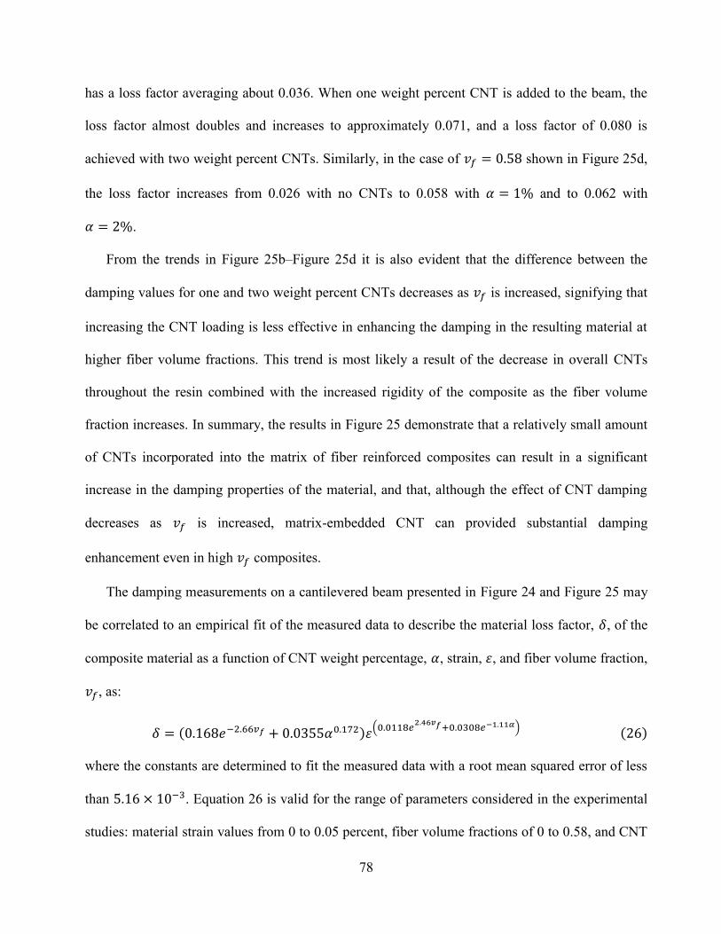
78
has a loss factor averaging about 0.036. When one weight percent CNT is added to the beam, the
loss factor almost doubles and increases to approximately 0.071, and a loss factor of 0.080 is
achieved with two weight percent CNTs. Similarly, in the case of shown in Figure 25d,
the loss factor increases from 0.026 with no CNTs to 0.058 with and to 0.062 with
.
From the trends in Figure 25b–Figure 25d it is also evident that the difference between the
damping values for one and two weight percent CNTs decreases as is increased, signifying that
increasing the CNT loading is less effective in enhancing the damping in the resulting material at
higher fiber volume fractions. This trend is most likely a result of the decrease in overall CNTs
throughout the resin combined with the increased rigidity of the composite as the fiber volume
fraction increases. In summary, the results in Figure 25 demonstrate that a relatively small amount
of CNTs incorporated into the matrix of fiber reinforced composites can result in a significant
increase in the damping properties of the material, and that, although the effect of CNT damping
decreases as is increased, matrix-embedded CNT can provided substantial damping
enhancement even in high composites.
The damping measurements on a cantilevered beam presented in Figure 24 and Figure 25 may
be correlated to an empirical fit of the measured data to describe the material loss factor, , of the
composite material as a function of CNT weight percentage, , strain, , and fiber volume fraction,
, as:
where the constants are determined to fit the measured data with a root mean squared error of less
than . Equation 26 is valid for the range of parameters considered in the experimental
studies: material strain values from 0 to 0.05 percent, fiber volume fractions of 0 to 0.58, and CNT
79
weight percentage loadings of zero to two weight percent. The power-law form of the equation
reflects the monotonic increase in the material loss factor with increasing strain, noted in Figure 24
and Figure 25. In addition, the constants in Equation 26 designate that the loss factor increases
with increasing CNT weight fraction and decreases as the volume fraction of the fiber
reinforcement is increased, reproducing the trends observed in Figure 24 and Figure 25. Equation
26 serves as a quantitative tool for relating the loss factor damping as a function of the
aforementioned material design parameters, and may be used in computational modeling of
composite systems with embedded carbon nanotubes.
4.4 Damping in Rotating Beams
The effect of rotation on the characteristics of the CNT-infused composite materials is explored
using the rotating test stand described in Chapter 4.1.2, where the beams are tested at different
angular velocities ranging from 0 to 500 RPM in increments of 100 RPM. Carbon fiber reinforced
composite beams with matrix-embedded SWCNTs are considered using two different values of
0.46 and 0.58, and aluminum beams of the same dimensions are used for a baseline material. For
each case, three different beams are tested to calculate the natural frequency and damping values in
each of the first three transverse modes of vibration.
A study is first conducted to validate the rotating experimental test rig by considering the
effects of different test methods and clamping conditions on the damping measurements of the
beams, where the results are summarized in Figure 26. As a baseline material, several beams are
machined out of 2024 aluminum to match the dimensions of the composite beams described in
Chapter 4.1.1, and modal hammer and base excitation tests are performed on both the aluminum
and composite beams using free-free and clamped-free boundary conditions with several different
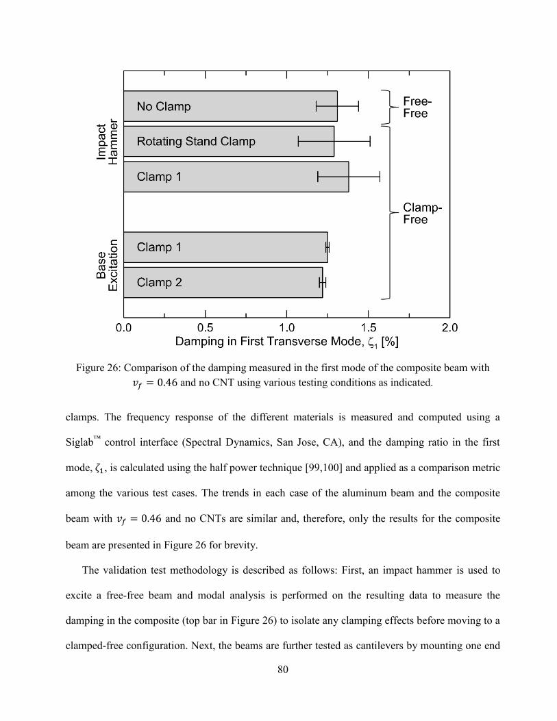
80
Figure 26: Comparison of the damping measured in the first mode of the composite beam with
and no CNT using various testing conditions as indicated.
clamps. The frequency response of the different materials is measured and computed using a
Siglab™
control interface (Spectral Dynamics, San Jose, CA), and the damping ratio in the first
mode, , is calculated using the half power technique [99,100] and applied as a comparison metric
among the various test cases. The trends in each case of the aluminum beam and the composite
beam with and no CNTs are similar and, therefore, only the results for the composite
beam are presented in Figure 26 for brevity.
The validation test methodology is described as follows: First, an impact hammer is used to
excite a free-free beam and modal analysis is performed on the resulting data to measure the
damping in the composite (top bar in Figure 26) to isolate any clamping effects before moving to a
clamped-free configuration. Next, the beams are further tested as cantilevers by mounting one end
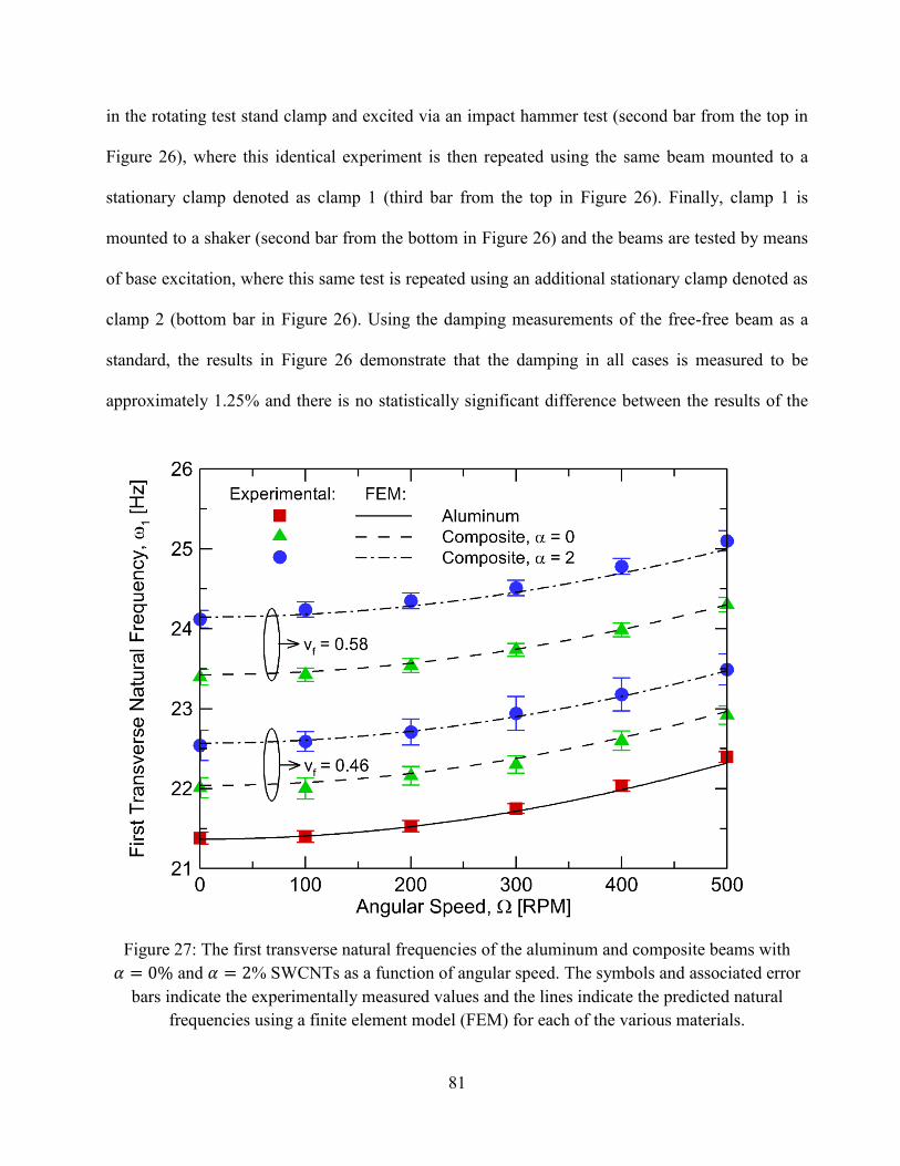
81
in the rotating test stand clamp and excited via an impact hammer test (second bar from the top in
Figure 26), where this identical experiment is then repeated using the same beam mounted to a
stationary clamp denoted as clamp 1 (third bar from the top in Figure 26). Finally, clamp 1 is
mounted to a shaker (second bar from the bottom in Figure 26) and the beams are tested by means
of base excitation, where this same test is repeated using an additional stationary clamp denoted as
clamp 2 (bottom bar in Figure 26). Using the damping measurements of the free-free beam as a
standard, the results in Figure 26 demonstrate that the damping in all cases is measured to be
approximately 1.25% and there is no statistically significant difference between the results of the
Figure 27: The first transverse natural frequencies of the aluminum and composite beams with
and % SWCNTs as a function of angular speed. The symbols and associated error
bars indicate the experimentally measured values and the lines indicate the predicted natural
frequencies using a finite element model (FEM) for each of the various materials.
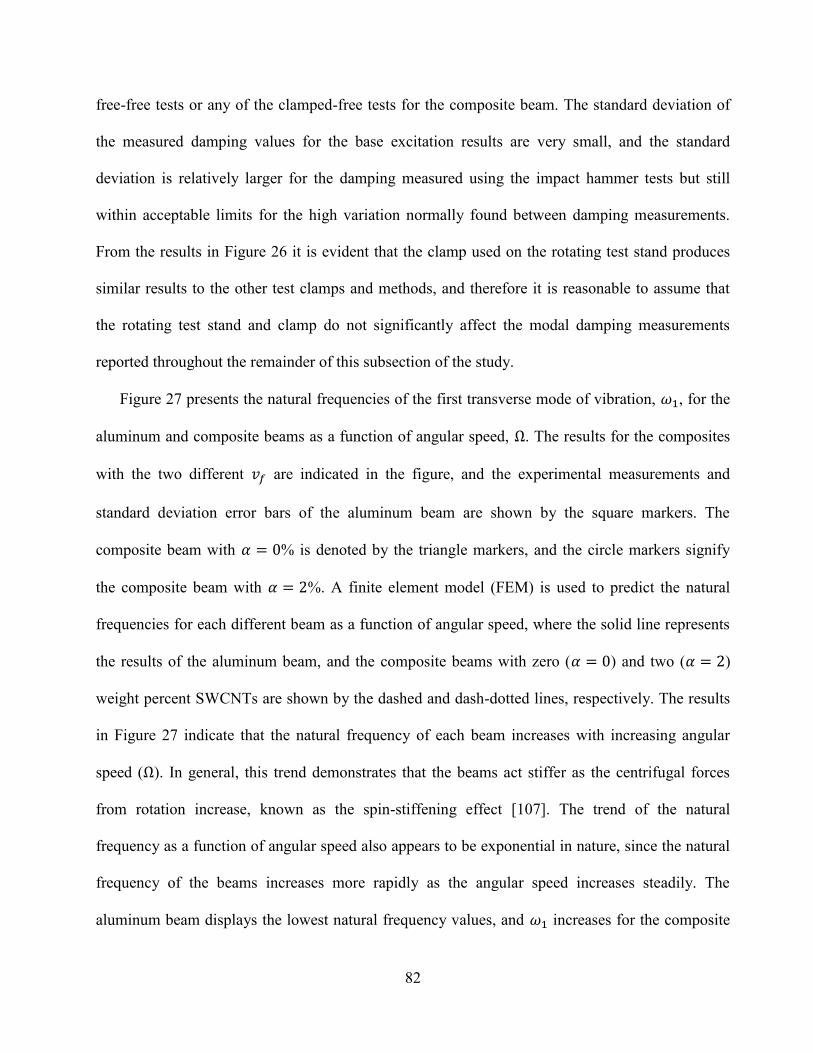
82
free-free tests or any of the clamped-free tests for the composite beam. The standard deviation of
the measured damping values for the base excitation results are very small, and the standard
deviation is relatively larger for the damping measured using the impact hammer tests but still
within acceptable limits for the high variation normally found between damping measurements.
From the results in Figure 26 it is evident that the clamp used on the rotating test stand produces
similar results to the other test clamps and methods, and therefore it is reasonable to assume that
the rotating test stand and clamp do not significantly affect the modal damping measurements
reported throughout the remainder of this subsection of the study.
Figure 27 presents the natural frequencies of the first transverse mode of vibration, , for the
aluminum and composite beams as a function of angular speed, . The results for the composites
with the two different are indicated in the figure, and the experimental measurements and
standard deviation error bars of the aluminum beam are shown by the square markers. The
composite beam with % is denoted by the triangle markers, and the circle markers signify
the composite beam with %. A finite element model (FEM) is used to predict the natural
frequencies for each different beam as a function of angular speed, where the solid line represents
the results of the aluminum beam, and the composite beams with zero ( ) and two ( )
weight percent SWCNTs are shown by the dashed and dash-dotted lines, respectively. The results
in Figure 27 indicate that the natural frequency of each beam increases with increasing angular
speed ( ). In general, this trend demonstrates that the beams act stiffer as the centrifugal forces
from rotation increase, known as the spin-stiffening effect [107]. The trend of the natural
frequency as a function of angular speed also appears to be exponential in nature, since the natural
frequency of the beams increases more rapidly as the angular speed increases steadily. The
aluminum beam displays the lowest natural frequency values, and increases for the composite
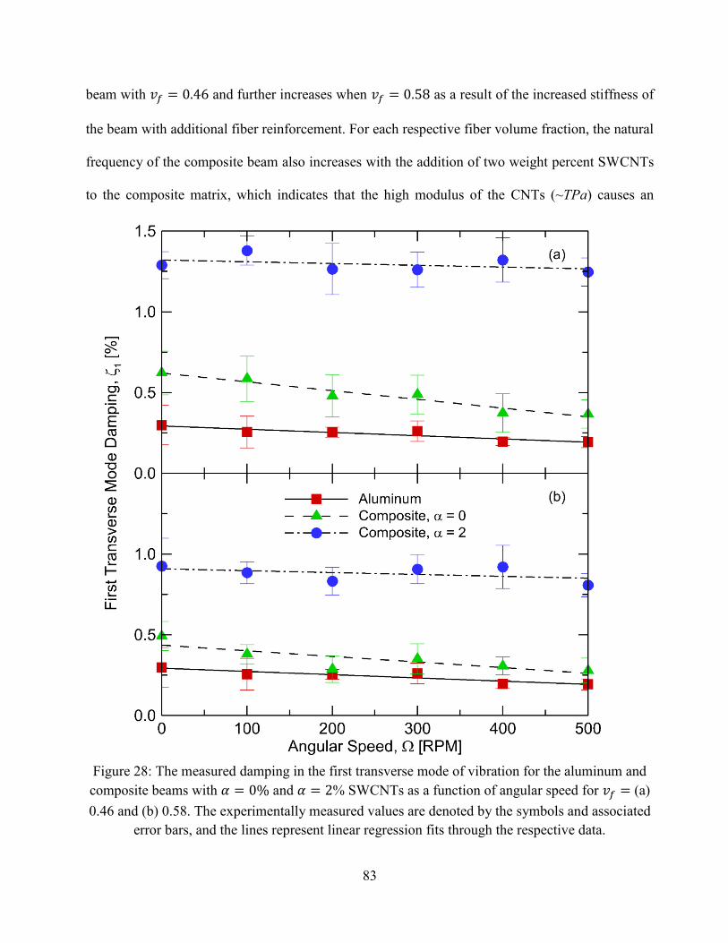
83
beam with and further increases when as a result of the increased stiffness of
the beam with additional fiber reinforcement. For each respective fiber volume fraction, the natural
frequency of the composite beam also increases with the addition of two weight percent SWCNTs
to the composite matrix, which indicates that the high modulus of the CNTs (~TPa) causes an
Figure 28: The measured damping in the first transverse mode of vibration for the aluminum and
composite beams with and % SWCNTs as a function of angular speed for (a)
0.46 and (b) 0.58. The experimentally measured values are denoted by the symbols and associated
error bars, and the lines represent linear regression fits through the respective data.
84
increase in the overall stiffness of the composite material. It is important to note that the
experimental measurements of the natural frequency are in very good agreement with the values
predicted from the finite element model, which further supports the validity of the data being
collected and analyzed from the rotating experimental apparatus.
The measured damping in the first transverse mode of vibration for the aluminum and
composite beams are shown in Figure 28 as a function of angular speed, , where the composite
samples with are shown in Figure 28a and the composites with are presented
in Figure 28b. As in Figure 27, the square markers and the solid line denote the aluminum beam,
the composite beam without SWCNTs is shown by the dashed line and the triangle markers, and
the circle markers and the dash-dotted line represent the composite beam with . Note that the
solid, the dashed, and the dash-dotted lines in Figure 28 are linear regression fits through the
respective data. In addition, the standard deviation of each damping measurement for the various
test conditions is shown by the respective error bars on each data point in Figure 28.
The damping values of the aluminum beam in Figure 28 serve as a baseline for comparing the
trends of the different composite beams, as aluminum is a well-understood material with linear
material properties under the current excitation conditions [108–110]. As is increased from zero,
the damping measured in the aluminum beam tends to decrease linearly from a value of
approximately 0.30 to about 0.19 when RPM. Similarly, for the composite beam in
Figure 28a with and no CNT, the damping measured in the beam tends to decrease as
the angular speed is increased, a trend which has been observed in similar studies [111,112]. Note
that the damping values for the composite beam with no CNTs and range from 0.62 to
0.37 and are significantly greater than those of the aluminum beam. Figure 28a further reveals that
the magnitude of the slope of the linear variation indicates that for the composite with no CNT, the
85
damping decreases as a function of more sharply than for the aluminum beam. The data for the
composite beam with and shows a considerable increase in damping over the
composite beam without CNT at the same fiber volume fraction, ranging from 1.38 at RPM
to 1.24 at RPM. As in the other materials, the damping in the beam decreases as the
angular speed is increased, but the slope of the linear variation demonstrates that the decrease in
damping is not nearly as large as in the case of the composite without CNT. Trends similar to those
observed in Figure 28a with are seen in the damping measurements of the composite
beam with , presented in Figure 28b. However, a primary difference is observed in the
magnitude of the damping values between the two cases in Figure 28a and Figure 28b, where
the 0.58 fiber volume fraction composites have lower damping characteristics for similar nanotube
weight percentage values. In the case of with no CNT loading the damping values range
from 0.49 at RPM to 0.28 at RPM, and from 0.93 to 0.81 when two weight percent
SWCNTs are incorporated into the composite matrix. Also, the magnitude of the slopes for the
composite beam data with are smaller than those for the composite with ,
indicating that the damping characteristics of the composite material are less dependent on the
angular velocity at increasing fiber volume fractions.
The data presented in Figure 28 indicate that for each of the various materials tested, the
damping characteristics are related to angular speed, and, in general, the measured damping
decreases with increasing angular speed. As is noted earlier and discussed in Figure 27, there is
evidence of the beam undergoing spin-stiffening effects, which may explain the reduced damping
characteristics of the material as the angular speed is increased and the beam's specific stiffness
increases. The trends displayed by the data in Figure 28 suggest that the damping characteristics of
the composite beam without CNT decreases more rapidly with increasing than the composite
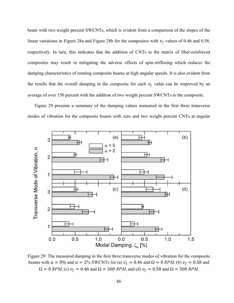
86
beam with two weight percent SWCNTs, which is evident from a comparison of the slopes of the
linear variations in Figure 28a and Figure 28b for the composites with values of 0.46 and 0.58,
respectively. In turn, this indicates that the addition of CNTs to the matrix of fiber-reinforced
composites may result in mitigating the adverse effects of spin-stiffening which reduces the
damping characteristics of rotating composite beams at high angular speeds. It is also evident from
the results that the overall damping in the composite for each value can be improved by an
average of over 150 percent with the addition of two weight percent SWCNTs to the composite.
Figure 29 presents a summary of the damping values measured in the first three transverse
modes of vibration for the composite beams with zero and two weight percent CNTs at angular
Figure 29: The measured damping in the first three transverse modes of vibration for the composite
beams with and % SWCNTs for (a) and RPM, (b) and
RPM, (c) and RPM, and (d) and RPM.
87
speeds of 0 and 500 RPM. Figure 29a and Figure 29b present the results for RPM for
and , respectively, and the results for RPM are shown in Figure 29c and
Figure 29d for and , respectively. The standard deviation of each damping value is
also presented as the error tails on each bar graph, and the white-shaded bars represent the
composite beam without CNT ( ) while the composite beam with two weight percent
SWCNTs ( ) is represented by the bars shaded in grey. By comparing Figure 29a and Figure
29b—or similarly Figure 29c and Figure 29d—the effect of varying the fiber volume fraction on
the damping values can be seen for constant angular speed values. To explore the effect of varying
the angular speed on the damping values for constant values, a comparison can be made
between the results in Figure 29a and Figure 29c—or similarly Figure 29b and Figure 29d.
In general, the results in Figure 29 demonstrate that the damping values measured in the first
three transverse modes of vibration for the composite with are all significantly greater than
the damping measured in the composite beam with . In each case it is also evident that the
damping either decreases or stays approximately constant in the first two modes of vibration as the
fiber volume fraction increases from 0.46 to 0.58, but the damping in the third mode increases
slightly as increases from 0.46 to 0.58 (comparing Figure 29a with Figure 29b, or Figure 29c
with Figure 29d). Additionally, for a constant fiber volume fraction, the damping in the first two
modes either decreases or stays the same with increasing angular speed, whereas the damping
actually increases with increasing angular speed in the third mode. Lastly, the difference in the
damping values between the cases with and for both fiber volume fraction
composites are especially pronounced in the case of RPM (Figure 29c and Figure 29d) in
the first and third modes of vibration, whereas the differences between the damping values for
these same cases in the second mode of vibration are not as significant. These results indicate that
88
CNT damping may be even more effective at high angular speeds in the first and third transverse
modes of vibration, but, in general, that CNTs are effective at increasing the damping in each of
the first three transverse modes of vibration for rotating fiber-reinforced composite beams.
The results presented in this chapter have experimentally investigated the effects of ultrasonic
dispersion on the damping in high fiber volume fraction composites with CNT reinforcement as
well as the damping augmentation provided to stationary and rotating composite beams from
matrix-embedded CNTs. An analytical model is developed in Chapter 5 to describe this CNT
damping effect on the dynamic response of a rotating composite beam.
4.5 Nomenclature used in Chapter 4
D diameter of CNT [nm]
L length of CNT [ ]
ultrasonic processing time [min]
fiber volume fraction
Greek symbols
weight percent CNT loading [%]
material damping loss factor
strain [%]
modal damping coefficient [%]
natural frequency [Hz]
angular speed [RPM]
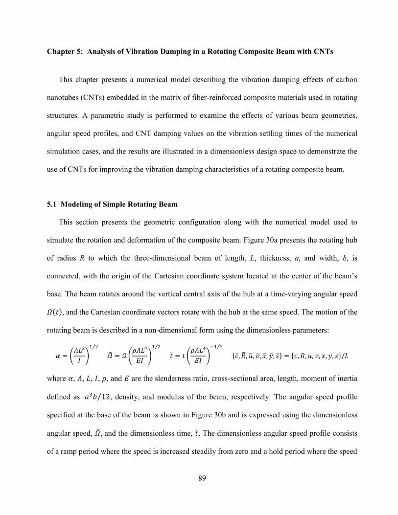
89
Chapter 5: Analysis of Vibration Damping in a Rotating Composite Beam with CNTs
This chapter presents a numerical model describing the vibration damping effects of carbon
nanotubes (CNTs) embedded in the matrix of fiber-reinforced composite materials used in rotating
structures. A parametric study is performed to examine the effects of various beam geometries,
angular speed profiles, and CNT damping values on the vibration settling times of the numerical
simulation cases, and the results are illustrated in a dimensionless design space to demonstrate the
use of CNTs for improving the vibration damping characteristics of a rotating composite beam.
5.1 Modeling of Simple Rotating Beam
This section presents the geometric configuration along with the numerical model used to
simulate the rotation and deformation of the composite beam. Figure 30a presents the rotating hub
of radius R to which the three-dimensional beam of length, L, thickness, a, and width, b, is
connected, with the origin of the Cartesian coordinate system located at the center of the beam’s
base. The beam rotates around the vertical central axis of the hub at a time-varying angular speed
, and the Cartesian coordinate vectors rotate with the hub at the same speed. The motion of the
rotating beam is described in a non-dimensional form using the dimensionless parameters:
where , , , , , and are the slenderness ratio, cross-sectional area, length, moment of inertia
defined as , density, and modulus of the beam, respectively. The angular speed profile
specified at the base of the beam is shown in Figure 30b and is expressed using the dimensionless
angular speed, , and the dimensionless time, . The dimensionless angular speed profile consists
of a ramp period where the speed is increased steadily from zero and a hold period where the speed
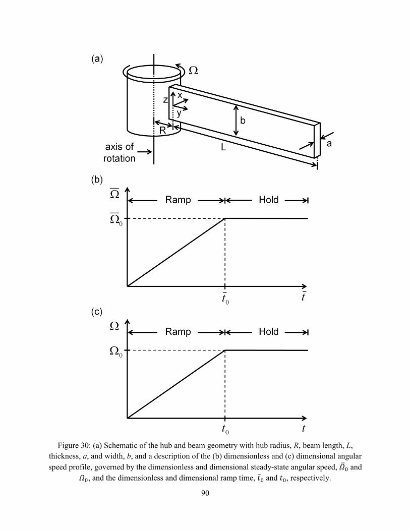
90
Figure 30: (a) Schematic of the hub and beam geometry with hub radius, R, beam length, L,
thickness, a, and width, b, and a description of the (b) dimensionless and (c) dimensional angular
speed profile, governed by the dimensionless and dimensional steady-state angular speed, and
, and the dimensionless and dimensional ramp time, and , respectively.
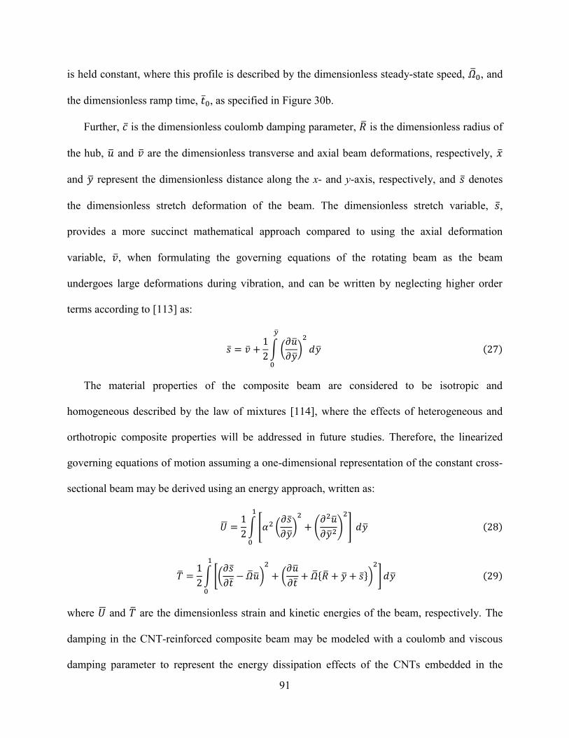
91
is held constant, where this profile is described by the dimensionless steady-state speed, , and
the dimensionless ramp time, , as specified in Figure 30b.
Further, is the dimensionless coulomb damping parameter, is the dimensionless radius of
the hub, and are the dimensionless transverse and axial beam deformations, respectively,
and represent the dimensionless distance along the x- and y-axis, respectively, and denotes
the dimensionless stretch deformation of the beam. The dimensionless stretch variable, ,
provides a more succinct mathematical approach compared to using the axial deformation
variable, , when formulating the governing equations of the rotating beam as the beam
undergoes large deformations during vibration, and can be written by neglecting higher order
terms according to [113] as:
The material properties of the composite beam are considered to be isotropic and
homogeneous described by the law of mixtures [114], where the effects of heterogeneous and
orthotropic composite properties will be addressed in future studies. Therefore, the linearized
governing equations of motion assuming a one-dimensional representation of the constant cross-
sectional beam may be derived using an energy approach, written as:
where and are the dimensionless strain and kinetic energies of the beam, respectively. The
damping in the CNT-reinforced composite beam may be modeled with a coulomb and viscous
damping parameter to represent the energy dissipation effects of the CNTs embedded in the
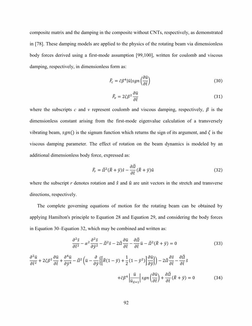
92
composite matrix and the damping in the composite without CNTs, respectively, as demonstrated
in [78]. These damping models are applied to the physics of the rotating beam via dimensionless
body forces derived using a first-mode assumption [99,100], written for coulomb and viscous
damping, respectively, in dimensionless form as:
where the subscripts c and v represent coulomb and viscous damping, respectively, is the
dimensionless constant arising from the first-mode eigenvalue calculation of a transversely
vibrating beam, is the signum function which returns the sign of its argument, and is the
viscous damping parameter. The effect of rotation on the beam dynamics is modeled by an
additional dimensionless body force, expressed as:
where the subscript r denotes rotation and and are unit vectors in the stretch and transverse
directions, respectively.
The complete governing equations of motion for the rotating beam can be obtained by
applying Hamilton's principle to Equation 28 and Equation 29, and considering the body forces
in Equation 30–Equation 32, which may be combined and written as:
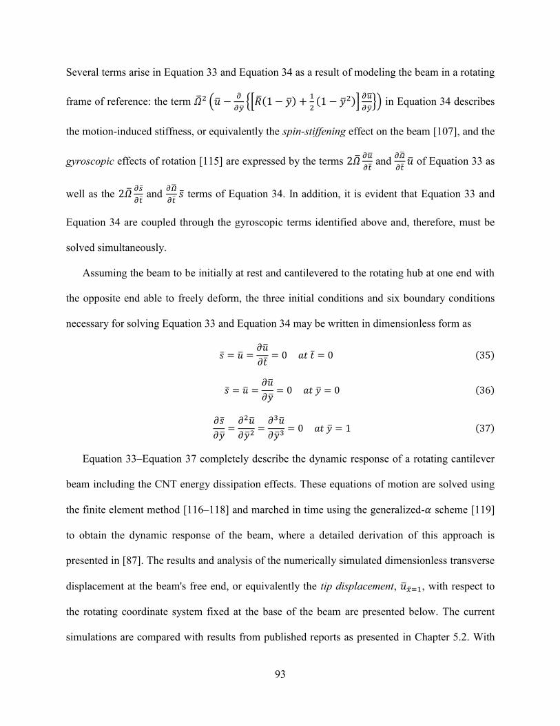
93
Several terms arise in Equation 33 and Equation 34 as a result of modeling the beam in a rotating
frame of reference: the term
in Equation 34 describes
the motion-induced stiffness, or equivalently the spin-stiffening effect on the beam [107], and the
gyroscopic effects of rotation [115] are expressed by the terms
and
of Equation 33 as
well as the
and
terms of Equation 34. In addition, it is evident that Equation 33 and
Equation 34 are coupled through the gyroscopic terms identified above and, therefore, must be
solved simultaneously.
Assuming the beam to be initially at rest and cantilevered to the rotating hub at one end with
the opposite end able to freely deform, the three initial conditions and six boundary conditions
necessary for solving Equation 33 and Equation 34 may be written in dimensionless form as
Equation 33–Equation 37 completely describe the dynamic response of a rotating cantilever
beam including the CNT energy dissipation effects. These equations of motion are solved using
the finite element method [116–118] and marched in time using the generalized- scheme [119]
to obtain the dynamic response of the beam, where a detailed derivation of this approach is
presented in [87]. The results and analysis of the numerically simulated dimensionless transverse
displacement at the beam's free end, or equivalently the tip displacement, , with respect to
the rotating coordinate system fixed at the base of the beam are presented below. The current
simulations are compared with results from published reports as presented in Chapter 5.2. With
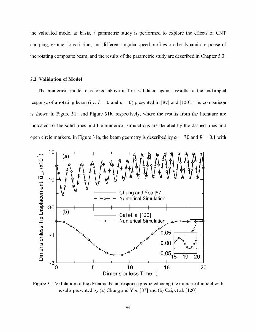
94
the validated model as basis, a parametric study is performed to explore the effects of CNT
damping, geometric variation, and different angular speed profiles on the dynamic response of
the rotating composite beam, and the results of the parametric study are described in Chapter 5.3.
5.2 Validation of Model
The numerical model developed above is first validated against results of the undamped
response of a rotating beam (i.e. and ) presented in [87] and [120]. The comparison
is shown in Figure 31a and Figure 31b, respectively, where the results from the literature are
indicated by the solid lines and the numerical simulations are denoted by the dashed lines and
open circle markers. In Figure 31a, the beam geometry is described by and with
Figure 31: Validation of the dynamic beam response predicted using the numerical model with
results presented by (a) Chung and Yoo [87] and (b) Cai, et al. [120].
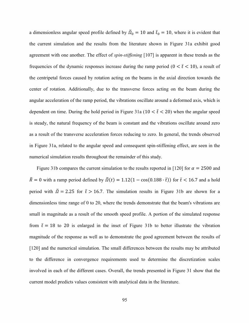
95
a dimensionless angular speed profile defined by and , where it is evident that
the current simulation and the results from the literature shown in Figure 31a exhibit good
agreement with one another. The effect of spin-stiffening [107] is apparent in these trends as the
frequencies of the dynamic responses increase during the ramp period ( ), a result of
the centripetal forces caused by rotation acting on the beams in the axial direction towards the
center of rotation. Additionally, due to the transverse forces acting on the beam during the
angular acceleration of the ramp period, the vibrations oscillate around a deformed axis, which is
dependent on time. During the hold period in Figure 31a ( ) when the angular speed
is steady, the natural frequency of the beam is constant and the vibrations oscillate around zero
as a result of the transverse acceleration forces reducing to zero. In general, the trends observed
in Figure 31a, related to the angular speed and consequent spin-stiffening effect, are seen in the
numerical simulation results throughout the remainder of this study.
Figure 31b compares the current simulation to the results reported in [120] for and
with a ramp period defined by for and a hold
period with for . The simulation results in Figure 31b are shown for a
dimensionless time range of 0 to 20, where the trends demonstrate that the beam's vibrations are
small in magnitude as a result of the smooth speed profile. A portion of the simulated response
from to is enlarged in the inset of Figure 31b to better illustrate the vibration
magnitude of the response as well as to demonstrate the good agreement between the results of
[120] and the numerical simulation. The small differences between the results may be attributed
to the difference in convergence requirements used to determine the discretization scales
involved in each of the different cases. Overall, the trends presented in Figure 31 show that the
current model predicts values consistent with analytical data in the literature.
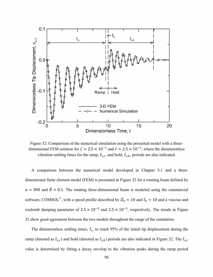
96
Figure 32: Comparison of the numerical simulation using the presented model with a three-
dimensional FEM solution for and , where the dimensionless
vibration settling times for the ramp, , and hold, , periods are also indicated.
A comparison between the numerical model developed in Chapter 5.1 and a three-
dimensional finite element model (FEM) is presented in Figure 32 for a rotating beam defined by
and . The rotating three-dimensional beam is modeled using the commercial
software, COMSOL©
, with a speed profile described by and and a viscous and
coulomb damping parameter of and , respectively. The trends in Figure
32 show good agreement between the two models throughout the range of the simulation.
The dimensionless settling times, , to reach 95% of the initial tip displacement during the
ramp (denoted as ) and hold (denoted as ) periods are also indicated in Figure 32. The
value is determined by fitting a decay envelop to the vibration peaks during the ramp period
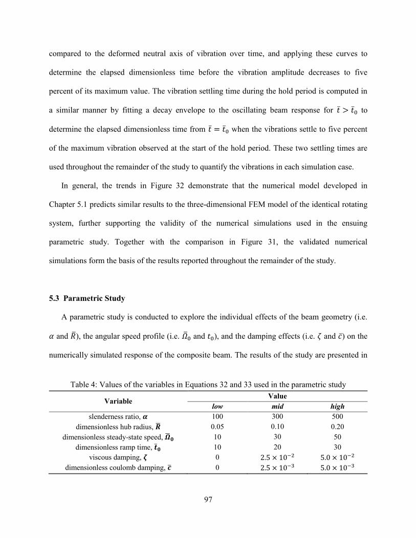
97
compared to the deformed neutral axis of vibration over time, and applying these curves to
determine the elapsed dimensionless time before the vibration amplitude decreases to five
percent of its maximum value. The vibration settling time during the hold period is computed in
a similar manner by fitting a decay envelope to the oscillating beam response for to
determine the elapsed dimensionless time from when the vibrations settle to five percent
of the maximum vibration observed at the start of the hold period. These two settling times are
used throughout the remainder of the study to quantify the vibrations in each simulation case.
In general, the trends in Figure 32 demonstrate that the numerical model developed in
Chapter 5.1 predicts similar results to the three-dimensional FEM model of the identical rotating
system, further supporting the validity of the numerical simulations used in the ensuing
parametric study. Together with the comparison in Figure 31, the validated numerical
simulations form the basis of the results reported throughout the remainder of the study.
5.3 Parametric Study
A parametric study is conducted to explore the individual effects of the beam geometry (i.e.
and ), the angular speed profile (i.e. and ), and the damping effects (i.e. and ) on the
numerically simulated response of the composite beam. The results of the study are presented in
Table 4: Values of the variables in Equations 32 and 33 used in the parametric study
Variable Value
low mid high
slenderness ratio, 100 300 500
dimensionless hub radius, 0.05 0.10 0.20
dimensionless steady-state speed, 10 30 50
dimensionless ramp time, 10 20 30
viscous damping, 0
dimensionless coulomb damping, 0
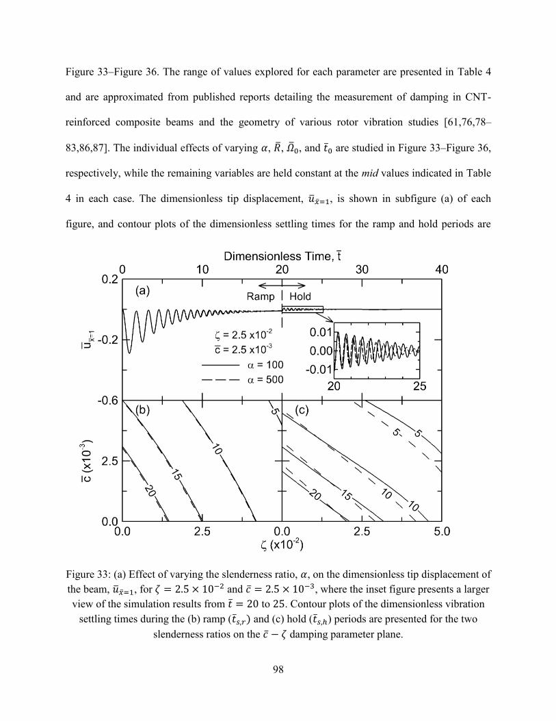
98
Figure 33–Figure 36. The range of values explored for each parameter are presented in Table 4
and are approximated from published reports detailing the measurement of damping in CNT-
reinforced composite beams and the geometry of various rotor vibration studies [61,76,78–
83,86,87]. The individual effects of varying , , , and are studied in Figure 33–Figure 36,
respectively, while the remaining variables are held constant at the mid values indicated in Table
4 in each case. The dimensionless tip displacement, , is shown in subfigure (a) of each
figure, and contour plots of the dimensionless settling times for the ramp and hold periods are
Figure 33: (a) Effect of varying the slenderness ratio, , on the dimensionless tip displacement of
the beam, , for and , where the inset figure presents a larger
view of the simulation results from to . Contour plots of the dimensionless vibration
settling times during the (b) ramp ( and (c) hold ( ) periods are presented for the two
slenderness ratios on the damping parameter plane.
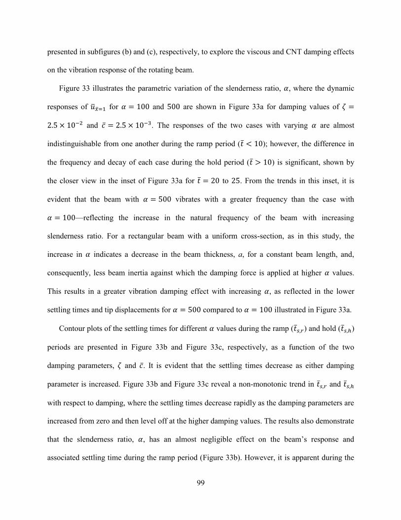
99
presented in subfigures (b) and (c), respectively, to explore the viscous and CNT damping effects
on the vibration response of the rotating beam.
Figure 33 illustrates the parametric variation of the slenderness ratio, , where the dynamic
responses of for and are shown in Figure 33a for damping values of
and . The responses of the two cases with varying are almost
indistinguishable from one another during the ramp period ( ); however, the difference in
the frequency and decay of each case during the hold period ( ) is significant, shown by
the closer view in the inset of Figure 33a for to . From the trends in this inset, it is
evident that the beam with vibrates with a greater frequency than the case with
—reflecting the increase in the natural frequency of the beam with increasing
slenderness ratio. For a rectangular beam with a uniform cross-section, as in this study, the
increase in indicates a decrease in the beam thickness, a, for a constant beam length, and,
consequently, less beam inertia against which the damping force is applied at higher values.
This results in a greater vibration damping effect with increasing , as reflected in the lower
settling times and tip displacements for compared to illustrated in Figure 33a.
Contour plots of the settling times for different values during the ramp ( ) and hold ( )
periods are presented in Figure 33b and Figure 33c, respectively, as a function of the two
damping parameters, and . It is evident that the settling times decrease as either damping
parameter is increased. Figure 33b and Figure 33c reveal a non-monotonic trend in and
with respect to damping, where the settling times decrease rapidly as the damping parameters are
increased from zero and then level off at the higher damping values. The results also demonstrate
that the slenderness ratio, , has an almost negligible effect on the beam’s response and
associated settling time during the ramp period (Figure 33b). However, it is apparent during the
100
hold period (Figure 33c) that, at high damping levels, as is increased, the required damping
decreases (either viscous or coulomb) to achieve the same value. During the hold period for
, similar damping parameters result in lower settling times for higher values of ,
indicating that the damping in this region is more effective at reducing the settling times as the
beam becomes more slender. For situations with less viscous damping ( ), the
aforementioned trends during the hold period are reversed and an increase in is seen to result
in slightly higher settling times at similar damping value.
Figure 34: (a) Effect of varying the dimensionless hub radius, , on the dimensionless tip
displacement of the beam, , for and , where the inset figure
presents a larger view of the simulation results from to . Contour plots of the
dimensionless vibration settling times during the (b) ramp ( and (c) hold ( ) periods are
presented for the two dimensionless hub radii on the damping parameter plane.
101
The results of the parametric variation of with damping values of and
are shown in Figure 34, and it is evident from the trends in Figure 34a that the
simulated response during the ramp period when settles slightly faster and has a
smaller amplitude of vibration than the case with . For a constant beam length, an
increase in results in a greater rotational body force acting on the beam. This, in turn, results in
a larger initial deflection of the beam's free end, causing higher magnitude vibrations during the
ramp period, as exemplified for in Figure 34a. The response for settles to a
deformed amplitude with negligible vibration by , resulting in a large initial beam
deflection at the start of the hold period that is significantly greater than the case with .
However, the vibrations in both cases, and , settle towards zero at
approximately the same rate (shown by the inset in Figure 34a). In addition, the frequency of
vibration when is much greater than the case with , demonstrating an effect
of greater spin-stiffening forces on the beam at higher . In general, the trends in Figure 34a
demonstrate that an increase in results in higher initial displacements and lower settling times
during the ramp period, and lower vibration magnitudes and settling times are observed for
increasing during the hold period due to the spin-stiffening effects on the beam.
Figure 34b and Figure 34c present the contours of and during the ramp and hold
periods, respectively, in terms of the two damping parameters, and , for a parameter variation
of . The overall trends are similar to those exhibited in Figure 33b and Figure 33c, where the
settling times decrease at higher damping values and there is a non-linear trend
in with respect to the damping parameters. The contours in Figure 34b show greater
distinction than those in Figure 33b, indicating that the parameter variation of the dimensionless
hub radius has a greater effect during the ramp period than the variation of the slenderness ratio.
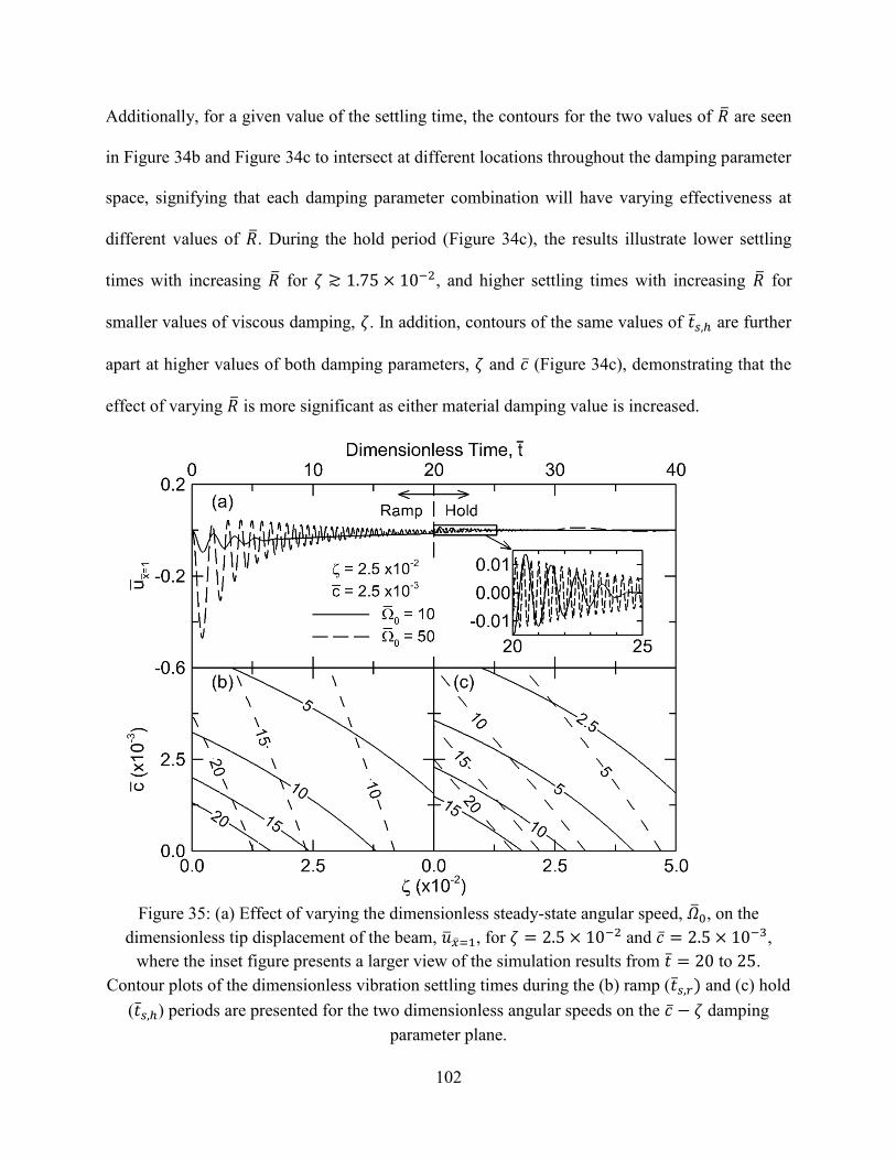
102
Additionally, for a given value of the settling time, the contours for the two values of are seen
in Figure 34b and Figure 34c to intersect at different locations throughout the damping parameter
space, signifying that each damping parameter combination will have varying effectiveness at
different values of . During the hold period (Figure 34c), the results illustrate lower settling
times with increasing for , and higher settling times with increasing for
smaller values of viscous damping, . In addition, contours of the same values of are further
apart at higher values of both damping parameters, and (Figure 34c), demonstrating that the
effect of varying is more significant as either material damping value is increased.
Figure 35: (a) Effect of varying the dimensionless steady-state angular speed, , on the
dimensionless tip displacement of the beam, , for and ,
where the inset figure presents a larger view of the simulation results from to .
Contour plots of the dimensionless vibration settling times during the (b) ramp ( and (c) hold
( ) periods are presented for the two dimensionless angular speeds on the damping
parameter plane.
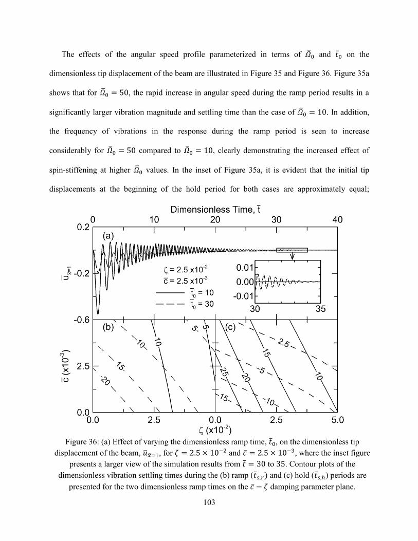
103
The effects of the angular speed profile parameterized in terms of and on the
dimensionless tip displacement of the beam are illustrated in Figure 35 and Figure 36. Figure 35a
shows that for , the rapid increase in angular speed during the ramp period results in a
significantly larger vibration magnitude and settling time than the case of . In addition,
the frequency of vibrations in the response during the ramp period is seen to increase
considerably for compared to , clearly demonstrating the increased effect of
spin-stiffening at higher values. In the inset of Figure 35a, it is evident that the initial tip
displacements at the beginning of the hold period for both cases are approximately equal;
Figure 36: (a) Effect of varying the dimensionless ramp time, , on the dimensionless tip
displacement of the beam, , for and , where the inset figure
presents a larger view of the simulation results from to . Contour plots of the
dimensionless vibration settling times during the (b) ramp ( and (c) hold ( ) periods are
presented for the two dimensionless ramp times on the damping parameter plane.
104
however, the vibrations are quickly reduced to almost zero in the case of , whereas the
vibrations settle much slower in the case of , resulting in an increase in the dimensionless
settling time at the larger dimensionless angular velocities.
Figure 36a shows the dynamic response of the beam for the parametric variation of . In
general, the trends in Figure 36a are similar to those in Figure 35a, except that the effects of
increasing are similar to those of decreasing . It is evident that the magnitude of the response
throughout the majority of the simulation is greater for compared to . In addition,
the trends in Figure 36a show that the frequency of the response increases more rapidly throughout
the ramp period with decreasing due to the effect of spin-stiffening. The similarity of the trends
in Figure 35a and Figure 36a is a result of the relationship of and to the slope of the angular
speed profile, or equivalently the angular acceleration of the beam during the ramp period. From
inspection of Figure 30b, it is evident that the slope of the speed profile is directly proportional to
and inversely proportional to , indicating that when is increased or is decreased the
slope of the speed profile becomes steeper. In turn, as the slope of the angular speed profile—or,
equivalently, the angular acceleration—increases, the vibration magnitudes and settling times will
increase because of the greater transverse forces acting on the beam, as exemplified by the
simulation trends shown in Figure 35a and Figure 36a. Therefore, the rotating composite beam will
generally experience lower magnitude vibrations and decreased settling times at low values of
and high parameters.
The contour plots in Figure 35b–c and Figure 36b–c demonstrate the effect of damping on the
response of the rotating beam for different dimensionless angular speed profiles. At the lower
value of in Figure 35b–c, or the higher value of in Figure 36b–c, the contour
lines are less steep on the plane indicating that, in general, an increase in —equivalently an
105
increase in the energy dissipation due to the presence of CNTs—will have a greater effect on
reducing the vibration of the rotating beam under these conditions. As a result, a slight increase in
the coulomb damping has a significant effect on reducing the and values, whereas a much
greater increase in the viscous parameter is necessary to achieve a similar reduction in the settling
times. In Figure 35b, the spacing between the contour lines increases at the larger value of
, indicating the need for more damping in order to reduce the settling time during the
ramp period, as the steady-state dimensionless angular speed increases. Additionally, the results in
Figure 35c demonstrate that lower settling times will occur during the hold period for similar
damping values, as the steady-state angular velocity is decreased.
The trends in Figure 36b for the parameter variation of are similar to those in Figure 35b and
illustrate that the settling time during the ramp period, , decreases at the higher value of 30
and increases when the ramp time is reduced. During the hold period (Figure 36c), the maximum
values for are relatively larger than the maximum settling times of the other design
cases presented in Figure 33–Figure 35 for similar damping values as a result of the high
transverse acceleration loads applied to the beam during the rapid ramp, which causes larger initial
beam displacements and greater vibration magnitudes. In general, the results in Figure 35 and
Figure 36 demonstrate that the slope of the angular speed profile and the steady state angular speed
have a significant effect on the response of the rotating composite beam, and as is increased or
is decreased, the system requires more damping to achieve similar and values.
The use of the simulations for an actual application is examined by considering the parameters
of the helicopter rotor vibration control study in [81]. To this end, Figure 37a and Figure 37b
present the contour plots of the and values during the ramp and hold periods, respectively,
on a parameter space of coulomb and viscous damping, for a composite beam described by
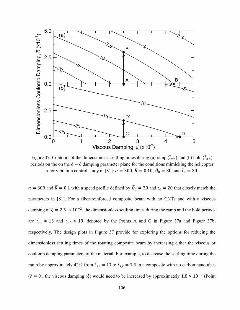
106
Figure 37: Contours of the dimensionless settling times during (a) ramp ( and (b) hold ( )
periods on the on the damping parameter plane for the conditions mimicking the helicopter
rotor vibration control study in [81]: , , , and .
and with a speed profile defined by and that closely match the
parameters in [81]. For a fiber-reinforced composite beam with no CNTs and with a viscous
damping of , the dimensionless settling times during the ramp and the hold periods
are and , denoted by the Points A and C in Figure 37a and Figure 37b,
respectively. The design plots in Figure 37 provide for exploring the options for reducing the
dimensionless settling times of the rotating composite beam by increasing either the viscous or
coulomb damping parameters of the material. For example, to decrease the settling time during the
ramp by approximately 42% from 13 to 7.5 in a composite with no carbon nanotubes
( 0), the viscous damping ( ) would need to be increased by approximately (Point
107
B in Figure 37a). Alternatively, the same decrease in settling time may be achieved without
altering the viscous damping of by introducing a coulomb damping parameter of
, (Point B' in Figure 37a) corresponding to the addition of about one weight percent
CNTs into the matrix of the composite based on the measurements in [78]. Similar trends are
demonstrated for the settling time reduction during the hold period in Figure 37b, where an
increase in the viscous damping parameter of (Point D in Figure 37b) is required to
reduce by 21% from 19 to 15 in a composite with no carbon nanotubes ( 0), compared to
an increase in the coulomb damping value of , while keeping (Point
D' in Figure 37b) to achieve the same damping enhancement. Additionally, the results in Figure
37a and Figure 37b indicate that as the value of is increased to , or equivalently about
two weight percent matrix-embedded CNTs according to the measurements in [78], the settling
times will be reduced during the ramp and hold periods by an average of 60% over the baseline
beam without CNTs. In general, Figure 37 demonstrates how the numerical simulations and the
resulting trends in Figure 33–Figure 36 may be applied to explore the effects of damping
augmentation provided to rotating composite beams through the addition of CNTs to the composite
matrix.
This chapter presented a numerical model of the effects of CNT-based damping in a rotating
fiber-reinforced composite beam using a stick-slip coulomb damping term to describe the frictional
behavior at the nanotube-matrix interface as the material is deformed. This model is extended to
incorporate the effects of strain-dependent damping and higher complexity rotating composite
structures in Chapter 6.

108
5.4 Nomenclature used in Chapter 5
hub radius [m]
cross-sectional area [m2]
coulomb damping coefficient [m]
modulus of elasticity [Pa]
force [N]
moment of inertia [m4]
beam length [m]
stretch deformation [m]
t time [s]
T kinetic energy [J]
transverse deformation [m]
U strain energy [J]
axial deformation [m]
x-direction coordinate [m]
y-direction coordinate [m]
z-direction coordinate [m]
Greek symbols
slenderness ratio
eigenvalue of first transverse vibration mode
viscous damping coefficient
density [kg/m3]
109
angular speed [rad/s]
Subscripts/Superscripts
dimensionless value
weighting function
constant parameter
110
Chapter 6: Numerical Simulation of CNT-based Damping in Rotating Composite Structures
This last portion of this dissertation presents the results of numerical simulations exploring the
effect of CNT damping, angular speed, and geometric variation on the dynamic response of
various rotating composite structures. The numerical model is first validated and subsequently
used to quantify the performance of CNT-damped composites in terms of the structures maximum
tip displacement and vibration settling time.
6.1 Three-Dimensional Rotating Beam Model
The fundamental goal of this portion of the dissertation is to investigate the effects of CNT
damping on rotating composite structures subject to various angular speed profiles using the finite
element method. To this end, Figure 30a presents a general schematic of the rotating structure
configuration, illustrated using a simple rectangular beam of length L attached to a rotating hub of
radius R. The base of the beam is rigidly connected to the hub and is described by cantilever
boundary conditions. A Cartesian coordinate system is defined at the base of the beam with the
origin lying at the center of beam's base as indicated in Figure 30a. The rotation of the structure is
oriented around the vertical central axis (positive z-direction) of the hub and is described by the
angular speed, , with the coordinate system rotating at the same speed. A schematic of the
dimensional angular speed profile specified at the base of the beam is shown in Figure 30c,
consisting of a 'ramp' period where the speed is increased linearly from zero and a 'hold' period
where the speed is held constant. The ramp period is defined by the steady-state angular speed, ,
and the time to reach this final speed (i.e. the ramp time), , as denoted in Figure 30c.
As a first-order modeling approach, the composite beam is considered to be isotropic with
homogeneous properties, where the issues of orthotropic and heterogeneous composite material
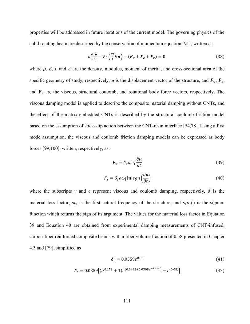
111
properties will be addressed in future iterations of the current model. The governing physics of the
solid rotating beam are described by the conservation of momentum equation [91], written as
where , E, I, and A are the density, modulus, moment of inertia, and cross-sectional area of the
specific geometry of study, respectively, u is the displacement vector of the structure, and , ,
and are the viscous, structural coulomb, and rotational body force vectors, respectively. The
viscous damping model is applied to describe the composite material damping without CNTs, and
the effect of the matrix-embedded CNTs is described by the structural coulomb friction model
based on the assumption of stick-slip action between the CNT-resin interface [54,78]. Using a first
mode assumption, the viscous and coulomb friction damping models can be expressed as body
forces [99,100], written, respectively, as:
where the subscripts v and c represent viscous and coulomb damping, respectively, is the
material loss factor, is the first natural frequency of the structure, and is the signum
function which returns the sign of its argument. The values for the material loss factor in Equation
39 and Equation 40 are obtained from experimental damping measurements of CNT-infused,
carbon-fiber reinforced composite beams with a fiber volume fraction of 0.58 presented in Chapter
4.3 and [79], simplified as
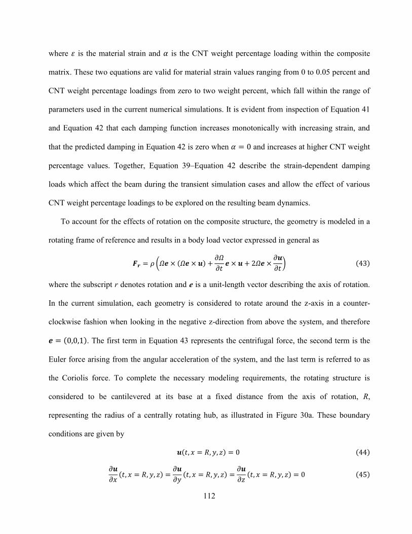
112
where is the material strain and is the CNT weight percentage loading within the composite
matrix. These two equations are valid for material strain values ranging from 0 to 0.05 percent and
CNT weight percentage loadings from zero to two weight percent, which fall within the range of
parameters used in the current numerical simulations. It is evident from inspection of Equation 41
and Equation 42 that each damping function increases monotonically with increasing strain, and
that the predicted damping in Equation 42 is zero when and increases at higher CNT weight
percentage values. Together, Equation 39–Equation 42 describe the strain-dependent damping
loads which affect the beam during the transient simulation cases and allow the effect of various
CNT weight percentage loadings to be explored on the resulting beam dynamics.
To account for the effects of rotation on the composite structure, the geometry is modeled in a
rotating frame of reference and results in a body load vector expressed in general as
where the subscript r denotes rotation and e is a unit-length vector describing the axis of rotation.
In the current simulation, each geometry is considered to rotate around the z-axis in a counter-
clockwise fashion when looking in the negative z-direction from above the system, and therefore
. The first term in Equation 43 represents the centrifugal force, the second term is the
Euler force arising from the angular acceleration of the system, and the last term is referred to as
the Coriolis force. To complete the necessary modeling requirements, the rotating structure is
considered to be cantilevered at its base at a fixed distance from the axis of rotation, R,
representing the radius of a centrally rotating hub, as illustrated in Figure 30a. These boundary
conditions are given by
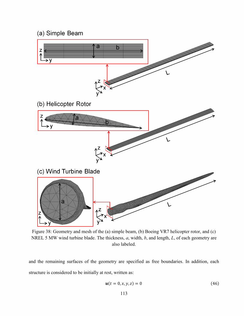
113
Figure 38: Geometry and mesh of the (a) simple beam, (b) Boeing VR7 helicopter rotor, and (c)
NREL 5 MW wind turbine blade. The thickness, a, width, b, and length, L, of each geometry are
also labeled.
and the remaining surfaces of the geometry are specified as free boundaries. In addition, each
structure is considered to be initially at rest, written as:
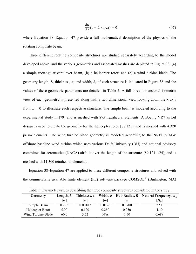
114
where Equation 38–Equation 47 provide a full mathematical description of the physics of the
rotating composite beam.
Three different rotating composite structures are studied separately according to the model
developed above, and the various geometries and associated meshes are depicted in Figure 38: (a)
a simple rectangular cantilever beam, (b) a helicopter rotor, and (c) a wind turbine blade. The
geometry length, L, thickness, a, and width, b, of each structure is indicated in Figure 38 and the
values of these geometric parameters are detailed in Table 5. A full three-dimensional isometric
view of each geometry is presented along with a two-dimensional view looking down the x-axis
from to illustrate each respective structure. The simple beam is modeled according to the
experimental study in [79] and is meshed with 875 hexahedral elements. A Boeing VR7 airfoil
design is used to create the geometry for the helicopter rotor [88,121], and is meshed with 4,320
prism elements. The wind turbine blade geometry is modeled according to the NREL 5 MW
offshore baseline wind turbine which uses various Delft University (DU) and national advisory
committee for aeronautics (NACA) airfoils over the length of the structure [89,121–124], and is
meshed with 11,300 tetrahedral elements.
Equation 38–Equation 47 are applied to these different composite structures and solved with
the commercially available finite element (FE) software package COMSOL©
(Burlington, MA)
Table 5: Parameter values describing the three composite structures considered in the study.
Geometry Length, L
[m]
Thickness, a
[m]
Width, b
[m]
Hub Radius, R
[m]
Natural Frequency,
[Hz]
Simple Beam 0.295 0.00187 0.0126 0.0700 22.1
Helicopter Rotor 5.00 0.120 0.250 0.250 4.19
Wind Turbine Blade 60.0 3.52 N/A 1.50 0.689
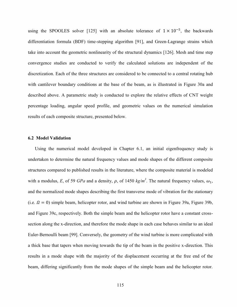
115
using the SPOOLES solver [125] with an absolute tolerance of , the backwards
differentiation formula (BDF) time-stepping algorithm [91], and Green-Lagrange strains which
take into account the geometric nonlinearity of the structural dynamics [126]. Mesh and time step
convergence studies are conducted to verify the calculated solutions are independent of the
discretization. Each of the three structures are considered to be connected to a central rotating hub
with cantilever boundary conditions at the base of the beam, as is illustrated in Figure 30a and
described above. A parametric study is conducted to explore the relative effects of CNT weight
percentage loading, angular speed profile, and geometric values on the numerical simulation
results of each composite structure, presented below.
6.2 Model Validation
Using the numerical model developed in Chapter 6.1, an initial eigenfrequency study is
undertaken to determine the natural frequency values and mode shapes of the different composite
structures compared to published results in the literature, where the composite material is modeled
with a modulus, E, of 59 GPa and a density, , of 1450 kg/m3. The natural frequency values, ,
and the normalized mode shapes describing the first transverse mode of vibration for the stationary
(i.e. ) simple beam, helicopter rotor, and wind turbine are shown in Figure 39a, Figure 39b,
and Figure 39c, respectively. Both the simple beam and the helicopter rotor have a constant cross-
section along the x-direction, and therefore the mode shape in each case behaves similar to an ideal
Euler-Bernoulli beam [99]. Conversely, the geometry of the wind turbine is more complicated with
a thick base that tapers when moving towards the tip of the beam in the positive x-direction. This
results in a mode shape with the majority of the displacement occurring at the free end of the
beam, differing significantly from the mode shapes of the simple beam and the helicopter rotor.
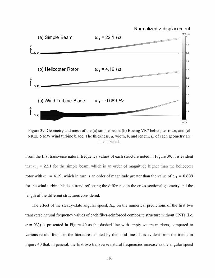
116
Figure 39: Geometry and mesh of the (a) simple beam, (b) Boeing VR7 helicopter rotor, and (c)
NREL 5 MW wind turbine blade. The thickness, a, width, b, and length, L, of each geometry are
also labeled.
From the first transverse natural frequency values of each structure noted in Figure 39, it is evident
that for the simple beam, which is an order of magnitude higher than the helicopter
rotor with , which in turn is an order of magnitude greater than the value of
for the wind turbine blade, a trend reflecting the difference in the cross-sectional geometry and the
length of the different structures considered.
The effect of the steady-state angular speed, , on the numerical predictions of the first two
transverse natural frequency values of each fiber-reinforced composite structure without CNTs (i.e.
) is presented in Figure 40 as the dashed line with empty square markers, compared to
various results found in the literature denoted by the solid lines. It is evident from the trends in
Figure 40 that, in general, the first two transverse natural frequencies increase as the angular speed
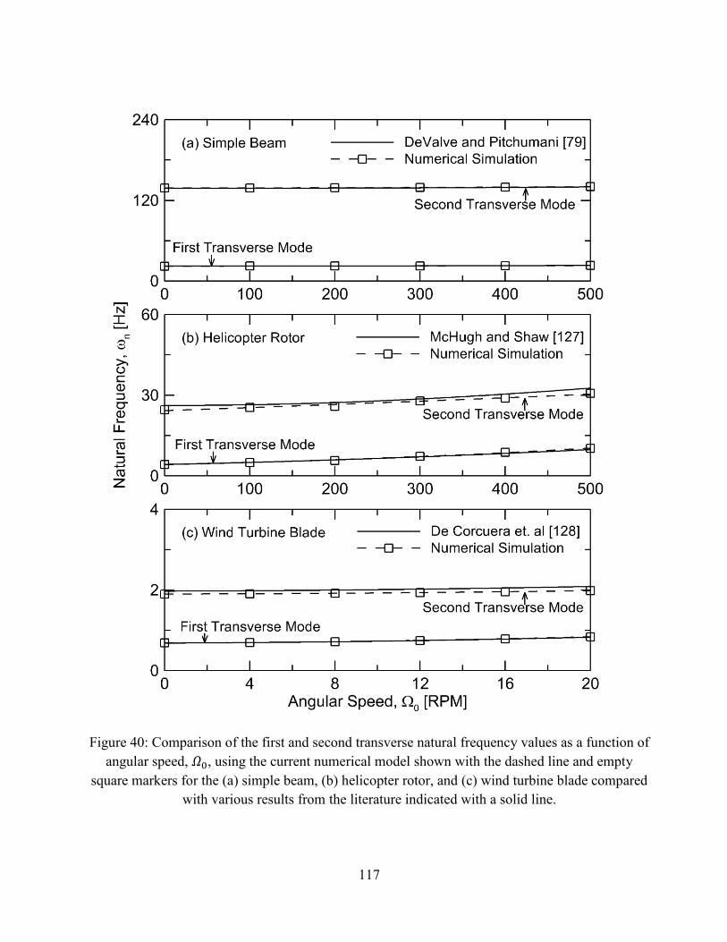
117
Figure 40: Comparison of the first and second transverse natural frequency values as a function of
angular speed, , using the current numerical model shown with the dashed line and empty
square markers for the (a) simple beam, (b) helicopter rotor, and (c) wind turbine blade compared
with various results from the literature indicated with a solid line.
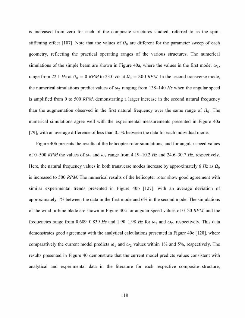
118
is increased from zero for each of the composite structures studied, referred to as the spin-
stiffening effect [107]. Note that the values of are different for the parameter sweep of each
geometry, reflecting the practical operating ranges of the various structures. The numerical
simulations of the simple beam are shown in Figure 40a, where the values in the first mode, ,
range from 22.1 Hz at RPM to 23.0 Hz at RPM. In the second transverse mode,
the numerical simulations predict values of ranging from 138–140 Hz when the angular speed
is amplified from 0 to 500 RPM, demonstrating a larger increase in the second natural frequency
than the augmentation observed in the first natural frequency over the same range of . The
numerical simulations agree well with the experimental measurements presented in Figure 40a
[79], with an average difference of less than 0.5% between the data for each individual mode.
Figure 40b presents the results of the helicopter rotor simulations, and for angular speed values
of 0–500 RPM the values of and range from 4.19–10.2 Hz and 24.6–30.7 Hz, respectively.
Here, the natural frequency values in both transverse modes increase by approximately 6 Hz as
is increased to 500 RPM. The numerical results of the helicopter rotor show good agreement with
similar experimental trends presented in Figure 40b [127], with an average deviation of
approximately 1% between the data in the first mode and 6% in the second mode. The simulations
of the wind turbine blade are shown in Figure 40c for angular speed values of 0–20 RPM, and the
frequencies range from 0.689–0.839 Hz and 1.90–1.98 Hz for and , respectively. This data
demonstrates good agreement with the analytical calculations presented in Figure 40c [128], where
comparatively the current model predicts and values within 1% and 5%, respectively. The
results presented in Figure 40 demonstrate that the current model predicts values consistent with
analytical and experimental data in the literature for each respective composite structure,
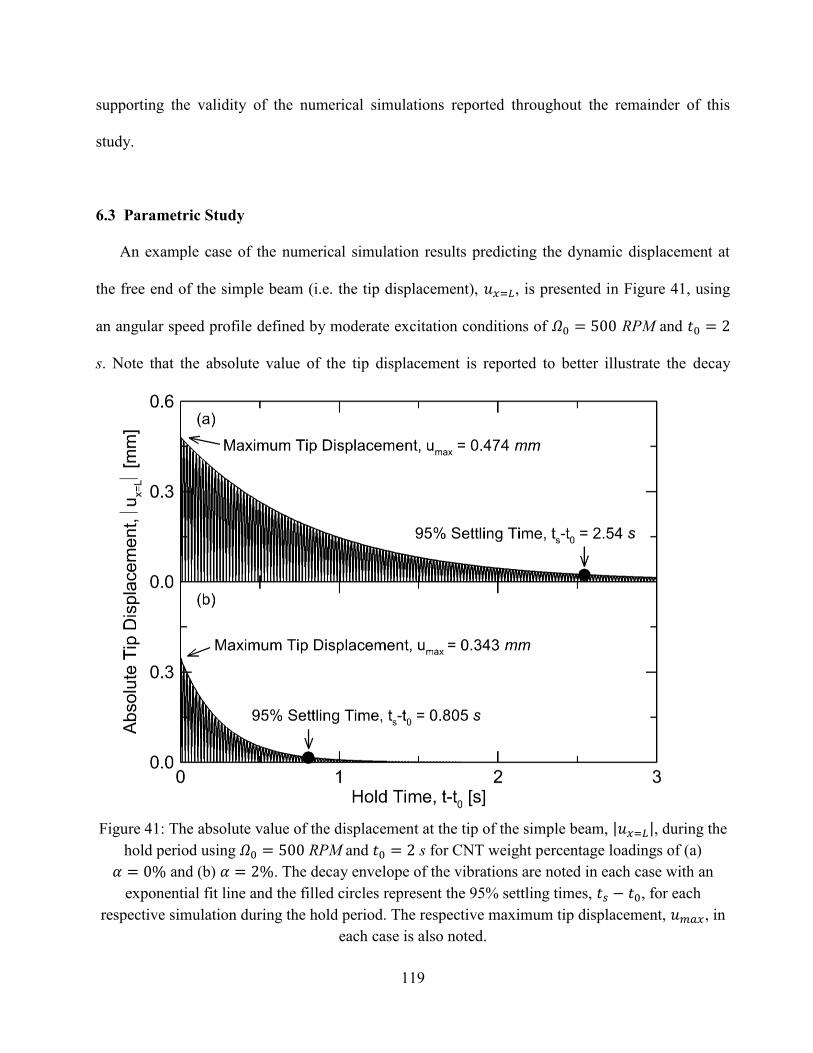
119
supporting the validity of the numerical simulations reported throughout the remainder of this
study.
6.3 Parametric Study
An example case of the numerical simulation results predicting the dynamic displacement at
the free end of the simple beam (i.e. the tip displacement), , is presented in Figure 41, using
an angular speed profile defined by moderate excitation conditions of RPM and
s. Note that the absolute value of the tip displacement is reported to better illustrate the decay
Figure 41: The absolute value of the displacement at the tip of the simple beam, , during the
hold period using RPM and s for CNT weight percentage loadings of (a)
and (b) . The decay envelope of the vibrations are noted in each case with an
exponential fit line and the filled circles represent the 95% settling times, , for each
respective simulation during the hold period. The respective maximum tip displacement, , in
each case is also noted.
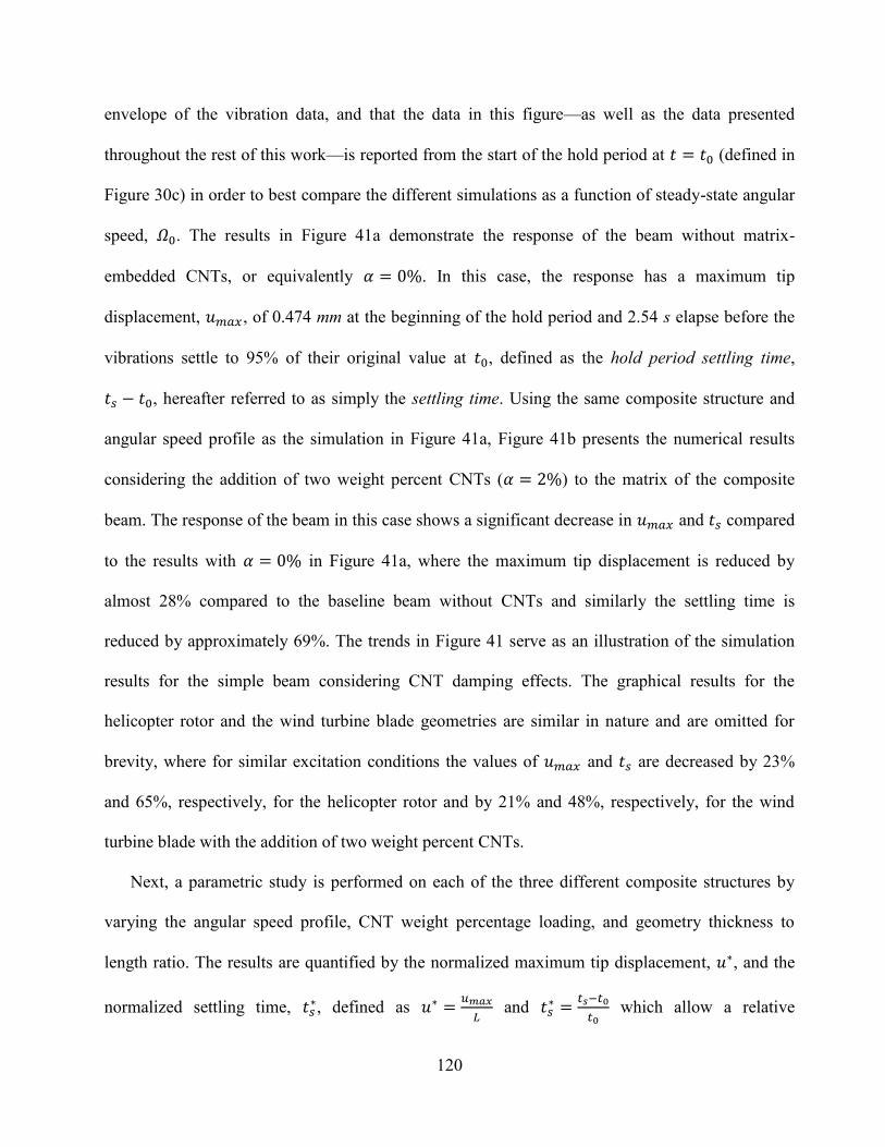
120
envelope of the vibration data, and that the data in this figure—as well as the data presented
throughout the rest of this work—is reported from the start of the hold period at (defined in
Figure 30c) in order to best compare the different simulations as a function of steady-state angular
speed, . The results in Figure 41a demonstrate the response of the beam without matrix-
embedded CNTs, or equivalently . In this case, the response has a maximum tip
displacement, , of 0.474 mm at the beginning of the hold period and 2.54 s elapse before the
vibrations settle to 95% of their original value at , defined as the hold period settling time,
, hereafter referred to as simply the settling time. Using the same composite structure and
angular speed profile as the simulation in Figure 41a, Figure 41b presents the numerical results
considering the addition of two weight percent CNTs ( ) to the matrix of the composite
beam. The response of the beam in this case shows a significant decrease in and compared
to the results with in Figure 41a, where the maximum tip displacement is reduced by
almost 28% compared to the baseline beam without CNTs and similarly the settling time is
reduced by approximately 69%. The trends in Figure 41 serve as an illustration of the simulation
results for the simple beam considering CNT damping effects. The graphical results for the
helicopter rotor and the wind turbine blade geometries are similar in nature and are omitted for
brevity, where for similar excitation conditions the values of and are decreased by 23%
and 65%, respectively, for the helicopter rotor and by 21% and 48%, respectively, for the wind
turbine blade with the addition of two weight percent CNTs.
Next, a parametric study is performed on each of the three different composite structures by
varying the angular speed profile, CNT weight percentage loading, and geometry thickness to
length ratio. The results are quantified by the normalized maximum tip displacement, , and the
normalized settling time, , defined as
and
which allow a relative
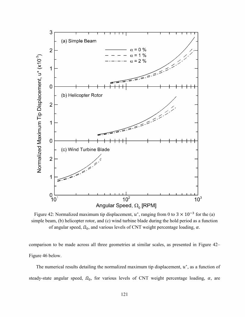
121
Figure 42: Normalized maximum tip displacement, , ranging from 0 to for the (a)
simple beam, (b) helicopter rotor, and (c) wind turbine blade during the hold period as a function
of angular speed, , and various levels of CNT weight percentage loading, .
comparison to be made across all three geometries at similar scales, as presented in Figure 42–
Figure 46 below.
The numerical results detailing the normalized maximum tip displacement, , as a function of
steady-state angular speed, , for various levels of CNT weight percentage loading, , are
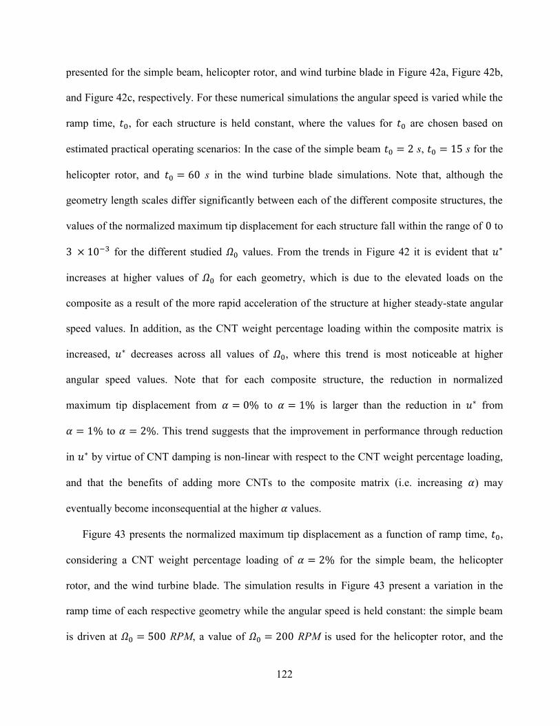
122
presented for the simple beam, helicopter rotor, and wind turbine blade in Figure 42a, Figure 42b,
and Figure 42c, respectively. For these numerical simulations the angular speed is varied while the
ramp time, , for each structure is held constant, where the values for are chosen based on
estimated practical operating scenarios: In the case of the simple beam s, s for the
helicopter rotor, and s in the wind turbine blade simulations. Note that, although the
geometry length scales differ significantly between each of the different composite structures, the
values of the normalized maximum tip displacement for each structure fall within the range of to
for the different studied values. From the trends in Figure 42 it is evident that
increases at higher values of for each geometry, which is due to the elevated loads on the
composite as a result of the more rapid acceleration of the structure at higher steady-state angular
speed values. In addition, as the CNT weight percentage loading within the composite matrix is
increased, decreases across all values of , where this trend is most noticeable at higher
angular speed values. Note that for each composite structure, the reduction in normalized
maximum tip displacement from to is larger than the reduction in from
to . This trend suggests that the improvement in performance through reduction
in by virtue of CNT damping is non-linear with respect to the CNT weight percentage loading,
and that the benefits of adding more CNTs to the composite matrix (i.e. increasing ) may
eventually become inconsequential at the higher values.
Figure 43 presents the normalized maximum tip displacement as a function of ramp time, ,
considering a CNT weight percentage loading of for the simple beam, the helicopter
rotor, and the wind turbine blade. The simulation results in Figure 43 present a variation in the
ramp time of each respective geometry while the angular speed is held constant: the simple beam
is driven at RPM, a value of RPM is used for the helicopter rotor, and the
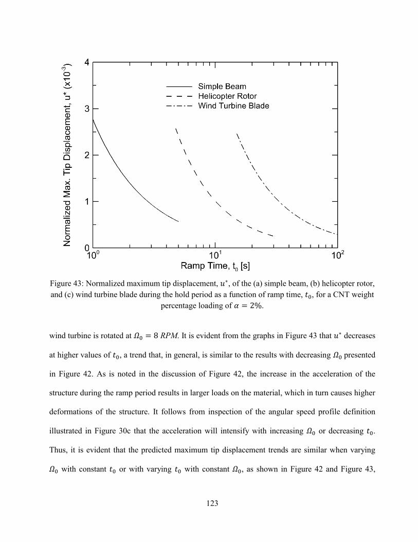
123
Figure 43: Normalized maximum tip displacement, , of the (a) simple beam, (b) helicopter rotor,
and (c) wind turbine blade during the hold period as a function of ramp time, , for a CNT weight
percentage loading of .
wind turbine is rotated at RPM. It is evident from the graphs in Figure 43 that decreases
at higher values of , a trend that, in general, is similar to the results with decreasing presented
in Figure 42. As is noted in the discussion of Figure 42, the increase in the acceleration of the
structure during the ramp period results in larger loads on the material, which in turn causes higher
deformations of the structure. It follows from inspection of the angular speed profile definition
illustrated in Figure 30c that the acceleration will intensify with increasing or decreasing .
Thus, it is evident that the predicted maximum tip displacement trends are similar when varying
with constant or with varying with constant , as shown in Figure 42 and Figure 43,
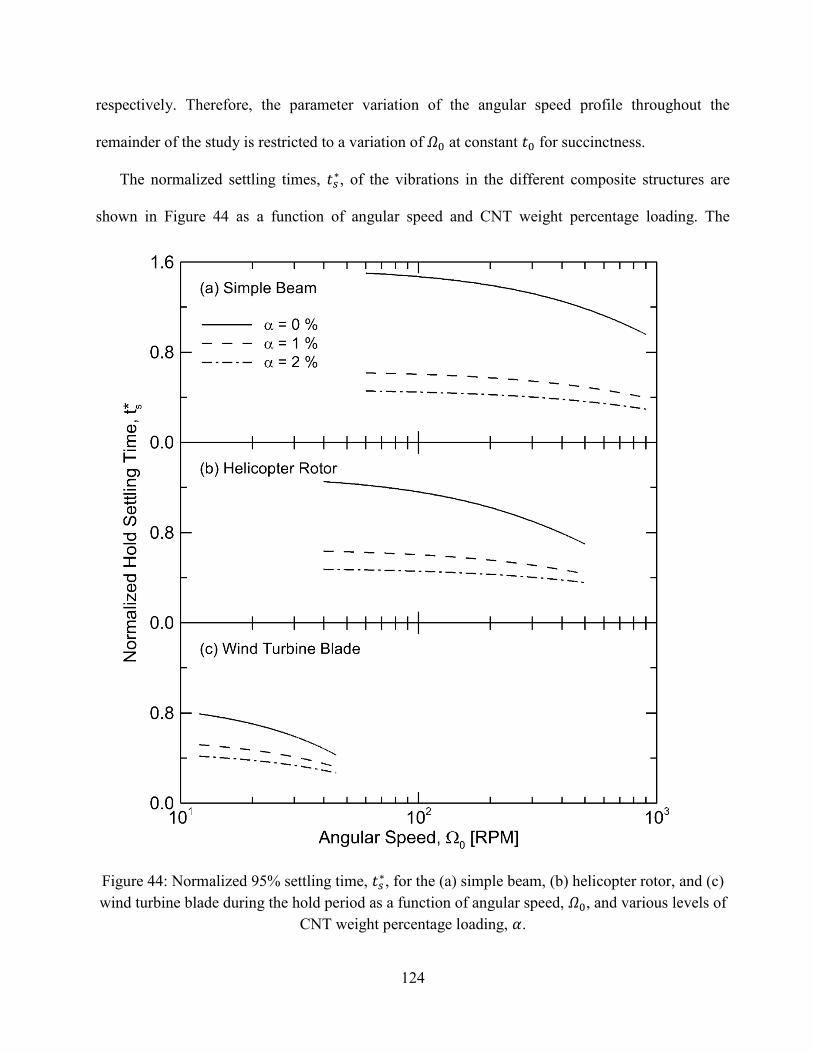
124
respectively. Therefore, the parameter variation of the angular speed profile throughout the
remainder of the study is restricted to a variation of at constant for succinctness.
The normalized settling times, , of the vibrations in the different composite structures are
shown in Figure 44 as a function of angular speed and CNT weight percentage loading. The
Figure 44: Normalized 95% settling time, , for the (a) simple beam, (b) helicopter rotor, and (c)
wind turbine blade during the hold period as a function of angular speed, , and various levels of
CNT weight percentage loading, .
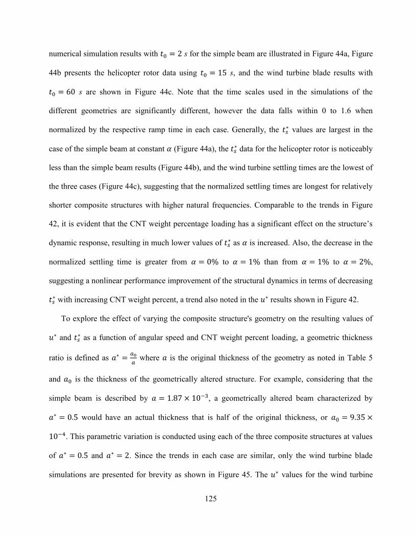
125
numerical simulation results with s for the simple beam are illustrated in Figure 44a, Figure
44b presents the helicopter rotor data using s, and the wind turbine blade results with
s are shown in Figure 44c. Note that the time scales used in the simulations of the
different geometries are significantly different, however the data falls within 0 to 1.6 when
normalized by the respective ramp time in each case. Generally, the values are largest in the
case of the simple beam at constant (Figure 44a), the data for the helicopter rotor is noticeably
less than the simple beam results (Figure 44b), and the wind turbine settling times are the lowest of
the three cases (Figure 44c), suggesting that the normalized settling times are longest for relatively
shorter composite structures with higher natural frequencies. Comparable to the trends in Figure
42, it is evident that the CNT weight percentage loading has a significant effect on the structure’s
dynamic response, resulting in much lower values of as is increased. Also, the decrease in the
normalized settling time is greater from to than from to ,
suggesting a nonlinear performance improvement of the structural dynamics in terms of decreasing
with increasing CNT weight percent, a trend also noted in the results shown in Figure 42.
To explore the effect of varying the composite structure's geometry on the resulting values of
and as a function of angular speed and CNT weight percent loading, a geometric thickness
ratio is defined as
where is the original thickness of the geometry as noted in Table 5
and is the thickness of the geometrically altered structure. For example, considering that the
simple beam is described by , a geometrically altered beam characterized by
would have an actual thickness that is half of the original thickness, or
. This parametric variation is conducted using each of the three composite structures at values
of and . Since the trends in each case are similar, only the wind turbine blade
simulations are presented for brevity as shown in Figure 45. The values for the wind turbine
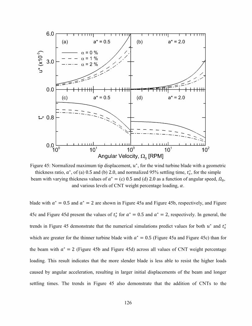
126
Figure 45: Normalized maximum tip displacement, , for the wind turbine blade with a geometric
thickness ratio, , of (a) and (b) , and normalized 95% settling time, , for the simple
beam with varying thickness values of (c) and (d) as a function of angular speed, ,
and various levels of CNT weight percentage loading, .
blade with and are shown in Figure 45a and Figure 45b, respectively, and Figure
45c and Figure 45d present the values of for and , respectively. In general, the
trends in Figure 45 demonstrate that the numerical simulations predict values for both and
which are greater for the thinner turbine blade with (Figure 45a and Figure 45c) than for
the beam with (Figure 45b and Figure 45d) across all values of CNT weight percentage
loading. This result indicates that the more slender blade is less able to resist the higher loads
caused by angular acceleration, resulting in larger initial displacements of the beam and longer
settling times. The trends in Figure 45 also demonstrate that the addition of CNTs to the
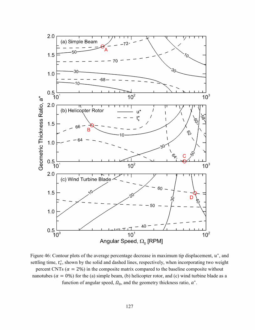
127
Figure 46: Contour plots of the average percentage decrease in maximum tip displacement, , and
settling time, , shown by the solid and dashed lines, respectively, when incorporating two weight
percent CNTs ( ) in the composite matrix compared to the baseline composite without
nanotubes ( ) for the (a) simple beam, (b) helicopter rotor, and (c) wind turbine blade as a
function of angular speed, , and the geometry thickness ratio, .
128
composite matrix remains effective at reducing the displacements and settling times of the wind
turbine blade for both thickness ratio cases. Again, as is noted in the discussion of Figure 42 and
Figure 44 above, there is an apparent nonlinear increase in performance gains when increasing
from 0 to 1 weight percent CNTs when compared to the increase from 1 to 2 weight percent CNTs.
However, the difference in the results when versus remains significant, and
future studies may address a cost-benefit analysis to determine an optimal CNT loading parameter.
Based on the results presented thus far, the improvement in performance by incorporating CNT
damping in each composite structure is quantified by calculating the percentage decrease in and
, respectively, when the CNT loading is increased from zero to two weight percent. Contour
maps of these percentage performance gains are presented for the simple beam, helicopter rotor,
and wind turbine blade in Figure 46a, Figure 46b, and Figure 46c, respectively, as a function of the
geometric thickness ratio, , and angular speed, . The trends displayed by the contour lines of
each structure are diverse, reflecting the various geometric complexities, length scales, and natural
frequencies of each case. In Figure 46a for the simple beam, the decrease in and are
maximized at approximately 50% (solid line) and 72% (dashed line), respectively, both occurring
at a low angular speed of RPM and a high value of (Point A in Figure 46a). For
the helicopter rotor in Figure 46b, the percentage decrease in is similar to the trend in Figure 46a
and is maximized at 66% (dashed line) for low to moderate angular velocities and high values,
corresponding to a decrease in of 10% at and RPM (Point B in Figure 46b).
However, the contour lines for the helicopter rotor show a different trend and demonstrate a
maximum decrease of about 50% (solid line) for high angular speeds across all values of ,
exhibited at RPM and for a decrease in of 64% (Point C in Figure 46b). In
Figure 46c, the contours for the wind turbine geometry show that the decrease in is greatest at
129
40% (solid line) for a geometric thickness ratio greater than approximately 0.8 and high values of
. In addition, the settling times are improved by up to 60% (dashed line) at high values of and
moderate to high angular speeds. For example, the design Point D in Figure 46c at RPM
and corresponds to a decrease in the maximum amplitude of 40% (solid line) and a
decrease in the settling time of 60% (dashed line) by the addition of 2% CNT.
The trends shown in Figure 46 demonstrate that the addition of two weight percent CNTs to
the composite matrix of each geometry has a significant impact on the structure’s performance,
decreasing the maximum tip displacement by 10–50% and the settling time by 40–72% across all
simulation cases. In general, the values show a minor variation across the parameter sweep for
each different structure, changing by about 4%, 8%, and 20% for the simple beam (Figure 46a),
helicopter rotor (Figure 46b), and wind turbine blade (Figure 46c), respectively, between the
different simulation cases. In contrast, the performance improvement in varies from 50 to 10
percent for the simple beam and helicopter rotor and from 40 to 10 percent for the wind turbine
blade across the same parameter space, indicating that the maximum tip displacement has a greater
dependence on the CNT weight percentage loading over the studied ranges of and . Figure 46
may be applied as a first-order design tool for developing operating ranges and geometric
parameters of rotating composite structures with material damping augmentation from matrix-
embedded CNTs.
This chapter developed a mathematical model of a rotating, cantilevered geometry and
presented a parametric study of different rotating composite structures considering the effects of
geometric variation, diverse angular velocities, and various levels of CNT damping. The
conclusions drawn from this research along with the previous studies detailed in Chapter 2–
Chapter 5 are presented in Chapter 7 to summarize the findings in this dissertation on composites
130
technology regarding void formation in composite molding processes and structural damping in
fiber-reinforced composites with nanoscale reinforcements.
6.4 Nomenclature used in Chapter 6
cross-sectional area [m2]
a thickness of geometry [m]
b width of geometry [m]
modulus of elasticity [Pa]
moment of inertia [m4]
L length of geometry [m]
R hub radius [m]
u beam displacement vector [m]
ramp time [s]
settling time [s]
Greek symbols
weight percent CNT loading [%]
material damping loss factor
strain [%]
density [kg/m3]
transverse natural frequency [Hz]
angular speed [RPM]
steady-state angular speed [RPM]
131
Chapter 7: Conclusions and Future Work
The presented studies provide significant contributions to composites technology in the areas
of void formation prediction in composites processing and damping augmentation in fiber-
reinforced composites using nanoscale reinforcement. Overall, the presented studies provide
simulation tools for the improvement of composites manufacturing and insight into advanced
composite material design for rotating composite structures through matrix-embedded CNTs.
7.1 Numerical Simulation of Void Formation in LCM Processes
In the first part of this dissertation, an analytical series solution was developed for the
longitudinal fluid flow through aligned rigid fibers which was used to establish a relationship
between the dimensionless permeability, , the fiber volume fraction, , the relative fiber
arrangement, and the fiber packing angle. The results are valid for all fiber volume fractions,
including the fiber packing limit. The analytical model together with the coefficients in Table 1
and Table 2 serve to obtain the values of the longitudinal flow permeability in simulation of resin
flow through aligned fibrous media, providing a method for predicting the local longitudinal
permeability of fiber tows in preform materials used in composites manufacturing.
Next, a numerical model was presented to investigate dual scale resin flow through two
commercially-available nested plain weave preform architectures, considering capillary effects
within each individual fiber bundle. The results of the numerical simulations were applied to
illustrate the air entrapment locations within the fiber preform along with a quantitative prediction
of the evolution and final size of the entrapped air voids. The steady state average and maximum
void entrapment volumes were compared across different Reynolds and Capillary numbers, along
with a description of the associated processing time needed for complete mold fill. Processing
132
under the competing considerations of simultaneously minimizing the final void content and the
processing time were presented and the impact of processing choices on the resulting volume of air
entrapment were discussed. Further, it was shown that simulation of the three dimensional flow
through an exact plain weave preform architecture in nested configuration may be achieved in a
computationally efficient manner without loss of accuracy through the assemblage of flow
simulations through multiple two-dimensional planar cross sections.
7.2 CNT Damping in Fiber-Reinforced Composite Structures
The second portion of this dissertation presented an investigation of the damping enhancement
provided to fiber reinforced composites from matrix embedded CNTs. The experimental study
explored different weight percentages and types of CNTs along with a systematic examination of
the ultrasonic processing time of the CNT-resin mixture in order to maximize the damping effect
in the final composite. Stationary damping measurements were taken using dynamic mechanical
analysis (DMA) and traditional modal analysis techniques to explore CNT-damping effects in
composites with different fiber volume fractions, and a 133% increase in damping was observed in
a carbon fiber reinforced composite with and two weight percent SWCNTs. The final
portion of the study focused on measuring the damping in rotating composite beams in order to
study the effect of rotation on CNT-infused composite materials. It was found that CNTs may be
increasingly effective at augmenting the damping as the angular velocity is increased, reflecting
the strain-dependent nature of the CNT damping phenomenon. These results provide greater
insight into the design of CNT-infused composites for applications such as helicopter rotors or
wind turbines, which are currently fabricated from composite materials and would benefit from the
reduction of vibrations through a passive damping mechanism such as matrix-embedded CNTs.

133
The dissertation also developed a numerical model, formulated using the Euler-Bernoulli beam
equation in a rotating frame and solved using the finite element method, to describe the effects of
CNT-based damping in a rotating fiber-reinforced composite beam. The model considered viscous
damping of the matrix material along with the energy dissipation from the matrix-embedded CNTs
in the composite, expressed using a stick-slip coulomb damping term describing the frictional
behavior at the nanotube-matrix interface as the material is deformed. The model was validated
with data from the literature and a systematic study of the governing dimensionless parameters was
conducted to investigate the effects of the beam geometry, angular speed, and viscous and
coulomb damping parameters on the dynamic response and vibration settling time of a rotating
composite beam. An application of the numerical model was presented by considering the typical
parameters of a helicopter rotor blade, to demonstrate the performance gains that may be achieved
by employing matrix-embedded CNTs in the design. The simulations show that a dimensionless
coulomb damping factor on the order of , that can be achieved with 1-2% by weight of CNT,
can reduce the vibration settling time of a rotating composite beam by an average of 40–60%.
Lastly, this dissertation presented a parametric study on rotating composite structures
considering the effects of geometric variation, diverse angular velocities, and various levels of
CNT damping. A mathematical model of a rotating, cantilevered geometry was developed and the
finite element method was applied to simulate three different composite structures, specifically a
simple beam, a helicopter rotor, and a wind turbine blade. The dynamic results of the numerical
simulations were quantified in terms of the normalized maximum tip displacement and the
normalized settling time. These metrics were used to elucidate the effects of each parameter on the
resulting structural dynamics, focusing primarily on the influence of CNT damping. To complete
this portion of the dissertation, contour plots for each composite structure were presented to
134
summarize the percentage improvement in performance when incorporating two weight percent
CNTs in the composite matrix, where the maximum tip displacements were found to improve by
up to 50% and the settling times were improved by up to 72%.
7.3 Future Work
In future studies involving the longitudinal permeability prediction of aligned rigid fiber
bundles, the model may be extended to include capillary forces in the governing physics to better
quantify the capillary effects on the analytical longitudinal permeability predictions. The twisting
of fiber bundles may also be included in this model to better reflect conditions found in physical
woven fibrous preforms. Improvements may be made to the numerical void prediction model by
including the effects of cure kinetics in the fluid modeling, and additional preform geometries may
also be considered to widen the base of understanding about the location of voids in different
preform fabrics. The model may also be extended to look at downstream flow field effects, the
flow close to the mold edges, and more complex mold cavities found in physical composite
manufacturing scenarios.
Future experimental work with matrix-embedded CNTs in fiber-reinforced composite materials
may address the effects of different fiber materials (e.g. glass), various fabric types (e.g.
unidirectional, random, etc.), and higher CNT weight percentage loadings on the resulting
damping measurements. Further investigation may be undertaken to better understand how rotation
affects the physics of the overall composite material and specifically the CNT-matrix interface,
and how this interaction may be exploited to an engineering design advantage. The current model
of the rotating composite beam considering CNT damping may be extended to include the effects
of orthotropic and heterogeneous material properties to better simulate the composite material

135
effects on the structural dynamics of each geometry. In addition, higher modes of vibration and the
associated modal damping parameters may be included in the governing equations to improve the
accuracy of the current numerical model, and the effects of higher CNT weight percentage
loadings within the composite material may also be considered.
136
Bibliography
[1] G. W. Jackson and D. F. James, “The permeability of fibrous porous media,” Canadian
Journal of Chemical Engineering, vol. 64, no. 3, pp. 364–374, 1986.
[2] A. S. Sangani and C. Yao, “Transport processes in random arrays of cylinders. II. Viscous
flow,” Physics of Fluids, vol. 31, no. 9, p. 2435, 1988.
[3] M. V Bruschke and S. G. Advani, “Flow of generalized Newtonian fluids across a periodic
array of cylinders,” Journal of Rheology, vol. 37, no. 3, p. 479, May 1993.
[4] J. Happel, “Viscous flow relative to arrays of cylinders,” AIChE Journal, vol. 5, no. 2, pp.
174–177, Jun. 1959.
[5] E. M. Sparrow and A. L. Loeffler, “Longitudinal laminar flow between cylinders arranged
in regular array,” AIChE Journal, vol. 5, no. 3, pp. 325–330, Sep. 1959.
[6] J. E. Drummond and M. I. Tahir, “Laminar viscous flow through regular arrays of parallel
solid cylinders,” International Journal of Multiphase Flow, vol. 10, no. 5, pp. 515–540, Oct.
1984.
[7] C. Y. Wang, “Longitudinal flow through an array of rectangular cylinders,” IMA Journal of
Applied Mathematics, vol. 58, no. 2, pp. 111–120, Apr. 1997.
[8] C. Y. Wang, “Longitudinal flow past cylinders arranged in a triangular array,” Applied
Mathematical Modelling, vol. 23, no. 3, pp. 219–230, Mar. 1999.
[9] S. Toll, “A solution technique for longitudinal Stokes flow around multiple aligned
cylinders,” Journal of Fluid Mechanics, vol. 439, pp. 199–216, 2001.
[10] R. Pitchumani and B. Ramakrishnan, “A fractal geometry model for evaluating
permeabilities of porous preforms used in liquid composite molding,” International Journal
of Heat and Mass Transfer, vol. 42, no. 12, pp. 2219–2232, Jun. 1999.
[11] B. Ramakrishnan and R. Pitchumani, “Fractal permeation characteristics of preforms used
in liquid composite molding,” Polymer Composites, vol. 21, no. 2, pp. 281–296, Apr. 2000.
[12] S. Zhao and A. Povitsky, “Method of fundamental solutions for partial-slip fibrous filtration
flows,” International Journal for Numerical Methods in Fluids, vol. 61, no. 3, pp. 255–274,
Sep. 2009.
[13] N. D. Ngo and K. K. Tamma, “Microscale permeability predictions of porous fibrous
media,” International Journal of Heat and Mass Transfer, vol. 44, no. 16, pp. 3135–3145,
Aug. 2001.
137
[14] F. Zhou, N. Kuentzer, P. Simacek, S. G. Advani, and S. M. Walsh, “Analytic
characterization of the permeability of dual-scale fibrous porous media,” Composites
Science and Technology, vol. 66, no. 15, pp. 2795–2803, Dec. 2006.
[15] K. Han, C. W. Lee, and B. P. Rice, “Measurements of the permeability of fiber preforms
and applications,” Composites Science and Technology, vol. 60, no. 12–13, pp. 2435–2441,
Sep. 2000.
[16] A. Shojaei, “An experimental study of saturated and unsaturated permeabilities in resin
transfer molding based on unidirectional flow measurements,” Journal of Reinforced
Plastics and Composites, vol. 23, no. 14, pp. 1515–1536, Sep. 2004.
[17] E. Rodriguez, F. Giacomelli, and A. Vazquez, “Permeability-porosity relationship in RTM
for different fiberglass and natural reinforcements,” Journal of Composite Materials, vol.
38, no. 3, pp. 259–268, Feb. 2004.
[18] A. Endruweit, K. S. Matthys, J. Peiro, and A. C. Long, “Effect of differential compression
on in-plane permeability tensor of heterogeneous multilayer carbon fibre preforms,”
Plastics, Rubber and Composites, vol. 38, no. 1, pp. 1–9, Feb. 2009.
[19] K. P. Brennan and D. E. Walrath, “Macroscale simulation of fiber bed impregnation
utilizing microscale material properties,” Journal of Reinforced Plastics and Composites,
vol. 29, no. 8, pp. 1248–1266, May 2009.
[20] K. P. Brennan, B. Straka, and D. E. Walrath, “Investigation of a simple tensorial
permeameter,” Polymer Composites, vol. 31, no. 3, pp. 434–442, 2010.
[21] V. Antonucci, M. Esposito, M. R. Ricciardi, M. Raffone, M. Zarelli, and M. Giordano,
“Permeability characterization of stitched carbon fiber preforms by fiber optic sensors,”
Express Polymer Letters, vol. 5, no. 12, pp. 1075–1084, Oct. 2011.
[22] S. Sharma and D. A. Siginer, “Permeability measurement methods in porous media of fiber
reinforced composites,” Applied Mechanics Reviews, vol. 63, no. 2, p. 020802, 2010.
[23] M. Li, S. Wang, Y. Gu, Z. Zhang, Y. Li, and K. Potter, “Dynamic capillary impact on
longitudinal micro-flow in vacuum assisted impregnation and the unsaturated permeability
of inner fiber tows,” Composites Science and Technology, vol. 70, no. 11, pp. 1628–1636,
Oct. 2010.
[24] L. S. Han and A. A. Cosner, “Effective thermal conductivities of fibrous composites,”
Journal of Heat Transfer, vol. 103, no. 2, p. 387, 1981.
[25] R. C. Averill and G. P. Carman, “Analytical modeling of micromechanical stress variations
in continuous fiber-reinforced composites,” in IUTAM Symposium, 1991, pp. 27–61.
138
[26] S. G. Advani, Flow and Rheology in Polymer Composites Manufacturing. Elsevier Science,
1994, p. 626.
[27] C. DeValve and R. Pitchumani, “An analytical model for the longitudinal permeability of
aligned fibrous media,” Composites Science and Technology, vol. 72, no. 13, pp. 1500–
1507, Aug. 2012.
[28] W. B. Young, “The effect of surface tension on tow impregnation of unidirectional fibrous
preform in resin transfer molding,” Journal of Composite Materials1, vol. 30, no. 11, pp.
1191–1209, 1996.
[29] E. Bayramli and R. L. Powell, “Impregnation dynamics of carbon fiber tows,” Journal of
Composite Materials, vol. 26, no. 10, pp. 1427–1442, Jan. 1992.
[30] K. M. Pillai, “Modeling the unsaturated flow in liquid composite molding processes: A
review and some thoughts,” Journal of Composite Materials, vol. 38, no. 23, pp. 2097–
2118, Dec. 2004.
[31] F. Trochu, E. Ruiz, V. Achim, and S. Soukane, “Advanced numerical simulation of liquid
composite molding for process analysis and optimization,” Composites Part A: Applied
Science and Manufacturing, vol. 37, no. 6, pp. 890–902, Jun. 2006.
[32] C. H. Park and L. Woo, “Modeling void formation and unsaturated flow in liquid composite
molding processes: a survey and review,” Journal of Reinforced Plastics and Composites,
vol. 30, no. 11, pp. 957–977, Aug. 2011.
[33] K. M. Pillai, “Governing equations for unsaturated flow through woven fiber mats. Part 1.
Isothermal flows,” Composites Part A: Applied Science and Manufacturing, vol. 33, no. 7,
pp. 1007–1019, Jul. 2002.
[34] R. S. Parnas, Liquid Composite Molding. Hanser Publishers, 2000, p. 170.
[35] M. E. Foley, “Modeling the effect of fiber diameter and fiber bundle count on tow
impregnation during liquid molding processes,” Journal of Composite Materials, vol. 39,
no. 12, pp. 1045–1065, Jun. 2005.
[36] B. Gourichon, C. Binetruy, and P. Krawczak, “A new numerical procedure to predict
dynamic void content in liquid composite molding,” Composites Part A: Applied Science
and Manufacturing, vol. 37, no. 11, pp. 1961–1969, Nov. 2006.
[37] N. Patel and J. Lee, “Modeling of void formation and removal in liquid composite molding.
Part II: Model development and implementation,” Polymer Composites, vol. 17, no. 1, pp.
104–114, Feb. 1996.
139
[38] L. Labat, J. Bréard, S. Pillut-Lesavre, and G. Bouquet, “Void fraction prevision in LCM
parts,” The European Physical Journal Applied Physics, vol. 16, no. 2, pp. 157–164, Nov.
2001.
[39] H. Jinlian, L. Yi, and S. Xueming, “Study on void formation in multi-layer woven fabrics,”
Composites Part A: Applied Science and Manufacturing, vol. 35, pp. 595–603, 2004.
[40] M. A. A. Spaid and F. R. Phelan, “Modeling void formation dynamics in fibrous porous
media with the lattice Boltzmann method,” Composites Part A: Applied Science and
Manufacturing, vol. 29, no. 7, pp. 749–755, Jul. 1998.
[41] E. Ruiz, V. Achim, S. Soukane, F. Trochu, and J. Breard, “Optimization of injection flow
rate to minimize micro/macro-voids formation in resin transfer molded composites,”
Composites Science and Technology, vol. 66, no. 3–4, pp. 475–486, Mar. 2006.
[42] C. H. Park, A. Lebel, A. Saouab, J. Bréard, and W. Il Lee, “Modeling and simulation of
voids and saturation in liquid composite molding processes,” Composites Part A: Applied
Science and Manufacturing, vol. 42, no. 6, pp. 658–668, Jun. 2011.
[43] J. S. U. Schell, M. Deleglise, C. Binetruy, P. Krawczak, and P. Ermanni, “Numerical
prediction and experimental characterisation of meso-scale-voids in liquid composite
moulding,” Composites Part A: Applied Science and Manufacturing, vol. 38, no. 12, pp.
2460–2470, Dec. 2007.
[44] C. Soutis, “Carbon fiber reinforced plastics in aircraft construction,” Materials Science and
Engineering: A, vol. 412, no. 1–2, pp. 171–176, Dec. 2005.
[45] A. M. K. Esawi and M. M. Farag, “Carbon nanotube reinforced composites: Potential and
current challenges,” Materials & Design, vol. 28, no. 9, pp. 2394–2401, Jan. 2007.
[46] M. O. L. Hansen, J. N. Sørensen, S. Voutsinas, N. Sørensen, and H. A. Madsen, “State of
the art in wind turbine aerodynamics and aeroelasticity,” Progress in Aerospace Sciences,
vol. 42, no. 4, pp. 285–330, Jun. 2006.
[47] J.-S. Jang, J. Varischetti, and J. Suhr, “Strain dependent energy dissipation in multi-scale
carbon fiber composites containing carbon nanofibers,” Carbon, vol. 50, no. 11, pp. 4283–
4277, May 2012.
[48] B. Wetzel, F. Haupert, and M. Q. Zhang, “Epoxy nanocomposites with high mechanical and
tribological performance,” Composites Science and Technology, vol. 63, no. 14, pp. 2055–
2067, Nov. 2003.
[49] E. T. Thostenson, Z. Ren, and T.-W. Chou, “Advances in the science and technology of
carbon nanotubes and their composites: a review,” Composites Science and Technology,
vol. 61, no. 13, pp. 1899–1912, Oct. 2001.
140
[50] M. Moniruzzaman and K. I. Winey, “Polymer nanocomposites containing carbon
nanotubes,” Macromolecules, vol. 39, no. 16, pp. 5194–5205, Aug. 2006.
[51] R. F. Gibson, E. O. Ayorinde, and Y.-F. Wen, “Vibrations of carbon nanotubes and their
composites: A review,” Composites Science and Technology, vol. 67, no. 1, pp. 1–28, 2007.
[52] H. Rajoria and N. Jalili, “Passive vibration damping enhancement using carbon nanotube-
epoxy reinforced composites,” Composites Science and Technology, vol. 65, no. 14, pp.
2079–2093, 2005.
[53] K. Lau and D. Hui, “The revolutionary creation of new advanced materials - carbon
nanotube composites,” Composites Part B: Engineering, vol. 33, no. 4, pp. 263–277, 2002.
[54] J. Suhr and N. A. Koratkar, “Energy dissipation in carbon nanotube composites: a review,”
Journal of Materials Science, vol. 43, no. 13, pp. 4370–4382, Apr. 2008.
[55] N. A. Koratkar, J. Suhr, A. Joshi, R. S. Kane, L. S. Schadler, P. M. Ajayan, and S.
Bartolucci, “Characterizating energy dissipation in single-walled carbon nanotube
polycarbonate composites,” Applied Physics Letters, vol. 87, pp. 1–3, 2005.
[56] J. Zhu, J. Kim, H. Peng, J. L. Margrave, V. N. Khabashesku, and E. V. Barrera, “Improving
the dispersion and integration of single-walled carbon nanotubes in epoxy composites
through functionalization,” Nano Letters, vol. 3, no. 8, pp. 1107–1113, Aug. 2003.
[57] J. A. Kim, D. G. Seong, T. J. Kang, and J. R. Youn, “Effects of surface modification on
rheological and mechanical properties of CNT/epoxy composites,” Carbon, vol. 44, no. 10,
pp. 1898–1905, Aug. 2006.
[58] J. Che, W. Yuan, G. Jiang, J. Dai, S. Y. Lim, and M. B. Chan-Park, “Epoxy composite
fibers reinforced with aligned single-walled carbon nanotubes functionalized with
generation 0−2 dendritic poly(amidoamine),” Chemistry of Materials, vol. 21, no. 8, pp.
1471–1479, Apr. 2009.
[59] M. T. Byrne and Y. K. Gun’ko, “Recent advances in research on carbon nanotube-polymer
composites.,” Advanced materials (Deerfield Beach, Fla.), vol. 22, no. 15, pp. 1672–88,
Apr. 2010.
[60] X. Zhou, K. W. Wang, and C. E. Bakis, “The investigation of carbon nanotube based
polymers for improved structural damping,” Smart Structures and Materials, vol. 5386, pp.
162–173, 2004.
[61] R. L. Dai and W. H. Liao, “Fabrication, testing, and modeling of carbon nanotube
composites for vibration damping,” Journal of Vibration and Acoustics, vol. 131, no. 5, pp.
1–9, 2009.
141
[62] R. M. Lin and C. Lu, “Modeling of interfacial friction damping of carbon nanotube-based
nanocomposites,” Mechanical Systems and Signal Processing, vol. 24, no. 8, pp. 2996–
3012, 2010.
[63] R. F. Gibson, “A review of recent research on mechanics of multifunctional composite
materials and structures,” Composite Structures, vol. 92, no. 12, pp. 2793–2810, Nov. 2010.
[64] E. A. Lass, N. A. Koratkar, P. M. Ajayan, B. Q. Wei, and P. Keblinski, “Damping and
stiffness enhancement in composite systems with carbon nanotubes films,” in Material
Research Society Symposium, 2003, pp. 371–376.
[65] N. A. Koratkar, B. Wei, and P. M. Ajayan, “Multifunctional structural reinforcement
featuring carbon nanotube films,” Composites Science and Technology, vol. 63, no. 11, pp.
1525–1531, 2003.
[66] M. Damu, A. Lumsdaine, and M. Parsons, “Topology optimization of carbon nanotube
reinforced composite laminated structures for vibration damping,” in SPIE Conference on
Smart Structures and Materials 2005: Damping and Isolation, 2005, pp. 188–195.
[67] M. Ray and R. Batra, “A single-walled carbon nanotube reinforced 1-3 piezoelectric
composite for active control of smart structures,” Smart Materials and Structures, vol. 16,
no. 5, pp. 1936–1947, 2007.
[68] J. Suhr, N. A. Koratkar, P. Keblinski, and P. M. Ajayan, “Viscoelasticity in carbon nanotube
composites,” Nature Materials Letters, vol. 4, pp. 134–137, 2005.
[69] S. N. Mahmoodi, S. E. Khadem, and N. Jalili, “Theoretical development and closed-form
solution of nonlinear vibrations of a directly excited nanotube-reinforced composite
cantilevered beam,” Arch Appl Mech, vol. 75, no. 2–3, pp. 153–163, 2006.
[70] M. V Kireitseu, D. Hui, and G. R. Tomlinson, “Advanced shock-resistant and vibration
damping of nanoparticle-reinforced compisite material,” Composites Part B: Engineering,
vol. 39, no. 1, pp. 128–138, 2008.
[71] M.-K. Yeh and T.-H. Hsieh, “Dynamic properties of sandwich beams with MWNT/polymer
nanocomposites as core materials,” Composites Science and Technology, vol. 68, no. 14, pp.
2930–2936, 2008.
[72] R. L. Dai and W. H. Liao, “Modeling of carbon nanotube composites for vibration
damping,” in Proceedings of SPIE, 2007, vol. 6528, pp. 652809–652809–10.
[73] X. Zhou, E. Shin, K. W. Wang, and C. E. Bakis, “Interfacial damping characteristics of
carbon nanotube-based composites,” Composites Science and Technology, vol. 64, no. 15,
pp. 2425–2437, 2004.
142
[74] M. V Kireitseu, G. R. Tomlinson, A. V Ivanenko, and L. V Bochkareva, “Dynamics and
vibration damping behavior of advanced meso/nanoparticle-reinforced composites,”
Mechanics of Advanced Materials and Structures, vol. 14, no. 8, pp. 603–617, 2007.
[75] J. Suhr, N. A. Koratkar, and P. Ajayan, “Damping characterization of carbon nanotube thin
films,” in SPIE Conference on Smart Structures and Materials 2004: Damping and
Isolation, 2004, pp. 153–161.
[76] S. U. Khan, C. Y. Li, N. A. Siddiqui, and J.-K. Kim, “Vibration damping characteristics of
carbon fiber-reinforced composites containing multi-walled carbon nanotubes,” Composites
Science and Technology, vol. 71, no. 12, pp. 1486–1494, 2011.
[77] M. Tehrani, M. Safdari, S. W. Case, and M. S. Al-Haik, “Using multiscale carbon
fiber/carbon nanotubes composites for damping applications,” in ASME 2011 Conference on
Smart Materials, Adaptive Structures, and Intelligent Systems, 2011, pp. 1–5.
[78] R. J. Johnson, J. Tang, and R. Pitchumani, “Characterization of damping in carbon-nanotube
filled fiberglass reinforced thermosetting-matrix composites,” Journal of Materials Science,
vol. 46, no. 13, pp. 4545–4554, Feb. 2011.
[79] C. DeValve and R. Pitchumani, “Experimental investigation of the damping enhancement in
fiber-reinforced composites with carbon nanotubes,” Carbon, vol. In Review, 2013.
[80] S. Murugan and R. Ganguli, “Aeroelastic stability enhancement and vibration supression in
a composite helicopter rotor,” Journal of Aircraft, vol. 42, no. 4, pp. 1013–1024, 2005.
[81] U. Dalli and S. Yuksel, “Identification of flap motion parameters for vibration reduction in
helicopter rotors with multiple active trailing edge flaps,” Shock and Vibration, vol. 18, pp.
727–745, 2011.
[82] T. K. Barlas and G. A. M. van Kuik, “Review of state of the art in smart rotor control
research for wind turbines,” Progress in Aerospace Sciences, vol. 46, no. 1, pp. 1–27, 2010.
[83] D. Patt, L. Liu, J. Chandrasekar, D. S. Bernstein, and P. P. Friedmann, “Higher-harmonic-
control algorithm for helicopter vibration reduction revisited,” Journal of Guidance,
Control, and Dynamics, vol. 28, no. 5, pp. 918–930, 2005.
[84] H. Tan, L. Y. Jiang, Y. Huang, B. Liu, and K. C. Hwang, “The effect of van der Waals-
based interface cohesive law on carbon nanotube-reinforced composite materials,”
Composites Science and Technology, vol. 67, no. 14, pp. 2941–2946, Nov. 2007.
[85] Y. Huang and X. W. Tangpong, “A distributed friction model for energy dissipation in
carbon nanotube-based composites,” Communications in Nonlinear Scientific Numerical
Simulations, vol. 15, no. 12, pp. 4171–4180, 2010.
143
[86] P. P. Friedmann and T. A. Millott, “Vibration reduction in rotorcraft using active control: A
comparison of various approaches,” Journal of Guidance, Control, and Dynamics, vol. 18,
no. 4, pp. 664–673, 1995.
[87] J. Chung and H. H. Yoo, “Dynamic analysis of a rotating cantilever beam by using the finite
element method,” Journal of Sound and Vibration, vol. 249, no. 1, pp. 147–164, Jan. 2002.
[88] D. Weaver, K. McAlister, and J. Tso, “Control of VR-7 dynamic stall by strong steady
blowing,” Journal of Aircraft, vol. 41, no. 6, pp. 1404–1413, Nov. 2004.
[89] Y. Bazilevs, M. C. Hsu, I. Akkerman, S. Wright, K. Takizawa, B. Henicke, T. Spielman,
and T. E. Tezduyar, “3D simulation of wind turbine rotors at full scale. Part I: Geometry
modeling and aerodynamics,” International Journal for Numerical Methods in Fluids, vol.
65, no. 1–3, pp. 207–235, 2011.
[90] B. R. Munson, D. F. Young, and T. H. Okiishi, Fundamentals of Fluid Mechanics. Wiley,
2005, p. 816.
[91] E. Kreyszig, Advanced Engineering Mathematics, 9th ed. Hoboken, NJ: John Wiley &
Sons, Inc., 2006.
[92] C. W. Hirt and B. D. Nichols, “Volume of fluid (VOF) method for the dynamics of free
boundaries,” Journal of Computational Physics, vol. 39, no. 1, pp. 201–225, Jan. 1981.
[93] J. U. Brackbill, D. B. Kothe, and C. Zemach, “A continuum method for modeling surface
tension,” Journal of Computational Physics, vol. 100, no. 2, pp. 335–354, Jun. 1992.
[94] Y. W. Zhang and A. Faghri, “Numerical simulation of condensation on a capillary grooved
structure,” Numerical Heat Transfer Part A: Applications, vol. 39, no. 3, pp. 227–243,
2001.
[95] R. I. Issa, B. Ahmadi-Befrui, K. R. Beshay, and A. D. Gosman, “Solution of the implicitly
discretised reacting flow equations by operator-splitting,” Journal of Computational
Physics, vol. 93, no. 2, pp. 388–410, Apr. 1991.
[96] O. Ubbink, “Numerical prediction of two fluid systems with sharp interfaces,” Imperial
College of Science, Technology and Medicine, London, 1997.
[97] J. S. Leclerc and E. Ruiz, “Porosity reduction using optimized flow velocity in Resin
Transfer Molding,” Composites Part A: Applied Science and Manufacturing, vol. 39, no.
12, pp. 1859–1868, Dec. 2008.
[98] V. Rohatgi, N. Patel, and J. Lee, “Experimental investigation of flow-induced microvoids
during impregnation of unidirectional stitched fiberglass mat,” Polymer Composites, vol.
17, no. 2, pp. 161–170, Apr. 1996.
144
[99] D. J. Inman, Engineering Vibration, Second Edition. Prentice Hall, 2000, p. 621.
[100] P. Macioce, “Viscoelastic Damping 101,” Sound and Vibration, vol. 37, no. 4, pp. 8–10,
2003.
[101] E. Reynders, “System identification methods for (operational) modal analysis: Review and
comparison,” Archives of Computational Methods in Engineering, vol. 19, no. 1, pp. 51–
124, Feb. 2012.
[102] P. Mohanty and D. J. Rixen, “Operational modal analysis in the presence of harmonic
excitation,” Journal of Sound and Vibration, vol. 270, no. 1–2, pp. 93–109, Feb. 2004.
[103] L. Hermans and H. Van der Auweraer, “Modal testing and analysis of structures under
operational conditions: industrial applications,” Mechanical Systems and Signal Processing,
vol. 13, no. 2, pp. 193–216, 1999.
[104] M. Dohler, P. Andersen, and L. Mevel, “Operational modal analysis using fast stochastic
subspace identification method,” in Proceedings of the 30th International Modal Analysis
Conference (IMAC), 2012, pp. 1–7.
[105] R. Brincker and P. Andersen, “Understanding stochastic subspace identification,” in
Proceedings of the 24th International Modal Analysis Conference (IMAC), 2006, pp. 1–6.
[106] X. Xie, Y. Mai, and X. Zhou, “Dispersion and alignment of carbon nanotubes in polymer
matrix: A review,” Materials Science and Engineering: R: Reports, vol. 49, no. 4, pp. 89–
112, May 2005.
[107] A. D. Wright, C. E. Smith, R. W. Thresher, and J. L. C. Wang, “Vibration modes of
centrifugally stiffened beams,” Journal of Applied Mechanics, vol. 49, no. 1, pp. 197–202,
1982.
[108] N. Granick and J. E. Stern, “Material damping of aluminum by a resonant-dwell technique,”
Greenbelt, Maryland, 1965.
[109] W. E. Baker, W. E. Woolam, and D. Young, “Air and internal damping of thin cantilever
beams,” International Journal of Mechanical Sciences, vol. 9, pp. 743–766, 1967.
[110] J. M. Lee and K. G. McConnell, “Experimental cross-verification of damping in three
metals,” Experimental Mechanics, vol. 15, no. 9, pp. 347–353, 1975.
[111] K. Gupta and S. P. Singh, “Damping measurements in fiber reinforced composite rotors,”
Journal of Sound and Vibration, vol. 211, no. 3, pp. 513–520, 1998.
[112] J. Kielb and R. Abhari, “Experimental study of aerodynamic and structural damping in a
full-scale rotating turbine,” ASME Journal of Engineering for Gas Turbines and Power, vol.
125, pp. 102–112, 2001.
145
[113] H. H. Yoo, R. R. Ryan, and R. A. Scott, “Dynamics of flexible beams undergoing overall
motions,” Journal of Sound and Vibration, vol. 181, no. 2, pp. 261–278, Mar. 1995.
[114] Z. Fan, P. Tsakiropoulos, and A. P. Miodownik, “A generalized law of mixtures,” Journal
of Materials Science, vol. 29, no. 1, pp. 141–150, 1994.
[115] G. Sauer and M. Wolf, “Finite element analysis of gyroscopic effects,” Finite Elements in
Analysis and Design, vol. 5, pp. 131–140, 1989.
[116] C. Johnson, Numerical Solution of Partial Differential Equations by the Finite Element
Method. Mineola, New York: Dover Publications, 2009, p. 288.
[117] J. Yu and A. Craggs, “3-D solid finite element modeling of rotating shafts,” in Proceedings
of the International Modal Analysis Conference, 1997, vol. 11, no. 8–10, pp. 1488–1494.
[118] S. K. Clark, Dynamics of Continuous Elements (Prentice-Hall international series in
dynamics). Prentice Hall, 1972, p. 272.
[119] J. Chung and G. M. Hulbert, “A time integration algorithm for structural dynamics with
improved numerical dissipation: the generalized-α method,” Journal of applied mechanics,
vol. 60, no. 2, pp. 371–375, 1993.
[120] G.-P. Cai, J.-Z. Hong, and S. X. Yang, “Model study and active control of a rotating flexible
cantilever beam,” International Journal of Mechanical Sciences, vol. 46, no. 6, pp. 871–
889, Jun. 2004.
[121] M. S. Selig, “UIUC Airfoil Coordinates Database,” 2012. [Online]. Available:
http://www.ae.illinois.edu/m-selig/ads/coord_database.html#X. [Accessed: 01-Jun-2012].
[122] J. Jonkman, S. Butterfield, W. Musial, and G. Scott, “Definition of a 5-MW reference wind
turbine for offshore system development,” Golden, Colorado, 2009.
[123] W. A. Timmer and R. P. J. O. M. van Rooij, “Summary of the Delft University wind turbine
dedicated airfoils,” ASME Journal of Solar Energy Engineering, vol. 125, pp. 488–496,
2003.
[124] T. Lutz, A. Wolf, W. Wurz, and J.-G. Jeremiasz, “Design and verification of an airfoil with
trailing-edge flap and unsteady wind-tunnel tests,” Stuttgart, Germany, 2011.
[125] C. Ashcraft, R. Grimes, D. Pierce, and D. Wah, “The user manual for SPOOLES, release
2.0: An object oriented software library for solving sparse linear systems of equations.”
Boeing Shared Services Group, Seattle, WA 28124 USA, 1998.
[126] P. Pedersen, “Analytical stiffness matrices with Green-Lagrange strain measure,”
International Journal for Numerical Methods in Engineering, vol. 62, no. 3, pp. 334–352,
Jan. 2005.

146
[127] F. J. McHugh and J. Shaw, “Helicopter vibration reduction with higher harmonic blade
pitch,” Journal of the American Helicopter Society, pp. 26–35, 1978.
[128] A. D. de Corcuera, A. Pujana-Arrese, J. M. Ezquerra, E. Segurola, and J. Landaluze, “H∞
based control for load mitigation in wind turbines,” Energies, vol. 5, no. 4, pp. 938–967,
Apr. 2012.